arX

iv:0

708.

2959

v1 [

astr

o-ph

] 2

2 A

ug 2

007

Molecular Line Observations of the Small Protostellar Group

L1251B

Jeong-Eun Lee1,2, James Di Francesco3, Tyler L. Bourke4, Neal J. Evans II5, Jingwen Wu4,

ABSTRACT

We present molecular line observations of L1251B, a small group of pre-

and protostellar objects, and its immediate environment in the dense C18O core

L1251E. These data are complementary to near-infrared, submillimeter and mil-

limeter continuum observations reported by Lee et al. (2006, ApJ, 648, 491;

Paper I). The single-dish data of L1251B described here show very complex kine-

matics including infall, rotation and outflow motions, and the interferometer

data reveal these in greater detail. Interferometer data of N2H+ 1−0 suggest a

very rapidly rotating flattened envelope between two young stellar objects, IRS1

and IRS2. Also, interferometer data of CO 2−1 resolve the outflow associated

with L1251B seen in single-dish maps into a few narrow and compact compo-

nents. Furthermore, the high resolution data support recent theoretical studies

of molecular depletions and enhancements that accompany the formation of pro-

tostars within dense cores. Beyond L1251B, single-dish data are also presented of

a dense core located ∼150′′ to the east that, in Paper I, was detected at 850 µm

but has no associated point sources at near- and mid-infrared wavelengths. The

relative brightness between molecules, which have different chemical timescales,

suggests it is less chemically evolved than L1251B. This core may be a site for

future star formation, however, since line profiles of HCO+, CS, and HCN show

asymmetry with a stronger blue peak, which is interpreted as an infall signature.

Subject headings: line: profile — ISM: individual (L1251B) — stars: formation

1Department of Astronomy and Space Science, Sejong University, Seoul 143-747, Korea; jelee@sejong.ac.kr

2Hubble Fellow, Physics and Astronomy Department, The University of California at Los Angeles, PAB,

430 Portola Plaza, Box 951547, Los Angeles, CA 90095-1547

3National Research Council of Canada, Herzberg Institute of Astrophysics, 5071 West Saanich Road,

Victoria, BC V9E 2E7, Canada; james.difrancesco@nrc-cnrc.gc.ca

4Smithsonian Astrophysical Observatory, 60 Garden Street, Cambridge, MA 02138;

tbourke@cfa.harvard.edu

5Astronomy Department, The University of Texas at Austin, 1 University Station C1400, Austin, TX

78712-0259; nje@astro.as.utexas.edu, jingwen@astro.as.utexas.edu

– 2 –

1. INTRODUCTION

Most young stars in our Galaxy formed within groups or clusters (Lada and Lada 2003).

Small, nearby groups of protostellar objects provide compelling cases for investigating the

physical processes involved with such formation since the numbers involved are relatively

small (e.g., N < 10) and the interactions of these objects with themselves and their envi-

ronments are less complicated. For example, observational study of kinematics associated

with young stars within groups and their immediate dense gas surroundings could provide

evidence for a specific formation scenario, e.g., fragmentation or triggering, that is easier to

see because of the simpler nature of groups relative to clusters.

Kinematic study of the gas surroundings of protostellar objects is achieved through

observation and interpretation of molecular rotational transitions, since line profiles can be

shaped by the motions within the source gas (see Di Francesco et al. 2006 for a review.)

For example, outflow motions from young stellar objects were first seen in the low-intensity

wings of CO 1−0 emission (e.g., Snell, Loren & Plambeck 1980). In addition, rotational

motions in dense cores have been suggested from the detection of the shift of centroid ve-

locities along different lines of sight in optically thin molecular transitions (e.g,. Goodman

et al. 1993). Finally, infall motions in dense cores have been the interpretation of profiles

of moderately optically thick lines that are asymmetric with a stronger blue peak relative

to optically thin lines (e.g., Zhou et al. 1993; Myers, Evans & Ohashi 2000). Such kine-

matic evidence has come primarily from single-dish telescopes, i.e., of relatively low spatial

resolution, in studies of isolated protostellar objects. For protostellar groups, however, the

surface density of objects can be high, and single-dish telescopes may not have the resolution

needed to associate kinematics with particular protostars within the group. Instead, data

from interferometers are very highly suited for such studies, especially when used in tandem

with data from single-dish telescopes.

The use of molecular lines to study kinematics is complicated by potentially significant

molecular abundance variations along the lines of sight toward dense gas both before and

after star formation. Such abundance changes can be due to chemical evolution, intertwined

with the YSO luminosity evolution since luminosity affects the temperatures of nearby dust

grains that interact with gaseous molecules (see Rawlings & Yates 2001; Doty et al. 2002;

Lee, Bergin & Evans 2004). Of course, YSO luminosity evolution is itself intertwined with

dynamical evolution of the surrounding gas, as much of the luminosity originates from ac-

cretion. Hence, a holistic approach in general is required that includes luminosity, dynamics

and chemistry, to understand best the environments from which stars form (see Bergin et

al. 1997 and Aikawa et al. 2001 for early examples of such models).

Located at 300 pc ± 50 pc (Kun & Prusti 1993), L1251B is an excellent example of

– 3 –

a small, nearby group of protostellar objects where molecular line observations can probe

the kinematics and chemistry of its environment and yield clues about its origins. L1251B

is located within L1251E, the densest C18O core in L1251 (Sato et al. 1994). L1251B is

associated with a single IRAS point source, IRAS 22376+7455, and was found associated with

CO outflow by Sato & Fukui (1989). In Lee et al. (2006; Paper I), we showed via single-dish

data that IRAS 22376+7455 was associated with a local maximum of submillimeter emission,

although significant peaks of 850 µm emission were also seen ∼150′′ to the east. In addition,

we showed Spitzer Space Telescope (SST) observations of the region that revealed ∼20 YSOs

within ∼1 pc2 covering L1251B and its surroundings, indicative of the formation of a group

of low-mass stars. Within L1251B itself, these data revealed three Class 0/I objects (IRS1,

IRS2, and IRS4) and three Class II objects (IRS3, IRS5, and IRS6), within a projected

diameter of 55′′. (No near- or mid-infrared sources were found to be associated with other

locations of submillimeter emission adjacent to L1251B.) Finally, we showed Submillimeter

Array (SMA) continuum observations of L1251B in Paper I that revealed two compact

locations of high column density between IRS1 and IRS2 that may be starless condensations.

Paper I revealed clearly L1251B as a region of recent (and possibly continuing) star formation

within a small group.

In this paper, we examine line emission associated with L1251B and the core ∼150′′

to its east (henceforth, the “east core”), to probe kinematic and chemical processes in the

region. The three embedded Class 0/I sources and two starless objects within L1251B are

especially emphasized; IRS1 is the most luminous object, IRS2 is located southeast of IRS1

and is associated with a near-infrared bipolar nebula, and IRS4 is located at the west of

IRS1. The two starless objects are named as SMA-N (the northern one) and SMA-S (the

southern one) in this paper. Besides the outflow noted by Sato & Fukui, earlier molecular

line observations have also provided evidence for rotational and infall motions in L1251B. For

example, a velocity gradient of ∼2.3 km s−1 pc−1 in the northeast–southwest direction across

L1251B suggestive of rotational motion was detected by Goodman et al. (1993) in NH3 (1,1)

(also Sato et al. 1994; Toth & Walmsley 1996; Anglada et al. 1997; Morata et al. 1997). In

addition, infall motions toward L1251B were suggested from the detections of asymmetric

profiles with stronger blue peaks in HCO+ 1−0 and 3−2, CS 2−1 and H2CO 212–111 by

Gregersen et al. (2000) and Mardones et al. (1997), though observations were published

only toward the IRAS point source position. Since the relative intensity of a given molecular

line depends upon distributions of density, temperature and molecular abundance along the

line of sight, many other transitions and positions needed to be observed within L1251B and

its surroundings to understand correctly their physical conditions and dynamical processes.

Here, we have gathered with single-dish telescopes or interferometers new observations of

L1251B in CS 2−1, 3−2, and 5−4, HCN 1−0, CO 2−1, 13CO 2−1, C18O 2−1, HCO+ 1−0

– 4 –

and 3−2, H13CO+ 1−0, DCO+ 3−2, N2H+ 1−0 and H2CO 312–211.

Details of the acquisition of observations of L1251B for this paper are summarized in

§2. Results and analysis of the data are described in §3 and §4. In §5, we discuss the

chemical and dynamical conditions in L1251B and the east core. Finally, a summary of the

conclusions of this paper appears in §6.

2. OBSERVATIONS

2.1. The Five College Radio Astronomy Observatory (FCRAO) Observations

Observations of N2H+ 1−0 toward L1251B were made in December 1996 with the

FCRAO 14-m telescope near New Salem, MA using QUARRY, the 15-element focal plane

heterodyne receiver array. Observations of HCO+ 1−0 and H13CO+ 1−0 were made to-

ward L1251B also at FCRAO in April 1997 and May 2000, using the QUARRY (1997)

and the 32-element SEQUOIA (2000) focal plane arrays respectively. The autocorrelator

spectrometer was configured with a band width of 20 MHz over 1024 channels, providing a

channel separation of ∼20 kHz (∼0.07 km s−1). Typical system temperatures were 500-700

K (QUARRY) and 200-250 K (SEQUOIA). Observations of HCN J=1−0 and CS 2−1 to-

ward L1251B were also made at FCRAO in February 2005 in OTF mode using SEQUOIA

with a system temperature of ∼120 K. A velocity resolution of 0.1 km s−1 was achieved

with the 25 MHz band width on the dual channel correlator and the data were acquired in

frequency-switching mode with an 8 MHz throw. The average pointing accuracy was about

4.5′′. Table 1 summarizes observational details of the FCRAO data, including the frequency

(ν), velocity resolution (δv), the FWHM beam size (θmb), the main beam efficiency (ηmb),

and the observing date for each line.

2.2. The Caltech Submillimeter Observatory (CSO) Observations

We observed the HCO+ 3−2, CO 2−1, and DCO+ 3−2 lines with the 10.4 m telescope

of the CSO at Mauna Kea, HI in June 1997 and July 2003. HCO+ 3−2 had been observed

as part of the survey for infall signatures by Gregersen et al. (2000). We used an SIS

receiver with an acousto-optic spectrometer (AOS) with a 50 MHz band width and 1024

channels. The frequency resolution was about 2 to 2.5 channels, i.e., ∼0.13 km s−1 at 220

GHz. The pointing uncertainty was approximately 4′′ on average. Table 1 also summarizes

observational details of these data.

– 5 –

2.3. The Caltech Owens Valley Radio Observatory (OVRO) Millimeter Array

Observations

L1251B was observed in several transitions and continuum emission in the 1 mm or 3

mm bands of the OVRO Millimeter Array near Big Pine, CA over several observing seasons.

The continuum data have been presented in Paper I. Table 2 summarizes the line data, i.e.,

the frequencies observed and the band widths used, as well as the velocity channel spacings,

the synthesized beam FWHMs, and the 1σ rms values achieved.

In Fall 1997 and Spring 1998, H2CO JK−1K+1

= 312–211 at 225.6977750 GHz (Pickett

et al. 1998) was observed over 2 L-configuration and 1 H-configuration tracks for spatial

frequency coverages of ∼11-156 kλ. These data were retrieved from the OVRO archive.

In Fall 1998 and Spring 1999, HCO+ 1–0 at 89.1885230 GHz (Pickett et al. 1998) was

observed over 3 L-configuration tracks, for spatial frequency coverages of 4-35 kλ. These

data were also retrieved from the OVRO archive. In Spring 2001 and Fall 2001, N2H+ 1–0

at 93.1762650 GHz1 (Caselli, Myers & Thaddeus 1995) was observed over 5 L-configuration

and 1 H-configuration tracks, for spatial frequency coverage of 4-64 kλ. These data were

obtained specifically for this project. Refer to Paper I for details about observations and

data processing.

2.4. The Submillimeter Array (SMA) Observations

L1251B was observed on 25 September 2005 from the summit of Mauna Kea, HI, with

the Submillimeter Array (SMA) in its most compact configuration. The 230 GHz SMA

receiver was tuned to observe CO 2−1, 13CO 2−1, C18O 2−1, N2D+ 3−2, SO 56–45, and

H213CO 312–211 in separate correlator windows of various band widths and channel spacings.

Table 3 lists the respective frequencies, sidebands of observation, correlator windows, band

widths, and channel spacings for these lines. Out of the 24 windows in each sideband, the

remaining correlator windows were used to observe continuum emission over effectively ∼2

GHz in each sideband. The continuum data have been presented in Paper I. Refer to Paper

I for general information on observations and data processing.

We used the MIRIAD software package for imaging and deconvolution. For the CO

and 13CO data, natural weighting was used without any tapering to make the respective

193.1762650 GHz is the frequency of the N2H+ 101-012 transition found by Caselli, Myers & Thaddeus

(1995). The other 6 hyperfine components to the 1–0 transition, at frequencies <6 MHz from that of 101-012

were also observed.

– 6 –

data cubes. The C18O and N2D+ data, however, were tapered with a circular Gaussian of 4′′

FWHM during inversion to increase the beam size up to ∼5′′ FWHM for improved brightness

sensitivity. Furthermore, only 20 velocity channels around the central velocity were used for

the integrated intensity calculation to bring out low-brightness features. Finally, the SO and

H132 CO data were tapered with Gaussians of 6′′ FWHM, also to improve brightness sensitivity,

but no detections of either line were obtained. To calculate the integrated intensities, all

channels were used with a 2 σ rms clip.

2.5. Data from Other Observations

J. Williams (private communication) provided us with unpublished CS 3−2 and 5−4

data that were obtained with the NRAO 12-m telescope2 on Kitt Peak, AZ in May 1996 (CS

5−4) and October 1997 (CS 3−2). The backend used was the Millimeter AutoCorrelator

(MAC) with a channel spacing of ∼48.8 kHz (∼0.1 km s−1 for CS 2−1 and ∼0.06 km s−1

for CS 5−4). Typical system temperatures were 250-300 K (CS 3−2) and 450-600 K (CS

5−4). Details of these line observations are also summarized in Table 1.

3. RESULTS

In this study, we use coordinates in the J2000 epoch, so the (α, δ) coordinates of

IRAS 22376+7455, the IRAS point source associated with L1251B, are (22h38m47.16s,

+7511′28.71′′). This position defines the reference center for all figures that use offsets

in their axes. For example, IRS1 is located at (0′′, +5′′).

3.1. Observations with Single-Dish Telescopes

Figure 1 presents the integrated intensity maps of CS 2−1, HCN 1−0, HCO+ 1−0 and

N2H+ 1−0, obtained at FCRAO. In general, these lines trace moderately dense (n ≤ 3× 105

cm−3) gas, i.e., they have low excitation requirements compared to other lines in this study.

In each panel, line emission is shown overlaid onto a map of 850 µm continuum emission

2The Kitt Peak 12 Meter telescope was operated by NRAO, a facility of the National Science Founda-

tion, operated under cooperative agreement by Associated Universities, Inc. It presently operated by the

Arizona Radio Observatory (ARO), Steward Observatory, University of Arizona, with partial funding from

the Research Corporation.

– 7 –

(see Paper I) and the locations of the YSOs IRS1, IRS2 and IRS4 are denoted by a circle,

square and triangle respectively. Notably, the line maps of Figure 1 differ from the (low

resolution) map of integrated CS 1−0 intensity by Morata et al. (1997), which instead

shows a maximum of emission ∼200′′ north of L1251B and no obvious structure around

L1251B itself. These line maps are similar to that of NH3 integrated intensity by Toth &

Walmsley (1996), however. Figure 1 shows that L1251B is coincident with line emission

maxima in all four tracers, suggesting it is associated with moderately dense gas. Significant

line emission is also seen throughout the region beyond L1251B, however. For example, CS

2−1 shows a third maximum ∼130′′ north of L1251B, but no other tracer in Figure 1 shows

a maximum towards that general location. In addition, other maxima are seen ∼100–160′′

to the east of L1251B, associated with the “east core” identified from 850 µm emission in

Paper I. These eastern maxima are not coincident with each other, however. Also, a thin

ridge of emission extends northward from the east core in all maps. The brightnesses of the

maxima are similar for CS 2−1, HCN 1−0, and H13CO+ 1−0 (not shown) in the east core

and L1251B. The east core, however, is slightly brighter in HCO+ 1−0 but much weaker in

N2H+ 1−0 than L1251B, although it was not mapped as extensively in the latter line.

Figure 2 presents the integrated intensity maps of CS 3−2 and 5−4, HCO+ 3−2 and

DCO+ 3−2 obtained with the NRAO 12-m telescope or the CSO. In general, these lines

trace gas of higher density (n ≥ 1 × 106 cm−3) than those shown in Figure 1, i.e., they have

relatively high excitation requirements. The maps of integrated intensity in Figure 2 are

overlaid onto maps of 1.3 mm continuum emission, which traces the column density very

well. (As described in Paper I, a shift in the location of the continuum emission maximum

associated with L1251B to the south is seen with increasing wavelength.) The positions of

IRS1, IRS2 and IRS4 are shown as in Figure 1, but here “square-X” symbols denote the

locations the starless objects from Paper I, SMA-N and SMA-S. Figure 2 shows that L1251B

also contains maxima of higher excitation lines, suggesting even higher densities than those

traced by the lines shown in Figure 1. (These maps, however, do not extend as widely as

those in Figure 1, so the larger-scale distribution of these lines, e.g., toward the east core,

is not known.) As in the single-dish continuum data, however, Figure 2 also shows that

the integrated intensity maxima of dense gas tracers are located consistently off-center from

IRS1. For example, the maximum of CS 5−4 is located ∼15′′ (greater than a half beam

size) south of IRS1. These shifts seen in continuum and molecular emission maps suggest

that within L1251B the maximum column density, and probably the density, resides between

IRS1 and IRS2.

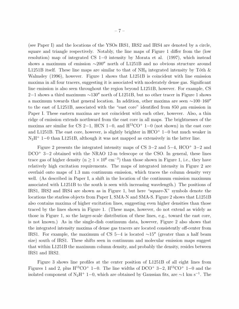
Figure 3 shows line profiles at the center position of L1251B of all eight lines from

Figures 1 and 2, plus H13CO+ 1−0. The line widths of DCO+ 3−2, H13CO+ 1−0 and the

isolated component of N2H+ 1−0, which are obtained by Gaussian fits, are ∼1 km s−1. The

– 8 –

line widths of HCN 1−0 and N2H+ 1−0, which are obtained by their hyperfine structure

fits, are ∼1.4 and ∼1.2 km s−1, respectively, probably affected by their optical depths. The

width of CS 5−4, however, is ∼2.6 km s−1. Line wings are seen in the spectra of HCO+ 3−2,

CS 5−4 and HCN 1−0. All profiles in Figure 3, except for H13CO+ 1−0, DCO+ 3−2, and

the isolated component of N2H+ 1−0 are asymmetric with blueshifted peak temperatures.

The peak temperatures of the isolated component of N2H+ 1−0 and DCO+ 3−2 lines are

located close to the central velocity of L1251B, i.e., where the deepest dips are seen in the

other lines. We determined the central velocities of L1251B (−3.65 km s−1) and the east

core (−4.13 km s−1) by the Gaussian fitting of the isolated component of N2H+ 1−0 and

H13CO+ 1−0, respectively. Figure 4 shows profiles of five lines toward the east core, where

again asymmetric profiles with stronger blue peaks are seen in HCO+ 1−0, CS 2−1, and

HCN 1−0 but not H13CO 1−0. Such profiles are not seen everywhere across the region,

however, indicating a complex velocity distribution. For example, the CS 2−1 line profile

(not shown) has reversed asymmetry toward the northern maximum of CS 2−1. HCN 1−0

(not shown) also has a reversed profile between the east core and L1251B.

Figure 5a shows a map of red and blue components of CO 2−1 emission toward L1251B

only, from data obtained with the CSO 10.4-m Telescope. The velocity ranges for the red

and blue components of the outflow have been determined very conservatively from blue-

and red-free spectra (Figure 5b).

The extended outflow from L1251B, as seen by others, is plainly noticeable. The pro-

jected orientation of the CO outflow is northwest–southeast with blue or red components

respectively in the northwest or southeast. The two components overlap significantly at

L1251B, however, and the origin of the outflow is not easily identifiable due to the low

resolution of the map.

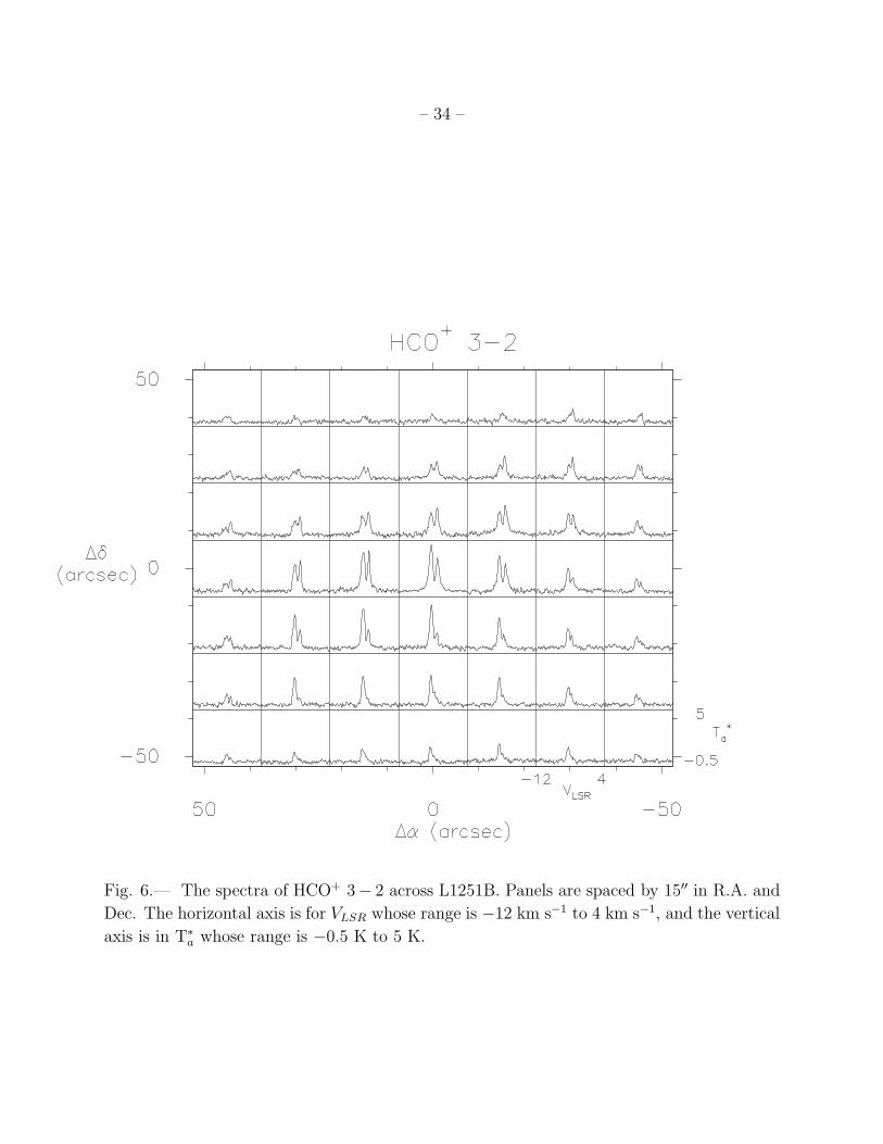
Figure 6 shows HCO+ 3−2 spectra from locations across L1251B. As seen in Figure 3,

the central spectrum shows a very strong self-absorption dip and an asymmetric profile with a

stronger blue peak. Figure 6 also reveals that the majority of lines off-center to L1251B have

asymmetric profiles with stronger blue peaks, especially with increasing of the asymmetry

with a stronger blue peak to the south. Not all the spectra are asymmetric with stronger blue

peaks, however. To the north, the spectra are double-peaked more symmetrically, and in

the north, reversed (red) asymmetry is seen. Note that the distribution of HCO+ integrated

intensities at L1251B (Figure 2c) is elongated through the northwest–southeast direction.

The outflow map (not shown) from the HCO+ 3−2 wing components seen in Figure 3 shows

the same trend as seen in the CO 2−1 outflow map, i.e., a northwest–southeast extension

and a significant positional overlap between the blue and red components.

– 9 –

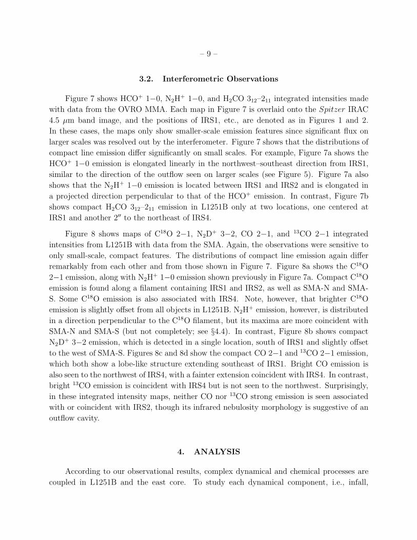
3.2. Interferometric Observations

Figure 7 shows HCO+ 1−0, N2H+ 1−0, and H2CO 312–211 integrated intensities made

with data from the OVRO MMA. Each map in Figure 7 is overlaid onto the Spitzer IRAC

4.5 µm band image, and the positions of IRS1, etc., are denoted as in Figures 1 and 2.

In these cases, the maps only show smaller-scale emission features since significant flux on

larger scales was resolved out by the interferometer. Figure 7 shows that the distributions of

compact line emission differ significantly on small scales. For example, Figure 7a shows the

HCO+ 1−0 emission is elongated linearly in the northwest–southeast direction from IRS1,

similar to the direction of the outflow seen on larger scales (see Figure 5). Figure 7a also

shows that the N2H+ 1−0 emission is located between IRS1 and IRS2 and is elongated in

a projected direction perpendicular to that of the HCO+ emission. In contrast, Figure 7b

shows compact H2CO 312–211 emission in L1251B only at two locations, one centered at

IRS1 and another 2′′ to the northeast of IRS4.

Figure 8 shows maps of C18O 2−1, N2D+ 3−2, CO 2−1, and 13CO 2−1 integrated

intensities from L1251B with data from the SMA. Again, the observations were sensitive to

only small-scale, compact features. The distributions of compact line emission again differ

remarkably from each other and from those shown in Figure 7. Figure 8a shows the C18O

2−1 emission, along with N2H+ 1−0 emission shown previously in Figure 7a. Compact C18O

emission is found along a filament containing IRS1 and IRS2, as well as SMA-N and SMA-

S. Some C18O emission is also associated with IRS4. Note, however, that brighter C18O

emission is slightly offset from all objects in L1251B. N2H+ emission, however, is distributed

in a direction perpendicular to the C18O filament, but its maxima are more coincident with

SMA-N and SMA-S (but not completely; see §4.4). In contrast, Figure 8b shows compact

N2D+ 3−2 emission, which is detected in a single location, south of IRS1 and slightly offset

to the west of SMA-S. Figures 8c and 8d show the compact CO 2−1 and 13CO 2−1 emission,

which both show a lobe-like structure extending southeast of IRS1. Bright CO emission is

also seen to the northwest of IRS4, with a fainter extension coincident with IRS4. In contrast,

bright 13CO emission is coincident with IRS4 but is not seen to the northwest. Surprisingly,

in these integrated intensity maps, neither CO nor 13CO strong emission is seen associated

with or coincident with IRS2, though its infrared nebulosity morphology is suggestive of an

outflow cavity.

4. ANALYSIS

According to our observational results, complex dynamical and chemical processes are

coupled in L1251B and the east core. To study each dynamical component, i.e., infall,

– 10 –

rotation, and outflow, in detail, we describe in this section the analysis of line profiles using

line radiative transfer calculations and the simulation of observed line profiles (§4.1), centroid

velocity maps and a position-velocity diagram (§4.2), and channel maps (§4.3), respectively.

In addition, we calculate the chemical evolution coupled with the evolution of density and

luminosity to compare the relative distribution of observed various molecular line emission

with a chemical model (§4.4).

4.1. Infall

Toward L1251B, optically thick molecular transitions such as HCO+ 1−0 and 3−2 show

an asymmetrical profile with the brighter blue peak (see Figure 3). In addition, optically

thin molecular transitions, such as H13CO+ 1-0 and DCO+ 3-2 line are symmetrical, and

peak at the velocities of the deepest dips of the other lines. Taken together, such profiles

can be indicative of infall motions (see Zhou et al. 1993). In general, infalling gas will have

motions both positive and negative along the line of sight, and if an excitation gradient exists

also along line of the sight, redward self-absorption of gas emission can occur.

L1251B was modeled as an inside-out collapsing sphere (cf. Shu 1977) by Young et al.

(2003), using continuum emission at 450 µm and 850 µm to find density and temperature

profiles of the core. The model parameters provided by Young et al., however, do not

correspond to the best-fit model (C. Young, personal communication). Instead, the infall

radius of the actual best-fit collapse model of L1251B is 5000 AU, equivalent to an infall

timescale of 5×104 years, rather than the 3000 AU provided by Young et al. Other parameters

of the best-fit model are the same, i.e., an effective sound speed of 0.46 km s−1 and a total

luminosity of 10 L⊙. The model with a 5000 AU infall radius provides much better SED fit.

In the current best-fit model, the reduced χ2 for intensity profiles at 450 µm and 850 µm

and the SED are 17, 27, and 3, respectively (compare with χ2 in Table 9 and 11 of Young

et al.)

Figure 9 shows the density and velocity profiles of the best-fit inside-out collapse model.

We have used the physical profiles to model HCO+ 3−2/1−0, H13CO+ 1−0 and CS 5−4 lines

with a Monte-Carlo radiative transfer code (Choi et al. 1995). These lines trace the densest

region, i.e., where the infall velocity is significant, among the lines observed with single dish

telescopes. To minimize a contribution from rotational motions, line profiles observed only at

the core center have been modeled. The kinetic temperature profile (the dotted line in Figure

9a) has been calculated with a gas energetics code (Young et al. 2004; Doty & Neufeld 1997)

from the dust temperature profile obtained from the dust continuum modeling. Abundance

profiles of HCO+ and CS were calculated with the chemo-dynamical model developed by

– 11 –

Lee et al. (2004). (This chemical calculation and its results will be described in §4.4.)

Although an interferometric observation is necessary to study whether the high velocity

wings of CS 5−4 are affected by outflow, Figure 10 shows that the density and infall velocity

structures from the best-fit model of dust continuum observations can reproduce reasonably

well the observed line profiles detected at the center of the core, especially CS 5−4. Note,

however, that it was necessary to reduce the abundance profile of HCO+ by a factor of

2 from that calculated by the chemical model, to fit the HCO+ 3−2/1−0 line. The line

profile of H13CO+ 1−0 was also fitted reasonably well with the HCO+ abundance profile and

the isotopic ratio of 12C/13C= 77 (Wilson and Rood 1994). The dotted line in the Figure

presents the comparison case without infall. In this model, constant turbulent widths of

0.6 km s−1 and 0.25 km s−1 (FWHM = 1 and 0.4 km s−1, respectively) were assumed at

radii respectively less than and greater than the infall radius. Having less turbulent motion

in the outer stationary envelope than in the inner infalling envelope is necessary to fit the

width of the self-absorption feature, especially that in HCO+ 3−2. The broad line wings of

HCO+ 3−2/1−0 and H13CO+ 1−0, particularly pronounced in the blueshifted emission, are

probably caused by outflowing material, which is not considered in this model. The higher

ratio between blue and red peaks of the observed line profiles than the modeled ones, which

is commonly seen and never understood, might be affected by the rotational motion or the

non-spherical geometry.

4.2. Rotation

Beyond the central position of L1251B, variations of the line profiles and position-

velocity diagrams suggest rotational motions. For example, the HCO+ 3−2 line profiles

shown in Figure 6 at positions offset from (0,0) show asymmetry reversals and increases

that may be caused by rotational motions (e.g., see Walker et al. 1994; Zhou 1995; Ward-

Thompson & Buckley 2001). A simulation of the HCO+ 3−2 spectra with a 2-D Monte Carlo

molecular line radiative transfer code (Hogerheijde & van der Tak 2000) for the collapse from

a rotating dense cloud (Terebey, Shu & Cassen 1984) indeed produces the distribution of

blue- and red-asymmetric profiles observed in L1251B (Lee et al., in preparation). Note,

however, that the wings of line profiles along the projected outflow direction may be still

affected by outflow motions (see §4.3 below).

Previous studies (Goodman et al. 1993; Sato et al. 1994; Toth & Walmsley 1996;

Anglada et al. 1997; Morata et al. 1997) determined that the overall velocity gradient in the

L1251B neighborhood, i.e., that covered by the extended 850 µm map in Figure 1, was ∼1-2

km s−1 pc−1 in the northeast–southwest direction. Observations by Caselli et al. (2002),

– 12 –

however, revealed a more complex velocity distribution in the neighborhood, with gradients

of opposite direction. Namely, L1251B itself is associated with a southwest–northeast gra-

dient, while the east core is associated with a northeast–southwest gradient. The average

direction reported in their paper, however, is also northeast–southwest, suggesting that the

previous studies, with poorer resolutions, averaged out the velocity gradient associated with

L1251B, whose velocity gradient is only about half of that in the east core. To determine the

velocity gradient associated with L1251B and the east core at higher resolution, we fitted

the hyperfine structures of HCN 1−0 and N2H+ 1−0 and the Gaussian profile of H13CO+

1−0, and found the same result as shown in Figure 6 of Caselli et al. For illustration, Figure

11 shows the centroid velocity distribution obtained from HCN 1−0, which shows different

velocity gradients in L1251B and the east core. The derived velocity gradient from HCN

1−0 in L1251B within 80′′ is ∼ 3/cos(i) km s−1 pc−1 in the southwest–northeast direction

but the velocity gradient in the east core is ∼ 6/cos(i) km s−1 pc−1 in the opposite direction,

i.e., consistent with the direction predicted from previous studies. Here, i is the inclination

of the rotational axis from the plane of sky.

We have analyzed the centroid velocity shift in L1251B with the N2H+ 1−0 interferom-

eter data (see Figures 7a and 8a). Figure 12a shows a 2-D distribution of the mean centroid

velocity with the integrated intensity contours of the isolated component of N2H+ 1−0 ,

which were calculated with the AIPS task, MOMNT. A clear shift of the centroid velocity

is seen from the southwest to the northeast, along a direction perpendicular to the outflow

direction. This southwest–northeast direction is opposite to directions of velocity gradient

seen in previous studies with lower resolution but consistent with the result of Caselli et al.

(2002) and that seen in HCN 1−0 (Figure 11) toward L1251B. A position-velocity diagram

taken along a cut centered at (9′′, −2′′) and along P.A. = 33 (similar to the direction of

maximum elongation of the N2H+ emission) is seen in Figure 12b. The rotational motion

suggested by this gradient is very fast, i.e., 30/cos(i) km s−1 pc−1, Ω ∼ 10−12/cos(i) s−1

within 30′′. This gradient is ∼1 order of magnitude larger than what is seen on larger scales,

such as in the HCN map (Fig. 11), suggesting an increased importance of rotation on small

scales.

4.3. Outflow

In this section, we examine at high angular resolution the outflowing gas from the young

stellar objects in L1251B, and provide an initial interpretation of the data. Although the

evidence for outflows in this region is strong, the spatial distribution of this gas is very

irregular, making it difficult to associate the observed outflow features with specific objects.

– 13 –

Figure 13 shows the CO 2−1 integrated intensity across L1251B as observed from the

SMA, divided into red and blue components (emission at line center is excluded). For

reference, the CO components are overlaid onto the 1.3 mm continuum emission across

L1251B, also observed from the SMA. Figures 14 and 15 show channel maps of CO 2−1

respectively for red- and blueshifted emission. For reference, the CO emission in each channel

is overlaid here onto the N2H+ 1-0 integrated intensity as observed from the OVRO millimeter

array. (Note that the velocity range definitions of red- and blueshifted emission are slightly

different in these Figures than those used for Figures 5 and 13 because of the difference

in their velocity resolutions.) In Figures 14 and 15, we also include more channel maps at

-1.2 km s−1, and -5.4 and -6.5 km s−1, in the red- and blueshifted emission, respectively, to

resolve different outflow components. For an alternative view of the outflows associated with

L1251B, Figure 16 shows channel maps of HCO+ 1-0 observed from OVRO. In the channel

maps, especially for blueshifted emission (Figure 15 and 16), velocities closer to the central

velocity than defined conservatively in Figure 5 and 13 are covered. While the HCO+ 1-0

emission around the central velocity peaks at SMA-S, which is the densest part in L1251B,

at -5.2 and -5.6 km s−1, it has peaks at IRS1 and southeast of IRS4 with a weaker tail

toward the northwest of IRS4. Therefore, HCO+ 1-0 mainly traces the outflowing material

even at the velocity up to ∼ −5 km s−1. In addition, the comparison between the model and

observation of HCO+ 1-0 in Figure 5b suggests that the emission at -5 km s−1 is affected

only by the outflow.

As can be seen from Figure 13, significant outflow appears to be associated with IRS1.

This emission, however, may also include a component from SMA-S. Bright emission is seen

extending southeast of IRS1, with blueshifted emission to the east-southeast and redshifted

emission to the south-southeast and some positional overlap of these components to the

southeast. The overlap of the components could indicate a single outflow where the in-

clination of the axis from the plane of sky is not large and the blue and red components

respectively trace the front and back components of an outflow cone. Note, however, that

in the redshifted -1.2 km s−1 channel of Figure 14, the feature divides into two components,

one associated to the west and southwest of IRS1 and another to the southwest of SMA-S.

Note also the pair of distinct components seen in Figure 15, associated with IRS1 in one

blueshifted pair of channels at -5.4 km s−1 and -6.5 km s−1 and associated with SMA-S in

another blueshifted pair of channels at -9.6 km s−1 and -11 km s−1. In the latter case, the

emission may have been made compact and elongated in the northwest-southeast direction

due to higher densities to its immediate northeast, as evident from the N2H+ emission and

the higher-excitation line emission (see Figure 2).

For IRS2, a single redshifted feature is seen extending to its southeast in Figure 13, and

this feature is also seen in the CO channel maps from 2 km s−1 to -1.2 km s−1 of Figure 14. No

– 14 –

corresponding blueshifted feature is obviously associated with IRS2, however. It is possible

that the blueshifted feature near IRS1 seen at -5.4 km s−1 and -6.5 km s−1 is associated

with IRS2 instead. For example, CO may be severely depleted in the dense regions between

IRS1 and IRS2, and the blueshifted outflow from IRS2 may be only visible in CO near IRS1

because of localized high CO abundance due to the evaporation of CO from nearby dust

grains. Note, however, that this blueshifted emission lies in a similar northwest-southeast

direction as redshifted emission from IRS1. Alternatively, the extended redshifted feature

southeast of IRS2 may be related to IRS1 itself.

Northwest of IRS4, Figure 13 shows red- and blueshifted features with very significant

positional coincidence. Again, these features could be due to a single outflow of low in-

clination. The channel maps of Figure 14 and 15 suggest a more complex interpretation,

however, with weak red- and blueshifted emission seen both northwest and east of IRS4 at

-1.2 km s−1, -5.4 km s−1 and -6.5 km s−1. Figure 16 shows blueshifted emission from HCO+

1-0 also located to the east and the northwest of IRS4. Instead, there may be two outflows

present, one centered at IRS4 and another to the northwest. This latter may originate from

IRS1 and could be the counterpart to the redshifted emission seen southeast of IRS2. Note

that not much material is seen between IRS4 and IRS1, in the continuum emission maps of

Figures 2 and 9 or the CO 2−1 channel maps of Figure 13. Compact HCO+ 1−0 emission

is seen between IRS4 and IRS1, however, in Figure 16 from -6 km s−1 to -5 km s−1. The

strongest HCO+ emission is seen southeast of IRS4, and this may constitute a blueshifted

outflow component from IRS4.

A summary of the possible outflows in the L1251B region is shown in Figure 17, with

outflow components schematically plotted over the 1.3 mm continuum emission observed

with the SMA. In this picture, IRS1, IRS2, IRS4 and even SMA-S all have outflows, some

of which interact with each other. If SMA-S indeed has an outflow, it is not a starless

condensation after all. Instead, it may harbor a very low luminosity protostellar object that

was undetected by Spitzer. The existence of such objects has been surmised by others; e.g.,

Rebull et al. (2007) suggested that several objects unseen at λ < 70 µm could be driving

numerous outflows observed in HH 211. Future observations of L1251B, at even higher

resolutions or using various lines that clearly trace gas shocked by outflow motions (e.g.,

mid-infrared lines of H2 or millimeter lines of SiO), will be very helpful in disentangling the

association of the outflows with specific sources and their effects on the evolution of the

L1251B core.

– 15 –

4.4. Chemistry

Within L1251B, our high-resolution maps provide continued evidence for the expected

chemical behavior of dense gas not associated with protostars. For example, the HCO+

features shown in Figure 7a likely traces outflowing dense gas, since HCO+ can be made

abundant through shocks (see Rawlings et al. 2004). As with HCO+, the CO, 13CO, and

diffuse C18O emission seen in Figures 8a, c and d may also be due to extensive depletion

in the extended envelope and enhancements along the outflow axis due to liberation from

grains. Emission from these lines indeed share some common features, but note that no

compact CO, 13CO, or C18O emission is seen between IRS1 and IRS4. A faint ridge of

HCO+ 1−0 emission is seen at that location in the level of 2 σ, however.

In addition, the N2H+ feature shown in Figure 7a likely traces non-outflowing gas,

since N2H+ can remain abundant in cold dense material and can be depleted significantly in

outflows. N2H+ is a chemical daughter of N2, which forms slowly. The interactions between

N2H+ and grains replenish N2 in the gas phase because N2H

+ recombines with electrons

on the grain surfaces. The principal destroyers of N2H+ in the gas phase are CO and

electrons. CO can be significantly depleted in starless cores (Bergin & Langer 1997) because

the only source of heating is the interstellar radiation field and the inner temperatures of

such cores can be correspondingly very low (e.g., ∼7 K; see Evans et al. 2001). Also, the

electron abundance can be very low (∼ 10−9, Williams et al. 1998) in dense gas that is

highly extincted, like that in starless cores. The N2H+ emission seen in Figure 7a and 8a is

consistent with the 1.3 mm dust continuum emission mapped by the IRAM 30-m Telescope

(see Paper I), suggesting it is also tracing cold, dense gas.

N2H+ (and N2D

+) will also deplete at densities greater than 106 cm−3 (Di Francesco,

Andre & Myers 2004; Pagani et al. 2005). Note that the two N2H+ intensity maxima

in Figure 7a and 8a are offset slightly to the east from SMA-N and SMA-S, which trace

the densest parts of L1251B. (The C18O emission observed with the SMA does not have

maxima at SMA-N and SMA-S either.) In addition, an N2D+ emission maximum is found

between IRS1 and SMA-S. Finally, no such emission is associated with SMA-N. The offset

of the N2H+ maxima and deficiencies of N2D

+ from these objects are possibly caused by the

depletion from the gas phase at densities greater than 106 cm−3. The N2D+ emission may be

identifying a less dense location that has a high enough temperature to populate significantly

N2D+ at J=3. For example, the J=3 level of N2D

+ has its maximum population in thermal

equilibrium at ∼20 K, and this may be caused by heating by IRS1. (Note, however, that

the temperature there cannot be greater than 30 K, because otherwise CO would evaporate

off dust grains and reduce the N2D+ abundance.)

Our high-resolution observations of L1251B show further examples of the chemical be-

– 16 –

havior expected in the presence of nearby protostellar heating. Once a protostar forms, the

surrounding material is heated up to the CO evaporation temperature (∼25 K in the case

of bare SiO2 dust grains). The desorbed CO destroys N2H+, producing an N2H

+ emission

“hole” around the central heating source, that is potentially observable with interferometers.

Such holes may explain the lack of N2H+ emission coincident with IRS1 and IRS2, as seen

in Figures 7a and 8a. In contrast, the abundances of other molecules such as CS, H2CO,

and HCO+ can be enhanced due to protostellar heating resulting in the desorption of CO or

the desorption of themselves off of dust grain mantles (Lee, Bergin & Evans 2004) as seen

in Figure 7b. In L1251B, IRS1 is luminous enough to evaporate CO in its inner envelope.

Similar N2H+ emission holes have been seen toward NGC 1333 IRAS 4A (Di Francesco et

al. 2001) and L483 (Jørgensen 2004).

Figure 18 shows the results of a chemical evolution model made specifically for L1251B

to quantify the observed line emission distributions. For this model, we used the chemo-

dynamical model developed by Lee et al. (2004). We updated the chemical network to

include more recent results on the N2H+ chemistry, however, including a new binding energy

of N2, which is the same as that of CO (Oberg et al. 2005), and new rates of dissociative

recombination of N2H+ with electrons (Geppert et al. 2004). We also increased the initial

abundance of sulfur by a factor of 3 to fit the CS 5−4 line profile in Figure 10a. The

initial abundances of other species are the same as those in Table 3 of Lee et al. (2004).

For a dynamical model, we adopted the best-fit Shu inside-out collapse model to the dust

continuum emission as described in §4.1. Although L1251B has several sources, only one

internal luminosity source at the center of a spherically symmetric envelope was assumed

in the model. Since IRS1 is the dominant luminosity source by a factor of ∼10, however

(see Paper I), this model is a reasonable first approximation, especially for interpreting the

single dish observations. For this model, the infall rate from the disk to central protostar

was tuned appropriately to match the luminosity calculated by observations at the given

timescale (Young & Evans 2005). In addition, the interstellar radiation field was assumed to

be attenuated to G0 = 0.3 for consistency with the dust continuum modeling. An outflow

was not included.

We do not compare this chemical model with interferometric observations quantitatively

since the density profile assumed in the 1-D model is not appropriate for the high resolution

observations that reveal multiple sources. The chemical distribution close to the central

source, however, is most sensitive to the temperature environment, so we can look for the

effects of temperature increases around IRS1 on the chemical abundances. As seen in Figure

18, the model predicts a CO evaporation radius (which accordingly is also the N2H+ depletion

radius) of ∼0.007 pc (∼4′′), i.e., similar to the observed radius of the N2H+ hole at a 2 σ level

of integrated intensity (see Figure 7a). Furthermore, the model predicts an H2CO abundance

– 17 –

peak at a radius of ∼0.003 pc (∼2′′), similar to the radius of the H2CO emission at the 2 σ

level of the integrated intensity (Figure 7b). A second H2CO abundance peak seen in Figure

18 caused by CO evaporation does not affect significantly the H2CO emission distribution

likely because of the lower density and temperature of material at ∼0.006 pc relative to

material at ∼0.003 pc associated with the inner abundance peak. Therefore, this simple

model is in good agreement with our observations close to the central source, where infall

is kinematically dominant, and chemistry mainly depends on the evaporation of molecules

from grain surfaces by heating.

Near IRS4, the associated H2CO emission may not be due to an increased abundance

due to localized dust grain heating. That source may not be luminous enough to heat grains

above the H2CO evaporation temperature at a projected distance of 600 AU. The coincidence

of the maxima of the integrated intensity of H2CO 312–211 (see Figure 7b) to one of that of

HCO+ 1-0 (see Figure 7a) suggests a possible origin from shocked outflow material. Note

that the H2CO emission close to IRS4 lies at redshifted velocities of −1.5 km s−1 to −3

km s−1, and lies spatially at a full synthesized beam width (2′′) northeast of IRS4.

5. DISCUSSION

5.1. L1251B

L1251B harbors a small group of starless and protostellar objects. Three of the latter

are classified as Class 0/I candidates, which are associated with dense envelopes. The obser-

vations of molecular lines around L1251B have revealed active processes, either dynamical

(infall, rotation and outflow) or chemical (depletion and enhancement).

The 1.3 mm dust continuum observations of L1251B with the SMA revealed two con-

densations (SMA-N and SMA-S) unassociated with any detected near-infrared source. (Note

that SMA-S may contain a newly formed protostellar object if an outflow originates from it;

see Figs. 14 and 15, and §4.3). Table 4 shows masses along the line of sight towards IRS1,

IRS2, SMA-N and SMA-S, determined using the peak intensities of the 1.3 mm image and

assuming a dust temperature of 20 K. We determined masses along the lines of sight rather

than total masses from the respective fluxes because the extents of each were difficult to

define with certainty in the crowded field, especially for SMA-N and SMA-S. Furthermore,

any differences in mass along the line of sight could be more easily discerned with a sin-

gle sampling. Table 4 shows that the peak intensities are quite similar (i.e., within 50%),

suggesting quite similar masses along the line of sight if the temperatures are common. If

we assume for SMA-N and SMA-S a lower temperature of 10 K, which is more commonly

– 18 –

adopted for starless cores, their masses along the line of sight are greater than those for 20

K (and IRS1 and IRS2) by a factor of ∼3.

Given their designations as protostars, the fluxes of IRS1 and IRS2 likely include emis-

sion from their respective disk components. In particular, IRS2 is not resolved at the ∼4′′

resolution of the data, which is equivalent to a ∼1200 AU linear distance at the 300 pc dis-

tance of L1251B. Since these sources are also highly embedded, however, the 1.3 mm fluxes

also likely contain emission from their inner envelopes. In contrast, the fluxes of SMA-N and

SMA-S likely include emission only from envelopes since these sources are not seen if lower

spatial frequences (i.e., <11 kλ) are excluded, as discussed in Paper I. To distinguish the

disks of IRS1 and IRS2 (as well as a possible disk of SMA-S) associated with outflows (§4.3),

observations with higher resolution are needed. Note that 1.3 mm continuum emission is not

detected towards IRS4, suggesting that it is not associated with any disk or inner envelope

that could be detected at our sensitivity and resolution.

All objects in L1251B possibly form by fragmentation during gravitational collapse

(Boss 1997; Machida et al. 2005). Turbulent fragmentation seems unlikely since the lines

observed toward L1251B are not so broad as to be considered dominated by turbulence.

For example, tracers of very dense gas such as DCO+ 3−2, N2H+ 1−0, and H13CO+ 1−0

have line widths of ∼ 1 km s−1, consistent with the infall velocity at n ∼ 106 cm−3 in the

best fit inside-out collapse model of L1251B. In addition, CS 5−4, which traces much higher

densities (n ≥ 5 × 106 cm−3), shows the broadest line width among all the high density

tracers we observed toward L1251B, i.e., ∼ 2.6 km s−1. Indeed, our inside-out collapse

model shows an infall velocity at 5 × 106 cm−3 of ∼ 2 km s−1. Also, the infall velocity

profile this model fits the observed CS 5−4 and HCO+ 3−2 reasonably well, with constant

turbulent widths of 0.6 km s−1 and 0.25 km s−1 at radii less than and greater than the infall

radius respectively (see Figure 10a). The velocity dispersions implied from such widths are

not much greater than the thermal velocity dispersion before collapse. (The dotted line in

Figure 10 presents the case without the infall velocity structure.) Therefore, the dynamics

of L1251B seem dominated by gravitational collapse, combined with rotation and outflows,

rather than turbulent motions.

5.2. The East Core

The east core seen in Figure 1 at 850 µm and in various molecular lines has a radius

of about 0.1 pc. The 850 µm emission shows several sub-cores inside a larger structure

traced by molecular emission. This difference may be related to a bias towards imaging

smaller-scale emission in the continuum data and related to high optical depths in the line

– 19 –

data. For the continuum data, the SCUBA observations were made by chopping onto the

sky, effectively filtering out emission on angular scales greater than the ∼120′′ chop throw

(see Di Francesco et al. 2007), i.e., those traced by the molecular line data. In addition,

the 850 µm continuum emission is very likely optically thin, tracing quite dense material

within a molecular core. For the line data, the molecular emission (see Figure 1) may have

high optical depths and the sub-cores may not be visible, despite the similarities between

the densities these particular lines trace and the mean density of the sub-cores, i.e., ∼105

cm−3. Differences in the positions of maximum integrated intensities between these lines

may also be due to their relative (but high) optical depths. (To determine if the ∼3× higher

resolution of the 850 µm map relative to the molecular line maps in Figure 1 contributed to

the different appearance of the continuum and line maxima, we smoothed the 850 µm map

to a resolution similar to that of the line maps (60′′). The smoothed 850 µm map, however,

still shows an emission hole near the maxima of the line maps.)

The low optical depth of the 850 µm emission suggests that the much stronger continuum

peak toward L1251B (∼1 Jy beam−1) relative to the east core (∼0.2 Jy beam−1) is indicative

of a larger column density toward L1251B even if L1251B has been heated by internal sources.

(Note that the 850 µm emission peaks close to SMA-S, not toward IRS1, as seen in Figure

6 of Paper I) The 850 µm fluxes of L1251B and the whole east core are similar, suggesting

that their masses are also similar if their temperatures and dust opacities are themselves

similar, i.e., ∼ 4 Jy and ∼ 2 M⊙ if T = 20 K and κ1.3mm = 0.02 cm2 g−1 (Krugel &

Siebenmorgen 1994). Since L1251B contains several YSOs but the east core does not, it

is likely that L1251B is warmer than the east core, however. Continuum observations at

multiple wavelengths and modeling are needed to determine better relative values of dust

temperature.

Table 5 lists the integrated intensities of molecular lines observed toward the centers of

L1251B and the east core. To probe for any relative chemical evolution in the two cores,

we compare the relative integrated intensities of the 1−0 transitions of H13CO+ 1−0 and

N2H+, molecules found to be abundant respectively at earlier and later times in models of

chemical evolution (e.g., Lee et al. 2003 and references therein). For H13CO+ 1−0, the

integrated intensities of L1251B and the east core are similar (i.e., ∼1.3 K km s−1 and ∼1.1

K km s−1 respectively). For N2H+, however, the integrated intensity towards L1251B is

larger than that towards the east core by a factor of two (i.e., ∼4 K km s−1 vs ∼2 K km s−1

respectively). The relative integrated intensity ratio between these lines, i.e., ∼6 for L1251B

and ∼3 for the east core, may be due to the relative chemical evolution, with L1251B being

more chemically evolved. (Note that the difference in N2H+ abundance might be greater than

the difference in the N2H+ 1−0 intensity due to the higher optical depth in L1251B.) Such

differences in chemical evolution may result from differences in density since the chemical

– 20 –

timescale shortens at a higher density. In addition, H13CO+ and its isotopologue HCO+

deplete significantly more than N2H+ in cold, dense environments such as in L1251B (except

in the immediate vicinities of protostellar objects). Therefore, the higher ratio between the

N2H+ and H13CO+ intensities in L1251B than in the east core (Figure 1) may be caused by

a denser environment in L1251B.

Various lines toward the east core suggest infall motions. Therefore, the east core may

be in earlier states of dynamical and chemical evolution than those of L1251B, and may

harbor star formation in the future.

6. SUMMARY

L1251E, the densest C18O core of L1251 (Sato et al. 1994), has been observed at various

molecular line transitions with single-dish telescopes, and L1251B, the protostellar group in

the C18O core, has been observed with millimeter interferometers. We have compared these

molecular line data to continuum data presented in Paper I to study this region of L1251

more comprehensively. Our results include:

1. L1251E contains at least two cores, one coincident with L1251B and an east core

detected from 850 µm continuum emission and various emission lines. The integrated in-

tensities of these lines show primary maxima that are coincident with L1251B and other,

secondary maxima associated with the east core which are non-coincident. No embedded

sources have been detected in the Spitzer IRAC or MIPS bands toward the east core (Paper

I), suggesting it is starless. Asymmetric profiles with stronger blue peaks have been detected

toward the eastern core, however, that are suggestive of infall motions. The east core appears

less dense and less chemically evolved than L1251B.

2. The large-scale outflow associated with L1251B has been mapped in CO 2−1 with

the CSO. Red and blue components of the outflow overlap around the brightest protostar,

IRS1, and the near-infrared bipolar nebula source, IRS2. The CO 2−1 and 13CO 2−1 maps

observed with the SMA resolve the outflow into a few components.

3. HCO+ 3−2 line emission observed with the CSO across L1251B shows widespread

line asymmetry that suggests infall motions towards the central group, with evidence for

rotational or outflow motions from modifications of the line profiles at many off-center loca-

tions.

4. On a large scale, L1251B has a velocity gradient that is half the magnitude of that

in the starless east core and is opposite in direction. Previous low-resolution observations

– 21 –

averaged the velocity gradients of both, causing rotational motions in the region to be mis-

interpreted.

5. HCO+ 1−0 line emission observed with the OVRO MMA is centered at IRS1 and

distributed linearly along the northwest–southeast direction of the larger-scale outflow. In

contrast, the N2H+ 1−0 line emission also observed with the OVRO MMA is distributed

between IRS1 and IRS2 (like the position of maximum brightness of the IRAM 1.3 mm

continuum emission) and extended perpendicular to the outflow, i.e,. along the southwest–

northeast direction. A position-velocity diagram of N2H+ 1−0 indicates very fast rotation in

this flattened envelope, i.e., Ω ∼ 10−12/cos(i) s−1, where i is the inclination of the rotational

axis from the plane of sky.

6. The maxima of N2H+ 1−0 and N2D

+ 3−2 integrated intensity observed with the

OVRO MMA and SMA are offset from locations of maximum continuum brightness from

the two starless objects, which were newly detected at 1.3 mm with the SMA (Paper I). This

offset may be due to reduction of N2H+ and N2D

+ abundances at very high densities.

7. OVRO MMA and SMA observations reveal a lack of N2H+ emission at IRS1 (i.e., a

“hole”) but C18O and the H2CO emission is coincident with IRS1. These results are consis-

tent with a chemo-dynamical evolution model where a central protostar heats up surrounding

material. In this model, CO and H2CO are abundant close to the protostar where they are

released into the gas phase from grain mantles, but N2H+ has had its abundance sharply

reduced since it is depleted by reactions with gas-phase CO.

Support for this study was provided by NASA through Hubble Fellowship grant HST-

HF-01187 awarded by the Space Telescope Science Institute, which is operated by the As-

sociation of Universities for Research in Astronomy, Inc., for NASA, under contract NAS

5-26555. This work was also supported by NSF grant AST-0307350 to the University of

Texas at Austin and by the State of Texas. We are very grateful to an anonymous referee

for valuable comments. We thank Jonathan Williams for allowing us to use his unpublished

molecular line data, and we also thank Chad Young for his help for the dust continuum

modeling of L1251B. We are also very grateful to Anneila Sargent for providing us the

opportunity to observe L1251B with the OVRO MMA.

REFERENCES

Aikawa, Y., Ohashi, N., Inutsuka, S.-I., Herbst, E. & Takakuwa, S. 2001, ApJ, 552, 639

Anglada, G., Sepulveda, I., & Gomez, J.F. 1997, A&AS, 121, 255

– 22 –

Bergin, E.A. & Langer, W.D. 1997, ApJ, 486, 316

Boss, A.P. 1997, ApJ, 483, 309

Caselli, P., Benson, P. J., Myers, P. C., & Tafalla, M. 2002, ApJ, 572, 238

Caselli, P., Myers, P. C., & Thaddeus P. 1995, ApJ, 455, L77

Choi, M., Evans, N. J., II, Gregersen, E. M., & Wang, Y. 1995, ApJ, 448, 742

Di Francesco, J., Myers, P. C., Wilner, D. J., Ohashi, N. & Mardones, D. 2001, ApJ, 562,

770

Di Francesco, J., Andre, P., and Myers, P. C. 2004, ApJ, 617, 425

Di Francesco, J., Evans, N.J., II, Caselli, P., Myers, P.C., Aikawa, Y., & Tafalla, M. 2006,

in Protostars and Planets V, eds. B. Reipurth, D. Jewitt, & K. Kiel, (University of

Arizona: Tucson), in press (astro-ph/0602379)

Di Francesco, J., Johnstone, D., Kirk, H. M., MacKenzie, T. & Ledwosinska, E. 2007, ApJS,

submitted.

Doty, S.D. & Neufeld, D.A. 1997, 489, 122

Doty, S.D., van Dishoeck, E.F., van der Tak, F.F.S., & Boonman, A.M.S. 2002, A&A, 389,

446

Evans, N.J.II, Rawlings, J.M.C., Shirley, Y., & Mundy, L.G. 2001, ApJ, 557, 193

Geppert, W. D., Thomas, R., Semaniak, J., Ehlerding, A., Millar, T., Osterdahl, F., af

Ugglas, M., Djuric, N., Paal, A., & Larsson, M. 2004, ApJ, 609, 459

Goodman, A.A., Benson, P.J., Fuller, G.A., & Myers, P. 1993, ApJ, 406, 528

Gregersen, E.M., Evans, N.J.,II, Mardones, D.M., & Myers, P.C. 2000, ApJ, 533, 440

Hogerheijde, M.R. & van der Tak, F.F.S. 2000, A&A, 362, 697

Jørgensen, J.K. 2004, 424, 589

Kruegel, E. & Siebenmorgen, R. 1994, A&A, 288, 929

Kun, M. & Prusti, T. 1993, A&A, 272, 235

Lada, C.J. & Lada, E.A 2003, ARA&A, 41, 57

Lee, J.-E., Evans, N.J.,II, Shirley, Y.L., & Tatematsu, K. 2003, ApJ, 583, 789

Lee, J.-E., Bergin, E.A., & Evans, N.J.II 2004, ApJ, 617, 360

Lee, J.-E., et al. 2006, ApJ, 648, 491

Mardones, D., Myers, P. C., Tafalla, M., Wilner, D. J., Bachiller, R., Garay, G. 1997, ApJ,

489, 719

– 23 –

Machida, M.N., Matsumoto, T., Hanawa, T., & Tomisaka, K. 2005, MNRAS, 362, 382

Morata, O., Estalella, R., Lopez, R., & Planesas, P. 1997, MNRAS, 292, 120 ApJ, 376, 618

275

Myers, P. C., Evans, N. J., II, & Ohashi, N. 2000, in “Protostars and Planets IV,” eds. V.

Mannings, A. P. Boss & S. S. Russell, (University of Arizona: Tucson), p. 217

Oberg K. I., van Broekhuizen, F., Fraser, H. J., Bisschop, S. E., van Dishoeck, E. F., &

Schlemmer, S. 2005, ApJ, 621, 33

Pagani, L., Pardo, J.-R., Apponi, A. J., Bacmann, A. & Cabrit, S. 2005, A&A, 429, 181

H. M. Pickett, R. L. Poynter, E. A. Cohen, M. L. Delitsky, J. C. Pearson, and H. S. P. Muller

1998, ”Submillimeter, Millimeter, and Microwave Spectral Line Catalog,” J. Quant.

Spectrosc. & Rad. Transfer 60, 883-890

Rawlings, J.M.C. & Yates, J.A., 2001, MNRAS, 326, 1423

Rawlings, J.M.C., Redman, M. P., Keto, E. & Williams, D. A. 2004, MNRAS, 351, 1054

Rebull, L. M., et al. 2007, ApJS, in press (astro-ph/0701711)

Sato, F. & Fukui, Y. 1989, ApJ, 343, 773

Sato, F., Mizuno, A., Nagahama, T., Onishi, T., Yonecura, Y., & Fukui, Y. 1994, 435, 279

Shu, F.H. 1977, ApJ, 214, 488

Shirley, Y.L., Evans, N.J.II, Rawlings, J.M.C. & Gregersen, E.M. 2000, ApJS, 131, 249

Snell, R. L., Loren, R. B., & Plambeck, R. L. 1980, ApJ, 239, L17

Terebey, S., Shu, F.H., & Cassen, P. 1984, ApJ, 286, 529

Toth, L.V. & Walmsley, C.M 1996, A&A, 311, 981

Walker, C.K., Narayanan, G., & Boss, A.P. 1994, ApJ, 431, 767

Ward-Thompson, D. & Buckley, H.D. 2001, MNRAS, 327, 955

Williams, J.P, Bergin, E.A., Caselli, P., Myers, P.C., & Plume, R. 1998, ApJ, 503, 689

Wilson, T.L. & Rood, R.T., 1944, ARAA, 32, 191

Young, C.H., Shirley, Y.L., Evans, N.J.II, & Rawlings, J.M.C. 2003, ApJS, 145, 111

Young, K.E., Lee, J.-E., Evans, N.J.,II, Goldsmith, P.F., & Doty, S.D. 2004, ApJ, 614, 252

Young, C.H. & Evans, N.J.II 2005, ApJ, 627, 293

Zhou, S., Evans, N.J.II, Koempe, C., & Walmsley, C.M 1993, 404, 232

– 24 –

Zhou, S. 1995, ApJ, 442, 685

This preprint was prepared with the AAS LATEX macros v5.2.

– 25 –

Table 1. Molecular line observations with single-dish telescopes

Line ν δv θmb ηmba Observing Dates Observatory

(GHz) (km s−1) (arcsec)

H13CO+ 1−0 86.754285 0.14 62 0.5 April 1997, May 2000 FCRAO

HCN 1 − 0 88.631847 0.10 61 0.5 February 2005 FCRAO

HCO+ 1−0 89.188523 0.13 60 0.5 April 1997, May 2000 FCRAO

N2H+ 1−0 93.176265 0.13 58 0.5 December 1996 FCRAO

CS 2 − 1 97.980968 0.10 55 0.5 February 2005 FCRAO

DCO+ 3 − 2 216.112605 0.13 34.7 0.74 July 2003 CSO

CO 2 − 1 230.53800 0.12 32.5 0.64 July 2003 CSO

HCO+ 3−2 267.557526 0.12 22.5 0.67 June 1997, July 1998 CSO

CS 3 − 2 146.969048 0.10 43 0.8b October 1997 NRAO

CS 5 − 4 244.935606 0.12 26 0.5b May 1996 NRAO

aThis main beam efficiency is used to convert the antenna temperature (T ∗

a ), only corrected

for atmospheric attenuation, radiative loss and reward scattering and spillover, to the radiation

temperature.

bThese numbers represent the corrected main beam efficiencies (η∗

m) to convert the antenna

temperature (T ∗

R), corrected for forward scattering and spillover as well as atmospheric attenu-

ation, radiative loss and reward scattering and spillover, to the radiation temperature.

–26

–

Table 2. OVRO Observational Summary

Channel Gaussian Synthesized Synthesized

Bandwidth Spacing Taper FWHM Beam FWHM Beam P.A. 1 σ rmsa

Tracer Transition (MHz) (km s−1) (′′ × ′′) (′′ × ′′) () (Jy beam−1)

H2CO 312–211 7.00 0.17 1.60 × 1.60 2.5 × 2.3 304 0.1

HCO+ 1–0 8.00 0.42 5.5 × 5.5 7.5 × 6.9 313 0.09

N2H+ 1–0 7.50 0.20 4.0 × 4.0 6.5 × 5.2 334 0.07

a1 σ rms computed from signal-free regions of the deconvolved maps.

– 27 –

Table 3. SMA Line Observations

Line Freq.a S-band Window Chans ∆V Beam FWHM P.A.

(GHz) (km s−1) (′′x ′′) (degree)

CO 2–1 230.5380000 USB 14 128 1.06 4.1 × 3.1 -26.213CO 2–1 220.3986765 LSB 13 512 0.26 4.3 × 3.4 -23.5

C18O 2–1 219.5603568 LSB 23 512 0.26 5.3 × 5.0 b 0.50

N2D+ 3–2 231.3216650 USB 23 512 0.26 5.1 × 5.0 b 10.4

SO 56–45 219.9494420 LSB 18 256 0.53 8.0 × 6.3 b,c 68.3

H132 CO 312–211 219.9085250 LSB 19 256 0.53 8.0 × 6.3b,c 68.3

aAll line frequencies listed were obtained from Pickett et al. (1998)

bBeam attained after tapering with a 4′′ × 4′′ FWHM Gaussian

cBeam attained after tapering with a 6′′ × 6′′ FWHM Gaussian

Table 4. SMA 1.3 mm peak intensities and masses

Source Peak Intensity, I(λ) (Jy beam−1)a Mass (M⊙ beam−1)b

IRS1 0.035 0.031

IRS2 0.023 0.020

SMA-N 0.023 0.020 (0.055)c

SMA-S 0.029 0.026 (0.070)c

aUncertainties on the peak intensities are 4 mJy beam−1.

bMasses have been calculated based on the equation,

Mass (M⊙ beam−1) = I(λ) d2

κλBλ(Tdust)= 0.88 × I(λ) (Jy beam−1) at

d = 300 pc and λ = 1.3 mm, which is derived from the assumptions

of (1) the 1.3 mm opacity (κλ) of 2 × 10−2 cm2 g−1 (Kruegel &

Siebenmorgen 1994) and (2) the dust temperature (Tdust) of 20 K

for the Planck function, Bλ.

cThe mass if Tdust = 10 K.

– 28 –

Table 5. Integrated Intensities of Molecular Lines (K km s−1)

Line L1251B East Core

HCO+ 1−0 6.6 7.6

H13CO+ 1−0 1.3 1.1

CS 2−1 3.2 2.8

HCN 1−0 4.2 (4)a 3.0 (0.85)a

N2H+ 1−0 7.8 (2.2)a 3.8 (1.7)a

aThe optical depth of the main

component obtained by the hyperfine

structure fit.

– 29 –

Fig. 1.— Integrated intensity maps (contours) of CS 2−1, HCN 1−0, HCO+ 1−0, and

N2H+ 1−0 on top of the 850 µm emission map (grey scale). The (0,0) position of this map

represents the coordinates of IRAS 22376+7455. In each panel, the small white circle, box

and triangle denote the positions of IRS1, IRS2 and IRS4 respectively. In each panel, the

grey scale used ranges from 0.084 to 0.420 Jy beam−1, roughly 2 σ to 10 σ, where 1 σ ≈

0.042 Jy beam−1. In each panel, the large black circle at lower left shows the beam FWHM.

In each panel, the dotted rectangle shows the extent of the map in the respective line. (For

CS 2−1 and HCN 1−0, the map was larger than the area shown.) a) Integrated intensity

map of CS 2−1. The velocity range used is −6.5 to −0.5 km s−1. The contours begin at 10

σ and increase by 6 σ where 1 σ = 0.06 K km s−1. b) Integrated intensity map of HCN 1−0.

The velocity range used is −13.5 to 4 km s−1. The contours begin at 10 σ and increase in

steps of 5 σ where 1 σ = 0.106 K km s−1. c) Integrated intensity map of HCO+ 1−0. The

velocity range used is −6 to −2 km s−1. The contours begin at 6 σ and increase in steps of

1.5 σ where 1 σ = 0.42 K km s−1. d) Integrated intensity map of N2H+ 1−0. The velocity

range used is −13 to 4 km s−1. The contours begin at 15 σ and increase in steps of 5 σ

where 1 σ = 0.166 K km s−1.

– 30 –

Fig. 2.— Integrated intensity maps (contours) of CS 3 − 2, 5 − 4, HCO+ 3−2, and DCO+

3−2 on top of the 1.3 mm dust continuum emission map (grey scale). The grey scale ranges

from 0.025 to 0.125 Jy beam−1 or about 2 σ to 10 σ, where 1 σ = 0.0125 Jy beam−1. In each

panel, the dotted rectangle denotes the extent of the map in the respective line. Symbols

are defined as in Figure 1 but here the square-X symbols indicate positions of peak intensity

of prestellar condensations detected in SMA 1.3 mm observations (see Figure 8 of Paper I).

a) Integrated intensity map of CS 3−2. The velocity range used is −6.5 to −0.5 km s−1.

The contours begin at 15 σ and increase in steps of 5 σ where 1 σ = 0.066 K km s−1. b)

Integrated intensity map of CS 5−4. The velocity range used is −6.5 to −0.5 km s−1. The

contours begin at 10 σ and increase in steps of 4 σ where 1 σ = 0.112 K km s−1. c) Integrated

intensity map of HCO+ 3−2. The velocity range used is −8 to 0 km s−1. The contours begin

at 3 σ and increase in steps of 3 σ where 1 σ = 0.545 K km s−1. d) Integrated intensity map

of DCO+ 3−2. The velocity range used is −5 to −2.5 km s−1. The contours begin at 3 σ

and increase in steps of 1 σ where 1 σ = 0.097 K km s−1.

– 31 –

Fig. 3.— The spectra of all molecular transitions observed with single dish telescopes (Table

1) at the center position. To present line profiles better, the order of lines has been chosen

arbitrarily, and spectra have been shifted up. The dotted vertical line indicates the centroid

velocity of L1251B, -3.65 km s−1.

– 32 –

Fig. 4.— The spectra of some molecular transitions observed with single-dish telescopes

toward the starless east core at (150′′, 25′′). To present line profiles better, the order of

lines has been chosen arbitrarily, and spectra have been shifted up. The dotted vertical

line indicates the centroid velocity of the east core, -4.13 km s−1 which is derived from the

Gaussian line fitting of H13CO+ 1−0.

– 33 –

Fig. 5.— a) The distribution of the outflow in L1251B in CO 2−1. Symbols are defined as

in Figure 1. The solid contours and dashed contours represent the blue and red components

of the outflow, respectively. Contours are every 1 K km s−1 from 1 K km s−1 (1 σ = 0.5

K km s−1). The velocity range used for the blue and red components are −15 to −8 km

s−1 and 0 to 7.5 km s−1, respectively. b) The spectrum at the center compared with blue-

(left) and red-free (right) spectra. Arrows indicate the velocity ranges for the blue and red

components.

– 34 –

Fig. 6.— The spectra of HCO+ 3− 2 across L1251B. Panels are spaced by 15′′ in R.A. and

Dec. The horizontal axis is for VLSR whose range is −12 km s−1 to 4 km s−1, and the vertical

axis is in T∗

a whose range is −0.5 K to 5 K.

– 35 –

Fig. 7.— Integrated intensities of molecular transitions observed at OVRO, found by de-

termining the “zeroth-moment,” i.e., summing over channels with emission >| 2 | σ. In

all cases, no corrections for primary beam attenuation have been made. Each contour set

begins at the respective 2 σ level and increases in steps of the respective 2 σ. Integrated

intensities are overlaid onto an image of the same region as seen in IRAC Band 2 (inverted

grey scale). In each panel, the ellipse to the lower right denotes the size and P.A. of the

synthesized beam FHWM. Symbols are defined as in Figure 2, although the position of IRAS

22376+7455 is shown as a circle-cross symbol. a) N2H+ 1−0 (thick contours) and HCO+

1−0 (thin contours) where 1 σ = 1.5 K km s−1 for N2H+ 1−0 and 1 σ = 1.3 K km s−1 for

HCO+ 1−0. (The beam FWHM shown is that of the HCO+ 1−0 data.) The outer large

circle shows the FWHM of the primary beam of the HCO+ data while the inner large circle

shows the FWHM of the primary beam of the N2H+ data. For the IRAC Band 2 data, the

grey scale range is -0.5−100 MJy sr−1. b) Integrated intensities of H2CO 312–211 (contours),

where 1 σ = 0.54 K km s−1. The large circle shows the FWHM of the primary beam of

H2CO data. For the IRAC Band 2 data, the grey scale range is -0.5−10 MJy sr−1. The

numbers shown identify individual IR sources described in the text. (IRS1, IRS2, and IRS4

were classified as Class 0/I objects, and IRS3, IRS5, and IRS6 were classified as Class II

sources in Paper I.)

– 36 –

Fig. 8.— Integrated intensities of molecular transitions observed at SMA, found by deter-

mining the “zeroth-moment,” i.e., summing over channels with emission > | 2 | σ. Each

contour set begins at the respective 2 σ level and increases in steps of respective 1 σ. In each

panel, the ellipse to the lower right denotes the size and P.A. of the respective synthesized

beam FWHM. In each panel, the large oval denotes the extent of the half-power sensitivity

of the two-pointing mosaic, obtained from the continuum data obtained when the lines were

observed. (The primary beam attenuation was corrected when these mosaics were made.)

Various symbols are defined as in previous Figures. a) Integrated intensities of C18O 2−1

(thick contours) where 1 σ ≈ 0.5 K km s−1. For comparison, the integrated intensities of

N2H+ 1−0 from Figure 7a are also shown. (The outer large circle denotes the primary beam

FWHM of the N2H+ data.) b) Integrated intensities of N2D

+ 3−2 where 1 σ ≈ 0.5 K km

s−1. (The contours just south of the half-power sensitivity oval are tracing amplified noise

and not N2D+ emission.) Integrated intensities of 12CO 2−1 where 1 σ ≈ 7 K km s−1. d)

Integrated intensities of 13CO 2−1 where 1 σ ≈ 2 K km s−1.

– 37 –

Fig. 9.— Density (a) and infall velocity (b) profiles of the best-fit inside-out collapse model

of L1251B for the dust continuum observations at 450 µm and 850 µm. The infall radius

is 5000 AU, equivalent to an infall timescale of 5 × 104 years. The kinetic temperature

profile in (a) has been calculated by balancing the heating and cooling of gas from the dust

temperature profile obtained from the dust continuum modeling (See Young et al. 2003 for

details of the dust modeling process.) At small radii, the kinetic temperature is well coupled

with the dust temperature, but at large radii, it is higher than the dust temperature mainly

due to the photoelectric heating.

– 38 –

Fig. 10.— Comparisons between observations (histogram) and models with (solid line) and

without (dotted line) the consideration of infall velocity profile in CS 5−4 (a) and HCO+

3−2 and H13CO+ 1−0 (b). For the line radiative transfer calculations, physical conditions

in Figure 9 have been used, and the abundance profiles were adopted from Fig. 18. For the

H13CO+ abundance profile, the abundance ratio, 12C/13C= 77 was assumed, and the HCO+

abundance profile for HCO+ 3−2 has been reduced by a factor of 2 from the profile seen

in Fig. 18. The infall velocity profile is important to produce the broad wings of CS 5−4,

which traces very high densities. The line wings of HCO+ 3−2 and H13CO+ 1−0 may be

also affected by outflow, which is not considered in this modeling.

– 39 –

Fig. 11.— The centroid velocity distribution of HCN 1−0 as observed from FCRAO overlaid

onto its integrated intensity map. Centroid velocities were calculated by fitting the hyperfine

structure of HCN 1 − 0. The interval of contours is 0.1 km s−1 and numbers indicate local

extrema of centroid velocity. The arrows indicate the directions of velocity gradients from

blue to red. The uncertainty of fitting of the centroid velocity is less than 0.1 km s−1.

– 40 –

Fig. 12.— (a) The integrated intensity contours overlaid onto the mean centroid velocity

image of the isolated component (F= 01 − 12) of N2H+ 1−0 observed at the OVRO. The

moments were calculated in channels with emission > 2σ. The contours begin at 3 σ and

increase in steps of 3 σ, where 1 σ is 1.5 K km s−1. Crosses denote the positions of IRS1

and IRS2, and the square-X symbols indicate the positions of SMA-N and SMA-S. The

ellipse to the lower left represents the synthesized beam of the N2H+ 1−0 observation. The

overlaid line indicates the direction for the position-velocity diagram in (b). (b) The position-

velocity diagram of the isolated component along the cut that centers at the emission peak,

(∆α, ∆δ) = (9′′,−2′′) with P.A.= 33. This cut is basically along the integrated intensity

map elongated in the direction of northeast–southwest crossing the emission peak. For these

figures, the isolated component has been shifted in velocity by 8.0 km s−1. The contours

begin at 2 σ and increase in steps of 2 σ, where 1 σ is 0.25 K beam−1.

– 41 –

SMA-N

SMA-S

0.05 pc

4

2

1

Fig. 13.— Integrated intensities of red- and blueshifted emission of 12CO 2−1 overlaid onto

the 1.3 mm continuum emission image observed at the SMA. Red and blue contours denote

intensities calculated over “blue” and “red” velocity ranges, respectively. The same velocity

ranges as in Figure 5 were used. Numbers indicate positions of IRS1, IRS2, and IRS4. Two

starless condensations are named SMA-N and SMA-S. The ellipse to the upper left denotes

the synthesized beam of the CO 2−1 observation. The contours begin at 4 σ and increase in

steps of 4 σ, where 1 σ = 2.14 K km s−1. The grey scale range is 0.01 − 0.0275 Jy beam−1.

– 42 –

Fig. 14.— The channel map of redshifted emission of 12CO 2−1 observed at the SMA

overlaid onto the integrated intensity image of N2H+ 1−0 observed at the OVRO. The

contours begin at 6 σ and increase in steps of 9 σ, where 1 σ is 0.36 K. The grey scale range

is 1.5 K km s−1 to 15 K km s−1. Two square-X symbols indicate the positions of SMA-N

and SMA-S, and crosses denote the positions of IRS1, IRS2, and IRS4. The ellipse to the

lower right in each panel denotes the synthesized beam of the CO 2−1 observation.

– 43 –

Fig. 15.— The channel map of blueshifted emission of 12CO 2−1 observed at the SMA

overlaid onto the integrated intensity image of N2H+ 1−0 observed at the OVRO. The

contour levels and grey scale are the same as in Figure 14.

– 44 –

Fig. 16.— The channel map of blueshifted emission of HCO+ 1−0 observed at the OVRO.

Symbols are the same as in Figure 14 and 15. The contours begin at 2 σ and increase in

steps of 2 σ, where 1 σ = 0.22 K.

– 45 –

SMA-S4

1

1

2

4

2

SMA-S

0.05 pc

4

2

1

Fig. 17.— A possible explanation of the origin of each outflow. The grey image is the same as

that in Figure 13. Black and white numbers denote the positions of IRS1, IRS2, and IRS4.

Red and blue lobes describe the red and blue components each outflow identified in the

channel maps of CO 2−1 and HCO+ 1−0 observed at the SMA and the OVRO, respectively.

Red and blue numbers and texts indicate the red- and blueshifted lobes originated from their

corresponding sources.

– 46 –

Fig. 18.— Abundance profiles of various molecules observed for this study. The profiles

have been calculated using an evolutionary chemical model (Lee et al. 2004) defined on the

basis of the physical parameters of L1251B. Two vertical lines indicate the infall radius of

the inside-out collapse and the radius where CO starts to evaporate. Profiles are shifted

up and down for easier comparisons, so the ordinate gives correct abundance of only CO.

Abundances of CS and H2CO are shifted up by 3.0 and 0.2 orders of magnitude respectively,

while those of HCN, N2H+, and HCO+ are shifted down by 1.0, 2.5, and 6.0 orders of

magnitude respectively.