Broken line smoothing for data series interpolation by

incorporating an explanatory variable with denser

observations: Application to soil-water and rainfall data

Nikolaos Malamos1*

and Demetris Koutsoyiannis2

1Department of Agricultural Technology, Technological Educational Institute of Western Greece,

Amaliada, Greece 2Department of Water Resources and Environmental Engineering, School of Civil Engineering,

National Technical University of Athens, Zographou, Greece

*nmalamos@teimes.gr

Abstract Broken line smoothing is a simple technique for smoothing a broken line fit to

observational data and provides flexible means for interpolation. Here an extension of this

technique is proposed, which can be utilized to perform various interpolation tasks, by

incorporating, in an objective manner, an explanatory variable available at a considerably denser

dataset than the initial main variable. The technique incorporates smoothing terms with adjustable

weights, defined by means of the angles formed by the consecutive segments of two broken lines.

The mathematical framework and details of the method as well as practical aspects of its

application are presented and discussed. Also, examples using both synthesized and real world (soil

water dynamics and hydrological) data are presented to explore and illustrate the methodology.

Key words broken line smoothing; interpolation; explanatory variable; GCV; hydraulic

conductivity; rainfall

INTRODUCTION

In numerous scientific and engineering applications the dependence of a

variable y on another variable x, described by a fitted curve, is exploited for purposes

such as interpolation between measurements, prediction, filling in missing values in

time series, estimation and removal of the measurement errors, etc. Whenever the

mathematical expression of the dependence of y on x is of an a priori known type (e.g.

linear, logarithmic, power, polynomial, etc.) the problem of curve fitting is simplified

as the only requirement is the determination of the parameters of this expression, a

task typically accomplished using regression techniques. The difficulty arises when

such an expression is not known and cannot be approximated by a simple easily

recognizable formulation.

Currently, a lot of methods exist which can accomplish this task using

appropriate computer codes and they are mainly used for spatial interpolation in

environmental studies. They fall into three categories (Li and Heap 2008):

(1) Non-geostatistical methods such as: splines (Craven and Wahba 1979 ; Wahba

and Wendelberger 1980) and regression methods (Davis 1986);

(2) Geostatistical methods including different approaches of kriging, such as:

universal kriging, kriging with an external drift or cokriging (Goovaerts, 1997;

Burrough and McDonnell 1998); and

(3) Combined methods such as: trend surface analysis combined with kriging

(Wang et al. 2005) and regression kriging (Hengl et al. 2007).

Koutsoyiannis (2000), introduced the easy method of broken line smoothing

(BLS) as a simple alternative to numerical smoothing and interpolating methods,

closely related to piecewise linear regression and to smoothing splines. The idea is to

approximate a smooth curve that may be drawn for the data points (xi, yi) with a

broken line or open polygon which can be numerically estimated by means of a least

squares fitting procedure. The abscissae of the vertices of the broken line do not

necessarily coincide with xi’s but they can form a series of points with some chosen,

lower or higher, resolution. The main concept of the method is the trade-off between

two objectives, i.e. minimizing the fitting error and the roughness of the broken line.

The larger the relative weight of the second objective is, the smoother the broken line

resulting by the fitting procedure will be.

This study is focused in the combination of two broken lines into a piecewise

linear regression model with known break points and adjustable weights. The first

broken line is fitted to the available data points while the second incorporates, in an

objective manner, the influence of an explanatory variable available at a considerable

denser dataset. The objective is to make the interpolation across the data points as

accurate as possible.

The method is illustrated using three applications: a) a theoretical -

investigational, b) the interpolation of hydraulic conductivity function using water

retention data as explanatory variable and vice versa and c) the spatial interpolation of

rainfall data using the surface elevation as explanatory variable.

METHODOLOGY

Mathematical framework

Let (xi, yi) be a set of n points at the x y plane for i = 1,…, n. Let cj, j = 0, …, m, m+1

points of the x-axis so that the interval [c0, cm] contain all xi. For simplicity we will

assume that the points are equidistant, i.e. cj – cj–1 = δ and that for every x value we

know the value of an explanatory variable t. Therefore, for each point (xi, yi) there

corresponds a value t(xi), for i=1, …, n and for a value cj there corresponds a value

t(cj), for j=0, …, m.

We make the assumption that the dependent variable y in every position x can

be expressed as a linear function of the variable t, i.e.

y = d + e t (1)

where d and e are coefficients, with their values changing according to x. This is not a

global linear relationship but a local linear one as the quantities d and e change with x.

Their variation is expressed from two broken piecewise straight lines. At the vertices

of the broken lines, the above relationship becomes:

yj = dj + ej tj (2)

We wish to find the m+1 values dj and ej, so that the curve which is defined by

the m+1 points (cj, dj + tj ej) and consists of a combination of the two broken lines and

of the t(x) curve, ‘fits’ the set of points (xi, yi). This fit is meant in terms of

minimizing the total square error among the set of original points (xi, yi) and the fitted

curve, i.e.

p = i = 1

n

(yi – yi

)2 (3)

where yi

is the estimate of yi given by the broken lines for the known xi.

In matrix form, this can be written as:

p = ||y – y

||2 (4)

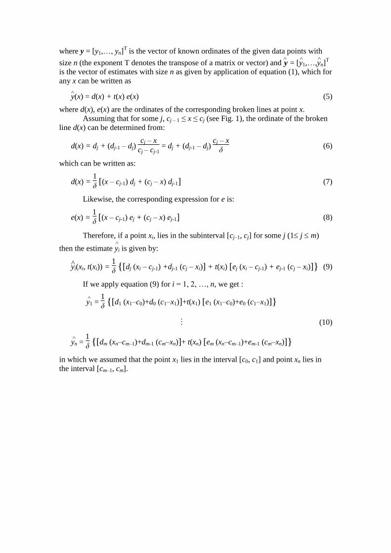
where y = [y1,…, yn]T is the vector of known ordinates of the given data points with

size n (the exponent T denotes the transpose of a matrix or vector) and y

= [y1

,…,yn

]

Τ

is the vector of estimates with size n as given by application of equation (1), which for

any x can be written as

y(x) = d(x) + t(x) e(x) (5)

where d(x), e(x) are the ordinates of the corresponding broken lines at point x.

Assuming that for some j, cj – 1 ≤ x ≤ cj (see Fig. 1), the ordinate of the broken

line d(x) can be determined from:

d(x) = dj + (dj-1 – dj) cj – x

cj – cj-1 = dj + (dj-1 – dj)

cj – x

δ (6)

which can be written as:

d(x) = 1

δ [ ](x – cj-1) dj + (cj – x) dj-1 (7)

Likewise, the corresponding expression for e is:

e(x) = 1

δ [ ](x – cj-1) ej + (cj – x) ej-1 (8)

Therefore, if a point xi, lies in the subinterval [cj–1, cj] for some j (1 j m)

then the estimate yi

is given by:

yi(xi, t(xi))^ =

1

δ { }[ ]dj (xi – cj-1) +dj-1 (cj – xi) + t(xi) [ ]ej (xi – cj-1) + ej-1 (cj – xi) (9)

If we apply equation (9) for i = 1, 2, …, n, we get :

y1

=

1

δ { }[ ]d1 (x1–c0)+d0 (c1–x1) +t(x1) [ ]e1 (x1–c0)+e0 (c1–x1)

yn

=

1

δ { }[ ]dm (xn–cm–1)+dm-1 (cm–xn) + t(xn) [ ]em (xn–cm–1)+em-1 (cm–xn)

(10)

in which we assumed that the point x1 lies in the interval [c0, c1] and point xn lies in

the interval [cm–1, cm].

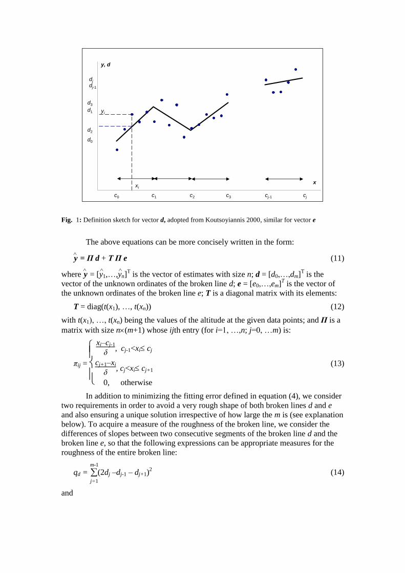
Fig. 1: Definition sketch for vector d, adopted from Koutsoyiannis 2000, similar for vector e

The above equations can be more concisely written in the form:

y

= Π d + Τ Π e (11)

where y

= [y1

,…,yn

]

Τ is the vector of estimates with size n; d = [d0,…,dm]

T is the

vector of the unknown ordinates of the broken line d; e = [e0,…,em]T is the vector of

the unknown ordinates of the broken line e; T is a diagonal matrix with its elements:

T = diag(t(x1), …, t(xn)) (12)

with t(x1), …, t(xn) being the values of the altitude at the given data points; and Π is a

matrix with size n(m+1) whose ijth entry (for i=1, …,n; j=0, …m) is:

πij =

xi–cj-1

δ, cj-1<xi cj

cj+1–xi

δ, cj<xi cj+1

0, otherwise

(13)

In addition to minimizing the fitting error defined in equation (4), we consider

two requirements in order to avoid a very rough shape of both broken lines d and e

and also ensuring a unique solution irrespective of how large the m is (see explanation

below). To acquire a measure of the roughness of the broken line, we consider the

differences of slopes between two consecutive segments of the broken line d and the

broken line e, so that the following expressions can be appropriate measures for the

roughness of the entire broken line:

qd = j=1

m-1

(2dj –dj-1 – dj+1)2 (14)

and

y, d

x

c0 c1 c2 c3 cj-1 cj

d0

d3

d1

dj

dj-1

d2

xi

yi

qe = j=1

m-1

(2ej –ej-1 – ej+1)2 (15)

These can be written in matrix form as:

qd = dT Ψ

Τ Ψ d (16)

and

qe = eT Ψ

Τ Ψ e (17)

where Ψ is a matrix with size (m–1)(m+1) and ijth entry:

ψij =

2, j=i+1

–1, | j–i–1|=1

0, othewise

(18)

Apparently, ΨΤ Ψ = 0 for the special case m = 1.

Combining equations (4), (11), (16), (17) and introducing the dimensionless

multipliers λ, μ 0 for qd and qe, respectively, we form the generalized objective

function to be minimized:

f(d,e):= p + λ qd + μ qe = || y – y

||2 +λ d

T Ψ

Τ Ψ d + μ e

T Ψ

Τ Ψ e (19)

By differentiating equation (19) with respect to d and e and equating them to

zero, we obtain, respectively:

f1

d = – 2y

T Π + 2d

T Π

Τ Π + 2e

TΠ

Τ T

ΤΠ + 2 λ d

T Ψ

Τ Ψ = 0 (20)

f2

e = – 2y

T TΠ + 2d

T Π

Τ TΠ + 2e

TΠ

Τ Τ

ΤΤΠ + 2 μ e

T Ψ

Τ Ψ = 0 (21)

The solution of the set of equations (20) and (21), which minimizes (19), is

obtained after applying the typical rules of derivatives involving matrices and it has

the following form:

d

e =

Π

T Π + λ Ψ

Τ Ψ Π

T TΠ

ΠT

ΤΠ ΠT

ΤΤ ΤΠ + μ Ψ

Τ Ψ

–1

Π

Τy

ΠΤ

TΤy

(22)

The vector of estimates, y, is obtained from equation (11), once d and e

vectors are calculated from equation (22). Also, from equation (9), we can estimate

the ordinate y of any x that lies in the interval [co, cm] if we know the value of

parameter t at that point.

We observe that the three matrices B:=ΠTΠ, C:=Ψ

TΨ and D:= Π

ΤΤ

ΤΤΠ

appearing in (22) are square matrices with size (m+1)×(m+1). B and D are tridiagonal

while C is five-banded. B can be singular (not invertible) if one or more columns of Π

have zero elements, that is, if at least two consecutive intervals [cj–1, cj] contain no

xi’s. However, C is always singular and, hence, for λ, μ > 0, the sums B + λC and D +

μC are non-singular and, thus, their inverses exist.

Choice of parameters

It is apparent that the method has three adjustable parameters: the number of intervals,

m, and the smoothing parameters λ and μ corresponding to vectors d and e,

respectively. The choice of parameters can be made by assessing the achieved data

smoothing either graphically in the case of limited amount of given data points (n ≤

3), or by using standard objective ways as described by the following analysis.

In order to provide a convenient search of the two smoothing parameters, we

selected a transformation of λ and μ in terms of what has been called tension

parameters, τλ and τμ, whose values are restricted in the interval [0, 1). These were

derived from the numerical investigation performed by Koutsoyiannis (2000),

concerning the transformation of the smoothing parameter λ, and have the form:

λ =

10 m lnτm

lnτλ

κλ, μ =

10 m lnτm

lnτμ

κμ (23)

where τm = 0.99 is the maximum allowed tension, corresponding to the upper bound

of λ and μ, set for numerical stability equal to:

λm = trace(B)

trace(C) 10

8, μm =

trace(D)

trace(C) 10

8 (24)

The exponents in equations (23) are determined by the relations:

κλ = lnλm

ln(10m), κμ =

lnμm

ln(10m) (25)

which are obtained by combining equations (23) and (24). The minimum allowed

values of λ, μ is 0 if the inverse of matrixes B and D exist; otherwise they are

estimated from equations (23) using small values of τλ and τμ, such as: τλ =1 – τm =

0.01 and τμ =1 – τm = 0.01.

Combining equations (11), (22) we obtain:

y = A y (26)

where A is a n n symmetric matrix given by:

A = [Π ΤΠ]

Π

T Π + λ Ψ

Τ Ψ Π

T TΠ

ΠT

ΤΠ ΠT

ΤΤ ΤΠ + μ Ψ

Τ Ψ

–1

[Π ΤΠ]Τ (27)

depending on all adjustable parameters: m, τλ, τμ.

The estimation of these adjustable parameters can be done by minimizing the

generalized cross-validation (GCV; Craven and Wahba 1979), defined by:

GCV =

1

n ||(I–A)y||

2

1

n trace(I–A)

2 (28)

For a given number of segments m the minimization of GCV, results in the

optimum values of τλ and τμ. This can be repeated for several trial values of m until the

global minimum of GCV is reached.

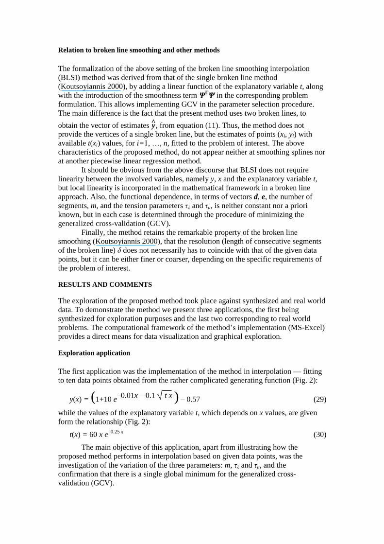
Relation to broken line smoothing and other methods

The formalization of the above setting of the broken line smoothing interpolation

(BLSI) method was derived from that of the single broken line method

(Koutsoyiannis 2000), by adding a linear function of the explanatory variable t, along

with the introduction of the smoothness term ΨTΨ in the corresponding problem

formulation. This allows implementing GCV in the parameter selection procedure.

The main difference is the fact that the present method uses two broken lines, to

obtain the vector of estimates y , from equation (11). Thus, the method does not

provide the vertices of a single broken line, but the estimates of points (xi, yi) with

available t(xi) values, for i=1, …, n, fitted to the problem of interest. The above

characteristics of the proposed method, do not appear neither at smoothing splines nor

at another piecewise linear regression method.

It should be obvious from the above discourse that BLSI does not require

linearity between the involved variables, namely y, x and the explanatory variable t,

but local linearity is incorporated in the mathematical framework in a broken line

approach. Also, the functional dependence, in terms of vectors d, e, the number of

segments, m, and the tension parameters τλ and τμ, is neither constant nor a priori

known, but in each case is determined through the procedure of minimizing the

generalized cross-validation (GCV).

Finally, the method retains the remarkable property of the broken line

smoothing (Koutsoyiannis 2000), that the resolution (length of consecutive segments

of the broken line) δ does not necessarily has to coincide with that of the given data

points, but it can be either finer or coarser, depending on the specific requirements of

the problem of interest.

RESULTS AND COMMENTS

The exploration of the proposed method took place against synthesized and real world

data. To demonstrate the method we present three applications, the first being

synthesized for exploration purposes and the last two corresponding to real world

problems. The computational framework of the method’s implementation (MS-Excel)

provides a direct means for data visualization and graphical exploration.

Exploration application

The first application was the implementation of the method in interpolation — fitting

to ten data points obtained from the rather complicated generating function (Fig. 2):

y(x) = ( )1+10 e–0.01x – 0.1 t x

– 0.57 (29)

while the values of the explanatory variable t, which depends on x values, are given

form the relationship (Fig. 2):

t(x) = 60 x e–0.25 x

(30)

The main objective of this application, apart from illustrating how the

proposed method performs in interpolation based on given data points, was the

investigation of the variation of the three parameters: m, τλ and τμ, and the

confirmation that there is a single global minimum for the generalized cross-

validation (GCV).

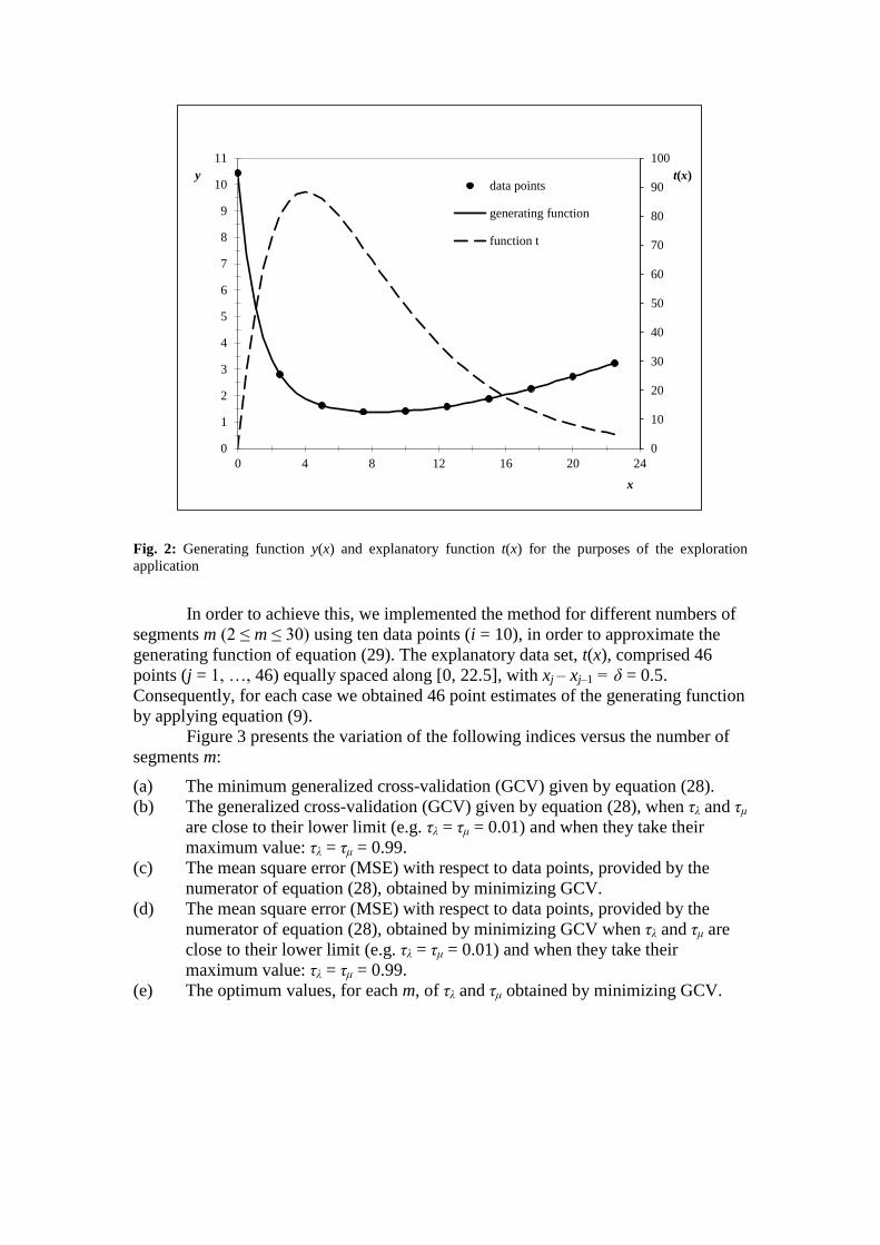
Fig. 2: Generating function y(x) and explanatory function t(x) for the purposes of the exploration

application

In order to achieve this, we implemented the method for different numbers of

segments m (2 ≤ m ≤ 30) using ten data points (i = 10), in order to approximate the

generating function of equation (29). The explanatory data set, t(x), comprised 46

points (j = 1, …, 46) equally spaced along [0, 22.5], with xj – xj–1 = δ = 0.5.

Consequently, for each case we obtained 46 point estimates of the generating function

by applying equation (9).

Figure 3 presents the variation of the following indices versus the number of

segments m:

(a) The minimum generalized cross-validation (GCV) given by equation (28).

(b) The generalized cross-validation (GCV) given by equation (28), when τλ and τμ

are close to their lower limit (e.g. τλ = τμ = 0.01) and when they take their

maximum value: τλ = τμ = 0.99.

(c) The mean square error (MSE) with respect to data points, provided by the

numerator of equation (28), obtained by minimizing GCV.

(d) The mean square error (MSE) with respect to data points, provided by the

numerator of equation (28), obtained by minimizing GCV when τλ and τμ are

close to their lower limit (e.g. τλ = τμ = 0.01) and when they take their

maximum value: τλ = τμ = 0.99.

(e) The optimum values, for each m, of τλ and τμ obtained by minimizing GCV.

0

10

20

30

40

50

60

70

80

90

100

0

1

2

3

4

5

6

7

8

9

10

11

0 4 8 12 16 20 24

t(x)y

x

data points

generating function

function t

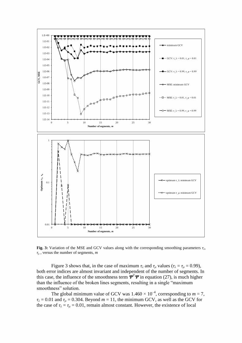
Fig. 3: Variation of the MSE and GCV values along with the corresponding smoothing parameters τλ,

τμ , versus the number of segments, m

Figure 3 shows that, in the case of maximum τλ and τμ values (τλ = τμ = 0.99),

both error indices are almost invariant and independent of the number of segments. In

this case, the influence of the smoothness term ΨTΨ in equation (27), is much higher

than the influence of the broken lines segments, resulting in a single “maximum

smoothness” solution.

The global minimum value of GCV was 1.460 × 10–4

, corresponding to m = 7,

τλ = 0.01 and τμ = 0.304. Beyond m = 11, the minimum GCV, as well as the GCV for

the case of τλ = τμ = 0.01, remain almost constant. However, the existence of local

1.E-14

1.E-13

1.E-12

1.E-11

1.E-10

1.E-09

1.E-08

1.E-07

1.E-06

1.E-05

1.E-04

1.E-03

1.E-02

1.E-01

1.E+00

0 5 10 15 20 25 30

GC

V,

MS

E

Number of segments, m

minimum GCV

GCV: τ_λ = 0.01, τ_μ = 0.01

GCV: τ_λ = 0.99, τ_μ = 0.99

MSE: minimum GCV

MSE: τ_λ = 0.01, τ_μ = 0.01

MSE: τ_λ = 0.99, τ_μ = 0.99

0.01

0.1

1

0 5 10 15 20 25 30

Op

tim

um

τλ,

τ

μ

Number of segments, m

optimum τ_λ: minimum GCV

optimum τ_μ: minimum GCV

minima should be taken into consideration during the parameters estimation

procedure.

When GCV is minimized, MSE follows a similar pattern to the GCV

variation, with its minimum value being 2.540 × 10–8

for m = 7, τλ = 0.01 and τμ =

0.304. However, the global minimum value of MSE was 8.099 × 10–14

and occurred

in the case of minimum tension values, i.e. τλ = τμ = 0.01 and m = 9. This complies

with the formulation of equation (19) concerning the roughness of the broken lines.

Also, Fig. 3 shows that in this case, the values of MSE, tend to remain stable for

larger values of m.

The optimum values of τλ and τμ that achieved by minimizing GVC, versus

different numbers of segments m, are presented in Fig. 3. Even though they appear in

different scale, their pattern is similar to these of the error indices, being almost stable

after m = 6 for τλ and m = 9 for τμ.

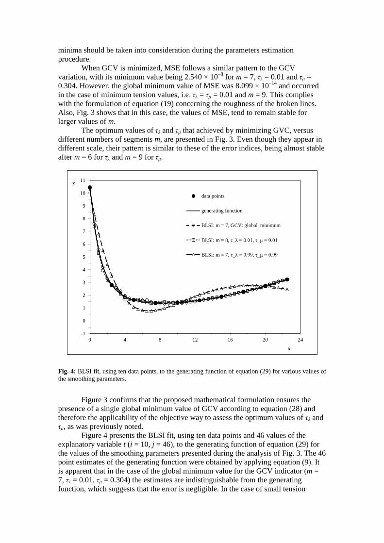
Fig. 4: BLSI fit, using ten data points, to the generating function of equation (29) for various values of

the smoothing parameters.

Figure 3 confirms that the proposed mathematical formulation ensures the

presence of a single global minimum value of GCV according to equation (28) and

therefore the applicability of the objective way to assess the optimum values of τλ and

τμ, as was previously noted.

Figure 4 presents the BLSI fit, using ten data points and 46 values of the

explanatory variable t (i = 10, j = 46), to the generating function of equation (29) for

the values of the smoothing parameters presented during the analysis of Fig. 3. The 46

point estimates of the generating function were obtained by applying equation (9). It

is apparent that in the case of the global minimum value for the GCV indicator (m =

7, τλ = 0.01, τμ = 0.304) the estimates are indistinguishable from the generating

function, which suggests that the error is negligible. In the case of small tension

-1

0

1

2

3

4

5

6

7

8

9

10

11

0 4 8 12 16 20 24

y

x

data points

generating function

BLSI: m = 7, GCV: global minimum

BLSI: m = 8, τ_λ = 0.01, τ_μ = 0.01

BLSI: m = 7, τ_λ = 0.99, τ_μ = 0.99

values (m = 8, τλ = τμ = 0.01), the estimates are also very close to the generating

function but the overall appearance is somewhat rough with deviations between the

data points. This characteristic was expected since the GCV values for both cases

were very close. On the other hand, the maximum tension case of τλ = τμ = 0.99

resulted in a smoother curve but a worse approximation of the generating function.

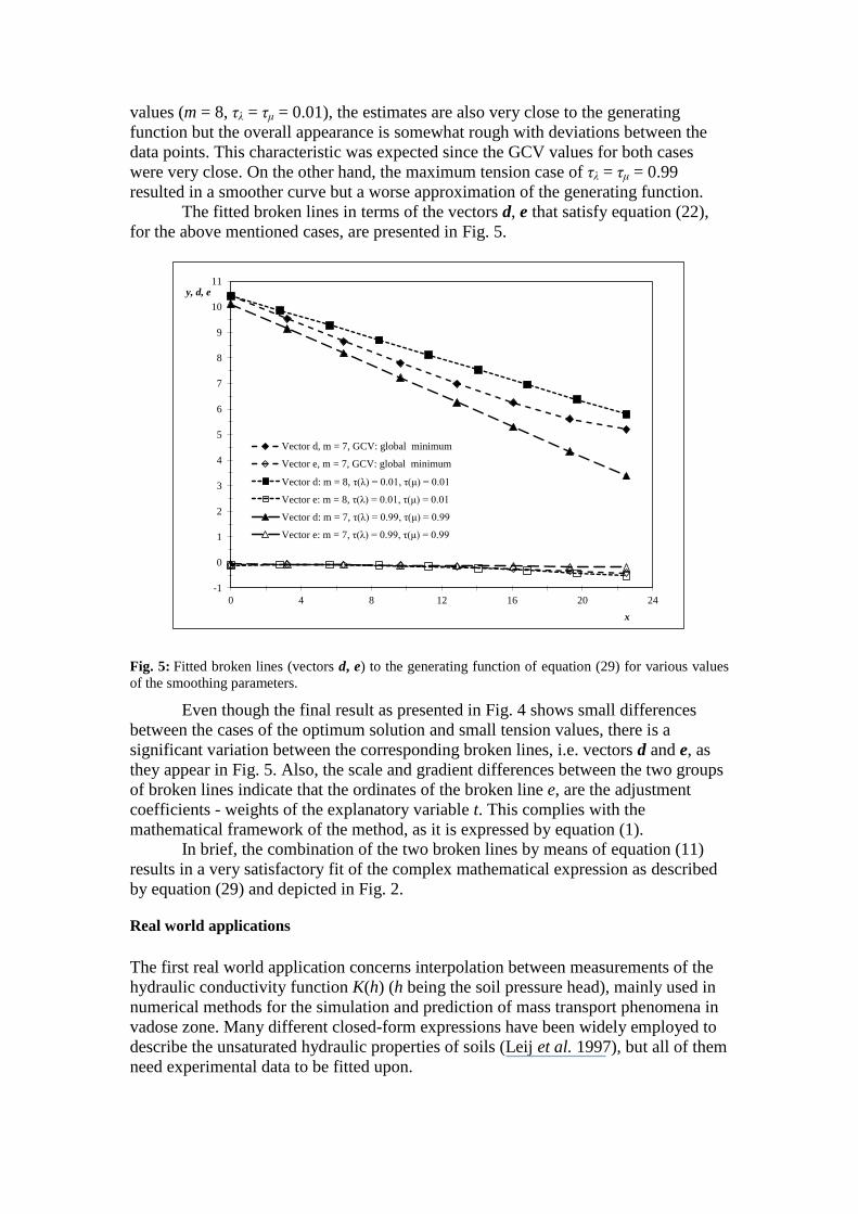
The fitted broken lines in terms of the vectors d, e that satisfy equation (22),

for the above mentioned cases, are presented in Fig. 5.

Fig. 5: Fitted broken lines (vectors d, e) to the generating function of equation (29) for various values

of the smoothing parameters.

Even though the final result as presented in Fig. 4 shows small differences

between the cases of the optimum solution and small tension values, there is a

significant variation between the corresponding broken lines, i.e. vectors d and e, as

they appear in Fig. 5. Also, the scale and gradient differences between the two groups

of broken lines indicate that the ordinates of the broken line e, are the adjustment

coefficients - weights of the explanatory variable t. This complies with the

mathematical framework of the method, as it is expressed by equation (1).

In brief, the combination of the two broken lines by means of equation (11)

results in a very satisfactory fit of the complex mathematical expression as described

by equation (29) and depicted in Fig. 2.

Real world applications

The first real world application concerns interpolation between measurements of the

hydraulic conductivity function K(h) (h being the soil pressure head), mainly used in

numerical methods for the simulation and prediction of mass transport phenomena in

vadose zone. Many different closed-form expressions have been widely employed to

describe the unsaturated hydraulic properties of soils (Leij et al. 1997), but all of them

need experimental data to be fitted upon.

-1

0

1

2

3

4

5

6

7

8

9

10

11

0 4 8 12 16 20 24

y, d, e

x

Vector d, m = 7, GCV: global minimum

Vector e, m = 7, GCV: global minimum

Vector d: m = 8, τ(λ) = 0.01, τ(μ) = 0.01

Vector e: m = 8, τ(λ) = 0.01, τ(μ) = 0.01

Vector d: m = 7, τ(λ) = 0.99, τ(μ) = 0.99

Vector e: m = 7, τ(λ) = 0.99, τ(μ) = 0.99

For the experimental determination of the hydraulic conductivity function, a

number of methods have been developed. Direct methods for measuring the K(h)

functions in laboratory can be classified according to the flow mode as steady state

(conventional constant head, constant flow, centrifuge) or unsteady state methods

(outflow-inflow, instantaneous profile, thermal method) (Masrouri et al. 2008). Most

of them are time consuming and laborious, leading scientists to consider other

methods e.g. conceptual models which could predict K(h) from data obtained from the

soil moisture retention curve and supportively coupled by Ks, measured independently

at saturation, with the use of permeameters (Argyrokastritis et al. 2009).

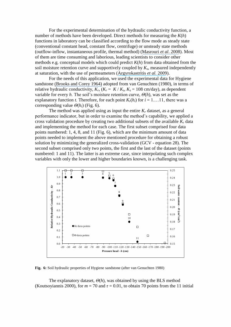
For the needs of this application, we used the experimental data for Hygiene

sandstone (Brooks and Corey 1964) adopted from van Genuchten (1980), in terms of

relative hydraulic conductivity, Kr, (Kr = K / Ks, Ks = 108 cm/day), as dependent

variable for every h. The soil’s moisture retention curve, Θ(h), was set as the

explanatory function t. Therefore, for each point Kr(hi) for i = 1.…11, there was a

corresponding value Θ(hi) (Fig. 6).

The method was applied using as input the entire Kr dataset, as a general

performance indicator, but in order to examine the method’s capability, we applied a

cross validation procedure by creating two additional subsets of the available Kr data

and implementing the method for each case. The first subset comprised four data

points numbered: 1, 4, 8, and 11 (Fig. 6), which are the minimum amount of data

points needed to implement the above mentioned procedure for obtaining a robust

solution by minimizing the generalized cross-validation (GCV - equation 28). The

second subset comprised only two points, the first and the last of the dataset (points

numbered: 1 and 11). The latter is an extreme case, since interpolating such complex

variables with only the lower and higher boundaries known, is a challenging task.

Fig. 6: Soil hydraulic properties of Hygiene sandstone (after van Genuchten 1980)

The explanatory dataset, Θ(h), was obtained by using the BLS method

(Koutsoyiannis 2000), for m = 70 and τ = 0.01, to obtain 70 points from the 11 initial

1 2 3 4 56

7

8

9

10

11

0.15

0.16

0.17

0.18

0.19

0.20

0.21

0.22

0.23

0.24

0.25

0.0

0.1

0.2

0.3

0.4

0.5

0.6

0.7

0.8

0.9

1.0

1.1

-200-190-180-170-160-150-140-130-120-110-100-90-80-70-60-50-40-30-20

So

il wa

ter c

on

ten

t -Θ

(cm

3/cm

3)R

ela

tiv

e H

yd

ra

uli

c C

on

du

cti

vit

y -

Kr

Pressure head - h (cm)

Kr data points

Θ data points

data points. Therefore, in each case the outcome of the BLSI method was 70 point

estimates of Kr.

In the case of the entire Kr dataset and four available data points, the method

was implemented for different number of segments, m (2 ≤ m ≤ 30) and for each one

the GCV was minimized, by altering τλ and τμ values. In this way, the global

minimum of GCV was reached. In order to obtain the optimum fit for the case of two

available data points, we varied the m, τλ and τμ parameters and graphically assessed

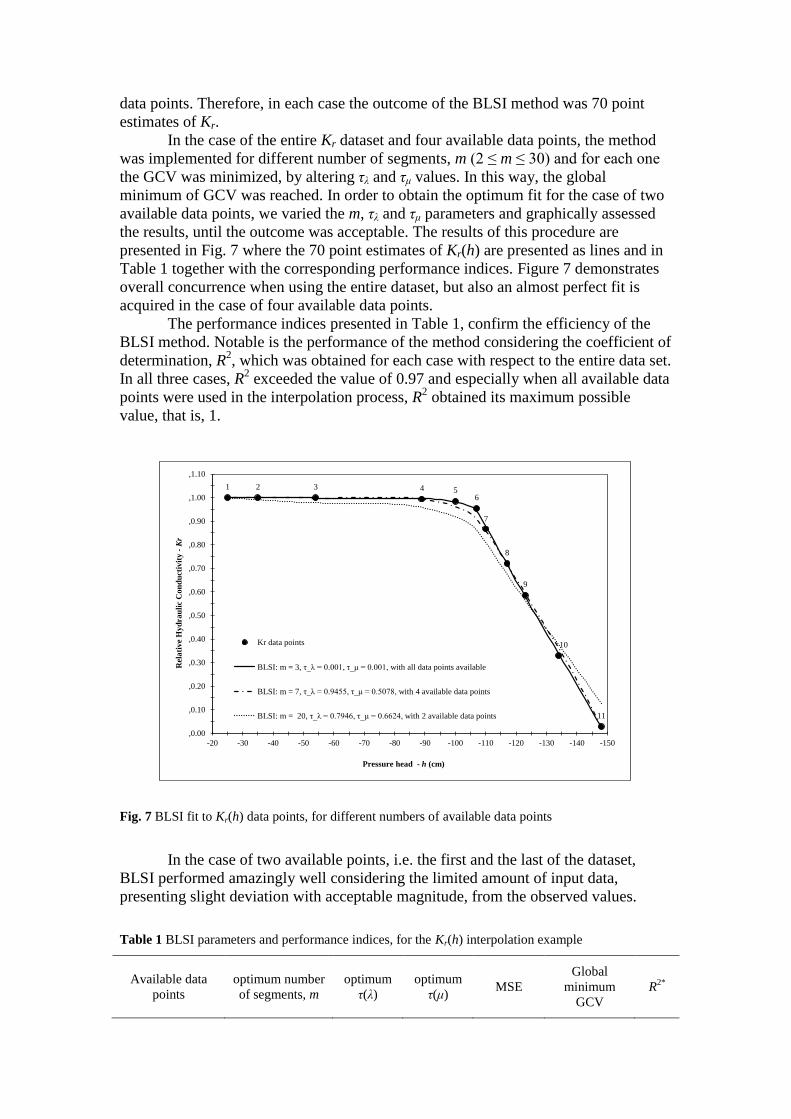
the results, until the outcome was acceptable. The results of this procedure are

presented in Fig. 7 where the 70 point estimates of Kr(h) are presented as lines and in

Table 1 together with the corresponding performance indices. Figure 7 demonstrates

overall concurrence when using the entire dataset, but also an almost perfect fit is

acquired in the case of four available data points.

The performance indices presented in Table 1, confirm the efficiency of the

BLSI method. Notable is the performance of the method considering the coefficient of

determination, R2, which was obtained for each case with respect to the entire data set.

In all three cases, R2 exceeded the value of 0.97 and especially when all available data

points were used in the interpolation process, R2 obtained its maximum possible

value, that is, 1.

Fig. 7 BLSI fit to Kr(h) data points, for different numbers of available data points

In the case of two available points, i.e. the first and the last of the dataset,

BLSI performed amazingly well considering the limited amount of input data,

presenting slight deviation with acceptable magnitude, from the observed values.

Table 1 BLSI parameters and performance indices, for the Kr(h) interpolation example

Available data

points

optimum number

of segments, m

optimum

τ(λ)

optimum

τ(μ) MSE

Global

minimum

GCV

R2*

1 2 3 4 56

7

8

9

10

11

,0.00

,0.10

,0.20

,0.30

,0.40

,0.50

,0.60

,0.70

,0.80

,0.90

,1.00

,1.10

-150-140-130-120-110-100-90-80-70-60-50-40-30-20

Rel

ati

ve

Hy

dra

uli

c C

on

du

ctiv

ity

-K

r

Pressure head - h (cm)

Kr data points

BLSI: m = 3, τ_λ = 0.001, τ_μ = 0.001, with all data points available

BLSI: m = 7, τ_λ = 0.9455, τ_μ = 0.5078, with 4 available data points

BLSI: m = 20, τ_λ = 0.7946, τ_μ = 0.6624, with 2 available data points

All 3 0.001 0.001 2.06×10–5

1.17×10–4

1.000

Four (1, 4, 8, 11) 7 0.9455 0.5078 3.99×10–22

5.041×0–5

0.997

Two (1, 11) 20 0.7946 0.6624 4.72×10–3

1.71×10–1

0.971

* With respect to the entire data set

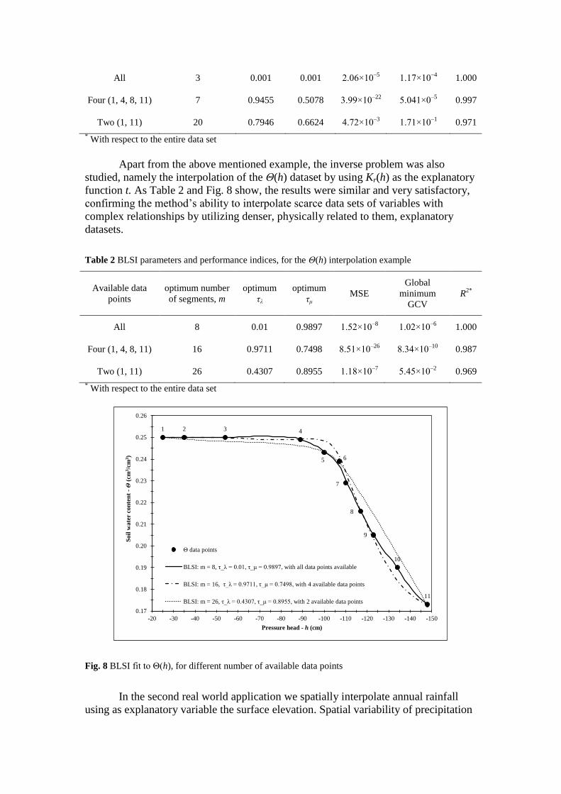
Apart from the above mentioned example, the inverse problem was also

studied, namely the interpolation of the Θ(h) dataset by using Kr(h) as the explanatory

function t. As Table 2 and Fig. 8 show, the results were similar and very satisfactory,

confirming the method’s ability to interpolate scarce data sets of variables with

complex relationships by utilizing denser, physically related to them, explanatory

datasets.

Table 2 BLSI parameters and performance indices, for the Θ(h) interpolation example

Available data

points

optimum number

of segments, m

optimum

τλ

optimum

τμ MSE

Global

minimum

GCV

R2*

All 8 0.01 0.9897 1.52×10–8

1.02×10–6

1.000

Four (1, 4, 8, 11) 16 0.9711 0.7498 8.51×10–26

8.34×10–10

0.987

Two (1, 11) 26 0.4307 0.8955 1.18×10–7

5.45×10–2

0.969

* With respect to the entire data set

Fig. 8 BLSI fit to Θ(h), for different number of available data points

In the second real world application we spatially interpolate annual rainfall

using as explanatory variable the surface elevation. Spatial variability of precipitation

1 2 3 4

5 6

7

8

9

10

11

0.17

0.18

0.19

0.20

0.21

0.22

0.23

0.24

0.25

0.26

-150-140-130-120-110-100-90-80-70-60-50-40-30-20

So

il w

ate

r c

on

ten

t -

Θ(c

m3/c

m3)

Pressure head - h (cm)

Θ data points

BLSI: m = 8, τ_λ = 0.01, τ_μ = 0.9897, with all data points available

BLSI: m = 16, τ_λ = 0.9711, τ_μ = 0.7498, with 4 available data points

BLSI: m = 26, τ_λ = 0.4307, τ_μ = 0.8955, with 2 available data points

is influenced by many factors; some of them connected to the chaotic nature of the

atmospheric processes. In over-annual scale abutting on the sea and orography have

significant effects (Goovaerts 2000). Hevesi et al (1992a; 1992b) reported a

significant correlation of 0.75 between average annual precipitation and elevation.

The objective of the application was: a) to verify the method’s applicability

against a hydrological variable with significant correlation to an easily measurable,

hence available at considerably higher resolution, explanatory variable and b) to

verify the method’s versatility in terms of handling extensive datasets.

The study area was the region of the Central Greece (Sterea Hellas) area (Fig.

9a). The data consist of the mean rainfall at the 71 meteorological stations network of

the specified area, derived from all available measurements until the year 1992

(Christofides and Mamassis 1995), while the surface elevation of the study area was

obtained from the Digital Elevation Model (DEM) SRTM Data Version 4.1 (Jarvis et

al. 2008) and aggregated to a 2×2 km square grid (Fig. 9a) for practical and

computational reasons, covering approximately an area of 25 620 km2. The result was

6405 points of known elevation, which constituted the explanatory variable dataset.

Since the BLSI method is one-dimensional, in terms of the independent

variable x, the points spatial coordinates, (xi, yi), were projected onto a x' axis,

according to the following expression:

g(xi, yi) = g(xi´), xi´ = xi + tan φ yi (31)

for alternative angles φ, namely:

φ = 30o, tan φ =

3

3, xi´ = xi +

3

3 yi (32)

φ = 45o, tan φ = 1, xi´ = xi + yi (33)

φ = 60o, tan φ = 3, xi´ = xi + 3 yi (34)

The global minimum of GCV, for all three cases, was reached by

implementing the method for different number of segments, m (2 ≤ m ≤ 30) and

minimizing GCV for each one, by altering τλ and τμ. The results of the above

procedure are presented in Table 3.

Table 3 BLSI parameters and performance indices, for the rainfall interpolation example

Projection

angle, φ

optimum number of

segments, m optimum τλ optimum τμ MSE

Global minimum

GCV

30o 13 0.141 0.986 4.01×10

4 5.63×10

4

45o 17 0.435 0.796 4.86×10

4 6.71×10

4

60o 8 0.282 0.984 5.74×10

4 7.41×10

4

As quality measure for the evaluation of the method’s efficiency, we utilized

the minimum and maximum rainfall of the available meteorological stations data,

along with their corresponding elevation. Those values, compared to the minimum

and maximum rainfall obtained from implementing BLSI for each one of the three

cases are presented in Table 4.

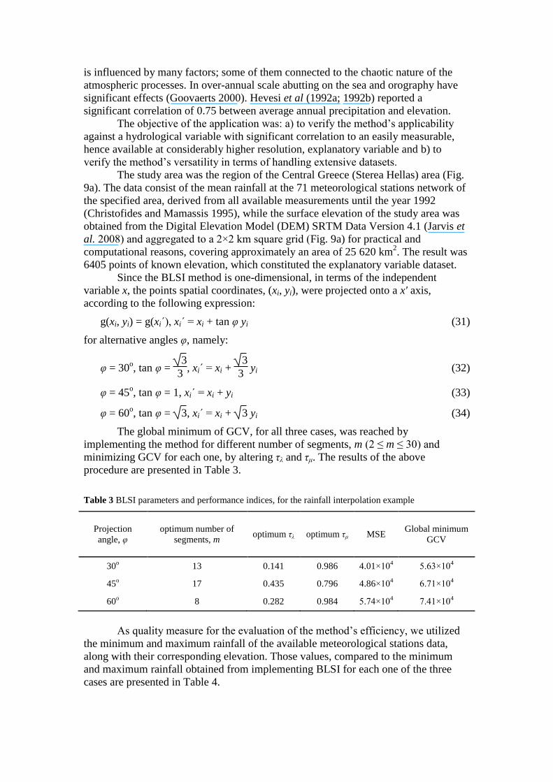
(a) (b)

(c) (d)

Fig. 9 (a) Elevation map and meteorological stations; (b)-(d) rainfall maps produced for the three cases of projection angles.

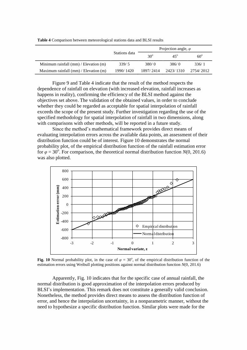
Table 4 Comparison between meteorological stations data and BLSI results

Stations data Projection angle, φ

30

o 45

o 60

o

Minimum rainfall (mm) / Elevation (m) 339/ 5 380/ 0 386/ 0 336/ 1

Maximum rainfall (mm) / Elevation (m) 1990/ 1420 1897/ 2414 2423/ 1310 2754/ 2012

Figure 9 and Table 4 indicate that the result of the method respects the

dependence of rainfall on elevation (with increased elevation, rainfall increases as

happens in reality), confirming the efficiency of the BLSI method against the

objectives set above. The validation of the obtained values, in order to conclude

whether they could be regarded as acceptable for spatial interpolation of rainfall

exceeds the scope of the present study. Further investigation regarding the use of the

specified methodology for spatial interpolation of rainfall in two dimensions, along

with comparisons with other methods, will be reported in a future study.

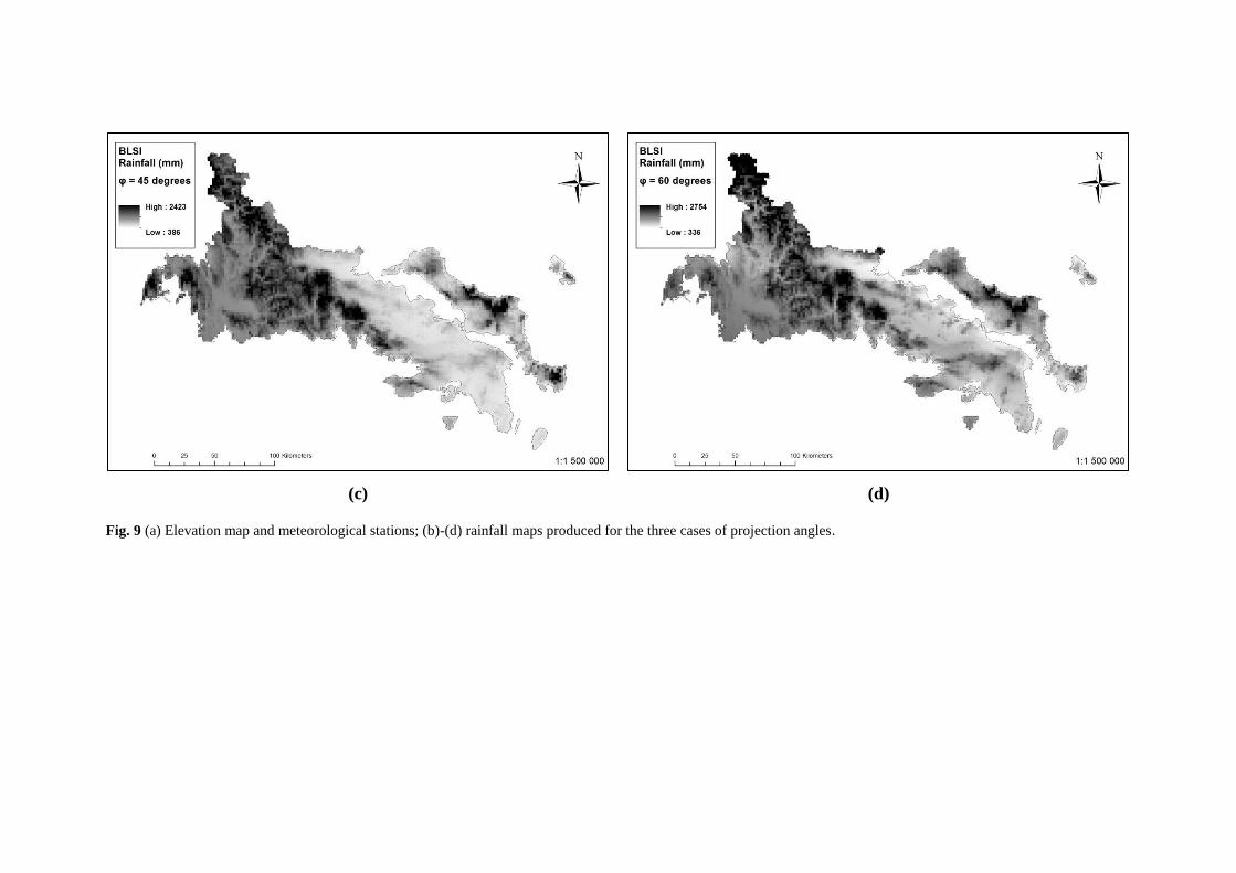
Since the method’s mathematical framework provides direct means of

evaluating interpolation errors across the available data points, an assessment of their

distribution function could be of interest. Figure 10 demonstrates the normal

probability plot, of the empirical distribution function of the rainfall estimation error

for φ = 30o. For comparison, the theoretical normal distribution function N(0, 201.6)

was also plotted.

Fig. 10 Normal probability plot, in the case of φ = 30o, of the empirical distribution function of the

estimation errors using Weibull plotting positions against normal distribution function N(0, 201.6)

Apparently, Fig. 10 indicates that for the specific case of annual rainfall, the

normal distribution is good approximation of the interpolation errors produced by

BLSI’s implementation. This remark does not constitute a generally valid conclusion.

Nonetheless, the method provides direct means to assess the distribution function of

error, and hence the interpolation uncertainty, in a nonparametric manner, without the

need to hypothesize a specific distribution function. Similar plots were made for the

-800

-600

-400

-200

0

200

400

600

800

-3 -2 -1 0 1 2 3

Est

ima

tio

n e

rro

r (m

m)

Normal variate, z

Empirical distribution

Normal distribution

other two cases studied, namely φ = 45o and φ = 60

o (not shown here) and the results

were found to be analogous to those for φ = 30o.

CONCLUSIONS

An innovative method which can be utilized to perform various interpolation tasks, by

incorporating, in an objective manner, an explanatory variable available at a

considerably denser dataset than the main variable, is described. The technique

incorporates smoothing terms with adjustable weights, defined by means of the angles

formed by the consecutive segments of two broken lines into a piecewise linear

regression model with known break points.

Apart from the demonstration of the mathematical framework, the method was

illustrated and tested against three applications, a theoretical one with synthetic data

from a known generating function and two real world examples: the interpolation of

hydraulic conductivity function using water retention data as explanatory variable and

vice versa, and the spatial interpolation of rainfall data using the surface elevation as

explanatory variable. In every case, the method’s efficiency to perform interpolation,

as well as smoothing, between data points that are interrelated in a complicated

manner, by incorporating the explanatory variable, was confirmed, indicating its

applicability for diverse scientific and engineering tasks. A notable property of the

proposed method is the fact that the resolution (length of consecutive segments of the

broken line) does not necessarily have to coincide with that of the given data points,

but it can be either finer or coarser, depending on the specific requirements of the

problem of interest. This is an important property that makes the method applicable

and reliable even in the case of scarce data sets (e.g. with as few as two points, as in

the second case study, the method gave amazingly good results).

The third application showed that the method can be useful in spatial

interpolation. However, the current formulation is not fully two dimensional but the

general methodology allows an extension in many dimensions. The extension of the

methodology for spatial (two dimensional) interpolation of variables, will be reported

in future studies.

ACKNOWLEDGMENT

We thank the Associate Editor Alin Castreanu, the eponymous reviewer Alberto

Montanari and an anonymous reviewer for their comments and suggestions which

helped us to improve the presentation of the study.

REFERENCES

Argyrokastritis, I., Kargas, G., Kerkides, P., 2009. Simulation of Soil Moisture

Profiles Using K(h) from Coupling Experimental Retention Curves and One-

Step Outflow Data. Water Resources Management 23 (15), 3255-3266.

Brooks, R.H., Corey, A.T., 1964. Hydraulic properties of porous media, Hydrology

Papers, 3, Colorado State University. Fort Collins, Colorado.

Burrough, P.A. and McDonnell, R.A., 1998. Principles of Geographical Information

Systems. Oxford University Press, Oxford, 333 pp.

Christofides, A., and N. Mamassis, Hydrometeorological data processing, Evaluation

of Management of the Water Resources of Sterea Hellas - Phase 2, Report 18,

268 pages, Department of Water Resources, Hydraulic and Maritime

Engineering - National Technical University of Athens, Athens,

September 1995.

Craven, P., Wahba, G., 1979. Smoothing noisy data with spline functions.

Numerische Mathematik 31 (4), 377-403.

Davis C., J., 1986. Statistics and Data Analysis in Geology, 2nd

ed. John Wiley &

Sons Canada, Ltd.

Goovaerts, P., 1997. Geostatistics for Natural Resources Evaluation. Oxford

University Press, New York, 483 pp.

Goovaerts, P., 2000. Geostatistical approaches for incorporating elevation into the

spatial interpolation of rainfall. Journal of Hydrology 228 (1-2), 113-129.

Hengl, T., Heuvelink, G.B.M., Rossiter, D.G., 2007. About regression-kriging: From

equations to case studies. Computers & Geosciences 33 (10), 1301-1315.

Hevesi, J.A., Flint, A.L., Istok, J.D., 1992a. Precipitation estimation in mountainous

terrain using multivariate geostatistics. Part I: structural analysis. J. Appl.

Meteor. 31, 661-676.

Hevesi, J.A., Flint, A.L., Istok, J.D., 1992b. Precipitation estimation in mountainous

terrain using multivariate geostatistics. Part II: Isohyetal maps. J. Appl.

Meteor. 31, 677-688.

Jarvis A., H.I. Reuter, A. Nelson, E. Guevara, 2008. Hole-filled seamless SRTM data

V4, International Centre for Tropical Agriculture (CIAT).

Koutsoyiannis, D., 2000. Broken line smoothing: a simple method for interpolating

and smoothing data series. Environmental Modelling & Software 15 (2), 139-

149.

Leij, F.J., Russell, W.B., Lesch, S.M., 1997. Closed-Form Expressions for Water

Retention and Conductivity Data. Ground Water 35 (5), 848-858.

Li, J., Heap, A.D., 2008. A Review of Spatial Interpolation Methods for

Environmental Scientists, Geoscience Australia. Geoscience Australia, GPO

Box 378, Canberra, ACT 2601, Australia.

Masrouri, F., Bicalho, K. V., Kawai, K., 2008. Laboratory Hydraulic Testing in

Unsaturated Soils. Geotechnical and Geological Engineering 26 (6), 691-704.

Van Genuchten, M.T., 1980. A Closed-form Equation for Predicting the Hydraulic

Conductivity of Unsaturated Soils. Soil Science Society of America Journal

44, 892-898.

Wahba, G., Wendelberger, J., 1980. Some New Mathematical Methods for

Variational Objective Analysis Using Splines and Cross Validation. Monthly

Weather Review 108 (8), 1122-1143.

Wang, H., Liu, G. and Gong, P., 2005. Use of cokriging to improve estimates of soil

salt solute spatial distribution in the Yellow River delta. Acta Geographica

Sinica, 60(3): 511-518.