Neurocomputing 184 (2016) 207–220

Contents lists available at ScienceDirect

Neurocomputing

http://d0925-23

n CorrE-mURL

journal homepage: www.elsevier.com/locate/neucom

Hierarchical line matching based on Line–Junction–Line structuredescriptor and local homography estimation

Kai Li a, Jian Yao a,n, Xiaohu Lu a, Li Li a, Zhichao Zhang a,b

a School of Remote Sensing and Information Engineering, Wuhan University, Wuhan, Hubei, PR Chinab Collaborative Innovation Center of Geospatial Technology, Wuhan, Hubei, PR China

a r t i c l e i n f o

Article history:Received 1 January 2015Received in revised form18 May 2015Accepted 27 July 2015Available online 13 January 2016

Keywords:Line matchingHierarchical matchingLocal feature descriptorHomography estimation

x.doi.org/10.1016/j.neucom.2015.07.13712/& 2015 Elsevier B.V. All rights reserved.

esponding author.ail address: jian.yao@whu.edu.cn (J. Yao).: http://www.cvrs.whu.edu.cn/ (J. Yao).

a b s t r a c t

This paper presents a hierarchical method for matching line segments from two images. Line segmentsare matched first in groups and then in individuals. While matched in groups, the line segments lyingadjacently are intersected to form junctions. At the places of the junctions, the structures are constructedcalled Line–Junction–Line (LJL), which consists of two adjacent line segments and their intersectingjunction. To reliably deal with the possible scale change between the two images to be matched, wepropose to describe LJLs by a robust descriptor in the multi-scale pyramids of images constructed fromtwo original images. By evaluating the description vector distances of LJLs from the two images, somecandidate LJL matches are obtained, which are then refined and expanded by an effective match-propagation strategy. The line segments used to construct LJLs are matched when the LJLs they formedare matched. For those left unmatched line segments, we match them in individuals by utilizing the localhomographies estimated from their neighboring matched LJLs. Experiments demonstrate the super-iorities of the proposed method to the state-of-the-art methods for its robustness in more difficultsituations, the larger amounts of correct matches, and the higher accuracy in most cases.

& 2015 Elsevier B.V. All rights reserved.

1. Introduction

As a low-level vision task, image matching is fundamental formany applications which require recovering the 3D scene structurefrom 2D images, like robotic navigation, structure from motion, 3Dreconstruction, and scene interpretation. The majority of imagematching methods are feature point based [1–6] which commencethe extraction of feature points from images, followed by the uti-lization of the photometric information adjacently associated withthe extracted points to match them. Objects in real scenes, however,can be easily outlined by line segments, especially for man-madescenes. This indicates that it is better to recover 3D scene structuresbased on line segments than that on feature points, at least forsome scenes [7–12]. For example, for poorly textured scenes, wherefeature points are hard to be detected and matched, recoveringtheir 3D structures from line matches seems the only choicebecause their structures can be easily outlined by several edge linesegments [13]. Despite these advantages, both the lack of point-to-point correspondence and the loss of connectivity and complete-ness of the extracted line segments make line segment matching a

tough task, which also partly explains why line segment matchinghas been less investigated.

Line matching methods in existing literatures can generally beclassified into two categories: the methods that match line seg-ments in individuals and those in groups. Some methods matchingline segments in individuals exploit the photometric informationassociated with individual line segments, such as intensity [14,15],gradient [16–18], and color [19] in the local regions around linesegments. All these methods underlie the assumption that thereare considerable overlaps between corresponding line segments.This assumption leads to the failure of these methods in situationswhere corresponding line segments share insufficient corre-sponding parts. Besides, in regions with repetitive textures, thesemethods tend to produce false matches since the lack of variationsin the photometric information for some line segments. Othermethods matching line segments in individuals leverage pointmatches for line matching [20–23]. These methods first find alarge group of point matches using the existing point matchingmethods, and then exploit the invariants between coplanar pointsand line(s) under certain image transformations to evaluate thecorrespondence of the line segments from two images. The linesegments which meet the invariants are regarded to be in corre-spondence. These methods utilize geometric relationship betweenline segments and points, rather than photometric information inthe local regions around line segments, and are thus robust even

K. Li et al. / Neurocomputing 184 (2016) 207–220208

when local shape distortions are severe. However, these methodsshare a common disadvantage that they are incapable of proces-sing images in which the scenes captured are poorly textured sincefeature points are hard to be detected and matched in this kind ofscenes, which consequently disables the use of point matches forline segment matching.

Matching line segments in groups is more complex, but moreconstraints are available for disambiguation. Most of these meth-ods [13,24–26,32] first use some strategies to intersect line seg-ments to form junction points and then utilize features associatedwith the generated junction points for line segment matching.These methods transfer line matching to point matching, a widelyinvestigated problem which many effective algorithms target tosolve. But junction points contain more information than featurepoints detected by some detectors [27–30]. They are the results ofintersecting pairs of adjacent line segments and the relationshipbetween junction points and line segments forming them isadditional and important information that can be exploited formatching them. How to effectively exploit features associated withjunction points to help match them is still an open issue. In [31],rather than exploiting features of junctions for line segmentmatching, the stability of the relative positions of the endpoints ofa group of line segments in a local region under various imagetransformations is exploited. This method first divides line seg-ments into groups and then generates a description of the con-figuration of the line segments in each group by calculating therelative positions of these line segments. Since the configuration ofa group of line segments in a local region is fairly stable undermost image transformations, the description of the configurationsof two groups of line segments in correspondence should besimilar. In this way, groups of line segments can be matched. Thismethod is robust in many challenging situations, but the depen-dence on the approximately corresponding relationship betweenthe endpoints of corresponding line segments leads to the ten-dency of this method to produce false matches when substantialdisparity exists in the locations of the endpoints.

Our proposed line matching method in this paper is a combi-nation of the two categories methods described above. It matchesline segments both in groups and in individuals under a hier-archical framework. The framework is composed of three stageswhere line segments are matched in groups in the first two stageswhile in individuals in the third stage. The three-stage flowchart ofthe proposed line matching algorithm is illustrated in Fig. 1. Fortwo sets of line segments extracted from two images, the first

Fig. 1. The flowchart of the propo

stage commences intersecting neighboring line segments to formjunction points. At the places of the formed junction points, weform the structures called Line–Junction–Line (LJL), utilizing twoadjacent line segments and their intersecting junction. To greatlyreduce the effect of the scale change between the two images, wepropose to build Gaussian image pyramids for the original imagesand adjust the LJLs constructed in the original images to fit eachimage in the image pyramids and described them there by theproposed LJL descriptor. Some initial LJL matches can be found byevaluating the description vector distances of LJLs from the twoimages. These LJL matches are then refined and expanded in thesecond stage, where we propagate LJL matches by iterativelyadding new matches while deleting possibly false ones. In theabove two stages, the line segments lying closely with each otherfrom the two images are matched along with their constructedand matched LJLs. For those line segments lying far away fromothers and are not used to constructed LJLs, we match them inindividuals in the third stage by utilizing the local homographiesestimated from their neighboring matched LJLs.

This work is an extension of our work presented in [32].Compared with the previous one, this work makes promotions inthe following aspects. First, a more general way is utilized togenerate junctions using adjacent line segments. In [32], sets ofline segments extracted by some line segment detectors in a imageare processed in advance before they are used for matching by aseries of procedures to obtain a new line segment set where someline segments are extended to be longer and are connected withothers. In this work, the line segments extracted by line detectorsare not required to be refined in advance, and can be used togenerate junctions directly based on the local spatial proximity.This promotion helps generate more junctions and contributes tobetter matching results. Second, a more robust descriptor is pro-posed to describe the structure (called RPR in [32], while LJL in thispaper) formed by two adjacent line segments and their inter-secting junction. Third, we propose a more reasonable strategy todeal with the possible scale change between images. To match linesegments from two images with scale change, in [32], the globalscale change factor between the two original images is estimatedand one of the two images is adjusted to the same scale as theother one. This strategy is reasonable only when the scale changebetween the two images is a global one. When scale changesbetween the two images vary with local regions (often introducedby viewpoint changes), this strategy is unable to reliably work.This disadvantage is solved in this paper and the proposed strategy

sed line matching algorithm.

K. Li et al. / Neurocomputing 184 (2016) 207–220 209

can deal with both global scale changes and locally variant ones.Fourth, a more sophisticated way to match individual line seg-ments is proposed. For line segments which cannot be matched ingroups (in RPRs in [32] while in LJLs in this paper), in [32], they areused to intersect with those matched line segments to constructnew RPRs and matched along with the newly constructed RPRagain. In this paper, they are matched by the local homographiesestimated from their neighboring corresponding LJLs. All theabove promotions together contribute to the better performanceof this work than our previous one.

Experimental results substantiate the advantages of this workover the previous one and other state-of-the-art line matchingmethods for its robustness under more severe image transforma-tions, its better performance for poorly textured scenes, the largeramount of correct line matches obtained, and higher accuracy inthe majority of cases.

The remainder of the paper is organized as follows. Section 2introduces the details of constructing, describing and matchingLJLs. The adopted match propagation strategy is described inSection 3. The step of matching individual line segments failed tobe matched along with LJLs is described in Section 4. Experimentalresults are presented in Section 5 and some discussion about thealgorithm is given in Section 6. The conclusions are finally drawnin Section 7.

Fig. 2. An illustration of finding line segments possibly coplanar in 3D space. Therectangle filled in yellow is the affect region of l1. l2, l3 and l4 are the threeneighbors of l1. w is a parameter controlling the size of the affect region of l1. (Forinterpretation of the references to color in this figure caption, the reader is referredto the web version of this paper.)

Fig. 3. Two configurations of a pair of line segments intersecting with each other.

Fig. 4. An illustration of describing a LJL, (OA, O, OB), with the proposed LJLdescriptor.

2. Initial LJL match generation

The endpoints of line segments are unreliable for line segmentmatching since there often does not exist accurate point-to-pointcorrespondence for the endpoints of corresponding line segments.The intersecting junctions of line segments coplanar in 3D spaceare however invariant under projective transformation and arethus reliable to be exploited for matching line segments. If the twointersecting junctions of two pairs of line segments are success-fully matched, it is then easy to determine the correspondingrelationship between the two pairs of line segments formingthem. Therefore, what needs to do first is to find some line seg-ments coplanar in 3D space to generate junctions.

2.1. LJL construction

It is hardly possible to determine which line segments arecoplanar in 3D space only from a 2D image without the projectiveinformation of the camera. But adjacent line segments possess ahigher probability to be coplanar in 3D space due to the spatialproximity. So, it is a good choice to intersect neighboring linesegments to obtain reliable junctions. We use a similar method asthat presented in [26] to generate junctions. Refer to Fig. 2, for aline segment l1, we define its affect region as a rectangle (filled inyellow in the figure), which centers at the midpoint of l1 and hasthe length j l1 j þ2w and the width of 2w, where j l1 j denotes thelength of l1 and w is a user-defined parameter. Any line segmentsatisfying the following two conditions is assumed to be coplanarwith l1 in 3D space. First, at least one of its two endpoints drops inthe affect region of l1. Second, its intersection with l1 also drops inthe affect region of l1. Under these two conditions, in Fig. 2, only l2is accepted to be coplanar with l1 in 3D space. l3 is rejectedbecause its intersection with l1 is not within the affect region of l1despite that one of its endpoint drops inside it. l4 is rejected forneither of its two endpoints drops in the affect region of l1.

The configurations of two line segments assumed to be coplanarin 3D space exist in the two forms as shown in Fig. 3. In Fig. 3(a), theintersection lies on one of the two line segments (not on theirextensions). In this case, two LJLs, (OA, O, OC) and (OB, O, OC), are

constructed. In Fig. 3(b), the intersection lies on neither of the twoline segments. Only one LJL, (OA, O, OC), is constructed.

2.2. LJL description

The relationship between the junction and the two line seg-ments in a LJL is invariant under image transformations, which isexploited by our method to generate our proposed LJL descriptor.Inspired by SIFT [1], we construct gradient orientation histogramsin the local region around the junction in a LJL to generate the LJLdescriptor. Refer to Fig. 4, the local region covered by two con-centric circles centered at the junction is exploited. The radius r ofthe smaller circle is half as that of the bigger one. The two circlesare divided by the two line segments in the LJL and their exten-sions into four parts. Each part contains a sector and a ring-shapedregion, which is then evenly divided into three subregions,resulting in that the three subregions have the same area with thesector. Therefore, there are totally 16 regions, two groups of eightregions with the same areas, for constructing gradient orientationhistograms with 8 bins, producing a vector of 128 dimensions as

K. Li et al. / Neurocomputing 184 (2016) 207–220210

the descriptor of a LJL. The strategy of assigning a weight to thegradient magnitude of a sample point and the way of eliminatingboundary effects are the same as those in SIFT. A normalization onthe description vector is necessary to reduce the effect of illumi-nation change. Since a LJL descriptor is generated by concatenatingtwo groups of histograms constructed in regions with differentareas and the numbers of sample points contributing to the his-tograms are different, the normalization should be conductedseparately among each group of eight histograms constructed inregions with the same area. After that, same as SIFT, a truncation oflarge gradient magnitudes at a certain value, v (v¼0.3 in thispaper), is applied to give greater emphasis on the distribution ofthe orientations.

2.3. LJL matching

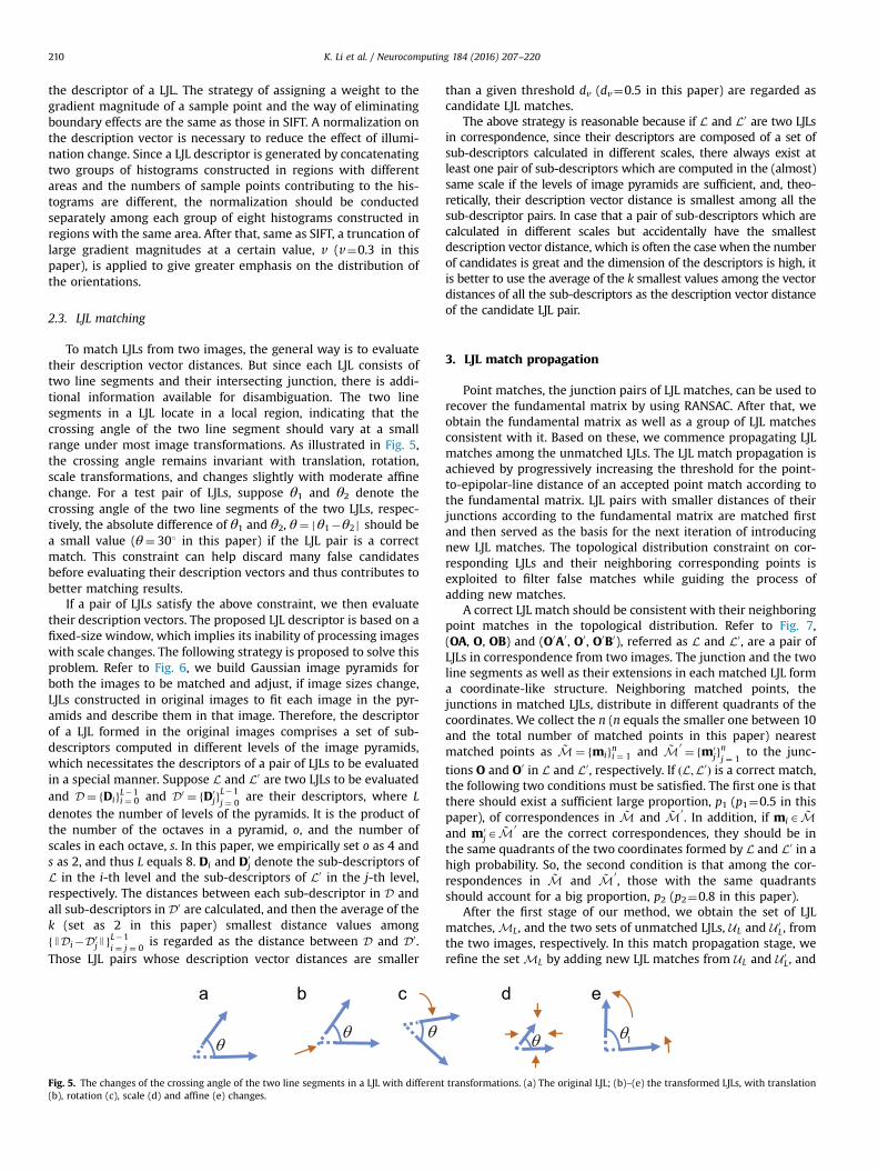
To match LJLs from two images, the general way is to evaluatetheir description vector distances. But since each LJL consists oftwo line segments and their intersecting junction, there is addi-tional information available for disambiguation. The two linesegments in a LJL locate in a local region, indicating that thecrossing angle of the two line segment should vary at a smallrange under most image transformations. As illustrated in Fig. 5,the crossing angle remains invariant with translation, rotation,scale transformations, and changes slightly with moderate affinechange. For a test pair of LJLs, suppose θ1 and θ2 denote thecrossing angle of the two line segments of the two LJLs, respec-tively, the absolute difference of θ1 and θ2, θ¼ jθ1�θ2 j should bea small value (θ¼ 301 in this paper) if the LJL pair is a correctmatch. This constraint can help discard many false candidatesbefore evaluating their description vectors and thus contributes tobetter matching results.

If a pair of LJLs satisfy the above constraint, we then evaluatetheir description vectors. The proposed LJL descriptor is based on afixed-size window, which implies its inability of processing imageswith scale changes. The following strategy is proposed to solve thisproblem. Refer to Fig. 6, we build Gaussian image pyramids forboth the images to be matched and adjust, if image sizes change,LJLs constructed in original images to fit each image in the pyr-amids and describe them in that image. Therefore, the descriptorof a LJL formed in the original images comprises a set of sub-descriptors computed in different levels of the image pyramids,which necessitates the descriptors of a pair of LJLs to be evaluatedin a special manner. Suppose L and L0 are two LJLs to be evaluatedand D¼ fDigL�1

i ¼ 0 and D0 ¼ fD0jgL�1j ¼ 0

are their descriptors, where Ldenotes the number of levels of the pyramids. It is the product ofthe number of the octaves in a pyramid, o, and the number ofscales in each octave, s. In this paper, we empirically set o as 4 ands as 2, and thus L equals 8. Di and D0

j denote the sub-descriptors ofL in the i-th level and the sub-descriptors of L0 in the j-th level,respectively. The distances between each sub-descriptor in D andall sub-descriptors in D0 are calculated, and then the average of thek (set as 2 in this paper) smallest distance values amongfJDi�D0

j JgL�1i ¼ j ¼ 0

is regarded as the distance between D and D0.Those LJL pairs whose description vector distances are smaller

Fig. 5. The changes of the crossing angle of the two line segments in a LJL with different(b), rotation (c), scale (d) and affine (e) changes.

than a given threshold dv (dv¼0.5 in this paper) are regarded ascandidate LJL matches.

The above strategy is reasonable because if L and L0 are two LJLsin correspondence, since their descriptors are composed of a set ofsub-descriptors calculated in different scales, there always exist atleast one pair of sub-descriptors which are computed in the (almost)same scale if the levels of image pyramids are sufficient, and, theo-retically, their description vector distance is smallest among all thesub-descriptor pairs. In case that a pair of sub-descriptors which arecalculated in different scales but accidentally have the smallestdescription vector distance, which is often the case when the numberof candidates is great and the dimension of the descriptors is high, itis better to use the average of the k smallest values among the vectordistances of all the sub-descriptors as the description vector distanceof the candidate LJL pair.

3. LJL match propagation

Point matches, the junction pairs of LJL matches, can be used torecover the fundamental matrix by using RANSAC. After that, weobtain the fundamental matrix as well as a group of LJL matchesconsistent with it. Based on these, we commence propagating LJLmatches among the unmatched LJLs. The LJL match propagation isachieved by progressively increasing the threshold for the point-to-epipolar-line distance of an accepted point match according tothe fundamental matrix. LJL pairs with smaller distances of theirjunctions according to the fundamental matrix are matched firstand then served as the basis for the next iteration of introducingnew LJL matches. The topological distribution constraint on cor-responding LJLs and their neighboring corresponding points isexploited to filter false matches while guiding the process ofadding new matches.

A correct LJL match should be consistent with their neighboringpoint matches in the topological distribution. Refer to Fig. 7,(OA, O, OB) and (O0A0, O0, O0B0), referred as L and L0, are a pair ofLJLs in correspondence from two images. The junction and the twoline segments as well as their extensions in each matched LJL forma coordinate-like structure. Neighboring matched points, thejunctions in matched LJLs, distribute in different quadrants of thecoordinates. We collect the n (n equals the smaller one between 10and the total number of matched points in this paper) nearestmatched points as ~M ¼ fmigni ¼ 1 and ~M 0 ¼ fm0

jgnj ¼ 1to the junc-

tions O and O0 in L and L0, respectively. If ðL;L0Þ is a correct match,the following two conditions must be satisfied. The first one is thatthere should exist a sufficient large proportion, p1 (p1¼0.5 in thispaper), of correspondences in ~M and ~M0

. In addition, if miA ~Mand m0

jA~M 0

are the correct correspondences, they should be inthe same quadrants of the two coordinates formed by L and L0 in ahigh probability. So, the second condition is that among the cor-respondences in ~M and ~M 0

, those with the same quadrantsshould account for a big proportion, p2 (p2¼0.8 in this paper).

After the first stage of our method, we obtain the set of LJLmatches, ML, and the two sets of unmatched LJLs, UL and U 0

L, fromthe two images, respectively. In this match propagation stage, werefine the set ML by adding new LJL matches from UL and U 0

L, and

transformations. (a) The original LJL; (b)–(e) the transformed LJLs, with translation

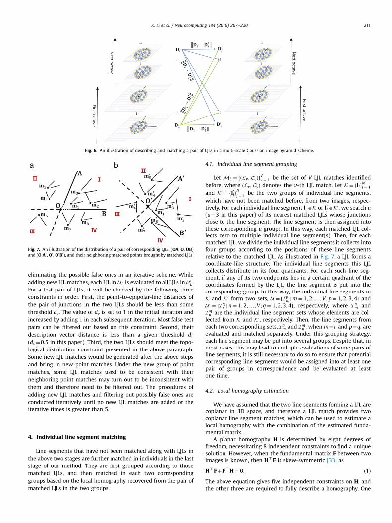
Fig. 6. An illustration of describing and matching a pair of LJLs in a multi-scale Gaussian image pyramid scheme.

Fig. 7. An illustration of the distribution of a pair of corresponding LJLs, (OA, O, OB)and (O0A0 , O0 , O0B0), and their neighboring matched points brought by matched LJLs.

K. Li et al. / Neurocomputing 184 (2016) 207–220 211

eliminating the possible false ones in an iterative scheme. Whileadding new LJL matches, each LJL in UL is evaluated to all LJLs in U 0

L.For a test pair of LJLs, it will be checked by the following threeconstraints in order. First, the point-to-epipolar-line distances ofthe pair of junctions in the two LJLs should be less than somethreshold de. The value of de is set to 1 in the initial iteration andincreased by adding 1 in each subsequent iteration. Most false testpairs can be filtered out based on this constraint. Second, theirdescription vector distance is less than a given threshold dv(dv¼0.5 in this paper). Third, the two LJLs should meet the topo-logical distribution constraint presented in the above paragraph.Some new LJL matches would be generated after the above stepsand bring in new point matches. Under the new group of pointmatches, some LJL matches used to be consistent with theirneighboring point matches may turn out to be inconsistent withthem and therefore need to be filtered out. The procedures ofadding new LJL matches and filtering out possibly false ones areconducted iteratively until no new LJL matches are added or theiterative times is greater than 5.

4. Individual line segment matching

Line segments that have not been matched along with LJLs inthe above two stages are further matched in individuals in the laststage of our method. They are first grouped according to thosematched LJLs, and then matched in each two correspondinggroups based on the local homography recovered from the pair ofmatched LJLs in the two groups.

4.1. Individual line segment grouping

Let ML ¼ fðLv;L0vÞgVv ¼ 1 be the set of V LJL matches identified

before, where ðLv;L0vÞ denotes the v-th LJL match. Let K¼ fligMi ¼ 1

and K0 ¼ fl0jgN

j ¼ 1be the two groups of individual line segments,

which have not been matched before, from two images, respec-tively. For each individual line segment liAK or l0jAK0, we search u(u¼3 in this paper) of its nearest matched LJLs whose junctionsclose to the line segment. The line segment is then assigned intothese corresponding u groups. In this way, each matched LJL col-lects zero to multiple individual line segment(s). Then, for eachmatched LJL, we divide the individual line segments it collects intofour groups according to the positions of these line segmentsrelative to the matched LJL. As illustrated in Fig. 7, a LJL forms acoordinate-like structure. The individual line segments this LJLcollects distribute in its four quadrants. For each such line seg-ment, if any of its two endpoints lies in a certain quadrant of thecoordinates formed by the LJL, the line segment is put into thecorresponding group. In this way, the individual line segments inK and K0 form two sets, U ¼ fIp

m jm¼ 1;2;…;V ; p¼ 1;2;3;4g andU 0 ¼ fI 0q

n jn¼ 1;2;…;V ; q¼ 1;2;3;4g, respectively, where Ipm and

I 0qn are the individual line segment sets whose elements are col-

lected from K and K0, respectively. Then, the line segments fromeach two corresponding sets, Ip

m and I 0qn , when m¼n and p¼q, are

evaluated and matched separately. Under this grouping strategy,each line segment may be put into several groups. Despite that, inmost cases, this may lead to multiple evaluations of some pairs ofline segments, it is still necessary to do so to ensure that potentialcorresponding line segments would be assigned into at least onepair of groups in correspondence and be evaluated at leastone time.

4.2. Local homography estimation

We have assumed that the two line segments forming a LJL arecoplanar in 3D space, and therefore a LJL match provides twocoplanar line segment matches, which can be used to estimate alocal homography with the combination of the estimated funda-mental matrix.

A planar homography H is determined by eight degrees offreedom, necessitating 8 independent constraints to find a uniquesolution. However, when the fundamental matrix F between twoimages is known, then H>F is skew-symmetric [33] as

H>FþF>H¼ 0: ð1ÞThe above equation gives five independent constraints on H, andthe other three are required to fully describe a homography. One

Fig. 8. An illustration of evaluating a pair of candidate line segment corre-spondences using the estimated local homography. l and l0 are the two line seg-ments to be evaluated, lh and l0h are their correspondences mapped by the esti-mated homography.

K. Li et al. / Neurocomputing 184 (2016) 207–220212

line match provides two independent constraints [34], resulting inthe system that is over-constrained since two coplanar line mat-ches exist in our case.

The homography induced by a 3D plane π can be representedas

H¼A�e0v> ; ð2Þwhere the 3D plane is represented by π¼ ðv> ;1Þ in the projectivereconstruction with the camera matrices C¼ ½Ij0� and C0 ¼ ½Aje0�.The homography maps a point from one 2D plane to another 2Dplane. For a line segment match ðl; l0Þ, suppose x is an endpoint of l,the homography maps it to its correspondence point x0 as

x0 ¼Hx: ð3ÞSince l and l0 correspond with each other, x0 must be a point lyingon l0, which results in

l0 >x0 ¼ 0: ð4ÞCombining (2)–(4), we obtain

l0 > ðA�e0v> Þx¼ 0: ð5ÞArranging the above equation, we finally get

x> v¼ x>A> l0

e0> l0; ð6Þ

which is linear in v. Each endpoint of a line segment in a linematch provides a constraint equation, and two line segmentmatches totally provide four constraint equations. A least-squaresolution of v can be obtained from the four equations. The localhomograpy H is then computed from Eq. (2).

4.3. Individual line segment matching

After grouping, the individual line segments in one group froman image are only evaluated and matched with the individual linesegments in the corresponding group from the other image, whichdecreases the candidate pairs that need to be evaluated and thusimprove the efficiency of our method and also the accuracy of linematching results since less interferences are involved when find-ing the correspondence for a line segment. Suppose l and l0 are apair of individual line segments to be evaluated and they arecollected by the pair of matched LJLs, L and L0, respectively. TheLJL match, (L, L0), brings one point match, (j; j0), and two linesegment matches, (lm; l

0m) and (ln; l0n). From L and L0, the local

homography, H, is estimated, using the strategy presented inSection 4.2.

We first check whether the rotation angle of l and l0 is con-sistent with the rotation angles of the two pairs of matched linesegments brought by L and L0. Correctly matched line segments inlocal regions possess similar rotation angles under image trans-formations. Suppose the rotation angle of lm and l0m is σm, and thatof ln and l0n is σn, If there exists

σ�σmþσn

2

���

���oβ; ð7Þ

where σ denotes the rotation angle of l and l0, and β is a user-defined angle threshold set as 201 in this paper, we accept (l; l0)temporarily as a candidate match and take it for furtherevaluation.

We then evaluate the candidate match (l; l0) by the localhomography estimated from (L, L0). This method is reasonableonly when the 3D correspondence(s) of l and l0 lie in the same 3Dplane as that of the 3D correspondences of lm (l0m) and ln (l0n). It ishardly possible to determine whether the 3D correspondences ofseveral 2D line segments are in same 3D plane without the pro-jective information of the cameras. But the strategies used in ouralgorithm ensure the rationality of this method. The first is the

exploitation of the local spatial proximity. Line segments adjacentwith each other in 2D images are highly possible to be coplanar in3D space. The two line segment triples, (lm, ln, l) and (l0m, l

0n, l

0), areclustered based on the local spatial proximity, which guarantees afairly high possibility that the 3D correspondences of the linesegments in the two triples are on the same plane. On the otherhand, the success of matching the two LJLs, though we cannotabsolutely ensure the correctness of the matching, substantiatesthat the 3D correspondences of lm (l0m) and ln (l0n) are on the same3D plane. The second is the redundant grouping strategy. Eachindividual line segment is redundantly collected by severalneighboring matched LJLs, which greatly increases the possibilitythat two potential corresponding line segments are distributedinto at least one pair of groups where they are coplanar with thetwo pairs of matched lines in 3D space.

If (l, l0) is a correct match, the correspondences of the twoendpoints of l, mapped by the estimated local homography, mustbe adjacent with (ideally on) l0, and the same goes with the end-points of l0. We use the affect region of a line segment to apply thisconstraint. The affect region of a line segment is illustrated inFig. 2. It is a rectangle around the line segment with a parametercontrolling the size of the rectangle. This parameter w (see Fig. 2)is set as 3 in pixels when applying this constraint. Refer to Fig. 8,we map l and l0 to their correspondences by the estimated localhomography, generating lh and l0h for l and l0, respectively. If both lhand l0h intersect with the affect regions of l0 and l (the rectanglesfilled in yellow around l0 and l), the match (l, l0) is temporarilyaccepted and is taken for further evaluation. Here, a line segmentintersects with a region means there exists at least one point (notjust the two endpoints) on the line segment which is within theregion. We define the average of the four distances, including theperpendicular distances of two endpoints of l0h to l and the per-pendicular distances of the two endpoints of lh to l0, as themapping error of (l, l0), which is used to measure the similarity of land l0. The four distances are denoted as d1, d2, d3 and d4 in Fig. 8,then, the mapping error of (l, l0) is:

Eðl; l0Þ ¼ d1þd2þd3þd44

: ð8Þ

While finding the correspondence for a line segment, the aboveconstraints are unable to discern the false candidates when theyhave similar directions with the correct one and are adjacent withit. Refer to Fig. 9, while we find the correspondence for l, both l01and l02 may be accepted by the above constraints because they areclose with each other and have similar directions. We use a simplebut effective way to enforce the constraints on correct line seg-ment matches by finding the brighter sides of line segments. Referto Fig. 9, we calculate the average intensity values of pixels in thetwo small rectangles lying in the two sides of a line segment andregard the side where the average intensity value is higher as thebrighter side. Since the brighter side of a line segment indicatesthe relative brightness of the two small regions along with a linesegment, it is invariant under almost all image transformationsand thus can be exploited to find the correct correspondences forline segments. In Fig. 9, we finally pick out l01 as the correct cor-respondence of l since it has the same brighter side as l.

Fig. 9. An illustration of using the brighter side constraint to help match line segments. l is a line segment from a image. l01 and l02 are the two candidate correspondences for lfrom the other image. l01 is accepted as the correspondence for l because its brighter side is the same as l.

K. Li et al. / Neurocomputing 184 (2016) 207–220 213

After that, there may exist the cases that one line segment inone image is matched with several line segments in the otherimage. We select the pair with the minimal mapping error as thecorrect match and reject the others.

5. Experimental results

Extensive experiments on representative image pairs wereconducted to select proper values for some parameters of theproposed method and to evaluate its performance under variousimage transformations and in some special scenes, as well as tocompare it with the state-of-the-art line matching methods.

5.1. Parameter selection

Our algorithm has some parameters, but only two of them arekey to influence the performance of the algorithm. Other para-meters are used to strengthen some constraints and the fluctua-tions of their values make slight differences on the results. Thefirst parameter is w which controls the size of the affect region of aline segment when constructing LJLs. The second parameter is r,the radius of the smaller of circle when describing a LJL. The fiverepresentative image pairs [37] shown in Fig. 10 were employed tohelp fix the two parameters. There are illumination change, imageblur, JPEG compression, viewpoint change, scale and rotationchanges between the two images in the five image pairs in order.Since the two images in each image pair are related by a knownhomography, we can evaluate the performance generated by dif-ferent parameters conveniently and reliably, which benefits us toselect optimal values for the parameters.

We first conducted experiments to select a proper value for w.It is obvious that a big value for w results in a big affect region of aline segment and more intersections of line segments and moreLJLs. Sufficient LJLs are the guarantee to produce enough initial LJLmatches and are therefore crucial to the final line matching resultsbecause the subsequent steps of adding more line segment mat-ches are based on the initial LJL matches. However, excessive LJLs,especially when many of them cannot find their correspondencesin the other group of LJLs, will harm the matching of them sincemore interferences are introduced, and will increase both thecomputation time and memory to match them. We employed theway introduced in [37] by calculating the repeatability of twogroups of points to select a proper value for w. In [37], therepeatability score is used to evaluate different local regiondetectors under various image transformations. It measures howthe number of correspondences depends on the transformationbetween two images. Higher repeatability indicates better per-formance of the image feature detection and is generally moreconducive for matching these features. We calculated the repeat-ability of the junction points in constructed LJLs under variousvalues of w and fixed w at the value with the highest repeatability.All the five image pairs shown in Fig. 10 were employed forexperiments and the average repeatability of the junctions inconstructed LJLs in all image pairs is calculated. The change of the

average repeatability with respect to w is shown in Fig. 11. Weobserve from this figure that the repeatability curve increaseswhen w is less than 20, and is stable until w is bigger than 25,where the curve begins to drop. Thus, both 20 and 25 are propervalues for w. To reduce the computation time, w¼20 was selectedin this paper.

We then conducted experiments to find a proper value for theparameter r, which determines the size of the local patch exploi-ted for describing a LJL. The LJL descriptor is often more dis-criminative but more sensitive to shape distortion when a biggerpatch is used. Table 1 shows the accuracies of the matching resultsof the LJLs with various values of r on the five image pairs shownin Fig. 10. Since the average accuracy reaches its maximum atr¼10, this setting was therefore applied in our algorithm. Notethat the correctness of a LJL match is assessed in this way: let (j; j0)be the pair of junctions in a LJL match, we map j and j0 by theknown homography, generating their estimated correspondences,jh and j0h, for j and j0, respectively. If both the distance between j0hand j and the distance between jh and j0 are less than 5 pixels, weregard the LJL match as a correct one. This correctness-assessstrategy for point matches seems problematical since it may labela false point match as a correct one when one point in the matchlies near the actual correspondence of the other point. However,since in our situation, the matched points are the intersectingjunctions of line segments, the distribution of which is often muchsparser and their numbers are often smaller than the detectedfeature points by some detectors. The cases that several matchedpoints cluster in a very small region are scarce. This fact ensuresthe reasonableness of our correctness-access strategy and thereliableness of the value we set for r.

5.2. Robustness of the LJL descriptor

After the key parameter for constructing a LJL descriptor beingfixed, we conducted experiments to compare our LJL descriptorwith other local region descriptor(s) for the effectiveness todescribe the local regions around LJLs. The famous SIFT descriptor[1] was employed for the comparison. The two descriptors, LJL andSIFT, were used to describe the junctions in the constructed LJLs onthe five image pairs as shown in Fig. 10. The junctions were mat-ched under the same threshold for their description vector dis-tances for both the descriptors. Note that since both SIFT and LJLare based on fixed-size windows and are unable to deal with scalechanges, we described the junctions in LJLs using the twodescriptors both in the multi-scale image pyramid framework weproposed in Section 2.3.

Table 2 shows the accuracies of the matching results of the twodescriptors. It can be observed from this table that on all of the fiveimage pairs, where various extreme image transformations exist,the proposed LJL descriptor produced matching results withhigher accuracies than SIFT. On some image pairs, graffiti and boat,the advantage is fairly remarkable: the results of LJL descriptorpresent the accuracy more than twice as that of SIFT. This goodperformance of our LJL descriptor on the matching accuracy iscrucial for our method because it requires estimating a precise

Fig. 10. The five image pairs, leuven, bikes, ubc, graffiti, and boat, used for selecting proper values for the two key parameters in our method and for evaluating the proposedLJL descriptor.

Fig. 11. The changes of the average repeatability of the junction points in the con-structed LJL from images shown in Fig. 10 with different values of the parameter w.

Table 1The accuracies of the LJL structure matching results on the five image pairs shownin Fig. 10 under various values of the parameter r.

r¼4 r¼6 r¼8 r¼10 r¼12 r¼14

leuven 0.81 0.85 0.87 0.84 0.85 0.84bikes 0.63 0.64 0.61 0.59 0.58 0.60ubc 0.74 0.74 0.77 0.72 0.72 0.69graffiti 0.30 0.45 0.64 0.76 0.69 0.65boat 0.09 0.21 0.31 0.44 0.40 0.27Average 0.51 0.58 0.64 0.67 0.65 0.61

Table 2The comparative junction point matching accuracies based on the description bythe proposed LJL descriptor and SIFT descriptor on the five image pairs shown inFig. 10.

leuven bikes ubc graffiti boat

LJL 0.84 0.59 0.72 0.76 0.44SIFT 0.71 0.48 0.71 0.37 0.19

K. Li et al. / Neurocomputing 184 (2016) 207–220214

fundamental matrix from the initial LJL matches. A large propor-tion of correct matches certainly contribute to better estimationresult of the fundamental matrix. We did not use the well-knownlocal descriptor evaluation method introduced in [36] because theproposed LJL descriptor is specially designed for LJLs. It describes

the circular regions centered at the junctions in LJLs, rather thanaffine invariant regions detected by some detectors, which is theprerequisite of that famous local descriptor evaluation method.

The better performance of our proposed LJL descriptor overSIFT in describing the local regions around the junctions of LJLsowes to the following two factors. The first one is that the regionsfor constructing the orientation histograms for LJL descriptor aremore likely to correspond with each other for correspondingjunctions than that of SIFT. We have clear and precise dominantdirections to deal with possible rotation changes. Either of thedirections of the two line segments forming a junction can beregarded as the dominant direction of the junction, according towhich the region exploited for constructing the orientation his-tograms is rotated. While in SIFT, the dominant direction of a pointis calculated from its neighboring region, which is absolutely lessprecise than ours. Besides, the configuration of the two line seg-ments forming the junction in a LJL is exploited for dividing theregion around the junction into subregions, where the orientationhistograms are constructed. Since the two line segments are clearand precise, subregions divided by them are more likely to cor-respond with each other for corresponding junctions than that ofSIFT, in which subregions are obtained by dividing the regionregularly with the same angle span (90°). The second one is theexploitation of the constraint that the crossing angle of the twoline segments in a LJL should vary in a small range under imagetransformations, which helps discard many false candidate LJLpairs before evaluating their description vector distances andhence contributes to better matching results.

5.3. Line matching results

Fig. 12 shows the line matching results of the proposed methodon eight representative image pairs which contain various imagetransformations and were captured from both planar and non-planar scenes. All these image pairs were used in the publishedpapers [22,37], except the image pair (d), in which a poorly tex-tured scene was captured in the two images. The aim weemployed this image pair is to evaluate the performance of ourmethod in poorly textured scenes. The line segments used formatching were extracted by the famous line segment detector, LSD[35]. The correctness of the obtained matches was accessed byvisual inspection.

It is observed that our algorithm is robust under commonimage transformations, namely illumination, scale, rotation,viewpoint changes, image blur, and JPEG compression and inpoorly textured scene. The accuracies are above 95% on all theimage pairs. The robustness of our method owes to the followingfactors. The first one is the robust LJL descriptor. It is speciallydesigned for LJL while incorporates many benefits of SIFT, leading

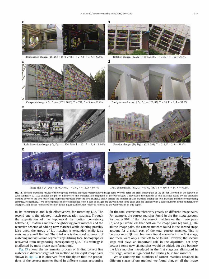
Fig. 12. The line matching results of the proposed method on eight representative image pairs. We will refer the eight image pairs as (a)–(h) for later use. In the caption ofeach subfigure, ðD1 ;D2Þ denotes the pair of numbers of the extracted line segments in the two images. T represents the number of total matches found by the proposedmethod between the two sets of line segments extracted from the two images. F and A denote the number of false matches among the total matches and the correspondingaccuracy, respectively. Two line segments in correspondence from a pair of images are drawn in the same color and are labeled with a same number at the middles. (Forinterpretation of the references to color in this figure caption, the reader is referred to the web version of this paper.)

K. Li et al. / Neurocomputing 184 (2016) 207–220 215

to its robustness and high effectiveness for matching LJLs. Thesecond one is the adopted match-propagation strategy. Throughthe exploitation of the topological distribution consistencybetween LJL matches and their neighboring point matches and therecursive scheme of adding new matches while deleting possiblyfalse ones, the group of LJL matches is expanded while falsematches are well limited. The third one is the novel approach ofmatching individual line segments by utilizing local homographiesrecovered from neighboring corresponding LJLs. This strategy isunaffected by most image transformations.

Fig. 13 shows the incremental process of finding correct linematches in different stages of our method on the eight image pairsshown in Fig. 12. It is observed from this figure that the propor-tions of the correct matches found in different stages accounting

for the total correct matches vary greatly on different image pairs.For example, the correct matches found in the first stage accountfor nearly 90% of the total correct matches on the image pairs(b) and (c), while less than 50% on the image pairs (e) and (g). Onall the image pairs, the correct matches found in the second stageaccount for a small part of the total correct matches. This isbecause most LJL matches were found correctly in the first stage,and there were only a few left to be found. However, the secondstage still plays an important role in the algorithm, not onlybecause some new LJL matches would be added, but also becausethe false matches introduced in the first stage are eliminated inthis stage, which is significant for limiting false line matches.

While counting the numbers of correct matches obtained indifferent stages of our method, we found that, on all the image

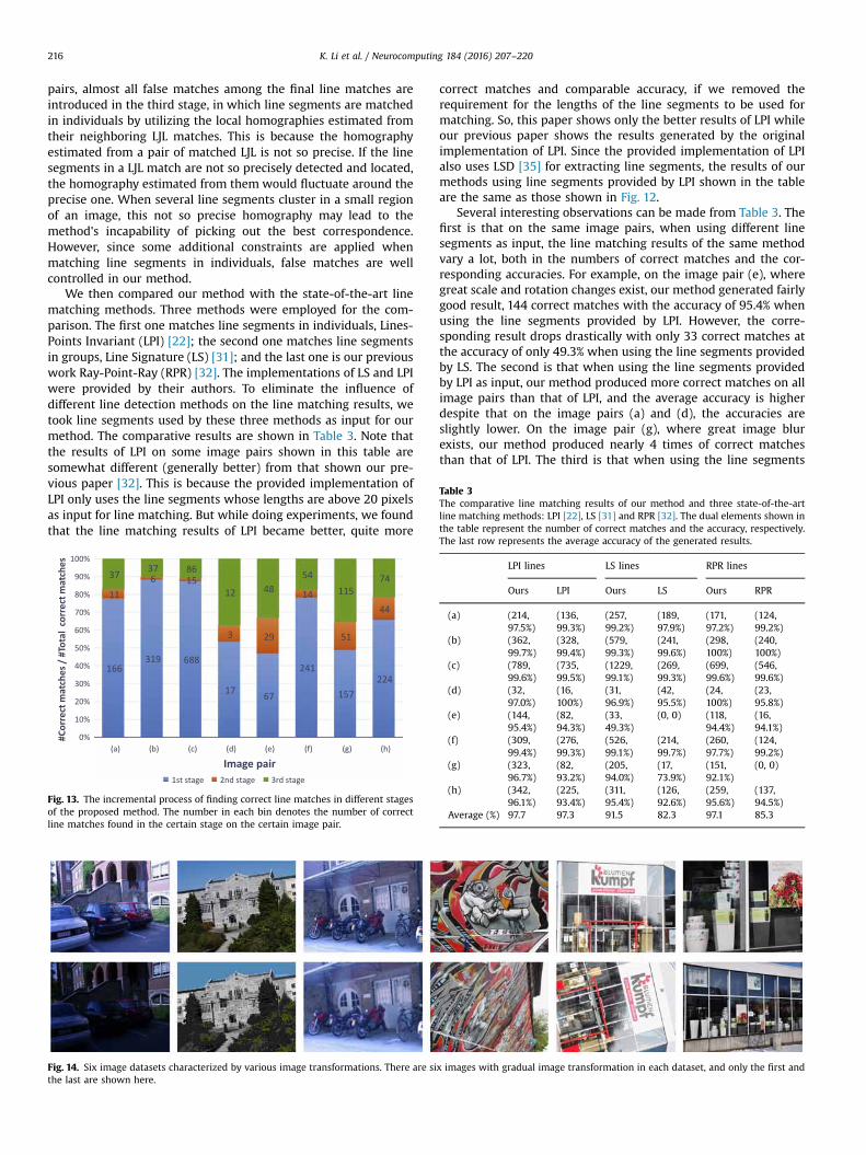
Table 3The comparative line matching results of our method and three state-of-the-artline matching methods: LPI [22], LS [31] and RPR [32]. The dual elements shown inthe table represent the number of correct matches and the accuracy, respectively.

K. Li et al. / Neurocomputing 184 (2016) 207–220216

pairs, almost all false matches among the final line matches areintroduced in the third stage, in which line segments are matchedin individuals by utilizing the local homographies estimated fromtheir neighboring LJL matches. This is because the homographyestimated from a pair of matched LJL is not so precise. If the linesegments in a LJL match are not so precisely detected and located,the homography estimated from them would fluctuate around theprecise one. When several line segments cluster in a small regionof an image, this not so precise homography may lead to themethod's incapability of picking out the best correspondence.However, since some additional constraints are applied whenmatching line segments in individuals, false matches are wellcontrolled in our method.

We then compared our method with the state-of-the-art linematching methods. Three methods were employed for the com-parison. The first one matches line segments in individuals, Lines-Points Invariant (LPI) [22]; the second one matches line segmentsin groups, Line Signature (LS) [31]; and the last one is our previouswork Ray-Point-Ray (RPR) [32]. The implementations of LS and LPIwere provided by their authors. To eliminate the influence ofdifferent line detection methods on the line matching results, wetook line segments used by these three methods as input for ourmethod. The comparative results are shown in Table 3. Note thatthe results of LPI on some image pairs shown in this table aresomewhat different (generally better) from that shown our pre-vious paper [32]. This is because the provided implementation ofLPI only uses the line segments whose lengths are above 20 pixelsas input for line matching. But while doing experiments, we foundthat the line matching results of LPI became better, quite more

Fig. 13. The incremental process of finding correct line matches in different stagesof the proposed method. The number in each bin denotes the number of correctline matches found in the certain stage on the certain image pair.

Fig. 14. Six image datasets characterized by various image transformations. There are sithe last are shown here.

correct matches and comparable accuracy, if we removed therequirement for the lengths of the line segments to be used formatching. So, this paper shows only the better results of LPI whileour previous paper shows the results generated by the originalimplementation of LPI. Since the provided implementation of LPIalso uses LSD [35] for extracting line segments, the results of ourmethods using line segments provided by LPI shown in the tableare the same as those shown in Fig. 12.

Several interesting observations can be made from Table 3. Thefirst is that on the same image pairs, when using different linesegments as input, the line matching results of the same methodvary a lot, both in the numbers of correct matches and the cor-responding accuracies. For example, on the image pair (e), wheregreat scale and rotation changes exist, our method generated fairlygood result, 144 correct matches with the accuracy of 95.4% whenusing the line segments provided by LPI. However, the corre-sponding result drops drastically with only 33 correct matches atthe accuracy of only 49.3% when using the line segments providedby LS. The second is that when using the line segments providedby LPI as input, our method produced more correct matches on allimage pairs than that of LPI, and the average accuracy is higherdespite that on the image pairs (a) and (d), the accuracies areslightly lower. On the image pair (g), where great image blurexists, our method produced nearly 4 times of correct matchesthan that of LPI. The third is that when using the line segments

The last row represents the average accuracy of the generated results.

LPI lines LS lines RPR lines

Ours LPI Ours LS Ours RPR

(a) (214,97.5%)

(136,99.3%)

(257,99.2%)

(189,97.9%)

(171,97.2%)

(124,99.2%)

(b) (362,99.7%)

(328,99.4%)

(579,99.3%)

(241,99.6%)

(298,100%)

(240,100%)

(c) (789,99.6%)

(735,99.5%)

(1229,99.1%)

(269,99.3%)

(699,99.6%)

(546,99.6%)

(d) (32,97.0%)

(16,100%)

(31,96.9%)

(42,95.5%)

(24,100%)

(23,95.8%)

(e) (144,95.4%)

(82,94.3%)

(33,49.3%)

(0, 0) (118,94.4%)

(16,94.1%)

(f) (309,99.4%)

(276,99.3%)

(526,99.1%)

(214,99.7%)

(260,97.7%)

(124,99.2%)

(g) (323,96.7%)

(82,93.2%)

(205,94.0%)

(17,73.9%)

(151,92.1%)

(0, 0)

(h) (342,96.1%)

(225,93.4%)

(311,95.4%)

(126,92.6%)

(259,95.6%)

(137,94.5%)

Average (%) 97.7 97.3 91.5 82.3 97.1 85.3

x images with gradual image transformation in each dataset, and only the first and

K. Li et al. / Neurocomputing 184 (2016) 207–220 217

detected by LS as input, our method has quite better performancethan LS itself. Due to the multi-scale scheme, LS produced largegroups of line segments, which caused matching them being verytime-consuming and memory-consuming. With such large groupsof line segments as input, compared with LS, our method pro-duced line matches with much higher average accuracies andowned an overwhelming advantage in the amount of correctmatches on some images pairs. Our method found more than 12times of correct matches than that of LS on the image pair (g) andnearly 5 times of correct matches on the image pair (c). Besides, onthe image pair (e), LS failed to produce any correct line match,while our method can still produce some through with a lowaccuracy. The fourth is that, by taking the line segments used inRPR as input, the proposed method excels both at the amount ofcorrect matches and the accuracy. Remarkably, RPR failed on theimage pair (g), where there is great blur between the two images,while the proposed method can still produce good results. Itgenerated 151 correct matches with the accuracy of 92.1%. Theseadvantages of the proposed method over RPR prove the effec-tiveness of the promotions we have made based on RPR.

5.4. Further comparison with LPI

From Table 3, we can conclude that our method and LPI are thetwo most robust line matching methods. We conducted additionalexperiments to further evaluate the two methods.

We first experimented on some datasets related by globalhomographies. The six image datasets [37,17] shown in Fig. 14were employed. These image datasets are characterized by illu-mination, rotation, viewpoint and scale changes, image blur andJPEG compression among the images, respectively. The reason weemployed them for experiments is because the global homo-graphies between images in the datasets are known. Thus, theground truth of the line segment matches between images can beestablished by mapping line segments detected in one image toanother one and finding if there are line segments in the very closeregions around the mapped line segments. With the ground truthof line segment matches between images, the recalls (the ratiobetween the number of correct matches and the number of

Fig. 15. The recalls of the line matching results of the proposed me

ground truth correspondences) of line matching results of thesetwo methods can be calculated. In each datasets, the line segmentsdetected in the first image were matched with those detected inthe other five images. The recalls of the matching results for thetwo methods are shown in Fig. 15. It is observed from this figurethat the recalls of the line matching results generated by ourmethod are higher than those of LPI on almost all image pairsunder all these six kinds of image transformations except the twoimage pairs where JPEG compression between images exists.

Besides experimenting on the common datasets, we had con-ducted additional experiments on some very challenging imagepairs. The experimental results are shown in Fig. 16, from whichwe can observe that under these challenging cases, our method ismore robust and produces quite more correct matches.

6. Discussion

All the line matching results of our method presented aboveare based on the fixed parameters, which we have discussed inSection 5.1. In this section, we will discuss further about how toadjust the values of some parameters to improve the performanceof our method for some specific applications.

6.1. Time performance

Fig. 17 shows the elapsed time of each stage of our method andthe percentage it accounts for the corresponding total elapsed timeon each of the eight image pairs shown in Fig. 12. The proposedmethod was implemented with Cþþ and the computation timewas measured on a 3.4 GHz Inter (R) Core(TM) processor with12 GB of RAM. It can be observed from this figure that the totalelapsed time of our method varies a lot on different image pairs.Our method took nearly 660 s on the image pair (c) while less than2 s on the image pair (d). Generally, the more complex the scenescaptured are, the more time it takes for our method to match theline segments extracted from the images. This is because more linesegments can be detected in images of complex scenes andmatching larger groups of line segments costs more time. Another

thod and LPI [22] on the six image datasets shown in Fig. 14.

Fig. 16. The comparative results between our method and LPI on some challenging image pairs. Zoom in for better interpretation.

Fig. 17. The elapsed time (in seconds) of each stage of our method and the per-centage it accounts for the corresponding total elapsed time on each of the eightimage pairs shown in Fig. 12. The number in each bin denotes the elapsed time ofthe proposed method in a certain stage on a certain image pair.

Table 4The line matching results and running time of the proposed algorithm generated bybuilding Gaussian image pyramids (M-I) and without building Gaussian imagepyramids (M-II) on some image pairs shown in Fig. 12. The last column shows thedrop ratios of the running time of M-II relative to M-I.

Matching results Running times (s)

M-I M-II M-I M-II Drop (%)

(a) (214, 97.5%) (212, 99.1%) 56.3 11.2 80.1(b) (362, 99.7%) (379, 99.2%) 74.3 27.2 63.4(c) (789, 99.6%) (786, 99.6%) 658.9 241.5 63.3(d) (32,97.0%) (24,100%) 1.9 0.7 62.0(f) (309, 99.4%) (317, 99.1%) 61.4 13.9 77.4(h) (342, 96.1%) (334, 96.5%) 75.0 12.4 83.5

K. Li et al. / Neurocomputing 184 (2016) 207–220218

observation from this figure is that the time spent in the first stageof our method makes a dominant account for the total elapsed timeon all image pairs. The reason behind is that by building image

K. Li et al. / Neurocomputing 184 (2016) 207–220 219

pyramids, each LJL constructed in the original images is adjusted toall images in the pyramids and is described there. The time ofdescribing and matching LJLs from two images increase with thenumber of the levels of the image pyramids. For example, on theimage pair (c), which took the most time by our method, 4856 LJLswere constructed in the first image and 4693 LJLs in the secondimage. When the Gaussian image pyramids built for the two ori-ginal images have 4 octaves with 2 scales in each octave, there are4856�8¼38,848 LJLs and 4693�8¼37,544 LJLs required to bedescribed for the two images, respectively. A LJL descriptor is avector of 128 dimensions. It is sure that matching such large twogroups of LJLs by evaluating the distances between their descriptionvectors in such a high dimension is time-consuming. It seems thatour method is impractical for some applications which have strictrequirement on the running time. However, the time performanceof our method can be tremendously improved by adjusting someparameters for specific scenes.

The majority of the running time of our method was spent indescribing and matching LJLs from two images. There are threeparameters that control the number of the LJLs to be described andmatched. These three parameters are w that controls the size ofthe affect region of a line segment, o, the number of octaves of theimage pyramids, and the number of scales per octave of a pyramid,s. Both o and s are introduced when building Gaussian imagepyramids to deal with the possible scale changes between images.If we have a priori that there is no or merely slight scale change orsome fixed scale change between images, then all the stepsintended to deal with scale changes between images are needless.We can match LJLs constructed in the original images or somespecifically scaled ones directly, which would save plenty of time.

Table 4 shows the comparative line matching results and thecorresponding running time on the six image pairs, (a)–(d), (f) and(h) shown in Fig. 12, with building the Gaussian image pyramids(M-I), and without building the Gaussian image pyramids (M-II).All these six image pairs share the similarity that there are verylittle scale changes between the two images and thus buildingGaussian image pyramids is unnecessary for them. From Table 4,we can see that the matching results generated by M-II are similarwith M-I both in the amounts of correct matches and the accuracy,but the running time dropped drastically. On the all image pairs,M-II took less than half of the running time of M-I. Remarkably, onthe image pairs, (a) and (h), the drop ratios are more than 80%,which means M-II used less than 20% of the running time of M-I.

Apart from choosing to not build image pyramids for imageswith very little scale change to save time, decreasing the value ofthe parameter w can also help reduce the running time since lessLJLs are constructed with a smaller value of w. This strategy isespecially efficient when scenes are rich-textured. For example, onthe image pair (c), where the scene has rich texture and more than1000 line segments were extracted in both images, when the valueof w was set as 20 in pixels, our method spent 658.9 s matching theextracted line segments when building the Gaussian image pyr-amids and 241.5 s without building Gaussian image pyramids. Butwhen we set w¼5 without building the Gaussian image pyramids,our method spent only 17.2 s and produced 788 correct line mat-ches with the accuracy of 99.6%. The matching result is similar withthose generated under a greater value of w, but the cost time dropsdrastically. So, for scenes with rich texture, selecting a smaller valuefor w can greatly promote the efficiency of the method.

6.2. Poorly textured scenes

While conducting experiments, we found that for image pairsthat were captured from poorly textured scenes, if we increase thevalue of the parameter w that controls the size of the affect regionof a line segment when constructing LJLs, the line matching results

are generally better. For example, on the image pair (d) shown inFig. 12, when we varied w from 10 to 60 at the step of 10, weobtained 28, 33, 36, 37, 37 and 36 correct matches in order. Thoughthe increasing is not quantitatively significant, it is particularlymeaningful for this special scene because a more complete sketchof the scene can be obtained with even slight increasing of theobtained line segment matches.

The reason for the better matching results of our proposedmethod on poorly textured scenes with bigger w is as follows. Inpoorly textured scenes, only a small amount of line segments canbe detected. With a greater value of w, more line segments can beregraded as adjacent line segments and used to generate junctionsand construct LJLs. More LJLs in poorly textured scenes often resultin a larger group of initial LJL matches, which improves the linematching results in the following three aspects. First, more linesegments can be matched along with LJL. Second, a generallyprecise fundamental matrix can be obtained, which helps bothpropagate LJL match (in the second stage) and match line seg-ments in individuals (in the third stage). Third, the obtained LJLmatches may distribute in more 3D planes. The third stage of ourmethod, matching line segments in individuals, underlies theassumption that the 3D correspondences of the two line segmentsto be matched lie in the same 3D plane lay by the 3D corre-spondences of the two pairs of matched line segments brought bya pair of matched LJLs. If two individual line segments whose 3Dcorrespondences lie in a 3D plane where none of the 3D corre-spondences of matched LJLs exist, the two line segments cannot bematched by our method. Thus, a larger group of initial LJL matchescan help us to bring in more individual line segment matches.

7. Conclusions

This paper has presented a hierarchical line matching methodin which line segments are first matched along with the structurescalled Line–Junction–Line (LJL) formed by two adjacent line seg-ments and their intersecting junction, and then matched in indi-viduals. While matching LJLs, a robust descriptor as well as aneffective strategy to deal with the possible scale changes betweenimages is proposed to obtain the initial LJL matches, which arethen refined and expanded by an effective match-propagationscheme. Those left unmatched line segments are further matchedby exploiting the local homographies estimated from theirneighboring LJL matches. The experimental results show therobustness of the proposed LJL descriptor for matching LJLs andthe good performance of the proposed method under most kindsof image transformations and in poorly textured scenes. Thesuperiorities of the proposed method to the state-of-the-art linematching methods include its robustness for more kinds ofsituations, the larger amounts of correct matches, and the higheraccuracy in most cases.

Acknowledgments

This work was partially supported by the National NaturalScience Foundation of China (Project no. 41571436), the HubeiProvince Science and Technology Support Program, China (Projectno. 2015BAA027), the National Basic Research Program of China(Project no. 2012CB719904), and the National Natural ScienceFoundation of China (Project no. 41271431). Thanks for Bin Fan,Lilian Zhang and Lu Wang for providing the implementations oftheir methods and some test images.

K. Li et al. / Neurocomputing 184 (2016) 207–220220

References

[1] D.G. Lowe, Distinctive image features from scale-invariant keypoints, Int.J. Comput. Vis. 60 (2) (2004) 91–110.

[2] Z. Wang, B. Fan, F. Wu, Local intensity order pattern for feature description, in:ICCV, 2011.

[3] J.M. Morel, G. Yu, ASIFT: a new framework for fully affine invariant imagecomparison, SIAM J. Imaging Sci. 2 (2) (2009) 438–469.

[4] S. Winder, G. Hua, M. Brown, Picking the best daisy, in: CVPR, 2009.[5] Y. Ke, R. Sukthankar, PCA-SIFT: a more distinctive representation for local

image descriptors, in: CVPR, 2004.[6] H. Bay, T. Tuytelaars, G.L. Van, Surf: speeded up robust features, in: ECCV, 2006.[7] C.J. Taylor, D. Kriegman, Structure and motion from line segments in multiple

images, IEEE Trans. Pattern Anal. Mach. Intell. 17 (11) (1995) 1021–1032.[8] A. Bartoli, P. Sturm, Structure-from-motion using lines: representation, trian-

gulation, and bundle adjustment, Comput. Vis. Image Underst. 100 (3) (2005)416–441.

[9] A.W.K. Tang, T.P. Ng, Y.S. Hung, C.H. Leung, Projective reconstruction from line-correspondences in multiple uncalibrated images, Pattern Recognit. 39 (5)(2006) 889–896.

[10] M. Chandraker, J. Lim, D. Kriegman, Moving in stereo: efficient structure andmotion using lines, in: ICCV, 2009.

[11] S. Ramalingam, M. Brand, Lifting 3D Manhattan lines from a single image, in:ICCV, 2013.

[12] M. Hofer, M. Maurer, H. Bischof, Improving sparse 3D models for man-madeenvironments using line-based 3D reconstruction, in: 3DV, 2014.

[13] H. Bay, A. Ess, A. Neubeck, L. Van Gool, 3D from line segments in two poorly-textured, uncalibrated images, in: 3DPVT, 2006.

[14] C. Schmid, A. Zisserman, Automatic line matching across views, in: CVPR, 1997.[15] C. Baillard, C. Schmid, A. Zisserman, A. Fitzgibbon, Automatic line matching

and 3D reconstruction of buildings from multiple views, in: ISPRS Conferenceon Automatic Extraction of GIS Objects from Digital Imagery, 1999.

[16] Z. Wang, F. Wu, Z. Hu, MSLD: a robust descriptor for line matching, PatternRecognit. 42 (5) (2009) 941–953.

[17] L. Zhang, R. Koch, An efficient and robust line segment matching approachbased on LBD descriptor and pairwise geometric consistency, J. Vis. Commun.Image Represent. 24 (7) (2013) 794–805.

[18] B. Verhagen, R. Timofte, L.G. Van, Scale-invariant line descriptors for widebaseline matching, in: WACV, 2014.

[19] H. Bay, V. Ferrari, L. Van Gool, Wide-baseline stereo matching with line seg-ments, in: CVPR, 2005.

[20] M.I. Lourakis, S.T. Halkidis, S.C. Orphanoudakis, Matching disparate views ofplanar surfaces using projective invariants, Image Vis. Comput. 18 (9) (2000)673–683.

[21] B. Fan, F. Wu, Z. Hu, Line matching leveraged by point correspondences, in:CVPR, 2010.

[22] B. Fan, F. Wu, Z. Hu, Robust line matching through line-point invariants, Pat-tern Recognit. 45 (2) (2012) 794–805.

[23] M. Chen, Z. Shao, Robust affine-invariant line matching for high resolutionremote sensing images, Photogramm. Eng. Remote Sens. 79 (8) (2013)753–760.

[24] B. Micusik, H. Wildenauer, J. Kosecka, Detection and matching of rectilinearstructures, in: CVPR, 2008.

[25] H. Kim, S. Lee, Simultaneous line matching and epipolar geometry estimationbased on the intersection context of coplanar line pairs, Pattern Recognit. Lett.33 (10) (2012) 1349–1363.

[26] H. Kim, S. Lee, Y. Lee, Wide-baseline stereo matching based on the lineintersection context for real-time workspace modeling, J. Opt. Soc. Am. A Opt.Image Sci. Vis. 31 (2) (2014) 421–435.

[27] K. Mikolajczyk, C. Schmid, Scale and affine invariant interest point detectors,Int. J. Comput. Vis. 60 (1) (2004) 63–86.

[28] T. Tuytelaars, L. Van Gool, Matching widely separated views based on affineinvariant regions, Int. J. Comput. Vis. 59 (1) (2004) 61–85.

[29] J. Matas, O. Chum, M. Urban, T. Pajdla, Robust wide baseline stereo frommaximally stable extremal regions, in: BMVC, 2004.

[30] T. Kadir, A. Zisserman, M. Brady, An affine invariant salient region detector, in:ECCV, 2004.

[31] L. Wang, U. Neumann, S. You, Wide-baseline image matching using line sig-natures, in: ICCV, 2009.

[32] K. Li, J. Yao, X. Lu. Robust line matching based on Ray-Point-Ray descriptor. InACCV 2014 Workshop on Robust Local Descriptors for Computer Vision, 2014.

[33] Q.-T. Luong, T. Viville, Canonical representations for the geometries of multipleprojective views, Comput. Vis. Image Underst. 64 (2) (1996) 193–229.

[34] A. Anubhav, C.V. Jawahar, P.J. Narayanan, A Survey of Planar HomographyEstimation Techniques. Centre for Visual Information Technology. TechnicalReport IIIT/TR/2005/12, 2005.

[35] R.G. Von Gioi, J. Jakubowicz, J.-M. Morel, G. Randall, LSD: a fast line segmentdetector with a false detection control, IEEE Trans. Pattern Anal. Mach. Intell.32 (4) (2012) 722–732.

[36] K. Mikolajczyk, C. Schmid, A performance evaluation of local descriptors, IEEETrans. Pattern Anal. Mach. Intell. 27 (10) (2005) 1615–1630.

[37] K. Mikolajczyk, T. Tuytelaars, C. Schmid, A. Zisserman, J. Matas, F. Schaffalitzky,T. Kadir, L. Van Gool, A comparison of affine region detectors, Int. J. Comput.Vis. 65 (1/2) (2005) 43–72.

Kai Li received the B.E. degree from Wuhan University,China, in 2014. He is studying for a M.Eng. degree atSchool of Remote Sensing and Information Engineering,Wuhan University, Wuhan, China. He is mainly engagedin the research on image matching and photogrammetry.

Jian Yao received the B.Sc. degree in Automation in1997 from Xiamen University, PR China, the M.Sc.degree in Computer Science from Wuhan University,PR China, and the Ph.D. degree in Electronic Engineer-ing, in 2006, from The Chinese University of HongKong. From 2001 to 2002, he has ever worked as aResearch Assistant at Shenzhen R&D Centre of CityUniversity of Hong Kong. From 2006 to 2008, heworked as a Postdoctoral Fellow in Computer VisionGroup of IDIAP Research Institute, Martigny, Switzer-land. From 2009 to 2011, he worked as a ResearchGrantholder in the Institute for the Protection and

Security of the Citizen, European Commission – Joint

Research Centre (JRC), Ispra, Italy. From 2011 to 2012, he worked as a Professor inShenzhen Institutes of Advanced Technology (SIAT), Chinese Academy of Sciences,PR China. Since April 2012, he has been a Professor with School of Remote Sensingand Information Engineering, Wuhan University, PR China, and the director ofComputer Vision and Remote Sensing (CVRS) Lab (CVRS Website: http://cvrs.whu.edu.cn/). He has published over half hundred papers in international journals andproceedings of major conferences and is the inventor of a number of patents. Hiscurrent research interests mainly include Computer Vision, Machine Vision, ImageProcessing, Pattern Recognition, Machine Learning, and LiDAR Data Processing.

Xiaohu Lu received the B.E. degree from Wuhan Uni-versity, China, in 2014. He is studying for a M.Eng.degree at School of Remote Sensing and InformationEngineering, Wuhan University, Wuhan, China. He ismainly engaged in the research on line segmentsdetection and 3D reconstruction.

Li Li received the B.E. degree from Wuhan University,China, in 2013. He is studying for a M.Eng. degree atSchool of Remote Sensing and Information Engineering,Wuhan University, Wuhan, China. He is mainly engagedin the research on Image Segmentation, LiDAR DataProcessing and Optimal Seamline detection.

Zhichao Zhang now works as a Lecturer in School ofRemote Sensing and Information Engineering WuhanUniversity. He finished bachelor's degree in School ofGeodesy and Geomatics Wuhan University in 2005. Hegot Ph.D. degree in Photogrammetry and Remote Sen-sing from State Key Lab of Information Engineering inSurveying, Mapping and Remote Sensing Wuhan Uni-versity in 2010. From 2010 to 2012, he worked as apost-doc in Institute of Conservation and BuildingResearch ETH Zurich.