Astronomy Fifth Edition, 2007, Karttunen-et al.
507
Transcript of Astronomy Fifth Edition, 2007, Karttunen-et al.


FundamentalAstronomy


H. KarttunenP. KrögerH. OjaM. PoutanenK. J. Donner (Eds.)
FundamentalAstronomyFifth EditionWith 449 IllustrationsIncluding 34 Colour Platesand 75 Exercises with Solutions
123

Dr. Hannu KarttunenUniversity of Turku, Tuorla Observatory,21500 Piikkiö, Finlande-mail: [email protected]
Dr. Pekka KrögerIsonniitynkatu 9 C 9, 00520 Helsinki, Finlande-mail: [email protected]
Dr. Heikki OjaObservatory, University of Helsinki,Tähtitorninmäki (PO Box 14), 00014 Helsinki, Finlande-mail: [email protected]
Dr. Markku PoutanenFinnish Geodetic Institute,Dept. Geodesy and Geodynamics,Geodeetinrinne 2, 02430 Masala, Finlande-mail: [email protected]
Dr. Karl Johan DonnerObservatory, University of Helsinki,Tähtitorninmäki (PO Box 14), 00014 Helsinki, Finlande-mail: [email protected]
ISBN 978-3-540-34143-7 5th EditionSpringer Berlin Heidelberg New York
ISBN 978-3-540-00179-9 4th EditionSpringer-Verlag Berlin Heidelberg New York
Library of Congress Control Number: 2007924821
Cover picture: The James Clerk Maxwell Telescope. Photo credit:Robin Phillips and Royal Observatory, Edinburgh. Image courtesy ofthe James Clerk Maxwell Telescope, Mauna Kea Observatory, Hawaii
Frontispiece: The Horsehead Nebula, officially called Barnard 33,in the constellation of Orion, is a dense dust cloud on the edge ofa bright HII region. The photograph was taken with the 8.2 meterKueyen telescope (VLT 2) at Paranal. (Photograph European SouthernObservatory)
Title of original Finnish edition:Tähtitieteen perusteet (Ursan julkaisuja 56)© Tähtitieteellinen yhdistys Ursa Helsinki 1984, 1995, 2003
Sources for the illustrations are given in the captions and more fullyat the end of the book. Most of the uncredited illustrations are© Ursa Astronomical Association, Raatimiehenkatu 3A2,00140 Helsinki, Finland
This work is subject to copyright. All rights are reserved, whether thewhole or part of the material is concerned, specifically the rights oftranslation, reprinting, reuse of illustrations, recitation, broadcasting,reproduction on microfilm or in any other way, and storage in databanks. Duplication of this publication or parts thereof is permitted onlyunder the provisions of the German Copyright Law of September 9,1965, in its current version, and permission for use must always beobtained from Springer-Verlag. Violations are liable for prosecutionunder the German Copyright Law.
Springer is a part Springer Science+Business Media
www.springer.com
© Springer-Verlag Berlin Heidelberg 1987, 1994, 1996, 2003, 2007
The use of general descriptive names, registered names, trademarks,etc. in this publication does not imply, even in the absence of a specificstatement, that such names are exempt from the relevant protectivelaws and regulations and therefore free for general use.
Typesetting and Production:LE-TeX, Jelonek, Schmidt & Vöckler GbR, LeipzigCover design: Erich Kirchner, Heidelberg/WMXDesign, HeidelbergLayout: Schreiber VIS, Seeheim
Printed on acid-free paperSPIN: 11685739 55/3180/YL 5 4 3 2 1 0

V
Preface to the Fifth Edition
As the title suggests, this book is about fundamentalthings that one might expect to remain fairly the same.Yet astronomy has evolved enormously over the last fewyears, and only a few chapters of this book have beenleft unmodified.
Cosmology has especially changed very rapidlyfrom speculations to an exact empirical science andthis process was happening when we were workingwith the previous edition. Therefore it is understand-able that many readers wanted us to expand thechapters on extragalactic and cosmological matters.We hope that the current edition is more in thisdirection. There are also many revisions and addi-tions to the chapters on the Milky Way, galaxies, andcosmology.
While we were working on the new edition, theInternational Astronomical Union decided on a precisedefinition of a planet, which meant that the chapter onthe solar system had to be completely restructured andpartly rewritten.
Over the last decade, many new exoplanets have alsobeen discovered and this is one reason for the increasinginterest in a new branch of science – astrobiology, whichnow has its own new chapter.
In addition, several other chapters contain smallerrevisions and many of the previous images have beenreplaced with newer ones.
Helsinki The EditorsDecember 2006

VI
Preface to the First Edition
The main purpose of this book is to serve as a universitytextbook for a first course in astronomy. However, webelieve that the audience will also include many seriousamateurs, who often find the popular texts too trivial.The lack of a good handbook for amateurs has becomea problem lately, as more and more people are buyingpersonal computers and need exact, but comprehensible,mathematical formalism for their programs. The readerof this book is assumed to have only a standard high-school knowledge of mathematics and physics (as theyare taught in Finland); everything more advanced is usu-ally derived step by step from simple basic principles.The mathematical background needed includes planetrigonometry, basic differential and integral calculus,and (only in the chapter dealing with celestial mechan-ics) some vector calculus. Some mathematical conceptsthe reader may not be familiar with are briefly explainedin the appendices or can be understood by studyingthe numerous exercises and examples. However, mostof the book can be read with very little knowledge ofmathematics, and even if the reader skips the mathemat-ically more involved sections, (s)he should get a goodoverview of the field of astronomy.
This book has evolved in the course of many yearsand through the work of several authors and editors. Thefirst version consisted of lecture notes by one of the edi-tors (Oja). These were later modified and augmented bythe other editors and authors. Hannu Karttunen wrotethe chapters on spherical astronomy and celestial me-chanics; Vilppu Piirola added parts to the chapter onobservational instruments, and Göran Sandell wrote thepart about radio astronomy; chapters on magnitudes, ra-diation mechanisms and temperature were rewritten by
the editors; Markku Poutanen wrote the chapter on thesolar system; Juhani Kyröläinen expanded the chapteron stellar spectra; Timo Rahunen rewrote most of thechapters on stellar structure and evolution; Ilkka Tuomi-nen revised the chapter on the Sun; Kalevi Mattila wrotethe chapter on interstellar matter; Tapio Markkanenwrote the chapters on star clusters and the Milky Way;Karl Johan Donner wrote the major part of the chapteron galaxies; Mauri Valtonen wrote parts of the galaxychapter, and, in collaboration with Pekka Teerikorpi, thechapter on cosmology. Finally, the resulting, somewhatinhomogeneous, material was made consistent by theeditors.
The English text was written by the editors, whotranslated parts of the original Finnish text, and rewroteother parts, updating the text and correcting errors foundin the original edition. The parts of text set in smallerprint are less important material that may still be ofinterest to the reader.
For the illustrations, we received help from VeikkoSinkkonen, Mirva Vuori and several observatories andindividuals mentioned in the figure captions. In thepractical work, we were assisted by Arja Kyröläinenand Merja Karsma. A part of the translation was readand corrected by Brian Skiff. We want to express ourwarmest thanks to all of them.
Financial support was given by the Finnish Ministryof Education and Suomalaisen kirjallisuuden edistämis-varojen valtuuskunta (a foundation promoting Finnishliterature), to whom we express our gratitude.
Helsinki The EditorsJune 1987

VII
Contents
1. Introduction 1.1 The Role of Astronomy . . . . . . . . . . . . . . . . . . . . . . . . . . . . . . . . . . . . . . . . 31.2 Astronomical Objects of Research . . . . . . . . . . . . . . . . . . . . . . . . . . . . . 41.3 The Scale of the Universe . . . . . . . . . . . . . . . . . . . . . . . . . . . . . . . . . . . . . . 8
2. Spherical Astronomy 2.1 Spherical Trigonometry . . . . . . . . . . . . . . . . . . . . . . . . . . . . . . . . . . . . . . . . 112.2 The Earth . . . . . . . . . . . . . . . . . . . . . . . . . . . . . . . . . . . . . . . . . . . . . . . . . . . . . . . 142.3 The Celestial Sphere . . . . . . . . . . . . . . . . . . . . . . . . . . . . . . . . . . . . . . . . . . . 162.4 The Horizontal System . . . . . . . . . . . . . . . . . . . . . . . . . . . . . . . . . . . . . . . . . 162.5 The Equatorial System . . . . . . . . . . . . . . . . . . . . . . . . . . . . . . . . . . . . . . . . 172.6 Rising and Setting Times . . . . . . . . . . . . . . . . . . . . . . . . . . . . . . . . . . . . . . . 202.7 The Ecliptic System . . . . . . . . . . . . . . . . . . . . . . . . . . . . . . . . . . . . . . . . . . . . 202.8 The Galactic Coordinates . . . . . . . . . . . . . . . . . . . . . . . . . . . . . . . . . . . . . . 212.9 Perturbations of Coordinates . . . . . . . . . . . . . . . . . . . . . . . . . . . . . . . . . . . 212.10 Positional Astronomy . . . . . . . . . . . . . . . . . . . . . . . . . . . . . . . . . . . . . . . . . . 252.11 Constellations . . . . . . . . . . . . . . . . . . . . . . . . . . . . . . . . . . . . . . . . . . . . . . . . . . 292.12 Star Catalogues and Maps . . . . . . . . . . . . . . . . . . . . . . . . . . . . . . . . . . . . . . 302.13 Sidereal and Solar Time . . . . . . . . . . . . . . . . . . . . . . . . . . . . . . . . . . . . . . . . 322.14 Astronomical Time Systems . . . . . . . . . . . . . . . . . . . . . . . . . . . . . . . . . . . 342.15 Calendars . . . . . . . . . . . . . . . . . . . . . . . . . . . . . . . . . . . . . . . . . . . . . . . . . . . . . . . 382.16 Examples . . . . . . . . . . . . . . . . . . . . . . . . . . . . . . . . . . . . . . . . . . . . . . . . . . . . . . . 412.17 Exercises . . . . . . . . . . . . . . . . . . . . . . . . . . . . . . . . . . . . . . . . . . . . . . . . . . . . . . . . 45
3. Observationsand Instruments
3.1 Observing Through the Atmosphere . . . . . . . . . . . . . . . . . . . . . . . . . . . 473.2 Optical Telescopes . . . . . . . . . . . . . . . . . . . . . . . . . . . . . . . . . . . . . . . . . . . . . 493.3 Detectors and Instruments . . . . . . . . . . . . . . . . . . . . . . . . . . . . . . . . . . . . . 643.4 Radio Telescopes . . . . . . . . . . . . . . . . . . . . . . . . . . . . . . . . . . . . . . . . . . . . . . . 693.5 Other Wavelength Regions . . . . . . . . . . . . . . . . . . . . . . . . . . . . . . . . . . . . . 763.6 Other Forms of Energy . . . . . . . . . . . . . . . . . . . . . . . . . . . . . . . . . . . . . . . . . 793.7 Examples . . . . . . . . . . . . . . . . . . . . . . . . . . . . . . . . . . . . . . . . . . . . . . . . . . . . . . . 823.8 Exercises . . . . . . . . . . . . . . . . . . . . . . . . . . . . . . . . . . . . . . . . . . . . . . . . . . . . . . . . 82
4. Photometric Conceptsand Magnitudes
4.1 Intensity, Flux Density and Luminosity . . . . . . . . . . . . . . . . . . . . . . . 834.2 Apparent Magnitudes . . . . . . . . . . . . . . . . . . . . . . . . . . . . . . . . . . . . . . . . . . 854.3 Magnitude Systems . . . . . . . . . . . . . . . . . . . . . . . . . . . . . . . . . . . . . . . . . . . . 864.4 Absolute Magnitudes . . . . . . . . . . . . . . . . . . . . . . . . . . . . . . . . . . . . . . . . . . . 884.5 Extinction and Optical Thickness . . . . . . . . . . . . . . . . . . . . . . . . . . . . . . 884.6 Examples . . . . . . . . . . . . . . . . . . . . . . . . . . . . . . . . . . . . . . . . . . . . . . . . . . . . . . . 914.7 Exercises . . . . . . . . . . . . . . . . . . . . . . . . . . . . . . . . . . . . . . . . . . . . . . . . . . . . . . . . 93
5. Radiation Mechanisms 5.1 Radiation of Atoms and Molecules . . . . . . . . . . . . . . . . . . . . . . . . . . . . 955.2 The Hydrogen Atom . . . . . . . . . . . . . . . . . . . . . . . . . . . . . . . . . . . . . . . . . . . 975.3 Line Profiles . . . . . . . . . . . . . . . . . . . . . . . . . . . . . . . . . . . . . . . . . . . . . . . . . . . . 995.4 Quantum Numbers, Selection Rules, Population Numbers . . . 1005.5 Molecular Spectra . . . . . . . . . . . . . . . . . . . . . . . . . . . . . . . . . . . . . . . . . . . . . . 102

VIII
Contents
5.6 Continuous Spectra . . . . . . . . . . . . . . . . . . . . . . . . . . . . . . . . . . . . . . . . . . . . . 1025.7 Blackbody Radiation . . . . . . . . . . . . . . . . . . . . . . . . . . . . . . . . . . . . . . . . . . . 1035.8 Temperatures . . . . . . . . . . . . . . . . . . . . . . . . . . . . . . . . . . . . . . . . . . . . . . . . . . . 1055.9 Other Radiation Mechanisms . . . . . . . . . . . . . . . . . . . . . . . . . . . . . . . . . . 1075.10 Radiative Transfer . . . . . . . . . . . . . . . . . . . . . . . . . . . . . . . . . . . . . . . . . . . . . . 1085.11 Examples . . . . . . . . . . . . . . . . . . . . . . . . . . . . . . . . . . . . . . . . . . . . . . . . . . . . . . . 1095.12 Exercises . . . . . . . . . . . . . . . . . . . . . . . . . . . . . . . . . . . . . . . . . . . . . . . . . . . . . . . . 111
6. Celestial Mechanics 6.1 Equations of Motion . . . . . . . . . . . . . . . . . . . . . . . . . . . . . . . . . . . . . . . . . . . 1136.2 Solution of the Equation of Motion . . . . . . . . . . . . . . . . . . . . . . . . . . . . 1146.3 Equation of the Orbit and Kepler’s First Law . . . . . . . . . . . . . . . . . 1166.4 Orbital Elements . . . . . . . . . . . . . . . . . . . . . . . . . . . . . . . . . . . . . . . . . . . . . . . 1166.5 Kepler’s Second and Third Law . . . . . . . . . . . . . . . . . . . . . . . . . . . . . . . 1186.6 Systems of Several Bodies . . . . . . . . . . . . . . . . . . . . . . . . . . . . . . . . . . . . . 1206.7 Orbit Determination . . . . . . . . . . . . . . . . . . . . . . . . . . . . . . . . . . . . . . . . . . . . 1216.8 Position in the Orbit . . . . . . . . . . . . . . . . . . . . . . . . . . . . . . . . . . . . . . . . . . . . 1216.9 Escape Velocity . . . . . . . . . . . . . . . . . . . . . . . . . . . . . . . . . . . . . . . . . . . . . . . . 1236.10 Virial Theorem . . . . . . . . . . . . . . . . . . . . . . . . . . . . . . . . . . . . . . . . . . . . . . . . . 1246.11 The Jeans Limit . . . . . . . . . . . . . . . . . . . . . . . . . . . . . . . . . . . . . . . . . . . . . . . . 1256.12 Examples . . . . . . . . . . . . . . . . . . . . . . . . . . . . . . . . . . . . . . . . . . . . . . . . . . . . . . . 1266.13 Exercises . . . . . . . . . . . . . . . . . . . . . . . . . . . . . . . . . . . . . . . . . . . . . . . . . . . . . . . . 129
7. The Solar System 7.1 Planetary Configurations . . . . . . . . . . . . . . . . . . . . . . . . . . . . . . . . . . . . . . . 1337.2 Orbit of the Earth and Visibility of the Sun . . . . . . . . . . . . . . . . . . . . 1347.3 The Orbit of the Moon . . . . . . . . . . . . . . . . . . . . . . . . . . . . . . . . . . . . . . . . . 1357.4 Eclipses and Occultations . . . . . . . . . . . . . . . . . . . . . . . . . . . . . . . . . . . . . . 1387.5 The Structure and Surfaces of Planets . . . . . . . . . . . . . . . . . . . . . . . . . . 1407.6 Atmospheres and Magnetospheres . . . . . . . . . . . . . . . . . . . . . . . . . . . . . 1447.7 Albedos . . . . . . . . . . . . . . . . . . . . . . . . . . . . . . . . . . . . . . . . . . . . . . . . . . . . . . . . . 1497.8 Photometry, Polarimetry and Spectroscopy . . . . . . . . . . . . . . . . . . . 1517.9 Thermal Radiation of the Planets . . . . . . . . . . . . . . . . . . . . . . . . . . . . . . 1557.10 Mercury . . . . . . . . . . . . . . . . . . . . . . . . . . . . . . . . . . . . . . . . . . . . . . . . . . . . . . . . . 1557.11 Venus . . . . . . . . . . . . . . . . . . . . . . . . . . . . . . . . . . . . . . . . . . . . . . . . . . . . . . . . . . . 1587.12 The Earth and the Moon . . . . . . . . . . . . . . . . . . . . . . . . . . . . . . . . . . . . . . . 1617.13 Mars . . . . . . . . . . . . . . . . . . . . . . . . . . . . . . . . . . . . . . . . . . . . . . . . . . . . . . . . . . . . 1687.14 Jupiter . . . . . . . . . . . . . . . . . . . . . . . . . . . . . . . . . . . . . . . . . . . . . . . . . . . . . . . . . . 1717.15 Saturn . . . . . . . . . . . . . . . . . . . . . . . . . . . . . . . . . . . . . . . . . . . . . . . . . . . . . . . . . . . 1787.16 Uranus and Neptune . . . . . . . . . . . . . . . . . . . . . . . . . . . . . . . . . . . . . . . . . . . . 1817.17 Minor Bodies of the Solar System . . . . . . . . . . . . . . . . . . . . . . . . . . . . . 1867.18 Origin of the Solar System . . . . . . . . . . . . . . . . . . . . . . . . . . . . . . . . . . . . . 1977.19 Examples . . . . . . . . . . . . . . . . . . . . . . . . . . . . . . . . . . . . . . . . . . . . . . . . . . . . . . . 2017.20 Exercises . . . . . . . . . . . . . . . . . . . . . . . . . . . . . . . . . . . . . . . . . . . . . . . . . . . . . . . . 204
8. Stellar Spectra 8.1 Measuring Spectra . . . . . . . . . . . . . . . . . . . . . . . . . . . . . . . . . . . . . . . . . . . . . 2078.2 The Harvard Spectral Classification . . . . . . . . . . . . . . . . . . . . . . . . . . . 2098.3 The Yerkes Spectral Classification . . . . . . . . . . . . . . . . . . . . . . . . . . . . . 2128.4 Peculiar Spectra . . . . . . . . . . . . . . . . . . . . . . . . . . . . . . . . . . . . . . . . . . . . . . . . 2138.5 The Hertzsprung--Russell Diagram . . . . . . . . . . . . . . . . . . . . . . . . . . . . 2158.6 Model Atmospheres . . . . . . . . . . . . . . . . . . . . . . . . . . . . . . . . . . . . . . . . . . . . 216

Contents
IX
8.7 What Do the Observations Tell Us? . . . . . . . . . . . . . . . . . . . . . . . . . . . 2178.8 Exercise . . . . . . . . . . . . . . . . . . . . . . . . . . . . . . . . . . . . . . . . . . . . . . . . . . . . . . . . . 219
9. Binary Starsand Stellar Masses
9.1 Visual Binaries . . . . . . . . . . . . . . . . . . . . . . . . . . . . . . . . . . . . . . . . . . . . . . . . . 2229.2 Astrometric Binary Stars . . . . . . . . . . . . . . . . . . . . . . . . . . . . . . . . . . . . . . . 2229.3 Spectroscopic Binaries . . . . . . . . . . . . . . . . . . . . . . . . . . . . . . . . . . . . . . . . . 2229.4 Photometric Binary Stars . . . . . . . . . . . . . . . . . . . . . . . . . . . . . . . . . . . . . . 2249.5 Examples . . . . . . . . . . . . . . . . . . . . . . . . . . . . . . . . . . . . . . . . . . . . . . . . . . . . . . . 2269.6 Exercises . . . . . . . . . . . . . . . . . . . . . . . . . . . . . . . . . . . . . . . . . . . . . . . . . . . . . . . . 227
10. Stellar Structure 10.1 Internal Equilibrium Conditions . . . . . . . . . . . . . . . . . . . . . . . . . . . . . . . 22910.2 Physical State of the Gas . . . . . . . . . . . . . . . . . . . . . . . . . . . . . . . . . . . . . . . 23210.3 Stellar Energy Sources . . . . . . . . . . . . . . . . . . . . . . . . . . . . . . . . . . . . . . . . . 23310.4 Stellar Models . . . . . . . . . . . . . . . . . . . . . . . . . . . . . . . . . . . . . . . . . . . . . . . . . . 23710.5 Examples . . . . . . . . . . . . . . . . . . . . . . . . . . . . . . . . . . . . . . . . . . . . . . . . . . . . . . . 24010.6 Exercises . . . . . . . . . . . . . . . . . . . . . . . . . . . . . . . . . . . . . . . . . . . . . . . . . . . . . . . . 242
11. Stellar Evolution 11.1 Evolutionary Time Scales . . . . . . . . . . . . . . . . . . . . . . . . . . . . . . . . . . . . . . 24311.2 The Contraction of Stars Towards the Main Sequence . . . . . . . . 24411.3 The Main Sequence Phase . . . . . . . . . . . . . . . . . . . . . . . . . . . . . . . . . . . . . 24611.4 The Giant Phase . . . . . . . . . . . . . . . . . . . . . . . . . . . . . . . . . . . . . . . . . . . . . . . . 24911.5 The Final Stages of Evolution . . . . . . . . . . . . . . . . . . . . . . . . . . . . . . . . . 25211.6 The Evolution of Close Binary Stars . . . . . . . . . . . . . . . . . . . . . . . . . . 25411.7 Comparison with Observations . . . . . . . . . . . . . . . . . . . . . . . . . . . . . . . . 25511.8 The Origin of the Elements . . . . . . . . . . . . . . . . . . . . . . . . . . . . . . . . . . . . 25711.9 Example . . . . . . . . . . . . . . . . . . . . . . . . . . . . . . . . . . . . . . . . . . . . . . . . . . . . . . . . 25911.10 Exercises . . . . . . . . . . . . . . . . . . . . . . . . . . . . . . . . . . . . . . . . . . . . . . . . . . . . . . . . 260
12. The Sun 12.1 Internal Structure . . . . . . . . . . . . . . . . . . . . . . . . . . . . . . . . . . . . . . . . . . . . . . . 26312.2 The Atmosphere . . . . . . . . . . . . . . . . . . . . . . . . . . . . . . . . . . . . . . . . . . . . . . . . 26612.3 Solar Activity . . . . . . . . . . . . . . . . . . . . . . . . . . . . . . . . . . . . . . . . . . . . . . . . . . . 27012.4 Example . . . . . . . . . . . . . . . . . . . . . . . . . . . . . . . . . . . . . . . . . . . . . . . . . . . . . . . . 27612.5 Exercises . . . . . . . . . . . . . . . . . . . . . . . . . . . . . . . . . . . . . . . . . . . . . . . . . . . . . . . . 276
13. Variable Stars 13.1 Classification . . . . . . . . . . . . . . . . . . . . . . . . . . . . . . . . . . . . . . . . . . . . . . . . . . . 28013.2 Pulsating Variables . . . . . . . . . . . . . . . . . . . . . . . . . . . . . . . . . . . . . . . . . . . . . 28113.3 Eruptive Variables . . . . . . . . . . . . . . . . . . . . . . . . . . . . . . . . . . . . . . . . . . . . . . 28313.4 Examples . . . . . . . . . . . . . . . . . . . . . . . . . . . . . . . . . . . . . . . . . . . . . . . . . . . . . . . 28913.5 Exercises . . . . . . . . . . . . . . . . . . . . . . . . . . . . . . . . . . . . . . . . . . . . . . . . . . . . . . . . 290
14. Compact Stars 14.1 White Dwarfs . . . . . . . . . . . . . . . . . . . . . . . . . . . . . . . . . . . . . . . . . . . . . . . . . . . 29114.2 Neutron Stars . . . . . . . . . . . . . . . . . . . . . . . . . . . . . . . . . . . . . . . . . . . . . . . . . . . 29214.3 Black Holes . . . . . . . . . . . . . . . . . . . . . . . . . . . . . . . . . . . . . . . . . . . . . . . . . . . . . 29814.4 X-ray Binaries . . . . . . . . . . . . . . . . . . . . . . . . . . . . . . . . . . . . . . . . . . . . . . . . . . 30214.5 Examples . . . . . . . . . . . . . . . . . . . . . . . . . . . . . . . . . . . . . . . . . . . . . . . . . . . . . . . 30414.6 Exercises . . . . . . . . . . . . . . . . . . . . . . . . . . . . . . . . . . . . . . . . . . . . . . . . . . . . . . . . 305
15. The Interstellar Medium 15.1 Interstellar Dust . . . . . . . . . . . . . . . . . . . . . . . . . . . . . . . . . . . . . . . . . . . . . . . . 30715.2 Interstellar Gas . . . . . . . . . . . . . . . . . . . . . . . . . . . . . . . . . . . . . . . . . . . . . . . . . 31815.3 Interstellar Molecules . . . . . . . . . . . . . . . . . . . . . . . . . . . . . . . . . . . . . . . . . . 32615.4 The Formation of Protostars . . . . . . . . . . . . . . . . . . . . . . . . . . . . . . . . . . . . 329

X
Contents
15.5 Planetary Nebulae . . . . . . . . . . . . . . . . . . . . . . . . . . . . . . . . . . . . . . . . . . . . . . 33115.6 Supernova Remnants . . . . . . . . . . . . . . . . . . . . . . . . . . . . . . . . . . . . . . . . . . . 33215.7 The Hot Corona of the Milky Way . . . . . . . . . . . . . . . . . . . . . . . . . . . . . 33515.8 Cosmic Rays and the Interstellar Magnetic Field . . . . . . . . . . . . . . 33615.9 Examples . . . . . . . . . . . . . . . . . . . . . . . . . . . . . . . . . . . . . . . . . . . . . . . . . . . . . . . . 33715.10 Exercises . . . . . . . . . . . . . . . . . . . . . . . . . . . . . . . . . . . . . . . . . . . . . . . . . . . . . . . . 338
16. Star Clustersand Associations
16.1 Associations . . . . . . . . . . . . . . . . . . . . . . . . . . . . . . . . . . . . . . . . . . . . . . . . . . . . . 33916.2 Open Star Clusters . . . . . . . . . . . . . . . . . . . . . . . . . . . . . . . . . . . . . . . . . . . . . 33916.3 Globular Star Clusters . . . . . . . . . . . . . . . . . . . . . . . . . . . . . . . . . . . . . . . . . . 34316.4 Example . . . . . . . . . . . . . . . . . . . . . . . . . . . . . . . . . . . . . . . . . . . . . . . . . . . . . . . . . 34416.5 Exercises . . . . . . . . . . . . . . . . . . . . . . . . . . . . . . . . . . . . . . . . . . . . . . . . . . . . . . . . 345
17. The Milky Way 17.1 Methods of Distance Measurement . . . . . . . . . . . . . . . . . . . . . . . . . . . . . 34917.2 Stellar Statistics . . . . . . . . . . . . . . . . . . . . . . . . . . . . . . . . . . . . . . . . . . . . . . . . . 35117.3 The Rotation of the Milky Way . . . . . . . . . . . . . . . . . . . . . . . . . . . . . . . . . 35517.4 Structural Components of the Milky Way . . . . . . . . . . . . . . . . . . . . . . 36117.5 The Formation and Evolution of the Milky Way . . . . . . . . . . . . . . . 36317.6 Examples . . . . . . . . . . . . . . . . . . . . . . . . . . . . . . . . . . . . . . . . . . . . . . . . . . . . . . . . 36517.7 Exercises . . . . . . . . . . . . . . . . . . . . . . . . . . . . . . . . . . . . . . . . . . . . . . . . . . . . . . . . 366
18. Galaxies 18.1 The Classification of Galaxies . . . . . . . . . . . . . . . . . . . . . . . . . . . . . . . . . . 36718.2 Luminosities and Masses . . . . . . . . . . . . . . . . . . . . . . . . . . . . . . . . . . . . . . . 37218.3 Galactic Structures . . . . . . . . . . . . . . . . . . . . . . . . . . . . . . . . . . . . . . . . . . . . . . 37518.4 Dynamics of Galaxies . . . . . . . . . . . . . . . . . . . . . . . . . . . . . . . . . . . . . . . . . . 37918.5 Stellar Ages and Element Abundances in Galaxies . . . . . . . . . . . . 38118.6 Systems of Galaxies . . . . . . . . . . . . . . . . . . . . . . . . . . . . . . . . . . . . . . . . . . . . 38118.7 Active Galaxies and Quasars . . . . . . . . . . . . . . . . . . . . . . . . . . . . . . . . . . . 38418.8 The Origin and Evolution of Galaxies . . . . . . . . . . . . . . . . . . . . . . . . . . 38918.9 Exercises . . . . . . . . . . . . . . . . . . . . . . . . . . . . . . . . . . . . . . . . . . . . . . . . . . . . . . . . 391
19. Cosmology 19.1 Cosmological Observations . . . . . . . . . . . . . . . . . . . . . . . . . . . . . . . . . . . . . 39319.2 The Cosmological Principle . . . . . . . . . . . . . . . . . . . . . . . . . . . . . . . . . . . . 39819.3 Homogeneous and Isotropic Universes . . . . . . . . . . . . . . . . . . . . . . . . . 39919.4 The Friedmann Models . . . . . . . . . . . . . . . . . . . . . . . . . . . . . . . . . . . . . . . . . 40119.5 Cosmological Tests . . . . . . . . . . . . . . . . . . . . . . . . . . . . . . . . . . . . . . . . . . . . . 40319.6 History of the Universe . . . . . . . . . . . . . . . . . . . . . . . . . . . . . . . . . . . . . . . . . 40519.7 The Formation of Structure . . . . . . . . . . . . . . . . . . . . . . . . . . . . . . . . . . . . . 40619.8 The Future of the Universe . . . . . . . . . . . . . . . . . . . . . . . . . . . . . . . . . . . . . 41019.9 Examples . . . . . . . . . . . . . . . . . . . . . . . . . . . . . . . . . . . . . . . . . . . . . . . . . . . . . . . . 41319.10 Exercises . . . . . . . . . . . . . . . . . . . . . . . . . . . . . . . . . . . . . . . . . . . . . . . . . . . . . . . . 414
20. Astrobiology 20.1 What is life? . . . . . . . . . . . . . . . . . . . . . . . . . . . . . . . . . . . . . . . . . . . . . . . . . . . . . 41520.2 Chemistry of life . . . . . . . . . . . . . . . . . . . . . . . . . . . . . . . . . . . . . . . . . . . . . . . . 41620.3 Prerequisites of life . . . . . . . . . . . . . . . . . . . . . . . . . . . . . . . . . . . . . . . . . . . . . 41720.4 Hazards . . . . . . . . . . . . . . . . . . . . . . . . . . . . . . . . . . . . . . . . . . . . . . . . . . . . . . . . . . 41820.5 Origin of life . . . . . . . . . . . . . . . . . . . . . . . . . . . . . . . . . . . . . . . . . . . . . . . . . . . . 41920.6 Are we Martians? . . . . . . . . . . . . . . . . . . . . . . . . . . . . . . . . . . . . . . . . . . . . . . . 42220.7 Life in the Solar system . . . . . . . . . . . . . . . . . . . . . . . . . . . . . . . . . . . . . . . . . 42420.8 Exoplanets . . . . . . . . . . . . . . . . . . . . . . . . . . . . . . . . . . . . . . . . . . . . . . . . . . . . . . 424

Contents
XI
20.9 Detecting life . . . . . . . . . . . . . . . . . . . . . . . . . . . . . . . . . . . . . . . . . . . . . . . . . . . . 42620.10 SETI — detecting intelligent life . . . . . . . . . . . . . . . . . . . . . . . . . . . . . . . 42620.11 Number of civilizations . . . . . . . . . . . . . . . . . . . . . . . . . . . . . . . . . . . . . . . . . 42720.12 Exercises . . . . . . . . . . . . . . . . . . . . . . . . . . . . . . . . . . . . . . . . . . . . . . . . . . . . . . . . 428
Appendices . . . . . . . . . . . . . . . . . . . . . . . . . . . . . . . . . . . . . . . . . . . . . . . . . . . . . . . . . . . . . . . . . . . . . . . . . . . . . . . . . . . . . . . . . . . . . . . . . . . . . . . . 431
A. Mathematics . . . . . . . . . . . . . . . . . . . . . . . . . . . . . . . . . . . . . . . . . . . . . . . . . . . . . . . . . . . . . . . . . . . . . . . . . . . . . . . . . . . . . . . . . . . . . . . . . 432A.1 Geometry . . . . . . . . . . . . . . . . . . . . . . . . . . . . . . . . . . . . . . . . . . . . . . . . . . . . . . . 432A.2 Conic Sections . . . . . . . . . . . . . . . . . . . . . . . . . . . . . . . . . . . . . . . . . . . . . . . . . . 432A.3 Taylor Series . . . . . . . . . . . . . . . . . . . . . . . . . . . . . . . . . . . . . . . . . . . . . . . . . . . . 434A.4 Vector Calculus . . . . . . . . . . . . . . . . . . . . . . . . . . . . . . . . . . . . . . . . . . . . . . . . . 434A.5 Matrices . . . . . . . . . . . . . . . . . . . . . . . . . . . . . . . . . . . . . . . . . . . . . . . . . . . . . . . . 436A.6 Multiple Integrals . . . . . . . . . . . . . . . . . . . . . . . . . . . . . . . . . . . . . . . . . . . . . . 438A.7 Numerical Solution of an Equation . . . . . . . . . . . . . . . . . . . . . . . . . . . . 439
B. Theory of Relativity . . . . . . . . . . . . . . . . . . . . . . . . . . . . . . . . . . . . . . . . . . . . . . . . . . . . . . . . . . . . . . . . . . . . . . . . . . . . . . . . . . . . . . . . . . 441B.1 Basic Concepts . . . . . . . . . . . . . . . . . . . . . . . . . . . . . . . . . . . . . . . . . . . . . . . . . . 441B.2 Lorentz Transformation. Minkowski Space . . . . . . . . . . . . . . . . . . . . 442B.3 General Relativity . . . . . . . . . . . . . . . . . . . . . . . . . . . . . . . . . . . . . . . . . . . . . . . 443B.4 Tests of General Relativity . . . . . . . . . . . . . . . . . . . . . . . . . . . . . . . . . . . . . . 443
C. Tables . . . . . . . . . . . . . . . . . . . . . . . . . . . . . . . . . . . . . . . . . . . . . . . . . . . . . . . . . . . . . . . . . . . . . . . . . . . . . . . . . . . . . . . . . . . . . . . . . . . . . . . . . 445
Answers to Exercises . . . . . . . . . . . . . . . . . . . . . . . . . . . . . . . . . . . . . . . . . . . . . . . . . . . . . . . . . . . . . . . . . . . . . . . . . . . . . . . . . . . . . . . . . . . . . 467Further Reading . . . . . . . . . . . . . . . . . . . . . . . . . . . . . . . . . . . . . . . . . . . . . . . . . . . . . . . . . . . . . . . . . . . . . . . . . . . . . . . . . . . . . . . . . . . . . . . . . . 471
Photograph Credits . . . . . . . . . . . . . . . . . . . . . . . . . . . . . . . . . . . . . . . . . . . . . . . . . . . . . . . . . . . . . . . . . . . . . . . . . . . . . . . . . . . . . . . . . . . . . . 475
Name and Subject Index . . . . . . . . . . . . . . . . . . . . . . . . . . . . . . . . . . . . . . . . . . . . . . . . . . . . . . . . . . . . . . . . . . . . . . . . . . . . . . . . . . . . . . . . . 477
Colour Supplement . . . . . . . . . . . . . . . . . . . . . . . . . . . . . . . . . . . . . . . . . . . . . . . . . . . . . . . . . . . . . . . . . . . . . . . . . . . . . . . . . . . . . . . . . . . . . . . 491

1

Hannu Karttunen et al. (Eds.), Introduction.In: Hannu Karttunen et al. (Eds.), Fundamental Astronomy, 5th Edition. pp. 3–9 (2007)DOI: 11685739_1 © Springer-Verlag Berlin Heidelberg 2007
3
1. Introduction
1.1 The Role of Astronomy
On a dark, cloudless night, at a distant location far awayfrom the city lights, the starry sky can be seen in allits splendour (Fig. 1.1). It is easy to understand howthese thousands of lights in the sky have affected peo-ple throughout the ages. After the Sun, necessary to alllife, the Moon, governing the night sky and continuouslychanging its phases, is the most conspicuous object inthe sky. The stars seem to stay fixed. Only some rela-
Fig. 1.1. The North America nebula in the constellation of Cygnus. The brightest star on the right is α Cygni or Deneb. (PhotoM. Poutanen and H. Virtanen)
tively bright objects, the planets, move with respect tothe stars.
The phenomena of the sky aroused people’s inter-est a long time ago. The Cro Magnon people madebone engravings 30,000 years ago, which may depictthe phases of the Moon. These calendars are the old-est astronomical documents, 25,000 years older thanwriting.
Agriculture required a good knowledge of the sea-sons. Religious rituals and prognostication were based

4
1. Introduction
on the locations of the celestial bodies. Thus time reck-oning became more and more accurate, and peoplelearned to calculate the movements of celestial bodiesin advance.
During the rapid development of seafaring, whenvoyages extended farther and farther from home ports,position determination presented a problem for whichastronomy offered a practical solution. Solving theseproblems of navigation were the most important tasksof astronomy in the 17th and 18th centuries, whenthe first precise tables on the movements of the plan-ets and on other celestial phenomena were published.The basis for these developments was the discov-ery of the laws governing the motions of the planetsby Copernicus, Tycho Brahe, Kepler, Galilei andNewton.
Fig. 1.2. Although spaceprobes and satellites havegathered remarkable newinformation, a great ma-jority of astronomicalobservations is still Earth-based. The most importantobservatories are usuallylocated at high altitudesfar from densely populatedareas. One such observa-tory is on Mt Paranal inChile, which houses theEuropean VLT telescopes.(Photo ESO)
Astronomical research has changed man’s view ofthe world from geocentric, anthropocentric conceptionsto the modern view of a vast universe where man and theEarth play an insignificant role. Astronomy has taughtus the real scale of the nature surrounding us.
Modern astronomy is fundamental science, moti-vated mainly by man’s curiosity, his wish to know moreabout Nature and the Universe. Astronomy has a centralrole in forming a scientific view of the world. “A scien-tific view of the world” means a model of the universebased on observations, thoroughly tested theories andlogical reasoning. Observations are always the ultimatetest of a model: if the model does not fit the observa-tions, it has to be changed, and this process must notbe limited by any philosophical, political or religiousconceptions or beliefs.

1.2 Astronomical Objects of Research
5
1.2 Astronomical Objects of Research
Modern astronomy explores the whole Universe and itsdifferent forms of matter and energy. Astronomers studythe contents of the Universe from the level of elementaryparticles and molecules (with masses of 10−30 kg) tothe largest superclusters of galaxies (with masses of1050 kg).
Astronomy can be divided into different branches inseveral ways. The division can be made according toeither the methods or the objects of research.
The Earth (Fig. 1.3) is of interest to astronomy formany reasons. Nearly all observations must be madethrough the atmosphere, and the phenomena of theupper atmosphere and magnetosphere reflect the stateof interplanetary space. The Earth is also the mostimportant object of comparison for planetologists.
The Moon is still studied by astronomical methods,although spacecraft and astronauts have visited its sur-face and brought samples back to the Earth. To amateurastronomers, the Moon is an interesting and easy objectfor observations.
In the study of the planets of the solar system,the situation in the 1980’s was the same as in lunarexploration 20 years earlier: the surfaces of the plan-ets and their moons have been mapped by fly-bys ofspacecraft or by orbiters, and spacecraft have soft-landed on Mars and Venus. This kind of explorationhas tremendously added to our knowledge of the con-ditions on the planets. Continuous monitoring of theplanets, however, can still only be made from the Earth,and many bodies in the solar system still await theirspacecraft.
The Solar System is governed by the Sun, whichproduces energy in its centre by nuclear fusion. TheSun is our nearest star, and its study lends insight intoconditions on other stars.
Some thousands of stars can be seen with thenaked eye, but even a small telescope reveals mil-lions of them. Stars can be classified according totheir observed characteristics. A majority are like theSun; we call them main sequence stars. However,some stars are much larger, giants or supergiants,and some are much smaller, white dwarfs. Differenttypes of stars represent different stages of stellar evo-lution. Most stars are components of binary or multiple
Fig. 1.3. The Earth as seen from the Moon. The picture wastaken on the first Apollo flight around the Moon, Apollo 8 in1968. (Photo NASA)
systems, many are variable: their brightness is notconstant.
Among the newest objects studied by astronomersare the compact stars: neutron stars and black holes. Inthem, matter has been so greatly compressed and thegravitational field is so strong that Einstein’s general

6
1. Introduction
Fig. 1.4. The dimensions of the Universe

1.2 Astronomical Objects of Research
7
theory of relativity must be used to describe matter andspace.
Stars are points of light in an otherwise seeminglyempty space. Yet interstellar space is not empty, butcontains large clouds of atoms, molecules, elemen-tary particles and dust. New matter is injected intointerstellar space by erupting and exploding stars; atother places, new stars are formed from contractinginterstellar clouds.
Stars are not evenly distributed in space, but formconcentrations, clusters of stars. These consist of starsborn near each other, and in some cases, remainingtogether for billions of years.
The largest concentration of stars in the sky is theMilky Way. It is a massive stellar system, a galaxy,consisting of over 200 billion stars. All the stars visibleto the naked eye belong to the Milky Way. Light travelsacross our galaxy in 100,000 years.
The Milky Way is not the only galaxy, but one ofalmost innumerable others. Galaxies often form clustersof galaxies, and these clusters can be clumped togetherinto superclusters. Galaxies are seen at all distances as
Fig. 1.5. The globular clus-ter M13. There are overa million stars in thecluster. (Photo PalomarObservatory)
far away as our observations reach. Still further out wesee quasars – the light of the most distant quasars wesee now was emitted when the Universe was one-tenthof its present age.
The largest object studied by astronomers is thewhole Universe. Cosmology, once the domain oftheologicians and philosophers, has become the sub-ject of physical theories and concrete astronomicalobservations.
Among the different branches of research, spher-ical, or positional, astronomy studies the coordinatesystems on the celestial sphere, their changes and theapparent places of celestial bodies in the sky. Celes-tial mechanics studies the movements of bodies inthe solar system, in stellar systems and among thegalaxies and clusters of galaxies. Astrophysics is con-cerned with the physical properties of celestial objects;it employs methods of modern physics. It thus hasa central position in almost all branches of astronomy(Table 1.1).
Astronomy can be divided into different areas ac-cording to the wavelength used in observations. We can

8
1. Introduction
Table 1.1. The share of different branches of astronomy in1980, 1998 and 2005. For the first two years, the percantageof the number of publications was estimated from the printedpages of Astronomy and Astrophysics Abstracts, published bythe Astronomische Rechen-Institut, Heidelberg. The publica-tion of the series was discontinued in 2000, and for 2005, anestimate was made from the Smithsonian/NASA AstrophysicsData System (ADS) Abstract Service in the net. The differ-ence between 1998 and 2005 may reflect different methodsof classification, rather than actual changes in the direction ofresearch.
Branch of Percentage of publicationsAstronomy in the year
1980 1998 2005
Astronomical instruments and techniques 6 6 8Positional astronomy, celestial mechanics 4 2 5Space research 2 1 9Theoretical astrophysics 10 13 6Sun 8 8 8Earth 5 4 3Planetary system 16 9 11Interstellar matter, nebulae 7 6 5Radio sources, X-ray sources, cosmic rays 9 5 12Stellar systems, Galaxy, extragalacticobjects, cosmology 14 29 22
Fig. 1.6. The Large Mag-ellanic Cloud, our nearestneighbour galaxy. (PhotoNational Optical Astron-omy Observatories, CerroTololo Inter-AmericanObservatory)
speak of radio, infrared, optical, ultraviolet, X-ray orgamma astronomy, depending on which wavelengthsof the electromagnetic spectrum are used. In the fu-ture, neutrinos and gravitational waves may also be ob-served.
1.3 The Scale of the Universe
The masses and sizes of astronomical objects areusually enormously large. But to understand their prop-erties, the smallest parts of matter, molecules, atomsand elementary particles, must be studied. The densi-ties, temperatures and magnetic fields in the Universevary within much larger limits than can be reached inlaboratories on the Earth.
The greatest natural density met on the Earth is22,500 kg m−3 (osmium), while in neutron stars den-sities of the order of 1018 kg m−3 are possible. Thedensity in the best vacuum achieved on the Earth isonly 10−9 kg m−3, but in interstellar space the density

1.3 The Scale of the Universe
9
of the gas may be 10−21 kg m−3 or even less. Modernaccelerators can give particles energies of the order of1012 electron volts (eV). Cosmic rays coming from thesky may have energies of over 1020 eV.
It has taken man a long time to grasp the vast di-mensions of space. Already Hipparchos in the secondcentury B.C. obtained a reasonably correct value forthe distance of the Moon. The scale of the solar systemwas established together with the heliocentric system inthe 17th century. The first measurements of stellar dis-tances were made in the 1830’s, and the distances to thegalaxies were determined only in the 1920’s.
We can get some kind of picture of the distances in-volved (Fig. 1.4) by considering the time required forlight to travel from a source to the retina of the humaneye. It takes 8 minutes for light to travel from the Sun,
5 12 hours from Pluto and 4 years from the nearest star.
We cannot see the centre of the Milky Way, but the manyglobular clusters around the Milky Way are at approxi-mately similar distances. It takes about 20,000 years forthe light from the globular cluster of Fig. 1.5 to reachthe Earth. It takes 150,000 years to travel the distancefrom the nearest galaxy, the Magellanic Cloud seen onthe southern sky (Fig. 1.6). The photons that we see nowstarted their voyage when Neanderthal Man lived on theEarth. The light coming from the Andromeda Galaxy inthe northern sky originated 2 million years ago. Aroundthe same time the first actual human using tools, Homohabilis, appeared. The most distant objects known, thequasars, are so far away that their radiation, seen on theEarth now, was emitted long before the Sun or the Earthwere born.

Hannu Karttunen et al. (Eds.), Spherical Astronomy.In: Hannu Karttunen et al. (Eds.), Fundamental Astronomy, 5th Edition. pp. 11–45 (2007)DOI: 11685739_2 © Springer-Verlag Berlin Heidelberg 2007
11
2. Spherical Astronomy
Spherical astronomy is a science studying astronomicalcoordinate frames, directions and apparent motions
of celestial objects, determination of position from astro-nomical observations, observational errors, etc. We shallconcentrate mainly on astronomical coordinates, appar-ent motions of stars and time reckoning. Also, some ofthe most important star catalogues will be introduced.
For simplicity we will assume that the observer isalways on the northern hemisphere. Although all def-initions and equations are easily generalized for bothhemispheres, this might be unnecessarily confusing. Inspherical astronomy all angles are usually expressedin degrees; we will also use degrees unless otherwisementioned.
2.1 Spherical Trigonometry
For the coordinate transformations of spherical astron-omy, we need some mathematical tools, which wepresent now.
If a plane passes through the centre of a sphere, it willsplit the sphere into two identical hemispheres alonga circle called a great circle (Fig. 2.1). A line perpen-dicular to the plane and passing through the centre ofthe sphere intersects the sphere at the poles P and P′.If a sphere is intersected by a plane not containing thecentre, the intersection curve is a small circle. Thereis exactly one great circle passing through two givenpoints Q and Q′ on a sphere (unless these points are an-
Fig. 2.1. A great circle is the intersection of a sphere anda plane passing through its centre. P and P′ are the poles ofthe great circle. The shortest path from Q to Q′ follows thegreat circle
tipodal, in which case all circles passing through bothof them are great circles). The arc QQ′ of this greatcircle is the shortest path on the surface of the spherebetween these points.
A spherical triangle is not just any three-corneredfigure lying on a sphere; its sides must be arcs of greatcircles. The spherical triangle ABC in Fig. 2.2 has thearcs AB, BC and AC as its sides. If the radius of thesphere is r, the length of the arc AB is
|AB| = rc , [c] = rad ,
where c is the angle subtended by the arc AB as seenfrom the centre. This angle is called the central angleof the side AB. Because lengths of sides and central
Fig. 2.2. A spherical triangle is bounded by three arcs of greatcircles, AB, BC and CA. The corresponding central anglesare c, a, and b

12
2. Spherical Astronomy
angles correspond to each other in a unique way, it iscustomary to give the central angles instead of the sides.In this way, the radius of the sphere does not enter intothe equations of spherical trigonometry. An angle ofa spherical triangle can be defined as the angle betweenthe tangents of the two sides meeting at a vertex, or asthe dihedral angle between the planes intersecting thesphere along these two sides. We denote the angles ofa spherical triangle by capital letters (A, B, C) and theopposing sides, or, more correctly, the correspondingcentral angles, by lowercase letters (a, b, c).
The sum of the angles of a spherical triangle is alwaysgreater than 180 degrees; the excess
E = A + B +C −180 (2.1)
is called the spherical excess. It is not a constant, butdepends on the triangle. Unlike in plane geometry, it isnot enough to know two of the angles to determine thethird one. The area of a spherical triangle is related tothe spherical excess in a very simple way:
Area = Er2 , [E] = rad . (2.2)
This shows that the spherical excess equals the solidangle in steradians (see Appendix A.1), subtended bythe triangle as seen from the centre.
Fig. 2.3. If the sides of a spherical triangle are extended allthe way around the sphere, they form another triangle ∆′,antipodal and equal to the original triangle ∆. The shadedarea is the slice S(A)
To prove (2.2), we extend all sides of the triangle ∆to great circles (Fig. 2.3). These great circles will formanother triangle ∆′, congruent with ∆ but antipodal toit. If the angle A is expressed in radians, the area of theslice S(A) bounded by the two sides of A (the shadedarea in Fig. 2.3) is obviously 2A/2π = A/π times thearea of the sphere, 4πr2. Similarly, the slices S(B) andS(C) cover fractions B/π and C/π of the whole sphere.
Together, the three slices cover the whole surfaceof the sphere, the equal triangles ∆ and ∆′ belongingto every slice, and each point outside the triangles, toexactly one slice. Thus the area of the slices S(A), S(B)and S(C) equals the area of the sphere plus four timesthe area of ∆, A(∆):
A + B +C
π4πr2 = 4πr2 +4A(∆) ,
whence
A(∆)= (A + B +C −π)r2 = Er2 .
As in the case of plane triangles, we can derive re-lationships between the sides and angles of sphericaltriangles. The easiest way to do this is by inspectingcertain coordinate transformations.
Fig. 2.4. The location of a point P on the surface of a unitsphere can be expressed by rectangular xyz coordinates or bytwo angles, ψ and θ. The x′y′z′ frame is obtained by rotatingthe xyz frame around its x axis by an angle χ

2.1 Spherical Trigonometry
13
Fig. 2.5. The coordinates of the point P in the rotated frameare x′ = x, y′ = y cosχ+ z sinχ, z′ = z cosχ− y sinχ
Suppose we have two rectangular coordinate framesOxyz and Ox′y′z′ (Fig. 2.4), such that the x′y′z′ frameis obtained from the xyz frame by rotating it around thex axis by an angle χ.
The position of a point P on a unit sphere is uniquelydetermined by giving two angles. The angle ψ is mea-sured counterclockwise from the positive x axis alongthe xy plane; the other angle θ tells the angular distancefrom the xy plane. In an analogous way, we can de-fine the angles ψ ′ and θ ′, which give the position of thepoint P in the x′y′z′ frame. The rectangular coordinatesof the point P as functions of these angles are:
x = cosψ cos θ , x′ = cosψ ′ cos θ ′ ,y = sinψ cos θ , y′ = sinψ ′ cos θ ′, (2.3)
z = sin θ, z′ = sin θ ′.
We also know that the dashed coordinates are obtainedfrom the undashed ones by a rotation in the yz plane(Fig. 2.5):
x′ = x ,
y′ = y cosχ+ z sinχ , (2.4)
z′ = −y sinχ+ z cosχ .
By substituting the expressions of the rectangularcoordinates (2.3) into (2.4), we have
cosψ ′ cos θ ′ = cosψ cos θ ,
sinψ ′ cos θ ′ = sinψ cos θ cosχ+ sin θ sinχ , (2.5)
sin θ ′ = − sinψ cos θ sinχ+ sin θ cosχ .
Fig. 2.6. To derive triangulation formulas for the sphericaltriangle ABC, the spherical coordinates ψ, θ, ψ′ and θ ′ of thevertex C are expressed in terms of the sides and angles of thetriangle
In fact, these equations are quite sufficient for all co-ordinate transformations we may encounter. However,we shall also derive the usual equations for sphericaltriangles. To do this, we set up the coordinate frames ina suitable way (Fig. 2.6). The z axis points towards thevertex A and the z′ axis, towards B. Now the vertex Ccorresponds to the point P in Fig. 2.4. The angles ψ, θ,ψ ′, θ ′ and χ can be expressed in terms of the angles andsides of the spherical triangle:
ψ = A −90 , θ = 90 −b ,
ψ ′ = 90 − B , θ ′ = 90 −a , χ = c .(2.6)
Substitution into (2.5) gives
cos(90 − B) cos(90 −a)
= cos(A −90) cos(90 −b) ,
sin(90 − B) cos(90 −a)
= sin(A −90) cos(90 −b) cos c
+ sin(90 −b) sin c ,
sin(90 −a)
= − sin(A −90) cos(90 −b) sin c
+ sin(90 −b) cos c ,
14
2. Spherical Astronomy
or
sin B sin a = sin A sin b ,
cos B sin a = − cos A sin b cos c+ cos b sin c , (2.7)
cos a = cos A sin b sin c+ cos b cos c .
Equations for other sides and angles are obtained bycyclic permutations of the sides a, b, c and the anglesA, B, C. For instance, the first equation also yields
sin C sin b = sin B sin c ,
sin A sin c = sin C sin a .
All these variations of the sine formula can be writtenin an easily remembered form:
sin a
sin A= sin b
sin B= sin c
sin C. (2.8)
If we take the limit, letting the sides a, b and c shrinkto zero, the spherical triangle becomes a plane trian-gle. If all angles are expressed in radians, we haveapproximately
sin a ≈ a , cos a ≈ 1− 1
2a2 .
Substituting these approximations into the sine formula,we get the familiar sine formula of plane geometry:
a
sin A= b
sin B= c
sin C.
The second equation in (2.7) is the sine-cosine for-mula, and the corresponding plane formula is a trivialone:
c = b cos A +a cos B .
This is obtained by substituting the approximations ofsine and cosine into the sine-cosine formula and ignor-ing all quadratic and higher-order terms. In the sameway we can use the third equation in (2.7), the cosineformula, to derive the planar cosine formula:
a2 = b2 + c2 −2bc cos A .
2.2 The Earth
A position on the Earth is usually given by two sphericalcoordinates (although in some calculations rectangularor other coordinates may be more convenient). If neces-
sary, also a third coordinate, e. g. the distance from thecentre, can be used.
The reference plane is the equatorial plane, perpen-dicular to the rotation axis and intersecting the surface ofthe Earth along the equator. Small circles parallel to theequator are called parallels of latitude. Semicircles frompole to pole are meridians. The geographical longitudeis the angle between the meridian and the zero meridianpassing through Greenwich Observatory. We shall usepositive values for longitudes east of Greenwich andnegative values west of Greenwich. Sign convention,however, varies, and negative longitudes are not used inmaps; so it is usually better to say explicitly whether thelongitude is east or west of Greenwich.
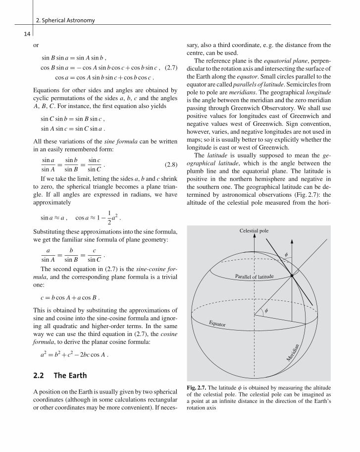
The latitude is usually supposed to mean the ge-ographical latitude, which is the angle between theplumb line and the equatorial plane. The latitude ispositive in the northern hemisphere and negative inthe southern one. The geographical latitude can be de-termined by astronomical observations (Fig. 2.7): thealtitude of the celestial pole measured from the hori-
Fig. 2.7. The latitude φ is obtained by measuring the altitudeof the celestial pole. The celestial pole can be imagined asa point at an infinite distance in the direction of the Earth’srotation axis

2.2 The Earth
15
zon equals the geographical latitude. (The celestial poleis the intersection of the rotation axis of the Earth andthe infinitely distant celestial sphere; we shall return tothese concepts a little later.)
Because the Earth is rotating, it is slightly flattened.The exact shape is rather complicated, but for most pur-poses it can by approximated by an oblate spheroid,the short axis of which coincides with the rotationaxis (Sect. 7.5). In 1979 the International Union ofGeodesy and Geophysics (IUGG) adopted the Geode-tic Reference System 1980 (GRS-80), which is usedwhen global reference frames fixed to the Earth are de-fined. The GRS-80 reference ellipsoid has the followingdimensions:
equatorial radius a = 6,378,137 m,
polar radius b = 6,356,752 m,
flattening f = (a −b)/a
= 1/298.25722210.
The shape defined by the surface of the oceans, calledthe geoid, differs from this spheroid at most by about100 m.
The angle between the equator and the normal tothe ellipsoid approximating the true Earth is called thegeodetic latitude. Because the surface of a liquid (like anocean) is perpendicular to the plumb line, the geodeticand geographical latitudes are practically the same.
Because of the flattening, the plumb line does notpoint to the centre of the Earth except at the poles andon the equator. An angle corresponding to the ordinaryspherical coordinate (the angle between the equator andthe line from the centre to a point on the surface), thegeocentric latitude φ′ is therefore a little smaller thanthe geographic latitude φ (Fig. 2.8).
We now derive an equation between the geographiclatitude φ and geocentric latitude φ′, assuming the Earthis an oblate spheroid and the geographic and geodesiclatitudes are equal. The equation of the meridionalellipse is
x2
a2+ y2
b2= 1 .
The direction of the normal to the ellipse at a point (x, y)is given by
tanφ = −dx
dy= a2
b2
y
x.
Fig. 2.8. Due to the flattening of the Earth, the geographiclatitude φ and geocentric latitude φ′ are different
The geocentric latitude is obtained from
tanφ′ = y/x .
Hence
tanφ′ = b2
a2tanφ = (1− e2) tanφ , (2.9)
where
e =√
1−b2/a2
is the eccentricity of the ellipse. The difference ∆φ =φ−φ′ has a maximum 11.5′ at the latitude 45.
Since the coordinates of celestial bodies in astro-nomical almanacs are given with respect to the centreof the Earth, the coordinates of nearby objects must becorrected for the difference in the position of the ob-server, if high accuracy is required. This means thatone has to calculate the topocentric coordinates, cen-tered at the observer. The easiest way to do this is to userectangular coordinates of the object and the observer(Example 2.5).
One arc minute along a meridian is called a nauticalmile. Since the radius of curvature varies with latitude,the length of the nautical mile so defined would dependon the latitude. Therefore one nautical mile has been

16
2. Spherical Astronomy
defined to be equal to one minute of arc at φ = 45,whence 1 nautical mile = 1852 m.
2.3 The Celestial Sphere
The ancient universe was confined within a finite spher-ical shell. The stars were fixed to this shell and thuswere all equidistant from the Earth, which was at thecentre of the spherical universe. This simple model isstill in many ways as useful as it was in antiquity: ithelps us to easily understand the diurnal and annualmotions of stars, and, more important, to predict thesemotions in a relatively simple way. Therefore we willassume for the time being that all the stars are locatedon the surface of an enormous sphere and that we are atits centre. Because the radius of this celestial sphere ispractically infinite, we can neglect the effects due to thechanging position of the observer, caused by the rota-tion and orbital motion of the Earth. These effects willbe considered later in Sects. 2.9 and 2.10.
Since the distances of the stars are ignored, we needonly two coordinates to specify their directions. Eachcoordinate frame has some fixed reference plane passingthrough the centre of the celestial sphere and dividingthe sphere into two hemispheres along a great circle.One of the coordinates indicates the angular distancefrom this reference plane. There is exactly one greatcircle going through the object and intersecting thisplane perpendicularly; the second coordinate gives theangle between that point of intersection and some fixeddirection.
2.4 The Horizontal System
The most natural coordinate frame from the observer’spoint of view is the horizontal frame (Fig. 2.9). Its ref-erence plane is the tangent plane of the Earth passingthrough the observer; this horizontal plane intersectsthe celestial sphere along the horizon. The point justabove the observer is called the zenith and the antipodalpoint below the observer is the nadir. (These two pointsare the poles corresponding to the horizon.) Great cir-cles through the zenith are called verticals. All verticalsintersect the horizon perpendicularly.
By observing the motion of a star over the course ofa night, an observer finds out that it follows a tracklike one of those in Fig. 2.9. Stars rise in the east,reach their highest point, or culminate, on the verti-cal NZS, and set in the west. The vertical NZS is calledthe meridian. North and south directions are defined asthe intersections of the meridian and the horizon.
One of the horizontal coordinates is the altitude orelevation, a, which is measured from the horizon alongthe vertical passing through the object. The altitude liesin the range [−90,+90]; it is positive for objectsabove the horizon and negative for the objects belowthe horizon. The zenith distance, or the angle between
Fig. 2.9. (a) The apparent motions of stars during a night asseen from latitude φ = 45. (b) The same stars seen fromlatitude φ = 10

2.5 The Equatorial System
17
the object and the zenith, is obviously
z = 90 −a . (2.10)
The second coordinate is the azimuth, A; it is the an-gular distance of the vertical of the object from somefixed direction. Unfortunately, in different contexts, dif-ferent fixed directions are used; thus it is always advis-able to check which definition is employed. The azimuthis usually measured from the north or south, and thoughclockwise is the preferred direction, counterclockwisemeasurements are also occasionally made. In this bookwe have adopted a fairly common astronomical conven-tion, measuring the azimuth clockwise from the south.Its values are usually normalized between 0 and 360.
In Fig. 2.9a we can see the altitude and azimuth ofa star B at some instant. As the star moves along itsdaily track, both of its coordinates will change. Anotherdifficulty with this coordinate frame is its local charac-ter. In Fig. 2.9b we have the same stars, but the observeris now further south. We can see that the coordinates ofthe same star at the same moment are different for dif-ferent observers. Since the horizontal coordinates aretime and position dependent, they cannot be used, forinstance, in star catalogues.
2.5 The Equatorial System
The direction of the rotation axis of the Earth remainsalmost constant and so does the equatorial plane per-pendicular to this axis. Therefore the equatorial planeis a suitable reference plane for a coordinate frame thathas to be independent of time and the position of theobserver.
The intersection of the celestial sphere and the equa-torial plane is a great circle, which is called the equatorof the celestial sphere. The north pole of the celestialsphere is one of the poles corresponding to this greatcircle. It is also the point in the northern sky where theextension of the Earth’s rotational axis meets the celes-tial sphere. The celestial north pole is at a distance ofabout one degree (which is equivalent to two full moons)from the moderately bright star Polaris. The meridianalways passes through the north pole; it is divided bythe pole into north and south meridians.
Fig. 2.10. At night, stars seem to revolve around the celestialpole. The altitude of the pole from the horizon equals thelatitude of the observer. (Photo Pekka Parviainen)
The angular separation of a star from the equatorialplane is not affected by the rotation of the Earth. Thisangle is called the declination δ.
Stars seem to revolve around the pole once everyday (Fig. 2.10). To define the second coordinate, wemust again agree on a fixed direction, unaffected by theEarth’s rotation. From a mathematical point of view, itdoes not matter which point on the equator is selected.However, for later purposes, it is more appropriate toemploy a certain point with some valuable properties,which will be explained in the next section. This pointis called the vernal equinox. Because it used to be in theconstellation Aries (the Ram), it is also called the firstpoint of Aries ant denoted by the sign of Aries, . Nowwe can define the second coordinate as the angle from

18
2. Spherical Astronomy
the vernal equinox measured along the equator. Thisangle is the right ascension α (or R.A.) of the object,measured counterclockwise from .
Since declination and right ascension are indepen-dent of the position of the observer and the motions ofthe Earth, they can be used in star maps and catalogues.As will be explained later, in many telescopes one of theaxes (the hour axis) is parallel to the rotation axis of theEarth. The other axis (declination axis) is perpendicularto the hour axis. Declinations can be read immediatelyon the declination dial of the telescope. But the zeropoint of the right ascension seems to move in the sky,due to the diurnal rotation of the Earth. So we cannotuse the right ascension to find an object unless we knowthe direction of the vernal equinox.
Since the south meridian is a well-defined line inthe sky, we use it to establish a local coordinate cor-responding to the right ascension. The hour angle ismeasured clockwise from the meridian. The hour angleof an object is not a constant, but grows at a steady rate,due to the Earth’s rotation. The hour angle of the ver-nal equinox is called the sidereal time Θ. Figure 2.11shows that for any object,
Θ = h +α , (2.11)
where h is the object’s hour angle and α its rightascension.
Fig. 2.11. The sidereal time Θ (the hour angle of the vernalequinox) equals the hour angle plus right ascension of anyobject
Since hour angle and sidereal time change with timeat a constant rate, it is practical to express them inunits of time. Also the closely related right ascen-sion is customarily given in time units. Thus 24 hoursequals 360 degrees, 1 hour = 15 degrees, 1 minute oftime = 15 minutes of arc, and so on. All these quantitiesare in the range [0 h, 24 h).
In practice, the sidereal time can be readily de-termined by pointing the telescope to an easilyrecognisable star and reading its hour angle on the hourangle dial of the telescope. The right ascension foundin a catalogue is then added to the hour angle, givingthe sidereal time at the moment of observation. For anyother time, the sidereal time can be evaluated by addingthe time elapsed since the observation. If we want tobe accurate, we have to use a sidereal clock to measuretime intervals. A sidereal clock runs 3 min 56.56 s fasta day as compared with an ordinary solar time clock:
24 h solar time
= 24 h 3 min 56.56 s sidereal time .(2.12)
The reason for this is the orbital motion of the Earth:stars seem to move faster than the Sun across the sky;hence, a sidereal clock must run faster. (This is furtherdiscussed in Sect. 2.13.)
Transformations between the horizontal and equa-torial frames are easily obtained from spherical
Fig. 2.12. The nautical triangle for deriving transformationsbetween the horizontal and equatorial frames

2.5 The Equatorial System
19
trigonometry. Comparing Figs. 2.6 and 2.12, we findthat we must make the following substitutions into (2.5):
ψ = 90 − A , θ = a ,
ψ ′ = 90 −h , θ ′ = δ , χ = 90 −φ . (2.13)
The angle φ in the last equation is the altitude of thecelestial pole, or the latitude of the observer. Makingthe substitutions, we get
sin h cos δ= sin A cos a ,
cos h cos δ= cos A cos a sinφ+ sin a cosφ , (2.14)
sin δ= − cos A cos a cosφ+ sin a sinφ .
The inverse transformation is obtained by substitut-ing
ψ = 90 −h , θ = δ , (2.15)
ψ ′ = 90 − A , θ ′ = a , χ = −(90 −φ) ,whence
sin A cos a = sin h cos δ ,
cos A cos a = cos h cos δ sinφ− sin δ cosφ , (2.16)
sin a = cos h cos δ cosφ+ sin δ sinφ .
Since the altitude and declination are in the range[−90,+90], it suffices to know the sine of one ofthese angles to determine the other angle unambigu-ously. Azimuth and right ascension, however, can haveany value from 0 to 360 (or from 0 h to 24 h), andto solve for them, we have to know both the sine andcosine to choose the correct quadrant.
The altitude of an object is greatest when it is onthe south meridian (the great circle arc between thecelestial poles containing the zenith). At that moment(called upper culmination, or transit) its hour angle is0 h. At the lower culmination the hour angle is h = 12 h.When h = 0 h, we get from the last equation in (2.16)
sin a = cos δ cosφ+ sin δ sinφ
= cos(φ− δ)= sin(90 −φ+ δ) .Thus the altitude at the upper culmination is
amax =
⎧⎪⎪⎪⎪⎨⎪⎪⎪⎪⎩
90 −φ+ δ , if the object culminatessouth of zenith ,
90 +φ− δ , if the object culminatesnorth of zenith .
(2.17)
Fig. 2.13. The altitude of a circumpolar star at upper and lowerculmination
The altitude is positive for objects with δ > φ−90.Objects with declinations less than φ−90 can never beseen at the latitude φ. On the other hand, when h = 12 hwe have
sin a = − cos δ cosφ+ sin δ sinφ
= − cos(δ+φ)= sin(δ+φ−90) ,
and the altitude at the lower culmination is
amin = δ+φ−90 . (2.18)
Stars with δ > 90 −φ will never set. For example, inHelsinki (φ ≈ 60), all stars with a declination higherthan 30 are such circumpolar stars. And stars witha declination less than −30 can never be observedthere.
We shall now study briefly how the (α, δ) frame canbe established by observations. Suppose we observea circumpolar star at its upper and lower culmination(Fig. 2.13). At the upper transit, its altitude is amax =90 −φ+ δ and at the lower transit, amin = δ+φ−90.Eliminating the latitude, we get
δ= 1
2(amin +amax) . (2.19)
Thus we get the same value for the declination, inde-pendent of the observer’s location. Therefore we canuse it as one of the absolute coordinates. From the sameobservations, we can also determine the direction of thecelestial pole as well as the latitude of the observer. Af-ter these preparations, we can find the declination ofany object by measuring its distance from the pole.
The equator can be now defined as the great circleall of whose points are at a distance of 90 from the

20
2. Spherical Astronomy
pole. The zero point of the second coordinate (rightascension) can then be defined as the point where theSun seems to cross the equator from south to north.
In practice the situation is more complicated, sincethe direction of Earth’s rotation axis changes due to per-turbations. Therefore the equatorial coordinate frame isnowadays defined using certain standard objects the po-sitions of which are known very accurately. The bestaccuracy is achieved by using the most distant objects,quasars (Sect. 18.7), which remain in the same directionover very long intervals of time.
2.6 Rising and Setting Times
From the last equation (2.16), we find the hour angle hof an object at the moment its altitude is a:
cos h = − tan δ tanφ+ sin a
cos δ cosφ. (2.20)
This equation can be used for computing rising andsetting times. Then a = 0 and the hour angles cor-responding to rising and setting times are obtainedfrom
cos h = − tan δ tanφ . (2.21)
If the right ascension α is known, we can use (2.11)to compute the sidereal time Θ. (Later, in Sect. 2.14,we shall study how to transform the sidereal time toordinary time.)
If higher accuracy is needed, we have to correct forthe refraction of light caused by the atmosphere of theEarth (see Sect. 2.9). In that case, we must use a smallnegative value for a in (2.20). This value, the horizontalrefraction, is about −34′.
The rising and setting times of the Sun given in al-manacs refer to the time when the upper edge of theSolar disk just touches the horizon. To compute thesetimes, we must set a = −50′ (= −34′−16′).
Also for the Moon almanacs give rising and settingtimes of the upper edge of the disk. Since the distanceof the Moon varies considerably, we cannot use anyconstant value for the radius of the Moon, but it has tobe calculated separately each time. The Moon is also soclose that its direction with respect to the backgroundstars varies due to the rotation of the Earth. Thus therising and setting times of the Moon are defined as the
instants when the altitude of the Moon is −34′ − s +π,where s is the apparent radius (15.5′ on the average) andπ the parallax (57′ on the average). The latter quantityis explained in Sect. 2.9.
Finding the rising and setting times of the Sun, plan-ets and especially the Moon is complicated by theirmotion with respect to the stars. We can use, for exam-ple, the coordinates for the noon to calculate estimatesfor the rising and setting times, which can then be used tointerpolate more accurate coordinates for the rising andsetting times. When these coordinates are used to com-pute new times a pretty good accuracy can be obtained.The iteration can be repeated if even higher precision isrequired.
2.7 The Ecliptic System
The orbital plane of the Earth, the ecliptic, is the refer-ence plane of another important coordinate frame. Theecliptic can also be defined as the great circle on thecelestial sphere described by the Sun in the course ofone year. This frame is used mainly for planets and otherbodies of the solar system. The orientation of the Earth’sequatorial plane remains invariant, unaffected by an-nual motion. In spring, the Sun appears to move fromthe southern hemisphere to the northern one (Fig. 2.14).The time of this remarkable event as well as the direc-tion to the Sun at that moment are called the vernalequinox. At the vernal equinox, the Sun’s right ascen-sion and declination are zero. The equatorial and ecliptic
Fig. 2.14. The ecliptic geocentric (λ, β) and heliocentric(λ′, β′) coordinates are equal only if the object is very faraway. The geocentric coordinates depend also on the Earth’sposition in its orbit

2.9 Perturbations of Coordinates
21
planes intersect along a straight line directed towards thevernal equinox. Thus we can use this direction as thezero point for both the equatorial and ecliptic coordi-nate frames. The point opposite the vernal equinox isthe autumnal equinox, it is the point at which the Suncrosses the equator from north to south.
The ecliptic latitude β is the angular distance fromthe ecliptic; it is in the range [−90,+90]. Theother coordinate is the ecliptic longitude λ, measuredcounterclockwise from the vernal equinox.
Transformation equations between the equatorial andecliptic frames can be derived analogously to (2.14) and(2.16):
sin λ cosβ = sin δ sin ε+ cos δ cos ε sinα ,
cos λ cosβ = cos δ cosα , (2.22)
sinβ = sin δ cos ε− cos δ sin ε sinα ,
sinα cos δ= − sinβ sin ε+ cosβ cos ε sin λ ,
cosα cos δ= cos λ cosβ , (2.23)
sin δ= sinβ cos ε+ cosβ sin ε sin λ .
The angle ε appearing in these equations is the obliq-uity of the ecliptic, or the angle between the equatorialand ecliptic planes. Its value is roughly 2326′ (a moreaccurate value is given in *Reduction of Coordinates,p. 38).
Depending on the problem to be solved, we mayencounter heliocentric (origin at the Sun), geocentric(origin at the centre of the Earth) or topocentric (originat the observer) coordinates. For very distant objects thedifferences are negligible, but not for bodies of the solarsystem. To transform heliocentric coordinates to geo-centric coordinates or vice versa, we must also know thedistance of the object. This transformation is most easilyaccomplished by computing the rectangular coordinatesof the object and the new origin, then changing the ori-gin and finally evaluating the new latitude and longitudefrom the rectangular coordinates (see Examples 2.4 and2.5).
2.8 The Galactic Coordinates
For studies of the Milky Way Galaxy, the most nat-ural reference plane is the plane of the Milky Way(Fig. 2.15). Since the Sun lies very close to that plane,
Fig. 2.15. The galactic coordinates l and b
we can put the origin at the Sun. The galactic longitude lis measured counterclockwise (like right ascension)from the direction of the centre of the Milky Way(in Sagittarius, α = 17 h 45.7 min, δ = −2900′). Thegalactic latitude b is measured from the galactic plane,positive northwards and negative southwards. This def-inition was officially adopted only in 1959, when thedirection of the galactic centre was determined fromradio observations accurately enough. The old galacticcoordinates lI and bI had the intersection of the equatorand the galactic plane as their zero point.
The galactic coordinates can be obtained from theequatorial ones with the transformation equations
sin(lN − l) cos b = cos δ sin(α−αP) ,
cos(lN − l) cos b = − cos δ sin δP cos(α−αP)
+ sin δ cos δP ,
sin b = cos δ cos δP cos(α−αP)
+ sin δ sin δP ,
(2.24)
where the direction of the Galactic north pole is αP =12 h 51.4 min, δP = 2708′, and the galactic longitudeof the celestial pole, lN = 123.0.
2.9 Perturbations of Coordinates
Even if a star remains fixed with respect to the Sun,its coordinates can change, due to several disturbingeffects. Naturally its altitude and azimuth change con-stantly because of the rotation of the Earth, but even itsright ascension and declination are not quite free fromperturbations.
Precession. Since most of the members of the solarsystem orbit close to the ecliptic, they tend to pull theequatorial bulge of the Earth towards it. Most of this“flattening” torque is caused by the Moon and the Sun.

22
2. Spherical Astronomy
Fig. 2.16. Due to preces-sion the rotation axis ofthe Earth turns around theecliptic north pole. Nuta-tion is the small wobbledisturbing the smoothprecessional motion. Inthis figure the magnitudeof the nutation is highlyexaggerated
But the Earth is rotating and therefore the torque can-not change the inclination of the equator relative to theecliptic. Instead, the rotation axis turns in a directionperpendicular to the axis and the torque, thus describinga cone once in roughly 26,000 years. This slow turningof the rotation axis is called precession (Fig. 2.16). Be-cause of precession, the vernal equinox moves along theecliptic clockwise about 50 seconds of arc every year,thus increasing the ecliptic longitudes of all objects atthe same rate. At present the rotation axis points aboutone degree away from Polaris, but after 12,000 years,the celestial pole will be roughly in the direction ofVega. The changing ecliptic longitudes also affect theright ascension and declination. Thus we have to knowthe instant of time, or epoch, for which the coordinatesare given.
Currently most maps and catalogues use the epochJ2000.0, which means the beginning of the year 2000,or, to be exact, the noon of January 1, 2000, or the Juliandate 2,451,545.0 (see Sect. 2.15).
Let us now derive expressions for the changes inright ascension and declination. Taking the last trans-formation equation in (2.23),
sin δ= cos ε sinβ+ sin ε cosβ sinλ ,
and differentiating, we get
cos δ dδ= sin ε cosβ cos λ dλ .
Applying the second equation in (2.22) to the right-handside, we have, for the change in declination,
dδ= dλ sin ε cosα . (2.25)
By differentiating the equation
cosα cos δ= cosβ cos λ ,
we get
− sinα cos δ dα− cosα sin δ dδ= − cosβ sin λ dλ ;and, by substituting the previously obtained expressionfor dδ and applying the first equation (2.22), we have
sinα cos δ dα= dλ(cosβ sin λ− sin ε cos2 α sin δ)
= dλ(sin δ sin ε+ cos δ cos ε sinα
− sin ε cos2 α sin δ) .
Simplifying this, we get
dα= dλ(sinα sin ε tan δ+ cos ε) . (2.26)
If dλ is the annual increment of the ecliptic longitude(about 50′′), the precessional changes in right ascensionand declination in one year are thus
dδ= dλ sin ε cosα ,
dα= dλ(sin ε sinα tan δ+ cos ε) .(2.27)
These expressions are usually written in the form
dδ= n cosα ,
dα= m +n sinα tan δ ,(2.28)
where
m = dλ cos ε ,
n = dλ sin ε(2.29)
are the precession constants. Since the obliquity of theecliptic is not exactly a constant but changes with time,m and n also vary slowly with time. However, this vari-ation is so slow that usually we can regard m and nas constants unless the time interval is very long. Thevalues of these constants for some epochs are given in
Table 2.1. Precession constants m and n. Here, “a” meansa tropical year
Epoch m n
1800 3.07048 s/a 1.33703 s/a = 20.0554′′/a1850 3.07141 1.33674 20.05111900 3.07234 1.33646 20.04681950 3.07327 1.33617 20.04262000 3.07419 1.33589 20.0383

2.9 Perturbations of Coordinates
23
Fig. 2.17. The horizontalparallax π of an object isthe angle subtended by theEarth’s equatorial radius asseen from the object
Table 2.1. For intervals longer than a few decades a morerigorous method should be used. Its derivation exceedsthe level of this book, but the necessary formulas aregiven in *Reduction of Coordinates (p. 38).
Nutation. The Moon’s orbit is inclined with respect tothe ecliptic, resulting in precession of its orbital plane.One revolution takes 18.6 years, producing perturba-tions with the same period in the precession of the Earth.This effect, nutation, changes ecliptic longitudes as wellas the obliquity of the ecliptic (Fig. 2.16). Calculationsare now much more complicated, but fortunately nuta-tional perturbations are relatively small, only fractionsof an arc minute.
Parallax. If we observe an object from different points,we see it in different directions. The difference of theobserved directions is called the parallax. Since theamount of parallax depends on the distance of the ob-server from the object, we can utilize the parallax tomeasure distances. Human stereoscopic vision is based(at least to some extent) on this effect. For astronom-ical purposes we need much longer baselines than thedistance between our eyes (about 7 cm). Appropriatelylarge and convenient baselines are the radius of the Earthand the radius of its orbit.
Distances to the nearest stars can be determined fromthe annual parallax, which is the angle subtended bythe radius of the Earth’s orbit (called the astronomicalunit, AU) as seen from the star. (We shall discuss thisfurther in Sect. 2.10.)
By diurnal parallax we mean the change of direc-tion due to the daily rotation of the Earth. In addition tothe distance of the object, the diurnal parallax also de-pends on the latitude of the observer. If we talk aboutthe parallax of a body in our solar system, we alwaysmean the angle subtended by the Earth’s equatorial ra-dius (6378 km) as seen from the object (Fig. 2.17). Thisequals the apparent shift of the object with respect to
the background stars seen by an observer at the equa-tor if (s)he observes the object moving from the horizonto the zenith. The parallax of the Moon, for example, isabout 57′, and that of the Sun 8.79′′.
In astronomy parallax may also refer to distance ingeneral, even if it is not measured using the shift in theobserved direction.
Aberration. Because of the finite speed of light, anobserver in motion sees an object shifted in the directionof her/his motion (Figs. 2.18 and 2.19). This changeof apparent direction is called aberration. To derive
Fig. 2.18a,b. The effect of aberration on the apparent directionof an object. (a) Observer at rest. (b) Observer in motion

24
2. Spherical Astronomy
Fig. 2.19. A telescope is pointed in the true direction of a star.It takes a time t = l/c for the light to travel the length of thetelescope. The telescope is moving with velocity v, which hasa component v sin θ, perpendicular to the direction of the lightbeam. The beam will hit the bottom of the telescope displacedfrom the optical axis by a distance x = tv sin θ = l(v/c) sin θ.Thus the change of direction in radians is a = x/l = (v/c) sin θ
the exact value we have to use the special theory ofrelativity, but for practical purposes it suffices to use theapproximate value
a = v
csin θ , [a] = rad , (2.30)
where v is the velocity of the observer, c is the speedof light and θ is the angle between the true directionof the object and the velocity vector of the observer.The greatest possible value of the aberration due to theorbital motion of the Earth, v/c, called the aberrationconstant, is 21′′. The maximal shift due to the Earth’s ro-tation, the diurnal aberration constant, is much smaller,about 0.3′′.
Refraction. Since light is refracted by the atmosphere,the direction of an object differs from the true directionby an amount depending on the atmospheric conditionsalong the line of sight. Since this refraction varies withatmospheric pressure and temperature, it is very diffi-cult to predict it accurately. However, an approximationgood enough for most practical purposes is easily de-rived. If the object is not too far from the zenith, theatmosphere between the object and the observer can beapproximated by a stack of parallel planar layers, eachof which has a certain index of refraction ni (Fig. 2.20).Outside the atmosphere, we have n = 1.
Fig. 2.20. Refraction of a light ray travelling through theatmosphere
Let the true zenith distance be z and the apparentone, ζ . Using the notations of Fig. 2.20, we obtain thefollowing equations for the boundaries of the successivelayers:
sin z = nk sin zk ,...
n2 sin z2 = n1 sin z1 ,
n1 sin z1 = n0 sin ζ ,
or
sin z = n0 sin ζ . (2.31)
When the refraction angle R = z − ζ is small and isexpressed in radians, we have
n0 sin ζ = sin z = sin(R + ζ)= sin R cos ζ + cos R sin ζ
≈ R cos ζ + sin ζ .
Thus we get
R = (n0 −1) tan ζ , [R] = rad . (2.32)
The index of refraction depends on the density ofthe air, which further depends on the pressure and tem-perature. When the altitude is over 15, we can use anapproximate formula
R = P
273+ T0.00452 tan(90 −a) , (2.33)

2.10 Positional Astronomy
25
where a is the altitude in degrees, T temperature indegrees Celsius, and P the atmospheric pressure inhectopascals (or, equivalently, in millibars). At loweraltitudes the curvature of the atmosphere must be takeninto account. An approximate formula for the refractionis then
R = P
273+ T
0.1594+0.0196a +0.00002a2
1+0.505a +0.0845a2.
(2.34)
These formulas are widely used, although they areagainst the rules of dimensional analysis. To get cor-rect values, all quantities must be expressed in correctunits. Figure 2.21 shows the refraction under differentconditions evaluated from these formulas.
Altitude is always (except very close to zenith) in-creased by refraction. On the horizon the change is about34′, which is slightly more than the diameter of the Sun.When the lower limb of the Sun just touches the horizon,the Sun has in reality already set.
Light coming from the zenith is not refracted at all ifthe boundaries between the layers are horizontal. Undersome climatic conditions, a boundary (e.g. between coldand warm layers) can be slanted, and in this case, therecan be a small zenith refraction, which is of the orderof a few arc seconds.
Stellar positions given in star catalogues are meanplaces, from which the effects of parallax, aberrationand nutation have been removed. The mean place ofthe date (i. e. at the observing time) is obtained by cor-
Fig. 2.21. Refraction at different altitudes. The refraction an-gle R tells how much higher the object seems to be comparedwith its true altitude a. Refraction depends on the density andthus on the pressure and temperature of the air. The uppercurves give the refraction at sea level during rather extremeweather conditions. At the altitude of 2.5 kilometers the aver-age pressure is only 700 hPa, and thus the effect of refractionsmaller (lowest curve)
recting the mean place for the proper motion of thestar (Sect. 2.10) and precession. The apparent place isobtained by correcting this place further for nutation,parallax and aberration. There is a catalogue publishedannually that gives the apparent places of certain refer-ences stars at intervals of a few days. These positionshave been corrected for precession, nutation, parallaxand annual aberration. The effects of diurnal aberrationand refraction are not included because they depend onthe location of the observer.
2.10 Positional Astronomy
The position of a star can be measured either withrespect to some reference stars (relative astrometry)or with respect to a fixed coordinate frame (absoluteastrometry).
Fig. 2.22. Astronomers discussing observations with thetransit circle of Helsinki Observatory in 1904

26
2. Spherical Astronomy

2.10 Positional Astronomy
27
Absolute coordinates are usually determined usinga meridian circle, which is a telescope that can be turnedonly in the meridional plane (Fig. 2.22). It has only oneaxis, which is aligned exactly in the east-west direction.Since all stars cross the meridian in the course of a day,they all come to the field of the meridian circle at sometime or other. When a star culminates, its altitude and thetime of the transit are recorded. If the time is determinedwith a sidereal clock, the sidereal time immediatelygives the right ascension of the star, since the hour angleis h = 0 h. The other coordinate, the declination δ, isobtained from the altitude:
δ= a − (90 −φ) ,where a is the observed altitude and φ is the geographiclatitude of the observatory.
Relative coordinates are measured on photographicplates (Fig. 2.23) or CCD images containing someknown reference stars. The scale of the plate as wellas the orientation of the coordinate frame can be de-termined from the reference stars. After this has beendone, the right ascension and declination of any objectin the image can be calculated if its coordinates in theimage are measured.
All stars in a small field are almost equally affectedby the dominant perturbations, precession, nutation, andaberration. The much smaller effect of parallax, on theother hand, changes the relative positions of the stars.
The shift in the direction of a star with respect to dis-tant background stars due to the annual motion of theEarth is called the trigonometric parallax of the star.It gives the distance of the star: the smaller the paral-lax, the farther away the star is. Trigonometric parallaxis, in fact, the only direct method we currently have ofmeasuring distances to stars. Later we shall be intro-duced to some other, indirect methods, which require
Fig. 2.23. (a) A plate photographed for the Carte du Cielproject in Helsinki on November 21, 1902. The centre of thefield is at α= 18 h 40 min, δ= 46, and the area is 2 ×2.Distance between coordinate lines (exposed separately on theplate) is 5 minutes of arc. (b) The framed region on the sameplate. (c) The same area on a plate taken on November 7,1948. The bright star in the lower right corner (SAO 47747)has moved about 12 seconds of arc. The brighter, slightlydrop-shaped star to the left is a binary star (SAO 47767); theseparation between its components is 8′′
Fig. 2.24. The trigonometric parallax π of a star S is the an-gle subtended by the radius of the orbit of the Earth, or oneastronomical unit, as seen from the star
certain assumptions on the motions or structure of stars.The same method of triangulation is employed to mea-sure distances of earthly objects. To measure distancesto stars, we have to use the longest baseline available,the diameter of the orbit of the Earth.
During the course of one year, a star will appearto describe a circle if it is at the pole of the ecliptic,a segment of line if it is in the ecliptic, or an ellipseotherwise. The semimajor axis of this ellipse is calledthe parallax of the star. It is usually denoted by π. Itequals the angle subtended by the radius of the Earth’sorbit as seen from the star (Fig. 2.24).
The unit of distance used in astronomy is parsec(pc). At a distance of one parsec, one astronomicalunit subtends an angle of one arc second. Since oneradian is about 206,265′′, 1 pc equals 206,265 AU.Furthermore, because 1 AU = 1.496×10¹¹ m, 1 pc ≈3.086×10¹⁶ m. If the parallax is given in arc seconds,the distance is simply
r = 1/π , [r] = pc , [π] = ′′ . (2.35)
In popular astronomical texts, distances are usuallygiven in light-years, one light-year being the distancelight travels in one year, or 9.5×10¹⁵ m. Thus oneparsec is about 3.26 light-years.
The first parallax measurement was accomplishedby Friedrich Wilhelm Bessel (1784–1846) in 1838. Hefound the parallax of 61 Cygni to be 0.3′′. The neareststar Proxima Centauri has a parallax of 0.762′′ and thusa distance of 1.31 pc.

28
2. Spherical Astronomy
Fig. 2.25a–c. Proper motions of stars slowly change the ap-pearance of constellations. (a) The Big Dipper during the last
ice age 30,000 years ago, (b) nowadays, and (c) after 30,000years
In addition to the motion due to the annual parallax,many stars seem to move slowly in a direction that doesnot change with time. This effect is caused by the rela-tive motion of the Sun and the stars through space; it iscalled the proper motion. The appearance of the sky andthe shapes of the constellations are constantly, althoughextremely slowly, changed by the proper motions of thestars (Fig. 2.25).
The velocity of a star with respect to the Sun can bedivided into two components (Fig. 2.26), one of whichis directed along the line of sight (the radial componentor the radial velocity), and the other perpendicular to it(the tangential component). The tangential velocity re-sults in the proper motion, which can be measured bytaking plates at intervals of several years or decades.The proper motion µ has two components, one givingthe change in declination µδ and the other, in right as-cension,µα cos δ. The coefficient cos δ is used to correctthe scale of right ascension: hour circles (the great cir-cles with α= constant) approach each other towards thepoles, so the coordinate difference must be multipliedby cos δ to obtain the true angular separation. The total
Fig. 2.26. The radial and tangential components, vr and vt ofthe velocity v of a star. The latter component is observed asproper motion
proper motion is
µ=√µ2α cos2 δ+µ2
δ . (2.36)
The greatest known proper motion belongs to Barnard’sStar, which moves across the sky at the enormous speedof 10.3 arc seconds per year. It needs less than 200 yearsto travel the diameter of a full moon.
In order to measure proper motions, we must ob-serve stars for decades. The radial component, on theother hand, is readily obtained from a single observa-tion, thanks to the Doppler effect. By the Doppler effectwe mean the change in frequency and wavelength of ra-diation due to the radial velocity of the radiation source.The same effect can be observed, for example, in thesound of an ambulance, the pitch being higher when theambulance is approaching and lower when it is receding.
The formula for the Doppler effect for small ve-locities can be derived as in Fig. 2.27. The source ofradiation transmits electromagnetic waves, the period ofone cycle being T . In time T , the radiation approachesthe observer by a distance s = cT , where c is the speedof propagation. During the same time, the source moveswith respect to the observer a distance s′ = vT , wherev is the speed of the source, positive for a recedingsource and negative for an approaching one. We findthat the length of one cycle, the wavelength λ, equals
λ= s + s′ = cT +vT .
Fig. 2.27. The wavelength of radiation increases if the sourceis receding

2.11 Constellations
29
If the source were at rest, the wavelength of its radiationwould be λ0 = cT . The motion of the source changesthe wavelength by an amount
∆λ= λ−λ0 = cT +vT − cT = vT ,
and the relative change ∆λ of the wavelength is∆λ
λ0= v
c. (2.37)
This is valid only when v c. For very high velocities,we must use the relativistic formula
∆λ
λ0=√
1+v/c1−v/c −1 . (2.38)
In astronomy the Doppler effect can be seen in stellarspectra, in which the spectral lines are often displacedtowards the blue (shorter wavelengths) or red (longerwavelengths) end of the spectrum. A blueshift meansthat the star is approaching, while a redshift indicatesthat it is receding.
The displacements due to the Doppler effect areusually very small. In order to measure them, a ref-erence spectrum is exposed on the plate next to thestellar spectrum. Now that CCD-cameras have replacedphotographic plates, separate calibration exposures ofreference spectra are taken to determine the wavelengthscale. The lines in the reference spectrum are producedby a light source at rest in the laboratory. If the referencespectrum contains some lines found also in the stellarspectrum, the displacements can be measured.
Displacements of spectral lines give the radial ve-locity vr of the star, and the proper motion µ can bemeasured from photographic plates or CCD images. Tofind the tangential velocity vt, we have to know the dis-tance r, obtainable from e.g. parallax measurements.Tangential velocity and proper motion are related by
vt = µr . (2.39)
If µ is given in arc seconds per year and r in parsecswe have to make the following unit transformations toget vt in km/s:
1 rad = 206,265′′ , 1 year = 3.156×10⁷ s ,
1 pc = 3.086×10¹³ km .
Hencevt = 4.74µr , [vt] = km/s ,
[µ] = ′′/a , [r] = pc .(2.40)
The total velocity v of the star is then
v=√v2
r +v2t . (2.41)
2.11 Constellations
At any one time, about 1000–1500 stars can be seen inthe sky (above the horizon). Under ideal conditions, thenumber of stars visible to the naked eye can be as high as3000 on a hemisphere, or 6000 altogether. Some starsseem to form figures vaguely resembling something;they have been ascribed to various mythological andother animals. This grouping of stars into constellationsis a product of human imagination without any physicalbasis. Different cultures have different constellations,depending on their mythology, history and environment.
About half of the shapes and names of the constella-tions we are familiar with date back to Mediterraneanantiquity. But the names and boundaries were far fromunambiguous as late as the 19th century. Thereforethe International Astronomical Union (IAU) confirmedfixed boundaries at its 1928 meeting.
The official boundaries of the constellations were es-tablished along lines of constant right ascension anddeclination for the epoch 1875. During the time elapsedsince then, precession has noticeably turned the equato-rial frame. However, the boundaries remain fixed withrespect to the stars. So a star belonging to a constella-tion will belong to it forever (unless it is moved acrossthe boundary by its proper motion).
The names of the 88 constellations confirmed by theIAU are given in Table C.21 at the end of the book.The table also gives the abbreviation of the Latin name,its genitive (needed for names of stars) and the Englishname.
In his star atlas Uranometria (1603) Johannes Bayerstarted the current practice to denote the brightest starsof each constellation by Greek letters. The brighteststar is usually α (alpha), e. g. Deneb in the constella-tion Cygnus is αCygni, which is abbreviated as αCyg.The second brightest star is β (beta), the next one γ(gamma) and so on. There are, however, several ex-ceptions to this rule; for example, the stars of the BigDipper are named in the order they appear in the con-stellation. After the Greek alphabet has been exhausted,Latin letters can be employed. Another method is to use

30
2. Spherical Astronomy
numbers, which are assigned in the order of increasingright ascension; e. g. 30 Tau is a bright binary star inthe constellation Taurus. Moreover, variable stars havetheir special identifiers (Sect. 13.1). About two hundredbright stars have a proper name; e.g. the bright αAur iscalled also Capella.
As telescopes evolved, more and more stars wereseen and catalogued. It soon became impractical to con-tinue this method of naming. Thus most of the stars areknown only by their catalogue index numbers. One starmay have many different numbers; e. g. the abovemen-tioned Capella (αAur) is number BD+45 1077 in theBonner Durchmusterung and HD 34029 in the HenryDraper catalogue.
2.12 Star Catalogues and Maps
The first actual star catalogue was published by Ptolemyin the second century; this catalogue appeared in thebook to be known later as Almagest (which is a Latincorruption of the name of the Arabic translation, Al-mijisti). It had 1025 entries; the positions of these brightstars had been measured by Hipparchos 250 years ear-lier. Ptolemy’s catalogue was the only widely used oneprior to the 17th century.
The first catalogues still being used by astronomerswere prepared under the direction of Friedrich WilhelmAugust Argelander (1799–1875). Argelander worked inTurku and later served as professor of astronomy inHelsinki, but he made his major contributions in Bonn.Using a 72 mm telescope, he and his assistants measuredthe positions and estimated the magnitudes of 320,000stars. The catalogue, Bonner Durchmusterung, containsnearly all stars brighter than magnitude 9.5 between thenorth pole and declination −2. (Magnitudes are furtherdiscussed in Chap. 4.) Argelander’s work was later usedas a model for two other large catalogues covering thewhole sky. The total number of stars in these cataloguesis close to one million.
The purpose of these Durchmusterungen or generalcatalogues was to systematically list a great number ofstars. In the zone catalogues, the main goal is to givethe positions of stars as exactly as possible. A typicalzone catalogue is the German Katalog der Astronomi-schen Gesellschaft (AGK). Twelve observatories, eachmeasuring a certain region in the sky, contributed to
this catalogue. The work was begun in the 1870’s andcompleted at the turn of the century.
General and zone catalogues were based on visualobservations with a telescope. The evolution of photog-raphy made this kind of work unnecessary at the endof the 19th century. Photographic plates could be storedfor future purposes, and measuring the positions of starsbecame easier and faster, making it possible to measuremany more stars.
A great international program was started at theend of the 19th century in order to photograph theentire sky. Eighteen observatories participated in thisCarte du Ciel project, all using similar instrumentsand plates. The positions of stars were first measuredwith respect to a rectangular grid exposed on each plate(Fig. 2.23a). These coordinates could then be convertedinto declination and right ascension.
Positions of stars in catalogues are measured withrespect to certain comparison stars, the coordinates ofwhich are known with high accuracy. The coordinatesof these reference stars are published in fundamentalcatalogues. The first such catalogue was needed for theAGK catalogue; it was published in Germany in 1879.This Fundamental Katalog (FK 1) gives the positionsof over 500 stars.
The fundamental catalogues are usually revised everyfew decades. The fifth edition, the FK 5, appeared in1984. At the same time, a new system of astronomicalconstants was adopted. The catalogue contains 1535fundamental and 3117 additional stars.
A widely used catalogue is the SAO catalogue, pub-lished by the Smithsonian Astrophysical Observatory inthe 1960’s. It contains the exact positions, magnitudes,proper motions, spectral classifications, etc. of 258,997stars brighter than magnitude 9. The catalogue was ac-companied by a star map containing all the stars in thecatalogue.
Fig. 2.28. The representations in four atlases of the Hyades cluster in the constellation Taurus. (a) Heis: Atlas Coelestis,published in 1872. (b) Bonner Durchmusterung. (c) SAO,(d) Palomar Sky Atlas, red plate. The big blob is the brighteststar of Taurus, or αTauri alias Aldebaran. (e) All the stars inthe Tycho Catalog, numbering over one million, are markedon an all-sky chart. The bright lane is the Milky Way. (PictureDavid Seal, NASA/JPL/Caltech)

2.12 Star Catalogues and Maps
31

32
2. Spherical Astronomy
In the 1990’s a large astrometric catalogue, PPM (Po-sitions and Proper Motions), was published to replacethe AGK and SAO catalogues. It contained all starsbrighter than 7.5 magnitudes, and was almost completeto magnitude 8.5. Altogether, the four volumes of thecatalogue contained information on 378,910 stars.
The PPM was effectively replaced by the Tycho cat-alogue from Hipparcos satellite. Hipparcos was the firstastrometric satellite, and was launched by the Euro-pean Space Agency (ESA) in 1989. Although Hipparcosdidn’t reach the planned geosynchronous orbit, it gaveexact positions of over a hundred thousand stars. TheHipparcos catalogue, based on the measurements of thesatellite, contains astrometric and photometric data of118,000 stars. The coordinates are precise to a coupleof milliarcseconds. The less precise Tycho cataloguecontains the data of about one million stars.
In 1999 and 2000, the sixth version of the Funda-mental Katalog, the FK6, was published. It combinedthe Hipparcos data and FK5 for 4150 fundamental stars.The typical mean error in proper motion was 0.35milliarcseconds per year for the basic stars. With theadvance of the Internet, the printed versions of star cat-alogues were discontinued in the first years of the newmillennium, and the catalogues were moved to compactdiscs and the net.
With the new media, the size of the star cataloguesexploded. The first Hubble Guide Star Catalog fromthe early 1990’s contained 18 million stars and the sec-ond Guide Star Catalog from the year 2001, nearly 500million stars. It was surpassed by the U.S. Naval Ob-servatory USNO-B1.0 Catalog, which contains entriesfor 1,024,618,261 stars and galaxies from digitized im-ages of several photographic sky surveys. The cataloguepresents right ascension and declination, proper motionand magnitude estimates.
The next step in the accuracy of astrometry will beachieved in the 2010’s with a new European astrometricsatellite. The Gaia satellite, planned to be launched inabout 2014, is expected to improve the accurary to about10−5 seconds of arc.
Star maps have been published since ancient times,but the earliest maps were globes showing the celestialsphere as seen from the outside. At the beginning of the17th century, a German, Johannes Bayer, published thefirst map showing the stars as seen from inside the ce-lestial sphere, as we see them in the sky. Constellations
were usually decorated with drawings of mythologicalfigures. The Uranometria Nova (1843) by Argelanderrepresents a transition towards modern maps: mytho-logical figures are beginning to fade away. The mapaccompanying the Bonner Durchmusterung carried thisevolution to its extreme. The sheets contain nothing butstars and coordinate lines.
Most maps are based on star catalogues. Photogra-phy made it possible to produce star maps without thecataloguing stage. The most important of such mapsis a photographic atlas the full name of which is TheNational Geographic Society – Palomar ObservatorySky Atlas. The plates for this atlas were taken with the1.2 m Schmidt camera on Mount Palomar. The Palo-mar Sky Atlas was completed in the 1950’s. It consistsof 935 pairs of photographs: each region has been pho-tographed in red and blue light. The size of each plate isabout 35 cm×35 cm, covering an area of 6.6 ×6.6.The prints are negatives (black stars on a light back-ground), because in this way, fainter objects are visible.The limiting magnitude is about 19 in blue and 20 in red.
The Palomar atlas covers the sky down to −30.Work to map the rest of the sky was carried out later attwo observatories in the southern hemisphere, at SidingSpring Observatory in Australia, and at the EuropeanSouthern Observatory (ESO) in Chile. The instrumentsand the scale on the plates are similar to those usedearlier for the Palomar plates, but the atlas is distributedon film transparencies instead of paper prints.
For amateurs there are several star maps of variouskinds. Some of them are mentioned in the references.
2.13 Sidereal and Solar Time
Time measurements can be based on the rotation ofthe Earth, orbital motion around the Sun, or on atomicclocks. The last-mentioned will be discussed in the nextsection. Here we consider the sidereal and solar timesrelated to the rotation of the Earth.
We defined the sidereal time as the hour angle ofthe vernal equinox. A good basic unit is a sidereal day,which is the time between two successive upper culmi-nations of the vernal equinox. After one sidereal daythe celestial sphere with all its stars has returned to itsoriginal position with respect to the observer. The flowof sidereal time is as constant as the rotation of the

2.13 Sidereal and Solar Time
33
Earth. The rotation rate is slowly decreasing, and thusthe length of the sidereal day is increasing. In additionto the smooth slowing down irregular variations of theorder of one millisecond have been observed.
Unfortunately, also the sidereal time comes in two va-rieties, apparent and mean. The apparent sidereal timeis determined by the true vernal equinox, and so it isobtained directly from observations.
Because of the precession the ecliptic longitude ofthe vernal equinox increases by about 50′′ a year. Thismotion is very smooth. Nutation causes more compli-cated wobbling. The mean equinox is the point wherethe vernal equinox would be if there were no nutation.The mean sidereal time is the hour angle of this meanequinox.
The difference of the apparent and mean sidereal timeis called the equation of equinoxes:
Θa −ΘM =∆ψ cos ε , (2.42)
where ε is the obliquity of the ecliptic at the instant ofthe observation, and∆ψ, the nutation in longitude. Thisvalue is tabulated for each day e.g. in the AstronomicalAlmanac. It can also be computed from the formulaegiven in *Reduction of Coordinates. It is at most aboutone second, so it has to be taken into account only inthe most precise calculations.
Figure 2.29 shows the Sun and the Earth at vernalequinox. When the Earth is at the point A, the Sunculminates and, at the same time, a new sidereal day
Fig. 2.29. One sidereal day is the time between two successivetransits or upper culminations of the vernal equinox. By thetime the Earth has moved from A to B, one sidereal day haselapsed. The angle ∆ is greatly exaggerated; in reality, it isslightly less than one degree
begins in the city with the huge black arrow standingin its central square. After one sidereal day, the Earthhas moved along its orbit almost one degree of arc tothe point B. Therefore the Earth has to turn almosta degree further before the Sun will culminate. Thesolar or synodic day is therefore 3 min 56.56 s (siderealtime) longer than the sidereal day. This means that thebeginning of the sidereal day will move around the clockduring the course of one year. After one year, siderealand solar time will again be in phase. The number ofsidereal days in one year is one higher than the numberof solar days.
When we talk about rotational periods of planets, weusually mean sidereal periods. The length of day, onthe other hand, means the rotation period with respectto the Sun. If the orbital period around the Sun is P,sidereal rotation period τ∗ and synodic day τ , we nowknow that the number of sidereal days in time P, P/τ∗,is one higher than the number of synodic days, P/τ :
P
τ∗− P
τ= 1 ,
or1
τ= 1
τ∗− 1
P. (2.43)
This holds for a planet rotating in the direction of itsorbital motion (counterclockwise). If the sense of rota-tion is opposite, or retrograde, the number of siderealdays in one orbital period is one less than the numberof synodic days, and the equation becomes
1
τ= 1
τ∗+ 1
P. (2.44)
For the Earth, we have P = 365.2564 d, and τ = 1 d,whence (2.43) gives τ∗ = 0.99727 d = 23 h 56 min 4 s,solar time.
Since our everyday life follows the alternation of dayand night, it is more convenient to base our timekeepingon the apparent motion of the Sun rather than that ofthe stars. Unfortunately, solar time does not flow ata constant rate. There are two reasons for this. First, theorbit of the Earth is not exactly circular, but an ellipse,which means that the velocity of the Earth along itsorbit is not constant. Second, the Sun moves along theecliptic, not the equator. Thus its right ascension doesnot increase at a constant rate. The change is fastest atthe end of December (4 min 27 s per day) and slowest in

34
2. Spherical Astronomy
mid-September (3 min 35 s per day). As a consequence,the hour angle of the Sun (which determines the solartime) also grows at an uneven rate.
To find a solar time flowing at a constant rate, wedefine a fictitious mean sun, which moves along the ce-lestial equator with constant angular velocity, makinga complete revolution in one year. By year we meanhere the tropical year, which is the time it takes forthe Sun to move from one vernal equinox to the next.In one tropical year, the right ascension of the Sun in-creases exactly 24 hours. The length of the tropical yearis 365 d 5 h 48 min 46 s = 365.2422 d. Since the direc-tion of the vernal equinox moves due to precession,the tropical year differs from the sidereal year, duringwhich the Sun makes one revolution with respect to thebackground stars. One sidereal year is 365.2564 d.
Using our artificial mean sun, we now define anevenly flowing solar time, the mean solar time (or sim-ply mean time) TM, which is equal to the hour angle hM
of the centre of the mean sun plus 12 hours (so that thedate will change at midnight, to annoy astronomers):
TM = hM +12 h . (2.45)
The difference between the true solar time T and themean time TM is called the equation of time:
E.T. = T − TM . (2.46)
(In spite of the identical abbreviation, this has nothingto do with a certain species of little green men.) Thegreatest positive value of E.T. is about 16 minutes andthe greatest negative value about −14 minutes (see Fig.2.30). This is also the difference between the true noon(the meridian transit of the Sun) and the mean noon.
Both the true solar time and mean time are localtimes, depending on the hour angle of the Sun, real orartificial. If one observes the true solar time by directmeasurement and computes the mean time from (2.46),a digital watch will probably be found to disagree withboth of them. The reason for this is that we do not uselocal time in our everyday life; instead we use the zonaltime of the nearest time zone.
In the past, each city had its own local time. Whentravelling became faster and more popular, the great va-riety of local times became an inconvenience. At the endof the 19th century, the Earth was divided into 24 zones,the time of each zone differing from the neighboringones by one hour. On the surface of the Earth, one hour
Fig. 2.30. Equation of time. A sundial always shows (if cor-rectly installed) true local solar time. To find the local meantime the equation of time must be subtracted from the localsolar time
in time corresponds to 15 in longitude; the time of eachzone is determined by the local mean time at one of thelongitudes 0, 15, . . . , 345.
The time of the zero meridian going through Green-wich is used as an international reference, UniversalTime. In most European countries, time is one hourahead of this (Fig. 2.31).
In summer, many countries switch to daylight savingtime, during which time is one hour ahead of the ordi-nary time. The purpose of this is to make the time whenpeople are awake coincide with daytime in order to saveelectricity, particularly in the evening, when people goto bed one hour earlier. During daylight saving time, thedifference between the true solar time and the officialtime can grow even larger.
In the EU countries the daylight saving time begins onthe last Sunday of March, at 1 o’clock UTC in the morn-ing, when the clocks are moved forward to read 2 AM,and ends on the last Sunday of October at 1 o’clock.
2.14 Astronomical Time Systems
Time can be defined using several different phenomena:
1. The solar and sidereal times are based on the rota-tion of the Earth.
2. The standard unit of time in the current SI system,the second, is based on quantum mechanical atom-ary phenomena.
3. Equations of physics like the ones describing themotions of celestial bodies involve a time variable

2.14 Astronomical Time Systems
35
Fig. 2.31. The timezones. The map givesthe difference of thelocal zonal time fromthe Greenwich meantime (UT). Duringdaylight saving time,one hour must beadded to the givenfigures. When travel-ling across the dateline westward, thedate must be incre-mented by one day,and decremented ifgoing eastward. Forexample, a travellertaking a flight fromHonolulu to Tokyoon Monday morningwill arrive on Tues-day, even though (s)hedoes not see a sin-gle night en route.(Drawing U.S. NvalObservatory)

36
2. Spherical Astronomy
corresponding to an ideal time running at a con-stant pace. The ephemeris time and dynamical timediscussed a little later are such times.
Observations give directly the apparent sidereal timeas the hour angle of the true vernal equinox. From theapparent sidereal time the mean sidereal time can becalculated.
The universal time UT is defined by the equation
GMST(0 UT)= 24,110.54841 s
+ T ×8,640,184.812866 s
+ T 2 ×0.093104 s
− T 3 ×0.0000062 s ,
(2.47)
where GMST is the Greenwich mean sidereal time andT the Julian century. The latter is obtained from theJulian date J , which is a running number of the day(Sect. 2.15 and *Julian date, p. 41):
T = J −2,451,545.0
36,525. (2.48)
This gives the time elapsed since January 1, 2000, inJulian centuries.
Sidereal time and hence also UT are related to therotation of the Earth, and thus contain perturbations dueto the irregular variations, mainly slowing down, of therotation.
In (2.47) the constant 8,640,184.812866 s tells howmuch sidereal time runs fast compared to the UT ina Julian century. As the rotation of the Earth is slowingdown the solar day becomes longer. Since the Juliancentury T contains a fixed number of days, it will alsobecome longer. This gives rise to the small correctionterms in (2.47).
Strictly speaking this universal time is the time de-noted by UT1. Observations give UT0, which containsa small perturbation due to the wandering of the geo-graphical pole, or polar variation. The direction of theaxis with respect to the solid surface varies by about0.1′′ (a few metres on the surface) with a period ofabout 430 days (Chandler period). In addition to this,the polar motion contains a slow nonperiodic part.
The z axis of the astronomical coordinates is alignedwith the angular momentum vector of the Earth, butthe terrestrial coordinates refer to the axis at the epoch1903.5. In the most accurate calculations this has to betaken into account.
Nowadays the SI unit of time, the second, is de-fined in a way that has nothing to do with celestialphenomena. Periods of quantum mechanical phenom-ena remain more stable than the motions of celestialbodies involving complicated perturbations.
In 1967, one second was defined as 9,192,631,770times the period of the light emitted by cesium 133 iso-tope in its ground state, transiting from hyperfine levelF = 4 to F = 3. Later, this definition was revised toinclude small relativistic effects produced by gravita-tional fields. The relative accuracy of this atomic timeis about 10−12.
The international atomic time, TAI, was adoptedas the basis of time signals in 1972. The time is main-tained by the Bureau International des Poids et Mesuresin Paris, and it is the average of several accurate atomicclocks.
Even before atomic clocks there was a need for anideal time proceeding at a perfectly constant rate, cor-responding to the time variable in the equations ofNewtonian mechanics. The ephemeris time was sucha time. It was used e.g. for tabulating ephemerides.The unit of ephemeris time was the ephemeris second,which is the length of the tropical year 1900 dividedby 31,556,925.9747. Ephemeris time was not known inadvance. Only afterwards was it possible to determinethe difference of ET and UT from observational data.
In 1984 ephemeris time was replaced by dynamicaltime. It comes in two varieties.
The terrestrial dynamical time (TDT) corresponds tothe proper time of an observer moving with the Earth.The time scale is affected by the relativistic time dila-tion due to the orbital speed of the Earth. The rotationvelocity depends on the latitude, and thus in TDT it isassumed that the observer is not rotating with the Earth.The zero point of TDT was chosen so that the old ETchanged without a jump to TDT.
In 1991 a new standard time, the terrestrial time (TT),was adopted. Practically it is equivalent to TDT.
TT (or TDT) is the time currently used for tabulat-ing ephemerides of planets and other celestial bodies.For example, the Astronomical Almanac gives thecoordinates of the planets for each day at 0 TT.
The Astronomical Almanac also gives the difference
∆T = TDT−UT (2.49)

2.14 Astronomical Time Systems
37
Fig. 2.32. The difference between the universal time UT1,based on the rotation of the Earth, and the coordinated uni-versal time UTC during 1972–2002. Because the rotation ofthe Earth is slowing down, the UT1 will run slow of the UTCby about 0.8 seconds a year. Leap seconds are added to theUTC when necessary to keep the times approximately equal.In the graph these leap seconds are seen as one second jumpsupward
for earlier years. For the present year and some futureyears a prediction extrapolated from the earlier years isgiven. Its accuracy is about 0.1 s. At the beginning of1990 the difference was 56.7 s; it increases every yearby an amount that is usually a little less than one second.
The terrestrial time differs from the atomic time bya constant offset
TT = TAI+32.184 s . (2.50)
TT is well suited for ephemerides of phenomena asseen from the Earth. The equations of motion of thesolar system, however, are solved in a frame the ori-gin of which is the centre of mass or barycentre ofthe solar system. The coordinate time of this frame iscalled the barycentric dynamical time, TDB. The unitof TDB is defined so that, on the average, it runs at thesame rate as TT, the difference containing only periodicterms depending on the orbital motion of the Earth. Thedifference can usually be neglected, since it is at mostabout 0.002 seconds.
Which of these many times should we use in ouralarm-clocks? None of them. Yet another time is neededfor that purpose. This official wall-clock time is calledthe coordinated universal time, UTC. The zonal timefollows UTC but differs from it usually by an integralnumber of hours.
UTC is defined so that it proceeds at the same rateas TAI, but differs from it by an integral number ofseconds. These leap seconds are used to adjust UTC sothat the difference from UT1 never exceeds 0.9 seconds.
A leap second is added either at the beginning of a yearor the night between June and July.
The difference
∆AT = TAI−UTC (2.51)
is also tabulated in the Astronomical Almanac. Accord-ing to the definition of UTC the difference in secondsis always an integer. The difference cannot be predictedvery far to the future.
From (2.50) and (2.51) we get
TT = UTC+32.184 s+∆AT , (2.52)
which gives the terrestrial time TT corresponding toa given UTC. Table 2.2 gives this correction. The tableis easy to extend to the future. When it is told in thenews that a leap second will be added the differencewill increase by one second. In case the number of leapseconds is not known, it can be approximated that a leapsecond will be added every 1.25 years.
The unit of the coordinated universal time UTC,atomic time TAI and terrestrial time TT is the same
Table 2.2. Differences of the atomic time and UTC (∆AT) andthe terrestrial time TT and UTC. The terrestrial time TT usedin ephemerides is obtained by adding ∆AT+32.184 s to theordinary time UTC
∆AT TT−UTC
1.1.1972– 30.6.1972 10 s 42.184 s1.7.1972–31.12.1972 11 s 43.184 s1.1.1973–31.12.1973 12 s 44.184 s1.1.1974–31.12.1974 13 s 45.184 s1.1.1975–31.12.1975 14 s 46.184 s1.1.1976–31.12.1976 15 s 47.184 s1.1.1977–31.12.1977 16 s 48.184 s1.1.1978–31.12.1978 17 s 49.184 s1.1.1979–31.12.1979 18 s 50.184 s1.1.1980– 30.6.1981 19 s 51.184 s1.7.1981– 30.6.1982 20 s 52.184 s1.7.1982– 30.6.1983 21 s 53.184 s1.7.1983– 30.6.1985 22 s 54.184 s1.7.1985–31.12.1987 23 s 55.184 s1.1.1988–31.12.1989 24 s 56.184 s1.1.1990–31.12.1990 25 s 57.184 s1.1.1991– 30.6.1992 26 s 58.184 s1.7.1992– 30.6.1993 27 s 59.184 s1.7.1993– 30.6.1994 28 s 60.184 s1.7.1994–31.12.1995 29 s 61.184 s1.1.1996– 31.6.1997 30 s 62.184 s1.7.1997–31.12.1998 31 s 63.184 s1.1.1999–31.12.2005 32 s 64.184 s1.1.2006– 33 s 65.184 s
38
2. Spherical Astronomy
second of the SI system. Hence all these times proceedat the same rate, the only difference being in their zeropoints. The difference of the TAI and TT is always thesame, but due to the leap seconds the UTC will fallbehind in a slightly irregular way.
Culminations and rising and setting times of celes-tial bodies are related to the rotation of the Earth. Thusthe sidereal time and hence the UT of such an event canbe calculated precisely. The corresponding UTC cannotdiffer from the UT by more than 0.9 seconds, but theexact value is not known in advance. The future coor-dinates of the Sun, Moon and planets can be calculatedas functions of the TT, but the corresponding UTC canonly be estimated.
2.15 Calendars
Our calendar is a result of long evolution. The mainproblem it must contend with is the incommensurabilityof the basic units, day, month and year: the numbers ofdays and months in a year are not integers. This makesit rather complicated to develop a calendar that takescorrectly into account the alternation of seasons, dayand night, and perhaps also the lunar phases.
Our calendar has its origin in the Roman calendar,which, in its earliest form, was based on the phases ofthe Moon. From around 700 B.C. on, the length of theyear has followed the apparent motion of the Sun; thusoriginated the division of the year into twelve months.One month, however, still had a length roughly equalto the lunar cycle. Hence one year was only 354 dayslong. To keep the year synchronised with the seasons,a leap month had to be added to every other year.
Eventually the Roman calendar got mixed up. Themess was cleared by Julius Caesar in about 46 B.C.,when the Julian calendar was developed upon his or-ders. The year had 365 days and a leap day was addedto every fourth year.
In the Julian calendar, the average length of one yearis 365 d 6 h, but the tropical year is 11 min 14 s shorter.After 128 years, the Julian year begins almost one daytoo late. The difference was already 10 days in 1582,when a calendar reform was carried out by Pope Gre-gory XIII. In the Gregorian calendar, every fourth yearis a leap year, the years divisible by 100 being excep-tions. Of these, only the years divisible by 400 are leap
years. Thus 1900 was not a leap year, but 2000 was.The Gregorian calendar was adopted slowly, at differ-ent times in different countries. The transition perioddid not end before the 20th century.
Even the Gregorian calendar is not perfect. The dif-ferences from the tropical year will accumulate to oneday in about 3300 years.
Since years and months of variable length make itdifficult to compute time differences, especially as-tronomers have employed various methods to give eachday a running number. The most widely used numbersare the Julian dates. In spite of their name, they are notrelated to the Julian calendar. The only connection isthe length of a Julian century of 36,525 days, a quantityappearing in many formulas involving Julian dates. TheJulian day number 0 dawned about 4700 B.C. The daynumber changes always at 12 : 00 UT. For example, theJulian day 2,451,545 began at noon in January 1, 2000.The Julian date can be computed using the formulasgiven in *Julian Date (p. 41).
Julian dates are uncomfortably big numbers, andtherefore modified Julian dates are often used. The zeropoint can be e.g. January 1, 2000. Sometimes 0.5 issubtracted from the date to make it to coincide with thedate corresponding to the UTC. When using such dates,the zero point should always be mentioned.
* Reduction of Coordinates
Star catalogues give coordinates for some standardepoch. In the following we give the formulas neededto reduce the coordinates to a given date and time.The full reduction is rather laborious, but the follow-ing simplified version is sufficient for most practicalpurposes.
We assume that the coordinates are given for theepoch J2000.0.
1. First correct the place for proper motion unless it isnegligible.
2. Precess the coordinates to the time of the observation.First we use the coordinates of the standard epoch(α0, δ0) to find a unit vector pointing in the directionof the star:
p0 =⎛⎜⎝cos δ0 cosα0
cos δ0 sinα0
sin δ0
⎞⎟⎠ .

2.15 Calendars
39
Precession changes the ecliptic longitude of the ob-ject. The effect on right ascension and declination canbe calculated as three rotations, given by three rota-tion matrices. By multiplying these matrices we getthe combined precession matrix that maps the previ-ous unit vector to its precessed equivalent. A similarmatrix can be derived for the nutation. The transfor-mations and constants given here are based on thesystem standardized by the IAU in 1976.The precession and nutation matrices contain sev-eral quantities depending on time. The time variablesappearing in their expressions are
t = J −2,451,545.0 ,
T = J −2,451,545.0
36,525.
Here J is the Julian date of the observation, t thenumber of days since the epoch J2000.0 (i. e. noonof January 1, 2000), and T the same interval of timein Julian centuries.The following three angles are needed for theprecession matrix
ζ = 2306.2181′′T +0.30188′′T 2 +0.017998′′T 3 ,
z = 2306.2181′′T +1.09468′′T 2 +0.018203′′T 3 ,
θ = 2004.3109′′T −0.42665′′T 2 −0.041833′′T 3 .
The precession matrix is now
P =⎛⎜⎝P11 P12 P13
P21 P22 P23
P31 P32 P33
⎞⎟⎠ .
The elements of this matrix in terms of theabovementioned angles are
P11 = cos z cos θ cos ζ − sin z sin ζ ,
P12 = − cos z cos θ sin ζ − sin z cos ζ ,
P13 = − cos z sin θ ,
P21 = sin z cos θ cos ζ + cos z sin ζ ,
P22 = − sin z cos θ sin ζ + cos z cos ζ ,
P23 = − sin z sin θ ,
P31 = sin θ cos ζ ,
P32 = − sin θ sin ζ ,
P33 = cos θ .
The new coordinates are now obtained by multiply-ing the coordinates of the standard epoch by theprecession matrix:
p1 = Pp0 .
This is the mean place at the given time and date.If the standard epoch is not J2000.0, it is proba-bly easiest to first transform the given coordinates tothe epoch J2000.0. This can be done by computingthe precession matrix for the given epoch and multi-plying the coordinates by the inverse of this matrix.Inverting the precession matrix is easy: we just trans-pose it, i. e. interchange its rows and columns. Thuscoordinates given for some epoch can be precessedto J2000.0 by multiplying them by
P−1 =⎛⎜⎝P11 P21 P31
P12 P22 P32
P13 P23 P33
⎞⎟⎠ .
In case the required accuracy is higher than aboutone minute of arc, we have to do the following fur-ther corrections.
3. The full nutation correction is rather complicated.The nutation used in astronomical almanacs involvesseries expansions containing over a hundred terms.Very often, though, the following simple form is suf-ficient. We begin by finding the mean obliquity ofthe ecliptic at the observation time:
ε0 = 23 26′ 21.448′′ −46.8150′′T−0.00059′′T 2 +0.001813′′T 3 .
The mean obliquity means that periodic perturba-tions have been omitted. The formula is valid a fewcenturies before and after the year 2000.The true obliquity of the ecliptic, ε, is obtained byadding the nutation correction to the mean obliquity:
ε= ε0 +∆ε .The effect of the nutation on the ecliptic longitude(denoted usually by ∆ψ) and the obliquity of theecliptic can be found from
C1 = 125 −0.05295t ,
C2 = 200.9 +1.97129t ,
∆ψ = −0.0048 sin C1 −0.0004 sin C2 ,
∆ε= 0.0026 cos C1 +0.0002 cos C2 .

40
2. Spherical Astronomy
Since ∆ψ and ∆ε are very small angles, we have,for example, sin∆ψ ≈∆ψ and cos∆ψ ≈ 1, whenthe angles are expressed in radians. Thus we get thenutation matrix
N =⎛⎜⎝ 1 −∆ψ cos ε −∆ψ sin ε
∆ψ cos ε 1 −∆ε∆ψ sin ε ∆ε 1
⎞⎟⎠ .
This is a linearized version of the full transformation.The angles here must be in radians. The place in thecoordinate frame of the observing time is now
p2 = Np1 .
4. The annual aberration can affect the place about asmuch as the nutation. Approximate corrections areobtained from
∆α cos δ= −20.5′′ sinα sinλ
−18.8′′ cosα cos λ ,
∆δ= 20.5′′ cosα sin δ sin λ
+18.8′′ sinα sin δ cos λ−8.1′′ cos δ cos λ ,
where λ is the ecliptic longitude of the Sun. Suf-ficiently accurate value for this purpose is givenby
G = 357.528 +0.985600t ,
λ= 280.460 +0.985647t
+1.915 sin G +0.020 sin 2G .
These reductions give the apparent place of the datewith an accuracy of a few seconds of arc. The effectsof parallax and diurnal aberration are even smaller.
Example. The coordinates of Regulus (αLeo) for theepoch J2000.0 are
α= 10 h 8 min 22.2 s = 10.139500 h ,
δ= 11 58′ 02′′ = 11.967222 .
Find the apparent place of Regulus on March 12, 1995.We start by finding the unit vector corresponding to
the catalogued place:
p0 =⎛⎜⎝−0.86449829
0.45787318
0.20735204
⎞⎟⎠ .
The Julian date is J = 2,449,789.0, and thust = −1756 and T = −0.04807666. The anglesof the precession matrix are ζ = −0.03079849,z = −0.03079798 and θ = −0.02676709. The pre-cession matrix is then
P =⎛⎜⎝ 0.99999931 0.00107506 0.00046717
−0.00107506 0.99999942 −0.00000025
−0.00046717 −0.00000025 0.99999989
⎞⎟⎠ .
The precessed unit vector is
p1 =⎛⎜⎝−0.86390858
0.45880225
0.20775577
⎞⎟⎠ .
The angles needed for the nutation are ∆ψ =0.00309516,∆ε= −0.00186227, ε= 23.43805403,which give the nutation matrix
N =⎛⎜⎝ 1 −0.00004956 −0.00002149
0.00004956 1 0.00003250
0.00002149 −0.00003250 1
⎞⎟⎠ .
The place in the frame of the date is
p2 =⎛⎜⎝−0.86393578
0.45876618
0.20772230
⎞⎟⎠ ,
whence
α= 10.135390 h ,
δ= 11.988906 .To correct for the aberration we first find the longi-
tude of the Sun: G = −1373.2 = 66.8, λ= −8.6.The correction terms are then
∆α= 18.25′′ = 0.0050
∆δ= −5.46′′ = −0.0015 .Adding these to the previously obtained coordinates weget the apparent place of Regulus on March 12, 1995:
α= 10.1357 h = 10 h 8 min 8.5 s,
δ= 11.9874 = 11 59′ 15′′ .Comparison with the places given in the catalogue Ap-parent Places of Fundamental Stars shows that weare within about 3′′ of the correct place, which isa satisfactory result.

2.16 Examples
41
* Julian Date
There are several methods for finding the Julian date.The following one, developed by Fliegel and Van Flan-dern in 1968, is well adapted for computer programs.Let y be the year (with all four digits), m the month andd the day. The Julian date J at noon is then
J = 367y −7[y + (m +9)/12]/4− (3[y + (m −9)/7]/100+1)/4+275m/9+d +1721029 .
The division here means an integer division, the decimalpart being truncated: e. g. 7/3 = 2 and −7/3 = −2.
Example. Find the Julian date on January 1, 1990.Now y = 1990, m = 1 and d = 1.
J = 367×1990−7×[1990+ (1+9)/12]/4−3×[1990+ (1−9)/7]/100+1/4+275×1/9+1+1,721,029
= 730,330−3482−15+30+1+1,721,029
= 2,447,893 .
Astronomical tables usually give the Julian date at 0 UT.In this case that would be 2,447,892.5.
The inverse procedure is a little more complicated.In the following J is the Julian date at noon (so that itwill be an integer):
a = J +68,569 ,
b = (4a)/146,097 ,
c = a − (146,097b+3)/4 ,
d = [4000(c+1)]/1,461,001 ,
e = c− (1461d)/4+31 ,
f = (80e)/2447 ,
day = e− (2447 f)/80 ,
g = f/11 ,
month = f +2−12g ,
year = 100(b−49)+d + g .
Example. In the previous example we got J =2,447,893. Let’s check this by calculating thecorresponding calendar date:
a = 2,447,893+68,569 = 2,516,462 ,
b = (4×2,516,462)/146,097 = 68 ,
c = 2,516,462− (146,097×68+3)/4 = 32,813 ,
d = [4000(32,813+1)]/1,461,001 = 89 ,
e = 32,813− (1461×89)/4+31 = 337 ,
f = (80×337)/2447 = 11 ,
day = 337− (2447×11)/80 = 1 ,
g = 11/11 = 1 ,
month = 11+2−12×1 = 1 ,
year = 100(68−49)+89+1 = 1990 .
Thus we arrived back to the original date.Since the days of the week repeat in seven day cy-
cles, the remainder of the division J/7 unambiguouslydetermines the day of the week. If J is the Julian dateat noon, the remainder of J/7 tells the day of the weekin the following way:
0 = Monday ,...
5 = Saturday ,
6 = Sunday .
Example. The Julian date corresponding to January 1,1990 was 2,447,893. Since 2,447,893 = 7×349,699,the remainder is zero, and the day was Monday.
2.16 Examples
Example 2.1 Trigonometric Functions in a Rectan-gular Spherical Triangle
Let the angle A be a right angle. When the figureis a plane triangle, the trigonometric functions of theangle B would be:
sin B = b/a , cos B = c/a , tan B = b/c .

42
2. Spherical Astronomy
For the spherical triangle we have to use the equationsin (2.7), which are now simply:
sin B sin a = sin b ,
cos B sin a
= cos b sin c ,
cos a = cos b cos c .
The first equation gives the sine of B:
sin B = sin b/sin a .
Dividing the second equation by the third one, we getthe cosine of B:
cos B = tan c/tan a .
And the tangent is obtained by dividing the first equationby the second one:
tan B = tan b/sin c .
The third equation is the equivalent of the Pythagoreantheorem for rectangular triangles.
Example 2.2 The Coordinates of New York City
The geographic coordinates are 41 north and 74 westof Greenwich, or φ = +41, λ= −74. In time units,the longitude would be 74/15 h = 4 h 56 min west ofGreenwich. The geocentric latitude is obtained from
tanφ′ = b2
a2tanφ =
(6,356,752
6,378,137
)2
tan 41
= 0.86347 ⇒ φ′ = 40 48′ 34′′ .
The geocentric latitude is 11′ 26′′ less than thegeographic latitude.
Example 2.3 The angular separation of two objectsin the sky is quite different from their coordinate differ-ence.
Suppose the coordinates of a star A are α1 = 10 h, δ1 =70 and those of another star B, α2 = 11 h, δ2 = 80.
Using the Pythagorean theorem for plane triangles,we would get
d =√(15)2 + (10)2 = 18 .
But if we use the third equation in (2.7), we get
cos d = cos(α1 −α2)
× sin(90 − δ1) sin(90 − δ2)
+ cos(90 − δ1) cos(90 − δ2)
= cos(α1 −α2) cos δ1 cos δ2
+ sin δ1 sin δ2
= cos 15 cos 70 cos 80
+ sin 70 sin 80
= 0.983 ,
which yields d = 10.6. The figure shows why the resultobtained from the Pythagorean theorem is so far frombeing correct: hour circles (circles with α = constant)approach each other towards the poles and their angu-lar separation becomes smaller, though the coordinatedifference remains the same.
Example 2.4 Find the altitude and azimuth of theMoon in Helsinki at midnight at the beginning of 1996.
The right ascension is α = 2 h 55 min 7 s = 2.9186 hand declination δ = 14 42′ = 14.70, the siderealtime is Θ = 6 h 19 min 26 s = 6.3239 h and latitudeφ = 60.16.
The hour angle is h =Θ−α = 3.4053 h = 51.08.Next we apply the equations in (2.16):
sin A cos a = sin 51.08 cos 14.70 = 0.7526 ,
cos A cos a = cos 51.08 cos 14.70 sin 60.16
− sin 14.70 cos 60.16
= 0.4008 ,
sin a = cos 51.08 cos 14.70 cos 60.16
+ sin 14.70 sin 60.16
= 0.5225.
Thus the altitude is a = 31.5. To find the azimuth wehave to compute its sine and cosine:
sin A = 0.8827 , cos A = 0.4701 .
Hence the azimuth is A = 62.0. The Moon is in thesouthwest, 31.5 degrees above the horizon. Actually,this would be the direction if the Moon were infinitelydistant.

2.16 Examples
43
Example 2.5 Find the topocentric place of the Moonin the case of the previous example.
The geocentric distance of the Moon at that time isR = 62.58 equatorial radii of the Earth. For simplicity,we can assume that the Earth is spherical.
We set up a rectangular coordinate frame in sucha way that the z axis points towards the celestial poleand the observing site is in the xz plane. When the radiusof the Earth is used as the unit of distance, the radiusvector of the observing site is
r0 =⎛⎜⎝cosφ
0
sinφ
⎞⎟⎠=
⎛⎜⎝0.4976
0
0.8674
⎞⎟⎠ .
The radius vector of the Moon is
r = R
⎛⎜⎝ cos δ cos h
− cos δ sin h
sin δ
⎞⎟⎠= 62.58
⎛⎜⎝ 0.6077
−0.7526
0.2538
⎞⎟⎠ .
The topocentric place of the Moon is
r′ = r− r0 =⎛⎜⎝ 37.53
−47.10
15.02
⎞⎟⎠ .
We divide this vector by its length 62.07 to get the unitvector e pointing to the direction of the Moon. This canbe expressed in terms of the topocentric coordinatesδ′ and h′:
e =⎛⎜⎝ 0.6047
−0.7588
0.2420
⎞⎟⎠=
⎛⎜⎝ cos δ′ cos h′
− cos δ′ sin h′
sin δ′
⎞⎟⎠ ,
which gives δ′ = 14.00 and h′ = 51.45. Next we cancalculate the altitude and azimuth as in the previousexample, and we get a = 30.7, A = 61.9.
Another way to find the altitude is to take the scalarproduct of the vectors e and r0, which gives the cosineof the zenith distance:
cos z = e · r0 = 0.6047×0.4976+0.2420×0.8674
= 0.5108 ,
whence z = 59.3 and a = 90 − z = 30.7. We see thatthis is 0.8 less than the geocentric altitude; i. e. thedifference is more than the apparent diameter of theMoon.
Example 2.6 The coordinates of Arcturus are α =14 h 15.7 min, δ= 19 1′1′. Find the sidereal time at themoment Arcturus rises or sets in Boston (φ = 42 19′).
Neglecting refraction, we get
cos h = − tan 19 11′ tan 42 19′
= −0.348×0.910 = −0.317 .
Hence, h = ±108.47 = 7 h 14 min. The more accurateresult is
cos h = − tan 19 11′ tan 42 19′
− sin 35′
cos 19 11′ cos 4219′= −0.331 ,
whence h = ±109.35 = 7 h 17 min. The plus and mi-nus signs correspond to setting ant rising, respectively.When Arcturus rises, the sidereal time is
Θ = α+h = 14 h 16 min−7 h 17 min
= 6 h 59 min
and when it sets, the sidereal time is
Θ = 14 h 16 min+7 h 17 min
= 21 h 33 min .
Note that the result is independent of the date: a starrises and sets at the same sidereal time every day.
Example 2.7 The proper motion of Aldebaran is µ=0.20′′/a and parallax π = 0.048′′. The spectral line ofiron at λ= 440.5 nm is displaced 0.079 nm towards the

44
2. Spherical Astronomy
red. What are the radial and tangential velocities andthe total velocity?
The radial velocity is found from
∆λ
λ= vr
c⇒ vr = 0.079
440.5·3×108 m/s = 5.4×10⁴ m/s
= 54 km/s .
The tangential velocity is now given by (2.40), sinceµ and π are in correct units:
vt = 4.74µr = 4.74µ/π = 4.74×0.20
0.048= 20 km/s .
The total velocity is
v=√v2
r +v2t =
√542 +202 km/s = 58 km/s .
Example 2.8 Find the local time in Paris (longitudeλ= 2) at 12:00.
Local time coincides with the zonal time along themeridian 15 east of Greenwich. Longitude difference15 −2 = 13 equals (13/15)×60 min = 52 min-utes. The local time is 52 minutes less than the officialtime, or 11:08. This is mean solar time. To find thetrue solar time, we must add the equation of time. Inearly February, E.T. = −14 min and the true solar timeis 11:08−14 min = 10:54. At the beginning of Novem-ber, ET = +16 min and the solar time would be 11:24.Since −14 min and +16 min are the extreme values ofE.T., the true solar time is in the range 10:54–11:24,the exact time depending on the day of the year. Dur-ing daylight saving time, we must still subtract one hourfrom these times.
Example 2.9 Estimating Sidereal Time
Since the sidereal time is the hour angle of the vernalequinox , it is 0 h when culminates or transits thesouth meridian. At the moment of the vernal equinox,the Sun is in the direction of and thus culminates atthe same time as . So the sidereal time at 12:00 localsolar time is 0:00, and at the time of the vernal equinox,we have
Θ = T +12 h ,
where T is the local solar time. This is accurate withina couple of minutes. Since the sidereal time runs about4 minutes fast a day, the sidereal time, n days after thevernal equinox, is
Θ ≈ T +12 h+n ×4 min .
At autumnal equinox culminates at 0:00 local time,and sidereal and solar times are equal.
Let us try to find the sidereal time in Paris on April15 at 22:00, Central European standard time (= 23:00daylight saving time). The vernal equinox occurs on theaverage on March 21; thus the time elapsed since theequinox is 10+15 = 25 days. Neglecting the equationof time, the local time T is 52 minutes less than thezonal time. Hence
Θ = T +12 h+n ×4 min
= 21 h 8 min+12 h+25×4 min
= 34 h 48 min = 10 h 48 min .
The time of the vernal equinox can vary about oneday in either direction from the average. Therefore theaccuracy of the result is roughly 5 min.
Example 2.10 Find the rising time of Arcturus inBoston on January 10.
In Example 2.6 we found the sidereal time of this event,Θ = 6 h 59 min. Since we do not know the year, weuse the rough method of Example 2.9. The time be-tween January 1 and vernal equinox (March 21) is about70 days. Thus the sidereal time on January 1 is
Θ ≈ T +12 h−70×4 min = T +7 h 20 min ,
from which
T =Θ−7 h 20 min = 6 h 59 min−7 h 20 min
= 30 h 59 min−7 h 20 min = 23 h 39 min .
The longitude of Boston is 71 W, and the Eastern stan-dard time is (4/15)×60 min = 16 minutes less, or23:23.
Example 2.11 Find the sidereal time in Helsinki onApril 15, 1982 at 20:00 UT.

2.17 Exercises
45
The Julian date is J = 2,445,074.5 and
T = 2,445,074.5−2,451,545.0
36,525= −0.1771526 .
Next, we use (2.47) to find the sidereal time at 0 UT:
Θ0 = −1,506,521.0 s = −418 h 28 min 41 s
= 13 h 31 min 19 s .
Since the sidereal time runs 3 min 57 s fast a day ascompared to the solar time, the difference in 20 hourswill be
20
24×3 min 57 s = 3 min 17 s ,
and the sidereal time at 20 UT will be 13 h 31 min 19 s+20 h 3 min 17 s = 33 h 34 min 36 s = 9 h 34 min 36 s.
At the same time (at 22:00 Finnish time, 23:00 day-light saving time) in Helsinki the sidereal time is aheadof this by the amount corresponding to the longitudeof Helsinki, 25, i. e. 1 h 40 min 00 s. Thus the siderealtime is 11 h 14 min 36 s.
2.17 Exercises
Exercise 2.1 Find the distance between Helsinki andSeattle along the shortest route. Where is the northern-most point of the route, and what is its distance from theNorth Pole? The longitude of Helsinki is 25E and lati-tude 60; the longitude of Seattle is 122W and latitude48. Assume that the radius of the Earth is 6370 km.
Exercise 2.2 A star crosses the south meridian at analtitude of 85, and the north meridian at 45. Find thedeclination of the star and the latitude of the observer.
Exercise 2.3 Where are the following statements true?
a) Castor (αGem, declination δ= 3153′) is circumpo-lar.
b) Betelgeuze (αOri, δ= 7 24′) culminates at zenith.c) αCen (δ= −60 50′) rises to an altitude of 30.
Exercise 2.4 In his Old Man and the Sea Hemingwaywrote:
It was dark now as it becomes dark quickly afterthe Sun sets in September. He lay against theworn wood of the bow and rested all that hecould. The first stars were out. He did not knowthe name of Rigel but he saw it and knew soonthey would all be out and he would have all hisdistant friends.
How was Hemingway’s astronomy?
Exercise 2.5 The right ascension of the Sun on June 1,1983, was 4 h 35 min and declination 22 00′. Find theecliptic longitude and latitude of the Sun and the Earth.
Exercise 2.6 Show that on the Arctic Circle the Sun
a) rises at the same sidereal time Θ0 between Decem-ber 22 and June 22,
b) sets at the same sidereal time Θ0 between June 22and December 22.
What is Θ0?
Exercise 2.7 Derive the equations (2.24), which givethe galactic coordinates as functions of the eclipticcoordinates.
Exercise 2.8 The coordinates of Sirius for the epoch1900.0 were α = 6 h 40 min 45 s, δ = −16 35′,and the components of its proper motion wereµα = −0.037 s/a, µδ = −1.12′′a−1. Find the coordi-nates of Sirius for 2000.0. The precession must also betaken into account.
Exercise 2.9 The parallax of Sirius is 0.375′′ andradial velocity −8 km/s.
a) What are the tangential and total velocities of Sirius?(See also the previous exercise.)
b) When will Sirius be closest to the Sun?c) What will its proper motion and parallax be then?

Hannu Karttunen et al. (Eds.), Observations and Instruments.In: Hannu Karttunen et al. (Eds.), Fundamental Astronomy, 5th Edition. pp. 47–82 (2007)DOI: 11685739_3 © Springer-Verlag Berlin Heidelberg 2007
47
3. Observations and Instruments
Up to the end of the Middle Ages, the most impor-tant means of observation in astronomy was the
human eye. It was aided by various mechanical devicesto measure the positions of celestial bodies in the sky.The telescope was invented in Holland at the beginningof the 17th century, and in 1609 Galileo Galilei madehis first astronomical observations with this new instru-
ment. Astronomical photography was introduced at theend of the 19th century, and during the last few decadesmany kinds of electronic detectors have been adopted forthe study of electromagnetic radiation from space. Theelectromagnetic spectrum from the shortest gamma raysto long radio waves can now be used for astronomicalobservations.
3.1 ObservingThrough the Atmosphere
With satellites and spacecraft, observations can be madeoutside the atmosphere. Yet, the great majority of astro-nomical observations are carried out from the surface ofthe Earth. In the preceding chapter, we discussed refrac-tion, which changes the apparent altitudes of objects.The atmosphere affects observations in many other waysas well. The air is never quite steady, and there are lay-ers with different temperatures and densities; this causesconvection and turbulence. When the light from a starpasses through the unsteady air, rapid changes in re-fraction in different directions result. Thus, the amountof light reaching a detector, e. g. the human eye, con-stantly varies; the star is said to scintillate (Fig. 3.1).Planets shine more steadily, since they are not pointsources like the stars.
A telescope collects light over a larger area, whichevens out rapid changes and diminishes scintillation.Instead, differences in refraction along different paths oflight through the atmosphere smear the image and pointsources are seen in telescopes as vibrating speckles. This
Fig. 3.1. Scintillation ofSirius during four passesacross the field of view. Thestar was very low on thehorizon. (Photo by PekkaParviainen)
phenomenon is called seeing, and the size of the seeingdisc may vary from less than an arc second to severaltens of arc seconds. If the size of the seeing disc is small,we speak of good seeing. Seeing and scintillation bothtend to blot out small details when one looks througha telescope, for example, at a planet.
Some wavelength regions in the electromagneticspectrum are strongly absorbed by the atmosphere. Themost important transparent interval is the optical win-dow from about 300 to 800 nm. This interval coincideswith the region of sensitivity of the human eye (about400–700 nm).
At wavelengths under 300 nm absorption by atmo-spheric ozone prevents radiation from reaching theground. The ozone is concentrated in a thin layerat a height of about 20–30 km, and this layer pro-tects the Earth from harmful ultraviolet radiation. Atstill shorter wavelengths, the main absorbers are O2,N2 and free atoms. Nearly all of the radiation un-der 300 nm is absorbed by the upper parts of theatmosphere.
At wavelengths longer than visible light, in the near-infrared region, the atmosphere is fairly transparent up

48
3. Observations and Instruments
Fig. 3.2. The transparency of the atmosphere at different wave-lengths. 100% transmission means that all radiation reachesthe surface of the Earth. The radiation is also absorbed by inter-
stellar gas, as shown in the lowermost very schematic figure.The interstellar absorption also varies very much dependingon the direction (Chap. 15)
to 1.3µm. There are some absorption belts caused bywater and molecular oxygen, but the atmosphere getsmore opaque only at wavelengths of longer than 1.3µm.At these wavelengths, radiation reaches the lower partsof the atmosphere only in a few narrow windows. Allwavelengths between 20µm and 1 mm are totally ab-sorbed. At wavelengths longer than 1 mm, there is theradio window extending up to about 20 m. At still longerwavelengths, the ionosphere in the upper parts of theatmosphere reflects all radiation (Fig. 3.2). The exactupper limit of the radio window depends on the strengthof the ionosphere, which varies during the day. (Thestructure of the atmosphere is described in Chap. 7.)
At optical wavelengths (300–800 nm), light is scat-tered by the molecules and dust in the atmosphere,and the radiation is attenuated. Scattering and absorp-tion together are called extinction. Extinction must betaken into account when one measures the brightness ofcelestial bodies (Chap. 4).
In the 19th century Lord Rayleigh succeeded in ex-plaining why the sky is blue. Scattering caused by themolecules in the atmosphere is inversely proportionalto the fourth power of the wavelength. Thus, blue lightis scattered more than red light. The blue light we seeall over the sky is scattered sunlight. The same phe-nomenon colours the setting sun red, because owing to

3.2 Optical Telescopes
49
the long, oblique path through the atmosphere, all theblue light has been scattered away.
In astronomy one often has to observe very faintobjects. Thus, it is important that the background sky beas dark as possible, and the atmosphere as transparentas possible. That is why the large observatories havebeen built on mountain tops far from the cities. The airabove an observatory site must be very dry, the numberof cloudy nights few, and the seeing good.
Astronomers have looked all over the Earth for opti-mal conditions and have found some exceptional sites.In the 1970’s, several new major observatories werefounded at these sites. Among the best sites in the worldare: the extinguished volcano Mauna Kea on Hawaii, ris-ing more than 4000 m above the sea; the dry mountainsin northern Chile; the Sonoran desert in the U.S., nearthe border of Mexico; and the mountains on La Palma,in the Canary Islands. Many older observatories areseverely plagued by the lights of nearby cities (Fig. 3.3).
In radio astronomy atmospheric conditions are notvery critical except when observing at the shortest wave-
Fig. 3.3. Night views from the top of Mount Wilson. Theupper photo was taken in 1908, the lower one in 1988. Thelights of Los Angeles, Pasadena, Hollywood and more than 40other towns are reflected in the sky, causing considerable dis-turbance to astronomical observations. (Photos by FerdinandEllerman and International Dark-Sky Association)
lengths. Constructors of radio telescopes have muchgreater freedom in choosing their sites than opticalastronomers. Still, radio telescopes are also often con-structed in uninhabited places to isolate them fromdisturbing radio and television broadcasts.
3.2 Optical Telescopes
The telescope fulfills three major tasks in astronomicalobservations:
1. It collects light from a large area, making it possibleto study very faint sources.
2. It increases the apparent angular diameter of the ob-ject and thus improves resolution.
3. It is used to measure the positions of objects.
The light-collecting surface in a telescope is eithera lens or a mirror. Thus, optical telescopes are dividedinto two types, lens telescopes or refractors and mirrortelescopes or reflectors (Fig. 3.4).
Geometrical Optics. Refractors have two lenses, theobjective which collects the incoming light and formsan image in the focal plane, and the eyepiece whichis a small magnifying glass for looking at the image(Fig. 3.5). The lenses are at the opposite ends of a tubewhich can be directed towards any desired point. Thedistance between the eyepiece and the focal plane can beadjusted to get the image into focus. The image formed
Fig. 3.4. A lens telescope or refractor and a mirror telescopeor reflector

50
3. Observations and Instruments
Fig. 3.5. The scale and magnification of a refractor. The objectsubtends an angle u. The objective forms an image of theobject in the focal plane. When the image is viewed throughthe eyepiece, it is seen at an angle u′
by the objective lens can also be registered, e. g. ona photographic film, as in an ordinary camera.
The diameter of the objective, D, is called the aper-ture of the telescope. The ratio of the aperture D to thefocal length f , F = D/ f , is called the aperture ratio.This quantity is used to characterize the light-gatheringpower of the telescope. If the aperture ratio is large,near unity, one has a powerful, “fast” telescope; thismeans that one can take photographs using short expo-sures, since the image is bright. A small aperture ratio(the focal length much greater than the aperture) meansa “slow” telescope.
In astronomy, as in photography, the aperture ratiois often denoted by f/n (e. g. f/8), where n is the fo-cal length divided by the aperture. For fast telescopesthis ratio can be f/1 . . . f/3, but usually it is smaller,f/8 . . . f/15.
The scale of the image formed in the focal planeof a refractor can be geometrically determined fromFig. 3.5. When the object is seen at the angle u, it formsan image of height s,
s = f tan u ≈ fu , (3.1)
since u is a very small angle. If the telescope has a fo-cal length of, for instance, 343 cm, one arc minutecorresponds to
s = 343 cm×1′
= 343 cm× (1/60)× (π/180)
= 1 mm .
The magnification ω is (from Fig. 3.5)
ω= u′/u ≈ f/ f ′ , (3.2)
where we have used the equation s = fu. Here, f is thefocal length of the objective and f ′ that of the eyepiece.For example, if f = 100 cm and we use an eyepiecewith f ′ = 2 cm, the magnification is 50-fold. The mag-nification is not an essential feature of a telescope, sinceit can be changed simply by changing the eyepiece.
A more important characteristic, which depends onthe aperture of the telescope, is the resolving power,which determines, for example, the minimum angularseparation of the components of a binary star that canbe seen as two separate stars. The theoretical limit forthe resolution is set by the diffraction of light: The tele-scope does not form a point image of a star, but rathera small disc, since light “bends around the corner” likeall radiation (Fig. 3.6).
The theoretical resolution of a telescope is of-ten given in the form introduced by Rayleigh (see*Diffraction by a Circular Aperture, p. 81)
sin θ ≈ θ = 1.22λ/D , [θ] = rad . (3.3)
As a practical rule, we can say that two objects are seenas separate if the angular distance between them is
θ λ/D , [θ] = rad . (3.4)
This formula can be applied to optical as well as ra-dio telescopes. For example, if one makes observationsat a typical yellow wavelength (λ= 550 nm), the re-solving power of a reflector with an aperture of 1 m isabout 0.2′′. However, seeing spreads out the image toa diameter of typically one arc second. Thus, the the-oretical diffraction limit cannot usually be reached onthe surface of the Earth.
In photography the image is further spread in the pho-tographic plate, decreasing the resolution as comparedwith visual observations. The grain size of photographicemulsions is about 0.01–0.03 mm, which is also theminimum size of the image. For a focal length of 1 m, thescale is 1 mm = 206′′, and thus 0.01 mm corresponds toabout 2 arc seconds. This is similar to the theoreticalresolution of a telescope with an aperture of 7 cm invisual observations.
In practice, the resolution of visual observations isdetermined by the ability of the eye to see details.

3.2 Optical Telescopes
51
Fig. 3.6a–e. Diffraction and resolving power. The image ofa single star (a) consists of concentric diffraction rings, whichcan be displayed as a mountain diagram (b). Wide pairsof stars can be easily resolved (c). For resolving close bi-
naries, different criteria can be used. One is the Rayleighlimit 1.22 λ/D (d). In practice, the resolution can be writ-ten λ/D, which is near the Dawes limit (e). (Photo (a) Skyand Telescope)
In night vision (when the eye is perfectly adapted todarkness) the resolving capability of the human eye isabout 2′.
The maximum magnification ωmax is the largest mag-nification that is worth using in telescopic observations.Its value is obtained from the ratio of the resolvingcapability of the eye, e ≈ 2′ = 5.8×10⁻⁴ rad, to theresolving power of the telescope, θ,
ωmax = e/θ ≈ eD/λ= 5.8×10⁻⁴ D
5.5×10⁻⁷ m
≈ D/1 mm .
(3.5)
If we use, for example, an objective with a diameter of100 mm, the maximum magnification is about 100. Theeye has no use for larger magnifications.
The minimum magnification ωmin is the smallestmagnification that is useful in visual observations. Itsvalue is obtained from the condition that the diameterof the exit pupil L of the telescope must be smaller thanor equal to the pupil of the eye.
The exit pupil is the image of the objective lens,formed by the eyepiece, through which the light from
the objective goes behind the eyepiece. From Fig. 3.7we obtain
L = f ′
fD = D
ω. (3.6)
Thus the condition L ≤ d means that
ω≥ D/d . (3.7)
In the night, the diameter of the pupil of the human eyeis about 6 mm, and thus the minimum magnification ofa 100 mm telescope is about 17.
Fig. 3.7. The exit pupil L is the image of the objective lensformed by the eyepiece

52
3. Observations and Instruments
Refractors. In the first refractors, which had a sim-ple objective lens, the observations were hampered bythe chromatic aberration. Since glass refracts differ-ent colours by different amounts, all colours do notmeet at the same focal point (Fig. 3.8), but the fo-cal length increases with increasing wavelength. Toremove this aberration, achromatic lenses consistingof two parts were developed in the 18th century. Thecolour dependence of the focal length is much smallerthan in single lenses, and at some wavelength, λ0,the focal length has an extremum (usually a min-imum). Near this point the change of focal lengthwith wavelength is very small (Fig. 3.9). If the tele-scope is intended for visual observations, we chooseλ0 = 550 nm, corresponding to the maximum sensitiv-ity of the eye. Objectives for photographic refractorsare usually constructed with λ0 ≈ 425 nm, since normalphotographic plates are most sensitive to the blue partof the spectrum.
By combining three or even more lenses of differentglasses in the objective, the chromatic aberration canbe corrected still better (as in apochromatic objectives).Also, special glasses have been developed where thewavelength dependences of the refractive index cancelout so well that two lenses already give a very good cor-rection of the chromatic aberration. They have, however,hardly been used in astronomy so far.
The largest refractors in the world have an apertureof about one metre (102 cm in the Yerkes Observatorytelescope (Fig. 3.10), finished in 1897, and 91 cm in theLick Observatory telescope (1888)). The aperture ratiois typically f/10 . . . f/20.
The use of refractors is limited by their small fieldof view and awkwardly long structure. Refractors are
Fig. 3.8. Chromatic aberration. Light rays of different coloursare refracted to different focal points (left). The aberration canbe corrected with an achromatic lens consisting of two parts(right)
Fig. 3.9. The wavelength dependence of the focal length ofa typical achromatic objective for visual observations. Thefocal length has a minimum near λ= 550 nm, where the eyeis most sensitive. In bluer light (λ= 450 nm) or in redderlight (λ= 800 nm), the focal length increases by a factor ofabout 1.002
used, e. g. for visual observations of binary stars and invarious meridian telescopes for measuring the positionsof stars. In photography they can be used for accurateposition measurements, for example, to find parallaxes.
A wider field of view is obtained by using morecomplex lens systems, and telescopes of this kindare called astrographs. Astrographs have an objectivemade up of typically 3–5 lenses and an aperture ofless than 60 cm. The aperture ratio is f/5 . . . f/7 andthe field of view about 5. Astrographs are used tophotograph large areas of the sky, e. g. for proper mo-tion studies and for statistical brightness studies of thestars.
Reflectors. The most common telescope type in astro-physical research is the mirror telescope or reflector.As a light-collecting surface, it employs a mirrorcoated with a thin layer of aluminium. The form ofthe mirror is usually parabolic. A parabolic mirrorreflects all light rays entering the telescope parallelto the main axis into the same focal point. The im-age formed at this point can be observed through aneyepiece or registered with a detector. One of theadvantages of reflectors is the absence of chromaticaberration, since all wavelengths are reflected to thesame point.
In the very largest telescopes, the observer can sitwith his instruments in a special cage at the primary

3.2 Optical Telescopes
53
Fig. 3.10. The largest refractor in the world is at the Yerkes Observatory, University of Chicago. It has an objective lens witha diameter of 102 cm. (Photo by Yerkes Observatory)

54
3. Observations and Instruments
Fig. 3.11. Different locations of the focus in reflectors: pri-mary focus, Newton focus, Cassegrain focus and coudefocus. The coude system in this figure cannot be used for
observations near the celestial pole. More complex coude sys-tems usually have three flat mirrors after the primary andsecondary mirrors
focus (Fig. 3.11) without eclipsing too much of the in-coming light. In smaller telescopes, this is not possible,and the image must be inspected from outside the tele-scope. In modern telescopes instruments are remotelycontrolled, and the observer must stay away from thetelescope to reduce thermal turbulence.
In 1663 James Gregory (1638–1675) described a re-flector. The first practical reflector, however, was builtby Isaac Newton. He guided the light perpendicularlyout from the telescope with a small flat mirror. There-fore the focus of the image in such a system is called theNewton focus. A typical aperture ratio of a Newtoniantelescope is f/3 . . . f/10. Another possibility is to borea hole at the centre of the primary mirror and reflectthe rays through it with a small hyperbolic secondarymirror in the front end of the telescope. In such a de-sign, the rays meet in the Cassegrain focus. Cassegrainsystems have aperture ratios of f/8 . . . f/15.
The effective focal length ( fe) of a Cassegrain tele-scope is determined by the position and convexity ofthe secondary mirror. Using the notations of Fig. 3.12,we get
fe = b
afp . (3.8)
If we choose a b, we have fe fp. In this way onecan construct short telescopes with long focal lengths.Cassegrain systems are especially well suited for spec-trographic, photometric and other instruments, whichcan be mounted in the secondary focus, easily accessibleto the observers.
Fig. 3.12. The principle of a Cassegrain reflector. A concave(paraboloid) primary mirror M1 reflects the light rays parallelto the main axis towards the primary focus S1. A convex sec-ondary mirror M2 (hyperboloid) reflects the rays back througha small hole at the centre of the main mirror to the secondaryfocus S2 outside the telescope
More complicated arrangements use several mirrorsto guide the light through the declination axis of thetelescope to a fixed coude focus (from the French wordcouder, to bend), which can even be situated in a sepa-rate room near the telescope (Fig. 3.13). The focal lengthis thus very long and the aperture ratio f/30 . . . f/40.The coude focus is used mainly for accurate spec-troscopy, since the large spectrographs can be stationaryand their temperature can be held accurately constant.A drawback is that much light is lost in the reflections inthe several mirrors of the coude system. An aluminizedmirror reflects about 80% of the light falling on it, andthus in a coude system of, e. g. five mirrors (includingthe primary and secondary mirrors), only 0.85 ≈ 30%of the light reaches the detector.

3.2 Optical Telescopes
55
Fig. 3.13. The coudè system of the Kitt Peak 2.1 m reflector. (Drawing National Optical Astronomy Observatories, Kitt PeakNational Observatory)
The reflector has its own aberration, coma. It affectsimages displaced from the optical axis. Light rays donot converge at one point, but form a figure like a comet.Due to the coma, the classical reflector with a paraboloidmirror has a very small correct field of view. The comalimits the diameter of the useful field to 2–20 minutes ofarc, depending on the aperture ratio of the telescope. The5 m Palomar telescope, for instance, has a useful fieldof view of about 4′, corresponding to about one-eighthof the diameter of the Moon. In practice, the small fieldof view can be enlarged by various correcting lenses.
If the primary mirror were spherical, there wouldbe no coma. However, this kind of mirror has its ownerror, spherical aberration: light rays from the cen-tre and edges converge at different points. To removethe spherical aberration, the Estonian astronomer Bern-hard Schmidt developed a thin correcting lens that isplaced in the way of the incoming light. Schmidt cam-eras (Figs. 3.14 and 3.15) have a very wide (about 7),nearly faultless field of view, and the correcting lens is
Fig. 3.14. The principle of the Schmidt camera. A correctingglass at the centre of curvature of a concave spherical mirrordeviates parallel rays of light and compensates for the spheri-cal aberration of the spherical mirror. (In the figure, the formof the correcting glass and the change of direction of the lightrays have been greatly exaggerated.) Since the correcting glasslies at the centre of curvature, the image is practically inde-pendent of the incoming angle of the light rays. Thus there isno coma or astigmatism, and the images of stars are points ona spherical surface at a distance of R/2, where R is the radiusof curvature of the spherical mirror. In photography, the platemust be bent into the form of the focal surface, or the fieldrectified with a corrector lens

56
3. Observations and Instruments

3.2 Optical Telescopes
57
so thin that it absorbs very little light. The images of thestars are very sharp.
In Schmidt telescopes the diaphragm with the cor-recting lens is positioned at the centre of the radiusof curvature of the mirror (this radius equals twice thefocal length). To collect all the light from the edgesof the field of view, the diameter of the mirror mustbe larger than that of the correcting glass. The PalomarSchmidt camera, for example, has an aperture of 122 cm(correcting lens)/183 cm (mirror) and a focal length of300 cm. The largest Schmidt telescope in the world isin Tautenburg, Germany, and its corresponding valuesare 134/203/400 cm.
A disadvantage of the Schmidt telescope is the curvedfocal plane, consisting of a part of a sphere. When thetelescope is used for photography, the plate must bebent along the curved focal plane. Another possibilityof correcting the curvature of the field of view is touse an extra correcting lens near the focal plane. Sucha solution was developed by the Finnish astronomerYrjö Väisälä in the 1930’s, independently of Schmidt.Schmidt cameras have proved to be very effective inmapping the sky. They have been used to photographthe Palomar Sky Atlas mentioned in the previous chapterand its continuation, the ESO/SRC Southern Sky Atlas.
The Schmidt camera is an example of a catadiop-tric telescope, which has both lenses and mirrors.Schmidt–Cassegrain telescopes used by many amateursare modifications of the Schmidt camera. They havea secondary mirror mounted at the centre of the correct-ing lens; the mirror reflects the image through a hole inthe primary mirror. Thus the effective focal length canbe rather long, although the telescope itself is very short.Another common catadioptric telescope is the Maksu-tov telescope. Both surfaces of the correcting lens aswell as the primary mirror of a Maksutov telescope areconcentric spheres.
Another way of removing the coma of the classicalreflectors is to use more complicated mirror surfaces.The Ritchey–Chrétien system has hyperboloidal pri-mary and secondary mirrors, providing a fairly wideuseful field of view. Ritchey–Chrétien optics are usedin many large telescopes.
Fig. 3.15. The large Schmidt telescope of the European South-ern Observatory. The diameter of the mirror is 1.62 m and ofthe free aperture 1 m. (Photo ESO)
Mountings of Telescopes. A telescope has to bemounted on a steady support to prevent its shaking,and it must be smoothly rotated during observations.There are two principal types of mounting, equatorialand azimuthal (Fig. 3.16).
In the equatorial mounting, one of the axes is directedtowards the celestial pole. It is called the polar axisor hour axis. The other one, the declination axis, isperpendicular to it. Since the hour axis is parallel to theaxis of the Earth, the apparent rotation of the sky canbe compensated for by turning the telescope around thisaxis at a constant rate.
The declination axis is the main technical problem ofthe equatorial mounting. When the telescope is pointingto the south its weight causes a force perpendicular tothe axis. When the telescope is tracking an object andturns westward, the bearings must take an increasingload parallel with the declination axis.
In the azimuthal mounting, one of the axes is ver-tical, the other one horizontal. This mounting is easierto construct than the equatorial mounting and is morestable for very large telescopes. In order to followthe rotation of the sky, the telescope must be turnedaround both of the axes with changing velocities.The field of view will also rotate; this rotation mustbe compensated for when the telescope is used forphotography.
If an object goes close to the zenith, its azimuth willchange 180 in a very short time. Therefore, around thezenith there is a small region where observations withan azimuthal telescope are not possible.
The largest telescopes in the world were equato-rially mounted until the development of computersmade possible the more complicated guidance neededfor azimuthal mountings. Most of the recently builtlarge telescopes are already azimuthally mounted. Az-imuthally mounted telescopes have two additionalobvious places for foci, the Nasmyth foci at both endsof the horizontal axis.
The Dobson mounting, used in many amateurtelescopes, is azimuthal. The magnification of the New-tonian telescope is usually small, and the telescope restson pieces of teflon, which make it very easy to move.Thus the object can easily be tracked manually.
Another type of mounting is the coelostat, where ro-tating mirrors guide the light into a stationary telescope.This system is used especially in solar telescopes.

58
3. Observations and Instruments
Fig. 3.16. The equatorial mounting (left) and the azimuthal mounting (right)
To measure absolute positions of stars and accuratetime, telescopes aligned with the north–south directionare used. They can be rotated around one axis only, theeast–west horizontal axis. Meridian circles or transitinstruments with this kind of mounting were widelyconstructed for different observatories during the 19thcentury. A few are still used for astrometry, but theyare now highly automatic like the meridian circle on LaPalma funded by the Carlsberg foundation.
New Techniques. Detectors are already approachingthe theoretical limit of efficiency, where all incidentphotons are registered. Ultimately, to detect even fainterobjects the only solution is to increase the light gath-ering area, but also the mirrors are getting close to thepractical maximum size. Thus, new technical solutionsare needed.
One new feature is active optics, used e.g. in the ESO3.5 metre NTT telescope (New Technology Telescope)at La Silla, Chile. The mirror is very thin, but its shapeis kept exactly correct by a computer controlled supportmechanism. The weight and production cost of sucha mirror are much smaller compared with a conventional
thick mirror. Because of the smaller weight also thesupporting structure can be made lighter.
Developing the support mechanism further leads toadaptive optics. A reference star (or an artificial beam)is monitored constantly in order to obtain the shapeof the seeing disk. The shape of the main mirror ora smaller auxiliary mirror is adjusted up to hundredsof times a second to keep the image as concentratedas possible. Adaptive optics has been taken into use inthe largest telescopes of the world from about the year2000 on.
Fig. 3.17a–c. The largest telescopes in the world in 1947–2000. (a) For nearly 30 years, the 5.1 m Hale telescope onMount Palomar, California, USA, was the largest telescopein the world. (b) The BTA, Big Azimuthal Telescope, is situ-ated in the Caucasus in the southern Soviet Union. Its mirrorhas a diameter of 6 m. It was set in operation at the end of1975. (c) The William M. Keck Telescope on the summit ofMauna Kea, Hawaii, was completed in 1992. The 10 m mirrorconsists of 36 hexagonal segments. (Photos Palomar Ob-servatory, Spetsialnaya Astrofizitsheskaya Observatorya, andRoger Ressmeyer – Starlight for the California Associationfor Research in Astronomy)

3.2 Optical Telescopes
59

60
3. Observations and Instruments

3.2 Optical Telescopes
61

62
3. Observations and Instruments

3.2 Optical Telescopes
63
Fig. 3.19. The mirror ofa telescope can be madeup of several smaller seg-ments, which are mucheasier to manufacture, asin the Hobby–Eberle Tele-scope on Mount Fowlkes,Texas. The effective diam-eter of the mirror is 9.1 m.A similar telescope is beingbuilt in South Africa. (PhotoMacDonald Observatory)
Fig. 3.18a–c. Some new large telescopes. (a) The 8.1 mGemini North telescope on Mauna Kea, Hawaii, was set inoperation in 1999. Its twin, Gemini South, was dedicated in2000. (b) The European Southern Observatory (ESO) wasfounded by Belgium, France, the Netherlands, Sweden andWest Germany in 1962. Other European countries have joinedthem later. The VLT (Very Large Telescope) on Cerro Paranalin Northern Chile, was inaugurated in 1998–2000. (c) Thefirst big Japanese telescope, the 8.3 m Subaru on Mauna Kea,Hawaii, started observations in 1999. (Photos National OpticalAstronomy Observatories, European Southern Observatoryand Subaru Observatory)
The mirrors of large telescopes need not be mono-lithic, but can be made of smaller pieces that are, e. g.hexagonal. These mosaic mirrors are very light and canbe used to build up mirrors with diameters of several tensof metres (Fig. 3.19). Using active optics, the hexagonscan be accurately focussed. The California Associationfor Research in Astronomy has constructed the WilliamM. Keck telescope with a 10 m mosaic mirror. It islocated on Mauna Kea, and the last segment was in-stalled in 1992. A second, similar telescope Keck II wascompleted in 1996, the pair forming a huge binoculartelescope.
The reflecting surface does not have to be continu-ous, but can consist of several separate mirrors. Such
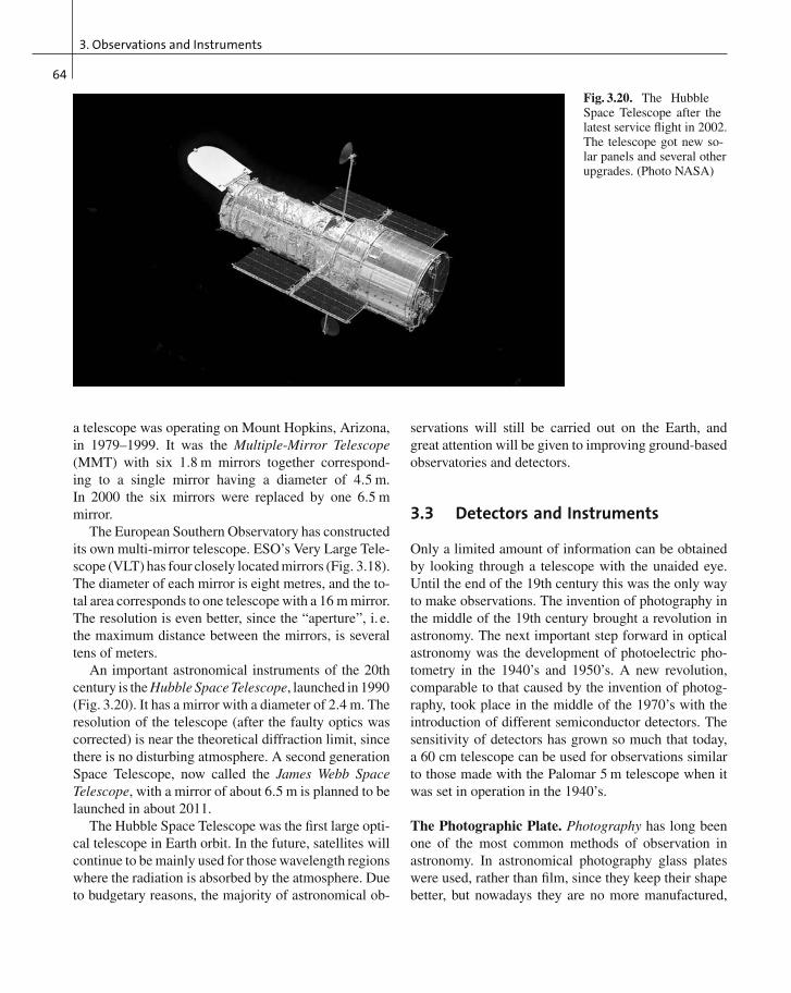
64
3. Observations and Instruments
Fig. 3.20. The HubbleSpace Telescope after thelatest service flight in 2002.The telescope got new so-lar panels and several otherupgrades. (Photo NASA)
a telescope was operating on Mount Hopkins, Arizona,in 1979–1999. It was the Multiple-Mirror Telescope(MMT) with six 1.8 m mirrors together correspond-ing to a single mirror having a diameter of 4.5 m.In 2000 the six mirrors were replaced by one 6.5 mmirror.
The European Southern Observatory has constructedits own multi-mirror telescope. ESO’s Very Large Tele-scope (VLT) has four closely located mirrors (Fig. 3.18).The diameter of each mirror is eight metres, and the to-tal area corresponds to one telescope with a 16 m mirror.The resolution is even better, since the “aperture”, i. e.the maximum distance between the mirrors, is severaltens of meters.
An important astronomical instruments of the 20thcentury is the Hubble Space Telescope, launched in 1990(Fig. 3.20). It has a mirror with a diameter of 2.4 m. Theresolution of the telescope (after the faulty optics wascorrected) is near the theoretical diffraction limit, sincethere is no disturbing atmosphere. A second generationSpace Telescope, now called the James Webb SpaceTelescope, with a mirror of about 6.5 m is planned to belaunched in about 2011.
The Hubble Space Telescope was the first large opti-cal telescope in Earth orbit. In the future, satellites willcontinue to be mainly used for those wavelength regionswhere the radiation is absorbed by the atmosphere. Dueto budgetary reasons, the majority of astronomical ob-
servations will still be carried out on the Earth, andgreat attention will be given to improving ground-basedobservatories and detectors.
3.3 Detectors and Instruments
Only a limited amount of information can be obtainedby looking through a telescope with the unaided eye.Until the end of the 19th century this was the only wayto make observations. The invention of photography inthe middle of the 19th century brought a revolution inastronomy. The next important step forward in opticalastronomy was the development of photoelectric pho-tometry in the 1940’s and 1950’s. A new revolution,comparable to that caused by the invention of photog-raphy, took place in the middle of the 1970’s with theintroduction of different semiconductor detectors. Thesensitivity of detectors has grown so much that today,a 60 cm telescope can be used for observations similarto those made with the Palomar 5 m telescope when itwas set in operation in the 1940’s.
The Photographic Plate. Photography has long beenone of the most common methods of observation inastronomy. In astronomical photography glass plateswere used, rather than film, since they keep their shapebetter, but nowadays they are no more manufactured,

3.3 Detectors and Instruments
65
and CCD-cameras have largely replaced photography.The sensitive layer on the surface of the film or plateis made up of a silver halide, usually silver bromide,AgBr. A photon absorbed by the halide excites an elec-tron that can move from one atom to another. A silverion, Ag+, can catch the electron, becoming a neutralatom. When the necessary amount of silver atoms havebeen accumulated at one place, they form a latent image.The latent image can be made into a permanent nega-tive by treating the plate after exposure with variouschemicals, which transform the silver bromide crystalsenclosing the latent image into silver (“development”),and remove the unexposed crystals (“fixing”).
The photographic plate has many advantages overthe human eye. The plate can register up to millions ofstars (picture elements) at one time, while the eye canobserve at most one or two objects at a time. The imageon a plate is practically permanent – the picture can bestudied at any time. In addition, the photographic plateis cheap and easy to use, as compared to many otherdetectors. The most important feature of a plate is itscapability to collect light over an extended time: thelonger exposures are used, the more silver atoms areformed on the plate (the plate darkens). By increasingthe exposure times, fainter objects can be photographed.The eye has no such capacity: if a faint object does notshow through a telescope, it cannot been seen, no matterhow long one stares.
One disadvantage of the photographic plate is its lowsensitivity. Only one photon in a thousand causes a re-action leading to the formation of a silver grain. Thusthe quantum efficiency of the plate is only 0.1%. Severalchemical treatments can be used to sensitize the platebefore exposure. This brings the quantum efficiencyup to a few percent. Another disadvantage is the factthat a silver bromide crystal that has been exposed oncedoes not register anything more, i. e. a saturation point isreached. On the other hand, a certain number of photonsare needed to produce an image. Doubling the numberof photons does not necessarily double the density (the‘blackness’ of the image): the density of the plate de-pends nonlinearly on the amount of incoming light. Thesensitivity of the plate is also strongly dependent onthe wavelength of the light. For the reasons mentionedabove the accuracy with which brightness can be mea-sured on a photographic plate is usually worse thanabout 5%. Thus the photographic plate makes a poor
photometer, but it can be excellently used, e. g. for mea-suring the positions of stars (positional astronomy) andfor mapping the sky.
Photocathodes, Photomultipliers. A photocathode isa more effective detector than the photographic plate.It is based on the photoelectric effect. A light quantum,or photon, hits the photocathode and loosens an elec-tron. The electron moves to the positive electrode, oranode, and gives rise to an electric current that can bemeasured. The quantum efficiency of a photocathode isabout 10–20 times better than that of a photographicplate; optimally, an efficiency of 30% can be reached.A photocathode is also a linear detector: if the numberof electrons is doubled, the outcoming current is alsodoubled.
The photomultiplier is one of the most importantapplications of the photocathode. In this device, theelectrons leaving the photocathode hit a dynode. Foreach electron hitting the dynode, several others are re-leased. When there are several dynodes in a row, theoriginal weak current can be intensified a millionfold.The photomultiplier measures all the light entering it,but does not form an image. Photomultipliers are mostlyused in photometry, and an accuracy of 0.1–1% can beattained.
Photometers, Polarimeters. A detector measuringbrightness, a photometer, is usually located behind thetelescope in the Cassegrain focus. In the focal planethere is a small hole, the diaphragm, which lets throughlight from the object under observation. In this way,light from other stars in the field of view can be pre-vented from entering the photometer. A field lens behindthe diaphragm refracts the light rays onto a photocath-ode. The outcoming current is intensified further ina preamplifier. The photomultiplier needs a voltage of1000–1500 volts.
Observations are often made in a certain wavelengthinterval, instead of measuring all the radiation enter-ing the detector. In this case a filter is used to preventother wavelengths from reaching the photomultiplier.A photometer can also consist of several photomultipli-ers (Fig. 3.21), which measure simultaneously differentwavelength bands. In such an instrument beam splittersor semitransparent mirrors split the light beam throughfixed filters to the photomultipliers.

66
3. Observations and Instruments
Fig. 3.21. The principle of a photoelectric multicolour pho-tometer. Light collected by the telescope arrives from the left.The light enters the photometer through a small hole in thefocal plane, the diaphragm. A lens collimates the light intoa parallel beam. Semitransparent mirrors divide the beam toseveral photomultipliers. A field lens guides the light througha filter onto the photocathode of the photomultiplier. Thequanta of light, photons, release electrons from the cathodes.The electrons are accelerated towards the dynodes with a volt-age of about 1500 V. The electrons hitting the dynodes releasestill more electrons, and the current is greatly enhanced. Ev-ery electron emitted from the cathode gives rise to a pulse ofup to 108 electrons at the anode; the pulse is amplified andregistered by a pulse counter. In this way, the photons fromthe star are counted
In a device called the photopolarimeter, a polarizingfilter is used, either alone or in combination with otherfilters. The degree and direction of polarization can befound by measuring the intensity of the radiation withdifferent orientations of the polarizers.
In practice, the diaphragm of a photometer will al-ways also let through part of the background sky aroundthe observed object. The measured brightness is in re-ality the combined brightness of the object and the sky.In order to find the brightness of the object, the back-ground brightness must be measured separately andsubtracted from the combined brightness. The accuracyof the measurements is decreased if long observationtimes are used and the background brightness undergoesfast changes. The problem can be solved by observingthe brightness of the background sky and the objectsimultaneously.
Photometric observations are often relative. If one isobserving, e. g. a variable star, a reference star close to
the actual target is observed at regular intervals. Usingthe observations of this reference star it is possible toderive a model for the slow changes in the atmosphericextinction (see Chap. 4) and remove their effect. The in-strument can be calibrated by observing some standardstars, whose brightness is known very accurately.
Image Intensifiers. Different image intensifiers basedon the photocathode have been used since the 1960’s. Inthe intensifier the information about the starting pointof the electron on the photocathode is preserved and theintensified image is formed on a fluorescent screen. Theimage can then be registered, e. g. with a CCD camera.One of the advantages of the image intensifier is thateven faint objects can be imaged using relatively shortexposures, and observations can be made at wavelengthswhere the detector is insensitive.
Another common type of detector is based on theTV camera (Vidicon camera). The electrons releasedfrom the photocathode are accelerated with a voltage ofa few kilovolts before they hit the electrode where theyform an image in the form of an electric charge dis-tribution. After exposure, the charge at different pointsof the electrode is read by scanning its surface with anelectron beam row by row. This produces a video sig-nal, which can be transformed into a visible image ona TV tube. The information can also be saved in digitalform. In the most advanced systems, the scintillationscaused by single electrons on the fluorescent screen ofthe image intensifier can be registered and stored in thememory of a computer. For each point in the imagethere is a memory location, called a picture element orpixel.
Since the middle of the 1970’s, detectors usingsemiconductor techniques began to be used in increas-ing numbers. With semiconductor detectors a quantumefficiency of about 70–80% can be attained; thus, sensi-tivity cannot be improved much more. The wavelengthregions suitable for these new detectors are much widerthan in the case of the photographic plate. The detec-tors are also linear. Computers are used for collecting,saving and analyzing the output data available in digitalform.
CCD Camera. The most important new detector is theCCD camera (Charge Coupled Device). The detectorconsists of a surface made up of light sensitive silicon

3.3 Detectors and Instruments
67
Fig. 3.22a–e. The principle of reading a CCD camera. (a) Dur-ing an exposure electrons are trapped in potential wellscorresponding to pixels of the camera. The number at eachpixel shows the number of electrons. (b) After the expo-sure each horizontal line is moved one pixel to the right;the rightmost row moves to the readout buffer. (c) The con-
tents of the buffer is moved down by one pixel. The lowermostcharge moves to the A/D converter, which sends the numberof electrons to the computer. (d) After moving the buffer downseveral times one vertical row has been read. (e) The imageis again shifted right by one pixel. This procedure is repeatedtill the whole image is read
diodes, arranged in a rectangular array of image ele-ments or pixels. The largest cameras can have as manyas 4096×4096 pixels, although most are considerablysmaller.
A photon hitting the detector can release an elec-tron, which will remain trapped inside a pixel. Afterthe exposure varying potential differences are used tomove the accumulated charges row by row to a read-out buffer. In the buffer the charges are moved pixel bypixel to an analogy/digital converter, which transmitsthe digital value to a computer. Reading an image alsoclears the detector (Fig. 3.22). If the exposures are veryshort the readout times may take a substantial part ofthe observing time.
The CCD camera is nearly linear: the number ofelectrons is directly proportional to the number of pho-tons. Calibration of the data is much easier than withphotographic plates.
The quantum efficiency, i. e. the number of electronsper incident photon, is high, and the CCD camera is
much more sensitive than a photographic plate. Thesensitivity is highest in the red wavelength range, about600–800 nm, where the quantum efficiency can be80–90% or even higher.
The range of the camera extends far to the infrared. Inthe ultraviolet the sensitivity drops due to the absorptionof the silicon very rapidly below about 500 nm. Twomethods have been used to avoid this problem. One isto use a coating that absorbs the ultraviolet photons andemits light of longer wavelength. Another possibility isto turn the chip upside down and make it very thin toreduce the absorption.
The thermal noise of the camera generates dark cur-rent even if the camera is in total darkness. To reducethe noise the camera must be cooled. Astronomical CCDcameras are usually cooled with liquid nitrogen, whichefficiently removes most of the dark current. How-ever, the sensitivity is also reduced when the camerais cooled; so too cold is not good either. The tempera-ture must be kept constant in order to obtain consistent

68
3. Observations and Instruments
data. For amateurs there are already moderately pricedCCD cameras, which are electrically cooled. Many ofthem are good enough also for scientific work, if veryhigh sensitivity is not required.
The dark current can easily be measured by takingexposures with the shutter closed. Subtracting this fromthe observed image gives the real number of electronsdue to incident light.
The sensitivity of individual pixels may be slightlydifferent. This can be corrected for by taking an im-age of an evenly illuminated field, like a twilight sky.This image is called a flat-field. When observations aredivided by the flat-field, the error caused by differentpixels is removed.
The CCD camera is very stable. Therefore it isnot necessary to repeat the dark current and flat-fieldobservations very frequently. Typically these calibra-tion exposures are taken during evening and morningtwilights, just before and after actual observations.
Cosmic rays are charged particles that can produceextraneous bright dots in CCD images. They are usuallylimited to one or two pixels, and are easily identified.Typically a short exposure of a few minutes containsa few traces of cosmic rays. Instead of a single longexposure it is usually better to take several short ones,clean the images from cosmic rays, and finally add theimages on a computer.
A more serious problem is the readout noise of theelectronics. In the first cameras it could be hundredsof electrons per pixel. In modern cameras it is a fewelectrons. This gives a limit to the faintest detectablesignal: if the signal is weaker than the readout noise, itis indistinguishable from the noise.
Although the CCD camera is a very sensitivedetector, even bright light cannot damage it. A pho-tomultiplier, on the other hand, can be easily destroyedby letting in too much light. However, one pixel canonly store a certain number of electrons, after whichit becomes saturated. Excessive saturation can makethe charge to overflow also to the neighboring pixels.If the camera becomes badly saturated it may haveto be read several times to completely remove thecharges.
The largest CCD cameras are quite expensive, andeven they are still rather small compared with photo-graphic plates and films. Therefore photography stillhas some use in recording extended objects.
Spectrographs. The simplest spectrograph is a prismthat is placed in front of a telescope. This kind of de-vice is called the objective prism spectrograph. Theprism spreads out the different wavelengths of lightinto a spectrum which can be registered. During theexposure, the telescope is usually slightly moved per-pendicularly to the spectrum, in order to increase thewidth of the spectrum. With an objective prism spectro-graph, large numbers of spectra can be photographed,e. g. for spectral classification.
For more accurate information the slit spectrographmust be used (Fig. 3.23). It has a narrow slit in the fo-cal plane of the telescope. The light is guided throughthe slit to a collimator that reflects or refracts all thelight rays into a parallel beam. After this, the light isdispersed into a spectrum by a prism and focused witha camera onto a detector, which nowadays is usuallya CCD camera. A comparison spectrum is exposed nextto the stellar spectrum to determine the precise wave-lengths. In modern spectrographs using CCD cameras,the comparison spectrum is usually exposed as a sepa-rate image. A big slit spectrograph is often placed at thecoudé or Nasmyth focus of the telescope.
Instead of the prism a diffraction grating can be usedto form the spectrum. A grating has narrow grooves,side by side, typically several hundred per millimetre.When light is reflected by the walls of the grooves, theadjoining rays interfere with each other and give riseto spectra of different orders. There are two kinds ofgratings: reflection and transmission gratings. In a re-flection grating no light is absorbed by the glass as inthe prism or transmission grating. A grating usuallyhas higher dispersion, or ability to spread the spectrum,
Fig. 3.23. The principle of the slit spectrograph. Light raysentering through a slit are collimated (made parallel to eachother), dispersed into a spectrum by a prism and projectedonto a photographic plate or a CCD

3.4 Radio Telescopes
69
than a prism. The dispersion can be increased by in-creasing the density of the grooves of the grating. In slitspectrographs the reflection grating is most commonlyused.
Interferometers. The resolution of a big telescope isin practice limited by seeing, and thus increasing theaperture does not necessarily improve the resolution.To get nearer to the theoretical resolution limit set bydiffraction (Fig. 3.6), different interferometers can beused.
There are two types of optical interferometers. Onekind uses an existing large telescope; the other a systemof two or more separate telescopes. In both cases thelight rays are allowed to interfere. By analyzing theoutcoming interference pattern, the structures of closebinaries can be studied, apparent angular diameters ofthe stars can be measured, etc.
One of the earliest interferometers was the Michelsoninterferometer that was built shortly before 1920 for thelargest telescope of that time. In front of the telescope,at the ends of a six metre long beam, there were flatmirrors reflecting the light into the telescope. The formof the interference pattern changed when the separationof the mirrors was varied. In practice, the interferencepattern was disturbed by seeing, and only a few positiveresults were obtained with this instrument.
The diameters of over 30 of the brightest stars havebeen measured using intensity interferometers. Sucha device consists of two separate telescopes that can bemoved in relation to each other. This method is suitablefor the brightest objects only.
In 1970 the Frenchman Antoine Labeyrie introducedthe principle of speckle interferometry. In traditionalimaging the pictures from long exposures consist ofa large number of instantaneous images, “speckles”, thattogether form the seeing disc. In speckle interferometryvery short exposures and large magnifications are usedand hundreds of pictures are taken. When these picturesare combined and analyzed (usually in digital form),the actual resolution of the telescope can nearly bereached.
The accuracy of interferometric techniques was im-proved at the beginning of 00’s. The first experimentsto use the two 10 m Keck telescopes as one interfero-meter, were made in 2001. Similarly, the ESO VLT willbe used as an interferometer.
3.4 Radio Telescopes
Radio astronomy represents a relatively new branchof astronomy. It covers a frequency range from a fewmegahertz (100 m) up to frequencies of about 300 GHz(1 mm), thereby extending the observable electromag-netic spectrum by many orders of magnitude. Thelow-frequency limit of the radio band is determined bythe opacity of the ionosphere, while the high-frequencylimit is due to the strong absorption from oxygen andwater bands in the lower atmosphere. Neither of theselimits is very strict, and under favourable conditions ra-dio astronomers can work into the submillimetre regionor through ionospheric holes during sunspot minima.
At the beginning of the 20th century attempts weremade to observe radio emission from the Sun. Theseexperiments, however, failed because of the low sensi-tivity of the antenna–receiver systems, and because ofthe opaqueness of the ionosphere at the low frequen-cies at which most of the experiments were carried out.The first observations of cosmic radio emission werelater made by the American engineer Karl G. Jansky in1932, while studying thunderstorm radio disturbancesat a frequency of 20.5 MHz (14.6 m). He discoveredradio emission of unknown origin, which varied withina 24 hour period. Somewhat later he identified the sourceof this radiation to be in the direction of the centre ofour Galaxy.
The real birth of radio astronomy may perhaps bedated to the late 1930’s, when Grote Reber startedsystematic observations with his homemade 9.5 mparaboloid antenna. Thereafter radio astronomy de-veloped quite rapidly and has greatly improved ourknowledge of the Universe.
Observations are made both in the continuum (broadband) and in spectral lines (radio spectroscopy). Muchof our knowledge about the structure of our Milky Waycomes from radio observations of the 21 cm line of neu-tral hydrogen and, more recently, from the 2.6 mm lineof the carbon monoxide molecule. Radio astronomy hasresulted in many important discoveries; e. g. both pul-sars and quasars were first found by radio astronomicalobservations. The importance of the field can also beseen from the fact that the Nobel prize in physics hasrecently been awarded twice to radio astronomers.
A radio telescope collects radiation in an apertureor antenna, from which it is transformed to an electric

70
3. Observations and Instruments
signal by a receiver, called a radiometer. This signal isthen amplified, detected and integrated, and the outputis registered on some recording device, nowadays usu-ally by a computer. Because the received signal is veryweak, one has to use sensitive receivers. These are of-ten cooled to minimize the noise, which could otherwisemask the signal from the source. Because radio wavesare electromagnetic radiation, they are reflected and re-fracted like ordinary light waves. In radio astronomy,however, mostly reflecting telescopes are used.
At low frequencies the antennas are usually dipoles(similar to those used for radio or TV), but in order toincrease the collecting area and improve the resolution,one uses dipole arrays, where all dipole elements areconnected to each other.
The most common antenna type, however, isa parabolic reflector, which works exactly as an opti-cal mirror telescope. At long wavelengths the reflectingsurface does not need to be solid, because the longwavelength photons cannot see the holes in the reflec-tor, and the antenna is therefore usually made in the
Fig. 3.24. The largest radio telescope in the world is theArecibo dish in Puerto Rico. It has been constructed over
a natural bowl and is 300 m in diameter. (Photo AreciboObservatory)
form of a metal mesh. At high frequencies the surfacehas to be smooth, and in the millimetre-submillimetrerange, radio astronomers even use large optical tele-scopes, which they equip with their own radiometers.To ensure a coherent amplification of the signal, the sur-face irregularities should be less than one-tenth of thewavelength used.
The main difference between a radio telescope andan optical telescope is in the recording of the signal.Radio telescopes are not imaging telescopes (exceptfor synthesis telescopes, which will be described later);instead, a feed horn, which is located at the antennafocus, transfers the signal to a receiver. The wavelengthand phase information is, however, preserved.
The resolving power of a radio telescope, θ, canbe deduced from the same formula (3.4) as for opti-cal telescopes, i. e. λ/D, where λ is the wavelengthused and D is the diameter of the aperture. Since thewavelength ratio between radio and visible light is ofthe order of 10,000, radio antennas with diameters ofseveral kilometres are needed in order to achieve the

3.4 Radio Telescopes
71
Fig. 3.25. The largest fully steerable radio telescope is in Green Bank, Virginia. Its diameter is 100×110 m. (Photo NRAO)
same resolution as for optical telescopes. In the earlydays of radio astronomy poor resolution was the biggestdrawback for the development and recognition of radioastronomy. For example, the antenna used by Janskyhad a fan beam with a resolution of about 30 in thenarrower direction. Therefore radio observations couldnot be compared with optical observations. Neither wasit possible to identify the radio sources with opticalcounterparts.
The world’s biggest radio telescope is the Arecibo an-tenna in Puerto Rico, whose main reflector is fixed andbuilt into a 305 m diameter, natural round valley cov-ered by a metal mesh (Fig. 3.24). In the late 1970’s theantenna surface and receivers were upgraded, enablingthe antenna to be used down to wavelengths of 5 cm.The mirror of the Arecibo telescope is not parabolic butspherical, and the antenna is equipped with a movablefeed system, which makes observations possible withina 20 radius around the zenith.
The biggest completely steerable radio telescope isthe Green Bank telescope in Virginia, U.S.A., dedicatedat the end of 2000. It is slightly asymmetric with a di-
ameter of 100×110 m (Fig. 3.25). Before the GreenBank telescope, for over two decades the largest tele-scope was the Effelsberg telescope in Germany. Thisantenna has a parabolic main reflector with a diameterof 100 m. The inner 80 m of the dish is made of solidaluminium panels, while the outmost portion of the diskis a metal mesh structure. By using only the inner por-tion of the telescope, it has been possible to observedown to wavelengths of 4 mm. The oldest and perhapsbest-known big radio telescope is the 76 m antenna atJodrell Bank in Britain, which was completed in the endof the 1950’s.
The biggest telescopes are usually incapable of op-erating below wavelengths of 1 cm, because the surfacecannot be made accurate enough. However, the millime-tre range has become more and more important. In thiswavelength range there are many transitions of interstel-lar molecules, and one can achieve quite high angularresolution even with a single dish telescope. At present,the typical size of a mirror of a millimetre telescope isabout 15 m. The development of this field is rapid, andat present several big millimetre telescopes are in opera-

72
3. Observations and Instruments
Fig. 3.26. The 15 metreMaxwell submillimetretelescope on Mauna Kea,Hawaii, is located in a dryclimate at an altitudeof 4100 m. Observationscan be made down towavelengths of 0.5 mm.(Photo Royal Observatory,Edinburgh)
tion (Table C.24). Among them are the 40 m Nobeyamatelescope in Japan, which can be used down to 3 mm,the 30 m IRAM telescope at Pico Veleta in Spain, whichis usable down to 1 mm, and the 15 m UK James ClerkMaxwell Telescope on Mauna Kea, Hawaii, operatingdown to 0.5 mm (Fig. 3.26). The largest project in thefirst decade of the 21st century is ALMA (AtacamaLarge Millimetre Array), which comprises of 50 tele-scopes with a diameter of 12 m (Fig. 3.27). It will bebuilt as an international project by the United States,Europe and Japan.
As already mentioned, the resolving power of a radiotelescope is far poorer than that of an optical telescope.The biggest radio telescopes can at present reach a reso-lution of 5 arc seconds, and that only at the very highest
frequencies. To improve the resolution by increasingthe size is difficult, because the present telescopes arealready close to the practical upper limit. However,by combining radio telescopes and interferometers, itis possible to achieve even better resolution than withoptical telescopes.
As early as 1891 Michelson used an interferometerfor astronomical purposes. While the use of interfer-ometers has proved to be quite difficult in the opticalwavelength regime, interferometers are extremely use-ful in the radio region. To form an interferometer, oneneeds at least two antennas coupled together. The spac-ing between the antennas, D, is called the baseline. Letus first assume that the baseline is perpendicular to theline of sight (Fig. 3.28). Then the radiation arrives at

3.4 Radio Telescopes
73
Fig. 3.27. The Atacama Large Millimetre Array (ALMA) willbe built in cooperation by Europe, U.S.A. and Japan. The
original plan was to have 64 antennas, but for financial reasonsthe number has been reduced to 50. (Drawing ESO/NOAJ)
both antennas with the same phase, and the summedsignal shows a maximum. However, due to the rotationof the Earth, the direction of the baseline changes, pro-ducing a phase difference between the two signals. Theresult is a sinusoidal interference pattern, in which min-ima occur when the phase difference is 180 degrees.The distance between the peaks is given by
θD = λ ,
where θ is the angle the baseline has turned and λ is thewavelength of the received signal. The resolution of theinterferometer is thus equal to that of an antenna witha linear size equal to D.
If the source is not a point source, the radiation emit-ted from different parts of the source will have phasedifferences when it enters the antennas. In this case theminima of the interference pattern will not be zero, butwill have some positive value Pmin. If we denote themaximum value of the interference pattern by Pmax, the
ratioPmax − Pmin
Pmax + Pmin
gives a measure of the source size (fringe visibility).
Fig. 3.28. The principle of an interferometer. If the radiationreaches the radio telescopes in the same phase, the waves am-plify each other and a maximum is obtained in the combinedradiation (cases 1 and 3). If the incoming waves are in oppositephase, they cancel each other (case 2)

74
3. Observations and Instruments
More accurate information about the source structurecan be obtained by changing the spacing between theantennas, i. e. by moving the antennas with respect toeach other. If this is done, interferometry is transformedinto a technique called aperture synthesis.
The theory and techniques of aperture synthesis weredeveloped by the British astronomer Sir Martin Ryle.In Fig. 3.29 the principle of aperture synthesis is il-lustrated. If the telescopes are located on an east–westtrack, the spacing between them, projected onto the sky,will describe a circle or an ellipse, depending on theposition of the source as the the Earth rotates aroundits axis. If one varies the distance between the tele-scopes, one will get a series of circles or ellipses onthe sky during a 12 hour interval. As we can see fromFig. 3.29, one does not have to cover all the spacings be-tween the telescopes, because any antenna combinationwhich has the same relative distance will describe thesame path on the sky. In this way one can synthesize anantenna, a filled aperture, with a size equal to the max-imum spacing between the telescopes. Interferometersworking according to this principle are called aperturesynthesis telescopes. If one covers all the spacings upto the maximum baseline, the result will be an accuratemap of the source over the primary beam of an indi-vidual antenna element. Aperture synthesis telescopestherefore produce an image of the sky, i. e. a “radiophotograph”.
A typical aperture synthesis telescope consists of onefixed telescope and a number of movable telescopes,usually located on an east–west track, although T orY configurations are also quite common. The numberof telescopes used determines how fast one can syn-thesize a larger disk, because the number of possibleantenna combinations increases as n(n −1), where n isthe number of telescopes. It is also possible to syn-thesize a large telescope with only one fixed and onemovable telescope by changing the spacing betweenthe telescopes every 12 hours, but then a full aperturesynthesis can require several months of observing time.In order for this technique to work, the source must beconstant, i. e. the signal cannot be time variable duringthe observing session.
The most efficient aperture synthesis telescope atpresent is the VLA (Very Large Array) in New Mexico,USA (Fig. 3.30). It consists of 27 paraboloid anten-nas, each with a diameter of 25 m, which are located
Fig. 3.29a–c. To illustrate the principle of aperture synthesis,let us consider an east–west oriented interferometer pointedtowards the celestial north. Each antenna is identical, hasa diameter D and operates at a wavelength λ. The minimumspacing between each antenna element is a, and the maximumspacing is 6a. In (a) there are only two antennas, A and B,displaced by the maximum spacing 6a. When the earth ro-tates, antennas A and B will, in the course of 12 hours, tracka circle on the plane of the sky with a diameter λ/(6a), themaximum resolution that can be achieved with this interfer-ometer. In (b) the antenna C is added to the interferometer,thus providing two more baselines, which track the circles ACand BC with radii of λ/(2a) and λ/(4a), respectively. In (c)there is still another antenna D added to the interferometer.In this case two of the baselines are equal, AD and CD, andtherefore only two new circles are covered on the plane of thesky. By adding more interferometer elements, one can fill inthe missing parts within the primary beam, i. e. the beam ofone single dish, and thus obtain a full coverage of the beam.It is also evident from (c), that not all of the antenna positionsare needed to provide all the different spacings; some antennaspacings will in such a case be equal and therefore provideno additional information. Obtaining a full aperture synthesiswith an east–west interferometer always takes 12 hours, if allspacings are available. Usually, however, several antenna el-ements are movable, in which case a full aperture synthesiscan take a long time before all spacings are filled in
on a Y-shaped track. The Y-formation was chosen be-cause it provides a full aperture synthesis in 8 hours.Each antenna can be moved by a specially built carrier,

3.4 Radio Telescopes
75
Fig. 3.30. The VLA at Socorro, New Mexico, is a synthesis telescope consisting of 27 movable antennas
and the locations of the telescopes are chosen to giveoptimal spacings for each configuration. In the largestconfiguration each arm is about 21 km long, therebyresulting in an antenna with an effective diameter of35 km. If the VLA is used in its largest configuration andat its highest frequency, 23 GHz (1.3 cm), the resolutionachieved is 0.1 arc second, clearly superior to any opticaltelescope. Similar resolution can also be obtained withthe British MERLIN telescope, where already existingtelescopes have been coupled together by radio links.Other well-known synthesis telescopes are the Cam-bridge 5 km array in Britain and the Westerbork array inthe Netherlands, both located on east–west tracks.
Even higher resolution can be obtained with an ex-tension of the aperture synthesis technique, called VLBI(Very Long Baseline Interferometry). With the VLBItechnique the spacing between the antennas is restrictedonly by the size of the Earth. VLBI uses existing an-tennas (often on different continents), which are allpointed towards the same source. In this case the signalis recorded together with accurate timing signals fromatomic clocks. The data files are correlated against each
other, resulting in maps similar to those obtained witha normal aperture synthesis telescope. With VLBI tech-niques it is possible to achieve resolutions of 0.0001′′.Because interferometry is very sensitive to the distancebetween the telescopes, the VLBI technique also pro-vides one of the most accurate methods to measuredistances. Currently one can measure distances withan accuracy of a few centimetres on intercontinentalbaselines. This is utilized in geodetic VLBI experi-ments, which study continental drift and polar motionas a function of time.
In radio astronomy the maximum size of single an-tennas has also been reached. The trend is to buildsynthesis antennas, similar to the VLA in New Mex-ico. In the 1990’s The United States built a chain ofantennas extending across the whole continent, and theAustralians have constructed a similar, but north–southantenna chain across their country.
More and more observations are being made in thesubmillimetre region. The disturbing effect of atmo-spheric water vapour becomes more serious at shorterwavelengths; thus, submillimetre telescopes must be lo-

76
3. Observations and Instruments
cated on mountain tops, like optical telescopes. All partsof the mirror are actively controlled in order to accu-rately maintain the proper form like in the new opticaltelescopes. Several new submillimetre telescopes areunder construction.
3.5 Other Wavelength Regions
All wavelengths of the electromagnetic spectrum en-ter the Earth from the sky. However, as mentionedin Sect. 3.1, not all radiation reaches the ground. Thewavelength regions absorbed by the atmosphere havebeen studied more extensively since the 1970’s, usingEarth-orbiting satellites. Besides the optical and radioregions, there are only some narrow wavelength rangesin the infrared that can be observed from high mountaintops.
The first observations in each new wavelength regionwere usually carried out from balloons, but not untilrockets came into use could observations be made fromoutside the atmosphere. The first actual observations ofan X-ray source, for instance, were made on a rocketflight in June 1962, when the detector rose above theatmosphere for about 6 minutes. Satellites have made itpossible to map the whole sky in the wavelength regionsinvisible from the ground.
Gamma Radiation. Gamma ray astronomy stud-ies radiation quanta with energies of 105–1014 eV.The boundary between gamma and X-ray astron-omy, 105 eV, corresponds to a wavelength of 10−11 m.The boundary is not fixed; the regions of hard(= high-energy) X-rays and soft gamma rays partlyoverlap.
While ultraviolet, visible and infrared radiation areall produced by changes in the energy states of theelectron envelopes of atoms, gamma and hard X-raysare produced by transitions in atomic nuclei or inmutual interactions of elementary particles. Thus ob-servations of the shortest wavelengths give informationon processes different from those giving rise to longerwavelengths.
The first observations of gamma sources were ob-tained at the end of the 1960’s, when a device inthe OSO 3 satellite (Orbiting Solar Observatory) de-tected gamma rays from the Milky Way. Later on, some
satellites were especially designed for gamma astron-omy, notably SAS 2, COS B, HEAO 1 and 3, and theCompton Gamma Ray Observatory. The most effectivesatellite at present is the European Integral, launched in2002.
The quanta of gamma radiation have energies a mil-lion times greater than those of visible light, but theycannot be observed with the same detectors. Theseobservations are made with various scintillation de-tectors, usually composed of several layers of detectorplates, where gamma radiation is transformed by thephotoelectric effect into visible light, detectable byphotomultipliers.
The energy of a gamma quantum can be determinedfrom the depth to which it penetrates the detector. An-alyzing the trails left by the quanta gives informationon their approximate direction. The field of view is lim-ited by the grating. The directional accuracy is low, andin gamma astronomy the resolution is far below that inother wavelength regions.
X-rays. The observational domain of X-ray astronomyincludes the energies between 102 and 105 eV, or thewavelengths 10–0.01 nm. The regions 10–0.1 nm and0.1–0.01 nm are called soft and hard X-rays, respec-tively. X-rays were discovered in the late 19th century.Systematic studies of the sky at X-ray wavelengths onlybecame possible in the 1970’s with the advent of satellitetechnology.
The first all-sky mapping was made in the early1970’s by SAS 1 (Small Astronomical Satellite), alsocalled Uhuru. At the end of the 1970’s, two High-Energy Astronomy Observatories, HEAO 1 and 2 (thelatter called Einstein), mapped the sky with much highersensitivity than Uhuru.
The Einstein Observatory was able to detect sourcesabout a thousand times fainter than earlier X-ray tele-scopes. In optical astronomy, this would correspond toa jump from a 15 cm reflector to a 5 m telescope. ThusX-ray astronomy has developed in 20 years as much asoptical astronomy in 300 years.
The latest X-ray satellites have been the Ameri-can Chandra and the European XMM-Newton, bothlaunched in 1999.
Besides satellites mapping the whole sky, there havebeen several satellites observing the X-ray radiation ofthe Sun. The first effective telescopes were installed in

3.5 Other Wavelength Regions
77
Fig. 3.31. (a) X-rays are not reflected by an ordinary mirror,and the principle of grazing reflection must be used for col-lecting them. Radiation meets the paraboloid mirror at a verysmall angle, is reflected onto a hyperboloid mirror and further
to a focal point. In practice, several mirrors are placed one in-side another, collecting radiation in a common focus (b) TheEuropean Integral gamma ray observatory was launched in2002. (Picture ESA)
the Skylab space station, and they were used to studythe Sun in 1973–74. In the 1990’s, the European Sohostarted making regular X-ray observations of the Sun.
The first X-ray telescopes used detectors similar tothose in gamma astronomy. Their directional accuracywas never better than a few arc minutes. The more pre-cise X-ray telescopes utilize the principle of grazingreflection (Fig. 3.31). An X-ray hitting a surface per-pendicularly is not reflected, but absorbed. If, however,X-rays meet the mirror nearly parallel to its surface, justgrazing it, a high quality surface can reflect the ray.
The mirror of an X-ray reflector is on the inner sur-face of a slowly narrowing cone. The outer part of thesurface is a paraboloid and the inner part a hyperboloid.The rays are reflected by both surfaces and meet at a fo-cal plane. In practice, several tubes are installed onewithin another. For instance, the four cones of the Ein-stein Observatory had as much polished optical surfaceas a normal telescope with a diameter of 2.5 m. The res-olution in X-ray telescopes is of the order of a few arcseconds and the field of view about 1 deg.
The detectors in X-ray astronomy are usuallyGeiger–Müller counters, proportional counters or scin-tillation detectors. Geiger–Müller and proportionalcounters are boxes filled with gas. The walls form a cath-ode, and an anode wire runs through the middle of thebox; in more accurate counters, there are several anodewires. An X-ray quantum entering the box ionizes thegas, and the potential difference between the anode andcathode gives rise to a current of electrons and positiveions.
Ultraviolet Radiation. Between X-rays and the opti-cal region lies the domain of ultraviolet radiation, withwavelengths between 10 and 400 nm. Most ultravioletobservations have been carried out in the soft UV re-gion, at wavelengths near those of optical light, sincemost of the UV radiation is absorbed by the atmosphere.The wavelengths below 300 nm are completely blockedout. The short wavelength region from 10 to 91.2 nm iscalled the extreme ultraviolet (EUV, XUV).
Extreme ultraviolet was one of the last regions ofthe electromagnetic radiation to be observed system-atically. The reason for this is that the absorption ofinterstellar hydrogen makes the sky practically opaqueat these wavelengths. The visibility in most directionsis limited to some hundred light years in the vicinityof the Sun. In some directions, however, the density ofthe interstellar gas is so low that even extragalactic ob-jects can be seen. The first dedicated EUV satellite wasthe Extreme Ultraviolet Explorer (EUVE), operating in1992–2000. It observed about a thousand EUV sources.In EUV grazing reflection telescopes similar to thoseused in X-ray astronomy are employed.
In nearly all branches of astronomy important in-formation is obtained by observations of ultravioletradiation. Many emission lines from stellar chromo-spheres or coronas, the Lyman lines of atomic hydrogen,and most of the radiation from hot stars are found in theUV domain. In the near-ultraviolet, telescopes can bemade similar to optical telescopes and, equipped witha photometer or spectrometer, installed in a satelliteorbiting the Earth.
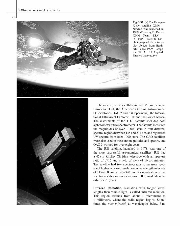
78
3. Observations and Instruments
Fig. 3.32. (a) The EuropeanX-ray satellite XMM-Newton was launched in1999. (Drawing D. Ducros,XMM Team, ESA)(b) FUSE satellite hasphotographed far ultravi-olet objects from Earthorbit since 1999. (Graph-ics NASA/JHU AppliedPhysics Laboratory)
The most effective satellites in the UV have been theEuropean TD-1, the American Orbiting AstronomicalObservatories OAO 2 and 3 (Copernicus), the Interna-tional Ultraviolet Explorer IUE and the Soviet Astron.The instruments of the TD-1 satellite included botha photometer and a spectrometer. The satellite measuredthe magnitudes of over 30,000 stars in four differentspectral regions between 135 and 274 nm, and registeredUV spectra from over 1000 stars. The OAO satelliteswere also used to measure magnitudes and spectra, andOAO 3 worked for over eight years.
The IUE satellite, launched in 1978, was one ofthe most successful astronomical satellites. IUE hada 45 cm Ritchey-Chrétien telescope with an apertureratio of f/15 and a field of view of 16 arc minutes.The satellite had two spectrographs to measure spec-tra of higher or lower resolution in wavelength intervalsof 115–200 nm or 190–320 nm. For registration of thespectra, a Vidicon camera was used. IUE worked on theorbit for 20 years.
Infrared Radiation. Radiation with longer wave-lengths than visible light is called infrared radiation.This region extends from about 1 micrometre to1 millimetre, where the radio region begins. Some-times the near-infrared, at wavelengths below 5 m,

3.6 Other Forms of Energy
79
Fig. 3.33. Refractors arenot suitable for infraredtelescopes, because in-frared radiation cannotpenetrate glass. TheCassegrain reflectors in-tended especially forinfrared observationshave secondary mirrorsnodding rapidly back andforth between the ob-ject and the backgroundnear the object. By sub-tracting the brightness ofthe background from thebrightness of the object,the background can beeliminated
and the submillimetre domain, at wavelengths between0.1 and 1 mm, are considered separate wavelengthregions.
In infrared observations radiation is collected bya telescope, as in the optical region. The incomingradiation consists of radiation from the object, fromthe background and from the telescope itself. Boththe source and the background must be continuallymeasured, the difference giving the radiation from theobject. The background measurements are usually madewith a Cassegrain secondary mirror oscillating be-tween the source and the background at a rate of, say,100 oscillations per second, and thus the changing back-ground can be eliminated. To register the measurements,semiconductor detectors are used. The detector must al-ways be cooled to minimize its own thermal radiation.Sometimes the whole telescope is cooled.
Infrared observatories have been built on high moun-tain tops, where most of the atmospheric water vapourremains below. Some favourable sites are, e. g. MaunaKea on Hawaii, Mount Lemon in Arizona and Pico delTeide on Tenerife. For observations in the far-infraredthese mountains are not high enough; these observationsare carried out, e. g. on aeroplanes. One of the best-equipped planes is the Kuiper Airborne Observatory,named after the well-known planetary scientist GerardKuiper.
Fig. 3.34. The most effective infrared satellite at present is theAmerican Spitzer, launched in 2003. (Drawing NASA)
Balloons and satellites are also used for infraredobservations. The most successful infrared observato-ries so far have been the InfraRed Astronomy SatelliteIRAS, the European Infrared Space Observatory ISO,and the present-day Spitzer (originally SIRTF, SpaceInfraRed Telescope Facility). A very succesful satellitewas the 1989 launched COBE (Cosmic BackgroundExplorer), which mapped the background radiationin submillimetre and infrared wavelengths. The Mi-crowave Anisotropy Probe (MAP) has continued thework of COBE, starting in 2001.
3.6 Other Forms of Energy
Besides electromagnetic radiation, energy arrives fromspace in other forms: particles (cosmic rays, neutrinos)and gravitational radiation.
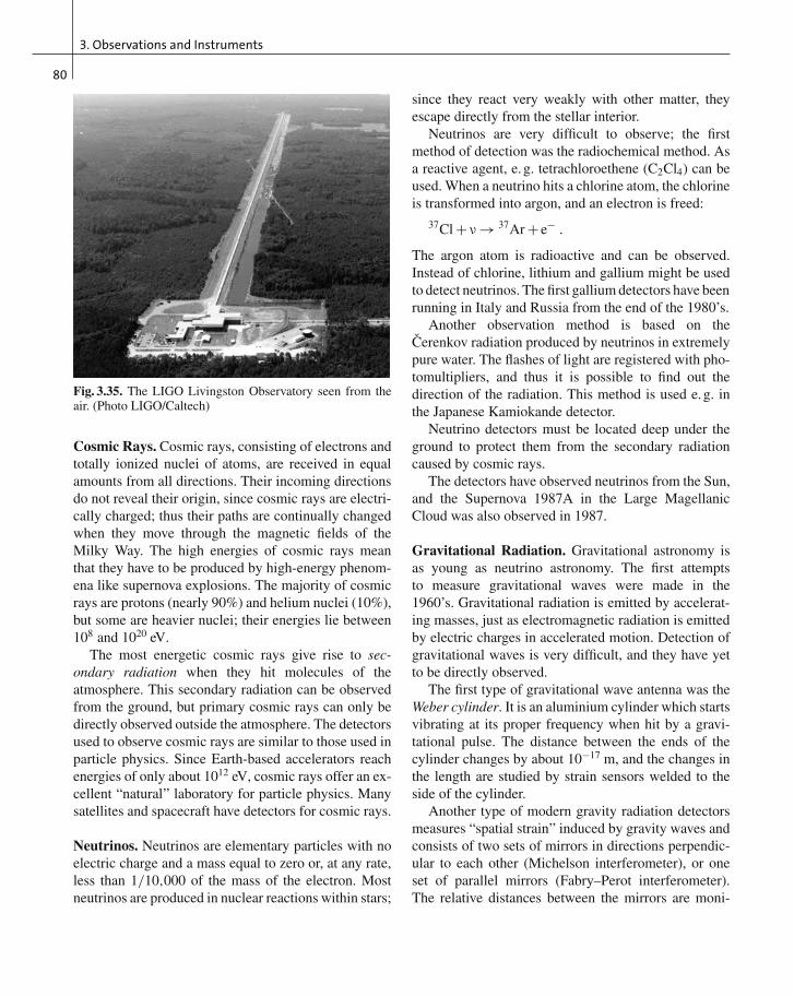
80
3. Observations and Instruments
Fig. 3.35. The LIGO Livingston Observatory seen from theair. (Photo LIGO/Caltech)
Cosmic Rays. Cosmic rays, consisting of electrons andtotally ionized nuclei of atoms, are received in equalamounts from all directions. Their incoming directionsdo not reveal their origin, since cosmic rays are electri-cally charged; thus their paths are continually changedwhen they move through the magnetic fields of theMilky Way. The high energies of cosmic rays meanthat they have to be produced by high-energy phenom-ena like supernova explosions. The majority of cosmicrays are protons (nearly 90%) and helium nuclei (10%),but some are heavier nuclei; their energies lie between108 and 1020 eV.
The most energetic cosmic rays give rise to sec-ondary radiation when they hit molecules of theatmosphere. This secondary radiation can be observedfrom the ground, but primary cosmic rays can only bedirectly observed outside the atmosphere. The detectorsused to observe cosmic rays are similar to those used inparticle physics. Since Earth-based accelerators reachenergies of only about 1012 eV, cosmic rays offer an ex-cellent “natural” laboratory for particle physics. Manysatellites and spacecraft have detectors for cosmic rays.
Neutrinos. Neutrinos are elementary particles with noelectric charge and a mass equal to zero or, at any rate,less than 1/10,000 of the mass of the electron. Mostneutrinos are produced in nuclear reactions within stars;
since they react very weakly with other matter, theyescape directly from the stellar interior.
Neutrinos are very difficult to observe; the firstmethod of detection was the radiochemical method. Asa reactive agent, e. g. tetrachloroethene (C2Cl4) can beused. When a neutrino hits a chlorine atom, the chlorineis transformed into argon, and an electron is freed:
37Cl +ν→ 37Ar + e− .
The argon atom is radioactive and can be observed.Instead of chlorine, lithium and gallium might be usedto detect neutrinos. The first gallium detectors have beenrunning in Italy and Russia from the end of the 1980’s.
Another observation method is based on theCerenkov radiation produced by neutrinos in extremelypure water. The flashes of light are registered with pho-tomultipliers, and thus it is possible to find out thedirection of the radiation. This method is used e.g. inthe Japanese Kamiokande detector.
Neutrino detectors must be located deep under theground to protect them from the secondary radiationcaused by cosmic rays.
The detectors have observed neutrinos from the Sun,and the Supernova 1987A in the Large MagellanicCloud was also observed in 1987.
Gravitational Radiation. Gravitational astronomy isas young as neutrino astronomy. The first attemptsto measure gravitational waves were made in the1960’s. Gravitational radiation is emitted by accelerat-ing masses, just as electromagnetic radiation is emittedby electric charges in accelerated motion. Detection ofgravitational waves is very difficult, and they have yetto be directly observed.
The first type of gravitational wave antenna was theWeber cylinder. It is an aluminium cylinder which startsvibrating at its proper frequency when hit by a gravi-tational pulse. The distance between the ends of thecylinder changes by about 10−17 m, and the changes inthe length are studied by strain sensors welded to theside of the cylinder.
Another type of modern gravity radiation detectorsmeasures “spatial strain” induced by gravity waves andconsists of two sets of mirrors in directions perpendic-ular to each other (Michelson interferometer), or oneset of parallel mirrors (Fabry–Perot interferometer).The relative distances between the mirrors are moni-

3.6 Other Forms of Energy
81
tored by laser interferometers. If a gravity pulse passesthe detector, the distances change and the changes canbe measured. The longest baseline between the mir-rors is in the American LIGO (Laser InterferometerGravitational-wave Observatory) system, about 25 km(Fig. 3.35). LIGO made the first scientific observationsin 2002.
* Diffraction by a Circular Aperture
Consider a circular hole of radius R in the xy plane.Coherent light enters the hole from the direction ofthe negative z axis (see figure). We consider light raysleaving the hole parallel to the xz plane forming anangle θ with the z axis. The light waves interfere ona screen far away. The phase difference between a wavethrough a point (x, y) and a wave going through thecentre of the hole can be calculated from the differentpath lengths s = x sin θ:
δ= s
λ2π = 2π sin θ
λx ≡ kx .
Thus, the phase difference δ depends on the x co-ordinate only. The sum of the amplitudes of the wavesfrom a small surface element is proportional to the areaof the element dx dy. Let the amplitude coming through
the centre of the hole be da0 = dx dyi. The amplitudecoming from the point (x, y) is then
da = dx dy (cos δ i + sin δ j) .
We sum up the amplitudes coming from differentpoints of the hole:
a =∫
Aperture
da
=R∫
x =−R
√R2−x2∫
y =−√
R2−x2
(cos kx i + sin kx j) dy dx
= 2
R∫−R
√R2 − x2(cos kx i + sin kx j) dx .
Since sine is an odd function (sin(−kx)= − sin(kx)),we get zero when we integrate the second term. Cosineis an even function, and so
a ∝R∫
0
√R2 − x2 cos kx dx .
We substitute x = Rt and define p = kR =(2πr sin θ)/λ, thus getting
a ∝1∫
0
√1− t2 cos pt dt .
The zero points of the intensity observed on thescreen are obtained from the zero points of theamplitude,
J(p)=1∫
0
√1− t2 cos pt dt = 0 .

82
3. Observations and Instruments
Inspecting the function J(p), we see that the first zerois at p = 3.8317, or
2πR sin θ
λ= 3.8317 .
The radius of the diffraction disc in angular units canbe estimated from the condition
sin θ = 3.8317λ
2πR≈ 1.22
λ
D,
where D = 2R is the diameter of the hole.In mirror telescopes diffraction is caused also by the
support structure of the secondary mirror. If the aper-ture is more complex and only elementary mathematicsis used calculations may become rather cumbersome.However, it can be shown that the diffraction pattern canbe obtained as the Fourier transform of the aperture.
3.7 Examples
Example 3.1 The distance between the componentsof the binary star ζ Herculis is 1.38′′. What shouldthe diameter of a telescope be to resolve the binary?If the focal length of the objective is 80 cm, whatshould the focal length of the eyepiece be to resolvethe components, when the resolution of the eye is 2′?
In the optical region, we can use the wavelength valueof λ≈ 550 nm. The diameter of the objective is obtainedfrom the equation for the resolution (3.4),
D ≈ λ
θ= 550×10−9
(1.38/3600)× (π/180)m
= 0.08 m = 8 cm .
The required magnification is
ω= 2′
1.38′′ = 87 .
The magnification is given by
ω= f
f ′ ,
and, thus, the focal length of the eyepiece should be
f ′ = f
ω= 80 cm
87= 0.9 cm .
Example 3.2 A telescope has an objective witha diameter of 90 mm and focal length of 1200 mm.
a) What is the focal length of an eyepiece, the exit pupilof which is 6 mm (about the size of the pupil of theeye)?
b) What is the magnification of such an eyepiece?c) What is the angular diameter of the Moon seen
through this telescope and eyepiece?
a) From Fig. 3.7 we get
L = f ′
fD ,
whence
f ′ = fL
D= 1200 mm
6 mm
90 mm
= 80 mm .
b) The magnification is ω= f/ f ′ = 1200 mm/80 mm= 15.
c) Assuming the angular diameter of the Moon isα = 31′ = 0.52, its diameter through the telescopeis ωα= 7.8.
3.8 Exercises
Exercise 3.1 The Moon was photographed with a tele-scope, the objective of which had a diameter of 20 cmand focal length of 150 cm. The exposure time was 0.1 s.
a) What should the exposure time be, if the diameter ofthe objective were 15 cm and focal length 200 cm?
b) What is the size of the image of the Moon in bothcases?
c) Both telescopes are used to look at the Moon with aneyepiece the focal length of which is 25 mm. Whatare the magnifications?
Exercise 3.2 The radio telescopes at Amherst, Mas-sachusetts, and Onsala, Sweden, are used as aninterferometer, the baseline being 2900 km.
a) What is the resolution at 22 GHz in the direction ofthe baseline?
b) What should be the size of an optical telescope withthe same resolution?

Hannu Karttunen et al. (Eds.), Photometric Concepts and Magnitudes.In: Hannu Karttunen et al. (Eds.), Fundamental Astronomy, 5th Edition. pp. 83–93 (2007)DOI: 11685739_4 © Springer-Verlag Berlin Heidelberg 2007
83
4. Photometric Concepts and Magnitudes
Most astronomical observations utilize electromag-netic radiation in one way or another. We can
obtain information on the physical nature of a radia-tion source by studying the energy distribution of itsradiation. We shall now introduce some basic conceptsthat characterize electromagnetic radiation.
4.1 Intensity, Flux Densityand Luminosity
Let us assume we have some radiation passing througha surface element d A (Fig. 4.1). Some of the radiationwill leave d A within a solid angle dω; the angle betweendω and the normal to the surface is denoted by θ. Theamount of energy with frequency in the range [ν, ν+dν]entering this solid angle in time dt is
dEν = Iν cos θ d A dν dω dt . (4.1)
Here, the coefficient Iν is the specific intensity of theradiation at the frequency ν in the direction of the solidangle dω. Its dimension is W m−2 Hz−1 sterad−1.
Fig. 4.1. The intensity Iν of radiation is related to the energypassing through a surface element d A into a solid angle dω,in a direction θ
The projection of the surface element d A as seenfrom the direction θ is d An = d A cos θ, which explainsthe factor cos θ. If the intensity does not depend ondirection, the energy dEν is directly proportional to thesurface element perpendicular to the direction of theradiation.
The intensity including all possible frequencies iscalled the total intensity I , and is obtained by integratingIν over all frequencies:
I =∞∫
0
Iν dν .
More important quantities from the observationalpoint of view are the energy flux (Lν, L) or, briefly, theflux and the flux density (Fν, F). The flux density givesthe power of radiation per unit area; hence its dimensionis W m−2 Hz−1 or W m−2, depending on whether we aretalking about the flux density at a certain frequency orabout the total flux density.
Observed flux densities are usually rather small, andW m−2 would be an inconveniently large unit. There-fore, especially in radio astronomy, flux densities areoften expressed in Janskys; one Jansky (Jy) equals10−26 W m−2 Hz−1.
When we are observing a radiation source, we infact measure the energy collected by the detector dur-ing some period of time, which equals the flux densityintegrated over the radiation-collecting area of theinstrument and the time interval.
The flux density Fν at a frequency ν can be expressedin terms of the intensity as
Fν = 1
d A dν dt
∫S
dEν
=∫S
Iν cos θ dω , (4.2)
where the integration is extended over all possibledirections. Analogously, the total flux density is
F =∫S
I cos θ dω .

84
4. Photometric Concepts and Magnitudes
For example, if the radiation is isotropic, i. e. if I isindependent of the direction, we get
F =∫S
I cos θ dω= I∫S
cos θ dω . (4.3)
The solid angle element dω is equal to a surface elementon a unit sphere. In spherical coordinates it is (Fig. 4.2;also c. f. Appendix A.5):
dω= sin θ dθ dφ .
Substitution into (4.3) gives
F = I
π∫θ= 0
2π∫φ= 0
cos θ sin θ dθ dφ = 0 ,
so there is no net flux of radiation. This means that thereare equal amounts of radiation entering and leaving thesurface. If we want to know the amount of radiationpassing through the surface, we can find, for example,the radiation leaving the surface. For isotropic radiationthis is
Fl = I
π/2∫θ = 0
2π∫φ= 0
cos θ sin θ dθ dφ = πI . (4.4)
Fig. 4.2. An infinitesimal solid angle dω is equal tothe corresponding surface element on a unit sphere:dω= sin θ dθ dφ
In the astronomical literature, terms such as intensityand brightness are used rather vaguely. Flux density ishardly ever called flux density but intensity or (withluck) flux. Therefore the reader should always carefullycheck the meaning of these terms.
Flux means the power going through some surface,expressed in watts. The flux emitted by a star intoa solid angle ω is L = ωr2 F, where F is the flux densityobserved at a distance r. Total flux is the flux pass-ing through a closed surface encompassing the source.Astronomers usually call the total flux of a star the lu-minosity L. We can also talk about the luminosity Lν ata frequency ν ([Lν] = W Hz−1). (This must not be con-fused with the luminous flux used in physics; the lattertakes into account the sensitivity of the eye.)
If the source (like a typical star) radiates isotropically,its radiation at a distance r is distributed evenly ona spherical surface whose area is 4πr2 (Fig. 4.3). If theflux density of the radiation passing through this surfaceis F, the total flux is
L = 4πr2 F . (4.5)
Fig. 4.3. An energy flux which at a distance r from a pointsource is distributed over an area A is spread over an area 4Aat a distance 2r. Thus the flux density decreases inverselyproportional to the distance squared

4.2 Apparent Magnitudes
85
Fig. 4.4. An observer seesradiation coming froma constant solid angle ω.The area giving off ra-diation into this solidangle increases when thesource moves further away(A ∝ r2). Therefore thesurface brightness or theobserved flux density perunit solid angle remainsconstant
If we are outside the source, where radiation is notcreated or destroyed, the luminosity does not depend ondistance. The flux density, on the other hand, falls offproportional to 1/r2.
For extended objects (as opposed to objects such asstars visible only as points) we can define the surfacebrightness as the flux density per unit solid angle (Fig.4.4). Now the observer is at the apex of the solid angle.The surface brightness is independent of distance, whichcan be understood in the following way. The flux densityarriving from an area A is inversely proportional to thedistance squared. But also the solid angle subtended bythe area A is proportional to 1/r2 (ω= A/r2). Thus thesurface brightness B = F/ω remains constant.
The energy density u of radiation is the amount ofenergy per unit volume (J m−3):
u = 1
c
∫S
I dω . (4.6)
Fig. 4.5. In time dt, the radiation fills a volume dV = c dt d A,where d A is the surface element perpendicular to thepropagation direction of the radiation
This can be seen as follows. Suppose we have radiationwith intensity I arriving from a solid angle dω per-pendicular to the surface d A (Fig. 4.5). In the time dt,the radiation travels a distance c dt and fills a volumedV = c dt d A. Thus the energy in the volume dV is(now cos θ = 1)
dE = I d A dω dt = 1
cI dω dV .
Hence the energy density du of the radiation arrivingfrom the solid angle dω is
du = dE
dV= 1
cI dω ,
and the total energy density is obtained by integratingthis over all directions. For isotropic radiation we get
u = 4π
cI . (4.7)
4.2 Apparent Magnitudes
As early as the second century B. C., Hipparchos di-vided the visible stars into six classes according to theirapparent brightness. The first class contained the bright-est stars and the sixth the faintest ones still visible to thenaked eye.
The response of the human eye to the brightness oflight is not linear. If the flux densities of three stars are inthe proportion 1:10:100, the brightness difference of the

86
4. Photometric Concepts and Magnitudes
first and second star seems to be equal to the differenceof the second and third star. Equal brightness ratioscorrespond to equal apparent brightness differences: thehuman perception of brightness is logarithmic.
The rather vague classification of Hipparchos was re-placed in 1856 by Norman R. Pogson. The new, moreaccurate classification followed the old one as closelyas possible, resulting in another of those illogical defini-tions typical of astronomy. Since a star of the first classis about one hundred times brighter than a star of thesixth class, Pogson defined the ratio of the brightnessesof classes n and n +1 as 5
√100 = 2.512.
The brightness class or magnitude can be definedaccurately in terms of the observed flux density F([F] = W m−2). We decide that the magnitude 0 cor-responds to some preselected flux density F0. All othermagnitudes are then defined by the equation
m = −2.5 lgF
F0. (4.8)
Note that the coefficient is exactly 2.5, not 2.512! Mag-nitudes are dimensionless quantities, but to remind usthat a certain value is a magnitude, we can write it, forexample, as 5 mag or 5m.
It is easy to see that (4.8) is equivalent to Pog-son’s definition. If the magnitudes of two stars are mand m +1 and their flux densities Fm and Fm+1,respectively, we have
m − (m +1)= −2.5 lgFm
F0+2.5 lg
Fm+1
F0
= −2.5 lgFm
Fm+1,
whenceFm
Fm+1= 5
√100 .
In the same way we can show that the magnitudes m1
and m2 of two stars and the corresponding flux densitiesF1 and F2 are related by
m1 −m2 = −2.5 lgF1
F2. (4.9)
Magnitudes extend both ways from the original sixvalues. The magnitude of the brightest star, Sirius, is infact negative −1.5. The magnitude of the Sun is −26.8and that of a full moon −12.5. The magnitude of thefaintest objects observed depends on the size of the tele-
scope, the sensitivity of the detector and the exposuretime. The limit keeps being pushed towards fainter ob-jects; currently the magnitudes of the faintest observedobjects are over 30.
4.3 Magnitude Systems
The apparent magnitude m, which we have just de-fined, depends on the instrument we use to measure it.The sensitivity of the detector is different at differentwavelengths. Also, different instruments detect differentwavelength ranges. Thus the flux measured by the instru-ment equals not the total flux, but only a fraction of it.Depending on the method of observation, we can definevarious magnitude systems. Different magnitudes havedifferent zero points, i. e. they have different flux densi-ties F0 corresponding to themagnitude0.Thezeropointsare usually defined by a few selected standard stars.
In daylight the human eye is most sensitive toradiation with a wavelength of about 550 nm, the sen-sitivity decreasing towards red (longer wavelengths)and violet (shorter wavelengths). The magnitude cor-responding to the sensitivity of the eye is called thevisual magnitude mv.
Photographic plates are usually most sensitive at blueand violet wavelengths, but they are also able to registerradiation not visible to the human eye. Thus the photo-graphic magnitude mpg usually differs from the visualmagnitude. The sensitivity of the eye can be simulatedby using a yellow filter and plates sensitised to yellowand green light. Magnitudes thus observed are calledphotovisual magnitudes mpv.
If, in ideal case, we were able to measure the radiationat all wavelengths, we would get the bolometric magni-tude mbol. In practice this is very difficult, since part ofthe radiation is absorbed by the atmosphere; also, dif-ferent wavelengths require different detectors. (In factthere is a gadget called the bolometer, which, however,is not a real bolometer but an infrared detector.) Thebolometric magnitude can be derived from the visualmagnitude if we know the bolometric correction BC:
mbol = mv −BC . (4.10)
By definition, the bolometric correction is zero for radi-ation of solar type stars (or, more precisely, stars of thespectral class F5). Although the visual and bolometric

4.3 Magnitude Systems
87
magnitudes can be equal, the flux density correspondingto the bolometric magnitude must always be higher. Thereason of this apparent contradiction is in the differentvalues of F0.
The more the radiation distribution differs from thatof the Sun, the higher the bolometric correction is. Thecorrection is positive for stars both cooler or hotter thanthe Sun. Sometimes the correction is defined as mbol =mv +BC in which case BC ≤ 0 always. The chancefor errors is, however, very small, since we must havembol ≤ mv.
The most accurate magnitude measurements aremade using photoelectric photometers. Usually filtersare used to allow only a certain wavelength band toenter the detector. One of the multicolour magnitudesystems used widely in photoeletric photometry is theUBV system developed in the early 1950’s by HaroldL. Johnson and William W. Morgan. Magnitudes aremeasured through three filters, U = ultraviolet, B = blueand V = visual. Figure 4.6 and Table 4.1 give the wave-length bands of these filters. The magnitudes observedthrough these filters are called U , B and V magnitudes,respectively.
The UBV system was later augmented by addingmore bands. One commonly used system is the fivecolour UBVRI system, which includes R = red andI = infrared filters.
There are also other broad band systems, but theyare not as well standardised as the UBV, which hasbeen defined moderately well using a great number of
Fig. 4.6. Relative transmission profiles of filters used in theUBVRI magnitude system. The maxima of the bands are nor-malized to unity. The R and I bands are based on the systemof Johnson, Cousins and Glass, which includes also infraredbands J, H, K, L and M. Previously used R and I bands differconsiderably from these
Table 4.1. Wavelength bands of the UBVRI and uvby filtersand their effective (≈ average) wavelengths
Magnitude Band width Effective[nm] wavelength [nm]
U ultraviolet 66 367B blue 94 436V visual 88 545R red 138 638I infrared 149 797
u ultraviolet 30 349v violet 19 411b blue 18 467y yellow 23 547
standard stars all over the sky. The magnitude of anobject is obtained by comparing it to the magnitudes ofstandard stars.
In Strömgren’s four-colour or uvby system, the bandspassed by the filters are much narrower than in the UBVsystem. The uvby system is also well standardized, butit is not quite as common as the UBV. Other narrowband systems exist as well. By adding more filters,more information on the radiation distribution can beobtained.
In any multicolour system, we can define colourindices; a colour index is the difference of two mag-nitudes. By subtracting the B magnitude from U we getthe colour index U − B, and so on. If the UBV systemis used, it is common to give only the V magnitude andthe colour indices U − B and B − V .
The constants F0 in (4.8) for U , B and V magnitudeshave been selected in such a way that the colour indicesB − V and U − B are zero for stars of spectral type A0(for spectral types, see Chap. 8). The surface tempera-ture of such a star is about 10,000 K. For example, Vega(αLyr, spectral class A0V) has V = 0.03, B − V = U −B = 0.00. The Sun has V = −26.8, B − V = 0.62 andU − B = 0.10.
Before the UBV system was developed, a colourindex C.I., defined as
C.I. = mpg −mv ,
was used. Since mpg gives the magnitude in blue andmv in visual, this index is related to B − V . In fact,
C.I. = (B − V)−0.11 .

88
4. Photometric Concepts and Magnitudes
4.4 Absolute Magnitudes
Thus far we have discussed only apparent magnitudes.They do not tell us anything about the true brightness ofstars, since the distances differ. A quantity measuringthe intrinsic brightness of a star is the absolute magni-tude. It is defined as the apparent magnitude at a distanceof 10 parsecs from the star (Fig. 4.7).
We shall now derive an equation which relates theapparent magnitude m, the absolute magnitude M andthe distance r. Because the flux emanating from a starinto a solid angle ω has, at a distance r, spread over anareaωr2, the flux density is inversely proportional to thedistance squared. Therefore the ratio of the flux densityat a distance r, F(r), to the flux density at a distance of10 parsecs, F(10), is
F(r)
F(10)=(10 pc
r
)2.
Thus the difference of magnitudes at r and 10 pc, or thedistance modulus m − M, is
m − M = −2.5 lgF(r)
F(10)= −2.5 lg
(10 pc
r
)2
or
m − M = 5 lgr
10 pc. (4.11)
Fig. 4.7. The flux density at a distance of 10 parsecs from thestar defines its absolute magnitude
For historical reasons, this equation is almost alwayswritten as
m − M = 5 lg r −5 , (4.12)
which is valid only if the distance is expressed in par-secs. (The logarithm of a dimensional quantity is, infact, physically absurd.) Sometimes the distance is givenin kiloparsecs or megaparsecs, which require differentconstant terms in (4.12). To avoid confusion, we highlyrecommend the form (4.11).
Absolute magnitudes are usually denoted by capitalletters. Note, however, that the U , B and V magnitudesare apparent magnitudes. The corresponding absolutemagnitudes are MU, MB and MV.
The absolute bolometric magnitude can be expressedin terms of the luminosity. Let the total flux density ata distance r = 10 pc be F and let F be the equivalentquantity for the Sun. Since the luminosity is L = 4πr2 F,we get
Mbol − Mbol, = −2.5 lgF
F= −2.5 lg
L/4πr2
L/4πr2,
or
Mbol − Mbol, = −2.5 lgL
L. (4.13)
The absolute bolometric magnitude Mbol = 0 corre-sponds to a luminosity L0 = 3.0×1028 W.
4.5 Extinction and Optical Thickness
Equation (4.11) shows how the apparent magnitudeincreases (and brightness decreases!) with increasingdistance. If the space between the radiation source andthe observer is not completely empty, but contains someinterstellar medium, (4.11) no longer holds, because partof the radiation is absorbed by the medium (and usu-ally re-emitted at a different wavelength, which may beoutside the band defining the magnitude), or scatteredaway from the line of sight. All these radiation lossesare called the extinction.
Now we want to find out how the extinction de-pends on the distance. Assume we have a star radiatinga flux L0 into a solid angle ω in some wavelength range.Since the medium absorbs and scatters radiation, the

4.5 Extinction and Optical Thickness
89
flux L will now decrease with increasing distance r(Fig. 4.8). In a short distance interval [r, r +dr], the ex-tinction dL is proportional to the flux L and the distancetravelled in the medium:
dL = −αL dr . (4.14)
The factor α tells how effectively the medium can ob-scure radiation. It is called the opacity. From (4.14) wesee that its dimension is [α] = m−1. The opacity is zerofor a perfect vacuum and approaches infinity when thesubstance becomes really murky. We can now definea dimensionless quantity, the optical thickness τ by
dτ = α dr . (4.15)
Substituting this into (4.14) we get
dL = −L dτ .
Next we integrate this from the source (where L = L0
and r = 0) to the observer:
L∫L0
dL
L= −
τ∫0
dτ ,
which gives
L = L0e−τ . (4.16)
Here, τ is the optical thickness of the material betweenthe source and the observer and L, the observed flux.Now, the flux L falls off exponentially with increasing
Fig. 4.8. The interstellar medium absorbs and scatters radiation; this usually reduces the energy flux L in the solid angle ω(dL ≤ 0)
optical thickness. Empty space is perfectly transpar-ent, i. e. its opacity is α= 0; thus the optical thicknessdoes not increase in empty space, and the flux remainsconstant.
Let F0 be the flux density on the surface of a star andF(r), the flux density at a distance r. We can express thefluxes as
L = ωr2 F(r) , L0 = ωR2 F0 ,
where R is the radius of the star. Substitution into (4.16)gives
F(r)= F0R2
r2e−τ .
For the absolute magnitude we need the flux density ata distance of 10 parsecs, F(10), which is still evaluatedwithout extinction:
F(10)= F0R2
(10 pc)2.
The distance modulus m − M is now
m − M = −2.5 lgF(r)
F(10)
= 5 lgr
10 pc−2.5 lg e−τ
= 5 lgr
10 pc+ (2.5 lg e)τ
or
m − M = 5 lgr
10 pc+ A , (4.17)

90
4. Photometric Concepts and Magnitudes
where A ≥ 0 is the extinction in magnitudes due to theentire medium between the star and the observer. If theopacity is constant along the line of sight, we have
τ = α
r∫0
dr = αr ,
and (4.17) becomes
m − M = 5 lgr
10 pc+ar , (4.18)
where the constant a = 2.5α lg e gives the extinction inmagnitudes per unit distance.
Colour Excess. Another effect caused by the interstellarmedium is the reddening of light: blue light is scatteredand absorbed more than red. Therefore the colour indexB − V increases. The visual magnitude of a star is, from(4.17),
V = MV +5 lgr
10 pc+ AV , (4.19)
where MV is the absolute visual magnitude and AV isthe extinction in the V passband. Similarly, we get forthe blue magnitudes
B = MB +5 lgr
10 pc+ AB .
The observed colour index is now
B − V = MB − MV + AB − AV ,
or
B − V = (B − V )0 + EB−V , (4.20)
where (B − V )0 = MB − MV is the intrinsic colour ofthe star and EB−V = (B − V )− (B − V )0 is the colourexcess. Studies of the interstellar medium show that theratio of the visual extinction AV to the colour excessEB−V is almost constant for all stars:
R = AV
EB−V≈ 3.0 .
This makes it possible to find the visual extinction if thecolour excess is known:
AV ≈ 3.0 EB−V . (4.21)
When AV is obtained, the distance can be solved directlyfrom (4.19), when V and MV are known.
We shall study interstellar extinction in more detailin Sect. 15.1 (“Interstellar Dust”).
Atmospheric Extinction. As we mentioned in Sect.3.1, the Earth’s atmosphere also causes extinction.The observed magnitude m depends on the locationof the observer and the zenith distance of the ob-ject, since these factors determine the distance thelight has to travel in the atmosphere. To compare dif-ferent observations, we must first reduce them, i. e.remove the atmospheric effects somehow. The magni-tude m0 thus obtained can then be compared with otherobservations.
If the zenith distance z is not too large, we can ap-proximate the atmosphere by a plane layer of constantthickness (Fig. 4.9). If the thickness of the atmosphereis used as a unit, the light must travel a distance
X = 1/ cos z = sec z (4.22)
in the atmosphere. The quantity X is the air mass. Ac-cording to (4.18), the magnitude increases linearly withthe distance X:
m = m0 + kX , (4.23)
where k is the extinction coefficient.The extinction coefficient can be determined by ob-
serving the same source several times during a nightwith as wide a zenith distance range as possible. Theobserved magnitudes are plotted in a diagram as a func-tion of the air mass X. The points lie on a straight line theslope of which gives the extinction coefficient k. When
Fig. 4.9. If the zenith distance of a star is z, the light of the startravels a distance H/ cos z in the atmosphere; H is the heightof the atmosphere

4.6 Examples
91
this line is extrapolated to X = 0, we get the magni-tude m0, which is the apparent magnitude outside theatmosphere.
In practice, observations with zenith distances higherthan 70 (or altitudes less than 20) are not used todetermine k and m0, since at low altitudes the curva-ture of the atmosphere begins to complicate matters.The value of the extinction coefficient k depends onthe observation site and time and also on the wave-length, since extinction increases strongly towards shortwavelengths.
4.6 Examples
Example 4.1 Show that intensity is independent ofdistance.
Suppose we have some radiation leaving the surfaceelement d A in the direction θ. The energy entering thesolid angle dω in time dt is
dE = I cos θ d A dω dt ,
where I is the intensity. If we have another surface d A′at a distance r receiving this radiation from direction θ ′,we have
dω= d A′ cos θ ′/r2 .
The definition of the intensity gives
dE = I ′ cos θ ′ d A′ dω′ dt ,
where I ′ is the intensity at d A′ and
dω′ = d A cos θ/r2 .
Substitution of dω and dω′ into the expressions of dEgives
I cos θ dθ d Ad A′ cos θ ′
r2dt
= I ′ cos θ ′ d A′ d A cos θ
r2dt ⇒ I ′ = I .
Thus the intensity remains constant in empty space.
Example 4.2 Surface Brightness of the Sun
Assume that the Sun radiates isotropically. Let R be theradius of the Sun, F the flux density on the surface ofthe Sun and F the flux density at a distance r. Since theluminosity is constant,
L = 4πR2 F = 4πr2 F ,
the flux density equals
F = FR2
r2.
At a distance r R, the Sun subtends a solid angle
ω= A
r2= πR2
r2,
where A = πR2 is the cross section of the Sun. Thesurface brightness B is
B = F
ω= F
π.
Applying (4.4) we get
B = I .
Thus the surface brightness is independent of dis-tance and equals the intensity. We have found a simple

92
4. Photometric Concepts and Magnitudes
interpretation for the somewhat abstract concept ofintensity.
The flux density of the Sun on the Earth, the solarconstant, is S ≈ 1370 W m−2. The angular diameter ofthe Sun is α= 32′, whence
R
r= α
2= 1
2× 32
60× π
180= 0.00465 rad .
The solid angle subtended by the Sun is
ω= π
(R
r
)2
= π×0.004652
= 6.81×10⁻⁵ sterad .
and the surface brightness
B = Sω
= 2.01×10⁷ W m−2 sterad−1 .
Example 4.3 Magnitude of a Binary Star
Since magnitudes are logarithmic quantities, they canbe a little awkward for some purposes. For example, wecannot add magnitudes like flux densities. If the mag-nitudes of the components of a binary star are 1 and 2,the total magnitude is certainly not 3. To find the totalmagnitude, we must first solve the flux densities from
1 = −2.5 lgF1
F0, 2 = −2.5 lg
F2
F0,
which give
F1 = F0 ×10−0.4 , F2 = F0 ×10−0.8 .
Thus the total flux density is
F = F1 + F2 = F0(10−0.4 +10−0.8)
and the total magnitude,
m = −2.5 lgF0(10−0.4 +10−0.8)
F0
= −2.5 lg 0.5566 = 0.64 .
Example 4.4 The distance of a star is r = 100 pcand its apparent magnitude m = 6. What is its absolutemagnitude?
Substitution into (4.11)
m − M = 5 lgr
10 pc
gives
M = 6−5 lg100
10= 1 .
Example 4.5 The absolute magnitude of a star is M =−2 and the apparent magnitude m = 8. What is thedistance of the star?
We can solve the distance r from (4.11):
r = 10 pc×10(m − M )/5 = 10×1010/5pc
= 1000 pc = 1 kpc .
Example 4.6 Although the amount of interstellar ex-tinction varies considerably from place to place, wecan use an average value of 2 mag/kpc near the galac-tic plane. Find the distance of the star in Example 4.5,assuming such extinction.
Now the distance must be solved from (4.18):
8− (−2)= 5 lgr
10+0.002 r ,
where r is in parsecs. This equation cannot be solvedanalytically, but we can always use a numerical method.We try a simple iteration (Appendix A.7), rewriting theequation as
r = 10×102−0.0004 r .
The value r = 1000 pc found previously is a good initialguess:
r0 = 1000
r1 = 10×102 − 0.0004 × 1000 = 398
r2 = 693
...
r12 = r13 = 584 .
The distance is r ≈ 580 pc, which is much less thanour earlier value 1000 pc. This should be quite obvious,

4.7 Exercises
93
since due to extinction, radiation is now reduced muchfaster than in empty space.
Example 4.7 What is the optical thickness of a layerof fog, if the Sun seen through the fog seems as brightas a full moon in a cloudless sky?
The apparent magnitudes of the Sun and the Moonare −26.8 and −12.5, respectively. Thus the totalextinction in the cloud must be A = 14.3. Since
A = (2.5 lg e)τ ,
we get
τ = A/(2.5 lg e)= 14.3/1.086 = 13.2 .
The optical thickness of the fog is 13.2. In reality, a frac-tion of the light scatters several times, and a few of themultiply scattered photons leave the cloud along theline of sight, reducing the total extinction. Thereforethe optical thickness must be slightly higher than ourvalue.
Example 4.8 Reduction of Observations
The altitude and magnitude of a star were measuredseveral times during a night. The results are given in thefollowing table.
Altitude Zenith distance Air mass Magnitude
50 40 1.31 0.9035 55 1.74 0.9825 65 2.37 1.0720 70 2.92 1.17
By plotting the observations as in the following fig-ure, we can determine the extinction coefficient k andthe magnitude m0 outside the atmosphere. This canbe done graphically (as here) or using a least-squaresfit.
Extrapolation to the air mass X = 0 gives m0 = 0.68.The slope of the line gives k = 0.17.
4.7 Exercises
Exercise 4.1 The total magnitude of a triple star is 0.0.Two of its components have magnitudes 1.0 and 2.0.What is the magnitude of the third component?
Exercise 4.2 The absolute magnitude of a star in theAndromeda galaxy (distance 690 kpc) is M = 5. It ex-plodes as a supernova, becoming one billion (109) timesbrighter. What is its apparent magnitude?
Exercise 4.3 Assume that all stars have the same ab-solute magnitude and stars are evenly distributed inspace. Let N(m) be the number of stars brighter thanm magnitudes. Find the ratio N(m +1)/N(m).
Exercise 4.4 The V magnitude of a star is 15.1,B − V = 1.6, and absolute magnitude MV = 1.3. Theextinction in the direction of the star in the visual bandis aV = 1 mag kpc−1. What is the intrinsic colour of thestar?
Exercise 4.5 Stars are observed through a triple win-dow. Each surface reflects away 15% of the incidentlight.
a) What is the magnitude of Regulus (MV = 1.36) seenthrough the window?
b) What is the optical thickness of the window?

Hannu Karttunen et al. (Eds.), Radiation Mechanisms.In: Hannu Karttunen et al. (Eds.), Fundamental Astronomy, 5th Edition. pp. 95–112 (2007)DOI: 11685739_5 © Springer-Verlag Berlin Heidelberg 2007
95
5. Radiation Mechanisms
In the previous chapters we have studied the physicalproperties and detection of electromagnetic radiation.
Next we shall briefly discuss concepts related to emis-sion and absorption of radiation. Since we can give hereonly a summary of some essential results without delv-ing into quantum mechanical explanations, the readerinterested in the details is advised to consult any goodphysics textbook.
5.1 Radiation of Atoms and Molecules
Electromagnetic radiation is emitted or absorbed whenan atom or a molecule moves from one energy levelto another. If the energy of the atom decreases by anamount ∆E, the atom emits or radiates a quantumof electromagnetic radiation, called a photon, whosefrequency ν is given by the equation
∆E = hν , (5.1)
where h is the Planck constant, h = 6.6256×10⁻³⁴ J s.Similarly, if the atom receives or absorbs a photon ofa frequency ν, its energy increases by ∆E = hν.
The classical model describes an atom as a nucleussurrounded by a swarm of electrons. The nucleus con-sists of Z protons, each having a charge +e and Nelectrically neutral neutrons; Z is the charge number ofthe atom and A = Z + N is its mass number. A neutralatom has as many electrons (charge −e) as protons.
An energy level of an atom usually refers to an energylevel of its electrons. The energy E of an electron cannottake arbitrary values; only certain energies are allowed:the energy levels are quantized. An atom can emit orabsorb radiation only at certain frequencies νif corre-sponding to energy differences between some initialand final states i and f : |Ei − Ef| = hνif. This gives riseto the line spectrum, specific for each element (Fig. 5.1).Hot gas under low pressure produces an emission spec-trum consisting of such discrete lines. If the same gasis cooled down and observed against a source of whitelight (which has a continuous spectrum), the same linesare seen as dark absorption lines.
At low temperatures most atoms are in their lowestenergy state, the ground state. Higher energy levels areexcitation states; a transition from lower to higher stateis called excitation. Usually the excited atom will re-turn to the lower state very rapidly, radiating a photon(spontaneous emission); a typical lifetime of an excitedstate might be 10−8 seconds. The frequency of the emit-ted photon is given by (5.1). The atom may return to thelower state directly or through some intermediate states,emitting one photon in each transition.
Downward transitions can also be induced by radi-ation. Suppose our atom has swallowed a photon andbecome excited. Another photon, whose frequency νcorresponds to some possible downward transition fromthe excited state, can now irritate the atom, causing itto jump to a lower state, emitting a photon with thesame frequency ν. This is called induced or stimu-lated emission. Photons emitted spontaneously leavethe atom randomly in all directions with random phases:the radiation is isotropic and incoherent. Induced radi-ation, on the other hand, is coherent; it propagates inthe same direction as and in phase with the inducingradiation.
The zero level of the energy states is usually chosenso that a bound electron has negative energy and a freeelectron positive energy (cf. the energy integral of plan-etary orbits, Chap. 6). If an electron with energy E < 0receives more energy than |E|, it will leave the atom,which becomes an ion. In astrophysics ionization is of-ten called a bound-free transition (Fig. 5.2). Unlike inexcitation all values of energy (E > 0) are now possi-ble. The extraneous part of the absorbed energy goes tothe kinetic energy of the liberated electron. The inverseprocess, in which an atom captures a free electron, isthe recombination or free–bound transition.
When an electron scatters from a nucleus or an ionwithout being captured, the electromagnetic interactioncan change the kinetic energy of the electron produc-ing free–free radiation. In a very hot gas (T> 106 K)hydrogen is fully ionized, and the free–free radiation isthe most important source of emission. It is then usu-ally called thermal bremsstrahlung. The latter part ofthe name derives from the fact that decelerating elec-trons hitting the anode of an X-ray tube emit similar

96
5. Radiation Mechanisms
Fig. 5.1a,b. Origin of line spectra. (a) Emission spectrum.Atoms of glowing gas returning from excited states to lowerstates emit photons with frequencies corresponding to theenergy difference of the states. Each element emits its owncharacteristic wavelengths, which can be measured by spread-
ing the light into a spectrum with a prism or diffractiongrating. (b) Absorption spectrum. When white light con-taining all wavelengths travels through gas, the wavelengthscharacteristic of the gas are absorbed
Fig. 5.2. Different kinds of transitions between energy levels.Absorption and emission occur between two bound states,whereas ionization and recombination occur between a boundand a free state. Interaction of an atom with an free electroncan result in a free–free transition
radiation. In an analogous way the absorption processcan be called a bound–bound transition.
Electromagnetic radiation is transverse wave motion;the electric and magnetic fields oscillate perpendicularto each other and also perpendicular to the directionof propagation. The light of an ordinary incandescentlamp has a random distribution of electric fields vi-brating in all directions. If the directions of electricfields in the plane perpendicular to the direction ofpropagation are not evenly distributed, the radiation ispolarized (Fig. 5.3). The direction of polarization of lin-early polarized light means the plane determined bythe electric vector and the direction of the light ray.If the electric vector describes a circle, the radiationis circularly polarized. If the amplitude of the elec-tric field varies at the same time, the polarization iselliptic.

5.2 The Hydrogen Atom
97
Fig. 5.3. Polarization of light. The light of an incandescentbulb contains all possible directions of vibration and is there-fore unpolarized. Some crystals, for example, pass electricfields oscillating only in certain directions, and the transmit-ted part of the light becomes linearly polarized. E is the electricfield and B the magnetic field
If polarized radiation travels through a magneticfield, the direction of the polarization will rotate. Theamount of such Faraday rotation is proportional to thecomponent of the magnetic field parallel to the line ofsight, number of electrons along the line of sight, dis-tance travelled, and square of the wavelength of theradiation.
Scattering is an absorption followed by an instan-taneous emission at the same wavelength but usuallyin a new direction. On the macroscopic scale, radia-tion seems to be reflected by the medium. The lightcoming from the sky is sunlight scattered from atmo-spheric molecules. Scattered light is always polarized,the degree of polarization being highest in the directionperpendicular to the direction of the original radiation.
5.2 The Hydrogen Atom
The hydrogen atom is the simplest atom, consisting ofa proton and an electron. According to the Bohr modelthe electron orbits the proton in a circular orbit. (Inspite of the fact that this model has very little to dowith reality, it can be successfully used to predict someproperties of the hydrogen atom.) Bohr’s first postulatesays that the angular momentum of the electron must bea multiple of :
mvr = n , (5.2)
where
m = mass of the electron ,
v= speed of the electron ,
r = radius of the orbit ,
n = the principal quantum number ,
n = 1, 2, 3, . . . ,
= h/2π ,
h = the Planck constant .
The quantum mechanical interpretation of Bohr’sfirst postulate is obvious: the electron is representedas a standing wave, and the “length of the orbit”must be a multiple of the de Broglie wavelength,λ= /p = /mv.
A charged particle in a circular orbit (and thus inaccelerated motion) should emit electromagnetic radia-tion, losing energy, were it to obey the rules of classicalelectrodynamics. Therefore our electron should spiraldown towards the nucleus. But obviously, Nature doesnot behave this way, and we have to accept Bohr’s sec-ond postulate, which says that an electron moving inan allowed orbit around a nucleus does not radiate. Ra-diation is emitted only when the electron jumps froma higher energy state to a lower one. The emitted quan-tum has an energy hν, equal to the energy difference ofthese states:
hν = En2 − En1 . (5.3)
We shall now try to find the energy of an electron inthe state En . Coulomb’s law gives the force pulling theelectron towards the proton:
F = 1
4πε0
e2
r2n
, (5.4)
where
ε0 = the vacuum permittivity
= 8.85×10⁻¹² N−1 m−2 C2 ,
e = the charge of the electron = 1.6×10⁻¹⁹ C ,
rn = the distance between the electronand the proton .
The acceleration of a particle moving in a circularorbit of radius rn is
a = v2n
rn,
and applying Newton’s second law (F = ma), we get
mv2n
rn= 1
4πε0
e2
r2n. (5.5)

98
5. Radiation Mechanisms
From (5.2) and (5.5) it follows that
vn = e2
4πε0
1
n, rn = 4πε0
2
me2n2 .
The total energy of an electron in the orbit n is now
En = T + V = 1
2mv2
n − 1
4πε0
e2
rn
= − me4
32π2ε20
2
1
n2≡ −C
1
n2,
(5.6)
where C is a constant. For the ground state (n = 1), weget from (5.6)
E1 = −2.18×10⁻¹⁸ J = −13.6 eV .
Fig. 5.4. Transitions of a hy-drogen atom. The lowerpicture shows a part ofthe spectrum of the starHD193182. On both sidesof the stellar spectrum wesee an emission spectrumof iron. The wavelengthsof the reference lines areknown, and they can beused to calibrate the wave-lengths of the observedstellar spectrum. The hy-drogen Balmer lines areseen as dark absorptionlines converging towardsthe Balmer ionization limit(also called the Balmer dis-continuity) at λ= 364.7 nmto the left. The numbers(15, . . . , 40) refer to thequantum number n of thehigher energy level. (Photoby Mt. Wilson Observatory)
From (5.3) and (5.6) we get the energy of the quantumemitted in the transition En2 → En1 :
hν = En2 − En1 = C
(1
n21
− 1
n22
). (5.7)
In terms of the wavelength λ this can be expressed as
1
λ= ν
c= C
hc
(1
n21
− 1
n22
)≡ R
(1
n21
− 1
n22
), (5.8)
where R is the Rydberg constant, R = 1.097×10⁷ m−1.Equation (5.8) was derived experimentally for n1 = 2
by Johann Jakob Balmer as early as 1885. That is whywe call the set of lines produced by transitions En → E2
the Balmer series. These lines are in the visible part ofthe spectrum. For historical reasons the Balmer lines areoften denoted by symbols Hα, Hβ, Hγ etc. If the electronreturns to its ground state (En → E1), we get the Lyman

5.3 Line Profiles
99
series, which is in the ultraviolet. The other series withspecific names are the Paschen series (n1 = 3), Bracketseries (n1 = 4) and Pfund series (n1 = 5) (see Fig. 5.4).
5.3 Line Profiles
The previous discussion suggests that spectral lineswould be infinitely narrow and sharp. In reality, how-ever, they are somewhat broadened. We will nowconsider briefly the factors affecting the shape of a spec-tral line, called a line profile. An exact treatment wouldtake us too deep into quantum mechanics, so we cannotgo into the details here.
According to quantum mechanics everything cannotbe measured accurately at the same time. For example,even in principle, there is no way to determine the x co-ordinate and the momentum px in the direction of thex axis with arbitrary precision simultaneously. Thesequantities have small uncertainties ∆x and ∆px , suchthat
∆x∆px ≈ .A similar relation holds for other directions, too.Time and energy are also connected by an uncertaintyrelation,
∆E∆t ≈ .The natural width of spectral lines is a consequence ofthis Heisenberg uncertainty principle.
If the average lifetime of an excitation state is T , theenergy corresponding to the transition can only be de-termined with an accuracy of ∆E = /T = h/(2πT ).From (5.1) it follows that ∆ν =∆E/h. In fact, the un-certainty of the energy depends on the lifetimes of boththe initial and final states. The natural width of a line isdefined as
γ = ∆Ei +∆Ef
= 1
Ti+ 1
Tf. (5.9)
It can be shown that the corresponding line profile is
Iν = γ
2π
I0
(ν−ν0)2 +γ 2/4, (5.10)
where ν0 is the frequency at the centre of the line andI0 the total intensity of the line. At the centre of the linethe intensity per frequency unit is
Iν0 = 2
πγI0 ,
and at the frequency ν = ν0 +γ/2,
Iν0+γ/2 = 1
πγI0 = 1
2Iν0 .
Thus the width γ is the width of the line profile ata depth where the intensity is half of the maximum.This is called the full width at half maximum (FWHM).
Doppler Broadening. Atoms of a gas are moving thefaster the higher the temperature of the gas. Thus spec-tral lines arising from individual atoms are shifted bythe Doppler effect. The observed line consists of a col-lection of lines with different Doppler shifts, and theshape of the line depends on the number of atoms withdifferent velocities.
Each Doppler shifted line has its characteristic natu-ral width. The resulting line profile is obtained by givingeach Doppler shifted line a weight proportional to thenumber of atoms given by the velocity distribution andintegrating over all velocities. This gives rise to the Voigtprofile (Fig. 5.5), which already describes most spectrallines quite well. The shapes of different profiles don’t
Fig. 5.5. Each spectral line has its characteristic natural width(solid line). Motions of particles broaden the line further dueto the Doppler effect, resulting in the Voigt profile (dashedline). Both profiles have the same area

100
5. Radiation Mechanisms
Fig. 5.6. The full width at half maximum (FWHM) of a spec-tral line is the width at the depth where the intensity is half ofthe maximum. The equivalent width W is defined so that theline and the shaded rectangle have the same area in the pic-ture. The two measures are not generally the same, althoughthey usually are close to each other
seem very different; the most obvious consequence ofthe broadening is that the maximum depth decreases.
One way to describe the width of a line is to give itsfull width at half maximum (Fig. 5.6). Due to Dopplerbroadening this is usually greater than the natural width.The equivalent width is another measure of a linestrength. It is the area of a rectangular line that hasthe same area as the line profile and that emits no lightat all. The equivalent width can be used to describethe energy corresponding to a line independently of theshape of the line profile.
5.4 Quantum Numbers, SelectionRules, Population Numbers
Quantum Numbers. The Bohr model needs only onequantum number, n, to describe all the energy levels ofthe electron. This can explain only the coarse featuresof an atom with a single electron.
Quantum mechanics describes the electron as a threedimensional wave, which only gives the probability offinding the electron in a certain place. Quantum me-chanics has accurately predicted all the energy levelsof hydrogen atoms. The energy levels of heavier atomsand molecules can also be computed; however, suchcalculations are very complicated. Also the existence of
quantum numbers can be understood from the quantummechanical point of view.
The quantum mechanical description involves fourquantum numbers, one of which is our n, the principalquantum number. The principal quantum number de-scribes the quantized energy levels of the electron. Theclassical interpretation of discrete energy levels allowsonly certain orbits given by (5.6). The orbital angularmomentum of the electron is also quantized. This is de-scribed by the angular momentum quantum number l.The angular momentum corresponding to a quantumnumber l is
L =√l(l +1) .
The classical analogy would be to allow some ellipticorbits. The quantum number l can take only the values
l = 0, 1, . . . , n −1 .
For historical reasons, these are often denoted by theletters s, p, d, f , g, h, i, j.
Although l determines the magnitude of the angularmomentum, it does not give its direction. In a mag-netic field this direction is important, since the orbitingelectron also generates a tiny magnetic field. In anyexperiment, only one component of the angular momen-tum can be measured at a time. In a given direction z(e. g. in the direction of the applied magnetic field), theprojection of the angular momentum can have only thevalues
Lz = ml ,
where ml is the magnetic quantum number
ml = 0,±1,±2, . . . ,±l .
The magnetic quantum number is responsible forthe splitting of spectral lines in strong magnetic fields,known as the Zeeman effect. For example, if l = 1, ml
can have 2l +1 = 3 different values. Thus, the line aris-ing from the transition l = 1 → l = 0 will split into threecomponents in a magnetic field (Fig. 5.7).
The fourth quantum number is the spin describingthe intrinsic angular momentum of the electron. Thespin of the electron is
S =√s(s +1) ,

5.4 Quantum Numbers, Selection Rules, Population Numbers
101
Fig. 5.7. The Zeeman effect. In strong magnetic fields eachenergy level of a hydrogen atom splits into (2l +1) separatelevels, which correspond to different values of the magneticquantum number ml = l, l −1, . . . ,−l. The energy differencesof the successive levels have the same constant value∆E. Forexample the p state (l = 1) splits into three and the d state(l = 2) into five sublevels. The selection rules require thatin electric dipole transitions ∆ml equals 0 or ±1, and onlynine different transitions between p and d states are possible.Moreover, the transitions with the same ∆ml have the sameenergy difference. Thus the spectrum has only three separatelines
where the spin quantum number is s = 12 . In a given
direction z, the spin is
Sz = ms ,
where ms can have one of the two values:
ms = ±1
2.
All particles have a spin quantum number. Parti-cles with an integral spin are called bosons (photon,mesons); particles with a half-integral spin are fermions(proton, neutron, electron, neutrino etc.).
Classically, spin can be interpreted as the rotation ofa particle; this analogy, however, should not be takentoo literally.
The total angular momentum J of an electron is thesum of its orbital and spin angular momentum:
J = L + S .
Depending on the mutual orientation of the vectors Land S the quantum number j of total angular momentumcan have one of two possible values,
j = l ± 1
2,
(except if l = 0, when j = 12 ). The z component of the
total angular momentum can have the values
m j = 0,±1,±2, . . .± j .
Spin also gives rise to the fine structure of spectrallines. Lines appear as close pairs or doublets.
Selection Rules. The state of an electron cannot changearbitrarily; transitions are restricted by selection rules,which follow from certain conservation laws. The se-lection rules express how the quantum numbers mustchange in a transition. Most probable are the electricdipole transitions, which make the atom behave like anoscillating dipole. The conservation laws require that ina transition we have
∆l = ±1 ,
∆ml = 0,±1 .
In terms of the total angular momentum the selectionrules are
∆l = ±1 ,
∆ j = 0,±1 ,
∆m j = 0,±1 .
The probabilities of all other transitions are muchsmaller, and they are called forbidden transitions; exam-ples are magnetic dipole transitions and all quadrupoleand higher multipole transitions.
Spectral lines originating in forbidden transitions arecalled forbidden lines. The probability of such a tran-sition is so low that under normal circumstances, thetransition cannot take place before collisions force theelectron to change state. Forbidden lines are possibleonly if the gas is extremely rarified (like in auroras andplanetary nebulae).

102
5. Radiation Mechanisms
Fig. 5.8. The origin of the hydrogen 21 cm line. The spins ofthe electron and the proton may be either parallel or opposite.The energy of the former state is slightly larger. The wave-length of a photon corresponding to a transition between thesestates is 21 cm
The spins of an electron and nucleus of a hydrogenatom can be either parallel or antiparallel (Fig. 5.8). Theenergy of the former state is 0.0000059 eV higher. Butthe selection rules make an electric dipole transition be-tween these states impossible. The transition, which isa magnetic dipole transition, has a very low probability,A = 2.8×10⁻¹⁵ s−1. This means that the average life-time of the higher state is T = 1/A = 11×106 years.Usually collisions change the state of the electron wellbefore this period of time has elapsed. But in interstel-lar space the density of hydrogen is so low and the totalamount of hydrogen so great that a considerable numberof these transitions can take place.
The wavelength of the radiation emitted by thistransition is 21 cm, which is in the radio band of thespectrum. Extinction at radio wavelengths is very small,and we can observe more distant objects than by usingoptical wavelengths. The 21 cm radiation has been ofcrucial importance for surveys of interstellar hydrogen.
Population Numbers. The population number ni of anenergy state i means the number of atoms in that stateper unit volume. In thermal equilibrium, the population
Fig. 5.9. Spectrum of carbon monoxide CO from 430 nm to670 nm. The various bands correspond to different vibrationaltransitions. Each band is composed of numerous rotationallines. Near the right edge of each band the lines are so closely
packed that they overlap and at this resolution, the spectrumlooks continuous. (R.W.B. Pearse, A.G. Gaydon: The Identi-fication of Molecular Spectra (Chapman & Hall Ltd., London1976) p. 394)
numbers obey the Boltzmann distribution:ni
n0= gi
g0e−∆E/(kT ) , (5.11)
where T is the temperature, k is the Boltzmann constant,∆E = Ei − E0 = hν is the energy difference betweenthe excited and ground state, and gi is the statisticalweight of the level i (it is the number of different stateswith the same energy Ei). The subscript 0 always refersto the ground state. Often the population numbers differfrom the values given by (5.11), but still we can definean excitation temperature Texc in such a way that (5.11)gives correct population numbers, when T is replacedby Texc. The excitation temperature may be different fordifferent energy levels.
5.5 Molecular Spectra
The energy levels of an atom are determined by its elec-trons. In the case of a molecule, there are many morepossibilities: atoms can vibrate around their equilibriaand the molecule can rotate around some axis. Both vi-brational and rotational states are quantized. Transitionsbetween successive vibrational states typically involvephotons in the infrared band, while transitions betweenrotational states involve photons in the microwave band.These combined with transitions of electrons producea band spectrum, characteristic for molecules (Fig. 5.9).The spectrum has several narrow bands composed ofa great number of lines.
5.6 Continuous Spectra
We have already mentioned some processes that pro-duce continuous spectra. Continuous emission spectracan originate in recombinations and free–free tran-sitions. In recombination, an atom captures a free

5.7 Blackbody Radiation
103
electron whose energy is not quantized; in free–freetransitions, both initial and final states are unquan-tized. Thus the emission line can have any frequencywhatsoever. Similarly, ionizations and free–free tran-sitions can give rise to a continuous absorptionspectrum.
Each spectrum contains a continuous component, orcontinuum, and spectral lines. Sometimes, however, thelines are so closely packed and so broad that they seemto form a nearly continuous spectrum.
When the pressure of hot gas is increased, the spec-tral lines begin to broaden. At high pressure, atomsbump into each other more frequently, and the closeneighbors disturb the energy levels. When the pres-sure is high enough, the lines begin to overlap. Thusthe spectrum of hot gas at high pressure is continu-ous. Electric fields also broaden spectral lines (the Starkeffect).
In liquids and solids the atoms are more denselypacked than in gaseous substances. Their mutualperturbations broaden the energy levels, producinga continuous spectrum.
5.7 Blackbody Radiation
A blackbody is defined as an object that does not reflector scatter radiation shining upon it, but absorbs and re-emits the radiation completely. A blackbody is a kind ofan ideal radiator, which cannot exist in the real world.Yet many objects behave very much as if they wereblackbodies.
The radiation of a blackbody depends only on itstemperature, being perfectly independent of its shape,material and internal constitution. The wavelength dis-tribution of the radiation follows Planck’s law, whichis a function of temperature only. The intensity ata frequency ν of a blackbody at temperature T is
Bν(T )= B(ν; T )= 2hν3
c2
1
ehν/(kT )−1, (5.12)
where
h = the Planck constant = 6.63×10⁻³⁴ J s ,
c = the speed of light ≈ 3×10⁸ m s−1 ,
k = the Boltzmann constant = 1.38×10⁻²³ J K−1 .
By definition of the intensity, the dimension of Bν isW m−2 Hz−1 sterad−1.
Blackbody radiation can be produced in a closedcavity whose walls absorb all radiation incident uponthem (and coming from inside the cavity). The wallsand the radiation in the cavity are in equilibrium; bothare at the same temperature, and the walls emit all theenergy they receive. Since radiation energy is constantlytransformed into thermal energy of the atoms of thewalls and back to radiation, the blackbody radiation isalso called thermal radiation.
The spectrum of a blackbody given by Planck’s law(5.12) is continuous. This is true if the size of the radiatoris very large compared with the dominant wavelengths.In the case of the cavity, this can be understood by con-sidering the radiation as standing waves trapped in thecavity. The number of different wavelengths is larger,the shorter the wavelengths are compared with the sizeof the cavity. We already mentioned that spectra of solidbodies are continuous; very often such spectra can bequite well approximated by Planck’s law.
We can also write Planck’s law as a function ofthe wavelength. We require that Bν dν = −Bλ dλ. Thewavelength decreases with increasing frequency; hencethe minus sign. Since ν = c/λ, we have
dν
dλ= − c
λ2, (5.13)
whence
Bλ = −Bνdν
dλ= Bν
c
λ2, (5.14)
or
Bλ(T )= 2hc2
λ5
1
ehc/(λkT )−1,
[Bλ] = W m−2 m−1 sterad−1 .
(5.15)
The functions Bν and Bλ are defined in such a way thatthe total intensity can be obtained in the same way usingeither of them:
B(T )=∞∫
0
Bν dν =∞∫
0
Bλ dλ .
Let us now try to find the total intensity using thefirst of these integrals:
B(T )=∞∫
0
Bν(T ) dν = 2h
c2
∞∫0
ν3 dν
ehν/(kT )−1.

104
5. Radiation Mechanisms
We now change the integration variable to x = hν/(kT ),whence dν = (kT/h)dx:
B(T )= 2h
c2
k4
h4T 4
∞∫0
x3 dx
ex −1.
The definite integral in this expression is just a realnumber, independent of the temperature. Thus we findthat
B(T )= AT 4 , (5.16)
where the constant A has the value
A = 2k4
c2h3
π4
15. (5.17)
(In order to get the value of A we have to evaluate theintegral. There is no elementary way to do that. We cantell those who are familiar with all the exotic functionsso beloved by theoretical physicists, that the integral canrather easily be expressed as Γ(4)ζ(4), where ζ is theRiemann zeta function and Γ is the gamma function.For integral values, Γ(n) is simply the factorial (n −1)!.The difficult part is showing that ζ(4)= π4/90. This canbe done by expanding x4 − x2 as a Fourier-series andevaluating the series at x = π.)
The flux density F for isotropic radiation of intensityB is (Sect. 4.1):
F = πB
or
F = σT 4 . (5.18)
This is the Stefan-Boltzmann law, and the constant σ(= πA) is the Stefan-Boltzmann constant,
σ = 5.67×10⁻⁸ W m−2 K−4 .
From the Stefan-Boltzmann law we get a relationbetween the luminosity and temperature of a star. If theradius of the star is R, its surface area is 4πR2, and ifthe flux density on the surface is F, we have
L = 4πR2 F .
If the star is assumed to radiate like a blackbody, wehave F = σT 4, which gives
L = 4πσR2T 4 . (5.19)
In fact this defines the effective temperature of the star,discussed in more detail in the next section.
The luminosity, radius and temperature of a star areinterdependent quantities, as we can see from (5.19).They are also related to the absolute bolometric magni-tude of the star. Equation (4.13) gives the difference ofthe absolute bolometric magnitude of the star and theSun:
Mbol − Mbol, = −2.5 lgL
L. (5.20)
But we can now use (5.19) to express the luminositiesin terms of the radii and temperatures:
Mbol − Mbol, = −5 lgR
R−10 lg
T
T. (5.21)
As we can see in Fig. 5.10, the wavelength of themaximum intensity decreases with increasing total in-tensity (equal to the area below the curve). We can findthe wavelength λmax corresponding to the maximum in-tensity by differentiating Planck’s function Bλ(T ) with
Fig. 5.10. Intensity distributions of blackbodies at temperature12,000 K, 9000 K and 6000 K. Since the ratios of the temper-atures are 4:3:2, the wavelengths of intensity maxima givenby the Wien displacement law are in the proportions 1:4, 1:3and 1:2, or 3, 4 and 6. The actual wavelengths of the maximaare 241.5 nm, 322 nm and 483 nm. The total intensities or theareas below the curves are proportional to 44, 34 and 24

5.8 Temperatures
105
respect to λ and finding zero of the derivative. The resultis the Wien displacement law:
λmaxT = b = const , (5.22)
where the Wien displacement constant b is
b = 0.0028978 K m .
We can use the same procedure to find the maximumof Bν. But the frequency νmax thus obtained is differentfrom νmax = c/λmax given by (5.22). The reason for thisis the fact that the intensities are given per unit frequencyor unit wavelength, and the dependence of frequency onwavelength is nonlinear.
When the wavelength is near the maximum or muchlonger than λmax Planck’s function can be approx-imated by simpler expressions. When λ ≈ λmax (orhc/(λkT ) 1), we have
ehc/(λkT ) 1 .
In this case we get the Wien approximation
Bλ(T )≈ 2hc2
λ5e−hc/(λkT ) . (5.23)
When hc/(λkT ) 1 (λ λmax), we have
ehc/λkT ≈ 1+hc/(λkT ) ,
which gives the Rayleigh–Jeans approximation
Bλ(T )≈ 2hc2
λ5
λkT
hc= 2ckT
λ4. (5.24)
This is particularly useful in radio astronomy.Classical physics predicted only the Rayleigh–Jeans
approximation. Were (5.24) true for all wavelengths, theintensity would grow beyond all limits when the wave-length approaches zero, contrary to observations. Thiscontradiction was known as the ultraviolet catastrophe.
5.8 Temperatures
Temperatures of astronomical objects range from al-most absolute zero to millions of degrees. Temperaturecan be defined in a variety of ways, and its numericalvalue depends on the specific definition used. All thesedifferent temperatures are needed to describe different
physical phenomena, and often there is no unique ‘true’temperature.
Often the temperature is determined by comparingthe object, a star for instance, with a blackbody. Al-though real stars do not radiate exactly like blackbodies,their spectra can usually be approximated by blackbodyspectra after the effect of spectral lines has been elim-inated. The resulting temperature depends on the exactcriterion used to fit Planck’s function to observations.
The most important quantity describing the surfacetemperature of a star is the effective temperature Te.It is defined as the temperature of a blackbody whichradiates with the same total flux density as the star.Since the effective temperature depends only on thetotal radiation power integrated over all frequencies, itis well defined for all energy distributions even if theydeviate far from Planck’s law.
In the previous section we derived the Stefan-Boltzmann law, which gives the total flux density asa function of the temperature. If we now find a value Te
of the temperature such that the Stefan-Boltzmann lawgives the correct flux density F on the surface of thestar, we have found the effective temperature. The fluxdensity on the surface is
F = σT 4e . (5.25)
The total flux is L = 4πR2 F, where R is the radius ofthe star, and the flux density at a distance r is
F ′ = L
4πr2= R2
r2F =
(α2
)2σT 4
e , (5.26)
where α= 2R/r is the observed angular diameter of thestar. For direct determination of the effective tempera-ture, we have to measure the total flux density and theangular diameter of the star. This is possible only inthe few cases in which the diameter has been found byinterferometry.
If we assume that at some wavelength λ the fluxdensity Fλ on the surface of the star is obtained fromPlanck’s law, we get the brightness temperature Tb. Inthe isotropic case we have then Fλ = πBλ(Tb). If theradius of the star is R and distance from the Earth r, theobserved flux density is
F ′λ = R2
r2Fλ .

106
5. Radiation Mechanisms
Again Fλ can be determined only if the angular diame-ter α is known. The brightness temperature Tb can thenbe solved from
F ′λ =
(α2
)2πBλ(Tb) . (5.27)
Since the star does not radiate like a blackbody,its brightness temperature depends on the particularwavelength used in (5.27).
In radio astronomy, brightness temperature is usedto express the intensity (or surface brightness) of thesource. If the intensity at frequency ν is Iν, the brightnesstemperature is obtained from
Iν = Bν(Tb) .
Tb gives the temperature of a blackbody with the samesurface brightness as the observed source.
Since radio wavelengths are very long, the conditionhν kT of the Rayleigh–Jeans approximation is usu-ally satisfied (except for millimetre and submillimetrebands), and we can write Planck’s law as
Bν(Tb)= 2hν3
c2
1
ehν/(kTb)−1
= 2hν3
c2
1
1+hν/(kTb)+ . . .−1
≈ 2kν2
c2Tb .
Thus we get the following expression for the radioastronomical brightness temperature:
Tb = c2
2kν2Iν = λ2
2kIν . (5.28)
A measure of the signal registered by a radiotelescope is the antenna temperature TA. After the an-tenna temperature is measured, we get the brightnesstemperature from
TA = ηTb , (5.29)
where η is the beam efficiency of the antenna (typically0.4 η 0.8). Equation (5.29) holds if the source iswide enough to cover the whole beam, i. e. the solidangle ΩA from which the antenna receives radiation. Ifthe solid angle subtended by the source, ΩS, is smallerthan ΩA, the observed antenna temperature is
TA = ηΩS
ΩATb , (ΩS <ΩA) . (5.30)
The colour temperature Tc can be determined evenif the angular diameter of the source is unknown(Fig. 5.11). We only have to know the relative energydistribution in some wavelength range [λ1, λ2]; the ab-solute value of the flux is not needed. The observed fluxdensity as a function of wavelength is compared withPlanck’s function at different temperatures. The tem-perature giving the best fit is the colour temperature inthe interval [λ1, λ2]. The colour temperature is usuallydifferent for different wavelength intervals, since theshape of the observed energy distribution may be quitedifferent from the blackbody spectrum.
A simple method for finding a colour temperature isthe following. We measure the flux density F ′
λ at twowavelengths λ1 and λ2. If we assume that the intensitydistribution follows Planck’s law, the ratio of these fluxdensities must be the same as the ratio obtained fromPlanck’s law:
F ′λ1(T )
F ′λ2(T )
= Bλ1(T )
Bλ2(T )= λ5
2
λ51
ehc/(λ2kT )−1
ehc/(λ1kT )−1. (5.31)
The temperature T solved from this equation is a colourtemperature.
The observed flux densities correspond to certainmagnitudes mλ1 and mλ2 . The definition of magnitudesgives
mλ1 −mλ2 = −2.5 lgF ′λ1
F ′λ2
+ const ,
where the constant term is a consequence of the differentzero points of the magnitude scales. If the temperature
Fig. 5.11. Determination of the colour temperature. The ratioof the flux densities at wavelengths λ1 and λ2 gives the tem-perature of a blackbody with the same ratio. In general theresult depends on the wavelengths chosen

5.9 Other Radiation Mechanisms
107
is not too high, we can use the Wien approximation inthe optical part of the spectrum:
mλ1 −mλ2 = −2.5 lgBλ1
Bλ2
+ const
= −2.5 lg
(λ2
λ1
)5
+2.5hc
kT
(1
λ1− 1
λ2
)lg e+ const .
This can be written as
mλ1 −mλ2 = a +b/Tc , (5.32)
where a and b are constants. This shows that thereis a simple relationship between the difference of twomagnitudes and the colour temperature.
Strictly speaking, the magnitudes in (5.32) aremonochromatic, but the same relation can be also usedwith broadband magnitudes like B and V . In that case,the two wavelengths are essentially the effective wave-lengths of the B and V bands. The constant is chosenso that B − V = 0 for stars of the spectral type A0(see Chap. 8). Thus the colour index B − V also givesa colour temperature.
The kinetic temperature Tk, is related to the averagespeed of gas molecules. The kinetic energy of an idealgas molecule as a function of temperature follows fromthe kinetic gas theory:
Kinetic energy = 1
2mv2 = 3
2kTk .
Solving for Tk we get
Tk = mv2
3k, (5.33)
where m is the mass of the molecule, v its average ve-locity (or rather its r.m. s velocity, which means thatv2 is the average of the squared velocities), and k, theBoltzmann constant. For ideal gases the pressure is di-rectly proportional to the kinetic temperature (c. f. *GasPressure and Radiation Pressure, p. 238):
P = nkTk , (5.34)
where n is the number density of the molecules(molecules per unit volume). We previously defined theexcitation temperature Texc as a temperature which, ifsubstituted into the Boltzmann distribution (5.11), gives
the observed population numbers. If the distribution ofatoms in different levels is a result of mutual collisionsof the atoms only, the excitation temperature equals thekinetic temperature, Texc = Tk.
The ionization temperature Ti is found by compar-ing the number of atoms in different states of ionization.Since stars are not exactly blackbodies, the values ofexcitation and ionization temperatures usually vary, de-pending on the element whose spectral lines were usedfor temperature determination.
In thermodynamic equilibrium all these varioustemperatures are equal.
5.9 Other Radiation Mechanisms
The radiation of a gas in thermodynamic equilib-rium depends on the temperature and density only. Inastrophysical objects deviations from thermodynamicequilibrium are, however, quite common. Some ex-amples of non-thermal radiation arising under suchconditions are mentioned in the following.
Maser and Laser (Fig. 5.12). The Boltzmann distri-bution (5.11) shows that usually there are fewer atomsin excited states than in the ground state. There are,however, means to produce a population inversion, anexcited state containing more atoms than the groundstate. This inversion is essential for both the maser andthe laser (Microwave/Light Amplification by Stimu-lated Emission of Radiation). If the excited atoms arenow illuminated with photons having energies equal tothe excitation energy, the radiation will induce down-ward transitions. The number of photons emitted greatlyexceeds the number of absorbed photons, and radiationis amplified. Typically the excited state is a metastablestate, a state with a very long average lifetime, whichmeans that the contribution of spontaneous emission isnegligible. Therefore the resulting radiation is coher-ent and monochromatic. Several maser sources havebeen found in interstellar molecular clouds and dustenvelopes around stars.
Synchrotron Radiation. A free charge in acceleratedmotion will emit electromagnetic radiation. Chargedparticles moving in a magnetic field follow helicesaround the field lines. As seen from the direction of

108
5. Radiation Mechanisms
Fig. 5.12. The operational principle of the maser and the laser.A metastable state (a state with a relatively long average life-time) stores atoms where they accumulate; there are moreatoms in the metastable state than in the ground state. This pop-ulation inversion is maintained by radiatively exciting atomsto a higher excitation state (“pumping”), from which theyspontaneously jump down to the metastable state. When theatoms are illuminated by photons with energies equal to theexcitation energy of the metastable state, the photons will in-duce more radiation of the same wavelength, and the radiationis amplified in geometric progression
the field, the motion is circular and therefore acceler-ated. The moving charge will radiate in the direction ofits velocity vector. Such radiation is called synchrotronradiation. It will be further discussed in Chap. 15.
5.10 Radiative Transfer
Propagation of radiation in a medium, also calledradiative transfer, is one of the basic problems of astro-physics. The subject is too complicated to be discussedhere in any detail. The fundamental equation of radiativetransfer is, however, easily derived.
Assume we have a small cylinder, the bottom ofwhich has an area d A and the length of which is dr.Let Iν be the intensity of radiation perpendicularto the bottom surface going into a solid angle dω([Iν] = W m−2 Hz−1 sterad−1). If the intensity changesby an amount d Iν in the distance dr, the energy changes
by
dE = d Iν d A dν dω dt
in the cylinder in time dt. This equals the emissionminus absorption in the cylinder. The absorbed energyis (c. f. (4.14))
dEabs = αν Iν dr d A dν dω dt , (5.35)
where αν is the opacity of the medium at frequency ν.Let the amount of energy emitted per hertz at fre-quency ν into unit solid angle from unit volume andper unit time be jν ([ jν] = W m−3 Hz−1 sterad−1). Thisis called the emission coefficient of the medium. Theenergy emitted into solid angle dω from the cylinder isthen
dEem = jν dr d A dν dω dt . (5.36)
The equation
dE = −dEabs +dEem
gives then
d Iν = −αν Iνdr + jνdr
or
d Iναν dr
= −Iν + jναν. (5.37)
We shall denote the ratio of the emission coefficient jνto the absorption coefficient or opacity αν by Sν:
Sν = jναν. (5.38)
Sν is called the source function. Because αν dr = dτν,where τν is the optical thickness at frequency ν, (5.37)can be written as
d Iνdτν
= −Iν + Sν . (5.39)
Equation (5.39) is the basic equation of radiativetransfer. Without solving the equation, we see that ifIν < Sν, then d Iν/dτν > 0, and the intensity tends to in-crease in the direction of propagation. And, if Iν > Sν,then d Iν/dτν < 0, and Iν will decrease. In an equilib-rium the emitted and absorbed energies are equal, inwhich case we find from (5.35) and (5.36)
Iν = jν/αν = Sν . (5.40)

5.11 Examples
109
Substituting this into (5.39), we see that d Iν/dτν = 0. Inthermodynamic equilibrium the radiation of the mediumis blackbody radiation, and the source function is givenby Planck’s law:
Sν = Bν(T )= 2hν3
c2
1
ehν/(kT )−1.
Even if the system is not in thermodynamic equilibrium,it may be possible to find an excitation temperature Texc
such that Bν(Texc)= Sν. This temperature may dependon frequency.
A formal solution of (5.39) is
Iν(τν)= Iν(0) e−τν +τν∫
0
e−(τν−t)Sν(t) dt . (5.41)
Here Iν(0) is the intensity of the background radiation,coming through the medium (e. g. an interstellar cloud)and decaying exponentially in the medium. The secondterm gives the emission in the medium. The solutionis only formal, since in general, the source function Sνis unknown and must be solved simultaneously withthe intensity. If Sν(τν) is constant in the cloud and thebackground radiation is ignored, we get
Iν(τν)= Sν
τν∫0
e−(τν−t)dt = Sν(1− e−τν ) . (5.42)
If the cloud is optically thick (τν 1), we have
Iν = Sν , (5.43)
i. e. the intensity equals the source function, and theemission and absorption processes are in equilibrium.
An important field of application of the theory ofradiative transfer is in the study of planetary and stellaratmospheres. In this case, to a good approximation, theproperties of the medium only vary in one direction, sayalong the z axis. The intensity will then depend only on zand θ, where θ is the angle between the z axis and thedirection of propagation of the radiation.
In applications to atmospheres it is customary todefine the optical depth τν in the vertical direction as
dτν = −αν dz .
Conventionally z increases upwards and the opticaldepth inwards in the atmosphere. The vertical line el-
ement dz is related to that along the light ray, dr,according to
dz = dr cos θ .
With these notational conventions, (5.39) now yields
cos θd Iν(z, θ)
dτν= Iν − Sν . (5.44)
This is the form of the equation of radiative transferusually encountered in the study of stellar and planetaryatmospheres.
A formal expression for the intensity emergingfrom an atmosphere can be obtained by integrating(5.44) from τν = ∞ (we assume that the bottom ofthe atmosphere is at infinite optical depth) to τν = 0(corresponding to the top of the atmosphere). This yields
Iν(0, θ)=∞∫
0
Sν e−τν sec θ sec θ dτν . (5.45)
This expression will be used later in Chap. 8 on theinterpretation of stellar spectra.
5.11 Examples
Example 5.1 Find the wavelength of the photon emit-ted in the transition of a hydrogen atom from n2 = 110to n1 = 109.
Equation (5.8) gives
1
λ= R
(1
n21
− 1
n22
)
= 1.097×10⁷ m−1(
1
1092− 1
1102
)= 16.71 m−1 ,
whence
λ= 0.060 m .
This is in the radio band. Such radiation was observedfor the first time in 1965 by an NRAO radio telescope.
Example 5.2 The effective temperature of a star is12,000 K and the absolute bolometric magnitude 0.0.Find the radius of the star, when the effective tempera-ture of the Sun is 5000 K and the absolute bolometricmagnitude 4.7.

110
5. Radiation Mechanisms
We can apply (5.21):
Mbol − Mbol, = −5 lgR
R−10 lg
T
T
⇒ R
R=(
TeTe
)2
10−0.2(−Mbol,)
=(
5800
12000
)2
10−0.2(0.0−4.7)
= 2.0 .
Thus the radius is twice the Solar radius.
Example 5.3 Derive the Wien displacement laws.Let us denote x = hc/(λkT ). Planck’s law then
becomes
Bλ(T )= 2k5T 5
h4c3
x5
ex −1.
For a given temperature, the first factor is constant.Thus, it is sufficient to find the maximum of the functionf(x)= x5/(ex −1).
First we must evaluate the derivative of f :
f ′(x)= 5x4(ex −1)− x5ex
(ex −1)2
= x4ex
(ex −1)2(5−5e−x − x) .
By definition, x is always strictly positive. Hencef ′(x) can be zero only if the factor 5−5e−x − x iszero. This equation cannot be solved analytically. In-stead we write the equation as x = 5−5e−x and solveit by iteration:
x0 = 5 , (this is just a guess)
x1 = 5−5e−x0 = 4.96631 ,
...
x5 = 4.96511 .
Thus the result is x = 4.965. The Wien displacementlaw is then
λmaxT = hc
xk= b = 2.898×10⁻³ K m .
In terms of frequency Planck’s law is
Bν(T )= 2hν3
c2
1
ehν/(kT )−1.
Substituting x = hν/(kT ) we get
Bν(T )= 2k3T 3
h2c2
x3
ex −1.
Now we study the function f(x)= x3/(ex −1):
f ′(x)= 3x2(ex −1)− x3ex
(ex −1)2
= x2ex
(ex −1)2(3−3e−x − x) .
This vanishes, when 3−3e−x − x = 0. The solution ofthis equation is x = 2.821. Hence
cT
νmax= hc
kx= b′ = 5.100×10⁻³ K m
orT
νmax= 1.701×10⁻¹¹ K s .
Note that the wavelength corresponding to νmax is dif-ferent from λmax. The reason is that we have usedtwo different forms of Planck’s function, one givingthe intensity per unit wavelength, the other per unitfrequency.
Example 5.4 a) Find the fraction of radiation thata blackbody emits in the range [λ1, λ2], where λ1 andλ2 λmax. b) How much energy does a 100 W in-candescent light bulb radiate in the radio wavelengths,λ≥ 1 cm? Assume the temperature is 2500 K.
Since the wavelengths are much longer than λmax
we can use the Rayleigh–Jeans approximation Bλ(T )≈2ckT/λ4. Then
B′ =λ2∫λ1
Bλ(T )dλ≈ 2ckT
λ2∫λ1
dλ
λ4
= 2ckT
3
(1
λ31
− 1
λ32
),
and henceB′
Btot= 5c3h3
k3π4
1
T 3
(1
λ31
− 1
λ32
).
Now the temperature is T = 2500 K and the wavelengthrange [0.01 m,∞), and so
B′ = 100 W×1.529×10−7 1
25003
1
0.013
= 9.8×10⁻¹⁰ W .

5.12 Exercises
111
It is quite difficult to listen to the radio emission ofa light bulb with an ordinary radio receiver.
Example 5.5 Determination of Effective Temperature
The observed flux density of Arcturus is
F ′ = 4.5×10⁻⁸ W m−2 .
Interferometric measurements give an angular diameterof α= 0.020′′. Thus, α/2 = 4.85×10⁻⁸ radians. From(5.26) we get
Te =(
4.5×10⁻⁸
(4.85×10⁻⁸)2 ×5.669×10−8
)1/4
K
= 4300 K .
Example 5.6 Flux densities at the wavelengths440 nm and 550 nm are 1.30 and 1.00 W m−2 m−1,respectively. Find the colour temperature.
If the flux densities at the wavelengths λ1 and λ2 areF1 and F2, respectively, the colour temperature can besolved from the equation
F1
F2= Bλ1(Tc)
Bλ2(Tc)=(λ2
λ1
)5 ehc/(λ2kTc)−1
ehc/(λ1kTc)−1.
If we denote
A = F1
F2
(λ1
λ2
)5
,
B1 = hc
λ1k,
B2 = hc
λ2k,
we get the equation
A = eB2/Tc −1
eB1/Tc −1
for the colour temperature Tc. This equation must besolved numerically.
In our example the constants have the followingvalues:
A = 1.00
1.30
(550
440
)5
= 2.348 ,
B1 = 32,700 K , B2 = 26,160 K .
By substituting different values for Tc, we find that Tc =7545 K satisfies our equation.
5.12 Exercises
Exercise 5.1 Show that in the Wien approximationthe relative error of Bλ is∆BλBλ
= −e−hc/(λkT ) .
Exercise 5.2 If the transition of the hydrogen atomn +1 → n were to correspond to the wavelength21.05 cm, what would the quantum number n be? Theinterstellar medium emits strong radiation at this wave-length. Can this radiation be due to such transitions?
Exercise 5.3 The space is filled with background radi-ation, remnant of the early age of the universe. Currentlythe distribution of this radiation is similar to the ra-diation of a blackbody at the temperature of 2.7 K.What is λmax corresponding to this radiation? What isits total intensity? Compare the intensity of the back-ground radiation to the intensity of the Sun at the visualwavelengths.
Exercise 5.4 The temperature of a red giant is T =2500 K and radius 100 times the solar radius.
a) Find the total luminosity of the star, and the luminos-ity in the visual band 400 nm ≤ λ≤ 700 nm.
b) Compare the star with a 100 W lamp that radiates 5%of its energy in the visual band. What is the distanceof the lamp if it looks as bright as the star?
Exercise 5.5 The effective temperature of Sirius is10,000 K, apparent visual magnitude −1.5, distance2.67 kpc and bolometric correction 0.5. What is theradius of Sirius?
Exercise 5.6 The observed flux density of the Sun atλ= 300 nm is 0.59 W m−2 nm−1. Find the brightnesstemperature of the Sun at this wavelength.
Exercise 5.7 The colour temperature can be deter-mined from two magnitudes corresponding to two

112
5. Radiation Mechanisms
different wavelengths. Show that
Tc = 7000 K
(B − V )+0.47.
The wavelengths of the B and V bands are 440 nm and548 nm, respectively, and we assume that B = V for
stars of the spectral class A0, the colour temperature ofwhich is about 15,000 K.
Exercise 5.8 The kinetic temperature of the plasmain the solar corona can reach 106 K. Find the averagespeed of the electrons in such a plasma.

Hannu Karttunen et al. (Eds.), Celestial Mechanics.In: Hannu Karttunen et al. (Eds.), Fundamental Astronomy, 5th Edition. pp. 113–130 (2007)DOI: 11685739_6 © Springer-Verlag Berlin Heidelberg 2007
113
6. Celestial Mechanics
Celestial mechanics, the study of motions of celes-tial bodies, together with spherical astronomy, was
the main branch of astronomy until the end of the19th century, when astrophysics began to evolve rapidly.The primary task of classical celestial mechanics was toexplain and predict the motions of planets and theirsatellites. Several empirical models, like epicycles and Ke-pler’s laws, were employed to describe these motions.But none of these models explained why the planetsmoved the way they did. It was only in the 1680’sthat a simple explanation was found for all these mo-
tions − Newton’s law of universal gravitation. In thischapter, we will derive some properties of orbital mo-tion. The physics we need for this is simple indeed,just Newton’s laws. (For a review, see *Newton’s Laws,p. 126)
This chapter is mathematically slightly more involvedthan the rest of the book. We shall use some vector cal-culus to derive our results, which, however, can be easilyunderstood with very elementary mathematics. A sum-mary of the basic facts of vector calculus is given inAppendix A.4.
6.1 Equations of Motion
We shall concentrate on the systems of only two bodies.In fact, this is the most complicated case that allowsa neat analytical solution. For simplicity, let us call thebodies the Sun and a planet, although they could quiteas well be a planet and its moon, or the two componentsof a binary star.
Let the masses of the two bodies be m1 and m2 and theradius vectors in some fixed inertial coordinate framer1 and r2 (Fig. 6.1). The position of the planet relativeto the Sun is denoted by r = r2 − r1. According to New-ton’s law of gravitation the planet feels a gravitationalpull proportional to the masses m1 and m2 and inverselyproportional to the square of the distance r. Since theforce is directed towards the Sun, it can be expressed as
F = Gm1m2
r2
−rr
= −Gm1m2r
r3, (6.1)
where G is the gravitational constant. (More about thisin Sect. 6.5.)
Newton’s second law tells us that the acceleration r2
of the planet is proportional to the applied force:
F = m2 r2 . (6.2)
Combining (6.1) and (6.2), we get the equation ofmotion of the planet
m2 r2 = −Gm1m2r
r3. (6.3)
Fig. 6.1. The radius vectors of the Sun and a planet in anarbitrary inertial frame are r1 and r2, and r = r2 − r1 is theposition of the planet relative to the Sun
Since the Sun feels the same gravitational pull, butin the opposite direction, we can immediately write theequation of motion of the Sun:
m1 r1 = +Gm1m2r
r3. (6.4)
We are mainly interested in the relative motion ofthe planet with respect to the Sun. To find the equationof the relative orbit, we cancel the masses appearing onboth sides of (6.3) and (6.4), and subtract (6.4) from(6.3) to get
r = −µ rr3, (6.5)
where we have denoted
µ= G(m1 +m2) . (6.6)

114
6. Celestial Mechanics
The solution of (6.5) now gives the relative orbitof the planet. The equation involves the radius vectorand its second time derivative. In principle, the solu-tion should yield the radius vector as a function of time,r = r(t). Unfortunately things are not this simple inpractice; in fact, there is no way to express the radiusvector as a function of time in a closed form (i. e. asa finite expression involving familiar elementary func-tions). Although there are several ways to solve theequation of motion, we must resort to mathematicalmanipulation in one form or another to figure out theessential properties of the orbit. Next we shall study onepossible method.
6.2 Solution of the Equation of Motion
The equation of motion (6.5) is a second-order (i. e.contains second derivatives) vector valued differentialequation. Therefore we need six integration constantsor integrals for the complete solution. The solution isan infinite family of orbits with different sizes, shapesand orientations. A particular solution (e.g. the orbitof Jupiter) is selected by fixing the values of the sixintegrals. The fate of a planet is unambiguously deter-mined by its position and velocity at any given moment;thus we could take the position and velocity vectors atsome moment as our integrals. Although they do nottell us anything about the geometry of the orbit, theycan be used as initial values when integrating the orbitnumerically with a computer. Another set of integrals,the orbital elements, contains geometric quantities de-scribing the orbit in a very clear and concrete way. Weshall return to these later. A third possible set involvescertain physical quantities, which we shall derive next.
We begin by showing that the angular momentumremains constant. The angular momentum of the planetin the heliocentric frame is
L = m2r× r . (6.7)
Celestial mechanicians usually prefer to use the angularmomentum divided by the planet’s mass
k = r× r . (6.8)
Let us find the time derivative of this:
k = r× r+ r× r .
The latter term vanishes as a vector product of twoparallel vectors. The former term contains r, which isgiven by the equation of motion:
k = r× (−µr/r3)= −(µ/r3)r× r = 0 .
Thus k is a constant vector independent of time (as is L,of course).
Since the angular momentum vector is always per-pendicular to the motion (this follows from (6.8)), themotion is at all times restricted to the invariable planeperpendicular to k (Fig. 6.2).
To find another constant vector, we compute thevector product k× r:
k× r = (r× r)× (−µr/r3)
= −µ
r3[(r · r)r− (r · r)r] .
The time derivative of the distance r is equal to theprojection of r in the direction of r (Fig. 6.3); thus, usingthe properties of the scalar product, we get r = r · r/r,which gives
r · r = rr . (6.9)
Hence,
k× r = −µ(r/r − rr/r2)= d
dt(−µr/r) .
The vector product can also be expressed as
k× r = d
dt(k× r) ,
Fig. 6.2. The angular momentum vector k is perpendicularto the radius and velocity vectors of the planet. Since k isa constant vector, the motion of the planet is restricted to theplane perpendicular to k

6.2 Solution of the Equation of Motion
115
Fig. 6.3. The radial velocity r is the projection of the velocityvector r in the direction of the radius vector r
since k is a constant vector. Combining this with theprevious equation, we have
d
dt(k× r+µr/r)= 0
and
k× r+µr/r = const = −µe . (6.10)
Since k is perpendicular to the orbital plane, k× rmust lie in that plane. Thus, e is a linear combinationof two vectors in the orbital plane; so e itself must bein the orbital plane (Fig. 6.4). Later we shall see that itpoints to the direction where the planet is closest to theSun in its orbit. This point is called the perihelion.
One more constant is found by computing r · r:
r · r = −µr · r/r3 = −µrr/r3
= −µr/r2 = d
dt(µ/r) .
Since we also have
r · r = d
dt
(1
2r · r),
we get
d
dt
(1
2r · r− µ
r
)= 0
or1
2v2 −µ/r = const = h . (6.11)
Here v is the speed of the planet relative to the Sun. Theconstant h is called the energy integral; the total energyof the planet is m2h. We must not forget that energy
Fig. 6.4. The orbit of an object in the gravitational field of an-other object is a conic section: ellipse, parabola or hyperbola.Vector e points to the direction of the pericentre, where the or-biting object is closest to central body. If the central body isthe Sun, this direction is called the perihelion; if some otherstar, periastron; if the Earth, perigee, etc. The true anomaly fis measured from the pericentre
and angular momentum depend on the coordinate frameused. Here we have used a heliocentric frame, which infact is in accelerated motion.
So far, we have found two constant vectors and oneconstant scalar. It looks as though we already have sevenintegrals, i. e. one too many. But not all of these con-stants are independent; specifically, the following tworelations hold:
k · e = 0 , (6.12)
µ2(e2 −1)= 2hk2 , (6.13)
where e and k are the lengths of e and k. The firstequation is obvious from the definitions of e and k. To

116
6. Celestial Mechanics
prove (6.13), we square both sides of (6.10) to get
µ2e2 = (k× r) · (k× r)+µ2 r · rr2
+2(k× r) · µrr.
Since k is perpendicular to r, the length of k× r is|k||r| = kv and (k× r) · (k× r)= k2v2. Thus, we have
µ2e2 = k2v2 +µ2 + 2µ
r(k× r · r) .
The last term contains a scalar triple product, where wecan exchange the dot and cross to get k · r× r. Next wereverse the order of the two last factors. Because thevector product is anticommutative, we have to changethe sign of the product:
µ2(e2 −1)= k2v2 − 2µ
r(k · r× r)= k2v2 − 2µ
rk2
= 2k2(
1
2v2 − µ
r
)= 2k2h .
This completes the proof of (6.13).The relations (6.12) and (6.13) reduce the number
of independent integrals by two, so we still need onemore. The constants we have describe the size, shapeand orientation of the orbit completely, but we do notyet know where the planet is! To fix its position in theorbit, we have to determine where the planet is at somegiven instant of time t = t0, or alternatively, at what timeit is in some given direction. We use the latter methodby specifying the time of perihelion passage, the timeof perihelion τ .
6.3 Equation of the Orbitand Kepler’s First Law
In order to find the geometric shape of the orbit, wenow derive the equation of the orbit. Since e is a con-stant vector lying in the orbital plane, we choose it asthe reference direction. We denote the angle betweenthe radius vector r and e by f . The angle f is calledthe true anomaly. (There is nothing false or anomalousin this and other anomalies we shall meet later. Anglesmeasured from the perihelion point are called anoma-lies to distinguish them from longitudes measured fromsome other reference point, usually the vernal equinox.)Using the properties of the scalar product we get
r · e = re cos f .
But the product r · e can also be evaluated using thedefinition of e:
r · e = − 1
µ(r ·k× r+µr · r/r)
= − 1
µ(k · r× r+µr)= − 1
µ(−k2 +µr)
= k2
µ−r .
Equating the two expressions of r · e we get
r = k2/µ
1+ e cos f. (6.14)
This is the general equation of a conic section in polarcoordinates (Fig. 6.4; see Appendix A.2 for a brief sum-mary of conic sections). The magnitude of e gives theeccentricity of the conic:
e = 0 circle ,
0< e< 1 ellipse ,
e = 1 parabola ,
e> 1 hyperbola .
Inspecting (6.14), we find that r attains its minimumwhen f = 0, i. e. in the direction of the vector e. Thus,e indeed points to the direction of the perihelion.
Starting with Newton’s laws, we have thus managedto prove Kepler’s first law:
The orbit of a planet is an ellipse, one focus ofwhich is in the Sun.
Without any extra effort, we have shown that alsoother conic sections, the parabola and hyperbola, arepossible orbits.
6.4 Orbital Elements
We have derived a set of integrals convenient for study-ing the dynamics of orbital motion. We now turn toanother collection of constants more appropriate for de-scribing the geometry of the orbit. The following sixquantities are called the orbital elements (Fig. 6.5):
– semimajor axis a,– eccentricity e,– inclination i (or ι),

6.4 Orbital Elements
117
Fig. 6.5a–c. Six integration constants are needed to describea planet’s orbit. These constants can be chosen in variousways. (a) If the orbit is to be computed numerically, the sim-plest choice is to use the initial values of the radius and velocityvectors. (b) Another possibility is to use the angular momen-tum k, the direction of the perihelion e (the length of which
gives the eccentricity), and the perihelion time τ . (c) Thethird method best describes the geometry of the orbit. Theconstants are the longitude of the ascending nodeΩ, the argu-ment of perihelion ω, the inclination i, the semimajor axis a,the eccentricity e and the time of perihelion τ
– longitude of the ascending node Ω,– argument of the perihelion ω,– time of the perihelion τ .
The eccentricity is obtained readily as the length ofthe vector e. From the equation of the orbit (6.14), wesee that the parameter (or semilatus rectum) of the orbitis p = k2/µ. But the parameter of a conic section isalways a|1− e2|, which gives the semimajor axis, ife and k are known:
a = k2/µ
|1− e2| . (6.15)
By applying (6.13), we get an important relationbetween the size of the orbit and the energy integral h:
a =⎧⎨⎩−µ/2h , if the orbit is an ellipse ,
µ/2h , if the orbit is a hyperbola .(6.16)
For a bound system (elliptical orbit), the total energyand the energy integral are negative. For a hyperbolicorbit h is positive; the kinetic energy is so high thatthe particle can escape the system (or more correctly,recede without any limit). The parabola, with h = 0, isa limiting case between elliptical and hyperbolic orbits.In reality parabolic orbits do not exist, since hardlyany object can have an energy integral exactly zero.
However, if the eccentricity is very close to one (as withmany comets), the orbit is usually considered parabolicto simplify calculations.
The orientation of the orbit is determined by the di-rections of the two vectors k (perpendicular to the orbitalplane) and e (pointing towards the perihelion). The threeangles i, Ω and ω contain the same information.
The inclination i gives the obliquity of the orbitalplane relative to some fixed reference plane. For bod-ies in the solar system, the reference plane is usuallythe ecliptic. For objects moving in the usual fashion,i. e. counterclockwise, the inclination is in the interval[0, 90]; for retrograde orbits (clockwise motion), theinclination is in the range (90, 180]. For example, theinclination of Halley’s comet is 162, which means thatthe motion is retrograde and the angle between its orbitalplane and the ecliptic is 180 −162 = 18.
The longitude of the ascending node, Ω, indicateswhere the object crosses the ecliptic from south tonorth. It is measured counterclockwise from the vernalequinox. The orbital elements i and Ω together de-termine the orientation of the orbital plane, and theycorrespond to the direction of k, i. e. the ratios of itscomponents.
The argument of the perihelion ω gives the directionof the perihelion, measured from the ascending node

118
6. Celestial Mechanics
in the direction of motion. The same information iscontained in the direction of e. Very often another angle,the longitude of the perihelion (pronounced as pi), isused instead of ω. It is defined as
=Ω+ω . (6.17)
This is a rather peculiar angle, as it is measured partlyalong the ecliptic, partly along the orbital plane. How-ever, it is often more practical than the argument ofperihelion, since it is well defined even when the incli-nation is close to zero in which case the direction of theascending node becomes indeterminate.
We have assumed up to this point that each planetforms a separate two-body system with the Sun. Inreality planets interfere with each other by disturb-ing each other’s orbits. Still their motions do notdeviate very far from the shape of conic sections,and we can use orbital elements to describe the or-bits. But the elements are no longer constant; theyvary slowly with time. Moreover, their geometric in-terpretation is no longer quite as obvious as before.Such elements are osculating elements that would de-scribe the orbit if all perturbations were to suddenlydisappear. They can be used to find the positionsand velocities of the planets exactly as if the ele-ments were constants. The only difference is that wehave to use different elements for each moment oftime.
Table C.12 (at the end of the book) gives the mean or-bital elements for the nine planets for the epoch J2000.0as well as their first time derivatives. In addition to thesesecular variations the orbital elements suffer from peri-odic disturbations, which are not included in the table.Thus only approximate positions can be calculated withthese elements. Instead of the time of perihelion thetable gives the mean longitude
L = M +ω+Ω , (6.18)
which gives directly the mean anomaly M (which willbe defined in Sect. 6.7).
6.5 Kepler’s Second and Third Law
The radius vector of a planet in polar coordinates issimply
r = r er , (6.19)
where er is a unit vector parallel with r (Fig. 6.6). If theplanet moves with angular velocity f , the direction ofthis unit vector also changes at the same rate:
˙er = f ef , (6.20)
where ef is a unit vector perpendicular to er . The veloc-ity of the planet is found by taking the time derivativeof (6.19):
r = r er +r ˙er = r er +r f ef . (6.21)
The angular momentum k can now be evaluated using(6.19) and (6.21):
k = r× r = r2 f ez , (6.22)
where ez is a unit vector perpendicular to the orbitalplane. The magnitude of k is
k = r2 f . (6.23)
The surface velocity of a planet means the area sweptby the radius vector per unit of time. This is obviouslythe time derivative of some area, so let us call it A. Interms of the distance r and true anomaly f , the surfacevelocity is
A = 1
2r2 f . (6.24)
Fig. 6.6. Unit vectors er and e f of the polar coordinate frame.The directions of these change while the planet moves alongits orbit

6.5 Kepler’s Second and Third Law
119
By comparing this with the length of k (6.23), we findthat
A = 1
2k . (6.25)
Since k is constant, so is the surface velocity. Hence wehave Kepler’s second law:
The radius vector of a planet sweeps equal areasin equal amounts of time.
Since the Sun–planet distance varies, the orbital ve-locity must also vary (Fig. 6.7). From Kepler’s secondlaw it follows that a planet must move fastest when it isclosest to the Sun (near perihelion). Motion is slowestwhen the planet is farthest from the Sun at aphelion.
We can write (6.25) in the form
d A = 1
2k dt , (6.26)
and integrate over one complete period:
∫orbital ellipse
d A = 1
2k
P∫0
dt , (6.27)
where P is the orbital period. Since the area of theellipse is
πab = πa2√
1− e2 , (6.28)
Fig. 6.7. The areas of the shaded sectors of the ellipse areequal. According to Kepler’s second law, it takes equal timesto travel distances AB, CD and EF
where a and b are the semimajor and semiminor axesand e the eccentricity, we get
πa2√
1− e2 = 1
2kP . (6.29)
To find the length of k, we substitute the energy inte-gral h as a function of semimajor axis (6.16) into (6.13)to get
k =√
G(m1 +m2)a (1− e2) . (6.30)
When this is substituted into (6.29) we have
P2 = 4π2
G(m1 +m2)a3 . (6.31)
This is the exact form of Kepler’s third law as derivedfrom Newton’s laws. The original version was
The ratio of the cubes of the semimajor axes ofthe orbits of two planets is equal to the ratio ofthe squares of their orbital periods.
In this form the law is not exactly valid, even forplanets of the solar system, since their own masses in-fluence their periods. The errors due to ignoring thiseffect are very small, however.
Kepler’s third law becomes remarkably simple ifwe express distances in astronomical units (AU), timesin sidereal years (the abbreviation is unfortunately a,not to be confused with the semimajor axis, denotedby a somewhat similar symbol a) and masses in solarmasses (M). Then G = 4π2 and
a3 = (m1 +m2)P2 . (6.32)
The masses of objects orbiting around the Sun can safelybe ignored (except for the largest planets), and we havethe original law P2 = a3. This is very useful for deter-mining distances of various objects whose periods havebeen observed. For absolute distances we have to mea-sure at least one distance in metres to find the lengthof one AU. Earlier, triangulation was used to measurethe parallax of the Sun or a minor planet, such as Eros,that comes very close to the Earth. Nowadays, radiote-lescopes are used as radar to very accurately measure,for example, the distance to Venus. Since changes inthe value of one AU also change all other distances, theInternational Astronomical Union decided in 1968 toadopt the value 1 AU = 1.496000×10¹¹ m. The semi-major axis of Earth’s orbit is then slightly over one AU.

120
6. Celestial Mechanics
But constants tend to change. And so, after 1984, theastronomical unit has a new value,
1 AU = 1.49597870×10¹¹ m .
Another important application of Kepler’s third lawis the determination of masses. By observing the periodof a natural or artificial satellite, the mass of the centralbody can be obtained immediately. The same methodis used to determine masses of binary stars (more aboutthis subject in Chap. 9).
Although the values of the AU and year are accu-rately known in SI-units, the gravitational constant isknown only approximately. Astronomical observationsgive the product G(m1 +m2), but there is no way to dis-tinguish between the contributions of the gravitationalconstant and those of the masses. The gravitational con-stant must be measured in the laboratory; this is verydifficult because of the weakness of gravitation. There-fore, if a precision higher than 2–3 significant digits isrequired, the SI-units cannot be used. Instead we haveto use the solar mass as a unit of mass (or, for example,the Earth’s mass after Gm⊕ has been determined fromobservations of satellite orbits).
6.6 Systems of Several Bodies
This far we have discussed systems consisting of onlytwo bodies. In fact it is the most complex system forwhich a complete solution is known. The equations ofmotion are easily generalized, though. As in (6.5) weget the equation of motion for the body k, k = 1, . . . , n:
rk =i = n∑
i = 1, i = k
Gmiri − rk
|ri − rk|3 , (6.33)
where mi is the mass of the ith body and ri its radiusvector. On the right hand side of the equation we nowhave the total gravitational force due to all other objects,instead of the force of just one body. If there are morethan two bodies, these equations cannot be solved ana-lytically in a closed form. The only integrals that can beeasily derived in the general case are the total energy,total momentum, and total angular momentum.
If the radius and velocity vectors of all bodies areknown for a certain instant of time, the positions atsome other time can easily be calculated numerically
from the equations of motion. For example, the plan-etary positions needed for astronomical yearbooks arecomputed by integrating the equations numerically.
Another method can be applied if the gravity ofone body dominates like in the solar system. Plan-etary orbits can then be calculated as in a two-bodysystem, and the effects of other planets taken into ac-count as small perturbations. For these perturbationsseveral series expansions have been derived.
The restricted three-body problem is an extensivelystudied special case. It consists of two massive bodies orprimaries, moving on circular orbits around each other,and a third, massless body, moving in the same planewith the primaries. This small object does in no waydisturb the motion of the primaries. Thus the orbits ofthe massive bodies are as simple as possible, and theirpositions are easily computed for all times. The problemis to find the orbit of the third body. It turns out that thereis no finite expression for this orbit.
The Finnish astronomer Karl Frithiof Sundman(1873–1949) managed to show that a solution existsand derive a series expansion for the orbit. The seriesconverges so slowly that it has no practical use, but asa mathematical result it was remarkable, since manymathematicians had for a long time tried to attack theproblem without success.
Fig. 6.8. The Lagrangian points of the restricted three-bodyproblem. The points L1, L2 and L3 are on the same line withthe primaries, but the numbering may vary. The points L4and L5 form equilateral triangles with the primaries

6.8 Position in the Orbit
121
The three-body problem has some interesting specialsolutions. It can be shown that in certain points the thirdbody can remain at rest with respect to the primaries.There are five such points, known as the Lagrangianpoints L1, . . . , L5 (Fig. 6.8). Three of them are on thestraight line determined by the primaries. These pointsare unstable: if a body in any of these points is disturbed,it will escape. The two other points, on the other hand,are stable. These points together with the primaries formequilateral triangles. For example, some asteroids havebeen found around the Lagrangian points L4 and L5 ofJupiter and Mars. The first of them were named afterheroes of the Trojan war, and so they are called Trojanasteroids. They move around the Lagrangian points andcan actually travel quite far from them, but they can-not escape. Fig. 7.56 shows two distinct condensationsaround the Lagrangian points of Jupiter.
6.7 Orbit Determination
Celestial mechanics has two very practical tasks:to determine orbital elements from observations andto predict positions of celestial bodies with knownelements. Planetary orbits are already known very ac-curately, but new comets and minor planets are foundfrequently, requiring orbit determination.
The first practical methods for orbit determinationwere developed by Johann Karl Friedrich Gauss (1777–1855) at the beginning of the 19th century. By that timethe first minor planets had been discovered, and thanksto Gauss’s orbit determinations, they could be foundand observed at any time.
At least three observations are needed for computingthe orbital elements. The directions are usually mea-sured from pictures taken a few nights apart. Usingthese directions, it is possible to find the correspondingabsolute positions (the rectangular components of theradius vector). To be able to do this, we need someadditional constraints on the orbit; we must assumethat the object moves along a conic section lying ina plane that passes through the Sun. When the three ra-dius vectors are known, the ellipse (or some other conicsection) going through these three points can be de-termined. In practice, more observations are used. Theelements determined are more accurate if there are moreobservations and if they cover the orbit more completely.
Although the calculations for orbit determination arenot too involved mathematically, they are relativelylong and laborious. Several methods can be found intextbooks of celestial mechanics.
6.8 Position in the Orbit
Although we already know everything about the geom-etry of the orbit, we still cannot find the planet at a giventime, since we do not know the radius vector r as a func-tion of time. The variable in the equation of the orbit isan angle, the true anomaly f , measured from the perihe-lion. From Kepler’s second law it follows that f cannotincrease at a constant rate with time. Therefore we needsome preparations before we can find the radius vectorat a given instant.
The radius vector can be expressed as
r = a(cos E − e)i +b sin E j , (6.34)
where i and j are unit vectors parallel with the major andminor axes, respectively. The angle E is the eccentricanomaly; its slightly eccentric definition is shown inFig. 6.9. Many formulas of elliptical motion becomevery simple if either time or true anomaly is replaced
Fig. 6.9. Definition of the eccentric anomaly E. The planet isat P, and r is its radius vector

122
6. Celestial Mechanics
by the eccentric anomaly. As an example, we take thesquare of (6.34) to find the distance from the Sun:
r2 = r · r
= a2(cos E − e)2 +b2 sin2 E
= a2[(cos E − e)2 + (1− e2)(1− cos2 E)]= a2[1−2e cos E + e2 cos2 E] ,
whence
r = a (1− e cos E) . (6.35)
Our next problem is to find how to calculate E fora given moment of time. According to Kepler’s secondlaw, the surface velocity is constant. Thus the area ofthe shaded sector in Fig. 6.10 is
A = πabt − τ
P, (6.36)
where t −τ is the time elapsed since the perihelion, andP is the orbital period. But the area of a part of anellipse is obtained by reducing the area of the corre-sponding part of the circumscribed circle by the axialratio b/a. (As the mathematicians say, an ellipse is an
Fig. 6.10. The area of the shaded sector equals b/a times thearea SP′ X. S = the Sun, P = the planet, X = the perihelion
affine transformation of a circle.) Hence the area of SPXis
A = b
a(area of SP′ X )
= b
a(area of the sector CP′ X
− area of the triangle CP′S)
= b
a
(1
2a ·aE − 1
2ae ·a sin E
)
= 1
2ab(E − e sin E) .
By equating these two expressions for the area A, weget the famous Kepler’s equation,
E − e sin e = M , (6.37)
where
M = 2π
P(t − τ) (6.38)
is the mean anomaly of the planet at time t. Themean anomaly increases at a constant rate with time.It indicates where the planet would be if it moved ina circular orbit of radius a. For circular orbits all threeanomalies f , E, and M are always equal.
If we know the period and the time elapsed after theperihelion, we can use (6.38) to find the mean anomaly.Next we must solve for the eccentric anomaly fromKepler’s equation (6.37). Finally the radius vector isgiven by (6.35). Since the components of r expressedin terms of the true anomaly are r cos f and r sin f , wefind
cos f = a(cos E − e)
r= cos E − e
1− e cos E,
sin f = b sin E
r=√
1− e2sin E
1− e cos E.
(6.39)
These determine the true anomaly, should it be ofinterest.
Now we know the position in the orbital plane.This must usually be transformed to some other pre-viously selected reference frame. For example, we maywant to know the ecliptic longitude and latitude, whichcan later be used to find the right ascension and dec-lination. These transformations belong to the realmof spherical astronomy and are briefly discussed inExamples 6.5–6.7.

6.9 Escape Velocity
123
6.9 Escape Velocity
If an object moves fast enough, it can escape from thegravitational field of the central body (to be precise:the field extends to infinity, so the object never re-ally escapes, but is able to recede without any limit).If the escaping object has the minimum velocity allow-ing escape, it will have lost all its velocity at infinity(Fig. 6.11). There its kinetic energy is zero, since v= 0,and the potential energy is also zero, since the distance ris infinite. At infinite distance the total energy as well asthe energy integral h are zero. The law of conservationof energy gives, then:
1
2v2 − µ
R= 0 , (6.40)
Fig. 6.11. A projectile isshot horizontally froma mountain on an atmo-sphereless planet. If theinitial velocity is small, theorbit is an ellipse whosepericentre is inside theplanet, and the projectilewill hit the surface of theplanet. When the velocityis increased, the pericentremoves outside the planet.When the initial velocityis vc, the orbit is circular. Ifthe velocity is increased fur-ther, the eccentricity of theorbit grows again and thepericentre is at the heightof the cannon. The apocen-tre moves further away untilthe orbit becomes parabolicwhen the initial velocityis ve. With even higher ve-locities, the orbit becomeshyperbolic
where R is the initial distance at which the object ismoving with velocity v. From this we can solve theescape velocity:
ve =√
2µ
R=√
2G(m1 +m2)
R. (6.41)
For example on the surface of the Earth, ve is about11 km/s (if m2 m⊕).
The escape velocity can also be expressed using theorbital velocity of a circular orbit. The orbital period Pas a function of the radius R of the orbit and the orbitalvelocity vc is
P = 2πR
vc.

124
6. Celestial Mechanics
Substitution into Kepler’s third law yields
4π2 R2
v2c
= 4π2 R3
G(m1 +m2).
From this we can solve the velocity vc in a circular orbitof radius R:
vc =√
G(m1 +m2)
R. (6.42)
Comparing this with the expression (6.41) of the escapevelocity, we see that
ve = √2vc . (6.43)
6.10 Virial Theorem
If a system consists of more than two objects, the equa-tions of motion cannot in general be solved analytically(Fig. 6.12). Given some initial values, the orbits can, ofcourse, be found by numerical integration, but this doesnot tell us anything about the general properties of allpossible orbits. The only integration constants availablefor an arbitrary system are the total momentum, angularmomentum and energy. In addition to these, it is pos-sible to derive certain statistical results, like the virialtheorem. It concerns time averages only, but does notsay anything about the actual state of the system at somespecified moment.
Suppose we have a system of n point masses mi withradius vectors ri and velocities ri . We define a quantity A(the “virial” of the system) as follows:
A =n∑
i = 1
mi ri · ri . (6.44)
The time derivative of this is
A =n∑
i = 1
(mi ri · ri +mi ri · ri) . (6.45)
The first term equals twice the kinetic energy of theith particle, and the second term contains a factor mi ri
which, according to Newton’s laws, equals the forceapplied to the ith particle. Thus we have
A = 2T +n∑
i = 1
Fi · ri , (6.46)
Fig. 6.12. When a system consists of more than two bodies, theequations of motion cannot be solved analytically. In the solarsystem the mutual disturbances of the planets are usually smalland can be taken into account as small perturbations in the or-bital elements. K.F. Sundman designed a machine to carry outthe tedious integration of the perturbation equations. This ma-chine, called the perturbograph, is one of the earliest analoguecomputers; unfortunately it was never built. Shown is a designfor one component that evaluates a certain integral occurring inthe equations. (The picture appeared in K.F. Sundman’s paperin Festskrift tillegnad Anders Donner in 1915.)
where T is the total kinetic energy of the system. If 〈x〉denotes the time average of x in the time interval [0, τ],we have
〈 A〉 = 1
τ
τ∫0
A dt = 〈2T 〉+⟨
n∑i = 1
Fi · ri
⟩. (6.47)

6.11 The Jeans Limit
125
If the system remains bounded, i. e. none of the particlesescapes, all ri’s as well as all velocities will remainbounded. In such a case, A does not grow without limit,and the integral of the previous equation remains finite.When the time interval becomes longer (τ → ∞), 〈 A〉approaches zero, and we get
〈2T 〉+⟨
n∑i = 1
Fi · ri
⟩= 0 . (6.48)
This is the general form of the virial theorem. If theforces are due to mutual gravitation only, they have theexpressions
Fi = −Gmi
n∑j = 1, j = i
m jri − r j
r3ij
, (6.49)
where rij = |ri − r j |. The latter term in the virial theoremis now
n∑i = 1
Fi · ri = −Gn∑
i = 1
n∑j = 1, j = i
mim jri − r j
r3ij
· ri
= −Gn∑
i = 1
n∑j = i + 1
mim jri − r j
r3ij
· (ri − r j) ,
where the latter form is obtained by rearranging thedouble sum, combining the terms
mim jri − r j
r3ij
· ri
and
m jmir j − ri
r3ji
· r j = mim jri − r j
r3ij
· (−r j) .
Since (ri − r j) · (ri − r j)= r2ij the sum reduces to
−Gn∑
i = 1
n∑j = i + 1
mim j
rij= U ,
where U is the potential energy of the system. Thus, thevirial theorem becomes simply
〈T 〉 = −1
2〈U〉 . (6.50)
6.11 The Jeans Limit
We shall later study the birth of stars and galaxies. Theinitial stage is, roughly speaking, a gas cloud that beginsto collapse due to its own gravitation. If the mass of thecloud is high enough, its potential energy exceeds thekinetic energy and the cloud collapses. From the virialtheorem we can deduce that the potential energy must beat least twice the kinetic energy. This provides a criterionfor the critical mass necessary for the cloud of collapse.This criterion was first suggested by Sir James Jeans in1902.
The critical mass will obviously depend on thepressure P and density ρ. Since gravitation is thecompressing force, the gravitational constant G willprobably also enter our expression. Thus the criticalmass is of the form
M = CPaGbρc , (6.51)
where C is a dimensionless constant, and the constantsa, b and c are determined so that the right-hand sidehas the dimension of mass. The dimension of pressureis kg m−1 s−2, of gravitational constant kg−1 m3 s−2 andof density kg m−3. Thus the dimension of the right-handside is
kg(a−b+c) m(−a+3b−3c) s(−2a−2b) .
Since this must be kilograms ultimately, we get thefollowing set of equations:
a −b+ c = 1 , −a +3b−3c = 0
−2a −2b = 0 .
The solution of this is a = 3/2, b = −3/2 and c = −2.Hence the critical mass is
MJ = CP3/2
G3/2ρ2. (6.52)
This is called the Jeans mass. In order to determine theconstant C, we naturally must calculate both kinetic andpotential energy. Another method based on the propa-gation of waves determines the diameter of the cloud,the Jeans length λJ, by requiring that a disturbance ofsize λJ grow unbounded. The value of the constant Cdepends on the exact form of the perturbation, but itstypical values are in the range [1/π, 2π]. We can takeC = 1 as well, in which case (6.52) gives a correct or-der of magnitude for the critical mass. If the mass of

126
6. Celestial Mechanics
a cloud is much higher than MJ, it will collapse by itsown gravitation.
In (6.52) the pressure can be replaced by the kinetictemperature Tk of the gas (see Sect. 5.8 for a definition).According to the kinetic gas theory, the pressure is
P = nkTk , (6.53)
where n is the number density (particles per unit vol-ume) and k is Boltzmann’s constant. The number densityis obtained by dividing the density of the gas ρ by theaverage molecular weight µ:
n = ρ/µ ,
whence
P = ρkTk/µ .
By substituting this into (6.52) we get
MJ = C
(kTk
µG
)3/2 1√ρ. (6.54)
* Newton’s Laws
1. In the absence of external forces, a particle willremain at rest or move along a straight line withconstant speed.
2. The rate of change of the momentum of a particle isequal to the applied force F:
p = d
dt(mv)= F .
3. If particle A exerts a force F on another particle B,B will exert an equal but opposite force −F on A.
If several forces F1, F2, . . . are applied on a particle,the effect is equal to that caused by one force F whichis the vector sum of the individual forces (F = F1 + F2
+ . . . ).Law of gravitation: If the masses of particles A and B
are m A and m B and their mutual distance r, the forceexerted on A by B is directed towards B and has the mag-nitude Gm A m B/r2, where G is a constant dependingon the units chosen.
Newton denoted the derivative of a function f by fand the integral function by f ′. The corresponding no-tations used by Leibniz were d f/dt and
∫f dx. Of
Newton’s notations, only the dot is still used, alwayssignifying the time derivative: f ≡ d f/dt. For example,the velocity r is the time derivative of r, the accelerationr its second derivative, etc.
6.12 Examples
Example 6.1 Find the orbital elements of Jupiter onAugust 23, 1996.
The Julian date is 2,450,319, hence from (6.17), T =−0.0336. By substituting this into the expressions ofTable C.12, we get
a = 5.2033 ,
e = 0.0484 ,
i = 1.3053 ,Ω = 100.5448 , = 14.7460 ,L = −67.460 = 292.540 .
From these we can compute the argument of perihelionand mean anomaly:
ω=−Ω = −85.7988 = 274.201 ,M = L − = −82.2060 = 277.794 .
Example 6.2 Orbital Velocity
a) Comet Austin (1982g) moves in a parabolic orbit.Find its velocity on October 8, 1982, when the distancefrom the Sun was 1.10 AU.
The energy integral for a parabola is h = 0. Thus(6.11) gives the velocity v:
v=√
2µ
r=√
2G Mr
=√
2×4π2 ×1
1.10= 8.47722 AU/a
= 8.47722×1.496×1011 m
365.2564×24×3600 s≈ 40 km/s .
b) The semimajor axis of the minor planet 1982 RA is1.568 AU and the distance from the Sun on October 8,1982, was 1.17 AU. Find its velocity.

6.12 Examples
127
The energy integral (6.16) is now
h = −µ/2a .
Hence
1
2v2 − µ
r= − µ
2a,
which gives
v=õ
(2
r− 1
a
)
=√
4π2
(2
1.17− 1
1.568
)
= 6.5044 AU/a ≈ 31 km/s .
Example 6.3 In an otherwise empty universe, tworocks of 5 kg each orbit each other at a distance of 1 m.What is the orbital period?
The period is obtained from Kepler’s third law:
P2 = 4π2a3
G(m1 +m2)
= 4π21
6.67×10⁻¹¹(5+5)s2
= 5.9×10¹⁰ s2 ,
whence
P = 243,000 s = 2.8 d .
Example 6.4 The period of the Martian moon Phobosis 0.3189 d and the radius of the orbit 9370 km. What isthe mass of Mars?
First we change to more appropriate units:
P = 0.3189 d = 0.0008731 sidereal years ,
a = 9370 km = 6.2634×10⁻⁵ AU .
Equation (6.32) gives (it is safe to assume that mPhobos mMars)
mMars = a3/P2 = 0.000000322 M(≈ 0.107 M⊕) .
Example 6.5 Derive formulas for a planet’s heliocen-tric longitude and latitude, given its orbital elements andtrue anomaly.
We apply the sine formula to the spherical triangleof the figure:
sinβ
sin i= sin(ω+ f )
sin(π/2)or
sinβ = sin i sin(ω+ f ) .
The sine-cosine formula gives
cos(π/2) sinβ
= − cos i sin(ω+ f ) cos(λ−Ω)+ cos(ω+ f ) sin(λ−Ω) ,
whence
tan(λ−Ω)= cos i tan(ω+ f ) .
Example 6.6 Find the radius vector and heliocentriclongitude and latitude of Jupiter on August 23, 1996.
The orbital elements were computed in Example 6.1:
a = 5.2033 AU ,
e = 0.0484 ,
i = 1.3053 ,Ω = 100.5448 ,ω= 274.2012 ,M = 277.7940 = 4.8484 rad .

128
6. Celestial Mechanics
Since the mean anomaly was obtained directly, we neednot compute the time elapsed since perihelion.
Now we have to solve Kepler’s equation. It cannot besolved analytically, and we are obliged to take the bruteforce approach (also called numerical analysis) in theform of iteration. For iteration, we write the equationas
En+1 = M + e sin En ,
where En is the value found in the nth iteration.The mean anomaly is a reasonable initial guess, E0.(N.B.: Here, all angles must be in radians; other-wise, nonsense results!) The iteration proceeds asfollows:
E0 = M = 4.8484 ,
E1 = M + e sin E0 = 4.8004 ,
E2 = M + e sin E1 = 4.8002 ,
E3 = M + e sin E2 = 4.8002 ,
after which successive approximations no longerchange, which means that the solution, accurate to fourdecimal places, is
E = 4.8002 = 275.0 .
The radius vector is
r = a(cos E − e) i +a√
1− e2 sin E j
= 0.2045 i −5.1772 j
and the distance from the Sun,
r = a(1− e cos E)= 5.1813 AU .
The signs of the components of the radius vector showthat the planet is in the fourth quadrant. The trueanomaly is
f = arctan−5.1772
0.2045= 272.3 .
Applying the results of the previous example, we findthe latitude and longitude:
sinβ = sin i sin(ω+ f )
= sin 1.3 sin(274.2 +272.3)= −0.0026
⇒ β = −0.15 ,
tan(λ−Ω)= cos i tan(ω+ f )
= cos 1.3 tan(274.2 +272.3)= 0.1139
⇒ λ=Ω+186.5
= 100.5 +186.5
= 287.0 .
(We must be careful here; the equation for tan(λ−Ω)allows two solutions. If necessary, a figure can be drawnto decide which is the correct one.)
Example 6.7 Find Jupiter’s right ascension anddeclination on August 23, 1996.
In Example 6.6, we found the longitude and lat-itude, λ = 287.0, β = −0.15. The correspondingrectangular (heliocentric) coordinates are:
x = r cos λ cosβ = 1.5154 AU ,
y = r sin λ cosβ = −4.9547 AU ,
z = r sinβ = −0.0133 AU .
Jupiter’s ecliptic coordinates must be transformed toequatorial ones by rotating them around the x-axis byan angle ε, the obliquity of the ecliptic (see *Reductionof Coordinates, p. 38):
XJ = x = 1.5154 AU ,
YJ = y cos ε− z sin ε= −4.5405 AU ,
ZJ = y sin ε+ z cos ε= −1.9831 AU .
To find the direction relative to the Earth, we haveto find where the Earth is. In principle, we could repeatthe previous procedure with the orbital elements of theEarth. Or, if we are lazy, we could pick up the near-est Astronomical Almanac, which lists the equatorial

6.13 Exercises
129
coordinates of the Earth:
X⊕ = 0.8815 AU ,
Y⊕ = −0.4543 AU ,
Z⊕ = −0.1970 AU .
Then the position relative to the Earth is
X0 = XJ − X⊕ = 0.6339 AU ,
Y0 = YJ −Y⊕ = −4.0862 AU ,
Z0 = ZJ − Z⊕ = −1.7861 AU .
And finally, the right ascension and declination are
α= arctan(Y0/X0)= 278.82 = 18 h 35 min ,
δ= arctanZ0√
X20 +Y 2
0
= −23.4 .
If the values given by the Astronomical Almanac arerounded to the same accuracy, the same result is ob-tained. We should not expect a very precise positionsince we have neglected all short-period perturbationsin Jupiter’s orbital elements.
Example 6.8 Which is easier, to send a probe to theSun or away from the Solar system?
The orbital velocity of the Earth is about 30 km/s.Thus the escape velocity from the Solar system is√
2×30 ≈ 42 km/s. A probe that is sent from the Earthalready has a velocity equal to the orbital velocity ofthe Earth. Hence an extra velocity of only 12 km/s isneeded. In addition, the probe has to escape from theEarth, which requires 11 km/s. Thus the total velocitychanges are about 23 km/s.
If the probe has to fall to the Sun it has to get rid of theorbital velocity of the Earth 30 km/s. In this case, too,the probe has first to be lifted from the Earth. Thus thetotal velocity change needed is 41 km/s. This is nearlyimpossible with current technology. Therefore a probeto be sent to the Sun is first directed close to someplanet, and the gravitational field of the planet is usedto accelerate the probe towards its final destination.
Example 6.9 An interstellar hydrogen cloud contains10 atoms per cm3. How big must the cloud be to collapse
due to its own gravitation? The temperature of the cloudis 100 K.
The mass of one hydrogen atom is 1.67×10⁻²⁷ kg,which gives a density
ρ = nµ= 107 m−3 ×1.67×10−27 kg
= 1.67×10⁻²⁰ kg/m3 .
The critical mass is
MJ =(
1.38×10⁻²³ J/K×100 K
1.67×10−27 kg×6.67×10−11 N m2 kg−2
)3/2
× 1√1.67×10⁻²⁰ kg/m3
≈ 1×1034 kg ≈ 5000 M .
The radius of the cloud is
R = 3
√3
4π
M
ρ≈ 5×10¹⁷ m ≈ 20 pc .
6.13 Exercises
Exercise 6.1 Find the ratio of the orbital velocities ataphelion and perihelion va/vp. What is this ratio for theEarth?
Exercise 6.2 The perihelion and aphelion of the orbitof Eros are 1.1084 and 1.8078 astronomical units fromthe Sun. What is the velocity of Eros when its distancefrom the Sun equals the mean distance of Mars?
Exercise 6.3 Find the radius of the orbit of a geosta-tionary satellite; such a satellite remains always over thesame point of the equator of the Earth. Are there areason the surface of the Earth that cannot be seen from anygeostationary satellite? If so, what fraction of the totalsurface area?
Exercise 6.4 From the angular diameter of the Sunand the length of the year, derive the mean density ofthe Sun.

130
6. Celestial Mechanics
Exercise 6.5 Find the mean, eccentric and true anoma-lies of the Earth one quarter of a year after theperihelion.
Exercise 6.6 The velocity of a comet is 5 m/s, whenit is very far from the Sun. If it moved along a straightline, it would pass the Sun at a distance of 1 AU. Find
the eccentricity, semimajor axis and perihelion distanceof the orbit. What will happen to the comet?
Exercise 6.7 a) Find the ecliptic geocentric radiusvector of the Sun on May 1, 1997 (J = 2450570).b) What are the declination and right ascension of theSun then?

Hannu Karttunen et al. (Eds.), The Solar System.In: Hannu Karttunen et al. (Eds.), Fundamental Astronomy, 5th Edition. pp. 131–205 (2007)DOI: 11685739_7 © Springer-Verlag Berlin Heidelberg 2007
131
7. The Solar System
The solar systemconsists ofa central star, called the Sun,eight planets, several dwarf planets, dozens of moons
or satellites, millions of asteroids and Trans-NeptunianObjects (TNOs), and myriads of comets and meteoroids.
Borders between the categories are not clear. Discov-eries of new Solar System bodies caused that in 2006
the International Astronomical Union (IAU) in its GeneralAssembly defined three distinct categories to clarify thesituation:
(1) A planet is a celestial body that: (a) is in orbit aroundthe Sun, (b) has sufficient mass for its self-gravity to over-come rigid body forces so that it assumes a hydrostaticequilibrium (nearly round) shape, and (c) has cleared theneighbourhood around its orbit.
(2) A dwarf planet or a planetoid is a celestial bodythat: (a) is in orbit around the Sun, (b) has sufficient massfor its self-gravity to overcome rigid body forces so that itassumes a hydrostatic equilibrium (nearly round) shape,(c) has not cleared the neighbourhood around its orbit,and (d) is not a satellite.
(3) All other objects orbiting the Sun shall be referredto collectively as Small Solar System Bodies. These includemost of the asteroids, Trans-Neptunian Objects, comets,and other small bodies.
A satellite is a body which orbits the primary body sothat the centre of mass (barycentre) is inside the primary.If this is not the case, then the system is called a binarysystem. For example, in the case of the Earth and Moonthe barycentre of the system is inside the Earth, and theMoon is Earth’s satellite. In the Pluto-Charon system thecentre of mass is outside Pluto, and therefore they arecalled a binary system.
The planets in order from the Sun are: Mercury, Venus,Earth, Mars, Jupiter, Saturn, Uranus, and Neptune.
According to the IAU 2006 definition, Pluto isa dwarf planet and the prototype of a new category ofTrans-Neptunian objects.
The planets from Mercury to Saturn are bright and wellvisible with a naked eye. Uranus and Neptune can be seenwith a pair of binoculars. In addition to the bright planets,only the brightest comets are visible with a naked eye.
Distances in the solar system are often measured inastronomical units (AU), the mean distance of the Sunand Earth. The semimajor axis of the orbit of Mercury is
0.39 AU, and the distance of Neptune is 30 AU. Beyond theorbit of Neptune there is a huge population of small icybodies extending out to tens of thousands AUs. The SolarSystem has no obvious outer edge. The distance to thenearest star, Proxima Centauri is over 270,000 AU.
Gravitation controls the motion of the solar systembodies. The planetary orbits around the Sun (Fig. 7.1) arealmost coplanar ellipses which deviate only slightly fromcircles. The orbital planes of asteroids, minor bodies thatcircle the Sun mainly between the orbits of Mars andJupiter, are often more tilted than the planes of the plane-taryorbits.AsteroidsanddistantTrans-NeptunianObjectsrevolve in thesamedirectionas themajorplanets; comets,however, may move in the opposite direction. Cometaryorbits can be very elongated, even hyperbolic. Most of thesatellites circle their parent planets in the same directionas the planet moves around the Sun. Only the motionsof the smallest particles, gas and dust are affected by thesolar wind, radiation pressure and magnetic fields.
The planets can be divided into physically differentgroups (see Fig. Fig. 7.2). Mercury, Venus, Earth, and Marsare called terrestrial (Earth-like) planets; they have a solidsurface, are of almost equal size (diameters from 5000
to 12,000 km), and have quite a high mean density(4000−5000 kg m−3; thedensityofwater is1000 kg m−3).The planets from Jupiter to Neptune are called Jovian(Jupiter-like) or giant planets. The densities of the giantplanets are about 1000−2000 kg m−3, and most of theirvolume is liquid. Diameters are ten times greater thanthose of the terrestrial planets.
Dwarf planet Pluto is falling outside this classification.Pluto is the prototype to the family of icy bodies orbitingthe Sun at the outer edges of the solar system. The dis-covery of large objects since early 1990’s beyond the orbitof Neptune raised the question of the status of Pluto. Thediscussion culminated in the General Assembly of the IAUin 2006 when a new planetary definition was accepted.This reduced the number of major planets to eight.
Mostandmostaccuratesolarsystemdataaretodaycol-lected by spacecraft. Many methods used in geosciencesare nowadays applied in planetary studies. Landers havebeensenttoMoon,Venus,Mars,andSaturnianmoonTitanand all major planets, their satellites, and many asteroidsandcometshavebeenstudiedwithspacecraft.

Fig. 7.1. (a) Planetary orbits from Mercury to Mars. Thedashed line represents the part of the orbit below the ecliptic;the arrows show the distances travelled by the planets dur-ing one month (January 2000). (b) Planets from Jupiter to
Neptune and the dwarf planet Pluto. The arrows indicate thedistances travelled by the planets during the 10 year interval2000–2010.
Fig. 7.2. Major planets from Mercury to Neptune. Four inner-most planets are called terrestrial planets and four outermostones are giant planets. Three dwarf planets are also shown.
Relative size of the Sun is shown at left. Planetary distancesto the Sun are not in scale. (The International AstronomicalUnion/Martin Kornmesser)
132
7. The Solar System

7.1 Planetary Configurations
133
7.1 Planetary Configurations
The apparent motions of the planets are quite com-plicated, partly because they reflect the motion of theEarth around the Sun (Fig. 7.3). Normally the planetsmove eastward (direct motion, counterclockwise as seenfrom the Northern hemisphere) when compared with thestars. Sometimes the motion reverses to the opposite orretrograde direction. After a few weeks of retrogrademotion, the direction is changed again, and the planetcontinues in the original direction. It is quite understand-able that the ancient astronomers had great difficultiesin explaining and modelling such complicated turns andloops.
Figure 7.4 explains some basic planetary configura-tions. A superior planet (planet outside the orbit of theEarth) is said to be in opposition when it is exactly op-posite the Sun, i. e. when the Earth is between the planetand the Sun. When the planet is behind the Sun, it isin conjunction. In practise, the planet may not be ex-actly opposite or behind the Sun because the orbits ofthe planet and the Earth are not in the same plane. In as-tronomical almanacs oppositions and conjunctions aredefined in terms of ecliptic longitudes. The longitudesof a body and the Sun differ by 180 at the momentof opposition; in conjunction the longitudes are equal.However, the right ascension is used if the other body is
Fig. 7.3. (a) Apparent motion of Mars during the 1995 op-position. (b) Relative positions of the Earth and Mars. Theprojection of the Earth–Mars direction on the infinitely distantcelestial sphere results in (a)
Fig. 7.4. Planetary configurations. The angle α (Sun–object–Earth) is the phase angle and ε (Sun–Earth–object) is theelongation
not the Sun. Those points at which the apparent motionof a planet turns toward the opposite direction are calledstationary points. Opposition occurs in the middle of theretrograde loop.
Inferior planets (Mercury and Venus) are never inopposition. The configuration occurring when either ofthese planets is between the Earth and the Sun is calledinferior conjunction. The conjunction corresponding tothat of a superior planet is called upper conjunction orsuperior conjunction. The maximum (eastern or west-ern) elongation, i. e. the angular distance of the planetfrom the Sun is 28 for Mercury and 47 for Venus.Elongations are called eastern or western, depending onwhich side of the Sun the planet is seen. The planet isan “evening star” and sets after the Sun when it is ineastern elongation; in western elongation the planet isseen in the morning sky as a “morning star”.
The synodic period is the time interval between twosuccessive events (e. g. oppositions). The period whichwe used in the previous chapters is the sidereal pe-riod, the true time of revolution around the Sun, unique

134
7. The Solar System
for each object. The synodic period depends on thedifference of the sidereal periods of two bodies.
Let the sidereal periods of two planets be P1 and P2
(assume that P1 < P2). Their mean angular velocities(mean motions) are 2π/P1 and 2π/P2. After one syn-odic period P1,2, the inner planet has made one fullrevolution more than the outer planet:
P1,22π
P1= 2π+ P1,2
2π
P2,
or1
P1,2= 1
P1− 1
P2. (7.1)
The angle Sun–planet–Earth is called the phase an-gle, often denoted by the Greek letter α. The phaseangle is between 0 and 180 in the case of Mercuryand Venus. This means that we can see “full Venus”,“half Venus”, and so on, exactly as in the phases of theMoon. The phase angle range for the superior planets ismore limited. For Mars the maximum phase is 41, forJupiter 11, and for Neptune only 2.
7.2 Orbit of the Earthand Visibility of the Sun
The sidereal year is the real orbital period of the Eartharound the Sun. After one sidereal year, the Sun is seenat the same position relative to the stars. The lengthof the sidereal year is 365.256363051 days of 86,400SI seconds at the epoch J2000.0 = 2000 January 112:00:00 TT.
We noted earlier that, owing to precession, the direc-tion of the vernal equinox moves along the ecliptic atabout 50′′ per year. This means that the Sun returns tothe vernal equinox before one complete sidereal yearhas elapsed. This time interval, called the tropical year,is 365.24218967 days.
A third definition of the year is based on the perihe-lion passages of the Earth. Planetary perturbations causea gradual change in the direction of the Earth’s perihe-lion. The time interval between two perihelion passagesis called the anomalistic year, the length of which is365.259635864 days, a little longer than the siderealyear. It takes about 21,000 years for the perihelion torevolve 360 relative to the vernal equinox.
The equator of the Earth is tilted about 23.5 withrespect to the ecliptic. Owing to perturbations, this angle
changes with time. If periodic terms are neglected, theobliquity of the ecliptic ε can be expressed as:
ε= 2326′21.448′′ −46.8150′′T−0.00059′′T 2 +0.001813′′T 3 ,
(7.2)
where T is the time elapsed since the epoch 2000.0 inJulian centuries (see Sect. 2.14). The expression is validfor a few centuries before and after the year 2000. Theobliquity varies between 22.1 and 24.5 with a 41,000year periodicity. At present the tilt is decreasing. Thereare also small short term variations, the nutation.
The declination of the Sun varies between −ε and +εduring the year. At any given time, the Sun is seenat zenith from one point on the surface of the Earth.The latitude of this point is the same as the declinationof the Sun. At the latitudes −ε (the Tropic of Capri-corn) and +ε (the Tropic of Cancer), the Sun is seenat zenith once every year, and between these latitudestwice a year. In the Northern hemisphere the Sun willnot set if the latitude is greater than 90 − δ, where δ isthe declination of the Sun.
The southernmost latitude where the midnight Suncan be seen is thus 90 − ε= 66.55. This is calledthe Arctic Circle. (The same holds true in the South-ern hemisphere.) The Arctic Circle is the southernmostplace where the Sun is (in theory) below the horizonduring the whole day at the winter solstice. The sunlesstime lasts longer and longer when one goes north (southin the Southern hemisphere). At the poles, day and nightlast half a year each. In practise, refraction and locationof the observing site will have a large influence on thevisibility of the midnight Sun and the number of sun-less days. Because refraction raises objects seen at thehorizon, the midnight Sun can be seen a little furthersouth than at the Arctic Circle. For the same reason theSun can be seen simultaneously at both poles aroundthe time of vernal and autumnal equinox.
The eccentricity of the Earth’s orbit is about 0.0167.The distance from the Sun varies between 147–152million km. The flux density of solar radiation variessomewhat at different parts of the Earth’s orbit, but thishas practically no effect on the seasons. In fact the Earthis at perihelion in the beginning of January, in the middleof the northern hemisphere’s winter. The seasons are dueto the obliquity of the ecliptic.
The energy received from the Sun depends on threefactors. First the flux per unit area is proportional to

7.3 The Orbit of the Moon
135
sin a, where a is the altitude of the Sun. In summer thealtitude can have greater values than in winter, givingmore energy per unit area. Another effect is due tothe atmosphere: When the Sun is near the horizon, theradiation must penetrate thick atmospheric layers. Thismeans large extinction and less radiation at the surface.The third factor is the length of the time the Sun is abovethe horizon. This is important at high latitudes, wherethe low altitude of the Sun is compensated by the longdaylight time in summer. These effects are discussed indetail in Example 7.2.
There are also long-term variations in the annualSolar flux. Serbian geophysicist Milutin Milankovic(1879–1958) published in the 1930’s and 1940’s his the-ory of ice ages. During last 2–3 million years, large iceages have been repeated approximately every 100,000years. He proposed that variations of the Earth’s orbitcause long-term periodic climate change, now known asMilankovic cycles. Milankovic claimed that the cycles ineccentricity, direction of the perigee, obliquity, and pre-cession result in 100,000 year ice age cycle. The cycleof precession is 26,000 years, direction of the perigeerelative to the equinoxes is 22,000 years, and the obliq-uity of the ecliptic has a 41,000 year cycle. Changes inorbital eccentricity are not fully periodic but some peri-ods above 100,000 years can be found. The eccentricityvaries between 0.005–0.058 and is currently 0.0167.
The annual incoming Solar flux varies with theseorbital changes and the effect is largest at high lati-tudes. If, for example, the eccentricity is high, and theEarth is near the apogee during the hemisphere’s win-ter, then winters are long and cold and summers areshort. However, the theory is controversial, orbital forc-ing on the climate change is not well understood, andprobably not enough to trigger glaciation. There ex-ist also positive feedback loops, like the effect of lowalbedo of snow and ice. It means that ice reflects moreradiation back into space, thus cooling the climate. Thesystem is highly chaotic so that even minor changes inthe primary conditions will result in large differencesin the outcome. There are also other effects causingclimate change, including emerging gases from largelava flows and eruptions of volcanos and, nowadays,anthropogenic reasons.
The future is also uncertain. Some theories predictthat the warm period will continue next 50,000 years,whereas others conclude that the climate is already
cooling. Anthropogenic reasons, like ever increasingfraction of green house gases, e.g. carbon dioxide, willchange the short-term predictions.
7.3 The Orbit of the Moon
The Earth’s satellite, the Moon, circles the Earth coun-terclockwise. One revolution, the sidereal month, takesabout 27.322 days. In practise, a more important periodis the synodic month, the duration of the Lunar phases(e. g. from full moon to full moon). In the course of onesidereal month the Earth has travelled almost 1/12 ofits orbit around the Sun. The Moon still has about 1/12of its orbit to go before the Earth–Moon–Sun configu-ration is again the same. This takes about 2 days, so thephases of the Moon are repeated every 29 days. Moreexactly, the length of the synodic month is 29.531 days.
The new moon is that instant when the Moon is inconjunction with the Sun. Almanacs define the phases ofthe Moon in terms of ecliptic longitudes; the longitudesof the new moon and the Sun are equal. Usually the newmoon is slightly north or south of the Sun because thelunar orbit is tilted 5 with respect to the ecliptic.
About 2 days after the new moon, the waxing crescentmoon can be seen in the western evening sky. About1 week after the new moon, the first quarter follows,when the longitudes of the Moon and the Sun differby 90. The right half of the Moon is seen lit (lefthalf when seen from the Southern hemisphere). Thefull moon appears a fortnight after the new moon, and1 week after this the last quarter. Finally the waningcrescent moon disappears in the glory of the morningsky.
The orbit of the Moon is approximately elliptic. Thelength of the semimajor axis is 384,400 km and the ec-centricity 0.055. Owing to perturbations caused mainlyby the Sun, the orbital elements vary with time. Theminimum distance of the Moon from the centre ofthe Earth is 356,400 km, and the maximum distance406,700 km. This range is larger than the one calcu-lated from the semimajor axis and the eccentricity. Theapparent angular diameter is in the range 29.4′–33.5′.
The rotation time of the Moon is equal to the siderealmonth, so the same side of the Moon always faces theEarth. Such synchronous rotation is common among

136
7. The Solar System
Fig. 7.5. Librations of the Moon can be seen in this pair of photographs taken when the Moon was close to the perigee and theapogee, respectively. (Helsinki University Observatory)
the satellites of the solar system: almost all large moonsrotate synchronously.
The orbital speed of the Moon varies according toKepler’s second law. The rotation period, however, re-mains constant. This means that, at different phases ofthe lunar orbit, we can see slightly different parts ofthe surface. When the Moon is close to its perigee, itsspeed is greater than average (and thus greater thanthe mean rotation rate), and we can see more of theright-hand edge of the Moon’s limb (as seen from theNorthern hemisphere). Correspondingly, at the apogeewe see “behind” the left edge. Owing to the libration,a total of 59% of the surface area can be seen from theEarth (Fig. 7.5). The libration is quite easy to see if onefollows some detail at the edge of the lunar limb.
The orbital plane of the Moon is tilted only about 5 tothe ecliptic. However, the orbital plane changes gradu-ally with time, owing mainly to the perturbations causedby the Earth and the Sun. These perturbations cause thenodal line (the intersection of the plane of the ecliptic
and the orbital plane of the Moon) to make one full rev-olution in 18.6 years. We have already encountered thesame period in the nutation. When the ascending nodeof the lunar orbit is close to the vernal equinox, theMoon can be 23.5 +5 = 28.5 north or south of theequator. When the descending node is close to the vernalequinox, the zone where the Moon can be found extendsonly 23.5 −5 = 18.5 north or south of the equator.
The nodical or draconic month is the time in whichthe Moon moves from one ascending node back to thenext one. Because the line of nodes is rotating, the nod-ical month is 3 hours shorter than the sidereal month,i. e. 27.212 days. The orbital ellipse itself also precessesslowly. The orbital period from perigee to perigee, theanomalistic month, is 5.5 h longer than the siderealmonth, or about 27.555 days.
Gravitational differences caused by the Moon andthe Sun on different parts of the Earth’s surface giverise to the tides. Gravitation is greatest at the sub-lunarpoint and smallest at the opposite side of the Earth. At

7.3 The Orbit of the Moon
137
these points, the surface of the seas is highest (high tide,flood). About 6 h after flood, the surface is lowest (lowtide, ebb). The tide generated by the Sun is less than halfof the lunar tide. When the Sun and the Moon are in thesame direction with respect to the Earth (new moon) oropposite each other (full moon), the tidal effect reachesits maximum; this is called spring tide.
The sea level typically varies 1 m, but in some narrowstraits, the difference can be as great as 15 m. Due tothe irregular shape of the oceans, the true pattern of theoceanic tide is very complicated. The solid surface ofthe Earth also suffers tidal effects, but the amplitude ismuch smaller, about 30 cm.
Tides generate friction, which dissipates the rota-tional and orbital kinetic energy of the Earth–Moonsystem. This energy loss induces some changes in thesystem. First, the rotation of the Earth slows down untilthe Earth also rotates synchronously, i. e. the same sideof Earth will always face the Moon. Secondly, the semi-major axis of the orbit of the Moon increases, and theMoon drifts away about 3 cm per year.
* Tides
Let the tide generating body, the mass of which is M tobe at point Q at a distance d from the centre of the Earth.The potential V at the point A caused by the body Q is
V(A)= G M
s, (7.3)
where s is the distance of the point A from the body Q.
Applying the cosine law in the triangle OAQ, thedistance s can be expressed in terms of the other sidesand the angle z = AOQ
s2 = d2 +r2 −2dr cos z ,
where r is the distance of the point A from the centre ofthe Earth. We can now rewrite (7.3)
V(A)= G M√d2 +r2 −2dr cos z
. (7.4)
When the denominator is expanded into a Taylor series
(1+ x)−12 ≈ 1− 1
2x + 3
8x2 −· · ·
where
x = r2
d2−2
r
dcos z
and ignoring all terms higher than or equal to 1/d4 oneobtains
V(A)= G M
d+ G M
d2r cos z
+ G Mr2
d3
1
2(3 cos2 z −1) .
(7.5)
The gradient of the potential V(A) gives a force vec-tor per mass unit. The first term of (7.5) vanishes, andthe second term is a constant and independent of r.It represents the central motion. The third term of theforce vector, however, depends on r. It is the main termof the tidal force. As one can see, it depends inverselyon the third power of the distance d. The tidal forcesare diminished very rapidly when the distance of a bodyincreases. Therefore the tidal force caused by the Sunis less than half of that of the Moon in spite of muchgreater mass of the Sun.
We may rewrite the third term of (7.5) as
V2 = 2D
(cos2 z − 1
3
), (7.6)
where
D = 3
4G M
r2
d3
is called Doodson’s tidal constant. It’s value for theMoon is 2.628 m2 s−2 and for the Sun 1.208 m2 s−2. Wecan approximate that z is the zenith angle of the body.The zenith angle z can be expressed in terms of the hourangle h and declination δ of the body and the latitude φof the observer
cos z = cos h cos δ cosφ+ sin δ sinφ .

138
7. The Solar System
Inserting this into (7.6) we obtain after a lengthyalgebraic operation
V2 = D
(cos2 φ cos2 δ cos 2h
+ sin 2φ cos 2δ cos h
+ (3 sin2 φ−1)
(sin2 δ− 1
3
))
= D(S + T + Z ) .
(7.7)
Equation (7.7) is the traditional basic equation of thetidal potential, the Laplace’s tidal equation.
In (7.7) one can directly see several characteristics oftides. The term S causes the semi-diurnal tide because itdepends on cos 2h. It has two daily maxima and minima,separated by 12 hours, exactly as one can obtain infollowing the ebb and flood. It reaches its maximum atthe equator and is zero at the poles (cos2 φ).
The term T expresses the diurnal tides (cos h). Ithas its maximum at the latitude ±45 and is zero at theequator and at the poles (sin 2φ). The third term Z isindependent of the rotation of the Earth. It causes thelong period tides, the period of which is half the or-bital period of the body (about 14 days in the case of theMoon and 6 months for the Sun). It is zero at the latitude±35.27 and has its maximum at the poles. Moreover,the time average of Z is non-zero, causing a permanentdeformation of the Earth. This is called the permanenttide. It slightly increases the flattening of the Earth andit is inseparable from the flattening due to the rotation.
The total value of the tidal potential can be computedsimply adding the potentials caused by the Moon andthe Sun. Due to the tidal forces, the whole body of theEarth is deformed. The vertical motion ∆r of the crustcan be computed from
∆r = hV2
g≈ 0.06 V2 [m] , (7.8)
where g is the mean free fall acceleration,g ≈ 9.81 m s−2 and h is a dimensionless number, theLove number, h ≈ 0.6, which describes the elastic-ity of the Earth. In the picture below, one can seethe vertical motion of the crust in Helsinki, Finland(φ= 60, λ= 25) in January 1995. The non-zero valueof the temporal mean can already be seen in this picture.
The tides have other consequences, too. Because theEarth rotates faster than the Moon orbits the Earth, thetidal bulge does not lie on the Moon–Earth line but isslightly ahead (in the direction of Earth’s rotation), seebelow.
Due to the drag, the rotation of the Earth slowsdown by about 1–2 ms per century. The same reasonhas caused the Moon’s period of rotation to slow downto its orbital period and the Moon faces the same side to-wards the Earth. The misaligned bulge pulls the Moonforward. The acceleration causes the increase in thesemimajor axis of the Moon, about 3 cm per year.
7.4 Eclipses and Occultations
An eclipse is an event in which a body goes throughthe shadow of another body. The most frequently ob-served eclipses are the lunar eclipses and the eclipsesof the large satellites of Jupiter. An occultation takesplace when an occulting body goes in front of anotherobject; typical examples are stellar occultations causedby the Moon. Generally, occultations can be seen onlyin a narrow strip; an eclipse is visible wherever the bodyis above the horizon.
Solar and lunar eclipses are the most spectacularevents in the sky. A solar eclipse occurs when the Moonis between the Earth and the Sun (Fig. 7.6). (According
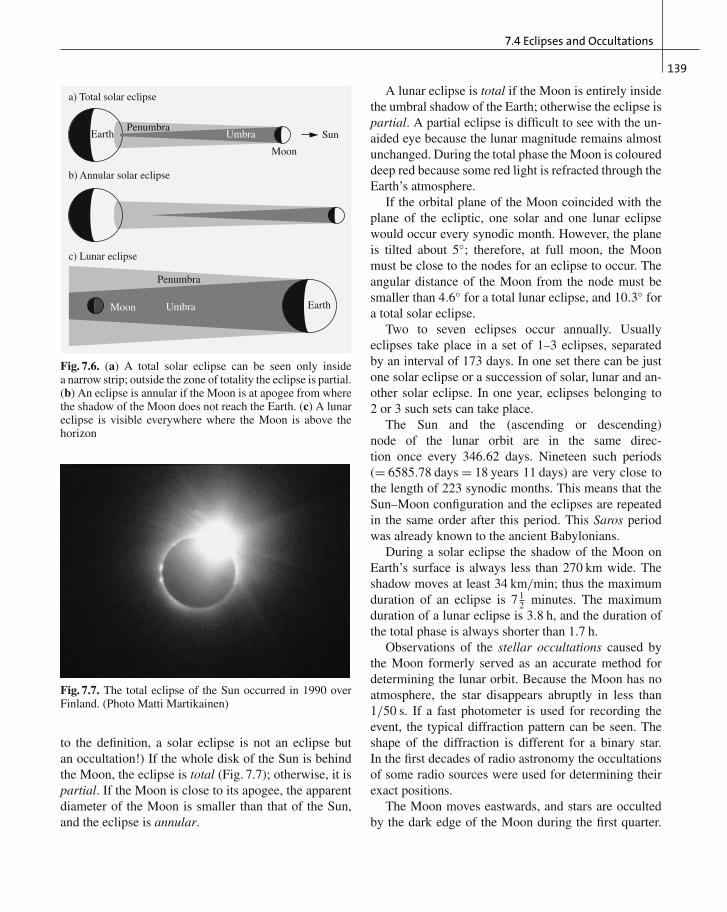
7.4 Eclipses and Occultations
139
Fig. 7.6. (a) A total solar eclipse can be seen only insidea narrow strip; outside the zone of totality the eclipse is partial.(b) An eclipse is annular if the Moon is at apogee from wherethe shadow of the Moon does not reach the Earth. (c) A lunareclipse is visible everywhere where the Moon is above thehorizon
Fig. 7.7. The total eclipse of the Sun occurred in 1990 overFinland. (Photo Matti Martikainen)
to the definition, a solar eclipse is not an eclipse butan occultation!) If the whole disk of the Sun is behindthe Moon, the eclipse is total (Fig. 7.7); otherwise, it ispartial. If the Moon is close to its apogee, the apparentdiameter of the Moon is smaller than that of the Sun,and the eclipse is annular.
A lunar eclipse is total if the Moon is entirely insidethe umbral shadow of the Earth; otherwise the eclipse ispartial. A partial eclipse is difficult to see with the un-aided eye because the lunar magnitude remains almostunchanged. During the total phase the Moon is coloureddeep red because some red light is refracted through theEarth’s atmosphere.
If the orbital plane of the Moon coincided with theplane of the ecliptic, one solar and one lunar eclipsewould occur every synodic month. However, the planeis tilted about 5; therefore, at full moon, the Moonmust be close to the nodes for an eclipse to occur. Theangular distance of the Moon from the node must besmaller than 4.6 for a total lunar eclipse, and 10.3 fora total solar eclipse.
Two to seven eclipses occur annually. Usuallyeclipses take place in a set of 1–3 eclipses, separatedby an interval of 173 days. In one set there can be justone solar eclipse or a succession of solar, lunar and an-other solar eclipse. In one year, eclipses belonging to2 or 3 such sets can take place.
The Sun and the (ascending or descending)node of the lunar orbit are in the same direc-tion once every 346.62 days. Nineteen such periods(= 6585.78 days = 18 years 11 days) are very close tothe length of 223 synodic months. This means that theSun–Moon configuration and the eclipses are repeatedin the same order after this period. This Saros periodwas already known to the ancient Babylonians.
During a solar eclipse the shadow of the Moon onEarth’s surface is always less than 270 km wide. Theshadow moves at least 34 km/min; thus the maximumduration of an eclipse is 7 1
2 minutes. The maximumduration of a lunar eclipse is 3.8 h, and the duration ofthe total phase is always shorter than 1.7 h.
Observations of the stellar occultations caused bythe Moon formerly served as an accurate method fordetermining the lunar orbit. Because the Moon has noatmosphere, the star disappears abruptly in less than1/50 s. If a fast photometer is used for recording theevent, the typical diffraction pattern can be seen. Theshape of the diffraction is different for a binary star.In the first decades of radio astronomy the occultationsof some radio sources were used for determining theirexact positions.
The Moon moves eastwards, and stars are occultedby the dark edge of the Moon during the first quarter.

140
7. The Solar System
Therefore occultation is easier to observe, and photo-metric measurements are possible; at the same time itis much more difficult to observe the appearance ofan object. There are some bright stars and planets in-side the 11 wide zone where the Moon moves, but theoccultation of a bright, naked-eye object is quite rare.
Occultations are also caused by planets and asteroids.Accurate predictions are complicated because such anevent is visible only in a very narrow path. The Uranianrings were found during an occultation in 1977, and theshapes of some asteroids have been studied during somefavourable events, timed exactly by several observerslocated along the predicted path.
A transit is an event in which Mercury or Venusmoves across the Solar disk as seen from the Earth.A transit can occur only when the planet is close to itsorbital node at the time of inferior conjunction. Transitsof Mercury occur about 13 times per century; transitsof Venus only twice. The next transits of Mercury are:May 9, 2016; Nov 11, 2019; Nov 13, 2032 and Nov 7,2039. The next transits of Venus are: Jun 6, 2012;Dec 11, 2117; Dec 8, 2125 and Jun 11, 2247. In the18th century the two transits of Venus (1761 and 1769)were used for determining the value of the astronomicalunit.
7.5 The Structure and Surfacesof Planets
Since the 1960’s a vast amount of data have been col-lected using spacecraft, either during a flyby, orbitinga body, or directly landing on the surface. This givesa great advantage compared to other astronomical ob-servations. We may even speak of revolution: the solarsystem bodies have turned from astronomical objectsto geophysical ones. Many methods traditionally usedin various sibling branches of geophysics can now beapplied to planetary studies.
The shape and irregularities of the gravitation fieldgenerated by a planet reflects its shape, internal structureand mass distribution. Also the surface gives certainindications on internal structure and processes.
The perturbations in the orbit of a satellite or space-craft can be used in studying the internal structure ofa planet. Any deviation from spherical symmetry isvisible in the external gravitational field.
The IAU planet definition states that planets are bod-ies in hydrostatic equilibrium. Gravity of a body willpull its material inwards, but the body resist the pullif the strength of the material is greater than the pres-sure exerted by the overlying layers. If the diameter islarger than about 800–1000 km, gravity is able to de-form rocky bodies into spherical shape. Smaller bodiesthan this have irregular shapes. On the other hand, e.g.icy moons of Saturn are spherical because ice is moreeasily deformed than rock.
Hydrostatic equilibrium means that the surface ofthe body approximately follows an equipotential sur-face of gravity. This is true e.g. on the Earth, where thesea surface very closely follows the equipotential sur-face called the geoid. Due to internal strength of rocks,continents can deviate from the geoid surface by a fewkilometers but compared to the diameter of the Earththe surface topography is negligible.
A rotating planet is always flattened. The amount offlattening depends on the rotation rate and the strengthof the material; a liquid drop is more easily deformedthan a rock. The shape of a rotating body in hydrostaticequilibrium can be derived from the equations of mo-tion. If the rotation rate is moderate, the equilibriumshape of a liquid body is an ellipsoid of revolution. Theshortest axis is the axis of rotation.
If Re and Rp are the equatorial and polar radii, re-spectively, the shape of the planet can be expressed as
x2
R2e
+ y2
R2e
+ z2
R2p
= 1 .
The dynamical flattening, denoted by f is defined as
f = Re − Rp
Re. (7.9)
Because Re > Rp, the flattening f is always positive.The giant planets are in practise close to hydrostatic
equilibrium, and their shape is determined by the rota-tion. The rotation period of Saturn is only 10.5 h, andits dynamical flattening is 1/10 which is easily visible.
Asteroids and other minor bodies are so small thatthey are not flattened by rotation. However, there is anupper limit for a rotation rate of an asteroid before itbreaks apart due to centrifugal forces. If we assumethat the body is held together only by gravity, we canapproximate the the maximum rotation rate by setting

7.5 The Structure and Surfaces of Planets
141
the centrifugal force equal to the gravitational force:
G Mm
R2= mv2
R, (7.10)
where m is a small test mass on the surface at a dis-tance of R from the center of the body. Substituting therotation period P,
P = 2πR
v,
we get
G M
R2= 4π2 R
P2,
or
P = 2π
√R3
G M= 2π
√3
4πGρ=√
3π
Gρ. (7.11)
If we substitute the density ρ with the mean densityof terrestrial rocks, i.e. 2700 kg m−3, we get for theminimum rotation period P ≈ 2 hours.
The structure of the terrestrial planets (Fig. 7.8) canalso be studied with seismic waves. The waves formed inan earthquake are reflected and refracted inside a planetlike any other wave at the boundary of two differentlayers. The waves are longitudinal or transversal (P andS waves, respectively). Both can propagate in solid ma-terials such as rock. However, only the longitudinal
Fig. 7.8. Internal structure and relative sizes of the terrestrialplanets. The percentage shows the volume of the core relativeto the total volume of the planet. In the case of the Earth, thepercentage includes both the outer and the inner core
wave can penetrate liquids. One can determine whethera part of the interior material is in the liquid state andwhere the boundaries of the layers are by studying therecordings of seismometers placed on the surface ofa planet. Naturally the Earth is the best-known body,but quakes of the Moon, Venus, and Mars have alsobeen observed.
The terrestrial planets have an iron-nickel core. Mer-cury has the relatively largest core; Mars the smallest.The core of the Earth can be divided into an inner andan outer core. The outer core (2900–5150 km) is liq-uid but the inner core (from 5150 km to the centre) issolid.
Around the Fe–Ni core is a mantle, composed ofsilicates (compounds of silicon). The density of the out-ermost layers is about 3000 kg m−3. The mean densityof the terrestrial planets is 3500–5500 kg m−3.
The internal structure of the giant planets (Fig. 7.9)cannot be observed with seismic waves since the planetsdo not have a solid surface. An alternative is to study theshape of the gravitational field by observing the orbit ofa spacecraft when it passes (or orbits) the planet. Thiswill give some information on the internal structure, butthe details depend on the mathematical and physicalmodels used for interpretation.
Fig. 7.9. Internal structure and relative sizes of the giant plan-ets. Differences in size and distance from the Sun causedifferences in the chemical composition and internal struc-ture. Due to smaller size, Uranus and Neptune do not haveany layer of metallic hydrogen. The Earth is shown inscale

142
7. The Solar System
Fig. 7.10. Ages of the surfaces of Mercury, the Earth, the Moonand Mars. The curve represents the fraction of the surfacewhich existed at a certain time. Most of the surface of theMoon, Mercury and Mars are more than 3500 million yearsold, whereas the surface of the Earth is mostly younger than200 million years
Fig. 7.11. An example ofresurfacing. Two volcanicplumes on Jupiter’s moon Ioobserved by Galileo space-craft in 1997. One plumewas captured on the brightlimb or edge of the moon(inset at upper right), erupt-ing over a caldera namedPillan Patera. The plume is140 kilometers high. Thesecond plume, seen nearthe terminator, is calledPrometheus. The shadowof the 75 km high airborneplume can be seen ex-tending to the right of theeruption vent. (NASA/JPL)
The mean densities of the giant planets are quite low;the density of Saturn, for example, is only 700 kg m−3.(If Saturn were put in a gigantic bathtub, it would floaton the water!) Most of the volume of a giant planet isa mixture of hydrogen and helium. In the centre, there ispossibly a silicate core, the mass of which is a few Earthmasses. The core is surrounded by a layer of metallichydrogen. Due to the extreme pressure, hydrogen is notin its normal molecular form H2, but dissociated intoatoms. In this state, hydrogen is electrically conducting.The magnetic fields of the giant planets may originatein the layer of metallic hydrogen.
Closer to the surface, the pressure is lower and hy-drogen is in molecular form. The relative thickness ofthe layers of metallic and molecular hydrogen vary fromplanet to planet. Uranus and Neptune may not have anylayer of metallic hydrogen because their internal pres-sure is too low for dissociation of the hydrogen. Instead,a layer of “ices” surround the core. This is a layer ofa water-dominant mixture of water, methane and am-monia. Under the high pressure and temperature themixture is partly dissolved into its components and it

7.5 The Structure and Surfaces of Planets
143
Fig. 7.12. The number of meteorite impact craters is an indi-cator of the age of the surface and the shapes of the cratersgive information on the strength of the material. The upperrow shows Mercury (left) and the Moon, and the second row,the Jovian moons Europa (left), Ganymede (centre) and Cal-listo. The pictures of the Jovian moons were taken by theGalileo orbiter with a resolution of 150 metres/pixel. Europahas only a few craters, there are areas of different ages on thesurface Ganymede and the surface of Callisto is the oldest.
Note the grooves and ridges that indicate different geologi-cal processes. IN the bottom there are two volcanic plumes onJupiter’s moon Io observed by Galileo spacecraft in 1997. Oneplume was captured on the bright limb or edge of the moon(inset at upper right), erupting over a caldera named PillanPatera. The plume is 140 kilometers high. The second plume,seen near the terminator, is called Prometheus. The shadow ofthe 75 km high airborne plume can be seen extending to theright of the eruption vent.(NASA/JPL and DLR)

144
7. The Solar System
behaves more like a molten salt and it is also electricallyconductive like the metallic hydrogen.
On top of everything is a gaseous atmosphere, onlya few hundred kilometres thick. The clouds at the top ofthe atmosphere form the visible “surface” of the giantplanets.
The interior temperatures of the planets are con-siderably larger than the surface temperatures. Forexample, the temperature in the Earth’s core isabout 4500–5000 K, and in the core of Jupiter about30,000 K.
A part of that heat is the remnant of the released po-tential energy from the gravitational contraction duringthe formation of planets. Decay of radioactive isotopesalso releases heat. Soon after the formation of planets in-tense meteorite bombardment was an important sourceof heat. Together with heat from short-lived radioactiveisotopes this caused melting of terrestrial planets. Theplanets were differentiated: the originally relatively ho-mogeneous material became segregated into layers ofdifferent chemical composition. The heaviest elementssank into centre thus forming the Fe–Ni core.
The material of the giant planets is differentiated aswell. In Saturn the differentiation may still be going on.Saturn is radiating about 2.8 times the heat it gets fromthe Sun, more than any other planet. This heat is sus-pected to originate from the separation of hydrogen andhelium, where the heavier helium is gradually sinkingtoward the centre of the planet.
Planetary surfaces are modified by several ge-ological processes. These include continental drift,volcanism, meteorite impacts and climate. The Earthis an example of a body whose surface has been re-newed many times during past aeons. The age of thesurface depends on the processes and thus implies thegeological evolutionary history of the planet Figs. 7.10,7.11, 7.12).
Continental drift gives rise, for example, to mountainformation. The Earth is the only planet where platetectonics is active today. On other terrestrial planetsthe process has either ceased long ago or has neveroccurred.
Volcanism is a minor factor on the Earth (at leastnow), but the surface of the Jovian moon Io is changingrapidly due to violent volcanic eruptions (Fig. 7.11).Volcanoes have been observed on Mars and Venus, butnot on the Moon.
Lunar craters are meteorite impact craters, commonon almost every body with a solid surface. Meteoritesare bombarding the planets continuously, but the ratehas been diminishing since the beginnings of the solarsystem. The number of impact craters reflects the ageof the surface (Fig. 7.12).
The Jovian moon Callisto is an example of a bodywith an ancient surface which is not fully inactive. Lackof small craters indicates some resurfacing process fill-ing and degrading the minor surface features. The Earthis an example of a body, whose atmosphere both pro-tects the surface and destroys the traces of impacts. Allsmaller meteorites are burned to ashes in the atmosphere(one need only note the number of shooting stars), andsome larger bodies are bounced back to outer space. Thetraces on the surface are destroyed very quickly by ero-sion in less than a few million years. Venus is an evenmore extreme case where all small craters are missingdue to a thick protective atmosphere.
Climate has the greatest influence on the Earth andVenus. Both planets have a thick atmosphere. On Mars,powerful dust storms deform the landscape, too, oftencovering the planet with yellowish dust clouds.
7.6 Atmospheres and Magnetospheres
Excluding Mercury, all major planets have an at-mosphere. The composition, thickness, density andstructure of the atmosphere vary from planet to planet,but some common features can be found (see, e. g.,Figs. 7.13, 7.14).
Let us first study the dependence of the tempera-ture T , pressure P, and density ρ on the height h. Let usconsider a cylinder with a length dh. The change in thepressure d P from the height h to h +dh is proportionalto the mass of the gas in the cylinder:
d P = −gρ dh , (7.12)
where g is the acceleration of gravity. Equation (7.12) isthe equation of hydrostatic equilibrium. (It is discussedin detail in Chap. 10.)
As a first approximation, we may assume that g doesnot depend on height. In the case of the Earth, the erroris only about 3% if g is considered constant from thesurface to a height of 100 km.

7.6 Atmospheres and Magnetospheres
145
Fig. 7.13. (a) Temperature as a function of height in the atmo-spheres of Venus, Earth, and Mars. (b) Temperature profiles ofthe atmospheres of Jupiter and Saturn. The zero height is cho-sen to be the point where the pressure is 100 mbar. Numbersalong the curves are pressures in millibars
The equation of state of the ideal gas
PV = NkT (7.13)
gives the expression for the pressure P
P = ρkT
µ, (7.14)
Fig. 7.14. Relative abun-dances of the mostabundant gases in the at-mospheres of Venus, Earth,and Mars. The number atthe bottom of each cir-cle denotes the surfacepressure in atms
where N is the number of atoms or molecules, k isthe Boltzmann constant, µ is the mass of one atom ormolecule and
ρ = µN
V. (7.15)
By using the equation of hydrostatic equilibrium (7.12)and the equation of state (7.14), we obtain
d P
P= −g
µ
kTdh .
Integration yields P as a function of height:
P = P0 exp
⎛⎝−
h∫0
µg
kTdh
⎞⎠
= P0 exp
⎛⎝−
h∫0
dh
H
⎞⎠ .
(7.16)
The variable H , which has the dimension of length, iscalled the scale height:
H = kT
µg. (7.17)
The scale height defines the height at which the pressurehas decreased by a factor e. H is a function of height,but here we may assume that it is constant. With thisapproximation, we obtain
− h
H= ln
P
P0
or, using (7.14),
ρT(h)
ρ0T0= e−h/H . (7.18)

146
7. The Solar System
Table 7.1. Scale heights of some gases in the atmospheres ofVenus, Earth, and Mars
Gas Molecular Earth Venus Marsweight [amu] H [km] H [km] H [km]
H2 2 120 360 290O2 32 7 23 18H2O 18 13 40 32CO2 44 5 16 13N2 28 8 26 20
Temperature [K] 275 750 260Acceleration ofgravity [m/s2] 9.81 8.61 3.77
The scale height is an important parameter in manyformulas describing the structure of the atmosphere(Table 7.1). For example, if the change of the pressureor the density is known as a function of height, the meanmolecular weight of the atmosphere can be computed.The scale height of the Jovian atmosphere was deter-mined in 1952 when Jupiter occulted a star. With theseobservations, the scale height was calculated to be 8 km,and the mean molecular weight 3–5 amu (atomic massunit, 1/12 of the mass of 12C). Thus the main compo-nents are hydrogen and helium, a result later confirmedby spacecraft data.
In terrestrial observations, infrared data are limitedby water vapour and carbon dioxide. The scale heightof CO2 is 5 km, which means that the partial pres-sure is already halved at a height of 3.5 km. Thusinfrared observations can be made on top of high moun-tains (like Mauna Kea in Hawaii). The scale heightof water vapour is 13 km, but the relative humidityand hence the actual water content is very site- andtime-dependent.
The scale height and the temperature of the atmo-sphere define the permanence of the atmosphere. If thespeed of a molecule is greater than the escape veloc-ity, the molecule will escape into space. The wholeatmosphere could disappear in a relatively short time.
According to the kinetic gas theory, the mean ve-locity v of a molecule depends both on the kinetictemperature Tk of the gas and the mass m of themolecule:
v=√
3kTk
m.
If the mass of a planet is M and its radius R, the escapevelocity is
ve =√
2G M
R.
Even if the mean velocity is smaller than the escape ve-locity, the atmosphere can evaporate into space if thereis enough time, since some molecules will always havevelocities exceeding ve. Assuming a velocity distribu-tion, one can calculate the probability for v > ve Henceit is possible to estimate what fraction of the atmospherewill disappear in, say, 109 years. As a rule of thumb, itcan be said that at least half of the atmosphere willremain over 1000 million years if the mean velocityv < 0.2ve.
The probability that a molecule close to the surfacewill escape is insignificantly small. The free mean pathof a molecule is very small when the gas density ishigh (Fig. 7.15). Thus the escaping molecule is mostprobably leaving from the uppermost layers. The crit-ical layer is defined as a height at which a molecule,
Fig. 7.15. Close to the surface, the mean free path ofa molecule is smaller than higher in the atmosphere wherethe gas density is smaller. The escaping molecules originateclose to the critical layer

7.6 Atmospheres and Magnetospheres
147
Fig. 7.16. Structure of the magnetosphere of the Earth. (A. Nurmi/Tiede 2000)
moving upward, has a probability 1/e of hitting anothermolecule. The part of the atmosphere above the criti-cal layer is called the exosphere. The exosphere of theEarth begins at a height of 500 km, where the kinetictemperature of the gas is 1500–2000 K and the pressureis lower than in the best terrestrial vacuums.
The magnetosphere is the “outer boundary” ofa planet. Size and shape depend on the strength of themagnetic field of the planet and on the solar wind. Thesolar wind is a flux of charged particles, mostly elec-trons and protons, outflowing from the Sun. The speedof the wind at the distance of the Earth is about 400 km/sand the density 10 particles/cm3 but both values canchange considerably depending on the solar activity.
On the solar side there is a bow shock (Fig. 7.16),typically at a distance of a few tens of planetary radii(Table 7.2). At the bow shock, particles of the solarwind first hit the magnetosphere. The magnetosphereis limited by the magnetopause, flattened on the so-lar side and extended to a long tail on the oppositeside. Charged particles inside the magnetopause arecaptured by the magnetic field and some particles areaccelerated to great velocities. If the velocities are in-terpreted according to the kinetic gas theory, thesevelocities even correspond to millions of kelvins. How-ever, the density, and thus the total energy, is verysmall. The “hottest” places found are around Jupiterand Saturn.

148
7. The Solar System
Table 7.2. Planetary magnetic fields
Dipole moment Field strength Polarity2 Angle3 Magneto-(Earth = 1) (gauss)1 pause4
Mercury 0.0007 0.003 ⇑ 14 1.5
Venus < 0.0004 < 0.00003 – – –
Earth 1.0 0.305 ⇑ 11 10
Mars < 0.0002 < 0.0003 – – –
Jupiter 20,000. 4.28 ⇓ 10 80
Saturn 600. 0.22 ⇓ < 1 20
Uranus 50. 0.23 ⇓ 59 20
Neptune 25. 0.14 ⇓ 47 25
1 at equator (1 gauss equals 10−4 T);2 ⇑ same as the Earth, ⇓ opposite;3 angle between magnetic and rotational axes;4 average magnetopause distance in the direction of the Sun in planetary radii
The region of space containing trapped charged par-ticles, the radiation belts around the Earth, are namedvan Allen’s belts (Fig. 7.17). These radiation zones werediscovered by the first US satellite, Explorer 1, in 1958.
Fig. 7.17. A glow of hot plasma trapped inside the Earth’smagnetosphere. The picture was taken by NASA’s Imagerfor Magnetopause to Aurora Global Exploration (IMAGE)spacecraft on August 11, 2000 at 18:00 UT. The Sun is outsidethe picture area toward the top right corner. (NASA and theIMAGE science team)
The number of charged particles increases after strongsolar bursts. Some of these particles “leak” to the atmo-sphere, resulting in auroras. Similar effects have alsobeen detected in Jupiter, Saturn and Uranus.
The solar magnetic field arises from the turbulentmotions of the electrically conductive matter. The en-ergy driving the convection in the layer is coming fromthe nuclear fusion in the core. This, however, cannotexplain planetary magnetism. Neither can the remanentprimordial magnetic field explain it because the inter-nal temperature of planets is well above the Curie point(about 850 K for magnetite). If the temperature is abovethe Curie point, ferromagnetic materials will lose theirremanent magnetism.
The planetary dynamo generating the magnetic fieldrequires that the planet is rotating and has a convec-tive layer of electrically conductive material. Terrestrialplanets have a liquid Fe–Ni core, or a liquid layer in thecore, Jupiter and Saturn have a layer of liquid metallichydrogen and Uranus and Neptune have a mixture ofwater, ammonia and methane. In all cases the tempera-ture gradient between the bottom and top of the layer islarge enough to cause the convection.
The strength of the magnetic field varies a lotfrom planet to planet. It can be characterised bythe dipole magnetic moment. The magnetic momentof Jupiter is about 100 million times that of Mer-cury. The magnetic moment of the Earth is about7.9×1025 gauss cm3 that can be compared to the typicalstrong electromagnetic fields achieved in the laborato-ries, about 100,000 gauss cm3. Inducing such a strongfield requires currents that are of the order of 109 Am-

7.7 Albedos
149
Fig. 7.18. Planetary magnetic fields
peres. When divided by the cube of planetary radii,one gets an estimate of the field strength on theequator.
The alignment of the magnetic field with respect tothe rotation axis of a planet differs from planet to planet(Fig. 7.18). Saturn’s magnetic field is close to the idealcase where rotational axis and magnetic axis coincide.Also the Earth and Jupiter show reasonably good pointdipole field with a tilt of about 10. However, fieldsof Uranus and Neptune are both offset from the centreof the planet and tilted by about 50 from the rotationaxis. This may indicate a different mechanism for thedynamo.
The magnetic fields of Mercury and the Earth havean opposite polarity than the fields of other planets. Itis known that the polarity of the Earth’s magnetic fieldhas reversed several times over geologic time scales,previously about 750,000 years ago. There are someindications that the reversal of the polarity is begin-ning now because the field strength is declining aboutone percent per decade, magnetic poles are movingmore rapidly and the field asymmetry is increasing. Thewhole process will take several thousand years duringwhich the Earth’s surface is more open to the cosmicrays.
The Galileo mission also revealed that the Jovianmoon Ganymede has a magnetic field. The field is weakand too small to have a magnetotail or trapped particlesaround the moon. Callisto, which is of the same size,does not show any magnetosphere. Neither does ourMoon have any global magnetic field.
7.7 Albedos
The planets and all other bodies of the solar system onlyreflect the radiation of the Sun (we may neglect herethe thermal and radio wave radiation and concentratemainly on the visual wavelengths). The brightness ofa body depends on its distance from the Sun and theEarth, and on the albedo of its surface. The term albedodefines the ability of a body to reflect light.
If the luminosity of the Sun is L, the flux density atthe distance r is (Fig. 7.19)
F = L4πr2
. (7.19)
If the radius of the planet is R, the area of its crosssection is πR2, and the total flux incident on the surface
Fig. 7.19. Symbols used in the photometric formulas

150
7. The Solar System
of the planet is
L in = πR2 L4πr2
= L R2
4r2. (7.20)
Only a part of the incident flux is reflected back. Theother part is absorbed and converted into heat whichis then emitted as a thermal emission from the planet.The Bond albedo A (or spherical albedo) is definedas the ratio of the emergent flux to the incident flux(0 ≤ A ≤ 1). The flux reflected by the planet is thus
Lout = AL in = AL R2
4r2. (7.21)
The planet is observed at a distance∆. If radiation isreflected isotropically, the observed flux density shouldbe
F = Lout
4π∆2. (7.22)
In reality, however, radiation is reflected anisotropically.If we assume that the reflecting object is a homoge-neous sphere, the distribution of the reflected radiationdepends on the phase angle α only. Thus we can expressthe flux density observed at a distance ∆ as
F = CΦ(α)Lout
4π∆2. (7.23)
The function Φ giving the phase angle dependenceis called the phase function. It is normalised so thatΦ(α= 0)= 1.
Since all the radiation reflected from the planet isfound somewhere on the surface of the sphere, we musthave∫
S
CΦ(α)Lout
4π∆2dS = Lout (7.24)
orC
4π∆2
∫S
Φ(α) dS = 1 , (7.25)
where the integration is extended over the surface of thesphere of radius∆. The surface element of such a sphereis dS =∆2 dα sinα dφ, and we have∫
S
Φ(α) dS =∆2
π∫α= 0
2π∫φ= 0
Φ(α) sinα dα dφ
=∆22π
π∫0
Φ(α) sinα dα .
(7.26)
The normalisation constant C is
C = 4π∆2∫S Φ(α) dS
= 2∫ π0 Φ(α) sinα dα
. (7.27)
The quantity
q = 2
π∫0
Φ(α) sinα dα (7.28)
is the phase integral. In terms of the phase integral thenormalisation constant is
C = 4
q. (7.29)
Remembering that Lout = AL in, the equation (7.23) canbe written in the form
F = CA
4πΦ(α)
1
∆2L in . (7.30)
The first factor is intrinsic for each object, the secondgives the phase angle dependence, the third the distancedependence and the fourth, the incident radiation power.The first factor is often denoted by
Γ = CA
4π. (7.31)
When we substitute here the expression of C (7.29), andsolve for the Bond albedo, we get
A = 4πΓ
C= πΓ
4
C= πΓq = pq . (7.32)
Here p = πΓ is called the geometric albedo and q is thepreviously introduced phase integral. These quantitiesare related by
A = pq . (7.33)
The geometric albedo seems to have appeared as anarbitrary factor with no obvious physical interpretation.We’ll now try to explain this quantity using a Lam-bertian surface. A Lambertian surface is defined as anabsolutely white, diffuse surface which reflects all radia-tion, i. e. its Bond albedo is A = 1. Moreover, its surfacebrightness is the same for all viewing directions, whichmeans that the phase function is
Φ(α)=⎧⎨⎩cosα , if 0 ≤ α ≤ π/2 ,
0 , otherwise .(7.34)

7.8 Photometry, Polarimetry and Spectroscopy
151
In reality, no such surface exists but there are some ma-terials which behave almost like a Lambertian surface.A wall with a mat white finish is a good approxima-tion; although it doesn’t reflect all incident light, thedistribution of the reflected light is about right, and itsbrightness looks the same from all directions.
For a Lambertian surface the constant C is
C = 2∫ π0 Φ(α) sinα dα
= 2∫ π/20 cosα sinα dα
(7.35)
= 2
1/2= 4 .
Thus the geometric albedo of a Lambertian surface is
p = πΓ = CA
4= 4×1
4= 1 . (7.36)
At the phase angle zero Φ(α = 0) = 1 and thereflected flux density is
F = CA
4π
1
∆2L in .
If we replace the object with a Lambertian surface ofthe same size, we get
FL = 4
4π
1
∆2L in .
The ratio of these flux densities isF
FL= CA
4= πΓ = p . (7.37)
Now we have found a physical interpretation for p:the geometric albedo is the ratio of the flux densi-ties at phase angle α = 0 reflected by a planet anda Lambertian surface of the same cross section.
The geometric albedo depends on the reflectance ofthe surface but also on the phase function Φ. Manyrough surfaces reflect most of the incident radiation di-rectly backward. In such a case the geometric albedo pis greater than in the case of an isotropically reflect-ing surface. On some surfaces p> 1, and in the mostextreme case, the specular reflection, p = ∞. The ge-ometric albedo of solar system bodies vary between0.03–1. The geometric albedo of the Moon is p = 0.12and the greatest value, p = 1.0, has been measured forthe Saturnian moon Enceladus.
It turns out that p can be derived from the observa-tions, but the Bond albedo A can be determined only ifthe phase integral q is also known. That will be discussedin the next section.
7.8 Photometry, Polarimetryand Spectroscopy
Having defined the phase function and albedos we areready to derive a formula for planetary magnitudes. Theflux density of the reflected light is
F = CA
4πΦ(α)
1
∆2L in .
We now substitute the incident flux
L in = L R2
4r2
and the constant factor expressed in terms of thegeometric albedo
CA
4π= Γ = p
π.
Thus we get
F = p
πΦ(α)
1
∆2
L R2
4r2. (7.38)
The observed solar flux density at a distance of a =1 AU from the Sun is
F = L4πa2
. (7.39)
The ratio of these isF
F= pΦ(α)R2a2
∆2r2. (7.40)
If the apparent solar magnitude at a distance of 1 AUis m and the apparent magnitude of the planet m wehave
m −m = −2.5 lgF
F
= −2.5 lgpΦ(α)R2a2
∆2r2
= −2.5 lgpR2
a2
a4
∆2r2Φ(α) (7.41)
= −2.5 lg pR2
a2−2.5 lg
a4
∆2r2−2.5 lgΦ(α)
= −2.5 lg pR2
a2+5 lg
∆r
a2−2.5 lgΦ(α) .

152
7. The Solar System
If we denote
V(1, 0)≡ m −2.5 lg pR2
a2, (7.42)
then the magnitude of a planet can be expressed as
m = V(1, 0)+5 lgr∆
a2−2.5 lgΦ(α) . (7.43)
The first term V(1, 0) depends only on the size of theplanet and its reflection properties. So it is a quantityintrinsic to the planet, and it is called the absolute mag-nitude (not to be confused with the absolute magnitudein stellar astronomy!). The second term contains the dis-
Fig. 7.20. The phase curves and polarization of different typesof asteroids. The asteroid characteristics are discussed in moredetail in Sect. 7.14. (From Muinonen et al., Asteroid pho-
tometric and polarimetric phase effects, in Bottke, Binzel,Cellino, Paolizhi (Eds.) Asteroids III, University of ArizonaPress, Tucson.)
tance dependence and the third one the dependence onthe phase angle.
If the phase angle is zero, and we set r =∆= a,(7.43) becomes simply m = V(1, 0). The absolute mag-nitude can be interpreted as the magnitude of a body ifit is at a distance of 1 AU from the Earth and the Sunat a phase angle α = 0. As will be immediately no-ticed, this is physically impossible because the observerwould be in the very centre of the Sun. Thus V(1, 0) cannever be observed.
The last term in (7.43) is the most problematic one.For many objects the phase function is not known verywell. This means that from the observations, one can

7.8 Photometry, Polarimetry and Spectroscopy
153
calculate only
V(1, α)≡ V(1, 0)−2.5 lgΦ(α) , (7.44)
which is the absolute magnitude at phase angle α.V(1, α), plotted as a function of the phase angle, iscalled the phase curve (Fig. 7.20). The phase curveextrapolated to α= 0 gives V(1, 0).
By using (7.41) at α= 0, the geometric albedo canbe solved for in terms of observed values:
p =(
r∆
aR
)2
10−0.4(m0 − m) , (7.45)
where m0 = m(α= 0). As can easily be seen, p can begreater than unity but in the real world, it is normallywell below that. A typical value for p is 0.1–0.5.
The Bond albedo can be determined only if the phasefunctionΦ is known. Superior planets (and other bodiesorbiting outside the orbit of the Earth) can be observedonly in a limited phase angle range, and therefore Φ ispoorly known. The situation is somewhat better for theinferior planets. Especially in popular texts the Bondalbedo is given instead of p (naturally without men-tioning the exact names!). A good excuse for this is theobvious physical meaning of the former, and also thefact that the Bond albedo is normalised to [0, 1].
Opposition Effect. The brightness of an atmosphere-less body increases rapidly when the phase angleapproaches zero. When the phase is larger thanabout 10, the changes are smaller. This rapid brighten-ing close to the opposition is called the opposition effect.The full explanation is still in dispute. A qualitative(but only partial) explanation is that close to the oppo-sition, no shadows are visible. When the phase angleincreases, the shadows become visible and the bright-ness drops. An atmosphere destroys the oppositioneffect.
The shape of the phase curve depends on the geo-metric albedo. It is possible to estimate the geometricalbedo if the phase curve is known. This requires atleast a few observations at different phase angles. Mostcritical is the range 0–10. A known phase curve canbe used to determine the diameter of the body, e. g.the size of an asteroid. Apparent diameters of asteroidsare so small that for ground based observations onehas to use indirect methods, like polarimetric or radio-metric (thermal radiation) observations. Beginning from
the 1990’s, imaging made during spacecraft fly-bys andwith the Hubble Space Telescope have given also directmeasures of the diameter and shape of asteroids.
Magnitudes of Asteroids. When the phase angle isgreater than a few degrees, the magnitude of an aster-oid depends almost linearly on the phase angle. Earlierthis linear part was extrapolated to α= 0 to estimatethe opposition magnitude of an asteroid. Due to the op-position effect the actual opposition magnitude can beconsiderably brighter.
In 1985 the IAU adopted the semi-empirical HG sys-tem where the magnitude of an asteroid is described bytwo constants H and G. Let
a1 = (1− G)×10−0.4 H ,
a2 = G ×10−0.4 H .(7.46)
The phase curve can be approximated by
V(1, α)= −2.5
× log
[a1 exp
(−3.33
(tan
α
2
)0.63)
(7.47)
+a2 exp
(−1.87
(tan
α
2
)1.22)]
.
When the phase angle is α= 0 (7.47) becomes
V(1, 0)= −2.5 log(a1 +a2)
= −2.5 log 10−0.4 H = H .(7.48)
The constant H is thus the absolute magnitude and G de-scribes the shape of the phase curve. If G is great, thephase curve is steeper and the brightness is decreasingrapidly with the phase angle. For very gentle slopes Gcan be negative. H and G can be determined with a leastsquares fit to the phase observations.
Polarimetric Observations. The light reflected by thebodies of the solar system is usually polarized. Theamount of polarization depends on the reflecting mate-rial and also on the geometry: polarization is a functionof the phase angle. The degree of polarization P isdefined as
P = F⊥ − F‖F⊥ + F‖
, (7.49)
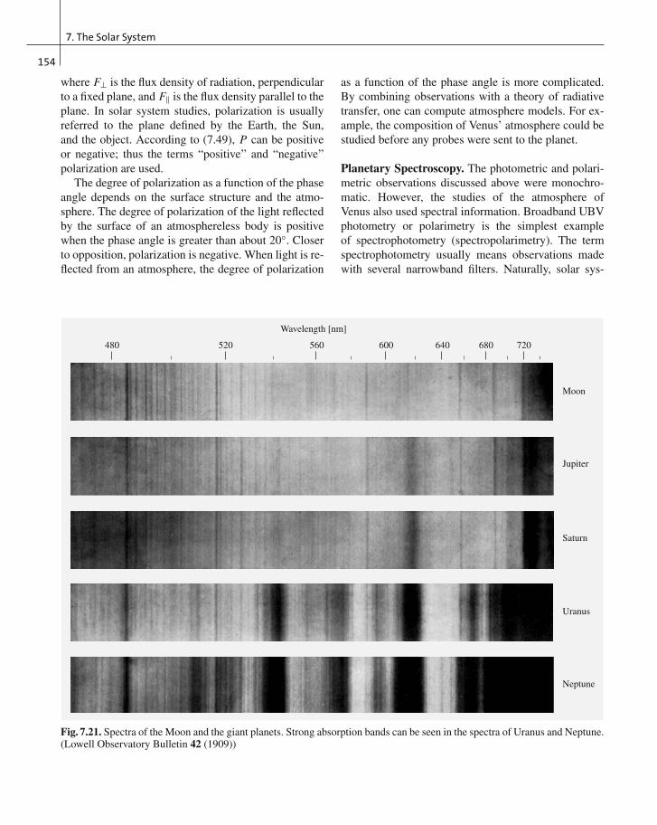
154
7. The Solar System
where F⊥ is the flux density of radiation, perpendicularto a fixed plane, and F‖ is the flux density parallel to theplane. In solar system studies, polarization is usuallyreferred to the plane defined by the Earth, the Sun,and the object. According to (7.49), P can be positiveor negative; thus the terms “positive” and “negative”polarization are used.
The degree of polarization as a function of the phaseangle depends on the surface structure and the atmo-sphere. The degree of polarization of the light reflectedby the surface of an atmosphereless body is positivewhen the phase angle is greater than about 20. Closerto opposition, polarization is negative. When light is re-flected from an atmosphere, the degree of polarization
Fig. 7.21. Spectra of the Moon and the giant planets. Strong absorption bands can be seen in the spectra of Uranus and Neptune.(Lowell Observatory Bulletin 42 (1909))
as a function of the phase angle is more complicated.By combining observations with a theory of radiativetransfer, one can compute atmosphere models. For ex-ample, the composition of Venus’ atmosphere could bestudied before any probes were sent to the planet.
Planetary Spectroscopy. The photometric and polari-metric observations discussed above were monochro-matic. However, the studies of the atmosphere ofVenus also used spectral information. Broadband UBVphotometry or polarimetry is the simplest exampleof spectrophotometry (spectropolarimetry). The termspectrophotometry usually means observations madewith several narrowband filters. Naturally, solar sys-

7.10 Mercury
155
tem objects are also observed by means of “classical”spectroscopy.
Spectrophotometry and polarimetry give informationat discrete wavelengths only. In practise, the number ofpoints of the spectrum (or the number of filters available)is often limited to 20–30. This means that no detailscan be seen in the spectra. On the other hand, in or-dinary spectroscopy, the limiting magnitude is smaller,although the situation is rapidly improving with the newgeneration detectors, such as the CCD camera.
The spectrum observed is the spectrum of the Sun.Generally, the planetary contribution is relatively small,and these differences can be seen when the solar spec-trum is subtracted. The Uranian spectrum is a typicalexample (Fig. 7.21). There are strong absorption bandsin the near-infrared. Laboratory measurements haveshown that these are due to methane. A portion of thered light is also absorbed, causing the greenish colour ofthe planet. The general techniques of spectral observa-tions are discussed in the context of stellar spectroscopyin Chap. 8.
7.9 Thermal Radiation of the Planets
Thermal radiation of the solar system bodies dependson the albedo and the distance from the Sun, i. e. on theamount of absorbed radiation. Internal heat is importantin Jupiter and Saturn, but we may neglect it at this point.
By using the Stefan-Boltzmann law, the flux on thesurface of the Sun can be expressed as
L = 4πR2σT 4
.
If the Bond albedo of the body is A, the fraction of theradiation absorbed by the planet is (1− A). This is lateremitted as heat. If the body is at a distance r from theSun, the absorbed flux is
Labs = R2σT 4πR2
r2(1− A) . (7.50)
There are good reasons to assume that the body is inthermal equilibrium, i. e. the emitted and the absorbedfluxes are equal. If not, the body will warm up or cooldown until equilibrium is reached.
Let us first assume that the body is rotating slowly.The dark side has had time to cool down, and the thermalradiation is emitted mainly from one hemisphere. The
flux emitted is
Lem = 2πR2σT 4 , (7.51)
where T is the temperature of the body and 2πR2 is thearea of one hemisphere. In thermal equilibrium, (7.50)and (7.51) are equal:
R2T 4r2
(1− A)= 2T 4 ,
whence
T = T(
1− A
2
)1/4 ( Rr
)1/2
. (7.52)
A body rotating quickly emits an approximately equalflux from all parts of its surface. The emitted flux is then
Lem = 4πR2σT 4
and the temperature
T = T(
1− A
4
)1/4 ( Rr
)1/2
. (7.53)
The theoretical temperatures obtained above are notvalid for most of the major planets. The main “culprits”responsible here are the atmosphere and the internalheat. Measured and theoretical temperatures of somemajor planets are compared in Table 7.3. Venus is anextreme example of the disagreement between theoret-ical and actual figures. The reason is the greenhouseeffect: radiation is allowed to enter, but not to exit. Thesame effect is at work in the Earth’s atmosphere. With-out the greenhouse effect, the mean temperature couldbe well below the freezing point and the whole Earthwould be ice-covered.
7.10 Mercury
Mercury is the innermost planet of the solar system.Its diameter is 4800 km and its mean distance fromthe Sun 0.39 AU. The eccentricity of the orbit is 0.21,which means that the distance varies between 0.31 and0.47 AU. Because of the high eccentricity, the surfacetemperature of the subsolar point varies substantially:at the perihelion, the temperature is about 700 K; atthe aphelion, it is 100 K lower. Temperature variationson Mercury are the most extreme in the solar system

156
7. The Solar System
Table 7.3. Theoretical and observed temperatures of some planets
Albedo Distance from Theoretical Observed maximumthe Sun [AU] temperature [K] temperature [K]
(7.52) (7.53)
Mercury 0.06 0.39 525 440 700
Venus 0.76 0.72 270 230 750
Earth 0.36 1.00 290 250 310
Mars 0.16 1.52 260 215 290
Jupiter 0.73 5.20 110 90 130
because in the night side the temperature drops below100 K.
The precession of the perihelion of Mercury is morethan 0.15 per century. When the Newtonian perturba-tions are subtracted, there remains an excess of 43′′.This is fully explained by the general theory of rela-tivity. The explanation of the perihelion precession wasone of the first tests of the general theory of relativity.
Mercury is always found in the vicinity of the Sun;its maximum elongation is only 28. Observations aredifficult because Mercury is always seen in a bright skyand close to the horizon. Moreover, when closest to theEarth in the inferior conjunction, the dark side of theplanet is toward us.
The first maps of Mercury were drawn at the end ofthe 19th century but the reality of the details was notconfirmed. As late as in the beginning of the 1960’s, itwas believed that Mercury always turns the same sidetoward the Sun. However, measurements of the thermalradio emission showed that the temperature of the nightside is too high, about 100 K, instead of almost absolutezero. Finally, the rotation period was established byradar. One revolution around the Sun takes 88 days. Therotation period is two-thirds of this, 59 days. This meansthat every second time the planet is in, say, perihelion,the same hemisphere faces the Sun (Fig. 7.22). Thiskind of spin–orbit coupling can result from tidal forcesexerted by a central body on an object moving in a fairlyeccentric orbit.
Re-examination of old observations revealed whyMercury had been presumed to rotate synchronously.Owing to its geometry, Mercury is easiest to observe inspring and autumn. In six months, Mercury orbits twicearound the Sun, rotating exactly three times around itsown axis. Consequently, during observations, the sameside was always facing the Sun! The details visibleon the surface are very obscure and the few excep-
tional observations were interpreted as observationalerrors.
The best (and thus far unique) data were received in1974 and 1975, when the US space craft Mariner 10passed Mercury three times. The orbital period ofMariner 10 around the Sun was exactly twice the periodof Mercury. The two-thirds-factor meant that the sameside of the planet was illuminated during every fly-by!The other side is still unknown.
The Mariner 10 data revealed a moon-like landscape(Fig. 7.23). Mercury’s surface is marked by cratersand larger circular areas, caused by impacts of minorplanets. The craters are 3000–4000 million years old,indicating that the surface is old and undisturbed by
Fig. 7.22. Length of day in Mercury. The positions of Mercuryduring the first revolution are shown outside the ellipse. Uponreturning to the aphelion, the planet has turned 540 (1½revolutions). After two full cycles the planet has rotated threetimes around its axis and the same side points toward the Sun.The length of the day is 176 d, longer than on any other planet
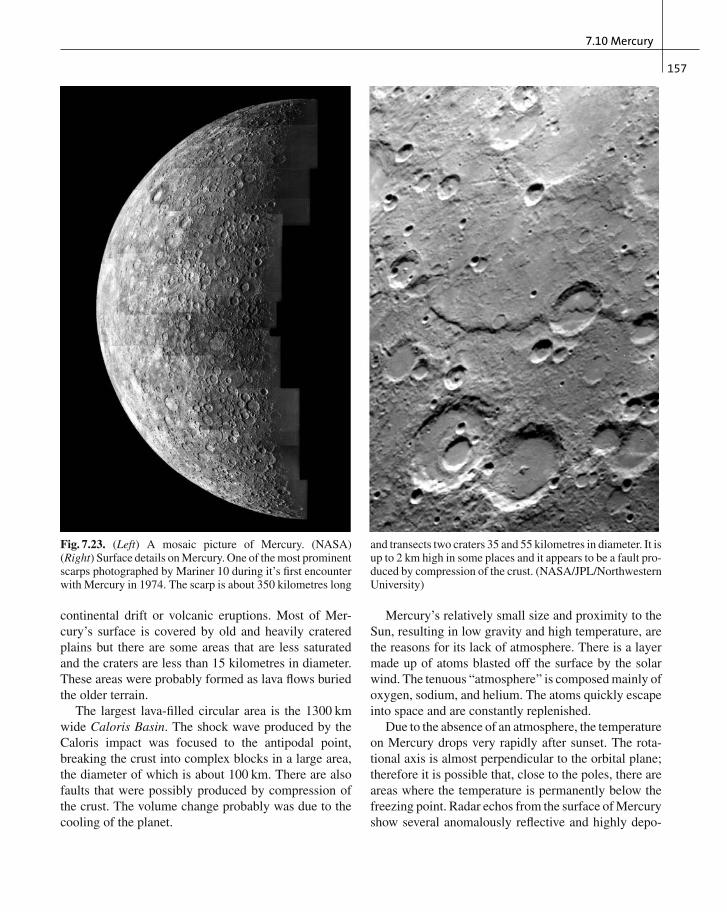
7.10 Mercury
157
Fig. 7.23. (Left) A mosaic picture of Mercury. (NASA)(Right) Surface details on Mercury. One of the most prominentscarps photographed by Mariner 10 during it’s first encounterwith Mercury in 1974. The scarp is about 350 kilometres long
and transects two craters 35 and 55 kilometres in diameter. It isup to 2 km high in some places and it appears to be a fault pro-duced by compression of the crust. (NASA/JPL/NorthwesternUniversity)
continental drift or volcanic eruptions. Most of Mer-cury’s surface is covered by old and heavily crateredplains but there are some areas that are less saturatedand the craters are less than 15 kilometres in diameter.These areas were probably formed as lava flows buriedthe older terrain.
The largest lava-filled circular area is the 1300 kmwide Caloris Basin. The shock wave produced by theCaloris impact was focused to the antipodal point,breaking the crust into complex blocks in a large area,the diameter of which is about 100 km. There are alsofaults that were possibly produced by compression ofthe crust. The volume change probably was due to thecooling of the planet.
Mercury’s relatively small size and proximity to theSun, resulting in low gravity and high temperature, arethe reasons for its lack of atmosphere. There is a layermade up of atoms blasted off the surface by the solarwind. The tenuous “atmosphere” is composed mainly ofoxygen, sodium, and helium. The atoms quickly escapeinto space and are constantly replenished.
Due to the absence of an atmosphere, the temperatureon Mercury drops very rapidly after sunset. The rota-tional axis is almost perpendicular to the orbital plane;therefore it is possible that, close to the poles, there areareas where the temperature is permanently below thefreezing point. Radar echos from the surface of Mercuryshow several anomalously reflective and highly depo-

158
7. The Solar System
larized features at the north and south poles. Some ofthese areas can be addressed to the craters, the bottomsof which are permanently in shadow. One candidate ofthe radar-bright features is water ice that has survivedin the permanent shadow.
The only relevant data concerning the interior of Mer-cury were obtained during the Mariner 10 fly-by whenthe gravity field was measured. Since Mercury has nosatellites, the mass (and mass distribution) and densitycould not be determined before the force exerted by thegravitational field on a spacecraft was measured.
It has been said that Mercury looks like the Moonfrom the outside but is terrestrial from the inside. Ac-cording to theoretical models, the internal structure issimilar to that of the Earth but the core is substantiallylarger. The density of the planet is about the same asthat of the Earth, indicating that the size of the Fe–Nicore is roughly about 75% of the planet’s radius.
Due to the vicinity of the Sun, the temperature ofthe primeval nebula at the distance of Mercury wasquite high during planetary formation. Thus the relativeabundances of the volatile elements are smaller than onany other terrestrial planet.
Mercury has a weak magnetic field, about 1% asstrong as that of the Earth. The presence of the magneticfield is unexpected because Mercury is much smallerthan the Earth and it rotates slowly. According to thedynamo theory, a magnetic field is generated by flowsin a liquid, electrically conducting core. The magneticfield cannot be a remnant from ancient times, since theinternal temperature of the planet must have exceededthe critical Curie point. Therefore, it must be assumedthat a part of the core is molten.
7.11 Venus
Venus is the brightest object in the sky, after the Sunand the Moon. Like Mercury, Venus can be seen onlyin the morning or in the evening sky. (It is sometimespossible to see Venus even if the Sun is above the hori-zon, if its exact position is known.) In antiquity, Venuswas thought to be two different planets, Hesperos andPhosphorus, evening star and morning star.
The maximum elongation of Venus is about 47.Venus is a remarkable object when shining in the darksky at its brightest, 35 days before or after the inferior
Fig. 7.24. The phases of Venus were discovered by GalileoGalilei in 1610. This drawing illustrates how the apparent sizeof Venus changes with phase. The planet is far behind the Sunwhen the illuminated side faces the Earth
conjunction, when one-third of the surface is seen lit(Fig. 7.24). At the inferior conjunction, the Earth–Venusdistance is only 42 million km. The diameter of Venus isabout 12,000 km, which means that the apparent diam-eter can be as large as one arc minute. Under favourableconditions it is even possible to see the shape of the cres-cent Venus with binoculars. At the superior conjunction,the apparent diameter is only 10 arc seconds.
Venus is covered by clouds. Its surface is nowherevisible; only featureless yellowish cloud tops can beseen (Fig. 7.25). The rotation period was long unknown,and the measured 4-day period was the rotation timeof the clouds. Finally, in 1962, radar measurements re-vealed that the rotation period is 243 days in a retrogradedirection, i. e. opposite to the rotation of other planets.The axis of rotation is almost perpendicular to the orbitalplane; the inclination is 177.
The temperature at the cloud tops is about 250 K.Because the Bond albedo is as high as 75%, the surfacetemperature was believed to be moderate, even suitablefor life. Opinions changed dramatically when thermalradio emission was measured at the end of the 1950’s.This emission originates on the surface of the planetand can penetrate the clouds. The surface temperatureturned out to be 750 K, well above the melting point oflead. The reason for this is the greenhouse effect. Theoutgoing infrared radiation is blocked by atmosphericcarbon dioxide, the main component of the atmosphere.
The chemical composition of the Venusian atmo-sphere was known prior to the space age. Spectroscopicobservations revealed CO2, and some clues to the cloudcomposition were obtained from polarimetric observa-tions. The famous French planetary astronomer BernardLyot made polarimetric observations in the 1920’s, butnot until decades later was it realised that his obser-vations could be explained by assuming that light was

7.11 Venus
159
Fig. 7.25. Left: Venus in visible light imaged by the Galileoorbiter in February 1990. The cloud features are caused bywinds that blow from east to west at about 100 m/s. Right:The northern hemisphere of Venus in a computer-generated
picture of the radar observations. The north pole is at the centreof the image of the Magellan synthetic aperture radar mosaic.(NASA/JPL)
scattered by liquid spherical particles whose index ofrefraction is 1.44. This is significantly higher than theindex of refraction of water, 1.33. Moreover, water isnot liquid at that temperature. A good candidate wassulphuric acid H2SO4. Later, spacecraft confirmed thisinterpretation.
Venus’ atmosphere is very dry: the amount of watervapour present is only 1/1,000,000 of that in the Earth’satmosphere. One possible explanation is that, due to so-lar UV radiation, the water has dissociated to hydrogenand oxygen in the upper layers of the atmosphere, theformer escaping into interplanetary space.
About 1% of the incident light reaches the surfaceof Venus; this light is deep red after travelling throughclouds and the thick atmosphere. Most of the incidentlight, about 75%, is reflected back from the upper layersof clouds. The absorbed light is emitted back in in-frared. The carbon dioxide atmosphere very effectivelyprevents the infrared radiation from escaping, and thetemperature had not reached the equilibrium until at750 K.
The pressure of the atmosphere at the surface is90 atm. The visibility is several kilometres, and even
in the clouds, a few hundred metres. The densest cloudsare at a height of 50 km, but their thickness is only2–3 km. Above this, there are haze-like layers whichform the visible “surface” of the planet. The uppermostclouds move rapidly; they rotate around the planet inabout 4 days, pushed by strong winds powered by theSun. The sulphuric acid droplets do not rain on the Venu-sian surface but they evaporate in the lower atmospherebefore reaching the surface.
Mariner 2 (1962) was the first spacecraft to encounterthe planet. Five years later, the Soviet Venera 4 sentthe first data from below the clouds, and the first pic-tures of the surface were sent by Venera 9 and 10 in1975. The first radar map was completed in 1980, after18 months of mapping by the US Pioneer Venus 1. Thebest and the most complete maps (about 98% of theplanet’s surface) were made using the synthetic aper-ture radar observations of the Magellan spacecraft in1990–1994. The resolution of the maps is as high as100 m and the elevation was measured with a resolutionof 30 metres.
Radar mapping revealed canyons, mountains, craters,volcanoes and other volcanic formations (Fig. 7.26).

160
7. The Solar System
Fig. 7.26. Surface features of Venus. (Top left): A Magel-lan image of a 50 km peak-ring crater Barton at 27.4 N and337.5 E. (Top right): A Magellan radar image of a region300 km across, located in a vast plain to the south of AphroditeTerra. The large circular structure near the centre of the im-age is a corona, approximately 200 km in diameter. North of
the corona is a 35 km flat-topped volcanic construct known asa pancake dome. Complex fracture patterns like in the upperright of the image are often observed in association with coro-nas and various volcanic features. (NASA/JPL). (Bottom):The surface of Venus photographed by the Venera 14 landerin March 1982
The surface of Venus is covered by about 20% of low-land plains, 70% of gently rolling uplands and lavaflows, and 10% of highlands. There are only two majorhighland areas. The largest continent, Aphrodite Terra,is close to the equator of Venus; its size is similar toSouth America. Another large continent at the latitude70 N is called Ishtar Terra, where the highest mountainon Venus, the 12 km high Maxwell Montes is situ-ated. (IAU has decided that the Venusian nomenclaturehas to be feminine. Maxwell Montes, after the famousphysicist James Clerk Maxwell, is an exception.)
Unlike the Earth, volcanic features are quite evenlydistributed all over the surface of Venus. There is noevidence of massive tectonic movement although localdeformations can exist. Almost all volcanism on Venusseems to involve fluid lava flows without any explosive
eruptions. Due to the high air pressure, Venusian lavasneed a much higher gas content than the Earth lavasto erupt explosively. The main gas driving lava explo-sions on the Earth is water, which does not exist onVenus.
Venus has more volcanoes than any other planet inthe solar system. Over 1500 major volcanoes or vol-canic features are known, and there may even be onemillion smaller ones. Most are shield volcanoes, butthere are also many complex features. None are knownto be active at present, although large variations of sul-phur dioxide in the atmosphere may indicate that somevolcanoes are active.
Flat-topped volcanic constructs known as pancakedomes are probably formed by the eruption of an ex-tremely viscous lava. A corona is a circular trench

7.12 The Earth and the Moon
161
surrounding an elevated plain, the diameter of whichcan be as big as several hundreds of kilometres. Theyare possibly examples of local hot spots, mantle up-wellings that have expanded and formed bulges. Whenthe flow has stopped, the bulge has sunk and formeda set of ring mountains.
In other places fluid lava flows have produced long,sinuous channels extending for hundreds of kilometres.
Most of the Venusian impact craters are undeformed.This indicates that the Venusian surface must be youngbecause erosion, volcanism and tectonic forces shouldaffect the craters, too. Resurfacing processes may fre-quently cover the old craters, and all craters visibleare therefore young, presumably less than 500 millionyears. There are no impact crates smaller than about1.5–2 km because smaller meteoroids are burned in thethick atmosphere.
The Earth and Venus are almost equal in size, andtheir interiors are assumed to be similar. Venus has aniron core about 3000 km in radius and a molten rockymantle covering the majority of the planet. Probably dueto its slow rotation, however, Venus has no magneticfield. The analyses made by the Venera landers haveshown that the surface material of Venus is similar toterrestrial granite and basalt (Fig. 7.26).
Venus has no satellites.
7.12 The Earth and the Moon
The third planet from the Sun, the Earth, and its satellite,the Moon, form almost a double planet. The relative sizeof the Moon is larger than that of any other satellite,excluding the moon of Pluto. Usually satellites are muchsmaller than their parent planets.
The Earth is a unique body, since a considerableamount of free water is found on its surface. This is pos-sible only because the temperature is above the freezingpoint and below the boiling point of water and the atmo-sphere is thick enough. The Earth is also the only planetwhere life is known to exist. (Whether it is intelligent ornot is yet to be resolved. . . ). The moderate temperatureand the water are essential for terrestrial life, althoughsome life forms can be found in extreme conditions.
The diameter of the Earth is 12,000 km. At the centre,there is an iron–nickel core where the temperature is
Fig. 7.27. Internal structure of the Earth. The speed of theseismic waves, density, pressure, and temperature are shownas a function of depth
5000 K, the pressure 3×10¹¹ N m−2 and the density12,000 kg m−3 (Fig. 7.27).
The core is divided into two layers, inner and outercore. The inner core, below 5150 km comprises only of1.7% of the mass of the Earth. It is solid because ofhigh pressure. The nonexistence of the seismic trans-verse S waves below a depth of 2890 km indicates thatthe outer core is molten. However, the speed of the lon-gitudinal P waves change rapidly at a depth of 5150 kmshowing an obvious phase transition. It has been dis-covered that the solid inner core rotates with respect tothe outer core and mantle.

162
7. The Solar System
The outer core comprises about 31% of the mass ofthe Earth. It is a hot, electrically conducting layer ofliquid Fe–Ni where the convective motions take place.There are strong currents in the conductive layer thatare responsible for the magnetic field.
Between the outer core and the lower mantle there isa 200 km thick transition layer. Although this D′′ layeris often included as a part of the lower mantle, seismicdiscontinuities suggest that it might differ chemicallyfrom the lower mantle.
A silicate mantle extends from 2890 km upward upto a depth of few tens of kilometres. The part below650 km is often identified as the lower mantle. It con-tains about 49% of the mass and is composed mainly ofsilicon, magnesium, and oxygen but some iron, calcium,and aluminium may also exist. The major mineralsare olivine (Mg,Fe)2SiO4 and pyroxene (Mg,Fe)SiO3.Under pressure the material behaves like a viscous liq-uid or an amorphous medium, resulting in slow verticalflows.
Between the lower and upper mantle there isa 250 km thick transition region or mesosphere. Itis the source of basaltic magmas and is rich in cal-cium and aluminium. The upper mantle, betweensome tens of kilometres down to 400 km containsabout 10% of the mass. Part of the upper man-tle, called the asthenosphere, might be partiallymolten.
A thin crust floats on the mantle. The thickness ofthe crust is only 10–70 km; it is thickest below highmountain ranges such as the Himalayas and thinnestbelow the mid-ocean basins. The seismic discontinu-ity showing the border between the crust and mantlewas discovered in 1909 by the Croatian scientist An-drija Mohorovicic, and it is now known as the Mohodiscontinuity.
The basaltic oceanic crust is very young, mostlyless than 100 million years and nowhere more than200 Ma. It is made through tectonic activity at themid-ocean ridges. The continental crust is mainly com-posed of crystalline rocks that are dominated by quartz(SiO2) and feldspars (metal-poor silicates). Because thecontinental crust is lighter than the oceanic crust (aver-age densities are about 2700 kg m−3 and 3000 kg m−3,respectively), the continents are floating on top ofother layers, and currently they are neither created nordestroyed.
The lithosphere is the rigid outer part of the Earth(crust and the topmost part of the upper mantle). Belowthat is the partially molten asthenosphere where thedamping of seismic waves is stronger than in the rigidlithosphere.
The lithosphere is not a single rigid and seamlesslayer; instead it is divided into more than 20 individualplates. The plate tectonics (“continental drift”) is pow-ered by the motion of the material in the mantle. Newmaterial is flowing up at the mid-ocean ridges, pushingthe tectonic plates apart. New oceanic crust is gener-ated at the rate of 17 km3 per year. The Earth is theonly planet that shows any large-scale tectonic activ-ity. The history of the motion can be studied by usinge.g. the paleomagnetic data of magnetic orientation ofcrystallised rocks.
At the end of the Precambrian era, about 700 millionyears ago, more than half of the continents were togetherforming the continent known as Gondwana, contain-ing Africa, South America, Australia and Antarctica.About 350 million years ago Gondwana was on theSouth Pole but it moved toward the equator before thefinal breakup. Mutual collisions formed new mountainsand finally in the beginning of the Mesozoic era, about200 million years ago, all the continents were joinedinto one supercontinent, Pangaea.
Quite soon the flow pattern in the mantle changed andthe Pangaea broke up. The Atlantic Ocean is still grow-ing and new material is flowing up at the mid-Atlanticridge. North America is drifting away from Europe atthe rate of a few centimetres per year (your fingernailsare growing at the same speed). At the same time, partsof the Pacific oceanic plate are disappearing below otherplates. When an oceanic crust is pushed below a conti-nental crust, a zone of active volcanoes is created. Theearthquakes in the subduction zones can even originate600 km below the surface. In the mid-ocean ridges, thedepth is only tens of kilometres (Fig. 7.28).
Mountains are formed when two plates collide.The push of the African plate toward the Eurasianplate formed the Alps about 45 million years ago.The collision of the Indian plate created the Hi-malayas some 40 million years ago, and they are stillgrowing.
Most of the surface is covered with water whichcondensed from the water vapour released in volcaniceruptions. The primordial atmosphere of the Earth was

7.12 The Earth and the Moon
163
Fig. 7.28. The tectonic plates. The dots on the map indicatethe location of earthquakes with magnitudes greater than 5in the years 1980–1989. Arrows show the velocities observed
with permanent GPS (Global Positioning System) trackingstations. The velocity scale is shown at lower left
very different from the modern one; there was, for ex-ample, no oxygen. When organic chemical processesstarted in the oceans more than 2×10⁹ years ago, theamount of oxygen rapidly increased (and was poisonto the first forms of life!). The original carbon dioxideis now mainly concentrated in carbonate rocks, suchas limestone, and the methane was dissociated by solarUV radiation.
The Earth’s main atmospheric constituents are nitro-gen (77% by volume) and oxygen (21%). Other gases,such as argon, carbon dioxide, and water vapour arepresent in minor amounts. The chemical composition isunchanged in the lower part of the atmosphere, calledthe troposphere. Most of the climatic phenomena occurin the troposphere, which reaches up to 8–10 km. Theheight of the layer is variable, being lowest at the poles,and highest at the equator, where it can extend up to18 km.
The layer above the troposphere is the stratosphere,extending up to 60 km. The boundary between the tropo-sphere and the stratosphere is called the tropopause. Inthe troposphere, the temperature decreases 5–7 K/km,
but in the stratosphere it begins to rise, due to the ab-sorption of solar radiation by carbon dioxide, watervapour and ozone. The ozone layer, which shields theEarth from the solar UV radiation, is at a height of20–25 km.
A total of 99% of air is in the troposphere andstratosphere. The stratopause at a height of 50–60 kmseparates the stratosphere from the mesosphere.
The mesosphere extends up to 85 km. In this layer,the temperature decreases again, reaching the mini-mum of about −90 C at the height of 80–90 km in themesopause. Chemicals in the mesosphere are mostly inan excited state, as they absorb energy from the Sun.
Above the mesopause is the thermosphere that ex-tends up to 500 kilometres. The temperatures increaseswith altitude and can be above 1200 C at the height of500 km. The gas is in the form of a fully ionised plasma.Therefore, the layer above the mesopause is also calledthe ionosphere.
The density of air below a height of 150 km is highenough to cause colliding meteoroids to burn into ashesdue to friction. It also plays an important role in radio
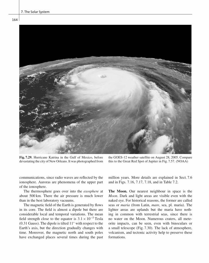
164
7. The Solar System
Fig. 7.29. Hurricane Katrina in the Gulf of Mexico, beforedevastating the city of New Orleans. It was photographed from
the GOES-12 weather satellite on August 28, 2005. Comparethis to the Great Red Spot of Jupiter in Fig. 7.57. (NOAA)
communications, since radio waves are reflected by theionosphere. Auroras are phenomena of the upper partof the ionosphere.
The thermosphere goes over into the exosphere atabout 500 km. There the air pressure is much lowerthan in the best laboratory vacuums.
The magnetic field of the Earth is generated by flowsin its core. The field is almost a dipole but there areconsiderable local and temporal variations. The meanfield strength close to the equator is 3.1×10⁻⁵ Tesla(0.31 Gauss). The dipole is tilted 11 with respect to theEarth’s axis, but the direction gradually changes withtime. Moreover, the magnetic north and south poleshave exchanged places several times during the past
million years. More details are explained in Sect. 7.6and in Figs. 7.16, 7.17, 7.18, and in Table 7.2.
The Moon. Our nearest neighbour in space is theMoon. Dark and light areas are visible even with thenaked eye. For historical reasons, the former are calledseas or maria (from Latin, mare, sea, pl. maria). Thelighter areas are uplands but the maria have noth-ing in common with terrestrial seas, since there isno water on the Moon. Numerous craters, all mete-orite impacts, can be seen, even with binoculars ora small telescope (Fig. 7.30). The lack of atmosphere,volcanism, and tectonic activity help to preserve theseformations.

7.12 The Earth and the Moon
165
Fig. 7.30. A map of the Lunar surface, composed of imagestaken by the Clementine space probe in 1994. Note the largeareas of maria in the Lunar near side, at the centre of the figure,
as compared to the almost complete absence of the maria atthe Lunar far side. (US Naval Observatory)
The Moon is the best-known body after the Earth.The first man landed on the Moon in 1969 during theApollo 11 flight. A total of over 2000 samples, weigh-ing 382 kg, were collected during the six Apollo flights(Fig. 7.31). Moreover, the unmanned Soviet Luna space-craft collected and returned about 310 grams of Lunarsoil. Instruments placed on the Moon by the Apolloastronauts operated as long as eight years. These in-cluded seismometers, which detected moonquakes andmeteorite impacts, and passive laser reflectors whichmade exact Earth–Moon distance measurements possi-ble. The reflectors are still used for Lunar laser ranging(LLR) measurements.
Seismometric and gravimetric measurements havesupplied basic information on the internal structureof the Moon. Moonquakes take place at a depth of800–1000 km, considerably deeper than earthquakes,and they are also much weaker than on the Earth. Mostof the quakes occur at the boundary of the solid mantle,the lithosphere, and the asthenosphere (Fig. 7.32). Thetransversal S waves cannot penetrate the asthenosphere,indicating that it is at least partially molten. Tidal forcesmay generate at least some of the moonquakes becausemost of them occur close to perigee or apogee.
Lunar orbiters have observed local mass concen-trations, mascons, beneath the maria. These are largebasaltic blocks, formed after the huge impacts whichproduced the maria. The craters were filled by lava flowsduring the next billion years or so in several phases. Thiscan be seen, e. g. in the area of Mare Imbrium. Largemaria were formed about 4×10⁹ years ago when me-teorite bombardment was much heavier than today. Thelast 3×10⁹ years have been quite peaceful, without anymajor events.
The centre of mass is not at the geometric centre ofthe Moon but about 2.5 km away due to the 20–30 kmthick basaltic plates below the large maria. Moreover,the thickness of the crust varies, being the thickest at thefar side of the Moon, about 100 km. On the near sidethe thickness of the crust is about 60 km.
The mean density of the Moon is 3400 kg m−3, whichis comparable to that of basaltic lavas on the Earth. TheMoon is covered with a layer of soil with scattered rocks,regolith. It consists of the debris blasted out by meteoriteimpacts. The original surface is nowhere visible. Thethickness of the regolith is estimated to be at least tensof metres. A special type of rock, breccia, which isa fragment of different rocks compacted and welded

166
7. The Solar System
Fig. 7.31. Apollo 17 astronaut Harrison Schmitt on the Moon in 1972. (NASA)
together by meteor impacts, is found everywhere on theMoon.
The maria are mostly composed of dark basalts,which form from rapid cooling of massive lava flows.The highlands are largely composed of anorthosite, anigneous rock that forms when lava cools more slowlythan in the case of basalts. This implies that the rocksof the maria and highlands cooled at different ratesfrom the molten state and were formed under differentconditions.
Data returned by the Lunar Prospector and Clemen-tine spacecraft indicated that water ice is present at both
the north and south lunar poles. Data indicates that theremay be nearly pure water ice buried beneath the dry re-golith. The ice is concentrated at the bottoms of deepvalleys and craters that are in a permanent shadow wherethe temperature is below 100 K.
The Moon has no global magnetic field. Someof the rocks have remanent magnetism indicatinga possible global magnetic field early in the Moon’shistory. Without the atmosphere and magnetic field,the solar wind can reach the Moon’s surface di-rectly. The ions from the solar wind have embeddedin the regolith. Thus samples returned by the Apollo

7.12 The Earth and the Moon
167
Fig. 7.32. Structure of the Moon. The height differences of thesurface are strongly exaggerated
missions proved valuable in studies of the solarwind.
The origin of the Moon is still uncertain; it has,however, not been torn off from the Earth at the Pa-cific Ocean, as is sometimes believed. The Pacific isless than 200 million years old and formed as a re-sult of continental drift. Also, the chemical compositionof the lunar soil is different from that of terrestrialmaterial.
Left: A typical halo; Right: Auroras (Photos P. Parviainen)
Recently it was suggested that the Moon was formedin the early stages of the formation of the Earth, whena lot of protoplanet embryos were orbiting the Sun.An off-axis collision of a Mars-size body resulted inejection of a large amount of debris, a part of whichthen accreted to form the Moon. Differences in chemicalcompositions of the modern Earth and the Moon can beexplained with the theory, as well as the orientation andevolution of the Moon’s orbit and the Earth’s relativelyfast spin rate.
* Atmospheric Phenomena
The best-known atmospheric phenomenon is the rain-bow, which is due to the refraction of light fromwater droplets. The radius of the arc of the rainbowis about 41 and the width, 1.7. The centre of the arcis opposite the Sun (or any other source of light). Whenthe light is refracted inside a water droplet, it is di-vided into a spectrum, where the red colour is at theouter edge and blue, at the inner edge. Light can be re-flected twice inside the droplet, resulting in a secondaryrainbow outside the primary one. The colours of thesecondary rainbow are in reversed order and its radiusis 52. A rainbow caused by the Moon is usually very

168
7. The Solar System
weak and colourless, since the human eye is incapableof resolving colours of a dim object.
A halo results when the solar or lunar light is reflectedfrom atmospheric ice crystals. The most common halois a 22 arc or circle around the Sun or the Moon.Usually the halo is white, but occasionally even brightcolours can be seen. Another common form is the sidelobes which are at the same height as the Sun but ata distance of 22 from it. All other forms of halo areless common. The best “weather” for halos is whenthere are cirrostratus or cirrus clouds or an icy fog inthe sky.
Noctilucent clouds are thin formations of cloud, ata height of approximately 80 km. The clouds containparticles, which are less than one micron in diameter,and become visible only when the Sun (which is belowthe horizon) illuminates the clouds. Most favourableconditions are at the northern latitudes during the sum-mer nights when the Sun is only a few degrees belowthe horizon.
The night sky is never absolutely dark. One reason(in addition to light pollution) is the airglow or lightemitted by excited atmospheric molecules. Most of theradiation is in the infrared domain, but e. g. the forbiddenline of oxygen at 558 nm, has also been detected.
The same greenish oxygen line is clearly seen inauroras, which are formed at a height of 80–300 km.Auroras can be seen mainly from relatively high north-ern or southern latitudes because the Earth’s magneticfield forces charged particles, coming from the Sun,close toward the magnetic poles. Alaska and northernScandinavia are the best places to observe auroras. Oc-casionally, auroras can be seen as far south as 40. Theyare usually greenish or yellow-green, but red aurorashave been observed, too. They most commonly appearas arcs, which are often dim and motionless, or as belts,which are more active and may contain rapidly varyingvertical rays.
Meteors (also called shooting stars although theyhave nothing to do with stars) are small grains of sand,a few micrograms or grams in weight, which hit theEarth’s atmosphere. Due to friction, the body heatsup and starts to glow at a height of 100 km. Some20–40 km lower, the whole grain has burnt to ashes.The duration of a typical meteor is less than a second.The brightest meteors are called bolides (magnitudesmaller than about −2). Even larger particles may sur-
vive down to the Earth. Meteors are further discussed inSect. 7.18.
7.13 Mars
Mars is the outermost of the terrestrial planets. Its di-ameter is only half of that of the Earth. Seen througha telescope, Mars seems to be a reddish disk with darkspots and white polar caps. The polar caps wax andwane with the Martian seasons, indicating that they arecomposed of ice. Darker areas were suspected to bevegetation. At the end of the 19th century, an Italian as-tronomer, Giovanni Schiaparelli claimed that there arecanals on Mars.
In the United States, the famous planetary as-tronomer Percival Lowell studied the canals and evenpublished books on the topic. Martians were also verypopular in science fiction literature. Now the canals areknown to be nonexistent, an optical illusion when theobscure details at the limit of visibility seem to formstraight lines, canals. Finally, the first clear pictures byMariner 4 in 1965 buried even the most optimistic hopesconcerning life on Mars. Later spacecraft revealed moredetails of the planet.
Mars is a superior planet, which means that it is mosteasily observable when it is closest to the Earth, i. e.during opposition, when the planet is above the horizonall night long.
The rotation axis of Mars is tilted 25 to the ecliptic,about the same amount as the Earth’s axis. A Martianday is only half an hour longer than a terrestrial day.Mars’ orbit is significantly elliptical, resulting in tem-perature variations of about 30 C at the subsolar pointbetween the aphelion and perihelion. This has a majorinfluence on the climate. Huge dust storms are occa-sionally seen on Mars (Fig. 7.33). Usually the stormsbegin when Mars is at the perihelion. Heating of thesurface gives rise to large temperature differences thatin turn cause strong winds. The wind-driven dust ab-sorbs more heat and finally the whole planet is coveredby a dust storm where the wind speeds exceed 100 m/s.
The atmosphere of Mars is mainly composed of car-bon dioxide (95%). It contains only 2% nitrogen and0.1–0.4% oxygen. The atmosphere is very dry: if allthe moisture were condensed on the surface, the wa-ter layer would be thinner than 0.1 mm. Even the minor

7.13 Mars
169
Fig. 7.33. Two pictures of Mars, taken by the Mars GlobalSurveyor in June and July 2001. The view from June (left)shows the Tharsis volcanic region, Valles Marineris and the
late winter south polar cap. The view from July shows the sameregions, but most of the details are hidden by dust storms andhaze. (NASA/JPL/Malin Space Science Systems)
Fig. 7.34. A topographic shade map of Mars made from theMars Global Surveyor data. The most prominent featuresare the large shield volcanoes in the northern hemisphere
and the Valles Marineris canyon system that is more than3000 km long and up to 8 km deep. (MOLA ScienceTeam/NASA)

170
7. The Solar System
amount of water vapour is sufficient to occasionallyform some thin clouds or haze.
The air pressure is only 5–8 mbar. A part of the at-mosphere has escaped but it is probable that Mars neverhad a thick atmosphere. The primordial atmosphere ofMars was, however, somewhat similar to that of theEarth. Almost all of its carbon dioxide was used up toform carbonate rocks. Because there are no plate tec-tonics on Mars, the carbon dioxide was not recycledback into the atmosphere as on the Earth. Therefore, thegreenhouse effect on Mars is significantly smaller thanon the Earth.
Craters were already found in the first pictures. Thesouthern hemisphere is especially marked by craters, in-dicating that the original surface is still visible there. Thelargest impacts, Hellas and Argyre are about 2000 km indiameter. On the other hand, the northern hemispherehas an abundance of large lava basins and volcanoes(Fig. 7.34). The surface is younger than in the south-
Fig. 7.35a–c. Volcanoes, impact craters and rivers. (a) MarsGlobal Surveyor wide-angle view of Olympus Mons inApril 1998. (b) Small impact craters and sand duneswuth a resolution of 1.5 m per pixel. The picture coversa 1.5 km wide portion of Isidis Planitia. (c) Three ma-jor valley systems east of the Hellas plains. These valleys
have probably been formed by large outbursts of liquidwater but the age of the valleys is unknown. The valleysare all roughly 1 km deep and 10–40 km wide. The pic-ture covers an area approximately 800 km across. (MarsGlobal Surveyor, 2000) (NASA/JPL/Malin Space ScienceSystems)
ern hemisphere. The largest volcano, Olympus Mons(Fig. 7.35), protrudes more than 20 km above the sur-rounding terrain. The diameter at the bottom is about600 km.
There are no active volcanoes on Mars. The mare-like plains on Mars are of the same age as the Lunarmaria, about 3×10⁹ years old. Volcanism in the high-land and mare-like plains stopped at that time, butthe giant shield volcanoes are much younger, pos-sibly 1–2×10⁹ years. The youngest lava flows onOlympus Mons are possibly less than 100 millionyears old. Mars shows no sign of plate tectonics. Ithas no mountain chains, nor any global patterns ofvolcanism.
There are also several canyons, the largest of whichis Valles Marineris (Fig. 7.34). Its length is 5000 km,width 200 km, and depth about 6 km. Compared withValles Marineris, the Grand Canyon is merely a scratchon the surface.

7.14 Jupiter
171
Fig. 7.36. The 360 degree panorama was taken by the Mars Pathfinder Lander in 1997. The Sojourner rover is visible near thecentre of the panorama, in front of the ramp. (NASA/JPL)
Ancient riverbeds (Fig. 7.35), too small to be seenfrom the Earth, were also discovered by spacecraft.Rivers were probably formed soon after the formationof Mars itself, when there was a great deal of water andthe atmospheric pressure and temperature were higher.At present, the temperature and air pressure on Mars aretoo low for free water to exist, although there have beenspeculations on warm weather cycles in the more re-cent history of the planet. The mean temperature is nowbelow −50 C and, on a warm summer day, the tem-perature can rise close to zero near the equator. Mostof the water is contained in kilometres deep permafrostbelow the surface and in the polar caps. The theorywas confirmed in 2002, when the Mars Odyssey space-craft detected a large supply of subsurface water ice ofa wide area near the south pole. The ice is mixed intothe soil a meter below the surface. Two rovers, Spiritand Opportunity, operating on the Mars discovered in2004 minerals like hematite and goethite which provedthe existence of liquid water on the surface of Mars. Theperiod when the liquid water existed is unknown.
The polar caps are composed both of water and car-bon dioxide ice. The northern cap is almost season-independent, extending down to latitude 70. On theother hand, the southern cap, which reaches to the lati-tude −60 in the southern winter, disappears almosttotally during the summer. The southern cap consistsmostly of CO2 ice. The permanent parts are of ordinarywater ice, since the temperature, −73 C, is too high forCO2 ice. The water ice layers can be hundreds of metresthick.
The dark areas are not vegetation, but loose dust,moved around by strong winds. These winds raise thedust high into the atmosphere, colouring the Martiansky red. The Mars landers have revealed a reddish re-golithic surface, scattered with boulders (Fig. 7.36). The
red colour is caused mainly by iron oxide, rust; alreadyin the 1950’s, the existence of limonite (2 FeO3 3 H2O)was deduced from polarization measurements. The on-site analysis showed that the soil consists of 13% ironand 21% silicon. The abundance of sulphur was foundto be ten times that found on the Earth.
The interior of Mars is not well known. Mars hasprobably a dense core approximately 1700 km in radius,a molten rocky mantle which is denser than the Earth’smantle and a thin crust. The crust is 80 km thick inthe southern hemisphere but only about 35 km thick inthe northern one. The low mean density compared withother terrestrial planets may indicate that in additionto iron the core contains a relatively large fraction ofsulphur .
The Mars Global Surveyor confirmed in 1997 a weakmagnetic field. It is probably a remnant of an ear-lier global field that has since disappeared. This hasimportant implications for the structure of Mars’ inte-rior. There are no electric currents creating a magneticfield and therefore the core may be (at least partially)solid.
Three biological experiments of the Viking landers in1976 searched for signs of life. No organic compoundswere found – however, the biological tests did give someunexpected results. A closer look at the results indicatedno life, but some uncommon chemical reactions.
Mars has two moons, Phobos and Deimos (Fig. 7.37).The size of Phobos is roughly 27 km×21 km×19 km,and the orbital period around Mars is only 7 h 39 min.In the Martian sky, Phobos rises in the west andsets in the east. Deimos is smaller. Its diameter is15 km × 12 km × 11 km. There are craters on bothmoons. Polarimetric and photometric results show thatthey are composed of material resembling carbonaceouschondrite meteorites.

172
7. The Solar System
Fig. 7.37. Phobos (left) and Deimos, the two moons of Mars. They can be captured asteroids. (NASA)
7.14 Jupiter
The realm of terrestrial planets ends at the asteroid belt.Outside this, the relative abundance of volatile elementsis higher and the original composition of the solar nebulais still preserved in the giant planets. The first and largestis Jupiter. Its mass is 2.5 times the total mass of allother planets, almost 1/1000 of the solar mass. Thebulk of Jupiter is mainly hydrogen and helium. Therelative abundance of these elements are approximatelythe same as in the Sun, and the density is of the sameorder of magnitude, namely 1330 kg m−3.
During oppositions, the angular diameter of Jupiteris as large as 50′′. The dark belts and lighter zones arevisible even with a small telescope. These are cloud for-mations, parallel to the equator (Fig. 7.38). The most fa-mous detail is the Great Red Spot, a huge cyclone, rotat-ing counterclockwise once every six days. The spot wasdiscovered by Giovanni Cassini in 1655; it has survivedfor centuries, but its true age is unknown (Fig. 7.39).
The rotation of Jupiter is rapid; one revolution takes9 h 55 min 29.7 s. This is the period determined fromthe variation of the magnetic field, and it reflects thespeed of Jupiter’s interiors where the magnetic field isborn. As might be expected, Jupiter does not behavelike a rigid body. The rotation period of the clouds isabout five minutes longer in the polar region than at theequator. Due to its rapid rotation, Jupiter is nonspherical;flattening is as large as 1/15.
There is possibly an iron-nickel core in the centreof Jupiter. The mass of the core is probably equal toa few tens of Earth masses. The core is surrounded bya layer of metallic liquid hydrogen, where the temper-ature is over 10,000 K and the pressure, three millionatm. Owing to this huge pressure, the hydrogen is dis-sociated into single atoms, a state unknown in ordinarylaboratory environments. In this exotic state, hydro-gen has many features typical of metals. This layeris electrically conductive, giving rise to a strong mag-netic field. Closer to the surface where the pressure

7.14 Jupiter
173
Fig. 7.38. A composed image of Jupiter taken by theCassini spacecraft in December 2000. The resolution is
114 km/pixel. The dark dot is the shadow of the moon Europa.(NASA/JPL/University of Arizona)
is lower, the hydrogen is present as normal molecu-lar hydrogen, H2. At the top there is a 1000 km thickatmosphere.
The atmospheric state and composition of Jupiter hasbeen accurately measured by the spacecraft. In situ ob-servations were obtained in 1995, when the probe ofthe Galileo spacecraft was dropped into Jupiter’s atmo-sphere. It survived nearly an hour before crushing underthe pressure, collecting the first direct measurements ofJupiter’s atmosphere.
Belts and zones are stable cloud formations (Fig.7.38). Their width and colour may vary with time, butthe semi-regular pattern can be seen up to the latitude50. The colour of the polar areas is close to that of thebelts. The belts are reddish or brownish, and the motionof the gas inside a belt is downward. The gas flowsupward in the white zones. The clouds in the zones areslightly higher and have a lower temperature than thosein the belts. Strong winds or jet streams blow along thezones and belts. The speed of the wind reaches 150 m/sat some places in the upper atmosphere. According tothe measurements of the Galileo probe, the wind speeds
in the lower cloud layers can reach up to 500 m/s. Thisindicates that the winds in deeper atmospheric layersare driven by the outflowing flux of the internal heat,not the solar heating.
The colour of the Great Red Spot (GRS) resemblesthe colour of the belts (Fig. 7.39). Sometimes it is almostcolourless, but shows no signs of decrepitude. The GRSis 14,000 km wide and 30,000–40,000 km long. Somesmaller red and white spots can also be observed onJupiter, but their lifetime is generally much less thana few years.
The ratio of helium to hydrogen in the deep atmo-sphere is about the same as in the Sun. The results ofthe Galileo spacecraft gave considerably higher abun-dance than previous estimates. It means that there are nosignificant differentiation of helium, i. e. helium is notsinking to the interior of the planet as was expected ac-cording to the earlier results. Other compounds found inthe atmosphere include methane, ethane and ammonia.The temperature in the cloud tops is about 130 K.
Jupiter radiates twice the amount of heat that it re-ceives from the Sun. This heat is a remnant of the

174
7. The Solar System
Fig. 7.39. Jupiter’s Great Red Spot and its surroundings with several smaller ovals as seen by Voyager 1 in 1979. Cloud detailsof 160 kilometres are visible. (NASA)
energy released in the gravitational contraction duringthe formation of the planet. Thus Jupiter is still grad-ually cooling. The internal heat is transferred outwardby convection; this gives rise to flows in the metallichydrogen, causing the strong magnetic field (Fig. 7.41).
The ring of Jupiter (Fig. 7.40) was discovered in1979. The innermost toroid-shaped halo is between92,000–122,500 km from Jupiter’s centre. It consists of
dust falling from the main ring toward the planet. Themain ring extends from the halo boundary out to about128,940 km, just inside the orbit of the moon Adrastea.The ring particles are small, a few microns only, andthey scatter light forward much more effectively thanbackward. Therefore, they were not discovered priorthe Voyager flyby. A ring consisting of such smallparticles cannot be stable, and new material must en-

7.14 Jupiter
175
Fig. 7.40. Mosaic of Jupiter’s ring system taken by the Galileospacecraft when the spacecraft was in Jupiter’s shadow look-ing back toward the Sun. Jupiter’s ring system is composedof three parts: a thin outermost ring, a flat main ring, and
an innermost doughnut-shaped halo. These rings are madeup of dust-sized particles that originate from Io, or areblasted off from the nearby inner satellites by small impacts.(NASA/University of Arizona)
Fig. 7.41. Left: NASA Hubble Space Telescope close-up viewof an aurora on Jupiter. The image shows the main oval of theaurora, centred over the magnetic north pole, and diffuse emis-sions inside the polar cap. (NASA, John Clarke/Universityof Michigan) Right: The image taken on January 2001 by
NASA’s Cassini spacecraft shows the bubble of chargedparticles trapped in the magnetosphere. The magnetic fieldand the torus of the ionised material from the volcanoesof Io are drawn over the image. (NASA/JPL/Johns HopkinsUniversity)

176
7. The Solar System
ter the ring continuously. The most probable source isIo.
The two faint outermost rings are fairly uniform innature. The inner of them extends from the orbit ofAdrastea out to the orbit of Amalthea at 181,000 km.The fainter outermost ring extends out to Thebe’s orbitat 221,000 km.
Jupiter’s rings and moons exist within an intenseradiation belt of Jupiter’s magnetic field. The magne-tosphere extends 3–7 million kilometres toward theSun, depending on the strength of the solar wind. Inthe opposite direction it stretches to a distance of atleast 750 million kilometres, behind Saturn’s orbit.
Jupiter is an intense radio source. Its radio emissioncan be divided into three components, namely thermalmillimetre and centimetre radiation, nonthermal deci-metric radiation and burstal-decametric radiation. Thenonthermal emission is most interesting; it is partly syn-chrotron radiation, generated by relativistic electrons inthe Jovian magnetosphere. Its intensity varies in phasewith Jupiter’s rotation; thus the radio emission can beused for determining the exact rotation rate. The deca-metric bursts are related to the position of the innermostlarge moon, Io, and are possibly generated by the mil-lion Ampere electric current observed between Jupiterand the plasma torus at the orbit of Io.
In the beginning of year 2006 there were 63 knownmoons of Jupiter. The four largest, Io, Europa,Ganymede and Callisto are called the Galilean satellites
Fig. 7.42. (Top) The Galilean satellites of Jupiter. From leftto right: Io, Europa, Ganymede, and Callisto (NASA/DLR).(Right page top) Surface details of Io and Europa. (Right
page bottom) Surface details of Ganymede and Callisto(NASA/Brown University, NASA/JPL)
(Fig. 7.42), in honour of Galileo Galilei, who discov-ered them in 1610. The Galilean satellites can alreadybe seen with ordinary binoculars. They are the size ofthe Moon or even planet Mercury. The other moons aresmall, most of them only a few kilometres in diameter.
Owing to tidal forces, the orbits of Io, Europa andGanymede have been locked into a resonance, so thattheir longitudes λ strictly satisfy the equation
λIo −3λEuropa +2λGanymede = 180 . (7.54)
Hence the moons can never be in the same directionwhen seen from Jupiter.
Io is the innermost Galilean satellite. It is a littlelarger than the Moon. Its surface is spotted by numer-ous calderas, volcanoes without a mountain. The moltenmaterial is ejected up to a height of 250 km, and a partof the gas gets into Io’s orbit. The volcanic activity onIo is much stronger than on the Earth. There is a 100 mbulk of the permanent tide raised by Jupiter. Due to theorbital perturbations caused by Europa and Ganymedethe orbit of Io is slightly elliptical and therefore the or-bital speed varies. The tidal bulk is forced to move withrespect to the surface. This generates friction, which istransformed to heat. This heat keeps the sulphur com-pounds molten beneath the colourful surface of Io. Notraces of impact craters are visible. The whole surfaceis new, being renewed continuously by eruptions. Thereis no water on Io.

7.14 Jupiter
177
Europa is the smallest of the Galilean satellites, a lit-tle smaller than the Moon. The surface is ice-coveredand the geometric albedo is as high as 0.6. The surfaceis smooth with only a few features more than a hundredmetres high. Most of the markings seem to be albedofeatures with very low relief. Only a few impact craters
have been found indicating that the surface is young.The surface is renewed by fresh water, trickling fromthe internal ocean. Galileo spacecraft has found a veryweak magnetic field. The field varies periodically asit passes through Jupiter’s magnetic field. This showsthat there is a conducting material beneath Europa’s sur-
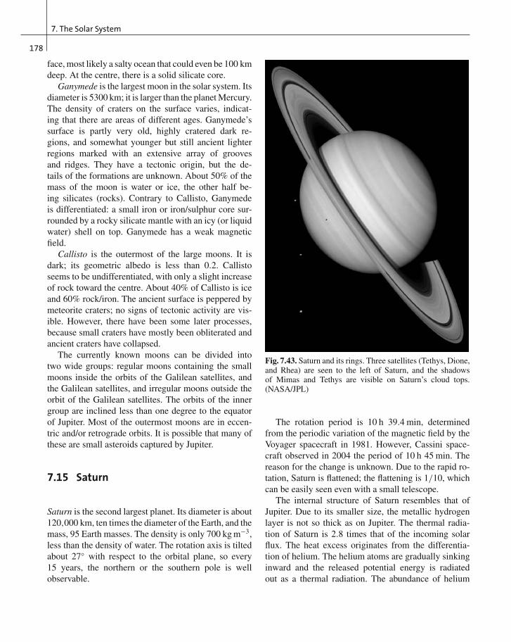
178
7. The Solar System
face, most likely a salty ocean that could even be 100 kmdeep. At the centre, there is a solid silicate core.
Ganymede is the largest moon in the solar system. Itsdiameter is 5300 km; it is larger than the planet Mercury.The density of craters on the surface varies, indicat-ing that there are areas of different ages. Ganymede’ssurface is partly very old, highly cratered dark re-gions, and somewhat younger but still ancient lighterregions marked with an extensive array of groovesand ridges. They have a tectonic origin, but the de-tails of the formations are unknown. About 50% of themass of the moon is water or ice, the other half be-ing silicates (rocks). Contrary to Callisto, Ganymedeis differentiated: a small iron or iron/sulphur core sur-rounded by a rocky silicate mantle with an icy (or liquidwater) shell on top. Ganymede has a weak magneticfield.
Callisto is the outermost of the large moons. It isdark; its geometric albedo is less than 0.2. Callistoseems to be undifferentiated, with only a slight increaseof rock toward the centre. About 40% of Callisto is iceand 60% rock/iron. The ancient surface is peppered bymeteorite craters; no signs of tectonic activity are vis-ible. However, there have been some later processes,because small craters have mostly been obliterated andancient craters have collapsed.
The currently known moons can be divided intotwo wide groups: regular moons containing the smallmoons inside the orbits of the Galilean satellites, andthe Galilean satellites, and irregular moons outside theorbit of the Galilean satellites. The orbits of the innergroup are inclined less than one degree to the equatorof Jupiter. Most of the outermost moons are in eccen-tric and/or retrograde orbits. It is possible that many ofthese are small asteroids captured by Jupiter.
7.15 Saturn
Saturn is the second largest planet. Its diameter is about120,000 km, ten times the diameter of the Earth, and themass, 95 Earth masses. The density is only 700 kg m−3,less than the density of water. The rotation axis is tiltedabout 27 with respect to the orbital plane, so every15 years, the northern or the southern pole is wellobservable.
Fig. 7.43. Saturn and its rings. Three satellites (Tethys, Dione,and Rhea) are seen to the left of Saturn, and the shadowsof Mimas and Tethys are visible on Saturn’s cloud tops.(NASA/JPL)
The rotation period is 10 h 39.4 min, determinedfrom the periodic variation of the magnetic field by theVoyager spacecraft in 1981. However, Cassini space-craft observed in 2004 the period of 10 h 45 min. Thereason for the change is unknown. Due to the rapid ro-tation, Saturn is flattened; the flattening is 1/10, whichcan be easily seen even with a small telescope.
The internal structure of Saturn resembles that ofJupiter. Due to its smaller size, the metallic hydrogenlayer is not so thick as on Jupiter. The thermal radia-tion of Saturn is 2.8 times that of the incoming solarflux. The heat excess originates from the differentia-tion of helium. The helium atoms are gradually sinkinginward and the released potential energy is radiatedout as a thermal radiation. The abundance of helium

7.15 Saturn
179
in Saturn’s atmosphere is only about half of that onJupiter.
The winds, or jet streams, are similar to those ofJupiter but Saturn’s appearance is less colourful. Viewedfrom the Earth, Saturn is a yellowish disk withoutany conspicuous details. The clouds have fewer fea-tures than those on Jupiter, because a haze, composedof hydrogen, ammonium and methane floats abovethe cloud tops. Furthermore, Saturn is farther fromthe Sun than Jupiter and thus has a different energybudget.
The temperature at the cloud tops is about 94 K.Close to the equator the wind speeds exceed 400 m/sand the zone in which the direction of the wind re-mains the same extends 40 from the equator. Such highspeeds cannot be explained with external solar heat, butthe reason for the winds is the internal flux of heat.
Saturn’s most remarkable feature is a thin ring system(Fig. 7.44, 7.45), lying in the planet’s equatorial plane.The Saturnian rings can be seen even with a small tele-scope. The rings were discovered by Galileo Galilei in1610; only 45 years later did Christian Huygens estab-lish that the formation observed was actually a ring,and not two oddly behaving bulbs, as they appearedto Galileo. In 1857 James Clerk Maxwell showed the-oretically that the rings cannot be solid but must becomposed of small particles.
The rings are made of normal water ice. The sizeof the ring particles ranges from microns to truck-sizechunks. Most of the particles are in range of centime-tres to metres. The width of the ring system is morethan 60,000 km (about the radius of Saturn) and the
Fig. 7.44. A schematic drawing of the structure of theSaturnian rings
Fig. 7.45. At a close distance, the rings can be seen to bedivided into thousands of narrow ringlets. (JPL/NASA)
thickness, at most 100 m, and possibly only a fewmetres. Cassini spacecraft discovered also molecularoxygen around the rings, probably as a product of thedisintegration of water ice from the rings.
According to Earth-based observations, the rings aredivided into three parts, called simply A, B, and C. Theinnermost C ring is 17,000 km wide and consists ofvery thin material. There is some material even insidethis (referred to as the D ring), and a haze of particlesmay extend down to the clouds of Saturn.
The B ring is the brightest ring. Its total width is26,000 km, but the ring is divided into thousands ofnarrow ringlets, seen only by the spacecraft (Fig. 7.45).From the Earth, the ring seems more or less uniform.Between B and A, there is a 3000 km wide gap, theCassini division. It is not totally void, as was previouslybelieved; some material and even narrow ringlets havebeen found in the division by the Voyager space probes.
The A ring is not divided into narrow ringlets asclearly as the B ring. There is one narrow but obviousgap, Encke’s division, close to the outer edge of thering. The outer edge is very sharp, due to the “shepherd”moon, some 800 km outside the ring. The moon preventsthe ring particles from spreading out to larger orbits.It is possible that the appearance of B is due to yet-undiscovered moonlets inside the ring.

180
7. The Solar System
The F ring, discovered in 1979, is about 3000 km out-side A. The ring is only a few hundred kilometres wide.On both sides there is a small moon; these shepherdsprevent the ring from spreading. An interior moon pass-ing a ring particle causes the particle to move to a largerorbit. Similarly, at the outer edge of the ring, a second
moon forces the particles inward. The net result is thatthe ring is kept narrow.
Outside the F ring, there are some zones ofvery sparse material, sometimes referred to as theG and E rings. These are merely collections of smallparticles.

7.16 Uranus and Neptune
181
Fig. 7.46a–e. Saturnianmoons photographed bythe Cassini spacecraft in2005–2006 (a) Hyperion,(b) Enceladus, (c) Iapetusand (d) Tethys. (e) A radarpicture of the northern lat-itudes of Titan, taken byCassini in summer 2006.The black patches are prob-ably methane lakes. Thewidth of the picture is about450 km. (Photo NASA)
The Saturnian rings were possibly formed togetherwith Saturn and are not debris from some cosmic catas-trophe, like remnants of a broken moon. The total massof the rings is 10−7 of the mass of Saturn. If all ring par-ticles were collected together, they would form an iceball, 600 km in diameter.
A total of 56 moons (late 2006) of Saturn are known.Many of the large Saturnian moons (Fig. 7.46) wereobserved by Pioneer 11 and Voyager 1 and 2 spacecrafts.Large moons (excluding Titan) are composed mainlyof ice. The temperature of the primeval nebula at thedistance of Saturn was so low that bodies of pure icecould form and survive.
Some moons are dynamically interesting; some havean exotic geological past. Outside the F ring, thereare two moonlets, Epimetheus and Janus, almost inthe same orbit; the difference of the semimajor axesis about 50 km, less than the radii of the moons. Theinner moon is gaining on the outer one. The moonswill not collide, since the speed of the trailing moonincreases and the moon moves outward. The speed ofthe leading moon decreases and it drops inward. Themoons exchange their roles roughly every four years.There are also several shepherding satellites, like At-las, Prometheus and Pandora that keep rings in theirplace. Their gravitational pull prevents ring particlesfrom drifting away.
The innermost of the “old” moons is Mimas. Thereis a huge crater on Mimas’ surface with a diameter of100 km and a depth of 9 km (Fig. 7.46). Bigger cratersexist in the solar system, but relative to the size of theparent body, this is almost the biggest crater there couldbe room for (otherwise the crater would be bigger than
Mimas itself). On the opposite side, some grooves canbe seen, possibly signifying that impact has almost tornthe moon apart.
The surface of the next moon, Enceladus, consists ofalmost pure ice, and one side is nearly craterless. Cratersand grooves can be found on the other hemisphere. Tidalforces result in volcanic activity where water (not lavaor other “hot” material) is discharged to the surface.
Titan is the largest of the Saturnian moons. Its di-ameter is 5150 km, so it is only slightly smaller thanJupiter’s moon Ganymede. Titan is the only moon witha dense atmosphere. The atmosphere is mainly nitrogen(98.4%) and methane, and the pressure at the surfaceis 1.5–2 bar. The temperature is about 90 K. Reddishclouds form the visible surface some 200 km abovethe solid body. Measurements and images of Huy-gens probe landing on Titan in 2005 did not revealliquid methane lakes. However, Cassini orbiter radardata in 2006 strongly indicate the presence of the lakes(Fig. 7.44). An independent proof of liquids in the re-cent past can be seen in several surface features whichpossibly have been formed by flowing fluids.
7.16 Uranus and Neptune
The planets from Mercury to Saturn were already knownin antiquity. Uranus and Neptune can only be observedwith a telescope. Uranus and Neptune are giants, similarto Jupiter and Saturn.
Uranus. The famous German-English amateur as-tronomer William Herschel discovered Uranus in 1781.

182
7. The Solar System
Herschel himself first thought that the new object wasa comet. However, the extremely slow motion revealedthat the body was far beyond the orbit of Saturn. Basedon the first observations, the Finnish astronomer AndersLexell calculated a circular orbit. He was one of the firstto propose that the newly discovered object was a planet.Johann Bode of the Berlin Observatory suggested thename Uranus but more than five decades passed beforethe name was unanimously accepted.
The mean distance of Uranus is 19 AU, and the or-bital period 84 years. The inclination of the rotationaxis is 98, which is totally different from the otherplanets. Due to this uncommon geometry, the poles areeither lit or in darkness for decades. The rotation period,confirmed by the Voyager 2 magnetometric measure-ments in 1986, is 17.3 hours; the exact period had beenuncertain prior to the fly-by.
Uranus is greenish, as viewed through a telescope.Its colour is due to the strong methane absorption bandsin the near-infrared. A part of the red light is alsoabsorbed, leaving the green and blue part of the spec-trum untouched. Uranus is almost featureless (Fig. 7.47)because its clouds are below a thick haze or smog.
The strong limb darkening makes the terrestrial de-termination of the Uranus’ size difficult. Therefore, the
Fig. 7.47. Two views of Uranus. The left picture shows Uranusas it would appear to the naked eye. (NASA). At the right thereis a Hubble Space Telescope view of Uranus surrounded by
its rings. Also 10 satellites are visible in the original picture.(Seidelmann, U.S. Naval Observatory, and NASA)
radius was not accurately determined until 1977 dur-ing a stellar occultation caused by Uranus. The rings ofUranus were discovered at the same time.
The internal structure of Uranus is thought to beslightly different from that of other giant planets. Abovethe innermost rocky core, there is a layer of water,which, in turn, is surrounded by a mantle of hydrogenand helium. The mixture of water and ammonia andmethane therein are dissociated to ions under the heavypressure. This mixture behaves more like a molten saltthan water. The convection flows in this electrically con-ductive “sea” give rise to the Uranian magnetic field.The strength of the magnetic field at the cloud topsis comparable to the terrestrial field. However, Uranusis much larger then the Earth, so the true strength ofthe field is 50 times greater than that of the Earth. TheUranian magnetic field is tilted 60 with respect to therotation axis. No other planet has such a highly inclinedmagnetic field.
The Uranian rings (Fig. 7.48) were discovered in1977, during a stellar occultation. Secondary occulta-tions were observed before and after the main event.A total of 13 rings are known, nine of which were dis-covered in the occultation. The innermost ring is broadand diffuse. All other rings are dark and very narrow,

7.16 Uranus and Neptune
183
Fig. 7.48. Left: The rings of Uranus are very narrow and com-posed of a dark material. Nine rings are visible in the pictureof Voyager in 1986. Right: Rings seen in the light scattered
forward when the Voyager spacecraft was in the shadow ofthe planet. (NASA)
only a few hundred metres or a few kilometres wide.The Voyager 2 results showed that the rings containvery little dust, unlike those of Jupiter and Saturn. Themean size of the ring particles is more than 1 metre. Thering particles are darker than practically any known ma-terial in the solar system; the cause of this dark colouris unknown.
There are 27 moons (2006 number) orbiting aroundUranus, ten of which were discovered by Voyager 2. Thegeological history of some moons is puzzling, and manyfeatures reminiscent of an active past can be found.
The innermost of the large moons, Miranda, is one ofthe most peculiar objects discovered (Fig. 7.49). It hasseveral geological formations also found elsewhere (buthere they are all mixed together), in addition to the quiteunique V-shaped formations. It is possible that Miran-da’s present appearance is the result of a vast collisionthat broke the moon apart; some pieces may have latersettled down, inside out. Another peculiar object is Um-briel. It belongs to the ever increasing family of unusualdark bodies (such as the Uranian rings, one side of Ia-petus and Halley’s comet). The dark surface of Umbrielis covered by craters without any traces of geologicalactivity.
Neptune. The orbit of Uranus was already well knownin the beginning of the 19th century. However, someunknown perturbations displaced Uranus from its pre-dicted orbit. Based on these perturbations, John CouchAdams, of Cambridge, and Urbain Jean-Joseph Le Ver-rier, of Paris, independently predicted the position ofthe unknown perturbing planet.
The new planet was discovered in 1846 by JohannGottfried Galle at the Berlin Observatory; Le Verrier’sprediction was found to be only 1 off. The discov-ery gave rise to a heated controversy as to who shouldbe given the honour of the discovery, since Adams’calculations were not published outside the CambridgeObservatory. When the quarrel was settled years later,both men were equally honoured. The discovery of Nep-tune was also a great triumph of the Newtonian theoryof gravitation.
The semimajor axis of the orbit of Neptune is 30 AUand the orbital period around the Sun 165 years. The in-ternal rotation period, confirmed by Voyager 2 in 1989,is 16 hours 7 minutes and the rotation period of the outerlayers of the clouds is about 17 hours. The obliquity ofthe rotation axis is 29 but the magnetic field is tiltedsome 50 with respect to the rotation axis. The mag-

184
7. The Solar System
Fig. 7.49. Four Uranian moons (from top left to lower right): Miranda, Ariel, Titania and Umbriel. (NASA)
netic field is tilted like in Uranus, but the field strengthis much smaller.
The density of Neptune is 1660 kg m−3, and thediameter 48,600 km. Thus the density of Neptune ishigher than that of other giant planets. The inter-nal structure is quite simple: The core, composed
of silicates (rocks) is about 16000 km in diame-ter. This is surrounded by a layer of water andliquid methane and the outermost gaseous layer, at-mosphere, is mainly composed of hydrogen andhelium, methane and ethane being a minor com-ponents.

7.16 Uranus and Neptune
185
Fig. 7.50. (Left) Neptune shows more features than Uranus.In the picture of Voyager 2 the Great Dark Spot, ac-companied by bright, white clouds is well visible. Theirappearance is changing rapidly. To the south of the GreatDark Spot is a bright feature and still farther south is an-other dark spot. Each feature moves eastward at a different
velocity. (Right) Details of the Southern Dark Spot. TheV-shaped structure near the right edge of the bright areaindicates that the spot rotates clockwise. Unlike the GreatRed Spot on Jupiter, which rotates counterclockwise, thematerial in the Neptune’s dark oval will be descending.(NASA/JPL)
Cloud structures are more complicated than onUranus, and some dark spots, like in Jupiter, were visi-ble during the Voyager fly-by (Fig. 7.50). The speed ofthe winds are high, up to 400 m/s.
Like other giants, Neptune also has rings (Fig. 7.51).The rings were discovered by Voyager 2, although theirexistence was already expected prior the fly-by. Tworelatively bright but very narrow rings are at a distanceof 53,000 and 62,000 km from the centre of the planet.Moreover, there are some faint areas of fine dust.
There are 13 known moons, six of which were dis-covered by Voyager 2. The largest of the moons, Triton,is 2700 km in diameter, and it has a thin atmosphere,mainly composed of nitrogen. The albedo is high: Tri-ton reflects 60–80% of the incident light. The surfaceis relatively young, without any considerable impactcraters (Fig. 7.52). There are some active “geysers” ofliquid nitrogen, which partly explains the high albedo
Fig. 7.51. The rings of Neptune. Ring particles are small andbest visible in the forward scattered light. There are severalbrightenings in the outermost ring. One of the rings appearsto have a twisted structure. Neptune at left is overexposed.(NASA/JPL)

186
7. The Solar System
Fig. 7.52. The southern hemisphere of Triton, Neptune’slargest satellite in a picture taken in 1989 by Voyager 2. Thedark spots may indicate eruptions of “icy volcanoes”. Voy-ager 2 images showed active geyser-like eruptions spewingnitrogen gas and dark dust particles several kilometres intothe atmosphere. (NASA)
and the lack of the craters. The low surface tempera-ture of Triton, 37 K, means that the nitrogen is solidand covers the surface like snow. It is the lowest surfacetemperature known in the solar system.
7.17 Minor Bodies of the Solar System
So far we have considered only planets and planetarysatellites. There is a great number of other bodies inthe solar system, like dwarf planets, asteroids, comets,meteoroids and interplanetary dust. However, there areno distinct borders between different types of objects.Some asteroids have similar features or origin as thecomets, and some near-Earth asteroids are possiblycometary remnants where all volatile elements havedisappeared. Thus our classification has been basedmore on the visual appearance and tradition than onreal physical differences.
In 2006 the International Astronomical Union (IAU)in its General Assembly defined three distinct cate-gories, namely planets, dwarf planets, and Small SolarSystem Bodies which include the rest of the Solar Sys-tem bodies, like asteroids, Trans-Neptunian Objects,comets and meteoroids.
Dwarf planets. According to the IAU definition a dwarfplanet is a celestial body that: (a) is in orbit aroundthe Sun, (b) has sufficient mass for its self-gravity toovercome rigid body forces so that it assumes a hy-drostatic equilibrium (nearly round) shape, (c) has notcleared the neighbourhood around its orbit, and (d) isnot a satellite.
The upper and lower limits to the size and mass ofdwarf planets are not strictly specified. The lower limit,however, is determined by the hydrostatic equilibriumshape, but the size at which this happens may varyaccording to the composition and history of the object.It is estimated that up to 40–50 dwarf planets will bediscovered in coming years.
Currently, there are three dwarf planets in the SolarSystem, namely Ceres, Pluto and Eris. Ceres was for-merly counted as an asteroid, Pluto was a planet andEris (2003 UB 313, known also by the nickname Xena)was the first Trans-Neptunian object which turned outto be larger than Pluto.
Pluto was discovered in 1930 at the Lowell Obser-vatory, Arizona, after an extensive photographic search(Fig. 7.53). This search had already been initiated in thebeginning of the century by Percival Lowell, on the ba-sis of the perturbations observed in the orbits of Uranusand Neptune. Finally, Clyde Tombaugh discovered Plutoless than 6 off the predicted position. However, Plutoturned out to be far too small to cause any perturba-tions on Uranus or Neptune. Thus the discovery waspurely accidental, and the perturbations observed werenot real, but caused by minor errors of old observations.
Pluto has no visible disk as seen with terrestrialtelescopes; instead, it resembles a point, like a star(Fig. 7.54). This fact gave an upper limit for the di-ameter of Pluto, which turned out to be about 3000 km.The exact mass was unknown until the discovery of thePlutonian moon, Charon, in 1978. The mass of Plutois only 0.2% of the mass of the Earth. The orbital pe-riod of Charon is 6.39 days, and this is also the periodof rotation of both bodies. Pluto and Charon rotate syn-chronously, each turning the same side towards the otherbody. The rotation axis of Pluto is close to the orbitalplane: the tilt is 122.
Mutual occultations of Pluto and Charon in 1985–1987 gave accurate diameters of each body: Thediameter of Pluto is 2300 km and that of Charon,1200 km. The density of Pluto turned out to be about

7.17 Minor Bodies of the Solar System
187
Fig. 7.53. A small portion of the pair of pictures where Pluto was discovered in 1930. The planet is marked with an arrow.(Lowell Observatory)
2100 kg m−3. Thus Pluto is not a huge iceball but about2/3 of its mass is composed of rocks. The relativelysmall abundance of ices is possibly due to the low tem-perature during the planetary accretion when most of thefree oxygen was combined with carbon forming carbonmonoxide. The computed lower limit for water ice isabout 30% which is fairly close to the value observedin Pluto.
Pluto has a thin methane atmosphere and there ispossibly a thin haze over the surface. The surface pres-sure is 10−5–10−6 atm. It has been speculated that when
Fig. 7.54. Even with large terrestrial telescopes Pluto is seenonly as a point of light. The best views have been ob-tained from the Hubble Space Telescope showing somealbedo differences on the surface. (Alan Stern/SouthwestResearch Institute, Marc Buie/Lowell Observatory, NASAand ESA). (right) The Hubble Space Telescope pho-
tographed Pluto and its three known moons in February2006. The smaller moons were found in 2005, andwere later named Nix and Hydra. Their diameter is es-timated as 40–160 km. (M. Mutchler (STScI), A. Stern(SwRI), and the HST Pluto Companion Search Team, ESA,NASA)
Pluto is far from perihelion, the whole atmosphere willbecome frozen and fall on the surface.
Pluto has three satellites. Two of them were discov-ered by the Hubble Space Telescope in 2005 (Fig. 7.54).They orbit Pluto counterclockwise twice the distance ofCharon.
The orbit of Pluto is different from planetary orbits.The eccentricity is 0.25 and the inclination is 17. Dur-ing its 250 year orbit, Pluto is closer to the Sun thanNeptune for 20 years; one such period lasted from 1979to 1999. There is no danger of Pluto and Neptune col-

188
7. The Solar System
liding, since Pluto is high above the ecliptic when at thedistance of Neptune. Pluto’s orbital period is in a 3:2resonance with Neptune.
Since 1990’s a number of distant Trans-Neptunianobjects (TNOs) have been discovered. In the Kuiperbelt, a vast collection of icy bodies beyond the orbit ofNeptune, there are objects even larger than Pluto. One ofthem is Eris which is now classified as a dwarf planet. Itwas discovered in 2003, and it was for some time knownby an unofficial name Xena. Eris is slightly larger thanPluto; the diameter is estimated to be about 2400 km.The semimajor axis of the orbit is 97 AU, orbital period560 years and inclination 45.
The third dwarf planet Ceres was the first asteroiddiscovered in 1801 by Giuseppe Piazzi. The diameterof Ceres is about 1000 km, thus exceeding the limit tobe in the hydrostatic equilibrium. Contrary to Pluto andEris, Ceres is a more close object. It orbits the Sun in themain asteroid belt between Mars and Jupiter. We willdiscuss asteroids and other Small Solar System Bodiesbelow.
Asteroids. Asteroids form a large and scattered group ofSun-orbiting bodies. The oldest and best-known groupform the main asteroid belt between Mars and Jupiter,with distances of 2.2–3.3 AU from the Sun (Fig. 7.56).The most distant asteroids are far beyond the orbit ofPluto, and there are a number of asteroids that comecloser to the Sun than the Earth. Diameters of asteroidsvary from hundreds of meters to hundreds of kilometers.The largest asteroid (1) Ceres is classified as a dwarfplanet and the border between smallest asteroids andmeteoroids is not specified. Structure and compositionof asteroids range from comet-like icy and loose clumpsof material to iron-nickel or stony hard and solid bodies.
An asteroid observer needs a telescope, since even thebrightest asteroids are too faint to be seen with the nakedeye. Asteroids are points of light like a star, even if seenthrough a large telescope; only their slow motion againstthe stellar background reveals that they are membersof the solar system. The rotation of an asteroid givesrise to a regular light variation. The amplitude of lightvariation is in most cases well below 1 magnitude andtypical rotation periods range from 4 to 15 hours.
At the end of year 2006 there were more than 140,000numbered asteroids. The number of catalogued aster-oids increases currently by thousands every month. It
has been estimated that more than one million asteroidslarger than 1 km exist in the Solar System.
The characteristics of the main belt asteroids are bestknown. Total mass of the main belt asteroids is less than1/1000 of the mass of the Earth. The centre of the as-teroid belt is at a distance of approximately 2.8 AU,as predicted by the Titius–Bode law (Sect. 7.19). Ac-cording to a formerly popular theory, asteroids werethought to be debris from the explosion of a planet.This theory, like catastrophe theories in general, hasbeen abandoned.
The currently accepted theory assumes that asteroidswere formed simultaneously with the major planets. Theprimeval asteroids were large chunks, most of them or-biting between the orbits of Mars and Jupiter. Due tomutual collisions and fragmentation, the present aster-oids are debris of those primordial bodies which werenever able to form a large planet. Some of the biggestasteroids may be those original bodies. The orbital el-ements of some asteroids are very similar. These arecalled the Hirayama families. They are probably rem-nants of a single, large body that was broken into a groupof smaller asteroids. There are tens of identified Hi-rayama families, the largest ones including Hungarias,Floras, Eos, Themis, and Hildas (named after the mainasteroid in the group).
The distribution of asteroids inside the asteroid beltis uneven (Fig. 7.56); they seem to avoid some areasknown as the Kirkwood gaps. The most prominent voidareas are at distances where the orbital period of anasteroid around the Sun (given by Kepler’s third law)is in the ratio 1:3, 2:5, 3:7, or 1:2 to the orbital periodof Jupiter. The motion of an asteroid orbiting in sucha gap would be in resonance with Jupiter, and even smallperturbations would tend to grow with time. The bodywould eventually be moved to another orbit. However,the resonance effects are not so simple: sometimes anorbit is “locked” to a resonance, e. g. the Trojans movealong the same orbit as Jupiter (1:1 resonance), and theHilda group is in the 2:3 resonance.
Many groups of asteroids orbit the Sun outside themain belt. These include the above-mentioned Trojans,which orbit 60 behind and ahead of Jupiter. The Tro-jans, which are close to the special points L4 and L5
of the solution of the restricted three-body problem. Atthese Lagrangian points, a massless body can remainstationary with respect to the massive primaries (in this

7.17 Minor Bodies of the Solar System
189
Fig. 7.55. Left: Asteroid (951) Gaspra was photographed bythe Galileo spacecraft in October 1991. The illuminated partof the asteroid is about 16×12 km. The smallest craters inthis view are about 300 m across. Right: A mosaic of asteroid
(433) Eros was taken by the NEAR spacecraft from a distanceof 200 km. The crater on top is about 5 km in diameter. TheNEAR spacecraft orbited Eros for one year and finally landedon it in 2001. (JPL/NASA)
case, Jupiter and the Sun). In fact, the asteroids are oscil-lating around the stationary points, but the mean orbitscan be shown to be stable against perturbations.
Another large family is the Apollo-Amor asteroids.The perihelia of Apollo and Amor are inside the Earth’sorbit and between the orbits of the Earth and Mars, re-spectively. These asteroids are all small, less than 30 kmin diameter. The most famous is 433 Eros (Fig. 7.55),which was used in the early 20th century for determin-ing the length of the astronomical unit. When closest tothe Earth, Eros is at a distance of only 20 million kmand the distance can be directly measured using thetrigonometric parallax. Some of the Apollo-Amor as-teroids could be remnants of short-period comets thathave lost all their volatile elements.
There is a marginal probability that some Earth-crossing asteroids will collide with the Earth. It has beenestimated that, on the average, a collision of a large aster-oid causing a global catastrophe may take place once inone million years. Collisions of smaller bodies, causingdamage similar to a nuclear bomb, may happen once percentury. It has been estimated that there are 500–1000
near-Earth asteroids larger than one kilometre in di-ameter but possibly tens of thousands smaller objects.Programs have been started to detect and catalogue allnear-Earth asteroids and to predict the probabilities ofhazardous collisions.
Distant asteroids form the third large group out-side the main asteroid belt. The first asteroid belongingto this group (2060) Chiron, was discovered in 1977.Chiron’s aphelion is close to the orbit of Uranus andthe perihelion is slightly inside the orbit of Saturn.Distant asteroids are very faint and thus difficult tofind.
Already in the 1950’s Gerard Kuiper suggested thatcomet-like debris from the formation of the solar systemcan exist beyond the orbit of Neptune as an additionalsource of comets to the more distant Oort cloud. Later,computer simulations of the solar system’s formationshowed that a disk of debris should form at the outeredge of the solar system. The disk is now known as theKuiper belt (Fig. 7.58).
The first Trans-Neptunian asteroid (1992 QB1) wasdiscovered in 1992, and in the beginning of year 2006

190
7. The Solar System
Fig. 7.56. (a) Most of the asteroids orbit the Sun in the asteroidbelt between Mars and Jupiter. The figure shows the positionsof about 96,000 catalogued asteroids on January 1, 2000, andthe orbits and the positions of some major planets. The orbitalelements of the asteroids are from the Lowell Observatory data
base. (b) The total number of asteroids as a function of thedistance from the Sun. Each bin corresponds to 0.1 AU. Theempty areas, the Kirkwood gaps, are at those points, where theorbital period of an asteroid is in a simple ratio to the orbitalperiod of Jupiter
there were about 1000 known members. The total num-ber of Kuiper belt objects larger than 100 km in diameteris estimated to be over 70,000. Some of them maybe even larger than Pluto. The Kuiper belt objects areremnants from the early accretion phases of the solarsystem. Several of the Trans-Neptunian objects are inor near a 3:2 orbital period resonance with Neptune, thesame resonance as Pluto.
The exact sizes of asteroids were long unknown. Ed-ward E. Barnard of the Lick Observatory determinedvisually the diameters of (1) Ceres, (2) Vesta, (3) Juno,and (4) Pallas in the 1890’s (Fig. 7.57). Practically noother reliable results existed prior to the 1960’s, whenindirect methods applying photometry and spectroscopywere adopted. Moreover, several stellar occultationscaused by asteroids have been observed since 1980’s.
The first images of asteroids were obtained in theearly 1990’s. In 1991 the Galileo spacecraft passed as-teroid (951) Gaspra, and in 1993 asteroid (243) Ida, onits long way to Jupiter (see Sect. 7.15). Finally, in 2001,the NEAR spacecraft landed on asteroid (433) Eros afterorbiting it for one year.
Fig. 7.57. Sizes of some asteroids compared with the Moon.(Moon image, NASA)

7.17 Minor Bodies of the Solar System
191
Fig. 7.58. The Kuiper Beltis a disk-shaped cloud ofdistant icy bodies inside thehalo of the Oort cloud. Theshort-period comets orig-inate in the Kuiper belt,whereas a huge amount oficy bodies that form a sourceof long period comets re-sides in the Oort cloud (seeSect. 7.18). (JPL/NASA)
The images of asteroids (Fig. 7.55) show irregular,crater-filled bodies with regolith and pulverised rock ontheir surface. Some asteroids may once have been twoseparate objects that merged into one. In 1992 aster-oid (4179) Toutatis passed the Earth only by 4 millionkilometres. Radar images revealed a two-body system,where the components were touching each other. Dou-ble asteroids may be quite common, and there exist lightcurves of some asteroids which have been interpretedas results of twin bodies. Another example of a twinasteroid is 243 Ida that has a “moon”, a smaller bodygravitationally bound to it.
The composition of main belt asteroids is similarto that of iron, stone and iron-stone meteorites. Mostasteroids can be divided into three groups, according totheir photometric and polarimetric properties. 95% ofthe classified asteroids belong to the types C and S types.Metal-rich M type asteroids are rarer.
About 75 percent of asteroids belong to the typeC type. The C asteroids are dark due to radiation dark-ening (geometric albedo p ≈ 0.06 or less), and theycontain a considerable amount of carbon (mnemonicC for carbon). They resemble stony meteorites. Thematerial is undifferentiated and thus they belong to themost primordial bodies of the solar system. The re-flectivity of silicate-rich S asteroids is higher and theirspectra are close to those of stone-iron meteorites. Theirspectra show signs of silicates, such as olivine, e. g. fos-terite Mg2SiO4 or fayalite Fe2SiO4. M type asteroidshave more metals, mostly nickel and iron; they haveundergone at least a partial differentiation.
The compositions and even sizes of the Trans-Neptunian objects are difficult to determine. They aredim, and due to their low temperature, the black-bodyradiation maximum is around 60 µm. This wavelengthis almost impossible to observe on the Earth. Even the

192
7. The Solar System
Fig. 7.59. Top: Comet Mrkos in 1957. (Palomar Observatory).Lower left: The impactor of the Deep Impact spacecraft col-lided with the nucleus of comet Tempel 1 in July 2005. In thispicture, the collision point is between the two sharp cratersin the lower part of the body. The diameter of the nucleus is
about 5 km. (Photo NASA) Lower right: A composite im-age of the nucleus of comet P/Halley taken by ESA Giottospacecraft in 1986. The size of the nucleus is approximately13×7 km. Dust jets are originating from two regions on thenucleus. (ESA/Max Planck Institut für Aeronomie)

7.17 Minor Bodies of the Solar System
193
estimations of the albedos, and therefore the diameterare very uncertain.
Colors of TNOs range from blue-grey to red and thedistribution appears to be uniform. However, popula-tion of the low-inclination objects seem to be red andhigh-inclination objects blue. The unperturbed orbits ofthe low-inclination objects suggest that they representa relic of the original population of the Kuiper belt.
Interpretations of the spectra are ambiguous andspectra may not describe the composition of the whole
Fig. 7.60. Orbits of short period comets projected to the planeof the ecliptic
Fig. 7.61. Comet Shoemaker–Levy 9 five months before its collision to Jupiter as seen by the Hubble Space Telescope.(JPL/NASA)
object. The surface is altered by intense radiation, solarwind and micrometeorites and it can be quite differentfrom the regolith and deeper layers underneath.
Small TNOs are probably mixtures of rock andice with some organic surface material. The com-position is similar to the comets. High density(2000–3000 kg m−3) of some large objects suggestsa high non-ice content, similar to Pluto.
Comets. Comets are agglomerates of ice, snow, anddust; a typical diameter is of the order of 10 km or less.The nucleus contains icy chunks and frozen gases withembedded rock and dust. At its centre, there can bea small, rocky core.
A comet is invisible when far from the Sun; when itgets closer than about 2 AU, the heat of the Sun starts tomelt the ice and snow. The outflowing gas and dust forman envelope, the coma around the nucleus. Radiationpressure and the solar wind push ionised gas and dustaway from the Sun, resulting in the typical long-tailedshape of a comet (Fig. 7.59).
The tail is always pointing away from the Sun, a factwhich was noticed in the 16th century. Usually, there aretwo tails, an ion tail (gas tail) and a dust tail. The partlyionised gas and very fine dust in the ion tail are driven bythe solar wind. Some of the light is reflected solar light,but the brightness of the ion tail is mostly due to emis-sion by the excited atoms. The dust tail is caused by the

194
7. The Solar System
Fig. 7.62. A schematic diagram of the distribution of the semi-major axes of long-period comets. The abscissa is the inverseof the semimajor axis, 1/a [AU]−1. The Oort cloud is visi-ble as a strong peak at the very small positive values of 1/a.The orbits shown here are the “original orbits”, i. e. computedbackward in time to remove all known perturbations
radiation pressure. Because the velocities of the parti-cles of the dust tail are lower than the velocities in the iontail, the dust tail is often more curved than the ion tail.
Fred Whipple introduced in 1950’s a “dirty snow-ball” theory to describe the cometary structure.According to this model, cometary nuclei are composedof ice mixed with gravel and dust. The observations haverevealed that the classical dirty snowball model is notquite accurate; at least the surface is more dirt than snow,also containing organic compounds. Several chemicalcompounds have been observed, including water ice,which probably makes up 75–80% of the volatile ma-terial. Other common compounds are carbon monoxide(CO), carbon dioxide (CO2), methane (CH4), ammonia(NH3), and formaldehyde (H2CO).
The most famous (and also best known) periodiccomet is Halley’s comet. Its orbital period is about76 years; it was last in perihelion in 1986. During thelast apparition, the comet was also observed by space-craft, revealing the solid cometary body itself for thefirst time. Halley is a 13×7 km, peanut-shaped chunkwhose surface is covered by an extremely black layerof a possibly tar-like organic or other similar material.Violent outbursts of gas and dust make an exact pre-diction of its brightness impossible, as often noticed
when cometary magnitudes have been predicted. Nearthe perihelion, several tons of gas and dust burst outevery second.
Cometary material is very loose. Ablation of gasand dust, large temperature variations and tidal forcessometimes cause the whole comet to break apart. CometShoemaker–Levy 9 which impacted into Jupiter in 1994was torn apart two years earlier when it passed Jupiterat a distance of 21,000 km (Fig. 7.63). The impact ofShoemaker–Levy 9 showed that there can be densityvariation (and perhaps variation in composition, too)inside the original cometary body.
Comets are rather ephemeral things, surviving onlya few thousand revolutions around the Sun or less. Theshort-period comets are all newcomers and can surviveonly a short time here, in the central part of the solarsystem.
Since comets in the central solar system are rapidlydestroyed, there has to be some source of new short-period comets. In 1950 Jan Oort discovered a strongpeak for aphelia of long period comets at a distanceof about 50,000 AU, and that there is no preferentialdirection from which comets come (Fig. 7.62). He pro-posed that there is a vast cloud of comets at the outerreaches of the solar system, now know as the Oort cloud(Fig. 7.60). The total mass of the Oort cloud is esti-mated to be tens of Earth masses, containing more than1012 comets.
A year later Gerard Kuiper showed that there is a sep-arate population of comets. Many of the short periodcomets, with periods less than 200 years, have the or-bital inclination less than 40, and they orbit the Sun inthe same direction as the Earth. The orbital inclinationof long period comets are not peaked around the planeof the ecliptic but they are more random. Kuiper arguedthat the short period comets originate from a separatepopulation of comets that resides in a disk-like cloudbeyond the orbit of Neptune. The area is now known asthe Kuiper belt (Fig. 7.60).
Occasionally perturbations from passing stars sendsome of the comets in the Oort cloud into orbits, whichbring them into the central parts of the solar system,where they are seen as long-period comets. Arounda dozen “new” comets are discovered each year. Most ofthese are visible only with a telescope, and only a cou-ple of times per decade one can see a bright naked-eyecomet.

7.17 Minor Bodies of the Solar System
195
Fig. 7.63. Meteors are easy to capture on film: one just leavesa camera loaded with a sensitive film on a tripod with the
shutter open for an hour or so. Stars make curved trails on thefilm. (L. Häkkinen)
Some of the long period comets are put into shortperiod orbits by the perturbations of Jupiter and Sat-urn, whereas some others can be ejected from the solarsystem. However, there are no comets that have beenproven to come from interstellar space, and the relativeabundances of several isotopes in the cometary matterare the same as in other bodies of our solar system.
The origin of the Oort cloud and Kuiper belt is differ-ent. The Oort cloud objects were formed near the giantplanets and have been ejected to the outer edge of thesolar system by gravitational perturbations soon afterthe formation of the solar system. Small objects beyondthe orbit of Neptune had no such interactions and theyremained near the accretion disk.
Meteoroids. Solid bodies smaller than asteroids arecalled meteoroids. The boundary between asteroids and
meteoroids, however, is diffuse; it is a matter of tastewhether a ten metre body is called an asteroid or a me-teoroid. We could say that it is an asteroid if it has beenobserved so often that its orbital elements are known.
When a meteoroid hits the atmosphere, an opticalphenomenon, called a meteor (“shooting star”) is seen(Fig. 7.63). The smallest bodies causing meteors havea mass of about 1 gram; the (micro)meteoroids smallerthan this do not result in optical phenomena. However,even these can be observed with radar which is ableto detect the column of ionised air. Micrometeoroidscan also be studied with particle detectors installed insatellites and space crafts. Bright meteors are calledbolides.
The number of meteoroids increases rapidly as theirsize diminishes. It has been estimated that at least 105 kgof meteoritic material falls on the Earth each day. Most

196
7. The Solar System
of this material is micrometeoroids and causes no visiblephenomena.
Due to perspective, all meteors coming from the samedirection seem to radiate from the same point. Suchmeteor streams (meteor showers) are, e. g. the Perseidsin August and the Geminides in December; the namesare given according to the constellation in which theradiation point seems to be. On the average, one cansee a few sporadic meteors per hour. During a strongmeteor shower one can see even tens of meteors perminute, although a normal rate is some tens per hour.
Most of the meteoroids are small and burn to ashes ata height of 100 km. However, larger bodies may comethrough and fall to the Earth. These are called mete-orites. The relative speed of a typical meteoroid variesin the range 10–70 km/s. The speed of the largest bod-ies does not diminish in the atmosphere; thus, they hitthe Earth at their cosmic speeds, resulting in large im-pact craters. Smaller bodies slow down and drop likestones but impacts of large bodies (diameter meters ormore) may cause large-scale disaster.
Iron meteorites or irons, composed of almost purenickel-iron, comprise about one quarter of all mete-orites. Actually the irons are in a minority among
Fig. 7.64. A projection of the entire infrared sky created fromobservations of the COBE satellite. The bright horizontal bandis the Milky Way. The dust of the solar system, visible on the
Earth as zodiacal light is an S-shaped glow across the image.(G. Greaney and NASA)
meteoroids, but they survive their violent voyagethrough the atmosphere more easily than weaker bod-ies. Three-quarters are stony meteorites, or stone-ironmeteorites.
Meteoroids themselves can be divided into threegroups of roughly equal size. One-third is ordinarystones, chondrites. The second class contains weakercarbonaceous chondrites and the third class includescometary material, loose bodies of ice and snow whichare unable to survive down to the Earth.
Many meteor streams are in the same orbit as a knowncomet, so at least some meteoroids are of cometaryorigin. Near a perihelion passage, every second sev-eral tons of gravel is left on the orbit of a comet.There are several examples of meteorites that havetheir origin in the Moon or Mars. Debris of large im-pacts may have been ejected into space and finallyended up on the Earth. Some meteoroids are debris ofasteroids.
Interplanetary Dust. Two faint light phenomena,namely zodiacal light and gegenschein (counterglow)make it possible to observe interplanetary dust, smalldust particles reflecting the light of the Sun (Fig. 7.64).
7.18 Origin of the Solar System
197
This weak glow can be seen above the rising or settingSun (zodiacal light) or exactly opposite the Sun (gegen-schein). The interplanetary dust is concentrated near theplane of the ecliptic. The typical sizes of the particlesare in the range of 10–100µm.
Solar Wind. Elementary particles hitting the Earth orig-inate both in the Sun and outside the solar system.Charged particles, mainly protons, electrons and alphaparticles (helium nuclei) flow continuously out of theSun. At the distance of the Earth, the speed of this so-lar wind is 300–500 km/s. The particles interact withthe solar magnetic field. The strength of the solar mag-netic field at the Earth’s distance is about 1/1000 of thatof the Earth. Particles coming from outside the solarsystem are called cosmic rays (Sect. 15.8).
7.18 Origin of the Solar System
Cosmogony is a branch of astronomy which studies theorigin of the solar system. The first steps of the plan-etary formation processes are closely connected to starformation.
The solar system has some very distinct featureswhich have to be explained by any serious cosmogonicaltheory. These include:
– planetary orbits are almost coplanar and also paral-lel to the solar equator;
– orbits are almost circular;– planets orbit the Sun counterclockwise, which is also
the direction of solar rotation;– planets also rotate around their axes counterclock-
wise (excluding Venus, Uranus and Pluto);– planetary distances approximately obey the empiri-
cal Titius-Bode law, i. e.
a = 0.4+0.3×2n ,
n = −∞, 0, 1, 2, · · · (7.55)
where the semimajor axis a is expressed in AU;– planets have 98% of the angular momentum of the
solar system but only 0.15% of the total mass;– terrestrial and giant planets exhibit physical and
chemical differences;– the structure of planetary satellite systems resembles
miniature solar systems.
The first modern cosmogonical theories were intro-duced in the 18th century. One of the first cosmogonistswas Immanuel Kant, who in 1755 presented his nebularhypothesis. According to this theory, the solar systemcondensed from a large rotating nebula. Kant’s nebu-lar hypothesis is surprisingly close to the basic ideas ofmodern cosmogonical models. In a similar vein, PierreSimon de Laplace suggested in 1796 that the planetshave formed from gas rings ejected from the equator ofthe collapsing Sun.
The main difficulty of the nebular hypothesis was itsinability to explain the distribution of angular momen-tum in the solar system. Although the planets representless than 1% of the total mass, they possess 98% of theangular momentum. There appeared to be no way ofachieving such an unequal distribution. A second ob-jection to the nebular hypothesis was that it providedno mechanism to form planets from the postulated gasrings.
Already in 1745, Georges Louis Leclerc de Buffonhad proposed that the planets were formed from a vastoutflow of solar material, ejected upon the impact ofa large comet. Various catastrophe theories were pop-ular in the 19th century and in the first decades of the20th century when the cometary impact was replacedby a close encounter with another star. The theory wasdeveloped, e. g. by Forest R. Moulton (1905) and JamesJeans (1917).
Strong tidal forces during the closest approach wouldtear some gas out of the Sun; this material would lateraccrete into planets. Such a close encounter would bean extremely rare event. Assuming a typical star densityof 0.15 stars per cubic parsec and an average relativevelocity of 20 km/s, only a few encounters would havetaken place in the whole Galaxy during the last 5×10⁹
years. The solar system could be a unique specimen.The main objection to the collision theory is that
most of the hot material torn off the Sun would becaptured by the passing star, rather than remaining inorbit around the Sun. There also was no obvious wayhow the material could form a planetary system.
In the face of the dynamical and statistical difficul-ties of the collision theory, the nebular hypothesis wasrevised and modified in the 1940’s. In particular, it be-came clear that magnetic forces and gas outflow couldefficiently transfer angular momentum from the Sunto the planetary nebula. The main principles of plane-

198
7. The Solar System
Fig. 7.65. Hubble SpaceTelescope images of fourprotoplanetary disks, “pro-plyds”, around young starsin the Orion nebula. Thedisk diameters are twoto eight times the diam-eter of our solar system.There is a T Tauri star inthe centre of each disk.(Mark McCaughrean/Max-Planck-Institute for Astron-omy, C. Robert O’Dell/RiceUniversity, and NASA)
tary formation are now thought to be reasonably wellunderstood.
The oldest rocks found on the Earth are about3.9×109 years old; some lunar and meteorite samplesare somewhat older. When all the facts are put together,it can be estimated that the Earth and other planets wereformed about 4.6×10⁹ years ago. On the other hand,the age of the Galaxy is at least twice as high, so theoverall conditions have not changed significantly dur-ing the lifetime of the solar system. Moreover, there iseven direct evidence nowadays, such as other planetarysystems and protoplanetary disks, proplyds (Fig. 7.65).
The Sun and practically the whole solar systemsimultaneously condensed from a rotating collapsingcloud of dust and gas, the density of which was some10,000 atoms or molecules per cm3 and the temper-
ature 10–50 K (Fig. 7.66). The elements heavier thanhelium were formed in the interiors of stars of preced-ing generations, as will be explained in Sect. 11.8. Thecollapse of the cloud was initiated perhaps by a shockwave emanating from a nearby supernova explosion.
The original mass of the cloud must be thousands ofSolar masses to exceed the Jeans mass. When the cloudcontract the Jeans mass decrease. Cloud fragments andeach fragment contract independently as explained inlater chapters of star formation. One of the fragmentsbecame the Sun.
When the fragment continued its collapse, parti-cles inside the cloud collided with each other. Rotationof the cloud allowed the particles to sink toward thesame plane, perpendicular to the rotation axis of thecloud, but prevented them from moving toward the axis.

7.18 Origin of the Solar System
199
Fig. 7.66a–g. A schematic plot on the forma-tion of the solar system. (a) A large rotatingcloud, the mass of which was 3–4 solarmasses, began to condense. (b) The inner-most part condensed most rapidly and a diskof gas and dust formed around the proto-sun. (c) Dust particles in the disk collidedwith each other forming larger particles andsinking rapidly to a single plane. (d) Par-ticles clumped together into planetesimalswhich were of the size of present asteroids.(e) These clumps drifted together, formingplanet-size bodies which began (f) to col-lect gas and dust from the surrounding cloud.(g) The strong solar wind “blew” away ex-tra gas and dust; the planet formation wasfinished

200
7. The Solar System
Fig. 7.67. Temperature distribution in the solar system dur-ing planet formation. The present chemical composition ofthe planets reflects this temperature distribution. The approxi-mate condensing temperatures of some compounds have beenindicated
This explains why the planetary orbits are in the sameplane.
The mass of the proto-Sun was larger than the mass ofthe modern Sun. The flat disk in the plane of the eclipticcontained perhaps 1/10 of the total mass. Moreover, faroutside, the remnants of the outer edges of the originalcloud were still moving toward the centre. The Sun waslosing its angular momentum to the surrounding gas bymeans of the magnetic field. When nuclear reactionswere ignited, a strong solar wind carried away moreangular momentum from the Sun. The final result wasthe modern, slowly rotating Sun.
The small particles in the disk were accreting to largerclumps by means of continuous mutual collisions, re-sulting finally in asteroid-size bodies, planetesimals.The gravitation of the clumps pulled them together,forming ever growing seeds of planets. When theseprotoplanets were large enough, they started to ac-crete gas and dust from the surrounding cloud. Someminor clumps were orbiting planets; these becamemoons. Mutual perturbations may have prevented plan-etesimals in the current asteroid belt from ever beingable to become “grown-up” planets. Moreover, reso-nances could explain the Titius-Bode law: the planetswere able to accrete in very limited zones only(Table 7.4).
The temperature distribution of the primordial cloudexplains the differences of the chemical composition ofthe planets (Fig. 7.67). The volatile elements (such as
Table 7.4. True distances of the planets from the Sun anddistances according to the Titius–Bode law (7.55)
Planet n Calculated Truedistance distance[AU] [AU]
Mercury −∞ 0.4 0.4Venus 0 0.7 0.7Earth 1 1.0 1.0Mars 2 1.6 1.5Ceres 3 2.8 2.8Jupiter 4 5.2 5.2Saturn 5 10.0 9.2Uranus 6 19.6 19.2Neptune 7 38.8 30.1Pluto 8 77.2 39.5
hydrogen and helium, and ices) are almost totally ab-sent in the innermost planets. The planets from Mercuryto Mars are composed of “rocks”, relatively heavy ma-terial which condenses above 500 K or so. The relativeabundance of this material in the primeval nebula wasonly 0.4%. Thus the masses of terrestrial planets are rel-atively small. More than 99% of the material was leftover.
At the distance of Mercury, the temperature wasabout 1400 K. At this temperature, iron and nickel com-pounds begin to condense. The relative abundance ofthese compounds is greatest on Mercury and smalleston Mars, where the temperature was only 450 K. Thusthe amount of iron(II)oxide, FeO, is relatively high onMars, whereas there is practically no FeO on Mercury.
At the distance of Saturn, the temperature was so lowthat bodies of ice could form; e.g. some moons of Saturnare almost pure water ice. Because 98.2% of the primor-dial material was hydrogen and helium, the abundanceof hydrogen and helium in Jupiter and Saturn is close tothose values. However, the relative importance of icesbecame more prominent at the distance of Uranus andNeptune. A considerable amount of the mass of theseplanets can be water.
Meteorite bombardment, contraction and radioactivedecay produced a great deal of heat after the planetaryformation. This gave rise to the partial melting of someterrestrial planets, resulting in differentiation of mate-rial: the heavy elements sank to the centre and the lightdross was left to float on the surface.
The left over material wandered among the planets.Planetary perturbations caused bodies in unstable or-

7.19 Examples
201
bits to collide with planets or to be slung outer edgesof the solar system, as happened to the bodies now inthe Oort cloud. Asteroids remained in their stable or-bits. On the outskirts of the solar system, bodies of iceand dust, such as the Kuiper belt objects, could alsosurvive.
The beginning of the solar nuclear reactions meantthe end of planetary formation. The Sun was in theT Tauri phase losing mass to a strong solar wind. Themass loss was as high as 10−7 M/a. However, thisphase was relatively short and the total mass loss didnot exceed 0.1 M. The solar wind “blew” away theinterplanetary gas and dust, and the gas accretion to theplanets was over.
The solar wind or radiation pressure has no effecton millimetre- and centimetre-sized particles. However,they will drift into the Sun because of the Poynting–Robertson effect, first introduced by John P. Poynting in1903. Later H.P. Robertson derived the effect by usingthe theory of relativity. When a small body absorbs andemits radiation, it loses its orbital angular momentumand the body spirals to the Sun. At the distance of the as-teroid belt, this process takes only a million years or so.
7.19 Examples
Example 7.1 Sidereal and Synodic Period
The time interval between two successive oppositions ofMars is 779.9 d. Calculate the semimajor axis of Mars’orbit.
The synodic period is 779.9 d = 2.14 years. Weobtain from (7.1)
1
P2= 1
1− 1
2.14= 0.53 ⇒ P2 = 1.88 a .
By using Kepler’s third law, (m M), the semimajoraxis is found to be
a = P2/3 = 1.882/3 = 1.52 AU .
Example 7.2 Solar Energy Flux on the Earth
Calculate the diurnal solar energy flux per unit area atthe distance of the Earth.
The solar flux density outside the Earth’s atmosphere(the solar constant) is S0 = 1370 W/m2. Consider a sit-uation at latitude φ, when the solar declination is δ. Ifthe atmospheric extinction is neglected, the flux densityon the surface is
S = S0 sin a ,
where a is the elevation of the Sun. We can write sin aas a function of latitude, declination, and hour angle h:
sin a = sin δ sinφ+ cos δ cosφ cos h .
On a cloudless day, the energy is received between sun-rise and sunset. The corresponding hour angles can beobtained from the equation above, when a = 0:
cos h0 = − tan δ tanφ .
In the course of one day, the energy received on a unitarea is
W =h0∫
−h0
S dt .
The hour angle h is expressed in radians, so the time tis
t = h
2πP ,
where P = 1 d = 24 h. The total energy is thus
W =h0∫
−h0
S0(sin δ sinφ+ cos δ cosφ cos h)P
2πdh
= S0 P
π(h0 sin δ sinφ+ cos δ cosφ sin h0) ,
where
h0 = arccos(− tan δ tanφ) .
For example near the equator (φ = 0) cos h0 = 0 and
W(φ = 0)= S0 P
πcos δ .
At those latitudes where the Sun will not set, h0 = π
and
Wcirc = S0 P sin δ sinφ .

202
7. The Solar System
Near the poles, the Sun is always circumpolar whenabove the horizon, and so
W(φ = 90)= S0 P sin δ .
Interestingly enough, during the summer when the dec-lination of the Sun is large, the polar areas receive moreenergy than the areas close to the equator. This is truewhen
W(φ = 90) > W(φ = 0)
⇔ S0 P sin δ > S0 P cos δ/π
⇔ tan δ > 1/π
⇔ δ > 17.7 .
The declination of the Sun is greater than this about twomonths every summer.
However, atmospheric extinction diminishes thesevalues, and the loss is at its greatest at the poles, wherethe elevation of the Sun is always relatively small. Ra-diation must penetrate thick layers of the atmosphereand the path length is comparable to 1/ sin a. If it is as-sumed that the fraction k of the flux density reaches thesurface when the Sun is at zenith, the flux density whenthe Sun is at the elevation a is
S′ = S0 sin a k1/ sin a .
The total energy received during one day is thus
W =h0∫
−h0
S′dt =h0∫
−h0
S0 sin a k1/ sin adt .
This cannot be solved in a closed form and numericalmethods must be used.
The figure on next page shows the daily receivedenergy W [kWh/m2] during a year at latitudes φ =0, 60, and 90 without extinction, and when k = 0.8,which is close to the real value.
Example 7.3 Magnitude of a Planet
The apparent magnitude of Mars during the 1975 op-position was m1 = −1.6 and the distance to the Sun,r1 = 1.55 AU. During the 1982 opposition, the distancewas r2 = 1.64 AU. Calculate the apparent magnitude inthe 1982 opposition.
At opposition, the distance of Mars from the Earthis ∆= r −1. The observed flux density depends on thedistances to the Earth and the Sun,
F ∝ 1
r2∆2.
Using the magnitude formula (4.9) we obtain
m1 −m2 = −2.5 lgr2
2(r2 −1)2
r21(r1 −1)2
⇒ m2 = m1 +5 lgr2(r2 −1)
r1(r1 −1)
= −1.6+5 lg1.64×0.64
1.55×0.55≈ −1.1 .
The same result is obtained if (7.43) is separately writtenfor both oppositions.
Example 7.4 The Brightness of Venus
Find the instant when Venus is brightest if the brightnessis proportional to the projected size of the illuminatedsurface. The orbits are assumed to be circular.

7.19 Examples
203
The size of the illuminated surface is the area of thesemicircle ACE± half the area of the ellipse ABCD.The semiaxes of the ellipse are R and R cosα. If theradius of the planet is R, the illuminated area is
πR2
2+ 1
2πR × R cosα= π
2R2(1+ cosα) ,
where α is the phase angle. The flux density is inverselyproportional to the square of the distance ∆. Thus
F ∝ 1+ cosα
∆2.
The cosine formula yields
M2⊕ = r2 +∆2 −2∆r cosα .
When cosα is solved and inserted in the flux density weobtain
F ∝ 2∆r +r2 +∆2 − M2⊕2r∆3
.
The minimum of the equation yields the distance whereVenus is brightest:
∂F
∂∆= −4r∆+3r2 −3 M2⊕ +∆2
2r∆4= 0
⇒ ∆= −2r ±√
r2 +3 M2⊕ .
If r = 0.723 AU and R⊕ = 1 AU, the distance is ∆=0.43 AU and the corresponding phase angle isα= 118.
Thus Venus is brightest shortly after the largesteastern elongation and before the largest western
elongation. From the sine formula we obtain
sin ε
r= sinα
M⊕.
The corresponding elongation is ε= 40, and
1+ cosα
2×100% = 27%
of the surface is seen lit.
Example 7.5 Size of an Asteroid
The apparent visual magnitude V of a minor planet atthe moment of opposition was observed to be V0 = 10.0.Give an estimate of the asteroid’s size when the geo-metric albedo is assumed to be p = 0.15. Give an errorestimate if the geometric albedo is wrong by a factor oftwo. The visual magnitude of the Sun is V = −26.8,and the distance of the asteroid from the Earth was∆= 3 AU.
At opposition the distance of a body from the Sun isr =∆+1. Assuming that r⊕ = 1 AU, the radius R can

204
7. The Solar System
be solved from (7.45)
R = r∆
r⊕
√10−0.4(V0−V)
p
= 3 ·4
1
√10−0.4(10+26.8)
0.15×1.5×108 km
= 200 km .
If p = 0.075, the size of the asteroid is R = 290 km andif p = 0.3, the radius will be R = 140 km.
Example 7.6 The Roche Limit
A French mathematician Edouard Roche computed in1848 a limit where a moon will be torn apart due tothe tidal forces if it approaches its parent planet. Rocheproposed that the Saturnian rings were formed in thatway.
We can compute the Roche limit for a body ata distance R of a planet the mass of which is M ap-proximating the body with two small spheres of radius rand mass m. The difference of gravitation affecting thesmall spheres by the planet is
∆F = G Mm
[1
(R −r)2− 1
(R +r)2
]
R r≈ G Mm4r
R3.
The gravitational force between the small spheres is
F ′ = Gm2
4r2.
If ∆F> F ′, the small spheres will be pulled apart. Theforces are equal at the Roche limit:
G Mm4r
R3= Gm2
4r2.
Thus the distance of the Roche limit R is
R = 3
√16r3 M
m.
Inserting the masses of the planet and the spheres interms of the radii of the planet S and spheres r, andassuming that the densities ρ are equal, m = 4
3πr3ρ,M = 4
3πS3ρ, we obtain
R ≈ 2.5× S .
Our result is valid only for a body without any internalstrength. Smaller bodies with internal strength can sur-vive inside the Roche limit. You, dear reader, act as anexcellent example of this, because you read this exam-ple well inside the Roche limit of the Earth. A 100 kmstony asteroid will survive even if it orbits the Earth justabove the atmosphere but a sphere of water of the samesize would break apart.
7.20 Exercises
Exercise 7.1 What is the greatest possible elongationof Mercury, Venus and Mars? How long before sunriseor after sunset is the planet visible? Assume that thedeclination of the planet and the Sun is δ= 0.
Exercise 7.2 a) What is the greatest possible geocen-tric latitude of Venus, i. e. how far from the Sun can theplanet be at the inferior conjunction? Assume the or-bits are circular. b) When is the situation possible? Thelongitude of the ascending node of Venus is 77.
Exercise 7.3 The interval between two oppositions ofa planet was 398.9 d. The angular diameter of the planetat the opposition was 47.2′′. Find the sidereal period,semimajor axis, and the true diameter (in kilometres) ofthe planet. Which planet was it?
Exercise 7.4 a) Assume that three bodies move alongcircular orbits with angular velocities (mean motions)n1, n2 and n3. Show that these bodies have a commonsynodic period if and only if there are nonzero integers

7.20 Exercises
205
k1, k2 and k3 such that
k1n1 + k2n2 + k3n3 = 0 , k1 + k2 + k3 = 0 .
b) The resonance of the Galilean satellites can beexpressed in terms of their mean motions as
nIo −3nEuropa +2nGanymede = 0 .
Find the synodic period of these three moons.
Exercise 7.5 a) Find the daily retrograde apparent mo-tion of an exterior planet at its opposition. Assume thatthe planet and the Earth have circular orbits. b) Plutowas found in 1930 from two plates, exposed 6 days apartduring the opposition of the planet. On those plates onedegree corresponded to 3 cm. How much (in cm) hadPluto moved between the exposures? How much doesa typical main belt asteroid move in the same time?
Exercise 7.6 A planet is observed at the oppositionor inferior conjunction. Due to the finite speed of lightthe apparent direction of the planet differs from the trueplace. Find this difference as a function of the radius ofthe orbit. You can assume the orbits are circular. Whichplanet has the largest deviation?
Exercise 7.7 The angular diameter of the Moonis 0.5. The full moon has an apparent magnitudeof −12.5 and the Sun −26.7. Find the geometric andBond albedos of the Moon, assuming that the reflectedlight is isotropic (into a solid angle 2π sterad).
Exercise 7.8 The eccentricity of the orbit of Mercuryis 0.206. How much does the apparent magnitude of theSun vary as seen from Mercury? How does the surfacebrightness of the Sun vary?
Exercise 7.9 An asteroid with a diameter of 100 mapproaches the Earth at a velocity of 30 km s−1. Findthe apparent magnitude of the asteroid a) one week,b) one day before the collision. Assume that the phaseangle is α= 0 and the geometric albedo of the asteroidis p = 0.1. What do you think about the chances offinding the asteroid well in advance the crash?
Exercise 7.10 Find the distance of a comet from theSun when its temperature reaches 0 C and 100 C.Assume the Bond albedo of the comet is 0.05.
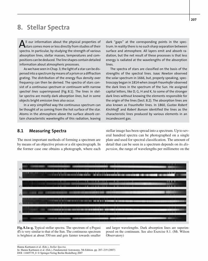
Hannu Karttunen et al. (Eds.), Stellar Spectra.In: Hannu Karttunen et al. (Eds.), Fundamental Astronomy, 5th Edition. pp. 207–219 (2007)DOI: 11685739_8 © Springer-Verlag Berlin Heidelberg 2007
207
8. Stellar Spectra
All our information about the physical properties ofstars comes more or less directly from studies of their
spectra. In particular, by studying the strength of variousabsorption lines, stellar masses, temperatures and com-positions canbededuced. The line shapes containdetailedinformation about atmospheric processes.
As we have seen in Chap. 3, the light of a star can be dis-persed intoaspectrumbymeansofaprismoradiffractiongrating. The distribution of the energy flux density overfrequency can then be derived. The spectra of stars con-sist of a continuous spectrum or continuum with narrowspectral lines superimposed (Fig. 8.1). The lines in stel-lar spectra are mostly dark absorption lines, but in someobjects bright emission lines also occur.
In a very simplified way the continuous spectrum canbe thought of as coming from the hot surface of the star.Atoms in the atmosphere above the surface absorb cer-tain characteristic wavelengths of this radiation, leaving
dark ‘‘gaps’’ at the corresponding points in the spec-trum. In reality there is no such sharp separation betweensurface and atmosphere. All layers emit and absorb ra-diation, but the net result of these processes is that lessenergy is radiated at the wavelengths of the absorptionlines.
The spectra of stars are classified on the basis of thestrengths of the spectral lines. Isaac Newton observedthe solar spectrum in 1666, but, properly speaking, spec-troscopy began in 1814 when Joseph Fraunhofer observedthe dark lines in the spectrum of the Sun. He assignedcapital letters, like D, G, H and K, to some of the strongerdark lines without knowing the elements responsible forthe origin of the lines (Sect. 8.2). The absorption lines arealso known as Fraunhofer lines. In 1860, Gustav RobertKirchhoff and Robert Bunsen identified the lines as thecharacteristic lines produced by various elements in anincandescent gas.
8.1 Measuring Spectra
The most important methods of forming a spectrum areby means of an objective prism or a slit spectrograph. Inthe former case one obtains a photograph, where each
Fig. 8.1a–g. Typical stellar spectra. The spectrum of ηPegasi(f) is very similar to that of the Sun. The continuous spectrumis brightest at about 550 nm and gets fainter towards smaller
and larger wavelengths. Dark absorption lines are superim-posed on the continuum. See also Exercise 8.1. (Mt. WilsonObservatory)
stellar image has been spread into a spectrum. Up to sev-eral hundred spectra can be photographed on a singleplate and used for spectral classification. The amount ofdetail that can be seen in a spectrum depends on its dis-persion, the range of wavelengths per millimetre on the

208
8. Stellar Spectra
plate (or per pixel on a CCD). The dispersion of an ob-jective prism is a few tens of nanometres per millimetre.More detailed observations require a slit spectrograph,which can reach a dispersion 1–0.01 nm/mm. The de-tailed shape of individual spectral lines can then bestudied.
The photograph of the spectrum is converted to anintensity tracing showing the flux density as a functionof wavelength. This is done by means of a microden-sitometer, measuring the amount of light transmitted bythe recorded spectrum. Since the blackening of a pho-tographic plate is not linearly related to the amountof energy it has received, the measured blackeninghas to be calibrated by comparison with known ex-
Fig. 8.2. (a) A section of a photograph of a stellar spectrumand the corresponding rectified microdensitometer intensitytracing. The original spectrum was taken at the Crimean Ob-servatory. (b) A more extensive part of the spectrum. (c) The
picture the intensity curve of the first picture has been rec-tified by normalizing the value of the continuum intensityto one. (Pictures by J. Kyröläinen and H. Virtanen, HelsinkiObservatory)
posures. In modern CCD spectrographs the intensitycurve is determined directly without the interveningstep of a photographic plate. For measurements of linestrengths the spectrum is usually rectified by dividingby the continuum intensity.
Figure 8.2 shows a photograph of the spectrum ofa star and the intensity curve obtained from a calibratedand rectified microdensitometer tracing. The secondpair of pictures shows the intensity curve before andafter the normalisation. The absorption lines appear astroughs of various sizes in the curve. In addition tothe clear and deep lines, there are large numbers ofweaker lines that can barely be discerned. The graini-ness of the photographic emulsion is a source of noise

8.2 The Harvard Spectral Classification
209
which appears as irregular fluctuations of the intensitycurve. Some lines are so close together that they appearblended at this dispersion.
The detailed shape of a spectral line is called theline profile (Sect. 5.3). The true shape of the line re-flects the properties of the stellar atmosphere, but theobserved profile is also spread out by the measuringinstrument. However, the total absorption in the line,usually expressed in terms of the equivalent width, isless sensitive to observational effects (see Fig. 5.6).
The equivalent width of a spectral line depends onhow many atoms in the atmosphere are in a state inwhich they can absorb the wavelength in question. Themore atoms there are, the stronger and broader the spec-tral line is. For example, a typical equivalent widthof a metal line (Fe) in the solar spectrum is about10 pm. Line widths are often expressed in ångströms(1 Å = 10−10 m = 0.1 nm).
Only in weak lines the equivalent width depends lin-early on the number of absorbing atoms. The equivalentwidth as a function of the amount of absorbing atomsis known as the curve of growth. It is, however, beyondthe scope of this book.
Line profiles are also broadened by the Doppler ef-fect. In stellar atmospheres there are motions of smalland large scale, like thermal motion of the atoms andconvective flows.
The chemical composition of the atmosphere can bedetermined from the strengths of the spectral lines. Withthe introduction of large computers it has become fea-sible to construct quite detailed models of the structureof stellar atmospheres, and to compute the emergentspectrum for a given model. The computed syntheticspectrum can be compared with the observations andthe theoretical model modified until a good fit is ob-tained. The theoretical models then give the number ofabsorbing atoms, and hence the element abundances, inthe atmosphere. The construction of model atmosphereswill be discussed in Sect. 8.6.
8.2 The Harvard Spectral Classification
The spectral classification scheme in present use wasdeveloped at Harvard Observatory in the United Statesin the early 20th century. The work was begun by HenryDraper who in 1872 took the first photograph of the
spectrum of Vega. Later Draper’s widow donated theobserving equipment and a sum of money to HarvardObservatory to continue the work of classification.
The main part of the classification was done by AnnieJump Cannon using objective prism spectra. The HenryDraper Catalogue (HD) was published in 1918–1924. Itcontains 225,000 stars extending down to 9 magnitudes.Altogether more than 390,000 stars were classified atHarvard.
The Harvard classification is based on lines that aremainly sensitive to the stellar temperature, rather thanto gravity or luminosity. Important lines are the hydro-gen Balmer lines, the lines of neutral helium, the ironlines, the H and K doublet of ionized calcium at 396.8and 393.3 nm, the G band due to the CH molecule andsome metals around 431 nm, the neutral calcium line at422.7 nm and the lines of titanium oxide (TiO).
The main types in the Harvard classification are de-noted by capital letters. They were initially ordered inalphabetical sequence, but subsequently it was noticedthat they could be ordered according to temperature.With the temperature decreasing towards the right thesequence is
C
O−B−A−F−G−K−M−L−T .
SAdditional notations are Q for novae, P for planetarynebulae and W for Wolf–Rayet stars. The class C con-sists of the earlier types R and N. The spectral classes Cand S represent parallel branches to types G–M, dif-fering in their surface chemical composition. The mostrecent addition are the spectral classes L and T con-tinuing the sequence beyond M, representing browndwarfs. There is a well-known mnemonic for the spec-tral classes, but due to its chauvinistic tone we refuse totell it.
The spectral classes are divided into subclasses de-noted by the numbers 0 . . . 9; sometimes decimals areused, e. g. B 0.5 (Figs. 8.3 and 8.4). Spectra of browndwarfs are shown in Fig. 8.4a compared with those ofM dwarfs.
The main characteristics of the different classes are:
O Blue stars, surface temperature 20,000–35,000 K.Spectrum with lines from multiply ionized atoms,e. g. He II, C III, N III, O III, Si V. He I visible, H Ilines weak.

210
8. Stellar Spectra
Fig. 8.3a,b. Spectra of early and late spectral type stars be-tween 375 and 390 nm. (a) The upper star is Vega, of spectraltype A0, and (b) the lower one is Aldebaran, of spectral type
K5. The hydrogen Balmer lines are strong in the spectrum ofVega; in that of Aldebaran, there are many metal lines. (LickObservatory)
B Blue-white stars, surface temperature about15,000 K. He II lines have disappeared, He I(403 nm) lines are strongest at B2, then get weakerand have disappeared at type B9. The K line of Ca IIbecomes visible at type B3. H I lines getting stronger.O II, Si II and Mg II lines visible.
A White stars, surface temperature about 9000 K. TheH I lines are very strong at A0 and dominate thewhole spectrum, then get weaker. H and K lines ofCa II getting stronger. He I no longer visible. Neutralmetal lines begin to appear.
F Yellow-white stars, surface temperature about7000 K. H I lines getting weaker, H and K of Ca IIgetting stronger. Many other metal lines, e. g. Fe I,Fe II, Cr II, Ti II, clear and getting stronger.
G Yellow stars like the Sun, surface temperature about5500 K. The H I lines still getting weaker, H andK lines very strong, strongest at G0. Metal lines get-ting stronger. G band clearly visible. CN lines seenin giant stars.
K Orange-yellow stars, surface temperature about4000 K. Spectrum dominated by metal lines. H I linesinsignificant. Ca I 422.7 nm clearly visible. Strong Hand K lines and G band. TiO bands become visibleat K5.
M Red stars, surface temperature about 3000 K. TiObands getting stronger. Ca I 422.7 nm very strong.Many neutral metal lines.
L Brown (actually dark red) stars, surface temperatureabout 2000 K. The TiO and VO bands disappear forearly L class. Very strong and broad lines of Na I andK I.
T Brown dwarfs, surface temperature about 1000 K.Very strong molecular absorption bands of CH4 andH2O.
C Carbon stars, previously R and N. Very red stars,surface temperature about 3000 K. Strong molecu-lar bands, e. g. C2, CN and CH. No TiO bands. Linespectrum like in the types K and M.
S Red low-temperature stars (about 3000 K). Very clearZrO bands. Also other molecular bands, e. g. YO,LaO and TiO.
The main characteristics of the classification schemecan be seen in Fig. 8.5 showing the variations of sometypical absorption lines in the different spectral classes.Different spectral features are mainly due to different ef-fective temparatures. Different pressures and chemicalcompositions of stellar atmospheres are not very impor-tant factors in the spectral classification, execpt in somepeculiar stars. The early, i. e. hot, spectral classes arecharacterised by the lines of ionized atoms, whereas thecool, or late, spectral types have lines of neutral atoms.In hot stars molecules dissociate into atoms; thus the ab-sorption bands of molecules appear only in the spectraof cool stars of late spectral types.
To see how the strengths of the spectral lines aredetermined by the temperature, we consider, for exam-ple, the neutral helium lines at 402.6 nm and 447.2 nm.These are only seen in the spectra of hot stars. The rea-son for this is that the lines are due to absorption byexcited atoms, and that a high temperature is requiredto produce any appreciable excitation. As the stellartemperature increases, more atoms are in the requiredexcited state, and the strength of the helium lines in-creases. When the temperature becomes even higher,helium begins to be ionized, and the strength of theneutral helium lines begins to decrease. In a similarway one can understand the variation with temperatureof other important lines, such as the calcium H and K

8.2 The Harvard Spectral Classification
211
Fig. 8.4. (a) Intensitycurves for various spectralclasses showing charac-teristic spectral features.The name of the star andits spectral and luminos-ity class are given next toeach curve, and the mostimportant spectral featuresare identified. (Drawingby J. Dufay) (b) Opticalspectra of M stars andbrown dwarfs. In an ap-proximate sense, the browndwarfs continue the spec-tral sequence towards lowertemperatures, although inmany respects they differfrom the earlier spectraltypes. (J.D. Kirkpatrick2005, ARAA 43, 205)

212
8. Stellar Spectra
Fig. 8.5. Equivalent widthsof some important spec-tral lines in the variousspectral classes. [Struve, O.(1959): Elementary Astron-omy (Oxford UniversityPress, New York) p. 259]
lines. These lines are due to singly ionized calcium,and the temperature must be just right to remove oneelectron but no more.
The hydrogen Balmer lines Hβ, Hγ and Hδ arestongest in the spectral class A2. These lines corre-spond to transitions to the level the principal quantumnumber of which is n = 2. If the temprature is too highthe hydrogen is ionized and such transitions are notpossible.
8.3 The Yerkes Spectral Classification
The Harvard classification only takes into account theeffect of the temperature on the spectrum. For a moreprecise classification, one also has to take into ac-count the luminosity of the star, since two stars withthe same effective temperature may have widely differ-ent luminosities. A two-dimensional system of spectralclassification was introduced by William W. Morgan,Philip C. Keenan and Edith Kellman of Yerkes Obser-vatory. This system is known as the MKK or Yerkesclassification. (The MK classification is a modified,later version.) The MKK classification is based onthe visual scrutiny of slit spectra with a dispersion of11.5 nm/mm. It is carefully defined on the basis of stan-dard stars and the specification of luminosity criteria.Six different luminosity classes are distinguished:
– Ia most luminous supergiants,– Ib less luminous supergiants,
– II luminous giants,– III normal giants,– IV subgiants,– V main sequence stars (dwarfs).
The luminosity class is determined from spectrallines that depend strongly on the stellar surface gravity,which is closely related to the luminosity. The massesof giants and dwarfs are roughly similar, but the radii ofgiants are much larger than those of dwarfs. Thereforethe gravitational acceleration g = G M/R2 at the surfaceof a giant is much smaller than for a dwarf. In conse-quence, the gas density and pressure in the atmosphereof a giant is much smaller. This gives rise to luminos-ity effects in the stellar spectrum, which can be used todistinguish between stars of different luminosities.
1. For spectral types B–F, the lines of neutral hydrogenare deeper and narrower for stars of higher lumi-nosities. The reason for this is that the metal ionsgive rise to a fluctuating electric field near the hydro-gen atoms. This field leads to shifts in the hydrogenenergy levels (the Stark effect), appearing as a broad-ening of the lines. The effect becomes stronger as thedensity increases. Thus the hydrogen lines are nar-row in absolutely bright stars, and become broaderin main sequence stars and even more so in whitedwarfs (Fig. 8.6).
2. The lines from ionized elements are relativelystronger in high-luminosity stars. This is because thehigher density makes it easier for electrons and ionsto recombine to neutral atoms. On the other hand, the

8.4 Peculiar Spectra
213
Fig. 8.6. Luminosity effects inthe hydrogen Hγ line in A stars.The vertical axis gives the nor-malized intensity. HD 223385(upper left) is an A2 supergiant,where the line is very weak,θ Aurigae A is a giant star andα2 Geminorum is a main se-quence star, where the line isvery broad. [Aller, L.H. (1953):Astrophysics. The Atmospheresof the Sun and Stars(The Ronald Press Company,New York) p. 318]
rate of ionization is essentially determined by the ra-diation field, and is not appreciably affected by thegas density. Thus a given radiation field can main-tain a higher degree of ionization in stars with moreextended atmospheres. For example, in the spectralclasses F–G, the relative strengths of the ionizedstrontium (Sr II) and neutral iron (Fe I) lines can beused as a luminosity indicator. Both lines depend onthe temperature in roughly the same way, but the Sr IIlines become relatively much stronger as the lumi-nosity increases.
3. Giant stars are redder than dwarfs of the same spec-tral type. The spectral type is determined from thestrengths of spectral lines, including ion lines. Sincethese are stronger in giants, a giant will be cooler,and thus also redder, than a dwarf of the same spec-tral type.
4. There is a strong cyanogen (CN) absorption bandin the spectra of giant stars, which is almost totallyabsent in dwarfs. This is partly a temperature ef-fect, since the cooler atmospheres of giants are moresuitable for the formation of cyanogen.

214
8. Stellar Spectra
8.4 Peculiar Spectra
The spectra of some stars differ from what one wouldexpect on the basis of their temperature and luminos-ity (see, e. g., Fig. 8.7). Such stars are celled peculiar.The most common peculiar spectral types will now beconsidered.
The Wolf–Rayet stars are very hot stars; the first ex-amples were discovered by Charles Wolf and GeorgesRayet in 1867. The spectra of Wolf–Rayet stars havebroad emission lines of hydrogen and ionized helium,carbon, nitrogen and oxygen. There are hardly any ab-sorption lines. The Wolf–Rayet stars are thought to bevery massive stars that have lost their outer layers ina strong stellar wind. This has exposed the stellar in-terior, which gives rise to a different spectrum thanthe normal outer layers. Many Wolf–Rayet stars aremembers of binary systems.
In some O and B stars the hydrogen absorption lineshave weak emission components either at the line centreor in its wings. These stars are called Be and shell stars(the letter e after the spectral type indicates that there areemission lines in the spectrum). The emission lines areformed in a rotationally flattened gas shell around thestar. The shell and Be stars show irregular variations,apparently related to structural changes in the shell.
Fig. 8.7a,b. Peculiar spectra. (a) R Geminorum (above) isan emission line star, with bright emission lines, indicatedby arrows, in its spectrum; (b) the spectrum of a normal
star is compared with one in which the zirconium linesare unusually strong. (Mt. Wilson Observatory and HelsinkiObservatory)
About 15% of all O and B stars have emission lines intheir spectra.
The strongest emission lines are those of the P Cygnistars, which have one or more sharp absorption lineson the short wavelength side of the emission line. Itis thought that the lines are formed in a thick expand-ing envelope. The P Cygni stars are often variable. Forexample, P Cygni itself has varied between three andsix magnitudes during the past centuries. At present itsmagnitude is about 5.
The peculiar A stars or Ap stars (p = peculiar) areusually strongly magnetic stars, where the lines aresplit into several components by the Zeeman effect. Thelines of certain elements, such as magnesium, silicon,europium, chromium and strontium, are exceptionallystrong in the Ap stars. Lines of rarer elements such asmercury, gallium or krypton may also be present. Other-wise, the Ap stars are like normal main sequence stars.
The Am stars (m = metallic) also have anomalouselement abundances, but not to the same extent as theAp stars. The lines of e. g. the rare earths and the heaviestelements are strong in their spectra; those of calcium andscandium are weak.
We have already mentioned the S and C stars, whichare special classes of K and M giants with anoma-lous element abundances. In the S stars, the normal

8.5 The Hertzsprung--Russell Diagram
215
lines of titanium, scandium and vanadium oxide arereplaced with oxides of heavier elements, zirconium,yttrium and barium. A large fraction of the S starsare irregular variables. The name of the C stars refersto carbon. The metal oxide lines are almost com-pletely absent in their spectra; instead, various carboncompounds (CN, C2, CH) are strong. The abundanceof carbon relative to oxygen is 4–5 times greater inthe C stars than in normal stars. The C stars aredivided into two groups, hotter R stars and coolerN stars.
Another type of giant stars with abundance anomaliesare the barium stars. The lines of barium, strontium, rareearths and some carbon compounds are strong in theirspectra. Apparently nuclear reaction products have beenmixed up to the surface in these stars.
Fig. 8.8. The Hertzsprung–Russell diagram. Thehorizontal coordinate canbe either the colour indexB − V , obtained directlyfrom observations, or thespectral class. In theoreticalstudies the effective tem-perature Te is commonlyused. These correspondto each other but thedependence varies some-what with luminosity. Thevertical axis gives theabsolute magnitude. Ina (lg(L/L), lg Te) plotthe curves of constant ra-dius are straight lines. Thedensest areas are the mainsequence and the horizon-tal, red giant and asymptoticbranches consisting of gi-ant stars. The supergiantsare scattered above the gi-ants. To the lower left aresome white dwarfs about10 magnitudes below themain sequence. The appar-ently brightest stars (m < 4)are marked with crosses andthe nearest stars (r < 50 ly)with dots. The data are fromthe Hipparcos catalogue
8.5 The Hertzsprung--Russell Diagram
Around 1910, Ejnar Hertzsprung and Henry NorrisRussell studied the relation between the absolute mag-nitudes and the spectral types of stars. The diagramshowing these two variables is now known as theHertzsprung–Russell diagram or simply the HR dia-gram (Fig. 8.8). It has turned out to be an important aidin studies of stellar evolution.
In view of the fact that stellar radii, luminosities andsurface temperatures vary widely, one might have ex-pected the stars to be uniformly distributed in the HRdiagram. However, it is found that most stars are lo-cated along a roughly diagonal curve called the mainsequence. The Sun is situated about the middle of themain sequence.

216
8. Stellar Spectra
The HR diagram also shows that the yellow andred stars (spectral types G-K-M) are clustered into twoclearly separate groups: the main sequence of dwarfstars and the giants. The giant stars fall into severaldistinct groups. The horizontal branch is an almost hor-izontal sequence, about absolute visual magnitude zero.The red giant branch rises almost vertically from themain sequence at spectral types K and M in the HR di-agram. Finally, the asymptotic branch rises from thehorizontal branch and approaches the bright end of thered giant branch. These various branches represent dif-ferent phases of stellar evolution (c. f. Sects. 11.3 and11.4): dense areas correspond to evolutionary stages inwhich stars stay a long time.
A typical horizontal branch giant is about a hundredtimes brighter than the Sun. Since giants and dwarfsof the same spectral class have nearly the same surfacetemperature, the difference in luminosity must be due toa difference in radius according to (5.21). For exampleArcturus, which is one of the brightest stars in the sky,has a radius about thirty times that of the Sun.
The brightest red giants are the supergiants with mag-nitudes up to MV = −7. One example is Betelgeuze. inOrion, with a radius of 400 solar radii and 20,000 timesmore luminous than the Sun.
About 10 magnitudes below the main sequence arethe white dwarfs. They are quite numerous in space, butfaint and difficult to find. The best-known example isSirius B, the companion of Sirius.
There are some stars in the HR diagram whichare located below the giant branch, but still clearlyabove the main sequence. These are known as sub-giants. Similarly, there are stars below the mainsequence, but brighter than the white dwarfs, knownas subdwarfs.
When interpreting the HR diagram, one has to takeinto account selection effects: absolutely bright starsare more likely to be included in the sample, sincethey can be discovered at greater distances. If onlystars within a certain distance from the Sun are in-cluded, the distribution of stars in the HR diagramlooks quite different. This can be seen in Fig. 8.8:there are no giant or bright main sequence stars amongthese.
The HR diagrams of star clusters are particularlyimportant for the theory of stellar evolution. They willbe discussed in Chap. 16.
8.6 Model Atmospheres
The stellar atmosphere consists of those layers of thestar where the radiation that is transmitted directly tothe observer originates. Thus in order to interpret stellarspectra, one needs to be able to compute the structureof the atmosphere and the emerging radiation.
In actual stars there are many factors, such as rota-tion and magnetic fields, that complicate the problemof computing the structure of the atmosphere. We shallonly consider the classical problem of finding the struc-ture, i. e. the distribution of pressure and temperaturewith depth, in a static, unmagnetized atmosphere. Inthat case a model atmosphere is completely specifiedby giving the chemical composition, the gravitationalacceleration at the surface, g, and the energy fluxfrom the stellar interior, or equivalently, the effectivetemperature Te.
The basic principles involved in computing a modelstellar atmosphere are the same as for stellar interiorsand will be discussed in Chap. 10. Essentially, there aretwo differential equations to be solved: the equation ofhydrostatic equilibrium, which fixes the distribution ofpressure, and an equation of energy transport, which willhave a different form depending on whether the atmo-sphere is radiative or convective, and which determinesthe temperature distribution.
The values of the various physical quantities in anatmosphere are usually given as functions of somesuitably defined continuum optical depth τ . Thus pres-sure, temperature, density, ionization and the populationnumbers of various energy levels can all be obtainedas functions of τ . When these are known, the inten-sity of radiation emerging from the atmosphere can becomputed. In *The Intensity Emerging from a StellarAtmosphere (p. 218), it is shown that approximatelythe emergent spectrum originates at unit optical depth,measured along each light ray. On this basis, one canpredict whether a given spectral line will be present inthe spectrum.
Consider a spectral line formed when an atom (orion) in a given energy state absorbs a photon. Fromthe model atmosphere, the occupation number of theabsorbing level is known as a function of the (con-tinuum) optical depth τ . If now there is a layer abovethe depth τ = 1 where the absorbing level has a high oc-cupancy, the optical depth in the line will become unity

8.7 What Do the Observations Tell Us?
217
before τ = 1, i. e. the radiation in the line will origi-nate higher in the atmosphere. Because the temperatureincreases inwards, the intensity in the line will corre-spond to a lower temperature, and the line will appeardark. On the other hand, if the absorbing level is un-occupied, the optical depth at the line frequency willbe the same as the continuum optical depth. The radia-tion at the line frequency will then come from the samedepth as the adjacent continuum, and no absorption linewill be formed.
The expression for the intensity derived in *The In-tensity Emerging from a Stellar Atmosphere (p. 218)also explains the phenomenon of limb darkening seenin the Sun (Sect. 12.2). The radiation that reaches usfrom near the edge of the solar disc emerges at a veryoblique angle (θ near 90), i. e. cos θ is small. Thus thisradiation originates at small values of τ , and hence atlow temperatures. In consequence, the intensity com-ing from near the edge will be lower, and the solar discwill appear darker towards the limb. The amount oflimb darkening also gives an empirical way of deter-mining the temperature distribution in the solar atmo-sphere.
Our presentation of stellar atmospheres has beenhighly simplified. In practice, the spectrum is computednumerically for a range of parameter values. The val-ues of Te and element abundances for various stars canthen be found by comparing the observed line strengthsand other spectral features with the theoretical ones. Weshall not go into details on the procedures used.
8.7 What Do the Observations Tell Us?
To conclude this chapter, we shall give a summary ofthe properties of stars revealed by the observations. Atthe end of the book, there are tables of the brightest andof the nearest stars.
Of the brightest stars, four have a negative magnitude.Some of the apparently bright stars are absolutely brightsupergiants, others are simply nearby.
In the list of the nearest stars, the dominance of faintdwarf stars, already apparent in the HR diagram, isworth noting. Most of these belong to the spectral typesK and M. Some nearby stars also have very faint com-panions with masses about that of Jupiter, i. e. planets.They have not been included in the table.
Stellar spectroscopy offers an important way of de-termining fundamental stellar parameters, in particularmass and radius. However, the spectral informationneeds to be calibrated by means of direct measurementsof these quantities. These will be considered next.
The masses of stars can be determined in the caseof double stars orbiting each other. (The details of themethod will be discussed in Chap. 9.) These observa-tions have shown that the larger the mass of a mainsequence star becomes, the higher on the main se-quence it is located. One thus obtains an empiricalmass–luminosity relation, which can be used to estimatestellar masses on the basis of the spectral type.
The observed relation between mass and luminos-ity is shown in Fig. 8.9. The luminosity is roughlyproportional to the power 3.8 of the mass:
L ∝ M3.8 . (8.1)
The relations is only approximate. According to it, a tensolar mass star is about 6300 times brighter than theSun, corresponding to 9.5 magnitudes.
The smallest observed stellar masses are about 1/20of the solar mass, corresponding to stars in the lowerright-hand part of the HR diagram. The masses of whitedwarfs are less than one solar mass. The masses of themost massive main sequence and supergiant stars arebetween 10 and possibly even 150 M.
Direct interferometric measurements of stellar an-gular diameters have been made for only a few dozenstars. When the distances are known, these immediatelyyield the value of the radius. In eclipsing binaries, theradius can also be directly measured (see Sect. 9.4). Al-together, close to a hundred stellar radii are known fromdirect measurements. In other cases, the radius mustbe estimated from the absolute luminosity and effectivetemperature.
In discussing stellar radii, it is convenient to usea version of the HR diagram with lg Te on the hori-zontal and Mbol or lg(L/L) on the vertical axis. Ifthe value of the radius R is fixed, then (5.21) yieldsa linear relation between the bolometric magnitude andlg Te. Thus lines of constant radius in the HR diagramare straight. Lines corresponding to various values ofthe radius are shown in Fig. 8.8. The smallest stars arethe white dwarfs with radii of about one per cent ofthe solar radius, whereas the largest supergiants have

218
8. Stellar Spectra
Fig. 8.9. Mass–luminosity relation. The picture is based on bi-naries with known masses. Different symbols refer to differentkinds of binaries. (From Böhm-Vitense: Introduction to StellarAstrophysics, Cambridge University Press (1989–1992))
radii several thousand times larger than the Sun. Notincluded in the figure are the compact stars (neutronstars and black holes) with typical radii of a few tens ofkilometres.
Since the stellar radii vary so widely, so do the den-sities of stars. The density of giant stars may be only10−4 kg/m3, whereas the density of white dwarfs isabout 109 kg/m3.
The range of values for stellar effective temper-atures and luminosities can be immediately seen in
the HR diagram. The range of effective temperatureis 2,000–40,000 K, and that of luminosity 10−4–106
L.The rotation of stars appears as a broadening of the
spectral lines. One edge of the stellar disc is approach-ing us, the other edge is receding, and the radiationfrom the edges is Doppler shifted accordingly. Therotational velocity observed in this way is only thecomponent along the line of sight. The true velocityis obtained by dividing with sin i, where i is the an-gle between the line of sight and the rotational axis.A star seen from the direction of the pole will show norotation.
Assuming the axes of rotation to be randomly ori-ented, the distribution of rotational velocities can bestatistically estimated. The hottest stars appear to rotatefaster than the cooler ones. The rotational velocity at theequator varies from 200–250 km/s for O and B stars toabout 20 km/s for spectral type G. In shell stars, therotational velocity may reach 500 km/s.
The chemical composition of the outer layers is de-duced from the strengths of the spectral lines. Aboutthree-fourths of the stellar mass is hydrogen. Heliumcomprises about one-fourth, and the abundance of otherelements is very small. The abundance of heavy ele-ments in young stars (about 2%) is much larger than inold ones, where it is less than 0.02%.
* The Intensity Emergingfrom a Stellar Atmosphere
The intensity of radiation emerging from an atmosphereis given by the expression (5.45), i. e.
Iν(0, θ)=∞∫
0
Sν(τν) e−τν sec θ sec θ dτν . (8.2)
If a model atmosphere has been computed, the sourcefunction Sν is known.
An approximate formula for the intensity can be de-rived as follows. Let us expand the source function asa Taylor series about some arbitrary point τ∗, thus
Sν = Sν(τ∗)+ (τν − τ∗)S′
ν(τ∗)+ . . .
where the dash denotes a derivative. With this ex-pression, the integral in (8.2) can be evaluated,

8.8 Exercise
219
yielding
Iν(0, θ)= Sν(τ∗)+ (cos θ− τ∗)S′
ν(τ∗)+ . . . .
If we now choose τ∗ = cos θ, the second term willvanish. In local thermodynamic equilibrium the sourcefunction will be the Planck function Bν(T ). We thusobtain the Eddington–Barbier approximation
Iν(0, θ)= Bν(T [τν = cos θ]) .
According to this expression, the radiation emerging ina given direction originated at unit optical depth alongthat direction.
8.8 Exercise
Exercise 8.1 Arrange the spectra in Fig. 8.1 in theorder of decreasing temperature.

Hannu Karttunen et al. (Eds.), Binary Stars and Stellar Masses.In: Hannu Karttunen et al. (Eds.), Fundamental Astronomy, 5th Edition. pp. 221–227 (2007)DOI: 11685739_9 © Springer-Verlag Berlin Heidelberg 2007
221
9. Binary Stars and Stellar Masses
Quite often, two stars may appear to be close togetherin the sky, although they are really at very different
distances. Such chance pairs are called optical binary stars.However, many close pairs of stars really are at the samedistance and form a physical system in which two starsare orbiting around each other. Less than half of all starsare single stars like the Sun. More than 50 % belong tosystems containing two or more members. In general, themultiple systems have a hierarchical structure: a star anda binary orbiting around each other in triple systems, twobinaries orbiting around each other in quadruple systems.Thus most multiple systems can be described as binarieswith several levels.
Binaries are classified on the basis of the method oftheir discovery. Visual binaries can be seen as two sepa-rate components, i. e. the separation between the stars islarger than about 0.1 arc seconds. The relative position ofthe components changes over the years as they move intheir orbits (Fig. 9.1). In astrometric binary stars only onecomponent is seen, but its variable proper motion showsthat a second invisible component must be present. Thespectroscopic binary stars are discovered on the basis of
their spectra. Either two sets of spectral lines are seen orelse the Doppler shift of the observed lines varies period-ically, indicating an invisible companion. The fourth classof binaries are the photometric binary stars or eclipsingvariables. In these systems the components of the pairregularly pass in front of each other, causing a change inthe total apparent magnitude.
Binary stars can also be classified on the basis oftheir mutual separation. In distant binaries the separa-tion between the components is tens or hundreds ofastronomical units and their orbital periods are from tensto thousands of years. In close binaries the separation isfrom about one AU down to the radius of the stars. Theorbital period ranges from a few hours to a few years. Thecomponents of contact binaries are so close that they aretouching each other.
The stars in a binary system move in an elliptical or-bit around the centre of mass of the system. In Chap. 6it was shown that the relative orbit, too, is an ellipse,and thus the observations are often described as if onecomponent remained stationary and the other orbitedaround it.
Fig. 9.1. When a visual binary is followed for a long time, the components can be seen to move with respect to each other.Picture of Krüger 60. (Yerkes Observatory)

222
9. Binary Stars and Stellar Masses
9.1 Visual Binaries
We consider a visual binary, assuming initially that thebrighter primary component is stationary and the faintersecondary component is orbiting around it. The angu-lar separation of the stars and the angular direction tothe secondary can be directly observed. Making use ofobservations extending over many years or decades, therelative orbit of the secondary can be determined. Thefirst binary orbit to be determined was that of ξ UMa in1830 (Fig. 9.2).
The observations of visual binaries only give the pro-jection of the relative orbital ellipse on the plane of thesky. The shape and position of the true orbit are notknown. However, they can be calculated if one makesuse of the fact that the primary should be located ata focal point of the relative orbit. The deviation ofthe projected position of the primary from the focusof the projected relative orbit allows one to determinethe orientation of the true orbit.
The absolute size of the orbit can only be found ifthe distance of the binary is known. Knowing this, thetotal mass of the system can be calculated from Kepler’sthird law.
The masses of the individual components can be de-termined by observing the motions of both componentsrelative to the centre of mass (Fig. 9.3). Let the semi-major axes of the orbital ellipses of the primary and thesecondary be a1 and a2. Then, according to the definitionof the centre of mass,
a1
a2= m2
m1, (9.1)
Fig. 9.2. In 1830 the orbit of ξ Ursae Majoris was the firstbinary orbit determined observationally
Fig. 9.3. The components of a binary system move aroundtheir common centre of mass. A1, A2 denote the positions ofthe stars at a given time A, and similarly for B and C
where m1 and m2 are the component masses. Thesemimajor axis of the relative orbit is
a = a1 +a2 . (9.2)
For example, the masses of the components of ξ UMahave been found to be 1.3 and 1.0 solar masses.
9.2 Astrometric Binary Stars
In astrometric binaries, only the orbit of the brightercomponent about the centre of mass can be observed.If the mass of the visible component is estimated, e. g.from its luminosity, the mass of the invisible companioncan also be estimated.
The first astrometric binary was Sirius, which inthe 1830’s was observed to have an undulating propermotion. It was concluded that it had a small compan-ion, which was visually discovered a few decades later(Figs. 9.4 and 14.1). The companion, Sirius B, wasa completely new type of object, a white dwarf.
The proper motions of nearby stars have beencarefully studied in the search for planetary systems.Although e.g. Barnard’s star may have unseen compan-ions, the existence of planetary systems around otherstars was not established by proper motion studies butwith spectroscopic observations (see below).
9.3 Spectroscopic Binaries
The spectroscopic binaries (Fig. 9.5) appear as singlestars in even the most powerful telescopes, but their

9.3 Spectroscopic Binaries
223
Fig. 9.4. The apparent pathsof Sirius and its companionin the sky
spectra show a regular variation. The first spectroscopicbinary was discovered in the 1880’s, when it was foundthat the spectral lines of ζ UMa or Mizar split into twoat regular intervals.
The Doppler shift of a spectral line is directly propor-tional to the radial velocity. Thus the separation of thespectral lines is largest when one component is directlyapproaching and the other is receding from the observer.The period of the variation is the orbital period of thestars. Unfortunately, there is no general way of deter-mining the position of the orbit in space. The observedvelocity v is related to the true velocity v0 according to
v= v0 sin i , (9.3)
where the inclination i is the angle between the line ofsight and the normal of the orbital plane.
Fig. 9.5. Spectrum of the spectroscopic binary κArietis. In the upper spectrum the spectral lines are single, in the lower onedoubled. (Lick Observatory)
Consider a binary where the components move incircular orbits about the centre of mass. Let the radiiof the orbits be a1 and a2. From the definition of thecentre of mass m1a1 = m2a2, and writing a = a1 +a2,one obtains
a1 = am2
m1 +m2. (9.4)
The true orbital velocity is
v0,1 = 2πa1
P,
where P is the orbital period. The observed orbitalvelocity according to (9.3) is thus
v1 = 2πa1 sin i
P. (9.5)
224
9. Binary Stars and Stellar Masses
Substituting (9.4), one obtains
v1 = 2πa
P
m2 sin i
m1 +m2.
Solving for a and substituting it in Kepler’s third law,one obtains the mass function equation:
m32 sin3 i
(m1 +m2)2= v3
1 P
2πG. (9.6)
If one component in a spectroscopic binary is so faintthat its spectral lines cannot be observed, only P and v1
are observed. Equation (9.6) then gives the value of themass function, which is the expression on the left-handside. Neither the masses of the components nor the totalmass can be determined. If the spectral lines of bothcomponents can be observed, v2 is also known. Then(9.5) gives
v1
v2= a1
a2
and furthermore the definition of the centre of massgives
m1 = m2v2
v1.
When this is substituted in (9.6), the value of m2 sin3 i,and correspondingly, m1 sin3 i, can be determined.However, the actual masses cannot be found withoutknowing the inclination.
The size of the binary orbit (the semimajor axis a)is obtained from (9.5) apart from a factor sin i. In gen-eral the orbits of binary stars are not circular and thepreceding expressions cannot be applied as they stand.For an eccentric orbit, the shape of the velocity varia-tion departs more and more from a simple sine curve asthe eccentricity increases. From the shape of the veloc-ity variation, both the eccentricity and the longitude ofthe periastron can be determined. Knowing these, themass function or the individual masses can again bedetermined to within a factor sin3 i.
From accurate studies of the spectra of nearby stars,several planet-sized companions have been found. Inthe years 1995–2002, about 100 extrasolar planets wereobserved, with masses in the range of 0.1 up to 13 Jupitermasses.
9.4 Photometric Binary Stars
In the photometric binaries, a periodic variation in thetotal brightness is caused by the motions of the com-ponents in a double system. Usually the photometricbinaries are eclipsing variables, where the brightnessvariations are due to the components passing in front ofeach other. A class of photometric binaries where thereare no actual eclipses are the ellipsoidal variables. Inthese systems, at least one of the components has beendistorted into an ellipsoidal shape by the tidal pull ofthe other one. At different phases of the orbit, the pro-jected surface area of the distorted component varies.The surface temperature will also be lower at the endsof the tidal bulges. Together these factors cause a smallvariation in brightness.
The inclination of the orbit of an eclipsing binarymust be very close to 90. These are the only spectro-scopic binaries for which the inclination is known andthus the masses can be uniquely determined.
The variation of the magnitude of eclipsing variablesas a function of time is called the lightcurve. Accordingto the shape of the lightcurve, they are grouped intothree main types: Algol, β Lyrae and W Ursae Majoristype (Fig. 9.6).
Algol Stars. The Algol-type eclipsing variables havebeen named after β Persei or Algol. During most ofthe period, the lightcurve is fairly constant. This corre-sponds to phases during which the stars are seen separatefrom each other and the total magnitude remains con-stant. There are two different minima in the lightcurve,one of which, the primary minimum, is usually muchdeeper than the other one. This is due to the bright-ness difference of the stars. When the larger star, whichis usually a cool giant, eclipses the smaller and hottercomponent, there is a deep minimum in the lightcurve.When the small, bright star passes across the disc of thegiant, the total magnitude of the system does not changeby much.
The shape of the minima depends on whether theeclipses are partial or total. In a partial eclipse thelightcurve is smooth, since the brightness changessmoothly as the depth of the eclipse varies. In a totaleclipse there is an interval during which one componentis completely invisible. The total brightness is then con-stant and the lightcurve has a flat bottomed minimum.

9.4 Photometric Binary Stars
225
Fig. 9.6. Typical lightcurves and schematic views of Algol,β Lyrae and W Ursae Majoris type binary systems. The sizeof the Sun is shown for comparison
The shape of the minima in Algol variables thus givesinformation on the inclination of the orbit.
The duration of the minima depends on the ratioof the stellar radii to the size of the orbit. If the staris also a spectroscopic binary, the true dimensions of
the orbit can be obtained. In that case the masses andthe size of the orbit, and thus also the radii can bedetermined without having to know the distance of thesystem.
βLyrae Stars. In the β Lyrae-type binaries, the totalmagnitude varies continuously. The stars are so closeto each other that one of them has been pulled into el-lipsoidal shape. Thus the brightness varies also outsidethe eclipses. The β Lyrae variables can be describedas eclipsing ellipsoidal variables. In the β Lyrae sys-tem itself, one star has overfilled its Roche lobe (seeSect. 11.6) and is steadily losing mass to its compan-ion. The mass transfer causes additional features in thelightcurve.
W UMa Stars. In W UMa stars, the lightcurve minimaare almost identical, very round and broad. These areclose binary systems where both components overfilltheir Roche lobes, forming a contact binary system.
The observed lightcurves of photometric binariesmay contain many additional features that confuse thepreceding classification.
– The shape of the star may be distorted by the tidalforce of the companion. The star may be ellipsoidalor fill its Roche surface, in which case it becomesdrop-like in shape.
– The limb darkening (Sects. 8.6 and 12.2) of the starmay be considerable. If the radiation from the edgesof the stellar disc is fainter than that from the centre,it will tend to round off the lightcurve.
– In elongated stars there is gravity darkening: the partsmost distant from the centre are cooler and radiateless energy.
– There are also reflection phenomena in stars. If thestars are close together, they will heat the sides facingeach other. The heated part of the surface will thenbe brighter.
– In systems with mass transfer, the material fallingonto one of the components will change the surfacetemperature.
All these additional effects cause difficulties ininterpreting the lightcurve. Usually one computes a the-oretical model and the corresponding lightcurve, whichis then compared with the observations. The model isvaried until a satisfactory fit is obtained.

226
9. Binary Stars and Stellar Masses
So far we have been concerned solely with the prop-erties of binary systems in the optical domain. Recentlymany double systems that radiate strongly at other wave-lengths have been discovered. Particularly interestingare the binary pulsars, where the velocity variationcan be determined from radio observations. Many dif-ferent types of binaries have also been discovered atX-ray wavelengths. These systems will be discussed inChap. 14.
The binary stars are the only stars with accuratelyknown masses. The masses for other stars are estimatedfrom the mass-luminosity relation (Sect. 8.7), but thishas to be calibrated by means of binary observations.
9.5 Examples
Example 9.1 The Mass of a Binary Star
The distance of a binary star is 10 pc and the largest an-gular separation of the components is 7′′ and the smallestis 1′′. The orbital period is 100 years. The mass of the bi-nary is to be determined, assuming that the orbital planeis normal to the line of sight.
From the angular separation and the distance, thesemimajor axis is
a = 4′′ ×10 pc = 40 AU .
According to Kepler’s third law
m1 +m2 = a3
P2= 403
1002M = 6.4 M .
Let the semimajor axis of one component be a1 = 3′′ andfor the other a2 = 1′′. Now the masses of the componentscan be determined separately:
m1a1 = m2a2 ⇒ m1 = a2
a1m2 = m2
3,
m1 +m2 = 6.4 ⇒ m1 = 1.6 , m2 = 4.8 .
Example 9.2 The Lightcurve of a Binary
Let us suppose that the line of sight lies in the orbitalplane of an Algol type binary, where both componentshave the same radius. The lightcurve is essentially asshown in the figure. The primary minimum occurs whenthe brighter component is eclipsed. The depth of theminima will be calculated.
If the effective temperatures of the stars are TA andTB and their radius is R, their luminosities are given by
L A = 4πR2σT 4A , L B = 4πR2σT 4
B .
The flat part of the curve corresponds to the totalluminosity
L tot = L A + L B .
The luminosities may be expressed as absolute bolomet-ric magnitudes by means of (4.13). Since the distancemoduli of the components are the same, the apparentbolometric magnitude at the primary minimum will be
m A −mtot = MA − Mtot
= −2.5 lgL A
L tot= +2.5 lg
L tot
L A
= 2.5 lg4πR2σT 4
A +4πR2σT 4B
4πR2σT 4A
= 2.5 lg
(1+
(TB
TA
)4).
Similarly the depth of the secondary minimum is
m B −mtot = 2.5 lg
(1+
(TA
TB
)4).
Let the effective temperatures of the stars beTA = 5,000 K and TB = 12,000 K. The depth of theprimary minimum is then
m A −mtot = 2.5 lg
(1+
(12,000
5,000
)4)
≈ 3.8 mag .

9.6 Exercises
227
The secondary minimum is
m B −mtot = 2.5 lg
(1+
(5000
12000
)4)
≈ 0.03 mag .
9.6 Exercises
Exercise 9.1 The components of a binary move alongcircular orbits. The mutual distance is 1 AU, and themass of each component is 1 M. An observer in theplane of the orbit will see periodic splitting of thespectral lines. What is the maximum separation of thecomponents of the Hγ line.
Exercise 9.2 A planet (mass m) is orbiting a star(mass M) at a distance a. The distance of the star fromthe centre of gravity of the system is a′. Show that
MP2 = a2 (a −a′) ,
where P is period in years, distances are in AU’s andmasses in solar masses.
Exercise 9.3 The distance of Barnard’s star is 1.83 pcand mass 0.135 M. It has been suggested that it oscil-lates with an amplitude of 0.026′′ in 25 year periods.Assuming this oscillation is caused by a planet, find themass and radius of the orbit of this planet.

Hannu Karttunen et al. (Eds.), Stellar Structure.In: Hannu Karttunen et al. (Eds.), Fundamental Astronomy, 5th Edition. pp. 229–242 (2007)DOI: 11685739_10 © Springer-Verlag Berlin Heidelberg 2007
229
10. Stellar Structure
The stars are huge gas spheres, hundreds of thou-sands or millions of times more massive than the
Earth. A star such as the Sun can go on shining steadilyfor thousands of millions of years. This is shown by stud-ies of the prehistory of the Earth, which indicate that theenergyradiatedbytheSunhasnotchangedbymuchdur-ing the last four thousand million years. The equilibriumof a star must remain stable for such periods.
10.1 Internal Equilibrium Conditions
Mathematically the conditions for the internal equilib-rium of a star can be expressed as four differentialequations governing the distribution of mass, gas pres-sure and energy production and transport in the star.These equations will now be derived.
Hydrostatic Equilibrium. The force of gravity pullsthe stellar material towards the centre. It is resisted bythe pressure force due to the thermal motions of the gasmolecules. The first equilibrium condition is that theseforces be in equilibrium.
Consider a cylindrical volume element at the distancer from the centre of the star (Fig. 10.1). Its volume isdV = d A dr, where d A is its base area and dr its height;its mass is dm = ρ d A dr, where ρ = ρ(r) is the gasdensity at the radius r. If the mass inside radius r is Mr ,the gravitational force on the volume element will be
dFg = −G Mr dm
r2= −G Mrρ
r2d A dr ,
where G is the gravitational constant. The minus sign inthis expression means that the force is directed towardsthe centre of the star. If the pressure at the lower surfaceof the volume element is P and at its upper surfaceP +d P, the net force of pressure acting on the elementis
dFp = P d A − (P +d P)d A
= −dP d A .
Fig. 10.1. In hydrostatic equilibrium the sum of the gravi-tational and pressure force acting on a volume element iszero
Since the pressure decreases outwards, dP will benegative and the force dFp positive. The equilibriumcondition is that the total force acting on the volumeelement should be zero, i. e.
0 = dFg +dFp
= −G Mrρ
r2d A dr −d P d A
or
dP
dr= −G Mrρ
r2. (10.1)
This is the equation of hydrostatic equilibrium.
Mass Distribution. The second equation gives the masscontained within a given radius. Consider a sphericalshell of thickness dr at the distance r from the centre(Fig. 10.2). Its mass is
dMr = 4πr2ρ dr ,
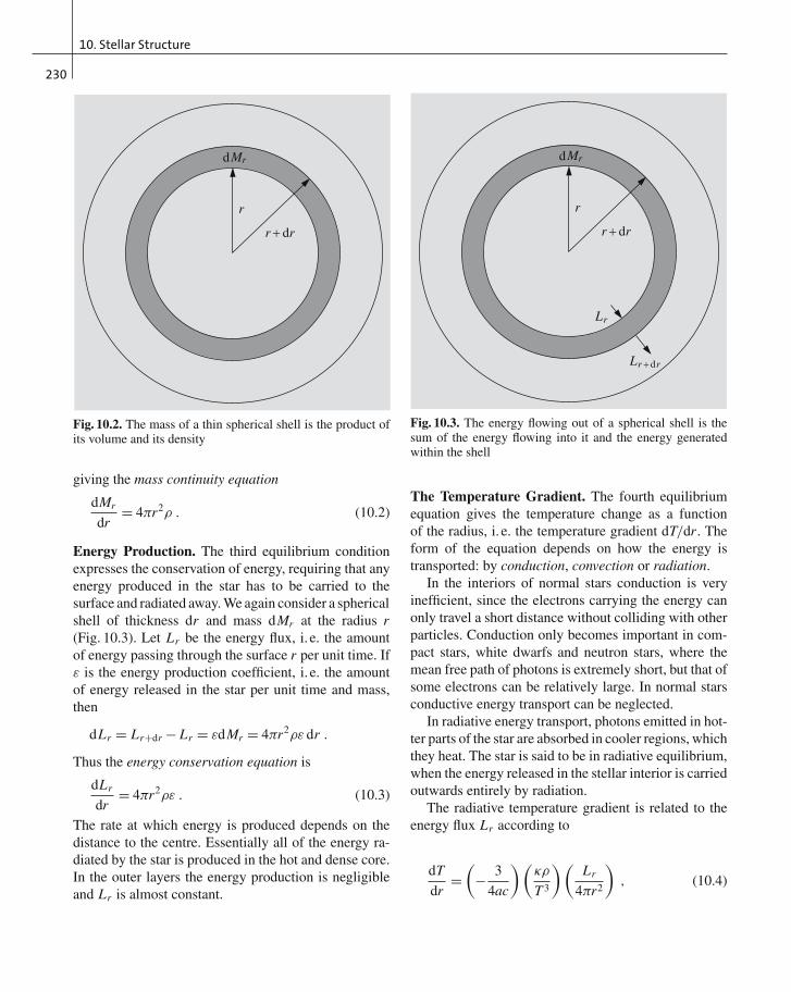
230
10. Stellar Structure
Fig. 10.2. The mass of a thin spherical shell is the product ofits volume and its density
giving the mass continuity equation
dMr
dr= 4πr2ρ . (10.2)
Energy Production. The third equilibrium conditionexpresses the conservation of energy, requiring that anyenergy produced in the star has to be carried to thesurface and radiated away. We again consider a sphericalshell of thickness dr and mass dMr at the radius r(Fig. 10.3). Let Lr be the energy flux, i. e. the amountof energy passing through the surface r per unit time. Ifε is the energy production coefficient, i. e. the amountof energy released in the star per unit time and mass,then
dLr = Lr+dr − Lr = εdMr = 4πr2ρε dr .
Thus the energy conservation equation is
dLr
dr= 4πr2ρε . (10.3)
The rate at which energy is produced depends on thedistance to the centre. Essentially all of the energy ra-diated by the star is produced in the hot and dense core.In the outer layers the energy production is negligibleand Lr is almost constant.
Fig. 10.3. The energy flowing out of a spherical shell is thesum of the energy flowing into it and the energy generatedwithin the shell
The Temperature Gradient. The fourth equilibriumequation gives the temperature change as a functionof the radius, i. e. the temperature gradient dT/dr. Theform of the equation depends on how the energy istransported: by conduction, convection or radiation.
In the interiors of normal stars conduction is veryinefficient, since the electrons carrying the energy canonly travel a short distance without colliding with otherparticles. Conduction only becomes important in com-pact stars, white dwarfs and neutron stars, where themean free path of photons is extremely short, but that ofsome electrons can be relatively large. In normal starsconductive energy transport can be neglected.
In radiative energy transport, photons emitted in hot-ter parts of the star are absorbed in cooler regions, whichthey heat. The star is said to be in radiative equilibrium,when the energy released in the stellar interior is carriedoutwards entirely by radiation.
The radiative temperature gradient is related to theenergy flux Lr according to
dT
dr=(
− 3
4ac
)(κρ
T 3
)(Lr
4πr2
), (10.4)

10.1 Internal Equilibrium Conditions
231
where a = 4σ/c = 7.564×10⁻¹⁶ J m−3 K−4 is the radi-ation constant, c the speed of light, and ρ the density.The mass absorption coefficient κ gives the amountof absorption per unit mass. Its value depends on thetemperature, density and chemical composition.
In order to derive (10.4), we consider the equation ofradiative transfer (5.44). In terms of the variables usedin the present chapter, it may be written
cos θdIνdr
= −κνρIν + jν .
In this equation κν is replaced with a suitable meanvalue κ. The equation is then multiplied with cos θ andintegrated over all directions and frequencies. On theleft hand side, Iν may be approximated with the Planckfunction Bν. The frequency integral may then be eval-uated by means of (5.16). On the right-hand side, thefirst term can be expressed in terms of the flux densityaccording to (4.2) and the integral over directions of thesecond gives zero, since jν does not depend on θ. Onethus obtains
4π
3
d
dr
( ac
4πT 4)
= −κρFr .
Finally, using the relation
Fr = Lr
4πr2,
between the flux density Fr and the energy flux Lr , oneobtains (10.4).
The derivative dT/dr is negative, since the tem-perature increases inwards. Clearly there has to bea temperature gradient, if energy is to be transportedby radiation: otherwise the radiation field would bethe same in all directions and the net flux Fr wouldvanish.
If the radiative transfer of energy becomes inefficient,the absolute value of the radiative temperature gradientbecomes very large. In that case motions are set up in thegas, which carry the energy outwards more efficientlythan the radiation. In these convective motions, hot gasrises upwards into cooler layers, where it loses its energyand sinks again. The rising and sinking gas elementsalso mix the stellar material, and the composition ofthe convective parts of a star becomes homogeneous.Radiation and conduction, on the other hand, do notmix the material, since they move only energy, not gas.
In order to derive the temperature gradient for theconvective case, consider a rising bubble. Assume that
the gas moving with the bubble obeys the adiabaticequation of state
T ∝ P1− 1γ , (10.5)
where P is the pressure of the gas and γ , the adiabaticexponent
γ = CP/CV , (10.6)
is the ratio of the specific heats in constant pressure andconstant volume. This ratio of the specific heats dependson the ionization of the gas, and can be computed whenthe temperature, density and chemical composition areknown.
Taking the derivative of (10.5) we get the expressionfor the convective temperature gradient
dT
dr=(
1− 1
γ
)T
P
dP
dr. (10.7)
In the practical computation of stellar structure, oneuses either (10.4) or (10.7), depending on which equa-tion gives a less steep temperature gradient. In theoutermost layers of stars heat exchange with the sur-roundings must be taken into account, and (10.7) is nolonger a good approximation. An often used methodfor calculating the convective temperature gradient inthat case is the mixing-length theory. The theory ofconvection is a difficult and still imperfectly under-stood problem, which is beyond the scope of thispresentation.
The convective motions set in when the radiative tem-perature gradient becomes larger in absolute value thanthe adiabatic gradient, i. e. if either the radiative gradi-ent becomes steep or if the convective gradient becomessmall. From (10.4) it can be seen that a steep radiativegradient is expected, if either the energy flux densityor the mass absorption coefficient becomes large. Theconvective gradient may become small, if the adiabaticexponent approaches 1.
Boundary Conditions. In order to obtain a well-posed problem, some boundary conditions have to beprescribed for the preceding differential equations:
– There are no sources of energy or mass at the centreinside the radius r = 0; thus M0 = 0 and L0 = 0.
– The total mass within the radius R of the star is fixed,MR = M.

232
10. Stellar Structure
– The temperature and pressure at the stellar surfacehave some determinate values, TR and PR. Thesewill be very small compared to those in the interior,and thus it is usually sufficient to take TR = 0 andPR = 0.
In addition to these boundary conditions one needsan expression for the pressure, which is given by theequation of state as well as expressions for the massabsorption coefficient and the energy generation rate,which will be considered later. The solution of the ba-sic differential equations give the mass, temperature,density and energy flux as functions of the radius. Thestellar radius and luminosity can then be calculated andcompared with the observations.
The properties of a stellar equilibrium model are es-sentially determined once the mass and the chemicalcomposition have been given. This result is known asthe Vogt–Russell theorem.
10.2 Physical State of the Gas
Due to the high temperature the gas in the stars is almostcompletely ionized. The interactions between individualparticles are small, so that, to a good approximation, thegas obeys the perfect gas equation of state,
P = k
µmHρT , (10.8)
where k is Boltzmann’s constant, µ the mean molecularweight in units of mH, and mH the mass of the hydrogenatom.
The mean molecular weight can be approximatelycalculated assuming complete ionization. An atom withnuclear charge Z then produces Z +1 free particles (thenucleus and Z electrons). Hydrogen gives rise to twoparticles per atomic mass unit; helium gives rise to threeparticles per four atomic mass units. For all elementsheavier than hydrogen and helium it is usually sufficientto take Z +1 to be half the atomic weight. (Exact valuescould easily be calculated, but the abundance of heavyelements is so small that this is usually not necessary.)In astrophysics the relative mass fraction of hydrogen isconventionally denoted by X, that of helium by Y andthat of all heavier elements by Z, so that
X +Y + Z = 1 . (10.9)
(The Z occuring in this equation should not be confusedwith the nuclear charge, which is unfortunately denotedby the same letter.) Thus the mean molecular weightwill be
µ= 1
2X + 34 Y + 1
2 Z. (10.10)
At high temperatures the radiation pressure has tobe added to the gas pressure described by the perfectgas equation. The pressure exerted by radiation is (seep. 239)
Prad = 1
3aT 4 , (10.11)
where a is the radiation constant. Thus the total pressureis
P = k
µmHρT + 1
3aT 4 . (10.12)
The perfect gas law does not apply at very highdensities.
The Pauli exclusion principle states that an atom withseveral electrons cannot have more than one electronwith all four quantum numbers equal. This can also begeneralized to a gas consisting of electrons (or otherfermions). A phase space can be used to describe theelectrons. The phase space is a 6-dimensional space,three coordinates of which give the position of the par-ticle and the other three coordinates the momenta in x,y and z directions. A volume element of the phase spaceis
∆V =∆x∆y∆z∆px∆py∆pz . (10.13)
From the uncertainty principle it follows that the small-est meaningful volume element is of the order of h3.According to the exclusion principle there can be onlytwo electrons with opposite spins in such a volume ele-ment. When density becomes high enough, all volumeelements of the phase space will be filled up to a certainlimiting momentum. Such matter is called degenerate.
Electron gas begins to degenerate when the densityis of the order 107 kg/m3. In ordinary stars the gasis usually nondegenerate, but in white dwarfs and inneutron stars, degeneracy is of central importance. Thepressure of a degenerate electron gas is (see p. 239)
P ≈(
h2
me
)(N
V
)5/3
, (10.14)

10.3 Stellar Energy Sources
233
where me is the electron mass and N/V the number ofelectrons per unit volume. This equation may be writtenin terms of the density
ρ = NµemH/V ,
whereµe is the mean molecular weight per free electronin units of mH. An expression for µe may be derived inanalogy with (10.10):
µe = 1
X + 24 Y + 1
2 Z= 2
X +1. (10.15)
For the solar hydrogen abundance this yields
µe = 2/(0.71+1)= 1.17 .
The final expression for the pressure is
P ≈(
h2
me
)(ρ
µemH
)5/3
. (10.16)
This is the equation of state of a degenerate electrongas. In contrast to the perfect gas law the pressure nolonger depends on the temperature, only on the densityand on the particle masses.
In normal stars the degenerate gas pressure is negli-gible, but in the central parts of giant stars and in whitedwarfs, where the density is of the order of 108 kg/m3,the degenerate gas pressure is dominant, in spite of thehigh temperature.
At even higher densities the electron momenta be-come so large that their velocities approach the speedof light. In this case the formulas of the special theory ofrelativity have to be used. The pressure of a relativisticdegenerate gas is
P ≈ hc
(N
V
)4/3
= hc
(ρ
µemH
)4/3
. (10.17)
In the relativistic case the pressure is proportional tothe density to the power 4/3, rather than 5/3 as forthe nonrelativistic case. The transition to the relativisticsituation takes place roughly at the density 109 kg/m3.
In general the pressure inside a star depends on thetemperature (except for a completely degenerate gas),density and chemical composition. In actual stars the gaswill never be totally ionized or completely degenerate.The pressure will then be given by more complicatedexpressions. Still it can be calculated for each case ofinterest. One may then write
P = P(T, ρ, X,Y, Z) , (10.18)
giving the pressure as a known function of thetemperature, density and chemical composition.
The opacity of the gas describes how difficult it is forradiation to propagate through it. The change d I of theintensity in a distance dr can be expressed as
d I = −Iα dr ,
where α is the opacity (Sect. 4.5). The opacity dependson the chemical composition, temperature and densityof the gas. It is usually written as α= κρ, where ρ is thedensity of the gas and κ the mass absorption coefficient([κ] = m2/kg).
The inverse of the opacity represents the mean freepath of radiation in the medium, i. e. the distance itcan propagate without being scattered or absorbed. Thedifferent types of absorption processes (bound–bound,bound–free, free–free) have been described in Sect. 5.1.The opacity of the stellar material due to each processcan be calculated for relevant values of temperature anddensity.
10.3 Stellar Energy Sources
When the equations of stellar structure were derived,the character of the source of stellar energy was left un-specified. Knowing a typical stellar luminosity, one cancalculate how long different energy sources would last.For instance, normal chemical burning could produceenergy for only a few thousand years. The energy re-leased by the contraction of a star would last slightlylonger, but after a few million years this energy sourcewould also run out.
Terrestrial biological and geological evidence showsthat the solar luminosity has remained fairly constantfor at least a few thousand million years. Since the ageof the Earth is about 5000 million years, the Sun haspresumably existed at least for that time. Since the solarluminosity is 4×1026 W, it has radiated about 6×1043 Jin 5×10⁹ years. The Sun’s mass is 2×1030 kg; thus itmust be able to produce at least 3×10¹³ J/kg.
The general conditions in the solar interior areknown, regardless of the exact energy source. Thus, inExample 10.5, it will be estimated that the temperatureat half the radius is about 5 million degrees. The centraltemperature must be about ten million kelvins, which is

234
10. Stellar Structure
Fig. 10.4. The nuclear bind-ing energy per nucleon asa function of the atomicweight. Among isotopeswith the same atomicweight the one with thelargest binding energy isshown. The points cor-respond to nuclei witheven proton and neutronnumbers, the crosses tonuclei with odd massnumbers. Preston, M.A.(1962): Physics of theNucleus (Addison-WesleyPublishing Company, Inc.,Reading, Mass.)
high enough for thermonuclear fusion reactions to takeplace.
In fusion reactions light elements are transformedinto heavier ones. The final reaction products havea smaller total mass than the initial nuclei. This massdifference is released as energy according to Einstein’srelation E = mc2. Thermonuclear reactions are com-monly referred to as burning, although they have norelation to the chemical burning of ordinary fuels.
The atomic nucleus consists of protons and neutrons,together referred to as nucleons. We define
mp = proton mass ,
mn = neutron mass ,
Z = nuclear charge = atomic number ,
N = neutron number ,
A = Z + N = atomic weight ,
m(Z, N)= mass of the nucleus .
The mass of the nucleus is smaller than the sum ofthe masses of all its nucleons. The difference is calledthe binding energy. The binding energy per nucleon is
Q = 1
A(Zmp + Nmn −m(Z, N))c2 . (10.19)
It turns out that Q increases towards heavier elementsup to iron (Z = 26). Beyond iron the binding energyagain begins to decrease (Fig. 10.4).
It is known that the stars consist mostly of hydrogen.Let us consider how much energy would be releasedby the fusion of four hydrogen nuclei into a helium nu-cleus. The mass of a proton is 1.672×10⁻²⁷ kg andthat of a helium nucleus is 6.644×10⁻²⁷ kg. The massdifference, 4.6×10⁻²⁹ kg, corresponds to an energydifference E = 4.1×10⁻¹² J. Thus 0.7% of the massis turned into energy in the reaction, corresponding toan energy release of 6.4×10¹⁴ J per one kilogram ofhydrogen. This should be compared with our previousestimate that 3×10¹³ J/kg is needed.
Already in the 1930’s it was generally acceptedthat stellar energy had to be produced by nuclear fu-sion. In 1938 Hans Bethe and independently CarlFriedrich von Weizsäcker put forward the first de-tailed mechanism for energy production in the stars, thecarbon–nitrogen–oxygen (CNO) cycle. The other im-portant energy generation processes (the proton–protonchain and the triple-alpha reaction) were not proposeduntil the 1950’s.
The Proton–Proton Chain (Fig. 10.5). In stars withmasses of about that of the Sun or smaller, the energy

10.3 Stellar Energy Sources
235
Fig. 10.5. The proton–proton chain. In theppI branch, four pro-tons are transformed intoone helium nucleus, twopositrons, two neutrinosand radiation. The relativeweights of the reactionsare given for conditions inthe Sun. The pp chain isthe most important energysource in stars with massbelow 1.5 M
is produced by the proton–proton (pp) chain. It consistsof the following steps:
ppI: (1) 1H + 1H → 2H + e+ +νe ,
1H + 1H + e− → 2H +νe ,
(2) 2H + 1H → 3He +γ ,
(3) 3He + 3He → 4He +2 1H .
For each reaction (3) the reactions (1) and (2) haveto take place twice. The first reaction step has a verysmall probability, which has not been measured in the
laboratory. At the central density and temperature ofthe Sun, the expected time for a proton to collide withanother one to form a deuteron is 1010 years on theaverage. It is only thanks to the slowness of this reactionthat the Sun is still shining. If it were faster, the Sunwould have burnt out long ago. The neutrino producedin the reaction (1) can escape freely from the star andcarries away some of the energy released. The positrone+ is immediately annihilated together with an electron,giving rise to two gamma quanta.
The second reaction, where a deuteron and a pro-ton unite to form the helium isotope 3He, is very fast

236
10. Stellar Structure
compared to the preceding one. Thus the abundance ofdeuterons inside stars is very small.
The last step in the pp chain can take three differentforms. The ppI chain shown above is the most probableone. In the Sun 91% of the energy is produced by theppI chain. It is also possible for 3He nuclei to unite into4He nuclei in two additional branches of the pp chain.
ppII: (3) 3He + 4He → 7Be +γ ,
(4) 7Be + e− → 7Li +νe ,
(5) 7Li + 1H → 4He + 4He ,
ppIII: (3) 3He + 4He → 7Be +γ ,
(4) 7Be + 1H → 8B +γ ,
(5) 8B → 8Be + e+ +νe ,
(6) 8Be → 4He + 4He .
The Carbon Cycle (Fig. 10.6). At temperatures below20 million degrees the pp chain is the main energyproduction mechanism. At higher temperatures corre-sponding to stars with masses above 1.5 M, the carbon(CNO) cycle becomes dominant, because its reactionrate increases more rapidly with temperature. In theCNO cycle carbon, oxygen and nitrogen act as catalysts.The reaction cycle is the following:
(1) 12C + 1H → 13N +γ ,
(2) 13N → 13C + e+ +νe ,
(3) 13C + 1H → 14N +γ ,
(4) 14N + 1H → 15O +γ ,
(5) 15O → 15N +γ+νe ,
(6) 15N + 1H → 12C + 4He .
Reaction (4) is the slowest, and thus determines therate of the CNO cycle. At a temperature of 20 milliondegrees the reaction time for the reaction (4) is a millionyears.
The fraction of energy released as radiation in theCNO cycle is slightly smaller than in the pp chain,because more energy is carried away by neutrinos.
The Triple Alpha Reaction. As a result of the pre-ceding reactions, the abundance of helium in the stellarinterior increases. At a temperature above 108 degrees
Fig. 10.6. The CNO cycle is catalysed by 12C. It transformsfour protons into a helium nucleus, two positrons, two neutri-nos and radiation. It is the dominant energy source for starsmore massive than 1.5 M
the helium can be transformed into carbon in the triplealpha reaction:
(1) 4He + 4He ↔ 8Be ,
(2) 8Be + 4He → 12C +γ .
Here 8Be is unstable and decays into two heliumnuclei or alpha particles in 2.6×10⁻¹⁶ seconds. Theproduction of carbon thus requires the almost simulta-neous collision of three particles. The reaction is oftenwritten
3 4He → 12C +γ .
Once helium burning has been completed, at highertemperatures other reactions become possible, in whichheavier elements up to iron and nickel are built up.Examples of such reactions are various alpha reactionsand oxygen, carbon and silicon burning.
Alpha Reactions. During helium burning some of thecarbon nuclei produced react with helium nuclei to form

10.4 Stellar Models
237
oxygen, which in turn reacts to form neon, etc. Thesereactions are fairly rare and thus are not important asstellar energy sources. Examples are
12C + 4He → 16O +γ ,
16O + 4He → 20Ne +γ ,
20Ne + 4He → 24Mg +γ .
Carbon Burning. After the helium is exhausted, carbonburning sets in at the temperature (5–8)×1010 K:
12C + 12C → 24Mg +γ
→ 23Na + 1H
→ 20Ne + 4He
→ 23Mg +n
→ 16O +2 4He .
Oxygen Burning. Oxygen is consumed at slightlyhigher temperatures in the reactions
16O + 16O → 32S +γ
→ 31P + 1H
→ 28Si + 4He
→ 31S +n
→ 24Mg +2 4He .
Silicon Burning. After several intermediate steps theburning of silicon produces nickel and iron. The totalprocess may be expressed as
28Si + 28Si → 56Ni +γ ,
56Ni → 56Fe +2 e+ +2 νe .
When the temperature becomes higher than about109 K, the energy of the photons becomes large enoughto destroy certain nuclei. Such reactions are calledphotonuclear reactions or photodissociations.
The production of elements heavier than iron requiresan input of energy, and therefore such elements can-not be produced by thermonuclear reactions. Elementsheavier than iron are almost exclusively produced byneutron capture during the final violent stages of stellarevolution (Sect. 11.5).
The rates of the reactions presented above can bedetermined by laboratory experiments or by theoreti-cal calculations. Knowing them, one can calculate therate at which energy is released per unit mass and timeas a function of the density, temperature and chemicalcomposition:
ε= ε(T, ρ, X,Y, Z) . (10.20)
In reality the relative abundance of each of the heav-ier nuclei needs to be known, not just their totalabundance Z.
10.4 Stellar Models
A theoretical stellar model is obtained if one solves thedifferential equations for stellar structure. As we havealready noted, the model is uniquely defined once thechemical composition and the mass of the star have beengiven.
Stars just formed out of the interstellar medium arechemically homogeneous. When stellar models for ho-mogeneous stars are plotted in the HR diagram, they fallalong the lower edge of the main sequence. The theo-retical sequence obtained in this way is called the zeroage main sequence, ZAMS. The exact position of theZAMS depends on the initial chemical composition. Forstars with an initial abundance of heavy elements likethat in the Sun, the computed ZAMS is in good agree-ment with the observations. If the initial value of Z issmaller, the theoretical ZAMS falls below the main se-quence in the subdwarf region of the HR diagram. Thisis related to the classification of stars into populations Iand II, which is discussed in Sect. 17.2.
The theoretical models also provide an explanationfor the mass–luminosity relation. The computed proper-ties of zero age main sequence stars of different massesare given in Table 10.1. The chemical composition as-sumed is X = 0.71 (hydrogen mass fraction), Y = 0.27(helium) and Z = 0.02 (heavier elements), except forthe 30 M star, which has X = 0.70 and Y = 0.28. Theluminosity of a one solar mass star is 0.74 L and theradius 0.87 R. Thus the Sun has brightened and ex-panded to some extent during its evolution. However,these changes are small and do not conflict with the ev-idence for a steady solar energy output. In addition the

238
10. Stellar Structure
Table 10.1. Properties of zero age main sequence stars.(Tc = central temperature;ρc = central density; Mci = relative
mass of convective interior; Mce = relative mass of convectiveenvelope)
M R L Te Tc ρc Mci Mce
[M] [R] [L] [K] [106 K] [kg/m3] [M] [M]
30 6.6 140,000 44,000 36 3,000 0.60 015 4.7 21,000 32,000 34 6,200 0.39 09 3.5 4,500 26,000 31 7,900 0.26 05 2.2 630 20,000 27 26,000 0.22 03 1.7 93 14,000 24 42,000 0.18 01.5 1.2 5.4 8,100 19 95,000 0.06 01.0 0.87 0.74 5,800 14 89,000 0 0.010.5 0.44 0.038 3,900 9.1 78,000 0 0.41
biological evidence only goes back about 3000 millionyears.
The model calculations show that the central tem-perature in the smallest stars (M ≈ 0.08 M) is about4×106 K, which is the minimum temperature requiredfor the onset of thermonuclear reactions. In the biggeststars (M ≈ 50 M), the central temperature reaches4×107 K.
The changes in chemical composition caused by thenuclear reactions can be computed, since the rates ofthe various reactions at different depths in the star areknown. For example, the change ∆X of the hydrogenabundance in the time interval ∆t is proportional to therate of energy generation ε and to ∆t:
∆X ∝ −ε∆t . (10.21)
The constant of proportionality is clearly the amount ofhydrogen consumed per unit energy [kg/J]. The valueof this constant of proportionality is different for the ppchain and the CNO cycle. Therefore the contributionfrom each reaction chain must be calculated separatelyin (10.21). For elements that are produced by the nuclearreactions, the right-hand side contribution in (10.21) ispositive. If the star is convective, the change in compo-sition is obtained by taking the average of (10.21) overthe convection zone.
* Gas Pressure and Radiation Pressure
Let us consider noninteracting particles in a rectangularbox. The particles may also be photons. Let the sidesof the box be ∆x, ∆y and ∆z, and the number of par-ticles, N . The pressure is caused by the collisions ofthe particles with the sides of the box. When a particle
hits a wall perpendicular to the x axis, its momentum inthe x direction, px , changes by ∆p = 2px . The particlewill return to the same wall after the time∆t = 2∆x/vx .Thus the pressure exerted by the particles on the wall(surface area A =∆y∆z) is
P = F
A=∑∆p/∆t
A=∑
pxvx
∆x∆y∆z= N〈pxvx〉
V,
where V =∆x∆y∆z is the volume of the box and theangular brackets represent the average value. The mo-mentum is px = mvx (where m = hν/c2 for photons),and hence
P = Nm〈v2x〉
V.
Suppose the velocities of the particles are isotropicallydistributed. Then 〈v2
x〉 = 〈v2y〉 = 〈v2
z 〉, and thus
〈v2〉 = 〈v2x〉+〈v2
y〉+〈v2z 〉 = 3〈v2
x〉and
P = Nm〈v2〉3V
.
If the particles are gas molecules, the energy ofa molecule is ε= 1
2 mv2. The total energy of the gas isE = N〈ε〉 = 1
2 Nm〈v2〉, and the pressure may be written
P = 2
3
E
V(gas) .
If the particles are photons, they move with the speedof light and their energy is ε= mc2. The total energy ofa photon gas is thus E = N〈ε〉 = Nmc2 and the pressureis
P = 1
3
E
V(radiation) .

10.4 Stellar Models
239
According to (4.7), (4.4) and (5.16) the energydensity of blackbody radiation is
E
V= u = 4π
cI = 4
cF = 4
cσT 4 ≡ aT 4 ,
where a = 4σ/c is the radiation constant. Thus theradiation pressure is
Prad = a T 4/3 .
* The Pressure of a Degenerate Gas
A gas where all available energy levels up to a lim-iting momentum p0, known as the Fermi momentum,are filled is called degenerate. We shall determine thepressure of a completely degenerate electron gas.
Let the volume of the gas be V . We consider electronswith momenta in the range [p, p+d p]. Their avail-able phase space volume is 4πp2d pV . According to theHeisenberg uncertainty relation the elementary volumein phase space is h3 and, according to the Pauli exclu-sion principle, this volume can contain two electronswith opposite spins. Thus the number of electrons inthe momentum interval [p, p+d p] is
dN = 24πp2d p V
h3.
The total number of electrons with momenta smallerthan p0 is
N =∫
dN = 8πV
h3
p0∫0
p2 d p = 8πV
3h3p3
0 .
Hence the Fermi momentum p0 is
p0 =(
3
π
)1/3 h
2
(N
V
)1/3
.
Nonrelativistic Gas. The kinetic energy of an electronis ε= p2/2me. The total energy of the gas is
E =∫ε dN = 4πV
meh3
p0∫0
p4 d p
= 4πV
5 meh3p5
0 .
Introducing the expression for the Fermi momentum p0,one obtains
E = π
40
(3
π
)5/3 h2
meV
(N
V
)5/3
.
The pressure of the gas was derived in *Gas Pressureand Radiation Pressure:
P = 2
3
E
V
= 1
20
(3
π
)2/3 h2
me
(N
V
)5/3
(nonrelativistic) .
Here N/V is the number density of electrons.
Relativistic Gas. If the density becomes so large thatthe electron kinetic energy ε corresponding to the Fermimomentum exceeds the rest energy mec2, the relativisticexpression for the electron energy has to be used. In theextreme relativistic case ε= cp and the total energy
E =∫ε dN = 8πcV
h3
p0∫0
p3 d p
= 2πcV
h3p4
0 .
The expression for the Fermi momentum remainsunchanged, and hence
E = π
8
(3
π
)4/3
hcV
(N
V
)4/3
.
The pressure of the relativistic electron gas is obtainedfrom the formula derived for a photon gas in *GasPressure and Radiation Pressure:
P = 1
3
E
V
= 1
8
(3
π
)1/3
hc
(N
V
)4/3
(relativistic) .
We have obtained the nonrelativistic and extreme rel-ativistic approximations to the pressure. In intermediatecases the exact expression for the electron energy,
ε= (m2ec4 + p2c2)1/2 ,
has to be used.The preceding derivations are rigorously valid only
at zero temperature. However, the densities in compact
240
10. Stellar Structure
stars are so high that the effects of a nonzero temper-ature are negligible, and the gas may be consideredcompletely degenerate.
10.5 Examples
Example 10.1 The Gravitational Acceleration at theSolar Surface
The expression for the gravitational acceleration is
g = G MR2
.
Using the solar mass M = 1.989×1030 kg and radiusR = 6.96×10⁸ m, one obtains
g = 274 m s−2 ≈ 28 g0 ,
where g0 = 9.81 m s−2 is the gravitational accelerationat the surface of the Earth.
Example 10.2 The Average Density of the Sun
The volume of a sphere with radius R is
V = 4
3πR3 ;
thus the average density of the Sun is
ρ = M
V= 3M
4πR3≈ 1410 kg m−3 .
Example 10.3 Pressure at Half the Solar Radius
The pressure can be estimated from the condition forthe hydrostatic equilibrium (10.1). Suppose the densityis constant and equal to the average density ρ. Then themass within the radius r is
Mr = 4
3πρr3 ,
and the hydrostatic equation can be written
dP
dr= −G Mrρ
r2= −4πGρ2r
3.
This can be integrated from half the solar radius, r =R/2, to the surface, where the pressure vanishes:
0∫P
d P = −4
3πGρ2
R∫R/2
r dr ,
which gives
P = 1
2πGρ2 R2
≈ 1
2π 6.67×10−11 ×14102 × (6.96×108)2N/m2
≈ 1014 Pa .
This estimate is extremely rough, since the densityincreases strongly inwards.
Example 10.4 The Mean Molecular Weight of the Sun
In the outer layers of the Sun the initial chemical com-position has not been changed by nuclear reactions. Inthis case one can use the values X = 0.71, Y = 0.27 andZ = 0.02. The mean molecular weight (10.10) is then
µ= 1
2×0.71+0.75×0.27+0.5×0.02≈ 0.61 .
When the hydrogen is completely exhausted, X = 0 andY = 0.98, and hence
µ= 1
0.75×0.98+0.5×0.02≈ 1.34 .
Example 10.5 The Temperature of the Sun atr = R/2
Using the density from Example 10.2 and the pressurefrom Example 10.3, the temperature can be estimatedfrom the perfect gas law (10.8). Assuming the surfacevalue for the mean molecular weight (Example 10.4),one obtains the temperature
T = µmH P
kρ= 0.61×1.67×10−27 ×1.0×1014
1.38×10−23 ×1410
≈ 5×10⁶ K .

10.5 Examples
241
Example 10.6 The Radiation Pressure in the Sun atr = R/2
In the previous example we found that the temperatureis T ≈ 5×10⁶ K. Thus the radiation pressure given by(10.11) is
Prad = 1
3aT 4 = 1
3×7.564×10−16 × (5×106)4
≈ 2×10¹¹ Pa .
This is about a thousand times smaller than the gaspressure estimated in Example 10.3. Thus it confirmsthat the use of the perfect gas law in Example 10.5 wascorrect.
Example 10.7 The Path of a Photon from the Centreof a Star to Its Surface
Radiative energy transport can be described as a randomwalk, where a photon is repeatedly absorbed and re-emitted in a random direction. Let the step length of thewalk (the mean free path) be d. Consider, for simplicity,the random walk in a plane. After one step the photonis absorbed at
x1 = d cos θ1 , y1 = d sin θ1 ,
where θ1 is an angle giving the direction of the step.After N steps the coordinates are
x =N∑
i = 1
d cos θi , y =N∑
i = 1
d sin θi ,
and the distance from the starting point is
r2 = x2 + y2
= d2
⎡⎣( N∑
1
cos θi
)2
+(
N∑1
sin θi
)2⎤⎦ .
The first term in square brackets can be written(N∑1
cos θi
)2
= (cos θ1 + cos θ2 + . . .+ cos θN)2
=N∑1
cos2 θi +∑i = j
cos θi cos θ j .
Since the directions θi are randomly distributed andindependent,∑
i = j
cos θi cos θ j = 0 .
The same result applies for the second term in squarebrackets. Thus
r2 = d2N∑1
(cos2 θi + sin2 θi)= Nd2 .
After N steps the photon is at the distance r = d√
Nfrom the starting point. Similarly, a drunkard takinga hundred one-metre steps at random will have wan-dered ten metres from his/her starting point. The sameresult applies in three dimensions.
The time taken by a photon to reach the sur-face from the centre depends on the mean free pathd = 1/α = 1/κρ. The value of κ at half the solar ra-dius can be estimated from the values of density andtemperature obtained in Example 10.2 and 10.5. Themass absorption coefficient in these conditions is foundto be κ = 10 m2/kg. (We shall not enter on how it iscalculated.) The photon mean free path is then
d = 1
κρ≈ 10−4 m .
This should be a reasonable estimate in most of thesolar interior. Since the solar radius r = 109 m, thenumber of steps needed to reach the surface will beN = (r/d)2 = 1026. The total path travelled by thephoton is s = Nd = 1022 m, and the time taken ist = s/c = 106 years; a more careful calculation givest = 107 years. Thus it takes 10 million years for theenergy generated at the centre to radiate into space. Of

242
10. Stellar Structure
course the radiation that leaves the surface does not con-sist of the same gamma photons that were produced nearthe centre. The intervening scattering, emission and ab-sorption processes have transformed the radiation intovisible light (as can easily be seen).
10.6 Exercises
Exercise 10.1 How many hydrogen atoms are therein the Sun per each helium atom?
Exercise 10.2 a) How many pp reactions take placein the Sun every second? The luminosity of the Sunis 3.9×1026 W, the mass of a proton is 1.00728 amu,and that of the α particle 4.001514 amu (1 amu is1.6604×10−27 kg).
b) How many neutrinos produced in these ppreactions will hit the Earth in one second?
Exercise 10.3 The mass absorption coefficient ofa neutrino is κ = 10−21 m2 kg−1. Find the mean freepath at the centre of the Sun.
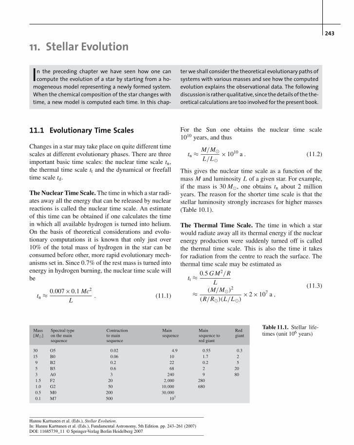
Hannu Karttunen et al. (Eds.), Stellar Evolution.In: Hannu Karttunen et al. (Eds.), Fundamental Astronomy, 5th Edition. pp. 243–261 (2007)DOI: 11685739_11 © Springer-Verlag Berlin Heidelberg 2007
243
11. Stellar Evolution
In the preceding chapter we have seen how one cancompute the evolution of a star by starting from a ho-
mogeneous model representing a newly formed system.When the chemical composition of the star changes withtime, a new model is computed each time. In this chap-
ter we shall consider the theoretical evolutionary paths ofsystems with various masses and see how the computedevolution explains the observational data. The followingdiscussion is ratherqualitative, since thedetailsof the the-oretical calculations are too involved for the present book.
11.1 Evolutionary Time Scales
Changes in a star may take place on quite different timescales at different evolutionary phases. There are threeimportant basic time scales: the nuclear time scale tn,the thermal time scale tt and the dynamical or freefalltime scale td.
The Nuclear Time Scale. The time in which a star radi-ates away all the energy that can be released by nuclearreactions is called the nuclear time scale. An estimateof this time can be obtained if one calculates the timein which all available hydrogen is turned into helium.On the basis of theoretical considerations and evolu-tionary computations it is known that only just over10% of the total mass of hydrogen in the star can beconsumed before other, more rapid evolutionary mech-anisms set in. Since 0.7% of the rest mass is turned intoenergy in hydrogen burning, the nuclear time scale willbe
tn ≈ 0.007×0.1 Mc2
L. (11.1)
Mass Spectral type Contraction Main Main Red[M] on the main to main sequence sequence to giant
sequence sequence red giant
30 O5 0.02 4.9 0.55 0.315 B0 0.06 10 1.7 29 B2 0.2 22 0.2 55 B5 0.6 68 2 203 A0 3 240 9 801.5 F2 20 2,000 2801.0 G2 50 10,000 6800.5 M0 200 30,0000.1 M7 500 107
Table 11.1. Stellar life-times (unit 106 years)
For the Sun one obtains the nuclear time scale1010 years, and thus
tn ≈ M/ML/L
×1010 a . (11.2)
This gives the nuclear time scale as a function of themass M and luminosity L of a given star. For example,if the mass is 30 M, one obtains tn about 2 millionyears. The reason for the shorter time scale is that thestellar luminosity strongly increases for higher masses(Table 10.1).
The Thermal Time Scale. The time in which a starwould radiate away all its thermal energy if the nuclearenergy production were suddenly turned off is calledthe thermal time scale. This is also the time it takesfor radiation from the centre to reach the surface. Thethermal time scale may be estimated as
tt ≈ 0.5 G M2/R
L
≈ (M/M)2
(R/R)(L/L)×2×107 a ,
(11.3)

244
11. Stellar Evolution
where G is the constant of gravity and R the stellarradius. For the Sun the thermal time scale is about20 million years or 1/500 of the nuclear time scale.
The Dynamical Time Scale. The third and shortesttime scale is the time it would take a star to collapse ifthe pressure supporting it against gravity were suddenlyremoved. It can be estimated from the time it would takefor a particle to fall freely from the stellar surface to thecentre. This is half of the period given by Kepler’s thirdlaw, where the semimajor axis of the orbit correspondsto half the stellar radius R:
td = 2π
2
√(R/2)3
G M≈√
R3
G M. (11.4)
The dynamical time scale of the Sun is about half anhour.
The ordering of the time scales is normally like thatin the Sun, i. e. td tt tn.
11.2 The Contraction of Stars Towardsthe Main Sequence
The formation and subsequent gravitational collapse ofcondensations in the interstellar medium will be con-sidered in a later chapter. Here we shall follow thebehaviour of such a protostar, when it is already inthe process of contraction.
When a cloud contracts, gravitational potential en-ergy is released and transformed into thermal energyof the gas and into radiation. Initially the radiation canpropagate freely through the material, because the den-sity is low and the opacity small. Therefore most of theliberated energy is radiated away and the temperaturedoes not increase. The contraction takes place on thedynamical time scale; the gas is falling freely inwards.
The density and the pressure increase most rapidlynear the centre of the cloud. As the density increases, sodoes the opacity. A larger fraction of the released energyis then turned into heat, and the temperature begins torise. This leads to a further increase in the pressure thatis resisting the free fall. The contraction of the centralpart of the cloud slows down. The outer parts, however,are still falling freely.
At this stage, the cloud may already be considereda protostar. It consists mainly of hydrogen in molec-
ular form. When the temperature reaches 1800 K, thehydrogen molecules are dissociated into atoms. The dis-sociation consumes energy, and the rise in temperatureis slowed down. The pressure then also grows moreslowly and this in turn means that the rate of contrac-tion increases. The same sequence of events is repeated,first when hydrogen is ionized at 104 K, and then whenhelium is ionized. When the temperature has reachedabout 105 K, the gas is essentially completely ionized.
The contraction of a protostar only stops when a largefraction of the gas is fully ionized in the form of plasma.The star then settles into hydrostatic equilibrium. Its fur-ther evolution takes place on the thermal time scale,i. e. much more slowly. The radius of the protostarhas shrunk from its original value of about 100 AU toabout 1/4 AU. It will usually be located inside a largergas cloud and will be accreting material from its sur-roundings. Its mass therefore grows, and the centraltemperature and density increase.
The temperature of a star that has just reached equi-librium is still low and its opacity correspondingly large.Thus it will be convective in its centre. The convectiveenergy transfer is quite efficient and the surface of theprotostar will therefore be relatively bright.
We now describe the evolution in the HR diagram.Initially the protostar will be faint and cool, and it willreside at the lower far right in the HR diagram (outsideFig. 11.1). During the collapse its surface rapidly heatsup and brightens and it moves to the upper right ofFig. 11.1. At the end of the collapse the star will settleat a point corresponding to its mass on the Hayashitrack. The Hayashi track (Fig. 11.1) gives the locationin the HR diagram of completely convective stars. Starsto its right cannot be in equilibrium and will collapseon the dynamic time scale.
The star will now evolve almost along the Hayashitrack on the thermal time scale. In the HR diagram itmoves almost vertically downwards, its radius decreasesand its luminosity drops (Fig. 11.1). As the temperaturegoes on increasing in its centre, the opacity diminishesand energy begins to be transported by radiation. Themass of the radiative region will gradually grow untilfinally most of the star is radiative. By then the cen-tral temperature will have become so large that nuclearreactions begin. Previously all the stellar energy hadbeen released potential energy, but now the nuclear re-actions make a growing contribution and the luminosity

11.2 The Contraction of Stars Towards the Main Sequence
245
Fig. 11.1. The paths in theHR diagram of stars contract-ing to the main sequence onthe thermal time scale. Af-ter a rapid dynamical collapsethe stars settle on the Hayashitrack and evolve towards themain sequence on the thermaltime scale. (Models by Iben, I.(1965): Astrophys. J. 141, 993)
increases. The stellar surface temperature will also in-crease and the star will move slightly upwards to theleft in the HR diagram. In massive stars, this turn to theleft occurs much earlier, because their central tempera-tures are higher and the nuclear reactions are initiatedearlier.
For solar mass stars, the rapid collapse of the proto-stellar cloud only lasts for a few hundred years. The finalstage of condensation is much slower, lasting severaltens of millions of years. This length of time strongly
depends on the stellar mass because of the luminositydependence of the thermal time scale. A 15 M star con-denses to the main sequence in 60,000 years, whereasfor a 0.1 M star, the time is hundreds of millions ofyears.
Some of the hydrogen burning reactions start alreadyat a few million degrees. For example, lithium, beryl-lium and boron burn to helium in the ppII and ppIIIbranches of the pp chain long before the complete chainhas turned on. Because the star is convective and thus

246
11. Stellar Evolution
Fig. 11.2. Herbig–Haro ob-ject number 555 lies atthe end of the “elephant’strunk" in Pelican Nebula inCygnus. The small wingsare shockwaves, whichgive evidence for power-ful outflows from newlyformed stars embeddedwithin the clouds. (PhotoUniversity of Colorado,University of Hawaii andNOAO/AURA/NSF)
well mixed during the early stages, even its surface ma-terial will have been processed in the centre. Althoughthe abundances of the above-mentioned elements aresmall, they give important information on the centraltemperature.
The beginning of the main sequence phase is markedby the start of hydrogen burning in the pp chain ata temperature of about 4 million degrees. The new formof energy production completely supersedes the energyrelease due to contraction. As the contraction is halted,the star makes a few oscillations in the HR diagram, butsoon settles in an equilibrium and the long, quiet mainsequence phase begins.
It is difficult to observe stars during contraction, be-cause the new-born stars are usually hidden amongdense clouds of dust and gas. However, some con-densations in interstellar clouds have been discoveredand near them, very young stars. One example arethe T Tauri stars. Their lithium abundance is relativelyhigh, which indicates that they are newly formed starsin which the central temperature has not yet becomelarge enough to destroy lithium. Near the T Tauri stars,small, bright, star-like nebulae, Herbig–Haro objects,
have been discovered. These are thought to be pro-duced in the interaction between a stellar wind and thesurrounding interstellar medium.
11.3 The Main Sequence Phase
The main sequence phase is that evolutionary stage inwhich the energy released by the burning of hydrogenin the core is the only source of stellar energy. Dur-ing this stage, the star is in stable equilibrium, and itsstructure changes only because its chemical composi-tion is gradually altered by the nuclear reactions. Thusthe evolution takes place on a nuclear time scale, whichmeans that the main sequence phase is the longest partof the life of a star. For example, for a solar mass star,the main sequence phase lasts for about 10,000 millionyears. More massive stars evolve more rapidly, becausethey radiate much more power. Thus the main sequencephase of a 15 solar mass star is only about 10 mil-lion years. On the other hand, less massive stars havea longer main sequence lifetime: a 0.25 M star spendsabout 70,000 million years on the main sequence.

11.3 The Main Sequence Phase
247
Since stars are most likely to be found in the stage ofsteady hydrogen burning, the main sequence in the HRdiagram is richly populated, in particular at its low-massend. The more massive upper main sequence stars areless abundant because of their shorter main sequencelifetimes.
If the mass of a star becomes too large, the forceof gravity can no longer resist the radiation pressure.Stars more massive than this upper limit cannot form,because they cannot accrete additional mass during thecontraction phase. Theoretical computations give a lim-iting mass of about 120 M; the most massive starsobserved are claimed to be about 150 M.
There is also a lower-mass limit of the main sequence.Stars below 0.08 M never become hot enough for hy-drogen burning to begin. They can still generate someluminosity from the burning of deuterium, but this en-ergy source is rapidly exhausted. These brown dwarfshave surface temperatures in the range of 1000–2000 KHundreds of brown dwarfs have now been found in ded-icated surveys. The lower limit for brown dwarf mass issometimes taken to be about 0.015,M, correspondingto the minimum mass for deuterium burning.
If the mass is even lower there are no nuclear sourcesof energy. The smallest protostars therefore contract toplanet-like dwarfs. During the contraction phase theyradiate because potential energy is released, but even-tually they begin to cool. In the HR diagram such starsfirst move almost vertically downwards and then furtherdownwards to the right.
Is there a difference between the lowest-mass browndwarfs and the most massive planets? If brown dwarfshave formed by gravitational collapse and fragmen-tation as described in the previous section and inAbschn. 15.4, there is no reason not to count them asstars, although they are not producing energy by nu-clear reactions. Planets in contrast are thought to formmuch more slowly by the clumping of solids and accre-tion of gas in a protoplanetary disc. The objects formedby this mechanism start out with a quite different struc-ture. Whether such a clear-cut distinction between theformation mechanisms of dark stars and planets reallycan be made still remains an open question.
The Upper Main Sequence. The stars on the uppermain sequence are so massive and their central tem-perature so high that the CNO cycle can operate. On
the lower main sequence the energy is produced by thepp chain. The pp chain and the CNO cycle are equallyefficient at a temperature of 18 million degrees, corre-sponding to the central temperature of a 1.5 M star.The boundary between the upper and the lower mainsequence corresponds roughly to this mass.
The energy production in the CNO cycle is verystrongly concentrated at the core. The outward energyflux will then become very large, and can no longerbe maintained by radiative transport. Thus the uppermain sequence stars have a convective core, i. e. theenergy is transported by material motions. These keepthe material well mixed, and thus the hydrogen abun-dance decreases uniformly with time within the entireconvective region.
Outside the core, there is radiative equilibrium, i. e.the energy is carried by radiation and there are no nu-clear reactions. Between the core and the envelope, thereis a transition region where the hydrogen abundancedecreases inwards.
The mass of the convective core will gradually dimin-ish as the hydrogen is consumed. In the HR diagram thestar will slowly shift to the upper right as its luminositygrows and its surface temperature decreases (Fig. 11.3).When the central hydrogen supply becomes exhausted,the core of the star will begin to shrink rapidly. The sur-face temperature will increase and the star will quicklymove to the upper left. Because of the contraction of thecore, the temperature in the hydrogen shell just outsidethe core will increase. It rapidly becomes high enoughfor hydrogen burning to set in again.
The Lower Main Sequence. On the lower mainsequence, the central temperature is lower than for mas-sive stars, and the energy is generated by the pp chain.Since the rate of the pp chain is not as sensitive totemperature as that of the CNO cycle, the energy pro-duction is spread over a larger region than in the moremassive stars (Fig. 11.4). In consequence, the core neverbecomes convectively unstable, but remains radiative.
In the outer layers of lower main sequence stars, theopacity is high because of the low temperature. Ra-diation can then no longer carry all the energy, andconvection will set in. The structure of lower main se-quence stars is thus opposite to that of the upper mainsequence: the centre is radiative and the envelope isconvective. Since there is no mixing of material in

248
11. Stellar Evolution
Fig. 11.3. Stellar evolution-ary paths in the HR diagramat the main sequence phaseand later. On the main se-quence, bounded by dashedcurves, the evolution is onthe nuclear time scale. Thepost-main sequence evolu-tion to the red giant phaseis on the thermal time scale.The point marked He cor-responds to helium ignitionand in low-mass stars thehelium flash. The straightline shows the location ofstars with the same radius.(Iben, I. (1967): AnnualRev. Astron. Astrophys.5, 571; data for 30 Mfrom Stothers, R. (1966):Astrophys. J. 143, 91)
the core, the hydrogen is most rapidly consumed atthe very centre, and the hydrogen abundance increasesoutwards.
As the amount of hydrogen in the core decreases,the star will slowly move upwards in the HR diagram,almost along the main sequence (Fig. 11.3). It becomesslightly brighter and hotter, but its radius will not change
by much. The evolutionary track of the star will thenbend to the right, as hydrogen in the core nears its end.Eventually the core is almost pure helium. Hydrogenwill continue to burn in a thick shell around the core.
Stars with masses between 0.08 M and 0.26 Mhave a very simple evolution. During their whole mainsequence phase they are fully convective, which means

11.4 The Giant Phase
249
Fig. 11.4a–c. Energy transport in the main sequence phase.(a) The least massive stars (M < 0.26 M) are convec-tive throughout. (b) For 0.26 M < M < 1.5 M the coreis radiative and the envelope convective. (c) Massive stars(M > 1.5 M) have a convective core and a radiativeenvelope
that their entire hydrogen content is available as fuel.These stars evolve very slowly toward the upper leftin the HR diagram. Finally, when all their hydrogenhas burned to helium, they contract to become whitedwarfs.
11.4 The Giant Phase
The main-sequence phase of stellar evolution ends whenhydrogen is exhausted at the centre. The star then set-tles in a state in which hydrogen is burning in a shellsurrounding a helium core. As we have seen, the transi-tion takes place gradually in lower main-sequence stars,giving rise to the Subgiant Branch in the HR diagram,while the upper main-sequence stars make a rapid jumpat this point.
The mass of the helium core is increased by the hy-drogen burning in the shell. This leads to the expansionof the envelope of the star, which moves almost horizon-tally to the right in the HR diagram. As the convectiveenvelope becomes more extensive, the star approachesthe Hayashi track. Since it cannot pass further to theright, and since its radius continues to grow, the star hasto move upwards along the Hayashi track towards largerluminosities (Fig. 11.3). The star has become a red giant.
In low-mass stars (M ≤ 2.3 M), as the mass of thecore grows, its density will eventually become so highthat it becomes degenerate. The central temperature willcontinue to rise. The whole helium core will have a uni-form temperature because of the high conductivity ofthe degenerate gas. If the mass of the star is larger than0.26 M the central temperature will eventually reach
about 100 million degrees, which is enough for heliumto burn to carbon in the triple alpha process.
Helium burning will set in simultaneously in thewhole central region and will suddenly raise its tem-perature. Unlike a normal gas, the degenerate corecannot expand, although the temperature increases(c. f. (10.16)), and therefore the increase in tempera-ture will only lead to a further acceleration of the rate ofthe nuclear reactions. When the temperature increasesfurther, the degeneracy of the gas is removed and thecore will begin to expand violently. Only a few secondsafter the ignition of helium, there is an explosion, thehelium flash.
The energy from the helium flash is absorbed by theouter layers, and thus it does not lead to the completedisruption of the star. In fact the luminosity of the stardrops in the flash, because when the centre expands,the outer layers contract. The energy released in theflash is turned into potential energy of the expandedcore. Thus after the helium flash, the star settles intoa new state, where helium is steadily burning to carbonin a nondegenerate core.
After the helium flash the star finds itself on thehorizontal giant branch in the HR diagram. The exactposition of a star on the horizontal branch after the he-lium flash is a sensitive function of its envelope mass.This in turn depends on the amount of mass lost by thestar in the helium flash, which can vary randomly fromstar to star. While the luminosity does not vary muchalong the horizontal branch, the effective temperaturesare higher for stars with less mass in the envelope. Thehorizontal branch is divided into a blue and a red partby a gap corresponding to the pulsational instabilityleading to RR Lyrae variables (see Section 13.2). Theform of the horizontal branch for a collection of starsdepends on their metal-abundance, in the sense thata lower metal abundance is related to a more promi-nent blue horizontal branch. Thus the blue horizontalbranch in globular clusters with low metal-abundancesis strong and prominent (Section 16.3). For stars withsolar element abundances the horizontal branch is re-duced to a short stump, the red clump, where it joins thered giant branch.
In intermediate-mass stars (2.3 M ≤ M ≤ 8 M),the central temperature is higher and the central den-sity lower, and the core will therefore not be degenerate.Thus helium burning can set in non-catastrophically as
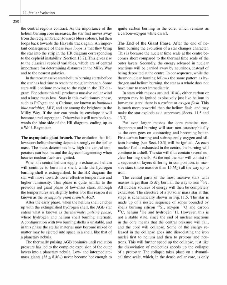
250
11. Stellar Evolution
the central regions contract. As the importance of thehelium burning core increases, the star first moves awayfrom the red giant branch towards bluer colours, but thenloops back towards the Hayashi track again. An impor-tant consequence of these blue loops is that they bringthe star into the strip in the HR diagram correspondingto the cepheid instability (Section 13.2). This gives riseto the classical cepheid variables, which are of centralimportance for determining distances in the Milky Wayand to the nearest galaxies.
In the most massive stars helium burning starts beforethe star has had time to reach the red giant branch. Somestars will continue moving to the right in the HR dia-gram. For others this will produce a massive stellar windand a large mass loss. Stars in this evolutionary phase,such as P Cygni and η Carinae, are known as luminousblue variables, LBV, and are among the brightest in theMilky Way. If the star can retain its envelope it willbecome a red supergiant. Otherwise it will turn back to-wards the blue side of the HR diagram, ending up asa Wolf–Rayet star.
The asymptotic giant branch. The evolution that fol-lows core helium burning depends strongly on the stellarmass. The mass determines how high the central tem-perature can become and the degree of degeneracy whenheavier nuclear fuels are ignited.
When the central helium supply is exhausted, heliumwill continue to burn in a shell, while the hydrogenburning shell is extinguished. In the HR diagram thestar will move towards lower effective temperature andhigher luminosity. This phase is quite similar to theprevious red giant phase of low-mass stars, althoughthe temperatures are slightly hotter. For this reason it isknown as the asymptotic giant branch, AGB.
After the early phase, when the helium shell catchesup with the extinguished hydrogen shell, the AGB starenters what is known as the thermally pulsing phase,where hydrogen and helium shell burning alternate.A configuration with two burning shells is unstable, andin this phase the stellar material may become mixed ormatter may be ejected into space in a shell, like that ofa planetary nebula.
The thermally pulsing AGB coninues until radiationpressure has led to the complete expulsion of the outerlayers into a planetary nebula. Low- and intermediate-mass giants (M ≤ 8 M) never become hot enough to
ignite carbon burning in the core, which remains asa carbon–oxygen white dwarf.
The End of the Giant Phase. After the end of he-lium burning the evolution of a star changes character.This is because the nuclear time scale at the centre be-comes short compared to the thermal time scale of theouter layers. Secondly, the energy released in nuclearreactions will be carried away by neutrinos, instead ofbeing deposited at the centre. In consequence, while thethermonuclear burning follows the same pattern as hy-drogen and helium burning, the star as a whole does nothave time to react immediately.
In stars with masses around 10 M either carbon oroxygen may be ignited explosively just like helium inlow-mass stars: there is a carbon or oxygen flash. Thisis much more powerful than the helium flash, and maymake the star explode as a supernova (Sects. 11.5 and13.3).
For even larger masses the core remains non-degenerate and burning will start non-catastrophicallyas the core goes on contracting and becoming hotter.First carbon burning and subsequently oxygen and sil-icon burning (see Sect. 10.3) will be ignited. As eachnuclear fuel is exhausted in the centre, the burning willcontinue in a shell. The star will thus contain several nu-clear burning shells. At the end the star will consist ofa sequence of layers differing in composition, in mas-sive stars (more massive than 15 M) all the way up toiron.
The central parts of the most massive stars withmasses larger than 15 M burn all the way to iron 56Fe.All nuclear sources of energy will then be completelyexhausted. The structure of a 30 solar mass star at thisstage is schematically shown in Fig. 11.5. The star ismade up of a nested sequence of zones bounded byshells burning silicon 28Si, oxygen 16O and carbon12C, helium 4He and hydrogen 1H. However, this isnot a stable state, since the end of nuclear reactionsin the core means that the central pressure will fall,and the core will collapse. Some of the energy re-leased in the collapse goes into dissociating the ironnuclei first to helium and then to protons and neu-trons. This will further speed up the collapse, just likethe dissociation of molecules speeds up the collapseof a protostar. The collapse takes place on a dynami-cal time scale, which, in the dense stellar core, is only

11.4 The Giant Phase
251
Fig. 11.5. The structure of a massive star (30 M) at a lateevolutionary stage. The star consists of layers with differentcomposition separated by nuclear burning shells
a fraction of a second. The outer parts will also col-lapse, but more slowly. In consequence, the temperature
Fig. 11.6. The usual endpoint for the development of a starwith a mass of less than three solar masses, is a white dwarf,with an expanding planetary nebula around it. On the left, theplanetary nebula NGC 6369, photographed with the 8-meterGemini South telescope. For a massive star, the life ends with
a supernova explosion. On the right, the supernova remnantCassiopeia A on radio wavelengths. The image was cre-ated by the VLA telescope. (Images Gemini Observatory/AbuTeam/NOAO/AURA/NSF and NRAO/AUI)
will increase in layers containing unburnt nuclear fuel.This will burn explosively, releasing immense amountsof energy in a few seconds, principally in the form ofneutrinos.
The final stages of stellar evolution may be describedas an implosion of the core, which is briefly halted everytime a new source of nuclear fuel becomes availablefor burning It is still an open problem how exactly theenergy released in this collapse is transformed into thedisrupton of the entire star and the ejection of its outerlayers. It is also still unclear whether in a given case theremnant will be a neutron star or a black hole.
Although the exact mechanism is not yet understood,the end-point of the evolution of stars more massive theabout 8 M is that the outer layers explode as a super-nova. In the dense central core, the protons and electronscombine to form neutrons. The core will finally consistalmost entirely of neutrons, which become degeneratebecause of the high density. The degeneracy pressureof the neutrons will stop the collapse of a small masscore. However, if the mass of the core is large enough,a black hole will probably be formed.

252
11. Stellar Evolution
11.5 The Final Stages of Evolution
The endpoints of stellar evolution can be seen fromFig. 11.8. This shows the relation between mass andcentral density for a body at zero temperature, i. e. the fi-nal equilibrium when a massive body has cooled. Thereare two maxima on the curve. The mass correspondingto the left-hand maximum is called the Chandrasekharmass, MCh ≈ 1.2–1.4 M, and that corresponding tothe right-hand one, the Oppenheimer–Volkoff mass,MOV ≈ 1.5–2 M.
Let us first consider a star with mass less than MCh.Suppose the mass does not change. When the nu-
Fig. 11.7. Evolution schemes for stars with different masses.The radius is scaled to be the same in all drawings. In real-ity, there are vast differences in the sizes of different stars anddifferent phases of evolution. In the beginning (1) a gas cloudis contracting rapidly in free fall. Because the gas is quite rar-efied, radiation escapes easily from the cloud. As the densityincreases, radiation transport becomes more difficult, and thereleased energy tends to warm up the gas. The contraction
lasts until the gas is completely ionized, and the star, whichhas become a protostar, is in hydrostatic equilibrium (2). Thestar is convective throughout its interior.
Now evolution continues on a thermal time scale. The con-traction is much slower than in the free-fall phase. The phasesof further evolution are determined by the mass M of thestar. For M< 0.08 M the temperature in the centre does notrise high enough for hydrogen burning, and these stars con-
clear fuel is exhausted, the star will become a whitedwarf, which will gradually cool down and contract. InFig. 11.8 it moves horizontally to the right. Finally itwill reach zero temperature and end up on the left-handrising part of the equilibrium curve. Its final equilibriumis a completely degenerate black dwarf.
If the mass of the star is larger than MCh butsmaller than MOV, it can continue cooling until itreaches the right-hand rising section of the curve. Againthere is a stable final state, this time corresponding toa completely degenerate neutron star.
An even more massive star with mass larger thanMOV will go on contracting past the density correspond-

11.5 The Final Stages of Evolution
253
tract to planetlike brown dwarfs. Stars with M ≥ 0.08 Mstart hydrogen burning when the temperature has reachedabout 4×10⁶ K. This is the beginning of the main sequencephase. In the main sequence, the lowest-mass stars with0.08 M ≤ M ≤ 0.26 M are entirely convective, and thusthey remain homogeneous (3). Their evolution is very slow,and after all the hydrogen has been burnt to helium, they con-tract to white dwarfs (4).
The increasing temperature makes the stars withM > 0.26 M radiative in the centre as the opacity de-creases (5). The low-mass stars with 0.26 M ≤ M ≤ 1.5 Mremain radiative in the centre during the main sequencephase (6) as they burn their hydrogen through the pp chain.The outer part is convective. At the end of the main sequencephase, hydrogen burning continues in a shell surrounding thehelium core (7).
The outer part expands, and the giant phase begins. Thecontracting helium core is degenerate and warms up. At about108 K, the triple alpha process begins and leads immediatelyto the helium flash (8). The explosion is damped by the outerparts, and helium burning goes on in the core (9). Hydrogenis still burning in an outer shell. As the central helium is ex-hausted, helium burning moves over to a shell (10). At the
same time, the outer part expands and the star loses someof its mass. The expanding envelope forms a planetary neb-ula (11). The star in the centre of the nebula becomes a whitedwarf (12).
In the upper main sequence with M ≥ 1.5 M energy isreleased through the CNO cycle, and the core becomes convec-tive, while the outer part is radiative (13). The main sequencephase ends as the hydrogen in the core is exhausted, and shellburning begins (14). The helium core remains convective andnondegenerate, and helium burning begins without perturba-tions (15 and 19). Afterwards, helium burning moves over toa shell (16 and 20). For stars with 3 M ≤ M ≤ 15 M the car-bon in the core is degenerate, and a carbon flash occurs (17).This leads to a supernova explosion (18) and possibly to thecomplete destruction of the star.
For the most massive stars with M ≥ 15 M the carboncore remains convective, and carbon burns to oxygen and mag-nesium. Finally, the star consists of an iron core surroundedby shells with silicon, oxygen, carbon, helium and hydro-gen (21). The nuclear fuel is now exhausted, and the starcollapses on a dynamical time scale. The result is a super-nova (22). The outer parts explode, but the remaining corecontinues to contract to a neutron star or a black hole

254
11. Stellar Evolution
Fig. 11.8. The evolutionary end points of stars with differ-ent masses shown as a function of central density. The curveshows the behaviour of the central density of completely de-generate (T = 0 K) bodies. The Chandrasekhar mass MCh andthe Oppenheimer–Volkoff mass MOV correspond to maximaon this curve
ing to a neutron star. There is then no longer any knownpossible stable equilibrium, and the star must go oncontracting to form a black hole.
The only endpoints of stellar evolution predicted bytheory are the two stable states of Fig. 11.8 and thetwo extreme possibilities, collapse to a black hole orexplosive disruption.
The preceding considerations are purely theoretical.The final evolutionary stages of real stars involve manyimperfectly known factors, which may affect the finalequilibrium. Perhaps most important is the question ofmass loss, which is very difficult to settle either obser-vationally or theoretically. For example, in a supernovaexplosion the whole star may be disrupted and it is veryuncertain whether what remains will be a neutron star,a black hole or nothing at all. (The structure of compactstars will be discussed in Chap. 14.)
A summary of the variuos evolutionary paths is givenin Fig. 11.7.
11.6 The Evolution of Close Binary Stars
If the components of a binary star are well separated,they do not significantly perturb one another. Whenstudying their evolution, one can regard them as twosingle stars evolving independently, as described above.
Fig. 11.9a–c. The typesof close binary sys-tems: (a) detached,(b) semidetached and(c) contact binary
However, in close binary pairs, this will no longer bethe case.
Close binary stars are divided into three classes, asshown in Fig. 11.9: detached, semidetached and contactbinaries. The figure-eight curve drawn in the figure isan equipotential surface called the Roche surface. If thestar becomes larger than this surface, it begins to losemass to its companion through the waist of the Rochesurface.
During the main sequence phase the stellar radiusdoes not change much, and each component will re-main within its own Roche lobe. When the hydrogenis exhausted, the stellar core will rapidly shrink and theouter layers expand, as we have seen. At this stage a starmay exceed its Roche lobe and mass transfer may set in.
Close binary stars are usually seen as eclipsing bina-ries. One example is Algol in the constellation Perseus.The components in this binary system are a normalmain sequence star and a subgiant, which is muchless massive than the main sequence star. The sub-giant has a high luminosity and thus has apparentlyalready left the main sequence. This is unexpected, sincethe components were presumably formed at the sametime, and the more massive star should evolve morerapidly. The situation is known as the Algol paradox:for some reason, the less massive star has evolved morerapidly.
In the 1950’s a solution to the paradox proposed thatthe subgiant was originally more massive, but that ithad lost mass to its companion during its evolution.

11.7 Comparison with Observations
255
Fig. 11.10a–f. Evolu-tion of a low-massbinary: (a) both com-ponents on the mainsequence; (b) masstransfer from the moremassive component;(c) light subgiant andmassive main sequencestar; (d) white dwarfand main sequence star;(e) mass transferred tothe white dwarf fromthe more massive com-ponent leads to novaoutbursts; (f) the whitedwarf mass exceeds theChandrasekhar massand explodes as a typeI supernova
Since the 1960’s mass transfer in close binary systemshas been much studied, and has turned out be a verysignificant factor in the evolution of close binaries.
As an example, let us consider a close binary,where the initial masses of the components are 1 and2 solar masses and the initial orbital period 1.4 days(Fig. 11.10). After evolving away from the main se-quence the more massive component will exceed theRoche limit and begin to lose mass to its companion.Initially the mass will be transferred on the thermaltime scale, and after a few million years the roles ofthe components will be changed: the initially moremassive component has become less massive than itscompanion.
The binary is now semidetached and can be observedas an Algol-type eclipsing binary. The two compo-nents are a more massive main sequence star and a lessmassive subgiant filling its Roche surface. The masstransfer will continue, but on the much slower nucleartime scale. Finally, mass transfer will cease and theless massive component will contract to a 0.6 M whitedwarf.
The more massive 2.4 M star now evolves and be-gins to lose mass, which will accumulate on the surfaceof the white dwarf. The accumulated mass may giverise to nova outbursts, where material is ejected intospace by large explosions. Despite this, the mass of thewhite dwarf will gradually grow and may eventuallyexceed the Chandrasekhar mass. The white dwarf willthen collapse and explode as a type I supernova.
As a second example, we can take a massive bi-nary with the initial masses 20 and 8 M and the initialperiod 4.7 days (Fig. 11.11). The more massive compo-nent evolves rapidly, and at the end of the main sequencephase, it will transfer more than 15 M of its materialto the secondary. The mass transfer will occur on thethermal time scale, which, in this case, is only a fewten thousand years. The end result is a helium star,having as a companion an unevolved main sequencestar. The properties of the helium star are like those ofa Wolf–Rayet star.
Helium continues to burn to carbon in the core of thehelium star, and the mass of the carbon core will grow.Eventually the carbon will be explosively ignited, andthe star will explode as a supernova. The consequencesof this explosion are not known, but let us suppose thata 2 M compact remnant is left. As the more massivestar expands, its stellar wind will become stronger, giv-ing rise to strong X-ray emission as it hits the compactstar. This X-ray emission will only cease when the moremassive star exceeds its Roche surface.
The system will now rapidly lose mass and angularmomentum. A steady state is finally reached when thesystem contains a 6 M helium star in addition to the2 M compact star. The helium star is seen as a Wolf–Rayet star, which, after about a million years, explodesas a supernova. This will probably lead to the breakupof the binary system. However, for certain values ofthe mass, the binary may remain bound. Thus a binaryneutron star may be formed.

256
11. Stellar Evolution
11.7 Comparison with Observations
The most important direct support for the theoreticalevolutionary models is obtained from the properties ofobserved HR diagrams. If the theoretical models arecorrect, the observed number of stars should reflect theduration of the various evolutionary phases. These aregiven for stars of different masses in Table 11.1. The
Fig. 11.11a–h. Evolution of a massive binary. It has been as-sumed that the supernova explosion of a 5 M helium starleaves a 2 M compact remnant (neutron star or black hole).(a) Main sequence phase; (b) beginning of the first mass trans-fer phase; (c) end of the first mass transfer phase; the firstWolf–Rayet phase begins; (d) the helium star (Wolf–Rayetstar) has exploded as a supernova; (e) the 23 M componentbecomes a supergiant; the compact component is a strong X-ray source; (f) beginning of the second mass transfer phase;the X-ray source is throttled and large-scale mass loss be-gins; (g) second Wolf–Rayet phase; (h) the 6 M helium starhas exploded as a supernova; the binary may or may not bedisrupted, depending on the remaining mass
stars are most numerous along the main sequence. Gi-ants are also common and, in addition to these, there arewhite dwarfs, subgiants, etc. The sparsely populated re-gion to the right of the main sequence, the Hertzsprunggap, is explained by the rapid transition from the mainsequence to the giant phase.
The cepheids provide an important test for theevolutionary models. The pulsations and the relationbetween period and luminosity for the cepheids can beunderstood on the basis of theoretical stellar models.
The evolutionary models can also explain the HRdiagrams of star clusters. Let us assume that all thestars in a cluster were formed at the same time. Inthe youngest systems, the associations, the stars willmainly be found on the upper main sequence, since themost massive stars evolve most rapidly. To the right ofthe main sequence, there will be less massive T Tauristars, which are still contracting. In intermediate ageopen clusters, the main sequence will be well devel-oped and its upper end should bend to the right, sincethe most massive stars will already have begun to evolveoff the main sequence. In the old globular clusters, thegiant branch should increase in importance in the olderclusters. These predictions are confirmed by the obser-vations, which will be further discussed in Chap. 16 onstar clusters.
Of course, the most detailed observations can bemade of the Sun, which is therefore a crucial point ofcomparison for the theoretical models. If a star of onesolar mass with an initial composition of 71% hydro-gen, 27% helium and 2% heavier elements is allowedto evolve for 5000 million years, it will be very sim-ilar to our present Sun. In particular, it will have thesame radius, surface temperature and luminosity. Ac-cording to calculations, about half of the Sun’s supply
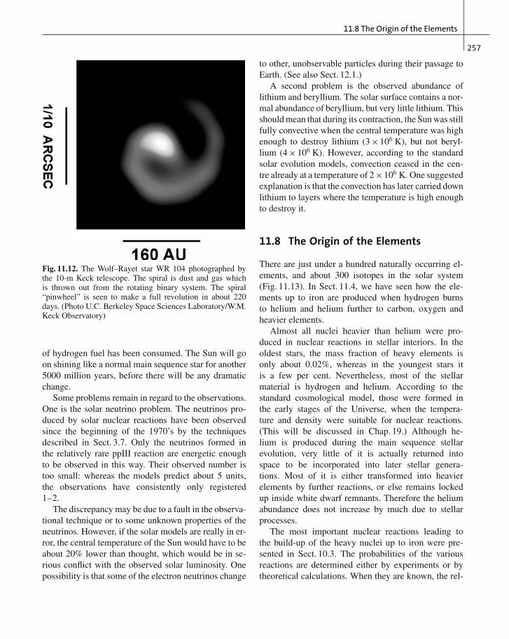
11.8 The Origin of the Elements
257
Fig. 11.12. The Wolf–Rayet star WR 104 photographed bythe 10-m Keck telescope. The spiral is dust and gas whichis thrown out from the rotating binary system. The spiral“pinwheel” is seen to make a full revolution in about 220days. (Photo U.C. Berkeley Space Sciences Laboratory/W.M.Keck Observatory)
of hydrogen fuel has been consumed. The Sun will goon shining like a normal main sequence star for another5000 million years, before there will be any dramaticchange.
Some problems remain in regard to the observations.One is the solar neutrino problem. The neutrinos pro-duced by solar nuclear reactions have been observedsince the beginning of the 1970’s by the techniquesdescribed in Sect. 3.7. Only the neutrinos formed inthe relatively rare ppIII reaction are energetic enoughto be observed in this way. Their observed number istoo small: whereas the models predict about 5 units,the observations have consistently only registered1–2.
The discrepancy may be due to a fault in the observa-tional technique or to some unknown properties of theneutrinos. However, if the solar models are really in er-ror, the central temperature of the Sun would have to beabout 20% lower than thought, which would be in se-rious conflict with the observed solar luminosity. Onepossibility is that some of the electron neutrinos change
to other, unobservable particles during their passage toEarth. (See also Sect. 12.1.)
A second problem is the observed abundance oflithium and beryllium. The solar surface contains a nor-mal abundance of beryllium, but very little lithium. Thisshould mean that during its contraction, the Sun was stillfully convective when the central temperature was highenough to destroy lithium (3×10⁶ K), but not beryl-lium (4×10⁶ K). However, according to the standardsolar evolution models, convection ceased in the cen-tre already at a temperature of 2×10⁶ K. One suggestedexplanation is that the convection has later carried downlithium to layers where the temperature is high enoughto destroy it.
11.8 The Origin of the Elements
There are just under a hundred naturally occurring el-ements, and about 300 isotopes in the solar system(Fig. 11.13). In Sect. 11.4, we have seen how the ele-ments up to iron are produced when hydrogen burnsto helium and helium further to carbon, oxygen andheavier elements.
Almost all nuclei heavier than helium were pro-duced in nuclear reactions in stellar interiors. In theoldest stars, the mass fraction of heavy elements isonly about 0.02%, whereas in the youngest stars itis a few per cent. Nevertheless, most of the stellarmaterial is hydrogen and helium. According to thestandard cosmological model, those were formed inthe early stages of the Universe, when the tempera-ture and density were suitable for nuclear reactions.(This will be discussed in Chap. 19.) Although he-lium is produced during the main sequence stellarevolution, very little of it is actually returned intospace to be incorporated into later stellar genera-tions. Most of it is either transformed into heavierelements by further reactions, or else remains lockedup inside white dwarf remnants. Therefore the heliumabundance does not increase by much due to stellarprocesses.
The most important nuclear reactions leading tothe build-up of the heavy nuclei up to iron were pre-sented in Sect. 10.3. The probabilities of the variousreactions are determined either by experiments or bytheoretical calculations. When they are known, the rel-

258
11. Stellar Evolution
Fig. 11.13. Element abun-dances in the solar systemas a function of the nu-clear mass number. Theabundance of Si has beennormalized as 106
ative abundances of the various nuclei produced can becalculated.
The formation of elements heavier than iron requiresan input of energy, and thus they cannot be explainedin the same manner. Still heavy nuclei are continuallyproduced. In 1952 technetium was discovered in theatmosphere of a red giant. The half-life of the mostlonglived isotope 98Tc is about 1.5×10⁶ years, so thatthe observed technetium must have been produced inthe star.
Most of the nuclei more massive than iron are formedby neutron capture. Since the neutron does not have
an electric charge, it can easily penetrate into the nu-cleus. The probability for neutron capture dependsboth on the kinetic energy of the incoming neutronand on the mass number of the nucleus. For example,in the solar system the abundances of isotopes showmaxima at the mass numbers A = 70–90, 130, 138,195 and 208. These mass numbers correspond to nu-clei with closed neutron shells at the neutron numbersN = 50, 82, and 126. The neutron capture probabilityfor these nuclei is very small. The closed shell nucleithus react more slowly and are accumulated in greaterabundances.

11.9 Example
259
In a neutron capture, a nucleus with mass number Ais transformed into a more massive nucleus:
(Z, A)+n → (Z, A +1)+γ .
The newly formed nucleus may be unstable to β decay,where one neutron is transformed into a proton:
(Z, A +1)→ (Z +1, A +1)+ e− +νe .
Two kinds of neutron capture processes are encoun-tered, depending on the value of the neutron flux. Inthe slow s-process, the neutron flux is so small that anyβ decays have had time to occur before the next neutroncapture reaction takes place. The most stable nuclei upto mass number 210 are formed by the s-process. Thesenuclei are said to correspond to the β stability valley.The s-process explains the abundance peaks at the massnumbers 88, 138 and 208.
When the neutron flux is large, β decays do not havetime to happen before the next neutron capture. Onethen speaks of the rapid r-process, which gives riseto more neutron-rich isotopes. The abundance maximaproduced by the r-process lie at mass numbers about tenunits smaller than those of the s-process.
A neutron flux sufficient for the s-process is obtainedin the course of normal stellar evolution. For example,some of the carbon and oxygen burning reactions pro-duce free neutrons. If there is convection between thehydrogen and helium burning shells, free protons may becarried into the carbon-rich layers. Then the followingneutron-producing reaction chain becomes important:
12C +p → 13N +γ ,
13N → 13C + e+ +νe ,
13C + 4He → 16O +n .
The convection can also carry the reaction productsnearer to the surface.
The neutron flux required for the r-process is about1022 cm−3, which is too large to be produced duringnormal stellar evolution. The only presently known sitewhere a large enough neutron flux is expected is neara neutron star forming in a supernova explosion. In thiscase, the rapid neutron capture leads to nuclei that can-not capture more neutrons without becoming stronglyunstable. After one or more rapid β decays, the processcontinues.
The r-process stops when the neutron flux decreases.The nuclei produced then gradually decay by the β-
process towards more stable isotopes. Since the path ofthe r-process goes about ten mass units below the stabil-ity valley, the abundance peaks produced will fall aboutten units below those of the s-process. This is shownin Fig. 11.14. The most massive naturally occurring el-ements, such as uranium, thorium and plutonium, areformed by the r-process.
There are about 40 isotopes on the proton-richside of the β stability valley that cannot be pro-duced by neutron capture processes. Their abundancesare very small, relative to the neighbouring isotopes.They are formed in supernova explosions at temper-atures higher than 109 K by reactions known as thep-process. At this temperature, pair formation can takeplace:
γ→e+ + e− .
The positron may either be annihilated immediately orbe consumed in the reaction
e+ + (Z, A)→ (Z +1, A)+νe .
Another reaction in the p-process is
(Z, A)+p → (Z +1, A +1)+γ .
Finally, the fission of some heavier isotopes may giverise to p-process nuclei. Examples of this are the iso-topes 184W, 190Pt and 196Hg formed by the fission oflead.
All the preceding reaction products are ejected intothe interstellar medium in the supernova explosion. Col-lisions between cosmic rays and heavy nuclei thenfinally give rise to the light elements lithium, beryl-lium and boron. Thus the abundances of essentially allnaturally occurring isotopes can be explained.
During succeeding generations of stars the relativeabundance of heavy elements increases in the interstel-lar medium. They can then be incorporated into newstars, planets – and living beings.
11.9 Example
Example 11.1 An interstellar cloud has a mass of onesolar mass and density of 1010 hydrogen atoms per cm3.Its rotation period is 1000 years. What is the rotationperiod after the cloud has condensed into a star of solarsize?

260
11. Stellar Evolution
Fig. 11.14. Neutron capture paths for the s-process and r-process (from left to right). The s-process follows a path alongthe line of beta stability. The stable r-process nuclei (smallcircles) result from beta decay of their neutron rich progenitorson the shaded path shown lower. Beta decay occurs along
straight lines A = const. The closed neutron shells in nucleiat N = 50, 82 and 126 correspond to abundance peaks in s-process nuclei at A = 88, 138 and 208, and in r-process nucleiat A = 80, 130 and 195. (Seeger, P.A., Fowler, W.A., Clayton,D.D. (1965): Astrophys. J. Suppl. 11, 121)
The angular momentum is L = Iω, where ω is theangular velocity and I is the moment of inertia. Fora homogeneous sphere
I = 2
5MR2 ,
where M is the mass and R the radius. From theconservation of the angular momentum we get
L = I1ω1 = I2ω2
⇒ I12π
P1= I22π
P2
⇒ P2 = P1I2
I1= P1
25 MR2
225 MR2
1
= P1
(R2
R1
)2
,
where P1 and P2 are the rotation periods before andafter the collapse. The mass of the cloud is
M = 4
3πR3ρ
= 4
3πR3 ×1016 ×1.6734×10−27 kg
= 1 M = 1.989×1030 kg .
Solving for the radius we get R = 3×10¹³ m. Therotation period after the collapse is
P2 = 1000 a×(
6.96×10⁸ m
3×10¹³ m
)2
= 5.4×10⁻⁷ a = 17 s .

11.10 Exercises
261
This is several orders of magnitude shorter than theactual period. Somehow the star has to get rid of mostof its angular momentum during the process.
11.10 Exercises
Exercise 11.1 Find the free fall time scale for a hydro-gen cloud, if the density of H2 molecules is 3000 cm−3.Assume that stars condense from such clouds, thereare 100 clouds in the Galaxy, the mass of each cloudis 5×10⁴ M, and 10% of the mass is converted into
stars. Also assume that the average mass of a star is1 M. How many stars are born in one year?
Exercise 11.2 The mass of Vega (spectral class A0 V)is 2 M, radius 3 R, and luminosity 60 L. Find itsthermal and nuclear time scales.
Exercise 11.3 Assume that a star remains 109 years inthe main sequence and burns 10% of its hydrogen. Thenthe star will expand into a red giant, and its luminositywill increase by a factor of 100. How long is the redgiant stage, if we assume that the energy is producedonly by burning the remaining hydrogen?

Hannu Karttunen et al. (Eds.), The Sun.In: Hannu Karttunen et al. (Eds.), Fundamental Astronomy, 5th Edition. pp. 263–277 (2007)DOI: 11685739_12 © Springer-Verlag Berlin Heidelberg 2007
263
12. The Sun
The Sun is our nearest star. It is important for astron-omy because many phenomena which can only be
studied indirectly in other stars can be directly observedin the Sun (e.g. stellar rotation, starspots, the structureof the stellar surface). Our present picture of the Sun is
based both on observations and on theoretical calcula-tions. Some observations of the Sun disagree with thetheoretical solar models. The details of the models willhave to be changed, but the general picture should remainvalid.
12.1 Internal Structure
The Sun is a typical main sequence star. Its principalproperties are:
mass m = M = 1.989×1030 kgradius R = R = 6.960×10⁸ mmean density ρ = 1409 kg/m3
central density ρc = 1.6×10⁵ kg/m3
luminosity L = L = 3.9×1026 Weffective temperature Te = 5785 Kcentral temperature Tc = 1.5×10⁷ Kabsolute bolometric magnitude Mbol = 4.72absolute visual magnitude MV = 4.79spectral class G2 Vcolour indices B − V = 0.62
U − B = 0.10surface chemical composition X = 0.71
Y = 0.27Z = 0.02
rotational periodat the equator 25 dat latitude 60 29 d
On the basis of these data, the solar model shown inFig. 12.1 has been calculated. The energy is producedby the pp chain in a small central region. 99% of thesolar energy is produced within a quarter of the solarradius.
The Sun produces energy at the rate of 4×1026 W,which is equivalent to changing about four milliontonnes of mass into energy every second. The massof the Sun is so large, about 330,000 times that of theEarth, that during the whole main sequence lifetime ofthe Sun less than 0.1% of its mass is turned into energy.
When the Sun formed about 5000 million years ago,its composition was the same everywhere as its presentsurface composition. Since energy production is con-centrated at the very centre, hydrogen is consumed most
Fig. 12.1. The distribution of temperature, pressure, energyproduction and mass as functions of radius in the Sun
rapidly there. At about a quarter of the radius the hydro-gen abundance is still the same as in the surface layers,but going inwards from that point it rapidly decreases.In the central core only 40% of the material is hydrogen.About 5% of the hydrogen in the Sun has been turnedinto helium.
The radiative central part of the Sun extends toabout 70% of the radius. At that radius the temper-ature has dropped so much that the gas is no longercompletely ionized. The opacity of the solar materialthen strongly increases, inhibiting the propagation ofradiation. In consequence, convection becomes a moreefficient means of energy transport. Thus the Sun hasa convective envelope (Fig. 12.2).
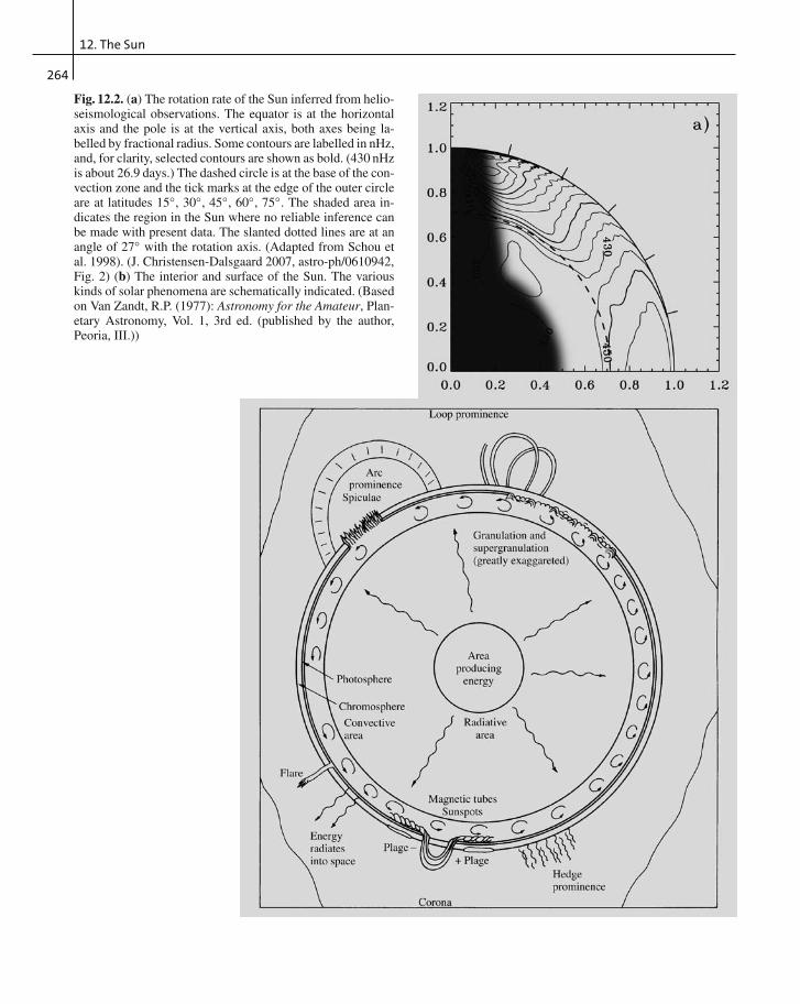
Fig. 12.2. (a) The rotation rate of the Sun inferred from helio-seismological observations. The equator is at the horizontalaxis and the pole is at the vertical axis, both axes being la-belled by fractional radius. Some contours are labelled in nHz,and, for clarity, selected contours are shown as bold. (430 nHzis about 26.9 days.) The dashed circle is at the base of the con-vection zone and the tick marks at the edge of the outer circleare at latitudes 15, 30, 45, 60, 75. The shaded area in-dicates the region in the Sun where no reliable inference canbe made with present data. The slanted dotted lines are at anangle of 27 with the rotation axis. (Adapted from Schou etal. 1998). (J. Christensen-Dalsgaard 2007, astro-ph/0610942,Fig. 2) (b) The interior and surface of the Sun. The variouskinds of solar phenomena are schematically indicated. (Basedon Van Zandt, R.P. (1977): Astronomy for the Amateur, Plan-etary Astronomy, Vol. 1, 3rd ed. (published by the author,Peoria, III.))
12. The Sun
264

12.1 Internal Structure
265
The Solar Neutrino Problem. The central nuclear re-actions produce neutrinos at several of the steps in thepp chain (see Fig. 10.5). These neutrinos can propagatefreely through the outer layers, and thus give direct in-formation about conditions near the centre of the Sun.When neutrinos from the Sun were first observed in the1970’s, their number was found to be only about a thirdof what was predicted. This disagreement is called thesolar neutrino problem.
In the first experiments only neutrinos from the ppIIand ppIII branches were observed (Sect. 10.3). Sinceonly a small fraction of the solar luminosity is producedin these reactions, it was not clear what were the conse-quences of these results for solar models. In the 1990’sneutrinos produced in the ppI branch, the main branchof the pp chain, were observed. Although the disagree-ment with the standard models was slightly smaller inthese observations (about 60% of the predicted flux wasobserved), the neutrino problem still remained.
Perhaps the most popular explanation for the solarneutrino problem was based on neutrino oscillations.According to this explanation, if neutrinos have a smallmass (about 10−2 eV), an electron neutrino could changeinto a µ or a τ neutrino as it passed through the outerparts of the Sun. In the early experiments only electronneutrinos were observed, representing only part of thetotal number of neutrinos produced.
In 2001 results were announced from experimentsin Canada and Japan that measured both the numberof electron neutrinos and the total number of neutrinosarriving from the Sun. The total flux agreed with thepredictions of the standard solar model, whereas the fluxof electron neutrinos were in agreement with the lowervalues measured in the earlier experiments. This resultproved the existence of neutrino oscillations turningsome of the electron neutrinos produced in the centre ofthe sun into other kinds.
The solar neutrino problem can now be considered tobe solved. The solution is a great success for the standardsolar model. But it has also revealed the existence ofneutrino oscillations, proving that neutrinos have a smallbut non-zero rest mass. This shows that the standardmodel of particle physics needs to be revised in somerespects.
The Solar Rotation. As soon as telescopes were intro-duced, it was observed from the motions of sunspots
that the Sun is rotating with a rotational period of about27 days. As early as 1630 Christoph Scheiner showedthat there was differential rotation: the rotational periodnear the poles was more than 30 days, while it was only25 days at the equator. The rotational axis of the Sun isinclined at 7 with respect to the plane of the ecliptic,so that the North Pole of the Sun is best visible from theEarth in September.
The motions of sunspots still give the best informa-tion on the rotation near the surface of the Sun. Othersurface features also have been used for this purpose.The rotational velocity has also been measured directlyfrom the Doppler effect. The angular velocity is usuallywritten
Ω = A − B sin2 ψ , (12.1)
where ψ is the latitude with respect to the equator. Themeasured values of the coefficients are A = 14.5 andB = 2.9 degrees/day.
The rotational velocity deeper down in the Sun can-not be directly observed. In the 1980’s a method toestimate the rotation in the interior became available,when it became possible to measure the frequencies ofsolar oscillations from the variations in spectral lines.These oscillations are essentially sound waves producedby turbulent gas motions in the convection zone. Thesesound waves have calculable oscillation periods (about3–12 minutes), which depend on the conditions in thesolar interior. By comparing the observed and theoreti-cal values one can get information about the conditionsdeep inside the Sun. The idea of the method is the sameas that used when studying the interior of the Earth bymeans of waves from earthquakes, and it is thereforecalled helioseismology.
Using helioseismology, models for the solar rotationthroughout the convection zone have been deduced. Itappears that the angular velocity in the whole convec-tion zone is almost the same as at the surface, althoughit decreases slightly with radius near the equator, andincreases near the poles. The angular velocity of the ra-diative core is still uncertain, but there are indicationsthat the core is rotating as a solid body with approx-imately the average surface angular velocity. At thebottom of the convection zone there is a thin layerknown as the tachocline, where the angular velocitychanges rapidly with radius. The internal solar rotation

266
12. The Sun
according to the helioseismological studies is shown inFig. 12.2a.
The solar differential rotation is maintained by gasmotions in the convection zone. Explaining the ob-served behaviour is a difficult problem that is not yetcompletely understood.
12.2 The Atmosphere
The solar atmosphere is divided into the photosphereand the chromosphere. Outside the actual atmosphere,the corona extends much further outwards.
The Photosphere. The innermost layer of the at-mosphere is the photosphere, which is only about300–500 km thick. The photosphere is the visible sur-face of the Sun, where the density rapidly increasesinwards, hiding the interior from sight. The tempera-ture at the inner boundary of the photosphere is 8000 Kand at the outer boundary 4500 K. Near the edgeof the solar disc, the line of sight enters the pho-tosphere at a very small angle and never penetratesto large depths. Near the edges one therefore onlysees light from the cooler, higher layers. For thisreason, the edges appear darker; this phenomenon isknown as limb darkening. Both the continuous spectrum
Fig. 12.3. The granula-tion of the solar surface.The granules are pro-duced by streaming gas.Their typical diameteris 1000 km. (PhotographT. Rimmele/Richard B.Dunn Solar Telescope,NSO/AURA/NSF)
and the absorption lines are formed in the photo-sphere, but the light in the absorption lines comesfrom higher layers and therefore the lines appeardark.
The solar convection is visible on the surface as thegranulation (Fig. 12.3), an uneven, constantly changinggranular pattern. At the bright centre of each granule,gas is rising upward, and at the darker granule bound-aries, it is sinking down again. The size of a granule seenfrom the Earth is typically 1′′, corresponding to about1000 km on the solar surface. There is also a larger scaleconvection called supergranulation in the photosphere.The cells of the supergranulation may be about 1′ in di-ameter. The observed velocities in the supergranulationare mainly directed along the solar surface.
The Chromosphere. Outside the photosphere there isa layer, perhaps about 500 km thick, where the tem-perature increases from 4500 K to about 6000 K, thechromosphere. Outside this layer, there is a transitionregion of a few thousand kilometres, where the chromo-sphere gradually goes over into the corona. In the outerparts of the transition region, the kinetic temperature isalready about 106 K.
Normally the chromosphere is not visible, because itsradiation is so much weaker than that of the photosphere.However, during total solar eclipses, the chromosphere

12.2 The Atmosphere
267
Fig. 12.4. Flash spectrumof the solar chromosphere,showing bright emissionlines
Fig. 12.5. The solar sur-face in the hydrogen Hα
line. Active regions appearbright; the dark filamentsare prominences. Limbdarkening has been re-moved artificially, whichbrings to light spiculesand prominences above thelimb. The photograph wastaken in October 1997.(Photograph Big Bear SolarObservatory/NJIT)

268
12. The Sun
shines into view for a few seconds at both ends of thetotal phase, when the Moon hides the photosphere com-pletely. The chromosphere then appears as a thin reddishsickle or ring.
During eclipses the chromospheric spectrum, calledthe flash spectrum, can be observed (Fig. 12.4). It is anemission line spectrum with more than 3000 identifiedlines. Brightest among these are the lines of hydrogen,helium and certain metals.
One of the strongest chromospheric emission linesis the hydrogen Balmer α line (Fig. 12.5) at a wave-length of 656.3 nm. Since the Hα line in the normalsolar spectrum is a very dark absorption line, a pho-tograph taken at this wavelength will show the solarchromosphere. For this purpose, one uses narrow-bandfilters letting through only the light in the Hα line. Theresulting pictures show the solar surface as a mottled,wavy disc. The bright regions are usually the size ofa supergranule, and are bounded by spicules (Fig. 12.6).These are flamelike structures rising up to 10,000 kmabove the chromosphere, and lasting for a few min-utes. Against the bright surface of the Sun, they look
Fig. 12.6. Spicules, flamelike uprisings near the edge of the solar disc. (Photograph Big Bear Solar Observatory)
like dark streaks; at the edges, they look like brightflames.
The Corona. The chromosphere gradually goes overinto the corona. The corona is also best seen duringtotal solar eclipses (Fig. 12.7). It then appears as a haloof light extending out to a few solar radii. The surfacebrightness of the corona is about that of the full moon,and it is therefore difficult to see next to the brightphotosphere.
The inner part of the corona, the K corona, hasa continuous spectrum formed by the scattering of thephotospheric light by electrons. Further out, a few solarradii from the surface, is the F corona, which has a spec-trum showing Fraunhofer absorption lines. The light ofthe F corona is sunlight scattered by dust.
In the latter part of the 19th century strong emissionlines, which did not correspond to those of any knownelement, were discovered in the corona (Fig. 12.8). Itwas thought that a new element, called coronium, hadbeen found – a little earlier, helium had been discoveredin the Sun before it was known on Earth. About 1940, it

12.2 The Atmosphere
269
Fig. 12.7. Previously, thecorona could be studiedonly during total solareclipses. The picture is fromthe eclipse on March 7,1970. Nowadays the coronacan be studied continuouslyusing a device called thecoronagraph
Fig. 12.8. The presenceof lines from highly ion-ized atoms in the coronalspectrum shows that thetemperature of the coronahas to be very high

270
12. The Sun
was established that the coronal lines were due to highlyionized atoms, e. g. thirteen times ionized iron. Muchenergy is needed to remove so many electrons from theatoms. The entire corona has to have a temperature ofabout a million degrees.
A continuous supply of energy is needed in order tomaintain the high temperature of the corona. Accordingto earlier theories, the energy came in the form of acous-tic or magnetohydrodynamic shock waves generated atthe solar surface by the convection. Most recently, heat-ing by electric currents induced by changing magneticfields has been suggested. Heat would then be gen-erated in the corona almost like in an ordinary lightbulb.
In spite of its high temperature the coronal gas isso diffuse that the total energy stored in it is small. Itis constantly streaming outwards, gradually becominga solar wind, which carries a flux of particles awayfrom the Sun. The gas lost in this way is replaced withnew material from the chromosphere. Near the Earth thedensity of the solar wind is typically 5–10 particles/cm3
and its velocity about 500 km/s. The mass loss of theSun due to the solar wind is about 10−13 M per year.
12.3 Solar Activity
Sunspots. The clearest visible sign of solar activityare the sunspots. The existence of sunspots has beenknown for long (Fig. 12.9), since the largest ones can beseen with the naked eye by looking at the Sun througha suitably dense layer of fog. More precise observationsbecame available beginning in the 17th century, whenGalilei started to use the telescope for astronomicalobservations.
A sunspot looks like a ragged hole in the solar sur-face. In the interior of the spot there is a dark umbra andaround it, a less dark penumbra. By looking at spotsnear the edge of the solar disc, it can be seen that thespots are slightly depressed with respect to the rest of thesurface. The surface temperature in a sunspot is about1500 K below that of its surroundings, which explainsthe dark colour of the spots.
The diameter of a typical sunspot is about 10,000 kmand its lifetime is from a few days to several months,depending on its size. The larger spots are more likelyto be long-lived. Sunspots often occur in pairs or in
larger groups. By following the motions of the spots,the period of rotation of the Sun can be determined.
The variations in the number of sunspots have beenfollowed for almost 250 years. The frequency of spotsis described by the Zürich sunspot number Z:
Z = C(S +10 G) , (12.2)
where S is the number of spots and G the number ofspot groups visible at a particular time. C is a con-stant depending on the observer and the conditions ofobservation.
In Fig. 12.10, the variations in the Zürich sunspotnumber between the 18th century and the present areshown. Evidently the number of spots varies with an av-erage period of about 11 years. The actual period may bebetween 7 and 17 years. In the past decades, it has beenabout 10.5 years. Usually the activity rises to its maxi-mum in about 3–4 years, and then falls off slightly moreslowly. The period was first noted by Samuel HeinrichSchwabe in 1843.
The variations in the number of sunspots have beenfairly regular since the beginning of the 18th century.However, in the 17th century there were long intervalswhen there were essentially no spots at all. This quies-cent period is called the Maunder minimum. The similarSpörer minimum occurred in the 15th century, and otherquiet intervals have been inferred at earlier epochs. Themechanism behind these irregular variations in solaractivity is not yet understood.
The magnetic fields in sunspots are measured on thebasis of the Zeeman effect, and may be as large as0.45 tesla. (The magnetic field of the Earth is 0.03 mT.)The strong magnetic field inhibits convective energytransport, which explains the lower temperature of thespots.
Sunspots often occur in pairs where the componentshave opposite polarity. The structure of such bipolargroups can be understood if the field rises into a loopabove the solar surface, connecting the components ofthe pair. If gas is streaming along such a loop, it becomesvisible as a loop prominence (Fig. 12.11).
The periodic variation in the number of sunspots re-flects a variation in the general solar magnetic field.At the beginning of a new activity cycle spots first be-gin to appear at latitudes of about ±40. As the cycleadvances, the spots move closer to the equator. Thecharacteristic pattern in which spots appear, shown in

12.3 Solar Activity
271
Fig. 12.9. The sunspots arethe form of solar activ-ity that has been knownfor the longest time. Thephotograph was taken withthe Swedish 1-meter So-lar Telescope in July 2002.(Photograph Royal SwedishAcademy of Sciences)
Fig. 12.10. The Zürich sunspot number from 1700 to 2001.Prior to 1700 there are only occasional observations. The
number of sunspots and spot groups varies with a period ofabout 11 years

272
12. The Sun
Fig. 12.11. In pairs of sunspots the magnetic field lines forma loop outside the solar surface. Material streaming along thefield lines may form loop prominences. Loops of different size
can be seen in this image, which the Trace satellite took in1999. (Photo Trace)
Fig. 12.12, is known as the butterfly diagram. Spots ofthe next cycle begin to appear while those of the oldone are still present near the equator. Spots belonging
Fig. 12.12. At the begin-ning of an activity cycle,sunspots appear at highlatitudes. As the cycle ad-vances the spots movetowards the equator. (Dia-gram by H. Virtanen, basedon Greenwich Observatoryobservations)
to the new cycle have a polarity opposite to that of theold ones. (Spots in opposite hemispheres also have op-posite polarity.) Since the field is thus reversed between

12.3 Solar Activity
273
Fig. 12.13. Because the Sun rotates faster at the equator than at the poles, the field lines of the solar magnetic field are drawnout into a tight spiral
consecutive 11 year cycles the complete period of solarmagnetic activity is 22 years.
The following general qualitative description of themechanism of the solar cycle was proposed by Ho-race W. Babcock. Starting at a solar minimum, thefield will be of a generally dipolar character. Becausea conducting medium, such as the outer layers of theSun, cannot move across the field lines, these will befrozen into the plasma and carried along by it. Thusthe differential rotation will draw the field into a tightspiral (Fig. 12.13). In the process the field becomes
Fig. 12.14. A quiet Sun in August 2006 around the last sunspotminimum. Both pictures were taken by the Michelson DopplerImager on the SOHO satellite. On the left the Sun in visible
light, on the right a magnetogram, which shows the oppositepolarities of the magnetic fields as black and white. (PhotoSOHO/NASA/ESA)
stronger, and this amplification will be a function oflatitude.
When the subsurface field becomes strong enough,it gives rise to a “magnetic buoyancy” that lifts ropes ofmagnetic flux above the surface. This happens first ata latitude about 40, and later at lower latitudes. Theseprotruding flux ropes expand into loops forming bipo-lar groups of spots. As the loops continue expandingthey make contact with the general dipolar field, whichstill remains in the polar regions. This leads to a rapidreconnection of the field lines neutralising the general

274
12. The Sun
Fig. 12.15. (a) Quiescent “hedgerow” prominence (Photo-graph Sacramento Peak Observatory). (b) Larger eruptiveprominence (Photograph Big Bear Solar Observatory)
field. The final result when activity subsides is a dipolarfield with a polarity opposite the initial one.
Thus the Babcock model accounts for the butterflydiagram, the formation of bipolar magnetic regions andthe general field reversal between activity maxima. Nev-ertheless, it remains an essentially phenomenologicalmodel, and alternative scenarios have been proposed.In dynamo theory quantitative models for the origin ofmagnetic fields in the Sun and other celestial bodies arestudied. In these models the field is produced by convec-tion and differential rotation of the gas. A completelysatisfactory dynamo model for the solar magnetic cyclehas not yet been found. For example, it is not yet knownwhether the field is produced everywhere in the con-vection zone, or just in the boundary layer between theconvective and radiative regions, as some indicationssuggest.
Other Activity. The Sun shows several other typesof surface activity: faculae and plages; prominences;flares.
The faculae and plages are local bright regions inthe photosphere and chromosphere, respectively. Ob-servations of the plages are made in the hydrogen Hα
or the calcium K lines (Fig. 12.14). The plages usuallyoccur where new sunspots are forming, and disappear

12.3 Solar Activity
275
Fig. 12.16. A violent flarenear some small sunspots.(Photograph SacramentoPeak Observatory)
when the spots disappear. Apparently they are causedby the enhanced heating of the chromosphere in strongmagnetic fields.
The prominences are among the most spectacularsolar phenomena. They are glowing gas masses in thecorona, easily observed near the edge of the Sun. Thereare several types of prominences (Fig. 12.15): the quies-cent prominences, where the gas is slowly sinking alongthe magnetic field lines; loop prominences, connectedwith magnetic field loops in sunspots; and the rarereruptive prominences, where gas is violently thrownoutwards.
The temperature of prominences is about10,000–20,000 K. In Hα photographs of the chro-mosphere, the prominences appear as dark filamentsagainst the solar surface.
The flare outbursts are among the most violent formsof solar activity (Fig. 12.16). They appear as brightflashes, lasting from one second to just under an hour.In the flares a large amount of energy stored in the mag-netic field is suddenly released. The detailed mechanismis not yet known.
Flares can be observed at all wavelengths. The hardX-ray emission of the Sun may increase hundredfold
during a flare. Several different types of flares are ob-served at radio wavelengths (Fig. 12.17). The emissionof solar cosmic ray particles also rises.
The flares give rise to disturbances on the Earth. TheX-rays cause changes in the ionosphere, which affectshort-wave radio communications. The flare particlesgive rise to strong auroras when they enter the Earth’smagnetic field a few days after the outburst.
Solar Radio Emission. The Sun is the strongest ra-dio source in the sky and has been observed sincethe 1940’s. In contrast to optical emission the radiopicture of the Sun shows a strong limb brightening.This is because the radio radiation comes from theupper layers of the atmosphere. Since the propaga-tion of radio waves is obstructed by free electrons,the high electron density near the surface prevents ra-dio radiation from getting out. Shorter wavelengths canpropagate more easily, and thus millimetre-wavelengthobservations give a picture of deeper layers in the atmo-sphere, whereas the long wavelengths show the upperlayers. (The 10 cm emission originates in the upper lay-ers of the chromosphere and the 1 m emission, in thecorona.)

276
12. The Sun
Fig. 12.17. An X-ray picture of the active Sun, taken by theJapanese Yohkoh satellite in 1999, around the last maximumof sunspot activity. (Photo JAXA)
The Sun looks different at different wavelengths.At long wavelengths the radiation is coming from thelargest area, and its electron temperature is about 106 K,since it originates in the corona.
The radio emission of the Sun is constantly changingaccording to solar activity. During large storms the totalemission may be 100,000 times higher than normal.
X-ray and UV Radiation. The X-ray emission of theSun is also related to active regions. Signs of activityare bright X-ray regions and smaller X-ray bright points,which last for around ten hours. The inner solar coronaalso emits X-rays. Near the solar poles there are coronalholes, where the X-ray emission is weak.
Ultraviolet pictures of the solar surface show it asmuch more irregular than it appears in visible light.Most of the surface does not emit much UV radiation,but there are large active regions that are very bright inthe ultraviolet.
Several satellites have made observations of the Sunat UV and X-ray wavelengths, for example Soho (Solarand Heliospheric Observatory, 1995–). These observa-tions have made possible detailed studies of the outerlayers of the Sun. Observations of other stars have re-
Fig. 12.18. The SOHO (Solar and Heliospheric Observatory)satellite keeps a constant watch on the Sun and its surround-ings in many wavelengths. Here the LASCO (Large Angle andSpectrometric Coronagraph) instrument sees a large CoronalMass Ejection erupting from the Sun. The surface of the Sunis covered by a disk, and the size and position of the Sun isindicated by the white circle. (Photo SOHO/NASA/ESA)
vealed coronae, chromospheres and magnetic variationssimilar to those in the Sun. Thus the new observationaltechniques have brought the physics of the Sun and thestars nearer to each other.
12.4 Example
Example 12.1 Assume that the Sun converts 0.8% ofits mass into energy. Find an upper limit for the ageof the Sun, assuming that its luminosity has remainedconstant.
The total amount of energy released is
E = mc2 = 0.008 Mc2
= 0.008×2×1030 kg× (3×108 ms−1)2
= 1.4×1045 J .
The time needed to radiate this energy is
t = E
L= 1.4×1045 J
3.9×1026 W
= 3.6×10¹⁸ s ≈ 1011 years .

12.5 Exercises
277
12.5 Exercises
Exercise 12.1 The solar constant, i. e. the flux densityof the solar radiation at the distance of the Earth is1370 W m−2.
a) Find the flux density on the surface of the Sun, whenthe apparent diameter of the Sun is 32′′.
b) How many square metres of solar surface is neededto produce 1000 megawatts?
Exercise 12.2 Some theories have assumed that theeffective temperature of the Sun 4.5 billion years agowas 5000 K and radius 1.02 times the current radius.What was the solar constant then? Assume that the orbitof the Earth has not changed.

Hannu Karttunen et al. (Eds.), Variable Stars.In: Hannu Karttunen et al. (Eds.), Fundamental Astronomy, 5th Edition. pp. 279–290 (2007)DOI: 11685739_13 © Springer-Verlag Berlin Heidelberg 2007
279
13. Variable Stars
Stars with changing magnitudes are called variables(Fig. 13.1). Variations in the brightness of stars were
first noted in Europe at the end of the 16th century, whenTycho Brahe’s supernova lit up (1572) and the regular lightvariation of the star o Ceti (Mira) was observed (1596).The number of known variables has grown steadily asobservational precision has improved (Fig. 13.2). The mostrecent catalogues contain about 40,000 stars known orsuspected to be variable.
Strictly speaking, all stars are variable. As was seen inChap. 11, the structure and brightness of a star change asit evolves. Although these changes are usually slow, someevolutionary phases may be extremely rapid. In certainevolutionary stages, there will also be periodic variations,for example pulsations of the outer layers of a star.
Small variations in stellar brightness are also caused byhotandcool spotsonastar’s surface, appearinganddisap-
pearing as it rotates about its axis. The luminosity of theSun changes slightly because of the sunspots. Probablythere are similar spots on almost all stars.
Initially stellar brightnesses were determined visuallyby comparing stars near each other. Later on, comparisonswere made on photographic plates. At present the mostaccurate observations are made photoelectrically or usinga CCD camera. The magnitude variation as a function oftime is called the lightcurve of a star (Fig. 13.3). From it oneobtains the amplitude of the magnitude variation and itsperiod, if the variation is periodic.
The basic reference catalogue of variable stars is theGeneral Catalogue of Variable Stars by the Soviet as-tronomer Boris Vasilyevich Kukarkin. New, supplementededitions appear at times; the fourth edition publishedin 1985−1987, edited by P.N. Kholopov, contains about32,000 variables of the Milky Way galaxy.
Fig. 13.1. The variablesare stars changing inbrightness. Two vari-ables in Scorpius, R andS Sco (Photograph YerkesObservatory)

280
13. Variable Stars
Fig. 13.2. The location ofvariables in the HR diagram
13.1 Classification
When a new variable is discovered, it is given a nameaccording to the constellation in which it is located. Thename of the first variable in a given constellation is R,followed by the name of the constellation (in the gen-itive case). The symbol for the second variable is S,and so on, to Z. After these, the two-letter symbols RR,RS, . . . to ZZ are used, and then AA to QZ (omitting I).This is only enough for 334 variables, a number that haslong been exceeded in most constellations. The number-ing therefore continues: V335, V336, etc. (V stands forvariable). For some stars the established Greek lettersymbol has been kept, although they have later beenfound to be variable (e. g. δCephei).
The classification of variables is based on the shapeof the lightcurve, and on the spectral class and ob-served radial motions. The spectrum may also containdark absorption lines from material around the star. Ob-
servations can be made outside the optical region aswell. Thus the radio emission of some variables (e. g.flare stars) increases strongly, simultaneously with theiroptical brightness. Examples of radio and X-ray vari-ables are the radio and X-ray pulsars, and the X-raybursters.
Variables are usually divided into three maintypes: pulsating, eruptive and eclipsing variables. Theeclipsing variables are binary systems in which thecomponents periodically pass in front of each other.In these variables the light variations do not corre-spond to any physical change in the stars. They havebeen treated in connection with the binary stars. In theother variables the brightness variations are intrinsicto the stars. In the pulsating variables the variationsare due to the expansion and contraction of the outerlayers. These variables are giants and supergiants thathave reached an unstable stage in their evolution. Theeruptive variables are usually faint stars ejecting mass.

13.2 Pulsating Variables
281
Fig. 13.3. The variation of brightness, colour and size ofa cepheid during its pulsation
They are mostly members of close binary systems inwhich mass is transferred from one component to theother.
In addition a few rotating variables are known, wherethe brightness variations are due to an uneven temper-ature distribution on the surface, starspots coming intosight when the star rotates. Such stars may be quitecommon – after all, our Sun is a weak rotating vari-able. The most prominent group of rotating variablesare the magnetic A stars (e. g. the α2 Canum Venatico-rum stars). These stars have strong magnetic fields thatmay be giving rise to starspots. The periods of rotat-ing variables range from about 1 day to 25 d, and theamplitudes are less than 0.1 mag.
13.2 Pulsating Variables
The wavelengths of the spectral lines of the pulsatingvariables change along with the brightness variations(Table 13.1). These changes are due to the Dopplereffect, showing that the outer layers of the star are indeed
Table 13.1. The main properties of pulsating variables (N ,number of stars of the given type in Kukarkin’s catalogue,P, pulsation period in days, ∆m, pulsation amplitude inmagnitudes)
Variable N P Spectrum ∆m
Classical cepheids 800 1–135 F–K I 2(δCep, W Vir)
RR Lyrae 6100 < 1 A–F8 2
Dwarf cepheids 200 0.05–7 A–F 1(δ Scuti)
β Cephei 90 0.1–0.6 B1–B3 III 0.3
Mira variables 5800 80–1000 M–C 2.5
RV Tauri 120 30–150 G–M 4
Semiregular 3400 30–1000 K–C 4.5
Irregular 2300 – K–M 2
pulsating. The observed gas velocities are in the rangeof 40–200 km/s.
The period of pulsation corresponds to a proper fre-quency of the star. Just like a tuning fork vibrates witha characteristic frequency when hit, a star has a fun-damental frequency of vibration. In addition to thefundamental frequency other frequencies, “overtones”,are possible. The observed brightness variation can beunderstood as a superposition of all these modes ofvibration. Around 1920, the English astrophysicist SirArthur Eddington showed that the period of pulsation Pis inversely proportional to the square root of the meandensity,
P ∝ 1√ρ. (13.1)
The diameter of the star may double during the pulsa-tion, but usually the changes in size are minor. The maincause of the light variation is the periodic variation of thesurface temperature. We have seen in Sect. 5.6 that theluminosity of a star depends sensitively on its effectivetemperature, L ∝ T 4
e . Thus a small change in effectivetemperature leads to a large brightness variation.
Normally a star is in stable hydrostatic equilibrium.If its outer layers expand, the density and temperaturedecrease. The pressure then becomes smaller and theforce of gravity compresses the gas again. However,unless energy can be transferred to the gas motions,these oscillations will be damped.
The flux of radiative energy from the stellar interiorcould provide a source of energy for the stellar oscil-

282
13. Variable Stars
lations, if it were preferentially absorbed in regions ofhigher gas density. Usually this is not the case but inthe ionization zones, where hydrogen and helium arepartially ionized, the opacity in fact becomes largerwhen the gas is compressed. If the ionization zonesare at a suitable depth in the atmosphere, the energyabsorbed during compression and released during ex-pansion of an ionization zone can drive an oscillation.Stars with surface temperatures of 6000–9000 K are li-able to this instability. The corresponding section of theHR diagram is called the cepheid instability strip.
Cepheids. Among the most important pulsating vari-ables are the cepheids, named after δCephei (Fig. 13.3).They are population I supergiants (stellar populationsare discussed in Sect. 17.2) of spectral class F–K. Theirperiods are 1–50 days and their amplitudes, 0.1–2.5magnitudes. The shape of the light curve is regular,showing a fairly rapid brightening, followed by a slowerfall off. There is a relationship between the period ofa cepheid and its absolute magnitude (i. e. luminosity),discovered in 1912 by Henrietta Leavitt from cepheidsin the Small Magellanic Cloud. This period–luminosityrelation (Fig. 13.4) can be used to measure distances ofstars and nearby galaxies.
We have already noted that the pulsation period isrelated to the mean density. On the other hand the size
Fig. 13.4. The period–luminosity relation for cepheids. Theblack points and squares are theoretically calculated values,the crosses and the straight line represent the observed relation.(Drawing from Novotny, E. (1973): Introduction to StellarAtmospheres and Interiors (Oxford University Press, NewYork) p. 359)
of a star, and hence its mean density, is related to its totalluminosity. Thus one can understand why there shouldbe a relation between the period and the luminosity ofa pulsating star.
The magnitudes M and periods P of classicalcepheids are shown in Fig. 13.4. The relation between Mand log P is linear. However, to some extent, thecepheid luminosities also depend on colour: bluer starsare brighter. For accurate distance determinations, thiseffect needs to be taken into consideration.
W Virginis Stars. In 1952 Walter Baade noted that thereare in fact two types of cepheids: the classical cepheidsand the W Virginis stars. Both types obey a period–luminosity relation, but the W Vir stars of a given periodare 1.5 magnitudes fainter than the corresponding clas-sical cepheids. This difference is due to the fact thatthe classical cepheids are young population I objects,whereas the W Vir stars are old stars of population II.Otherwise, the two classes of variables are similar.
Earlier, the W Vir period–luminosity relation hadbeen used for both types of cepheids. Consequentlythe calculated distances to classical cepheids were toosmall. For example, the distance to the AndromedaGalaxy had been based on classical cepheids, sinceonly these were bright enough to be visible at thatdistance. When the correct period–luminosity relationwas used, all extragalactic distances had to be doubled.Distances within the Milky Way did not have to bechanged, since their measurements were based on othermethods.
RR Lyrae Stars. The third important class of pulsatingvariables are the RR Lyrae stars. Their brightness vari-ations are smaller than those of the cepheids, usuallyless than a magnitude. Their periods are also shorter,less than a day. Like the W Vir stars, the RR Lyrae starsare old population II stars. They are very common inthe globular star clusters and were therefore previouslycalled cluster variables.
The absolute magnitudes of the RR Lyrae stars areabout MV = 0.6±0.3. They are all of roughly the sameage and mass, and thus represent the same evolutionaryphase, where helium is just beginning to burn in the core.Since the absolute magnitudes of the RR Lyrae variablesare known, they can be used to determine distances tothe globular clusters.

13.3 Eruptive Variables
283
Fig. 13.5. The lightcurve of a long period Mira variable
Mira Variables (Fig. 13.5). The Mira variables (namedafter Mira Ceti) are supergiants of spectral classes M,S or C, usually with emission lines in their spectrum.They are losing gas in a steady stellar wind. Their pe-riods are normally 100–500 days, and for this reason,they are also sometimes called long period variables.The amplitude of the light variations is typically about6 magnitudes in the visual region. The period of Miraitself is about 330 days and its diameter is about 2 AU.At its brightest, Mira has the magnitude 2–4, but at lightminimum, it may be down to 12. The effective temper-ature of the Mira variables is only about 2000 K. Thus95% of their radiation is in the infrared, which meansthat a very small change in temperature can cause a verylarge change in visual brightness.
Other Pulsating Variables. One additional large groupof pulsating stars are the semiregular and irregular vari-ables. They are supergiants, often very massive youngstars with unsteady pulsations in their extended outerlayers. If there is some periodicity in the pulsations,these variables are called semiregular; otherwise theyare irregular. An example of a semiregular variableis Betelgeuse (αOrionis). The pulsation mechanism ofthese stars is not well understood, since their outer lay-ers are convective, and the theory of stellar convectionis still poorly developed.
In addition to the main types of pulsating vari-ables, there are some smaller separate classes, shownin Fig. 13.2.
The dwarf cepheid and the δ Scuti stars, which aresometimes counted as a separate type, are located belowthe RR Lyrae stars in the cepheid instability strip in theHR diagram. The dwarf cepheids are fainter and morerapidly varying than the classical cepheids. Their light
curves often show a beating due to interference betweenthe fundamental frequency and the first overtone.
The β Cephei stars are located in a different partof the HR diagram than the other variables. They arehot massive stars, radiating mainly in the ultraviolet.The variations are rapid and of small amplitude. Thepulsation mechanism of the β Cephei stars is unknown.
The RV Tauri stars lie between the cepheids and theMira variables in the HR diagram. Their period dependsslightly on the luminosity. There are some unexplainedfeatures in the light curves of the RV Tauri stars, e. g.the minima are alternately deep and shallow.
13.3 Eruptive Variables
In the eruptive variables there are no regular pulsations.Instead sudden outbursts occur in which material isejected into space. Nowadays such stars are dividedinto two main categories, eruptive and cataclysmicvariables. Brightness changes of eruptive variablesare caused by sudden eruptions in the chromosphereor corona, the contributions of which are, however,rather small in the stellar scale. These stars are usu-ally surrounded by a gas shell or interstellar matterparticipating in the eruption. This group includes e.g.flare stars, various kinds of nebular variables, and RCoronae Borealis stars. Eruptions of the cataclysmicvariables are due to nuclear reactions on the stellar sur-face or interior. Explosions are so violent that they caneven destroy the whole star. This group includes no-vae and nova-like stars, dwarf novae and supernovae(Table 13.2).
Flare Stars. The flare or UV Ceti stars are dwarf stars ofspectral class M. They are young stars, mostly found inyoung star clusters and associations. At irregular inter-vals there are flare outbursts on the surface of the starssimilar to those on the Sun. The flares are related to dis-turbances in the surface magnetic fields. The energy ofthe outbursts of the flare stars is apparently about thesame as in solar flares, but because the stars are muchfainter than the Sun, a flare can cause a brightening byup to 4–5 magnitudes. A flare lights up in a few sec-onds and then fades away in a few minutes (Fig. 13.6).The same star may flare several times in one day. Theoptical flare is accompanied by a radio outburst, like in

284
13. Variable Stars
Table 13.2. Main properties of eruptive variables (N , numberof stars of the given type in Kukarkin’s catalogue,∆m, changein brightness in magnitudes. The velocity is the expansionvelocity in km/s, based on the Doppler shifts of the spectrallines)
Variable N ∆m Velocity
Supernovae 7 20 4000–10000Ordinary novae 7–18 200–3500
210Recurrent novae 10 600Nova-like stars 80 2 30–100
(P Cygni, symbiotic)Dwarf novae 330 2–6 (700)
(SS Cyg = U Gem, ZZ Cam)R Coronae Borealis 40 1–9 –Irregular 1450 4 (300)
(nebular variables,T Tau, RW Aur)
Flare stars 750 6 2000(UV Ceti)
Fig. 13.6. The outbursts of typical flare stars are of shortduration
the Sun. In fact, the flare stars were the first stars to bedetected as radio sources.
Nebular Variables. In connection with bright and darkinterstellar clouds e.g. in the constellations of Orion,Taurus and Auriga, there are variable stars. The T Tauristars are the most interesting of them. These stars arenewly formed or just contracting towards the main se-quence. The brightness variations of the T Tauri starsare irregular (Fig. 13.7). Their spectra contain brightemission lines, formed in the stellar chromosphere, andforbidden lines, which can only be formed at extremelylow densities. The spectral lines also show that matteris streaming out from the stars.
Fig. 13.7. Light curve of a T Tauri variable
Fig. 13.8. In 1969–1970, the star V1057 Cygni brightened byalmost 6 magnitudes
Since the T Tauri stars are situated inside dense gasclouds, they are difficult to observe. However, this situ-ation has improved with the development of radio andinfrared techniques.
Stars in the process of formation may change inbrightness very rapidly. For example, in 1937, FU Ori-onis brightened by 6 magnitudes. This star is a strongsource of infrared radiation, which shows that it is stillenveloped by large quantities of interstellar dust and gas.A similar brightening by six magnitudes was observedin 1969 in V1057 Cygni (Fig. 13.8). Before its bright-ening, it was an irregular T Tauri variable; since then, ithas remained a fairly constant tenth-magnitude AB star.
Stars of the R Coronae Borealis type have “inversenova” light curves. Their brightness may drop by al-most ten magnitudes and stay low for years, beforethe star brightens to its normal luminosity. For exam-ple, R CrB itself is of magnitude 5.8, but may fade to14.8 magnitudes. Figure 13.9 shows its recent decline,based on observations by Finnish and French amateurs.The R CrB stars are rich in carbon and the decline is pro-

13.3 Eruptive Variables
285
Fig. 13.9. The decline ofR Coronae Borealis in1977–1978; observationsby Finnish and Frenchamateur astronomers. (Kel-lomaki, Tahdet ja Avaruus5/1978)
duced when the carbon condenses into a circumstellardust shell.
One very interesting variable is ηCarinae (Fig.13.10). At present it is a six magnitude star surroundedby a thick, extensive envelope of dust and gas. In theearly 19th century ηCarinae was the second brighteststar in the sky after Sirius. Around the middle of thecentury it rapidly dimmed to magnitude 8, but during
Fig. 13.10. In the 19th century,ηCarinae was one of the bright-est stars in the sky; since then it has dimmed considerably. Inan outburst in 1843 the star ejected an expanding nebula, which
has been called “Homunculus”. The Hubble photograph hasbeen printed negative, to show finer details in the bipolaroutflow. (Photograph NASA/HST/University of Minnesota)
the 20th century it has brightened somewhat. The cir-cumstellar dust cloud is the brightest infrared source inthe sky outside the solar system. The energy radiated byηCarinae is absorbed by the nebula and re-radiated atinfrared wavelengths. It is not known whether ηCarinaeis related to the novae or whether it is a very young starthat cannot evolve in the normal way because of thevery thick cloud surrounding it.

286
13. Variable Stars
Fig. 13.11. The light curveof the dwarf nova SSCygni in the beginningof 1966. (Drawing byMartti Perala is based onobservations by Nordicamateurs)
Novae. One of the best known types of eruptivevariables are the novae. They are classified into sev-eral subtypes: ordinary novae, recurrent novae andnova-like variables. The dwarf novae (Fig. 13.11) arenova-like rather frequently eruptive stars with somespecial characteristics. They are nowadays divided intothree subgroups.
The outbursts of all novae are rapid. Within a dayor two the brightness rises to a maximum, which maybe 7–18 magnitudes brighter than the normal luminos-ity. This is followed by a gradual decline, which maygo on for months or years. The light curve of a typ-ical nova is shown in Fig. 13.12. This light curve ofNova Cygni 1975 has been composed from hundreds ofobservations, mostly by amateurs.
In recurrent novae, the brightening is somewhat lessthan 10 magnitudes and in dwarf novae, 2–6 magni-tudes. In both types there are repeated outbursts. Forrecurrent novae the time between outbursts is a fewdecades and for the dwarf novae 20–600 days. The inter-val depends on the strength of the outburst: the strongerthe outburst, the longer the time until the next one. Thebrightening in magnitudes is roughly proportional to thelogarithm of the recharging interval. It is possible thatordinary novae obey the same relationship. However,their amplitude is so much larger that the time betweenoutbursts should be thousands or millions of years.
Observations have shown all novae and dwarf novaeto be members of close binary systems. One componentof the system is a normal star and the other is a whitedwarf surrounded by a gas ring. (The evolution of closebinary systems was considered in Sect. 11.6, where itwas seen how this kind of system might have beenformed.) The normal star fills its Roche surface, and
material from it streams over to the white dwarf. Whenenough mass has collected on the surface of the whitedwarf, the hydrogen is explosively ignited and the outershell is ejected. The brightness of the star grows rapidly.As the ejected shell expands, the temperature of the stardrops and the luminosity gradually decreases. However,the outburst does not stop the mass transfer from thecompanion star, and gradually the white dwarf accretesnew material for the next explosion (Fig. 13.13).
The emission and absorption lines from the expand-ing gas shell can be observed in the spectrum of a nova.The Doppler shifts correspond to an expansion velocityof about 1000 km/s. As the gas shell disperses, its spec-trum becomes that of a typical diffuse emission nebula.The expanding shell around a nova can also sometimesbe directly seen in photographs.
A considerable fraction of the novae in our Galaxyare hidden by interstellar clouds and their numberis therefore difficult to estimate. In the AndromedaGalaxy, observations indicate 25–30 nova explosionsper year. The number of dwarf novae is much larger. Inaddition there are nova-like variables, which share manyof the properties of novae, such as emission lines fromcircumstellar gas and rapid brightness variations. Thesevariables, some of which are called symbiotic stars, areclose binaries with mass transfer. Gas streaming fromthe primary hits a gas disc around the secondary in a hotspot, but there are no nova outbursts.
Supernovae. The supernovae are stars with the largestbrightness variations. In a few days their brightness mayrise more than 20 magnitudes, i. e. the luminosity mayincrease by a factor of a hundred million. After themaximum, there is a slow decline lasting several years.

13.3 Eruptive Variables
287
Fig. 13.12. In 1975 a newvariable, Nova Cygni orV1500 Cygni, was dis-covered in Cygnus. Inthe upper photograph thenova is at its brightest(about 2 magnitudes), andin the lower photographit has faded to magni-tude 15. (Photographs LickObservatory)

288
13. Variable Stars
Fig. 13.13. The novae are thought tobe white dwarfs accreting matter froma nearby companion star. At times, nu-clear reactions burning the accretedhydrogen are ignited, and this is seen asthe flare-up of a nova
The supernovae are exploding stars. In the explo-sion a gas shell expanding with a velocity around10,000 km/s is ejected. The expanding gas shell re-mains visible for thousands of years. A few tens of suchsupernova remnants have been discovered in the MilkyWay. The remnant of the actual star may be a neutronstar or a black hole.
The supernovae are classified as type I and type IIbased on whether their spectra show evidence of hydro-gen. Type I supernovae are further divided into types Ia(silicon is present), Ib (no silicon, but helium present),and Ic (no silicon, little helium).
Fig. 13.14. The lightcurves of the two types of super-novae. Above SN 1972e type I and below SN 1970g type II.(Kirchner, R.P. (1976): Sci. Am. 235, No. 6, 88)
The supernova types also differ in regard to theirlight curves (Fig. 13.14). Type I supernovae fade awayin a regular manner, almost exponentially. The declineof a type II supernova is less regular and its maximumluminosity is smaller. Type II supernovae have beenfurther subdivided into several classes on the basis oftheir light curves.
In Chap. 11 it was mentioned that there are severalpossible ways in which a star may come to explodeat the end of its evolution. The type II supernova isthe natural endpoint of the evolution of a single star.Types Ib and Ic also arise from massive stars that havelost their hydrogen envelope by winds or to a companion(e. g. Wolf–Rayet stars). These types are collectivelyreferred to as core-collapse supernovae.
The type Ia supernovae, on the other hand, have aboutthe mass of the Sun and should end up as white dwarfs.However, if a star is accreting mass from a binary com-panion, it will undergo repeated nova outbursts. Someof the accreted material will then be turned into he-lium or carbon and oxygen, and will collect on the starand increase its mass. Finally the mass may exceed theChandrasekhar limit. The star will then collapse andexplode as a supernova.
At least six supernova explosions have been ob-served in the Milky Way. Best known are the “gueststar” seen in China in 1054 (whose remnant is theCrab nebula), Tycho Brahe’s supernova in 1572 andKepler’s supernova in 1604. On the basis of observa-tions of other Sb–Sc-type spiral galaxies, the intervalbetween supernova explosions in the Milky Way is

13.4 Examples
289
Fig. 13.15. Supernova 1987A in the Large Magellanic Cloud before and after the explosion. (Photographs ESO)
predicted to be about 50 years. Some will be hid-den by obscuring material, but the 400 years’ intervalsince the last observed supernova explosion is unusuallylong.
On February 23, 1987 the first burst of light froma supernova in the Large Magellanic Cloud, the smallcompanion galaxy of the Milky Way, reached the Earth(Fig. 13.15). This supernova, SN 1987A, was of type II,and was the brightest supernova for 383 years. Afterits first detection, SN 1987A was studied in great detailby all available means. Although the general ideas ofSects. 11.4 and 11.5 on the final stages of stellar evolu-tion have been confirmed, there are complications. Thuse.g. the progenitor star was a blue rather than a red giantas expected, perhaps because of the lower abundance ofheavy elements in the Large Magellanic Cloud com-pared to that in the Milky Way. The collapse of its corereleased a vast amount of energy as a pulse of neutrinos,which was detected in Japan and the USA. The amount
of energy released indicates that the remnant is a neu-tron star. As of January 2006 the remnant has, however,not been seen yet.
13.4 Examples
Example 13.1 The observed period of a cepheid is20 days and its mean apparent magnitude m = 20. FromFig. 13.4, its absolute magnitude is M ≈ −5. Accordingto (4.11), the distance of the cepheid is
r = 10×10(m − M)/5 = 10×10(20 + 5)/5
= 106 pc = 1 Mpc .
Example 13.2 The brightness of a cepheid varies2 mag. If the effective temperature is 6000 K at the max-imum and 5000 K at the minimum, how much does theradius change?

290
13. Variable Stars
The luminosity varies between
Lmax = 4πR2maxσT 4
max,
Lmin = 4πR2minσT 4
min .
In magnitudes the difference is
∆m = −2.5 lgLmin
Lmax= −2.5 lg
4πR2minσT 4
min
4πR2maxσT 4
max
= −5 lgRmin
Rmax−10 lg
Tmin
Tmax.
This gives
lgRmin
Rmax= −0.2∆m −2 lg
Tmin
Tmax
= −0.4−2 lg5000
6000= −0.24 ,
whence
Rmin
Rmax= 0.57 .
13.5 Exercises
Exercise 13.1 The absolute visual magnitude ofRR Lyrae variables is 0.6±0.3. What is the relativeerror of distances due to the deviation in the magnitude?Exercise 13.2 The bolometric magnitude of a longperiod variable varies by one magnitude. The effectivetemperature at the maximum is 4500 K.a) What is the temperature at the minimum, if the vari-ation is due to temperature change only?b) If the temperature remains constant, what is therelative variation in the radius?
Exercise 13.3 In 1983 the radius of the Crab nebulawas about 3′. It is expanding 0.21′′ a year. Radial ve-locities of 1300 km s−1 with respect to the central starhave been observed in the nebula.
a) What is the distance of the nebula, assuming its ex-pansion is symmetric?
b) A supernova explosion has been observed in the di-rection of the nebula. Estimate, how long time ago?
c) What was the apparent magnitude of the supernova,if the absolute magnitude was a typical −18?

Hannu Karttunen et al. (Eds.), Compact Stars.In: Hannu Karttunen et al. (Eds.), Fundamental Astronomy, 5th Edition. pp. 291–305 (2007)DOI: 11685739_14 © Springer-Verlag Berlin Heidelberg 2007
291
14. Compact Stars
In astrophysics those stars in which the density of matteris much larger than in ordinary stars are known as com-
pact objects. These include white dwarfs, neutron stars,and black holes. In addition to a very high density, thecompact objects are characterised by the fact that nuclearreactions have completely ceased in their interiors. Conse-quently they cannot support themselves against gravityby thermal gas pressure. In the white dwarfs and neutronstars, gravity is resisted by the pressure of a degenerategas. In the black holes the force of gravity is completely
dominant and compresses the stellar material to infinitedensity.
Compact stars in binary systems give rise to a varietyof striking new phenomena. If the companion star is los-ing mass by a stellar wind or a Roche lobe overflow, thegas that is shed may be accreted by the compact object.This will release gravitational energy that can be observ-able in the form of X-ray emission and strong and rapidbrightness variations.
14.1 White Dwarfs
As was mentioned in Sect. 10.2, in ordinary stars thepressure of the gas obeys the equation of state of anideal gas. In stellar interiors the gas is fully ionized, i. e.it is plasma consisting of ions and free electrons. The
Fig. 14.1. Two views of the best-known white dwarf Sirius B,the small companion to Sirius. On the left, a picture in visiblelight by the Hubble Space Telescope. Sirius B is the tiny whitedot on lower left from the overexposed image of Sirius. On the
right, an X-ray picture of the pair taken by the Chandra X-rayobservatory. Sirius B is now the brighter source, and Sirius isweaker, because its surface is much cooler than the surface ofthe white dwarf. (Photos NASA / HST and Chandra)
partial pressures of the ions and electrons together withthe radiation pressure important in hot stars comprisethe total pressure balancing gravitation. When the starruns out of its nuclear fuel, the density in the interiorincreases, but the temperature does not change much.The electrons become degenerate, and the pressure is

292
14. Compact Stars
mainly due to the pressure of the degenerate electrongas, the pressure due to the ions and radiation beingnegligible. The star becomes a white dwarf.
As will be explained in *The Radius of White Dwarfsand Neutron Stars (p. 298) the radius of a degeneratestar is inversely proportional to the cubic root of themass. Unlike in a normal star the radius decreases asthe mass increases.
The first white dwarf to be discovered was Sirius B,the companion of Sirius (Fig. 14.1). Its exceptional na-ture was realized in 1915, when it was discovered thatits effective temperature was very high. Since it is faint,this meant that its radius had to be very small, slightlysmaller than that of the Earth. The mass of Sirius B wasknown to be about equal to that of the Sun, so its densityhad to be extremely large.
The high density of Sirius B was confirmed in 1925,when the gravitational redshift of its spectral lines wasmeasured. This measurement also provided early obser-vational support to Einstein’s general theory of relativity.
White dwarfs occur both as single stars and in binarysystems. Their spectral lines are broadened by the stronggravitational field at the surface. In some white dwarfsthe spectral lines are further broadened by rapid rotation.Strong magnetic fields have also been observed.
White dwarfs have no internal sources of energy,but further gravitational contraction is prevented bythe pressure of the degenerate electron gas. Radiatingaway the remaining heat, white dwarfs will slowly cool,changing in colour from white to red and finally to black.The cooling time is comparable to the age of the Uni-verse, and even the oldest white dwarfs should still beobservable. Looking for the faintest white dwarfs hasbeen used as a way to set a lower limit on the age of theUniverse.
Cataclysmic variables. When a white dwarf is a mem-ber of a close binary system, it can accrete mass fromits companion star. The most interesting case is wherea main sequence star is filling its Roche lobe, the largestvolume it can have without spilling over to the whitedwarf. As the secondary evolves, it expands and beginsto lose mass, which is eventually accreted by the pri-mary. Binary stars of this kind are known as cataclysmicvariables.
The present definition of the class of cataclysmicvariables has gradually evolved, and in consequence
many types of systems that were earlier viewed as sep-arate are now collected under this heading. In principle,even type Ia supernovae should be included. The clas-sical novae, whose eruptions are caused by the suddenignition of hydrogen that has collected on the surfaceof the white dwarf, have been described in Sect. 13.3.In the eruptions most of the accreted gas is expelledin a shell, but if the mass transfer continues in the sys-tem further eruptions may occur, giving rise to recurrentnovae. Finally, cataclysmic variables without eruptions,for example pre-novae or post-novae, are classified asnova-like variables.
The dwarf novae, also described in Sect. 13.3, areproduced by a quite different mechanism. In their casethe outbursts are not caused by thermonuclear reactions,but by instabilities in the accretion flow around the whitedwarf. Although the details of the outburst mechanismare still not completely clear, the basic picture is thatthe disc has two possible states, a hot and a cool one,available. Under some conditions the disc cannot remainpermanently in either of these states, and has to jumprepeatedly between the hot outburst state and the coolquiescent state.
A special type of nova-like variables are the magneticcataclysmic variables. In the polars the magnetic field isso strong that the accreted gas cannot settle into an ac-cretion disc. Instead it is forced to follow the magneticfield lines, forming an accretion column. As the gas hitsthe surface of the white dwarf it is strongly heated givingrise rise to bright X-ray emission, which is a character-istic feature of polars. Systems with a slightly weakermagnetic field are called intermediate polars. These sys-tems exhibit both X-ray emission and variations due toan accretion disc.
14.2 Neutron Stars
If the mass of a star is large enough, the density of mat-ter may grow even larger than in normal white dwarfs.The equation of state of a classical degenerate electrongas then has to be replaced with the corresponding rel-ativistic formula. In this case decreasing the radius ofthe star no longer helps in resisting the gravitationalattraction. Equilibrium is possible only for one partic-ular value of the mass, the Chandrasekhar mass MCh,already introduced in Sect. 11.5. The value of MCh is

14.2 Neutron Stars
293
about 1.4 M, which is thus the upper limit to themass of a white dwarf. If the mass of the star is largerthan MCh, gravity overwhelms the pressure and the starwill rapidly contract towards higher densities. The finalstable state reached after this collapse will be a neu-tron star (Fig. 14.2). On the other hand, if the mass issmaller than MCh, the pressure dominates. The star willthen expand until the density is small enough to allowan equilibrium state with a less relativistic equation ofstate.
When a massive star reaches the end of its evolutionand explodes as a supernova, the simultaneous collapseof its core will not necessarily stop at the density ofa white dwarf. If the mass of the collapsing core is largerthan the Chandrasekhar mass ( 1.4 M), the collapsecontinues to a neutron star.
An important particle reaction during the final stagesof stellar evolution is the URCA process, which was putforward by Schonberg and Gamow in the 1940’s andwhich produces a large neutrino emission without oth-erwise affecting the composition of matter. (The URCAprocess was invented in Rio de Janeiro and named aftera local casino. Apparently money disappeared at URCAjust as energy disappeared from stellar interiors in theform of neutrinos. It is claimed that the casino wasclosed by the authorities when this similarity becameknown.) The URCA process consists of the reactions
(Z, A)+ e− → (Z −1, A)+νe ,
(Z −1, A)→ (Z, A)+ e− + νe ,
where Z is the number of protons in a nucleus; A themass number; e− an electron; and νe and νe the electronneutrino and antineutrino. When the electron gas is de-generate, the latter reaction is suppressed by the Pauli
Fig. 14.2. The structure ofa neutron star. The crust is rigidsolid material and the mantlea freely streaming superfluid
exclusion principle. In consequence the protons in thenuclei are transformed into neutrons. As the numberof neutrons in the nuclei grows, their binding energiesdecrease. At densities of about 4×10¹⁴ kg/m3 the neu-trons begin to leak out of the nucleus, and at 1017 kg/m3
the nuclei disappear altogether. Matter then consists ofa neutron “porridge”, mixed with about 0.5% electronsand protons.
Neutron stars are supported against gravity by thepressure of the degenerate neutron gas, just as whitedwarfs are supported by electron pressure. The equa-tion of state is the same, except that the electron mass isreplaced by the neutron mass, and that the mean molec-ular weight is defined with respect to the number offree neutrons. Since the gas consists almost entirely ofneutrons, the mean molecular weight is approximatelyone.
The typical diameters of neutron stars are about10 km. Unlike ordinary stars they have a well-definedsolid surface. The atmosphere above it is a few cen-timetres thick. The upper crust is a metallic solid withthe density growing rapidly inwards. Most of the staris a neutron superfluid, and in the centre, where thedensity exceeds 1018 kg/m3, there may be a solid nu-cleus of heavier particles (hyperons), or of quark matter,where the quarks that normally constitute neutrons havebecome unconfined.
A neutron star formed in the explosion and collapseof a supernova will initially rotate rapidly, because itsangular momentum is unchanged while its radius ismuch smaller than before. In a few hours the star willsettle in a flattened equilibrium, rotating several hun-dred times per second. The initial magnetic field of theneutron star will also be compressed in the collapse,so that there will be a strong field coupling the star

294
14. Compact Stars
to the surrounding material. The angular momentumof the neutron star is steadily decreased by the emis-sion of electromagnetic radiation, neutrinos, cosmic rayparticles and possibly gravitational radiation. Thus theangular velocity decreases. The rotation can also breakthe star into several separate objects. They will even-tually recombine when the energy of the system isreduced. In some cases the stars can remain separated,resulting e. g. in a binary neutron star.
The theory of neutron stars was developed in the1930’s, but the first observations were not made untilthe 1960’s. At that time the pulsars, a new type of rapidlypulsating radio sources, were discovered and identi-fied as neutron stars. In the 1970’s neutron stars werealso seen as members of X-ray binaries, such as X-raypulsars and X-ray bursters (Fig. 14.9) (see Sect. 14.4).
Pulsars. The pulsars were discovered in 1967, whenAnthony Hewish and Jocelyn Bell in Cambridge, Eng-land, detected sharp, regular radio pulses coming fromthe sky. Since then about 1500 pulsars have been dis-covered (Fig. 14.4). Their periods range from 0.0016 s(for the pulsar 1937+214) up to 20 minutes.
In addition to the steady slowing down of the rota-tion, sometimes small sudden jumps in the period areobserved. These might be a sign of rapid mass move-ments in the neutron star crust (“starquakes”) or in itssurroundings.
The origin of the radio pulses can be understoodif the magnetic field is tilted at an angle of 45 −90with respect to the rotation axis. There will then bea magnetosphere around the star, where the particlesare tied to the magnetic field and rotate with it (Fig.14.3). At a certain distance from the star, the speedof rotation approaches the speed of light. The rapidlymoving particles will there emit radiation in a narrowcone in their direction of motion. As the star rotates, thiscone sweeps around like a lighthouse beam, and is seenas rapid pulses. At the same time relativistic particlesstream out from the neutron star.
The best-known pulsar is located in the Crab nebula(Fig. 14.5). This small nebula in the constellation Tauruswas noted by the French astronomer Charles Messierin the middle of the 18th century and became the firstobject in the Messier catalogue, M1. The Crab nebulawas found to be a strong radio source in 1948 and anX-ray source in 1964. The pulsar was discovered in
Fig. 14.3. The magnetic field around a rotating neutron starcarries plasma with it. At a certain distance the speed ofthe plasma approaches the speed of light. At this distancethe radiating regions S emit radiation in a narrow forwardbeam. Radiation from the point P hits the observer locatedin the direction of the arrow. (Drawing from Smith, F.G.(1977): Pulsars (Cambridge University Press, Cambridge)p. 189)
Fig. 14.4. Consecutive radio pulses at 408 MHz from twopulsars. To the left PSR 1642-03 and to the right PSR 1133+16.Observations made at Jodrell Bank. (Picture from Smith, F.G.(1977): Pulsars (Cambridge University Press, Cambridge) pp.93, 95)

14.2 Neutron Stars
295
Fig. 14.5. A time-sequenceof the pulsation of theCrab pulsar in visible light.The pictures were takenonce about every millisec-ond; the period of thepulsar is about 33 mil-liseconds. (Photos N.A.Sharp/NOAO/AURA/NSF)
1968. In the following year it was observed opticallyand was also found to be an X-ray emitter.
Neutron stars are difficult to study optically, sincetheir luminosity in the visible region is very small (typ-ically about 10−6 L). For instance the Vela pulsar hasbeen observed at a visual magnitude of about 25. In theradio region, it is a very strong pulsating source.
A few pulsars have been discovered in binary sys-tems; the first one, PSR 1913+16, in 1974. In 1993Joseph Taylor and Russell Hulse were awarded the No-bel prize for the detection and studies of this pulsar. Thepulsar orbits about a companion, presumably anotherneutron star, with the orbital eccentricity 0.6 and the pe-riod 8 hours. The observed period of the pulses is alteredby the Doppler effect, and this allows one to determinethe velocity curve of the pulsar. These observations canbe made very accurately, and it has therefore been pos-sible to follow the changes in the orbital elements ofthe system over a period of several years. For example,the periastron direction of the binary pulsar has beenfound to rotate about 4 per year. This phenomenon canbe explained by means of the general theory of rela-tivity; in the solar system, the corresponding rotation(the minor fraction of the rotation not explained by the
Newtonian mechanics) of the perihelion of Mercury is43 arc seconds per century.
The binary pulsar PSR 1913+16 has also provided thefirst strong evidence for the existence of gravitationalwaves. During the time of observation the orbital periodof the system has steadily decreased. This shows thatthe system is losing orbital energy at a rate that agreesexactly with that predicted by the general theory ofrelativity. The lost energy is radiated as gravitationalwaves.
Magnetars. The energy emitted by common pulsars hasits origin in the slowing down of their rotation. In someneutron stars, the magnetars, the magnetic field is sostrong that the energy released in the decay of the fieldis the main source of energy. Whereas in ordinary pul-sars the magnetic field is typically 108 T, in magnetarsa typical value may be 109–1011 T.
Magnetars were first invoked as an explanation of thesoft gamma repeaters (SGR), X-ray stars that irregularlyemit bright, short (0.1 s) repeating flashes of low-energygamma rays. Later a second class of mysterious objects,the anomalous X-ray pulsars (AXP), were identifiedas magnetars. AXP are slowly rotating pulsars, with a

296
14. Compact Stars
rotation period of 6 to 12 seconds. Despite this they arebright X-ray sources, which can be understood if theirenergy is of magnetic origin.
It is thought that magnetars are the remnants ofstars that were more massive and rapidly rotating thanthose giving rise to ordinary pulsars, although the de-tails are still subject to debate. A magnetar first appearsas a SGR. During this phase, which only lasts about10,000 years, the very strong magnetic field is slow-ing down the rate of rotation. At the same time the fieldis drifting with respect to the neutron star crust. Thiscauses shifts in the crust structure, leading to powerfulmagnetic flares and the observed outbursts. After about10,000 years the rotation has slowed down so much thatthe outbursts cease, leaving the neutron star observableas an AXP.
Gamma ray bursts. For a long time the gamma raybursts (GRB), very short and sharp gamma ray pulsesfirst discovered in 1973, remained a mystery. Unlike themuch less common SGR, the GRB never recurred, andthey had no optical or X-ray counterparts. A first ma-jor advance was made when satellite observations withthe Compton Gamma Ray Observatory showed that thegamma ray bursts are almost uniformly distributed inthe sky, unlike the known neutron stars.
The nature of the gamma ray bursts is now becom-ing clear thanks to dedicated observing programmesthat have used burst detections by gamma and X-raysatellites such as Beppo-SAX and, in particular, Swiftrapidly to look for afterglows of the GRB at opti-cal wavelengths. The detection of these afterglows hasmade it possible to determine distances to the bursts andtheir location in their host galaxies (see Fig. 14.6).
It has become clear that there are at least two kinds ofbursts, with the self-descriptive names long soft bursts,and short hard bursts. The long soft gamma ray bursts,lasting longer than 2 seconds, have now been convinc-ingly shown to be produced in the explosions of massivestars at the end of their life, specifically supernovae oftypes Ib and Ic (Sect. 13.3). Only a small fraction ofall type Ibc SNe give rise to GRB. The explosions thatproduce GRB have been called hypernovae, and areamong the brightest objects in the Universe. A gammaray burst observed in late 2005 took place when theUniverse was only 900 million years old, making itone of the most distant objects ever observed. The con-
Fig. 14.6. The location of the peculiar type Ibc supernovaSN 1998bw at redshift z = 0.0085 is in the circle to the lowerleft. This was also the position of the faint gamma-ray burstGRB 980425, the first GRB to be connected with a supernova.The circle on the upper right marks an ultraluminous X-raysource. (C.Kouveliotou et al. 2004, ApJ 608, 872, Fig. 1)
Fig. 14.7. Some pulsars shine brightly in gamma-rays. In thecenter the Crab pulsar and on the upper left the gamma sourceGeminga, which was identified in 1992 to be the nearest pul-sar with a distance of about 100 pc from the Sun. (Photo byCompton Gamma Ray Observatory)
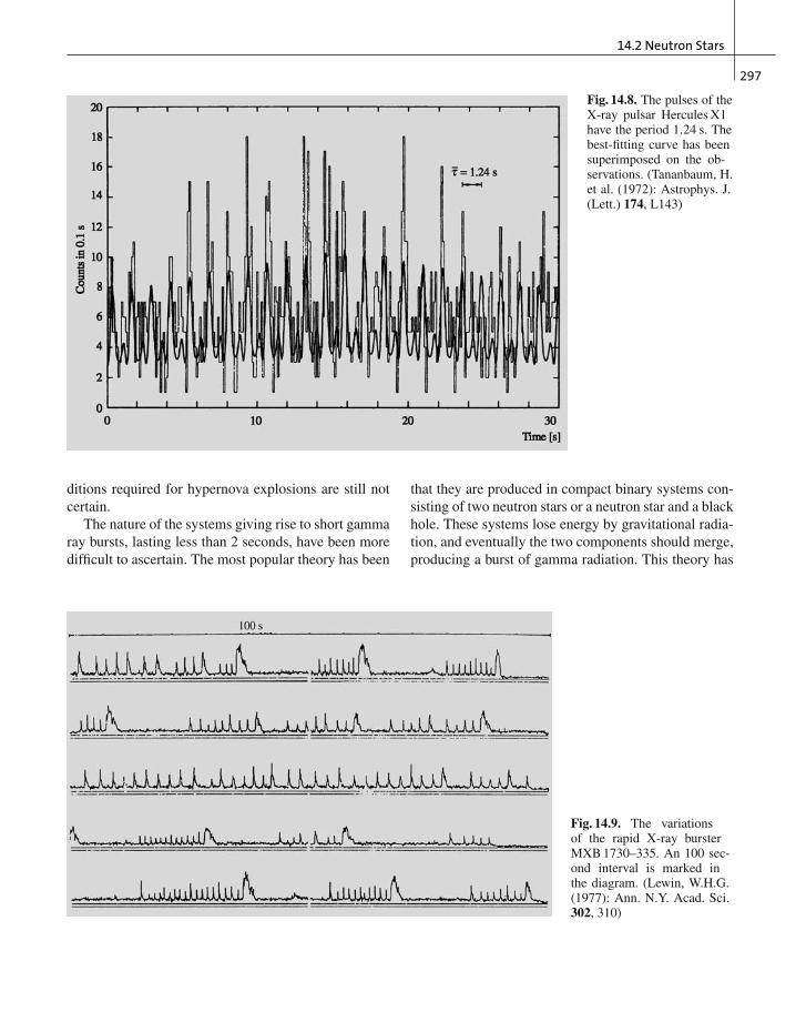
14.2 Neutron Stars
297
Fig. 14.8. The pulses of theX-ray pulsar Hercules X1have the period 1.24 s. Thebest-fitting curve has beensuperimposed on the ob-servations. (Tananbaum, H.et al. (1972): Astrophys. J.(Lett.) 174, L143)
ditions required for hypernova explosions are still notcertain.
The nature of the systems giving rise to short gammaray bursts, lasting less than 2 seconds, have been moredifficult to ascertain. The most popular theory has been
Fig. 14.9. The variationsof the rapid X-ray bursterMXB 1730–335. An 100 sec-ond interval is marked inthe diagram. (Lewin, W.H.G.(1977): Ann. N.Y. Acad. Sci.302, 310)
that they are produced in compact binary systems con-sisting of two neutron stars or a neutron star and a blackhole. These systems lose energy by gravitational radia-tion, and eventually the two components should merge,producing a burst of gamma radiation. This theory has

298
14. Compact Stars
now received strong support when the afterglow of afew short bursts has been detected in the outer parts oftheir host galaxies. Since the stars in these regions areall old and no longer give rise to core-collapse super-novae, the neutron star merger hypothesis appears mostlikely. However, it is still also possible that some of theshort bursts are exceptionally bright magnetar flares.
* The Radius of White Dwarfs and Neutron Stars
The mass of a white dwarf or a neutron star determinesits radius. This follows from the equation of hydro-static equilibrium and from the pressure-density relationfor a degenerate gas. Using the hydrostatic equilibriumequation (10.1)
dP
dr= −G Mrρ
r2
one can estimate the average pressure P:∣∣∣∣dP
dr
∣∣∣∣≈ P
R∝ M × M/R3
R2= M2
R5.
Here we have used ρ ∝ M/R3. Thus the pressure obeys
P ∝ M2/R4 . (14.1)
In the nonrelativistic case, the pressure of a degenerateelectron gas is given by (10.16):
P ≈ (h2/me)(µemH)−5/3ρ5/3
and hence
P ∝ ρ5/3
meµ5/3e
. (14.2)
By combining (14.1) and (14.2) we obtain
M2
R4∝ M5/3
R5meµ5/3e
or
R ∝ 1
M1/3meµ5/3e
∝ M−1/3 .
Thus the smaller the radius of a white dwarf is, the largerits mass will be. If the density becomes so large that therelativistic equation of state (10.17) has to be used, theexpression for the pressure is
P ∝ ρ4/3 ∝ M4/3
R4.
As the star contracts, the pressure grows at the samerate as demanded by the condition for hydrostatic sup-port (14.1). Once contraction has begun, it can onlystop when the state of matter changes: the electrons andprotons combine into neutrons. Only a star that is mas-sive enough can give rise to a relativistic degeneratepressure.
The neutrons are fermions, just like the electrons.They obey the Pauli exclusion principle, and the de-generate neutron gas pressure is obtained from anexpression analogous to (14.2):
Pn ∝ ρ5/3
mnµ5/3n
,
where mn is the neutron mass and µn, the molecularweight per free neutron. Correspondingly, the radius ofa neutron star is given by
Rns ∝ 1
M1/3mnµ5/3n
.
If a white dwarf consists purely of helium, µe = 2; fora neutron star, µn ≈ 1. If a white dwarf and a neutronstar have the same mass, the ratio of their radii is
Rwd
Rns=(
Mns
Mwd
)1/3 (µn
µe
)5/3 mn
me
≈ 1×(
1
2
)5/3
×1840 ≈ 600 .
Thus the radius of a neutron star is about 1/600 of thatof a white dwarf. Typically Rns is about 10 km.
14.3 Black Holes
If the mass of a star exceeds MOV, and if it does notlose mass during its evolution it can no longer reachany stable final state. The force of gravity will dominateover all other forces, and the star will collapse to a blackhole. A black hole is black because not even light canescape from it. Already at the end of the 18th centuryLaplace showed that a sufficiently massive body wouldprevent the escape of light from its surface. Accordingto classical mechanics, the escape velocity from a bodyof radius R and mass M is
ve =√
2G M
R.
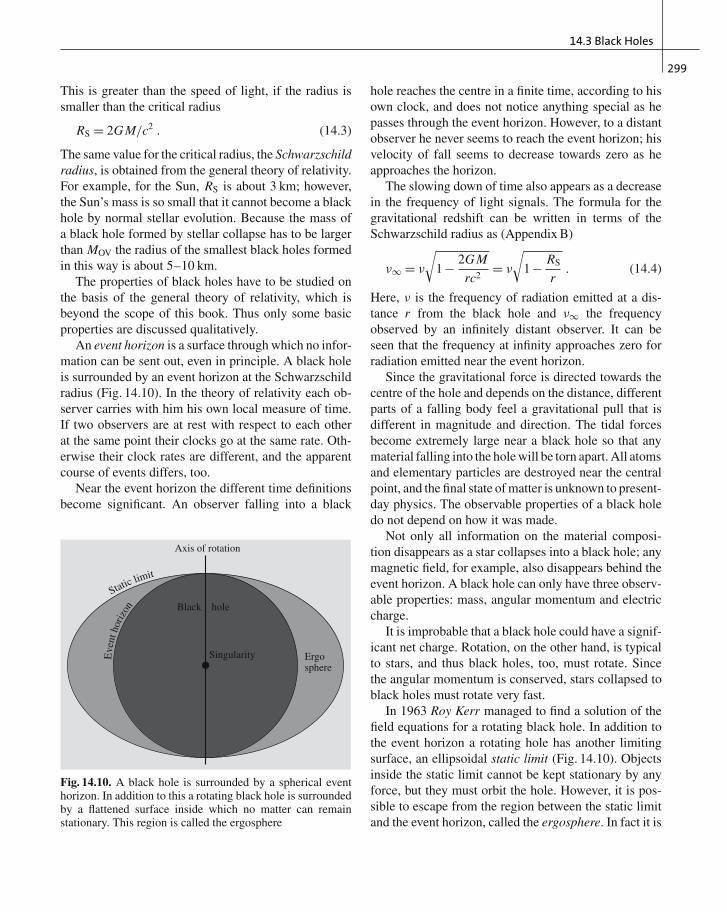
14.3 Black Holes
299
This is greater than the speed of light, if the radius issmaller than the critical radius
RS = 2G M/c2 . (14.3)
The same value for the critical radius, the Schwarzschildradius, is obtained from the general theory of relativity.For example, for the Sun, RS is about 3 km; however,the Sun’s mass is so small that it cannot become a blackhole by normal stellar evolution. Because the mass ofa black hole formed by stellar collapse has to be largerthan MOV the radius of the smallest black holes formedin this way is about 5–10 km.
The properties of black holes have to be studied onthe basis of the general theory of relativity, which isbeyond the scope of this book. Thus only some basicproperties are discussed qualitatively.
An event horizon is a surface through which no infor-mation can be sent out, even in principle. A black holeis surrounded by an event horizon at the Schwarzschildradius (Fig. 14.10). In the theory of relativity each ob-server carries with him his own local measure of time.If two observers are at rest with respect to each otherat the same point their clocks go at the same rate. Oth-erwise their clock rates are different, and the apparentcourse of events differs, too.
Near the event horizon the different time definitionsbecome significant. An observer falling into a black
Fig. 14.10. A black hole is surrounded by a spherical eventhorizon. In addition to this a rotating black hole is surroundedby a flattened surface inside which no matter can remainstationary. This region is called the ergosphere
hole reaches the centre in a finite time, according to hisown clock, and does not notice anything special as hepasses through the event horizon. However, to a distantobserver he never seems to reach the event horizon; hisvelocity of fall seems to decrease towards zero as heapproaches the horizon.
The slowing down of time also appears as a decreasein the frequency of light signals. The formula for thegravitational redshift can be written in terms of theSchwarzschild radius as (Appendix B)
ν∞ = ν
√1− 2G M
rc2= ν
√1− RS
r. (14.4)
Here, ν is the frequency of radiation emitted at a dis-tance r from the black hole and ν∞ the frequencyobserved by an infinitely distant observer. It can beseen that the frequency at infinity approaches zero forradiation emitted near the event horizon.
Since the gravitational force is directed towards thecentre of the hole and depends on the distance, differentparts of a falling body feel a gravitational pull that isdifferent in magnitude and direction. The tidal forcesbecome extremely large near a black hole so that anymaterial falling into the hole will be torn apart. All atomsand elementary particles are destroyed near the centralpoint, and the final state of matter is unknown to present-day physics. The observable properties of a black holedo not depend on how it was made.
Not only all information on the material composi-tion disappears as a star collapses into a black hole; anymagnetic field, for example, also disappears behind theevent horizon. A black hole can only have three observ-able properties: mass, angular momentum and electriccharge.
It is improbable that a black hole could have a signif-icant net charge. Rotation, on the other hand, is typicalto stars, and thus black holes, too, must rotate. Sincethe angular momentum is conserved, stars collapsed toblack holes must rotate very fast.
In 1963 Roy Kerr managed to find a solution of thefield equations for a rotating black hole. In addition tothe event horizon a rotating hole has another limitingsurface, an ellipsoidal static limit (Fig. 14.10). Objectsinside the static limit cannot be kept stationary by anyforce, but they must orbit the hole. However, it is pos-sible to escape from the region between the static limitand the event horizon, called the ergosphere. In fact it is

300
14. Compact Stars
Fig. 14.11. The arrowshows the variable starV1357 Cyg. Its companionis the suspected black holeCygnus X-1. The bright starto the lower right of V1357is ηCygni, one of the bright-est stars in the constellationCygnus
possible to utilize the rotational energy of a black holeby dropping an object to the ergosphere in such a waythat part of the object falls into the hole and another partis slung out. The outcoming part may then have consid-erably more kinetic energy than the original object.
At present the only known way in which a black holecould be directly observed is by means of the radiationfrom gas falling into it. For example, if a black hole ispart of a binary system, gas streaming from the com-panion will settle into a disc around the hole. Matter at

14.3 Black Holes
301
Fig. 14.12. Scale drawings of 16 black-hole binaries in theMilky Way (courtesy of J.Orosz). The Sun–Mercury distance(0.4AU) is shown at the top. The estimated binary inclination
is indicated by the tilt of the accretion disk. The colour ofthe companion star roughly indicates its surface temperature.(R.A.Remillard, J.E.McClintock 2006, ARAA 44, 54)
the inner edge of the disc will fall into the hole. The ac-creting gas will lose a considerable part of its energy(up to 40% of the rest mass) as radiation, which shouldbe observable in the X-ray region.
Some rapidly and irregularly varying X-ray sourcesof the right kind have been discovered. The first strongevidence for black hole in an X-ray binary was forCygnus X-1 (Fig. 14.10). Its luminosity varies on the

302
14. Compact Stars
time scale of 0.001 s, which means that the emittingregion must be only 0.001 light-seconds or a few hun-dred kilometres in size. Only neutron stars and blackholes are small and dense enough to give rise to suchhigh-energy processes. Cygnus X-1 is the smaller com-ponent of the double system HDE 226868. The largercomponent is an optically visible supergiant with a mass20–25 M. The mass of the unseen component has beencalculated to be 10–15 M. If this is correct, the massof the secondary component is much larger than the up-per limit for a neutron star, and thus it has to be a blackhole.
Today 20 such systems are known, where the com-pact component has a mass larger than 3 M, andtherefore is probably a black hole. As shown inFig. 14.12 these can be of very different sizes. Nearlyall of them have been discovered as X-ray novae.
Many frightening stories about black holes have beeninvented. It should therefore be stressed that they obeythe same dynamical laws as other stars – they are notlurking in the darkness of space to attack innocentpassers-by. If the Sun became a black hole, the plan-ets would continue in their orbits as if nothing hadhappened.
So far we have discussed only black holes withmasses in the range of stellar masses. There is howeverno upper limit to the mass of a black hole. Many activephenomena in the nuclei of galaxies can be explainedwith supermassive black holes with masses of millionsor thousands of millions solar masses (see Sect. 18.4and 19.9).
14.4 X-ray Binaries
Close binaries where a neutron star or a black hole isaccreting matter from its companion, usually a main se-quence star, will be visible as strong X-ray sources. Theyare generally classified as high-mass X-ray binaries(HMXB), when the companion has a mass larger thanabout 10 M, and low-mass X-ray binaries (LMXB)with a companion mass smaller than 1.2 M. In HMXBsthe source of of the accreted material is a strong stellarwind. LMXBs are produced by Roche-lobe overflow ofthe companion star, either because the major axis of thebinary decreases due to angular momentum loss from
the system, or else because the radius of the companionis increasing as it evolves.
Because of the rapid evolution of the massivecomponent in HMXBs these systems are young andshort-lived, 105–107 a. In LMXBs the lifetime is deter-mined by the mass-transfer process, and may be longer,107–109 a). In many respects they are similar to cata-clysmic variables (see Sect. 14.1), and may give rise toanalogous phenomena.
Many kinds of variable X-ray sources have been dis-covered since they were first observed in the 1970’s.Among these, the X-ray pulsars and the X-ray bursterscan only be neutron stars. In other types of X-ray bina-ries it can be difficult to determine whether the primaryis a neutron star or a black hole.
Neutron stars and black holes are formed in super-nova explosions, and in a binary system the explosionwould normally be expected to disrupt the binary. AnX-ray binary will only form under special conditions.Some examples are shown in Sect. 11.6.
X-ray Pulsars. X-ray pulsars always belong to bi-nary systems and may be either HMXBs or LMXBs.The pulse periods of X-ray pulsars in high-masssystems are significantly longer than those of ra-dio pulsars, from a few seconds to tens of minutes.In contrast to radio pulsars, the period of thepulsed emission of these pulsars decreases withtime.
The characteristic properties of X-ray pulsars canbe understood from their binary nature. A neutron starformed in a binary system is first seen as a normalradio pulsar. Initially, the strong radiation of the pulsarprevents gas from falling onto it. However, as it slowsdown, its energy decreases, and eventually the stellarwind from the companion can reach its surface. Theincoming gas is channelled to the magnetic polar capsof the neutron star, where it emits strong X-ray radiationas it hits the surface. This produces the observed pulsedemission.
In low-mass systems, the angular momentum of theincoming gas speeds up the rotation of the pulsar. Themaximum possible rotation rate of a neutron star be-fore centrifugal forces start to break it up correspondsto a period of about a millisecond. A few millisecondpulsars with periods of this order are known, both in theradio and in the X-ray region. It is thought that these

14.4 X-ray Binaries
303
are (or, in the radio case, have once been) members ofbinary systems.
The emission curve of a typical fast X-ray pulsar,Hercules X1, is shown in Fig. 14.8. The period of thepulses is 1.24 s. This neutron star is part of an eclips-ing binary system, known from optical observations asHZ Herculis. The orbital properties of the system cantherefore be determined. Thus e.g. the mass of the pul-sar is about one solar mass, reasonable for a neutronstar.
X-ray Bursters. X-ray bursters are irregular variables,showing sudden brightenings, known as type I X-raybursts, at random times (Fig. 14.9). The typical intervalbetween outbursts is a few hours or days, but more rapidbursters are also known. The strength of the outburstseems to be related to the recharging time.
Type I X-ray bursts are analogous to the eruptionsof classical novae. However, the source of radiation inX-ray bursters cannot be the ignition of hydrogen, sincethe maximum emission is in the X-ray region. Instead,gas from the companion settles on the surface of theneutron star, where hydrogen burns steadily to helium.Then, when the growing shell of helium reaches a crit-ical temperature, it burns to carbon in a rapid heliumflash. Since, in this case, there are no thick damp-ing outer layers, the flash appears as a burst of X-rayradiation.
Fig. 14.13. Light-curves of a neutron-star (Aql X-1) and a black-hole(GRO J1655-40) transient source, asobserved by the All Sky Monitoron RXTE. (D.Psaltis 2006, in Com-pact Stellar X-ray Sources, ed. Lewin,vdKlis, CUP, p. 16, Fig. 1.9)
X-ray Novae. The X-ray pulsars and bursters have tobe neutron stars. Other X-ray binaries may be eitherneutron stars or black holes. All compact X-ray sourcesare variable to some extent. In the persistent sources thevariations are moderate, an the sources always visible.The majority of sources are transient.
If the X-ray bursters correspond to classical novae,the counterparts of dwarf novae are the X-ray novae,also known as soft X-ray transients (SXT). Quantita-tively there are large differences between these types ofsystems. Dwarf novae have outbursts lasting for a fewdays at intervals of a few months, for SXTs the outburstshappen at decade-long intervals and last for months.A dwarf nova brightens by a factor about 100 duringoutbursts, a SXT by a factor of 106. The light-curvesof neutron-star and black-hole SXTs are compared inFig. 14.13.
The SXTs are alternating between (at least) twostates: During the high state thermal radiation from theaccretion disc dominates, whereas in the low state theX-ray have a higher energy, and are produced by Comp-ton scattering by hot electrons in a disc corona or a jet.
Microquasars. One interesting aspect of X-ray bina-ries is their connection to models of active galacticnuclei (AGN, Sect. 18.7). In both systems a black hole,which in the case of AGN may have a mass in the range106–109 M, is surrounded by an accretion disc.

304
14. Compact Stars
In an X-ray binary there is similarly an accretiondisc surrounding a compact object, a stellar-mass blackhole. It will exhibit phenomena in many respects similarto those in AGN. Since the galactic sources are muchnearer, and vary on much shorter time-scales, they mayallow more detailed observations of these phenomena.
For example, relativistic jets perpendicular to the discare common in AGN, and they can also be expected inX-ray binaries. A few examples of such microquasarshave been discovered, see Fig. 14.14.
Furthermore, in AGN the jet may sometimes bepointing straight at us. Relativistic effects will then leadto a brightening of the source. In a microquasar theremight be a similar effect, which would provide oneexplanation for the ulraluminous X-ray sources (ULX),sources which appear to be too luminous to be producedby ordinary stellar-mass black holes. This is important,because according to an alternative model ULXs con-tain an intermediate mass black hole with a mass about103 M. The origin of such intermediate mass blackholes, if they exist, is an intriguing problem.
Fig. 14.14. Observed outburst of the microquasar GRS1915+105 on 9 September, 1997. The disappearance ofthe internal part of the accretion disc (decrease in the X-ray flux) is followed by an ejection of relativistic plasmaclouds (oscillation in the infrared and radio). (S. Chaty,astro-ph/0607668)
14.5 Examples
Example 14.1 Assume that the Sun collapses intoa neutron star with a radius of 20 km. a) What willbe the mean density of the neutron star? b) What wouldbe it rotation period?
a) The mean density is
ρ = M43πR3
= 2×1030 kg43π(20×103)3 m3
≈ 6×10¹⁶ kg/m3 .
One cubic millimetre of this substance would weigh60 million kilos.
b) To obtain an exact value, we should take into ac-count the mass distributions of the Sun and the resultingneutron star. Very rough estimates can be found as-suming that both are homogeneous. Then the momentof inertia is I = 2
5 MR2, and the angular momentumis L = Iω. The rotation period is then obtained as inExample 11.1:
P = P(
R
R
)2
= 25 d
(20×103 m
6.96×10⁸ m
)2
= 2.064×10⁻⁸ d
≈ 0.0018 s .
The Sun would make over 550 revolutions per second.
Example 14.2 What should be the radius of the Sunif the escape velocity from the surface were to exceedthe speed of light?
The escape velocity exceeds the speed of light if√2G M
R> c
or
R<2G M
c2= RS .
For the Sun we have
RS = 2×6.67×10−11 m3 s−2 kg−1 ×1.989×1030 kg
(2.998×10⁸ m s−1)2
= 2950 m .
14.6 Exercises
305
14.6 Exercises
Exercise 14.1 The mass of a pulsar is 1.5 M, radius10 km, and rotation period 0.033 s. What is the angularmomentum of the pulsar? Variations of 0.0003 s are ob-served in the period. If they are due to radial oscillations(“starquakes”), how large are these oscillations?
Exercise 14.2 In Dragon’s Egg by Robert L. Forwarda spaceship orbits a neutron star at a distance of 406 kmfrom the centre of the star. The orbital period is the sameas the rotation period of the star, 0.1993 s.
a) Find the mass of the star and the gravitationalacceleration felt by the spaceship.
b) What is the effect of the gravitation on a 175 cmtall astronaut, if (s)he stands with her/his feet pointingtowards the star? And if (s)he is lying tangential to theorbit?
Exercise 14.3 A photon leaves the surface of a starat a frequency νe. An infinitely distant observer findsthat its frequency is ν. If the difference is due togravitation only, the change in the energy of the pho-ton, h∆ν, equals the change in its potential energy.Find the relation between ν and νe, assuming themass and radius of the star are M and R. How muchwill the solar radiation redshift on its way to theEarth?

Hannu Karttunen et al. (Eds.), The Interstellar Medium.In: Hannu Karttunen et al. (Eds.), Fundamental Astronomy, 5th Edition. pp. 307–338 (2007)DOI: 11685739_15 © Springer-Verlag Berlin Heidelberg 2007
307
15. The Interstellar Medium
Although most of the mass of the Milky Way Galaxy iscondensed into stars, interstellar space is not com-
pletely empty. It contains gas and dust in the formboth of individual clouds and of a diffuse medium. In-terstellar space typically contains about one gas atomper cubic centimetre and 100 dust particles per cubickilometre.
Altogether, about 10 % of the mass of the Milky Wayconsists of interstellar gas. Since the gas is strongly con-centrated in the galactic plane and the spiral arms, inthese regions there are many places where the quanti-ties of stars and interstellar matter are about equal. Thedust (a better name would be ‘‘smoke’’, since the particlesizes are much smaller than in terrestrial dust) constitutesabout one percent of the gas. High-energy cosmic ray par-ticlesaremixedwiththegasanddust. There isalsoaweak,but still very important, galactic magnetic field.
At present the most important observations of theinterstellar medium are made at radio and infrared wave-lengths, since the peak of the emission often lies at thesewavelengths. But many forms of interstellar matter (such
as solid bodies with diameters larger than 1 mm) wouldbe almost impossible to detect on the basis of their emis-sion or absorption. In principle, the mass of these formsof matter might be larger than the observed mass of allother forms put together. However, an upper limit on thetotal mass of interstellar matter, regardless of its form,can be derived on the basis of its gravitational effects.This is the Oort limit. The galactic gravitational field isdetermined by the distribution of matter. By observingthe motions of stars perpendicular to the galactic plane,the vertical gravitational force and hence the amount ofmass in the galactic plane can be determined. The re-sult is that the local density within 1 kpc of the Sun is(7.3−10.0) × 10
−21 kg m−3. The density of known stars is(5.9−6.7) × 10
−21 kg m−3 and that of known interstellarmatter about 1.7 × 10
−21 kg m−3. Thus there is very littleroom for unknown forms of mass in the solar neighbour-hood. However, the limit concerns only the dark matterconcentrated in the galactic plane. There are indicationsthat the Milky Way is surrounded by a spherical halo ofdark matter (Chap. 17).
15.1 Interstellar Dust
The first clear evidence for the existence of interstel-lar dust was obtained around 1930. Before that, it hadbeen generally thought that space is completely trans-parent and that light can propagate indefinitely withoutextinction.
In 1930 Robert Trumpler published his study of thespace distribution of the open clusters. The absolutemagnitudes M of the brightest stars could be estimatedon the basis of the spectral type. Thus the distance rto the clusters could be calculated from the observedapparent magnitudes m of the bright stars:
m − M = 5 lgr
10 pc. (15.1)
Trumpler also studied the diameters of the clusters. Thelinear diameter D is obtained from the apparent angulardiameter d by means of the formula
D = dr , (15.2)where r is the distance of the cluster.
It caught Trumpler’s attention that the more distantclusters appeared to be systematically larger than thenearer ones (Fig. 15.1). Since this could hardly be true,the distances of the more distant clusters must havebeen overestimated. Trumpler concluded that space isnot completely transparent, but that the light of a star isdimmed by some intervening material. To take this intoaccount, (15.1) has to be replaced with (4.17)
m − M = 5 lgr
10 pc+ A , (15.3)
where A ≥ 0 is the extinction in magnitudes due tothe intervening medium. If the opacity of the mediumis assumed to be the same at all distances and in alldirections, A can be written
A = ar , (15.4)
where a is a constant. Trumpler obtained for the averagevalue of a in the galactic plane, apg = 0.79 mag/kpc,in photographic magnitudes. At present, a value of2 mag/kpc is used for the average extinction. Thus theextinction over a 5 kpc path is already 10 magnitudes.

308
15. The Interstellar Medium
Fig. 15.1. The diameters of open star clusters calculated withthe distance given by the formula (15.1) according to Trumpler(1930). The increase of the diameter with distance is not a realphenomenon, but an effect of interstellar extinction, which wasdiscovered in this way
Extinction due to dust varies strongly with direc-tion. For example, visible light from the galactic centre(distance 8–9 kpc) is dimmed by 30 magnitudes. There-fore the galactic centre cannot be observed at opticalwavelengths.
Extinction is due to dust grains that have diame-ters near the wavelength of the light. Such particlesscatter light extremely efficiently. Gas can also causeextinction by scattering, but its scattering efficiency perunit mass is much smaller. The total amount of gas al-lowed by the Oort limit is so small that scattering by
Fig. 15.2. Extinction by a distribution of particles. In thevolume element with length dl and cross section d A, thereare n d A dl particles, where n is the particle density in themedium. If the extinction cross section of one particle is Cext,
the total area covered by the particles is n d A dl Cext. Thusthe fractional decrease in intensity over the distance dl isd I/I = −n d A dl Cext/d A = −n Cext dl
gas is negligible in interstellar space. (This is in con-trast with the Earth’s atmosphere, where air moleculesmake a significant contribution to the total extinction).
Interstellar particles can cause extinction in twoways:
1. In absorption the radiant energy is transformed intoheat, which is then re-radiated at infrared wave-lengths corresponding to the temperature of the dustparticles.
2. In scattering the direction of light propagation ischanged, leading to a reduced intensity in the originaldirection of propagation.
An expression for interstellar extinction will nowbe derived. The size, index of refraction and num-ber density of the particles are assumed to be known.For simplicity we shall assume that all particles arespheres with the same radius a and the geometricalcross section πa2. The true extinction cross section ofthe particles Cext will be
Cext = Qextπa2 , (15.5)
where Qext is the extinction efficiency factor.Let us consider a volume element with length dl and
cross section d A, normal to the direction of propagation(Fig. 15.2). It is assumed that the particles inside theelement do not shadow each other. If the particle densityis n, there are n dl d A particles in the volume element

15.1 Interstellar Dust
309
and they will cover the fraction dτ of the area d A, where
dτ = n d A dl Cext
d A= n Cext dl .
In the length dl the intensity is thus changed by
d I = −I dτ . (15.6)
On the basis of (15.6) dτ can be identified as the opticaldepth.
The total optical depth between the star and the Earthis
τ(r)=r∫
0
dτ =r∫
0
n Cext dl = Cextnr ,
where n is the average particle density along the givenpath. According to (4.18) the extinction in magnitudesis
A = (2.5 lg e)τ ,
and hence
A(r)= (2.5 lg e)Cextnr . (15.7)
This formula can also be inverted to calculate n, if theother quantities are known.
The extinction efficiency factor Qext can be calcu-lated exactly for spherical particles with given radius aand refractive index m. In general,
Qext = Qabs + Qsca ,
where
Qabs = absorption efficiency factor ,
Qsca = scattering efficiency factor .
If we define
x = 2πa/λ , (15.8)
where λ is the wavelength of the radiation, then
Qext = Qext(x,m) . (15.9)
The exact expression for Qext is a series expansionin x that converges more slowly for larger values of x.When x 1, the process is called Rayleigh scattering;otherwise it is known as Mie scattering. Figure 15.3shows Qext as a function of x for m = 1.5 and m = 1.33.For very large particles, (x 1) Qext = 2, as appears
Fig. 15.3. Mie scattering: the extinction efficiency factor forspherical particles for the refractive indices m = 1.5 and m =1.33 (refractive index of water). The horizontal axis is relatedto the size of the particle according to x = 2πa/λ, where a isthe particle radius and λ, the wavelength of the radiation
from Fig. 15.3. Purely geometrically one would haveexpected Qext = 1; the two times larger scattering effi-ciency is due to the diffraction of light at the edges ofthe particle.
Other observable phenomena, apart from extinction,are also caused by interstellar dust. One of these is thereddening of the light of stars. (This should not be con-fused with the redshift of spectral lines.) Reddening isdue to the fact that the amount of extinction becomeslarger for shorter wavelengths. Going from red to ultra-violet, the extinction is roughly inversely proportionalto wavelength. For this reason the light of distant starsis redder than would be expected on the basis of theirspectral class. The spectral class is defined on the basisof the relative strengths of the spectral lines which arenot affected by extinction.
According to (4.20), the observed colour index B − Vof a star is
B − V = MB − MV + AB − AB
= (B − V )0 + EB−V , (15.10)
where (B − V )0 is the intrinsic colour of the star andEB−V the colour excess. As noted in Sect. 4.5 the ratiobetween the visual extinction AV and the colour excessis approximately constant:
R = AV
EB−V= AV
AB − AV≈ 3.0 . (15.11)

310
15. The Interstellar Medium
Fig. 15.4. (a) Schematicrepresentation of the in-terstellar extinction. Asthe wavelength increases,the extinction approacheszero. (Drawing based onGreenberg, J. M. (1968):“Interstellar Grains”, inNebulae and InterstellarMatter, ed. by Middle-hurst, B.M., Aller, L.H.,Stars and Stellar Systems,Vol. VII (The Universityof Chicago Press, Chicago)p. 224). (b) Measured ex-tinction curve, normalizedto make EB−V = 1. (Hoyle,F., Narlikar, J. (1980): ThePhysics-Astronomy Fron-tier (W. H. Freeman andCompany, San Francisco)p. 156. Used by permission)
R does not depend on the properties of the star or theamount of extinction. This is particularly important inphotometric distance determinations because of the factthat the colour excess EB−V can be directly determinedfrom the difference between the observed colour in-dex B −V and the intrinsic colour (B −V )0 known fromthe spectral class. One can then calculate the extinction
AV ≈ 3.0 EB−V (15.12)
and finally the distance. Since the interstellar medium isfar from homogeneous, the colour excess method givesa much more reliable value than using some averagevalue for the extinction in (4.18).
The wavelength dependence of the extinction, A(λ),can be studied by comparing the magnitudes of starsof the same spectral class in different colours. Thesemeasurements have shown that A(λ) approaches zeroas λ becomes very large. In practice A(λ) can be mea-sured up to a wavelength of about two micrometres. Theextrapolation to zero inverse wavelength is then fairlyreliable. Figure 15.4a shows A(λ) as a function of in-verse wavelength. It also illustrates how the quantitiesAV and EB−V, which are needed in order to calculate thevalue of R, are obtained from this extinction or redden-ing curve. Figure 15.4b shows the observed extinctioncurve. The points in the ultraviolet (λ≤ 0.3 m) are basedon rocket measurements.
It is clear from Fig. 15.4b that interstellar extinctionis largest at short wavelengths in the ultraviolet anddecreases for longer wavelengths. In the infrared it isonly about ten percent of the optical extinction and inthe radio region it is vanishingly small. Objects that areinvisible in the optical region can therefore be studiedat infrared and radio wavelengths.
Another observed phenomenon caused by dust is thepolarization of the light of the stars. Since sphericalparticles cannot produce any polarization, the interstel-lar dust particles have to be nonspherical in shape.
Fig. 15.5. In a homogeneous medium the extinction in mag-nitudes is proportional to the pathlength traversed. If theextinction in the direction of the galactic pole is ∆m, thenthe extinction at the galactic latitude b will be ∆m/ sin b

15.1 Interstellar Dust
311
If the particles in a cloud are aligned by the inter-stellar magnetic field, they will polarize the radiationpassing through the cloud. The degree of polariza-tion and its wavelength dependence give informationon the properties of the dust particles. By study-ing the direction of polarization in various directions,one can map the structure of the galactic magneticfield.
Fig. 15.6. The Coalsack is a dark nebula next to the Southern Cross. (Photograph K. Mattila, Helsinki University)
In the Milky Way interstellar dust is essentially con-fined to a very thin, about 100 pc, layer in the galacticplane. The dust in other spiral galaxies has a similardistribution and is directly visible as a dark band in thedisc of the galaxy (Fig. 18.12b). The Sun is located nearthe central plane of the galactic dust layer, and thus theextinction in the direction of the galactic plane is verylarge, whereas the total extinction towards the galactic

312
15. The Interstellar Medium
poles may be less than 0.1 magnitudes. This is appar-ent in the distribution of galaxies in the sky: at highgalactic latitudes, there are many galaxies, while nearthe galactic plane, there is a 20 zone where hardly anygalaxies are seen. This empty region is called the zoneof avoidance.
If a homogeneous dust layer gives rise to a total ex-tinction of∆m magnitudes in the vertical direction, thenaccording to Fig. 15.5, the total extinction at galacticlatitude b will be
∆m(b)=∆m/ sin b . (15.13)
If the galaxies are uniformly distributed in space, thenin the absence of extinction, the number of galaxies persquare degree brighter than the magnitude m would be
lg N0(m)= 0.6 m +C , (15.14)
where C is a constant (see Exercise 17.1). However,due to extinction, a galaxy that would otherwise havethe apparent magnitude m0 will have the magnitude
m(b)= m0 +∆m(b)= m0 +∆m/ sin b , (15.15)
where b is the galactic latitude. Thus the observablenumber of galaxies at latitude b will be
lg N(m, b)= lg N0(m −∆m(b))
= 0.6(m −∆m(b))+C
= lg N0(m)−0.6∆m(b)
or
lg N(m, b)= C′ −0.6∆m
sin b, (15.16)
where C′ = lg N0(m) does not depend on the galacticlatitude. By making galaxy counts at various latitudes b,the extinction ∆m can be determined. The value ob-tained from galaxy counts made at Lick Observatory is∆mpg = 0.51 mag.
The total vertical extinction of the Milky Way hasalso been determined from the colour excesses of stars.These investigations have yielded much smaller extinc-tion values, about 0.1 mag. In the direction of the northpole, extinction is only 0.03 mag. The disagreement be-tween the two extinction values is probably largely dueto the fact that the dust layer is not really homogeneous.If the Sun is located in a local region of low dust con-tent, the view towards the galactic poles might be almostunobstructed by dust.
Dark Nebulae. Observations of other galaxies showthat the dust is concentrated in the spiral arms, in partic-ular at their inner edge. In addition dust is concentratedin individual clouds, which appear as star-poor regionsor dark nebulae against the background of the MilkyWay. Examples of dark nebulae are the Coalsack inthe southern sky (Fig. 15.6) and the Horsehead nebulain Orion. Sometimes the dark nebulae form extendedwinding bands, and sometimes small, almost spheri-cal, objects. Objects of the latter type are most easy tosee against a bright background, e. g. a gas nebula (seeFig. 15.19). These objects have been named globules byBart J. Bok, who put forward the hypothesis that theyare clouds that are just beginning to contract into stars.
The extinction by a dark nebula can be illustrated andstudied by means of a Wolf diagram, shown schemat-ically in Fig. 15.7. The diagram is constructed on thebasis of star counts. The number of stars per squaredegree in some magnitude interval (e. g. between mag-nitudes 14 and 15) in the cloud is counted and comparedwith the number outside the nebula. In the compari-son area, the number of stars increases monotonicallytowards fainter magnitudes. In the dark nebula the num-
Fig. 15.7. Wolf diagram. The horizontal coordinate is the mag-nitude and the vertical coordinate is the number of stars persquare degree in the sky brighter than that magnitude. A darknebula diminishes the brightness of stars lying behind it bythe amount ∆m

15.1 Interstellar Dust
313
bers first increase in the same way, but beyond somelimiting magnitude (10 in the figure) the number ofstars falls below that outside the cloud. The reason forthis is that the fainter stars are predominantly behind the
Fig. 15.8a–c. Bright and dark nebulae in Scorpius andOphiuchus. Photograph (a) was taken in the blue colourregion, λ= 350–500 nm, and (b) in the red colour region,λ = 600–680 nm. (The sharp rings in (b) are reflectionsof Antares in the correction lens of the Schmidt camera.)The nebulae located in the area are identified in draw-ing (c). B44 and H4 are dark nebulae. There is a largereflection nebula around Antares, which is faintly visiblein the blue (a), but bright in the red (b) regions. Antaresis very red (spectral class M1) and therefore the reflec-
tion nebula is also red. In contrast, the reflection nebulaearound the blue stars ρOphiuchi (B2), CD-24 12684 (B3),22 Scorpii (B2) and σ Scorpii (B1) are blue and are visi-ble only in (a). In (b) there is an elongated nebula to theright of σ Scorpii, which is invisible in (a). This is an emis-sion nebula, which is very bright in the red hydrogen Hα
line (656 nm). In this way reflection and emission nebulaecan be distinguished by means of pictures taken in differ-ent wavelength regions. (Photograph (a) E. Barnard, and (b)K. Mattila)
nebula, and their brightness is reduced by some constantamount ∆m (2 magnitudes in the figure). The brighterstars are mostly in front of the nebula and suffer noextinction.

314
15. The Interstellar Medium
Fig. 15.9. The reflectionnebula NGC 2068 (M78)in Orion. In the middle ofthe nebula there are twostars of about magnitude 11.The northern one (at thetop) is the illuminating star,while the other one proba-bly lies in the foreground.(Photography Lunar andPlanetary Laboratory,Catalina Observatory)
Reflection Nebulae. If a dust cloud is near a brightstar, it will scatter, i. e. reflect the light of the star. Thusindividual dust clouds can sometimes be observed asbright reflection nebulae. Some 500 reflection nebulaeare known.
The regions in the sky richest in reflection nebulaeare the areas around the Pleiades and around the gi-ant star Antares. Antares itself is surrounded by a largered reflection nebula. This region is shown in Fig. 15.8.Figure 15.9 shows the reflection nebula NGC 2068,which is located near a large, thick dust cloud a fewdegrees northwest of Orion’s belt. It is one of the bright-est reflection nebulae and the only one included in theMessier catalogue (M78). In the middle of the neb-ula there are two stars of about 11 magnitudes. Thenorthern star illuminates the nebula, while the other oneis probably in front of the nebula. Figure 15.10 showsthe reflection nebula NGC 1435 around Merope in thePleiades. Another bright and much-studied reflectionnebula is NGC 7023 in Cepheus. It, too, is connectedwith a dark nebula. The illuminating star has emissionlines in its spectrum (spectral type Be). Infrared stars
have also been discovered in the area of the nebula,probably a region of star formation.
In 1922 Edwin Hubble published a fundamental in-vestigation of bright nebulae in the Milky Way. Onthe basis of extensive photographic and spectroscopicobservations, he was able to establish two interestingrelationships. First he found that emission nebulae onlyoccur near stars with spectral class earlier than B0,whereas reflection nebulae may be found near stars ofspectral class B1 and later. Secondly Hubble discovereda relationship between the angular size R of the neb-ula and the apparent magnitude m of the illuminatingstar:
5 lg R = −m + const . (15.17)
Thus the angular diameter of a reflection nebula islarger for a brighter illuminating star. Since the mea-sured size of a nebula generally increases for longerexposures, i. e. fainter limiting surface brightness, thevalue of R should be defined to correspond to a fixedlimiting surface brightness. The value of the constant inthe Hubble relation depends on this limiting surface

15.1 Interstellar Dust
315
Fig. 15.10. The reflection nebula NGC 1435 around Merope(23 Tau, spectral class B6) in the Pleiades. This figureshould be compared with Fig. 16.1, where Merope is visible
as the lowest of the bright stars in the Pleiades. (Na-tional Optical Astronomy Observatories, Kitt Peak NationalObservatory)

316
15. The Interstellar Medium
Fig. 15.12a,b. Interstellar dust is best seen in infraredwavelengths. Two examples of the images by the IRASsatellite. (a) In a view towards the Galactic centre, thedust is seen to be concentrated in a narrow layer inthe galactic plane. Several separate clouds are also seen.
(b) Most of the constellation Orion is covered by a com-plex area of interstellar matter. The densest concentrationsof dust below the centre of the image, are in the regionof the Horsehead nebula and the Orion nebula. (PhotosNASA)
Fig. 15.11. The Hubble relation for reflection nebulae. Thehorizontal axis shows the radius R of the nebulae in arc min-utes and the vertical axis, the (blue) apparent magnitude m ofthe central star. No measurements were made in the hatchedregion. (van den Bergh, S. (1966): Astron. J. 71, 990)
brightness. The Hubble relation for reflection nebu-lae is shown in Fig. 15.11, based on measurementsby Sidney van den Bergh from Palomar Sky Atlasplates. Each point corresponds to a reflection nebula andthe straight line represents the relation (15.17), wherethe value of the constant is 12.0 (R is given in arcminutes).

15.1 Interstellar Dust
317
The Hubble relation can be derived theoretically, ifit is assumed that the illumination of a dust cloud isinversely proportional to the square of the distance to theilluminating star, and that the dust clouds are uniformlydistributed in space. The theoretical Hubble relation alsogives an expression for the constant on the right-handside, which involves the albedo and the phase functionof the grains.
The observations of reflection nebulae show that thealbedo of interstellar grains must be quite high. It has notyet been possible to obtain its precise numerical valuein this way, since the distances between the nebulae andtheir illuminating stars are not known well enough.
One may also consider the surface brightness of darknebulae that are not close enough to a star to be visibleas reflection nebulae. These nebulae will still reflect thediffuse galactic light from all the stars in the MilkyWay. Calculations show that if the dust grains havea large albedo, then the reflected diffuse light should bebright enough to be observable, and it has indeed beenobserved. Thus the dark nebulae are not totally dark.The diffuse galactic light constitutes about 20–30% ofthe total brightness of the Milky Way.
Dust Temperature. In addition to scattering the inter-stellar grains also absorb radiation. The absorbed energyis re-radiated by the grains at infrared wavelengths cor-responding to their temperatures. The temperature ofdust in interstellar space (including dark nebulae) isabout 10–20 K. The corresponding wavelength accord-ing to Wien’s displacement law (5.21) is 300–150µm.Near a hot star the temperature of the dust may be100–600 K and the maximum emission is then at30–5µm. In H II regions the dust temperature is about70–100 K.
The rapid development of infrared astronomy in the1970’s has brought all the above-mentioned dust sourceswithin the reach of observations (Fig. 15.12). In additioninfrared radiation from the nuclei of normal and activegalaxies is largely thermal radiation from dust. Thermaldust emission is one of the most important sources ofinfrared radiation in astronomy.
One of the strongest infrared sources in the sky is thenebula around the star ηCarinae. The nebula consistsof ionized gas, but infrared radiation from dust is alsoclearly visible in its spectrum (Fig. 15.13). In even moreextreme cases, the central star may be completely ob-
Fig. 15.13. More than 99% of the radiation from the ηCarinaenebula (Fig. 13.10) is in the infrared. The peak in the visualregion is from the hydrogen Hα line (0.66µm). In the infrared,the silicate emission from dust is evident at 10µm. (Allen,D.A. (1975): Infrared, the New Astronomy (Keith Reid Ltd.,Shaldon) p. 103)
scured, but revealed by the infrared emission from hotdust.
Composition and Origin of the Dust (Table 15.1).From the peaks in the extinction curve, it may beconcluded that interstellar dust contains water ice andsilicates, and probably graphite as well. The sizes ofthe grains can be deduced from their scattering proper-ties; usually they are smaller than one micrometre. Thestrongest scattering is due to grains of about 0.3µm butsmaller particles must also be present.
Dust grains are formed in the atmospheres of starsof late spectral types (K, M). Gas condenses into grainsjust as water in the Earth’s atmosphere may condenseinto snow and ice. The grains are then expelled intointerstellar space by the radiation pressure. Grains may

318
15. The Interstellar Medium
Property Gas Dust
Mass fraction 10% 0.1%
Composition H I, H II, H2 (70%) Solid particlesHe (28%) d ≈ 0.1–1µmC, N, O, Ne, Na, H2O (ice), silicates,Mg, Al, Si, S, ... (2%) graphite + impurities
Particle density 1 /cm3 10−13 /cm3 = 100 /km3
Mass density 10−21 kg/m3 10−23 kg/m3
Temperature 100 K (H I), 104 K (H II) 10–20 K50 K (H2)
Method of study Absorption lines in stellar Absorption and scatteringspectra. of starlight.Optical:
Ca I, Ca II, Na I, Interstellar reddeningK I, Ti II, Fe I, Interstellar polarizationCN, CH, CH+ Thermal infrared emission
Ultraviolet:H2, CO, HD
Radio lines:hydrogen 21 cmemission and absorption;H II, He II, C IIrecombination lines;molecular emission andabsorption linesOH, H2CO, NH3, H2O,CO, H2C2HCN, C2H5OH
Table 15.1. Main proper-ties of interstellar gas anddust
also form in connection with star formation and possiblydirectly from atoms and molecules in interstellar cloudsas well.
15.2 Interstellar Gas
The mass of gas in interstellar space is a hundred timeslarger than that of dust. Although there is more gas,it is less easily observed, since the gas does not causea general extinction of light. In the optical region it canonly be observed on the basis of a small number ofspectral lines.
The existence of interstellar gas began to be sus-pected in the first decade of the 20th century, when in1904 Johannes Hartmann observed that some absorp-tion lines in the spectra of certain binary stars were notDoppler shifted by the motions of the stars like the otherlines. It was concluded that these absorption lines wereformed in gas clouds in the space between the Earth andthe stars. In some stars there were several lines, appar-ently formed in clouds moving with different velocities.The strongest lines in the visible region are those of neu-
tral sodium and singly ionized calcium (Fig. 15.14). Inthe ultraviolet region, the lines are more numerous. Thestrongest one is the hydrogen Lyman α line (121.6 nm).
On the basis of the optical and ultraviolet lines, it hasbeen found that many atoms are ionized in interstellarspace. This ionization is mainly due to ultraviolet radi-ation from stars and, to some extent, to ionization bycosmic rays. Since the density of interstellar matter isvery low, the free electrons only rarely encounter ions,and the gas remains ionized.
About thirty elements have been discovered by ab-sorption line observations in the visible and ultravioletregion. With a few exceptions, all elements from hy-drogen to zinc (atomic number 30) and a few additionalheavier elements have been detected (Table 15.3). Likein the stars, most of the mass is hydrogen (about 70%)and helium (almost 30%). On the other hand, heavy el-ements are significantly less abundant than in the Sunand other population I stars. It is thought that they havebeen incorporated into dust grains, where they do notproduce any absorption lines. The element abundancesin the interstellar medium (gas + dust) would then benormal, although the interstellar gas is depleted in heavy

15.2 Interstellar Gas
319
Observable phenomenon Cause
Interstellar extinction and polarization Non-spherical dust grains aligned by magnetic field
Dark nebulae, uneven distribution Dust cloudsof stars and galaxies
Interstellar absorption lines in Atoms and molecules in the interstellar gasstellar spectra
Reflection nebulae Interstellar dust clouds illuminated by nearby stars
Emission nebulae or H II regions Interstellar gas and dust cloud, where a nearby hot(optical, infrared and radio emission) star ionizes the gas and heats the dust to 50–100 K
Optical galactic background (diffuse Interstellar dust illuminated by the integratedgalactic light) light of all stars
Galactic background radiation:a) short wavelength ( 1 m) Free–free emission from hot interstellar gasb) long wavelength ( 1 m) Synchrotron radiation from cosmic ray electrons
in the magnetic field
Galactic 21 cm emission Cold (100 K) interstellar neutral hydrogen clouds(H I regions)
Molecular line emission (extended) Giant molecular clouds (masses even105 –106 M),dark nebulae
Point-like OH, H2O and SiO sources Maser sources near protostars andlong-period variables
Table 15.2. Phenomenacaused by the interstellarmedium
Fig. 15.14. (a) The D linesD1 and D2 of interstellarsodium (rest wavelengths589.89 and 589.00 nm) inthe spectrum of the starHD 14134. Both lines con-sist of two componentsformed in the gas cloudsof two spiral arms. The ra-dial velocity difference ofthe arms is about 30 km/s.(Mt. Wilson Observatory).(b) The interstellar absorp-tion lines of ionized calciumCa II and ionized methyli-dyne CH+ in the spectra ofseveral stars. The emissionspectrum of iron is shownfor comparison in (a) and(b). (Lick Observatory)

320
15. The Interstellar Medium
Table 15.3. Element abundances in the interstellar mediumtowards ζ Ophiuchi and in the Sun. The abundances are givenrelative to that of hydrogen, which has been defined to be
1,000,000. An asterisk (*) means that the abundance has beendetermined from meteorites. The last column gives the ratioof the abundances in the interstellar medium and in the Sun
Atomic Name Chemical Interstellar Solar Abundancenumber symbol abundance abundance ratio
1 Hydrogen H 1,000,000 1,000,000 1.002 Helium He 85,000 85,000 ≈ 13 Lithium Li 0.000051 0.00158* 0.0344 Beryllium Be < 0.000070 0.000012 < 5.85 Boron B 0.000074 0.0046* 0.0166 Carbon C 74 370 0.207 Nitrogen N 21 110 0.198 Oxygen O 172 660 0.269 Fluorine F – 0.040 –
10 Neon Ne – 83 –11 Sodium Na 0.22 1.7 0.1312 Magnesium Mg 1.05 35 0.03013 Aluminium Al 0.0013 2.5 0.0005214 Silicon Si 0.81 35 0.02315 Phosphorus P 0.021 0.27 0.07916 Sulfur S 8.2 16 0.5117 Chlorine Cl 0.099 0.45 0.2218 Argon Ar 0.86 4.5 0.1919 Potassium K 0.010 0.11 0.09420 Calcium Ca 0.00046 2.1 0.0002221 Scandium Sc – 0.0017 –22 Titanium Ti 0.00018 0.055 0.003223 Vanadium V < 0.0032 0.013 < 0.2524 Chromium Cr < 0.002 0.50 < 0.00425 Manganese Mn 0.014 0.26 0.05526 Iron Fe 0.28 25 0.01127 Cobalt Co < 0.19 0.032 < 5.828 Nickel Ni 0.0065 1.3 0.005029 Copper Cu 0.00064 0.028 0.02330 Zinc Zn 0.014 0.026 0.53
elements. This interpretation is supported by the obser-vation that in regions where the amount of dust is smallerthan usual, the element abundances in the gas are closerto normal.
Atomic Hydrogen. Ultraviolet observations have pro-vided an excellent way of studying interstellar neutralhydrogen. The strongest interstellar absorption line, ashas already been mentioned, is the hydrogen Lymanα line (Fig. 15.15). This line corresponds to the transi-tion of the electron in the hydrogen atom from a statewith principal quantum number n = 1 to one with n = 2.The conditions in interstellar space are such that almostall hydrogen atoms are in the ground state with n = 1.Therefore the Lyman α line is a strong absorption line,whereas the Balmer absorption lines, which arise fromthe excited initial state n = 2, are unobservable. (The
Balmer lines are strong in stellar atmospheres with tem-peratures of about 10,000 K, where a large number ofatoms are in the first excited state.)
The first observations of the interstellar Lyman α linewere made from a rocket already in 1967. More exten-sive observations comprising 95 stars were obtained bythe OAO 2 satellite. The distances of the observed starsare between 100 and 1000 parsecs.
Comparison of the Lyman α observations with ob-servations of the 21 cm neutral hydrogen line have beenespecially useful. The distribution of neutral hydrogenover the whole sky has been mapped by means of the21 cm line. However, the distances to nearby hydrogenclouds are difficult to determine from these observa-tions. In the Lyman α observations one usually knowsthe distance to the star in front of which the absorbingclouds must lie.

15.2 Interstellar Gas
321
Fig. 15.15. Interstellar absorption lines in the ultraviolet spec-trum of ζ Ophiuchi. The strongest line is the hydrogen Lymanα line (equivalent width, more than 1 nm). The observa-
tions were made with the Copernicus satellite. (Morton, D.C.(1975): Astrophys. J. 197, 85)
The average gas density within about 1 kpc ofthe Sun derived from the Lyman α observations is0.7 atoms/cm3. Because the interstellar Lyman α lineis so strong, it can be observed even in the spectra ofvery nearby stars. For example, it has been detected bythe Copernicus satellite in the spectrum of Arcturus,whose distance is only 11 parsecs. The deduced densityof neutral hydrogen between the Sun and Arcturus is0.02–0.1 atoms/cm3. Thus the Sun is situated in a clear-ing in the interstellar medium, where the density is lessthan one tenth of the average density.
If a hydrogen atom in its ground state absorbs radia-tion with a wavelength smaller than 91.2 nm, it will beionized. Knowing the density of neutral hydrogen, onecan calculate the expected distance a 91.2 nm photoncan propagate before being absorbed in the ionizationof a hydrogen atom. Even in the close neighbourhoodof the Sun, where the density is exceptionally low, themean free path of a 91.2 nm photon is only about a par-sec and that of a 10 nm photon a few hundred parsecs.Thus only the closest neighbourhood of the Sun canbe studied in the extreme ultraviolet (XUV) spectralregion.
The Hydrogen 21 cm Line. The spins of the electronand proton in the neutral hydrogen atom in the groundstate may be either parallel or opposite. The energy dif-ference between these two states corresponds to thefrequency of 1420.4 MHz. Thus transitions betweenthese two hyperfine structure energy levels will giverise to a spectral line at the wavelength of 21.049 cm(Fig. 5.8). The existence of the line was theoretically
predicted by Hendrick van de Hulst in 1944, and wasfirst observed by Harold Ewen and Edward Purcell in1951. Studies of this line have revealed more aboutthe properties of the interstellar medium than any other
Fig. 15.16. Hydrogen 21 cm emission line profiles in the galac-tic plane at longitude 180, 90 and 1 (in the direction l = 0there is strong absorption). The horizontal axis gives the radialvelocity according to the Doppler formula, the vertical axisgives the brightness temperature. (Burton, W. B. (1974): “TheLarge Scale Distribution of Neutral Hydrogen in the Galaxy”,in Galactic and Extra-Galactic Radio Astronomy, ed. by Ver-schuur, G.L., Kellermann, K.I. (Springer, Berlin, Heidelberg,New York) p. 91)

322
15. The Interstellar Medium
method – one might even speak of a special branch of21 cm astronomy. The spiral structure and rotation ofthe Milky Way and other galaxies can also be studiedby means of the 21 cm line.
Usually the hydrogen 21 cm line occurs in emission.Because of the large abundance of hydrogen, it can beobserved in all directions in the sky. Some observed21 cm line profiles are shown in Fig. 15.16. Rather thanfrequency or wavelength, the radial velocity calculatedfrom the Doppler formula is plotted on the horizon-tal axis. This is because the broadening of the 21 cmspectral line is always due to gas motions either withinthe cloud (turbulence) or of the cloud as a whole. Thevertical axis is mostly plotted in terms of the antennatemperature TA (see Chap. 5), the usual radio astronom-ical measure of intensity. The brightness temperature ofan extended source is then Tb = TA/ηB, where ηB is thebeam efficiency of the antenna.
Fig. 15.17. The distributionof neutral hydrogen in thegalaxy from the Leiden andParkes surveys. The den-sity is given in atoms/cm3.(Oort, J.H., Kerr, P.T., West-erhout, G.L. (1958): Mon.Not. R. Astron. Soc. 118,379)
For the 21 cm line hν/k = 0.07 K, and thushν/kT 1 for all relevant temperatures. One maytherefore use the Rayleigh–Jeans approximation (5.24)
Iν = 2ν2kT
c2. (15.18)
In the solution of the equation of radiative transfer (5.42)the intensity can thus be directly related to a corre-sponding temperature. By definition, Iν is related to thebrightness temperature Tb, and the source function Sν isrelated to the excitation temperature Texc, i. e.
Tb = Texc(1− e−τν ) . (15.19)
In certain directions in the Milky Way there is somuch hydrogen along the line of sight that the 21 cmline is optically thick, τν 1. In that case
Tb = Texc , (15.20)

15.2 Interstellar Gas
323
i. e. the brightness temperature immediately yields theexcitation temperature of the cloud. This is oftenreferred to as the spin temperature TS.
The excitation temperature need not always agreewith the kinetic temperature of the gas. However, in thepresent case the population numbers of the hyperfinelevels are determined by mutual collisions of hydro-gen atoms: the time between collisions is 400 years onthe average, whereas the time for spontaneous radiativetransitions is 11 million years; thus the excitation tem-perature will be the same as the kinetic temperature.The observed temperature is T ≈ 125 K.
The distance to a source cannot be obtained directlyfrom the observed emission. Thus one can only study thenumber of hydrogen atoms in a cylinder with a 1 cm2
base area extending from the observer to outside theMilky Way along the line of sight. This is called theprojected or column density and is denoted by N . Onemay also consider the column density N(v) dv of atomswith velocities in the interval [v, v+dv].
It can be shown that if the gas is optically thin, thebrightness temperature in a spectral line is directly pro-portional to the column density N of atoms with thecorresponding radial velocity. Hence, if the diameter Lof a cloud along the line of sight is known, the gas den-sity can be determined from the observed line profile:
n = N/L .
The diameter L can be obtained from the apparent diam-eter, if the distance and shape of the cloud are assumedknown.
The distances of clouds can be determined from theirradial velocities by making use of the rotation of theMilky Way (Sect. 17.3). Thus if the observed peaks inthe 21 cm line profiles (Fig. 15.16) are due to individualclouds, their distances and densities can be obtained.Since radio observations are not affected by extinction,it has been possible in this way to map the density distri-bution of neutral hydrogen in the whole galactic plane.The resulting distribution, based on observations at Lei-den and Parkes, is shown in Fig. 15.17. It appears thatthe Milky Way is a spiral galaxy and that the interstellarhydrogen is concentrated in the spiral arms. The av-erage density of interstellar hydrogen is 1 atom/cm3,but the distribution is very inhomogeneous. Typicallythe hydrogen forms denser regions, a few parsecs in
size, where the densities may be 10–100 atoms/cm3.Regions where the hydrogen is predominantly neutralare known as H I regions (in contrast to H II regions ofionized hydrogen).
The hydrogen 21 cm line may also occur in absorp-tion, when the light from a bright radio source, e. g.a quasar, passes through an intervening cloud. Thesame cloud may give rise to both an absorption andan emission spectrum. In that case the temperature, op-tical thickness and hydrogen content of the cloud canall be derived.
Like interstellar dust hydrogen is concentrated ina thin disc in the galactic plane. The thickness of thehydrogen layer is about twice that of the dust or about200 pc.
H II Regions. In many parts of space hydrogen doesnot occur as neutral atoms, but is ionized. This is truein particular around hot O stars, which radiate stronglyin the ultraviolet. If there is enough hydrogen aroundsuch a star, it will be visible as an emission nebulaof ionized hydrogen. Such nebulae are known as H IIregion (Figs. 15.18 and 15.19).
A typical emission nebula is the great nebula inOrion, M42. It is visible even to the unaided eye, and isa beautiful sight when seen through a telescope. In themiddle of the nebula there is a group of four hot starsknown as the Trapezium, which can be distinguished in-side the bright nebula, even with a small telescope. TheTrapezium stars emit strong ultraviolet radiation, whichkeeps the gas nebula ionized.
Unlike a star a cloud of ionized gas has a spectrumdominated by a few narrow emission lines. The contin-uous spectrum of H II regions is weak. In the visibleregion the hydrogen Balmer emission lines are particu-larly strong. These are formed when a hydrogen atomrecombines into an excited state and subsequently re-turns to the ground state via a sequence of radiativetransitions. Typically a hydrogen atom in a H II regionremains ionized for several hundred years. Upon recom-bination it stays neutral for some months, before beingionized again by a photon from a nearby star.
The number of recombinations per unit time and vol-ume is proportional to the product of the densities ofelectrons and ions,
nrec ∝ neni . (15.21)

324
15. The Interstellar Medium

15.2 Interstellar Gas
325
Fig. 15.18. The great nebula in Orion (M42, NGC 1976). Thenebula gets its energy from newly formed hot stars. The darkregions are opaque dust clouds in front of the nebula. Radioand infrared observations have revealed a rich molecular cloudbehind the nebula (Fig. 15.20). In the upper part of this pictureis the gas nebula NGC 1977, in the lower part the bright starιOrionis. (Lick Observatory)
In completely ionized hydrogen, ne = ni, and hence
nrec ∝ n2e . (15.22)
Most recombinations will include the transition n =3 → 2, i. e. will lead to the emission of a Hα photon.
Fig. 15.19. The Lagoon nebula (M8, NGC 6523) in Sagittar-ius. This H II region contains many stars of early spectraltypes and stars that are still contracting towards the mainsequence. Small, round dark nebulae, globules, are also vis-
ible against the bright background. These are presumablygas clouds in the process of condensation into stars. (Na-tional Optical Astronomy Observatories, Kitt Peak NationalObservatory)
Thus the surface brightness of a nebula in the Hα linewill be proportional to the emission measure,
EM =∫
n2e dl , (15.23)
where the integral is along the line of sight through thenebula.
The ionization of a helium atom requires more energythan that of a hydrogen atom, and thus regions of ionizedhelium are formed only around the hottest stars. In thesecases, a large H II region will surround a smaller central

326
15. The Interstellar Medium
He+ or He++ region. The helium lines will then bestrong in the spectrum of the nebula.
Although hydrogen and helium are the main con-stituents of clouds, their emission lines are not alwaysstrongest in the spectrum. At the beginning of this cen-tury it was even suggested that some strong unidentifiedlines in the spectra of nebulae were due to the new ele-ment nebulium. However, in 1927 Ira S. Bowen showedthat they were forbidden lines of ionized oxygen andnitrogen, O+, O++ and N+. Forbidden lines are ex-tremely difficult to observe in the laboratory, becausetheir transition probabilities are so small that at labora-tory densities the ions are de-excited by collisions beforethey have had time to radiate. In the extremely diffuseinterstellar gas, collisions are much less frequent, andthus there is a chance that an excited ion will make thetransition to a lower state by emitting a photon.
Because of interstellar extinction, only the nearestH II regions can be studied in visible light. At infraredand radio wavelengths much more distant regions can bestudied. The most important lines at radio wavelengthsare recombination lines of hydrogen and helium; thusthe hydrogen transition between energy levels 110 and109 at 5.01 GHz has been much studied. These lines arealso important because with their help radial velocities,and hence (using the galactic rotation law), distancesof H II regions can be determined, just as for neutralhydrogen.
The physical properties of H II regions can also bestudied by means of their continuum radio emission.The radiation is due to bremsstrahlung or free–freeemission from the electrons. The intensity of the ra-diation is proportional to the emission measure EMdefined in (15.23). H II regions also have a strong in-frared continuum emission. This is thermal radiationfrom dust inside the nebula.
H II regions are formed when a hot O or B star beginsto ionize its surrounding gas. The ionization steadilypropagates away from the star. Because neutral hy-drogen absorbs ultraviolet radiation so efficiently, theboundary between the H II region and the neutral gas isvery sharp. In a homogeneous medium the H II regionaround a single star will be spherical, forming a Ström-gren sphere. For a B0 V star the radius of the Strömgrensphere is 50 pc and for an A0 V star only 1 pc.
The temperature of a H II region is higher than thatof the surrounding gas, and it therefore tends to ex-
pand. After millions of years, it will have becomeextremely diffuse and will eventually merge with thegeneral interstellar medium.
15.3 Interstellar Molecules
The first interstellar molecules were discovered in1937–1938, when molecular absorption lines werefound in the spectra of some stars. Three simple di-atomic molecules were detected: methylidyne CH, itspositive ion CH+ and cyanogen CN. A few othermolecules were later discovered by the same methodin the ultraviolet. Thus molecular hydrogen H2 wasdiscovered in the early 1970’s, and carbon monoxide,which had been discovered by radio observations, wasalso detected in the ultraviolet. Molecular hydrogen isthe most abundant interstellar molecule, followed bycarbon monoxide.
Molecular Hydrogen. The detection and study ofmolecular hydrogen has been one of the most importantachievements of UV astronomy. Molecular hydrogenhas a strong absorption band at 105 nm, which was firstobserved in a rocket experiment in 1970 by George R.Carruthers, but more extensive observations could onlybe made with the Copernicus satellite. The observationsshowed that a significant fraction of interstellar hydro-gen is molecular, and that this fraction increases stronglyfor denser clouds with higher extinction. In clouds withvisual extinction larger than one magnitude essentiallyall the hydrogen is molecular.
Hydrogen molecules are formed on the surface ofinterstellar grains, which thus act as a chemical catalyst.Dust is also needed to shield the molecules from thestellar UV radiation, which would otherwise destroythem. Molecular hydrogen is thus found where dust isabundant. It is of interest to know whether gas and dustare well mixed or whether they form separate cloudsand condensations.
UV observations have provided a reliable way ofcomparing the distribution of interstellar gas and dust.The amount of dust between the observer and a star isobtained from the extinction of the stellar light. Fur-thermore, the absorption lines of atomic and molecularhydrogen in the ultraviolet spectrum of the same starcan be observed. Thus the total amount of hydrogen

15.3 Interstellar Molecules
327
(atomic + molecular) between the observer and the starcan also be determined.
Observations indicate that the gas and dust are wellmixed. The amount of dust giving rise to one magnitudevisual extinction corresponds to 1.9×10²¹ hydrogenatoms (one molecule is counted as two atoms). Themass ratio of gas and dust obtained in this way is 100.
Radio Spectroscopy. Absorption lines can only be ob-served if there is a bright star behind the molecularcloud. Because of the large dust extinction, no observa-tions of molecules in the densest clouds can be made inthe optical and ultraviolet spectral regions. Thus onlyradio observations are possible for these objects, wheremolecules are especially abundant.
Radio spectroscopy signifies an immense step for-ward in the study of interstellar molecules. In the early1960’s, it was still not believed that there might be morecomplicated molecules than diatomic ones in interstel-lar space. It was thought that the gas was too diffuse formolecules to form and that any that formed would bedestroyed by ultraviolet radiation. The first molecular
Fig. 15.20. Radio map ofthe distribution of carbonmonoxide 13C16O in themolecular cloud near theOrion nebula. The curvesare lines of constant inten-sity. (Kutner, M. L., Evans11, N. J., Tucker K. D.(1976): Astrophys. J. 209,452)
radio line, the hydroxyl radical OH, was discovered in1963. Many other molecules have been discovered sincethen. By 2002, about 130 molecules had been detected,the heaviest one being the 13-atom molecule HC11N.
Molecular lines in the radio region may be ob-served either in absorption or in emission. Radiationfrom diatomic molecules like CO (see Fig. 15.20) maycorrespond to three kinds of transitions. (1) Electrontransitions correspond to changes in the electron cloudof the molecule. These are like the transitions in singleatoms, and their wavelengths lie in the optical or ultra-violet region. (2) Vibrational transitions correspond tochanges in the vibrational energy of the molecule. Theirenergies are usually in the infrared region. (3) Mostimportant for radio spectroscopy are the rotational tran-sitions, which are changes in the rotational energy ofthe molecule. Molecules in their ground state do not ro-tate, i. e. their angular momentum is zero, but they maybe excited and start rotating in collisions with othermolecules. For example, carbon sulfide CS returns toits ground state in a few hours by emitting a millimetreregion photon.

328
15. The Interstellar Medium
Table 15.4. Some molecules observed in the interstellarmedium
Molecule Name Year of discovery
Discovered in the optical and ultraviolet region:
CH methylidyne 1937CH+ methylidyne ion 1937CN cyanogen 1938H2 hydrogen molecule 1970CO carbon monoxide 1971
Discovered in the radio region:
OH hydroxyl radical 1963CO carbon monoxide 1970CS carbon monosulfide 1971SiO silicon monoxide 1971SO sulfur monoxide 1973H2O water 1969HCN hydrogen cyanide 1970NH3 ammonia 1968H2CO formaldehyde 1969HCOOH formic acid 1975HCCNC isocyanoacetylene 1991C2H4O vinyl alcohol 2001H2CCCC cumulene carbene 1991(CH3)2O dimethyl ether 1974C2H5OH ethanol 1975HC11N cyanopentacetylene 1981
A number of interstellar molecules are listed in Ta-ble 15.4. Many of them have only been detected inthe densest clouds (mainly the Sagittarius B2 cloud atthe galactic centre), but others are very common. Themost abundant molecule H2 cannot be observed at ra-dio wavelengths, because it has no suitable spectrallines. The next most abundant molecules are carbonmonoxide CO, the hydroxyl radical OH and ammoniaNH3, although their abundance is only a small fractionof that of hydrogen. However, the masses of interstel-lar clouds are so large that the number of moleculesis still considerable. (The Sagittarius B2 cloud con-tains enough ethanol, C2H5OH, for 1028 bottles ofvodka.)
Both the formation and survival of interstellarmolecules requires a higher density than is commonin interstellar clouds; thus they are most common indense clouds. Molecules are formed in collisions ofatoms or simpler molecules or catalysed on dust grains.Molecular clouds must also contain a lot of dust to ab-sorb the ultraviolet radiation entering from outside thatotherwise would disrupt the molecules. The most suit-
able conditions are thus found inside dust and molecularclouds near dense dark nebulae and H II regions.
Most of the molecules in Table 15.4 have only beendetected in dense molecular clouds occurring in con-nection with H II regions. Almost every molecule yetdiscovered has been detected in Sagittarius B2 near thegalactic centre. Another very rich molecular cloud hasbeen observed near the H II region Orion A. In visi-ble light this region has long been known as the Orionnebula M42 (Fig. 15.18). Inside the actual H II regionsthere are no molecules, since they would be rapidly dis-sociated by the high temperature and strong ultravioletradiation. Three types of molecular sources have beenfound near H II regions (Fig. 15.21):
Fig. 15.21. Infrared map of the central part of the Orion nebula.In the lower part are the four Trapezium stars. Above is aninfrared source of about 0.5′′ diameter, the Kleinmann–Lownebula (KL). BN is an infrared point source, the Becklin–Neugebauer object. Other infrared sources are denoted IRS.The large crosses indicate OH masers and the small crossesH2O masers. On the scale of Fig. 15.18 this region wouldonly be a few millimetres in size. (Goudis, C. (1982): TheOrion Complex: A Case Study of Interstellar Matter (Reidel,Dordrecht) p. 176)

15.4 The Formation of Protostars
329
T n[K] [cm−3]
1. Very cold molecular gas clouds (mostly hydrogen H2) 20 103
2. Cold gas clouds (mostly atomic neutral hydrogen) 100 203. Warm neutral gas enveloping the cooler clouds 6000 0.05–0.34. Hot ionized gas (mainly H II regions around hot stars) 8000 > 0.55. Very hot and diffuse ionized coronal gas, ionized and 106 10−3
heated by supernova explosions
Table 15.5. The five phasesof interstellar gas
1. Large gas and dust envelopes around the H II region.2. Small dense clouds inside these envelopes.3. Very compact OH and H2O maser sources.
The large envelopes have been discovered primarilyby CO observations. OH and H2CO have also beendetected. Like in the dark nebulae the gas in these cloudsis probably mainly molecular hydrogen. Because of thelarge size and density (n ≈ 103–104 molecules/cm3) ofthese clouds, their masses are very large, 105 or even 106
solar masses (Sgr B2). They are among the most massiveobjects in the Milky Way. The dust in molecular cloudscan be observed on the basis of its thermal radiation. Itspeak falls at wavelengths of 10–100µm, correspondingto a dust temperature of 30–300 K.
Some interstellar clouds contain very small masersources. In these the emission lines of OH, H2O andSiO may be many million times stronger than else-where. The diameter of the radiating regions is onlyabout 5–10 AU. The conditions in these clouds are suchthat radiation in some spectral lines is amplified bystimulated emission as it propagates through the cloud.Hydroxyl and water masers occur in connection withdense H II regions and infrared sources, and appear tobe related to the formation of protostars. In additionmaser emission (OH, H2O and SiO) occurs in connec-tion with Mira variables and some red supergiant stars.This maser emission comes from a molecule and dustenvelope around the star, which also gives rise to anobservable infrared excess.
15.4 The Formation of Protostars
The mass of the Milky Way is about 1011 solar masses.Since its age is about 1010 years, stars have been formingat the average rate of 10 M per year. This estimate isonly an upper limit for the present rate, because earlier
the rate of star formation must have been much higher.Since the lifetime of O stars is only about a millionyears, a better estimate of the star formation rate canbe made, based on the observed number of O stars.Accordingly, it has been concluded that at present, newstars are forming in the Milky Way at a rate of aboutthree solar masses per year.
Stars are now believed to form inside large denseinterstellar clouds mostly located in the spiral arms ofthe Galaxy. Under its own gravity, a cloud begins tocontract and fragment into parts that will become pro-tostars. The observations seem to indicate that stars arenot formed individually, but in larger groups. Youngstars are found in open clusters and in loose associa-tions, typically containing a few hundred stars whichmust have formed simultaneously.
Theoretical calculations confirm that the formationof single stars is almost impossible. An interstellar cloudcan contract only if its mass is large enough for gravityto overwhelm the pressure. As early as in the 1920’s,James Jeans calculated that a cloud with a certain tem-perature and density can condense only if its mass ishigh enough. If the mass is too small the pressure of thegas is sufficient to prevent the gravitational contraction.The limiting mass is the Jeans mass (Sect. 6.11), givenby
MJ ≈ 3×10⁴
√T 3
nM ,
where n is the density in atoms/m3 and T the tem-perature.
In a typical interstellar neutral hydrogen cloud n =106 and T = 100 K, giving the Jeans mass, 30,000 M.In the densest dark clouds n = 1012 and T = 10 K andhence, MJ = 1 M.
It is thought that star formation begins in clouds ofa few thousand solar masses and diameters of about10 pc. The cloud begins to contract, but does not heat

330
15. The Interstellar Medium
up because the liberated energy is carried away by ra-diation. As the density increases, the Jeans mass thusdecreases. Because of this, separate condensation nu-clei are formed in the cloud, which go on contractingindependently: the cloud fragments. Fragmentation isfurther advanced by the increasing rotation velocity. Theoriginal cloud has a certain angular momentum whichis conserved during the contraction; thus the angularvelocity must increase.
This contraction and fragmentation continues untilthe density becomes so high that the individual frag-ments become optically thick. The energy liberated bythe contraction can then no longer escape, and the tem-
Fig. 15.22. The Helix nebula (NGC 7293). The planetarynebulae are formed during the final stages of evolution ofsolar-type stars. The centrally visible star has ejected its outer
layers into space. (National Optical Astronomy Observatories,Kitt Peak National Observatory)
perature will begin to rise. In consequence the Jeansmass begins to increase, further fragmentation ceasesand the rising pressure in existing fragments stops theircontraction. Some of the protostars formed in this waymay still be rotating too rapidly. These may split intotwo, thus forming double systems. The further evolutionof protostars has been described in Sect. 11.2.
Although the view that stars are formed by the col-lapse of interstellar clouds is generally accepted, manydetails of the fragmentation process are still highly con-jectural. Thus the effects of rotation, magnetic fieldsand energy input are very imperfectly known. Whya cloud begins to contract is also not certain; one theory

15.5 Planetary Nebulae
331
is that passage through a spiral arm compresses cloudsand triggers contraction (see Sect. 17.4). This would ex-plain why young stars are predominantly found in thespiral arms of the Milky Way and other galaxies. Thecontraction of an interstellar cloud might also be ini-tiated by a nearby expanding H II region or supernovaexplosion.
Star formation can be observed particularly well inthe infrared, since the temperatures of of the condens-ing clouds and protostars are of the order 100–1000 Kand the infrared radiation can escape even the dens-est dust clouds. For example, in connection with theOrion nebula there is a large cloud of hydrogen, found
Fig. 15.23. The Crab nebula (M1, NGC 1952) in Taurus isthe remnant of a supernova explosion observed in 1054. Thephotograph was taken at red wavelengths. The nebula is also
a strong radio source. Its energy source is the central rapidlyrotating neutron star, pulsar, which is the collapsed core of theoriginal star. (Palomar Observatory)
in radio observations, containing small infrared sources.E.g. the Becklin–Neugebauer object has a temperatureof a couple of hundred kelvins but a luminosity that isthousandfold compared with the Sun. It is a strong H2Omaser source, located next to a large H II region.
15.5 Planetary Nebulae
Bright regions of ionized gas do not occur only in con-nection with newly formed stars, but also around starsin late stages of their evolution. The planetary nebu-lae are gas shells around small hot blue stars. As we

332
15. The Interstellar Medium
have seen in connection with stellar evolution, instabil-ities may develop at the stage of helium burning. Somestars begin to pulsate, while in others the whole outeratmosphere may be violently ejected into space. In thelatter case, a gas shell expanding at 20–30 km/s willbe formed around a small and hot (50,000–100,000 K)star, the core of the original star.
The expanding gas in a planetary nebula is ionizedby ultraviolet radiation from the central star, and itsspectrum contains many of the same bright emissionlines as that of an H II region. Planetary nebulae are,however, generally much more symmetrical in shapethan most H II regions, and they expand more rapidly.For example, the well-known Ring nebula in Lyra (M57)has expanded visibly in photographs taken at 50-yearintervals. In a few ten thousand years, the planetarynebulae disappear in the general interstellar mediumand their central stars cool to become white dwarfs.
The planetary nebulae were given their name in the19th century, because certain small nebulae visuallylook quite like planets such as Uranus. The apparent di-ameter of the smallest known planetary nebulae is onlya few arc seconds, whereas the largest ones (like the He-lix nebula) may be one degree in diameter (Fig. 15.22).
The brightest emission lines are often due to forbid-den transitions, like in H II regions. For example, thegreen colour of the central parts of the Ring nebula inLyra is due to the forbidden lines of doubly ionized oxy-gen at 495.9 and 500.7 nm. The red colour of the outerparts is due to the hydrogen Balmer α line (656.3 nm)and the forbidden lines of ionized nitrogen (654.8 nm,658.3 nm).
The total number of planetary nebulae in the MilkyWay has been estimated to be 50,000. About 2000 haveactually been observed.
15.6 Supernova Remnants
In Chap. 11 we have seen that massive stars end theirevolution in a supernova explosion. The collapse of thestellar core leads to the violent ejection of the outerlayers, which then remain as an expanding gas cloud.
About 120 supernova remnants (SNR’s) have beendiscovered in the Milky Way. Some of them are opticallyvisible as a ring or an irregular nebula (e. g. the Crabnebula; see Fig. 15.23), but most are detectable only
Fig. 15.24. The radio spectra of typical H II regions and su-pernova remnants. The radiation of H II regions is thermal andobeys the Rayleigh–Jeans law, I ∝ ν2, at wavelengths largerthan 1 m. In supernova remnants the intensity decreases withincreasing frequency. (After Scheffler, H., Elsasser, H. (1987):Physics of the Galaxy and the Interstellar Matter (Springer,Berlin, Heidelberg, New York))
in the radio region (because radio emission suffers noextinction).
In the radio region the SNR’s are extended sourcessimilar to H II regions. However, unlike H II regions theradiation from SNR’s is often polarized. Another char-acteristic difference between these two kinds of sourcesis that whereas the radio brightness of H II regions growsor remains constant as the frequency increases, thatof SNR’s falls off almost linearly (in a log Iν − log νdiagram) with increasing frequency (Fig. 15.24).
These differences are due to the different emissionprocesses in H II regions and in SNR’s. In an H II re-gion, the radio emission is free–free radiation fromthe hot plasma. In a SNR it is synchrotron radiationfrom relativistic electrons moving in spiral orbits aroundthe magnetic field lines. The synchrotron process givesrise to a continuous spectrum extending over all wave-
Fig. 15.25. The Veil nebula (NGC 6960 at the right, NGC 6992at the left) in Cygnus is the remnant of a supernova explosionwhich occurred several ten thousand years ago. (Mt. WilsonObservatory)

15.6 Supernova Remnants
333

334
15. The Interstellar Medium
length regions. For example, the Crab nebula looksblue or green in colour photographs because of opticalsynchrotron radiation.
In the Crab nebula red filaments are also visibleagainst the bright background. Their emission is princi-pally in the hydrogen Hα line. The hydrogen in a SNRis not ionized by a central star as in the H II regions, butby the ultraviolet synchrotron radiation.
The supernova remnants in the Milky Way fall intotwo classes. One type has a clearly ring-like structure(e. g. Cassiopeia A or the Veil nebula in Cygnus; seeFig. 15.25); another is irregular and bright at the middle(like the Crab nebula). In the remnants of the Crabnebula type there is always a rapidly rotating pulsar atthe centre. This pulsar provides most of the energy of theremnant by continuously injecting relativistic electronsinto the cloud. The evolution of this type of SNR reflectsthat of the pulsar and for this reason has a time scale ofa few ten thousand years.
Ring-like SNR’s do not contain an energetic pulsar;their energy comes from the actual supernova explo-sion. After the explosion, the cloud expands at a speedof 10,000–20,000 km/s. About 50–100 years after theexplosion the remnant begins to form a spherical shellas the ejected gas starts to sweep up interstellar gasand to slow down in its outer parts. The swept-up shellexpands with a decreasing velocity and cools until, af-ter about 100,000 years, it merges into the interstellarmedium. The two types of supernova remnants may berelated to the two types (I and II) of supernovae.
* Synchrotron Radiation
Synchrotron radiation was first observed in 1948 byFrank Elder, Robert Langmuir and Herbert Pollack,who were experimenting with an electron synchrotron,in which electrons were accelerated to relativistic en-ergies in a magnetic field. It was observed that theelectrons radiated visible light in a narrow cone alongtheir momentary direction of motion. In astrophysicssynchrotron radiation was first invoked as an explana-tion of the radio emission of the Milky Way, discoveredby Karl Jansky in 1931. This radiation had a spec-trum and a large metre-wave brightness temperature(more than 105 K) which were inconsistent with ordi-nary thermal free-free emission from ionized gas. In1950 Hannes Alfven and Nicolai Herlofson as well as
Karl-Otto Kiepenheuer proposed that the galactic radiobackground was due to synchrotron radiation. Accord-ing to Kiepenheuer the high-energy cosmic ray electronswould emit radio radiation in the weak galactic magneticfield. This explanation has turned out to be correct. Syn-chrotron radiation is also an important emission processin supernova remnants, radio galaxies and quasars. It isa non-thermal radiation process, i. e. the energy of theradiating electrons is not due to thermal motions.
The emission of synchrotron radiation. A charged particle(electron) propagating in a magnetic field moves in a spi-ral. Because of the centripetal acceleration, the particle emitselectromagnetic radiation
The origin of synchrotron radiation is schematicallyshown in the figure. The magnetic field forces the elec-tron to move in a spiral orbit. The electron is thusconstantly accelerated and will emit electromagneticradiation. According to the special theory of relativ-ity, the emission from a relativistic electron will beconcentrated in a narrow cone. Like the beam froma lighthouse, this cone sweeps across the observer’sfield of vision once for each revolution. Thus the ob-server sees a sequence of radiation flashes of very shortduration compared with their interval. (In the total emis-sion of a large number of electrons, separate flashescannot be distinguished.) When this series of pulses isrepresented as a sum of different frequency components(Fourier transform), a broad spectrum is obtained witha maximum at
νmax = aB⊥E2 ,

15.7 The Hot Corona of the Milky Way
335
where B⊥ is the magnetic field component perpendicu-lar to the velocity of the electron, and E its energy, a isa constant of proportionality.
The table gives the frequency and wavelength of themaximum as functions of the electron energy for thetypical galactic field strength 0.5 nT:
λmax νmax [Hz] E [eV]
300 nm 1015 6.6×10¹²
30µm 1013 6.6×10¹¹
3 mm 1011 6.6×10¹⁰
30 cm 109 6.6×10⁹
30 m 107 6.6×10⁸
To produce even radio synchrotron radiation, veryenergetic electrons are required, but these are knownto be present in the cosmic radiation. In the opticalgalactic background radiation, the contribution fromsynchrotron radiation is negligible, but, for example, inthe Crab nebula, a significant part of the optical emissionis due to this mechanism.
Fig. 15.26. Galaxy’s hot corona. NGC 2403 is a spiral galaxy,similar to our Milky Way. On the right, it is photographedin visual light. On the left, in a VLA radio image, on thesame scale with the optical image, a large hydrogen corona
is seen around the galaxy. Large holes created by supernovaexplosions are seen in the gas corona. (Image NRAO/AUI andTom Oosterloo, Astron, The Netherlands)
15.7 The Hot Corona of the Milky Way
As early as 1956 Lyman Spitzer showed that the MilkyWay has to be surrounded by a large envelope of very hotgas (Fig. 15.26). Almost two decades later the Coperni-cus satellite, whose scientific program was directed bySpitzer, found evidence for this kind of gas, which be-gan to be called galactic coronal gas, in analogy withthe solar corona. The satellite observed emission lines ofe.g. five times ionized oxygen (O VI), four times ion-ized nitrogen (N V) and triply ionized carbon (C IV).The formation of these lines requires a high tempera-ture (100,000–1,000,000 K), and a high temperature isalso indicated by the broadening of the lines.
Galactic coronal gas is distributed through the wholeMilky Way and extends several thousand parsecs fromthe galactic plane. Its density is only of the order of10−3 atoms/cm3 (recall that the mean density in thegalactic plane is 1 atom/cm3). Thus coronal gas formsa kind of background sea, from which the denser andcooler forms of interstellar matter, such as neutral hy-

336
15. The Interstellar Medium
drogen and molecular clouds, rise as islands. In the early1980’s the IUE satellite also detected similar coronaein the Large Magellanic Cloud and in the spiral galaxyM100. Coronal gas is probably quite a common andimportant form of matter in galaxies.
Supernova explosions are probably the source of bothcoronal gas and its energy. When a supernova explodes,it forms a hot bubble in the surrounding medium. Thebubbles from neighbouring supernovae will expand andmerge, forming a foamlike structure. In addition to su-pernovae, stellar winds from hot stars may provide someof the energy of the coronal gas.
15.8 Cosmic Raysand the Interstellar Magnetic Field
Cosmic Rays. Elementary particles and atomic nucleireaching the Earth from space are called cosmic rays.They occur throughout interstellar space with an energydensity of the same order of magnitude as that of the ra-diation from stars. Cosmic rays are therefore importantfor the ionization and heating of interstellar gas.
Since cosmic rays are charged, their direction ofpropagation in space is constantly changed by the mag-netic field. Their direction of arrival therefore gives noinformation about their place of origin. The most im-portant properties of cosmic rays that can be observedfrom the Earth are their particle composition and energydistribution. As noted in Sect. 3.6, these observationshave to be made in the upper atmosphere or from satel-lites, since cosmic ray particles are destroyed in theatmosphere.
The main constituent of the cosmic rays (about 90%)is hydrogen nuclei or protons. The second most im-portant constituent (about 9%) is helium nuclei orα particles. The rest of the particles are electrons andnuclei more massive than helium.
Most cosmic rays have an energy smaller than109 eV. The number of more energetic particles dropsrapidly with increasing energy. The most energetic pro-tons have an energy of 1020 eV, but such particles arevery rare – the energy of one such proton could liftthis book about one centimetre. (The largest particleaccelerators reach “only” energies of 1012 eV.)
The distribution of low-energy (less than 108 eV) cos-mic rays cannot be reliably determined from the Earth,
since solar “cosmic rays”, high-energy protons and elec-trons formed in solar flares fill the solar system andstrongly affect the motion of low-energy cosmic rays.
The distribution of cosmic rays in the Milky Waycan be directly inferred from gamma-ray and radio ob-servations. The collisions of cosmic ray protons withinterstellar hydrogen atoms gives rise to pions whichthen decay to form a gamma-ray background. The radiobackground is formed by cosmic ray electrons whichemit synchrotron radiation in the interstellar magneticfield.
Both radio and gamma-ray emission are stronglyconcentrated in the galactic plane. From this it has beenconcluded that the sources of cosmic rays must alsobe located in the galactic plane. In addition there areindividual peaks in the backgrounds around known su-pernova remnants. In the gamma-ray region such peaksare observed at e. g. the Crab nebula and the Vela pul-sar; in the radio region the North Polar Spur is a large,nearby ring-like region of enhanced emission.
Apparently a large fraction of cosmic rays have theirorigin in supernovae. An actual supernova explosionwill give rise to energetic particles. If a pulsar is formed,observations show that it will accelerate particles inits surroundings. Finally the shock waves formed inthe expanding supernova remnant will also give rise torelativistic particles.
On the basis of the relative abundances of variouscosmic ray nuclei, it can be calculated how far theyhave travelled before reaching the Earth. It has beenfound that typical cosmic ray protons have travelledfor a period of a few million years (and hence alsoa distance of a few million light-years) from their pointof origin. Since the diameter of the Milky Way is about100,000 light-years, the protons have crossed the MilkyWay tens of times in the galactic field.
The Interstellar Magnetic Field. The strength and di-rection of the interstellar magnetic field are difficult todetermine reliably. Direct measurements are impossi-ble, since the magnetic fields of the Earth and the Sunare much stronger. However, using various sources ithas been possible to deduce the existence and strengthof the field.
We have already seen that interstellar grains give riseto interstellar polarization. In order to polarize light, thedust grains have to be similarly oriented; this can only

15.9 Examples
337
Fig. 15.27. The polarization of starlight. The dashes givethe direction and degree of the polarization. The thinnerdashes correspond to stars with polarization smaller than0.6%; the thicker dashes to stars with larger polarization.
The scale is shown in the upper left-hand corner. Stars withpolarization smaller than 0.08% are indicated by a small cir-cle. (Mathewson, D.S., Ford, V.L. (1970): Mem. R.A.S. 74,139)
be achieved by a general magnetic field. Figure 15.27shows the distribution of interstellar polarization overthe sky. Stars near each other generally have the samepolarization. At low galactic latitudes the polarization isalmost parallel to the galactic plane, except where oneis looking along a spiral arm.
More precise estimates of the strength of the mag-netic field can be obtained from the rotation of theplane of polarization of the radio radiation from dis-tant sources. This Faraday rotation is proportional tothe strength of the magnetic field and to the electrondensity. Another method is to measure the Zeeman split-ting of the 21 cm radio line. These measurements havefairly consistently given a value of 10−10–10−9 T forthe strength of the interstellar magnetic field. This isabout one millionth of the interplanetary field in thesolar system.
15.9 Examples
Example 15.1 Estimate the dust grain size andnumber density in the galactic plane.
Let us compare the interstellar extinction curve inFig. 15.4b with the Mie scattering curves in Fig. 15.3.We see that the leftmost parts of the curves may corre-spond to each other: the interval 0< x< 5 with m = 1.5
in Fig. 15.3 matches the interval 0< 1/λ < 5µm−1 inFig. 15.4b. Remembering that x = 2πa/λ, this suggestsa constant grain radius a, given by 2πa ≈ 1µm, ora ≈ 0.16µm.
In the blue wavelength region (λ= 0.44µm), x = 2.3and, according to the upper Fig. 15.3, Qext ≈ 2. UsingA = 2 mag for the interstellar extinction at r = 1 kpc, weget, substituting (15.5) into (15.7), n ≈ 4×10⁻⁷ m−3.This should give the order of magnitude of theinterstellar dust density.
As a summary we could say that a considerable frac-tion of the interstellar extinction might be due to grainsof diameter 0.3µm and particle density of the order of10−7 m−3 = 100 km−3.
Example 15.2 Estimate the time interval between suc-cessive collisions of a hydrogen atom in interstellargas.
Two atoms will collide if the separation between theircentres becomes less than 2r, where r is the radius ofthe atom. Thus, the microscopic cross section for thecollision is σ = π(2r)2 = 4πr2. The macroscopic crosssection, or the number of collisions of an H atom per unitlength, is then Σ = nσ , where n is the number densityof the H atoms. The mean free path l of an atom is theinverse of the macroscopic cross section, l = 1/Σ, and
338
15. The Interstellar Medium
the time between two collisions is t = l/v, where v isthe velocity of the atom.
Considering the numerical values, the Bohr radius ofan H atom is r = 5.3×10⁻¹¹ m. Taking n = 1 cm−3 weget l = 2.8×10¹³ m ≈ 0.0009 pc. The average velocityis not far from the root mean square velocity at T =125 K, given by (5.33):
v=√
3kT
m= 1760 m s−1 .
These values of l and v give t = l/v = 510 years forthe collision interval. Taking into account the velocitydistribution in the gas, the mean free path appears to beshorter by a factor of 1/
√2, which reduces the time to
about 400 years.
Example 15.3 Consider the lowest rotational tran-sition of the CO molecule. For 12CO the frequencyof this line is ν(12CO)= 115.27 GHz, and for 13CO,ν(13CO) = 110.20 GHz. Estimate the optical thick-ness of each line in a molecular cloud, where theobserved brightness temperatures of the lines areTb(
12CO)= 40 K and Tb(13CO)= 9 K.
For the 12CO line, hν/k = 5.5 K. Thus, the Rayleigh–Jeans approximation is valid if the temperature isconsiderably higher than 5 K. This is not always thecase, but the measured value of Tb(
12CO) suggests thatthe approximation can be used.
Ignoring the background, (15.19) gives
Tb = Texc(1− e−τν) .
The optical thickness τν is proportional to the opacityor the absorption coefficient αν [see (4.15)], and αν isevidently proportional to the number of CO moleculespresent. Other differences between the lines are small,so we can write
τν(12CO)
τν(13CO)≈ n(12CO)
n(13CO).
Adopting the terrestrial value n(12CO)/n(13CO)= 89,we set
τν(12CO)= 89τν(
13CO) .
Assuming the excitation temperatures equal anddenoting τν(12CO) by τ , we get
Texc(1− e−τ)= 40 ,
Texc(1− e−τ/89)= 9 .
The solution of this pair of equations is
τν(12CO)= 23, τν(
13CO)= 0.25, Texc = 40 K .
Thus, the 12CO line seems to be optically thick, andTexc = Tb(
12CO). If also the 13CO line were opticallythick, the brightness temperatures would be practi-cally equal, and the optical thicknesses could not bedetermined.
15.10 Exercises
Exercise 15.1 Two open clusters, which are seennear each other in the galactic plane, have angu-lar diameters α and 3α, and distance moduli 16.0and 11.0, respectively. Assuming their actual diame-ters are equal, find their distances and the interstellarextinction coefficient a in (15.4).
Exercise 15.2 Estimate the free fall velocity on thesurface of a spherical gas cloud contracting under theinfluence of its own gravity. Assume n(H2)= 103 cm−3
and R = 5 pc.
Exercise 15.3 The force F exerted by a magneticfield B on a charge q moving with velocity v isF = qv× B. If v is perpendicular to B, the path of thecharge is circular. Find the radius of the path of an in-terstellar proton with a kinetic energy of 1 MeV. UseB = 0.1 nT for the galactic magnetic field.

Hannu Karttunen et al. (Eds.), Star Clusters and Associations.In: Hannu Karttunen et al. (Eds.), Fundamental Astronomy, 5th Edition. pp. 339–345 (2007)DOI: 11685739_16 © Springer-Verlag Berlin Heidelberg 2007
339
16. Star Clusters and Associations
Several collections of stars can be picked out in the sky,even with the naked eye. Closer study reveals that they
really do form separate clusters in space. E.g. the Pleiadesin Taurus and the Hyades around Aldebaran, the brighteststar inTaurus,aresuchopenstarclusters.Almost thewholeof the constellation Coma Berenices is also an open starcluster. Many objects appearing as nebulous patches tothe unaided eye, when looked at with a telescope, turnout to be star clusters, like Praesepe in the constellationCancer, or Misan, the double cluster in Perseus (Fig. 16.1).In addition to open clusters some apparently nebulousobjects are very dense globular clusters, such as those inHercules and in Canes Venatici (Fig. 16.2).
The first catalogue of star clusters was prepared by theFrench astronomer Charles Messier in 1784. Among his103 objects there were about 30 globular clusters and thesame number of open clusters, in addition to gas nebulaeand galaxies. A larger catalogue, published in 1888, wastheNewGeneralCatalogueofNebulaeandClustersof Starspreparedby theDanishastronomer JohnLouis EmilDreyer.The catalogue numbers of objects in this list are precededby the initials NGC. For example, the large globular clusterin Hercules is object M13 in the Messier catalogue, and itis also known as NGC 6205. The NGC catalogue was sup-plemented with the Index Catalogue in 1895 and 1910.The objects of this catalogue are given the initials IC.
16.1 Associations
In 1947 the Soviet astronomer Viktor AmazaspovichAmbartsumyan discovered that there are groups ofyoung stars scattered over so large regions of the skythat they would be very difficult to identify merely onthe basis of their appearance. These associations mayhave a few tens of members. One association is foundaround the star ζ Persei, and in the region of Orion, thereare several associations.
Associations are groups of very young stars. They areusually identified on the basis either of absolutely brightmain sequence stars or of T Tauri stars. According to thetype, one speaks of OB associations and T Tauri associ-ations. The most massive stars of spectral class O stayon the main sequence for only a few million years, andtherefore associations containing them are necessarilyyoung. The T Tauri stars are even younger stars that arein the process of contracting towards the main sequence.
Studies of the internal motions in associations showthat they are rapidly dispersing. There are so few starsin an association that their gravity cannot hold themtogether for any length of time. The observed motionshave often confirmed that the stars in an association werevery close together a few million years ago (Fig. 16.3).
Large amounts of interstellar matter, gas and dustnebulae often occur in connection with associations,supplying information about the connection betweenstar formation and the interstellar medium. Infrared ob-
servations have shown that stars are now forming orhave recently formed in many dense interstellar clouds.
Associations are strongly concentrated in the spiralarms in the plane of the Milky Way. Both in the Orion re-gion and in the direction of Cepheus, three generationsof associations have been identified, the oldest onesbeing most extended and the youngest ones, most dense.
16.2 Open Star Clusters
Open clusters usually contain from a few tens to a fewhundreds of stars. The kinetic energy of the clus-ter members, the differential rotation of the MilkyWay (Sect. 17.3) and external gravitational disturbancestend to gradually disperse the open clusters. Still,many of them are fairly permanent; for example, thePleiades is many hundreds of millions of years old, butnevertheless, quite a dense cluster.
The distances of star clusters – and also of asso-ciations – can be obtained from the photometric orspectroscopic distances of their brightest members. Forthe nearest clusters, in particular for the Hyades, one canuse the method of kinematic parallaxes, which is basedon the fact that the stars in a cluster all have the same av-erage space velocity with respect to the Sun. The propermotions in the Hyades are shown in Fig. 16.4a. They allappear to be directed to the same point. Figure 16.4bexplains how this convergence can be understood as an

340
16. Star Clusters and Associations
effect of perspective, if all cluster members have thesame velocity vector with respect to the observer. Let θbe the angular distance of a given star from the conver-gence point. The angle between the velocity of the starand the line of sight will then also be θ. The velocitycomponents along the line of sight and at right anglesto it, vr and vt, are therefore given by
vr = v cos θ ,
vt = v sin θ .(16.1)
The radial velocity vr can be measured from the Dopplershift of the stellar spectrum. The tangential velocity vt
is related to the proper motion µ and the distance r:
vt = µr . (16.2)
Fig. 16.1a–c. Open clusters. (a) The Hyades slightly to thelower left in the photograph. Above them to the right thePleiades (Photograph M. Korpi). (b) The Pleiades pho-tographed with the Metsahovi Schmidt camera. The diameterof the cluster is about 1. Reflection nebulae are visible aroundsome of the stars (Photograph M. Poutanen and H. Virtanen,Helsinki University). (c) Misan or h and χ Persei, the doublecluster in Perseus. The separation between the clusters is about25′. Picture taken with the Metsahovi 60-cm Ritchey Chretientelescope (Photograph T. Markkanen, Helsinki University)
Thus the distance can be calculated:
r = vt
µ= v sin θ
µ= vr
µtan θ . (16.3)
By means of this method, the distances of the indi-vidual stars can be determined from the motion of thecluster as a whole. Since the method of (ground-based)trigonometric parallaxes is reliable only out to a distanceof 30 pc, the moving cluster method is an indispensableway of determining stellar distances. The distance of theHyades obtained in this way is about 46 pc. The Hyadesis the nearest open cluster.
The observed HR diagram or the correspondingcolour–magnitude diagram of the Hyades and othernearby star clusters show a very well-defined and narrowmain sequence (Fig. 16.5). Most of the cluster mem-

16.2 Open Star Clusters
341
Fig. 16.2. The globular clus-ter ωCentauri. The picturewas taken with the Danish1.5-m telescope at La Silla,Chile. Thanks to the ex-cellent seeing, one can seethrough the entire clusterin some places. (Photo-graph T. Korhonen, TurkuUniversity)
Fig. 16.3. ζ Persei associ-ation. O and B stars areshown as open circles. Theproper motion vectors showthe movements of the starsin the next 500,000 years

342
16. Star Clusters and Associations
Fig. 16.4. (a) Proper motions of the Hyades. The vectorsshow the movement of the stars in about 10,000 years. (vanBueren, H. G. (1952): Bull. Astr. Inst. Neth. 11). (b) If all
stars move in the same direction, their tangential velocitycomponents appear to be directed towards the convergencepoint K
bers are main sequence stars; there are only a fewgiants. There are quite a few stars slightly less thanone magnitude above the main sequence. These are ap-parently binary stars whose components have not beenresolved. To see this, let us consider a binary, where bothcomponents have the same magnitude m and the samecolour index. If this system is unresolved, the colour in-dex will still be the same, but the observed magnitudewill be m −0.75, i. e. slightly less than one magnitudebrighter.
The main sequences of open clusters are generally lo-cated in the same section of the HR or colour-magnitudediagram (Fig. 16.6). This is because the material fromwhich the clusters formed has not varied much, i. e. theirinitial chemical composition has been fairly constant. Inyounger clusters the main sequence extends to brighterand hotter stars and earlier spectral types. Usually onecan clearly see the point in the diagram where the main
sequence ends and bends over towards the giant branch.This point will depend very strongly on the age of thecluster. It can therefore be used in determining the agesof open clusters. Star clusters are of central importancein the study of stellar evolution.
The colour–magnitude diagrams of star clusters canalso be used to determine their distances. The method iscalled main sequence fitting. By means of multicolourphotometry the reddening due to interstellar dust canbe removed from the observed colours B − V of thestars, yielding the intrinsic colours (B − V )0. Most starclusters are so far away from us that all cluster memberscan be taken to be at the same distance. The distancemodulus
mV0 − MV = 5 lgr
10 pc(16.4)
will then be the same for all members. In (16.4), mV0 isthe apparent, MV the absolute visual magnitude of a star,

16.3 Globular Star Clusters
343
Fig. 16.5. Colour–magnitude diagram of the Hyades. Appar-ent visual magnitude on the left-hand vertical axis; absolutevisual magnitude on the right-hand one
Fig. 16.6. Schematic colour–magnitude diagrams of star clus-ters. M3 is a globular cluster; the others are open clusters.Cluster ages are shown along the main sequence. The age ofa cluster can be told from the point where its stars begin toturn off the main sequence. (Sandage, A. (1956): Publ. Astron.Soc. Pac. 68, 498)
and r the distance. It has been assumed that the extinc-tion due to interstellar dust AV has been determinedfrom multicolour photometry and its effect removedfrom the observed visual magnitude mV:
mV0 = mV − AV .
When the observed colour–magnitude diagram of thecluster is plotted using the apparent magnitude mV0
rather than the absolute magnitude MV on the verticalaxis, the only change will be that the position of themain sequence is shifted vertically by an amount corre-sponding to the distance modulus. The observed (mV0 ,(B − V )0) diagram may now be compared with theHyades (MV, (B − V )0) diagram used as a standard. Bydemanding that the main sequences of the two diagramsagree, the distance modulus and hence the distance canbe determined. The method is very accurate and effi-cient. It can be used to determine cluster distances outto many kiloparsecs.
16.3 Globular Star Clusters
Globular star clusters usually contain about 105 stars.The distribution of the stars is spherically symmetric,and the central densities are about ten times larger thanin open clusters. Stars in globular clusters are amongthe oldest in the Milky Way, and therefore they are ofgreat importance for studies of stellar evolution. Thereare about 150–200 globular clusters in the Milky Way.
The colour-magnitude diagram of a typical globu-lar cluster is shown in Fig. 16.7. The main sequenceonly contains faint red stars; there is a prominent giantbranch, and the horizontal and asymptotic branches areclearly seen. The main sequence is lower than that ofthe open clusters, because the metal abundance is muchlower in the globular clusters.
The horizontal branch stars have a known absolutemagnitude, which has been calibrated using principallyRR Lyrae type variables. Because the horizontal branchstars are bright, they can be observed even in distantclusters, and thus using them the distances of globularclusters can be well determined.
Using the known distances, the linear sizes of globu-lar clusters can be calculated. It is found that most of themass is concentrated to a central core with a radius ofabout 0.3–10 pc. Outside this there is an extended en-

344
16. Star Clusters and Associations
Fig. 16.7. Colour–magnitude diagram of the globular clus-ter M5. In addition to the main sequence one can see thegiant branch bending to the right and to its left the horizontalbrunch. (Arp, H. (1962): Astrophys. J. 135, 311)
velope with a radius that may be 10–100 times larger.At even larger radii stars will escape from the clusterbecause of the tidal force of the Galaxy.
The masses of globular clusters can be roughly esti-mated from the virial theorem, if the stellar velocities inthe cluster have been measured. More precise values arecalculated by fitting theoretical models to the observeddensity and velocity distributions. In this way masses inthe range 104–106 M have been obtained.
The globular clusters in the Milky Way fall into twoclasses. In the classification given in Table 17.1 thesecorrespond to intermediate and halo population II. Thedisc globular clusters are concentrated towards the cen-tre and the plane of the Milky Way and they forma system that is rotating with the general rotation ofthe Milky Way. In contrast, the halo clusters are al-most spherically distributed in an extensive distributionreaching out to at least 35 kpc. The system of haloclusters does not rotate, but instead the velocities ofindividual clusters are uniformly distributed in all direc-tions. The abundance of heavy elements is also differentin the two classes of clusters. For disc clusters it is typ-ically about 30% of the solar value, for halo clusters itis only about 1%. The smallest known heavy elementabundances, about 10−3 times the solar value, have been
detected in some halo globular clusters. They thereforegive important information about the production of el-ements in the early Universe and during the formationof the Milky Way.
All globular clusters are old, and the halo clustersare among the oldest known astronomical objects. De-termining a precise age is difficult, and requires bothaccurate observations of the turn-off point of the mainsequence in the HR diagram, as well detailed theoret-ical stellar evolution models. The ages obtained havebeen about (13–16)×109 years. This age is close to theage of the Universe calculated from its rate of expansion(see Chap. 19).
16.4 Example
Example 16.1 Assume that a globular cluster has a di-ameter of 40 pc and contains 100,000 stars of one solarmass each.
a) Use the virial theorem to find the average velocity ofthe stars. You can assume that the average distancebetween stars equals the radius of the cluster.
b) Find the escape velocity.
c) Comparing these velocities, can you tell somethingabout the stability of the cluster?
a) First, we have to estimate the potential energy. Thereare n(n −1)/2 ≈ n2/2 pairs of stars in the cluster,and the average distance of each pair is R. Thus thepotential energy is about
U = −Gm2
R
n2
2,
where m = 1 M. The kinetic energy is
T = 1
2mv2n ,
where v is the root mean square velocity. Accordingto the virial theorem we have T = −1/2U , whence
1
2mv2n = 1
2G
m2
R
n2
2.

16.5 Exercises
345
Solving for the velocity we get
v2 = Gmn
2R
= 6.7×10⁻¹¹ m3 kg−1 s−2 ×2.0×1030 kg×105
40×3.1×1016 m
= 1.1×10⁷ m2 s−2 ,
which gives v≈ 3 km s−1.
b) The escape velocity from the edge of the cluster is
ve =√
2Gmn
R
=√
4v2 = 2v= 6 km s−1 .
c) No. The average velocity seems to be smaller thanthe escape velocity, but it was derived from the virialtheorem assuming that the cluster is stable.
16.5 Exercises
Exercise 16.1 A globular cluster consists of100,000 stars of the solar absolute magnitude. Calcu-late the total apparent magnitude of the cluster, if itsdistance is 10 kpc.
Exercise 16.2 The Pleiades open cluster contains230 stars within 4 pc. Estimate the velocities of the starsin the cluster using the virial theorem. For simplicity,let the mass of each star be replaced by 1 M.

Hannu Karttunen et al. (Eds.), The Milky Way.In: Hannu Karttunen et al. (Eds.), Fundamental Astronomy, 5th Edition. pp. 347–366 (2007)DOI: 11685739_17 © Springer-Verlag Berlin Heidelberg 2007
347
17. The Milky Way
On clear, moonless nights a nebulous band of lightcan be seen stretching across the sky. This is the
Milky Way (Fig. 17.1). The name is used both for thephenomenon in the sky and for the large stellar systemcausing it. The Milky Way system is also called the Galaxy− with a capital letter. The general term galaxy is used torefer to the countless stellar systems more or less like ourMilky Way.
The band of the Milky Way extends round the wholecelestial sphere. It is a huge system consisting mostlyof stars, among them the Sun. The stars of the MilkyWay form a flattened disc-like system. In the directionof the plane of the disc huge numbers of stars are visible,whereas relatively few are seen in the perpendicular direc-tion. The faint light of distant stars merges into a uniformglow, and therefore the Milky Way appears as a nebu-lous band to the naked eye. A long-exposure photographreveals hundreds of thousands of stars (Fig. 17.2).
In the early 17th century Galileo Galilei, using his firsttelescope, discovered that the Milky Way consists of innu-merable stars. In the late 18th century William Herschelattempted to determine the size and shape of the MilkyWay by means of star counts. Only early in the 20th cen-tury did the Dutch astronomer Jacobus Kapteyn obtain thefirst estimate of the size of the Milky Way. The true sizeof the Milky Way and the Sun’s position in it became clearin the 1920’s from Harlow Shapley’s studies of the spacedistribution of globular clusters.
In studying the structure of the Milky Way, it is con-venient to choose a spherical coordinate system so thatthe fundamental plane is the symmetry plane of theMilky Way. This is defined to be the symmetry planeof the distribution of neutral hydrogen, and it agreesquite closely with the symmetry plane defined by thedistribution of stars in the solar neighbourhood (withina few kpc).
Fig. 17.1. The nebulous band of the Milky Way stretches across the entire sky. (Photograph M. and T. Keskula, Lund Observatory)

348
17. The Milky Way
The basic direction in the fundamental plane hasbeen chosen to be the direction of the centre of theMilky Way. This is located in the constellation Sagittarius(α= 17 h 45.7 min, δ =− 29
00
′, epoch 2000.0) at a dis-tance of about 8.5 kpc. The galactic latitude is counted
from the plane of the Galaxy to its pole, going from 0 to
+ 90, and to the galactic south pole, from 0
to − 90.
The galactic coordinate system is shown in Fig. 17.3 (seealso Sect. 2.8).
Fig. 17.2. A section ofabout 40 of the MilkyWay between the con-stellations of Cygnus andAquila. The brightest starat the upper right is Vega(αLyrae). (PhotographPalomar Observatory)

17.1 Methods of Distance Measurement
349
Fig. 17.3. The directions to the galactic centre and the Northgalactic pole (NGP) in equatorial coordinates. The galacticlongitude l is measured from the galactic centre along thegalactic plane. The coordinates of the Galactic centre areprecessed from the defining equinox 1950 and are not veryaccurate (see A.P. Lane (1979), PASP, 91, 405)
17.1 Methods of Distance Measurement
In order to study the structure of the Milky Way, oneneeds to know how various kinds of objects, such asstars, star clusters and interstellar matter, are distributedin space. The most important ways of measuring thedistances will first be considered.
Trigonometric Parallaxes. The method of trigono-metric parallaxes is based on the apparent yearlyback-and-forth movement of stars in the sky, causedby the orbital motion of the Earth. From Earth-basedobservations the trigonometric parallaxes can be reli-ably measured out to a distance of about 30 pc; beyond100 pc this method is no longer useful. The situa-tion is, however, changing. The limit has already beenpushed to a few hundred parsecs by the Hipparcossatellite, and Gaia will mean another major leap in theaccuracy.
Fig. 17.4. Because of the motion of the Sun towards the apex,the average radial velocity of the nearby stars appears largestin the apex and antapex directions
The Motion of the Sun with Respect to the Neigh-bouring Stars. The Local Standard of Rest. Themotion of the Sun with respect to the neighbouringstars is reflected in their proper motions and radial ve-locities (Fig. 17.4). The point towards which the Sun’smotion among the stars seems to be directed is calledthe apex. The opposite point is the antapex. The starsnear the apex appear to be approaching; their (nega-tive) radial velocities are smallest, on the average. Inthe direction of the antapex the largest (positive) radialvelocities are observed. On the great circle perpendic-ular to the apex-antapex direction, the radial velocitiesare zero on the average, but the proper motions are large.The average proper motions decrease towards the apexand the antapex, but always point from the apex towardsthe antapex.
In order to study the true motions of the stars, one hasto define a coordinate system with respect to which themotions are to be defined. The most practical frame ofreference is defined so that the stars in the solar neigh-bourhood are at rest, on the average. More precisely,this local standard of rest (LSR) is defined as follows:
Let us suppose the velocities of the stars being con-sidered are distributed at random. Their velocities withrespect to the Sun, i. e. their radial velocities, proper mo-tions and distances, are assumed to be known. The localstandard of rest is then defined so that the mean valueof the velocity vectors is opposite to the velocity of theSun with respect to the LSR. Clearly the mean velocity
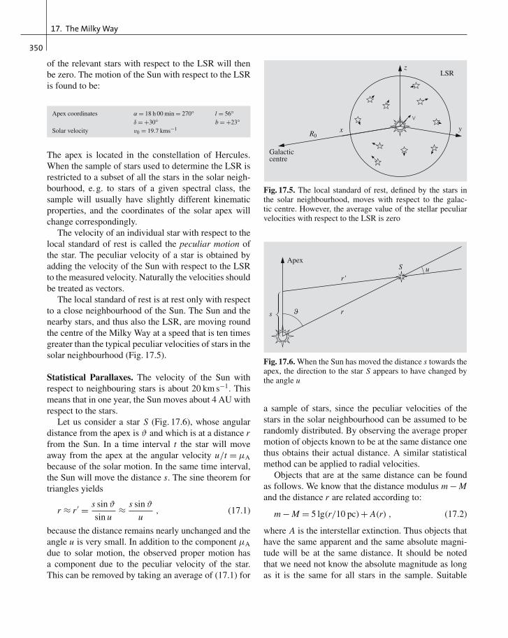
350
17. The Milky Way
of the relevant stars with respect to the LSR will thenbe zero. The motion of the Sun with respect to the LSRis found to be:
Apex coordinates α= 18 h 00 min = 270 l = 56δ= +30 b = +23
Solar velocity v0 = 19.7 kms−1
The apex is located in the constellation of Hercules.When the sample of stars used to determine the LSR isrestricted to a subset of all the stars in the solar neigh-bourhood, e. g. to stars of a given spectral class, thesample will usually have slightly different kinematicproperties, and the coordinates of the solar apex willchange correspondingly.
The velocity of an individual star with respect to thelocal standard of rest is called the peculiar motion ofthe star. The peculiar velocity of a star is obtained byadding the velocity of the Sun with respect to the LSRto the measured velocity. Naturally the velocities shouldbe treated as vectors.
The local standard of rest is at rest only with respectto a close neighbourhood of the Sun. The Sun and thenearby stars, and thus also the LSR, are moving roundthe centre of the Milky Way at a speed that is ten timesgreater than the typical peculiar velocities of stars in thesolar neighbourhood (Fig. 17.5).
Statistical Parallaxes. The velocity of the Sun withrespect to neighbouring stars is about 20 km s−1. Thismeans that in one year, the Sun moves about 4 AU withrespect to the stars.
Let us consider a star S (Fig. 17.6), whose angulardistance from the apex is ϑ and which is at a distance rfrom the Sun. In a time interval t the star will moveaway from the apex at the angular velocity u/t = µA
because of the solar motion. In the same time interval,the Sun will move the distance s. The sine theorem fortriangles yields
r ≈ r ′ = s sinϑ
sin u≈ s sinϑ
u, (17.1)
because the distance remains nearly unchanged and theangle u is very small. In addition to the component µA
due to solar motion, the observed proper motion hasa component due to the peculiar velocity of the star.This can be removed by taking an average of (17.1) for
Fig. 17.5. The local standard of rest, defined by the stars inthe solar neighbourhood, moves with respect to the galac-tic centre. However, the average value of the stellar peculiarvelocities with respect to the LSR is zero
Fig. 17.6. When the Sun has moved the distance s towards theapex, the direction to the star S appears to have changed bythe angle u
a sample of stars, since the peculiar velocities of thestars in the solar neighbourhood can be assumed to berandomly distributed. By observing the average propermotion of objects known to be at the same distance onethus obtains their actual distance. A similar statisticalmethod can be applied to radial velocities.
Objects that are at the same distance can be foundas follows. We know that the distance modulus m − Mand the distance r are related according to:
m − M = 5 lg(r/10 pc)+ A(r) , (17.2)
where A is the interstellar extinction. Thus objects thathave the same apparent and the same absolute magni-tude will be at the same distance. It should be notedthat we need not know the absolute magnitude as longas it is the same for all stars in the sample. Suitable

17.2 Stellar Statistics
351
classes of stars are main sequence A4 stars, RR Lyraevariables and classical cepheids with some given pe-riod. The stars in a cluster are also all at the samedistance. This method has been used, for example, todetermine the distance to the Hyades as explained inSect. 16.2.
Parallaxes based on the peculiar or apex motion ofthe Sun are called statistical or secular parallaxes.
Main Sequence Fitting. If the distance of a clusteris known, it is possible to plot its HR diagram withthe absolute magnitude as the vertical coordinate. An-other cluster, whose distance is to be determined, canthen be plotted in the same diagram using the apparentmagnitudes as the vertical coordinate. Now the verticaldistance of the main sequences tells how much the ap-parent magnitudes differ from the absolute ones. Thusthe distance modulus m − M can be measured. Thismethod, known as the main sequence fitting, works forclusters whose stars are roughly at the same distance;if the distances vary too much, a clear main sequencecannot be distinguished.
Photometric Parallaxes. The determination of the dis-tance directly from (17.2) is called the photometricmethod of distance determination and the correspondingparallax, the photometric parallax. The most difficulttask when using this method usually involves findingthe absolute magnitude; there are many ways of doingthis. For example, the two-dimensional MKK spectralclassification allows one to determine the absolute mag-nitude from the spectrum. The absolute magnitudes ofcepheids can be obtained from their periods. A spe-cially useful method for star clusters is the procedureof main sequence fitting. A condition for the photomet-ric method is that the absolute magnitude scale first becalibrated by some other method.
Trigonometric parallaxes do not reach very far. Forexample, even with the Hipparcos satellite, only a fewcepheid distances have been accurately measured bythis method. The method of statistical parallaxes is in-dispensable for calibrating the absolute magnitudes ofbright objects. When this has been done, the photomet-ric method can be used to obtain distances of objectseven further away.
Other examples of indicators of brightness, lumi-nosity criteria, are characteristic spectral lines or the
periods of cepheids. Again, their use requires that theyfirst be calibrated by means of some other method. Itis a characteristic feature of astronomical distance de-terminations that the measurement of large distancesis based on knowledge of the distances to nearerobjects.
17.2 Stellar Statistics
The Stellar Luminosity Function. By systematicallyobserving all stars in the solar neighbourhood, one canfind the distribution of their absolute magnitudes. Thisis given by the luminosity function Φ(M), which givesthe relative number of main sequence stars with absolutemagnitudes in the range [M −1/2,M +1/2]. No starsappear to be forming at present in the region of spacewhere the luminosity function has been determined.The age of the Milky Way is 10–15 Ga, which meansthat all stars less massive than 0.9 M, will still be onthe main sequence. On the other hand, more massivestars, formed early in the history of the Milky Way, willhave completed their evolution and disappeared. Low-mass stars have accumulated in the luminosity functionfor many generations of star formation, whereasbright, high-mass stars are the result of recent starformation.
By taking into account the different main sequencelifetimes of stars of different masses and hence of differ-ent magnitudes, one can determine the initial luminosityfunction Ψ(M), which gives the brightness distributionat the time of star formation, the zero age main se-quence luminosity function. The relation between thefunction Ψ and the observed luminosity function is
Ψ(M)=Φ(M)T0/tE(M) , (17.3)
where T0 is the age of the Milky Way and tE(M) is themain sequence lifetime of stars of magnitude M. Herewe assume that the birth rate of stars of magnitude M hasremained constant during the lifetime of the Milky Way.The initial luminosity function is shown in Fig. 17.7.
The Fundamental Equation of Stellar Statistics. TheStellar Density. A crucial problem for studies of thestructure of the Milky Way is to find out how the densityof stars varies in space. The number of stars per unit
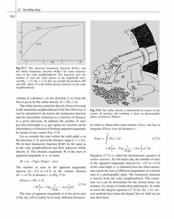
352
17. The Milky Way
Fig. 17.7. The observed luminosity function Φ(MV) andthe initial luminosity function Ψ(MV) for main sequencestars in the solar neighbourhood. The functions give thenumber of stars per cubic parsec in the magnitude inter-val [MV −1/2, MV +1/2]; they are actually the products DΦand DΨ , where D is the stellar density function (in the solarneighbourhood)
volume at a distance r in the direction (l, b) from theSun is given by the stellar density D = D(r, l, b).
The stellar density cannot be directly observed exceptin the immediate neighbourhood of the Sun. However, itcan be calculated if one knows the luminosity functionand the interstellar extinction as a function of distancein a given direction. In addition the number of starsper unit solid angle (e. g. per square arc second) can bedetermined as a function of limiting apparent magnitudeby means of star counts (Fig. 17.8).
Let us consider the stars within the solid angle ω inthe direction (l, b) and in the distance range [r, r +dr].We let their luminosity function Φ(M) be the same asin the solar neighbourhood and their unknown stellardensity D. The absolute magnitude M of the stars ofapparent magnitude m is, as usual,
M = m −5 lg(r/10 pc)− A(r) .
The number of stars in the apparent magnitudeinterval [m − 0.5,m + 0.5] in the volume elementdV = ωr2dr at distance r is (Fig. 17.9)
dN(m)= D(r, l, b)
×Φ[m −5 lg
r
10 pc− A(r)
]dV .
(17.4)
The stars of apparent magnitude m in the given areaof the sky will in reality be at many different distances.
Fig. 17.8. The stellar density is determined by means of starcounts. In practice, the counting is done on photographicplates. (Cartoon S. Harris)
In order to obtain their total number N(m), one has tointegrate dN(m) over all distances r:
N(m)=∞∫
0
D(r, l, b) (17.5)
×Φ[m −5 lg
r
10 pc− A(r)
]ωr2 dr .
Equation (17.5) is called the fundamental equation ofstellar statistics. Its left-hand side, the number of starsin the apparent magnitude interval [m −0.5,m +0.5]in the solid angle ω, is obtained from the observations:one counts the stars of different magnitudes in a chosenarea of a photographic plate. The luminosity functionis known from the solar neighbourhood. The extinc-tion A(r) can be determined for the chosen areas, forinstance, by means of multicolour photometry. In orderto solve the integral equation (17.5) for D(r, l, b), sev-eral methods have been developed, but we shall not gointo them here.

17.2 Stellar Statistics
353
Fig. 17.9. The size of the volume element at distance r in thedirection (l, b) is ωr2dr
Figure 17.10a shows the stellar density in the so-lar neighbourhood in the plane of the Milky Way, andFig. 17.10b in the direction perpendicular to the plane.There are several individual concentrations, but e. g. spi-ral structure cannot be observed in such a limited regionof space.
The Distribution of Bright Objects. Using stellarstatistical methods, one can only study the close neigh-bourhood of the Sun, out to about 1 kpc at the most.Absolutely faint objects cannot be observed very far.Since the solar neighbourhood appears to be fairly rep-resentative of the general properties of the Milky Way,its study is naturally important, giving information e.g.
Fig. 17.10a,b. The stel-lar density near the Sun.(a) The stellar density ofspectral classes A2–A5 inthe galactic plane, accord-ing to S.W. McCuskey.The numbers next to theisodensity curves givethe number of stars in10,000 pc3. (b) The distri-bution of different spectralclasses perpendicularly tothe galactic plane accordingto T. Elvius. The density inthe galactic plane has beennormalized to one
on the distributions and luminosity functions of starsof various spectral types. However, in order to get anidea of the larger-scale structure of the Milky Way, onehas to make use of objects that are as absolutely brightas possible, and which can be observed even at largedistances.
Examples of suitable objects are stars of early spec-tral types, H II regions, OB associations, open starclusters, cepheids, RR Lyrae stars, supergiants and gi-ants of late spectral types, and globular clusters. Someof these objects differ greatly in age, such as the youngOB associations, on the one hand, and the old globularclusters, on the other. Any differences in their space dis-tribution tell us about changes in the general structureof the Milky Way.
The young optical objects, the H II regions, OB asso-ciations and open clusters, are strongly concentrated inthe plane of the Milky Way (Table 17.1). Figure 17.11shows that they also appear to be concentrated in threedrawn-out bands, at least within the observed region.Since these types of objects in other galaxies are knownto be part of a spiral structure, the observed bands inthe Milky Way have been interpreted as portions ofthree spiral arms passing through the solar neighbour-hood. Stars of later spectral types seem to be much moreevenly distributed. Apart from a few special directions,interstellar dust limits observations in the galactic planeto within 3–4 kpc.

354
17. The Milky Way
Population Typical Average age z vr Metalobjects [109 a] [pc] [k/s] abundance
Halo population II Subdwarfs, 14–12 2000 75 0.001globular clustersRR Lyr (P> 0.4 d)
Intermediate population II Long period 12–10 700 25 0.005variables
Disc population Planetary 12–2 400 18 0.01–0.02nebulae, novaebright redgiants
Old population I A stars, 2–0.1 160 10 0.02Me dwarfsclassicalcepheids
Young population I Gas, dust, 0.1 120 0.03–0.04supergiants,T Tau stars
Table 17.1. Populations ofthe Milky Way; z is thevertical distance from thegalactic plane, and vr thevelocity component per-pendicular to the galacticplane
Fig. 17.11. The distribu-tion of various objects inthe galactic plane. Threecondensations can be dis-cerned: the Sagittarius arm(lowest), the local arm nearthe Sun and (outermost) thePerseus arm
Old objects, particularly the globular clusters, havean almost spherical distribution about the centre of theMilky Way (Fig. 17.12). The space density of old objectsincreases towards the galactic centre. They can be usedto determine the distance of the Sun from the galacticcentre; the value of this distance is about 8.5 kpc.
Stellar Populations. Studies of the motions of the starsin the Milky Way have revealed that the orbits of starsmoving in the galactic plane are almost circular. Thesestars are also usually young, a few hundred millionyears at the most. They also contain a relatively largeamount of heavy elements, about 2–4%. The interstel-
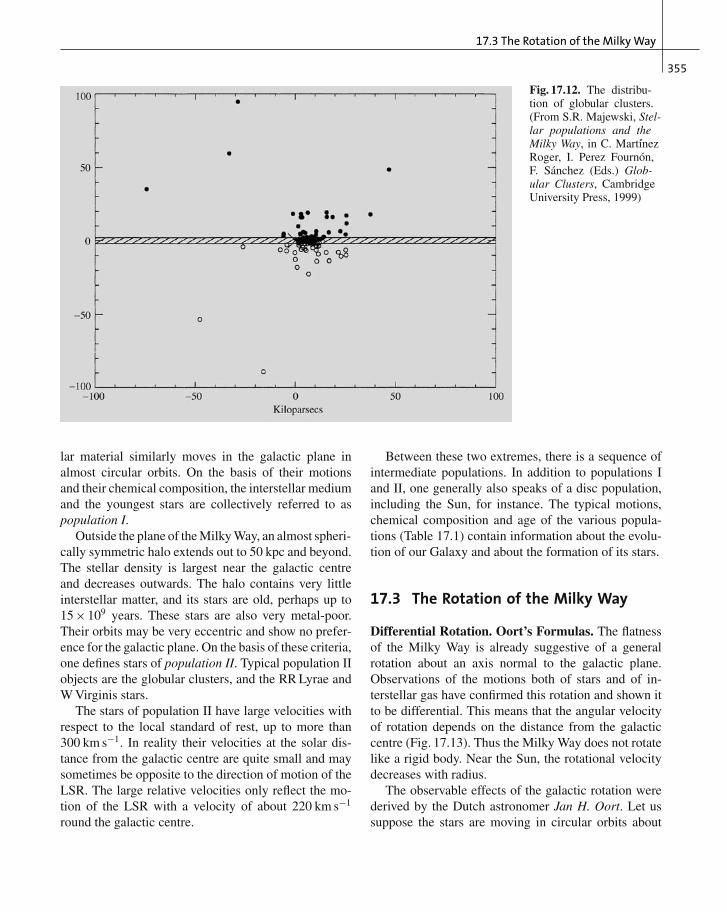
17.3 The Rotation of the Milky Way
355
Fig. 17.12. The distribu-tion of globular clusters.(From S.R. Majewski, Stel-lar populations and theMilky Way, in C. MartinezRoger, I. Perez Fournon,F. Sanchez (Eds.) Glob-ular Clusters, CambridgeUniversity Press, 1999)
lar material similarly moves in the galactic plane inalmost circular orbits. On the basis of their motionsand their chemical composition, the interstellar mediumand the youngest stars are collectively referred to aspopulation I.
Outside the plane of the Milky Way, an almost spheri-cally symmetric halo extends out to 50 kpc and beyond.The stellar density is largest near the galactic centreand decreases outwards. The halo contains very littleinterstellar matter, and its stars are old, perhaps up to15×109 years. These stars are also very metal-poor.Their orbits may be very eccentric and show no prefer-ence for the galactic plane. On the basis of these criteria,one defines stars of population II. Typical population IIobjects are the globular clusters, and the RR Lyrae andW Virginis stars.
The stars of population II have large velocities withrespect to the local standard of rest, up to more than300 km s−1. In reality their velocities at the solar dis-tance from the galactic centre are quite small and maysometimes be opposite to the direction of motion of theLSR. The large relative velocities only reflect the mo-tion of the LSR with a velocity of about 220 km s−1
round the galactic centre.
Between these two extremes, there is a sequence ofintermediate populations. In addition to populations Iand II, one generally also speaks of a disc population,including the Sun, for instance. The typical motions,chemical composition and age of the various popula-tions (Table 17.1) contain information about the evolu-tion of our Galaxy and about the formation of its stars.
17.3 The Rotation of the Milky Way
Differential Rotation. Oort’s Formulas. The flatnessof the Milky Way is already suggestive of a generalrotation about an axis normal to the galactic plane.Observations of the motions both of stars and of in-terstellar gas have confirmed this rotation and shown itto be differential. This means that the angular velocityof rotation depends on the distance from the galacticcentre (Fig. 17.13). Thus the Milky Way does not rotatelike a rigid body. Near the Sun, the rotational velocitydecreases with radius.
The observable effects of the galactic rotation werederived by the Dutch astronomer Jan H. Oort. Let ussuppose the stars are moving in circular orbits about

356
17. The Milky Way
Fig. 17.13a–d. The effect of differential rotation on the radialvelocities and proper motions of stars. (a) Near the Sun theorbital velocities of stars decrease outwards in the Galaxy.(b) The relative velocity with respect to the Sun is obtained by
subtracting the solar velocity from the velocity vectors in (a).(c) The radial components of the velocities with respect to theSun. This component vanishes for stars on the same orbit asthe Sun. (d) The tangential components of the velocities
the galactic centre (Fig. 17.14). This approximation isacceptable for population I stars and gas. The star S,seen from the Sun at galactic longitude l at distance r,has circular velocity V at a distance R from the centre.Similarly for the Sun the galactic radius and velocityare R0 and V0. The relative radial velocity vr of the starwith respect to the Sun is the difference between theprojections of the circular velocities on the line of sight:
vr = V cosα− V0 sin l , (17.6)
where α is the angle between the velocity vector ofthe star and the line of sight. From Fig. 17.14 the an-gle CS = α+90. By applying the sine theorem tothe triangle CS one obtains
sin(α+90)sin l
= R0
Ror
cosα= R0
Rsin l . (17.7)
Denoting the angular velocity of the star byω= V/Rand that of the Sun by ω0 = V0/R0, one obtains the
observable radial velocity in the form
vr = R0(ω−ω0) sin l . (17.8)
The tangential component of the relative velocityof the Sun and the star is obtained as follows. FromFig. 17.14,
vt = V sinα− V0 cos l = Rω sinα− R0ω0 cos l .
The triangle CP gives
R sinα= R0 cos l −r ,
and hence
vt = R0(ω−ω0) cos l −ωr . (17.9)
Oort noted that in the close neighbourhood of the Sun(r R0), the difference of the angular velocities willbe very small. Therefore a good approximation for theexact equations (17.8) and (17.9) is obtained by keepingonly the first term of the Taylor series of ω−ω0 in theneighbourhood of R = R0:
ω−ω0 =(
dω
dR
)R=R0
(R − R0)+ . . . .
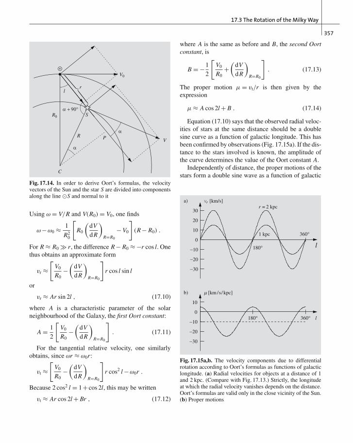
17.3 The Rotation of the Milky Way
357
Fig. 17.14. In order to derive Oort’s formulas, the velocityvectors of the Sun and the star S are divided into componentsalong the line S and normal to it
Using ω= V/R and V(R0)= V0, one finds
ω−ω0 ≈ 1
R20
[R0
(dV
dR
)R=R0
− V0
](R − R0) .
For R ≈ R0 r, the difference R − R0 ≈ −r cos l. Onethus obtains an approximate form
vr ≈[
V0
R0−(
dV
dR
)R=R0
]r cos l sin l
or
vr ≈ Ar sin 2l , (17.10)
where A is a characteristic parameter of the solarneighbourhood of the Galaxy, the first Oort constant:
A = 1
2
[V0
R0−(
dV
dR
)R=R0
]. (17.11)
For the tangential relative velocity, one similarlyobtains, since ωr ≈ ω0r:
vt ≈[
V0
R0−(
dV
dR
)R=R0
]r cos2 l −ω0r .
Because 2 cos2 l = 1+ cos 2l, this may be written
vt ≈ Ar cos 2l + Br , (17.12)
where A is the same as before and B, the second Oortconstant, is
B = −1
2
[V0
R0+(
dV
dR
)R=R0
]. (17.13)
The proper motion µ = vt/r is then given by theexpression
µ≈ A cos 2l + B . (17.14)
Equation (17.10) says that the observed radial veloc-ities of stars at the same distance should be a doublesine curve as a function of galactic longitude. This hasbeen confirmed by observations (Fig. 17.15a). If the dis-tance to the stars involved is known, the amplitude ofthe curve determines the value of the Oort constant A.
Independently of distance, the proper motions of thestars form a double sine wave as a function of galactic
Fig. 17.15a,b. The velocity components due to differentialrotation according to Oort’s formulas as functions of galacticlongitude. (a) Radial velocities for objects at a distance of 1and 2 kpc. (Compare with Fig. 17.13.) Strictly, the longitudeat which the radial velocity vanishes depends on the distance.Oort’s formulas are valid only in the close vicinity of the Sun.(b) Proper motions

358
17. The Milky Way
longitude, as seen in Fig. 17.15b. The amplitude of thecurve is A and its mean value, B.
In 1927 on the basis of this kind of analysis, Oortestablished that the observed motions of the stars indi-cated a differential rotation of the Milky Way. Takinginto account an extensive set of observational data, theInternational Astronomical Union IAU has confirmedthe present recommended values for the Oort constants:
A = 15 km s−1 kpc−1, B = −10 km s−1 kpc−1 .
The Oort constants obey some interesting relations.By subtracting (17.13) from (17.11), one obtains
A − B = V0
R0= ω0 . (17.15)
Adding (17.13) and (17.11) gives
A + B = −(
dV
dR
)R=R0
. (17.16)
Knowing the values of A and B, one can calculatethe angular velocity ω0 = 0.0053′′/year, which is theangular velocity of the local standard of rest around thegalactic centre.
The circular velocity of the Sun and the LSR can bemeasured in an independent way by using extragalacticobjects as a reference. In this way a value of about220 km s−1 has been obtained for V0. Using (17.15) onecan now calculate the distance of the galactic centre R0.The result is about 8.5 kpc, in good agreement with thedistance to the centre of the globular cluster system.The direction to the galactic centre obtained from thedistribution of radial velocities and proper motions bymeans of (17.10) and (17.14) also agrees with othermeasurements.
The orbital period of the Sun in the Galaxy accord-ing to these results is about 2.5×10⁸ years. Since theSun’s age is nearly 5×10⁹ years, it has made about 20revolutions around the galactic centre. At the end of theprevious revolution, the Carboniferous period had endedon Earth and the first mammals would soon appear.
The Distribution of Interstellar Matter. Radio radi-ation from interstellar gas, in particular that of neutralhydrogen, is not strongly absorbed or scattered by inter-stellar dust. It can therefore be used to map the structure
Fig. 17.16. Clouds P1, P2, . . . seen in the same direction atvarious distances
of the Milky Way on large scales. Radio signals can bedetected even from the opposite edge of the Milky Way.
The position of a radio source, for example anH I cloud, in the Galaxy cannot be directly deter-mined. However, an indirect method exists, based onthe differential rotation of the Galaxy.
Figure 17.16 is a schematic view of a situation inwhich gas clouds on the circles P1, P2, . . . are observedin the direction l (−90 < l< 90). The angular velocityincreases inwards, and therefore the greatest angularvelocity along the line of sight is obtained at the point Pk ,where the line of sight is tangent to a circle. This meansthat the radial velocity of the clouds in a fixed directiongrows with distance up to the maximum velocity atcloud Pk:
vr,max = Rk(ω−ω0) , (17.17)
where Rk = R0 sin l. The distance of cloud Pk from theSun is r = R0 cos l. When r increases further, vr de-creases monotonically. Figure 17.17 shows how theobserved radial velocity in a given direction varies withdistance r, if the gas moves in circular orbits and theangular velocity decreases outwards.

17.3 The Rotation of the Milky Way
359
Fig. 17.17. The radial velocity as a function of distance (shownschematically)
The neutral hydrogen 21 cm line has been par-ticularly important for mapping the Milky Way.Figure 17.18 gives a schematic view of how the hy-drogen spectral line is made up of the radiation of manyindividual concentrations of neutral hydrogen, cloudsor spiral arms. The line component produced by eachcloud has a wavelength which depends on the radialvelocity of the cloud and a strength depending on itsmass and density. The total emission is the sum of thesecontributions.
By making observations at various galactic longi-tudes and assuming that the clouds form at least partlycontinuous spiral arms, the distribution of neutral hydro-gen in the galactic plane can be mapped. Figure 15.17shows a map of the Milky Way obtained from 21 cmline observations of neutral hydrogen. It appears that theneutral hydrogen is concentrated in spiral arms. How-ever, interpretation of the details is difficult because ofthe uncertainties of the map. In order to obtain the dis-tances to the gas clouds, one has to know the rotationcurve, the circular velocity as a function of the galacticradius. This is determined from the same radial veloc-ity observations and involves assumptions concerningthe density and rotation of the gas. The interpretation of
Fig. 17.18. Clouds at different distances have different veloc-ities and therefore give rise to emission lines with differentDoppler shifts. The observed flux density profile (continu-ous curve) is the sum of the line profiles of all the individualline profiles (dashed curves). The numbers of the line profilescorrespond to the clouds in the upper picture
the spiral structure obtained from radio observationsis also still uncertain. For example, it is difficult tofit the radio spiral structure to the one obtained nearthe Sun from optical observations of young stars andassociations.
The Rotation, Mass Distribution and Total Mass ofthe Milky Way. In (17.17) the galactic longitude l givesthe galactic radius Rk of the clouds with maximumradial velocity. By making observations at differentlongitudes, one can therefore use (17.17) to determinethe angular velocity of the gas for various distancesfrom the galactic centre. (Circular motions must be as-sumed.) In this way, the rotation curve ω= ω(R) andthe corresponding velocity curve V = V(R) (= ωR) areobtained.
Figure 17.19 shows the rotation curve of the MilkyWay. Its central part rotates like a rigid body, i. e. the

360
17. The Milky Way
Fig. 17.19. Rotation curveof the Milky Way based onthe motions of hydrogenclouds. Each point repre-sents one cloud. The thickline represents the rota-tion curve determined byMaarten Schmidt in 1965. Ifall mass were concentratedwithin the radius 20 kpc,the curve would continueaccording to Kepler’s thirdlaw (broken line). The ro-tation curve determinedby Leo Blitz on the basisof more recent observa-tions begins to rise againat 12 kpc
angular velocity is independent of the radius. Outsidethis region, the velocity first drops and then begins torise gradually. A maximum velocity is reached at about8 kpc from the centre. Near the Sun, about 8.5 kpc fromthe centre, the rotational velocity is about 220 km s−1.According to earlier opinions, the velocity continues todecrease outwards. This would mean that most of themass is inside the solar radius. This mass could thenbe determined from Kepler’s third law. According to(6.34),
M = R0V 20 /G .
Using the values R0 = 8.5 kpc and V0 = 220 km s−1,one obtains
M = 1.9×1041 kg = 1.0×10¹¹ M .
The escape velocity at radius R is
Ve =√
2G M
R= V
√2 . (17.18)
This gives an escape velocity near the SunVe = 310 km s−1. One therefore should not see manystars moving in the direction of galactic rotation,l = 90, with velocities larger than 90 km s−1 with re-spect to the local standard of rest, since the velocity of
such stars would exceed the escape velocity. This hasbeen confirmed by observations.
The preceding considerations have been based onthe assumption that near the Sun, the whole mass ofthe Galaxy can be taken to be concentrated in a centralpoint. If this were true, the rotation curve should beof the Keplerian form, V ∝ R−1/2. That this is not thecase can be established from the values of the Oortconstants.
The derivative of the Keplerian relation
V =√
G M
R= √
G M R−1/2
yields
dV
dR= −1
2
√G M R−3/2 = −1
2
V
R.
Using the properties (17.15) and (17.16) of the Oortconstants, one finds
(A − B)/(A + B)= 2 (17.19)
for a Keplerian rotation curve. This disagrees with theobserved value and thus the assumed Keplerian law doesnot apply.
The mass distribution in the Milky Way can be stud-ied on the basis of the rotation curve. One looks for

17.4 Structural Components of the Milky Way
361
a suitable mass distribution, such that the correct ro-tation curve is reproduced. Recently distant globularclusters have been discovered, showing that the MilkyWay is larger than expected. Also, observations of therotation curve outside the solar circle suggest that therotational velocity might begin to rise again. These re-sults suggest that the mass of the Galaxy might be asmuch as ten times larger than had been thought.
17.4 Structural Componentsof the Milky Way
We have seen how the structure of the Milky Way can beglobally described by means of an almost spherical haloof old stars and and a disc of gas and young and middle-aged stars. In a more detailed picture more small-scalefeatures can also be distinguished.
The Thick Disc. In the traditional scheme dividing thestars of the Milky Way into a series of populations itwas left undecided whether the populations should beconsidered as qualitatively different classes or merelysteps along a continuous sequence. As the quality andquantity of observations have improved, it has becomeclear that what was defined as the intermediate popu-lation II really represents a separate component of theMilky Way with a pattern of element abundances stellarmotions that separate it clearly from the old (thin) disc.This population is now referred to as the thick galacticdisc. A thick disc has also been detected in some othergalaxies, but it does not appear to be a universal featureof all disc galaxies.
The Galactic Bar. As will be seen in the next chap-ter, Sect. 18.1, a large fraction of all disc galaxies arebarred, with an elongated light distribution at the cen-tre. The first indication that this might also be the casefor the Milky Way was found in velocity measure-ments of neutral hydrogen, which were incompatiblewith gas moving along circular orbits. In 1971 W. W.Shane showed that the motions of the gas could be ex-plained, if there is a central bar pointing about 20 awayfrom the direction of the Galatic centre.
It is more difficult to detect a bar in observations ofthe stars. This was first done using the COBE satel-lite, which (apart from mapping the cosmic microwave
background, see Sect. 19.7) also made a map of the skyat the infrared wavelengths dominated by the light of oldstars. Because of perspective, the nearer end of the barat positive galactic longitude will look slightly differentthan the farther end. Such an asymmetry was presentin the infrared map, consistent with a bar with an axialratio of 0.6.
Later confirmation of the existence of the bar hascome from mapping of the central distribution of oldstars using near-infrared photometric distances, see Fig.17.20.
Spiral Structure. As mentioned earlier, the Milky Wayappears to be a spiral galaxy, but there is no generalagreement on the detailed form of the spiral pattern. Forexample, in 1976 Y.M. Georgelin and Y.P. Georgelindetermined the distances of H II regions by radio andoptical observations. In the optical region their methodis independent of assumptions about the galactic rota-tion law. They then fitted four spiral arms through theH II regions.
Fig. 17.20. The Milky Way bar viewed from the North Galacticpole. Solid symbols indicate the mean positions of red clumpgiants in given directions, and the thick grey lines represent therange of their distances. The line through the mean distancesillustrates a bar of 3 kpc length inclined 22.5 to the direc-tion to the Galactic centre. The contour map shows a modelof the bar derived from infrared observations. (C.Babusiaux,G.Gilmore 2005, MNRAS 358, 1309, Fig.6)

362
17. The Milky Way
Later investigations using a variety of methods, bothoptical and radio have confirmed that a four-armed pat-tern gives the best description of the spiral structure inthe Sun’s vicinity (Fig. 17.22). The pitch angle of thespiral in this model is about 11.3. Three of the armsstart at the position of the galactic bar.
The cause of the spiral structure is a long-standingproblem. A small perturbation in the disc will quicklybe stretched into a spiral shape by differential rotation.However, such a spiral would disappear in a few galacticrevolutions, a few hundred million years.
An important step forward in the study of the spi-ral structure was the density wave theory developed byChia-Chiao Lin and Frank H. Shu in the 1960’s. Thespiral structure is taken to be a wavelike variation of thedensity of the disc. The spiral pattern rotates as a solidbody with an angular velocity smaller than that of thegalactic rotation, while the stars and gas in the disc passthrough the wave.
Fig. 17.21. The central parts of the Milky Way in a radiopicture. The observations were made with the VLA telescope.(Image Kassim et. al., Naval Research Laboratory)
Fig. 17.22. General view of the spiral pattern of the Milky Way.Different tracers of spiral arms lead to somewhat differentpatterns, but they tend to agree that a four-armed pattern likethe the one indicated here gives the best overall representation.The names of the arms are those most commonly used. Seealso Fig. 17.11. (Y.Xu et al. 2006, Science 311,54)
The density wave theory explains in a natural waywhy young objects, like molecular clouds, H II regionsand bright young stars are found in the spiral arms. Asgas passes through the wave, it is strongly compressed.The internal gravity of the gas clouds then becomesmore important and causes them to collapse and formstars.
It takes about 107 years for the material to passthrough a spiral arm. By that time, the hot, bright starshave finished their evolution, their ultraviolet radiationhas ceased and the H II regions have disappeared. Theless massive stars formed in the spiral arms are spreadout in the disc by their peculiar velocities.
It is not yet clear what gives rise to the spiral wave.For some further discussion of spiral structure, seeSect. 18.4.
The Galactic Centre. Our knowledge of the centre ofthe Milky Way is mostly based on radio and infraredobservations. In the optical region the view to the cen-tre is blocked by the dark clouds in the Sagittarius spiralarm about 2 kpc from us. The galactic centre is inter-

17.5 The Formation and Evolution of the Milky Way
363
esting because it may be a small-scale version of themuch more violently active nuclei of some externalgalaxies (see Sect. 18.7). It therefore provides oppor-tunities to study at close hand phenomena related toactive galaxies. Since active galactic nuclei are thoughtto contain black holes with masses larger than 107 M,there may also be a large black hole at the galacticcentre.
As one approaches the galactic centre the stellar den-sity continues to rise towards a sharp central peak. Incontrast, the galactic gas disc has a central hole of ra-dius about 3 kpc. This may be due to the galactic bar,which will channel gas into the galactic nucleus leavinga gas-free zone at larger radii.
Inside the central hole is a dense nuclear gas disc.Its radius is about 1.5 kpc in neutral hydrogen, but mostof its mass is molecular and concentrated within 300 pcof the nucleus. In this region the mass of moleculargas is about 108 M, or 5% of the total molecular massof the Milky Way. The molecular clouds are proba-bly confined by the pressure from surrounding very hot(T ≈ 108 K) gas. This hot gas may then expand verti-cally, forming a galactic wind. Gas lost to a wind orto star formation is replenished with infalling gas fromlarger radii.
The central 10 pc are dominated by the radio contin-uum source Sgr A and a dense star cluster observed inthe infrared. There is also molecular gas with complexmotions and signs of star formation activity. WithinSgr A there is a unique point-like radio continuumsource known as Sgr A∗. The position of Sgr A∗ agreesto within 1′′ with the centre of a cluster of stars thatis much denser than anything observed in the galacticdisc. If the galactic centre contains a large black hole,Sgr A∗ is the natural candidate.
The luminosity of the galactic centre could be pro-vided by the central star cluster, but there are still reasonsto expect that a large black hole may be present. Thecentral mass distribution can be estimated by modellingthe observed motions of stars and gas (cf. Sect. 18.2).In particular it has recently become possible to measurethe proper motion of stars in the central cluster, whichhas allowed the determination of their orbits. The bestfit with the observations is obtained with models with anextended stellar mass distribution together with a point-mass of about 3×10⁶ M. The size of Sgr A∗ measuredby very long baseline interferometry is less than 10 AU.
The most plausible explanation of this very compactstructure is that Sgr A∗ is indeed a black hole with massof a few million solar masses.
17.5 The Formation and Evolutionof the Milky Way
Like all galaxies the Milky Way is supposed to haveformed through the collapse of a region of higher thanaverage density in the Universe. The general view ofhow this happened will be presented in the next twochapters,in particular in Sects. 18.8 and 19.7. Sometraces of the formation process will be preserved in theproperties of local stars of different ages. These repre-sent information about the formation of the Milky Waythat is not available for other galaxies.
The Ages of Stars. The most direct way of studying theevolution of the Milky Way is by means of the observedages of stars. The tradional sequence of populationsdescribed in Sect. 17.2 is also a sequence correspondingto stars of different ages. The oldest component, thestellar halo forms an almost spherical distribution ofstars with ages 12–14 Ga, representing the oldest partof the Milky Way.
In contrast, the old and young population I consistsof stars with ages less than 10 Ga, which were initiallyformed in a very thin layer that has been thickenedby encounters with spiral arms and molecular cloudcomplexes.
Intermediate between these two, as we have noted,is the thick disc with an age about 10–12 Ga. Anotherintermediate population in the Milky Way is the centralbulge including the galactic bar, and containing stars ofages 7–11 Ga.
Chemical Enrichment. The history of the formation ofthe Milky Way is preserved in the properties of its olderstars, above all in their “chemical” composition, i. e.the abundances of elements and isotopes heavier thanhelium. (All these heavier elements are often referredto as “metals” in the astrophysical jargon.)
Only hydrogen and helium were were present asthe first stars formed. As successive generations ofstars evolved, nuclear reactions produced heavy ele-

364
17. The Milky Way
ments, some of which were returned to the interstellargas in supernova explosions or stellar winds. Theseheavy elements were then incorporated into the follow-ing generation of stars, gradually increasing the metalabundance in the interstellar medium.
Some of the stars formed were of low mass, andhad life-times long enough that they are still present.Their chemical composition will reflect the abundancesin the interstellar medium at the time they were formed.Studying the chemical abundances of stars of differentages therefore gives information on the star forma-tion history of the Milky Way, both on the rate atwhich stars have formed at a given epoch and on themasses and other characteristics of those stars whenthey formed.
One commonly used indicator of the metal abun-dance in stars is the mass of iron relative to hydrogen,in logarithmic units and measured relative to the solarvalues, [Fe/H]. Fig. 17.23 shows the value of [FE/H] fordifferent types of objects of various ages. The generalpicture is that the metal abundance rose rapidly duringthe first billion years and has afterwards grown onlyslowly. The lowest values of [Fe/H] discovered in oldhalo stars are about −5. Many models have been de-veloped describing the chemical evolution of the Milky
Fig. 17.23. The age–metallicity relation of theMilky Way for differentcomponents. TDO: thindisc open clusters; TDG:thick disc globulars; B:bulge; YHG: young haloglobulars; OHG: old haloglobulars. The shaded ar-eas correspond to thin discfield stars, thick disc fieldstars, and halo field stars,in order of increasing age.(K. Freeman, J. Bland-Hawthorn 2002, ARAA 40,487, Fig. 2)
Way and other galaxies, incorporating prescriptions forstar formation, and infall of gas from the outside. Inparticular the rapid early rise of the metal abundanceis difficult to explain in the simplest models. This dif-ficulty, the scarcity of old metal-poor disc stars, hasbecome known as the “G dwarf problem”, since theoldest stars still on the main series are of spectral classG. The most direct way that the G dwarf problem canbe avoided is to suppose that a large portion of the inter-stellar gas was accreted after the formation of the oldeststars.
Formation of the Milky Way. Galaxies are thoughtto be formed when gas clouds of higher than averagedensity in the Universe collapse under the force of theirown gravity. As the gas is compressed stars are born init. After the end of the collapse the cloud settles into aquasi-stationary state. Evolution continues at a slowerpace. Evolving stars return chemically enriched gas tointerstellar space, where it is mixed with remaining,unprocessed gas and star formation continues.
There are two competing pictures of how galaxy for-mation proceeds. In the monolithic collapse model itis assumed that large galaxies form coherently in thecollapse of a massive cloud containing the bulk of the

17.6 Examples
365
material constituting the galaxy. In the hierarchical pic-ture most of the stars form in much smaller clouds,which later agglomerate together to form the galaxieswe now observe. The evidence for these pictures in othergalaxies will be considered in the next chapter.
The case of the Milky Way already shows that thecontrast of the monolithic and the hierarchical pictureis oversimplified. Some aspects of galactic structure fitmore naturally into a monolithic theory. For example,the rapid collapse of the halo, followed by a more grad-ual build-up of the disc fits with this picture. The patternof chemical abundances are also homogeneous in a waythat is more compatible with a pattern of star formationthat was uniform throughout galactic history.
Other observations are indicative of a hierarchicalformation history. For example, stellar abundance pat-terns in the thick disc differ from those in the old thindisc. The most natural way of explaining this is thatthe thick disc formed by the accretion of one or moresmall satellite galaxies with different histories of starformation. Another sign of the importance of the infallof satellite galaxies is the existence of systems such asthe Sagittarius dwarf galaxy, which appears to be in thecourse of being disrupted by the Milky Way.
17.6 Examples
Example 17.1 Show that if the stars are uniformly dis-tributed in space and there is no interstellar extinction,the number of stars brighter than apparent magnitude mis
N0(m)= N0(0)×100.6 m .
Let us suppose first that all stars have the same ab-solute magnitude M. The distance in parsecs of thosestars having the apparent magnitude m is
r = 10×100.2(m−M ) .
In order to appear brighter than m, a star has to bewithin a sphere of radius r. Because the stellar densityis constant, the number of such stars is proportional tothe volume:
N0(m)∝ r3 ∝ 100.6 m .
The result does not depend on the absolute magni-tudes of the stars, so that the same result still applieswhen the magnitudes are not equal, as long as the lumi-nosity function does not depend on distance. Thus theequation is generally valid under the stated conditions.
Example 17.2 The Estimation of Distances by Meansof Oort’s Formulas
An object in the galactic plane at longitude l = 45 hasthe radial velocity of 30 km s−1 with respect to the LSR.What is its distance?
According to (17.10),
vr = Ar sin 2l .
Thus
r = vr
A sin 2l= 30 km s−1
15 km s−1 kpc−1 = 2 kpc .
In practice, the peculiar velocities are so large thatthis method cannot be used for distance determination.Oort’s formulas are mostly suitable only for statisticalstudies.
Example 17.3 Discussion of the Gravitational Fieldof a Uniform Disc
It can be shown that the gravitational field of a homoge-neous infinite thin disc is constant and directed towardsthe plane of the disc. If the mass per unit area of the discis σ , the gravitational field is
g = 2πGσ .
A test particle located outside the plane will thereforeget a constant acceleration towards the plane. Takinga numerical example, assume a mass of 1011 M dis-tributed uniformly on a circular disc 20 kpc in diameter.The mass per unit area will be a
σ = 1011 ×2×1030 kg
π(104 ×3.086×1016 m)2
= 0.67 kg m−2 .

366
17. The Milky Way
The corresponding gravitational field is
g = 2.8×10⁻¹⁰ m s−2 .
Let a star be located at d = 1 kpc above the plane, ini-tially at rest (not very near the edge of the disk, in orderto keep our approximation valid). The disc will pull ittowards the plane, and when the star crosses the plane,it has acquired a velocity given by
v=√2gd = 130 km s−1 .
The time required to reach the plane is
t = v/g = 15×106 a .
17.7 Exercises
Exercise 17.1 Assume that the Sun and a star movearound the Galaxy at the same speed in the same circularorbit in the galactic plane. Show that the proper motionof the star is independent of its distance. How big is thisproper motion?
Exercise 17.2 a) A cepheid has a radial velocity of80 km s−1, and its galactic longitude is 145. What isthe distance of the cepheid?
b) The period of the cepheid is 3.16 d, and theapparent visual magnitude is 12.3. What is the dis-tance derived from this information? Are the distancesconsistent?
Exercise 17.3 a) How many of the nearest stars(Table C.15) are also among the brightest stars(Table C.16)? Explain.
b) If the stellar density were constant, how many starswould there be within the distance of Canopus?
Exercise 17.4 a) Assume that the Galaxy is a homo-geneous disk and the Sun lies in the central plane of thedisk. The absolute magnitude of a star is M, galacticlatitude b, and distance from the central plane z. Whatis the apparent magnitude of the star, if the extinctioninside the Galaxy is a mag kpc−1?
b) Assume that the thickness of the galactic disk is200 pc. Find the apparent magnitude of a star with M =0.0, b = 30, distance r = 1 kpc, and a = 1 mag kpc−1.

Hannu Karttunen et al. (Eds.), Galaxies.In: Hannu Karttunen et al. (Eds.), Fundamental Astronomy, 5th Edition. pp. 367–391 (2007)DOI: 11685739_18 © Springer-Verlag Berlin Heidelberg 2007
367
18. Galaxies
The galaxies are the fundamental building blocks of theUniverse. Some of them are very simple in structure,
containing only normal stars and showing no particularindividual features. There are also galaxies that are almostentirely made of neutral gas. On the other hand, othersare complex systems, built up from many separate com-ponents − stars, neutral and ionized gas, dust, molecularclouds, magnetic fields, cosmic rays . . . . The galaxies mayform small groups or large clusters in space. At the cen-tre of many galaxies, there is a compact nucleus that maysometimes be so bright that it overwhelms all the normalradiation of the galaxy.
The luminosity of the brightest normal galaxies maycorrespond to 10
12 solar luminosities, but most of themare much fainter − the smallest ones that have beendiscovered are about 10
5 L. Since galaxies do not havea sharp outer edge, to some extent their masses and
radii depend on how these quantities are defined. Ifonly the bright central parts are included, a giant galaxymay typically have a mass of about 10
13 M, and a ra-dius of 30 kpc, and a dwarf, correspondingly, 10
7 M, and0.5 kpc. In addition, it seems that the outer parts of mostgalaxies contain large quantities of non-luminous mat-ter that might increase galaxy masses by an order ofmagnitude.
The density of matter may be very different in differentgalaxies and in different parts of the same galaxy. Thusthe evolution of a galaxy will be the result of processesoccurring on vastly different time and energy scales, andno generally accepted comprehensive picture of it existsas yet. In the following, the most important observedproperties of galaxies will be presented. Many of themstill await an explanation in current theories of galaxyevolution.
18.1 The Classification of Galaxies
A useful first step towards an understanding of galaxiesis a classification based on their various forms. Althoughsuch a morphological classification must always be tosome extent subjective, it provides a framework withinwhich the quantitative properties of galaxies can bediscussed in a systematic fashion. However, it shouldalways be remembered that the picture thus obtainedwill be limited to those galaxies that are large and brightenough to be easily visible in the sky. An idea of theconsequent limitations can be obtained from Fig. 18.1,showing the radii and magnitudes of normal galaxies.One sees that only within a narrow region of this dia-gram can galaxies be easily found. If a galaxy has toolarge a radius for its magnitude (small surface bright-ness), it will disappear in the background light from the
Fig. 18.1. Magnitudes and diameters of observable extragalac-tic objects. Objects to the upper left look like stars. The quasarsin this region have been discovered on the basis of their spec-tra. Objects to the lower right have a surface brightness muchsmaller than that of the night sky. In recent years large num-bers of low surface brightness galaxies have been discoveredin this region. (Arp, H. (1965): Astrophys. J. 142, 402)

368
18. Galaxies
night sky. On the other hand, if its radius is too small,it looks like a star and is not noticed on a photographicplate. In the following, we shall mainly be concernedwith bright galaxies that fit within these limits.
If a classification is to be useful, it should at leastroughly correspond to important physical properties ofthe galaxies. Most classifications accord in their mainfeatures with the one put forward by Edwin Hubble in1926. Hubble’s own version of the Hubble sequence isshown in Fig. 18.2. The various types of galaxies areordered in a sequence from early to late types. Thereare three main types: elliptical, lenticular, and spiralgalaxies. The spirals are divided into two sequences,normal and barred spirals. In addition, Hubble includeda class of irregular galaxies.
The elliptical galaxies appear in the sky as ellipticalconcentrations of stars, in which the density falls off ina regular fashion as one goes outwards. Usually thereare no signs of interstellar matter (dark bands of dust,bright young stars). The ellipticals differ from each otheronly in shape and on this basis they are classified as E0,E1, . . . , E7. If the major and minor axes of an ellipticalgalaxy are a and b, its type is defined to be En, where
n = 10
(1− b
a
). (18.1)
An E0 galaxy thus looks circular in the sky. The apparentshape of an E galaxy depends on the direction fromwhich it is seen. In reality an E0 galaxy may thereforebe truly spherical or it may be a circular disc vieweddirectly from above.
A later addition to the Hubble sequence is a class ofgiant elliptical galaxies denoted cD. These are gener-
Fig. 18.2. The Hubble se-quence in Hubble’s 1936version. At this stage theexistence of type S0 wasstill doubtful. Photographsof the Hubble types areshown in Figs. 18.6 and18.15 (E); 18.3 and 18.4(S0 and S); 18.12 (S andIrr II); 18.5 (Irr I and dE).(Hubble, E.P. (1936): TheRealm of the Nebulae(Yale University Press, NewHaven))
ally found in the middle of clusters of galaxies. Theyconsist of a central part looking like a normal ellipticalsurrounded by an extended fainter halo of stars.
In the Hubble sequence the lenticulars or S0 galaxiesare placed between the elliptical and the spiral types.Like the ellipticals they contain only little interstellarmatter and show no signs of spiral structure. However,in addition to the usual elliptical stellar component, theyalso contain a flat disc made up of stars. In this respectthey are like spiral galaxies (Figs. 18.3, 18.4).
The characteristic feature of spiral galaxies is a moreor less well-defined spiral pattern in the disc. Spiralgalaxies consist of a central bulge, which is structurallysimilar to an E galaxy, and of a stellar disc, like in anS0 galaxy. In addition to these, there is a thin disc of gasand other interstellar matter, where young stars are beingborn, forming the spiral pattern. There are two sequencesof spirals, normal Sa–Sb–Sc, and barred SBa–SBb–SBcspirals. In the barred spirals the spiral pattern ends ata central bar, whereas in the normal spirals the spiral pat-tern may end at an inner ring or continue all the way tothe centre. The position of a galaxy within the spiral se-quence is determined on the basis of three criteria (whichare not always in agreement): later types have a smallercentral bulge, more narrow spiral arms and a more openspiral pattern. The Milky Way Galaxy is thought to beof type SABbc (intermediate between Sb and Sc, andbetween normal and barred spirals).
The classical Hubble sequence is essentially basedon bright galaxies; faint galaxies have been less easy tofit into it (Fig. 18.5). For example, the irregular galaxiesof the original Hubble sequence can be divided into theclasses Irr I and Irr II. The Irr I galaxies form a continua-
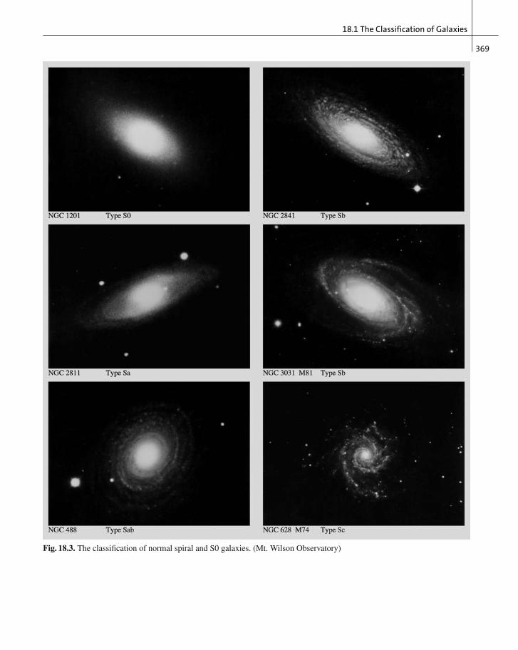
18.1 The Classification of Galaxies
369
Fig. 18.3. The classification of normal spiral and S0 galaxies. (Mt. Wilson Observatory)
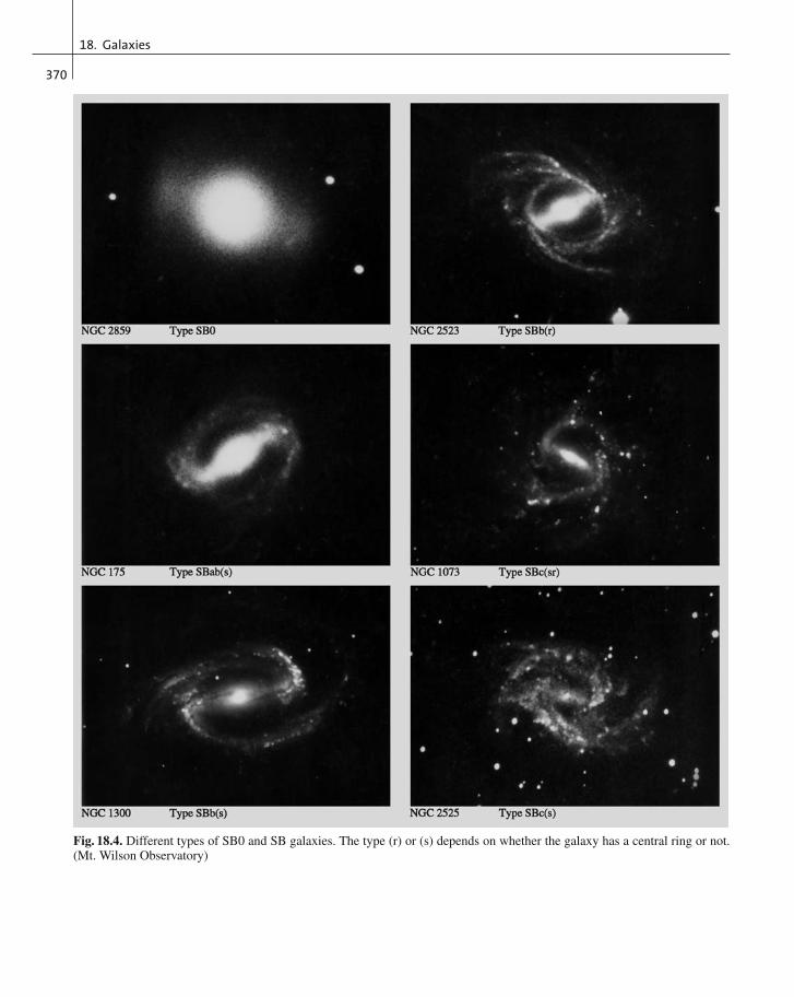
370
18. Galaxies
Fig. 18.4. Different types of SB0 and SB galaxies. The type (r) or (s) depends on whether the galaxy has a central ring or not.(Mt. Wilson Observatory)
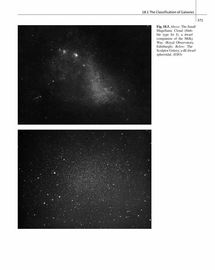
18.1 The Classification of Galaxies
371
Fig. 18.5. Above: The SmallMagellanic Cloud (Hub-ble type Irr I), a dwarfcompanion of the MilkyWay. (Royal Observatory,Edinburgh). Below: TheSculptor Galaxy, a dE dwarfspheroidal. (ESO)

372
18. Galaxies
Fig. 18.6. M32 (type E2),a small elliptical companionof the Andromeda Galaxy.(NOAO/Kitt Peak NationalObservatory)
tion of the Hubble sequence towards later types beyondthe Sc galaxies. They are rich in gas and contain manyyoung stars. Type Irr II are dusty, somewhat irregularsmall ellipticals. Other types of dwarf galaxies are of-ten introduced. One example is the dwarf spheroidaltype dE, similar to the ellipticals, but with a much lesscentrally concentrated star distribution. Another is theblue compact galaxies (also called extragalactic H II re-gions), in which essentially all the light comes froma small region of bright, newly formed stars.
18.2 Luminosities and Masses
Distances. In order to determine the absolute lumi-nosities and linear dimensions of galaxies one needsto know their distances. Distances are also needed inorder to estimate the masses of galaxies, because theseestimates depend on the absolute linear size. Distanceswithin the Local Group can be measured by the samemethods as inside the Milky Way, most importantly bymeans of variable stars. On the very large scale (beyond50 Mpc), the distances can be deduced on the basis of
the expansion of the Universe (see Sect. 19.1). In or-der to connect these two regions one needs methodsof distance determination based on the properties ofindividual galaxies.
To some extent local distances can be determined us-ing structural components of galaxies, such as the sizesof H II regions or the magnitudes of globular clusters.However, to measure distances of tens of megaparsecs,one needs a distance-independent method to determinethe absolute luminosities of entire galaxies. Several suchmethods have been proposed. For example, a luminosityclassification has been introduced for late spiral typesby Sidney van den Bergh. This is based on a correlationbetween the luminosity of a galaxy and the prominenceof its spiral pattern.
Other distance indicators are obtained if there is someintrinsic property of the galaxy, which is correlated withits total luminosity, and which can be measured indepen-dently of the distance. Such properties are the colour, thesurface brightness and the internal velocities in galax-ies. All of these have been used to measure distancesto both spiral and elliptical galaxies. For example, theabsolute luminosity of a galaxy should depend on its

18.2 Luminosities and Masses
373
Fig. 18.7. Compound luminosity function of thirteen clustersof galaxies. The open symbols have been obtained by omittingthe cD galaxies. The distribution is then well described by(18.2). The cD galaxies (filled symbols) cause a deviation atthe bright end. (Schechter, P. (1976): Astrophys. J. 203, 297)
mass. The mass, in turn, will be reflected in the veloc-ities of stars and gas in the galaxy. Accordingly thereis a relationship between the absolute luminosity andthe velocity dispersion (in ellipticals) and the rotationalvelocity (in spirals). Since rotational velocities can bemeasured very accurately from the width of the hy-drogen 21-cm line, the latter relationship (known asthe Tully–Fisher relation) is perhaps the best distanceindicator currently available.
The luminosity of the brightest galaxies in clustershas been found to be reasonably constant. This factcan be used to measure even larger distances, providinga method which is important in cosmology.
Luminosities. The definition of the total luminosity ofa galaxy is to some extent arbitrary, since galaxies donot have a sharp outer edge. The usual convention is to
measure the luminosity of a galaxy out to a given valueof the surface brightness, e. g. to 26.5 mag/sq.arcsec.For a given Hubble type, the total luminosity L mayvary widely.
As in the case of stars, the distribution of galaxy lu-minosities is described by the luminosity functionΦ(L).This is defined so that the space density of galaxies withluminosities between L and L +dL is Φ(L) dL. It canbe determined from the observed magnitudes of galax-ies, once their distances have been estimated in someway. In practice, one assumes some suitable functionalform for Φ(L), which is then fitted to the observations.One common form is Schechter’s luminosity function,
Φ(L) dL =Φ∗(
L
L∗
)αe−L/L∗
d
(L
L∗
). (18.2)
The values of the parametersΦ∗, L∗, α are observation-ally determined for different types of objects; in general,they will be functions of position.
The shape of the luminosity function is describedby the parameters α and L∗. The relative numberof faint galaxies is described by α. Since its ob-served value is about −1.1, the density of galaxiesgrows monotonically as one goes towards fainter lu-minosities. The luminosity function falls off steeplyabove the luminosity L∗, which therefore representsa characteristic luminosity of bright galaxies. Theobserved L∗ corresponds to an absolute magnitudeM∗ = −21.0 mag. The corresponding magnitude forthe Milky Way Galaxy is probably −20.2 mag. ThecD giant galaxies do not obey this brightness distri-bution; their magnitudes may be −24 mag and evenbrighter.
The parameter Φ∗ is proportional to the space den-sity of galaxies and is therefore a strong function ofposition. Since the total number density of galaxiespredicted by relation (18.2) is infinite, we define n∗ =density of galaxies with luminosity> L∗. The observedaverage value of n∗ over a large volume of space isn∗ = 3.5×10⁻³ Mpc−3. The mean separation betweengalaxies corresponding to this density is 4 Mpc. Sincemost galaxies are fainter than L∗, and since, in addition,they often belong to groups, we see that the distancesbetween normal galaxies are generally not much largerthan their diameters.

374
18. Galaxies
Masses. The distribution of mass in galaxies is a cru-cial quantity, both for cosmology and for theories ofthe origin and evolution of galaxies. Observationallyit is determined from the velocities of the stars andinterstellar gas. Total masses of galaxies can also bederived from their motions in clusters of galaxies. Theresults are usually given in terms of the correspond-ing mass-luminosity ratio M/L, using the solar massand luminosity as units. The value measured in thesolar neighbourhood of the Milky Way is M/L = 3.If M/L were constant, the mass distribution could bedetermined from the observed luminosity distributionby multiplying with M/L.
The masses of eliptical galaxies may be obtainedfrom the stellar velocity dispersion given by the broad-ening of spectral lines. The method is based on the virialtheorem (see Sect. 6.10), which says that in a systemin equilibrium, the kinetic energy T and the potentialenergy U are related according to the equation
2T +U = 0 . (18.3)
Since ellipticals rotate slowly, the kinetic energy of thestars may be written
T = Mv2/2 , (18.4)
where M is the total mass of the galaxy and v the velocitywidth of the spectral lines. The potential energy is
U = −G M2/2R , (18.5)
Fig. 18.8. Velocity of rotation V(R) [km s−1] and velocity dis-persionσ(R) [km s−1] as functions of radius [kpc] for types E2
and E5. The latter galaxy is rotating, the former is not. (Davies,R. L. (1981): Mon. Not. R. Astron. Soc. 194, 879)
where R is a suitable average radius of the galaxy thatcan be estimated or calculated from the light distri-bution. Introducing (18.4) and (18.5) into (18.3) weobtain:
M = 2v2 R/G . (18.6)
From this formula the mass of an elliptical galaxy can becalculated when v2 and R are known. Some observationsof velocities in elliptical galaxies are given in Fig. 18.8.These will be further discussed in Sect. 18.4. The valueof M/L derived from such observations is about 10within a radius of 10 kpc. The mass of a bright ellipticalmight thus be up to 1013 M.
The masses of spiral galaxies are obtained from theirrotation curve v(R), which gives the variation of theirrotational velocity with radius. Assuming that most ofthe mass is in the almost spherical bulge, the mass withinradius R, M(R), can be estimated from Kepler’s thirdlaw:
M(R)= Rv(R)2/G . (18.7)
Some typical rotation curves are shown in Fig. 18.9. Inthe outer parts of many spirals, v(R) does not dependon R. This means that M(R) is directly proportional tothe radius – the further out one goes, the larger the in-terior mass is. Since the outer parts of spirals are veryfaint, at large radii the value of M/L is directly propor-tional to the radius. For the disc, one finds that M/L = 8for early and M/L = 4 for late spiral types. The largestmeasured total mass is 2×10¹² M.

18.3 Galactic Structures
375
Fig. 18.9. Rotation curvesfor seven spiral galaxies.(Rubin, V.C., Ford, W.K.,Thonnard, N. (1978): As-trophys. J. (Lett.) 225,L107)
In order to measure the mass at even larger radiiwhere no emission can be detected, motions in systemsof galaxies have to be used. One possibility is to usepairs of galaxies. In principle, the method is the sameas for binary stars. However, because the orbital periodof a binary galaxy is about 109 years, only statisticalinformation can be obtained in this way. The results arestill uncertain, but seem to indicate values of M/L =20–30 at pair separations of about 50 kpc.
A fourth method to determine galaxy masses is toapply the virial theorem to clusters of galaxies, assum-ing that these are in equilibrium. The kinetic energy Tin (18.4) can then be calculated from the observed red-shifts and the potential energy U , from the separationsbetween cluster galaxies. If it is assumed that the massesof galaxies are proportional to their luminosities, it isfound that M/L is about 200 within 1 Mpc of the clustercentre. However, there is a large variation from clusterto cluster.
Present results suggest that as one samples largervolumes of space, one obtains larger values for the mass-luminosity ratio. Thus a large fraction of the total massof galaxies must be in an invisible and unknown form,mostly found in the outer parts. This is known as themissing mass problem, and is one of the central unsolvedquestions of extragalactic astronomy.
18.3 Galactic Structures
Ellipticals and Bulges. In all galaxies the oldest starshave a more or less round distribution. In the Milky Waythis component is represented by the population II stars.Its inner parts are called the bulge, and its outer partsare often referred to as the halo. There does not appearto be any physically significant difference between thebulge and the halo. The population of old stars canbe best studied in ellipticals, which only contain thiscomponent. The bulges of spiral and S0 galaxies arevery similar to ellipticals of the same size.
The surface brightness distribution in elliptical galax-ies essentially depends only on the distance from thecentre and the orientation of the major and minor axis.If r is the radius along the major axis, the surfacebrightness I(r) is well described by de Vaucouleurs’law:
logI(r)
Ie= −3.33
[(r
re
)1/4
−1
]. (18.8)
The constants in (18.8) have been chosen so that halfof the total light of the galaxy is radiated from withinthe radius re and the surface brightness at that radiusis Ie. The parameters re and Ie are determined by fitting(18.8) to observed brightness profiles. Typical values for

376
18. Galaxies
elliptical, normal spiral and S0 galaxies are in the rangesre = 1–10 kpc and Ie corresponds to 20–23 magnitudesper square arc second.
Although de Vaucouleurs’ law is a purely empiricalrelation, it still gives a remarkably good representationof the observed light distribution. However, in the outerregions of elliptical galaxies, departures may often oc-cur: the surface brightness of dwarf spheroidals oftenfalls off more rapidly than (18.8), perhaps because theouter parts of these galaxies have been torn off in tidalencounters with other galaxies. In the giant galaxies oftype cD, the surface brightness falls off more slowly(see Fig. 18.10). It is thought that this is connected withtheir central position in clusters of galaxies.
Although the isophotes in elliptical galaxies are el-lipses to a good approximation, their ellipticities andthe orientation of their major axes may vary as a func-tion of radius. Different galaxies differ widely in thisrespect, indicating that the structure of ellipticals isnot as simple as it might appear. In particular, the factthat the direction of the major axis sometimes changeswithin a galaxy suggests that some ellipticals may notbe axially symmetric in shape.
From the distribution of surface brightness, the three-dimensional structure of a galaxy may be inferred asexplained in *Three-Dimensional Shape of Galaxies.
Fig. 18.10. The distribu-tion of surface brightnessin E and cD galaxies. Or-dinate: surface magnitude,mag/sq.arcsec; abscissa:(radius [kpc])1/4. Equa-tion (18.8) corresponds toa straight line in this repre-sentation. It fits well withan E galaxy, but for type cDthe luminosity falls off moreslowly in the outer regions.Comparison with Fig. 18.11shows that the brightnessdistribution in S0 galaxiesbehaves in a similar fashion.cD galaxies have often beenerroneously classified as S0.(Thuan, T.X., Romanishin,W. (1981): Astrophys. J.248, 439)
The relation (18.8) gives a brightness profile which isvery strongly peaked towards the centre. The real distri-bution of axial ratios for ellipticals can be statisticallyinferred from the observed one. On the (questionable)assumption that they are rotationally symmetric, oneobtains a broad distribution with a maximum corre-sponding to types E3–E4. If the true shape is notaxisymmetric, it cannot even statistically be uniquelydetermined from the observations.
Discs. A bright, massive stellar disc is characteristicfor S0 and spiral galaxies, which are therefore calleddisc galaxies. There are indications that in some el-lipticals there is also a faint disc hidden behind thebright bulge. In the Milky Way the disc is formed bypopulation I stars.
The distribution of surface brightness in the disc isdescribed by the expression
I(r)= I0 e−r/r0 . (18.9)
Figure 18.11 shows how the observed radial bright-ness distribution can be decomposed into a sumof two components: a centrally dominant bulgeand a disc contributing significantly at larger radii.The central surface brightness I0 typically corre-sponds to 21–22 mag./sq.arcsec, and the radial scale
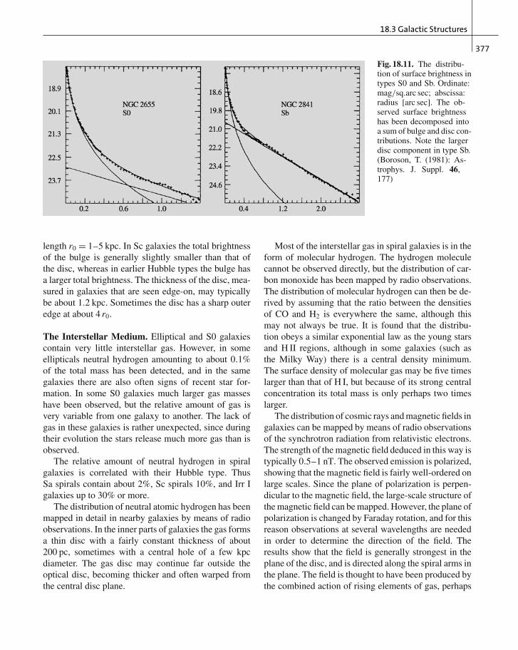
18.3 Galactic Structures
377
Fig. 18.11. The distribu-tion of surface brightness intypes S0 and Sb. Ordinate:mag/sq.arc sec; abscissa:radius [arc sec]. The ob-served surface brightnesshas been decomposed intoa sum of bulge and disc con-tributions. Note the largerdisc component in type Sb.(Boroson, T. (1981): As-trophys. J. Suppl. 46,177)
length r0 = 1–5 kpc. In Sc galaxies the total brightnessof the bulge is generally slightly smaller than that ofthe disc, whereas in earlier Hubble types the bulge hasa larger total brightness. The thickness of the disc, mea-sured in galaxies that are seen edge-on, may typicallybe about 1.2 kpc. Sometimes the disc has a sharp outeredge at about 4 r0.
The Interstellar Medium. Elliptical and S0 galaxiescontain very little interstellar gas. However, in someellipticals neutral hydrogen amounting to about 0.1%of the total mass has been detected, and in the samegalaxies there are also often signs of recent star for-mation. In some S0 galaxies much larger gas masseshave been observed, but the relative amount of gas isvery variable from one galaxy to another. The lack ofgas in these galaxies is rather unexpected, since duringtheir evolution the stars release much more gas than isobserved.
The relative amount of neutral hydrogen in spiralgalaxies is correlated with their Hubble type. ThusSa spirals contain about 2%, Sc spirals 10%, and Irr Igalaxies up to 30% or more.
The distribution of neutral atomic hydrogen has beenmapped in detail in nearby galaxies by means of radioobservations. In the inner parts of galaxies the gas formsa thin disc with a fairly constant thickness of about200 pc, sometimes with a central hole of a few kpcdiameter. The gas disc may continue far outside theoptical disc, becoming thicker and often warped fromthe central disc plane.
Most of the interstellar gas in spiral galaxies is in theform of molecular hydrogen. The hydrogen moleculecannot be observed directly, but the distribution of car-bon monoxide has been mapped by radio observations.The distribution of molecular hydrogen can then be de-rived by assuming that the ratio between the densitiesof CO and H2 is everywhere the same, although thismay not always be true. It is found that the distribu-tion obeys a similar exponential law as the young starsand H II regions, although in some galaxies (such asthe Milky Way) there is a central density minimum.The surface density of molecular gas may be five timeslarger than that of H I, but because of its strong centralconcentration its total mass is only perhaps two timeslarger.
The distribution of cosmic rays and magnetic fields ingalaxies can be mapped by means of radio observationsof the synchrotron radiation from relativistic electrons.The strength of the magnetic field deduced in this way istypically 0.5–1 nT. The observed emission is polarized,showing that the magnetic field is fairly well-ordered onlarge scales. Since the plane of polarization is perpen-dicular to the magnetic field, the large-scale structure ofthe magnetic field can be mapped. However, the plane ofpolarization is changed by Faraday rotation, and for thisreason observations at several wavelengths are neededin order to determine the direction of the field. Theresults show that the field is generally strongest in theplane of the disc, and is directed along the spiral arms inthe plane. The field is thought to have been produced bythe combined action of rising elements of gas, perhaps

378
18. Galaxies
produced by supernova explosions, and the differentialrotation, in principle in the same way as the productionof solar magnetic fields was explained in Chapter 12.
* Three-Dimensional Shape of Galaxies
Equations (18.8) and (18.9) describe the distributionof galactic light projected on the plane of the sky.The actual three-dimensional luminosity distribution ina galaxy is obtained by inverting the projection. This iseasiest for spherical galaxies.
Let us suppose that a spherical galaxy has the pro-jected luminosity distribution I(r) (e. g. as in (18.8)).With coordinates chosen according to the figure, I(r) isgiven in terms of the three-dimensional luminositydistribution ρ(R) by
I(r)=∞∫
−∞ρ(R) dz .
Since z2 = R2 − r2, a change of the variable ofintegration yields
I(r)= 2
∞∫r
ρ(R)R dR√R2 −r2
.
This is known as an Abel integral equation for ρ(R),and has the solution
ρ(R)= − 1
πR
d
dR
∞∫R
I(r)r dr√r2 − R2
= − 1
π
∞∫R
(d I/dr) dr√r2 − R2
.
Introducing the observed I(r) into this expression, oneobtains the actual luminosity distribution ρ(R). In thefigure the solid curve shows the three-dimensional lu-minosity distribution obtained from the Vancouleurs’law (the dashed line).
If the galaxy is not spherical, its three-dimensionalshape can only be determined if its inclination withrespect to the line of sight is known. Since galactic discsare thin and of constant thickness, the inclination i ofa disc galaxy is obtained directly from the axis ratio ofits projected image: sin i = b/a.
When the inclination is known, the real axis ratioof the bulge q0 can be determined from the projectedvalue q. For a rotationally symmetric bulge the relationbetween q and q0 is
cos2 i = 1−q2
1−q20
.
The flattenings of disc galaxy bulges obtained from thisrelation lie in the range q0 = 0.3–0.5. Since the incli-nations of ellipticals are generally unknown, only thestatistical distribution of q can be determined from thatof q0.

18.4 Dynamics of Galaxies
379
18.4 Dynamics of Galaxies
We have seen how the masses of galaxies can be derivedfrom observed velocities of stars and gas. The same ob-servations can be used to study the internal distributionof mass in more detail.
Slowly Rotating Systems. The dynamics of ellipticalgalaxies and disc galaxy bulges are studied by meansof the Doppler shifts and broadenings of stellar absorp-tion lines. Since a given absorption line is the sum ofcontributions from many individual stars, its Dopplershift gives their mean velocity, while its broadening isincreased by an amount depending on the dispersion ofstellar velocities around the mean. By observing howthe wavelengths and widths of spectral lines behave asfunctions of the radius, one can get some insight intothe distribution of mass in the galaxy.
Examples of the observed radial dependence of therotational velocity and velocity dispersion derived forsome ellipticals were given in Fig. 18.8. The observedrotational velocities are often small (< 100 km s−1),while the velocity dispersion may typically be about200 km s−1. If elliptical galaxies were in fact ellip-soids of revolution, there should be a statistical relation(when projection effects have been taken into account)between flatness, rotational velocity and velocity disper-sion. Such a relationship has been observed for fainterellipticals and for disc galaxy bulges. However, someof the brightest ellipticals rotate very slowly. Thereforetheir flattening cannot be due to rotation.
The radial dependence of the velocity dispersiongives information on the distribution of mass within thegalaxy. Since it also depends on how the shapes of stel-lar orbits in the galaxy are distributed, its interpretationrequires detailed dynamical models.
Rotation Curves. In spiral galaxies the distribution ofmass can be studied directly using the observed ro-tational velocities of the interstellar gas. This can beobserved either at optical wavelengths from the emis-sion lines of ionised gas in H II regions or at radiowavelengths from the hydrogen 21 cm line. Typicalgalactic rotation curves were shown in Fig. 18.9.
The qualitative behaviour of the rotation curve inall spiral galaxies is similar to the rotation curve ofthe Milky Way: there is a central portion, where the
rotational velocity is directly proportional to the radius,corresponding to solid body rotation. At a few kpc radiusthe curve turns over and becomes flat, i. e. the rotationalvelocity does not depend on the radius. In early Hubbletypes, the rotation curve rises more steeply near thecentre and reaches larger velocities in the flat region(Sa about 300 km s−1, Sc about 200 km s−1). A higherrotational velocity indicates a larger mass accordingto (18.7), and thus Sa types must have a larger massdensity near the centre. This is not unexpected, sincea more massive bulge is one of the defining propertiesof early type spirals.
A decrease of the rotational velocity at large radiiwould be an indication that most of the mass is in-side that radius. In some galaxies such a decrease hasbeen detected, in others the rotational velocity remainsconstant as far out as the observations can reach.
Spiral Structure. Spiral galaxies are relatively brightobjects. Some have a well-defined, large-scale two-armed spiral pattern, whereas in others the spiralstructure is made up of a large number of short fila-mentary arms. From galaxies where the pattern is seenin front of the central bulge, it has been deduced that thesense of winding of the spiral is trailing with respect tothe rotation of the galaxy.
The spiral structure is most clearly seen in the in-terstellar dust, H II regions, and the OB associationsformed by young stars. The dust often forms thin lanesalong the inner edge of the spiral arms, with star formingregions on their outside. Enhanced synchrotron radioemission associated with spiral arms has also beendetected.
The spiral pattern is generally thought to be a wave inthe density of the stellar disc, as discussed in Sect. 17.4.As the interstellar gas streams through the density wavea shock, marked by the dust lanes, is formed as theinterstellar gas is compressed, leading to the collapseof molecular clouds and the formation of stars. Thedensity wave theory predicts characteristic streamingmotions within the arm, which have been detected insome galaxies by observations of the H I 21 cm line.
It is not known how the spiral wave was produced. Inmultiarmed galaxies the spiral arms may be short-lived,constantly forming and disappearing, but extensive, reg-ular, two-armed patterns have to be more long-lived. Inbarred spirals the bar can drive a spiral wave in the

380
18. Galaxies
Fig. 18.12. Above: A spi-ral galaxy from above: M51(type Sc). The interactingcompanion is NGC 5195(type Irr II). (Lick Obser-vatory). Below: A spiralgalaxy from the side:the Sb spiral NGC 4565.(NOAO/Kitt Peak NationalObservatory)

18.6 Systems of Galaxies
381
gas. Some normal spirals may have been produced bythe tidal force from another galaxy passing nearby. Fi-nally, in some galaxies a two-armed spiral may havebeen spontaneously generated by an instability of thedisc.
18.5 Stellar Ages and ElementAbundances in Galaxies
From the Milky Way we know that stars of populations Iand II are different not only in respect to their spatialdistribution, but also in respect to their ages and heavyelement abundances. This fact gives important evidenceabout the formation of the Milky Way, and it is thereforeof interest if a similar connection can be found in othergalaxies.
The indicators of composition most easily measuredare the variations of colour indices inside galaxies andbetween different galaxies. Two regularities have beendiscovered in these variations: First, according to thecolour–luminosity relation for elliptical and S0 galaxies,brighter galaxies are redder. Secondly, there is a colour–aperture effect, so that the central parts of galaxies areredder. For spirals this relationship is due to the presenceof young, massive stars in the disc, but it has also beenobserved for elliptical and S0 galaxies.
Galactic spectra are composed of the spectra of alltheir stars added together. Thus the colours depend bothon the ages of the stars (young stars are bluer) and onthe heavy element abundance Z (stars with larger Z areredder). The interpretation of the observational resultsthus has to be based on detailed modelling of the stellarcomposition of galaxies or population synthesis.
Stars of different spectral classes contribute differentcharacteristic absorption features to the galaxy spec-trum. By observing the strength of various spectralfeatures, one can find out about the masses, ages andchemical composition of the stars that make up thegalaxy. For this purpose, a large number of character-istic properties of the spectrum, strengths of absorptionlines and broad-band colours are measured. One thenattempts to reproduce these data, using a represen-tative collection of stellar spectra. If no satisfactorysolution can be found, more stars have to be addedto the model. The final result is a population model,giving the stellar composition of the galaxy. Combin-
ing this with theoretical stellar evolution calculations,the evolution of the light of the galaxy can also becomputed.
Population synthesis of E galaxies show that practi-cally all their stars were formed simultaneously about15×109 years ago. Most of their light comes from redgiants, whereas most of their mass resides in lower mainsequence stars of less than one solar mass. Since allstars have roughly the same age, the colours of ellip-tical galaxies are directly related to their metallicities.Thus the colour–luminosity relation indicates that Z ingiant ellipticals may be double that in the solar neigh-bourhood, while it may be smaller by a factor 100 indwarfs. Similarly, the radial dependence of the colourscan be explained if the value of Z at the centre is anorder of magnitude larger than it is at larger radii.
The stellar composition of disc galaxy bulges isgenerally similar to that of ellipticals. The element abun-dances in the gas in spirals can be studied by means ofthe emission lines from H II regions ionised by newlyformed stars. In this case too, the metallicity increasestowards the centre, but the size of the variation varies indifferent galaxies, and is not yet well understood.
18.6 Systems of Galaxies
The galaxies are not smoothly distributed in space;rather, they form systems of all sizes: galaxy pairs,small groups, large clusters and superclusters formedfrom several groups and clusters. The larger a givensystem, the less its density exceeds the mean density ofthe Universe. On the average, the density is twice thebackground density for systems of radius 5 Mpc and10% above the background at radius 20 Mpc.
Interactions of Galaxies. The frequency of differ-ent types of galaxies varies in the various kinds ofgroups. This could either be because certain types ofgalaxies are formed preferentially in certain environ-ments, or because interactions between galaxies havechanged their shapes. There are many observed inter-acting systems where strong tidal forces have producedstriking distortions, “bridges” and “tails” in the membergalaxies.
The interactions between galaxies are not always dra-matic. For example, the Milky Way has two satellites,

382
18. Galaxies
Fig. 18.13. Above: The ir-regular Virgo Cluster ofgalaxies. Below: The reg-ular Coma Cluster (ESOand Karl-Schwarzschild-Observatorium)

18.6 Systems of Galaxies
383
the Large and Small Magellanic Clouds (see Fig. 18.5),which are Irr I type dwarf galaxies at about 60 kpc dis-tance. It is thought that approximately 5×10⁸ yearsago, these passed the Milky Way at a distance of about10–15 kpc, leaving behind the Magellanic Stream,a 180 long thin stream of neutral hydrogen clouds.Systems of this type, where a giant galaxy is sur-rounded by a few small companions, are quite common.Computations show that in many such cases the tidalinteractions are so strong that the companions willmerge with the parent galaxy at the next close ap-proach. This is likely to happen to the MagellanicClouds.
During earlier epochs in the Universe, when the den-sity was larger, interactions between galaxies must havebeen much more common than at present. Thus it hasbeen proposed that a large fraction of bright galaxieshave undergone major mergers at some stage in their his-tory. In particular, there are good reasons to believe thatthe slowly rotating, non-axisymmetric giant ellipticalsmay have formed by the merger of disc galaxies.
Groups. The most common type of galaxy systemsare small, irregular groups of a few tens of galaxies.A typical example is the Local Group, which containstwo larger galaxies in addition to the Milky Way – theAndromeda Galaxy M31, an Sb spiral of about the samesize as the Milky Way with two dwarf companions,and the smaller Sc spiral M33. The rest of the about35 members of the Local Group are dwarfs; about 20are of type dE and 10 of type Irr I. The diameter of theLocal Group is about 1.2 Mpc.
Clusters. A system of galaxies may be defined to bea cluster if it contains a larger number (at least 50) ofbright galaxies. The number of members and the size ofa cluster depend on how they are defined. One way ofdoing this is to fit the observed distribution of galaxieswithin a cluster with an expression of the form (18.8). Inthis way a characteristic cluster radius of about 2–5 Mpcis obtained. The number of members depends both onthe cluster radius and on the limiting magnitude. A largecluster may contain several hundred galaxies that areless than two magnitudes fainter than the characteristicluminosity L∗ of (18.2).
Clusters of galaxies can be ordered in a sequencefrom extended, low-density, irregular systems (some-
times called clouds of galaxies) to denser and moreregular structures (Fig. 18.13). The galaxy type com-position also varies along this sequence in the sensethat in the loose irregular clusters, the bright galax-ies are predominantly spirals, whereas the members ofdense clusters are almost exclusively type E and S0.The nearest cluster of galaxies is the Virgo Cluster ata distance of about 15 Mpc. It is a relatively irregularcluster, where a denser central region containing earlygalaxy types is surrounded by a more extended distri-bution of mainly spiral galaxies. The nearest regularcluster is the Coma Cluster, roughly 90 Mpc away. Inthe Coma Cluster a central pair of giant ellipticals issurrounded by a flattened (axis ratio about 2 : 1) systemof early type galaxies.
X-ray emission from hot gas has been detected inmany clusters. In irregular clusters the gas temperatureis about 107 K and the emission is generally concen-trated near individual galaxies; in the regular ones thegas is hotter, 108 K, and the emission tends to be moreevenly distributed over the whole cluster area. By andlarge, the X-ray emission follows the distribution of thegalaxies. The amount of gas needed to explain this emis-sion is about equal to the mass of the galaxies – thusit cannot solve the missing mass problem. X-ray emis-sion lines from multiply ionised iron have also beenobserved. On basis of these lines, it has been concludedthat the metal abundance of intergalactic gas is roughlyequal to that of the Sun. For this reason it is most likelythat the gas has been ejected from the galaxies in thecluster.
Superclusters. Groups and clusters of galaxies mayform even larger systems, superclusters. For example,the Local Group belongs to the Local Supercluster,a flattened system whose centre is the Virgo Cluster,containing tens of smaller groups and clouds of galax-ies. The Coma Cluster is part of another supercluster.The diameters of superclusters are 10–20 Mpc. How-ever, on this scale, it is no longer clear whether onecan reasonably speak of individual systems. Perhapsit would be more accurate to think of the distributionof galaxies as a continuous network, where the largeclusters are connected by walls and strings formed bysmaller systems. Between these there remain empty re-gions containing very few galaxies, which can be up to50 Mpc in diameter (Fig. 18.14).

384
18. Galaxies
Fig. 18.14. The large-scale spacedistribution of 245 591 galaxies.The radial co-ordinate is the red-shift, which can be translated intoa distance using a value for theHubble constant. The thickness ofthe slices is about 10. (2dFGRSTeam, http://www2.aao.gov.au/TDFgg/)
18.7 Active Galaxies and Quasars
So far in this chapter we have been concerned withthe properties of normal galaxies. In some galaxies,however, the normal galaxy is overshadowed by violentactivity. This activity is produced in the nucleus, whichis then called an active galactic nucleus (AGN).
The luminosities of active galactic nuclei may beextremely large, sometimes much larger than that of
the rest of the galaxy. It seems unlikely that a galaxycould maintain such a large power output for long. Forthis reason it is thought that active galaxies do not forma separate class of galaxy, but rather represent a passingstage in the evolution of normal galaxies.
Activity appears in many different forms. Somegalaxies have an exceptionally bright nucleus similarto a large region of ionised hydrogen. These may beyoung galaxies, where near the centre large numbers of

18.7 Active Galaxies and Quasars
385
stars are forming and evolving into supernovae (star-burst nuclei). In other nuclei the radiation cannot havebeen produced by stars, and the most plausible sourceof energy in these nuclei is the gravitational energy ofa supermassive black hole (mass > 108 M). In somegalaxies, the spectral lines are unusually broad, indi-cating large internal velocities. These may be eitherrotational velocities near a black hole or due to explo-sive events in the nucleus. In some galaxies, jets areseen coming out of the nucleus. Many active galaxiesradiate a nonthermal spectrum, apparently synchrotronradiation produced by fast electrons in a magneticfield.
The classification of active galaxies has been de-veloped rather unsystematically, since many of themhave been discovered only recently, and have not beencompletely studied. For example, the Markarian galax-ies catalogued by Benyamin Yerishevich Markarian inthe early 1970’s are defined by strong ultraviolet emis-sion. Many Markarian galaxies are Seyfert galaxies;others are galaxies undergoing a burst of star formation.The N galaxies form another class closely similar to theSeyfert galaxies.
Two natural basic classes of active galaxies are theSeyfert galaxies and the radio galaxies. The formerare spirals; the latter are ellipticals. Some astronomersthink that the Seyfert galaxies represent the active stageof normal spiral galaxies and the radio galaxies that ofellipticals.
Seyfert Galaxies. The Seyfert galaxies are named afterCarl Seyfert, who discovered them in 1943. Their mostimportant characteristics are a bright, pointlike centralnucleus and a spectrum showing broad emission lines.The continuous spectrum has a nonthermal component,which is most prominent in the ultraviolet. The emissionlines are thought to be produced in gas clouds movingclose to the nucleus with large velocities.
On the basis of the spectrum, Seyfert galaxies areclassified as type 1 or 2. In a type 1 spectrum, the al-lowed lines are broad (corresponding to a velocity of104 km s−1), much broader than the forbidden lines. Intype 2, all lines are similar and narrower (< 103 km s−1).Transitions between these types and intermediate caseshave sometimes been observed. The reason for the dif-ference is thought to be that the allowed lines are formedin denser gas near the nucleus, and the forbidden lines in
more diffuse gas further out. In type 2 Seyfert galaxies,the denser gas is missing or obscured.
Almost all Seyfert galaxies with known Hubble typesare spirals; the possible exceptions are of type 2. Theyare strong infrared sources. Type 1 galaxies often showstrong X-ray emission.
The true Seyfert galaxies are relatively weak radiosources. However, there are compact radio galaxies withan optical spectrum that is essentially the same as forSeyfert galaxies. These should probably be classifiedwith the Seyfert galaxies. In general, the stronger radioemission seems to come with a type 2 spectrum.
It is estimated that about 1% of all bright spiral galax-ies are Seyfert galaxies. The luminosities of their nucleiare about 1036–1038 W, of the same order as all the restof the galaxy. Brightness variations are common.
Radio Galaxies. By definition, radio galaxies are galax-ies that are powerful radio sources. The radio emissionof a radio galaxy is non-thermal synchrotron radia-tion. The radio luminosity of radio galaxies is typically1033–1038 W, and may thus be as large as the totalluminosity of a normal galaxy. The main problem inexplaining radio emission is to understand how the elec-trons and magnetic fields are produced, and above all,where the electrons get their energy.
The forms and sizes of the radio emitting regionsof radio galaxies have been studied ever since the1950’s, when radio interferometers achieved the res-olution of optical telescopes. The characteristic featureof a strong radio galaxy is a double structure: thereare two large radio emitting regions on opposite sidesof the observed galaxy. The radio emitting regionsof some radio galaxies are as far apart as 6 Mpc, al-most ten times the distance between the Milky Wayand Andromeda galaxies. One of the smallest doubleradio sources is the galaxy M87 (Fig. 18.15), whosetwo components are only a few kpc distant from eachother.
The double structure of radio galaxies appears to beproduced by ejections from the nucleus. However, theelectrons in the radio lobes cannot be coming from thecentre of the galaxy, because they would lose all theirenergy during such a long transit. Therefore electronshave to be continuously accelerated within the radio-emitting regions. Within the radio lobes there are almostpoint-like regions, hot spots. These are generally sym-

386
18. Galaxies
Fig. 18.15. Above: The ac-tive galaxy M87. In thelower right-hand cornera short exposure of thecore region has been in-serted (same scale as inthe main photograph). Onesees a blue jet coming outof the nucleus of a nor-mal E0 galaxy. (NOAO/KittPeak National Observa-tory). Below: In the radiomap made using the VLAthe jet is observed to betwo-sided. The area shownis much smaller than in theupper picture. (Owen, F.N.,Hardee, P.E., Bignell, R.C.(1980): Astrophys. J. (Lett.)239, L11)
metrically placed with respect to the nucleus, and areapparently consequences of nuclear ejections.
“Tailed” radio sources also exist. Their radio emis-sion mainly comes from one side of the galaxy, forming
a curved tail, which is often tens of times longer thanthe diameter of the galaxy. The best examples areNGC 1265 in the Perseus cluster of galaxies and 3C129,which appears to be in an elliptical orbit around a com-

18.7 Active Galaxies and Quasars
387
panion galaxy. The tail is interpreted as the trail left bythe radio galaxy in intergalactic space.
Another special feature revealed by the radio mapsis the presence of jets, narrow lines of radio emission,usually starting in the nucleus and stretching far outsidethe galaxy. The best known may be the M87 jet, whichhas also been observed as an optical and X-ray jet. Theoptically observed jet is surrounded by a radio source.A similar radio source is seen on the opposite side of thenucleus, where no optical jet is seen. Our nearest radiogalaxy Centaurus A also has a jet extending from the nu-cleus to near the edge of the galaxy. VLBI observationsof radio jets have also revealed superluminal motions:in many compact sources the components appear to beseparating faster than the speed of light. Since suchvelocities are impossible according to the theory of rel-ativity, the observed velocities can only be apparent, andseveral models have been proposed to account for them.
Quasars. The first quasar was discovered in 1963, whenMaarten Schmidt interpreted the optical emission linesof the known radio source 3C273 as hydrogen Balmerlines redshifted by 16%. Such large redshifts are themost remarkable characteristics of the quasars. Prop-erly speaking, the word quasar is an abbreviation forquasistellar radio source, and some astronomers preferto use the designation QSO (quasistellar object), sincenot all quasars emit radio radiation.
Optically the quasars appear almost as point sources,although improved observational techniques have re-vealed an increasing number of quasars located insidemore or less normal galaxies (Fig. 18.16). Although thefirst quasars where discovered by radio observations,only a small fraction of all optically identified quasarsare bright radio sources. Most radio quasars are pointsources, but some have a double structure like the radiogalaxies. Satellite X-ray pictures also show the quasarsto be pointlike.
In the visible region the quasar spectra are dominatedby spectral lines with rest wavelengths in the ultravio-let. The first observed quasar redshifts were z = 0.16and 0.37, and later searches have continued to turn upever larger redshifts. The present record is 6.3. Thelight left the quasar when the Universe was less thanone-tenth of its present age. The large inferred dis-tances of the quasars mean that their luminosities haveto be extremely large. Typical values lie in the range
of 1038–1041 W. The brightness of quasars may varyrapidly, within a few days or less. Thus the emitting re-gion can be no larger than a few light-days, i. e. about100 AU.
The quasars often have both emission and absorptionlines in their spectra. The emission lines are very broadand are probably produced in the quasar itself. Much ofthe absorption spectrum consists of densely distributednarrow lines that are thought to be hydrogen Lymanα lines formed in gas clouds along the line of sight tothe quasar. The clouds producing this “Lyman α forest”are young galaxies or protogalaxies, and they there-fore provide important evidence about the formation ofgalaxies.
Some astronomers have questioned the cosmolog-ical interpretation of the redshift. Thus Halton Arphas discovered small systems of quasars and galaxieswhere some of the components have widely discrepantredshifts. For this reason, Arp thinks that the quasarredshifts are produced by some unknown process. Thisclaim is highly controversial.
Unified Models. Although the forms of galactic activ-ity may at first sight appear diverse, they can be unifiedwithin a fairly widely accepted schematic model. Ac-cording to this model, most galaxies contain a compactcentral nucleus, which is a supermassive black hole,with mass 107–109 M, surrounded by a disc or ring ofgas. The source of energy is the gravitational energy re-leased as gas is accreted into the black hole. The discmay also give rise to a jet, where some of the energyis converted into perpendicular motions along the rota-tional axis. Thus active galactic nuclei are similar to thenucleus of the Milky Way, although the masses of boththe black hole and the gas disc may be much larger.
Deducing the mass of the central black hole is diffi-cult and uncertain. However, using a variety of methodsinvolving the motions of stars and gas at the centre ofnearby galaxies black hole masses for about 30 galax-ies have been determined. The most important result ofthese studies is that there is a close relationship betweenthe black hole mass and the central velocity dispersionof the galaxy. According to the virial theorem the ve-locity dispersion is a measure of the bulge mass, andtherefore the conclusion is that there is a close relation-ship between the mass of the bulge and the mass of thecentral black hole.

388
18. Galaxies
Fig. 18.16. One of the nearest quasars, 3C 273, photographedwith two cameras aboard the Hubble Space Telescope. Onthe left, the Wide Field Planetary Camera sees a bright point-like source, with a jet blasted out from the quasar (towards 5o’clock). On the right, a coronagraph in the Advanced Cam-era for Surveys blocks out the brightest parts of the quasar.Spiral arms in the host galaxy can be seen, with dark dustlanes, as well as new details in the path of the jet. (PhotosHubble/NASA/ESA)
A first characteristic parameter of the unified modelis obviously the total luminosity. For example, the onlyessential difference between Seyfert 1 galaxies andradio-quiet quasars is the larger luminosity of quasars.A second basic parameter is the radio brightness, whichmay be related to the strength of a jet. On the basis oftheir radio luminosity one can connect Seyfert galaxies
Fig. 18.17. (a) The components of the Einstein cross are grav-itationally lensed images of the same quasar. (ESA/NASA)(b) The massive galaxy cluster Abell 2218 deflects light rayspassing through it and acts as a giant gravitational lens. In
this Hubble picture from January 2000, dozens of arc-shapedimages of distant galaxies can be seen. (Photo A. Fruchter,S. Baggett, R. Hook and Z. Levay, NASA/STScI)
and radio-quiet quasars on one hand, and radio galaxiesand radio quasars on the other.
The third important parameter of unified models isthe angle from which we happen to view the nucleardisc. For example, if the disc is seen edge-on, the actualnucleus is obscured by the disc. This could explain thedifference between Seyfert types 1 and 2: in type 2 we donot see the broad emission lines formed near the blackhole, but only the narrower lines from the disc. Similarlya galaxy that looks like a double radio source when seenedge-on, would look like a radio quasar if the disc wereseen face-on. In the latter case there is a possibilitythat we may be seeing an object directly along the jet.It will then appear as a blazar, an object with rapidand violent variations in brightness and polarization,and very weak or invisible emission lines. If the jet isalmost relativistic, its transverse velocity may appearlarger than the speed of light, and thus superluminalmotions can also be understood.
One prediction of the unified model is that thereshould be a large number of quasars where the nucleus isobscured by the disc as in the Seyfert 2 galaxies. In anal-ogy with the Seyfert galaxies these objects are referredto as type 2 AGN or quasars. Because of the obscurationsuch sources would not be included in surveys at opti-cal, UV, or soft X-ray wavelengths. In hard X-rays theobscuration is less, and in the far infrared the absorbedenergy is re-radiated. Searches for type 2 quasars have

18.8 The Origin and Evolution of Galaxies
389
been made at these wavelengths with the Chandra X-raysatellite and with the Spitzer Space Telescope. The in-dications from these searches are that at least 3/4 of allsupermassive black holes are heavily obscured.
Gravitational Lenses. An interesting phenomenon firstdiscovered in connection with quasars are gravitationallenses. Since light rays are bent by gravitational fields,a mass (e. g. a galaxy) placed between a distant quasarand the observer will distort the image of the quasar.The first example of this effect was discovered in 1979,when it was found that two quasars, 5.7′′ apart in thesky, had essentially identical spectra. It was concludedthat the “pair” was really a double image of a singlequasar. Since then several other gravitationally lensedquasars have been discovered (Fig. 18.17).
Gravitational lenses have also been discovered inclusters of galaxies. Here the gravitational field of thecluster distorts the images of distant galaxies into arcsaround the cluster centre. In addition in 1993 microlens-ing was observed in the Milky Way, where the brightnessof a star is momentarily increased by the lensing effectfrom a mass passing in front of the star. Thus the study ofgravitational lens effects offers a new promising methodof obtaining information on the distribution of mass inthe Universe.
18.8 The Origin and Evolutionof Galaxies
Because the speed of light is finite we see distant galax-ies at earlier stages in their life. In the next chapterwe show how the age of a galaxy with given redshiftcan be calculated based on the rate of expansion of theUniverse. However, this relationship will depend on thecosmological model, which therefore always has to bespecified when studying the evolution of galaxies.
The beginning of galaxy evolution was marked by theformation of the first stars at a redshift around 10–20.The ultraviolet radiation of the earliest objets reionisedthe intergalactic gas, which made the Universe trans-parent to radiation, and thus made the distant galaxiesand quasars visible in principle. The largest observedredshifts known at present are about 6.5.
According to the currently widely accepted cosmo-logical models most of the matter in the Universe is
in a form that emits no radiation, and is only observ-able from its gravitational effects. In this Cold DarkMatter (CDM) theory (see Sect. 19.7) the first systemsto collapse and start forming stars were small, withmasses like those of dwarf galaxies. Larger galaxieswere formed later as these smaller fragments collectedinto larger clumps. This model, where most stars areformed in small galaxies is usually described as the hi-erarchical model. Before the introduction of the CDMmodel, the dominant model was one where the mostmassive systems are the first to start forming stars, whichis often called the monolithic model. We have alreadyseen in Sect. 17.5 that the formation of the Milky Wayshows aspects of both types of models.
A large part of our theoretical ideas on galaxy evo-lution is based on numerical simulations of the collapseof gas clouds and star formation in them. Using someprescription for star formation one can try to computethe evolution of the spectral energy distribution andthe chemical abundances in the resulting galaxies. Theresults of the models can be compared with the obser-vational data presented in the previous sections of thischapter.
The density distribution of dark matter is expectedto be very irregular, containing numerous small-scaleclumps. The collapse will therefore be highly in-homogeneous, both in the hierarchical and in themonolithic picture, and subsequent mergers betweensmaller systems should be common. There are addi-tional complicating factors. Gas may be expelled fromthe galaxy, or there may be an influx of fresh gas. In-teractions with the surroundings may radically alter thecourse of evolution – in dense systems they may leadto the complete merging of the individual galaxies intoone giant elliptical. Much remains to be learned abouthow the formation of stars is affected by the general dy-namical state of the galaxy and of how an active nucleusmay influence the formation process.
Our observational knowledge of galaxy evolutionis advancing very rapidly. Essentially all the relation-ships described earlier in this chapter have been studiedas functions of time. Still, a complete generally ac-cepted description of the way the Universe reached itspresent state has not yet been established. Here wecan only mention a few of the most central aspectsof the processes leading to the galaxies we observeto-day.

390
18. Galaxies
Fig. 18.18. Galaxy counts in the U, B, I, and K wavelengthbands. The counts are compared to those in a cosmologicalmodel without evolution. The cosmological parameters cor-respond to the currently preferred “concordance” model (seeSect. 19.5). (H.C. Ferguson et al. 2000, ARAA 38, 667, Fig. 4)
Density and Luminosity Evolution The the most basicway of studying the formation and evolution of galaxiesis by counting their numbers, either the number brighterthan some given magnitude limit (as was already doneby Hubble in the 1930’s, see Sect. 19.1) or else thenumber density as a function of redshift. The countscan be compared with the numbers expected if there isno evolution, which depend on the cosmological model.They can therefore be used either as a cosmologicaltest, or as a test of evolutionary models. However, thepresent situation is that more reliable cosmological testsare available, and the number counts are mainly used tostudy the evolution of galaxies.
There are two ways in which the number countsare affected by galaxy evolution. In density evolutionthe actual number of galaxies is changing, whereas inluminosity evolution only the luminosity of individualgalaxies is evolving. The simplest form of luminos-ity evolution is called passive luminosity evolution,
and is due to the changing luminosity of stars duringnormal stellar evolution. Pure luminosity evolution isexpected to be predominant in the monolithic picture.In the hierarchical picture density evolution will be moreprominent, since in this picture smaller galaxies are toa greater extent being destroyed to produce larger moreluminous ones.
Figure 18.18 gives an example of the results of num-ber counts. A model without evolution cannot explainthese observed counts, and various models incorporat-ing evolutionary effects have to be introduced. However,a unique model cannot be determined using just thenumber counts.
Distant Galaxies. A more direct approach to galaxyformation is the direct search for the most distant ob-jects visible. In Fig. 18.19 we show the Hubble DeepField (HDF), an area of the sky observed at severalwavelengths with the Hubble Space Telescope using avery long exposure. These images show large numbersof galaxies with redshifts about 2.5–3.5, when the Uni-verse was about 2 Ga old. The galaxies visible in theHDF appear to be bluer and more irregular than the
Fig. 18.19. The Hubble Deep Field South in the direction ofthe Tucana constellation (NASA; a colour version of the samepicture is seen as Plate 33 in the colout supplement)

18.9 Exercises
391
galaxies in our present neighbourhood, suggesting thatthey in the process of formation.
One striking result that the search for very distantgalaxies has revealed is that some galaxies with stel-lar masses 1011–1012 M had already formed arounda redshift of 1–2, and with masses 1010 M at theredshift 3, or even 5–6, when the Universe was only1 Ga old. This rapid onset of star formation in massivegalaxies is against the expectations that the first starsshould be found in dwarf galaxies. Even for nearby sys-tems there is a scarcity of dwarfs compared to the mostimmediate estimates of the CDM theory. The observa-tional evidence seems to be pointing in the direction ofdownsizing: star formation is initially largely confinedto massive systems, and starts to shift to smaller sys-tems at a redshift about 2–1. The processes invoked inthe hierarchical scheme may then take over as the mostimportant force driving galaxy evolution.
The unexpected discovery of old galaxies at largeredshifts has led to a classification of distant galax-ies into a red and a blue class depending on whetherstar formation is still going on. These two classes willhave different evolutionary histories, and by chartingthese histories we may learn better to understand thewhole process of galactic evolution. The distant red ob-jects have also inspired searches for their progenitors.Some such progenitors have been identified as ultralu-minous infrared galaxies and as submillimeter galaxies,but general agreement about their status does not yetexist.
Evolution of AGN The first clear indication of cos-mic evolution was in the numbers of radio galaxies andquasars. Already in the late 1960’s it was becoming clearthat the density of quasars was increasing dramaticallytowards higher redshifts. Roughly, the number densityof quasars increases relative to the present density bya factor 100 out to a broad maximum at redshift about2. The observed behaviour may be due to either densityor luminosity evolution. The density of radio galaxiesalso has a maximum at redshifts about 1.5–3, which issometimes referred to as the quasar era.
The Star Formation History of the Universe. Sincethe Universe contained only neutral gas as the first starsbegan to form, the most general description of howgalaxies came to be is in terms of the rate at which
Fig. 18.20. Star formation history of the Universe. The rate atwhich gas is being turned into stars is fairly well-determinedup to a redshift of about 6. Estimates for even more dis-tant epochs are still uncertain. The symbols refer to differentsearches for distant galaxies. The shaded and hatched regionsindicate theoretical fits using various models for the initialmass function of the stars. The dashed line corresponds to thelevel of star formation required to reionise the Universe at thatredshift. (A.M. Hopkins 2006, astro-ph/0611283, Fig. 3)
the gas is being turned into stars. The star formationhistory going back to a redshift about 6 is shown inFig. 18.20. The star formation rate was about an orderof magnitude larger than its current value at redshift1–2. For even larger redshifts it seems to have remainednearly constant or decreased slowly.
18.9 Exercises
Exercise 18.1 The galaxy NGC 772 is an Sb spiral,similar to M31. Its angular diameter is 7′ and appar-ent magnitude 12.0. The corresponding values of M31are 3.0 and 5.0. Find the ratio of the distances of thegalaxies
a) assuming their sizes are equal,b) assuming they are equally bright.
Exercise 18.2 The brightness of the quasar 3C279has shown changes with the time scale of one week.Estimate the size of the region producing the radiation.The apparent magnitude is 18. If the distance of thequasar is 2000 Mpc, what is its absolute magnitude andluminosity? How much energy is produced per AU3?

Hannu Karttunen et al. (Eds.), Cosmology.In: Hannu Karttunen et al. (Eds.), Fundamental Astronomy, 5th Edition. pp. 393–414 (2007)DOI: 11685739_19 © Springer-Verlag Berlin Heidelberg 2007
393
19. Cosmology
After the demise of the Aristotelian world picture, ittook hundreds of years of astronomical observations
and physical theories to reach a level at which a satis-factory modern scientific picture of the physical universecould be formed. The decisive steps in the developmentwere the clarification of the nature of the galaxies in the1920’s and the general theory of relativity developed by
Einstein in the 1910’s. Research in cosmology tries to an-swer questions such as: How large and how old is theUniverse? How is matter distributed? How were the ele-ments formed? What will be the future of the Universe?The central tenet of modern cosmology is the model ofthe expanding universe. On the basis of this model, it hasbeen possible to approach these questions.
19.1 Cosmological Observations
The Olbers Paradox. The simplest cosmological ob-servation may be that the sky is dark at night. This factwas first noted by Johannes Kepler, who, in 1610, used itas evidence for a finite universe. As the idea of an infinitespace filled with stars like the Sun became widespread inconsequence of the Copernican revolution, the questionof the dark night sky remained a problem. In the 18thand 19th centuries Edmond Halley, Loys de Cheseauxand Heinrich Olbers considered it in their writings. Ithas become known as the Olbers paradox (Fig. 19.1).
The paradox is the following: Let us suppose theUniverse is infinite and that the stars are uniformly dis-tributed in space. No matter in what direction one looks,
Fig. 19.1. The Olbers paradox. If the stars were uniformlydistributed in an unending, unchanging space, the sky shouldbe as bright as the surface of the Sun, since each line of sightwould eventually meet the surface of a star. A two-dimensional
analogy can be found in an optically thick pine forest wherethe line of sight meets a trunk wherever one looks. (Photo M.Poutanen and H. Karttunen)
sooner or later the line of sight will encounter the surfaceof a star. Since the surface brightness does not dependon distance, each point in the sky should appear to beas bright as the surface of the Sun. This clearly is nottrue. The modern explanation of the paradox is that thestars have only existed for a finite time, so that the lightfrom very distant stars has not yet reached us. Ratherthan proving the world to be finite in space, the Olbersparadox has shown it to be of a finite age.
Extragalactic Space. In 1923 Edwin Hubble showedthat the Andromeda Galaxy M31 was far outside theMilky Way, thus settling a long-standing controversyconcerning the relationship between the nebulae andthe Milky Way. The numerous galaxies seen in pho-

394
19. Cosmology
tographs form an extragalactic space vastly larger thanthe dimensions of the Milky Way. It is important forcosmology that the distribution and motions of the ba-sic components of extragalactic space, the galaxies andclusters of galaxies, should everywhere be the same asin our local part of the Universe. Galaxies generally oc-cur in various systems, ranging from small groups toclusters of galaxies and even larger superclusters. Thelargest structures observed are about 100 Mpc in size(see Sect. 18.6). They are thus significantly smaller thanthe volume of space ( a few thousand Mpc in size) inwhich the distribution of galaxies has been investigated.One way of studying the large-scale homogeneity of thegalaxy distribution is to count the number of galaxiesbrighter than some limiting magnitude m. If the galaxiesare uniformly distributed in space, this number shouldbe proportional to 100.6m (see Example 17.1). For exam-ple, the galaxy counts made by Hubble in 1934, whichincluded 44,000 galaxies, were consistent with a galaxydistribution independent of position (homogeneity) andof direction (isotropy). Hubble found no “edge” of theUniverse, nor have later galaxy counts found one.
Similar counts have been made for extragalacticradio sources. (Instead of magnitudes, flux densi-ties are used. If F is the flux density, then becausem = −2.5 lg(F/F0), the number count will be propor-tional to F−3/2.) These counts mainly involve verydistant radio galaxies and quasars (Fig. 19.3). The re-sults seem to indicate that the radio sources were eithermuch brighter or much more common at earlier epochsthan at present (Sect. 18.8). This constitutes evidence infavour of an evolving, expanding universe.
In general the simple geometric relation betweenbrightness and number counts will only hold for objectsthat are uniformly distributed in space. Local inho-mogeneities will cause departures from the expectedrelationship. For more distant sources the geometry ofthe Universe as well as cosmic evolution will changethe basic 100.6m behaviour.
Hubble’s Law (Fig. 19.4). In the late 1920’s, Hub-ble discovered that the spectral lines of galaxies wereshifted towards the red by an amount proportional totheir distances. If the redshift is due to the Doppler ef-fect, this means that the galaxies move away from eachother with velocities proportional to their separations,i. e. that the Universe is expanding as a whole.
In terms of the redshift z = (λ−λ0)/λ0, Hubble’slaw can be written as
z = (H/c)r , (19.1)
where c is the speed of light, H is the Hubble constantand r the distance of the galaxy. For small velocities(V c) the Doppler redshift z = V/c, and hence
V = Hr , (19.2)
which is the most commonly used form of Hubble’s law.For a set of observed “standard candles”, i. e. galaxies
whose absolute magnitudes are close to some mean M0,Hubble’s law corresponds to a linear relationship be-tween the apparent magnitude m and the logarithm ofthe redshift, lg z. This is because a galaxy at distance rhas an apparent magnitude m = M0 +5 lg(r/10 pc), andhence Hubble’s law yields
m = M0 +5 lg
(cz
H ×10 pc
)= 5 lg z +C , (19.3)
where the constant C depends on H and M0. Suitablestandard candles are e.g. the brightest galaxies in clus-ters and Sc galaxies of a known luminosity class. Someother methods of distance determination for galaxieswere discussed in Sect. 18.2. Most recently, type Ia su-pernovae (Sect. 13.3) in distant galaxies have been usedto determine distances out to the redshift z = 1, wheredepartures from Hubble’s law are already detectable.
If the Universe is expanding, the galaxies were oncemuch nearer to each other. If the rate of expansion hadbeen unchanging, the inverse of the Hubble constant,T = H−1, would represent the age of the Universe. Ifthe expansion is gradually slowing down, the inverseHubble constant gives an upper limit on the age of theUniverse (Fig. 19.4). According to present estimates,60 km s−1 Mpc−1<H<80 km s−1 Mpc−1, correspond-ing to 11 Ga< T< 17 Ga. In fact, current indications(discussed later in this chapter) are that the rate of ex-pansion is accelerating at present. In that case the ageof the Universe may also be larger. However, H−1 willstill be an estimate for the age of the Universe.
Fig. 19.2. The quasar 3C295 and its spectrum. The quasarsare among the most distant cosmological objects. (PhotographPalomar Observatory)

19.1 Cosmological Observations
395

396
19. Cosmology
Fig. 19.3. Hubble’s law for type Ia supernovae. The solid curverepresents the “concordance” model. The other curves showthat models with a vanishing cosmological constant can beexcluded. (R.A. Knop et al. 2003, ApJ 598,102; taken fromhttp://supernova.lbl.gov/)
One reason for the difficulty in determining the valueof the Hubble constant is the uncertainty in extragalacticdistances. A second problem is that the measured val-ues of the velocity V , corrected to take into account themotion of the Sun within the Local Group, contain a sig-nificant component due to the peculiar motions of thegalaxies. These peculiar velocities are caused by localmass concentrations like groups and clusters of galax-ies. It is possible that the Local Group has a significantvelocity towards the centre of the Local Supercluster(the Virgo Cluster). Because the Virgo Cluster is of-ten used to determine the value of H , neglecting thispeculiar velocity leads to a large error in H . The sizeof the peculiar velocity is not yet well known, but it isprobably about 250 km s−1.
The most ambitious recent project for determin-ing H used the Hubble Space Telescope in orderto measure cepheid distances to a set of nearbygalaxies. These distances were then used to calibrateother distance indicators, such as the Tully–Fisherrelation and type Ia supernovae. The final resultwas H = (72±8) km s−1 Mpc−1. The largest remain-ing source of error in this result is the distance to
Fig. 19.4. If the expansion of the Universe is slowing down,the inverse Hubble constant gives an upper limit of the age.The real age depends on the variable rate of expansion
Fig. 19.5. A regular expansion according with Hubble’s lawdoes not mean that the Milky Way (O) is the centre of theUniverse. Observers at any other galaxy (O′) will see thesame Hubble flow (dashed lines)
the Large Magellanic Cloud, used for calibrating thecepheid luminosity.
The form of Hubble’s law might give the impressionthat the Milky Way is the centre of the expansion, inapparent contradiction with the Copernican principle.Figure 19.5 shows that, in fact, the same Hubble’s lawis valid at each point in a regularly expanding universe.There is no particular centre of expansion.
The Thermal Microwave Background Radiation.The most important cosmological discovery since Hub-ble’s law was made in 1965. In that year Arno Penzias
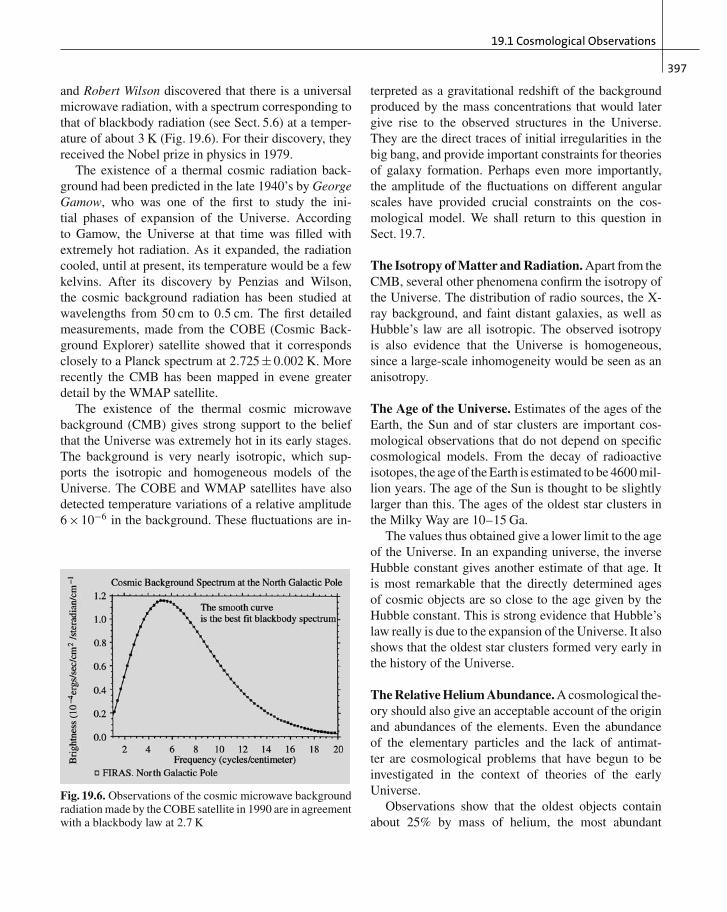
19.1 Cosmological Observations
397
and Robert Wilson discovered that there is a universalmicrowave radiation, with a spectrum corresponding tothat of blackbody radiation (see Sect. 5.6) at a temper-ature of about 3 K (Fig. 19.6). For their discovery, theyreceived the Nobel prize in physics in 1979.
The existence of a thermal cosmic radiation back-ground had been predicted in the late 1940’s by GeorgeGamow, who was one of the first to study the ini-tial phases of expansion of the Universe. Accordingto Gamow, the Universe at that time was filled withextremely hot radiation. As it expanded, the radiationcooled, until at present, its temperature would be a fewkelvins. After its discovery by Penzias and Wilson,the cosmic background radiation has been studied atwavelengths from 50 cm to 0.5 cm. The first detailedmeasurements, made from the COBE (Cosmic Back-ground Explorer) satellite showed that it correspondsclosely to a Planck spectrum at 2.725±0.002 K. Morerecently the CMB has been mapped in evene greaterdetail by the WMAP satellite.
The existence of the thermal cosmic microwavebackground (CMB) gives strong support to the beliefthat the Universe was extremely hot in its early stages.The background is very nearly isotropic, which sup-ports the isotropic and homogeneous models of theUniverse. The COBE and WMAP satellites have alsodetected temperature variations of a relative amplitude6×10−6 in the background. These fluctuations are in-
Fig. 19.6. Observations of the cosmic microwave backgroundradiation made by the COBE satellite in 1990 are in agreementwith a blackbody law at 2.7 K
terpreted as a gravitational redshift of the backgroundproduced by the mass concentrations that would latergive rise to the observed structures in the Universe.They are the direct traces of initial irregularities in thebig bang, and provide important constraints for theoriesof galaxy formation. Perhaps even more importantly,the amplitude of the fluctuations on different angularscales have provided crucial constraints on the cos-mological model. We shall return to this question inSect. 19.7.
The Isotropy of Matter and Radiation. Apart from theCMB, several other phenomena confirm the isotropy ofthe Universe. The distribution of radio sources, the X-ray background, and faint distant galaxies, as well asHubble’s law are all isotropic. The observed isotropyis also evidence that the Universe is homogeneous,since a large-scale inhomogeneity would be seen as ananisotropy.
The Age of the Universe. Estimates of the ages of theEarth, the Sun and of star clusters are important cos-mological observations that do not depend on specificcosmological models. From the decay of radioactiveisotopes, the age of the Earth is estimated to be 4600 mil-lion years. The age of the Sun is thought to be slightlylarger than this. The ages of the oldest star clusters inthe Milky Way are 10–15 Ga.
The values thus obtained give a lower limit to the ageof the Universe. In an expanding universe, the inverseHubble constant gives another estimate of that age. Itis most remarkable that the directly determined agesof cosmic objects are so close to the age given by theHubble constant. This is strong evidence that Hubble’slaw really is due to the expansion of the Universe. It alsoshows that the oldest star clusters formed very early inthe history of the Universe.
The Relative Helium Abundance. A cosmological the-ory should also give an acceptable account of the originand abundances of the elements. Even the abundanceof the elementary particles and the lack of antimat-ter are cosmological problems that have begun to beinvestigated in the context of theories of the earlyUniverse.
Observations show that the oldest objects containabout 25% by mass of helium, the most abundant

398
19. Cosmology
element after hydrogen. The amount of helium pro-duced is sensitive to the temperature of the Universe,which is related to that of the background radiation.The computations made for the standard models ofthe expanding Universe (the Friedmann models) yielda helium abundance of exactly the right size.
19.2 The Cosmological Principle
One hopes that as ever larger volumes of the Universeare observed, its average properties will become simpleand well defined. Figure 19.7 attempts to show this.It shows a distribution of galaxies in the plane. Asthe circle surrounding the observer O becomes larger,the mean density inside the circle becomes practicallyindependent of its size. The same behaviour occurs, re-gardless of the position of the centre of O: at closedistances, the density varies randomly (Fig. 19.8), butin a large enough volume, the average density is con-stant. This is an example of the cosmological principle:apart from local irregularities, the Universe looks thesame from all positions in space.
Fig. 19.7. The cosmologi-cal principle. In the smallcircle (A) about the ob-server (O) the distributionof galaxies does not yetrepresent the large-scaledistribution. In the largercircle (B) the distributionis already uniform on theaverage
The cosmological principle is a far-reaching assump-tion, which has been invoked in order to put constraintson the large variety of possible cosmological theories.If in addition to the cosmological principle one alsoassumes that the Universe is isotropic, then the onlypossible cosmic flow is a global expansion. In that case,the local velocity difference V between two nearbypoints has to be directly proportional to their separation(V = Hr); i. e. Hubble’s law must apply.
The plane universe of Fig. 19.7 is homogeneous andisotropic, apart from local irregularities. Isotropy at eachpoint implies homogeneity, but homogeneity does notrequire isotropy. An example of an anisotropic, homoge-neous universe would be a model containing a constantmagnetic field: because the field has a fixed direction,space cannot be isotropic.
We have already seen that astronomical observationssupport the homogeneity and isotropy of our observ-able neighbourhood, the metagalaxy. On the groundsof the cosmological principle, these properties may beextended to the whole of the Universe.
The cosmological principle is closely related tothe Copernican principle that our position in the

19.3 Homogeneous and Isotropic Universes
399
Fig. 19.8. The galaxies seem to be distributed in a “foamlike” way. Dense strings and shells are surrounded by relatively emptyregions. (Seldner, M. et al. (1977): Astron. J. 82, 249)
Universe is in no way special. From this principle,it is only a short step to assume that on a largeenough scale, the local properties of the metagalaxyare the same as the global properties of the Uni-verse.
Homogeneity and isotropy are important simplify-ing assumptions when trying to construct cosmologicalmodels which can be compared with local observations.They may therefore reasonably be adopted, at least asa preliminary hypothesis.

400
19. Cosmology
19.3 Homogeneousand Isotropic Universes
Under general conditions, space and time coordinatesin a universe may be chosen so that the values of thespace coordinates of observers moving with the matterare constant. It can be shown that in a homogeneous andisotropic universe, the line element (Appendix B) thentakes the form
ds2 = − c2dt2 + R2(t)
×[
dr2
1− kr2+r2(dθ2 + cos2 θdφ2)
],
(19.4)
known as the Robertson–Walker line element. (The ra-dial coordinate r is defined to be dimensionless.) R(t) isa time-dependent quantity representing the scale of theUniverse. If R increases with time, all distances, includ-ing those between galaxies, will grow. The coefficient kmay be +1, 0 or −1, corresponding to the three possiblegeometries of space, the elliptic or closed, the parabolicand the hyperbolic or open model.
The space described by these models need not beEuclidean, but can have positive or negative curvature.Depending on the curvature, the volume of the universemay be finite or infinite. In neither case does it havea visible edge.
The two-dimensional analogy to elliptical (k = +1)geometry is the surface of a sphere (Fig. 19.9): its sur-face area is finite, but has no edge. The scale factor R(t)represents the size of the sphere. When R changes, thedistances between points on the surface change in the
Fig. 19.9. The two-dimensional analogues of the Friedmannmodels: A spherical surface, a plane and a saddle surface
same way. Similarly, a three-dimensional “spherical sur-face”, or the space of elliptical geometry, has a finitevolume, but no edge. Starting off in an arbitrary direc-tion and going on for long enough, one always returnsto the initial point.
When k = 0, space is flat or Euclidean, and the ex-pression for the line element (19.4) is almost the same asin the Minkowski space. The only difference is the scalefactor R(t). All distances in a Euclidean space changewith time. The two-dimensional analogue of this spaceis a plane.
The volume of space in the hyperbolic geometry(k = −1) is also infinite. A two-dimensional idea ofthe geometry in this case is given by a saddle surface.
In a homogeneous and isotropic universe, all phys-ical quantities will depend on time through the scalefactor R(t). For example, from the form of the line ele-ment, it is evident that all distances will be proportionalto R (Fig. 19.10). Thus, if the distance to a galaxy is rat time t, then at time t0 (in cosmology, the subscript 0refers to the present value) it will be
R(t0)
R(t)r . (19.5)
Similarly, all volumes will be proportional to R3. Fromthis it follows that the density of any conserved quantity(e. g. mass) will behave as R−3.
It can be shown that the wavelength of radiation in anexpanding universe is proportional to R, like all otherlengths. If the wavelength at the time of emission, cor-responding to the scale factor R, is λ, then it will be λ0
Fig. 19.10. When space expands, all galaxy separations growwith the scale factor R: r ′ = [R(t′0)/R(t0)]r

19.4 The Friedmann Models
401
when the scale factor has increased to R0:
λ0
λ= R0
R. (19.6)
The redshift is z = (λ0 −λ)/λ, and hence
1+ z = R0
R; (19.7)
i. e. the redshift of a galaxy expresses how much thescale factor has changed since the light was emitted.For example, the light from a quasar with z = 1 wasemitted at a time when all distances were half theirpresent values.
For small values of the redshift, (19.7) approaches theusual form of Hubble’s law. This can be seen as follows.When z is small, the change in R during the propagationof a light signal will also be small and proportional tothe light travel time t. Because t = r/c approximately,where r is the distance of the source, the redshift willbe proportional to r. If the constant of proportionalityis denoted by H/c, one has
z = Hr/c . (19.8)
This is formally identical to Hubble’s law (19.1).However, the redshift is now interpreted in the senseof (19.7).
As the universe expands, the photons in the back-ground radiation will also be redshifted. The energy ofeach photon is inversely proportional to its wavelength,and will therefore behave as R−1. It can be shown thatthe number of photons will be conserved, and thus theirnumber density will behave as R−3. Combining thesetwo results, one finds that the energy density of the back-ground radiation is proportional to R−4. The energydensity of blackbody radiation is proportional to T 4,where T is the temperature. Thus the temperature ofcosmic background radiation will vary as R−1.
19.4 The Friedmann Models
The results of the preceding section are valid in any ho-mogeneous and isotropic universe. In order to determinethe precise time-dependence of the scale factor R(t)a theory of gravity is required.
In 1917 Albert Einstein presented a model of theUniverse based on his general theory of relativity. Itdescribed a geometrically symmetric (spherical) spacewith finite volume but no boundary. In accordance withthe cosmological principle, the model was homoge-neous and isotropic. It was also static: the volume ofspace did not change.
In order to obtain a static model, Einstein hadto introduce a new repulsive force, the cosmologicalterm, in his equations. The size of this cosmologicalterm is given by the cosmological constant Λ. Ein-stein presented his model before the redshifts of thegalaxies were known, and taking the Universe to bestatic was then reasonable. When the expansion of theUniverse was discovered, this argument in favour ofthe cosmological constant vanished. Einstein himselflater called it the biggest blunder of his life. Nev-ertheless, the most recent observations now seem toindicate that a non-zero cosmological constant has tobe present.
The St. Petersburg physicist Alexander Friedmannand later, independently, the Belgian Georges Lemaitrestudied the cosmological solutions of Einstein’s equa-tions. IfΛ= 0, only evolving, expanding or contractingmodels of the Universe are possible. From the Fried-mann models exact formulas for the redshift andHubble’s law may be derived.
The general relativistic derivation of the law of ex-pansion for the Friedmann models will not be givenhere. It is interesting that the existence of three typesof models and their law of expansion can be derivedfrom purely Newtonian considerations, with results incomplete agreement with the relativistic treatment. Thedetailed derivation is given on p. 411, but the essentialcharacter of the motion can be obtained from a simpleenergy argument.
Let us consider a small expanding spherical regionin the Universe. In a spherical distribution of matter,the gravitational force on a given spherical shell de-pends only on the mass inside that shell. We shall hereassume Λ= 0.
We can now consider the motion of a galaxy ofmass m at the edge of our spherical region. Accord-ing to Hubble’s law, its velocity will be V = Hr and thecorresponding kinetic energy,
T = mV 2/2 . (19.9)

402
19. Cosmology
The potential energy at the edge of a sphere of mass Mis U = −G Mm/r. Thus the total energy is
E = T +U = mV 2/2− G Mm/r , (19.10)
which has to be constant. If the mean density of the Uni-verse is ρ, the mass is M = (4πr3/3)ρ. The value of ρcorresponding to E = 0 is called the critical density, ρc.We have
E = 1
2m H2r2 − G Mm
r
= 1
2m H2r2 − Gm
4π
3
r3ρc
r
= mr2(
1
2H2 − 4
3πGρc
)= 0 ,
(19.11)
whence
ρc = 3H2
8πG. (19.12)
The expansion of the Universe can be comparedto the motion of a mass launched vertically from thesurface of a celestial body. The form of the orbit de-pends on the initial energy. In order to compute thecomplete orbit, the mass M of the main body and theinitial velocity have to be known. In cosmology, thecorresponding parameters are the mean density and theHubble constant.
The E = 0 model corresponds to the Euclidean Fried-mann model, the Einstein–de Sitter model. If the densityexceeds the critical density, the expansion of any spher-ical region will turn to a contraction and it will collapseto a point. This corresponds to the closed Friedmannmodel. Finally, if ρ < ρc, the ever expanding hyperbolicmodel is obtained. The behaviour of the scale factor inthese three cases is shown in Fig. 19.11.
These three models of the universe are called thestandard models. They are the simplest relativistic cos-mological models for Λ= 0. Models with Λ = 0 aremathematically more complicated, but show the samegeneral behaviour.
The simple Newtonian treatment of the expansionproblem is possible because Newtonian mechanics isapproximately valid in small regions of the Universe.However, although the resulting equations are formallysimilar, the interpretation of the quantities involved (e.g.the parameter k) is not the same as in the relativistic
Fig. 19.11. The time dependence of the scale factor fordifferent values of k. The cosmological constant Λ= 0
context. The global geometry of the Friedmann modelscan only be understood within the general theory ofrelativity.
Consider two points at a separation r. Let theirrelative velocity be V . Then
r = R(t)
R(t0)r0 and V = r = R(t)
R(t0)r0 , (19.13)
and thus the Hubble constant is
H = V
r= R(t)
R(t). (19.14)
The deceleration of the expansion is described by thedeceleration parameter q, defined as
q = −RR/R2 . (19.15)
The deceleration parameter describes the change of therate of the expansion R. The additional factors havebeen included in order to make it dimensionless, i. e.independent of the choice of units of length and time.
The value of the deceleration parameter can be ex-pressed in terms of the mean density. The densityparameter Ω is defined as Ω = ρ/ρc, so that Ω = 1corresponds to the Einstein–de Sitter model. From theconservation of mass, it follows that ρ0 R3
0 = ρR3. Us-ing expression (19.12) for the critical density, one thenobtains
Ω = 8πG
3
ρ0 R30
R3 H2. (19.16)

19.5 Cosmological Tests
403
On the other hand, using (19.26), q can be written
q = 4πG
3
ρ0 R30
R3 H2. (19.17)
Thus there is a simple relation between Ω and q:
Ω = 2q . (19.18)
The value q = 1/2 of the deceleration parameter corre-sponds to the critical densityΩ = 1. Both quantities arein common use in cosmology. It should be noted thatthe density and the deceleration can be observed inde-pendently. The validity of (19.18) is thus a test for thecorrectness of general relativity with Λ= 0.
19.5 Cosmological Tests
A central cosmological problem is the question of whichFriedmann model best represents the real Universe. Dif-ferent models make different observational predictions.Recently there has been considerable progress in the de-termination of the cosmological parameters, and for thefirst time there is now a set of parameters that appearcapable of accounting for all observations. In the fol-lowing, some possible tests will be considered. Thesetests are related to the average properties of the Uni-verse. Further cosmological constraints can be obtainedfrom the observed structures. These will be discussedin Sect. 19.7.
The Critical Density. If the average density ρ is largerthan the critical density ρc, the Universe is closed. Forthe Hubble constant H = 100 km s−1 Mpc−1, the valueof ρc = 1.9×10⁻²⁶ kg m−3, corresponding to roughlyten hydrogen atoms per cubic metre. Mass determina-tions for individual galaxies lead to smaller values forthe density, favouring an open model. However, the den-sity determined in this way is a lower limit, since theremay be significant amounts of invisible mass outsidethe main parts of the galaxies.
If most of the mass of clusters of galaxies is dark andinvisible, it will increase the mean density nearer thecritical value. Using the virial masses of X-ray clustersof galaxies (Sect. 18.2), one finds Ω0 = 0.3. Consider-ations of the observed velocities of clusters of galaxiesindicate that the relative amount of dark matter does notincrease further on even larger scales.
It may be that the neutrino has a small mass (about10−4 electron mass). A large neutrino backgroundshould have been produced in the big bang. In spite ofthe small suggested mass of the neutrino, it would stillbe large enough to make neutrinos the dominant form ofmass in the Universe, and would probably make the den-sity larger than critical. Laboratory measurement of themass of the neutrino is very difficult, and the claims fora measured nonzero mass have not won general accep-tance. Instead much recent work in cosmology has beenbased on the hypothesis of Cold Dark Matter (CDM),i. e. the idea that a significant part of the mass of theUniverse is in the form of non-relativistic particles ofan unknown kind.
The Magnitude-Redshift Test. Although for smallredshifts, all models predict the Hubble relationshipm = 5 lg z +C for standard candles, for larger redshiftsthere are differences, depending on the decelerationparameter q. This provides a way of measuring q.
The models predict that galaxies at a given redshiftlook brighter in the closed models than in the open ones(see Fig. 19.4). Measurements of type Ia supernovaeout to redshifts z = 1 using the Hubble Space Telescopehave now shown that the observed q is inconsistent withmodels havingΛ= 0. AssumingΩ0 = 0.3 these obser-vations require ΩΛ = 0.7, where ΩΛ is defined below((19.30)). The Hubble diagram for Type Ia supernovaeis shown in Colour Supplement Plate 34.
The Angular Diameter–Redshift Test. Along with themagnitude-redshift test, the relation between angular di-ameter and redshift has been used as a cosmologicaltest. Let us first consider how the angular diameter θof a standard object varies with distance in static mod-els with different geometries. In a Euclidean geometry,the angular diameter is inversely proportional to the dis-tance. In an elliptical geometry, θ decreases more slowlywith distance, and even begins to increase beyond a cer-tain point. The reason for this can be understood bythinking of the surface of a sphere. For an observer atthe pole, the angular diameter is the angle between twomeridians marking the edges of his standard object. Thisangle is smallest when the object is at the equator, andgrows without limit towards the opposite pole. In a hy-perbolic geometry, the angle θ decreases more rapidlywith distance than in the Euclidean case.

404
19. Cosmology
In an expanding closed universe the angular diametershould begin to increase at a redshift of about one. Thiseffect has been looked for in the diameters of radiogalaxies and quasars. No turnover has been observed,but this may also be due to evolution of the radio sourcesor to the selection of the observational data. At smallerredshifts, the use of the diameters of clusters of galaxieshas yielded equally inconclusive results.
Basically the same idea can be applied to the an-gular scale of the strongest fluctuation in the cosmicmicrowave background. The linear size of these de-pends only weakly on the cosmological model and cantherefore be treated as a standard measuring rod. Theirredshift is determined by the decoupling of matter andradiation (see Sect. 19.6). Observations of their angularsize have provided strong evidence that Ω0 +ΩΛ = 1,i. e. the Universe is flat.
Primordial Nucleosynthesis. The standard model pre-dicts that 25% of the mass of the Universe turned intohelium in the “big bang”. This amount is not sensi-tive to the density and thus does not provide a strongcosmological test. However, the amount of deuteriumleft over from helium synthesis does depend stronglyon the density. Almost all deuterons formed in the bigbang unite into helium nuclei. For a larger density thecollisions destroying deuterium were more frequent.Thus a small present deuterium abundance indicatesa high cosmological density. Similar arguments applyto the amounts of 3He and 7Li produced in the bigbang. The interpretation of the observed abundancesis difficult, since they have been changed by laternuclear processes. Still, present results for the abun-dances of these nuclei are consistent with each otherand with a density corresponding to Ω0 about 0.04.Note that this number only refers to the mass in theform of baryons, i. e. protons and neutrons. Since thevirial masses of clusters of galaxies indicate that Ω0 isabout 0.3, this has stimulated models such as the CDMmodel, where most of the mass is not in the form ofbaryons.
Ages. The ages of different Friedmann models can becompared with known ages of various systems. The
age t0 of a Friedmann model with given Ω0 and ΩΛ isobtained by integrating equation (19.30). This gives
t0 = H−10
1∫0
da(Ω0a−1 +ΩΛa2 +1−Ω0 −ΩΛ
)−1/2.
(19.19)
This age is required to be larger than the ages of theoldest known astronomical objects.
If the density is critical andΛ= 0, t0 H0 = 2/3. Thusif H0 = 75 km s−1 Mpc−1, the age is t0 = 9 Ga. Largervalues ofΩ0 give smaller ages, whereas positive valuesof Λ lead to larger ages. It has been a source of em-barrassment that the best values of H have tended togive an age for the Universe only marginally consistentwith the ages of the oldest astronomical objects. Withthe introduction of a positive cosmological constant anda slight downward revision of stellar ages this problemhas disappeared. The best current parameter values give13–14 Ga for the age of the Universe.
The “Concordance” Model. In summary there hasbeen a remarkable recent convergence between differentcosmological tests. The resulting model has a positivecosmological constant, and most of the matter is coldand dark. It is thus referred to as the ΛCDM model.The best parameter values are H = 70 km s−1 Mpc−1,ΩΛ = 0.7, Ω0 = 0.3, with cold dark matter making up85% of the total density.
The concordance model is by no means definitive.In particular the reason for the cosmological constantis a major puzzle. In order to allow for the possibilitythat Λ is variable it has become customary to refer to itas dark energy, saving the term cosmological constantfor the case of a constant Λ. Even if some alternativemechanism can produce the same effect as a non-zeroΛ,finding at least one set of acceptable parameters is animportant step forward.
An additional set of constraints on the cosmologi-cal model comes from the large-scale structures of theUniverse. These constraints, which contribute furthersupport for the concordance model, will be consideredin Sect. 19.8.

19.6 History of the Universe
405
19.6 History of the Universe
We have seen how the density of matter and of radiationenergy and temperature can be computed as functionsof the scale factor R. Since the scale factor is knownas a function of time, these quantities can be calculatedbackwards in time.
At the earliest times, densities and temperatures wereso immense that all theories about the physical pro-cesses taking place are highly conjectural. Neverthelessfirst attempts have been made at understanding the mostfundamental properties of the Universe on the basis ofmodern theories of particle physics. For example, noindications of significant amounts of antimatter in theUniverse have been discovered. Thus, for some reason,the number of matter particles must have exceeded thatof antimatter particles by a factor of 1.000000001. Be-cause of this symmetry breaking, when 99.9999999%of the hadrons were annihilated, 10−7% was left laterto form galaxies and everything else. It has been spec-ulated that the broken symmetry originated in particleprocesses about 10−35 s after the initial time.
The breaking of fundamental symmetries in the earlyUniverse may lead to what is known as inflation of theUniverse. In consequence of symmetry breaking, thedominant energy density may be the zero-point energyof a quantum field. This energy density will lead toinflation, a strongly accelerated expansion, which willdilute irregularities and drive the density very close tothe critical value. One may thus understand how thepresent homogeneity, isotropy and flatness of the Uni-verse have come about. In the inflationary picture theUniverse has to be very nearly flat, Ω0 +ΩΛ = 1. Theinflationary models also make specific predictions forthe form of the irregularities in the CMB. These pre-dictions are in general agreement with what has beenobserved.
As the Universe expanded, the density and tempera-ture decreased (Fig. 19.12) and conditions became suchthat known physical principles can be applied. Dur-ing the hot early stages, photons and massive particleswere continually changing into each other: high-energyphotons collided to produce particle-antiparticle pairs,which then were annihilated and produced photons. Asthe Universe cooled, the photon energies became toosmall to maintain this equilibrium. There is a thresholdtemperature below which particles of a given type are
Fig. 19.12. The energy densities of matter and radiation de-crease as the Universe expands. Nucleon–antinucleon pairsannihilate at 10−4 s; electron–positron pairs at 1 s
no longer produced. For example, the threshold tem-perature for hadrons (protons, neutrons and mesons)is T = 1012 K, reached at the time t = 10−4 s. Thus thepresent building blocks of the atomic nuclei, protons andneutrons, are relics from the time 10−8–10−4 s, knownas the hadron era.
The Lepton Era. In the time period 10−4 –1 s, the leptonera, the photon energies were large enough to producelight particles, such as electron–positron pairs. Becauseof matter-antimatter symmetry breaking, some of theelectrons were left over to produce present astronomi-cal bodies. During the lepton era neutrino decouplingtook place. Previously the neutrinos had been kept inequilibrium with other particles by fast particle reac-tions. As the density and temperature decreased, so didthe reaction rates, and finally they could no longer keepthe neutrinos in equilibrium. The neutrinos decoupledfrom other matter and were left to propagate throughspace without any appreciable interactions. It has beencalculated that there are at present 600 such cosmolog-ical neutrinos per cubic centimetre, but their negligibleinteractions make them extremely difficult to observe.
The Radiation Era. After the end of the lepton era,about 1 s after the initial time, the most important formof energy was electromagnetic radiation. This stageis called the radiation era. At its beginning the tem-perature was about 1010 K and at its end, about onemillion years later, when the radiation energy densityhad dropped to that of the particles, it had fallen to

406
19. Cosmology
about 40,000 degrees. At the very beginning of the ra-diation era within a few hundred seconds helium wasproduced.
Just before the epoch of helium synthesis, the numberratio of free protons and neutrons was changing becauseof the decay of the free neutrons. After about 100 sthe temperature had dropped to about 109 K, which islow enough for deuterons to be formed. All remainingneutrons were then incorporated in deuterons; these, inturn, were almost entirely consumed to produce heliumnuclei. Thus the amount of helium synthesized was de-termined by the number ratio of protons and neutronsat the time of deuterium production t = 100 s. Calcu-lations show that this ratio was about 14 : 2. Thus, outof 16 nucleons, 2 protons and 2 neutrons were incorpo-rated in a helium nucleus. Consequently 4/16 = 25% ofthe mass turned into helium. This is remarkably closeto the measured primordial helium abundance.
Only the isotopes 2H, 3He, 4He and 7Li were pro-duced in appreciable numbers by nuclear processes inthe big bang. The heavier elements have formed later instellar interiors, in supernova explosions and perhaps inenergetic events in galactic nuclei.
Radiation Decoupling. The Matter Era. As we haveseen, the mass density of radiation (obtained from theformula E = mc2) behaves as R−4, whereas that of or-dinary matter behaves as R−3. Thus the radiation massdensity decreases more rapidly. At the end of the radia-tion era it became smaller than the ordinary mass den-sity. The matter era began, bringing with it the formationof galaxies, stars, planets and human life. At present, themass density of radiation is much smaller than that ofmatter. Therefore the dynamics of the Universe is com-pletely determined by the density of massive particles.
Soon after the end of the radiation era, radiationdecoupled from matter. This happened when the tem-perature had dropped to a few thousand degrees, andthe protons and electrons combined to form hydro-gen atoms. It was the beginning of the “dark ages” atredshifts z = 1000–100, before stars and galaxies hadformed, when the Universe only contained dark matter,blackbody radiation, and slowly cooling neutral gas.
At present, light can propagate freely through space.The world is transparent to radiation: the light from dis-tant galaxies is weakened only by the r−2 law and by theredshift. Since there is no certain detection of absorp-
Fig. 19.13. The motion of the Milky Way in relation to themicrowave background can be seen in the measurements ofWMAP. One side of the sky is darker (colder), and the otherside is lighter (warmer). The horizontal stripe is the densestpart of the Milky Way. (Photo NASA)
tion by neutral gas, there must have been a reionisationof the Universe. It is thought that this occurred aroundz = 5–10.
19.7 The Formation of Structure
As we go backward in time from the present, the dis-tances between galaxies and clusters of galaxies becomesmaller. For example, the typical separation betweengalaxies is 100 times their diameter. At the redshiftz = 101 most galaxies must have been practically incontact. For this reason galaxies in their present formcannot have existed much earlier than about z = 100.Since the stars were presumably formed after the galax-ies, all present astronomical systems must have formedlater than this.
It is thought that all observed structures in theUniverse have arisen by the gravitational collapse ofsmall overdensities. Whereas the presently observablegalaxies have undergone considerable evolution, whichmakes it difficult to deduce their initial state, on largerscales the density variations should still be small andeasier to study. These are the structures considered inthe present section. The later evolution of galaxies isdiscussed in Sect. 18.8, and the formation of the MilkyWay in Sect. 17.5.
The Statistical Description of Large-scale Structure.The departures from strict homogeneity in the Universeare random in character, and must therefore be described

19.7 The Formation of Structure
407
using statistical methods. Perhaps the most straightfor-ward way of doing this is to take regions of a given size,specified in terms of their mass, and give the probabilitydistribution for relative density variations on that scale.
A second method is to consider the spatial separa-tions between individual objects such as galaxies orclusters. The distribution of these separations is used todefine the correlation function, which is a measure ofthe clustering of the objects in question.
A third method to describe large-scale fluctuationsis by means of the power spectrum. Here the densityvariations (in space or in projection on the sky) arerepresented as sum of waves. The power spectrum isthe squared amplitude of these waves as a function ofwavelength.
All three methods are representations of the densityvariations in the Universe, and they are theoreticallyclosely related. However, in practice they are observedin different ways, and therefore, which representation ismost suitable depends on what kind of observations arebeing analysed. The density variations are usually de-scribed by means of a spectral index n and an amplitudeσ8 to be introduced below.
The Growth of Perturbations. In order to describe thegrowth of structures in the Universe, consider a givenregion containing the mass M. If its denity is slightlylarger than the mean density, its expansion will beslightly slower than that of the rest of the Universe, andits relative overdensity will grow. The rate of growthas a function of mass depends on the relative impor-tance of the material components of the Universe, darkmatter, radiation, and ordinary baryonic matter.
It is assumed that there is an initial distribution of per-turbations where the fluctuations with mass M have anamplitude that is proportional to M−(n+3)/6. The spectralindex n is a cosmological parameter to be determinedfrom observations.
The first step in structure formation is when a givenmass comes within the horizon, i. e. when there hasbeen enough time since the big bang for light signalsto cross the given region. During the radiation era thehorizon mass grows proportionally to t3/2, and thus thetime at which the mass M comes within the horizonwill be proportional to M2/3 . Any perturbation will ini-tially be larger than the horizon mass, and while this isthe case it grows in proportion to t. Once a matter per-
turbation comes inside the horizon its amplitude willremain constant. This constant amplitude will behaveas tM−(n+3)/6, which is proportional to M−(n−1)/6. Ifn = 1, the perturbations enter the horizon with an am-plitude that is independent of mass. We shall see thatthe observed value of n is in fact very close to 1.
Perturbations of both dark and baryonic matter den-sity will behave as described above during the radiationera. At the end of the radiation era at time tEQ, when themass densities of radiation and (non-relativistic) mat-ter become equal, the amplitude of the perturbationswill be given by the horizon mass MEQ ≈ 1016 M forM MEQ, and will be proportional to M−(n+3)/6 forM MEQ. After equality the dark matter perturbationswill be free to start growing again as t2/3, independentof mass.
Unlike dark matter, ordinary baryonic matter per-turbations cannot grow as long as the Universe remainsionised. Instead there is a minimum mass of a collapsinggas cloud given by the Jeans mass MJ:
MJ ≈ P3/2
G3/2ρ2, (19.20)
where ρ and P are the density and pressure in the cloud(see Sect. 6.11). The value of MJ before decoupling was
MJ = 1018 M (19.21)
and after decoupling
MJ = 105 M . (19.22)
The reason for the large difference is that before decou-pling, matter feels the large radiation pressure (P = u/3,see *Gas Pressure and Radiation Pressure, p. 238). Afterdecoupling, this pressure no longer affects the gas.
The large Jeans mass before decoupling means thatoverdense regions of normal gas cannot start growingbefore z = 1000. Rather than growing they oscillate likesound waves. After decoupling a large range of massesbecome Jeans unstable. By then density perturbationsof dark matter have had time to grow, and the gas willtherefore rapidly fall into their potential wells. The firststars will start forming in the collapsing regions, andwill reionise the Universe.
Because the expansion of the Universe works againstthe collapse, the density of Jeans unstable regions grows

408
19. Cosmology
rather slowly. In order to produce the observed systems,the density perturbations at decoupling cannot be toosmall. In models without dark matter the variations inthe CMB predicted on this basis tended to be too large.In the CDM model the predicted variations are of theexpected amplitude.
In the CDM model the amplitude of fluctuations onscales about MEQ and smaller depends only weakly onmass. This is why the CDM model leads to an hierar-chical description of structure formation. In this picture,systems of all masses above 105 M begin forming af-ter decoupling. Because smaller systems will collapsemore rapidly, they are the first to form, at redshiftsabout 2 0. Once the first sources of light, starburstsor AGNs, had formed, they could reionise the gas.This marked the ending of the dark ages at redshiftsz = 10–5.
The redshift of reionisation is still not well known,and is therefore treated as a parameter to be determinedin tests based on large-scale structures. It is usuallyexpressed by means of τ , the optical depth to electronscattering of the background radiation. A larger valueof τ corresponds to a higher electron density, implyingreionisation at a higher redshift. Since galaxies can beseen at redshifts larger than 6, the corresponding valueof τ = 0.03 represents a minimum. The result of the firstyear of observations with WMAP gave τ = 0.16, whichwould have corresponded to a redshift 17.
One finally has to ask where the initial perturba-tions came from. An attractive feature of the inflationarymodel is that it makes specific predictions for these ini-tial perturbations, deriving them from quantum effectsat very early times. In this way the observed propertiesof the largest astronomical systems contain informationabout the earliest stages of our Universe.
Fluctuations of the Cosmic Microwave Background.One important way of studying the large-scale structureof the early Universe is by means of the irregularitiesof the cosmic microwave background. The overdensi-ties that were later to give rise to observed structuresshould also give rise to temperature variations of theCMB.
The temperature variations in the microwave back-ground have been mapped, first by the COBE satellite,and later by WMAP. A map of the CMB according toWMAP is shown in Colour Supplement Plate 34. The
observed variations are in qualitative agreement withthe scenario for structure formation described above.
A more quantitative view of the observations is pro-vided by the power spectrum of the observations shownin Fig. 19.14. This shows the amplitude of the tempera-ture variations as a function of angular scale on the sky.
The physical processes we have described give riseto the features in the power spectrum. Thus the firstpeak is produced by perturbations that have just hadtime to collapse to a maximum density since equalityof matter and radiation, before bouncing back. The lin-ear size of this peak does not depend strongly on theexact parameters of the model, and its postion (angu-lar scale) can therefore be used as a standard measuringrod in the diameterâ“redshift test. The second and thirdpeaks in the power spectrum, the “acoustic peaks”,correspond to perturbations that have bounced back andcollapsed again, respectively. The positions and ampli-tudes of these features in the power spectrum depend onthe cosmological parameters. Thus the WMAP observa-tions of the CMB can be fitted using a model containingsix free parameters: the Hubble constant, the densitiesof dark matter and baryons, the optical depth τ , and theamplitude σ8 and shape n of the initial perturbations.The curvature of the Universe, 1−Ω0 −ΩΛ can be setequal to zero, which determines the value of ΩΛ. Theresults of three years of observations with WMAP havegiven values for these parameters in full agreement withthe concordance model. In particular, the optical depthτ = 0.1, corresponding to a redshift 7–12.
Very Large Scale Structure. After decoupling struc-tures on different scales are free to grow. The importantdividing line is whether a given overdensity is still ex-panding with the rest of the Universe or whether ithas had time to recollapse. Systems that have recol-lapsed will fairly rapidly virialise, i. e. settle down intoa stationary state. Such systems can be considered realastronomical systems.
The largest astronomical systems are clusters ofgalaxies. For some time there was controversy aboutwhether even larger structures, superclusters, existed.The controversy was settled in the 1970’s when it wasrealized that this largely depended on what was meantby superclusters. Regions of higher density existed onscales larger than clusters of galaxies (a few Mpc), allthe way up to 100 Mpc, but they did not really form in-

19.7 The Formation of Structure
409
Fig. 19.14. Angular power spectrum of the temperature varia-tions of the cosmic microwave background from the three-yearresults the WMAP satellite. This gives the square of the ampli-
tude of the temperature variations on different angular scales.(http://map.gsfc.nasa.gov/m_mm.html)
dividual structures in approximate equilibrium like theclusters of galaxies.
Between these two alternatives are structures that areonly now turning round and beginning to recollapse.One way of specifying the amplitude of the initial fluc-tuations is to give the scale of this transition point. Thisscale corresponds roughly to a present linear size of8 Mpc, and for this reason the fluctuation amplitude iscommonly given by means of σ8, the amplitude of thefluctuations at present scale 8 Mpc. Because of the wayit has been chosen σ8 should be close to 1.
Smaller systems will already have collapsed. Thereare many ways of statistically describing their large-scale distribution. One of the most studied descriptors
of clustering is the correlation function, ξ(r). Considertwo infinitesimal volumes dV1 and dV2 separated bythe distance r. If there were no clustering, the prob-ability of finding galaxies in these volumes wouldbe N2dV1dV2, where N is the number density ofgalaxies. Because of clustering this probability is actu-ally N2(1+ ξ(r))dV1dV2. The correlation function thusmeasures the higher probabilty of finding galaxies neareach other.
Although there are ways of estimating the correlationfunction from the distribution on the sky, a more reli-able estimate can be made by mapping the distributionof galaxies in three dimensions, using redshifts to de-termine their distances. The distribution from one such

410
19. Cosmology
Fig. 19.15. Correlation function for galaxies in the 2dF GalaxyRedshift Survey (see Fig. 18.14). The galaxies have been di-vided into passive and actively star-forming types based ontheir spectra, roughly corresponding to the division into early(E and S0) and late (spiral and irregular) Hubble types. Over alarge range of separations the correlation functions are well de-scribed by power laws with slopes 1.93 and 1.50, respectively.(D.S. Madgwick et al. 2003, MNRAS 344, 847, Fig. 3)
survey, the Two-degree Field Galaxy Redshift Survey(2dFGRS) is shown in Fig. 19.15.
It has been known since the 1970’s that the correla-tion function is approximately proportional to rγ . Theconstant of proportionality is related to the amplitudeσ8 and the exponent γ is related to the index n of theinitial perturbations. The observed value of γ is about1.8, depending to some extent on the sample of objectsstudied.
In order to determine the cosmological parametersthe (three-dimensional) power spectrum of the galaxydistribution is usually used. It is then compared to the-oretical power spectra that depend on the parameters inorder to find the best-fitting model. The optical depthparameter τ does not affect these tests. The resultshave been completely consistent with the concordancemodel.
The Concordance Model Again. We have discussedthe use of the cosmic microwave background andthe large-scale distribution of galaxies in order todetermine the cosmological parameters. Both meth-ods independently give consistent results. Combiningthem produces even more (formally) accurate values.Furthermore, these values are in agreement with theones obtained from the traditional cosmological testsdiscussed in Sect. 19.5.
There are eight basic parameters describing theconcordance model. Currently their values, with anaccuracy of about 10%, are: Hubble constant H0
73 km s−1 Mpc−1, baryon density parameter Ωb 0.04,mass density parameter Ω0 0.24, optical depth τ 0.1,spectral index n 0.95, fluctuation amplitude σ8 0.75.
Other, less comprehensive tests, such as the grav-itational lensing by cosmic structures, the velocitiesinduced by mass concentrations, and the number ofclusters of galaxies, have added support to the con-cordance model. This remarkable agreement betweenmany independent determinations of the cosmologicalparameters have earned the model its name. Once theparameters necessary for a general description of theUniverse are reasonably well known, other components,such as gravitational waves or neutrinos, can be includedin the cosmological model. This new development hasbeen called the era of precision cosmology. However, itshould still not be forgotten that in the model one has toassume the presence of both dark matter and dark en-ergy, neither of which is based on any evidence apartfrom their role in cosmology.
19.8 The Future of the Universe
The standard models allow two alternative prospectsfor the future development of the Universe. Expansionmay either go on forever, or it may reverse to a contrac-tion, where everything is eventually squeezed back toa point. In the final squeeze, the early history of the Uni-verse would be repeated backwards: in turn, galaxies,stars, atoms and nucleons would be broken up. Finallythe state of the Universe could no longer be treated bypresent-day physics.
In the open models the future is quite different. Theevolution of the stars may lead to one of four end results:a white dwarf, a neutron star or a black hole may be

19.8 The Future of the Universe
411
formed, or the star may be completely disrupted. Afterabout 1011 years, all present stars will have used up theirnuclear fuel and reached one of these four final states.
Some of the stars will be ejected from their galaxies;others will form a dense cluster at the centre. In about1027 years the central star clusters will become so densethat a black hole is formed. Similarly the galaxies inlarge clusters will collide and form very massive blackholes.
Not even black holes last forever. By a quantum me-chanical tunnelling process, mass can cross the eventhorizon and escape to infinity – the black hole is said to“evaporate”. The rate of this phenomenon, known as theHawking process, is inversely proportional to the massof the hole. For a galactic-mass black hole, the evapora-tion time is roughly 1098 years. After this time, almostall black holes will have disappeared.
The ever expanding space now contains black dwarfs,neutron stars and planet-size bodies (unless the pre-dictions of a finite proton lifetime of about 1031 yearsare confirmed; in that case all these systems will havebeen destroyed by proton decay). The temperature ofthe cosmic background radiation will have dropped to10−20 K.
Even further in the future, other quantum phenomenacome into play. By a tunnelling process, black dwarfscan change into neutron stars and these, in turn, intoblack holes. In this way, all stars are turned into blackholes, which will then evaporate. The time required hasbeen estimated to be 101026
years! At the end, onlyradiation cooling towards absolute zero will remain.
It is of course highly doubtful whether our cur-rent cosmological theories really are secure enoughto allow such far-reaching predictions. New theoriesand observations may completely change our presentcosmological ideas.
* Newtonian Derivation of a Differential Equationfor the Scale Factor R(t)Let us consider a galaxy at the edge of a massive sphere(see figure). It will be affected by a central force due togravity and the cosmological force
mr = −4πG
3
r3ρm
r2+ 1
3mΛr ,
or
r = −4π
3Gρr + 1
3Λr . (19.23)
In these equations, the radius r and the density ρ arechanging with time. They may be expressed in terms ofthe scale factor R:
r = (R/R0)r0 , (19.24)
where R is defined to be R0 when the radius r = r0.
ρ = (R0/R)3ρ0 , (19.25)
where the density ρ = ρ0 when R = R0. Introducing(19.24) and (19.25) in (19.23), one obtains
R = − a
R2+ 1
3ΛR , (19.26)
where a = 4πG R30ρ0/3. If (19.26) is multiplied on both
sides by R, the left-hand side yields
R R = 1
2
d(R2)
dt,
and thus (19.26) takes the form
d(R2)= − 2a
R2dR + 2
3ΛRdR . (19.27)
Let us define R0 = R(t0). Integrating (19.27) from t0 tot gives
R2 − R20 = 2a
(1
R− 1
R0
)
+ 1
3Λ(R2 − R2
0) .
(19.28)
The constants R0 and a can be eliminated in favour ofthe Hubble constant H0 and the density parameter Ω0.Because ρc = 3H2
0 /8πG,
2a = 8πG R30ρ0/3
= H20 R3
0ρ0/ρc = H20 R3
0Ω0 ,(19.29)

412
19. Cosmology
where Ω0 = ρ0/ρc. Using expression (19.29) andR0 = H0 R0 in (19.28), and defining ΩΛ =Λ/(3H2
0 ),one obtains
R2
H20 R2
0
=Ω0R0
R+ΩΛ
(R
R0
)2
+1−Ω0 −ΩΛ
(19.30)
as the basic differential equation governing R(t).For simplicity we now set ΩΛ = 0. Then the time
behaviour of the scale factor R depends on the valueof the density parameter Ω0. Because R2 > 0 always,according to (19.30)
Ω0R0
R−Ω0 +1 ≥ 0 ,
or
R0
R≥ Ω0 −1
Ω0. (19.31)
If Ω0 > 1, this means that
R ≤ R0Ω0
Ω0 −1≡ Rmax .
When the scale factor reaches its maximum value Rmax,then according to (19.30), R = 0, and the expansionturns into contraction. If Ω0 < 1, the right-hand side of(19.30) is always positive and the expansion continuesforever.
The equation for the time dependence of the scalefactor in the general theory of relativity contains theconstant k which determines the geometry of space:
R2 = 8πG R30ρ0
3R− kc2 . (19.32)
Equations (19.32) and (19.28) (or (19.30)) can be madeidentical if one chooses
H20 R2
0(Ω0 −1)= kc2 .
Thus, complete agreement between the Newtonian andthe relativistic equation for R is obtained. The valuesof the geometrical constant k = +1, 0, −1 correspondrespectively to Ω0 > 1, = 1 and < 1. More generally,the condition for a flat model, k = 0, corresponds toΩ0 +ΩΛ = 1.
When k = 0, the time dependence of the expansionis very simple. Setting Ω0 = 1 and using (19.32) and
(19.29), one obtains
R2 = H20 R3
0
R.
The solution of this equation is
R =(
3H0t
2
)2/3
R0 . (19.33)
It is also easy to calculate the time from the beginningof the expansion: R = R0 at the time
t0 = 2
3
1
H0.
This is the age of the Universe in the Einstein–de Sittermodel.
* Three Redshifts
The redshift of a distant galaxy is the result of threedifferent mechanisms acting together. The first one isthe peculiar velocity of the observer with respect to themean expansion: the Earth moves about the Sun, theSun about the centre of the Milky Way, and the MilkyWay and the Local Group of galaxies is falling towardsthe Virgo Cluster. The apparatus measuring the lightfrom a distant galaxy is not at rest; the velocity of theinstrument gives rise to a Doppler shift that has to becorrected for. Usually the velocities are much smallerthan the speed of light. The Doppler shift is then
zD = v/c . (19.34)
For large velocities the relativistic formula has to beused:
zD =√
c+vc−v −1 . (19.35)
The redshift appearing in Hubble’s law is the cosmo-logical redshift zc. It only depends on the values of thescale factor at the times of emission and detection of theradiation (R and R0) according to
zc = R0/R −1 . (19.36)

19.9 Examples
413
The third type of redshift is the gravitational redshift zg.According to general relativity, light will be redshiftedby a gravitational field. For example, the redshift ofradiation from the surface of a star of radius R andmass M will be
zg = 1√1− RS/R
−1 , (19.37)
where RS = 2G M/c2 is the Schwarzschild radius ofthe star. The gravitational redshift of the radiation fromgalaxies is normally insignificant.
The combined effect of the redshifts can be calculatedas follows. If the rest wavelength λ0 is redshifted by theamounts z1 and z2 by two different processes, so that
z = λ2 −λ0
λ0= λ2
λ0−1 = λ2
λ1
λ1
λ0−1 ,
or
(1+ z)= (1+ z1)(1+ z2) .
Similarly, the three redshifts zD, zc and zg will combineto give an observed redshift z, according to
1+ z = (1+ zD)(1+ zc)(1+ zg) . (19.38)
19.9 Examples
Example 19.1 a) In a forest there are n trees perhectare, evenly spaced. The thickness of each trunkis D. What is the distance of the wood not seen forthe trees? (Find the probability that the line of sight willhit a trunk within a distance x.) b) How is this relatedto the Olbers paradox?
a) Imagine a circle with radius x around the observer.A fraction s(x), 0 ≤ s(x) ≤ 1, is covered by trees.Then we’ll move a distance dx outward, and draw an-other circle. There are 2πnx dx trees growing in theannulus limited by these two circles. They hide a dis-tance 2πxnD dx or a fraction nD dx of the perimeterof the circle. Since a fraction s(x) was already hid-den, the contribution is only (1− s(x))nD dx. Weget
s(x +dx)= s(x)+ (1− s(x))nD dx ,
which gives a differential equation for s:
ds(x)
dx= (1− s(x))nD .
This is a separable equation, which can be integrated:
s∫0
ds
1− s=
x∫0
nD dx .
This yields the solution
s(x)= 1− e−nDx .
This is the probability that in a random direction wecan see at most to a distance x. This function s is a cu-mulative probability distribution. The correspondingprobability density is its derivative ds/dx. The meanfree path λ is the expectation of this distribution:
λ=∞∫
0
x
(ds(x)
dx
)dx = 1
nD.
For example, if there are 2000 trees per hectare, andeach trunk is 10 cm thick, we can see to a distance of50 m, on the average.
b) The result can easily be generalized into three di-mensions. Assume there are n stars per unit volume,and each has a diameter D and surface A = πD2
perpendicular to the line of sight. Then we have
s(x)= 1− e−n Ax ,
where
λ= 1/n A .
For example, if there were one sun per cubic parsec,the mean free path would be 1.6×10⁴ parsecs. If theuniverse were infinitely old and infinite in size, theline of sight would eventually meet a stellar surface inany direction, although we could see very far indeed.

414
19. Cosmology
Example 19.2 Find the photon density of the 2.7 Kbackground radiation.
The intensity of the radiation is
Bν = 2hν3
c2
1
ehν/(kT )−1
and the energy density
uν = 4π
cBν = 8πhν3
c3
1
ehν/(kT )−1.
The number of photons per unit volume is found bydividing the energy density by the energy of a singlephoton, and integrating over all frequencies:
N =∞∫
0
uνdν
hν= 8π
c3
∞∫0
ν2 dν
ehν/(kT )−1.
We substitute hν/kT = x and dν = (kT/h)dx:
N = 8π
(kT
hc
)3 ∞∫0
x2 dx
ex −1.
The integral cannot be expressed in terms of elementaryfunctions (however, it can be expressed as an infinitesum 2
∑∞n=0(1/n
3)), but it can be evaluated numerically.
Its value is 2.4041. Thus the photon density at 2.7 K is
N = 16π
(1.3805×10⁻²³ J K−1 ×2.7 K
6.6256×10−34 Js×2.9979×108 m s−1
)3
×1.20206
= 3.99×10⁸ m−3 ≈ 400 cm−3 .
19.10 Exercises
Exercise 19.1 The apparent diameter of the galaxyNGC 3159 is 1.3′, apparent magnitude 14.4, and radialvelocity with respect to the Milky Way 6940 km s−1.Find the distance, diameter and absolute magnitude ofthe galaxy. What potential sources of error can you thinkof?
Exercise 19.2 The radial velocity of NGC 772 is2562 km s−1. Compute the distance obtained from thisinformation and compare the result with Exercise 18.1.
Exercise 19.3 If the neutrinos have nonzero mass, theuniverse can be closed. What is the minimum massneeded for this? Assume thatΛ= 0, the density of neu-trinos is 600 cm−3, and the density of other matter isone tenth of the critical density.

Hannu Karttunen et al. (Eds.), Astrobiology.In: Hannu Karttunen et al. (Eds.), Fundamental Astronomy, 5th Edition. pp. 415–428 (2007)DOI: 11685739_20 © Springer-Verlag Berlin Heidelberg 2007
415
20. Astrobiology
Is there life elsewhere in the universe? And if there is,are there any intelligent beings? How did life emerge
on the Earth, and, as a matter of fact, how do we definelife and intelligence? These are probably the most inter-
esting unsolved questions in science. During the last fewdecades a whole new field of astrobiology has evolvedaround these problems.
20.1 What is life?
There have been several science fiction tv-series show-ing extraterrestrial life forms. Usually the sentientbeings have appeared quite humanlike, except of someappendices or other rather trivial features that try tomake them unattractive. They may even have sexwith humans. However, if the foreign life forms haveevolved independently, interbreeding would be totallyimpossible.
The chemistry of foreign beings could be totally dif-ferent from ours. Could we even understand that theyare living beings? In fact, what is life? It seems thatlife is an elusive concept, difficult to define in terms ofjust a few properties. We have only one example of life,and therefore it is difficult to make general conclusionsof its properties. However, we can assume that certainproperties of the known life forms may be generalisedalso to foreign life.
Common features of all terrestrial life forms are re-production and evolution. If living beings producedexact replicas of themselves, there would be no evo-lution and no adaptation to changing environments.Thus the reproduction process must be slightly im-perfect leading to a variety of descendants. This willgive material for the natural selection, ‘survival of thefittest’.
Natural selection is a fairly general principle, work-ing in some sense also outside of biology. Are there anyother general principles related to the evolution of life?If we could find even one example of life that evolvedindependently of ours, this would vastly improve ourknowledge.
Energy consumption is also characteristic of life. Liferequires increasing order, i.e. decreasing entropy. Localdecrease of entropy is not against thermodynamics: itonly means that a living being must be able to take
energy in some form and utilize it for reproduction,growth, motion or other purposes.
To produce similar offsprings a living being musthave the ability to store information and pass it toits descendants. All terrestrial life forms use DNA orRNA molecules composed of nucleotides for storinginformation (see next section).
Carbon can combine to form very complexmolecules. Silicon can also form large molecules butthey are not as stable as carbon compounds, and siliconcannot form rings like carbon. Maybe some simple lifeforms could be based on silicon, or on something quitedifferent that we have not even thought of.
Also a liquid solvent is needed. Our own life wouldnot be possible without water. It remains liquid ina much wider temperature range than most other sub-stances, which makes it a good solvent. Yet in theastronomical sense the temperature range is rather lim-ited. In a colder environment, methane or ammoniummight act as the solvent.
The basic building block of all terrestrial life formsis the cell. It has a membrane surrounding liquid cy-toplasm. The cell membrane is semipermeable andfunctions as a two-way filter that lets certain moleculesgo in and others come out; this selective transport ismediated via specific proteinaceous channels. There aretwo kinds of cells, simpler prokaryotic cells and morecomplex eukaryotic cells. In eukaryotic cells the ge-netic material, in the form of DNA molecules, is insidea nucleus, surrounded by a nuclear membrane. In theprokaryotic cells there is no separate nucleus, and theDNA floats coiled in the cytoplasm.
Terrestrial life is divided into three domains, Bacte-ria, Archaea and Eukarya. Both Bacteria and Archaeacontain usually a single prokaryotic cell. Eukaryacontains all more complex beings, like animals andplants.

416
20. Astrobiology
According to this scheme viruses are not alive al-though they have certain properties common to livingbeings. There are also some other molecules, such asviroids and prions, that are not classified as living; yetthey are not quite inanimate.
If even the definition of terrestrial life leads to suchborderline cases, a more general definition of all possi-ble kinds of life is truly challenging. Facing this problemwe have to restrict our discussion to life that, at least tosome extent, resembles our own.
20.2 Chemistry of life
The set of really important elements is relatively small;it includes hydrogen (H), oxygen (O), nitrogen (N),carbon (C), sulphur (S) and phosphor (P). The heavierelements can be remembered by the mnemonic SPONC.
The importance of carbon is in its ability to make lotsof different very complex molecules, which are essentialfor life. There are three basic types of molecules thatfunction as common building blocks to all life: lipidsfor membranes, nucleotides and amino acids.
Amino acids consist of three different components,a carboxyl (COOH), an amine part (NH2) and a sidechain, which can be just a single hydrogen or a morecomplex structure. Altogether there are dozens of dif-ferent amino acids, but only 20 of them are used ingenetically coded proteins.
Amino acids can join to form more complexmolecules, proteins. Typically, up to several hundredamino acids are needed for a protein molecule. Pro-teins have numerous functions: they support structures,they act as catalysts in nearly all biological reactions, inwhich case they are called enzymes, they carry messagesas hormons, and so on.
Nucleotides are basic building blocks of the ge-netic material, DNA and RNA. A nucleotide has threecomponents, a sugar, a phosphate group and a base.The phosphate parts are always the same. All DNAmolecules have the same sugar part; also all RNAmolecules have the same sugar part, which, however,differs from the sugar of the DNA molecules by hav-ing one additional oxygen atom. The base can be one offive different types, adenine (A), guanine (G), cytosine(C), thymine (T), or uracil (U). DNA molecules containbases A, G, C and T, and RNA molecules A, G, C and U.
Nucleotides join to form long chains. The deoxyri-bonucleic acid or DNA (Fig. 20.1) consists of twosuch chains that are bound together as two intertwinedhelices. The corresponding bases join together by hy-drogen bonds. The bases come always in matching pairs,AT, TA, CG, or GC.
A helix is like a screw that can be either left- orrighthanded. All terrestrial DNA molecules have thesame handedness or chirality: they are all of L-type, orlefthanded. The reason for the asymmetry is not quiteunderstood.
The DNA molecule contains information on howto make proteins. Three consequtive base pairs forma code, called a codon, that specifies one amino acid.Usually thousands of such triplets together containinstructions for building a protein.
The basic units of heredity are called genes. They areregions of DNA whose final products are either proteinsor RNA molecules.
Human cells contain some 25 000 genes, and theDNA consists of 3×10⁹ base pairs. In plants thenumbers can be much higher, but the simplest knownbacterial genomes have only a few hundred genes. Ithas been estimated that the minimum number of genesneeded for a living being is about 200–300.
Actually, only a part of the DNA contains geneticinformation. The rest is called junk-DNA since it hasno known function. The fraction of the junk-DNA ishighly variable; in some bacteria the amount is verysmall.
The DNA is the storage of the genetic code, but thecode is not functional directly from the DNA. Insteada complex molecular translation machinery is needed toexecute the instructions.
First, the instructions encoded in the genetic se-quence are copied (or transcribed) into another typeof nucleic acid. This ribonucleic acid or RNA resem-bles the DNA but has one more oxygen atom in itssugar. Different RNA molecules serve several roles inthe translation process. Messenger RNA (mRNA) car-ries the information in the DNA to an organ calledribosome, composed of several RNA’s and multiple pro-teins. There another RNA, the transfer RNA (tRNA),brings amino acids into the reaction site, and still an-other RNA molecule, or one of the ribosomal RNA’s(rRNA) forms the linkages (peptide bonds) between theadjacent amino acids.

20.3 Prerequisites of life
417
RNA molecules have to carry instructions for makingjust one protein, and thus they are much shorter thanDNA molecules. Still they contain similar information,and in some simple life forms like viruses they can actas the storage of the genetic code.
Fig. 20.1. (a) The DNA molecule consists of two strands of al-ternating phosphate groups and sugars connected by matchingbase pairs. When the information stored in a fragment of theDNA is needed, the strands separate and the bases are used toproduce an RNA molecule that will contain the same informa-tion. (b) The strands coil to form a double helix. (Webb: Whereis everybody?)
20.3 Prerequisites of life
Just after the big bang there were hardly any other el-ements than hydrogen and helium. Heavier elementsare needed, both for life itself and for solid planets onwhich life can evolve. Thus at least some of the earlieststars had to explode as supernovas and eject their fusionproducts to the interstellar space.
Most stars in elliptic galaxies and globular clustersare very old and have a low metallicity. Therefore theyare not very probable locations for life. The most suit-able places for life seem to be the disk populations

418
20. Astrobiology
of spiral galaxies, containing young stars with highabundances of heavier elements.
Not all places of the galactic disk are equally prof-itable. Far out from the galactic centre the star birth rateand consequently the metallicity is low. Close to thecentre, metallicity is high but the environment is ratherhostile. Star density is very high, and therefore radia-tion is intense, and nearby stars disturb planetary orbits.A rough estimate is that only about 20% of the stars ofthe Milky Way or a similar galaxy lie within the galactichabitable zone.
Assume that a star is in the galactic habitable zone.The star has its own habitable zone where habitableplanets can exist. This zone is usually defined as theregion where the temperature is between the freez-ing and boiling points of water. For a fast-rotatingperfect blackbody (A = 0 in Eq. (7.53)) orbiting theSun this would mean that its distance should be in therange 0.56–1.04 AU. Planets, however, are not black-bodies, and the real situation is more complicated. Ifa planet has a high albedo, it reflects away most ofthe incident radiation and its temperature will be muchlower. But depending on the chemical composition ofthe atmosphere and possible clouds the greenhouse ef-fect may increase the temperature considerably. Manygases are transparent to visible light, allowing it toheat the surface. Most of the energy is emitted backin the infrared region, which is effectively absorbed bythese greenhouse gases, such as water vapour, carbondioxide and methane, and thus remains trapped in theatmosphere.
If the star is cool, the habitable zone is very narrow.Hot stars have wider habitable zones, but their mainsequence phase is short, giving little time for life toevolve. Thus main sequence stars not too different fromthe Sun are usually considered the best candidates forhaving habitable planets.
During the main sequence phase a star will be-come a little brighter, which will push the habitablezone slightly outwards. Thus the region where the tem-perature remains suitable for a long period of time isnarrower than the habitable zone at any given moment.The continuously habitable zone can be defined as theregion that remains habitable for a time that is compa-rable to the main sequence phase of the star. For theSun the estimates of the width of this region vary atleast from 0.06 AU up to 0.2 AU. The problem is how
to model albedo and greenhouse effects over a very longperiod of time.
Binary stars are very common, but at least earlier itwas thought that they could not have habitable planets,since planetary orbits would be complicated or unstable.However, there are two kinds of possible orbits thatmight be suitable. If the components of a binary arefar away from each other, each component could havea planetary system of its own. Or, if it’s a close binary,there can be distant planets orbiting the whole binarysystem.
20.4 Hazards
Even if life could emerge, there are many hazards thatmay wipe it out. By looking at the Moon we can see thatmeteor bombardment was very intense in the young so-lar system. Collision of a big asteroid or comet couldbe fatal, the immediate devastation caused by the explo-sion being only one of the consequences. The collisionwould eject a lot of dust to the atmosphere cooling theclimate for several years. The mass extinction 65 millionyears ago seems to have been caused by such an event.As the comet Shoemaker-Levy hitting Jupiter in 1994showed, such collisions are still possible. Fortunatelythey are not very frequent any more.
Almost all of the currently known exoplanets areJupiter-like giants. They seem to be necessary for habit-able planets, because their perturbations clean the youngsolar system from debris by ejecting it outside the plane-tary system. However, many of the known giant planetsmove on highly eccentric orbits, and they may disturbalso the orbits of earthlike planets. Thus it is further re-quired that the giant planets should be on nearly circularorbits and not too close to the star.
Also smaller planets have participated in clearing theregions around their orbits, which is reflected in the newdefinition of a planet.
Seasons depend on the obliquity of the rotation axisand the eccentricity of the orbit. High values will leadto strong seasonal temperature variations. In the case ofthe Earth the Moon seems to have a stabilizing effect;without the Moon the tilt of the axis would have variedmuch more, possibly causing more severe ice ages fatalto life. Hence also a relatively big moon seems to be inthe shopping list of a habitable planet.

20.5 Origin of life
419
We have only recently started to understand the ratherdelicate balance and complex feedback effects workingin the atmosphere. Currently the climate is warmingdue to the increasing greenhouse effect, but the Earthhas experienced also quite opposite phases. If the albedoincreases, the amount of energy reaching the surface de-creases, glaciers and snow cover expand, and the amountof clouds increases till most of the atmospheric humid-ity is solidified as snow and ice. All this will increase thealbedo further, speeding up this icehouse effect. Thereis geological evidence of global glaciation periods 750–580 million years ago and possibly also 2.3 billion yearsago. The Snowball Earth hypothesis assumes that theclimate cooled down for millions of years and the wholesurface was covered by a layer of ice at least one kilo-meter thick. During the long cold period most of theliving organisms, all of which at that time lived in wa-ter, became extinct. Volcanic activity was still goingon, adding more carbon dioxide to the atmosphere. Fi-nally the resulting greenhouse effect started to warm theclimate.
There are many factors that seem to be crucial forlife. Some of them may not look very important, butmight still have made it impossible for life to emerge.However, in many cases we don’t know how importantthey really are or if they are equally crucial for foreignlife forms.
20.5 Origin of life
One way to try to understand the origin of the ter-restrial life is to start with the available atoms andmolecules and see if they could produce life. Duringthe last decades there has been considerable progress,but the process is very complicated and not yet well un-derstood. Here we can only outline briefly how it mighthave happened.
In a famous experiment in 1953 Harold Urey andStanley Miller sent energy in the form of electric sparksthrough a gas mixture supposed to be similar to theearly atmosphere of the Earth, containing methane, am-monia, hydrogen and water vapour. After a few daysthe solution contained several organic compounds, in-cluding some amino acids. At that time it was assumedthat the early atmosphere was reducing. More recentstudies suggest that this is not quite true, and the ear-
liest atmosphere was rather neutral, containing mostlyCO2, CO, N2, H2O and maybe some H2. Such an atmo-sphere would have produced organic compounds muchslowlier, if at all.
Some amino acids have been found in meteorites.Thus they seem to have been already present in thenebula from which the planetary system condensed.Complex organic molecules have been found also ininterstellar molecule clouds (Sect. 15.3). There haveeven been claims of detecting the simplest amino acid,glycine, but the results are controversial.
The next step, putting the basic blocks together toform DNA or RNA molecules, is much more difficult.This looks like the chicken and egg paradox: the in-formation contained in the DNA is needed to makeproteins, and proteins are needed to catalyse the produc-tion of the nucleotides, which are the building blocks ofthe nucleic acids. So which came first?
In the 1980’s Sidney Altman and Thomas Cech foundthat some RNA molecules can act as catalysts. SinceRNA resembles DNA, it can store genetic material tosome extent. Thus there is no need for the DNA andproteins. Even RNA fragments cannot be synthesizedeasily, but as they act as enzymes and can replicate, itis assumed that the initial chemical evolution first led toshort and relatively simple RNA molecules. Eventuallysome of then combined to more complex ones, someof which were better adapted to the environment eitherby replicating faster or by being more durable. Thusthe natural selection started to produce more complexmolecules; this chemical evolution was working alreadybefore actual life emerged.
The first cell-like structures could evolve from asym-metric molecules or lipids, one end of which attractswater and the other end repels water. In water suchmolecules tend to form bi-layered membranes wherethe hydrophilic or water-attracting end points outwardsand hydrophobic or water-repelling end inwards. Fur-ther on, such membranes form spontaneously sphericalvesicles. If RNA happened to get inside such a mem-brane, it may have been protected from the environment,and could have been contained within its own chemicalenvironment. In some cases this could have improvedits replication, and thus led to further increase itsconcentration within the vesicle.
It is currently assumed that the first primitive lifeforms were RNA life. RNA has, however, some draw-

420
20. Astrobiology
Fig. 20.2. Black smokers in the Mid-Atlantic Ridge are hydrothermal ventsthat sprout hot mineral-rich water.(Photo: P. Rona, Credit: OAR/NationalUndersea Research Program (NURP);NOAA)
backs. It is not as stable as DNA, and its replication isnot as accurate as the protein mediated replication ofDNA. Evolution of RNA led finally to the appearanceof DNA molecules. Since DNA is superior to RNA dueto its stability, it soon took over the role of informationcarrier.
Currently the energy of sunlight is utilized by plantsand some bacteria in photosynthesis, which produces
carbohydrates from water and carbon dioxide. Thereare also organisms that do not need sunlight but canuse chemical energy to produce organic matter in a pro-cess called chemosynthesis. Such organisms have beenfound e.g. near hydrothermal vents on mid-ocean ridges(Fig. 20.2). These vents eject hot mineral-rich water tothe ocean. Even though the temperature can be as high as400 C, the high pressure prevents the water from boil-

20.5 Origin of life
421
ing. Although this is too hot for life, there are regionsaround the vents where the temperature is suitable forsuch thermophiles. They could have been the first lifeforms, in which case life did not emerge in a Darwinianwarm pond but in a hot pressure kettle.
This kind of bottom-up approach tries to buildlife from the simple constituents already available inthe interstellar space. Another approach, the top-downmethod, tries to trace life back in time as far as possible.
The oldest sediment rocks on the Earth, found inIsua in western Greenland, are 3.8 Ga old. Since theycontain sediments, deposited by water, and pillow lavas,formed in water, the temperature at that time could nothave a value very different from the current one. Thesolar luminosity was then lower than nowadays, butthe difference was compensated by a higher amount ofdecaying radioactive materials and remanent heat of therecently born Earth.
Oldest signs of life are almost as old. These signsare, however, just isotope ratios that can be inter-
Fig. 20.3. A simplified phylogenetictree. A branch is the older the closerit is to the last common ancestor,LUCA. (Adapted from Webb: Whereis everybody?)
preted as results of bacterial life. The carbon isotope12C is about 100 times as abundant as the heavierisotope 13C. The lighter isotope is somewhat more re-active and tends to be enriched in living organisms.In the Isua rocks there are sediments with a smallexcess of 12C, which might indicate some kind oflife.
In the Warrawoona Group in Australia there are3.5 Ga old formations that look like stromatolites,mounds consisting of layers of microbial cells and cal-cium carbonate. If they are real stromatolites, they mayhave been formed by cyanobacteria, but this is stilla matter of debate.
In the early times, at least for a billion years,photosynthesis was non-oxygenic. Cyanobacteria werepossibly the first organisms capable of oxygenic photo-synthesis. They started to produce oxygen, but initiallyit was dissolved in water and consumed in differentoxidation reactions. Eventually also the amount of at-mospheric oxygen started to rise, and 2.2 Ga ago it

422
20. Astrobiology
reached 10% of the current value, i.e. about 2% of thetotal abundance in the atmosphere.
First eukaryotes appeared in the fossil record 2.1 Gaago and multicellular organisms 1.5 Ga ago. The fossilevidence becomes much clearer towards the end of theProterozoic era. The Ediacara fauna, which is about 600million years old, contains the oldest fossils of big andcomplex animals. These were softbodied animals. Atthe end of the Cambrian period 543 million years agotraces of the Ediacara fauna disappear and are replacedby a huge variety of new animals, many with protectingshields. This increase in the variety of life forms is calledthe Cambrian explosion.
All life forms use similar genetic codes, which in-dicates that they have the same origin. This forefatherof all life is called LUCA, the Last Universal CommonAncestor.
Relationships of living beings can be studied by com-paring their DNA or RNA. The more the molecules oftwo species differ, the more distant the species are inthe evolutionary sense. These distances can be plottedas a map, called the phylogenetic tree (Fig. 20.3).
The phylogenetic tree, as we now know it, hasthree branches, the domains of Archaea, Bacteria andEukarya. The organisms closest to the root are ther-mophiles that live close to hydrothermal vents or in hotwater. Obviously, the LUCA lived in such a hot envi-ronment. However, RNA molecules do not remain intactin such hot environments. If the earliest life was RNAlife, it would have evolved in a cooler environment.Currently we do not know the real birthplace of life.
Although the phylogenetic tree points to a commonorigin, there may have been other starts, too, but naturalselection has eliminated the other ones that were lesscompetitive.
20.6 Are we Martians?
Mars and the Earth have very similar rotation periodsand axial tilts. Since the notorius ‘discovery’ of canals,Mars and its inhabitants have been a popular subjectin science fiction stories. Later observations revealeda very thin atmosphere and low temperature, whichmake Mars a rather hostile place. Finally, the Vikinglanders showed a marred planet. Yet the possibility ofsome simple life forms cannot be excluded.
In 1984 a meteorite was found in the Allan Hillsregion in Antarctica and labelled as ALH 84001 (Fig.20.4). The piece of rock was estimated to be 3.9 Ga old.Chemistry of the meteorite shows that it had originatedon Mars; an impact had thrown it to an orbit that broughtit to the Earth.
In 1996 a group of NASA scientists announced thatthe meteorite contained structures resembling fossilizedmicrobes and compounds that could be products ofliving organisms, such as polycyclic aromatic hydro-carbons (or PAH) and magnetite. However, they can beproduced by other processes, too. Not surprisingly, theresults and the implications of Martian life caused a lotof skepticism. Only further Mars expeditions and pos-sible in situ experiments can decide whether there hasbeen life on Mars.
In case there has really been life on Mars, there areseveral possibilities:
Life originated independently on the Earth and Mars.
Life originated only on the Earth and was then trans-ported to Mars.
Life originated only on Mars and was transported to theEarth.
It seems that life on the Earth emerged almost as soonas the conditions became favourable. It has been arguedthat the life appeared even too quickly. This problemwould be solved if life originated on Mars. The surfaceof the more distant and smaller Mars had cooled downfaster to become habitable before the Earth. Thus lifewould have had more time to evolve on Mars, and wastransferred to the Earth when conditions here becamesuitable. Thus our earliest ancestors could be Martianbacteria. Presently such considerations are, however,just speculations.
The idea of life spreading from one celestial bodyto another is known as panspermia. The idea datesback to the antiquity, but its first serious advocate wasthe Swedish chemist Svante Arrhenius, who publisheda book on the subject in 1908. Of the later propo-nents, Sir Fred Hoyle was the most famous. Panspermiafit well to his cosmology: the universe had no begin-ning, neither did life, but had always existed. Thusthe tough problem of the origin of life was neatlyavoided.

20.6 Are we Martians?
423
Fig. 20.4. The meteoriteALH 84001 found inAntarctica has a chemicalcomposition that indicatesits Martian origin. Themeteorite contains sub-stances that can be producedby living organisms. Thewormlike structures resem-ble bacteria. It is, however,reasonable to ask whetherone single sample can provethat once there was life onMars. (NASA)

424
20. Astrobiology
Now panspermia, in a certain more limited sense,begins to seem a little more possible theory. Primitivelife forms can survive inside meteorites in the coldnessand lethal radiation of the interplanetary space longenought to travel from one planet to another. Interstellardistances, though, are too long, and the probability ofa meteoroid from one planetary system hitting anothersystem is too low. It seems obvious that our life hasoriginated here in our own solar system.
20.7 Life in the Solar system
Once there may have been life on Mars. Althoughprobes have not detected signs of life, it is not impossi-ble that there might still be some microscopic life, butwe cannot expect to find any macroscopic life forms.The same is true for other places in our solar system.
Mercury has no atmosphere, Venus is too hot, and thegiant planets have no solid surface. Besides the Earthand Mars this leaves only some satellites as possiblehabitats. It has also been speculated that there mightbe living things floating in the atmospheres of the giantplanets, but the emergence and evolution of such thingsseems rather improbable.
Europa as well as some other icy satellites are nowa-days considered potential places for life. Their surfacesare too cold, but tidal heating keeps the interiors warmenough. Big satellites rotate synchronously, but if theorbit is not perfectly circular, the orbital velocity variesaccording to Kepler’s second law. Thus the satellite li-brates just like our Moon, which means that the directionof the tidal distortion keeps changing. Also the distanceto the planet varies, and therefore the magnitude of thetidal force varies, too. These effects deform the satellitecontinuously giving rise to tidal heating.
Europa’s surface is covered by ice. In some placesthe ice cover is broken into plates that obviously havemoved relative to each other. The rotation period of thesurface differs from the rotation period of the magneticfield, which is frozen to the interior. Observations seemto indicate that the ice cover floats on an ocean.
The illumination under the ice is too dim for pho-tosynthesis, but there might be thermal vents as inthe oceans of the Earth. Hence the ocean could bea habitat for microbes that can utilize the thermalenergy.
Titan is the only satellite with a thick atmosphere.The atmosphere is also rich in organic compounds, likemethane. Methane dissociates rapidly, and thus the highmethane content means that there must be a source ofnew methane. Living organisms are one such source, butbecause of its coldness Titan does not look like a promis-ing place for life. A more plausible theory was that therewas a methane ocean on Titan but the Huygens proberevealed a rather dry landscape, which, however, hassigns of liquid flows. Radar images sent by the Cassiniprobe show some dark areas that might be methane lakes(Fig. 7.44).
20.8 Exoplanets
Planetary systems are common around stars. However,such systems are difficult to observe, since the bright-ness of a planet is much less than the brightness of thenearby star.
Earliest observations were based on astrometric mea-surements. A planet orbiting a star makes the starwobble in a periodic manner. Sinc this motion is veryminute, it is difficult to measure reliably, and the resultswere not conclusive.
An easier method for detecting possible planets is toobserve the spectrum of the star. The periodic perturba-tions caused by a planet can also be seen as Dopplershifts in the spectral lines. The first candidate wasdiscovered in 1992 orbiting a pulsar. The first planetorbiting a normal star, 51 Pegasi, was discovered in1995.
Yet another method is based on occultations. If wehappen to be in the plane of the planetary orbit, theplanet will periodically cross the stellar disk, whichwill be seen as a small decrese in the brightness.
Theoretical models predict that planetesimals are ac-creting to planets much like in our solar system. One ofthe best examples is the accretion disk around β Pictoris(Fig. 20.5). There are also several other examples ofdisks.
Most calculations have dealt with single stars aroundwhich stable planetary orbits are easier to find. However,stable orbits can also be found around binary stars eitherclose to one of the components, or far from both.
At the end of 2006 over 200 planetary systems hadbeen found. Most of the planetary systems have a planet

20.8 Exoplanets
425
Fig. 20.5. A detailed image of the circumstellar disk aroundβ Pictoris was obtained with the ESO ADONIS adaptive op-tics system at the 3.6 m telescope at La Silla, Chile, and theObservatoire de Grenoble coronagraph at the wavelength of1.25 microns in 1996. The full extent of the disk is about1500 AU. The area around the star masked by the corona-graph is only 24 AU (corresponding to a distance from theSun to halfway between Uranus and Neptune). No planets aredirectly seen but their gravitational effects can be detected asa bending of the main plane in the inner part of the disk. (ESO)
Fig. 20.6. Distribution of the orbits and masses of the extraso-lar planets known at the end of 2006. Open circles are planetsorbiting a pulsar.
Fig. 20.7. The first image of an exoplanet was obtained in2004 with the VLT telescope. The mass of the planet is aboutfive times the mass of Jupiter and it orbits a brown dwarf ata distance of 55 AU. (ESO)
or planets that are more massive than Jupiter and theirdistance from the central star is small (Fig. 20.6). Suchbodies are easier to discover than smaller and moredistant planets but it is only a question of observing ac-curacy and time. With the aid of new giant telescopesand adaptive optics, the observing accuracy will im-prove so that it will also become possible to detectsmaller planets. First images of giant exoplanets havealready been obtained (Fig. 20.7), but we are still farfrom direct imaging of earthlike planets outside oursolar system.
Our picture on other solar systems has changedrapidly in the beginning of the new millennium. Spec-ulations have changed to discoveries and we now haveseveral examples of planetary systems.

426
20. Astrobiology
20.9 Detecting life
If we find a potentially habitable planet, is there anyhope that we can see if life has emerged on it? Thequestion can be answered by studying whether we canfind life on the Earth from satellite observations. In 1990the Galileo probe made just such experiments, and itseems that it is indeed possible to detect life, at least thekind of life we have on the Earth. Similar observationsof the Moon showed no traces of life.
The detection is based on spectroscopic observationsthat can reveal some signatures of life. These signaturesare in the infrared part of the spectrum, thus requiringobservations made outside the atmosphere.
There are two emission features that are strongindicators of life, ozone and methane. Photosynthe-sis is the most probable source of molecular oxygen,which is then broken into two oxygen atoms byultraviolet radiation. The free oxygen atoms jointo molecules to form ozone. Methane is also pro-duced by living beings. It is quickly oxidized, andhas to be continuously replenished to keep the levelnoticeable. However, there can be large reservoirsof methane, particularly in cold environments. Thusmethane itself is not a sign of life, but if it isfound together with ozone, the evidence becomes moreconvincing.
Another feature is the infrared reflectance spectrumof the green plants. Chlorophyll absorbs visible light,particularly blue and red, but there is a distinct cutoffcalled the red-edge, seen as a steep gradient of the spec-trum between 690 and 740 nm. Longer wavelengths arevery effectively reflected to avoid excessive heating.
20.10 SETI — detecting intelligent life
Mankind has been sending radio transmissions for al-most a century. Our radio signals are now filling a spherewith a radius of almost one hundred lightyears. Anothercivilization orbiting a nearby star might be able to pickup this transmission with a big radio telescope. Suchleakage radiation is, however, very weak. Sensitivity ofour own radio receivers has increased enormously sincethey were invented. Thus it has been possible to reducethe power of the transmitters, and the signals leakingto space have become weaker. Also, more and more
signals are sent in cables and optical fibres. If anothercivilization has undergone similar development, detect-ing leakage signals is extremely difficult. Chances aremuch better if the signal has been sent intentionally to-wards potential receivers in the hope that somebody willdetect it.
One might think that galaxies and star clusters areworth listening, since there are many stars in the nar-row beam of the telescope. Unfortunately, it is notquite so. Other galaxies are so far away that the sig-nal could be too weak to be detected. Globular clustersconsist of very old stars with low metallicity. Thusthe probability of finding a habitable planet is tinyindeed. Open clusters are relatively young, and lifemay not have had time to evolve to a communicatingcivilization.
What frequency should we use? If the sending andreceiving party have developed radio astronomy, theymust be aware of certain common frequencies, like thehydrogen 21 cm radiation. Such a wavelength itself maynot be a good choice because of the background noise,but some of its multiples or a sum of two commonfrequencies might fall in the quiet part of the radiospectrum. A good frequency could be the H2O maseremission at 22 GHz. Around this frequency the skyis pretty quiet except for a few sources. But it is notenough to listen to those frequencies only, since theyare Doppler shifted due to the relative motion of thetransmitter and receiver. And if the transmitter and/orreceiver are on planets orbiting a star, the Dopplershift will change periodically. Fortunately, current re-ceivers are capable of following millions of frequenciessimultaneously.
Radio emission from natural sources can be steadynoise or vary in a periodic, quasiperiodic or chaoticmanner. If we want to send a signal to be recognisedas artificial, it should contain a pattern that cannot arisenaturally. It could e.g. contain an increasing number ofpulses representing the first few prime numbers.
Although most SETI research concentrates on ra-dio frequencies, also optical wavelengths have recentlybeen considered seriously. Pulsed lasers pack a lot ofenergy to a short pulse (lasting typically one nanosec-ond) confined to a very narrow wavelength band anda narrow beam. The flash can be even brighter than thecentral star. If such a signal were pointed towards us, itshould be relatively easy to detect. Such optical SETI

20.11 Number of civilizations
427
research, or OSETI, has already been started, but it isstill behind the radioastronomical SETI.
In 1974 Frank Drake used the Arecibo radio tele-scope to send a message towards the globular clusterM13 (which is not a good place for life). The messagecontained 1679 pulses. This number has exactly twofactors, 23 and 73. Thus the receiver, who obviouslymust understand some mathematics, could guess thatthe message contains a two-dimensional picture. If weever detect such a message, we can be pretty certain ofits artificial origin, even if we were not able to interpretthe message.
The first serious SETI project (Search for ExtraTer-restrial Civilizations) was carried out in 1960, also byFrank Drake. This project Ozma observed two nearbystars, τ Cet and ε Eri, at the 21 cm wavelength. Sincethen radio technology has improved enormously, andcurrently we are able to listen to a huge number ofchannels at the same time.
There are two basic search strategies. In a targetedsearch we listen to a few objects that are potential can-didates for harbouring life. In a wide-sky survey largeareas of the sky are scanned. Most current projectsbelong to the latter category.
Observing time with large telescopes is expensive,and priority is given to projects that can be expectedto produce positive results. In some projects, likeSERENDIP, this problem is avoided by having thereceiver sit piggyback on some other instrument andlisten to whatever the telescope happens to be observ-ing. Thus the SETI project does not need any dedicatedtime of its own. The drawback is, of course, that manyof the target areas may not be interesting in the SETIsense.
Detecting a potentially artificial signal among thehuge amount of data requires a lot of computing power.The seti@home project has connected millions of com-puters to an enormous virtual machine to analyzethe data. Anyone with a computer connected to theInternet can load a screensaver program that will au-tomatically fetch packets of data and send back theresults.
Thus far not a single message sent by another civ-ilization has been confirmed. There have been someinteresting cases, but they have been single bursts ofunknown origin. They have not been detected later, noteven with more sensitive instruments.
20.11 Number of civilizations
Although no extraterrestrial civilization has been found,we can try to estimate their number. The SETI pioneerFrank Drake suggested a formula for calculating thenumber of civilizations in the Milky Way capable ofcommunication at a given instant:
N = R × fp × fh × fl × fi × fc × L, (20.1)
where N is the total number of communicating civiliza-tions in the Milky Way, R is the annual birth rate ofstars, fp is the fraction of stars possessing planets, fh isthe fraction of planets being habitable, fl is the fractionof habitable planets having some kind of life, fi is thefraction of these planets having intelligent life, fc is thefraction of intelligent civilizations that have developedmeans for interstellar communication, and finally L isthe time in years that such a civilization has been com-municating. All the f -factors are probabilities that arein the range [0, 1].
The astronomical factors (R, fp and fh) are theonly ones that are known with any accuracy. The bi-ological factors, fl and fi, involve a lot of guesswork.The last two factors, fc and L, are even harder, sincethey are related to the sociological behaviour of theexocivilization.
Actually, the formula was intended as the basis of theagenda of an influential SETI meeting held in GreenBank in 1961. It splits the problem nicely into smallersubproblems that can be discussed separately. But usingthe formula to find the actual number of civilizations isnot very meaningful, since so many of the factors are to-tally unknown. In the most “optimistic” case we couldfind out that the distance between neighbouring civiliza-tions is just a few parsecs, but giving the probabilitiessmall (possibly more realistic) values, their product mightbe so minute that we ought to be alone in the Milky Way.At least the formula shows how little we know.
Even if favourable conditions and evolution of com-municating civilizations were relatively common, thelast factor may turn out to be the limiting one. If thelifetime of a civilization is short compared to the ageof the universe, the chances of hearing a message fromanother star are poor.
Earlier many astronomers seemed to think that ex-ocivilizations would not be that rare, while biologistsshowed that the evolution of life had so many obsta-

428
20. Astrobiology
cles that we should not expect to find other civilizationsin our neighbourhood. Now we understand better boththe biochemistry of early life and the many prob-lems in having a habitable planet. Although opinionsvary considerably, we might guess that very simplemicrobe-like life is relatively common, but intelligent,communicating beings might be extremely rare.
20.12 Exercises
Exercise 20.1 Calculate the limits of the habitablezone of the Sun assuming the planet is a fast-rotating
blackbody with a Bond albedo of 0.3. What is the con-tinuously habitable zone, if the luminosity of the Sunwas originally 0.7 times the current value?
Exercise 20.2 Assume there are n stars in a cubicparsec and a fraction p of them have communicatingcivilizations. What is the average distance between twoneighbouring civilizations? Apply the result to the solarvicinity. The stellar density can be estimated from Ta-ble C.17. What is the average distance between nearestcivilizations, if the probability of a star having a planetwith a civilization is a) 0.01, b) 0.00001 ?

Photograph on opposite page: Peculiar spiral galaxyESO 510-13 in the southern constellation Hydra (TheWater-snake). It resembles the famous “Sombrero”galaxy, but its equatorial dust plane is pronouncedlywarped. The photo is credit ESO and was obtained withVLT ANTU and FORS

431
Appendices

Hannu Karttunen et al. (Eds.), Mathematics.In: Hannu Karttunen et al. (Eds.), Fundamental Astronomy, 5th Edition. pp. 432–440 (2007)DOI: 11685739_A © Springer-Verlag Berlin Heidelberg 2007
A. Mathematics
A.1 Geometry
Units of Angle and Solid Angle. Radian is the angularunit most suitable for theoretical studies. One radianis the angle subtended by a circular arc whose lengthequals the radius. If r is the radius of a circle and s thelength of an arc, the arc subtends an angle
α= s/r .
Since the circumference of the circle is 2πr, we have
2π rad = 360 or 1 rad = 180/π .
In an analogous way we can define a steradian, a unitof solid angle, as the solid angle subtended by a unit areaon the surface of a unit sphere as seen from the centre.An area A on the surface of a sphere with radius rsubtends a solid angle
ω= A/r2 .
Since the area of the sphere is 4πr2, a full solid angleequals 4π steradians.
Circle
Area A = πr2 .
Area of a sector As = 1
2αr2 .
Sphere
Area A = 4πr2 .
Volume V = 4
3πr3 .
Volume of a sector Vs = 2
3πr2h = 2
3πr3(1− cosα)
= Vsphere havα .
Area of a segment As = 2πrh = 2πr2(1− cosα)
= Asphere havα .
A.2 Conic Sections
As the name already says, conic sections are curvesobtained by intersecting circular cones with planes.

A.2 Conic Sections
433
Ellipse. Equation in rectangular coordinates
x2
a2+ y2
b2= 1 .
a = the semimajor axis,
b = the semiminor axis b = a√
1− e2,
e = eccentricity 0 ≤ e< 1.
Distance of the foci from the centre c = ea.
Parameter (semilatus rectum) p = a(1− e2).
Area A = πab.
Equation in polar coordinates
r = p
1+ e cos f,
where the distance r is measured from one focus, notfrom the centre.
When e = 0, the curve becomes a circle.
Hyperbola. Equations in rectangular and polarcoordinates
x2
a2− y2
b2= 1 , r = p
1+ e cos f.
Eccentricity e> 1.
Semi-minor axis b = a√
e2 −1.
Parameter p = a(e2 −1).
Asymptotes y = ± ba x.
Parabola. Parabola is a limiting case between theprevious ones; its eccentricity is e = 1.
Equations
x = −ay2 , r = p
1+ cos f.
Distance of the focus from the apex h = 1/4 a.Parameter p = 1/2 a.

434
A. Mathematics
A.3 Taylor Series
Let us consider a differentiable real-valued function ofone variable f : R → R. The tangent to the graph of thefunction at x0 is
y = f(x0)+ f ′(x0)(x − x0) ,
where f ′(x0) is the derivative of f at x0. Now, if x isclose to x0, the graph of the tangent at x will not be veryfar from the graph of the function itself. Thus, we canapproximate the function by
f(x)≈ f(x0)+ f ′(x0)(x − x0) .
The approximation becomes worse, the more the deriva-tive f ′ varies in the interval [x0, x]. The rate of changeof f ′ is described by the second derivative f ′′, andso on. To improve accuracy, we have to also includehigher derivatives. It can be shown that the value ofthe function f at x is (assuming that the derivativesexist)
f(x)= f(x0)+ f ′(x0)(x − x0)
+ 1
2f ′′(x0)(x − x0)
2 + . . .
+ 1
n! f (n)(x0)(x − x0)n + . . . ,
where f (n)(x0) is the nth derivative at x0 and n! is then-factorial, n! = 1 ·2 ·3 · . . . ·n. This expansion is calledthe Taylor series of the function at x0.
The following list gives some useful Taylor series (inall these cases we have x0 = 0):
1
1+ x= 1− x + x2 − x3 + . . .
converges if |x|< 1
1
1− x= 1+ x + x2 + x3 + . . .
√1+ x = 1+ 1
2x − 1
8x2 + 1
16x3 − . . .
√1− x = 1− 1
2x − 1
8x2 − 1
16x3 − . . .
1√1+ x
= 1− 1
2x + 3
8x2 − 5
16x3 − . . .
1√1− x
= 1+ 1
2x + 3
8x2 + 5
16x3 + . . .
ex = 1+ x + 1
2! x2 + 1
3! x3 + . . .+ 1
n! xn + . . .converges for all x
ln(1+ x)= x − 1
2x2 + 1
3x3 − 1
4x4 + . . .
x ∈ (−1, 1]
sin x = x − 1
3! x3 + 1
5! x5 − . . . for all x
cos x = 1− 1
2! x2 + 1
4! x4 − . . . for all x
tan x = x + 1
3x3 + 2
15x5 + . . . |x|< π
2.
Many problems involve small perturbations, in whichcase it is usually possible to find expressions having veryrapidly converging Taylor expansions. The great advan-tage of this is the reduction of complicated functionsto simple polynomials. Particularly useful are linearapproximations, such as
√1+ x ≈ 1+ 1
2x ,
1√1+ x
≈ 1− 1
2x , etc.
A.4 Vector Calculus
A vector is an entity with two essential properties: mag-nitude and direction. Vectors are usually denoted byboldface letters a, b, A, B etc. The sum of the vectors

A.4 Vector Calculus
435
A and B can be determined graphically by moving theorigin of B to the tip of A and connecting the origin ofA to the tip of B. The vector −A has the same mag-nitude as A, is parallel to A, but points in the oppositedirection. The difference A− B is defined as A+ (−B).
Addition of vectors satisfies the ordinary rules ofcommutativity and associativity,
A+ B = B+ A ,
A+ (B+C)= (A+ B)+C .
A point in a coordinate frame can be specified bygiving its position or radius vector, which extends fromthe origin of the frame to the point. The position vector rcan be expressed in terms of basis vectors, which areusually unit vectors, i. e. have a length of one distanceunit. In a rectangular xyz-frame, we denote the basisvectors parallel to the coordinate axes by i, j and k. Theposition vector corresponding to the point (x, y, z) isthen
r = x i + y j + zk .
The numbers x, y and z are the components of r. Vectorscan be added by adding their components. For example,the sum of
A = ax i +ay j +az k ,
B = bx i +by j +bz k ,
is
A+ B = (ax +bx)i + (ay +by) j + (az +bz)k .
The magnitude of a vector r in terms of itscomponents is
r = |r| =√
x2 + y2 + z2 .
The scalar product of two vectors A and B is a realnumber (scalar)
A · B = axbx +ayby +azbz = |A||B| cos(A, B) ,
where (A, B) is the angle between the vectors A and B.We can also think of the scalar product as the projec-tion of, say, A in the direction of B multiplied by thelength of B. If A and B are perpendicular, their scalarproduct vanishes. The magnitude of a vector expressedas a scalar product is A = |A| = √
A · A.The vector product of the vectors A and B is a vector
A× B = (aybz −azby)i + (azbx −axbz) j
+ (axby −aybx)k
=
∣∣∣∣∣∣∣i j k
ax ay az
bx by bz
∣∣∣∣∣∣∣ .This is perpendicular to both A and B. Its length givesthe area of the parallelogram spanned by A and B. Thevector product of parallel vectors is a null vector. Thevector product is anti-commutative:
A× B = −B× A .

436
A. Mathematics
Scalar and vector products satisfy the laws ofdistributivity:
A · (B+C)= A · B+ A ·C ,
A× (B+C)= A× B+ A×C ,
(A+ B) ·C = A ·C + B ·C ,
(A+ B)×C = A×C + B×C .
A scalar triple product is a scalar
A× B ·C =
∣∣∣∣∣∣∣∣ax ay az
bx by bz
cx cy cz
∣∣∣∣∣∣∣∣.
Here the cross and dot can be interchanged and thefactors permuted cyclically without affecting the valueof the product. For example A× B ·C = B×C · A = B ·C × A, but A× B ·C = −B× A ·C.
A vector triple product is a vector, which can beevaluated using one of the expansions
A× (B×C)= B(A ·C)−C(A · B) ,
(A× B)×C = B(A ·C)− A(B ·C) .
In all these products, scalar factors can be movedaround without affecting the product:
A · kB = k(A · B) ,
A× (B× kC)= k(A× (B×C)) .
The position vector of a particle is usually a functionof time r = r(t)= x(t)i + y(t) j + z(t)k. The velocity ofthe particle is a vector, tangent to the trajectory, obtainedby taking the derivative of r with respect to time:
v = d
dtr(t)= r = x i + y j + zk .
The acceleration is the second derivative, r.Derivatives of the various products obey the same
rules as derivatives of products of real-valued function:
d
dt(A · B)= A · B+ A · B ,
d
dt(A× B)= A× B+ A× B .
When computing a derivative of a vector product, onemust be careful to retain the order of the factors, sincethe sign of the vector product changes if the factors areinterchanged.
A.5 Matrices
Assume we have a vector x with components (x, y, z).We can calculate another vector x′ = (x′, y′, z′), thecomponents of which are linear combinations of theoriginal components:
x′ = a11x +a12 y +a13z ,
y′ = a21x +a22 y +a23z ,
z′ = a31x +a32 y +a33z .
This is a linear transform that maps the vector x toa vector x′.
We can collect the coefficients to an array, calleda matrix A:
A =⎛⎜⎝a11 a12 a13
a21 a22 a23
a31 a32 a33
⎞⎟⎠ .
A general matrix can consist of an arbitrary number ofrows and columns. In this book we need only matri-ces operating on vectors of a three-dimensional space,and they always have three rows and columns. Two sub-scripts refer to the different elements of the matrix, thefirst one giving the row and the second one the column.

A.5 Matrices
437
When using matrix formalism it is convenient towrite vectors in the form of column vectors:
A =⎛⎜⎝x
y
z
⎞⎟⎠ .
We now define that the product of a matrix anda column vector
x′ = Ax
or ⎛⎜⎝x′
y′
z′
⎞⎟⎠=
⎛⎜⎝a11 a12 a13
a21 a22 a23
a31 a32 a33
⎞⎟⎠⎛⎜⎝x
y
z
⎞⎟⎠
means just
x′ = a11x +a12 y +a13z ,
y′ = a21x +a22 y +a23z ,
z′ = a31x +a32 y +a33z .
Comparing these equations we see, for example, thatthe first component of x′ is obtained by taking the firstrow of the matrix, multiplying the components of thevector x by the corresponding components of that row,and finally adding the products.
This definition can easily be generalised to theproduct of two matrices. The elements of the matrix
C = AB
are
cij =∑
k
aikbk j .
This is easy to remember by noting that we take therow i of the first factor A and the column j of thesecond factor B and evaluate the scalar product of thetwo vectors. For example⎛⎜⎝1 1 1
0 1 2
1 2 3
⎞⎟⎠⎛⎜⎝1 2 0
2 1 1
1 3 2
⎞⎟⎠
=⎛⎜⎝1+2+1 2+1+3 0+1+2
0+2+2 0+1+6 0+1+4
1+4+3 2+2+9 0+2+6
⎞⎟⎠
=⎛⎜⎝4 6 3
4 7 5
8 13 8
⎞⎟⎠ .
When multiplying matrices, we have to be carefulwith the order of the factors, because usually AB = BA.If we multiply the matrices of the previous example inthe reverse order, we get quite a different result:⎛⎜⎝1 2 0
2 1 1
1 3 2
⎞⎟⎠⎛⎜⎝1 1 1
0 1 2
1 2 3
⎞⎟⎠=
⎛⎜⎝1 3 5
3 5 7
3 8 13
⎞⎟⎠ .
A unit matrix I is a matrix, which has ones on itsdiagonal and zeros elsewhere:
I =⎛⎜⎝1 0 0
0 1 0
0 0 1
⎞⎟⎠ .
If a vector or a matrix is multiplied by a unit matrix, itwill remain unchanged.
If the product of two matrices is a unit matrix, thetwo matrices are inverse matrices of each others. Theinverse matrix of A is denoted by A−1. It satisfies theequations
A−1 A = AA−1 = I .
In spherical astronomy we need mainly rotation ma-trices, describing the rotation of a coordinate frame. Thefollowing matrices correspond to rotations around thex, y and z axes, respectively:
Rx(α)=⎛⎜⎝1 0 0
0 cosα sinα
0 − sinα cosα
⎞⎟⎠ ,
Ry(α)=⎛⎜⎝ cosα 0 sinα
0 1 0
− sinα 0 cosα
⎞⎟⎠ ,
Rz(α)=⎛⎜⎝ cosα sinα 0
− sinα cosα 0
0 0 1
⎞⎟⎠ .
If the angle is α= 0, only a unit matrix remains.The elements of a rotation matrix can easily be de-
termined. For example, a rotation around the x axis willleave the x coordinate unaffected, and thus the first rowand column must be zeroes, except for the diagonal ele-ment, which must be one. This will leave four elements.When the angle is zero, the matrix has to reduce to a unit

438
A. Mathematics
matrix; thus the diagonal elements must be cosines andthe other ones sines. The only problem is to decide,which of the sines will get the minus sign. This is mosteasily done by testing the effect of the matrix on somebasis vector.
The inverse matrix of a rotation matrix correspondsto a rotation in the opposite direction. Thus it is obtainedfrom the original matrix by replacing the angle α by −α.The only change in the matrix is that the signs of thesines are changed.
For example, the precession matrix is a product ofthree rotation matrices. Since the matrix product is notcommutative, these rotations must be carried out in thecorrect order.
A.6 Multiple Integrals
An integral of a function f over a surface A
I =∫A
f d A
can be evaluated as a double integral by expressing thesurface element d A in terms of coordinate differentials.In rectangular coordinates,
d A = dx dy
and in polar coordinates
d A = r dr dϕ .
The integration limits of the innermost integral maydepend on the other integration variable. For example,the function xey integrated over the shaded area is
I =∫A
xey d A =1∫
x = 0
2x∫y = 0
xey dx dy
=1∫
0
[∣∣∣∣2x
0xey
]dx =
1∫0
(xe2x − x) dx
=∣∣∣∣1
0
1
2xe2x − 1
4e2x − 1
2x2 = 1
4(e2 −1) .
The surface need not be confined to a plane. Forexample, the area of a sphere is
A =∫S
dS ,
where the integration is extended over the surface S ofthe sphere. In this case the surface element is
dS = R2 cos θ dϕ dθ ,
and the area is
A =2π∫
ϕ= 0
π/2∫θ =−π/2
R2 cos θ dϕ dθ
=2π∫
0
[∣∣∣∣π /2
−π /2R2 sin θ
]dϕ
=2π∫
0
2R2 dϕ = 4πR2 .

A.7 Numerical Solution of an Equation
439
Similarly, a volume integral
I =∫V
f dV
can be evaluated as a triple integral. In rectangularcoordinates, the volume element dV is
dV = dx dy dz ;in cylindrical coordinates
dV = r dr dϕ dz ,
and in spherical coordinates
dV = r2 cos θ dr dϕ dθ
(θ measured from the xy plane)
or
dV = r2 sin θ dr dϕ dθ
(θ measured from the z axis) .
For example, the volume of a sphere with radius R is
V =∫V
dV
=R∫
r = 0
2π∫ϕ= 0
π /2∫θ =−π /2
r2 cos θ dr dϕ dθ
=R∫
0
2π∫0
[∣∣∣∣π/2
−π/2r2 sin θ
]dr dϕ
=R∫
0
2π∫0
2r2 dr dϕ
=R∫
0
4πr2 dr =∣∣∣∣
R
0
4πr3
3= 4
3πR3 .
A.7 Numerical Solution of an Equation
We frequently meet equations defying analytical so-lutions. Kepler’s equation is a typical example. If wecannot do anything else, we can always apply some nu-merical method. Next we shall present two very simplemethods, the first of which is particularly suitable forcalculators.
Method 1: Direct Iteration. We shall write the equationas f(x)= x. Next we have to find an initial value x0 forthe solution. This can be done, for example, graphicallyor by just guessing. Then we compute a succession ofnew iterates x1 = f(x0), x2 = f(x1), and so on, untilthe difference of successive solutions becomes smallerthan some preset limit. The last iterate xi is the solution.After computing a few xi’s, it is easy to see if they aregoing to converge. If not, we rewrite the equation asf −1(x)= x and try again. ( f −1 is the inverse functionof f .)
As an example, let us solve the equation x = − ln x.We guess x0 = 0.5 and find
x1 = − ln 0.5 = 0.69 , x2 = 0.37 , x3 = 1.00 .

440
A. Mathematics
This already shows that something is wrong. Thereforewe change our equation to x = e−x and start again:
x0 = 0.5 ,
x1 = e−0.5 = 0.61 ,
x2 = 0.55 ,
x3 = 0.58 ,
x4 = 0.56 ,
x5 = 0.57 ,
x6 = 0.57 .
Thus the solution, accurate to two decimal places, is0.57.
Method 2. Interval Halving. In some pathologicalcases the previous method may refuse to converge. Insuch situations we can use the foolproof method of in-terval halving. If the function is continuous (as mostfunctions of classical physics are) and we manage to findtwo points x1 and x2 such that f(x1) > 0 and f(x2) < 0,we know that somewhere between x1 and x2 there mustbe a point x in which f(x)= 0. Now we find the sign
of f in the midpoint of the interval, and select the halfof the interval in which f changes sign. We repeat thisprocedure until the interval containing the solution issmall enough.
We shall try also this method on our equationx = − ln x, which is now written as f(x)= 0, wheref(x)= x + ln x. Because f(x)→ −∞, when x → 0 andf(1) > 0, the solution must be in the range (0, 1). Sincef(0.5) < 0, we know that x ∈ (0.5, 1). We continue inthis way:
f(0.75) > 0 ⇒ x ∈ (0.5, 0.75) ,
f(0.625) > 0 ⇒ x ∈ (0.5, 0.625) ,
f(0.563) < 0 ⇒ x ∈ (0.563, 0.625) ,
f(0.594) > 0 ⇒ x ∈ (0.563, 0.594) .
The convergence is slow but certain. Each iterationrestricts the solution to an interval which is half as largeas the previous one, thus improving the solution by onebinary digit.

Hannu Karttunen et al. (Eds.), Theory of Relativity.In: Hannu Karttunen et al. (Eds.), Fundamental Astronomy, 5th Edition. pp. 441–444 (2007)DOI: 11685739_B © Springer-Verlag Berlin Heidelberg 2007
441
B. Theory of Relativity
Albert Einstein published his special theory of relativ-ity in 1905 and the general theory of relativity ten
years later. Especially the general theory, which is es-sentially a gravitation theory, has turned out to be veryimportant for the theories of the evolution of the Uni-verse. Therefore it is appropriate to consider here somebasic principles of relativity theory. A more detailed dis-cussion would require sophisticated mathematics, andis beyond the scope of this very elementary book.
B.1 Basic Concepts
Everyone knows the famous Pythagorean theorem
∆s2 =∆x2 +∆y2 ,
where∆s is the length of the hypotenuse of a right-angletriangle, and∆x and∆y are the lengths of the other twosides. (For brevity, we have denoted∆s2 = (∆s)2.) Thisis easily generalized to three dimensions:
∆s2 =∆x2 +∆y2 +∆z2 .
This equation describes the metric of an ordinary rect-angular frame in a Euclidean space, i. e. tells us how tomeasure distances.
Generally the expression for the distance betweentwo points depends on the exact location of the points.In such a case the metric must be expressed in termsof infinitesimal distances in order to correctly take intoaccount the curvature of the coordinate curves. (A co-ordinate curve is a curve along which one coordinatechanges while all the others remain constant.) An in-finitesimal distance ds is called the line element. Ina rectangular frame of a Euclidean space it is
ds2 = dx2 +dy2 +dz2 ,
and in spherical coordinates
ds2 = dr2 +r2(dθ2 + cos2 θ dφ2) .
Generally ds2 can be expressed as
ds2 =∑i, j
gij dxi dx j ,
where the xi’s are arbitrary coordinates, and the co-efficients gij are components of the metric tensor.These can be functions of the coordinates, as in thecase of the spherical coordinates. The metric ten-sor of an n-dimensional space can be expressed asan n ×n matrix. Since dxi dx j = dx jdxi , the metrictensor is symmetric, i. e. gij = g ji . If all coordinatecurves intersect perpendicularly, the coordinate frameis orthogonal. In an orthogonal frame, gij = 0 for alli = j. For example, the spherical coordinates form anorthogonal frame, the metric tensor of which is
(gij)=⎛⎜⎝1 0 0
0 r2 0
0 0 r2 cos2 θ
⎞⎟⎠ .
If it is possible to find a frame in which all thecomponents of g are constant, the space is flat. Inthe rectangular frame of a Euclidean space, we haveg11 = g22 = g33 = 1; hence the space is flat. The spher-ical coordinates show that even in a flat space, we canuse frames in which the components of the metric tensorare not constant. The line element of a two-dimensionalspherical surface is obtained from the metric of thespherical coordinate frame by assigning to r some fixedvalue R:
ds2 = R2(dθ2 + cos2 θ dφ2) .
The metric tensor is
(gij)=(
1 0
0 cos2 φ
).
This cannot be transformed to a constant tensor. Thusthe surface of a sphere is a curved space.
If we know the metric tensor in some frame, wecan compute a fourth-order tensor, the curvature ten-sor Rijkl , which tells us whether the space is curvedor flat. Unfortunately the calculations are slightly toolaborious to be presented here.
The metric tensor is needed for all computations in-volving distances, magnitudes of vectors, areas, and soon. Also, to evaluate a scalar product, we must knowthe metric. In fact the components of the metric tensor

442
B. Theory of Relativity
can be expressed as scalar products of the basis vectors:
gij = ei · e j .
If A and B are two arbitrary vectors
A =∑
i
ai ei , B =∑
i
bi ei ,
their scalar product is
A · B =∑
i
∑j
aib j ei · e j =∑
i
∑j
gijaib j .
B.2 Lorentz Transformation.Minkowski Space
The special theory of relativity abandoned the absoluteNewtonian time, supposed to flow at the same rate forevery observer. Instead it required that the speed of lightmust have the same value c in all coordinate frames. Theconstancy of the speed of light follows immediatelyfrom the basic assumptions of the special theory ofrelativity. This is possible only if different observersmeasure time intervals differently.
Let us send a beam of light from the origin. It travelsalong a straight line at the speed c. Thus, at the moment tits space and time coordinates satisfy the equation
x2 + y2 + z2 = c2t2 . (B.1)
Next we study what the situation looks like in anotherframe, x′y′z′, moving at a velocity v with respect tothe xyz frame. Let us select the new frame so that itcoincides with the xyz frame at t = 0. Also, let the timecoordinate t ′ of the x′y′z′ frame be t ′ = 0 when t = 0.And finally we assume that the x′y′z′ frame moves inthe direction of the positive x axis. Since the beam oflight must also travel at the speed c in the x′y′z′ frame,we must have
x′2 + y′2 + z′2 = c2t ′2 .
If we require that the new (dashed) coordinates be ob-tained from the old ones by a linear transformation, andalso that the inverse transformation be obtained simplyby replacing v by −v, we find that the transformation
must be
x′ = x −vt√1−v2/c2
,
y′ = y ,
z′ = z ,
t ′ = t −vx/c2√1−v2/c2
.
(B.2)
This transformation between frames moving at a con-stant speed with respect to each other is called theLorentz transformation.
Because the Lorentz transformation is derived as-suming the invariance of (B.1), it is obvious that theinterval
∆s2 = −c2∆t2 +∆x2 +∆y2 +∆z2
of any two events remains invariant in all Lorentztransformations. This interval defines a metric in four-dimensional spacetime. A space having such a metricis called the Minkowski space or Lorentz space. Thecomponents of the metric tensor g are
(gij)=
⎛⎜⎜⎜⎝
−c2 0 0 0
0 1 0 0
0 0 1 0
0 0 0 1
⎞⎟⎟⎟⎠ .
Since this is constant, the space is flat. But it is nolonger an ordinary Euclidean space, because the sign ofthe time component differs from the sign of the spacecomponents. In the older literature, a variable ict isoften used instead of time, i being the imaginary unit.Then the metric looks Euclidean, which is misleading;the properties of the space cannot be changed just bychanging notation.
In a Minkowski space position, velocity, momen-tum and other vector quantities are described byfour-vectors, which have one time and three space com-ponents. The components of a four-vector obey theLorentz transformation when we transform them fromone frame to another, both moving along a straight lineat a constant speed.
According to classical physics the distance of twoevents depends on the motion of the observer, but the

B.4 Tests of General Relativity
443
time interval between the events is the same for allobservers. The world of special relativity is more an-archistic: even time intervals have different values fordifferent observers.
B.3 General Relativity
The Equivalence Principle. Newton’s laws relate theacceleration, a, of a particle and the applied force F by
F = mia ,
where mi is the inertial mass of the particle, resistingthe force trying to move the particle. The gravitationalforce felt by the particle is
F = mg f ,
where mg is the gravitational mass of the particle, andf is a factor depending only on other masses. Themasses mi and mg appear as coefficients related to to-tally different phenomena. There is no physical reasonto assume that the two masses should have anything incommon. However, already the experiments made byGalilei showed that evidently mi = mg. This has beenverified later with very high accuracy.
The weak equivalence principle, which states thatmi = mg, can therefore be accepted as a physical axiom.The strong equivalence principle generalises this: if werestrict our observations to a sufficiently small region ofspacetime, there is no way to tell whether we are subjectto a gravitational field or are in uniformly acceleratedmotion. The strong equivalence principle is one of thefundamental postulates of general relativity.
Curvature of Space. General relativity describes grav-itation as a geometric property of the spacetime. Theequivalence principle is an obvious consequence of thisidea. Particles moving through spacetime follow theshortest possible paths, geodesics. The projection ofa geodesic onto a three-dimensional space need not bethe shortest way between the points.
The geometry of spacetime is determined by the massand energy distribution. If this distribution is known,we can write the field equations, which are partial dif-ferential equations connecting the metric to the massand energy distribution and describing the curvature ofspacetime.
In the case of a single-point mass, the field equa-tions yield the Schwarzschild metric, the line elementof which is
ds2 = −(
1− 2G M
c2r
)c2 dt2 + dr2
1−2G M/c2r
+r2(dθ2 + cos2 θ dφ2) .
Here M is the mass of the point; r, θ and φ are or-dinary spherical coordinates. It can be shown that thecomponents cannot be transformed to constants simul-taneously: spacetime must be curved due to the mass.
If we study a very small region of spacetime, thecurvature has little effect. Locally the space is alwaysa Minkowski space where special relativity can be used.Locality means not only a limited spatial volume butalso a limited interval in time.
Unlike in the Newtonian formalism in general rela-tivity there are no equations of motion describing themotion of a particle. It is possible to use the positions ofthe bodies to compute the metric tensor of the space andthen the geodesics representing the orbits of the bodies.When the bodies are moving, the metric of the spacekeeps changing, and thus this method is very laborious.The PPN (Parametrized Post-Newtonian) formalismhas been developed for practical calculations, yieldingapproximate equations of motion. It contains ten con-stants, the values of which are specific for Einstein’s the-ory of gravity. Alternative theories give different valuesfor these constants. The formalism therefore providesa framework for experimental tests of general relativity.
The PPN formalism is an approximation that can beused if velocities are well below the speed of light andthe gravitational field is weak and hence the curvatureof the space is low.
B.4 Tests of General Relativity
General relativity gives predictions different from clas-sical physics. Although the differences are usually verysmall, there are some phenomena in which the deviationcan be measured and used to test the validity of generalrelativity. At presents five different astronomical testshave verified the theory.
First of all the orbit of a planet is no longer a closedKeplerian eclipse. The effect is strongest for the inner-most planets, whose perihelia should turn little by little.

444
B. Theory of Relativity
Most of the motion of the perihelion of Mercury is pre-dicted by Newtonian mechanics; only a small excess of43 arc seconds per century remains unexplained. And itso happens that this is exactly the correction suggestedby general relativity.
Secondly a beam of light should bend when it trav-els close to the Sun. For a beam grazing the surface,the deviation should be about 1.75′′. Such effects havebeen observed during total solar eclipses and also byobserving pointlike radio sources, just before and afteroccultation by the Sun.
The third classical way of testing general relativ-ity is to measure the redshift of a photon climbing ina gravitational field. We can understand the redshiftas an energy loss while the photon does work againstthe gravitational potential. Or we can think of the red-shift as caused by the metric only: a distant observerfinds that near a mass, time runs slower, and the fre-quency of the radiation is lower. The time dilation inthe Schwarzschild metric is described by the coefficientof dt; thus it is not surprising that the radiation emitted
at a frequency ν from a distance r from a mass M hasthe frequency
ν∞ = ν
√1− 2G M
c2r, (B.3)
if observed very far from the source. This grav-itational redshift has been verified by laboratoryexperiments.
The fourth test employs the slowing down of thespeed of light in a gravitational field near the Sun. Thishas been verified by radar experiments.
The previous tests concern the solar system. Outsidethe solar system binary pulsars have been used to testgeneral relativity. An asymmetric system in acceleratedmotion (like a binary star) loses energy as it radiatesgravitational waves. It follows that the components ap-proach each other, and the period decreases. Usually thegravitational waves play a minor role, but in the case ofa compact source the effect may be strong enough to beobserved. The first source to show this predicted short-ening of period was the binary pulsar PSR 1913+16.

Hannu Karttunen et al. (Eds.), Tables.In: Hannu Karttunen et al. (Eds.), Fundamental Astronomy, 5th Edition. pp. 445–465 (2007)DOI: 11685739_C © Springer-Verlag Berlin Heidelberg 2007
445
C. TablesTable C.1. SI basic units
Quantity Symbol Unit Abbr. Definition
Length l, s, . . . Metre m The length of the path travelled by light invacuum during a time interval of 1/299,792,458of a second.
Mass m, M Kilogram kg Equal to the mass of the internationalprototype of the kilogram.
Time t Second s The duration of 9,192,631,770 periods of theradiation corresponding to the transitionbetween two hyperfine levels of the groundstate of the caesium-133 atom.
Electric current I Ampere A That constant current which, if maintained intwo straight parallel conductors of infinitelength, of negligible circular cross section andplaced 1 metre apart in a vacuum, wouldproduce a force equal to 2×10⁻⁷ Newton permetre of length between these conductors.
Temperature T Kelvin K The fraction 1/273.16 of the thermodynamictemperature of the triple point of water.
Amount of substance n Mole mol The amount of substance of a system whichcontains as many elementary entities as there.are atoms in 0.012 kg of 12C
Luminous intensity I Candela cd The luminous intensity in a given direction ofa source which emits monochromatic radiationof frequency 540×1012 Hz and of which theradiant intensity in that direction is 1/683Watt per steradian.
Table C.2. Prefixes for orders of ten
Prefix Symbol Multiple Prefix Symbol Multiple
yocto y 10−24 deca da 101
zepto z 10−21 hecto h 102
atto a 10−18 kilo k 103
femto f 10−15 Mega M 106
pico p 10−12 Giga G 109
nano n 10−9 Tera T 1012
micro µ 10−6 Peta P 1015
milli m 10−3 Exa E 1018
centi c 10−2 Zetta Z 1021
deci d 10−1 Yotta Y 1024

446
C. Tables
Table C.3. Constants and units
Radian 1 rad = 180/π = 57.2957795= 206,264.8′′
Degree 1 = 0.01745329 rad
Arc second 1′′ = 0.000004848 rad
Velocity of light c = 299,792,458 m s−1
Gravitational constant G = 6.673×10⁻¹¹ m3 kg−1 s−2
= 4π2 AU3 M−1 a−2
= 3,986,005×108 m3 M−1⊕ s−2
Planck constant h = 6.6261×10⁻³⁴ J s = h/2π = 1.0546×10⁻³⁴ J s
Boltzmann constant k = 1.3807×10⁻²³ J K−1
Radiation density constant a = 7.5659×10⁻¹⁶ J m−3 K−4
Stefan-Boltzmann constant σ = ac/4= 5.6705×10⁻⁸ W m−2 K−4
Atomic mass unit amu = 1.6605×10⁻²⁷ kg
Electron volt eV = 1.6022×10⁻¹⁹ J
Electron charge e = 1.6022×10⁻¹⁹ C
Mass of electron me = 9.1094×10⁻³¹ kg= 0.511 MeV
Mass of proton mp = 1.6726×10⁻²⁷ kg= 938.3 MeV
Mass of neutron mn = 1.6749×10⁻²⁷ kg= 939.6 MeV
Mass of 1H atom mH = 1.6735×10⁻²⁷ kg= 1.0078 amu
Mass of 42He atom mHe = 6.6465×10⁻²⁷ kg
= 4.0026 amu
Rydberg constant for 1H RH = 1.0968×10⁷ m−1
Rydberg consnat for ∞ mass R∞ = 1.0974×10⁷ m−1
Gas constant R = 8.3145 J K−1mol−1
Normal atmospheric pressure atm = 101,325 Pa = 1013 mbar= 760 mmHg
Astronomical unit AU = 1.49597870×10¹¹ m
Parsec pc = 3.0857×10¹⁶ m = 206,265 AU= 3.26 ly
Light-year ly = 0.9461×10¹⁶ m = 0.3066 pc
Table C.5. The Greek alphabet
A, α B, β Γ, γ ∆, δ E, ε, ε Z, ζ H, η Θ, θ , ϑalpha beta gamma delta epsilon zeta eta theta
I, ι K, κ Λ, λ M, µ N, ν Ξ, ξ O, o Π, π, iota kappa lambda mu nu xi omicron pi
P, ρ Σ, σ, ς T, τ Υ, υ Φ, φ, ϕ X, χ Ψ, ψ Ω, ωrho sigma tau upsilon phi chi psi omega
Table C.4. Units of time
Unit Equivalent to
Sidereal year 365.2564 d (with respect to fixed stars)
Tropical year 365.2422 d (equinox to equinox)
Anomalistic year 365.2596 d (perihelion to perihelion)
Gregorian calendar year 365.2425 d
Julian year 365.25 d
Julian century 36,525 d
Eclipse year 346.6200 d (with respect to the ascending nodeof the Moon)
Lunar year 354.367 d = 12 synodical months
Synodical month 29.5306 d (newmoon to newmoon)
Sidereal month 27.3217 d (with respect to fixed stars)
Tropical month 27.3216 d (with respect to the vernal equinox)
Anomalistic month 27.5546 d (perigee to perigee)
Draconic month 27.2122 d (node to node)
Mean solar day 24 h mean solar time= 24 h 03 min 56.56 s siderel time= 1.00273791 sidereal days
Sidereal day 24 h sidereal time= 23 h 56 min 04.09 s mean solar time= 0.99726957 mean solar days
Rotation period of the 1.000000097 sidereal daysEarth (referred to = 23 h 56 min 04.10 s mean solar timefixed stars)

C. Tables
447
Table C.6. The Sun
Property Symbol Numerical value
Mass M 1.989×1030 kg
Radius R 6.960×10⁸ m= 0.00465 AU
Effective temperature Te 5785 K
Luminosity L 3.9×1026 W
Apparent visual magnitude V −26.78
Colour indices B − V 0.62U − B 0.10
Absolute visual magnitude MV 4.79
Absolute bolometric magnitude Mbol 4.72
Inclination of equator to ecliptic 715′
Equatorial horizontal parallax π 8.794′′
Motion: direction of apex α= 270δ= 30
velocity in LSR 19.7 km s−1
Distance from galactic centre 8.5 kpc
Table C.7. The Earth
Property Symbol Numerical value
Mass M⊕ = M/332,946= 5.974×1024 kg
Mass, Earth+Moon M⊕ + M = M/328,900.5= 6.048×1024 kg
Equatorial radius Re = 6,378,137 m
Polar radius Rp = 6,356,752 m
Flattening f = (Re − Rp)/Re
= 1/298.257
Surface gravity g = 9.81 m s−2
Table C.8. The Moon
Property Symbol Numerical value
Mass M = M⊕/81.30= 7.348×10²² kg
Radius R = 1738 km
Surface gravity g = 1.62 m s−2
= 0.17 g
Mean equatorial horizontal parallax π = 57′
Semimajor axis of the orbit a = 384,400 km
Smallest distance from Earth rmin = 356,400 km
Greatest distance from Earth rmax = 406,700 km
Mean inclination of orbit to ecliptic ι = 5.145

448
C. Tables
Table C.9. Planets. Re = equatorial radius, ρ = mean den-sity, τsid = sidereal rotation period (R indicates retrograderotation), ε= inclination of the equator with respect to theecliptic (at the beginning of 2000), f = flattening, T = surface
temperature, p = geometric albedo, V0 = mean oppositionmagnitude. The data are based mostly on the AstronomicalAlmanac
Name Re Mass ρ Number ofknown
planet planet + satellites satellites[km] [kg] [M⊕] [M] [g/cm3]
Mercury 2,440 3.30×10²³ 0.0553 1/6,023,600 5.4 –Venus 6,052 4.87×1024 0.8150 1/408,523.5 5.2 –Earth 6,378 5.97×1024 1.0123 1/328,900.5 5.5 1Mars 3,397 6.42×10²³ 0.1074 1/3,098,710 3.9 2Jupiter 71,492 1.90×1027 317.89 1/1,047.355 1.3 63Saturn 60,268 5.69×1026 95.17 1/3,498.5 0.7 56Uranus 25,559 8.66×1025 14.56 1/22,869 1.3 27Neptune 24,764 1.03×1026 17.24 1/19,314 1.8 13
Name τsid ε f T p V0
[deg] [K]
Mercury 58.646 d 0.0 0 130–615 0.106 –Venus 243.019 d R 177.4 0 750 0.65 –Earth 23 h 56 min 04.1 s 23.4 0.003353 300 0.367 –Mars 24 h 37 min 22.6 s 25.2 0.006476 220 0.150 − 2.01Jupiter 9 h 55 min 30 s 3.1 0.06487 140 0.52 − 2.70Saturn 10 h 39 min 22 s 26.7 0.09796 100 0.47 + 0.67Uranus 17 h 14 min 24 s R 97.8 0.02293 65 0.51 + 5.52Neptune 16 h 06 min 36 s 28.3 0.01708 55 0.41 + 7.84
Table C.10. Magnitudes of the planets. The table gives theexpressions used in the Astronomical Almanac. They give themagnitudes as functions of the phase angle α. Interior planetscan be observed at relatively large phase angles, and thusseveral terms are needed to describe their phase curves. Phaseangles of the exterior planets are always small, and thus verysimple expressions are sufficient. The magnitude of Saturnmeans the magnitude of the planet only; the total magnitudealso depends on the orientation of the rings
V(1, 0) V(1, α)
Mercury −0.36 V(1, 0)+3.80(α/100)−2.73(α/100)2 +2.00(α/100)3
Venus −4.29 V(1, 0)+0.09(α/100)+2.39(α/100)2 −0.65(α/100)3
Mars −1.52 V(1, 0)+1.60(α/100)Jupiter −9.25 V(1, 0)+0.5(α/100)Saturn −8.88
Uranus −7.19 V(1, 0)+0.28(α/100)Neptune −6.87 V(1, 0)
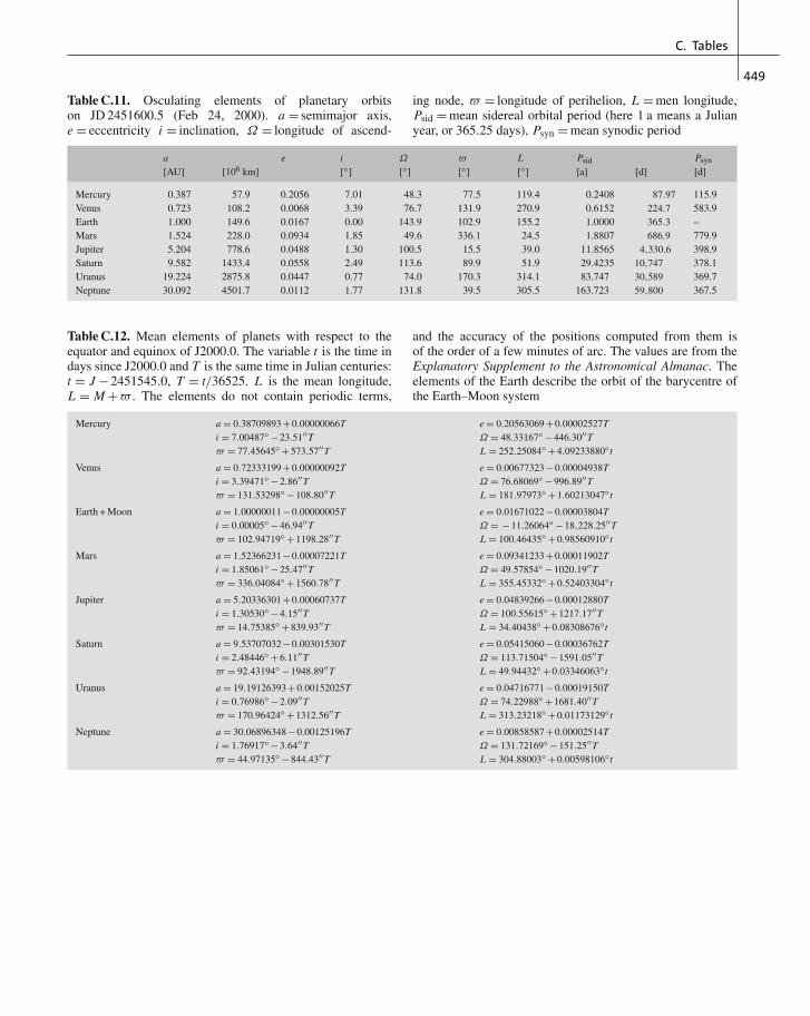
C. Tables
449
Table C.11. Osculating elements of planetary orbitson JD 2451600.5 (Feb 24, 2000). a = semimajor axis,e = eccentricity i = inclination, Ω = longitude of ascend-
ing node, = longitude of perihelion, L = men longitude,Psid = mean sidereal orbital period (here 1 a means a Julianyear, or 365.25 days), Psyn = mean synodic period
a e i Ω L Psid Psyn
[AU] [106 km] [] [] [] [] [a] [d] [d]
Mercury 0.387 57.9 0.2056 7.01 48.3 77.5 119.4 0.2408 87.97 115.9Venus 0.723 108.2 0.0068 3.39 76.7 131.9 270.9 0.6152 224.7 583.9Earth 1.000 149.6 0.0167 0.00 143.9 102.9 155.2 1.0000 365.3 –Mars 1.524 228.0 0.0934 1.85 49.6 336.1 24.5 1.8807 686.9 779.9Jupiter 5.204 778.6 0.0488 1.30 100.5 15.5 39.0 11.8565 4,330.6 398.9Saturn 9.582 1433.4 0.0558 2.49 113.6 89.9 51.9 29.4235 10,747 378.1Uranus 19.224 2875.8 0.0447 0.77 74.0 170.3 314.1 83.747 30,589 369.7Neptune 30.092 4501.7 0.0112 1.77 131.8 39.5 305.5 163.723 59,800 367.5
Table C.12. Mean elements of planets with respect to theequator and equinox of J2000.0. The variable t is the time indays since J2000.0 and T is the same time in Julian centuries:t = J −2451545.0, T = t/36525. L is the mean longitude,L = M + . The elements do not contain periodic terms,
and the accuracy of the positions computed from them isof the order of a few minutes of arc. The values are from theExplanatory Supplement to the Astronomical Almanac. Theelements of the Earth describe the orbit of the barycentre ofthe Earth–Moon system
Mercury a = 0.38709893+0.00000066T e = 0.20563069+0.00002527Ti = 7.00487 −23.51′′T Ω = 48.33167 −446.30′′T = 77.45645 +573.57′′T L = 252.25084 +4.09233880t
Venus a = 0.72333199+0.00000092T e = 0.00677323−0.00004938Ti = 3.39471 −2.86′′T Ω = 76.68069 −996.89′′T = 131.53298 −108.80′′T L = 181.97973 +1.60213047t
Earth + Moon a = 1.00000011−0.00000005T e = 0.01671022−0.00003804Ti = 0.00005 −46.94′′T Ω = −11.26064 −18,228.25′′T = 102.94719 +1198.28′′T L = 100.46435 +0.98560910t
Mars a = 1.52366231−0.00007221T e = 0.09341233+0.00011902Ti = 1.85061 −25.47′′T Ω = 49.57854 −1020.19′′T = 336.04084 +1560.78′′T L = 355.45332 +0.52403304t
Jupiter a = 5.20336301+0.00060737T e = 0.04839266−0.00012880Ti = 1.30530 −4.15′′T Ω = 100.55615 +1217.17′′T = 14.75385 +839.93′′T L = 34.40438 +0.08308676t
Saturn a = 9.53707032−0.00301530T e = 0.05415060−0.00036762Ti = 2.48446 +6.11′′T Ω = 113.71504 −1591.05′′T = 92.43194 −1948.89′′T L = 49.94432 +0.03346063t
Uranus a = 19.19126393+0.00152025T e = 0.04716771−0.00019150Ti = 0.76986 −2.09′′T Ω = 74.22988 +1681.40′′T = 170.96424 +1312.56′′T L = 313.23218 +0.01173129t
Neptune a = 30.06896348−0.00125196T e = 0.00858587+0.00002514Ti = 1.76917 −3.64′′T Ω = 131.72169 −151.25′′T = 44.97135 −844.43′′T L = 304.88003 +0.00598106t
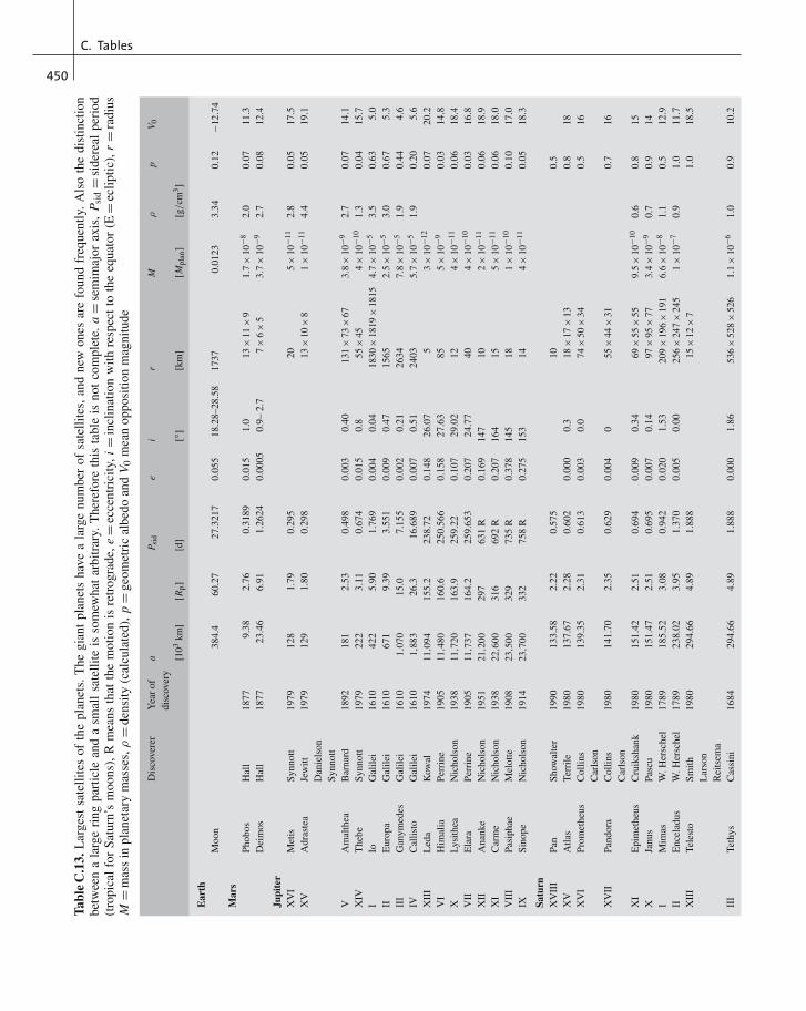
450
C. Tables
Tabl
eC
.13.
Lar
gest
sate
llite
sof
the
plan
ets.
The
gian
tpl
anet
sha
vea
larg
enu
mbe
rof
sate
llite
s,an
dne
won
esar
efo
und
freq
uent
ly.
Als
oth
edi
stin
ctio
nbe
twee
na
larg
eri
ngpa
rtic
lean
da
smal
lsa
telli
teis
som
ewha
tar
bitr
ary.
The
refo
reth
ista
ble
isno
tco
mpl
ete.
a=
sem
imaj
orax
is,
P sid
=si
dere
alpe
riod
(tro
pica
lfo
rSa
turn
’sm
oons
),R
mea
nsth
atth
em
otio
nis
retr
ogra
de,e
=ec
cent
rici
ty,i
=in
clin
atio
nw
ithre
spec
tto
the
equa
tor
(E=
eclip
tic),
r=
radi
usM
=m
ass
inpl
anet
ary
mas
ses,ρ
=de
nsity
(cal
cula
ted)
,p
=ge
omet
ric
albe
doan
dV
0m
ean
oppo
sitio
nm
agni
tude
Dis
cove
rer
Yea
rof
aP s
ide
ir
Mρ
pV
0
disc
over
y[1
03km
][R
p]
[d]
[]
[km
][M
plan
][g/cm
3]
Ear
thM
oon
384.
460
.27
27.3
217
0.05
518
.28–
28.5
817
370.
0123
3.34
0.12
−12.
74
Mar
sPh
obos
Hal
l18
779.
382.
760.
3189
0.01
51.
013
×11×9
1.7×1
0−8
2.0
0.07
11.3
Dei
mos
Hal
l18
7723
.46
6.91
1.26
240.
0005
0.9–
2.7
7×6
×53.
7×1
0−9
2.7
0.08
12.4
Jupi
ter
XV
IM
etis
Synn
ott
1979
128
1.79
0.29
520
5×1
0−11
2.8
0.05
17.5
XV
Adr
aste
aJe
witt
1979
129
1.80
0.29
813
×10×8
1×1
0−11
4.4
0.05
19.1
Dan
iels
onSy
nnot
tV
Am
alth
eaB
arna
rd18
9218
12.
530.
498
0.00
30.
4013
1×7
3×6
73.
8×1
0−9
2.7
0.07
14.1
XIV
The
beSy
nnot
t19
7922
23.
110.
674
0.01
50.
855
×45
4×1
0−10
1.3
0.04
15.7
IIo
Gal
ilei
1610
422
5.90
1.76
90.
004
0.04
1830
×181
9×1
815
4.7×1
0−5
3.5
0.63
5.0
IIE
urop
aG
alile
i16
1067
19.
393.
551
0.00
90.
4715
652.
5×1
0−5
3.0
0.67
5.3
III
Gan
ymed
esG
alile
i16
101,
070
15.0
7.15
50.
002
0.21
2634
7.8×1
0−5
1.9
0.44
4.6
IVC
allis
toG
alile
i16
101,
883
26.3
16.6
890.
007
0.51
2403
5.7×1
0−5
1.9
0.20
5.6
XII
IL
eda
Kow
al19
7411,0
9415
5.2
238.
720.
148
26.0
75
3×1
0−12
0.07
20.2
VI
Him
alia
Perr
ine
1905
11,4
8016
0.6
250.
566
0.15
827
.63
855×1
0−9
0.03
14.8
XLy
sith
eaN
icho
lson
1938
11,7
2016
3.9
259.
220.
107
29.0
212
4×1
0−11
0.06
18.4
VII
Ela
raPe
rrin
e19
0511,7
3716
4.2
259.
653
0.20
724
.77
404×1
0−10
0.03
16.8
XII
Ana
nke
Nic
hols
on19
5121,2
0029
763
1R
0.16
914
710
2×1
0−11
0.06
18.9
XI
Car
me
Nic
hols
on19
3822,6
0031
669
2R
0.20
716
415
5×1
0−11
0.06
18.0
VII
IPa
siph
aeM
elot
te19
0823,5
0032
973
5R
0.37
814
518
1×1
0−10
0.10
17.0
IXSi
nope
Nic
hols
on19
1423,7
0033
275
8R
0.27
515
314
4×1
0−11
0.05
18.3
Satu
rnX
VII
IPa
nSh
owal
ter
1990
133.
582.
220.
575
100.
5X
VA
tlas
Terr
ile19
8013
7.67
2.28
0.60
20.
000
0.3
18×1
7×1
30.
818
XV
IPr
omet
heus
Col
lins
1980
139.
352.
310.
613
0.00
30.
074
×50×3
40.
516
Car
lson
XV
IIPa
ndor
aC
ollin
s19
8014
1.70
2.35
0.62
90.
004
055
×44×3
10.
716
Car
lson
XI
Epi
met
heus
Cru
iksh
ank
1980
151.
422.
510.
694
0.00
90.
3469
×55×5
59.
5×1
0−10
0.6
0.8
15X
Janu
sPa
scu
1980
151.
472.
510.
695
0.00
70.
1497
×95×7
73.
4×1
0−9
0.7
0.9
14I
Mim
asW
.Her
sche
l17
8918
5.52
3.08
0.94
20.
020
1.53
209×1
96×1
916.
6×1
0−8
1.1
0.5
12.9
IIE
ncel
adus
W.H
ersc
hel
1789
238.
023.
951.
370
0.00
50.
0025
6×2
47×2
451×1
0−7
0.9
1.0
11.7
XII
ITe
lest
oSm
ith19
8029
4.66
4.89
1.88
815
×12×7
1.0
18.5
Lar
son
Rei
tsem
aII
ITe
thys
Cas
sini
1684
294.
664.
891.
888
0.00
01.
8653
6×5
28×5
261.
1×1
0−6
1.0
0.9
10.2

C. Tables
451
Dis
cove
rer
Yea
rof
aP s
ide
ir
Mρ
pV
0
disc
over
y[1
03km
][R
p]
[d]
[]
[km
][M
plan
][g/cm
3]
XIV
Cal
ypso
Pasc
u19
8029
4.66
4.89
1.88
815
×8×8
1.0
18.7
Seid
elm
ann
Bau
mC
urri
eIV
Dio
neC
assi
ni16
8437
7.40
6.26
2.73
70.
002
0.02
560
1.9×1
0−6
1.5
0.7
10.4
XII
Hel
ene
Laq
ues
1980
377.
406.
262.
737
0.00
50.
018
×16×1
50.
718
Lec
ache
uxV
Rhe
aC
assi
ni16
7252
7.04
8.74
4.51
70.
001
0.35
764
4.1×1
0−6
1.2
0.7
9.7
VI
Tita
nH
uyge
ns16
651,
221.
8320
.315
.945
0.03
0.33
2575
2.4×1
0−4
1.9
0.22
8.3
VII
Hyp
erio
nB
ond
1848
1,48
1.1
24.6
21.2
770.
100.
4318
0×1
40×1
134×1
0−8
1.4
0.3
14.2
VII
IIa
petu
sC
assi
ni16
713,
561.
359
.179
.330
0.02
814
.72
718
2.8×1
0−6
1.0
0.5/
0.05
11.1
IXPh
oebe
Pick
erin
g18
9812,9
5221
555
0.48
R0.
163
177
E11
07×1
0−10
?0.
0616
.4
Ura
nus
VI
Cor
delia
Voy
ager
219
8649
.77
1.95
0.33
50.
000.
0813
0.07
24.1
VII
Oph
elia
Voy
ager
219
8653
.79
2.10
0.37
60.
010.
1015
0.07
23.8
VII
IB
ianc
aV
oyag
er2
1986
59.1
72.
320.
435
0.00
0.19
210.
0723
.0IX
Cre
ssid
aV
oyag
er2
1986
61.7
82.
420.
464
0.00
0.01
310.
0722
.2X
Des
dem
ona
Voy
ager
219
8662
.68
2.45
0.47
40.
000.
1127
0.07
22.5
XI
Julie
tV
oyag
er2
1986
64.3
52.
520.
493
0.00
0.07
420.
0721
.5X
IIPo
rtia
Voy
ager
219
8666
.09
2.59
0.51
30.
000.
0654
0.07
21.0
XII
IR
osal
ind
Voy
ager
219
8669
.94
2.74
0.55
80.
000.
2827
0.07
22.5
XIV
Bel
inda
Voy
ager
219
8675
.26
2.94
0.62
40.
000.
0333
0.07
22.1
XV
III
S/19
86U
10K
arko
schk
a19
9977
.30
3.0
0.63
720
0.07
XV
Puck
Voy
ager
219
8586
.01
3.37
0.76
20.
000.
3277
0.07
20.2
VM
iran
daK
uipe
r19
4812
9.39
5.06
1.41
30.
003
4.2
240×2
34×2
338×1
0−7
1.3
0.27
16.3
IA
riel
Las
sell
1851
191.
027.
472.
520
0.00
30.
358
1×5
78×5
781.
6×1
0−5
1.7
0.35
14.2
IIU
mbr
iel
Las
sell
1851
266.
3010
.42
4.14
40.
005
0.36
585
1.4×1
0−5
1.4
0.19
14.8
III
Tita
nia
W.H
ersc
hel
1787
435.
9117
.06
8.70
60.
002
0.14
789
4.1×1
0−5
1.7
0.28
13.7
IVO
bero
nW
.Her
sche
l17
8758
3.52
22.8
313
.463
0.00
10.
1076
13.
5×1
0−5
1.6
0.25
13.9
XV
IC
alib
anN
icho
lson
1997
7,16
928
157
9R
0.08
140
E30
0.07
22.4
XV
IISy
cora
xN
icho
lson
1997
12,2
1447
71,
289
R0.
515
3E
600.
0720
.9
Nep
tune
III
Nai
adV
oyag
er2
1989
48.2
31.
950.
294
0.00
04.
7429
0.06
24.7
IVT
hala
ssa
Voy
ager
219
8950
.07
2.02
0.31
10.
000
0.21
400.
0623
.8V
Des
pina
Voy
ager
219
8952
.53
2.12
0.33
50.
000
0.07
740.
0622
.6V
IG
alat
eaV
oyag
er2
1989
61.9
52.
500.
429
0.00
00.
0579
0.06
22.3
VII
Lar
issa
Voy
ager
219
8973
.55
2.97
0.55
50.
001
0.20
104×8
90.
0622
.0V
III
Prot
eus
Voy
ager
219
8911
7.65
4.75
1.12
20.
000
0.55
218×2
08×2
010.
0620
.3I
Tri
ton
Las
sell
1846
354.
7614
.33
5.87
7R0.
000
157.
3513
532.
1×1
0−4
2.1
0.77
13.5
IIN
erei
dK
uipe
r19
495,
513.
422
2.6
360.
136
0.75
127
.617
02×1
0−7
1.0
0.4
18.7
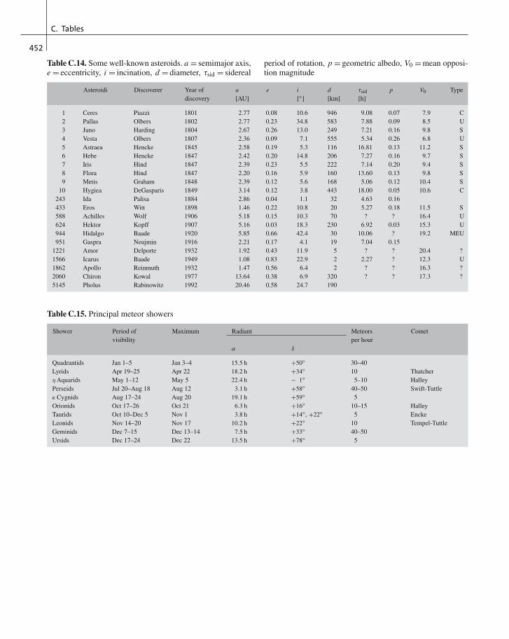
452
C. Tables
Table C.14. Some well-known asteroids. a = semimajor axis,e = eccentricity, i = incination, d = diameter, τsid = sidereal
period of rotation, p = geometric albedo, V0 = mean opposi-tion magnitude
Asteroidi Discoverer Year of a e i d τsid p V0 Typediscovery [AU] [] [km] [h]
1 Ceres Piazzi 1801 2.77 0.08 10.6 946 9.08 0.07 7.9 C2 Pallas Olbers 1802 2.77 0.23 34.8 583 7.88 0.09 8.5 U3 Juno Harding 1804 2.67 0.26 13.0 249 7.21 0.16 9.8 S4 Vesta Olbers 1807 2.36 0.09 7.1 555 5.34 0.26 6.8 U5 Astraea Hencke 1845 2.58 0.19 5.3 116 16.81 0.13 11.2 S6 Hebe Hencke 1847 2.42 0.20 14.8 206 7.27 0.16 9.7 S7 Iris Hind 1847 2.39 0.23 5.5 222 7.14 0.20 9.4 S8 Flora Hind 1847 2.20 0.16 5.9 160 13.60 0.13 9.8 S9 Metis Graham 1848 2.39 0.12 5.6 168 5.06 0.12 10.4 S
10 Hygiea DeGasparis 1849 3.14 0.12 3.8 443 18.00 0.05 10.6 C243 Ida Palisa 1884 2.86 0.04 1.1 32 4.63 0.16433 Eros Witt 1898 1.46 0.22 10.8 20 5.27 0.18 11.5 S588 Achilles Wolf 1906 5.18 0.15 10.3 70 ? ? 16.4 U624 Hektor Kopff 1907 5.16 0.03 18.3 230 6.92 0.03 15.3 U944 Hidalgo Baade 1920 5.85 0.66 42.4 30 10.06 ? 19.2 MEU951 Gaspra Neujmin 1916 2.21 0.17 4.1 19 7.04 0.15
1221 Amor Delporte 1932 1.92 0.43 11.9 5 ? ? 20.4 ?1566 Icarus Baade 1949 1.08 0.83 22.9 2 2.27 ? 12.3 U1862 Apollo Reinmuth 1932 1.47 0.56 6.4 2 ? ? 16.3 ?2060 Chiron Kowal 1977 13.64 0.38 6.9 320 ? ? 17.3 ?5145 Pholus Rabinowitz 1992 20.46 0.58 24.7 190
Table C.15. Principal meteor showers
Shower Period of Maximum Radiant Meteors Cometvisibility per hour
α δ
Quadrantids Jan 1–5 Jan 3–4 15.5 h +50 30–40Lyrids Apr 19–25 Apr 22 18.2 h +34 10 ThatcherηAquarids May 1–12 May 5 22.4 h − 1 5–10 HalleyPerseids Jul 20–Aug 18 Aug 12 3.1 h +58 40–50 Swift-Tuttleκ Cygnids Aug 17–24 Aug 20 19.1 h +59 5Orionids Oct 17–26 Oct 21 6.3 h +16 10–15 HalleyTaurids Oct 10–Dec 5 Nov 1 3.8 h +14, +22 5 EnckeLeonids Nov 14–20 Nov 17 10.2 h +22 10 Tempel-TuttleGeminids Dec 7–15 Dec 13–14 7.5 h +33 40–50Ursids Dec 17–24 Dec 22 13.5 h +78 5

C. Tables
453
Table C.16. Periodic comets with several perihelion pas-sages observed. N = number of passages observed, τ = timeof perihelion passage, P = sidereal period, q = periheliondistance, e = eccentricity, ω = argument of perihelion(1950.0), Ω = longitude of ascending node (1950.0),i = inclination, l = longitude of perihelion, defined here
as l =Ω+ arctan(tanω cos i), b = latitude of perihelion(sin b = sinω sin i), Q = aphelion distance. The elements areaffected by planetary perturbations as well as reaction forcesdue to evaporating material the amount of which is difficult topredict
Comet N τ P q e ω Ω i l b Q[a] [AU] [] [] [] [] [] [AU]
Encke 56 Feb 9, 1994 3.28 0.331 0.850 186.3 334.0 11.9 160.2 − 1.3 4.09Grigg-Skjellerup 16 Jul 24, 1992 5.10 0.995 0.664 359.3 212.6 21.1 212.0 − 0.3 4.93Honda-Mrkos-
Pajdusakova 8 Sep 12, 1990 5.30 0.541 0.822 325.8 88.6 4.2 54.5 − 2.4 5.54Tuttle-Giacobini-
Kresak 8 Feb 8, 1990 5.46 1.068 0.656 61.6 140.9 9.2 202.1 8.1 5.14Tempel 2 19 Mar 16, 1994 5.48 1.484 0.522 194.9 117.6 12.0 312.1 − 3.1 4.73Wirtanen 8 Sep 21, 1991 5.50 1.083 0.652 356.2 81.6 11.7 77.9 − 0.8 5.15Clark 8 Nov 28, 1989 5.51 1.556 0.501 208.9 59.1 9.5 267.7 − 4.6 4.68Forbes 8 Mar 15, 1993 6.14 1.450 0.568 310.6 333.6 7.2 284.5 − 5.4 5.25Pons-Winnecke 20 Aug 19, 1989 6.38 1.261 0.634 172.3 92.8 22.3 265.6 2.9 5.62d’Arrest 15 Feb 4, 1989 6.39 1.292 0.625 177.1 138.8 19.4 316.0 1.0 5.59Schwassmann-
Wachmann 2 11 Jan 24, 1994 6.39 2.070 0.399 358.2 125.6 3.8 123.8 − 0.1 4.82Wolf-Harrington 8 Apr 4, 1991 6.51 1.608 0.539 187.0 254.2 18.5 80.8 − 2.2 5.37Ciacobini-Zinner 12 Apr 14, 1992 6.61 1.034 0.707 172.5 194.7 31.8 8.3 3.9 6.01Reinmuth 2 8 Jun 29, 1994 6.64 1.893 0.464 45.9 295.4 7.0 341.1 5.0 5.17Perrine-Mrkos 8 Mar 1, 1989 6.78 1.298 0.638 166.6 239.4 17.8 46.6 4.1 5.87Arend-Rigaux 7 Oct 3, 1991 6.82 1.438 0.600 329.1 121.4 17.9 91.7 − 9.1 5.75Borrelly 11 Dec 18, 1987 6.86 1.357 0.624 353.3 74.8 30.3 69.0 − 3.4 5.86Brooks 2 14 Sep 1, 1994 6.89 1.843 0.491 198.0 176.2 5.5 14.1 − 1.7 5.40Finlay 11 Jun 5, 1988 6.95 1.094 0.700 322.2 41.7 3.6 4.0 − 2.2 6.19Johnson 7 Nov 19, 1990 6.97 2.313 0.366 208.3 116.7 13.7 324.3 − 6.4 4.98Daniel 8 Aug 31, 1992 7.06 1.650 0.552 11.0 68.4 20.1 78.7 3.8 5.71Holmes 8 Apr 10, 1993 7.09 2.177 0.410 23.2 327.3 19.2 349.4 7.4 5.21Reinmuth 1 8 May 10, 1988 7.29 1.869 0.503 13.0 119.2 8.1 132.0 1.8 5.65Faye 19 Nov 15, 1991 7.34 1.593 0.578 204.0 198.9 9.1 42.6 − 3.7 5.96Ashbrook-
Jackson 7 Jul 13, 1993 7.49 2.316 0.395 348.7 2.0 12.5 350.9 − 2.4 5.34Schaumasse 10 Mar 5, 1993 8.22 1.202 0.705 57.5 80.4 11.8 137.3 10.0 6.94Wolf 14 Aug 28, 1992 8.25 2.428 0.406 162.3 203.4 27.5 7.6 8.1 5.74Whipple 9 Dec 22, 1994 8.53 3.094 0.259 201.9 181.8 9.9 23.4 − 3.7 5.25Comas Sola 8 Aug 18, 1987 8.78 1.830 0.570 45.5 60.4 13.0 105.2 9.2 6.68Vaisala 1 6 Apr 29, 1993 10.8 1.783 0.635 47.4 134.4 11.6 181.2 8.5 7.98Tuttle 11 Jun 27, 1994 13.5 0.998 0.824 206.7 269.8 54.7 106.1 −21.5 10.3Halley 30 Feb 9, 1986 76.0 0.587 0.967 111.8 58.1 162.2 305.3 16.4 35.3

454
C. Tables
Table C.17. Nearest stars. V = apparent visual magnitude, B − V = colour index, r = distance, µ= proper motion, vr = radialvelocity, (positive for receding objects)
Name α2000 δ2000 V B − V Spectrum r µ vr
[h] [min] [] [′] [pc] [′′/a] [km/s]
Sun −26.8 0.6 G2VαCen C (Proxima) 14 29.7 −62 41 11.0 2.0 M5eV 1.30 3.9 − 16αCen A 14 39.6 −60 50 − 0.0 0.7 G2V 1.33 3.7 − 22αCen B 14 39.6 −60 50 1.3 0.9 K1V 1.33 3.7 − 22Barnard’s star 17 57.8 4 42 9.5 1.7 M5V 1.83 10.3 −108Wolf 359 10 56.5 7 01 13.5 2.0 M6eV 2.39 4.7 + 13BD+362147 11 03.3 35 58 7.5 1.5 M2V 2.54 4.8 − 86αCMa (Sirius) A 6 45.1 −16 43 − 1.5 0.0 A1V 2.66 1.3 − 8αCMa (Sirius) B 6 45.1 −16 43 8.4 wdA 2.66 1.3 − 8Luyten 726–8 A 1 39.0 −17 57 12.5 M6eV 2.66 3.3 + 29Luyten 726–8 B 1 39.0 −17 57 13.0 M6eV 2.66 3.3 + 32
(UV Cet)Ross 154 18 49.8 −23 50 10.4 M4eV 2.92 0.7 − 4Ross 248 23 41.9 44 11 12.2 1.9 M5eV 3.13 1.6 − 81εEri 3 32.9 − 9 27 3.7 0.9 K2V 3.26 1.0 + 16Ross 128 11 47.7 0 48 11.1 1.8 M5V 3.31 1.4 − 13Luyten 789–6 A 22 38.6 −15 17 12.8 2.0 M5eV 3.40 3.3 − 60Luyten 789–6 B 22 38.6 −15 17 13.3 3.40 3.3 − 60BD+4344 A 0 18.4 44 01 8.1 1.6 M3V 3.44 2.9 + 13BD+4344 B 0 18.4 44 01 11.0 1.8 M6V 3.44 2.9 + 20ε Ind 22 03.4 −56 47 4.7 1.1 K5V 3.45 4.7 − 40BD+591915 A 18 42.8 59 38 8.9 1.5 M4V 3.45 2.3 0BD+591915 B 18 42.8 59 38 9.7 1.6 M4V 3.45 2.3 + 1061 Cyg A 21 06.9 38 45 5.2 1.2 K5V 3.46 5.2 − 6461 Cyg B 21 06.9 38 45 6.0 1.4 K7V 3.46 5.2 − 64τ Cet 1 43.1 −15 56 3.5 0.7 G8V 3.48 1.9 − 16CD−3615693 23 05.9 −35 51 7.4 1.5 M2V 3.51 6.9 + 10αCMi (Procyon) A 7 39.3 5 14 0.4 0.4 F5IV 3.51 1.3 − 3αCMi (Procyon) B 7 39.3 5 14 10.7 wdF 3.51 1.3G 51–15 8 29.8 26 47 14.8 M7V 3.62 1.3BD+51668 7 27.4 5 13 9.8 1.6 M4V 3.76 3.8 + 26Luyten 725–32 1 12.6 −17 00 11.8 M6eV 3.77 1.4Kapteyn’s star 5 11.7 −45 01 8.8 1.6 M1VI 3.85 8.8 +245CD−3914192 21 17.2 −38 52 6.7 1.4 M0eV 3.85 3.5 + 21Krüger 60 A 22 28.0 57 42 9.9 1.6 M3V 3.95 0.9 − 26Krüger 60 B 22 28.0 57 42 11.5 1.8 M4eV 3.95 0.9 − 26Ross 614 A 6 29.4 − 2 49 11.2 1.7 M4eV 4.13 1.0 + 24Ross 614 B 6 29.4 − 2 49 14.8 4.13 1.0 + 24BD−124523 16 30.3 −12 40 10.2 1.6 M5V 4.15 1.2 − 13Wolf 424 A 12 33.3 9 01 13.2 1.8 M6V 4.29 1.8 − 5Wolf 424 B 12 33.3 9 01 13.2 4.29 1.8 − 5van Maanen’s star 0 49.2 5 23 12.4 0.6 wdG 4.33 3.0 + 54Luyten 1159–16 2 00.2 13 03 12.2 M5eV 4.48 2.1CD−3715492 0 05.4 −37 21 8.6 1.5 M3V 4.48 6.1 + 23Luyten 143–23 10 44.5 −61 12 13.9 dM 4.48 1.7CD−4611540 17 28.7 −46 54 9.4 1.5 M3 4.52 1.1LP 731–58 10 48.2 −11 20 15.6 M7V 4.55 1.6Luyten 145–141 11 45.7 −64 50 11.4 0.2 wdA 4.57 2.7BD+68946 17 36.4 68 20 9.1 1.5 M3V 4.63 1.3 − 22CD−4913515 21 33.6 −49 01 8.7 1.5 M2V 4.63 0.8 + 8BD+501725 10 11.3 49 27 6.6 1.4 K2V 4.67 1.5 − 26G 158–27 0 06.7 −07 32 13.7 M5V 4.67 2.1BD−156290 22 53.3 −14 18 10.2 1.6 M4V 4.69 1.1 + 9CD−4411909 17 37.1 −44 19 11.0 M5V 4.72 1.1
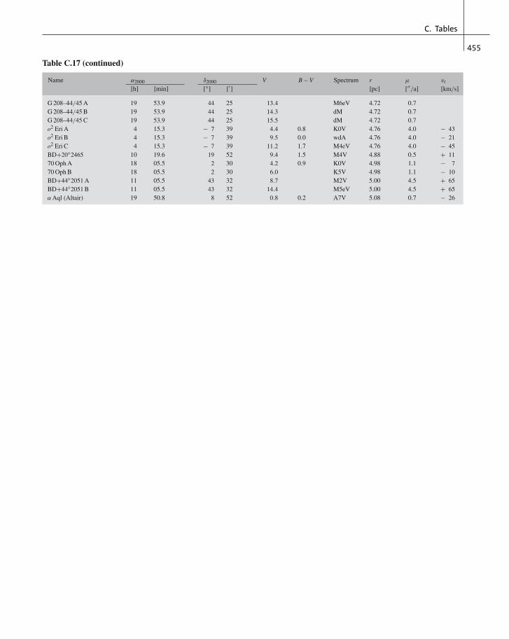
C. Tables
455
Table C.17 (continued)
Name α2000 δ2000 V B − V Spectrum r µ vr
[h] [min] [] [′] [pc] [′′/a] [km/s]
G 208–44/45 A 19 53.9 44 25 13.4 M6eV 4.72 0.7G 208–44/45 B 19 53.9 44 25 14.3 dM 4.72 0.7G 208–44/45 C 19 53.9 44 25 15.5 dM 4.72 0.7o2 Eri A 4 15.3 − 7 39 4.4 0.8 K0V 4.76 4.0 − 43o2 Eri B 4 15.3 − 7 39 9.5 0.0 wdA 4.76 4.0 − 21o2 Eri C 4 15.3 − 7 39 11.2 1.7 M4eV 4.76 4.0 − 45BD+202465 10 19.6 19 52 9.4 1.5 M4V 4.88 0.5 + 1170 Oph A 18 05.5 2 30 4.2 0.9 K0V 4.98 1.1 − 770 Oph B 18 05.5 2 30 6.0 K5V 4.98 1.1 − 10BD+442051 A 11 05.5 43 32 8.7 M2V 5.00 4.5 + 65BD+442051 B 11 05.5 43 32 14.4 M5eV 5.00 4.5 + 65αAql (Altair) 19 50.8 8 52 0.8 0.2 A7V 5.08 0.7 − 26

456
C. Tables
Table C.18. Brightest stars (V ≤ 2). V = apparent visual magnitude, B − V = colour index, r = distance. Remarks: b=binary,sb=spectroscopic binary, v=variable
Name α2000 δ2000 V B − V Spectrum r Remarks[h] [min] [] [′] [pc]
αCMa Sirius 6 45.2 −16 43 −1.5 0.0 A1V,wdA 2.7 bαCar Canopus 6 24.0 −52 42 −0.7 0.2 A9II 60αCen Rigil 14 39.6 −60 50 −0.3 0.7 G2V,K1V 1.3 b, Proxima
Kentaurus 2.2 apartαBoo Arcturus 14 15.7 19 11 −0.0 1.2 K2IIIp 11αLyr Vega 18 36.9 38 47 0.0 0.0 A0V 8αAur Capella 5 16.7 46 00 0.1 0.8 G2III,G6III 14 bβOri Rigel 5 14.5 − 8 12 0.1 −0.0 B8Ia 90 bαCMi Procyon 7 39.3 5 14 0.4 0.4 F5IV,wdF 3.5 bαEri Achernar 1 37.7 −57 14 0.5 −0.2 B3Vp 40αOri Betelgeuze 5 55.2 7 24 0.5 1.9 M2I 200 v 0.4−1.3, sbβ Cen Hadar 14 03.8 −60 22 0.6 −0.2 B1III 60 bαAql Altair 19 50.8 8 52 0.8 0.2 A7V 5.1αCru Acrux 12 26.6 −63 06 0.8 −0.3 B0.5IV,B1V 120 b 1.6+2.1αTau Aldebaran 4 35.9 16 31 0.9 1.5 K5III 20 b, vαVir Spica 13 25.2 −11 10 1.0 −0.2 B1IV 50 sb, several comp.α Sco Antares 16 29.4 −26 26 1.0 1.8 M1.5I,B2.5V 50 v 0.9−1.8βGem Pollux 7 45.3 28 02 1.2 1.1 K0III 11α PsA Fomalhaut 22 57.6 −29 37 1.2 0.1 A3V 7.0αCyg Deneb 20 41.4 45 17 1.3 0.1 A2Ia 500β Cru Mimosa 12 47.7 −59 41 1.3 −0.2 B0.5III 150 v, sbαLeo Regulus 10 08.4 11 58 1.4 −0.1 B7V 26 bεCMa Adhara 6 58.6 −28 58 1.5 −0.2 B2II 170 bαGem Castor 7 34.6 31 53 1.6 0.0 A1V,A2V 14 bγ Cru Gacrux 12 31.2 −57 07 1.6 1.6 M3.5III 40 vλSco Shaula 17 33.6 −37 06 1.6 −0.2 B1.5IV vγ Ori Bellatrix 5 25.1 6 21 1.6 −0.2 B2III 40β Tau Elnath 5 26.3 28 36 1.7 −0.1 B7III 55β Car Miaplacidus 9 13.2 −69 43 1.7 0.0 A1III 30εOri Alnilam 5 36.2 − 1 12 1.7 −0.2 B0IaαGru Al Na’ir 22 08.2 −46 58 1.7 −0.1 B7IV 20εUMa Alioth 12 54.0 55 58 1.8 −0.0 A0IVp 120 vγ Vel Regor 8 09.5 −47 20 1.8 −0.2 WC8,B1IV b 1.8+4.3, each sbα Per Mirfak 3 24.3 49 52 1.8 0.5 F5Ib 35αUMa Dubhe 11 03.7 61 45 1.8 1.1 K0III 30 bε Sgr Kaus Australis 18 24.2 −34 23 1.9 −0.0 A0II 70δCMa Wezen 7 08.4 −26 23 1.9 0.7 F8IaεCar Avior 8 22.5 −59 31 1.9 1.3 K3III,B2V 25 sbηUMa Alkaid 13 47.5 49 19 1.9 −0.2 B3Vθ Sco Girtab 17 37.3 −43 00 1.9 0.4 F0II 50βAur Menkalinan 5 59.6 44 57 1.9 0.0 A1IV 30ζ Ori Alnitak 5 40.8 − 1 57 1.9 −0.2 O9.5Ib, B0III 45 b 2.1+4.2αTrA Atria 16 48.7 −69 02 1.9 1.4 K2II–III 40γ Gem Alhena 6 37.7 16 24 1.9 0.0 A1IV 30α Pav Peacock 20 25.7 −56 44 1.9 −0.2 B3VδVel 8 44.7 −54 43 2.0 0.0 A1V 20β CMa Mirzam 6 22.7 −17 57 2.0 −0.2 B1II–III 70 vαHya Alphard 9 27.6 − 8 40 2.0 1.4 K3II–III 60αAri Hamal 2 07.2 23 28 2.0 1.2 K2III 25

C. Tables
457
Table C.19. Some double stars. Magnitudes of the components are m1 and m2, and the angular separation d; r is the distanceof the star
Name α2000 δ2000 m1 m2 Spectrum d r[h] [min] [] [′] [′′] [pc]
ηCas Achird 0 49.1 57 49 3.7 7.5 G0V M0 12 6γ Ari Mesarthim 1 53.5 19 18 4.8 4.9 A1p B9V 8 40α Psc Alrescha 2 02.0 2 46 4.3 5.3 A0p A3m 2 60γ And Alamak 2 03.9 42 20 2.4 5.1 K3IIb B8V,A0V 10 100δOri Mintaka 5 32.0 − 0 18 2.5 7.0 B0III,O9V B2V 52 70λOri Meissa 5 35.1 9 56 3.7 5.7 O8e B0.5V 4 140ζ Ori Alnitak 5 40.8 − 1 56 2.1 4.2 O9.51be B0III 2 40αGem Castor 7 34.6 31 53 2.0 3.0 A1V A5Vm 3 15γ Leo Algieba 10 20.0 19 50 2.6 3.8 K1III G7III 4 80ξ UMa Alula Australis 11 18.2 31 32 4.4 4.9 G0V G0V 1 7αCru Acrux 12 26.6 −63 06 1.6 2.1 B0.5IV B1V 4 120γ Vir Porrima 12 41.7 − 1 27 3.7 3.7 F0V F0V 3 10αCVn Cor Caroli 12 56.1 38 18 2.9 5.5 A0p F0V 20 40ζ UMa Mizar 13 23.9 54 56 2.4 4.1 A1Vp A1m 14 21αCen Rigil Kentaurus 14 39.6 −60 50 0.0 1.3 G2V K1V 21 1.3εBoo Izar 14 45.0 27 04 2.7 5.3 K0II-III A2V 3 60δ Ser 15 34.8 10 32 4.2 5.3 F0IV F0IV 4 50β Sco Graffias 16 05.4 −19 48 2.6 4.9 B1V B2V 14 110αHer Rasalgethi 17 14.6 14 23 3.0–4.0 5.7 M5Ib-II G5III,F2V 5 120ρHer 17 23.7 37 08 4.5 5.5 B9.5III A0V 470 Oph 18 05.5 2 30 4.3 6.1 K0V K5V 2 5ε Lyr 18 44.3 39 40 4.8 4.4 A4V,F1V A8V,F0V 208 50ε1 Lyr 18 44.3 39 40 5.1 6.2 A4V F1V 3 50ε2 Lyr 18 44.4 39 37 5.1 5.3 A8V F0V 2 50ζ Lyr 18 44.8 37 36 4.3 5.7 Am F0IV 44 30θ Ser Alya 18 56.2 4 12 4.5 4.9 A5V A5V 22 30γ Del 20 46.7 16 07 4.5 5.4 K1IV F7V 10 40ζ Aqr 22 28.8 − 0 01 4.4 4.6 F3V F6IV 2 30δCep 22 29.1 58 24 3.5–4.3 7.5 F5Ib–G2Ib B7IV 41 90
Table C.20. Milky Way Galaxy
Property Value
Mass > 2×10¹¹ MDisc diameter 30 kpc
Disc thickness (stars) 1 kpc
Disc thickness (gas and dust) 200 pc
Halo diameter 50 kpc
Sun’s distance from the centre 8.5 kpc
Sun’s orbital velocity 220 km s−1
Sun’s period 240×106 a
Direction of the centre (2000.0) α= 17 h 45.7 minδ= −2900′
Direction of the north pole (2000.0) α= 12 h 51.4 minδ= +2708′
Galactic coordinates of the l = 12300′
celestial north pole b = +2708′

458
C. Tables
Table C.21. Members of the Local Group of Galaxies. V = apparent visual magnitude, MV = absolute visual magnitude,r = distance
α2000 δ2000 Type V MV r[h] [min] [] [′] [kpc]
Milky Way 17 45.7 −29 00 Sbc −20.9 8NGC 224 = M31 00 42.7 41 16 Sb 3.2 −21.2 760NGC 598 = M33 01 33.8 30 30 Sc 5.6 −18.9 790Large Magellanic Cloud 05 19.6 −69 27 Irr 0.0 −18.5 50Small Magellanic Cloud 00 52.6 −72 48 Irr 1.8 −17.1 60NGC 221 = M32 00 42.7 40 52 E2 7.9 −16.5 760NGC 205 00 40.4 41 41 dE5 8.0 −16.4 760IC 10 00 20.4 59 17 Irr 7.8 −16.3 660NGC 6822 19 44.9 −14 48 Irr 7.5 −16.0 500NGC 185 00 39.0 48 20 dE3 8.5 −15.6 660IC 1613 01 04.8 02 08 Irr 9.0 −15.3 720NGC 147 00 33.2 48 30 dE4 9.0 −15.1 660WLM 00 02.0 −15 28 Irr 10.4 −14.4 930Sagittarius 18 55.1 −30 29 dE7 3.1 −13.8 24Fornax 02 39.9 −34 30 dE3 7.6 −13.1 140Pegasus 23 28.6 14 45 Irr 12.1 −12.3 760Leo I 10 08.4 12 18 dE3 10.1 −11.9 250And II 01 16.5 33 26 dE3 12.4 −11.8 700And I 00 45.7 38 00 dE0 12.7 −11.8 810Leo A 09 59.4 30 45 Irr 12.7 −11.5 690Aquarius 20 46.9 −12 51 Irr 13.7 −11.3 1020SagDIG 19 30.0 −17 41 Irr 15.0 −10.7 1400Pegasus II = And VI 23 51.7 24 36 dE 14.0 −10.6 830Pisces = LGS 3 01 03.9 21 54 Irr 14.1 −10.4 810And III 00 35.3 36 30 dE6 14.2 −10.2 760And V 01 10.3 47 38 dE 14.3 −10.2 810Leo II 11 13.5 22 10 dE0 11.5 −10.1 210Cetus 00 26.1 −11 02 dE 14.3 −10.1 780Sculptor 01 00.1 −33 43 dE3 10.0 − 9.8 90Phoenix 01 51.1 −44 27 Irr 13.2 − 9.8 400Tucana 22 41.8 −64 25 dE5 15.1 − 9.6 870Sextans 10 13.0 −01 37 dE4 10.3 − 9.5 90Cassiopeia = And VII 23 26.5 50 42 dE 14.7 − 9.5 690Carina 06 41.6 −50 58 dE4 10.6 − 9.4 100Ursa Minor 15 08.8 67 07 dE5 10.0 − 8.9 60Draco 17 20.3 57 55 dE3 10.9 − 8.6 80Ursa Major 158 43.2 51 55 dE 13.2 −6.8 100Canes Venatici 13 28.0 33 33 dE 13.9 −7.9 220Bootes 14 00.0 14 30 dE 13.3 −5.7 60Ursa Major II 08 51.5 63 08 dE 14.3 −3.8 30Coma Berenices 12 27.0 23 54 dE 14.5 −3.7 44Canes Venatici II 12 57.2 34 19 dE 15.1 −4.8 150Hercules 16 31.0 12 47.5 dE 14.7 −6.0 140Leo IV 11 33.0 −0 32 dE 15.9 −5.1 160And IX 00 52.9 43 12 dE 16.2 −8.3 760And X 01 06.5 44 48 dE 16.1 −8.1 710And XI 00 46.3 33 48 dE 17.2 −7.3 760And XII 00 47.5 34 22 dE 18.1 −6.4 760And XIII 00 51.8 33 00 dE 17.6 −6.9 760

C. Tables
459
Table C.22. Optically brightest galaxies. B = apparent blue magnitude, d = apparent diameter, r = distance
Name α2000 δ2000 Type B d r[h] [min] [] [′] [′′] [Mpc]
NGC 55 0 15.1 −39 13 Sc/Irr 7.9 30×5 2.3NGC 205 0 40.4 41 41 E6 8.9 12×6 0.7NGC 221 = M32 0 42.7 40 52 E2 9.1 3.4×2.9 0.7NGC 224 = M31 0 42.8 41 16 Sb 4.3 163×42 0.7NGC 247 0 47.2 −20 46 S 9.5 21×8 2.3NGC 253 0 47.6 −25 17 Sc 7.0 22×5 2.3Small Magellanic Cloud 0 52.6 −72 48 Irr 2.9 216×216 0.06NGC 300 0 54.9 −37 41 Sc 8.7 22×16 2.3NGC 598 = M33 1 33.9 30 39 Sc 6.2 61×42 0.7Fornax 2 39.9 −34 32 dE 9.1 50×35 0.2Large Magellanic Cloud 5 23.6 −69 45 Irr/Sc 0.9 432×432 0.05NGC 2403 7 36.9 65 36 Sc 8.8 22×12 2.0NGC 2903 9 32.1 21 30 Sb 9.5 16×7 5.8NGC 3031 = M81 9 55.6 69 04 Sb 7.8 25×12 2.0NGC 3034 = M82 9 55.9 69 41 Sc 9.2 10×1.5 2.0NGC 4258 = M106 12 19.0 47 18 Sb 8.9 19×7 4.3NGC 4472 = M49 12 29.8 8 00 E4 9.3 10×7 11NGC 4594 = M104 12 40.0 −11 37 Sb 9.2 8×5 11NGC 4736 = M94 12 50.9 41 07 Sb 8.9 13×12 4.3NGC 4826 = M64 12 56.8 21 41 9.3 10×4 3.7NGC 4945 13 05.4 −49 28 Sb 8.0 20×4 3.9NGC 5055 = M63 13 15.8 42 02 Sb 9.3 8×3 4.3NGC 5128 = Cen A 13 25.5 −43 01 E0 7.9 23×20 3.9NGC 5194 = M51 13 29.9 47 12 Sc 8.9 11×6 4.3NGC 5236 = M83 13 37.0 −29 52 Sc 7.0 13×12 2.4NGC 5457 = M101 14 03.2 54 21 Sc 8.2 23×21 4.3NGC 6822 19 45.0 −14 48 Irr 9.2 20×10 0.7

460
C. Tables
Table C.23. Constellations. The first column gives the abbreviation of the Latin name used to form star names
Abbreviation Latin name Genitive English name
And Andromeda Andromedae AndromedaAnt Antlia Antliae Air PumpAps Apus Apodis Bird of ParadiseAql Aquila Aquilae EagleAqr Aquarius Aquarii Water-bearerAra Ara Arae AltarAri Aries Arietis RamAur Auriga Aurigae CharioteerBoo Boötes Boötis HerdsmanCae Caelum Caeli ChiselCam Camelopardalis Camelopardalis GiraffeCnc Cancer Cancri CrabCMa Canis Major Canis Majoris Great DogCMi Canis Minor Canis Minoris Little DogCap Capricornus Capricorni Sea-goatCar Carina Carinae KeelCas Cassiopeia Cassiopeiae CassiopeiaCen Centaurus Centauri CentaurusCep Cepheus Cephei CepheusCet Cetus Ceti WhaleCha Chamaeleon Chamaeleontis ChameleonCir Circinus Circini CompassesCol Columba Columbae DoveCom Coma Berenices Comae Berenices Berenice’s HairCrA Corona Austrina Coronae Austrinae Southern CrownCrB Corona Borealis Coronae Borealis Northern CrownCrv Corvus Corvi CrowCrt Crater Crateris CupCru Crux Crucis Southern CrossCVn Canes Venatici Canum Venaticorum Hunting DogsCyg Cygnus Cygni SwanDel Delphinus Delphini DolphinDor Dorado Doradus SwordfishDra Draco Draconis DragonEqu Equuleus Equulei Little HorseEri Eridanus Eridani EridanusFor Fornax Fornacis FurnaceGem Gemini Geminorum TwinsGru Grus Gruis CraneHer Hercules Herculis HerculesHor Horologium Horologii ClockHya Hydra Hydrae Water SerpentHyi Hydrus Hydri Water SnakeInd Indus Indi IndianLac Lacerta Lacertae LizardLeo Leo Leonis LionLep Lepus Leporis HareLib Libra Librae ScalesLMi Leo Minor Leonis Minoris Little LionLup Lupus Lupi WolfLyn Lynx Lyncis LynxLyr Lyra Lyrae LyreMen Mensa Mensae Table MountainMic Microscopium Microscopii MicroscpeMon Monoceros Monocerotis UnicornMus Musca Muscae Fly

C. Tables
461
Table C.23 (continued)
Abbreviation Latin name Genitive English name
Nor Norma Normae SquarePer Perseus Persei PerseusPhe Phoenix Phoenicis PhoenixPic Pictor Pictoris PainterPsA Piscis Austrinus Piscis Austrini Southern FishPsc Pisces Piscium FishesPup Puppis Puppis PoopPyx Pyxis Pyxidis CompassRet Reticulum Reticuli NetScl Sculptor Sculptoris SculptorSco Scorpius Scorpii ScorpionSct Scutum Scuti Sobieski’s ShieldSer Serpens Serpentis SerpentSex Sextans Sextantis SextantSge Sagitta Sagittae ArrowSgr Sagittarius Sagittarii ArcherTau Taurus Tauri BullTel Telescopium Telescopii TelescopeTrA Triangulum Australe Trianguli Australis Southern TriangleTri Triangulum Trianguli TriangleTuc Tucana Tucanae ToucanUMa Ursa Major Ursae Majoris Great BearUMi Ursa Minor Ursae Minoris Little BearVel Vela Velorum SailsVir Virgo Virginis VirginVol Volans Volantis Flying FishVul Vulpecula Vulpeculae FoxOct Octans Octantis OctantOph Ophiuchus Ophiuchi Serpent-bearerOri Orion Orionis OrionPav Pavo Pavonis PeacockPeg Pegasus Pegasi Pegasus
Table C.24. Largest optical telescopes. D = diameter of the mirror
Telescope Location Completion Dyear [m]
William M. Keck Telescope I Mauna Kea, Hawaii 1992 10William M. Keck Telescope II Mauna Kea, Hawaii 1996 10Southern African Large Telescope Sutherland, South Africa 2005 10Subaru Telescope Mauna Kea, Hawaii 1999 8.3Large Binocular Telescope 1 Mt. Graham, Arizona 2005 8.4Kueyen Telescope (VLT 2) Cerro Paranal, Chile 1999 8.2Melipal Telescope (VLT 3) Cerro Paranal, Chile 2000 8.2Yepun Telescope (VLT 4) Cerro Paranal, Chile 2000 8.2Gemini North Telescope Mauna Kea, Hawaii 1999 8.1Gemini South Telescope Cerro Pachon, Chile 2000 8.1Multi-Mirror Telescope Mt. Hopkins, Arizona 1999 6.5Walter Baade (Magellan 1 Telescope) Las Campanas, Chile 2000 6.5Landon Clay (Magellan 2 Telescope) Las Campanas, Chile 2002 6.5

462
C. Tables
Table C.25. Largest parabolic radio telescopes. D = diameter of the antenna, λmin = shortest wavelength
Completion D λmin Remarksyear [m] [cm]
Arecibo Puerto Rico, USA 1963 305 5 Fixed disk; limited trackingGreen Bank West Virginia, USA 2001 100×110 0.3 The largest fully
steerable telescopeEffelsberg Bonn, Germany 1973 100 0.8Jodrell Bank Macclesfield, Great Britain 1957 76.2 10–20 First large paraboloid antennaJevpatoria Crimea 1979 70 1.5Parkes Australia 1961 64 2.5 Innermost 17 m of dish can
be used down to 3 mmwavelengths
Goldstone California, USA 64 1.5 Belongs to NASA deep space networkTidbinbilla Australia 64 1.3 NASAMadrid Spain 64 1.3 NASA

C. Tables
463
Table C.26. Millimetre and submillimetre telescopes and interferometers. h = altitude above sea level, D = diameter of theantenna, λmin = shortest wavelength
Institute Location h D λmin Remarks;[m] [m] [mm] operational since
NRAO, VLA New Mexico, USA 2124 25 7 27 antennasdmax = 36.6 km1976
NRAO, VLBA USA 16–3720 25 13 10 antennas1988–1993
Max-Planck-lnstitut für Mt. Graham, USA 3250 10 0.3 1994Radioastronomie&University of Arizona
California Institute of Mauna Kea, Hawaii 4100 10.4 0.3 1986Technology
Science Research Council Mauna Kea, Hawaii 4100 15.0 0.5 The JamesEngland & Holland Clerk Maxwell
Telescope1986
California Institute of Owens Valley, USA 1220 10.4 0.5 3 antennaTechnology interferometer
1980Sweden-ESO Southern La Silla, Chile 2400 15.0 0.6 1987
Hemisphere MillimeterAntenna (SEST)
Institut de Radioastronomie Plateau de Bure, 2550 15.0 0.6 3 antennaMillimetrique (IRAM), France interferometerFrance & Germany 1990;
fourth antenna1993
IRAM Pico Veleta, Spain 2850 30.0 0.9 1984National Radio Astronomy Kitt Peak, USA 1940 12.0 0.9 1983 (1969)
Observatory (NRAO)University of Massachusetts New Salem, USA 300 13.7 1.9 radom
1978University of California, Hat Creek Observatory 1040 6.1 2 3 antenna
Berkeley interferometer1968
Purple Mountain Nanjing, China 3000 13.7 2 radomObservatory 1987
Daeduk Radio Astronomy Soul, South-Korea 300 13.7 2 radomObservatory 1987
University of Tokyo Nobeyama, Japan 1350 45.0 2.6 1982University of Tokyo Nobeyama, Japan 1350 10.0 2.6 5 antenna
interferometer1984
Chalmers University of Onsala, Sweden 10 20.0 2.6 radomTechnology 1976

464
C. Tables
Table C.27. Some important astronomical satellites and space probes 1980–2002
Satellite Launch date Target
Solar Max USA Feb 14, 1980 SunVenera 13 SU Oct 30, 1981 VenusVenera 14 SU Nov 4, 1981 VenusIRAS USA Jan 25, 1983 infraredAstron SU Mar 23, 1983 ultravioletVenera 15 SU Jun 2, 1983 VenusVenera 16 SU Jun 7, 1983 VenusExosat ESA/USA May 26, 1983 X-rayVega 1 SU Dec 15 1984 Venus/HalleyVega 2 SU Dec 21, 1984 Venus/HalleyGiotto ESA Jul 2, 1985 HalleySuisei Japan Aug 18, 1985 HalleyGinga Japan Feb 5, 1987 X-rayMagellan USA May 4, 1989 VenusHipparcos ESA Aug 8, 1989 astrometryCOBE USA Nov 18, 1989 cosmic background radiationGalileo USA Oct 18, 1989 Jupiter etc.Granat SU Dec 1, 1989 gamma rayHubble USA/ESA Apr 24, 1990 UV, visibleRosat Germany Jun 1, 1990 X-rayGamma SU Jul 11, 1990 gamma rayUlysses ESA Oct 6, 1990 SunCompton USA Apr 5, 1991 gamma rayEUVE USA Jun 7, 1992 extreme UVAsuka Japan Feb 20, 1993 X-rayClementine USA Jan 25, 1994 MoonISO ESA Nov 17, 1995 infrredSOHO ESA Dec 2, 1995 SunNear-Shoemaker USA Feb 17, 1996 Mathilde, ErosBeppoSAX Italy Apr 30, 1996 X-rayMars Global Surveyor USA Nov 7, 1996 MarsCassini/Huygens USA/ESA Oct 15, 1997 Saturn, TitanMars Pathfinder/Sojourner USA Dec 4, 1996 MarsLunar Prospector USA Jan 6, 1998 MoonNozomi Japan Jul 4, 1998 MarsDeep Space 1 USA Oct 24, 1998 Braille, BorrellyStardust USA Feb 7, 1999 Wild 2Chandra USA Jul 23, 1999 X-rayXMM-Newton ESA Dec 10, 1999 X-rayHete 2 USA Oct 9, 2000 gamma rayMars Odyssey USA Apr 7, 2001 MarsMAP USA Jun 30, 2001 cosmic background radiationGenesis USA Aug 8, 2001 solar particlesRHESSI USA Feb 5, 2002 SunGrace Gemany-USA Mar 17, 2002 Earth’s gravityIntegral ESA Oct 17, 2002 gamma rayGalex USA Apr 28, 2003 galaxiesHayabusa Japan May 9, 2003 ItokawaMars Express ESA Jun 2, 2003 MarsSpirit USA Jun 10, 2003 MarsOpportunity USA Jul 8, 2003 MarsSpitzer USA Jun 10, 2003 infrared

C. Tables
465
Table C.27 (continued)
Satellite Launch date Target
Smart-1 ESA Sep 28, 2003 MoonRosetta ESA Mar 2, 2004 Churyumov-GerasimenkoGravity Probe B USA Apr 20, 2004 relativityMessenger USA Aug 3, 2004 MercurySwift USA Nov 20, 2004 gamma ray burstsDeep Impact USA Jan 12, 2005 Tempel 1Mars Recon Orbiter USA Aug 12, 2005 MarsVenus Express ESA Nov 9, 2005 VenusNew Horizons USA Jan 19, 2006 PlutoAkari Japan Feb 22, 2006 infrared

467
Answers to Exercises
Chapter 2
2.1 The distance is ≈ 7640 km, the northernmostpoint is 79N, 45W, in North Greenland, 1250 km fromthe North Pole.
2.2 The star can culminate south or north of zenith.In the former case we get δ= 65, φ = 70, and in thelatter δ= 70, φ = 65.
2.3 a) φ > 587′. If refraction is taken intoaccount, the limit is 5724′. b) φ = δ = 724′.c) −5910′ ≤ φ ≤ −050′.
2.4 Pretty bad.
2.5 λ = 7022′, β = 00′, λ⊕ = 25022′, β⊕ =00′.
2.6 c) Θ0 = 18 h.
2.8 α= 6 h 45 min 9 s, δ= −1643′.
2.9 vt = 16.7 km s−1, v = 18.5 km s−1, after ≈61,000 years. µ= 1.62′′ per year, parallax 0.42′′.
Chapter 3
3.1 a) The flux density in the focal plane as wellas the exposure time are proportional to (D/ f )2. Thusthe required exposure is 3.2 s. b) 1.35 cm and 1.80 cm.c) 60 and 80.
3.2 a) 0.001′′ (note that the aperture is a line ratherthan circular; therefore the coefficient 1.22 should notbe used). b) 140 m.
Chapter 4
4.1 0.9.
4.2 The absolute magnitude will be −17.5 and ap-parent 6.7.
4.3 N(m +1)/N(m)= 103/5 = 3.98.
4.4 r = 2.1 kpc, EB−V = 0.7, and (B − V )0 = 0.9.
4.5 a) ∆m = 1.06 mag, m = 2.42. b) τ =− ln 0.856 ≈ 0.98.
Chapter 5
5.2 n = 166, which corresponds to λ= 21.04 cm.Such transitions would keep the population of the staten = 166 very high, resulting in downward transitionsalso from this state. Such transitions have not beendetected. Hence, the line is produced by some otherprocess.
5.3 If we express the intensity as something per unitwavelength, we get λmax = 1.1 mm. If the intensity isgiven per unit frequency, we have λmax = 1.9 mm. Thetotal intensity is 2.6×10¹³ W m−2 sterad−1. At 550 nmthe intensity is practically zero.
5.4 a) L = 1.35×1029 W. The flux in the giveninterval can be found by integrating Planck’s lawnumerically. Using the Wien approximation a rathercomplicated expression can be derived. Both methodsgive the result that 3.3% of the radiation is in the vi-sual range, thus LV = 4.45×1027 W. b) At a distanceof 10 pc the observed flux density is 3.7×10⁻⁹ W m−2.b) 10.3 km.
5.5 Mbol = 0.87, whence R = 2.0 R.
5.6 T = 1380 K. There are several strong absorptionlines in this spectral region, reducing the brightness tem-perature.
5.8 vrms ≈ 6700 km s−1.
Chapter 6
6.1 va/vp = (1 − e)/(1 + e). For the Earth thisis 0.97.

468
Answers to Exercises
6.2 a = 1.4581 AU, v≈ 23.6 km s−1.
6.3 The period must equal the sidereal rotation pe-riod of the Earth. r = 42,339 km = 6.64 R⊕. Areaswithin 8.6 from the poles cannot be seen from geo-stationary satellites. The hidden area is 1.1% of thetotal surface area.
6.4 ρ = 3π/(G P2(α/2)3)≈ 1400 kg m−3.
6.5 M = 90, E = 90.96, f = 91.91.
6.6 The orbit is hyperbolic, a = 3.55×10⁷ AU,e = 1+3.97×10⁻¹⁶, rp = 2.1 km. The comet will hitthe Sun.
6.7 The orbital elements of the Earth calculated fromTable C.12 are a = 1.0000, e = 0.0167, i = 0.0004,Ω = −11.13, = 102.9, L = 219.5. The geocen-tric radius vector of the Sun in the ecliptic coordinatesis
r =⎛⎜⎝0.7583
0.6673
0.0
⎞⎟⎠ .
The corresponding equatorial radius vector is
r =⎛⎜⎝0.7583
0.6089
0.2640
⎞⎟⎠ ,
which gives α≈ 2 h 35 min 3 s, δ≈ 15.19. The exactdirection is α= 2 h 34 min 53 s, δ= 15.17.
Chapter 7
7.1 Assuming the orbits are circular, the greatestelongation is arcsin(a/1 AU). For Mercury this is 23and for Venus 46. The elongation of a superior planetcan be anything up to 180. The sky revolves about 15per hour, and thus corresponding times for Mercury andVenus are 1 h 30 min and 3 h 5 min, respectively. In op-position Mars is visible the whole night. These values,however, depend on the actual declinations of the plan-ets.
7.2 a) 8.7. b) The Earth must be 90 from the as-cending node of Venus, which is the situation about
13 days before vernal and autumnal equinoxes, aroundMarch 8 and September 10.
7.3 Psid = 11.9 a, a = 5.20 AU, d = 144,000 km.Obviously the planet is Jupiter.
7.4 a) Hint: If there is a synodic period P there mustbe integers p and q such that (n2 −n1)P = 2πp and(n3 −n1)P = 2πq. Sometimes one can see claims thatthe configuration of the whole planetary system will re-cur after a certain period. Such claims are obviouslynonsense. b) 7.06 d.
7.5 a) If the radii of the orbits are a1 and a2, theangular velocity of the retrograde motion is
dλ
dt=
√G M√
a1a2(√
a1 +√a2)
.
b) In six days Pluto moves about 0.128 correspondingto 4 mm. For a main belt asteroid the displacement isalmost 4 cm.
7.6 If the orbital velocity of the planet is v thedeviation in radians is
α= v
c= 1
c
√G M
a.
This is greatest for Mercury, α = 0.00016 rad = 33′′.This planetary aberration must be taken into accountwhen computing accurate ephemerides. The deviationis largest when the planet is in conjunction or oppo-sition and moves almost perpendicularly to the line ofsight.
7.7 p = 0.11, q = 2, and A = 0.2. In reality theMoon reflects most of the light directly backwards (op-position effect), and thus q and A are much smaller.
7.8 ∆m = 0.9. The surface brightness remains con-stant.
7.9 The absolute magnitude is V(1, 0) = 23.a) m = 18.7. b) m = 14.2. At least a 15 cm telescope isneeded to detect the asteroid even one day before thecollision.

Answers to Exercises
469
7.10 Assuming the comet rotates slowly the distancesare 1.4 AU and 0.8 AU.
Chapter 8
8.1 c g a d f e b; the actual spectral classes from topto bottom are A0, M5, O6, F2, K5, G2, B3.
Chapter 9
9.1 The period is P = 1/√
2 years and the relativevelocity 42,100 m s−1. The maximum separation of thelines is 0.061 nm.
9.3 Substituting the values to the equation of Ex-ample 9.1 we get an equation for a. The solution isa = 4.4 AU. The mass of the planet is 0.0015 M.
Chapter 10
10.1 10.5.
10.2 a) 9.5×1037 s−1. b) The neutrino productionrate is 1.9×1038 s−1, and each second 9×1028 neutri-nos hit the Earth.
10.3 The mean free path is 1/κρ ≈ 42,000 AU.
Chapter 11
11.1 tff = 6.7×10⁵ a. Stars are born at the rate0.75 M per year.
11.2 tt ≈ 400,000 a, tn ≈ 3×10⁸ a.
11.3 About 900 million years.
Chapter 12
12.1 a) 6.3×10⁷ W m−2. b) 16 m2.
12.2 807 W m−2.
Chapter 13
13.1 dr/r = −0.46 dM = 0.14.
13.2 a) T = 3570 K. b) Rmin/Rmax = 0.63.
13.3 a) 1300 pc. b) 860 years ago; due to inaccuraciesa safe estimate would be 860±100 years. Actually, theexplosion was observed in 1054. c) −7.4.
Chapter 14
14.1 L = 2.3×1040 kg m2 s−1. dR = 45 m.
14.2 a) M = 0.5 M, a = 0.49×10⁹ m s−2 ≈4×10⁷g. b) A standing astronaut will be subject toa stretching tidal force. The gravitational accelerationfelt by the feet is 3479 m s−2 ≈ 355 g larger than thatfelt by the head. If the astronaut lies tangentially, (s)hewill experience a compressing force of 177 g.
14.3 ν = νe(1− G M/(Rc2)
). If ∆ν/ν is small, we
have also ∆λ= (G M/Rc2)λe. A photon emitted fromthe Sun is reddened by 2.1×10⁻⁶λe. In yellow light(550 nm) the change is 0.0012 nm.
Chapter 15
15.1 2.6 kpc and 0.9 kpc, a = 1.5 mag/kpc.
15.2 7 km s−1.
15.3 The velocity of the proton is v = 0.0462c =1.38×10⁷ m s−1. The radius of the orbit isr = mv/qB = 0.01 AU.
Chapter 16
16.1 7.3.
16.2 The potential energy is approximately U =−G(m2n2/(2R)), where m is the mass of one star, n thenumber of stars (there are n(n −1)/2 ≈ n2/2 pairs),and R the radius of the cluster. The average velocity is≈ √
Gmn/(2R)= 0.5 km s−1.

470
Answers to Exercises
Chapter 17
17.1 µ= 0.0055′′ a−1.
17.2 a) 5.7 kpc. b) 11 kpc. Possible reasons for thediscrepancy include: 1) The distance is so large that theapproximations used for deriving Oort’s formulae arenot very good. 2) Taking into account the interstellarextinction will reduce the distance in b). 3) The pecu-liar velocity of the star was neglected.
17.3 a) 3 (and the Sun). b) The number is of the or-der of 100,000. This is a typical selection effect: brightstars are rare but they are visible overt long distances.
17.4 a) If the thickness of the disk is H , the lighthas to to travel a distance s = minr, (H/2)sec b inthe interstellar medium. Thus the magnitude will bem = M +5 lg(r/10 pc)+as. b) s = 200 pc, m = 10.2.
Chapter 18
18.1 a) 26, b) 25.
18.2 The diameter must be of the order one one light-week ≈ 1200 AU. M = −23.5. If this is the bolometricmagnitude, the luminosity is L ≈ 2×10¹¹ L, corre-sponding to 210 LAU−3.
Chapter 19
19.1 r = v/H = 93 Mpc (if H = 75), diameter is35 kpc, M = −20.4. Potential sources of error include:
1) inaccuracy of the Hubble constant, 2) peculiar ve-locity of the galaxy, 3) intergalactic extinction, 4) only2-dimensional projection is observed, and the edge de-pends on the limiting magnitude used.
19.2 If H = 50 km s−1Mpc−1, r = 51 Mpc, or74 times the distance of M31. If H is doubled, thedistance is reduced to half of that, but is still higher thanthe value obtained in Exercise 18.1. A possible expla-nation is the peculiar velocity of the galaxy.
19.3 mν = 1.5×10⁻³⁵ kg, or 0.00002 times the massof the electron.
Chapter 20
20.1 If the greenhouse effect is neglected, the dis-tances corresponding to temperatures 373 K and 273 Kare 0.47 AU and 0.87 AU, respectively. The effec-tive temperature of the young Sun was T = 4
√0.7×
5785 K = 5291 K. The corresponding limits then were0.39 AU and 0.73 AU. Thus the continuously habitablezone would extend from 0.47 to 0.73 AU.
20.2 If there are n stars in a volume V , the dis-tance between the nearest neighbours is of the order3√
V/n. If binary and triple stars in Table C.17are counted as single objects, there are 47 stars ina volume of 520 cubic parsecs. a) If a fraction0.01 of them is habited, the average distance be-tween neighbouring civilizations is 10 parsecs; b) 100parsecs.

471
Further Reading
The following list of references is not intended as a com-plete bibliography. It gives a number of intermediatelevel or more advanced works, which can serve as start-ing points for those who wish to learn about somespecific topic in more detail or depth.
General Reference WorksCox: Allen’s Astrophysical Quantities, Springer 2000.Harwit: Astrophysical Concepts, 4th ed., Springer 2006.Kutner: Astronomy: A Physical Perspective, 2nd ed.,
Cambridge University Press 2003.Lang: Astrophysical Formulae, 3rd ed., Springer 1999.Maran (ed.): The Astronomy and Astrophysics Encyclo-
pedia, Van Nostrand – Cambridge University Press1992.
Meeus: Astronomical Algorithms, Willman-Bell 1991.Schaifers, Voigt (eds.): Landolt-Börnstein Astronomy
and Astrophysics, Springer 1981–82.Shu: The Physical Universe, University Science Books
1982.Unsöld, Baschek: The New Cosmos, 5th ed., Springer
2002.
Chapter 2. Spherical AstronomyGreen: Spherical Astronomy, Cambridge University
Press 1985.Seidelmann (ed.): Explanatory Supplement to the As-
tronomical Almanac, University Science Books1992.
Smart: Spherical Astronomy, Cambridge UniversityPress 1931.
Chapter 3. Observations and InstrumentsEvans: Observation in Modern Astronomy, English
Universities Press 1968.Hecht, Zajac (1974): Optics, Addison-Wesley 1974.Howell (ed.): Astronomical CCD Observing and Re-
duction Techniques, ASP Conference Series 23,1992.
King: The History of the Telescope, Charles Griffin &Co. 1955, Dover 1979.
Kitchin: Astrophysical Techniques, Hilger 1984; 4th ed.,Institute of Physics Publishing 2003.
Lena: Observational Astrophysics, Springer 1998.Roth (ed.): Compendium of Practical Astronomy 1–3,
Springer 1994.Rutten, van Venrooij: Telescope Optics, Willman-Bell
1988.
Chapters 4 and 5. Photometryand Radiation MechanismsChandrasekhar: Radiative Transfer, Dover 1960.Emerson: Interpreting Astronomical Spectra, Wiley
1996; reprinted 1997.Rybicki, Lightman: Radiative Processes in Astro-
physics, Wiley 1979.
Chapter 6. Celestial MechanicsBrouwer, Clemence: Methods of Celestial Mechanics,
Academic Press 1960.Danby: Fundamentals of Celestial Mechanics, MacMil-
lan 1962; 2nd ed. Willman-Bell, 3rd revised andenlarged printing 1992.
Goldstein: Classical Mechanics, Addison-Wesley 1950.Roy: Orbital Motion, John Wiley & Sons 1978; 3rd ed.
Institute of Physics Publishing 1988, reprinted 1991,1994.
Valtonen and Karttunen: The Three-Body Problem,Cambridge University Press 2006.
Chapter 7. The Solar SystemAtreya, Pollack, Matthews (eds.): Origin and Evolution
of Planetary and Satellite Atmospheres, 1989;Bergstrahl, Miner, Matthews (eds.): Uranus, 1991;Binzel, Gehrels, Matthews (eds.): Asteroids II, 1989;Burns, Matthews (ed.): Satellites, 1986;Cruikshank: Neptune and Triton, 1996;Gehrels (ed.): Jupiter, 1976;Gehrels (ed.): Asteroids, 1979;Gehrels (ed.): Saturn, 1984;Gehrels (ed.): Hazards due to Comets and Asteroids,
1994;Greenberg, Brahic (eds.): Planetary Rings, 1984;Hunten, Colin, Donahue, Moroz (eds.): Venus, 1983;Kieffer, Jakosky, Snyder, Matthews (eds.): Mars, 1992;Lewis, Matthews, Guerreri (eds.): Resources of Near-
Earth Space, 1993;

472
Further Reading
Morrison (ed.): Satellites of Jupiter, 1982;Vilas, Chapman, Matthews (eds.): Mercury, 1988;Wilkening (ed.): Comets, 1982;
The previous items belong to a series of books on plan-etary astronomy published by Arizona University Press.
Beatty, Chaikin (eds.): The New Solar System, SkyPublishing, 3rd ed. 1990.
Encrenaz et al.: The Solar System, 3rd ed., Springer2004.
Heiken, Vaniman, French (eds.): Lunar Sourcebook,Cambridge University Press 1991.
Lewis: Physics and Chemistry of the Solar System,Academic Press, Revised Edition 1997.
Minnaert: Light and Color in the Outdoors, Springer1993.
Schmadel: Dictionary of Minor Planet Names, 5th ed.,Springer 2003.
Chapter 8. Stellar SpectraBohm-Vitense: Introduction to Stellar Astrophysics,
Cambridge University Press, Vol. 1–3, 1989–1992.Gray: Lectures on Spectral-line Analysis: F, G, and K
stars, Arva, Ontario, 1988.Gray: The Observation and Analysis of Stellar Photo-
spheres, 2nd edition, Cambridge University Press1992.
Mihalas: Stellar Atmospheres, Freeman 1978.Novotny: Introduction to Stellar Atmospheres and
Interiors, Oxford University Press 1973.
Chapter 9. Binary StarsAitken: The Binary Stars, Dover 1935, 1964.Heinz: Double Stars, Reidel 1978.Hilditch: An Introduction to Close Binary Stars,
Cambridge University Press 2001.Sahade, Wood: Interacting Binary Stars, Pergamon
Press 1978.
Chapters 10 and 11. Stellar Structureand Stellar EvolutionBowers, Deeming: Astrophysics I: Stars, Jones and
Bartlett Publishers 1984.Bohm-Vitense: Introduction to Stellar Astrophysics;
Cambridge University Press, Vol. 1–3 1989–1992.
Clayton: Principles of Stellar Evolution and Nucleosyn-thesis, McGraw-Hill 1968.
Eggleton: Evolutionary Processes in Binary andMultiple Stars, Cambridge University Press 2006.
Hansen, Kawaler: Stellar interiors, Physical principles,structure and evolution, Springer 1994.
Harpaz: Stellar Evolution, Peters Wellesley 1994.Kippenhahn, Weigert: Stellar Structure and Evolution,
Springer, 2nd ed. 1994.Phillips: The physics of Stars, Manchester Phys. Ser.
1994, 2nd ed. 1999.Salaris, Cassisi: Evolution of Stars and Stellar
Populations, Wiley 2005.Taylor: The Stars: their structure and evolution,
Cambridge University Press 1994.
Chapter 12. The SunGolub, Pasachoff: The Solar Corona, Cambridge
university Press 1997.Priest: Solar Magnetohydrodynamics, Reidel 1982.Stix: The Sun 2nd ed., Springer 2002.Taylor: The Sun as a Star, Cambridge University Press
1997.
Chapter 13. Variable StarsCox: Theory of Stellar Pulsations, Princeton University
Press 1980.Glasby: Variable Stars, Constable 1968.Warner: Cataclysmic Variable Stars, Cambridge Uni-
versity Press 1995; paperback ed. 2003.
Chapter 14. Compact StarsCamenzind: Compact Objects in Astrophysics, Springer
2007.Chandrasekhar: The Mathematical Theory of Black
Holes, Oxford University Press 1983.Frank, King, Raine: Accretion Power in Astro-
physics, Cambridge Astrophysics series 21, 2nd ed.,Cambridge University Press 1992.
Glendenning: Compact Stars, 2nd ed., Springer 2000.Lewin, van Paradijs, van den Heuvel (eds.), X-ray
Binaries, Cambridge University Press 1995.Manchester, Taylor: Pulsars, Freeman 1977.Smith: Pulsars, Cambridge University Press 1977.Poutanen, Svensson: High energy processes in accret-
ing black holes, Astronomical Society of PacificConference series Vol. 161, 1999.

Further Reading
473
Shapiro, Teukolsky: Black Holes, White Dwarfs andNeutron Stars, Wiley 1983.
Chapter 15. Interstellar MatterDopita, Sutherland: Astrophysics of the Diffuse Uni-
verse, Springer 2003.Dyson, Williams: The Physics of the Interstellar
Medium, Manchester University Press 1980.Longair: High Energy Astrophysics, Cambridge Univer-
sity Press, 2nd ed. Vol. 1–2 1992, 1994.Spitzer: Physical Processes in the Interstellar Medium,
Wiley 1978.Tielens: The Physics and Chemistry of the Interstellar
Medium, Cambridge University Press 2005.
Chapter 16. Stellar ClustersAshman, Zepf: Globular Cluster Systems, Cambridge
University Press 1998.Hanes, Madore (eds.): Globular Clusters, Cambridge
University Press 1980.Spitzer: Dynamical Evolution of Globular Clusters,
Princeton University Press 1987.
Chapter 17. The Milky WayBinney, Merrifield: Galactic Astronomy, Princeton
University Press 1998.Bok, Bok: Milky Way, Harvard University Press, 5.
painos 1982.Gilmore, King, van der Kruit: The Milky Way as
a Galaxy, University Science Books 1990Mihalas, Binney: Galactic Astronomy, Freeman 1981.Scheffler, Elsässer: Physics of the Galaxy and the
Interstellar Matter, Springer 1988.
Chapter 18. Galaxiesvan den Bergh: Galaxy Morphology and Classification,
Cambridge University Press 1998.Binney, Tremaine: Galactic Dynamics, Princeton
University Press 1987.Combes, Boisse, Mazure, Blanchard: Galaxies and
Cosmology, Springer 1995; 2nd ed. 2001.Frank, King, Raine: Accretion Power in Astro-
physics, Cambridge Astrophysics series 21, 2nd ed.,Cambridge University Press 1992.
Salaris, Cassisi: Evolution of Stars and StellarPopulations, Wiley 2005.
Krolik: Active Galactic Nuclei, Princeton UniversityPress 1999.
Sandage: The Hubble Atlas of Galaxies, CarnegieInstitution 1961.
Sparke, Gallagher: Galaxies in the Universe, Cam-bridge University Press 2000.
Chapter 19. CosmologyDodelson: Modern Cosmology, Academic Press 2003.Harrison: Cosmology, Cambridge University Press
1981.Kolb, Turner: The Early Universe, Perseus Books 1993.Peacock: Cosmological Physics, Cambridge University
Press 1999.Peebles: Physical Cosmology, Princeton University
Press 1971.Peebles: Principles of Physical Cosmology, Princeton
University Press 1993.Raine: The Isotropic Universe, Hilger 1981.Roos: Introduction to Cosmology, Wiley 1994, 2nd ed.
1997.Weinberg: Gravitation and Cosmology, Wiley 1972.
Chapter 20. AstrobiologyCassen, Guillot, Quirrenbach: Extrasolar Planets,
Springer 2006.Gargaud, Barbier, Martin, Reisse (Eds.): Lectures in
Astrobiology, Springer Vol I (2006), Vol II (2007)Gilmour, Sephton: An Introduction to Astrobiology, The
Open University, Cambridge University Press 2004.Rettberg, Horneck (eds.): Complete Course in Astro-
biology, Wiley-VCH 2007.Webb: Where is everybody? Copernicus Books in
association with Praxis Publishing 2002.
PhysicsFeynman, Leighton, Sands: The Feynman Lectures on
Physics I-III, Addison-Wesley 1963.Shu: The Physics of Astrophysics I–II, University
Science Books 1991Taylor, Wheeler: Spacetime Physics, Freeman 1963.Misner, Thorne, Wheeler: Gravitation, Freeman
1970.

474
Further Reading
Maps and CataloguesBurnham: Burnham’s Celestial Handbook I, II, III,
Dover 1966, 2nd ed. 1978.de Vaucouleurs et al.: Reference Catalogue of Bright
Galaxies, University of Texas Press 1964, 2ndcatalogue 1976.
Hirshfeld, Sinnott: Sky Catalogue 2000.0, Sky Publish-ing 1985.
Hoffleit: Bright Star Catalogue, Yale UniversityObservatory 1982.
Kholopov (ed.): Obshij katalog peremennyh zvezd,Nauka, 4th edition 1985.
Luginbuhl, Skiff: Observing Handbook and Catalogueof Deep-sky Objects, Cambridge University Press1989.
Ridpath: Norton’s 2000.0, Longman 1989.Rukl: Atlas of the Moon, Hamlyn 1991.Ruprecht, Balaz, White: Catalogue of Star Clusters
and Associations, Akademiai Kiado (Budapest)1981.
Tirion: Sky Atlas 2000.0, Sky Publishing 1981.Tirion, Rappaport, Lovi: Uranometria 2000.0,
Willman-Bell 1987.Greeley, Batson: The NASA Atlas of the Solar System,
Cambridge University Press 1997.
YearbooksThe Astronomical Almanac, Her Majesty’s Stationery
Office.
Useful Internet addressesApparent Places of Fundamental Stars
http://www.ari.uni-heidelberg.de/ariapfs/The Astronomical Almanac Online
http://asa.usno.navy.mil/ and http://asa.nao.rl.ac.uk/ESO
http://www.eso.org/ESA http://www.esa.int/H.M. Nautical Almanac Office
http://www.nao.rl.ac.uk/Hubble Space Telescope
http://oposite.stsci.edu/IAU
http://www.iau.orgIAU Central Bureau for Astronomical Telegrams
http://cfa-www.harvard.edu/cfa/ps/cbat.htmlJet Propulsion Laboratory
http://www.jpl.nasa.gov/Mauna Kea Observatories
http://www.ifa.hawaii.edu/mko/maunakea.htmNasa
http://www.nasa.gov/Nasa Planetary Photojournal
http://photojournal.jpl.nasa.gov/National Optical Astronomy Observatory
http://www.noao.edu/National Radio Astronomy Observatory
http://www.nrao.edu/National Space Science Data Center
http://nssdc.gsfc.nasa.gov/U.S. Naval Observatory
http://aa.usno.navy.mil/

475
Photograph Credits
We are grateful to the following institutions who kindly gave us permission to use illustrations (abbreviated refer-ences in the figure captions)
Anglo-Australian Observatory, photograph by DavidR. Malin
Arecibo Observatory, National Astronomy and Iono-sphere Center, Cornell University
Arp, Halton C., Mount Wilson and Las Campanas Ob-servatories (colour representation of plate by JeanLorre)
Big Bear Solar Observatory, California Institute ofTechnology
Catalina Observatory, Lunar and Planetary LaboratoryCSIRO (Commonwealth Scientific and Industrial Re-
search Organisation), Division of Radiophysics,Sydney, Australia
ESA (copyright Max-Planck-Institut für Astronomie,Lindau, Harz, FRG)
European Southern Observatory (ESO)Helsinki University ObservatoryHigh Altitude Observatory, National Center for Atmo-
spheric Research, National Science Foundation
Karl-Schwarzschild-Observatory Tautenburg of theCentral Institute of Astrophysics of the Academyof Sciences of the GDR (Archives)
Lick Observatory, University of California at Santa CruzLowell ObservatoryLund ObservatoryMauna Kea Observatory Hawaii, The James Clerk
Maxwell TelescopeMount Wilson and Las Campanas Observatories,
Carnegie Institution of WashingtonNASA(NationalAeronauticsandSpaceAdministration)National Optical Astronomy Observatories, operated
by the Association of Universities for Researchin Astronomy (AURA), Inc., under contract to theNational Science Foundation
NRL-ROG (Space Research Laboratory, University ofGroningen)
Palomar Observatory, California Institute of TechnologyYerkes Observatory, University of Chicago

477
Name and Subject Index
A
aberration 23– annual 40– chromatic see chromatic aberration– diurnal 24aberration constant 24absolute magnitude 152absorption 48, 95, 96, 308– atmospheric 47– interstellar 88, 89absorption efficiency factor 309absorption line 96, 207abundance– helium 397accretion 288, 301achromatic lens 52active galactic nucleus 384– type 2 388active optics 58Adams, John C. 183adaptive optics 58adiabatic equation of state 231adiabatic exponent 231AGN see active galactic nucleusair mass 90airglow 168albedo 149– Bond 150, 153, 155– geometric 150, 153– of interstellar grains 317Aldebaran 30, 210, 339Alfven, Hannes 334Algol 254Algol paradox 254Algol stars 224, 225ALH 84001 422, 423Almagest 30alpha reactions 236altitude 16, 25Altman, Sidney 419Am star 214Ambartsumyan, Viktor 339
amino acid 416, 419ammonia 328Andromeda Galaxy 9angle 432ångström unit 209angular diameter–redshift test 403angular momentum 118– of a planet 114– of a contracting cloud 260– of electron 97, 100, 101angular momentum quantum number
100angular velocity– of orbital motion 118annual parallax 23anomalistic month 136anomalistic year 134anomalous X-ray pulsars 295anomaly 116– eccentric 121– mean 122– true 122antapex 349Antares 313, 314antenna 69– dipole 70– parabolic 70antimatter 405aperture 50aperture ratio 50aperture synthesis 74apex 349, 350aphelion 119Aphrodite Terra 160Apollo 11 165Apollo-Amor asteroids 189apparent motions 133apparent place 25, 40Ap star 214Aquila 348Arctic Circle 134Arcturus 321Argelander, F.W.A. 30, 32argument of perihelion 117
Ariel 184Aries 17Arp, Halton 387Arrhenius, Svante 422association 329, 339– OB 339, 353– T Tauri 339asteroids 131, 186, 188, 452– collision 189– composition 191– distances 188– formation 188– magnitude 153– mass 188– number of 188– orbits 188– rotation 188– shape 140– size 188asthenosphere 162astrograph 52astrometry– absolute 25– relative 25Astronomical Almanac 33, 36, 37astronomical unit 23, 27, 119, 131,
140, 446astrophysics 7asymptotic branch 216, 250, 343Atlas 181Atlas Coelestis 30atmosphere– planetary 109– solar 266– stellar 109, 209, 216, 218atom 95– nucleus 234atomic mass unit (amu) 446atomic number 234atomic weight 234AU see astronomical unitaurora 148, 164, 168, 275autumnal equinox 21, 134azimuth 17

478
Name and Subject Index
B
Baade, Walter 282Babcock, Horace W. 273background radiation 396Balmer discontinuity 98Balmer lines 209, 210, 268Balmer series 98Balmer, Johann 98barium star 215Barnard’s Star 28Barnard, E.E. 190basis vector 435Bayer, Johannes 29, 32Be star 214beam efficiency 106Becklin–Neugebauer object 328, 331Bell, Jocelyn 294beryllium 257, 259Bessel, F.W. 27β Cephei star 280–283β decay 259β Lyrae star 225β Pictoris 424Betelgeuse 283Betelgeuze 216Bethe, Hans 234Big Dipper 28, 29binary pulsar 226binary stars 5, 221, 457– astrometric 221, 222– close 221, 254, 286– contact 221, 225, 254– detached 254– distant 221– evolution 254–256– mass transfer 255– masses 222, 224, 226– nova 286– optical 221– photometric 221, 224– semidetached 254– spectroscopic 221–223– visual 221, 222binding energy, nuclear 234black dwarf 252black hole 5, 251, 252, 254, 291, 298,
363, 387, 411– rotating 299– supermassive 302blackbody 103, 104, 397, 401
blazar 388blue loop 250blueshift 29Bode, Johann 182Bohr model 97Bok, Bart 312bolides 168, 195bolometric correction 86Boltzmann constant 103, 145, 446Boltzmann distribution 102, 107Bond albedo see albedo, BondBonner Durchmusterung 30, 32boron 259Borrelly 192boson 101bow shock 147Bowen, Ira S. 326Brackett series 99breccia 165bremsstrahlung 95brown dwarfs 209, 247, 252BTA 58bulge, galactic 368, 375Bunsen, Robert 207Bureau International des Poids et
Mesures 36burning 234butterfly diagram 272
C
C asteroids 191Caesar, Julius 38calcium 209, 274– interstellar 318, 319calendar 3, 38– Gregorian 38– Julian 38– Roman 38Callisto 176, 178Caloris Basin 157Cannon, Annie Jump 209Capella 30carbon 415, 421carbon burning 237, 250carbon cycle see CNO cyclecarbon flash 250, 252carbon monoxide 326, 328carbon-nitrogen-oxygen cycle
see CNO cycle
carbonaceous chondrites 196Carlsberg foundation 58Carruthers, George R. 326Carte du Ciel 27, 30Cassini division 179Cassini, G. 172Cassiopeia A 334cataclysmic variables 283catastrophe theories 197CCD camera 66, 67CDM see cold dark matterCech, Thomas 419celestial mechanics 7, 113celestial pole 14, 17, 19celestial sphere 16cell, eukaryotic 415, 422cell, prokaryotic 415Centaurus A 387central angle 11cepheid 250, 256, 280–282, 289, 351Ceres 186, 188Cerro Paranal 63Chandler period 36Chandrasekhar mass 252, 254, 288,
292charge number 95Charon 186chemosynthesis 420Chile 49chirality 416Chiron 189chondrites 196chromatic aberration 52chromosphere 266, 267, 274, 275circle 432circumpolar 19Clementine 166cloud– interstellar 7– molecular 328cluster– globular 9, 339, 343, 354, 355– open 339, 353cluster variable 282CMB see cosmic microwave
backgroundCNO cycle 236, 247, 252Coalsack 311, 312COBE 397codon 416coelostat 57

Name and Subject Index
479
coherent radiation 95Cold Dark Matter 403cold dark matter 389, 404colour excess 90, 309colour index 87, 215, 309colour–aperture effect 381colour–luminosity relation 381colour–magnitude diagram 340, 343– of globular clusters 343, 344column density 323coma 55, 193Coma Berenices 339Coma Cluster 383comets 131, 186– orbit 193– origin 194– periodic 453– structure 193– tail 193compact star 5, 291conduction 230conic section 115, 116, 432conjunction 133, 135– inferior 133– superior 133constellation 29, 460continental drift 162continuously habitable zone 418continuum 103convection 231, 244, 247, 249, 259,
266convective temperature gradient 231coordinated universal time see time,
coordinated universalcoordinates– absolute 27– ecliptic 20, 21– equatorial 17, 20, 21, 128– galactic 21, 347, 349– geocentric 20, 21– heliocentric 20, 21– heliocentric ecliptic 127– horizontal 16– inertial 113– perturbations 21– polar 116, 118– reduction of 38– relative 27– terrestrial 36– topocentric 15, 21Copernican principle 398
Copernicus 4core 141, 161core rotation 161corona 160, 268, 269, 275coronagraph 269coronal holes 276coronium 268correlation function 407cosine formula 14cosmic microwave background 397cosmic ray 9, 68, 80, 259, 275, 307,
336, 377cosmogony 197cosmological constant 401, 404cosmological model 399cosmological principle 398cosmological term 401cosmology 7, 393Coulomb’s law 97Crab nebula 288, 294, 331, 332, 334,
336Crab pulsar 294–296critical density 402, 403critical layer 146Cro Magnon people 3culmination 16, 38Curie point 148curvature tensor 441curve of growth 209curved space 441cyanobacteria 421cyanogen 326Cygnus 348Cygnus X-1 300, 301
D
D′′ layer 162dark current 67dark energy 404dark matter 389, 403dark nebula 312Dawes limit 51day 38, 446– length 33– sidereal 32, 33– solar 33– synodic 33de Buffon 197de Cheseaux, Loys 393
de Vaucouleurs’ law 375, 378deceleration parameter 396, 402declination 17, 19, 22, 27, 137declination axis 18, 57degenerate matter 232, 249, 251, 291,
298degenerate neutron gas 293Deimos 171δ Scuti star 283Deneb 3, 29density 8density parameter 402density wave theory 362detectors 64deuterium 404deuteron 235diaphragm 65differential rotation– Milky Way 355–357– Sun 265, 273differentiation 144, 200diffraction 51, 81, 309diffraction grating 68diffuse galactic light 317dipole magnetic moment 148direct motion 133dirty snowball 194dispersion 207dissociation 244distance modulus 88, 89, 350, 351distances– extragalactic 282diurnal parallax 23diurnal tides 138DNA 416, 417, 419Doodson’s tidal constant 137Doppler broadening 99Doppler effect 28, 209, 223, 281,
318, 340, 394draconic month 136Drake formula 427Drake, Frank 427Draper, Henry 209Dreyer, J.L.E. 339dust tail 193dust, interstellar 246, 307dwarf cepheid 280, 281, 283dwarf nova 280, 283, 284, 286dwarf planet 131, 186dwarf spheroidal 372dwarf stars 217

480
Name and Subject Index
dynamo 148, 274dynode 65
E
E.T. see equation of timeEarth 5, 14, 131, 161, 447– core 161– crust 162– density 161– flattening 15, 138– greenhouse effect 155– life 161– magnetic field 149, 162, 164– magnetic field polarity 149, 164– mantle 162– radius 15, 23– rotation 32, 34, 36, 37– surface 144– temperature 144, 156earthquakes 141ebb 137eccentricity 116, 117, 433eclipse 138– annular 139– lunar 138– solar 138eclipsing binary 254eclipsing variable 221, 224ecliptic 20, 117, 134ecliptic latitude 21ecliptic longitude 21, 22ecliptic system 20Eddington, Sir Arthur 281Eddington–Barbier approximation
219Einstein cross 388Einstein, Albert 393, 401Einstein–de Sitter model 402Elder, Frank 334electric dipole transitions 101electromagnetic radiation 95electron 95, 446electron gas 232electron volt 446elements– abundances 258– origin 257elevation 16ellipse 116, 433
ellipsoidal variables 224elongation 133emission 95–97– induced 95, 107– spontaneous 95emission coefficient 108emission line 96, 207, 284emission measure 325emission nebula 286Enceladus 151, 181Encke’s division 179energy conservation equation 230energy density 85, 401energy integral 115, 117, 123energy level 95, 96, 100energy production in stars 230energy transport 216, 249enzyme 416ephemeris second 36Epimetheus 181epoch 22equation of a planetary orbit 116equation of equinoxes 33equation of motion 113, 120equation of state– of degenerate electron gas 233– of perfect gas 232– of degenerate gas 292equation of time 34equator 14, 19, 134equatorial system 17equivalence principle 443equivalent width 100, 209, 212ergosphere 299Eris 186, 188Eros 119ESA 32escape velocity 123, 298– from the Galaxy 360ESO 32, 58, 63, 64ηCarinae 250, 285, 317ethanol 328Euclidean space 441Europa 176, 177, 424– water 178European Southern Observatory
see ESOEuropean Space Agency see ESAEUV 77evening star 133, 158event horizon 299
Ewen, Harold 321excitation 95excitation state 95– lifetime 99, 102, 107exit pupil 51exoplanet 425exosphere 147, 164Explorer 1 148extinction 48, 88, 90– atmospheric 90– interstellar 90, 92, 307, 308, 310,
311extinction coefficient 90extinction curve 310, 317extinction efficiency 309extinction efficiency factor 308, 309extreme ultraviolet 77eye 50eyepiece 49
F
facula 274Faraday rotation 97, 337, 377fermion 101field equation 443filter 65, 87fission 259FK 5 30FK 6 32flare 275flare star 280, 283, 284flash spectrum 267, 268flat-field 68flattening 140flood 137flux 83, 84, 89– total 84flux density 83–89, 105focal length 50focal plane 49focus– Cassegrain 54– coude 54– coudè 54, 55– Nasmyth 57– Newton 54– of an ellipse 433– primary 52, 54forbidden line 101, 284, 326

Name and Subject Index
481
forbidden transition 101, 332four-vector 442Fraunhofer, Joseph 207free–free radiation 95, 96, 332Friedmann– Alexander 401Friedmann model 401FU Orionis 284full moon 135, 137full width at half maximum
see FWHMFundamental Katalog 30fusion of hydrogen 234fusion reaction 234FWHM 99, 100
G
Gaia 349galactic coronal gas 335galactic habitable zone 418Galactic north pole 21galaxies 7, 367– active 384– age 381– barred spiral 361, 368– blue compact 372– brightest 459– cD 368, 376– classification 367– dE 371, 372– disc 376– distances 372, 394– distribution 312, 394– dynamics 379– element abundances 381– elliptical 368, 375– evolution 389– irregular 368– lenticular 368, 369– luminosity 367, 373– luminosity classification 372– mass 367, 374– rotation 379– shape 378– spiral 368–370– spiral structure 379– structure 375– surface brightness 375– unified models 387
galaxy cluster 7, 381, 383galaxy group 381, 383Galilean satellites 176Galilei, Galileo 4, 47, 176, 179, 270,
347, 443Galle, J.G. 183gamma ray bursts 296gamma rays 76, 336Gamow, George 293, 397Ganymede 176, 178– magnetic field 149gas constant 446gas, interstellar 246, 307Gauss, J.K.F. 121gegenschein 196Geiger–Müller counter 77Geminga 296Geminides 196gene 416general catalogue 30General Catalogue of Variable Stars
279general theory of relativity 156, 393,
401geodesic 443geoid 15, 140geometric albedo see albedo,
geometricGeorgelin, Y.M. and Y.P. 361geoscience 131giant 216giant branch 256giant phase 249, 252, 256giant planets 131– atmosphere 144giant star 5, 212globular cluster 7, 249, 256, 282globule 312Gondwana 162granulation 266graphite 317gravitation 131– Newton’s law 113, 126gravitational constant 113, 120, 446gravitational lens 389gravitational radiation 80gravitational waves 295, 444grazing reflection 77great circle 11Great Red Spot 172greenhouse effect 155, 158, 418
Greenwich 14, 34Gregory XIII, Pope 38Gregory, James 54ground state 95GRS-80 15
H
h and χ Persei 340Hα line 267Hα line 268, 274H I region 323H II region 317, 323, 325, 328, 332,
353, 361habitable zone 418hadron 405hadron era 405Halley’s comet 117, 192, 194Halley, Edmond 393halo 168– galactic 375Hartmann, Johannes 318Hawking process 411Hayashi track 244, 249, 250HDE 226868 302Heisenberg uncertainty principle
99helioseismology 265helium 235, 406helium burning 249helium flash 248, 249, 252helium star 255, 256Helix nebula 330, 332Henry Draper catalogue 30, 209Herbig–Haro object 246Herbig–Haro objects 246Hercules 350Hercules X1 297, 303Herlofson, Nicolai 334Herschel, William 181, 347Hertzsprung gap 256Hertzsprung, Ejnar 215Hertzsprung–Russell diagram see HR
diagramHesperos 158Hewish, Anthony 294HG system 153Hipparchos 9, 30, 85Hirayama families 188Homo habilis 9Homunculus nebula 285

482
Name and Subject Index
horizon 16horizontal branch 216, 249, 343horizontal parallax 23horizontal refraction 20horizontal system 16Horsehead nebula 312, 316hour angle 18, 137hour axis 18, 57Hoyle, Fred 422HR diagram 215, 237, 244, 245, 248,
351– variables 280Hubble constant 394, 396, 402Hubble Guide Star Catalog 32Hubble relation for reflection nebulae
314, 316Hubble sequence 368Hubble Space Telescope 64, 390,
396, 403Hubble’s law 394, 401Hubble, Edwin 314, 368, 393Hulse, Russell 295Huygens 181Huygens, C. 179Hyades 30, 339, 340, 342– colour–magnitude diagram 343– distance 340Hydra 187hydrogen– 21 cm line 102, 320, 321, 359– interstellar 102, 320– molecular 326– neutral 212– structure of atom 97– transitions 98hydrogen burning 243, 245, 246,
252hydrostatic equilibrium 140, 216,
229, 244, 252, 281, 298hydroxyl radical 327, 328hyperbola 116, 117, 433Hyperion 181HZ Herculis 303
I
Iapetus 181IAU 29, 39, 119, 358ice, interstellar 317icehouse effect 418
image intensifier 66impact crater 196inclination 116, 117, 223Index Catalogue 339index of refraction 24inferior conjunction 133, 156inferior planet 133inflation 405, 408infrared radiation 47, 78integral, of equation of motion
114intensity 83, 91– specific 83– total 83interferometer 69, 73– intensity 69– Michelson 69, 80– speckle 69International Astronomical Union
see IAU, 131, 186interplanetary dust 186interstellar cloud– fragmentation 330interstellar dust 307– albedo 317– density 337– grain size 337– origin 317– properties 318– temperature 317interstellar gas 318– atomic hydrogen 320– hydrogen distribution 322– properties 318interstellar matter 307, 339– distribution 358– element abundances 320– in galaxies 377interstellar molecules 71, 326, 328interval 442interval halving 440intrinsic colour 90, 309inverse matrix 437Io 142, 176– volcanic activity 176ion tail 193ionization 95, 96, 244ionization zone 282ionosphere 48, 69, 163IRAS 316iron 234, 250
iron meteorites 196irregular variable 281, 284Ishtar Terra 160isotopes 257isotropic radiation 84isotropy, of the Universe 397Isua 421iteration 439IUE 336IUGG 15
J
J2000.0 22James Webb Space Telescope 64Jansky (Jy) 83Jansky, Karl 69, 334Janus 181Jeans length 125Jeans limit 125Jeans mass 125, 198, 329, 407Jeans, James 125, 197, 329jet, galactic 387Johnson, Harold L. 87Julian century 36, 38, 134Julian date 36, 38, 41Jupiter 131, 172– atmosphere 146– belts 172, 173– composition 172– helium abundance 173– magnetic field 149, 174, 176– moons 176– radio emission 176– ring 176– rotation 172– structure 172– temperature 144, 156– winds 173– zones 172, 173
K
Kamiokande neutrino detector 80Kant, I. 197Kapteyn, Jacobus 347Katalog der Astronomischen
Gesellschaft 30Katrina 131Keenan, Philip C. 212

Name and Subject Index
483
Kellman, Edith 212Kepler’s equation 122, 128Kepler’s first law 116Kepler’s second law 119, 122, 136Kepler’s supernova 288Kepler’s third law 119, 188, 222, 224Kepler, Johannes 4, 393Kerr, Roy 299Kholopov, P.N. 279Kiepenheuer, Karl-Otto 334kinematic parallax 339Kirchhoff, Gustav R. 207Kirkwood gaps 188Kitt Peak 55Kleinmann–Low nebula 328Krüger 60 221Kuiper Airborne Observatory 79Kuiper belt 188, 189, 194, 201Kuiper, Gerard 79, 189, 194Kukarkin, Boris 279
L
La Palma 49La Silla 58Labeyrie, Anton 69Lagoon nebula 325Lagrangian points 120, 121, 188ΛCDM model 404Lambertian surface 150Langmuir, Robert 334Laplace 197, 298Laplace’s tidal equation 138Large Magellanic Cloud 8, 336, 383,
396– supernova 289laser 107, 108Last Universal Common Ancestor
422latitude 14, 137– geodetic 15– galactic 312– geocentric 15– geographic 15– geographical 14Le Verrier, U.J.J. 183lead 259leap day 38leap second 37Leavitt, Henrietta 282
Lemaitre, Georges 401lepton era 405Lexell, Anders 182libration 136life 161, 415– detection of 426– intelligent 426light-year 27, 446lightcurve– of a binary 224–226– stellar 279LIGO 80, 81limb brightening 275limb darkening 182, 217, 225, 266Lin, Chia-Chiao 362line element 400, 441line profile 99, 209line spectrum 95lithium 246, 257, 259lithosphere 162local arm 354Local Group 383, 458local standard of rest 349, 350, 355Local Supercluster 383, 396long period comets 194long period tides 138long period variable 280, 283longitude 14, 116– ecliptic 22, 23, 133– galactic 21longitude of perihelion 118longitude of the ascending node 117Lorentz transformation 442Love number 138Lowell Observatory 186Lowell, P. 168, 186lower culmination 19LUCA 421, 422luminosity 84, 88, 104, 212luminosity class 212luminosity function 351, 352, 373– initial 351luminous blue variable 250Luna 165lunar eclipse 138Lunar phases 135Lunar Prospector 166Lyman α line 318, 320, 321Lyman α forest 387Lyman series 98Lyot, Bernard 158
M
M1 294, 331M100 336M13 7, 339, 427M31 383, 393M32 372M33 383M42 323, 325, 328M5 344M51 380M57 332M78 314M8 325M87 385–387Magellan 159Magellanic Stream 383magnetars 295magnetic field 97, 100, 107, 131,
147, 162, 334– galactic 307, 377– interstellar 311, 336– of neutron stars 293, 294– of pulsar 294– solar 270, 272, 273magnetic quantum number 100magnetic variable 280magnetopause 147magnetosphere 147, 176magnification 50magnitude 86, 107– absolute 88, 89, 215, 351– absolute bolometric 88, 104– apparent 86– bolometric 86– of a binary star 92– photographic 86– photovisual 86– UBV 87– visual 86magnitude-redshift test 403main sequence 5, 212, 215, 237, 245,
246, 248, 249, 252, 256– of globular clusters 343– of open clusters 342main sequence fitting 342, 351Maksutov telescope 57mantle 162mare 164Mare Imbrium 165Mariner 10 156

484
Name and Subject Index
Mariner 2 159Markarian galaxy 385Markarian, Benyamin 385Mars 131, 168, 422– atmosphere 168– canals 168– composition 171– ice 171– life 171– magnetic field 171– polar caps 168, 171– rivers 171– structure 171– temperature 156, 171– volcanoes 170Mars Global Surveyor 169, 171Mars Odyssey 171mascons 165maser 107, 108– interstellar 328, 329mass– gravitational 443– inertial 443mass absorption coefficient 231, 233,
241mass continuity equation 230mass distribution of stars 229mass function 224mass number 95mass transfer 256mass–luminosity relation 217, 218,
237matrix 436matrix product 437matter era 406Mauna Kea 49, 63, 72, 79, 146Maunder minimum 270maximum magnification 51Maxwell Montes 160Maxwell, James Clerk 160, 179mean equinox 33mean free path 233, 241mean longitude 118mean motion 134mean place 25, 39mean sun 34Mercury 131, 156– advance of perihelion 156, 443– atmosphere 157– diameter 156– distance 156
– ice 157– length of day 156– magnetic field 149, 158– orbit 156– temperature 156– transit 140meridian 14, 16, 18meridian circle 27, 58Merope 314, 315mesopause 163mesosphere 163Messier catalogue 339Messier, Charles 294, 339metagalaxy 398metallic hydrogen 142, 172, 178metastable state 107meteor 168, 195meteor shower 196, 452meteor streams 196meteorites 196meteoroids 131, 163, 186, 195meteors– origin 196methane 426methylidyne 326metric tensor 441metric, of space 441Michelson 72micrometeoroids 195mid-Atlantic ridge 162mid-ocean ridge 162midnight Sun 134Mie scattering 309Milankovic– Milutin 135Milankovic cycle 135Milky Way 7, 21, 347, 457– bar 361– centre 362– corona 335– metallicity 364– rotation 323, 359, 360– spiral arms 329, 362– spiral structure 353, 359, 361– supernovae 288– thick disc 361MilkyWay– G dwarf problem 364Miller, Stanley 419Mimas 181minimum magnification 51
Minkowski space 442Mira Ceti 279, 283Mira star 281, 283, 329Miranda 183, 184Misan 339, 340missing mass 375Mizar 223MKK spectral classification 351Moho discontinuity 162Mohorovicic, A. 162molecular weight 232month 38, 446Moon 5, 135, 161, 164, 447– asthenosphere 165– craters 164– first quarter 135– laser ranging 165– last quarter 135– lithosphere 165– nodes 139– orbit 135, 139– orbit change 137– orbital perturbations 136– origin 167– perigee 136– phases 135– seismometry 165– water 166moonquakes 165moons 131Morgan, William W. 87, 212morning star 133, 158mosaic mirror 63Moulton, F.R. 197Mount Fowlkes 63Mount Hopkins 64Mount Lemon 79Mount Palomar 32, 58Mount Wilson 49mounting– azimuthal 57, 58– Dobson 57– equatorial 57, 58Mrkos 192Mt Paranal 4MXB 1730–335 297
N
N galaxy 385nadir 16

Name and Subject Index
485
nautical mile 15nautical triangle 18NEAR 190near-Earth asteroids 186, 189nebula– dark 312, 313, 328– emission 313, 323– reflection 313, 314, 340nebular hypothesis 197nebular variable 283, 284Neptune 131, 183– discovery 183– magnetic field 149, 183– moons 185– orbit 183– rings 185– rotation 183– structure 184neutrino 403neutrino decoupling 405neutrino detectors 80neutrinos 80– from pp chain 235– from supernova 289– from URCA process 293– mass 265– solar 257, 265neutron 95, 446neutron capture 237, 258neutron star 5, 8, 252, 289–293– radius 298– rotation 293New General Catalogue of Nebulae
and Clusters of Stars 339new moon 135Newton’s laws 126Newton, Isaac 4, 54, 207NGC 1265 386NGC 1435 314, 315NGC 1952 331NGC 1976 325NGC 2068 314NGC 4565 380NGC 5195 380NGC 6523 325NGC 6960 332NGC 6992 332NGC 7023 314NGC 7293 330Nix 187noctilucent clouds 168
nodal line 136North America nebula 3North Polar Spur 336nova 209, 283, 284, 286, 288– dwarf 286– ordinary 286– recurrent 286Nova Cygni 287nova outburst 255nova-like star 283, 284nova-like variable 286nucleosynthesis 404nucleotide 416numerical solution of an equation 439nutation 22, 23, 33, 39, 134, 136
O
OAO 2 320objective 49objective prism 207, 209obliquity of the ecliptic 21–23, 33,
39, 134occultation 138, 139Olbers paradox 393Olbers, Heinrich 393Olympus Mons 170ωCentauri 341Oort cloud 189, 191, 194, 201Oort constant 357, 358Oort limit 307Oort’s formulas 355, 357, 365Oort, Jan 194, 355opacity 89, 233, 244, 282open cluster 256, 307, 329open star cluster 308Ophiuchus 313Oppenheimer–Volkoff mass 252, 254opposition 133opposition effect 153optical depth 109, 216, 309optical SETI 426optical thickness 89, 93optical window 47orbit determination 121orbital elements 114, 116, 117, 126orbital resonance 176orbital velocity 123, 126Orion 316Orion nebula 316, 323, 325, 327, 328
osculating elements 118, 449OSETI 426other planetary systems 424oxygen burning 237, 250oxygen flash 250Ozma 427ozone 47, 426ozone layer 163
P
P waves 141, 161p-process 259PAH 422pair formation 259Palomar Sky Atlas 30, 32pancake domes 160Pandora 181Pangaea 162panspermia 422parabola 116, 117, 433parallax 23, 27– annual 23– diurnal 23– of the Moon 23– of the Sun 23– photometric 351– statistical 350– trigonometric 27, 349, 351parallel of latitude 14parameter, of a conic section 117, 433Parametrized Post-Newtonian 443parsec 27, 446Paschen series 99Pauli exclusion principle 232, 293P Cygni 250P Cygni star 214peculiar motion 350peculiar velocity 396Pelican Nebula 246penumbra 270Penzias, Arno 397periastron 115pericentre 115perigee 115perihelion 115, 116, 134period– pulsation 281– sidereal 33, 133– synodic 133

486
Name and Subject Index
period–luminosity relation 256, 282permanent tide 138Perseids 196Perseus arm 354perturbations 120perturbograph 124phase angle 134, 150, 152, 448phase curve 153phase function 150phase integral 150phase space 232Phobos 171Phosphorus 158photocathode 65photodissociation 237photography 30, 50, 64photometer 65, 66, 87photometry 65photomultiplier 65photon 95photonuclear reaction 237photopolarimeter 66photosphere 266, 274photosynthesis 420phylogenetic tree 421, 422Piazzi, G. 188Pico del Teide 79Pico Veleta 72Pillan Patera 142Pioneer 11 181Pioneer Venus 1 159pixel 66place 274Planck constant 95, 97, 446Planck’s law 103, 109planetary nebula 209, 250, 252, 331planetary surfaces 144planetesimals 200planets 131, 186– extrasolar 224– magnitudes 151, 448– mean elements 449– satellites 450plasma 163, 244, 332plate tectonics 144, 162Pleiades 314, 315, 339, 340Pluto 131, 186, 187– atmosphere 187– composition 187– discovery 186– mass 186
– orbit 187– rotation 186– size 187Pogson, Norman R. 86polar axis 57polar variation 36Polaris 17, 22polarization 66, 96, 97, 154, 336,
337, 377– interstellar 310pole, of a spherical triangle 11Pollack, Herbert 334population 354– I 282, 355– II 282, 344, 355– intermediate 355population inversion 107population numbers 102population synthesis 381positional astronomy 25positron 235power spectrum 407Poynting, J.P. 201Poynting–Robertson effect 201pp chain 234, 235, 245, 247, 252, 263ppI chain 236ppIII 236, 257PPM 32PPN 443Praesepe 339precession 21, 22, 29, 33, 34, 39, 134precession constants 22pressure– of degenerate electron gas 232– of degenerate gas 239– of gas 238– of relativistic degenerate gas 233– radiation 238principal quantum number 97, 100Prometheus 142, 181prominence 267, 274, 275– loop 270, 272, 275proper frequency 281proper motion 28, 29, 222, 339, 342,
357proplyd 198proportional counter 77protein 416proton 95, 411, 446proton-proton chain see pp chainprotostar 244, 252, 329
Proxima Centauri 27, 131PSR 1133+16 294PSR 1642-03 294PSR 1913+16 295, 444Ptolemy 30pulsar 294, 334– binary 295Purcell, Edward 321
Q
QSO 387quantum efficiency 65–67quantum numbers 100quasar 7, 20, 387, 394
R
R Coronae Borealis star 283–285r-process 259radial velocity 28, 29– interstellar clouds 358radian 432radiation 244, 249– blackbody 109– coherent 107– non-thermal 107, 334radiation constant 231, 239radiation decoupling 406radiation density constant 446radiation era 405radiation pressure 131, 232radiative energy transport 230radiative temperature gradient 230radiative transfer 108, 231, 322radio galaxy 385, 394radio spectroscopy 327radio telescope 69radio window 48radiometer 70radius vector, of a planet 121rainbow 167random walk 241Rayet, Georges 214Rayleigh limit 51Rayleigh scattering 309Rayleigh, Lord 48Rayleigh–Jeans approximation 105,
106, 322, 332readout noise 68

Name and Subject Index
487
Reber, Grote 69recombination 95, 96, 323recurrent nova 286red clump 249red giant 215, 248, 249red giant branch 216red-edge 426reddening 90, 309, 342reddening curve 310redshift 29, 387, 394, 401– gravitational 292, 299, 397, 444reduction of observations 90, 93reflection nebula 314reflector 49, 52refraction 20, 24, 25, 47refraction angle 24refractor 49, 52regolith 165relativity theory 299, 441– general 7, 292, 295, 443
tests of 443resolving power 50, 51, 70, 72retrograde motion 117, 133retrograde rotation 33right ascension 18, 20, 22, 27Ring nebula 332rising and setting times 20, 38RNA 416, 419Robertson, H.P. 201Robertson–Walker line element 400Roche surface 225, 254, 255, 286rotation curve 359, 360, 374, 375,
379rotation matrix 437rotational transition 327RR Lyrae star 249, 280–282, 343,
351, 355Russell, Henry Norris 215RV Tauri star 280, 281, 283Rydberg constant 98, 446Ryle, Sir Martin 74
S
S asteroids 191S waves 141, 161s-process 259Sagittarius arm 354, 362Sagittarius B2 328, 329SAO 30
SAO catalogue 30Saros 139satellite 131, 464, 465– Astron 78– Beppo-SAX 296– Chandra 76, 389– COBE 79, 196, 361, 397, 408– Compton Gamma Ray Observatory
76, 296– Copernicus 321, 326, 335– COS B 76– Einstein 76, 77– EUVE 77– Gaia 32– HEAO 1 and 3 76– Hipparcos 32, 349, 351– Integral 76, 77– IRAS 79– ISO 79– IUE 78– MAP 79– OAO 78– OSO 3 76– SAS 1 76– SAS 2 76– SOHO 276– Soho 77– Spitzer 79– Swift 296– TD-1 78– Uhuru 76– WMAP 397, 408– XMM 76, 78– Yohkoh 276saturation 65, 68Saturn 131, 178– density 142, 178– differentiation 178– flattening 140– helium abundance 178– magnetic field 149– moons 181– origin of rings 181– rings 179– rotation 178– winds 179scalar product 435scalar triple product 436scale factor 400, 402, 411scale height 145scale, of a telescope 50
scattering 48, 97, 308scattering efficiency factor 309Schonberg 293Schechter’s luminosity function 373Scheiner, Christoph 265Schiaparelli, G. 168Schmidt camera 55Schmidt, Bernhard 55Schmidt, Maarten 387Schwabe, Samuel Heinrich 270Schwarzschild metric 443Schwarzschild radius 299scintillation 47scintillation detector 76Scorpius 313Sculptor Galaxy 371second 34, 36seeing 47, 50seismic waves 141selection effect 216selection rules 101semi-diurnal tide 138semilatus rectum 433semimajor axis 116, 117, 433semiminor axis 433semiregular variable 280, 281SERENDIP 427SETI 426setiathome 427Seyfert galaxy 385Seyfert, Carl 385Sgr A 363Sgr A∗ 363Shane, W. W. 361Shapley, Harlow 347shell star 214Shoemaker–Levy 9 193, 194short period comets 194Shu, Frank H. 362SI units 120, 445sidereal month 135sidereal period 133sidereal year 134Siding Spring 32silicates 317silicon burning 237, 250sine formula 14sine-cosine formula 14Sirius 86, 222, 223Sirius B 216, 222, 291, 292Skylab 77

488
Name and Subject Index
slit spectrograph 207small circle 11Small Magellanic Cloud 282, 371,
383Small Solar System Bodies 186, 188Smithsonian Astrophysical
Observatory see SAOSN 1987A 289Snowball Earth 418Socorro 75sodium– interstellar 318, 319soft gamma repeaters 295SOHO 273Soho 276solar activity 270solar constant 92solar eclipse 138, 268, 269solar system 5– origin 197solar wind 131, 147, 197solid angle 432Sonoran desert 49source function 108, 322space– elliptical 400– Euclidean 400– flat 400– hyperbolic 400– Minkowski 400space, curved 441, 443spectral class 209, 215– early 210– late 210spectral classification– Harvard 209– Yerkes (MKK) 212spectral line 103, 207– natural width 99spectrograph 68– objective prism 68– slit 68spectrum 29– absorption 95, 96– blackbody 103– continuous 102, 207– emission 95, 96, 214, 268– luminosity effects 212, 213– molecular 102– peculiar 214– stellar 207
sphere 432spherical aberration 55spherical astronomy 7, 11spherical excess 12spherical triangle 11spherical trigonometry 11spicule 268spin 100, 102Spitzer Space Telescope 389Spitzer, Lyman 335spring tide 137Spörer minimum 270SS Cygni 286standard models, of the Universe 402star catalogue 30star map 32Stark effect 103, 212starquake 294stars– binary see binary stars– brightest 456– central temperature 238– chemical composition 218– densities 218– diameters 217– distances 27, 282– energy production 233– evolution 243, 252– luminosity 104, 218– masses 217, 221, 226– motion 354– nearest 454– number density 352– populations 237– radius 104, 216, 217– rotation 218– structure 229– temperature 104, 218– variable see variablesstatic limit 299stationary points 133Stefan-Boltzmann constant 104, 446Stefan-Boltzmann law 104, 105, 155stellar model 237stellar statistics 351– fundamental equation 352stellar wind 246, 283steradian 432stone-iron meteorites 196stony meteorites 196stratosphere 163
stromatolite 421Strömgren sphere 326Strömgren’s four-colour system 87subduction zone 162subdwarf 216subgiant 212, 216, 249Sun 5, 131, 243, 263, 447– activity 270– at zenith 134– atmosphere 266– coordinates 33– declination 134– density 263– energy production 263, 276– evolution 256– gravitational acceleration 240– luminosity 263– magnitude 263– mass 263– mean molecular weight 240– motion 349, 350– orbital period 358– pressure 263– radio emission 275– radius 263– rotation 263, 265– spectral class 263– temperature 240, 263– UV radiation 276– X-rays 276Sundman, Karl F. 120, 124sunspot number 270, 271sunspots 265, 270–272supercluster 7, 381, 383supergiant 5, 212, 215, 216, 282,
283, 329supergranulation 266superior conjunction 133superior planet 133superluminal motion 387supernova 198, 252, 255, 256, 259,
283, 284, 286, 336, 394, 396– lighcurve 288– type I 255, 288, 296, 403– type II 288supernova remnant 288, 332surface brightness 85, 91, 106, 393surface gravity 212surface velocity 118symbiotic stars 286symmetry breaking 405

Name and Subject Index
489
synchronous rotation 135synchrotron radiation 107, 332, 334,
377synodic month 135synodic period 133synthetic aperture radar 159
T
T Tauri star 198, 201, 246, 256, 280,284
TAI see time, atomictangential velocity 28, 29Tautenburg 57Taylor series 434Taylor, Joseph 295TDB see time, barycentric dynamicalTDT see time, terrestrial dynamicaltechnetium 258telescope– ALMA 72, 73– Arecibo 70, 71– Cambridge array 75– Cassegrain 54, 79– catadioptric 57– Effelsberg 71– Gemini 63– Green Bank 71– Hobby-Eberle 63– infrared 79– IRAM 72– James Clerk Maxwell 72– Jodrell Bank 71– Keck 58, 63, 69– Maksutov 57– MERLIN 75– MMT 64– Newton 54– Nobeyama 72– NTT 58– Ritchey–Chrétien 57– Schmidt 55– Schmidt–Cassegrain 57– Subaru 63– VLA 74, 75– VLT 63, 64, 69– Westerbork array 75telescope mounting 57telescopes– millimetre and submillimetre 463
– optical 461– radio 462temperature 105– antenna 106, 322– brightness 105, 106, 322– colour 106, 111– effective 104, 105, 111, 212, 215– excitation 102, 107, 322– ionization 107– kinetic 107, 126– spin 323temperature gradient in stars 230terrestrial planets 131– core 141– mantle 141Tethys 181thermal equilibrium 155thermal radiation 103, 155thermodynamic equilibrium 107, 109thermosphere 163three-body problem 120, 188threshold temperature 405tidal force 299tidal heating 424tides 136time– apparent sidereal 33, 36– atomic 36– barycentric dynamical 37– coordinated universal 37– daylight saving 34, 35– dynamical 36– ephemeris 36– Greenwich mean sidereal 36– mean 34– mean sidereal 33, 36– mean solar 34– SI unit 34, 36– sidereal 18, 32, 34, 44– solar 18, 33, 34– terrestrial 36, 37– terrestrial dynamical 36– units 446– universal 34, 36, 37– zonal 34, 37time of perihelion 116, 117time scale– dynamical 244, 250– nuclear 243, 246– thermal 243, 244time zone 34, 35
Titan 131, 181, 424Titania 184Titius–Bode law 188, 197, 200TM see time, mean solarTombaugh, C. 186Trans-Neptunian Objects 131Trans-Neptunian objects 188transit 19, 33, 140transit circle 25transparency of the atmosphere
48Trapezium 323, 328triple alpha process 236, 249, 252Triton 185Trojan asteroids 121, 188Tropic of Cancer 134Tropic of Capricorn 134tropical year 134tropopause 163troposphere 163true anomaly 115, 116Trumpler, Robert 307TT see time, terrestrialTully–Fisher relation 373, 396tunnelling 411Tycho Brahe 4Tycho Brahe’s supernova 279, 288Tycho catalogue 32
U
UBV system 87UBVRI passbands 87UBVRI system 87ultraviolet catastrophe 105ultraviolet radiation 47, 77umbra 270Umbriel 184unit matrix 437unit vector 435universal time see time, universalUniverse– age 396, 397, 404– expansion 394, 396– flat 405– future 410– geometry 400– homogeneous 398, 400, 405– isotropic 398, 400, 405– scale 400

490
Name and Subject Index
– static 401– structures 406upper conjunction 133upper culmination 19Uranometria 29Uranometria Nova 32Uranus 131, 181– discovery 182– magnetic field 149, 182– rings 182, 183– rotation 182URCA process 293Urey, Harold 419USNO-B1.0 Catalog 32UT see time, universalUT0 36UT1 36, 37UTC see time, coordinated universalUV Ceti stars 283uvby system 87
V
V1057 Cygni 284V1357 Cyg 300V1500 Cygni 287Valles Marineris 169, 170van Allen’s belts 148van de Hulst, Hendrik 321van den Bergh, Sidney 316, 372variable stars see variablesvariables 5, 279– classification 280– eclipsing 280– eruptive 280, 283, 284– irregular 283– names 280– pulsating 280, 281– rotating 281– semiregular 283vector 434vector product 435vector triple product 436Vega 22, 87, 210, 348Veil nebula 332, 334Vela pulsar 295, 336
velocity– radial 340– tangential 340velocity of light 446Venera 159Venus 131, 158– atmosphere 158, 159– atmospheric pressure 159– clouds 159– greenhouse effect 155– impact craters 161– lava flows 161– phases 158– rotation 158– surface 161– temperature 156, 158– transit 140– volcanoes 160vernal equinox 17, 20, 22, 32, 33,
116, 134vertical 16vibrational transitions 327Vidicon camera 66Viking 171Virgo Cluster 382, 383, 396virial 124virial theorem 124, 374VLBI 75Vogt–Russell theorem 232Voigt profile 99Voyager 1 181Voyager 2 181Väisälä, Yrjö 57
W
W UMa stars 225W Virginis star 280, 282, 355Warrawoona Group 421wavelength 28, 400Weber cylinder 80Weizsäcker, Carl Friedrich von 234Whipple, F. 194white dwarf 5, 215, 216, 249, 250,
252, 291– radius 292, 298
Wien approximation 105, 107Wien displacement constant 105Wien displacement law 104, 105, 110Wilson, Robert 397winter solstice 134Wolf diagram 312Wolf, Charles 214Wolf–Rayet star 209, 214, 250,
255–257, 288
X
X-ray burster 297, 303X-ray pulsar 297, 302X-rays 76, 77, 383– solar 275, 276XUV 77
Y
year 38, 446– anomalistic 134– sidereal 34, 119, 134– tropical 34, 134Yerkes Observatory 52, 53
Z
ZAMS 237Zeeman effect 100, 101, 214, 270,
337zenith 16zenith angle 137zenith distance 16, 24, 90zero age main sequence see ZAMSzero-point energy 405ζ Persei 339, 341zodiacal light 196zone catalogue 30zone of avoidance 3123C129 3863C273 387, 3883C295 39451 Pegasi 42461 Cygni 27

491
Colour Supplement

492
Colour Supplement
Photograph on previous page. NGC 6872 and IC 4970 area pair of interacting galaxies far south in the constellationPavo (the Peacock). NGC 6872 is one of the largest knownbarred spiral galaxies; its diameter is over 7 arcmin corre-sponding about 200,000 pc. It is accompanied by a smallergalaxy IC 4970 of type S0 (just above the centre). Their dis-tance is about 90 million pc. North is to the upper right.(Photograph European Southern Observatory)
Chapter 2. Spherical Astronomy
Plate 1. A long exposure shows the apparent motion of thecelestial sphere. Pekka Parviainen has caught in his imagethe star trails, a trail of the crescent moon, and a trail ofthe rising Sun, taken through a 24 stop ND-filter. (Photowww.polarimage.fi)
Plate 2. Atmospheric refraction has distorted and discolouredthe image of the setting Sun. A rare green segment can be seenabove the Sun. (Photo Pekka Parviainen)
Chapter 3. Observations and Instruments
Plate 3. Astronomical observatories are built in high, dryplaces with a clear sky. The picture shows the summit ofMauna Kea in Hawaii with the twin domes of the world’slargest telescopes, the William M. Keck Telescopes. Each ofthem has a mosaic mirror with a diameter of 10 meters. (PhotoW.M. Keck Observatory)
Plate 4. The next generation space telescope, James Webb,is under construction in the U.S. It will be launched about2013. It will have a 6.5 meter mirror made of 18 segments.The telescope will be situated at the L2 point of the Sun-Earth system, about 1.5 million kilometers from the Earth.(Illustration NASA)
Chapter 7. The Solar System
Plate 5. The transits of Mercury over the disk of the Sun werewidely observed in 1999 and 2003. The planet is nearing thelimb of the Sun at the end of the latter transit. The photographwas taken with the 1 meter Swedish solar telescope on LaPalma. (Photo Royal Swedish Academy of Sciences)
Plate 6. Eclipses are astronomical phenomena that tend toattract the attention of the general public. A composite madefrom five different exposures shows the extent of the Earth’sshadow and the movement of the Moon from lower rightto upper left. The eclipse occurred in October 2004. (PhotoPekka Parviainen)
Plate 7. The first and so far only colour pictures from thesurface of Venus were obtained in 1982. Panoramic viewsfrom Venera 13 (above) and Venera 14 (below). At the edges,the camera is looking at the horizon and in the centre, at theground around the base of the space probe. Parts of the base,the protective covers of the camera and a colour map can beseen. (Photo Soviet Academy of Science)
Plate 8. One of the largest impact craters on the surfaceof the Earth, Lake Manicouagan in northern Canada. Theancient impact structure is about 70 kilometers in diame-ter. This natural-colour image of the crater was acquiredby Nasa’s Terra satellite in June 2001. The impact isthought to have occurred about 212 million years ago. (PhotoNASA/JPL/MISR)
Plate 9. The last people to have walked on the Moon weregeologist Harrison Schmitt (in the picture) and Eugene Cer-nan, who took the photo. Schmitt is studying a big boulder atthe Taurus-Littrow landing site of Apollo 17 spacecraft in De-cember 1972, with the lunar rover in the foreground. (PhotoNASA)
Plate 10. The “Burns Cliff” in the “Endurance Crater” onMars. The photo was taken by the Opportunity Mars rover inNovember 2004. Opportunity and its twin Spirit have studiedthe surface of Mars in unprecedented detail since their landingin early 2002. The mosaic spans about 180 degrees from sideto side. (Photo NASA)
Plate 11. Colour-enhanced picture of the surface of Europa.The surface is criss-crossed by lineaments, and the colourdifferences show that they are younger than the surroundingareas. The surface is mainly water ice. (Photo Galileo/NASA)
Plate 12. A true colour mosaic of Jupiter was taken by Cassinispacecraft in 2000, when Cassini made its closest approachto Jupiter on its way to Saturn. The clouds of the giant planetmove in reddish-brown and white bands, with the Great RedSpot and several smaller white ovals in view. The smallestvisible features are about 60 kilometers across. (Photo NASA)
Plate 13. A simulated image of the rings of Saturn, basedon radio occultation measurements by Cassini spacecraft inMay 2005. Green and blue shades indicate regions wherethe particles are smaller than 5 centimeters and 1 centimeteracross. In purple regions, the particles are mostly larger than5 centimeters. The white area is the thickest part of B-ring,where radio signals were blocked. (Photo NASA)

Colour Supplement
493
Plate 14. The first view from the surface of Titan, the largestmoon of Saturn, was obtained in January 2005, when the Eu-ropean Huygens probe made a soft landing. The boulders aremade of water ice, and their size is mostly 10-20 centime-ters. The surface itself is methane-filled mud and sand. (PhotoESA/NASA)
Plate 15. Details of the icy surface of Triton, the largest satel-lite of Neptune. The plain in the center is called Tuonela. Thealbedo of Triton is very similar to that of Pluto, and thus thiskind of feature may be seen by the New Horizons spacecraftin July 2015 when it flies by Pluto. (Photo Voyager 2/NASA)
Plate 16. Surface and jets of Comet Wild 2. The Stardustspacraft flew by the head of comet Wild 2 in January 2004.The best black-and-white photo of the comet´s surface hasbeen merged with a long-exposure photo showing the faintdust jets emanating from the surface. The diameter of thecomet’s head is about 5 km. (Photo NASA)
Chapter 8. Stellar Spectra
Plate 17. Spectra of stars of different spectral classes. Thewavelength range is in the visual part, from 400 to 700nanometers. The O stars at the top are hottest, and the Mstars at the bottom, the coolest. (Photo NOAO/AURA/NSF)
Chapter 12. The Sun
Plate 18. Three-colour composite of the solar surface, pho-tographed by the Extreme Ultraviolet Imaging Telescope ofSOHO satellite in May 1998. Three ultraviolet images takenat different wavelenths (17.1 nm, 19.5 nm and 28.4 nm) werecoded red, yellow and blue and merged into one picture. (PhotoSOHO/EIT/NASA/Goddard Space Flight Center)
Chapter 15. The Interstellar Medium
Plate 19. One of the most detailed visual-wavelength picturesof the Orion Nebula was published in 2006. It was takenby the Hubble Space Telescope, which used 105 orbits tophotograph the nebula. The original picture has 1000 millionpixels. Thousands of previously unknown stars were found inthe picture, and also many new brown dwarfs. Orion Nebulais a large dust and gas region, giving rise to new stars. Thewidth of the picture is about half a degree (the same as fullMoon). (Photo NASA/ESA/M. Robberto)
Plate 20. Orion Nebula photographed by the Spitzer Telescopein infrared light in 2006. While the Hubble picture (Plate 19)shows bright gas, with dark dust lanes, Spitzer sees the dust
as bright regions. The wavelength of 8 micrometers has beencoded red, and 5.8 microns, orange. They represent dust heatedby the stars. Light of 4.5 microns (green) shows hot gas anddust, and light of 3.6 microns (blue) is from starlight. (PhotoNASA)
Plate 21. The dark cloud Barnard 68 in the constellation ofOphiuchus. B68 is a dense molecular cloud, which is juststarting to contract and later form new stars. The diameterof the cloud is 7 light-months (0.2 parsecs), and its distanceis about 500 light-years. It was photographed by the Antu(VLT 1) Telescope in 1999. (Photo ESO)
Plate 22. The star V838 Monocerotis brightened suddenly inearly 2002. The outburst lasted several weeks and sent a sphereof light spreading into the surrounding interstellar medium.The light-echo has illuminated the dust clouds around the starand unveiled never-before-seen patterns. This photo was takenby the Hubble Space Telescope at the end of 2004, nearly threeyears after the outburst. (Photo NASA/ESA)
Plate 23. The Rosette Nebula in Monoceros belongs to thesame extensive dust and gas complex as the Orion Nebula.Within the Rosette Nebula there is a young star cluster calledNGC 2244, which gives energy to the cloud. The ultravioletlight from the stars makes the hydrogen glow red, and theoxygen, greenish. The picture is about 1 degree wide, and itwas taken by the MegaPrime Camera at the Canada-France-Hawaii Telescope on Mauna Kea in 2003. (Photo CFHT/J.-C.Cuillandre)
Plate 24. The Helix Nebula is one of the nearest planetarynebulae and also one of the apparently widest. Its diameteris nearly one degree (two full Moons side by side), but itssurface brightness is so low it cannot be seen by the naked eye.It is located in the constellation of Aquarius. This compositephotograph combines an ultra-sharp mosaic by the HubbleSpace Telescope with a wide view by the WIYN 0.9 meterTelescope on Kitt Peak. (Photo NASA/NOAO/ESA)
Plate 25. Radio image of the Cassiopeia A supernova remnant.Cas A is one of the brightest radio sources in the sky. This im-age was made at three different frequencies: 1.4 GHz, 5.0 GHzand 8.4 GHz, with the Very Large Array radio telescope inNew Mexico. The radiation comes mainly from relativisticelectrons. (Image NRAO/AUI)
Plate 26. The remnant of the Tycho supernova in X-rays.The supernova exploded in 1572 and was observed by TychoBrahe. During the last years, the Chandra X-Ray Observatory

494
Colour Supplement
has made observations of this object. The image shows anexpanding bubble of extremely hot gas (in green and red)inside a shell of rapidly moving electrons (blue). (ImageNASA/Chandra)
Chapter 18. Galaxies
Plate 27. Part of the Andromeda Galaxy M31, photographedwith the Japanese Subaru 8.4 m telescope on Mauna Kea,Hawaii. The nucleus of the galaxy is outside the picture onthe upper left. The stars with the vertical lines are foregroundstars in our Milky Way. M31 is a sister galaxy to our MilkyWay, with similar star clusters, dust and gas clouds and spiralarms. (Photo Subaru Telescope, NOAJ)
Plate 28. The most detailed infrared view of the AndromedaGalaxy so far was obtained by the Spitzer Telescope in 2004.While the Subaru picture (Plate 27) shows the starlight fromthe galaxy, the Spitzer picture records the infrared radiationfrom the dust in the spiral arms at the wavelength of 24micrometers. The spiral arms with their warm dust and star-forming clouds can be seen much more clearly than at visualwavelengths. (Photo Spitzer/NASA)
Plate 29. The central part of the active galaxy Centaurus A,NGC 5128, seen by the Hubble Space Telescope. The wholegalaxy is crossed by a thick dust lane with intricate wisps ofwarm dust and gas. At the centre of the galaxy, behind thedust shroud, lies a black hole, which sends powerful jets intwo directions. The jets can be seen only in X-rays or at radiowavelengths. For a wider view of Centaurus A see the nextPlate. (Photo NASA)
Plate 30. New pictures of the outer parts of Centaurus A haverevealed several ring-like features, which contain faint bluestars. The rings may have been formed in interactions withother, smaller galaxies, which have collided with Centaurus
A and lost part of their stars to this giant galaxy. (Photo CerroTololo International Observatory, NOAO/NSF)
Plate 31. A well-kown galaxy-quasar pair: in the center thegalaxy NGC 4319, and on the upper right, the quasar Markar-ian 215. Alhough the pair seems to belong together, in realitythis is a case of chance alignment. The distance to the quasar is14 times larger than the distance to the galaxy. (Photo HubbleSpace Telescope/NASA)
Plate 32. A small group of interacting galaxies called Seyfert’sSextet. As the name implies, there seem to be six galaxies en-gaging in a cosmic dance. The number of interacting galaxiesis however only four. The small well-defined spiral galaxy tothe right of the center, lies nearly five times further away thanthe others. And the rightmost “galaxy” isn’t actually a galaxyat all, but a long “tidal tail” of stars torn off from the othergalaxies. (Photo Hubble Space Telescope/NASA)
Chapter 19. Cosmology
Plate 33. The Hubble Space Telescope has photographedseveral deep sky fields to get representative samples of theUniverse. This photograph is the Hubble Deep Field South inthe constellation Tucana, and it contains thousands of never-before seen galaxies up to the distance of 12 Ga. The small reddot in the middle of the photograph is a distant quasar, whoselight was studied with the Space Telescope Imaging Spectro-graph, to map invisible clouds of hydrogen gas between usand the quasar. (Photo NASA)
Plate 34. Temperature fluctuations in the cosmic microwavebackground. The observations were made with the Wilkin-son Microwave Anisotropy Probe (WMAP) in 2002. Fromthe scale dependence of the fluctuations we can estimate theaverage density of the Universe (very near the critical den-sity), and the age of the Universe (about 13.7 Ga). (PhotoWMAP/NASA)

Colour Supplement
495
Plate 1
Plate 2
496
Colour Supplement
Plate 3
Plate 4

Colour Supplement
497
Plate 5
Plate 6

498
Colour Supplement
Plate 7
Plate 8

Colour Supplement
499
Plate 9
Plate 10

500
Colour Supplement
Plate 11
Plate 12

Colour Supplement
501
Plate 14
Plate 13

502
Colour Supplement
Plate 15
Plate 16

Colour Supplement
503
Plate 17
Plate 18 Plate 19

504
Colour Supplement
Plate 20
Plate 21 Plate 22

Colour Supplement
505
Plate 23
Plate 24
Plate 25

506
Colour Supplement
Plate 26
Plate 28
Plate 27

Colour Supplement
507
Plate 29

508
Colour Supplement
Plate 30

Colour Supplement
509
Plate 31
Plate 32

510
Colour Supplement
Plate 33
Plate 34