ORNL/TM-2011/404

ORNL ADCP Post-Processing Guide and

MATLAB Algorithms for MHK Site Flow

and Turbulence Analysis

September 2011

Prepared by Budi Gunawan, Ph.D. Vincent S. Neary, Ph.D., P.E.

DOCUMENT AVAILABILITY

Reports produced after January 1, 1996, are generally available free via the U.S. Department of Energy (DOE) Information Bridge. Web site http://www.osti.gov/bridge Reports produced before January 1, 1996, may be purchased by members of the public from the following source. National Technical Information Service 5285 Port Royal Road Springfield, VA 22161 Telephone 703-605-6000 (1-800-553-6847) TDD 703-487-4639 Fax 703-605-6900 E-mail info@ntis.gov Web site http://www.ntis.gov/support/ordernowabout.htm Reports are available to DOE employees, DOE contractors, Energy Technology Data Exchange (ETDE) representatives, and International Nuclear Information System (INIS) representatives from the following source. Office of Scientific and Technical Information P.O. Box 62 Oak Ridge, TN 37831 Telephone 865-576-8401 Fax 865-576-5728 E-mail reports@osti.gov Web site http://www.osti.gov/contact.html

This report was prepared as an account of work sponsored by an agency of the United States Government. Neither the United States Government nor any agency thereof, nor any of their employees, makes any warranty, express or implied, or assumes any legal liability or responsibility for the accuracy, completeness, or usefulness of any information, apparatus, product, or process disclosed, or represents that its use would not infringe privately owned rights. Reference herein to any specific commercial product, process, or service by trade name, trademark, manufacturer, or otherwise, does not necessarily constitute or imply its endorsement, recommendation, or favoring by the United States Government or any agency thereof. The views and opinions of authors expressed herein do not necessarily state or reflect those of the United States Government or any agency thereof.

ORNL/TM-2011/404

Environmental Science Division

ORNL ADCP POST-PROCESSING GUIDE AND MATLAB

ALGORITHMS FOR MHK SITE FLOW AND TURBULENCE ANALYSIS

Budi Gunawan, Ph.D.

Vincent S. Neary, Ph.D., P.E.

Date Published: September 30, 2011

Prepared by

OAK RIDGE NATIONAL LABORATORY

Oak Ridge, Tennessee 37831-6283

managed by

UT-BATTELLE, LLC

for the

U.S. DEPARTMENT OF ENERGY

under contract DE-AC05-00OR22725

iv

v

CONTENTS

CONTENTS ...............................................................................................................................v

LIST OF FIGURES ............................................................................................................... viii

LIST OF TABLES ................................................................................................................... xi

NOTATION ........................................................................................................................... xiii

ACKNOWLEDGMENTS .......................................................................................................xv

1 INTRODUCTION ...............................................................................................................1

2 ACOUSTIC DOPPLER CURRENT PROFILER METHOD .............................................3

2.1 ADCP PRINCIPLE OF OPERATION .......................................................................5

2.1.1 Doppler shift principle .................................................................................. 5

2.1.2 The broadband ADCP .................................................................................. 7

2.1.3 Bin depth computation ................................................................................. 8

2.1.4 Transformation from beam to orthogonal coordinate system ...................... 9

2.1.5 Bottom tracking .......................................................................................... 10

2.2 ADCP MEASUREMENT AND DEPLOYMENT METHODS ...............................10

2.3 ADCP MEASUREMENT UNCERTAINTY ............................................................12

2.3.1 3D velocity sampling volume ..................................................................... 12

2.3.2 Beam sampling volume .............................................................................. 12

2.3.3 Echo attenuation ......................................................................................... 13

2.3.4 Lack of scatterers ........................................................................................ 13

2.3.5 Side lobe interference ................................................................................. 13

2.3.6 Transducers ringing .................................................................................... 14

2.3.7 Ambiguity ................................................................................................... 14

2.3.8 Moving-bed condition ................................................................................ 15

2.3.9 The presence of submerged vegetation ...................................................... 15

2.3.10 Air bubbles ................................................................................................. 15

2.4 PROTOCOLS FOR REDUCING ERROR ...............................................................15

2.4.1 Temporal averaging .................................................................................... 15

2.4.2 Spatial averaging ........................................................................................ 16

2.4.3 Histogram inspection .................................................................................. 19

2.4.4 Spike identification, removal and replacement .......................................... 19

3 ORNL ADCP DATA POST-PROCESSING METHODOLOGY ....................................20

3.1 ALGORITHM ...........................................................................................................20

3.1.1 Phase-Space Thresholding method ............................................................ 21

3.1.2 Data replacements ...................................................................................... 22

3.1.3 Spectral energy density .............................................................................. 22

3.2 INPUT/OUTPUT ......................................................................................................24

3.3 DATA ANALYSIS ...................................................................................................26

3.3.1 Description of the data ............................................................................... 26

3.3.2 Percentage of outliers ................................................................................. 27

3.3.3 Mean velocity and velocity RMS (standard deviation) .............................. 31

3.3.4 Spectral energy density .............................................................................. 34

3.3.5 Summary of Results ................................................................................... 35

4 FUTURE WORK ...............................................................................................................37

vi

REFERENCES ........................................................................................................................38

APPENDIX: NUMBER OF OUTLIERS FOR CASES 2 AND 3 ..........................................43

vii

viii

LIST OF FIGURES

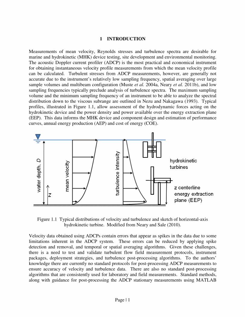
Figure 1.1 Typical distributions of velocity and turbulence and sketch of horizontal-axis

hydrokinetic turbine. Modified from Neary and Sale (2010). ....................................................... 1

Figure 2.1 Different types of ADCP beam configurations (RDI 2011a). ...................................... 4

Figure 2.2 Contour of velocity magnitude in a river cross section measured using an RDI Rio

Grande broadband ADCP (Gunawan 2010). .................................................................................. 4

Figure 2.3 Variation of the streamwise velocity and standard deviation corresponding to a set of

stationary measurements in a river (Gunawan et al. 2010a). .......................................................... 4

Figure 2.4 The Doppler principle and a water-wave analogy (Simpson 2001). ............................ 5

Figure 2.5 Sound wave transmission and reflection by particles (Simpson 2001). ....................... 6

Figure 2.6 Reflected pulse shows two Doppler shifts (Simpson 2001). ........................................ 6

Figure 2.7 Transformation of velocity component into beam coordinate system (RDI 1996). ..... 7

Figure 2.8 Acoustic pulses of narrow band and broadband ADCP technologies (Muller and

Wagner 2009).................................................................................................................................. 8

Figure 2.9 Time dilation principle ................................................................................................. 8

Figure 2.10 Beam velocity components (RDI, 1996). ................................................................... 9

Figure 2.11 Velocity magnitude and direction in the E-W and N-S axis (RDI, 1996). ................. 9

Figure 2.12 ADCP deployment methods: (a) mooring, (b) mounted, (c) underwater vehicle, (d)

remote controlled boat (RDI 2011b; Muller and Wagner 2009). ................................................. 11

Figure 2.13 Two views of shipboard ADCP side-swing mount on a 30-meter (95-foot) vessel

(Simpson 2001). ............................................................................................................................ 11

Figure 2.14 Left: schematic of a four-beam ADCP showing typical sampling volume (Neary et

al. 2011a); right: non-homogeneous horizontal velocities (Simpson 2001). ................................ 12

Figure 2.15 Contours of velocity magnitude at a location in Puget Sound, WA, obtained from an

upward looking ADCP (courtesy of the Northwest National Marine Renewable Energy Center,

University of Washington). ........................................................................................................... 14

Figure 2.16 Conceptual layout with schematic of perturbed turbulent ........................................ 17

Figure 2.17 Results of ADCP transect averaging; top: contour of normalized streamwise

velocity (��), bottom: V and W velocity vectors (Gunawan 2010b). .......................................... 18

Figure 2.18 Difference between Ud values obtained from ADCP stationary measurements and

ADCP transect averaging results at two cross sections (Gunawan 2010). ................................... 18

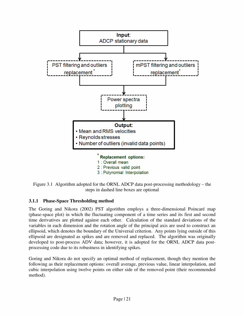
Figure 3.1 Algorithm adopted for the ORNL ADCP data post-processing methodology – the

steps in dashed line boxes are optional ......................................................................................... 21

Figure 3.2 Decomposition of u into U and u’ .............................................................................. 23

Figure 3.3 Spectral energy density plot for u ............................................................................... 24

Figure 3.4 Input format for the ORNL ADCP stationary data post-processing code .................. 25

Figure 3.5 Measurement setting at the St. Anthony Falls Laboratory. ........................................ 26

Figure 3.6 The SonTek ADP used in the experiment. ................................................................. 27

Figure 3.7 Correlation value at one of the ADP beams for the measurement at 1.0m upstream of

the turbine. .................................................................................................................................... 27

Figure 3.8 Number of outliers (in percent) at different bins for the X velocity component at 1.0m

upstream of the turbine model. ..................................................................................................... 28

Figure 3.9 Number of outliers (in percent) at different bins for the Y velocity component at 1.0m

upstream of the turbine model. ..................................................................................................... 29

Figure 3.10 Number of outliers (in percent) at different bins for the Z velocity component at

ix

1.0m upstream of the turbine model. ............................................................................................ 30

Figure 3.11 Streamwise, lateral and vertical velocities with respect to distance from bed at 2

diameters, 2D, (1.0m) upstream of the turbine model. ................................................................. 32

Figure 3.12 Variation of URMS and Iu with the distance upstream of the MHK model turbine.... 32

Figure 3.13 RMS values of streamwise, lateral and vertical velocities with respect to distance

from bed at 2 diameters, 2D, (1.0m) upstream of the turbine model. ........................................... 33

Figure 3.14 RMS values of streamwise, lateral and vertical velocities with respect to distance

from bed at 3 diameters, 3D, (1.5m) upstream of the turbine model. ........................................... 33

Figure 3.15 RMS values of streamwise, lateral and vertical velocities with respect to distance

from bed at 5 diameters, 5D, (2.5m) upstream of the turbine model. ........................................... 34

Figure 3.16 SED plot for the streamwise velocity at 1.0m upstream of the turbine model (at the

turbine hub height, z = 0.425m). ................................................................................................... 35

x

xi

LIST OF TABLES

Table 2.1 Minimum averaging time for ADCP stationary measurement in rivers suggested by

different researchers. ..................................................................................................................... 16

Table 3.1 Output file generated by ORNL ADCP data post-processing code ............................. 25

Table 3.2 Percent reduction of u’ compared to raw data after applying PST and mPST filtering

at 2D (1.0m), 3D (1.5m) and 5D (2.5m) upstream of the turbine model. ..................................... 34

xii

xiii

NOTATION

α the angle between the velocity vector and the transducer beam (degree)

β absorption coefficient (dB/m)

C speed of sound (ms-1

)

C1 first reconstruction constant, a calibration parameter in mPST (-)

C2 second reconstruction constant, a calibration parameter in mPST (-)

ds cylinder diameter (m)

dt turbine blade diameter (m)

EI echo intensity (dB)

f frequency band (Hz)

fR sampling frequency (Hz)

fs shedding frequency (Hz)

FD Doppler Shift frequency (Hz)

FS frequency of the source (Hz)

H flow depth in the main channel (m)

Iu turbulence intensity of the velocity in the streamwise direction,

�u�� U�

(-)

Lx energy containing length scale/macroscale turbulence (m)

RMS root mean square or standard deviation, ���

(the unit of x)

R distance from the transducer to the depth cell (m)

Ruu autocorrelation of the streamwise velocity component (m2 s

-2)

σ standard deviation of velocity (ms-1

)

S frequency of the transmitted sound (Hz)

SL source level or transmitted power (dB)

Su Fourier transform of uu (m2 s

-1)

SV water-mass volume backscattering strength (dB)

τ time shift (s)

u instantaneous velocity in the streamwise direction (ms-1

)

u’ instantaneous velocity fluctuation in the streamwise direction (ms-1

) U mean streamwise velocity with respect to time (ms

-1)

�� cross section mean streamwise velocity (ms-1

)

Uc convective velocity (ms-1

)

Ud depth-averaged streamwise velocity (ms-1

)

Uin inflow mean streamwise velocity (ms-1

)

Uout outflow mean streamwise velocity (ms-1

) URMS RMS value of the streamwise velocity (ms

-1)

v instantaneous velocity in the lateral direction (ms-1

)

v’ instantaneous velocity fluctuation in the lateral direction (ms-1

) V mean lateral velocity with respect to time (ms

-1)

VRMS RMS value or standard deviation of the lateral velocity (ms-1

) VSO relative velocity between the sound source and the observer (ms

-1)

w instantaneous velocity in the vertical direction (ms-1

)

w’ instantaneous velocity fluctuation in the vertical direction (ms-1

)

xiv

W average vertical velocity with respect to time (ms-1

) WRMS RMS value or standard deviation of the vertical velocity (ms

-1)

z vertical distance from the bed (m)

xv

ACKNOWLEDGMENTS

The authors thank DOE/EERE for supporting the development of the ORNL post-processing

algorithms under CPS Project No. 20689, CPS Agreement Nos. 20065 and 20070. The

pst_outlier, pst, mpst_outlier and mpst algorithms as they appear in the appendix originated from

algorithms developed by Nobuhito Mori, of Tokyo University in Japan, who maintains a GNU

license to the algorithms. The authors also thank Dr. Leonardo Chamorro, Mr. Craig Hill and

Mr. Scott Morton from the St. Anthony Falls Laboratory (SAFL), Minneapolis, Minnesota, for

providing the original algorithm for plotting Power Spectral Density and acoustic Doppler

current profiler data from the SAFL, main channel. Student interns who assisted with MATLAB

code development and testing include James McNutt, Bennett Flanders, Pablo Rosado, Danny

Sale, Andrew Hansen and Sreekanth Bangaru.

Page | 1

1 INTRODUCTION

Measurements of mean velocity, Reynolds stresses and turbulence spectra are desirable for

marine and hydrokinetic (MHK) device testing, site development and environmental monitoring.

The acoustic Doppler current profiler (ADCP) is the most practical and economical instrument

for obtaining instantaneous velocity profile measurements from which the mean velocity profile

can be calculated. Turbulent stresses from ADCP measurements, however, are generally not

accurate due to the instrument’s relatively low sampling frequency, spatial averaging over large

sample volumes and multibeam configuration (Muste et al. 2004a, Neary et al. 2011b), and low

sampling frequencies typically preclude analysis of turbulence spectra. The maximum sampling

volume and the minimum sampling frequency of an instrument to be able to analyze the spectral

distribution down to the viscous subrange are outlined in Nezu and Nakagawa (1993). Typical

profiles, illustrated in Figure 1.1, allow assessment of the hydrodynamic forces acting on the

hydrokinetic device and the power density and power available over the energy extraction plane

(EEP). This data informs the MHK device and component design and estimation of performance

curves, annual energy production (AEP) and cost of energy (COE).

Figure 1.1 Typical distributions of velocity and turbulence and sketch of horizontal-axis

hydrokinetic turbine. Modified from Neary and Sale (2010).

Velocity data obtained using ADCPs contain errors that appear as spikes in the data due to some

limitations inherent in the ADCP system. These errors can be reduced by applying spike

detection and removal, and temporal or spatial averaging algorithms. Given these challenges,

there is a need to test and validate turbulent flow field measurement protocols, instrument

packages, deployment strategies, and turbulence post-processing algorithms. To the authors’

knowledge there are currently no standard protocols for post-processing ADCP measurements to

ensure accuracy of velocity and turbulence data. There are also no standard post-processing

algorithms that are consistently used for laboratory and field measurements. Standard methods,

along with guidance for post-processing the ADCP stationary measurements using MATLAB

Page | 2

algorithms that were evaluated and tested by Oak Ridge National Laboratory (ORNL), are

presented following an overview of the ADCP operating principles, deployment methods, error

sources and recommended protocols for removing and replacing spurious data. The spatial and

temporal averaging algorithm for the ADCP shipboard data is currently under development, and

is expected to be incorporated in this report by September 2012.

Page | 3

2 ACOUSTIC DOPPLER CURRENT PROFILER METHOD

An ADCP measures velocity based on the Doppler principle and, depending on its type and

deployment method, can also be utilized to measure bed profiles or water surface elevations.

The ADCP is as an adaptation of a speed log, an instrument used to measure the speed of ships,

which was introduced in the mid-1970s (Rowe and Young 1979). ADCPs have two to five

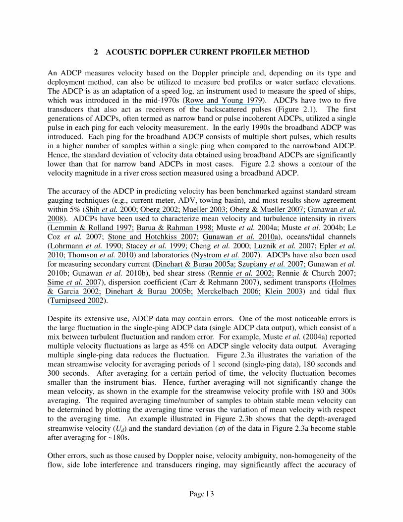
transducers that also act as receivers of the backscattered pulses (Figure 2.1). The first

generations of ADCPs, often termed as narrow band or pulse incoherent ADCPs, utilized a single

pulse in each ping for each velocity measurement. In the early 1990s the broadband ADCP was

introduced. Each ping for the broadband ADCP consists of multiple short pulses, which results

in a higher number of samples within a single ping when compared to the narrowband ADCP.

Hence, the standard deviation of velocity data obtained using broadband ADCPs are significantly

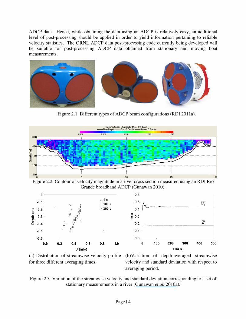
lower than that for narrow band ADCPs in most cases. Figure 2.2 shows a contour of the

velocity magnitude in a river cross section measured using a broadband ADCP.

The accuracy of the ADCP in predicting velocity has been benchmarked against standard stream

gauging techniques (e.g., current meter, ADV, towing basin), and most results show agreement

within 5% (Shih et al. 2000; Oberg 2002; Mueller 2003; Oberg & Mueller 2007; Gunawan et al.

2008). ADCPs have been used to characterize mean velocity and turbulence intensity in rivers

(Lemmin & Rolland 1997; Barua & Rahman 1998; Muste et al. 2004a; Muste et al. 2004b; Le

Coz et al. 2007; Stone and Hotchkiss 2007; Gunawan et al. 2010a), oceans/tidal channels

(Lohrmann et al. 1990; Stacey et al. 1999; Cheng et al. 2000; Luznik et al. 2007; Epler et al.

2010; Thomson et al. 2010) and laboratories (Nystrom et al. 2007). ADCPs have also been used

for measuring secondary current (Dinehart & Burau 2005a; Szupiany et al. 2007; Gunawan et al.

2010b; Gunawan et al. 2010b), bed shear stress (Rennie et al. 2002; Rennie & Church 2007;

Sime et al. 2007), dispersion coefficient (Carr & Rehmann 2007), sediment transports (Holmes

& Garcia 2002; Dinehart & Burau 2005b; Merckelbach 2006; Klein 2003) and tidal flux

(Turnipseed 2002).

Despite its extensive use, ADCP data may contain errors. One of the most noticeable errors is

the large fluctuation in the single-ping ADCP data (single ADCP data output), which consist of a

mix between turbulent fluctuation and random error. For example, Muste et al. (2004a) reported

multiple velocity fluctuations as large as 45% on ADCP single velocity data output. Averaging

multiple single-ping data reduces the fluctuation. Figure 2.3a illustrates the variation of the

mean streamwise velocity for averaging periods of 1 second (single-ping data), 180 seconds and

300 seconds. After averaging for a certain period of time, the velocity fluctuation becomes

smaller than the instrument bias. Hence, further averaging will not significantly change the

mean velocity, as shown in the example for the streamwise velocity profile with 180 and 300s

averaging. The required averaging time/number of samples to obtain stable mean velocity can

be determined by plotting the averaging time versus the variation of mean velocity with respect

to the averaging time. An example illustrated in Figure 2.3b shows that the depth-averaged

streamwise velocity (Ud) and the standard deviation (σ) of the data in Figure 2.3a become stable

after averaging for ~180s.

Other errors, such as those caused by Doppler noise, velocity ambiguity, non-homogeneity of the

flow, side lobe interference and transducers ringing, may significantly affect the accuracy of

Page | 4

ADCP data. Hence, while obtaining the data using an ADCP is relatively easy, an additional

level of post-processing should be applied in order to yield information pertaining to reliable

velocity statistics. The ORNL ADCP data post-processing code currently being developed will

be suitable for post-processing ADCP data obtained from stationary and moving boat

measurements.

Figure 2.1 Different types of ADCP beam configurations (RDI 2011a).

Figure 2.2 Contour of velocity magnitude in a river cross section measured using an RDI Rio

Grande broadband ADCP (Gunawan 2010).

(a) Distribution of streamwise velocity profile

for three different averaging times.

(b)Variation of depth-averaged streamwise

velocity and standard deviation with respect to

averaging period.

Figure 2.3 Variation of the streamwise velocity and standard deviation corresponding to a set of

stationary measurements in a river (Gunawan et al. 2010a).

Page | 5

2.1 ADCP PRINCIPLE OF OPERATION

An ADCP measures the movement of particles in the water relative to the ADCP position. As

most of the particles in the water are small, it can be assumed that the velocity of the particles is

the same as the velocity of the water. Most applications require the velocity of the water relative

to a known reference, such as the earth coordinate system or the bottom boundary. This is not an

issue if the ADCP is mounted in a fixed platform, such as river or sea bed. If the ADCP is

deployed from a moving platform, such as a moving ship, the position of the ADCP at all times

during the measurement has to be known. The ADCP bottom tracking capability or a GPS is

typically used for such a purpose. When the position of the ADCP with respect to measurement

time is known, the water velocity relative to the reference can be calculated by superimposing

the velocity of the particles relatively to the ADCP position and the velocity of the ADCP

instrument relative to the reference.

2.1.1 Doppler shift principle

The narrow band ADCPs measure the difference in frequency between the sound pulses emitted

by the ADCP transducers and those reflected by particles in the water and received by the ADCP

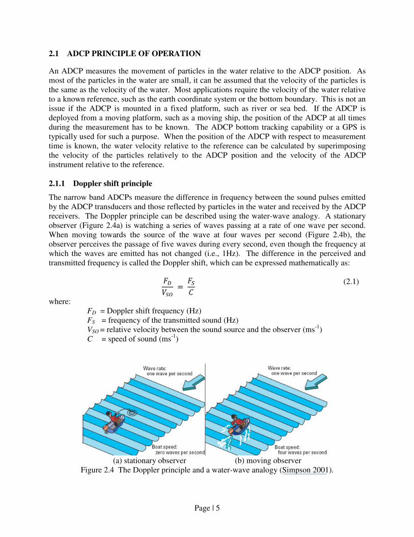
receivers. The Doppler principle can be described using the water-wave analogy. A stationary

observer (Figure 2.4a) is watching a series of waves passing at a rate of one wave per second.

When moving towards the source of the wave at four waves per second (Figure 2.4b), the

observer perceives the passage of five waves during every second, even though the frequency at

which the waves are emitted has not changed (i.e., 1Hz). The difference in the perceived and

transmitted frequency is called the Doppler shift, which can be expressed mathematically as:

����� = ���

(2.1)

where:

FD = Doppler shift frequency (Hz)

FS = frequency of the transmitted sound (Hz)

VSO = relative velocity between the sound source and the observer (ms-1

)

C = speed of sound (ms-1

)

(a) stationary observer (b) moving observer

Figure 2.4 The Doppler principle and a water-wave analogy (Simpson 2001).

Page | 6

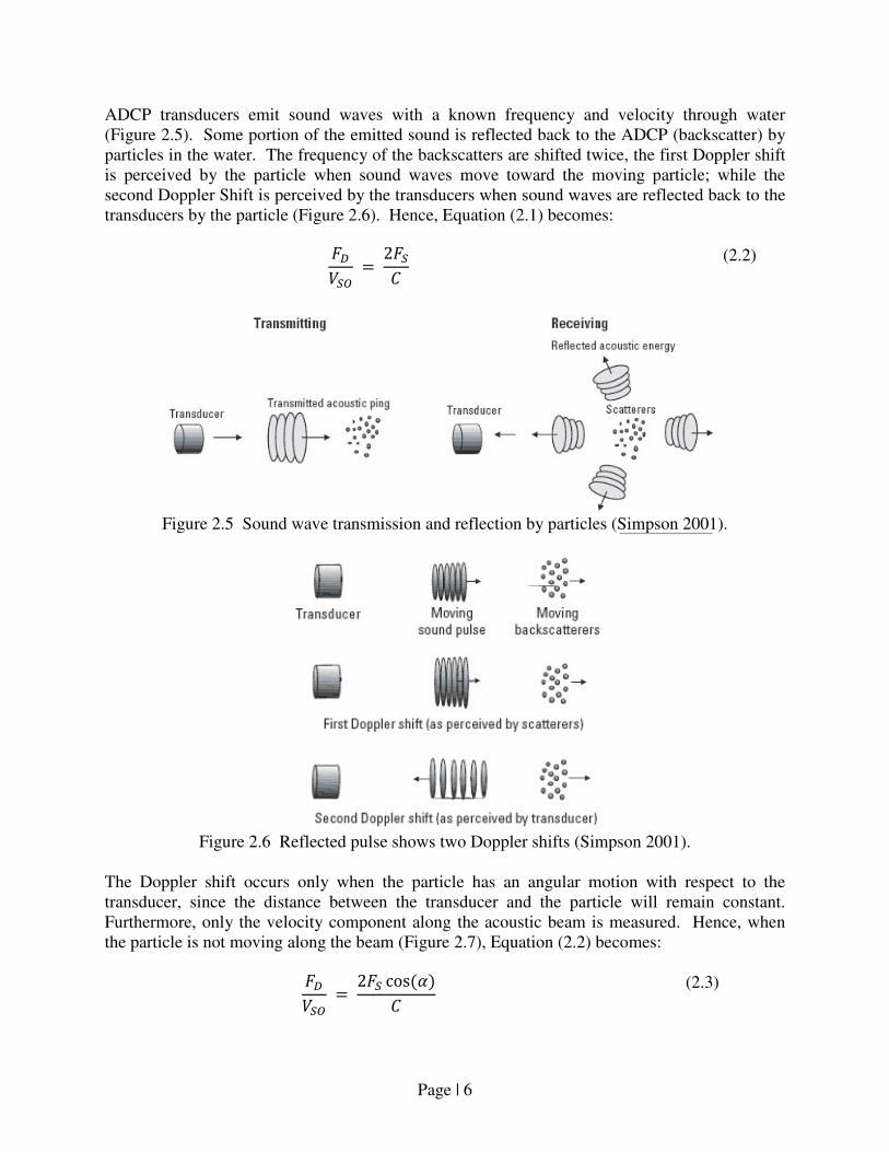
ADCP transducers emit sound waves with a known frequency and velocity through water

(Figure 2.5). Some portion of the emitted sound is reflected back to the ADCP (backscatter) by

particles in the water. The frequency of the backscatters are shifted twice, the first Doppler shift

is perceived by the particle when sound waves move toward the moving particle; while the

second Doppler Shift is perceived by the transducers when sound waves are reflected back to the

transducers by the particle (Figure 2.6). Hence, Equation (2.1) becomes:

����� = 2���

(2.2)

Figure 2.5 Sound wave transmission and reflection by particles (Simpson 2001).

Figure 2.6 Reflected pulse shows two Doppler shifts (Simpson 2001).

The Doppler shift occurs only when the particle has an angular motion with respect to the

transducer, since the distance between the transducer and the particle will remain constant.

Furthermore, only the velocity component along the acoustic beam is measured. Hence, when

the particle is not moving along the beam (Figure 2.7), Equation (2.2) becomes:

����� = 2�� cos(�)�

(2.3)

Page | 7

where α is the angle between the velocity vector and the transducer beam.

Figure 2.7 Transformation of velocity component into beam coordinate system (RDI 1996).

2.1.2 The broadband ADCP

The term broadband is used because the bandwidth of the ADCP was increased to accommodate

the signal processing of a narrow-pulse pair (Muller and Wagner 2009). As bandwidth is

synonymous with sampling rate, the number of samples taken per depth cell (bin) by a single

ping increases if the bandwidth is increased. More samples in a single ping help reduce the

single-ping standard deviation of velocity. The broadband ADCPs obtained hundreds of samples

per ping, while only a few are obtained for the narrowband ADCPs (RDI 2011b). Figure 2.8

illustrates the difference between the narrow band and broadband ADCP pulses. The

narrowband pulses are monochromatic, while the broadband pulses consist of many code

elements having a phase shift of either a 0-degree or 180-degree system arranged in a

pseudorandom order and having some lags. The broadband ADCP measures velocity using a

different approach from the narrow band ADCP in a way that it measures the phase difference

between the emitted sinusoidal pulses and their echoes to calculate the Doppler Shift, instead of

using the frequency shift between the pulses. ADCP data are typically output for each single

ping, the entirety of the sound generated by an ADCP transducer for a single measurement cycle

(RDI 2011b).

The broadband ADCPs use the autocorrelation method to compare echoes from the same bin.

An ADCP transmits a series of coded pulses and lags within a single long pulse, and receives

numerous echoes from many sound scatterers from the same bin, all combined into a single echo.

A high correlation value indicates the similarity of the echoes. The autocorrelation function is

also used to compute the propagation delay, the change of travel time caused by the changing of

the distance travelled by the pulses.

αααα

Page | 8

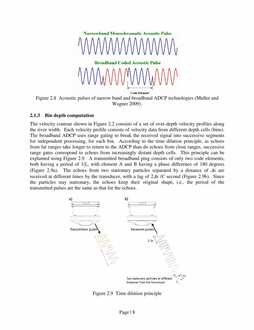
Figure 2.8 Acoustic pulses of narrow band and broadband ADCP technologies (Muller and

Wagner 2009).

2.1.3 Bin depth computation

The velocity contour shown in Figure 2.2 consists of a set of over-depth velocity profiles along

the river width. Each velocity profile consists of velocity data from different depth cells (bins).

The broadband ADCP uses range gating to break the received signal into successive segments

for independent processing, for each bin. According to the time dilation principle, as echoes

from far ranges take longer to return to the ADCP than do echoes from close ranges, successive

range gates correspond to echoes from increasingly distant depth cells. This principle can be

explained using Figure 2.9. A transmitted broadband ping consists of only two code elements,

both having a period of 1/fs, with element A and B having a phase difference of 180 degrees

(Figure 2.9a). The echoes from two stationary particles separated by a distance of ∆x are

received at different times by the transducer, with a lag of 2∆x /C second (Figure 2.9b). Since

the particles stay stationary, the echoes keep their original shape, i.e., the period of the

transmitted pulses are the same as that for the echoes.

Figure 2.9 Time dilation principle

Page | 9

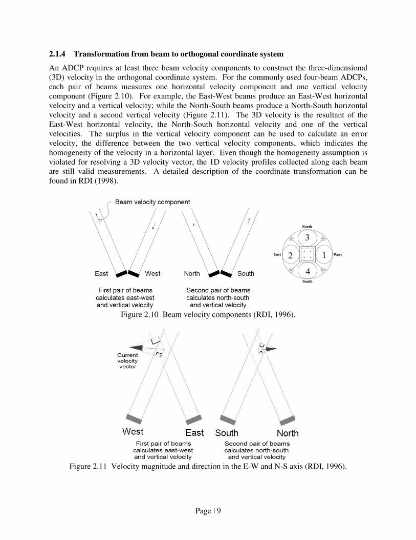
2.1.4 Transformation from beam to orthogonal coordinate system

An ADCP requires at least three beam velocity components to construct the three-dimensional

(3D) velocity in the orthogonal coordinate system. For the commonly used four-beam ADCPs,

each pair of beams measures one horizontal velocity component and one vertical velocity

component (Figure 2.10). For example, the East-West beams produce an East-West horizontal

velocity and a vertical velocity; while the North-South beams produce a North-South horizontal

velocity and a second vertical velocity (Figure 2.11). The 3D velocity is the resultant of the

East-West horizontal velocity, the North-South horizontal velocity and one of the vertical

velocities. The surplus in the vertical velocity component can be used to calculate an error

velocity, the difference between the two vertical velocity components, which indicates the

homogeneity of the velocity in a horizontal layer. Even though the homogeneity assumption is

violated for resolving a 3D velocity vector, the 1D velocity profiles collected along each beam

are still valid measurements. A detailed description of the coordinate transformation can be

found in RDI (1998).

Figure 2.10 Beam velocity components (RDI, 1996).

Figure 2.11 Velocity magnitude and direction in the E-W and N-S axis (RDI, 1996).

Page | 10

2.1.5 Bottom tracking

Bottom-tracking pings are used to measure the bottom depth and ADCP boat velocity relative to

the bed. The bottom-tracking pings have a lower frequency (longer pulse) than the water

velocity profiling pings in order to properly illuminate the bed. The concept of the bottom depth

and boat velocity measurements is similar to the one for the water profiling. Here, the particles

are replaced by the river bottom. The boat velocity is also measured using the Doppler shift

concept, but this time the boat is moving while the river bottom is standing still. Knowing the

boat velocity and movement time, the boat path can be computed. As the water velocity relative

to the ADCP and the velocity of the ADCP relative to the river bottom are known, the water

velocity relative to the bottom can be calculated.

2.2 ADCP MEASUREMENT AND DEPLOYMENT METHODS

Common ADCP deployment methods include mooring and riverbed/seabed mounted for

stationary measurements, as shown in Figure 2.12. The stationary measurements refer to fixing

the ADCP at a location to sample the data at a period of time. This method provides accurate

mean velocity data when some samples are averaged over a long period, and can be used to

monitor water level changes. Another type of measurement is the ADCP moving-boat

measurement. For this type of measurement, the ADCP is mounted on an underwater vehicle

(Figure 2.12c), a remote-controlled boat (Figure 2.12d) or a large ship (Figure 2.13). Then, the

ADCP measures velocity data while the boat is moving. This method is suitable to obtain

velocity data for a large region, such as for the tidal current resource assessment of a region.

Page | 11

Figure 2.12 ADCP deployment methods: (a) mooring, (b) mounted, (c) underwater vehicle, (d)

remote controlled boat (RDI 2011b; Muller and Wagner 2009).

Figure 2.13 Two views of shipboard ADCP side-swing mount on a 30-meter (95-foot) vessel

(Simpson 2001).

Page | 12

2.3 ADCP MEASUREMENT UNCERTAINTY

ADCP velocity measurement uncertainty is caused by random error and bias (systematic error).

Random errors depend on internal and external factors such as the ADCP frequency, depth cell

size, number of pings averaged together, beam geometry, turbulence, internal waves and ADCP

motion. Random errors can be reduced by averaging the data over a long period of time. The

bias errors are influenced by several factors that include temperature, mean current speed, signal-

to-noise ratio (SNR) and beam geometry. Bias cannot be calibrated or removed, but its

magnitude is typically less than 10 mm/s (RDI 1996). Other errors, such as the presence of

materials that obstruct the sound pulses transmission, can disturb the velocity measurements.

Some of the causes of errors are described below.

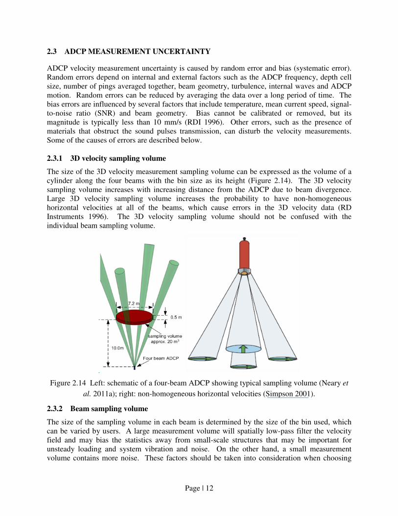
2.3.1 3D velocity sampling volume

The size of the 3D velocity measurement sampling volume can be expressed as the volume of a

cylinder along the four beams with the bin size as its height (Figure 2.14). The 3D velocity

sampling volume increases with increasing distance from the ADCP due to beam divergence.

Large 3D velocity sampling volume increases the probability to have non-homogeneous

horizontal velocities at all of the beams, which cause errors in the 3D velocity data (RD

Instruments 1996). The 3D velocity sampling volume should not be confused with the

individual beam sampling volume.

Figure 2.14 Left: schematic of a four-beam ADCP showing typical sampling volume (Neary et

al. 2011a); right: non-homogeneous horizontal velocities (Simpson 2001).

2.3.2 Beam sampling volume

The size of the sampling volume in each beam is determined by the size of the bin used, which

can be varied by users. A large measurement volume will spatially low-pass filter the velocity

field and may bias the statistics away from small-scale structures that may be important for

unsteady loading and system vibration and noise. On the other hand, a small measurement

volume contains more noise. These factors should be taken into consideration when choosing

Page | 13

the bin size to be used in the deployment setting.

2.3.3 Echo attenuation

Echo intensity (EI) is a measure of signal strength of the echo returned to the ADCP. When the

level of echo intensity drops below the noise level of the instrument, the ADCP cannot

accurately calculate Doppler Shifts; hence, this parameter governs the ADCP measurement

range. EI is affected by sound absorption in the water, beam spreading, transmitted power and

backscatter coefficient. Their relation can be expressed as follows:

EI = SL + SV + constant -20log(R) -2βR (2.4)

where:

EI is the echo intensity (dB)

SL is the source level or transmitted power (dB)

SV is the water-mass volume backscattering strength (dB)

β is the absorption coefficient (dB/m)

R is the distance from the transducer to the depth cell (m)

EI is a relative parameter in the sense that the ADCP can detect variations in EI, but cannot make

absolute measurements that can be compared with other ADCPs. The constant is included

because the measurement is relative rather than absolute. A high concentration of scatterers

corresponds to the higher EI rather than in a low concentration of scatterers because more sounds

are reflected by the scatterers. Sound pulses spread as a function of distance from the

transducers once they are transmitted. Hence, the intensity of the echoes received by the

transducer also decreases with the distance from the transducer. Sound absorption by the water

reduces the strength of the echoes and is affected by the physical and chemical processes in the

water.

2.3.4 Lack of scatterers

Velocity data cannot be measured when sound scatterers do not exist in the water column. The

amount of suspended sediments in rivers is generally sufficient to produce strong echoes. In an

ocean environment, lack of scatterers at a certain depth is not uncommon. For example, on a

cruise near Mauritius only one-third of the nominal range contain velocity data, and this kind of

condition is occurring less than 10% of the time (RDI 1996).

2.3.5 Side lobe interference

Due to some technical limitations, instead of only transmitting sound pulses through the main

lobe (main beam), the ADCP also transmits sounds through the side lobes, but at a lower

intensity than the sound transmitted through the main lobe. The angle between the main lobe

and the side lobe is typically around 30–40º. The returning echoes from the side lobe sound

reflected by the hard surface, such as ocean bed or water surface, have a similar intensity as the

returning echoes from the main lobe sound reflected by the particles in the water. For a 20º

beam angle ADCP deployed upward looking, the echoes from the side lobe sound reflected by

the water surface are received by the transducers at the same time as the echoes from the main

Page | 14

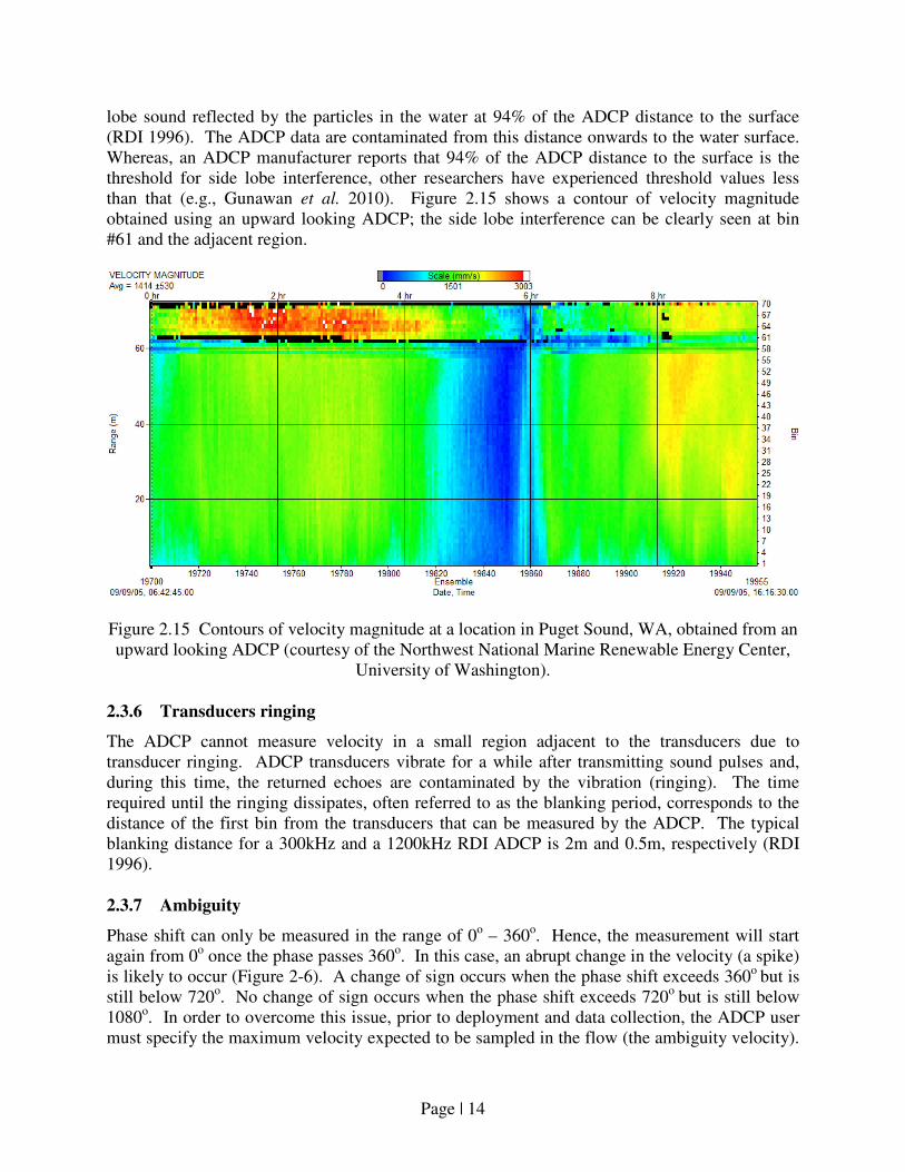
lobe sound reflected by the particles in the water at 94% of the ADCP distance to the surface

(RDI 1996). The ADCP data are contaminated from this distance onwards to the water surface.

Whereas, an ADCP manufacturer reports that 94% of the ADCP distance to the surface is the

threshold for side lobe interference, other researchers have experienced threshold values less

than that (e.g., Gunawan et al. 2010). Figure 2.15 shows a contour of velocity magnitude

obtained using an upward looking ADCP; the side lobe interference can be clearly seen at bin

#61 and the adjacent region.

Figure 2.15 Contours of velocity magnitude at a location in Puget Sound, WA, obtained from an

upward looking ADCP (courtesy of the Northwest National Marine Renewable Energy Center,

University of Washington).

2.3.6 Transducers ringing

The ADCP cannot measure velocity in a small region adjacent to the transducers due to

transducer ringing. ADCP transducers vibrate for a while after transmitting sound pulses and,

during this time, the returned echoes are contaminated by the vibration (ringing). The time

required until the ringing dissipates, often referred to as the blanking period, corresponds to the

distance of the first bin from the transducers that can be measured by the ADCP. The typical

blanking distance for a 300kHz and a 1200kHz RDI ADCP is 2m and 0.5m, respectively (RDI

1996).

2.3.7 Ambiguity

Phase shift can only be measured in the range of 0o – 360

o. Hence, the measurement will start

again from 0o once the phase passes 360

o. In this case, an abrupt change in the velocity (a spike)

is likely to occur (Figure 2-6). A change of sign occurs when the phase shift exceeds 360o

but is

still below 720o. No change of sign occurs when the phase shift exceeds 720

o but is still below

1080o. In order to overcome this issue, prior to deployment and data collection, the ADCP user

must specify the maximum velocity expected to be sampled in the flow (the ambiguity velocity).

Page | 15

The ambiguity velocity is the maximum allowable radial motion for phase measurements to be

unambiguous.

2.3.8 Moving-bed condition

ADCP bottom track or GPS data is required to take into account the movement of the ADCP

when calculating water velocity. The ADCP bottom track fails if high amounts of material, such

as clay or sand, are moving near the bed. Such a condition typically happens in rivers during

high flow; whereas, high velocity causes the river bed to be eroded. A moving bed condition can

be detected by examining the ADCP stationary measurement data. Significant movements of the

ADCP shown in the data indicate that moving bed condition is likely to happen.

2.3.9 The presence of submerged vegetation

The presence of vegetation can significantly inhibit the ability of the ADCP to give reliable

measurements as the bottom tracking is disrupted (Gunawan et al. 2010). This is perhaps not too

surprising if one considers the principle of operation. Vegetation near the channel bed has the

propensity to disrupt the bottom tracking and also to cause anomalous velocity measurements.

2.3.10 Air bubbles

Breaking waves generate bubbles below the ocean surface. Passing under the ship’s hull, the

bubbles can act as a shield that distracts the transmission of sound pulses. They can reduce the

ADCP profiling range and, in the worst case, completely block the sound transmission.

2.4 PROTOCOLS FOR REDUCING ERROR

Errors in the ADCP velocity data can be reduced using several methods outlined below.

2.4.1 Temporal averaging

One method often used to reduce the velocity fluctuations is to average the velocity data over a

reasonably long period of time (e.g., 3 to 15 minutes). However, this method is only suitable for

a stationary ADCP measurement since the measurement location does not change with respect to

time when this deployment method is used. After averaging for a certain period of time, the

mean velocity becomes statistically stable, i.e., it does not change significantly with more

samples to be averaged. The averaging time to obtain stable mean streamwise velocity in rivers

depends on many variables, such as the flow characteristics of the site and bin size; but is

typically less than 15 minutes. A summary of the suggested averaging time by different

researchers is presented in Table 2.1. Gunawan (2010) reported that out of 31 stationary

measurements undertaken at two river cross sections, 30 satisfied the 5% convergence level for

the mean streamwise velocity when averaged over 300s. The 5% convergence level indicates

that the difference between the mean streamwise velocity averaged over 300s and the last 20

samples is less than 5%. Knowledge of the minimum averaging time is beneficial, especially

when conducting a stationary measurement using a boat-mounted ADCP (the boat position is

fixed during the measurement). Using the minimum averaging time ensures that adequate

accuracy on the mean velocity profile is achieved within the shortest measurement time possible.

Page | 16

Table 2.1 Minimum averaging time for ADCP stationary measurement in rivers suggested by

different researchers.

Source Barua & Rahman Stone & Hotchkiss Szupiany et al Gunawan

(1998) (2007) (2007) (2010)

Suggested averaging time 900s 100 - 250s 420 - 600s 300s

River width ~ 11,000m 12.8 -15.4m 600 – 2,500m ~ 5 - 8m

River depth 8.3 - 10m 0.75 – 1.1m 5 – 12m ~0.6 – 1.2m

ADCP model

RDI Broadband

ADCP

1200kHz RDI Broadband

Rio Grande ADCP

1000kHz SonTek

ADP

2MHz RDI Broadband

StreamPro ADCP

Sampling frequency 0.5Hz ~1Hz 12Hz 1Hz

Bin size 50cm 5cm 50 - 75cm 5-10cm

Max. boat movement 3m N/A 5m 0.1m

2.4.2 Spatial averaging

The ADCP stationary measurement is not suitable for measuring the mean velocity at many

locations within a short time, as it is very time-consuming and costly. Moving-boat ADCP

measurement reduces the measurement time significantly, but it has its own issue. As the ADCP

(and the boat) is moving during the measurement, only one profile sample is obtained at every

boat position. The number of samples is not sufficient for reducing the random error in the data.

Spatial averaging helps reduce the random error in the data.

Obtaining velocity data at numerous locations is required for many purposes, such as to

investigate the detailed flow structures in a river cross section and to assess the potential MHK

energy resources in a tidal channel. The detailed flow structures in a river cross section are

crucial to identify the best location to place the MHK devices and to investigate the coherent

structures in the flow which cause extra structural loads and moments on the MHK devices.

Coherent flow structures can be caused by the internal or external flow disturbance in the river.

The internal disturbances include the helical secondary flow motion along the longitudinal

direction caused by turbulence or centrifugal force (Einstein & Li 1958; Perkins 1970) and the

plan-form vortices due to the high velocity gradient typically occur during an overbank flow

condition (Sellin 1964; Ikeda 2001; Knight et al. 2009). The external disturbance of the flow is

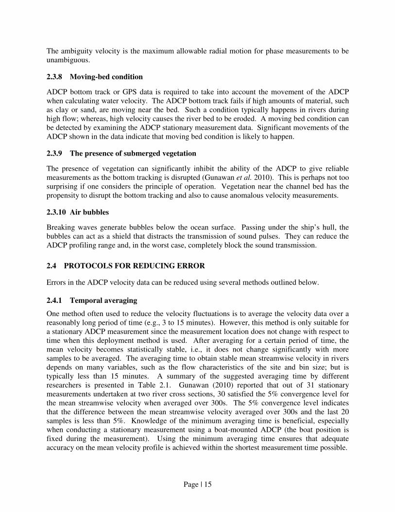
caused by an external structure, such as the MHK device itself or a bridge pier. Figure 2.16

illustrates vortex shedding affecting an MHK turbine downstream of a cylinder structure. Apart

from causing an extra load, coherent structures can potentially cause a resonance failure if the

resonance frequency of a moving or vibrating component of the MHK device is the same as the

frequency of the coherent structures.

A regional assessment of MHK energy resources potential requires a great number of data to be

collected along a large region. ADCP moving-boat data can be used for this purpose; but, data

post-processing, mainly to reduce the random errors and to extrapolate the data to the

unmeasured region, should be performed.

Page | 17

Figure 2.16 Conceptual layout with schematic of perturbed turbulent

inflow approaching turbine (Neary et al. 2011a).

The detailed flow structures in a river cross section can be obtained by averaging several ADCP

transects data together. The ADCP transect data are obtained by traversing the ADCP in a river

cross section. Averaging several transects together reduces the data fluctuation due to random

errors and turbulence, and helps to obtain a clearer pattern of the secondary flow circulation

(Dinehart and Burau 2005; Szupiany et al. 2007; Gunawan et al. 2010b). An example of a

transect averaging result is shown in Figure 2.17. One of the key points when conducting

transect averaging is to ensure that the transect data are obtained at the same cross section.

Dinehart and Burau (2005) averaged the velocity data from each ADCP transect by interpolating

them into a 2D grid representing the cross section of the corresponding measurement. The value

at each node of the grid was calculated using an inverse distance weighting (IDW) method (six

samples points were selected by an equipartite arrangement). Each set of the interpolation grids

was averaged together to obtain the final velocity grid. Szupiany et al. (2007) used a SonTek

ADP (Acoustic Doppler Profiler) to measure the 3D velocity in River Parana, Argentina, at

several cross sections of 600-2400m widths. Szupiany et al. (2007) suggests that the finer detail

of the existence of secondary flow cells can be obtained by averaging five transects. Le Coz et

al. (2007) used the IDW method to average the ADCP transect data obtained from a 100m wide

river. Their results suggest that the number of data points considered for calculating the IDW

interpolation value at each node of the grid affects the smoothness of the velocity profiles in the

IDW-interpolated grid. As a quality measure, Le Coz et al. (2007) report that the difference

between the discharge in the river before and after the IDW interpolation is always within 3%.

Gunawan et al. (2010a) reported that the transect averaging results depend on the size of the

interpolation grid and the distance between the measurement data point and the IDW

interpolation node in the grid. When a data point is too close to the interpolation node, the

velocity value at that data point has a dominant influence on the interpolated velocity at the node.

If the data point close to the interpolation node is a spike, the IDW interpolation method will

only have a minor effect in smoothing the spike. Gunawan (2010) conducted measurements in

two river cross sections and compared the depth-averaged streamwise velocity of the ADCP

transect averaging results and the time-averaged stationary ADCP data. An average difference

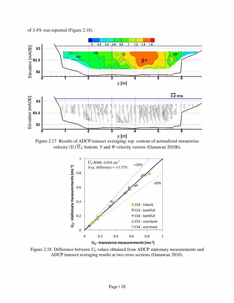
Page | 18

of 3.4% was reported (Figure 2.18).

Figure 2.17 Results of ADCP transect averaging; top: contour of normalized streamwise

velocity (� ��⁄ ), bottom: V and W velocity vectors (Gunawan 2010b).

Figure 2.18 Difference between Ud values obtained from ADCP stationary measurements and

ADCP transect averaging results at two cross sections (Gunawan 2010).

+20%

-20%

0

0.2

0.4

0.6

0.8

1

0 0.2 0.4 0.6 0.8 1

Ud

-st

ati

on

ary

me

asu

rem

en

ts (

ms-1

)

Ud - transverse measurements (ms-1)

CS4 - inbank

CS2 - bankfull

CS4 - bankfull

CS2 - overbank

CS4 - overbank

Ud RMS: 0.054 ms-1

Avg. difference = +3.37%

Page | 19

2.4.3 Histogram inspection

Effects of over-ranging on data are easy to identify. The probability density function (PDF) of a

time series (in the beam coordinate system) may demonstrate a sudden velocity cut-off beyond

which no data will be registered, which is often caused by the ambiguity problem. If this abrupt

discontinuity is observed in a data sample, the user should attempt to increase the user defined

velocity range until the histogram of the time series no longer demonstrate such characteristics.

Optimally the user should select the smallest velocity range (in either beam or earth coordinates)

for which no cut-off is observed in the histogram.

2.4.4 Spike identification, removal and replacement

Baldwin et al. (1993) and Petrie et al. (1988) first applied a velocity hodograph elliptical filtering

technique to laser Doppler velocimeter (LDV) measurements as an effective means of filtering

LDV measured noise. In this technique, the measured data are rotated into the principal stress

coordinates and an elliptic filter of size N principal stresses in the minor and major axes is

applied to the 2D probability density function (PDF). Velocity ensembles occurring outside the

defined ellipse are filtered from the data set. Fontaine et al. (1996) extended the 2D elliptic filter

technique to the 3D flow application with a principal stress 3D ellipsoid filter on three-

component LDV measured data.

The Phase-Space Thresholding (PST) technique, developed by Goring and Nikora (2002), is

another ellipsoidal filter technique where invalid points are identified as those lying outside of

the universal threshold defined ellipsoid in a 3D Poincaré phase space. While the ellipsoidal

filter technique of Fontaine et al. (1996) operates on the instantaneous velocity hodograph (u vs v

vs w) with filtering applied in the principal stress space, the PST technique operates on the

instantaneous velocity and it’s local accelerations (u vs du/dt). The PST technique has been

critically analyzed and improved upon by a number of peers (Pasheh et al. 2010; Wahl 2003).

The use of the PST algorithm has grown in acceptance and is now the standard means of filtering

data. Nevertheless, improvements to the PST algorithm have been proposed to address the main

criticism that it was replacing valid data around spikes. While removal has negligible effects on

the value of bulk statistical moments, it has been shown by (Pasheh et al. 2010) to compromise

time-dependent indicators such as the power and energy spectra. Goring and Nikora (2002) have

suggested cubic interpolation by the twelve points on either side of an identified invalid datum

and they seem to be one of the few researchers to have compared various methods. Pasheh et al.

(2010) have proposed a modified Phase-Space-Thresholding Sample and Hold algorithm (mPST-

SH) that evaluates the validity of data in three stages: first, any velocity measurements near the

average are incontrovertibly marked as valid; then, any data far from the average are marked as

invalid and are removed; finally, the data are filtered using the PST technique.

Page | 20

3 ORNL ADCP DATA POST-PROCESSING METHODOLOGY

The current version of the ORNL ADCP data post-processing methodology is capable of

detecting, removing and replacing invalid data (outliers) from the ADCP stationary data using

the Phase-Space Thresholding (PST) and the modified Phase-Space Thresholding (mPST)

methods. Three schemes of data replacement are available: replacement by the overall average,

replacement by the previous valid point and replacement by polynomial interpolation. The

ORNL ADCP data post-processing methodology also calculates the mean velocities, RMS

velocities and Reynolds stresses at each velocity bin. The code to spatially average the ADCP

transects data is currently under development and is expected to be publicly available in mid-

2012.

3.1 ALGORITHM

The algorithm of the ORNL ADCP data post-processing code is written in MATLAB and

consists of several independent functions that are called by the main program (Figure 3.1). The

ORNL ADCP data post-processing to post-process the ADCP stationary data is a modification of

the ORNL ADV data post-processing code (Gunawan et al. 2011). The major difference lies in

the data input; instead of using one velocity measurement or multiple point velocity

measurements, all the bins along the ADCP measurement depths are used. The first step to run

the code is to export the ADCP data into the MATLAB workspace. If the data are in Microsoft

Excel-compatible format, such as *.csv, the MATLAB function xlsread would be convenient to

use as it detects and removes the unused file headers. The user is then given the choice to

implement Phase-Space Threshold (PST) filtering, modified Phase-Space Threshold (mPST)

filtering or to bypass PST altogether. The outliers can be replaced by selecting from three

replacement methods. The number of outliers is then computed and the user will be given the

option to draw the velocity time series (3 velocity components) with the outliers marked with red

circles. When the PST or mPST filter is chosen, the number of outliers is computed and the user

will be given the option to plot the velocity time series and the ellipsoid that delineates the

threshold for outliers. Once the filtering process is completed, the user is given the option to plot

the velocity power spectra. The user inputs the sampling rate of the ADCP used during

measurements if this option is chosen.

Page | 21

Figure 3.1 Algorithm adopted for the ORNL ADCP data post-processing methodology – the

steps in dashed line boxes are optional

3.1.1 Phase-Space Thresholding method

The Goring and Nikora (2002) PST algorithm employs a three-dimensional Poincaré map

(phase-space plot) in which the fluctuating component of a time series and its first and second

time derivatives are plotted against each other. Calculation of the standard deviations of the

variables in each dimension and the rotation angle of the principal axis are used to construct an

ellipsoid, which denotes the boundary of the Universal criterion. Any points lying outside of this

ellipsoid are designated as spikes and are removed and replaced. The algorithm was originally

developed to post-process ADV data; however, it is adopted for the ORNL ADCP data post-

processing code due to its robustness in identifying spikes.

Goring and Nikora do not specify an optimal method of replacement, though they mention the

following as their replacement options: overall average, previous value, linear interpolation, and

cubic interpolation using twelve points on either side of the removed point (their recommended

method).

Page | 22

The replacement method is iterated until no points lie outside of the ellipsoid, or the maximum

number of iterations is reached. The ellipsoid may shrink upon iteration corresponding to the

diminishing standard deviations of the velocity during subsequent iterations. No effect on

further replacement is defined as a condition in which the spikes that are identified in one

iteration are the same as those identified in the previous iteration; and therefore, would be

identified in any subsequent iteration without change.

Parsheh et al. (2010) adapted the algorithm described by Goring and Nikora, but shared the

widely held concern that the method in previous implementations identified several data points

as spikes that were valid according to Parsheh et al. (2010). They also considered the effects of

filtering on the power spectra and prescribed their so-called modified Phase-Space Thresholding

Sample and Hold algorithm (mPST-SH).

The mPST-SH algorithm evaluates the validity of data in three stages. First, any velocity

measurements near the average are incontrovertibly marked as valid. Then, any data found to

depart significantly from the average are marked as invalid and are removed. It should be noted

that the user provides input variables to determine this threshold of significant departure.

Finally, the data are subjected to modified phase-space thresholding in which the median of the

absolute deviation is used rather than the standard deviation since the former is more robust and

values termed as spikes are replaced. However, if any of the data points which the PST filter

identified as spikes were previously identified as incontrovertibly valid (those near the average),

they are not replaced. Parsheh et al. (2010) adopted replacement by the last valid point as their

replacement strategy and did not examine the effects of other replacement methods.

3.1.2 Data replacements

The replacement function allows the user to select from among replacement data by the overall

average, by the previous valid point, or by polynomial interpolation. As emphasized earlier,

replacement is not aimed to reconstruct the dataset, which would have been measured when

errors in the dataset do not exist; but rather, to fill in the data gaps so that they are continuous

with respect to time, which is the prerequisite for power spectra computation. It is always a good

practice to compare the results from the different replacement methods.

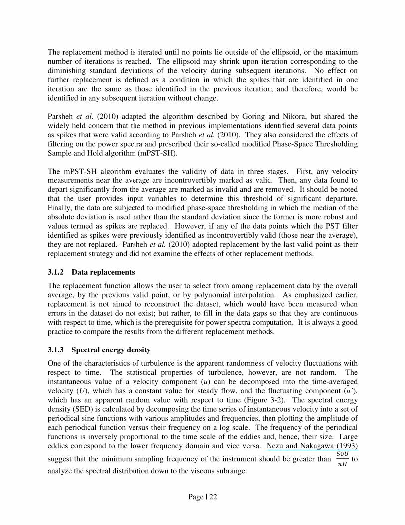
3.1.3 Spectral energy density

One of the characteristics of turbulence is the apparent randomness of velocity fluctuations with

respect to time. The statistical properties of turbulence, however, are not random. The

instantaneous value of a velocity component (u) can be decomposed into the time-averaged

velocity (U), which has a constant value for steady flow, and the fluctuating component (u’),

which has an apparent random value with respect to time (Figure 3-2). The spectral energy

density (SED) is calculated by decomposing the time series of instantaneous velocity into a set of

periodical sine functions with various amplitudes and frequencies, then plotting the amplitude of

each periodical function versus their frequency on a log scale. The frequency of the periodical

functions is inversely proportional to the time scale of the eddies and, hence, their size. Large

eddies correspond to the lower frequency domain and vice versa. Nezu and Nakagawa (1993)

suggest that the minimum sampling frequency of the instrument should be greater than � !"# to

analyze the spectral distribution down to the viscous subrange.

Page | 23

Figure 3.2 Decomposition of u into U and u’

The SED can be computed via the autocorrelation of velocity where the autocorrelation of the

streamwise velocity component is expressed as

$%%(&) =< (())(() + &) > (3.1)

and u = velocity component in the streamwise direction, t = fixed time, & = time shift and < >

denotes ensemble averaging (Landahl and Mollo-Christensen 1992). The SED of Equation (3.1)

for a discrete measurement time of T can be expressed as

,%%(-, /) = 0$%%(-, &)123�"456

267& = |,%(-, /)|�

-

(3.2)

where Su is the Fourier transform of uu, f = frequency band, i = imaginary unit number with i2 = -

1 (Pope 2000; Howard 2002). The ORNL ADCP data post-processing code computes the SED

using the expression on the right hand side of Equation (3.2). The proof of the equality

expressed by Equation (3.2).can be found in Howard (2002, page 81). It first computes the SED

of the fluctuating component of the velocity, squares its absolute value and then divides it with

the total sampling time. The spectral energy densities contained beyond ½fR experience aliasing,

which constitutes a potential source of error (Bendat and Piersol 1971, page 28). Hence, only the

spectral energy densities contained up to ½fR (often termed as the Nyquist or folding frequency)

are plotted. Due to the relatively low sampling rate, only the lower frequency domain of the

SED can typically be observed.

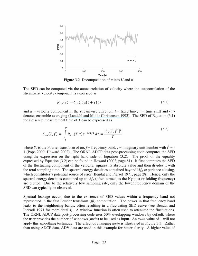
Spectral leakage occurs due to the existence of SED values within a frequency band not

represented in the fast Fourier transform (fft) computation. The power in that frequency band

leaks to the neighboring bands, often resulting in a fluctuating SED curve (see Bendat and

Piersoll 1971 for more details). A window function is often used to attenuate the fluctuations.

The ORNL ADCP data post-processing code uses 50% overlapping windows by default, where

the user provides the number of windows (nwin) to be used as input. An nwin value of 1 will not

apply this smoothing technique. The effect of changing nwin is illustrated in Figure 3.3. Rather

than using ADCP data, ADV data are used in this example for better clarity. A higher value of

0

0.1

0.2

0.3

0.4

0.5

0.6

0 100 200 300 400

(m/

s)

Time (s)

u

U

Page | 24

nwin increases smoothing, but also the lowest frequency of the SED. An nwin value will have a

different smoothing level in two datasets if the number of samples of those datasets is different.

In order to have a similar level of smoothing, a dataset with a high number of samples requires a

higher nwin value than the nwin value used for a dataset with a low number of samples. When

the SED plot is used to determine the peaking of energy at a certain frequency, and its peak

value, the user should recognize that the magnitude of the peaks may change with the smoothing

level.

Figure 3.3 Spectral energy density plot for u

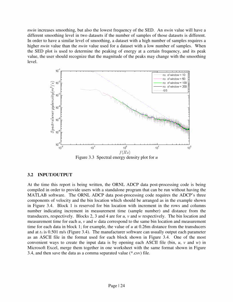
3.2 INPUT/OUTPUT

At the time this report is being written, the ORNL ADCP data post-processing code is being

compiled in order to provide users with a standalone program that can be run without having the

MATLAB software. The ORNL ADCP data post-processing code requires the ADCP’s three

components of velocity and the bin location which should be arranged as in the example shown

in Figure 3.4. Block 1 is reserved for bin location with increment in the rows and columns

number indicating increment in measurement time (sample number) and distance from the

transducers, respectively. Blocks 2, 3 and 4 are for u, v and w respectively. The bin location and

measurement time for each u, v and w data correspond to the same bin location and measurement

time for each data in block 1; for example, the value of u at 0.26m distance from the transducers

and at t5 is 0.501 m/s (Figure 3.4). The manufacturer software can usually output each parameter

as an ASCII file in the format used for each block shown in Figure 3.4. One of the most

convenient ways to create the input data is by opening each ASCII file (bin, u, v and w) in

Microsoft Excel, merge them together in one worksheet with the same format shown in Figure

3.4, and then save the data as a comma separated value (*.csv) file.

Page | 25

Figure 3.4 Input format for the ORNL ADCP stationary data post-processing code

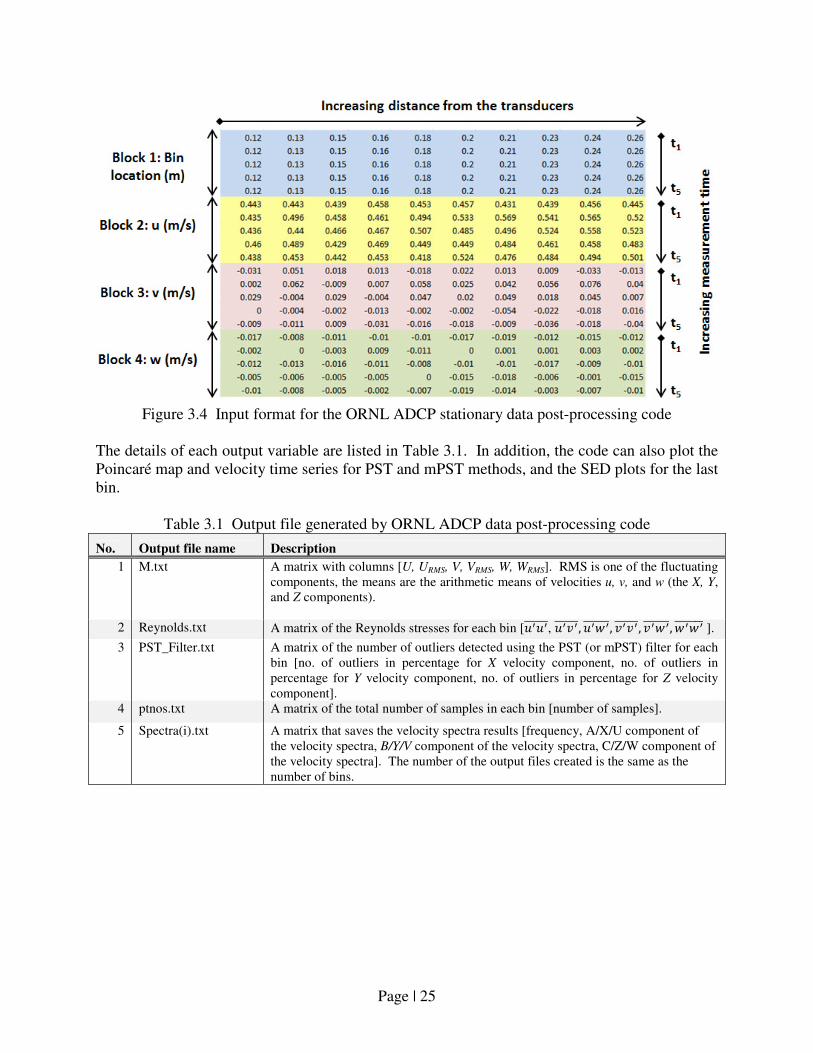
The details of each output variable are listed in Table 3.1. In addition, the code can also plot the

Poincaré map and velocity time series for PST and mPST methods, and the SED plots for the last

bin.

Table 3.1 Output file generated by ORNL ADCP data post-processing code

No. Output file name Description

1 M.txt A matrix with columns [U, URMS, V, VRMS, W, WRMS]. RMS is one of the fluctuating

components, the means are the arithmetic means of velocities u, v, and w (the X, Y,

and Z components).

2 Reynolds.txt A matrix of the Reynolds stresses for each bin [(�(�999999, (�:�999999, (�;�999999, :�:�999999, :�;�999999, ;�;�9999999]. 3 PST_Filter.txt A matrix of the number of outliers detected using the PST (or mPST) filter for each

bin [no. of outliers in percentage for X velocity component, no. of outliers in

percentage for Y velocity component, no. of outliers in percentage for Z velocity

component].

4 ptnos.txt A matrix of the total number of samples in each bin [number of samples].

5 Spectra(i).txt A matrix that saves the velocity spectra results [frequency, A/X/U component of

the velocity spectra, B/Y/V component of the velocity spectra, C/Z/W component of

the velocity spectra]. The number of the output files created is the same as the

number of bins.

Page | 26

3.3 DATA ANALYSIS

The results from different filtering and replacement schemes are compared and analyzed below

to provide a demonstration of the ORNL ADCP data post-processing code. The PST and mPST

filtering, constant calibration parameters values (C1 = 1.1 and C2 = 1.5) are tested. For each

case, three data replacement methods are considered: replacement by the overall average (option

0), replacement by the previous valid point (option 1) and replacement by polynomial

interpolation (option 2). The number of outliers detected, mean velocity, RMS velocity and

power spectral densities (SED) are reported for each case. The measured data used for this

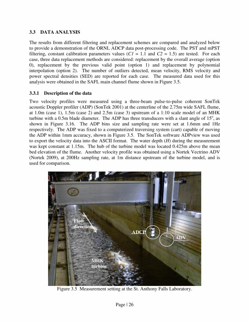
analysis were obtained in the SAFL main channel flume shown in Figure 3.5.

3.3.1 Description of the data

Two velocity profiles were measured using a three-beam pulse-to-pulse coherent SonTek

acoustic Doppler profiler (ADP) (SonTek 2001) at the centerline of the 2.75m wide SAFL flume,

at 1.0m (case 1), 1.5m (case 2) and 2.5m (case 3) upstream of a 1:10 scale model of an MHK

turbine with a 0.5m blade diameter. The ADP has three transducers with a slant angle of 15o, as

shown in Figure 3.16. The ADP bins size and sampling rate were set at 1.6mm and 1Hz

respectively. The ADP was fixed to a computerized traversing system (cart) capable of moving

the ADP within 1mm accuracy, shown in Figure 3.5. The SonTek software ADPview was used

to export the velocity data into the ASCII format. The water depth (H) during the measurement

was kept constant at 1.15m. The hub of the turbine model was located 0.425m above the mean

bed elevation of the flume. Another velocity profile was obtained using a Nortek Vectrino ADV

(Nortek 2009), at 200Hz sampling rate, at 1m distance upstream of the turbine model, and is

used for comparison.

Figure 3.5 Measurement setting at the St. Anthony Falls Laboratory.

Flow

direction

MHK

turbine

ADCP

ADV

Page | 27

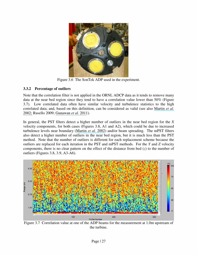
Figure 3.6 The SonTek ADP used in the experiment.

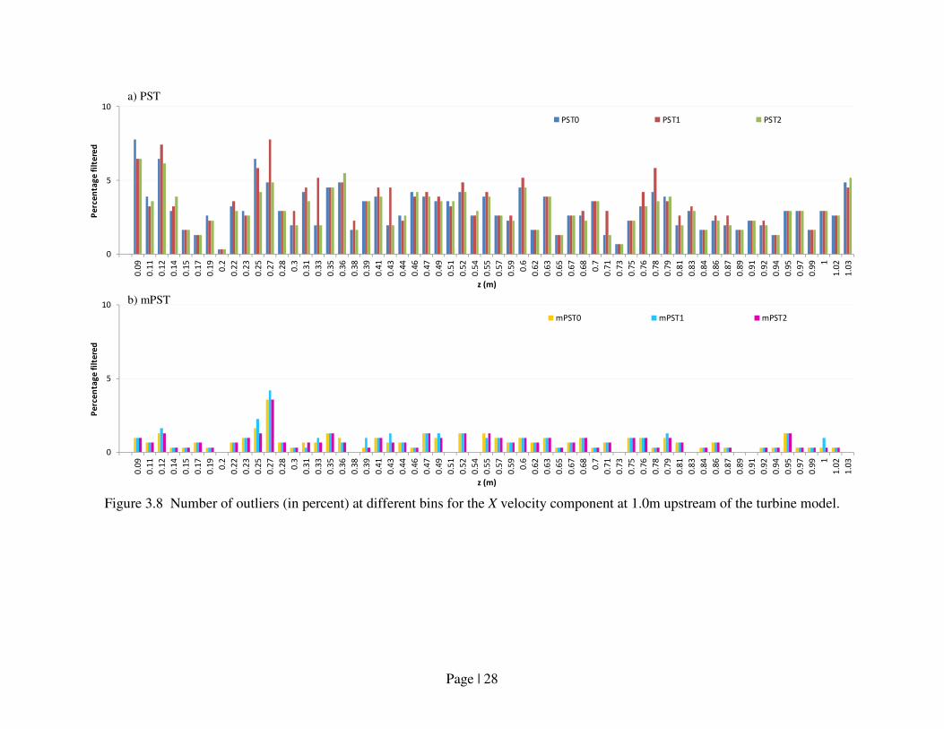
3.3.2 Percentage of outliers

Note that the correlation filter is not applied in the ORNL ADCP data as it tends to remove many

data at the near bed region since they tend to have a correlation value lower than 50% (Figure

3.7). Low correlated data often have similar velocity and turbulence statistics to the high

correlated data; and, based on this definition, can be considered as valid (see also Martin et al.

2002; Rusello 2009; Gunawan et al. 2011).

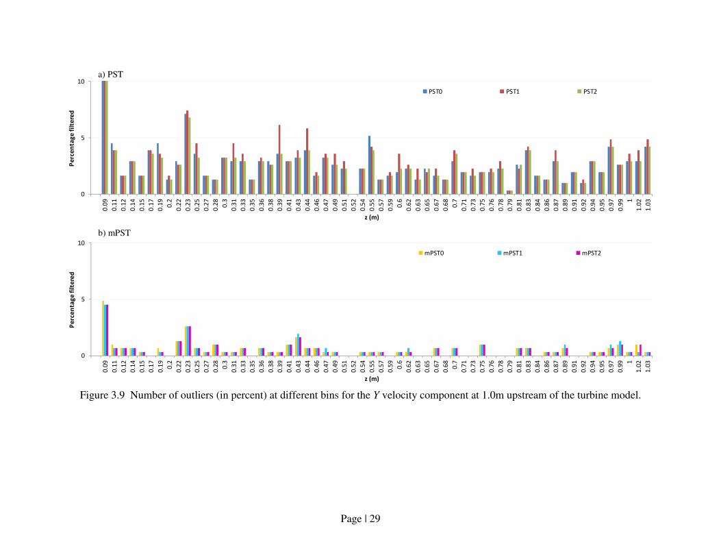
In general, the PST filters detect a higher number of outliers in the near bed region for the X

velocity components, for both cases (Figures 3.8, A1 and A2), which could be due to increased

turbulence levels near boundary (Martin et al. 2002) and/or beam spreading. The mPST filters

also detect a higher number of outliers in the near bed region, but it is much less than the PST

method. Note that the number of outliers is different for each replacement scheme because the

outliers are replaced for each iteration in the PST and mPST methods. For the Y and Z velocity

components, there is no clear pattern on the effect of the distance from bed (z) to the number of

outliers (Figures 3.8, 3.9, A3-A6).

Figure 3.7 Correlation value at one of the ADP beams for the measurement at 1.0m upstream of

the turbine.

Page | 28

Figure 3.8 Number of outliers (in percent) at different bins for the X velocity component at 1.0m upstream of the turbine model.

0

5

10

0.0

9

0.1

1

0.1

2

0.1

4

0.1

5

0.1

7

0.1

9

0.2

0.2

2

0.2

3

0.2

5

0.2

7

0.2

8

0.3

0.3

1

0.3

3

0.3

5

0.3

6

0.3

8

0.3

9

0.4

1

0.4

3

0.4

4

0.4

6

0.4

7

0.4

9

0.5

1

0.5

2

0.5

4

0.5

5

0.5

7

0.5

9

0.6

0.6

2

0.6

3

0.6

5

0.6

7

0.6

8

0.7

0.7

1

0.7

3

0.7

5

0.7

6

0.7

8

0.7

9

0.8

1

0.8

3

0.8

4

0.8

6

0.8

7

0.8

9

0.9

1

0.9

2

0.9

4

0.9

5

0.9

7

0.9

9 1

1.0

2

1.0

3

Pe

rce

nta

ge

fil

tere

d

z (m)

PST0 PST1 PST2

0

5

10

0.0

9

0.1

1

0.1

2

0.1

4

0.1

5

0.1

7

0.1

9

0.2

0.2

2

0.2

3

0.2

5

0.2

7

0.2

8

0.3

0.3

1

0.3

3

0.3

5

0.3

6

0.3

8

0.3

9

0.4

1

0.4

3

0.4

4

0.4

6

0.4

7

0.4

9

0.5

1

0.5

2

0.5

4

0.5

5

0.5

7

0.5

9

0.6

0.6

2

0.6

3

0.6

5

0.6

7

0.6

8

0.7

0.7

1

0.7

3

0.7

5

0.7

6

0.7

8

0.7

9

0.8

1

0.8

3

0.8

4

0.8

6

0.8

7

0.8

9

0.9

1

0.9

2

0.9

4

0.9

5

0.9

7

0.9

9 1

1.0

2

1.0

3

Pe

rce

nta

ge

fil

tere

d

z (m)

mPST0 mPST1 mPST2

a) PST

b) mPST

Page | 29

Figure 3.9 Number of outliers (in percent) at different bins for the Y velocity component at 1.0m upstream of the turbine model.

0

5

10

0.0

9

0.1

1

0.1

2

0.1

4

0.1

5

0.1

7

0.1

9

0.2

0.2

2

0.2

3

0.2

5

0.2

7

0.2

8

0.3

0.3

1

0.3

3

0.3

5

0.3

6

0.3

8

0.3

9

0.4

1

0.4

3

0.4

4

0.4

6

0.4

7

0.4

9

0.5

1

0.5

2

0.5

4

0.5

5

0.5

7

0.5

9

0.6

0.6

2

0.6

3

0.6

5

0.6

7

0.6

8

0.7

0.7

1

0.7

3

0.7

5

0.7

6

0.7

8

0.7

9

0.8

1

0.8

3

0.8

4

0.8

6

0.8

7

0.8

9

0.9

1

0.9

2

0.9

4

0.9

5

0.9

7

0.9

9 1

1.0

2

1.0

3

Pe

rce

nta

ge

fil

tere

d

z (m)

PST0 PST1 PST2

0

5

10

0.0

9

0.1

1

0.1

2

0.1

4

0.1

5

0.1

7

0.1

9

0.2

0.2

2

0.2

3

0.2

5

0.2

7

0.2

8

0.3

0.3

1

0.3

3

0.3

5

0.3

6

0.3

8

0.3

9

0.4

1

0.4

3

0.4

4

0.4

6

0.4

7

0.4

9

0.5

1

0.5

2

0.5

4

0.5

5

0.5

7

0.5

9

0.6

0.6

2

0.6

3

0.6

5

0.6

7

0.6

8

0.7

0.7

1

0.7

3

0.7

5

0.7

6

0.7

8

0.7

9

0.8

1

0.8

3

0.8

4

0.8

6

0.8

7

0.8

9

0.9

1

0.9

2

0.9

4

0.9

5

0.9

7

0.9

9 1

1.0

2

1.0

3

Pe

rce

nta

ge

fil

tere

d

z (m)

mPST0 mPST1 mPST2

a) PST

b) mPST

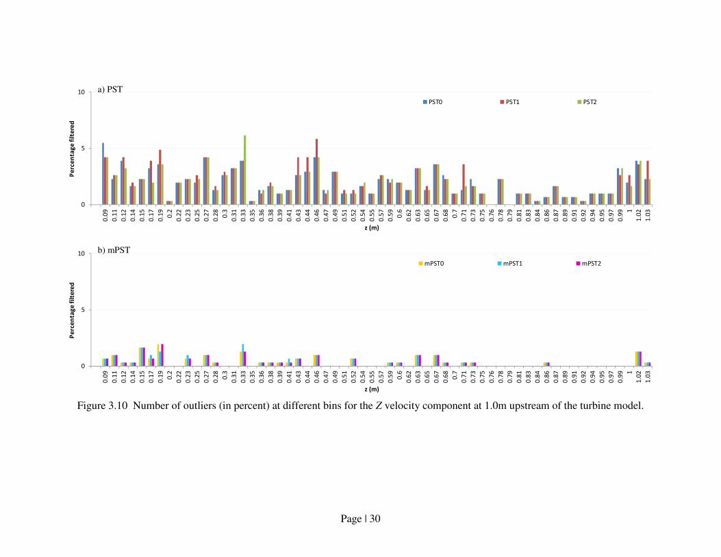
Page | 30

Figure 3.10 Number of outliers (in percent) at different bins for the Z velocity component at 1.0m upstream of the turbine model.

0

5

10

0.0

9

0.1

1

0.1

2

0.1

4

0.1

5

0.1

7

0.1

9

0.2

0.2

2

0.2

3

0.2

5

0.2

7

0.2

8

0.3

0.3

1

0.3

3

0.3

5

0.3

6

0.3

8

0.3

9

0.4

1

0.4

3

0.4

4

0.4

6

0.4

7

0.4

9

0.5

1

0.5

2

0.5

4

0.5

5

0.5

7

0.5

9

0.6

0.6

2

0.6

3

0.6

5

0.6

7

0.6

8

0.7

0.7

1

0.7

3

0.7

5

0.7

6

0.7

8

0.7

9

0.8

1

0.8

3

0.8

4

0.8

6

0.8

7

0.8

9

0.9

1

0.9

2

0.9

4

0.9

5

0.9

7

0.9

9 1

1.0

2

1.0

3

Pe

rce

nta

ge

fil

tere

d

z (m)

PST0 PST1 PST2

0

5

10

0.0

9

0.1

1

0.1

2

0.1

4

0.1

5

0.1

7

0.1

9

0.2

0.2

2

0.2

3

0.2

5

0.2

7

0.2

8

0.3

0.3

1

0.3

3

0.3

5

0.3

6

0.3

8

0.3

9

0.4

1

0.4

3

0.4

4

0.4

6

0.4

7

0.4

9

0.5

1

0.5

2

0.5

4

0.5

5

0.5

7

0.5

9

0.6

0.6

2

0.6

3

0.6

5

0.6

7

0.6

8

0.7

0.7

1

0.7

3

0.7

5

0.7

6

0.7

8

0.7

9

0.8

1

0.8

3

0.8

4

0.8

6

0.8

7

0.8

9

0.9

1

0.9

2

0.9

4

0.9

5

0.9

7

0.9

9 1

1.0

2

1.0

3

Pe

rce

nta

ge

fil

tere

d

z (m)

mPST0 mPST1 mPST2

a) PST

b) mPST

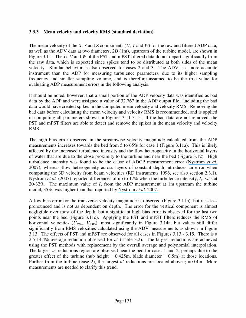
Page | 31

3.3.3 Mean velocity and velocity RMS (standard deviation)

The mean velocity of the X, Y and Z components (U, V and W) for the raw and filtered ADP data,

as well as the ADV data at two diameters, 2D (1m), upstream of the turbine model, are shown in

Figure 3.11. The U, V and W of the PST and mPST filtered data do not depart significantly from

the raw data, which is expected since spikes tend to be distributed at both sides of the mean

velocity. Similar behavior is also observed for cases 2 and 3. The ADV is a more accurate

instrument than the ADP for measuring turbulence parameters, due to its higher sampling

frequency and smaller sampling volume, and is therefore assumed to be the true value for

evaluating ADP measurement errors in the following analysis.

It should be noted, however, that a small portion of the ADP velocity data was identified as bad

data by the ADP and were assigned a value of 32.767 in the ADP output file. Including the bad

data would have created spikes in the computed mean velocity and velocity RMS. Removing the

bad data before calculating the mean velocity and velocity RMS is recommended, and is applied

in computing all parameters shown in Figures 3.11-3.15. If the bad data are not removed, the

PST and mPST filters are able to detect and remove the spikes in the mean velocity and velocity

RMS.

The high bias error observed in the streamwise velocity magnitude calculated from the ADP

measurements increases towards the bed from 5 to 65% for case 1 (Figure 3.11a). This is likely

affected by the increased turbulence intensity and the flow heterogeneity in the horizontal layers

of water that are due to the close proximity to the turbine and near the bed (Figure 3.12). High

turbulence intensity was found to be the cause of ADCP measurement error (Nystrom et al.

2007), whereas flow heterogeneity across layers of constant depth introduces an error when

computing the 3D velocity from beam velocities (RD instruments 1996, see also section 2.3.1).

Nystrom et al. (2007) reported differences of up to 17% when the turbulence intensity, Iu, was at

20-32%. The maximum value of Iu from the ADP measurement at 1m upstream the turbine

model, 35%, was higher than that reported by Nystrom et al. 2007.

A low bias error for the transverse velocity magnitude is observed (Figure 3.11b), but it is less

pronounced and is not as dependent on depth. The error for the vertical component is almost

negligible over most of the depth, but a significant high bias error is observed for the last two

points near the bed (Figure 3.11c). Applying the PST and mPST filters reduces the RMS of

horizontal velocities (URMS, VRMS), most significantly in Figure 3.14a, but values still differ

significantly from RMS velocities calculated using the ADV measurements as shown in Figure

3.13. The effects of PST and mPST are observed for all cases in Figures 3.13 - 3.15. There is a

2.5-14.4% average reduction observed for u’ (Table 3.2). The largest reductions are achieved

using the PST methods with replacement by the overall average and polynomial interpolation.

The largest u’ reductions region are observed near the bed for cases 1 and 2, perhaps due to the

greater effect of the turbine (hub height = 0.425m, blade diameter = 0.5m) at those locations.

Further from the turbine (case 2), the largest u’ reductions are located above z = 0.4m. More

measurements are needed to clarify this trend.

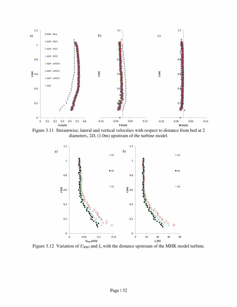
Page | 32

Figure 3.11 Streamwise, lateral and vertical velocities with respect to distance from bed at 2

diameters, 2D, (1.0m) upstream of the turbine model.

Figure 3.12 Variation of URMS and Iu with the distance upstream of the MHK model turbine.

0

0.2

0.4

0.6

0.8

1

1.2

0 0.1 0.2 0.3 0.4 0.5 0.6

z (m

)

U (m/s)

ADP - Raw

ADP - PST1

ADP - PST1

ADP - PST2

ADP - mPST0

ADP - mPST1

ADP - mPST2

ADV

0

0.2

0.4

0.6

0.8

1

1.2

-0.15 -0.05 0.05 0.15

z (m

)

V (m/s)

0

0.2

0.4

0.6

0.8

1

1.2

-0.15 -0.05 0.05 0.15

z (m

)

W (m/s)

0

0.2

0.4

0.6

0.8

1

1.2

0 0.05 0.1 0.15

z (m

)

URMS (m/s)

2D

3D

5D

0

0.2

0.4

0.6

0.8

1

1.2

0 10 20 30 40

z (m

)

Iu (%)

2D

3D

5D

a) b) c)

a) b)

Page | 33

Figure 3.13 RMS values of streamwise, lateral and vertical velocities with respect to distance

from bed at 2 diameters, 2D, (1.0m) upstream of the turbine model.

Figure 3.14 RMS values of streamwise, lateral and vertical velocities with respect to distance

from bed at 3 diameters, 3D, (1.5m) upstream of the turbine model.

0

0.2

0.4

0.6

0.8

1

1.2

0 0.05 0.1 0.15

z (m

)

URMS (m/s)

ADP - Raw

ADP - PST1

ADP - PST1

ADP - PST2

ADP - mPST0

ADP - mPST1

ADP - mPST2

ADV

0

0.2

0.4

0.6

0.8

1

1.2

0 0.05 0.1 0.15

z (m

)

VRMS (m/s)

0

0.2

0.4

0.6

0.8

1

1.2

0 0.05 0.1 0.15

z (m

)

WRMS (m/s)

0

0.2

0.4

0.6

0.8

1

1.2

0 0.05 0.1 0.15

z (m

)

URMS (m/s)

Raw data

PST0

PST1

PST2

mPST0

mPST1

mPST2

0

0.2

0.4

0.6

0.8

1

1.2

0 0.05 0.1 0.15

z (m

)

VRMS (m/s)

0

0.2

0.4

0.6

0.8

1

1.2

0 0.05 0.1 0.15

z (m

)

WRMS (m/s)

a) b)

b) a)

c)

c)

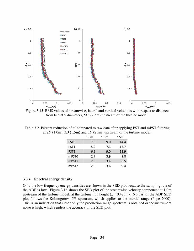
Page | 34

Figure 3.15 RMS values of streamwise, lateral and vertical velocities with respect to distance

from bed at 5 diameters, 5D, (2.5m) upstream of the turbine model.

Table 3.2 Percent reduction of u’ compared to raw data after applying PST and mPST filtering

at 2D (1.0m), 3D (1.5m) and 5D (2.5m) upstream of the turbine model.

1.0m 1.5m 2.5m

PST0 7.5 9.0 14.4

PST1 5.9 7.3 12.7

PST2 6.9 9.0 13.9

mPST0 2.7 3.9 9.8

mPST1 2.5 3.4 8.5

mPST2 2.5 3.6 9.4

3.3.4 Spectral energy density

Only the low frequency energy densities are shown in the SED plot because the sampling rate of

the ADP is low. Figure 3.16 shows the SED plot of the streamwise velocity component at 1.0m

upstream of the turbine model, at the turbine hub height (z = 0.425m). No part of the ADP SED

plot follows the Kolmogorov -5/3 spectrum, which applies to the inertial range (Pope 2000).

This is an indication that either only the production range spectrum is obtained or the instrument

noise is high, which renders the accuracy of the SED plot.

0

0.2

0.4

0.6

0.8

1

1.2

0 0.05 0.1 0.15

z (m

)

URMS (m/s)

Raw data

PST0

PST1

PST2

mPST0

mPST1

mPST2

0

0.2

0.4

0.6

0.8

1

1.2

0 0.05 0.1 0.15

z (m

)

VRMS (m/s)

0

0.2

0.4

0.6

0.8

1

1.2

0 0.05 0.1 0.15

z (m

)

WRMS (m/s)

b) a) c)

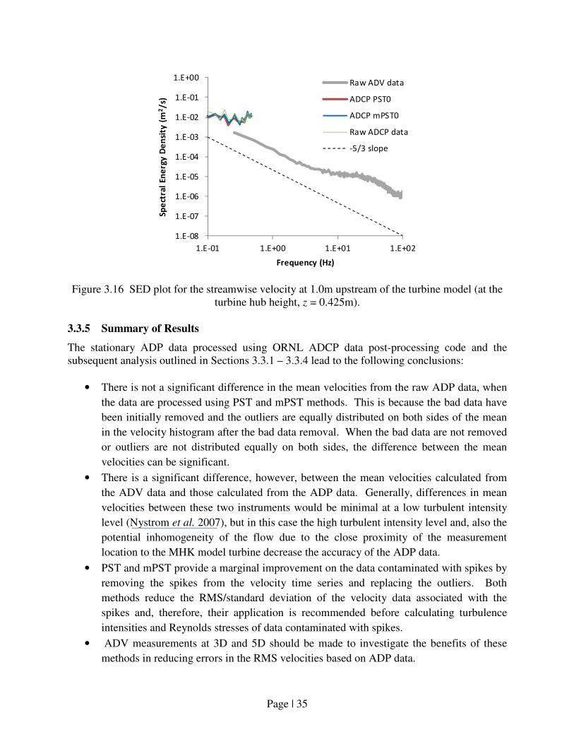
Page | 35

Figure 3.16 SED plot for the streamwise velocity at 1.0m upstream of the turbine model (at the

turbine hub height, z = 0.425m).

3.3.5 Summary of Results

The stationary ADP data processed using ORNL ADCP data post-processing code and the

subsequent analysis outlined in Sections 3.3.1 – 3.3.4 lead to the following conclusions:

• There is not a significant difference in the mean velocities from the raw ADP data, when

the data are processed using PST and mPST methods. This is because the bad data have

been initially removed and the outliers are equally distributed on both sides of the mean

in the velocity histogram after the bad data removal. When the bad data are not removed

or outliers are not distributed equally on both sides, the difference between the mean

velocities can be significant.

• There is a significant difference, however, between the mean velocities calculated from

the ADV data and those calculated from the ADP data. Generally, differences in mean

velocities between these two instruments would be minimal at a low turbulent intensity

level (Nystrom et al. 2007), but in this case the high turbulent intensity level and, also the

potential inhomogeneity of the flow due to the close proximity of the measurement

location to the MHK model turbine decrease the accuracy of the ADP data.

• PST and mPST provide a marginal improvement on the data contaminated with spikes by

removing the spikes from the velocity time series and replacing the outliers. Both

methods reduce the RMS/standard deviation of the velocity data associated with the

spikes and, therefore, their application is recommended before calculating turbulence

intensities and Reynolds stresses of data contaminated with spikes.

• ADV measurements at 3D and 5D should be made to investigate the benefits of these

methods in reducing errors in the RMS velocities based on ADP data.

1.E-08

1.E-07

1.E-06

1.E-05

1.E-04

1.E-03

1.E-02

1.E-01

1.E+00

1.E-01 1.E+00 1.E+01 1.E+02

Sp

ect

ral

En

erg

y D

en

sity

(m

2/

s)

Frequency (Hz)

Raw ADV data

ADCP PST0

ADCP mPST0

Raw ADCP data

-5/3 slope

Page | 36

• The spectral energy densities plot, based on the ADP data, is not suitable to analyze the

turbulent scales down to the viscous range due to the low sampling frequency, large

sampling volume and beam spreading of the ADP.

• The PST does not require parameterization, which is considered a practical advantage

over the mPST method.

Page | 37

4 FUTURE WORK

The ORNL ADCP data post-processing code provides an integrated tool to detect and replace

outliers using different methods to improve calculations of power density and annual energy

production at the MHK site. In order to improve and broaden the capability of the code, some

additional functions listed below will be added in the future:

1. Spatial averaging of velocity data obtained using ship-mounted ADCPs.

2. Calculation of the shear velocity from the data obtained from the ADCP stationary

measurement.

3. The addition of a plotting tool for mean velocity and velocity RMS.

Page | 38

REFERENCES

Baldwin, J. T., Deutsch, S., Petrie, H. L. and Tarbell, J. M. (1993). Determination of principal

Reynolds stresses in pulsatile flows after elliptical filtering of discrete velocity

measurements. J. Biomech. Eng., v 115, I4a, pg 396-404.

Barua, D.K. and Rahman, K.H. (1998). Some aspects of turbulent flow structure in large alluvial

rivers. Journal of Hydraulic Research, IAHR, 36,235–252.

Bendat, J. and Piersol, A. (1971). Random data: Analysis and measurement procedures. John

Wiley and Sons, Inc.

Carr, M.L and Rehman, C.R. (2007). Measuring the dispersion coefficient with Acoustic

Doppler Current Profilers. Journal of Hydraulic Engineering, ASCE, Vol. 133, No. 8.

Cheng, R. T., C. H. Ling and J. W. Gartner. (2000). Direct measurement of turbulence properties

by a BB-ADCP in bottom boundary layer, Interactions between Estuaries,Coastal Seas and

Shelf Seas, Ed. T. Yanagi, pp. 37-55.

Dinehart, R.L. & Burau, J.R. (2005a). Averaged indicators of secondary flow in repeated

acoustic Doppler current profiler crossings of bends. Water Resources Research, Vol. 41.

Dinehart, R.L. & Burau, J.R. (2005b). Repeated surveys by acoustic Doppler current profiler for

flow and sediment dynamics in a tidal river. Journal of Hydrology, XX 1–21.

Einstein, H. A. and Li, H. (1958). Secondary currents in straight channels. Transactions of the

American Geophysical Union, Vol. 39, No.6, pp 1085-1088.

Epler, J., Polagye, B., and Thomson, J. (2010). Shipboard acoustic Doppler current profiler

surveys to assess tidal current resources, MTS/IEEE Oceans 2010, Seattle, WA, September

20-23.

Fontaine, A.A., Ellis, J.T., Healy, T.M., Hopmeyer, J. and Yoganathan, A.P. (1996).

Identification of peak stresses in cardiac prostheses: A comparison of two-dimensional

versus three-dimensional principal stress analyses. American Society Artificial Internal

Organs Journal, Vol. 42, pp. 154-163.

Goring, D. G. and Nikora, V. I. (2002). Despiking acoustic Doppler velocimeter data. J.

Hydraulic Eng., 128(1) 117-126.

Gunawan, B., Sun, X., Sterling, M., Knight, D. W., Shiono, K., Chandler, J., Rameshwaran, P.,

Wright, N. G., Sellin, R. H. J., Tang, X. and Fujita, I. (2008). An integrated and novel

approach to estimating the conveyance capacity of the River Blackwater. Proceedings of the

Eight International Conference on Hydro-Science and Engineering, Nagoya, Japan,

Page | 39

September 8–12.

Gunawan, B. (2010). A study of flow structures in a two-stage channel using field data, physical

model and numerical modelling, PhD thesis, University of Birmingham, UK.

Gunawan, B., Sterling, M. and Knight, D. W. (2010a). Using an acoustic Doppler current

profiler in a small river. Water and Environment Journal, 24: 147–158. doi: 10.1111/j.1747-

6593.2009.00170.x

Gunawan, B., Sterling, M., Tang, X. and Knight, D. W. (2010b). Measuring and modeling flow

structures in a small river. Proceeding of the International Conference on Fluvial Hydraulics,

Braunschweig, Germany, September 8-10.

Gunawan, B., Neary, V. S. and McNutt, J. R. (2011). ORNL ADV post-processing guide and

MATLAB algorithms for MHK site flow and turbulence analysis. ORNL/TML-2011/338.

Howard, R. M. (2002). Principles of random signal analysis and low noise design: The power

spectral density and its applications. Wiley-IEEE Press; 1st edition (August 8).

Holmes, R.R. and Garcia, M.H. (2002). Velocity and sediment concentration measurements over

bedforms in sand-bed rivers. Proceedings of the ASCE/IAHR Hydraulic Measurements &

Experimental Methods Conference, Estes Park, CO (CD-ROM).

Holmes, R. R. and Garcia, M. H. (2008). Flow over bedforms in a large sand-bed river: A field

investigation. Journal of Hydraulic Research, 46(3): p. 322-333.

Ikeda, S., Sano, T., Fukumoto, M. And Kawamura, K. (2001) Organised horizontal vortices and

lateral sediment transport in compound channel flows, Journal of JSCE.

Klein, H. (2003). Investigating sediment re-mobilisation due to wave action by means of ADCP

echo intensity data field data from the Tromper Wiek, western Baltic Sea estuarine. Coastal

and Shelf Science 58 (2003) 467–474

Knight, D.W., Aya, S., Ikeda, S., Nezu, I and Shiono, K. (2009). Flow structure (Chapter 2) in

Flow and sediment transport in compound channels, e.d. Ikeda, S. and McEwan, I.K. IAHR

Monograph. IAHR Spain.

Landahl, M. T. and Mollo-Christensen, E. (1992). Turbulence and random processes in fluid

mechanics. Cambridge University Press.

Le Coz, J., Gilles, P., Magali, J., and Andre, P. (2007). Mean vertical velocity profiles from

ADCP river discharge measurement datasets, Proceedings 32nd Congress of International

Association of Hydraulic Engineering and Research (CD-ROM).

Lemmin, U. and Rolland, T. (1997). Acoustic velocity profiler for laboratory and field studies.

Journal of Hydraulic Engineering, ASCE, Vol.123/12.

Page | 40

Lohrmann, A., Hackett, B. and Røed, L. P. (1990). High resolution measurements of turbulence,

velocity and stress using a pulse-to-pulse coherent sonar. J. Atmos. Oceanic Technol., 7, 19–

37. doi: 10.1175/1520-0426(1990)007<0019:HRMOTV>2.0.CO;2

Luznik, L., Gurka, R., Nimmo Smith, W. A. M., Zhu, W., Katz, J. and Osborn, T. R. (2007).

Distribution of energy spectra, Reynolds stresses, turbulence production, and dissipation in a

tidally driven bottom boundary layer, Journal of Physical Oceanography, vol. 37, pp.1527–

1550.

Martin, V., Fisher, T. S. R., Millar, R. G. and Quick, M. C. (2002). ADV data analysis for

turbulent flows: Low correlation problem. Proceedings of Hydraulic Measurements and

Experimental Methods Conference 2002. ASCE Conf. Proc. doi:10.1061/40655(2002)101

Merckelbach, L.M. (2006). A model for high-frequency acoustic Doppler current profiler

backscatter from suspended sediment in strong currents. Continental Shelf Research,

26/1316–1335.

Mueller, D.S. (2003). Field Evaluation of boat-mounted Acoustic Doppler instruments used to

measure streamflow. Proc. of the IEEE/OES Seventh Working Conference on Current

Measurement Technology.

Mueller, D.S., and Wagner, C.R. (2009). Measuring discharge with acoustic Doppler current

profilers from a moving boat: U.S. Geological Survey Techniques and Methods 3A-22, 72 p.

U.S. Geological Survey. Online material available at http://pubs.water.usgs.gov/tm3a22.

(last accessed 9/19/2011).

Muste, M., Yu, K. and Spasojevic, M. (2004a). Practical aspects of ADCP data use for

quantification of mean river flow characteristics; Part I: Moving-vessel measurements. Flow

Measurement and Instrumentation, 15(1), 1-16.

Muste, M., Yu, K., Pratt, T. and Abraham, D. (2004b). Practical aspects of ADCP data use for

quantification of mean river flow characteristics; Part II: Fixed-vessel measurements. Flow

Measurement and Instrumentation, 15(1), 17-28.

Neary, V. S. and Sale, D. C. (2010). Flow characteristics of river resources for hydrokinetic

energy conversion. Conference Proceedings, HydroVision International, July 27-30, 2010,

Charlotte, NC.

Neary, V. S., Chamorro, L., Hill, C., Gunawan, B., Sotiropolous, F. and Kang, S. K. (2011a).

Experimental study of the effects of turbulence and large coherent structures on hydrokinetic

turbines. Poster presentation. HydroVision International, July 19-22, 2011, Sacramento, CA.

Neary, V. S., Gunawan, B., Bevelhimer, M. S., Polagye, B., Thomson, J., Richmond, M.C.,

Durgesh, V., Muste, M. and, Fontaine, A. (2011b). Field measurements for MHK site

development: Best practices manual. ORNL/TML-2011/419.

Page | 41

Nezu, I. and Nakagawa, H. (1993). Turbulence in open-channel flows. IAHR Monograph Series,

A. A. Balkema, Rotterdam

Nortek. (2009). Vectrino velocimeter user guide. Online material available at

http://www.nortekusa.com/en/support/manuals (last accessed 9/19/2011)

Nystrom, E. A., Rehmann, C. R., and Oberg, K. A. (2007). Evaluation of mean velocity and

turbulence measurements with ADCPs. Journal of Hydraulic Engineering, ASCE,

Vol.133/12.

Oberg, K.A. (2002). In search of easy-to-use methods for calibrating ADCP’s for velocity and

discharge measurements. Proc. Hydraulic Measurements & Experimental Methods 2002 CD-

ROM.

Oberg, K. & Mueller, D.S. (2007). Validation of Streamflow Measurements Made with Acoustic

Doppler Current Profilers. Journal of Hydraulic Engineering, ASCE, Vol.133/12.

Parsheh, M., Sotiropoulos, F. and Port´e-Agel, F. (2010). Estimation of Power Spectra of

acoustic-Doppler velocimetry data contaminated with intermittent spikes. J. Hydraulic Eng.

ASCE, Vol.136, 368 (2010); doi:10.1061/(ASCE)HY.1943-7900.0000202.

Petrie, H. L., Samimy, M. and Addy, A. L. (1988). Laser Doppler velocity bias in separated

turbulent flows. Exp. in Fluids, v 6, pg 80-88.

Perkins, H. J. (1970). The formation of streamwise vorticity in turbulent flow. Journal of Fluid

Mechanics, Cambridge University Press, 44 (04): 721-740.

RD Instruments. (1996). Acoustic Doppler current profilers - principle of operation, A practical

primer. San Diego, CA, RD Instruments.

RD Instruments. (1998). ADCP Coordinate transformation: Formulas and calculations.

Teledyne RD Instruments, Inc., San Diego, California.

RD Instruments. (2011a). ADCP brochures Online material available at

http://www.rdinstruments.com/default.aspx (last accessed 9/19/2011).

RD Instruments. (2011b). Introduction to the method used for measuring velocity profiles with

BroadBand ADCP. Online material available at

http://www.rdinstruments.com/tips/tips.aspx#primer (last accessed 9/19/2011).

Rennie, C.D., Millar, R.G. & Church, M.A. (2002). Measurement of bed load velocity using an

Acoustic Doppler Current Profiler. Journal of Hydraulic Engineering, ASCE, Vol.128/5.

Rennie, C.D. & Church, M. (2007). ADCP shear stress and bedload transport in a large

wandering gravel-bed river. IAHR Venice Congress 2007.

Page | 42

Rowe, F. and J. Young (1979). An ocean current profiler using Doppler sonar, Oceans ’79

Proceedings.

Rusello, P. J. (2009). A practical primer for pulse coherent instruments, Nortek technical note

No.: TN-027.

Sellin R.H.J. (1964). A laboratory investigation into the interaction between the flow in the

channel of a river and that over its floodplain, La Houille Blanche, Vol. 19, No. 7, pp 793-

801.

Shih, H.H., Payton, C., Sprenke, J. & Mero, T. (2000). Towing basin speed calibration of

acoustic Doppler current profiling instruments. Proc. 2000 Joint Conf. on Water Resources

Engineering and Water Resources Planning and Management, ASCE, Reston, Va.

Sime, L.C., Ferguson, R.I. & Church, M. (2007). Estimating shear stress from moving boat

acoustic Doppler velocity measurements in a large gravel bed river. Water Resources

Research, Vol. 43.

Simpson, M.R. (2001). Discharge Measurements Using a Broad-Band Acoustic Doppler Current

Profiler. Online material available at http://pubs.usgs.gov/of/2001/ofr0101/text.pdf (last

accessed: 9/19/2011).

Stone, M.C. and Hotchkiss, R.H. (2007). Evaluating velocity measurement techniques in shallow

streams. Journal of Hydraulic Research, IAHR, Vol. 45, No. 6, pp. 752 – 762.

SonTek. (2001). Acoustic Doppler profiler technical documentation.

Stacey, M. T., Monismith, S. G., and Burau, J. R. (1999). Measurements of Reynolds stress

profiles in unstratified tidal flow. Journal of Geophysical Research-Oceans, 104(C5), 10933-

10949.

Szupiany, R.N., Amsler, M.L., Best, J.L. & Parsons, D.R. (2007). Comparison of fixed- and

moving-vessel flow measurements with an aDP in a large river. Journal of Hydraulic

Engineering, ASCE, pp. 1299-1309

Thomson J., Polagye, B., Richmond, M., and Durgesh, V. (2010). Quantifying turbulence for

tidal power applications, MTS/IEEE Oceans 2010, Seattle, WA September 20-23.

Turnipseed, D.P. (2002). Tidal Flux Variation in the Lower Pearl River and Lake Pontchartrain

Estuaries of Mississippi and Louisiana. Proceedings of the Hydraulic Measurements and

Experimental Methods Conference 2002.

Wahl, T. L. (2003). Discussion of despiking acoustic Doppler velocimeter data. J. Hydraulic

Eng., 129(6), 484 - 487.

Page | 43

APPENDIX: NUMBER OF OUTLIERS FOR CASES 2 AND 3

Page | 44

Figure A1 Number of outliers (in percent) at different bins for the X velocity component at 1.5m upstream the turbine model.

0

5

10

0.0

7

0.0

9

0.1

1

0.1

2

0.1

4

0.1

5

0.1

7

0.1

9

0.2

0.2

2

0.2

3

0.2

5

0.2

7

0.2

8

0.3

0.3

1

0.3

3

0.3

5

0.3

6

0.3

8

0.3

9

0.4

1

0.4

3

0.4

4

0.4

6

0.4

7

0.4

9

0.5

1

0.5

2

0.5

4

0.5

5

0.5

7

0.5

9

0.6

0.6

2

0.6

3

0.6

5

0.6

7

0.6

8

0.7

0.7

1

0.7

3

0.7

5

0.7

6

0.7

8

0.7

9

0.8

1

0.8

3

0.8

4

0.8

6

0.8

7

0.8

9

0.9

1

0.9

2

0.9

4

0.9

5

0.9

7

0.9

9 1

1.0

2

1.0

3

Pe

rce

nta

ge

fil

tere

d

z (m)

PST0 PST1 PST2

0

5

10

0.0

7

0.0

9

0.1

1

0.1

2

0.1

4

0.1

5

0.1

7

0.1

9

0.2

0.2

2

0.2

3

0.2

5

0.2

7

0.2

8

0.3

0.3

1

0.3

3

0.3

5

0.3

6

0.3

8

0.3

9

0.4

1

0.4

3

0.4

4

0.4

6

0.4

7

0.4

9

0.5

1

0.5

2

0.5

4

0.5

5

0.5

7

0.5

9

0.6

0.6

2

0.6

3

0.6

5

0.6

7

0.6

8

0.7

0.7

1

0.7

3

0.7

5

0.7

6

0.7

8

0.7

9

0.8

1

0.8

3

0.8

4

0.8

6

0.8

7

0.8

9

0.9

1

0.9

2

0.9

4

0.9

5

0.9

7

0.9

9 1

1.0

2

1.0

3

Pe

rce

nta

ge

fil

tere

d

z (m)

mPST0 mPST1 mPST2

a) PST

b) mPST

Page | 45

Figure A2 Number of outliers (in percent) at different bins for the X velocity component at 2.5m upstream the turbine model.

0

5

10

0.1

1

0.1

2

0.1

4

0.1

5

0.1

7

0.1

9

0.2

0.2

2

0.2

3

0.2

5

0.2

7

0.2

8

0.3

0.3

1

0.3

3

0.3

5

0.3

6

0.3

8

0.3

9

0.4

1

0.4

3

0.4

4

0.4

6

0.4

7

0.4

9

0.5

1

0.5

2

0.5

4

0.5

5

0.5

7

0.5

9

0.6

0.6

2

0.6

3

0.6

5

0.6

7

0.6

8

0.7

0.7

1

0.7

3

0.7

5

0.7

6

0.7

8

0.7

9

0.8

1

0.8

3

0.8

4

0.8

6

0.8

7

0.8

9

0.9

1

0.9

2

0.9

4

0.9

5

0.9

7

0.9

9 1

1.0

2

1.0

3

Pe

rce

nta

ge

fil

tere

d

z (m)

PST0 PST1 PST2

0

5

10

0.1

1

0.1

2

0.1

4

0.1

5

0.1

7

0.1

9

0.2

0.2

2

0.2

3

0.2

5

0.2

7

0.2

8

0.3

0.3

1

0.3

3

0.3

5

0.3

6

0.3

8

0.3

9

0.4

1

0.4

3

0.4

4

0.4

6

0.4

7

0.4

9

0.5

1

0.5

2

0.5

4

0.5

5

0.5

7

0.5

9

0.6

0.6

2

0.6

3

0.6

5

0.6

7

0.6

8

0.7

0.7

1

0.7

3

0.7

5

0.7

6

0.7

8

0.7

9

0.8

1

0.8

3

0.8

4

0.8

6

0.8

7

0.8

9

0.9

1

0.9

2

0.9

4

0.9

5

0.9

7

0.9

9 1

1.0

2

1.0

3

Pe

rce

nta

ge

fil

tere

d

z (m)

mPST0 mPST1 mPST2

a) PST

b) mPST

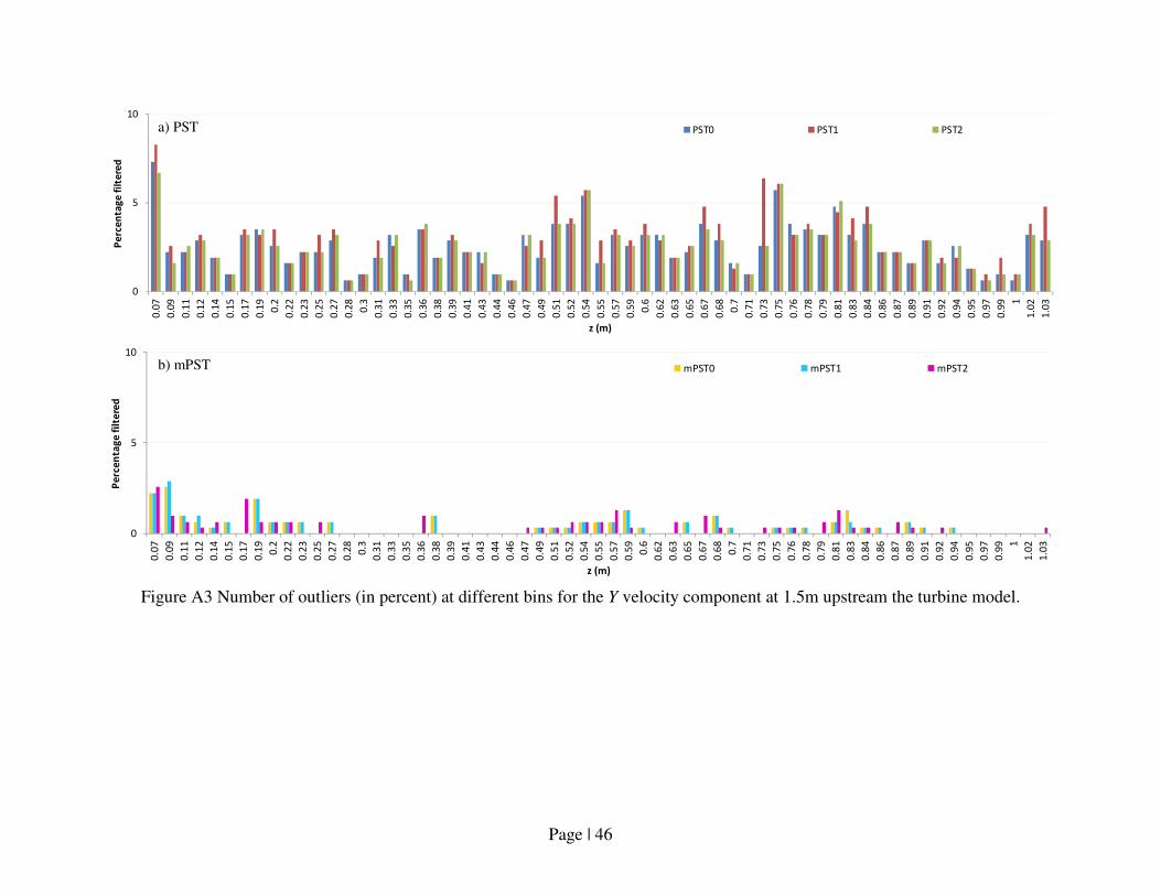
Page | 46

Figure A3 Number of outliers (in percent) at different bins for the Y velocity component at 1.5m upstream the turbine model.

0

5

10

0.0

7

0.0

9

0.1

1

0.1

2

0.1

4

0.1

5

0.1

7

0.1

9

0.2

0.2

2

0.2

3

0.2

5

0.2

7

0.2

8

0.3

0.3

1

0.3

3

0.3

5

0.3

6

0.3

8

0.3

9

0.4

1

0.4

3

0.4

4

0.4

6

0.4

7

0.4

9

0.5

1

0.5

2

0.5

4

0.5

5

0.5

7

0.5

9

0.6

0.6

2

0.6

3

0.6

5

0.6

7

0.6

8

0.7

0.7

1

0.7

3

0.7

5

0.7

6

0.7

8

0.7

9

0.8

1

0.8

3

0.8

4

0.8

6

0.8

7

0.8

9

0.9

1

0.9

2

0.9

4

0.9

5

0.9

7

0.9

9 1

1.0

2

1.0

3

Pe

rce

nta

ge

fil

tere

d

z (m)

PST0 PST1 PST2

0

5

10

0.0

7

0.0

9

0.1

1

0.1

2

0.1

4

0.1

5

0.1

7

0.1

9

0.2

0.2

2

0.2

3

0.2

5

0.2

7

0.2

8

0.3

0.3

1

0.3

3

0.3

5

0.3

6

0.3

8

0.3

9

0.4

1

0.4

3

0.4

4

0.4

6

0.4

7

0.4

9

0.5

1

0.5

2

0.5

4

0.5

5

0.5

7

0.5

9

0.6

0.6

2

0.6

3

0.6

5

0.6

7

0.6

8

0.7

0.7

1

0.7

3

0.7

5

0.7

6

0.7

8

0.7

9

0.8

1

0.8

3

0.8

4

0.8

6

0.8

7

0.8

9

0.9

1

0.9

2

0.9

4

0.9

5

0.9

7

0.9

9 1

1.0

2

1.0

3

Pe

rce

nta

ge

fil

tere

d

z (m)

mPST0 mPST1 mPST2

a) PST

b) mPST

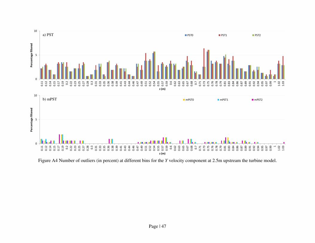
Page | 47

Figure A4 Number of outliers (in percent) at different bins for the Y velocity component at 2.5m upstream the turbine model.

0

5

10

0.1

1

0.1

2

0.1

4

0.1

5

0.1

7

0.1

9

0.2

0.2

2

0.2

3

0.2

5

0.2

7

0.2

8

0.3

0.3

1

0.3

3

0.3

5

0.3

6

0.3

8

0.3

9

0.4

1

0.4

3

0.4

4

0.4

6

0.4

7

0.4

9

0.5

1

0.5

2

0.5

4

0.5

5

0.5

7

0.5

9

0.6

0.6

2

0.6

3

0.6

5

0.6

7

0.6

8

0.7

0.7

1

0.7

3

0.7

5

0.7

6

0.7

8

0.7

9

0.8

1

0.8

3

0.8

4

0.8

6

0.8

7

0.8

9

0.9

1

0.9

2

0.9

4

0.9

5

0.9

7

0.9

9 1

1.0

2

1.0

3

Pe

rce

nta

ge

fil

tere

d

z (m)

PST0 PST1 PST2

0

5

10

0.1

1

0.1

2

0.1

4

0.1

5

0.1

7

0.1

9

0.2

0.2

2

0.2

3

0.2

5

0.2

7

0.2

8

0.3

0.3

1

0.3

3

0.3

5

0.3

6

0.3

8

0.3

9

0.4

1

0.4

3

0.4

4

0.4

6

0.4

7

0.4

9

0.5

1

0.5

2

0.5

4

0.5

5

0.5

7

0.5

9

0.6

0.6

2

0.6

3

0.6

5

0.6

7

0.6

8

0.7

0.7

1

0.7

3

0.7

5

0.7

6

0.7

8

0.7

9

0.8

1

0.8

3

0.8

4

0.8

6

0.8

7

0.8

9

0.9

1

0.9

2

0.9

4

0.9

5

0.9

7

0.9

9 1

1.0

2

1.0

3

Pe

rce

nta

ge

fil

tere

d

z (m)

mPST0 mPST1 mPST2

a) PST

b) mPST

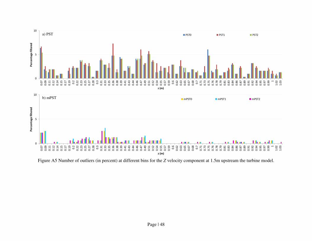
Page | 48

Figure A5 Number of outliers (in percent) at different bins for the Z velocity component at 1.5m upstream the turbine model.

0

5

10

0.0

7

0.0

9

0.1

1

0.1

2

0.1

4

0.1

5

0.1

7

0.1

9

0.2

0.2

2

0.2

3

0.2

5

0.2

7

0.2

8

0.3

0.3

1

0.3

3

0.3

5

0.3

6

0.3

8

0.3

9

0.4

1

0.4

3

0.4

4

0.4

6

0.4

7

0.4

9

0.5

1

0.5

2

0.5

4

0.5

5

0.5

7

0.5

9

0.6

0.6

2

0.6

3

0.6

5

0.6

7

0.6

8

0.7

0.7

1

0.7

3

0.7

5

0.7

6

0.7

8

0.7

9

0.8

1

0.8

3

0.8

4

0.8

6

0.8

7

0.8

9

0.9

1

0.9

2

0.9

4

0.9

5

0.9

7

0.9

9 1

1.0

2

1.0

3

Pe

rce

nta

ge

fil

tere

d

z (m)

PST0 PST1 PST2

0

5

10

0.0

7

0.0

9

0.1

1

0.1

2

0.1

4

0.1

5

0.1

7

0.1

9

0.2

0.2

2

0.2

3

0.2

5

0.2

7

0.2

8

0.3

0.3

1

0.3

3

0.3

5

0.3

6

0.3

8

0.3

9

0.4

1

0.4

3

0.4

4

0.4

6

0.4

7

0.4

9

0.5

1

0.5

2

0.5

4

0.5

5

0.5

7

0.5

9

0.6

0.6

2

0.6

3

0.6

5

0.6

7

0.6

8

0.7

0.7

1

0.7

3

0.7

5

0.7

6

0.7

8

0.7

9

0.8

1

0.8

3

0.8

4

0.8

6

0.8

7

0.8

9

0.9

1

0.9

2

0.9

4

0.9

5

0.9

7

0.9

9 1

1.0

2

1.0

3

Pe

rce

nta

ge

fil

tere

d

z (m)

mPST0 mPST1 mPST2

a) PST

b) mPST

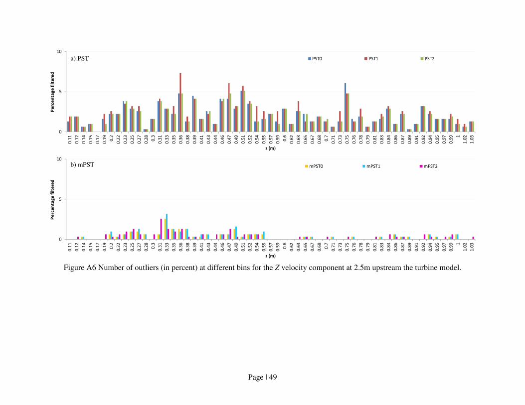
Page | 49

Figure A6 Number of outliers (in percent) at different bins for the Z velocity component at 2.5m upstream the turbine model.

0

5

10

0.1

1

0.1

2

0.1

4

0.1

5

0.1

7

0.1

9

0.2

0.2

2

0.2

3

0.2

5

0.2

7

0.2

8

0.3

0.3

1

0.3

3

0.3

5

0.3

6

0.3

8

0.3

9

0.4

1

0.4

3

0.4

4

0.4

6

0.4

7

0.4

9

0.5

1

0.5

2

0.5

4

0.5

5

0.5

7

0.5

9

0.6

0.6

2

0.6

3

0.6

5

0.6

7

0.6

8

0.7

0.7

1

0.7

3

0.7

5

0.7

6

0.7

8

0.7

9

0.8

1

0.8

3

0.8

4

0.8

6

0.8

7

0.8

9

0.9

1

0.9

2

0.9

4

0.9

5

0.9

7

0.9

9 1

1.0

2

1.0

3

Pe

rce

nta

ge

fil

tere

d

z (m)

PST0 PST1 PST2

0

5

10

0.1

1

0.1

2

0.1

4

0.1

5

0.1

7

0.1

9

0.2

0.2

2

0.2

3

0.2

5

0.2

7

0.2

8

0.3

0.3

1

0.3

3

0.3

5

0.3

6

0.3

8

0.3

9

0.4

1

0.4

3

0.4

4

0.4

6

0.4

7

0.4

9

0.5

1

0.5

2

0.5

4

0.5

5

0.5

7

0.5

9

0.6

0.6

2

0.6

3

0.6

5

0.6

7

0.6

8

0.7

0.7

1

0.7

3

0.7

5

0.7

6

0.7

8

0.7

9

0.8

1

0.8

3

0.8

4

0.8

6

0.8

7

0.8

9

0.9

1

0.9

2

0.9

4

0.9

5

0.9

7

0.9

9 1

1.0

2

1.0

3

Pe

rce

nta

ge

fil

tere

d

z (m)

mPST0 mPST1 mPST2

a) PST

b) mPST