Research papers

Assessing shelf mixing using CTD, ADCP, and free falling shear probeturbulence data

Sotiris Kioroglou a,b,n, Elina Tragou b, Vassilis Zervakis b

a Institute of Oceanography, Hellenic Centre for Marine Research, Greeceb Department of Marine Sciences, University of the Aegean, Greece

a r t i c l e i n f o

Article history:Received 18 October 2012Received in revised form20 May 2013Accepted 13 September 2013

Keywords:OverturnsDissipationTurbulent mixingVertical diffusivityThermaikosMicroprofilers

a b s t r a c t

CTD, ADCP and free-falling microstructure profiler data from Thermaikos Gulf of Northern Aegean Sea inGreece are analyzed in order to (a) gain an insight in the vertical diffusion processes of the area and(b) compare the methods of vertical diffusivity assessment based on microstructure profiler shear dataand on potential density overturns. The analysis reveals the presence of mixing events at the top mixedlayer as well as above the upper thermocline boundary. It is consistent with a notable change in thesusceptibility of the water column to turbulent events, within a month's period as well as convectiveinstability possibly related to riverine discharge. The comparison of the profiles of vertical shear ofhorizontal velocity and of density presumes isotropy of the turbulent field.

& 2013 Published by Elsevier Ltd.

1. Introduction

Turbulent mixing is a crucial process in the world ocean, and thedetermination of its spatio-temporal variability remains one of theaims of modern physical oceanography. Diapycnal mixing balances theupwelling over the global subtropical ocean, maintaining the thermo-cline structure and, thus, is a significant factor of the thermohalinecirculation (Munk, 1966; Mohammad and Nilsson, 2003; Rahmstorf,2006). Turbulent mixing can become a dominant factor in thedetermination of hydrographic properties of the water column inotherwise stagnant waters (Stigebrandt, 1976; Stigebrandt and Aure,1989; Zervakis et al., 2003). Furthermore, turbulent diapycnal mixingplays a major role on the diffusion of biogeochemical properties in theworld ocean (Cullen et al., 1983; Crawford and Dewey, 1989; Huismanet al., 2004) and may also become the dominant process duringstagnation (Stigebrandt et al., 1996; Zervakis et al., 2003). Due to thesignificant role in physical and biological processes in the ocean, thespecification of the crucial parameter scales of diapycnal turbulentmixing, such as length or duration, is of crucial importance (Gregg,1989).

1.1. Principles and methods

The typical length scale of ocean mixing can be very small, of theorder of a few centimeters, therefore requiring specially designedinstruments, such as shear probes, for its measurement and estima-tion (Simpson, 1972; Osborn, 1974; Osborn and Crawford, 1978).Microstructure profiling instruments (henceforth: MSP) are costlyand highly demanding in skilled personnel and manpower.

Alternatively, certain properties of mixing, with larger lengthscales can be inferred from CTD measurements through identifica-tion of the scale and potential density vertical distribution ofoverturning eddies (Thorpe, 1977; Dillon, 1982; Fer et al., 2004;Sherwin and Turell, 2005; Hall et al., 2011). In this way widelyavailable CTD measurements covering almost all the world oceansthrough a span of several decades could be quite helpful forspatio-temporal studies of oceanic diffusion. On the other handCTD measurements could also be used for contemporary diffusionstudies, once the CTD's data acquisition frequency is optimized.

The use of CTD-inferred density profiles as a means forestimating turbulent diffusion parameters, is based on the factthat within an isotropic turbulent eddy, there are always unstable‘overturning’motions, i.e. motions, during which heavy masses aredetected over light masses within the same water patch and aretraced as local sets of density inversions.

In particular, Thorpe (1977) devised the objective estimation ofa length scale, Thorpe scale, LT, directly associated with overturningeddies defined as the root-mean-square of the displacements

Contents lists available at ScienceDirect

journal homepage: www.elsevier.com/locate/csr

Continental Shelf Research

0278-4343/$ - see front matter & 2013 Published by Elsevier Ltd.http://dx.doi.org/10.1016/j.csr.2013.09.014

n Corresponding author at: Institute of Oceanography, Hellenic Centre for MarineResearch, Greece. Tel.: þ306976000786.

E-mail address: skior@hcmr.gr (S. Kioroglou).

Please cite this article as: Kioroglou, S., et al., Assessing shelf mixing using CTD, ADCP, and free falling shear probe turbulence data.Continental Shelf Research (2013), http://dx.doi.org/10.1016/j.csr.2013.09.014i

Continental Shelf Research ∎ (∎∎∎∎) ∎∎∎–∎∎∎

necessary to make the density increasing monotonically within aninversion patch. LT was later found to be approximately equal tothe Ozmidov scale LO (Ozmidov 1965) i.e. the maximum lengthover which an eddy could expand without losing its isotropy(Thorpe, 2005). The Ozmidov scale, is defined by

LO ¼ εovtΝ3

� �1=2

ð1Þ

where N is the buoyancy frequency and εovt is an approximation ofε, the dissipation rate of kinetic energy within the regime of theoverturning eddy. The latter is specified for the case of isotropicturbulence in terms of the vertically averaged squared gradient ofthe horizontal flow velocity as (Batchelor, 1959; Tennekes andLumley, 1972)

ε¼ 152ν

∂u∂z

� �2

ð2Þ

Dillon (1982) has shown that the Thorpe scale is smaller thanthe Ozmidov scale by a factor of 0.8:

LT � 0:8 LO ð3Þ

Furthermore the estimation of vertical eddy diffusivity of mass,Kρ, is given by the following relation derived by Osborn (1980),(also refer to Oakey (1982))

Kρ ¼ΓεovtN2 ð4Þ

where Γ is a mixing efficiency coefficient defined as the ratio ofturbulent potential energy production over turbulent kineticenergy dissipation and is approximately equal to 0.2

Eq. (4) results from the simplification of the turbulent energyequation (Tennekes and Lumley, 1972) if one assumes constant andhomogeneous turbulence and horizontal mean flow velocity. Thisresults in the elimination of the time derivatives and the divergenceterms and hence in a local balance between (i) turbulent kineticenergy production, (ii) dissipation rate, ε and (iii) the rate ofturbulent energy removal by buoyancy, gowρ4 , as expressed bythe equation

ouw4dUdz

þεþ gρ0

owρ4 ¼ 0 ð5Þ

where brackets denote averages over turbulent fluctuations of hori-zontal flow velocity, u vertical flow velocity, w and density, ρ, ρ0

represents the mean density and dU/dz, the shear of mean horizontalveloity, dU/dz.

Invoking in (5) the flux Richardson number, Rf, given by

Rf ¼ðg=ρ0Þowρ4

�ouw4 ðdU=dzÞ ð6Þ

and the mixing efficiency, Γ, yields

Γ ¼ Rf

1�Rfð7Þ

The set of relations (1, 3 and 4) enable the estimation of theeddy diffusion parameters Κρ and ε, on the basis of the identifica-tion of potential density overturns, provided they have passed theappropriate quality control tests that assure that the detectedoverturns are real and not an artifact of sampling.

εovt ¼LT

2N3

0:64ð8Þ

Kρ ¼ΓLT

2Ν0:64

ð9Þ

where the estimation of N appearing in Eqs. (8) and (9), is basedon ‘reordered’ overturn density profiles, for which densityincreases ‘stably’ with depth (Fer et al., 2004).

Galbraith and Kelley (1996) have introduced a method (hence-forth called GK method) providing criteria for distinguishing ‘real’from ‘fake’ overturns caused by either instrument errors or noise.

The first criterion introduced by GK is related to the so-calledrun-length, i.e. the population of groups of adjacent water parcelsof the water column, moving to the same direction to obtain stablestratification. This criterion determines the acceptable, noise freeoverturns by comparing the rms value of the runlength of anoverturn with the rms runlength of a noisy signal. The second GKcriterion is a water-mass criterion, exploiting the nature oftemperature and salinity turbulent mixing in the ocean, thusrequiring every T, S measurement within an overturn patch tomore or less lie within a straight line defining a water mass.

The GK criteria about the instrument-error-induced overturnshas been proven robust in other studies too (Stansfield et al.,2001). However Johnson and Garrett (2004) have shown that it istoo strict and insufficient to ‘simulate’ noisy overturns as puredensity noise, without taking into account the mean ‘background’density profile of the overturn. Therefore they introduced amethod (henceforth called JG method) of simulating noisy over-turns as ‘superpositions’ of the background linear potential density

Fig. 1. Map of the area of the experiments in September 2001 (left panel) and October 2001 (right panel). The bathymetric contours are overlaid in color scale. Points, circles,rhombes and crosses denote CTD stations, CTD stations with overturns, MSP stations and MSP stations with overturns respectively. Sections S1 (solid line) and S2 (dashedline) are shown with overlaid station numbers.

S. Kioroglou et al. / Continental Shelf Research ∎ (∎∎∎∎) ∎∎∎–∎∎∎2

Please cite this article as: Kioroglou, S., et al., Assessing shelf mixing using CTD, ADCP, and free falling shear probe turbulence data.Continental Shelf Research (2013), http://dx.doi.org/10.1016/j.csr.2013.09.014i

profile and normally or uniformly distributed potential densitynoise, of amplitude equal to the instrument's resolution limit,before proceeding to the aforementioned statistical comparison ofsimulated with the measured overturns regarding their rmsrunlengths. Both GK and JG criteria are analyzed in Appendixand the reader is also referred to the above cited publicationsregarding the criteria for a deeper insight.

In the present study, the eddy diffusion parameters Κρ and εovtare estimated by the application of our own algorithmic versionfor identifying and qualifying (according to a mixture of GK and JGcriteria) overturns. Our algorithm is applied on both CTD and datafrom a free-falling microstructure profiler, henceforth referred toas MSP, from the initials of ‘Microstructure Shear Profiler’equipped with shear probes and pressure, temperature and con-ductivity sensors. The data were obtained in the Thermaikos Gulf,a coastal region in the Aegean Sea, NorthEastern Mediterraneanwithin the framework of the project INTERPOL (Impact of Naturaland Trawling Events on Resuspension, dispersion and fate of POLlu-tants, contract no. EVK3_CT_2000_00023).

1.2. Introduction to the area of application and experiment

The application area, lying within Thermaikos Gulf in the NorthAegean Sea, is shown in Fig. 1 along with the sections used for ouranalysis in September 2001 (left panel) and October 2001 (rightpanel).

One can see that the depth ranges from 5 m nearshore toapproximately 100 m at the south middle of the gulf, and that theshelf has a rather smooth inclination. It can also be seen that4 rivers discharge into the gulf. The hydrography of the gulf can besummarized as a 2 layer system, separated by a relatively sharpthermocline, and the general circulation is characterized by acyclone at the center of the gulf and a nearby anticyclone at thegulf's northern part (Zervakis et al., 2005).

2. Methodology and data

2.1. Instruments and datasets

The CTD data used in our analysis were acquired with a SeabirdElectronics SBE 9/11þ unit, sampling at a rate of 24 Hz, which, ifcombined with our CTD descent rate of about 1 ms�1, results in anapproximate data resolution of 1 measurement for every 4 cm.However, only the mean value over every 10 measurements wasfinally recorded, (1 value for every 40 cm). While this data recordingrate is satisfactory for basic hydrographic and oceanographic estima-tions, it however restricts the ‘detectability’ of overturns to the limitof the large, energy containing eddies (Thorpe, 1977).

For the elimination of instrumental errors, standard CTD datapostprocessing as specified by the manufacturer was performed forcompensating the effect of the thermal inertia of the conductivityprobe on the measurements, as well as for synchronizing tempera-ture and conductivity signals whose phase difference were caused bythe physical separation of the corresponding probes.

In addition to the above standard methodology, we excludedmeasurements that did not fulfill the GK water-mass criterion(described in detail in Section A.3 of Appendix), applied quiteloosely, with the quantitative linearity indices ξS, ξT (as defined byAppendix Eqs. A7 and A8) required to be lower than 5 (as comparedto a more strict criterion suggested by GK of ξS, ξTo0.5). This‘generosity’ was compensated by careful visual inspection of the‘dubious’ overturns (see Section A.4 of Appendix). Relaxing thewater mass criterion is partly justified by the observation that,overturns attributed to the sensors' time responses mismatch weremost often characterized by ξS and ξT values near 20, i.e. much

larger than the GK imposed value of 0.5, while overturns withreasonably linear sθ versus T and sθ versus S relations werecharacterized by ξS and ξT values that were approximately equal to 5.

In addition to the CTD profiler, a fine resolution quasi-freefalling microstructure shear profiler sampling at 256 Hz (Wolket al. 2001), equipped with an Osborn – type shear sensor (Ninnis,1984), an FP-07 fast response thermistor and a standard set of CTDsensors and accelerometers, was deployed at several stations bothin September and October of 2001, as a means of gaining a detailedinsight into the vertical diffusion processes in the area.

Two versions of sθ profiles were produced by the MSP, i.e.,a version where the necessary temperature measurements wereprovided by the platinum wire sensor (henceforth referred to as‘Tslow’ set, because of the relatively slow response time of theplatinum wire probe for temperature with respect to the almostimmediate response time of the conductivity probe), and anotherone by the MSP's thermistor (henceforth referred to as ‘Tfast’ setdue to the very small (almost zero) response time of the thermis-tor probe).

In order to make a fair comparison of methods, not affected byspatiotemporal differences between the CTD and MSP stations,we applied both the “reference” shear spectral method and theoverturn method to MSP data. The use of Tfast and Tslow datasetsenabled the indirect estimation of dissipation rates and verticaleddy diffusivities via implementation of the overturn theory inaccord to Eqs. (8) and (9). These estimations were supplementaryto the direct estimations of dissipation rates according to Eq. (2),via integration over the wavenumber space of the MSP spectraldensity of the vertical shear.

Both Tslow and Tfast sets were undergone the basic processingrecommended by the manufacturer (Wolk et al., 2001) beforeusing them for evaluating the sθ profile to be used for the overturnidentification, i.e., despiking, elimination of data correlated to MSPdescent rate fluctuations, lagged cross correlations, phase shiftsbetween temperature and conductivity and compensating for thefinite bandwidth response of the MSP electronics.

Finally, low pass filtering was applied with cut-off frequency of25 Hz, which is the Nyquist frequency corresponding to thepressure sampling frequency of 50 Hz that is required for having1 pressure sample for every 0.01 dbar (pressure resolution) ofdescent, taking into account the nominal descent rate of 0.5 m s�1

(the full rate of data acquisition of 256 Hz corresponded to 5 datapoints for every 0.01 dbar). The lowpass filtering results in smoothingthe vertical T, S and sθ structure to the pressure resolution limit of0.01 dbar, thus losing detail of scales less than this.

In order to avoid losing this kind of detail, we alternativelyinterpolated the pressure data to approximately 0.01/5¼0.002 dbarbins ( in fact we used bin size¼depth range/total number of datapoints, such that the total number of interpolated pressure pointsequals the total number of data records). It was thus possible to useall the raw T, S, and sθ values, combined with the aforementionedinterpolated pressure values, for producing profiles of raw dataassigned to interpolated pressure values. This approach gives rela-tively precise profiles of T, S and sθ, provided that the descent rate isconstant throughout the descent. Pressure errors (interpolated – realvalue) due to variations of the instrument's descent speed areminuscule and do not affect the vertical overturn appearance exceptfrom a minor apparent contraction or expansion of its verticalstructure. Tslow and Tfast density overturns were also detected basedon the aforementioned pressure interpolated profiles.

Conclusively, 2 kinds of MSP overturn sets were identified,a low passed one and a non-low passed (raw) one with inter-polated pressure values, resulting in 4 overturn versions, the lowpassed Tfast and Tslow and the non-low passed Tfast and Tslow ones.

The thermistor and the inductance conductivity cell were bothcharacterized by almost zero response time and therefore the Tfast

S. Kioroglou et al. / Continental Shelf Research ∎ (∎∎∎∎) ∎∎∎–∎∎∎ 3

Please cite this article as: Kioroglou, S., et al., Assessing shelf mixing using CTD, ADCP, and free falling shear probe turbulence data.Continental Shelf Research (2013), http://dx.doi.org/10.1016/j.csr.2013.09.014i

dataset was much more efficient than Tslow dataset in ‘depicting’fast changes in the vertical sθ structure.

Finally an RDI ADCP sampling at 150 KHz, attached on anA-frame and lowered at a transducer-depth of 4 m, was used toprovide in situ flow velocity versus depth measurements.

2.2. Methodology analysis

The computational work can be divided into three major stages.At the first stage we located overturns on the data set. The

boundaries of each overturn were identified on the basis of twodifferent criteria described in detail in section A.1 of Appendix.

The second stage of the analysis consisted of identifying andrejecting ‘apparent’ overturns by applying the first criterion of theGK method for identifying ‘spiky’ overturns, as well as the JGmethod for tracing ‘noisy’ overturns. Finally, special care was alsotaken for visual inspection of the identified overturns one by one,for additionally excluding some overturn cases which satisfy thespike and noise criteria without being induced by ‘real’ marineturbulence, such as those of single or a few neighboring largespikes, or those that are caused by coupling of instrument's toship's motion.

The third stage of our calculations was to estimate the Thorpescale for each overturn, and proceed to estimate εovt and Kρ byEqs. (8) and (9), at all stations where both MSP and CTD weredeployed, whereby the estimation of the byouancy frequency,N was based on the ‘stably’ reordered potential density gradientover the length-scale of the overturn (Fer et al., 2004).

Two methods were followed for the derivation of spectraldissipation rates via the shear measurements.

The first method, henceforth referred to as method ‘A’ requiresthe data to be divided into three categories of 5 m bins (2560samples), 2 m bins (1024 samples), and 1 m bins (512 samples)and the shear spectral density, shear variance and dissipation ratebe separately assessed in each bin, by integrating the shear overthe wavenumber space using the manufacturer's routines. Infollow up, the dissipation value whose bin size and position bestmatch the ones of the overturn under comparison can be finallyselected as a reference value.

The second method, henceforth referred to as method ‘B’,consists of integration over the wavenumber space of the shearspectrum estimated exclusively within each overturn.

The analysis was applied on data from two cruises (September2001, October 2001) of the INTERPOL project and overturns weredetected for both CTD and MSP profiles, in parallel with the useand interpretation of ADCP measured flow field, possibly related tovertical diffusion. In stations where CTD and ADCP were (to a good

approximation) concurrent, values of gradient Richardson numberRi¼N2ð∂u=∂zÞ�2 were estimated. Areas of Rio0:25 are potentialcandidates for Kelvin Helmholz instability leading to evolvingturbulence (Miles, 1961). In our study Ri was computed both over5 m bins (when using ADCP and CTD measurements) and over theMSP resolution scale (when using the rms MSP measurements forboth density and shear).

3. Results

A total of 303 complete overturns for the September cruise and282 ones for the October cruise were detected in the CTD data.Almost all of them satisfied the JG noise criterion. The reason forthis is that the depth resolution was relatively coarse, resulting toan average density difference between adjacent data points muchlarger than the noise amplitude (taken equal to the instrumentdensity resolution). The overturn quality control was thereforefocused on rejecting overturns that resulted from either instru-ment spikes or instrument interaction with the sea water.

Our approximate GK water mass criterion was satisfied by 111out of a total of 303 overturns for the September 01 data and by119 out of 282 overturns for the October 01 data. However, thefinal accepted data set consisted of only 36 out off the 111 and 19out off the 119 overturns respectively, the rest ones having beenrejected because of their coupling to the ship motion or because oftheir very small point population (less than 5, the minimumrequired to define a Z shaped overturn).

Comparison of MSP-derived sθ profiles computed using bothTfast and Tslow data led to the selection of the Tfast data set as moreproper for identification of small scale overturns. The Tslow data setwas used as auxiliary data set for identifying overturns of largerscale (tens of cm) and for validity tests via comparisons with theTfast dataset products.

A total of 8458 and 6820 Tfast overturns were identified in theSeptember 01 and October 01 profiles respectively, out off which174 and 154 satisfied the water mass criterion. Of these 111(September) and 143 (October) satisfied the JG noise criterion,out off which only 36 and 30 respectively were finally selected, therest ones having been rejected due to small population of pointswithin the overturn.

Also, before proceeding to the analysis of the time and spacevariability, we attempted to compare the diffusivity related para-meters of our method (CTD and MSP overturn evaluation) with thecorresponding ones that were obtained at approximately samedepth and time regimes by the MSP, by integration of the shearspectral density. The stations where the comparison was possibleare shown in Fig. 1, while Figs. 2–4 show the comparative results

Fig. 2. Comparison of mixing parameters, vertical eddy diffusivity, KCTD and dissipation rate εCTD assessed via CTD overturns versus the corresponding MSP parameters, KMSP,εMSP based on the integration of the shear spectrum over the wavenumber space. The standard errors are calculated over the MSP replicates in each station.

S. Kioroglou et al. / Continental Shelf Research ∎ (∎∎∎∎) ∎∎∎–∎∎∎4

Please cite this article as: Kioroglou, S., et al., Assessing shelf mixing using CTD, ADCP, and free falling shear probe turbulence data.Continental Shelf Research (2013), http://dx.doi.org/10.1016/j.csr.2013.09.014i

of CTD overturn versus MSP shear spectrum and MSP overturnversus MSP shear spectrum.

As to the CTD overturn data, only overturns characterized by ξS andξT less than 1 were used for the comparison, although in general weused for our data analysis the more generous limit of 5. For eachstation with both MSP and CTD data, we compared CTD overturn datawith MSP bin data, making sure that the center and the verticaldimension of the bin be as close as possible to the ones of theoverturn. For example, for overturn sizes less than one, we used thebin of the same depth and of width 1 m. Having in mind that thelifetime of an overturn is comparable to the local buoyancy period(Dillon, 1982), we confirmed that the deployment times of the CTDand MSP data to be compared were not more than half an hour apart,to make sure that both instruments measured as similar conditions aspossible. This objective of course is very difficult to achieve (ideally, tomeasure the same overturn twice, with two different instruments),since the first of the two instruments will perturb the area during themeasurement and also due to other practical reasons such as the shipdrifting. However the minimization of time and space differencebetween the two kinds of measurements makes sense in cases oflocally isotropic and homogeneous turbulent environment.

The partial absence of correlation in the CTD/MSP comparison,evident in Fig. 2, was rather expected and could be attributed to anumber of reasons, such as the difference of the samplingfrequencies, the impossibility of complete time and space con-currency of the two kinds of measurements, and the inherentlyintermittent nature of turbulence. Nonetheless, the partial agree-ment in the order of magnitude for a few overturns is encouraging,although this is not statistically significant.

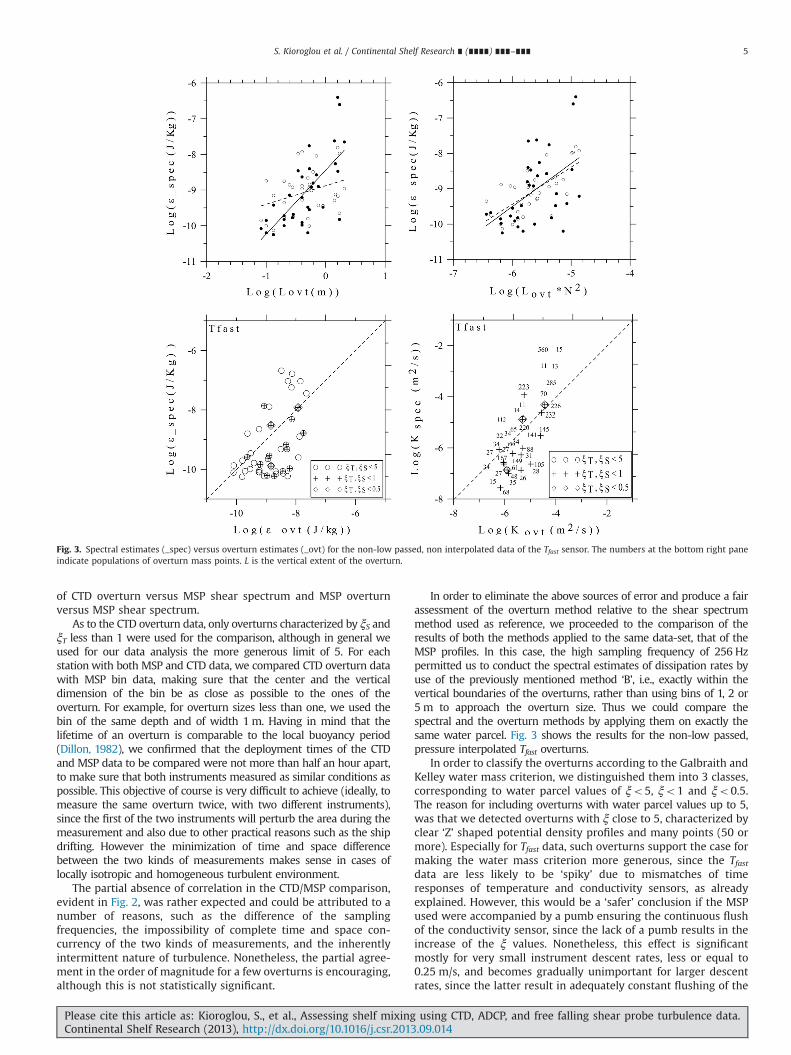
In order to eliminate the above sources of error and produce a fairassessment of the overturn method relative to the shear spectrummethod used as reference, we proceeded to the comparison of theresults of both the methods applied to the same data-set, that of theMSP profiles. In this case, the high sampling frequency of 256 Hzpermitted us to conduct the spectral estimates of dissipation rates byuse of the previously mentioned method ‘B’, i.e., exactly within thevertical boundaries of the overturns, rather than using bins of 1, 2 or5 m to approach the overturn size. Thus we could compare thespectral and the overturn methods by applying them on exactly thesame water parcel. Fig. 3 shows the results for the non-low passed,pressure interpolated Tfast overturns.

In order to classify the overturns according to the Galbraith andKelley water mass criterion, we distinguished them into 3 classes,corresponding to water parcel values of ξo5, ξo1 and ξo0.5.The reason for including overturns with water parcel values up to 5,was that we detected overturns with ξ close to 5, characterized byclear ‘Z’ shaped potential density profiles and many points (50 ormore). Especially for Tfast data, such overturns support the case formaking the water mass criterion more generous, since the Tfastdata are less likely to be ‘spiky’ due to mismatches of timeresponses of temperature and conductivity sensors, as alreadyexplained. However, this would be a ‘safer’ conclusion if the MSPused were accompanied by a pumb ensuring the continuous flushof the conductivity sensor, since the lack of a pumb results in theincrease of the ξ values. Nonetheless, this effect is significantmostly for very small instrument descent rates, less or equal to0.25 m/s, and becomes gradually unimportant for larger descentrates, since the latter result in adequately constant flushing of the

Fig. 3. Spectral estimates (_spec) versus overturn estimates (_ovt) for the non-low passed, non interpolated data of the Tfast sensor. The numbers at the bottom right paneindicate populations of overturn mass points. L is the vertical extent of the overturn.

S. Kioroglou et al. / Continental Shelf Research ∎ (∎∎∎∎) ∎∎∎–∎∎∎ 5

Please cite this article as: Kioroglou, S., et al., Assessing shelf mixing using CTD, ADCP, and free falling shear probe turbulence data.Continental Shelf Research (2013), http://dx.doi.org/10.1016/j.csr.2013.09.014i

conductivity sensors (Gregg et al., 1982). Our MSP nominal descentrate was 0.5 m/s. For the Tslow data in turn, no overturn withξo0.5 was identified and the Tfast overturns with ξo0.5 are sparse(only 3), two of them lying almost on figure's 3 ‘ideal’ dashed lineof ε¼εovt, the third one deviating to ε being smaller than εovt by anorder of magnitude. We can also notice that at the extreme ofsmall values of dissipation rates, the Tfast overturns with ξo1 andξo5 are both characterized by ε values which are smaller thanεovt by two orders of magnitude, the same being valid for the Tslowoverturns (not shown). In the opposite extreme of large values ofdissipation rate on the contrary, ε values appear to be larger thanεovt values. In this case the Tfast overturns with ξo5 and ξo1 andthe Tslow overturns with ξo1, reach maximum differences of 2,1 and 3 orders of magnitude respectively. The same overall patternis confirmed for diffusivities too. However the statistical certaintyof these observations is not enough to support general conclusionsand it would be interesting to test them with more studies of thesame direction as the one of the present work.

Fig. 4 illustrates statistical differences of Tslow and Tfast over-turns. The histograms are plotted for overturns corresponding to ξvalues 1 and 5 respectively. One can confirm that the Tfast sensor‘captured’ many more (120) overturns with height less than 10 cmthan the Tslow sensor did, since it is much more sensitive to ‘fast’temperature (and consequently density) changes. Both Tslow andTfast histograms seem to follow normal distribution, in particularthe ones corresponding to the more generous case of ξ¼5. It isalso notable that the Tslow are shifted to larger values, (mostfrequent diffusivities 10–7 and 10–6 and most frequent dissipationrates 10–10 and 10–9 for Tfast and Tslow respectively). This lastremark is again more evident in the plots for which ξ¼5.

After the necessary comparisons of the measurements, wecould proceed with the synthesis of the turbulent diffusionprocesses revealed by the data.

According to hydrology and circulation studies (Zervakis et al.,2005) the area is well modeled in the Fall as 2 layer system, i.e.,top and bottom mixed layers separated by a sharp thermocline.Figs. 5 and 6 show profiles of diffusivity at all common MSP/CTDstations, for September and October cruises respectively. Almostall stations (17, 18, 27, 38, 41) are common for both periods and arelocated at the west part of the gulf, apart from station 30 ofOctober 01 data, which is located in the center of the gulf. It isevident from the common stations that the September 01 diffu-sivities tend to be vertically more homogeneous (stations 18b,27b) than the October 01 ones, which present a much morepronounced thermocline minimum. Some of the September 01profiles present a local maximum at the boundaries between thethermocline and the mixed top (17b) or bottom (38a) layers. Theenhanced turbulence at the boundary sheet between the thermo-cline and the mixed layers, where turbulence makes its wayagainst the thermocline stratification, is further confirmed by theincreased number of overturns there. Inside the thermocline onthe other hand the stratification dominates and results in diffu-sivity minima in both September 01 and October 01. The diffusiv-ities therein have similarly small magnitudes (10–5 to 10–6).The thermocline diffusivity minimum of the October 01 profile isapparently much more pronounced, because the October 01 topmixed layer diffusivities are 1–3 orders of magnitude larger thanthe September 01 ones (10–1 to 100 versus 10–3 to 10–2). This is inconsistence with more enhanced vertical mixing in October 01 atthe top mixed layer (see also the discussion section). The bottom

Fig. 4. Histograms of population of overturns whose overturn eddy diffusivity, Kovt and dissipation rate, εovt, lie within value bands. Top and bottom panels correspond toGalbraith and Kelley water mass criterion values ξo1 and ξo5.

S. Kioroglou et al. / Continental Shelf Research ∎ (∎∎∎∎) ∎∎∎–∎∎∎6

Please cite this article as: Kioroglou, S., et al., Assessing shelf mixing using CTD, ADCP, and free falling shear probe turbulence data.Continental Shelf Research (2013), http://dx.doi.org/10.1016/j.csr.2013.09.014i

layer diffusivities on the other hand have similar magnitudes inboth months (10–2 to10–3).

The degree of water column stability is indicated by thegradient Richardson number Ri, as estimated by ADCP/CTD mea-surements. The profiles of this number (not shown) indicate that ittends to be larger than 1 in the thermocline core where thestratification dominates, but also to approach the value 1 at theupper thermocline interface where most of the overturns wererecorded. In the September stations 38a, 41b, Ri tends to besteadily small throughout the thermocline (fluctuating between1 and 0.25 and even becoming smaller than 0.25), in accordancewith our conclusion that the September thermocline stratification

is less efficient in inhibiting vertical turbulent propagation. Thisrange of values is also in partial accordance with numerical modelresults (Smyth and Moum, 2000), suggesting that in fully devel-oped turbulence the Richardson number tends to be equal to 0.3.The small scale Richardson number based on the rms. spectralMSP shear on the other side, was found steadily smaller than 0.25,which verifies that in the very small scale the shear is much moreefficient in locally overturning the water column.

Figs. 7 and 8 show transects depicting the vertical distributionof mean hydrology and vertical turbulent transport parameterswhich were measured during the September and October cruisesrespectively. In particular, transect S1, shown at the left panels is

Fig. 5. September 01 profiles of logarithm of vertical eddy diffusivity log(K) evaluated by MSP shear spectrum (dark lines with error bars), MSP overturns (crosses) and CTD(light gray circles). The dark points indicate MSP shear spectrum values corresponding to the MSP replicates.

Fig. 6. Same as Fig. 7, for October 01 data set.

S. Kioroglou et al. / Continental Shelf Research ∎ (∎∎∎∎) ∎∎∎–∎∎∎ 7

Please cite this article as: Kioroglou, S., et al., Assessing shelf mixing using CTD, ADCP, and free falling shear probe turbulence data.Continental Shelf Research (2013), http://dx.doi.org/10.1016/j.csr.2013.09.014i

an alongshore, approximately longitudinal transect extending inthe proximity and along the west coast of the gulf, whereas S2 isapproximately zonal and across-shore. The transect routes are

inlaid in the maps of the left top panels. One can see that in S1 theMSP stations have both larger population and are more uniformlydistributed in space than MSP stations of S2. Indeed, only station

Fig. 7. INTERPOL, September 01. Panels from top to bottom show, temperature (1C) salinity (psu) and log scaled N2 (s�2) for the longitudinal (along shore) transect S1 (leftpanels) and the zonal (across shore) transect S2 (right panels). S1 and S2 are illustrated in the inlay of the top left panel. The log scaled circles denote, diffusivity K (m2/s) (toppanels) dissipation rate ε (J/kg) (middle panels) and vertical shear S (s�1) of horizontal flow velocity (bottom panels), with blue, cyan and yellow corresponding to valuesinduced by the CTD overturn, MSP overturn and MSP shear spectrum methods respectively. The rhombes and the black points correspond to areas with CTD–ADCPRichardson number less than 0.25 and 1 respectively.

Fig. 8. Same as 7 for October.

S. Kioroglou et al. / Continental Shelf Research ∎ (∎∎∎∎) ∎∎∎–∎∎∎8

Please cite this article as: Kioroglou, S., et al., Assessing shelf mixing using CTD, ADCP, and free falling shear probe turbulence data.Continental Shelf Research (2013), http://dx.doi.org/10.1016/j.csr.2013.09.014i

30 in the October across-shore transect provides a profile ofvertical diffusivities right in the middle of the gulf, within an areaof cyclonic circulation (Zervakis et al., 2005). These differencesshould be kept in mind for not misinterpreting the lack of MSPeddy diffusivity data as indication of nonexistent vertical mixing inthe across-shore direction.

Transects verify our already mentioned observation that the topmixed-layer diffusivities are larger in October 01 (as high as1 m2 s�1). Consideration of diffusivity Eqs. (8) and (9), results inthe conclusion that the larger October 01 diffusivities are due to thesmaller stratification of the October 01 top layer, as can be seen in theN2 transects, since the dissipation rates in the two months are ofcomparable magnitude. The October 01 top layer seems to havedeepened and be more efficiently mixed and therefore also moresusceptible to new overturning instabilities, as can be seen by themany positions characterized by Richardson number less than 0.25.It is notable though that all these positions are distributed within thetop layer, none of them under it, within the stratified thermoclinearea, or even within the bottom mixed layer.

In September however, stations 38 and 41 seem to be anexception to this rule since for station 41 the Richardson numberis less 0.25 both above and below the thermocline and less than1 inside the thermocline, and for station 38 less than 1 above andbelow the thermocline. Richardson values between 0.25 and 1 arenot sufficient for overturning instability, but they are not far fromthe critical value of 0.25. The overall small Richardson values atthese stations are certainly associated with the lesser stratificationthere, as manifested by small N2 values. It seems that in this areathe stratification has been smoothed out by convective instability.This in turn might be caused by the discharge of cold (althoughfresh) riverine waters since these stations lie against the mouth ofriver Pinios. The riverine water plume is advected and diffused byoffshore moving currents as was manifested by the CTD salinityfields (Zervakis et al., 2005).

The same kind of convective instability might have been a partialreason for the homogenization of the area of the October 01alongshore transect S1, that is included between stations 4 and 13,against the mouths of Aliakmon, Loudias and Axios rivers. Bothtemperature and salinity of these stations are completely homo-genized and equal to thermocline values of the rest of the transect.The temperature (20–22 1C) of this mass is 2 1C less than the rest(southwards) top layer waters. It seems that this mass, comprising avertically homogenous fresh and cold front, ‘feeds’ the thermoclineby settling at its depth and dispersing horizontally. The intensehomogenization there coordinates itself with a CTD-recorded largeoverturn at the top boundary of the thermocline (station 10) andlarge dissipation rates and diffusivities (station 17).

4. Discussion and conclusions

4.1. Discussion about the results

In the present study we analyzed CTD, ADCP and free-fallingMSP records to assess vertical diffusion processes of the Thermai-kos gulf in the northern Aegean Sea. The free falling MSPs are thestate of the art instruments for studying turbulent diffusionprocesses, since one can measure horizontal shear along withstandard water properties such as temperature and conductivity(and hence derive salinity and density) with satisfactory precisionand very high resolution.

The standard use is to focus on the measurements of thehorizontal shear to derive dissipation rates and from them verticaldiffusivities of great precision and resolution. However large dissipa-tion (or horizontal shear) values are indices and not manifestations ofturbulence. Since turbulence is 3 dimensional, one needs to identify

overturns for manifesting turbulent patches. Having this fact in mindwe have put a lot of effort for identifying genuine overturns withboth the CTD and MSP, although it is well known that, in the majorityof circumstances, microstructure shear will give a better estimationof turbulent mixing than Thorpe scaling and also that CTD measure-ments have insufficient resolution to directly measure small-scaleturbulent overturns.

Indeed, the CTD identified overturns were of restricted valuedue to the low vertical density resolution (1 measurement forevery 30 cm) and to problems such as coupling of the instrumentto the ship motion. Inevitably the CTD provided information onlyabout the very large and energetic eddies.

The MSP overturns were more valuable because the sensors aremuch less prone to spikes that could be misconceived as realoverturns, and also because the instrument is free falling and thusdecoupled from ship motion.

Furthermore, application of the density overturn method to afree-falling, fast sampling instrument that measures turbulencethrough an alternative method permits a “fair” assessment of thevalidity and possibilities of the former method relative to areference.

We stress hereby that although our algorithms traced approxi-mately 5000 MSP overturns, only 150–200 did satisfied the criteriaof genuinity. The Tfast (thermistor) overturns seemed to be the bestand most analytically ‘capturing’ the vertical microstructure,because of the fast response of the MSP thermistor. The Tslowoverturns corresponded to the standard CTD probes of conductiv-ity and platinumwire thermometer, and lagged a bit in quality dueto the response delay of the thermometer. Both the Tslow and Tfastoverturns however were robust with many points along thevertical forming ‘Z’ shapes. Our analysis suggests that the water-mass criterion can cautiously be raised to a value between 1 and 5,from the strict 0.5. We exploited to the maximum the high dataacquisition rate, by use of pressure interpolation, in order to use allthe data and estimate dissipation rates and diffusivities using theOzmidov/Thorpe scale analysis of the typical length (LThorpe) andthe vertical density structure (N2).

Alternatively, we applied the same calculations on low passeddensity profiles for matching the higher data acquisition rate tothe inherent pressure resolution; this resulted in 5 T C recordsaggregating with one only valid pressure measurement. The‘vertical’ dissipation rates of these methods induced by theThorpe/Ozmidov overturn method (i.e., the approximations bythis method of the values of dissipation rate terms related tohorizontal shear of vertical velocities) were compared to the apriori considered as ‘horizontal’ dissipation rates, derived directlyby integration of the horizontal shear spectrum.

The differences between the ‘vertical’ and ‘horizontal’ dissipa-tion rates could be cautiously attributed to anisotropy, betweenthe vertical and horizontal scales. Eq. (2) is derived by a simpli-fication of

ε¼ ν2

∂ui

∂xjþ∂uj

∂xi

� �2

ð10Þ

based on the assumption of isotropy, where i¼1,2,3 with 1, 2 corre-sponding to horizontal and 3 to vertical directions, and the summa-tion is taken over repeated indices (Tennekes and Lumley, 1972).In (2) one multiplies the horizontal constituent, νð∂u=∂zÞ2 by 15,based on the assumption of isotropy, thus the value of (2) is anupper bound to the total horizontal component of dissipation rate.Eqs. (1) and (3), (8) and (9) on the other hand, provide an estimate ofdissipation rate along the vertical, based on the vertical length(Ozmidov length scale) that the overturn would reach if the availablepotential energy in the overturn was consumed to kinetic energydissipation, εovt , and work against stratification N2.

S. Kioroglou et al. / Continental Shelf Research ∎ (∎∎∎∎) ∎∎∎–∎∎∎ 9

Please cite this article as: Kioroglou, S., et al., Assessing shelf mixing using CTD, ADCP, and free falling shear probe turbulence data.Continental Shelf Research (2013), http://dx.doi.org/10.1016/j.csr.2013.09.014i

Furthermore the dissipation rates εovt , ε seem to be grosslyanalogous to both the overturn height and the gross overturndensity variations as shown in the top panels of figure Fig. 3. Thisanalogy is straightforward as far as εovt is concerned (Eqs. (1) and(3)) but not clear regarding ε. One reason might be that largeroverturns need larger rms shear, ð∂u=∂zÞ2 to both onset andexpand them vertically.

Furthermore, ε seems to increase faster with overturn heightthan εovt does. Having in mind the aforementioned considerationswe suggest that the ε values are larger than the εovt values for themost energetic overturns (410–7 J/kg) due to eddy anisotropyinduced at larger scales by stratification (Gargett, 1984). Anotherpossible cause of deviation of εovt from ε is the absence ofdependence on the Richardson number in the scale Eqs. (1) and(3), on which estimation of εovt relies. This absence was justified bythe assumption that in fully developed turbulence the Richardsonnumber adopts the universal value of 1 (Thorpe, 2005). Such anassumption is not always valid, and the introduced error might bemore serious if Richardson number deviated from 1 by more thanone order of magnitude. However our data reveal that theRichardson number does not differ by more than 1 order ofmagnitude from 1 within the overturn range, so the aforemen-tioned error is rather small, if we take into account that thecomparison of the dissipation values is done in logarithmic scale.

On the other hand, the differences of ε and εovt are larger forthe non-low-passed data versions (2 or 3 orders of magnitude)than for the low-passed ones (at most one order of magnitude),and this may happen because in the former, the lack of smoothinglets more details of the vertical density structure into play. Thegross distribution of ε versus εovt points however seems the same,ranging from εovt being larger in the least and smaller in the mostenergetic areas, with a crucial quantity of data points lyingproximal enough to the ‘ideal’ case of isotropy, represented bythe dashed diagonal line for each point of which it is valid thatε¼ εovt .

As deviations of ε versus εovt could be attributed to theanisotropy of the larger eddies, we proceeded further to calculatethe isotropy index I (Thorpe, 2005), as follows

I¼ ενN2 ð11Þ

which manifests a large range of scales of isotropic turbulence if it islarger (the more the better) than the limiting value of 200. Thepanels of Fig. 9 below show the profiles of the Ozmidov scale (Eq. (1))and of the isotropy factor corresponding to all the MSP deployments.It is evident that the surface and bottom mixed layers havesufficiently larger isotropy factor values than those required forisotropy. These are the areas where overturning instabilities of largescales (equal at most to the local Ozmidov scales) could easily occur,since there is no significant stratification to inhibit turbulence. In thethermocline area on the other side, the isotropy factor ranges fromthe threshold 200 to even smaller values, since the intense stratifica-tion inhibits large overturning motions that could bear a cascading

range of ever smaller scales tending to be isotropic. This supports oursuggestion of lack of isotropy as agent of deviations betweenhorizontal and vertical turbulence.

It would be certainly interesting to further perform suchstudies on more available profiles of MSP density, for increasingthe statistical certainty of derivations, being aware of the limita-tion that in the present stage only the vertical profile of thevertical gradient of horizontal velocity ð∂u=∂z ðzÞÞ can be recordedin great detail, not the vertical profile of the horizontal gradient ofthe vertical velocities ð∂w=∂x ðzÞÞ that would provide direct dis-sipation rates due to shear of the vertical micromotions. Indeed,ð∂w=∂x ðzÞÞ would be very difficult to distinguish from verticalmotion of the profiler even if shear probes were mounted in suchan orientation.

The density profile, if detailed enough, fills partially this gap,because it gives information about the vertical structure of theoverturns. However, only density data from the profiler could beused for a direct comparison due to the intermittency of turbulentoverturns. If the MSP recording of ð∂w=∂x ðzÞÞ were possible itcould be further possible to compare ð∂w=∂x ðzÞÞ induced dissipa-tion rates with the ones induced by the overturn method ofthe Thorpe/Ozmidov scale, in order to confirm and/or improvethe accordance of the two measurements. For the moment,the comparison of ð∂u=∂z ðzÞÞ induced dissipation rates with theOzmidov scale presumes isotropy, or inversely, if one assumesagreement between ð∂w=∂x ðzÞÞ induced dissipation rates with theOzmidov scale induced ones, the aforementioned comparison isthen a test of isotropy of the examined turbulent mixing events.

Moreover, the knowledge of the hydrology and circulation ofthe area is a prerequisite for assessing implications of verticalturbulent mixing in the dynamics of the area. The mean hydrologyand circulation has been studied elsewhere (Zervakis et al., 2005).This study confirmed the existence of a doubly stable two layerwater column in both September 01 and October 01, characterizedby warm and fresh water at the top, mostly attributed to theinflow of Black Sea surface water outflowing from the Turkishstraits into the Aegean Sea and to a lesser degree to riverine inflow.The combined examination of the horizontal contours of thedynamic heights and ADCP measured flow velocities revealed abasically baroclinic circulation, dominated by a cyclone at thecenter of the gulf, and anticyclonic circulation at the gulf's innernorthern part. Observation of the T–S diagrams verified that thewater mass remained the same across the September 01–October01 period, but also that during the aforementioned period heatwas lost in the atmosphere, resulting in the cooling of the watersurface. This water surface cooling might be related to theobserved enhancement of the top layer turbulent diffusivity,induced by the local instability accompanying the formation ofheavier/cooler water mass at the top of the water column.

The synthesis revealed further details about the diffusionprocesses in the area of consideration. Overturns were located intheir majority either at the top and bottom boundary layers or atthe thermocline boundaries where turbulence makes its wayagainst stratification. The profiles of the dissipation rates anddiffusivities derived by integration of horizontal velocity shear,revealed moderate turbulence levels, however the September 01thermocline proved to be generally more susceptible to verticalturbulent penetration. Offshore, next to the west coast of the gulf,near the mouth of Pinios river the thermocline stratificationseemed to have been leveled out due to a convective mixing eventthat might be related to the river outflow. The water column at thisarea (stations 38, 41) was apparently much more susceptible tooverturning instabilities, due to the vertically homogenized (rela-tively more than other stations) density. More to the north alongthe same coast, in the proximity of Axios, Loudias and Aliakmonasriver mouths, a vertically homogenized cold and fresh frontFig. 9. Profiles of Ozmidov scale (left) and of isotropy factor (right).

S. Kioroglou et al. / Continental Shelf Research ∎ (∎∎∎∎) ∎∎∎–∎∎∎10

Please cite this article as: Kioroglou, S., et al., Assessing shelf mixing using CTD, ADCP, and free falling shear probe turbulence data.Continental Shelf Research (2013), http://dx.doi.org/10.1016/j.csr.2013.09.014i

constituted another area of enhanced overturning activity. Finally,the relatively enhanced turbulent activity at the center of the gulf(station 30 of October 01 data) might be related to the upwellingof cold and saline water, induced by the cyclonic circulation.

4.2. Conclusions

This work was based on the assumption that the identificationof density overturns in the water column by either CTD or MSPinstruments manifests turbulent vertical mixing events.

It has been confirmed that the number, vertical detail andresolution of overturns gets maximized if we use MSP equippedwith thermistors rather than regular platinumwire thermometers.

Also the results of our analysis are in agreement with thepresence of isotropic turbulence and more overturning in areas oflow stratification such as the top or the bottom mixed layers orwithin convective patches while evidence of anisotropic turbulenceis found in the pyclocline. This conclusion however presumes thatthe Thorpe/Ozmidov method is characterized by satisfactory pre-cision in determining the terms of dissipation rate ascribed to shearof vertical velocities. It would certainly be interesting to pursuemore studies in the future testing this presumption.

Overall, the application of the overturn method on the CTDdata, as well as the slow (CTD-like) and fast temperature sensormeasurements of the MSP showed that the method can revealturbulence in potentially stratified regions, like the mixing layerand the pycnocline, however it is not applicable (as expected) inwell-mixed layers.

Thus, the application of the overturn methods on historical CTDobservations would greatly underestimate the dissipation anddiffusivity in the mixed layers, while overestimating the sameparameters within stratified regions (due to the identification ofthe most energetic structures). This result holds of course for thecurrent observations for Thermaikos Gulf.

Overall, the MSP measurements within the Thermaikos Gulfrevealed diffusivities varying from 10–6 (in the most stratifiedareas) to almost 1 m2 s�1 (in the surface mixed layer). Highdiffusivities were often also recorded in the bottom mixed layer.

The intense riverine outflow at the western shore seems to berelated to the mixing processes. It facilitates the ‘weakening’ of thethermocline stratification via the horizontal dispersion of cold andfresh water to the degree that vertical convective events occur. Theexperiments took place at the beginning of the Autumn, and it wasconfirmed that in this transitional period, vertical turbulentdiffusion progresses to gradually overcoming stratification andeffectively deepening the top mixed layer of the study area. It wasalso confirmed that the aforementioned process is aided by theinflow of cold and fresh riverine water as well as by the gradualseasonal removal of heat to the atmosphere.

The high diffusivities of the surface layer effectively mix theriverine waters with the incoming Black Sea Waters of the mixedlayer. Due to the low volume of the riverine inflow, its signatureaway from the river mouths becomes untraceable (also due to thelow-salinity signature of the BSW (Zervakis et al., 2005)).

The high diffusivities recorded in the bottom mixed-layers of theThermaikos Gulf have a significant biogeochemical role in the coastalecosystem. Thermaikos Gulf is a very significant bottom-trawleractivity region. Large amounts of sediment are resuspended duringthe fishing season by trawlers, and a portion of the resuspendedmaterial is spread around the Gulf as a bottom nepheloid layer(Tragou et al., 2005; Kombiadou and Krestenitis, 2011). Anthropo-genic resuspension greatly surpasses natural resuspension in theGulf, however it is the naturally present mixing processes within thebottom nepheloid layer that keep part of the resuspended sedimentfrom settling (Tragou et al., 2005). Further study of such propertiesusing traditional hydrographic instrumentation is limited by the

density overturn method's sensitivity, which is greatly reducedwithin surface and bottom mixed layers. A thorough study ofturbulent diffusion within these layers still requires the use of MSPs.

Appendix

A.1. Detection criterion of the overturns' vertical limits.

The Thorpe displacement Lν of a particle within an overturn isdefined as the virtual displacement of this particle from its initiallyunstable position to its finally stable position, within the overturnboundaries. An overturn is ‘complete’ if all the overturning motiontakes place within its own boundaries (Dillon, 1982).

The standard method for identifying these boundaries is toseek vertical water column sections for which the sum of Thorpedisplacements is equal to zero

Σ i ¼ ηi ¼ 1Li¼ 0 ðA1Þ

where

Li ¼ zSj �zUi ¼ zSðsUθ ιÞ�zU ðsUθ ιÞ ðA2Þand sUθ ¼ sUθ ðzUÞ is the profile of the unstable (original) potentialdensity versus depth and sSθ ¼ sSθðzSÞ is final profile of potentialdensity versus depth, produced by the reordering algorithm. Inthis context, the series of ‘Thorpe fluctuations’ of potential densityis defined as

δsTθ i ¼ sSθ i�sUθ i ðA3ÞEq. (A1) is a direct consequence of mass conservation within theoverturn regime which can be stated otherwise as a condition thatthe ‘complete’ overturn’s fluid ‘body’ constitutes a ‘continuum’,both before and after the stabilizisation - reordering process. Thisfact sets the constraint that the redistribution of the verticalpositions be done in such a way that each position is ‘assigned’to only one point mass and vice versa, both before and after therelocation, so that no ‘fluid gap’ exists. Additionally it is imposedthat the positions of the overturn boundaries should not bemodified during the relocations, otherwise the overturn wouldnot be complete. More mathematically, the right hand side termsof (A2), zSj , z

Ui are required to draw values from the same set of

positions zi, i¼ 1:::n, once as ‘stable’ position version zSi , and onceas an unstable subtracting one, �zUj , j¼ 1:::n, thus their substitu-

tion into Σ i ¼ ηi ¼ 1Li verifies (A.1), i.e., ∑i ¼ η

i ¼ 1Li¼∑i ¼ ηi ¼ 1Zi�∑j ¼ η

j ¼ 1zj ¼ 0

A digital realization of (A1) was implemented as follows

∑ν ¼ η

ν ¼ 1Lν

∑ν ¼ η

ν ¼ 1jLνj

rc ðA4Þ

where c is a suitably small number (for example equal to a 0.1 or to0.2). It is therefore evident that the criterion depends heavily onthe value of c. If for example parameter ‘c’ were set to c¼0.1, thensome overturns would be identified, if c¼0.2, even more overturnswould be detected, the number of identified overturns increasingwith increasing value of c. A detection algorithm based on ((A4))was developed, however the results were dependent on the‘subjectively’ set value of c.

An alternative precise method, is not based on Eq. (A4), butrather on the ‘topological’ condition that all displacements berestricted within the overturn’s boundaries.

In more detail, we identified for each point of ith order, locatedat depth zUi in the unstable series, a ‘where to’ depth, i.e. the depthat which this point will be located as member of the stable series,zSt i ¼ zSðsUθ ιÞ, and a ‘where from’ depth, zUf i, i.e. the depth of the

S. Kioroglou et al. / Continental Shelf Research ∎ (∎∎∎∎) ∎∎∎–∎∎∎ 11

Please cite this article as: Kioroglou, S., et al., Assessing shelf mixing using CTD, ADCP, and free falling shear probe turbulence data.Continental Shelf Research (2013), http://dx.doi.org/10.1016/j.csr.2013.09.014i

unstable series from which a point will come to replace the ithunstable point.

Afterwards, our algorithm ‘scanned’ along the unstable profile,resulting in the identification of each point with nonzero Thorpedisplacement value as a potential upper boundary of an overturn.The downwards scanning was performed in parallel with compar-ing the zSti and zUf i values of each ith point, with the ‘current’overturn depth – boundary values, zup; zdn, which were reset asfollows, zdn ¼ minðzdn; zSti; zUf iÞ and zup ¼ maxðzup; zSti; zUf iÞ. The pro-cess got terminated upon identification of the overturn's lowerboundary signaled by the condition zUi ¼ zdn.

This method overestimates the extend of an overturn only incase of existing potential density spikes that are so large, thateither undershooting of zup or overshooting of zdn, or both, occur.This spike induced overestimate of an overturn's vertical exten-sion, could lead to notable miscalculation of the diffusivity para-meters which depend mostly on the large overturn displacements(Stansfield et al., 2001).

Ultimately, we subtracted from the set of points of the over-turns the edge points (upper and lower) and repeated the abovedescribed process for the rest of the overturn points, in an effort totrace smaller complete overturns included inside the larger one,possibly ‘masked’ by larger movements of some ‘overweight’ or‘overlight’ fluid points. This step was performed iteratively, in aneffort to trace ever smaller complete overturns, each new onebeing nested into its older one. In this way we tried to tracesnapshots of some kind of energy cascading from larger to eversmaller becoming eddies as analyzed in the theory of turbulence.Unfortunately no nested overturns were traced, either in the CTDor in the MSP data.

A.2. Rejection of overturns resulting from sensor noise

The algorithmic checking of whether a detected completeoverturn is a product of instrumental noise or not can be outlinedas follows, according to the GK method criterion: for every

complete overturn, say the jth, groups of successive Thorpedisplacements Li of the same sign are considered as individualruns, assuming the population or run length, of the k-th group tobe equal to Njk with root mean square values ⟨Nj⟩

obsrms.

The values Njk ¼ nobs are the measured runlengths of an‘instant’ overturn, thus their expected frequency of appearance isgiven by a probability density function, PobsðnobsÞ and according tothe GK noise criterion, for distinguishing the measured overturnsinto real and noisy, a comparison is performed of the correspond-ing Pobs(n) and the probability density function PnoiseðnÞ of artificialoverturns, detected as a result of noise.

In this context, Galbraith and Kelley (1996) stated that large run-lengths are expected at the edges of a real (not noisy) overturn, dueto the increased densities of heavy particles at the top edge tendingto move to the lower half at their stable positions and of lightparticles at the bottom edge tending to move to the upper half attheir stable positions. This results in PobsðnÞ tending to be large forlarge values of n, in contrast to PnoiseðnÞ which tends to zero.

The GK method quantifies this difference by introducing athreshold ⟨Nj⟩rms value, n0, that, in the plot of PðnÞ divides the run-length axis into the area of real overturns (with n4n0) and thearea of noisy overturns ( with non0).

The above mentioned theoretical approach about the distin-guishing of the real from the noisy overturns, has been improvedby the JG methodology. According to this, the effect of noise increating ‘fake’ overturns at the potential density profile isdescribed better by the superposition of two constituents. Theone constituent is normally distributed noise of amplitude equal tothe instrument resolution and extent and population of pointsequal to the ones of the overturn. The other constituent is a linearmodel of the ‘background’ sθ profile of the measured overturn.

This approach showed that indeed, the superposition of noiseon the background density profile results in the stabilized super-position sθ values being smaller (larger) than the linearly modeledbackground ones at the upper and lower overturn edges respec-tively (see Fig. A1). This deflection causes the shifting towards the

Fig. A1. The potential density profile resulting from superposition of a linear model of a stabilized overturn with normally distributed noise of amplitude equal to theinstrument (CTD, MSP) sθ resolution. The superpositions have been iterated as many times as required for 1000 runs to complete. The left and right panels show the Thorpedensity fluctuation and the superposition model profiles respectively. The noise amplitude is exaggerated.

S. Kioroglou et al. / Continental Shelf Research ∎ (∎∎∎∎) ∎∎∎–∎∎∎12

Please cite this article as: Kioroglou, S., et al., Assessing shelf mixing using CTD, ADCP, and free falling shear probe turbulence data.Continental Shelf Research (2013), http://dx.doi.org/10.1016/j.csr.2013.09.014i

negative (respectively positive) axis of sθ Thorpe fluctuations andcreates a bias towards large runs there, that increases ⟨Nj⟩rms value,just as in the case of real overturns. Hence the GK noise criterionthat real overturns should be characterized by larger ⟨Nj⟩rms valuesthan the noisy ones becomes invalid and in this way it was proventhat one cannot distinguish real from noisy overturns basedexclusively on the GK proposed probability distribution of therunlength.

For this reason we preferred the JG over the GK approach, asoutlined in Fig. A1 above.

On the right panel we visualize the superposition model. Itconsists of the linear fit (black line) to the overturn's stable sSθjbackground, on which there lie vertically equidistant points (blackpoints) with sθ value of the i-th point equal to slmθj and populationequal to the one of the overturn data; the noisy, unstable snuθjprofiles (red) and the noisy snsθ j stabilized profiles (magenta). Thedeflection of snsθ j from linear slmθj , resulting in a corresponding biastowards large runs, is evident at top and bottom. On the left panelthere are shown the corresponding Thorpe density fluctuationprofiles (yellow), δρ¼ δsΤθ . The vertical axis is scaled with theoverturn data point sequence number decreasing, in order for theplots to resemble depth profiles.

The potential density resolution seems to be the key factor inthe above-mentioned methodology. We used a method similar tothe one stated by Stansfield et al. (2001) (the footnote of theirTable 1), by applying the equations of seawater state (Fofonoff andMillard, 1983) iteratively over a range of values characteristic ofthe area, of conductivity C, temperature T and pressure P, thusevaluating for each triad of T7ΔT , C7ΔC, P7ΔP the corre-sponding density sθ7 Δsθ , where ΔT ,ΔC,ΔT are the proberesolutions and Δsθ is the density error corresponding to the3 previous resolutions. The Δsθ maximum over the whole set ofcalculations was taken to be equal to the density resolution, Δsθ .The probe resolutions ΔT,ΔC, ΔP for the SBE 9/11þ CTD platformare specified in Stansfield et al. (2001) whereas the correspondingones for the MSP are stated in Wolk et al. (2001). Table A1summarizes the resulting calculations for the density resolutionscorresponding to the CTD and the MSP probes (2 separateresolutions were estimated based on the two T resolutions, ofthe fast response thermistor, Tfast, and of the slower platinum wirethermometer, Tslow, both attached to the MSP).

A.3 Rejection of overturns resulting from instrumental errors andperturbation of the ambient water by the instrument

Erroneous apparent instablilities in the measured densityprofile, looking like overturns, might result from asynchronizationof temperature and conductivity probes caused by their physicalseparation in the instrument, mismatches in their response times,or the thermal inertia of the conductivity cells. These effects mightbe more pronounced in case of lack of a pumb flushing the watersample to the conductivity sensor (case of our MSP). The problemis worst in regions of large temperature and conductivity gradientssuch as abrupt thermoclines or doubly diffusive areas. We appliedthe Galbraith and Kelley water mass criterion (1996) for identifyingoverturns caused by such errors.

This criterion is based on the fact that the water parcels of anoverturning patch have the same ‘water mass’ characteristicsbefore and after the rearrangement, which to a good precisioncan be ‘represented’ by a straight line on the T–S diagram. Thisrequirement is implemented by the estimation of the simplest(linear) model of smooth T–S covariance, i.e. linear equations ofpotential density, sSθ , s

Tθ versus Salinity, S and Temperature, T,

sSθ ¼ aSþbSS ðA5Þ

sTθ ¼ aT þbTT ðA6Þthat best match (through a least squares fit) the measuredpotential density values, sθ. The model provides a quantifiedcriterion of ‘divergence’ from T–S linearity (or water mass ‘tight-ness’) in the form of the rms values of the ðsθ�sSθÞ, ðsθ�sΤθ Þnormalized by the rms value of Thorpe fluctuations about theoverturn averaged sθ , i.e.,

ξS ¼ rms ðΞSÞ ðA7Þ

ξT ¼ rms ðΞT Þ ðA8Þwhere

ΞS ¼sθ�sSθ

rms ðsθ�sθÞðA9Þ

ΞT ¼sθ�sTθ

rms ðsθ�sθÞðA10Þ

Galbraith and Kelley (1996) suggested that the values ξS and ξTcorrespond to ‘spiky’ overturns if they are larger than 0.5, on thebasis of detailed comparison of numerous ξS and ξT value pairswith the visually inspected properly or improperly linear T–Sappearance within the limits of the corresponding overturns.

We applied also the above-mentioned visual inspection, byplotting for each overturn the ΞS and ΞT profiles as well as graphsof sθ versus salinity and temperature with overlaid the linearregression lines represented by A5 and A6 above (see section A.4for details of the visual inspection).

A.4. The visual inspection of overturns

Fig. A2 shows an example plot enabling the visual inspection,regarding a ‘valid’ MSP overturn (such plots were produced inautomated way for each overturn separately).

The 16 panels are, from left to right and from top to bottom,profiles of Temperature T , Salinity S, potential density sθ referred tosurface, Temperature–Salinity diagram (T–S) with overlaid isopyc-nals, sθ versus T with overlaid linear regression line, profile ofequation's (A9) ΞT , sθ .versus S with overlaid linear regression line,profile of equation's (A10) ΞS, Thorpe displacement L, Thorpe densityfluctuation, Δsθ , squared Brunt Väisala frequency in log scalelog ðN2Þ, shear du=dz, Richardson number based on MSP probemeasurements in log scale log ðRiÞ with overlaid the isolines ofRi¼ 1 and Ri¼ 0:25 (dashed), MSP descent rate dz=dt, MSP accel-eration Accel:, and logarithmically scaled dissipation rate log ðεÞbased on MSP shear spectrum integration per bin. The solid linesand points correspond to the unstable (as measured) andstable (density Thorpe ordered) profiles respectively. The numbersalong the curves are the sequence numbers of the top, middle andbottom overturn point. On top of the figure are shown from left toright, station name, values of mean dissipation rate over the overturnrange ε and of vertical eddy diffusivity ΚZ , ratio of the overturn'smeasured rms runlength over the rms runlength of the overturn'snoise and water mass (wm) criterion numbers ξΤ , ξS of A7 and A8.

The temperature, salinity and sθ profiles show the overturn'sunstable vertical structure (solid lines) versus its ‘stabilized’ or

Table A1The resolutions of temperature ΔT , conductivity ΔC, pressure ΔP, and potentialdensity Δsθ_r, for the CTD and the MSP profilers.

ΔT (1C) ΔC (S/m) ΔP (dbar) Δsθ (kg/m3)

CTD (SBE 9/11þ) 2�10–4 4�10–5 1.1�10–1 6�10–4

MSP, Tfast 10–4 2�10–4 1�10–2 11�10–4

MSP, Tslow 10–3 2�10–4 1�10–2 21�10–4

S. Kioroglou et al. / Continental Shelf Research ∎ (∎∎∎∎) ∎∎∎–∎∎∎ 13

Please cite this article as: Kioroglou, S., et al., Assessing shelf mixing using CTD, ADCP, and free falling shear probe turbulence data.Continental Shelf Research (2013), http://dx.doi.org/10.1016/j.csr.2013.09.014i

‘Thorpe-ordered’ version (points). The T–S diagram along withpotential density versus temperature and potential density versussalinity diagrams show the degree of T–S correlation within theoverturning mass, and the ΞT and ΞS profiles provide insight intothe ‘contribution’ of each mass point to the overturn's overall (rms)‘departure’ from linearity. The ‘ideal’ potential density profile of anoverturn should be characterized by a ‘Ζ’ shape with heavy massesoverlying light ones and an approximately linear variation of densitywith depth at the intermediate area; the departure from this picturecould be checked with figure's Thorpe displacement, Thorpe densityfluctuation and Brunt Vaisala frequency profiles.

Finally, the instrument's descent rate and vertical accelerationprofiles in figure, contribute to the identification of instrumentinduced overturns. Indeed, the ship – instrument coupling (CTD),especially under heavy weather conditions, or other reasons, such asinterference with fish schools or particles (MSP), could cause abruptchanges in the instrument's descent rate, which in turn produceinertial accelerations to the water beneath. An instrument decelera-tion would result in the inertial acceleration (with respect to theinstrument) of the water mass just under the instrument's lowerboundary layer. This mass would be possibly traced later on duringthe descent, being located in a heavier ambient environment. Suchoverturns with their vertical structure correlated to the descent rate'svertical structure were therefore flagged during the ‘visual inspec-tion’ as ‘disqualified’ even if they satisfied the noise and water masscriteria. Finally, the even more extreme cases of ship induced over-turns caused by pressure reversals (CTD) were also ‘flagged’ asdisqualified, in an automated way, during the data processing.

The ship – instrument coupling effect is generally morepronounced for the CTD and rather small or even negligible forsemi free falling MSPs as ours.

The visual inspection was almost the same for the CTD and theMSP overturns apart from minor differences in the subplots.

References

Batchelor, G.K, 1959. Small scale variation of convected quantities like temperaturein turbulent fluids. Journal of Fluid Mechanics 5, 113–133.

Crawford, W.R., Dewey, R.K., 1989. Turbulence and mixing: sources of nutrients onthe Vancouver Island Continental Shelf. Atmosphere—Ocean 27 (2), 428–442.

Cullen, J.J., Stewart, E., Renger, E., Eppley, R.W., Winnant, C.D., 1983. Vertical motionof the thermocline, nitracline and chlorophyll maximum layers in relation tocurrents on Southern Californian Shelf. Journal of Marine Research 41, 239–262.

Dillon, T.M., 1982. Vertical overturns: a comparison of Thorpe and Ozmidov lengthscales. Journal of Geophysical Research 87, 9601–9613.

Fer, I., Ragnheid, S., Haugan, P.M., 2004. Mixing of the Storfjorden overflowCsvalbard Archipelago, inferred from density overturns. Journal of GeophysicalResearch 109, C0105. (comment 3b of reviewer 2).

Fofonoff, P., Millard, R.C., 1983. Algorithms for computation of fundamentalproperties of seawater. UNESCO Technical Papers in Marine Science 44, 53.

Galbraith, P.S., Kelley, D.E., 1996. Identifying overturns in CTD Profiles. Journal ofAtmospheric and Oceanic Technology 13, 688–702.

Gargett, A.E., 1984. Vertical Eddy diffusivity in the ocean interior. Journal of MarineResearch 42, 359–393.

Gregg, M.C., Shedvin, J.C, Hess, W.C., Meagher, T.B, 1982. Dynamic responsecalibration of the Neil Brown conductivity cell. Journal of Physical Oceanography12, 720–741.

Gregg, M.C., 1989. Scaling turbulent dissipation in the thermocline. Journal ofGeophysical Research 94, 9686–9698.

Hall, R., Huthance, J.M., Williams, R.G., 2011. Internal tides, nonlinear internal wavetrains and mixing in the Faroe Shetland channel. Journal of GeophysicalResearch 116, CO3008. (15 pages).

Huisman, J., Sharples, J., Stroom, J.M., Visser, P.M., Kardinaal, W.E.A., Verspragen, J.M.H,Sommeijer, B., 2004. Changes in turbulent mixing shift competition for lightbetween phytoplankton species. Ecology 85 (11), 2960–2970.

Johnson, H.L., Garrett, C., 2004. Effects of noise on Thorpe scales and run lengths.Journal of Physical Oceanography 34, 2359–2371.

Miles, J.W., 1961. On the stability of heterogenous flows. Journal of Fluid Mechanics10, 496–508.

Kombiadou, K., Krestenitis, Y.N., 2011. Simulating the fate of mechanically erodedmasses in the Thermaikos Gulf. Continental Shelf Research 31, 817–831.

Mohammad, R., Nilsson, J., 2003. The role of diapycnal mixing for the equilibriumresponse of thermohaline circulation. Ocean Dynamics XX, 1–12, http://dx.doi.org/10.1007/s10236-003-0065-4.

Munk, W., 1966. Abyssal recipes. Deep-Sea Research 13, 707–730.Ninnis, R., 1984. The effects of spatial averaging on airfoil probe measurements of

oceanic velocity microstructure (Ph.D. thesis). University of British, Columbia.Oakey, N.S., 1982. Determination of the rate of dissipation of turbulent energy from

simultaneous temperature and velocity shear microstructure measurements.Journal of Physical Oceanography 12, 256–271.

Osborn, T.R., 1974. Vertical profiling of velocity microstructure. Journal of PhysicalOceanography 4, 109–115.

Osborn, T.R.,, W.R. Crawford, 1978. Turbulent velocity measurements with an airfoilprobe. In: Proceedings of Instruments and Methods in Air–Sea Interaction,preprint volume for NATO School, Ustaoset, Norway, April 1978, NATO ScienceCommittee, pp. 18.

Osborn, T.R., 1980. Estimates of local rate of vertical diffusion from dissipationmeasurements. Journal of Physical Oceanography 10, 83–89.

Fig. A2. Graphs of parameters of a September 01 MSP detected overturn (using the thermistor and conductivity data) which satisfies the validity criteria.

S. Kioroglou et al. / Continental Shelf Research ∎ (∎∎∎∎) ∎∎∎–∎∎∎14

Please cite this article as: Kioroglou, S., et al., Assessing shelf mixing using CTD, ADCP, and free falling shear probe turbulence data.Continental Shelf Research (2013), http://dx.doi.org/10.1016/j.csr.2013.09.014i

Rahmstorf, S., 2006. Thermohaline ocean circulation. In: Elias, S.A. (Ed.), Encyclo-pedia of Quaternary Sciences. Elsevier, Amsterdam, p. 2006.

Simpson, J.H., 1972. A free fall probe for the measurement of velocity microstruc-ture. Deep-Sea Research 19, 331–336.

Sherwin, T.J., Turell, W., 2005. Mixing and advection of a cold water cascade acrossthe Wyville Thomson Ridge. Deep Sea Research I 52, 1392–1413. (Comment 3bof reviewer 2).

Stansfield, K., Garett, C., Dewey, R., 2001. The probability distribution of the Thorpedisplacement within overturns in Juan de Fuca Strait. Journal of PhysicalOceanography 31 (I), 3421–3434.

Smyth, W.D, Moum, J.N., 2000. Anisotropy of turbulence in stably stratified mixinglayers. Physics of Fluids 12, 1343–1362.

Stigebrandt, A., 1976. Vertical diffusion driven by internal waves in a sill Fjord.Journal of Physical Oceanography 6, 486–495.

Stigebrandt, A., Aure, J., 1989. Vertical mixing in Basin waters of Fjords. Journal ofPhysical Oceanography 19, 917–926.

Stigebrandt, A., Aure, J., Molvaer, J., 1996. Oxygen budget methods to determine thevertical flux of particulate matter with application to the coastal waters offwestern Scandinavia. Deep-Sea Research II 43 (1), 7–21.

Thorpe, S., 1977. Turbulence and mixing in a Scottish loch. Philosophical Transac-tions of the Royal Society of London 286A, 125–181.

Thorpe, S.A., 2005. The Turbulent Ocean. Cambridge University Press, The Edin-burgh Building, Cambridge CB2 2RU, UK. (ISBN-13: 978-0-521-83543-5).

Tennekes, H., Lumley, J.L, 1972. A First Course in Turbulence. MIT press, New York.Tragou, E., Zervakis, V., Papageorgiou, E., Stavrakakis, S., Lykousis, V., 2005.

Monitoring the physical forcing of resuspension events in the ThermaikosGulf—NW Aegean during 2001–2003. Continental Shelf Research 25,2315–2331.

Wolk, F., Yamazaki, H., Seuront, L., Lueck, R.G., 2001. A new free autumn profiler formeasuring bio-physical microstructure. Journal of Atmospheric and OceanicTechnology 19, 780–793.

Zervakis, V., Krassakopoulou, E., Georgopoulos, D., Souvermezoglou, E., 2003.Vertical diffusion and oxygen consumption during stagnation periods in thedeep North Aegean. Deep Sea Research Ι 50, 53–71.

Zervakis, V., Karageorgis, A.P., Kontoyiannis, H., Papadopoulos, V., Lykousis, V., 2005.Hydrology, circulation and distribution of particulate matter in Thermaikos Gulf(NW Aegean Sea), during September 2001–October 2001 and February 2002.Continental Shelf Research, 25, pp. 2332–2349.

S. Kioroglou et al. / Continental Shelf Research ∎ (∎∎∎∎) ∎∎∎–∎∎∎ 15

Please cite this article as: Kioroglou, S., et al., Assessing shelf mixing using CTD, ADCP, and free falling shear probe turbulence data.Continental Shelf Research (2013), http://dx.doi.org/10.1016/j.csr.2013.09.014i