Int. J. Multiphase Flow Vol. 14, No. 1, pp. 13-33, 1988 0301-9322/88 $3.00+0.00 Printed in Great Britain. All rights reserved Copyright © 1988 Pergamon Journals/Elsevier

R E W E T T I N G O F H O T S U R F A C E S B Y F A L L I N G L I Q U I D

F I L M S A S A C O N J U G A T E H E A T T R A N S F E R P R O B L E M

S. OLEK, 1 Y, ZVIRIN 1 and E. ELIAS 2 *Faculty of Mechanical Engineering and 2Department of Nuclear Engineering, Technion,

Israel Institute of Technology, Haifa 32000, Israel

(Received 12 January 1987; in revised form 20 August 1987)

Abstraet--Rewetting of hot surfaces by falling liquid films is considered as a conjugate heat transfer problem, in which the temperature distributions in the solid and the liquid are determined simultaneously. A two-dimensional analytical model is presented for both the fluid and the solid. The heat transfer coefficient is not needed as an input parameter and it can, in fact, be calculated as part of the solution. This way the arbitrariness of the choice of a heat transfer coefficient is removed. Moreover, the new approach enables the investigation of various interesting points that cannot be addressed by existing methods which regard the problem as heat conduction in the solid only, such as the effect of the coolant flow rate on the rewetting velocity or its effect on the heat transfer coefficient. Rewetting velocity predictions by the model compare favorably with a wide range of experimental data, especially for low liquid flow rates.

1. I N T R O D U C T I O N

The process of quenching of hot surfaces is of importance in the chemical, metallurgical and nuclear industries. For example, postulated loss-of-coolant accidents (LOCAs) in nuclear reactors may lead to core uncovery and heat-up. To bring the reactor to a cooled shutdown condition and prevent further damage, emergency coolant is injected to "reflood" and "rewet" the core, i.e. to quench the hot fuel. Similar phenomena, but in different geometries, may occur during startup of L N G pipelines, filling of cryogenic vessels at room temperature, cooling of large superconducting magnets by cryogenes and heat treatment of various materials.

Rewetting is the re-establishment of liquid contact with a solid surface whose initial temperature is higher than the rewetting temperature (known also as Leidenfrost, sputtering or minimum film boiling temperature), the maximal one for which the surface may wet.

In the following we consider top flooding of a single surface in an open geometry. When a liquid jet is directed at a hot surface, a local wet patch is formed almost instantaneously. At the edge of this wet patch violent boiling occurs, resulting in large drops of liquid ejecting from the surface together with an aerosol of droplets and a cloud of condensed vapor. For a sustained jet the edge eventually advances down the surface with an almost constant velocity, the rewetting velocity, which is lower by 1-2 orders of magnitude than the average velocity of the falling liquid film. That part of the liquid jet supplied in excess of the rate at which the patch can spread (the carryover) falls as large drops under gravity. Above the edge of the liquid film, known as the quench front, the liquid wets the surface and heat transfer coefficients in this region are several orders of magnitude greater than those in the "d ry" region, below the quench front. The cooling in the region below the quench front (the precursory cooling) is by heat transfer to the liquid drops and to the vapor.

Prediction of the rewetting velocity has been the main goal of many theoretical investigations of the rewetting problem. Reviews on the subject were presented by Sawan & Carbon (1975), Butterworth & Owen (1975), Elias & Yadigaroglu (1978) and Carbajo & Siegel (1980). Theoretical models for this problem involve the solution of the Fourier heat conduction equation in the solid for specified boundary conditions, representative of the heat transfer processes at the surface of the solid. The one-dimensional models assume a uniform temperature distribution in the solid in a direction perpendicular to the liquid flow. In most of these models the heat transfer coefficient in the wet region is chosen as a constant high value and zero in the dry region. With a suitable choice of the heat transfer coefficient and the rewetting temperature these models predict the

13

14 S. OLEK et al.

rewetting velocity quite well for low coolant flow rates. For high flow rates the one-dimensional models seem to need extremely high values for the heat transfer coefficient in order to fit results of a specific model with experimental data. In order to overcome this problem two-dimensional models were presented. The,more advanced models, either the one-dimensional like that of Elias & Yadigaroglu (1977) or the two-dimensional, e.g. Bonakdar & McAssey (1981) and Sawan & Temraz (1981), divide the solid into several regions in which different heat transfer coefficients are assumed. The common element in these models is the use of the heat transfer coefficient and the rewetting temperature as input parameters. These two input parameters are chosen rather arbitrarily. As Linehan et al. (1979) remark, within the framework of available analyses, one can often show good date correlation by playing assumptions of these two parameters against one another.

In order to decrease the arbitrariness of the choice of the above-mentioned parameters, the rewetting problem is considered in the present analysis as a conjugate heat transfer problem. The energy equation is solved simultaneously in the liquid (convection) and the solid (conduction). The heat transfer coefficient is not specified a priori but obtained as part of the solution.

The new method of addressing the problem enables the investigation of various interesting phenomena, which could not be done by the previous more simplified theoretical methods, e.g. the effect of coolant flow rate on the rewetting velocity and the heat transfer coefficient, or the effect of the initial wall temperature on the heat transfer coefficient.

In the following, the basic assumptions underlying the new model will be stated and explained. Then the mathematical formulation of the problem will be outlined and results of the new approach will be presented and discussed.

2. THE THEORETICAL METHOD

2. I. Basic assumptions

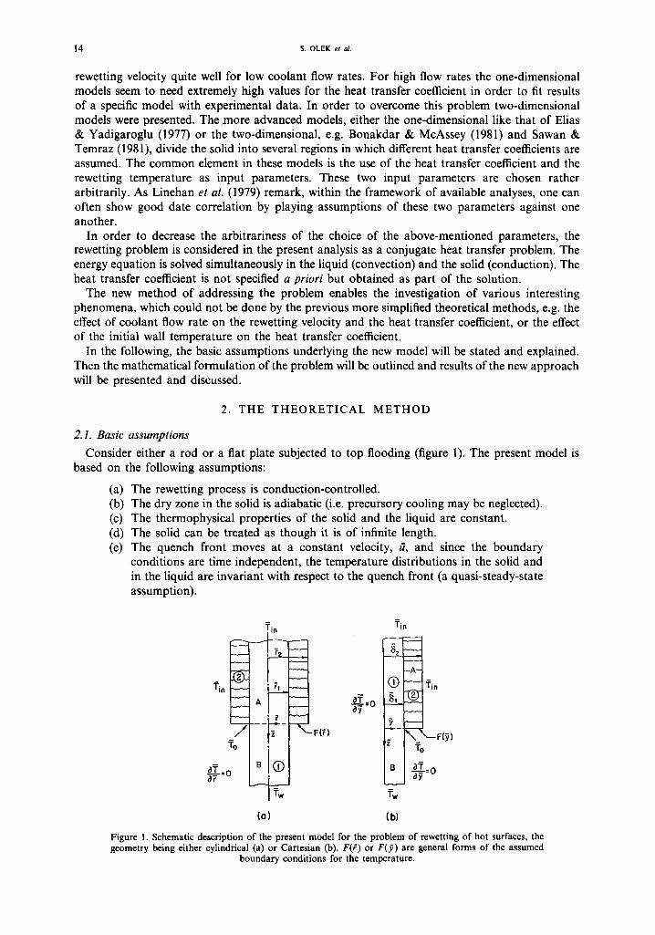
Consider either a rod or a flat plate subjected to top flooding (figure 1). The present model is based on the following assumptions:

(a) The rewetting process is conduction-controlled. (b) The dry zone in the solid is adiabatic (i.e. precursory cooling may be neglected). (c) The thermophysical properties of the solid and the liquid are constant. (d) The solid can be treated as though it is of infinite length. (el The quench front moves at a constant velocity, if, and since the boundary

conditions are time independent, the temperature distributions in the solid and in the liquid are invariant with respect to the quench front (a quasi-steady-state assumption).

Tin

~=o 87

fo .

BI® .~.-_1

I v.

IF(~) a~_O T~'-

Tin

L_ _ F(~I B a~_ .~--0

Tw

(Q) (b)

Figure 1. Schematic description of the present model for the problem of rewetting of hot surfaces, the geometry being either cylindrical (a) or Cartesian (b). F(F) or F07) are general forms of the assumed

boundary conditions for the temperature.

REWETTING AS A CONJUGATE HEAT TRANSFER PROBLEM 15

(f) The liquid wets the solid up to the point at which the temperature becomes the rewetting temperature, the value of which is constant in time and space.

(g) For a cylindrical geometry the quench front is symmetrical with respect to the rod axis and for a Cartesian geometry it is uniform in the x-direction.

(h) Far from the quench front the temperatures in the solid and the liquid approach fixed values.

(i) The liquid film moves at a constant average velocity, ~, and it has the flat shape shown in figure 1.

(j) The liquid film is of uniform thickness, which can be calculated for laminar flow by Nusselt's theory, and for turbulent flow from the correlations of Br6tz (1954) or Brier (Yih &Chen 1982).

(k) The temperature over the film-free surface is identical to the inlet liquid temperature.

(1) A first kind boundary condition may be specified at the bottom edge of the liquid film.

(m) The effect of secondary factors like the system pressure, surface finish etc., are either negligible or affect the rewetting temperature only.

(n) Heat sources in the solid and heat sinks in the liquid may be neglected.

Most assumptions which are not related to the liquid are common in rewetting models; only the principal assumptions pertaining to the liquid will be discussed here. More details are given by Olek (1986). According to assumption (b), precursory cooling is neglected. In previous works this assumption was found to be justified for low liquid flow rates. For high flow rates, neglecting the precursory cooling will result in an underprediction of the rewetting velocity. In assumptions (i) and (j) some simplification of the film geometry and movement were introduced, since its true shape and motion are very complicated and unknown. Assumption (k), regarding the temperature of the film-free surface, is based on the experimental evidence of Howard (1976), who collected the drops ejected at the quench front into a container of low heat capacity. He found that their measured temperature was not much higher than the liquid inlet temperature: 8-17°C, compared to liquid superheats of over 120°C at the quench front. Assumption (1) was made since the actual boundary condition at the edge of the liquid film is unknown, again. All we know is that the temperature distribution there must satisfy the rewetting temperature, To, at the liquid-solid interface, and the inlet liquid temperature, ~ , , at the film-free surface. Using several temperature distributions in the present model has shown that the exact form of the boundary condition at the advancing edge of the liquid film has only a negligible effect on the results obtained for the rewetting velocity, the calculated heat transfer coefficient and the heat flux from the wall to the liquid. Assumption (n) means that the heat generation in the solid and the vapor generation in the liquid above the quench front are neglected. The reason for the former is that the present method is applied here to cases corresponding to experiments, during which either the heat source is shut down or a low electrical power remains in the solid, whose effect on the rewetting velocity is negligible. It is noted that the method can be extended to include heat sources, as has been done by Olek (1986). Heat sinks due to vapor generation in the bulk of the liquid are neglected. At the quench front there exists a situation of very fast heating of the liquid to a high degree of superheat without substantial vapor generation at the ready boiling centers. The liquid boils violently on fluctuating centers similar to homogeneous nucleation. This boiling occurs over a very limited spatial region at the solid-liquid-vapor interline, probably of the order of a critical bubble diameter.

2.2. Analysis--governing equations In the following, a theoretical analysis for the application of the new approach will be described.

The formulation is valid both for Cartesian and cylindrical coordinate systems, see figure 1. The two-dimensional energy equations for the solid and the liquid, respectively, are:

~? =~, ~ ~- -~- /+-~Tj , 0~<~<~,, - ~ < i < ~ , ~>0, [1]

16 S. OLEK et aL

and

where

a-T + ~ T i Lra#\ -~ - /+ T U ] ' 5 < # ~ & , - ~ < 2 ~ < 0 , ? > 0 , [2]

01 for a Cartesian geometry, with ? =)7, ~l ~- #', /72 ~- ~2

v = for a cylindrical geometry.

The subscripts 1 and 2 denote the solid and the liquid, A denotes the region above the quench front, both in the solid and in the liquid, and B denotes the "dry region" in the solid, below the quench front. The thermal diffusivity is ~, # is the density and ? is the specific heat. All the variables are dimensional. Let us rewrite [1] and [2] in a unified form, after making use of the quasi-steady- state assumption (OT/O? = - a O T / 8 2 ) :

1 fff(f OT ) d2T ti, c3T r ~ + T ~ - + ~ - ~ = 0 , 0-.<#~<6, - ~ < ~ < ~ , [3]

where

u~= -5' ~ / = ~z # ! < # ~ < # 2 " [4]

The following normalized variables are defined:

O - Tw ~ ' r ==--~2, r l = - - , z =_ _ , - - r 2 r2

[5]

where Tw is the initial solid temperature and ~, is the liquid inlet temperature. Utilizing [5], the energy equations [3] are transformed into the following dimensionless form:

where

- - r v + - ~ z 2 + U*(r ) =0 , r ~ ~r ~z

u*(r) = f subject to the boundary conditions:

u * ur2 O <<. r <~ r,

(5 - - v ) 5 u * = - - rl < 1

~z

r =0, - - ~ < z ~<0:

r = 1, - ~ < z ~<0:

r = r l , - - ~ < z ~<0:

z ~ - - ~ , 0<~r~<l:

z = 0 , O <<. r <~ rl:

Z = 0 , r~<r~<l :

0 ~ < z < ~ :

0 ~ < z < ~ :

r = 0 ,

00 A - 0 ;

Or

0A = 0;

o~ =o~,

0a--* 0;

0a = 0B,

E, OO A _ O0 + .

Ez Or Or '

OOA d o n .

Oz ~ z '

F(F) - Tin. 0a = f ( r ) = T w - Ti. '

dos - - --0; 0r

dos - - --0; Or

[6]

[7]

[8a]

[8b]

[8c,d]

[8e]

[8f, g]

[8h]

[8i]

[8j]

REWETTING AS A CONJUGATE HEAT TRANSFER PROBLEM 17

z ---, 0% 0 ~< r ~< rl: 0B = 1 ; [8k]

z = 0 , r = r l : 0B=00 or 0A=00; [81]

where /~ and k" 2 are the thermal conductivities of the solid and the liquid, respectively. As explained above, several functions forf(r), [8h], have been used and the effect on the results

was negligible.

2.3. Method of solution Although the problem is actually a conjugate heat transfer problem, the above mathematical

formulation resembles that of conduction in a composite medium. Therefore, we will adopt relatively new methods, which were developed, among other things, for the solution of heat conduction problems in laminated media. Here the new methods are applied for the first time to a conjugate heat transfer problem. The method of solution chosen here is an extended version of separation of variables. The problem at hand poses three difficulties for the standard method of separation of variables: (a) discontinuity of the physical properties (solid, liquid) which renders the eigenfunctions in the traversal direction nonorthogonal with respect to the usual weight functions; (b) equation [6] is nonseparable due to the term u*(r)OO/dz; and (c) complicated geometry (a "jump" in the geometry).

Mathematical methods developed by Yeh (1975, 1976, 1980) extended the standard method of separation of variables and enable one to overcome all the difficulties mentioned above.

The solution is iterative in nature: a value for the rewetting velocity, t2, is first assumed. Then [6] is solved subject to boundary conditions [8a-l] and the temperature distributions in the solid and in the liquid are obtained. Finally, the correctness of the assumption is checked by the requirement that at the triple interface line the temperature be equal to the rewetting temperature within an acceptable error tolerance. In the present analysis the rewetting temperature is considered as an input parameter.

Let us assume that the temperature distribution in region A (above the quench front) can be represented in the following form:

OA(r , Z ) = ~ RA.(r)ZA.(Z). [9] n = l

The sets of functions {RA.(r)} and {ZA.(Z)} are determined in the following way. First, we define the former as the eigenfunctions obtained by substituting [9] into [6] with constant u*(r), and separating the variables:

d(rvdRA ~ d r \ dr / +22rvRA=0, [10]

where 2 are the eigenvalues of the eigenproblem posed by [10] and the boundary conditions

r =0:

r = r l ~

r - - l :

obtained from [8a-d]:

dRA - 0; [1 la]

dr

RA = R~ /~1 dRg _ dRy . [1 lb,c] ' k~ d ~ - - d--~-'

RA = 0. [1 ld]

After a special set of orthogonal functions {RA,(r)} is constructed, the last term in [6] is expanded by them and in the next stage the solution is completed by satisfying [6] with a proper choice of the set of functions {ZA,(Z)}. The general solution of [10] is of the following form:

fRAI = C A I X(gr) + DAI Y(2r), 0 ~< r ~< rl RA(r) = IRA2 CA2X(Ar) + DA2 Y(Ar), rl < r ~< 1"

[12]

The eigenfunctions for a Cartesian geometry are given by

X(2r) = cos(2r), Y(2r) = sin(2r); [13a]

M,F 14/I B

18 s. OLEK et al.

and for a cylindrical geometry by

X(2r) = J0(2r), Y(2r) = Y0(2r),

where J0 and Y0 are zero-order Bessel functions of the first and second kind, respectively. The constants in [12] are determined by the boundary conditions [1 l a d ] , which lead to:

[13b]

b12 CA2 q- btaDA2 = 0, [14a]

b21CAI -F b22 CA2 -F b23DA2 = 0; [14b]

b31 CAI + b32CA2 + b33DA2 = 0; [14c]

where Dgl = 0 and the coefficients are given by

blE=X(2) , b13=Y(2), b 2 1 = - X ( A r l ) , b22=X(2r l ) , b23=Y(Ar~),

b3, = - ~ r X ( 2 r ) l , = , , , b 3 2 = - ~ b3,, b33= ~ r Y(2r)l,=r,; [151

[14] are homogeneous simultaneous equations for CA~, CA2 and DA2. Nontrivial solutions exist if the determinant of the coefficients is zero:

b21 b32b13 + bal b12bE3 - b l a b 2 2 b 3 1 - b33b~2b21 = 0. [16]

The eigenvalues 2n are the positive roots of [16]. For each eigenvalue 2n satisfying [16], only two of the three equations [14a-c] are independent, and each pair of the unknowns can be solved from these equations in terms of the remaining third unknown.

It is possible to express, say, CA~ and DA2 in terms of CA2, and the result is

CA~=fA~CA2, DA2=gAnCA2, [17]

where

(b12b23 - b13b22 ) bl2 fA~-- b1362t , gA~-- hi3" [18]

The function RAg(r), aside from the constant multiplier CA2, is given by

Rk~(r) = - ~ RAIn(r) = fA~ X(2 , r ) . [19] [Rg2,(r) = X(2 , r ) + gA~ Y(2 , r )

The functions {RA~(r)} do not form an orthogonal set, because the derivative of RAg(r) is discontinuous at r = r~, as may be realized from the boundary condition [1 lc]. Therefore, the Sturm-Liouville theorem of orthogonality does not apply. The eigenfunctions, however, can be made orthogonal to each other with respect to a proper choice of a weighting function which can be found using Yeh's theorem (Yeh 1980), cf. the appendix.

To apply the theorem, we re-write [10]:

drr FAirY + 2 2 F ^ f R A = 0, r~_t < r < r , i = l, 2, [20]

where r0 - 0, r~ = ?J/f2, r2 - 1 and FA~ is a constant, yet unknown, within the interval r~_~ < r < ri. In order to determine FA~ from Yeh's theorem such that the solution R~ (r) obtained is orthogonal with respect to the weighting function FAir v, i.e.

r { R ~ ( r ) R ~ ( r ) F A i r vdr = 0 n C m [21]

i=1 ~_~ =/=0 n = m '

compare [20] with [A.1] and [ l lb , c] with [A.3a, b]. The following relations are obtained:

Btl=l, B2I=~, b=l, B31=0, B4z=0;

p = FAir v, w = FAir v, q = O, ri_ 1 < r < r i i = 1, 2. [22]

REWETTING AS A CONJUGATE HEAT TRANSFER PROBLEM

substituting [22] in the condition of orthogonality [A.4], yields

FA, /71

19

[23]

Since the proportionality constant is immaterial, as it does not affect the orthogonal relation [21], FA, is taken as the dimensionless quantities

/71 FA, = ~ , Fm = 1. [24]

Substituting [9] in [6], gives

1 d / vdRA-\ _ d 2ZA. , dZk. .=, r~ dr~r-~r )ZA.+ ~ + ~ --0. - - - - . = , l~g" ~ . = , U ( r ) R a . ~ z [25]

The product u*(r)RA~(r) is expanded now into a series of the eigenfunctions RA~(r):

u*(r)RA~(r) = ~ UA~i RAi(r), [26] i = l

where the constants UA~ are defined as

~r~' u*(r)RA~(r)RAi(r)FAjrv dr j = l - I

[27] UA.,-- J=,~ f, f R~'(r)FAjr~d

Substituting [26] into [25] and utilizing [10], yields

--~ ~2RAnZAn-~- ~ RAI1ZAn + ~ ~ ZtAnUAniRAi=O. [28] n = l n = l n = [ i = l

Interchanging the dummy indices n and i in the last term, [28] becomes

n--~l RAn , 2 (r Z L + UA,,ZA,- 2,ZA~ = 0. [29] i = 1

Since, in general, RA~ 4: 0, the expression in the large parentheses must vanish:

' --2,ZA~ =0 , n = 1 , 2 , . . . . [30] Z Ant' .q_ U Ain Z A i 2 i = l

Equation [30] represents a system of an infinite number of differential equations which is to be solved for an infinite number of variables, ZA.. AS is common practice in all series solutions, numerical calculations are carried out by taking a finite number of terms only. Thus, in solving [30] only a finite number of equations and ZA., say n = l, 2 . . . . . N, are considered. Since [30] are linear equations, the solutions can be written as

ZA~ (z) = A, exp(sz), [31 ]

where A, and s are constants to be determined. Substituting [31] into [30] results in the following:

N

s2A, + ~, UA~. sAi -- 2,2A = 0, n = 1, 2 . . . . . N, [32] i = 1

representing simultaneous homogeneous linear equations for the unknowns A,. Nontrivial solutions exist only if the determinant of the coefficients is zero, i.e.

(s 2 + UA,,S - ,Z~) UA2,S . . .

UAI2S (s 2 + UA22S - , ~ ) . . . = 0. [33]

U~,~s UA~3S . . .

20 s, OLEK et al.

In general, [33] can be solved to obtain N positive roots, s.. For each root, say s = sj, only N - 1 equations in [32] are independent; they can be solved for the N - 1 unknowns A. in terms of the remaining one, say Aj, giving

A. = a.jAj, n = 1, 2 . . . . . N, [34]

where az= 1. The function ZA.(Z) is the sum of all solutions, i.e. N

ZAn(X ) ~- ~ a.jAj exp(sjz). [35 ] j = l

For a finite number of terms N, the solution [9] can be written as

,36,

The solution for the temperature distribution in region B can be obtained by a standard separation of variables, using boundary conditions [8i-k]. The resulting relations are

N

OB = 1 + ~ B.RB.(r)ZB.(z), n = 1, 2 . . . . . N, [37]

where

and

n = l

While for a Cartesian geometry,

and ft. are the positive roots of

For a cylindrical geometry,

and ft. are the positive roots of

ZB.(z) = e x p ( - t.z) [38]

u* u .2 \1/2 t.=~-"}-(-~--~--'k-fl2.) . [39]

RB. (r) = cos(l/, r) [40]

sin(fl.rl) = 0. [41]

RB.(r) = Jo(fl.r) [42]

Ji (flnrl) = 0 . [43]

The complicated geometry poses a difficulty when one tries to determine the coefficients Aj and B. in the series by the matching conditions, using the orthogonality properties of the eigenfunctions. The difficulty stems from the fact that the eigenfunctions {RA. (r)} and {RB. (r)} are not orthogonal over the same interval. {RA.(r)} are orthogonal over the interval (0, 1), whereas {RB.(r)} are orthogonal over the interval (0, rj ). It turns out that in order to be able to determine the coefficients Aj and B., boundary conditions [8f] and [8h] must be combined in the following way [for a full explanation see Yeh (1975)]:

~ OB, O < < . r ~ r l , z = 0 OA= ( f ir ) , r l < r ~ l , z=O"

[44]

The first group of linear equations is obtained by multiplying [44] by RAn (r)FAir v and integrating over the interval (0, 1) and the second group of algebraic linear equations is obtained by multiplying [8g] by RB.(r)r v and integrating over the interval (0, rl). Performing the above multiplications and integrations gives

rVRM,.(r) RM.(r ) a m A i dr + rVRAz,.(r) RA2.(r ) ~, a.~A i dr k2 n = l i=1 I n = l i = l

= f ~ 'fcl~r'RAIm(r)[1 +~=B.N RB.(r )]dr+;rrVRmm(r) f ( r )d r l [45]

R E W E T T I N G AS A C O N J U G A T E H E A T T R A N S F E R PROBLEM 21

and

r~RB,.(r) RAt.(r ) sianiA i dr = - r~RBm(r) ~. RB.(r)t.B. dr. [46] n = l i = 1 n = l

After utilizing the orthogonality properties of the eigenfunctions {R~(r)} and {RB.(r)}, the following linear equations for A~ and B. are obtained from [45] and [46]:

N N

N ~ a m ~ A , = P m + 2 B. Qm., r e = l , 2 . . . . . N, [471 i = 1 n = |

n = | i = 1

where

and

fo I kl r~R2glm(r) dr + f j N ~ - ~ r~R2A2m(r ) dr, [49a] l

fo Pm- ~ rVRk~m(r) dr rVRA2m(r)f(r) dr, [49b] I

Q,.. - ~r RMm(r)R~.(r) dr, [49c]

f0' NBm -- rVR~(r) dr [49d]

~0 1

W,.. ==- r~RB,.(r)RAI.(r) dr. [49e]

Equations [47] and [48] represent 2N equations which can be solved simultaneously for 2N unknown coefficients A~ and B.. However, B. can be expressed in terms of A~ by [48] and then substituted in [47], so that only N equations need to be solved.

The conditions of equality of the temperature at the triple interface to the rewetting temperature, [81] can be written as

N N

~. R~(r,) ~ a.~A~ = 00 [50a] n = l i ~ l

o r

N

1 + ~ B.RB.(r,) = 00. [50b] n = l

In summary the solution scheme is as follows. A rewetting velocity ,2 is guessed and the eigenvalues 2. are calculated from [16]. The eigenvalues s. are calculated from [33] with UA~i given in [27]. The parameters t. are calculated from [39] where the eigenvalues ft. are given in [41] (or [43]). The coefficients Ai and B. of the temperature distributions in the wet and dry regions are obtained from [47] and [48] where the eigenfunctions {RA.(r)} are given in [19] and the eigenfunctions {Rs.(r)} are given in [40] (or [42]). The correctness of the assumed value of ti is then examined by [50a] or [50b] in an iterative manner until a convergence to a predetermined criterion is obtained.

The numerical solution of the problem consisted of the prediction of the rewetting velocity, the calculation of the temperature distributions in both the solid and the liquid, determining the axial and normal heat fluxes in each zone, and evaluating the wet side heat transfer coefficient. The problem was solved throughout in a Cartesian geometry. The eigenvalues ).. were determined as the positive roots of [16], using a combination of the Newton-Raphson and bisection methods. The positive roots s. of the determinant [33] were obtained using the EISPAC software, which solves eigenvalues and eigenvector problems with very high accuracy, even for large matrices. The various integrals in [49a-e] were evaluated analytically. Finally, the linear system of equations [47, 48] was solved by the LEQT2F subroutine from the IMSL library. This subroutine performs

22 s. O L E K et al.

Gaussian elimination (Crout algorithm) with equilibration, partial pivoting and iterative im- provement as required. Computation time varied with the number of terms used in the series. It ranged between about 20 s for 20 terms to about 700 s for 50 terms (on the IBM 3081 D computer). The iterative solution for the rewetting velocity was considered to converge when the relative error between 0A or 0B and 00 was < 1%. The convergence of the series was checked in all the cases presented here. It was found to be faster (a) the smaller the flow rate is, (b) the higher the initial solid temperature is, (c) the smaller the rod diameter (or solid circumference) is and (d) the smaller the wall thickness is. Details of the solution scheme can be found in Olek (1986). The next section includes results obtained by applying the method described above to several specific examples.

3. RESULTS AND DISCUSSION

In the following, numerical results of the method described above will be presented. The problem was solved throughout in a Cartesian geometry. In these calculations the rewetting temperature has been generally assumed as the minimum film boiling temperature, and in some cases as the quench front temperature reported in experiments.

3.1. Rewetting velocity--comparison with experimental results

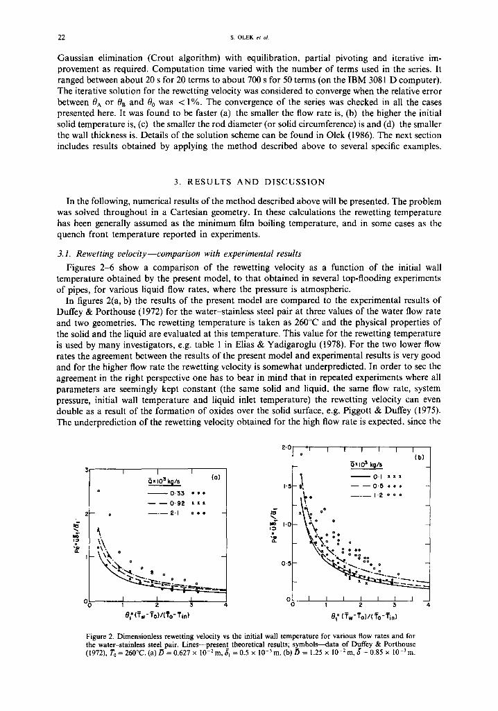
Figures 2-6 show a comparison of the rewetting velocity as a function of the initial wall temperature obtained by the present model, to that obtained in several top-flooding experiments of pipes, for various liquid flow rates, where the pressure is atmospheric.

In figures 2(a, b) the results of the present model are compared to the experimental results of Duffey & Porthouse (1972) for the water-stainless steel pair at three values of the water flow rate and two geometries. The rewetting temperature is taken as 260°C and the physical properties of the solid and the liquid are evaluated at this temperature. This value for the rewetting temperature is used by many investigators, e.g. table 1 in Elias & Yadigaroglu (1978). For the two lower flow rates the agreement between the results of the present model and experimental results is very good and for the higher flow rate the rewetting velocity is somewhat underpredicted. In order to see the agreement in the right perspective one has to bear in mind that in repeated experiments where all parameters are seemingly kept constant (the same solid and liquid, the same flow rate, system pressure, initial wall temperature and liquid inlet temperature) the rewetting velocity can even double as a result of the formation of oxides over the solid surface, e.g. Piggott & Duffey (1975). The underprediction of the rewetting velocity obtained for the high flow rate is expected, since the

I I I

GxlO 3 kg/s (o)

• 0 , 3 3 • • •

----0'92 x l x

- - o - - - - - 2 " 1 o o o

/

O,o , , ,

0~ (Tw- T o ) / t T o - Tin)

mT

o.

2.0

I',,.

I.C

0., i

o

- - 0 ' 1 x x x

, - - - - 0 " 5 o . *

~ o 1'2 o o o

x~e~° o ° ° o

O:oO \x~%. oOO0O

- - % : : . . 4 ° ::o o

J I I I 1 ] } 1 2 3

Ol = ( ~ w - T ' o ) / ( T o - T i n )

al I I I I I I (b)

F i g u r e 2. Dimens ion less rewet t ing veloci ty vs the ini t ia l wall t empera tu re for var ious flow rates and for the wa te r - s t a in less steel pair . L ine s - -p r e sen t theoret ical results; s y m b o l s ~ a t a o f Duffey & Por thouse (1972), T 0 = 260°C. (a) D = 0.627 x 10 -2 m, 6t = 0.5 x l0 -3 m. (b) D = 1.25 x l0 -2 m, 6 = 0.85 × 10 -3 m.

REWETTING AS A C O N J U G A T E HEAT TRANSFER PROBLEM 23

0.32 i I

o

OqE o

.~, o

o.o~ " ~ - - . o

oo

, -

o .o ,

0"02 0"1207 .~ .= ~ ' ~

- - - - - 0"3556 o o

I 0.01 '~ 4

e~=(Tw" ~o)/(To-Tin)

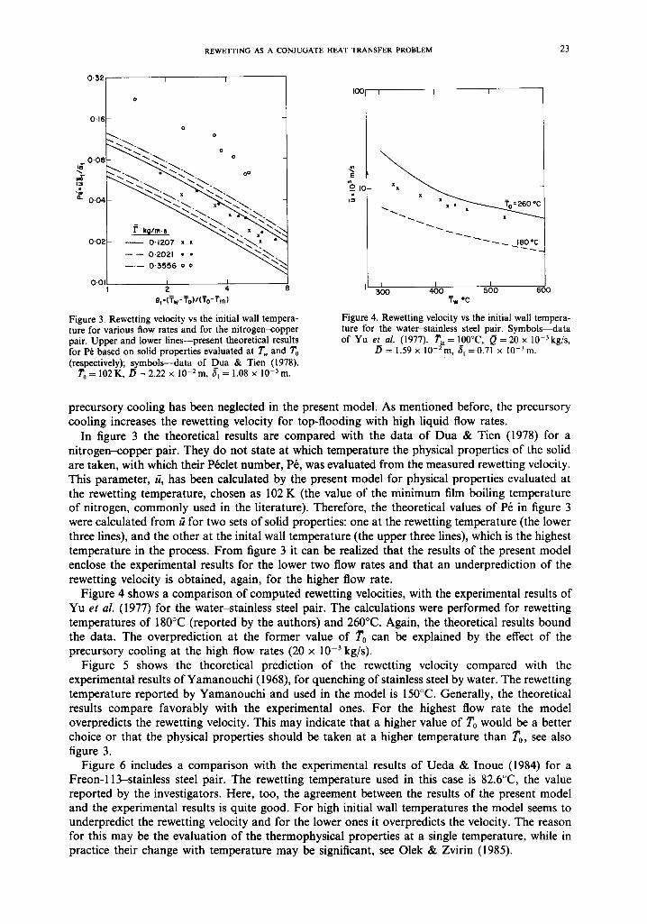
Figure 3. Rewetting velocity vs the initial wall tempera- ture for various flow rates and for the nitrogen-copper pair. Upper and lower lines--present theoretical results for P6 based on solid properties evaluated at 7'~ and T o (respectively); symbols--data of Dua & Tien (1978).

T 0=102K,/~=2.22x 10 -2m,c~ 1=l.08x 10 -3m.

lOG

E

~o x

I I I

x x

~ 1 8 0 %

I L I 300 400 500 600

Tw °C

Figure 4. Rewetting velocity vs the initial wall tempera- ture for the water-stainless steel pair. Symbols--data of Yu et al. (1977). Ti, = 100°C, O = 20 x 10 -3 kg/s,

/~ = 1.59 x 10-2m, 61 =0.71 x 10-3m.

precursory cooling has been neglected in the present model. As mentioned before, the precursory cooling increases the rewetting velocity for top-flooding with high liquid flow rates.

In figure 3 the theoretical results are compared with the data of Dua & Tien (1978) for a nitrogen-copper pair. They do not state at which temperature the physical properties of the solid are taken, with which their P6clet number, P6, was evaluated from the measured rewetting velocity. This parameter, if, has been calculated by the present model for physical properties evaluated at the rewetting temperature, chosen as 102 K (the value of the minimum film boiling temperature of nitrogen, commonly used in the literature). Therefore, the theoretical values of P6 in figure 3 were calculated from ff for two sets of solid properties: one at the rewetting temperature (the lower three lines), and the other at the inital wall temperature (the upper three lines), which is the highest temperature in the process. From figure 3 it can be realized that the results of the present model enclose the experimental results for the lower two flow rates and that an underprediction of the rewetting velocity is obtained, again, for the higher flow rate.

Figure 4 shows a comparison of computed rewetting velocities, with the experimental results of Yu e t al. (1977) for the water-stainless steel pair. The calculations were performed for rewetting temperatures of 180°C (reported by the authors) and 260°C. Again, the theoretical results bound the data. The overprediction at the former value of To can be explained by the effect of the precursory cooling at the high flow rates (20 x 10 -3 kg/s).

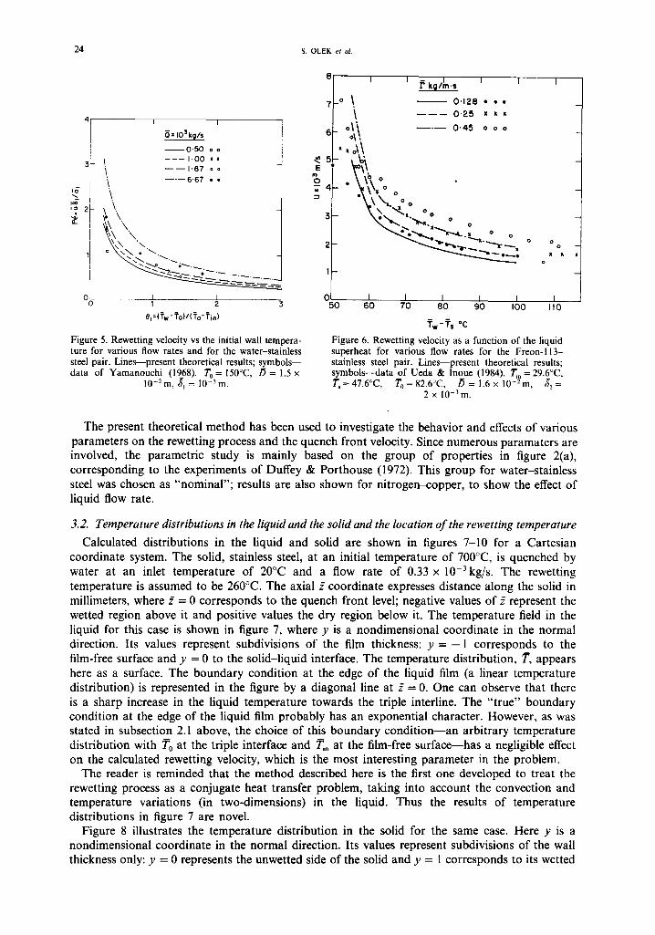
Figure 5 shows the theoretical prediction of the rewetting velocity compared with the experimental results of Yamanouchi (1968), for quenching of stainless steel by water. The rewetting temperature reported by Yamanouchi and used in the model is 150°C. Generally, the theoretical results compare favorably with the experimental ones. For the highest flow rate the model overpredicts the rewetting velocity. This may indicate that a higher value of To would be a better choice or that the physical properties should be taken at a higher temperature than To, see also figure 3.

Figure 6 includes a comparison with the experimental results of Ueda & Inoue (1984) for a Freon-113-stainless steel pair. The rewetting temperature used in this case is 82.6°C, the value reported by the investigators. Here, too, the agreement between the results of the present model and the experimental results is quite good. For high initial wall temperatures the model seems to underpredict the rewetting velocity and for the lower ones it overpredicts the velocity. The reason for this may be the evaluation of the thermophysical properties at a single temperature, while in practice their change with temperature may be significant, see Olek & Zvirin (1985).

2 4 s. O L E K et al.

i f f

I*K

i

o!

\

I I

x IO s kg/s

- - 0 " 5 0 = = . . . . I ' 00 xx - - - - 1 " 6 7 o . - - - - - 6'67 • .

\ \ . ,

\ , \

~ ~ - ~ . . , ~ ~ - ~ . ~

I I I 2

01= (?w - ~o)/11"o- ?inl

Figure 5. Rewetting velocity vs the initial wall tempera- ture for various flow rates and for the water-stainless steel pair. Lines--present theoretical results; symbols-- data of Yamanouchi (1968). T o = 150°C, /~ = 1.5 ×

10 -2 m, gt = 10-3 m.

E O B

e t J ~ k g / m . s t I I

71-o \ - - - - O .12e • • .

/ \ - - - 0 2 5 , , ,

6 L 0 ~ \ . . . . 0 " 4 5 o . .

5 = ~ ~°~ ~=~ t

4 • ~ i ° ° o " L \ \ . Oo

3 ,,,,~. ~ . o . o

" ~ ' ~ - . " ~ - ~ - - L , ° o 2 " ' ' " ~ = ~ r - ~ " ~ " ~ ' ~ x o o o

1

oi ~ I I I t i 5 0 6 0 70 80 90 I00 I tO

T w - ? s *C

Figure 6. Rewetting velocity as a function of the liquid superheat for various flow rates for the Freon-ll3- stainless steel pair. Lines--present theoretical results; symbols--data of Ueda & Inoue (1984). T~. = 29.6°C, T,=47.6°C, T 0=82.6°C, /5=1.6x10 -2m, 6~=

2 x 10 -3 m.

The present theoretical method has been used to investigate the behavior and effects of various parameters on the rewetting process and the quench front velocity. Since numerous paramaters are involved, the parametric study is mainly based on the group of properties in figure 2(a), corresponding to the experiments of Duffey & Porthouse (1972). This group for water-stainless steel was chosen as "nominal"; results are also shown for nitrogen-copper, to show the effect of liquid flow rate.

3.2. Temperature distributions in the liquid and the solid and the location of the rewetting temperature

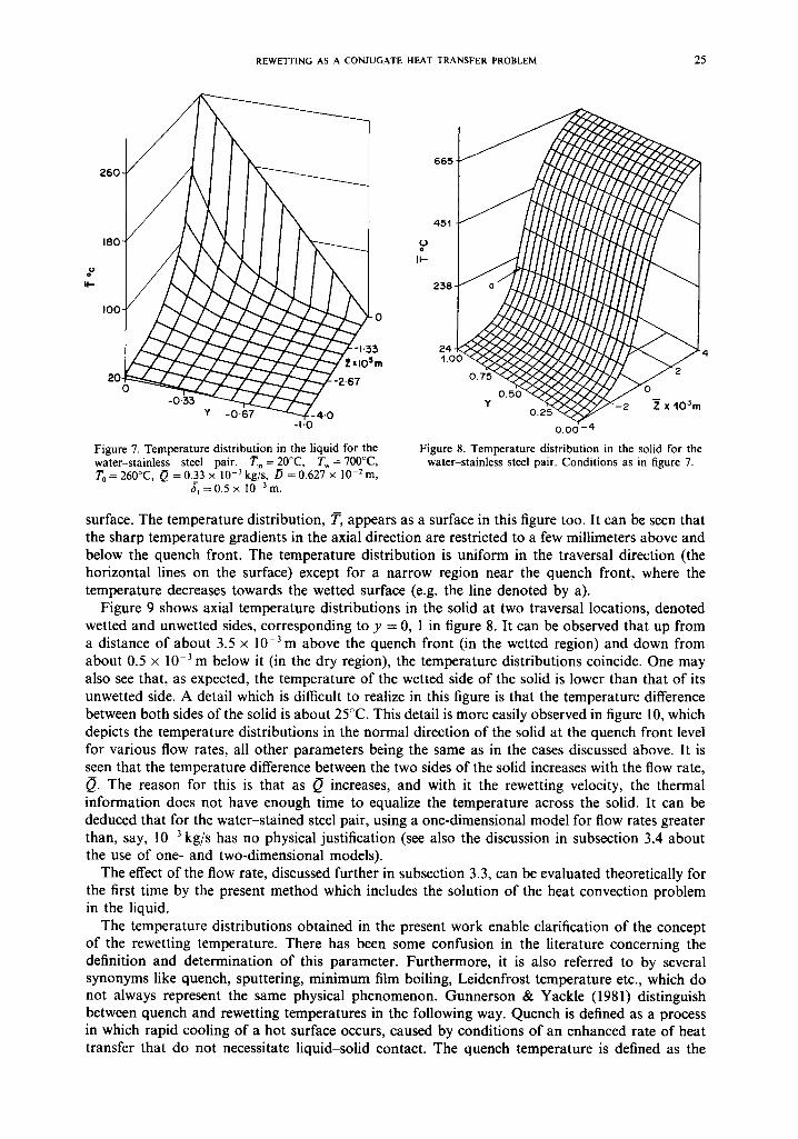
Calculated distributions in the liquid and solid are shown in figures 7-10 for a Cartesian coordinate system. The solid, stainless steel, at an initial temperature of 700°C, is quenched by water at an inlet temperature of 20°C and a flow rate of 0.33 × 10 -3 kg/s. The rewetting temperature is assumed to be 260°C. The axial :~ coordinate expresses distance along the solid in millimeters, where :~ = 0 corresponds to the quench front level; negative values of :? represent the wetted region above it and positive values the dry region below it. The temperature field in the liquid for this case is shown in figure 7, where y is a nondimensional coordinate in the normal direction. Its values represent subdivisions of the film thickness: y = - 1 corresponds to the film-free surface and y = 0 to the solid-liquid interface. The temperature distribution, T, appears here as a surface. The boundary condition at the edge of the liquid film (a linear temperature distribution) is represented in the figure by a diagonal line at f = 0. One can observe that there is a sharp increase in the liquid temperature towards the triple interline. The " t rue" boundary condition at the edge of the liquid film probably has an exponential character. However, as was stated in subsection 2.1 above, the choice of this boundary condi t ion--an arbitrary temperature distribution with To at the triple interface and ~ , at the film-free surface--has a negligible effect on the calculated rewetting velocity, which is the most interesting parameter in the problem.

The reader is reminded that the method described here is the first one developed to treat the rewetting process as a conjugate heat transfer problem, taking into account the convection and temperature variations (in two-dimensions) in the liquid. Thus the results of temperature distributions in figure 7 are novel.

Figure 8 illustrates the temperature distribution in the solid for the same case. Here y is a nondimensional coordinate in the normal direction. Its values represent subdivisions of the wall thickness only: y = 0 represents the unwetted side of the solid and y = 1 corresponds to its wetted

REWETTING AS A CONJUGATE HEAT TRANSFER PROBLEM 25

,o i i-

260 -

180"

I00-

3 ~m

204 (

'O

-I.O

Figure 7. Temperature distribution in the liquid for the water-stainless steel pair. ~ , = 20°C, Tw = 700°C, T0 = 260°C, O =0 .33 x 10-3 kg/s, /~ =0 .627 x 10-2m,

~ =0 .5 x 10-3m.

665

'oo 0.75 -2

o

Y 0 . 2 5 " 5 ~ ~ - 2 Z x I03m - % . . -

0.00 - 4

Figure 8. Temperature distribution in the solid for the water-stainless steel pair. Conditions as in figure 7.

surface. The temperature distribution, T, appears as a surface in this figure too. It can be seen that the sharp temperature gradients in the axial direction are restricted to a few millimeters above and below the quench front. The temperature distribution is uniform in the traversal direction (the horizontal lines on the surface) except for a narrow region near the quench front, where the temperature decreases towards the wetted surface (e.g. the line denoted by a).

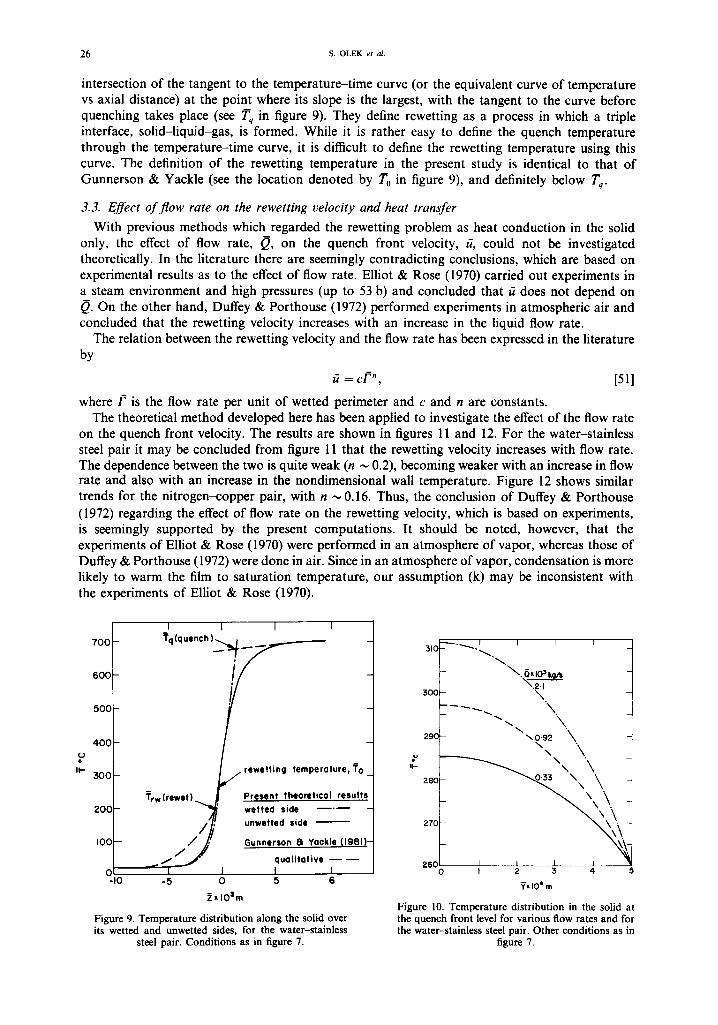
Figure 9 shows axial temperature distributions in the solid at two traversal locations, denoted wetted and unwetted sides, corresponding to y = 0, 1 in figure 8. It can be observed that up from a distance of about 3.5 x 10 -3 m above the quench front (in the wetted region) and down from about 0.5 x 10-3m below it (in the dry region), the temperature distributions coincide. One may also see that, as expected, the temperature of the wetted side of the solid is lower than that of its unwetted side. A detail which is difficult to realize in this figure is that the temperature difference between both sides of the solid is about 25°C. This detail is more easily observed in figure 10, which depicts the temperature distributions in the normal direction of the solid at the quench front level for various flow rates, all other parameters being the same as in the cases discussed above. It is seen that the temperature difference between the two sides of the solid increases with the flow rate, Q. The reason for this is that as Q increases, and with it the rewetting velocity, the thermal information does not have enough time to equalize the temperature across the solid. It can be deduced that for the water-stained steel pair, using a one-dimensional model for flow rates greater than, say, 10 3 kg/s has no physical justification (see also the discussion in subsection 3.4 about the use of one- and two-dimensional models).

The effect of the flow rate, discussed further in subsection 3.3, can be evaluated theoretically for the first time by the present method which includes the solution of the heat convection problem in the liquid.

The temperature distributions obtained in the present work enable clarification of the concept of the rewetting temperature. There has been some confusion in the literature concerning the definition and determination of this parameter. Furthermore, it is also referred to by several synonyms like quench, sputtering, minimum film boiling, Leidenfrost temperature etc., which do not always represent the same physical phenomenon. Gunnerson & Yackle (1981) distinguish between quench and rewetting temperatures in the following way. Quench is defined as a process in which rapid cooling of a hot surface occurs, caused by conditions of an enhanced rate of heat transfer that do not necessitate liquid-solid contact. The quench temperature is defined as the

26 s. OLEK et al.

intersection of the tangent to the temperature-time curve (or the equivalent curve of temperature vs axial distance) at the point where its slope is the largest, with the tangent to the curve before quenching takes place (see Tq in figure 9). They define rewetting as a process in which a triple interface, solid-liquid-gas, is formed. While it is rather easy to define the quench temperature through the temperature-time curve, it is difficult to define the rewetting temperature using this curve. The definition of the rewetting temperature in the present study is identical to that of Gunnerson & Yackle (see the location denoted by To in figure 9), and definitely below Tq.

3.3. Effect of flow rate on the rewetting velocity and heat transfer

With previous methods which regarded the rewetting problem as heat conduction in the solid only, the effect of flow rate, ~., on the quench front velocity, ti, could not be investigated theoretically. In the literature there are seemingly contradicting conclusions, which are based on experimental results as to the effect of flow rate. Elliot & Rose (1970) carried out experiments in a steam environment and high pressures (up to 53 b) and concluded that ff does not depend on ~. On the other hand, Duffey & Porthouse (1972) performed experiments in atmospheric air and concluded that the rewetting velocity increases with an increase in the liquid flow rate.

The relation between the rewetting velocity and the flow rate has been expressed in the literature by

a =c•", [51]

where f is the flow rate per unit of wetted perimeter and c and n are constants. The theoretical method developed here has been applied to investigate the effect of the flow rate

on the quench front velocity. The results are shown in figures 11 and 12. For the water-stainless steel pair it may be concluded from figure 11 that the rewetting velocity increases with flow rate. The dependence between the two is quite weak (n ~ 0.2), becoming weaker with an increase in flow rate and also with an increase in the nondimensional wall temperature. Figure 12 shows similar trends for the nitrogen--copper pair, with n ~ 0.16. Thus, the conclusion of Duffey & Porthouse (1972) regarding the effect of flow rate on the rewetting velocity, which is based on experiments, is seemingly supported by the present computations. It should be noted, however, that the experiments of Elliot & Rose (1970) were performed in an atmosphere of vapor, whereas those of Duffey & Porthouse (1972) were done in air. Since in an atmosphere of vapor, condensation is more likely to warm the film to saturation temperature, our assumption (k) may be inconsistent with the experiments of Elliot & Rose (1970).

f..) o II-.-

700

60C

500

4 0 0

:300

200

I00

0

I I I Tq (q uench ) ~ / ~ ~ . . . , ~

_ Trw (rewet) " ~ q / t

_

- I0 -5 0

x IOSm

Figure 9. Temperature distribution along the solid over i t s wetted and unwetted sides, for the water-stainless

steel pair. Conditions as in figure 7.

j rewetting temperature, To I

Present theoreticol results wetted side unwetted side

Gunnerson 8t Yaekle (1981)- qualitative m I I 5 6

310 - ~ """~" - r I I I ~ - ~

" ~ . ~, I03 kg/s \.2.1

300 \ .

-. \ 290 ~. 0"92

\ -, \

';~ 280 - - - - ~ ~ \ \ \ \ \ ' \

270

260 I I I I 0 I 2 3 4 5

~x I04 m

Figure 10. Temperature distribution in the solid at t h e quench front level for various flow rates and for t h e water-stainless steel pair. Other conditions as in

figure 7.

REWETTING AS A CONJUGATE HEAT TRANSFER PROBLEM 27

l eo

, c o

I'E

1.4

I-2

I-0

0.8

0'6

0.4

0.2

I i / /

I-OO_ _

_..&4..o9__..._

I I I I 0"4 0-8 1"2 1"6 2"0

~x103 kQ/s

Figure 11. Rewetting velocity as a function of flow rate for the water-stainless steel pair at various initial wall temperatures. Ti, =20°C, To = 260°C, D = 0.627 x

10-2m, 61 =0.5 x 10-3m.

0I(

0"08

'7

0.04

0-02

0 . 0 1

I I I I

2

4

6 . . . . . . . . . . . . . .

e__

I I I I 0"15 0"20 0"25 0"30

kg/m.s

Figure 12. Rewetting velocity as a function of flow rate for the nitrogen-copper pair at various initial wall temperatures. T i . = 7 7 K , T 0 = 1 0 2 K , D = 2 . 2 2 x

10-2m, 3, = 1.08 x 10-3m, 0, = ( T , - To)/(To- ~).

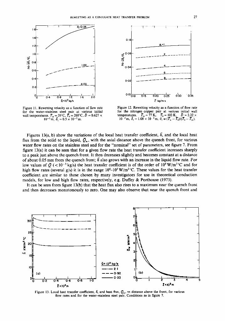
Figures 13(a, b) show the variations of the local heat transfer coefficient, h', and the local heat flux from the solid to the liquid, Qw, with the axial distance above the quench front, for various water flow rates on the stainless steel and for the "nominal" set of parameters, see figure 7. From figure 13(a) it can be seen that for a given flow rate the heat transfer coefficient increases sharply to a peak just above the quench front. It then decreases slightly and becomes constant at a distance of about 0.05 mm from the quench front; h also grows with an increase in the liquid flow rate. For low values of Q (< 10 -3 kg/s) the heat transfer coefficient is of the order of 104 W/m2°C and for high flow rates (several g/s) it is in the range 104-105 W/m2°C. These values for the heat transfer coefficient are similar to those chosen by many investigators for use in theoretical conduction models, for low and high flow rates, respectively, e.g. Duffey & Porthouse (1973).

It can be seen from figure 13(b) that the heat flux also rises to a maximum near the quench front and then decreases monotonously to zero. One may also observe that near the quench front and

30

25

.u

"e ac

i e -

IS

I0

I

. ° ~ . _

I I I

(a)

3 I I I I 0 0 . 2 0 . 4 0 . 6 0 - 8

~ ' x l O S m

I i ~ I I I I

6

L °i!

I o 3

2 (~x I 0 a k g / s

~ - ~ 2 '1 I - - - - - - 0 . 9 2 ( b )

I - - 0 -33 0 I I K I 1.0 0 I 2 3 4

IF x l O a m

Figure 13. Local heat transfer coet~cient, h', and heat flux, Q,,, vs distance above the front, for various flow rates and for the water-stainless steel pair. Conditions as in figure 7.

28 s. OLEK et al.

35 p ~xlO m k g / s / . ~

/ 30 / " 0 .92 t " " /

/ " 7 7 /

, / 25 / / "s / /

/ IJE 2O /

15

0 I 0.1 1.0 10

0 t : ('Tw "'To)/(To" 1"in )

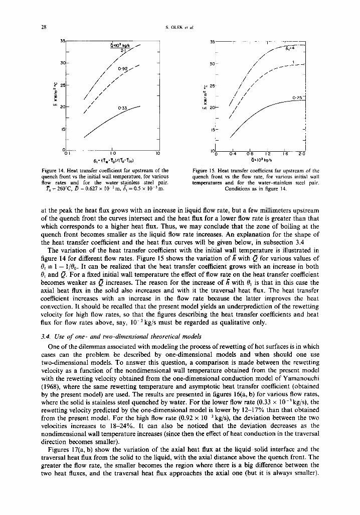
Figure 14. Heat transfer coefficient far upstream of the quench front vs the initial wall temperature, for various flow rates and for the water-stainless steel pair.

T O = 260°C, /~ = 0.627 x 10 -2 m, ~, = 0.5 × 10 .3 m.

351 I I [ - ~ / . I - 0,-4

/ 30 / ' I

/ / , / .o 25 / / /

/ / ' / / / / o25

u= 20

15

IC I I I I 0 .4 0.8 1.2 1.6 2.0

~ I03 k(J/s

Figure 15. Heat transfer coefficient far upstream of the quench front vs the flow rate, for various initial wall temperatures and for the water-stainless steel pair.

Conditions as in figure 14.

at the peak the heat flux grows with an increase in liquid flow rate, but a few millimeters upstream of the quench front the curves intersect and the heat flux for a lower flow rate is greater than that which corresponds to a higher heat flux. Thus, we may conclude that the zone of boiling at the quench front becomes smaller as the liquid flow rate increases. An explanation for the shape of the heat transfer coefficient and the heat flux curves will be given below, in subsection 3.4

The variation of the heat transfer coefficient with the initial wall temperature is illustrated in figure 14 for different flow rates. Figure 15 shows the variation of h" with ~. for various values of 0, = 1 - 1/00. It can be realized that the heat transfer coefficient grows with an increase in both 0, and ~. For a fixed initial wall temperature the effect of flow rate on the heat transfer coefficient becomes weaker as ~. increases. The reason for the increase of h" with 0, is that in this case the axial heat flux in the solid also increases and with it the traversal heat flux. The heat transfer coefficient increases with an increase in the flow rate because the latter improves the heat convection. It should be recalled that the present model yields an underprediction of the rewetting velocity for high flow rates, so that the figures describing the heat transfer coefficients and heat flux for flow rates above, say, 10 -3 kg/s must be regarded as qualitative only.

3.4. Use o f one- and two-dimensional theoretical models

One of the dilemmas associated with modeling the process of rewetting of hot surfaces is in which cases can the problem be described by one-dimensional models and when should one use two-dimensional models. To answer this question, a comparison is made between the rewetting velocity as a function of the nondimensional wall temperature obtained from the present model with the rewetting velocity obtained from the one-dimensional conduction model of Yamanouchi (1968), where the same rewetting temperature and asymptotic heat transfer coefficient (obtained by the present model) are used. The results are presented in figures 16(a, b) for various flow rates, where the solid is stainless steel quenched by water. For the lower flow rate (0.33 x 10 -3 kg/s), the rewetting velocity predicted by the one-dimensional model is lower by 12-17% than that obtained from the present model. For the high flow rate (0.92 x 10 -3 kg/s), the deviation between the two velocities increases to 18-24%. It can also be noticed that the deviation decreases as the nondimensional wall temperature increases (since then the effect of heat conduction in the traversal direction becomes smaller).

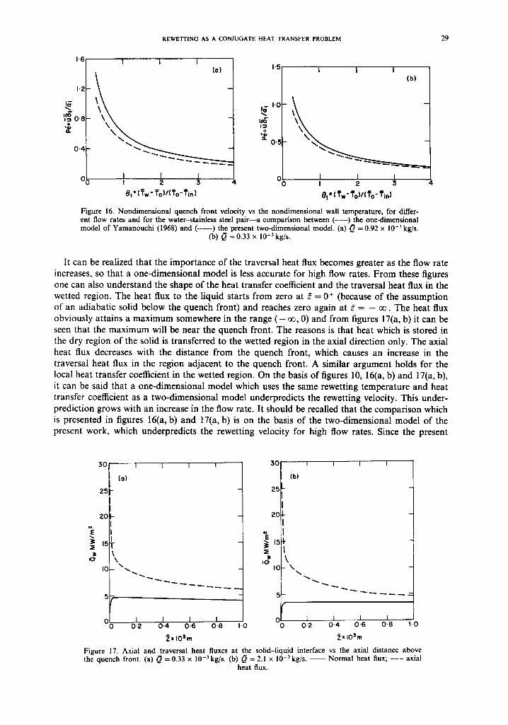
Figures 17(a, b) show the variation of the axial heat flux at the liquid-solid interface and the traversal heat flux from the solid to the liquid, with the axial distance above the quench front. The greater the flow rate, the smaller becomes the region where there is a big difference between the two heat fluxes, and the traversal heat flux approaches the axial one (but it is always smaller).

REWETTING AS A CONJUGATE HEAT TRANSFER PROBLEM 29

1.6

1.2

~ 0 ' 8 ,k

0 .4

I 1 I (o)

\ \ _

I I I I 2 3 4

et = (Tw - To ) / (?o- ?in)

1.5

L•I.C n

"~ o . s

I I I (b)

\ \ \

1 I I I 2 3

01 = [ 'Tw" To) / I To" Tin)

Figure 16. Nondimensional quench front velocity vs the nondimensional wall temperature, for differ- ent flow rates and for the water-stainless steel pa i r - -a comparison between ( - - - ) the one-dimensional model of Yamanouchi (1968) and ( ) the present two-dimensional model. (a) L7 = 0.92 x 10 -3 kg/s.

(b) Q = 0.33 x 10 -3 kg/s.

It can be realized that the importance of the traversal heat flux becomes greater as the flow rate increases, so that a one-dimensional model is less accurate for high flow rates. From these figures one can also understand the shape of the heat transfer coefficient and the traversal heat flux in the wetted region. The heat flux to the liquid starts from zero at :? = 0 ÷ (because of the assumption of an adiabatic solid below the quench front) and reaches zero again at f = - ~ . The heat flux obviously attains a maximum somewhere in the range ( - oo, 0) and from figures 17(a, b) it can be seen that the maximum will be near the quench front. The reasons is that heat which is stored in the dry region of the solid is transferred to the wetted region in the axial direction only. The axial heat flux decreases with the distance from the quench front, which causes an increase in the traversal heat flux in the region adjacent to the quench front. A similar argument holds for the local heat transfer coefficient in the wetted region. On the basis of figures 10, 16(a, b) and 17(a, b), it can be said that a one-dimensional model which uses the same rewetting temperature and heat transfer coefficient as a two-dimensional model underpredicts the rewetting velocity. This under- prediction grows with an increase in the flow rate. It should be recalled that the comparison which is presented in figures 16(a, b) and 17(a, b) is on the basis of the two-dimensional model of the present work, which underpredicts the rewetting velocity for high flow rates. Since the present

:.30 I 1 I ~ $01 ~ I I l

(a) I (b)

25 ~-5 t I

2 0 - z o ~ I

"E i I ,5 - .~ ,sh ~

- \ IO \ =0

5 -

0 I I I I I I I I 0 0"2 0 .4 0-6 0 -8 I-0 0 0 .2 0 .4 0 -6 0 .8 I -0

= l0 s m ~ x 103 m

F igure 17. A x i a l and traversa] heat f luxes at the so l i d - l i qu id in ter lace vs the ax ia l distance above the quench f ront . (a) (~ = 0 . 3 3 x ] 0 -3kg /s . (b) ~ = 2.1 x 10-3kg/s . - - N o r m a l heat f lux; - - - ax ia l

heat f lux.

30 S. OLEK et aL

16

15

14

°u 12

i 1 -

I0

9

8

7

6 0

I 1 I I

-I . . . . ?o=Z4o*c

260"C

I I I I 0"2 0 '4 0'6 0 '8 I '0

[PxlO3m

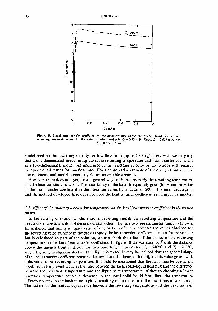
Figure 18. Local heat transfer coefficient vs the axial distance above the quench front, for different rewetting temperatures and for the water-stainless steel pair. ~ = 0.33 x 10 -3 kg/s,/5 = 0.627 x 10 -2 m,

~l = 0.5 x 10 -~ m.

model predicts the rewetting velocity for low flow rates (up to 10 -3 kg/s) very well, we may say that a one-dimensional model using the same rewetting temperature and heat transfer coefficient as a two-dimensional model will underpredict the rewetting velocity by up to 20% with respect to experimental results for low flow rates. For a conservative estimate of the quench front velocity a one-dimensional model seems to yield an acceptable accuracy.

However, there does not, yet, exist a general way to choose properly the rewetting temperature and the heat transfer coefficient. The uncertainty of the latter is especially great (for water the value of the heat transfer coefficient in the literature varies by a factor of 200). It is reminded, again, that the method developed here does not need the heat transfer coefficient as an input parameter.

3.5. Effect of the choice of a rewetting temperature on the local heat transfer coefficient in the wetted region

In the existing one- and two-dimensional rewetting models the rewetting temperature and the heat transfer coefficient do not depend on each other. They are two free parameters and it is known, for instance, that taking a higher value of one or both of them increases the values obtained for the rewetting velocity. Since in the present study the heat transfer coefficient is not a free parameter but is calculated as part of the solution, we can check the effect of the choice of the rewetting temperature on the local heat transfer coefficient. In figure 18 the variation of h- with the distance above the quench front is shown for two rewetting temperatures: To = 240°C and To = 260°C, where the solid is stainless steel and the liquid is water. It may be realized that the general shape of the heat transfer coefficient remains the same [see also figures 13(a, b)], and its value grows with a decrease in the rewetting temperature. It should be mentioned that the heat transfer coefficient is defined in the present work as the ratio between the local solid-liquid heat flux and the difference between the local wall temperature and the liquid inlet temperature. Although choosing a lower rewetting temperature causes a decrease in the local solid-liquid heat flux, the temperature difference seems to diminish more rapidly, resulting in an increase in the heat transfer coefficient. The nature of the mutual dependence between the rewetting temperature and the heat transfer

REWETTING AS A CONJUGATE HEAT TRANSFER PROBLEM 31

coefficient, which was obtained here on a theoretical basis, resembles that obtained by Yu et al. (1977) on the basis of their experimental results: (To - Tq)x/~ = const, where Tq is the temperature of the water at the quench front and h" is the heat transfer coefficient. This form of relationship between the rewetting temperature and the heat transfer coefficient leads to the conclusion that they cannot be chosen as independent parameters in rewetting models.

4. CONCLUSIONS

In the present study a new approach to address the rewetting phenomena has been presented. It regards the process as a conjugate heat transfer problem in which the temperature distributions in the solid and the liquid are solved simultaneously, unlike existing theoretical methods which regard the problem as heat conduction in the solid only. In this new method the heat transfer coefficient need not be specified and, in fact, it may be obtained as part of the solution. The rewetting temperature is the only arbitrary input parameter in the method.

Several comparisons between theoretical results obtained by the present method and experi- mental results for the rewetting velocity show good agreement in most cases, especially at low flow rates. For high flow rates (> l0 -3 kg/s), the present model somewhat underpredicts the quench front velocity. This discrepancy is mainly due to neglecting the precursory cooling in the model, which is known to increase the rewetting velocity.

In addition, the method has been applied to study several effects theoretically, which could not be done by previous methods; examples of which are: the effect of flow rate on the rewetting velocity; the heat transfer coefficient and the heat flux from the solid to the liquid; and the effect of the initial wall temperature on the heat transfer coefficient.

Conclusions related to the effect of various parameters on the rewetting velocity, which can be obtained by previous theoretical methods also, will not be elaborated here. Instead, we will confine ourselves to examples of conclusions which are unique to the present method:

(a) The rewetting velocity increases with liquid flow rate. The rate of increase in the velocity becomes smaller as the flow rate grows.

(b) The heat transfer coefficient and solid-liquid heat flux rise with flow rate, where the rate of growth becomes more moderate for higher flow rates.

(c) The zone which characterizes the quench phenomenon becomes smaller with increasing flow rate.

(d) The heat transfer coefficient increases with the initial wall temperature and decreases with higher values of the rewetting temperature.

(e) One-dimensional models which use the same values of rewetting temperature and heat transfer coefficient as two-dimensional models, underpredict the rewetting velocity. The deviation increases with the flow rate.

The analytical method used here for the solution of the conjugate heat transfer problem can also be applied to the solution of a more complicated fuel and cladding model, including precursory cooling and heat sources. In order for the latter to be amenable to solution by separation of variables, these heat sources should be represented by a product of functions, each in just one spatial variable.

REFERENCES

BONAKDAR, H. & McAssEY, JR 1981 A method for determining the rewetting velocity under generalized boiling conditions. Nucl. Engng Des. 66, 7-12.

BR6TZ, W. 1954 l~lber die Vorausberechnung der Absorptionsgeschwindigkeit von Gasen in Str6menden Fliissigkeitsschichten. Chemie-Ingr.-Tech. 26, 470-478.

BUTTERWORTH, D. & OWEN, R. G. 1975 The quenching of hot surfaces by top and bottom flooding--a review. Report No. AERE-R7992, AERE Harwell, Oxon.

CARBAJO, J. J. (~ SIEGEL, A. D. 1980 Review and comparison among the different models for rewetting in LWRs. Nucl. Engng Des. 58, 33-44.

32 s. OLEK et al.

DUA, S. S. & TIEN, C. L. 1978 An experimental investigation of falling-film rewetting. Int. J. Heat Mass Transfer 21, 955-965.

DUEFEY, R. B. & PORTHOUSE, D. Z. C. 1972 Experiments on the cooling of high temperature surfaces by water jets and drops. Report No. RD/B/N 2386, CEGB Nuclear Labs, Glos.

DUFFEY, R. B. & PORTHOUSE, D. T. C. 1973 The physics of rewetting in water reactor emergency core cooling. Nucl. Engng Des. 25, 379-394.

ELIAS, E. t~¢ YADIGAROGLU, G. 1977 A general one-dimensional model for conduction-controlled rewetting of a surface. Nucl. Engng Des. 42, 185-194.

ELIAS, E. & YADIGAROGLU, G. 1978 The reflooding phase of the LOCA in PWRs, Part II. Rewetting and liquid entrainment. Nucl. Safety 19, 160-175.

ELLIOT, D. F. & ROSE, P. W. 1970 The quenching of a heated surface by a film of water in a steam environment of pressures up to 53 bar. Report No. AEEW-M976, UKAEA, Winfrith, Dorset.

GUNNERSON, F. S. t~; YACKLE, T. R. 1981 Quenching and rewetting of nuclear fuel rods. Nucl. Technol. 54, ll3-117.

HOWARD, P. A. 1976 An experimental and analytical study of the sputtering phenomena. Report No. ANL-76-41, Argonne National Lab., Argonne, Ill.

LINEHAN, J. H., HOWARD, P. A. & GROLMES, M. A. 1979 The stationary boiling front in liquid film cooling of a vertical heated rod. Nucl. Engng Des. 52, 201-218.

OLEK, S. 1986 Rewetting of hot surfaces. D.Sc. Thesis, Technion, IIT, Haifa, Israel. OLEK, S. • ZVIRIN, Y. 1985 The effect of temperature dependent properties on the rewetting

velocity. Int. J. Multiphase Flow 11, 577-581. PIGGOTT, B. D. G & DUEEEY, R. B. 1975 The quenching of irradiated fuel pins. Nucl. Engng Des.

32, 182-190. SAWAN, M. E. & CARBON, M. W. 1975 A review of spray-cooling and bottom flooding work for

LWR cores. Nucl. Engng Des. 32, 191-207. SAWAN, M. E. & TEMRAZ, H. M. 1981 A three regions semi-analytical rewetting model. Nucl. Engng

Des. 64, 319-327. UEDA, U. & INOUE, M. 1984 Rewetting of a hot surface by a falling liquid film--effect of liquid

subcooling. Int. J. Heat Mass Transfer 27, 999-1005. YAMANOUCHI, A. 1968 Effect of core spray cooling in transient state after loss of coolant accident.

J. nucl. Sci. Technol. 5, 547-558. YEH, H.-C. 1975 An analysis of rewetting of a nuclear fuel rod in water reactor emergency core

cooling. Nucl. Engng Des. 34, 317-322. YEn, H.-C. 1976 Extension of the method of solving potential field problems for complicated

geometries. J. appl. Phys. 47, 2923-2928. YEn, H.-C. 1977 Solving potential field problems in composite media with complicated geometries.

J. appl. Phys. 48, 4423-4429. YEH, H.-C. 1980 An analytical solution to fuel-and-cladding model of the rewetting of a nuclear

fuel rod. Nucl. Engng Des. 61, 101-112. YIH, S. M. & CHEN, K. Y. 1982 Gas absorption into wavy and turbulent falling liquid films in a

wetted wall column. Chem. Engng Commun. 17, 123-136. Yu, S. K. W., FARMER, P. R. & CONEY, M. W. E. 1977 Methods and correlations for the prediction

of quenching rates on hot surfaces. Int. J. Multiphase Flow 3, 415-443.

A P P E N D I X

Yeh's Theorem

Theorem

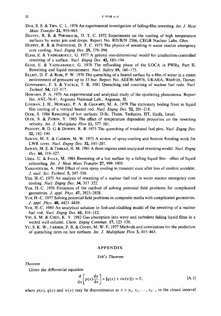
Given the differential equation

d [p(X)~xxl + [q(x) + 2w(x)]y =0, [A.I]

where p(x), q(x) and w(x) may be discontinuous at x = x~, xz . . . . . xu t in the closed interval

REWETTING AS A CONJUGATE HEAT TRANSFER PROBLEM 33

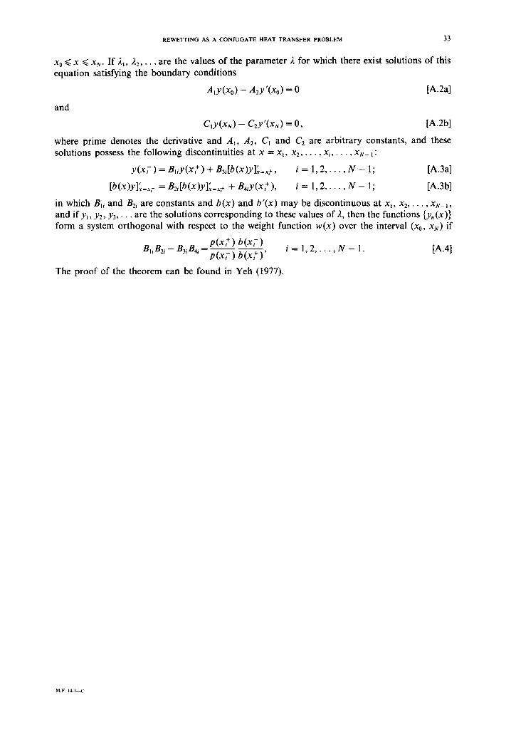
x0 ~< x ~< xu. I f 2~, 22 . . . . are the values o f the parameter 2 for which there exist solutions o f this equat ion satisfying the boundary condit ions

Aly(xo) - A2y'(xo) = 0 [A.2a]

and

C,y(xN) -- C2y'(xu) = 0, [A.2b]

where prime denotes the derivative and A~, A2, C~ and C2 are arbi t rary constants, and these solutions possess the following discontinuities at x = x~, x2 . . . . . xt . . . . . xu_ ]:

y(x7 ) = B~iy(x +) + Ba,[b(x)y]'~=x:, i = 1, 2 , . . . , N - 1; [A.3a]

[b(x)y]':,=x; = Bz~[b(x)y]'~=x,+ + B4iy(x + ), i = 1, 2 . . . . , N - 1; [A.3b]

in which B~i and B2i are constants and b(x) and b'(x) may be discontinuous at x~, x2 . . . . . xu_, , and if yl, Y2, Y3 . . . . are the solutions corresponding to these values o f 2, then the functions {y. (x)} form a system or thogona l with respect to the weight function w(x) over the interval (x0, xu) if

p(x~ + ) b(x? ) B]~B2g- B3iB4~-p(x?--~) b(x+~) ' i = 1, 2 . . . . . N - 1. [A.4]

The p r o o f o f the theorem can be found in Yeh (1977).

M.F. 14 /1~