HAL Id: hal-03165049https://hal.archives-ouvertes.fr/hal-03165049

Submitted on 10 Mar 2021

HAL is a multi-disciplinary open accessarchive for the deposit and dissemination of sci-entific research documents, whether they are pub-lished or not. The documents may come fromteaching and research institutions in France orabroad, or from public or private research centers.

L’archive ouverte pluridisciplinaire HAL, estdestinée au dépôt et à la diffusion de documentsscientifiques de niveau recherche, publiés ou non,émanant des établissements d’enseignement et derecherche français ou étrangers, des laboratoirespublics ou privés.

Numerical study of conjugate mass transfer from aspherical droplet at moderate Reynolds number

Azeddine Rachih, Dominique Legendre, Éric Climent, Sophie Charton

To cite this version:Azeddine Rachih, Dominique Legendre, Éric Climent, Sophie Charton. Numerical study of conjugatemass transfer from a spherical droplet at moderate Reynolds number. International Journal of Heatand Mass Transfer, Elsevier, 2020, 157, pp.119958. �10.1016/j.ijheatmasstransfer.2020.119958�. �hal-03165049�

OATAO is an open access repository that collects the work of Toulouse researchers and makes it freely available over the web where possible

Any correspondence concerning this service should be sent

to the repository administrator: tech-oatao@listes-diff.inp-toulouse.fr

This is an author’s version published in: https://oatao.univ-toulouse.fr/27534

To cite this version:

Rachih, Azeddine and Legendre, Dominique and Climent, Éric and

Charton, Sophie Numerical study of conjugate mass transfer from a

spherical droplet at moderate Reynolds number. (2020)

International Journal of Heat and Mass Transfer, 157. 119958. ISSN

0017-9310

Open Archive Toulouse Archive Ouverte

Official URL : https://doi.org/10.1016/j.ijheatmasstransfer.2020.119958

Numerical study of conjugate mass transfer from a spherical droplet

at moderate Reynolds number

Azeddine Rachih

a , b , Dominique Legendre

b , Eric Climent b , Sophie Charton

a , ∗

a CEA,DES, ISEC, DMRC, Univ. Montpellier, Marcoule, Franceb Institut de Mécanique des Fluides de Toulouse (IMFT), Université de Toulouse, CNRS, Univ. Paul Sabatier, Toulouse INP, Toulouse 31400, France

a r t i c l e i n f o

Article history:

Received 10 January 2020

Revised 22 April 2020

Accepted 12 May 2020

Keywords:

Sherwood number

Internal problem

External problem

Drop

Simulations

a b s t r a c t

Hydrodynamics and conjugate mass transfer from a spherical droplet at low to moderate Reynolds num-

ber have been investigated by direct numerical simulation. The study particularly focuses on the coupling

between the internal and external flows, and their respective effects on the resulting mass transfer of a

solute under 2D axi-symmetric configuration. The influence of the viscosity, density, and diffusivity ratios

( μ∗, ρ∗ and D

∗ respectively) between the two phases, as well as that of the equilibrium constant k (or

Henry’s number) characterizing thermodynamic equilibrium at the interface, has been studied in a range

of flow Reynolds numbers relevant for solvent extraction processes (up to Reynolds number 100).

The temporal evolution of the Sherwood number has been analyzed and a general correlation is pro-

posed for its steady state regime. Interestingly, simulation results show that correlations available in the

literature in the limiting cases k √

D

∗ � 1 and k √

D

∗ � 1 , referred to as internal and external mass trans-

fer regimes, are not always appropriate in the context of conjugate mass transfer. This limits the use

of the addition rule of transfer resistances, which reflects the flux continuity in the double stagnant film

model. Indeed, a significant discrepancy is observed under specific configurations, especially at low Péclet

number ( Pe ≤ 500) where non uniform interface concentration prevails.

1

q

a

s

m

p

e

p

a

C

p

m

s

p

R

m

s

w

d

f

y

t

r

m

d

r

s

f

l

r

b

f

c

i

h

. Introduction

Mass transfer to/from a translating drop in an immiscible and

uiescent liquid has been widely investigated, both experimentally

nd numerically for liquid-liquid mixtures typically encountered in

olvent extraction processes [1] . It is intrinsically a complex and

ulti-variable problem, as under most operating conditions, de-

ending on their size and relative velocity, droplets can be seen

ither as rigid objects, where diffusion is the only internal trans-

ort mechanism, or with internal circulation, where both diffusion

nd advection contribute to the inner mass transfer process [2,3] .

oupling between mass transfer and hydrodynamics is making the

hysics sensitive to many dimensionless numbers such as viscosity,

ass diffusivity and density ratios.

The first comprehensive study of droplet hydrodynamics is the

eminal book by Clift et al. [4] , where the shape of drops is

articularly discussed, depending on the respective values of the

eynolds, Eötvos (or Bond) and Morton numbers. A droplet re-

ains spherical as long as both the Bond and Weber number are

∗ Corresponding author.

E-mail address: sophie.charton@cea.fr (S. Charton).

c

i

m

u

ttps://doi.org/10.1016/j.ijheatmasstransfer.2020.119958

maller than unity. Considering for example a liquid-liquid system

ith a difference of density of order 200 kg/m

3 , densities of or-

er 10 3 kg/m

3 , dynamic viscosities of order 10 −3 Pa s and a sur-

ace tension of order 0.02 N/m, the Bond number condition Bo < 1

ields droplet diameter smaller than 3 mm while the condition on

he Weber number (based on the terminal velocity) We < 1 cor-

esponds to droplet diameter smaller than 2 mm. Thus, for com-

on liquid-liquid system the sphericity condition is satisfied for

roplets smaller than 2 mm.

Regarding the mass transfer problem, as for heat transfer, three

egimes are usually distinguished depending on the location of the

trongest mass transfer resistance. These regimes are generally re-

erred to as: (i) internal problem, when the dominant resistance is

ocated in the particle, (ii) external problem, when the strongest

esistance is located outside, and (iii) conjugate problem, when

oth resistances are of similar order of magnitude. The major dif-

erence between heat and mass transfer resides in the interface

onditions. Indeed, while in thermal problem the two sides of the

nterface share the same temperature, a discontinuity of the con-

entration of the transferred species generally prevails across the

nterface, which value, in a non reactive system, is fixed by ther-

odynamic equilibrium. Given the concentration ratio at interface

nder equilibrium, k , also known as the Henry’s coefficient, and

D

t

m

C

f

s

t

b

S

o

l

i

t

t

t

S

[

n

R

l

s

v

t

t

w

s

t

[

i

d

t

1

f

a

[

t

t

e

s

u

s

s

a

p

t

l

s

t

m

c

l

s

a

i

h

R

f

s

o

Nomenclature

C D drag coefficient

C bubble D

drag coefficient of a bubble

C particle D

drag coefficient of a solid particle

C mass concentration of the solute specie

C e 0

initial concentration in the external fluid

C i 0

initial droplet concentration

C e ∞

free-stream concentration (far from drop)

C i volume average concentration in the drop

C i S

surface average concentration on the inner

side of the interface

C e S

surface average concentration on the outer

side of the interface

D

e diffusion coefficient in the external fluid

D

i diffusion coefficient in the internal fluid

D

∗=

Di

D

e diffusivity ratio

F o =

D

e t

R 2 external Fourier number

F o i =

D

i t

R 2 internal Fourier number

F D drag force

h i internal mass transfer coefficient

h e external mass transfer coefficient

h INT mass transfer coefficient of the internal prob-

lem

h EXT mass transfer coefficient of the external prob-

lem

I identity tensor

k =

C i S

C e S

equilibrium (Henry) coefficient

Pe =

2 RU 0

D

e external Péclet number

Pe i =

2 RU 0

D

i internal Péclet number

Pe i e f f

internal effective Péclet number

p pressure

R radius of the spherical droplet

r radial coordinate

Re =

2 ρe U 0 R

μe external Reynolds number

Sh global Sherwood number of the conjugate

problem

Sh e external Sherwood number

Sh i internal Sherwood number

Sh EXT Sherwood number of an external problem

Sh INT Sherwood number of an internal problem

Sh θ local Sherwood number at angular position θSh ∞

steady-state global Sherwood number

t time

U 0 free-stream velocity

u velocity field

μe kinematic viscosity of the external fluid

μi kinematic viscosity of the internal fluid

μ∗=

μi

μe viscosity ratio

ρe density of the external fluid

ρ i density of the internal fluid

ρ∗=

ρ i

ρe density ratio

τ viscous stress tensor

θ angular coordinate (taken from the front of

the droplet)

∗ = D

i /D

e the solute diffusivity ratio, the asymptotic behaviour of

he mass transfer regime can be assessed by the value of the di-

ensionless quantity k √

D

∗ [5] .

For internal problems ( k √

D

∗ � 1 ), the interface concentration

s is fixed by the external flow, and is supposed constant and uni-

orm. An analytic solution was proposed by Newman [6] in the

implified case of pure diffusion in a spherical droplet. The au-

hor has shown that an asymptotic value of the Sherwood num-

er, here noted as Sh INT = h INT R/D

i , is reached corresponding to

h Newman = 6 . 58 . Later, Kronig and Brink [7] considered the case

f a circulating droplet in a creeping flow ( Re � 1). They high-

ighted a significant increase in the mass transfer rate due to the

nternal flow circulation obtaining a distinct asymptotic value for

he internal Sherwood number Sh INT = Sh Kronig = 17 . 9 . Except from

hese simplified configurations, the derivation of an analytic solu-

ion is not straightforward, and a numerical approach is required.

till assuming creeping flow, Juncu [2] , Wylock et al. [5] , Brignell

8] solved the mass transfer equation assuming droplet hydrody-

amics is following the Hadamard-Rybczynski analytic solution.

More recently, Colombet et al. [9] considered the effect of higher

eynolds number flows (0.1 ≤ Re ≤ 100) thanks to numerical simu-

ations of both the Navier-Stokes and mass transfer equations. The

tudy was however restricted to the case of bubbles, i.e. with small

iscosity ratio ( μ∗ = 0 . 018 ) and concentration continuity at the in-

erface ( k = 1) .

In the case of an external problem ( k √

D

∗ � 1 ), the resolu-

ion is generally easier, since uniform concentration prevails both

ithin the droplet and at the interface. Thus, most of the reported

tudies consider a steady and uniform concentration (or tempera-

ure) at the interface. In their seminal work, Feng and Michaelides

10] have studied numerically the effect of the particle viscos-

ty on mass transfer at low Re , Abramzon and Fishbein [11] ad-

ressed numerically the solution of the convection-diffusion equa-

ion case in a creeping flow, from moderate to high Péclet numbers

< Pe < 10 0 0 0 [12] . Since then, many correlations were proposed

or the Sherwood number of the external problem, here referred to

s Sh EXT , for intermediate Reynolds, and focusing e.g. on the effects

of density [13] and viscosity [14] ratios or surface contamination

15] . Considering gas dissolution problems, the effect of surface ac-

ive chemical species [16] , or bubble shape (in term of aspect ra-

io) and shape transition [17] on the liquid-side mass transfer co-

fficient have been studied experimentally. In both studies, rising

ingle CO 2 bubbles were monitored in time thanks to a high speed

camera and proper image processing is used to measure their vol-

me providing information on mass transfer.

While the internal and external problems have been extensively

tudied, conjugate interfacial transfer is still an open area for re-

earch. Indeed, tackling the conjugate problem involves taking into

ccount the concentration in both the continuous and the dis-

ersed phases. As mentioned previously, one particularity is that

he interfacial concentration is ruled by both thermodynamic equi-

ibrium (Henry’s law) and the continuity of mass flux. Reported

tudies and correlations are hence restricted to particular condi-

ions for which hydrodynamics can be simplified. A review of the

ain empirical correlations relevant for solvent extraction appli-

ations was proposed by Kumar and Hartland [18] . A first ana-

ytic solution for the Sherwood number was derived by Rucken-

tein [19] under creeping flow assumption, using similarity vari-

bles to simplify the set of equations. Regarding numerical stud-

es, Oliver and Chung [20] solved the transient diffusive convective

eat balance equation in a flow field governed by the Hadamard-

ybczynski flow. They studied the effect of the heat capacity ratio

or different Péclet numbers. Kleinman and Reed [21] performed

imilar study in the case of mass transfer, including the influence

f k in their parametric study. They were the first to report an in-

c

r

l

r

s

e

n

P

d

s

o

a

t

s

m

d

m

v

T

S

d

S

r

p

C

o

2

2

c

t

s

c

T

o

c

E

∇

ρ

w

s

t

I

l

f

t

2

a

c

i

w

t

Fig. 1. 2D mesh and boundary conditions (see notations in Appendix A.2 ). The bot-

tom boundary corresponds to symmetry axis e x of the problem.

T

s

c

a

a

t

t

R

a

T

c

u

2

i

l

c

t

i

t

u

u

w

f

c

c

a

e

g

C

D

w

t

c

a

T

A

onsistency in the use of the asymptotic values, i.e. Sh INT and Sh EXT ,

espectively relative to the simplified internal and external prob-

ems, to estimate the global Sh of the conjugate problem from the

esistances addition rule. Based on CFD simulations on a 2D axi-

ymmetric domain, Paschedag et al. [22] , carried out a more gen-

ral parametric study of the temporal evolution of the Sherwood

umber. However, while the authors investigated the effects of Re,

e and μ∗, they did not consider the influence of solute thermo-

ynamic equilibrium between the two phases, which makes their

tudy equivalent to conjugate heat transfer one ( k = 1 ).

In the present work, a study of conjugate mass transfer based

n direct numerical simulations (DNS) is reported. DNS permits to

chieve a comprehensive parametric analysis, without any restric-

ion regarding the flow and mass transfer regimes ( Re, Pe ), the fluid

ystem ( μ∗, ρ∗, D

∗), and the equilibrium conditions ( k � = 1) which is

uch more complicate by experiments (regarding e.g. initial con-

itions, pollutants and surface contamination). Numerical experi-

ents also provide access to all time and local variables, which is

ery valuable for understanding. The paper is organized as follows.

he numerical approach and resolution procedure are described in

ection 2 where the governing equations, mesh, and typical con-

itions implemented at the interface are successively introduced.

ection 3 is dedicated to the preliminary validations. In this aim,

elevant references from the literature are considered to assess the

erformances of the developed model in terms of drag coefficient

D , and Sherwood number Sh . Finally, a detailed parametric study

f the conjugate mass transfer problem is commented in Section 4 .

. Numerical model

.1. Governing equations

A spherical, non-deformable, and non contaminated droplet is

onsidered. Both internal and external fluids are assumed New-

onian, and with constant and uniform physical properties (den-

ity, viscosity) in each phase. The transferred solute undergoes no

hemical reaction. The problem is assumed to be axi-symmetric.

he resulting 2D domain is divided into two distinct sub-domains:

ne referring to the droplet inner phase ( δ = i ) and the second one

orresponding to the continuous outer phase ( δ = e ).

The unsteady Navier-Stokes and mass balance equations

qs. (1) –(3) , are considered in both phases:

· u

δ = 0 (1)

δ

(∂u

δ

∂t + ∇(u

δu

δ )

)= ∇ · (−p δI + τδ ) (2)

∂C δ

∂t + ∇ ·

(C δu

δ)

= D

δ∇

2 C δ (3)

here ρδ is the fluid density, u

δ the velocity field, p δ is the pres-

ure, τδ the viscous stress tensor, C δ the transferred specie concen-

ration, and D

δ its diffusion coefficient in the considered phase δ.

the identity tensor. Balance equations are solved in a dimension-

ess frame, using the drop radius R as the reference length, and the

ree stream velocity U 0 as the velocity scale. The discretized equa-

ions are provided in Appendix A.1 .

.2. Mesh and discretization

An orthogonal curvilinear coordinates system ( ξ 1 , ξ 2 ) is used,

s proposed by Magnaudet et al. [23] . It is depicted in Fig. 1 . It

onsists in two adjacent domains, one of them (the droplet, phase

) is discretized using a polar mesh centred at the droplet center,

hile the other (the external phase, e ) is based on the equipoten-

ials and streamlines of an inviscid fluid flow around a cylinder.

his mesh is then used for 2D axi-symmetric simulations around a

pherical droplet. In order to ensure constant and uniform far-field

onditions, the global size of the computational domain was set to

pproximately 50 R .

The mesh is refined at the interface in order to ensure that

t least 4 grid cells are enclosed in both the hydrodynamic and

he mass transfer boundary layers, approximating the thickness of

hese boundary layers by R / Re 1/2 and R / Pe 1/2 respectively (where

e and Pe refer to the external phase).

The dimensionless Navier-Stokes and solute transport equations

re solved in a finite volume discrete form, on a staggered mesh.

he pressure nodes are located at the center of the cell while

urvilinear velocities are located on the faces of each control vol-

me.

.3. Interface boundary conditions

The tangential velocity and shear stress are continuous at the

nterface while the velocity normal component is equal to 0 (so-

ute is very dilute). Moreover, since no deformation of the spheri-

al droplet occurs, no condition is needed for the normal stress at

he interface. Therefore, the hydrodynamic jump conditions at the

nterface are expressed as follows, where ( n, t ) are the normal and

angential vectors to the interface, respectively:

iS · t = u

e S · t

iS · n = u

e S · n = 0

( τi S · n ) · t = ( τe

S · n ) · t

(4)

here the subscript S denotes quantities evaluated at the inter-

ace. Physical properties are constant (not depending on solute lo-

al concentration) which yields that Marangoni effect is neglected.

On the other hand, the mass flux of the transferred specie is

ontinuous (no accumulation) and thermodynamic equilibrium is

ssumed to prevail at the interface. This results in the following

quations for the interface concentration and the concentration

radients normal to the interface:

i S = kC e S

i ∂C i

∂r

∣∣∣∣R −

= D

e ∂C e

∂r

∣∣∣∣R +

(5)

here k is the dimensionless Henry coefficient. Since the computa-

ional domain consists in two coupled fluid domains, the interface

onditions Eqs. (4) and (5) are implemented as coupled bound-

ry conditions at the joint interface between the two domains.

he expressions of the discretized interface conditions are given in

ppendix A.1 . The ability of the implemented jump conditions to

Fig. 2. Radial and angular parameters of mesh refinement.

Table 1

Effect of mesh refinement on Sh for various Pe ( μ∗ = 1 , D ∗ = 1 , and Re = 100 ).

Pe Mesh N r × N θ

50 × 80 60 × 100 70 × 100 100 × 120

10 1.742 1.745 1.745 1.746

100 5.501 5.505 5.507 5.507

1000 12.404 12.413 12.399 12.385

10000 16.911 16.903 16.9 16.87

S

w

C

C

C

w

p

fi

s

c

p

u

2

m

s

g

g

r

s

S

handle the concentration jump at the interface has been verified

in the case of 1D diffusion problems, for hich an analytic solution

exists (see Appendix A.2 ).

Besides the interface conditions, the following conditions are

applied at the domain boundaries ( Fig. 1 ). The external flow far

from the droplet is assumed to be uniform with a velocity U 0 e x .

Note that in the fixed grid domain, U 0 e x represents the relative

velocity between the droplet and the continuous phase. Constant

velocity U 0 and concentration C e ∞

are imposed at the domain inlet.

A symmetry condition is defined along the e x axis. The top bound-

ary is supposed to be far enough from the droplet to consider a

constant velocity. Following Magnaudet et al. [23] prior work, an

outflow boundary condition is defined at the downstream bound-

ary. At last for the concentration, a Neumann condition is imposed

at the top boundary, at the axis and at the outlet where the nor-

mal concentration gradient is null.

2.4. Numerical method and simulation strategy

The set of balance equations is solved using the code JADIM

developed at IMFT [23–28] . The spatial discretization is based on

second order-centered central difference scheme. The advective

and viscous terms are calculated through a Runge-Kutta/Crank-

Nicholson time advancement scheme. At the end of each time

step, the divergence free condition is imposed by solving a Pois-

son equation on an auxiliary potential, independently inside and

outside the droplet. The overall algorithm is second-order accurate

both in time and space.

As we assume that the density and the viscosity of the two

phases are not changing with the solute concentration, the conti-

nuity and the momentum transport equations can be solved sepa-

rately from the mass transport equations. The hydrodynamic prob-

lem is solved first, for a given Reynolds number Re , viscosity ratio

μ∗ and density ratio ρ∗, until the steady state is reached. Then, the

transient concentration equation is solved in the frozen velocity

field, for a given Péclet number Pe , diffusivity ratio D

∗ and Henry

coefficient k . As previously mentioned, the transfer is assumed to

proceed from the droplet (with initial concentration C i 0

= 1 ), to the

continuous phase (with initial concentration C e 0

= 0 ). The calcula-

tion is stopped when the mean dimensionless concentration falls

below 10 −5 inside the droplet.

2.5. Post-processing

The contour maps of velocity and concentration, and their gra-

dients, are calculated at each time-step. Note that under a dimen-

sionless framework, the governing time-scale for the transport pro-

cess is expressed by the external Fourier number F o = D

e t / R 2 . Var-

ious mass transfer quantities can be derived from the DNS results

to assess the evolution of mass transfer.

The internal and the external Sherwood number, Sh i and Sh e ,

are defined by Eqs. (6) and (7) considering the respective driving

concentration differences �C i = C i − C i S

and �C e = C e S

− C e ∞

. With

these definitions, C i stands for the volume average concentration

within the spherical droplet, and ( C i S , C e

S ) for the surface average

concentrations on both sides of the interface. We remind that in

virtue of the thermodynamic equilibrium, these latter verify the

Henry’s relation C i S

= k C e S .

Sh

i =

− ∫ S

∂C i

∂r

∣∣∣∣r= R −

dS

4 πR

(C i − C i

S

) (6)

h

e =

− ∫ S

∂C e

∂r

∣∣∣∣r= R +

dS

4 πR

(C e

S − C e ∞

) (7)

here the average concentrations are obtained according to:

i S

=

1

2

∫ π

0

C i S (θ, t) sin ( θ ) dθ (8)

e S

=

1

2

∫ π

0

C e S (θ, t) sin ( θ ) dθ (9)

i =

3

2 R

3

∫ R

0

∫ π

0

C i (r, θ, t) r 2 sin (θ ) d rd θ (10)

here r and θ are the radial coordinate and polar angle used to

arameterize the drop volume. The global Sherwood number is de-

ned considering as driving force the difference between the in-

tantaneous droplet average concentration, C i , and the free stream

oncentration C e ∞

:

Sh =

−R

2

(C i −C e ∞

) ∫ π0

∂C i

∂r

∣∣∣∣R −

sin (θ ) dθ (11)

At last, the local Sherwood number, i.e. at a particular angular

osition θ along the interface, can also be deduced from the sim-

lation results. It is defined by:

Sh θ =

−R (C i −C i

S

) ∂C i

∂r

∣∣∣∣R −

(12)

.6. Mesh convergence analysis

Particular care was taken to properly set the radial and angular

esh refinement around the droplet (see Fig. 2 ). The same expan-

ion ratio was considered on each side of the interface in order to

uarantee a smooth transition from the inside to the external re-

ion of the drop. Due to the specific structure of the external mesh,

efining angular mesh yields refining the outer region just out-

ide the droplet. Mesh sensitivity of the steady-state values of the

herwood number is reported in Table 1 . For low Péclet number,

Fig. 3. Time evolution of the Sherwood number Sh INT for different values of

Pe/ (μ∗ + 1) . The solid line represents the DNS results, and dashed lines those from

Clift et al. [4] .

n

t

A

c

3

a

c

3

v

e

C

w

s

F

w

A

s

w

(

3

b

e

i

o

F

fl

b

D

Fig. 4. Angular profiles of the local Sherwood number for different Fourier num-

bers. Comparison between our DNS results (in black) and [30] (in blue) ( Pe = 10 0 0 ,

ρ∗ = 1 , μ∗ = 1 , D ∗ = 1 ). (For interpretation of the references to colour in this figure

legend, the reader is referred to the web version of this article.)

Table 2

Steady-state Sherwood number Sh ∞ for conjugate mass transfer at low Reynolds

( Re = 0 . 1 ) and ( μ∗ = 1 ). Comparison between our DNS results and data from Oliver

and Chung [20] .

Pe 50 100 200 500 10 0 0

Present simulations 2.72 3.6 4.8 7.19 9.14

Olivier & Chung 2.67 3.6 4.8 7.2 9.2

fi

a

m

3

(

s

t

b

[

n

l

a

o

a

c

o

s

F

H

r

e

n

o significant deviation is observed over the wide range of condi-

ions investigated highlighting that mesh convergence is achieved.

t high Pe number ( Pe > 10 0 0), a finer mesh was required to reach

onvergence of numerical results due to thinner boundary layer.

. Validation and preliminary results

Prior to the investigation on conjugate mass transfer problem

t moderate Re , different case-studies from the literature were first

onsidered in order to further validate the numerical accuracy.

.1. Drag coefficient

The drag coefficient C D is a global physical quantity relevant to

alidate hydrodynamic simulations. It is defined, with the consid-

red notations by:

D = 2

F D · e x

πρe U

2 0

R

2 (13)

here F D , the total drag force exerted by the uniform flow on the

phere, can be obtained from the DNS results using:

D =

∫ S

[ −p e n + ( τeI · n ) ] dS (14)

The C D values obtained by DNS are in excellent agreement

ith the correlation of Feng and Michaelides [29] ( Eq. (B.4) in

ppendix B ), with a difference of less than 1%. Thus, numerical

imulations accurately predict the hydrodynamics of the particle,

hich is also highlighted by the analysis of the separation angle

see Appendix B.1 ).

.2. Internal transfer under Stokes flow

Mass transfer simulations were achieved at low Reynolds num-

er ( i.e. Re = 0 . 1 ). Uniform and constant concentration was consid-

red in the external fluid and at the droplet interface, to simulate

nternal transfer under Stokes flow conditions. The time evolution

f the Sherwood number ( Sh INT ) predicted by DNS is compared in

ig. 3 with the predictions from Clift et al. [4] , in which the Stokes

ow is prescribed by Hadamard-Rybczynski analytical solution for

oth external and internal velocity distributions.

The transient and steady regimes are well reproduced by our

NS results, both for the “rigid” and the “circulating” droplet cases.

• For a rigid sphere ( Peμ∗+1 → 0 ), where diffusion is dominating

mass transfer, the simulation correctly predicts the monotonic

decrease of the Sherwood number. The value of Sh INT converges

towards Sh Newman = 6 . 58 , in agreement with the steady value

predicted by Newman [6] . • When circulation flow (Hill’s vortex) takes place inside the

droplet ( Pe μ∗+1 → ∞ ), oscillations of mass transfer are observed,

whose amplitude reduces over time, before reaching the steady

value Sh Kronig = 17 . 9 predicted by Kronig and Brink [7] .

Moreover, our simulations accurately predict mass transfer pro-

les along the interface, as illustrated in Fig. 4 , where the local (or

ngular) Sherwood number Sh θ , Eq. (12) is compared to the nu-

erical data provided by Juncu [30] .

.2.1. Conjugate mass transfer with moderate Reynolds number

Re ≤ 10)

When the resistance to transfer is evenly distributed on both

ides of the interface, one must solve the mass balance equa-

ions in both the internal and the external fluids with appropriate

oundary conditions at the interface. Referring to Oliver and Chung

20] , we considered the case of a spherical droplet, at low Reynolds

umber ( Re = 0 . 1 ) and fluids with equal viscosities μ∗ = 1 . The in-

et concentration is fixed while outlet and interface concentrations

re free to evolve. As summarized in Table 2 , the steady values

f the Sherwood number Sh ∞

predicted from the DNS results are

gain consistent with the literature data, in the whole range of Pe

onsidered by the authors.

Still at low Reynolds, a parametric study was carried out, based

n the work of Kleinman and Reed [21] , where the main dimen-

ionless physical properties affecting mass transfer are studied.

ig. 5 illustrates the effects of the diffusivity ratio, D

∗, and of the

enry coefficient, k . The behaviour reported by the authors is well

eproduced by the numerical simulations, as e.g. the accelerating

ffect of the inner circulation occurring at high Pe . In addition, we

ote that:

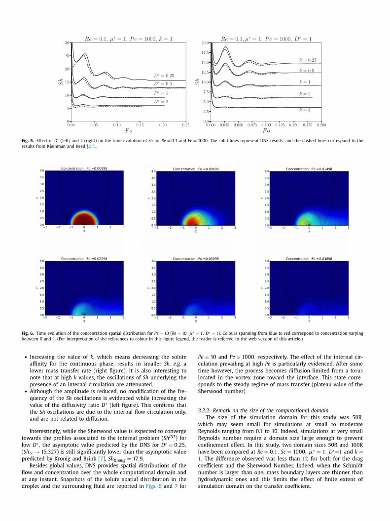
Fig. 5. Effect of D ∗ (left) and k (right) on the time-evolution of Sh for Re = 0 . 1 and Pe = 10 0 0 . The solid lines represent DNS results, and the dashed lines correspond to the

results from Kleinman and Reed [21] ..

Fig. 6. Time evolution of the concentration spatial distribution for Pe = 10 ( Re = 10 , μ∗ = 1 , D ∗ = 1 ). Colours spanning from blue to red correspond to concentration varying

between 0 and 1. (For interpretation of the references to colour in this figure legend, the reader is referred to the web version of this article.)

P

c

t

l

s

S

3

w

R

R

c

h

1

c

n

h

s

• Increasing the value of k , which means decreasing the solute

affinity for the continuous phase, results in smaller Sh, e.g. a

lower mass transfer rate (right figure). It is also interesting to

note that at high k values, the oscillations of Sh underlying the

presence of an internal circulation are attenuated.• Although the amplitude is reduced, no modification of the fre-

quency of the Sh oscillations is evidenced while increasing the

value of the diffusivity ratio D

∗ (left figure). This confirms that

the Sh oscillations are due to the internal flow circulation only,

and are not related to diffusion.

Interestingly, while the Sherwood value is expected to converge

towards the profiles associated to the internal problem ( Sh INT ) for

low D

∗, the asymptotic value predicted by the DNS for D

∗ = 0 . 25 ,

( Sh ∞

→ 15.327) is still significantly lower than the asymptotic value

predicted by Kronig and Brink [7] , Sh Kronig = 17 . 9 .

Besides global values, DNS provides spatial distributions of the

flow and concentration over the whole computational domain and

at any instant. Snapshots of the solute spatial distribution in the

droplet and the surrounding fluid are reported in Figs. 6 and 7 for

e = 10 and Pe = 10 0 0 , respectively. The effect of the internal cir-

ulation prevailing at high Pe is particularly evidenced. After some

ime however, the process becomes diffusion limited from a torus

ocated in the vortex zone toward the interface. This state corre-

ponds to the steady regime of mass transfer (plateau value of the

herwood number).

.2.2. Remark on the size of the computational domain

The size of the simulation domain for this study was 50R,

hich may seem small for simulations at small to moderate

eynolds ranging from 0.1 to 10. Indeed, simulations at very small

eynolds number require a domain size large enough to prevent

onfinement effect. In this study, two domain sizes 50R and 100R

ave been compared at Re = 0 . 1 , Sc = 10 0 0 , μ∗ = 1 , D

∗= 1 and k = . The difference observed was less than 1% for both for the drag

oefficient and the Sherwood Number. Indeed, when the Schmidt

umber is larger than one, mass boundary layers are thinner than

ydrodynamic ones and this limits the effect of finite extent of

imulation domain on the transfer coefficient.

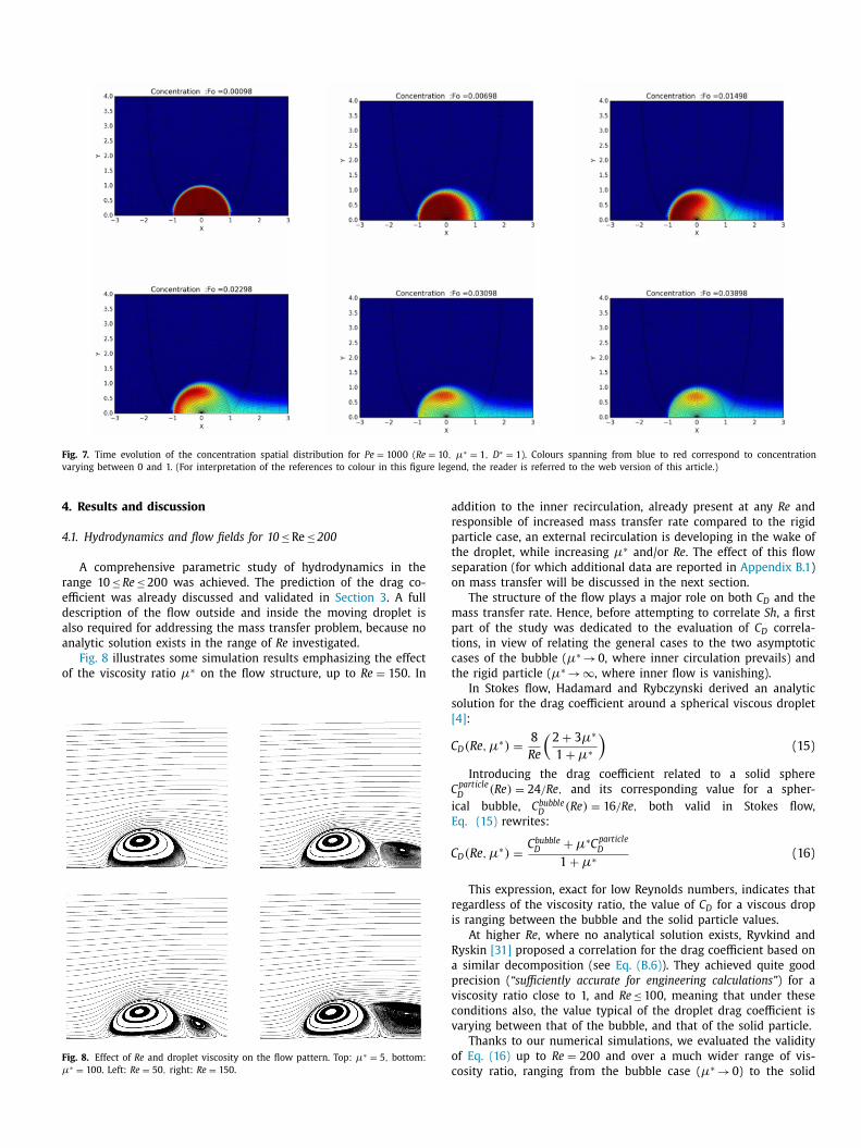
Fig. 7. Time evolution of the concentration spatial distribution for Pe = 10 0 0 ( Re = 10 , μ∗ = 1 , D ∗ = 1 ). Colours spanning from blue to red correspond to concentration

varying between 0 and 1. (For interpretation of the references to colour in this figure legend, the reader is referred to the web version of this article.)

4

4

r

e

d

a

a

o

F

μ

a

r

p

t

s

o

m

p

t

c

t

. Results and discussion

.1. Hydrodynamics and flow fields for 10 ≤ Re ≤ 200

A comprehensive parametric study of hydrodynamics in the

ange 10 ≤ Re ≤ 200 was achieved. The prediction of the drag co-

fficient was already discussed and validated in Section 3 . A full

escription of the flow outside and inside the moving droplet is

lso required for addressing the mass transfer problem, because no

nalytic solution exists in the range of Re investigated.

Fig. 8 illustrates some simulation results emphasizing the effect

f the viscosity ratio μ∗ on the flow structure, up to Re = 150 . In

ig. 8. Effect of Re and droplet viscosity on the flow pattern. Top: μ∗ = 5 , bottom: ∗ = 100 . Left: Re = 50 , right: Re = 150 .

s

[

C

C

i

E

C

r

i

R

a

p

v

c

v

o

c

ddition to the inner recirculation, already present at any Re and

esponsible of increased mass transfer rate compared to the rigid

article case, an external recirculation is developing in the wake of

he droplet, while increasing μ∗ and/or Re . The effect of this flow

eparation (for which additional data are reported in Appendix B.1 )

n mass transfer will be discussed in the next section.

The structure of the flow plays a major role on both C D and the

ass transfer rate. Hence, before attempting to correlate Sh , a first

art of the study was dedicated to the evaluation of C D correla-

ions, in view of relating the general cases to the two asymptotic

ases of the bubble ( μ∗ → 0, where inner circulation prevails) and

he rigid particle ( μ∗ → ∞ , where inner flow is vanishing).

In Stokes flow, Hadamard and Rybczynski derived an analytic

olution for the drag coefficient around a spherical viscous droplet

4] :

D (Re, μ∗) =

8

Re

(2 + 3 μ∗

1 + μ∗

)(15)

Introducing the drag coefficient related to a solid sphere

particle D

(Re ) = 24 /Re, and its corresponding value for a spher-

cal bubble, C bubble D

(Re ) = 16 /Re, both valid in Stokes flow,

q. (15) rewrites:

D (Re, μ∗) =

C bubbleD + μ∗C particle

D

1 + μ∗ (16)

This expression, exact for low Reynolds numbers, indicates that

egardless of the viscosity ratio, the value of C D for a viscous drop

s ranging between the bubble and the solid particle values.

At higher Re , where no analytical solution exists, Ryvkind and

yskin [31] proposed a correlation for the drag coefficient based on

similar decomposition (see Eq. (B.6) ). They achieved quite good

recision ( “sufficiently accurate for engineering calculations”) for a

iscosity ratio close to 1, and Re ≤ 100, meaning that under these

onditions also, the value typical of the droplet drag coefficient is

arying between that of the bubble, and that of the solid particle.

Thanks to our numerical simulations, we evaluated the validity

f Eq. (16) up to Re = 200 and over a much wider range of vis-

osity ratio, ranging from the bubble case ( μ∗ → 0) to the solid

Fig. 9. Evolution of the drag coefficient with Re for bubbles, droplets and solid par-

ticles. Comparison between present simulations (symbols) and the predictions of

Eq. (16) (dashed lines) using Eq. (B.8) [32] and (B.7) [33] for bubbles and particles

respectively (solid lines).

Table 3

Effect of the density ratio and Reynolds number on the drag coefficient C D .

Re / ρ∗ 0.1 0.5 1 5 10

10 3.345 3.345 3.344 3.342 3.342

50 1.088 1.086 1.083 1.07 1.07

100 0.671 0.667 0.662 0.66 0.66

4

h

c

a

t

4

c

a

c

R

o

t

p

c

t

g

a

r

particle ones ( μ∗ → ∞ ). Adequate correlations from the literature

were used in this aim, respectively reported by Mei et al. [32] and

Schiller and Nauman [33] for C bubble D

and C particle D

(see Appendix B.2 ).

As evidenced by Fig. 9 , Eq. (16) yields interestingly a very good

prediction of C D values over the whole range of viscosity ratio con-

sidered. As in Stokes flow, the drag coefficient is observed to stand

between the corresponding values for the particle and the bubble.

Note that while μ∗ and Re are the main parameters influencing

C D , as already evidenced by Feng and Michaelides [29] , the density

ratio ρ∗ on the other hand has a negligible effect (see Table 3 ).

Besides the steady drag force, the DNS model was also used to

investigate the Basset-Boussinesq (or history) force experienced by

the droplet [34] .

Fig. 10. Superimposed concentration contours and streamlines ( F o i = 0 . 15 , Re = 100 , Pe

nd viscosity ratio (from left to right: μ∗ = 0 . 25 , 1 , 5 ). Colours spanning from blue to re

eferences to colour in this figure legend, the reader is referred to the web version of this

.2. Conjugate mass transfer up to Re = 100

Different mass transfer simulations were performed for each

ydrodynamic configuration of Section 4.1 , yielding more than 200

ases for the parametric study of the influence of Re, Pe, μ∗, D

∗,

nd k on the internal, external, and global mass transfer resis-

ances.

.2.1. Comments on spatial solute distribution

Examples of instantaneous solute concentrations contours in

onjugate regimes are reported in Fig. 10 . Those snapshots give

first overview of the effects likely to influence mass transfer in

onditions typical of most engineering applications ( i.e. k � = 1 and

e � 10).

As previously observed in Fig. 5 for creeping flow, the effect

f both internal and external flow circulations on conjugate mass

ransfer is weakened when the thermodynamic equilibrium is op-

osed to the solute transfer (case k = 5 ). Hence, the problem is

ontrolled by the external transfer resistance, and the concentra-

ion inside the droplet is nearly uniform. Fig. 10 provides indeed a

ood illustration of the combined effect of μ∗ and k :

• For the case Pe = 10 0 0 , the internal circulation plays a ma-

jor role in the mass transfer process. As the viscosity ratio in-

creases (from left to right), the intensity of circulation reduces

and its center shifts towards the droplet front. The solute dif-

fuses then slowly from the core to the interface of the droplet.• On the other hand, while k increases (from top to bottom), the

transfer resistance shifts from internal to external location. The

effect of the internal circulation on the concentration spatial

= 10 0 0 , D ∗ = 1 ) for different equilibrium constants (top: k = 1 , bottom: k = 0 . 1 )

d correspond to concentration varying between 0 and 1. (For interpretation of the

article.)

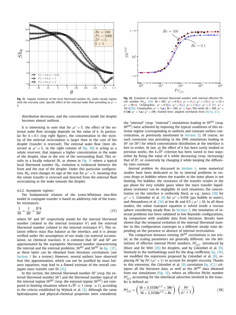
Fig. 11. Angular evolution of the local Sherwood number Sh θ under steady regime

with the viscosity ratio. Specific effect of the external wake flow prevailing at μ∗ =

5 .

t

l

i

d

s

s

o

s

l

f

t

t

r

4

m

f

w

n

S

l

v

l

a

t

a

S

t

a

j

t

t

p

t

h

Fig. 12. Evolution of steady internal Sherwood number with internal effective Pé-

clet number Pe i e f f

[14] : Re = 100 , μ∗ = 0 . 5 ( ) μ∗ = 1 ( ) μ∗ = 1 . 5 ( ) μ∗ = 2 ( )

μ∗ = 10 ( ); Creeping flow , μ∗ = 0 . 5 ( ) μ∗ = 1 ( ) μ∗ = 1 . 5 ( ) μ∗ = 2 ( ) μ∗ =

10 ( ) [30] .: Creeping flow , μ∗ = 1 ( ); Re = 100 , μ∗ = 1 ( ). This work: Re = 100 , μ∗ =

0 . 5 ( ) μ∗ = 1 ( ) μ∗ = 2 ( ). Dashed lines: adapted correlation from [9] Eq. (C.1) .

t

S

t

c

s

S

f

p

e

t

i

s

c

l

g

p

t

μ

a

s

s

t

b

s

b

p

i

i

O

S

w

p

t

l

f

P

f

P

distribution decreases, and the concentration inside the droplet

becomes almost uniform.

It is interesting to note that for μ∗ = 5 , the effect of the ex-

ernal wake flow strongly depends on the value of k . In particu-

ar for k = 0 . 1 (top right figure), the concentration in the vicin-

ty of the external recirculation is larger than in the core of the

roplet (transfer is reversed). The external wake flow (here ob-

erved at μ∗ = 5 , in the right column of Fig. 10 ) is acting as a

olute reservoir, that imposes a higher concentration in the wake

f the droplet, than in the rest of the surrounding fluid. This re-

ults in a locally reduced Sh , as shown in Fig. 11 where a typical

ocal Sherwood number Sh θ evolution is evidenced between the

ront and the rear of the droplet. Under this particular configura-

ion, Sh θ even changes its sign at the rear for μ∗ = 5 , meaning that

he solute transfer is reversed and directed from the external fluid

ecirculating in the wake towards the droplet.

.2.2. Asymptotic regimes

The fundamental relation of the Lewis-Whitman two-film

odel in conjugate transfer is based on additivity rule of the trans-

er resistances:

1

Sh

=

1

Sh

i + D

∗k

Sh

e(17)

here Sh i and Sh e respectively stands for the internal Sherwood

umber (related to the internal resistance h i ) and the external

herwood number (related to the external resistance h e ). This re-

ation reflects mass flux balance at the interface, and it is always

erified under the assumptions of our study (no material accumu-

ation, no chemical reaction). It is common that Sh i and Sh e are

pproximated by the asymptotic Sherwood number characterizing

he internal and the external problems, Sh INT and Sh EXT in Eq. (17) ,

s these latter can be obtained from literature correlations (see

ection 1 for a review). However, several authors have observed

hat this approximation, which can not be justified by mass bal-

nce equations, may lead to a flawed estimate of the overall con-

ugate mass transfer rate Sh [21] .

In this section, the internal Sherwood number Sh i (resp. the ex-

ernal Sherwood number Sh e ) and the Sherwood number typical of

he internal regime Sh INT (resp. the external regime Sh EXT ) are com-

ared in limiting situations where k √

D

∗ � 1 (resp. � 1), according

o the criteria established by Wylock et al. [5] . Although the same

ydrodynamic and physical-chemical properties were considered,

he “internal” (resp. “external”) simulations leading to Sh INT (resp.

h EXT ) were achieved by imposing the typical conditions of this ex-

reme regime (corresponding to uniform and constant surface con-

entration, as previously mentioned in Section 3 ). Of course, no

uch constraint was prevailing in the DNS simulations leading to

h i (or Sh e ) for which concentration distribution at the interface is

ree to evolve. At last, as the effect of k has been rarely studied in

revious works, the k √

D

∗ criterion has been varied in two ways:

ither by fixing the value of k while decreasing (resp. increasing)

hat of D

∗, or conversely by changing k while keeping the diffusiv-

ty ratio constant.

Internal problem As discussed in Section 1 , some numerical

tudies have been dedicated so far to internal problems in vis-

ous drops or bubbles where the transfer in the outer phase is not

imiting. For bubbles, the resistance of the transfer resides in the

as phase for very soluble gases when the mass transfer liquid-

hase resistance can be negligible. In such situations, the concen-

ration on the interface is uniformly fixed, as e.g. : Juncu [30] for∗ = 1 , Colombet et al. [9] for μ∗ = 0 . 018 (gas bubble in water),

nd Alexandrova et al. [14] at low Re and 0.5 ≤μ∗ ≤ 10. In all these

tudies, the solute transport equation is solved inside a viscous

phere considering steady flow. In Section 3 , the simulation of in-

ernal problems has been validated in low Reynolds configurations,

y comparison with available data from literature. Results have

hown that the temporal evolution of the internal Sherwood num-

er in this configuration converges to a different steady state de-

ending on the presence or absence of internal recirculation.

The comparison between existing Sh INT correlations is not triv-

al, as the scaling parameters are generally different: see the def-

nitions of effective internal Péclet numbers, Pe i e f f

, introduced by

liver and De Witt [35] for droplets, and by Colombet et al. [9] .

imilarly to the methodology used for the drag coefficient, Eq. (16) ,

e modified the expression proposed by Colombet et al. [9] , re-

lacing Pe i by Pe i / (μ∗ + 1) to account for droplet viscosity. Thanks

o this extension, the Colombet et al. [9] correlation Eq. (C.1) col-

apses all the literature data, as well as the Sh INT data obtained

rom our simulations ( Fig. 12 ), where an effective Péclet number

e i e f f

accounting for the interfacial advection involved in the trans-

er is defined as:

e i e f f =(

16 + 3 . 315 Re 1 / 2 + 3 Re

16 + 3 . 315 Re 1 / 2 + Re

)·(

P e i

μ∗ + 1

)(18)

Fig. 13. Evolution of internal Sherwood number Sh i (red circles) and comparison with the Sherwood number of the internal problem Sh INT (black dots). Sh INT data of Juncu

[30] (green symbols) and correlation of Colombet et al. [9] (blue dash line) are reported for comparison. On the left: k = 1 , D ∗ is varied. On the right: k is varied, D ∗ = 1 .

(For interpretation of the references to colour in this figure legend, the reader is referred to the web version of this article.)

Fig. 14. Evolution of external Sherwood number Sh e (red circles) and comparison with the Sherwood number of the external problem Sh EXT (black squares). Sh EXT data and

correlation of Feng and Michaelides [13] (blue triangles and blue line) are reported for comparison. On the left: k = 1 , D ∗ is varied. On the right: k is varied, D ∗ = 1 . (For

interpretation of the references to colour in this figure legend, the reader is referred to the web version of this article.)

s

d

b

i

c

p

b

r

t

r

a

c

S

e

t

i

t

1

t

t

c

a

p

H

d

v

k

Internal problem and internal transfer Transfer is expected to

be controlled by internal features when k √

D

∗ � 1 . The Sherwood

number of the internal problem Sh INT , Eq. (C.1) , and the internal

Sherwood number Sh i predicted by DNS without any assumption

regarding the surface and external concentrations are compared in

Fig. 13 .

Discrepancy between Sh i and Sh INT is observed in conjugate

transfer, as the internal resistance to mass transfer is not equal

to the one of the internal problem. The discrepancy is reduced

for k = 1 when D

∗ decreases (left figure), and similarly for D

∗ = 1

when k decreases (right figure). Hence, in the first case, the reduc-

tion of D

∗ corresponds to an increase of D

e , which was observed

to homogenize the spatial distribution of the solute outside the

drop, and so the interface concentration. Conversely, as mentioned

above, reducing k (at fixed D

∗) confines the solute inside the drop.

Although the transfer is slower, this tends to homogenize the con-

centration inside the drop, and so the interface concentration. For

high Pe i these configurations are comparable to an internal prob-

lem. A small gap between Sh i and Sh INT is however still prevail-

ing in configurations where k √

D

∗ � 1 at small values of the Péclet

number. Indeed, as illustrated by Fig. C.23 in Appendix C , the tem-

poral evolution of Sh i in this configuration does not converge to

well established steady value, as it is the case for higher Pe i . De-

spite this evolution, the average value is close to the corresponding

Sh INT , and a deviation of less than 4% is observed.

External problem In an external problem, the transfer resistance

is mainly located outside the drop. Many correlations have been

developed for the external Sherwood number Sh EXT that are cited

in Section 1 . Aoki et al. [16] experimentally confirmed the effect of

urface active component adsorption on the mass transfer from a

issolving bubble and proposed, for fully contaminated Taylor bub-

les, a correlation for the Sh EXT based on the Eotvos number. Us-

ng the same experimental setup, Hori et al. [17] observed a de-

rease of the Sh with increasing salt concentration in the liquid

hase. As no effect was observed on the rising velocity of the bub-

le, the decrease in the mass transfer rate was attributed to the

eduction of the dissolved gas diffusivity in the liquid phase. In

he case of clean and spherical droplets, the DNS values of Sh EXT

eveal excellent agreement with the correlation proposed by Feng

nd Michaelides [13] ( Eq. (C.2) in Appendix C ).

External problem and external transfer Transfer is expected to be

ontrolled by external mass boundary layer when k √

D

∗ � 1 . The

herwood number of the external problem Sh EXT , Eq. (C.2) , and the

xternal Sherwood number Sh e predicted by DNS (surface and ex-

ernal concentrations free to evolved) are compared in Fig. 14 .

Larger discrepancies between Sh e and Sh EXT are observed

n conjugate transfer, compared to cases for internal resis-

ance/problem. The difference is about 10% for Pe = 10 0 0 and D

∗ =00 . In order to understand the origin of this discrepancy between

he steady value of Sh e and Sh EXT , the steady-state concentration at

he interface was plot for k = 1 (see Fig. C.24 ). A non uniform con-

entration distribution is observed for D

∗ = 100 , for both Pe = 100

nd Pe = 10 0 0 . This is the origin of the difference with external

roblem for which uniform concentration is fixed at the interface.

owever, when k is increased (right part of Fig. 14 ), the gap re-

uces as the mass transfer is further shifted outwards by the ad-

erse thermodynamic conditions. The deviation is less than 1% for

= 10 .

Fig. 15. Evolution of global Sherwood number Sh of the conjugate mass transfer problem with internal Péclet Pe i at Re = 100 and for μ∗ = 1 . Comparison of the DNS results

(symbols) with Eq (19) (solid lines). The error bars represent the extreme values of Sh within the time interval for averaging.

Fig. 16. Parity plot of Sherwood number. Re = 50 , k = 1 (left), D ∗ = 1 (right). Sh corr corresponds to Sherwood number from correlation Eq (19) and Sh sim to DNS results.

4

n

g

n

S

O

o

v

t

N

P

E

b

f

i

s

u

i

u

t

w

T

l

b

t

T

t

k

f

h

t

t

u

t

v

s

s

f

d

p

t

.2.3. Global transfer in a conjugate regime for Re ≤ 100

Substituting Sh i (resp. Sh e ) with Sh INT (resp. Sh EXT ) in Eq. 17 is

ot rigorously exact. Several attempts have been made to relate the

lobal Sherwood number of a conjugate problem to the Sherwood

umbers associated respectively to the internal Sh INT and external

h EXT problems assuming additivity rule of transfer resistances [21] ,

liver and Chung [36] , Nguyen et al. [37] :

1

Sh

=

1

Sh

INT + D

∗k

Sh

EXT(19)

Thanks to the results of the DNS parametric study, the validity

f Eq. (19) could be investigated. Correlations (C.2) and (C.1) , pre-

iously introduced for the external and internal problems, are used

o evaluate the global Sherwood number according to Eq. (19) .

ote that since Sh INT and Sh EXT correlations rely respectively on

e i and Pe , we replaced Pe by its equivalent formulation D

∗Pe i in

q. (C.2) and used Pe i as the reference value of the Péclet num-

er. The evolution of the global Sherwood number Sh obtained

rom DNS simulations (conjugate problem), with Pe i is illustrated

n Fig. 15 at Re = 100 for μ∗ = 1 . It is compared with the corre-

ponding evolution of Sh , estimated from Eq. (19) . In the left fig-

re, the influence of D

∗ is assessed for k = 1 , while the effect of k

s illustrated at a constant diffusivity ratio D

∗ = 1 in the right fig-

re.

For small values of Pe i , the temporal evolution of Sh given by

he DNS simulations does not converge to a well defined value

hen D

∗ (resp. k ) decreases while keeping k = 1 (resp. D

∗ = 1 ).

his behaviour has been already observed for the internal prob-

em study (i.e. Appendix C ). In that case, the time-average of Sh ,

etween the time Fo at which the last oscillation is observed and

he final value of Fo (corresponding to C i ≈ 10 −4 ), is considered.

he error bars in Fig. 15 represent the extreme values of Sh within

he time interval for averaging.

The trend is consistent with previous comments. Hence, for

= 1 (meaning concentration continuity at the interface, which is

ormally equivalent to heat transfer case), the figure on the left

and side highlights the typical effects of diffusion and convec-

ion already observed at small Re . Similarly, as already observed

he higher the value of k ( i.e. the affinity of the solute for the liq-

id in the droplet), the lower the mass transfer rate (smaller Sh ).

The accuracy of Eq. (19) decreases at small Pe i , which is consis-

ent with the previous comparisons of Sh e with the corresponding

alues for the external regimes Sh EXT due to non-uniform and un-

teady surface concentration. Interestingly, the agreement between

imulations and the Sh correlation improves as k increases. While

or small values of the equilibrium constant k ≤ 1 (when thermo-

ynamics is adverse to the solute transfer towards the continuous

hase), only high Pe i yields good agreement between the simula-

ions and the correlation. Moreover, for k = 1 , good agreement is

C

d

F

a

A

(

P

s

i

A

A

t

H

w

r

o

a

i

C

f

t

P

d

s

t

τ

observed only for Pe i > 100, whichever value of D

∗. Same conclu-

sions were drawn for different viscosity ratios (see Appendix C ).

Following the previous analysis, parity plots gathering more re-

sults of the parametric study (0.25 ≤μ∗, D

∗, k ≤ 5) have been con-

structed ( Fig. 16 ) For every values of Pe i , Sh values from correlation

and simulations have been represented with the same colour, in-

dependently of the values of μ∗, D

∗ and k . In agreement with the

previous observations and discussion, the present simulations and

the predictions based on additivity rule agree with 30% error for

Pe i ≥ 500. When the Péclet decreases to 10, a significant deviation

is observed (blue squares).

5. Conclusion

A detailed hydrodynamic analysis of a droplet embedded in a

moderate Reynolds number flow has been carried out by DNS.

The effects of the external Reynolds, and the viscosity ratio have

been studied in configurations involving both internal and exter-

nal flows. Using the limits of high viscosity ratio (typical of a rigid

particle), and low viscosity ratio (corresponding to a bubble), a cor-

relation of the drag coefficient has been proposed and validated up

to Re ≤ 200. Moreover, the condition under which an external cir-

culation occurs in the wake of the drop has been obtained, and we

proposed a correlation for the separation angle.

Based on this flow analysis, mass transfer simulations were per-

formed for Reynolds numbers up to Re = 100 and over a wide

range of physical properties. Preliminary results, at moderated Re ,

revealed perfect agreement between the DNS results and previous

works from literature. The coupled effects of hydrodynamic and

physical properties on the local and the global Sherwood numbers,

and on the spatial distribution of the solute concentration have

been analyzed. The possible relation with the internal/external

problems has been described. i) Regarding internal transfer, the

diffusivity ratio and partition coefficient play an equivalent role in

shifting the mass transfer resistance towards the drop internal re-

gion. The internal Sherwood number Sh i converges to the corre-

sponding value Sh INT of an internal problem when k √

D

∗ � 1 . i) For

external transfer, only k plays a major role in moving the resistance

towards the outer phase. The effect of D

∗ for high k is weak. For

high diffusivity ratio, concentration at the interface is usually not

uniform which results in a significant deviation between the exter-

nal Sherwood number Sh e and corresponding Sh EXT for low Pe . In

this case, an increase of k allows to reduce the difference between

Sh e and Sh EXT .

At last, regarding the prediction of the global Sherwood num-

ber typical of a conjugate problem, the relevance of using correla-

tions valid for the asymptotic “External” and “Internal” mass trans-

fer regimes, in the additivity rule of transfer resistances, known as

the Lewis-Whitman double film-model, was evidenced for high in-

ternal Péclet number and high partition coefficient. This common

assumption is actually incorrect at low Pe , for which discrepancy

larger than 30% was observed. Besides this important recommen-

dation, it was however not possible to propose a universal correla-

tion for the conjugate mass transfer problem. Indeed, as discussed

in Section 4.2 , the internal and external resistances that actually

prevail on both sides of the interface can not be easily correlated

in this case, due to either radial concentration gradients in the

droplet, or local variations over the interface and/or outside con-

centration, etc.

Declaration of Competing Interest

The authors declare that they have no known competing finan-

cial interests or personal relationships that could have appeared to

influence the work reported in this paper.

RediT authorship contribution statement

Azeddine Rachih: Investigation, Software, Writing - original

raft. Dominique Legendre: Software, Methodology, Validation,

ormal analysis. Eric Climent: Supervision, Formal analysis, Visu-

lization. Sophie Charton: Conceptualization, Visualization.

cknowledgements

This work was supported by the Division of Energies of CEA

program SIACY). The authors acknowledge Kevin LARNIER, Annaïg

EDRONO from the COSINUS service at IMFT for their technical

upport. Simulations have been carried out on the supercomput-

ng facilities at CALMIP under the project #P18028.

ppendix A. Complementary model description

1. Dimensionless and discretized forms of governing equations

The dimensionless form of the Navier-Stokes Eqs. (1) and (2) in

he curvilinear coordinate system ξi = (ξ1 , ξ2 ) writes in phases δ =(i, e ) for internal and external fluid:

∂V

δj

∂ξ j

= 0 (A.1)

∂V δi

∂t+

∂ ( V δi V δj )

∂ξ j= − ∂ p δ

∂ξi+

∂ ( τδi j )

∂ξ j+ H

i j

(V

δj V

δj

− τδj j

)− H

i j

(V

δi

V

δj

− τδi j

)(A.2)

The stretching factors (curvature terms) H

j i

are defined as:

j i

=

1 hi

∂hi

∂ξ j(A.3)

here h k denotes the scale factor along the direction ξ k , and τδi j

epresents the dimensionless viscous stress given in the considered

rthogonal curvilinear coordinates by:

τi i j

= 1Re

[∂V i

i

∂ξ j+

∂V ij

∂ξi− H

i j V

ij− H

j i V

i i + 2 H

k i V

i k δi j

]τe

i j =

μ∗Re

[∂V e

i

∂ξ j+

∂V ej

∂ξi− H

i j V e

j− H

j i V

e i

+ 2 H

k i V

e k δi j

] (A.4)

Re is expressed relatively to the continuous (external) phase

nd δij is the Kronecker delta symbol.

The solute balance equation Eq. (3) in phases δ writes:

∂C i

∂t+

∂ ( V i j C δ )

∂ξ j=

1 Pe

∂ 2 C i

∂ ξ j ∂ ξ j

∂C e

∂t+

∂ ( V e j C e )

∂ξ j=

D ∗Pe

∂ 2 C e

∂ ξ j ∂ ξ j

(A.5)

The dimensionless concentration of the solute in each phase δs defined as:

δ =

C ′ δ−C ′ e∞C ′ i

0 −C ′ e∞

(A.6)

The prime refers to dimensional concentration, while C ′ i 0

stands

or the droplet initial concentration (assumed uniform) and C ′ e ∞

for

he solute concentration in the fluid flow, far from the droplet.

e =

2 U 0 R D e

is the external Péclet number and D

∗ is the ratio of mass

iffusivities D

i / D

e .

The interface conditions Eqs. (4) and (5) are discretized using

econd order differentiation ( Fig. A.17 ) in order to express the in-

erfacial shear:

i 12 ,S = τe

12 ,S = μ∗�i

3 V 1 , j−2 − �i 2 V 1 , j−1 +

(�i 1 −H 2 1 ,S )(�

e 2 V 1 , j −�e

3 V 1 , j+1 )

�e 1 + H 2

1 ,S

1 + μ∗ �i 1 −H 2

1 ,S

�e 1 + H 2

1 ,S

,

(A.7)

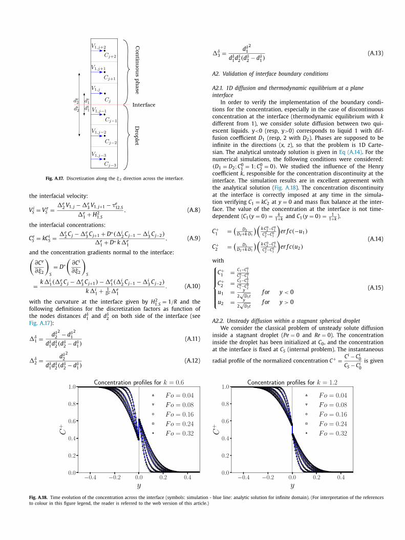
Fig. A.17. Discretization along the ξ 2 direction across the interface.

t

V

t

C

a(

w

f

t

F

�

�

�

A

A

i

t

c

d

e

f

i

s

n

c

i

t

a

t

f

d

C

C

w⎧⎪⎪⎪⎪⎨⎪⎪⎪⎪⎩A

i

i

a

r

F

t

he interfacial velocity:

i S = V

e S =

�e 2 V 1 , j − �e

3 V 1 , j+1 − τe 12 ,S

�e 1

+ H

21 ,S

, (A.8)

he interfacial concentrations:

e S = kC i S =

�e 2 C j − �e

3 C j+1 + D

∗(�i 2 C j−1 − �i

3 C j−2 )

�e 1

+ D

∗ k �e1

, (A.9)

nd the concentration gradients normal to the interface:

∂C e

∂ξ2

)S

= D

∗(

∂C i

∂ξ2

)S

=

k �i 1 (�

e 2 C j − �e

3 C j+1 ) − �e 1 (�

i 2 C j−1 − �i

3 C j−2 )

k �i 1

+

1 D ∗ �

e1

. (A.10)

ith the curvature at the interface given by H

2 1 ,S

= 1 /R and the

ollowing definitions for the discretization factors as function of

he nodes distances d δ1 and d δ2 on both side of the interface (see

ig. A.17 ):

δ1 =

d δ2 2 − d δ1

2

d δ1 d δ

2 (d δ

2 − d δ

1 )

(A.11)

δ2 =

d δ2 2

d δd δ(d δ − d δ ) (A.12)

1 2 2 1

ig. A.18. Time evolution of the concentration across the interface (symbols: simulation -

o colour in this figure legend, the reader is referred to the web version of this article.)

δ3 =

d δ1 2

d δ1 d δ

2 (d δ

2 − d δ

1 )

(A.13)

2. Validation of interface boundary conditions

2.1. 1D diffusion and thermodynamic equilibrium at a plane

nterface

In order to verify the implementation of the boundary condi-

ions for the concentration, especially in the case of discontinuous

oncentration at the interface (thermodynamic equilibrium with k

ifferent from 1), we consider solute diffusion between two qui-

scent liquids. y < 0 (resp, y > 0) corresponds to liquid 1 with dif-

usion coefficient D 1 (resp, 2 with D 2 ). Phases are supposed to be

nfinite in the directions ( x, z ), so that the problem is 1D Carte-

ian. The analytical unsteady solution is given in Eq (A.14) . For the

umerical simulations, the following conditions were considered:

(D 1 = D 2 ;C 0 1

= 1 ;C 0 2

= 0) . We studied the influence of the Henry

oefficient k , responsible for the concentration discontinuity at the

nterface. The simulation results are in excellent agreement with

he analytical solution ( Fig. A.18 ). The concentration discontinuity

t the interface is correctly imposed at any time in the simula-

ion verifying C 1 = kC 2 at y = 0 and mass flux balance at the inter-

ace. The value of the concentration at the interface is not time-

ependent ( C 1 (y = 0) =

k 1+ k and C 1 (y = 0) =

1 1+ k ).

+ 1

=

(D 2

D 2 + k ·D 1 )( k ·C0

2 −C 0 1

C 0 2 −C 0

1

)er f c(−u 1 )

+ 2

=

(D 1

D 2 + k ·D 1 )( k ·C0

2 −C 0 1

C 0 2−C 0

1

)er f c(u 2 )

(A.14)

ith

C + 1

=

C 1 −C 0 1

C 0 2−C 0

1

C + 2

=

C 2 −C 0 2

C 0 1 −C 0

2

u 1 =

y

2√

D 1 tf or y < 0

u 2 =

y

2√

D 2 tf or y > 0

(A.15)

2.2. Unsteady diffusion within a stagnant spherical droplet

We consider the classical problem of unsteady solute diffusion

nside a stagnant droplet ( Pe = 0 and Re = 0 ). The concentration

nside the droplet has been initialized at C 0 , and the concentration

t the interface is fixed at C S (internal problem). The instantaneous

adial profile of the normalized concentration C + =

C i − C i0

C S − C i0

is given

blue line: analytic solution for infinite domain). (For interpretation of the references

Fig. A.19. Time evolution of the concentration within a stagnant droplet.

C

Fig. B.20. Schematic external bifurcation diagram ( ρ∗ = 1 ).

Fig. B.21. Vorticity profiles along the interface ( Re = 1 , ρ∗ = 1 ).

o

f

2

θ

s

[

t

o

a

g

t

v

o

r

(

e

h

fi

R

h

S

by Newman [6] in Eq. (A.16) .

+ = 1 +

2

r +

+ ∞ ∑

n =1

(−1) n

nπexp

(−(nπ) 2 F o i

)sin

(nπ r +

)(A.16)

R has been chosen as a reference length such that r + = r/R . The

Fourier number is defined by F o i =

D i t R 2

with D

i the diffusion coeffi-

cient of the solute inside the droplet. The instantaneous Sherwood

number is given by Eq. (A.17) :

Sh =

2 π2

3

∑ + ∞

n =1 exp

(−(nπ) 2 F o i

)∑ + ∞

n =1 1 n 2

exp

(−(nπ) 2 F o i

) (A.17)

The Sherwood number reaches the steady state value

Sh Newman = 2 π2 / 3 ≈ 6 . 58 in the limit of F o i −→ ∞ . Radial con-

centration profiles from Eq (A.17) and our DNS simulation are

compared in Fig. A.19 for different dimensionless times. A very

good agreement is observed between our simulations (symbols)

and the Newman’s solution (lines). The corresponding asymptotic

Sherwood number obtained by DNS is Sh ∞

= 6 . 56 , which differs

only by 0.2% from Newman’s theoretical prediction.

Appendix B. Complementary hydrodynamic data and results

B1. Prediction of the separation angle

For intermediate to high Reynolds number flow and viscosity

ratio, an external circulation may occur in the wake of the droplet.

Comparing with a solid particle, the internal circulation delays

both the onset of flow separation and wake formation in the exter-

nal fluid for a circulating drop. The separation angle θd measures

the angle at which the external boundary layer is detached from

the spherical surface. This angle can characterize also the position

at which the vorticity ω

e S

of the external phase changes its sign at

the interface.

ω

e S = −∂V

e 1

∂ξ2

∣∣∣S

−H

2 1 V

e S (B.1)

Clift et al. [4] have shown that for a solid particle, the flow is

unseparated for 0 < Re < 20, while a steady wake region is then

developed for 20 < Re < 130. Thus, Re = 20 represents the onset

f separation for infinite viscosity ratio. The authors reported the

ollowing correlation of the separation angle which is valid for

0 < Re < 400.

d = 42 . 5 [ log (Re/ 20) ] 0 . 483 (B.2)

For a spherical gas bubble in liquid clear of surfactants, no

eparation is predicted ( θd = 0 ) whatever the Reynolds number

38] . This is supported by our results that for small viscosity ra-

io (less than μ∗ = 0 . 02 ), no recirculation is observed in the range

f Reynold number Re ≤ 200. Fig. B.21 shows the vorticity profiles

long the interface for different configurations. We note that for a

iven Reynolds number (here Re = 100 ), the maximum of the in-

erface vorticity increases with the viscosity ratio. For μ∗ ≥ 5, the

orticity changes its sign, which proves that an external separation

ccurs at an angle where ω S = 0 .

We can characterize the presence or the absence of the external

ecirculation by a schematic curve ( Fig. B.20 ). In the pink region

i.e. below the curve) the external flow is unseparated, whereas an

xternal recirculation is occurring in the blue area. As μ∗ tends to

igher values, the droplet behaves live a solid particle which justi-

es that the critical Reynolds number of separation tends towards

e = 20 . On the oher hand, at low viscosity, the bubble-like be-

aviour is observed and no separation occurs.

Table B.5 reports the angles of separation for different ( Re, μ∗).

ome of the corresponding streamlines are highlighted in Fig. 8 .

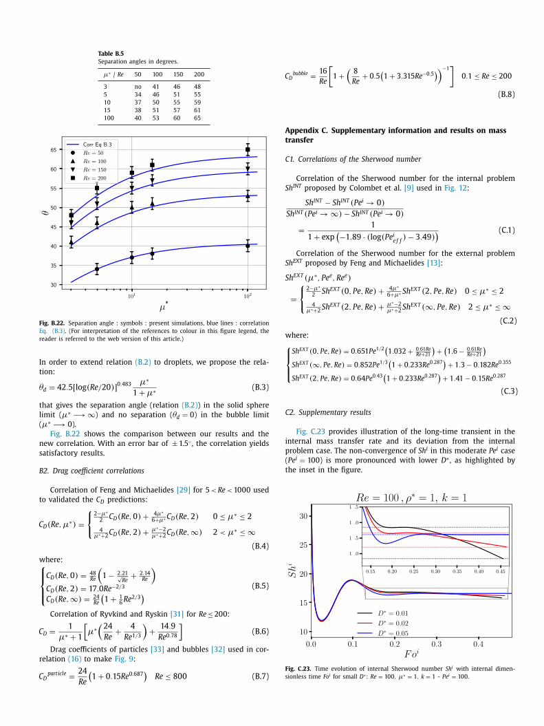
Table B.5

Separation angles in degrees.

μ∗ / Re 50 100 150 200

3 no 41 46 48

5 34 46 51 55

10 37 50 55 59

15 38 51 57 61

100 40 53 60 65

Fig. B.22. Separation angle : symbols : present simulations, blue lines : correlation

Eq. (B.3) . (For interpretation of the references to colour in this figure legend, the

reader is referred to the web version of this article.)

I

t

θ

t

l

(

n

s

B

t

C

w⎧⎪⎨⎪⎩

C

r

C

C

A

t

C

S

S

S

w⎧⎪⎨⎪⎩

C

i

p

(

t

Fig. C.23. Time evolution of internal Sherwood number Sh i with internal dimen-

sionless time Fo i for small D ∗: Re = 100 , μ∗ = 1 , k = 1 - Pe i = 100 .

n order to extend relation (B.2) to droplets, we propose the rela-

ion:

d = 42 . 5 [ log (Re/ 20) ] 0 . 483 μ∗

1 + μ∗ (B.3)

hat gives the separation angle (relation (B.2) ) in the solid sphere

imit ( μ∗ −→ ∞ ) and no separation ( θd = 0 ) in the bubble limit

μ∗ −→ 0 ).

Fig. B.22 shows the comparison between our results and the

ew correlation. With an error bar of ± 1.5 ◦, the correlation yields

atisfactory results.

2. Drag coefficient correlations

Correlation of Feng and Michaelides [29] for 5 < Re < 10 0 0 used

o validated the C D predictions:

D (Re, μ∗) ={

2 −μ∗2

C D (Re, 0) +

4 μ∗6+ μ∗ C D (Re, 2) 0 ≤ μ∗ ≤ 2

4μ∗+2

C D (Re, 2) + μ∗−2 μ∗+2

C D (Re, ∞ ) 2 < μ∗ ≤ ∞

(B.4)

here:

C D (Re, 0) =

48 Re

(1 − 2 . 21 √

Re+ 2 . 14

Re

)C D (Re, 2) = 17 . 0 Re −2 / 3

C D (Re, ∞ ) =

24 Re

(1 +

1 6

Re 2 / 3 ) (B.5)

Correlation of Ryvkind and Ryskin [31] for Re ≤ 200:

D =

1

μ∗ + 1

[μ∗

(24

Re + 4

Re 1 / 3

)+ 14 . 9

Re 0 . 78

](B.6)

Drag coefficients of particles [33] and bubbles [32] used in cor-

elation (16) to make Fig. 9 :

D particle =

24

(1 + 0 . 15 Re 0 . 687

)Re ≤ 800 (B.7)

Re

D bubble =

16

Re

[1 +

(8

Re + 0 . 5

(1 + 3 . 315 Re −0 . 5

))−1 ]

0 . 1 ≤ Re ≤ 200

(B.8)

ppendix C. Supplementary information and results on mass

ransfer

1. Correlations of the Sherwood number

Correlation of the Sherwood number for the internal problem

h INT proposed by Colombet et al. [9] used in Fig. 12 :

Sh

INT − Sh

INT (P e i → 0)

Sh

INT (P e i → ∞ ) − Sh

INT (P e i → 0)

=

1

1 + exp

(−1 . 89 · ( log (P e i

e f f ) − 3 . 49)

) (C.1)

Correlation of the Sherwood number for the external problem

h EXT proposed by Feng and Michaelides [13] :

h

EXT (μ∗, P e e , Re e )

=

{

2 −μ∗2

Sh

EXT (0 , P e, Re ) +

4 μ∗6+ μ∗ Sh

EXT (2 , P e, Re ) 0 ≤ μ∗ ≤ 2

4μ∗+2

Sh

EXT (2 , P e, Re ) +

μ∗−2 μ∗+2

Sh

EXT (∞ , P e, Re ) 2 ≤ μ∗ ≤ ∞

(C.2)

here:

Sh EXT (0 , Pe, Re ) = 0 . 651 Pe 1 / 2 (1 . 032 +

0 . 61 Re Re +21

)+

(1 . 6 − 0 . 61 Re

Re +21

)Sh EXT (∞ , Pe, Re ) = 0 . 852 Pe 1 / 3

(1 + 0 . 233 Re 0 . 287

)+ 1 . 3 − 0 . 182 Re 0 . 355

Sh EXT (2 , Pe, Re ) = 0 . 64 Pe 0 . 43 (1 + 0 . 233 Re 0 . 287

)+ 1 . 41 − 0 . 15 Re 0 . 287

(C.3)

2. Supplementary results

Fig. C.23 provides illustration of the long-time transient in the

nternal mass transfer rate and its deviation from the internal

roblem case. The non-convergence of Sh i in this moderate Pe i case

Pe i = 100 ) is more pronounced with lower D

∗, as highlighted by

he inset in the figure.

Fig. C.24. Steady profile of normalized concentration at the interface C e s / C i : Re = 100 , μ∗ = 1 , k = 1 - Pe = 100 (left), Pe = 10 0 0 (right).

Fig. C.25. Evolution of global Sherwood number Sh of the conjugate mass transfer problem with internal Péclet Pe i at Re = 100 and for μ∗ = 2 . Continuous lines: Eq. (19) ,

symbols: DNS results. The error bars represent the extreme values of Sh within the time interval for averaging.

Fig. C.26. Evolution of global Sherwood number Sh of the conjugate mass transfer problem with internal Péclet Pe i at Re = 100 and for μ∗ = 0 . 5 . Continuous lines: Eq. (19) ,

symbols: DNS results. The error bars represent the extreme values of Sh within the time interval for averaging.

Fig. C.24 highlights the non-uniform surface distribution of the

solute concentration achieved at steady-state, which explains the

discrepancies between Sh EXT and Sh e in Fig. 14 .

Complementing Fig. 15 (for μ∗ = 1 ), Figs. C.25 and C.26 high-

light the good agreement of the proposed correlation at high Pe

and/or high k values, in the case of μ∗ = 2 and μ∗ = 0 . 5 , respec-

tively.

References

[1] M. Wegener , N. Paul , M. Kraume , Fluid dynamics and mass transfer at single

droplets in liquid/liquid systems, Int. J. Heat Mass Transf. 71 (2014) 475–495 .[2] G. Juncu , Unsteady heat and/or mass transfer from a fluid sphere in creeping

flow, Int. J. Heat Mass Transf. 44 (12) (2001) 2239–2246 .

[3] G. Juncu , Unsteady ternary mass transfer from a sphere in creeping flow, Int.

J. Therm. Sci. 44 (3) (2005) 255–266 .[4] R. Clift , J. Grace , M. Weber , Bubbles, Drops, and Particles, Academic Press Inc.,

1978 .

[5] C. Wylock , P. Colinet , B. Haut , Gas absorption into a spherical liquid droplet:numerical and theoretical study, Chem. Eng. J. 207 (2012) 851–864 .

[6] A.B. Newman , The drying of porous solids: diffusion and surface emissionequations, AIChE Trans. 27 (1931) 203–220 .

[7] R. Kronig , J. Brink , On the theory of extraction from falling droplets, Appl. Sci.Res. 2 (1) (1951) 142 .

[8] A. Brignell , Solute extraction from an internally circulating spherical liquid

drop, Int. J. Heat Mass Transf. 18 (1) (1975) 61–68 .[9] D. Colombet , D. Legendre , A. Cockx , P. Guiraud , Mass or heat transfer inside a

spherical gas bubble at low to moderate Reynolds number, Int. J. Heat MassTransf. 67 (2013) 1096–1105 .

[10] Z. Feng , E.E. Michaelides , Mass and heat transfer from fluid spheres at lowReynolds numbers, Powder Technol. 1123 (20 0 0) 63–69 .

[

[

[

[

[

[

[

[

[

[

[

[

[

[

[

[11] B. Abramzon , G. Fishbein , Some problems of convective diffusion to a sphericalparticle with Pe ≤ 10 0 0 , J. Eng. Phys. 32 (6) (1977) 6 82–6 86 .

[12] B. Abramzon , C. Elata , Unsteady heat transfer from a single sphere in stokesflow, Int. J. Heat Mass Transf. 27 (5) (1984) 687–695 .

[13] Z. Feng , E. Michaelides , Heat and mass transfer coefficients of viscous spheres,Int. J. Heat Mass Transf. 44 (23) (2001) 4445–4454 .

[14] S. Alexandrova , M. Karsheva , A. Saboni , C. Gourdon , Effect of the viscosity ratioon the mass transfer into a spherical drop in liquid-liquid dispersions, J. Chem.

Technol. Metall. 49 (5) (2014) 429–434 .

[15] A. Saboni , S. Alexandrova , M. Karsheva , C. Gourdon , Mass transfer from a con-taminated fluid sphere, AlChE J. 57 (7) (2011) 1684–1692 .

[16] J. Aoki , Y. Hori , K. Hayashi , S. Hosokawa , A. Tomiyama , Mass transfer from sin-gle carbon dioxide bubbles in alcohol aqueous solutions in vertical pipes, Int.

J. Heat Mass Transf. 108 (B) (2017) 1991–2001 .[17] Y. Hori , K. Hayashi , S. Hosokawa , A. Tomiyama , Mass transfer from single car-

bon-dioxide bubbles in electrolyte aqueous solutions in vertical pipes, 115, Part

A, 663–671, 2017, Int. J. Heat Mass Transf. 115 (A) (2017) 663–671 .[18] A. Kumar , S. Hartland , Correlations for prediction of mass transfer coefficients

in single drop systems and liquid–liquid extraction columns, Chem. Eng. Res.Des. 77 (5) (1999) 372–384 .

[19] E. Ruckenstein , Mass transfer between a single drop and a continuous phase,Int. J. Heat Mass Transf. 10 (12) (1967) 1785–1792 .

20] D. Oliver , J. Chung , Conjugate unsteady heat transfer from a spherical droplet

at low Reynolds numbers, Int. J. Heat Mass 29 (6) (1986) 879–887 .[21] L.S. Kleinman , X. Reed , Unsteady conjugate mass transfer between a single

droplet and an ambient flow with external chemical reaction, Ind. Eng. Chem.Res. 35 (9) (1996) 2875–2888 .

22] A. Paschedag , W. Piarah , M. Kraume , Sensitivity study for the mass transfer ata single droplet, Int. J. Heat Mass Transf. 48 (16) (2005) 3402–3410 .

23] J. Magnaudet , M. Rivero , J. Fabre , Accelerated flows past a rigid sphere or

a spherical bubble. Part 1. Steady straining flow, J. Fluid Mech. 284 (1995)97–135 .

24] D. Legendre , J. Magnaudet , The lift force on a spherical body in a viscous linearshear flow, J. Fluid Mech. 368 (1998) 81–126 .

25] D. Legendre , J. Magnaudet , G. Mougin , Hydrodynamic interactions betweentwo spherical bubbles rising side by side in a viscous liquid, J. Fluid Mech.

497 (2003) 133–166 .26] A. Merle , D. Legendre , J. Magnaudet , Forces on a high-re spherical bubble in a

turbulent flow, J. Fluid Mech. 532 (2005) 53–62 .[27] B. Figueroa , D. Legendre , Mass or heat transfer from spheroidal gas bubbles

rising through a stationary liquid, Chem. Eng. Sci. 65 (2010) 6296–6309 .28] Y. Hallez , D. Legendre , Interaction between two spherical bubbles rising in a

viscous liquid, J. Fluid Mech. 673 (2011) 406–431 .

29] Z. Feng , E.E. Michaelides , Drag coefficients of viscous spheres at intermediateand high Reynolds numbers, J. Fluids Eng. 123 (4) (2001) 841–849 .

30] G. Juncu , A numerical study of the unsteady heat/mass transfer inside a circu-lating sphere, Int. J. Heat Mass Transf. 53 (15–16) (2010) 3006–3012 .

[31] V. Ryvkind , G. Ryskin , Flow structure in motion of a spherical drop in a fluidmedium at intermediate Reynolds number, Fluid Dyn. 11 (5) (1976) .

32] R. Mei , J.F. Klausner , C.J. Lawrence , A note on the history force on a spherical

bubble at finite Reynolds number, Phys. Fluids 6 (1) (1994) 418–420 .33] L. Schiller , A.Z. Nauman , A drag coefficient correlation, Ver. Deut. Ing. Zeitung

77 (1933) 318–321 .34] D. Legendre , A. Rachih , C. Souilliez , S. Charton , E. Climent , The Basset-Boussi-

nesq history force of a fluid sphere, Phys. Rev. Fluids 4 (2019) 073603 .35] D. Oliver , K. De Witt , Heat transfer in bubbles and droplets at moderate

Reynolds numbers: interior problem, in: National Heat Transfer Conference,

Portland, OR (United States), 1995 .36] D. Oliver , J. Chung , Unsteady conjugate heat transfer from a translating fluid

sphere at moderate Reynolds numbers, Int. J. Heat Mass Transf. 33 (3) (1990)401–408 .

[37] H.D. Nguyen , S. Paik , J.N. Chung , Unsteady conjugate heat transfer associatedwith a translating spherical droplet: a direct numerical simulation, Numer.

Heat Transf. Part A 24 (2) (1993) 161–180 .

38] A. Blanco , J. Magnaudet , The structure of the axisymmetric high-Reynoldsnumber flow around an ellipsoidal bubble of fixed shape, Phys Fluids 7 (1995)

1265 .