A stable and high-order accurate conjugate heat

transfer problem

Jens Lindström and Jan Nordström

Post Print

N.B.: When citing this work, cite the original article.

Original Publication:

Jens Lindström and Jan Nordström, A stable and high-order accurate conjugate heat transfer

problem, 2010, Journal of Computational Physics, (229), 5440-5456.

http://dx.doi.org/10.1016/j.jcp.2010.04.010

Copyright: Elsevier Science B.V., Amsterdam

http://www.elsevier.com/

Postprint available at: Linköping University Electronic Press

http://urn.kb.se/resolve?urn=urn:nbn:se:liu:diva-68563

A Stable and High Order Accurate Conjugate Heat Transfer

Problem

Jens LindstromUppsala University, Department of Information Technology, 751 05, Uppsala , Sweden

Jan NordstromSchool of Mechanical, Industrial and Aeronautical Engineering

University of the Witvatersrand, PO WITS 2050, Johannesburg, South AfricaFOI, The Swedish Defence Research Agency,

Department of Aeronautics and Systems Integration, Stockholm, 164 90, SwedenUppsala University, Department of Information Technology, 751 05, Uppsala, Sweden

Abstract

This paper analyzes well-posedness and stability of a conjugate heat transfer prob-lem in one space dimension. We study a model problem for heat transfer between afluid and a solid. The energy method is used to derive boundary and interface con-ditions that make the continuous problem well-posed and the semi-discrete problemstable. The numerical scheme is implemented using 2nd, 3rd and 4th order finitedifference operators on Summation-By-Parts (SBP) form. The boundary and inter-face conditions are implemented weakly. We investigate the spectrum of the spatialdiscretization to determine which type of coupling that gives attractive convergenceproperties. The rate of convergence is verified using the method of manufacturedsolutions.

1 Introduction

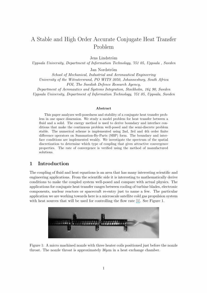
The coupling of fluid and heat equations is an area that has many interesting scientific andengineering applications. From the scientific side it is interesting to mathematically deriveconditions to make the coupled system well-posed and compare with actual physics. Theapplications for conjugate heat transfer ranges between cooling of turbine blades, electroniccomponents, nuclear reactors or spacecraft re-entry just to name a few. The particularapplication we are working towards here is a microscale satellite cold gas propulsion systemwith heat sources that will be used for controlling the flow rate [1]. See Figure 1.

Figure 1: A micro machined nozzle with three heater coils positioned just before the nozzlethroat. The nozzle throat is approximately 30µm in a heat exchange chamber.

1

This paper is the first step of understanding the coupling procedure within our frame-work. The computational method that we are using is a finite difference method onSummation-By-Parts (SBP) form with the Simultaneous Approximation Term (SAT), aweak coupling at the fluid-solid interface. This method has been developed in many papers[2, 3, 4, 5, 6, 7] and used for many difficult problems where it has proven to be robust[8, 9, 10, 11]. The extensions to multiple dimensions is relatively straightforward oncethe one-dimensional case has been investigated. The difficulty in extending to multipledimensions lies rather in a high performance implementation than in the theory.

The main idea of the SBP and SAT framework is that the difference operators shouldmimic integration by parts in the continuous case. This framework makes the discreteequations closely related to the PDE:s themselves. The difference operators are con-structed such that they shift to one-sided close to the boundaries. This results in anenergy estimate which gives stability for a well-posed Cauchy problem. The SAT methodimplements the boundary conditions weakly and an energy estimate, and hence stability,can be obtained for a well-posed initial boundary value problem.

Since the operators shift to one-sided close to boundaries and interfaces there is noneed to introduce ghost points or extrapolate values which in general causes stabilityissues. Once the scheme is correctly written and all coefficients determined the order ofthe scheme depends only on the order of the difference operators. In this paper we willpresent 2nd, 3rd and 4th order operators and study their performance. The details ofthese operators can be found in for example [2, 3, 12].

2 The continuous problem

The equations we are studying in this paper are motivated by a gas flow in a long channelwith heat sources. The channel is long compared to the height and hence the changes inthe tangential direction are small in comparison to the changes in the normal direction,see Figure 2.

Figure 2: By assuming an infinitely long channel with homogenicity in the tangentialdirection y we get a one-dimensional problem in the normal direction x for the conjugateheat transfer problem

The equations are an incompletely parabolic system of equations for the flow and the

2

scalar heat equation for the heat transfer,

wt +Awx = εBwxx, −1 ≤ x ≤ 0, (1)

andTt = kTxx, 0 ≤ x ≤ 1, (2)

where

w =

ρuT

, A =

a b 0b a c0 c a

, B =

0 0 00 α 00 0 β

. (3)

We can view (1) as the Navier-Stokes equations linearized and symmetrized around aconstant state. In that case we would have

a = u, b =c√γ, c = c

√γ − 1γ

, α =λ+ 2µρ

, β =γµ

Prρ, (4)

where u, ρ and c is the mean velocity, density and speed of sound. γ is the ratio ofspecific heats, Pr the Prandtl number and λ and µ are the second and dynamic viscosities,[13, 8, 14]. At this point the only assumption on the coefficients is that α, β > 0.

Our objective is to couple (1) and (2) at x = 0 and investigate which boundary andinterface conditions that will lead to a well-posed coupled system.

The number of boundary conditions at each boundary for (1) can be obtained by theLaplace transform technique [15]. Taking the Laplace transform in time of (1) gives us

sw +Awx = εBwxx (5)

and by the ansatz w = ψekεx we get

(sI3 + kA− k2B)︸ ︷︷ ︸E(s,k)

ψ = 0, s = εs (6)

where I3 is the 3× 3 identity matrix. The polynomial degree in k of det(E(s, k)) gives thetotal number of boundary conditions needed and the sign of the roots as <(s)→∞ givesthe number at each boundary [15]. By expanding det(E(s, k)) we get

det(E(s, k)) = aαβk5

+ (sαβ + b2β − a2β − a2α)k4

+ a(a2 − b2 − c2 − 2sβ − 2sα)k3 (7)

+ (−s2β + 3sa2 − sc2 − s2α− b2s)k2

+ 3as2k

+ s3

which is a 5th degree polynomial in k and hence (1) requires a total of five boundaryconditions. To get the sign of the roots we let k = c0s

η which is inserted into (7). Byletting <(s) → ∞ we can balance the expression and see that η = 1 and η = 1

2 are theonly possible choices. By inserting η = 1 and η = 1

2 into (7) we can compute all leadingcoefficients c0 which are

c0 = −1a, c0 = ± 1√

α, c0 = ± 1√

β. (8)

This gives the number of boundary conditions at each boundary summarized in Table 1.

To simplify we assume for the rest of the paper that a > 0.

3

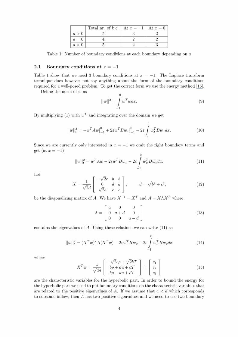
Total nr. of b.c. At x = −1 At x = 0a > 0 5 3 2a = 0 4 2 2a < 0 5 2 3

Table 1: Number of boundary conditions at each boundary depending on a

2.1 Boundary conditions at x = −1

Table 1 show that we need 3 boundary conditions at x = −1. The Laplace transformtechnique does however not say anything about the form of the boundary conditionsrequired for a well-posed problem. To get the correct form we use the energy method [15].

Define the norm of w as

||w||2 =

0∫−1

wTwdx. (9)

By multiplying (1) with wT and integrating over the domain we get

||w||2t = −wTAw∣∣0−1+ 2εwTBwx

∣∣0−1− 2ε

0∫−1

wTxBwxdx. (10)

Since we are currently only interested in x = −1 we omit the right boundary terms andget (at x = −1)

||w||2t = wTAw − 2εwTBwx − 2ε

0∫−1

wTxBwxdx. (11)

Let

X =1√2d

−√2c b b0 d d√2b c c

, d =√b2 + c2, (12)

be the diagonalizing matrix of A. We have X−1 = XT and A = XΛXT where

Λ =

a 0 00 a+ d 00 0 a− d

(13)

contains the eigenvalues of A. Using these relations we can write (11) as

||w||2t = (XTw)TΛ(XTw)− 2εwTBwx − 2ε

0∫−1

wTxBwxdx (14)

where

XTw =1√2d

−√2cρ+√

2bTbρ+ du+ cTbρ− du+ cT

=

c1

c2

c3

(15)

are the characteristic variables for the hyperbolic part. In order to bound the energy forthe hyperbolic part we need to put boundary conditions on the characteristic variables thatare related to the positive eigenvalues of A. If we assume that a < d which correspondsto subsonic inflow, then A has two positive eigenvalues and we need to use two boundary

4

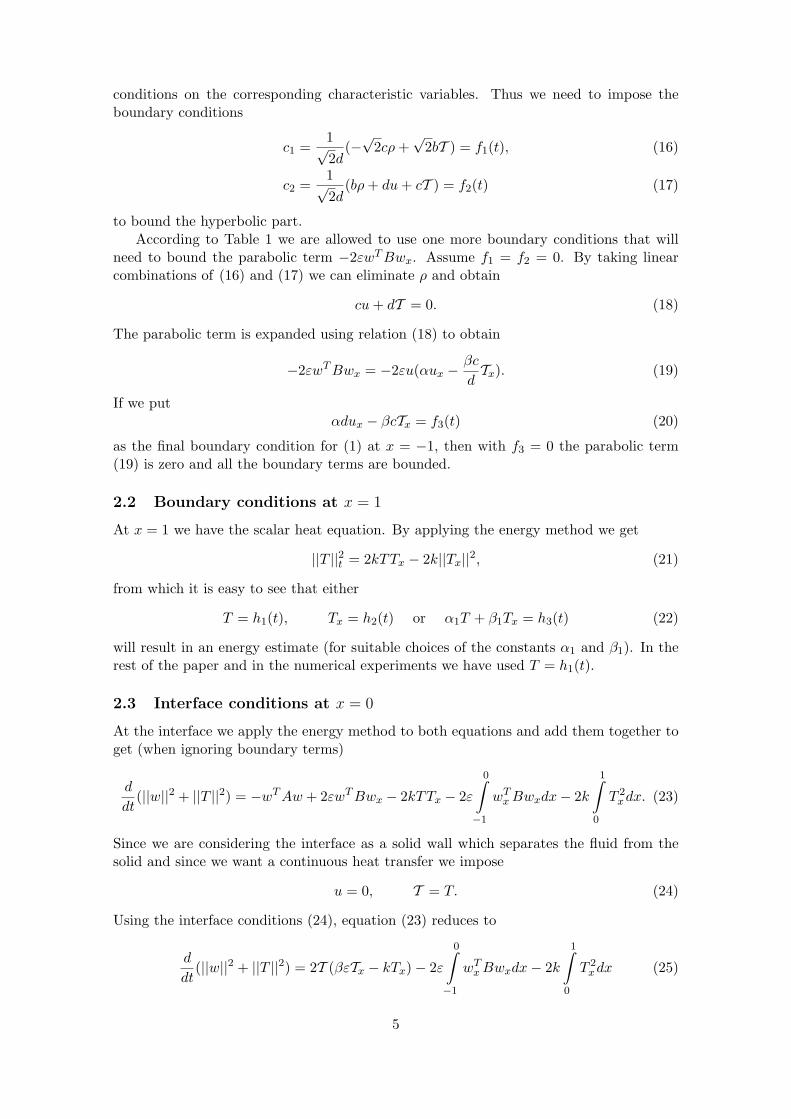
conditions on the corresponding characteristic variables. Thus we need to impose theboundary conditions

c1 =1√2d

(−√

2cρ+√

2bT ) = f1(t), (16)

c2 =1√2d

(bρ+ du+ cT ) = f2(t) (17)

to bound the hyperbolic part.According to Table 1 we are allowed to use one more boundary conditions that will

need to bound the parabolic term −2εwTBwx. Assume f1 = f2 = 0. By taking linearcombinations of (16) and (17) we can eliminate ρ and obtain

cu+ dT = 0. (18)

The parabolic term is expanded using relation (18) to obtain

−2εwTBwx = −2εu(αux − βc

dTx). (19)

If we putαdux − βcTx = f3(t) (20)

as the final boundary condition for (1) at x = −1, then with f3 = 0 the parabolic term(19) is zero and all the boundary terms are bounded.

2.2 Boundary conditions at x = 1

At x = 1 we have the scalar heat equation. By applying the energy method we get

||T ||2t = 2kTTx − 2k||Tx||2, (21)

from which it is easy to see that either

T = h1(t), Tx = h2(t) or α1T + β1Tx = h3(t) (22)

will result in an energy estimate (for suitable choices of the constants α1 and β1). In therest of the paper and in the numerical experiments we have used T = h1(t).

2.3 Interface conditions at x = 0

At the interface we apply the energy method to both equations and add them together toget (when ignoring boundary terms)

d

dt(||w||2 + ||T ||2) = −wTAw + 2εwTBwx − 2kTTx − 2ε

0∫−1

wTxBwxdx− 2k

1∫0

T 2xdx. (23)

Since we are considering the interface as a solid wall which separates the fluid from thesolid and since we want a continuous heat transfer we impose

u = 0, T = T. (24)

Using the interface conditions (24), equation (23) reduces to

d

dt(||w||2 + ||T ||2) = 2T (βεTx − kTx)− 2ε

0∫−1

wTxBwxdx− 2k

1∫0

T 2xdx (25)

5

and we can easily see that if we impose

βεTx − kTx = 0 (26)

as the final interface condition we get an energy estimate. Without (26), the interface canact as an unphysical heat source or sink.

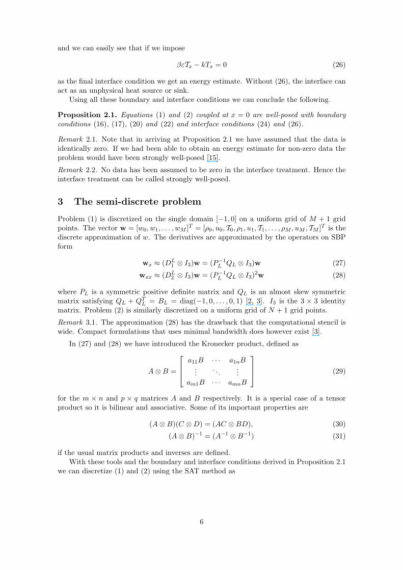
Using all these boundary and interface conditions we can conclude the following.

Proposition 2.1. Equations (1) and (2) coupled at x = 0 are well-posed with boundaryconditions (16), (17), (20) and (22) and interface conditions (24) and (26).

Remark 2.1. Note that in arriving at Proposition 2.1 we have assumed that the data isidentically zero. If we had been able to obtain an energy estimate for non-zero data theproblem would have been strongly well-posed [15].

Remark 2.2. No data has been assumed to be zero in the interface treatment. Hence theinterface treatment can be called strongly well-posed.

3 The semi-discrete problem

Problem (1) is discretized on the single domain [−1, 0] on a uniform grid of M + 1 gridpoints. The vector w = [w0, w1, . . . , wM ]T = [ρ0, u0, T0, ρ1, u1, T1, . . . , ρM , uM , TM ]T is thediscrete approximation of w. The derivatives are approximated by the operators on SBPform

wx ≈ (DL1 ⊗ I3)w = (P−1

L QL ⊗ I3)w (27)

wxx ≈ (DL2 ⊗ I3)w = (P−1

L QL ⊗ I3)2w (28)

where PL is a symmetric positive definite matrix and QL is an almost skew symmetricmatrix satisfying QL + QTL = BL = diag(−1, 0, . . . , 0, 1) [2, 3]. I3 is the 3 × 3 identitymatrix. Problem (2) is similarly discretized on a uniform grid of N + 1 grid points.

Remark 3.1. The approximation (28) has the drawback that the computational stencil iswide. Compact formulations that uses minimal bandwidth does however exist [3].

In (27) and (28) we have introduced the Kronecker product, defined as

A⊗B =

a11B · · · a1nB...

. . ....

am1B · · · amnB

(29)

for the m × n and p × q matrices A and B respectively. It is a special case of a tensorproduct so it is bilinear and associative. Some of its important properties are

(A⊗B)(C ⊗D) = (AC ⊗BD), (30)

(A⊗B)−1 = (A−1 ⊗B−1) (31)

if the usual matrix products and inverses are defined.With these tools and the boundary and interface conditions derived in Proposition 2.1

we can discretize (1) and (2) using the SAT method as

6

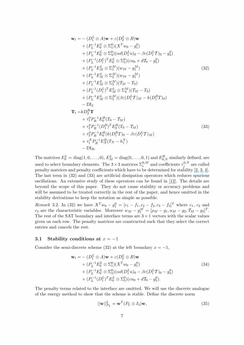
wt =− (DL1 ⊗A)w + ε(DL

2 ⊗B)w

+ (P−1L EL0 ⊗ Σ0

1)(XTw0 − g01)

+ (P−1L EL0 ⊗ Σ0

3)(αd(DL1 u)0 − βc(DL

1 T )0 − g03)

+ (P−1L (DL

1 )TEL0 ⊗ Σ05)(cu0 + dT0 − g0

5)

+ (P−1L ELM ⊗ ΣM

1 )(wM − gM1 ) (32)

+ (P−1L ELM ⊗ ΣM

2 )(wM − gM1 )

+ (P−1L ELM ⊗ ΣM

3 )(TM − T0)

+ (P−1L (DL

1 )TELM ⊗ ΣM4 )(TM − T0)

+ (P−1L ELM ⊗ ΣM

5 )(βε(DL1 T )M − k(DR

1 T )0)−DIL

Tt =kDR2 T

+ τ01P

−1R ER0 (T0 − TM )

+ τ02P

−1R (DR

1 )TER0 (T0 − TM ) (33)

+ τ03P

−1R ER0 (k(DR

1 T )0 − βε(DL1 T )M )

+ τN1 P−1R ERN (TN − hN1 )

−DIR.

The matrices EL0 = diag(1, 0, . . . , 0), ELM = diag(0, . . . , 0, 1) and ER0,N similarly defined, areused to select boundary elements. The 3×3 matrices Σ0,M

i and coefficients τ0,Nj are called

penalty matrices and penalty coefficients which have to be determined for stability [2, 3, 4].The last term in (32) and (33) are artificial dissipation operators which reduces spuriousoscillations. An extensive study of these operators can be found in [12]. The details arebeyond the scope of this paper. They do not cause stability or accuracy problems andwill be assumed to be treated correctly in the rest of the paper, and hence omitted in thestability derivations to keep the notation as simple as possible.

Remark 3.2. In (32) we have XTw0 − g01 = [c1 − f1, c2 − f2, c3 − f3]T where c1, c2 and

c3 are the characteristic variables. Moreover wM − gM1 = [ρM − g1, uM − g2, TM − g3]T .The rest of the SAT boundary and interface terms are 3× 1 vectors with the scalar valuesgiven on each row. The penalty matrices are constructed such that they select the correctentries and cancels the rest.

3.1 Stability conditions at x = −1

Consider the semi-discrete scheme (32) at the left boundary x = −1,

wt =− (DL1 ⊗A)w + ε(DL

2 ⊗B)w

+ (P−1L EL0 ⊗ Σ0

1)(XTw0 − g01) (34)

+ (P−1L EL0 ⊗ Σ0

3)(αd(DL1 u)0 − βc(DL

1 T )0 − g03)

+ (P−1L (DL

1 )TEL0 ⊗ Σ05)(cu0 + dT0 − g0

5).

The penalty terms related to the interface are omitted. We will use the discrete analogueof the energy method to show that the scheme is stable. Define the discrete norm

||w||2PL= wT (PL ⊗ I3)w, (35)

7

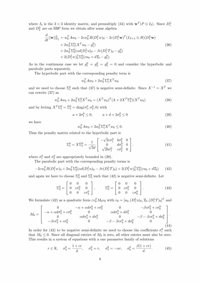
where I3 is the 3 × 3 identity matrix, and premultiply (34) with wT (P ⊗ I3). Since DL1

and DL2 are on SBP form we obtain after some algebra

d

dt||w||2PL

= wT0 Aw0 − 2εwT0 B(DL1w)0 − 2ε(DL

1 w)T (IN+1 ⊗B)(DL1 w)

+ 2wT0 Σ01(XTw0 − g0

1) (36)

+ 2wT0 Σ03(αd(DL

1 u)0 − βc(DL1 T )0 − g0

3)

+ 2(DL1w)T0 Σ0

5(cu0 + dT0 − g05).

As in the continuous case we let g01 = g0

3 = g05 = 0 and consider the hyperbolic and

parabolic parts separately.The hyperbolic part with the corresponding penalty term is

wT0 Aw0 + 2wT0 Σ01X

Tw0 (37)

and we need to choose Σ01 such that (37) is negative semi-definite. Since X−1 = XT we

can rewrite (37) as

wT0 Aw0 + 2wT0 Σ01X

Tw0 = (XTw0)T (Λ + 2XTΣ01)(XTw0) (38)

and by letting XTΣ01 = Σ0

1 = diag(σ01, σ

02, 0) with

a+ 2σ01 ≤ 0, a+ d+ 2σ0

2 ≤ 0 (39)

we havewT0 Aw0 + 2wT0 Σ0

1XTw0 ≤ 0. (40)

Thus the penalty matrix related to the hyperbolic part is

Σ01 = XΣ0

1 =1√2d

−√2cσ01 bσ0

2 00 dσ0

2 0√2bσ0

1 cσ02 0

. (41)

where σ01 and σ0

2 are appropriately bounded in (39).The parabolic part with the corresponding penalty terms is

−2εwT0 B(DL1w)0 + 2wT0 Σ0

3(αd(DL1 u)0 − βc(DL

1 T )0) + 2(DL1w)T0 Σ0

5(cu0 + dT0) (42)

and again we have to choose Σ03 and Σ0

5 such that (42) is negative semi-definite. Let

Σ03 =

0 0 00 εσ0

3 00 0 εσ0

4

, Σ05 =

0 0 00 εσ0

5 00 0 εσ0

6

. (43)

We formulate (42) as a quadratic form εvT0 M0v0 with v0 = [u0, (DL1 u)0, T0, (DL

1 T )0]T and

M0 =

0 −α+ αdσ0

3 + cσ05 0 −βcσ0

3 + cσ06

−α+ αdσ03 + cσ0

5 0 αdσ04 + dσ0

5 00 αdσ0

4 + dσ05 0 −β − βcσ0

4 + dσ06

−βcσ03 + cσ0

6 0 −β − βcσ04 + dσ0

6 0

.(44)

In order for (42) to be negative semi-definite we need to choose the coefficients σ0i such

that M0 ≤ 0. Since all diagonal entries of M0 is zero, all other entries must also be zero.This results in a system of equations with a one parameter family of solutions

r ∈ R, σ03 =

1 + cr

d, σ0

4 = r, σ05 = −αr, σ0

6 =β(1 + cr)

d. (45)

8

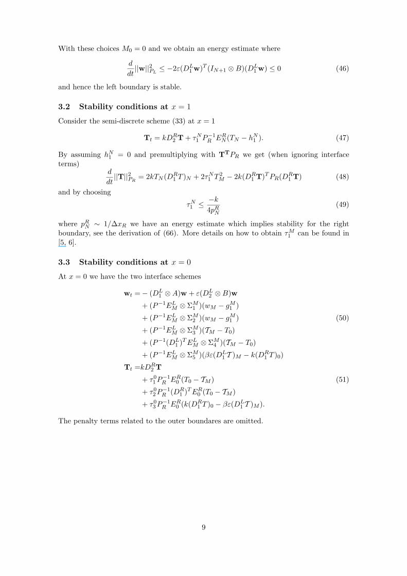
With these choices M0 = 0 and we obtain an energy estimate where

d

dt||w||2PL

≤ −2ε(DL1 w)T (IN+1 ⊗B)(DL

1 w) ≤ 0 (46)

and hence the left boundary is stable.

3.2 Stability conditions at x = 1

Consider the semi-discrete scheme (33) at x = 1

Tt = kDR2 T + τN1 P

−1R ERN (TN − hN1 ). (47)

By assuming hN1 = 0 and premultiplying with TTPR we get (when ignoring interfaceterms)

d

dt||T||2PR

= 2kTN (DR1 T )N + 2τN1 T

2M − 2k(DR

1 T)TPR(DR1 T) (48)

and by choosing

τN1 ≤−k4pRN

(49)

where pRN ∼ 1/∆xR we have an energy estimate which implies stability for the rightboundary, see the derivation of (66). More details on how to obtain τM1 can be found in[5, 6].

3.3 Stability conditions at x = 0

At x = 0 we have the two interface schemes

wt =− (DL1 ⊗A)w + ε(DL

2 ⊗B)w

+ (P−1ELM ⊗ ΣM1 )(wM − gM1 )

+ (P−1ELM ⊗ ΣM2 )(wM − gM1 ) (50)

+ (P−1ELM ⊗ ΣM3 )(TM − T0)

+ (P−1(DL1 )TELM ⊗ ΣM

4 )(TM − T0)

+ (P−1ELM ⊗ ΣM5 )(βε(DL

1 T )M − k(DR1 T )0)

Tt =kDR2 T

+ τ01P

−1R ER0 (T0 − TM ) (51)

+ τ02P

−1R (DR

1 )TER0 (T0 − TM )

+ τ03P

−1R ER0 (k(DR

1 T )0 − βε(DL1 T )M ).

The penalty terms related to the outer boundares are omitted.

9

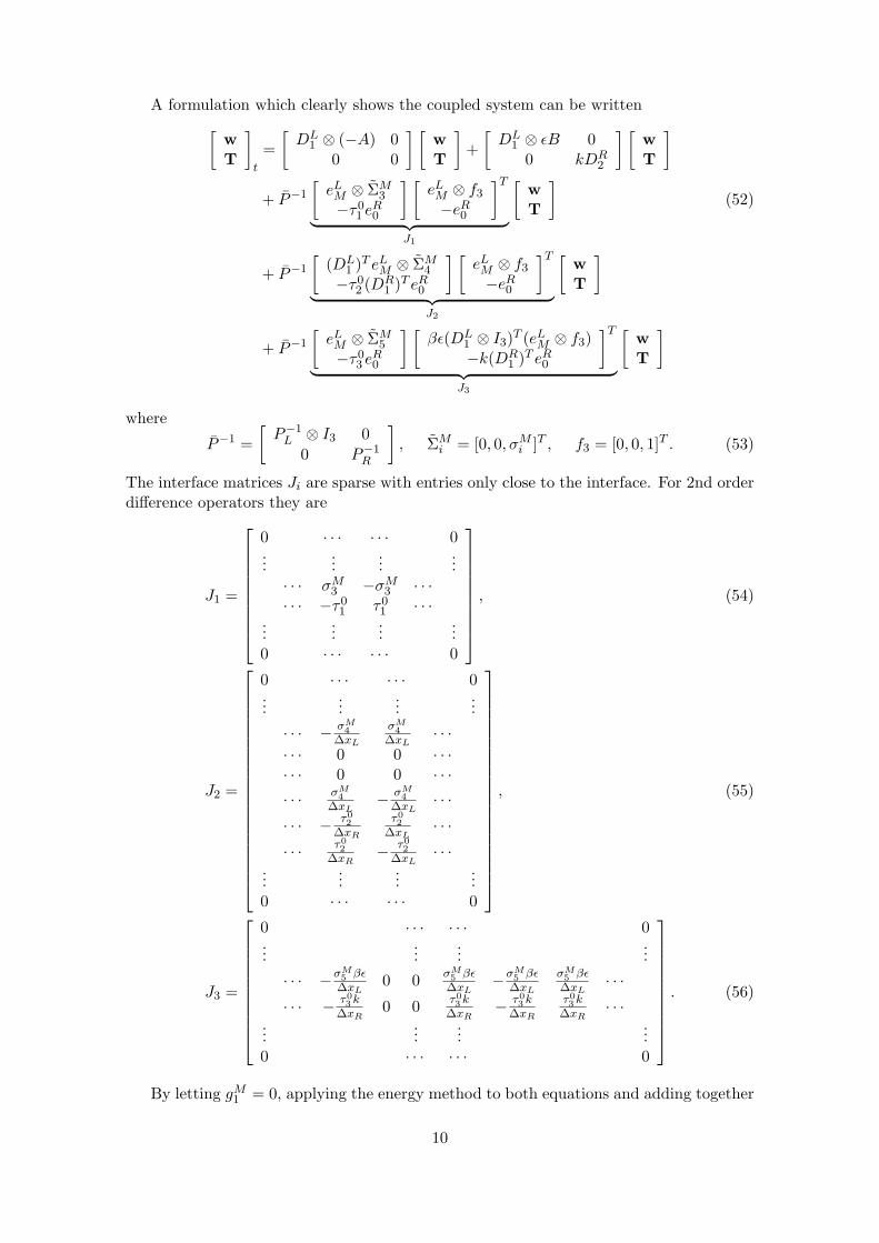
A formulation which clearly shows the coupled system can be written[wT

]t

=[DL

1 ⊗ (−A) 00 0

] [wT

]+[DL

1 ⊗ εB 00 kDR

2

] [wT

]+ P−1

[eLM ⊗ ΣM

3

−τ01 eR0

] [eLM ⊗ f3

−eR0

]T︸ ︷︷ ︸

J1

[wT

](52)

+ P−1

[(DL

1 )T eLM ⊗ ΣM4

−τ02 (DR

1 )T eR0

] [eLM ⊗ f3

−eR0

]T︸ ︷︷ ︸

J2

[wT

]

+ P−1

[eLM ⊗ ΣM

5

−τ03 eR0

] [βε(DL

1 ⊗ I3)T (eLM ⊗ f3)−k(DR

1 )T eR0

]T︸ ︷︷ ︸

J3

[wT

]

where

P−1 =[P−1L ⊗ I3 0

0 P−1R

], ΣM

i = [0, 0, σMi ]T , f3 = [0, 0, 1]T . (53)

The interface matrices Ji are sparse with entries only close to the interface. For 2nd orderdifference operators they are

J1 =

0 · · · · · · 0...

......

...· · · σM3 −σM3 · · ·· · · −τ0

1 τ01 · · ·

......

......

0 · · · · · · 0

, (54)

J2 =

0 · · · · · · 0...

......

...

· · · − σM4

∆xL

σM4

∆xL· · ·

· · · 0 0 · · ·· · · 0 0 · · ·· · · σM

4∆xL

− σM4

∆xL· · ·

· · · − τ02

∆xR

τ02

∆xL· · ·

· · · τ02

∆xR− τ0

2∆xL

· · ·...

......

...0 · · · · · · 0

, (55)

J3 =

0 · · · · · · 0...

......

...

· · · −σM5 βε

∆xL0 0 σM

5 βε∆xL

−σM5 βε

∆xL

σM5 βε

∆xL· · ·

· · · − τ03 k

∆xR0 0 τ0

3 k∆xR

− τ03 k

∆xR

τ03 k

∆xR· · ·

......

......

0 · · · · · · 0

. (56)

By letting gM1 = 0, applying the energy method to both equations and adding together

10

we get (when ignoring the outer boundary terms)

d

dt(||w||2PL

+ ||T||2PR) = −wTMAwM + 2εwTMB(DL

1w)M − 2ε(DL1 w)T (IN ⊗B)(DL

1 w)

+ 2wTMΣM1 wM + 2wTMΣM

2 wM

+ 2wTMΣM3 (TM − T0) + (DL

1w)TNΣM4 (TM − T0)

+ 2wTMΣM5 (βε(DL

1w)M − k(DR1 T )0) (57)

− 2kT0(DR1 T )0 − 2k(DR

1 T)TPR(DR1 T)

+ 2τ01T0(T0 − TM ) + 2τ0

2 (DR1 T )0(T0 − TM )

+ 2τ03T0(k(DR

1 T )0 − βε(DL1 T )M ).

As in the continuous case we have the hyperbolic part with the corresponding penaltyterm

−wTMAwM + 2wTMΣM1 wM = wTM (−A+ 2ΣM

1︸ ︷︷ ︸MH

)wM (58)

which we want to bound by making MH negative semi-definite. Note that A is symmetricby assumtion. By choosing

ΣM1 =

0 σH1 00 σH2 00 σH3 0

(59)

we can explicitly compute the eigenvalues of MH and see that with

σH1 =b

2, σH2 ≤ 0, σH3 =

c

2, (60)

we have MH ≤ 0. Note that ΣM1 acts on u only.

The parabolic part is split into parts containing u and T separately. For the interfacecondition on u at x = 0 we get by expanding (57)

2αεuM (DL1 u)M + 2wTMΣM

2 wM − 2αε(DL1 u)TPL(DL

1 u). (61)

We choose

ΣM2 =

0 0 00 σM2 00 0 0

(62)

and rewrite (61) as

2αεuM (DL1 u)M + 2σM2 u2

M − 2αε||DL1 u||2PL

. (63)

The last term in (63) can be written as

||DL1 u||2PL

= (DL1 u)TPL(DL

1 u)

=

(DL1 u)0...

(DL1 u)M

T P

(0,0)L · · · ....

. . ....

. · · · P(M,M)L

(DL

1 u)0...

(DL1 u)M

(64)

= (DL1 u)T PL(DL

1 u) + (DL1 u)TMp

LM (DL

1 u)M

11

where pLM > 0 is such that P (M,M)L − pLM ≥ 0. This means that the remaining matrix PL

is positive semi-definite and is as such a semi-norm. Using (64) we can write (63) as[uM

(DL1 u)M )

]T [ 2σM2 αεαε −2εpLM

]︸ ︷︷ ︸

Mu

[uM

(DL1 u)M )

](65)

where Mu ≤ 0 ifσu1 ≤

−αε4pLM

(66)

which can be seen by computing the eigenvalues of Mu.The remaining terms are used for coupling the two heat equations. Let the penalty

matrices have the form

ΣM3 =

0 0 00 0 00 0 σM3

, ΣM4 =

0 0 00 0 00 0 σM4

, ΣM5 =

0 0 00 0 00 0 σM5

, (67)

and expand the remaining terms. This gives us

2βεTM (DL1 T )M − 2βε(DL

1 T )TPL(DL1 T )

+ 2σM3 TM (TM − T0) + 2σM4 (DL1 T )M (TM − T0)

+ 2σM5 TM (βε(DL1 T )M − k(DR

1 T )0) (68)− 2kT0(DR

1 T )0 − 2k(DR1 T)TPR(DR

1 T)+ 2τ0

1T0(T0 − TM ) + 2τ02 (DR

1 T )0(T0 − TM )+ 2τ0

3T0(k(DR1 T )0 − βε(DL

1 T )M )

which we need to bound by choosing appropriate penalty coefficients. Expression (68) canbe written in matrix form as

vTI MIvI − 2βε||DL1 T ||2PL

− 2k||DR1 T||2PR

(69)

where vI = [TM , (DL1 T )M , T0, (DR

1 T )0]T and

MI =

2σM3 βε+ αεσM5 + σM4 −(σM3 + τ0

1 ) −(βkσM5 + τ02 )

βε+ αεσM5 + σM4 0 −(σM4 + αεσM3 ) 0−(σM3 + τ0

1 ) −(σM4 + αεσM3 ) 2τ01 −k + βkτ0

3 + τ02

−(βkσM5 + τ02 ) 0 −k + βkτ0

3 + τ02 0

.(70)

In order for the coupling terms to be bounded we need MI ≤ 0. The columns whichhave zero on the diagonal must be cancelled. This gives a system of equations with a oneparameter family of solutions

s ∈ R, σM4 = −βε(1 + s), σM5 = s, τ02 = −ks, τ0

3 = 1 + s. (71)

Using relations (71), MI reduces to

MI =

2σM3 0 −(σM3 + τ0

1 ) 00 0 0 0

−(σM3 + τ01 ) 0 2τ0

1 00 0 0 0

(72)

and by choosingσM3 = τ0

1 ≤ 0 (73)

we have MI ≤ 0 and all coupling terms are bounded.Using all the above we can thus conclude.

12

Proposition 3.1. The schemes (32) and (33) coupled at x = 0 are stable using the SATboundary and interface treatment with penalty coefficients given by (41), (45), (49), (60),(66), (71) and (73).

Remark 3.3. As in the continuous case we have assumed the boundary data to be identi-cally zero. If we would have obtained an energy estimate with non-zero data the coupledschemes would have been strongly stable [15]. No assumptions on the data at the interfacehave been made and hence the interface can be called strongly stable.

4 Order of convergence

The order of convergence is studied by the method of manufactured solutions. A smallenough time step has been chosen in order to minimize the errors from the time discretiza-tion, which in this case is done by the classical 4th order explicit Runge-Kutta method.We use the functions

ρ = xe−κt, u = sin(x)e−κt, T =1ε

sin(x)e−κt, T =1k

sin(x)e−κt, κ = 0.1 (74)

which inserted into (1) and (2) gives a modified system of equations with additional forcingfunctions. The functions (74) have been chosen since they satisfy the interface conditionsin a non-trivial way. Using (74) we create exact initial data and time dependent boundaryconditions while no data is created at the interface. The rate of convergence is obtainedas

qij = log10

(||uij−1 − vij−1||||uij − vij ||

)/ log10

(hjhj−1

)(75)

where qij denotes the convergence rate for either of the variables i = ρ, u, T , T at meshrefinement level j. uij is the exact analytic solution for either of the variables i at meshrefinement level j and vij is the discrete solution. The ratio hj/hj−1 is the ratio betweenthe number of grid points at each refinement level. The coefficients in (1) and (2) havebeen chosen as

a = 0.5, b =1√γ, c =

√γ − 1γ

, γ = 1.4, α = β = 1, ε = 0.1, k = 1. (76)

and the results are seen in Table 2.

13

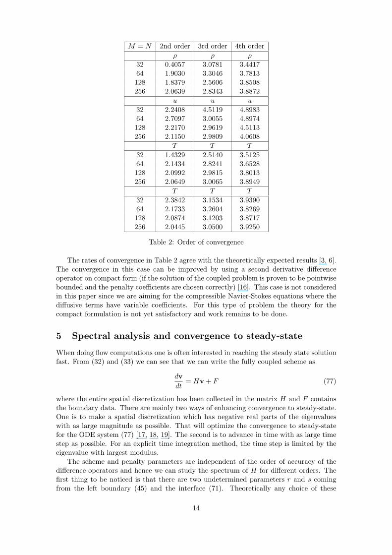
M = N 2nd order 3rd order 4th orderρ ρ ρ

32 0.4057 3.0781 3.441764 1.9030 3.3046 3.7813128 1.8379 2.5606 3.8508256 2.0639 2.8343 3.8872

u u u

32 2.2408 4.5119 4.898364 2.7097 3.0055 4.8974128 2.2170 2.9619 4.5113256 2.1150 2.9809 4.0608

T T T32 1.4329 2.5140 3.512564 2.1434 2.8241 3.6528128 2.0992 2.9815 3.8013256 2.0649 3.0065 3.8949

T T T

32 2.3842 3.1534 3.939064 2.1733 3.2604 3.8269128 2.0874 3.1203 3.8717256 2.0445 3.0500 3.9250

Table 2: Order of convergence

The rates of convergence in Table 2 agree with the theoretically expected results [3, 6].The convergence in this case can be improved by using a second derivative differenceoperator on compact form (if the solution of the coupled problem is proven to be pointwisebounded and the penalty coefficients are chosen correctly) [16]. This case is not consideredin this paper since we are aiming for the compressible Navier-Stokes equations where thediffusive terms have variable coefficients. For this type of problem the theory for thecompact formulation is not yet satisfactory and work remains to be done.

5 Spectral analysis and convergence to steady-state

When doing flow computations one is often interested in reaching the steady state solutionfast. From (32) and (33) we can see that we can write the fully coupled scheme as

dvdt

= Hv + F (77)

where the entire spatial discretization has been collected in the matrix H and F containsthe boundary data. There are mainly two ways of enhancing convergence to steady-state.One is to make a spatial discretization which has negative real parts of the eigenvalueswith as large magnitude as possible. That will optimize the convergence to steady-statefor the ODE system (77) [17, 18, 19]. The second is to advance in time with as large timestep as possible. For an explicit time integration method, the time step is limited by theeigenvalue with largest modulus.

The scheme and penalty parameters are independent of the order of accuracy of thedifference operators and hence we can study the spectrum of H for different orders. Thefirst thing to be noticed is that there are two undetermined parameters r and s comingfrom the left boundary (45) and the interface (71). Theoretically any choice of these

14

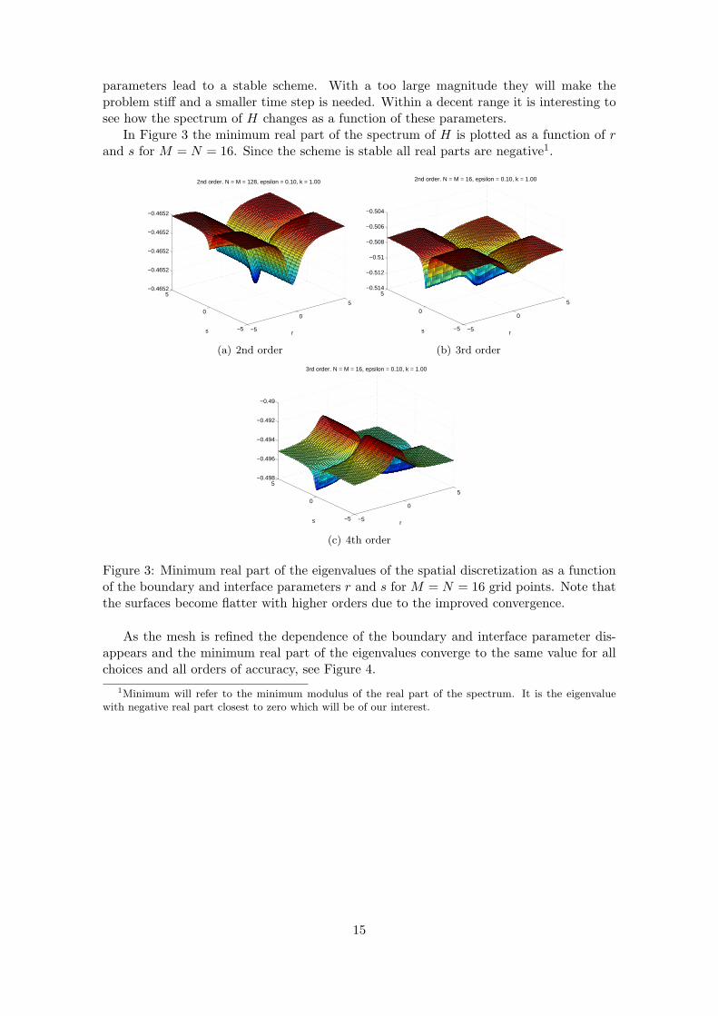
parameters lead to a stable scheme. With a too large magnitude they will make theproblem stiff and a smaller time step is needed. Within a decent range it is interesting tosee how the spectrum of H changes as a function of these parameters.

In Figure 3 the minimum real part of the spectrum of H is plotted as a function of rand s for M = N = 16. Since the scheme is stable all real parts are negative1.

−5

0

5

−5

0

5−0.4652

−0.4652

−0.4652

−0.4652

−0.4652

r

2nd order. N = M = 128, epsilon = 0.10, k = 1.00

s

(a) 2nd order

−5

0

5

−5

0

5−0.514

−0.512

−0.51

−0.508

−0.506

−0.504

r

2nd order. N = M = 16, epsilon = 0.10, k = 1.00

s

(b) 3rd order

−5

0

5

−5

0

5−0.498

−0.496

−0.494

−0.492

−0.49

r

3rd order. N = M = 16, epsilon = 0.10, k = 1.00

s

(c) 4th order

Figure 3: Minimum real part of the eigenvalues of the spatial discretization as a functionof the boundary and interface parameters r and s for M = N = 16 grid points. Note thatthe surfaces become flatter with higher orders due to the improved convergence.

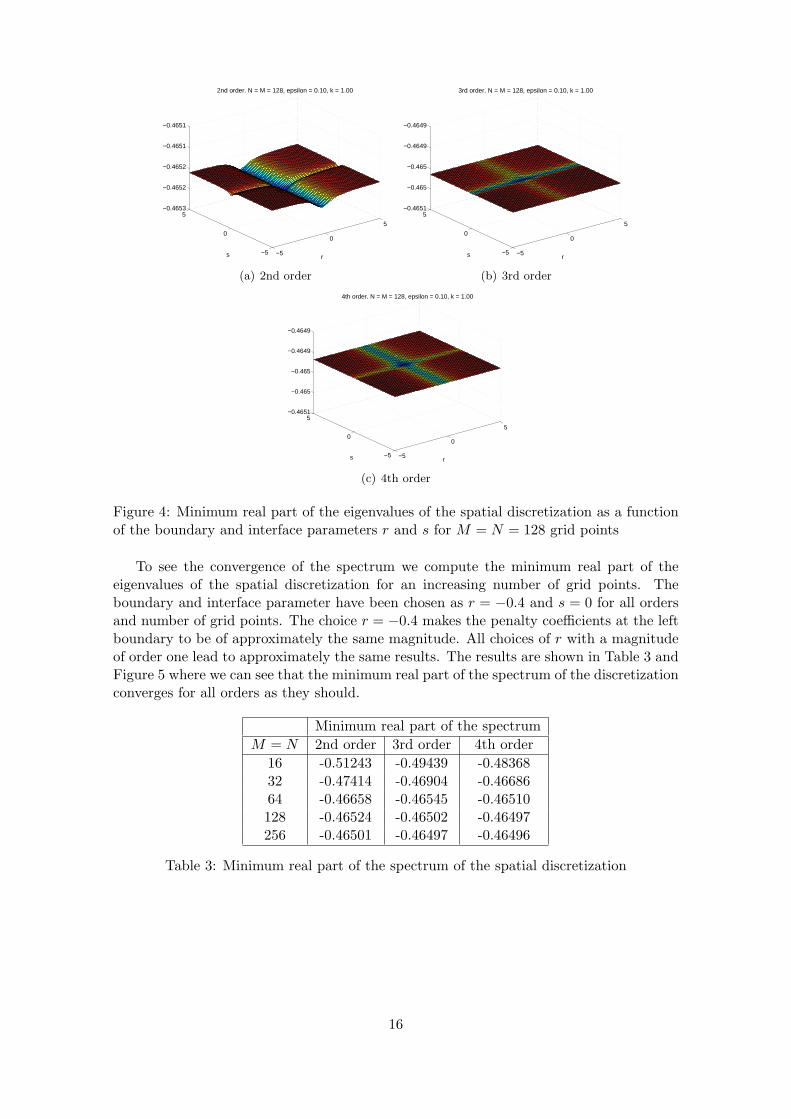
As the mesh is refined the dependence of the boundary and interface parameter dis-appears and the minimum real part of the eigenvalues converge to the same value for allchoices and all orders of accuracy, see Figure 4.

1Minimum will refer to the minimum modulus of the real part of the spectrum. It is the eigenvaluewith negative real part closest to zero which will be of our interest.

15

−5

0

5

−5

0

5−0.4653

−0.4652

−0.4652

−0.4651

−0.4651

r

2nd order. N = M = 128, epsilon = 0.10, k = 1.00

s

(a) 2nd order

−5

0

5

−5

0

5−0.4651

−0.465

−0.465

−0.4649

−0.4649

r

3rd order. N = M = 128, epsilon = 0.10, k = 1.00

s

(b) 3rd order

−5

0

5

−5

0

5−0.4651

−0.465

−0.465

−0.4649

−0.4649

r

4th order. N = M = 128, epsilon = 0.10, k = 1.00

s

(c) 4th order

Figure 4: Minimum real part of the eigenvalues of the spatial discretization as a functionof the boundary and interface parameters r and s for M = N = 128 grid points

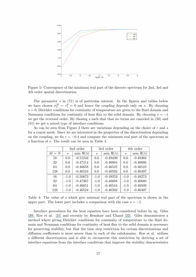
To see the convergence of the spectrum we compute the minimum real part of theeigenvalues of the spatial discretization for an increasing number of grid points. Theboundary and interface parameter have been chosen as r = −0.4 and s = 0 for all ordersand number of grid points. The choice r = −0.4 makes the penalty coefficients at the leftboundary to be of approximately the same magnitude. All choices of r with a magnitudeof order one lead to approximately the same results. The results are shown in Table 3 andFigure 5 where we can see that the minimum real part of the spectrum of the discretizationconverges for all orders as they should.

Minimum real part of the spectrumM = N 2nd order 3rd order 4th order

16 -0.51243 -0.49439 -0.4836832 -0.47414 -0.46904 -0.4668664 -0.46658 -0.46545 -0.46510128 -0.46524 -0.46502 -0.46497256 -0.46501 -0.46497 -0.46496

Table 3: Minimum real part of the spectrum of the spatial discretization

16

5 5.5 6 6.5 7 7.5 8 8.5 9−0.52

−0.51

−0.5

−0.49

−0.48

−0.47

−0.46

log2(M + N)

2nd3rd4th

Figure 5: Convergence of the minimum real part of the discrete spectrum for 2nd, 3rd and4th order spatial discretization

The parameter s in (71) is of particular interest. In the figures and tables belowwe have chosen σM3 = τ0

1 = 0 and hence the coupling depends only on s. By choosings = 0, Dirichlet conditions for continuity of temperature are given to the fluid domain andNeumann conditions for continuity of heat flux to the solid domain. By choosing s = −1we get the reversed order. By chosing s such that that no terms are canceled in (50) and(51) we get a mixed type of interface conditions.

As can be seen from Figure 3 there are variations depending on the choice of r and sfor a coarse mesh. Since we are interested in the properties of the discretization dependingon the coupling, we fix r = −0.4 and compute the minimum real part of the spectrum asa function of s. The result can be seen in Table 4.

2nd order 3rd order 4th orderM = N s min <(λ) s min <(λ) s min <(λ)

16 0.0 -0.51243 0.0 -0.49439 0.0 -0.4836832 0.0 -0.47414 0.0 -0.46904 0.0 -0.4668664 0.0 -0.46658 0.0 -0.46545 0.0 -0.46510128 0.0 -0.46524 0.0 -0.46502 0.0 -0.4649716 -1.0 -0.50873 -1.0 -0.49253 -1.0 -0.4827332 -1.0 -0.47367 -1.0 -0.46888 -1.0 -0.4668064 -1.0 -0.46651 -1.0 -0.46544 -1.0 -0.46509128 -1.0 -0.46524 -1.0 -0.46502 -1.0 -0.46497

Table 4: The value of s which give minimal real part of the spectrum is shown in theupper part. The lower part includes a comparison with the case s = −1.

Interface procedures for the heat equation have been considered before by eg. Giles[20], Roe et al. [21] and recently by Henshaw and Chand [22]. Giles demonstrates amethod where giving Dirichlet conditions for continuity of temperature to the fluid do-main and Neumann conditions for continuity of heat flux to the solid domain is necessaryfor preserving stability, but that the time step restriction for certain discretizations anddiffusion coefficients is more severe than in each of the subdomains. Roe et al. utilizesa different discretization and is able to circumvent this restriction by deriving a set ofinterface equations from the interface conditions that improve the stability characteristics

17

and also preserve the accuracy of the scheme. Henshaw and Chand considers many differ-ent interface procedures and prove both stability and second order accuracy independentof the diffusive properties in contrast to the results in [20]. They also state that moreattractive convergence results might be obtained by considering a mixed type of interfaceconditions.

As can be seen from Table 4 the choice s = 0, which correspond to the method in theabove papers, is preferable since it maximizes the real part of the spectrum and henceimproves the convergence. It is also clear that the difference between the results for s = 0and s = −1 are small. We investigated the intermediate values as well and not muchdifference in min <(λ) was found.

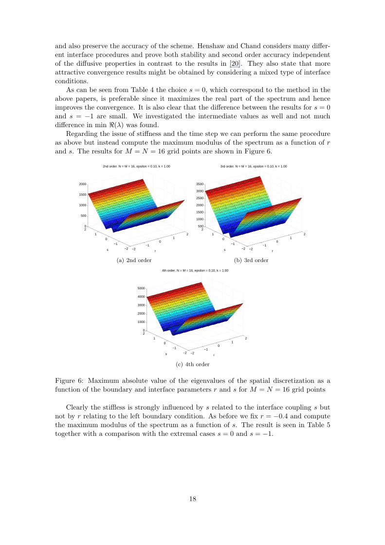
Regarding the issue of stiffness and the time step we can perform the same procedureas above but instead compute the maximum modulus of the spectrum as a function of rand s. The results for M = N = 16 grid points are shown in Figure 6.

−2−1

01

2

−2

−1

0

1

20

500

1000

1500

2000

r

2nd order. N = M = 16, epsilon = 0.10, k = 1.00

s

(a) 2nd order

−2−1

01

2

−2

−1

0

1

2500

1000

1500

2000

2500

3000

3500

r

3rd order. N = M = 16, epsilon = 0.10, k = 1.00

s

(b) 3rd order

−2−1

01

2

−2

−1

0

1

20

1000

2000

3000

4000

5000

r

4th order. N = M = 16, epsilon = 0.10, k = 1.00

s

(c) 4th order

Figure 6: Maximum absolute value of the eigenvalues of the spatial discretization as afunction of the boundary and interface parameters r and s for M = N = 16 grid points

Clearly the stiffless is strongly influenced by s related to the interface coupling s butnot by r relating to the left boundary condition. As before we fix r = −0.4 and computethe maximum modulus of the spectrum as a function of s. The result is seen in Table 5together with a comparison with the extremal cases s = 0 and s = −1.

18

2nd order 3rd order 4th orderM = N s max |λ| s max |λ| s max |λ|

16 0.27 262.19599 0.26 499.82195 -0.47 831.1646032 0.28 1048.61887 0.26 1956.94999 -0.47 3321.5352064 0.28 4130.98536 0.26 7730.09701 -0.47 13286.14080128 0.28 16385.83220 0.26 30875.13265 -0.47 53144.5632016 0.0 506.10401 0.0 946.87926 0.0 1461.3338932 0.0 2023.97316 0.0 3787.78434 0.0 5845.4894064 0.0 8095.61354 0.0 15151.67511 0.0 23382.27042128 0.0 32382.50222 0.0 60607.77891 0.0 93529.7106416 -1.0 736.43767 -1.0 1427.31703 -1.0 1889.0532132 -1.0 2941.31462 -1.0 5703.41160 -1.0 7548.9163464 -1.0 11756.61529 -1.0 22801.96629 -1.0 30181.10326128 -1.0 47009.40113 -1.0 91184.53704 -1.0 120695.31884

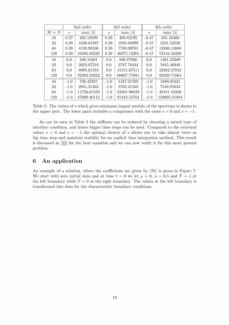
Table 5: The values of s which gives minimum largest modulo of the spectrum is shown inthe upper part. The lower parts includes a comparison with the cases s = 0 and s = −1.

As can be seen in Table 5 the stiffness can be reduced by choosing a mixed type ofinterface condition, and hence bigger time steps can be used. Compared to the extremalvalues s = 0 and s = −1 the optimal choices of s allows one to take almost twice asbig time step and maintain stability for an explicit time integration method. This resultis discussed in [22] for the heat equation and we can now verify it for this more generalproblem.

6 An application

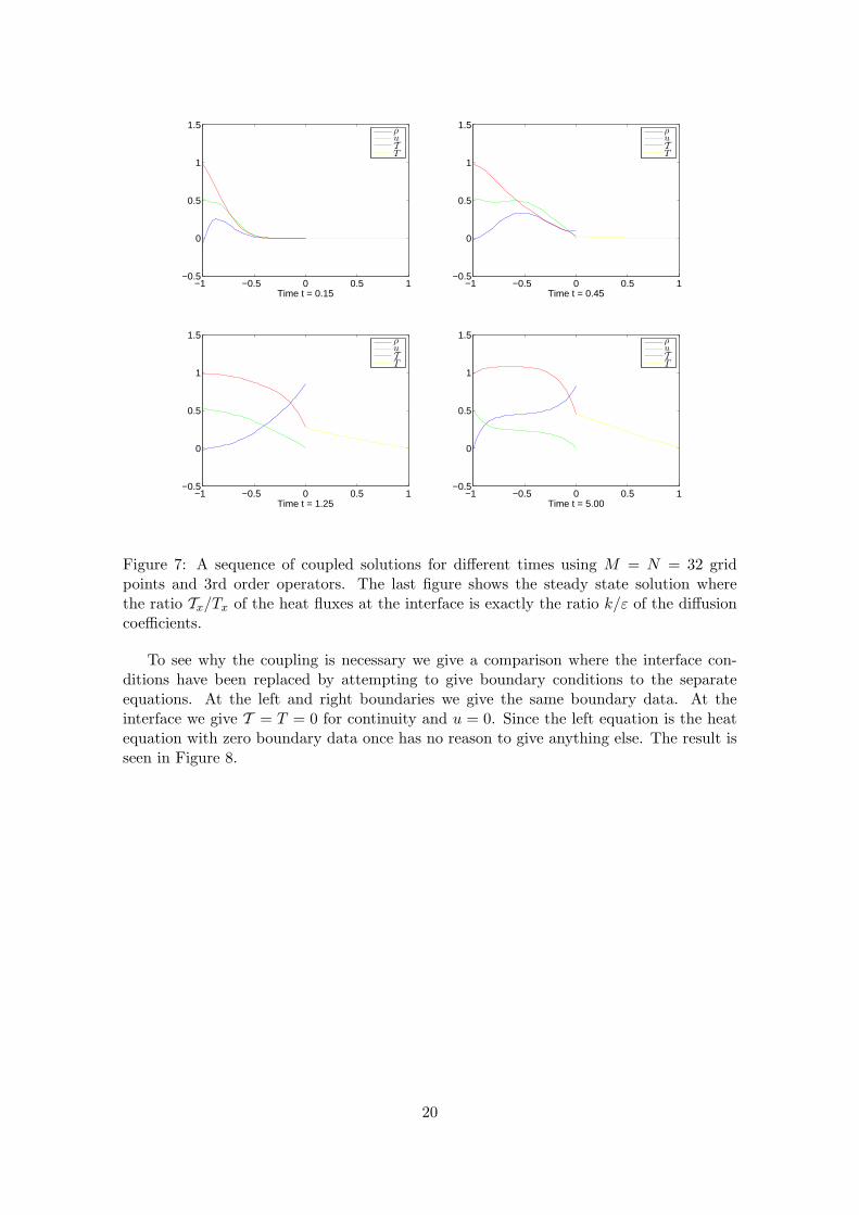
An example of a solution, where the coefficients are given by (76) is given in Figure 7.We start with zero initial data and at time t = 0 we let ρ = 0, u = 0.5 and T = 1 atthe left boundary while T = 0 at the right boundary. The values at the left boundary istransformed into data for the characteristic boundary conditions.

19

−1 −0.5 0 0.5 1−0.5

0

0.5

1

1.5

Time t = 0.15

ρuTT

−1 −0.5 0 0.5 1−0.5

0

0.5

1

1.5

Time t = 0.45

ρuTT

−1 −0.5 0 0.5 1−0.5

0

0.5

1

1.5

Time t = 1.25

ρuTT

−1 −0.5 0 0.5 1−0.5

0

0.5

1

1.5

Time t = 5.00

ρuTT

Figure 7: A sequence of coupled solutions for different times using M = N = 32 gridpoints and 3rd order operators. The last figure shows the steady state solution wherethe ratio Tx/Tx of the heat fluxes at the interface is exactly the ratio k/ε of the diffusioncoefficients.

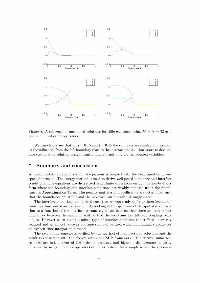
To see why the coupling is necessary we give a comparison where the interface con-ditions have been replaced by attempting to give boundary conditions to the separateequations. At the left and right boundaries we give the same boundary data. At theinterface we give T = T = 0 for continuity and u = 0. Since the left equation is the heatequation with zero boundary data once has no reason to give anything else. The result isseen in Figure 8.

20

−1 −0.5 0 0.5 1−0.5

0

0.5

1

1.5

Time t = 0.15

ρuTT

−1 −0.5 0 0.5 1−0.5

0

0.5

1

1.5

Time t = 0.45

ρuTT

−1 −0.5 0 0.5 1−0.5

0

0.5

1

1.5

Time t = 1.25

ρuTT

−1 −0.5 0 0.5 1−0.5

0

0.5

1

1.5

Time t = 5.00

ρuTT

Figure 8: A sequence of uncoupled solutions for different times using M = N = 32 gridpoints and 3rd order operators

We can clearly see that for t = 0.15 and t = 0.45 the solutions are similar, but as soonas the influences from the left boundary reaches the interface the solutions start to deviate.The steady-state solution is significantly different not only for the coupled variables.

7 Summary and conclusions

An incompletely parabolic system of equations is coupled with the heat equation in onespace dimension. The energy method is used to derive well-posed boundary and interfaceconditions. The equations are discretized using finite differences on Summation-by-Partsform where the boundary and interface conditions are weakly imposed using the Simul-taneous Approximation Term. The penalty matrices and coefficients are determined suchthat the boundaries are stable and the interface can be called strongly stable.

The interface conditions are derived such that we can study different interface condi-tions as a function of one parameter. By looking at the spectrum of the spatial discretiza-tion as a function of the interface parameter, it can be seen that there are only minordifferences between the minimun real part of the spectrum for different coupling tech-niques. However when giving a mixed type of interface condition the stiffness is greatlyreduced and an almost twice as big time step can be used while maintaining stability foran explicit time integration method.

The rate of convergence is verified by the method of manufactured solutions and theresult is consistent with the theory within the SBP framework. The derived numericalschemes are independent of the order of accuracy and higher order accuracy is easilyobtained by using difference operators of higher orders. An example where the system is

21

solved using 3rd order operators is shown and it can be seen that the correct interfaceconditions are obtained.

References

[1] Jens Lindstrom, Johan Bejhed, and Jan Nordstrom. Measurements and numericalmodelling of orifice flow in microchannels. In the 41st AIAA Thermophysics Confer-ence, AIAA Paper No. 2009-4098, San Antonio, USA, 22–25 June 2009.

[2] Bo Strand. Summation by Parts for Finite Difference Approximations for d/dx.Journal of Computational Physics, 110(1):47 – 67, 1994.

[3] Ken Mattsson and Jan Nordstrom. Summation by parts operators for finite differenceapproximations of second derivatives. Journal of Computational Physics, 199(2):503–540, 2004.

[4] Ken Mattsson. Boundary Procedures for Summation-by-Parts Operators. J. Sci.Comput., 18(1):133–153, 2003.

[5] Mark H. Carpenter, Jan Nordstrom, and David Gottlieb. A Stable and Conserva-tive Interface Treatment of Arbitrary Spatial Accuracy. Journal of ComputationalPhysics, 148(2):341 – 365, 1999.

[6] Jing Gong and Jan Nordstrom. Stable, Accurate and Efficient Interface Proceduresfor Viscous Problems. Report, Uppsala University, Disciplinary Domain of Scienceand Technology, Mathematics and Computer Science, Department of InformationTechnology, Numerical Analysis, Department of Information Technology, UppsalaUniversity, Uppsala, 2006.

[7] X. Huan, J.E. Hicken, and D.W. Zingg. Interface and Boundary Schemes for High-Order Methods . In the 39th AIAA Fluid Dynamics Conference, AIAA Paper No.2009-3658, San Antonio, USA, 22–25 June 2009.

[8] Magnus Svard, Mark H. Carpenter, and Jan Nordstrom. A stable high-order finitedifference scheme for the compressible Navier-Stokes equations, far-field boundaryconditions. J. Comput. Phys., 225(1):1020–1038, 2007.

[9] Magnus Svard and Jan Nordstrom. A stable high-order finite difference scheme forthe compressible Navier-Stokes equations: No-slip wall boundary conditions. Journalof Computational Physics, 227(10):4805 – 4824, 2008.

[10] Ken Mattsson, Magnus Svard, Mark Carpenter, and Jan Nordstrom. High-orderaccurate computations for unsteady aerodynamics. Computers and Fluids, 36(3):636– 649, 2007.

[11] Jan Nordstrom, Jing Gong, Edwin van der Weide, and Magnus Svard. A stableand conservative high order multi-block method for the compressible Navier-Stokesequations. Journal of Computational Physics, 2009.

[12] Ken Mattsson, Magnus Svard, and Jan Nordstrom. Stable and Accurate ArtificialDissipation. J. Sci. Comput., 21(1):57–79, 2004.

[13] Jan Nordstrom and Magnus Svard. Well-Posed Boundary Conditions for the Navier–Stokes Equations. SIAM J. Numer. Anal., 43(3):1231–1255, 2005.

22

[14] Saul Abarbanel and David Gottlieb. Optimal time splitting for two- and three-dimensional Navier-Stokes equations with mixed derivatives. Journal of Computa-tional Physics, 41(1):1 – 33, 1981.

[15] Bertil Gustafsson, Heinz-Otto Kreiss, and Joseph Oliger. Time Dependent Problemsand Difference Methods. Wiley Interscience, 1995.

[16] Magnus Svard and Jan Nordstrom. On the order of accuracy for difference ap-proximations of initial-boundary value problems. Journal of Computational Physics,218(1):333–352, 2006.

[17] Magnus Svard, Ken Mattsson, and Jan Nordstrom. Steady-State Computations UsingSummation-by-Parts Operators. J. Sci. Comput., 24(1):79–95, 2005.

[18] Jan Nordstrom. The influence of open boundary conditions on the convergence tosteady state for the Navier-Stokes equations. Journal of Computational Physics,85(1):210 – 244, 1989.

[19] Bjorn Engquist and Bertil Gustafsson. Steady state computations for wave propaga-tion problems. Mathematics of Computation, 49(179):39–64, 1987.

[20] M. B. Giles. Stability analysis of numerical interface conditions in fluid-structurethermal analysis. International Journal for Numerical Methods in Fluids, 25:421–436, August 1997.

[21] B. Roe, R. Jaiman, A. Haselbacher, and P. H. Geubelle. Combined interface bound-ary condition method for coupled thermal simulations. International Journal forNumerical Methods in Fluids, 57:329–354, May 2008.

[22] William D. Henshaw and Kyle K. Chand. A composite grid solver for conjugate heattransfer in fluid-structure systems. Journal of Computational Physics, 228(10):3708– 3741, 2009.

23