THEORETICAL ADVANCES

Accurate object detection using local shape descriptors

Mohammad Anvaripour • Hossein Ebrahimnezhad

Received: 1 April 2012 / Accepted: 24 May 2013

� Springer-Verlag London 2013

Abstract This paper proposes a novel object detection

approach based on local shape information. Boundary edge

fragments preserve some features like shape and position

which properly describe the outline of an object. Extraction

of object boundary fragments is a challenging task in object

detection. In this paper, a sophisticated system is proposed

to achieve this goal. We propose local shape descriptors

and present a boundary fragment extraction method using

Poisson equation properties, and then, we compute relation

between boundary fragments using GMM to obtain exact

boundaries and detect the object. To get more accurate

detection of the object, we employ a False Positive elimi-

nation stage based on local orientation histogram matching.

The proposed object detection system is applied on several

datasets containing object classes in cluttered images in

various forms of scale and translation. We compare our

approach with other similar methods that use shape infor-

mation for object detection. Experimental results show the

power of our proposed method in detection and its

robustness in face with scale and translation variations.

Keywords Object detection � Shape-based features �Poisson equation � False Positives elimination � Generic

model

1 Introduction

Object detection is of fundamental importance in the

computer vision and has received a great deal of attention

in the recent years. Detection is the process of localizing

and finding the scale of an object in an image. Humans find

objects in a scene by considering their shapes. So, shape

information is a significant cue for object detection. Shape

of objects can be inferred from the shape of boundary

edges or contours [1, 2]. While extracting sufficient shape

information still poses a large challenge, recent research in

detection allows extraction of local shape hypotheses.

In this paper, object descriptors are introduced as a

means of acquiring the object shape, configuration, and

model. Poisson equation properties are employed to extract

local features from edge image. Besides, boundary frag-

ments and local orientations of objects are utilized as local

features. Characteristics of boundary fragments are col-

lected in a class-specific codebook as a set of their local

orientations, scales, and positions according to the object

center. Object configuration is defined as the relation

between boundary fragments [3, 4]. Models are typically

identified as sparse collection of local features [5].

Gaussian mixture model (GMM) is utilized to develop the

object configuration as a complete graph. A generic model

is created and histograms of local orientations for desired

object are acquired for shape matching purpose.

The challenge is to find the object boundaries for

detection purpose. To extract the object boundaries from

edge points, some characteristics of edge fragments

including pose, local orientation and scale are employed.

To derive an automatic initialization for the location, scale,

and probable boundaries of the object, a Hough style voting

scheme [6] is implemented, which enables us to match the

object shape in database with severely cluttered images,

M. Anvaripour � H. Ebrahimnezhad (&)

Computer Vision Research Laboratory, Electrical Engineering

Faculty, Sahand University of Technology, Tabriz, Iran

e-mail: ebrahimnezhad@sut.ac.ir

M. Anvaripour

e-mail: m_anvaripour@sut.ac.ir

123

Pattern Anal Applic

DOI 10.1007/s10044-013-0342-x

where the object boundaries cover only a small fraction of

the edge points [7]. A Mean-Shift algorithm is also used to

find the local maxima and center of the object. In cluttered

images, some edges may be established as a part of object

boundary, incorrectly. To alleviate the problem, a trained

GMM is applied to find relation between the established

boundary fragments and launch the shape of object.

False Positive is a usual problem in detection tasks,

which occurs when incorrect objects are detected. In this

paper, a False Positive elimination procedure is proposed

by matching the histogram of local orientation of the model

with the extracted shape of object using Poisson equation

properties. Histogram of local orientation gives a descrip-

tion of object shape and helps us to find the object accu-

rately and remove false detections. Some examples of

detected objects by our approach are shown in Fig. 1 in

which a bounding box covers the object boundaries. Fig-

ure 2 illustrates the stages of our proposed method. A

preliminary version of this work has appeared in [8]. The

remainder of this paper is organized as follows. In Sect. 2,

the related studies of shape-based object detection are

presented. Section 3 introduces our proposed object

descriptors. In Sect. 4, the object detection stage is

described. Section 5 reports extensive experiments in

which our method has been evaluated and compared with

the previous studies. Finally, the conclusion of the paper

appears in Sect. 6.

2 Related works

Our method relies on localizing and finding the scale of the

object by considering its shape information. Shape of

object can be acquired using boundary edges or contours

[1] and segmentation methods [9]. This section concen-

trates on the most related studies that employ some con-

cepts of geometry or shape for various object classification

tasks in an image.

Contour was first used for template matching to detect

objects [10–12]. In [11], chamfer matching is used to find

proper contours. An alternative method is using of contour

fragments or boundary edge fragments as presented in [1,

13]. Authors of these papers used contour fragments as

local features of object boundaries and employed Hough

voting space for detection. A boosting algorithm is used to

train the shape and position of fragments in the coordinate

of object center. In [13], region of interest in image is

obtained by the searching algorithm presented in [14]. This

algorithm seeks regions for the most probable presence of

the object center according to contour fragments.

In some studies, edge points have been used as an

attractive feature. In [15], the number of edge points in a

region was used as a feature for shape representation.

Sampling edges and the relations between them are used in

some methods. In [7], a model is constructed using frag-

ments in the extracted codebook. Boundary of the model is

discretized to uniform samples of points. These points are

matched with extracted points in the image by TPS-RPM

algorithm that was presented in [16] for non-rigid shape

matching. In [17], geometric blur [18] is used as an oper-

ator for sampling the edges. Landmarks were introduced in

[19] to split boundaries and edges. In [19], Markov random

field has been proposed for modeling the shapes of the

objects in a variety of object poses using landmarks.

In [20], the edges of input image are partitioned into

contour segments and organized in an image representation

as contour segment network. The object detection problem is

treated by finding paths through the network resembling the

model boundary. The network is created by connecting

contour segments. This approach of connecting the segments

has been used by the same authors in their next study. They

present KAS features for detection in [21] and use SVM

classifier to train an explicit shape of the object and detect it.

Although object detection through edges was used in

many studies, the proper object boundary and object shape

may not be obtained in cluttered images. To this end,

Fig. 1 Two examples of detected objects by the proposed method

Pattern Anal Applic

123

graphs have been used as they are useful for perfect

localizing and extracting the shape of an object. The rela-

tion between local features such as graphs demonstrates

object structures. In [22], a geometrical arrangement of

parts was computed to make an explicit shape model of the

object. Most of these models have been developed to

increase the accuracy of recognition or classification, rather

than to accurately localize the constituent parts or the

objects [19]. However, such models can be developed for

object localization through local edges or contour

fragments.

The relation between local features induces False Posi-

tives in some clutter images, which can be fairly removed

by employing shape information. Shape of the object can

be obtained by class-based segmentation. Shape informa-

tion, existing in the image in the form of coherent image

regions or segments and their bounding contours, provides

a strong cue that can be used for detection [25]. In [9, 23],

images are segmented based on class-specific image fea-

tures for the class-based segmentation of the relevant

object class. These approaches, however, aim to maximize

the region of interest. Bottom-up segmentation is presented

in [24], which combines tiny segments to form larger

regions. In [25], Poisson equation is solved for a big region

with a tall effective boundary to describe shape of the

region and to find proper segments of the desired object.

Poisson equation has been presented in [26] for shape

classification. Solution of Poisson equation at a point in the

interior of a region represents the average time required for

a particle to hit the boundary at a random walk starting at a

specific point. Such a solution allows the smooth propa-

gation of contour information of a region to every internal

pixel [26]. Poisson equation has several useful properties

that can be used for detection and classification tasks.

In this paper, we propose a sophisticated object detec-

tion system by extracting object boundaries, constructing

object configuration, and making generic models including

histograms of local orientation of the objects to enhance the

removal of False Positives in cluttered images. The pro-

posed method has the better detection performance in face

with troubling edge fragments compared to state-of-the-art

methods. Enjoying a high detection performance, our

method removes the False Positives. In the following sec-

tions, the two main parts of the proposed approach

including object descriptor and detection task are

introduced.

3 Object descriptor

Our detection process is based on shape properties of

objects, in which the shape is identified using boundary

fragments and local orientations of the object. Boundary

fragments are used to expose presence of the object in the

image, and local orientation of the object parts are used to

match the local shape descriptor to obtain the nearest shape

to the model and overcome False Positives. The proposed

object descriptor is generated in three steps: creating

codebook from local boundary fragments, making object

configuration, and constructing generic model descriptor.

In the following subsection, the proposed object descriptor

has been described in detail (left part of Fig. 2 illustrates

object descriptor extraction process).

3.1 Codebook creation from local boundary fragments

Object boundaries are the best features for describing

object shape that are invariant to color and brightness

changes in images. However, it is difficult to extract object

boundaries thoroughly in natural images. Therefore, we use

local boundary fragments as the primitive descriptors and

store them in a class-specific collection called codebook.

Fig. 2 Overview of the proposed method

Pattern Anal Applic

123

At the beginning of feature extraction process, we find edge

points of the images using canny edge detector and split

them from junction points. These edges are still raw and

insufficient to explain shapes of the objects in images. To

get a more descriptive shape feature, we use the solution of

Poisson equation on these raw edges. Poisson equation has

several properties that are introduced in [26]. It can be used

to extract a wide variety of useful properties of a silhouette

binary image including segmentation of a silhouette into

parts, identifying corners at various resolution scales,

deriving a skeleton structure, and locally judging the ori-

entation. Poisson equation is solved on a binary edge

image. Equation (1) presents this equation in which U

refers to the solution of the equation:

r2U ¼ �1 ð1Þ

The concept of Poisson equation can be considered as a

set of particles that have random walk originated from a

point. Some statistics of this random walk can be measured

such as mean time required for a particle to hit the

boundary [26]. The numerical solution presented in [26] is

multigrid algorithm, because of the fast process of this

algorithm. In multigrid solution, the residual equation is

solved and averaged to represent them on a coarse grid

where the distance between neighborhoods grids is twice

the fine grid distance. The solution is interpolated to the

fine grid to have a good approximation for the smooth error

and correct the previous solution. This kind of relaxation

that is followed by a correction is called multigrid cycle.

This equation is solved under Dirichlet boundary condition

considering U(x,y) = 0 at the object contour in binary

image. The solution of the Poisson equation is very robust

in noisy boundaries, especially after relaxation sweep,

discussed in [26]. To reduce the noise near the boundaries,

a post processing stage is applied that solves the equation

Uxx þ Uyy ¼ �1 inside and Uxx þ Uyy ¼ 0 outside the

object in a binary image.

The Poisson equation can be also used to estimate the local

orientation of a shape. So, we compute the local orientation of

each edge fragment by employing the Poisson equation

solution. Local orientation is computed by Hessian matrix of

U in each edge point. The Eigen vector that corresponds to the

smaller Eigen value of Hessian matrix in an edge point is

considered as the local orientation of the edge in that point.

Local orientations which are obtained by explained procedure

describes edge orientation variation smoothly and more pre-

cise than other methods such as gradient. Equation (2) shows

the Hessian matrix of U at pixel (x, y):

H x; yð Þ ¼o2Uox2

o2Uoxoy

o2Uoyox

o2Uoy2

" #ð2Þ

We split edges from the high curvature points after

computing their local orientations and present each

fragment by three parameters: fragment length,

orientation of the left part (L), and orientation of the

right part (R). Orientation of each part is quantized into six

values (-p/3, -p/6, 0, p/6, p/3, p/2); therefore, each edge

fragment will acquire one of the 36 possible forms of the

L–R orientations.

To achieve the boundary fragments, we use a set of

natural images in which the interested object is surrounded

by bounding boxes. Before extraction of boundary frag-

ments, we resize the bounding boxes in different images to

a fixed size to get a scale invariant model. After extraction

of edge image from each image in dataset inside the

bounding box, it is decomposed to 36 different oriented

edge image layers based on the status of L–R orientation of

the edge fragments. So, each oriented edge image layer will

contain only the edge fragments with special orientation.

For example, the first and second layers contain the edge

fragments with the L–R orientations of (-p/3,-p/3) and

(-p/3,-p/6), respectively. As a general rule, the (i 9 j)th

layer contains the fragments with the L–R orientation of

(hi,hj), where hi and hj belong to the angle set (h1 = -p/3,

h2 = -p/6, h3 = 0, h4 = p/6, h5 = p/3, h6 = p/2).

As we know, the boundary fragments follow the shape

of the object. Supposing that the objects are surrounded by

the bounding boxes in all dataset images and they are

scaled to have equal sizes, thus, we can aggregate the

similar layers of edge fragments in different images of one

object class to separate boundary fragments from other

fragments. In fact, in the aggregated image of the similar

layers, we will find a large number of fragments in the

location of boundaries because of the same length and

orientation of such fragments. In the other words, boundary

fragments of an object in different images appear in a same

position with respect to the center of bounding box. Any

location in the aggregated image, which contains boundary

fragments, holds the large number of edge points, because

of the regular shape of such fragments. On the contrary,

any location of non-boundary fragments holds the small

number of edge points the aggregated image (because of

the random shape of such fragments). In consequence, we

can separate boundary fragments from other edge fragment

and store them in a codebook. For each boundary fragment,

a feature vector F defined in Eq. (3) is assigned and all of

the vectors are stored in a codebook as the possible

boundary fragments of the object.

F ¼ ½hl; hr; S; x; y� ð3Þ

In this equation, hl and hr are the orientation of left and

right parts of boundary fragment, S is the length (or scale)

of the boundary fragment, and x; yð Þ show the pose of the

Pattern Anal Applic

123

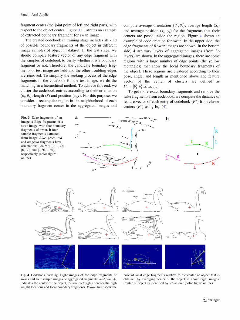
fragment center (the joint point of left and right parts) with

respect to the object center. Figure 3 illustrates an example

of extracted boundary fragment for swan image.

The created codebook in training stage includes all kind

of possible boundary fragments of the object in different

image samples of object in dataset. In the test stage, we

should compare feature vector of any edge fragment with

the samples of codebook to verify whether it is a boundary

fragment or not. Therefore, the candidate boundary frag-

ments of test image are held and the other troubling edges

are removed. To simplify the seeking process of the edge

fragments in the codebook for the test image, we do the

matching in a hierarchical method. To achieve this end, we

cluster the codebook entries according to their orientation

hl; hrð Þ, length (S) and position x; yð Þ. For this purpose, we

consider a rectangular region in the neighborhood of each

boundary fragment center in the aggregated images and

compute average orientation hrl ; h

rr

� �, average length (Sr)

and average position (xr, yr) for the fragments that their

centers are posed inside the region. Figure 4 shows an

example of code creation for swan. In the upper side, the

edge fragments of 8 swan images are shown. In the bottom

side, 4 arbitrary layers of aggregated images (from 36

layers) are shown. In the aggregated images, there are some

regions with a large number of edge points (the yellow

rectangles) that show the local boundary fragments of

the object. These regions are clustered according to their

pose, angle, and length as mentioned above and feature

vector of the center of clusters are defined as

Fr ¼ ½hrl ; h

rr ; Sr; xr; yr�.

To get more exact boundary fragments and remove the

false fragments from codebook, we compute the distance of

feature vector of each entry of codebook Fað Þ from cluster

centers Frð Þ using Eq. (4):

Fig. 3 Edge fragments of an

image. a Edge fragments of a

swan image, with four boundary

fragments of swan, b four

sample fragments extracted

from image. Blue, green, red

and magenta fragments have

orientations [90, 90], [0, -30],

[0, 30] and [-30, -60],

respectively (color figure

online)

Fig. 4 Codebook creating. Eight images of the edge fragments of

swans and four sample images of aggregated fragments. Red plus, ?,

indicates the center of the object, Yellow rectangles denotes the high

weight locations and local boundary fragments. Yellow lines show the

pose of local edge fragments relative to the center of object that is

obtained by averaging center of the object in above eight images.

Center of object is identified by white axis (color figure online)

Pattern Anal Applic

123

D Fr;Fað Þ ¼wh : 1�h~

r; h~

aD Eh~

r��� ��� h~

a��� ���

0B@

1CA

þ logSr

Sa

� ���������þ 1

Diag:

ffiffiffiffiffiffiffiffiffiffiffiffiffiffiffiffiffiffiffiffiffiffiffiffiffiffiffiffiffiffiffiffiffiffiffiffiffiffiffiffiffiffiffixr � xað Þ2þ yr � yað Þ2

q

¼wh : 1� hrl h

al þ hr

rharffiffiffiffiffiffiffiffiffiffiffiffiffiffiffiffiffiffiffiffiffiffiffiffiffi

hrl

� �2þ hrr

� �2q ffiffiffiffiffiffiffiffiffiffiffiffiffiffiffiffiffiffiffiffiffiffiffiffiffi

hal

� �2þ har

� �2q

0B@

1CA

þ logSr

Sa

� ���������þ 1

Diag:

ffiffiffiffiffiffiffiffiffiffiffiffiffiffiffiffiffiffiffiffiffiffiffiffiffiffiffiffiffiffiffiffiffiffiffiffiffiffiffiffiffiffiffixr � xað Þ2þ yr � yað Þ2

qð4Þ

In this equation, Fa is a feature vector of fragment a in

the codebook. At the first term of the equation, the

orientation difference of two fragments is computed. The

second term calculates the logarithm difference between

the lengths (scales) of two fragments. Finally, the third

term determines the Euclidean distance between locations

of the fragments. Diag is the diagonal length of training

image (or the bounding box of object), which is used for

normalization. xa and ya determine the position of the

center of the fragment. We set wh = 2 in our experiments

to indicate the importance of the orientation in the shape

similarity computation. Under the condition that

DðFr;FaÞ\0:01� Diag, the fragment Fa is counted as

cluster Fr in the codebook.

The generated codebook is adequate for the matching

process because all the features in the codebook clusters

have specific scales and angles and represent spatial

transformation of the fragments according to the center of

the object. By this way, the sequential form of fragment

matching can be converted into the hierarchical form in

which we find the similar cluster at first and find the exact

entry of codebook at final. Therefore, the matching process

will be easy and fast.

3.2 Object configuration

Relationships between the local features are important

shape cues that can be used in recognition and detection of

the object. Since extracting the complete shape of an object

in the cluttered natural images is impractical, relation

between the local features or graphs [27] helps us to rec-

ognize the object by indicating configuration of the local

features. In this paper, we deal with object configuration

through the relationships between its boundary fragments

stored in the codebook as a complete graph. We use such

relationships to find the true boundaries of the object from

the candidate boundary fragments obtained from the

codebook matching stage. Since, distribution of such local

features cannot be considered as a Gaussian function,

combination of two or more Gaussian functions gives more

precise representation of feature distribution. Thus, the

relations between these local features are constructed using

GMM.

We use the boundary fragments in the codebook clus-

ters. First, for each cluster in the codebook, we select the

edge fragment in the average length and the average dis-

tance from the object center as a representative fragment.

Then, we construct the relation between these local fea-

tures using GMM.

Let k = {wi, li, Ri, i = 1…N} be the set of the

parameters of a GMM, where wi, li and Ri denote weight,

mean, and covariance of Gaussian function i. If q be the

hidden mixture variable associated with the observation O,

then:

p O qjð Þ ¼XN

i¼1

wip O q ¼ i; kjð Þ; ð5Þ

with:

p O q ¼ i; kjð Þ ¼ 1

2pD=2 Rij j1=2: exp � 1

2O� lið ÞTR�1

i O� lið Þ

ð6Þ

where, D is the dimension of observation vector.

To train the object configuration using GMM, we use

training samples O = {ot, t = 1…T}, as a collection of

T observations. Estimation of k can be performed by

maximizing the log-likelihood function log p(O|k). Each

sample is considered as a feature vector containing nor-

malized distances, angles, and scales. In fact, the training

samples are fabricated by relationships between boundaries

fragments as the local features. Figure 5 shows an example

of this concept. Blue lines specify the relation between

boundary fragment 1 and other boundaries fragments. In

the same way, red lines specify the relation between

boundary fragment 4 and the others. We calculate the

length of the lines, the angles between the fragments, and

the scales of the fragments.

Fig. 5 Relation between parts 1 and 6 with boundary fragments of

the codebook for swan. Numbers denote codebook classes

Pattern Anal Applic

123

The observation O contains ot which is extracted from

the relation matrix R as defined in Eq. (7).

R ¼

s1; l11; h11ð Þ s2; l12; h12ð Þ . . . . . . ðsn; l1n; h1nÞs1; l21; h21ð Þ s2; l22; h22ð Þ . . . . . . ðsn; l2n; h2nÞ

. . . . . . si; lij; hij

� �. . . . . .

. . . . . . . . . . . . . . .s1; ln1; hn1ð Þ s2; ln2; hn2ð Þ . . . . . . sn; lnn; hnnð Þ

266664

377775ð7Þ

Rð:Þ ¼ ½Rð1; :Þ;Rð2; :Þ; � � � ;Rðn; :Þ�ot ¼ No redundant form of ðRð:ÞÞ

and removed the zero values

In this matrix, n shows the number of boundary

fragment of interested object or number of clusters in the

codebook. si indicates the normalized scale (or length) of

the ith boundary fragment, which is normalized by

summation over all scales. lij is the length of line that

connects the edge fragments i and j, which is normalized

by summation over all line lengths, and hij is the angle of

this line, which is normalized by dividing to 2p. As we see

in Eq. (7), dimension of the observation vector is

dependent to the number of fragments. In fact, to

construct the relation vector ot, we need to consider all

scales (or lengths) of fragments, all mutual distances of

fragment pairs and all mutual angles between fragment

pairs. Considering that lij ¼ lji; hji ¼ p� hij, we eliminate

the duplicated parameters from ot to remove redundant

features. Also, we use each si one time and remove lii; hii

from ot because they are always zero and have no valuable

information.

After constructing the observation collection O = {ot,

t = 1…T} based on boundary fragments relationships of

image samples {imt, t = 1…T}, we use them to train

GMM. Dimension of the GMM is selected as dimension

of ot which depends on the number of fragments. For

example, if the object contains 3 number of boundary

fragments, dimension of GMM will be 9 as illustrated at

the following:

R ¼s1; l11; h11ð Þ s2; l12; h12ð Þ s3; l13; h13ð Þs2; l21; h21ð Þ s2; l22; h22ð Þ s2; l23; h23ð Þs3; l31; h31ð Þ s3; l32; h32ð Þ s3; l33; h33ð Þ

264

375

)R :ð Þ ¼ s1; l11; h11; s2; l12; h12; s3; l13; h13; s2; l21; h21; s2;½

l22; h22; s2; l23; h23; s3; l31; h31; s3; l32; h32; s3; l33; h33�lij ¼ lji; hji ¼ p� hij; lii ¼ 0; hii ¼ 0;

)ot ¼ s1; s2; s3; l12; l13; l23; h12; h13; h23½ �)

D ¼ 9

The number of mixtures of GMM is selected arbitrarily.

We use 2 Gaussian mixtures because low complexity leads

to higher training speed. Furthermore, the acceptable

results are obtained by 2 Gaussian mixtures. To train the

GMM, the parameters of k are estimated by maximizing

the log-likelihood function log p(O|k) using the maximum

likelihood estimation (MLE) by EM algorithm.

3.3 Generic model descriptor

In this subsection, we propose an extra process of object

model construction that we use it to remove the False

Positives. False Positives are occurred in images when

some instances are detected and inferred as interest object

incongruously. Therefore, a known model of the object is

required to remove such incorrect detections.

As discussed before, the class-specific codebook con-

tains boundary fragments. We select a fragment from each

cluster of the codebook that has the mean scale and angle,

call them representative fragments (or center of clusters),

and link them to extract the outline of the object. The

sequences of representative fragments are linked manually

in an order to make the shape of the object proper. This

order will be used in detection stage to extract shape of the

object in the test image. Besides, the parameters of frag-

ments such as angle, length, and position in reference to the

center of object are useful to determine the linking order in

the detection stage. For example, as illustrated in Fig. 6,

the model of swan is extracted by connecting the boundary

fragments in the order of: (F1, F2, F3, F4, F5, F6, F7, F1),

where Fj represents the feature vector of the fragment j.

We fill inside the constructed contour and make a binary

image of the object. Then, we solve the Poisson equation

on this image. In fact, the solution of the Poisson equation

on the binary image represents the object shape by prop-

agating the boundary contour of the object to every internal

pixel [26]. The shape of the object may not be extracted

completely in natural images because of their complex

background. Then, the Poisson equation solution of the

detected object may not be same as the Poisson equation

solution of the model. Therefore, the solution of Poisson

equation is not appropriate for using in the False Positive

removing process for detection task. To get more robust

generic model of object, we use the local orientations. The

local orientations of the object are obtained by computing

Eigen vector corresponding to the smaller Eigen value of

Hessian matrix of the Poisson equation solution (U) in all

of the pixels inside the model (See Eq. 2). To simplify this

representation, we quantize the local orientations values to

six quantities, 0, 90, ±30, and ±60 so that we are able to

find a simpler description and use it as the generic model of

the object. Figure 6 shows the extracted shape (top left),

Pattern Anal Applic

123

the solution of the Poisson equation (top right), and the

generic model of the object (bottom). In this generic model,

the local orientations of each region are shown with dif-

ferent colors. For example, the green color region inside

the model indicates the angle of 0�, and the brown color in

the region of the neck specifies the angle of 90�.

To extract the shape feature, we divide the generic model to

multiple patches and obtain the histogram of local orientation

in each patch (See Fig. 7). Histograms are used to match the

model to the detected objects (we use 16 patches). They

contain information about the local orientation of the object.

Each bar in a histogram represents the number of quantized

local orientations that are normalized by the quantity of the

corresponding bar of the whole object histogram (HT). The

feature vector of the model is presented as follows:

H ¼ h1

hT1

;h2

hT2

; . . .;h16

hT16

� �ð8Þ

h ¼ N�p3;N�p

6;N0;Np

6;Np

3;Np

2

n oIn Eq. (8), hT is the histogram of the local orientation of

the Poisson equation of the whole object, h1,2,…,16 consti-

tute the histogram of the local orientation of the Poisson

equation of the 16 patches. N represents the quantities of

the bars of the histogram. The image dataset contains the

binary images of the object in natural images. We match

the histogram of local orientation came from the solution of

Poisson equation for binary shape with the histogram of the

generic model.

4 Object detection

In the object detection stage, we try to find the interested

object in the image. The proposed object detection process

as is illustrated in flowchart of Fig. 2 is divided into 3

steps:

1. Localizing objects in the most probable regions: in this

step, we extract the boundary fragments of the test

image and match them to the entries of the codebook.

2. Finding objects boundaries: the candidate boundary

fragments are then applied to the trained GMM model,

and the object configuration is extracted by finding the

object boundaries fromthe candidate boundary fragments.

3. False Positives elimination: False Positives are

removed by matching the generic shape model with

the extracted shapes.

4.1 Localizing objects in the most probable regions

In Sect. 3, we have represented the shape of an object as a

set of boundary fragments. Each fragment was defined with

a specific shape, location, and scale that are stored in a

Fig. 6 Generic model of the

object. Top left is a generic

shape extracted by linking the

representative fragments. Top

right is the solution of Poisson

equation on the shape. Bottom is

the big view of the generic

model of the object. Colors

indicate quantities of local

orientations (color figure online)

Pattern Anal Applic

123

clustered codebook. In the first step of detection stage, as a

similar method to training stage, the feature vector of edge

fragments of test image is constructed by solving the

Poisson equation on the edges, computing Eigen vector of

the smallest Eigen value of Hessian matrix of the Poisson

equation solution, disconnecting them from the high cur-

vature places, and quantizing the orientations. Then, we

match the edge fragments of test image with the fragments

in the codebook based on their shape similarities given in

Eq. (9). In this equation, Fa is an edge fragment in the

codebook, and Fb is an edge fragment in the test image.

D Fa;Fb� �

¼ 1�h~

r; h~

aD Eh~

r��� ��� h~

a��� ���

¼ 1� hal h

bl þ ha

r hbrffiffiffiffiffiffiffiffiffiffiffiffiffiffiffiffiffiffiffiffiffiffiffiffiffi

hal

� �2þ har

� �2q ffiffiffiffiffiffiffiffiffiffiffiffiffiffiffiffiffiffiffiffiffiffiffiffiffi

hbl

� �2þ hbr

� �2q ð9Þ

More precisely, an edge fragment of test image is

considered to be a match of a codebook fragment if

D \ 0.2. Since a pair of the matched edge fragments

induces a translation and scale transformation, each match

votes for the presence of an object boundary at a particular

location. Votes are weighted by 1-D so that the more

similar edges contain more weights. We make the vote

scale invariant by the following equations:

xh ¼ xct þ Dx � St

S

yh ¼ yct þ Dy � St

S

ð10Þ

In Eq. (10), xh and yh are the position of the vote in

Hough voting space, xct and yct define the center of the edge

fragment, Dx and Dy explain the position of the boundary

fragment with respect to the object center stored in the

codebook, St is the length of test image fragment and S is

the length of boundary fragment in the codebook.

Variation of color for each pixel suggests different regions

in the image and could be used as a feature to find the regions

belonging to the objects. In fact, object boundaries can be

considered as the edges between the regions with high color

(or intensity) difference. We call such strong edges as the

effective edges. Effective edges could be extracted using a

high threshold in the gradient of the image and decomposed

Fig. 7 Patches and histograms of a generic shape model. Each bar is normalized by the number of pixels in a patch

Pattern Anal Applic

123

to fragments as discussed before. Effective edge fragments

are used to vote for the object presence with the higher

weight. The object center is obtained by seeking the local

maximum regions in Hough voting space. We use Mean-

Shift algorithm [14] to find the regions that have enough total

weights and votes. The local maximums in the voting space

define rough estimates of the location and scale of the can-

didate object instances [14]. Figure 8 shows the local max-

imum that has been obtained by the boundary fragments. The

Local maximums with the value higher than a threshold are

preserved, and the others are removed.

4.2 Finding object boundaries

The above voting procedure delivers some local maxi-

mums in a typical cluttered image, as the local features are

not very distinctive. However, it could localize the objects

in the most probable places of the image. In this subsection,

we obtain the relationship between the boundaries to detect

the object in cluttered natural images where unrelated

fragments may vote for the object presence and be con-

sidered as the object boundaries, by mistake.

Object configuration can extract the shape of the object

using the relation between the boundary fragments and

remove the outliers. We use the trained GMM to extract the

proper fragments to specify the object boundaries from the

set of inliers and outlier boundary fragments.

To use the GMM in the detection stage, a set of test

observations, ot, must be created. To achieve this end, we

select the associated fragments in each detected region by

Mean-Shift. Different subsets of the associated fragments

are picked and the relations between them are computed

and so the test observations are created. The MLE

evaluates the quality of the correspondence of the test

and train observations [28]. Large amounts of MLE give

the proper boundaries fragments and remove the outliers.

Figure 9a shows the extracted boundary fragments in an

image.

4.3 False Positives elimination

In the previous subsection, we extracted the fragments as

the object boundaries. However, in cluttered images, some

instances may be found as outliers in different regions of an

image because of finding similar edge of test image to the

local boundary fragments stored in the codebook. It leads

to a false explanation of the objects in images, which is

referred to as False Positives.

Fig. 8 Hough voting space and edge fragments. a An image of the swan and Hough voting space. Yellow rectangle shows the regions

established by Mean-Shift. b Edge fragments and effective fragments of the image (color figure online)

Pattern Anal Applic

123

To extract the shapes of the objects, we connect all the

boundary fragments in detected regions that have been taken

from GMM. We connect them by a sequence that was specified

in the Generic Model Descriptor in Sect. 3.3 in order to extract

the object shape. By connecting the boundary fragments and

filling inside of the connected regions, we construct a binary

shape, which is utilized for the matching process.

We solve the Poisson equation on the binary images and

extract the local orientations of the object. Histograms of the

local orientations are computed for each patch as the proce-

dure that was discussed in Sect. 3.3, and used for matching. If

the value of C be obtained more than a threshold, it will be

considered as False Positive and so will be removed.

Figure 9 shows the detected object after pruning False

Positives. We show the detected object by a bounding box

that covers the object and a plus sign, ?, which lies in the

center of the extracted region by Mean-Shift algorithm.

5 Experimental results

We present an extensive evaluation of our method using

seven object classes from three challenging datasets,

ETHZ, Weizmann, and INRIA horses. The capability of

the shape extraction and the object detection in images,

both in terms of bounding boxes and binary shapes, is

measured. Our results were obtained after removing the

False Positives. Detection results are compared with other

state-of-the-art methods. We have demonstrated the results

in each database, separately.

5.1 ETHZ database

This database contains a total number of 255 images in five

diverse classes; i.e. bottles, swans, mugs, giraffes, and

apple logos [29]. It is highly challenging, as the objects

Table 1 Number of training and test images for experiment on

ETHZ dataset

Classes Apple

logos

Bottles Giraffes Mugs Swan

Training natural

images

20 24 44 24 16

Test pos. 20 24 44 24 16

Test neg. 215 207 167 207 223

Fig. 9 Shape explanation. a Edge fragments of image. Red edges

represent boundary fragments extracted by GMM and blue edges

represent boundary fragments connection. b Extracted binary shape

from image. c Local orientation of binary shape for evaluating

histograms and matching with generic model in Fig. 7 to remove false

positives. d Detected object (color figure online)

Pattern Anal Applic

123

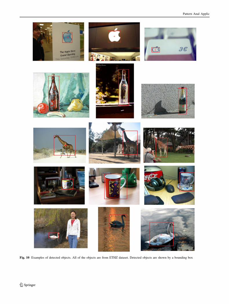
Fig. 10 Examples of detected objects. All of the objects are from ETHZ dataset. Detected objects are shown by a bounding box

Pattern Anal Applic

123

appear in a wide range of scales. It is considerable that

many images are severely cluttered with disturbing edges

and objects comprising only a fraction of the total image

area. We evaluate the performance of our method in

detecting objects of this database by comparing our results

with those of Ferrari et al. methods in [7, 20, 21, 30].

We used half of the images in each class for obtaining

object descriptors. Our method does not require any neg-

ative images for training. The test set consists of all other

images in the dataset. The test images in a class are used as

a positive test for own class and as a negative test for other

classes. The negative images are used to estimate False

Positive rates. Table 1 shows the number of training and

test images. Figure 10 shows some examples of the

detected objects of this database.

We compare the proposed method with the results in [7,

20, 21] under similar conditions. The number of the

selected images is the same as the number of training and

test images in those papers. An object was detected by

20 % IoU (Intersection of Union) criterion described in

[21]. Under this condition, the detection is counted as

positive if the object bounding box overlapped more than

20 % with the ground truth; otherwise, it is identified as a

False Positive. Figure 11 shows the plots of the detection

rate against the number of False Positives. In [20], a hand-

plotted model was used to detect the objects of each class.

Table 2 Comparison between

detection rates of different

methods according to plots in

Fig. 11, under 20 % IoU

criterion

Detection rates in 0.3/0.4 FPPI

Classes Our

method

Method of Ferrari

et al. [21]

Method of Ferrari

et al. [20]

Method of Ferrari

et al. [7]

Apple logos 0.96/0.96 0.568/0.728 0.65/0.832 0.777/0.85

Bottles 0.98/0.98 0.891/0.91 0.893/0.893 0.814/0.832

Giraffes 0.8/0.878 0.626/0.67 0.723/0.787 0.523/0.586

Mugs 0.92/0.98 0.70/0.78 0.80/0.8 0.781/0.836

Swan 1/1 0.72/0.9 0.647/0.647 0.68/0.754

Average 0.91/0.951 0.70/0.798 0.743/0.792 0.715/0.772

Fig. 11 Object detection results. Each plot shows four curves which

have been extracted under the 20 % IoU criterion. Magenta curves

show performance of our method. Blue, green and dotted red curves

show performances of methods in [21], [20] and [7], respectively

(color figure online)

Pattern Anal Applic

123

Detection rates in 0.3 and 0.4 False Positives per Image

(FPPI) represent the performances of methods. As the plots

show, the results of our method are better than the others

according to the detection rate in 0.3 and 0.4 FPPI.

Our method does not use discriminative learning like

Ferrari et al. [21]. It is obtained only from the positive

images. Models in our experiments are the average shape

of half of the objects in each class. Thus, they include rich

information about the shape of the objects. Furthermore, it

reveals the power of our method that can make worthwhile

detection results without employing negative images in

training stage. In [20], a hand-plotted model was used to

extract shapes from images. The relation between the

boundary fragments can model the shapes of the objects,

but TPS-RPM algorithm in [7] may match a model to the

disturbing edges and cause False Positives. We removed

the False Positives as described in Sect. 4 to detect the

objects correctly. This led to better results, as compared

with those of other studies. The results of the detection rate

in 0.3 and 0.4 False Positive per image are presented in

Table 2.

In [30], an object is detected by grouping boundaries

and detection succeeds if bounding box overlaps more than

80 % with ground truth. In the mentioned work, FPPI is not

reported. To compare with [30], we evaluate our method

over three classes of database. We use half of the images in

each class for training and the remainder for test. Method

in [30] uses a simple hand-plotted model to form the shape

of the object. Table 3 shows results of our method and [30]

which demonstrates our proposed method makes better

results than the compared one.

We compare our method with [7, 31, 32] by evaluating

PASCAL criterion. Under this condition, an object is

detected if bounding box overlaps more than 50 % with

ground truth. The number of selected images for training

and test images is the same as Table 1. Figure 12 shows the

plots of detection rate against the False Positives per image

of proposed method and methods of [7, 31]. Detection rates

in 0.3 and 0.4 False Positives per image are shown in

Table 4. As these tables show, our method has the best

performance in four classes (apple logos, bottles, mugs and

swan). Because of the clutters in giraffe images and tex-

tures of giraffe body, our method has the less detection rate

in comparison to [31] in giraffe class, because edge sam-

ples or geometric blur feature is not sensitive face to edge

breaking. Figure 13 illustrates the recall against precision

Table 3 Comparison between detection rate of [30] and our method

under 80 % IoU criterion without testing on negative images

Bottles

(%)

Giraffes

(%)

Swans

(%)

Our method 85 60 89

Method of Adluru and Latecki [30] 80 45.45 87.5

Fig. 12 Comparison of object detection rates under PASCAL criterion. Magenta curves show performance of our method. Green and dotted red

curves show performances of methods in [31] and [7], respectively (color figure online)

Pattern Anal Applic

123

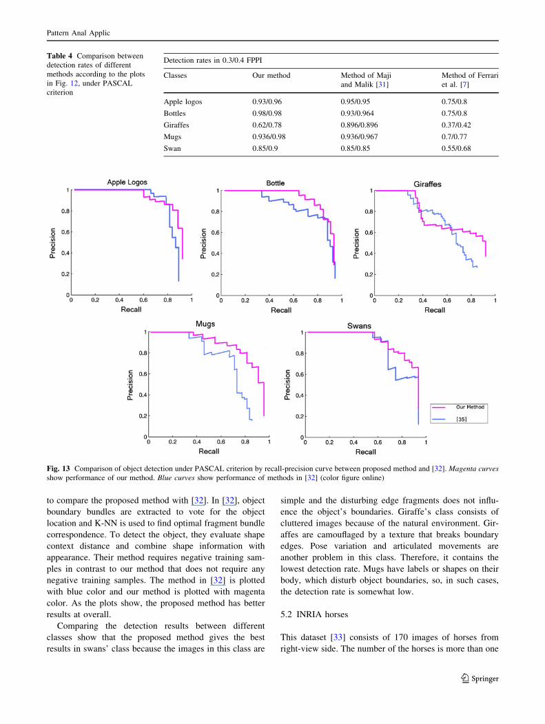
to compare the proposed method with [32]. In [32], object

boundary bundles are extracted to vote for the object

location and K-NN is used to find optimal fragment bundle

correspondence. To detect the object, they evaluate shape

context distance and combine shape information with

appearance. Their method requires negative training sam-

ples in contrast to our method that does not require any

negative training samples. The method in [32] is plotted

with blue color and our method is plotted with magenta

color. As the plots show, the proposed method has better

results at overall.

Comparing the detection results between different

classes show that the proposed method gives the best

results in swans’ class because the images in this class are

simple and the disturbing edge fragments does not influ-

ence the object’s boundaries. Giraffe’s class consists of

cluttered images because of the natural environment. Gir-

affes are camouflaged by a texture that breaks boundary

edges. Pose variation and articulated movements are

another problem in this class. Therefore, it contains the

lowest detection rate. Mugs have labels or shapes on their

body, which disturb object boundaries, so, in such cases,

the detection rate is somewhat low.

5.2 INRIA horses

This dataset [33] consists of 170 images of horses from

right-view side. The number of the horses is more than one

Table 4 Comparison between

detection rates of different

methods according to the plots

in Fig. 12, under PASCAL

criterion

Detection rates in 0.3/0.4 FPPI

Classes Our method Method of Maji

and Malik [31]

Method of Ferrari

et al. [7]

Apple logos 0.93/0.96 0.95/0.95 0.75/0.8

Bottles 0.98/0.98 0.93/0.964 0.75/0.8

Giraffes 0.62/0.78 0.896/0.896 0.37/0.42

Mugs 0.936/0.98 0.936/0.967 0.7/0.77

Swan 0.85/0.9 0.85/0.85 0.55/0.68

Fig. 13 Comparison of object detection under PASCAL criterion by recall-precision curve between proposed method and [32]. Magenta curves

show performance of our method. Blue curves show performance of methods in [32] (color figure online)

Pattern Anal Applic

123

in some images. They contain different colors and textures

and articulated movements in cluttered images. Some

detected samples of this dataset are illustrated in Fig. 14. As

conditions in [7] and [21], we selected 50 natural images for

the training stage and the remaining 120 natural images for

the detection stage. Detection performance in these papers

is reported in 20 % IoU criterion better than PASCAL. We

used 170 negative images for the test and False Positive

estimation. We evaluated the results by 20 % IoU criterion

and showed them in detection rate versus False Positive per

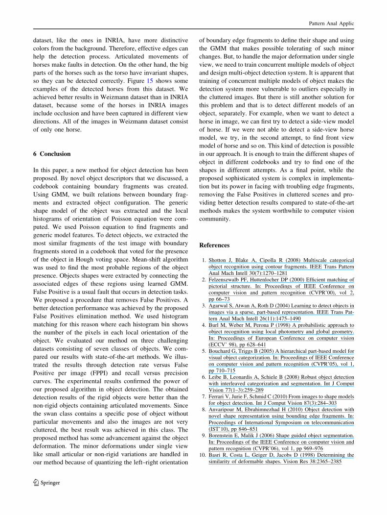
image curve. Figure 15 shows this plot. Table 5 demon-

strates the results of our method, [7] and [21] in 0.3 and 0.4

FPPI. As this table shows, our results are close to them.

However, our algorithm has better detection results in 0.4

FPPI of this dataset. The variation in the poses of the horses

in some images causes faults in detection.

5.3 Weizmann horses dataset

This dataset consists of 328 images of horses from a left-

side view and their silhouettes [34]. They contain different

Table 5 Comparisons results in INRIA horses detection under 20 %

IoU criterion

Detection rates in 0.3/0.4 FPPI

Our method Ferrari et al. [21] Ferrari et al. [7]

0.8/0.855 0.84/0.85 0.78/0.8

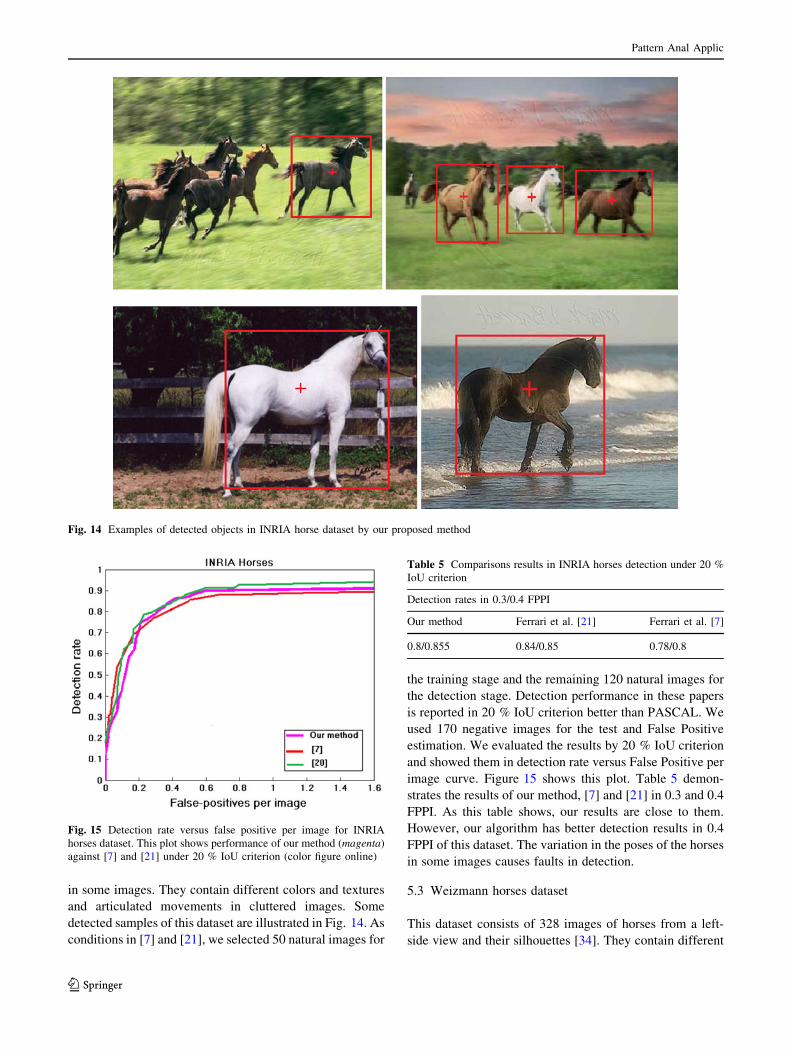
Fig. 14 Examples of detected objects in INRIA horse dataset by our proposed method

Fig. 15 Detection rate versus false positive per image for INRIA

horses dataset. This plot shows performance of our method (magenta)

against [7] and [21] under 20 % IoU criterion (color figure online)

Pattern Anal Applic

123

colors and textures with various scales and articulated

movements. Some samples of detected horses in this

dataset are illustrated in Fig. 16. To compare our method

against [1] and [21] in similar conditions, we chose the first

50 images of the dataset for the training stage. The test set

consists of 277 positive and 277 negative images, collected

from Caltech 101 [35] dataset.

We show the detection results in terms of recall-preci-

sion curve (RPC). The detection results in [21] are reported

based on 20 % IoU criterion. Figure 17 shows the recall-

precision plot of the detection results. As the plot shows,

the recall-precision equal error rate (EER) is 0.938. In [21],

equal error rates of 0.917 and 0.935 were obtained,

respectively, by PAS and 1AS. In [1], an object is detected

correctly if a peak lies within 25 pixels of correct Centroid

(a circle with a radius of 25 pixels corresponds to 20 % of

the average object size). This criterion is near to 20 % IoU.

The detection method of [1] yielded a recall-precision EER

of 0.921. Comparisons of the results are given in Table 6.

As the results show, our method has the good perfor-

mance of object detection in this dataset. Horses in this

Table 6 Comparisons of equal error rates (EER) of three methods

obtained from experiment on Weizmann horses dataset

Our method Method of Shotton et al. [1] Method of Ferrari et al.

[21]

PAS 1AS

0.938 0.921 0.917 0.935

Fig. 16 Examples of detected objects in Weizmann horse dataset by our proposed method

Fig. 17 Comparison of object detection using Weizmann horse

dataset under 20 % IoU criterion by recall-precision curves between

proposed method and [1, 21]. Magenta curves show performance of

our method (color figure online)

Pattern Anal Applic

123

dataset, like the ones in INRIA, have more distinctive

colors from the background. Therefore, effective edges can

help the detection process. Articulated movements of

horses make faults in detection. On the other hand, the big

parts of the horses such as the torso have invariant shapes,

so they can be detected correctly. Figure 15 shows some

examples of the detected horses from this dataset. We

achieved better results in Weizmann dataset than in INRIA

dataset, because some of the horses in INRIA images

include occlusion and have been captured in different view

directions. All of the images in Weizmann dataset consist

of only one horse.

6 Conclusion

In this paper, a new method for object detection has been

proposed. By novel object descriptors that we discussed, a

codebook containing boundary fragments was created.

Using GMM, we built relations between boundary frag-

ments and extracted object configuration. The generic

shape model of the object was extracted and the local

histograms of orientation of Poisson equation were com-

puted. We used Poisson equation to find fragments and

generic model features. To detect objects, we extracted the

most similar fragments of the test image with boundary

fragments stored in a codebook that voted for the presence

of the object in Hough voting space. Mean-shift algorithm

was used to find the most probable regions of the object

presence. Objects shapes were extracted by connecting the

associated edges of these regions using learned GMM.

False Positive is a usual fault that occurs in detection tasks.

We proposed a procedure that removes False Positives. A

better detection performance was achieved by the proposed

False Positives elimination method. We used histogram

matching for this reason where each histogram bin shows

the number of the pixels in each local orientation of the

object. We evaluated our method on three challenging

datasets consisting of seven classes of objects. We com-

pared our results with state-of-the-art methods. We illus-

trated the results through detection rate versus False

Positive per image (FPPI) and recall versus precision

curves. The experimental results confirmed the power of

our proposed algorithm in object detection. The obtained

detection results of the rigid objects were better than the

non-rigid objects containing articulated movements. Since

the swan class contains a specific pose of object without

particular movements and also the images are not very

cluttered, the best result was achieved in this class. The

proposed method has some advancement against the object

deformation. The minor deformations under single view

like small articular or non-rigid variations are handled in

our method because of quantizing the left–right orientation

of boundary edge fragments to define their shape and using

the GMM that makes possible tolerating of such minor

changes. But, to handle the major deformation under single

view, we need to train concurrent multiple models of object

and design multi-object detection system. It is apparent that

training of concurrent multiple models of object makes the

detection system more vulnerable to outliers especially in

the cluttered images. But there is still another solution for

this problem and that is to detect different models of an

object, separately. For example, when we want to detect a

horse in image, we can first try to detect a side-view model

of horse. If we were not able to detect a side-view horse

model, we try, in the second attempt, to find front view

model of horse and so on. This kind of detection is possible

in our approach. It is enough to train the different shapes of

object in different codebooks and try to find one of the

shapes in different attempts. As a final point, while the

proposed sophisticated system is complex in implementa-

tion but its power in facing with troubling edge fragments,

removing the False Positives in cluttered scenes and pro-

viding better detection results compared to state-of-the-art

methods makes the system worthwhile to computer vision

community.

References

1. Shotton J, Blake A, Cipolla R (2008) Multiscale categorical

object recognition using contour fragments. IEEE Trans Pattern

Anal Mach Intell 30(7):1270–1281

2. Felzenszwalb PF, Huttenlocher DP (2000) Efficient matching of

pictorial structure. In: Proceedings of IEEE Conference on

computer vision and pattern recognition (CVPR’00), vol 2,

pp 66–73

3. Agarwal S, Atwan A, Roth D (2004) Learning to detect objects in

images via a sparse, part-based representation. IEEE Trans Pat-

tern Anal Mach Intell 26(11):1475–1490

4. Burl M, Weber M, Perona P (1998) A probabilistic approach to

object recognition using local photometry and global geometry.

In: Proceedings of European Conference on computer vision

(ECCV’ 98), pp 628–641

5. Bouchard G, Triggs B (2005) A hierarchical part-based model for

visual object categorization. In: Proceedings of IEEE Conference

on computer vision and pattern recognition (CVPR’05), vol 1,

pp 710–715

6. Leibe B, Leonardis A, Schiele B (2008) Robust object detection

with interleaved categorization and segmentation. Int J Comput

Vision 77(1–3):259–289

7. Ferrari V, Jurie F, Schmid C (2010) From images to shape models

for object detection. Int J Comput Vision 87(3):284–303

8. Anvaripour M, Ebrahimnezhad H (2010) Object detection with

novel shape representation using bounding edge fragments. In:

Proceedings of International Symposium on telecommunication

(IST’10), pp 846–851

9. Borenstein E, Malik J (2006) Shape guided object segmentation.

In: Proceedings of the IEEE Conference on computer vision and

pattern recognition (CVPR’06), vol 1, pp 969–976

10. Basri R, Costa L, Geiger D, Jacobs D (1998) Determining the

similarity of deformable shapes. Vision Res 38:2365–2385

Pattern Anal Applic

123

11. Garvilla D (2000) Pedestrian detection from a moving vehicle. In:

Proceedings of European Conference on computer vision (ECCV’00),

pp 37–49

12. Grauman K, Darrell T (2005) The Pyramid match kernels: discrim-

inative classification with sets of image features. In: Proceedings of

International Conference on computer vision (ICCV’05), vol 2,

pp 1458–1465

13. Opelt A, Pinz A, Zisserman A (2006) A boundary-fragment

model for object detection. In: Proceedings of European Con-

ference on computer vision (ECCV’ 06), pp 575–588

14. Leibe B, Schiele B (2004) Scale-invariant object categorization

using a scale-adaptive mean-shift search. In: Proceedings of

DAGM’04 Pattern Recognition Symposium

15. Belongie S, Malik J (2002) Shape matching and object recogni-

tion using shape contexts. IEEE Trans Pattern Anal Mach Intell

24(4):509–522

16. Chui H, Rangarajan A (2003) A new point matching algorithm

for non-rigid registration. Comput Vis Image Underst 89(2–3):

114–141

17. Ommer B, Malik J (2009) Multi-scale object detection by clus-

tering lines. In: Proceedings of International Conference on

computer vision (ICCV’09), pp 484–491

18. Berg AC, Malik J (2001) Geometric blur for template matching.

In: Proceedings of IEEE Conference on computer vision and

pattern recognition, vol 1, pp 607–614

19. Geremy H, Gal E, Benjamin P, Daphne K (2009) Shape-based

object localization for descriptive classification. Int J Comput

Vision 84(1):40–62

20. Ferrari V, Jurie F, Schmid C (2006) Object detection with contour

segment networks. In: Proceedings of European Conference on

computer vision, pp 14–28

21. Ferrari V, Fevrier L, Jurie F, Schmid C (2007) Groups of adjacent

contour segments for object detection. IEEE Trans Pattern Anal

Mach Intell 30(1):36–51

22. Pham TV, Smeulders AWM (2005) Object recognition with

uncertain geometry and uncertain part detection. Comput Vis

Image Underst 99(2):241–258

23. Levin A, Weiss Y (2009) Learning to combine bottom-up and

top-down segmentation. Int J Comput Vision 81(1):105–118

24. Sharon E, Galun M, Sharon D, Basri R, Brandt A (2006) Hier-

archy and adaptivity in segmenting visual scenes. Nature 442:

810–813

25. Gorelick L, Basri R (2009) Shape based detection and top–down

delineation using image segments. Int J Comput Vision 83(3):

211–232

26. Gorelick L, Galun M, Sharon E, Basri R, Brandt A (2006) Shape

representation and classification using the Poisson equation.

IEEE Trans Pattern Anal Mach Intell 28(12):1991–2005

27. Bergtholdt M, Kappes J, Schmidt S, Schnorr C (2010) A study of

parts-based object class detection using complete graphs. Int J

Comput Vision 87(1–2):93–117

28. Perronnin F (2008) Universal and adapted vocabularies for gen-

eric visual categorization. IEEE Trans Pattern Anal Mach Intell

30(7):1243–1256

29. ETHZ Database (2007) Ferrari V http://www.vision.ee.ethz.ch/

datasets/downloads/ethz_shape_classes_v12.tgz. Accessed 2012

30. Adluru N, Latecki LJ (2009) Contour grouping based on contour-

skeleton duality. Int J Comput Vision 83(1):12–29

31. Maji S, Malik J (2009) Object detection using max-margin

Hough transform. In: Proceedings of IEEE Conference on com-

puter vision and pattern recognition (CVPR’09), pp 1038–1045

32. Lu C, Adluru N, Ling H, Zhu G, Latecki LJ (2010) Contour based

object detection using part bundles. Comput Vis Image Underst

114(7):827–834

33. Lear Data Sets and Images (2006-2013) LEAR-Learning and

Recognition in Vision http://lear.inrialpes.fr/data. Accessed 2012

34. Weizmann Horse Database (2005) Borenstein E http://www.

msri.org/people/members/eranb. Accessed 2012

35. Caltech101 Database (2006) Fei–Fei L, Fergus R, Perona P http://

www.vision.caltech.edu/Image_Datasets/Caltech101/Caltech101.

html. Accessed 2012

Pattern Anal Applic

123