Lecture 4 Feature Detectors and Descriptors: Corners, Blobs ...
73
COS 429: Computer Vision Lecture 4 Feature Detectors and Descriptors: Corners, Blobs and SIFT Slides adapted from: Szymon Rusinkiewicz, Jia Deng, Svetlana Lazebnik, Steve Seitz
-
Upload
khangminh22 -
Category
Documents
-
view
0 -
download
0
Transcript of Lecture 4 Feature Detectors and Descriptors: Corners, Blobs ...
COS 429: Computer Vision
Lecture 4Feature Detectors and Descriptors:
Corners, Blobs and SIFT
Slides adapted from: Szymon Rusinkiewicz, Jia Deng, Svetlana Lazebnik, Steve Seitz
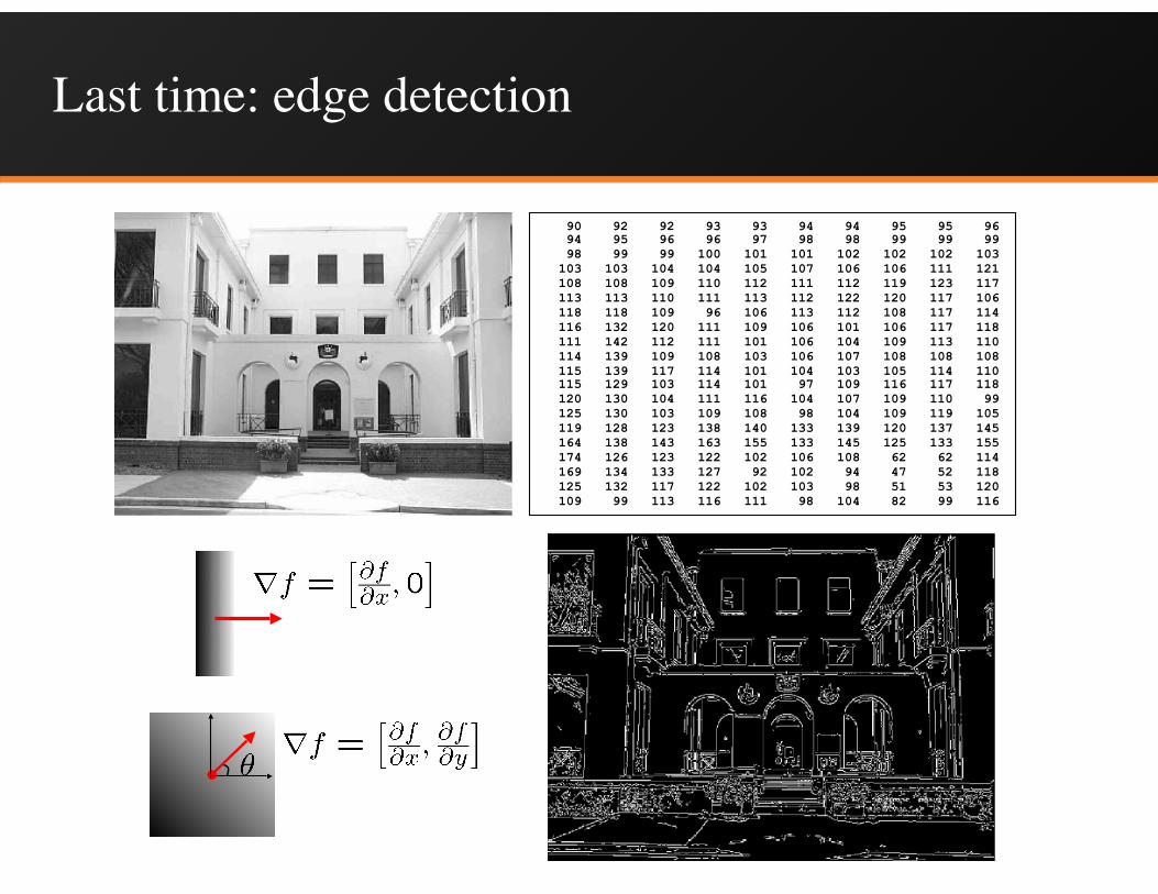
Last time: edge detection
90 92 92 93 93 94 94 95 95 96 94 95 96 96 97 98 98 99 99 99 98 99 99 100 101 101 102 102 102 103 103 103 104 104 105 107 106 106 111 121 108 108 109 110 112 111 112 119 123 117 113 113 110 111 113 112 122 120 117 106 118 118 109 96 106 113 112 108 117 114 116 132 120 111 109 106 101 106 117 118 111 142 112 111 101 106 104 109 113 110 114 139 109 108 103 106 107 108 108 108 115 139 117 114 101 104 103 105 114 110 115 129 103 114 101 97 109 116 117 118 120 130 104 111 116 104 107 109 110 99 125 130 103 109 108 98 104 109 119 105 119 128 123 138 140 133 139 120 137 145 164 138 143 163 155 133 145 125 133 155 174 126 123 122 102 106 108 62 62 114 169 134 133 127 92 102 94 47 52 118 125 132 117 122 102 103 98 51 53 120 109 99 113 116 111 98 104 82 99 116

• Corners
• Blobs
This time: keypoints
Why Extract Keypoints?
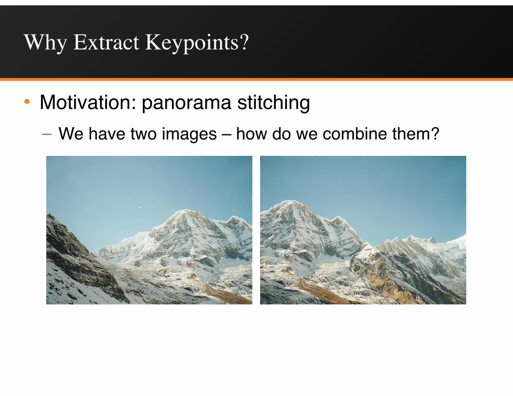
• Motivation: panorama stitching– We have two images – how do we combine them?

Why Extract Keypoints?
• Motivation: panorama stitching– We have two images – how do we combine them?
Step 1: extract keypointsStep 2: match keypoint features

Why Extract Keypoints?
• Motivation: panorama stitching– We have two images – how do we combine them?
Step 3: align images
Step 1: extract keypointsStep 2: match keypoint features
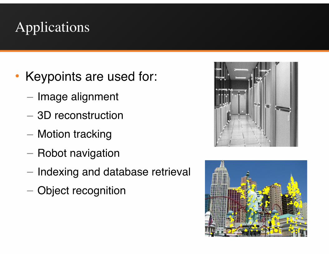
Applications
• Keypoints are used for:– Image alignment – 3D reconstruction– Motion tracking– Robot navigation– Indexing and database retrieval– Object recognition
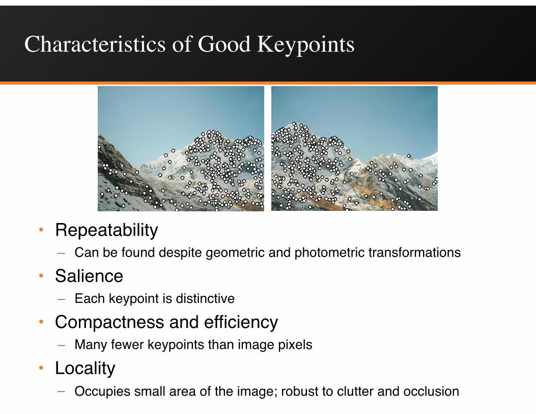
Characteristics of Good Keypoints
• Repeatability– Can be found despite geometric and photometric transformations
• Salience– Each keypoint is distinctive
• Compactness and efficiency– Many fewer keypoints than image pixels
• Locality– Occupies small area of the image; robust to clutter and occlusion

Corners
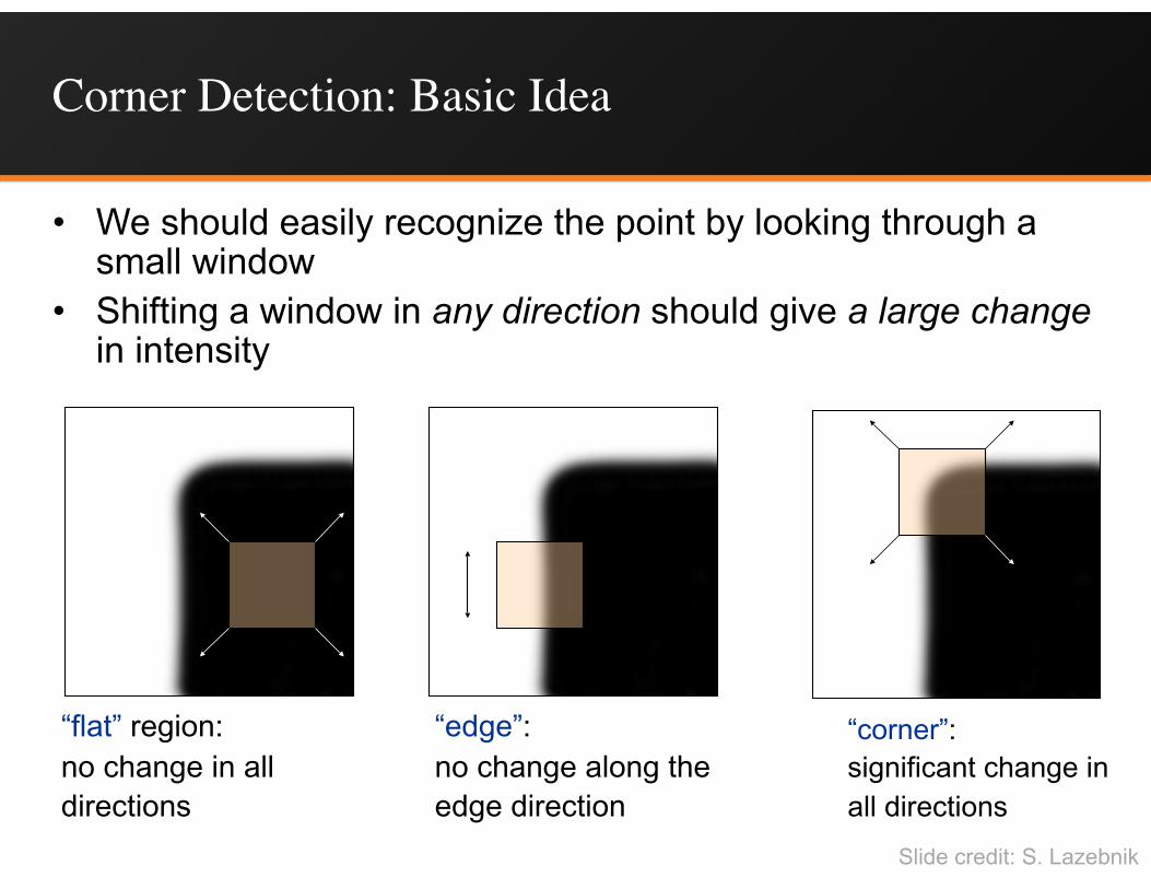
Corner Detection: Basic Idea
• We should easily recognize the point by looking through a small window
• Shifting a window in any direction should give a large change in intensity
“edge”:no change along the edge direction
“corner”:significant change in all directions
“flat” region:no change in all directions
Slide credit: S. Lazebnik
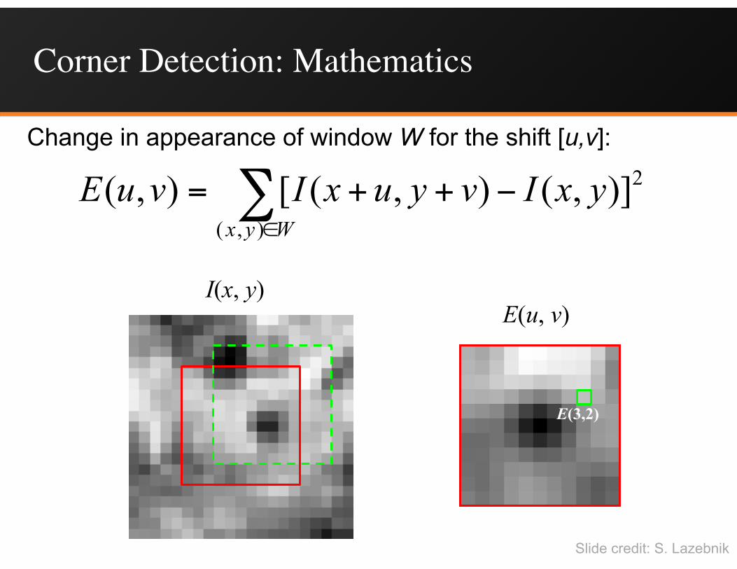
Corner Detection: Mathematics
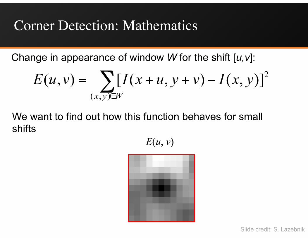
Change in appearance of window W for the shift [u,v]:
I(x, y)E(u, v)
E(3,2)
∑∈
−++=Wyx
yxIvyuxIvuE),(
2)],(),([),(
Slide credit: S. Lazebnik

Corner Detection: Mathematics
I(x, y)E(u, v)
E(0,0)
Change in appearance of window W for the shift [u,v]:
∑∈
−++=Wyx
yxIvyuxIvuE),(
2)],(),([),(
Slide credit: S. Lazebnik
Corner Detection: Mathematics
We want to find out how this function behaves for small shifts
E(u, v)
Change in appearance of window W for the shift [u,v]:
∑∈
−++=Wyx
yxIvyuxIvuE),(
2)],(),([),(
Slide credit: S. Lazebnik
Corner Detection: Mathematics
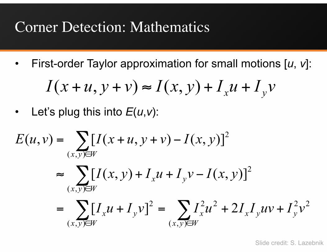
• First-order Taylor approximation for small motions [u, v]:
• Let’s plug this into E(u,v):
vIuIyxIvyuxI yx ++≈++ ),(),(
∑∑
∑
∑
∈∈
∈
∈
++=+=
−++≈
−++=
Wyxyyxx
Wyxyx
Wyxyx
Wyx
vIuvIIuIvIuI
yxIvIuIyxI
yxIvyuxIvuE
),(
2222
),(
2
),(
2
),(
2
2][
)],(),([
)],(),([),(
Slide credit: S. Lazebnik
∑∑
∑
∑
∈∈
∈
∈
++=+=
−++≈
−++=
Wyxyyxx
Wyxyx
Wyxyx
Wyx
vIuvIIuIvIuI
yxIvIuIyxI
yxIvyuxIvuE
),(
2222
),(
2
),(
2
),(
2
2][
)],(),([
)],(),([),(
∑∑
∑
∑
∈∈
∈
∈
++=+=
−++≈
−++=
Wyxyyxx
Wyxyx
Wyxyx
Wyx
vIuvIIuIvIuI
yxIvIuIyxI
yxIvyuxIvuE
),(
2222
),(
2
),(
2
),(
2
2][
)],(),([
)],(),([),(
Corner Detection: Mathematics
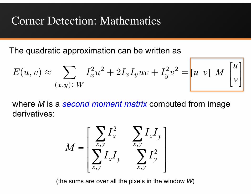
The quadratic approximation can be written as
where M is a second moment matrix computed from image derivatives:
⎥⎥⎥
⎦
⎤
⎢⎢⎢
⎣
⎡
=∑∑
∑∑
yxy
yxyx
yxyx
yxx
III
IIIM
,
2
,
,,
2
(the sums are over all the pixels in the window W)
E(u, v) ⇡X
(x,y)2W
I2x
u2 + 2Ix
Iy
uv + I2y
v2 = [u v]M [uv
] ⎥⎦
⎤⎢⎣
⎡≈
vu
MvuvuE ][),(
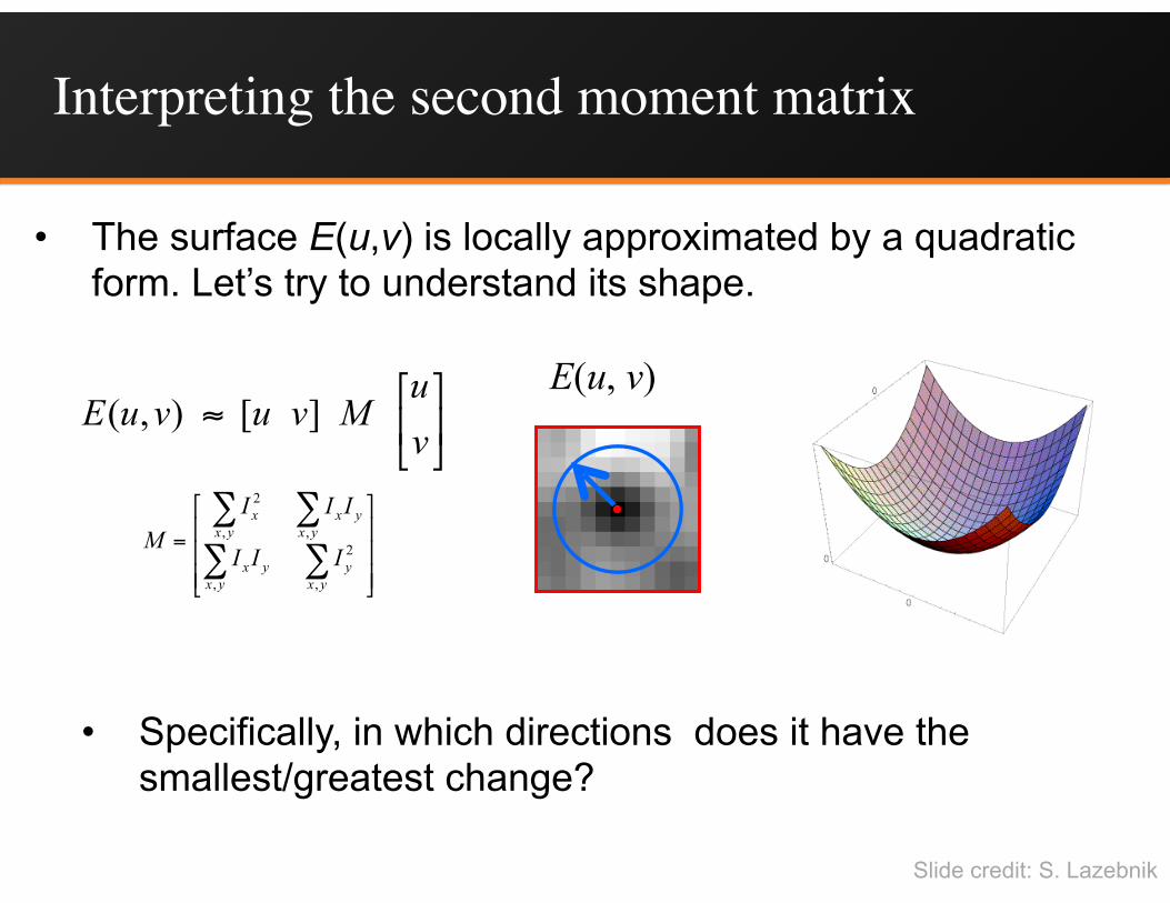
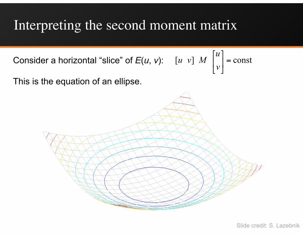
• The surface E(u,v) is locally approximated by a quadratic form. Let’s try to understand its shape.
Interpreting the second moment matrix
⎥⎦
⎤⎢⎣
⎡≈
vu
MvuvuE ][),(E(u, v)
⎥⎥⎥
⎦
⎤
⎢⎢⎢
⎣
⎡
=∑∑
∑∑
yxy
yxyx
yxyx
yxx
III
IIIM
,
2
,
,,
2
Slide credit: S. Lazebnik
• Specifically, in which directions does it have the smallest/greatest change?
Interpreting the second moment matrix
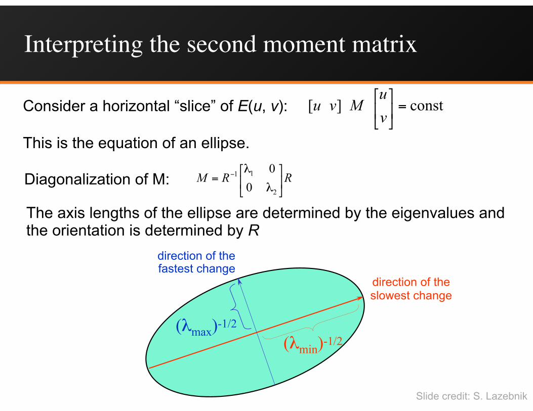
Consider a horizontal “slice” of E(u, v):
This is the equation of an ellipse.
const][ =⎥⎦
⎤⎢⎣
⎡
vu
Mvu
Slide credit: S. Lazebnik
Interpreting the second moment matrix
RRM ⎥⎦
⎤⎢⎣
⎡= −
2
11
00λ
λ
The axis lengths of the ellipse are determined by the eigenvalues and the orientation is determined by R
direction of the slowest change
direction of the fastest change
(λmax)-1/2
(λmin)-1/2
Diagonalization of M:
Consider a horizontal “slice” of E(u, v):
This is the equation of an ellipse.
const][ =⎥⎦
⎤⎢⎣
⎡
vu
Mvu
Slide credit: S. Lazebnik
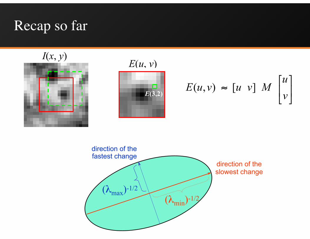
Recap so far
direction of the slowest change
direction of the fastest change
(λmax)-1/2
(λmin)-1/2
I(x, y)E(u, v)
E(3,2) ⎥⎦
⎤⎢⎣
⎡≈
vu
MvuvuE ][),(

At an edge
direction of the slowest change
direction of the fastest change
(λmax)-1/2
(λmin)-1/2
I(x, y)E(u, v)
E(3,2) ⎥⎦
⎤⎢⎣
⎡≈
vu
MvuvuE ][),(
• The direction along the edge results in no change
• λmin is very small
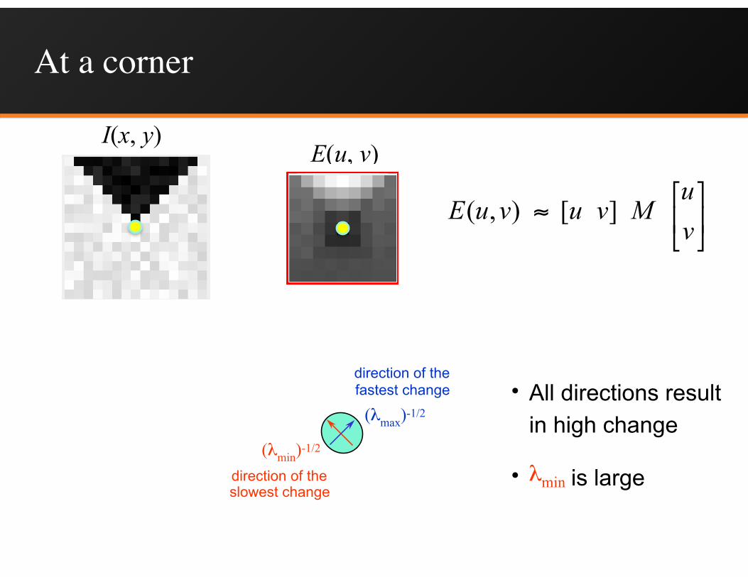
At a corner
direction of the slowest change
direction of the fastest change
(λmax)-1/2
(λmin)-1/2
I(x, y)E(u, v)
E(3,2) ⎥⎦
⎤⎢⎣
⎡≈
vu
MvuvuE ][),(
• All directions result in high change
• λmin is large

Slide credit: S. Lazebnik
Interpreting the eigenvalues
λ1
λ2
“Corner”λ1 and λ2 are large, λ1 ~ λ2;E increases in all directions
λ1 and λ2 are small; E is almost constant in all directions
“Edge” λ1 >> λ2
“Edge” λ2 >> λ1
“Flat” region
Classification of image points using eigenvalues of M:
Slide credit: S. Lazebnik
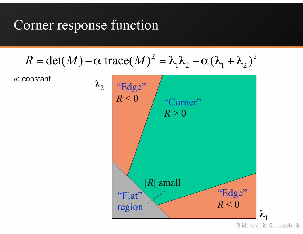
Corner response function
λ1
λ2
“Corner”R > 0
“Edge” R < 0
“Edge” R < 0
“Flat” region
22121
2 )()(trace)det( λλαλλα +−=−= MMRα: constant
|R| small
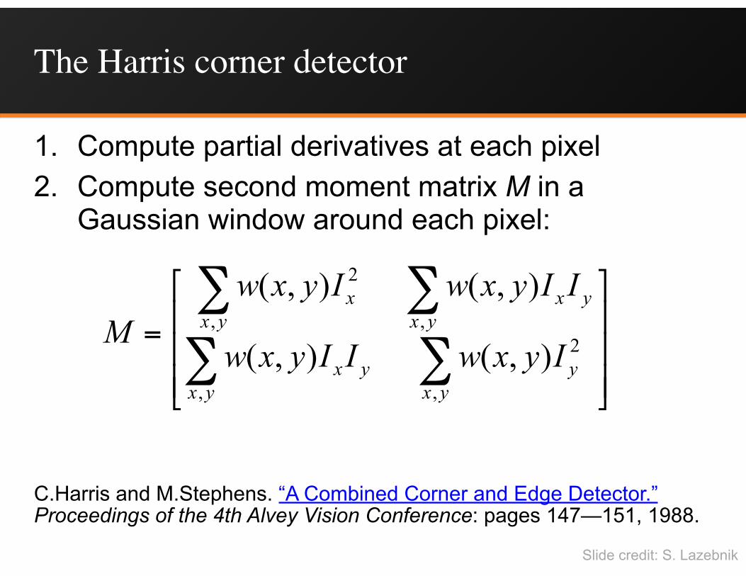
The Harris corner detector
1. Compute partial derivatives at each pixel 2. Compute second moment matrix M in a
Gaussian window around each pixel:
C.Harris and M.Stephens. “A Combined Corner and Edge Detector.” Proceedings of the 4th Alvey Vision Conference: pages 147—151, 1988.
⎥⎥⎥
⎦
⎤
⎢⎢⎢
⎣
⎡
=∑∑
∑∑
yxy
yxyx
yxyx
yxx
IyxwIIyxw
IIyxwIyxwM
,
2
,
,,
2
),(),(
),(),(
Slide credit: S. Lazebnik
The Harris corner detector
1. Compute partial derivatives at each pixel 2. Compute second moment matrix M in a
Gaussian window around each pixel 3. Compute corner response function R
C.Harris and M.Stephens. “A Combined Corner and Edge Detector.” Proceedings of the 4th Alvey Vision Conference: pages 147—151, 1988.
Slide credit: S. Lazebnik
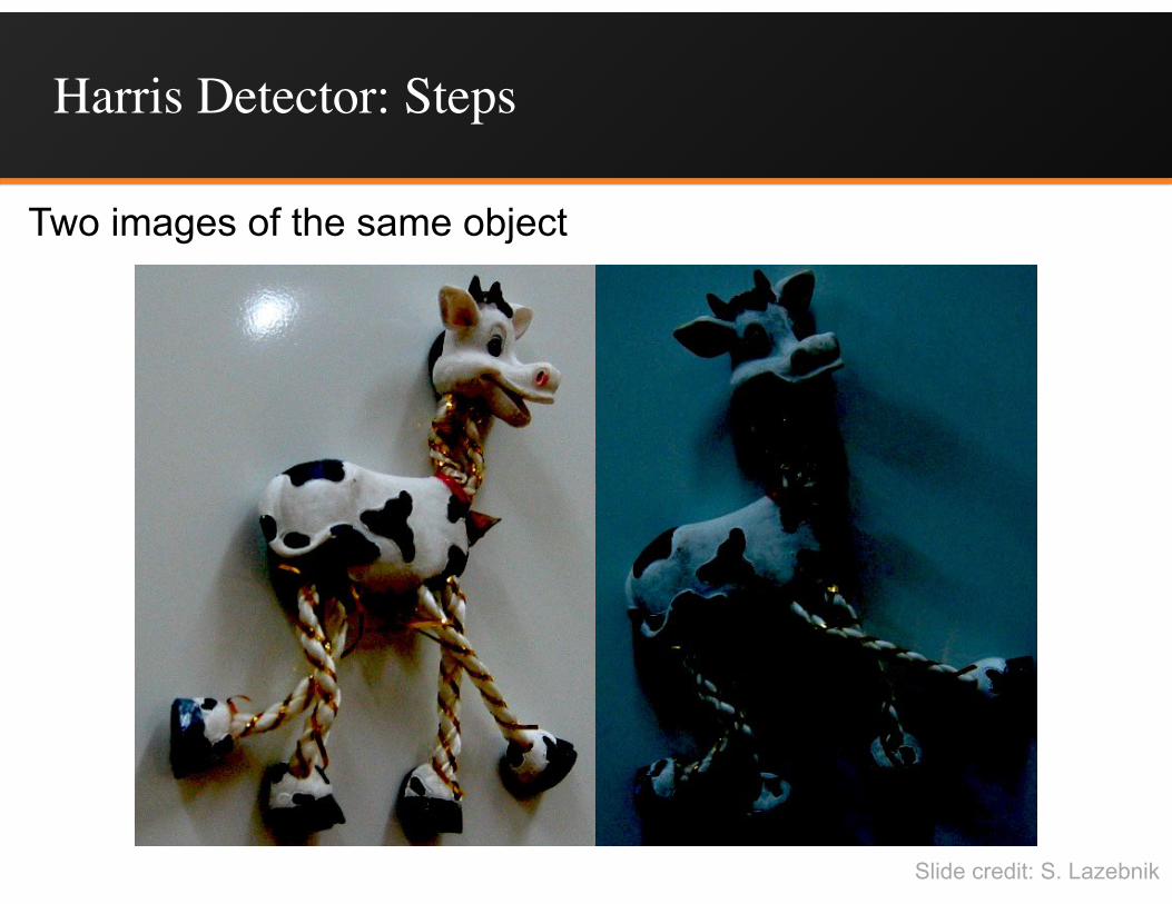
Harris Detector: Steps
Slide credit: S. Lazebnik
Two images of the same object
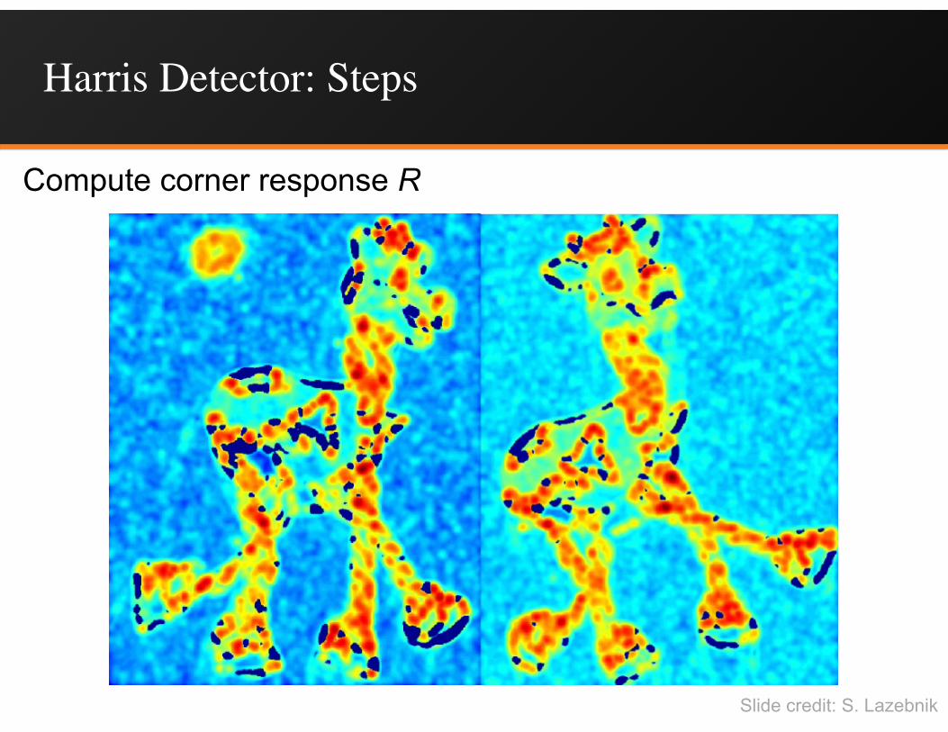
Harris Detector: Steps
Compute corner response R
Slide credit: S. Lazebnik

The Harris corner detector
1. Compute partial derivatives at each pixel 2. Compute second moment matrix M in a
Gaussian window around each pixel 3. Compute corner response function R 4. Threshold R5. Find local maxima of response function
(nonmaximum suppression)
C.Harris and M.Stephens. “A Combined Corner and Edge Detector.” Proceedings of the 4th Alvey Vision Conference: pages 147—151, 1988.
Slide credit: S. Lazebnik

Harris Detector: Steps
Find points with large corner response: R > threshold
Slide credit: S. Lazebnik
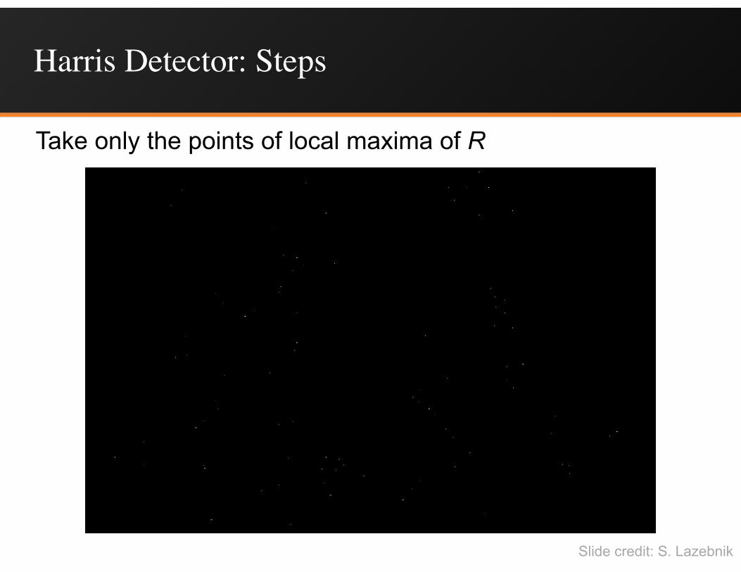
Harris Detector: Steps
Take only the points of local maxima of R
Slide credit: S. Lazebnik
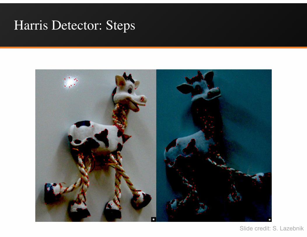
Harris Detector: Steps
Slide credit: S. Lazebnik
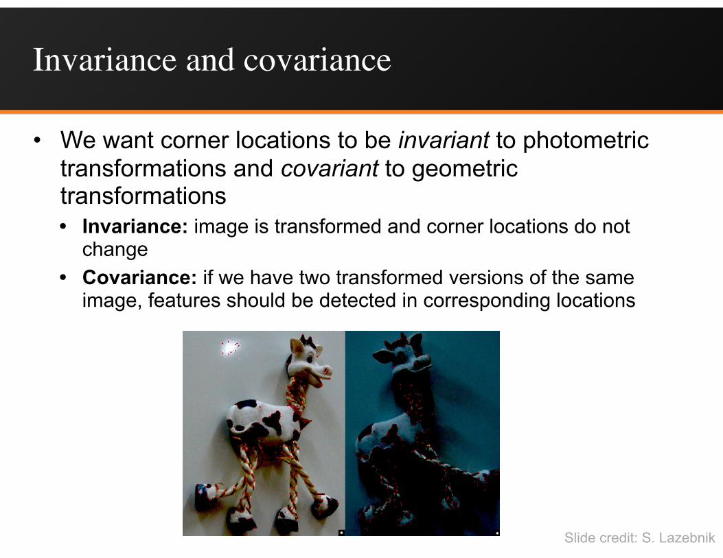
Invariance and covariance
• We want corner locations to be invariant to photometric transformations and covariant to geometric transformations • Invariance: image is transformed and corner locations do not
change • Covariance: if we have two transformed versions of the same
image, features should be detected in corresponding locations
Slide credit: S. Lazebnik

Affine intensity change
• Only derivatives are used => invariance to intensity shift I → I + b
• Intensity scaling: I → a I
R
x (image coordinate)
R
x (image coordinate)
threshold
Partially invariant to affine intensity change
I → a I + b
Slide: S. Lazebnik

Image translation
• Derivatives and window function are shift-invariant
Corner location is covariant w.r.t. translation
Slide: S. Lazebnik
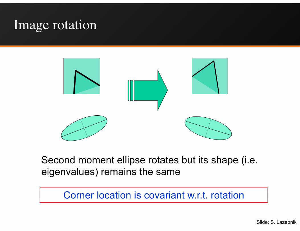
Image rotation
Second moment ellipse rotates but its shape (i.e. eigenvalues) remains the same
Corner location is covariant w.r.t. rotation
Slide: S. Lazebnik
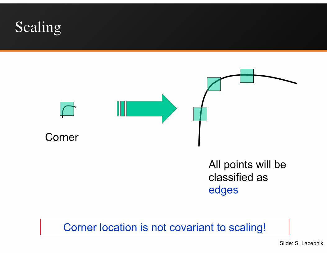
Scaling
All points will be classified as edges
Corner
Corner location is not covariant to scaling!Slide: S. Lazebnik

Blobs

Feature detection with scale selection
• We want to extract features with characteristic scale that is covariant with the image transformation
Slide: S. Lazebnik
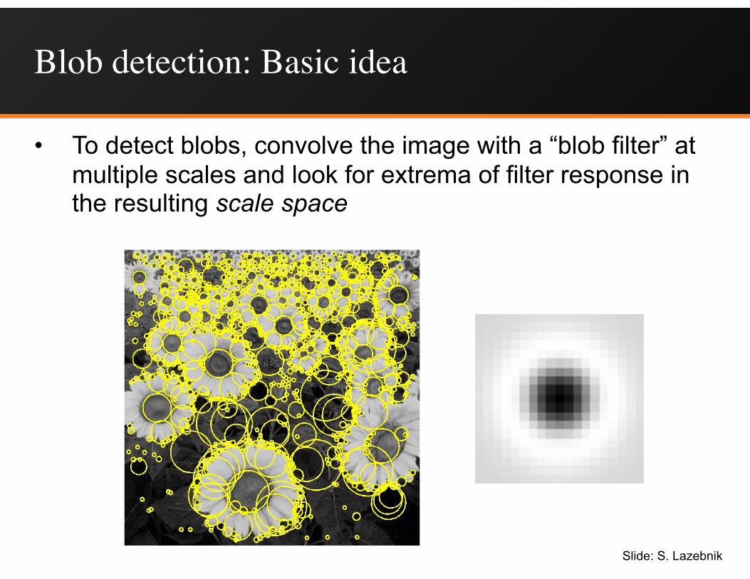
Blob detection: Basic idea
• To detect blobs, convolve the image with a “blob filter” at multiple scales and look for extrema of filter response in the resulting scale space
Slide: S. Lazebnik
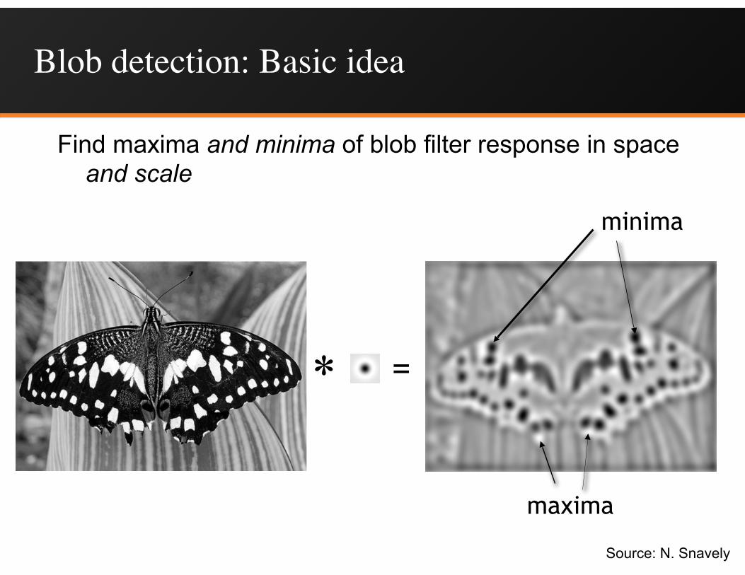
Blob detection: Basic idea
Find maxima and minima of blob filter response in space and scale
* =
maxima
minima
Source: N. Snavely
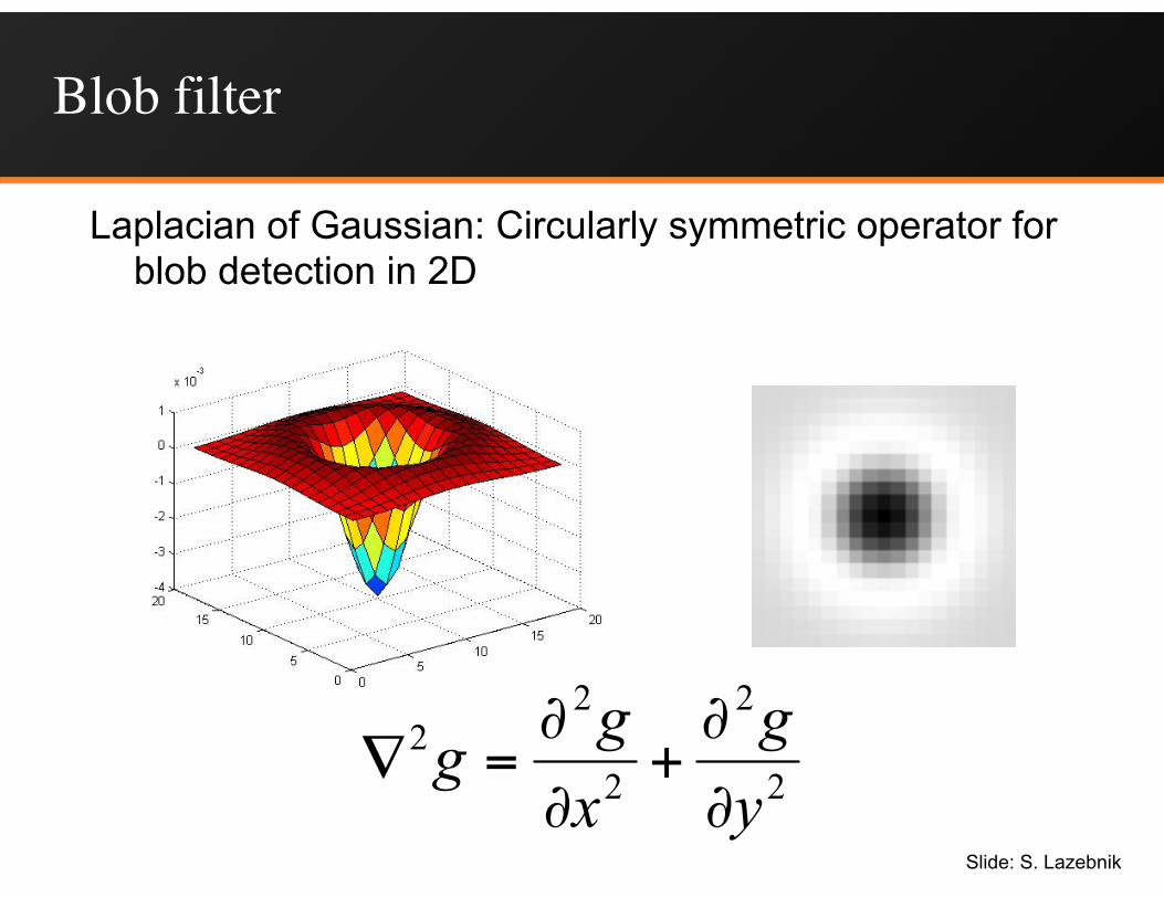
Blob filter
Laplacian of Gaussian: Circularly symmetric operator for blob detection in 2D
2
2
2
22
yg
xg
g∂
∂+
∂
∂=∇
Slide: S. Lazebnik

Recall: Edge detection
gdxd
f ∗
f
gdxd
Source: S. Seitz
Edge
Derivativeof Gaussian
Edge = maximumof derivative
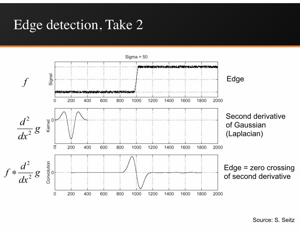
Edge detection, Take 2
gdxd
f 2
2
∗
f
gdxd2
2
Edge
Second derivativeof Gaussian (Laplacian)
Edge = zero crossingof second derivative
Source: S. Seitz

From edges to blobs
• Edge = ripple • Blob = superposition of two ripples
Spatial selection: the magnitude of the Laplacian response will achieve a maximum at the center of the blob, provided the scale of the Laplacian is “matched” to the scale of the blob
maximum
Slide: S. Lazebnik

Scale selection
• We want to find the characteristic scale of the blob by convolving it with Laplacians at several scales and looking for the maximum response
• However, Laplacian response decays as scale increases:
increasing σoriginal signal(radius=8)
Slide: S. Lazebnik
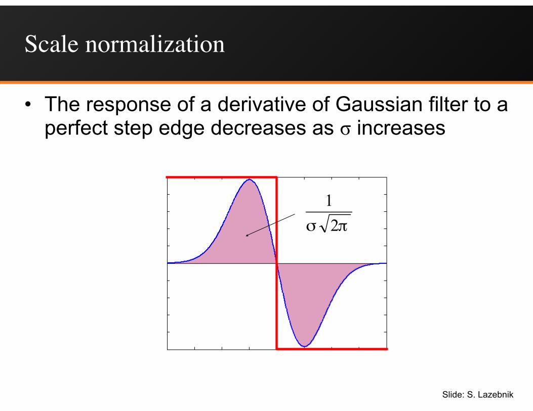
Scale normalization
• The response of a derivative of Gaussian filter to a perfect step edge decreases as σ increases
πσ 21
Slide: S. Lazebnik
Scale normalization
• The response of a derivative of Gaussian filter to a perfect step edge decreases as σ increases
• To keep response the same (scale-invariant), must multiply Gaussian derivative by σ
• Laplacian is the second Gaussian derivative, so it must be multiplied by σ2
Slide: S. Lazebnik
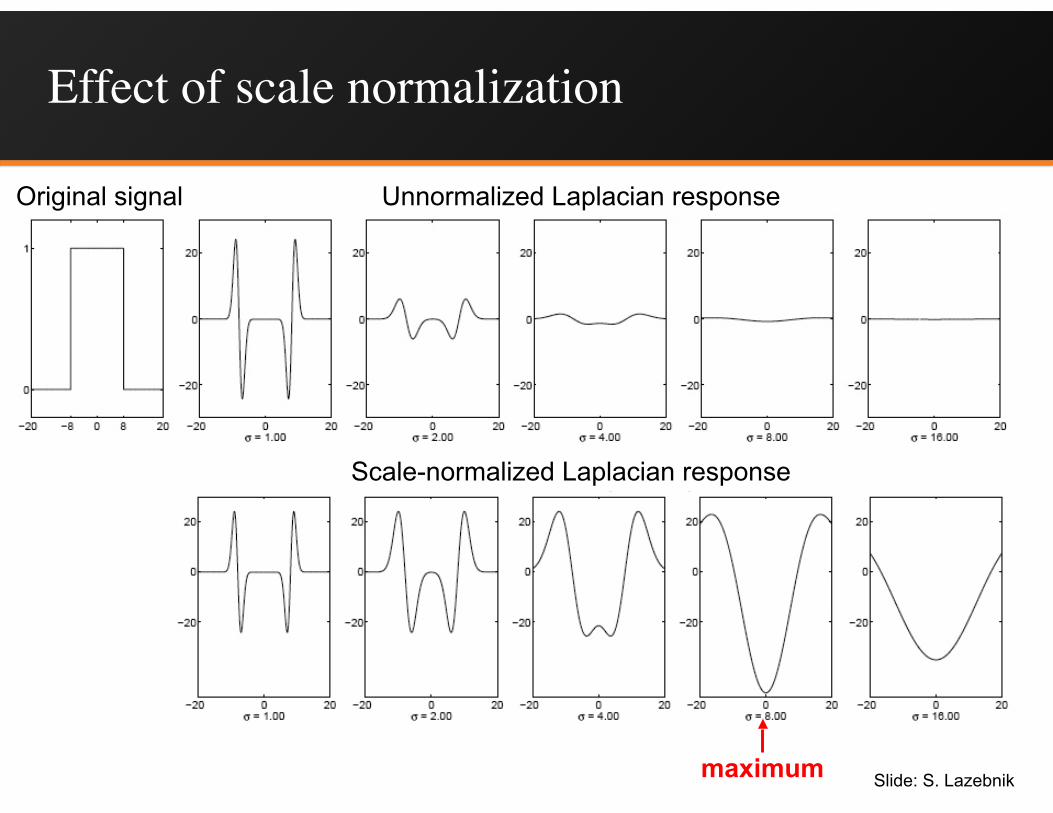
Effect of scale normalization
Scale-normalized Laplacian response
Unnormalized Laplacian responseOriginal signal
maximum Slide: S. Lazebnik
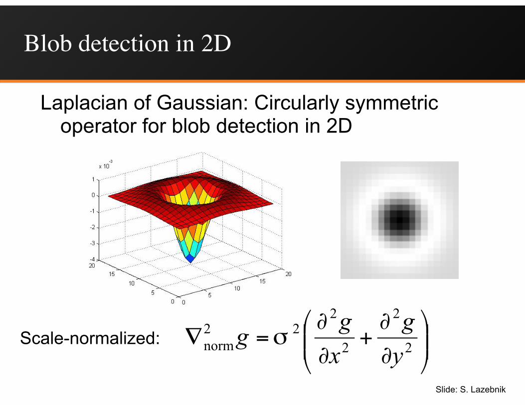
Blob detection in 2D
Laplacian of Gaussian: Circularly symmetric operator for blob detection in 2D
⎟⎟⎠
⎞⎜⎜⎝
⎛
∂
∂+
∂
∂=∇ 2
2
2
222
norm yg
xg
g σScale-normalized:
Slide: S. Lazebnik

Scale selection
LaplacianSlide: S. Lazebnik
r
image
• At what scale does the Laplacian achieve a maximum response to a binary circle of radius r?
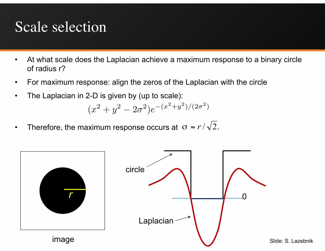
Scale selection
• At what scale does the Laplacian achieve a maximum response to a binary circle of radius r?
• For maximum response: align the zeros of the Laplacian with the circle
• The Laplacian in 2-D is given by (up to scale):
• Therefore, the maximum response occurs at
r
image
.2/r=σ
circle
Laplacian
0
Slide: S. Lazebnik
(x2 + y
2 � 2�2)e�(x2+y
2)/(2�2)
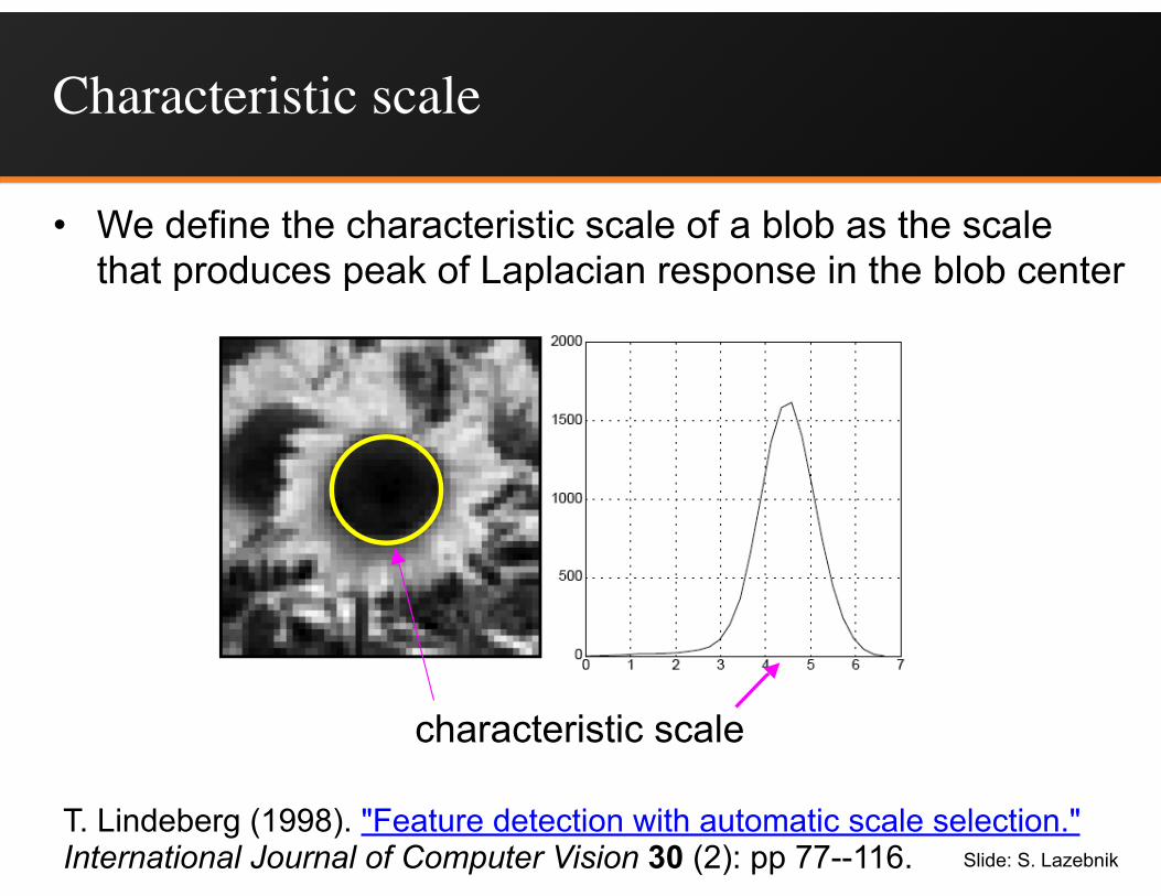
Characteristic scale
• We define the characteristic scale of a blob as the scale that produces peak of Laplacian response in the blob center
characteristic scale
T. Lindeberg (1998). "Feature detection with automatic scale selection." International Journal of Computer Vision 30 (2): pp 77--116. Slide: S. Lazebnik
Scale-space blob detector
1. Convolve image with scale-normalized Laplacian at several scales
Slide: S. Lazebnik
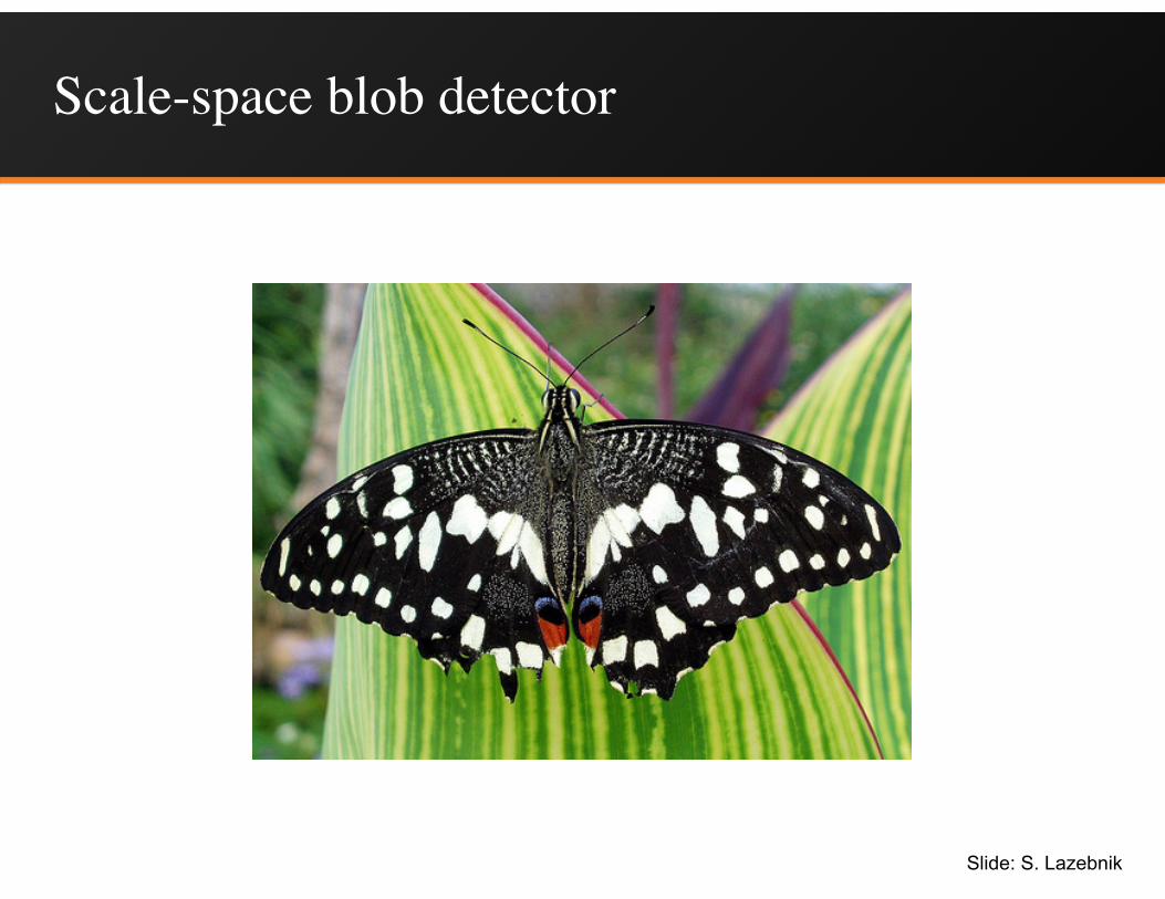
Scale-space blob detector
Slide: S. Lazebnik
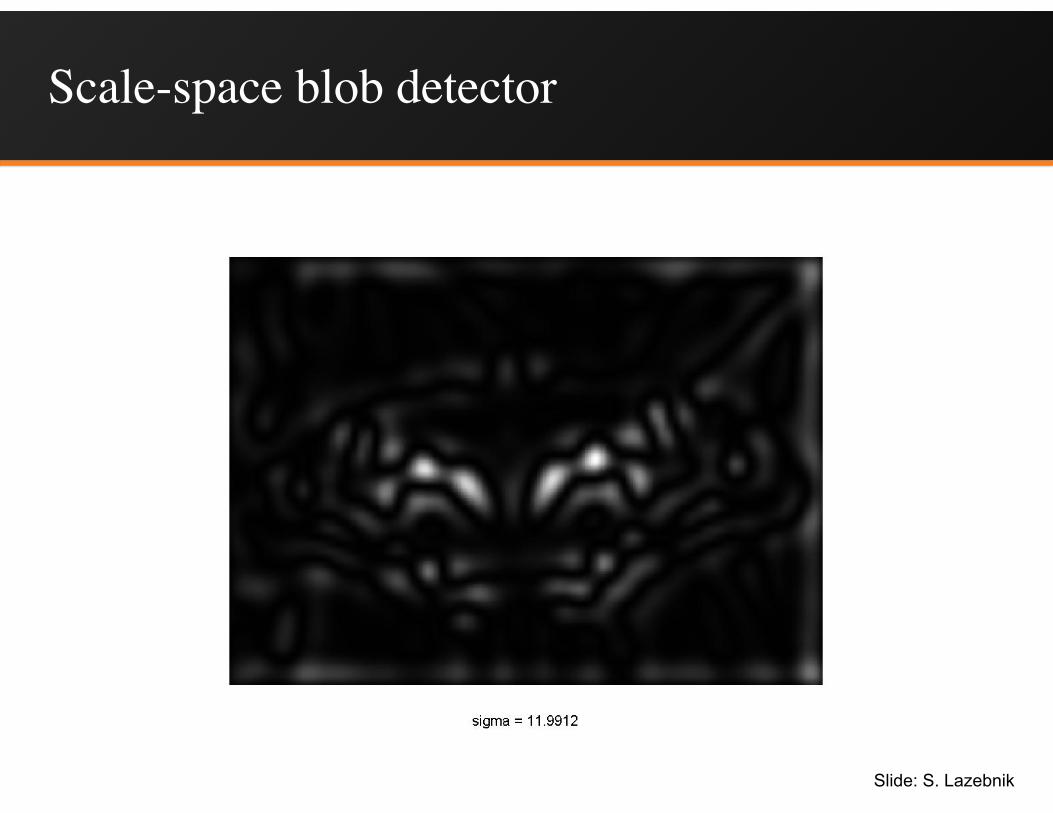
Scale-space blob detector
Slide: S. Lazebnik
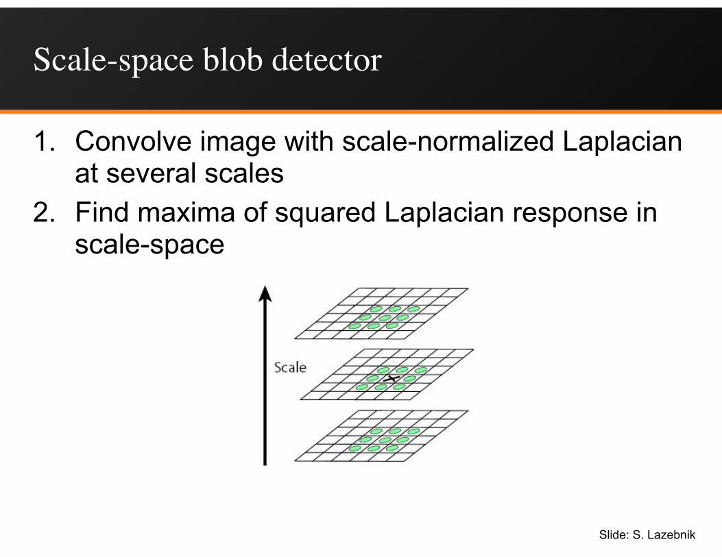
Scale-space blob detector
1. Convolve image with scale-normalized Laplacian at several scales
2. Find maxima of squared Laplacian response in scale-space
Slide: S. Lazebnik

Scale-space blob detector: Example
Slide: S. Lazebnik
Efficient implementation
• Laplacian of Gaussian can be approximated by Difference of Gaussians• Assignment 1, question 3

Efficient implementation
David G. Lowe. "Distinctive image features from scale-invariant keypoints.” IJCV 60 (2), pp. 91-110, 2004. Slide: S. Lazebnik
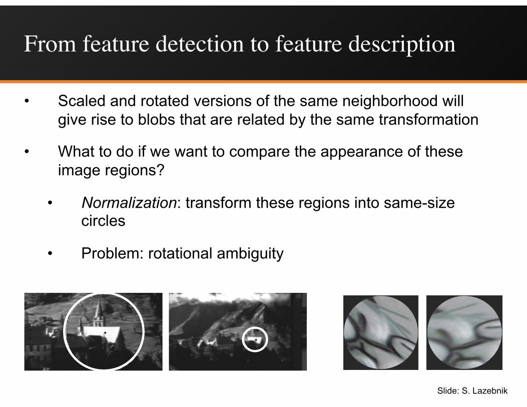
From feature detection to feature description
• Scaled and rotated versions of the same neighborhood will give rise to blobs that are related by the same transformation
• What to do if we want to compare the appearance of these image regions?
• Normalization: transform these regions into same-size circles
• Problem: rotational ambiguity
Slide: S. Lazebnik

SIFT descriptors
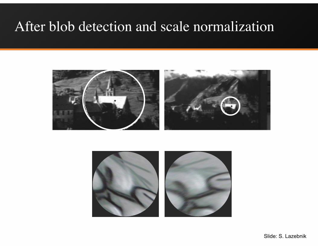
After blob detection and scale normalization
Slide: S. Lazebnik
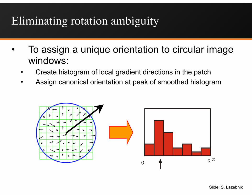
Eliminating rotation ambiguity
• To assign a unique orientation to circular image windows:
• Create histogram of local gradient directions in the patch • Assign canonical orientation at peak of smoothed histogram
0 2 π
Slide: S. Lazebnik

SIFT detected features
• Detected features with characteristic scales and orientations:
David G. Lowe. "Distinctive image features from scale-invariant keypoints.” IJCV 60 (2), pp. 91-110, 2004.
Slide: S. Lazebnik

From feature detection to feature description
Slide: S. Lazebnik

Properties of Feature Descriptors
• Easily compared (compact, fixed-dimensional)• Easily computed• Invariant
– Translation– Rotation– Scale– Change in image brightness– Change in perspective?
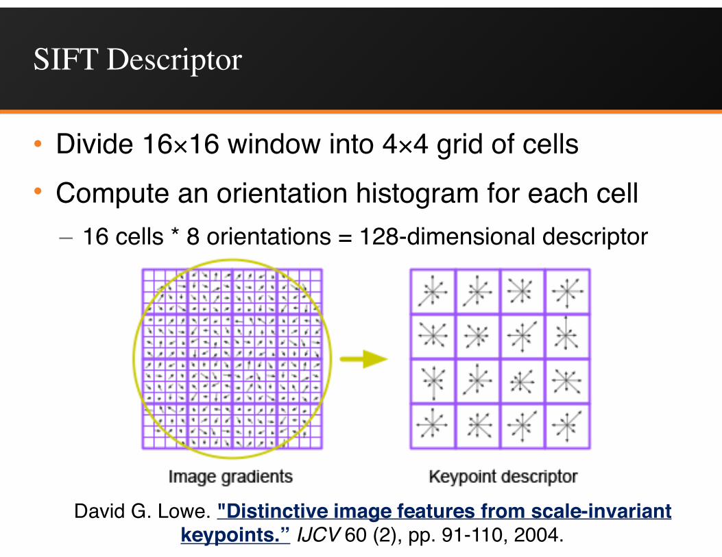
SIFT Descriptor
• Divide 16×16 window into 4×4 grid of cells• Compute an orientation histogram for each cell
– 16 cells * 8 orientations = 128-dimensional descriptor
David G. Lowe. "Distinctive image features from scale-invariant keypoints.” IJCV 60 (2), pp. 91-110, 2004.
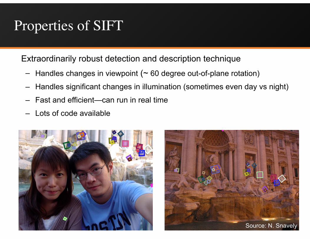
Properties of SIFT
Extraordinarily robust detection and description technique – Handles changes in viewpoint (~ 60 degree out-of-plane rotation)
– Handles significant changes in illumination (sometimes even day vs night)
– Fast and efficient—can run in real time – Lots of code available
Source: N. Snavely
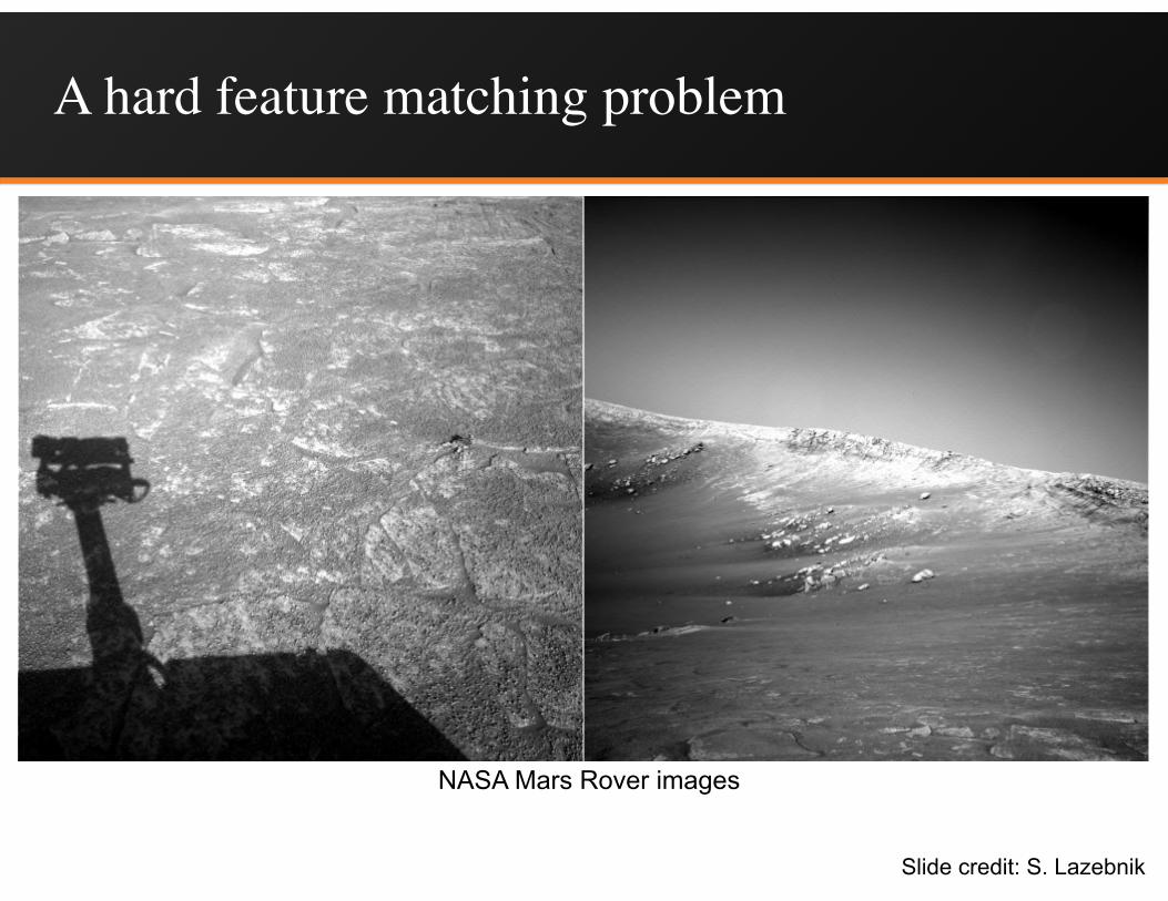
A hard feature matching problem
NASA Mars Rover images
Slide credit: S. Lazebnik

Answer below (look for tiny colored squares…)
NASA Mars Rover images with SIFT feature matchesFigure by Noah Snavely
Slide credit: S. Lazebnik
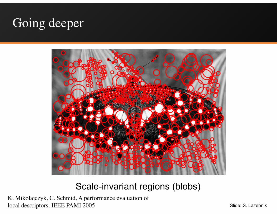
Going deeper
Scale-invariant regions (blobs)
Slide: S. LazebnikK. Mikolajczyk, C. Schmid, A performance evaluation of local descriptors. IEEE PAMI 2005
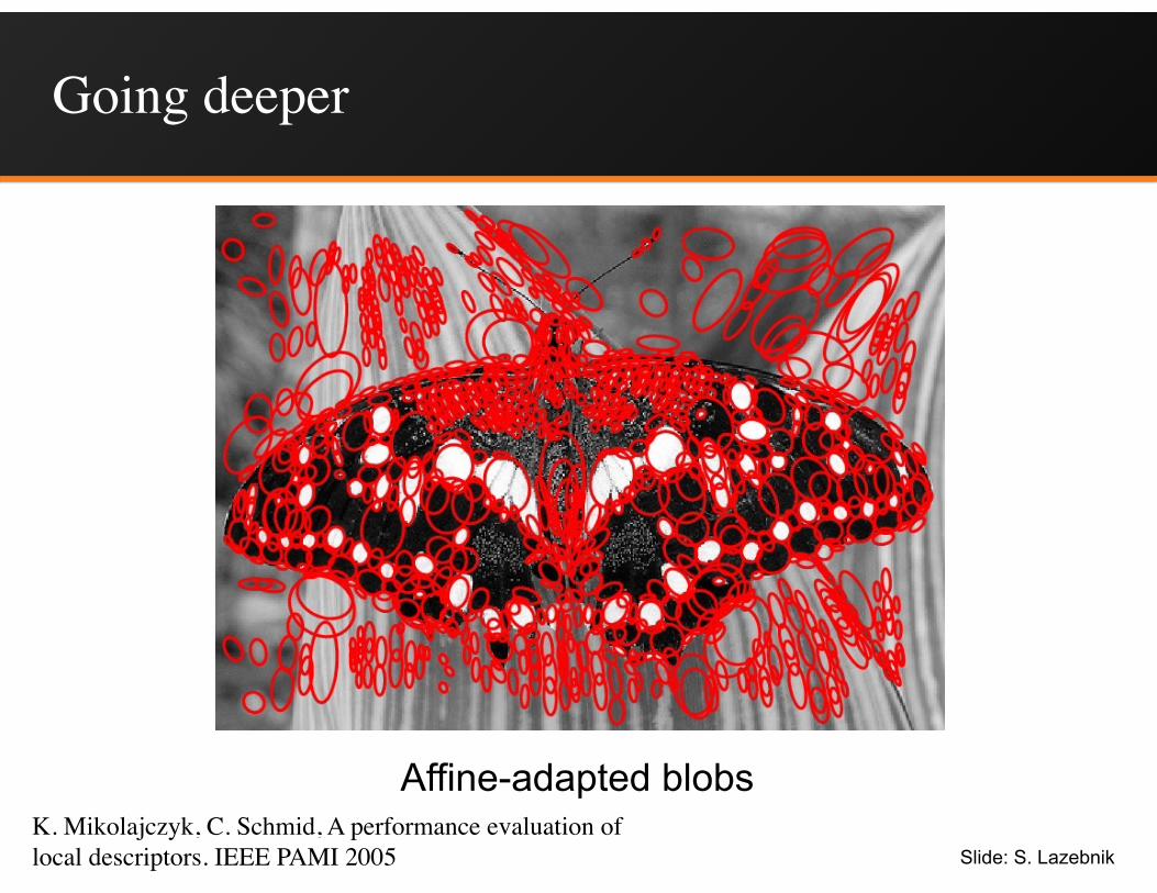
Going deeper
Affine-adapted blobs
Slide: S. LazebnikK. Mikolajczyk, C. Schmid, A performance evaluation of local descriptors. IEEE PAMI 2005

Next class: fitting, Hough transforms, RANSAC
b
a