
Performance Studies of Large Size Micromegas Detectors ...
83
Performance Studies of Large Size Micromegas Detectors Studien zum Betriebsverhalten von großflächigen Micromegas Detektoren Masterarbeit der Fakultät für Physik der Ludwig-Maximilians-Universität München vorgelegt von Philipp Lösel geboren in München München, den 02.10.2013
-
Upload
khangminh22 -
Category
Documents
-
view
0 -
download
0
Transcript of Performance Studies of Large Size Micromegas Detectors ...
Performance Studies ofLarge Size Micromegas Detectors
Studien zum Betriebsverhalten vongroßflächigen Micromegas Detektoren
Masterarbeit der Fakultät für Physikder
Ludwig-Maximilians-Universität München
vorgelegt vonPhilipp Lösel
geboren in München
München, den 02.10.2013


Gutachter: Prof. Dr. Otmar Biebel

Abstract
In 2018 the Large Hadron Collider at CERN will be upgraded to a higher instan-taneous luminosity of 3×1034cm−2s−1. Due to the similarly increasing backgroundhit rate in the Small Wheel region of the ATLAS experiment, the currently in-stalled Monitored Drift Tube chambers will no longer be able to cope with the hitrate and they will be replaced by small strip Thin Gap Chambers and Micromegasdetectors. The performance of these novel detectors is currently under test.In this thesis the performance of a large Micromegas detector with an active
area of 92 × 102cm2 and equipped with resistive strip readout plane is investi-gated in three measurement campaigns. First in a testbeam with 120GeV pionsat SPS/CERN, in which scans along the strips and variation of the incident pionangle as well as voltage variations were performed. Using a reference telescope,consisting of four reference Micromegas with two-dimensional readout, spatial andangular resolution, efficiency, homogeneity and signal propagation time on thestriplines of the readout structures were investigated. Second a dedicated mea-surement with cosmic muons in Garching/Munich is presented investigating thesignal propagation time with improved timing. Third, the homogeneity of the largeresistive strip Micromegas with respect to spatial and angular resolution, efficiency,pulse height and mechanical stability has been investigated in the Cosmic-Ray Fa-cility, which is a high precision test facility developed by LMU Munich for theinvestigation of Muon Drift Tube chambers.The large Micromegas chamber has shown efficiencies up to about 98%. The
averaged overall efficiency to cosmic muons is η = (95.18± 0.03) %. It has shownan averaged spatial resolution of σsr = (83.0± 0.9)µm in the scan along the stripswith perpendicular incident 120GeV pions. The measurement in the Cosmic-RayFacility has shown only a spatial resolution σsr = (238.7± 1.3)µm for track anglesbetween −1 and 1. It is not jet understood, why this result is three times higher.An angular resolution of σΘ ≈ 5 for large angles of incidence could be achieved.The analysis for the signal propagation time on the copper readout strips led to
two slightly different results, that agree well within their respective uncertainties.It is tpropagation = (5.60 ± 0.64) ns ·m−1 for the scan along the detector stripswith 120GeV pions and tpropagation = (6.59 ± 0.57) ns ·m−1 for the measurementwith cosmic muons. The averaged result agrees well with the literature value oftpropagation = 5.64 ns ·m−1.Overall the detector showed a good performance.

vi
Zusammenfassung
Im Jahr 2018 wird der Large Hadron Collider am CERN zu einer höheren in-stantanen Luminosität von 3× 1034cm−2s−1 aufgerüstet. Wegen der ähnlich starkansteigenden Untergrundtreffenrate in der Small Wheel Gegend des ATLAS Expe-riments, sind die derzeitig dort installierten Monitored Drift Tube Kammern nichtlänger in Lage mit der Trefferrate umzugehen und werden durch small strip ThinGap Chambers und Micromegas Detektoren ersetzt. Das Betriebsverhalten dieserneuartigen Detektoren wird derzeitig untersucht.In dieser Arbeit wird das Betriebsverhalten eines großflächigen Micromegas De-
tektors in drei Messaufbauten untersucht. Dieser Detektor hat eine aktive Flächevon 92× 102cm2 und ist mit einer resistiven Ausleseebene ausgestattet. Die erstevorgestellte Messkampagne ist ein Teststrahl mit 120GeV Pionen am SPS/CERN,in dem Messreihen entlang der Streifen, Veränderungen des Einfallswinkel der Pio-nen aber auch Messreihen mit verschiedenen Spannungen durchgeführt wurden.Mit einem Teleskop, bestehend aus vier Micromegas mit zweidimensionaler Ausle-se als Spureferenz, wurden Orts- und Winkelauflösung, Effizienz, Homogenität unddie Signalausbreitungszeit auf den Streifenbahnen der Auslesestruktur untersucht.Als zweites wird eine Messung mit kosmischen Myonen in Garching/Münchenvorgestellt, mit der die Signalausbreitungszeit mit verbesserter Zeitmessung un-tersucht wurde. Drittens, die Homogenität des großen Micromegas im Bezug aufOrts- und Winkelauflösung, Effizienz, Pulshöhen und mechanischer Stabilität wur-de in einem Teststand mit kosmischer Strahlung untersucht. Der Teststand wurdevon der LMU München für die Hochpräzesions Untersuchungen von Muon DriftTube Kammern entwickelt.Die große Micromegas Kammer zeigte Effizienzen bis zu 98%. Die über den gan-
zen Detektor gemittelte Effizienz für kosmische Myonen is η = (95.18 ± 0.03) %.Sie hatte eine gemittelte Ortsauflösung von σsr = (83.0 ± 0.9)µm in der Messrei-he entlang den Streifen mit 120GeV Pionen, die senkrecht zu der Detektorebeneeinfielen. Eine Ortsauflösung von σsr = (238.7 ± 1.3)µm für einen Einfallswinkelvon −1 and 1 zeigte sich im Teststand mit kosmischen Myonen, es ist noch nichtverstanden, warum dieses Ergebnis einen Faktor drei größer ist. Für große Winkelkonnte eine Winkelauflösung von σΘ ≈ 5 erreicht werden.Die Analyse zur Signalausbreitungszeit auf den Kupfer Auslesestreifen führte zu
zwei leicht unterschiedlichen Ergebnissen, die gut in ihren jeweiligen Unsicherhei-ten übereinstimmen. Für die Messreihe entlang den Detektorstreifen mit 120GeVPionen ist das Ergebnis tpropagation = (5.60 ± 0.64) ns ·m−1 und tpropagation =(6.59 ± 0.57) ns ·m−1 für die Messung mit kosmischen Myonen. Das gemittelteErgebniss stimmt gut mit dem Literaturwert von tpropagation = 5.64 ns ·m−1 über-ein.Im Großen und Ganzen zeigte der Detektor ein gutes Betriebsverhalten.

viii
Contents
1 Introduction 11.1 The Large Hadron Collider . . . . . . . . . . . . . . . . . . . . . . . 11.2 The ATLAS Experiment . . . . . . . . . . . . . . . . . . . . . . . . 21.3 Motivation . . . . . . . . . . . . . . . . . . . . . . . . . . . . . . . . 2
2 The Micromegas Detector 62.1 Interaction of Particles and Photons with Matter . . . . . . . . . . 6
2.1.1 Energy Loss According to Bethe-Bloch . . . . . . . . . . . . 62.1.2 Photons . . . . . . . . . . . . . . . . . . . . . . . . . . . . . 62.1.3 Ionization . . . . . . . . . . . . . . . . . . . . . . . . . . . . 8
2.2 Avalanche Multiplication . . . . . . . . . . . . . . . . . . . . . . . . 82.3 Working Principle of a Micromegas Detector . . . . . . . . . . . . . 92.4 Current Applications . . . . . . . . . . . . . . . . . . . . . . . . . . 112.5 Technical Properties of the Micromegas Used in this Work . . . . . 11
3 Readout Electronics 123.1 The charge sensitive APV25 ASIC . . . . . . . . . . . . . . . . . . . 123.2 The Scalable Readout System . . . . . . . . . . . . . . . . . . . . . 133.3 FEC Standalone Mode . . . . . . . . . . . . . . . . . . . . . . . . . 14
4 Analysis Tools 154.1 Signal Fit . . . . . . . . . . . . . . . . . . . . . . . . . . . . . . . . 154.2 Cluster Reconstruction . . . . . . . . . . . . . . . . . . . . . . . . . 164.3 Fit of Straight Lines . . . . . . . . . . . . . . . . . . . . . . . . . . 184.4 µTPC Mode . . . . . . . . . . . . . . . . . . . . . . . . . . . . . . . 19
5 Measurements 215.1 Pion Testbeam at SPS/CERN . . . . . . . . . . . . . . . . . . . . . 21
5.1.1 Experimental Setup . . . . . . . . . . . . . . . . . . . . . . . 215.1.2 Scans Along the Strips . . . . . . . . . . . . . . . . . . . . . 235.1.3 Alignment . . . . . . . . . . . . . . . . . . . . . . . . . . . . 235.1.4 Determination of the Track Accuracy . . . . . . . . . . . . . 26
5.2 Measurement with Cosmic Muons . . . . . . . . . . . . . . . . . . . 305.2.1 Experimental Setup . . . . . . . . . . . . . . . . . . . . . . . 30
5.3 Cosmic-Ray Facility . . . . . . . . . . . . . . . . . . . . . . . . . . . 315.3.1 Experimental Setup . . . . . . . . . . . . . . . . . . . . . . . 325.3.2 Optimization of the Micromegas Operational Parameters . . 335.3.3 Event Selection . . . . . . . . . . . . . . . . . . . . . . . . . 355.3.4 Alignment . . . . . . . . . . . . . . . . . . . . . . . . . . . . 35
ix

Contents
6 Results 406.1 Spatial Resolution . . . . . . . . . . . . . . . . . . . . . . . . . . . . 40
6.1.1 Pion Testbeam at SPS/CERN . . . . . . . . . . . . . . . . . 406.1.2 Cosmic-Ray Facility . . . . . . . . . . . . . . . . . . . . . . 436.1.3 Discussion . . . . . . . . . . . . . . . . . . . . . . . . . . . . 46
6.2 Efficiency . . . . . . . . . . . . . . . . . . . . . . . . . . . . . . . . 466.2.1 Pion Testbeam at SPS/CERN . . . . . . . . . . . . . . . . . 466.2.2 Cosmic-Ray Facility . . . . . . . . . . . . . . . . . . . . . . 516.2.3 Discussion . . . . . . . . . . . . . . . . . . . . . . . . . . . . 53
6.3 Signal Propagation Time . . . . . . . . . . . . . . . . . . . . . . . . 536.3.1 Pion Testbeam at SPS/CERN . . . . . . . . . . . . . . . . . 536.3.2 Measurement with Cosmic Muons . . . . . . . . . . . . . . . 546.3.3 Discussion . . . . . . . . . . . . . . . . . . . . . . . . . . . . 56
6.4 Angular Resolution . . . . . . . . . . . . . . . . . . . . . . . . . . . 576.4.1 Pion Testbeam at SPS/CERN . . . . . . . . . . . . . . . . . 576.4.2 Cosmic-Ray Facility . . . . . . . . . . . . . . . . . . . . . . 606.4.3 Discussion . . . . . . . . . . . . . . . . . . . . . . . . . . . . 62
7 Summary and Outlook 66
Bibliography 68
x
1 Introduction
1.1 The Large Hadron Collider
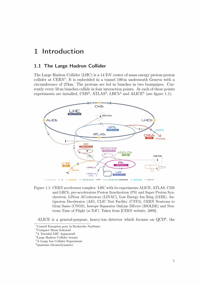
The Large Hadron Collider (LHC) is a 14TeV center of mass energy proton-protoncollider at CERN1. It is embedded in a tunnel 100m underneath Geneva with acircumference of 27km. The protons are led in bunches in two beampipes. Cur-rently every 50 ns bunches collide in four interaction points. At each of these pointsexperiments are installed, CMS2, ATLAS3, LHCb4 and ALICE5 (see figure 1.1).
Figure 1.1: CERN accelerator complex: LHC with its experiments ALICE, ATLAS, CMSand LHCb, pre-accelerators Proton Synchrotron (PS) and Super Proton Syn-chrotron, LINear ACcelerators (LINAC), Low Energy Ion Ring (LEIR), An-tiproton Decelerator (AD), CLIC Test Facility (CTF3), CERN Neutrons toGran Sasso (CNGS), Isotope Separator OnLine DEvice (ISOLDE) and Neu-trons Time of Flight (n-ToF). Taken from [CERN website, 2008].
ALICE is a general-purpose, heavy-ion detector which focuses on QCD6, the1Conseil Européen pour la Recherche Nucléaire2Compact Muon Solenoid3A Toroidal LHC ApparatuS4Large Hadron Collider beauty5A Large Ion Collider Experiment6quantum chromodynamics
1
1 Introduction
strong-interaction sector of the Standard Model. It is designed to address thephysics of strongly interacting matter and the quark-gluon plasma at extremevalues of energy density and temperature in nucleus-nucleus collisions [ALICECollaboration, 2008].The asymmetric LHCb detector is designed for precision measurements of CP
violation and rare decays of B hadrons [LHCb Collaboration, 2008].The CMS detector has been optimized for the search of the Standard Model
Higgs boson over a mass range from 90 GeV to 1 TeV, but it also allows detectionof a wide range of possible signatures from alternative electro-weak symmetrybreaking mechanisms. CMS is also well adapted for the study of top, beauty andtau physics at lower luminosities and will cover several important aspects of theheavy ion physics program [CMS Collaboration, 2008]. The ATLAS detector willbe treated separately in section 1.2.The LHC was running in 2011 with a center of mass energy of 7TeV and in 2012
with 8TeV. About 25 fb−1 data were collected with an instantaneous luminositiesup to of 6 × 1032cm−2s−1. Currently there is an upgrade ongoing, after whichalmost the design center of mass energy will be reached and the bunch spacingreduced to 25 ns. Until the year 2018 up to 100 fb−1 data will be collected withthe nominal luminosity of about 1× 1034cm−2s−1.
1.2 The ATLAS Experiment
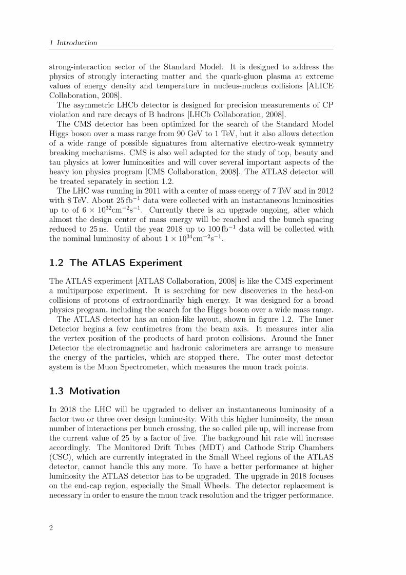
The ATLAS experiment [ATLAS Collaboration, 2008] is like the CMS experimenta multipurpose experiment. It is searching for new discoveries in the head-oncollisions of protons of extraordinarily high energy. It was designed for a broadphysics program, including the search for the Higgs boson over a wide mass range.The ATLAS detector has an onion-like layout, shown in figure 1.2. The Inner
Detector begins a few centimetres from the beam axis. It measures inter aliathe vertex position of the products of hard proton collisions. Around the InnerDetector the electromagnetic and hadronic calorimeters are arrange to measurethe energy of the particles, which are stopped there. The outer most detectorsystem is the Muon Spectrometer, which measures the muon track points.
1.3 Motivation
In 2018 the LHC will be upgraded to deliver an instantaneous luminosity of afactor two or three over design luminosity. With this higher luminosity, the meannumber of interactions per bunch crossing, the so called pile up, will increase fromthe current value of 25 by a factor of five. The background hit rate will increaseaccordingly. The Monitored Drift Tubes (MDT) and Cathode Strip Chambers(CSC), which are currently integrated in the Small Wheel regions of the ATLASdetector, cannot handle this any more. To have a better performance at higherluminosity the ATLAS detector has to be upgraded. The upgrade in 2018 focuseson the end-cap region, especially the Small Wheels. The detector replacement isnecessary in order to ensure the muon track resolution and the trigger performance.
2
1.3 Motivation
Figure 1.2: Cut-away view of the ATLAS detector, taken from [ATLAS Collaboration,2008].
For this purpose small strip Thin Gap Chambers and Micromegas will be used.This Thesis covers only Micromegas issues.The Small Wheel is separated in 16 sectors (see figure 1.3). The Micromegas
detectors will be arranged in small and large sectors, which require detectors witha strip length of up to 2m. Each sector consists of eight Micromegas layers, dividedin two multiplets of four layers. Figure 1.4 (left) shows the schematic arrangementof these detectors. In the multiplets the Micromegas are mounted pairwise back-to-back (see figure 1.4 (right)) [ATLAS Collaboration, 2013].Micromegas detectors should fulfill for that purpose the following requirement
[Nikolopoulos et al., 2009]:
• High counting rate capability, for hit rates > 20 kHz/cm2
• High single plane detection efficiency above 97%
• Good spatial resolution of approximately 100µm
• Second coordinate measurement
• Two-track separation at distance of 1mm to 2mm
• Good time resolution on the order of 5 ns to allow for bunch crossing identi-fication
• Level-1 triggering capability
• Good aging properties
3

1 Introduction
Figure 1.3: Components and layout of a present Small Wheel, taken from [ATLAS Col-laboration, 2013].
Figure 1.4: Arrangement of the detectors in a sector (left) and in a multiplet (right),taken from [ATLAS Collaboration, 2013].
4

1.3 Motivation
In this thesis a large Micromegas detector is under investigation to measure itsproperties. Its spatial resolution, measured with high energy pions and cosmicmuons, efficiencies, mechanical stability and pulse height homogeneity will be dis-cussed. Furthermore it will be shown, that the signal propagation time for chargesignal on the readout strips can be measured and, in timing applications, must becorrected for.
5
2 The Micromegas Detector
Particles are detected and investigated through their interaction with matter. Thischapter describes these interactions, the working principle of Micromegas detectorsand their current applications. As source for most of the theoretical backgroundthe textbook of Leo [Leo, 1994] was taken.
2.1 Interaction of Particles and Photons with Matter
2.1.1 Energy Loss According to Bethe-Bloch
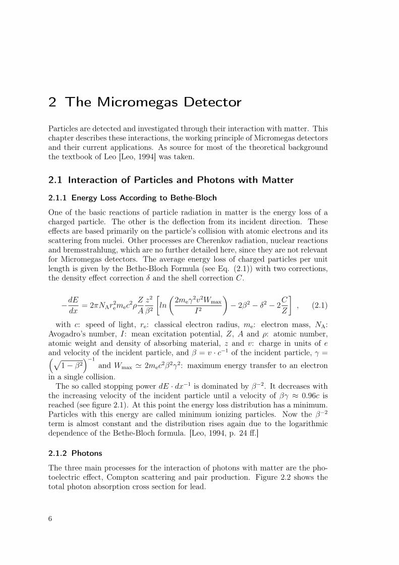
One of the basic reactions of particle radiation in matter is the energy loss of acharged particle. The other is the deflection from its incident direction. Theseeffects are based primarily on the particle’s collision with atomic electrons and itsscattering from nuclei. Other processes are Cherenkov radiation, nuclear reactionsand bremsstrahlung, which are no further detailed here, since they are not relevantfor Micromegas detectors. The average energy loss of charged particles per unitlength is given by the Bethe-Bloch Formula (see Eq. (2.1)) with two corrections,the density effect correction δ and the shell correction C.
−dEdx
= 2πNAr2emec
2ρZ
A
z2
β2
[ln
(2meγ
2v2Wmax
I2
)− 2β2 − δ2 − 2
C
Z
], (2.1)
with c: speed of light, re: classical electron radius, me: electron mass, NA:Avogadro’s number, I: mean excitation potential, Z, A and ρ: atomic number,atomic weight and density of absorbing material, z and v: charge in units of eand velocity of the incident particle, and β = v · c−1 of the incident particle, γ =(√
1− β2)−1
and Wmax ' 2mec2β2γ2: maximum energy transfer to an electron
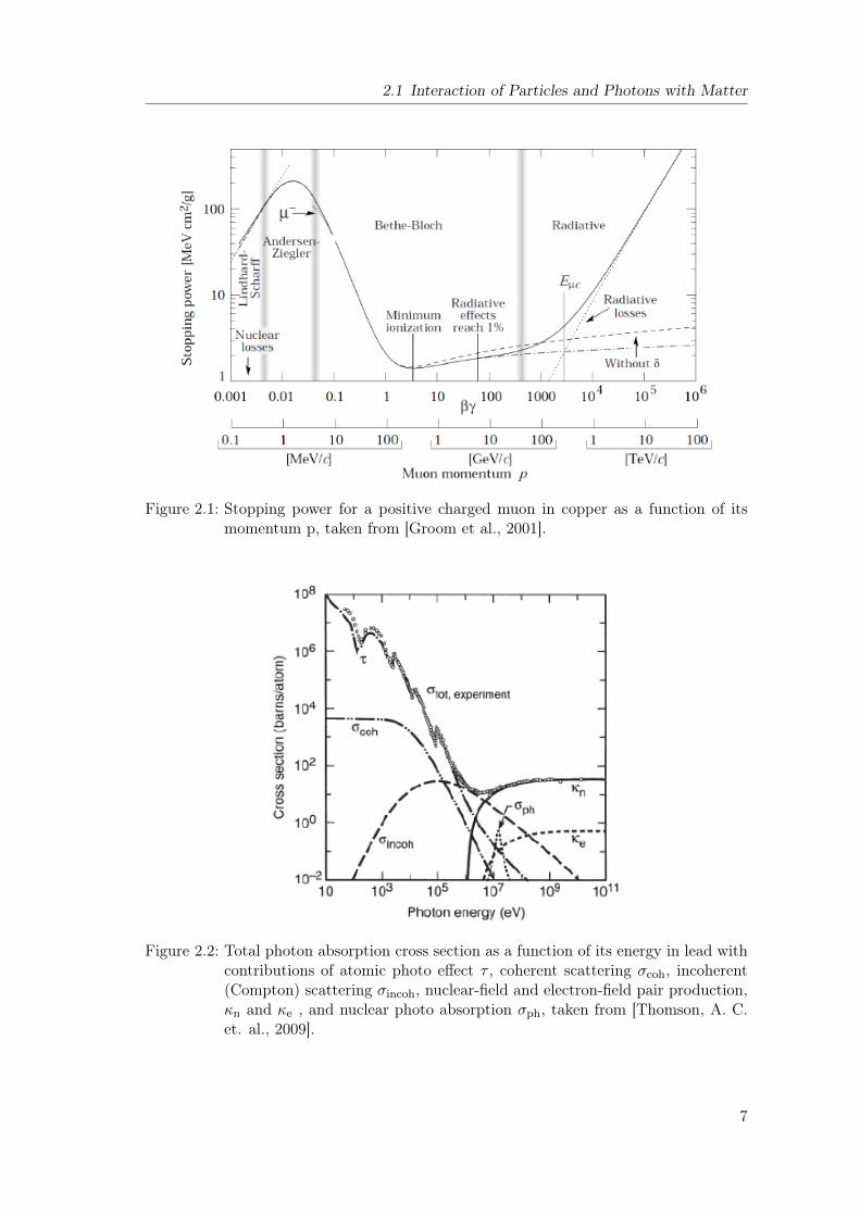
in a single collision.The so called stopping power dE · dx−1 is dominated by β−2. It decreases with
the increasing velocity of the incident particle until a velocity of βγ ≈ 0.96c isreached (see figure 2.1). At this point the energy loss distribution has a minimum.Particles with this energy are called minimum ionizing particles. Now the β−2
term is almost constant and the distribution rises again due to the logarithmicdependence of the Bethe-Bloch formula. [Leo, 1994, p. 24 ff.]
2.1.2 Photons
The three main processes for the interaction of photons with matter are the pho-toelectric effect, Compton scattering and pair production. Figure 2.2 shows thetotal photon absorption cross section for lead.
6
2.1 Interaction of Particles and Photons with Matter
Figure 2.1: Stopping power for a positive charged muon in copper as a function of itsmomentum p, taken from [Groom et al., 2001].
Figure 2.2: Total photon absorption cross section as a function of its energy in lead withcontributions of atomic photo effect τ , coherent scattering σcoh, incoherent(Compton) scattering σincoh, nuclear-field and electron-field pair production,κn and κe , and nuclear photo absorption σph, taken from [Thomson, A. C.et. al., 2009].
7
2 The Micromegas Detector
The absorption of a photon by an atomic electron, followed by the emissionof the electron from the atom is called photoelectric effect. Due to simultaneousenergy- and momentum-conservation only bound electrons can be involved in thiseffect with the nucleus absorbing the recoil momentum.For photon energies between 100 keV and 1MeV the dominating effect is the
Compton scattering. This can be understood as elastic scattering of a photon onan electron of the absorber material. The photon transfers some of its energy tothe electron.Pair production is the dominating process for higher energies. If the photon
has at least energies above the pair-production threshold, it can convert into anelectron-positron pair. This can only occur in the presence of a third body, toconserve the momentum. [Leo, 1994, p. 54 ff.]
2.1.3 Ionization
As previously explained, the two main processes of energy loss of charged particlesin matter are ionization and excitation. Excitation has a cross section of σmax '10−17 cm2 and ionization σmax ' 10−16 cm2. Nevertheless excitation is in generalthe dominant process because of the relatively high energy threshold of ionization.The ionization directly created by an incident particle in the gas detector is calledprimary ionization. Positive ions and electrons are created. If the energy transferto the electron through primary ionization is high enough, this electron creates newion-electron pairs (secondary ionization). Such high energy electrons are called δ-electrons. In argon at normal temperature and pressure, the mean energy necessaryto create an ion-electron pairs is 26eV [Beringer, J. et. al. (Particle Data Group),2012].In the absence of an external electric field the created electron can recombine
with an ion or can be captured by a gas atom, forming a negative ion. The latteris especially relevant in electronegative gases such as oxygen.In gas detectors the electrical field is used to separate the ion-electron pairs.
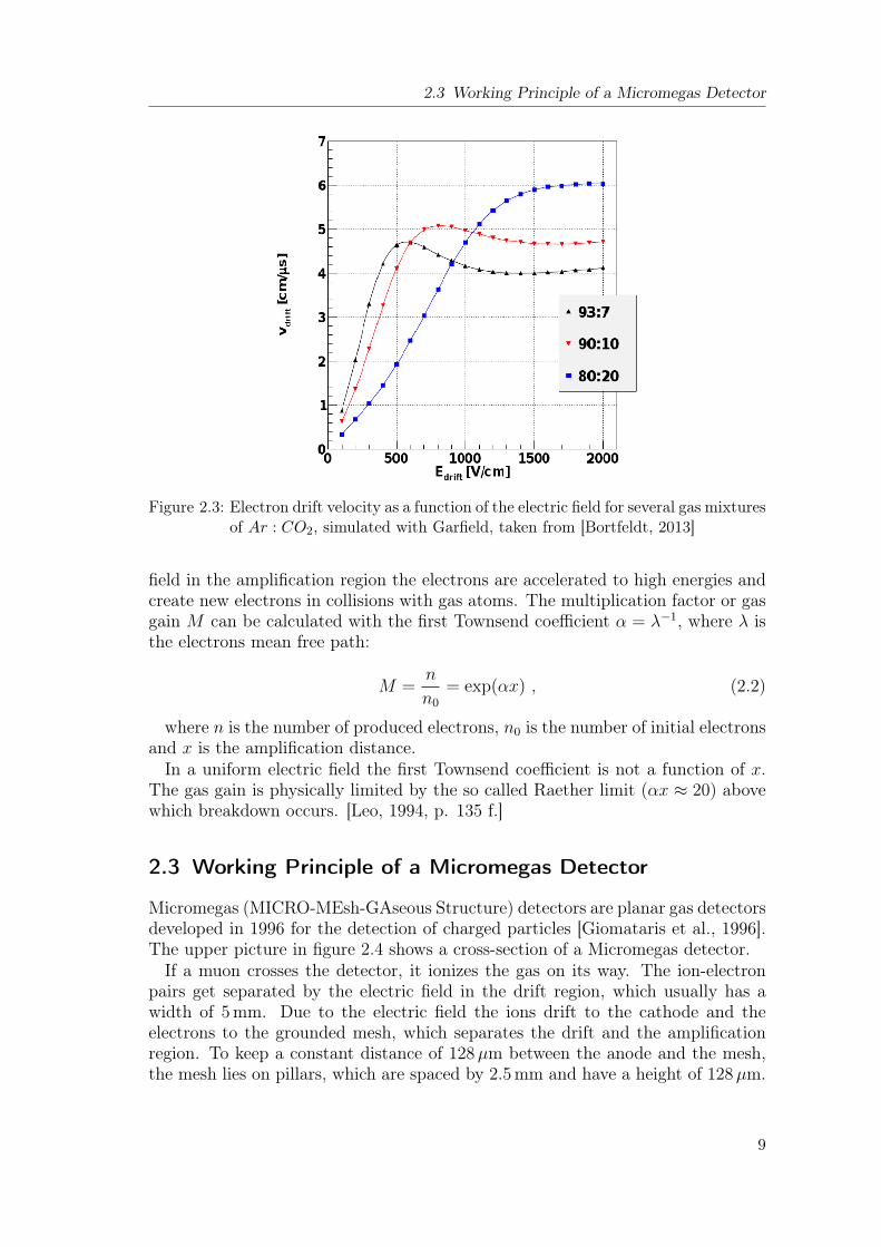
The electrons drift to the positively charged anode and the ions to the negativelycharged cathode. Their averaged velocity is called drift velocity and is limited byits collision with other particles. The drift velocity of electrons is about a factor of1000 higher as for ions because of their mass and depends on the electric field andthe pressure [Leo, 1994, p. 130 ff.]. Figure 2.3 shows the electron drift velocity asa function of the electric field for several gas mixtures of Ar : CO2, simulated withGarfield [Garfield, 2013].
2.2 Avalanche Multiplication
Because of the small amount of primary electrons in a gas detector, the charge hasto be multiplied for detection. In wire gas detectors, the drift field increases to-wards the very thin wire, reaching values sufficiently high for charge amplification.In Micromegas detectors, a planar high-field region is formed by a thin micro mesh,held at a distance of typically 100 um to the anode strips. By the strong electric
8
2.3 Working Principle of a Micromegas Detector
Figure 2.3: Electron drift velocity as a function of the electric field for several gas mixturesof Ar : CO2, simulated with Garfield, taken from [Bortfeldt, 2013]
field in the amplification region the electrons are accelerated to high energies andcreate new electrons in collisions with gas atoms. The multiplication factor or gasgain M can be calculated with the first Townsend coefficient α = λ−1, where λ isthe electrons mean free path:
M =n
n0
= exp(αx) , (2.2)
where n is the number of produced electrons, n0 is the number of initial electronsand x is the amplification distance.In a uniform electric field the first Townsend coefficient is not a function of x.
The gas gain is physically limited by the so called Raether limit (αx ≈ 20) abovewhich breakdown occurs. [Leo, 1994, p. 135 f.]
2.3 Working Principle of a Micromegas Detector
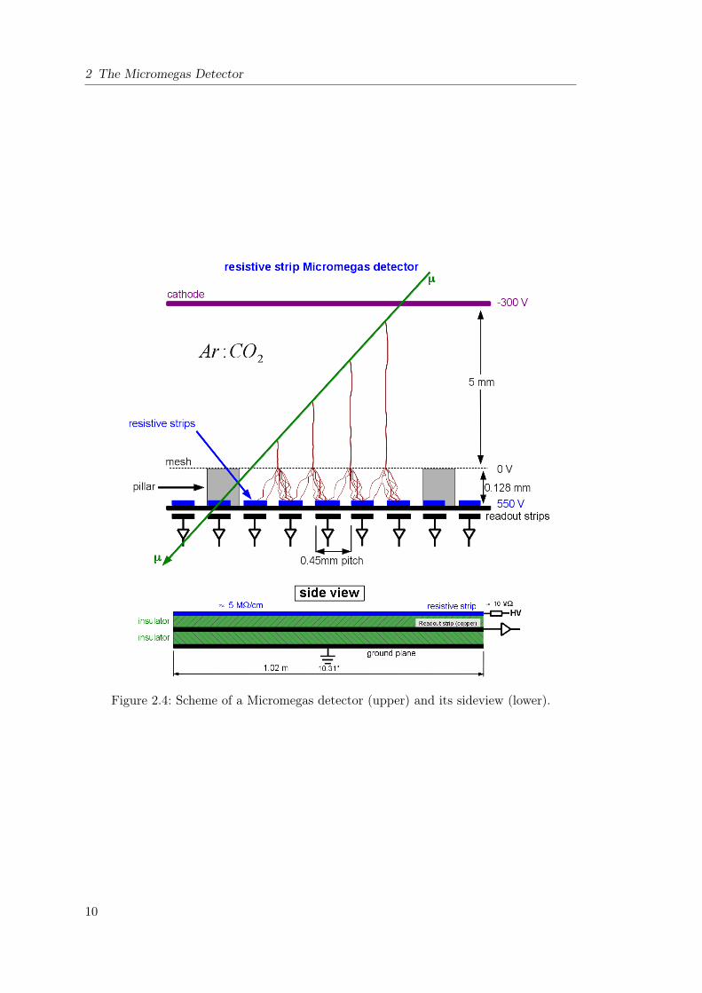
Micromegas (MICRO-MEsh-GAseous Structure) detectors are planar gas detectorsdeveloped in 1996 for the detection of charged particles [Giomataris et al., 1996].The upper picture in figure 2.4 shows a cross-section of a Micromegas detector.If a muon crosses the detector, it ionizes the gas on its way. The ion-electron
pairs get separated by the electric field in the drift region, which usually has awidth of 5mm. Due to the electric field the ions drift to the cathode and theelectrons to the grounded mesh, which separates the drift and the amplificationregion. To keep a constant distance of 128µm between the anode and the mesh,the mesh lies on pillars, which are spaced by 2.5mm and have a height of 128µm.
9
2 The Micromegas Detector
Figure 2.4: Scheme of a Micromegas detector (upper) and its sideview (lower).
10
2.4 Current Applications
In the amplification region the electrons are multiplied due to the high electricfield with the mechanism, described in section 2.2. The charge is collected onthe resistive strips with a resistivity of about 5MΩ per cm. An insulator layerseparates the resistive and the copper readout strips (see lower picture in figure2.4). The Micromegas detector becomes spark-insensitive by adding a layer ofresistive strips on top of the insulator above the readout strips. The readout stripsare no longer exposed to the charge created in the amplification region, insteadthe signals are capacitively coupled to the strips [ATLAS Collaboration, 2013].
2.4 Current Applications
Since Micromegas detectors were developed about 15 years ago, they are currentlyused in diverse experiments. In the following, two examples are described.Twelve planes of 40× 40 cm2 size Micromegas were installed in the COMPASS1
experiment at CERN. They were operated with efficiencies up to 99%. The spatialresolution was determined using all twelve planes for tracking. In the central zonea value of 65µm was optained at a strip-pitch of 360µm. [Platchkov et al., 2003]A Micromegas detector has been mounted on the CAST2-experiment at CERN.
It showed good stability and an energy resolution of 25% (FWHM) was measuredat 5.9 keV. [Andriamonje et al., 2004]
2.5 Technical Properties of the Micromegas Used in thisWork
The test chamber (L1), which is investigated in this thesis, is a resistive stripMicromegas detector. It has 2048 resistive and readout strips (copper), which areabout 102 cm long. The strip pitch is 0.45mm, so its active area is 92.16×102cm2.The drift and amplification gaps are 5mm and 128µm wide. The detectors havebeen operated with an Ar : CO2 93:7 %vol gas mixture at atmospheric pressure forthe measurement in the pion testbeam and with a small overpressure in the othermeasurements presented in this thesis. Because of the large size of the detector, itconsists of two PCB3 boards, glued together in the middle of the active area alongthe strips.The four Micromegas reference chambers, used for the track determination dur-
ing the scans of L1 with high energy pions, called Tmm2, Tmm3, Tmm5 andTmm6, are also resistive strip Micromegas. But they have two dimensional read-out and a strip pitch of 0.25mm.
1COmmon Muon Proton Apparatus for Structure and Spectroscopy2Cern Axion Solar Telescope3Printed Circuit Board
11
3 Readout Electronics
In the following chapter, the readout electronics that have been used to read outthe Micromegas in the test beam measurements at H6, in the laboratory in Munichand in the Cosmic Ray Facility will be described.The copper readout strips are connected to the readout frontend boards via 130
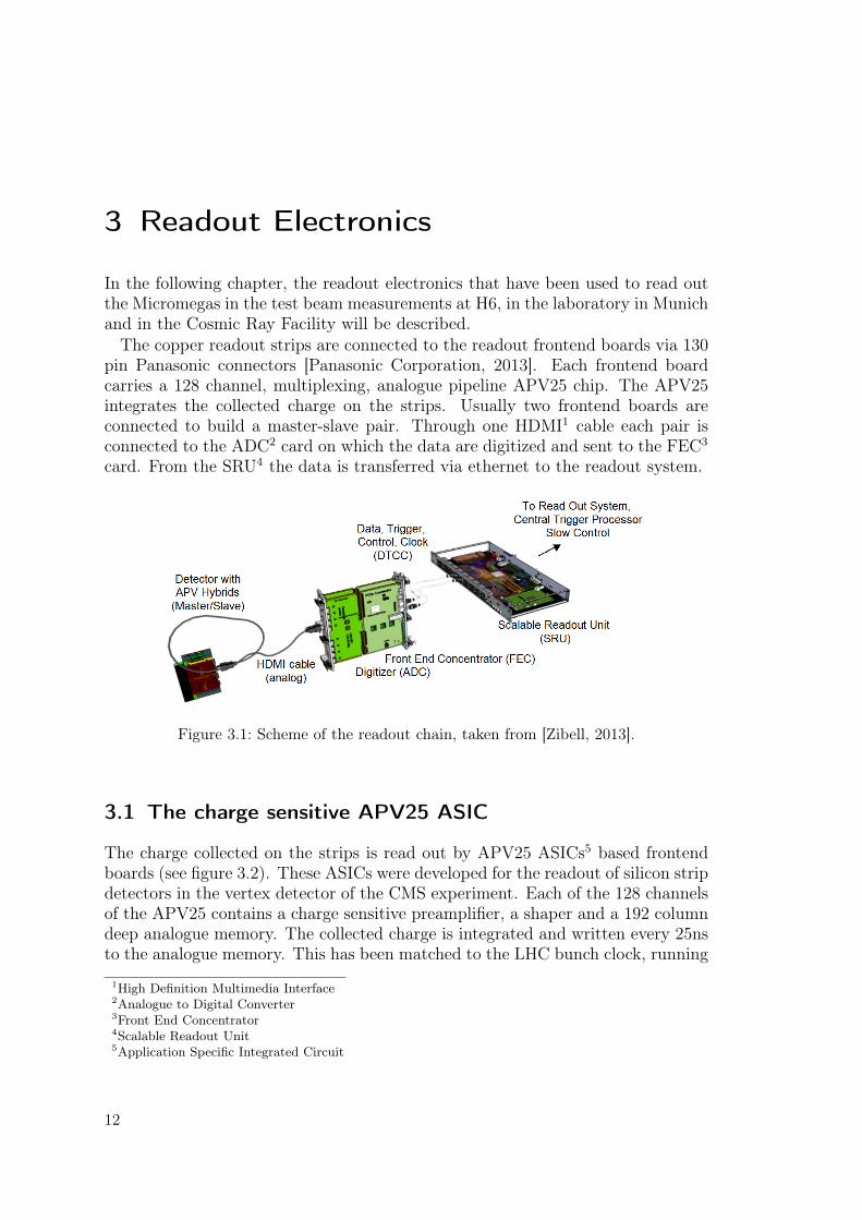
pin Panasonic connectors [Panasonic Corporation, 2013]. Each frontend boardcarries a 128 channel, multiplexing, analogue pipeline APV25 chip. The APV25integrates the collected charge on the strips. Usually two frontend boards areconnected to build a master-slave pair. Through one HDMI1 cable each pair isconnected to the ADC2 card on which the data are digitized and sent to the FEC3
card. From the SRU4 the data is transferred via ethernet to the readout system.
Figure 3.1: Scheme of the readout chain, taken from [Zibell, 2013].
3.1 The charge sensitive APV25 ASIC
The charge collected on the strips is read out by APV25 ASICs5 based frontendboards (see figure 3.2). These ASICs were developed for the readout of silicon stripdetectors in the vertex detector of the CMS experiment. Each of the 128 channelsof the APV25 contains a charge sensitive preamplifier, a shaper and a 192 columndeep analogue memory. The collected charge is integrated and written every 25nsto the analogue memory. This has been matched to the LHC bunch clock, running
1High Definition Multimedia Interface2Analogue to Digital Converter3Front End Concentrator4Scalable Readout Unit5Application Specific Integrated Circuit
12
3.2 The Scalable Readout System
at 40MHz. After reception of a trigger, a configurable number of so called timebins can be read out. [Jones, 2001]
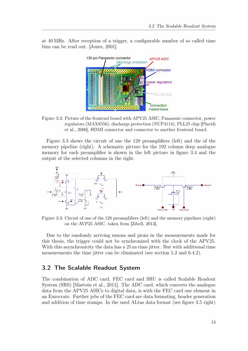
Figure 3.2: Picture of the frontend board with APV25 ASIC, Panasonic connector, powerregulators (MAX8556), discharge protection (NUP4114), PLL25 chip [Placidiet al., 2000], HDMI connector and connector to another frontend board.
Figure 3.3 shows the circuit of one the 128 preamplifiers (left) and the of thememory pipeline (right). A schematic picture for the 192 column deep analoguememory for each preamplifier is shown in the left picture in figure 3.4 and theoutput of the selected columns in the right.
Figure 3.3: Circuit of one of the 128 preamplifiers (left) and the memory pipelines (right)on the AVP25 ASIC, taken from [Zibell, 2013].
Due to the randomly arriving muons and pions in the measurements made forthis thesis, the trigger could not be synchronized with the clock of the APV25.With this asynchronicity the data has a 25 ns time jitter. But with additional timemeasurements the time jitter can be eliminated (see section 5.2 and 6.4.2).
3.2 The Scalable Readout System
The combination of ADC card, FEC card and SRU is called Scalable ReadoutSystem (SRS) [Martoiu et al., 2011]. The ADC card, which converts the analoguedata from the APV25 ASICs to digital data, is with the FEC card one element inan Eurocrate. Further jobs of the FEC card are data formating, header generationand addition of time stamps. In the used ALtas data format (see figure 3.5 right)
13
3 Readout Electronics
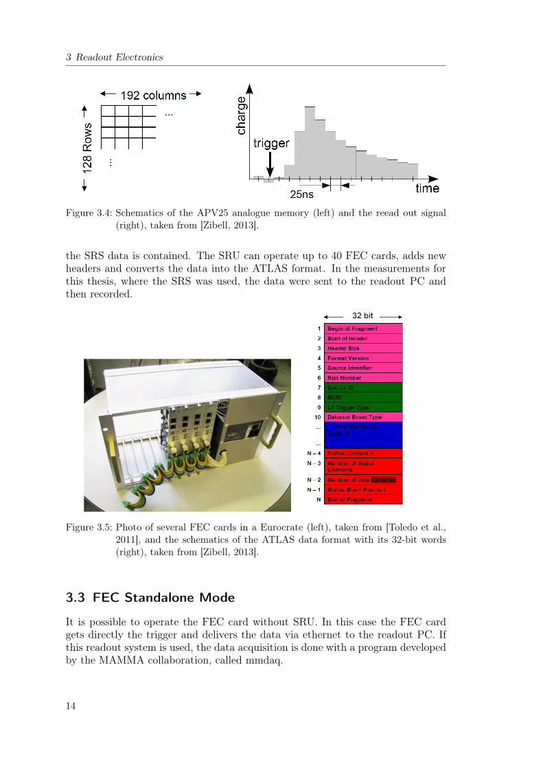
Figure 3.4: Schematics of the APV25 analogue memory (left) and the reead out signal(right), taken from [Zibell, 2013].
the SRS data is contained. The SRU can operate up to 40 FEC cards, adds newheaders and converts the data into the ATLAS format. In the measurements forthis thesis, where the SRS was used, the data were sent to the readout PC andthen recorded.
Figure 3.5: Photo of several FEC cards in a Eurocrate (left), taken from [Toledo et al.,2011], and the schematics of the ATLAS data format with its 32-bit words(right), taken from [Zibell, 2013].
3.3 FEC Standalone Mode
It is possible to operate the FEC card without SRU. In this case the FEC cardgets directly the trigger and delivers the data via ethernet to the readout PC. Ifthis readout system is used, the data acquisition is done with a program developedby the MAMMA collaboration, called mmdaq.
14
4 Analysis Tools
In this chapter tools which are needed for the analysis of the data are described.
4.1 Signal Fit
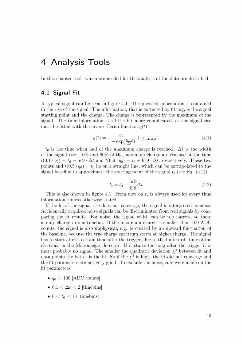
A typical signal can be seen in figure 4.1. The physical information is containedin the rise of the signal. The information, that is extracted by fitting, is the signalstarting point and the charge. The charge is represented by the maximum of thesignal. The time information is a little bit more complicated, as the signal risemust be fitted with the inverse Fermi function q(t):
q(t) =q0
1 + exp( t0−t∆t
)+ qpedestal . (4.1)
t0 is the time when half of the maximum charge is reached. ∆t is the widthof the signal rise. 10% and 90% of the maximum charge are reached at the timet(0.1 · q0) = t0 − ln 9 · ∆t and t(0.9 · q0) = t0 + ln 9 · ∆t, respectively. These twopoints and t(0.5 · q0) = t0 lie on a straight line, which can be extrapolated to thesignal baseline to approximate the starting point of the signal ts (see Eq. (4.2)).
ts = t0 −ln 9
0.8∆t (4.2)
This is also shown in figure 4.1. From now on ts is always used for every timeinformation, unless otherwise stated.If the fit of the signal rise does not converge, the signal is interpreted as noise.
Accidentally acquired noise signals can be discriminated from real signals by com-paring the fit results. For noise, the signal width can be too narrow, so thereis only charge in one timebin. If the maximum charge is smaller than 100 ADCcounts, the signal is also unphysical, e.g. is created by an upward fluctuation ofthe baseline, because the true charge spectrum starts at higher charge. The signalhas to start after a certain time after the trigger, due to the finite drift time of theelectrons in the Micromegas detector. If it starts too long after the trigger it ismost probably no signal. The smaller the quadratic deviation χ2 between fit anddata points the better is the fit. So if the χ2 is high, the fit did not converge andthe fit parameters are not very good. To exclude the noise, cuts were made on thefit parameters:
• q0 > 100 [ADC counts]
• 0.1 < ∆t < 2 [timebins]
• 0 < t0 < 13 [timebins]
15
4 Analysis Tools
time bins (25ns)
pulse height
0.9
0.5
0.1
25ns
extrapolation
q0
t 0
Δ t
Figure 4.1: Strip signal with fit and extrapolation.
• χ2
NdF< 50
where NdF is the number of degrees of freedom of the fit.
4.2 Cluster Reconstruction
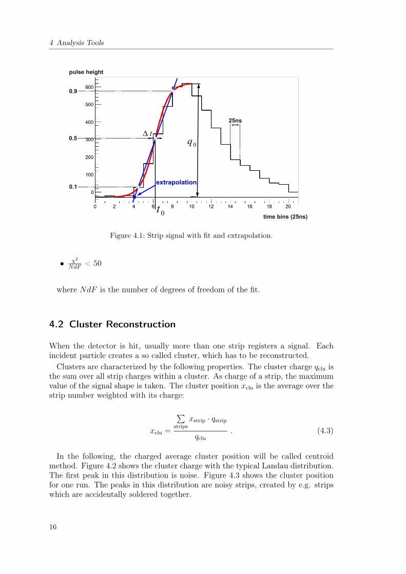
When the detector is hit, usually more than one strip registers a signal. Eachincident particle creates a so called cluster, which has to be reconstructed.Clusters are characterized by the following properties. The cluster charge qclu is
the sum over all strip charges within a cluster. As charge of a strip, the maximumvalue of the signal shape is taken. The cluster position xclu is the average over thestrip number weighted with its charge:
xclu =
∑strips
xstrip · qstrip
qclu
. (4.3)
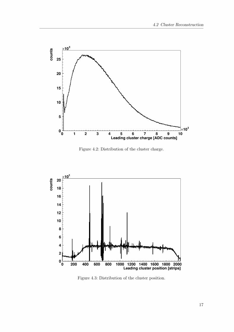
In the following, the charged average cluster position will be called centroidmethod. Figure 4.2 shows the cluster charge with the typical Landau distribution.The first peak in this distribution is noise. Figure 4.3 shows the cluster positionfor one run. The peaks in this distribution are noisy strips, created by e.g. stripswhich are accidentally soldered together.
16
4.2 Cluster Reconstruction
Figure 4.2: Distribution of the cluster charge.
Figure 4.3: Distribution of the cluster position.
17
4 Analysis Tools
4.3 Fit of Straight Lines
The method for the reconstruction of a straight track is taken from [Horvat, 2005,p. 194]. Slope m and intersection b of a straight track x = mz + b reconstructedthrough the track points (xi, zi), i = 1,...,N are determined by minimizing theχ2-function (see Eq. (4.4)). N is the number of detectors used for the track fit.The track points are recorded in the reference detectors and weighted with theirestimated spatial resolutions σi.
χ2 =N∑
i=1
1
σ2i
(xi − b−mzi)2 , (4.4)
From the minimization requirements ∂χ2
∂b= 0 and ∂χ2
∂m= 0 follows:
N∑i=1
1
σ2i
(xi − b−mzi) = 0 ,
N∑i=1
zi
σ2i
(xi − b−mzi) = 0 .
(4.5)
The new parameters g1, g2, Λ11, Λ12 and Λ22 are defined as
(g1, g2) =N∑
i=1
xi (1, zi)
σ2i
, (4.6)
(Λ11,Λ12,Λ22) =N∑
i=1
(1, zi, z2i )
σi2 . (4.7)
Inserting (4.7) in (4.5) gives
Λ11b+ Λ12m = g1 ,
Λ12b+ Λ22m = g2 .(4.8)
That yields the result
b =1
D(g1Λ22 − g2Λ12) (4.9)
and
m =1
D(−g1Λ12 + g2Λ11) , (4.10)
where
D = Λ11Λ22 − Λ212 (4.11)
Eq. (4.9) and Eq. (4.10) are intersection and slope of the reconstructed particle’strack.
18
4.4 µTPC Mode
4.4 µTPC Mode
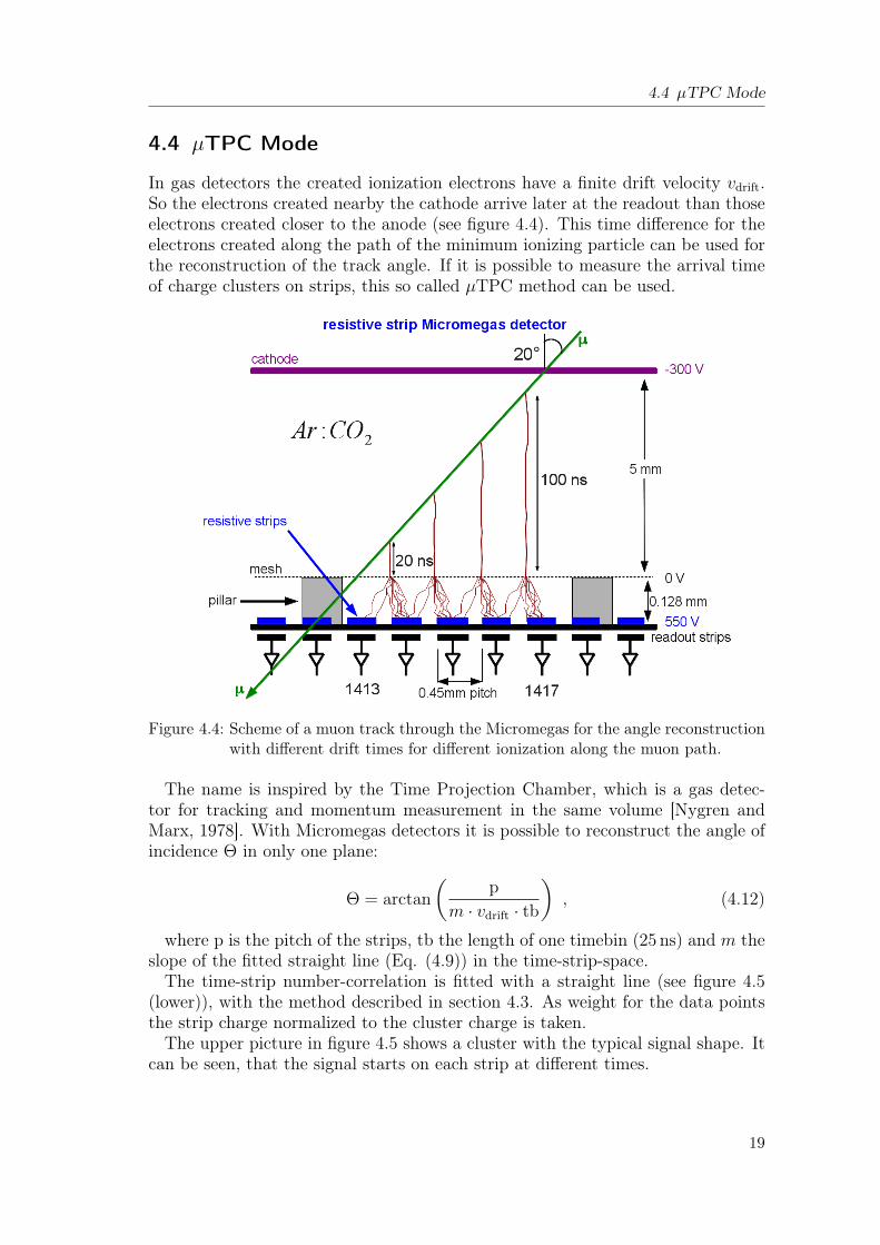
In gas detectors the created ionization electrons have a finite drift velocity vdrift.So the electrons created nearby the cathode arrive later at the readout than thoseelectrons created closer to the anode (see figure 4.4). This time difference for theelectrons created along the path of the minimum ionizing particle can be used forthe reconstruction of the track angle. If it is possible to measure the arrival timeof charge clusters on strips, this so called µTPC method can be used.
Figure 4.4: Scheme of a muon track through the Micromegas for the angle reconstructionwith different drift times for different ionization along the muon path.
The name is inspired by the Time Projection Chamber, which is a gas detec-tor for tracking and momentum measurement in the same volume [Nygren andMarx, 1978]. With Micromegas detectors it is possible to reconstruct the angle ofincidence Θ in only one plane:
Θ = arctan
(p
m · vdrift · tb
), (4.12)
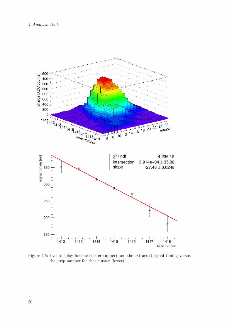
where p is the pitch of the strips, tb the length of one timebin (25 ns) and m theslope of the fitted straight line (Eq. (4.9)) in the time-strip-space.The time-strip number-correlation is fitted with a straight line (see figure 4.5
(lower)), with the method described in section 4.3. As weight for the data pointsthe strip charge normalized to the cluster charge is taken.The upper picture in figure 4.5 shows a cluster with the typical signal shape. It
can be seen, that the signal starts on each strip at different times.
19
4 Analysis Tools
Figure 4.5: Eventdisplay for one cluster (upper) and the extracted signal timing versusthe strip number for that cluster (lower).
20
5 Measurements
In order to investigate the large Micromegas chamber three measurement cam-paigns were performed. First a measurement with a telescope of Micromegasdetectors in a pion testbeam at SPS/CERN. Second, a measurement with Cos-mic muons without reference detectors to investigate the signal timing. And athird in the Cosmic-Ray Facility in Garching/Munich with two MDT chambers asreference detectors, which have a very good spatial resolution.
5.1 Pion Testbeam at SPS/CERN
The pion testbeam is at SPS is a well-defined and well focused beam with highenergy. It is a perpendicular to the detector planes and has low multiple scattering.So the tracking of the pions is easy . It is a good possibility to study spatialresolution.
5.1.1 Experimental Setup
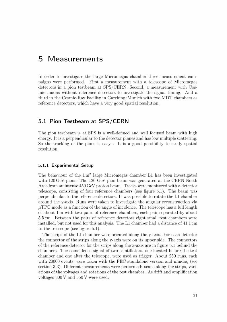
The behaviour of the 1m2 large Micromegas chamber L1 has been investigatedwith 120GeV pions. The 120 GeV pion beam was generated at the CERN NorthArea from an intense 450GeV proton beam. Tracks were monitored with a detectortelescope, consisting of four reference chambers (see figure 5.1). The beam wasperpendicular to the reference detectors. It was possible to rotate the L1 chamberaround the y-axis. Runs were taken to investigate the angular reconstruction viaµTPC mode as a function of the angle of incidence. The telescope has a full lengthof about 1m with two pairs of reference chambers, each pair separated by about5.5 cm. Between the pairs of reference detectors eight small test chambers wereinstalled, but not used for this analysis. The L1 chamber had a distance of 41.1 cmto the telescope (see figure 5.1).The strips of the L1 chamber were oriented along the y-axis. For each detector
the connector of the strips along the y-axis were on its upper side. The connectorsof the reference detector for the strips along the x-axis are in figure 5.1 behind thechambers. The coincidence signal of two scintillators, one located before the testchamber and one after the telescope, were used as trigger. About 250 runs, eachwith 20000 events, were taken with the FEC standalone version and mmdaq (seesection 3.3). Different measurements were performed: scans along the strips, vari-ations of the voltages and rotations of the test chamber. As drift and amplificationvoltages 300V and 550V were used.
21
5 Measurements
Figure 5.1: Schematic setup of the telescope in the testbeam.
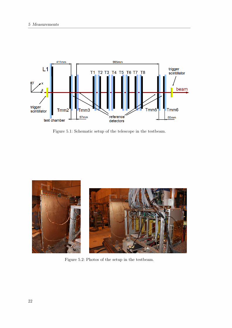
Figure 5.2: Photos of the setup in the testbeam.
22
5.1 Pion Testbeam at SPS/CERN
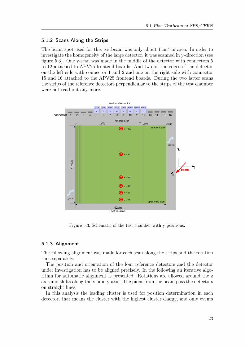
5.1.2 Scans Along the Strips
The beam spot used for this testbeam was only about 1 cm2 in area. In order toinvestigate the homogeneity of the large detector, it was scanned in y-direction (seefigure 5.3). One y-scan was made in the middle of the detector with connectors 5to 12 attached to APV25 frontend boards. And two on the edges of the detectoron the left side with connector 1 and 2 and one on the right side with connector15 and 16 attached to the APV25 frontend boards. During the two latter scansthe strips of the reference detectors perpendicular to the strips of the test chamberwere not read out any more.
connector 1 2 3 4 5 6 7 8 9 10 11 12 13 14 15 16
readout areas1 s513 s1536 s2048
gas in
gas out
z
x
y
APV7
M
APV6
S
APV4
S
APV8
S
APV10
S
APV5
M
APV9
M
APV11
M
Y = 27
Y = 37
Y = 47
Y = 67
Y = 97
Y = 127
102
cm
92cmactive area
readout side
open strip side
readout electronics
beam
Figure 5.3: Schematic of the test chamber with y positions.
5.1.3 Alignment
The following alignment was made for each scan along the strips and the rotationruns separately.The position and orientation of the four reference detectors and the detector
under investigation has to be aligned precisely. In the following an iterative algo-rithm for automatic alignment is presented. Rotations are allowed around the zaxis and shifts along the x- and y-axis. The pions from the beam pass the detectorson straight lines.In this analysis the leading cluster is used for position determination in each
detector, that means the cluster with the highest cluster charge, and only events
23
5 Measurements
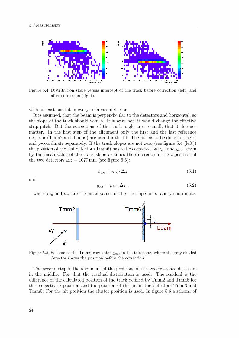
Figure 5.4: Distribution slope versus intercept of the track before correction (left) andafter correction (right).
with at least one hit in every reference detector.It is assumed, that the beam is perpendicular to the detectors and horizontal, so
the slope of the track should vanish. If it were not, it would change the effectivestrip-pitch. But the corrections of the track angle are so small, that it doe notmatter. In the first step of the alignment only the first and the last referencedetector (Tmm2 and Tmm6) are used for the fit. The fit has to be done for the x-and y-coordinate separately. If the track slopes are not zero (see figure 5.4 (left))the position of the last detector (Tmm6) has to be corrected by xcor and ycor, givenby the mean value of the track slope m times the difference in the z-position ofthe two detectors ∆z = 1077 mm (see figure 5.5):
xcor = mx ·∆z (5.1)
andycor = my ·∆z , (5.2)
where mx and my are the mean values of the the slope for x- and y-coordinate.
Figure 5.5: Scheme of the Tmm6 correction ycor in the telescope, where the grey shadeddetector shows the position before the correction.
The second step is the alignment of the positions of the two reference detectorsin the middle. For that the residual distribution is used. The residual is thedifference of the calculated position of the track defined by Tmm2 and Tmm6 forthe respective z-position and the position of the hit in the detectors Tmm3 andTmm5. For the hit position the cluster position is used. In figure 5.6 a scheme of
24

5.1 Pion Testbeam at SPS/CERN
the position corrections of the detectors is shown. They have to be shifted by thevalue of the Gaussian mean of these distributions ∆rTmm3 and ∆rTmm5 (see figure5.7).
Figure 5.6: Scheme of the Tmm3 and Tmm5 corrections ∆rTmm3 and ∆rTmm5, wherethe grey shaded detectors show their position before the correction.
Figure 5.7: Residual distributions for the telescope detectors in step 2 of the alignmentprocedure before corrections. Two distributions are exactly zero, becauseonly these to detectors were used for the track fit.
After the alignment of the reference detectors the mean of the residual distri-bution is zero (see figure 5.8) and all of them can be used for the fit of the track.Then the position of the test chamber can be corrected similarly using the residualdistribution.The third step is the correction of the rotation around the z-axis, for which
the two dimensions x and y are used. If the detector is not rotated around thez-axis, the residual distributions in y versus the x-coordinate of the cluster andthe residual in x (∆x) versus the y-coordinate of the cluster should have a slopeequal to zero. If the slope is not equal to zero, the correction α for the rotation
25

5 Measurements
Figure 5.8: Residual distributions for the telescope detectors after step 2. Two distri-butions are exactly zero, because only these two detectors were used for thetrack fit.
can be calculated with the slope a (see figure 5.9 left):
tanα = a =∆x
y
After that correction the slope in figure 5.9 (right) is zero. Now, a second iterationof the position alignment is necessary, because the rotational corrections can shiftthe detectors again. All detectors are thus shifted by the mean of the respectiveresidual distribution until it is zero. After this correction, the telescope and theL1 chambers are reasonable well aligned. This rotational correction could not bemade for the scans along the strip at the edges of the test detector, because of themissing information of the position perpendicular to the strips of the L1 chamber.
5.1.4 Determination of the Track Accuracy
The spatial resolution of a detector can be extracted from the standard deviationof the residual distribution. The width of the residual distribution σr, is given bythe quadratic sum of the intrinsic spatial resolution σsr and the track accuracyσtrack [Carnegie et al., 2005]:
σr =√σ2
sr + σ2track . (5.3)
To calculate the spatial resolution for the test chamber (L1) obviously the trackaccuracy is needed. The track accuracy can be calculated from the spatial resolu-tion of the reference detectors, determined with the method suggested by Carnegie.For each detector two values will be determined for the standard deviations of the
26
5.1 Pion Testbeam at SPS/CERN
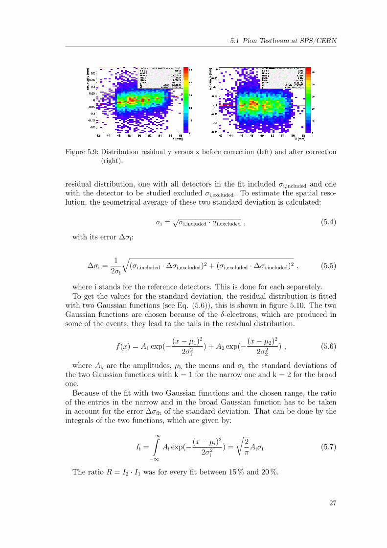
Figure 5.9: Distribution residual y versus x before correction (left) and after correction(right).
residual distribution, one with all detectors in the fit included σi,included and onewith the detector to be studied excluded σi,excluded. To estimate the spatial reso-lution, the geometrical average of these two standard deviation is calculated:
σi =√σi,included · σi,excluded , (5.4)
with its error ∆σi:
∆σi =1
2σi
√(σi,included ·∆σi,excluded)2 + (σi,excluded ·∆σi,included)2 , (5.5)
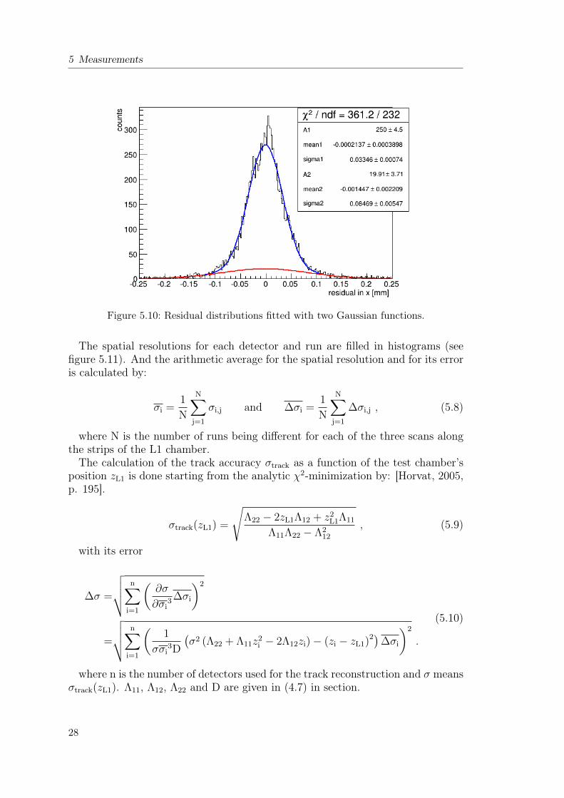
where i stands for the reference detectors. This is done for each separately.To get the values for the standard deviation, the residual distribution is fitted
with two Gaussian functions (see Eq. (5.6)), this is shown in figure 5.10. The twoGaussian functions are chosen because of the δ-electrons, which are produced insome of the events, they lead to the tails in the residual distribution.
f(x) = A1 exp(−(x− µ1)2
2σ21
) + A2 exp(−(x− µ2)2
2σ22
) , (5.6)
where Ak are the amplitudes, µk the means and σk the standard deviations ofthe two Gaussian functions with k = 1 for the narrow one and k = 2 for the broadone.Because of the fit with two Gaussian functions and the chosen range, the ratio
of the entries in the narrow and in the broad Gaussian function has to be takenin account for the error ∆σfit of the standard deviation. That can be done by theintegrals of the two functions, which are given by:
Ii =
∞∫−∞
Ai exp(−(x− µi)2
2σ2i
) =
√2
πAiσi (5.7)
The ratio R = I2 · I1 was for every fit between 15% and 20%.
27
5 Measurements
Figure 5.10: Residual distributions fitted with two Gaussian functions.
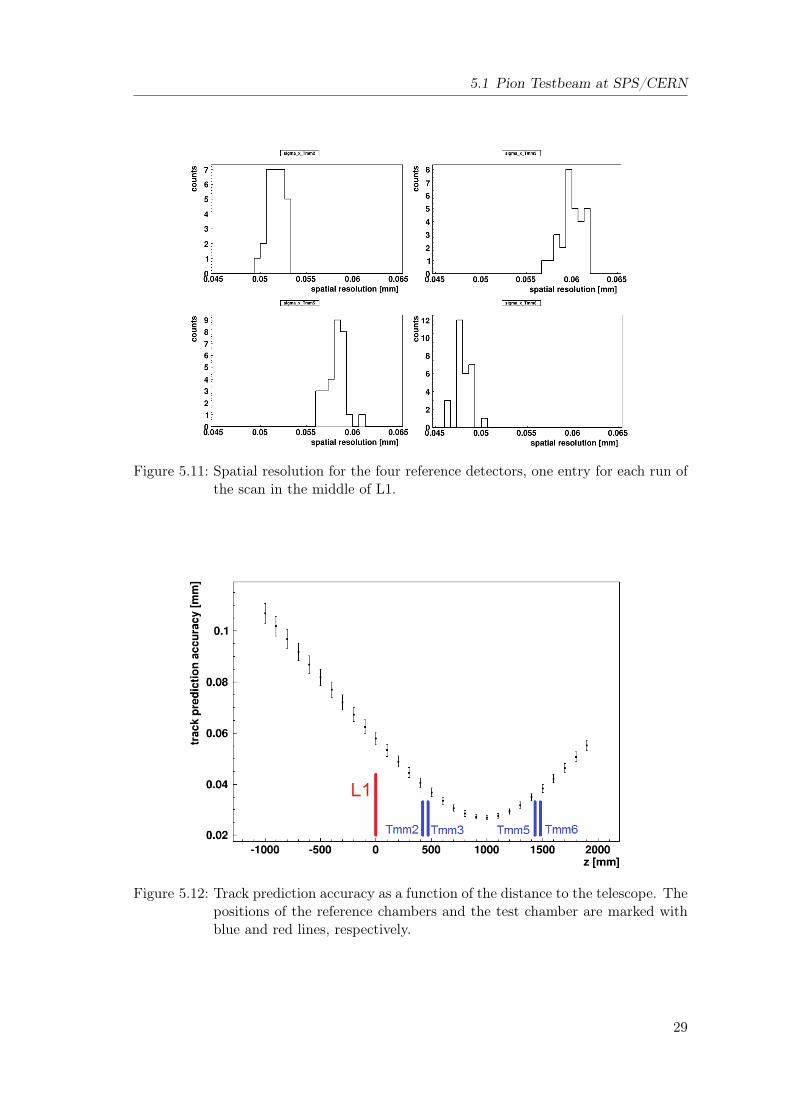
The spatial resolutions for each detector and run are filled in histograms (seefigure 5.11). And the arithmetic average for the spatial resolution and for its erroris calculated by:
σi =1
N
N∑j=1
σi,j and ∆σi =1
N
N∑j=1
∆σi,j , (5.8)
where N is the number of runs being different for each of the three scans alongthe strips of the L1 chamber.The calculation of the track accuracy σtrack as a function of the test chamber’s
position zL1 is done starting from the analytic χ2-minimization by: [Horvat, 2005,p. 195].
σtrack(zL1) =
√Λ22 − 2zL1Λ12 + z2
L1Λ11
Λ11Λ22 − Λ212
, (5.9)
with its error
∆σ =
√√√√ n∑i=1
(∂σ
∂σi3 ∆σi
)2
=
√√√√ n∑i=1
(1
σσi3D
(σ2 (Λ22 + Λ11z2
i − 2Λ12zi)− (zi − zL1)2)∆σi
)2
.
(5.10)
where n is the number of detectors used for the track reconstruction and σ meansσtrack(zL1). Λ11, Λ12, Λ22 and D are given in (4.7) in section.
28
5.1 Pion Testbeam at SPS/CERN
Figure 5.11: Spatial resolution for the four reference detectors, one entry for each run ofthe scan in the middle of L1.
Figure 5.12: Track prediction accuracy as a function of the distance to the telescope. Thepositions of the reference chambers and the test chamber are marked withblue and red lines, respectively.
29
5 Measurements
The track prediction accuracy as a function of the distance from the telescopeis plotted in figure 5.12. The best value for the track accuracy would be inside thereference telescope. For the actual position zL1 = 0 it yields the result for the scanin the middle:
σtrack,x = (57.8± 2.5)µm . (5.11)
The same analysis was made for the y-direction, which leads to the result
σtrack,y = (61.5± 2.8)µm . (5.12)
The latter will not be used in this analysis, since the test chamber has onlyone dimensional readout. For the scans along the strips on the edges the trackaccuracy was also determined, which yields the result:
σtrack,x = (63.3± 3.3)µm for the left side and
σtrack,x = (63.0± 3.4)µm for the right side .(5.13)
Due to the absence of the readout electronics for the strips in x-direction thecorrections of the rotation around the z-axis could not be made. So the referencedetectors are not totally aligned and the track accuracy gets worse. In section6.1.1 is shown, that this has an effect on the spatial resolution.
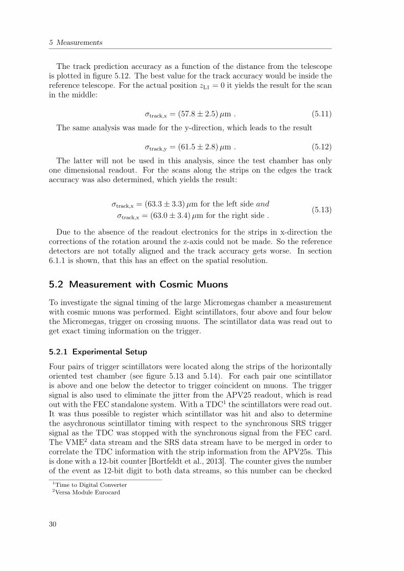
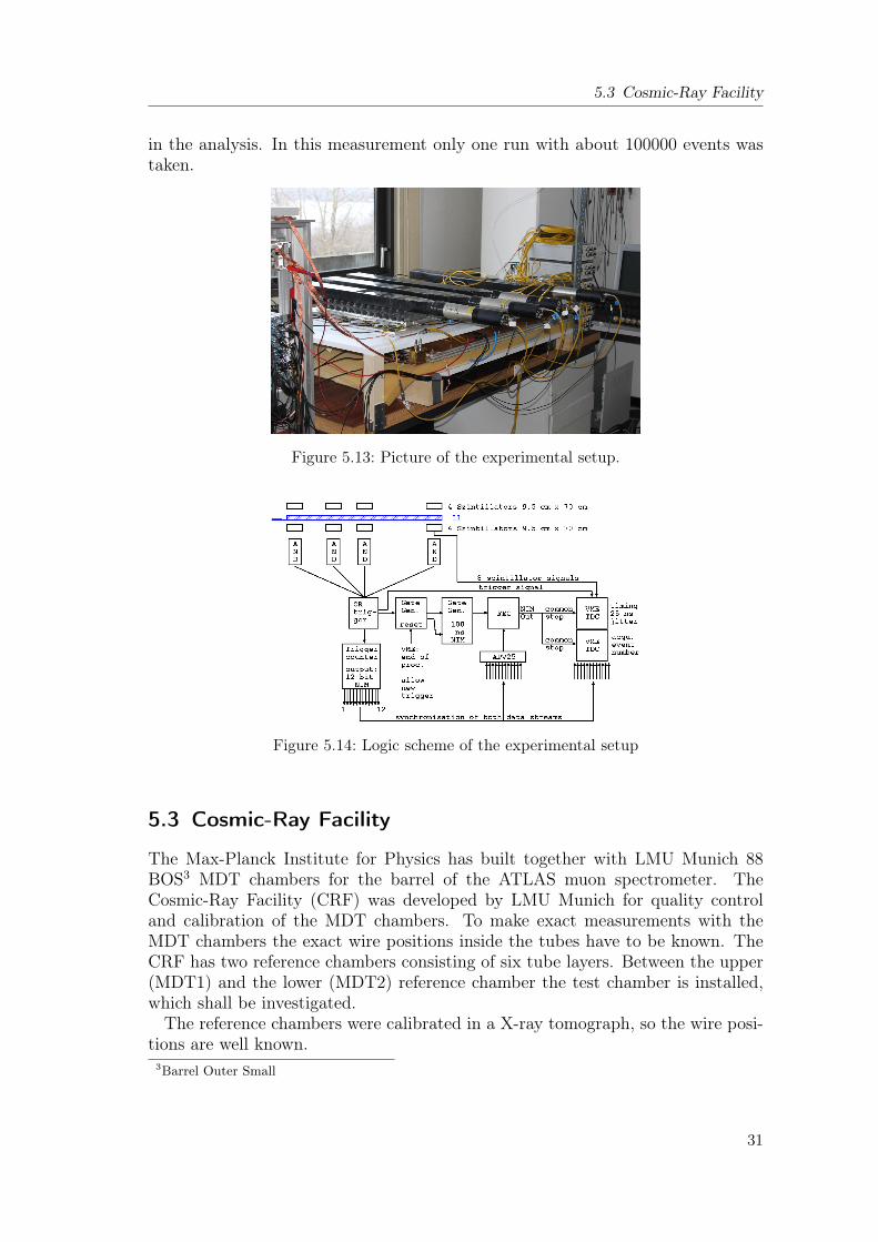
5.2 Measurement with Cosmic Muons
To investigate the signal timing of the large Micromegas chamber a measurementwith cosmic muons was performed. Eight scintillators, four above and four belowthe Micromegas, trigger on crossing muons. The scintillator data was read out toget exact timing information on the trigger.
5.2.1 Experimental Setup
Four pairs of trigger scintillators were located along the strips of the horizontallyoriented test chamber (see figure 5.13 and 5.14). For each pair one scintillatoris above and one below the detector to trigger coincident on muons. The triggersignal is also used to eliminate the jitter from the APV25 readout, which is readout with the FEC standalone system. With a TDC1 the scintillators were read out.It was thus possible to register which scintillator was hit and also to determinethe asychronous scintillator timing with respect to the synchronous SRS triggersignal as the TDC was stopped with the synchronous signal from the FEC card.The VME2 data stream and the SRS data stream have to be merged in order tocorrelate the TDC information with the strip information from the APV25s. Thisis done with a 12-bit counter [Bortfeldt et al., 2013]. The counter gives the numberof the event as 12-bit digit to both data streams, so this number can be checked
1Time to Digital Converter2Versa Module Eurocard
30
5.3 Cosmic-Ray Facility
in the analysis. In this measurement only one run with about 100000 events wastaken.
Figure 5.13: Picture of the experimental setup.
Figure 5.14: Logic scheme of the experimental setup
5.3 Cosmic-Ray Facility
The Max-Planck Institute for Physics has built together with LMU Munich 88BOS3 MDT chambers for the barrel of the ATLAS muon spectrometer. TheCosmic-Ray Facility (CRF) was developed by LMU Munich for quality controland calibration of the MDT chambers. To make exact measurements with theMDT chambers the exact wire positions inside the tubes have to be known. TheCRF has two reference chambers consisting of six tube layers. Between the upper(MDT1) and the lower (MDT2) reference chamber the test chamber is installed,which shall be investigated.The reference chambers were calibrated in a X-ray tomograph, so the wire posi-
tions are well known.3Barrel Outer Small
31
5 Measurements
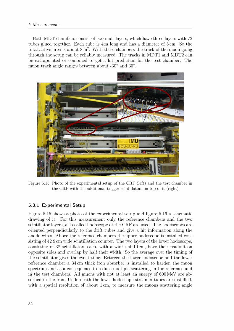
Both MDT chambers consist of two multilayers, which have three layers with 72tubes glued together. Each tube is 4m long and has a diameter of 3 cm. So thetotal active area is about 8m2. With these chambers the track of the muon goingthrough the setup can be reliably measured. The tracks in MDT1 and MDT2 canbe extrapolated or combined to get a hit prediction for the test chamber. Themuon track angle ranges between about -30 and 30.
Figure 5.15: Photo of the experimental setup of the CRF (left) and the test chamber inthe CRF with the additional trigger scintillators on top of it (right).
5.3.1 Experimental Setup
Figure 5.15 shows a photo of the experimental setup and figure 5.16 a schematicdrawing of it. For this measurement only the reference chambers and the twoscintillator layers, also called hodoscope of the CRF are used. The hodoscopes areoriented perpendicularly to the drift tubes and give a hit information along theanode wires. Above the reference chambers the upper hodoscope is installed con-sisting of 42 9 cm wide scintillation counter. The two layers of the lower hodoscope,consisting of 38 scintillators each, with a width of 10 cm, have their readout onopposite sides and overlap by half their width. So the average over the timing ofthe scintillator gives the event time. Between the lower hodoscope and the lowerreference chamber a 34 cm thick iron absorber is installed to harden the muonspectrum and as a consequence to reduce multiple scattering in the reference andin the test chambers. All muons with not at least an energy of 600MeV are ab-sorbed in the iron. Underneath the lower hodoscope streamer tubes are installed,with a spatial resolution of about 1 cm, to measure the muons scattering angle
32

5.3 Cosmic-Ray Facility
from interaction within the iron absorber. But these streamer tubes were not usedin this measurement. [Dubbert et al., 2002]
Figure 5.16: Schematic setup of the measurement.
Instead of a MDT test chamber the L1 Micromegas chamber is installed betweenthe reference chambers. On top of the Micromegas eleven additional 9.5 cm widescintillators, which are perpendicular to the strips, allow to trigger only on muons,that have crossed the active area of the Micromegas.The Micromegas detector was read out with SRS and the MDT chambers with an
ATLAS readout system especially modified for the CRF. Additionally to the CRF’sstandard readout system, which is described in [Rauscher, 2005], it is recorded,which scintillator, lying on top of the micromegas, has been hit. To merge thesetwo data streams, an event number was recorded by both streams. One long runover about five days were taken. Muon tracks that could not be used for theanalysis were excluded, afterward 6.7M evernts remained. Some short runs withabout 20000 events were taken for the optimization of the operational parameters
5.3.2 Optimization of the Micromegas Operational Parameters
To determine the working point of the test chamber several high voltage scans wereperformed. Runs were taken with different voltages, the leading cluster chargedistributions were fitted with a Landau function and the most probable valueswere plotted versus the electrical field strength.
33
5 Measurements
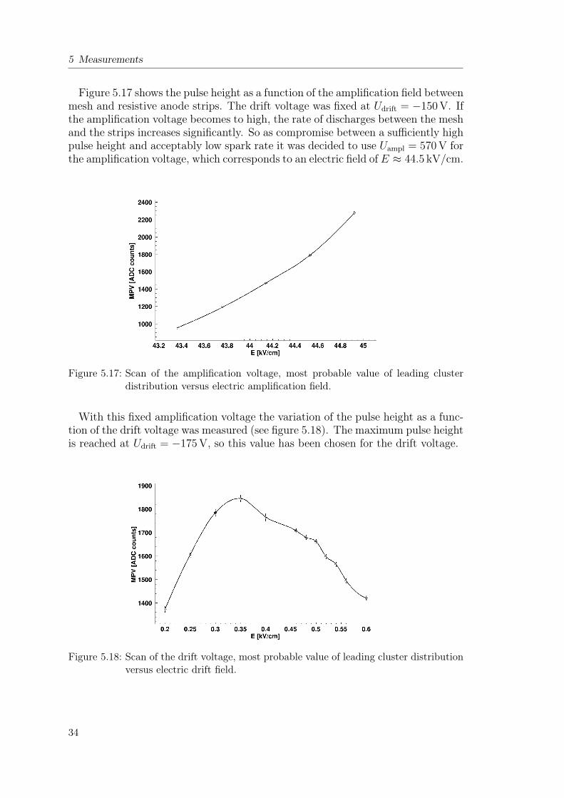
Figure 5.17 shows the pulse height as a function of the amplification field betweenmesh and resistive anode strips. The drift voltage was fixed at Udrift = −150 V. Ifthe amplification voltage becomes to high, the rate of discharges between the meshand the strips increases significantly. So as compromise between a sufficiently highpulse height and acceptably low spark rate it was decided to use Uampl = 570 V forthe amplification voltage, which corresponds to an electric field of E ≈ 44.5 kV/cm.
Figure 5.17: Scan of the amplification voltage, most probable value of leading clusterdistribution versus electric amplification field.
With this fixed amplification voltage the variation of the pulse height as a func-tion of the drift voltage was measured (see figure 5.18). The maximum pulse heightis reached at Udrift = −175 V, so this value has been chosen for the drift voltage.
Figure 5.18: Scan of the drift voltage, most probable value of leading cluster distributionversus electric drift field.
34
5.3 Cosmic-Ray Facility
5.3.3 Event Selection
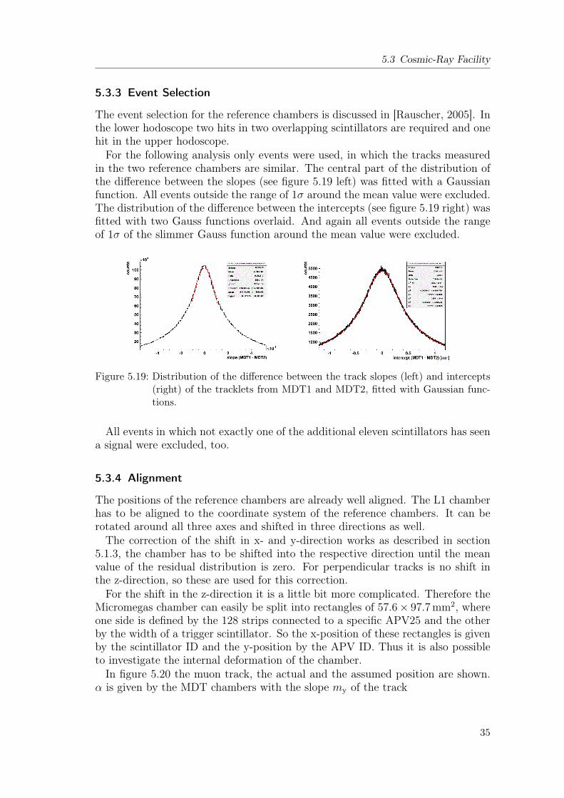
The event selection for the reference chambers is discussed in [Rauscher, 2005]. Inthe lower hodoscope two hits in two overlapping scintillators are required and onehit in the upper hodoscope.For the following analysis only events were used, in which the tracks measured
in the two reference chambers are similar. The central part of the distribution ofthe difference between the slopes (see figure 5.19 left) was fitted with a Gaussianfunction. All events outside the range of 1σ around the mean value were excluded.The distribution of the difference between the intercepts (see figure 5.19 right) wasfitted with two Gauss functions overlaid. And again all events outside the rangeof 1σ of the slimmer Gauss function around the mean value were excluded.
Figure 5.19: Distribution of the difference between the track slopes (left) and intercepts(right) of the tracklets from MDT1 and MDT2, fitted with Gaussian func-tions.
All events in which not exactly one of the additional eleven scintillators has seena signal were excluded, too.
5.3.4 Alignment
The positions of the reference chambers are already well aligned. The L1 chamberhas to be aligned to the coordinate system of the reference chambers. It can berotated around all three axes and shifted in three directions as well.The correction of the shift in x- and y-direction works as described in section
5.1.3, the chamber has to be shifted into the respective direction until the meanvalue of the residual distribution is zero. For perpendicular tracks is no shift inthe z-direction, so these are used for this correction.For the shift in the z-direction it is a little bit more complicated. Therefore the
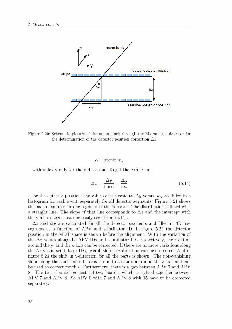
Micromegas chamber can easily be split into rectangles of 57.6× 97.7 mm2, whereone side is defined by the 128 strips connected to a specific APV25 and the otherby the width of a trigger scintillator. So the x-position of these rectangles is givenby the scintillator ID and the y-position by the APV ID. Thus it is also possibleto investigate the internal deformation of the chamber.In figure 5.20 the muon track, the actual and the assumed position are shown.
α is given by the MDT chambers with the slope my of the track
35
5 Measurements
Figure 5.20: Schematic picture of the muon track through the Micromegas detector forthe determination of the detector position correction ∆z.
α = arctanmy
with index y only for the y-direction. To get the correction
∆z =∆y
tanα=
∆y
my
(5.14)
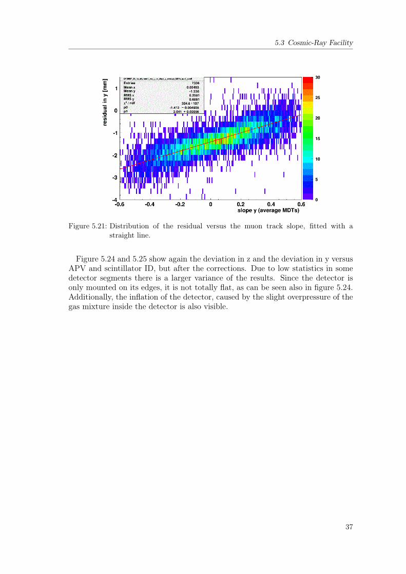
for the detector position, the values of the residual ∆y versus my are filled in ahistogram for each event, separately for all detector segments. Figure 5.21 showsthis as an example for one segment of the detector. The distribution is fitted witha straight line. The slope of that line corresponds to ∆z and the intercept withthe y-axis is ∆y as can be easily seen from (5.14).
∆z and ∆y are calculated for all the detector segments and filled in 3D his-tograms as a function of APV and scintillator ID. In figure 5.22 the detectorposition in the MDT space is shown before the alignment. With the variation ofthe ∆z values along the APV IDs and scintillator IDs, respectively, the rotationaround the y- and the x-axis can be corrected. If there are no more variations alongthe APV and scintillator IDs, overall shift in z-direction can be corrected. And infigure 5.23 the shift in y-direction for all the parts is shown. The non-vanishingslope along the scintillator ID-axis is due to a rotation around the z-axis and canbe used to correct for this. Furthermore, there is a gap between APV 7 and APV8. The test chamber consists of two boards, which are glued together betweenAPV 7 and APV 8. So APV 0 with 7 and APV 8 with 15 have to be correctedseparately.
36
5.3 Cosmic-Ray Facility
Figure 5.21: Distribution of the residual versus the muon track slope, fitted with astraight line.
Figure 5.24 and 5.25 show again the deviation in z and the deviation in y versusAPV and scintillator ID, but after the corrections. Due to low statistics in somedetector segments there is a larger variance of the results. Since the detector isonly mounted on its edges, it is not totally flat, as can be seen also in figure 5.24.Additionally, the inflation of the detector, caused by the slight overpressure of thegas mixture inside the detector is also visible.
37
5 Measurements
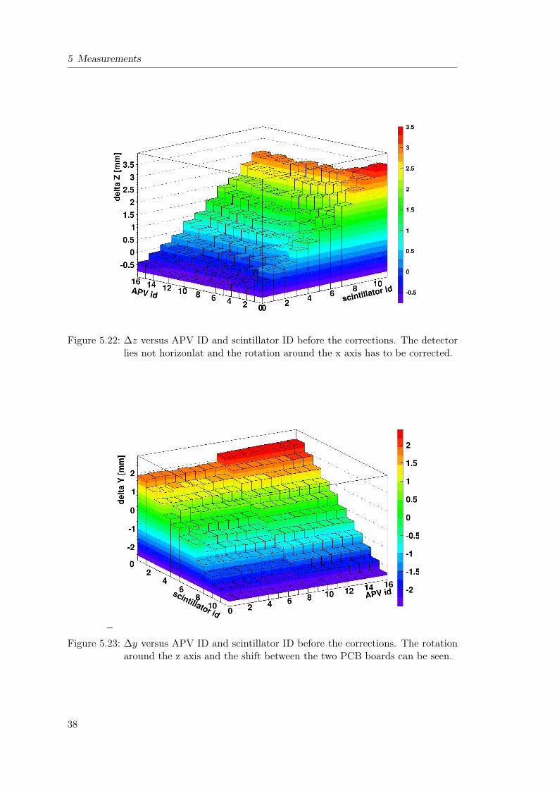
Figure 5.22: ∆z versus APV ID and scintillator ID before the corrections. The detectorlies not horizonlat and the rotation around the x axis has to be corrected.
Figure 5.23: ∆y versus APV ID and scintillator ID before the corrections. The rotationaround the z axis and the shift between the two PCB boards can be seen.
38
5.3 Cosmic-Ray Facility
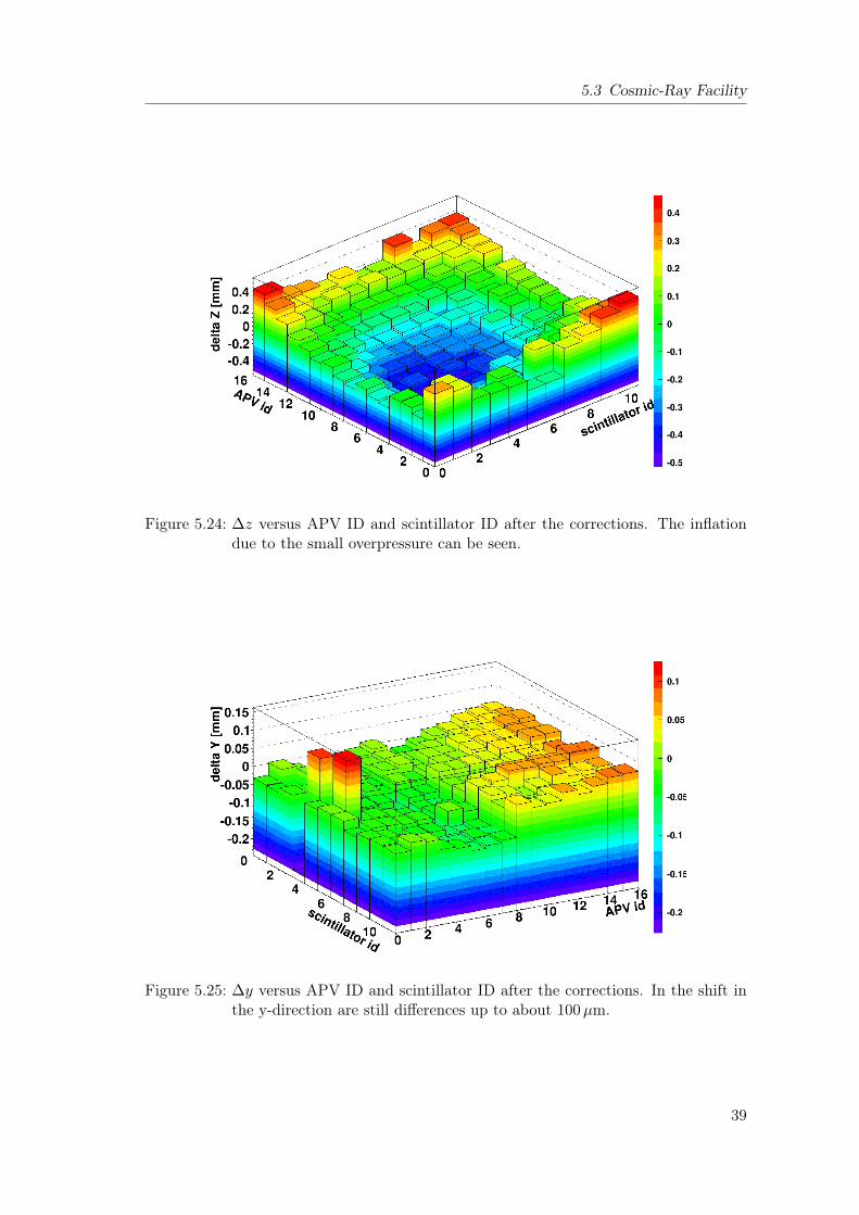
Figure 5.24: ∆z versus APV ID and scintillator ID after the corrections. The inflationdue to the small overpressure can be seen.
Figure 5.25: ∆y versus APV ID and scintillator ID after the corrections. In the shift inthe y-direction are still differences up to about 100µm.
39
6 Results
In the following chapter the results for spatial and angular resolution, signal timingand efficiency in the large L1 Micromegas chamber for the three measurementcampaigns are presented.
6.1 Spatial Resolution
One of the essential properties of a Micromegas chamber is the spatial resolution.It is important to have a good spatial resolution for track determination andmomentum measurements in magnetic fields. The results for the spatial resolutionof the L1 chamber are discussed in the following sections. The spatial resolutionfor 120 GeV pions and cosmic muons, measured with the centroid method (seesction 4.2) as well as with the µTPC-method for tracks, not perpendicular to thedetector, introduced in section 4.4, will be presented.
6.1.1 Pion Testbeam at SPS/CERN
The spatial resolution for the four measurements in the pion testbeam, discussedin section 5.1, was determined. Primarily the scan along the strips in the middleof the detector is presented. First the standard deviation σL1 of the residualdistribution of the test chamber, where all reference detectors are used in thetrack fit, is determined. The residual is the difference between the predicted hitposition and the measured hit position in the L1 chamber, as described in section5.1.3. Now, the spatial resolution σsr for the L1 detector can be calculated:
σsr =√σ2
L1 − σ2track , (6.1)
where σtrack is the track accuracy.As the uncertainties for σL1 the fitting error is used. This error, ∆σL1, and the
error of the track accuracy ∆σtrack yields the error of the spatial resolution:
∆σsr =1
σsr
√(σL1 ·∆σL1)2 + (σtrack ·∆σtrack)2 (6.2)
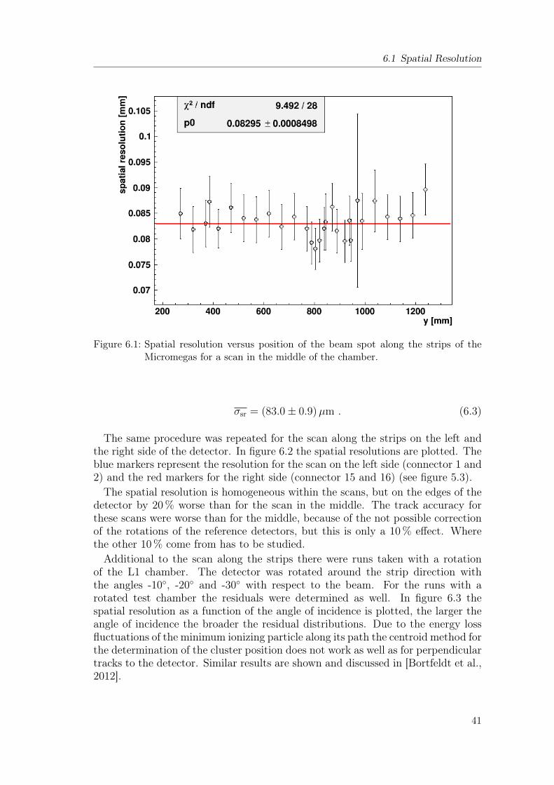
The spatial resolution was calculated for all beam positions in the scan andplotted in figure 6.1 versus the y position. Because of the movable table, on whichthe detector stood, the adjustment position is used as y position. So the scanalong the strips has an offset of about 25 cm, i.e. in figure 6.1 position 250mm iswhere the strips ended on the readout side.It can be seen that the spatial resolution in the detector is quite homogeneous.
Averaging over these values leads to a mean spatial resolution:
40
6.1 Spatial Resolution
Figure 6.1: Spatial resolution versus position of the beam spot along the strips of theMicromegas for a scan in the middle of the chamber.
σsr = (83.0± 0.9)µm . (6.3)
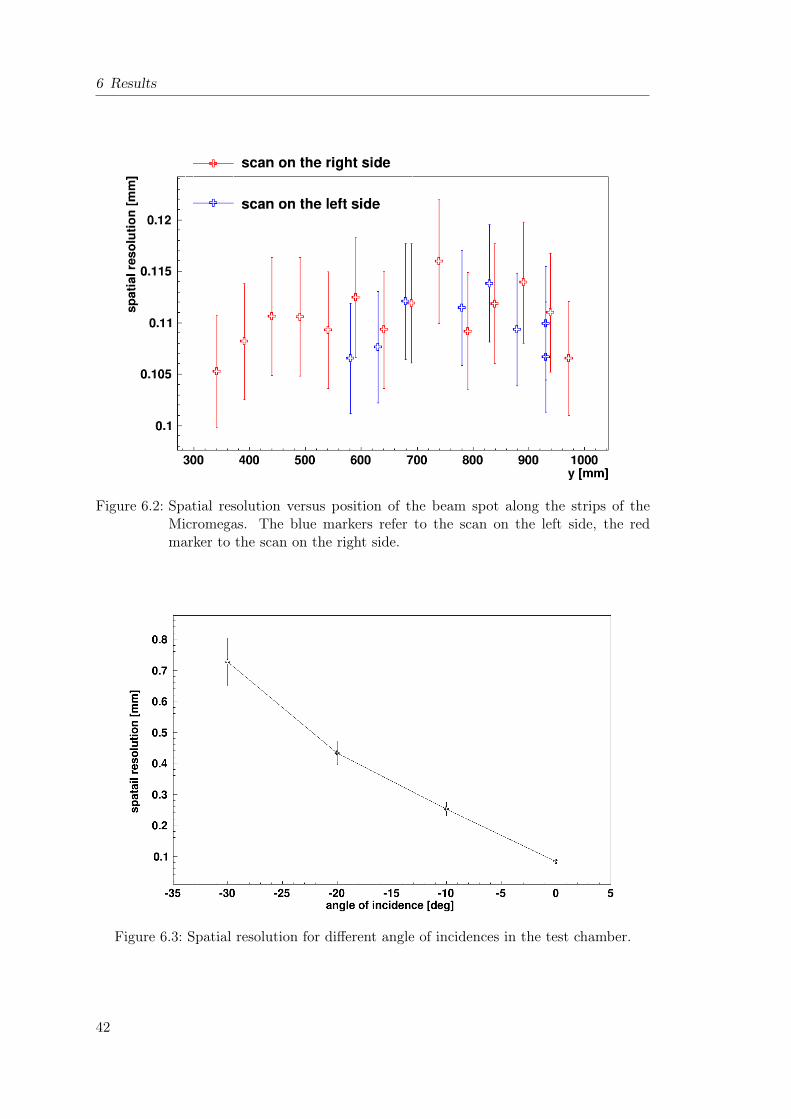
The same procedure was repeated for the scan along the strips on the left andthe right side of the detector. In figure 6.2 the spatial resolutions are plotted. Theblue markers represent the resolution for the scan on the left side (connector 1 and2) and the red markers for the right side (connector 15 and 16) (see figure 5.3).The spatial resolution is homogeneous within the scans, but on the edges of the
detector by 20% worse than for the scan in the middle. The track accuracy forthese scans were worse than for the middle, because of the not possible correctionof the rotations of the reference detectors, but this is only a 10% effect. Wherethe other 10% come from has to be studied.Additional to the scan along the strips there were runs taken with a rotation
of the L1 chamber. The detector was rotated around the strip direction withthe angles -10, -20 and -30 with respect to the beam. For the runs with arotated test chamber the residuals were determined as well. In figure 6.3 thespatial resolution as a function of the angle of incidence is plotted, the larger theangle of incidence the broader the residual distributions. Due to the energy lossfluctuations of the minimum ionizing particle along its path the centroid method forthe determination of the cluster position does not work as well as for perpendiculartracks to the detector. Similar results are shown and discussed in [Bortfeldt et al.,2012].
41
6 Results
Figure 6.2: Spatial resolution versus position of the beam spot along the strips of theMicromegas. The blue markers refer to the scan on the left side, the redmarker to the scan on the right side.
Figure 6.3: Spatial resolution for different angle of incidences in the test chamber.
42
6.1 Spatial Resolution
6.1.2 Cosmic-Ray Facility
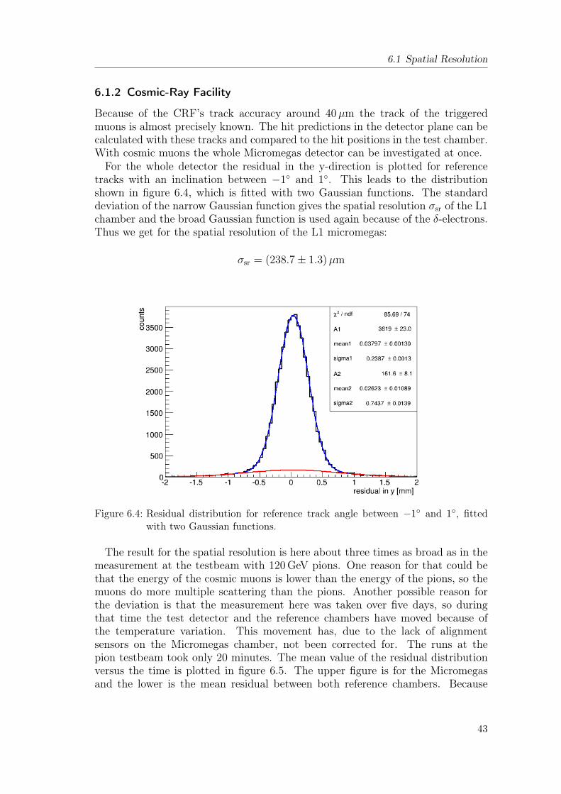
Because of the CRF’s track accuracy around 40µm the track of the triggeredmuons is almost precisely known. The hit predictions in the detector plane can becalculated with these tracks and compared to the hit positions in the test chamber.With cosmic muons the whole Micromegas detector can be investigated at once.For the whole detector the residual in the y-direction is plotted for reference
tracks with an inclination between −1 and 1. This leads to the distributionshown in figure 6.4, which is fitted with two Gaussian functions. The standarddeviation of the narrow Gaussian function gives the spatial resolution σsr of the L1chamber and the broad Gaussian function is used again because of the δ-electrons.Thus we get for the spatial resolution of the L1 micromegas:
σsr = (238.7± 1.3)µm
Figure 6.4: Residual distribution for reference track angle between −1 and 1, fittedwith two Gaussian functions.
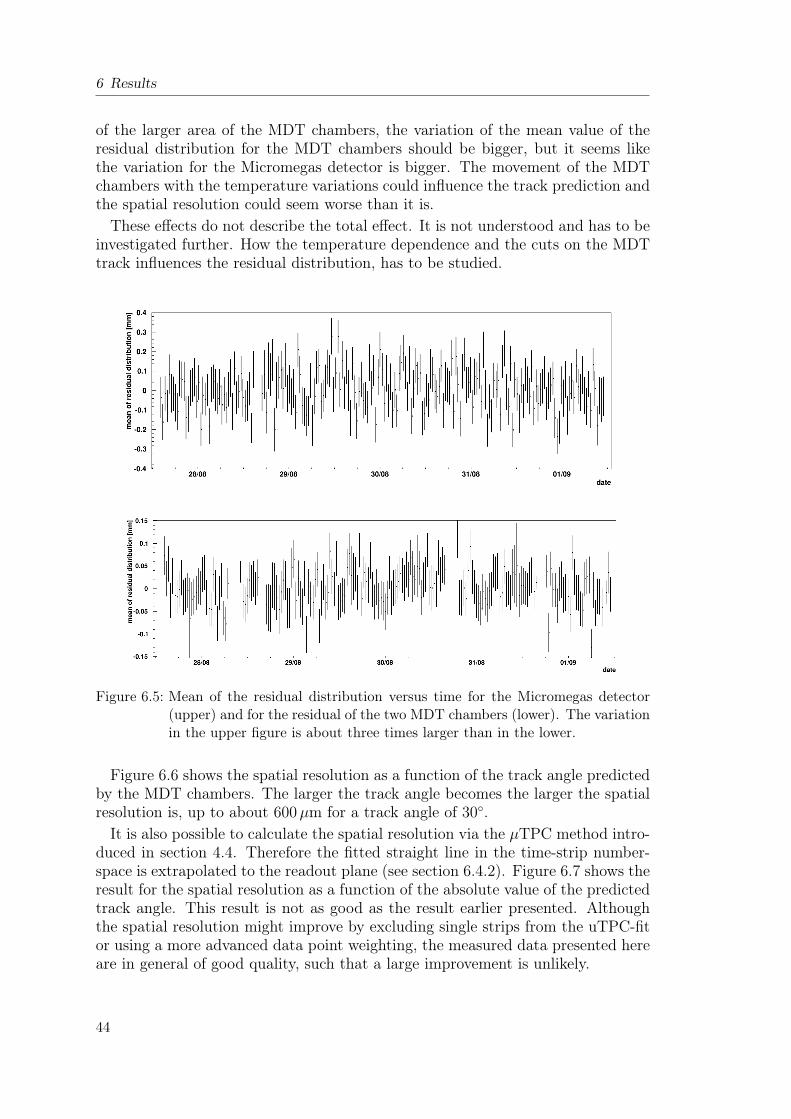
The result for the spatial resolution is here about three times as broad as in themeasurement at the testbeam with 120GeV pions. One reason for that could bethat the energy of the cosmic muons is lower than the energy of the pions, so themuons do more multiple scattering than the pions. Another possible reason forthe deviation is that the measurement here was taken over five days, so duringthat time the test detector and the reference chambers have moved because ofthe temperature variation. This movement has, due to the lack of alignmentsensors on the Micromegas chamber, not been corrected for. The runs at thepion testbeam took only 20 minutes. The mean value of the residual distributionversus the time is plotted in figure 6.5. The upper figure is for the Micromegasand the lower is the mean residual between both reference chambers. Because
43
6 Results
of the larger area of the MDT chambers, the variation of the mean value of theresidual distribution for the MDT chambers should be bigger, but it seems likethe variation for the Micromegas detector is bigger. The movement of the MDTchambers with the temperature variations could influence the track prediction andthe spatial resolution could seem worse than it is.These effects do not describe the total effect. It is not understood and has to be
investigated further. How the temperature dependence and the cuts on the MDTtrack influences the residual distribution, has to be studied.
Figure 6.5: Mean of the residual distribution versus time for the Micromegas detector(upper) and for the residual of the two MDT chambers (lower). The variationin the upper figure is about three times larger than in the lower.
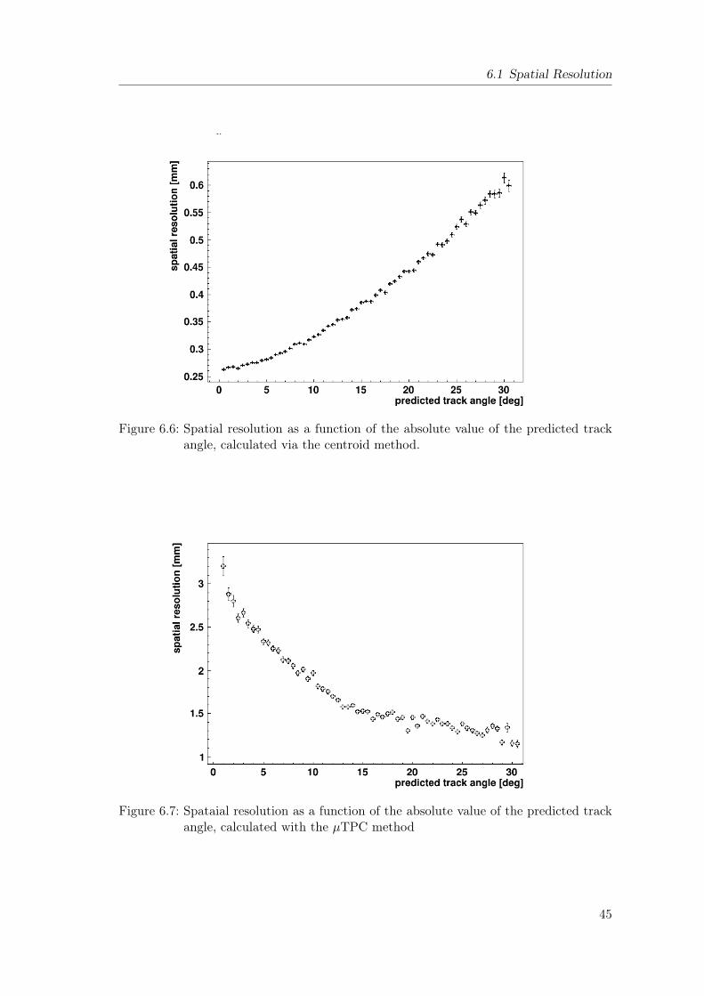
Figure 6.6 shows the spatial resolution as a function of the track angle predictedby the MDT chambers. The larger the track angle becomes the larger the spatialresolution is, up to about 600µm for a track angle of 30.It is also possible to calculate the spatial resolution via the µTPC method intro-
duced in section 4.4. Therefore the fitted straight line in the time-strip number-space is extrapolated to the readout plane (see section 6.4.2). Figure 6.7 shows theresult for the spatial resolution as a function of the absolute value of the predictedtrack angle. This result is not as good as the result earlier presented. Althoughthe spatial resolution might improve by excluding single strips from the uTPC-fitor using a more advanced data point weighting, the measured data presented hereare in general of good quality, such that a large improvement is unlikely.
44
6.1 Spatial Resolution
Figure 6.6: Spatial resolution as a function of the absolute value of the predicted trackangle, calculated via the centroid method.
Figure 6.7: Spataial resolution as a function of the absolute value of the predicted trackangle, calculated with the µTPC method
45
6 Results
6.1.3 Discussion
The large Micromegas detector has shown an averaged spatial resolution of σsr =(83.0 ± 0.9)µm in the scan along the strips with perpendicular incident 120GeVpions. The scans along the strips on the edges of the test chamber did not showsuch a good result, because of the not as good track accuracy as for the scan in themiddle of the detector. The measurement in the Cosmic-Ray Facility has shownonly a spatial resolution σsr = (238.7±1.3)µm for track angles between −1 and 1.It is not jet understood, why this result is three times higher. It is probably due tothe not optimized reference track reconstruction in this specific setup. The spatialresolution calculated with the centroid method is even for angles of 30 degreessmaller than the spatial resolution determined with the µTPC method. Aftersome necessary improvements, the µTPC spatial resolution should show similar orbetter results than the centroid method.
6.2 Efficiency
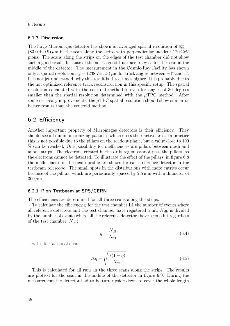
Another important property of Micromegas detectors is their efficiency. Theyshould see all minimum ionizing particles which cross their active area. In practicethis is not possible due to the pillars on the readout plane, but a value close to 100% can be reached. One possibility for inefficiencies are pillars between mesh andanode strips. The electrons created in the drift region cannot pass the pillars, sothe electrons cannot be detected. To illustrate the effect of the pillars, in figure 6.8the inefficiencies in the beam profile are shown for each reference detector in thetestbeam telescope. The small spots in the distributions with more entries occurbecause of the pillars, which are periodically spaced by 2.5mm with a diameter of300µm.
6.2.1 Pion Testbeam at SPS/CERN
The efficiencies are determined for all three scans along the strips.To calculate the efficiency η for the test chamber L1 the number of events where
all reference detectors and the test chamber have registered a hit, Nall, is dividedby the number of events where all the reference detectors have seen a hit regardlessof the test chamber, Nref :
η =Nall
Nref
(6.4)
with its statistical error
∆η =
√η (1− η)
Nref
(6.5)
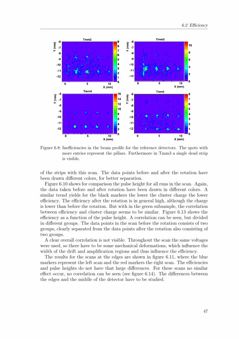
This is calculated for all runs in the three scans along the strips. The resultsare plotted for the scan in the middle of the detector in figure 6.9. During themeasurement the detector had to be turn upside down to cover the whole length
46
6.2 Efficiency
Figure 6.8: Inefficiencies in the beam profile for the reference detectors. The spots withmore entries represent the pillars. Furthermore in Tmm3 a single dead stripis visible.
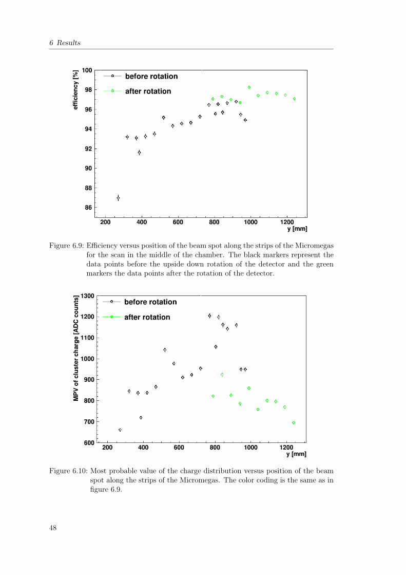
of the strips with this scan. The data points before and after the rotation havebeen drawn different colors, for better separation.Figure 6.10 shows for comparison the pulse height for all runs in the scan. Again,
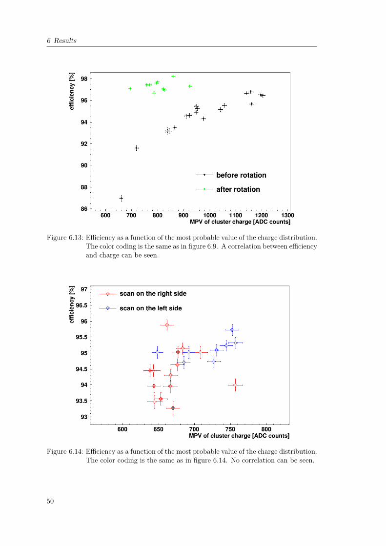
the data taken before and after rotation have been drawn in different colors. Asimilar trend yields for the black markers the lower the cluster charge the lowerefficiency. The efficiency after the rotation is in general high, although the chargeis lower than before the rotation. But with in the green subsample, the correlationbetween efficiency and cluster charge seems to be similar. Figure 6.13 shows theefficiency as a function of the pulse height. A correlation can be seen, but dividedin different groups. The data points in the scan before the rotation consists of twogroups, clearly separated from the data points after the rotation also consisting oftwo groups.A clear overall correlation is not visible. Throughout the scan the same voltages
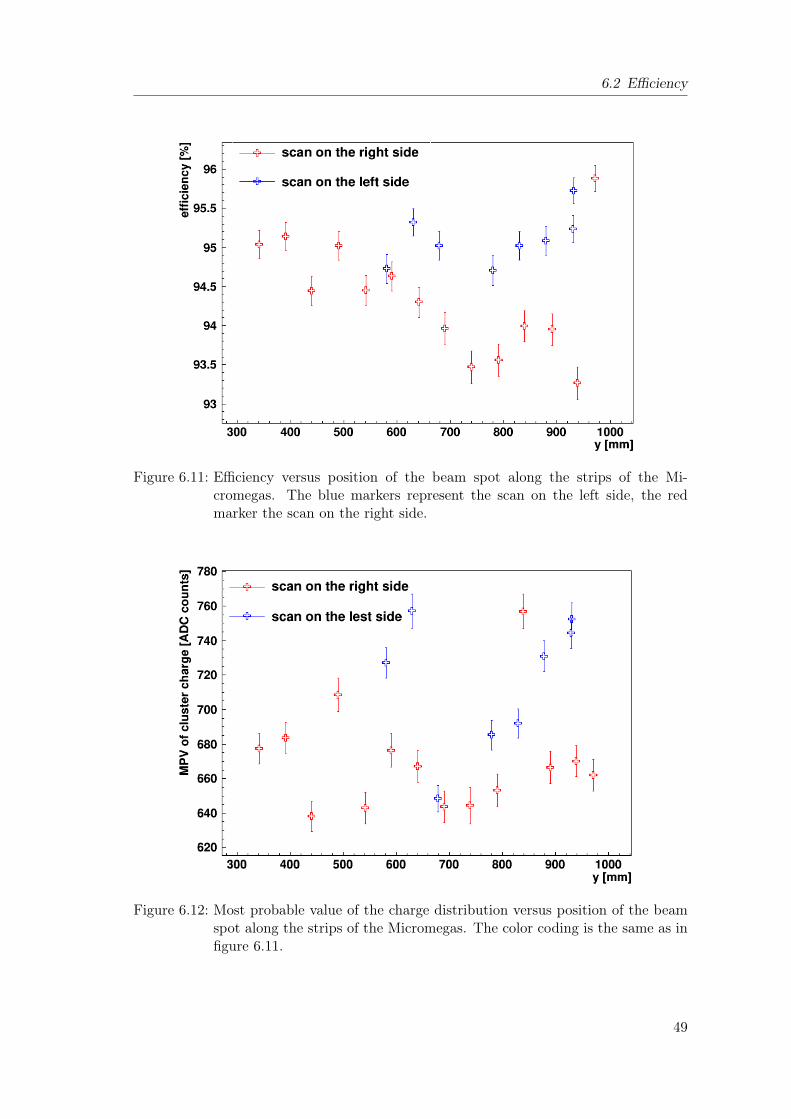
were used, so there have to be some mechanical deformations, which influence thewidth of the drift and amplification regions and thus influence the efficiency.The results for the scans at the edges are shown in figure 6.11, where the blue
markers represent the left scan and the red markers the right scan. The efficienciesand pulse heights do not have that large differences. For these scans no similareffect occur, no correlation can be seen (see figure 6.14). The differences betweenthe edges and the middle of the detector have to be studied.
47
6 Results
Figure 6.9: Efficiency versus position of the beam spot along the strips of the Micromegasfor the scan in the middle of the chamber. The black markers represent thedata points before the upside down rotation of the detector and the greenmarkers the data points after the rotation of the detector.
Figure 6.10: Most probable value of the charge distribution versus position of the beamspot along the strips of the Micromegas. The color coding is the same as infigure 6.9.
48
6.2 Efficiency
Figure 6.11: Efficiency versus position of the beam spot along the strips of the Mi-cromegas. The blue markers represent the scan on the left side, the redmarker the scan on the right side.
Figure 6.12: Most probable value of the charge distribution versus position of the beamspot along the strips of the Micromegas. The color coding is the same as infigure 6.11.
49
6 Results
Figure 6.13: Efficiency as a function of the most probable value of the charge distribution.The color coding is the same as in figure 6.9. A correlation between efficiencyand charge can be seen.
Figure 6.14: Efficiency as a function of the most probable value of the charge distribution.The color coding is the same as in figure 6.14. No correlation can be seen.
50
6.2 Efficiency
6.2.2 Cosmic-Ray Facility
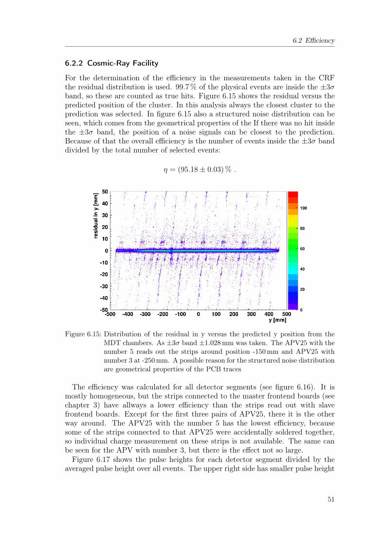
For the determination of the efficiency in the measurements taken in the CRFthe residual distribution is used. 99.7% of the physical events are inside the ±3σband, so these are counted as true hits. Figure 6.15 shows the residual versus thepredicted position of the cluster. In this analysis always the closest cluster to theprediction was selected. In figure 6.15 also a structured noise distribution can beseen, which comes from the geometrical properties of the If there was no hit insidethe ±3σ band, the position of a noise signals can be closest to the prediction.Because of that the overall efficiency is the number of events inside the ±3σ banddivided by the total number of selected events:
η = (95.18± 0.03) % .
Figure 6.15: Distribution of the residual in y versus the predicted y position from theMDT chambers. As ±3σ band ±1.028mm was taken. The APV25 with thenumber 5 reads out the strips around position -150mm and APV25 withnumber 3 at -250mm. A possible reason for the structured noise distributionare geometrical properties of the PCB traces
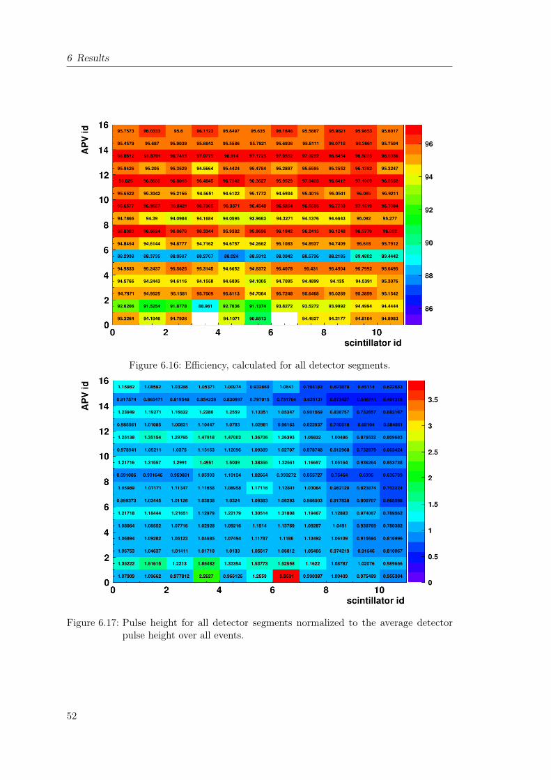
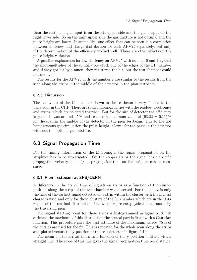
The efficiency was calculated for all detector segments (see figure 6.16). It ismostly homogeneous, but the strips connected to the master frontend boards (seechapter 3) have allways a lower efficiency than the strips read out with slavefrontend boards. Except for the first three pairs of APV25, there it is the otherway around. The APV25 with the number 5 has the lowest efficiency, becausesome of the strips connected to that APV25 were accidentally soldered together,so individual charge measurement on these strips is not available. The same canbe seen for the APV with number 3, but there is the effect not so large.Figure 6.17 shows the pulse heights for each detector segment divided by the
averaged pulse height over all events. The upper right side has smaller pulse height
51
6 Results
Figure 6.16: Efficiency, calculated for all detector segments.
Figure 6.17: Pulse height for all detector segments normalized to the average detectorpulse height over all events.
52
6.3 Signal Propagation Time
than the rest. The gas input is on the left upper side and the gas output on theright lower side. So on the right upper side the gas mixture is not optimal and thepulse height are lower. It seems like, one effect that can be seen is a correlationbetween efficiency and charge distribution for each APV25 separately, but onlyif the determination of the efficiency worked well. There are other effects on thepulse height variations.A possible explanation for low efficiency on APV25 with number 0 and 1 is, that
the photomultiplier of the scintillators stuck out of the edges of the L1 chamberand if they got hit by a muon, they registered the hit, but the test chamber couldnot see it.The results for the APV25 with the number 7 are similar to the results from the
scan along the strips in the middle of the detector in the pion testbeam.
6.2.3 Discussion
The behaviour of the L1 chamber shown in the testbeam is very similar to thebehaviour in the CRF. There are some inhomogeneities with the readout electronicsand strips, which are soldered together. But for the size of detector the efficiencyis good. It was around 95% and reached a maximum value of (98.22 ± 0.11)%for the scan in the middle of the detector in the pion testbeam. Due to the nothomogeneous gas circulation the pulse height is lower for the parts in the detectorwith not the optimal gas mixture.
6.3 Signal Propagation Time
For the timing information of the Micromegas the signal propagation on thestriplines has to be investigated. On the copper strips the signal has a specificpropagation velocity. The signal propagation time on the stripline can be mea-sured.
6.3.1 Pion Testbeam at SPS/CERN
A difference in the arrival time of signals on strips as a function of the clusterposition along the strips of the test chamber was observed. For this analysis onlythe time of the earliest signal detected on a strip within the cluster with the highestcharge is used and only for those clusters of the L1 chamber which are in the ±3σregion of the residual distribution, i.e. which represent physical hits, caused bythe traversing pion.The signal starting point for these strips is histogrammed in figure 6.18. To
estimate the maximum of this distribution the central part is fitted with a Gaussianfunction. This procedure gave the best estimate of the maximum, hereby 75% ofthe entries are used for the fit. This is repeated for the whole scan along the stripsand plotted versus the y position of the test detector in figure 6.19.The mean cluster arrival times as a function of the y position is fitted with a
straight line. The slope of this line gives the signal propagation time per distance:
53
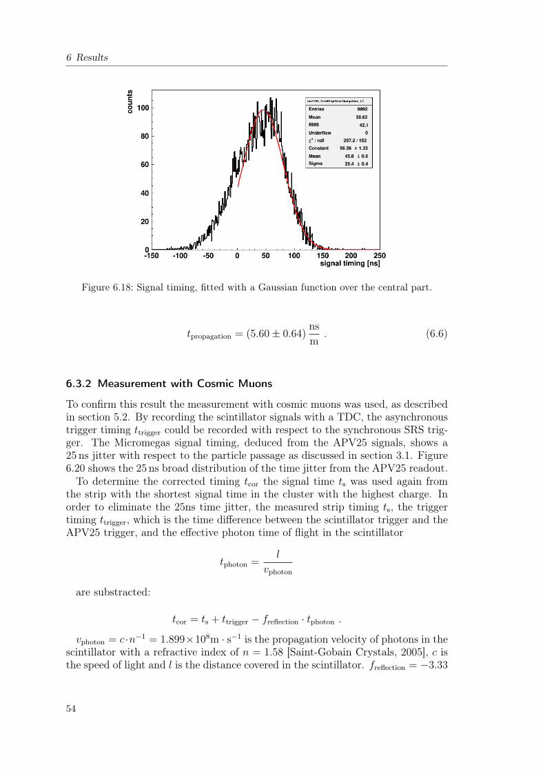
6 Results
Figure 6.18: Signal timing, fitted with a Gaussian function over the central part.
tpropagation = (5.60± 0.64)ns
m. (6.6)
6.3.2 Measurement with Cosmic Muons
To confirm this result the measurement with cosmic muons was used, as describedin section 5.2. By recording the scintillator signals with a TDC, the asynchronoustrigger timing ttrigger could be recorded with respect to the synchronous SRS trig-ger. The Micromegas signal timing, deduced from the APV25 signals, shows a25 ns jitter with respect to the particle passage as discussed in section 3.1. Figure6.20 shows the 25 ns broad distribution of the time jitter from the APV25 readout.To determine the corrected timing tcor the signal time ts was used again from
the strip with the shortest signal time in the cluster with the highest charge. Inorder to eliminate the 25ns time jitter, the measured strip timing ts, the triggertiming ttrigger, which is the time difference between the scintillator trigger and theAPV25 trigger, and the effective photon time of flight in the scintillator
tphoton =l
vphoton
are substracted:
tcor = ts + ttrigger − freflection · tphoton .
vphoton = c·n−1 = 1.899×10⁸m · s−1 is the propagation velocity of photons in thescintillator with a refractive index of n = 1.58 [Saint-Gobain Crystals, 2005], c isthe speed of light and l is the distance covered in the scintillator. freflection = −3.33
54
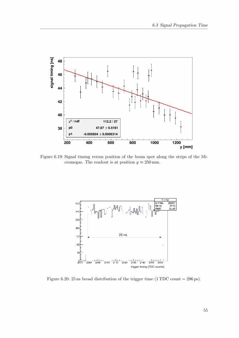
6.3 Signal Propagation Time
Figure 6.19: Signal timing versus position of the beam spot along the strips of the Mi-cromegas. The readout is at position y ≈ 250 mm.
trigger timing [TDC counts]
25 ns
Figure 6.20: 25 ns broad distribution of the trigger time (1 TDC count = 296 ps).
55

6 Results
is the correction factor of the reflections of the muons on the scintillator surfaces(see section 6.4.2).Figure 6.21 shows the values for tcor as a function of the muon hit position in
the detector, where the readout side is at position zero. Fitting this distributionwith a straight line gives for the signal propagation time:
tpropagation = (6.59± 0.57)ns
m. (6.7)
Although signal propagation time on the stripline is by about 18% higher thanthe value previously measured with pions the results from both measurementsagree within their errors. There could be a systematic error because of the 9.5 cmwide scintillators.
Figure 6.21: Signal timing as a function of the muon hit position, fitted with a straightline. The readout is at position zero.
6.3.3 Discussion
The two measured values agree within their quoted uncertainties. The aver-age from both measurements gives the mean signal propagation time of the thestriplines in resistive strip Micromegas:
tpropagation = (6.10± 0.61)ns
m.
tpropagation,lit = 0.0334√
0.48 · ε+ 0.7[ns
m
]= 5.64
ns
m, (6.8)
where ε = 4.5 is the dielectric constant of FR4 (PCB material). tpropagation,lit istaken from [Nührmann, 1994], which gives a description of the stripline with itssignal propagation time.
56
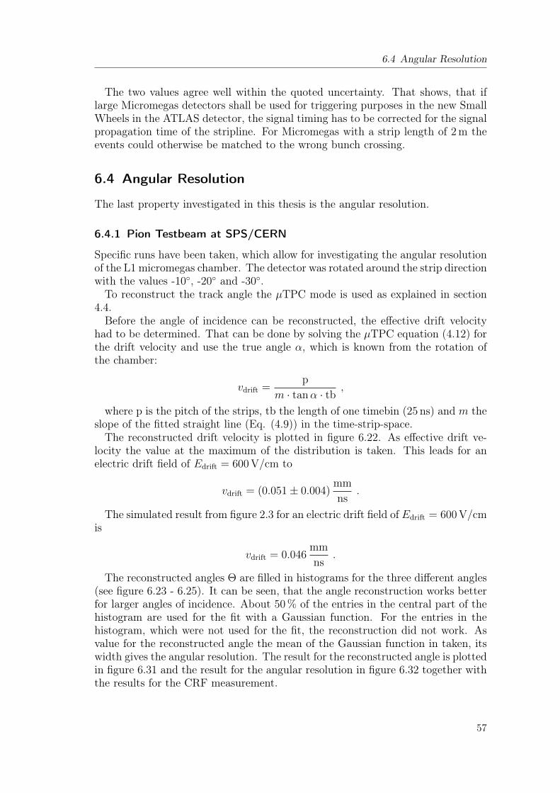
6.4 Angular Resolution
The two values agree well within the quoted uncertainty. That shows, that iflarge Micromegas detectors shall be used for triggering purposes in the new SmallWheels in the ATLAS detector, the signal timing has to be corrected for the signalpropagation time of the stripline. For Micromegas with a strip length of 2m theevents could otherwise be matched to the wrong bunch crossing.
6.4 Angular Resolution
The last property investigated in this thesis is the angular resolution.
6.4.1 Pion Testbeam at SPS/CERN
Specific runs have been taken, which allow for investigating the angular resolutionof the L1 micromegas chamber. The detector was rotated around the strip directionwith the values -10, -20 and -30.To reconstruct the track angle the µTPC mode is used as explained in section
4.4.Before the angle of incidence can be reconstructed, the effective drift velocity
had to be determined. That can be done by solving the µTPC equation (4.12) forthe drift velocity and use the true angle α, which is known from the rotation ofthe chamber:
vdrift =p
m · tanα · tb,
where p is the pitch of the strips, tb the length of one timebin (25 ns) and m theslope of the fitted straight line (Eq. (4.9)) in the time-strip-space.The reconstructed drift velocity is plotted in figure 6.22. As effective drift ve-
locity the value at the maximum of the distribution is taken. This leads for anelectric drift field of Edrift = 600 V/cm to
vdrift = (0.051± 0.004)mm
ns.
The simulated result from figure 2.3 for an electric drift field of Edrift = 600 V/cmis
vdrift = 0.046mm
ns.
The reconstructed angles Θ are filled in histograms for the three different angles(see figure 6.23 - 6.25). It can be seen, that the angle reconstruction works betterfor larger angles of incidence. About 50% of the entries in the central part of thehistogram are used for the fit with a Gaussian function. For the entries in thehistogram, which were not used for the fit, the reconstruction did not work. Asvalue for the reconstructed angle the mean of the Gaussian function in taken, itswidth gives the angular resolution. The result for the reconstructed angle is plottedin figure 6.31 and the result for the angular resolution in figure 6.32 together withthe results for the CRF measurement.
57
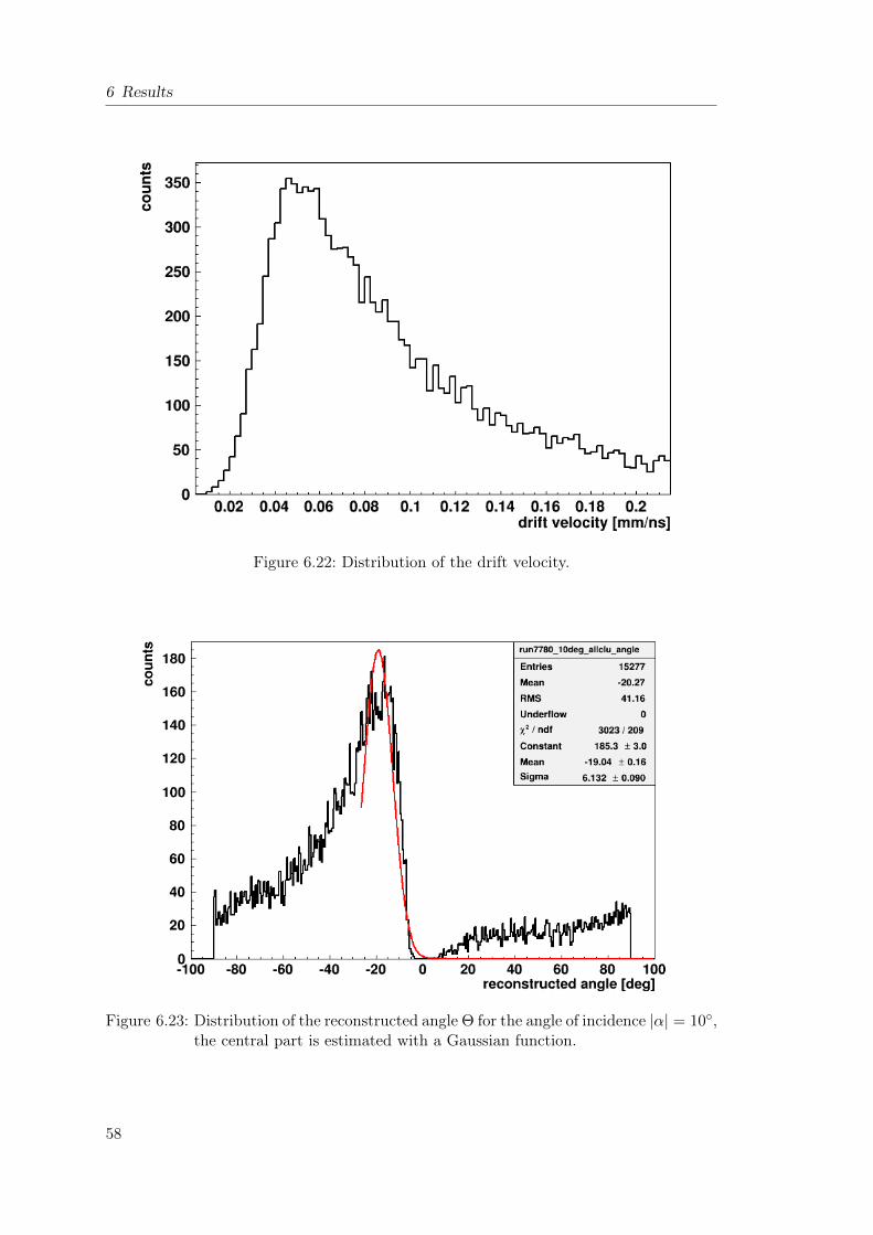
6 Results
Figure 6.22: Distribution of the drift velocity.
Figure 6.23: Distribution of the reconstructed angle Θ for the angle of incidence |α| = 10,the central part is estimated with a Gaussian function.
58
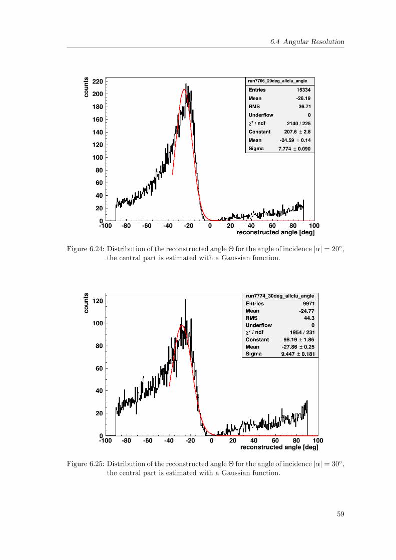
6.4 Angular Resolution
Figure 6.24: Distribution of the reconstructed angle Θ for the angle of incidence |α| = 20,the central part is estimated with a Gaussian function.
Figure 6.25: Distribution of the reconstructed angle Θ for the angle of incidence |α| = 30,the central part is estimated with a Gaussian function.
59
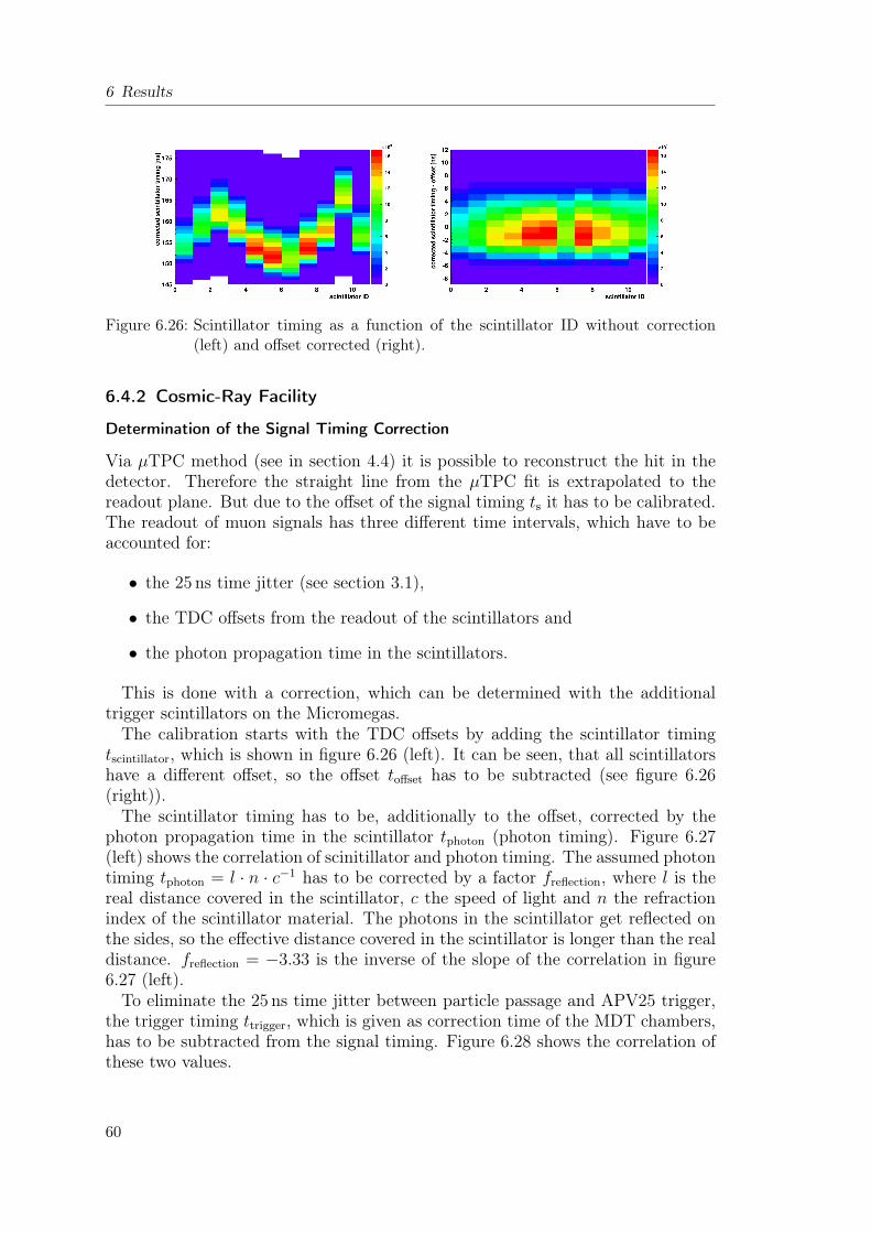
6 Results
Figure 6.26: Scintillator timing as a function of the scintillator ID without correction(left) and offset corrected (right).
6.4.2 Cosmic-Ray Facility
Determination of the Signal Timing Correction
Via µTPC method (see in section 4.4) it is possible to reconstruct the hit in thedetector. Therefore the straight line from the µTPC fit is extrapolated to thereadout plane. But due to the offset of the signal timing ts it has to be calibrated.The readout of muon signals has three different time intervals, which have to beaccounted for:
• the 25 ns time jitter (see section 3.1),
• the TDC offsets from the readout of the scintillators and
• the photon propagation time in the scintillators.
This is done with a correction, which can be determined with the additionaltrigger scintillators on the Micromegas.The calibration starts with the TDC offsets by adding the scintillator timing
tscintillator, which is shown in figure 6.26 (left). It can be seen, that all scintillatorshave a different offset, so the offset toffset has to be subtracted (see figure 6.26(right)).The scintillator timing has to be, additionally to the offset, corrected by the
photon propagation time in the scintillator tphoton (photon timing). Figure 6.27(left) shows the correlation of scinitillator and photon timing. The assumed photontiming tphoton = l · n · c−1 has to be corrected by a factor freflection, where l is thereal distance covered in the scintillator, c the speed of light and n the refractionindex of the scintillator material. The photons in the scintillator get reflected onthe sides, so the effective distance covered in the scintillator is longer than the realdistance. freflection = −3.33 is the inverse of the slope of the correlation in figure6.27 (left).To eliminate the 25 ns time jitter between particle passage and APV25 trigger,
the trigger timing ttrigger, which is given as correction time of the MDT chambers,has to be subtracted from the signal timing. Figure 6.28 shows the correlation ofthese two values.
60
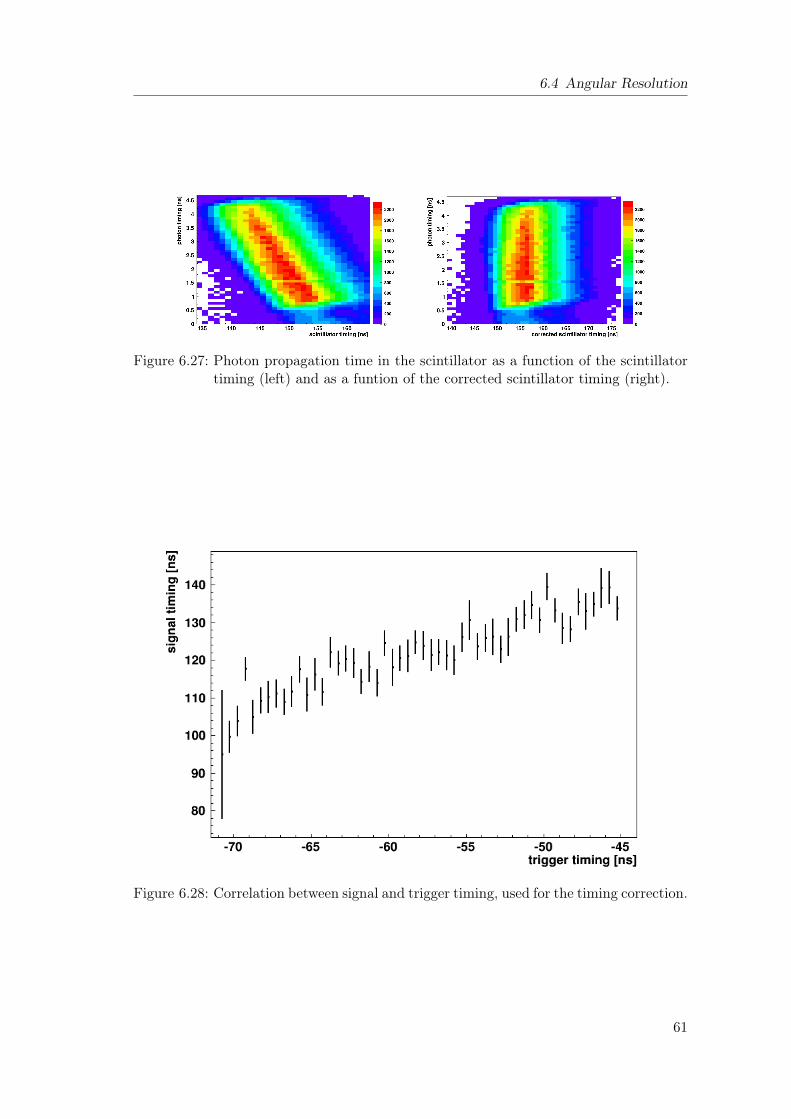
6.4 Angular Resolution
Figure 6.27: Photon propagation time in the scintillator as a function of the scintillatortiming (left) and as a funtion of the corrected scintillator timing (right).
Figure 6.28: Correlation between signal and trigger timing, used for the timing correction.
61
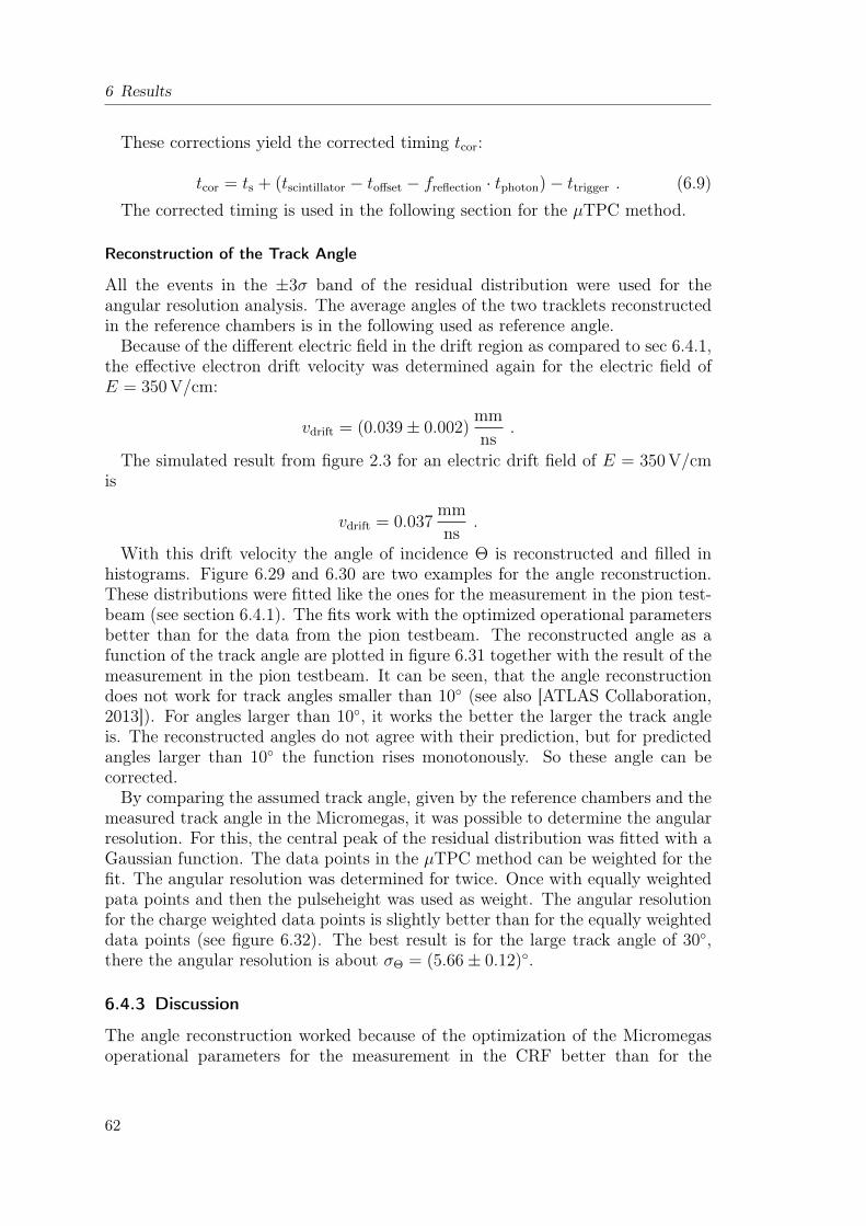
6 Results
These corrections yield the corrected timing tcor:
tcor = ts + (tscintillator − toffset − freflection · tphoton)− ttrigger . (6.9)The corrected timing is used in the following section for the µTPC method.
Reconstruction of the Track Angle
All the events in the ±3σ band of the residual distribution were used for theangular resolution analysis. The average angles of the two tracklets reconstructedin the reference chambers is in the following used as reference angle.Because of the different electric field in the drift region as compared to sec 6.4.1,
the effective electron drift velocity was determined again for the electric field ofE = 350 V/cm:
vdrift = (0.039± 0.002)mm
ns.
The simulated result from figure 2.3 for an electric drift field of E = 350 V/cmis
vdrift = 0.037mm
ns.
With this drift velocity the angle of incidence Θ is reconstructed and filled inhistograms. Figure 6.29 and 6.30 are two examples for the angle reconstruction.These distributions were fitted like the ones for the measurement in the pion test-beam (see section 6.4.1). The fits work with the optimized operational parametersbetter than for the data from the pion testbeam. The reconstructed angle as afunction of the track angle are plotted in figure 6.31 together with the result of themeasurement in the pion testbeam. It can be seen, that the angle reconstructiondoes not work for track angles smaller than 10 (see also [ATLAS Collaboration,2013]). For angles larger than 10, it works the better the larger the track angleis. The reconstructed angles do not agree with their prediction, but for predictedangles larger than 10 the function rises monotonously. So these angle can becorrected.By comparing the assumed track angle, given by the reference chambers and the
measured track angle in the Micromegas, it was possible to determine the angularresolution. For this, the central peak of the residual distribution was fitted with aGaussian function. The data points in the µTPC method can be weighted for thefit. The angular resolution was determined for twice. Once with equally weightedpata points and then the pulseheight was used as weight. The angular resolutionfor the charge weighted data points is slightly better than for the equally weighteddata points (see figure 6.32). The best result is for the large track angle of 30,there the angular resolution is about σΘ = (5.66± 0.12).
6.4.3 Discussion
The angle reconstruction worked because of the optimization of the Micromegasoperational parameters for the measurement in the CRF better than for the
62
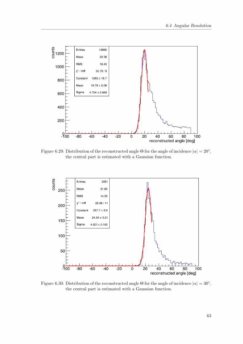
6.4 Angular Resolution
Figure 6.29: Distribution of the reconstructed angle Θ for the angle of incidence |α| = 20,the central part is estimated with a Gaussian function.
Figure 6.30: Distribution of the reconstructed angle Θ for the angle of incidence |α| = 30,the central part is estimated with a Gaussian function.
63
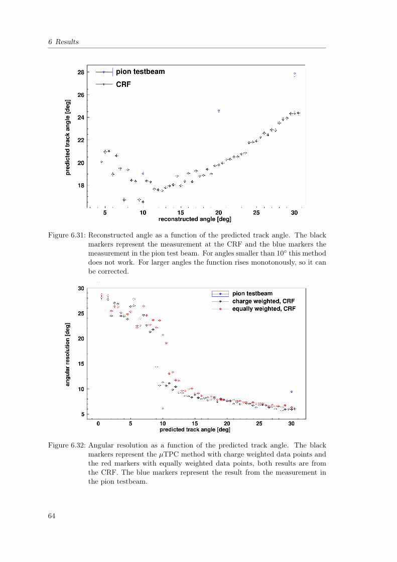
6 Results
Figure 6.31: Reconstructed angle as a function of the predicted track angle. The blackmarkers represent the measurement at the CRF and the blue markers themeasurement in the pion test beam. For angles smaller than 10 this methoddoes not work. For larger angles the function rises monotonously, so it canbe corrected.
Figure 6.32: Angular resolution as a function of the predicted track angle. The blackmarkers represent the µTPC method with charge weighted data points andthe red markers with equally weighted data points, both results are fromthe CRF. The blue markers represent the result from the measurement inthe pion testbeam.
64
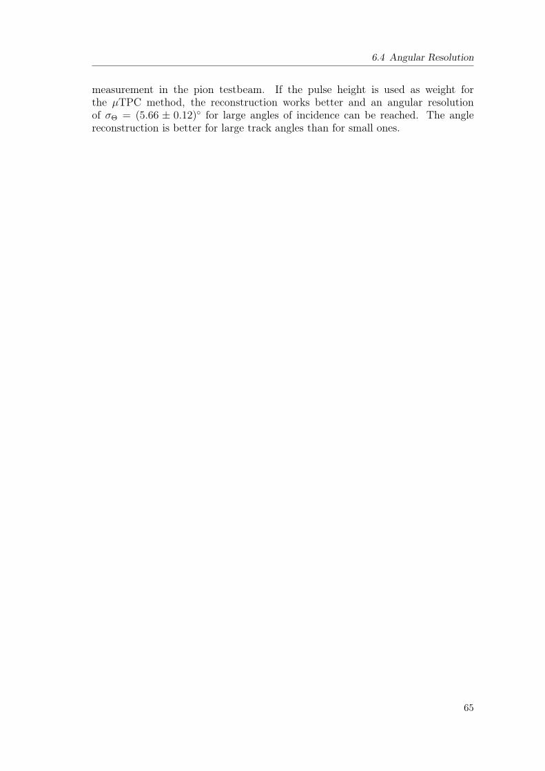
6.4 Angular Resolution
measurement in the pion testbeam. If the pulse height is used as weight forthe µTPC method, the reconstruction works better and an angular resolutionof σΘ = (5.66 ± 0.12) for large angles of incidence can be reached. The anglereconstruction is better for large track angles than for small ones.
65
7 Summary and Outlook
A 1m2 large Micromegas detector was investigated in three measurement cam-paigns. First, in a 120GeV pion testbeam at SPS/CERN, where the beam spothad a area of about 1 cm2 and, due to the high pion momentum multiple scat-tering. Then a dedicated measurement with cosmic muons in Garching/Munichis presented investigating the signal propagation time on readout strips with im-proved timing capabilities. Finally, the overall homogeneity with respect to pulseheight, efficiency, mechanical accuracy and spatial resolution was investigated inthe Cosmic-Ray Facility, which has a good track prediction of about 40µm. Inwhich the Micromegas detector could be installed on an aluminium support stage.Computer programs were developed to analyze the data from the three measure-ment and to merge different data streams.The large Micromegas detector has shown an averaged spatial resolution of σsr =
(83.0 ± 0.9)µm in the scan along the strips with perpendicular incident 120GeVpions. The scans along the strips on the edges of the test chamber did not showsuch a good result, because of the slightly degraded track accuracy as comparedto the scan in the middle of the detector. The results σsr = (238.7±1.3)µm in theCosmic-Ray were not as good as for the pion testbeam, but that is not entirelyunderstood. It is probably due to the not optimized reference track reconstructionin this specific setup. How the temperature dependence and the cuts on the MDTtrack influences the residual distribution, has to be studied. The spatial resolutioncalculated with the centroid method is even for angles of 30 degrees smaller thanthe spatial resolution determined with the µTPC method. After some necessaryimprovements, the µTPC spatial resolution should show similar or better resultsthan the centroid method.The behaviour of the L1 chamber demonstrated in the pion testbeam is very
similar to the behaviour in the CRF. There are some pulse height and efficiencyinhomogeneities due to the differing behavior of master and slave APV25 readoutelectronics and noisy regions in the detector, which are created by badly solderedor interconnected readout strips. But nevertheless for the size of detector theoverall efficiency of 95% is very satisfactory. It reached a maximum value of(98.22 ± 0.11)% for the scan in the middle of the detector in the pion testbeam.Due to the not homogeneous gas circulation within the detector the pulse heightis lower within the detector regions with the not optimal gas mixture. Althoughthe efficiency behavior seems to be complex correlation between pulse height andefficiency has been observed.The analysis for the signal propagation time on the readout strips led to two
consistent results. With 120GeV pions, a signal propagation time of tpropagation =(5.60±0.64) ns ·m−1 has been measured. With cosmic muons we observe a propa-gation time of tpropagation = (6.59±0.57) ns ·m−1. Both values are equivalent within
66
their respective uncertainty. The averaged result tpropagation = (6.10±0.61) ns ·m−1
agrees well with the literature value of tpropagation = 5.64 ns ·m−1. That shows, thatif large Micromegas detectors is to be used for triggering purposes in the new SmallWheels in the ATLAS detector, the signal timing has to be corrected for the signalpropagation time time of the stripline. For Micromegas with a strip length of 2mthe events could otherwise be matched to the wrong bunch crossing.It could be demonstrated, the with the large L1 Micromegas, a reconstruction
of the track inclination is possible in a single plane. The performance in the CRFhas been better than in the high-energy pion test beam, because of the explicitoptimization of the Micromegas operational parameters. If the single strip pulseheight is used as weight for the µTPC method, the reconstruction improves and anangular resolution of σΘ(5.66± 0.12) for large angles of incidence can be reached.As expected the angle reconstruction is better for large track angles than for smallones.Overall the detector showed a good performance.
67
Bibliography
[ALICE Collaboration, 2008] ALICE Collaboration (2008). The ALICE Experi-ment at the CERN LHC. JINST, 3.
[Andriamonje et al., 2004] Andriamonje, S., Aune, S., Dafni, T., Fanourakis, G.,Ferrer Ribas, E., Fischer, H., Franz, J., Geralis, T., Giganon, A., Giomataris, Y.,Heinsius, F., Königsmann, K., Papaevangelou, T., and Zachariadou, K. (2004).A Micromegas detector for Athe CAST experiment. Nucl.Instrum.Meth. A,518(1-2):252–255.
[ATLAS Collaboration, 2008] ATLAS Collaboration (2008). The ATLAS Experi-ment at the CERN Large Hadron Collider. JINST, 3.
[ATLAS Collaboration, 2013] ATLAS Collaboration (2013). New Small WheelTechnical Design Report. (May).
[Beringer, J. et. al. (Particle Data Group), 2012] Beringer, J. et. al. (ParticleData Group) (2012). Review of Particle Physics. Physical Review D,86(1):010001.
[Bortfeldt, 2013] Bortfeldt, J. (2013). Private conversation.
[Bortfeldt et al., 2012] Bortfeldt, J., Biebel, O., Heereman, D., and Hertenberger,R. (2012). Development of a High-Resolution Muon Tracking System Based onMicropattern Detectors. Nuclear Science, IEEE Transactions on, 59(4):1252–1258.
[Bortfeldt et al., 2013] Bortfeldt, J., Biebel, O., Hertenberger, R., Lösel, P., Moll,S., Müller, R., Ruschke, A., and Zibell, A. (2013). Floating Strip MicromegasDetector. poster, presented at 13th Vienna Conferece on Instrumentation -VCI2013.
[Carnegie et al., 2005] Carnegie, R. K., Dixit, M. S., Dubeau, J., and Karlen, D.(2005). Resolution studies of cosmic-ray tracks in a TPC with GEM readout.Nucl.Instrum.Meth. A, 538(February 2008):372–383.
[CERN website, 2008] CERN website (2008). Big Science.http://bigscience.web.cern.ch, (last visited 25.9.2013).
[CMS Collaboration, 2008] CMS Collaboration (2008). The CMS Experiment atthe CERN LHC. JINST, 3.
[Dubbert et al., 2002] Dubbert, J., Binder, M., Hertenberger, R., Elmsheuser, J.,Kortner, O., Rauscher, F., Rykaczewski, M., Sahr, O., Schaile, D., Staude, A.,
68
Bibliography
Steffens, H., Stiller, W., Zhuravlov, V., and Zupančič, C. (2002). First Resultsfrom the Cosmic-Ray Test-Facility at LMU Munich.
[Garfield, 2013] Garfield (2013). http://garfield.web.cern.ch/garfield/.
[Giomataris et al., 1996] Giomataris, Y., Rebourgeard, P., Robert, J. P., andCharpak, G. (1996). MICROMEGAS : a high-granularity position-sensitivedetector for high particle-flux environments. Nucl.Instrum.Meth. A, 376:29–35.
[Groom et al., 2001] Groom, D. E., Mokhov, N. V., and Striganov, S. I. (2001).Muon Stopping Power and Range Tables 10Mev - 100TeV. Atomic Dta andNulear Data Tables, 78(2):183–156.
[Horvat, 2005] Horvat, S. (2005). Study of the Higgs Discovery Potential in theProcess pp → H → 4µ. Dissertation (Zagreb University).
[Jones, 2001] Jones, L. (2001). APV25-S1 User Guide. (September):1–20.
[Leo, 1994] Leo, W. R. (1994). Techniques for Nulear and Particle Physics Exper-iments. Springer, second edition.
[LHCb Collaboration, 2008] LHCb Collaboration (2008). The LHCb Detector atthe LHC. JINST, 3.
[Martoiu et al., 2011] Martoiu, S., Muller, H., and Toledo, J. (2011). Front-endelectronics for the Scalable Readout System of RD51. Nuclear Science Sympo-sium and Medical Imaging Conference (NSS/MIC), pages 2036–2038.
[Nikolopoulos et al., 2009] Nikolopoulos, K., Alexopoulos, T., Altintas, A. A.,Alviggi, M., Arik, M., Cetin, S. A., Chernyatine, V., Cheu, E., Volpe, D. D.,Dris, M., Fassouliotis, D., Gazis, E. N., Giordano, R., Gratchev, V., Guan, L.,Iengo, P., Ioannou, P., Li, C., Johns, K., Kaushik, V., Khodinov, A., Kourk-oumelis, C., Maltezos, S., Mermigka, K., MÃijller, H., Park, W., Persembe, S.,Petridou, C., Petti, R., Polychronakos, V., Purohit, M. V., Sampsonidis, D.,Sekhniaidze, G., Shao, M., Sun, Y. J., Tsipolitis, G., Veenhof, R., Wang, X. L.,Wotschack, J., Wu, S. X., Zhao, T., and Zhao, Z. G. (2009). The ATLAS muonMicromegas R&D project: towards large-size chambers for the s-LHC. Journalof Instrumentation, 4(12):P12015.
[Nührmann, 1994] Nührmann, D. (1994). Das komplette Werkbuch Elektronik,Band 3&4. Franzis’.
[Nygren and Marx, 1978] Nygren, D. R. and Marx, J. N. (1978). The Time Pro-jection Chamber. Physics Today, (October):46.
[Panasonic Corporation, 2013] Panasonic Corporation (2013). P5K, P5KSSeries - For board-to-board Narrow pitch connectors (0.5mm pitch).http://pewa.panasonic.com/assets/pcsd/catalog/p5k-catalog.pdf.
[Placidi et al., 2000] Placidi, P., Marchioro, A., and Moreira, P. (2000). CMSTracker PLL Reference Manual. CERN - EP/MIC, Geneva Switzerland.
69
Bibliography
[Platchkov et al., 2003] Platchkov, S., Abbon, P., Ball, J., Bedfer, Y., Bernet, C.,Delagnes, E., Giganon, a., Kunne, F., Le Goff, J.-M., Magnon, a., Marchand,C., Neyret, D., Pereira, H., Rebourgeard, P., and Thers, D. (2003). A large sizeMICROMEGAS detector for the COMPASS experiment at CERN. 2002 IEEENuclear Science Symposium Conference Record, 1:292–296.
[Rauscher, 2005] Rauscher, F. (2005). Untersuchung des Verhaltens vonDriftrohren bei staker γ Bestrahlung sowie Vermessung von Driftrohrkammernmit Hilfe von Myonen der kosmischen Höhenstrahlung. Dissertation (LMU Mu-nich), pages 75–90.
[Saint-Gobain Crystals, 2005] Saint-Gobain Crystals (2005). Premium PlasticScintillators. Data Sheet.
[Thomson, A. C. et. al., 2009] Thomson, A. C. et. al. (2009). X-RAY DATABOOKLET. LBNL University of California.
[Toledo et al., 2011] Toledo, J., Muller, H., Esteve, R., MonzÃş, J. M., Tarazona,A., and Martoiu, S. (2011). The front-end concentrator card for the rd51 scalablereadout system. Journal of Instrumentation, 6(11):C11028.
[Zibell, 2013] Zibell, A. (2013). High Background Rate Investigation on smallMonitored Drift Tubes and Development of a Readout System for Micromegaswith SRS. Dissertation in preparation (LMU Munich).
70

Acknowledgments
Ich möchte folgenden Personen danken:
• Prof. Dr. Otmar Biebel für die Möglichkeit diese Arbeit am Lehrstuhl fürexperimentelle Teilchenphysik zu schreiben.
• Dr. Ralf Hertenberger für die herausragende Betreuung und die Unter-stützung bei allen Messungen.
• Prof. Dr. Dorothee Schaile für das gute Arbeitsklima an ihrem Lehrstuhl.
• Der MAMMA collaboration für die zur Verfügung Stellung des MicromegasDetektors.
• Jona Bortfeldt für die hervoragende Hilfe, immer wenn ich sie gebraucht habe,und die vielen guten Ideen.
• Dr. Felix Rauscher und Andre Zibell für die Hilfe beim Auslesen der Detek-toren.
• Der ganzen Hardware Gruppe, weil es echt Spaß gemacht hat.
• Und meiner Familie für die seelische und materielle Unterstützung.


Selbstständigkeitserklärung
Hiermit erkläre ich, dass ich die vorliegende Arbeit selbstständig angefertigt undkeine anderen als die angegebenen Quellen und Hilfsmittel benutzt habe.
München, den 2.10.2013