PHYSICAL REVIEW B 85, 245414 (2012)

Master equation approach of classical noise in intersubband detectors

A. Delga,1 M. Carras,2 V. Trinite,2 V. Gueriaux,2 L. Doyennette,1 A. Nedelcu,2 H. Schneider,3 and V. Berger1

1Univ Paris Diderot, Sorbonne Paris Cite, Laboratoire Materiaux et Phenomenes Quantiques, CNRS-UMR 7162, 10 rue Alice Domon etLeonie Duquet, 75205 Paris Cedex 13, France

2Alcatel Thales 3-5 lab, Campus Polytechnique, 1 Avenue Augustin Fresnel, 91767 Palaiseau, France3Helmholtz-Zentrum Dresden-Rossendorf (HZDR), P.O. Box 51 01 19, 01314 Dresden, Germany(Received 24 February 2012; revised manuscript received 10 May 2012; published 7 June 2012)

Electronic transport in intersubband detectors is investigated theoretically and experimentally. Within theframework of inter–Wannier-Stark levels electron scattering, consistent dark current and low-frequency noiseexpressions are obtained through the resolution of the two first moments of a master equation for classical particles.In particular, the formulation of noise bridges over the vision of uncorrelated Johnson and shot contributions.Theoretical predictions are compared to measurements for five quantum well detectors, either photovoltaic orphotoconductive, whose detection wavelength span from 8 µm to 17 µm. Quantitative agreement with experimentis found for a broad range of biases and temperatures. Correlation effects are discussed and proven to eitherreduce or enhance the noise.

DOI: 10.1103/PhysRevB.85.245414 PACS number(s): 73.50.Td, 85.60.Gz, 73.63.−b

I. INTRODUCTION

Electronic noise is the black sheep of intersubband devicephysics, tedious to measure experimentally and complex tointerpret theoretically. As a result insightful predictive modelsare scarce, and noise remains most of the time an empiricalquantity. However, it constitutes a fundamental limitation to in-tersubband device performances, and is also interesting per se,as it gives access to electronic transport mechanisms that arenot visible in average current investigations alone.

In solid state devices, the noise measured at the outputis generated by many different sources.1 The noise spectraldensity (NSD) SI , square of the measured noise current,usually comprises several terms. First, at low frequencies 1/fnoise is generally attributed to defect-induced fluctuations ofthe number of carriers by trapping and detrapping.2 However,it is most of the time negligible in intersubband detectors.Second, at equilibrium and nonzero temperature T , thermalagitation causes the electronic population to fluctuate awayfrom its thermodynamic average which is the Fermi-Dirac dis-tribution. The Johnson-Nyquist or thermal noise3 is related tothe conductance G of the device by the fluctuation-dissipationtheorem SI = 4kBT G. Third, the quantization of the electroniccharge e gives rise to nonequilibrium shot noise. Be it at asample contact (emission of an electron by the cathode), ina quantum well bound state (generation-recombination of acarrier) or because of a scattering process (e.g., diffusion by animpurity), any random event breaking the ballistic character ofelectron transport creates a noise that scales with the current I :SI = 2eFI . F is the Fano factor which compares the shot noiseto the Poisson value for classical particles.4 Characteristicscattering times governing the transport can be studied throughthe analysis of the shot noise spectrum.

Investigations on noise in intersubband detectors have firstbeen performed on quantum well infrared photodetectors(QWIPs).5,6 The zero-frequency noise is dominated by thermalfluctuations at equilibrium and by generation-recombination(GR) processes under standard operation conditions. Johnsonnoise and GR-shot noise are considered as independent sourcesand their contributions are quadratically added. Two mainproblems arise from such a description. Conceptually, the

macroscopic vision of independent noise sources is question-able, since on a microscopic scale scattering and thermalfluctuations are intimately correlated. Indeed, at nonzerotemperatures electrons can be scattered in a band of severalkBT around the Fermi energy precisely because the Fermi-Dirac distribution is not sharp. The other way around, thefluctuations out of the thermodynamic average are inducedby scattering. From a device point of view, the GR noisedepends on the so-called capture probability which is difficultto predict theoretically. In these structures noise has to bemeasured experimentally, which hinders quantum engineeringand performances optimization.

More recently, photovoltaic intersubband detectors7,8 havebeen developed. These devices work near equilibrium, whereshot and thermal noises crossover and cannot be consideredindependent. In the meantime, the understanding of transportin intersubband devices has improved greatly,9–12 along withthe development of quantum cascade lasers (QCLs). Whilecurrent is now calculated with good accuracy in midinfraredintersubband devices, noise predictions have yet to benefitfrom such conceptual progress.

The aim of the present work is to propose a unified for-mulation of noise in intersubband detectors that goes beyondthe description of uncorrelated thermal and shot contributions,and reproduces both near and far from equilibrium behaviorsas well as the crossover regime. We show that within theframework of a well-established intersubband hopping modelof current,9,13 noise can be calculated consistently withoutany additional error. Some of the ideas presented here havebeen around in the mesoscopic conductors community whereshot noise has been a subject of great interest for years.14 Inparticular, the thermal-shot crossover has been shown in manyclassical and quantum systems where shot noise formulationshad a Johnson limit at equilibrium.15,16

This paper is organized as follows. In Sec. II a masterequation approach for electronic transport is developed andapplied to current and shot noise calculations. Emphasis isput on deriving analytical expressions as straightforwardly aspossible. Discussion of the physics is postponed to Sec. III,where the theoretical results are compared to experimental

245414-11098-0121/2012/85(24)/245414(10) ©2012 American Physical Society

A. DELGA et al. PHYSICAL REVIEW B 85, 245414 (2012)

measurements on four different intersubband detectors: twoquantum cascade detectors (QCDs) detecting at 8 µm17

(QCD8) and 15 µm18 (QCD15), two photovoltaic QWIPs (pv-QWIPs) detecting at 10 µm,8 and one photoconductive QWIP(pc-QWIP) detecting at 17 µm.13 They all consist in a period-ical stacking of an optically active quantum well and an ex-traction region. In QWIPs the photoelectrons drift through thecontinuum of levels over the barriers, while in QCDs they flowthrough a cascade of levels bound in the quantum wells. Thedevice parameters are detailed in the corresponding references.

II. THEORY

A. Master equation approach of electronic transportin intersubband heterostructures

Electronic transport in intersubband heterostructures can bedescribed within the framework of inter–Wannier-Stark levelshopping. Epitaxial layers form quantum wells in the growth(z) direction, while in-plane transport is well described byfree-electron motion within the effective mass approximation.We are interested in the transport along the z direction,where each level bound in the quantum wells is associ-ated to a two-dimensional parabolic subband. The Wannier-Stark eigenstates are computed by solving the self-consistentSchrodinger-Poisson system. In this basis, electrons go fromone bound subband to another through scattering. It has beenproven effective for QWIPs to extend the two-dimensional(2D) model of bound subbands to the three-dimensional (3D)quasicontinuum above the barriers, since in these structures thebottleneck for transport is precisely the 2D-3D interaction.13

Contrary to phase-coherent systems, in intersubband detec-tors strong intrasubband scattering leads to decoherence. Withregard to the transport perpendicular to the layers, in-planetransport is ruled by relaxation times that are shorter.19 Conse-quently it proves reasonable and very effective to suppose thatthe subbands reach a quasithermal equilibrium on a muchfaster time scale than the intersubband transport. For thequasicontinuum levels such a physical assumption is less clear,and the model will find a justification a posteriori through itsprediction accuracy. The crucial hypothesis of intrasubbandthermalization enables us to derive a master equation forintersubband electronic transport, and in particular to calculatecurrent and noise.

A heterostructure with thermalized subbands can be viewedas an assembly of reservoirs stochastically exchanging elec-trons. The aim of this section is to determine the fluctuationsnear a steady state. More details on the subsequent derivationsare available in Ref. 20. Electronic transport is a Markovprocess where decoherence stands for the loss of memory. Therandom variable is the vector n of the population densities.Each component ni of n represents the population density ofone subband. As intersubband detectors are usually composedof many periods, it is fruitful to consider one period with rsubbands and apply periodic conditions. So the phase spaceis of dimension r . To avoid terminology confusions, we willhenceforth refer to electronic levels or subbands, while theterm states will be reserved to the statistical configurationsn. A stationary Markov process is entirely determined by theconditional probability p (n,t + !t |n0) that the populationsare in state n at time t + !t , while they were in state n0 at

t = 0. The evolution of this probability is ruled by the so-calledChapman-Kolmogorov-Smoluchovski (CKS) equation, whichstates that the way from n0 to n is obtained by averaging overall the possible configuration n′ at intermediate time:

p(n,t + !t |n0) =∫

dn′p(n,!t |n′)p(n′,t |n0) (1)

for all t,!t ! 0. Transitions between subbands are caused byscattering calculated using Fermi’s golden rule, which is basi-cally a linearization of transport mechanisms for small times. Itis justified by the fact that dephasing happens very quickly withregard to intersubband scattering or tunneling, and is consistentwith the assumption of intrasubband thermalization:

p(n,!t |n′) = δn,n′ (1 − #n!t) + !twn′n, (2)

where wn′n is the transition probability from n′ to n per timeunit, and #n the total rate out of state n: #n =

∫dn′wnn′ . The

probability p(n,t) to be in state n at time t is given by inte-grating over the initial conditions: p(n,t) =

∫dn0p (n,t |n0).

A similar integration of Eq. (1) gives the master equationgoverning its evolution:

dp(n,t)dt

= −#np(n,t) +∫

dn′wn′np(n′,t). (3)

It is formally a continuity equation for the probabilitydistribution p(n,t).

Bluntly solving the master equation may be possible inmesoscopic systems with a small phase space, but proves tobe very hard here. It is actually unnecessary: only some ofits moments are relevant. The first moment of this equationgives the mean value of the current, while the second momentis related to the noise. Higher moments can give some moreinsight into the nonlinear dynamics, but are beyond the scopeof this work. The master equation can be analytically solvedif the statistical distribution p(n,t) is assumed Gaussian.However, it is not the chosen method here. Fermi’s goldenrule guarantees that all the moments of Eq. (1) are linear in!t . In particular, for the two first moments,

∫dn p(n,!t |n′)(n − n′) = A(n′)!t, (4)

∫dn p(n,!t |n′)(n − n′)†(n − n′) = 2D(n′)!t, (5)

where A is the drift vector, D the diffusion matrix, and † standsfor the transpose of a vector. All higher moments are linear.If they were superlinear (∝ !tγ , with γ > 1), the masterequation (3) could be reduced to the Fokker-Planck equation.Using the linearity with regard to time, one gets

A(n′) =∫

dn (n − n′)wn′n,

(6)

D = 12

∫dn (n − n′)†(n − n′)wn′n.

Even if the theory is valid for nonquantized charges, from thispoint onward we will restrict ourselves to quantized chargesand switch to integer representation of n. In full generality wecould proceed further with either fermions, bosons, or classicalparticles. Fermions are the natural choice, and subbandsstatistics should be described by Fermi-Dirac distributions.

245414-2

MASTER EQUATION APPROACH OF CLASSICAL NOISE . . . PHYSICAL REVIEW B 85, 245414 (2012)

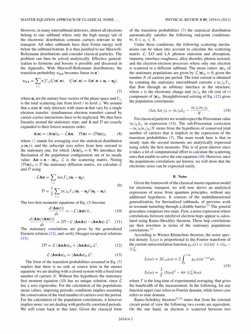
However, in many intersubband detectors, almost all electronsbelong to one subband where only the high energy tail ofthe electronic distribution contains carriers relevant to thetransport. All other subbands have their Fermi energy wellbelow the subband bottom. It is thus justified to use Maxwell-Boltzmann distributions and consider classical particles. Theproblem can then be solved analytically. Effective general-ization to fermions and bosons is possible and discussed inthe Appendix. With Maxwell-Boltzmann distributions, thetransition probability wn′n becomes linear in n′:

wn′n =∑

i,j

n′i#ijδ

ji (n′,n), δ

ji (n′,n) = δ(n′,n + ui − uj),

(7)

where ui are the unitary base vectors of the phase space and #ij

is the total scattering rate from level i to level j . We assumethat a state n′ only interacts with states n that vary by a singleelectron transfer: simultaneous electron transfers caused bycarrier-carrier interactions have to be neglected. We thus havelinearity around the stationary state, and A and D are exactlyexpanded to their lowest nonzero order:

A(n) = ⟨A(n)⟩0 − L!n, D(n) = ⟨D(n)⟩0, (8)

where ⟨ ⟩ stands for averaging over the statistical distributionp (n,t), and the subscript zero refers from here onward tothe stationary one, for which ⟨A(n)⟩0 = 0. We introduce thefluctuation of the population configuration out of its steadyvalue: !n = n − ⟨n⟩0. L is the scattering matrix. Noting⟨D(n)⟩0 = D the stationary diffusion matrix, we calculate Land D using

L!n =∑

i,j

!ni#ij (ui − uj),

(9)D = 1

2

∑

i,j

⟨ni⟩0 #ij (ui − uj)†(uj − ui).

The two first moments equations of Eq. (3) becomed⟨!n(t)⟩

dt= −L ⟨!n(t)⟩ , (10)

d⟨!n(t)!n(t)⟩dt

= 2D−L ⟨!n!n⟩−⟨!n!n⟩L†. (11)

The stationary correlations are given by the generalizedEinstein relation (12), and verify Onsager reciprocal relations(13):

2D = L ⟨!n!n⟩0 + ⟨!n!n⟩0 L†, (12)

L ⟨!n!n⟩0 = ⟨!n!n⟩0 L†. (13)

The form of the transition probabilities assumed in Eq. (7)implies that there is no sink or source term in the masterequation: we are dealing with a closed system with a fixed totalnumber of carriers N . Without this hypothesis the stationaryfirst moment equation (10) has no unique solution, since Lhas a zero eigenvalue. For the calculation of the populationsmean values, imposing periodic conditions implies assumingthe conservation of the total number of carriers over the period.For the calculation of the population correlations, it howeverimplies more: we are dealing with perfectly correlated periods.We will come back to this later. Given the classical form

of the transition probabilities (7) the statistical distributionautomatically satisfies the following end-point conditions:∀i, 0 " ni " N .

Under these conditions, the following scattering mecha-nisms can be taken into account to calculate the scatteringmatrix L: LO and LA phonon emission and absorption,impurity, interface roughness, alloy disorder, photon assisted,and the electron-electron processes where only one electronis scattered in a different subband. The mean values ⟨n⟩0 ofthe stationary populations are given by L ⟨n⟩0 = 0, given thenumber N of carriers per period. The total current is obtainedby counting the stationary intersubband currents e ⟨ni⟩0 #ij

that flow through an arbitrary interface in the structure,where e is the electronic charge and ⟨ni⟩0 the ith (out of r)component of ⟨n⟩0. Straightforward solving of Eq. (12) givesthe population correlations:

⟨!ni!nj ⟩0 = ⟨ni⟩0δij − ⟨ni⟩0⟨nj ⟩0

N. (14)

For classical particles we would expect the Poissonian value⟨ni⟩0 δij in expression (14). The sub-Poissonian correction−⟨ni⟩0⟨nj ⟩0/N stems from the hypothesis of conserved totalnumber of carriers that is implicit in the expression of thetransition probabilities (7). The main result here is that insteady state the second moments are analytically expressedusing solely the first moments. This is of great interest sinceit takes a lot of computational effort to calculate the scatteringrates that enable to solve the rate equation (10). However, oncethe populations correlations are known, we will show that theelectronic noise can be expressed easily.

B. Noise

Given the framework of the classical master equation modelfor electronic transport, we will now derive an analyticalexpression of noise from quantum principles, without anyadditional hypothesis. It consists of the multidimensionalgeneralization, for thermalized subbands, of previous workin resonant tunneling through a double barrier.21 The generalprocedure comprises two steps. First, a noise expression wherecorrelations between interlevel electron hops appear is calcu-lated using Ramo-Shockley theorem. These hop correlationsare then rewritten in terms of the stationary populationscorrelations.22

According to Wiener-Khintchine theorem, the noise spec-tral density SI (ω) is proportional to the Fourier transform ofthe current autocorrelation function gII (s) = ⟨i(t)i(t + s)⟩0 −⟨i⟩2

0,

SI (ω) = 2CII (ω) = 2∫ +∞

0gII (s)e−iωsds,

(15)

SI (ω) = 2T

|I (ω)|2 − 4π ⟨i⟩20 δ(ω),

where T is the long time of experimental averaging, that givesthe bandwidth of the measurement. In the following, for anyfunction upper case refers to Fourier domain, while lower caserefers to time domain.

Ramo-Schokley theorem23,24 states that from the externalcircuit point of view the following two events are equivalent.On the one hand, an electron is scattered between two

245414-3

A. DELGA et al. PHYSICAL REVIEW B 85, 245414 (2012)

quantum levels whose barycenters are separated by a distancel. On the other hand, an effective charge el/L is transferredballistically between the two electrodes separated by a distanceof L. We call zi the barycenter of the wave function ofthe ith subband and Lper the length of the period. For thescattering of an electron from level i to j the ratio betweeneffective and electron charge will have the algebraic valueαij = (zj − zi)/Lper. Ramo-Shockley theorem is often usedwith capacitances rather than barycenters, which does notchange the point here. The instantaneous value of the currentper surface unit is

i(t) = e∑

i,j

αij

∑

p

f(t − t ijp

), (16)

where p indexes all the times tijp of hops from level i to j during

the time of experiment T . f (t) gives the shape of the currentpulse in the external circuit. Its exact form is unknown but itis reasonable to suppose that the pulse length is considerablyshorter than the electronic times that will rule the noise. Sothe Fourier transform of f is given by F (ω) = 1 for all thefrequencies at stake.

The current Fourier transform and its square modulus aretherefore

I (ω) = eF (ω)

{∑

i,j

αij

∑

p

exp(iωt ijp )

}

, (17)

|I (ω)|2 = e2

{∑

i,j,k,l

αijαkl

∑

p,q

exp[iω

(t ijp − t kl

q

)]}

. (18)

Since no Auger-like effects are considered, there are nosimultaneous transitions on a sufficiently small time scale.We can now rewrite the double sum on p,q:

∑

p,q

exp[iω

(t ijp − t kl

q

)]

= NklT δij,kl +

∑

q

∑

p =q

exp[iω

(t ijp − t kl

q

)], (19)

where NklT is the mean number of k → l (noted kl) hops

during observation time. Again, the delta term embodies theassumption that intersubband scattering only involves oneparticle mechanism. For a very large number of hops (Tis long compared to electronic times and many electronscontribute to the current), the sum over p for a given q

converges toward∫ +∞−∞ exp[iω(t − t kl

q )]hij,kl(t − t klq )dt , where

the correlation function hij,kl(t) is the mean ij transition rate attime t , given there was a kl transition at initial time. Since thisexpression does not depend on the actual value of q, the sumover q can be replaced by Nkl

T times the integral value fort klq = 0. Thus

⟨∑

p,q

exp[iω

(t ijp − t kl

q

)]⟩

T

= NklT

[δij,kl +

∫ +∞

−∞hij,kl(t) exp (iωt)

]

= NklT [δij,kl + Hij,kl(ω)], (20)

with Hij,kl(ω) the Fourier transform of hij,kl(t). The correlationfunctions verify the symmetry condition hij,kl(t) = hkl,ij (−t).

Correlations vanish at large times, so their infinity limit isthe mean ij scattering rate in steady state limt→±∞hij,kl(t) =⟨wij ⟩0 = ⟨ni⟩0#ij .

It is insightful to subtract the static component to thecorrelators, and introduce the reduced correlation func-tions gij,kl(t) = hij,kl(t) − ⟨wij ⟩0. In Fourier space, we getGij,kl(ω) = hij,kl(ω) − 2π⟨wij ⟩0δ(ω). Using Nkl

T = ⟨wkl⟩0T ,Eq. (18) becomes

|I (ω)|2 = e2T

⎧⎨

⎩∑

i,j,k,l

αijαkl ⟨wkl⟩0 [δij,kl + Gij,kl(ω)]

⎫⎬

⎭

+ e22πδ(ω)T

⎧⎨

⎩∑

i,j,k,l

αijαkl ⟨wkl⟩0 ⟨wij ⟩0

⎫⎬

⎭, (21)

which in turn using Eq. (15) gives the final form of the noisespectral density:

SI (ω) = 2e2

⎧⎨

⎩∑

i,j,k,l

αijαkl ⟨wkl⟩0 [δij,kl + Gij,kl(ω)]

⎫⎬

⎭. (22)

In Eq. (22) the algebraic ratios αij are known by solving theself-consistent Schrodinger-Poisson equations, and the ⟨wkl⟩0are given by solving the rate equation (10). Only the derivationof the expression of the correlators Gij,kl(ω) remains.

To this end, we express the correlation functions hij,kl(t)which again represent for t > 0 the mean ij hopping rate a timet , given a kl transition at initial time. The general methodologyis to use CKS equation (1) to come back to the initial instant.The initial state is supposedly described by the stationarysolution p0 (n,t) of the master equation (3). Let pkl(n,t) bethe probability distribution of n at time t given there was a kltransition at initial time. Let also wij (n) = wn,n+uj−ui = ni#ij

be the ij transition rate when in configuration n. The correlatoris then given by

hij,kl(t) =∑

n

wij (n)pkl(n,t) (23)

=∑

n

wij (n)∑

m

p(n,t |m,0)pkl(m,0). (24)

The probability pkl(m,0) to be in state m just after a kl hopis proportional to the stationary distribution p0(m − ul + uk)weighted by the kl stationary transition rate:

pkl(m,0) = p0(m − ul + uk)wkl(m − ul + uk)∑m′ p0(m′)wkl(m′)

= ⟨wkl⟩−10 p0(m−ul+uk)wkl(m − ul + uk). (25)

The correlator becomes

hij,kl(t) = #ij#kl

⟨wkl⟩0

∑

n,m

ni(mk + 1)

×p(n,t |m,0)p0(m − ul + uk) (26)

= #ij

⟨nk⟩0

∑

m

(mk + 1)p0(m − ul + uk)

×∑

n

nip(n,t |m,0). (27)

245414-4

MASTER EQUATION APPROACH OF CLASSICAL NOISE . . . PHYSICAL REVIEW B 85, 245414 (2012)

The fact that we are dealing with classical particles is crucialhere. Indeed, it allows for the factorization of the scatteringrates #ij and #kl . The terms under summations will be reducedto population correlations. For bosons or fermions, see theAppendix. Another essential point is that

∑n nip(n,t |m,0)

is the ith component of the vector ⟨n(t)⟩|m, which gives thepopulations mean values at time t given the initial state wasm. As shown before, their evolution only depend on the rateequation (10), governed by the scattering matrix L. Henceby noting M(t) the time propagator, M(t) = e−Lt , the meanvalues are given by

⟨ni(t)⟩|m = ⟨ni⟩0 +r∑

s=1

Mis(t) (ms − ⟨ns⟩0) . (28)

From this point onward, straightforward but tedious calcula-tions lead to

hij,kl(t) = ⟨ni⟩0 #ij − #ij

r∑

s=1

Mis(t)( ⟨ns⟩0

N− δl,s

). (29)

At last, we obtained the form of the reduced correlators:

Gij,kl(ω) = −#ij

∑

s=1r

Mis(ω)( ⟨ns⟩0

N− δl,s

). (30)

Unlike usual results for shot noise calculations, theFano factor (ratio of shot noise to the Poissonian value2e ⟨I ⟩0) has no simple form for this multidimensionalcalculation.

Before going to the analysis of the results, let us give moredetails on the numerical implementation. The Schrodingerequation is solved numerically to get delocalized Wannier-Stark stationary levels. The scattering matrix L is calculatedin this basis after Eq. (9) using LO and LA phonons, alloydisorder, and interface roughness. Electron-electron scatteringis neglected because in intersubband detectors almost allthe electrons belong to the fundamental level of the opticaltransition for which LO phonon scattering is dominant, and theother subbands are not populated enough for this contributionto be significant.25 The parameters for these perturbationpotentials were extracted from experiments26,27 and thesame ones were used for all the samples. Solving the rateequation (10) gives the steady state mean population densities,and the current. For more details on the numerical implemen-tation, see Ref. 13.

The noise is calculated by injecting Eq. (30) in Eq. (22). Amore explicit description of how the matrixMis(ω) is obtainedis insightful. L is diagonalized to L, which may have complexeigenvalues. The Fourier transform of exp(−Lt) has a diagonalof terms where the real parts are Lorentzians 2τi/[1 + (ωτi)2].τi are the inverses of L eigenvalues, and are comparable tothe intersubband lifetimes of the quantum levels. The diagonalterm associated to the zero eigenvalue gives not a Lorentzian,but a Dirac delta that is zero outside ω = 0. M is obtainedusing the reverse of the transformation that lead from Lto L, through which all imaginary parts cancel out. Thusthe noise is frequency independent (white behavior) until

ωc = 1/max(τi), which is usually over several hundreds ofmegahertz.28

III. RESULTS

In this section the numerical results are analyzed. After asmall clarification on correlations between adjacent periods,some experimental details are given and theoretical predictionsare compared to measurements. Then the effects of intraperiodcorrelations are analyzed. Finally, the main limitations ofthe model and possible improvements are discussed in moredetail.

A. Interperiod correlations

As stated before, a periodic calculation with a fixednumber N of electrons models an infinite number of perfectlycorrelated periods. In reality intersubband detectors typicallycontain a few tens of periods. If two adjacent periods areperfectly correlated, they will produce the same noise inthe contacts as only one period. On the contrary, if theyare totally uncorrelated the total noise spectral density willbe divided by two, as shown by the intuitive picture oftwo resistors connected in series. The NSD S

sampleI of the

whole Np period sample should be in between the two limitsSI ! S

sampleI ! SI /Np.

A simple way to determine the exact dependence is tocalculate for each structure the noise of a superperiod con-taining several periods, with scattering into nearest neighborsonly. It is done by extending the scattering matrix L into atridiagonal per block one of size Np × r . The diagonal blockscorrespond to intraperiod scattering, while the upper (lower)diagonal blocks correspond to scattering in the next (previous)period. The periodic conditions are retrieved by filling the topright and bottom left blocks. An infinite number of perfectlycorrelated chains of Np periods in series is thus modeled. Thehomogeneous approximation holds in the sense that all theperiods are described by the same eigenstates and scatteringmatrix.

In all cases, it is found that the NSD scales exactly with1/Np, suggesting uncorrelated periods. It could be expectedfor QCDs and pv-QWIPs, since in these systems all theelectrons flow through the electron-populated long-lifetimefundamental level of the optically active well that acts as areservoir and effectively decouples adjacent periods. On thecontrary for pc-QWIPs the so-called probability of capturepc is believed to strongly impact the scaling with number ofperiods.5 The counterintuitive independence of our result withregard to pc stems from the chosen periodic conditions usedwith the Ramo-Schokley theorem. Indeed, in the representa-tion used here, the electrodes of the external circuit cannot belocalized. If the boundary conditions are chosen differently andelectrical contacts are positioned (as in Ref. 29), it is possibleto retrieve such a quantity. Nevertheless, we emphasize thathere it is irrelevant since interperiod correlation effects arealready included in our one-period calculation with periodicconditions. At last, all the investigated samples contain severaltenth of periods, so the influence of the actual contacts that arenot included in this work are believed to create only smallcorrections.

245414-5

A. DELGA et al. PHYSICAL REVIEW B 85, 245414 (2012)

TABLE I. Measurement parameters.

QCD8 QCD15 pv-QWIP pc-QWIP

Mesa area 100 × 100 µm2 0.23 mm2 30 × 30 µm2

Temperature (K) 80, 90 50, 60 77 45, 65

B. Experimental setup

The dark noise currents (square root of dark noise spectraldensities) were measured using a standard transimpedanceand spectrum analyzer setup.6,29 The experimental parametersare gathered in Table I. The sample noises were obtained byquadratically subtracting the contribution of the bench to totalmeasured noise. Figure 1 shows for instance the data for theQCD at 8 µm at 90 K: the expected white behavior is observedfrom 2 kHz up to 12.5 kHz, the limit of our measurements. Asa matter of fact, the model predicts frequency independenceuntil at least a few hundreds of megahertz.

The 1/f behavior is observed below 2 kHz and the peak at4 kHz are believed to be generated by the bench. The span of themeasurement is optimized for kHz range, and low frequencybehavior is overestimated. Furthermore, these noises were alsoobserved with the bench measuring smaller resistors than thebaseline. They are attributed to the source because they werestrongly reduced by plugging a low-pass filter to it. The otherpeak at 1.6 kHz is also believed to be a measurement artifact,as it nonreproducibly appears. The static noise was obtainedby averaging the noise currents away from the peaks from 2 to12.5 kHz for the two QCDs29 and the pc-QWIP. The value wastaken at 1430 Hz for the pv-QWIPs.6

C. Theory vs experiment

Figures 2–5 show the comparison between theory andexperiment for QCD8, QCD15, pv-QWIP, and pc-QWIP,respectively. The top of each figure presents dark currentcharacteristics, and the corresponding noise currents (squareroot of NSD) is on the bottom. For all samples nominal

FIG. 1. (Color online) Dark noise currents for the QCD at 8 µmmeasured at 90 K. The bench noise has been offset for clarity reasons,but is actually at 1.37 × 10−13 A Hz−1/2.

FIG. 2. (Color online) Top right: dark current model and mea-surements for the QCD detecting at 8 µm. Bottom left: correspondingdark noise characteristics. Plain lines are theory, while markers areexperiment.

growth parameters were input in the model, and the theoreticaltemperatures were adjusted in a 2 K range around nominalexperimental values to fit the dark currents.

On Fig. 2 (QCD8), the model for current agrees quanti-tatively with experiment between −0.2V and 0.2V for bothtemperatures. The spikes on the theoretical curves at −0.9V ,0V , and 0.15V are the signature that two levels belongingto adjacent periods of the structure anticross. Indeed, thestationary Schrodinger equation is solved in the Wannier-Starkdelocalized basis. No broadening effect due to the finitelifetimes are considered, so when two levels are resonant belowtheir Rabi splitting, the symmetric/antisymmetric representa-tion is used rather than the left/right one. As a consequence,incoming electrons get instantly delocalized over the wholeresonant levels: an enhancement of the current and noiseoccurs. Below −0.2V , the overestimate of the current and thespikes can be accounted for because here broad intraperiodanticrossings occur. Discrepancies between prediction andmeasurements decrease with increasing temperature, wherescattering strongly dominates resonant effects.

In this work we chose not to smooth the model predictionsand leave anticrossing-induced artifacts in the current andnoise curves. While they may reduce the accuracy of thetheoretical predictions, these errors are nonetheless an efficientcriterium to test the consistency of the master equationapproach and particularly the robustness of the noise model.Indeed, when focusing on noise comparisons for QCD8, thepredictions are quantitative in the same area as the current, andare hindered by the same resonant artifacts. In particular, theJohnson value is retrieved at zero bias and shotlike scalingwith the current shown far from equilibrium. The unifiedformulation of Johnson and shot noises is effective. In a moreapplicative perspective, the model also predicts accurately thereduction of noise for small reverse bias that characterizes thediodelike behavior of QCDs.30

For QCD15, equivalent conclusions can be drawn fromFig. 3 for both current and noise. The overall agreement is stillgood, except for anticrossings induced errors which are more

245414-6

MASTER EQUATION APPROACH OF CLASSICAL NOISE . . . PHYSICAL REVIEW B 85, 245414 (2012)

FIG. 3. (Color online) Top right: dark current model and measure-ments for the QCD detecting at 15 µm. Bottom left: correspondingdark noise characteristics. Plain lines are theory, while markers areexperiment.

important in this sample operating at longer wavelength andlower temperature. Resonant tunneling processes have herean increased effect with regard to scattering mechanisms. Ithas been shown that in THz range the former are even totallydominant.31 Interperiod anticrossing have a very small Rabisplitting, but strongly delocalize the electrons: their effectson the current and noise are sharp and high peaks. See, forinstance, the three spikes at −0.23V , 0V , and 0.18V . Thebroader peak at −0.83V is an artifact LO phonon resonancethat suffers from the same wave function delocalization effects.Nonetheless, we emphasize that noise regimes at and farfrom equilibrium are again well described within a singleformulation, and that bleaching of the recombination noiseis retrieved in a small bias range.

Photovoltaic QWIPs show similar features, as can be seenon Fig. 4. The resonant artifacts are more acute in these

FIG. 4. (Color online) Top right: dark current model and mea-surements for two pv-QWIPs detecting at 10 µm. Bottom left:corresponding dark noise characteristics. Plain lines are theory, whilemarkers are experiment. Sample 1 differs slightly from sample 2 inthe design of the capture well.

FIG. 5. (Color online) Top right: dark current model and mea-surements for the pc-QWIP detecting at 17 µm. Bottom left:corresponding dark noise characteristics. Plain lines are theory, whilemarkers are experiment.

samples. Numerous peaks appear when the electron populatedlevel bound in the optically active well starts to anticross withthe many levels of the quasicontinuum over the barriers. Forboth pv-QWIPs the regularly spaced peaks below −1V comeindeed from such short circuits. Around zero bias interperiodanticrossings in between quasicontinuum levels explain thespiky current and noise characteristics. The proposed modeldemonstrates its robustness by effectively reproducing thedifferences in the current and noise characteristics of two verysimilar structures of pv-QWIPs.8

The pc-QWIP on Fig. 5 does not show as many reso-nances as the pv-QWIP. The three spikes below −2.6V aresimilarly the onset of the fundamental-quasicontinuum combof anticrossings. For smaller bias quasicontinuum levels donot anticross.32 The current and noise theoretical curves showpurely numerical noise that is related to the quasicontinuummodeling, and is nonphysical. These structures being highlyresistive at zero bias, whether the zero bias Johnson noisevalue is retrieved or not is inconclusive. Out of equilibrium thecurrent and noise behavior of the sample is however accuratelypredicted.

The analysis on five samples has shown that in all casesthe theoretical baselines are in very good agreement withexperiments. The errors in the noise predictions stem from thesame origin as those for current, namely anticrossing inducedresonances. This advocates strongly for the consistency of thewhole theory and is promising as the way around such errorsis already known. These artifacts are indeed well understoodand a proper account for resonant tunneling in a partiallylocalized basis has been proven to efficiently circumvent themin midinfrared QCLs.33

D. Intraperiod correlations

In the expression (22) of the noise spectral density, onecould expect that the picture of classical particles in relaxedsubbands would result in negligible correlators Gij,kl(ω).However, these terms do not describe the correlations between

245414-7

A. DELGA et al. PHYSICAL REVIEW B 85, 245414 (2012)

FIG. 6. (Color online) Noise current densities without reducedcorrelations (dashed) and with reduced correlations (plain). While atlow bias correlations tend to decrease the noise, at high bias theyamplify fluctuations.

electrons, but rather how a local perturbation to the stationarystate impacts the future of electronic transport.

If at initial time a considered level benefits from an electronhop, the local current out of this state is temporarily increased,and a positive correlation appears. On the other hand, a reducedoutflowing current will follow an initial depletion of a givensubband. Again we are interested in the populations of thesubbands as a whole and do not look at electrons in detail,so correlations are a reminder of how far the subbands arefrom stationary state. The relaxation toward it is ruled bythe lifetimes of the electrons in the different subbands. Forgiven interlevel currents, when the lifetimes get smaller thesystem fluctuations are bleached. For further discussion in theone-dimensional case, see Ref. 21.

Figure 6 illustrates a rather counterintuitive point: correla-tions do not always reduce the noise, but can on the contraryincrease it. This can be clarified by the following consideration.Near thermodynamic equilibrium all the interlevel currents aresymmetric: ij currents are close to the related ji currents,and correlators such as hij,j i dominate. Correlations tend toforce the system to relax toward stationary state and smoothfluctuations. The overall noise is reduced. On the contrary, athigh bias when currents are highly asymmetrical, correlationstend to propagate fluctuations. If level i is drained into j andin turn j into k, when a supplementary electron hops from i toj over the ij mean current value, then this perturbation aroundstationary state will be injected in a jk increase of current.Everything will be as if the electron had been scattered directlyfrom i to k, leading to an effective increased charge transferred.The bias point where uncorrelated and correlated noise curvescross can be seen as a transition from photovoltaic (symmetriccurrents) to photoconductive (asymmetric currents) behavior.

E. Limitations and prospects

In this last section we review the main assumptions of theproposed model, and meanwhile briefly discuss its limitationsand possible improvements.

The Schrodinger equation is solved in the Wannier-Starkdelocalized basis, which gives rise to nonphysical resonanceswhen two stationary levels anticross. This is the main sourceof error that limits the precision of the model. However,cutting the structure in subperiods can effectively erase suchartifacts.33 Other basis, e.g. Wannier levels, have been used inGreen function calculations in QCLs.34

Only dark operating conditions were implemented, but lightoperation would not directly pose a problem, as one only needsto add photon-assisted scattering to account for it. The periodicrepresentation is more problematic. For instance, in QWIPsit is well known that the electric field is not homogeneousthroughout the structures even in dark conditions, and lightaggravates inhomogeneity. However, once a periodic current-noise vs bias characteristic is calculated in periodic conditions,such a block can be implemented in a general nonperiodicsolver. For photovoltaic devices homogeneous electric field isa robust approximation.

Electrons are considered as classical particles, but mile-stones toward the implementation of fermions and bosons aregiven. Maxwell-Boltzmann distribution is effective becausein each period all subbands have a Fermi level below thesubband bottom, except for the ground level of the opticalactive well that contains almost all the electrons. And forthis specific level, only electrons in the exponential tail ofFermi statistics take part in interlevel dark transitions. Thesuccess of this hypothesis backs theoretically the fundamentalassumption of other noise-related work,29 where intersubbandtransitions were modeled as vacuum diodes and the resultingPoissonian noise enabled prediction of QCDs performanceswith quantitative accuracy.

Subbands are assumed relaxed and thermalized, and in-tersubband electron hopping occurs through scattering only.While the first hypothesis is quite robust and widely usedin intersubband physics, resonant tunneling must and canbe considered to properly describe electronic transport. Thisbecomes more acute as the temperature and the detectionenergy decreases, and fully density-matrix based modelswould be more appropriate to describe THz structures.

Subband thermalization requires many electrons, so sys-tems like quantum dot infrared photodetectors (QDIPs) donot fall under the model presented here. They are nonethelessmade of two conceptual elements: a detecting region (the dots)and an extractor, which is either through a cascade or throughthe continuum over the barriers. Thus our model could beone of the two building blocks toward a theory of noise insuch structures, with two subbands acting as leads for thequantum dots region. The other building block already existssince noise in quantum dots has been investigated for years bythe mesoscopic community.35

IV. CONCLUSION

A unified description of noise sources in intersubbanddetectors has been proposed, that goes beyond the traditionalsummation of uncorrelated thermal and shot noises. A masterequation framework for electronic transport is derived fromthe picture of electron hopping between thermalized sub-bands. Current and noise are predicted consistently from a

245414-8

MASTER EQUATION APPROACH OF CLASSICAL NOISE . . . PHYSICAL REVIEW B 85, 245414 (2012)

microscopic point of view through the analytical resolution ofthe first moments of the master equation for classical particles.

For a broad range of photovoltaic and photoconductivequantum well devices, detecting energies, operating biases,and temperatures quantitative agreement between theory andexperiment is found while inputting nominal parameters inthe model. While noise was traditionally a measured quantity,predictive modeling is made possible here and can greatlysimplify the optimization of devices performances. The mainlimitations of the model are carefully discussed, and inparticular the anticrossing related phenomena which are alsobelieved to hinder responsivity models. Since effective waysaround are already known, a complete theoretical model ofelectronic transport and device performances for intersubbanddetectors is within grasp.

ACKNOWLEDGMENTS

The authors would like to thank B. Vinter and A. Andronicofor helpful discussions. This work was supported by FrenchANR.

APPENDIX: ABOUT FERMIONS AND BOSONS

Fermions in thermalized subbands are distributed alongFermi statistics, and bosons along Bose statistics:

f (E,µ) = 1

1 ± eE−µkB T

, (A1)

where µ is the subband chemical potential, kB the Boltzmannconstant, and T the temperature. For fermions and bosons, thetransition probability wn′n is not linear in n′ and independent

of n as it was the case for classical particles. Equation (7)becomes

wn′n =∑

i,j

#ij (n′i ,nj )δj

i (n′,n), (A2)

where #ij (n′i ,nj ) = n′

i#ij (n′i ,nj ). Let us tackle only the case

of fermions, as the discussion for bosons is practicallysimilar.

Because of Pauli principle #ij (n′i ,nj ) is now a decreasing

function of nj , and an increasing (but not necessarily linear)function of n′

i . In this case the mean values of the stationarypopulations are given by self-consistently solving the equationA(⟨n⟩0) = 0 which is written as

0 =∑

j

#ji(⟨nj ⟩0,⟨ni⟩0) − #ij (⟨ni⟩0,⟨nj ⟩0) ∀i. (A3)

The linearity around the stationary state is not exact anymore,and the expansions (8) are first nonzero order approximations.The scattering and diffusion matrices are calculated as inEq. (9) by inserting the linearized form of the probabilitytransition:

wn′n = w⟨n⟩0⟨n⟩0 + (n′ − ⟨n⟩0) · ∇n′wn′n|n′=⟨n⟩0

+ (n − ⟨n⟩0) · ∇nwn′n|n=⟨n⟩0. (A4)

In this expression the gradients are now independent of n′ andn, and can be calculated numerically around the stationarystate. A linear (but more complex) expression of the transitionprobability being at our disposal, the remainder of our noisederivation should stay valid. However, it all relies on thevalidity of the quasilinearization (A4) for which we give nophysical justification.

1A. Van der Ziel, Noise in Solid State Devices and Circuits (Wiley,New York, 1986).

2F. Hooge, IEEE Trans. Electron Devices 41, 1926 (1994).3H. Nyquist, Phys. Rev. 32, 110 (1928).4W. Schottky, Ann. Phys. (Leipzig) 362, 541 (1918).5W. Beck, Appl. Phys. Lett. 63, 3589 (1993).6C. Schonbein, H. Schneider, R. Rehm, and M. Walther, Appl. Phys.Lett. 73, 1251 (1998).

7L. Gendron, M. Carras, A. Huynh, V. Ortiz, C. Koeniguer, andV. Berger, Appl. Phys. Lett. 85, 2824 (2004).

8H. Schneider, C. Schonbein, M. Walther, K. Schwarz, J. Fleissner,and P. Koidl, Appl. Phys. Lett. 71, 246 (1997).

9V. Jovanovic, P. Harrison, Z. Ikonic, and D. Indjin, J. Appl. Phys.96, 269 (2004).

10R. C. Iotti, E. Ciancio, and F. Rossi, Phys. Rev. B 72, 125347 (2005).11S. C. Lee, F. Banit, M. Woerner, and A. Wacker, Phys. Rev. B 73,

245320 (2006).12F. Castellano, F. Rossi, J. Faist, E. Lhuillier, and V. Berger, Phys.

Rev. B 79, 205304 (2009).13V. Trinite, E. Ouerghemmi, V. Gueriaux, M. Carras, A. Nedelcu,

E. Costard, and J. Nagle, Infrared Phys. Technol. 54, 204 (2011).14Y. Blanter and M. Buttiker, Phys. Rep. 336, 1 (2000).15R. Landauer, Phys. Rev. B 47, 16427 (1993).16S. Hershfield, J. H. Davies, P. Hyldgaard, C. J. Stanton, and J. W.

Wilkins, Phys. Rev. B 47, 1967 (1993).

17L. Gendron, C. Koeniguer, V. Berger, and X. Marcadet, Appl. Phys.Lett. 86, 121116 (2005).

18A. Buffaz, M. Carras, L. Doyennette, A. Nedelcu, X. Marcadet, andV. Berger, Appl. Phys. Lett. 96, 172101 (2010).

19P. Harrison, Appl. Phys. Lett. 75, 2800 (1999).20M. Lax, Rev. Mod. Phys. 32, 25 (1960).21J. H. Davies, P. Hyldgaard, S. Hershfield, and J. W. Wilkins, Phys.

Rev. B 46, 9620 (1992).22Our derivation follows the structure of Sec. IV in Ref. 20, but

here the master equation cannot be solved analytically becauseseveral levels are taken into account. Indeed in Ref. 20 only oneelectronic level is considered. The steady-state distribution can bededuced by using a rate equation condition Eq. (3.12). Here wederive a noise expression while only partially solving the masterequation.

23W. Shockley, J. Appl. Phys. 9, 635 (1938).24S. Ramo, Proc. Inst. Radio Eng. 27, 584 (1939).25P. Kinsler, P. Harrison, and R. W. Kelsall, Phys. Rev. B 58, 4771

(1998).26A. Leuliet, A. Vasanelli, A. Wade, G. Fedorov, D. Smirnov,

G. Bastard, and C. Sirtori, Phys. Rev. B 73, 085311 (2006).27T. Unuma, M. Yoshita, T. Noda, H. Sakaki, and H. Akiyama,

J. Appl. Phys. 93, 1586 (2003).28Recharging processes can be very long for pc-QWIPs at low

temperatures and low background operations.

245414-9

A. DELGA et al. PHYSICAL REVIEW B 85, 245414 (2012)

29A. Delga, M. Carras, L. Doyennette, V. Trinite, A. Nedelcu, andV. Berger, Appl. Phys. Lett. 99, 252106 (2011).

30A. Buffaz, A. Gomez, M. Carras, L. Doyennette, and V. Berger,Phys. Rev. B 81, 075304 (2010).

31H. Callebaut and Q. Hu, J. Appl. Phys. 98, 104505(2005).

32In pc-QWIPs the levels over the barriers are calculated for apotential spanning over several periods and cannot anticross with

each other. On the contrary, in pv-QWIPS, AlAs barriers segmentthe quasicontinuum in adjacent super quantum wells, partiallylocalizing the related subbands. Stark shift creates many resonancesin between quasicontinuum levels.

33R. Terazzi and J. Faist, New J. Phys. 12, 033045 (2010).34A. Wacker and A. P. Jauho, Phys. Rev. Lett. 80, 369 (1998).35G. Kießlich, P. Samuelsson, A. Wacker, and E. Scholl, Phys. Rev.

B 73, 033312 (2006).

245414-10