Concept-based Explanations for Out-Of-Distribution Detectors

Concept-based Explanations for Out-Of-Distribution Detectors

Jihye Choi 1, Jayaram Raghuram 1, Ryan Feng 2, Jiefeng Chen 1, Somesh Jha 1, Atul Prakash 2

1 University of Wisconsin - Madison 2 University of Michigan{jihye, jayaramr, jiefeng, jha}@cs.wisc.edu

{rtfeng, aprakash}@umich.edu

ABSTRACT

Out-of-distribution (OOD) detection plays a crucial role in ensuring the safe deployment of deepneural network (DNN) classifiers. While a myriad of methods have focused on improving theperformance of OOD detectors, a critical gap remains in interpreting their decisions. We help bridgethis gap by providing explanations for OOD detectors based on learned high-level concepts. We firstpropose two new metrics for assessing the effectiveness of a particular set of concepts for explainingOOD detectors: 1) detection completeness, which quantifies the sufficiency of concepts for explainingan OOD-detector’s decisions, and 2) concept separability, which captures the distributional separationbetween in-distribution and OOD data in the concept space. Based on these metrics, we propose aframework for learning a set of concepts that satisfy the desired properties of detection completenessand concept separability and demonstrate the framework’s effectiveness in providing concept-basedexplanations for diverse OOD techniques. We also show how to identify prominent concepts thatcontribute to the detection results via a modified Shapley value-based importance score.

1 Introduction

It is well known that a machine learning (ML) model can yield uncertain and unreliable predictions on OOD inputsfrom an unknown distribution on which the model was not trained [1, 2, 3]. The most common line of defense in thissituation is to augment the ML model (e.g., a DNN classifier) with a detector that can identify and flag such inputsas being OOD. The ML model can then abstain from making predictions on such inputs [4, 5, 6]. Being a statisticalmodel, any OOD detector makes incorrect decisions, i.e., identifies in-distribution (ID) inputs as OOD and vice-versa.For instance, an OOD detector paired with a medical-diagnosis model may consistently detect a specific type of OODinput as ID, although the input may be clearly OOD to a human analyst. Such errors by an OOD detector withoutexplanations can reduce the trust of a human analyst in the detector’s predictions, thereby limiting the broad adoption ofOOD detectors in real systems.

Recently, the problem of learning OOD detectors with better performance is receiving increased attention [7, 6, 5, 8].However, the related problem of explaining the decisions of an OOD detector has remained largely unexplored. Naturally,one may consider running an existing interpretation (attribution) method for DNN classifiers with in-distribution andOOD data separately, and then inspecting the difference between the two generated explanations. Unfortunately, thereis no guarantee that an explanation method that can successfully explain class predictions can also be effective forOOD detectors. For instance, feature attributions, the most popular type of explanation [9, 10], may not capturevisual difference in the generated explanations between ID and OOD inputs [11]. Moreover, their explanations basedon pixel-level activations may not provide the most intuitive form of explanations for humans. On the other hand,concept-based explanations [12, 13, 14, 15] are another class of explanation methods that aims to reason about thebehavior of DNN classifiers in terms of high-level concepts that are more intuitive to humans. However, the use ofconcept-based explanations for OOD detectors still remains unexplored.

In this paper, we seek to address the above technical gap. Our main contribution is, to our knowledge, the first methodto help interpret the decisions of an OOD detector in terms of high-level concepts. For instance, Fig. 1 illustrates aconcept-based explanation of two inputs, both of which are classified as Zebra by a DNN classifier, but one is detectedas ID and the other is detected as OOD by an OOD detector. The high-level concepts in this example are whether animage contains stripes, oval face, sky, or greenery. However, a research question is how can one determine a good set ofconcepts that are appropriate to reason about why an OOD detector determines a certain input to be ID or OOD? Tothis end, we make the following contributions:

arX

iv:2

203.

0258

6v1

[cs

.LG

] 4

Mar

202

2


Figure 1: Concept-based explanation for OOD detector. "Stripe", "Oval Face", "Sky" and "Greenery" are conceptsthat completely explain the behavior of the classifier and OOD detector. Even though their class predictions are thesame, OOD-detected input may have very different concept patterns compared to that of ID-detected input.

• We propose metrics to quantify the effectiveness of concept-based explanation for OOD detection: detectioncompleteness and concept separability (§ 2.2, § 3.1, and § 3.2).

• We introduce regularization terms and propose a method, which given an OOD detector for a DNN classifier, learns aset of concepts that have good detection completeness and concept separability (§ 3.3);

• The empirical results with several popular OOD-detectors confirm our insight that concepts with high values for theproposed metrics offer a much clearer distinction in explaining ID- and OOD-detected inputs compared to those withlow values (§ 4). We also show how to identify prominent concepts that contribute to an OOD detector’s decisionsvia a modified Shapley value score that is based on our detection completeness metric (§ 4).

2 Problem Setup and Background

Notations. Let X ⊆ Ra0×b0×d0 denote the space of inputs 1 x, where d0 is the number of channels and a0 and b0 arethe image size along any channel. Let Y := {1, · · · , L} denote the space of output class labels y. Let ∆L denote theset of all probabilities over Y (i.e., the simplex in L-dimensions). We assume that natural inputs to the DNN classifierare sampled from an unknown probability distribution Pin over the space X × Y . The compact notation [n] denotes{1, · · · , n} for a positive integer n. Boldface symbols are used to denote both vectors and tensors. 〈x,x′〉 denotesthe inner-product between a pair of vectors or image tensors. The indicator function 1[c] takes value 1 (0) when thecondition c is true (false)

OOD Detector. The goal of an OOD detector is to determine if an input to the classifier is ID, i.e., (x, y) ∼ Pin;otherwise the input is considered to be OOD. Given a trained classifier f , the decision function of an OOD detector canbe generally defined as [7],

Dγ(x, f) =

{1, if S(x, f) ≥ γ0, otherwise

(1)

where S(x, f) ∈ R is the score function of the detector for an input x ∈ X and γ is the threshold. We follow theconvention that larger scores correspond to ID inputs, and the detector outputs of 1 and 0 correspond to ID andOOD respectively. Common choices for S(x, f) include the softmax confidence score (i.e., the maximum predictedprobability) [16], the Energy score computed from logits at the penultimate layer [7], the negative maximum of theunnormalized logits [17], and other combined statistics from the intermediate feature representations [18, 19]. In thiswork, we assume the availability a pre-trained DNN classifier and a paired OOD detector that is trained to detect inputsto the classifier.

2.1 Projection into Concept Space

Consider a pre-trained DNN classifier f : X 7→ ∆L that maps an input x to its corresponding predicted class probabilities.Without loss of generality, we can partition the DNN at a convolutional layer ` into two parts, i.e., f = h ◦ φ where:

1We focus on images, but the ideas extend to other domains.

2


1) φ : X 7→ Z := Ra`b`×d` (see footnote2) is the first half of f that maps an input x to the intermediate featurerepresentation φ(x), and 2) h : Z 7→ ∆L is the second half of f that maps φ(x) to the predicted class probabilityvector h(φ(x)). We denote the predicted probability of a class y by fy(x) = hy(φ(x)), and the prediction of theclassifier by y(x) = argmaxy fy(x).

We explore the setting where high-level concepts lie in a subspace of a feature-representation space Z of the classifier.Consider a projection matrix C = [c1, · · · , cm] ∈ Rd`×m (with m� d`) that maps from the space Z into a reduced-dimension concept space. C consists ofm unit (column) vectors ci, which is referred to as a concept vector representingthe i-th concept (e.g., "stripe", "oval face", etc.), and m is the number of concepts. We define the linear projection of ahigh-dimensional layer representation φ(x) ∈ Ra`b`×d` into the concept space by vC(x) := φ(x)C ∈ Ra`b`×m. Wealso define the mapping from the projected concept space back to the feature space by g : Ra`b`×m 7→ Ra`b`×d` . Wedefine this reconstruction of the feature representation at layer ` from the concept space by φg,C(x) := g(vC(x)).

2.2 Canonical World and Concept World

As shown in Fig. 2, we consider a “two-world” view of the classifier and OOD detector consisting of a canonical worldand concept world, defined as follows:

Canonical World. In this world, both the classifier and detector use the original layer representation φ(x) for theirpredictions, i.e., the prediction of the classifier is f(x) = h(φ(x)), and the decision function of the detector isDγ(x,h ◦ φ) with a score function S(x,h ◦ φ).

Concept World. Both the class prediction and OOD detection are based on the reconstructed feature representationφg,C(x). We define the corresponding classifier, detector, and score function in the concept world as follows:

f con(x) := h(φg,C(x)) = h(g(vC(x)))

Dconγ (x, f) := Dγ(x,h ◦ φg,C) = Dγ(x,h ◦ g ◦ vC)

Scon(x, f) := S(x,h ◦ φg,C) = S(x,h ◦ g ◦ vC). (2)

Note that we use the following observation in constructing the concept world: Both the classifier and the OOD detectorcan be modified to make predictions based on the reconstructed feature representation (i.e., using φg,C(x)) instead ofφ(x). We elaborate further on this two-world view and introduce two desirable properties: (1) detection completenessand (2) concept separability.

Detection Completeness. Given a fixed algorithmic approach for learning the classifier and OOD detector, andwith fixed internal parameters of f , we would ideally like the classifier prediction and the detection score to beindistinguishable between the two worlds. In other words, for the concepts to sufficiently explain the OOD detector, werequire that Dcon

γ (x, f) closely mimic Dγ(x, f). Likewise, we require f con(x) to closely mimic f(x) since the detectionmechanism of Dγ is closely paired to the classifier. We refer to this property as the completeness of a set of conceptswith respect to the OOD detector and its paired classifier. As discussed in Section 3.1, this extends the notion ofclassification completeness introduced by Yeh et al. [15].

Concept separability. To improve the interpretability of the resulting explanations for the detector, we require anotherdesirable property on the learned concepts: data detected as ID by Dγ (henceforth referred to as detected-ID data)and data detected as OOD by Dγ (henceforth referred to as detected-OOD data) should be well-separated in theconcept-score space. Consider the example in Fig. 1, which shows the concept scores of two input images correspondingto four concepts: “stripe”, “oval face”, “sky”, and “greenery”. While both the inputs are predicted into the “Zebra” classby the classifier, the detector predicts one as ID and the other as OOD. The two inputs show clear distinctive patternsfor the concepts “stripe” and “oval face”, but they have a similar concept-score pattern with respect to the other twoconcepts “sky” and “greenery”. Since our goal is to also guide an analyst to understand which concepts distinguishthe detected-ID data from the detected-OOD data, we would like to learn a set of concepts that have a well-separatedpattern for pairs from these two groups of inputs, even when classification labels (e.g., zebra) are identical.

3 Proposed Approach

Given a trained DNN classifier f and a paired OOD detector Dγ , our goal is to learn a set of concepts that has thedesirable properties of detection completeness and concept separability for providing explanations for the detector’s

2We flatten the first two dimensions of the feature representation, thus changing an a` × b` × d` tensor to an a`b` × d` matrix,where a` and b` are the filter size and d` is the number of channels.

3


Figure 2: Our two-world view for classifier and detector.

predictions. We first propose new metrics for quantifying the set of learned concepts, followed by a general frameworkfor learning the concepts.

ID and OOD Datasets. We assume the availability of a labeled ID training dataset Dtrin = {(xi, yi), i = 1, · · · , N tr

in}from the distribution Pin. We also assume the availability of an unlabeled training dataset Dtr

out = {xi, i = 1, · · · , N trout}

from a different distribution, referred to as the auxiliary OOD dataset. Similarly, we define the ID validation andtest datasets (sampled from Pin) as Dval

in and Dtein, and the OOD validation and test datasets as Dval

out and Dteout. We note

that the auxiliary OOD dataset Dtrin and validation OOD dataset Dval

in are sampled from the same auxiliary distribution(e.g., the MS-COCO dataset). However, the test OOD dataset can be from an entirely different distribution (e.g., theSUN dataset). All the OOD datasets are unlabeled since their label space can be different from Y .

Concept Scores. We refer the reader to Section 2.1, which introduced a projection matrix C ∈ Rd`×m that maps φ(x)to vC(x), and consists ofm unit concept vectors C := [c1 · · · cm]. The inner product between the feature representationand a concept vector is referred to as the concept score, and it quantifies how close an input is to the given concept [20, 12].Specifically, the concept score corresponding to concept i is defined as vci

(x) := 〈φ(x), ci〉 = φ(x) ci ∈ Ra`b` .The matrix of concept scores from all the concepts is simply the concatenation of the individual concept scores,i.e., vC(x) = φ(x)C = [vc1

(x) · · ·vcm(x)] ∈ Ra`b`×m.

We also define a dimension-reduced version of the concept scores that takes the maximum of the inner-product overeach a` × b` patch as follows: vC(x)T = [vc1

(x), · · · , vcm(x)] ∈ Rm, where vci

(x) = maxp,q |〈φp,q(x), ci〉| ∈ R.Here φp,q(x) is the feature representation corresponding to the (p, q)-th patch of input x (i.e., receptive field). Thisreduction operation is done to capture the most important correlations from each patch, and the m-dimensional conceptscore will be used to define our concept separability metric.

3.1 Metrics for Detection Completeness

To address the question of whether a set of learned concepts are sufficient to capture the behavior of the classifier andOOD detector, we next define completeness scores with respect to the classification task and the detection task.

Definition 1. Given a trained DNN classifier f = h ◦φ and a set of concept vectors C, the classification completenesswith respect to Pin(x, y) is defined as [15]:

ηf (C) :=supg E(x,y)∼Pin 1[y = argmaxy′ hy′(φg,C(x))] − ar

E(x,y)∼Pin 1[y = argmaxy′ hy′(φ(x))] − ar

where ar = 1/L is the accuracy of a random predictor.

4


The denominator of ηf (C) is the accuracy of the original classifier f , while the numerator is the maximum accuracythat can be achieved in the concept world using the feature representation reconstructed from the concept scores. Inpractice, the expectation is estimated using a held-out test dataset Dte

in from the ID distribution.Definition 2. Given a trained DNN classifier f = h ◦ φ, a trained OOD detector with score function S(x, f), and a setof concept vectors C, we introduce a detection completeness score with respect to ID distribution Pin(x, y) and OODdistribution Pout(x), defined as follows:

ηf ,S(C) :=supg AUC(h ◦ φg,C) − br

AUC(h ◦ φ) − br, (3)

where AUC(f) is the area under the ROC curve of an OOD detector based on f , defined as

AUC(f) := E(x,y)∼Pin

Ex′∼Pout

1[S(x, f) > S(x′, f)

], (4)

and br = 0.5 is the AUROC of a random detector.

The numerator term is the maximum achievable AUROC in the concept world via reconstructed features from conceptscores. In practice, AUC(f) is estimated using test datasets from the ID and OOD, i.e., Dte

in and Dteout.

Both the classification completeness and detection completeness scores are designed to be in the range [0, 1]. However,this is not strictly guaranteed since the classifier or OOD detector in the concept world may empirically have a better(corresponding) metric on a given ID/OOD dataset. A completeness score close to 1 indicates that the set of concepts Care close to complete in characterizing the behavior of the classifier and/or the OOD detector.

3.2 Concept Separability Score

To ensure better interpretability of the concept-based explanations for OOD detection, we pose the question: do the set ofconcepts show clear distinctions in their scores between detected-ID data and detected-OOD data? Formally, we wouldlike the set of concept-score vectors from the detected-ID class Vin(C) := {vC(x), x ∈ Dtr

in ∪Dtrout : Dγ(x, f) = 1},

and the set of concept-score vectors from the detected-OOD class Vout(C) := {vC(x), x ∈ Dtrin ∪Dtr

out : Dγ(x, f) =0} to be well separated. Let Jsep(Vin(C), Vout(C)) ∈ R define a general measure of separability between the two datasubsets, such that a larger value corresponds to higher separability. We discuss specific choices for Jsep for which it ispossible to tractably optimize the concept separability as part of the learning objective.

Global Concept Separability. Class separability metrics have been well studied in the pattern recognition literature,particularly for the two-class case [21] 3. Motivated by Fisher’s linear discriminant analysis (LDA), we explore the useof class-separability measures based on the within-class and between-class scatter matrices [22]. The goal of LDA isto find a projection vector (direction) such that data from the two classes are maximally separated and form compactclusters upon projection. Rather than finding an optimal projection direction, we are more interested in ensuring that theconcept-score vectors from the detected-ID and detected-OOD data have high separability. Consider the within-classand between-class scatter matrices based on Vin(C) and Vout(C), given by

Sw =∑

v∈Vin(C)

(v − µin) (v − µin)T +∑

v∈Vout(C)

(v − µout) (v − µout)T , (5)

Sb = (µout − µin) (µout − µin)T , (6)

where µin and µout are the mean concept-score vectors from Vin(C) and Vout(C) respectively. We define the followingseparability metric between based on the generalized eigenvalue equation solved by Fisher’s LDA [21]:

Jsep(C) := Jsep(Vin(C), Vout(C)) = tr[S−1w Sb

]. (7)

Maximizing the above metric is equivalent to maximizing the sum of eigenvalues of the matrix S−1w Sb, which in-turnensures a large between-class separability and a small within-class separability for the detected-ID and detected-OODconcept scores. We refer to this as a global concept separability metric because it does not analyze the separability on aper-class level. The separability metric is closely related to the Bhattacharya distance, which is an upper bound on theBayes error rate (see Appendix A.1).

Per-Class Variations. We also propose per-class measures for detection completeness and concept separability. Onecan simply compute Eqn. (3) and Eqn. (7) using the subset of ID and OOD data whose predictions are class y ∈ [L].We refer to these per-class variations as per-class detection completeness (denoted by ηyf ,S(C)) and per-class conceptseparability (denoted by Jysep(C)). For the formal definitions, please refer to Appendix A.2 and A.3.

3The two classes correspond to detected-ID and detected-OOD.

5


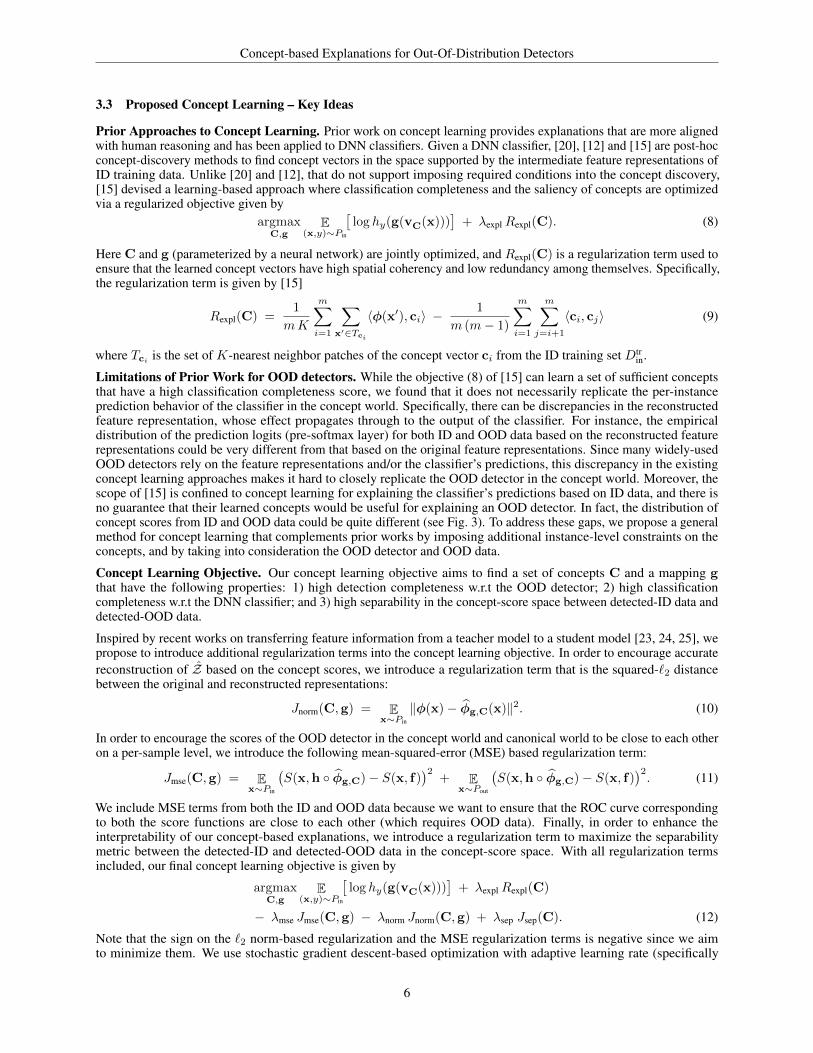
3.3 Proposed Concept Learning – Key Ideas

Prior Approaches to Concept Learning. Prior work on concept learning provides explanations that are more alignedwith human reasoning and has been applied to DNN classifiers. Given a DNN classifier, [20], [12] and [15] are post-hocconcept-discovery methods to find concept vectors in the space supported by the intermediate feature representations ofID training data. Unlike [20] and [12], that do not support imposing required conditions into the concept discovery,[15] devised a learning-based approach where classification completeness and the saliency of concepts are optimizedvia a regularized objective given by

argmaxC,g

E(x,y)∼Pin

[log hy(g(vC(x)))

]+ λexpl Rexpl(C). (8)

Here C and g (parameterized by a neural network) are jointly optimized, and Rexpl(C) is a regularization term used toensure that the learned concept vectors have high spatial coherency and low redundancy among themselves. Specifically,the regularization term is given by [15]

Rexpl(C) =1

mK

m∑i=1

∑x′∈Tci

〈φ(x′), ci〉 −1

m (m− 1)

m∑i=1

m∑j=i+1

〈ci, cj〉 (9)

where Tciis the set of K-nearest neighbor patches of the concept vector ci from the ID training set Dtr

in.

Limitations of Prior Work for OOD detectors. While the objective (8) of [15] can learn a set of sufficient conceptsthat have a high classification completeness score, we found that it does not necessarily replicate the per-instanceprediction behavior of the classifier in the concept world. Specifically, there can be discrepancies in the reconstructedfeature representation, whose effect propagates through to the output of the classifier. For instance, the empiricaldistribution of the prediction logits (pre-softmax layer) for both ID and OOD data based on the reconstructed featurerepresentations could be very different from that based on the original feature representations. Since many widely-usedOOD detectors rely on the feature representations and/or the classifier’s predictions, this discrepancy in the existingconcept learning approaches makes it hard to closely replicate the OOD detector in the concept world. Moreover, thescope of [15] is confined to concept learning for explaining the classifier’s predictions based on ID data, and there isno guarantee that their learned concepts would be useful for explaining an OOD detector. In fact, the distribution ofconcept scores from ID and OOD data could be quite different (see Fig. 3). To address these gaps, we propose a generalmethod for concept learning that complements prior works by imposing additional instance-level constraints on theconcepts, and by taking into consideration the OOD detector and OOD data.

Concept Learning Objective. Our concept learning objective aims to find a set of concepts C and a mapping gthat have the following properties: 1) high detection completeness w.r.t the OOD detector; 2) high classificationcompleteness w.r.t the DNN classifier; and 3) high separability in the concept-score space between detected-ID data anddetected-OOD data.

Inspired by recent works on transferring feature information from a teacher model to a student model [23, 24, 25], wepropose to introduce additional regularization terms into the concept learning objective. In order to encourage accuratereconstruction of Z based on the concept scores, we introduce a regularization term that is the squared-`2 distancebetween the original and reconstructed representations:

Jnorm(C,g) = Ex∼Pin

‖φ(x)− φg,C(x)‖2. (10)

In order to encourage the scores of the OOD detector in the concept world and canonical world to be close to each otheron a per-sample level, we introduce the following mean-squared-error (MSE) based regularization term:

Jmse(C,g) = Ex∼Pin

(S(x,h ◦ φg,C)− S(x, f)

)2+ E

x∼Pout

(S(x,h ◦ φg,C)− S(x, f)

)2. (11)

We include MSE terms from both the ID and OOD data because we want to ensure that the ROC curve correspondingto both the score functions are close to each other (which requires OOD data). Finally, in order to enhance theinterpretability of our concept-based explanations, we introduce a regularization term to maximize the separabilitymetric between the detected-ID and detected-OOD data in the concept-score space. With all regularization termsincluded, our final concept learning objective is given by

argmaxC,g

E(x,y)∼Pin

[log hy(g(vC(x)))

]+ λexpl Rexpl(C)

− λmse Jmse(C,g) − λnorm Jnorm(C,g) + λsep Jsep(C). (12)

Note that the sign on the `2 norm-based regularization and the MSE regularization terms is negative since we aimto minimize them. We use stochastic gradient descent-based optimization with adaptive learning rate (specifically

6


(a) MSP, target (b) MSP, baseline (c) MSP, ours

(d) Energy, target (e) Energy, baseline (f) Energy, ours

Figure 3: Estimated density of the score S(x, f) on the AwA test data (ID: blue) and the SUN dataset (OOD: red). The DNN classifieris Inception-V3 and the OOD detector is either MSP or Energy. Left: Target distribution of S(x, f) in the canonical world. Mid:Distribution of Scon(x, f) in the concept world, using concepts learned by [15] (i.e., λmse = λnorm = λsep = 0). Right: Distributionof Scon(x, f) in the concept world, using concepts learned by our method. For MSP we set λmse = 10, λnorm = 0.1, λsep = 0, andfor Energy we set λmse = 1, λnorm = 0.1, λsep = 0.

Adam [26]) to solve the learning objective. The expectations involved in each of the terms in the objective are calculatedusing sample estimates from the training ID and OOD datasets. Specifically, Dtr

in is used to compute the expectationover Pin, and Dtr

out is used to compute the expectation over Pout. We summarize our complete concept learning algorithmin Algorithm 1 (see Appendix A.4).

4 Experiments

In this section, we carry out experiments to evaluate the proposed method and address the following questions:

Q1. Does our concept learning objective effectively encourage concepts to have the desired properties of detectioncompleteness and concept separability?

Q2. Are the proposed evaluation metrics effective at providing better interpretability for the resulting concept-basedexplanations?

Q3. Given concepts learned by our approach, what insights can we provide for well-known OOD detectors?

To answer these questions, we apply our framework to interpret four popular OOD detectors from the literature:MSP [16], ODIN [27], Energy [7] and Mahalanobis [18] (henceforth abbreviated to Mahal). The OOD detectors arepaired with the widely-used Inception-V3 model [28] (following the setup in prior works [15, 12, 20]), trained on theAnimals-with-Attributes (AwA) dataset [29], which yields a test accuracy of 0.921.

Our main findings are summarized as follows:

A1. The regularization terms in our concept learning objective effectively improve detection completeness andconcept separability, without sacrificing the classification completeness. For instance, given the ODIN detectorand the SUN dataset [30] as OOD data, including our proposed regularization terms improves the detectioncompleteness of concepts from 0.869 to 0.969, and the relative concept separability is increased by 0.356,compared to when concepts are learned without the regularization terms (see Table 1).

A2. Concepts with a high completeness score enable to mimic the original behavior of the OOD detector moreprecisely, hence leading to more accurate explanations based on the concepts (see Fig. 3). Also, concepts witha higher concept separability score lead to more visually-distinctive interpretations between ID and OOD data

7


OODdetector Hyperparameters

ηf (C)

OOD dataPlaces SUN Textures iNaturalist

ηf ,S(C) Jsep(C,C′) ηf ,S(C) Jsep(C,C′) ηf ,S(C) Jsep(C,C′) ηf ,S(C) Jsep(C,C′)

MSP

λmse = 0, λnorm = 0, λsep = 0 0.990 0.849 0.0 0.848 0.0 0.824 0.0 0.958 0.0λmse = 10, λnorm = 0.1, λsep = 0 0.994 0.947 0.216 0.946 0.118 0.922 0.406 0.970 0.175λmse = 0, λnorm = 0, λsep = 50 0.980 0.815 0.412 0.816 0.303 0.773 0.376 0.863 0.267λmse = 10, λnorm = 0.1, λsep = 50 0.985 0.959 0.327 0.961 0.266 0.938 0.344 0.946 0.286

ODIN


Energy


Mahal

λmse = 0, λnorm = 0, λsep = 0 0.990 0.860 0.0 0.860 0.0 0.831 0.0 0.972 0.0λmse = 0.1, λnorm = 0.1, λsep = 0 0.994 0.962 0.153 0.963 0.176 0.962 0.351 0.955 0.169λmse = 0, λnorm = 0, λsep = 50 0.985 0.850 0.430 0.883 0.362 0.774 0.429 0.926 0.386λmse = 0.1, λnorm = 0.1, λsep = 50 0.991 0.971 0.370 0.970 0.388 0.970 0.397 0.972 0.351

Table 1: Results of concept learning with different parameter settings across various OOD detectors and OOD datasets.Larger values are better for all the metrics. Bold numbers indicate the best results (across the rows) for a given OOD detectionmethod and dataset. Note that by definition of Jsep(C,C

′) (Eqn. 13), the relative concept separability of the baseline [15] is always0, i.e., Jsep(C

′,C′) = 0.

compared to concepts with a lower concept separability score, by having more distinguishable concept-scorepatterns (see Fig. 4).

A3. We can rank the importance of each concept towards OOD detection using the Shapley value modified withour per-class detection completeness metric. When the concepts are only targeted at explaining the DNNclassifier (as in the baseline [15]), the behavior of the OOD detector is merely described by the common set ofconcepts that are important for the DNN classifier. On the other hand, when not only the DNN classifier butalso the OOD detector is taken into consideration during concept learning (i.e., our method), we obtain a morediverse and expanded set of concepts, and different concepts play a major role in interpreting the classificationand detection results (see Fig. 5).

4.1 Setup

Datasets. For the ID dataset, we use Animals with Attributes (AwA) [29] with 50 animal classes, and split it into atrain set (with 29841 images), validation set (with 3709 images), and test set (with 3772 images). We use the MSCOCOdataset [31] as the auxiliary OOD dataset Dtr

out for training and validation. For the OOD test dataset Dteout, we follow a

common setting in the literature of large-scale OOD detection [32] and use four different image datasets: Places365[33], SUN [30], Textures [34], iNaturalist [35]; all resized to the input size 224× 224.

Metrics. For each set of concepts learned with different OOD detectors and hyperparameters, we report the classificationcompleteness ηf (C), detection completeness ηf ,S(C), and the relative concept separability metric (defined below). Incontrast to the completeness scores that are almost always bounded to the range [0, 1] 4, it is hard to gauge the possiblerange of the separability score Jsep(C) (or Jysep(C)) across different settings (datasets, classification models, and OODdetectors), and whether the value represents a significant improvement in separability. Hence, we define the relativeconcept separability, which captures the relative improvement in concept separability between two different sets ofconcepts, as follows

Jsep(C,C′) = Median

({Jysep(C) − Jysep(C′)

Jysep(C′)

}Ly=1

). (13)

This metric measures the median of the relative increase in the per-class separability using concepts C, compared tothat of using a different set of concepts C′. We choose C′ to be the set of concepts learned by the baseline [15], whichis a special case of our learning objective when λmse = λnorm = λsep = 0. The set of concept C are obtained via ourconcept learning objective, with various combinations of hyperparameter values. For details on the hyperparametersetting, see Appendix A.5.

4In general, we observe that the performance of the classifier and OOD detector in the concept world does not exceed that of thecanonical world.

8


4.2 Effectiveness of Our Method

In this subsection, we elaborate on the experiments to answer the first question (Q1) on the effectiveness of ourconcept learning objective. The results are summarized in Table 1 for different OOD detection methods and OODdatasets. We consider the following four settings of the hyperparameters in order to evaluate the effectiveness of theproposed regularization terms in the concept-learning objective: i) all the hyperparameters are set to 0 (first row), whichcorresponds to the baseline method [15]; ii) only the regularization terms for reconstruction error Jnorm(C,g) andmean-squared error Jmse(C,g) are included (second row); iii) only the regularization term for concept separabilityJsep(C) is included (third row); iv) all the regularization terms are included (fourth row).

From Table 1, we observe that the regularization terms Jnorm(C,g) and Jmse(C,g) improve not only the detectioncompleteness by a large margin, but also the classification completeness, compared to the (baseline) case whereλnorm = λmse = 0. This validates our hypothesis that accurate reconstruction of the feature representation space Z andthe score functions are both crucial for closing the performance gap between the canonical world and concept worldof both the classifier and the OOD detector. We observe that the relative concept separability Jsep(C,C′) is largestmost often for the setting where λmse = λnorm = 0, and λsep > 0 (third row). However, the detection completenessdoes not improve and in some cases drops compared to the baseline setting, suggesting that there is a tradeoff betweenmaximizing the detection completeness and concept separability.

Finally, our method achieves the best detection completeness in most of the cases for the setting where all theregularization terms are included, i.e., λmse > 0, λnorm > 0, and λsep > 0. In this setting, there is a slight decrease therelative concept separability compared to the case where only the regularization term Jsep(C) is included (third row). Inother words, there is a tradeoff wherein we may have to sacrifice the concept separability a little in order to achieve thebest possible detection completeness. Further investigation including an ablation study on each regularization term canbe found in Appendix A.6. Interestingly, we observe that the concepts targeted for a particular type of OOD detectorcan also be applied to different types of OOD detectors (i.e., the learned concepts exhibit transferability). Refer toAppendix A.6 for the full discussion on concept transferability.

4.3 Interpretability of the Learned Concepts

We provide further insights on the interpretability of the learned concepts in order to address the second question(Q2). Specifically, we demonstrate that the concepts learned by our method enable more accurate, and more visuallydistinctive interpretations, compared to the concepts learned by the baseline method ([15]).

Detection completeness and accurate reconstruction of Z . In Fig. 3, we compare the distribution of the OODdetector scores in the canonical world and concept world using the concepts learned by our method and by [15] (havingdifferent detection completeness). The distribution of Scon(x, f) calculated based on the concepts learned by [15] (withdetection completeness ηf ,S(C) = 0.85 for both the MSP and Energy detectors) is significantly different from thatof the target distribution of S(x, f). See Fig. 3a vs. Fig. 3b, and Fig. 3d vs. Fig. 3e. This suggests that the conceptslearned by [15] can lead to a strong mis-match between the score distributions on both ID data and OOD data.

In contrast, Scon(x, f) calculated based on the concepts learned by our method (with ηf ,S(C) = 0.95 for the MSPdetector, and ηf ,S(C) = 0.97 for the Energy detector) approximates the target score distributions more closely on bothID data and OOD data. See Fig. 3a vs. Fig. 3c, and Fig. 3d vs. Fig. 3f. Overall, our experiments find that the proposedregularization terms reduce the performance gap (between the canonical world and concept world) of both the classifierand the OOD detector. This enables more accurate concept-based explanations for an OOD detector.

Concept separability and distinction in explanations. We investigate whether the concepts with a higher concept-separability measure lead to a more distinguishable pattern between the concept scores of detected-ID inputs anddetected-OOD inputs. Fig. 4 illustrates the concept score patterns of two different sets of concepts having differentconcept separability scores. We take the average of concept scores Vin(C) (or Vout(C)) among the inputs that arepredicted as class y, and detected as ID (or OOD) by the OOD detector (Energy-based OOD detection is used in thiscase). When using concepts that correspond to a relatively low per-class concept separability (Jysep(C) = 0.059), we failto observe any noticeable difference in the concept scores of detected-ID and detected-OOD data (see Figs. 4a and 4c).On the other hand, concepts with a higher per-class concept separability (Jysep(C) = 0.098) show clear distinguishablepatterns between detected-ID and detected-OOD data (see Figs. 4b and 4d). These observations confirm our designmotivation for the concept separability metric – that a higher value of the concept separability metric enables bettervisual distinction between the concept score patterns, suggesting better interpretability for humans.

9


(a) Set 1 with low concept separability, detected-ID (b) Set 2 with high concept separability, detected-ID

(c) Set 1 with low concept separability, detected-OOD (d) Set 2 with high concept separability, detected-OOD

Figure 4: Our concept separability metric and visual distinction in the concept score patterns. For the class "Giraffe", wecompare the concept score patterns using two different sets of concepts. Left: Averaged concept scores using concept set 1 (top-10important concepts out of the concepts learned with λmse = λnorm = λsep = 0). Right: Averaged concept scores using concept set 2(top-10 important concepts out of the concepts learned with λmse = 1, λnorm = 0.1, λsep = 50). Concept importance is measuredusing the Shapley value of Eqn. (14). Concept separability is measured based on the presented 10 concepts from each set.

4.4 Concept-based Explanations for OOD Detectors

Lastly, we illustrate how the concepts learned by our algorithm can be used to provide explanations for an OOD detector(addressing the last question (Q3)). By quantifying the contribution of each concept toward OOD detection results, wecan identify the major concepts that an OOD detector relies on to make decisions.

Contribution of each concept to detection. The proposed concept learning algorithm learns concepts for both theclassifier and OOD detector considering all the classes. Among all the concepts, we would like to specify the mostprominent concepts required for understanding the OOD detector with respect to a particular class. We address thefollowing question: how much does each concept contribute to the detection results for inputs predicted to a particularclass?. Recent works have adopted the Shapley value from Coalitional Game theory literature [36, 37] for scoring theimportance of a feature subset towards the predictions of a model [38, 39, 40]. Extending this idea, we modify thecharacteristic function of the Shapley value using our per-class detection completeness metric (Eqn. (15) in AppendixA.2). The modified Shapley value of a concept ci ∈ C with respect to the predicted class j ∈ [L] is defined as

SHAP(ηjf ,S , ci) :=∑

C′⊆C\{ci}

(m− |C′| − 1)! |C′|!m!

(ηjf ,S(C′ ∪ {ci})− ηjf ,S(C′)

), (14)

where C′ is a subset of C excluding concept ci, and ηjf ,S is the (per-class) detection completeness with respect to classj. This Shapley value captures the average marginal contribution (i.e., importance) of concept ci towards explaining thedecisions of the OOD detector for inputs that are predicted by the classifier into class j.

Based on this concept importance metric, we present the top-ranked concepts along with the visualized examples thatare nearest to the corresponding concept vector in Fig. 5. For the baseline method [15] (denoted “baseline” in Fig. 5),the learned concepts are solely intended for reconstructing the behavior of the classifier. In this case, we observe fromFig. 5 that interpretation of both the classifier and OOD detector depends on a common set of concepts (i.e., concepts32, 10, and 47). On the other hand, the concepts learned by our method focus on reconstructing the behavior of boththe OOD detector and the classifier. In this case, we observe from Fig. 5 that a distinct set of important concepts areselected for classification and OOD detection. We also observe that our method requires more concepts in order toaddress the decisions of both the classifier and OOD detector. For instance, the number of concepts obtained by our

10


Figure 5: Most important concepts for the Energy detector with respect to the predicted class “Buffalo”. We demonstraterandomly sampled images that are predicted by the classifier into this class. We compare the top-4 important concepts to describe theDNN classifier (and Energy detector), ranked by the Shapley value based on classification completeness SHAP(ηjf , ci) (and detectioncompleteness SHAP(ηjf ,S , ci)). “Baseline” corresponds to the case when the concepts are learned with λmse = λnorm = λsep = 0,whereas “Ours” corresponds to the concepts learned with λmse = 1, λnorm = 0.1, λsep = 0. To visualize what each concept represents,we display the top receptive fields from Dte

in whose inner-product with the corresponding concept vector is larger than 0.8.

method and the baseline are 78 and 53 (respectively), out of a total 100 concepts 5. More examples of concepts withhigh-ranking Shapley scores can be found in Appendix B.1. We further investigate the attribution of such top-rankedconcepts via counterfactual analysis in Appendix B.2.

5 Related Work

OOD detection. Starting with a simple baseline for OOD detection based on the maximum softmax probability (MSP)score [16], recent studies have designed various scoring functions based on the outputs from the final or penultimatelayers [27, 41], or a combination of different intermediate layers of DNN model [18]. Our general framework canbe applied to these existing OOD detection methods by choosing a suitable intermediate layer for concept-basedinterpretation 6. To further improve the OOD uncertainty estimation, several works attempt to finetune the DNNclassifier using auxiliary OOD training data [4, 42, 8]. Complementary to these, our work is a post-hoc method thataims to explain an already-trained DNN model and its paired OOD detector. Our concept learning algorithm discoversconcepts through optimization based on the feature representations from a DNN layer, without modifying the internalsof the DNN or the OOD detector.

Post-hoc interpretability. Feature attribution is the most commonly used post-hoc explanation method that attributesthe decision to local input features [43, 44, 45, 9], but recent works have demonstrated its vulnerability to e.g., adversarialperturbations [46, 47, 48]. Adebayo et al. [11] also conduct experimental analyses and a human subject study to assessthe effectiveness of feature attributions under various settings (including on OOD data), and show that feature attributionsbarely have any visual difference between ID inputs and OOD inputs.

On the other hand, concept-based explanation is another type of interpretation method, which is designed to bebetter-aligned with human reasoning [49, 50] and intuition [12, 13, 14, 15]. A common implicit assumption in theconcept-based explanation literature is linear interpretability, i.e., the concepts lie in a linearly-projected subspace ofintermediate DNN layer activations; our work is also based on this assumption. While the scope of existing worksis confined to explaining DNN classifiers, we extend the use of concept-based interpretability for explaining OODdetectors. Our work is inspired by [15], and we extend their concept-based explanation method for DNN classifiers toOOD detectors. As discussed in section 3.3, the concept learning objective of [15] can be obtained as a special case ofour concept learning objective for the hyper-parameter setting λnorm = λmse = λsep = 0.

5After removing redundant concepts for which the inner-product between the corresponding concept vector and any of theremaining concept vectors is larger than 0.95.

6For instance, if an OOD detector makes decisions based on outputs from an intermediate layer `, the user can explain it usingconcepts that can reconstruct the feature representations from layer `, or an earlier layer.

11


6 Conclusions and Future Work

In this work, we propose a first method (to the best of our knowledge) for providing concept-based attributions of thedecision of an OOD detector based on high-level concepts derived from the internal feature representations of a (paired)DNN classifier. We quantify how accurately and sufficiently a set of concepts can describe an OOD detector’s behaviorthrough a novel detection completeness metric. We also propose a general framework for learning concepts, that doesnot involve laborious human effort for concept annotations, by incorporating regularization terms to ensure the accuratereconstruction of the feature representation space based on concept scores. We propose a concept separability metricthat encourages better interpretability of the learned concepts, and can be directly plugged into our concept learningobjective. Our experiments with diverse OOD detectors and datasets confirms our insight that better separability in theconcept space leads to better distinction between the resulting explanations for detected-ID and detected-OOD inputs(bringing more intuitive interpretations).

In future work, one could reduce the performance gap of the DNN classifier and OOD detector even further inour “two-world” view by borrowing insights from the knowledge-distillation literature to the regularization design[51, 52]. Future work could also include human-centric evaluations [53, 54] to assess how real users find our concept-based explanations, compared to OOD detector explanations generated by prior works such as feature attribution orconcept-based interpretability (which mainly focus on class prediction).

7 Acknowledgement

We would like to thank Haizhong Zheng for his valuable comments. This work is partially supported by the NationalScience Foundation (NSF) Grants CCF-FMitF-1836978, SaTC-Frontiers-1804648, and CCF-2046710, and ARO grantnumber W911NF-17-1-0405, and DARPA-GARD problem under agreement number 885000.

References[1] Dario Amodei, Chris Olah, Jacob Steinhardt, Paul Christiano, John Schulman, and Dan Mané. Concrete problems in AI safety.

arXiv preprint arXiv:1606.06565, 2016.

[2] Ian J Goodfellow, Jonathon Shlens, and Christian Szegedy. Explaining and harnessing adversarial examples. In InternationalConference on Learning Representations, 2015.

[3] Khanh Xuan Nguyen and Brendan O’Connor. Posterior calibration and exploratory analysis for natural language processingmodels. In EMNLP, 2015.

[4] Dan Hendrycks, Mantas Mazeika, and Thomas Dietterich. Deep anomaly detection with outlier exposure. In InternationalConference on Learning Representations, 2018.

[5] Ziqian Lin, Sreya Dutta Roy, and Yixuan Li. MOOD: Multi-level out-of-distribution detection. In Proceedings of the IEEE/CVFConference on Computer Vision and Pattern Recognition, pages 15313–15323, 2021.

[6] Sina Mohseni, Mandar Pitale, JBS Yadawa, and Zhangyang Wang. Self-supervised learning for generalizable out-of-distributiondetection. In Proceedings of the AAAI Conference on Artificial Intelligence, volume 34, pages 5216–5223, 2020.

[7] Weitang Liu, Xiaoyun Wang, John Owens, and Yixuan Li. Energy-based out-of-distribution detection. Advances in NeuralInformation Processing Systems, 33, 2020.

[8] Jiefeng Chen, Yixuan Li, Xi Wu, Yingyu Liang, and Somesh Jha. Atom: Robustifying out-of-distribution detection usingoutlier mining. In Joint European Conference on Machine Learning and Knowledge Discovery in Databases, pages 430–445.Springer, 2021.

[9] Mukund Sundararajan, Ankur Taly, and Qiqi Yan. Axiomatic attribution for deep networks. In International Conference onMachine Learning, pages 3319–3328. PMLR, 2017.

[10] Marco Tulio Ribeiro, Sameer Singh, and Carlos Guestrin. " why should i trust you?" explaining the predictions of any classifier.In Proceedings of the 22nd ACM SIGKDD international conference on knowledge discovery and data mining, pages 1135–1144,2016.

[11] Julius Adebayo, Michael Muelly, Ilaria Liccardi, and Been Kim. Debugging tests for model explanations. In NeurIPS, 2020.

[12] Amirata Ghorbani, James Wexler, James Y Zou, and Been Kim. Towards automatic concept-based explanations. Advances inNeural Information Processing Systems, 32:9277–9286, 2019.

[13] Bolei Zhou, Yiyou Sun, David Bau, and Antonio Torralba. Interpretable basis decomposition for visual explanation. InProceedings of the European Conference on Computer Vision (ECCV), pages 119–134, 2018.

[14] Diane Bouchacourt and Ludovic Denoyer. Educe: Explaining model decisions through unsupervised concepts extraction. arXivpreprint arXiv:1905.11852, 2019.

12


[15] Chih-Kuan Yeh, Been Kim, Sercan Arik, Chun-Liang Li, Tomas Pfister, and Pradeep Ravikumar. On completeness-awareconcept-based explanations in deep neural networks. Advances in Neural Information Processing Systems, 33:20554–20565,2020.

[16] Dan Hendrycks and Kevin Gimpel. A baseline for detecting misclassified and out-of-distribution examples in neural networks.arXiv preprint arXiv:1610.02136, 2016.

[17] Dan Hendrycks, Steven Basart, Mantas Mazeika, Mohammadreza Mostajabi, Jacob Steinhardt, and Dawn Song. Scalingout-of-distribution detection for real-world settings. arXiv preprint arXiv:1911.11132, 2019.

[18] Kimin Lee, Kibok Lee, Honglak Lee, and Jinwoo Shin. A simple unified framework for detecting out-of-distribution samplesand adversarial attacks. Advances in neural information processing systems, 31, 2018.

[19] Jayaram Raghuram, Varun Chandrasekaran, Somesh Jha, and Suman Banerjee. A general framework for detecting anomalousinputs to DNN classifiers. In International Conference on Machine Learning, pages 8764–8775. PMLR, 2021.

[20] Been Kim, Martin Wattenberg, Justin Gilmer, Carrie Cai, James Wexler, Fernanda Viegas, et al. Interpretability beyond featureattribution: Quantitative testing with concept activation vectors (TCAV). In International conference on machine learning,pages 2668–2677. PMLR, 2018.

[21] Keinosuke Fukunaga. Introduction to Statistical Pattern Recognition, chapter 10, pages 446–451. Academic Press, 2 edition,1990.

[22] Kevin P Murphy. Machine Learning: A Probabilistic Perspective, chapter 8, pages 271–274. MIT press, 2012.

[23] Geoffrey Hinton, Oriol Vinyals, and Jeff Dean. Distilling the knowledge in a neural network. arXiv preprint arXiv:1503.02531,2015.

[24] Jimmy Ba and Rich Caruana. Do deep nets really need to be deep? Advances in Neural Information Processing Systems, 27,2014.

[25] Guorui Zhou, Ying Fan, Runpeng Cui, Weijie Bian, Xiaoqiang Zhu, and Kun Gai. Rocket launching: A universal and efficientframework for training well-performing light net. In Thirty-second AAAI conference on artificial intelligence, 2018.

[26] Diederik P Kingma and Jimmy Ba. Adam: A method for stochastic optimization. arXiv preprint arXiv:1412.6980, 2014.

[27] Shiyu Liang, Yixuan Li, and R Srikant. Enhancing the reliability of out-of-distribution image detection in neural networks. InInternational Conference on Learning Representations, 2018.

[28] Christian Szegedy, Vincent Vanhoucke, Sergey Ioffe, Jon Shlens, and Zbigniew Wojna. Rethinking the inception architecturefor computer vision. In Proceedings of the IEEE conference on computer vision and pattern recognition, pages 2818–2826,2016.

[29] Yongqin Xian, Christoph H Lampert, Bernt Schiele, and Zeynep Akata. Zero-shot learning—a comprehensive evaluation of thegood, the bad and the ugly. IEEE transactions on pattern analysis and machine intelligence, 41(9):2251–2265, 2018.

[30] Jianxiong Xiao, James Hays, Krista A Ehinger, Aude Oliva, and Antonio Torralba. Sun database: Large-scale scene recognitionfrom abbey to zoo. In 2010 IEEE computer society conference on computer vision and pattern recognition, pages 3485–3492.IEEE, 2010.

[31] Tsung-Yi Lin, Michael Maire, Serge J. Belongie, James Hays, Pietro Perona, Deva Ramanan, Piotr Dollár, and C. LawrenceZitnick. Microsoft COCO: Common objects in context. In European Conference on Computer Vision - ECCV, volume 8693 ofLecture Notes in Computer Science, pages 740–755. Springer, 2014.

[32] Rui Huang and Yixuan Li. MOS: Towards scaling out-of-distribution detection for large semantic space. In Proceedings of theIEEE/CVF Conference on Computer Vision and Pattern Recognition (CVPR), pages 8710–8719, June 2021.

[33] Bolei Zhou, Agata Lapedriza, Aditya Khosla, Aude Oliva, and Antonio Torralba. Places: A 10 million image database forscene recognition. IEEE transactions on pattern analysis and machine intelligence, 40(6):1452–1464, 2017.

[34] Mircea Cimpoi, Subhransu Maji, Iasonas Kokkinos, Sammy Mohamed, and Andrea Vedaldi. Describing textures in the wild.In Proceedings of the IEEE Conference on Computer Vision and Pattern Recognition, pages 3606–3613, 2014.

[35] Grant Van Horn, Oisin Mac Aodha, Yang Song, Yin Cui, Chen Sun, Alex Shepard, Hartwig Adam, Pietro Perona, and SergeBelongie. The INaturalist species classification and detection dataset. In Proceedings of the IEEE conference on computervision and pattern recognition, pages 8769–8778, 2018.

[36] LS Shapley. A value for n-person games. Contributions to the Theory of Games, (28):307–317, 1953.

[37] Katsushige Fujimoto, Ivan Kojadinovic, and Jean-Luc Marichal. Axiomatic characterizations of probabilistic and cardinal-probabilistic interaction indices. Games and Economic Behavior, 55(1):72–99, 2006.

[38] Jianbo Chen, Le Song, Martin J Wainwright, and Michael I Jordan. L-shapley and c-shapley: Efficient model interpretation forstructured data. In International Conference on Learning Representations, 2018.

[39] Scott M Lundberg and Su-In Lee. A unified approach to interpreting model predictions. In Proceedings of the 31st internationalconference on neural information processing systems, pages 4768–4777, 2017.

[40] Mukund Sundararajan and Amir Najmi. The many shapley values for model explanation. In International Conference onMachine Learning, pages 9269–9278. PMLR, 2020.

13


[41] Terrance DeVries and Graham W Taylor. Learning confidence for out-of-distribution detection in neural networks. arXivpreprint arXiv:1802.04865, 2018.

[42] Kimin Lee, Honglak Lee, Kibok Lee, and Jinwoo Shin. Training confidence-calibrated classifiers for detecting out-of-distribution samples. In International Conference on Learning Representations, 2018.

[43] David Baehrens, Timon Schroeter, Stefan Harmeling, Motoaki Kawanabe, Katja Hansen, and Klaus-Robert Müller. How toexplain individual classification decisions. arXiv preprint arXiv:0912.1128, 2009.

[44] Karen Simonyan, Andrea Vedaldi, and Andrew Zisserman. Deep inside convolutional networks: Visualising image classificationmodels and saliency maps. arXiv preprint arXiv:1312.6034, 2013.

[45] Daniel Smilkov, Nikhil Thorat, Been Kim, Fernanda Viégas, and Martin Wattenberg. Smoothgrad: removing noise by addingnoise. arXiv preprint arXiv:1706.03825, 2017.

[46] Amirata Ghorbani, Abubakar Abid, and James Zou. Interpretation of neural networks is fragile. In Proceedings of the AAAIConference on Artificial Intelligence, volume 33, pages 3681–3688, 2019.

[47] Juyeon Heo, Sunghwan Joo, and Taesup Moon. Fooling neural network interpretations via adversarial model manipulation.Advances in Neural Information Processing Systems, 32:2925–2936, 2019.

[48] Dylan Slack, Sophie Hilgard, Emily Jia, Sameer Singh, and Himabindu Lakkaraju. Fooling LIME and SHAP: Adversarialattacks on post hoc explanation methods. In Proceedings of the AAAI/ACM Conference on AI, Ethics, and Society, pages180–186, 2020.

[49] Sharon Lee Armstrong, Lila R Gleitman, and Henry Gleitman. What some concepts might not be. Cognition, 13(3):263–308,1983.

[50] Joshua Brett Tenenbaum. A Bayesian framework for concept learning. PhD thesis, Massachusetts Institute of Technology,1999.

[51] Adriana Romero, Nicolas Ballas, Samira Ebrahimi Kahou, Antoine Chassang, Carlo Gatta, and Yoshua Bengio. Fitnets: Hintsfor thin deep nets. arXiv preprint arXiv:1412.6550, 2014.

[52] Sergey Zagoruyko and Nikos Komodakis. Paying more attention to attention: Improving the performance of convolutionalneural networks via attention transfer. arXiv preprint arXiv:1612.03928, 2016.

[53] Finale Doshi-Velez and Been Kim. Towards a rigorous science of interpretable machine learning. arXiv preprintarXiv:1702.08608, 2017.

[54] Forough Poursabzi-Sangdeh, Daniel G Goldstein, Jake M Hofman, Jennifer Wortman Wortman Vaughan, and Hanna Wallach.Manipulating and measuring model interpretability. In Proceedings of the 2021 CHI Conference on Human Factors inComputing Systems, pages 1–52, 2021.

[55] Anil Bhattacharyya. On a measure of divergence between two statistical populations defined by their probability distributions.Bull. Calcutta Math. Soc., 35:99–109, 1943.

[56] Keinosuke Fukunaga. Introduction to Statistical Pattern Recognition, chapter 3, pages 97–103. Academic Press, 2 edition,1990.

14


A Concept Learning

A.1 Connection to the Bhattacharya Distance

We note that the separability metric in Eq. (7) is closely related to the Bhattacharya distance [55] for the special casewhen the concept scores from both ID and OOD data follow a multivariate Gaussian density. The Bhattacharya distanceis a well known measure of divergence between two probability distributions, and it has the nice property of being anupper bound to the Bayes error rate in the two-class case [56]. For the special case when the concept scores from bothID and OOD data follow a multivariate Gaussian with a shared covariance matrix, it can be shown that the Bhattacharyadistance reduces to the separability metric in Eq. (7) (ignoring scale factors).

A.2 Per-class Detection Completeness

Definition 3. Given a trained DNN classifier f = h ◦ φ, a trained OOD detector with score function S(x, f), and a setof concept vectors C, the detection completeness relative to class j ∈ [L] with respect to the ID distribution Pin(x, y)and OOD distribution Pout(x) is defined as

ηjf ,S(C) :=supg AUCj(h ◦ φg,C) − br

AUC(h ◦ φ) − br, (15)

where AUCj(h ◦ φg,C) is the AUROC of the detector conditioned on the event that the class predicted by the concept-world classifier h ◦ φg,C is j (note that the denominator has the global AUROC). The baseline AUROC br is equal to0.5 as before. This per-class detection completeness is used in the modified Shapley value defined in section 4.4.

A.3 Per-class Concept Separability

In section 3.2, we focused on the separability between the concept scores of ID and OOD data without consideringthe class prediction of the classifier. However, it would be more appropriate to impose a high separability betweenthe concept scores on a per-class level. In other words, we would like the concept scores of detected-ID and detected-OOD data, that are predicted by the classifier into any given class y ∈ [L] to be well separated. Consider the set ofconcept-score vectors from the detected-ID (or detected-OOD) dataset that are also predicted into class y:

V yin (C) := {vC(x), x ∈ Dtrin ∪Dtr

out : Dγ(x, f) = 1 and y(x) = y}V yout(C) := {vC(x), x ∈ Dtr

in ∪Dtrout : Dγ(x, f) = 0 and y(x) = y}. (16)

We can extend the definition of the global separability metric in Eq. (7) to a given predicted class y ∈ [L] as follows

Jysep(C) := Jsep(V yin (C), V yout(C)) = tr[(Syw)−1 Syb

]= (µyout − µyin)T (Syw)−1 (µyout − µyin). (17)

The scatter matrices Syw and Syb are defined similar to Eq. (5), using the per-class subset of concept scores V yin (C) orV yout(C), and the mean concept-score vectors from the detected-ID and detected-OOD dataset are also defined at aper-class level.

A.4 Algorithm for Concept Learning

To provide the readers with a clear overview of the proposed concept learning approach, we include Algorithm 1. Notethat in line 7 of Algorithm 1, the dimension reduction step in Vin(C) = {vC(x), x ∈ Dtr

in ∪Dtrout : Dγ(x, f) = 1}

and Vout(C) = {vC(x), x ∈ Dtrin∪Dtr

out : Dγ(x, f) = 0} involves the maximum function, which is not differentiable;specifically, the step vci

(x) = maxp,q |〈φp,q(x), ci〉|. For calculating the gradients (backward pass), we use thelog-sum-exp function with a temperature parameter to get a differentiable approximation of the maximum function,i.e., maxp,q |〈φp,q(x), ci〉| ≈ α log

[∑p,q exp

(1α |〈φ

p,q(x), ci〉|)]

as α → 0. In our experiments, we set thetemperature constant α = 0.001 upon checking that the approximate value of vci

(x) is sufficiently close to the originalvalue using the maximum function.

A.5 Implementation Details

In this section, we provide more details about our experiment setting.

15


Algorithm 1 Learning concepts for OOD detectorINPUT: Entire training set Dtr = {Dtr

in, Dtrout}, entire validation set Dval = {Dval

in , Dvalout}, classifier f , detector Dγ .

INITIALIZE: Concept vectors C = [c1 · · · cm] and parameters of the network g.OUTPUT: C and g.

1: Calculate threshold γ for Dγ using Dval as the score at which true positive rate is 95%.2: for t = 1, ...T epochs do3: Compute the prediction accuracy of the concept-world classifier f con using Dtr

in.4: Compute the explainability regularization term as defined in [15].5: Compute difference of feature representation between canonical world and concept world using Eqn. (10).6: Compute difference of detector outputs between canonical world and concept world using Eqn. (11).7: Compute Vin(C) and Vout(C) using Dtr,Dγ and C.8: Compute separability between Vin(C) and Vout(C) using Eqn. (7) or Eqn. (17).9: Perform a batch-SGD update of C and g using Eqn. (12) as the objective.

10: end for

OOD Datasets. For the auxiliary OOD dataset for concept learning (Dtrout), we use the unlabeled images from MSCOCO

dataset (120K images in total) [31]. We carefully curate the dataset to make sure that no images contain overlappinganimal objects with our ID dataset (i.e., 50 animal classes of Animals-with-Attributes [29]), then randomly sample 30Kimages. For OOD datasets for evaluation (Dte

out), we use the high-resolution image datasets processed by Huang andLi [32].

Hyperparameters. Throughout the experiments, we fix the number of concepts to m = 100 (unless specificallymentioned otherwise), and following the implementation of [15], we set λexpl = 10 and g to be a two-layer fully-connected neural network with 500 neurons in the hidden layer. We learn concepts based on feature representationsfrom the layer right before the global max-pooling layer of the Inception-V3 model. We set the range of λnorm, λmseand λsep (in Eqn. (12)) based on the scale of corresponding regularization terms (i.e., Jnorm(C,g), Jmse(C,g) andJsep(C), respectively), for a specific choice of the OOD detector. After concept learning with m concepts, we removeany duplicate (redundant) concept vectors by removing those with a dot product larger than 0.95 with the remainingconcept vectors [15].

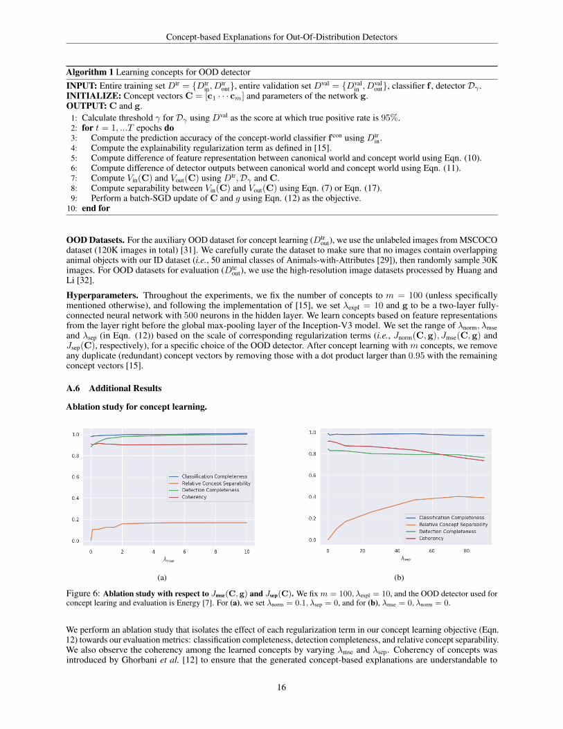
A.6 Additional Results

Ablation study for concept learning.

(a) (b)

Figure 6: Ablation study with respect to Jmse(C,g) and Jsep(C). We fix m = 100, λexpl = 10, and the OOD detector used forconcept learing and evaluation is Energy [7]. For (a), we set λnorm = 0.1, λsep = 0, and for (b), λmse = 0, λnorm = 0.

We perform an ablation study that isolates the effect of each regularization term in our concept learning objective (Eqn.12) towards our evaluation metrics: classification completeness, detection completeness, and relative concept separability.We also observe the coherency among the learned concepts by varying λmse and λsep. Coherency of concepts wasintroduced by Ghorbani et al. [12] to ensure that the generated concept-based explanations are understandable to

16


humans. It captures the idea that the examples for a concept should be similar to each other, while being different fromthe examples corresponding to other concepts. For the specific case of the image domain, the receptive fields mostcorrelated to a concept i (e.g., "stripe pattern") should look different from the receptive fields for a different concept j(e.g., "wavy surface of sea"). Yeh et al. [15] proposed to quantify the coherency of concepts as

1

mK

m∑i=1

∑x′∈Tci

〈φ(x′), ci〉, (18)

where Tci is the set of K-nearest neighbor patches of the concept vector ci from the ID training set Dtrin. We use this

metric to quantify how understandable our concepts are for different hyperparameter choices. Figure 6a shows thataligned with our intuition, large λmse helps to improve the detection completeness. Having non-zero λmse is also helpfulto improve the classification completeness even further, and surprisingly concept separability as well, without sacrificingthe coherency of concepts. On the other hand, in Figure 6b, we observe that large relative concept separability withlarge λsep comes at the expense of lower detection completeness and coherency. Recall that when visualizing what eachconcept represents for human’s convenience, we apply threshold 0.8 to only presents (see Figure 7). Low coherencywith respect to Eqn. 18 (i.e., 0.768 with λsep = 75) means that there are much less number of examples that can passthe threshold, meaning that users can hardly understand what the concepts at hand entails. This observation suggeststhat one needs to balance between concept coherency and concept separability depending on which property would bemore useful for a specific application of concepts.

Transferability of concepts across OOD detectors. Our work essentially suggests to use different set of conceptsfor a specific target OOD detector, as Jmse(C,g) and Jsep(C) in Eqn. (12) depend on a choice of OOD detector. Inpractice, however, one might not have enough computational capacity to prepare multiple sets of concepts for all typeof OOD detectors at hand. Here, we inspect whether the concepts targeted for a certain type of OOD detector are alsogood to be used for other OOD detectors.

We explore the transferability of concepts targeted to MSP [16] detector in Table 2, and Energy [7] in Table 3. Notsurprisingly, we observe that concepts targeted for Energy yields the best detection completeness score when testedwith the same type of OOD detector, but still make meaningful improvement with other detectors as well. When itcomes to relative concept separability, it is transferred even better across different OOD detectors. For instance, theconcepts lead to Jsep(C,C′) = 0.862 with Textures, the best relative concept separability is achieved with ODINdetector (i.e., Jsep(C,C′) = 0.862) and which is even higher than the best results we could obtain using the set ofconcepts targeted for ODIN (i.e., Jsep(C,C′) = 0.414 with λmse = 0, λnorm = 0, λsep = 50 in Table 1).

OOD dataset MetricsD

MSP ODIN Energy Mahal

Placesηf ,S(C) 0.959 0.952 0.938 0.947Jsep(C,C′) 0.327 0.288 0.361 0.338

SUNηf ,S(C) 0.961 0.954 0.945 0.953Jsep(C,C′) 0.266 0.294 0.390 0.351

Texturesηf ,S(C) 0.938 0.946 0.932 0.930Jsep(C,C′) 0.344 0.279 0.313 0.335

iNaturalistηf ,S(C) 0.946 0.946 0.933 0.930Jsep(C,C′) 0.286 0.181 0.229 0.197

Table 2: Transferability of concepts targeted for MSP with λmse = 10, λnorm = 0.1, λsep = 50

B Explanations

B.1 Important concepts for each OOD detector

We show additional examples for the top-ranked concepts by SHAP(ηf ,S , ci) in Figure 8. For each figure with a fixedchoice of class prediction, we present receptive fields from ID test set corresponding to top concepts that contribute themost to the decisions of each OOD detector. All receptive fields passed the threshold test that the inner product betweenthe feature representation and the corresponding concept vector is over 0.8.

17


OOD data MetricsOOD detector

MSP ODIN Energy Mahal

Placesηf ,S(C) 0.956 0.954 0.971 0.954Jsep(C,C′) 0.417 0.415 0.365 0.410

SUNηf ,S(C) 0.949 0.948 0.970 0.950Jsep(C,C′) 0.355 0.286 0.400 0.353

Texturesηf ,S(C) 0.931 0.943 0.964 0.947Jsep(C,C′) 0.567 0.862 0.494 0.701

iNaturalistηf ,S(C) 0.943 0.939 0.973 0.940Jsep(C,C′) 0.283 0.448 0.280 0.326

Table 3: Transferability of concepts targeted for Energy with λmse = 1, λnorm = 0.1, λsep = 50.

Figure 7: Top-6 important concepts for Energy with respect to class "Sheep".

B.2 Counterfactual analysis

To verify the important concepts identified by our modified Shapley value, we perform counterfactual analysis,addressing the following question: if the OOD detector thought the input has different score for this concept, would thedetection result be different? As we do not assume to have groundtruth annotation for concepts, we construct conceptscore profiles of detected-ID (or detected-OOD) inputs from held-out ID (or OOD) dataset, and refer to this as ID (orOOD) concept profile. With the guidance of ID and OOD concept profiles, we take intervention on the concept scoresof mis-detected inputs. Specifically, for ID data mis-detected as OOD, we update their concept scores using ID profiles,and similarlly, for OOD data mis-detected as ID, their concept scores are updated with OOD profiles. The number ofconcepts to be intervened can be varied. As shown in Figure 9, with intervention on more number of important concepts(ranked by SHAP(ηf ,S , ci))), we observe an improved performance of OOD detector in concept world.

18


Figure 8: Top-6 important concepts for Energy with respect to class "Giraffe"

Figure 9: Performance of MSP with test-time interventions on concept scoress.

19

Concept-based Explanations for Out-Of-Distribution Detectors

Documents

Transcript of Concept-based Explanations for Out-Of-Distribution Detectors