Vol.:(0123456789)

Wireless Personal Communicationshttps://doi.org/10.1007/s11277-019-06653-y

1 3

Low Complexity Lattice Reduction Aided Detectors for High Load Massive MIMO Systems

Thanh‑Binh Nguyen1  · Minh‑Tuan Le2 · Vu‑Duc Ngo3

© Springer Science+Business Media, LLC, part of Springer Nature 2019

AbstractIn this paper, a very low complexity Lattice Reduction technique, called Dual Shortest Longest Vector algorithm (SLV), is adopted to improve the Bit Error Rate (BER) perfor-mance of the Minimum Mean Square Error (MMSE) detector in high-load Massive MIMO systems, whereby resulting in the so-called SLV-aided MMSE (MMSE–SLV) detector. An efficient combination scheme of Generalized Group Detection (GGD) algorithm and the MMSE–SLV, called MMSE–GGD–SLV, is further proposed to enhance BER performance of the system more significantly. In order to do so, we first convert the Group Detection approach to the generalized one (GGD) by creating an arbitrary number of sub-systems. Then, an additional operation, i.e., channel matrix sorting, is applied to the GGD to reduce the error propagation between sub-systems. To make the detection complexities of the MMSE–GGD–SLV detector more practical, the MMSE–SLV detection procedure is only applied to the first sub-system. Various BER performance simulations and complexity analysis show that both the MMSE–GGD–SLV and the MMSE–SLV detectors noticeably outperform their conventional MMSE counterpart, yet at the cost of higher detection com-plexities. However, their complexities are kept at acceptable levels, which are much lower than those of the conventional BLAST detector. Therefore, the proposed detectors are very good candidates for signal recovery in high load Massive MIMO systems.

Keywords Massive MIMO · Low complexity receiver · Group detection · Lattice reduction aided detector

* Thanh-Binh Nguyen nguyenthanhbinhsqtt@gmail.com

Minh-Tuan Le tuan.minh@mobifone.vn

Vu-Duc Ngo duc.ngovu@hust.edu.vn

1 Faculty of Radio Electronics, Le Quy Don Technical University, No 236 Hoang Quoc Viet Street, Cau Giay Dist., Hanoi, Vietnam

2 MobiFone Research and Development Center, MobiFone Corporation, Hanoi, Vietnam3 Hanoi University of Science and Technology, Hanoi, Vietnam

T.-B. Nguyen et al.

1 3

1 Introduction

In the coming decades, wireless communication systems are required to provide high data rate and high quality of services. Massive Multiple-Input-Multiple-Output systems (Mas-sive MIMO), which have been intensively researched in recent years, are capable of meet-ing these demands and rapidly becomes a key technique in the Fifth Generation mobile communication (5G). Massive MIMO systems can provide not only a very large spectral efficiency but also huge energy efficiency thanks to hundreds of antennas deployed at each cell site [1–3].

In a Massive MIMO system, the tranceivers must be implemented with low complexi-ties, while providing good Bit Error Rate (BER) performance. Therefore, high quality detectors, such as Maximum Likelihood (ML), Sphere Detector (SD) or Bell Labora-tory Space Time (BLAST) [4], are not applicable in Massive MIMO systems due to their extremely high computational costs. Low complexity linear detectors including Zero-Forc-ing (ZF) and Minimum Mean Square Error (MMSE) ones are good candidates because they can provide near optimal qualities as the systems work in low-load conditions [1]. Unfortunately, in high load scenarios, their performances reduce remarkably, thereby mak-ing them impractical.

In order to address the performance problems of linear detectors in high load systems, a detection scheme using the Post Detection Spare Error Recovery (PDSR) algorithm was proposed in [5]. The empirical simulations showed that the PDSR detector achieves huge performance gain in the error performance compared to the conventional ones. However, this detector can be applied only for Binary Phase Shift Keying (BPSK) as well as Quad-rature Phase Shift Keying (QPSK) signals. Consequently, the overall throughput of the system is limited. Using search algorithms such as Likelihood Ascent Search (LAS) and Random Tabu Search (RTS) [6] ones is other way to improve BER performance of Mas-sive MIMO systems. Nevertheless, the complexities of these algorithm are proportional to the third order of the number of transmit antennas, thereby making the algrithms impracti-cal as the number of transmit antennas get sufficiently large. Nguyen et al. [7] utilized the Group Detection (GD) approach and proposed the ZF-GD and ZF-IGD detectors, which give higher BER performance than that of the classical ZF detector while their complexi-ties are comparable. The main drawback of these detectors is that their BER performance is poorer than that of the classical MMSE one in full load system.

Recently, a very low complexity Lattice Reduction technique, named Element Based Lattice Reduction (ELR), was proposed in [8]. This technique includes two versions called the Shortest Longest Vector (SLV) and the Shortest Longest Basis (SLB), which are suit-able for large scaled MIMO system [8]. The ELR methods are shown to attain better error performance than the state-of-the-art Lattice Reduction algorithms for large MIMO sys-tems while requiring lower complexity with respect to the number of arithmetic operations.

In this paper, we develop the so-called SLV-aided MMSE (MMSE–SLV) detector by utiliz-ing the very low complexity Dual Sorted Longest Vector algorithm (SLV) to improve the Bit Error Rate (BER) performance of the Minimum Mean Square Error (MMSE) detector in high-load Massive MIMO systems. An efficient combination scheme of Generalized Group Detec-tion (GGD) algorithm and the MMSE–SLV, called MMSE–GGD–SLV, is further proposed to enhance BER performance of the system more significantly. In order to do so, we first adopt the Group Detection (GD) approach to create the generalized one (GGD) with an arbitrary number of sub-systems. Then, the channel matrix sorting is additionally applied to the GGD to reduce the error propagation between sub-systems. To make the detection complexities of

Low Complexity Lattice Reduction Aided Detectors for High Load…

1 3

the MMSE–GGD–SLV detector more practical, the MMSE–SLV detection procedure is only applied to the first sub-system. Various simulation and analysis show that the proposed detec-tors significantly outperform their classical linear counterparts at comparable complexities. Therefore, they are good candidates to use in high load massive MIMO systems.

The rest of the paper is organized as follows: Sects. 2 and 3 respectively illustrate system model and Lattice Reduction aided detectors. BER performance comparison and complexity analysis are represented in Sect. 4. Finally, Sect. 5 concludes the paper.

Notations ℂ and ℤ denotes set of complex number and integer one; Q is slicing operation, where estimated symbol is sliced to the nearest value in the set of integer number represented QAM constellation; �N is N × N identity matrix, and �N is N × 1 one vector whose its ele-ments are 1; (·)T and (·)H are transpose and Hermitian transpose operations; �[·] and ⊗ denote expectation operation and Kronecker product, respectively; �† is pseudo- inverse of matrix � and ⌈·⌋ is round operation.

2 System Model

Let us consider an up-link Massive MIMO system as shown in Fig. 1. In the system, all K activated multiple-antennas-users simultaneously transmit their signals through wireless chan-nel to the Base Station (BS) using the same frequency resource. The received signals at the BS obtained from Nr receive antennas can be modeled as follows:

where pu is average transmit power of each user; Es is average energy of Mary-QAM (M_QAM) signal; � ∈ ℂ

N×1, N = KNT , is transmit signal vector collected from all users,

(1)� =

√pu

NTEs

�̄� + �,

NT

Nr

r

d0

Fig. 1 System model

T.-B. Nguyen et al.

1 3

�[��H

]= Es�N; � ∈ ℂ

Nr×1 denotes noise vector, whose entries are assumed to be i.i.d1 ran-dom variables with zero mean and unit variance; and �̄ ∈ ℂ

Nr×N is channel matrix between the BS and all K users. It is worth noting that the channel between the BS and the users suffers from both large scale and small scale fading effects. Hence, each entry of �̄ is deter-mined as a product of small scale fading coefficient and a large scale one. In addition, the large scale fading coefficients of a user are assumed to be equal due to the distance between the antennas on each user is much much smaller than that between this user to the BS. Therefore, �̄ is further represented as

where � ∈ ℂNr×N represents the small scale fading coefficients and is given by

� =[�1 �2 ⋯ �K

] , �i ∈ ℂ

Nr×NT , i = 1, 2,… ,K , denotes small scale fading matrix between ith user and the BS; � is a K × K diagonal matrix, in which the diagonal element, �i , shows the large scale component between ith user and the BS. In order to compute �i , we assume that the cell has circular sharp with the BS placed at its origin; all active users are distributed randomly between reference distance d0 and cell radius r. Let di be the dis-tance from the ith user to the BS. Then �i is given by [9]:

where zi is the log normal shadow fading coefficient with zero mean and standard deviation �shadow , and � is the path loss factor. For the sake of simplicity, let us define � =

√pu

NTEs

�̄ . Now, the Eq. (1) can be rewritten as follows:

3 Lattice Reduction Aided Detectors

3.1 Review of the MMSE Detector

The MMSE detector is preferred to use in Massive MIMO systems due to their low com-plexity. Using the MMSE detector, the transmit symbols from all K users can be recovered simultaneously as

where � denotes the MMSE weight matrix defined by

The error estimation given by MMSE detector is � = �̃ − � = �� . Therefore, the error co-variance matrix is [10]

(2)�̄ = �(�⊗ �NT)1∕2.

(3)�i =zi

(di∕d0)�,

(4)� = �� + �.

(5)�̂ = Q(�̃) = Q(��) = Q(� +��),

(6)� =

(�H� +

1

Es

�N

)−1

�H .

1 Independent identical distributed.

Low Complexity Lattice Reduction Aided Detectors for High Load…

1 3

There are two important notices when using the MMSE detector in Massive MIMO sys-tems: (1) The diagonal entry of Φ , i.e., Φk,k , k = 1, 2,… ,N , represents the estimation error of the kth transmit symbol and (2) Diversity order of the MMSE detector is just Nr − N + 1 [11]. Therefore, the BER performance of the MMSE detector is degraded as either the value of Φk,k is large or the system load is high (i.e., N approaches Nr).

3.2 Linear MMSE Detector Based on Lattice Reduction

As mentioned earlier, the main drawback of the MMSE detector in high load Massive MIMO systems is the degradation in the BER performance due to low diversity order. The problem can be addressed by adopting the Lattice Reduction techniques. The purpose of using LR is to find out the matrix � , whose columns are more orthogonal in pairs than those of � . Hence, LR-aided detectors always provide better performance than the original ones. The relation of � and � is

where � is uni-modular matrix having integer entries and det(�) = ± 1 . In [8], the authors represented a low complexity LR technique, called ELR, with two versions, namely, Short-est Longest Vector (SLV) technique and Shortest Longest Basis (SLB) one. Both versions find out � and � matrices from � by minimizing the diagonal elements of Φ in (7). How-ever, the difference between these versions is that while the SLB minimizes all diagonal entries of Φ , the SLV only performs on the maximum one. Therefore, BER performance given by the SLB aided detector is better than that of the SLV, yet at the cost of higher complexity. For the purpose of reducing detection complexity, only the SLV is utilized in this Sub-section to improve BER performance of the MMSE detector. The SLV can be found in [8] and summarized in Algorithm 1. The MMSE–SLV detector is described as follows. Rewrite Eq. (4) as

(7)Φ = �[��H

]=

(�H� +

1

Es

�N

)−1

.

(8)� = ��,

T.-B. Nguyen et al.

1 3

where � , � are generated by the SLV in Algorithm 1 and � =(�−��

) . Note that the entries

of � in LR domain must be selected from a set of consecutive integer numbers due to round operation in LR detection’s procedure. Hence, when a M−QAM modulation technique is used, the shift and scaling operations must be adopted at the receiver to recover the signals. Specifically, let us define m = log2 (M) , �̄� = 1∕2 , 𝛽 = (m − 1)(1 + j)∕2 . Then, the shifted and scaled transmit signal vector is �̄ = �̄�� + 𝛽 . This results in the shifted and scaled trans-mit signal vector in LR domain as follows [12]:

Using the MMSE detector, �̃ in (9) is recovered as follows:

Therefore, based on (10), the hard decision of �̃ is given by:

Once �̂ is determined, the estimation of x is easily obtained by utilizing the following operation:

The quality of estimating �̂ depends on the accuracy of recovering �̃ , which is determined by the following error co-variance matrix:

(9)� = (��)

(�−��

)+ �

= �� + �,

(10)�̄ = T−1x̄ = T−1(�̄�x + 𝛽) = �̄�c + 𝛽T−11N

(11)�̃ =

(�H� +

1

Es

�H�

)−1

�H�.

(12)�̂ =1

�̄�

(⌈�̄��� + 𝛽�−11N

⌋− 𝛽�−11

N

).

(13)�̂ = Q(T �̂).

Low Complexity Lattice Reduction Aided Detectors for High Load…

1 3

Shown in Fig.  2 is the Empirical Cumulative Distribution Function (Empirical CDF) of max

(Φk,k

) in (7) and (14) when Nr = N = 64 and Nr = N = 128 antennas realized with

104 iterations. It can be clearly seen from the figure that the SLV enables the system to significantly reduce the maximum value of the diagonal elements of the error co-variance matrix compared to those without LR. This implies that �̃ is recovered more reliably by the SLV-added detectors. A a consequence, the BER performance of the system is improved as shown in the below section.

3.3 A Combination of SLV Technique and Group Detection Aided MMSE Detector

As mentioned in the previous sub-section, the MMSE–SLV detector can improve BER per-formance of classical ones. However, the BER performance enhancements of these detectors are still limited because the SLV algorithm minimizes only the largest entry of the error co-variance matrix. In this sub-section, we propose an efficient scheme by combining the SLV technique with Group Detection algorithm to enhance the reliability of signal detection while remaining its complexity at practical levels. First, we modify the Group Detection approach

(14)Φ = �[(�̃ − �)(�̃ − �)H

]= �−1

(�H� +

1

Es

�N

)−1(�−�

)H.

ax(Φk,k )0 5 10 15 20 25 30 35 40 45 50

Em

piric

al C

DF

0

0.1

0.2

0.3

0.4

0.5

0.6

0.7

0.8

0.9

1

Nr=N=64 antennas, after SLV

Nr=N=64 antennas, before SLV

Nr=N=128 antennas, before SLV

Nr=N=128 antennas, after SLV

Fig. 2 Empirical CDF of the maximum diagonal entry of Φ with and without SLV when Nr = N = 64 and Nr = N = 128 . The channel coefficients are generated from i.i.d. small scaled fading coefficients and large scaled fading with SNR = 20 dB, � = 3.5 , �2

shadow= 8 dB, d0 = 100 m, r = 1000 m, d0 ≤ dk ≤ r , 4 − QAM

T.-B. Nguyen et al.

1 3

in [7] to create the so called Generalized Group Detection (GGD). After that, the SLV aided signal detection is applied to the sub-systems to recover transmitted signals.

3.3.1 GGD Algorithm

Figure 3 shows a detection scheme based on the GGD algorithm, which is modified from GD in [7] by generating an arbitrary number of sub-systems instead of 2. Moreover, two addi-tional blocks, called sorted channel and resort estimated signal one, are used in the GGD to reduce the error estimation within the sub-systems, whereby improving the overall quality of the system. The details of the GGD are described as follows. First, the channel matrix � is sorted to generate the sorted matrix �s , such that the norm square of its columns satisfy ‖‖�(1)s

‖‖2≤ ‖‖�(2)s

‖‖2≤ ⋯ ≤ ‖‖�(N)s

‖‖2 , where �(g)s , g = 1, 2,… ,N , is gth column of �s , and

the associated permutation vector, � . This operation is summarized in Algorithm  2. Sec-ond, let L be number of stages in the GGD method and lq ∈ ℤ

+ is the number of symbols, which are detected in qth stage (i.e

∑L

q=1lq = N ). Without loss of generality, we assume that

lq = l = N∕L then signal processing in each stage, say qth one, is carried out in the 3 follow-ing steps:

Step 1 Generate the qth sub-system corresponding to the qth stage, in which the transmit-ted sub-vector, �q ∈ ℂ

l×1 , is to be estimated. In this step the received vector, �̃(q) ∈ ℂNr×1 , and

channel matrix, �̃(q) ∈ ℂNr×l are generated before they are used to estimate �̂q in the next step.

In order to do so, let us define the sub-matrices �q ∈ ℂNr×l and �(q) ∈ ℂ

Nr×a, a = N − ql , as �q = �s(∶, (q − 1)l + 1 ∶ ql) and �(q) = �s(∶, ql + 1 ∶ N) then we can write:

where �(q) = (�Nr−�(q)�(q)†) is projection term, �(q) is received signal vector given by

(q − 1) th stage as in (19) in Step 3 below.Step 2 Recover �̂q by applying the classical MMSE detector to the sub-system with the

associated channel matrix, �̃(q) , and received signal vector, �̃(q) , which are constructed as in

(15)�̃(q) = �(q)�q,

(16)�̃(q) = �(q)�(q),

s

L

L

s qq

L

Fig. 3 Block diagram of a detector based on the GGD algorithm

Low Complexity Lattice Reduction Aided Detectors for High Load…

1 3

Step 1. The estimated signal vector and its co-variance error matrix are respectively given by:

Step 3 Generate the received signal vector for the next stage using the recovered signal vector �̂q as follows:

These above 3 steps are repeated for the first stage to the last one to recover all sub-vectors, �̂q, q = 1 ∶ L , which are subsequently rearranged as �̂s =

[�̂T1�̂T2⋯ �̂T

L

]T.Finally, the re-sorting operation using the permutation vector � is applied to �̂s to get the

estimated vector at the output of the detector as:

It is worth noting the following important remarks:

Remark 1 Signal detection in Step 2 is repeatedly carried out from Stage 1 to Stage L. In the 1st stage, �(1) = � while the channel matrix and received vector of Lth stage are already generated in (L − 1)th stage as �̃(q) = �L , �̃(q) = �(L).

Remark 2 In our proposed approach, we use the weight matrix as in (17) in stead of the exact weight matrix

(�̃(q)H�̃(q) +

1

Es

�(q)H�(q))−1

�̃(q)H because the term (�̃(q)H�̃(q) +

1

Es

�(q)H�(q)) is almost singular, and hence not invertible.

(17)�̃�q ≈

(�̃�(q)H�̃�(q) +

1

Es

𝐈N

)−1

�̃�(q)H �̃�q,

(18)Φ(q) =

(�̃(q)H�̃(q) +

1

Es

�N

)−1

.

(19)�(q+1) = �(q) −�q�̂q.

(20)�̂ = �̂s(�, ∶).

T.-B. Nguyen et al.

1 3

Remark 3 The aim of adopting the channel sorting and the re-sorting operations is to fur-ther improve the BER performance of the system. Illustrated in Fig. 4 is the ECDF of max-imum value of Φ(q), q = 1 ∶ L , in (18) with and without the channel sorting channel when the MMSE detector is used and the error propagation from one stage to the next is ignored. It can be clearly observed from the figure that the estimation error of the first L − 1 stages is increased significantly if the channel sorting operation is not used. This confirms the importance of the channel sorting operation in the proposed GGD algorithm to improve the quality of the overall signal detection process as confirmed by simulation results below.

Remark 4 The load factor of each sub-system is equal to � = l∕Nr , which is much smaller than � = N∕Nr of original system. In addition, the diversity order of qth sub-systems cor-responding to the qth stage equals Nr − l + 1 , which is much higher than that of original system in (4) (i.e., Nr − N + 1 ). Consequently, the BER performance of each sub-system when detected by the proposed GGD algorithm can be much better than that of original system. Note, however, that the error propagation from previous stages (especially from the 1st one) to the subsequent stages is the main factor to reduce the overall quality of the proposed GGD method.

max (Φ(q)k,k)

0 1 2 3 4 5 6

Em

piric

al C

DF

0

0.1

0.2

0.3

0.4

0.5

0.6

0.7

0.8

0.9

1

Group 1, unsorted channelGroup 2, unsorted channelGroup 3, unsorted channelGroup 4, unsorted channelGroup 1, sorted channelGroup 2, sorted channelGroup 3, sorted channelGroup 4, sorted channel

Fig. 4 Empirical CDF of max(Φ

(q)

k,k

) of all sub-systems with and without channel sorting operation when

Nr = N = 64 , L = 4 ; all large scaled fading coefficients are generated from SNR = 20  dB, � = 3.5 , �2

shadow= 8 dB, d0 = 100 m, r = 1000 m, d0 ≤ dk ≤ r , 4 − QAM

Low Complexity Lattice Reduction Aided Detectors for High Load…

1 3

3.3.2 Proposed MMSE–GGD–SLV Detector

In general, the proposed MMSE–SLV can be applied to all L stages in the GGD algo-rithm to improve BER performance of the system. However, the overall detection com-plexity of this approach will be significantly high. On the other hand, the quality of signal detection in L sub-systems is not identical. Therefore the MMSE–SLV detector should be applied to the stages, which inherently have large detection errors. Let us neglect the error propagation propagated from one stage to another and define an error metric for the qth stage as follows:

where Φ(q) is the error co-variance matrix in (18); e(q) denotes the error metric given by the summation of the squared errors at qth stage. It is noteworthy that the larger e(q) is, the poorer BER performance of qth sub-system becomes. Figure  5 shows e(q) when Nr = N = 64 , the number of sub-systems is L = 4 . The results are obtained using 104 reali-zations of the channel matrix. Other parameters are as follows: � = 3.5 , �shadow = 8  dB, d0 = 100 m, r = 1000  m, d0 ≤ dk ≤ r ,

(pu∕�

2)= [10 ∶ 3 ∶ 34]  dB. The results clearly

show that the 1st group have much larger error than the rest ones. Therefore, when the error propagation is taken into account, the large error given by the 1st stage sig-nificantly degrades the BER performance of the system. This allows us to create the MMSE–GGD–SLV detector by applying the MMSE–SLV to the first sub-system in order

(21)e(q) = trace(Φ(q)

),

pu/σ2 in dB10 15 20 25 30 35

Ave

rage

sum

of G

roup

's E

rror

0

200

400

600

800

1000

1200

1400

1600

1800

20001st group

2nd group

3rd group

4th group

Fig. 5 The error metric realized by averaging over 104 channel realizations; Nr = N = 64 , L = 4 , 4 − QAM , � = 3.5 , �2

shadow= 8 dB, d0 = 100 m, r = 1000 m, d0 ≤ dk ≤ r , SNR = [10 ∶ 3 ∶ 34] dB

T.-B. Nguyen et al.

1 3

to reduce the effect of error propagation of this sub-system to the remaining ones, while keeping the detection complexity at practical levels.

This proposed detector is further investigated by considering the Empirical CDF of max

(Φ

(q)

k,k

), q = 1 ∶ L , with and without SLV technique. Most of the simulation parame-

ters are the same as those used to generate Fig. 5 except the SNR (pu∕�

2)= 20 dB. The

results in Fig.  6 show that compared to the MMSE detector, the MMSE–SLV strongly improves the empirical CDF of the first stage. However, the improvements are marginal for the other stages. The results suggest us that the MMSE–SLV be adopted at the first stage, while the classical MMSE be used at the subsequent stages. This lead to the proposed MMSE–GGD–SLV detector, whose details are summarized in Algorithm 3.

max(Φ(q)k,k)

0 0.2 0.4 0.6 0.8 1 1.2 1.4 1.6 1.8 2

Em

piric

al C

DF

0

0.1

0.2

0.3

0.4

0.5

0.6

0.7

0.8

0.9

1

sub-system 2 with SLV

sub-system 2 without SLV

sub-system 1 with SLV

sub-system 1 without SLV

sub-system 4 with and without SLV

sub-system 3 with and without SLV

Fig. 6 Empirical CDF of max(Φ

(q)

k,k

) of all sub-systems with and without SLV when error propagation

between stages is ignored; Nr = N = 64 , L = 4 , � = 3.5 , �2

shadow= 8  dB, d0 = 100  m, r = 1000  m,

d0 ≤ dk < r , 4 − QAM , and SNR = 20 dB,

Low Complexity Lattice Reduction Aided Detectors for High Load…

1 3

4 Performance Comparison and Complexity Analysis

4.1 Performance Comparison

In this sub-section, BER performances of all proposed detectors, the conventional MMSE detectors as well as the BLAST one are evaluated. In the simulations, the channel is assumed to be block fading, i.e., it remains constant with a signal block and changes inde-pendently from one block to another. The main assumptions and simulation parameters are as follows. The cell radius r = 1000 m and the reference distance d0 = 100 m; all active users are randomly located in the cell with d0 ≤ dk < 990 m; the path loss component and the variance of the shadowing term are selected as � = 3.5 and �2

shadow= 8 dB, respectively;

The entries of noise vectors at the receiver are assumed to be i.i.d. with zero mean and variance of �2 = 1 . The BER curves are drawn versus the SNR defined as

(pu∕�

2) in dB.

T.-B. Nguyen et al.

1 3

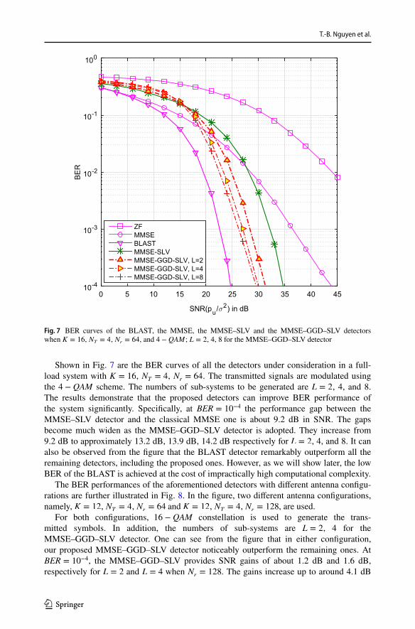
Shown in Fig. 7 are the BER curves of all the detectors under consideration in a full-load system with K = 16 , NT = 4 , Nr = 64 . The transmitted signals are modulated using the 4 − QAM scheme. The numbers of sub-systems to be generated are L = 2 , 4, and 8. The results demonstrate that the proposed detectors can improve BER performance of the system significantly. Specifically, at BER = 10−4 the performance gap between the MMSE–SLV detector and the classical MMSE one is about 9.2  dB in SNR. The gaps become much widen as the MMSE–GGD–SLV detector is adopted. They increase from 9.2 dB to approximately 13.2 dB, 13.9 dB, 14.2 dB respectively for L = 2 , 4, and 8. It can also be observed from the figure that the BLAST detector remarkably outperform all the remaining detectors, including the proposed ones. However, as we will show later, the low BER of the BLAST is achieved at the cost of impractically high computational complexity.

The BER performances of the aforementioned detectors with different antenna configu-rations are further illustrated in Fig. 8. In the figure, two different antenna configurations, namely, K = 12 , NT = 4 , Nr = 64 and K = 12 , NT = 4 , Nr = 128 , are used.

For both configurations, 16 − QAM constellation is used to generate the trans-mitted symbols. In addition, the numbers of sub-systems are L = 2 , 4 for the MMSE–GGD–SLV detector. One can see from the figure that in either configuration, our proposed MMSE–GGD–SLV detector noticeably outperform the remaining ones. At BER = 10−4 , the MMSE–GGD–SLV provides SNR gains of about 1.2  dB and 1.6  dB, respectively for L = 2 and L = 4 when Nr = 128 . The gains increase up to around 4.1 dB

SNR(pu/σ2) in dB

0 5 10 15 20 25 30 35 40 45

BE

R

10-4

10-3

10-2

10-1

100

ZFMMSEBLASTMMSE-SLVMMSE-GGD-SLV, L=2MMSE-GGD-SLV, L=4MMSE-GGD-SLV, L=8

Fig. 7 BER curves of the BLAST, the MMSE, the MMSE–SLV and the MMSE–GGD–SLV detectors when K = 16 , NT = 4 , Nr = 64 , and 4 − QAM ; L = 2 , 4, 8 for the MMSE–GGD–SLV detector

Low Complexity Lattice Reduction Aided Detectors for High Load…

1 3

and 5.1 dB as Nr reduces to 64. This confirm the advantage of our proposed detector when it work in systems with high loads, i.e., the number of data streams is comparable to that of the receive antennas. Unfortunately, the MMSE–SLV detector shows no advantage in term of SNR gain as the number of receive antenna increases from 64 to 128. This implies that when Nr is sufficiently large (i.e., when load factor is small enough), the classical MMSE detector becomes a good candidate for signal recovery in massive MIMO systems.

4.2 Complexity Analysis

In this sub-subsection, we evaluate the complexities of all proposed detectors as well as of the classical BLAST and MMSE ones. The complexity of a detector is computed by count-ing the necessary number of floating point operation (flops) to recover a transmit signal vector. In order to do so, we follows the method in [7, 13, 14] by assuming that each real operation such as a real addition, a real subtraction, a real multiplication, a real division or a square root of a real number is counted as a flop. By using this counting rule, a complex multiplication and a complex division are respectively counted as 8 flops and 11 flops. Besides, the inversion of a × a matrix requires a3 multiplications and a3 additions and the multiplication of a a × b matrix by a b × c requires acb multiplications and ac(b − 1) addi-tions [15]. In this paper, the complexity of slicing operation, matrix/vector transformations are ignored.

pu/σ2 in dB15 20 25 30 35 40

BE

R

10-4

10-3

10-2

10-1

100

ZFMMSEMMSE-SLVMMSE-GGD-SLV, L=4MMSE-GGD-SLV, L=2

Nr=64 antennas

Nr=128 antennas

Fig. 8 BER curves of the MMSE, the MMSE–SLV and the MMSE–GGD–SLV detectors when K = 12 , NT = 4 , Nr = 64, 128 , 16 − QAM ; L = 2 , 4 for the MMSE–GGD–SLV detector

T.-B. Nguyen et al.

1 3

Based on these assumptions and notices, the complexity of the classical MMSE detector is [14]

The results in (22) will be used to compute the computational complexities of proposed detectors in the next representations.

MMSE–SLV complexity evaluation. The computational cost of MMSE–SLV detector, CMMSE−SLV , can be determined as

where Cnew is number of required flops to implement the classical MMSE detection proce-dure in LR domain described in Sect. 3.2; CSLV denotes the SLV algorithm’s complexity.

Note that the dimensions of the original system and the one in LR domain are exactly the same. In addition, the MMSE–SLV is just different from the MMSE by the additional term 1

Es

�H� as shown in Eq.  (11). Evaluation of this term requires approximately 12N2 − 2N + 1 flops. The hard decision of �̂ in (12) requires 4N2 + 6N flops, and the esti-mation of �̃ in (13) needs to compute 8N2 − 2N flops. Therefore the total complexity of Cnew , in terms of flops, is:

Following Algorithm  1 line by line, the complexity of the SLV operation, CSLV , can be evaluated to be:

Substituting the results in (24) and (25) into (23), the overall complexity of the MMSE–SLV detector finally equals:

MMSE–GGD–SLV complexity. Following Algorithm  3, the complexity of the MMSE–GGD–SLV is determined as

where CSort is the complexity of the channel sorting procedure, CPre denotes the complex-ity of generating the L sub-systems corresponding to L stages, and CSub is that of using sub-detectors in L sub-systems. It is well known that sorting a complex m × n matrix needs 1

2

(n2 + 16mn − 7n

) flops. Thus, the computational cost of the channel sorting procedure is:

The remaining two terms in (27) are evaluated and respectively given by:

(22)CMMSE = 8N3 + 16N2Nr − 2N2 + 6NNr,

(23)CMMSE−SLV = Cnew + CSLV ,

(24)Cnew = CMMSE + 24N2 + 2N + 1

= 8N3 + 16N2Nr + 22N2 + 6NNr + 2N + 1.

(25)CSLV = 16N3 + 16N2Nr − 2N2 − 2NNr

+ 4C� + 10C△ + 24NCupdate (flops).

(26)CMMSE−SLV = 24N3 + 32N2Nr + 20N2 + 4NNr + 2N + 1

+ 4C� + 10C△ + 24NCupdate.

(27)CMMSE−GGD−SLV = CSort + CPre + CSub,

(28)CSort =1

2

(N2 + 16NrN − 7N

)(flops).

Low Complexity Lattice Reduction Aided Detectors for High Load…

1 3

and

where C(1)

MMSE−SLV is the complexity of MMSE–SLV detection procedure utilized on the

1st stage; C(q)

MMSE is the complexity of the classical MMSE detector on qth sub-system,

q = 2, 3,… , L . They are evaluated to be:

(29)

CPre = (L − 1)(8N2

rl + 6N2

r− Nr + 6Nrl

)

+

L−1∑

q=1

[8a3 + 16a2Nr − 2a2 − 2aNr + 8aN2

r

],

(30)CSub = C(1)

MMSE−SLV+ (L − 1)C

(q)

MMSE

(31)C(1)

MMSE−SLV= 24l3 + 32l2Nr + 20l2 + 4lNr + 2l + 1

+ 4C(1)

�+ 10C

(1)

△+ 24lC

(1)

update(flops),

(32)C(q)

MMSE= 8l3 + 16l2Nr − 2l2 + 6lNr (flops).

Number of antenna at the BS (Nr)60 80 100 120 140 160

Num

ber o

f flo

ps x

108

0

0.5

1

1.5

2

2.5

3

3.5

4MMSE

BLAST

MMSE-SLV

MMSE-GGD-SLV, L=4

MMSE-GGD-SLV, L=2

Fig. 9 Complexities of the classical MMSE, the BLAST detectors as well as the MMSE–SLV and the MMSE–GGD–SLV ones when Nr = N = [60 ∶ 20 ∶ 160] antennas

T.-B. Nguyen et al.

1 3

Number of antenntasN=48, Nr N,84=N46= r=128

Num

ber o

f Flo

ps (x

106 )

0

10

20

30

40

50

60

70

80

90BLAST

MMSE

MMSE-SLV

MMSE-GGD-SLV, L=2

MMSE-GGD-SLV, L=4

Fig. 10 Complexity comparison of the MMSE, the BLAST, the MMSE–SLV and the MMSE–GGD–SLV detectors in two system antenna’s configurations as N = 48, Nr = 64 and N = 48, Nr = 128

Table 1 Complexity comparison

N = KNT ; l = N∕L ; a = N − ql ; The average value of C�, C△, Cupdate , C(1)

�, C

(1)

△ and C(1)

update are given by

simulations

Detectors Number of required flops per vector

ZF [14] 8N3 + 16N2Nr − 2N2 + 6NNr − 2N

MMSE [14] 8N3 + 16N2Nr − 2N2 + 6NNr

BLAST [14] 15

4N4 + 2N3Nr + N2N2

r+ N

(16Nr − 2

)

MMSE–SLV 24N3 + 32N2Nr + 20N2 + 4NNr + 2N + 1 + 4C� + 10C△ + 24NCupdate

MMSE–GGD–SLV 1

2

�N2 + 16NrN − 7N

�+ (L − 1)

�8l3 + 16l2Nr − 2l2 + 6lNr

�

+ (L − 1)�8N2

rl + 6N2

r− Nr + 6Nrl

�

+L−1∑k=1

�8a3 + 16a2Nr − 2a2 − 2aNr + 8N2

ra�

+24l3 + 32l2Nr + 20l2 + 4lNr + 2l + 1 + 4C(1)

�+ 10C

(1)

△+ 24lC

(1)

update

Low Complexity Lattice Reduction Aided Detectors for High Load…

1 3

The total complexities of the proposed MMSE–SLV and MMSE–GGD–SLV detectors are computed and summarized in Table 1 together with those of the conventional MMSE and BLAST detectors.

Figure  9 illustrates the complexities of the aforementioned detectors in full load sys-tems, where Nr = N = [60 ∶ 20 ∶ 160] antennas. For the MMSE–GGD–SLV detector, the numbers of sub-systems under investigation are L = 2 and L = 4 . One can observe from the figure that the complexities of all the detectors are increased proportionally to the num-ber of antennas. Among the detectors, the BLAST has much higher complexity than those of the rest ones. Therefore, it could hardly be adopted in Massive MIMO systems, where large numbers of antennas are deployed at the cell sites. The results also show that the complexity of the MMSE–SLV detector is higher than those of the conventional MMSE and the MMSE–GGD–SLV ones. The higher complexity of the MMSE–SLV comes at a price of higher BER performance Interestingly, the MMSE–GGD–SLV detector has lower computational complexities than that of the MMSE–SLV one for all L. Its complexity is even comparable to that of the MMSE when L = 2 . The higher value of L is selected, the higher complexities are required for the MMSE–GGD–SLV detector. This means that L should be chosen sufficiently small for the trade-off between the BER performance and detection complexity.

In Fig. 10, the complexities of the four detectors are further illustrated when they are adopted in the systems with load factor of � =

N

Nr

= 0.75 and � = 0.375 , which are corre-sponding to two systems configurations: (1) N = 48, Nr = 64 and (2) N = 48, Nr = 128 . The results in Fig. 10 show that the complexities of proposed detectors are slightly higher than that of the MMSE one when � = 0.75 . However, when the load factor of the system reduces to � = 0.375 , the proposed detectors are of higher computational complexities than their conventional MMSE counterpart, especially for the case of the MMSE–GGD–SLV detector with L = 4 . It is clear from both the performance results and complexity analysis that the proposed detectors are more advantageous than the conventional MMSE one in Massive MIMO with sufficiently high loads. In low load scenarios, the MMSE obviously has stronger advantages.

5 Conclusion

In this paper, two efficient detectors, called MMSE–SLV and the MMSE–GGD–SLV, have proposed based on the SLV technique, the group detection technique, and the conventional MMSE detection procedure for signal detection in Massive MIMO systems. Simulation results and complexity analysis show that in the systems with sufficiently high loads, the proposed detectors achieve significantly BER performance improvement compared to the classical MMSE one, while their complexities are kept at practical levels. The big-ger the load factor is, the more performance improvement the proposed detectors achieve. As a consequence, they are good candidates for signal detection in the high-load Massive MIMO systems. On the contrary, the classical MMSE detector is still of the best candidate for signal recovery in low-load Massive MIMO systems.

T.-B. Nguyen et al.

1 3

References

1. Ngo, H. Q. (2015). Massive MIMO: Fundamentals and system designs (Vol. 1642). Linköping: Linköping University Electronic Press.

2. Marzetta, T. L. (2015). Massive mimo: An introduction. Bell Labs Technical Journal, 20, 11–22. 3. Marzetta, T. L., Larsson, E. G., Yang, H., & Ngo, H. Q. (2016). Fundamentals of massive MIMO.

Cambridge: Cambridge University Press. 4. Liu, T., Tong, J., Guo, Q., Xi, J., Yu, Y., & Xiao, Z. (2017). Energy efficiency of uplink massive mimo

systems with successive interference cancellation. IEEE Communications Letters, 21(3), 668–671. 5. Choi, J. W., & Shim, B. (2014). New approach for massive mimo detection using sparse error recovery.

In Global communications conference (GLOBECOM), 2014 IEEE, IEEE (pp. 3754–3759). 6. Chockalingam, A., & Rajan, B. S. (2014). Large MIMO systems. Cambridge: Cambridge University

Press. 7. Nguyen, T. B., Nguyen, T. D., Le, M. T., & Ngo, V. D. (2017). Efficiency zero forcing detectors

based on group detection algorithm for massive mimo systems. In: 2017 International conference on advanced technologies for communications (ATC) (pp. 48–53).

8. Zhou, Q., & Ma, X. (2013). Element-based lattice reduction algorithms for large mimo detection. IEEE Journal on Selected Areas in Communications, 31(2), 274–286.

9. Li, T., Patole, S., & Torlak, M. (2014). A multistage linear receiver approach for mmse detection in massive mimo. In 2014 48th Asilomar conference on signals, systems and computers (pp. 2067–2072). IEEE.

10. Hassibi, B. (2000). A fast square-root implementation for blast. In Conference record of the thirty-fourth asilomar conference on signals, systems and computers (Vol. 2, pp. 1255–1259). IEEE.

11. Ma, X., & Zhang, W. (2008). Performance analysis for mimo systems with lattice-reduction aided lin-ear equalization. IEEE Transactions on Communications, 56(2), 309–318.

12. Bai, L., Choi, J., & Yu, Q. (2014). Low complexity MIMO receivers. Berlin: Springer. 13. Tran, X. N., Ho, H. C., Fujino, T., & Karasawa, Y. (2008). Performance comparison of detection meth-

ods for combined stbc and sm systems. IEICE Transactions on Communications, 91(6), 1734–1742. 14. Nguyen, T. B., Le, M. T., Ngo, V. D., & Nguyen, V. G. (2018). Parralel group detection approach for

massive mimo systems. In 2018 International conference on advanced technologies for communica-tions (ATC) (pp. 160–165).

15. Golub, G. H., & Van Loan, C. F. (2012). Matrix computations (Vol. 3). Baltimore: JHU Press.

Publisher’s Note Springer Nature remains neutral with regard to jurisdictional claims in published maps and institutional affiliations.

Thanh‑Binh Nguyen was born in 1980 in Ha Nam, Vietnam. He received his B.E. degree in Telecommunication Engineering from Tel-ecommunication University, Vietnam in 2004, M.S. degree in Tele-communication Engineering from Posts and Telecommunication Insti-tute of Technology (PTIT), Vietnam in 2013. From 2004 to 2016 he worked as lecturer at Telecommunication University, Vietnam. He cur-rently is working toward his Ph.D. degree in Electronic Engineering at Le Quy Don Technical University,Vietnam.

Low Complexity Lattice Reduction Aided Detectors for High Load…

1 3

Minh‑Tuan Le was born in Thanh Hoa, Vietnam, in 1976. He received his B.E. degree in Electronic Engineering from Hanoi University of Science and Technology, Vietnam in 1999, M.S. degree and Ph.D. degree both in Electrical Engineering from Information and Commu-nication University, which is currently the Department of Electrical and Engineering of Korean Advanced Institute of Science and Tech-nology (KAIST), Daejon, Korea, in 2003 and 2007, respectively. From 1999 to 2001 and from 2007 to 2008 he worked as a lecturer at Posts and Telecommunication Institute of Technology (PTIT), Vietnam. From November 2012 to 2015, he worked at Hanoi Department of Sci-ence and Technology, Vietnam. He is currently working at MobiFone Reasearch and Development Center, MobiFone Corporation, Vietnam. His research interests include spacetime coding, space–time process-ing, and MIMO systems. Dr. Le is the recipient of the 2012 ATC Best Paper Award from the Radio Electronics Association of Vietnam (REV) and the IEEE Communications Society. He is a member of IEEE.

Dr. Vu‑Duc Ngo is currently a lecturer at School of Electronics and Tel-ecommunications, Hanoi University of Science and Technology, and a researcher at MobiFone Research and development Center, MobiFone corporation, Vietnam. He received the Ph.D. degree from Korea Advanced Institute of Science and Technology in 2011. During 2007–2009 he was a Co-founder and CTO of Wichip Technologies Inc, USA. Since 2009, he is also a Cofounder and Director of uVision Jsc, Vietnam. Since November 2012 Dr. Ngo has been serving as a BoM member of the National Program on Research, Training, and Construc-tion of High-Tech Engineering Infrastructure of Vietnam. His research interests are in the fields of SoC, NoC design and verification, and VLSI design for multimedia codecs as well as wireless communica-tions PHY layer. Dr. Ngo is recipient of IEEE 2006 ICCES and IEEE 2012 ATC best paper awards. Dr. Ngo is a member of IEEE.