Shape-Based Detection of Cortex Variability for More Accurate Discrimination Between Autistic and...
110
Shape-Based Detection of Cortex Variability for More Accurate Discrimination Between Autistic and Normal Brains By: Matthew Joseph Nitzken Bachelors of Science, University of Louisville Speed School of Engineering, August 15th, 2009 A Thesis Submitted to the Faculty of the University of Louisville J.B. Speed School of Engineering As Partial Fulfillment of the Requirements For the Professional Degree MASTER OF ENGINEERING Department of Biomedical Engineering August, 2010
Transcript of Shape-Based Detection of Cortex Variability for More Accurate Discrimination Between Autistic and...
Shape-Based Detection of Cortex Variability for More Accurate Discrimination Between Autistic and Normal Brains
By: Matthew Joseph Nitzken
Bachelors of Science, University of Louisville Speed School of Engineering, August 15th, 2009
A Thesis Submitted to the Faculty of the
University of Louisville J.B. Speed School of Engineering
As Partial Fulfillment of the Requirements For the Professional Degree
MASTER OF ENGINEERING Department of Biomedical Engineering
August, 2010

ii

iii
Shape-Based Detection of Cortex Variability for More Accurate Discrimination Between Autistic and Normal Brains
Submitted by: __________________________________ Matthew Joseph Nitzken
iv
A Thesis Approved On
___________________________________
Date
By the Following Reading and Examination Committee:
___________________________________ Ayman El-Baz, Ph.D
Thesis Director,
___________________________________ Manuel F. Casanova, M.D.
___________________________________ Guruprasad Giridharan, Ph.D.
___________________________________ Palaniappan Sethu, Ph.D.

v
ACKNOWLEDGEMENTS
I wanted to extend my thanks to a number of individuals who have helped me
see the work presented in this thesis through to this stage. First and foremost I want to
thank Dr. Ayman El-Baz for his countless hours of patience and assistance in helping me
overcome obstacles during this process. Thanks to his generous access to knowledge,
labs and vast resources I have been able to complete my work. It has been a great
honor to work with him and I could not have asked for a better advisor. Without his
enduring help and assistance this thesis would have been next to impossible to
complete.
I would also like to extend my thanks to Moo Chung, Qianqian Fang and John
Valdes for their helpful and much appreciated correspondence in the fields of mesh
generation and spherical harmonic analysis. Without their forward looking insights in to
this field this work and this field would not be where it is today.
I am grateful for everything that the University of Louisville Bioengineering
Department has given me as well. As a member of the first class of bioengineering
students I have gotten to see and experience the growth of the department and the
passion and dedication of the professors. I greatly appreciate everything I have been
taught and am tremendously grateful for the opportunities and support I have been
given from the faculty, staff and department as a whole.
Finally I want to profusely thank my family for the countless hours spent helping
me finalize this thesis, giving me inspiration and for the years of support they have given
me during this degree program and throughout life itself. I cannot thank them enough
for giving me the opportunities in education, allowing me to pursue my desired path
through life, and then giving me the assistance and loving support to walk that road.
Above all others, they are ultimately responsible for the work I present here, and all my
future endeavors.

vi
ABSTRACT
Introduction: Autism is a complex developmental disability that typically appears during
the first three years of life, and is the result of a neurological disorder that affects the
normal functioning of the brain, impacting development in the areas of social
interaction and communication skills. According to the Centers for Disease Control and
Prevention (CDC) in 2009, about 1 in 110 American children will fall somewhere in the
autistic spectrum. Although the cause of autism is still largely not clear, researchers
have suggested that genetic, developmental, and environmental factors may be the
cause or the predisposing effects towards developing autism. While shape based
statistical analysis methods for autism are still in their early stages, current results show
positive outlooks on the ability to detect differences between autistic and normal
patients.
Methods: The goal of this thesis is to construct a complete package that is capable of
taking 2-dimensional images from a standard medical scanner, and be able to construct
a three-dimensional representation of the object and examine it through combination
of its weighted linear spherical harmonics. The desired outcome is that a distinction can
be made between the analysis of autistic and normal brain data. The analysis package
created is divided into three distinct components that are capable of performing the
complete analysis on a subject. The components included in the package in order of
runtime are: volumetric extraction and mesh generation from 2-dimensional medical
scanner data, spherical deformation of the constructed mesh, and weighted spherical
harmonic representation and analysis.

vii
Results: The minimum error for each brain following spherical harmonic reconstruction
was calculated along with the fastest iteration at which the brain converged below the
error thresholds of 11% and 10%. It was expected that due to the complexity of an
Autistic brain these would require more iterations to converge to the same error level as
a normal brain. It was also likely that within the number of iterations tested the autistic
brains would record a larger final error due to this slower convergence rate. This was
confirmed by the data. A global result was examined as well for the autistic and normal
data groups. The overall minimum error for normal brain data was significantly lower
than the autistic brain data. The average error for autistic brain data was significantly
higher in both convergence measurements, but was dramatically higher in the 10%
category.
Conclusion: Using this method of analyzing data can demonstrate accurate differences
in normal and autistic brains. The research that has been generated in this thesis can
clearly demonstrate that the normal brain data converged both faster and with a lower
rate of error level than the Autistic brain data. This result proves that the autistic brain is
a more complex structure, and would be more difficult to reconstruct using this Shape-
Based Detection of Cortex Variability process.

viii
TABLE OF FIGURES Figure 1: Normal (a-b) and autistic (c-d) segmented brain images (page 13). Figure 2: Enhanced view of 3-dimensional binary voxels in a brain volume matrix (page
15). Figure 3: 3-dimensional binary representation of an autistic brain (page 15). Figure 4: 3-dimensional binary representation of a normal brain (page 16). Figure 5: (a) The original cube of pixels, (b) Showing the starting neighbor pixels in the 6
cardinal directions, (c) The outward directions of movement for the detection iterations (page 18).
Figure 6: Mesh renders for an autistic (a) and a normal (b) brain (page 19). Figure 7: (a) An autistic brain render and (b) the render after Laplacian smoothing. (C) A
normal brain render and (d) the render after Laplacian smoothing (page 25). Figure 8: Simple spherical inflation of normal brains (a,b) and an autistic brain (c) and
the spheres after 3 iterations of the Attraction-Repulsion algorithm have been applied (d-f) (page 29).
Figure 9: Simple spherical inflation of normal brains (a,b) and an autistic brain (c) and the spheres after 3 iterations of the Attraction-Repulsion algorithm have been applied (d-f) (page 29).
Figure 10: Autistic subject A9. (a) Original mesh, (b) Reconstruction with σ=0.01, (c) Reconstruction with σ=0.00001 (page 34).
Figure 11: Autistic subject A11. (a) Original mesh, (b) Reconstruction with σ=0.01, (c) Reconstruction with σ=0.00001 (page 34).
Figure 12: Normal subject N5. (a) Original mesh, (b) Reconstruction with σ=0.01, (c) Reconstruction with σ=0.00001 (page 35).
Figure 13: Normal subject N8. (a) Original mesh, (b) Reconstruction with σ=0.01, (c) Reconstruction with σ=0.00001 (page 35).
Figure 14: Error curves for autistic (black lines) and normal (blue lines) brains during reconstruction using a smoothing σ = 0.01 (page 37).
Figure 15: Probability Density Function graphs of smoothing σ = 0.001 for (a) 11% error, (b) 10% error, and (c) minimum error (page 38).
Figure 16: Error curves for autistic (black lines) and normal (blue lines) brains during reconstruction using a smoothing σ = 0.001 (page 41).
Figure 17: Probability Density Function graphs of smoothing σ = 0.001 for (a) 11% error, (b) 10% error, and (c) minimum error (page 43).
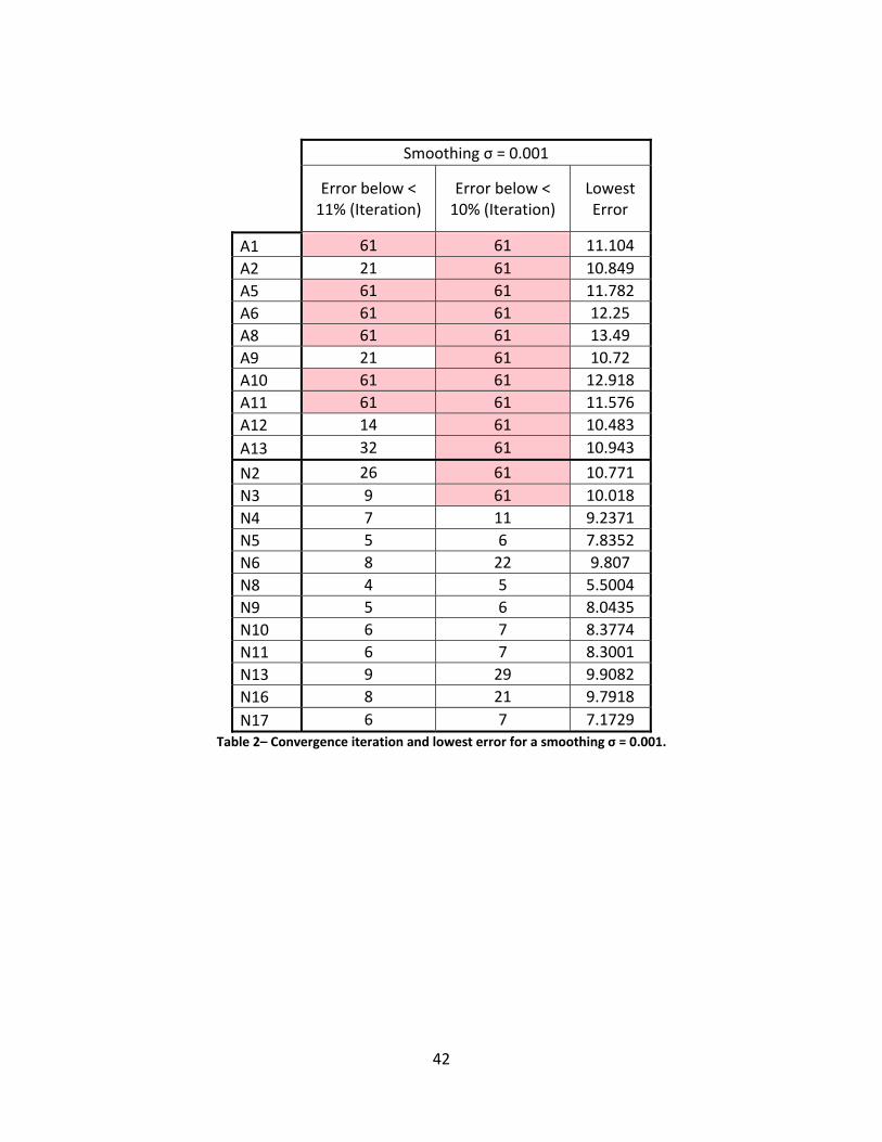
Figure 18: Error curves for autistic (black lines) and normal (blue lines) brains during reconstruction using a smoothing σ = 0.0001 (page 44).
Figure 19: Probability Density Function graphs of smoothing σ = 0.0001 for (a) 11% error, (b) 10% error, and (c) minimum error (page 46).
Figure 20: Error curves for autistic (black lines) and normal (blue lines) brains during reconstruction using a smoothing σ = 0.00001 (page 47).
Figure 21: Probability Density Function graphs of smoothing σ = 0.0001 for (a) 11% error, (b) 10% error, and (c) minimum error (page 49).

ix
LIST OF TABLES
1. Table 1: Convergence iteration and lowest error for a smoothing σ = 0.01.
2. Table 2: Convergence iteration and lowest error for a smoothing σ = 0.001.
3. Table 3: Convergence iteration and lowest error for a smoothing σ = 0.0001.
4. Table 4: Convergence iteration and lowest error for a smoothing σ = 0.00001.
5. Table 5: Average minimum error and convergence for autistic and normal data
groups

x
TABLE OF CONTENTS
APPROVAL PAGE ................................................................................................................. iv
ACKNOWLEDGEMENTS ........................................................................................................ v
ABSTRACT ............................................................................................................................ vi
TABLE OF FIGURES ............................................................................................................ viii
LIST OF TABLES .................................................................................................................... ix
I. INTRODUCTION ........................................................................................... 1
II. DATA ANALYSIS ......................................................................................... 12
III. RESULTS..................................................................................................... 33
IV. CONCLUSION AND FUTURE WORK ........................................................... 52
REFERENCES ...................................................................................................................... 55
APPENDIX 1: WAVEFRONT OBJ FORMAT ..................................................................... 58-61
A: FORMAT SPECIFICATION .................................................................................. 58
B: ingOBJSave.m MATLAB CODE ........................................................................... 60
C: ingOBJRead.m MATLAB CODE ......................................................................... 61 APPENDIX 2: DATA TABLES .......................................................................................... 62-84
A: AUSTIC DATA TABLE FOR RECONSTRUCTION SIGMA 0.01 ............................... 62 B: AUSTIC DATA TABLE FOR RECONSTRUCTION SIGMA 0.001 ............................. 65 C: AUSTIC DATA TABLE FOR RECONSTRUCTION SIGMA 0.0001 ........................... 68 D: AUSTIC DATA TABLE FOR RECONSTRUCTION SIGMA 0.00001 ........................ 71 E: NORMAL DATA TABLE FOR RECONSTRUCTION SIGMA 0.01 ............................ 74 F: NORMAL DATA TABLE FOR RECONSTRUCTION SIGMA 0.001 .......................... 77 G: NORMAL DATA TABLE FOR RECONSTRUCTION SIGMA 0.0001 ....................... 80 H: NORMAL DATA TABLE FOR RECONSTRUCTION SIGMA 0.00001 ..................... 83
APPENDIX 3: COMPLETE RECONSTRUCTION MESH REPRESENTATION .................... 85-100 A: NORMAL BRAIN ITERATIONS 1-60 MESH REPRESENTATION ........................... 85 B: AUTISTIC BRAIN ITERATIONS 1-60 MESH REPRESENTATION ........................... 93

1
I. Introduction
A. Defining Autism
Autism is a complex developmental disability that typically appears during the
first three years of life, and is the result of a neurological disorder that affects the
normal functioning of the brain, impacting development in the areas of social
interaction and communication skills. Difficulties can be identified in both children and
adults with autism. The symptoms are identifiable in verbal and non-verbal
communication, social interactions, and leisure or play activities. The classic form of
autism involves a triad of impairments, these are typically in social interaction, in
communication and the use of language, and in limited imagination as reflected in
restricted, repetitive and stereotyped patterns of behavior and activities [1].
B. Historical Perspective
It was in 1943, that Leo Kanner, a psychiatrist at Johns Hopkins University,
created the diagnosis of autism. Leo Kanner was an Austrian psychiatrist and physician
known for his work related to autism. Kanner's work formed the foundation of child
and adolescent psychiatry in the U.S. and worldwide. His first textbook, Child
Psychiatry in 1953, was the first English language textbook to focus on the psychiatric

2
problems of children [2]. His seminal 1943 paper, "Autistic Disturbances of Affective
Contact", together with the work of Hans Asperger, forms the basis of the modern study
of autism. By definition, patient symptoms are manifested by 36 months of age and are
characterized by delayed and disordered language, impaired social interaction,
abnormal responses to sensory stimuli, events and objects, poor eye contact, an
insistence on sameness, an unusual capacity for rote memory, repetitive and stereotypic
behavior and a normal physical appearance [3].
Relatively few neuropathological studies have been performed on the brains of
autistic subjects. Of those reported, abnormalities have been described in the cerebral
cortex, the brainstem, the limbic system and the cerebellum. Although, those
individuals who have the disorder present with a specific set of core characteristics,
each individual patient is somewhat different from another. Thus, it should not be
surprising that the brains of these subjects should show a wide range of abnormalities.
However, it is important to delineate the anatomic features, which are common to all
cases, regardless of age, sex and IQ, in order to begin to understand the central
neurobiological profile of this disorder. The results of systematic studies indicate that
the anatomic features that are consistently abnormal in all cases include a reduced
numbers of Purkinje cells in the cerebellum, and small tightly packed neurons in the
entorhinal cortex, and in the medially placed nuclei of the amygdala. It is known that the
limbic system is important for learning and memory, and that the amygdala plays a role
in emotion and behavior. Research in the cerebellum indicates that this structure is
important as a modulator of a variety of brain functions and impacts on language

3
processing, anticipatory and motor planning, mental imagery and timed sequencing.
Defining the differences and similarities in brain anatomy in autism and correlating
these observations with detailed clinical descriptions of the patient may allow us greater
insight into the underlying neurobiology of this disorder [4]
The many patterns of abnormal behavior that cause diagnostic confusion include
one originally described by the Austrian psychiatrist, Hans Asperger [5]. The name he
chose for this pattern was “autistic psychopathy” using the latter word in the technical
sense of an abnormality of personality. This has led to misunderstanding because of the
popular tendency to equate psychopathy with sociopathic behavior. Asperger
emphasized the stability of the clinical picture throughout childhood, adolescence, and
at least into early adult life, apart from the increase in skills brought about by
maturation. The major characteristics appear to be impervious to the effects of
environment and education. He considered the social prognosis to be generally good,
meaning that most developed far enough to be able to use their special skills to obtain
employment. He also observed that some who had especially high levels of ability in the
area of their special interests were able to follow careers in, for example, science and
mathematics.
C. Increase of Incidence
The reported incidence of autism spectrum disorders has increased markedly
over the past decade [6]. It is believed that autism affects the information processing
found in the brain through the alteration of nerve collections and their synapses [7].

4
From Congress to popular media, speculation is increasing that more children have
autism than ever before. The three classifications of autism include autism spectrum
disorders (ASD), Asperger syndrome (AS) and pervasive developmental disorder (PDD)
[8].
A study done in 2008 by Rapin et al, shows that autism is now recognized in one
out of 150 children making it a prevalent disorder [9, 10]. Additional studies by
DiGuiseppi show a high prevalence among screened American children with as high as
6.4% of screened children showing at least a mild form of an autistic spectrum disorder
[11, 12]. According to the Centers for Disease Control and Prevention (CDC) in 2009,
about 1 in 110 American children will fall somewhere in the autistic spectrum. Although
the cause of autism is still largely not clear, researchers have suggested that genetic,
developmental, and environmental factors may be the cause or the predisposing effects
towards developing autism [13].
There are other mathematical relationships between incidence and prevalence.
An important nuance about prevalence is that its accuracy is only as good as the degree
to which each individual who actually has the condition is counted (the numerator or
top number of the fraction), and the completeness with which the “general” or other
population has been counted (the denominator or bottom number of the fraction.)
Accuracy in these two figures can be hard to achieve. In fact, there are no scientifically
based epidemiological prevalence estimates for ASD in the United States at this time.
Federal agencies have, however, called upon researchers to submit proposals that will
develop better prevalence rates. [8].

5
Until research in the United States results in more accurate figures, the National
Institutes of Health (NIH) have suggested the following prevalence rates for ASD based
upon research in other Westernized, developing nations:
• 10/10,000 people with “classic” autism
• 20/10,000 people with ASD, including PDD
• 50/10,000 people with ASD, including PDD and Asperger syndrome.
These estimates are inclusive; that is, the third estimate includes people in the first two
groups. This means that in a given large population, on average 0.5%, one-half percent
of the population could be diagnosed with an ASD. [8]
D. Early Detection
Early detection allows for treatments to be attempted, thus minimizing the
impact of the autism on the individual. Given currently available diagnostic instruments,
autism and other pervasive developmental disorders (PDD) are difficult to detect in very
young children. This may be due to several factors: presentation of symptoms varies
from case to case; social and language deficits and delays may not be identified until the
child is given the opportunity for peer interaction in preschool, low incidence leads to a
low index of suspicion, and motor milestones are usually unaffected. Furthermore,
there is no standard and easily administered screening instrument for young children.
For all of these reasons, pediatric evaluations rarely identify autism before the age of 3
(Gillberg, 1990). However, evidence indicates that there is a large gap between the age

6
of the child at the parents’ first concern, the age of the first evaluation, and the age of a
definitive diagnosis [12]. Parents are typically first concerned between the ages of 15
and 22 months (earlier for children who have co-morbid mental retardation), but the
child is often not seen by a specialist until 20–27 months [14]. In addition, there is often
further delay between the first visit to a specialist and a definitive diagnosis (Siegel et
al., 1988). However, evidence shows that this delay in diagnosis causes additional
distress to parents, as well as wasting valuable intervention time, indicating that
professionals in the field of autism need instruments to aid in the detection of autism in
very young children. [14].
Some forms of autism merely result in the individual exhibiting low social
interaction, but more severe forms can result in severe mental retardation. These
individuals may be prone to self injuring and aggressive behavior. There is no current
cure for any forms, of autism. However, educational, behavioral, or skill-oriented
therapies were designed to remedy specific symptoms in each individual. Such therapies
can result in a notable improvement for the individual, especially when begun at a
young age. [14].
E. Neuropathology of Autism
In identification of autism, the analysis of the neuropathology is important. The role
of single-stranded microdeletions and epigenetic influences on brain development has
dramatically altered our understanding of the etiology of the autisms. Recent research
has focused on the role of synapse structure and function as central to the development

7
of autism and suggests possible targets of interventions. Brain under connectivity has
been a focus in recent imaging studies, and has become a central theme in
conceptualizing autism. Despite increased awareness of autism, there is no 'epidemic'
and no one cause for autism. Data from the sibling studies are identifying early markers
of autism and defining the broader autism phenotype. [9].
The three sections of the brain analyzed are the gray matter, the white matter
and the corpus callosum. Examination of the individual sections shows significant
changes to the neuropathology of autistic individuals, suggesting a higher complexity in
the autistic brain than the normal brain. [15]
The grey matter is the brain cortex that contains the nerve cells responsible for
routing sensory or motor stimuli to inter-neurons of the central nervous system. In
autistic individuals Abel et al. identified a decreased gray matter volume relative to a
control group in the right paracingulate sulcus, the left inferior frontal gyrus, and an
increased gray matter volume in amygdala and periamygda- loid cortex, middle
temporal gyrus, inferior temporal gyrus, and in regions of the cerebellum [16].
Additionally Boddaert et al. found significant decreases of grey matter concentration in
the superior temporal sulcus when comparing autistic child patients to normal child
patients[17]. The autistic children also demonstrated a decrease in white matter
concentration located in the right temporal pole and in the cerebellum. Herbert et al.
applied a voxel-based-morphometry (VBM) approach to male patients between the ages
of 7 and 11 years and showed that those with autism had a significantly larger volume of
cerebral white matter (CWM) while cerebral cortex and hippocampus-amygdala had

8
smaller volumes [18]. The corpus callosum is largest single fiber bundle in the brain and
is responsible for connecting the two hemispheres of the brain. It has been proposed
that there are significant differences between the CC of autistic and normal patients [19,
20].
The concept that the cerebellum might play a role in the coordination of
attention in a fashion analogous to the role it plays in motor control and that in autism,
cerebellum mal-development is a consistent feature that renders the child unable to
adjust his or her mental focus of attention to follow the rapidly changing verbal,
gestural, postural, tactile, and facial cues that signal changes in a stream of social
information [21]. Such cues signal the normal child to move his or her "spotlight of
attention" from one source of information (e.g., auditory) to another (e.g., visual). This
process involves disengaging attention from one source and then moving and
reengaging it on another (i.e., inhibition of one source and enhancement of another).
To selectively adjust the focus of attention, the nervous system must quickly and
accurately alter the pattern of neural responsiveness to sensory signals—from an
enhanced neural response to certain stimuli (e.g., vocalizations) to an enhanced
response to other stimuli (e.g., gestures), and from inhibited neural response to some
stimuli to inhibited response to others. [22, 23].
F. Autism Detection Methods
One method of early detection intervention, utilizes medical providers to screen
children using the M-CHAT as they were referred for early intervention services. The

9
Modified Checklist for Autism in Toddlers (M-CHAT) is designed to screen for early
identification of autism spectrum disorder (ASD) in toddlers over the age of 12 months.
Ideally, it is given at the 18-24 month well baby check. Parents complete the items on
the checklist independently or by interview. Meeting the criteria suggests the risk of
ASD and indicates a positive diagnosis for autism. The purpose is to survey parents to
determine how their child responds to varied stimuli from toddler locomotion to a
child’s reaction to other people. M-CHAT users also incorporate the M-CHAT Follow-up
Interview into the screening process, given that recent findings demonstrate that the
interview greatly reduces the false positive rate, which avoids unnecessary referrals
[14]. Therefore, these children were considered to be at risk for a developmental
disorder, but none had received any specific diagnoses and none had received more
than several weeks of minimal intervention services.
In new experiments at Yale University, the researchers studied a group of 2-year-
olds with autism, as well as typically developing children with developmental disabilities
other than autism. The Yale program of research focuses on mechanisms of socialization
and their disruption in the autism spectrum disorders. This work includes a close
collaboration with Warren Jones in the development of novel techniques to quantify
social processes using eye-tracking technologies with a view to visualize and measure
the ontogeny of social engagement. New data analysis strategies have been used with
children, adolescents, and adults with autism spectrum disorders revealing
abnormalities of visual scanning behaviors when viewing naturalistic social approaches
and situations. In this study autistic children showed a preference for audio-visual

10
synchronicity in the use of "pat-a-cake" videos, while the other children were more
interested in the figure's movements regardless of audio-visual synchronicity. That
pattern could be a clue about brain development and early signs of autism. [24, 25, 26,
27]
Dr. Klin of Yale University explains that within a few days after birth, normal
developing children prefer watching biological motion -- the movement of living beings,
such as their parents -- and that preference is an important survival skill and a building
block for relationships. [25]
But Klin's group found that autistic children were more interested in "nonsocial
contingencies," which are synchronicities that don't have any social meaning -- like two
balls colliding and making a sound, or a stone falling when someone drops it. [24]
Researchers hope that a simple brain scan performed in infants and toddlers can
presage the development of autism, leading to early detection and early intervention.
The test involved using functional MRI to measure brain responses to spoken words in
sleeping children. For this study, Dr. Eyler and her colleagues monitored the brain
activity of 30 children with an autism spectrum disorder (aged 14 months to 46 months)
and 14 "typical" children of roughly the same age. [28]
Children slept in the MRI machine while researchers read them bedtime stories.
This allowed the investigators to see which parts of the brain were being activated in
typical children versus children with autism. “In the typically developing children, both
sides of the brain involved in language processing were activated. In the youngest

11
children, the activation was about equal in both the right and left hemisphere, while in
the older children, activity became more pronounced on the left side, which is similar to
adult patterns and to be expected,” Dr. Lisa T. Eyler explained. But in the autistic
children, there was slightly more right hemisphere response than left hemisphere, and
there was no change in activity across the age range. [28]
This leads to the conclusion that, in many children with autism, there are
alterations either in structure growth or connectivity of the brain, but we really don't
understand the implications of that for core features of autism, one of which is the
problem with communication," David G. Amaral said. "This provides more evidence for
abnormal connectivity in the brain." [28].
Further analysis of neurological MRI scans has been pursued in automated
computer analysis of specific components of the brain. Approaches by El-baz et al.
examine the shape model comparison between the corpus callosum in individuals with
and without autism. This analysis focuses on comparison of the 3-dimensional voxel
positioning. In such an automated technique, specific areas of MRI scan images are
extracted. These images are then placed in a stack to recreate a volume of the image.
The difference between regions of this volume can be statistically measured. While
statistical analysis methods are still in their early stages, current results show positive
outlooks on the ability to detect differences between autistic and normal patients based
on voxel based analysis. The positive findings from automated analysis research provide
the basis for the research done in this thesis. [15]

12
II. Data Analysis
A. Introduction
The goal of this thesis is to construct a complete package that is capable of taking 2-
dimensional images from a standard medical scanner, and be able to construct a three-
dimensional representation of the object and examine it through combination of its
weighted linear spherical harmonics. The desired outcome is that a distinction can be
made between the analysis of autistic and normal brain data.
B. Data Acquisition
The data for this thesis was acquired from a 1.5 T Signa MRI scanner (General
Electric, Milwaukee, Wisconsin) using a 3-D spoiled gradient recall acquisition in the
steady state (time to echo, 5 ms; time to repeat, 24 ms; flip angle, 45◦; repetition, 1;
field of view, 24 cm2). Contiguous axial slices (1.5 mm thick) were obtained for each
subject with 124 slices acquired per brain. The images were collected in a 192×256
acquisition matrix, and were 0-filled in k space to yield an image of 256×256 pixels. The
effective voxel resolution of the scans is 0.9375×0.9375×1.5 mm3. The positioning and
placement of the subjects inside the MRI scanner was standardized. A total of 17
13
normal patients and 13 autistic brain data sets were used in this thesis. The test
subjects age range is from age 8 to age 38 for both groups.
C. Package Overview
The analysis package created is divided into three distinct components that are
capable of performing the complete analysis on a subject. The components included in
the package in order of runtime are:
• Volumetric Extraction and Mesh Generation
• Spherical Deformation of the Mesh
• Weighted Spherical Harmonic Analysis
D. Volumetric Extraction
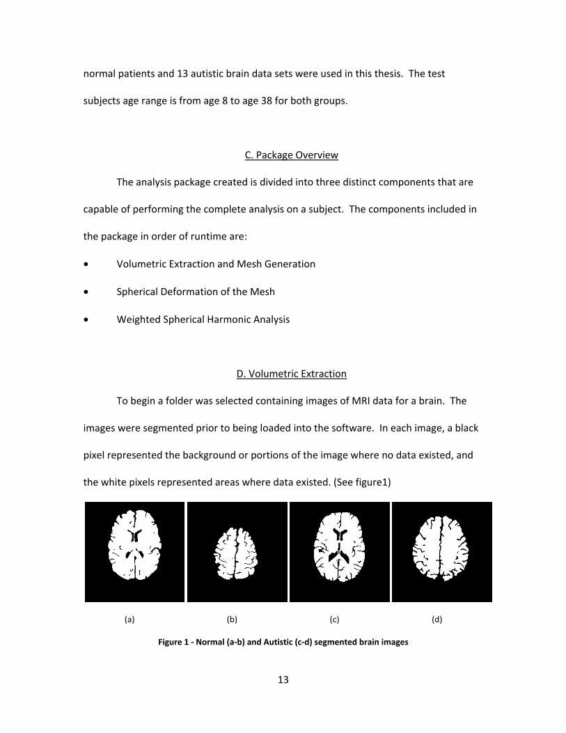
To begin a folder was selected containing images of MRI data for a brain. The
images were segmented prior to being loaded into the software. In each image, a black
pixel represented the background or portions of the image where no data existed, and
the white pixels represented areas where data existed. (See figure1)
(a) (b) (c) (d)
Figure 1 - Normal (a-b) and Autistic (c-d) segmented brain images

14
The images were loaded into the software one at a time. It was first necessary
to convert the images to binary format from their original grayscale format. It was
assumed that any pixel with a value greater than zero would constitute a pixel
containing data. Data values ranged from 0 to the maximum grayscale value (in many
cases this value was 255 and represented a white pixel.)
Instead of iterating through the image and setting, each pixel to a value of 0 or 1
a simple mathematic manipulation was used. All values in the image were divided by
the maximum value in the image. This made the upper bounds of the image 1 and the
lower bounds 0. The entire image was then modified by using the ceiling command to
raise all non-zero values to 1.
After each image was converted to a binary representation, the images were
assembled in a 3-dimensional matrix stack. Each matrix was represented by an X, Y and
Z dimension. The X dimensions represented the rows in an image. The Y dimension
represented the columns in an image. The Z dimension represented the layers in the
volume, with each layer containing a separate distinct image. Each X,Y,Z coordinate
represented a single voxel in 3-dimensional space. An enhanced close-up view of the
binary voxels in the brain volume matrix can be seen in Figure 2. Figures 3 and 4 show
the 3-dimensional binary surface representation of an autistic and normal brain.

15
Figure 2 – Enhanced view of 3-dimensional binary voxels in a brain volume matrix
Figure 3 –3-dimensional binary representation of an autistic brain

16
Figure 4 –3-dimensional binary representation of a normal brain
The MRI scan images were loaded into the memory with data holes intact. While
initially the decision was made to remove all holes in the 2-dimensional images prior to
being loaded into the program, this proved ineffective after the images were placed in a
3-dimensional volume. The initial hole removal procedure was done using Adobe
Photoshop CS2. The exterior of the image, the area outside the outer edge of the brain,
was initially selected as the mask. This mask was then inverted to select the outer
bounds of the brain and all pixels inside the brain slice. The area inside the mask was
then deleted. This process removed all holes found in the 2-dimensional image.
Initially, this technique was believed to be successful, but it was later determined that 3-
dimensional holes existed between image layers causing problems during mesh
generation.
17
To solve this problem, the images were loaded with 2-dimensional holes still
intact, as previously mentioned. The holes were removed using a custom algorithm.
The algorithm began by loading the images into the 3-dimensional volume matrix as
previously described. After creating the 3-dimensional volume matrix, an iterative pass
was made across the X, Y and Z axis of the volume using the Matlab " fillholes()"
command. To accomplish this, a 2-dimensional image slice was removed on each plane
of the volume. This image slice was then passed through the "fillholes()" algorithm, and
the modified image slice was reinserted into the volume. In this way, the holes were
removed from the 2-dimensional representations in the X, Y and Z directions. Following
this procedure, it was discovered that there still remained a large quantity of small holes
throughout the image that could not be removed by converging the image using a 2-
dimensional technique. These holes were formed from differing overlaps in the volume
between layers, and the tendency of the 2-dimensional algorithms to produce small
holes in the planes not being converged.
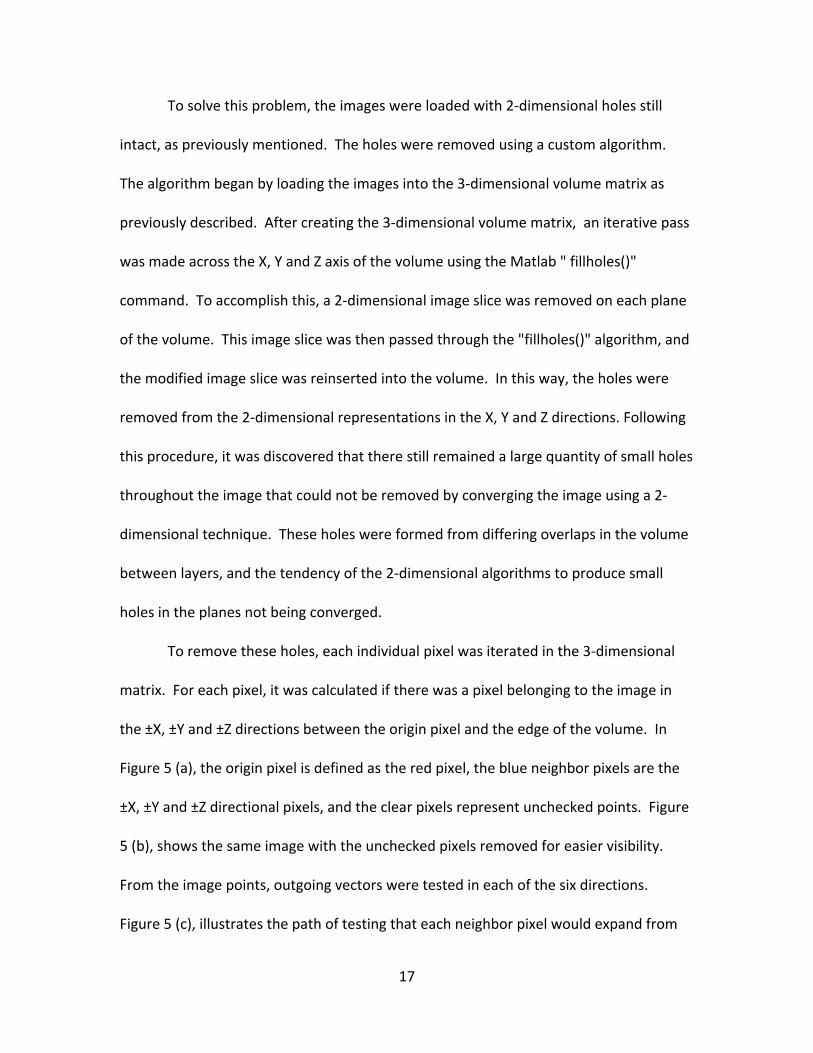
To remove these holes, each individual pixel was iterated in the 3-dimensional
matrix. For each pixel, it was calculated if there was a pixel belonging to the image in
the ±X, ±Y and ±Z directions between the origin pixel and the edge of the volume. In
Figure 5 (a), the origin pixel is defined as the red pixel, the blue neighbor pixels are the
±X, ±Y and ±Z directional pixels, and the clear pixels represent unchecked points. Figure
5 (b), shows the same image with the unchecked pixels removed for easier visibility.
From the image points, outgoing vectors were tested in each of the six directions.
Figure 5 (c), illustrates the path of testing that each neighbor pixel would expand from

18
towards the outer edge. If a pixel value of 1 was found in a given direction, a value of
true was marked for the boolean corresponding with that direction.
(a) (b) (c)
Figure 5 –(a) The original cube of pixels, (b) Showing the starting neighbor pixels in the 6 cardinal
directions, (c) The outward directions of movement for the detection iterations
If a pixel was found radiating out in all six directions, it was determined that the
pixel was a hole in the image. A pixel that did not contain pixels surrounding it on all six
sides was ignored. This procedure was repeated until holes no longer remained in the
image. This was often accomplished in a single iteration. To ensure that the volume
was clean, an additional iteration was always repeated to verify that no holes remained
in the volume. This procedure did add a significant amount of time to the pre-meshing
procedure, but the benefits of this step outweighed the time cost significantly because it
prevented the occurrence of holes during mesh construction.
E. Mesh Generation
Once the 3-dimensional volume had been properly constructed, the mesh was
generated. The mesh generation was performed using a modified version of the
iso2mesh Matlab based mesh generation system, written by Qianqian Fang and David
19
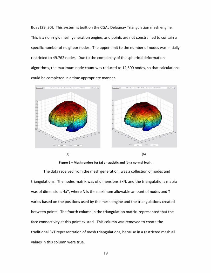
Boas [29, 30]. This system is built on the CGAL Delaunay Triangulation mesh engine.
This is a non-rigid mesh generation engine, and points are not constrained to contain a
specific number of neighbor nodes. The upper limit to the number of nodes was initially
restricted to 49,762 nodes. Due to the complexity of the spherical deformation
algorithms, the maximum node count was reduced to 12,500 nodes, so that calculations
could be completed in a time appropriate manner.
(a) (b)
Figure 6 – Mesh renders for (a) an autistic and (b) a normal brain.
The data received from the mesh generation, was a collection of nodes and
triangulations. The nodes matrix was of dimensions 3xN, and the triangulations matrix
was of dimensions 4xT, where N is the maximum allowable amount of nodes and T
varies based on the positions used by the mesh engine and the triangulations created
between points. The fourth column in the triangulation matrix, represented that the
face connectivity at this point existed. This column was removed to create the
traditional 3xT representation of mesh triangulations, because in a restricted mesh all
values in this column were true.

20
Once the initial mesh was created, it was necessary to reposition it in 3-
dimensional space and to resize the mesh to appropriate proportions. The centroid of
the mesh was calculated in the X, Y and Z directions. Using the coordinates of the
centroid, the mesh was repositioned so that it was centered on the origin in 3-
dimensional Cartesian space (x = 0,y = 0,z = 0). The initial mesh results were not scaled
properly due to the acquisition methods of the MRI scanner. To appropriately resize the
mesh, original image slice acquisition scaling was used. The images were repositioned
according to the X, Y and Z magnification parameters. The X and Y planes were
multiplied by a magnification factor of 0.93, taken from the MRI scanner acquisition
parameters. The Z plane was scaled by a factor of 1.5, the distance between slices taken
during MRI acquisition.
The mesh generation returned a node and face cluster where vertices were
positioned at sharp angles to one another. This made the mesh appear to be “spiky.”
To solve this problem, a Vertex-based anisotropic smoothing filter was applied to the
data. The filter performed a low-pass filter Laplace smoothing algorithm across the
exterior of the mesh. The low-pass filter Laplace smoothing algorithm was based on
code written by Zhang and Hamza in the paper “Vertex-based anisotropic smoothing of
3D mesh data, IEEE CCECE” [31]. The smoothing algorithm was applied iteratively three
times during the procedure, and was configured to smooth at a minimal value with each
pass. The result was a mesh with smooth and accurate contours.
The file format chosen to save the mesh was the Wavefront OBJ format,
developed by Wavefront Technologies. Initially, it was suggested to use the MNI OBJ
21
format. This format was ultimately decided against due to a restriction in the maximum
number of neighbor nodes it was capable of storing. Another factor was that it was
largely incompatible with the standardized Wavefront OBJ format that is the format of
choice for OBJ file representations in a majority of commercial applications. The
Wavefront OBJ format is capable of being read by nearly all modern commercial and
open-source application dealing with mesh analysis, and would allow for future
integration of the system with third-party software. The exact format can be found in
Appendix I. Custom algorithms were written to save and load meshes in this format.
F. Spherical Deformation
Following the generation of a stable, hole-free initial mesh, it was necessary to
generate a corresponding unit sphere. The accuracy of the sphere creation is relative to
the accuracy of the statistical analysis. There were several techniques attempted
including Cartesian and spherical registration methods.
The initial attempt to create a unit sphere was to simply inflate the original mesh
into a unit sphere. This technique was done by reducing all points in the mesh to a
maximum distance of 1.0 from the origin. Once the mesh had been scaled, all points
with a value less than 1.0 were upscaled to a value of 1.0. This inflation technique
resulted in numerous problems, with the most problematic being vertex overlap and
poor distribution of points. The natural shape of the brain sulci and the valley located
between hemispheres in the brain created this overlap by inverting points and face
connectivity, as they were forced to the outer edges of the inflated sphere.

22
In the creation of a unit sphere, it became imperative that all points remain in
their correct orientation with their neighbor points during the deformation process.
This means that during deformation the triangulation connections could not become
crossed. A unit sphere that contained crossed triangulations produced an erroneous
spherical representation. The spherical harmonics are based on angular values, and
points with incorrectly crossed angles caused the system to produce “garbage” result
data and a spherical representation could not be created.
The accuracy of the spherical representation was also based on the distribution
of the vertex coordinates throughout the sphere. A sphere with clusters of vertices and
other areas of sparse vertex placement produced significantly more error and had a
greater difficulty converging. The ideal spherical representation would have all vertices
spaced equidistant from one another across the surface of the sphere. While it is
possible to perform an analysis using an improperly spaced unit sphere, the results were
less than desirable. The original method left large clusters of vertices around areas of
significant sulcus curvature in the brain.
F. Cartesian Coordinate Registration
In an effort to refine the spherical representation, several approaches were
attempted. The first attempted method, was 3-dimensional Cartesian volume
registration. A perfect unit sphere was used as the destination mesh and the brain
mesh undergoing registration functioned as the origin mesh. Points were associated
with the nearest coordinate based on Euclidean distance. Once a point was identified,
23
the point was then removed from the possible pool of points to be selected from for
registration. This method seemed like it would be effective, but it was quickly
discovered that a representation of the brain is irregular. Points deep in between the
two lobes of the brain caused significant problems. These points would often be
associated with corresponding locations on the destination unit sphere on the opposite
side of the sphere from where they should be. Due to occurrences of this phenomenon
at numerous locations, the origin mesh became stretched inside out. While the
ultimate result did align all points on a sphere, it created an unusable mesh. Nearly 95%
of the triangulations became crossed during this process rendering the registration
invalid.
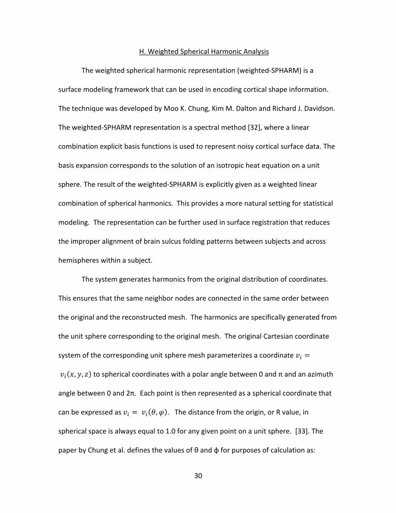
G. Spherical Coordinate Registration
Following the failure of the Cartesian registration, a registration technique based
on spherical angles was attempted. A perfect unit sphere was once again generated as
the destination mesh, and the inclination angle and azimuth angle for each coordinate
was extracted. The same angles were calculated for every point in the origin mesh. The
registration was based on angular locations as the difference in radial distance became
irrelevant. The following equation was used to calculate the error between angles. = − + − , 1 ≤ ≤ # , 1 ≤ ≤ #
Equation 1
(1)

24
The angles that produced the lowest error (closest to zero) were then registered to
one another. The registered coordinates were then removed to prevent reuse. This
method produced a more acceptable result but ultimately failed as well. This was due
to the positioning and number of neighbor triangulations in the unit sphere. A perfect
unit sphere has only 6 neighbor nodes for every point, while each node in the brain
mesh possessed between 3 and 14 neighbor nodes depending on its location. After the
discovery in the number of neighbor nodes, it was decided that this technique would
not be feasible without a highly complex unfolding algorithm to unravel the
triangulations after registration. This required the development of a method other than
registration to an already existing unit sphere.
G. Attraction-Repulsion Deformation
The final process, used in the creation of a unit sphere is a four phase
deformation technique, created for the purpose of deforming the brain meshes. Before
running the spherical deformation, the brain was heavily smoothed using a Laplacian
based smoothing algorithm. The mesh was loaded into the freely available software,
MeshLab v1.2.3b written by Paolo Cignoli. It was determined through trial and error
that an average smoothing of 400 iterations per 12,500 nodes deformed the mesh so
that no existing points in the mesh could be found residing on the same theta and
azimuth angles, when examined in spherical coordinate space. (See Figure 7) The choice
to use MeshLab instead of a Matlab based smoothing algorithm was made to improve
speed. The comparable Matlab algorithm took approximately 30 seconds to run one

25
complete Laplacian smoothing pass. The same algorithm run in MeshLab was capable of
performing 2000 Laplacian smoothing passes in slightly under one minute.
(a) (b)
(c) (d)
Figure 7 – (a) An autistic brain render and (b) the render after 400 iterations of Laplacian smoothing.
(c) A normal brain render and (d) the render after 400 iterations of Laplacian smoothing.
The technique is composed of the following four phases
• The Laplacian deformation step.
• The unit sphere distance deformation.
• The Attraction-Repulsion algorithm refinement step.
• A second unit sphere distance deformation.

26
In the Laplacian deformation phase, the brain is smoothed until all curves, peaks and
valleys of the cortex are flattened across the brain. This ensures that no more than one
point will be found for a given set (azimuth and theta angles) of spherical coordinates.
This mesh is then resaved as a smooth mesh object which will be loaded for the second
through fourth phases.
The unit sphere distance deformation involves inflating the smoothed mesh to the
distance of a unit sphere. To increase the speed of the spherical inflation it is necessary
to manipulate the mesh in the spherical coordinate domain. The Cartesian mesh is first
converted to spherical coordinates using the “cart2sph” command in Matlab. This
returns a Theta angle, Azimuth (Phi) angle and R distance for each point in the mesh.
The R distance is removed and replaced with a matrix of the same size with all values
equal to 1.0. The coordinates are then reconverted to Cartesian using the sph2cart
command in Matlab. This provides a fast and effective conversion that is extremely
efficient, because it requires no iterative processing and does not involve examining
each node individually or performing any distance calculations. These inflated points
are then passed on to the third phase.
In the third phase, the attraction-repulsion algorithm is used to refine the inflated
sphere. The attraction-repulsion algorithm is based on a standard spring algorithm. The
algorithm was inspired by a concept used in Graphic Art Design for inflating objects. The
purpose of this algorithm is to reposition the nodes in the mesh. After the second phase
of the spherical deformation, there are large clusters of nodes spaced near one another
in areas of the mesh that contain a high density of nodes. Looking at the mesh, it is

27
possible to see large clusters near the lower lobes of the brain and around complex
areas. As previously mentioned, it is necessary to evenly space the nodes across the
sphere. To accomplish this, the attraction-repulsion algorithm was created.
The attraction-repulsion algorithm is composed of two steps, the attraction step and
the repulsion step. Each node is altered by being processed in the attraction step and
then the repulsion step. In the attraction step the node is altered based on its neighbor
nodes. The distance between a node and each of its neighbor nodes is calculated. The
node is then pulled based on numerical weighting, so that it becomes centered between
its neighbors. The attraction for iteration is defined as: = + ( )(0.01) + . , 1 ≤ ≤ , 1 ≤ ≤ ℎ Equation 2 – Attraction algorithm
where represents the new node coordinate and is the original node
coordinate. P represents the original coordinate of the unmodified node that is and Q is
the coordinate of neighbor node N. The distance from P to Q is a 3-dimensional
Euclidean distance.
After the node has been centered between its neighbors it is processed in the
repulsion step. Here the node is slightly readjusted by every node in the mesh. Each
node minimally repels one another so that the nodes do not cross or touch. The
repulsion is defined as:
= + ( ) . ,
(2)
(3)

28
1 ≤ ≤ , 1 ≤ ≤
Equation 3 – Repulsion algorithm
where represents the new node coordinate and is the original node
coordinate. N represents the total number of nodes in the mesh. T is a value between 0
and 1 and stands for the time step of the algorithm. A larger time step enables the
algorithm to converge faster but increases the chance of error as nodes are capable of
moving larger distances.
This algorithm also causes an inflation effect to occur during repeat iterations as
each node is gently repelled from interior angles by nodes opposite it on the unit
sphere. Because there are no nodes outside the unit sphere to repel the nodes back
toward the center this inflation occurs. This step is repeated several times until a
satisfactory node distribution is reached. (See Figures 8 and 9)
Once the attraction-repulsion algorithm has completed, the nodes are more
evenly spaced on the sphere. Due to the previously described interior repulsion, the
sphere is also much larger than a unit sphere of radius 1 at this point. To alleviate this
phenomenon, the unit sphere distance deformation algorithm is run a second time.
While this algorithm does not alter the angular placement of the nodes, it will reduce
the R values back to 1 for all nodes. This is the same algorithm that is run during phase
2. Following this deformation the newly created unit sphere mesh is written back into a
Wavefront OBJ file. (See Appendix I)

29
(a) (b) (c)
(d) (e) (f)
Figure 8 – Simple spherical inflation of normal brains (a,b) and an autistic brain (c) and the spheres after
3 iterations of the Attraction-Repulsion algorithm have been applied (d-f).
Figure 9 – Simple spherical inflation of normal brains (a,b) and an autistic brain (c) and the spheres after
3 iterations of the Attraction-Repulsion algorithm have been applied (d-f).
30
H. Weighted Spherical Harmonic Analysis
The weighted spherical harmonic representation (weighted-SPHARM) is a
surface modeling framework that can be used in encoding cortical shape information.
The technique was developed by Moo K. Chung, Kim M. Dalton and Richard J. Davidson.
The weighted-SPHARM representation is a spectral method [32], where a linear
combination explicit basis functions is used to represent noisy cortical surface data. The
basis expansion corresponds to the solution of an isotropic heat equation on a unit
sphere. The result of the weighted-SPHARM is explicitly given as a weighted linear
combination of spherical harmonics. This provides a more natural setting for statistical
modeling. The representation can be further used in surface registration that reduces
the improper alignment of brain sulcus folding patterns between subjects and across
hemispheres within a subject.
The system generates harmonics from the original distribution of coordinates.
This ensures that the same neighbor nodes are connected in the same order between
the original and the reconstructed mesh. The harmonics are specifically generated from
the unit sphere corresponding to the original mesh. The original Cartesian coordinate
system of the corresponding unit sphere mesh parameterizes a coordinate = ( , , ) to spherical coordinates with a polar angle between 0 and π and an azimuth
angle between 0 and 2π. Each point is then represented as a spherical coordinate that
can be expressed as = ( , ). The distance from the origin, or R value, in
spherical space is always equal to 1.0 for any given point on a unit sphere. [33]. The
paper by Chung et al. defines the values of θ and φ for purposes of calculation as:

31
= − , = +
Equation 4
The spherical harmonic of degree l and order [5] [6]is defined as:
= | |( ) sin(| | ) , − ≤ ≤ −1,√ | |( ), = 0,| |( ) cos(| | ) , 1 ≤ ≤ ,
Equation 5
= ( | |)!( | |)! Equation 6
where | | is the associated Legendre polynomial of order [33,34]. These
form a form a polynomial sequence of orthogonal polynomials [33].
For the purpose of this thesis only positive degrees of harmonics were used. For
each degree represents the Fourier coefficients capable of reconstructing the
spherical harmonic as specified in code written by Moo K. Chung. This code saves the
coefficients of the spherical harmonic in a new file for each degree. These can then be
reloaded to expedite future calculations. [34].
A final reconstruction is created by iteratively using the desired number of
harmonics to reconstruct the original brain in a linear fashion. As each harmonic is
loaded into memory, it is multiplied by a factor sigma which is equivalent to the
smoothing of the harmonic. A larger sigma value indicates a higher degree of
smoothing, while a smaller sigma value preserves more of the data from the current
harmonic degree. These values are then linearly added to the previous coordinate
(4)
(5)
(6)

32
value, and the new coordinate is formed. During reconstruction of the original mesh,
the surface coordinates can be modeled independently according to the equation: ( , ) = ℎ ( , ) + ( , )
Equation 7
where ( , )represents the new coordinate, ℎ ( , ) represents the original
coordinate, and ( , ) is the linear modifier constructed from the combination of the
smoothing sigma value and the residual Fourier values for the specified coordinate
calculated for the current spherical harmonic degree. This procedure is repeated for the
desired number of harmonics, and a final resulting mesh is produced and returned to
the user [35].
The error between the reconstructed brain mesh and the original brain mesh is
found by calculating the 3-dimensional Euclidean distance between corresponding
points in the original mesh and the reconstructed mesh. Due to the strict ordering of
the data storage in the harmonics, the reconstructed mesh and the original mesh are
already registered to one another, and thus do not require additional registration,
simplifying the calculations required. Additionally, for visualization purposes, the same
connected set of faces is used for both the original and reconstructed mesh [35].
(7)

33
III. Results
A. Visualization
All subject data was processed identically, and results were analyzed for sigma
smoothing values of 0.01, 0.001, 0.0001 and 0.00001. Figure 10 through 13
demonstrate sample mesh visualizations for Autistic and normal patients. Full tables of
data may be found in Appendix II.

34
(a) (b) (c)
Figure 10 – Autistic subject A9. (a) Original mesh, (b) Reconstruction with σ=0.01, (c) Reconstruction
with σ=0.00001
(a) (b) (c)
Figure 11 – Autistic subject A11. (a) Original mesh, (b) Reconstruction with σ=0.01, (c) Reconstruction
with σ=0.00001

35
(a) (b) (c)
Figure 12 – Normal subject N5. (a) Original mesh, (b) Reconstruction with σ=0.01, (c) Reconstruction
with σ=0.00001
(a) (b) (c)
Figure 13 – Normal subject N8. (a) Original mesh, (b) Reconstruction with σ=0.01, (c) Reconstruction
with σ=0.00001

36
B. Statistical Analysis The error for each reconstruction was calculated for every set of harmonics in
each of the patients. These errors were then analyzed to find the iteration at which a
reconstructed brain demonstrated accuracy below a certain threshold. The thresholds
of 11% and 10% were selected for accuracy. Due to the slow convergence of many of
the autistic brains, an iteration value of 61 has been used to represent that the brain did
not converge below the threshold within the initial 60 iterations used. Additionally, the
maximum accuracy reached for each subject is included in addition to the iteration of
convergence. It should be noted, that a few of the tested meshes did not return a
numerical error matrix during the reconstruction. These data sets have been excluded,
because they were unable to be analyzed. This is due to an error in the mesh generating
singular Fourier residual matrices.
The error curves for each data set show the rate of convergence and the
maximum convergence visually for a specific brain. The black lines represent autistic
subjects while the blue lines represent normal patients.
C. Evaluation at σ = 0.01
With a smoothing value of σ = 0.01 the majority of the data is lost during the
reconstruction. It is of notable importance that there is little distinction between the
error curves of the normal and autistic brains. While final errors are ultimately reduced
in many of the data sets, there is no clear way to distinguish an autistic brain from a
normal brain based on data reconstructed with a smoothing σ = 0.01. (See Figure 14,
Table 1). A probability density functions for the autistic and normal data groups was

37
generated for number of iterations to reduce error below 11% and 10% in the brain
mesh and for the minimum error reached. While there is a clear distinction at some
levels there is significantly more overlap between the peaks found at this large sigma
value than the overlap found at smaller sigma values.
Figure 14 – Error curves for autistic (black lines) and normal (blue lines) brains during reconstruction
using a smoothing σ = 0.01.
0
5
10
15
20
25
30
35
40
0 10 20 30 40 50 60 70
Erro
r Per
cent
age
Number of Harmonics Used in Reconstruction
Smoothing σ = 0.01
Series1
Series2
Series3
Series4
Series5
Series6
Series7
Series8
Series9
Series10
Series11
Series12
Series13
Series14

38
(a) (b)
(c)
Figure 15– Probability Density Function graphs of smoothing σ = 0.001 for (a) 11% error, (b) 10% error,
and (c) minimum error.

39
Smoothing σ = 0.01
Error below < 11% (Iteration)
Error below < 10% (Iteration)
Lowest Error
A1 24 61 11 A2 9 61 10.677 A5 61 61 11.861 A6 61 61 11.548 A8 61 61 12.754 A9 11 61 10.602 A10 61 61 12.769 A11 61 61 11.342 A12 61 61 11.232 A13 61 61 11.185 N2 61 61 11.641 N3 8 61 10.461 N4 8 61 10.296 N5 5 6 8.2451 N6 8 61 10.286 N8 4 5 6.5738 N9 5 6 8.4194 N10 6 7 9.0182 N11 9 7 9.0953 N13 8 61 10.033 N16 9 61 10.526 N17 6 7 8.3444
Table 1– Convergence iteration and lowest error for a smoothing σ = 0.01.
40
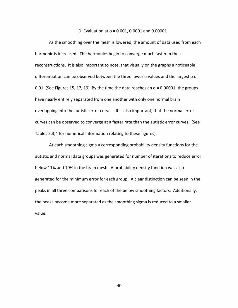
D. Evaluation at σ = 0.001, 0.0001 and 0.00001
As the smoothing over the mesh is lowered, the amount of data used from each
harmonic is increased. The harmonics begin to converge much faster in these
reconstructions. It is also important to note, that visually on the graphs a noticeable
differentiation can be observed between the three lower σ values and the largest σ of
0.01. (See Figures 15, 17, 19) By the time the data reaches an σ = 0.00001, the groups
have nearly entirely separated from one another with only one normal brain
overlapping into the autistic error curves. It is also important, that the normal error
curves can be observed to converge at a faster rate than the autistic error curves. (See
Tables 2,3,4 for numerical information relating to these figures).
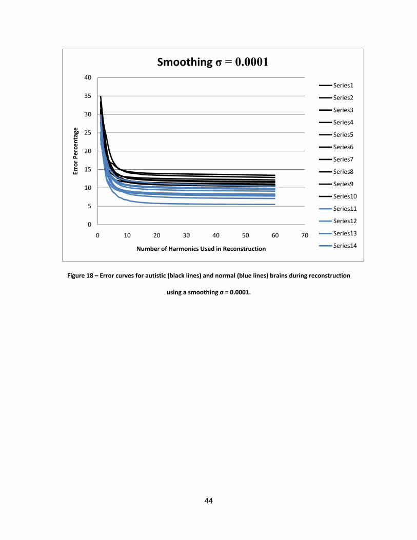
At each smoothing sigma a corresponding probability density functions for the
autistic and normal data groups was generated for number of iterations to reduce error
below 11% and 10% in the brain mesh. A probability density function was also
generated for the minimum error for each group. A clear distinction can be seen in the
peaks in all three comparisons for each of the below smoothing factors. Additionally,
the peaks become more separated as the smoothing sigma is reduced to a smaller
value.

41
Figure 16 – Error curves for autistic (black lines) and normal (blue lines) brains during reconstruction
using a smoothing σ = 0.001.
0
5
10
15
20
25
30
35
40
0 10 20 30 40 50 60 70
Erro
r Per
cent
age
Number of Harmonics Used in Reconstruction
Smoothing σ = 0.001
Series1
Series2
Series3
Series4
Series5
Series6
Series7
Series8
Series9
Series10
Series11
42
Smoothing σ = 0.001
Error below < 11% (Iteration)
Error below < 10% (Iteration)
Lowest Error
A1 61 61 11.104 A2 21 61 10.849 A5 61 61 11.782 A6 61 61 12.25 A8 61 61 13.49 A9 21 61 10.72 A10 61 61 12.918 A11 61 61 11.576 A12 14 61 10.483 A13 32 61 10.943 N2 26 61 10.771 N3 9 61 10.018 N4 7 11 9.2371 N5 5 6 7.8352 N6 8 22 9.807 N8 4 5 5.5004 N9 5 6 8.0435 N10 6 7 8.3774 N11 6 7 8.3001 N13 9 29 9.9082 N16 8 21 9.7918 N17 6 7 7.1729
Table 2– Convergence iteration and lowest error for a smoothing σ = 0.001.

43
(a) (b)
(c)
Figure 17– Probability Density Function graphs of smoothing σ = 0.001 for (a) 11% error, (b) 10% error,
and (c) minimum error.
44
Figure 18 – Error curves for autistic (black lines) and normal (blue lines) brains during reconstruction
using a smoothing σ = 0.0001.
0
5
10
15
20
25
30
35
40
0 10 20 30 40 50 60 70
Erro
r Per
cent
age
Number of Harmonics Used in Reconstruction
Smoothing σ = 0.0001
Series1
Series2
Series3
Series4
Series5
Series6
Series7
Series8
Series9
Series10
Series11
Series12
Series13
Series14

45
Smoothing σ = 0.0001
Error below < 11% (Iteration)
Error below < 10% (Iteration)
Lowest Error
A1 61 61 11.027 A2 25 61 10.693 A5 61 61 11.675 A6 61 61 12.134 A8 61 61 13.402 A9 27 61 10.674 A10 61 61 12.818 A11 61 61 11.507 A12 16 61 10.379 A13 34 61 10.788 N2 28 61 10.457 N3 9 42 9.8522 N4 8 11 9.1036 N5 5 7 7.7681 N6 9 27 9.6295 N8 4 5 5.4782 N9 5 6 7.9446 N10 6 7 8.3042 N11 6 7 8.1497 N13 9 37 9.7317 N16 9 22 9.6309 N17 6 7 7.0995
Table 3– Convergence iteration and lowest error for a smoothing σ = 0.0001.

46
(a) (b)
(c)
Figure 19– Probability Density Function graphs of smoothing σ = 0.0001 for (a) 11% error, (b) 10% error,
and (c) minimum error.

47
Figure 20 – Error curves for autistic (black lines) and normal (blue lines) brains during reconstruction
using a smoothing σ = 0.00001.
0
5
10
15
20
25
30
35
40
0 10 20 30 40 50 60 70
Erro
r Per
cent
age
Number of Harmonics Used in Reconstruction
Smoothing σ = 0.00001
Series1
Series2
Series3
Series4
Series5
Series6
Series7
Series8
Series9
Series10
Series11
Series12
Series13

48
Smoothing σ = 0.00001
Error below < 11% (Iteration)
Error below < 10% (Iteration)
Lowest Error
A1 61 61 11.004 A2 26 61 10.653 A5 61 61 11.648 A6 61 61 12.091 A8 61 61 13.364 A9 28 61 10.661 A10 61 61 12.799 A11 61 61 11.493 A12 17 61 10.367 A13 34 61 10.754 N2 28 61 10.421 N3 9 42 9.8132 N4 8 11 9.0887 N5 5 7 7.7562 N6 9 28 9.5951 N8 4 5 5.4744 N9 5 6 7.9267 N10 6 7 8.2921 N11 6 7 8.1369 N13 9 37 9.6941 N16 9 23 9.6041 N17 6 7 7.0942
Table 4– Convergence iteration and lowest error for a smoothing σ = 0.00001.
49
(a) (b)
(c)
Figure 21– Probability Density Function graphs of smoothing σ = 0.0001 for (a) 11% error, (b) 10% error,
and (c) minimum error.
50
E. Average Error and Minimum Convergence Iteration
The minimum error for each brain was then calculated along with the fastest
iteration at which the brain converged below the specified error. (See Table 5) It was
expected that due to the complexity of an Autistic brain these would require more
iterations to converge to the same error level as a normal brain. It was also likely that
within the number of iterations tested the autistic brains would record a larger final
error due to this slower convergence rate. This was confirmed by the data.
The average of the minimum error for each group was calculated along with the
lowest iteration at which that particular mesh dropped below a given error threshold.
(See Table 5). The overall minimum error for normal brain data was significantly lower
than the autistic brain data. The average error for autistic brain data was significantly
higher in both convergence measurements, but was dramatically higher in the 10%
category. This confirms the hypothesis that the autistic brain is significantly more
difficult to reconstruct than a normal brain.

51
Smoothing σ = 0.01 Lowest Error below 11% (Iteration)
Lowest Error below 10% (Iteration)
Minimum Error
Average Minimum Error (Autistic) 47.1±22.70 61±0 11.49±0.76
Average Minimum Error (Normal) 11.41±15.70 33.66±28.55 9.41±1.38
Smoothing σ = 0.001 Lowest Error below 11% (Iteration)
Lowest Error below 10% (Iteration)
Minimum Error
Average Minimum Error (Autistic) 45.4±20.59 61±0 11.61±1.00
Average Minimum Error (Normal) 8.25±5.81 20.25±20.56 8.73±1.48
Smoothing σ = 0.0001 Lowest Error below 11% (Iteration)
Lowest Error below 10% (Iteration)
Minimum Error
Average Minimum Error (Autistic) 46.8±18.82 61±0 11.50±1.00
Average Minimum Error (Normal) 8.66±6.35 19.91±18.30 8.59±1.41
Smoothing σ = 0.00001 Lowest Error below 11% (Iteration)
Lowest Error below 10% (Iteration)
Minimum Error
Average Minimum Error (Autistic) 47.1±18.39 61±0 11.48±1.00
Average Minimum Error (Normal) 8.66±6.35 20.08±18.35 8.57±1.40
Table 5– Average minimum error and convergence for autistic and normal data groups

52
IV. Conclusions and Future Work
Considering the data from previous methods including Modified Checklist for
Autism in Toddlers, eye-tracking technologies, and the prevalence of the disorder, it is
essential to find alternate and scientific methods that include brain analysis as a
diagnostic and evaluative method. The research of doctors at Yale has determined that
brain scans can predict the development of autism, leading to early detection and early
intervention.
Using this method of analyzing data can demonstrate accurate differences in
normal and autistic brains. The research that has been generated in this thesis can
clearly demonstrate that the normal brain data converged both faster and with a lower
rate of error level than the Autistic brain data. This result proves that the autistic brain is
a more complex structure, and would be more difficult to reconstruct using this Shape-
Based Detection of Cortex Variability process.
The flexibility of the created package is of additional importance to the
expansion of the project. The algorithms and theories introduced in this thesis can
readily be applied to any object freely. The object can be converted from 2-dimensional

53
scans into a 3-dimensional mesh, deformed and analyzed. This would allow for future
analysis of many other organs including cancerous growths and individual components
of the brain. Examining the difference between reconstructions can enable change in an
object to be tracked over time and compared as well. This would allow for an analysis
of the rate of the progression of autism in the individual. This can provide valuable
information that can be used to improve treatments by providing physicians with a
detailed mathematical representation of the current state of their patient. It is also
potentially possible to use this technique to understand what areas of the brain begin to
alter at different times in the subject and to track their impact on the overall autism.
Gaining a detailed understanding of the progression of autism in patients can help lead
to meaningful solutions for autistic patients.
Future plans are to improve the efficiency of the algorithms to allow accurate
deformation and analysis of larger and more detailed mesh structures. Improvements
in the algorithm will allow for faster and more accurate analysis of the subject. As
previously mentioned, it is also planned to make the package more flexible so that it can
readily be applied to a variety of structures and used as a meaningful evaluation
technique for multiple disorders.
After numerous attempts to create a package for Shape-Based Detection of
Cortex Variability, the primary difficulties arose in generating an accurate mesh from a
variety of data and deforming the mesh into an accurate unit sphere while preserving
the integrity and positioning of nodes within the mesh. Through the combination of
techniques from a variety of fields including engineering, computer science and

54
graphical art design these challenges were overcome. Using this technique it will be
possible to analyze a large variety of MRI scans to compare the complexities of normal
and Autistic brains.
55
II. References
1. Minshew, NJ, Payton, JB (1988). New perspectives in autism, Part I: The clinical spectrum of autism. Curr Probl Pediatr, 18, 10:561-610.
2. Kanner Child Psychiatry ISBN-10: 0398021996 Publisher: Charles C. Thomas, Publisher Ltd (April 1979)
3. Kanner L (1943). "Autistic disturbances of affective contact". Nerv Child 2: 217–50. Kanner, L (1968). "Reprint". Acta Paedopsychiatr 35 (4): 100–36.
4. Bauman ML, Kemper TL. The neuropathology of the autism spectrum disorders: what have we learned? Children's Neurology Service, Massachusetts General Hospital, 55 Fruit Street, Boston, MA 02114, USA.
5 Wing, L (1981). Asperger's syndrome: a clinical account. Psychol Med, 11, 1:115-29.
6. Schaefer, GB, Mendelsohn, NJ (2008). Clinical genetics evaluation in identifying the etiology of autism spectrum disorders. Genet. Med., 10, 4:301-5.
7. Losh, M, Adolphs, R, Poe, MD, Couture, S, Penn, D, Baranek, GT, Piven, J (2009). Neuropsychological profile of autism and the broad autism phenotype. Arch. Gen. Psychiatry, 66, 5:518-26.
8. Jacobson, JW. Is Autism on the Rise? 2000. Science in Autism Vol 2. No 1, 9. Rapin, I, Tuchman, RF (2008). What is new in autism?. Curr. Opin. Neurol., 21,
2:143-9. 10. Department of Developmental Services. (1999, March 1). Changes in the
population of persons with autism and pervasive developmental disorders in California’s developmental services system: 1987 through 1998. Sacramento, CA: Author.
11. Department of Education (1999). Digest of education statistics, 1998. Washington, DC: Author (GPO No. 065-000-01174-3, NCES No. NCES 1999036).
12. DiGuiseppi, C, Hepburn, S, Davis, JM, Fidler, DJ, Hartway, S, Lee, NR, Miller, L, Ruttenber, M, Robinson, C (2010). Screening for autism spectrum disorders in children with Down syndrome: population prevalence and screening test characteristics. J Dev Behav Pediatr, 31, 3:181-91.
13. Stevens, M., Fein, D., Dunn, M., Allen, D., Waterhouse, L. H., Feinstein, C., and Rapin, I., Subgroups of children with autism by cluster analysis: A longitudinal examination. J. Am. Acad. Child Adolesc. Psychiatry 39:346–352, 2000.
14. Robins, D.L., Fein, D, Barton, M, Green, J. The Modified Checklist for Autism in Toddlers: An Initial Study Investigating the Early Detection of Autism and Pervasive Developmental Disorders. Journal of Autism and Developmental Disorders, Vol. 31, No. 2, 2001

56
15. El-Baz, A., Elnakib A., Casanova M., Gimel’farb G., Switala, A., Jordan, D. Rainey, S. Accurate Automated Detection of Autism Related Corpus Callosum Abnormalities. J Med Syst. March 2010. DOI 10.1007/s10916-010-9510-3
16. Abell, F., Krams, M., Ashburner, J., Passingham, R., Friston, K., Frackowiak, R., Happe, F., Frith, C., and Frith, U., The neuro-anatomy of autism: A voxel-based whole brain analysis of structural scans. NeuroReport 10(8):647–1651, 1999.
17. Boddaert, N., Chabane, N., Gervais, H., Good, C. D., Bourgeois, M., Plumet, M. H., Barthelemy, C., Mouren, M. C., Artiges, E., Samson, Y., Brunelle, F., Frackowiak, R. S. J., and Zilbovicius, M., Superior temporal sulcus anatomical abnormalities in childhood autism: a voxel-based morphometry MRI study. Neuroimage 23:364–369, 2004.
18. Herbert, M. R., Ziegler, D. A., Deutsch, C. K., O’Brien, L. M., Lange, N., Bakardjiev, A., Hodgson, J., Adrien, K. T., Steele, S., Makris, N., Kennedy, D., Harris, G. J., and Caviness, V. S., Jr., Dissociations of cerebral cortex, subcortical and cerebral white matter volumes in autistic boys. Brain 126:1182–1192, 2003.
19. Egaas, B., Courchesne, E., and Saitoh, O., Reduced size of corpus 576 callosum in autism. Arch. Neurol. 52(8):794–801, 1995.
20. Schumann, CM, Barnes, CC, Lord, C, Courchesne, E (2009). Amygdala enlargement in toddlers with autism related to severity of social and communication impairments. Biol. Psychiatry, 66, 10:942-9.
21. Courchesne, E, Press, GA, Yeung-Courchesne, R (1993). Parietal lobe abnormalities detected with MR in patients with infantile autism. AJR Am J Roentgenol, 160, 2:387-93.
22. Schumann, CM, Bloss, CS, Barnes, CC, Wideman, GM, Carper, RA, Akshoomoff, N, Pierce, K, Hagler, D, Schork, N, Lord, C, Courchesne, E (2010). Longitudinal magnetic resonance imaging study of cortical development through early childhood in autism. J. Neurosci., 30, 12:4419-27.
23. Kennedy, DP, Courchesne, E (2008). Functional abnormalities of the default network during self- and other-reflection in autism. Soc Cogn Affect Neurosci, 3, 2:177-90.
24. Hitti, M., Chang, L. Autism: New Clue to Earlier Detection. WebMD Health News. March 29, 2009.
25. Klin, A, Lin, DJ, Gorrindo, P, Ramsay, G, Jones, W (2009). Two-year-olds with autism orient to non-social contingencies rather than biological motion. Nature, 459, 7244:257-61.
26. Jones, W, Klin, A (2009). Heterogeneity and homogeneity across the autism spectrum: the role of development. J Am Acad Child Adolesc Psychiatry, 48, 5:471-3.
27. Jones, W, Carr, K, Klin, A (2008). Absence of preferential looking to the eyes of approaching adults predicts level of social disability in 2-year-old toddlers with autism spectrum disorder. Arch. Gen. Psychiatry, 65, 8:946-54.
28. Gardner, A. New Hope for Early Detection of Autism. US News: Health Day. May 19, 2010

57
29. Fang, Q., Boas, D.A., "Tetrahedral mesh generation from volumetric binary and gray-scale images," Proceedings of IEEE International Symposium on Biomedical Imaging 2009, pp. 1142-1145, 2009
30. Fang, Q., Carp, S.A., Selb, J., Moore, R., Kopans, D.B., Miller, E.L., Brooks, D.H., Boas, D.A., "A Multi-Modality Image Reconstruction Platform for Diffuse Optical Tomography," Biomedical Optics 2008, BIOMED Poster Session II (BMD), Mar. 2008.
31. Zhang, Hamza, (2006) Vertex-based anisotropic smoothing of 3D mesh data, IEEE CCECE
32. Fornberg, B., A practical guide to pseudospectral methods. Cambridge University Press, 1998.
33. Chung. M.K., Shen, L., Dalton, K.M., Evans, A.C., Davidson, R.J. Weighted fourier representation and its application to quantifying the amount of gray matter. IEEE Transactions on Medical Imaging, 26:566–581, 2007.
34. Courant, R. and Hilbert, D. Methods of Mathematical Physics: Volume II. Interscience, New York, English edition, 1953.
35. Chung, M.K., Dalton, K.M., Shen, L., L., Evans, A.C., Davidson, R.J. 2007. Weighted Fourier series representation and its application to quantifying the amount of gray matter. IEEE Transactions on Medical Imaging, 26:566-581.

58
Appendix 1: Wavefront OBJ Format
i.) Format Specification
Lines beginning with a hash character (#) are comments.
# this is a comment
An OBJ file contains several types of definition:
# List of Vertices, with (x,y,z) coordinates. v 0.123 0.234 0.345 v ... ... # Texture coordinates, in (u,v) coordinates. vt 0.500 -1.352 vt ... ... # Normals in (x,y,z) form; normals might not be unit. vn 0.707 0.000 0.707 vn ...
..
Face Definitions
Faces are defined using lists of vertex, texture and normal indicies. Polygons such as
quadrilaterals can be defined by using more than three vertex/texture/normal indices.
OBJ files also support free form curved surface objects such as NURB surfaces.
There are several way to define a face, but each face line definition starts with "f" character.
Vertex
A valid vertex index starts from 1 and match first vertex element of vertex list previously defined.
Each face can contain more than three elements.
f v1 v2 v3 v4 ...
Vertex/Texture-coordinate
Each texture coordinate index must follow with no space the first slash. Texture coordinates index
are optional. A valid texture coordinate index starts from 1 and match first texture coordinate
element of texture coordinate list previously defined. Each face can contain more than three
elements.

59
f v1/vt1 v2/vt2 v3/vt3 ...
Vertex/Texture-coordinate/Normal
Each normal index must follow with no space the second slash. Normals index are optional. A
valid normal index starts from 1 and match first normal element of normal list previously defined.
Each face can contain more than three elements.
f v1/vt1/vn1 v2/vt2/vn2 v3/vt3/vn3 ...
Vertex/Normal
As texture coordinates are optional, one can define geometry without them, but one must put
normal index after second slash.
f v1//vn1 v2//vn2 v3//vn3 ...

60
ii.) ingOBJSave.m Matlab Code
function [null] = ingOBJSave(fileName,vertex,faces) fprintf('Saving data to OBJ file...'); [vertexN] = compute_normal(vertex',faces'); vertexN = vertexN'; vertCount = size(vertex,1); faceCount = size(faces,1); fid = fopen(fileName,'w'); fprintf(fid,'####\r\n'); fprintf(fid,'#\r\n'); fprintf(fid,'# OBJ File Generated by ingMesh\r\n'); fprintf(fid,'#\r\n'); fprintf(fid,'####\r\n'); fprintf(fid,'# Object %s\r\n',fileName); fprintf(fid,'#\r\n'); fprintf(fid,'# Vertices: %d\r\n',vertCount); fprintf(fid,'# Faces: %d\r\n',faceCount); fprintf(fid,'#\r\n'); fprintf(fid,'####\r\n'); for i=1:vertCount fprintf(fid,'vn %f %f %f\r\n',vertexN(i,1),vertexN(i,2),vertexN(i,3)); fprintf(fid,'v %f %f %f\r\n',vertex(i,1),vertex(i,2),vertex(i,3)); end fprintf(fid,'# %d vertices, %d vertices normals\r\n',vertCount,vertCount); fprintf(fid,'\r\n'); for i=1:faceCount fprintf(fid,'f %d//%d %d//%d %d//%d\r\n',faces(i,1),faces(i,1),faces(i,2),faces(i,2),faces(i,3),faces(i,3)); end fprintf(fid,'# %d faces, %d coords texture\r\n',faceCount,0); fprintf(fid,'\r\n'); fprintf(fid,'# End of File'); fprintf('Complete.\n'); fclose(fid); fprintf('File closed.\n');

61
iii.) ingOBJRead.m Matlab Code function [nodes faces] = ingOBJRead(filename) fprintf('Reading data from OBJ file...\n'); fid=fopen(filename); frewind(fid); for i=1:7 fgetl(fid); end fscanf(fid,'%s',2); n_nodes=fscanf(fid,'%i',1); fscanf(fid,'%s',2); n_faces=fscanf(fid,'%i',1); for i=1:3 fgetl(fid); end fprintf('Detected Nodes: %i Faces: %i\n',n_nodes,n_faces); nodes = zeros(n_nodes,3); normals = zeros(n_nodes,3); c_norm = 1; c_node = 1; for i = 1:(n_nodes*2) fscanf(fid,'%s',1); if (mod(i,2) == 1) temp = fscanf(fid,'%f',3); normals(c_norm,:) = temp; c_norm = c_norm + 1; else temp = fscanf(fid,'%f',3); nodes(c_node,:) = temp; c_node = c_node + 1; end end fscanf(fid,'%s',6); faces = zeros(n_faces,3); face_normals = zeros(n_faces,3); for i = 1:n_faces fscanf(fid,'%s',1); faces(i,1) = fscanf(fid,'%i',1); fscanf(fid,'%c',2); face_normals(i,1) = fscanf(fid,'%i',1); fscanf(fid,'%c',1); faces(i,2) = fscanf(fid,'%i',1); fscanf(fid,'%c',2); face_normals(i,2) = fscanf(fid,'%i',1); fscanf(fid,'%c',1); faces(i,3) = fscanf(fid,'%i',1); fscanf(fid,'%c',2); face_normals(i,3) = fscanf(fid,'%i',1); fscanf(fid,'%c',1); end fclose(fid); fprintf('File closed.\n');
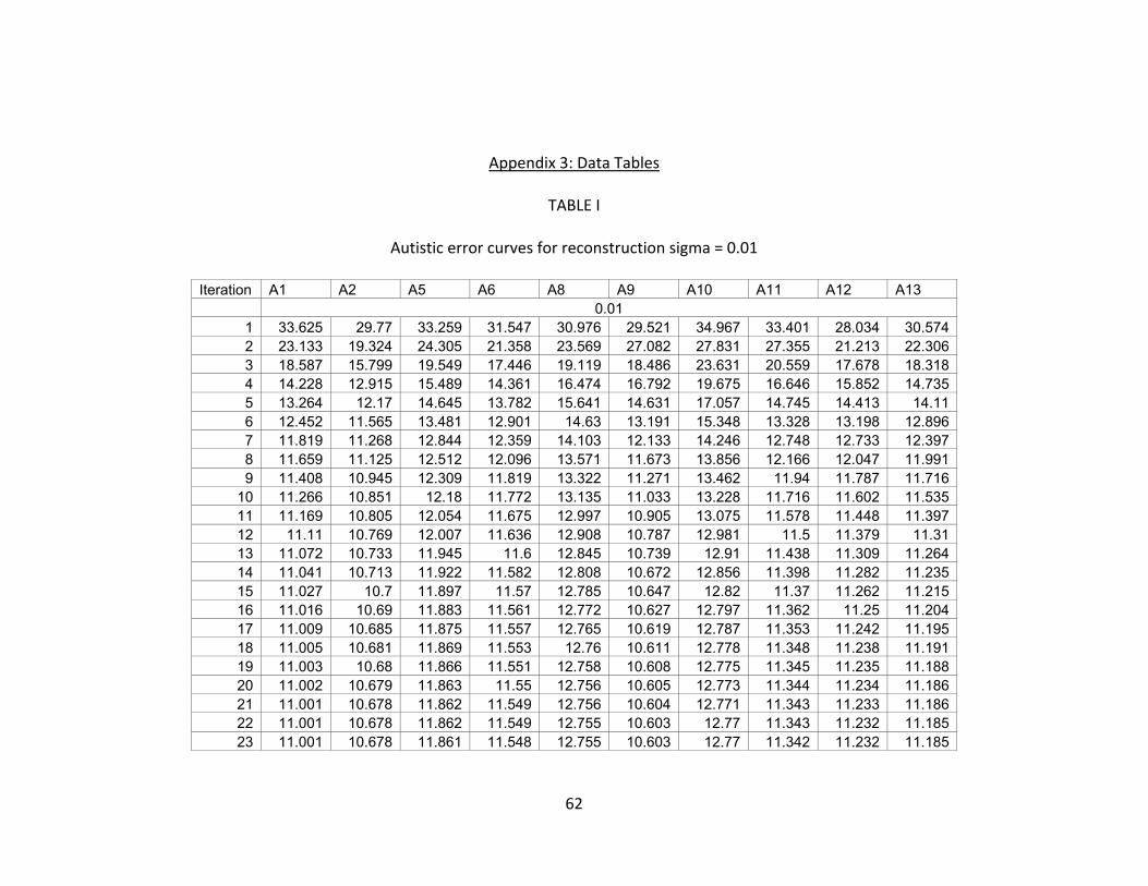
62
Appendix 3: Data Tables
TABLE I
Autistic error curves for reconstruction sigma = 0.01
Iteration A1 A2 A5 A6 A8 A9 A10 A11 A12 A13 0.01
1 33.625 29.77 33.259 31.547 30.976 29.521 34.967 33.401 28.034 30.5742 23.133 19.324 24.305 21.358 23.569 27.082 27.831 27.355 21.213 22.3063 18.587 15.799 19.549 17.446 19.119 18.486 23.631 20.559 17.678 18.3184 14.228 12.915 15.489 14.361 16.474 16.792 19.675 16.646 15.852 14.7355 13.264 12.17 14.645 13.782 15.641 14.631 17.057 14.745 14.413 14.116 12.452 11.565 13.481 12.901 14.63 13.191 15.348 13.328 13.198 12.8967 11.819 11.268 12.844 12.359 14.103 12.133 14.246 12.748 12.733 12.3978 11.659 11.125 12.512 12.096 13.571 11.673 13.856 12.166 12.047 11.9919 11.408 10.945 12.309 11.819 13.322 11.271 13.462 11.94 11.787 11.716
10 11.266 10.851 12.18 11.772 13.135 11.033 13.228 11.716 11.602 11.53511 11.169 10.805 12.054 11.675 12.997 10.905 13.075 11.578 11.448 11.39712 11.11 10.769 12.007 11.636 12.908 10.787 12.981 11.5 11.379 11.3113 11.072 10.733 11.945 11.6 12.845 10.739 12.91 11.438 11.309 11.26414 11.041 10.713 11.922 11.582 12.808 10.672 12.856 11.398 11.282 11.23515 11.027 10.7 11.897 11.57 12.785 10.647 12.82 11.37 11.262 11.21516 11.016 10.69 11.883 11.561 12.772 10.627 12.797 11.362 11.25 11.20417 11.009 10.685 11.875 11.557 12.765 10.619 12.787 11.353 11.242 11.19518 11.005 10.681 11.869 11.553 12.76 10.611 12.778 11.348 11.238 11.19119 11.003 10.68 11.866 11.551 12.758 10.608 12.775 11.345 11.235 11.18820 11.002 10.679 11.863 11.55 12.756 10.605 12.773 11.344 11.234 11.18621 11.001 10.678 11.862 11.549 12.756 10.604 12.771 11.343 11.233 11.18622 11.001 10.678 11.862 11.549 12.755 10.603 12.77 11.343 11.232 11.18523 11.001 10.678 11.861 11.548 12.755 10.603 12.77 11.342 11.232 11.185
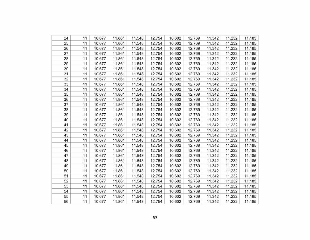
63
24 11 10.677 11.861 11.548 12.754 10.602 12.769 11.342 11.232 11.18525 11 10.677 11.861 11.548 12.754 10.602 12.769 11.342 11.232 11.18526 11 10.677 11.861 11.548 12.754 10.602 12.769 11.342 11.232 11.18527 11 10.677 11.861 11.548 12.754 10.602 12.769 11.342 11.232 11.18528 11 10.677 11.861 11.548 12.754 10.602 12.769 11.342 11.232 11.18529 11 10.677 11.861 11.548 12.754 10.602 12.769 11.342 11.232 11.18530 11 10.677 11.861 11.548 12.754 10.602 12.769 11.342 11.232 11.18531 11 10.677 11.861 11.548 12.754 10.602 12.769 11.342 11.232 11.18532 11 10.677 11.861 11.548 12.754 10.602 12.769 11.342 11.232 11.18533 11 10.677 11.861 11.548 12.754 10.602 12.769 11.342 11.232 11.18534 11 10.677 11.861 11.548 12.754 10.602 12.769 11.342 11.232 11.18535 11 10.677 11.861 11.548 12.754 10.602 12.769 11.342 11.232 11.18536 11 10.677 11.861 11.548 12.754 10.602 12.769 11.342 11.232 11.18537 11 10.677 11.861 11.548 12.754 10.602 12.769 11.342 11.232 11.18538 11 10.677 11.861 11.548 12.754 10.602 12.769 11.342 11.232 11.18539 11 10.677 11.861 11.548 12.754 10.602 12.769 11.342 11.232 11.18540 11 10.677 11.861 11.548 12.754 10.602 12.769 11.342 11.232 11.18541 11 10.677 11.861 11.548 12.754 10.602 12.769 11.342 11.232 11.18542 11 10.677 11.861 11.548 12.754 10.602 12.769 11.342 11.232 11.18543 11 10.677 11.861 11.548 12.754 10.602 12.769 11.342 11.232 11.18544 11 10.677 11.861 11.548 12.754 10.602 12.769 11.342 11.232 11.18545 11 10.677 11.861 11.548 12.754 10.602 12.769 11.342 11.232 11.18546 11 10.677 11.861 11.548 12.754 10.602 12.769 11.342 11.232 11.18547 11 10.677 11.861 11.548 12.754 10.602 12.769 11.342 11.232 11.18548 11 10.677 11.861 11.548 12.754 10.602 12.769 11.342 11.232 11.18549 11 10.677 11.861 11.548 12.754 10.602 12.769 11.342 11.232 11.18550 11 10.677 11.861 11.548 12.754 10.602 12.769 11.342 11.232 11.18551 11 10.677 11.861 11.548 12.754 10.602 12.769 11.342 11.232 11.18552 11 10.677 11.861 11.548 12.754 10.602 12.769 11.342 11.232 11.18553 11 10.677 11.861 11.548 12.754 10.602 12.769 11.342 11.232 11.18554 11 10.677 11.861 11.548 12.754 10.602 12.769 11.342 11.232 11.18555 11 10.677 11.861 11.548 12.754 10.602 12.769 11.342 11.232 11.18556 11 10.677 11.861 11.548 12.754 10.602 12.769 11.342 11.232 11.185

64
57 11 10.677 11.861 11.548 12.754 10.602 12.769 11.342 11.232 11.18558 11 10.677 11.861 11.548 12.754 10.602 12.769 11.342 11.232 11.18559 11 10.677 11.861 11.548 12.754 10.602 12.769 11.342 11.232 11.18560 11 10.677 11.861 11.548 12.754 10.602 12.769 11.342 11.232 11.185
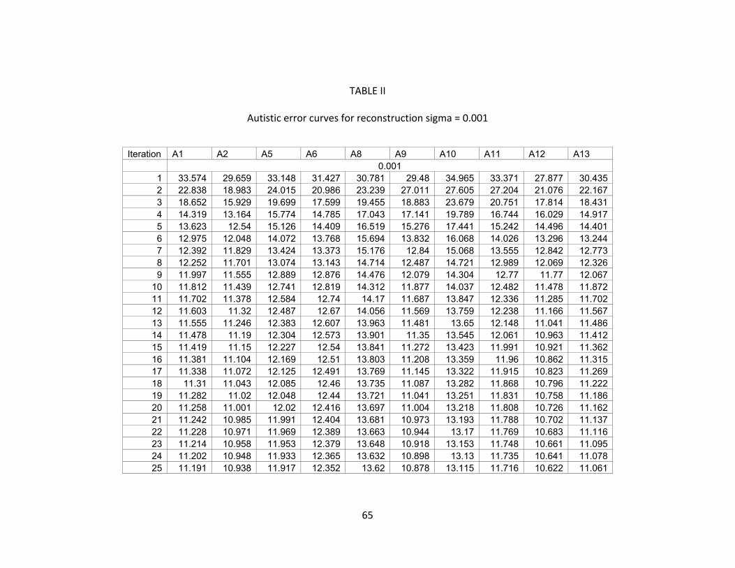
65
TABLE II
Autistic error curves for reconstruction sigma = 0.001
Iteration A1 A2 A5 A6 A8 A9 A10 A11 A12 A13 0.001
1 33.574 29.659 33.148 31.427 30.781 29.48 34.965 33.371 27.877 30.4352 22.838 18.983 24.015 20.986 23.239 27.011 27.605 27.204 21.076 22.1673 18.652 15.929 19.699 17.599 19.455 18.883 23.679 20.751 17.814 18.4314 14.319 13.164 15.774 14.785 17.043 17.141 19.789 16.744 16.029 14.9175 13.623 12.54 15.126 14.409 16.519 15.276 17.441 15.242 14.496 14.4016 12.975 12.048 14.072 13.768 15.694 13.832 16.068 14.026 13.296 13.2447 12.392 11.829 13.424 13.373 15.176 12.84 15.068 13.555 12.842 12.7738 12.252 11.701 13.074 13.143 14.714 12.487 14.721 12.989 12.069 12.3269 11.997 11.555 12.889 12.876 14.476 12.079 14.304 12.77 11.77 12.067
10 11.812 11.439 12.741 12.819 14.312 11.877 14.037 12.482 11.478 11.87211 11.702 11.378 12.584 12.74 14.17 11.687 13.847 12.336 11.285 11.70212 11.603 11.32 12.487 12.67 14.056 11.569 13.759 12.238 11.166 11.56713 11.555 11.246 12.383 12.607 13.963 11.481 13.65 12.148 11.041 11.48614 11.478 11.19 12.304 12.573 13.901 11.35 13.545 12.061 10.963 11.41215 11.419 11.15 12.227 12.54 13.841 11.272 13.423 11.991 10.921 11.36216 11.381 11.104 12.169 12.51 13.803 11.208 13.359 11.96 10.862 11.31517 11.338 11.072 12.125 12.491 13.769 11.145 13.322 11.915 10.823 11.26918 11.31 11.043 12.085 12.46 13.735 11.087 13.282 11.868 10.796 11.22219 11.282 11.02 12.048 12.44 13.721 11.041 13.251 11.831 10.758 11.18620 11.258 11.001 12.02 12.416 13.697 11.004 13.218 11.808 10.726 11.16221 11.242 10.985 11.991 12.404 13.681 10.973 13.193 11.788 10.702 11.13722 11.228 10.971 11.969 12.389 13.663 10.944 13.17 11.769 10.683 11.11623 11.214 10.958 11.953 12.379 13.648 10.918 13.153 11.748 10.661 11.09524 11.202 10.948 11.933 12.365 13.632 10.898 13.13 11.735 10.641 11.07825 11.191 10.938 11.917 12.352 13.62 10.878 13.115 11.716 10.622 11.061

66
26 11.184 10.93 11.903 12.34 13.611 10.859 13.095 11.705 10.609 11.04627 11.176 10.923 11.889 12.332 13.602 10.839 13.084 11.691 10.598 11.03628 11.167 10.915 11.881 12.322 13.59 10.824 13.068 11.679 10.589 11.02729 11.161 10.91 11.87 12.315 13.582 10.814 13.058 11.668 10.579 11.01630 11.155 10.905 11.861 12.308 13.573 10.801 13.045 11.658 10.567 11.00731 11.15 10.901 11.854 12.303 13.567 10.791 13.034 11.651 10.557 11.00132 11.145 10.896 11.847 12.298 13.561 10.781 13.02 11.644 10.551 10.99433 11.141 10.891 11.841 12.293 13.554 10.774 13.011 11.637 10.544 10.98834 11.138 10.888 11.834 12.29 13.548 10.768 13 11.632 10.539 10.98335 11.134 10.884 11.829 12.286 13.543 10.762 12.992 11.625 10.533 10.97936 11.13 10.88 11.824 12.283 13.537 10.756 12.985 11.62 10.527 10.97537 11.127 10.877 11.819 12.28 13.533 10.751 12.978 11.614 10.523 10.97238 11.125 10.874 11.814 12.276 13.529 10.747 12.973 11.609 10.519 10.96939 11.123 10.871 11.811 12.273 13.526 10.745 12.968 11.606 10.515 10.96640 11.121 10.868 11.807 12.271 13.522 10.741 12.962 11.602 10.511 10.96341 11.119 10.866 11.804 12.269 13.52 10.738 12.957 11.599 10.509 10.96142 11.117 10.865 11.802 12.267 13.517 10.736 12.953 11.596 10.506 10.95943 11.116 10.863 11.8 12.266 13.514 10.734 12.95 11.594 10.503 10.95744 11.115 10.861 11.798 12.264 13.512 10.732 12.946 11.591 10.501 10.95545 11.113 10.859 11.796 12.263 13.51 10.73 12.943 11.589 10.499 10.95446 11.112 10.857 11.794 12.262 13.508 10.729 12.94 11.587 10.497 10.95247 11.111 10.856 11.793 12.26 13.506 10.728 12.937 11.585 10.494 10.95148 11.11 10.855 11.791 12.259 13.504 10.726 12.935 11.584 10.493 10.9549 11.11 10.854 11.79 12.258 13.502 10.725 12.933 11.583 10.492 10.94950 11.109 10.854 11.789 12.257 13.501 10.725 12.931 11.582 10.491 10.94851 11.108 10.853 11.788 12.256 13.499 10.724 12.929 11.581 10.489 10.94852 11.107 10.852 11.787 12.255 13.498 10.723 12.927 11.58 10.488 10.94753 11.107 10.852 11.786 12.254 13.497 10.723 12.925 11.579 10.487 10.94654 11.106 10.851 11.785 12.253 13.496 10.722 12.924 11.579 10.486 10.94655 11.106 10.851 11.785 12.253 13.494 10.722 12.923 11.578 10.486 10.94556 11.105 10.85 11.784 12.252 13.493 10.721 12.922 11.577 10.485 10.94557 11.105 10.85 11.783 12.251 13.493 10.721 12.921 11.577 10.484 10.94458 11.104 10.85 11.783 12.251 13.492 10.72 12.92 11.577 10.484 10.944

67
59 11.104 10.849 11.782 12.25 13.491 10.72 12.919 11.576 10.483 10.94460 11.104 10.849 11.782 12.25 13.49 10.72 12.918 11.576 10.483 10.943
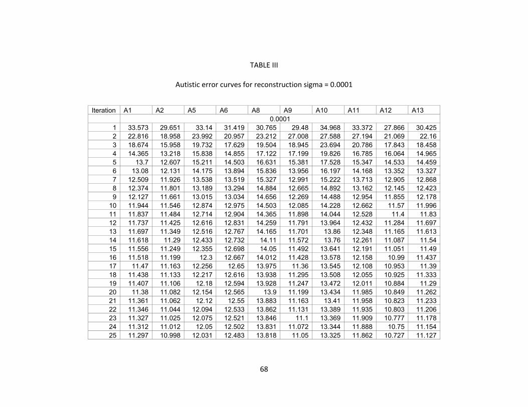
68
TABLE III
Autistic error curves for reconstruction sigma = 0.0001
Iteration A1 A2 A5 A6 A8 A9 A10 A11 A12 A13 0.0001
1 33.573 29.651 33.14 31.419 30.765 29.48 34.968 33.372 27.866 30.4252 22.816 18.958 23.992 20.957 23.212 27.008 27.588 27.194 21.069 22.163 18.674 15.958 19.732 17.629 19.504 18.945 23.694 20.786 17.843 18.4584 14.365 13.218 15.838 14.855 17.122 17.199 19.826 16.785 16.064 14.9655 13.7 12.607 15.211 14.503 16.631 15.381 17.528 15.347 14.533 14.4596 13.08 12.131 14.175 13.894 15.836 13.956 16.197 14.168 13.352 13.3277 12.509 11.926 13.538 13.519 15.327 12.991 15.222 13.713 12.905 12.8688 12.374 11.801 13.189 13.294 14.884 12.665 14.892 13.162 12.145 12.4239 12.127 11.661 13.015 13.034 14.656 12.269 14.488 12.954 11.855 12.178
10 11.944 11.546 12.874 12.975 14.503 12.085 14.228 12.662 11.57 11.99611 11.837 11.484 12.714 12.904 14.365 11.898 14.044 12.528 11.4 11.8312 11.737 11.425 12.616 12.831 14.259 11.791 13.964 12.432 11.284 11.69713 11.697 11.349 12.516 12.767 14.165 11.701 13.86 12.348 11.165 11.61314 11.618 11.29 12.433 12.732 14.11 11.572 13.76 12.261 11.087 11.5415 11.556 11.249 12.355 12.698 14.05 11.492 13.641 12.191 11.051 11.4916 11.518 11.199 12.3 12.667 14.012 11.428 13.578 12.158 10.99 11.43717 11.47 11.163 12.256 12.65 13.975 11.36 13.545 12.108 10.953 11.3918 11.438 11.133 12.217 12.616 13.938 11.295 13.508 12.055 10.925 11.33319 11.407 11.106 12.18 12.594 13.928 11.247 13.472 12.011 10.884 11.2920 11.38 11.082 12.154 12.565 13.9 11.199 13.434 11.985 10.849 11.26221 11.361 11.062 12.12 12.55 13.883 11.163 13.41 11.958 10.823 11.23322 11.346 11.044 12.094 12.533 13.862 11.131 13.389 11.935 10.803 11.20623 11.327 11.025 12.075 12.521 13.846 11.1 13.369 11.909 10.777 11.17824 11.312 11.012 12.05 12.502 13.831 11.072 13.344 11.888 10.75 11.15425 11.297 10.998 12.031 12.483 13.818 11.05 13.325 11.862 10.727 11.127

69
26 11.287 10.985 12.011 12.463 13.807 11.025 13.303 11.848 10.71 11.10627 11.276 10.975 11.994 12.452 13.798 10.995 13.286 11.829 10.696 11.09128 11.261 10.962 11.982 12.438 13.781 10.974 13.265 11.812 10.684 11.07529 11.251 10.954 11.967 12.426 13.77 10.957 13.248 11.796 10.67 11.05730 11.241 10.944 11.953 12.414 13.758 10.936 13.233 11.777 10.649 11.04131 11.232 10.936 11.942 12.405 13.749 10.92 13.219 11.764 10.635 11.0332 11.223 10.926 11.929 12.395 13.739 10.902 13.196 11.754 10.625 11.01733 11.214 10.915 11.919 12.386 13.729 10.891 13.179 11.742 10.615 11.00534 11.206 10.906 11.907 12.379 13.718 10.879 13.163 11.73 10.605 10.99435 11.196 10.896 11.897 12.37 13.707 10.866 13.148 11.717 10.595 10.98536 11.187 10.888 11.887 12.362 13.695 10.854 13.134 11.704 10.585 10.97537 11.179 10.876 11.877 12.353 13.685 10.841 13.119 11.692 10.578 10.96738 11.174 10.868 11.865 12.344 13.676 10.831 13.108 11.678 10.57 10.95739 11.167 10.86 11.857 12.335 13.667 10.823 13.097 11.669 10.559 10.94740 11.16 10.848 11.849 12.327 13.657 10.814 13.079 11.656 10.551 10.93841 11.153 10.839 11.842 12.32 13.649 10.804 13.06 11.646 10.546 10.93142 11.147 10.832 11.836 12.315 13.64 10.796 13.046 11.637 10.536 10.92343 11.141 10.822 11.828 12.308 13.63 10.787 13.037 11.631 10.528 10.91444 11.136 10.814 11.818 12.301 13.62 10.779 13.024 11.622 10.52 10.90745 11.13 10.803 11.808 12.295 13.61 10.773 13.013 11.612 10.514 10.946 11.123 10.792 11.799 12.287 13.599 10.767 12.998 11.603 10.505 10.89247 11.118 10.785 11.793 12.278 13.588 10.759 12.983 11.596 10.495 10.88448 11.113 10.778 11.785 12.271 13.576 10.752 12.974 11.59 10.49 10.87949 11.106 10.771 11.775 12.262 13.563 10.746 12.96 11.582 10.483 10.87350 11.099 10.764 11.767 12.253 13.551 10.739 12.945 11.574 10.474 10.86651 11.094 10.756 11.76 12.241 13.538 10.733 12.932 11.567 10.465 10.8652 11.088 10.75 11.751 12.229 13.526 10.728 12.92 11.56 10.457 10.85453 11.08 10.745 11.74 12.22 13.513 10.723 12.91 11.553 10.448 10.84554 11.074 10.737 11.731 12.21 13.499 10.717 12.897 11.547 10.438 10.83955 11.067 10.731 11.722 12.198 13.482 10.71 12.883 11.541 10.43 10.83256 11.061 10.724 11.713 12.184 13.466 10.704 12.871 11.534 10.421 10.82657 11.051 10.717 11.702 12.173 13.452 10.697 12.859 11.528 10.411 10.81858 11.042 10.707 11.691 12.163 13.437 10.69 12.847 11.521 10.398 10.809

70
59 11.033 10.698 11.684 12.149 13.42 10.683 12.833 11.514 10.39 10.79860 11.027 10.693 11.675 12.134 13.402 10.674 12.818 11.507 10.379 10.788

71
TABLE IV
Autistic error curves for reconstruction sigma = 0.00001
Iteration A1 A2 A5 A6 A8 A9 A10 A11 A12 A13 0.00001
1 33.573 29.651 33.14 31.418 30.764 29.48 34.968 33.372 27.865 30.4242 22.814 18.956 23.99 20.954 23.209 27.008 27.586 27.193 21.069 22.163 18.676 15.961 19.735 17.632 19.509 18.951 23.695 20.79 17.846 18.4614 14.37 13.224 15.844 14.863 17.131 17.205 19.83 16.79 16.068 14.975 13.708 12.614 15.22 14.513 16.643 15.392 17.537 15.358 14.537 14.4656 13.091 12.14 14.186 13.907 15.85 13.969 16.211 14.183 13.358 13.3367 12.521 11.936 13.55 13.534 15.342 13.007 15.238 13.729 12.912 12.8788 12.387 11.812 13.201 13.309 14.901 12.684 14.91 13.18 12.154 12.4339 12.141 11.672 13.029 13.05 14.675 12.29 14.508 12.974 11.865 12.19
10 11.958 11.557 12.888 12.991 14.523 12.108 14.248 12.681 11.581 12.00911 11.851 11.495 12.728 12.921 14.386 11.92 14.065 12.548 11.413 11.84412 11.752 11.436 12.63 12.847 14.28 11.815 13.986 12.453 11.297 11.71113 11.712 11.36 12.53 12.783 14.187 11.725 13.882 12.369 11.179 11.62714 11.634 11.3 12.447 12.749 14.133 11.596 13.784 12.283 11.101 11.55415 11.571 11.26 12.369 12.715 14.073 11.516 13.665 12.213 11.066 11.50416 11.534 11.209 12.315 12.684 14.035 11.452 13.603 12.179 11.006 11.45117 11.485 11.173 12.271 12.666 13.997 11.383 13.57 12.129 10.969 11.40318 11.453 11.143 12.233 12.632 13.96 11.319 13.534 12.076 10.941 11.34619 11.421 11.115 12.196 12.611 13.951 11.27 13.497 12.031 10.9 11.30320 11.394 11.091 12.17 12.581 13.922 11.222 13.459 12.005 10.864 11.27421 11.375 11.071 12.136 12.565 13.906 11.185 13.435 11.977 10.839 11.24422 11.36 11.052 12.109 12.549 13.884 11.153 13.414 11.954 10.819 11.21823 11.341 11.033 12.091 12.536 13.869 11.122 13.395 11.928 10.793 11.18924 11.325 11.019 12.066 12.517 13.853 11.093 13.369 11.906 10.765 11.16425 11.31 11.005 12.046 12.497 13.841 11.071 13.351 11.879 10.742 11.136

72
26 11.299 10.991 12.026 12.477 13.83 11.046 13.328 11.865 10.725 11.11527 11.288 10.981 12.008 12.466 13.821 11.015 13.312 11.846 10.711 11.09928 11.273 10.968 11.996 12.451 13.804 10.993 13.29 11.829 10.699 11.08229 11.263 10.959 11.981 12.439 13.793 10.975 13.272 11.812 10.685 11.06430 11.252 10.949 11.966 12.426 13.781 10.954 13.258 11.792 10.663 11.04731 11.243 10.941 11.955 12.416 13.772 10.938 13.244 11.779 10.649 11.03532 11.233 10.93 11.942 12.407 13.762 10.919 13.219 11.768 10.639 11.02233 11.223 10.917 11.931 12.396 13.752 10.908 13.203 11.755 10.628 11.0134 11.215 10.908 11.919 12.389 13.74 10.895 13.185 11.743 10.619 10.99735 11.204 10.898 11.908 12.379 13.728 10.881 13.17 11.73 10.609 10.98836 11.195 10.888 11.898 12.371 13.715 10.869 13.155 11.716 10.599 10.97737 11.186 10.875 11.887 12.362 13.705 10.855 13.141 11.703 10.592 10.96838 11.181 10.867 11.875 12.352 13.695 10.844 13.128 11.689 10.583 10.95839 11.173 10.857 11.866 12.342 13.686 10.836 13.117 11.678 10.573 10.94740 11.166 10.844 11.857 12.333 13.676 10.826 13.098 11.664 10.565 10.93641 11.158 10.834 11.85 12.326 13.666 10.815 13.077 11.653 10.56 10.92942 11.151 10.826 11.843 12.32 13.657 10.806 13.061 11.644 10.549 10.9243 11.145 10.814 11.834 12.312 13.645 10.797 13.051 11.637 10.541 10.9144 11.139 10.806 11.823 12.305 13.635 10.787 13.037 11.627 10.532 10.90245 11.132 10.792 11.812 12.298 13.624 10.781 13.025 11.617 10.527 10.89446 11.124 10.779 11.802 12.288 13.611 10.774 13.008 11.607 10.517 10.88447 11.119 10.771 11.795 12.277 13.599 10.765 12.991 11.599 10.506 10.87548 11.112 10.761 11.785 12.27 13.585 10.757 12.98 11.593 10.5 10.86949 11.104 10.753 11.774 12.258 13.569 10.749 12.965 11.583 10.493 10.86350 11.096 10.744 11.764 12.248 13.555 10.742 12.948 11.574 10.483 10.85551 11.09 10.735 11.755 12.233 13.54 10.735 12.933 11.566 10.472 10.84852 11.083 10.728 11.743 12.218 13.525 10.729 12.92 11.558 10.464 10.8453 11.073 10.721 11.729 12.207 13.509 10.723 12.908 11.55 10.453 10.8354 11.065 10.711 11.718 12.194 13.492 10.716 12.894 11.544 10.442 10.82155 11.057 10.704 11.707 12.178 13.47 10.707 12.877 11.537 10.431 10.81456 11.05 10.693 11.696 12.159 13.449 10.699 12.864 11.528 10.42 10.80757 11.036 10.684 11.681 12.145 13.431 10.691 12.849 11.52 10.407 10.79558 11.025 10.671 11.668 12.131 13.412 10.683 12.834 11.512 10.392 10.784

73
59 11.012 10.66 11.659 12.112 13.387 10.672 12.816 11.502 10.381 10.76960 11.004 10.653 11.648 12.091 13.364 10.661 12.799 11.493 10.367 10.754

74
TABLE V
Normal error curves for reconstruction sigma = 0.01
Iteration N2 N3 N4 N5 N6 N8 N9 N10 N11 N13 N16 N17 0.01
1 30.107 29.921 29.843 23.919 29.346 22.31 23.742 29.99 25.051 27.573 30.036 25.3522 20.777 21.202 21.009 18.735 19.062 19.93 17.667 20.49 18.748 19.098 19.499 20.7193 17.867 17.245 17.824 13.662 16.392 12.519 12.597 15.93 15.668 16.47 16.381 16.1964 15.279 13.616 13.736 12.097 13.781 10.652 11.212 12.156 12.79 13.701 13.906 13.4735 14.221 12.67 12.719 10.571 12.458 9.1408 10.092 11.233 11.369 12.582 12.97 11.3076 13.087 11.767 11.77 9.7784 11.633 8.4695 9.4532 10.221 10.367 11.785 12.002 10.2837 12.643 11.265 11.223 9.2005 11.192 7.605 9.1178 9.7655 10.021 11.024 11.277 9.63688 12.268 10.99 10.872 8.9251 10.849 7.363 8.881 9.5584 9.608 10.805 11.001 9.15999 12.079 10.827 10.671 8.6898 10.684 7.0062 8.7347 9.3557 9.4457 10.427 10.871 8.8911
10 11.933 10.715 10.514 8.5291 10.516 6.9002 8.6416 9.2341 9.3036 10.311 10.772 8.702811 11.825 10.641 10.431 8.4644 10.437 6.7431 8.5725 9.1607 9.2375 10.211 10.65 8.576612 11.768 10.571 10.39 8.3725 10.379 6.6949 8.5187 9.1152 9.1812 10.145 10.616 8.478613 11.721 10.527 10.351 8.328 10.344 6.6418 8.479 9.0739 9.1466 10.103 10.586 8.427314 11.695 10.503 10.334 8.2892 10.326 6.6223 8.4559 9.0555 9.1267 10.074 10.564 8.391915 11.674 10.486 10.319 8.2739 10.313 6.6012 8.4404 9.0422 9.1143 10.058 10.549 8.373316 11.662 10.477 10.31 8.2646 10.301 6.5906 8.4327 9.0349 9.1061 10.047 10.54 8.363217 11.653 10.471 10.305 8.2565 10.296 6.5827 8.4273 9.0284 9.1021 10.041 10.534 8.35618 11.649 10.468 10.301 8.2518 10.292 6.5789 8.4238 9.0245 9.0991 10.037 10.531 8.351619 11.646 10.465 10.299 8.2492 10.289 6.5762 8.4222 9.022 9.0975 10.035 10.529 8.348220 11.643 10.464 10.298 8.2475 10.288 6.5754 8.421 9.0204 9.0966 10.034 10.527 8.346721 11.642 10.462 10.297 8.2464 10.288 6.5745 8.4204 9.0194 9.0961 10.034 10.527 8.345822 11.642 10.462 10.296 8.2459 10.287 6.5742 8.4199 9.0188 9.0958 10.033 10.526 8.345223 11.641 10.462 10.296 8.2455 10.287 6.574 8.4196 9.0185 9.0956 10.033 10.526 8.344824 11.641 10.462 10.296 8.2453 10.287 6.5739 8.4195 9.0184 9.0955 10.033 10.526 8.344625 11.641 10.461 10.296 8.2452 10.287 6.5738 8.4195 9.0183 9.0954 10.033 10.526 8.3445

75
26 11.641 10.461 10.296 8.2451 10.287 6.5738 8.4194 9.0182 9.0954 10.033 10.526 8.344527 11.641 10.461 10.296 8.2451 10.286 6.5738 8.4194 9.0182 9.0953 10.033 10.526 8.344428 11.641 10.461 10.296 8.2451 10.286 6.5738 8.4194 9.0182 9.0953 10.033 10.526 8.344429 11.641 10.461 10.296 8.2451 10.286 6.5738 8.4194 9.0182 9.0953 10.033 10.526 8.344430 11.641 10.461 10.296 8.2451 10.286 6.5738 8.4194 9.0182 9.0953 10.033 10.526 8.344431 11.641 10.461 10.296 8.2451 10.286 6.5738 8.4194 9.0182 9.0953 10.033 10.526 8.344432 11.641 10.461 10.296 8.2451 10.286 6.5738 8.4194 9.0182 9.0953 10.033 10.526 8.344433 11.641 10.461 10.296 8.2451 10.286 6.5738 8.4194 9.0182 9.0953 10.033 10.526 8.344434 11.641 10.461 10.296 8.2451 10.286 6.5738 8.4194 9.0182 9.0953 10.033 10.526 8.344435 11.641 10.461 10.296 8.2451 10.286 6.5738 8.4194 9.0182 9.0953 10.033 10.526 8.344436 11.641 10.461 10.296 8.2451 10.286 6.5738 8.4194 9.0182 9.0953 10.033 10.526 8.344437 11.641 10.461 10.296 8.2451 10.286 6.5738 8.4194 9.0182 9.0953 10.033 10.526 8.344438 11.641 10.461 10.296 8.2451 10.286 6.5738 8.4194 9.0182 9.0953 10.033 10.526 8.344439 11.641 10.461 10.296 8.2451 10.286 6.5738 8.4194 9.0182 9.0953 10.033 10.526 8.344440 11.641 10.461 10.296 8.2451 10.286 6.5738 8.4194 9.0182 9.0953 10.033 10.526 8.344441 11.641 10.461 10.296 8.2451 10.286 6.5738 8.4194 9.0182 9.0953 10.033 10.526 8.344442 11.641 10.461 10.296 8.2451 10.286 6.5738 8.4194 9.0182 9.0953 10.033 10.526 8.344443 11.641 10.461 10.296 8.2451 10.286 6.5738 8.4194 9.0182 9.0953 10.033 10.526 8.344444 11.641 10.461 10.296 8.2451 10.286 6.5738 8.4194 9.0182 9.0953 10.033 10.526 8.344445 11.641 10.461 10.296 8.2451 10.286 6.5738 8.4194 9.0182 9.0953 10.033 10.526 8.344446 11.641 10.461 10.296 8.2451 10.286 6.5738 8.4194 9.0182 9.0953 10.033 10.526 8.344447 11.641 10.461 10.296 8.2451 10.286 6.5738 8.4194 9.0182 9.0953 10.033 10.526 8.344448 11.641 10.461 10.296 8.2451 10.286 6.5738 8.4194 9.0182 9.0953 10.033 10.526 8.344449 11.641 10.461 10.296 8.2451 10.286 6.5738 8.4194 9.0182 9.0953 10.033 10.526 8.344450 11.641 10.461 10.296 8.2451 10.286 6.5738 8.4194 9.0182 9.0953 10.033 10.526 8.344451 11.641 10.461 10.296 8.2451 10.286 6.5738 8.4194 9.0182 9.0953 10.033 10.526 8.344452 11.641 10.461 10.296 8.2451 10.286 6.5738 8.4194 9.0182 9.0953 10.033 10.526 8.344453 11.641 10.461 10.296 8.2451 10.286 6.5738 8.4194 9.0182 9.0953 10.033 10.526 8.344454 11.641 10.461 10.296 8.2451 10.286 6.5738 8.4194 9.0182 9.0953 10.033 10.526 8.344455 11.641 10.461 10.296 8.2451 10.286 6.5738 8.4194 9.0182 9.0953 10.033 10.526 8.344456 11.641 10.461 10.296 8.2451 10.286 6.5738 8.4194 9.0182 9.0953 10.033 10.526 8.344457 11.641 10.461 10.296 8.2451 10.286 6.5738 8.4194 9.0182 9.0953 10.033 10.526 8.344458 11.641 10.461 10.296 8.2451 10.286 6.5738 8.4194 9.0182 9.0953 10.033 10.526 8.3444

76
59 11.641 10.461 10.296 8.2451 10.286 6.5738 8.4194 9.0182 9.0953 10.033 10.526 8.344460 11.641 10.461 10.296 8.2451 10.286 6.5738 8.4194 9.0182 9.0953 10.033 10.526 8.3444

77
TABLE VI
Normal error curves for reconstruction sigma = 0.001
Iteration N2 N3 N4 N5 N6 N8 N9 N10 N11 N13 N16 N17 0.001
1 30.022 29.777 29.717 23.939 29.291 22.157 23.45 29.937 24.882 27.47 29.912 25.2882 20.414 20.969 20.856 18.6 18.748 19.837 17.527 20.336 18.657 18.749 19.29 20.7573 17.712 17.241 17.656 13.879 16.181 12.393 12.594 16.007 15.642 16.499 16.253 16.2394 15.099 13.51 13.379 12.223 13.703 10.526 11.188 11.918 12.545 13.859 13.769 13.4485 14.146 12.66 12.464 10.707 12.342 9.0403 10.153 11.173 11.071 12.894 12.922 11.2376 13.09 11.882 11.534 9.9931 11.69 8.3105 9.5223 10.296 10.148 12.156 12.016 10.187 12.651 11.365 10.973 9.3674 11.358 7.4729 9.2026 9.715 9.8082 11.532 11.257 9.45578 12.312 11.078 10.558 9.1024 10.999 7.1495 8.9916 9.5165 9.4054 11.29 10.941 9.02349 12.08 10.907 10.334 8.8508 10.819 6.7328 8.864 9.2366 9.233 10.831 10.784 8.6849
10 11.896 10.76 10.092 8.6646 10.628 6.5945 8.7402 9.1107 9.0836 10.683 10.644 8.383111 11.774 10.678 9.9397 8.5574 10.506 6.3095 8.6378 9.015 8.9678 10.553 10.439 8.181412 11.694 10.554 9.8605 8.4332 10.416 6.2051 8.5418 8.9238 8.8693 10.453 10.365 8.00113 11.602 10.468 9.7493 8.3674 10.351 6.0653 8.4723 8.8453 8.7822 10.391 10.289 7.882414 11.535 10.428 9.6953 8.3059 10.295 5.9795 8.4121 8.7895 8.7155 10.339 10.229 7.792515 11.449 10.376 9.6346 8.2692 10.245 5.8975 8.3634 8.7402 8.6651 10.281 10.171 7.709416 11.382 10.332 9.5855 8.234 10.175 5.8365 8.337 8.7041 8.6213 10.23 10.13 7.654517 11.315 10.304 9.5452 8.1939 10.136 5.7814 8.2964 8.665 8.5893 10.187 10.091 7.607118 11.265 10.274 9.5093 8.1539 10.109 5.7272 8.2687 8.6242 8.5638 10.164 10.059 7.559319 11.22 10.243 9.4808 8.1172 10.067 5.6895 8.2477 8.5963 8.5396 10.14 10.031 7.508520 11.177 10.221 9.4542 8.0939 10.042 5.664 8.2282 8.5673 8.5176 10.122 10.011 7.46821 11.144 10.199 9.4286 8.0625 10.017 5.64 8.2098 8.5425 8.5001 10.096 9.9789 7.432322 11.116 10.183 9.4039 8.0413 9.9958 5.6228 8.1883 8.5253 8.4806 10.075 9.9595 7.399223 11.079 10.168 9.3856 8.0161 9.9763 5.6087 8.1666 8.5054 8.4662 10.059 9.9427 7.360824 11.044 10.144 9.3758 7.9913 9.9536 5.5973 8.1497 8.4921 8.4486 10.047 9.9291 7.338125 11.022 10.132 9.3616 7.9732 9.9427 5.5848 8.1351 8.479 8.433 10.038 9.9129 7.3138

78
26 10.994 10.121 9.3478 7.9527 9.9267 5.5723 8.1245 8.4636 8.4213 10.023 9.8981 7.295627 10.975 10.108 9.3355 7.9386 9.9165 5.5638 8.1143 8.4553 8.4087 10.015 9.8846 7.27928 10.958 10.097 9.3234 7.926 9.9058 5.5562 8.1069 8.4444 8.3966 10.003 9.875 7.265129 10.94 10.089 9.314 7.9146 9.8972 5.5504 8.1007 8.4363 8.3896 9.9946 9.8657 7.252730 10.924 10.082 9.3041 7.9058 9.8869 5.545 8.0956 8.43 8.3802 9.9864 9.8573 7.243931 10.91 10.074 9.2971 7.8982 9.8787 5.5394 8.0882 8.4226 8.37 9.9794 9.85 7.237332 10.898 10.067 9.2903 7.8907 9.8711 5.5346 8.0844 8.4157 8.3631 9.9741 9.844 7.228733 10.886 10.063 9.2837 7.8832 9.8661 5.53 8.0801 8.4121 8.3572 9.9682 9.8395 7.22134 10.876 10.058 9.279 7.8788 9.8602 5.5265 8.0769 8.4069 8.3518 9.9639 9.8343 7.214735 10.867 10.054 9.2741 7.8741 9.8539 5.5232 8.0724 8.4033 8.3462 9.9581 9.8299 7.209236 10.857 10.05 9.2704 7.8706 9.8498 5.5207 8.0685 8.4002 8.3412 9.9541 9.8263 7.204437 10.849 10.047 9.267 7.8674 9.8461 5.5185 8.0653 8.3973 8.3362 9.9499 9.823 7.199938 10.839 10.044 9.2639 7.8638 9.8418 5.5159 8.0624 8.3955 8.3326 9.9463 9.8198 7.196139 10.833 10.042 9.2612 7.8615 9.8381 5.5139 8.0599 8.3938 8.3289 9.9423 9.8169 7.192640 10.827 10.039 9.2583 7.8596 9.835 5.5123 8.0581 8.3917 8.3258 9.9388 9.8144 7.189941 10.819 10.037 9.2559 7.8575 9.8325 5.5107 8.0564 8.3898 8.3226 9.9346 9.8122 7.187442 10.814 10.035 9.2542 7.8557 9.8301 5.5093 8.0549 8.3886 8.32 9.9319 9.81 7.185443 10.809 10.033 9.2522 7.8537 9.8276 5.508 8.0533 8.3875 8.3178 9.9286 9.8083 7.183444 10.806 10.031 9.2507 7.852 9.8256 5.5069 8.052 8.386 8.3159 9.9264 9.8064 7.182245 10.802 10.03 9.2492 7.8501 9.8233 5.5061 8.0509 8.385 8.3137 9.924 9.8046 7.180946 10.799 10.028 9.248 7.8481 9.8215 5.5052 8.05 8.3841 8.312 9.9222 9.8031 7.179647 10.796 10.027 9.2469 7.8462 9.82 5.5046 8.0491 8.3833 8.3105 9.9204 9.8015 7.178848 10.793 10.026 9.2456 7.8446 9.8186 5.5038 8.0483 8.3824 8.3091 9.9183 9.8002 7.17849 10.79 10.025 9.2446 7.843 9.8169 5.5032 8.0476 8.3818 8.3077 9.917 9.799 7.177250 10.787 10.024 9.2435 7.8417 9.8156 5.5027 8.0468 8.3809 8.3066 9.916 9.7981 7.176551 10.785 10.023 9.2427 7.8406 9.8146 5.5024 8.0462 8.3804 8.3056 9.9148 9.7971 7.175852 10.783 10.023 9.2418 7.8397 9.8134 5.5021 8.0457 8.38 8.3046 9.9137 9.7962 7.175353 10.781 10.022 9.2411 7.8389 9.8125 5.5018 8.0453 8.3796 8.3038 9.9127 9.7954 7.174854 10.779 10.021 9.2403 7.8383 9.8115 5.5015 8.045 8.3792 8.3031 9.9118 9.7947 7.174455 10.777 10.021 9.2398 7.8376 9.8105 5.5013 8.0446 8.3787 8.3024 9.9111 9.7941 7.174156 10.776 10.02 9.2392 7.8371 9.8096 5.501 8.0444 8.3784 8.3019 9.9104 9.7936 7.173857 10.774 10.02 9.2387 7.8365 9.8089 5.5009 8.0441 8.3781 8.3013 9.9097 9.7931 7.173558 10.773 10.019 9.2381 7.8361 9.8082 5.5007 8.0439 8.3778 8.3008 9.9091 9.7926 7.1733

79
59 10.772 10.019 9.2376 7.8356 9.8076 5.5005 8.0437 8.3776 8.3004 9.9087 9.7922 7.173160 10.771 10.018 9.2371 7.8352 9.807 5.5004 8.0435 8.3774 8.3001 9.9082 9.7918 7.1729

80
TABLE VII
Normal error curves for reconstruction sigma = 0.0001
Iteration N2 N3 N4 N5 N6 N8 N9 N10 N11 N13 N16 N17 0.0001
1 30.017 29.767 29.708 23.947 29.289 22.148 23.426 29.936 24.871 27.463 29.903 25.2862 20.387 20.955 20.848 18.593 18.728 19.833 17.521 20.328 18.656 18.723 19.278 20.7673 17.711 17.257 17.653 13.923 16.175 12.402 12.617 16.03 15.656 16.512 16.256 16.264 15.106 13.532 13.377 12.259 13.722 10.551 11.213 11.929 12.548 13.897 13.785 13.4715 14.172 12.699 12.48 10.755 12.366 9.0804 10.197 11.207 11.078 12.954 12.954 11.2746 13.136 11.942 11.562 10.061 11.745 8.3545 9.5725 10.357 10.178 12.228 12.067 10.2287 12.706 11.431 11.01 9.4405 11.426 7.5442 9.2601 9.772 9.8482 11.634 11.318 9.50998 12.378 11.149 10.595 9.1848 11.072 7.2218 9.0591 9.5814 9.4584 11.395 11.005 9.09969 12.148 10.983 10.381 8.9437 10.899 6.8223 8.9397 9.2941 9.2933 10.939 10.85 8.7688
10 11.964 10.839 10.142 8.7697 10.715 6.6874 8.8202 9.1732 9.1509 10.795 10.711 8.465711 11.848 10.761 9.991 8.662 10.591 6.4074 8.7186 9.0776 9.0349 10.673 10.508 8.267212 11.773 10.635 9.9094 8.5508 10.509 6.2999 8.6199 8.9846 8.9388 10.579 10.432 8.096313 11.681 10.55 9.7972 8.4893 10.449 6.1689 8.5545 8.9082 8.8486 10.525 10.356 7.985214 11.612 10.513 9.742 8.4314 10.394 6.083 8.4937 8.853 8.781 10.475 10.294 7.901315 11.523 10.463 9.6831 8.3957 10.345 6.003 8.4456 8.8015 8.7298 10.416 10.234 7.81616 11.452 10.415 9.6352 8.3605 10.274 5.941 8.4219 8.7642 8.6847 10.36 10.192 7.756917 11.379 10.387 9.5914 8.3189 10.233 5.8863 8.3774 8.7269 8.6507 10.316 10.15 7.711718 11.327 10.352 9.552 8.2775 10.209 5.8319 8.3497 8.685 8.6284 10.294 10.112 7.662519 11.281 10.319 9.5235 8.2405 10.167 5.7917 8.3255 8.6602 8.6027 10.265 10.08 7.609820 11.242 10.293 9.496 8.2212 10.14 5.7634 8.3054 8.6316 8.5794 10.247 10.059 7.566421 11.206 10.272 9.4663 8.1855 10.113 5.7378 8.2823 8.6094 8.562 10.213 10.021 7.526922 11.173 10.253 9.4341 8.1629 10.093 5.7184 8.2561 8.5935 8.538 10.189 9.9977 7.49123 11.129 10.235 9.4148 8.132 10.07 5.7029 8.2294 8.5731 8.5232 10.172 9.977 7.446924 11.088 10.202 9.4063 8.1033 10.042 5.6888 8.209 8.5582 8.503 10.158 9.961 7.422225 11.061 10.184 9.3906 8.0824 10.03 5.6722 8.1883 8.5402 8.481 10.147 9.9426 7.3945
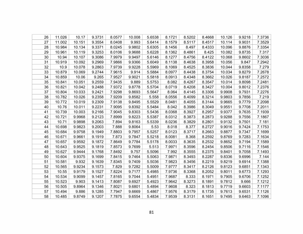
81
26 11.026 10.17 9.3731 8.0577 10.008 5.6538 8.1721 8.5202 8.4668 10.126 9.9218 7.373627 11.002 10.151 9.3554 8.0408 9.993 5.6414 8.1579 8.5117 8.4517 10.114 9.9031 7.352928 10.984 10.134 9.3371 8.0245 9.9802 5.6305 8.1456 8.497 8.4333 10.096 9.8876 7.335429 10.961 10.119 9.3253 8.0106 9.9688 5.6228 8.1362 8.4861 8.425 10.082 9.8735 7.31730 10.94 10.107 9.3086 7.9979 9.9497 5.6146 8.1277 8.4756 8.4122 10.068 9.8602 7.303631 10.919 10.092 9.2969 7.9866 9.9366 5.6049 8.1138 8.4638 8.3958 10.056 9.847 7.294232 10.9 10.078 9.2863 7.9739 9.9228 5.5969 8.1069 8.4525 8.3836 10.044 9.8358 7.27933 10.879 10.069 9.2744 7.9615 9.914 5.5884 8.0977 8.4438 8.3754 10.034 9.8279 7.267834 10.859 10.06 9.265 7.9527 9.9021 5.5818 8.0913 8.4348 8.3662 10.026 9.8187 7.257235 10.841 10.051 9.2559 7.9435 9.889 5.5753 8.082 8.4267 8.3547 10.014 9.8098 7.248136 10.821 10.042 9.2488 7.9372 9.8778 5.5704 8.0719 8.4208 8.3427 10.004 9.8012 7.237637 10.804 10.033 9.2421 7.9298 9.8693 5.5647 8.064 8.4145 8.3306 9.9908 9.7931 7.227638 10.782 10.026 9.2358 7.9209 9.8582 5.558 8.0556 8.4099 8.3214 9.9803 9.7856 7.21939 10.772 10.019 9.2309 7.9138 9.8495 5.5529 8.0481 8.4055 8.3144 9.9665 9.7779 7.209840 10.76 10.011 9.2231 7.9095 9.8392 5.5484 8.042 8.3986 8.3049 9.9551 9.7708 7.201141 10.739 10.003 9.2166 7.9045 9.8303 5.5436 8.0368 8.3927 8.2957 9.9377 9.7635 7.193942 10.721 9.9968 9.2123 7.8999 9.8223 5.5387 8.0312 8.3873 8.2873 9.9288 9.7556 7.186743 10.71 9.9898 9.2063 7.894 9.8163 5.5339 8.0236 8.3829 8.2801 9.9132 9.7501 7.18144 10.698 9.9823 9.2003 7.888 9.8064 5.53 8.018 8.377 8.2727 9.9016 9.7424 7.175345 10.684 9.9758 9.1949 7.8803 9.7957 5.5257 8.0123 8.3717 8.2663 9.8877 9.7347 7.169946 10.671 9.9661 9.1919 7.873 9.7847 5.5218 8.0081 8.368 8.2592 9.8769 9.7283 7.163447 10.657 9.9592 9.1872 7.8649 9.7784 5.5178 8.0033 8.3635 8.2532 9.8652 9.7194 7.158948 10.643 9.9525 9.1819 7.8573 9.7699 5.513 7.9971 8.3596 8.2454 9.8506 9.7116 7.154649 10.627 9.9444 9.1768 7.8492 9.757 5.5096 7.992 8.3555 8.2375 9.8401 9.7058 7.149350 10.604 9.9375 9.1699 7.8415 9.7464 5.5063 7.9871 8.3493 8.2287 9.8336 9.6996 7.14451 10.581 9.932 9.1639 7.8345 9.7409 5.5036 7.9823 8.3456 8.2219 9.8219 9.6914 7.138852 10.565 9.9234 9.1573 7.829 9.7282 5.5009 7.9777 8.3417 8.2126 9.8123 9.6851 7.134353 10.55 9.9179 9.1527 7.8224 9.7177 5.4985 7.9736 8.3368 8.2052 9.8011 9.6773 7.129354 10.534 9.9099 9.1457 7.8165 9.7044 5.4951 7.9687 8.333 8.1971 9.7905 9.6706 7.125255 10.523 9.903 9.1413 7.8087 9.6927 5.4923 7.9642 8.3273 8.1891 9.7812 9.666 7.121256 10.505 9.8964 9.1346 7.8021 9.6801 5.4894 7.9608 8.323 8.1813 9.7719 9.6603 7.117757 10.494 9.886 9.1285 7.7947 9.6669 5.4867 7.9576 8.3179 8.1735 9.7613 9.6531 7.112658 10.485 9.8749 9.1207 7.7875 9.6554 5.4834 7.9539 8.3131 8.1651 9.7495 9.6463 7.1096

82
59 10.471 9.8643 9.1116 7.7774 9.6412 5.4803 7.9496 8.3083 8.1558 9.7401 9.6394 7.104760 10.457 9.8522 9.1036 7.7681 9.6295 5.4782 7.9446 8.3042 8.1497 9.7317 9.6309 7.0995
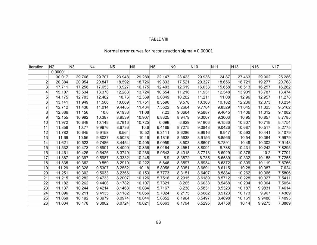
83
TABLE VIII
Normal error curves for reconstruction sigma = 0.00001
Iteration N2 N3 N4 N5 N6 N8 N9 N10 N11 N13 N16 N17
0.00001 1 30.017 29.766 29.707 23.948 29.289 22.147 23.423 29.936 24.87 27.463 29.902 25.2862 20.384 20.954 20.847 18.592 18.726 19.833 17.521 20.327 18.656 18.721 19.277 20.7683 17.711 17.258 17.653 13.927 16.175 12.403 12.619 16.033 15.658 16.513 16.257 16.2624 15.107 13.534 13.378 12.263 13.724 10.554 11.216 11.931 12.548 13.901 13.787 13.4745 14.175 12.703 12.482 10.76 12.369 9.0849 10.202 11.211 11.08 12.96 12.957 11.2786 13.141 11.949 11.566 10.069 11.751 8.3596 9.578 10.363 10.182 12.236 12.073 10.2347 12.712 11.438 11.014 9.4485 11.434 7.5522 9.2664 9.7784 9.8529 11.645 11.325 9.51628 12.386 11.156 10.6 9.1938 11.08 7.23 9.0664 9.5887 9.4645 11.406 11.012 9.10829 12.155 10.992 10.387 8.9539 10.907 6.8325 8.9479 9.3007 9.3003 10.95 10.857 8.7785
10 11.972 10.848 10.148 8.7813 10.725 6.698 8.829 9.1803 9.1586 10.807 10.718 8.475411 11.856 10.77 9.9976 8.6736 10.6 6.4189 8.7275 9.0848 9.0426 10.687 10.517 8.277512 11.782 10.645 9.9158 8.564 10.52 6.3111 8.6286 8.9916 8.947 10.593 10.441 8.107913 11.69 10.56 9.8037 8.5028 10.46 6.1816 8.5638 8.9156 8.8566 10.54 10.364 7.997914 11.621 10.523 9.7486 8.4454 10.405 6.0959 8.503 8.8607 8.7891 10.49 10.302 7.914815 11.532 10.473 9.6901 8.4099 10.356 6.0164 8.4551 8.8091 8.738 10.431 10.242 7.829516 11.461 10.425 9.6426 8.3749 10.286 5.9543 8.4318 8.7718 8.6929 10.376 10.2 7.770117 11.387 10.397 9.5987 8.3332 10.245 5.9 8.3872 8.735 8.6589 10.332 10.158 7.725518 11.335 10.362 9.559 8.2919 10.222 5.846 8.3597 8.6934 8.6372 10.309 10.119 7.676619 11.29 10.328 9.5307 8.2552 10.18 5.8058 8.3351 8.6691 8.6115 10.28 10.087 7.62420 11.251 10.302 9.5033 8.2366 10.153 5.7773 8.3151 8.6407 8.5884 10.262 10.066 7.580621 11.215 10.282 9.4733 8.2007 10.126 5.7516 8.2915 8.6189 8.5712 10.228 10.027 7.541122 11.182 10.262 9.4406 8.1782 10.107 5.7321 8.265 8.6033 8.5468 10.204 10.004 7.505423 11.137 10.244 9.4214 8.1468 10.084 5.7167 8.238 8.5831 8.5323 10.187 9.9831 7.461424 11.096 10.211 9.4135 8.1182 10.056 5.7024 8.2175 8.5682 8.5123 10.173 9.967 7.436925 11.069 10.192 9.3979 8.0974 10.044 5.6852 8.1964 8.5497 8.4898 10.161 9.9488 7.409526 11.034 10.178 9.3802 8.0724 10.021 5.6663 8.1794 8.5295 8.4758 10.14 9.9275 7.3889
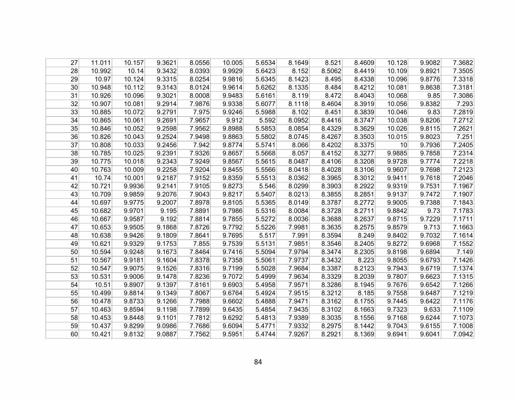
84
27 11.011 10.157 9.3621 8.0556 10.005 5.6534 8.1649 8.521 8.4609 10.128 9.9082 7.368228 10.992 10.14 9.3432 8.0393 9.9929 5.6423 8.152 8.5062 8.4419 10.109 9.8921 7.350529 10.97 10.124 9.3315 8.0254 9.9816 5.6345 8.1423 8.495 8.4338 10.096 9.8776 7.331830 10.948 10.112 9.3143 8.0124 9.9614 5.6262 8.1335 8.484 8.4212 10.081 9.8638 7.318131 10.926 10.096 9.3021 8.0008 9.9483 5.6161 8.119 8.472 8.4043 10.068 9.85 7.308632 10.907 10.081 9.2914 7.9876 9.9338 5.6077 8.1118 8.4604 8.3919 10.056 9.8382 7.29333 10.885 10.072 9.2791 7.975 9.9246 5.5988 8.102 8.451 8.3839 10.046 9.83 7.281934 10.865 10.061 9.2691 7.9657 9.912 5.592 8.0952 8.4416 8.3747 10.038 9.8206 7.271235 10.846 10.052 9.2598 7.9562 9.8988 5.5853 8.0854 8.4329 8.3629 10.026 9.8115 7.262136 10.826 10.043 9.2524 7.9498 9.8863 5.5802 8.0745 8.4267 8.3503 10.015 9.8023 7.25137 10.808 10.033 9.2456 7.942 9.8774 5.5741 8.066 8.4202 8.3375 10 9.7936 7.240538 10.785 10.025 9.2391 7.9326 9.8657 5.5668 8.057 8.4152 8.3277 9.9885 9.7858 7.231439 10.775 10.018 9.2343 7.9249 9.8567 5.5615 8.0487 8.4106 8.3208 9.9728 9.7774 7.221840 10.763 10.009 9.2258 7.9204 9.8455 5.5566 8.0418 8.4028 8.3106 9.9607 9.7698 7.212341 10.74 10.001 9.2187 7.9152 9.8359 5.5513 8.0362 8.3965 8.3012 9.9411 9.7618 7.204642 10.721 9.9936 9.2141 7.9105 9.8273 5.546 8.0299 8.3903 8.2922 9.9319 9.7531 7.196743 10.709 9.9859 9.2076 7.9043 9.8217 5.5407 8.0213 8.3855 8.2851 9.9137 9.7472 7.190744 10.697 9.9775 9.2007 7.8978 9.8105 5.5365 8.0149 8.3787 8.2772 9.9005 9.7388 7.184345 10.682 9.9701 9.195 7.8891 9.7986 5.5316 8.0084 8.3728 8.2711 9.8842 9.73 7.178346 10.667 9.9587 9.192 7.8814 9.7855 5.5272 8.0036 8.3688 8.2637 9.8715 9.7229 7.171147 10.653 9.9505 9.1868 7.8726 9.7792 5.5226 7.9981 8.3635 8.2575 9.8579 9.713 7.166348 10.638 9.9426 9.1809 7.8641 9.7695 5.517 7.991 8.3594 8.249 9.8402 9.7032 7.161449 10.621 9.9329 9.1753 7.855 9.7539 5.5131 7.9851 8.3546 8.2405 9.8272 9.6968 7.155250 10.594 9.9248 9.1673 7.8464 9.7416 5.5094 7.9794 8.3474 8.2305 9.8198 9.6894 7.14951 10.567 9.9181 9.1604 7.8378 9.7358 5.5061 7.9737 8.3432 8.223 9.8055 9.6793 7.142652 10.547 9.9075 9.1526 7.8316 9.7199 5.5028 7.9684 8.3387 8.2123 9.7943 9.6719 7.137453 10.531 9.9006 9.1478 7.8236 9.7072 5.4999 7.9634 8.3329 8.2039 9.7807 9.6623 7.131554 10.51 9.8907 9.1397 7.8161 9.6903 5.4958 7.9571 8.3286 8.1945 9.7676 9.6542 7.126655 10.499 9.8814 9.1349 7.8067 9.6764 5.4924 7.9515 8.3212 8.185 9.7558 9.6487 7.121956 10.478 9.8733 9.1266 7.7988 9.6602 5.4888 7.9471 8.3162 8.1755 9.7445 9.6422 7.117657 10.463 9.8594 9.1198 7.7899 9.6435 5.4854 7.9435 8.3102 8.1663 9.7323 9.633 7.110958 10.453 9.8448 9.1101 7.7812 9.6292 5.4813 7.9389 8.3035 8.1556 9.7168 9.6244 7.107359 10.437 9.8299 9.0986 7.7686 9.6094 5.4771 7.9332 8.2975 8.1442 9.7043 9.6155 7.100860 10.421 9.8132 9.0887 7.7562 9.5951 5.4744 7.9267 8.2921 8.1369 9.6941 9.6041 7.0942

85
Appendix 3: Complete Reconstruction Mesh Representation
i.) Normal Brain (N8) Iterations 1-60 Mesh Representation
1 2
3 4
5 6
7 (error < 10%) 8

86
9 (error < 7%) 10
11 12
13 14
15 16 (error < 6%)
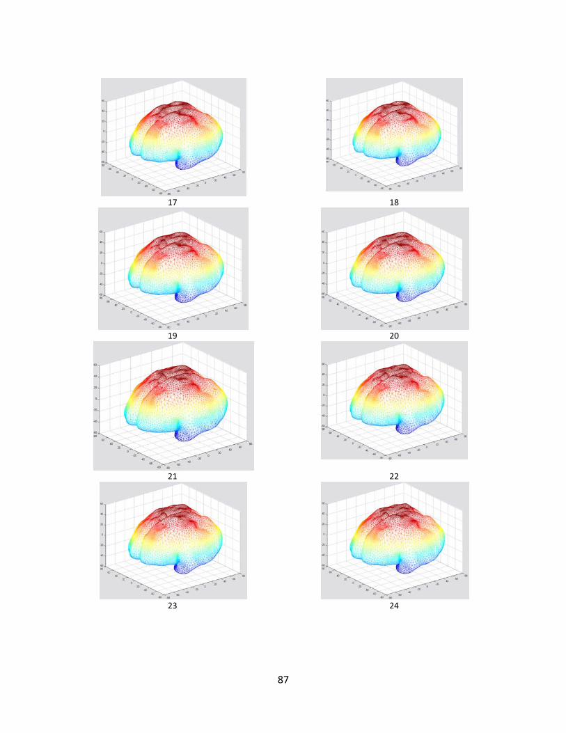
87
17 18
19 20
21 22
23 24
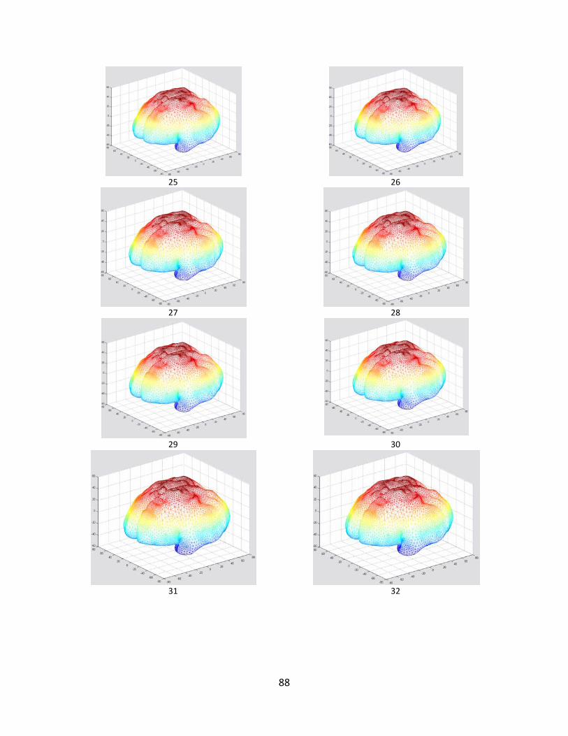
88
25 26
27 28
29 30
31 32

89
33 34
35 36
37 38
39 40
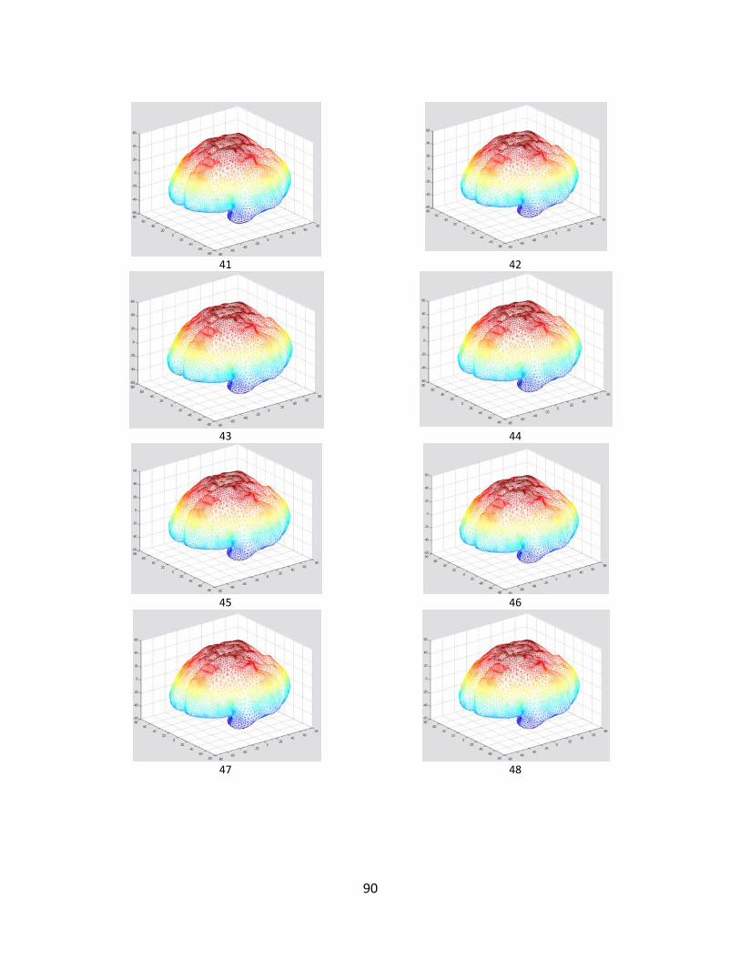
90
41 42
43 44
45 46
47 48

91
49 50
51 52
53 54
55 56

92
57 58
59 60 (error = 5.4744%)

93
ii.) Autistic Brain (A13) Iterations 1-60 Mesh Representation
1 2
3 4
5 6
7 8

94
9 10
11 12
13 14
15 16

95
17 18
19 20
21 22
23 24
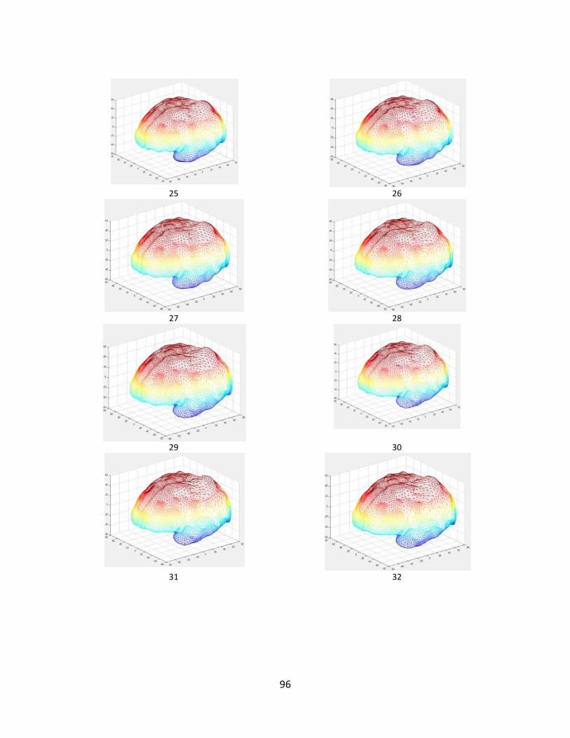
96
25 26
27 28
29 30
31 32

97
33 34
35 36
37 (error < 10%) 38
39 40

98
41 42
43 44
45 46
47 48

99
49 50
51 52
53 54
55 56

100
57 58
59 60 (error = 9.6941%)