Estimates of Turbulence from Numerical Weather Prediction Model Output with Applications to...

2308 VOLUME 132M O N T H L Y W E A T H E R R E V I E W

q 2004 American Meteorological Society

Estimates of Turbulence from Numerical Weather Prediction Model Output withApplications to Turbulence Diagnosis and Data Assimilation

ROD FREHLICH

Research Application Program, National Center for Atmospheric Research,* and CIRES, University of Colorado, Boulder, Colorado

ROBERT SHARMAN

Research Application Program, National Center for Atmospheric Research, Boulder, Colorado

(Manuscript received 2 January 2004, in final form 14 March 2004)

ABSTRACT

Estimates of small-scale turbulence from numerical model output are produced from local estimates of thespatial structure functions of model variables such as the velocity and temperature. The key assumptions usedare the existence of a universal statistical description of small-scale turbulence and a locally universal spatialfilter for the model variables. Under these assumptions, spatial structure functions of the model variables canbe related to the structure functions of the corresponding atmospheric variables. The shape of the model spatialfilter is determined by comparisons with the spatial structure functions from aircraft data collected at cruisingaltitudes. This universal filter is used to estimate the magnitude of the small-scale turbulence, that is, scalessmaller than the filter scale. A simple yet universal description of the basic statistics (such as the probabilitydensity function and the spatial correlation) of these small-scale turbulence levels in the upper troposphere andlower stratosphere is proposed. Various applications are presented including 1) predicting the statistics of tur-bulence experienced by aircraft at upper levels, 2) diagnosing and forecasting turbulence for aviation safety,and 3) estimating the total observation error for optimal data assimilation and for improving operational weatherprediction models. It is determined that the total observation error for typical rawinsonde measurements ofvelocity are dominated by the sampling error or ‘‘error of representativeness’’ resulting from the effects of small-scale turbulence.

1. Introduction

Fluid dynamical simulation models typically sufferfrom underrepresentation of the smallest scales of mo-tion resolvable by finite-difference numerical models.This underrepresentation comes from two sources (e.g.,Ferziger and Peric 2002): 1) truncation error (i.e., errorsdue to the discrete representation of continuous pro-cesses) and 2) error introduced by explicit and implicitmodel smoothing and filtering effects. We assume herethat both of these effects can be represented through auniversal spatial filter; that is, the functional form of thefilter is independent of horizontal location for a givenmodel and altitude region (Daley 1993; Pielke 2002).This spatial filtering is well characterized in large eddysimulation (LES) spectral models by the use of well-defined explicit filters and careful definitions of the re-

* The National Center for Atmospheric Research is sponsored bythe National Science Foundation.

Corresponding author address: Dr. Rod Frehlich, CIRES, 216UCB, University of Colorado, Boulder, CO 80309.E-mail: [email protected]

solved and the unresolved scales (e.g., Sullivan et al.2003). But in global and mesoscale atmospheric modelsthese effects are mostly undocumented since emphasishas traditionally been on accurate representations of thelarger-scale motions that contribute most significantlyto meteorological phenomena, and to some extent, theneed to produce numerically stable solutions rather thanto describe the details of the turbulence field. Since mostparameterizations of subgrid turbulent processes are afunction of the locally resolved fields, the effects ofmodel filtering should be included in the subgrid tur-bulence parameterization. In this paper we developmethods to quantify, for certain atmospheric regimes,the effects of spatial filtering in mesoscale models, andconsequently produce more accurate estimates of thesmall-scale turbulence. Here the term ‘‘small scale’’ isused to refer to the smallest resolvable scales of anatmospheric dynamical model (i.e., scales smaller thanthe filter scale), which with suitable extrapolation, maybe used to infer the magnitude of ‘‘subgrid’’ scale mo-tions as well.

This study is motivated by the realization that statis-tically, the atmospheric wind and temperature spatial

OCTOBER 2004 2309F R E H L I C H A N D S H A R M A N

FIG. 1. Longitudinal, transverse, vertical velocity, and temperaturespectra, denoted Su(k), Sy(k), Sw(k), and ST(k), respectively, as derivedfrom INDOEX field campaign data and the best-fit Kolmogorov slopeof 25/3 over the interval k 5 (0.0005–0.2 rad m21) as shown by thevertical line.

spectra at middle latitudes and upper levels exhibit ak25/3 behavior, where k is the horizontal wavenumber(or equivalently exhibit an s12/3 behavior for the second-order structure function, where s is the separation) fromscales ranging from about 400 km down to 1 km. Thiswas demonstrated rather convincingly by the Global At-mospheric Sampling Program (GASP) and Measure-ment of Ozone by Airbus In-Service Aircraft (MO-ZAIC) data analyses (Nastrom and Gage 1985; Lind-borg 1999; Cho and Lindborg 2001). These datasetswere obtained by specially instrumented commercialaircraft collecting wind and temperature data at aircraftcruise levels (approximately 8–10 km MSL) over sev-eral thousand flight legs.

Individual flights from National Aeronautics andSpace Administration (NASA) and National Center forAtmospheric Research (NCAR) research aircraft alsodisplay the k25/3 behavior. For example, Sharman andFrehlich (2003) consistently obtained a k25/3 behavioron scales from 600 km down to about 40 m from variousresearch aircraft field campaigns. In the Sharman andFrehlich paper some examples were provided from shortflight legs of the NASA B-757 research aircraft. Thespectra in the Sharman and Frehlich study always ex-hibited a k25/3 behavior for all 67 flight segments stud-ied, in both low- and high-turbulence regions. We didnot observe steeper spectral slopes as reported by Vin-nichenko (1970). The average of 40 nonoverlappingspectra produced from a particularly long (600 km) legof measurements from the NCAR EC-130 aircraft flyingabove the planetary boundary layer at 4806-m elevationas part of the Indian Ocean Experiment (INDOEX) isshown in Fig. 1. Details of the NCAR aircraft mea-surement systems can be found in Lenschow (1986),Lenschow and Spyers-Duran (1989), and Khelif et al.(1999). As can be seen, the 25/3 spectral slope is agood fit to all three velocity components and temper-ature spectra for wavelengths from about 6 km to about30 m. At scales smaller than about 30 m, the velocityspectra deviate from the 25/3 slope because of mea-suring difficulties of the differential pressure sensors andpossibly other effects. Also note that for scales less thanabout 600 m (k . 0.01 m21), the spectra of all threevelocity components have nearly the same magnitude,but the outer length scale for the vertical velocity com-ponent is 1–2 km, while the horizontal velocity com-ponents, consistent with the GASP and MOZAIC data,exhibit no identifiable length scale in the range of wave-lengths shown.

The cause of the observed k25/3 statistical behavior isat the moment not completely understood. Discussionsof competing theories are provided, for example byTung and Orlando (2003) and Koshyk and Hamilton(2001) within the context of recent simulation resultsthat seem to point to a downscale cascade. For our pur-poses, it is sufficient merely to accept the k25/3 spectralbehavior as a universal statistical description of mid-latitude upper-level ‘‘turbulence’’ so that this behavior

can be used as ‘‘truth’’ to quantify the underrepresen-tation of the small-scale motions in mesoscale models.Depending on the model numerics and filtering used, amesoscale model will in general show an energy deficitfrom this assumed universal statistical behavior, andgenerally this deficit will be largest for the smallestscales resolved by the model. This model-dependentdeficit can be estimated from the s dependence of model-derived second-order structure functions compared tothe expected s2/3 behavior. For this comparison the useof structure functions is preferred since they permit ac-curate measurements of turbulence over small mea-surement domains and are more robust compared withspectral methods, which suffer from windowing and al-iasing effects (Frehlich 1997; Frehlich et al. 1998,2001). Once the spatial filter of the model has beendetermined, information about turbulence levels can beextrapolated to scales smaller than the model resolutionto provide information about the energy content of thegrid scale and subgrid-scale turbulent motions.

The layout of the remainder of the paper is as follows.In section 2 results from aircraft measurements of thespatial statistics of upper-level turbulence are reviewed.Using these results and comparing to numerical weatherprediction (NWP) models, the National Centers for En-vironmental Prediction (NCEP) Rapid Update Cycle


(RUC) (Benjamin et al. 2004) and the fifth-generation(Pennsylvania State University) PSU–NCAR MesoscaleModel (MM5) (Grell et al. 1994; Davis et al. 1999) inparticular, universal filter functions for these models arederived in section 3. Similar methods are used to derivea universal filter function for the Clark–Hall cloud-re-solving model (Clark 1977; Clark and Hall 1991). Aprocedure to estimate small-scale turbulence intensitiesis outlined in section 4 along with some results usingthis procedure. The remainder of the paper presentssome applications of the technique. Section 5 providesan application of the estimated local turbulence inten-sities to produce estimates of sampling error or ‘‘errorof representativeness’’ of rawinsonde wind and tem-perature measurements. This provides a more accuratedescription of total observation error statistics (section6), which can be used for optimal data assimilation andfor improving ensemble forecasts based on more real-istic perturbations of the initial state. In section 7 thetechnique is used to provide model-derived turbulenceestimates as a diagnostic for aircraft-scale turbulence.The diagnostic is then used to derive a climatology ofaircraft-scale upper-level turbulence in section 8. Asummary and conclusions are provided in section 9.

2. Statistical description of upper-level turbulence

The most reliable statistical descriptions of turbulenceon spatial scales relevant to current mesoscale NWPmodels (1–200 km) have been produced by speciallyinstrumented commercial aircraft, in particular GASP(Nastrom and Gage 1985) in the United States and MO-ZAIC in Europe (Lindborg 1999; Cho and Lindborg2001). Since most of these flights were of fairly longduration, most of the measurements were taken at cruisealtitudes, that is, in the upper troposphere and lowerstratosphere.

The spatial statistics of upper-level turbulence maybe described by spatial structure functions. Longitudinaland transverse second-order structure functions are de-fined respectively by

2D (s) 5 ^[y (x) 2 y (x 1 s)] &,LL L L

2D (s) 5 ^[y (x) 2 y (x 1 s)] &, (2.1)NN N N

where yL(x) and yN(x) are the velocity components alongand transverse to the displacement vector s 5 (x, y, z),respectively, and ^ & denotes an ensemble average. Fol-lowing Lindborg (1999) and Cho and Lindborg (2001)we assume the statistics of the structure functions followsimple scaling laws for homogeneous turbulence, validfor either 2D or 3D isotropic conditions. For 3D iso-tropic turbulence, DNN(s) is related to DLL(s) by [Moninand Yaglom (1975), Eq. (13.70)]

s dD (s) 5 D (s) 1 D (s) (2.2)NN LL LL2 ds

and for 2D isotropic turbulence by (Lindborg 1999)

dD (s) 5 [sD (s)], (2.3)NN LLds

where s 5 | s | .The statistics of fully developed 3D isotropic turbu-

lence are well described by the Kolmogorov model, inwhich case the turbulence intensity, as measured by theeddy dissipation rate «, is related to DLL(s) and DNN(s)[Monin and Yaglom (1975), Eq. (2.17)] through

2/3 2/3 2/3 2/3D (s) 5 C « s ø 2« s ,LL K

4 82/3 2/3 2/3 2/3D (s) 5 C « s ø « s , (2.4)NN K3 3

where CK ø 2 is the Kolmogorov constant. For fullydeveloped 2D isotropic turbulence analogous relationscan be written as (Lindborg 1999)

2/3 2/3 2/3 2/3D (s) 5 C « s ø 2« s ,LL K

5 102/3 2/3 2/3 2/3D (s) 5 C « s ø « s , (2.5)NN K3 3

realizing that « as used here may not strictly satisfy thedefinition of 3D turbulence intensity.

Both the GASP and MOZAIC campaigns producedessentially the same average statistics for midlatitudeupper-level turbulence. The best-fit models to the com-bined datasets were derived by Lindborg (1999) as

2/3 2 2D (s) 5 a s 1 b s 2 c s lns, (2.6)LL 1 1 1

2/3 2 2D (s) 5 a s 1 b s 2 c s lns, (2.7)NN 2 2 2

where a1 ø 0.0036 m4/3 s22, a2 ø 0.004 m4/3 s22, b1 ø2.4 3 1029 s22, b2 ø 6.5 3 1029 s22, c1 ø 0.16 3 1029

s22, and c2 ø 0.43 3 1029 s22. Note that for smallspacings s, the first term dominates, and the structurefunctions recover the Kolmogorov form (2.4). For largerspacings, the second and third terms recover the so-called enstrophy cascade (k23) region observed at largerscales in both the GASP and MOZAIC data. Note thecoefficients in (2.6) and (2.7) are the original valuesfrom Lindborg (1999) and include measurements in boththe upper troposphere and lower stratosphere from lowlatitudes to high latitudes. Cho and Lindborg (2001)document a weak latitude dependence, but for the pur-poses of comparison to numerical model output wechoose to use the average values.

If (2.6) is used with the 2D isotropic assumption (2.3),the same form as Lindborg’s best-fit transverse structurefunction model (2.7) is recovered but with slightly dif-ferent coefficients

2/3 2 2D (s) 5 a s 1 b s 2 c s lns,NN 3 3 3 (2.8)

where a3 5 5/3 a1 ø 0.006 m4/3 s22, b3 5 3b1 2 c1 ø7.04 3 1029 s22, and c3 5 3c1 ø 0.48 3 1029 s22.

The structure function of temperature DT is more com-plicated because of the average temperature variation withlatitude. However, the structure function in the zonal di-rection (E–W) is approximately proportional to DLL:


2/3 2 2D (s) 5 a s 1 b s 2 c s lns.T 4 4 4 (2.9)

From Fig. 5 of Nastrom and Gage (1985), assuming theintegral of the temperature and velocity spectra are equalto their respective variances, the constants evaluate toa4 ø 6.36 3 1024 K2 m22/3, b4 ø 4.24 3 10210 K2 m22,and c4 ø 2.83 3 10211 K2 m22.

3. Statistical description of mesoscale modeloutput

A finite-difference numerical simulation model of theatmosphere consists of a discrete representation of theatmospheric-state variables on a finite-difference gridand a discrete representation of the governing equationsof motion. It is common practice to represent the desireddiscrete model variables (‘‘truth’’) as a spatial averageof the random atmospheric fields centered in a modelgrid cell (e.g., Daley 1993),

` ` `

y (r) 5 W(s 2 r)y(s) ds, (3.1)truth E E E2` 2` 2`

where r 5 (x, y, z) denotes the center of the grid cell,W(s) is the effective weighting function [filter functionwith normalization ### W(s) ds 5 1] of the model, andds denotes 3D integration. Assuming the filter functionis a spatial average over the grid cell (e.g., Deardorff1970; Pielke 2002), that is, W(s) 5 1/(LxLyLz) insidethe grid cell, 0 outside, (3.1) becomes

L /2 l /2 L /2x y z1y (r) 5 y(r 1 s) ds,truth E E EL L Lx y z 2L /2 2L /2 2L /2x y z

(3.2)

where Lx, Ly, Lz denote the dimensions (spacings) of themodel grid cell. We will call a model that satisfies thisfilter function in a statistical sense a ‘‘perfect’’ model.

For a homogeneous field the local horizontal spatialstatistics of a model output variable u is well describedby the spatial structure function defined by

2D (r, s) 5 ^[u(x, y, z) 2 u(x 1 r, y 1 s, z)] &.u

(3.3)

Assume the model values u are given by the generalform (3.1) and the filter function W(r) is a universalfunction locally (since the filter function may also de-pend on other conditions, e.g., stability and the subgridparameterization). Then unbiased estimates of the localstructure function in the (x, y) plane of u for a smallregion centered at coordinate (x, y, z) 5 (iLx, jLy, H)are given by

i1N j1Ni j1D (lL , mL , H ) 5 O Ou x y (2N 2 l)(2N 2 m) p5i2N q5j2Ni j i j

3 {u(pL , qL , H )x y

22 u[(p 1 l)L , (q 1 m)L , H ]} ,x y

(3.4)

where H denotes the altitude or pressure level of themodel grid cell, and Ni and Nj define the spatial domainin the x and y directions, respectively. The size of themeasurement domain is determined by the required sta-tistical accuracy. Note that the model structure functionis a filtered version of the actual structure function ofthe continuous random process for variable u becauseof the spatial filter of the model.

The ensemble average of the model structure functionis given by (Papoulis 1965; Frehlich 1997)

`

D (s) 5 ^D (s)& 5 D (s 2 r)V(r) drmodel u E u

2`

`

2 D (r)V(r) dr, (3.5)E u

2`

where

`

V(s) 5 W(r 2 s)W(r) dr (3.6)E2`

is the autocorrelation of the filter function W.Using these definitions, spatial statistics from NWP

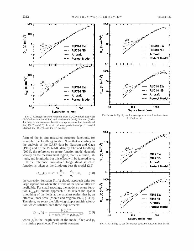
model output can be developed and compared to Lind-borg’s results to derive statistical metrics for NWP mod-el performance. These metrics have been derived forthree NWP models: NCEP’s RUC (Benjamin et al.2004) 20-km horizontal resolution model (RUC20) aswell as an earlier 40-km version (RUC40), and a 30-km horizontal resolution version of MM5 (Grell et al.1994; Davis et al. 1999) run operationally at the NCARMesoscale and Microscale Meteorology (MMM) Divi-sion. Examples of the average longitudinal and trans-verse model-derived structure functions using (3.4) from1 yr of RUC20, RUC40, and MM5 0000 UTC analysesare shown in Figs. 2 to 4, respectively. Also plotted arethe s2/3 scaling, Lindborg’s (1999) best-fit models (2.6)and (2.7), along with the prediction of a perfect model(3.5), assuming the spatial filter of a perfect model isthe average of the velocity field over the grid cell (3.2).As expected, the agreement with Lindborg’s (1999)best-fit models at large scales (;500 km) for all thethree NWP models is excellent, and the effective modelfilter is more pronounced than the perfect model filter.This comparison promotes the use of second-order spa-tial structure functions as a diagnostic for the spatialfilter of the model. Note that the absolute levels of thestructure functions derived from the various NWP mod-els agree very well.

An empirical function Dmodel(s) for the model-derivedstructure functions can be determined to explicitly ac-count for the model-dependent filter function. The sim-plest such empirical function has the form

D (s) 5 KD (s)D (s),model cor ref (3.7)

where K is a constant, Dcor(s) describes the correctionproduced by the model filter, and Dref(s) is a normalized


FIG. 2. Average structure functions from RUC20 model east–west(E–W) direction (solid line) and north-south (N–S) direction (dash–dot line), in situ measured best-fit average structure function (dottedline) [(2.6) and (2.7)] from aircraft data, prediction of perfect model(dashed line) [(3.5)], and the s2/3 scaling.

FIG. 3. As in Fig. 2, but for average structure functions fromRUC40 model.

FIG. 4. As in Fig. 2, but for average structure functions from MM5.

form of the in situ measured structure functions, forexample, the Lindborg model. Note that according tothe analysis of the GASP data by Nastrom and Gage(1985) and of the MOZAIC data by Cho and Lindborg(2001), the reference structure function model dependsweakly on the measurement region, that is, altitude, lat-itude, and longitude, but this effect will be ignored here.

If the reference normalized longitudinal structurefunction is taken as the Lindborg best-fit model (2.6)

b c1 12/3 2 2D (s) 5 s 1 s 2 s lns, (3.8)LLref a a1 1

the correction function Dcor(s) should approach unity forlarge separations where the effects of the spatial filter arenegligible. For small spacings, the model structure func-tion Dmodel(s) should approach s2 to reflect the spatialsmoothing of the fields at the smallest scales, that is, aneffective inner scale (Monin and Yaglom 1975, p. 353).Therefore, we select the following simple empirical func-tion which satisfies both these requirements:

4/3(s/p )1D (s) 5 , (3.9)LLcor 4/3 2/31 1 (s/p ) 1 p (s/p )1 2 1

where p1 is the length scale of the model filter, and p2

is a fitting parameter. The best-fit constant


FIG. 5. Average velocity structure functions from RUC20 (solidlines) for the longitudinal velocity in the east–west (E–W) directionand the transverse velocity in the north–south (N–S) direction, thebest-fit model [(3.7)] (dashed line) with parameters p1 and p2, thebest-fit reference models [(3.8) and (3.11)] (dotted line), the theo-retical predictions for a 60-km grid cell [(3.5)] (dash–dot line), andthe s2 scaling.

FIG. 6. Average temperature structure functions from RUC20 (solidlines) in the east–west (EW) direction, best-fit model [(3.7)] (dashedline) with parameters p1 and p2, best-fit reference model [(3.8)] (dottedline), and the s2 scaling.

2/3 2/3K 5 C « ø 2«K (3.10)

provides an estimate of «.Alternatively, if the reference normalized transverse

structure function is taken as the Lindborg 2D isotropicmodel (2.8)

9b 2 3c 9c1 1 12/3 2 2D (s) 5 s 1 s 2 s lns, (3.11)NNref 5a 5a1 1

then the best-fit constant

5 102/3 2/3K 5 C « ø « (3.12)K3 3

provides an estimate of «. Similarly, for estimates ofthe temperature structure function, the reference struc-ture function model is the same as (3.8), and the best-fit constant K 5 provides an estimate of the tem-2C T

perature turbulence level.The unknown parameters p1 and p2 are determined

by minimizing the chi-squared error (Press et al. 1986)between the empirical model and the average structurefunctions derived from the NWP model. Examples fromthe RUC20 analysis of Fig. 2 are shown in Fig. 5 forthe velocity structure functions and in Fig. 6 for thetemperature structure function in the east–west direc-tion. (The structure functions of temperature in thenorth–south direction were not computed because thestrong latitude dependence significantly alters the struc-ture function shape.) Note that the best-fit model struc-ture function is almost identical to the measured struc-ture function. Similar results were produced for theRUC40 and MM5 models. Also shown in Fig. 5 is thetheoretical calculation (3.5) of the longitudinal (LL60km) and transverse (NN60 km) structure functions fora 60-km grid cell and the 2D isotropic Lindborg model(2.6) and (2.8). The RUC20 analysis is well approxi-mated by the 60-km grid cell filtering for the longitu-dinal structure function while there is a small error forthe transverse structure function. This heavy filtering istypical of NWP models.

A similar procedure was also applied to output fromthe higher-resolution Clark–Hall anelastic cloud-resolv-ing model (e.g., Clark 1977; Clark and Hall 1991). Fig-ure 7 shows the best-fit global structure functions ob-tained from an analysis of a deep convective cloud sim-ulation from the Clark–Hall model (Lane et al. 2003)using a horizontal resolution of 25 m. Here the referencemodel is chosen as the Kolmogorov model (2.3) becauseof the clear s2/3 power-law region produced in the rangeof 500–2000-m separations. Thus the fitting procedureappears to work equally well for the microbeta scalesof the cloud-resolving model as for the mesoscale NWPmodels.

4. Estimates of small-scale turbulencea. Estimates of local turbulence intensities

Various methods have been proposed to estimate tur-bulence associated with unresolved scales [i.e., subgrid


FIG. 7. Average structure functions from the Clark–Hall cloud re-solving model (solid lines), best-fit model [(3.7)] (dashed line) withparameters p1 and p2, best-fit reference model [(2.4)] (dotted line),and the s2 scaling.

FIG. 8. Example estimates (●) of longitudinal velocity structurefunctions DLL(s) from the RUC20 model using 100 km 3 100 kmsubdomains, the best-fit model [(3.7)] (lines) with turbulence esti-mates «1/3 (m2/3 s21) given to the left of each line, and the s2 scalingfor reference.

scale (sgs)] from resolved-scale model fields. The mostcommon are based on prognostic equations of the sgsturbulent kinetic energy (TKE) (e.g., Deardorff 1970;Moeng 1984; Moeng and Sullivan 1994; Pielke 2002).This requires assumptions about the local conditions toconnect resolved-scale gradients to sgs TKE. Since thehorizontal statistics of the velocity and temperaturefields have a robust description, we propose instead toestimate local (i.e., all scales less than the model filtercutoff, including subgrid scales) turbulence intensitiesbased on the assumption of a universal spatial filter forthe model as outlined in the previous section. A similarapproach has been used to estimate the statistics ofsmall-scale turbulence from lidar measurements usinga correction for the spatial average of the lidar pulse(Frehlich 1997; Frehlich et al. 1998; Frehlich and Corn-man 2002). If the model has a universal filter function—that is, the functional form of the structure functions isindependent of location—then local estimates of the lev-el K (or equivalently of «2/3 or ) can be produced by2C T

a best fit to the shape of the structure functions [see(3.7)] where the reference models are given by (3.8)and (3.9) for the longitudinal and transverse structurefunctions, respectively. Local estimates of « can be pro-duced from the best-fit levels of the two longitudinaland two transverse structure functions using (3.10) and

(3.12). Since the longitudinal structure functions seemto have a slightly better defined s2/3 region (cf. Fig. 5),we use the average of the two longitudinal structurefunctions (east–west and north–south) with (3.10) toproduce local estimates of «. In Fig. 8 plots are providedof average longitudinal structure functions at variouslocations in a RUC20 model field at an altitude of 10km and the corresponding estimates of «1/3 derived froma 5 3 5 point horizontal domain (100 km 3 100 km).Note that at each location the fit is quite good, and theshape of the structure functions is approximately thesame, but the levels «1/3 can differ considerably.

b. Estimates of the probability density function

The statistical description of the structure functionestimates of the local turbulence levels « is fully de-scribed by the probability density function (PDF). ThePDF of the variations in the spectral level of the GASPdata is well described by a lognormal distribution (Nas-trom and Gage 1985). This is equivalent to a lognormalPDF for «, which is completely defined by two param-eters: ^log«& or the median value «50 and the standarddeviation slog« of log10«. From the GASP data, Frehlich(2001) derived these parameters as «50 5 2.66 3 1025

m2 s23, slog« 5 0.63, and in addition, ^«& 5 7.64 3 1025

m2 s23. The PDF of the RUC20 estimates of « fromlocal structure function estimates over an L 3 L sub-domain for two values of L are compared to the log-normal model with these parameters in Fig. 9. Similarly,the PDF of the RUC20 estimates of is shown in Fig.2C T

10. It should be pointed out that the estimates of « and


FIG. 9. PDF of RUC20 estimates of «(o) from two different squaresubdomains L 3 L, the lognormal model prediction based on themean and standard deviation of log« values (solid line), and thelognormal model prediction from the GASP data (dashed line) derivedby Frehlich (2001).

FIG. 10. PDF of RUC20 estimates of (o) from two different2C T

square subdomains L 3 L and the lognormal model prediction basedon the mean and standard deviation of log (solid line).2C T

FIG. 11. Parameters (o) of the lognormal PDF of « vs the averaginglength L. (top) The average of log«, and (bottom) the standard de-viation of log«. The best-fit straight line based on the first four datapoints is also shown.

from the GASP data were produced from the spectral2C T

level at a wavelength of 400 km for flight legs longerthan 2400 km (i.e., along a line), which will have dif-ferent statistics than the RUC20 estimates, which wereproduced over a square domain. However, all the PDFsagree well with the lognormal model, although theRUC20-derived estimates depend on the averaginglength L.

c. Scaling laws as a function of the averagingdimensions

As shown above, the statistics of « and log« dependon the averaging length L. To appreciate this dependence,the statistics of the lognormal PDF of « from RUC20analyses at 10-km altitude are plotted in Fig. 11 as afunction of L, as well as the best-fit power law from thefirst (i.e., smallest L) four data points, namely,

^log«& 5 0.41782 logL 2 6.6956, (4.1)20.19622s 5 7.5019L . (4.2)log«

These relations provide a simple scaling of the statisticsof « to any square L 3 L averaging domain. Note thatfor L larger than about 200 km, the fit deviates slightlyfrom the best-fit lines, probably due to the inclusion of


FIG. 12. Parameters of the lognormal PDF of vs the averaging2C T

length L(o). (top) The average of log , and (bottom) the standard2C T

deviation of log . The best-fit straight line based on the first four2C T

data points is also shown.

the enstrophy cascade region at larger scales as observedin the GASP data. Other simple scaling laws are derivedfrom the RUC20 data similarly:

24 20.068755^«& 5 2.5848 3 10 L , (4.3)2/3 23 10.043359^« & 5 1.04162 3 10 L , (4.4)

22 20.41150SD[«] 5 5.04535 3 10 L , (4.5)2/3 24 20.37429VAR[« ] 5 5.8795 3 10 L . (4.6)

Note that, consistent with refined similarity theory, thevariance of small-scale turbulence intensity increaseswith a decrease in the averaging domain L. Also, asexpected, the exponent of L in the ^«& and ^«2/3& ex-pressions is very small, indicating only a weak depen-dence on L.

The average longitudinal structure function derivedin Lindborg (1999) for all the cruising level aircraft dataproduced ^«& 5 7.64 3 1025 m2 s23 and similarly, for308–508-latitude tropospheric data Cho and Lindborg(2001, Table 1) found ^«& 5 7.0 3 1025 m2 s23. Notethat these estimates are determined from the averagestructure function level in the s2/3 power-law region, thatis, ^«& 5 (a1/CK)3/2 5 ^«2/3&3/2 since a1 5 CK^«2/3& [see(2.5) and (2.6)]. Using (4.4) the RUC20 value is ^«& 57.11 3 1025 m2 s23 for L 5 100 km, and ^«& 5 8.263 1025 m2 s23 for L 5 1000 km, in good agreementwith Lindborg’s estimate.

Similarly, the scaling of the parameters of the log-normal distribution of can be derived from the2C T

RUC20 data, and the results are shown in Fig. 12. Well-defined power-law scalings are produced for averaginglengths less than about 200 km:

2^logC & 5 26.7195 1 0.48755 logL (4.7)T

2 20.19131SD[logC ] 5 6.6724L , (4.8)T

2 24 0.046511^C & 5 1.2493 3 10 L , (4.9)T

2 24 20.61839VAR[C ] 5 5.1552 3 10 L . (4.10)T

Equivalent expressions for the statistics of « andcan be derived from the output of any NWP model2C T

provided the spatial resolution is adequate to resolve atleast part of the s2/3 region. Ideally, different NWP mod-els would produce the same climatology and statisticaldescription of the small-scale turbulence in concert withthe GASP and MOZAIC data.

The smallest scales for which these power-law scal-ings are valid is unclear. However, the GASP data in-dicate the spatial spectrum of velocity follows the25/3 power law to scales of a few kilometers, and air-craft data (e.g., Fig. 1) show this trend continues downto at least a few tens of meters, implying a universalbehavior. It is possible that the scaling for the variationsin turbulence levels « and also follows a universal2C T

power law down to very small scales. But this can onlybe verified by many high-resolution measurements ofupper-level turbulence, and at the moment these are notavailable.

The well-behaved power-law scalings of the statisticsof small-scale turbulence metrics « and are indica-2C T

tions of an underlying simple description of the spatialstatistics of these fields analogous to high Reynoldsnumber homogeneous and isotropic turbulence and Kol-mogorov’s refined similarity theory (Monin and Yaglom1975). Any scalar field with homogeneous statistics anda Gaussian or lognormal distribution function is com-pletely described by its covariance function, related tothe structure function through

C (s) 5 ^[q(s ) 2 ^q&][q(s 1 s) 2 ^q&]&q 0 0

25 s 2 D (s)/2.q q

(4.11)

A simple model for Cq that produces the power-lawscalings (4.3)–(4.10) is given by [e.g., Monin and Yag-lom 1975, Eq. (25.28)]

KqC (s) 5 , (4.12)q 2 2 b/2(L 1 s )0

where L0 is the turbulence length scale for the variationsof q, and b is the intermittency exponent, which maydepend on conditions (e.g., altitude). As shown in theappendix, the universal constants Kq and b for the scalarfield «2/3(x, y) can be estimated from the scaling lawsproduced from the RUC20 analysis as b 5 0.37429 andKq 5 4.21737 3 1024 m8/32b s24.

5. Application to estimates of sampling error orerror of representativeness

The correct statistical description of small-scale tur-bulence is critical for defining sensor data requirements


(Frehlich 2001) and for performing optimal data assim-ilation. The magnitude of local turbulence levels « istypically highly variable (e.g., Monin and Yaglom 1975;Frehlich 1992; section 4). This variability will impactthe sampling error associated with atmospheric mea-surement systems. In many cases the sampling error maybe significantly larger than the instrument error of theobservation. For example, the newer rawinsonde de-signs, namely, Vaisala’s RS80-15G based on GPS po-sitioning, have a stated accuracy of better than 0.5m s21 for each wind component (Jaatinen and Elms2000). The automated weather reports from commercialaircraft outfitted with the Aircraft Communication, Ad-dressing, and Reporting System (ACARS) have an es-timated wind component error of 1.1 m s21 (Benjaminet al. 1999). For comparison, research aircraft have anestimated accuracy of about 0.4 m s21 (Lenschow 1986;Khelif et al. 1999). As will be presently shown, sam-pling errors for wind observations can be much largerthan these instrument errors, as much as several metersper second.

a. Measurement errors

The error budget of NWP models can be separatedinto analysis errors, forecast errors, model errors, andmeasurement errors. A measurement can be decom-yposed as

y 5 y 1 e 1 BIAS ,truth y y (5.1)

where ytruth is the desired measurement or truth, ey is thetotal zero-mean random observation error, and BIASy

is the total measurement bias. The magnitude of therandom error ey is defined as the standard deviation Sy

of the measurement where

2 2 2S 5 ^[y 2 ^y&] & 5 ^e &, (5.2)y y

and the bias is defined as

BIAS 5 ^y 2 y &,y truth (5.3)

where ^ & denotes an ensemble average over many re-alizations of a statistically similar atmosphere. A criticalcomponent for the definition of error is the choice ofthe desired measurement ytruth, which will depend on theapplication.

Any measurement can also be represented by

y 5 y 1 i 1 b ,S y y (5.4)

where yS denotes the effective spatial sampling of thecontinuous random variable y (r), by is the instrumentbias, and iy is the zero-mean random instrument errorwith magnitude 5 ^ &. The total measurement bias2 2s iy y

is then

BIAS 5 ^y 1 b 2 y & 5 BIAS 1 b ,y S y truth atm y (5.5)

where BIASatm 5 ^yS 2 ytruth& is the bias from the sam-pling pattern of the atmosphere. For many applications

BIASatm 5 0 and BIASy 5 by. If the bias is zero, themagnitude of the total random error for the measurementof y is given by

2 2 2 2 2S 5^[y 2 y ] & 5 ^[y 1 i 2 y ] & 5 s 1 d ,y truth s y truth y y

(5.6)

where

2 2d 5 ^[y 2 y ] &y S truth (5.7)

is the sampling error and we have assumed that theinstrument error iy is uncorrelated with yS 2 ytruth; thatis, the instrument error is uncorrelated with the localturbulence intensities.

An important factor for future measurement systemsis the trade-off between the random error from the in-strument sy and the sampling error dy. For example, forDoppler lidar space-based wind measurements, the mag-nitude of both of these errors is a function of the lidarshot pattern and the statistical description of the tur-bulent velocity field (Frehlich 2001). Note that the sam-pling error is defined only by the sampling pattern ofthe instrument and the statistics of the random atmo-sphere. This is slightly different from past definitionsthat essentially define ytruth in terms of model interpo-lation filters (Lorenc 1986; Daley 1993; Cohn 1997).However, the concept of sampling error is the same; thatis, it defines the ability of the measurement to representthe intended spatial average or interpolation of the mod-el variable.

b. Sampling error

Rigorous numerical and theoretical analysis of thesampling error requires a complete statistical descriptionof the 3D random velocity field, that is, the small-scaleturbulence. Simple analytic results for sampling errorsassociated with random processes can be produced byintegrating over the z coordinate to produce a 2D ran-dom process:

L /2z1y (x, y, H ) 5 y(x, y, H 1 z) dz, (5.8)ELz 2L /2z

where H denotes the height of the center of the gridcell. The random field is now a two-dimensional field,which is more tractable for numerical (Frehlich 2000)and analytic analysis. For example, the definition of‘‘truth’’ as the average over the model grid cell becomes

L /2 L /2x y1y (p, q, H ) 5 y (p 1 x, q 1 y, H ) dx dy,truth E EL Lx y 2L /2 2L /2x y

(5.9)

which is more convenient for numerical analysis. Al-though the exact statistical description of the two-di-mensional random fields is not available, it is reasonable


to assume that the statistics of (x, y, H) are homoge-yneous in the horizontal plane and will be similar toaircraft measurements because the vertical dimension ofthe grid cell is typically much less than the horizontaldimensions (Lz K Lx, Ly) and the integration over z willhave only a small effect.

Assuming the 2D approximation for the random field,the sampling error for a rawinsonde measurement ran-domly located in the measurement volume is given by(Frehlich 2001)

L Ly x2 x y2d 5 1 2 1 2 D (x, y, 0) dx dy,y E E y1 21 2L L L Lx y x y0 0

(5.10)

where

D (x, y, z) 5 ^[y (x , y , z )y 0 0 0

22 y (x 1 x, y 1 y, z 1 z)] &0 0 0

(5.11)

is the structure function of any variable y over a locallyhomogeneous domain centered at (x0, y0, z0). Note thatthe variable y is general and the sampling error is com-pletely defined by its structure function Dy(x, y, 0).

Calculations of the sampling error component of thetotal observation error require the dimensions (Lx, Ly,Lz) of the chosen measurement volume, the samplingpattern of the measurement, and the spatial statistics ofthe small-scale turbulence. For measurements of windsby aircraft or by space-based lidar using linear trackswe define the horizontal velocity vector by its along-(u) and cross-track (y) components. Assuming the 3Disotropic Kolmogorov model for the horizontal velocityfield, the sampling errors for a square grid (Lx 5 Ly 5L) become (Frehlich 2001, Table 1)

1/3d 5 d 5 0.856835(«L)u y (5.12)

for a random rawinsonde measurement inside the mea-surement volume, and

1/3d 5 d 5 0.687592(«L)urc vrc (5.13)

for a rawinsonde measurement located at the center ofa measurement cell. For an observation that samples aline along the total length of the measurement cell inthe direction of u (profiler or lidar from space)

1/3d 5 0.350945(«L) , (5.14)u

1/3d 5 0.211040(«L) . (5.15)y

Similarly, the sampling error dT for temperature mea-surements with a rawinsonde randomly located insidea square measurement cell of length L is

1/3d 5 0.560930C L .T T (5.16)

The sampling error can be determined for any ob-servation system given information about the spatialstatistics of the measured variable. Therefore, the spatial

statistics of the total observation error can also be de-termined. This includes the variance and the error co-variance matrix of a collection of multiple observations.The local estimates of the observation error statisticscan then be used to improve data assimilation tech-niques. This requires estimates of the local turbulencelevels such as those provided here.

As an example, the magnitude of the sampling errorfor measurements of one component of horizontal ve-locity and temperature with a rawinsonde randomly lo-cated in a measurement cell is given by (5.12) and(5.16), respectively. Estimates of the sampling error us-ing (5.12) and (5.16) for a measurement of a singlecomponent of the horizontal velocity and temperaturefrom a rawinsonde randomly located in a 100 km 3100 km measurement cell based on the estimates of«1/3 and for the RUC20 domain for a particular case2C T

are shown in Fig. 13. Note the large variability in thesampling error (from near 0 to 8 m s21 for a singlecomponent of velocity and from near 0 to 5 K for tem-perature) and therefore the total observation error. Incontrast, current operational data assimilation schemes(Shaw et al. 1987; Courtier et al. 1998) assume theobservation error is independent of location (i.e., is con-stant) at a given altitude. Obviously this large variabilityin sampling error is a critical issue for optimal dataassimilation.

The recent development of ensemble forecasting tech-niques requires an appropriate selection of the membersof the ensemble, either by selecting ensembles of fore-casting algorithms, or of ensembles of initial states, orboth (Toth and Kalnay 1997; Kalnay 2003). The localestimates of the observation error statistics can be usedto generate realistic ensembles of observations for dataassimilation and for ensemble forecasts based solely onthe initial state of the atmosphere, thus providing amethodology to separate model errors from initial-stateerrors.

6. Comparison of sampling errors to operationalobservation errors

One of the standard input parameters for operationaldata assimilation is an estimate of the total observationerror. This is typically determined from short-term fore-cast errors (Hollingsworth and Lonnberg 1986; Lonn-berg and Hollingsworth 1986; Dee and Da Silva 1999;Dee et al. 1999). But an alternative, and probably moreaccurate, estimate of total observation error can be pro-duced directly from (5.6) where the instrument errorcomponent is given by the instrument specifications, andthe sampling error component is determined from thesampling pattern of the observation and the climatologyof the small-scale turbulence. For a rawinsonde obser-vation that randomly ascends through a square modelgrid cell of length L, the total sampling error for eachvelocity component is from (5.12),


FIG. 13. Estimates of the sampling error using (5.12) and (5.16) for a measurement of a single component of the horizontal velocity andtemperature from a rawinsonde randomly located in a 100 km 3 100 km measurement cell based on the estimates of «1/3 and for the2C T

RUC20 domain.

2 2 2/3 2/3^d & 5 ^d & 5 0.734166^« &L .u y (6.1)

Substituting (4.4) for the scaling law derived from theRUC20 analysis gives

2 2 23 10.7100^d & 5 ^d & 5 0.76472 3 10 Lu y (6.2)

at 10-km altitude (;250 hPa).

Note that (6.2) is a universal scaling based on theclimatology of small-scale turbulence extracted fromRUC20 analyses and therefore can be used to determinethe contribution of the sampling error to the total ob-servational error for any NWP model. For example, theNCEP (http://wwwt.emc.ncep.noaa.gov/gmb/bkistler/


FIG. 14. Histogram of aircraft turbulence level grms and the pre-diction (o) from the climatology determined from RUC20 turbulencestatistics.

oberr) and European Centre for Medium-Range WeatherForecasts (ECMWF) (Courtier et al. 1998) assimilationalgorithms assign a total rawinsonde observation errorin the east–west and north–south velocity componentsat 250 hPa of 3.2 and 3.5 m s21, respectively. For com-parison, the prediction of the average sampling errorfrom (6.2) for a T63 spectral code (L ; 210 km) is 2.1m s21, and 1.8 m s21 for a T254 code (L ; 55 km). Itis difficult to quantify the effective sampling pattern andthe correct definition of truth for NWP models; however,it is clear that the total observation error is dominatedby the sampling error.

In a similar manner, the average sampling error formeasurements of temperature from a rawinsonde as-cending randomly through a grid cell is from (5.16),

2 2 2/3^d & 5 0.31464^C & L .T T (6.3)

Substituting (4.9) for the scaling law of ^ & from the2C T

RUC20 analysis produces

2 25 10.7132^d & 5 3.9308 3 10 LT (6.4)

at 10-km altitude (;250 hPa). The total rawinsondeobservation error for temperature at 250 hPa used byNCEP is 2.3 K (http://wwwt.emc.ncep.noaa.gov/gmb/bkistler/oberr), which using (6.4), compares with a pre-dicted sampling error of 0.496 K for a T63 spectral code(L ; 210 km) and 0.307 K for a T254 code (L ; 55km). Since the reported instrument error sT for the Vais-ala rawinsonde is 0.5 K (Luers 1997), the total obser-vation error would be ( 1 )1/2 or only 0.7 and 0.582 2s dT T

K for T63 and T254 spectral codes, respectively. Thislarge disagreement may be due to the effects of globalmodel errors in the NCEP estimation of the total ob-servation error and larger instrument error for the globalsounding network.

7. Application to estimates of upper-levelturbulence climatology

A reasonable metric for the magnitude of turbulenceencountered by aircraft is

1/2L1 1/22/3g 5 « (x, 0) dx 5 q , (7.1)rms E[ ]L 0

which is proportional to the rms vertical accelerationexperienced by an aircraft (Cornman et al. 1995). Here,

is the average of q(x, 0) 5 «2/3 (x, 0) over the linearqdimension L [see (A. 1) in the appendix].

A climatology of grms can be inferred from the fol-lowing arguments. From section 4b, grms is expected toobey a lognormal distribution with parameters deter-mined from the scaling laws of small-scale turbulencederived from mesoscale model output. For RUC20, thetwo parameters of the lognormal distribution of grms arederived in the appendix as ^log grms& 5 21.6737 andSD[log grms] 5 0.34198.

The parameters for the RUC20-derived climatological

distribution of grms can be compared to atmospheric mea-surements produced from routine in situ measurementsof grms as described in Cornman et al. (1995). Currently,about 100 United Airlines 737-300 aircraft are equippedwith the Cornman algorithm, and the data is recordedas 1-min (thus L ø 10 km) median and peak values.For the calendar year 2002, slightly more than 4.4 mil-lion median and peak values were recorded. In Fig. 14the distribution of the binned median values is plottedas a histogram and compared to the predictions ofRUC20-derived lognormal grms climatology. Becausethe operational binning of the in situ data is very coarse,most of the data are contained in the first bin, but itdoes agree very well with climatological prediction. Theagreement is not as good for higher-turbulence values.However, it is difficult to remove random outliers in thedata, which would have a large impact on the smallnumber of occurrences in the higher-turbulence regions.Also, the data are probably biased low because com-mercial aircraft will attempt to avoid known regions ofstrong turbulence, an effect that is difficult to quantify.

8. Application to the diagnosis of upper-levelturbulence conditions

Over the years there have been continuous efforts tonowcast and forecast the occurrence upper-level aircraft-scale turbulence through the use of various manual andautomated turbulence diagnostics derived from NWPmodel output (e.g., Ellrod and Knapp 1992; Marroquin1998; Tebaldi et al. 2002). Most of these turbulencediagnostics do not have a rigorous basis from turbulencetheory, but rather relate expected turbulence intensitiesto larger-scale features in the atmosphere, such as upper-


FIG. 15. The probability of moderate-or-greater turbulence detec-tion PODY vs the probability of null turbulence detection PODNbased on comparison of turbulence pilot reports to RUC20-basedstructure function turbulence estimates (solid line), TKE diagnosticestimates (dashed line), and Ellrod–Knapp diagnostic estimates (dot-ted line). The case of no skill is also shown (dot–dash line).

level fronts and jet streams. However, we can apply theideas presented in the previous sections to use NWPmodel-derived structure functions to produce patternsof turbulence intensities «1/3 as shown in the exampleof Fig. 13.

The accuracy of these derived values of «1/3 can beassessed from the only routine observations of upper-level turbulence available, reports of encounters withturbulence by commercial airline pilots. Pilot reportsare semiautomated and give information about a tur-bulence encounter (time, latitude, longitude, altitude,severity). There is some subjectivity associated withthese reports, especially with regard to severity (re-ported on a five-point scale: null, light, moderate, se-vere, or extreme), and it must be realized that the reportis based on a turbulence experience along a flight path,that is, along a line. If the model-derived diagnosticsare supposed to be a gridpoint average, the correspon-dence to a line is not necessarily direct. Nevertheless,the relative performance of various diagnostics can beevaluated by comparisons to turbulence pilot reports asin Tebaldi et al. (2002). In that study the metric usedto evaluate the performance of various turbulence di-agnostics was the area contained under probability ofdetection (POD) curves, similar to radar operating char-acteristic curves. Figure 15 shows POD curves for twoof the more robust diagnostics determined in the Tebaldiet al. study [the Ellrod–Knapp (1992) frontogenesis-related diagnostic and the Marroquin (1998) TKE di-agnostic] compared to the «1/3 diagnostic based on struc-ture function computations. The Marroquin (1998) ap-

proach uses a steady-state approximation to the TKEprognostic equation and should therefore provide sim-ilar estimates of TKE to those produced by most subgridparameterizations used in current NWP models. All di-agnostics were computed from RUC20 0000 UTC anal-yses at upper levels over a 3-month period from No-vember 2002 to January 2003. A set of thresholds wasassumed for each diagnostic, and given that threshold,the diagnostic performance based on comparisons toavailable turbulence pilot reports was evaluated for bothnull (as measured by PODN, the fraction of null eventscorrectly detected) and moderate or greater turbulencereports (as measured by PODY, the fraction of moderateor greater turbulence events correctly detected). In Fig.15 PODY is plotted against PODN for various thresh-olds. For small values of the chosen threshold, PODYwill obviously be high, near unity, while PODN will below, near 0, and vice versa for large values of the chosenthreshold. For the range of thresholds selected, highercombinations of PODY and PODN, and therefore largerareas under the PODY–PODN curves, imply greaterskill in discriminating between null and moderate-or-greater turbulence events. Based on the area under thecurves, the structure-function-derived «1/3 diagnostic issuperior to the better performers identified in the Tebaldiet al. (2002) study. This algorithm is therefore poten-tially quite useful for operational forecasting of upper-level and midlevel turbulence, and its utility in that re-gard is currently being evaluated.

9. Summary and discussion

A procedure has been presented to estimate the small-scale turbulence levels from any mesoscale NWP modelusing estimates of the local structure functions of modelvariables, provided adequate spatial resolution is avail-able to resolve at least part of the s2/3 power-law region.The key assumptions for a given altitude of interest arethe existence of 1) a universal statistical description ofthe small-scale turbulence, and 2) a universal represen-tation of the spatial filter for the model. The extensivearchive of in situ aircraft measurements provided by theGASP and MOZAIC datasets has produced a robustuniversal description of the velocity and temperaturefields at typical aircraft cruising altitudes of 10 km. Thisdescription is duplicated by the average structure func-tions derived from three different mesoscale NWP mod-els (Figs. 2–4). An accurate estimate of the spatial filterof mesoscale models such as RUC20 and MM5 is pro-duced from the average structure functions of the modelvariables and the universal in situ model (Figs. 5 and6). The average velocity structure functions derivedfrom RUC20 analyses agree well with the theoreticalcalculation assuming the model values are produced asan average over a 60 km 3 60 km grid cell (Fig. 5),thus indicating the true spatial filtering of the model.For a high-resolution cloud-resolving model or LESmodel, the universal filter is obtained by comparisons


of the average structure function in convective regionsto the Kolmogorov in situ model (Fig. 7). In either case,the estimates of small-scale turbulence are producedfrom the scaling constant of the best-fit universal struc-ture function to the local structure function estimates(e.g., Fig. 8). These techniques could be applied to otherlevels (i.e., lower to mid-troposphere and stratosphere)if suitable estimates of the spatial statistics becomeavailable, either from data or reliable numerical simu-lation models.

The climatology of the small-scale turbulence is welldefined by the PDF and the spatial statistics of the es-timates. The PDF of small-scale turbulence levels forthe velocity field described by « (Fig. 9) and the tem-perature field described by (Fig. 10) is approximately2C T

lognormal; that is, the log10 of « and have a normal2C T

or Gaussian distribution.The parameters of the lognormal distribution depend

on the averaging length L and have simple scaling lawsas shown in Figs. 11 and 12. Similar results have beenproduced for surface-layer measurements of turbulence.Note that these scaling laws may depend slightly on theaveraging time, for example winter versus summer, al-though the overall shape is expected to be preserved,that is, expected to maintain a lognormal distributionand have a power-law dependence on the averaging do-main. The variability of the small-scale metrics for tur-bulence intensity is the essential component of Kol-mogorov’s refined similarity theory for velocity fieldsand the extension to the temperature field. An accuratestatistical description of atmospheric turbulence mustinclude this variability as outlined in the appendix.

There are many applications for these local turbulenceestimates. These include incorporating the turbulence-related variability into optimal data assimilation meth-ods, improving subgrid-scale turbulence parameteriza-tions, forecasting turbulence for aviation safety, extract-ing turbulence climatologies from archived model fields,and calculating accurate error bars for various statistics.With regards to optimal data assimilation, in many casesthe total observation error is dominated by samplingerrors produced by the measurement sampling pattern.This is particularly important for rawinsonde data asshown in Fig. 13. A point measurement is a poor rep-resentation of the average over the measurement vol-ume, especially in regions of high turbulence. There maybe little benefit in improving the instrument error of arawinsonde measurement if the sampling error is largerthan the instrument error for a large fraction of theobservation space. Next-generation forecast models willhave higher resolution and therefore may require higherdensity and more accurate observations. More spatialaveraging may be required to reduce the sampling error(e.g., line averages using Doppler lidar on multiple sat-ellites) as an alternative to increasing the density of therawinsonde network. A rigorous evaluation of the op-timal data density and measurement accuracy will re-quire Observing System Simulation Experiments (OSS-

Es) with the correct description of the sampling errorand turbulence statistics.

The climatology extracted from 1 yr of RUC20 datahas produced an estimate of the spatial distribution ofturbulence that might be encountered by aircraft at cruis-ing altitudes (Fig. 14). In addition, local estimates of «allow useful predictions of small-scale turbulence (Fig.15). As future operational models increase the spatialresolution and assimilate more accurate data, the truestatistical description of the atmospheric fields shouldbe revealed. This will permit still more accurate fore-casts of turbulence for aviation safety as well as providean improved understanding of turbulence processes pro-vided the universal description of turbulence can be de-termined globally.

Finally, it has been shown that the climatology ofsmall-scale turbulence is an ideal diagnostic of the totalobservation error used in NWP models. The samplingerror for rawinsonde velocity measurements is the dom-inant contribution to observation error at 250 hPa; how-ever, the sampling error for temperature at this level ismuch smaller than the current observation error used atNCEP. In principle, the sampling error, the total obser-vation error, and the climatology of the errors can beproduced using the local estimates of small-scale tur-bulence provided rigorous definitions of the errors areused (section 5). These estimates of total observationerror are useful diagnostics of the performance of dataassimilation algorithms since a perfect data assimilationscheme should produce an analysis error equal to thetotal observation error. In addition, the spatial statisticsof the sampling error and the total observation error canbe used for optimal data assimilation based on the mod-el-derived local estimates of turbulence (Daley 1991;Kalnay 2003). The random spatial variations of the sam-pling errors should also be included in OSSEs to cor-rectly represent the observation error statistics (Atlas1997; Rohaly and Krishnamurti 1993). The statisticalvariability of small-scale turbulence and its lognormalPDF should also be included in the calculation of errorbars for atmospheric statistics (Lenschow et al. 1994).

Acknowledgments. This research was funded in partby the FAA Aviation Weather Research Program, bythe NASA Aviation Safety Program, the National Sci-ence Foundation under Grant No. ATM 335205, andNASA Langley, with Michael Kavaya and Syed Ismailas technical monitors. The FAA-sponsored research isin response to requirements and funding by the FAA,and the views expressed are those of the authors anddo not necessarily represent the official policy or po-sition of the FAA. Thanks to Todd Lane for supplyingus with the Clark–Hall model output used in construct-ing Fig. 7. The authors are grateful for useful sugges-tions by Don Lenschow and Francois Vandenberghebased on a reading of the draft manuscript, and com-ments from the anonymous reviewers.


APPENDIX

Spatial Statistical Description ofSmall-Scale Turbulence

The universal description of the spatial statistics ofsmall-scale turbulence can be defined by the spatial co-variance Cq(s) of the turbulence statistic q, which canby approximated in the upper troposphere and lowerstratosphere by Eq. (4.12). The spatial covariance Cq(s)can be related to the statistics of q as follows:

The spatial average of q over a line of length L isL1

q 5 q(x, 0) dx. (A.1)EL 0

If q is a homogeneous isotropic random field, then ^ &q5 ^q& and the variance of isq

L2VAR[q] 5 C (x, 0)(1 2 x/L) dx. (A.2)E qL 0

For the covariance model (4.12)2bVAR[q] 5 2K L f (L /L, b),q 0 (A.3)

where1 (1 2 x) dx

f (a, b) 5 . (A.4)E 2 2 b/2(a 1 x )0

Similarly, in 2D, the spatial average of q over a squarewith side of length L is

L L1q 5 q(x, y) dx dy, (A.5)E E2L 0 0

and if q(x, y) is a homogeneous isotropic random field,the variance of isq

L L4 x yVAR[q] 5 C (x, y) 1 2 1 2 dx dy.E E q2 1 21 2L L L0 0

(A.6)

For the covariance model (4.12)

2bVAR[q] 5 4K L g(L /L, b),q 0 (A.7)

where1 1 (1 2 x)(1 2 y) dx dy

g(a, b) 5 . (A.8)E E 2 2 2 b/2(a 1 x 1 y )0 0

Thus the covariance Cq(s) of small-scale turbulencemetric q is the essential component for connecting aone-dimensional average to a two-dimensional average.

The universal constants Kq and b for the scalar field«2/3(x, y) can be estimated from the scaling laws above.For example, the aircraft turbulence metric grms is a func-tion of , the average of the scalar field q(x, y) 5q«2/3(x, y) along a line of length L [(A.1)]. The ensembleaverage of is approximated as the average of «2/3(x, y)qover a L 3 L square domain using the scaling of (4.4).

This is a good approximation because of the weak de-pendence on L in (4.4). If L 5 10 km, from RUC20analyses, ^ & 5 1.5529 3 1023 m4/3 s22. The universalqscaling constants Kq and b for the field «2/3(x, y) aredetermined by equating (A.7) and (4.6) assuming L0/L5 0, to give b 5 0.37429, g(0, b) 5 0.34853, and Kq

5 4.21737 3 1024 m8/320.37429 s24. The variance of [Eq.q(A.2)] then becomes VAR[ ] 5 2.6393 3 1025 m8/3 s24,qwhere L 5 10 km and f (0, b) 5 0.98307. The parametersof the lognormal distribution of are given by (Moninqand Yaglom 1975, p. 618; Frehlich 1992)

2VAR[lnq] 5 ln(1 1 VAR[q]/^q& ) 5 2.4803, (A.9)

^lnq& 5 ln^q& 2 VAR[q]/2 5 27.7078. (A.10)

Since grms 5 1/2, the parameters of the lognormal dis-qtribution of grms are

^lng & 5 ^lnq&/2 5 23.8539 and (A.11)rms

1/2SD[lng ] 5 SD[lnq]/2 5 VAR[lnq] /2 5 0.78745.rms

(A.12)

The lognormal parameters for log10grms (log grms) aregiven by ^log10grms& 5 ^ln grms&/ln10 5 21.6737 andSD[log10grms] 5 SD[ln grms]/ln10 5 0.34198.

REFERENCES

Atlas, R., 1997: Atmospheric observations and experiments to assesstheir usefulness in data assimilation. J. Meteor. Soc. Japan, 75B,111–130.

Benjamin, S. G., B. E. Schwartz, and R. E. Cole, 1999: Accuracy ofACARS wind and temperature observations determined by col-location. Wea. Forecasting, 14, 1032–1038.

——, G. A. Grell, J. M. Brown, and T. G. Smirnova, 2004: Mesoscaleweather prediction with the RUC hybrid isentropic-terrain-fol-lowing coordinate model. Mon. Wea. Rev., 132, 473–494.

Cho, J. Y. N., and E. Lindborg, 2001: Horizontal velocity structurefunctions in the upper troposphere and lower stratosphere. 1.Observations. J. Geophys. Res., 106, 10 223–10 232.

Clark, T. L., 1977: A small-scale dynamic model using a terrain-following coordinate system. J. Comput. Phys., 24, 186–215.

——, and W. D. Hall, 1991: Multi-domain simulations of the time-dependent Navier–Stokes equations: Benchmark error analysisof some nesting procedures. J. Comput. Phys., 92, 456–481.

Cohn, S. E., 1997: An introduction to estimation theory. J. Meteor.Soc. Japan, 75, 257–288.

Cornman, L. B., C. S. Morse, and G. Cunning, 1995: Real-time es-timation of atmospheric turbulence severity from in-situ aircraftmeasurements. J. Aircr., 32, 171–177.

Courtier, P., and Coauthors, 1998: The ECMWF implementation ofthree-dimensional variational assimilation (3D-Var). I: Formu-lation. Quart. J. Roy. Meteor. Soc., 124, 1783–1807.

Daley, R., 1991: Atmospheric Data Analysis. Cambridge UniversityPress, 457 pp.

——, 1993: Estimating observation error statistics for atmosphericdata assimilation. Ann. Geophys., 11, 634–647.

Davis, C., T. Warner, E. Astling, and J. Bowers, 1999: Developmentand application of an operational, relocatable, mesogamma-scaleweather analysis and forecasting system. Tellus, 51A, 710–727.

Deardorff, J. W., 1970: A numerical study of three-dimensional tur-bulent channel flow at large Reynolds numbers. J. Fluid Mech.,41, 453–480.

Dee, D. P., and A. M. Da Silva, 1999: Maximum-likelihood estimation


of forecast and observation error covariance parameters. Part I:Methodology. Mon. Wea. Rev., 127, 1822–1834.

——, G. Gaspari, C. Redder, L. Rukhovets, and A. M. Da Silva,1999: Maximum-likelihood estimation of forecast and obser-vation error covariance parameters. Part II: Applications. Mon.Wea. Rev., 127, 1835–1849.

Ellrod, G. P., and D. L. Knapp, 1992: An objective clear-air turbulenceforecasting technique: Verification and operational use. Wea.Forecasting, 7, 150–165.

Ferziger, J. H., and M. Peric, 2002: Computation Methods for FluidDynamics. Spinger-Verlag, 423 pp.

Frehlich, R., 1992: Laser scintillation measurements of the temper-ature spectrum in the atmospheric surface layer. J. Atmos. Sci.,49, 1494–1509.

——, 1997: Effects of wind turbulence on coherent Doppler lidarperformance. J. Atmos. Oceanic Technol., 14, 54–75.

——, 2000: Simulation of coherent Doppler lidar performance forspace-based platforms. J. Appl. Meteor., 39, 245–262.

——, 2001: Errors for space-based Doppler lidar wind measurements:Definition, performance, and verification. J. Atmos. OceanicTechnol., 18, 1749–1771.

——, and L. Cornman, 2002: Estimating spatial velocity statisticswith coherent Doppler lidar. J. Atmos. Oceanic Technol., 19,355–366.

——, S. Hannon, and S. Henderson, 1998: Coherent Doppler lidarmeasurements of wind field statistics. Bound.-Layer Meteor., 86,233–256.

——, L. Cornman, and R. Sharman, 2001: Simulation of three di-mensional turbulent velocity fields. J. Appl. Meteor., 40, 246–258.

Grell, G. A., J. Dudhia, and D. R. Stauffer, 1994: A description ofthe fifth-generation Penn State/NCAR Mesoscale Model (MM5).NCAR Tech. Note NCAR/TN-3981STR, 138 pp.

Hollingsworth, A., and P. Lonnberg, 1986: The statistical structureof short-range forecast errors as determined from radiosondedata. Part I: The wind field. Tellus, 38A, 111–136.

Jaatinen, J., and J. B. Elms, 2000: On the windfinding accuracy ofLoran-C, GPS and radar. Vaisala News, 152, 30–33.

Kalnay, E., 2003: Atmospheric Modeling, Data Assimilation and Pre-dictability. Cambridge University Press, 342 pp.

Khelif, D., S. P. Burns, and C. A. Friehe, 1999: Improved wind mea-surements on research aircraft. J. Atmos. Oceanic Technol., 16,860–875.

Koshyk, J. N., and K. Hamilton, 2001: The horizontal energy spec-trum and spectral budget simulated by a high-resolution tropo-sphere–stratosphere–mesosphere GCM. J. Atmos. Sci., 58, 329–348.

Lane, T. P., R. D. Sharman, T. L. Clark, and H.-M. Hsu, 2003: Aninvestigation of turbulence generation mechanisms above deepconvection. J. Atmos. Sci., 60, 1297–1321.

Lenschow, D. H., 1986: Aircraft measurements in the boundary layer.Probing the Atmospheric Boundary Layer, D. H. Lenschow, Ed.,Amer. Meteor. Soc., 39–55.

——, and P. Spyers-Duran, 1989: Measurement techniques: Air mo-tion sensing. NCAR Research Aviation Facility Bulletin 23,NCAR, Boulder, CO, 36 pp.

——, J. Mann, and L. Kristensen, 1994: How long is long enough

when measuring fluxes and other turbulence statistics? J. Atmos.Oceanic Technol., 11, 661–673.

Lindborg, E., 1999: Can the atmospheric kinetic energy spectrum beexplained by two-dimensional turbulence? J. Fluid Mech., 388,259–288.

Lonnberg, P., and A. Hollingsworth, 1986: The statistical structureof short-range forecast errors as determined from radiosondedata. Part II: The covariance of height and wind errors. Tellus,38A, 137–161.

Lorenc, A. C., 1986: Analysis methods for numerical weather pre-diction. Quart. J. Roy. Meteor. Soc., 112, 1177–1194.

Luers, J. K., 1997: Temperature error of the Vaisala RS90 radiosonde.J. Atmos. Oceanic Technol., 14, 1520–1532.

Marroquin, A., 1998: An advanced algorithm to diagnose atmosphericturbulence using numerical model output. Preprints, 16th Conf.on Weather Analysis and Forecasting, Phoenix, AZ, Amer. Me-teor. Soc., 79–81.

Moeng, C.-H., 1984: A large-eddy-simulation model for the study ofplanetary boundary-layer turbulence. J. Atmos. Sci., 41, 2052–2062.

——, and P. P. Sullivan, 1994: A comparison of shear- and buoyancy-driven planetary boundary layer flows. J. Atmos. Sci., 51, 999–1022.

Monin, A. S., and A. M. Yaglom, 1975: Statistical Fluid Mechanics:Mechanics of Turbulence. Vol. 2, MIT Press, 874 pp.

Nastrom, G. D., and K. S. Gage, 1985: A climatology of atmosphericwavenumber spectra of wind and temperature observed by com-mercial aircraft. J. Atmos. Sci., 42, 950–960.

Papoulis, A., 1965: Probability, Random Variables, and StochasticProcesses. McGraw-Hill, 583 pp.

Pielke, Roger A., Sr., 2002: Mesoscale Meteorological Modeling.Academic Press, 676 pp.

Press, W. H., B. P. Flannery, S. A. Teukolsky, and W. T. Vetterling,1986: Numerical Recipes: The Art of Scientific Computing. Cam-bridge University Press, 963 pp.

Rohaly, G. D., and T. N. Krishnamurti, 1993: An observing systemsimulation experiment for the laser atmospheric wind sounder(LAWS). J. Appl. Meteor., 32, 1452–1471.

Sharman, R., and R. Frehlich, 2003: Aircraft scale turbulence isotropyderived from measurements and simulations. Proc. AIAA 41stAerospace Science Meeting and Exhibit, Reno, NV, AIAA, 2003-194.

Shaw, D. B., P. Lonnberg, A. Hollingsworth, and P. Unden, 1987:Data assimilation: The 1984/85 revision of the ECMWF massand wind analysis. Quart. J. Roy. Meteor. Soc., 113, 533–566.

Sullivan, P. P., T. W. Horst, D. H. Lenschow, C.-H. Moeng, and J. C.Weil, 2003: Structure of subfilter-scale fluxes in the atmosphericsurface layer with application to large-eddy simulation model-ling. J. Fluid Mech., 482, 101–139.

Tebaldi, C., D. Nychka, B. G. Brown, and R. Sharman, 2002: Flexiblediscriminant techniques for forecasting clear-air turbulence. En-vironmetrics 2002, 13, 859–878.

Toth, Z., and E. Kalnay, 1997: Ensemble forecasting at NCEP andthe breeding method. Mon. Wea. Rev., 125, 3297–3319.

Tung, K. K., and W. W. Orlando, 2003: The k23 and k25/3 energyspectrum of atmospheric turbulence: Quasigeostrophic two-levelmodel simulation. J. Atmos. Sci., 60, 824–835.

Vinnichenko, N. K., 1970: The kinetic energy spectrum in the freeatmosphere—1 second to 5 years. Tellus, 22, 159–166.

Estimates of Turbulence from Numerical Weather Prediction Model Output with Applications to...

Documents

Transcript of Estimates of Turbulence from Numerical Weather Prediction Model Output with Applications to...