
ORNL REPORT COVER
298
OAK RIDGE NATIONAL LABORATORY MANAGED BY UT-BATTELLE FOR THE DEPARTMENT OF ENERGY ORNL-27 (4-00)
-
Upload
khangminh22 -
Category
Documents
-
view
2 -
download
0
Transcript of ORNL REPORT COVER

OAK RIDGE
NATIONAL LABORATORY
MANAGED BY UT-BATTELLEFOR THE DEPARTMENT OF ENERGY
DOCUMENT AVAILABILITY
Reports produced after January 1, 1996, are generally available free via the U.S. Department of Energy (DOE) Information Bridge.
W eb site http://www.osti.gov/bridge
Reports produced before January 1, 1996, may be purchased by members of the public from the following source.
National T echnical Information Service5285 Port Royal RoadSpringfield, V A 22161T elephone 703-605-6000 (1-800-553-6847) TDD 703-487-4639 Fax 703-605-6900E-mail [email protected]
Web site http://www.ntis.gov/support/ordernowabout.htm
Reports are available to DOE employees, DOE contractors, Energy Technology Data Exchange (ETDE) representatives, and
International Nuclear Information System (INIS) representatives from the following source.
Of fice of Scientific and Technical InformationP .O. Box 62Oak Ridge, TN 37831 Telephone 865-576-8401 Fax 865-576-5728 E-mail [email protected] Web site http://www.osti.gov/contact.html
This report was prepared as an account of work sponsored by an agency of the United States Government. Neither the United States Government nor any agency thereof, nor any of their employees, makes any warranty , express or implied, or assumes any legal liability or responsibility for the accuracy , completeness, or usefulness of any information, apparatus, product, or process disclosed, or represents that its use would not infringe privately owned rights. Reference herein to any specific commercial product, process, or service by trade name, trademark, manufacturer , or otherwise, does not necessarily constitute or imply its endorsement, recommendation, or favoring by the United States Government or any agency thereof. The views and opinions of authors expressed herein do not necessarily state or reflect those of the United States Government or any agency thereof.
ORNL-27 (4-00)
DOCUMENT AVAILABILITY
Reports produced after January 1, 1996, are generally available free via the U.S. Department of Energy (DOE) Information Bridge.
Web site http://www.osti.gov/bridge
Reports produced before January 1, 1996, may be purchased by members of the public from the following source.
National Technical Information Service5285 Port Royal RoadSpringfield, VA 22161Telephone 703-605-6000 (1-800-553-6847)TDD 703-487-4639Fax 703-605-6900E-mail [email protected] site http://www.ntis.gov/support/ordernowabout.htm
Reports are available to DOE employees, DOE contractors, Energy Technology Data Exchange (ETDE) representatives, and International Nuclear Information System (INIS) representatives from the following source.
Office of Scientific and Technical InformationP.O. Box 62Oak Ridge, TN 37831Telephone 865-576-8401Fax 865-576-5728E-mail [email protected] site http://www.osti.gov/contact.html
This report was prepared as an account of work sponsored by an agency of the United States Government. Neither the United States Government nor any agency thereof, nor any of their employees, makes any warranty, express or implied, or assumes any legal liability or responsibility for the accuracy, completeness, or usefulness of any information, apparatus, product, or process disclosed, or represents that its use would not infringe privately owned rights. Reference herein to any specific commercial product, process, or service by trade name, trademark, manufacturer, or otherwise, does not necessarily constitute or imply its endorsement, recommendation, or favoring by the United States Government or any agency thereof. The views and opinions of authors expressed herein do not necessarily state or reflect those of the United States Government or any agency thereof.

ORNL/TM-2010/218
Energy and Transportation Science Division
CRADA Final Report For
CRADA Number CR-98-000535
Testing of the 3M Company Composite Conductor
John P. Stovall D. Tom Rizy
Roger A. Kisner
Date Published: September 2010
Approved for Public Release
Prepared by OAK RIDGE NATIONAL LABORATORY
Oak Ridge, Tennessee 37831-6283 managed by
UT-BATTELLE, LLC for the
U.S. DEPARTMENT OF ENERGY under contract DE-AC05-00OR22725


CONTENTS
Page Contents.................................................................................................................................................iii Acknowledgments .................................................................................................................................. v Abstract ................................................................................................................................................vii 1. Statement of Objectives ................................................................................................................. 1 2. Benefits to the Funding DOE Office's Mission ............................................................................. 3 3. Technical Discussion of Work Performed by All Parties .............................................................. 5
3.1 TEST FACILITY DESIGN AND CONSTRUCTION ........................................................ 5 3.2 ACCR TESTING SUMMARY............................................................................................ 6
3.2.1 ACCR 477 Kcmil Test ............................................................................................ 6 3.2.2 ACCR 795 Kcmil Test ............................................................................................ 7 3.2.3 ACCR 1272 Kcmil Test .......................................................................................... 7 3.2.4 ACCR 675-TW Kcmil Test..................................................................................... 7
3.3 VARIABILITY OF CONDUCTOR TEMPERATURE ...................................................... 8 3.4 PROJECT PRESENTATIONS ............................................................................................ 8
4. Commercialization Possibilities .................................................................................................... 9 5. Conclusions ................................................................................................................................. 15 6. References.................................................................................................................................... 17 Appendix A.1 - ACCR 477 Kcmil Test Report Appendix A.2 - ACCR 795 Kcmil Report Appendix A.3 - ACCR 1272 Kcmil Report Appendix A.4 - ACCR 675-TW Kcmil Report Appendix B - Variability of Conductor Temperature in a Two Span Test Line Appendix C.1 - DOE Peer Review Presentation – May 20, 2002 Appendix C.2 - DOE Peer Review Presentation – January 29, 2004 Appendix C.3 - DOE Peer Review Presentation – October 12, 2005 Appendix C.4 - DOE Peer Review Presentation – October 17, 2006
iii


ACKNOWLEDGMENTS
This effort was conducted as part of the Transmission Reliability R&D Program within the U. S. Department of Energy, Office of Electricity Delivery and Energy Reliability. The authors are grateful for the support of Philip Overholt, U.S. Department of Energy, Office of Electricity Delivery and Energy Reliability and Steve Waslo, U.S. Department of Energy, Chicago Program Office.
v


ABSTRACT
The 3M Company has developed a high-temperature low-sag conductor referred to as Aluminum-
Conductor Composite-Reinforced or ACCR. The conductor uses an aluminum metal matrix material to replace the steel in conventional conductors so the core has a lower density and higher conductivity. The objective of this work is to accelerate the commercial acceptance by electric utilities of these new conductor designs by testing four representative conductor classes in controlled conditions.
Overhead transmission lines use bare aluminum conductor strands wrapped around a steel core
strands to transmit electricity. The typical cable is referred to as aluminum-conductor steel-reinforced (ACSR). The outer strands are aluminum, chosen for its conductivity, low weight, and low cost. The center strand is of steel for the strength required to support the weight without stretching the aluminum due to its ductility. The power density of a transmission corridor has been directly increased by increasing the voltage level. Transmission voltages have increased from 115-kV to 765-kV over the past 80 years. In the United States, further increasing the voltage level is not feasible at this point in time, so in order to further increase the power density of a transmission corridor, conductor designs that increase the current carrying capability have been examined.
One of the key limiting factors in the design of a transmission line is the conductor sag which
determines the clearance of the conductor above ground or underlying structures needed for electrical safety. Increasing the current carrying capability of a conductor increases the joule heating in the conductor which increases the conductor sag. A conductor designed for high-temperature and low-sag operation requires an engineered modification of the conductor materials.
To make an advanced cable, the 3M Company solution has been the development of a composite
conductor consisting of Nextel ceramic fibers to replace the steel core and an aluminum-zirconium alloy to improve the outer strands. The result is a cable that can carry more current than steel-aluminum lines without sagging as much at higher temperatures.
A unique facility called the Powerline Conductor Accelerated Testing (PCAT) Facility was built
at ORNL for testing overhead conductors. The PCAT has been uniquely designed for testing overhead bare transmission line conductors at high currents and temperatures after they have been installed and tensioned to the manufacturer's specifications. The ability to operate a transmission line conductor in this manner does not exist elsewhere in the United States. Four classes of ACCR cable designed by 3M have been successfully test at ORNL – small, medium, large and small/compact. Based on these and other manufacturer tests, the 3M Company has successfully introduced the ACCR into the commercial market and has completed over twenty installations for utility companies.
vii


1. STATEMENT OF OBJECTIVES
One of the critical aspects of increased power flow for utilities is the significant change in operating
conditions, and it is imperative to demonstrate to the utilities that composite conductor and accessories can operate safely at high-temperature and under thermal cycling. It is also important to demonstrate that the sag-temperature-current characteristics are predictable even after repeated thermal cycles.
Installation and operation of the composite conductor in field trials is typically not well suited for
controlled testing of elevated temperature cycling because the load is not easily controlled or predicted. The factors leading to high-temperature excursions include: line current loading, contingency conditions, wind, and solar exposure. Depending on these conditions, it can take a year or more for the conductor to experience a single emergency load.
High-temperature exposure and thermal cycling of the conductor and accessories under mechanical
load can be more easily achieved on a test line that operates at low voltage with a controlled current. Such a test line would be able to simulate thirty years of emergency conditions in three months. ORNL has built a low-voltage test line to evaluate the high-temperature operation of ACCR.
To move ahead and introduce the new technology, ACCR will be tested across the following critical
conductor classes or sizes which are typically used for U.S. grid installations: • Small size, round wire - 477 kcmil "Hawk" • Small size compact - 675 kcmil "Hawk/TW" • Medium size, round wire - 795 kcmil "Drake" • Large size, round wire - 1272 kcmil “Pheasant”
1

2
This page is intentionally left blank.

2. BENEFITS TO THE FUNDING DOE OFFICE'S MISSION ORNL has built a unique transmission test facility to support the nation’s need to address electricity
transmission reliability and security issues. While the demand for power in the U. S. is expected to rise 25% in the next 10 years, the current transmission capacity relative to growth has declined. The problems and solutions to this trend are highlighted in the “Report of the President’s National Energy Policy Development Study” [1] and the “National Transmission Grid Study” [2]. The specific recommendation in the Grid Study pertaining to the transmission test facility is as follows:
“DOE will develop national transmission-technology testing facilities that encourage partnering with industry to demonstrate advanced technologies in controlled environments. Working with TVA, DOE will create an industry cost-shared transmission line testing center at DOE ’s Oak Ridge National Laboratory.”
The transmission test facility has been uniquely designed for testing overhead bare transmission line conductors at high currents and temperatures after they have been installed and tensioned to manufacturer's specifications. The ability to operate a transmission line conductor in this manner does not exist elsewhere in the United States.
This CRADA benefits the DOE mission by the potential increase in electric transmission line
capacity without the construction of new lines. The line upgrading made possible by this work will improve energy efficiency of the electric grid without the adverse environmental impact of major line reconstruction.
3

4
This page is intentionally left blank.

3. TECHNICAL DISCUSSION OF WORK PERFORMED BY ALL PARTIES The project goal is to accelerate the commercial acceptance of the high-temperature low-sag
conductors. 3M Company has developed a new class of overhead conductors based upon a fundamental change in materials. These high-performance composite conductors, also referred to as Aluminum Conductor Composite Reinforced (ACCR), rely on a core of aluminum composite wires surrounded by temperature resistant aluminum-zirconium wires. They represent a major change in overhead conductors since conventional aluminum-steel reinforced conductors (ACSR) were introduced in the early 20th century.
The development of metal composite wire for overhead transmission lines offers two major benefits:
increased power flow and increased efficiency. On an everyday basis, ACCR operates with lower electrical losses due to the conductivity of the core material and lack of ferromagnetic losses. When required, ACCR can provide transmission capacities double that of existing systems. The low thermal expansion of the composite core keeps line sag within design limits when power flow increases. ACCR can be used as a replacement conductor, with quick installation and minimal disturbances to neighborhoods and the environment. No modifications on existing transmission towers or foundations are needed.
The project object has been to verify the aluminum composite conductor and accessory performance
by providing engineering performance data, based upon field testing including testing at rated conductor temperatures. ORNL entered into a cooperative research and development agreement with the 3M Company to test their conductor.
3.1 Test Facility Design and Construction
The ORNL test line incorporates multiple instrumentation systems including (1) a CAT-1 system for
measuring conductor tension and weather (ambient & solar temperatures and wind conditions), (2) multiple thermocouples mounted at various locations on the conductor and accessories and connected to A/D (analog/digital) modules and fiber optic modems to monitor temperature profiles, (3) measurement of the conductor voltage and current during the testing to calculate its resistance as a function of operating temperature, (4) a laser range finder for measuring conductor clearance and calculating sag during the tests and (5) a data acquisition system (computer, software and fiber optic network) for gathering, archiving, analyzing and displaying the data measurements and controlling the dc power supply.
The facility was designed and constructed in 2002 and 2003 with the assistance of TVA as shown in
Figure 1. The test line is 1200 feet in length with 600 ft. spans and the test conductor is installed as two circuits (a total of four 600 ft. spans). At the power supply end (Structure #1), the two circuits are connected to the positive and negative terminals of a dc power supply. At the far end (Structure #3), the circuits are connected together. The result is a 2400 ft. loop of conductor to the dc power supply as the resistive load. The dc power supply is rated at 5000 Adc and 400 Vdc.
5

Structure #1
Structure #2
Structure #3
PowerSupply
TreesideSouthwest
Northeast
Roadside
Structure #1
Structure #2
Structure #3
PowerSupply
TreesideSouthwest
Northeast
Roadside
Figure 1. Layout of PCAT Facility The following conductor tests can be performed: knee-point curve measurement, emissivity
measurement, constant current and temperature tests, current ramp tests, and thermal/mechanical cycling tests. A typical testing period is 4 to 10 months in duration.
During the testing, the following parameters are measured on a one-minute basis.
• Conductor temperature using Type T thermocouples placed on the surface of the conductor every 150 ft. along the 1200 ft. test length.
• Accessory temperatures using Type T thermocouples placed on the surface of two dead ends, two splices, one suspension and one jumper
• Conductor tension using a load cell. • Conductor clearance at one mid-span using a laser range finder. • Conductor current and conductor voltage drop as measured by the dc power supply. • Weather conditions – ambient temperature, wind speed and wind direction, solar radiation.
A 2.25 MW dc power supply is used to apply current to the test conductor. The power supply is rated
0 to 5000 Adc and 0 to 400 Vdc. A manual limit can be set to prevent the power supply from operating above a specified current. A conductor temperature limit can be set and based upon the real-time measured conductor temperature; the power supply can be turned off.
3.2 ACCR Testing Summary
Four sizes of ACCR were tested from August 2002 to August 2009. A summary of these tests are
given in this section and for each test a report can be found in Appendix A.
3.2.1 ACCR 477 Kcmil Test The ACCR 477 conductor was installed successfully on the ORNL- PCAT line using commercial
hardware and normal installation procedures. The conductor and accessories were thermally cycled from ambient to over 200ºC for several hundred hours, using DC power supply and as high current as 1200 amps. The measured sag matched the SAG-10 (recognized as the industry standard software for
6

calculating sag and tension prediction). Data analysis shows that the measured conductor current agrees well with the IEEE thermal rating model predicted values. After de-installation the conductor and accessories were tested for residual strength and degradation. Residual strength exceeded 100% RBS (rated breaking strength) and neither conductor nor accessories showed any signs of damage. Conductor resistance after cycling is equivalent to that of conductor not exposed to thermal cycling.
3.2.2 ACCR 795 Kcmil Test
The ACCR 795 conductor was successfully installed and tested at ORNL. It was thermally cycled
from ambient to over 200°C for several hundred hours, using a DC power supply. Measured temperature difference between conductor core and its surface was as low as 5°C and as high as 20°C degrees and depended on both wind speed and core temperatures at and above 200°C. Wind speeds above 0 fps (foot per second) produced larger temperature gradient from surface to core.
Data analysis shows that the measured conductor current agrees well with the IEEE thermal rating model [3] predicted values. The conductor is rated at 1653 A current for continuous operation at 210°C and at 1778 A emergency current at 240°C. The CIGRE model agrees with the IEEE 738 model.
Conductor tension was stable during and after thermal cycling. Measured line tension versus temperature agrees well with values computed using the strain summation method, STESS.
Both PLP (Preformed Line Products) and AFL (Alcoa Fujikura Limited) accessories ran cool, below 120°C at conductor's temperature exceeding 200°C. The conductor and accessories were exposed for up to 1000 hours at high temperature and show no visual damage. Conductor was de-installed in early 2006 and shipped to NEETRAC for inspection and mechanical testing (residual strength).
3.2.3 ACCR 1272 Kcmil Test
The ACCR 1272 conductor was successfully installed in Aug. 2004 and tested at ORNL. It was
thermally cycled from ambient to greater than 200ºC for several hundred hours, using DC power supply. Measured temperature difference between conductor core and its surface was only several degrees at cycling temperatures in excess of 200°C. The wind speed appears to have a strong effect on cooling of the conductor.
Data analysis shows that the measured conductor current agrees well with the IEEE thermal rating model predicted values. The conductor is rated at 2229 amps for continuous operation at 210ºC and 2402 amps emergency operation at 240ºC. The CIGRE model agrees well with the IEEE 738 model within 0.8%.
The conductor sag was stable during and after thermal cycling. Measured line tension agrees well with values computed using the strain summation method. Both PLP and AFL accessories ran cool, 120ºC and show no visual damage.
The conductor was de- installed in June 2005, and sent to NEETRAC (National Electric Energy Testing Research and Applications Center) for testing and evaluation.
3.2.4 ACCR 675-TW Kcmil Test
The ACCR 675 TW conductor was installed successfully on the ORNL PCAT Line using commercial
hardware and normal installation procedures. The conductor and accessories were thermally cycled from ambient to greater than 200ºC for several hundred hours, using a DC power supply and currents as high as 1500 amps. The measured sag matched the SAG-10 prediction. Data analysis shows that the measured conductor current agrees well with the IEEE thermal rating model predicted values. After-de installation the conductor and accessories were tested for residual strength and degradation. Residual strength exceeded 100% RBS and neither conductor nor accessories showed any signs of damage. Conductor resistance after cycling is equivalent to that of a conductor not exposed to thermal cycling.
7

8
3.3 Variability of Conductor Temperature
A large number of prior reports have indicated substantial temperature variability within a single span in test lines and significant variation of temperature between point measurements in adjacent spans due to varying wind conditions. More anecdotal evidence, e.g. in the discussion records of the Proceedings of the IEEE Panel on Dynamic Line Ratings on July 20-21, 1982, indicate that, at high temperature, longitudinal temperature variation of 10-25ºC had been observed in a single span. Accurate documentation of such variation is generally not available.
It is also generally recognized that the tension and sags of a line section between two dead-ends should be a function of the average temperature of the conductor. Observations have generally shown a good correlation between measured temperatures and sags, but high quality data for comparisons has typically not been available.
Because the high temperature conductor tests at the ORNL PCAT facility are extremely well instrumented, these tests can provide answers to the above questions. The complete report is in Appendix B and shows a much larger longitudinal temperature variation than previously documented.
3.4 Project Presentations
During the project, presentations were made at the U.S. Department of Energy’s Transmission Reliability Program Peer Reviews and these presentations are in Appendix C. Open to the public, these meetings reviewed the research and development projects designed to help modernize the nation’s electric grid. Energy sector stakeholders from outside the program attended the meetings to learn first-hand about the latest developments and integration activities. During the Peer Review, a panel of selected electricity industry experts performed a formal evaluation of projects, provided technical feedback and recommendations to ensure that the DOE continues to support projects that meet industry needs.

4. COMMERCIALIZATION POSSIBILITIES
The 3M Company has successfully implemented their commercialization plan for ACCR. The success, to date, is shown by the twenty-two utility customer installations of ACCR listed in Table 1. ACCR has been installed to meet challenges in a variety of locations, environments, and ampacity requirements.
Conductor Size 3M ACCR Installations Application kV (kcmil) (mm2)
Mumbai, India Load growth Dense population 110 300 150 TATA Power
Minneapolis, Minnesota Installation validation 115 477 238 Xcel Energy
Hawaiian Electric Company Oahu, Hawaii Corrosive environment 46 477 238
Western Area Power Administration Fargo, North Dakota Heavy ice and wind
loads 230 795 418
Bonneville Power Administration Washington State High temperature
operation 115 675-TW 322-TW
Western Area Power Administration Phoenix, Arizona Installation validation 230 1272 642
Salt River Project Phoenix, Arizona High current operation 69 795 418 Santa Clara, California
High temperature operation 115 477 238 Pacific Gas & Electric
Minneapolis, Minnesota
Environmentally sensitive area River crossing
115 795 418 Xcel Energy
Phoenix, Arizona Dense population Underbuilds 230 1272 642 Arizona Public Service
Western Area Power Administration
Arizona/California Border High growth 230 795 418
Shanghai Electric Shanghai, China Cost and time savings 115 795 418 Platte River Power Authority
Fort Collins, Colorado Increased reliability 230 954 490
Aha Macav Power Services Needles, California Increased reliability 69 300 150
West Virginia Underbuilt facilities Cost and time savings 138 1033 525 Allegheny Power
British Columbia Transmission Company (BC Hydro)
British Columbia River Crossing 230 788 400
Birmingham, Alabama
Underbuilt facilities Load growth 230 680 346 Alabama Power
City of Santa Clara, CA
Environmental and aesthetics Reliability
60 715 365 Silicon Valley Power
Chongqing Chongqing, China Load growth Time savings 220 680 346
9

Conductor Size 3M ACCR Installations Application kV (kcmil) (mm2) Companhia de Transmissao de Energia Eletrica Paulista
Sao Paulo, Brazil Cost, time and environmental impact savings
138 300 150
Birmingham, Alabama Cost and time savings 230 1033 525 Alabama Power
Jundiai, Brasil Load growth Cost and time savings Social impacts
88 336 171 CPFL Piratininga
Table 1: List of 3M ACCR Installations
TATA Power Company TATA Power is installing 125 miles (200 kilometers) of 300 kcmil 3M ACCR on two lines near
Mumbai, Borivali-Malad and Salsette-Saki. The lines were upgraded a few years ago from a single to a bundled ACSR, but they could not keep pace with the rapid demand growth in the area. In addition, residences had sprung up directly under the lines, and TATA did not want to disturb them, but did want to improve clearances over them.
Xcel Energy In 2001 Xcel Energy installed 477-kcmil ACCR in its 115 kV system in Minneapolis to feed power
from a generation plant to the network. It replaced a conventional ACSR conductor to increase the ampacity while keeping the same clearance and tower loads.
Hawaiian Electric Company Hawaiian Electric Company (HECO) installed a similar 477-kcmil 3M ACCR on a 46 kV line located
on the North Shore of Oahu for the evaluation of ACCR corrosion resistance. In particular, the installation tests the corrosion resistance of the conductor on their 46 kV network while also increasing the ampacity along the existing right-of-way by approximately 72%.
Western Area Power Administration (Western) Western is one of four power marketing administrations within the U.S. Department of Energy, and
serves nearly 700 wholesale power customers in a 1.3 million-square-mile area, including some 300 municipalities, as well as public utilities and utility districts, energy cooperatives, power marketers, irrigation districts, Native American tribal communities and government agencies.
In 2002 795-kcmil 3M ACCR was installed by Western on the Fargo-Jamestown 230 kV line near Fargo, North Dakota. The climatic conditions there exposed the cable to high winds, extreme cold, ice loading and conditions conducive to aeolian vibration. ACCR was installed on a 1-mile stretch of the circuit. The first two winters after the line was energized were mild. However, in the winter of 2005/2006, ice built up on the conductor, doubling the span’s mechanical loads. Despite the ice loading, there have been no problems since the line was installed. The line data follows the predictions made by models for sag, tension, and rating.
Bonneville Power Administration (BPA) In June of 2004 BPA installed ACCR 675T13-TW on a 115 kV line in Pascal, Washington as a
replacement for an existing Chuker 1780 kcmil (976 mm2) ACSR bottom phase. The purpose of the installation was to test the operation of the compact trap-wire ACCR at elevated temperatures. 3M provided its 675T13-TW conductor to BPA for installation at their Pasco site as a replacement for an existing Chuker 1780-kcmil (976 mmm2) ACSR bottom phase. The conductor was installed in June
10

2004, energized in August 2004, and has run continuously since then. Despite running at currents as high as 1,100 A, conductor temperatures did not exceed 80°C (computed). The mechanical load versus NRS (net radiation sensor) temperature data at low current level matches the predicted values and has essentially been unchanged over time.
Western Area Power Administration (Western) In January 2004 Western installed 1272-kcmil 3M ACCR at its Liberty-Parker location in Phoenix,
Arizona. The conductor was installed as an evaluation/validation cable for the installation of cable constructions with three layers of aluminum. The measured conductor tension and sag agree with predictive models. The line has been loaded to around 25% of its electrical rating since June 2004.
Salt River Project (SRP) 3M ACCR has been installed in several locations in proximity to generating stations in order to test
the conductor under high current loads where it will see high ambient temperatures. Conductors for these tests are sized so that they will operate at their maximum electrical design loads. SRP installed 795 ACCR on a 69 kV line at the expansion of their Santan generation plant in Gilbert, Arizona, in March of 2004. The 795 ACCR line delivers output of the Santan Expansion Project Unit 5b (combined cycle natural gas fired generator) to the 69 kV switchyard. The location is ideal to test 3M ACCR because it undergoes significant temperature swings and high summer peak demand (high conductor temperature) in desert conditions where ambient temperatures are very high.
Pacific Gas & Electric (PG&E) PG&E in Southern California installed 3M ACCR on line segments near a substation in Santa Clara. Xcel Energy 3M ACCR received its first commercial application when Minneapolis-based Xcel Energy installed it
on a ten-mile (sixteen-kilometer) transmission line in the Minneapolis-St. Paul region. Xcel Energy is using the conductor to increase the capacity of a transmission line that extends from Shakopee to Burnsville. The upgrade is part of a US$100 million expansion project at the utility’s Blue Lake peaking plant in Shakopee, which is needed to ensure a reliable supply of power to Xcel Energy’s customers in the Upper Midwest during periods of peak electricity demand. The line crosses an interstate and two major highways at multiple points, as well as traversing several residential and industrial areas.
Arizona Public Service (APS) APS installed 3M ACCR to increase capacity on a key overhead transmission line serving Phoenix, a
growing metropolitan area. The new conductor eliminated the need for the utility to site, acquire right-of-way, and construct a new power line route in a congested downtown business area.
3M ACCR was installed on a six-mile, 230 kV power line extending from a local area power plant to APS’ downtown substation. The installation provides increased capacity to service the fast-growing metropolitan area that experiences extreme summer heat. In this application, 3M’s ACCR 1272-kcmil conductor was used to upgrade a line that already had been upgraded once with ACSS.
The utility selected ACCR as a result of a twelve-month evaluation of various high temperature, low sag conductors. 3M’s ability to supply a complete package, including conductor hardware and installation support, was instrumental in the utility’s selection of ACCR.
The Western Area Power Administration (Western) Western, which delivers about 40 billion kilowatt-hours of hydroelectric power annually in fifteen
western and central states in the U.S., chose 3M ACCR to replace a key conventional power line in western Arizona.
3M ACCR is installed on a twenty-mile stretch of the Topock-Davis 230 kV line, which parallels the Colorado River along Arizona’s western border with California. The area of service includes fast-growing
11

communities such as Lake Havasu City and Bullhead City in Arizona; Laughlin, Nevada; and Needles, California.
Shanghai Electric Power Company, Ltd On October 14, 2007, Shanghai Electric became the first utility in Asia to install and energize 3M
ACCR. Shanghai Electric, a publicly owned utility whose major shareholders are China Power Investment Corp. and East China Power Development Company, serves the Shanghai metropolitan area with more than 2,800 megawatts of generating capacity. Shanghai is the largest city in the People’s Republic of China, and the eighth largest metropolis in the world. Shanghai Electric deployed 3M ACCR to shorten construction time and save costs while increasing capacity on a key 10-mile line serving the growing demand in the city of Shanghai.
Platte River Power Authority To ensure adequate transmission capacity during summer peak demand hours, Platte River Power
Authority installed the 3M ACCR as a replacement conductor on a key three-mile segment of a line that links Fort Collins and Loveland, extending from the Timberline Substation southward along the Union Pacific railroad right-of-way to the Harmony Substation.
Platte River Power Authority generates reliable, low-cost and environmentally responsible electricity for its owner communities of Estes Park, Fort Collins, Longmont and Loveland, Colorado, for delivery to their utility customers. Its facilities are located along the Front Range and northwestern Colorado in addition to near Medicine Bow, Wyoming. Installation is scheduled for Fall 2007.
Aha Macav Power Services Aha Macav Power Services, a utility owned and operated by the Fort Mojave Tribe in the Southwest,
is the first Native American utility to deploy 3M ACCR. Under an agreement with the Western Area Power Administration (Western), Aha Macav installed a
new four-mile 3M ACCR line linking a new substation in Arizona to a switchyard in Needles, CA, a city on the western bank of the Colorado River.
The new line substantially boosts power capacity and reliability for Needles and the surrounding area, which have been plagued by frequent electricity outages in recent years, often during periods of extreme high temperature. The Fort Mojave Tribe, whose reservation encompasses portions of eastern California, southern Nevada and western Arizona, is one of only a handful of tribes served by its own utility. Installation of the 3M ACCR was installed in March 2008.
Allegheny Power Allegheny Power, a division of Allegheny Energy Inc., installed 3M ACCR to upgrade a 138 kV line
linking the Bedington and Nipetown substations along Interstate-81 in West Virginia. The 1.7-mile upgrade boosted transmission capacity on a line some 50 miles northwest of Washington, D.C. The 138 kV line shares structures with three other lines for most of its length, including two under-built 12 kV lines, has a flow of 2,200 amps and is expected to peak at a temperature of 200°C. The line is built on self supporting steel poles with drilled pier concrete foundations.
3M ACCR gave Allegheny the ability to leave the under-built 12 kV circuits in service during
construction and to avoid structure replacement. It also sags neatly with an adjacent 954 ACSR conductor on the same structure.
British Columbia Transmission Company BCTC, the operator of the transmission system for the British Columbia province, installed 3M
ACCR on two segments of the Vancouver Island Transmission Reinforcement (VITR) Project to minimize the disruption to the ecology of diverse and sensitive waterways. Larger towers to accommodate larger conductors or double bundling would require bringing heavy equipment into remote
12

areas by barge; installing new foundations and towers; digging out the existing footings and then transporting the aggregate. Moreover, one of the segments goes through part of a provincial park where preserving the sightline was important. Using 3M ACCR, the transmission utility was able to meet these goals.
In addition, they were able to install the conductor through unusually long spans, avoiding adding
towers to the line. One segment, the Sansum Crossing, included a 5,800 foot (1,770 m) single span. The second segment, the Montague Crossing, was a 6,000 foot (1,830 m) multi-span installation.
Alabama Power Alabama Power Company, a subsidiary of Southern Company, will install 3M ACCR to upgrade a
1.7 mile line at their Miller Steam Plant, in Jefferson County, Alabama, approximately 25 miles northwest of Birmingham.
Alabama Power's upgrade, utilizing 3M ACCR 1033 kcmil 54/19 Curlew, will boost transmission capacity on a line that goes through and loops around the Miller Steam Plant. The upgrade is part of Alabama Power’s ongoing, multibillion-dollar environmental initiative, designed to reduce emissions from the company's power plants while continuing to meet the growing demand for power. The new 230 kV line, is rated to carry up to 2,000 amps and is expected to peak at a temperature of 200°C.
The existing line crosses below three 500KV line and above one 230KV line and is supported on five existing lattice steel structures. The 3M conductor provides the required capacity, while utilizing the existing structures and maintaining or improving the existing clearances to ground and other obstacles. As a result, significant savings were achieved in both time and cost by eliminating the need for the design, supply and construction of new towers.
Silicon Valley Power SVP, the municipal utility of the City of Santa Clara, California, is located in the heart of the Silicon
Valley area, where reliability is paramount for serving high-tech industries. Equally important are using existing structures and minimizing the disruption to both residential and business neighborhoods. This second installation of 3M ACCR will also be on an existing 60 kV line, from Keifer Receiving Station to Norman Avenue Junction, as well as two new sections from Norman Avenue to the new Palm Substation and back. The project also has to accommodate a 12 kV line running under the installation and a 115 kV line crossing above the installation in 2 locations, as well as multiple railroad and highway crossings. 3M ACCR’s strength to weight ratio and durable hardened aluminum will give them the needed reliability and additional capacity using only the existing structures.
Chongqing Electric Power Corporation Chongqing Electric needed extra capacity to meet anticipated heavy power demand for the summer
Olympics in Beijing and did not have time to construct new towers. Using existing towers, Chongqing Electric installed a two-circuit line of approximately 3.4 miles (5.5 kM), linking the Shuinian and Shuangshan substations. Chongqing is in a subtropical region with high humidity and frequently extreme summer heat, and 3M ACCR was chosen in part because of its proven reliability in difficult climates.
This installation will serve more than a half million residents within two districts in Chongqing City,
an ancient city with a population of approximately four million located on the Yangtze River in southwest China, within Sichuan Province.
Companhia de Transmissao de Energia Eletrica Paulista Companhia de Transmissao de Energia Eletrica Paulista (CTEEP) installed 300 kcmil 3M ACCR to
upgrade a 138 kV transmission line crossing an environmentally sensitive river bed. CTEEP, which is principally owned by Grupo Empresarial ISA (ISA Group), one of South America's largest electricity and telecommunications providers, supplies almost all of the electricity consumed in the State of Sao Paulo
13

14
and 30 percent of the electrical power consumed nationwide. The line boosts capacity for power transmission for the Jupiá Electrical System. The line crosses the nearly mile-wide Parana River and is subject to strong winds and extremely high temperatures. “3M ACCR was determined to be the most cost-effective, proven solution available,” says CTEEP engineering manager Caetano Cezario Neto. The installation was completed in just 6 days.
Alabama Power Southern Company subsidiary, Alabama Power, installed 3M ACCR to replace a key 10-mile (16-
kilometer) line in northeastern Alabama. The line was upgraded to meet contingency requirements resulting from the addition of generation to serve summer peak loads. 3M ACCR was chosen for this project to avoid replacing approximately half the transmission structures and installing eight additional structures, significantly reducing construction time and allowing the line to be taken out of service for this project without impacting grid reliability. Alabama Power Company supplies electricity to 1.3 million homes, businesses and industrial facilities.
CPFL Piratininga CPFL, part of CPFL Energy Group, used 3M ACCR to expand transmission capacity in Várzea
Paulista and Jundiaí (SP), Brazil. Because part of the existing line was located in an urban corridor with houses on both sides, installing new towers was deemed too risky, as the conductor ran over buildings and access to the line for foundation and structural work was difficult. Installing 3M ACCR provided the needed upgrade capacity without the need to construct new towers, accelerating and simplifying installation. CPFL Piratininga also chose 3M ACCR for its reliability.

5. CONCLUSIONS A unique facility has been constructed at ORNL for testing of overhead conductors in controlled conditions. Conductors can be operated to simulate the range of current loading found on the electric utility system. The objective of the testing program for the 3M Company was is to accelerate the commercial acceptance by electric utilities of these new conductor designs. Four classes of the conductors developed by the 3M Company have been tested. The conductors represent the range of conductor sizes that are in common use in the United States. A variety of tests were completed on each conductor including: knee-point curve measurement, emissivity measurement, constant current and constant temperature tests, current ramp tests, and thermal/mechanical cycling tests. The test reports for each conductor are in Appendix A. Based upon the tests completed at ORNL and others by the 3M Company, the ACCR cable has achieved commercial success based on over twenty installations worldwide. During the testing, conductor temperature variability within a single span of the test line and a variation of conductor temperature between point measurements in adjacent spans was noted and reported (Appendix C) to a CIGRE committee.
15


6. REFERENCES
1. National Energy Policy, .Report of the National Energy Policy Development Group, ISBN 0-16-050814-2, U.S. Government Printing Office, Washington, D.C., May 2001.
2. National Transmission Grid Study, U.S. Department of Energy, Washington, D.C., May 2002. 3. IEEE Std 738-1993, IEEE Standard for Calculation of Bare Overhead Conductor Temperature
and Ampacity Under Steady-State Conditions


Appendix A.1
ACCR 477 Kcmil Test Report

This page is intentionally left blank.

1
Composite Conductor Field Trial Summary Report: ORNL ACCR 477 Kcmil
Installation Date July 25, 2002 Field trial Location Oak Ridge, Tennessee, USA Line Characteristics Organization Oak Ridge National Laboratory Point of Contact John Stovall, ORNL Installation Date: July 25, 2002 Conductor Installed ACCR 477 Length of line: 1,200 feet (365.7 meters)- 4 spans Conductor diameter 0.858 inch, (21.8 mm) Voltage 400 VDC Ruling span length 600 feet, (183 meters) Structure Type Steel Poles Instrumentation: (1) Load cell
(2) Current, voltage (3) Weather station (4) Sag (5) Thermocouples in conductor and accessories
Hardware Suspension Hardware Preformed Line Product, THERMOLIGNR Suspensions TLS-
0101-SE Termination hardware PLP THERMOLIGNR Dead End TLDE-0104
Alcoa Compression dead end B9085-A PLP THERMOLIGNR Splice TLSP-0104 Alcoa compression splice B9095-A Alcoa terminal connector B9102-A
Dampers Alcoa Stockbridge dampers 1704-7 Insulator type Polymer Results and Measurements
Full range of temperature tests from 30oF – 412oF (0oC – 240oC) with currents ranging from 0 to 1,400 amps
• Conductor temperature (surface and core) • Sag temperature from 0oC – 240oC • Accessory temperature profile during thermal cycling • Conductor and accessory strength after thermal cycling • Measured vs predicted thermal rating
Acknowledgement: This material is based upon work supported by the U.S. Department of Energy under Award No. DE-FC02-02CH11111. Any opinions, findings or recommendations expressed in this material are those of the authors and do not necessarily reflect the views of the U.S. Department of Energy.
3M Copyright, 2004
2
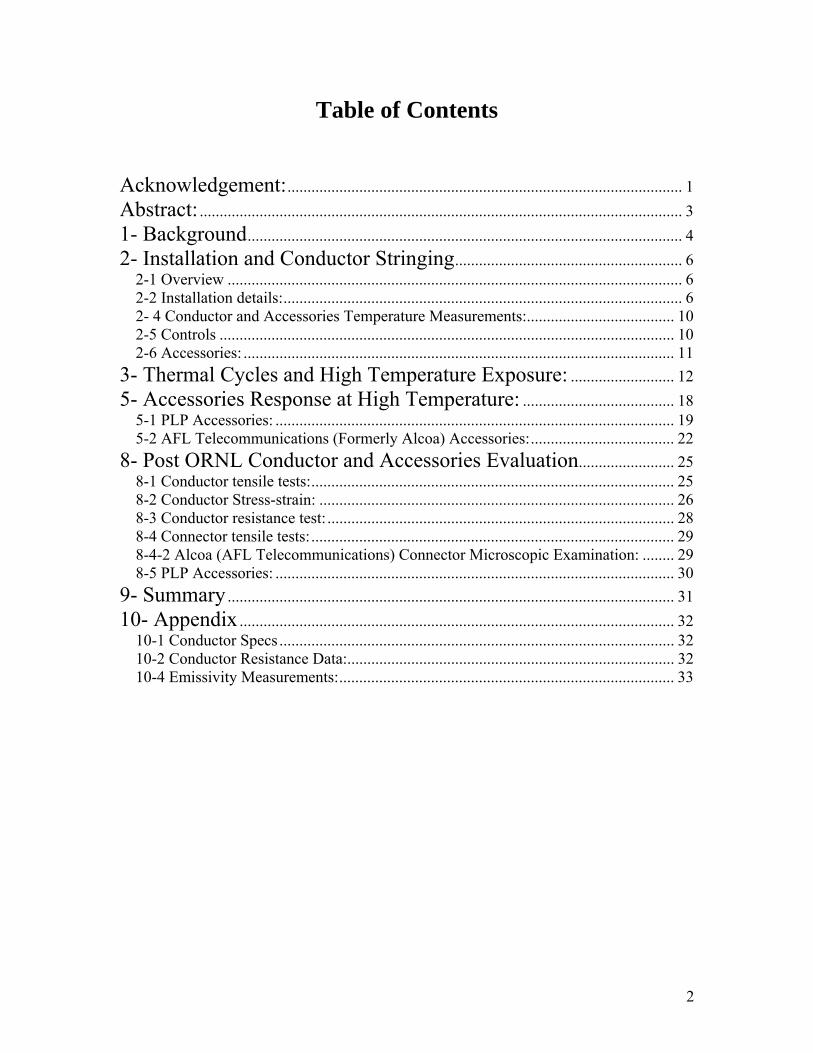
Table of Contents Acknowledgement:................................................................................................... 1 Abstract: ......................................................................................................................... 3 1- Background............................................................................................................. 4 2- Installation and Conductor Stringing......................................................... 6
2-1 Overview .................................................................................................................. 6 2-2 Installation details:.................................................................................................... 6 2- 4 Conductor and Accessories Temperature Measurements:..................................... 10 2-5 Controls .................................................................................................................. 10 2-6 Accessories: ............................................................................................................ 11
3- Thermal Cycles and High Temperature Exposure: .......................... 12 5- Accessories Response at High Temperature: ...................................... 18
5-1 PLP Accessories: .................................................................................................... 19 5-2 AFL Telecommunications (Formerly Alcoa) Accessories:.................................... 22
8- Post ORNL Conductor and Accessories Evaluation........................ 25 8-1 Conductor tensile tests:........................................................................................... 25 8-2 Conductor Stress-strain: ......................................................................................... 26 8-3 Conductor resistance test: ....................................................................................... 28 8-4 Connector tensile tests:........................................................................................... 29 8-4-2 Alcoa (AFL Telecommunications) Connector Microscopic Examination: ........ 29 8-5 PLP Accessories: .................................................................................................... 30
9- Summary................................................................................................................ 31 10- Appendix............................................................................................................. 32
10-1 Conductor Specs ................................................................................................... 32 10-2 Conductor Resistance Data:.................................................................................. 32 10-4 Emissivity Measurements:.................................................................................... 33

3
Abstract:
Under DOE funding Agreement No. DE-FC02-02CH11111, ORNL jointly with The
Tennessee Valley Group, TVA, successfully installed the ACCR 477 conductor on a high
temperature test line at ORNL in July 2002. The test line consists of two 600 foot spans;
two on the road side and two on the tree side between a steel suspension pole and two
guyed, dual steel pole dead-end poles. The test conductor forms a loop connected to a
DC power supply located at one end of the line, therefore a total of 2400 feet of
conductor was tested.
The conductor was installed with commercial hardware developed for ACCR conductors.
The line was fully instrumented with (1) thermocouples in the conductor and accessories,
(2) a CAT-1 system to measure tension and (3) a full weather station.
Oak Ridge National Laboratory subjected the line to severe thermal cycling and
extended high temperature load using 400 V DC and about 1200 amps depending on
weather conditions. The conductor was thermally cycled from May 2003 to October 2003
between ambient and over 2000 C for 200 hours. The conductor experienced over 100
cycles to elevated temperature. During the course of the cycling, conductor tension and
temperature were monitored. The measured conductor tension - temperature response
agreed with predictive models.
Predicted conductor current, using IEEE thermal rating ampacity method, agrees well
with measured values. Conductor’s emissivity of 0.347 was measured using IR method
and used in the IEEE conductor- rating model.
Conductor and accessories were taken down from the line after thermal cycling and
tested. The results showed that mechanical and electrical properties of the conductor and
accessories were unchanged.

4
1- Background
Reliable high temperature performance is one of the key requirements for
implementing new high temperature-low sag conductors. It is imperative to demonstrate
in the field that the conductor and accessories can operate as predicted at high-
temperature, under thermal cycling and without degradation. It is also important to
demonstrate that the sag-temperature-current characteristics can be predicted after
repeated thermal cycles. High-temperature exposure and thermal cycling of the conductor
and accessories can be achieved on a test line that operates at low voltage with a
controlled current. Such a test line is able to simulate lifetime field conditions in three
months by applying dozens of emergency cycles where the conductor temperature
exceeds the normal operating temperature of 210oC, (410oF) and where the line is
exposed to a range of wind speeds, directions, and tension.
ORNL built a fully instrumented low-voltage test line to evaluate the high-
temperature operation of ACCR conductors. The instrumentation includes mechanical
tension, full weather station with anemometer, voltage, current, laser sensor to measure
sag, and temperature thermocouples in multiple locations in the conductor and in all
accessories, Figure 1.
This report summarizes the ACCR 477 conductor installation, testing and analysis
at ORNL as well as post thermal cycling evaluation.

5
Aerial view of the line
Towers
Conductor cross section
Aerial view of the line
Towers
Conductor cross section
Figure 1- View of the ORNL test line and conductor cross-section

6
2- Installation and Conductor Stringing 2-1 Overview A four span test line was constructed on the grounds of the Oak Ridge National
Laboratory in Oak Ridge, Tennessee, as a part of a Department of Energy program. Oak
Ridge National Laboratory subcontracted the line engineering and construction to the
Tennessee Valley Authority, (TVA). The test line (Figure 2) consists of 2, 600 feet (183
meters) spans between a steel suspension pole and two guyed dual steel dead end poles.
The test conductor forms a loop over two spans connected to a DC power supply located
at one end of the line. Thermocouples were installed along the test conductor and on the
dead ends, suspensions and splices to measure the temperature of these components
during and after periods of high temperature operation.
2-2 Installation details: The installation of the 477 ACCR follows the IEEE 524 installation guideline for
overhead transmission conductors. The only conductor stringing method recommended is
the tension method. It is important that bending of the composite conductor during
installation be carefully planned to avoid damaging the composite core. The combination
Figure 2- Line layout and CAT-1 system

7
of bending and tension could damage the conductor if it exceeds the allowable core
strength. Therefore stringing blocks and bull wheels were selected to keep the stringing
loads below the conductor core strength. The crew used 28” diameter stringing blocks
and 36” diameter bull wheels diameter to meet such criteria; Table 2. Lined blocks are
recommended for use with ACCR. Cable spools around which the conductor is wrapped
must have 40” diameter to avoid core damage. Other installation procedure and hardware
used were very similar to that used for ACSR. PLP DG- Grips were used to pull the
conductor to sag and to install full tension splices.
Sagging procedures of ACCR conductor are very similar to that of ACSR. During
installations of this type of conductor, a dynometer was used to verify the final sag
tensions of the conductor. By using a chain hoist and a dynometer between a temporary
conductor grip and the tower structure, the final sag tension was set. Sufficient length of
conductor was provided to install the permanent Alcoa dead end. The conductor grip was
placed on the conductor at least 12 to 15 feet from the connection point to the insulator
string. After the final sag tension was set, the dead ends were installed onto the ACCR.
With the initial placement of the conductor grip at 12 to 15 feet, this allowed enough
slack in the conductor to maneuver it and apply the dead end assembly.
Table 1- Installation Equipment and Procedure
YesYesRunning ground
YesYesGrounding clamps
YesYesReel stands
YesYesCable cutter
Yes (48” drums)YesCable spool
Distribution grips, DGAnyConductor grip
YesYesSock splice
YesYesDrum Puller
Yes ( 54”)YesBull wheels
Yes ( 28”)YesStringing blocks
ACCRACSRInstallation Equipment
YesYesRunning ground
YesYesGrounding clamps
YesYesReel stands
YesYesCable cutter
Yes (48” drums)YesCable spool
Distribution grips, DGAnyConductor grip
YesYesSock splice
YesYesDrum Puller
Yes ( 54”)YesBull wheels
Yes ( 28”)YesStringing blocks
ACCRACSRInstallation Equipment

8
The following images and those under the next section are typical examples of the installation details
Figure 3- Conductor stringing
Figure 4- Sagging with chain hoist and dynometer
AnyAnyClipping
DG grips with chain hoist
AnyDead ending
Line of sight-Dynometer
AnySag tensioning
TensionTension/ slackCable stringing
ACCRACSRInstallation Procedure
AnyAnyClipping
DG grips with chain hoist
AnyDead ending
Line of sight-Dynometer
AnySag tensioning
TensionTension/ slackCable stringing
ACCRACSRInstallation Procedure

9
2-3- CAT-1 Instrumentation: A CAT-1 system with weather station was installed on one of the dead end
structures to monitor the conductor tension and weather conditions (temperature, wind
speed, and direction) at one-minute intervals. Conductor tension was measured by the
CAT-1 load cells, see Figure 5. The CAT-1 system includes an anemometer to measure
wind speed and direction and a net radiation sensor to measure ambient temperature and
solar radiation. Data acquisition was done at 1minute rate for all channels.
The CAT-1 main unit is in a NEMA-enclosed, solar powered, data acquisition and
processing unit. Net Radiation Temperature, (NRT), was measured by the net radiation
sensor, (NRS).
5-a Load cell to monitor tension
5-b CAT1 system
5-c Net radiation sensor, Measures no -load conductor temperature
Figure 5 CAT 1 System hardware
5-a Load cell to monitor tension
5-b CAT1 system
5- -load conductor temperature and solar radiation
Figure 5 CAT 1 System hardware
5-a Load cell to monitor tension
5-b CAT1 system
5-c Net radiation sensor, Measures no -load conductor temperature
Figure 5 CAT 1 System hardware
5-a Load cell to monitor tension
5-b CAT1 system
5- -load conductor temperature and solar radiation
Figure 5 CAT 1 System hardware

10
2- 4 Conductor and Accessories Temperature Measurements: Temperature was measured using thermocouples mounted at various locations along the
span, including ones directly touching the composite core and the conductor surface.
Additional thermocouples were mounted on all accessories.
A separate data acquisition system was used to collect the information from the
thermocouples. To accommodate the multiplicity of points along the conductor and
withstand the accumulated voltage drop, many fiber-connected, isolated measurement
nodes were used. A thermocouple measurement node is fabricated using a multiplexer
(ICPCON I-7018) and a RS-485-to-fiber modem (B&B FOSTCDR). Up to eight
thermocouples are monitored per node. The node requires 120 VAC power and is data
connected through a duplex fiber optic network. The multiplexer, fiber modem, and a
power supply are housed in a Preformed Line Product COYOTER RUN T enclosure.
2-5 Controls The line was operated under constant either current and / or constant conductor
temperature with thermal cycles lasting from less than one hour to several days. The
circuitry needed for controlling the 2MW power supply via software and analog to digital
modules was built and installed. Also, a lower panel was added to permit remote control
Figure 6- Thermocouple enclosure

11
(in the instrumentation trailer) of the power supply's reset, contactor, and DC circuit.
Previously, these were manually controlled at the power supply trailer only.
The power supply has a dual rating of 400 Vdc and 5000 amps or 600 Vdc and 3750
amps. The input voltage to the power supply is 4160 V, 3-phase. A dry-type ABB
transformer is used to step down the voltage from a 13.8 KV distribution line.
2-6 Accessories: Two types of full tension connectors were installed; a compression type made by Alcoa
and a formed wire type made by Preformed Line Products, see Figures 7 to 9. The
following is a list of all the accessories:
• Two ALCOA compression dead ends; part # B9085-A; those dead ends consist of
both direct core gripping parts and conductor gripping sleeve.
• One ALCOA full tension splice part# B9095-A; it has the same design as the dead
end for direct core gripping..
• Two THERMOLIGNR PLP Suspensions, part # TLS-0101-SE
• Two PLP THERMOLIGNR Dead Ends, part# TLDE-0104.
• One PLP THERMOLIGNR Splice, Part #TLSP-0104.
• Six Alcoa all aluminum terminal connectors; Part# B9102-A
• Four Alcoa Stockbridge dampers; part # 1704-7.
Figure 7- THERMOLIGNR Suspension

12
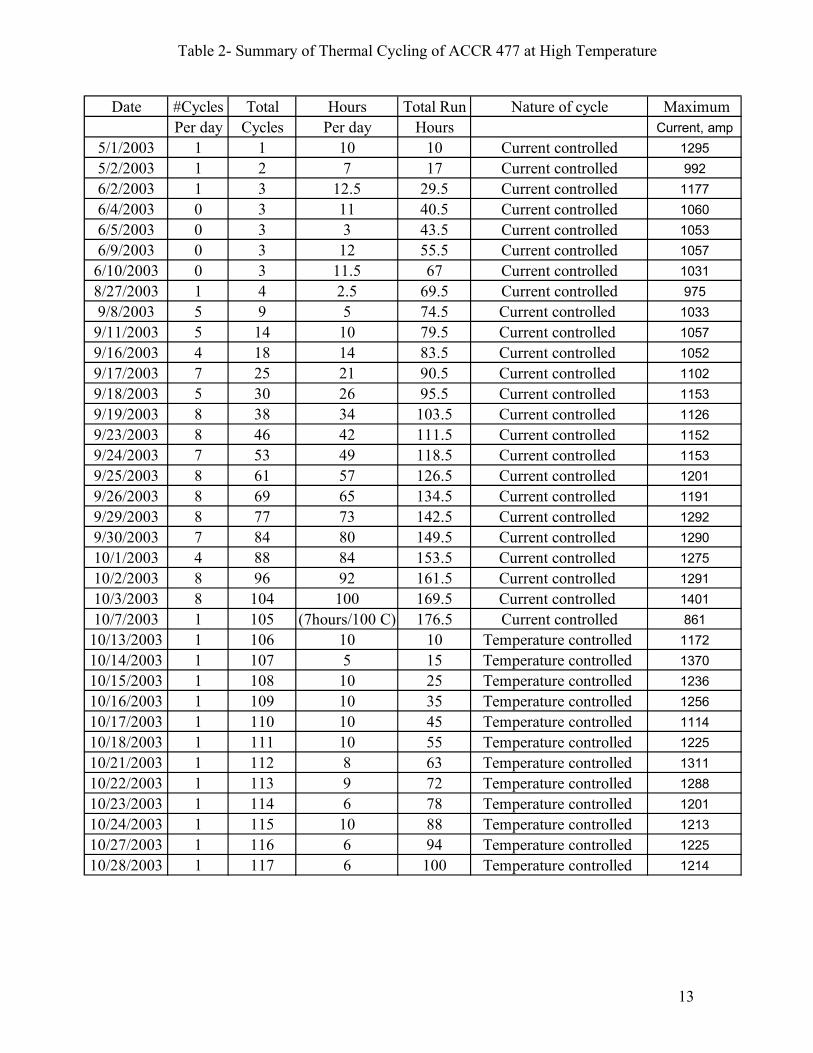
3- Thermal Cycles and High Temperature Exposure: The 477 conductor was thermally cycled from May 2003 to October 2003 between
ambient and over 2000 C for more than 200 hours under a wide range of weather and load
conditions, Table 2. Figure 10 shows the composite conductor core temperature during a
typical thermal cycle in temperature control. The temperature is maintained at 210-240 C
by controlling the current from 1000 amps to 1200 amps while the wind fluctuates
between 0 fpm and 15 fpm.
Figure 8- Installation of Alcoa compression splice.
Figure 10- shows an example of thermal cycling in one day at ORNL test line
Figure 9- Installed PLP THERMOLIGNR Splice
An Example of Current Cycling of ACCR 477 at ORNL Testing Site
0
50
100
150
200
9/18/0
3 5:45
AM
9/18/0
3 6:57
AM
9/18/0
3 8:09
AM
9/18/0
3 9:21
AM
9/18/0
3 10:33
AM
9/18/0
3 11:45
AM
9/18/0
3 12:57
PM
9/18/0
3 2:09
PM
Days in September, 2003
Con
duct
or T
empe
ratu
re,
C
0
400
800
1200
DC
Cur
rent
, am
p
Conductor Surface T
Idc, Power Supply DC Current(A)
13
Table 2- Summary of Thermal Cycling of ACCR 477 at High Temperature
Date #Cycles Total Hours Total Run Nature of cycle MaximumPer day Cycles Per day Hours Current, amp
5/1/2003 1 1 10 10 Current controlled 12955/2/2003 1 2 7 17 Current controlled 9926/2/2003 1 3 12.5 29.5 Current controlled 11776/4/2003 0 3 11 40.5 Current controlled 10606/5/2003 0 3 3 43.5 Current controlled 10536/9/2003 0 3 12 55.5 Current controlled 1057
6/10/2003 0 3 11.5 67 Current controlled 10318/27/2003 1 4 2.5 69.5 Current controlled 9759/8/2003 5 9 5 74.5 Current controlled 1033
9/11/2003 5 14 10 79.5 Current controlled 10579/16/2003 4 18 14 83.5 Current controlled 10529/17/2003 7 25 21 90.5 Current controlled 11029/18/2003 5 30 26 95.5 Current controlled 11539/19/2003 8 38 34 103.5 Current controlled 11269/23/2003 8 46 42 111.5 Current controlled 11529/24/2003 7 53 49 118.5 Current controlled 11539/25/2003 8 61 57 126.5 Current controlled 12019/26/2003 8 69 65 134.5 Current controlled 11919/29/2003 8 77 73 142.5 Current controlled 12929/30/2003 7 84 80 149.5 Current controlled 129010/1/2003 4 88 84 153.5 Current controlled 127510/2/2003 8 96 92 161.5 Current controlled 129110/3/2003 8 104 100 169.5 Current controlled 140110/7/2003 1 105 (7hours/100 C) 176.5 Current controlled 861
10/13/2003 1 106 10 10 Temperature controlled 117210/14/2003 1 107 5 15 Temperature controlled 137010/15/2003 1 108 10 25 Temperature controlled 123610/16/2003 1 109 10 35 Temperature controlled 125610/17/2003 1 110 10 45 Temperature controlled 111410/18/2003 1 111 10 55 Temperature controlled 122510/21/2003 1 112 8 63 Temperature controlled 131110/22/2003 1 113 9 72 Temperature controlled 128810/23/2003 1 114 6 78 Temperature controlled 120110/24/2003 1 115 10 88 Temperature controlled 121310/27/2003 1 116 6 94 Temperature controlled 122510/28/2003 1 117 6 100 Temperature controlled 1214

14
Thermocouples were installed along the length of the conductor in two different spans
and at different radial positions going from the conductor surface to contacting the
composite core, Figure 11. The thermocouples indicated that there were significant
temperature differences along the axial location and moderate gradients along the radial
position.
The radial gradient, when the conductor was above 200oC, was measured to fluctuate
between 2oC and 15oC. In average, the radial gradient was about 8oC when the conductor
was at 200oC, Figure 12a. Variation in wind speed and direction affected the magnitude
of the radial gradient with greater wind speeds causing a larger gradient.
Figure 11- Thermocouples were positioned along the length and in different radial positions.
Figure 12-a- Conductor core temperature is about 80 C higher than its surface temperature.
STR1 STR2 STR3STR1 STR2 STR3
150
160
170
180
190
200
210
220
230
1 29 57 85 113
141
169
197
225
253
281
309
337
365
393
421
449
477
TIME, HOURS
TEM
PER
ATU
RE,
(C)
SURFACECORE
SURFACE
CORE
MID SPAN 1 MID SPAN 2
Figure 12- a- Temperature difference between conductor surface and core at mid span

15
Temperature fluctuation along the length of the conductor varied between 5oC to 50oC
depending on wind conditions. Span 2 was more sheltered by trees than span1 and
consistently experienced higher temperatures. The difference between span 1 and 2 was
in average about 20oC when the conductor was above 200oC, Figure 12b. In some cycles
the difference between span 2 and 1 was as high as 50oC for a short period of time. As a
result the maximum temperature in span 2 reached as high as 270oC when the average
temperature was at about 230oC.
100
120
140
160
180
200
220
240
TIME (HOURS)
TEM
PER
ATU
RE
(C)
MID SPAN 2MID SPAN 1
4- Measured and Predicted Line Tension and Sag: Sag was computed using the Strain Summation Method (which accounts for the full
loading history) and the Graphic Method (Alcoa SAG-10). The main events, which cause
permanent- elongation, were included (creep, low temperatures).
The calculated and measured tension and sag values are plotted in Figures 13 to 16 as a
function of both conductor core and surface temperatures. The knee-point measured at
Figure 12- b An example of temperature difference along the conductor length.

16
about 80o C matches the prediction. It confirms the validity of the stress-strain, creep
properties and thermo-elastic behavior of the conductor.
Figure 13 shows good agreement between measured and predicted tension in the range of
00 C and 2500 C. The measured line tension lies in between values predicted using either
the strain summation method or the graphic one. The predictions assumed a compressive
stress of –1.45 Ksi in the aluminum after the knee point. The “October 28th” cycle was
the last of over 100 cycles after the conductor experienced over 200 hours of high
temperature exposure. It shows that the tension response remained predictable and stable
after long thermal exposure and numerous cycles.
There is a small hysteresis observed between the heating and cooling cycles mostly due
to variation in conductor temperature along the length of the line, and wire settling when
passing through the knee point.
Figure 13- Good agreement between calculated and measured tension for the last cycle on October 28,2003. The Strain Summation method was used with a 1.45 ksi compressive stress.
Tree side Tension 2 - October 28/03
1000
1500
2000
2500
3000
3500
4000
0 50 100 150 200 250Mid-span Core Temp, C
Tens
ion2
, lb
Calculated
Measured
Tree side Tension 2 - October 28/03
1000
1500
2000
2500
3000
3500
4000
0 50 100 150
Tree side Tension 2 - October 28/03
1000
1500
2000
2500
3000
3500
4000
0 50 100 150 200 250Mid-span Core Temp, C
Tens
ion2
, lb
Calculated
Measured
17
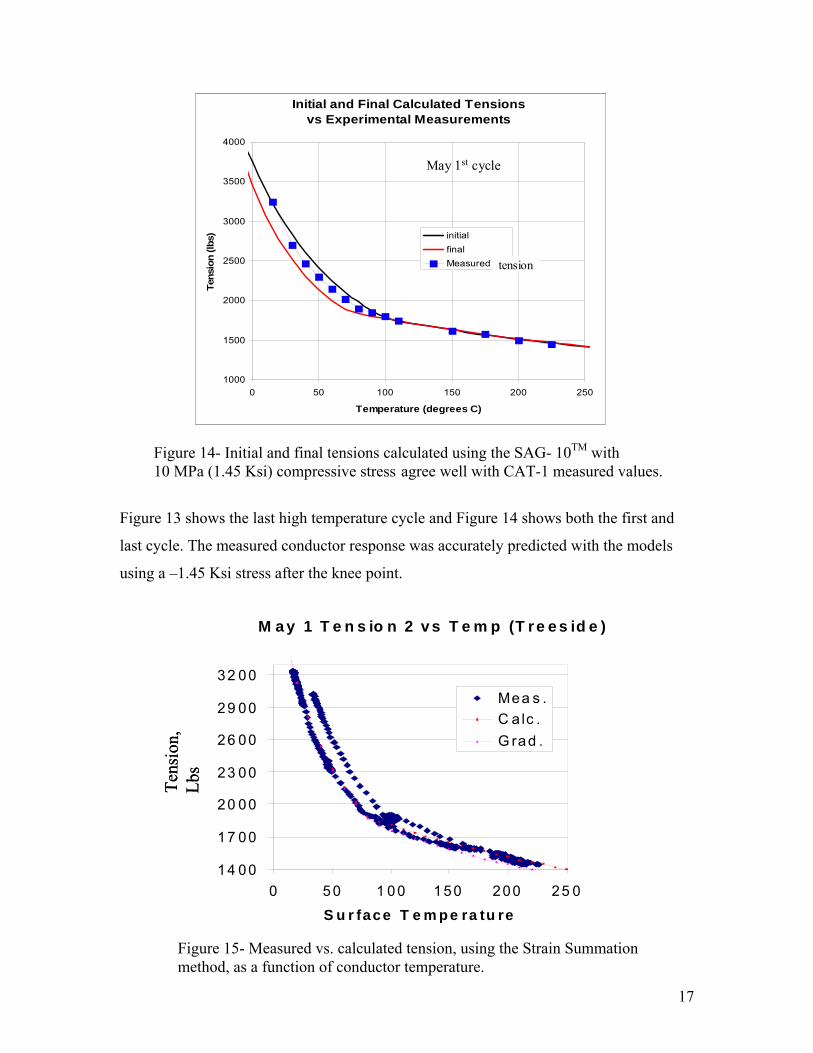
Figure 13 shows the last high temperature cycle and Figure 14 shows both the first and
last cycle. The measured conductor response was accurately predicted with the models
using a –1.45 Ksi stress after the knee point.
Figure 14- Initial and final tensions calculated using the SAG- 10TM with 10 MPa (1.45 Ksi) compressive stress agree well with CAT-1 measured values.
Figure 15- Measured vs. calculated tension, using the Strain Summation method, as a function of conductor temperature.
Initial and Final Calculated Tensionsvs Experimental Measurements
1000
1500
2000
2500
3000
3500
4000
0 50 100 150 200 250
Temperature (degrees C)
Tens
ion
(lbs) initial
finalMeasured Sagtension
May 1st cycle
Initial and Final Calculated Tensionsvs Experimental Measurements
1000
1500
2000
2500
3000
3500
4000
0 50 100 150 200 250
Temperature (degrees C)
Tens
ion
(lbs) initial
finalMeasured Sagtension
May 1st cycle
M a y 1 T e n s io n 2 v s T e m p (T re e s id e )
14 00
17 00
20 00
23 00
26 00
29 00
32 00
0 50 1 00 150 200 25 0S u r face T e m p e ra tu re
Mea s .C a lc .G rad .
Tens
ion,
Lb
s
M a y 1 T e n s io n 2 v s T e m p (T re e s id e )
14 00
17 00
20 00
23 00
26 00
29 00
32 00
0 50 1 00 150 200 25 0S u r face T e m p e ra tu re
Mea s .C a lc .G rad .
Tens
ion,
Lb
s

18
Figure 16 shows the tree-side line sag vs. conductor core temperature. The sag was
directly measured at the mid- span with a laser monitor. The sag measurements agree
with those calculated from tension within 0.2 feet.
Summary:
Predicted sag agrees well with measured values in the range of 00 C to 2500 C. The sag
remained predictable after thermal cycling and long exposure to high temperature. There
has been virtually no creep.
5- Accessories Response at High Temperature: The accessories performed well during conductor thermal cycling and high temperature
exposure; overall their maximum temperature was less than 1200 C.
Figure 16- Measured Sags Compared with Those Calculated from Tension.
6.00
7.00
8.00
9.00
10.00
11.00
12.00
13.00
14.00
15.00
16.00
17.00
18.00
0 50 100 150 200 250
g
Tree side sag, October 28, 03
Mid span conductor core temperature
Tension- Sag
Calculated
Laser
6.00
7.00
8.00
9.00
10.00
11.00
12.00
13.00
14.00
15.00
16.00
17.00
18.00
0 50 100 150 200 250
g
Tree side sag, October 28, 03
Mid span conductor core temperature
Tension- Sag
Calculated
Laser
Sag,
fe
et
6.00
7.00
8.00
9.00
10.00
11.00
12.00
13.00
14.00
15.00
16.00
17.00
18.00
0 50 100 150 200 250
g
Tree side sag, October 28, 03
Mid span conductor core temperature
Tension- Sag
Calculated
Laser
6.00
7.00
8.00
9.00
10.00
11.00
12.00
13.00
14.00
15.00
16.00
17.00
18.00
0 50 100 150 200 250
g
Tree side sag, October 28, 03
Mid span conductor core temperature
Tension- Sag
Calculated
Laser
Sag,
fe
et
19
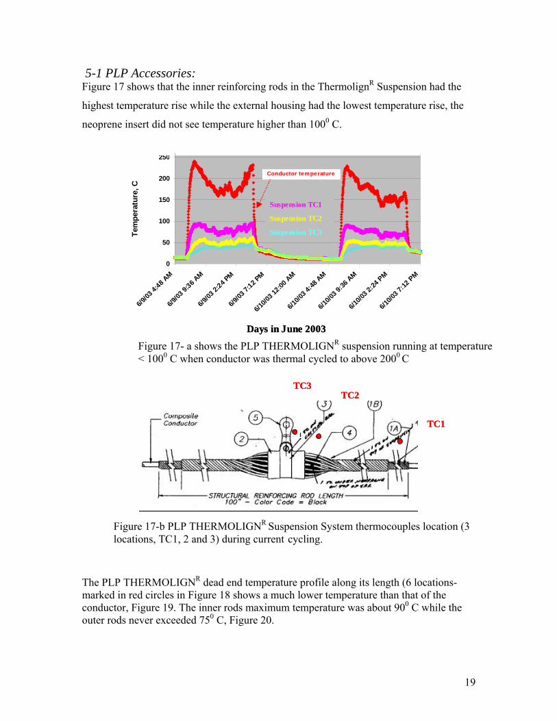
5-1 PLP Accessories: Figure 17 shows that the inner reinforcing rods in the ThermolignR Suspension had the
highest temperature rise while the external housing had the lowest temperature rise, the
neoprene insert did not see temperature higher than 1000 C.
The PLP THERMOLIGNR dead end temperature profile along its length (6 locations- marked in red circles in Figure 18 shows a much lower temperature than that of the conductor, Figure 19. The inner rods maximum temperature was about 900 C while the outer rods never exceeded 750 C, Figure 20.
Figure 17-b PLP THERMOLIGNR Suspension System thermocouples location (3 locations, TC1, 2 and 3) during current cycling.
TC3TC2
TC1
TC3TC2
TC1
0
50
100
150
200
250
6/9/03
4:48 A
M
6/9/03
9:36 A
M
6/9/03
2:24 P
M
6/9/03
7:12 P
M
6/10/0
3 12:00
AM
6/10/0
3 4:48
AM
6/10/0
3 9:36
AM
6/10/0
3 2:24
PM
6/10/0
3 7:12
PM
Tem
pera
ture
, C
Conductor temperature
Days in June 2003
Suspension TC1
Suspension TC2
Suspension TC3
0
50
100
150
200
250
6/9/03
4:48 A
M
6/9/03
9:36 A
M
6/9/03
2:24 P
M
6/9/03
7:12 P
M
6/10/0
3 12:00
AM
6/10/0
3 4:48
AM
6/10/0
3 9:36
AM
6/10/0
3 2:24
PM
6/10/0
3 7:12
PM
Tem
pera
ture
, C
Conductor temperature
Days in June 2003
Suspension TC1
Suspension TC2
Suspension TC3
Figure 17- a shows the PLP THERMOLIGNR suspension running at temperature < 1000 C when conductor was thermal cycled to above 2000 C

20
The PLP THERMOLIGNR Splice temperature was monitored at 4 locations on both
the inner stiffening rod and the outer one (Figure 19). The inner rod temperatures (PS1,
2) were slightly higher than those measured on the outer one- rod (PS3) and the inner
center of the splice (PS4) where conductor segments come together (because of its
proximity to the conductor); both splice rods ran cool (Figure 19).
Figure 18-a- Location of thermocouples in red, TC’s, on PLP THERMOLIGNR dead end
Figure 18-b An example of PLP THERMOLIGNR Dead End temperature profile thermal cycling of conductor to 2000 C.
TC2 and TC6 are on inner rods
TC 6
TC 2 TC 5TC 4TC 3TC 1
TC2 and TC6 are on inner rods
TC 6
TC 2 TC 5TC 4TC 3TC 1
0
50
100
150
200
250
10/17/03 4
:48
10/17/03 7
:12
10/17/03 9
:36
10/17/03 1
2:00
10/17/03 1
4:24
10/17/03 1
6:48
10/17/03 1
9:12
10/17/03 2
1:36
Time of the day
Tem
pera
ture
, C
Conductor SurfTTC 1
TC 2
TC 3
TC 4
TC 5
TC 6
PLP ThermolignR Dead End ran very cool during high temperature exposure of conductor

21
PLP THERMOLIGNR splice shows temperature gradient between inner and outer
rods as shown in figure 19-b; two thermocouples were mounted on each rod.. Both
rods ran much cooler than conductor, well below 1000 C.
To summarize all PLP accessories (dead end, splice and suspension) behaved
normally during high temperature exposure of the ACCR 477 conductor, their
maximum surface temperature was at or below 1000 C.
PS3/ PS4
PS1PS2
PS3/ PS4
PS1PS2
Figure 19- a- Thermocouple locations for temperature measurement of splice inner and outer rods.
Figure 19-b An example of a single thermal cycle showing the PLP THERMOLIGNR splice running very cool, temperature < 1000 C when conductor was around 2000 C.
0
50
100
150
200
250
10/15/03 4
:48 AM
10/15/03 7
:12 AM
10/15/03 9
:36 AM
10/15/03 1
2:00 PM
10/15/03 2
:24 PM
10/15/03 4
:48 PM
10/15/03 7
:12 PM
10/15/03 9
:36 PM
10/16/03 1
2:00 AM
Time of the day
Tem
pera
ture
, C
Conductor T
PS1, PLP Splice
PS2, PLP Splice
PS3, PLP Splice
PS4, PLP Splice
PLP THERMOLIGNR splice temperature profile during one cycle exposure of conductor
22
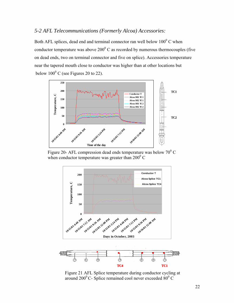
5-2 AFL Telecommunications (Formerly Alcoa) Accessories: Both AFL splices, dead end and terminal connector ran well below 1000 C when
conductor temperature was above 2000 C as recorded by numerous thermocouples (five
on dead ends, two on terminal connector and five on splice). Accessories temperature
near the tapered mouth close to conductor was higher than at other locations but
below 1000 C (see Figures 20 to 22).
Figure 20- AFL compression dead ends temperature was below 700 C when conductor temperature was greater than 2000 C
TC1
TC2
0
50
100
150
200
250
10/15
/03 4:
48 A
M
10/15
/03 9:
36 A
M
10/15
/03 2:
24 PM
10/15
/03 7:
12 PM
10/16
/03 12
:00 AM
Time of the day
Tem
pera
ture
, C
Conductor TAlcoa DE1 TC1Alcoa DE2 TC1Alcoa DE1 TC2Alcoa DE2 TC2
TC4 TC1
0
50
100
150
200
10/15/03 4
:48 AM
10/15/03 7
:12 AM
10/15/03 9
:36 AM
10/15/03 1
2:00 PM
10/15/03 2
:24 PM
10/15/03 4
:48 PM
10/15/03 7
:12 PM
10/15/03 9
:36 PM
10/16/03 1
2:00 AM
Days in October, 2003
Tem
pera
ture
, C
Conductor T
Alcoa Splice TC1
Alcoa Splice TC4
TC4 TC1
0
50
100
150
200
10/15/03 4
:48 AM
10/15/03 7
:12 AM
10/15/03 9
:36 AM
10/15/03 1
2:00 PM
10/15/03 2
:24 PM
10/15/03 4
:48 PM
10/15/03 7
:12 PM
10/15/03 9
:36 PM
10/16/03 1
2:00 AM
Days in October, 2003
Tem
pera
ture
, C
Conductor T
Alcoa Splice TC1
Alcoa Splice TC4
Figure 21 AFL Splice temperature during conductor cycling at around 2000 C- Splice remained cool never exceeded 800 C

23
7- Ampacity and Thermal Rating of Conductor
The steady state version of the IEEE STD 738-1993 “Standard for Calculating the
Current Temperature Relationship of Bare Overhead Conductors” was used to predict
conductor current during thermal cycling. The model balances resistive losses, solar
heating, convective and radiative heat losses. The data for current, wind speed and
direction was used in the model; wind speed and direction were averaged over 60 minutes
interval. Conductor emissivity ε = 0.347 was measured by ORNL using IR method. Both
Figure 23 and table 3 show measured and predicted current. Table 4 lists values of
parameters used in the model
Figure 22- AFL compression terminal connector temperature less than 50 C when conductor temperature was greater than 200 0C
Conductor Ambient Wind Wind Measured Computed temperature, C Temperature, C speed, f/s angle, degrees Current. Amp current, amp
196 14 5 3 1004 1011145 16 7 9 981 1011119 18 8 9 994 978162 20 9 9 1098 1120223 25 4 19 1135 1160162 26 4 20 986 1015203 17 4 13 1050 1065164 20 6 15 1050 1078169 27 5 22 1047 1076233 15 0 27 1049 1063174 26 4 24 1050 1075222 19 0 23 1025 1029186 25 3 18 1025 1008235 19 0 9 1024 1057157 30 8 10 999 1032
Table 3 - Ampacity Rating Conditions and Data
TC1TC2
0
50
100
150
200
250
10/15/03 6
:00 AM
10/15/03 8
:24 AM
10/15/03 10
:48 AM
10/15/03 1
:12 PM
10/15/03 3
:36 PM
10/15/03 6
:00 PM
10/15/03 8
:24 PM
10/15/03 1
0:48 PM
Time of the day
Tem
pera
ture
, C
Conductor T
Terminal connectorTC1( Pad)Terminal ConnectorTC2( Barrell)
TC1TC2
TC1TC2
0
50
100
150
200
250
10/15/03 6
:00 AM
10/15/03 8
:24 AM
10/15/03 10
:48 AM
10/15/03 1
:12 PM
10/15/03 3
:36 PM
10/15/03 6
:00 PM
10/15/03 8
:24 PM
10/15/03 1
0:48 PM
Time of the day
Tem
pera
ture
, C
Conductor T
Terminal connectorTC1( Pad)Terminal ConnectorTC2( Barrell)

24
Conductor temperature was used as input to the model along with other variables of
Table 4. The agreement between model and measurements is good.
In summary the IEEE model predicted conductor current agrees reasonably well with
that measured during thermal cycling at ORNL test line. The ACCR 477 conductor
was rated at 1169 amps for continuous operation at 2100 C and 1266 amps for
emergency at 2400 C using the model and 400 C ambient temperature, 2 f/s wind
speed, emissivity & solar absorption of 0.5 at Sea Level. Thermal cycling history
Figure 23- Predicted vs. Measured Steady State conductor current / rating
Computed Ampacity Agrees Well with Measured Values for ACCR 477 kcmil Conductor- ORNL Line
y = 0.8298x + 161.49
R 2 = 0.8825
900.0
1000.0
1100.0
1200.0
900.0 1000.0 1100.0 1200.0
Computed Ampacity
Mea
sure
dAm
paci
ty
IdcLinear (Idc)
Emissivity 0.35Solar Absorbtion 0.50Conductor Elevation ft above sea level 800.00latitude degrees 30.00Zc 180.00Sun Altitude degrees 54.00Theta radians 1.57density air lb/ft^3 0.0765Absolute Viscosity Air lb/h-ft 0.0433Thermal Conductivity Air W/ft.degreeC 0.01

25
reported in Table 2 shows that the conductor was exposed to a maximum current in
excess of 1350 amps without any degradation or damage, see Section 8 for details.
8- Post ORNL Conductor and Accessories Evaluation
The following tests & measurements were carried out on the conductor and accessories
after thermal cycling at ORNL:
8-1 Conductor tensile tests: Three samples from the “free-span” conductor were terminated using cast-resin
terminations. Clamps were used to preserve the as-received position of the conductor
layers until the resin cured. The sample preparation method ensures that the laboratory
tensile test loads each conductor strand in the same manner as a field overloads, and
thereby measures the in-service conductor strength. Free conductor between the end
fittings is 20 feet (6 meters).
The 1999 Aluminum Association guide for conductor stress-strain testing was followed
with the exception of special values for the elastic properties of the metal matrix
composite (MMC) core were used instead of values for steel core used in ACSR
conductors. The core strand from another sample is used to measure core stress-strain,
and determine the elastic properties of the composite conductor.
The results show that the conductor maintained its strength after thermal cycling at above
200C. The average of five measurements is 109 % RBS as shown in Table 3.
Table 5- Conductor test data
Sample Breaking
load,
Lbs
% RBS Failure Mode
04114T1 20,710 106 All strands fractured in the gage section
04114T2 19,860 102 All strands fractured in the resin fitting
04114T3 20,800 107 All strands fractured at the resin fitting

26
Stress- Strain-
conductor
20,350 104 Mid span break, all strands failed
Stress Strain-
Core
12,910 111 Mid span break, all strands failed
8-2 Conductor Stress-strain: Stress-strain results are similar to results from the same conductor prior to the field test.
The principal difference is that creep during the 30% load hold phase is less on the field
sample, apparently because the field loads caused the initial creep to be removed from the
conductor as shown in Figures 24 to 26.
Figure 24- Plot of raw core stress-strain data recorded during conductor stress-strain test (blue),
477 kcmil, Type 16 ACCR, 3M Composite ConductorStress-Strain
0
5000
10000
15000
20000
25000
30000
35000
0.00 0.05 0.10 0.15 0.20 0.25 0.30 0.35 0.40 0.45
Strain (%)
Str
ess
(psi
)
02-097 "As-manufactured"
04-114 Post ORNL

27
Figure 26- Combined stress- strain plot
477 kcmil, Type 16 ACCR, 3M Composite Conductor, MMC Core Stress-Strain
0
25000
50000
75000
100000
125000
150000
0.00 0.05 0.10 0.15 0.20 0.25 0.30 0.35 0.40 0.45Strain (%)
Stre
ss (p
si)
04-114 Post ORNL02-097 "As-Manufactured"
477 kcmil Type 16 ACCR, 3M Composite Conductor, Combined Stress-Strain DiagramPost ORNL Test Line
0
5000
10000
15000
20000
25000
30000
35000
0.000 0.050 0.100 0.150 0.200 0.250 0.300 0.350 0.400
Strain (%)
Stre
ss*a
rea
ratio
Initial Composite Final Composite Initial Core
Final Core Init ial Aluminum Final Aluminum
Figure 25- Core stress-strain shows essentially no change due to field test

28
8-3 Conductor resistance test:
Welded equalizers were installed at each end of a 19-foot long sample from the free-
span section. A second set of voltage equalizers in the form of tightly wrapped solid
copper strands are applied nominally 20 feet apart in the test section. The sample is
placed on a flat surface, and pulled with sufficient tension to remove any residual
curvature in the conductor. Tension was about 200 – 300 lb. A digital low-resistance
Ohmmeter was used to make a 4-wire resistance measurement for the conductor
section between the two voltage equalizers. A digital multi meter was used to verify
the sample was electrically isolated (see Figure 27).
Resistance of a 19 ft test section was measured. Readings were repeated later in the day
as noted below. The average of all readings is 0.1834 Ω/mile at 20° C. The published
value is 0.1832 Ω/mile at 20° C, very close to the measured value.
Figure 27- Resistance measuring set up and sample

29
8-4 Connector tensile tests: 8-4-1 Alcoa compression accessories
Two dead-ends were provided with cast resin fittings at free ends. The procedure
preserves the “as received” position of the conductor components, and thereby
assures that the breaking strength is the same as existed when the samples were in
service on the test span. Dead ends maintained their load carrying capability of 100%
RBS or more (see Table 6 and Figure 28).
Table 6- Connector tensile tests Sample Breaking Load,
Lbs
% RBS Failure Mode
04114DE1 20,380 105 All strands fractured ~ 5”
inside dead end
04114DE2 19,550 100 All strands fractured ~ 5”
inside dead end
8-4-2 Alcoa (AFL Telecommunications) Connector Microscopic Examination:
Figure 28 Connector tensile test plots
477 ACCR Post ORNL Tensile Results
0
5000
10000
15000
20000
25000
0.0 0.2 0.4 0.6 0.8 1.0 1.2 1.4 1.6 1.8 2.0Crosshead Position (inches)
Load
(lb)
Dead end 1
Dead end 2
95% RBS Acceptance Criterion
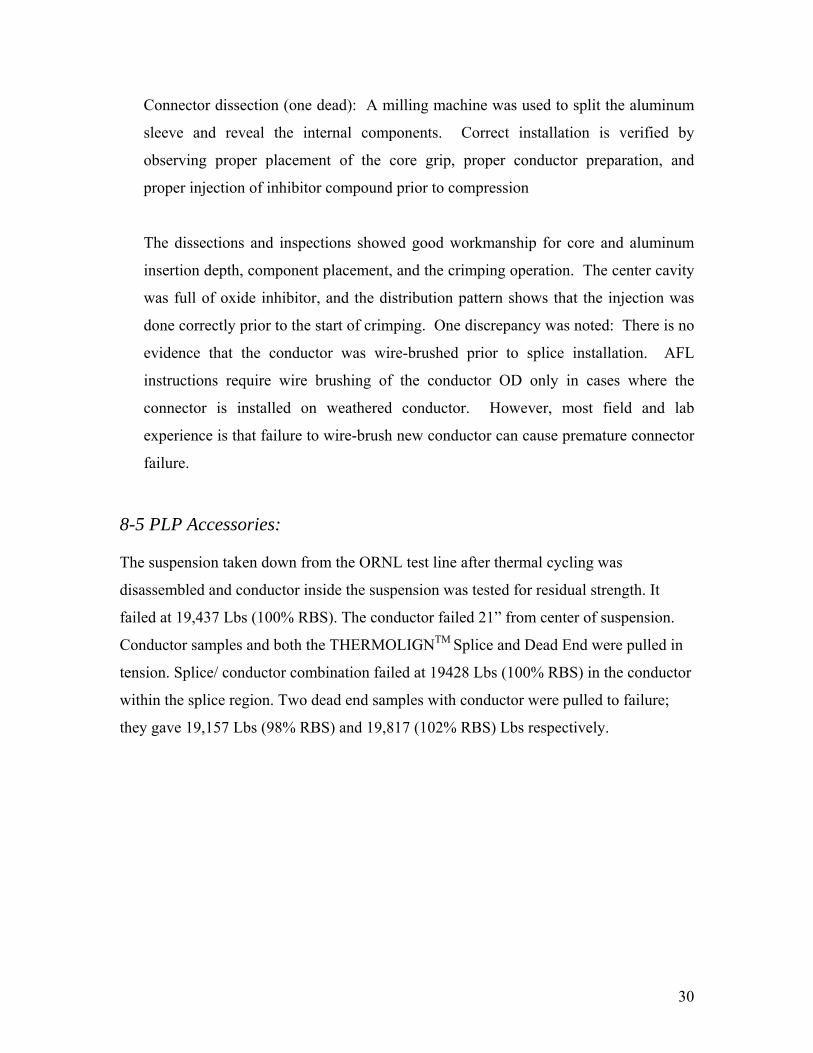
30
Connector dissection (one dead): A milling machine was used to split the aluminum
sleeve and reveal the internal components. Correct installation is verified by
observing proper placement of the core grip, proper conductor preparation, and
proper injection of inhibitor compound prior to compression
The dissections and inspections showed good workmanship for core and aluminum
insertion depth, component placement, and the crimping operation. The center cavity
was full of oxide inhibitor, and the distribution pattern shows that the injection was
done correctly prior to the start of crimping. One discrepancy was noted: There is no
evidence that the conductor was wire-brushed prior to splice installation. AFL
instructions require wire brushing of the conductor OD only in cases where the
connector is installed on weathered conductor. However, most field and lab
experience is that failure to wire-brush new conductor can cause premature connector
failure.
8-5 PLP Accessories: The suspension taken down from the ORNL test line after thermal cycling was
disassembled and conductor inside the suspension was tested for residual strength. It
failed at 19,437 Lbs (100% RBS). The conductor failed 21” from center of suspension.
Conductor samples and both the THERMOLIGNTM Splice and Dead End were pulled in
tension. Splice/ conductor combination failed at 19428 Lbs (100% RBS) in the conductor
within the splice region. Two dead end samples with conductor were pulled to failure;
they gave 19,157 Lbs (98% RBS) and 19,817 (102% RBS) Lbs respectively.

31
9- Summary
ACCR 477 conductor was installed successfully on the ORNL- PCAT line using
commercial hardware and normal installation procedures. The conductor and accessories
were thermally cycled from ambient to over 2000C for several hundred hours, using DC
power supply and as high current as 1200 amps. The measured sag matched the SAG-10
prediction. Data analysis shows that the measured conductor current agrees well with the
IEEE thermal rating model predicted values. After de-installation the conductor and
accessories were tested for residual strength and degradation. Residual strength exceeded
100% RBS and neither conductor nor accessories showed any signs of damage.
Conductor resistance after cycling is equivalent to that of conductor not exposed to
thermal cycling

32
10- Appendix 10-1 Conductor Specs
10-2 Conductor Resistance Data:
Conductor Physical PropertiesDesignation 477-T16Stranding 26/7kcmils kcmil 477
Diameter indiv Core in 0.105 indiv Al in 0.135 Core in 0.32 Total Diameter in 0.86
Area Al in^2 0.374 Total Area in^2 0.435
Weight lbs/linear ft 0.539
Breaking Strength Core lbs 11,632 Aluminum lbs 7,844 Complete Cable 000's lbs 19,476
Modulus Core msi 31.4 Aluminum msi 8.0 Complete Cable msi 11.2
Thermal Elongation Core 6 Aluminum 23 Complete Cable 16
Heat Capacity Core W-sec/ft-C 13 Aluminum W-sec/ft-C 194
Conductor Electrical PropertiesResistance DC @ 20C ohms/mile 0.1832 AC @ 25C ohms/mile 0.1875 AC @ 50C ohms/mile 0.2061 AC @ 75C ohms/mile 0.2247

33
10-4 Emissivity Measurements: Oak Ridge National Laboratory measured various 3M composite conductor emissivity
using IR Imaging. A calibrated IR Camera and Mikron M305 Blackbody calibration
source were used. Figures 29 shows the used hardware; the calibrated black body target
was multiplied by various emissivity values until a good fit occurs with the conductor
received signal (see Figure 30). Such fit yielded an average emissivity value of 0.345
within +- 2% (see Figure 31).
04-114 = Data Input CellsCQ1097 = Calculated ValueCN30220.0036
Conductor Temperature: 21.8 deg CTest Section: 19.000 ftResistance Reading 1 665.1 uOhms At 21.8 deg CResistance Reading 2 665.1 uOhms At 21.8 deg CResistance Reading 3 664.9 uOhms At 21.8 deg CAverage of 3 Readings 665.03 uOhms At 21.8 deg C
Ohms/ft: 3.5002E-05 Ohm/ft At 21.8 deg COhms/ft: 3.4775E-05 At 20.0 deg COhms/mi 0.184809 Ohm/mi At 21.8 deg COhms/mi @ 20C: 0.183612 Ohm/mi At 20.0 deg C
Conductor Temperature: 21.3 deg CTest Section: 19.000 ftResistance Reading 1 663.5 uOhms At 21.30 deg CResistance Reading 2 663.5 uOhms At 21.30 deg CResistance Reading 3 663.5 uOhms At 21.30 deg CAverage of 3 Readings 663.50 uOhms At 21.30 deg C
Ohms/ft: 3.4921E-05 Ohm/ft At 21.30 deg COhms/ft: 3.4695E-05 At 20.00 deg COhms/mi 0.184383 Ohm/mi At 21.30 deg COhms/mi @ 20C: 0.183188 At 20.00 deg C
Average
Ohms/mi @ 20C: 0.18340 At 20.0 deg C
3M nominal 0.18317 Ohm/mi At 20.0 deg C
Resistance measurement on a 477 ACCR sample from the ORNL test line. Bolted end fitting for equalizer (see photos), pulled to ~200 lbs tension w/a come-a-long
Temperature coefficient for resistance:
10/25/04 @ 10:19 AMThese readings taken manually @
These readings taken manually @ 10/25/04 @ 1:24 pm
Conductor ResistanceNEETRAC Project No.AVO (Biddle) DLRO, Calibration Control # Temperature Indicator (Instrument)
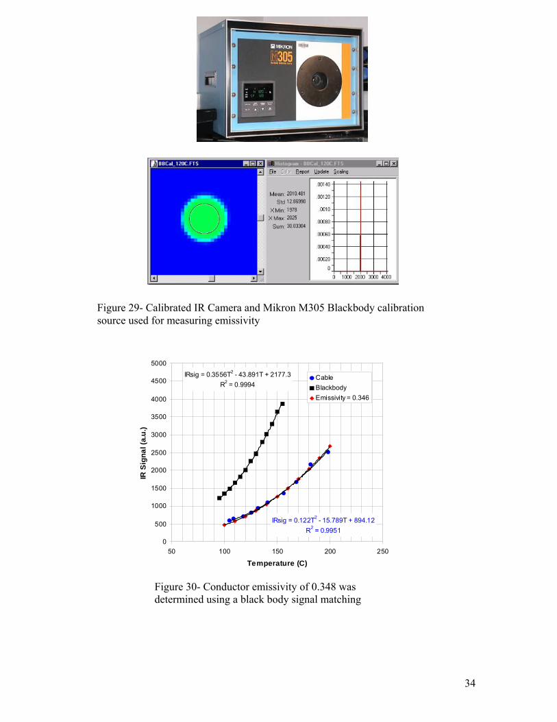
34
Figure 29- Calibrated IR Camera and Mikron M305 Blackbody calibration source used for measuring emissivity
IRsig = 0.3556T2 - 43.891T + 2177.3R2 = 0.9994
IRsig = 0.122T2 - 15.789T + 894.12R2 = 0.9951
0
500
1000
1500
2000
2500
3000
3500
4000
4500
5000
50 100 150 200 250
Temperature (C)
IR S
igna
l (a.
u.)
CableBlackbodyEmissivity = 0.346
Figure 30- Conductor emissivity of 0.348 was determined using a black body signal matching

35
Error in Predicting the IR Signal
-2
0
2
4
6
8
10
12
14
16
100 120 140 160 180 200T emperature, C
Pred
icte
d IR
Sig
nal E
rror
Emissivity = 0.351Emissivity - 0.346
Figure 31- Signal error is < 1% in the temperature range 120 to 200 C with an emissivity value of 0.346

This page is intentionally left blank.

Appendix A.2
ACCR 795 Kcmil Report

This page is intentionally left blank.

Composite Conductor Field Trial Summary Report: ORNL ACCR 795Kcmil
Field trial location Oak Ridge, Tennessee, USA
Line Characteristics
Organization Oak Ridge National Laboratory Point of Contact John Stovall, ORNL Installation date June 14, 2005 Conductor Installed ACCR 795 Length of line 1,200 feet (356.7 meters) Conductor diameter 1.108 inch, (28.1 mm) Voltage 400 VDC Ruling span length 600 feet, (183 meters) Structure Type Steel Poles Instrumentation: (1) Load cell
(2) Current, voltage (3) Weather station (4) Sag
(5) Thermocouples on conductor and accessories Hardware Suspension Hardware Preformed Line Product, THERMOLIGNTM
SUSPENSION-TLS-0108-SE Termination Hardware AFL compression dead end, Part# B9178-B
AFL compression splice, Part# B9095-B Insulator type Polymer Dampers Alcoa Dampers Part# 1707-13 Terminals AFL terminal connector (jumper terminal), Part# B9102-B
Transition plates, Part# ACP-E
PLP terminations PLP THERMOLIGNTM DEAD END, Part# TLDE-0114 PLP THERMOLIGNTM SPLICE, Part# TLSP-0114 DG- 4553
Results and Measurements
Temperature- cycling from -5oC to 240oC using currents ranging from 0 to 2300 amps.
Tension-temperature data from 00C to around 2400C Measured and computed thermal rating
This material is based upon work supported by the U.S. Department of Energy under
Award No. DE-FC02-02CH11111. Any opinions, findings or recommendations expressed in this material are those of the authors and do not necessarily reflect the views of the U.S. Department of Energy. 3M Copyright, 2004
1

Table of Contents
Abstract:........................................................................................................ 3
1- Background:............................................................................................ 3
2- Installation and Conductor Stringing: ............................................... 4
2-1 Overview:.............................................................................................. 4 2-2 Installation details: ................................................................................ 5 2-3- PCAT-1 Instrumentation: .................................................................... 9 2-4 Conductor and Accessories Temperature Measurements:.................. 10 2-5 Controls:.............................................................................................. 10
3- Thermal Cycles and High Temperature Exposure:...................... 11
3-1 Thermal cycles details:........................................................................ 11 3-2 High temperature Cycle: ..................................................................... 14
4- Measured and Predicted Line Tension and Sag:........................... 16
5- Accessories Response at High Temperature: ................................ 19
5-1 PLP Accessories:................................................................................. 19 5-2 Alcoa Accessories: .............................................................................. 21
6- Ampacity and Thermal Rating of Conductor:............................... 22
6-1 Ampacity Prediction using IEEE Model ............................................ 22 6-2 IEEE VS CIGRE’ Ampacity Model: .................................................. 23
7- Summary:............................................................................................... 24
8- Appendix................................................................................................ 25
2

Abstract: Under DOE funding Agreement No. DE-FC02-02CH11111, Oak Ridge National
Laboratory, ORNL, jointly with The Tennessee Valley Authority, TVA, installed a 795
kcmil ACCR conductor on ORNL high temperature test line on June 14, 2005. The line
is 1200 feet (365 meters) long, and the ruling span is 600 feet (183 meters).
ORNL subjected the line to extensive thermal cycling and high temperature load
using 400 V DC and currents from 800 to 2300 A. The conductor was thermally cycled
from ambient to up to 2400 C for about 1000 hours between September 13 and November
30, 2005 and over 600 hours operation continuously above 2000 C under changing wind
and ambient temperature conditions.
The measured conductor tension-temperature response agrees with predictive
models. The measured current-temperature response agrees well with the predicted
values, (IEEE 738 model).
The accessories performed well during the high temperature cycling and ran at
much cooler temperatures than the conductor. No visual changes were observed on the
conductor and accessories. The conductor and accessories will be de-installed and tested
when the thermal cycling is complete
1- Background:
ORNL has built a fully instrumented low-voltage test line to evaluate the high-
temperature operation of ACCR conductors by simulating numerous emergency cycles
where the conductor temperature reached operating temperature up to 2100 C under a
range of weather and ambient temperature conditions.
3

The ORNL test line instrumentation includes a CAT-1 system for measuring conductor
tension, ambient & solar temperature and weather. Multiple thermocouples were mounted
at various locations on the conductor and all accessories.
This report summarizes the 795 ACCR conductor installation, thermal cycling and data analysis.
Figure 1- ORNL test line view and conductor details
ACCR 795
ACCR 795
Arial view of the line
2- Installation and Conductor Stringing: 2-1 Overview: A two span test line (from dead end to dead end) was constructed on the grounds of the
Oak Ridge National Laboratory in Oak Ridge, TN, as a part of a Department of Energy
program, Figure 1. Several sizes of ACCR composite conductors were installed and
tested since then. ACCR 795 is the latest of such installations. The installation
4
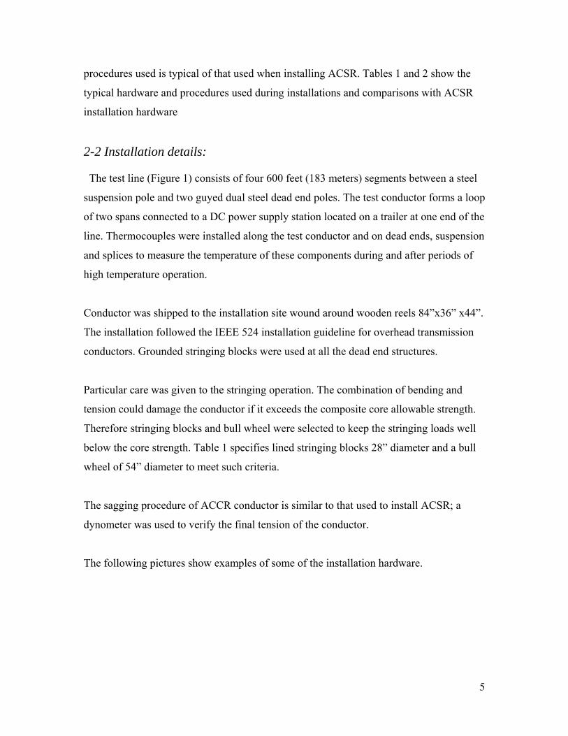
procedures used is typical of that used when installing ACSR. Tables 1 and 2 show the
typical hardware and procedures used during installations and comparisons with ACSR
installation hardware
2-2 Installation details: The test line (Figure 1) consists of four 600 feet (183 meters) segments between a steel
suspension pole and two guyed dual steel dead end poles. The test conductor forms a loop
of two spans connected to a DC power supply station located on a trailer at one end of the
line. Thermocouples were installed along the test conductor and on dead ends, suspension
and splices to measure the temperature of these components during and after periods of
high temperature operation.
Conductor was shipped to the installation site wound around wooden reels 84”x36” x44”.
The installation followed the IEEE 524 installation guideline for overhead transmission
conductors. Grounded stringing blocks were used at all the dead end structures.
Particular care was given to the stringing operation. The combination of bending and
tension could damage the conductor if it exceeds the composite core allowable strength.
Therefore stringing blocks and bull wheel were selected to keep the stringing loads well
below the core strength. Table 1 specifies lined stringing blocks 28” diameter and a bull
wheel of 54” diameter to meet such criteria.
The sagging procedure of ACCR conductor is similar to that used to install ACSR; a
dynometer was used to verify the final tension of the conductor.
The following pictures show examples of some of the installation hardware.
5
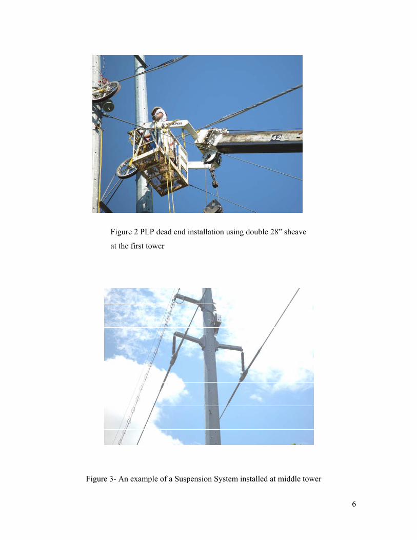
Figure 2 PLP dead end installation using double 28” sheave
at the first tower
Figure 3- An example of a Suspension System installed at middle tower
6

Figure 4 shows installed compression dead end and terminal connector
Figure 5 Conductor unwinding station
7

Figure 6 Thermocouples wiring for in-situ – temperature monitoring
Table 1- Installation Equipment
Equipment ACCR Stringing blocks 28" Suspension Stringing blocks 60" roller array block- dead ends
Bull wheel 54" Drum puller Yes Sock splice Yes (no bands)
Conductor grips DG grips Cable spools 40" drum min Cable cutter Yes Reel stand Yes
Grounding clamps Yes Running ground Yes
Table 2- Installation Procedure
Procedure ACCR
Cable stringing Tension Sag tensioning Dynometer, line of sight Dead ending Compression or
Preformed. Clipping Thermolign suspension
8
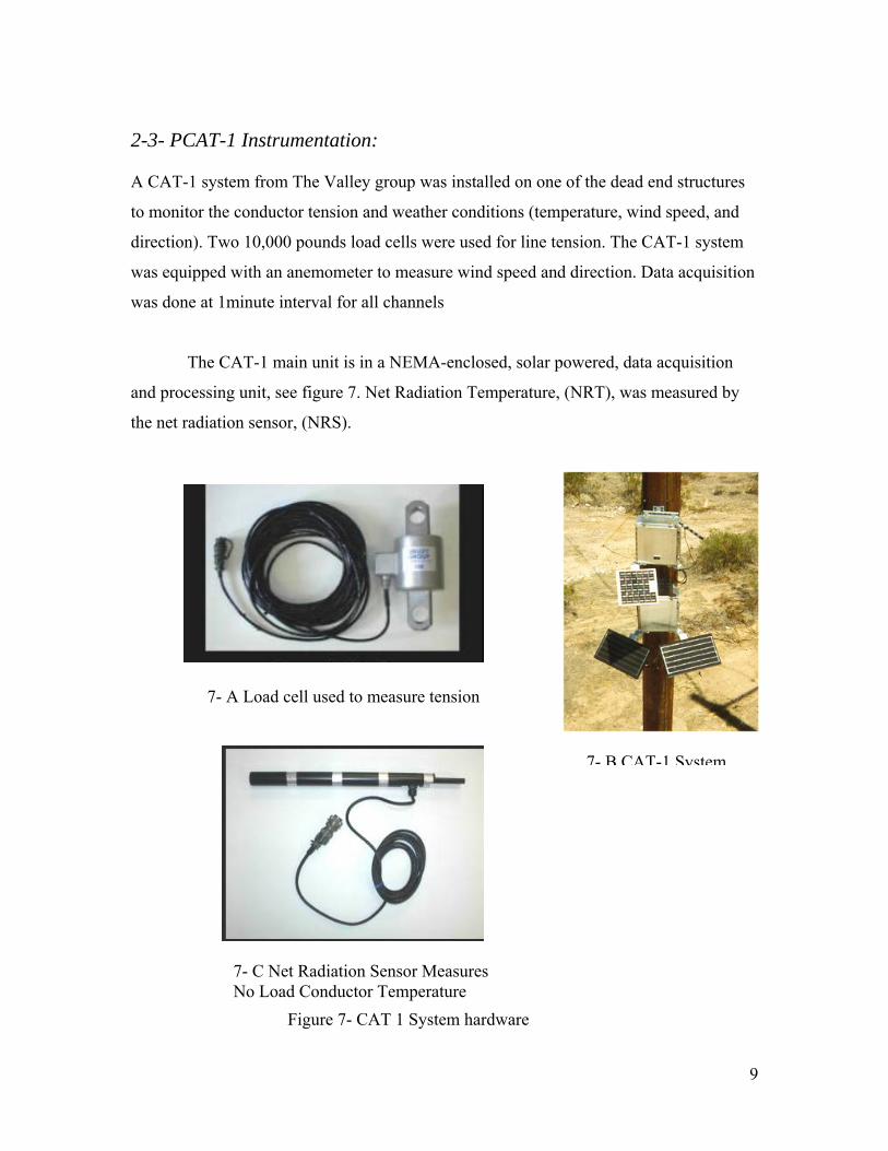
2-3- PCAT-1 Instrumentation: A CAT-1 system from The Valley group was installed on one of the dead end structures
to monitor the conductor tension and weather conditions (temperature, wind speed, and
direction). Two 10,000 pounds load cells were used for line tension. The CAT-1 system
was equipped with an anemometer to measure wind speed and direction. Data acquisition
was done at 1minute interval for all channels
The CAT-1 main unit is in a NEMA-enclosed, solar powered, data acquisition
and processing unit, see figure 7. Net Radiation Temperature, (NRT), was measured by
the net radiation sensor, (NRS).
7- A Load cell used to measure tension
Figure 7- CAT 1 System hardware
7- C Net Radiation Sensor Measures No Load Conductor Temperature
7- B CAT-1 System
9

2-4 Conductor and Accessories Temperature Measurements: A separate data acquisition system was used to collect the information from the
thermocouples every minute, see example in Figure 8.. Thermocouples were mounted at
various locations along the span on both conductor and all accessories. Both conductor
surface and core temperatures were measured.
2-5 Controls: The line was operated under either constant current and / or constant conductor
temperature with thermal cycles lasting from one hour to several days each. Multiple points along the length of the conductor were monitored this way using the
installed thermocouples. To accommodate the multiplicity of points along the conductor
and withstand the accumulated voltage drop, many fiber-connected, isolated
measurement nodes were used. A thermocouple measurement node was fabricated using
a multiplexer (ICPCON I-7018) and a RS-485-to-fiber modem (B&B FOSTCDR). Up to
eight thermocouples were monitored per node. The node required 120 VAC power and
was connected through a duplex fiber optic network. The multiplexer, fiber modem, and a
power supply were housed in an enclosure.
The power supply used has a dual rating of 400 Vdc and 5000 amps or 600 Vdc and 3750
amps. The input voltage to the power supply is 4160 V, 3-phase. A dry-type ABB
transformer was used to step down the voltage from a 13.8 KV distribution line.
2-6 Accessories:
Two types of accessories were installed; a compression type made by Alcoa (presently
known as American Fujikura Limited, AFL) and formed wire type made by Preformed
Line Products, PLP. The following specific parts were installed:
. Two ALCOA compression dead ends; Part # B9178-B
. One ALCOA full tension splice Part# B9095-B
. Four Alcoa jumper terminals (terminal connectors); Part# 9102-B
10

. Two transition plates, Part# ACP-E
. Two PLP THERMOLIGNTM, DEAD ENDS, Part# TLDE-0114 (includes extension link
and Thimble- Clevis) . PLP THERMOLIGNTM SPLICE Part # TLSP-0114
. Two THERMOLIGNTM PLP SUSPENSIONS with Socket eye, Part # TLS- 0108-SE
3- Thermal Cycles and High Temperature Exposure: 3-1 Thermal cycles details: The 795 Conductor was thermally cycled starting in September 2005, between ambient
temperature and 2000 C, sometimes above 2400C, under wide range of weather and load
conditions. Conductor surface temperature was measured at all locations while core
temperature was measured at two positions on the mid span; see example of a single
thermal cycle in figure 9. The conductor temperature dropped on rainy days by more than
400C. Figure 10 shows locations of the thermocouples used to measure both the
conductor and accessories temperature. There were two thermocouples on each
accessory, one to measure temperature at the tip of the accessory for the AFL
compression accessories or at the inner rod for the PLP accessories). The second
thermocouple measured the outer surface temperature for the compression accessories or
outer rod temperature for the PLP accessories. Table 3 gives a summary of the cycles
conducted from ambient to over 2400C.
11

0
50
100
150
200
250
300
350
11/27
/05 6:00 A
M
11/27
/05 9:36
AM
11/27
/05 1:12
PM
11/27
/05 4:48
PM
11/27
/05 8:24
PM
11/28
/05 12:0
0 AM
11/28
/05 3:36
AM
11/28
/05 7:12
AM
11/28
/05 10:4
8 AM
11/28
/05 2:24 P
M
Time
Tem
pera
ture
, C
0
500
1000
1500
2000
2500
3000
3500
Cur
rent
, A
Surface T at mid span 1
Idc, Power Supply DC Current (A)
Figure 8 shows a single cycle at 2000 C followed by a short cycle at 3000C. Conductor’s surface temperature dropped with rain on 11-28-05.
25’ from dead end
Jumper 1 terminal
Mid span 1
¾ from
25’ from
Figure 9- Schematics of thermocouples location along the test line spans from dead end tower DE1 to suspension tower, STR2 to dead end tower DE2.
The conductor was cycled from ambient to above 2000 C using either constant current or
constant temperature. It was given a short cycle from ambient to 3000C on 11-28-05.
DE1
DE1Conductor 1/4 out from STR2
¾ out from STR2
Jumper 225’from dead end
¼ span out from DE1
mid span 2
25’ from dead end
Jumper 1 terminal
Mid span 1
¾ from
25’ from
DE1
Conductor 1/4 out fromDE1 STR2
¾ out from STR2
Jumper 225’from dead end
¼ span out from DE1
mid span 2
Dead end tower 1, Suspension
tower, Dead end tower2, DE1
STR2 DE2
12

Figure 10 shows both a typical difference of about 5-100C between core and surface
temperatures when the conductor temperature is above 2000C.
175
180
185
190
195
200
205
210
1 61 121 181Time (hours)
Tem
pera
ture
(C)
CoreTemperatureSurfaceTemperature
Figure 10 shows both surface and core temperature
November 2005 data was reduced to include only 0 fps wind speed and core
temperature above 1500C and plotted in figure 11. The data suggests that a larger
temperature gradient occurs between core and surface at higher core temperatures.
Figure 11 shows that temperature gradient between conductor core
Figure 11 shows effect of conductor core temperature at 0 fps wind speeds
on temperature gradient between core and surface
0
10
20
30
100 150 200 250 300
Core temperature, C
(Tc-
Ts)
, C
0 fps wind speed
13

Data at wind speeds above zero was also examined and they show similar trend but
higher difference, see figure 12.
igure 12- Temperature difference between conductor core and surface increases with
-2 High temperature Cycle:
was conducted lasting about 40 minutes as shown in
and surface was about 15 to 200C at around 3000C core temperature
0
10
20
30
100 150 200 250 300
Core temperature, C
(Tc-
Ts)
, C
wind speedsabove 0 fps
Fincreased core temperature at higher wind speeds
3
high temperature cycle to 3000C A
figure 13. No additional 3000C cycles were performed because the thermocouple bond to
the conductor deteriorated and some thermocouples were damaged.
Figure 13- High temperature cycle, temperature difference between core
150
200
250
300
11/28/05
12:28 PM
11/28
/05 12:43 PM
11/28/05 12
:57 PM
11/28/05 1
:12 PM
11/28/0
5 1:26 PM
11/28/05 1:
40 PM
11/28/05
1:55 PM
Time, minutes
Tem
pera
ture
, C
Core temperature at mid span 1350 Surface temperature at mid span 1
14

Table 3- Summary of thermal cycling of ACCR 795 at ORNL
Date #Cycles Total # Hours Total run Nature of cycle Maximum Average Maximum Maximum Per day Cycles Per day hours surface T, C core T, C Core T, C
0 0 Conductor installed1 1 Constant current, 1025A 127 122 130
current, A6/16/2005 0 09/13/2005 1 1 10319/14/2005 1 2 13 14 Constant current,1200A 202 173 207 12269/15/2005 0 2 23 37 Constant current 1300A 196 177 199 12939/16/2005 0 2 20 57 Constant current1300A 211 187 216 13009/17/2005 0 2 1 58 Constant current, 1350A 207 205 211 13009/19/2005 1 3 16 74 Constant current 1300 A 208 183 214 13009/20/2005 0 3 24 98 Constant current 1300 A 213 192 221 13159/21/2005 0 3 24 122 Constant current, 1350A 246 208 252 13409/22/2005 0 3 24 146 Stepped current 1350A 226 200 230 13499/23/2005 0 3 4 150 Constant current, 1350A 205 203 208 134910/18/2005 1 4 2 152 Constant current, 1350A 156 156 160 134910/19/2005 1 5 15 167 Stepped current,1350A 199 156 201 134910/20/2005 0 5 24 191 Constant current, 1350A 222 210 228 135010/21/2005 1 6 24 215 Stepped current, 1350A 223 190 228 135010/22/2005 0 6 24 239 Constant current 1350 A 209 167 213 135010/23/2005 0 6 24 263 Tracking 1750C all day 208 176 212 135010/24/2005 1 7 16 279 Tracking 1900C, rain 253 199 253 135010/25/2005 0 7 24 303 Tracking 1900C all day 247 195 252 135110/26/2005 0 7 24 327 1900C then 1000C (4PM to midnight) 220 202 226 135110/27/2005 0 7 24 351 Tracking 1000C till noon, 1250C after 135 136 138 135110/28/2005 0 7 24 375 1350 A, tracking 1250C 162 141 170 135110/29/2005 0 7 24 399 1350 A, 1000C target 131 120 139 135510/30/2005 0 7 24 423 1350 A till 9PM, then 1025A 110 100 113 137510/31/2005 0 7 24 447 Constant current, 1025A 113 97 117 103511/1/2005 0 7 24 471 Constant T around 1000 C 126 109 130 160611/2/2005 0 7 24 495 1400 A tracking 1900C 256 210 267 140211/3/2005 1 8 23 518 1400 A tracking 2000C 247 215 255 137811/4/2005 0 8 24 542 Tracking T around 2000 C 233 208 242 139411/5/2005 0 8 24 566 T around 2000 C, very windy 234 205 235 148511/6/2005 1 9 22 588 1400 A tracking 1900C 247 217 255 140011/7/2005 0 9 24 612 1400 A, 1900C 242 208 256 140711/8/2005 0 9 24 636 1401 A, 1900C 217 204 224 142311/9/2005 0 9 24 660 1350A, 1900C, very windy, rain 241 211 252 143711/10/2005 0 9 24 684 1350 A, 1900C 237 204 243 145411/11/2005 0 9 20 704 Constant T around 2000 C 257 220 268 146911/12/2005 0 9 24 728 Constant T around 2000 C 243 217 254 148611/13/2005 0 9 24 752 1400A, 2000C 244 219 251 150211/14/2005 0 9 24 776 Constant current, 1400A 224 215 229 152511/15/2005 0 9 24 800 T, 2000 C 247 225 260 154311/16/2005 1 10 17 817 Current, 1550 A, storms, windy 251 221 259 155511/17/2005 0 10 24 841 Constant T, 2000C, sunny, T rise 241 229 251 156611/18/2005 0 10 24 865 Constant T around 2000C, sunny 275 223 293 163511/19/2005 0 10 24 889 Constant T around 2000 C 243 221 257 168811/20/2005 0 10 8 897 Constant T around 2000 C 217 214 225 170211/26/2005 1 11 8 905 Constant T, 2000 C 216 202 223 171811/27/2005 0 11 24 929 Constant T, 2000 C 249 225 263 177911/28/2005 1 12 21 950 T, 2000 C, rain 8-11AM, 3000 C spike 305 210 317 184311/29/2005 1 13 14 964 T around 2000 C, Rain 9:30 AM 260 217 267 189711/30/2005 0 13 24 988 T around 2000 C 261 227 272 2292
15
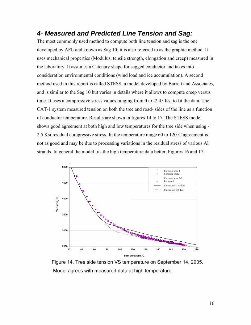
4- Measured and Predicted Line Tension and Sag: The most commonly used method to compute both line tension and sag is the one
developed by AFL and known as Sag 10; it is also referred to as the graphic method. It
uses mechanical properties (Modulus, tensile strength, elongation and creep) measured in
the laboratory. It assumes a Catenary shape for sagged conductor and takes into
consideration environmental conditions (wind load and ice accumulation). A second
method used in this report is called STESS, a model developed by Barrett and Associates,
and is similar to the Sag 10 but varies in details where it allows to compute creep versus
time. It uses a compressive stress values ranging from 0 to -2.45 Ksi to fit the data. The
CAT-1 system measured tension on both the tree and road- sides of the line as a function
of conductor temperature. Results are shown in figures 14 to 17. The STESS model
shows good agreement at both high and low temperatures for the tree side when using -
2.5 Ksi residual compressive stress. In the temperature range 60 to 1200C agreement is
not as good and may be due to processing variations in the residual stress of various Al
strands. In general the model fits the high temperature data better, Figures 16 and 17.
Model agrees with measured data at high temperature
2500
3000
3500
4000
4500
5000
20 40 60 80 100 120 140 160 180 200 220
Temperature, C
Tens
ion,
lb
Core mid span 1 Core mid span2
Core mid span 2-2 L/4 span 1
Calculated –1.45 Ksi
Calculated –2.5 Ksi
Figure 14. Tree side tension VS temperature on September 14, 2005.
16

17
2500
3000
3500
4000
4500
20 40 60 80 100 120 140 160 180 200 220
Temperature, C
Tens
ion,
lb
5000Surface Midspan 1, Column 43
Surface Midspan 1, Column 44
Surface Midspan 2, Column 97
Surface Midspan 2, Column 98
Calc 0 ksi
Calc -1.45 ksi
Figure 15- Road- side tension VS conductor surface temperature, September 14, 2005. Model fits data very well using a compressive stress of –1.45 Ksi particularly above 1000 C
Similar results were obtained by analyzing the ORNL data for November 6, 2005.
igure 16- Road- side tension VS temperature, November 2005. Model agrees with measured data above 1000C using a compressive stress of –1.45 Ksi F
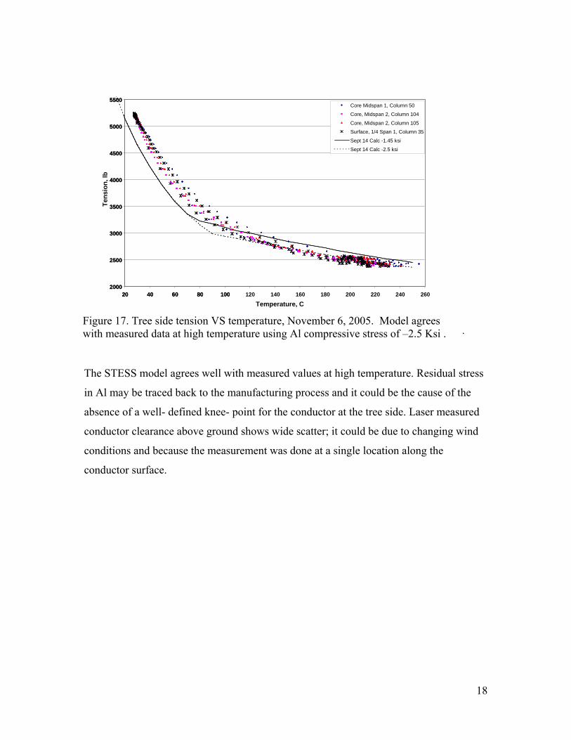
ter
2000
2500
3000
3500
4000
4500
5000
5500
20 40 60 80 1002000
2500
3000
3500
4000
4500
5000
5500
20 40 60 80 100 120 140 160 180 200 220 240 260
Temperature, C
Tens
ion,
lbCore Midspan 1, Column 50
Core, Midspan 2, Column 104
Core, Midspan 2, Column 105
Surface, 1/4 Span 1, Column 35
Sept 14 Calc -1.45 ksi
Sept 14 Calc -2.5 ksi
h
o ws that the line did not change its characteristics af
T e conductor test line was stable during the period analyzed here (September to
vember 2005). The data shoNFig
it perature using Al compressive stress of –2.5 Ksi . ure 17. Tree side tension VS temperature, November 6, 2005. Model agrees h measured data at high temw
Al may be traced back to the manufacturing process and it could be the cause of the
bsence of a well- defined knee- point for the conductor at the tree side. Laser measured
onductor clearance above ground shows wide scatter; it could be due to changing wind
onditions and because the measurement was done at a single location along the
onductor surface.
The STESS model agrees well with measured values at high temperature. Residual stress
in
a
c
c
c
18
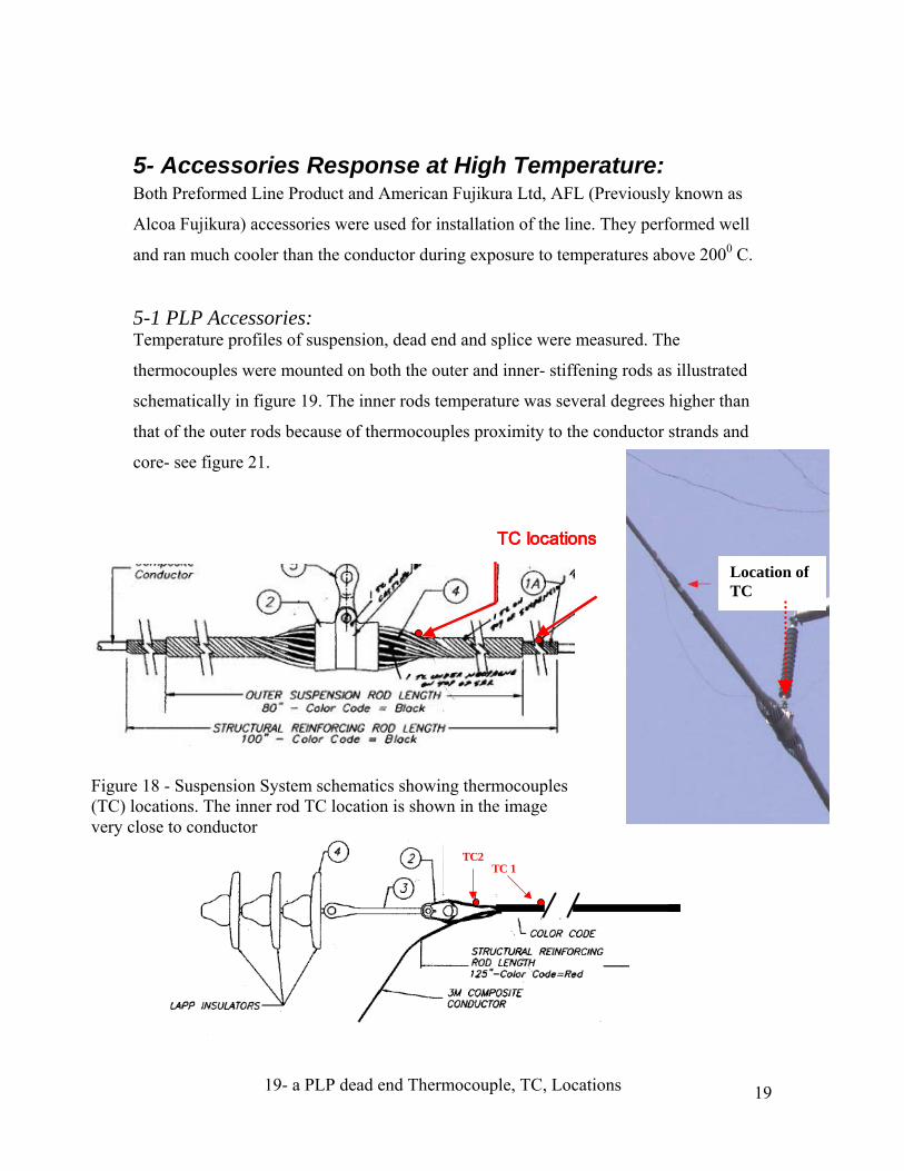
5- Accessories Response at High Temperature: Both Preformed Line Product and American Fujikura Ltd, AFL (Previously known as
Alcoa Fujikura) accessories were used for installation of the line. They performed well
and ran much cooler than the conductor during exposure to temperatures above 2000 C.
5-1 PLP Accessories: Temperature profiles of suspension, dead end and splice were measured. The
thermocouples were mounted on both the outer and inner- stiffening rods as illustrated
schematically in figure 19. The inner rods temperature was several degrees higher than
that of the outer rods because of thermocouples proximity to the conductor strands and
core- see figure 21.
TC locationsTC locations
Figure 18 - Suspension System schematics showing thermocouples (TC) locations. The inner rod TC location is shown in the image very close to conductor
Location of TC
TC 1TC2
TC 1TC2
1919- a PLP dead end Thermocouple, TC, Locations

19-c actual location of thermocouples on the PLP splice
TM DEAD two thermocouples.
19- b PLP Splice TC Locations
TC1
Figure 19- Schematics of thermocouples location on PLP THERMOLIGNEND and SPLICE and an image showing actual location of the
TC2
TC1
TC2
Splice inner rod TC Splice outer rod TC
20
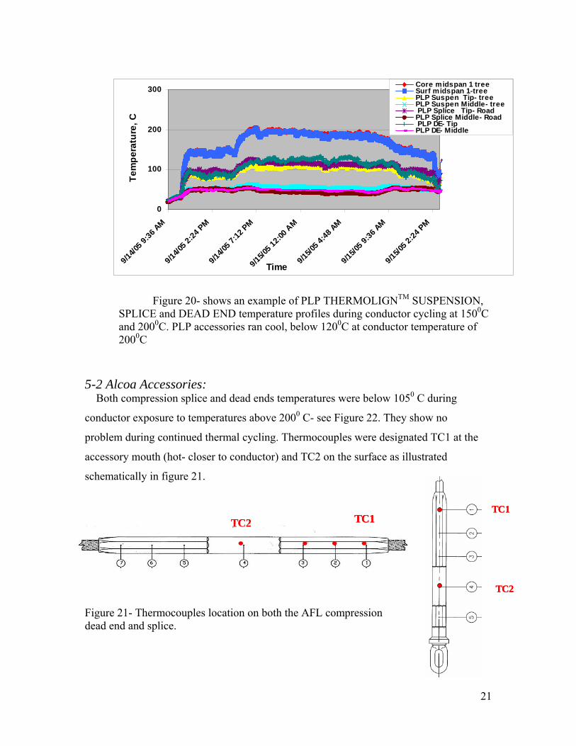
0
100
200
300
9/14/0
5 9:36
AM
9/14/0
5 2:24
PM
9/14/0
5 7
15/05
12
9/15/0
5 4:12
PM
9/
:00 A
M:48
AM
9/15/0
5 9:36
AM
9/15/0
5 2:24
PM
Time
Tem
pera
ture
, C
Core midspan 1 treeSurf midspan 1-tree PLP Suspen Tip- tree PLP Suspen Middle- tree PLP Splice Tip- Road PLP Splice Middle- Road PLP DE- TipPLP DE- Middle
SPLICE and DEAD END temperature profiles during conductor cycling at 150and 2000C. PLP accessories ran cool, below 1200C at conductor tem2000C
Both compression splice and dead ends temperatures were below 1050 C during
conductor exposure to temperatures above 2000 C- see Figure 22. They show no
problem during continued thermal cycling. Thermocouples were designated TC1 at the
ccesso ustrated
schematically in figure 21.
Figure 21- Thermocouples location on both the AFL compression dead end and splice.
Figure 20- shows an example of PLP THERMOLIGNTM SUSPENSION, 0C
perature of
5-2 Alcoa Accessories:
a ry mouth (hot- closer to conductor) and TC2 on the surface as ill
TC1
TC2
TC1
TC2
TC1TC2 TC1TC2
21
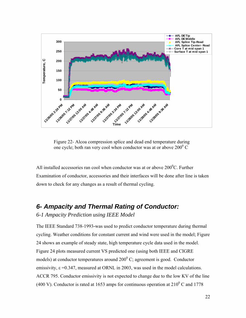
0
is taken
6-1 Ampacity Prediction using IEEE Model The IEEE Standard 738-1993-was used to predict conductor temperature during thermal
cycling. Weather conditions for constant current and wind were used in the model; Figure
4 shows an example of steady state, high temperature cycle data used in the model.
Figure 24 plots measured current VS predicted one (using both IEEE and CIGRE
d. Conductor
measured at ORNL in 2003, was used in the model calculations.
CCR 795. Conductor emissivity is not expected to change due to the low KV of the line
00 V). Conductor is rated at 1653 amps for continuous operation at 2100 C and 1778
0
50
100
150
200
250
300
11/26
/05 2:
24 PM
11/26
/05 7:
12 PM
11/27
/05 12
:00 A
M
11/27
/05 4:
48 A
M
11/27
/05 9:
36 A
M
11/27
/05 2:
24 PM
11/27
/05 7:
12 PM
11/28
/05 12
:00 A
M
11/28
/05 4:
48 A
M
11/28
/05 9:
36 A
M
Time
Tem
pera
ture
, C
AFL DE Tip AFL DE Middle AFL Splice Tip-Road AFL Splice Center- Road Core T at mid span 1Surface T at mid span 1
Figure 22- Alcoa compression splice and dead end temperature during one cycle; both ran very cool when conductor was at or above 2000 C
All installed accessories ran cool when conductor was at or above 200 C. Further
Examination of conductor, accessories and their interfaces will be done after line
down to check for any changes as a result of thermal cycling.
6- Ampacity and Thermal Rating of Conductor:
2
models) at conductor temperatures around 2000 C; agreement is goo
emissivity, ε =0.347,
A
(4
22

amps for emergency loading at 2400 C. The data shows the conductor was sometimes
xposed to temperatures higher than 2400C and current above 2200 amps.
it software. There were
mall differences between the two models in agreement with literature data. Predicted
e
Figure 23 shows an example of constant current thermal cycles data
6-2 IEEE VS CIGRE’ Ampacity Model: The CIGRE’ 1997 model was used to compute current to compare with the IEEE Std
736, both programs were provided by the Valley Group Rate k
s
current values agree well with measured current as plotted in figure 25..
used in the model prediction in October 2005
Figure 24- Comparison of both the IEEE and CIGRE predictive models with measured current data- Agreement is good
2500
500
1000
1500
2000
Pred
icte
d cu
rren
t, am
ps
00 500 1000 1500 2000 2500
23
Measured current, amps
Current, IEEE Current, CIGRE

24
was thermally
ycled from ambient to over 2000 C for several hundred hours, using a DC power supply.
easured temperature difference between conductor core and its surface was as low as 0C and as high as 200C degrees and depended on both wind speed and core temperatures
t and above 2000 C. Wind speeds above 0 fps produced larger temperature gradient from
rface to core.
ata analysis shows that the measured conductor current agrees well with the IEEE
ermal rating model predicted values. The conductor is rated at 1653 A current for
ontinuous operation at 2100 C and at 1778 A emergency current at 2400C. The CIGRE’
odel agrees with the IEEE 736 model.
onductor tension was stable during and after thermal cycling. Measured line tension
ersus tem n method,
TESS.
0
he results will be included in a follow up report.
7- Summary: ACCR 795 conductor was successfully installed and tested at ORNL. It
c
M
5
a
su
D
th
c
m
C
v perature agrees well with values computed using the strain summatio
S
Both PLP and AFL accessories ran cool, below 120 C at conductor’s temperature
exceeding 2000 C. The conductor and accessories were exposed for up to 1000 hours at
high temperature and show no visual damage. Conductor will be de-installed in early
2006 and shipped to NEETRAC for inspection and mechanical testing (residual strength).
T

8- Appendix 8-1 Conductor Specs Designation 795-T16 Stranding 26/19 Diameter individual Core in 0.082
individual Al in 0.175 Core in 0.41
eight lbs/linear ft 0.896
lete Cable 000's lbs 31,384
23.0 Complete Cable 10^-6/C 16.5
eat Capacity Core W-sec/ft-C 22 Aluminum W-sec/ft-C 324
Total Diameter in 1.11 Area Al in^2 0.624 Total Area in^2 0.724 W Breaking Strength Core lbs 18,556 Aluminum lbs 12,828 Comp Final Modulus Core msi 35.0 Aluminum msi 8.6 Complete Cable msi 12.3 Thermal Elongation Core 10^-6/C 6.3 Aluminum 10^-6/C H Resistance
DC @ 20C ohms/mile 0.1100 AC @ 25C ohms/mile 0.1126 AC @ 50C ohms/mile 0.1237 AC @ 75C ohms/mile 0.1349
AC @ 100C ohms/mile 0.1460 AC @ 210C ohms/mile 0.1951
25

AC @ 240C ohms/mile 0.2084
eometric Mean Radius actance (1 ft Spacing, 60hz)
hms/mile 0.399 ve X'a hms/mile 0.0912
G ft 0.0375
Re Inductive Xa o Capaciti o
26

Appendix A.3
ACCR 1272 Kcmil Report

This page is intentionally left blank.

1
Composite Conductor Field Trial Summary Report: ORNL ACCR 1277 Kcmil
Installation date August 9, 2004
Field trial location Oak Ridge, Tennessee, USA
Line Characteristics
Organization Oak Ridge National Laboratory Point of Contact John Stovall, ORNL Installation date August 9, 2004 Conductor Installed ACCR 1272 Length of line 1,200 feet (356.7 meters) Conductor diameter 0.858 inch, (21.8 mm) Voltage 400 VDC Ruling span length 600 feet, (183 meters) Structure Type Steel Poles Instrumentation: (1) Load cell
(2) Current, voltage (3) Weather station (4) Sag
(5) Thermocouples in conductor and accessories Hardware Suspension Hardware Preformed Line Product, THERMOLIGNTM
SUSPENSION-TLS-0116-SE Termination Hardware AFL compression dead end, part# 1272M-54/19-ACCR,
Drawing#B9085 AFL splice, part#1272M-54/19-ACCR, Drawing#B9095
Insulator type Polymer Dampers Alcoa Dampers part# 1707-13 Terminals AFL terminal connector, part#1272M-54/19-ACCR,
Drawing# B9102 PLP THERMOLIGNTM DEAD END, part# TLDE-1272-N
Results and Measurements
Full range of temperature tests from 30oF – 412oF (0oC – 240oC) with currents ranging from 0 to 1,800 amps
Sag-Temperature data from 0oC – 240oC Line tension data from 0 to > 200C Measured thermal rating

2
Table of Contents
Abstract:........................................................................................................ 3
1- Background ............................................................................................. 3
2- Installation and Conductor Stringing ................................................ 5
2-1 Overview............................................................................................... 5 2-2 Installation details: ................................................................................ 5 2-3- PCAT-1 Instrumentation: .................................................................... 7 2- 4 Conductor and Accessories Temperature Measurements:................... 9 2-5 Controls ................................................................................................. 9 2-6 Accessories:......................................................................................... 10
3- Thermal Cycles and High Temperature Exposure:...................... 11
3-1 Thermal cycles details:........................................................................ 11 3-2 Conductor Core VS Surface temperature: .......................................... 15
4- Measured and Predicted Line Tension and Sag:........................... 17
5- Accessories Response at High Temperature: ................................ 19
5-1 PLP Accessories:................................................................................. 20 5-2 Alcoa Accessories: .............................................................................. 23
6- Ampaciy and Thermal Rating of Conductor ................................. 24
6-1 Ampacity Prediction using IEEE Model: ....................................... 24 6-2 IEEE VS CIGRE’ Ampacity Model: .................................................. 27
7- Summary................................................................................................ 28
8- Appendix................................................................................................ 30
8-1 Conductor Specs ................................................................................. 30

3
Abstract: Under DOE funding Agreement No. DE-FC02-02CH11111 Oak Ridge National
Laboratory, ORNL, jointly with The Tennessee Valley Authority, TVA, successfully
installed ACCR 1272 conductor on ORNL high temperature test line. The line is 1200
feet (365 meters) long, and the ruling span is 600 feet (130 meters).
ORNL subjected the line to severe thermal cycling and extended high temperature
load using 400 V DC and current as high as 2700 amps. The conductor was thermally
cycled between ambient and 2000+ C for over 300 hours and over 100 hours operation
continuously above 2000 C under changing wind conditions.
The conductor tension and sag measured during the high temperature test trial agree with
predictive models.
Predicted conductor current, using IEEE thermal rating ampacity method, agree well with
measured values.
The accessories performed well during the high temperature cycling and ran at much
cooler temperature than the conductor.
1- Background
ORNL has built a fully instrumented low-voltage test line to evaluate the high-
temperature operation of ACCR conductors by simulating dozens of emergency cycles
where the conductor temperature reaches operating temperature 2100 C (400oF) and
higher under a range of ambient conditions.
The ORNL test line instrumentation includes conductor tension measuring device,
full weather station with anemometer, voltage, current, laser sensor device to measure

4
ACCR 1272
sag, and temperature thermocouples in multiple locations in the conductor and in all
accessories.
This report summarizes the 1272 ACCR conductor installation, testing and
analysis at ORNL.
Arial view of the line
Layout
High temperature Line at ORNL
Figure 1- Conductor details and ORNL test line view

5
2- Installation and Conductor Stringing 2-1 Overview A two span test line (from dead end to dead end) was constructed on the grounds of the
Oak Ridge national Laboratory in Oak Ridge, TN, as a part of a Department of Energy
program. Several sizes of ACCR composite conductors were installed and tested since
then. ACCR 1272 is the latest of such installations. The installation procedures used is
typical of that used when installing ACSR. Tables 2 and 3 show the typical hardware and
procedures used during installations and the comparisons of each type of conductor.
2-2 Installation details: The test line (Figure 1) consists of four 600 feet (183 meters) segments between a steel
suspension pole and two guyed dual steel dead end poles. The test conductor forms a loop
of two spans connected to a DC power supply located at one end of the line.
Thermocouples were installed along the test conductor and on dead end, suspension and
splice hardware to measure the temperature of these components during and after periods
of high temperature operation.
Conductor was shipped to the installation site wound around wooden reels 84 “ X36”
X44 “. The installation of 1272 followed the IEEE 524 installation guideline for overhead
transmission conductors. Grounded stringing blocks were used at all the dead end
structures.
Particular care was given to the stringing operation. The combination of bending and
tension if exceeds the core allowable strength could damage the conductor. Therefore
stringing blocks and bull wheels were selected to keep the stringing loads way below
conductor core strength. Table 2 specifies stringing blocks 28” diameter and bull wheels
of 36” diameter to meet such criteria. Lined blocks were used with ACCR.

6
Figure 1 line Layout and PCAT –1 system
Figure 2- Sheave used in the installation

7
The sagging procedure of ACCR conductor is similar to that used to install ACSR; a
dynometer was used to verify the final tension of the conductor.
Table 1- Installation Equipment and Procedure
Yes Yes Grounding Clamps Yes Yes Running Ground
Yes Yes Reel Stands Yes Yes Cable Cutter
Yes (40” Drum)Yes Cable Spools DG-Grips Any Conductor Grips
Yes Yes Sock Splice Yes Yes Drum Puller
Yes (36”) Yes Bull Wheel Yes (28”) Yes Stringing Blocks
ACCR ACSRInstallation Equipment
AnyAnyClipping
Use DG-Grip with chain hoists
AnyDead Ending
Line of sight,Dynometer
AnySag Tensioning
Tension Tension / Slack
Cable Stringing
ACCRACSRInstallationProcedure
AnyAnyClipping
Use DG-Grip with chain hoists
AnyDead Ending
Line of sight,Dynometer
AnySag Tensioning
Tension Tension / Slack
Cable Stringing
ACCRACSRInstallationProcedure
2-3- PCAT-1 Instrumentation: A CAT-1 system from The Valley group was installed on one of the dead end structures
to monitor the conductor tension and weather conditions (temperature, wind speed, and
direction) at intervals of 10 minutes; see Figure 3. Two 10,000 pounds load cells were

8
used for line tension. The CAT-1 system was equipped with anemometer to measure
wind speed and direction. Data acquisition was done at 1minute interval for all channels
The CAT-1 main unit is in a NEMA-enclosed, solar powered, data acquisition
and processing unit. Net Radiation Temperature, (NRT), was measured by the net
radiation sensor, (NRS).
Net Radiation Temperature (NRT) was measured by the Net Radiation Sensor,
Figure 3-C, which provides a simple method of combining ambient temperature with
wind and solar effects (emissivity and conductor time constant).
A- Load cell used to measure tension
B- CAT-1 System
Figure 3- CAT system hardware
3- C Net Radiation Sensor Measures No Load Conductor Temperature

9
2- 4 Conductor and Accessories Temperature Measurements: A separate data acquisition system was used to collect the information from the
thermocouples. Thermocouples were mounted at various locations along the span. The
thermocouples were located on the conductor surface and several at the core. Additional
thermocouples were installed on ALCOA compression dead ends, compression splice,
Alcoa jumpers, PLP suspension, PLP splices and PLP dead ends.
2-5 Controls The line was operated under either constant current and / or constant conductor
temperature with thermal cycles lasting from one hour to several days. Temperature data was acquired by thermocouples affixed directly to the outer surface and
couple to the core. Multiple points along the length of the conductor were monitored this
way. To accommodate the multiplicity of points along the conductor and withstand the
accumulated voltage drop, many fiber-connected, isolated measurement nodes were used.
A thermocouple measurement node was fabricated using a multiplexer (ICPCON I-7018)
and a RS-485-to-fiber modem (B&B FOSTCDR). Up to eight thermocouples were
monitored per node. The node required 120 VAC power and was connected through a
duplex fiber optic network. The multiplexer, fiber modem, and a power supply were
housed in an enclosure. The following images and those under accessories section show
typical examples of the installation details
Figure 4- Installation of PLP THERMOLIGNTM DEAD ENDS next to stringing chain

10
The power supply used has a dual rating of 400 Vdc and 5000 amps or 600 Vdc and 3750
amps. The input voltage to the power supply is 4160 V, 3-phase. A dry-type ABB
transformer was used to step down the voltage from a 13.8 KV distribution line.
2-6 Accessories:
Two types of accessories were installed; a compression type made by Alcoa (now named
American Fujikura Limited, AFL) and formed wire type made by Preformed Line
Products. The following specific parts were used:
. Four ALCOA compression dead ends; part # 1272-54/19-ACCR, Drawing # B9119,
Dead ends consist of both direct core gripping parts and conductor gripping sleeve,
. One ALCOA full tension splice part# 1272M-54/19-ACCR, Drawing# B9095-D, it has
the same design as the dead end for both direct core gripping and conductor.
. Six Alcoa terminal connectors; part# 1272M-54/19-ACCR, Drawing# B9102; those are
all Aluminum sleeve parts
. Four Alcoa Stockbridge dampers; part# 1707-13
. Two PLP THERMOLIGNTM, DEAD ENDS, part#TLDE-1272-N (includes extension
link and Thimble- Clevis),
. PLP THERMOLIGNTM SPLICE part # TLSP-1272
. Two THERMOLIGNTM PLP SUSPENSIONS with Socket eye, part # TLS- 0116-SE
Figure 5- Installed Alcoa compression dead end next to insulator and dead end tower

11
3- Thermal Cycles and High Temperature Exposure: 3-1 Thermal cycles details:
The 1272 Conductor was thermally cycled starting in October 2004, between ambient
temperature and 2000+ C under wide range of weather and load conditions. A single
cycle was carried out between ambient and 3000 C and both conductor surface and core
temperatures were recorded. Table 2 lists a summary of thermal cycles completed as of
4/6/2005
Figure 6- Compression of jumper connector

12
Date #Cycles Total # Hours Total Run Nature of cycle Maximum Maximum Per day Cycles Per day Hours Temperature, C Current, amps
8/13/2004 1 1 9 9 Hi-Temp Run 220 22438/14/2004 0 1 21 30 Hi-Temp Run 221 24888/16/2004 1 2 8.5 38.5 Hi-Temp Run 222 23998/17/2004 0 2 24 62.5 Hi-Temp Run 228 22048/18/2004 0 2 24 86.5 Hi-Temp Run 224 22848/19/2004 0 2 24 110.5 Hi-Temp Run 223 22768/20/2004 1 3 5.5 116 Hi-Temp Run, Knee-point curve 217 23988/27/2004 7 10 7 123 Thermal/Mechanical Cycling 221 25008/28/2004 3 13 3 126 Thermal/Mechanical Cycling 217 23998/30/2004 1 14 1 127 Thermal/Mechanical Cycling 206 24008/31/2004 5 19 6 133 Thermal/Mechanical Cycling 213 25009/1/2004 8 27 8 141 Thermal/Mechanical Cycling 217 25009/2/2004 6 33 6 147 Thermal/Mechanical Cycling, rain 211 24999/3/2004 2 35 2 149 Thermal/Mechanical Cycling 205 24009/9/2004 6 41 6 155 Thermal/Mechanical Cycling 215 24009/10/2004 8 49 8 163 Thermal/Mechanical Cycling 222 25019/11/2004 8 57 8 171 Thermal/Mechanical Cycling 221 25009/12/2004 8 65 8 179 Thermal/Mechanical Cycling 218 25009/20/2004 5 70 5 184 Thermal/Mechanical Cycling 218 25019/21/2004 8 78 8 192 Thermal/Mechanical Cycling 221 26009/22/2004 8 86 8 200 Thermal/Mechanical Cycling 223 26009/23/2004 8 94 8 208 Thermal/Mechanical Cycling 221 25989/24/2004 6 100 6 214 Thermal/Mechanical Cycling 218 259911/9/2004 1 101 0 214 Checkout run, 1800 amps 143 21022/24/2005 1 102 7 221 7.5 hours @ 2000 amps 185 20033/18/2005 5 107 5 226 Thermal/Mechanical Cycling 222 25013/19/2005 8 115 8 234 Thermal/Mechanical Cycling 237 27213/20/2005 8 123 8 242 Thermal/Mechanical Cycling 233 26013/21/2005 8 131 8 250 Thermal/Mechanical Cycling 231 26003/22/2005 6 137 6 256 Thermal/Mechanical Cycling 198 27003/23/2005 5 142 5 261 Thermal/Mechanical Cycling 207 27033/24/2005 8 150 8 269 Thermal/Mechanical Cycling 200 25993/25/2005 8 158 8 277 Thermal/Mechanical Cycling 208 25003/26/2005 8 166 8 285 Thermal/Mechanical Cycling 211 25003/27/2005 4 170 4 289 Thermal/Mechanical Cycling 205 26013/29/2005 5 175 5 294 Thermal/Mechanical Cycling 201 25993/30/2005 8 183 8 302 Thermal/Mechanical Cycling 209 26994/4/2005 5 188 5 307 Thermal/Mechanical Cycling 203 26004/5/2005 8 196 8 315 Thermal/Mechanical Cycling 211 26024/6/2005 6 202 6 321 Thermal/Mechanical Cycling 206 27285/17/2005 1 203 13 334 Constant current 264 20025/18/2005 203 24 358 Constant current 216 18525/19/2005 203 11 369 Constant current 96 12315/26/2005 1 204 13 382 Constant current 165 16635/27/2005 204 17 399 Constant current 177 17776/7/2005 1 205 11 410 300C for 1 hour - 6:30 to 7:30 am 347 22756/8/2005 1 206 12 422 Constant temperature tests 143 1566
Table 2- Summary of Thermal cycling of conductor up to April 6, 2005
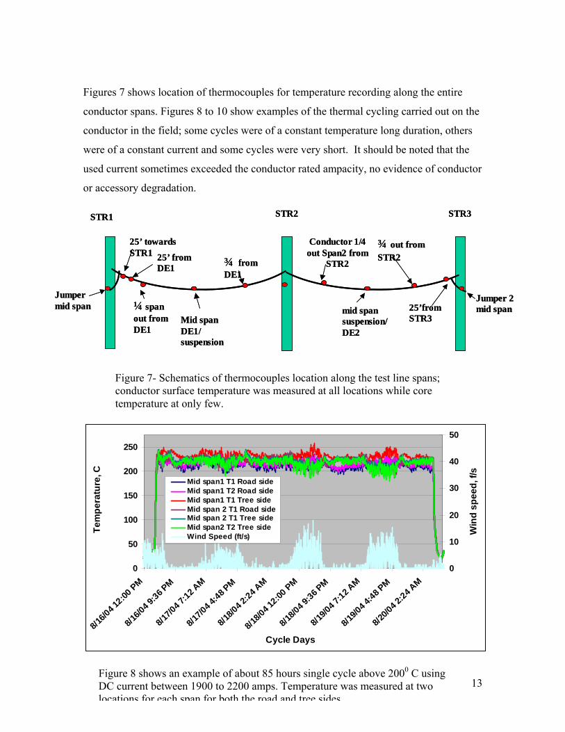
13
Figures 7 shows location of thermocouples for temperature recording along the entire
conductor spans. Figures 8 to 10 show examples of the thermal cycling carried out on the
conductor in the field; some cycles were of a constant temperature long duration, others
were of a constant current and some cycles were very short. It should be noted that the
used current sometimes exceeded the conductor rated ampacity, no evidence of conductor
or accessory degradation.
Figure 8 shows an example of about 85 hours single cycle above 2000 C using DC current between 1900 to 2200 amps. Temperature was measured at two locations for each span for both the road and tree sides
STR1 STR2 STR3
25’ from DE1
Jumper mid span
Mid span DE1/ suspension
¾ from DE1
25’ towards STR1
Conductor 1/4 out Span2 from
STR2
¾ out from STR2
Jumper 2 mid span25’from
STR3¼ span out from DE1
mid span suspension/ DE2
STR1 STR2 STR3
25’ from DE1
Jumper mid span
Mid span DE1/ suspension
¾ from DE1
25’ towards STR1
Conductor 1/4 out Span2 from
STR2
¾ out from STR2
Jumper 2 mid span25’from
STR3¼ span out from DE1
mid span suspension/ DE2
Figure 7- Schematics of thermocouples location along the test line spans; conductor surface temperature was measured at all locations while core temperature at only few.
0
50
100
150
200
250
8/16/0
4 12:00
PM
8/16/0
4 9:36 P
M
8/17/0
4 7:12 A
M
8/17/0
4 4:48 P
M
8/18/0
4 2:24 A
M
8/18/0
4 12:00
PM
8/18/0
4 9:36 P
M
8/19/0
4 7:12 A
M
8/19/0
4 4:48 P
M
8/20/0
4 2:24 A
M
Cycle Days
Tem
pera
ture
, C
0
10
20
30
40
50
Win
d sp
eed,
f/s
Mid span1 T1 Road sideMid span1 T2 Road sideMid span1 T1 Tree sideMid span 2 T1 Road sideMid span 2 T1 Tree sideMid span2 T2 Tree sideWind Speed (ft/s)
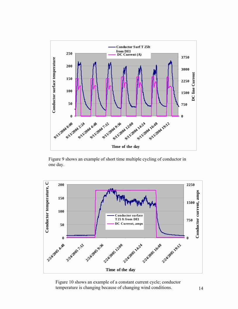
14
0
50
100
150
200
250
9/11/2004 0:00
9/11/2004 2:24
9/11/2004 4:48
9/11/2004 7:12
9/11/2004 9:36
9/11/2004 12:0
0
9/11/2004 14:2
4
9/11/2004 16:4
8
9/11/2004 19:1
2
Time of the day
Con
duct
or su
rfac
e te
mpe
ratu
re
0
750
1500
2250
3000
3750
DC
line
Cur
rent
Conductor Surf T 25ftfrom DE1 DC Current (A)
Figure 9 shows an example of short time multiple cycling of conductor in one day.
0
50
100
150
200
2/24/2005
4:48
2/24/2005
7:12
2/24/2005
9:36
2/24/2005
12:00
2/24/2005
14:24
2/24/2005
16:48
2/24/2005
19:12
Time of the day
Con
duct
or te
mpe
ratu
re, C
0
750
1500
2250
Con
duct
or c
urre
nt, a
mps
Conductor surfaceT 25 ft from DE1DC Current, amps
Figure 10 shows an example of a constant current cycle; conductor temperature is changing because of changing wind conditions.

15
3-2 Conductor Core VS Surface temperature: Limited number of thermal cycles both at constant current and / or high temperature long
time exposure was applied to ACCR 1272 while both core and surface temperatures were
measured. Result shows that the core was only several degrees hotter than the conductor
surface; see examples in figures 11 and 12. It also shows that the conductor was exposed
to temperatures in excess of 2300 C
0
50
100
150
200
250
300
5/17/05 7:12AM
5/17/0512:00 PM
5/17/05 4:48PM
5/17/05 9:36PM
5/18/05 2:24AM
Time of the day
Con
duct
or
Tem
pera
ture
, C a
nd
win
d sp
eed,
f/s
-500
0
500
1000
1500
2000
2500
Con
duct
or c
urre
nt, a
mp
Conductor surface Tat mid span1Conductor surface Tat mid span1-position2Conductor core T atmid span1Conductor core T atmid span1 position 2Wind Speed (ft/s)
Idc, Power Supply DC
Figure 11. An example of a constant current thermal cycle of ACCR 1272 at ORNL on May 17, 2005
0
30
60
90
120
150
180
5/26/05 9:36 PM 5/27/05 7:12 AM 5/27/05 4:48 PM 5/28/05 2:24 AMTime of the day
Tem
pera
ture
C,
win
d sp
eed
f/s
0
500
1000
1500
2000
2500
3000
Cur
rent
, am
p
Conductor surf Tat mid spanConductor core Tat midspanWind Speed (ft/s)
Current, amp
Figure 12. An example of a longer time thermal exposure with cycling around mid night of ACCR 1272 at ORNL on May 17, 2005

16
Wind speed appears to reduce both the Al strands surface temperature and core
significantly as shown in the following figures 13 and 14.
0
50
100
150
200
250
300
0 2 4 6 8 10 12Wind speed, f/s
Surf
ace
tem
pera
ture
, C
1950
1970
1990
2010
2030
2050
Cur
rent
, am
p.
Conductor surf T mid span 2Current, amp
Figure 13. Effect of wind speed on conductor surface temperature at mid span when line is energized to about a current of 2000
0
2
4
6
8
10
0.0 2.0 4.0 6.0 8.0 10.0 12.0
Wind speed, f/s
Tem
pera
ture
di
ffere
nce,
C
1950
1970
1990
2010
2030
2050
Cur
rent
, am
p
Temp. diff core to surface 2-Current, amp
Figure 14. Temperature difference between core and surface at mid span VS wind speed at a constant current of 2000 amps at ORNL test line-

17
Conductor was exposed to a 3000 C cycle for a short time and graph 15 shows the cycle
details.
Notice that the temperature gradient from surface to core was about several
degrees, much lower than temperature gradients measured on smaller conductors (ACCR
477). Conductor was taken down in June 2005 and examined visually; it showed no
damage and is being evaluated at NEETRAC Laboratories for effect of field testing.
4- Measured and Predicted Line Tension and Sag: Sag was computed using, the Strain Summation Method (which accounts for the full
loading history). The Strain Summation Method of Sag-Tension calculation takes into
account creep as a function of time. The spans considered are two, tree side and roadside.
Measured tension – temperature data is plotted in figure 16 for all tree side locations. The
difference in tension is believed to be caused by differences in wind- speed, net radiation
Figure 15 – Conductor core temperature and line DC current data measured during a 3000 C cycle at the middle of span 1. The other thermocouples mounted on the conductor failed above 3000 C.
0
100
200
300
400
6/7/05
4:19 A
M
6/7/05
5:02 A
M
6/7/05
5:45 A
M
6/7/05
6:28 A
M
6/7/05
7:12 A
M
6/7/05
7:55 A
M
6/7/05
8:38 A
M
6/7/05
9:21 A
M
Time of the Day
Tem
pera
ture
, C
0
500
1000
1500
2000
2500
Cur
rent
, Am
ps
Core 2 midspan
Idc, Power Supply DCCurrent (A)

18
temperature, NRC ( e.g. temperatures measured 25 ft from structure 3 in Span 2 were
lower than temperatures at 3/4 Span 1) and line hysteresis. Figure 16 shows model
predicted values using –1.45 Ksi compressive stress compared to measurement at ¾ span
1 and 25 feet away from STR3 on span 2; fit is good at high temperature. At lower
temperatures the residual tension from line hysteresis raised the measured values above
the computed ones. Calculated Curve is the same as that computed for the first heat cycle
conducted on August 13- 14.
Figure 16- Measured line tension at various locations of spas 1 and 2 along the tree side VS conductor surface temperature.
Tensions (and sag) remained stable throughout 195 hours of heat cycling (81 cycles) up
to nominally 220°C and sometimes up to 250°C.
3000
3500
4000
4500
5000
5500
6000
6500
7000
7500
8000
0 50 100 150 200 250
25'-SPAN11/4-SPAN11/2-25'-SPAN13/4-SPAN11/4-SPAN21/2-SPAN23/4-SPAN2
Surface temperature, C
Tree
sid
e te
nsio
n
3000
3500
4000
4500
5000
5500
6000
6500
7000
7500
8000
0 50 100 150 200 250
25'-SPAN11/4-SPAN11/2-25'-SPAN13/4-SPAN11/4-SPAN21/2-SPAN23/4-SPAN2
Surface temperature, C
Tree
sid
e te
nsio
n
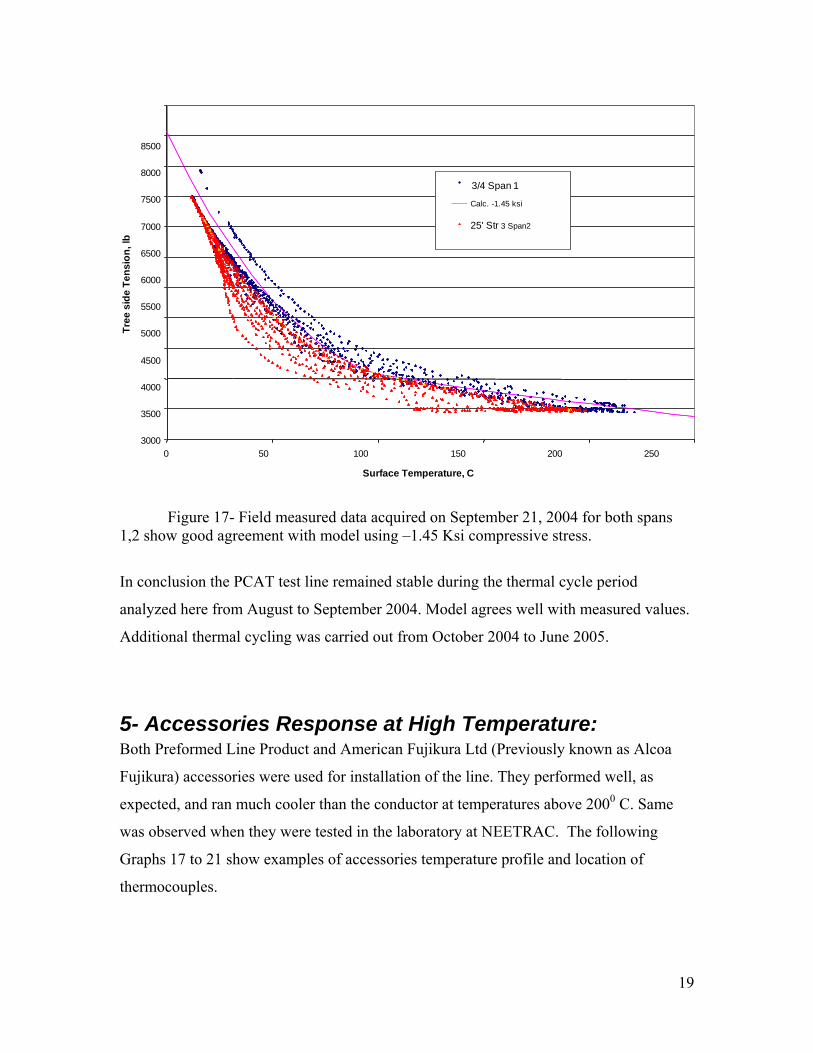
19
Figure 17- Field measured data acquired on September 21, 2004 for both spans
1,2 show good agreement with model using –1.45 Ksi compressive stress.
In conclusion the PCAT test line remained stable during the thermal cycle period
analyzed here from August to September 2004. Model agrees well with measured values.
Additional thermal cycling was carried out from October 2004 to June 2005.
5- Accessories Response at High Temperature: Both Preformed Line Product and American Fujikura Ltd (Previously known as Alcoa
Fujikura) accessories were used for installation of the line. They performed well, as
expected, and ran much cooler than the conductor at temperatures above 2000 C. Same
was observed when they were tested in the laboratory at NEETRAC. The following
Graphs 17 to 21 show examples of accessories temperature profile and location of
thermocouples.
3000
3500
4000
4500
5000
5500
6000
6500
7000
7500
8000
8500
0 50 100 150 200 250
Surface Temperature, C
Tree
sid
e Te
nsio
n, lb
3/4 Span 1
Calc. -1.45 ksi
25' Str 3 Span2

20
5-1 PLP Accessories: Temperature profiles of suspension, dead end and splice were measured, figures 19.
Figure 18 - Suspension System schematics showing thermocouples (TC) locations) , the inner rod TC location is shown in the image it is very close to conductor- the 1700C is its temperature during a 3000 C cycle
0
50
100
150
200
8/16/2
004 9
:36
8/16/2
004 2
1:36
8/17/2
004 9
:36
8/17/2
004 2
1:36
8/18/2
004 9
:36
8/18/2
004 2
1:36
8/19/2
004 9
:36
8/19/2
004 2
1:36
8/20/2
004 9
:36
Time of the day
Tem
pera
ture
, C
Conductor surface T
PLP THERMOLIGNTM Suspension T
0
50
100
150
200
8/16/2
004 9
:36
8/16/2
004 2
1:36
8/17/2
004 9
:36
8/17/2
004 2
1:36
8/18/2
004 9
:36
8/18/2
004 2
1:36
8/19/2
004 9
:36
8/19/2
004 2
1:36
8/20/2
004 9
:36
Time of the day
Tem
pera
ture
, C
Conductor surface T
PLP THERMOLIGNTM Suspension T
TC locationsTC locations
Figure 19 shows PLP THERMOLIGNTM SUSPENSION System temperature measured on the surface of the inner rod during a long time high temperature cycle- other location TC was not active.

21
Figure 20- Schematics of thermocouples location on PLP THERMOLIGNTM DEAD END and SPLICE. Image to the right shows location of the two thermocouples- temperatures of 190 and 1050 C were the highest when conductor was cycled to 3000 C.
TC1
TC2
TC1
TC2
TC 1TC2
TC 1TC2

22
High temperature cycle: The PLP accessories temperature profile was measured during a 3000 C single
cycle.- see figure 22:
Figure 21- PLP THERMOLIGNTM SPLICE and DEAD END ran cool, maximum temperature was below 1300 C when conductor was cycled to 2100 C
0
50
100
150
200
250
8/16/2004
10:48
8/16/2004
20:24
8/17/2004
6:00
8/17/2004
15:36
8/18/2004
1:12
8/18/2004
10:48
8/18/2004
20:24
8/19/2004
6:00
8/19/2004
15:36
8/20/2004
1:12
Time of the day
Tem
pera
ture
, C
Conductor SurftemperaturePLP Splice TC1
PLP Splice TC2
PLP DE TC1
PLP DE TC2
Figure 22- Temperature profile of PLP dead end, splice and suspension during 3000 C cycle of ACCR 1272 conductor. Some of the accessories temperature values was higher than 1500 C because of the location of the thermocouples very close to the conductor- explained below

23
The splice temperature was 1900 C and the suspension temperature was 1700 C
because thermocouples were placed on the inner rod first layer close to conductor.
When the thermocouple was placed on the second rod layer mid way along the axial
length of second layer of rods splice temperature dropped to 1050 C. Dead end
temperature was lower, 950 C (thermocouple placed on first layer of rod adjacent to
second layer and 650 C (thermocouple placed on second layer of rods mid way along
the axial length of the second layer of rods. The following images show location of
thermocouples.
5-2 Alcoa Accessories:
Both compression splice and dead ends temperatures were below 1050 C during
conductor exposure to temperatures above 2000 C- see Figure 22. They show no
problem during continued thermal cycling since October 2004.
Figure 22- Alcoa compression splice and dead end temperature during one cycle; both ran very cool when conductor was at or above 2000 C
0
50
100
150
200
250
8/16/2004 8:24
8/16/2004 20:2
4
8/17/2004 8:24
8/17/2004 20:2
4
8/18/2004 8:24
8/18/2004 20:2
4
8/19/2004 8:24
8/19/2004 20:2
4
8/20/2004 8:24
Time of the day
Tem
pera
ture
, C
Conductor SurftemperatureAlcoa DE TC1
Alcoa DE TC2
Alcoa Splice TC1
TC1
TC2
TC1
TC2
TC1TC2 TC1TC2

24
High temperature cycle: The Alcoa dead end and splice remained cool, below 1200 C when conductor was cycled
to 3000 C.
All 1272 installed accessories behaved normally during thermal cycling of the conductor
to above 2000 C. Post thermal cycle conductor and accessories are being evaluated at
NEETRAC.
6- Ampaciy and Thermal Rating of Conductor 6-1 Ampacity Prediction using IEEE Model: The IEEE Standard 738-1993-was used to predict conductor temperature during cycling.
The thermal cycle details are in Table 2. Weather conditions for constant current and
wind were used in the model; Figure 24 shows an example of steady state, high
0
100
200
300
400
6/7/05
4:48 A
M
6/7/05
5:16 A
M
6/7/05
5:45 A
M
6/7/05
6:14 A
M
6/7/05
6:43 A
M
6/7/05
7:12 A
M
6/7/05
7:40 A
M
6/7/05
8:09 A
M
6/7/05
8:38 A
M
6/7/05
9:07 A
M
6/7/05
9:36 A
M
Time of the day
Tem
pera
ture
, C
Alcoa Dead End Temperature near conductor Alcoa Splice temperature near conductor Alcoa Splice temperature at surfaceCore temperature for surviving thermocouple
Figure 23- temperature profile of Alcoa dead end and splice during thermal cycling of the conductor to 3000 C

25
temperature cycle data used in the model. Table 3 gives selective steady state data at
each wind speed while Figure 25 plots measured current VS predicted one at conductor
temperatures around 2000 C; agreement is very good. Conductor emissivity, ε was
measured at ORNL in 2003 and reported to be around 0.347 and used in the model.
0
1000
2000
3000
8/13/2004
12:00
8/13/2004
16:48
8/13/2004
21:36
8/14/2004
2:24
8/14/2004
7:12
8/14/2004
12:00
8/14/2004
16:48
8/14/2004
21:36
Time of the day
Cur
rent
, A
0
50
100
150
200
250
Con
duct
or te
mpe
ratu
re, C
and
Win
d Sp
eed,
f/s
DC Current (A)
Wind Speed (ft/s)
Conductor T
Figure 24- An example of high temperature steady state cycle conducted on ACCR 1272. Data from those cycles in August 2004 was used to predict current

26
Table 3 shows data for predicted VS measured current- IEEE Std. 738-1993 was used
Measured Ambient Wind Wind Conductor Wind Predicetd Measured Ambient Wind Wind Conductor Wind Predicetd
Current Temp. Speed Angle Temp. dirction Current Current Temp. Speed Angle Temp. dirction CurrentA C (ft/s) degrees C degrees A A C (ft/s) degrees C degrees A
0 23 0 10 23 0 0 1333 25 6 10 64 210 1141545 20 1 13 23 53 213 1344 24 7 31 61 189 1376698 20 0 30 26 10 309 1354 25 2 9 65 229 908699 21 0 21 28 331 342 1364 25 6 29 68 249 1384699 21 0 39 29 79 382 1376 25 3 4 68 224 938699 21 0 57 31 97 405 1387 25 3 11 68 151 992699 21 0 40 31 80 419 1396 25 5 15 69 235 1177699 22 0 71 34 111 463 1408 25 2 5 71 215 965700 20 0 18 27 328 327 1420 25 3 0 73 220 988700 21 0 53 29 103 362 1429 25 9 13 70 207 1390700 21 0 15 29 55 372 1439 25 11 14 70 206 1485700 21 1 68 30 108 439 1448 25 6 9 72 211 1254700 21 1 53 30 93 437 1459 25 7 14 67 206 1290700 21 0 18 33 58 448 1471 25 5 27 71 193 1319700 21 0 64 33 104 454 1480 25 6 36 66 176 1406701 21 1 60 30 100 520 1489 25 8 12 70 208 1360701 21 1 85 33 125 593 1499 25 5 12 73 208 1227701 21 0 78 33 142 446 1510 25 10 0 74 220 1283702 20 0 23 25 63 262 1520 25 13 2 72 218 1380702 21 0 30 28 10 348 1530 25 8 14 72 206 1383702 21 0 25 32 65 441 1540 25 5 38 75 182 1491706 22 0 28 35 68 485 1550 25 15 13 73 207 1646711 22 0 67 35 153 493 1561 25 13 7 75 213 1500719 22 1 38 35 182 592 1572 25 14 7 73 213 1503721 20 0 44 24 84 242 1581 25 8 1 75 221 1220727 22 1 51 35 169 621 1591 25 6 19 74 201 1361737 22 0 5 36 215 507 1601 25 8 0 77 220 1231746 22 0 41 36 269 515 1610 25 6 29 79 191 1556747 20 0 53 24 93 219 1621 25 12 0 77 220 1360756 22 0 33 37 187 522 1630 25 3 57 80 163 1370766 22 0 8 37 48 521 1639 25 8 10 77 210 1413774 22 0 74 37 114 522 1648 25 6 17 83 203 1477783 22 0 45 37 355 535 1657 25 5 56 88 276 1709791 22 1 37 37 183 636 1666 26 2 2 82 204 1085801 22 1 51 38 169 576 1674 26 6 6 87 180 1316810 22 0 45 38 175 557 1683 26 5 5 87 227 1228819 22 0 59 39 251 566 1692 26 11 11 89 227 1665827 22 0 68 39 152 564 1699 26 6 6 92 207 1405837 22 0 15 40 55 578 1709 26 7 7 94 235 1476844 22 0 47 40 267 574 1717 26 8 8 95 237 1518853 22 0 44 40 84 577 1728 26 8 8 96 238 1575862 22 0 47 40 173 585 1737 26 6 6 94 197 1419870 22 0 79 41 141 596 1746 26 5 5 91 269 1303877 22 1 19 41 201 640 1758 26 5 5 93 193 1314887 22 1 19 42 201 643 1772 26 3 3 96 197 1208895 22 1 24 43 196 632 1785 26 1 1 103 200 1264904 22 1 10 43 210 639 1798 26 5 5 99 215 1366914 22 1 54 44 166 671 1809 26 10 10 97 206 1659924 22 1 14 44 206 649 1825 26 8 8 103 237 1587936 22 1 5 44 215 643 1837 29 2 54 182 94 1951946 22 1 30 45 200 656 1837 26 12 12 105 224 1857956 22 1 40 45 180 766 1849 26 8 8 105 215 1657966 22 2 17 46 203 741 1859 26 5 5 107 234 1380975 22 3 16 45 204 810 1869 26 5 5 110 222 1450985 22 1 33 46 187 769 1879 26 4 4 110 218 1349998 22 1 27 46 193 745 1886 26 8 8 110 251 1651
1010 22 3 54 46 166 945 1889 21 0 88 197 132 18841020 22 0 36 47 184 693 1893 26 3 3 115 246 13631032 23 2 17 48 203 774 1899 30 1 25 208 245 18921045 23 1 12 47 232 697 1899 29 1 1 214 221 19231055 23 4 3 48 217 788 1900 26 9 9 116 217 17821066 23 3 29 49 191 913 1908 26 1 1 117 291 13761076 23 2 2 50 222 737 1910 21 1 45 203 355 19251089 23 2 16 51 214 805 1914 26 4 4 120 232 14131097 23 1 12 51 232 754 1922 26 4 4 121 238 14171107 23 2 13 52 207 803 1929 26 5 5 121 231 14721119 23 2 1 51 221 754 1936 26 5 5 126 208 15581127 23 1 26 55 246 844 1946 26 6 6 126 239 16621139 23 1 2 56 222 812 1953 26 3 3 127 193 14491150 23 0 2 56 152 816 1962 26 11 127 224 1446

27
ACCR 1272 Conductor was rated at 2229 amps continuous at 2100 C and at 2402 amps
emergency at 2400 C. The data shows the conductor was sometimes exposed to
temperature higher than 240C and current above 2400 amps
6-2 IEEE VS CIGRE’ Ampacity Model: The CIGRE’ 1997 model was used to compute current and to compare with the IEEE Std
736 used above- both programs were provided by the Valley Group Rate kit software.
There are small differences in the method of calculations and literature indicates that the
Figure 25- All Predicted VS measured current; IEEE Std 738 shows better agreement at temperatures above 10000 C.
y = 1.0003x - 255.18R2 = 0.9231
0
1000
2000
3000
0 1000 2000 3000
Measured DC Current, amps.
Pred
icet
d C
urre
nt, A
mps
. AmpacityLinear (Ampacity)
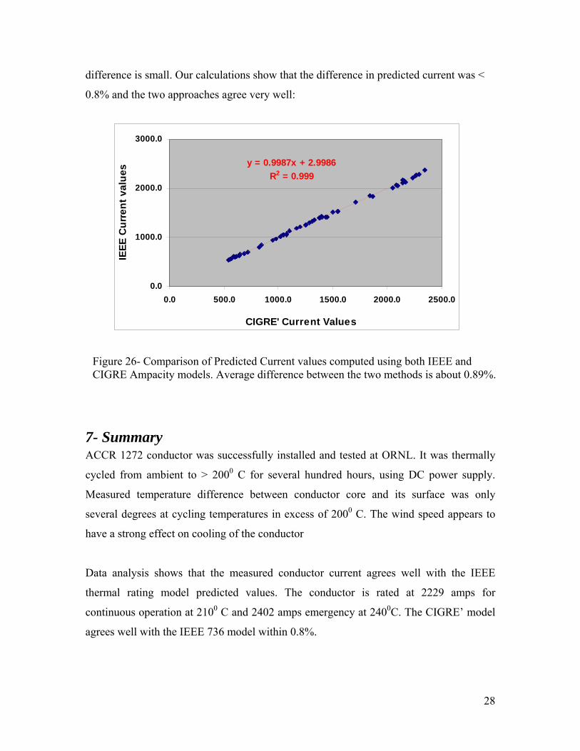
28
difference is small. Our calculations show that the difference in predicted current was <
0.8% and the two approaches agree very well:
7- Summary ACCR 1272 conductor was successfully installed and tested at ORNL. It was thermally
cycled from ambient to > 2000 C for several hundred hours, using DC power supply.
Measured temperature difference between conductor core and its surface was only
several degrees at cycling temperatures in excess of 2000 C. The wind speed appears to
have a strong effect on cooling of the conductor
Data analysis shows that the measured conductor current agrees well with the IEEE
thermal rating model predicted values. The conductor is rated at 2229 amps for
continuous operation at 2100 C and 2402 amps emergency at 2400C. The CIGRE’ model
agrees well with the IEEE 736 model within 0.8%.
y = 0.9987x + 2.9986R2 = 0.999
0.0
1000.0
2000.0
3000.0
0.0 500.0 1000.0 1500.0 2000.0 2500.0
CIGRE' Current Values
IEEE
Cur
rent
val
ues
Figure 26- Comparison of Predicted Current values computed using both IEEE and CIGRE Ampacity models. Average difference between the two methods is about 0.89%.

29
The conductor sag was stable during and after thermal cycling. Measured line tension
agrees well with values computed using the strain summation method.
Both PLP and AFL accessories ran cool, < 1200 C and show no visual damage.
Conductor was de- installed in June 2005, and sent to NEETRAC for testing and
evaluation.

30
8- Appendix 8-1 Conductor Specs
Conductor Specs Conductor Physical Properties Designation 1272-T13 Stranding 54/19 kcmils kcmil 1272 mm2 644.5 Diameter Individual Core in 0.092 Individual Aluminum in 0.153
Core Core diameter tolerance
In in
0.46 +/- 0.005
Total Diameter Total diameter tolerance in +/- 0.014
Area Al in2 0.999 Total Area in2 1.126 Weight lbs/ linear ft 1.392 Breaking Strength Core Lbs 23, 622 Aluminum Lbs 20,055 Complete Cable 000's lbs 43,677 Modulus Core Msi 31.4 Aluminum Msi 8.0 Complete Cable Msi 10.6 Thermal Elongation Core 6 Aluminum 23 Complete Cable 17 Heat Capacity Core W-sec/ft-C 28 Aluminum W-sec/ft-C 520
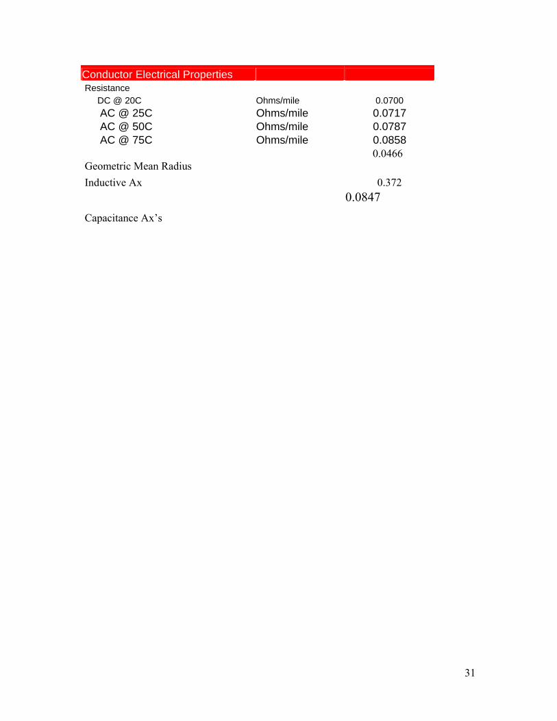
31
Conductor Electrical Properties Resistance DC @ 20C Ohms/mile 0.0700 AC @ 25C Ohms/mile 0.0717 AC @ 50C Ohms/mile 0.0787 AC @ 75C Ohms/mile 0.0858
Geometric Mean Radius 0.0466
Inductive Ax 0.372
Capacitance Ax’s
0.0847

This page is intentionally left blank.

Appendix A.4
ACCR 675-TW Kcmil Report

This page is intentionally left blank.
1
Composite Conductor Field Trial Summary Report: ORNL ACCR 675-TW Kcmil
Installation Date November 2003 Field trial Location Oak Ridge, Tennessee, USA
Organization Oak Ridge National Laboratory Point of Contact John Stovall, ORNL Installation Date: November 2003 Conductor Installed ACCR 675-TW Length of line: 2,400 feet (731 meters) Conductor diameter 0.901 inch, (22.9 mm) Voltage 400 VDC Ruling span length 600 feet, (183 meters) Structure Type Steel Poles Instrumentation: (1) Load cell
(2) Current, voltage (3) Weather station (4) Sag (5) Thermocouples in conductor at 25 different locations. (6) Thermocouples in accessories at 50 locations.
Suspension Hardware Preformed Line Product, THERMOLIGNTM Suspension TLS-675TW-CE
Termination Hardware Splice Jumper
Alcoa Compression Dead End B9085-C Alcoa Full Tension Splice, B9095-D Alcoa Compression Terminal Connector- B9102-D
Insulator type Polymer Dampers Alcoa Stockbridge Dampers- 1705-7 Results and Measurements Full range of temperature tests from 30oF – 412oF (0oC –
240oC) with currents ranging from 0 to 1500 amps • Sag-temperature from -10oC – 240oC • SAG after 300 hrs exposure at high temperature • SAG after over 26 cycles from RT to 240 C (464 F) • Accessory temperature profile after repeated thermal
cycles • Measured / predicted thermal rating • Conductor and accessory testing after thermal cycles
Acknowledgement: This material is based upon work supported by the U.S. Department of Energy under Award No. DE-FC02-02CH11111. Any opinions, findings or recommendations expressed in this material are those of the authors and do not necessarily reflect the views of the U.S. Department of Energy. 3M Copyright, 2004

2
Table of Contents Acknowledgement: ......................................................................................... 1 Abstract: .......................................................................................................... 3 1 -Background................................................................................................. 4 2- Installation and Conductor Stringing ......................................................... 6
2-1 Overview............................................................................................... 6
2-2 Installation details: ................................................................................ 6
2-3- CAT-1 Instrumentation: ...................................................................... 8
2- 4 Conductor and Accessories Temperature Measurements:................... 9
2-5 Controls ............................................................................................... 10
2-6 Accessories: ........................................................................................ 10
3- Thermal Cycles and High Temperature Exposure: .................................. 11 4- Measured and Predicted Line Tension and Sag: ...................................... 13 5- Additional Conductor Field Test data ...................................................... 15 6- Accessories Response at High Temperature: ........................................... 17
6-1 PLP Accessories: ................................................................................ 17
6-2 Alcoa Accessories:.............................................................................. 18
7- Ampacity and Thermal Rating of Conductor ........................................... 19 8- Post ORNL Conductor and Accessories Evaluation ................................ 20
8-1 Conductor tensile tests: ....................................................................... 20
8-2 Conductor Stress-strain:...................................................................... 21
8-3 Conductor resistance test: ................................................................... 23
8-4 Connector tensile tests: ....................................................................... 24
8-5 PLP Suspension: ................................................................................. 25
8-6 Connector Microscopic Examination: ................................................ 25
9- Summary................................................................................................... 26 10- Appendix ................................................................................................ 27
10-1 Conductor Specs (Table 1)................................................................ 27
10-2 Detailed Resistance Data: ................................................................. 28
10-3 Emissivity Measurements: ................................................................ 30

3
Abstract: Under DOE funding Agreement No. DE-FC02-02CH11111, ORNL jointly with
TVA installed the 3M ACCR 675TW Conductor on a high temperature test line. The
conductor was installed with commercial hardware developed for ACCR conductors.
The line was 1200 feet (365 meters) long, and the ruling span was 600 feet (183 meters).
Installation of the line was completed on November 6, 2003. The line was fully
instrumented with (1) thermocouples in the conductor and accessories, (2) a CAT-1
system to measure tension and (3) a full weather station.
Oak Ridge National Laboratory subjected the line to severe thermal cycling up to
240 C and extended times under high temperature load. Analyzed sag values agreed with
predicted models. Sag-temperature-current characteristics are predictable after repeated
thermal cycles. Current values agreed with IEEE thermal rating prediction model.
After the line was taken down both conductor and accessories were tested and
the results show that they maintained their strength with no degradation or damage. There
was no change in electrical conductivity of the conductor.

4
1 -Background
Reliable high temperature performance is one of the key requirements for
implementing new high temperature-low sag conductors. It is imperative to demonstrate
in the field that the conductor and accessories can operate safely at high-temperature,
under thermal cycling and without degradation. It is also important to demonstrate that
the sag-temperature-current characteristics can be predicted after repeated thermal cycles.
Installation and operation of the composite conductor in field trials is typically not
well suited for deliberately testing elevated temperature cycling because the thermal load
is not easily controlled or predicted. The factors leading to high-temperature excursions
include: line current loading under N-1 or N-2 contingencies, emergency conditions,
wind, and solar exposure. Depending on these conditions, it can take a year or more for
the conductor to experience a single emergency load to temperature greater than 200 C.
High-temperature exposure and thermal cycling with excursions of the conductor
and accessories can be more easily achieved on a test line that operates at low voltage
with a controlled current. Such a test line is able to approximately simulate forty years of
emergency conditions in three months by implementing sufficient emergency cycles
where the conductor temperature exceeds the rating temperature of 210oC, (410oF).
ORNL has built a fully instrumented low-voltage test line to evaluate the high-
temperature operation of 3M ACCR conductors. Line instrumentations include
mechanical tension, full weather station with anemometer, voltage, current, laser sensor
to measure sag, and temperature thermocouples in multiple locations on the conductor
and accessories.
This report summarizes ACCR 675TW conductor installation, testing and analysis
at ORNL and post thermal cycling examination of the ACCR conductor and accessories.

5
ACCR 675 TW
Aerial view of the line
Towers
ACCR 675 TW
Aerial view of the line
Towers
ACCR 675 TW
Aerial view of the line
Towers
ACCR 675 TW
Aerial view of the line
Towers

6
2- Installation and Conductor Stringing 2-1 Overview A two span test line was constructed on the grounds of the Oak Ridge National
Laboratory in Oak Ridge, Tennesse, as a part of a Department of Energy program. Oak
Ridge National Laboratory subcontracted the line engineering and construction to the
Tennessee Valley Authority, (TVA). The test line (Figure 2) consists of two 600 feet
(183 meters) spans between a steel suspension pole and two guyed dual steel dead end
poles. The test conductor forms a loop connected to a DC power supply located at one
end of the line. Thermocouples were installed along the test conductor and on dead end,
suspension and splice hardware to measure the temperature of these components during
and after periods of high temperature operation.
2-2 Installation details: The installation of the 675 TW ACCR followed the IEEE 524 installation guideline for
overhead transmission conductors. The standard applies with the following requirements:
Figure 2- Line Layout and PCAT –1 system

7
The only conductor stringing method recommended is the tension method. It is important
that bending of the composite conductor during installation be carefully estimated to
avoid damaging the composite core. If the combination of bending and tension exceeds
the allowable core strength it could damage the conductor. Therefore stringing blocks and
bull wheels are selected to keep the combined loads well below conductor core strength.
Table 2 specifies 28” diameter stringing blocks and 36” diameter or larger bull wheels to
meet such criteria. Lined blocks are recommended for use with ACCR. Other installation
procedure and hardware are very similar to those used for either ACSR or ACSS. A PLP
Distribution Grip was used to pull the conductor to sag and to install full tension splices.
Sagging procedures are very similar to that of ACSR, the load cells on the CAT-1 System
was used to verify the final sag tensions of the conductor. It is important to allow
sufficient length of conductor to apply the permanent Alcoa dead end connector and
assembly. The conductor grip was placed on the conductor 12 to 15 feet from the
connection point to the insulator string. After the final sag tension was set, the dead ends
were installed onto the ACCR.
Table 1- Installation hardware and Procedure Comparison
YesYesRunning ground
YesYesGrounding clamps
YesYesReel stands
YesYesCable cutter
Yes (48” drums)YesCable spool
Distribution grips, DGAnyConductor grip
YesYesSock splice
YesYesDrum Puller
Yes ( 54”)YesBull wheels
Yes ( 28”)YesStringing blocks
ACCRACSRInstallation Equipment
YesYesRunning ground
YesYesGrounding clamps
YesYesReel stands
YesYesCable cutter
Yes (48” drums)YesCable spool
Distribution grips, DGAnyConductor grip
YesYesSock splice
YesYesDrum Puller
Yes ( 54”)YesBull wheels
Yes ( 28”)YesStringing blocks
ACCRACSRInstallation Equipment
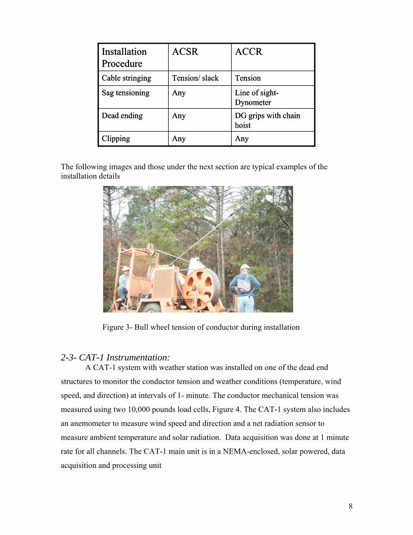
8
The following images and those under the next section are typical examples of the installation details
2-3- CAT-1 Instrumentation:
A CAT-1 system with weather station was installed on one of the dead end
structures to monitor the conductor tension and weather conditions (temperature, wind
speed, and direction) at intervals of 1- minute. The conductor mechanical tension was
measured using two 10,000 pounds load cells, Figure 4. The CAT-1 system also includes
an anemometer to measure wind speed and direction and a net radiation sensor to
measure ambient temperature and solar radiation. Data acquisition was done at 1 minute
rate for all channels. The CAT-1 main unit is in a NEMA-enclosed, solar powered, data
acquisition and processing unit
Figure 3- Bull wheel tension of conductor during installation
AnyAnyClipping
DG grips with chain hoist
AnyDead ending
Line of sight-Dynometer
AnySag tensioning
TensionTension/ slackCable stringing
ACCRACSRInstallation Procedure
AnyAnyClipping
DG grips with chain hoist
AnyDead ending
Line of sight-Dynometer
AnySag tensioning
TensionTension/ slackCable stringing
ACCRACSRInstallation Procedure
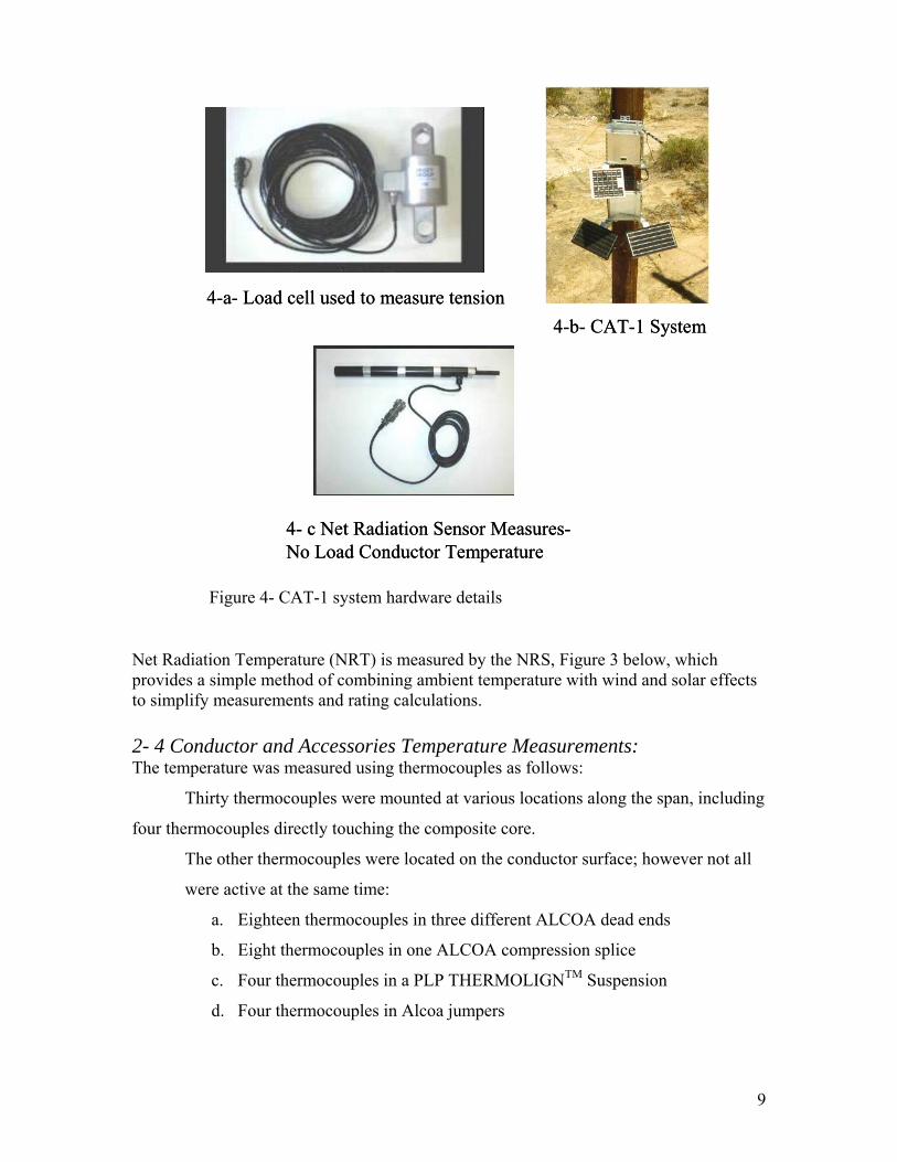
9
Net Radiation Temperature (NRT) is measured by the NRS, Figure 3 below, which provides a simple method of combining ambient temperature with wind and solar effects to simplify measurements and rating calculations. 2- 4 Conductor and Accessories Temperature Measurements: The temperature was measured using thermocouples as follows:
Thirty thermocouples were mounted at various locations along the span, including
four thermocouples directly touching the composite core.
The other thermocouples were located on the conductor surface; however not all
were active at the same time:
a. Eighteen thermocouples in three different ALCOA dead ends
b. Eight thermocouples in one ALCOA compression splice
c. Four thermocouples in a PLP THERMOLIGNTM Suspension
d. Four thermocouples in Alcoa jumpers
4-a- Load cell used to measure tension4-b- CAT-1 System
4- c Net Radiation Sensor Measures-No Load Conductor Temperature
4-a- Load cell used to measure tension4-b- CAT-1 System
4- c Net Radiation Sensor Measures-No Load Conductor Temperature
Figure 4- CAT-1 system hardware details

10
A separate data acquisition system was used to collect the information from the
thermocouples. To accommodate the multiplicity of points along the conductor and
withstand the accumulated voltage drop, many fiber-connected, isolated measurement
nodes were used. A thermocouple measurement node is fabricated using a multiplexer
(ICPCON I-7018) and a RS-485-to-fiber modem (B&B FOSTCDR). Up to eight
thermocouples are monitored per node. The node requires 120 VAC power and is data
connected through a duplex fiber optic network. The multiplexer, fiber modem, and a
power supply are housed in a Preformed Line Product enclosure.
2-5 Controls The line was operated under constant either current and / or constant conductor
temperature with thermal cycles lasting from less than one hour to several days.
2-6 Accessories: Compression type dead end and splice made by Alcoa were installed. The
following specific parts were used: (1) Four ALCOA compression dead ends; part/
drawing # B9085- those dead ends consist of both direct core gripping parts and
conductor gripping sleeve. (2) One ALCOA full tension splice part# B9095-D; it has the
same design as the dead-end for both direct core gripping and conductor. (3) Two high-
temperature commercial PLP THERMOLIGNTM Suspensions, (240 C conductor
temperature), Part # TLS-675TW-CE. (4) Six Alcoa terminal connectors; part# B9102-
D; those are all
Aluminum sleeve parts (5) Four Alcoa Stockbridge dampers, part# 1705-7
5- a compression splice
5-b Terminal connector / jumper installation
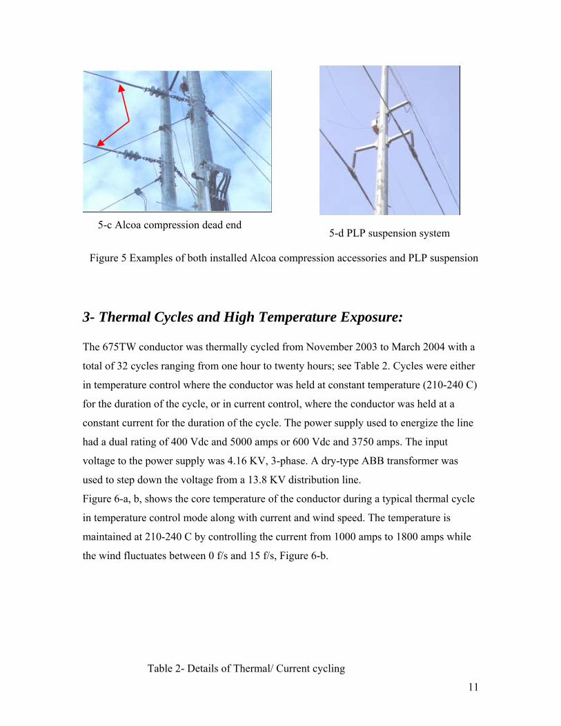
11
3- Thermal Cycles and High Temperature Exposure: The 675TW conductor was thermally cycled from November 2003 to March 2004 with a
total of 32 cycles ranging from one hour to twenty hours; see Table 2. Cycles were either
in temperature control where the conductor was held at constant temperature (210-240 C)
for the duration of the cycle, or in current control, where the conductor was held at a
constant current for the duration of the cycle. The power supply used to energize the line
had a dual rating of 400 Vdc and 5000 amps or 600 Vdc and 3750 amps. The input
voltage to the power supply was 4.16 KV, 3-phase. A dry-type ABB transformer was
used to step down the voltage from a 13.8 KV distribution line.
Figure 6-a, b, shows the core temperature of the conductor during a typical thermal cycle
in temperature control mode along with current and wind speed. The temperature is
maintained at 210-240 C by controlling the current from 1000 amps to 1800 amps while
the wind fluctuates between 0 f/s and 15 f/s, Figure 6-b.
Table 2- Details of Thermal/ Current cycling
Figure 5 Examples of both installed Alcoa compression accessories and PLP suspension
5-c Alcoa compression dead end 5-d PLP suspension system
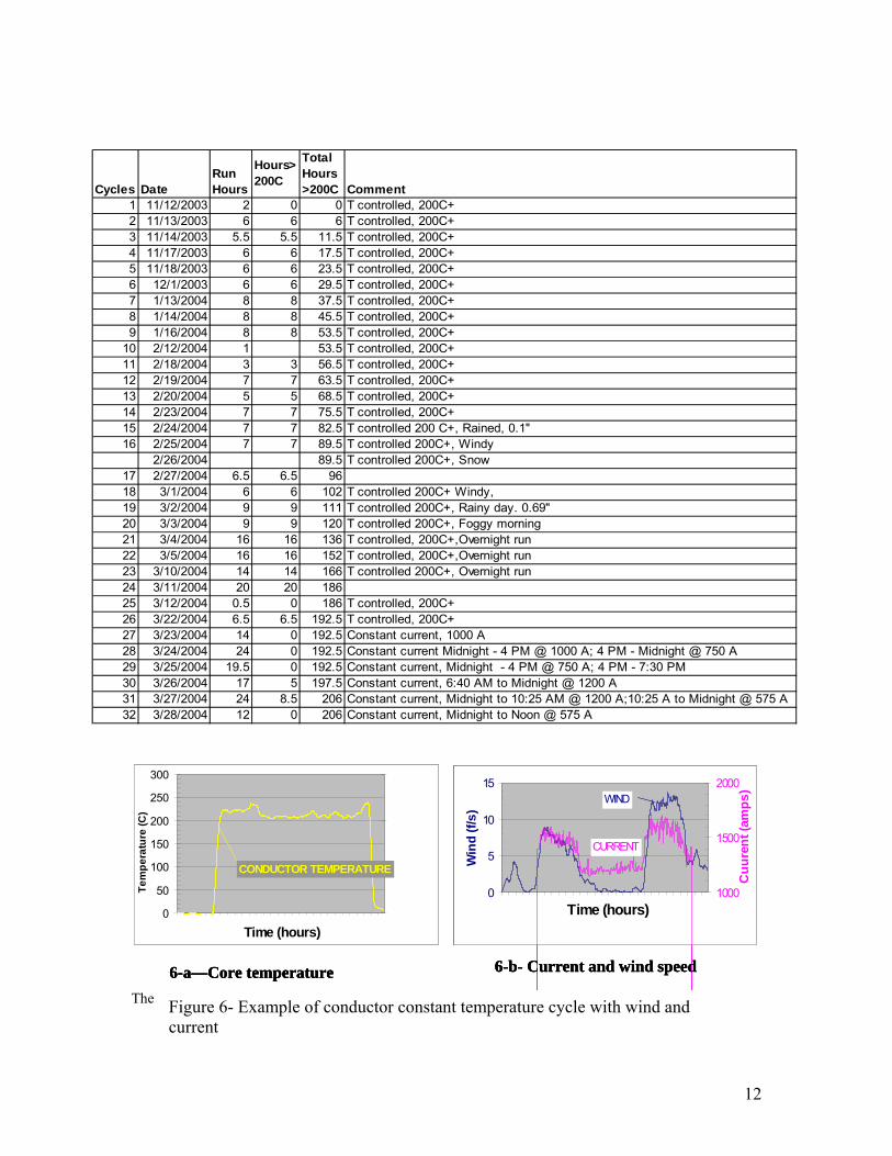
12
The next graph, Figure 7, shows the conductor subjected a constant current of 1,200 amps
Cycles DateRun Hours
Hours>200C
Total Hours>200C Comment
1 11/12/2003 2 0 0 T controlled, 200C+2 11/13/2003 6 6 6 T controlled, 200C+3 11/14/2003 5.5 5.5 11.5 T controlled, 200C+4 11/17/2003 6 6 17.5 T controlled, 200C+5 11/18/2003 6 6 23.5 T controlled, 200C+6 12/1/2003 6 6 29.5 T controlled, 200C+7 1/13/2004 8 8 37.5 T controlled, 200C+8 1/14/2004 8 8 45.5 T controlled, 200C+9 1/16/2004 8 8 53.5 T controlled, 200C+
10 2/12/2004 1 53.5 T controlled, 200C+11 2/18/2004 3 3 56.5 T controlled, 200C+12 2/19/2004 7 7 63.5 T controlled, 200C+13 2/20/2004 5 5 68.5 T controlled, 200C+14 2/23/2004 7 7 75.5 T controlled, 200C+15 2/24/2004 7 7 82.5 T controlled 200 C+, Rained, 0.1"16 2/25/2004 7 7 89.5 T controlled 200C+, Windy
2/26/2004 89.5 T controlled 200C+, Snow17 2/27/2004 6.5 6.5 9618 3/1/2004 6 6 102 T controlled 200C+ Windy, 19 3/2/2004 9 9 111 T controlled 200C+, Rainy day. 0.69"20 3/3/2004 9 9 120 T controlled 200C+, Foggy morning21 3/4/2004 16 16 136 T controlled, 200C+,Overnight run22 3/5/2004 16 16 152 T controlled, 200C+,Overnight run23 3/10/2004 14 14 166 T controlled 200C+, Overnight run24 3/11/2004 20 20 18625 3/12/2004 0.5 0 186 T controlled, 200C+26 3/22/2004 6.5 6.5 192.5 T controlled, 200C+27 3/23/2004 14 0 192.5 Constant current, 1000 A28 3/24/2004 24 0 192.5 Constant current Midnight - 4 PM @ 1000 A; 4 PM - Midnight @ 750 A29 3/25/2004 19.5 0 192.5 Constant current, Midnight - 4 PM @ 750 A; 4 PM - 7:30 PM 30 3/26/2004 17 5 197.5 Constant current, 6:40 AM to Midnight @ 1200 A31 3/27/2004 24 8.5 206 Constant current, Midnight to 10:25 AM @ 1200 A;10:25 A to Midnight @ 575 A32 3/28/2004 12 0 206 Constant current, Midnight to Noon @ 575 A
0
50
100
150
200
250
300
1 801 1601 2401Time (hours)
Tem
pera
ture
(C)
100
150
200
250
CONDUCTOR TEMPERATURE
0
5
10
15
1 801 1601 2401Time (hours)
Win
d (f/
s)
1000
1500
2000
Cuu
rent
(am
ps)
CURRENT
WIND
6-a—Core temperature 6-b- Current and wind speed
0
50
100
150
200
250
300
1 801 1601 2401Time (hours)
Tem
pera
ture
(C)
100
150
200
250
CONDUCTOR TEMPERATURE
0
5
10
15
1 801 1601 2401Time (hours)
Win
d (f/
s)
1000
1500
2000
Cuu
rent
(am
ps)
CURRENT
WIND
6-a—Core temperature 6-b- Current and wind speed
0
50
100
150
200
250
300
1 801 1601 2401Time (hours)
Tem
pera
ture
(C)
100
150
200
250
CONDUCTOR TEMPERATURE
0
5
10
15
1 801 1601 2401Time (hours)
Win
d (f/
s)
1000
1500
2000
Cuu
rent
(am
ps)
CURRENT
WIND
6-a—Core temperature 6-b- Current and wind speed
Figure 6- Example of conductor constant temperature cycle with wind and current

13
For 24 hours followed by 575 amps for another 24 hour. In this case, the conductor
temperature fluctuates between 230C and 50 C.
4- Measured and Predicted Line Tension and Sag: The following are two video frames showing the line before being energized and at
maximum sag after application of current.
Figure 7-Typical constant current cycle for 675 TW
11:29:08 – Before 11:54 – Maximum Sag
11:29:08 – Before 11:54 – Maximum Sag
Figure 8- Observation of line sag changes during current cycling
02468
101214161820
Time (hours)
win
d f/s
0
50
100
150
200
250
Con
duct
or T
emp
(C)
WIND
TEMPERATURE
1200 AMPS
575 AMPS
02468
101214161820
Time (hours)
win
d f/s
0
50
100
150
200
250
Con
duct
or T
emp
(C)
WIND
TEMPERATURE
1200 AMPS
575 AMPS

14
The sag was predicted with two methods: the Strain Summation Method to
account for the full loading history, and the more commonly used Graphic Method,
(Alcoa SAG-10). The Strain Summation Method of Sag-Tension Calculation takes
into account both creep and wind conditions as a function of time. A conductor data
file was created based on stress strain tests performed by NEETRAC on the conductor.
Compressive stresses of 0 and 1.45 Ksi were used to compute sag. Predicted sag values
appear to agree reasonably well within 2” sag value, see figure 9 and 10.
Data generated from November 2003 to March 2004, after additional 192.4 hours
exposure at > 200C is shown below in Figure 10. The data shows no change in the test
line and conductor as compared to its the initial performance in November (Figure 9).
There has been virtually no creep since Nov. 14/03; see figure 11
3M 675/TW kcmil ACCR - Nov. 14, 2003 Test
1500
1750
2000
2250
2500
2750
3000
-50 0 50 100 150 200 250 300
Avg. Core Thermocouple Temperature , ºC
Tens
ion,
lbs Road
TreeCalc -1.45 ksiCalc 0 ksi
RoadsideT reeside
3M 675/TW kcmil ACCR - Nov. 14, 2003 Test
1500
1750
2000
2250
2500
2750
3000
-50 0 50 100 150 200 250 300
Avg. Core Thermocouple Temperature , ºC
Tens
ion,
lbs Road
TreeCalc -1.45 ksiCalc 0 ksi
RoadsideT reeside
Figure 9- Measured VS predicted tension

15
5- Additional Conductor Field Test data
The next set of graphs 12, 13 show effect of both ice and rain on the conductor line
tension. Ice build up produced a 300 lbs increase in tension for about 17 hours, Figure 13.
1500
1700
1900
2100
2300
2500
2700
2900
0 50 100 150 200 250
Core Temperture, C - in Span #1 - Midspan
Tree
side
Tens
ion
Mar 26/04Nov 13/03 Fit -1.45 ksi0 ksi
1500
1700
1900
2100
2300
2500
2700
2900
0 50 100 150 200 250
Core Temperture, C - in Span #1 - Midspan
Tree
side
Tens
ion
Mar 26/04Nov 13/03 Fit -1.45 ksi0 ksi
Figure 10- Measured and predicted span tension (tree side) VS conductor core temperature after 192.4 hours above 200 C
Tens ion vs Tem p era tu re - T rees ide C ircuit U pd ated to Ap ril 5/04
0
500
1000
1500
2000
2500
3000
3500
4000
4500
-5 0 5 10 15 20 25 30 35
NRS Te mpera tu re , ºC
Tens
ion,
lbs
Instal l 0-24 hr24-40 hr40-88 hr88-109 hrNov 14Calc 24 hrCa lc Nov 14to Feb 29/04PM M ar 28/04Apr1-5/04
Tens ion vs Tem p era tu re - T rees ide C ircuit U pd ated to Ap ril 5/04
0
500
1000
1500
2000
2500
3000
3500
4000
4500
-5 0 5 10 15 20 25 30 35
NRS Te mpera tu re , ºC
Tens
ion,
lbs
Instal l 0-24 hr24-40 hr40-88 hr88-109 hrNov 14Calc 24 hrCa lc Nov 14to Feb 29/04PM M ar 28/04Apr1-5/04
Figure 11- ACCR 675 TW showing almost no creep after 192.4 hours above 200 C

16
There was no effect of rain on either conductor temperature or tension when line was
energized above 200C. The PCAT test line sag remained stable during the field trial.
High temperature was negligible.
-2
0
2
4
6
8
10
12
12 AM 12 PM 12 AM 12 PM 12 AM
Tem
pera
ture
, C
2500
2600
2700
2800
2900
3000
3100
3200
Tens
ion,
lbs.
NRS
Ambient
Treeside Circuit
Roadside Circuit
OAK RIDGE NATIONAL LABORATORYU.S. DEPARTMENT OF ENERGY
-2
0
2
4
6
8
10
12
12 AM 12 PM 12 AM 12 PM 12 AM
Tem
pera
ture
, C
2500
2600
2700
2800
2900
3000
3100
3200
Tens
ion,
lbs.
NRS
Ambient
Treeside Circuit
Roadside Circuit
OAK RIDGE NATIONAL LABORATORYU.S. DEPARTMENT OF ENERGY
-2
0
2
4
6
8
10
12
12 AM 12 PM 12 AM 12 PM 12 AM
Tem
pera
ture
, C
2500
2600
2700
2800
2900
3000
3100
3200
Tens
ion,
lbs.
NRS
Ambient
Treeside Circuit
Roadside Circuit
OAK RIDGE NATIONAL LABORATORYU.S. DEPARTMENT OF ENERGY
-2
0
2
4
6
8
10
12
12 AM 12 PM 12 AM 12 PM 12 AM
Tem
pera
ture
, C
2500
2600
2700
2800
2900
3000
3100
3200
Tens
ion,
lbs.
NRS
Ambient
Treeside Circuit
Roadside Circuit
OAK RIDGE NATIONAL LABORATORYU.S. DEPARTMENT OF ENERGY
Figure 12- Ice build up for 17 hours on ACCR 675 TW on February 15- 16, produced about 300 lbs increase in line
Rain
Rain
Figure 13- Rain on February 24, 2 hour shower (0.1”) had no effect on conductor temperature)

17
6- Accessories Response at High Temperature: Over 300 hours of high temperature operation were performed under either temperature
or current control. The line was subjected to a range of weather conditions during
thermal cycling (-10 C to 250 C, wind, rain, and ice). All accessories performed well;
maximum accessories temperature remained under 140 C as illustrated in Figures 15- 17.
6-1 PLP Accessories: PLP THERMOLIGNTM Suspension System ran under 100 C during high temperature
cycling
Figure 14- PLP THERMOLIGNTM Suspension ran cool at conductor temperature of > 2000 C
PLP Suspension System and Conductor Temperature Profile During Thermal Cycling at ORNL
0
50
100
150
200
250
3/10/0
4 12:0
0 AM
3/10/0
4 12:0
0 PM
3/11/0
4 12:0
0 AM
3/11/0
4 12:0
0 PM
3/12/0
4 12:0
0 AM
3/12/0
4 12:0
0 PM
Cycle Time
Tem
pera
ture
, C
Conductor TemperatureS1, PLP Suspen
End of inner rod TC location
TC location- S1

18
6-2 Alcoa Accessories: All Alcoa compression accessories showed normal behavior with no over heating during
conductor thermal cycling; examples are shown in figures 15 and 16.
Figure 15 Alcoa dead-end and splice temperature stayed below 100 C while conductor was cycled to above 200 C. TC locations are in green cicles; Locations 1 and 4 are for TC1 and TC2
Figure 16- Alcoa Compression terminal connector temperature- connector ran < 55 C when conductor was at 200 C
Temperature of Alcoa Dead End and Splice- ORNL ACCR 675 TW Test Line
0
50
100
150
200
250
3/10/04 7:12 A
M
3/10/04 4:48 P
M
3/11/04 2:24 A
M
3/11/04 12:00
PM
3/11/04 9:36 P
M
Cycle Time
Tem
pera
ture
, CAlcoa DE TC1 Tree side Alcoa DE TC2 Tree sideAlcoa Splice TC1 Road side Alcoa Splice TC2 Road sideConductor Temperature
TC1
TC2
TC1TC2
Active TC’s
Thermocouple on locations in red
Terminal Connector Temperature (Tree Side) during a thermal cycle of 675 TW up to > 200 C
0
50
100
150
200
250
1/13/2
004 4
:48
1/13/2
004 7
:12
1/13/2
004 9
:36
1/13/2
004 1
2:00
1/13/2
004 1
4:24
1/13/2
004 1
6:48
1/13/2
004 1
9:12
1/13/2
004 2
1:36
1/14/2
004 0
:00
Time
Tem
pera
ture
, C
CE1, Cdr Surf25ft from DE
TerminalConnector TC1
TerminalConnector TC2
TC1
TC2
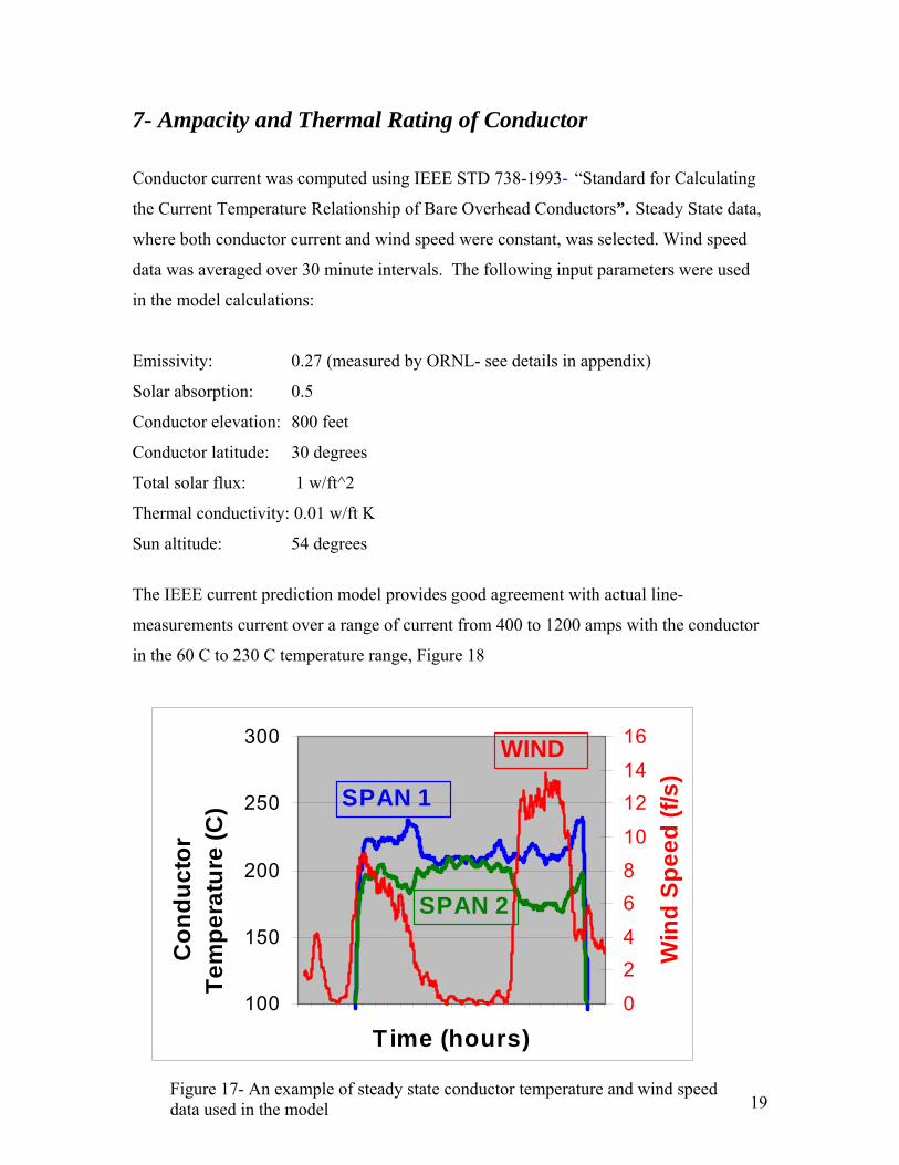
19
7- Ampacity and Thermal Rating of Conductor
Conductor current was computed using IEEE STD 738-1993- “Standard for Calculating
the Current Temperature Relationship of Bare Overhead Conductors”. Steady State data,
where both conductor current and wind speed were constant, was selected. Wind speed
data was averaged over 30 minute intervals. The following input parameters were used
in the model calculations:
Emissivity: 0.27 (measured by ORNL- see details in appendix)
Solar absorption: 0.5
Conductor elevation: 800 feet
Conductor latitude: 30 degrees
Total solar flux: 1 w/ft^2
Thermal conductivity: 0.01 w/ft K
Sun altitude: 54 degrees
The IEEE current prediction model provides good agreement with actual line-
measurements current over a range of current from 400 to 1200 amps with the conductor
in the 60 C to 230 C temperature range, Figure 18
Figure 17- An example of steady state conductor temperature and wind speed data used in the model
100
150
200
250
300
Time (hours)
Con
duct
or
Tem
pera
ture
(C)
0
24
68
10
1214
16
Win
d Sp
eed
(f/s)SPAN 1
SPAN 2
WIND

20
8- Post ORNL Conductor and Accessories Evaluation
The following tests & measurements were carried out on the conductor and accessories
after thermal cycling at ORNL:
8-1 Conductor tensile tests: Three samples from the “free-span” conductor were terminated using cast-resin
terminations. Clamps were used to preserve the as-received position of the conductor
layers until the resin cured. The sample preparation method ensures that the laboratory
tensile test loads each conductor strand in the same manner as a field overloads, and
thereby measures the in-service conductor strength. Free conductor between the end
fittings is 20 feet (6 meters).
0
500
1000
1500
2000
0 200 400 600 800 1000 1200 1400 1600 1800 2000Measured Ampacity (amps)
Pred
icte
d A
mpa
city
(am
ps)
Ambient = 9 CWind 8.4 f/sDirect 13 degTemp: 230C
Ambient = 12 CWind: 0 f/sDirect Temp: 235 C
Ambient = 6 CWind 0 f/sDirect Temp 145C
Ambient = 12 CWind :6.4 f/sDirect: 10 degTemp: 225C
Ambient = 17 CWind 0 f/sDirectTemp: 61C
Figure 18-Good agreement between Measured and predicted current. Predicted values were computed using IEEE ampacity rating steady state model
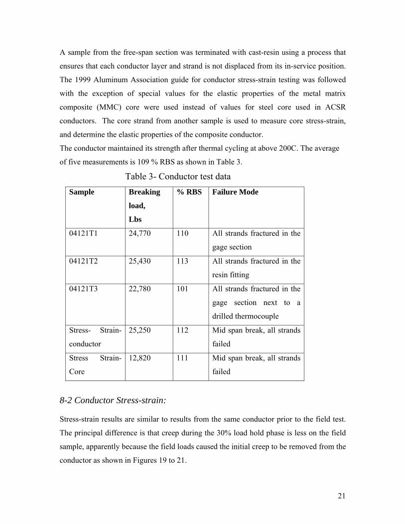
21
A sample from the free-span section was terminated with cast-resin using a process that
ensures that each conductor layer and strand is not displaced from its in-service position.
The 1999 Aluminum Association guide for conductor stress-strain testing was followed
with the exception of special values for the elastic properties of the metal matrix
composite (MMC) core were used instead of values for steel core used in ACSR
conductors. The core strand from another sample is used to measure core stress-strain,
and determine the elastic properties of the composite conductor.
The conductor maintained its strength after thermal cycling at above 200C. The average
of five measurements is 109 % RBS as shown in Table 3.
Table 3- Conductor test data Sample Breaking
load,
Lbs
% RBS Failure Mode
04121T1 24,770 110 All strands fractured in the
gage section
04121T2 25,430 113 All strands fractured in the
resin fitting
04121T3 22,780 101 All strands fractured in the
gage section next to a
drilled thermocouple
Stress- Strain-
conductor
25,250 112 Mid span break, all strands
failed
Stress Strain-
Core
12,820 111 Mid span break, all strands
failed
8-2 Conductor Stress-strain: Stress-strain results are similar to results from the same conductor prior to the field test.
The principal difference is that creep during the 30% load hold phase is less on the field
sample, apparently because the field loads caused the initial creep to be removed from the
conductor as shown in Figures 19 to 21.

22
Figure 19- Plot of raw data recorded during conductor stress-strain test (blue),
Agrees with data for conductor tested from same lot before the field test
Figure 20- Core stress-strain shows essentially no change due to field test
675 kcmil, Type 11 ACCR/TW, 3M Composite Conductor, MMC Core Stress-Strain
0
25000
50000
75000
100000
125000
150000
0.00 0.05 0.10 0.15 0.20 0.25 0.30 0.35 0.40 0.45Strain (%)
Stre
ss (p
si)
Post ORNL"As-Manufactured"
675 kcmil, Type 11 ACCR/TW 3M Composite ConductorStress-Strain Raw Test Data
0
5000
10000
15000
20000
25000
30000
0.00 0.05 0.10 0.15 0.20 0.25 0.30 0.35 0.40Strain (%)
Stre
ss (p
si)
Post ORNL Test Line"As-Manufactured" test data

23
8-3 Conductor resistance test:
Welded equalizers were installed at each end of a 22-foot long sample from the free-
span section. A second set of voltage equalizers in the form of tightly wrapped solid
copper strands are applied nominally 20 feet apart in the test section. The sample is
placed on a flat surface, and pulled with sufficient tension to remove any residual
curvature in the conductor. Tension was about 200 – 300 lb. A digital low-resistance
Ohmmeter was used to make a 4-wire resistance measurement for the conductor
section between the two voltage equalizers. A digital multi meter was used to verify
that the sample was electrically isolated.
22- a- Power connection to sample
675 kcmil Type 11 ACCR/TW 3M Composite Conductor, Combined Stress-Strain DiagramPost ORNL Test Line
0
5000
10000
15000
20000
25000
30000
0.000 0.050 0.100 0.150 0.200 0.250 0.300 0.350 0.400
Strain (%)
Stre
ss*a
rea
ratio
Initial Composite Final Composite Initial Core
Final Core Initial Aluminum Final Aluminum
Figure 21- Final stress strain plot after thermal cycling

24
Conductor resistance for an average of 5 readings on a 20 feet long sample was 0.1332
Ω/mile at 20°C; it is close to the conductor resistance of 0.1346 Ω/mile at 20° C before
thermal cycling.
8-4 Connector tensile tests:
8-4-1 Alcoa compression accessories Two dead-ends and two splices were provided with cast resin fittings at free ends
The procedure preserves the “as received” position of the conductor components, and
thereby assures that the breaking strength is the same as existed when the samples
were in service on the test span.
Both splice and dead end maintained their load carrying capability of 100% RBS or
more; details in table below
Table 4- Connector tensile tests Sample Breaking
Load, Lbs
% RBS Failure Mode
04121SP1
(Splice)
24,010 107 All strands fractured at the
resin fitting
04121SP2
(Splice)
24,530 109 All strands fractured ~5” inside
splice
04121DE1
(Dead end)
24,730 110 All strands fractured ~6” inside
dead end
04121DE2
Dead end)
22,330 99 All strands fractured ~5” inside
dead end
Figure 22- Set- up for conductor resistance measurements
post ORNL field-testing
22- b Sample-tensioning device

25
8-5 PLP Suspension: Visual examination of the suspension components showed neither fatigue nor wear
damage; conductor did not distort. Conductor segments which were inside the suspension
were pulled in tension and gave 24,740 Lbs (110% RBS) load to failure, conductor failed
in an area that was not under the suspension assembly
8-6 Connector Microscopic Examination:
One dead end and one splice were dissected using a milling machine to split the
aluminum sleeve and reveal the internal splice components. Correct installation is
verified by observing proper placement of the core grip, proper conductor preparation,
and proper injection of inhibitor compound prior to compression.
The dissections and inspections showed good workmanship for core and aluminum
insertion depth, component placement, and the crimping operation. Both conductor and
accessories gave >100% RBS. It was however noticed that the center cavity contained no
Figure 23 Tensile test data for accessories post ORNL Cycling current cycling
675/TW Post ORNL Tensile Results
0
5000
10000
15000
20000
25000
30000
0.0 0.5 1.0 1.5 2.0 2.5
Crosshead Position (inches)
Load
(lb
)
Splice 1 Splice 2 Dead end 1 Dead end 2 95% RBS Acceptance Criterrion

26
oxide inhibitor compound, showing that this step was omitted. Compound was applied
liberally on the conductor OD, so this is not a serious issue for a short-term, field test
Nevertheless installation instructions stipulate that the center cavity should be filled with
oxide inhibitor compound through an injection port. There is no evidence that the
conductor was wire-brushed prior to splice installation. AFL requires wire- brushing of
the conductor OD only in cases where the connector is installed on weathered conductor.
Proper wire brushing and the use of inhibitor compound have been reinforced in the
installation guide.
9- Summary
ACCR 675 TW conductor was installed successfully on ORNL- PCAT Line using
commercial hardware and normal installation procedures. The conductor and accessories
were thermally cycled from ambient to > 200C for several hundred hours, using DC
power supply and as high current as 1500 amps. The measured sag matched the SAG-10
prediction. Data analysis shows that the measured conductor current agrees well with the
IEEE thermal rating model predicted values. After-de installation the conductor and
accessories were tested for residual strength and degradation. Residual strength exceeded
100% RBS and neither conductor nor accessories showed any signs of damage.
Conductor resistance after cycling is equivalent to that of conductor not exposed to
thermal cycling

27
10- Appendix 10-1 Conductor Specs (Table 1)
Conductor Physical Properties Stranding 20/7 kcmils kcmil 676 Area Fraction Core % 10.25% Weight Fraction Core 12.50% Diameter indiv Core in 0.105 indiv Al in Core in 0.315 Total Diameter in 0.902 Area Al in^2 0.5309 Total Area in^2 0.5915 Weight lbs/linear ft 0.726 Breaking Strength Core lbs 11,564 Aluminum lbs 10,923 Complete Cable 000's lbs 22,487 Modulus Core msi 31.4 Aluminum msi 7.6 Complete Cable msi 10.1 Thermal Elongation Core 10-6/Co 6.35 Aluminum 10-6/Co 23.00 Complete Cable 10-6/Co 17.69 Heat Capacity Core W-sec/ft-C 13 Aluminum W-sec/ft-C 275 Conductor Electrical Properties Resistance DC @ 20C ohms/mile 0.1317

28
AC @ 25C ohms/mile 0.1348 AC @ 50C ohms/mile 0.1481 AC @ 75C ohms/mile 0.1615 Geometric Mean Radius ft 0.0355 Reactance (1 ft Spacing, 60hz) Inductive Xa ohms/mile 0.4052 Capacitive X'a ohms/mile 0.0973
10-2 Detailed Resistance Data:
NEETRAC Project No. 04-121 AVO (Biddle) DLRO, Calibration Control # CQ1097
Temperature coefficient for resistance: 0.0036
Resistance measurement on a 20' gage section of 675 ACCR/TW setup in the tensile room on the MTS frame, welded equalizers, pulled to ~200 lbs tension w/a come-a-long
These readings taken manually 10/14/04 @ 9:54 am
Conductor Temperature:
21.5 deg C
Test Section: 20.000 ft Resistance Readings 506.8 µΩ At 21.5 deg C
506.7 µΩ At 21.5 deg C 506.7 µΩ At 21.5 deg C
506.73 µΩ At 21.5 deg C
Ω/ft: 2.5337E-05
Ohm/ft At 21.5 deg C
Ω/ft: 2.5200E-05
At 20.0 deg C
Ω/mi 0.13378 Ohm/mi At 21.5 deg C Ω/mi @ 20C: 0.13306 At 20.0 deg C
These readings taken manually 10/14/04 @ 10:32 am
Conductor 21.8 deg C

29
Temperature: Test Section: 20.000 ft Resistance Readings 507.4 µΩ At 21.8 deg C
507.4 µΩ At 21.8 deg C 507.3 µΩ At 21.8 deg C
507.37 µΩ At 21.8 deg C
Ω/ft: 2.5368E-05
Ohm/ft At 21.8 deg C
Ω/ft: 2.5231E-05
At 20.0 deg C
Ω/mi 0.13394 Ohm/mi At 21.8 deg C Ω/mi @ 20C: 0.13322 At 20.0 deg C
These readings taken manually 10/14/04 @ 10:53 am
Conductor Temperature:
21.8 deg C
Test Section: 20.000 ft Resistance Readings 507.4 µΩ At 21.8 deg C
507.4 µΩ At 21.8 deg C 507.3 µΩ At 21.8 deg C
Average 507.37 µΩ At 21.8 deg C
Ω/ft: 2.5368E-05
Ohm/ft At 21.8 deg C
Ω/ft: 2.5231E-05
At 20.0 deg C
Ω/mi 0.13394 Ohm/mi At 21.8 deg C Ω/mi @ 20C: 0.13322 At 20.0 deg C
These readings taken manually 10/14/04 @ 2:34 pm
Conductor Temperature:
21.9 deg C
Test Section: 20.000 ft Resistance Readings 507.4 µΩ At 21.8 deg C
507.4 µΩ At 21.8 deg C 507.5 µΩ At 21.8 deg C
Average 507.43 µΩ At 21.8 deg C
Ω/ft: 2.5372E-05
Ohm/ft At 21.9 deg C

30
Ω/ft: 2.5235E-05
At 20.0 deg C
Ω/mi 0.13396 Ohm/mi
At 21.9 deg C
Ω/mi @ 20C: 0.13324 At 20.0 deg C
These readings taken manually 10/14/04 @ 4:52 pm
Conductor Temperature:
21.7 deg C
Test Section: 20.000 ft Resistance Readings 506.9 µΩ At 21.8 deg C
507.0 µΩ At 21.8 deg C 506.9 µΩ At 21.8 deg C
Average 506.93 µΩ At 21.8 deg C
Ω/ft: 2.5347E-05
Ohm/ft At 21.65
deg C
Ω/ft: 2.5210E-05
At 20.0 deg C
Ω/mi 0.13383 Ohm/mi
At 21.65
deg C
Ω/mi @ 20C: 0.13311 At 20.0 deg C
Errors: Gage length
0.05%
Instrument 0.20% Temperature
0.18%
RMS Error: 0.27%
Average, all readings: 0.13317 Ω/mi At 20.0 deg C 3M nominal 0.13170 Ohm/
miAt 20.0 deg C
10-3 Emissivity Measurements: Oak Ridge National Laboratory measured various 3M composite conductor emissivity
using IR Imaging. A calibrated IR Camera and Mikron M305 Blackbody calibration
source were used. Graph 24 shows the hardware used; the calibrated black body target
was multiplied by various emissivity values until a good fit occurs with the conductor
received signal. Such fit yielded an average emissivity value of 0.27 within +- 2%
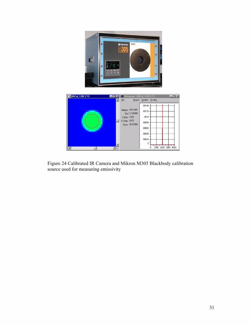
31
Figure 24 Calibrated IR Camera and Mikron M305 Blackbody calibration source used for measuring emissivity

This page is intentionally left blank.

Appendix B
Variability of Conductor Temperature in a Two Span Test Line

This page is intentionally left blank.

Document for CIGRE TF 12-6 (B2), October 21, 2004
Variability of Conductor Temperature in a Two Span Test Line
Tapani O. Seppa The Valley Group, Inc.
Robert Mohr The Valley Group, Inc.
Herve Deve 3M Company
John P. Stovall Oak Ridge National
Laboratory Background A large number of prior reports have indicated substantial temperature variability within a single span in test lines and significant variation of temperature between point measurements in adjacent spans. More anecdotal evidence, e.g. in the discussion records of the Proceedings of the IEEE Panel on Dynamic Line Ratings on July 20-21, 1982, indicate that, at high temperature, longitudinal temperature variation of 10-25oC had been observed in a single span. Accurate documentation of such variation is generally not available. It is also generally recognized that the tension and sags of a line section between two dead-ends should be a function of the average temperature of the conductor. Observations have generally shown a good correlation between measured temperatures and sags, but high quality data for comparisons has typically not been available. Because the high temperature conductor tests at the Oak Ridge PCAT facility are extremely well instrumented, these tests can provide answers to the above questions. Powerline Conductor Accelerated Testing Facility (PCAT) Testing Facility Description: The Powerline Conductor Accelerated Testing facility (PCAT) at Oak Ridge National Laboratory (ORNL) in Oak Ridge, Tennessee is an outdoor facility for thermal stress and age characterization tests of power line conductors, [1,2]. The facility includes a 2MW DC power supply fed by a 13.8kV/4160V transformer which can vary the loading of the conductor under test up to 400 Vdc and 5000 Adc.
Figure 1: Aerial view of PCAT facility
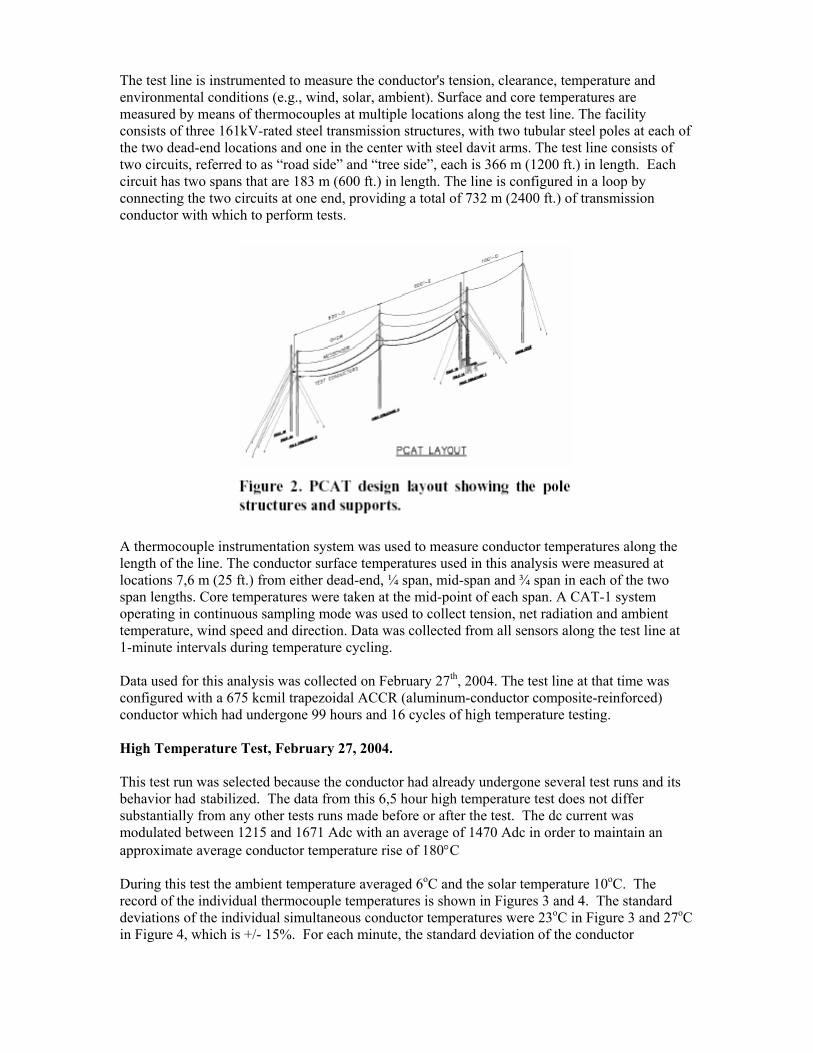
The test line is instrumented to measure the conductor's tension, clearance, temperature and environmental conditions (e.g., wind, solar, ambient). Surface and core temperatures are measured by means of thermocouples at multiple locations along the test line. The facility consists of three 161kV-rated steel transmission structures, with two tubular steel poles at each of the two dead-end locations and one in the center with steel davit arms. The test line consists of two circuits, referred to as “road side” and “tree side”, each is 366 m (1200 ft.) in length. Each circuit has two spans that are 183 m (600 ft.) in length. The line is configured in a loop by connecting the two circuits at one end, providing a total of 732 m (2400 ft.) of transmission conductor with which to perform tests.
A thermocouple instrumentation system was used to measure conductor temperatures along the length of the line. The conductor surface temperatures used in this analysis were measured at locations 7,6 m (25 ft.) from either dead-end, ¼ span, mid-span and ¾ span in each of the two span lengths. Core temperatures were taken at the mid-point of each span. A CAT-1 system operating in continuous sampling mode was used to collect tension, net radiation and ambient temperature, wind speed and direction. Data was collected from all sensors along the test line at 1-minute intervals during temperature cycling. Data used for this analysis was collected on February 27th, 2004. The test line at that time was configured with a 675 kcmil trapezoidal ACCR (aluminum-conductor composite-reinforced) conductor which had undergone 99 hours and 16 cycles of high temperature testing. High Temperature Test, February 27, 2004. This test run was selected because the conductor had already undergone several test runs and its behavior had stabilized. The data from this 6,5 hour high temperature test does not differ substantially from any other tests runs made before or after the test. The dc current was modulated between 1215 and 1671 Adc with an average of 1470 Adc in order to maintain an approximate average conductor temperature rise of 180°C During this test the ambient temperature averaged 6oC and the solar temperature 10oC. The record of the individual thermocouple temperatures is shown in Figures 3 and 4. The standard deviations of the individual simultaneous conductor temperatures were 23oC in Figure 3 and 27oC in Figure 4, which is +/- 15%. For each minute, the standard deviation of the conductor

temperatures was calculated and then these were averaged over the test period. These standard deviations characterize the systematic variation. This report does not analyze the dependence of conductor temperature on the weather variables. Such analysis is presented in [3] which concluded that the measured conductor temperatures were relatively close to those predicted by IEEE 738 standard and the measured weather parameters and line current. The temperature data shows that the conductor temperatures were generally higher at midspan. This could be anticipated because at maximum conductor temperatures the midspan clearance of the conductor was 7,0-7,3 m (23-24 ft.) from ground, compared to 12,5-12,8 m (41-42 ft.) from the ground at the thermocouples nearest to the ends of the span. Such a height difference can cause a substantial difference in the wind velocity. Because of the relatively small diameter of the compact conductor, the core temperatures were typically only 3-4oC higher than surface temperatures. The comparison between “treeside” and “roadside” circuits shows significant temperature differences from time to time. A comparison between average temperatures is shown Figure 5. The difference is most likely caused by the difference in wind speeds on different sides of the narrow line corridor. The conductor temperatures indicate that the average effective wind speed around noon was slightly below 0,6 m/s on the “treeside” and about 0,8 m/s on the “roadside” span. Comparison to the measured wind speed at 12:00 Noon (1,77 m/s (5.8 ft/sec) at 24 degrees angle) would imply a conductor temperature of 152oC. This compares reasonably well with the measured average temperatures of 176oC and 165oC for tree and road side spans respectively. Earlier and later tests indicate similar relative variations (also in the opposite direction) between the two sides of the test line. The conductor temperature showed a span wise trend of higher temperatures in the middle of the span than at the ends of the span, as shown in Figure 6. The calibrated relationship between the conductor tension measurements and the average temperature are shown in the calibration curves of Figures 7 and 8. Note that the measured tension/temperature relationship shows a certain amount of hysteresis. This can be explained by a combination of two processes:
1. The knee point of a layered conductor is actually a range of temperatures. The knee point of the 675 kcmil ACCR conductor falls between 95-110oC. Manufacturing tolerances make it impossible for all the wires in the outside layers to reach zero tensile stress simultaneously. When passing through the knee point range, each strand must settle in relationship to the others.
2. There is substantial longitudinal variability in the conductor temperature. This means that there are compressive and tensile stresses in the outside layers which will try to move the outside wires longitudinally. Such stresses are constrained by the friction between the core and the outside layers.
As a result, the tension-temperature equilibrium shown in Figures 6 and 7 will exhibit a clear, albeit minor, hysteretic behavior.

Figures 9 and 10 show the relationship between the measured average temperature of the two circuits and the conductor temperatures derived based on tension measurements. The close correlation between the measurements proves conclusively that the conductor tension is a function of the average temperature of the line section. Conclusions:
1. During the test, the average temperature rise was about 180oC as compared to solar temperature, and the longitudinal variation of individual temperature rises along the two spans was +/-40oC, i.e. about 22%.
2. The 22% variation is approximately one half systematic variations (some locations show,
on the average, higher temperatures than others) and approximately one half random variations.
3. Because the temperature rise tends to be highest at locations with the lowest clearance to
ground, conductor rating measurements should be based on temperatures at such locations, unless other locations are more sheltered from wind.
4. Conductor tension follows quite accurately the average temperatures of the line sections.
5. When conductor temperature excursions exceed the kneepoint temperature,
tension/temperature relationship indicates a moderate hysteresis.
Acknowledgement
This material is based upon work supported by the U.S. Department of Energy under Award No. DE-FC02-02CH11111. Any opinions, findings or recommendations expressed in this material are those of the authors and do not necessarily reflect the views of the U.S. Department of Energy. The Power-line Conductor Accelerated Test Facility is operated by Oak Ridge National Laboratory for the U.S. Department of Energy, Office of Electric Transmission and Distribution. The Oak Ridge National Laboratory is managed by UT-Battelle, LLC for the U.S. Department of Energy under contract no. DE-AC05-00OR22725. References [1] ORNL Reporter, No 40, August 2002 [2] http://www.ornl.gov/sci/oetd/about.htm [3] "Weather Observation and Thermal Ratings in a Short, High Temperature Test Line", Herve Deve, 3M. Presented at the IEEE TP&C Panel on Selection of Weather Parameters for Overhead Lines, Denver 2004.
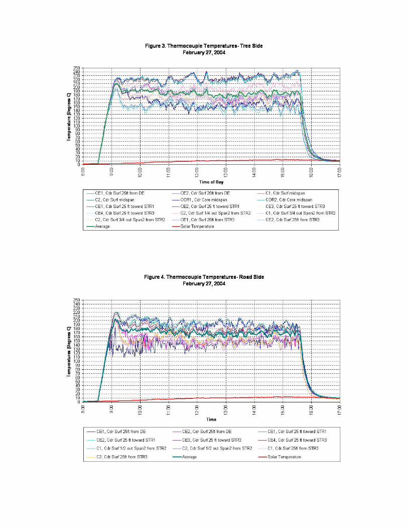


Appendix C.1
DOE Peer Review Presentation – May 20, 2002

This page is intentionally left blank.

Aluminum Composite Conductor Testsfor the 3M Company
U.S. Department of EnergyTransmission Reliability ProgramPeer Review
Doubletree Hotel Crystal CityArlington, VAMay 20, 2002
John P. StovallOak Ridge National Laboratory
ORNL Project TeamD. Tom RizyRoger A. KisnerJohn P. Stovall
Brendan J. KirbyCharles BruceLynn DegenhardtRandall Wetherington
OAK RIDGE NATIONAL LABORATORY
U.S. DEPARTMENT OF ENERGY

2
ORNL Project SummaryAluminum Composite Conductor Tests for the 3M Company
• New Project, start date March 25, 2002• FY 2002 Budget – $620,000• Duration – 3 years• Goal
− To accelerate the commercial acceptance of the aluminum composite conductor
• Objective− To verify the aluminum composite conductor and
accessory performance by providing performance data based upon field testing including through testing at rated conductor temperatures
OAK RIDGE NATIONAL LABORATORY
U.S. DEPARTMENT OF ENERGY

3
ORNL CRADA with 3M Company
• Project Plan (ORNL CRADA Tasks)
− Task 1 – Thermal Cycling Conductor Tests• ORNL to build outdoor test facility, install conductor, test at high-
current / low-voltage / rated conductor temperature of 210°C for approximately 500 thermal cycles
• Facility name is “PCAT” - Powerline Conductor Accelerated Test• Will measure sag, tension, current and conductor temperature to
quantify conductor performance• Will test 3 conductor sizes – 477, 795 and 1272 kcmil ACCR
− Task 2 – Measurement and Analysis for Conductor Field Tests • 3M to select several utility field test sites and install conductor with
host utilities• ORNL to provide monitoring hardware as necessary, collect and
analyze field data
OAK RIDGE NATIONAL LABORATORY
U.S. DEPARTMENT OF ENERGY

4
Bringing a New Conductor to Market
New ConductorDesign
Laboratory Testing of Conductor Strands
Laboratory Testing of Conductor
Field Demonstrations
Outdoor Test Line at Rated Temperature
(PCAT)
Time to commercialization
Additional testing will accelerate time to commercialization
NewStep
Task 1
Task 2
OAK RIDGE NATIONAL LABORATORY
U.S. DEPARTMENT OF ENERGY

5
PCAT - Profile View of Outdoor Test Line
• Test of conductor and accessories
Splices, suspension clamps, dead-end clamps
Task 1
OAK RIDGE NATIONAL LABORATORY
U.S. DEPARTMENT OF ENERGY

6
PCAT - Plan View of Outdoor Test Line
Existing 13.8-kV distribution line
Instrumentation shed
Dc Power supply
Test conductors
Test Line = 1200 ft. ( two 600 ft. spans )
Existing communications line (telephone or internet)
~7 ft.
60 - 80 ft steel poles
Trans-former
SplicesSuspension
clampsDead-end clamps
The temperature of the test conductors and accessories will measured using thermocouples
Conductor tension will be measured
using a CAT-1 system
Task 1
OAK RIDGE NATIONAL LABORATORY
U.S. DEPARTMENT OF ENERGY

7
PCAT - Thermal Cycling Will VerifyNew Conductor Performance and Existing Models
PCAT
Measuring All Parameters
Conductor Current/Temperature
Model
IEEE Std 738
Sag/Tension Data
Aluminum AssociationStress-StrainTensile Creep
ConductorSag
Conductor Temperature
Measured Parameters
CalculatedParameters
CalculatedParameters
Verification over entire temperature operating range
Task 1
OAK RIDGE NATIONAL LABORATORY
U.S. DEPARTMENT OF ENERGY

8
PCAT - Equipment needed for Outdoor Test Line
• dc power supply− Electronics van to house dc power
supply
• Standard transformer− 2.5 MVA, 13.8-kV / 4160V
• Line structures− Five standard utility steel poles,
guys, shield wires, etc.
• Instrumentation− CAT-1 (tension), thermocouples,
weather station, cable height meter
− Enclosure for instrumentation ~ 10 ft. X 12 ft.
Task 1
Surplus dc Power Supply Acquired600 Vdc, 3500 A or 400 Vdc, 5000 A
Transrex Model ISR 2294
OAK RIDGE NATIONAL LABORATORY
U.S. DEPARTMENT OF ENERGY

9
TVA Providing Line Structure Design
• TVA will perform the line structure design− Key design issue is horizontal deflection of
the steel poles− PLS-CADD (Power Line Systems - Computer
Aided Design and Drafting) being used
• ORNL will purchase purchase line structure materials and hardware from TVA
• Combination of TVA and ORNL Utility Services will install test line
Task 1
OAK RIDGE NATIONAL LABORATORY
U.S. DEPARTMENT OF ENERGY
Preliminary line design

10
Task 1 Project ScheduleTask Apr 02 May 02 Jun 02 Jul 02 Aug 02 Sep 02 Oct 02 Nov 02 Dec 02
1.Design/Construct Test Facility
1. a Power equipment
1. b Instrumentation system
2. Install 477 conductor
3. Test 477 conductor
4. Analyze and evaluate tests
Evaluation Guidelines• Project Performance
− The CRADA between 3M Company and ORNL has formalized and documented the management system; and the planning and coordination of accomplishments and future plans. The CRADA has established the public/private partnership, cost-sharing and technology transfer mechanism. In addition, ORNL has sought the assistance of TVA in the design and construction of the outdoor test line.
• Project Value− Project contributes directly to the following goal:− Department of Energy's FY 2002 Budget Request to Congress - “Power System Reliability
will develop advanced transmission technologies that promote competitive markets, ensure system reliability, increase network capacity for large scale, long distance power transfers, and …”
OAK RIDGE NATIONAL LABORATORY
U.S. DEPARTMENT OF ENERGY

Appendix C.2
DOE Peer Review Presentation – January 29, 2004

This page is intentionally left blank.

OAK RIDGE NATIONAL LABORATORYU. S. DEPARTMENT OF ENERGY
National Transmission Technology Research Center
U.S. Department of EnergyTransmission Reliability ProgramPeer Review
Marriott at Metro Center775 12th Street, N.W.Washington, D.C. 20005
January 29, 2004
John P. StovallOak Ridge National Laboratory
ORNL Project TeamD. Tom RizyRoger A. KisnerJohn P. Stovall

OAK RIDGE NATIONAL LABORATORYU. S. DEPARTMENT OF ENERGY
National Transmission Grid Study
One of the 51 Recommendations
“DOE will develop national transmission-technology testing facilities that encourage partnering with industry to demonstrate advanced technologies in controlled environments.
Working with TVA, DOE will create an industry cost-shared transmission line testing center at DOE ’s Oak Ridge National Laboratory (with at least a 50 percent industry cost share).*”
*National Transmission Grid Study, U.S. DOE, May 2002 www.ntgs.doe.gov

OAK RIDGE NATIONAL LABORATORYU. S. DEPARTMENT OF ENERGY
National Transmission Technology Research Center
T1Outdoor PCAT
Powerline Conductor Accelerated Test Facility
T2Indoor PCAT
Powerline ConductorAccelerated Test Facility
T3PCOT
(TVA lines)
Powerline ConductorOperational Test Facility
T4TPET
(Substation)
Transmission Power Electronics Test Facility

OAK RIDGE NATIONAL LABORATORYU. S. DEPARTMENT OF ENERGY
T1. PCAT - Profile View of Outdoor Test LinePCAT - Powerline Conductor Accelerated Test
Initial Concept for Test FacilityDeveloped with 3M Company
Splices, suspension clamps, dead-end clamps
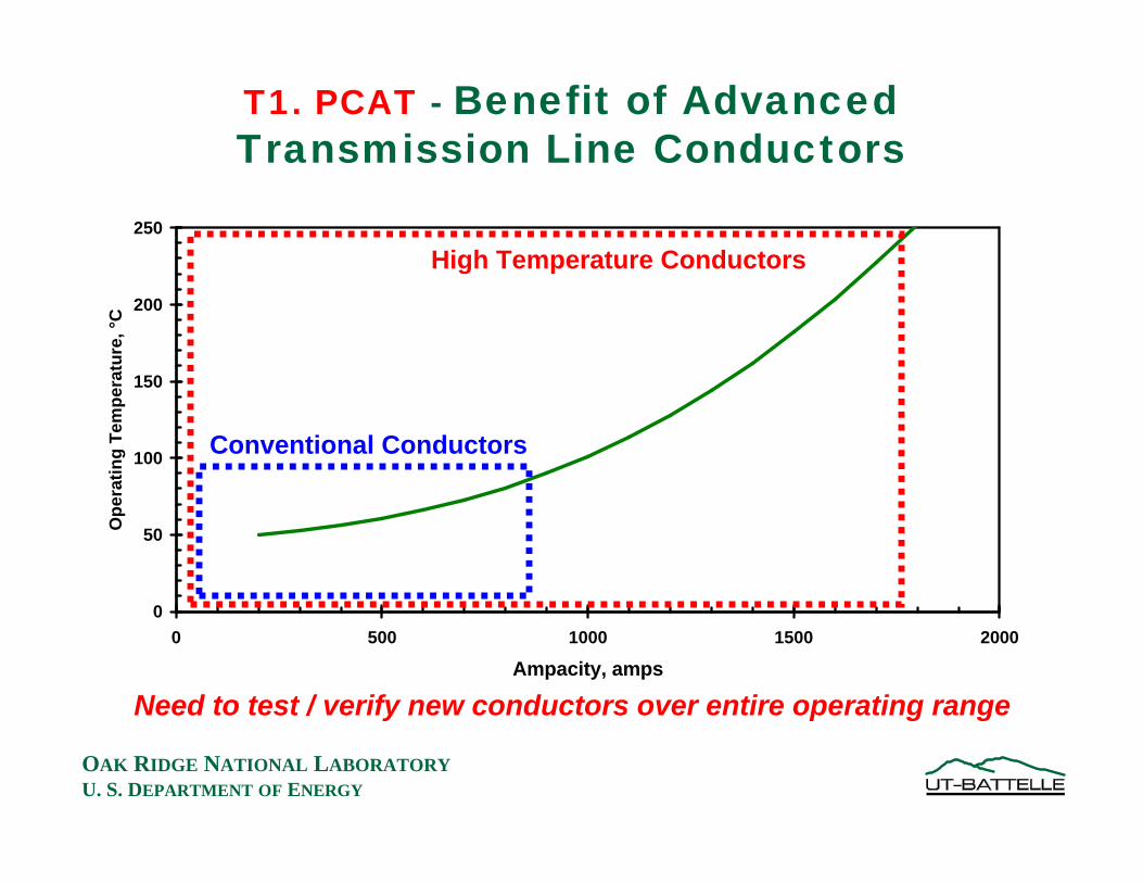
OAK RIDGE NATIONAL LABORATORYU. S. DEPARTMENT OF ENERGY
0
50
100
150
200
250
0 500 1000 1500 2000
Ampacity, amps
Op
erat
ing
Tem
per
atu
re, °
CT1. PCAT - Benefit of Advanced Transmission Line Conductors
Need to test / verify new conductors over entire operating range
Conventional Conductors
High Temperature Conductors

OAK RIDGE NATIONAL LABORATORYU. S. DEPARTMENT OF ENERGY
T1. PCAT - Project Schedule
FY 2003 FY 2004FY 2002
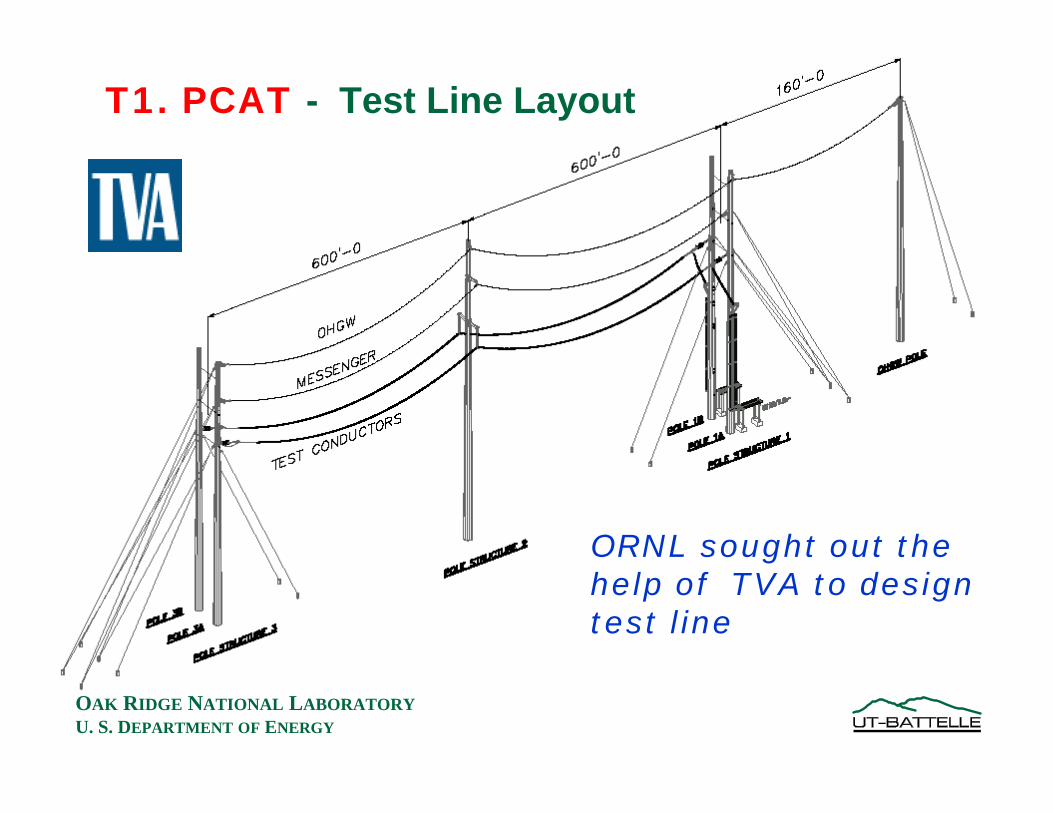
OAK RIDGE NATIONAL LABORATORYU. S. DEPARTMENT OF ENERGY
T1. PCAT - Test Line Layout
ORNL sought out the help of TVA to design test line

OAK RIDGE NATIONAL LABORATORYU. S. DEPARTMENT OF ENERGY
T1. PCAT - TVA Constructed the Test Line and Installed the First 3M Test Conductor in July 2002

OAK RIDGE NATIONAL LABORATORYU. S. DEPARTMENT OF ENERGY
T1. PCAT – A surplus power supply wasrefurbished and tested in June / July 2002

OAK RIDGE NATIONAL LABORATORYU. S. DEPARTMENT OF ENERGY
Structure #3, Dead-end
Structure #2, Suspension
Structure #1, Dead-end
Structure #0, Fiberglass Pole
T1. PCAT - Line Structures and Test Hardware
• Two 600 ft. spans with 2400 ft. of test conductor
• Four dead-end clamps
• Two suspension clamps
• Two splices
• Conductor clamps
• Jumpers and terminal pads

OAK RIDGE NATIONAL LABORATORYU. S. DEPARTMENT OF ENERGY
Structure #1 and #3 are dead-ends Structure #2, Suspension
T1. PCAT - Transmission Structures

OAK RIDGE NATIONAL LABORATORYU. S. DEPARTMENT OF ENERGY
T1. PCAT - CAT-1 Transmission Line Monitoring System
Wind Speed and direction
Net Radiation Sensor measuring combination of ambient, wind speed, wind direction and solar radiation on conductor equivalent
Electronics, solar panel, and ambient temperature
Load cells measuring conductor temperature

OAK RIDGE NATIONAL LABORATORYU. S. DEPARTMENT OF ENERGY
National Transmission Technology Research Center
PCAT – Powerline Conductor Accelerated Test Facility
PCAT

OAK RIDGE NATIONAL LABORATORYU. S. DEPARTMENT OF ENERGY
T1. PCAT – Facility Capabilities• Powerline Conductor Accelerated TestingØ Accelerated life-cycle testingØ Initially will test new 3M conductorsØ Will test other new conductor designs and
existing conductors
• Thermal Cycle Testing§ Controlled testing§ Conductor and accessories§ Up to 300oC
• Capabilities§ 2400 feet of conductor§ 2 – 600 foot spans§ Low Voltage, 0 to 400 Vdc§ High Current, up to 5,000 Adc

OAK RIDGE NATIONAL LABORATORYU. S. DEPARTMENT OF ENERGY
T1. PCAT - Measurements• Conductor/accessory temperature
Ø Direct contact on surface or conductor coreØ 128 thermocouples availableØ 40 to 80 thermocouples used for testing
• Applied current and voltageØ Measured by power supply
• Conductor sagØ Laser at mid-span #1 on tree side circuit
• Conductor tensionØ Load cells on both circuits
• WeatherØ Ambient temperature, wind speed, wind directionØ Conductor net radiation sensor
• PC-based data acquisition systemØ 10 second pollingØ 1 minute data archive

OAK RIDGE NATIONAL LABORATORYU. S. DEPARTMENT OF ENERGY
T1. PCAT – Constant Current TestCurrent, 6/9/2003
0
200
400
600
800
1000
1200
12:00 AM 6:00 AM 12:00 PM 6:00 PM 12:00 AM
Cu
rren
t, d
c am
ps
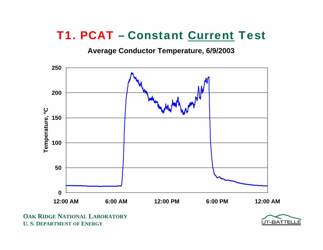
OAK RIDGE NATIONAL LABORATORYU. S. DEPARTMENT OF ENERGY
Average Conductor Temperature, 6/9/2003
0
50
100
150
200
250
12:00 AM 6:00 AM 12:00 PM 6:00 PM 12:00 AM
Tem
per
atu
re, º
CT1. PCAT – Constant Current Test

OAK RIDGE NATIONAL LABORATORYU. S. DEPARTMENT OF ENERGY
T1. PCAT – Constant Current TestWindspeed, 6/9/2003
0
2
4
6
8
10
12
14
16
12:00 AM 6:00 AM 12:00 PM 6:00 PM 12:00 AM
Win
dsp
eed
, fp
s

OAK RIDGE NATIONAL LABORATORYU. S. DEPARTMENT OF ENERGY
T1. PCAT – Constant Current TestConductor Tension, 6/9/2003
1000
1500
2000
2500
3000
3500
4000
12:00 AM 6:00 AM 12:00 PM 6:00 PM 12:00 AM
Ten
sio
n, l
bs.
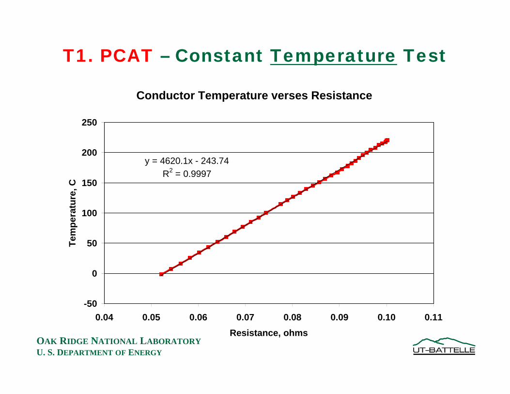
OAK RIDGE NATIONAL LABORATORYU. S. DEPARTMENT OF ENERGY
T1. PCAT – Constant Temperature Test
Conductor Temperature verses Resistance
y = 4620.1x - 243.74R2 = 0.9997
-50
0
50
100
150
200
250
0.04 0.05 0.06 0.07 0.08 0.09 0.10 0.11
Resistance, ohms
Tem
per
atu
re, C

OAK RIDGE NATIONAL LABORATORYU. S. DEPARTMENT OF ENERGY
T1. PCAT – Constant Temperature TestCircuit Resistance, 1/16/2004
0
0.02
0.04
0.06
0.08
0.1
0.12
12:00 AM 6:00 AM 12:00 PM 6:00 PM 12:00 AM
Res
ista
nce
, oh
ms

OAK RIDGE NATIONAL LABORATORYU. S. DEPARTMENT OF ENERGY
T1. PCAT – Constant Temperature TestCurrent, 1/16/2004
0
200
400
600
800
1000
1200
1400
1600
12:00 AM 6:00 AM 12:00 PM 6:00 PM 12:00 AM
Cu
rren
t, d
c am
ps

OAK RIDGE NATIONAL LABORATORYU. S. DEPARTMENT OF ENERGY
T1. PCAT – Constant Temperature TestConductor Core Temperature, 1/16/2004
-50
0
50
100
150
200
250
12:00 AM 6:00 AM 12:00 PM 6:00 PM 12:00 AM
Tem
per
atu
re, º
C

OAK RIDGE NATIONAL LABORATORYU. S. DEPARTMENT OF ENERGY
T1. PCAT – Constant Temperature TestWind Speed, 1/16/2004
0
2
4
6
8
10
12
12:00 AM 6:00 AM 12:00 PM 6:00 PM 12:00 AM
Win
d S
pee
d, f
ps

OAK RIDGE NATIONAL LABORATORYU. S. DEPARTMENT OF ENERGY
T1. PCAT – Constant Temperature TestConductor Tension, 1/16/2004
1000
1500
2000
2500
3000
3500
12:00 AM 6:00 AM 12:00 PM 6:00 PM 12:00 AM
Ten
sio
n, l
bs.

OAK RIDGE NATIONAL LABORATORYU. S. DEPARTMENT OF ENERGY
T1. PCAT – Constant Temperature TestConductor Sag, 1/16/2004
10
12
14
16
18
20
22
12:00 AM 6:00 AM 12:00 PM 6:00 PM 12:00 AM
Sag
, ft.
MeasuredCalculated

OAK RIDGE NATIONAL LABORATORYU. S. DEPARTMENT OF ENERGY
T1. PCAT – Thermal/Mechanical CyclingCircuit Resistance, 10/2/2003
0
0.02
0.04
0.06
0.08
0.1
0.12
0.14
0.16
12:00 AM 6:00 AM 12:00 PM 6:00 PM 12:00 AM
Res
ista
nce
, oh
ms

OAK RIDGE NATIONAL LABORATORYU. S. DEPARTMENT OF ENERGY
T1. PCAT – Thermal/Mechanical CyclingCurrent, 10/2/2003
0
200
400
600
800
1000
1200
1400
12:00 AM 6:00 AM 12:00 PM 6:00 PM 12:00 AM
Cu
rren
t, d
c am
ps
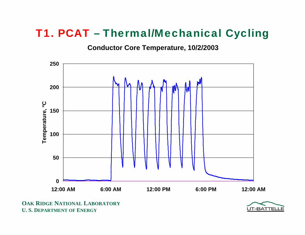
OAK RIDGE NATIONAL LABORATORYU. S. DEPARTMENT OF ENERGY
T1. PCAT – Thermal/Mechanical CyclingConductor Core Temperature, 10/2/2003
0
50
100
150
200
250
12:00 AM 6:00 AM 12:00 PM 6:00 PM 12:00 AM
Tem
per
atu
re, º
C

OAK RIDGE NATIONAL LABORATORYU. S. DEPARTMENT OF ENERGY
T1. PCAT – Thermal/Mechanical CyclingWind Speed, 10/2/2003
0
5
10
15
20
25
12:00 AM 6:00 AM 12:00 PM 6:00 PM 12:00 AM
Win
d S
pee
d, f
ps

OAK RIDGE NATIONAL LABORATORYU. S. DEPARTMENT OF ENERGY
T1. PCAT – Thermal/Mechanical CyclingConductor Tension, 10/2/2003
1000
1500
2000
2500
3000
3500
4000
4500
12:00 AM 6:00 AM 12:00 PM 6:00 PM 12:00 AM
Ten
sio
n, l
bs.

OAK RIDGE NATIONAL LABORATORYU. S. DEPARTMENT OF ENERGY
T1. PCAT – Thermal/Mechanical CyclingConductor Sag, 10/2/2003
6
8
10
12
14
16
18
12:00 AM 6:00 AM 12:00 PM 6:00 PM 12:00 AM
Sag
, ft.

OAK RIDGE NATIONAL LABORATORYU. S. DEPARTMENT OF ENERGY
T1. PCAT – Current / Temperature RampCurrent, 11/14/2003
0
200
400
600
800
1000
1200
1400
1600
8:00 AM 10:00 AM 12:00 PM 2:00 PM 4:00 PM
Cu
rren
t, d
c am
ps
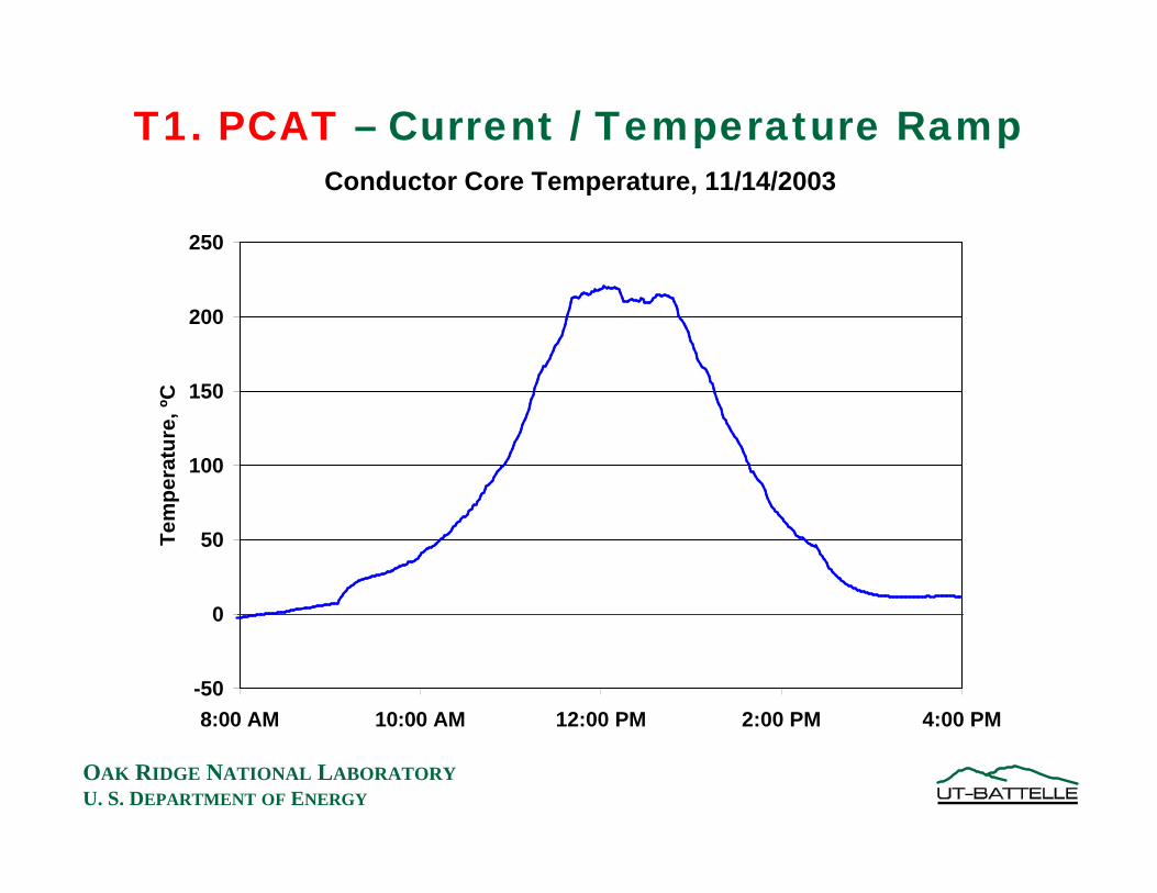
OAK RIDGE NATIONAL LABORATORYU. S. DEPARTMENT OF ENERGY
T1. PCAT – Current / Temperature RampConductor Core Temperature, 11/14/2003
-50
0
50
100
150
200
250
8:00 AM 10:00 AM 12:00 PM 2:00 PM 4:00 PM
Tem
per
atu
re, º
C

OAK RIDGE NATIONAL LABORATORYU. S. DEPARTMENT OF ENERGY
T1. PCAT – Ramp and HoldConductor Temperature, 10/23/2003
0
50
100
150
200
250
12:00 AM 6:00 AM 12:00 PM 6:00 PM 12:00 AM
Tem
per
atu
re, C

OAK RIDGE NATIONAL LABORATORYU. S. DEPARTMENT OF ENERGY
Click To Start Movie of Conductor Sag
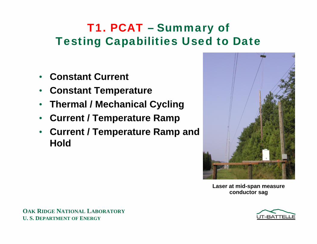
OAK RIDGE NATIONAL LABORATORYU. S. DEPARTMENT OF ENERGY
T1. PCAT – Summary ofTesting Capabilities Used to Date
• Constant Current• Constant Temperature• Thermal / Mechanical Cycling• Current / Temperature Ramp• Current / Temperature Ramp and
Hold
Laser at mid-span measure conductor sag

OAK RIDGE NATIONAL LABORATORYU. S. DEPARTMENT OF ENERGY
National Transmission Technology Research Center
Indoor PCAT – indoor Powerline Conductor Accelerated Test Facility
T2. - Indoor PCAT

OAK RIDGE NATIONAL LABORATORYU. S. DEPARTMENT OF ENERGY
T2. Indoor PCATFacility Offers Unique Capabilities
• Indoor version of outdoor Powerline Conductor Accelerated Test facility
• 54 ft. high, 40 ft. wide and 1456 ft. long bay
• No wind, rain, lightning, solar, temperature gradients
• Tighter measurement tolerances
• Easier instrumentation• Controlled accelerated aging of
components

OAK RIDGE NATIONAL LABORATORYU. S. DEPARTMENT OF ENERGY
National Transmission Technology Research Center
PCOT – Powerline Conductor Operational Test FacilityT3. PCOT

OAK RIDGE NATIONAL LABORATORYU. S. DEPARTMENT OF ENERGY
T3. PCOT Facility
• Powerline Conductor Operations TestingØ Test conductor at operating voltage and load
currentØ TVA 161-kV lines between TVA Kingston power
plant and TVA Roane substationØ On DOE property - no public exposureØ Unique location - ability to switch test in and out of service and control loadingØ Exceptional size - 2034 KCM ACSR - will not limit advanced conductor testØ Plan to heavily instrument facility - long life and multiple uses
CAT-1 Transmission Line Monitoring System has been purchased.
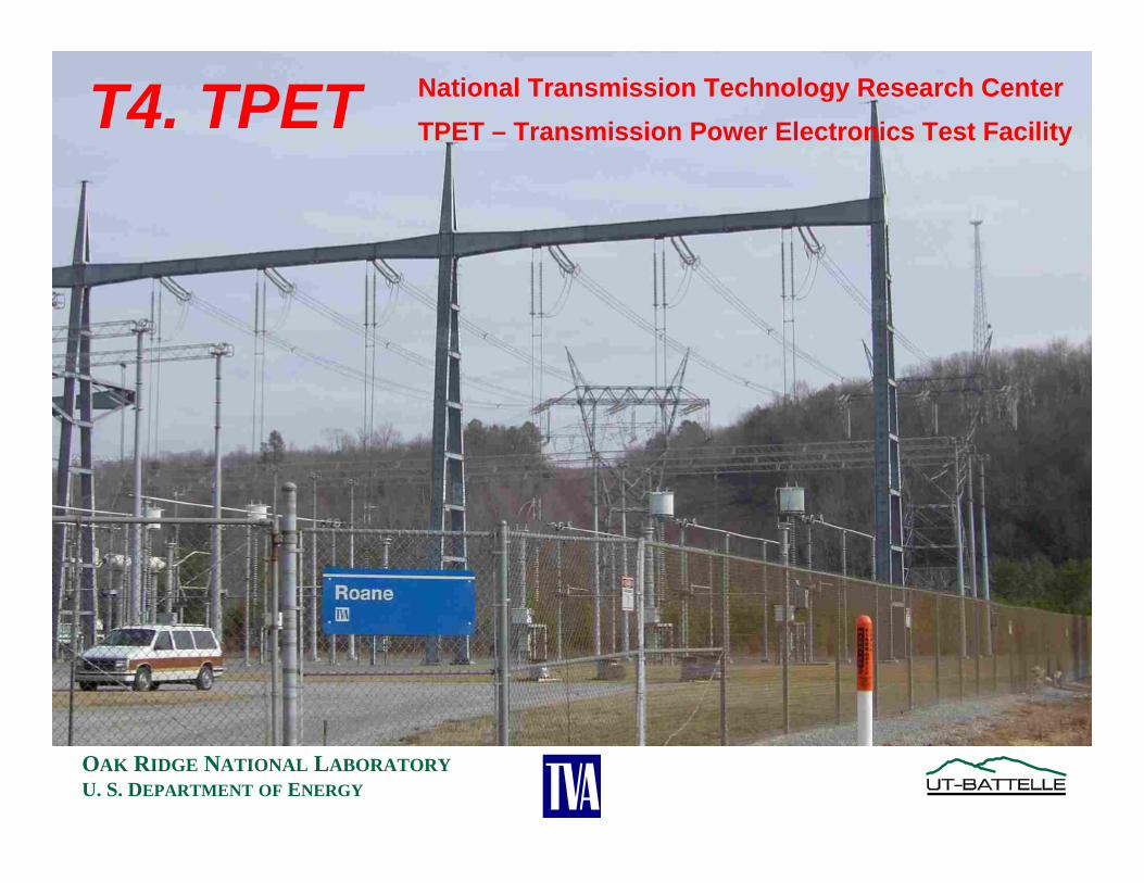
OAK RIDGE NATIONAL LABORATORYU. S. DEPARTMENT OF ENERGY
National Transmission Technology Research Center
TPET – Transmission Power Electronics Test FacilityT4. TPET
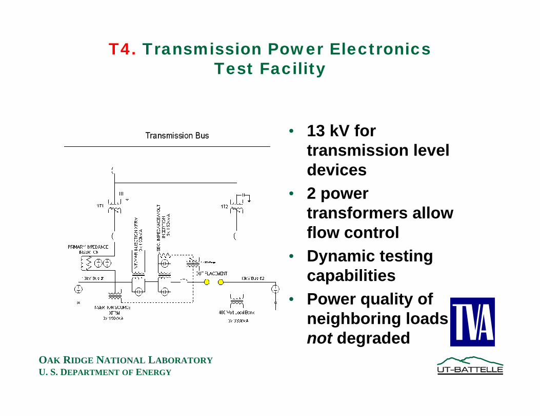
OAK RIDGE NATIONAL LABORATORYU. S. DEPARTMENT OF ENERGY
T4. Transmission Power ElectronicsTest Facility
• 13 kV for transmission level devices
• 2 power transformers allow flow control
• Dynamic testing capabilities
• Power quality of neighboring loads not degraded

OAK RIDGE NATIONAL LABORATORYU. S. DEPARTMENT OF ENERGY
National Transmission Technology Research Center
T1.Outdoor PCAT
Powerline Conductor Accelerated Test Facility
T2.Indoor PCAT
Powerline ConductorAccelerated Test Facility
T3.PCOT
(TVA lines)
Powerline ConductorOperational Test Facility
T4.TPET
(Substation)
Transmission Power Electronics Test Facility

OAK RIDGE NATIONAL LABORATORYU. S. DEPARTMENT OF ENERGY
Questions

OAK RIDGE NATIONAL LABORATORYU. S. DEPARTMENT OF ENERGY
Contact Information• Roger A. KisnerØ (865) 574-5567 VoiceØ (865) 574-1249 FaxØ [email protected]
• D. Tom RizyØ (865) 574-5203 VoiceØ (865) 574-9338 FaxØ [email protected]
• John P. StovallØ (865) 574-5198 VoiceØ (865) 574-9338 FaxØ [email protected]
Oak Ridge National LaboratoryP.O. Box 2008Oak Ridge, TN 37831

Appendix C.3
DOE Peer Review Presentation – October 12, 2005

This page is intentionally left blank.

OAK RIDGE NATIONAL LABORATORYU. S. DEPARTMENT OF ENERGY
Transmission Test Facility
U.S. Department of EnergyTransmission Reliability ProgramPeer Review
Washington Marriott Hotel1221 22nd St. NWWashington, D.C. 20005
October 12, 2005
John P. StovallOak Ridge National Laboratory
ORNL Project TeamD. Tom RizyRoger A. KisnerJohn P. Stovall

OAK RIDGE NATIONAL LABORATORYU. S. DEPARTMENT OF ENERGY
National Transmission Grid Study
One of the 51 Recommendations
“DOE will develop national transmission-technology testing facilities that encourage partnering with industry to demonstrate advanced technologies in controlled environments.
Working with TVA, DOE will create an industry cost-shared transmission line testing center at DOE ’s Oak Ridge National Laboratory (with at least a 50 percent industry cost share).*”
*National Transmission Grid Study, U.S. DOE, May 2002 www.ntgs.doe.gov
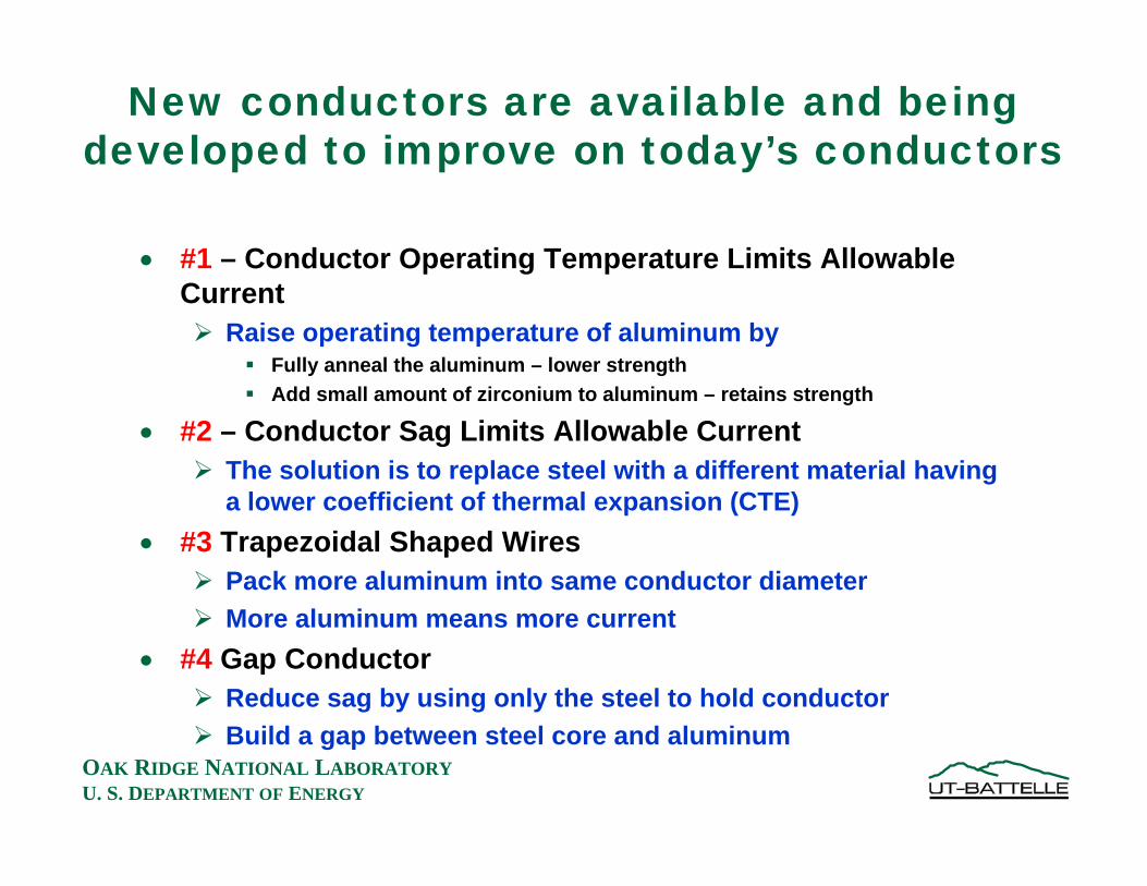
OAK RIDGE NATIONAL LABORATORYU. S. DEPARTMENT OF ENERGY
New conductors are available and being developed to improve on today’s conductors
• #1 – Conductor Operating Temperature Limits Allowable Current
Raise operating temperature of aluminum byFully anneal the aluminum – lower strengthAdd small amount of zirconium to aluminum – retains strength
• #2 – Conductor Sag Limits Allowable CurrentThe solution is to replace steel with a different material having a lower coefficient of thermal expansion (CTE)
• #3 Trapezoidal Shaped WiresPack more aluminum into same conductor diameterMore aluminum means more current
• #4 Gap ConductorReduce sag by using only the steel to hold conductorBuild a gap between steel core and aluminum

OAK RIDGE NATIONAL LABORATORYU. S. DEPARTMENT OF ENERGY
#1 Benefit of Higher Operating Temperatures is Higher Current Rating
Need to test / verify new conductors over entire operating range
0
50
100
150
200
250
0 500 1000 1500 2000
Ampacity, amps
Ope
ratin
g Te
mpe
ratu
re, °
C
Conventional Conductors
High Temperature Conductors

OAK RIDGE NATIONAL LABORATORYU. S. DEPARTMENT OF ENERGY
#2 Benefit of a Conductor that Expands at One-Half the Rate of ACSR
0
70
-500 0 500
ACSR
25 ft. Clearance
Low Sag Conductor with 7.5 ft. more clearance
1000 ft. Span
Ground

OAK RIDGE NATIONAL LABORATORYU. S. DEPARTMENT OF ENERGY
Conductor Road Map
Hard Aluminum1350-H19
Annealed Aluminum
1350-O
Aluminum-Zirconium
Steel
High Strength
Steel
INVAR
Metal Matrix
Composite
Carbon Fiber
Glass and Carbon Fibers
ACSR ACSR/TW
ACSS ACSS/TW
GZTACSR
ZTACIR
ACFR
TACFR
ACCR ACCR/TW
ACCC/TW
90°C - 125°C
200°C - 250°C
210°C - 240°C
Round Strands
Trapezoidal Strands
Trapezoidal Strands and Gap
Aluminum Processing
Core Material
#1 #2 #3 #3 & #4

OAK RIDGE NATIONAL LABORATORYU. S. DEPARTMENT OF ENERGY
Bringing a New Conductor to Market
New ConductorDesign
Laboratory Testing of Conductor Strands
Laboratory Testing of Conductor
Field Demonstrations
Outdoor Test Line at Rated Temperature
(PCAT)
Time to commercialization
Additional testing will accelerate time to commercialization
NewStep

OAK RIDGE NATIONAL LABORATORYU. S. DEPARTMENT OF ENERGY
Transmission Test Facility
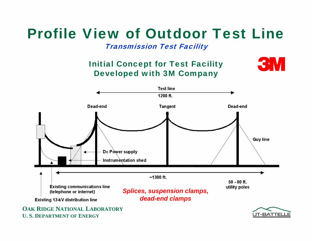
OAK RIDGE NATIONAL LABORATORYU. S. DEPARTMENT OF ENERGY
Profile View of Outdoor Test LineTransmission Test Facility
Initial Concept for Test FacilityDeveloped with 3M Company
Splices, suspension clamps, dead-end clamps

OAK RIDGE NATIONAL LABORATORYU. S. DEPARTMENT OF ENERGY
Test Line Layout
ORNL sought out the help of TVA to design test line

OAK RIDGE NATIONAL LABORATORYU. S. DEPARTMENT OF ENERGY
Structure #1Alcoa Dead-Ends and Jumpers

OAK RIDGE NATIONAL LABORATORYU. S. DEPARTMENT OF ENERGY
Structure #2PLP Suspensions

OAK RIDGE NATIONAL LABORATORYU. S. DEPARTMENT OF ENERGY
Structure #3PLP Dead-Ends and Alcoa Terminal Pads
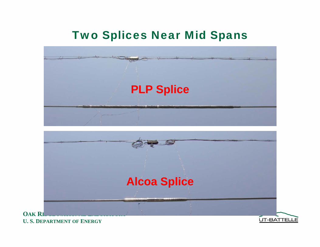
OAK RIDGE NATIONAL LABORATORYU. S. DEPARTMENT OF ENERGY
Two Splices Near Mid Spans
PLP Splice
Alcoa Splice

OAK RIDGE NATIONAL LABORATORYU. S. DEPARTMENT OF ENERGY
Installation of test conductor and accessories takes a transmission line construction crew three or four days
TVA Line Crew - Jonathan M. Rains, James E. Hampton, Randel Hurd, Alan W. Brown, Kevin R. Hodges, Robert Gunter, Lucus Marlow, and Richard B. Stewart
3M 1272 kcmil ACCR Installed on Aug. 9-11, 2004

OAK RIDGE NATIONAL LABORATORYU. S. DEPARTMENT OF ENERGY
Click To Start Movie of Conductor Sag

OAK RIDGE NATIONAL LABORATORYU. S. DEPARTMENT OF ENERGY
Example run shows wind cools the conductorCurrent, 6/9/2003
0
200
400
600
800
1000
1200
12:00 AM 6:00 AM 12:00 PM 6:00 PM 12:00 AM
Cur
rent
, dc
amps
Average Conductor Temperature, 6/9/2003
0
50
100
150
200
250
12:00 AM 6:00 AM 12:00 PM 6:00 PM 12:00 AM
Tem
pera
ture
, ºC
Windspeed, 6/9/2003
0
2
4
6
8
10
12
14
16
12:00 AM 6:00 AM 12:00 PM 6:00 PM 12:00 AM
Win
dspe
ed, f
ps
Conductor Tension, 6/9/2003
1000
1500
2000
2500
3000
3500
4000
12:00 AM 6:00 AM 12:00 PM 6:00 PM 12:00 AM
Tens
ion,
lbs.

OAK RIDGE NATIONAL LABORATORYU. S. DEPARTMENT OF ENERGY
Example of Thermal/Mechanical Cycling RunTu
esda
y, S
ept.
21, 2
004

OAK RIDGE NATIONAL LABORATORYU. S. DEPARTMENT OF ENERGY
IR Imaging SetupOne image per minute with Radiance-HS infrared
camera equipped with a 100mm lens
Target is 23ft from Camera

OAK RIDGE NATIONAL LABORATORYU. S. DEPARTMENT OF ENERGY
Blackbody Signal is multiplied by “emissivity”until it matches conductor signal
IRsig = 0.3556T2 - 43.891T + 2177.3R2 = 0.9994
IRsig = 0.122T2 - 15.789T + 894.12R2 = 0.9951
0
500
1000
1500
2000
2500
3000
3500
4000
4500
5000
50 100 150 200 250
Temperature (C)
IR S
igna
l (a.
u.)
CableBlackbodyEmissivity = 0.346
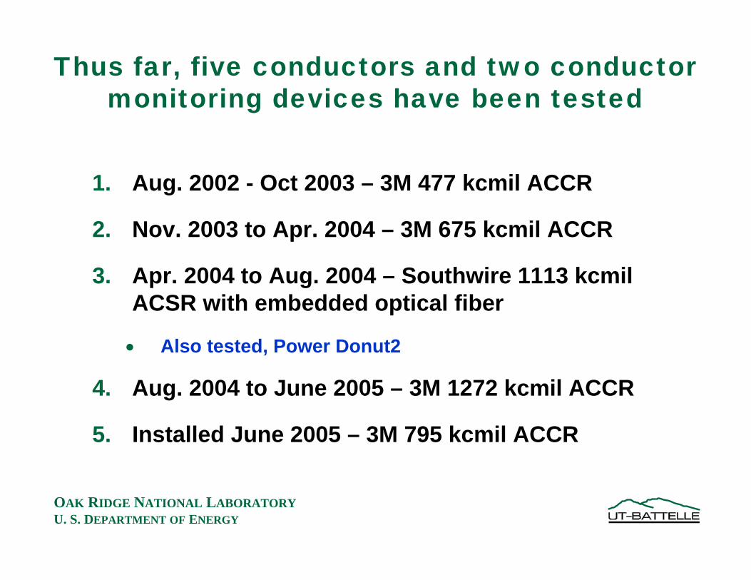
OAK RIDGE NATIONAL LABORATORYU. S. DEPARTMENT OF ENERGY
Thus far, five conductors and two conductor monitoring devices have been tested
1. Aug. 2002 - Oct 2003 – 3M 477 kcmil ACCR
2. Nov. 2003 to Apr. 2004 – 3M 675 kcmil ACCR
3. Apr. 2004 to Aug. 2004 – Southwire 1113 kcmilACSR with embedded optical fiber
• Also tested, Power Donut2
4. Aug. 2004 to June 2005 – 3M 1272 kcmil ACCR
5. Installed June 2005 – 3M 795 kcmil ACCR

OAK RIDGE NATIONAL LABORATORYU. S. DEPARTMENT OF ENERGY
Project Schedule
FY 2003 FY 2004FY 2002 FY 2005 FY 2006

OAK RIDGE NATIONAL LABORATORYU. S. DEPARTMENT OF ENERGY
Fiber Optic Transmission Conductor (FOTC)Measure Temperature Along Length
• Embed optical fibers in standard bare overhead conductors
Optical fiber allows temperature measurement every 2 meters along length of lineTemperature measurement uses the physical properties of the optical fiber (Raman backscattering)Commercially available equipment used to measure temperature profile
• Manufactured by Southwire Company• Testing and Field Demonstration
Small scale verification test at ORNL in 2001Field tested at ComEd, Feb. 2002 to present on 230 kV lineOutdoor verification test at ORNL, Apr. – Aug. 2004
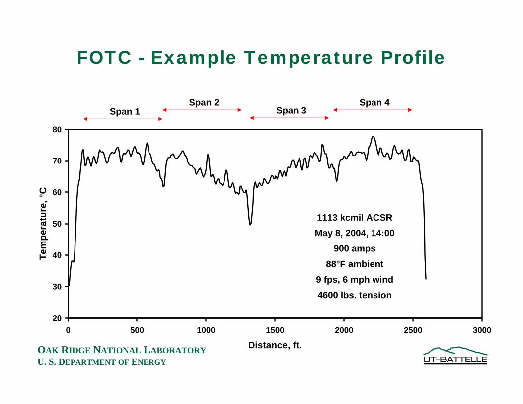
OAK RIDGE NATIONAL LABORATORYU. S. DEPARTMENT OF ENERGY
FOTC - Example Temperature Profile
20
30
40
50
60
70
80
0 500 1000 1500 2000 2500 3000
Distance, ft.
Tem
pera
ture
, °C
Span 1Span 2
Span 3Span 4
1113 kcmil ACSRMay 8, 2004, 14:00
900 amps88°F ambient
9 fps, 6 mph wind4600 lbs. tension

OAK RIDGE NATIONAL LABORATORYU. S. DEPARTMENT OF ENERGY
Real-Time Transmission Line Monitoring
• Power Donut2completely self contained and self poweredCompletely redesigned with new electronics and communications optionsattaches to the conductor using hot stickmeasures current, voltage, MW, MVars, MWh, conductor temperature, conductor inclinationstores data on board
transmits data continuously or on demand
• Testing at ORNL to gather operating data on a new measurement feature
Measuring conductor incline to determine conductor sag
• Line Rating Systems
• Manufactured by USi, Armonk, NYwww.usi-power.com
Wireless Communication to Ground Station

OAK RIDGE NATIONAL LABORATORYU. S. DEPARTMENT OF ENERGY
Facility Capabilities• Testing Capabilities
Controlled current or temperature testingConductor and accessoriesUp to 300oC
• Example testsConstant Current or Constant TemperatureThermal / Mechanical CyclingCurrent / Temperature RampCurrent / Temperature Steps and Hold
• Capabilities2400 feet of conductor2 – 600 foot spansLow Voltage, 0 to 400 VdcHigh Current, up to 5,000 Adc
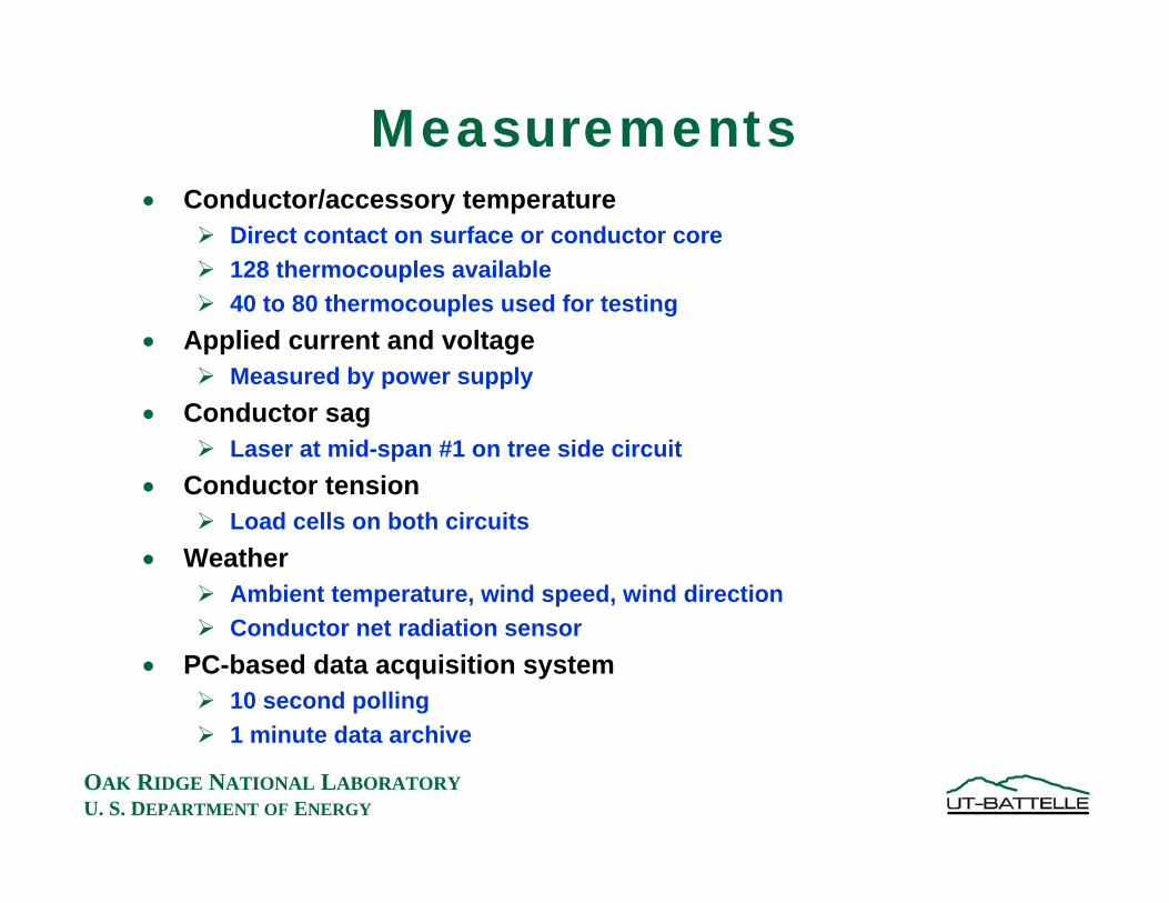
OAK RIDGE NATIONAL LABORATORYU. S. DEPARTMENT OF ENERGY
Measurements• Conductor/accessory temperature
Direct contact on surface or conductor core128 thermocouples available40 to 80 thermocouples used for testing
• Applied current and voltageMeasured by power supply
• Conductor sagLaser at mid-span #1 on tree side circuit
• Conductor tensionLoad cells on both circuits
• WeatherAmbient temperature, wind speed, wind directionConductor net radiation sensor
• PC-based data acquisition system10 second polling1 minute data archive

OAK RIDGE NATIONAL LABORATORYU. S. DEPARTMENT OF ENERGY
Project SummaryTransmission Test Facility
• Fulfilling a programmatic goal defined in a recommendation of the National Transmission Grid Study
• Provides a unique transmission conductor testing facility to augment utility field tests and demonstrations
• Each conductor test undertaken in collaboration with industrial partner Laser at mid-span measure
conductor sag

OAK RIDGE NATIONAL LABORATORYU. S. DEPARTMENT OF ENERGY
Questions

OAK RIDGE NATIONAL LABORATORYU. S. DEPARTMENT OF ENERGY
Contact Information• Roger A. Kisner
(865) 574-5567 Voice(865) 574-1249 [email protected]
• D. Tom Rizy(865) 574-5203 Voice(865) 574-9338 [email protected]
• John P. Stovall(865) 574-5198 Voice(865) 574-9338 [email protected]
Oak Ridge National LaboratoryP.O. Box 2008Oak Ridge, TN 37831

Appendix C.4
DOE Peer Review Presentation – October 17, 2006

This page is intentionally left blank.

OAK RIDGE NATIONAL LABORATORYU. S. DEPARTMENT OF ENERGY
Power Line ConductorAccelerated Testing
U.S. Department of EnergyVisualization and Controls ProgramPeer Review
Marriott Crystal City at Reagan National Airport1999 Jefferson Davis HighwayArlington, VA, 22202
October 17, 2006
John P. StovallOak Ridge National Laboratory
ORNL Project TeamD. Tom RizyRoger A. KisnerJohn P. Stovall

2
OAK RIDGE NATIONAL LABORATORYU. S. DEPARTMENT OF ENERGY
National Transmission Grid Study
One of the 51 Recommendations
“DOE will develop national transmission-technology testing facilities that encourage partnering with industry to demonstrate advanced technologies in controlled environments.
Working with TVA, DOE will create an industry cost-shared transmission line testing center at DOE ’s Oak Ridge National Laboratory (with at least a 50 percent industry cost share).*”
*National Transmission Grid Study, U.S. DOE, May 2002 www.ntgs.doe.gov

3
OAK RIDGE NATIONAL LABORATORYU. S. DEPARTMENT OF ENERGY
Transmission Test Facility
• The facility has been used for testing of:high-temperature low-sag conductors,conductor accessories, andconductor monitoring devices.

4
OAK RIDGE NATIONAL LABORATORYU. S. DEPARTMENT OF ENERGY
Test line layout replicates standard utility practices
ORNL sought out the help of TVA to design test line
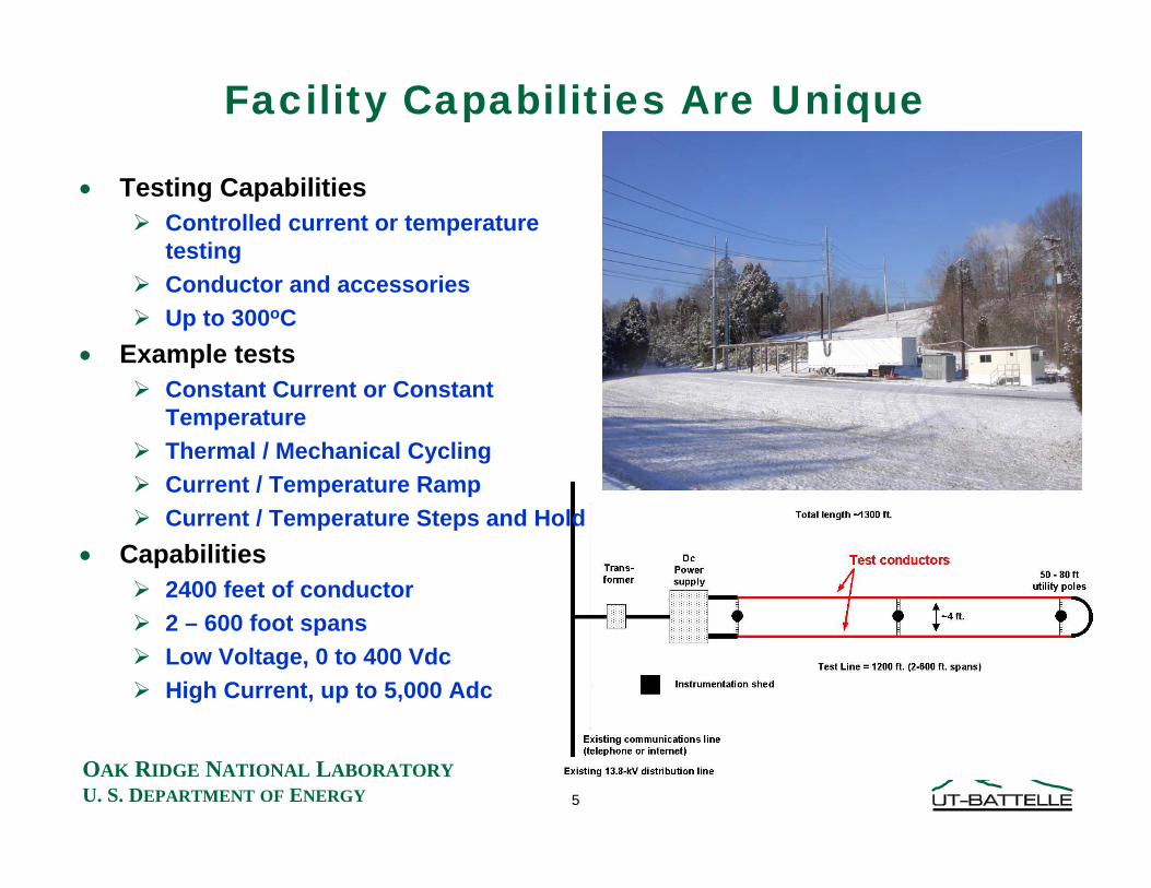
5
OAK RIDGE NATIONAL LABORATORYU. S. DEPARTMENT OF ENERGY
Facility Capabilities Are Unique
• Testing CapabilitiesControlled current or temperature testingConductor and accessoriesUp to 300oC
• Example testsConstant Current or Constant TemperatureThermal / Mechanical CyclingCurrent / Temperature RampCurrent / Temperature Steps and Hold
• Capabilities2400 feet of conductor2 – 600 foot spansLow Voltage, 0 to 400 VdcHigh Current, up to 5,000 Adc

6
OAK RIDGE NATIONAL LABORATORYU. S. DEPARTMENT OF ENERGY
Benefit of higher operating temperatures is higher current rating
Need to test / verify new conductors over entire operating range
0
50
100
150
200
250
0 500 1000 1500 2000
Ampacity, amps
Ope
ratin
g Te
mpe
ratu
re, °
C
Conventional Conductors
High Temperature Conductors

7
OAK RIDGE NATIONAL LABORATORYU. S. DEPARTMENT OF ENERGY
Benefit of a conductor that thermally expands at one-half the rate of ACSR is lower sag
0
70
-500 0 500
ACSR
25 ft. Clearance
Low Sag Conductor with 7.5 ft. more clearance
1000 ft. Span
Ground

8
OAK RIDGE NATIONAL LABORATORYU. S. DEPARTMENT OF ENERGY
Conductor Road Map
Hard Aluminum1350-H19
Annealed Aluminum
1350-O
Aluminum-Zirconium
Steel
High Strength
Steel
INVAR
Metal Matrix
Composite
Carbon Fiber
Glass and Carbon Fibers
ACSR ACSR/TW
ACSS ACSS/TW
GZTACSR
ZTACIR
ACFR
TACFR
ACCR ACCR/TW
ACCC/TW
90°C - 125°C
200°C - 250°C
210°C - 240°C
Round Strands
Trapezoidal Strands
Trapezoidal Strands and Gap
Aluminum Processing
Core Material
#1 #2 #3 #3 & #4
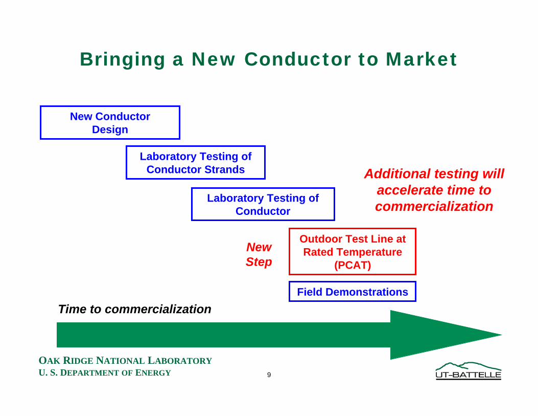
9
OAK RIDGE NATIONAL LABORATORYU. S. DEPARTMENT OF ENERGY
Bringing a New Conductor to Market
New ConductorDesign
Laboratory Testing of Conductor Strands
Laboratory Testing of Conductor
Field Demonstrations
Outdoor Test Line at Rated Temperature
(PCAT)
Time to commercialization
Additional testing will accelerate time to commercialization
NewStep

10
OAK RIDGE NATIONAL LABORATORYU. S. DEPARTMENT OF ENERGY
Structure #1 & #3Dead-Ends and Jumpers

11
OAK RIDGE NATIONAL LABORATORYU. S. DEPARTMENT OF ENERGY
Structure #2 and Mid-Spans
#1
#2
Suspensions Splices at Mid-Spans

12
OAK RIDGE NATIONAL LABORATORYU. S. DEPARTMENT OF ENERGY
Installation of test conductor and accessories takes a transmission line construction crew three or four days

13
OAK RIDGE NATIONAL LABORATORYU. S. DEPARTMENT OF ENERGY
Test Conductors Are Installed Using Standard Equipment

14
OAK RIDGE NATIONAL LABORATORYU. S. DEPARTMENT OF ENERGY
Click To Start Movie of Conductor Sag

15
OAK RIDGE NATIONAL LABORATORYU. S. DEPARTMENT OF ENERGY
Example run shows wind cools the conductorCurrent, 6/9/2003
0
200
400
600
800
1000
1200
12:00 AM 6:00 AM 12:00 PM 6:00 PM 12:00 AM
Cur
rent
, dc
amps
Average Conductor Temperature, 6/9/2003
0
50
100
150
200
250
12:00 AM 6:00 AM 12:00 PM 6:00 PM 12:00 AM
Tem
pera
ture
, ºC
Windspeed, 6/9/2003
0
2
4
6
8
10
12
14
16
12:00 AM 6:00 AM 12:00 PM 6:00 PM 12:00 AM
Win
dspe
ed, f
ps
Conductor Tension, 6/9/2003
1000
1500
2000
2500
3000
3500
4000
12:00 AM 6:00 AM 12:00 PM 6:00 PM 12:00 AM
Tens
ion,
lbs.
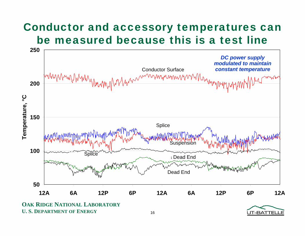
16
OAK RIDGE NATIONAL LABORATORYU. S. DEPARTMENT OF ENERGY
Conductor and accessory temperatures can be measured because this is a test line
50
100
150
200
250
12A 6A 12P 6P 12A 6A 12P 6P 12AAug. 17-18, 2004
Tem
pera
ture
, °C
Conductor Surface
PLP Splice
PLP Suspension
Alcoa Splice
PLP Dead End
Alcoa Dead End
DC power supply modulated to maintain constant temperature

17
OAK RIDGE NATIONAL LABORATORYU. S. DEPARTMENT OF ENERGY
All key parameters are being measured• Conductor/accessory temperature
Direct contact on surface or conductor core128 thermocouples available40 to 80 thermocouples used for testing
• Applied current and voltageMeasured by power supply
• Conductor sagLaser at mid-span #1 on tree side circuit
• Conductor tensionLoad cells on both circuits
• WeatherAmbient temperature, wind speed, wind directionConductor net radiation sensor
• PC-based data acquisition system10 second polling1 minute data archive

18
OAK RIDGE NATIONAL LABORATORYU. S. DEPARTMENT OF ENERGY
Thermal/mechanical cycling can simulate many years of operation

19
OAK RIDGE NATIONAL LABORATORYU. S. DEPARTMENT OF ENERGY
Knee-point test shows transition of tension
3000
4000
5000
6000
7000
8000
0 50 100 150 200 250Temperature, °C
Tens
ion,
lbs.
Roadside
Treeside
A one-day test sweeps the conductor over it’s entire
temperature operating range.

20
OAK RIDGE NATIONAL LABORATORYU. S. DEPARTMENT OF ENERGY
Axial Temperature Difference85°C between 600 ft. Mid-Spans
0
50
100
150
200
250
300
6:00 AM 8:00 AM 10:00 AM 12:00 PM 2:00 PM 4:00 PM 6:00 PM
Tem
pera
ture
, °C
236°C
151°C
85°C
Mid-span #1
Mid-span #2
Difference
AverageNoon to 2:45 PM
Nov. 18, 2003OAK RIDGE NATIONAL LABORATORYU.S. DEPARTMENT OF ENERGY
0
50
100
150
200
250
300
6:00 AM 8:00 AM 10:00 AM 12:00 PM 2:00 PM 4:00 PM 6:00 PM
Tem
pera
ture
, °C
236°C
151°C
85°C
Mid-span #1
Mid-span #2
Difference
AverageNoon to 2:45 PM
Nov. 18, 2003OAK RIDGE NATIONAL LABORATORYU.S. DEPARTMENT OF ENERGY

21
OAK RIDGE NATIONAL LABORATORYU. S. DEPARTMENT OF ENERGY
Ice on conductor, 300 lbs. for 17 hours
-2
0
2
4
6
8
10
12
12 AM 12 PM 12 AM 12 PM 12 AM
Tem
pera
ture
, C
2500
2600
2700
2800
2900
3000
3100
3200
Tens
ion,
lbs.
NRS
Ambient
Treeside Circuit
Roadside Circuit
OAK RIDGE NATIONAL LABORATORYU.S. DEPARTMENT OF ENERGY
-2
0
2
4
6
8
10
12
12 AM 12 PM 12 AM 12 PM 12 AM
Tem
pera
ture
, C
2500
2600
2700
2800
2900
3000
3100
3200
Tens
ion,
lbs.
NRS
Ambient
Treeside Circuit
Roadside Circuit
OAK RIDGE NATIONAL LABORATORYU.S. DEPARTMENT OF ENERGY

22
OAK RIDGE NATIONAL LABORATORYU. S. DEPARTMENT OF ENERGY
High-temperature operation – 2000 hours

23
OAK RIDGE NATIONAL LABORATORYU. S. DEPARTMENT OF ENERGY
0 500 1000 1500 2000 2500-50
0
50
100
150
200
250
300
Time, hours
Avg
Con
duct
or T
empe
ratu
re, °C
09/13/2005 - 03/31/2006 Idc On, Avg Conductor Temperature
tcdr
Average conductor temperature during extended high-temperature operation

24
OAK RIDGE NATIONAL LABORATORYU. S. DEPARTMENT OF ENERGY
Infrared imaging is used to measure conductor emissivity, a key design parameter
Target is 23ft from Camera
IRsig = 0.3556T2 - 43.891T + 2177.3R2 = 0.9994
IRsig = 0.122T2 - 15.789T + 894.12R2 = 0.9951
0
500
1000
1500
2000
2500
3000
3500
4000
4500
5000
50 100 150 200 250
Temperature (C)
IR S
igna
l (a.
u.)
CableBlackbodyEmissivity = 0.346
Blackbody Signal is multiplied by “emissivity” until it matches
conductor signal

25
OAK RIDGE NATIONAL LABORATORYU. S. DEPARTMENT OF ENERGY
Fiber Optic Transmission Conductor (FOTC)Measures Temperature Along Length
• Embed optical fibers in standard bare overhead conductorsOptical fiber allows temperature measurement every 2 meters along length of lineTemperature measurement uses the physical properties of the optical fiber (Raman backscattering)Commercially available equipment used to measure temperature profile
• Manufactured by Southwire Company, Testing and Field DemonstrationSmall scale verification test at ORNL in 2001Field tested at ComEd, Feb. 2002 to present on 230 kV lineOutdoor verification test at ORNL, Apr. – Aug. 2004
20
30
40
50
60
70
80
0 500 1000 1500 2000 2500 3000
Distance, ft.
Tempe
rature, °
C
Span 1 Span 2 Span 3 Span 4
1113 kcmil ACSR900 amps
88°F ambient9 fps, 6 mph wind4600 lbs. tension

26
OAK RIDGE NATIONAL LABORATORYU. S. DEPARTMENT OF ENERGY
Real-Time Transmission Line Monitoring
• Power Donut2completely self contained and self poweredCompletely redesigned with new electronics and communications optionsattaches to the conductor using hot stickmeasures current, voltage, MW, MVars, MWh, conductor temperature, conductor inclinationstores data on board
transmits data continuously or on demand
• Testing at ORNL to gather operating data on a new measurement feature
Measuring conductor incline to determine conductor sag
• Line Rating Systems
• Manufactured by USi, Armonk, NYwww.usi-power.com
Wireless Communication to Ground Station

27
OAK RIDGE NATIONAL LABORATORYU. S. DEPARTMENT OF ENERGY
Project Schedule
FY 2003 FY 2004 FY 2007FY 2005 FY 2006
1. Aug. 2002 - Oct 2003 – 3M 477 kcmil ACCR2. Nov. 2003 to Apr. 2004 – 3M 675 kcmil ACCR3. Apr. 2004 to Aug. 2004 – Southwire 1113 kcmil
ACSR with embedded optical fiber• Also tested, Power Donut2
4. Aug. 2004 to June 2005 – 3M 1272 kcmil ACCR5. Installed June 2005 – 3M 795 kcmil ACCR
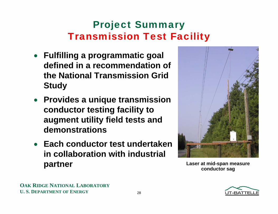
28
OAK RIDGE NATIONAL LABORATORYU. S. DEPARTMENT OF ENERGY
Project SummaryTransmission Test Facility
• Fulfilling a programmatic goal defined in a recommendation of the National Transmission Grid Study
• Provides a unique transmission conductor testing facility to augment utility field tests and demonstrations
• Each conductor test undertaken in collaboration with industrial partner Laser at mid-span measure
conductor sag
29
OAK RIDGE NATIONAL LABORATORYU. S. DEPARTMENT OF ENERGY
Questions?
30
OAK RIDGE NATIONAL LABORATORYU. S. DEPARTMENT OF ENERGY
Contact Information• Roger A. Kisner
(865) 574-5567 Voice(865) 574-1249 [email protected]
• D. Tom Rizy(865) 574-5203 Voice(865) 574-9338 [email protected]
• John P. Stovall(865) 574-5198 Voice(865) 574-9338 [email protected]
Oak Ridge National LaboratoryP.O. Box 2008Oak Ridge, TN 37831

This page is intentionally left blank.