Passing Efficiency of a Low Turbulence Inlet (PELTI)

Final Report to NSF

Prepared by the LTI Assessment Working Group:Barry J. Huebert1, Chair

Steven G. Howell1

David Covert 2

Antony Clarke1

James R. Anderson3

With Collaborating AuthorsBernard G. Lafleur4

Russ Seebaugh4

James Charles Wilson4

Dave Gesler4

Darrel Baumgardner5

Byron Blomquist1

1 Department of Oceanography, University of Hawaii, Honolulu, HI 968222 Atmospheric Science Dept, JISAO GJ-40, University of Washington, Seattle, WA 98195

3 Mechanical and Aerospace Engineering, Arizona State University, Tempe, AZ 852874 Department of Engineering, University of Denver, Denver, CO 80208

5 Centro de Ciencias de la Atmósfera – UNAM, Universidad Nacional Autónoma de México,Circuito Exterior s/n, Ciudad Universitaria, 04510 México City (D.F.)

Address inquiries to: huebert@soest.hawaii.edu

13 September, 2000

Disclaimer: The data on which this report is based was collected in July, 2000. This report isbeing submitted in September, 2000. It commonly takes multiple years for investigators toprocess, quality-check, and publish data from flight programs of this complexity. In view of theextremely short time from data collection to report, perhaps it is reasonable for the authors toattach a “preliminary” label to the tables and plots herein. Some errors will no doubt bediscovered and corrected. However, we are confident that they would not change thefundamental conclusions about the functioning of the LTI.

2

Table of Contents

3 Executive SummaryReport Summary

4 A. Introduction5 B. Approach6 C. LTI Modeled Performance6 D. Observations10 E. Conclusions11 Summary Figures

1. Introduction15 1.1 State of the Science16 1.2 PELTI

2. Methods17 2.1 Overall Approach19 2.2 LTI Configuration20 2.3 Location of Inlets, Plumbing, and Layout21 2.4 Bulk Chemical Analyses22 2.5 SEM Analyses23 2.6 Aerodynamic Particle Size Measurements24 2.7 FSSP-300 Observations25 2.8 Nephelometers

3. Results26 3.1 Flight Operations28 3.2 LTI Aerodynamic Performance30 3.3 Bulk Filter Data32 3.4 SEM Data35 3.5 APS Data37 3.6 FSSP-300 Measurements38 3.7 Lab Measurements of Losses in Tubing39 3.8 Modeling of Enhancements using Fluent42 3.9 Nephelometers

Discussion and Critiques of Methods43 4.1 Tasks Remaining43 4.2 Critique of APS Data – D. Covert44 4.3 Critique of Anion and Cation Data – B. Huebert45 4.4 Sources of Error in SEM Analyses – J. Anderson46 4.5 FSSP Data Concerns – A. Clarke48 4.6 Net LTI Passing Efficiency – J. C. Wilson49 4.7 What Does Particle Size Mean? – S. Howell

Recommendations and Conclusions52 5.1 Comparisons of Inlets53 5.2 Comparisons to Ambient Concentrations54 5.3 Recommendations54 References57 Figures

3

Executive Summary

In July, 2000 we tested the new porous-diffuser low-turbulence inlet (LTI), developed at theUniversity of Denver, by flying it and three other inlets on NCAR’s C-130 in the Caribbean,using both dust and sea salt as test aerosols. Aerosols were analyzed using bulk chemicalanalysis of ions on filters, scanning electron microscopy (SEM) of filters, TSI aerodynamicparticle sizers (APSs), and FSSP-300 (300) optical particle counters.

We found that the LTI consistently admitted more particles to the airplane than did either theNCAR Community Aerosol Inlet (CAI) or a shrouded solid-diffuser/curved-tube inlet (SD).APS size distributions behind the other inlets began to diverge from LTI values above 1-3 um,with mass concentrations of larger particles lower by as much as a factor of ten behind the CAIand a factor of 2 behind the SD. Modeling of particle trajectories in the LTI with Fluent predictsless than a factor of two enhancement of particles between a few and 7 microns. This wassupported by the SEM analyses of particles behind the LTI and TAS.

Comparisons of bulk chemistry with an external reference total aerosol sampler (TAS) found nosignificant differences between the LTI and TAS, but both the SD and CAI passed lower valuesfor most of the ions analyzed. Thus, the LTI filters can be used to determine the ambient massmixing ratios of the analyzed ions. The inertial enhancements in the LTI diffuser and estimatesof losses in transport to the LTI filter must be taken into account to accurately infer ambientconcentrations based on LTI sampling. When this is done, the ambient mass mixing ratiosestimated from the LTI filters agree within 20% with the mixing ratios determined from the TASfilters.

Relative to the LTI, the SD and CAI transmission efficiencies (the concentration in the sampleflow divided by the ambient concentration) was lowest for “wet” aerosol (i.e., sea-salt),apparently because salt droplets are more likely than dry dust to stick when they impact on thewalls of the other inlets.

We set out to test two hypotheses:

A. The LTI has a demonstrably higher aerosol sampling or transmission efficiency thanboth the CAI (the NCAR C-130 community aerosol inlet) and traditional solid diffusersfor particles in the 1-7 um range.

This hypothesis could not be falsified. All the chemical and physical evidence indicates that theLTI admits more particle mass in this range than the other inlets do.

However, we note that our real goal is to achieve efficiencies near unity. The ubiquity of lossesin earlier inlets lead us initially to state this hypothesis in terms of “higher” efficiency, butenhancement by the LTI may cause efficiencies substantially above 1 for particles larger than 3-5um. Since enhancements in laminar flow are calculable, most measurements can be corrected forthem.

4

B. It is possible, using the LTI, to sample and characterize the number-size and surfacearea-size distributions of ambient dust and seasalt inside an aircraft with enoughaccuracy that uncertainties arising from inlet losses will contribute less than 20% to theassessment of radiative impacts.

This hypothesis also could not be falsified. It essentially asks how well aerosol size distributionsbehind the LTI represent ambient particle distributions and light scattering. The LTI bulkchemical concentrations were statistically identical to the TAS bulk concentrations of Na+, Cl-,SO4

=, Mg++, and Ca++, which represent the ambient mixing ratios of those species. The SEManalyses showed that the LTI and TAS number concentrations were statistically identical up to 2µm; above 2 µm the LTI showed enhancement within model-predicted limits. When Fluentmodel-derived inertial enhancements associated with the LTI diffuser and losses associated withtransport to the LTI filter are taken into consideration, they explain the observed 20% agreementbetween LTI and TAS.

Corrections for modest but predictable LTI enhancements also provide light scatteringassessments that are representative of ambient size distributions up to 7um. Additionalcontributions to scattering from yet larger aerosol are unlikely to approach 20% for realisticaerosol cases. The error in radiative forcing due to positive and negative sampling biasesdepends both on the transmission efficiency and the fraction of the mass and total optical depthin each size interval. For those sizes that contribute little to the optical depth, a poor transmissionefficiency will cause little error in radiative forcing calcualtions. It is worth noting, however, thatover- or under-sampled sizes could still cause significant errors for other issues, such as thecomputation of deposition fluxes and heterogeneous reaction rates.

CONCLUSION: Our conclusion, therefore, is that the LTI represents a significant advance inour ability to sample populations of large particles from aircraft. Its efficiency is near enough tounity to enable defendable studies of the distributions and impacts of both mineral dust and seasalt. Corrections will need to be applied for enhancement of particles in the 3-7 um range. Werecommend that the ACE-Asia program use LTIs to provide samples to the various aerosolinstruments on board the NCAR C-130.

Report Summary

A. Introduction

It has long been known that typical diffuser-and-curved-tube airborne inlet systems removeparticles from sampled airstream, so that instruments downstream receive air that has beendepleted of supermicron particles. Since most instruments require that air be decelerated fromaircraft velocities to a few m/s prior to its analysis, decelerating diffusers have been widely usedin airborne sampling. Apparently the highly-turbulent flow just inside the tip of these conicaldiffusers causes the largest particles to be impacted on the walls of the diffuser. With thepossible exception of mineral particles that may bounce off the walls, this has the effect ofremoving large particles and distorting the particle-size spectrum behind diffusers.

5

A workshop was convened at NCAR in 1991 to assess the state of knowledge about inlet systems.Attendees concluded that it was not possible at that time to sample supermicron particles from aircraftwithout substantial and unquantifiable size-dependent negative biases, and made severalrecommendations for ways to study and improve airborne aerosol inlets (Baumgardner et al., 1991).The notion of a shallow angle diffuser with a shrouded inlet prompted the design of the NASA SDemployed in this study. Similarly the NCAR Community Aerosol Inlet (CAI) incorporated severalfeatures intended to minimize artifacts. One of the most promising suggestions from the 19901workshop was that of Denver University researcher Russell Seebaugh, who noted that aerodynamicengineers have for years suppressed turbulence in diffusers by using boundary layer suction to preventthe separation of the boundary layer from the diffuser walls. Since that time, Seebaugh and hiscolleagues Bernard LaFleur and James C. Wilson have developed that concept in the laboratory. Thisled to the fabrication of the LTI that is the focus of this report (Figure S1).

B. Approach

Hypothesis A can be tested relatively simply, since it only requires measurements inside theaircraft, on air streams that have already been decelerated. We used three matched aerodynamicparticle sizers (TSI Model 3320 APS’s) to measure the physical size distribution behind our threetest inlets: the LTI, CAI, and SD. The difference between the APS distributions provides a directtest of Hypothesis A. Nephelometers behind each inlet provided a real-time signal in flight toguide the test and a relevant integral measure of light scattering that is appropriate to the testsand one of the goals of ACE-Asia, radiative transfer. We also collected filter samples forchemical analysis behind each of these inlets. That included both Teflon filters for ion-chromatographic analysis of major anions and cations (Barry Huebert’s group) and streakerswith Nuclepore filters (SEM analyses by Jim Anderson). In dust, Anderson counted and sized theparticles behind each inlet with automated SEM (without chemical analysis) that could amassstatistics on thousands of particles.

Hypothesis B is considerably more difficult to test, since it involves comparing aerosoldistributions behind the LTI to those in ambient air. The crux of the problem is to measure theambient (reference) distribution with a system that does not itself suffer from inlet or otherartifacts. One of the most defendable external references is the bulk concentration of particles, asmeasured by the TAS designed and built in the NCAR shop. This external sampler permits ananalysis of every particle that enters the inlet tip, whether it has been deposited on the inside ofthe diffuser or collected on its filter. The diffuser is lined by removable cones, which arereplaced with each filter sample and extracted after the flights. As long as one samplesisokinetically, we can be assured that the sum of the cone extract and its filter contains everyparticle that entered the TAS tip and is representative of the ambient aerosol concentration. TASwas used to measure reference ambient concentrations of both seasalt and dust. When samplingdust, the size of mineral aerosol was preserved in the TAS extracts (except for aggregates), sothat the ambient (TAS) and LTI size distributions could both be measured directly by SEM. Onlycomparisons utilizing a single physical principal (either SEM or IC analyses) were considered tobe valid tests of the LTI.

The FSSP-300 is another external device that seemed to offer the best hope for characterizing theambient size distribution that could then be compared to a similar probe mounted internally

6

behind the LTI. However, inconsistencies in the internal FSSP data and uncertainties concerningthe nature of the flow in its sample volume led to comparisons that we are unable to reconcilewith the other aerosol measurements. It is worth noting that the counting efficiency of 300s inthese different configurations has never been calibrated, in contrast to their sizing ability. Hence,we have focussed on the TAS data as our external reference.

C. LTI Modeled Performance

The design of the LTI was expected to lead to some enhancement in larger particles. This occurswhen particles with sufficient inertia deviate from the curving streamlines caused by aspiratingmost of the flow through the sides of the LTI porous diffuser. However, losses of some largerparticles in this prototype are caused by the 90 deg bend in the tube behind the inlet (Fig. S1).Fluent calculations that account for these enhancements and losses (Fig S2) indicate that a netenhancement should become evident around 3µm and approach about 40% by 6µm. In the finalFigure of this Summary (Fig. S6) we correct for this enhancement

D. Observations

D.1. Aerodynamic Particle Sizers

Aerodynamic Particle Sizers (APS, Model 3320, TSI Inc, St. Paul MN) (Wilson and Liu, 1980)were used to count and size particles according to their aerodynamic diameter, Dae, in the rangefrom 0.8 to 13 µm downstream of each of the three inlets, the LTI, CAI, and SD. Each APS unitdrew its 5 l/min from an identical distribution plenum one of the inlets as described above. TheAPS measurements were overseen by Steve Howell of UH and Dave Covert, of the University ofWashington.

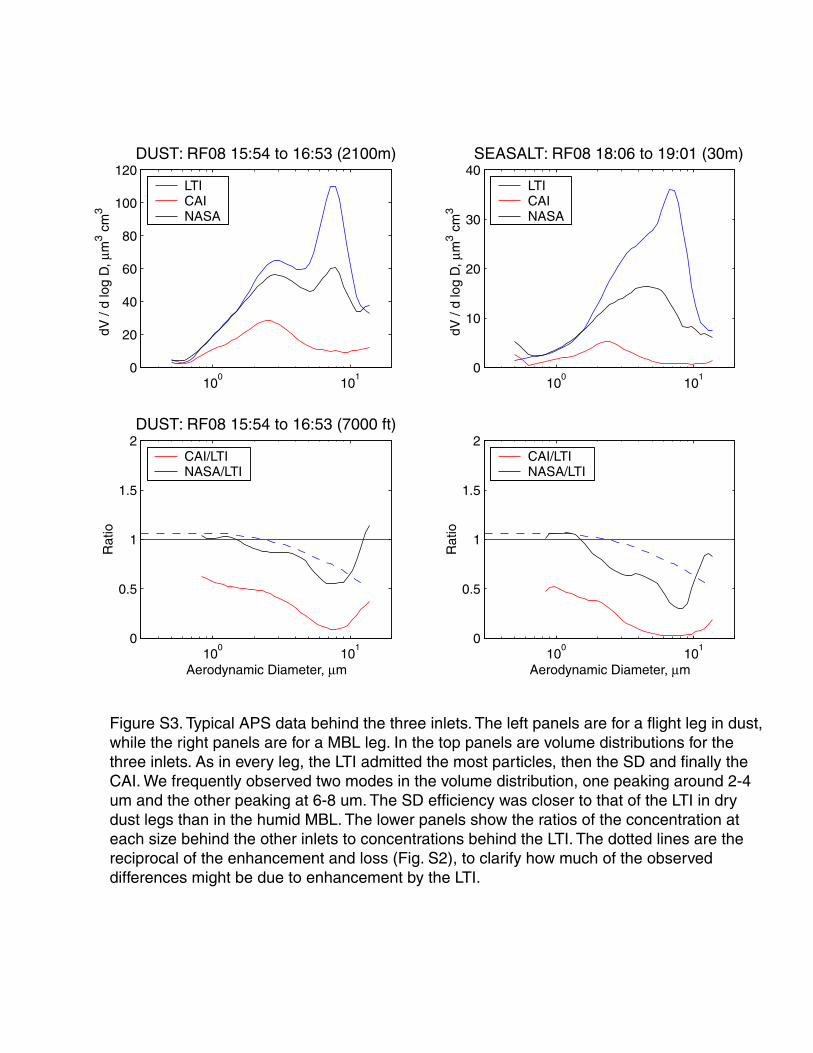
Figure S3 contains two examples of APS volume distribution data from Flight 8 collectedconcurrently from the LTI, CAI and SD for so called “dry” and “wet” conditions in the presenceof coarse aerosol. Note that we plot volume distributions (rather than number) to make factors oftwo or less differences in the largest sizes evident. “Dry” refers to low relative humidity (RH)conditions common above the marine inversion and in the presence of dry dust aerosol. “Wet”refers to higher RH conditions common to the marine boundary layer where coarse sea-salt isdeliquesced into a “wet” saline droplet (although at this low wind speed much of the small modemay be dust). In the “dry” case (Fig S3, Left) at 2100 m altitude the LTI and SD concentrationsare similar up to 1.5µm, after which SD concentrations are about 20% lower than the LTI.However, CAI concentrations are less than 50% of corresponding LTI values. In the “wet” case(Fig. S3, right) at 30 m discrepancies are much greater: SD concentrations are about 60% of LTIvalues between 2 and 7 µm while CAI values are far less: about 10-20% of the LTI values overthis range.

D.2. Bulk Analysis of Anions and Cations

Filter samplers behind each inlet were compared with data from the Total Aerosol Sampler,TAS. Since TAS enables an analysis of every particle that enters its tip (whether on the Teflonfilter or extracted from the interior walls of the inlet cone), it serves as an ambient reference for

7

other filter samplers. Because analyzing TAS samples involves handling and extracting a cone aswell as s filter, the precision of TAS will never be as good as that of a single filter analysis, butits lack of sampling bias means that it has a definable accuracy. Ion chromatography was used toanalyze all filters and TAS samples for Cl-, SO4

=, Na+, Ca++, and Mg++. The major source ofuncertainty was the variability of blank concentrations.

Figure S4 compares Cl- behind all the inlets with TAS Cl- in the left panel and with LTI Cl- inthe right panel. The LTI concentration is indistinguishable from that of TAS, while the SD andCAI brought considerably less Cl- into the cabin. We conclude that the LTI reproduces ambientCl- concentrations to within at least 20%, in spite of enhancements and losses that may affect thelarger end of the sea salt size distribution. The relative behavior of the inlets is clearer when SDand CAI samples are plotted against the LTI in the lower panel. Similar differences were notedfor the other ions:

Average Ratios of Species Concentrations Behind Various Inlets to TAS Concentrations

Ratio Cl SO4 Na Mg Ca NSS(Mg)

LTI/TAS 1.15 1.03 0.94 0.86 1.03 1.23Solid/TAS 0.58 0.84 0.54 0.51 0.74 1.32CFilt/TAS 0.17 0.52 0.20 0.19 0.25 0.86CImp/TAS 0.16 0.50 0.18 0.19 0.24 0.79

This chemical data suggests that the sea salt and dust modes are sampled with nearly-unitefficiency by the LTI. It also shows a demonstrable lowering of efficiency when the LTI flowwas made turbulent rather than laminar. In these cases the majority of the mass distribution wassmaller than 4 um so that LTI enhancement biases were not large.

D.3. Scanning Electron Microscopy

Streaker samplers enabled the collection of Nuclepore filter samples behind each inlet on everyflight leg. In addition, on high altitude legs we exposed Nuclepore filters in TAS, so that we hadan ambient SEM reference for mineral dust particles. Only about 10% of the dust particlesadhered to the TAS cone (dry particles tend to bounce off), so most of the particles did not needto be extracted for analysis. Thus, the SEM enabled comparisons of particle size distributionsbehind each inlet for comparison with the ambient distribution from TAS.

It should be noted that these size distributions differ from those measured by the APSs. Asignificant fraction of the large particles were tabular clays, whose complex shapes defy simpledescriptions such as diameter. Furthermore, the extra drag of these complex particles wouldcause them to appear small for their mass in the APS, where the smallest particles tend not todeviate from the path of the air. Ironically, because of their large surface to mass ratio, theywould size large for their mass in instruments that measure light scattering. Reconciling thesevarious measurements has given us many insights about ways to study dust particles in ACE-Asia.

8

Two dust samples from Flight 8 have been extensively analyzed by SEM. As Fig. S5demonstrates, there is good agreement (<20% in the number distribution) between TAS and theLTI below 2 um, which suggests that the sampled volumes have been correctly accounted for.Above 2 um the TAS and LTI distributions in this sample diverge to suggest an enhancement bythe LTI of a factor of 2 in the 3-8 um range. The other sample shows overlap up to about 6 umand then enhancement by only about 20% up to 8 um (see full report). This data, which is ourmost reliable comparison of ambient and internal particle sizes, is in general agreement with themodeling (suggesting a small enhancement) and the ion chemistry (suggesting that the bulk ofthe sea salt mode is sampled with no more than modest enhancement).

D.4. Nephelometer

The Radiance Research nephelometers (530nm) behind each inlet characterized the integral lightscattering of the aerosol from 8 to 168 deg. Larger particles concentrate a greater proportion oftheir scattered light in the forward direction such that this angular truncation underestimates thescattering contribution of the largest particles. However, we also used a second nephelometerbehind the LTI inlet with an aerodynamic size cut near 1µm to characterize the submicrometerscattering and subtract it from the total to identify coarse scattering only. For the PELTI datadiscussed here, submicrometer scattering was about 1/3 of the total such that total scatter wasdominated by coarse particle scattering in spite of possible truncation losses due to forwardscatter from the largest particles. Although the LTI consistently saw higher mass concentrations,light scattering values behind the LTI and SD inlets were virtually the same when compared overthe experiment, with leg average differences generally about 13% (see full report forFigure). On the other hand, scattering data behind the CAI was consistently about 40% less thanLTI or SD values. The relationship between size and scattering is explored in Section D.6.

D.5. FSSP-300 Wing/Cabin Comparison

Two FSSP-300s were provided by the NCAR Research Aviation Facility and NASA AmesResearch Center. Darrel Baumgardner and Jeff Stith oversaw these measurements. The gains ofthe amplification sections of both probes were adjusted to insure that each probe showed peaksin identical channels for the same calibration aerosol sizes. Small differences in collection angleswill make a small contribution to sizing differences and the Gaussian intensity distributions ofthe two laser beams may cause differences, although the average uncertainty should be similarfor the two instruments. There is approximately a 20% uncertainty in determining the size ofparticles from the FSSP scattered light measurements.

When mounted upon opposite wings both probes generally performed similarly, with flight-legaverage concentrations in identical size bins differing by between zero and 300% (Figure 3.6.1 infull report). However, when either probe was mounted inside the C-130 with a sample cavityarrangement designed to maximize sensitivity by focusing the particles into the center of thebeam, unexplainable sizing was evident in the cabin probe (see full report Figures 3.6.2 and3.6.3). Since we are aware of no tests of FSSP counting efficiency in this altered flowconfiguration and since no consistency was found between the FSSP and any of the other

9

observations reported above, we cannot defend the internal FSSP distributions as realisticrepresentations of the aerosol from the LTI.

D.6. Impact of Inlets on Optical Properties

The above data (chemistry, SEM, APS, light scattering) clearly show that the LTI passes moreaerosol mass than the SD and far more than the CAI. Model results indicate that some of thismay arise from enhancements in the transmission of larger aerosol. The light scattering dataindicate that for these test aerosols differences between LTI and SD transmission of the opticallysignificant sizes seen by the nephelometers are often similar (<10%) while the CAI transmitsonly about 60% of optically significant sizes for PELTI conditions. In order to bring thesevarious observations into focus we have taken the “wet” and “dry” cases illustrated above in theAPS data for flight 8 and presented them in Figure S6. In view of the large deficiencies of theCAI we will focus on differences between the LTI and shrouded SD inlets. We would prefer tocompare with ambient optical properties, but without a measure of optical depth through a layerwe have no such reference.

Is the more expensive and complex LTI a significant improvement over a shrouded SD formeasuring aerosol optical properties? To answer that we apply the corrections to LTI data formodel enhancements shown in Fig. S2 that reduce the original LTI concentrations. (This is nowour best guess at ambient properties.) Small corrections are also applied to the SD for large-particle transmission losses. Original and corrected data are shown for both LTI and SD data inFigure S6. Our best estimate of the performance differences are seen in the differences betweenthe bold green (corrected LTI) and bold red (corrected SD) lines. These are plotted as volumedistribution, scattering distribution and cumulative scattering for the “dry” and “wet” cases.For the “dry” case the differences in the dry volume distributions are small but do approachabout 20% in the 3.5 to 5µm range where volume is largest for this case. This also shows up as asimilar 20% difference in scattering extinction over this size range but because these particlesizes are less efficient at scattering light than smaller particles this is not a region that dominatesthe scattering distribution. Consequently, the effect on modeled cumulative scattering as sizeincreases only shows about a 6% lower value for the SD when compared to the LTI.

For the “wet” case, differences in corrected SD and LTI aerosol volume is significant betweenabout 1.5 and 6 µm with SD values about 35% lower than LTI values. The associated scatteringdistributions for this case are similarly lower over the same size range. In this case the LTIeffect on cumulative scattering is about 17%, indicating a significant improvement in opticalcharacterization with the LTI. This is somewhat larger than the difference measured by thenephelometers behind the two inlets, but it is dominated by particles larger than 3um wherenephelometer truncation (9-168deg) error leads to underestimates in scattering compared tomodeled results (0-180deg).

10

E. Conclusions

• The chemical and SEM data that show the LTI is admitting essentially all of the TAS mass.

• The SEM data indicates an enhancement of particles in the 2-8 um range of a factor of two orless.

• The FLUENT modeling of particle trajectories in the LTI predicts a slight enhancement,reaching 44% in the vicinity of 6 um.

• In view of these observations, we feel that the LTI is a clear improvement over other inletsand provides a means to characterize ambient optical properties well within the 20%uncertainty that was our goal. Because of the rapid fall-off in scattering efficiency with size,only very large increases in large particle mass with diameters above 7µm could introduceuncertainties in scattering due to losses through the LTI that might approach 20%.

Details of the methods, figures showing much of the data, and a critique of each method are allcontained in the full Report.

Figure S2. Fluent modeling of the enhancement in LTI sample flow due to inertial separationof particles from curving streamlines. Black circles: enhancement only. Blue squares: enhancement and losses in exit bend assuming laminar flow. Green diamonds: enhancementand losses assuming turbulent flow in exit bend. Modeling by D. Gesler.

101

100

101

0

0.5

1

1.5

2

2.5

3

Aerodynamic Diameter, µm

Sam

ple

/ am

bien

t con

cent

ratio

n

Modeled LTI transmission efficiency

19 July 2000 18:11:45 to 18:28:20Altitude 2911 m, P = 722 mbar, T = 11.8oCSample flow 180 lpmTotal flow 788 lpm

Diffuser alone Diffuser and laminar exit tube Diffuser and turbulent exit tube

Figure S1. Detail of the LTI. Porous diffuser is red, with suction plenums above and belowconnected to the yellow strut plenum. Sample flow passes through the curved blue tubingto enter the fuselage (below the bottom of the figure). When in use, the hot film anemometer probe is located in the left center of the orange section. The yellow section on the inlet tipis the elliptically-curved blunt leading edge.

100

101

0

20

40

60

80

100

120

dV /

d lo

g D

, µm

3 cm

3

DUST: RF08 15:54 to 16:53 (2100m)

LTI CAI NASA

LTI CAI NASA

100

101

0

0.5

1

1.5

2

Aerodynamic Diameter, µm

Rat

io

DUST: RF08 15:54 to 16:53 (7000 ft)

CAI/LTI NASA/LTI

100

101

0

10

20

30

40

dV /

d lo

g D

, µm

3 cm

3

SEASALT: RF08 18:06 to 19:01 (30m)

LTI CAI NASA

100

101

0

0.5

1

1.5

2

Aerodynamic Diameter, µm

Rat

ioCAI/LTI NASA/LTI

Figure S3. Typical APS data behind the three inlets. The left panels are for a flight leg in dust,while the right panels are for a MBL leg. In the top panels are volume distributions for thethree inlets. As in every leg, the LTI admitted the most particles, then the SD and finally theCAI. We frequently observed two modes in the volume distribution, one peaking around 2-4um and the other peaking at 6-8 um. The SD efficiency was closer to that of the LTI in drydust legs than in the humid MBL. The lower panels show the ratios of the concentration ateach size behind the other inlets to concentrations behind the LTI. The dotted lines are thereciprocal of the enhancement and loss (Fig. S2), to clarify how much of the observed differences might be due to enhancement by the LTI.

15

x10

3

10

50

Oth

er In

let

Chl

orid

e, n

g/m

3

15x103 1050

TAS Chloride, ng/m3

LTI Solid CAI Filt CAI Imp Fit SD Fit CAIFilt Fit CAIImp

15

x10

3

10

50

15x103 1050

LTI Chloride, ng/m3

Figure S4. A comparison of choride on filters behind the various inlets vs TAS Cl- (left panel) and LTI Cl (right). Linear fits are shown for the SD, CAI impactor, and CAI filter data. Boxes represent uncertainties derived from twice the blank variability, the detection limit, and flow uncertainty. The LTI reproduces the ambient chloride (represented by TAS) within 10-20%, while the other inlets are bised lower.

101

100

101

0

2

4

6

8

10

12

14

16

18

dN /

d lo

g D

, cm

3

DiameterV, µm

101

100

101

0

20

40

60

80

100

120

dV /

d lo

g D

, µm

3 cm3

DiameterV, µm

LTITAS

Figure S5. Comparison of SEM-derived size distributions behind the LTI and in TAS. Theleft panel is a number distribution, while the right is a volume distribution. The diameterwas derived from an estimate of the volume of each particle. No corection has been made for the enhancement by the porous diffuser.

100

101

0

5

10

15

20

25

30

d V

/ d

log

D, µ

m3 c

m3

Volume

Dust Case: 21 July 15:54

100

101

0

1

2

3

4

5

6x 10

5

d σ sc

a / d

log

D, M

m1

Scattering Raw LTI Corrected LTIRaw SD Corrected SD

100

101

0

1

2

3

4x 10

5

σ sca, M

m1

Diameter, µm

Cumulative Scattering

100

101

0

5

10

15

20

25

30

35

40

Volume

Seasalt Case: 21 July 18:02

100

101

0

1

2

3

4x 10

5

Scattering

100

101

0

1

2

3

4x 10

5

Diameter, µm

Cumulative Scattering

Figure S6. Accuracy of derived optical properties from the LTI and SD. The left panels are fora dry dust case, the right panels for a sea salt leg. The top panels show the best-guess corrections of both inlets for enhancement and tubing losses. The second panels use Mietheory to compute the scattering based on the size distributions and assumtions about thedensity and refractive indices of dust and sea salt. The bottom panels show the cumulative scattering. The leveling off at larger sizes is due to the fact that the mass scattering efficiencydrops for larger particles, so they have little radiative impact.

15

1. Introduction

1.1 State of the Science

It has long been known that typical diffuser-and-curved-tube airborne inlet systems removeparticles from sampled airstreams, so that instruments downstream receive air that has beendepleted of supermicron particles. Huebert et al. (1990) noted in the Dycoms experiment thatthere were apparently several times more ions/m3 in stratocumulus cloudwater than in theaerosols below those clouds. This discrepancy was explained in the PASIN experiment, in whichan external reference inlet was designed so that any deposits in the diffuser or tubing could bewashed out and analyzed after a flight. Concentrations of soluble ions collected on Teflon filtersbehind five inlets with different geometries were compared with those from the reference inlet.The conclusion was that even large-diameter, gradually-curved inlet systems deplete sea saltparticles by as much as 90%, although submicron particles also were depleted by tens of percent(Huebert et al. 1990).

In the PAIR program, it was further established that the losses are a strong function of aircraftspeed (B. Huebert, unpublished data). A removable and extractable external sampler was used asa reference on this and several subsequent field programs. It was designed so that it could besealed after cleaning and only opened to the airstream during sampling. Losses at 80 m/s true airspeed were significant, but smaller than those at 120 m/s. A similar study by Sheridan andNorton (1998) used a bag-shaped filter inside an inlet tip as a reference to collect all particlesthat entered the tip. This study also found that a conventional inlet caused large losses ofsupermicron species, as well as significant losses of species expected to be in submicronparticles.

A workshop was convened at NCAR in 1991 to assess the state of knowledge about inletsystems. The attendees concluded that it was not possible at that time to sample supermicronparticles from aircraft without substantial and unquantifiable size-dependent negative biases, andmade several recommendations for ways to study and improve airborne aerosol inlets(Baumgardner et al., 1991). Since most instruments require that air be decelerated to a few m/sprior to its analysis, decelerating diffusers have been widely used in airborne sampling.Apparently the highly-turbulent flow just inside the tip of these conical diffusers causes thelargest particles to be impacted on the walls of the diffuser. With the possible exception ofmineral particles that may bounce off the walls, this has the effect of removing large particlesand distorting the particle-size spectrum behind diffusers.

As a result of these concerns, NCAR’s RAF undertook the design of a common inlet to mitigatesome of these problems. This Community Aerosol Inlet (CAI) incorporated several featuressuggested by members of the community to minimize artifacts: the CAI’s tip was locatedforward of the nose of the C-130; all the deceleration took place in a straight line to avoid lossesin high-speed bends; the diffuser angles were much less than the typical 7 degrees of many otherinlets; and the flow was large enough to allow many users to sample the same air. Thiscommonality was particularly important, since it allowed local closure experiments on aerosolproperties; the aerosol spectrum would be similarly modified for all instruments that derivedtheir air from the CAI. The CAI was used by most aerosol instruments in both ACE-1 (Bates et

16

al., 1998) and INDOEX. An evaluation of the CAI efficiency in the Community Aerosol InletEvaluation Experiment (CAINE-2) showed that the CAI worked well for submicron particles,but its efficiency dropped rapidly above that, with a 50% cut size in the 2-3 µm range (Blomquistet al., 2000).

One of the most promising suggestions from the 1991 workshop was that of University ofDenver (DU) researcher Russ Seebaugh, who noted that boundary layer separation was likely inthe conical diffusers used for aerosol sampling and that they could use boundary layer suction tomitigate the effects of flow separation (Seebaugh & Childs, 1970). The technique was applied toairfoil surfaces (Lachman, 1961) and aircraft air inlets. For airfoils, it actually maintains laminarflow over substantial portions of the surfaces.

From 1991 through 1999 Seebaugh and his DU colleagues Bernard G. Lafleur, Chuck Wilson,and Jungho Kim developed the concept in the laboratory with support from NSF and NOAA(Seebaugh et al., 1997). They showed that suction through holes was effective in preventingseparation but did not markedly reduce turbulence intensities (RMS speed/mean speed) inconical diffusers. By using diffusers manufactured entirely from sintered porous plastic theyreduced the turbulence intensity at the diffuser exits from the 50-60% range typical of soliddiffusers to just a few percent (Seebaugh et al., 1996, Lafleur, 1998). The few percent residualwas often not due to turbulence generated within the diffuser, but represented low frequencydisturbances caused by the bulk air motion in the laboratory. Suction percentages (100 x porousdiffuser flow/total entrance flow) in the range of 20% to 80% eliminated turbulence under mostconditions in the laboratory.

DU researchers and Jack Fox of NCAR designed an airworthy aircraft aerosol inlet that wasfabricated in the NCAR shop to meet demanding schedules for flight testing. This inletincorporated a sintered stainless steel porous diffuser machined following recommendations ofMott Corporation. It featured a contoured leading edge which suppressed the effects of leadingedge separation and made the inlet performance robust under conditions of changing attitude.Relating sampled aerosol mixing ratios to ambient values requires understanding inertialenhancements in the conical diffuser. Particles separate from streamlines and concentrate in thesample flow. Calculations were made using laminar flow equations (Gesler, 2000).

These porous diffusers are the heart of a new Low Turbulence Inlet (LTI) that we hope to use inthe ACE-Asia experiment to characterize aerosols leaving Asia for the Pacific. However, beforeawarding fight hours for this program, NSF demanded an answer to a critical question: Does theremoval of turbulence from an inlet actually improve the efficiency with which it can bring largeparticles into an aircraft? Flight tests of the LTI efficiency for admitting sea salt and mineral dustparticles were necessary to answer that question.

1.2 PELTI

At the suggestion of Eric Saltzman, a small working group was convened to plan, execute, andassess the in-flight evaluation of the size-dependent passing efficiency of the LTI developed bythe University of Denver researchers. The working group concluded that two hypotheses shouldbe tested:

17

A. The LTI has a demonstrably higher aerosol sampling or transmission efficiency thanboth the CAI (the NCAR C-130 community aerosol inlet) and traditional solid diffusersfor particles in the 1-7 µm range.

B. It is possible, using the LTI, to sample and characterize the number-size and surfacearea-size distributions of ambient dust and seasalt inside an aircraft with enough accuracythat uncertainties arising from inlet losses will contribute less than 20% to the assessmentof radiative impacts.

Our focus is aerosol sampling and transmission efficiency, but our needs in this regard aredetermined by scientific questions regarding aerosol radiative forcing of climate. While it isdesirable to collect all sizes of particles efficiently from an aircraft, the criterion for decidingwhether ACE-Asia can meet its coarse-particle goals depends most strongly on samplingparticles in the radiatively and chemically important 1-7 µm range. Thus, we will determine size-dependent sampling efficiencies in the 1-10 µm range.

The optical depth for any component of the aerosol, τi, depends on the integral of extinction overall radii, r. For a non-absorbing aerosol, this is a function of the mass-scattering efficiency of thesubstance, αi(r), and the mass of the substance, mi(r), in each size interval, as well as thepathlength containing that type of material, Hi.

i=

i(r)m

i(r)H

idr

r∫

If the airborne inlet does not pass all sizes efficiently, an efficiency term, ε(r), must be inlcudedwith the mass to compute the apparent optical depth, τi’:

i' =

i(r) (r)m

i(r)H

idr

r∫

The error in radiative forcing due to sampling losses depends, then, on both the transmissionefficiency and the fraction of the mass and total optical depth in each size interval. For thosesizes that contribute little to the optical depth, a poor transmission efficiency will cause littleerror in radiative forcing calculations. It is worth noting, however, that undersampled sizes couldstill cause significant errors for other issues, such as the computation of deposition fluxes andheterogeneous reaction rates.

2. Methods

2.1 Overall approach

2.1.1. Testing Hypothesis A

Hypothesis A can be tested relatively simply, since it only requires measurements inside theaircraft, on several air streams that have already been decelerated. We used three matchedaerodynamic particle sizers (TSI Model 3320 APS’s) to measure the physical size distribution

18

behind our three test inlets: the LTI, CAI, and SD. The difference between the APS distributionsprovides a direct test of Hypothesis A. Nephelometers were used to compare the scatteringbehind each inlet and to provide a real-time signal in flight to guide the tests. They also provideda relevant integral measure of light scattering that is appropriate to the tests and one of the goalsof ACE-Asia, radiative transfer.

We also collected filter samples for chemical analysis behind each of these inlets. That includedboth Teflon filters for ion-chromatographic analysis (IC analysis of major anions and cations byBarry Huebert’s group) and streakers with Nuclepore filters (SEM analyses by Jim Anderson). Indust, Anderson counted and sized the particles behind each inlet. The SEM was set up to sizeparticles without chemical analysis, so that it could get statistics on thousands of particles.

2.1.2 Testing Hypothesis B

Hypothesis B is considerably more difficult to test, since it involves comparing aerosoldistributions behind the LTI to those in ambient air. The crux of the problem is to measure theambient (reference) distribution with a system that does not itself suffer from inlet or otherartifacts. The two devices that are the least likely to exhibit inlet losses are FSSP’s and totalaerosol samplers (TASs). Virtually all other samplers and OPCs (even wing-mounted ones)derive their samples from some type of inlet, whose potential for losses would compromise thetests.

The FSSP-300 seemed to offer the best hope for characterizing the ambient size distribution,even though its response depends strongly on assumptions about particle refractive index. Weflew three 300s, which were set up identically and intercalibrated in the laboratory at RAF tominimize differences. Two were flown on the wings, to assess the precision possible with 300s.The third was set up behind the LTI, where the airspeeds were much lower. As long as all threewere set up identically, using the same index of refraction, they should be able to identifydifferences caused by the LTI. Of course, if the choice of refractive index is wrong, this wouldcause errors in the apparent sizes at which efficiencies are calculated. In addition, the flowregimes in the sensing volumes are very different in the free ambient airstream and inside theaircraft, and this also introduces uncertainties. It is worth noting that the counting efficiency (y-axis) of 300s has rarely been calibrated, in contrast to their sizing ability (x-axis).

One of the most defendable references is the bulk concentration of particles, as measured by theTAS designed and built in the NCAR shop. This external sampler permits an analysis of everyparticle that enters the inlet tip, whether it has been deposited on the inside of the diffuser orcollected on its filter. The diffuser is lined by removable cones, which are replaced with eachfilter sample and extracted after the flights. As long as we sample isokinetically, we can beassured that the sum of the cone extract and its filter contains every particle that entered the TAStip. This was used to measure reference ambient concentrations of both seasalt and dust. Whensampling dust, the size of mineral aerosol was preserved in the TAS extracts (except foraggregates of big particles and clays), so that the ambient (TAS) and LTI size distributions couldboth be measured directly from filters by SEM.

19

2.2 LTI Configuration

The PELTI inlet was an extension of the flight inlets tested in April-June 2000 on the NCARElectra (Figure 2.2.1) developed by Bernard G. Lefleur, Russ Seebaugh, Dave Gesler, and J. C.Wilson at the University of Denver (DU). The porous diffuser for the Electra Low TurbulenceInlet (LTI) (Figure 2.2.2) was a slightly modified version of the most successful diffuserdeveloped and tested earlier in the DU laboratory. The evolution of the LTI was very rapid priorto PELTI due to the efficient airborne testing program facilitated by the NCAR ResearchAviation Facility and the design and fabrication assistance offered by Jack Fox in the NCARshop. The design parameters for the laboratory and Electra LTIs were:

• Porous diffuser 85.3 mm long constructed as single segment.• Diffuser entrance diameter 11.2 mm.• Diffuser exit diameter 18.9 mm, giving an area ratio of 2.3.• Compound internal expansion: a 4.4 mm segment at 0 degrees (straight section), then a 10.1

mm segment at 2.0 degrees (total angle), and finally the remainder of the diffuser at 6.0degrees.

• Porosity 20 micrometers.• Short solid entrance section upstream of the porous diffuser.• Outer sheath created a plenum chamber for suction flow that completely surrounded the

porous diffuser.

The mounting strut for the Electra LTI incorporated an access port for a hot film anemometerprobe to measure the mean flow velocity and the turbulence intensity at the diffuser exit duringflight. The sample flow was withdrawn through a 19.1 mm inside diameter tube attached to thediffuser exit. The limited space available on the window mounting plate required a small-radius90-degree bend in this sample flow line immediately behind the porous diffuser. The sample linepassed through the window plate to a laminar flow element (LFE) flow meter and vacuum pump.The suction flow was collected inside the strut and also passed through the window plate to asecond LFE flow meter and vacuum pump. Pressures were measured at the diffuser entrance (inthe solid entrance section) and at the diffuser exit.

The laboratory inlet and the first version of the Electra LTI used a porous plastic diffuser. Theporous plastic material was dimensionally unstable and the pores tended to close gradually withuse. There was also concern that any water ingested by the diffuser would freeze during highaltitude flight and damage the diffuser. The porous plastic diffuser was replaced with a porousstainless diffuser near the end of the Electra flight program. The porous material was MottCorporation’s 20 micron grade. [Note that the micro grade is a designation internal to MottCorporation and should not be interpreted as a pore size.]

Attempts were made to align the axis of the inlet to the average local flow direction at the inletlocation on the Electra by measuring the flow direction with a flow angle probe. Because therewas some flow interaction between the inlet/strut assembly and the flow angle probe, it wasimpossible to precisely align the inlet with the local flow. We believe, however, that the inletwas aligned within 2 degrees of the local flow direction with the inlet/strut installed at an aircraftangle of attack of 2 degrees. Excursions in aircraft angle of attack accompanying altitude

20

changes and fuel consumption resulted in an overall range of misalignment of about 1 to 3degrees.

Initially, a sharp leading edge was used on the Electra LTI. However, low turbulence levels atthe diffuser exit could not be achieved at isokinetic flow. It seemed likely that the flow separatedjust inside the sharp leading edge, inducing turbulence that could not be controlled using suction.After replacing the sharp leading edge with a blunt (elliptical) leading edge, turbulence waseliminated under most flight conditions by adjusting the suction flow. The bluntness of theleading edge was reduced by a factor of two and turbulence control was again achieved. Furtherreductions in leading edge bluntness resulted in a failure to reduce turbulence, so theintermediate contour was used. This elliptical contour has a leading edge whose radius is largerthan the radius of the inlet throat by approximately 6.5%. Thus the leading edge of the inletencompasses 13% more area than the throat area.

Several additional modifications to the Electra LTI were made in the design of the University ofDenver LTI used in PELTI:

• The diffuser exit was increased to 25.4 mm. This was the maximum value that hadconsistently achieved fully laminar flow in the laboratory facility, and was also the maximumvalue that could be incorporated into the strut and aircraft window. This increased the arearatio of the inlet to 5.2 (Figure 2.2.3).

• A 3-segment porous diffuser was used to facilitate manufacture. No variations inaerodynamic performance were observed as a result of the 3-segment configuration.

• The longer diffuser required a longer suction flow plenum; this extended the inlet leadingedge forward 61 mm.

• The axis of the PELTI inlet was aligned within 1-2 degrees of the average local flowdirection at the inlet location on the C-130.

The LTI was mounted on the right side of the C-130, in the forward-most access port (Figures2.2.4 and 2.2.5).

2.3 Location of inlets, plumbing, and layout

Since internal tubing has the potential to remove particles and mask the differences between theinlets themselves, we made every effort to design plumbing that would have minimal impact ofthe size distributions. A second design criterion was to make the plumbing as similar as possiblebetween the LTI, SD, and CAI systems, so that any unavoidable tubing losses would be similarbehind all the inlets. Tubing is diagrammed in Figures 2.3.1, 2.3.2, and 2.3.3.

The CAI “brewery” plumbing (Figure 2.3.4) that was used in ACE-1 and CAINE-2 was used asan example, because its passing efficiency vs size had been measured in the lab withmonodisperse uranine particles (Blomquist et al., 2000). It passed particles up to 6 µm withnearly unit efficiency, and had an overall 50% cut at 7 µm. Those measurements showed that themost serious losses were in the pickoff tube from the CAI. The 2.6 m-long arch of nickel-plated4.4 cm id copper tube had a high efficiency for particles below 10 µm at its design flowrate of200 lpm. Thus, for the LTI we used 2.7 m of 3.8 cm id tubing, while the NASA inlet used 3.5 m

21

of 3.2 cm id tubing (both for nominal 100 lpm flows; Figure 2.3.5). The main delivery tubesfrom all the inlets had residence times of 1-2 seconds, except when the LTI flow was decreasedto check for enhancement at lower flow rates (RF03:1718-1733 and RF05:1558-1610). At thoselow flows the residence time was around 5 sec, which could have permitted more sedimentationof the largest particles.

The longer run of tubing from the SD resulted from the fact that it was the only inlet on the leftside of the aircraft. All the fuselage apertures on the right side were used, with the LTI in thehighest one, TAS at shoulder-level, and the CAI pickoff tubes just above the cabin floor (Figure2.2.5). Immediately ahead of the LTI was an air-conditioning vent, whose flow almost certainlycould not reach out 30 cm from the fuselage to contaminate the flow into the LTI. Of greaterconcern was the CAI forward strut, whose wake propagated turbulence into the LTI when attackangles exceeded about 2 degrees. Relative to the nose, the LTI, SD, and TAS were within abouta meter of the same distance back. The CAI, by contrast, admitted its air almost at the plane ofthe nose.

All the filter samplers and APS/streaker/neph modules were located in the second rack on theright side of the cabin (Figure 2.3.6). Each inlet had its own 90 mm filter sampler as well as a“module,” consisting of an APS, a streaker, and a nephelometer. These modules had identicalflow distribution systems that drew 25 lpm of sample air from the respective inlets anddistributed it to the instruments. Flow distribution plenums (Figure 2.3.7) were made of 1.9 cmid copper tees with 1.3 cm id sidearms that sent air to the APS, streaker, and nephelometer, withthe excess going to either an OPC (only on the LTI) or to waste. The cabin FSSP-300 derived itsflow directly from the LTI, via an 82 cm length of 3.2 cm id PVC hose (Figure 2.3.8). Thedimensions of every plumbing piece upstream of the samplers has been tabulated and thisspreadsheet can be made available to anyone wanting to model these flows ( fromhuebert@soest.hawaii.edu).

The solid diffuser inlet (SD) was built by NASA for a GTE program, based on a design byAntony Clarke. It incorporates a constant-area shroud, a 4.5 degree diffuser half-angle (Figure2.3.9), and a 3.8 cm id tube with the largest-possible radius of curvature for a 45 deg bend tobring the air into the fuselage. Details are available from tclarke@soest.hawaii.edu.

2.4 Bulk chemical analyses

Filter collections for bulk chemical analysis were performed by Steve Howell, Barry Huebert,and Tim Bertram of the University of Hawaii. Analysis of the filters was done by LiangzhongZhuang of UH. Zefluor 90 mm Teflon filters were exposed in 5 locations during most samplelegs: in TAS and behind the LTI, SD, CAI, and the 1 µm CAI impactor. A field blank (on for 10sec) was also exposed for every sampler on each flight. The blank for each flight was subtractedfrom that flight’s samples, and the variability of that flight’s Teflon blanks was used to estimatethe uncertainty of each value. Tedlar substrates were used in the CAI impactor to collect particleslarger than 1 µm. Since only one substrate blank was exposed on each flight, the variability ofthe Tedlar blanks over all flights was used to estimate the uncertainty in analyte.

22

TAS cones were extracted by agitating for 2 minutes with 30 ml of DI water. These extracts werealso sent to UH for IC analysis. Only those TAS samples with Teflon filters were extracted andanalyzed by IC. TAS cones paired with Nuclepore filters were extracted with ultrasound andfiltered through small Nuclepore filters for SEM analysis (section 2.5).

All Teflon filters and impaction substrates were unloaded in the field, sealed into microcleanpolyethylene bags, and shipped by FedEx to UH for ultrasonic extraction (1 ml of ethanol and 9ml of DI water) and ion chromatographic analysis. The IC analysis procedures were identical tothose described by Huebert et al. (1998). Above-blank analyte masses (in ng) were then dividedby the volume of air drawn through each sampler to derive ng/m3 of analyte in ambient air.While each sample was analyzed for acetate, formate, methanesulfonate, chloride, nitrate,sulfate, oxalate, sodium, ammonium, potassium, magnesium, and calcium, some ions did notroutinely exceed the noise defined by twice the standard deviation of the blank. Thus, most of theconcentrations reported below are for chloride, sulfate, sodium, magnesium, and calcium.

We found several extremely high Na blanks during the experiment, in roughly 10% of thesamples. To determine the cause we analyzed ten Zefluor 90 mm Teflon filters directly fromtheir box and found that some had up to 10 ug of Na per filter. The fraction of contaminatedfilters is small enough that we failed to note it prior to using this lot for PELTI. Most of the Nadata is still useable (we loaded the filters heavily with sample when we realized the blanks werevariable), but the error-boxes are far greater than we would have preferred. In the future we willpre-wash all Zefluor filters, a tedious procedure that now appears to be essential for this productline.

Thus, the NSS values reported below are based on Mg rather than Na as an indicator of sea-saltsulfate. Since Mg also is likely to be present in dust, this will cause an underestimate of NSS inthe dustiest samples.

2.5 SEM analyses

SEM sample collection and analysis was performed by Dr. Jim Anderson, of Arizona StateUniversity. Samples for SEM were collected using programmable “streaker” aerosol samplers(PIXE International) set up as one-stage filters and using discreet movements of the filters (ratherthan continuous motion, from which the streaker derives its name). Each inlet (LTI, CAI, andNASA) had an identical streaker with an electronic mass flowmeter. The streakers used asucking orifice (1.5 x 8 mm) behind a rotating 85 mm filter stage; each sample on the stage wasseparated by a rotation of 9°, corresponding to about 5mm. All three streakers were operated bya single controller so that the three would simultaneously move to change samples. The streakerexposures were coordinated with the TAS and UH filters. Filters used were 90 mm Nucleporemembranes with 0.4 µm pores, the same filters used for free troposphere samples with the TAS.By using sucking orifices with no support bars, the streaker samples got uniform particle loadingand therefore avoided the problems associated with typical filter holders in trying toquantitatively determine particle concentration. Support plates for Nuclepore filters in the TASwere designed to mimic the streaker orifices as much as possible in that they had a uniformpattern of 2 mm holes; SEM analysis could be done on areas over the holes, avoiding areas

23

above support bars through which there was no flow. Concentrations for the TAS werecalculated for the effective filter area defined by the holes in the backing plate.

The instrument used for analysis was an automated JEOL 5900 SEM with a NORAN Voyager-4image analysis system using software routines developed by J. Anderson (Anderson et al., 1996).In order to analyze the size distributions and number concentrations of many thousands ofparticles (a minimum of 5,000 particles per sample and up to 25,000 particles in some samples),no chemical analysis by EDS was done. However, the samples were looked at briefly by manualmethods with qualitative EDS to determine the nature of the aerosol. The minimum particle sizeused was 0.2 µm diameter (larger than the usual 80 nm, due to use of lower magnification) andthere was no maximum except the practical limit for quantifying concentrations of around 10µm determined by the frame dimensions of 57 x 57 µm and a guard band of 4 µm. Pixel size was56 nm. Parameters directly measured included particle area, maximum diameter, minimumdiameter, and external perimeter. Derived parameters including aspect ratio, average diameter,circularity (a shape factor), and volume were calculated from these.

Because the TAS filters exhibited a systematic radial variation in particle loading, sections werecut from up to 4 locations across the radii of the TAS filters and analyzed. Particles that stuck tothe sides of the TAS cone were extracted using ultrasound and high purity, filtered water anddeposited on 25 mm Nuclepore membranes with 0.4 µm pores. A backing glass-fiber filter wasused to ensure even particle loading. These cone extract filters were also analyzed by SEM.Because of high particle loading on the samples discussed, the blanks were negligible.

Analysis of each sample was done by setting up a grid of the 57 x 57 µm frames, typically 15 x15 frames with 70 µm separations of their centers. This covered an area of roughly 1 x 1 mm,which fit within the areas of uniform loading for both the streaker and TAS. The analysis wasthen allowed to run until either a minimum number of particles was found or, on overnight runs,for the entire grid.

Most of the SEM data discussed below has not been processed other than to calculate the“average diameter” (the average of the minimum and maximum diameters) or a few otherderived parameters. The concentration data are binned either by average diameter or by adiameter derived from the area.

2.6 Aerodynamic particle size measurements

Aerodynamic Particle Sizers (APS, Model 3320, TSI Inc, St. Paul MN) (Wilson and Liu, 1980)were used to count and size particles according to their aerodynamic diameter, Dae, in the rangefrom 0.8 to 13 µm downstream of each of the three inlets, the LTI, CAI, and SD. The units wereoperated at the standard manufacturer's flow rates of 5.0 l/min total, 4.0 l/min sheath and 1.0l/min sample volumetric flow. APS control and data acquisition was done via computer anddigital communication which operated the three systems in parallel on a 5 minute, interruptiblesample cycle. The data were displayed in real time and stored for subsequent plotting andanalysis. Each APS unit drew its 5 l/min from a distribution plenum on each inlet, as describedabove. The APS measurements were overseen by Steve Howell of UH and Dave Covert, of theUniversity of Washington.

24

Before and after the PELTI flights, the size calibration of the three APS units was checked usingmonodisperse polystyrene latex spheres in the range 1 to 3 µm at the RAF facility. The relativecounting efficiency of the APS units was determined as a part of the size calibration tests withmonodisperse aerosol. Before flight 7 the APSs were also calibrated in the field, using both latexspheres and glass beads as large as 8 µm.

The flow calibration and sizing of the APS was tested as a function of pressure from 840 to 600mb prior to the flights. Volumetric total and sheath flows were maintained at the nominal values±2% over the range of pressures tested by the APS flow measurement and feedback circuitry.The 1 l/m sample flow, determined by the difference between the total and sheath flows, wasmaintained to better than ±2% since the total and sheath flows drifted proportionally as pressurechanged. For 1µm latex spheres the indicated size decreased by 3% when the pressure wasdecreased from 820 to 600 mb which is consistent with previous studies of the pressure effect onsizing (Rader et al., 1990).

For at least one interval during each flight, the inlet configuration of the three APS units wasreordered by switching Y-pattern ball valves such that all instruments sampled in common fromthe CAI inlet. This was then used as a reference measurement to which measurements anddifferences observed when sampling from the individual inlets could be compared. Two of theAPSs usually were in good agreement, but the third (usually behind SD) diverged enough thatwe include a corrected version of its data in many plots.

2.7 FSSP-300 observations

One approach to evaluate the passing efficiency of the LTI was to measure aerosol sizedistributions with two FSSP-300 optical spectrometers. One FSSP was mounted on the left wingpod and the other was located inside the cabin, behind the LTI. The FSSP-300 measures the lightscattered from individual particles that pass through a focused laser beam (0.6328 µmwavelength). This light level is converted to a particle size using Mie scattering theoryaccompanied by the assumptions that the particles are spherical with a known refractive index(Baumgardner et al., 1992) and that the Mie function is single-valued for each light level. Theconcentration of particles is determined by dividing the total number of particles in each sizecategory by the volume of air passing through the probe during a specific period of time.

Two FSSP-300s were provided by the NCAR Research Aviation Facility and NASA AmesResearch Center. Darrel Baumgardner and Jeff Stith oversaw these measurements. A third 300,from the University of Hawaii, was not included in this analysis due to instrumental difficulties.Prior to mounting on the aircraft, the probes were calibrated with spherical polystyrene latexbeads (refractive index = 1.58) and crown glass beads (refractive index = 1.51) over the entiresize range of the probes (nominally 0.3 – 20 µm at a refractive index of 1.58). The gains of theamplification sections of both probes were adjusted to insure that each probe showed peaks inidentical channels for the different calibration sizes. There is approximately a 20% uncertainty indetermining the size of particles from the FSSP scattered light measurements. The source of thisuncertainty is primarily from non-uniform laser light intensity, uncertainty in light collectionangles, and unknown refractive index. As we are assuming that both probes are measuring the

25

same type of particles, the uncertainty in refractive index may cause sizing errors, but will notcontribute to any differences that might be observed between the size distributions measured bythe cabin and wing-mounted probes. Small differences in collection angles will make a smallcontribution to sizing differences and the Gaussian intensity distribution of the laser beam maycause differences, although the average uncertainty should be similar for the two instruments.

The sample area of the FSSP-300 depends upon the size of the optical mask that selects thecenter of the laser beam, the preciseness of the optical alignment, and the ratio in gains betweenthe two detectors that define this optical sample volume. Care was taken to align the two probesas well as possible, but there is at least a 20% uncertainty in the sample area assumed for the twoprobes. The sample volume is the product of the sample area, the particle velocity, and thesample period. The particle velocity of the pod-mounted probe is assumed to be the ambient airspeed of the aircraft. This could be in error by as much as 10%, as we don’t know what effect themounting location has on the airflow. Modeling indicates that the airflow at the probe locationshould be near free-stream, but this has yet to be verified. The cabin-mounted probe wasinstalled in a pressure sealed vessel and a special insert in the probe sample inlet took the airfrom one of the LTI exhaust ports and directed it through the laser beam. Another insert,connected to a vacuum source, was located directly behind the laser beam and with an exit tubethe same diameter as the inlet tube (5.5 mm diameter) so that very little pressure drop wouldoccur between the inlet and exit. The particle velocity is calculated from the flowrate, recordedon the data system, divided by the cross-sectional area of the tube (23.8x10-6 m). All potentialsources of leaks in the probe sampling head were sealed to insure that the measured flowrate wasa true representation of the particle flow through the probe. The expected uncertainty in particlevelocity is on the order of 10%, primarily because of the possible deceleration of particles in thegap between inlet and exit tubes of the insert.

The expected error in determining concentration, using propagation of errors and assuminguncertainties of 20% and 10% in sample area and particle velocities, respectively, isapproximately 22%. The particle volume, determined by summing the individual samplevolumes, will have an uncertainty of approximately 40%. However, it is important to note thatwe do not know the exact nature of the flow through the sample volume of the cabin FSSP. Itmay be plug flow (in which case the flowrate computation above is fine) or it may be much morecomplex, involving eddies and turbulence that would invalidate the simple velocity calculation.The lack of any calibrations of concentration measurements makes it impossible for us to putrealistic error-bounds on concentrations from the cabin FSSP.

2.8 Nephelometers

Three identical Radiance Research single-wavelength nephelometers were used to continuouslymeasure total light scattering behind each inlet. A fourth was configured to measure onlysubmicron scattering behind the LTI. These generated a continuous record of light scattering tocompare with size distributions and chemical concentrations. Each neph drew 10 lpm from itsdistribution plenum.

26

3. Results

3.1 Flight operations

To gain access to both sea salt and mineral dust aerosols, the PELTI experiment was flow out ofthe St. Croix airport (STX) in the US Virgin Islands. We ferried from Colorado to MiamiInternational Airport on 5 July (FF01), then proceeded to STX on 6 July (RF01). We remained inSTX until 22 July, when we ferried back to Miami (RF09 or 10) and then to Colorado on 23 July(FF02). Although our stay in STX coincided with a minimum in dust concentrations betweentwo very large events, we encountered adequate dust and sea salt to test the LTI properly. Table3.1.1 lists the conditions of each flight leg. Flows are considered to be isokinetic if the velocity atthe leading edge of the inlet is equal to the free stream velocity. In this condition, the throatvelocity exceeds the free stream velocity by approximately 13%. Flight reports from all PELTIflights can be found on the ACE-Asia web site, saga.pmel.noaa.gov/aceasia/.

Table 3.1.1 PELTI Flight Legs. APS ON and APS OFF are the times the APS averages beganand ended. The APS times commonly differ by a few minutes from the filter sampling intervals.LTI % Suction is the fraction of total tip flow that is removed through the porous diffuser.

RF # Leg # APS ON APS OFF Alt. LTI LTI % LTI % Filter Exposure?CUT CUT m State Isokin Suction TAS-Tef/ Nuc.

3 1 17:18 17:33 60 Lam 97 94 N3 2 17:37 17:50 60 Lam 95 90 N3 3 17:57 18:07 60 Lam 95 87 N3 4 18:16 18:26 60 Trans. 96 78 N3 5 18:35 19:05 60 Lam 89 91 Y3 6 19:23 19:33 60 Turb 96 74 N3 7 19:47 20:22 60 Lam 78 90 Y3 8 20:39 20:49 60 Lam 111 86 N3 9 20:55 21:20 60 Turb 93 72 Y3 Com 21:22 21:32 60 na na na N

4 1 16:46 17:34 30 Lam 93 83 Y - Teflon4 2 17:50 18:37 900 Lam 92 81 Y - Teflon4 3 18:47 19:46 90 Lam 96 83 Y - Teflon4 4 19:55 20:54 2000 Lam 84 78 Y - Nucl4 Com 20:56 21:11 2000 na na na N

5 1 15:58 16:10 300 Lam 94 97 N5 2 16:21 16:44 300 Lam 97 85 Y5 3 16:54 17:21 300 Turb 102 60 Y5 4 17:30 17:42 300 Lam 60 78 N5 5 17:47 17:57 300 lam 108 87 N

5,6 Com 22:25 22:30 2300 na na na N

7 1 15:36 16:20 30 Lam 103 85 Y - Teflon7 2 16:28 17:20 30 Turb 103 72 Y - Teflon

27

7 3 17:44 18:43 2700 Lam 86 77 Y - Nucl7 4 18:57 19:39 230 Lam 96 81 Y - Teflon7 Com 19:40 19:54 230? na na na N

8 1 14:44 15:42 4100- Lam 85 77 Y - Nucl2270

8 2 15:54 16:53 2120 Lam 99 79 Y - Nucl8 3 17:12 17:53 2570 Lam 96 79 Y - Nucl8 4 18:02 19:01 30 Lam 106 84 Y - Teflon8 Com 19:04 19:31 30 na na na N

As is typical in many field programs, the first few flights involve the shakedown and resolutionof instrument problems. As an example, the TAS was not fully operational until RF04. DuringRF03 on 11 July we used many short periods at 30 m in the MBL to test the LTI performanceunder a variety of conditions: laminar, turbulent, isokinetic, subisokinetic, and superisokinetic.Unfortunately, the APS behind SD malfunctioned on this flight. We flew similar legs on RF05,exploring many different LTI settings. RF05 also included flight legs over the lidar at RooseveltRoads in Puerto Rico that was a part of the PRIDE experiment. (This was a relatively low-dustday.) After a stop in Puerto Rico to confer with the PRIDE investigators, the short ferry back toSTX was labeled RF06.

RF04 was directed at the gradient of sea salt with altitude, and consisted of four hour-long legs atdifferent altitudes. One of those was in the free troposphere (FT) at 2000 m. RF07 was similar,while RF08 included three hour-long FT legs and one MBL leg. The flights were generally flownto the east of STX, to avoid the inhomogeneity that would be caused by the wakes of otherAntilles islands. We still did have to contend with variability during our constant-altitude legs,however, as a result of rain showers and the sloping of FT aerosol layers.

On a typical flight we would begin with a sounding to 2400 m to assess layering, then descend toour first sampling altitude. Once the airspeed and altitude were stabilized, the LTI flows wouldfirst be adjusted to isokinetic and laminar (on most legs). Then we would start the APS computer(it averaged the three APS outputs over every 5 minutes of each leg) and begin filter sampling.Because of the large number of samplers, it commonly took several minutes to get all the filterflows adjusted so that the other inlets and TAS were isokinetic. The RAF data system wasprogrammed to read our flowmeters and other fight parameters, so it could display the fraction ofisokinetic for all but the LTI. The LTI flows were recorded and displayed on a separate DUcomputer system.

On the early research flights (1 and 2) we did not have all of our equipment running properly. Onflight 9 we quickly ran out of dust and flew in very low aerosol concentrations much of the time.Accordingly, most of the data analysis below is focused on flights 3, 4, 5, 7, and 8. Plots ofaltitude, RH, LTI fraction of isokinetic, LTI sample flow, filter exposure times, and an LTIlaminar flag (2=laminar, 1=transitional, 0=turbulent) can be found in Figures 3.1.1 – 3.1.6.

28

3.2 LTI Aerodynamic Performance

The NCAR Electra LTI flight program (April to June, 2000) and the PELTI deployment (July 5th

to 23rd, 2000) were instrumental in validating the aerodynamic behavior of the LTI developed atDU. The Electra program (1) confirmed that the diffuser internal aerodynamics were the sameairborne as they were in the laboratory and (2) provided an opportunity to test and evaluate theLTI aerodynamics under non-isoaxial and non-isokinetic flow conditions. The latter could notbe simulated in the laboratory. The PELTI mission tested the diffuser’s performance at sea leveland over extended use in a typical scientific setting. These flight programs validated the resultsobtained at DU’s diffuser testing facility.

The LTI’s aerodynamic performance was evaluated by measuring the turbulence intensity of theflow at the diffuser exit using a hot film anemometer (Lafleur, 1998). Extensive laboratorytesting demonstrated that if the flow very close to the wall at the diffuser exit was low-turbulencethen the entire diffuser flow was also low-turbulence. Further laboratory tests also showed thatthe velocity sensor could be recessed into the access port in the diffuser wall (out of the flow)and continue to quantitatively detect turbulent flow. This allowed continual monitoring of thediffuser flow while protecting the hot film anemometer and avoiding a flow obstruction.

A direct comparison of the turbulence intensity for identical flow conditions between thelaboratory and in flight was not possible. Diffuser profiles could not be acquired during PELTIusing identical operating parameters to those in the laboratory. However, the transition fromturbulent to low-turbulence flow was repeatable and consistent with laboratory measurements forsimilar static pressures and airspeeds at the diffuser entrance.

Distinctions between turbulent and low-turbulence flow both in the laboratory and in the flightwere unmistakable. Figure 3.2.1 shows an instantaneous velocity trace recorded in a laboratorysimulation of the LTI. The dramatic transition from turbulent to low-turbulence flow is evident.The probe is located near the wall at a position of r/ro = 0.90. The left side has turbulent flowwith an intensity of 29% when no suction is performed, and the right side has turbulent-free flowwith an intensity of 0.4% when the suction is suddenly turned on. Note that in the laboratoryconfiguration for the time period covered by the figure, the volume flow rate at the velocitysensor remained constant while the amount of suction changed.

A similar comparison performed in-flight on the PELTI LTI is shown in Figure 3.2.2 where 47%and 4% intensities for the turbulent and low-turbulence flow, respectively, are shown. Bothmeasurements were performed at r/ro = 0.90. Note that in the aircraft configuration, both thesample and suction flows had to be varied to transition between turbulent and low-turbulenceflows. The flow split between sample and suction flows that produces laminar flow in thediffuser depends on operating conditions such as pressure and total flow. Although the flow splitwhich produced laminar flow in the aircraft differed from that seen in the laboratory, the trendsin the required flow split with operating conditions were consistent between the aircraft andlaboratory observations.

Lower turbulence levels were measured in the laboratory than in flight for two reasons. Thevibration of the aircraft induced a vibration in the velocity sensor’s mounting shaft. This

29

vibration of the sensor results in a velocity signal as the probe moves relative to the air. Also,the TSI Constant Temperature Anemometer (CTA) used on the aircraft had higher levels ofelectronic noise in the output signal that did the CTA used in the laboratory.

The LTI diffuser performance at altitudes lower than Denver was studied in the PELTIdeployment. Increased air density increases the difficulty in maintaining low-turbulence flow ina diffuser. The ratio of suction flow to total flow was increased to maintain laminar flow asoperating pressure increased (Lafleur, 1998). Both altitude simulations in the DU test facilityand high altitude tests during the Electra program indicated that higher altitude (i.e., reducedambient pressure) permitted higher sample line flow rate while maintaining laminar flow. At thelower altitudes achieved during the PELTI mission the maximum sample line flow rate withlaminar flow decreased as expected (Table 3.2.1).

Table 3.2.1. LTI sample line flow rate as a function of aircraft pressure altitude where low-turbulence flow at the diffuser exit was observed.

Pressure Altitude Sample Flow Rate5330 m (17,500’) 270 lpm2290 m (7,500’) 220 lpm2590 m (8,500’)* 205 lpm*915 m (3,000’) 150 lpm

60 m (200’) 130 lpm* Laboratory measurements: accelerating air to aircraft speeds produces a simulated altitude ofapproximately 2590 m.

The flow rates in Table 3.2.1 should be identified as “worse-case” rather than limits for ACE-Asia. Both the Electra and PELTI programs have shown that the diffuser performance at the DUfacility does translate from the laboratory to the aircraft at the same pressure altitude. Webelieve that the diffusers that have currently flown represent the first step in optimizing thedistribution of suction along the axis of the diffuser. Further optimization in the laboratoryshould produce higher ratios of sample flow rate to total inlet flow rate.

Super/sub isokinetic conditions could not be achieved in the laboratory test facility. Deviationsfrom isokinetic conditions during the flight programs did not affect the ability of the LTI toreduce turbulence.

The inlet location on the C-130 (Figure 2.2.5) was directly behind one of the CAI mountingstruts. The strut produced a wake that made turbulence control by suction impossible when thewake impinged on the inlet. The interference was a function of the angle of attack of the aircraft.By increasing the research speed to 220 kts IAS in the MBL, the aircraft flattened out enoughthat its angle of attack caused the strut wake to miss the LTI. In future programs the CAI will notbe on the plane, so that the usual 200 kts IAS research speed can be used.

Laboratory tests were performed on the PELTI diffuser both before and after the deployment toevaluate the effects of extended use. The time-mean velocity and turbulence intensity as afunction of both radial position and percent suction flow were the same for both pre and post

30

deployment tests. A 5% increase in pressure drop across the porous material at a given flowratewas measured at the front of the diffuser while an 8% increase was measured at the rear.

The manufacturer of the porous material, the Mott Corporation, has devised a methodology forevaluating the pore blockage and for cleaning the porous material. DU, with Mott’s help, isadapting this methodology for maintaining diffusers used for aerosol sampling from aircraft.

3.3 Bulk filter data

The Total Aerosol Sampler was used as a reference for ambient concentrations of anions andcations. During MBL legs we put Teflon filters in TAS and ran IC analyses on the resulting TASfilters and deposits, which are compared below with filters (and one impaction substrate) behindthe other inlets. Mg was used to subtract out sea salt sulfate in the computation of non-sea saltsulfate, NSS(Mg), because of unusually large variability in the Na blanks.

Average Ratios of Species Concentrations Behind Various Inlets to TAS Concentrations

Ratio Cl SO4 Na Mg Ca NSS(Mg)

LTI/TAS 1.15 1.03 0.94 0.86 1.03 1.23Solid/TAS 0.58 0.84 0.54 0.51 0.74 1.32CFilt/TAS 0.17 0.52 0.20 0.19 0.25 0.86CImp/TAS 0.16 0.50 0.18 0.19 0.24 0.79

It is evident that most species have virtually identical average concentrations ± 15% in the TASand behind the LTI. That suggests that the LTI is properly representing ambient bulkconcentrations for these ambient mass size distributions and that the mass above about 5 µmwhere the LTI enhancement factor becomes large is a relatively small fraction of the total mass(see Fluent and APS results). This is consistent with the SEM volume weighted results in section3.4. The ratios to TAS then decrease (as we would expect from APS data in section 3.5) fromthe SD to the CAI filter and CAI impactor. Most of these species (Cl, Na, Mg, and Ca) can beexpected to exist primarily in supermicron particles, derived from sea salt or dust. However, NSSis in many cases primarily submicron, so it is not surprising that its efficiency relative to TAS isthe largest for the inlets that have been shown to discriminate against large particles. In virtuallyall the CAI impactor samples, more than 90% of the NSS(Mg) was submicron. Unfortunately,we did not have an impactor behind the CAI.

The NSS(Mg) is an interesting case. Even when we sampled in the MBL we were in the presenceof Saharan dust, which (based on our FT dust samples) contains some Mg salts. Dust-derived Mgwill bias NSS(Mg) low. If only a few dust-derived large particles (ca. > 5um diameter)containing Mg were collected by TAS (but similar ones could not pass through the tubing to theother samplers), that would artificially lower the NSS(Mg) in TAS relative to the actual NSS.That could very well explain the X/TAS ratios above 1 for NSS(Mg).

There were 7 flight legs with simultaneous Teflon-TAS and other filter samples. Figures 3.3.1 to3.3.6 show concentrations relative to TAS for (respectively) Cl-, SO4

=, Na+, Mg++, Ca++, and

31

NSS(Mg). The figures for Cl- and Mg++ most clearly show the relationship between TAS and theLTI, because their relative error-bars are smallest: within the uncertainty defined by the scatter,the average analyte found behind the LTI is the same as that in TAS, the ambient air reference.Although the other species have larger error-bars, the table above shows that their averagebehavior is similar. All other inlets fared less well relative to the ambient concentrations asmeasured by TAS.

In the lower panels of these same figures are plots of 15 samples in which the LTI could becompared with the three other inlets. The LTI figures also have linear fits to the data of eachother inlet. The LTI data is presented on the 1:1 line to illustrate the uncertainty ranges of theLTI data. It is clear from comparing the top and bottom panels that the LTI is a better reference,since the extraction of the TAS cone and filter contribute additional randomness to TAS data,relative to the single filter extraction for the LTI. TAS has a defendable physical principal behindit (it should be unbiased), but the realities of handling and extracting the cones in the field makeit hard to get high precision from it.

Turbulent/Laminar samples:

To assess the impact of turbulence on the LTI efficiency, the LTI was intentionally run in amoderately-turbulent mode on three MBL legs. Only one of these had valid TAS samples onboth the turbulent leg and a companion laminar leg flown immediately before the turbulent leg.The results from that one pair of samples is shown in Figure 3.3.7. The y-axis is the efficiencyrelative to TAS of the LTI when turbulent, while the x-axis is the same ratio when the LTI waslaminar. We see that for all but Mg, the LTI efficiency was notably higher when it was laminar.The difference in the tendency to bounce between mineral Mg and seasalt Mg particles mightplay a role here.

However, the normal uncertainty of these samples keeps this one pair of samples from beingconclusive. We thus used SD as an item for comparison, because it was operated in the samemanner, regardless of whether the LTI was turbulent or laminar. Since the SD is less efficientthan the LTI, the LTI/SD ratios are all greater than 1. The average LTI/SD ratios for turbulentand laminar legs are plotted in figure 3.3.8. Again, it is clear that the LTI is more efficient whenlaminar than turbulent, except for sulfate, whose large submicron fraction may explain its similarefficiency relative to SD.

It should be noted that the degree of turbulence in these legs was far less than that in soliddiffusers. We simply increased the sample flow until the traces were not clearly laminar (oftenabout 200 lpm in the MBL, as compared to the laminar flow of 120 lpm). At these times,however, the turbulence was a far cry from the extreme levels noticed when (for instance) asharp leading edge was used on the LTI during Electra test flights. These paired legs should not,therefore, be used as an indication of what to expect from other solid diffusers. As we noted, theLTI/SD ratios were all significantly greater than 1.

32

3.4 SEM data

3.4.1 Overview

While we flew dust legs on several flights, this single-particle analysis will focus primarily ontwo legs from RF08 (RF08-1444 and RF08-1553). Samples from the LTI streaker, CAI streaker,SD streaker, two places on the RF08-1444 TAS filter (center and outer third), four equallyspaced places on the RF08-1553 TAS filter, and the TAS cone extract have been analyzed. TheLTI and CAI streaker samples were also analyzed for RF08-1712. Samples from the other twodust legs and several of the MBL sea salt legs have been examined with SEM and some analyzedquantitatively.

3.4.2 Qualitative observations

The free troposphere dust samples consist primarily of the mineral species typically associatedwith North African dust: quartz, clays, micas, feldspars, and a variety of minor species. In thesupermicron size range aggregates of mineral particles are common, often with very irregularshapes (Figure 3.4.1). Overall the shape factors for these particles are higher (more complexshapes) than for typical Arizona desert dust. Also present in relatively minor concentrations arespherical flyash particles (indicative of coal combustion) and scattered super- and submicroncarbonaceous particles (probably soot). Running these samples using chemical analysis by EDSwould be necessary to derive quantitative concentrations of the anthropogenic species.

Many of the supermicron aggregates are aggregates of clays. Some of these clay aggregates areroughly spherical and others are more irregular in shape. These aggregates do not pose problemsfor the analysis of filter samples, but they potentially do for the TAS cone extracts. Theultrasonic extraction could have disaggregated the clay aggregates (or other aggregates, for thatmatter). This issue is discussed below.

The MBL samples examined show evidence of water droplets impacting on the face of the LTIstreaker filters along with varying external mixtures of sea salt and mineral dust. The presenceof residues from shattered water droplets makes the quantitative analysis of these samplesdifficult. On future use of the LTI in the MBL, the particles need to be dried before collection.

One other qualitative observation is of interest. We did a ground comparison of TAS and astreaker at ASU before PELTI. The (super-isokinetic) TAS produced clearly discernable particledistribution patterns on the Nuclepore filters. Such patterns from turbulence were not observedin the TAS samples from the C-130 during PELTI.

3.4.3 Quantitative results.

The size parameter used in the following discussion is the average diameter, calculated from themeasured minimum and maximum diameters. In some plots we also compare with an effectivediameter and volume computed from each particle’s area times its smallest dimension.Concentrations are reported as particles per cubic centimeter.

33

TAS filters and extracts. The TAS samples are assumed to represent the ambient aerosol, butmeasuring that ambient aerosol is not without complications. The distribution of particles on thefilters varies radially, with lower concentrations on the outer portions. However, the maximumvariation in number concentration across the filter is at most 12%. The TAS filter with thegreatest radial variation, RF08T1553, was analyzed at four distances from the center; the resultsare shown in Table 3.4.1. The concentration of particles in the cone was added to a weightedaverage of the four filter sections and the result is used for comparison with the LTI and CAI.The averaged values are very similar to those for section M, so for sample RF08T1444 (whichhas less radial variation) the values for the middle section are used.

Table 3.4.1. TAS sample RF08T1553. Four sections of the filter were analyzed: middle (M),annulus 10-20 mm (A), annulus 20-30 mm (B), and annulus 30-40 mm (O). Weighted average isbased on the area of each section. Number concentrations in particles/cm3; volumeconcentrations in µm3/cm3. A total of 55,270 particles were analyzed.

RF08T1553 Filt M Filt A Filt B Filt O Wtd.Avg Cone Wtd.Av+ Cone

DAV= 0.3 - 0.79 Num 5.27 5.15 4.84 4.90 4.95 0.31 5.26Vol 0.68 0.62 0.59 0.58 0.60 0.03 0.63

DAV= 0.8 – 1.99 Num 5.30 5.03 4.50 4.37 4.59 0.25 4.84Vol 7.55 7.12 6.16 5.93 6.32 0.32 6.64

DAV= 2.0 – 3.99 Num 1.46 1.52 1.30 1.17 1.29 0.08 1.37Vol 14.36 15.13 12.76 11.55 12.77 0.87 13.64

DAV= 4.0 – 8.0 Num 0.27 0.32 0.25 0.22 0.25 0.02 0.27Vol 11.85 13.68 11.87 10.75 11.72 1.21 12.93

Total Num 13.08 12.82 11.69 11.45 11.88 0.75 12.63Vol 38.06 44.75 36.40 33.66 36.86 3.11 39.97

In order to evaluate whether significant numbers of aggregate particles were present on the TAScone but disaggregated during extraction, a comparison can be made of the total number ofparticles and volume concentrations on the cones relative to those on the filters. Volume isconservative and would not be altered by extraction unless there were considerable solublematerial in the aerosol. The qualitative examination of the TAS filter sections did not reveal anysubstantial amount of sea salt, sulfate, or other possible soluble species. The loading on the coneextract for RF08T1444 was 7.24 x 106 total particles, versus a loading on the filter between 79.8x 106 (TAS filter center) and 71.6 x 106 total particles (outer part of TAS filter). (These arenumbers that are independent of airflow.) The cone has roughly 10% of the number loading onthe filter. The mean single particle volume (from direct measurement of particle area and itssmallest diameter) for the cone extract is 2.83 µm3 versus a mean volume on the filter ofbetween 3.70 µm3 (filter center) and 2.63 µm3 (outer part). Two conclusions can be reached bythis comparison and also from Table 3.4.1: (1) large particles have a greater radial variation thansmall particles, and (2) the TAS cone did not have a substantially enhanced concentration oflarger particles relative to the filter.

LTI streaker results. The streaker samples have uniform particle loading, so the calculation ofconcentrations and size distributions is straightforward. The only problem with the LTI samplesis that the calibration of the mass flowmeter used changed by 12 % between calibrations beforeand after PELTI (the same flowmeter had survived 7 weeks of INDOEX with no changes - the

34

problem in PELTI may be due to repeated exposure to wet sea salt). The calibration at the end ofPELTI is used, but the concentrations calculated using the first calibration are also presented forcomparison.

The number concentration for RF08LS1444 is 15.46 particles/cc [13.64 if the earlier calibrationis used] and that for RF08LS1553 is 14.82 [13.08]. These compare quite well with the totalconcentrations from the TAS filters.

CAI streaker results. The CAI streaker samples consistently have lower particle concentrationsthan the LTI streaker or the TAS. The total number concentrations for RF08CS1444 andRF08CS1553 are 11.18 and 8.12, respectively.

SD streaker results. The NASA inlet concentrations are only slight smaller than those of theTAS. Total number concentrations for RF08NS144 and RF08NS1553 are14.55 and 11.60,respectively.

Comparison of TAS, LTI, CAI, and SD inlets. In order to compare the results from the fourinlets, the data are split into four size ranges: 0.3 to 0.79 µm, 0.8 to 1.99 µm, 2.0 to 3.99 µm, and4.0 to 8.0 µm. Above 8 µm the results are strongly influenced by small numbers of very largeparticles (up to about 20 µm). Table 3.4.2 show the comparative data for RF08-1553. The TASand the LTI agree well in the first two size ranges, but the LTI shows enhancement in particleslarger than 2 µm, with an average enhancement of almost 2 in the 4 to 8 µm range. The CAI haslower concentrations at all sizes, but is worst at sizes above 2 µm. The SD streaker samples haveresults similar to the TAS below 2 µm and somewhat lower concentrations above 2 µm. The SDinlet appears to do well with dry mineral aerosols and its performance is consistently better thanthat of the CAI. For RF08-1444 (Table 3.4.3) the LTI does not show significant enhancement inthe first three size ranges, and shows only minor enhancement for the 4 to 8 µm range. Againthe CAI did not perform well. RF08-1444 was flown at several altitudes (13,500’,12,500’, etc.down to 7,500’) but on average higher than RF08-1553 at 7000’. Note that both are dry FT legs.Either the ambient pressure or the operating conditions of the LTI may have affected the degreeof enhancement in the larger size ranges. Size distributions for RF08-1553 and RF08-1444are shown in Figures 3.4.2 and 3.4.3, respectively.

Table 3.4.2. Number and volume concentrations for TAS, LTI, SD, and CAI samples of RF08-1553. Number concentrations in particles/cm3; volume concentrations in µm3/cm3. A total of55,270 TAS; 7,575 LTI; 28,781 SD; and 16,383 CAI particles were analyzed.RF08T1553 TAS LTI SD CAI LTI/TASDAV= 0.3 - 0.79 Num 5.26 5.77 4.87 3.62 1.10

Vol 0.63 0.72 0.58 0.43 1.15DAV= 0.8 – 1.99 Num 4.84 5.57 4.39 2.97 1.15

Vol 6.64 7.62 6.01 3.95 1.15DAV= 2.0 – 3.99 Num 1.37 2.06 1.29 0.80 1.50

Vol 13.64 20.11 12.09 7.44 1.47DAV= 4.0 – 8.0 Num 0.27 0.56 0.28 0.15 2.07

Vol 12.93 22.77 11.55 5.80 1.76Total Num 12.63 14.82 11.60 8.12 1.17

Vol 39.97 64.91 34.35 20.62 1.62

35

Table 3.4.3. Number and volume concentrations for TAS, LTI, SD, and CAI samples of RF08-1444. Number concentrations in particles/cm3; volume concentrations in µm3/cm3. A total of15,487 TAS; 13,437 LTI; 31,057 SD; and 16,383 CAI particles were analyzed.

RF08T1444 TAS LTI SD CAI LTI/TASDAV= 0.3 - 0.79 Num 5.79 5.88 6.22 4.97 1.02

Vol 0.69 0.71 0.74 0.58 1.03DAV= 0.8 – 1.99 Num 6.15 5.89 5.42 3.99 0.96

Vol 8.86 8.48 7.26 5.06 0.96DAV= 2.0 – 3.99 Num 2.10 2.12 1.55 1.09 1.01

Vol 21.65 21.34 14.58 9.98 0.99DAV= 4.0 – 8.0 Num 0.47 0.56 0.33 0.24 1.19

Vol 20.25 24.51 13.40 9.05 1.21Total Num 15.47 15.46 14.55 11.18 1.00

Vol 57.17 65.30 40.79 28.28 1.14

3.5 APS data

The identical APSs behind the three inlets offer one of the best opportunities to directly comparethe relative numbers of particles passing through each inlet as a function of particle size as wellas the variation of LTI performance with changing conditions. At least once on every flight allthree APSs were run for 10 minutes with air from a common source (a CAI pickoff tube) as areference so that their relative difference on the individual inlets could be assessed. Due to thelow concentrations of large particles from the CAI, however, these comparisons are frequentlynoisy and uncertain above 7 µm. The dotted trace in some figures represents an attempt tocorrect the distribution from one APS that deviated most widely from the other two.

Figures 3.5.1 through 3.5.5 summarize the comparisons on each of our flight legs. Each panelrepresents the mean of several 5 minute average APS distributions behind each inlet. Note thatthe x-axis is aerodynamic diameter, with no correction for density or shape. Using the higherdensities of seasalt (1-2 g/cm3) or minerals (>2 g/cm3) would move the peaks to smaller sizes bya factor of 1/√density. Particles of irregular shape would have greater drag (non-Stokesianbehavior) and thus appear to the APS to be smaller than they are. Thus, their actual size would begreater than that in these Figures.

Data was stored as 5 minute averages, which makes it possible to assess the variability ofambient distributions during flight legs. During most of the MBL legs the distribution wasinvariant, but during some FT legs the distribution varied significantly. Examples of both can beseen in Figure 3.5.6, which shows two FT legs in dust. The right panel demonstrates that the onemode could vary widely while the other remained essentially constant.

The most obvious feature of the distributions in 3.5.1 – 3.5.5 is that the LTI virtually always hadhigher concentrations of particles than the other inlets. The two general exceptions are below 0.8µm, where the APS counting efficiency is not robust, and at the largest sizes, where the numberof particles was often too small to provide good statistics. It is clear that the LTI is transmitting alarger number of particles from the atmosphere to the sensors than the other inlets do, especiallybetween 2 and 10 µm. This difference increases with increasing particle size. The extent to

36

which higher concentrations are due to enhancement in the LTI vs particle losses in the otherinlets is discussed below.

The distribution downstream of the SD follows that of the LTI more effectively than the CAIdoes (usually up to about 3 µm), when the LTI concentrations become considerably higher. Incases where dry dust was present, however (panels 1-3 of Figure 3.5.5 for example), the SD andLTI distributions can be quite similar. This may be due to the tendency of dry mineral particlesto bounce off surfaces and be re-entrained into the SD flow, while sea salt particles are morelikely to impact and adhere to the diffuser walls. In virtually every case the CAI efficiency is thelowest of the three.

A second feature of the distributions is that the LTI usually shows two distinct modes in thevolume distribution. The peak diameter of the smaller mode is around 3 µm, while that of thelarger mode is in the vicinity of 7 µm. We initially questioned whether the larger mode existed inthe ambient air or if it was simply an artifact caused by enhancement in the LTI and subsequentlosses of the largest particles in tubing. However, we noted on several flights that the modesvaried independently of one another (e.g., Figure 3.5.6), which argues that the modes are bothreal (even if there is some degree of enhancement). During the first leg of RF08 we observedperiods of each mode by itself and other periods containing mixtures of the two. At times the 2nd

mode was apparent in the samples from the CAI and SD inlets as well, though at much reducedconcentrations. The sharp decrease in volume concentration at diameters greater than about 7umis due to two causes. First, the ambient size distribution is decreasing in concentration withincreasing size as shown by the SEM analysis. Second, there is an increasing deposition rate inthe inlet tubing downstream of the LTI due to inertial impaction.

To examine the variation of these two modes we fitted lognormal curves to each (Figures 3.5.8 to3.5.19; note that these do not represent ambient modes but modes after inlet processing). Severalexamples showed the same features as 3.5.16, in which the larger mode is much broader behindSD than the LTI. The high-end cutoff of the LTI appears to be sharper than that of SD. That maybe due to the tendency of the small-radius bend immediately behind the porous diffuser toremove the largest particles, which might successfully pass the more gentle curve behind the SDdiffuser. [The need to extend a hot-film probe out the same aperture-plate that admitted thesample air necessitated this sharp bend. The ACE-Asia version of the LTI will use gently-curving concentric tubes for sample and suction flows, to avoid the sharp bend that wasnecessary in PELTI.]

In MBL legs the ratio of the small SD mode volume to the LTI mode volume is generally equalto that of the chemically analyzed sea salt components Mg++ and Na+, to within experimentalerror. For RF04 Leg 3 (Fig. 3.5.12), for instance, the SD/LTI ratios are 0.54 for Mg++, 0.46 forNa+ and 0.54 for the small mode volumes. This suggests that the small mode corresponds to thesea spray mode observed in other programs. However, the facts that 1) dry (relatively Na-free)dusty FT air also shows a mode with a peak in the vicinity of 3-4 µm and 2) this dust clearlymixes into the MBL suggest that there may also be a substantial mineral aerosol contribution tothe smaller mode in the MBL as well.

37

The ratios of APS volume (or number) concentrations of other inlets to that of the LTI areplotted in Figs 3.5.20 to 3.5.24. Again it is clear that the LTI passes more particles in the 2 – 10µm range than the other inlets. Even though the details of the ambient distributions differ fromleg to leg, the higher concentrations behind the LTI are robust. Comparing FT legs (e.g., RF07-17:44) with MBL legs (RF07 15:36) shows that the SD/LTI ratio is closer to unity in the FT thanin the MBL, presumably due to the rebound of mineral particles through the SD. These same legsdemonstrate that the CAI/LTI ratio was usually somewhat better in the FT as well.

The APS observations also permit an assessment of the impact of laminar vs turbulent flow inthe LTI. In RF05 there is a pair of turbulent (16:54) and laminar (16:21) legs in the MBL. Theratios in Figure 3.5.22 show that the SD and the turbulent LTI are very similar, while the SD getsmany fewer particles that the laminar LTI. The larger mode in the laminar leg (Fig. 3.5.14)almost disappears in the turbulent leg (3.5.15), while the smaller mode is nearly unchanged.

We decreased the flow rate in the LTI sample tube to see if that might increase the enhancementof large particles or decrease the loss of the biggest particles in the bend behind the porousdiffuser. Figure 3.5.3 (15:58) shows that the larger mode was indeed made larger when thesample flow was only 35 lpm, relative to the usual 120 lpm flow (16:21). The smaller modeheight did not change between these conditions. This possible enhancement was not evident in asimilar RF03 pair (35 lpm at 17:18 and 95 lpm at 17:57), which may be due to the marginalstatistics at these sizes. Together these cases cannot prove there is a significant effect.

The differences between slightly subisokinetic, isokinetic, and superisokinetic sampling rateswere also ambiguous. In RF05 (Fig. 3.5.3) the superisokinetic leg (17:47, 108% isokinetic)slightly de-emhasised the large mode relative to the small mode, as would be expected whenpulling streamlines into the inlet tip. No difference is evident, however, between the stronglysubisokinetic leg (17:30, 60% of isokinetic) and the isokinetic one (16:21, 97% of isokinetic).The same can be said of the RF03 isokinetic (17:57, 95%), subisokinetic (19:47, 78%), andsuperisokinetic (20:39, 111%) legs. Though possibly masked by natural variability, these smalleffects tend to confirm that ten percent deviations from isokinetic flow rates do not noticeablychange size distributions.

3.6 FSSP-300 measurements – Darrel Baumgardner

Disclaimer: While the FSSP-300 data represents a potentially-informative comparison oftwo similar instruments inside and outside the aircraft, the inside configuration (the firsttime we are aware of anyone using an FSSP-300 in this manner) has never beencalibrated for counting efficiency in the laboratory. The conversion of counts toconcentrations involves critical assumptions about the nature of the flow in the sensingvolume, which have not been experimentally verified. It suggests an altitude-dependentenhancement or loss (in contrast to the modeling and the TAS comparisons), but we haveno way to assess the validity of the FSSP data.

The principal focus of the FSSP-300 measurements was to determine how well the LTI passessuper-micron particles. Hence, the analysis deals only with comparisons between the probes ofconcentration and volume in the nominal size range of 1 – 20 µm in the two probes. The FSSP-

38

300 has 31 size channels. The lower size threshold of channel 13 is 0.95 µm, its upper sizethreshold is 1.140 µm. This threshold varies quite a bit, depending upon the actual refractiveindex, but for the purposes of these measurements, the concentrations and volumes will bedetermined between channels 13 and 31 of each probe.

In order to determine any differences between probes, unrelated to the effects of the LTI, the twoFSSP-300s were flown outside the aircraft on the ferry flights (RF09 and FF02) returning fromthe field site. One probe, the NASA probe, was mounted on the left pod and the NCAR probewas mounted on the left wing-tip. Figure 3.6.1 shows average size distributions from both of theprobes over the size range greater than 1.0 µm. Both MBL and FT data are shown. Thisdemonstrates that in the free stream the two instruments are in good agreement for numberconcentration. The factor-of-two differences in certain channels may be due to countingstatistics, which we have not yet been able to assess quantitatively.

Figure 3.6.2 illustrates a number of features of the cabin to wing FSSP-300 comparisons, usingaverages over one MBL and one FT leg. If we first look at the concentrations in the boundarylayer (left side of the figure) we see that the cabin FSSP is usually but not always higher than thewing FSSP, making the cabin/wing ratio generally greater than 1, in some cases by a factor of10. In the FT (right panels) by contrast, the wing FSSP concentrations are greater than the cabinbelow about 8 µm, above which they switch. The cabin/wing ratios vary in different ways onthese two legs, but each leg has sizes with ratios both greater and less than 1. The reasons for thisare not evident at this time, but we suspect it has to do with the nature of the flow in the cabinFSSP sensing volume.

The flow rate through the LTI was varied from leg to leg to assess the impact of the internal flowrate. The FSSP-300 measurements were stratified with respect to these different flows in Figure3.6.3 for Flights 5-8. In this figure, the plotted number equals 1/10 of the flow rate in lpm. It isevident that the ratio of the external to internal FSSP volumes depends on both altitude (the 40lpm points are illustrative) and on flow rate in the internal FSSP. We are unable to explain thisbehavior.

Since we do not understand the relationship between the flow rate and apparent concentration inthe cabin FSSP, we cannot defend the observed ratios. Thus, we cannot use the FSSP data indrawing conclusions about the LTI performance.

3.7 Lab measurements of losses in tubing

Obviously, the fidelity (to ambient) of the aerosol distributions measured behind each inlet is afunction of both the inlet efficiency and the passing efficiency of the tubing that conveyedparticles from that inlet to its samplers. We are using a vibrating orifice aerosol generator(VOAG) to make monodisperse uranine dye particles for directly measuring the size-dependentefficiency of each section of tubing (Blomquist et al., 2000). After passing each size of particlesthrough a section of tubing and collecting the particles that are passed through it, aspectrofluorometer is being used to measure the amount of uranine in the extract of each section.In this way, we are deriving loss-vs-size curves that will be used to isolate the separate impactsof the tubing and the inlet.

39

Since the shipment of interior tubing from PELTI did not arrive in Hawaii until 24 August, it wasnot possible for us to complete the laboratory tests of the passing efficiency of this tubing priorto the submission of this report.

3.8 Modeling of enhancements using Fluent

The LTI reduces turbulence in the diffuser cone and greatly reduces the unquantifiable impact ofturbulent deposition to the walls of the diffuser cone. However, the aerosol samples acquiredwith the LTI are not necessarily representative of the ambient aerosol. Two effects must beconsidered. The slowing of the air in the inlet will result in heating of the sample due toadiabatic compression. This heating occurs in all inlets that slow the flow, and the amount ofheating is identical in inlets in which the flow is slowed by the same amount. The second effectis an inertial enhancement of particles with large aerodynamic diameter. Inertial enhancementresults from the rapid bending of streamlines in the diffuser as the area expands and as most ofthe air is sucked through the porous diffuser wall. Particles unable to follow the bendingstreamlines are concentrated in the sample flow that exits the rear of the diffuser. The inabilityto follow the flow increases with aerodynamic diameter.

Numerical calculations have been used to determine the enhancement. This modeling was doneby David Gesler and Chuck Wilson of the University of Denver. The flow is first calculatedusing equations that include the effects of compressibility and the porous material. Then particletrajectories are calculated by integrating the laws of motion. The particle drag coefficientincludes the impact of particle Reynolds numbers that are outside of the Stokes regime.Calculations of this type have been used to accurately describe several situations involvinglaminar flows and particle motions. The list includes: 1) the performance of inertial impactors(Marple and Liu, 1974), 2) the use of velocimetric measurements to determine aerodynamicdiameter (Wilson and Liu, 1978), 3) the impact of aerosol density on the performance of the TSIAerodynamic Particle Sizer (Anath and Wilson, 1988), 3) the impact of anisokinetic samplingwith blunt tubes (Rader and Marple, 1988), and 4) the loss of particles in bends (Pui et al., 1987).By contrast, in most solutions of turbulent flow, the mean velocities are calculated and thefluctuations that actually account for the particle deposition are parameterized. Unlike numericalapproximations of aerosol deposition in turbulent flow, the laminar calculations described heredo not involve parameters that can vary from case to case and thus change the results.

The laminar flow through and particle trajectories in the LTI have been calculated using the CFDcode Fluent r5.2.3. The axisymmetric geometry and boundary conditions are shown in Figure3.8.1 (dimensions in inches). Grids were generated using the Fluent preprocessor, Gambit. Thegrid close to the internal walls is finer than that of the core flow to allow for viscous wall effectsto penetrate the core flow. An example is shown in Figure 3.8.2. Finer grids have beenevaluated; the calculated results do not change with grid size.

It should be noted Fluent does not recognize porous media as a wall but rather models it as a sinkin the momentum equations. The porous media sink is determined using Darcy’s Law forviscous losses given by:

40

2i2

12i VCV

x

P ρ+αµ=

δ∆

where µ is the gas dynamic viscosity, ρ the gas density, Vi the average normal velocity of theflow passing through the porous media, α the viscous permeability coefficient and C2 theinertial loss coefficient of the porous media. The values of α and C2 were determinedempirically for this diffuser were 7.752e-12 m2 and 1.78e6 m-1 respectively. This choice ofparameters results in the same splits between sample and suction flow as that are seen in theoperation of the inlet.

Two data points were evaluated from two different flights. The corresponding boundaryconditions used in the calculations are given in Table 3.8.1.

186rf0374350<UTS<74950

186rf0765501<UTS<66500

Ambient TotalPressure (Pa)

109446 80923

Mass Flow @ Inlet(kg/s)

0.0167 0.0116

T @ Inlet (K) 294.8 284.4Static Pressure@ Core Outlet (Pa)

107118 80832

T @ Core Outlet (K) 306.6 293.7

Static Pressure@ Suction Outlet(Pa)

90246 67923

T @ SuctionOutlet (K)

306.5 295.7

Suction/TotalMass Flow Split

0.855 0.772

Isokinetic Ratio 1.106 0.864

Table 3.8.1. Flight Data/Boundary Conditions for CFD Calculations

The laminar and compressible internal flows were first calculated. Particle injections were thengenerated. The injections represent a spatially uniform concentration of 1000 particles withdensity 1.6 g/cc and varying diameters that enter the calculation domain at the mass flow inletwith the same velocity and direction as the entrance flow. Diffuser passing efficiencies forparticles in the diameter range from 0.1 to 11 micrometers diffuser were calculated. The diffuserpassing efficiency equals the percentage of particles entering diffuser that are present in thesample flow. A sample is representative of the ambient aerosol when the diffuser passingefficiency equals the percentage of inlet flow which is present in the sample flow. Thecalculations include particle drag coefficients which accurately represent drag on spheres bothinside and outside of the Stokes regime. The use of ultra-Stokesian drag is necessary because the

41

particle Reynolds numbers exceed 0.1. The entrance and exit mixing ratios were calculated fromthe passing efficiency and the entrance and exit mass flows. The corresponding enhancementfactor and diffuser passing efficiencies are plotted against aerodynamic diameter in Figures 3.8.3and 3.8.4. Note that non-unity efficiencies for submicron particles are a statistical artifact,resulting from the fact that only 100 particles of each size were modeled to conserve computingresources.

In both cases, particles larger than 1 micrometer experience mixing ratio enhancements at thediffuser exit. Particles smaller than 1 micrometer experience exit mixing ratios that arerepresentative of the ambient. Figure 3.8.4 shows that the enhancement calculated for flightconditions at low altitude agreed well with those calculated for flight conditions at higheraltitude. Thus, the enhancement factor is not a strong function of aircraft altitude.

Figure 3.8.3 includes curves which combine the enhancement with particle losses expected in thebend that immediately follows the diffuser. Both laminar flow calculations and empiricalcorrelations from turbulent flow measurements (Pui et al., 1987) were used to estimate the bendlosses. The Reynolds number in the bend was approximately 8000 but the entering flow waslaminar. It is not clear which formulation should be more accurate; however, the results did notdiffer by much. These estimates did not account for the fact that the radial distribution ofparticles exiting the diffuser is not uniform, so the losses may be exaggerated. It is also likelythat in dry dust, bend losses will be reduced by particle bounce off the walls. These curves alsodo not include estimates of losses in the tubing between the inlet to the aircraft cabin and thefilter sampler. These losses are not expected to be large but may approach several percent forsupermicron particles.

The effect of the blunt leading edge external and probe geometry on aspiration coefficient havenot yet been evaluated. LTI isokinetic sampling is defined as occurring when the velocity at theblunt leading lip equals the free stream velocity. In this condition, the throat velocity is fasterthan the free stream velocity by about 16%. During the filter samples, the average ratio of LTIflow to the isokinetic flow was 0.94. Thus the throat flow averaged 1.1 times the free streamflow. Theoretical work suggests that the blunt leading edge may reduce the sensitivity of the ofthe sampling efficiency to the minor velocity mismatches seen here (Rader and Marple, 1998).

In order to determine the ambient mass mixing ratio for the analyzed ions on the filters, it isnecessary to combine the effects of anisokinetic sampling, inertial enhancements in the diffuser,losses in the bend and losses in transport from the bend exit to the filter. These effects depend onaerodynamic diameter of the particles sampled. The APS measurements and curve fits suggestthat the geometric mass mean aerodynamic diameter fell between 4 and 5 microns for themeasurements displayed above. The maximum anisokinetic and diffuser enhancements for 5micron particles combine to about 17%. Conservative estimates of bend loss and transport losscombine to losses near 10%. Thus, the mass mixing ratios determined from the filters behind theLTI could exceed the ambient values by about 10%.

A more detailed treatment of the radiative impact of various losses and enhancements can befound in section 4.2. These corrections are applied to APS data in Section 3.9 to see estimate the

42

ambient scattering. Otherwise, no data in this report has been corrected for enhancements andlosses unless the text specifically states that this correction has been made.

3.9 Nephelometers

One of the purposes of PELTI was to compare the suitability of the inlets for capturing asufficiently representative aerosol to permit accurate calculations of aerosol optical properties.To that end, Figure 3.9.1 shows the CAI and SD nephelometers (corrected for the common-inletcalibrations) plotted against the LTI nephelometer. As would be expected from the APS sizedistributions, the CAI gathered enough aerosol to produce only 72% of the scattering signal ofthe LTI. The solid diffuser produced scattering values roughly 87% of the LTI in the average,which is consistent with the chemical and APS data. Note that these data have not been stratifiedfor wet or dry conditions.

A full treatment of this topic is not possible in the time available, but there are two likely reasonsfor the lack of more enhanced scattering in the LTI. The first is that mass scattering efficiencypeaks at about 1 micron. The SD and LTI size distributions generally agree well up to 2 or 3microns, so the LTI enhancement at larger sizes involves too few particles to affect scattering bymore than about 10%. In addition, large particles scatter primarily in the forward direction,where the Radiance Research nephelometers we used are insensitive. This so-called truncationerror can be corrected with sufficient knowledge of the size distribution and nephelometergeometry, but we did not have the time to do so for this report.

The impact of the LTI and SD on scattering can be seen in Figure 3.9.2, in which the LTI APSdata is corrected for enhancement using the Fluent results, and both the LTI and SD are correctedfor losses in the long transport tubing. The upper panels are the raw and corrected volumes fromboth inlets, for dust and seasalt legs. The middle panels show the predicted scattering with sizefrom each inlet, while the bottom panels show plot the cumulative scattering from both. Thedifference between the two is on the order of 10% in the dust case and 20% in the sea salt case.The impact of the low mass scattering efficiency of the largest particles is evident as theflattening out of both cumulative scattering curves in the 7 – 10 µm region. Thus, a failure tosample these largest particles quantitatively will not degrade light scattering measurements.

The relatively poor performance of the CAI has some consequences for evaluating data fromprevious experiments. For calculating optical properties, PELTI was nearly a worst-casescenario, with scattering due primarily to large, difficult-to-measure particles. That was not thecase for INDOEX, where scattering due to submicron pollution particles generally dwarfed thedust and seasalt signals to the extent that a large error in sampling large particles would havelittle effect.

That was not the case for ACE-1, where the remarkably low pollution levels around Tasmaniameant that seasalt was the primary source of scattering in the marine boundary layer.

43

4. Discussion and Critique of Methods

4.1 Tasks remaining

Several important tasks remain unfinished. Perhaps the most obvious is the laboratorymeasurement of particle losses in the tubing used to move particles from inlets to instruments.That will allow us to be more certain of the enhancements caused by the LTI. Another is theSEM analysis of more samples, to increase the number of TAS/LTI size distributioncomparisons. The two samples run so far show quite different enhancements (20% vs 100% at 8µm); with just two samples it is not possible to determine which of these is more common.However, this kind of analysis is costly and time-consuming, so we may not be able to have allthe samples analyzed.

An important task that we do not have the resources to do is to calibrate the FSSP-300s forconcentration, rather than just sizing. This is critical is we are to continue using these devices ina quantitative manner. We also need research on the use of the FSSP in cabin-mountedconfigurations, since this should permit useful comparisons with ambient concentrations. Thenature of the flow in these configurations needs considerable study.

Since the reader must make judgements about which types of observations to put more or lessconfidence in, we critique below each of the measurements and models used in the assessment ofthe LTI. Each critique is signed, so that readers can judge the comments against the experienceof the author.

4.2 Critique of the APS data – Dave Covert

The starting point for the assessment of the APS measurements is a comparison of the data fromthe three instruments when they sampled in common from the CAI inlet. This inlet was chosenas the reference because we had most experience with it and it could provide adequate flow forall three modules. In retrospect we would have obtained better counting statistics if we had usedthe LTI as the common reference inlet for the APS samples. Small deviations noted during thecalibrations were used to correct the flight data.

The three APS units were tested at the RAF hangar (in the aircraft on the ground) prior to thePELTI campaign and again afterwards for flow rates, relative counting efficiencies with latexsphere particles, and particle sizing. The pressure dependence of the flow control and sizingwere tested as well. Flows and sizing were within a few percent of the nominal values and wereindependent of pressure from 950 to 600mb.

Ideally the three APS would have indicated the same particle concentration over the size range 1to 10 µm when operated on the CAI. From Figures 3.5.20 through 3.5.24 it is clear that whenoperated on the common CAI inlet during PELTI flights, the concentrations measured by thethree units varied by ±20% over the range 1 to 7 µm. Differences above 7µm were much largerand likely due to poor count statistics. The observed differences in the range 1 to 7 µm are largerthan can be attributed to uncertainties in the flows or sizing or counting efficiencies of theinstruments based on ground testing of the APSs. Thus, the test of whether the three APS unit

44

agreed within their uncertainties was negative. Either flight conditions caused the errors in theAPS to increase or the loss of particles in the flow distribution plenums and plumbing from theCAI to the three APSs was not identical and varied with flow conditions. Lab tests of thedistribution plenums may shed more light on this potential factor. Flow rates and alignment inthe APS may change with varying inlet and outlet pressure and aircraft vibration which wouldaffect counting efficiency and sizing. In-flight calibration of flow, counting efficiency or sizingwas not attempted. We relied on the APS's internal sensors and feedback circuitry to maintainconstant flow.

However, the differences in concentration measured by the three APSs when operated on theindividual CAI, LTI and SD inlets during PELTI was much greater than the 20% differencebetween units when operated on the common inlet. Thus, we can be assured that the conclusionsabout the relative passing efficiency of the inlets (and the enhancement factor for the LTI) arevalid and quantitative within the uncertainty determined by the common inlet tests.

The calibration and counting efficiency of the APS have not been studied rigorously in thelaboratory or under real field experiment conditions to determine accuracy, time stability andpressure dependence of its operation.

4.3 Critique of anion and cation data – Barry Huebert

On one hand, it seems that analyses from TAS should be the most fundamental data upon whichto base an analysis of the LTI efficiency: Everything that enters the tip gets analyzed. If a particlesticks on the cone wall or on a filter, it gets extracted and analyzed. The total can be defended forlack of bias from sampling losses.

However, this measurement is the opposite of a continuous instrument. One must clean the conesand filters carefully, transport them, open them in a dirty airplane, and then extract the depositedanalyte, all with minimal contamination. It involves a lot of manipulations under field conditions.The result is that TAS won’t ever give as fine a precision as a single filter. It is possible to defineits accuracy, though, in a way that is impossible for many other methods. Some examples ofblanks are tabulated below.

Nanograms TAS Cone Blanks Teflon Filter Blanks Teflon Filter Blanksof Analyte Flights 4-8 Ca++ Flight 8 Ca++ Flight 4 Na+

on Field Blanks 250 10801484 250 5911499 287 18601050 275 43871898 348 1210

Average 1483 282 1826Std Deviation 346 40 1502

The Teflon filter blank variability is just ± 40 ng Ca++, while the TAS cone-wash blankvariability is ± 346 ng Ca++, an order of magnitude larger. Thus, there will be more scatter in theTAS data than for the other samplers even though its bias is minimal. For some lots of filters,

45

however, there is a large and erratic blank variability such as that found during PELTI for Na+:82% of the blank average. It is this blank variability that in practice limits the accuracy of theanion and cation data. Generally the IC detection limit is not an issue for most species, nor is itscalibration: every 5th sample in the IC is a standard and the extracts being compared have similarconcentrations of analyte. However, collecting enough sample in a short time (30 to 60 minutesis a long aircraft sample) to exceed the blank variability can be difficult. When we collected25,700 ng of Na+ on one leg of RF04, the large Na+ blank variability was not a serious problem,but for many other legs it severely limited our precision. The error-boxes on the chemical figuresinclude 2x the blank variability, the detection limit for that species, plus 5% for flow uncertainty.(These filters can and will be pre-washed to reduce this variability.)

The other major factor limiting the accuracy of comparisons between filter samplers is themeasurement of the volumes of air sampled. Thermal mass flowmeters can have an accuracy ofseveral percent, but they must b e calibrated often. It is particularly important that they beintercalibrated by running them in series under the conditions of flight, so that any pressure ortemperature sensitivities can be calibrated out. In this way we feel confident that the 5%uncertainty we assign to the flow through each filter is very conservative. Two to three percent isprobably the relative uncertainty after those intercalibrations have been applied to the flow data.

It is difficult to combine all the individual sample uncertainties and the variability betweensamples to achieve a single percentage uncertainty. However, we believe the accuracy of theaverage ratios of the LTI filters to TAS is less than 20% for most species and may approach 10%for Cl- and Mg++.

[We are happy to share the IC/filter spreadsheets with anyone. huebert@soest.hawaii.edu]

4.4 Sources of error in SEM analysis – Jim Anderson

Sizing: Why do the SEM- and APS-derived size distributions differ? To start with, there areseveral possible ways to define a size parameter from the SEM two-dimensional measurement ofthree-dimensional particles: one can average 2-D maximum and minimum dimensions (Dmin);one can take the square root of the 2-D area; or if the Z dimension is similar to the dimensions inX and Y, one can assume that Z = Dmin to extend the 2-D area measurements to volume (fromwhich we derived our 3-D effective diameter). How well do any of these approximate reality?Confounding our 3-D approach is the fact that particles tend to lay flat on a filter: in cases wherethe Z dimension is substantially smaller than Dmin, the derived 3-D parameters will be unrealistic.The magnitude of their error can only be assessed qualitatively.

The PELTI dust samples are unusual in that many (not all) of the particles are rather flat, tabularparticles of clay. This effect is seen over the entire size range and tends to shift the volumesderived using Dmin to larger sizes. These samples are not like typical desert dust, but more likelyare from a clay-rich topsoil being blown off an area impacted by over-grazing or other poorfarming practices. The atypically flat shapes also impact optical measurements of particles (suchas the FSSP), since light scattering is related to surface area. If tabular particles become orientedin the air stream the laser beam may be scattered by a much larger surface than if a particle of thesame volume was spherical (which the optical analyses assume). Further, the flat surface may be

46

much more efficient at scattering light to the detector than a sphere with a similar projectedcross-sectional area. Thus both SEM and light scattering methods may oversize tabular particles.Methods based on aerodynamic drag, by contrast, will undersize these particles since theircomplex shapes will cause them to follow the streamlines like smaller particles do.

While this sort of problem may explain some of the differences between the APS and SEMmeasurements, the presence of some flat particles at all sizes should primarily shift the numbersize distributions for the SEM not just broaden them. However, the volume size distributionsfrom the SEM should be broadened as the error is greatly amplified in calculating volumes.Non-ideal sizing by the APS at the smallest and largest sizes must also play a role in generatingthe observed differences.

Concentration: Three main considerations determine the error in concentration: (1) how uniformis the loading on the filter and - if not uniform - was enough of the sample area analyzed to berepresentative; (2) how well is the sampled air volume known; and (3) for a given size bin wereenough particles analyzed to represent the entire population. The streaker filters have uniformloading, but the TAS filters do not, as discussed above. The error in the flow measurements forthe streakers may be on the order of 10% due to the calibration changing over time. On futureexperiments where we expect to encounter potentially corrosive aerosols, the calibrations mayneed to be done more frequently.

Validity of TAS-LTI comparison using SEM: The problems with shapes does not affect thecomparison of SEM data between inlets except to the extent that it might change the apparentsize at which loss or enhancement occurred. The errors in air flow would move the distributionsup or down but not change their sizes. The fact that the SEM results from TAS and the LTI agreevery well below 2 µm gives us confidence that this flow error is small. It appears, however, thatthe CAI under-performs the LTI at all size ranges since its small-particle deficit is greater thanour estimated flow uncertainty.

The shape problem does affect our ability to compare the SEM results with the APS and FSSPresults. To our knowledge, this is the first time that quantitative single-particle data has beencompared with aerodynamic and optical instruments such as the APS and FSSP in dust. Eachmethod uses different principles for defining “size” that make perfect agreement among themethods impossible. Even simple comparisons of particle number concentration are complicatedbecause the size bins of each instrument do not correspond to exactly the same sizes in the SEMdata. This disagreement between methods is to be expected. PELTI has been a very informativeexercise that is helping us to refine our understanding of particle size for use in future projects.

4.5 FSSP data concerns – Antony Clarke

The PELTI strategy for testing the LTI included comparing a wing mounted FSSP [ForwardScattering Spectrometer Probe] and a cabin FSSP downstream of the LTI, with the intention thatboth external and internal measurements could be made and compared using similar instruments.The plan was to directly compare ambient and aspirated (LTI) size distributions so that“absolute” LTI transmission performance could be assessed. These FSSP’s were bothconfigured so that they could be mounted on the wing together and compared, which was done.

47

They could also be interchanged, which was also done. Side by side performance while on thewing was within expected uncertainties (estimated by Darrel Baumgardner to average about22%) and relative performance when swapped inside vs. outside was similar, suggesting bothFSSP’s were performing within expected performance limits at each location and that noinstrument problems were evident per se. Larger bin to bin concentration differences evident forsize bins above about 5um (Figure 3.6.1) may be driven by sample statistics rather thaninstrument or calibration uncertainties.

However, in spite of apparent instrument functionality, the data from the internal FSSP behindthe LTI was generally far different in its measured concentrations and resulting size-distributionsthan would be expected. Moreover, at times both individual size distributions and their integralnumber and volume distributions (particularly for supermicrometer aerosol) for the internalFSSP far exceeded the external probe while at other times they were far less than the externalprobe. Most significantly, large excursions in apparent internal FSSP performance behind theLTI were not reflected in any of the other instruments sampling behind the LTI (APS,nephelometer and SEM data) or in their comparison to the external TAS data.

Because flows inside the FSSP were varied from 30 to 80lpm for different flights and at differentaltitudes, efforts were made to stratify internal/external FSSP relative performance. Plots ofrelative performance (Figure 3.6.4) indicated the most inconsistent performance between internaland external FSSP occurred for the higher flow rates, pointing to flow in the internal FSSP as apossible confounding factor. If only the lower flow (40 lpm) data were used, then the variationsin relative performance with altitude at least intimate a regular trend. This trend implies atendency for the internal FSSP to have two to three times higher concentrations then the externalFSSP at low altitude (below 1 km) but to approach similar concentrations as the wing probe athigher altitudes (3 km). However, even with this flow stratification, similar or related behavioris not evident in the other instruments or in their relationship to TAS, the other external sampler.Comparisons of internal/external FSSP size distributions still indicate inexplicable shiftsbehavior and even crossover (undercounting in smaller sizes and overcounting in larger sizes).Also, factors of 3 or so differences evident between internal/external FSSP concentrations nearor below 1µm diameter are disturbing, where both FLUENT modeling results and previouslymeasured inlet effects argue the differences should be small. Further analysis (D. Baumgardner)indicated that these differences could not be accounted for by FSSP electronic “roll off” relatedto differences in ambient and internal FSSP sample flows.

As suggested by the discussion above, this unexpected behavior is probably not related to theinternal FSSP instrument itself but instead to the way its sample flow had to be modified for useinside the aircraft. The normal large diameter “throat” of the instrument had to be “plugged” atthe inlet and outlet of the scattering region. Flow was accelerated and passed through smallorifices in the plugs that opened into the laser cavity. This is similar to the approach used toprepare the instrument for calibration in the laboratory. However, such calibrations areperformed at only one pressure and are designed to establish the size discrimination of theinstrument. To our knowledge there have never been evaluations of the size dependent countingefficiency (concentration) when the FSSP is operated in this configuration. Details of the “jetflow” (eg. possibly greater variation and uncertainty in axial and radial velocities, cross sectionalarea, turbulence, particle alignment etc.) of the air from the small inlet to the detection region

48

and possible changes with altitude (pressure) may impact concentration measurements more thansize. Both this untested configuration for the assessment of concentrations and the fact that theFSSP data includes many inconsistencies that are not presently understood (and are not evidentin other instruments) makes the FSSP data suspect. It should be discounted in the final PELTIanalysis.

4.6 Net LTI Passing Efficiency – J. C. Wilson

In order to relate measurements made down stream of the LTI to ambient aerosol properties, it isnecessary to know the passing efficiency of the LTI and associated plumbing. The net passingefficiency is defined as the aerosol mass mixing ratio in the sample delivered by the inlet dividedby the aerosol mass mixing ratio in the free stream. The net passing efficiency is probably afunction of aerodynamic diameter and density with aerodynamic diameter accounting for most ofthe variability. The passing efficiency is determined by fundamental considerations of flow andparticle motion. The PELTI measurements are very useful for validating the net passingefficiency determinations.. The net passing efficiency for PELTI will include the effects ofinertial enhancement in the diffuser, the effects of anisokinetic sampling at the diffuser entrance,and the effects of losses in the plumbing between the diffuser and the filter or instruments. TheAPS measurements from PELTI that were analyzed for this report showed aerodynamic massmedian diameters between 4 and 5 microns. Assuming that these distributions represent theaerosol collected on the PELTI filter samples, a representative, net LTI passing efficiency forparticles with an aerodynamic diameter of 5 microns was estimated for application to the filtercollections. This LTI passing efficiency was found to be 1±0.2. This estimate permitted thedirect comparison of the filters collected behind the LTI with the TAS. The accuracy of thepassing efficiency estimate is limited by the uncertainties in the estimates of transport losses, theuncertainties in the estimates of the inertial enhancements in the diffuser and uncertainties in theimpact of anisokinetic sampling. Each of those factors is discussed here.

The inertial enhancements in the diffuser are calculated numerically using Fluent (Section 3.8).Since the inlet maintains laminar flow and the free stream turbulence is usually quite small, theflow calculations use the equations governing laminar flow. The drag coefficients used for thecalculations include the effects of ultra-Stokesian flow. Laminar flow calculations have resultedin accurate predictions of spherical particle trajectories (Marple and Liu, 1974, Wilson and Liu,1980, Ananth and Wilson, 1988, Rader and Marple, 1988, Tsai and Pui, 1990). Insufficient griddensity, overly large integration steps in the particle trajectory calculations and incorrect dragcoefficients can lead to errors. These issues have been addressed in the present calculations byincreasing grid density, reducing step size and by checking particle Reynolds numbers. Theparticle Reynolds numbers were well outside of Stokes Regime but within the range covered bythe drag coefficient correlations. The grid and step sizes were reduced without change in theresult. Thus, the calculations meet the tests that are usually applied in this type of analysis. Theultra-Stokesian drag implies that the enhancement will depend on particle density as well asaerodynamic diameter (Ananth and Wilson, 1988). The density effect is expected to be small,but has not yet been explored. The calculations were done for particles with a density of 1.6.Laboratory validations of the enhancement calculations are difficult and have not been done.

49

The numerical calculations do not yet include the coupled flow around the inlet and into theinlet. Such calculations would account for the effects of anisokinetic sampling in the geometryused in the LTI. Rader and Marple (1988) showed that a blunt inlet performs like a thin-walledinlet in superisokinetic sampling. Using the throat velocity, the ratio of sample flow to thatneeded for isokinetic sampling varied from 0.76 to 1.26 in PELTI, and the average ratio was1.10. The average aspiration ratio predicted for thin walled inlets for particles having anaerodynamic diameter of 5 microns is 0.94. This estimate suggests that the effects ofanisokinetic sampling are small in PELTI and that they tend to reduce the effect of the inertialenhancements in the diffuser.

Losses in transport also tend to reduce the effect of the inertial enhancements in the diffuser.Estimates based on published experimental correlations suggest that these losses are less than theenhancement in the diffuser. Figure 3.8.3 includes estimates of the losses in the 90 degree bendthat follows the diffuser. Losses from both laminar and turbulent flow are plotted. The actualflow probably transitions from laminar to turbulent in the bend and the spatial distribution ofparticles entering the bend is probably not uniform. The predicted losses are not large forparticles having 5 micron aerodynamic diameter. The deviation from the assumed conditions isnot expected to increase the losses from the predicted range. Steven Howell at the University ofHawaii estimated the losses in the plumbing following the bend and preceding the filter holder.His estimates for losses of 5 micron particles are on the order of several percent but are not largecompared to the inertial enhancement. Experimental studies of transport losses are planned atthe University of Hawaii. Efforts are underway to avoid the 90 degree bend following thediffuser in ACE-Asia. This would reduce uncertainties in passing efficiency.

The largest effect is the inertial enhancement in the diffuser. That is also the best understood atthis time. Reasonable estimates of the impact of anisokinetic sampling and losses in transportreduce the LTI passing efficiency at 5 microns to around 1.1. The value of 1 was chosen topermit direct comparison of filter measurements and is certainly within the error bars.Improvements in these estimates are planned, but the effects are sufficiently well-understood tosay that significant changes are not expected.

4.7 What does “particle size” mean? – Steve Howell

One of the unusual features of the PELTI project is our redundant instrumentation. We areexamining the performance of the LTI with 5 quite different measurement techniques: opticalparticle counters, electron microscopy, bulk chemistry, aerodynamic size, and nephelometry. Asanyone who has participated in an intercomparison would predict, each set of instruments tells adifferent story about the LTI performance. We do not yet understand the very largeenhancements shown by the FSSP. There is a rough agreement between the other methods thatthe LTI collects more particles than the other inlets, and that enhancements are not as large as thefactor of 4 worst-case model prediction for the LTI. When trying to reconcile the differentmethods, we run into problems like the distributions shown in figure 4.7.1. While SEM and APSnumber distributions show very similar overall concentrations and median diameters, the SEMdistribution is lower and broader. When calculating particle volume this difference is magnifiedto a disagreement of a factor of 2 or more. The 6 micron mode evident in the upper right APSplot is apparently absent in the SEM distribution.

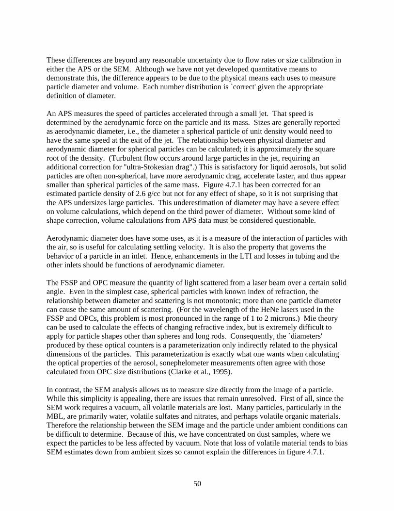
50

These differences are beyond any reasonable uncertainty due to flow rates or size calibration ineither the APS or the SEM. Although we have not yet developed quantitative means todemonstrate this, the difference appears to be due to the physical means each uses to measureparticle diameter and volume. Each number distribution is `correct' given the appropriatedefinition of diameter.

An APS measures the speed of particles accelerated through a small jet. That speed isdetermined by the aerodynamic force on the particle and its mass. Sizes are generally reportedas aerodynamic diameter, i.e., the diameter a spherical particle of unit density would need tohave the same speed at the exit of the jet. The relationship between physical diameter andaerodynamic diameter for spherical particles can be calculated; it is approximately the squareroot of the density. (Turbulent flow occurs around large particles in the jet, requiring anadditional correction for "ultra-Stokesian drag".) This is satisfactory for liquid aerosols, but solidparticles are often non-spherical, have more aerodynamic drag, accelerate faster, and thus appearsmaller than spherical particles of the same mass. Figure 4.7.1 has been corrected for anestimated particle density of 2.6 g/cc but not for any effect of shape, so it is not surprising thatthe APS undersizes large particles. This underestimation of diameter may have a severe effecton volume calculations, which depend on the third power of diameter. Without some kind ofshape correction, volume calculations from APS data must be considered questionable.

Aerodynamic diameter does have some uses, as it is a measure of the interaction of particles withthe air, so is useful for calculating settling velocity. It is also the property that governs thebehavior of a particle in an inlet. Hence, enhancements in the LTI and losses in tubing and theother inlets should be functions of aerodynamic diameter.

The FSSP and OPC measure the quantity of light scattered from a laser beam over a certain solidangle. Even in the simplest case, spherical particles with known index of refraction, therelationship between diameter and scattering is not monotonic; more than one particle diametercan cause the same amount of scattering. (For the wavelength of the HeNe lasers used in theFSSP and OPCs, this problem is most pronounced in the range of 1 to 2 microns.) Mie theorycan be used to calculate the effects of changing refractive index, but is extremely difficult toapply for particle shapes other than spheres and long rods. Consequently, the `diameters'produced by these optical counters is a parameterization only indirectly related to the physicaldimensions of the particles. This parameterization is exactly what one wants when calculatingthe optical properties of the aerosol, sonephelometer measurements often agree with thosecalculated from OPC size distributions (Clarke et al., 1995).

In contrast, the SEM analysis allows us to measure size directly from the image of a particle.While this simplicity is appealing, there are issues that remain unresolved. First of all, since theSEM work requires a vacuum, all volatile materials are lost. Many particles, particularly in theMBL, are primarily water, volatile sulfates and nitrates, and perhaps volatile organic materials.Therefore the relationship between the SEM image and the particle under ambient conditions canbe difficult to determine. Because of this, we have concentrated on dust samples, where weexpect the particles to be less affected by vacuum. Note that loss of volatile material tends to biasSEM estimates down from ambient sizes so cannot explain the differences in figure 4.7.1.

51

Another problem is that the SEM images are 2-dimensional; we do not get particle depth directly(this could be overcome using atomic force microscopy or related techniques, but those are fartoo time-consuming for this report). We calculate volume by assuming that particle depth isequal to the minimum width of the image. This is an admittedly crude assumption, but seems asreasonable as anything else.

Despite these difficulties with the SEM analysis, it gives a far richer description of the nature ofaerosol particles than the crude parameterizations of diameter provided by the APS and OPC. Itreveals that a single dimension parameter is absurd for many of the solid particles encounteredduring PELTI (see Figure 3.4.1 for a good example). While it is as yet unclear how to best touse the SEM particle dimensions in volume, scattering and aerodynamic diameter calculations, itis far more difficult to convert APS data to optical diameter or OPC data to aerodynamicdiameter.

The contention that particle shape is primarily responsible for the differences between APS andSEM distributions requires that the undersizing by the APS is worse for big particles. That couldonly be true if the larger particles have more complex shapes and therefore more aerodynamicdrag. This is indeed the case, as shown in Figure 4.7.2. Circularity is a shape factor calculatedfrom the area and perimeter, normalized so a circle has a circularity of 1.0 and more complexshapes have higher values. As Figure 4.7.2 demonstrates, small particles were very nearlycircular and shapes became more irregular for larger particles. Thus the APS undersizing shouldbe exacerbated for big particles, as is the case in Figure 4.7.1. It may be possible to usecircularity or some similar shape factor to approximate aerodynamic or optical diameters fromthe SEM data, but we have not yet developed any quantitative relationship.

It appears that the most appropriate measure of diameter depends on the calculations in whichdiameter needs to be used. Aerodynamic diameter is useful for describing behavior of particles inthe atmosphere and within inlets while optical diameter works for calculating scattering andother optical properties. None of these methods are adequate for finding particle mass, thoughthe SEM comes closest (for non-volatile particles), particularly when combined with EDSanalysis to determine particle composition. Cascade impactors classify particles by aerodynamicsize, but can be used to determine integral mass, so are probably the most direct means ofdetermining mass fluxes due to aerosol deposition. A single parameter (such as diameter) may beinadequate for some of the uses to which particle size information is put.

When working with the PELTI data it became clear how strikingly different these sizedistributions can be. When we use one type of size to estimate a different type of effect, we mayseriously misrepresent reality.

52

5. Recommendations and Conclusions

5.1 Comparison of inlets

Hypothesis A: The LTI has a demonstrably higher aerosol sampling or transmissionefficiency than both the CAI (the NCAR C-130 community aerosol inlet) and traditionalsolid diffusers for particles in the 1-7 µm range.

Conclusion: It is clear that the Hypothesis A cannot be disproven: the LTI consistentlyhad larger concentrations of particles than the SD or the CAI.

However, we note that our real goal is to achieve efficiencies near unity. The ubiquity of lossesin earlier inlets lead us initially to state this hypothesis in terms of "higher" efficiency, butenhancement by the LTI may in some cases cause efficiencies substantially above 1. Sinceenhancements in laminar flow are calculable many measurements can be corrected for them, butthe "highest" efficiency is not necessarily the most desirable one.

We base this conclusion on the following evidence:

• On virtually all legs the LTI APS distributions rose above those of the SD and the CAI. Theonly exceptions are very small and very large particle sizes, for which measurement errorsare prominent. The advantage over the other inlets increases with particle size from 2 toabout 8-9 µm.

• On virtually all legs the concentrations of anions and cations were greater on Teflon filtersbehind the LTI than on similar filters behind the SD and CAI and on an impactor behind theCAI.

• The SEM analysis of Nuclepore filters behind the LTI found considerably higherconcentrations of mineral aerosols than on Nuclepore filters behind the SD and CAI.

• Identical nephelometers found much higher scattering behind the LTI than behind the CAI,and about 13% increase was noted over the SD. Calculations of the non-truncated scatteringsuggest that the LTI may produce even larger improvements in sampling particles that have aradiative impact.

It should be noted that this conclusion does not address the issue of whether the LTI enhancedparticles of any size relative to ambient concentrations. It also does not involve anyquantification of the possible ways in which tubing behind the various inlets modified thedistributions. Although all the module plumbing was identical between inlets and the largedelivery tubes were similar, it is likely that the sharp bend immediately behind the porousdiffuser is responsible for its drop in concentrations above 8 µm.

53

5.2 Comparison of inlets to ambient concentrations

Hypothesis B: It is possible, using the LTI, to sample and characterize the number-sizeand surface area-size distributions of ambient dust and seasalt inside an aircraft withenough accuracy that uncertainties arising from inlet losses will contribute less than 20%to the assessment of radiative impacts.

We conclude that Hypothesis B also cannot be falsified.

Testing Hypothesis B requires comparing aerosols behind the LTI with those in ambient air. Thedifficulty, of course, involves defining the ambient concentrations. We used evidence from twoobservational approaches and one model to make that comparison:

• Ion-chromatographic analysis of Teflon filters in TAS showed statistically identicalconcentrations of Cl-, Na+, Mg++, Ca++, SO4=, and NSS[Mg] to those behind the LTI. Thenet enhancement of the sea salt mode must be less than 10- 20%.

• Scanning electron microscopic counting of particles on Nuclepore filters in TAS showedsimilar concentrations in size bins up to 2 µm. Above that the LTI concentration exceededthat in TAS by between 20 and 100% at the larger sizes. This argues that some LTI samplesshow little or no enhancement while others may as much as double the concentration ofparticles in the 4 to 8 µm range.

• Fluent modeling suggests that the LTI should pass particles with unit efficiency up to severalµm. Enhancement above that value may reach 30 - 40% for 6 µm particles. When FLUENTmodel-derived inertial enhancements associated with the LTI diffuser and losses associatedwith transport to the LTI filter are taken into consideration, they predict the observed 20%agreement between LTI and TAS.

• We do not yet know the extent to which losses of particles in tubing may offset anyenhancement of large particles by the LTI.

We have shown that corrections for modest but predictable LTI enhancements also can producelight scattering assessments that are representative of ambient size distributions up to 7um.Additional contributions to scattering from yet larger aerosol are unlikely to approach 20% forrealistic aerosol cases. The error in radiative forcing due to positive and negative sampling biasesdepends both on the transmission efficiency and the fraction of the mass and total optical depthin each size interval. For those sizes that contribute little to the optical depth, a poor transmissionefficiency will cause little error in radiative forcing calcualtions. It is worth noting, however, thatover- or under-sampled sizes could still cause significant errors for other issues, such as thecomputation of deposition fluxes and heterogeneous reaction rates.

54

5.3 Conclusion and Recommendations

CONCLUSION: Our conclusion, therefore, is that the LTI represents a significant advance inour ability to sample populations of large particles from aircraft. Its efficiency is near enough tounity to enable defendable studies of the distributions and impacts of both mineral dust and seasalt. Corrections can be applied for the enhancement of particles in the 3-7 µm range.

Our data suggests that even after estimated enhancements are considered, the LTI showsimproved efficiency (closer to unity) for transmission of larger aerosol compared to the SD andparticularly the CAI inlets evaluated here. We believe that tubing bends downstream of the LTIcompromised this assessments for particles larger than 8 µm, but expect that future versions willhave improved transmission efficiencies for these and larger sizes. Scattering extinctionmeasurements behind the CAI were about 40% below LTI values but the SD extinction was onlyslightly below that of the LTI for this dust aerosol. This reflects the generally reduced impact oflarger aerosol on scattering extinction. However, accurate assessment of scattering extinction forlarger aerosol require corrections for nephelometer truncation error that will depend uponrealistic coarse aerosol measurements. The LTI's improved coarse particle characterizationshould better constrain radiative assessments of aerosol properties. Studies of other issuesrelated to aerosol character, composition and mass fluxes should also be greatly improved. TheLTI's cost (in terms of both system complexity and the weight, power, and heat load from extrapumps) is more than offset by the improvement in large-particle data quality for those programsthat need to study supermicron aerosols.

WE RECOMMEND that a modified version of the LTI be used to sample aerosols from theNCAR C-130 during the ACE-Asia experiment. It is important that development workcontinue on the LTI, to address issues such as losses in tubing and the modeling ofenhancements. To make the LTI a practical device its low-altitude sample flowrate needs tobe increased and an automated control system must be added.

6. References

Ananth, G., Wilson, J.C., Theoretical Analysis of the Performance of the TSI AerodynamicParticle Sizer: The Effect of Density on Response, Aerosol Sci. Technol.,9:189-199, 1988.

Anderson, J.R., P.R. Buseck, T.L. Patterson, and R. Arimoto, Characterization of the Bermudatropospheric aerosol by combined individual-particle and bulk-aerosol analysis, Atmos.Environ., 30, 319-338, 1996.

Bates, T.S., B.J. Huebert, J.L. Gras, F.B. Griffiths, and P.A. Durkee, The International GlobalAtmospheric Chemistry (IGAC) Project's first aerosol characterization experiment (ACE-1) - Overview, J. Geophys. Res., 103, 16,297-16,318, 1998.

55

Baumgardner, D., B. Huebert, and C. Wilson, Meeting Review: Airborne Aerosol InletWorkshop, NCAR/TN-362+1A, National Center for Atmospheric Research, Boulder, CO,1991.

Baumgardner, D., J.E. Dye, R.G. Knollenberg, and B.W. Gandrud, Interpretation ofmeasurements made by the FSSP-300X during the Airborne Arctic StratosphericExpedition, J. Geophys. Res., 97, 8035-8046, 1992.

Blomquist, B.W., B.J. Huebert, S.G. Howell, M. Litchy, C. Twohy, D. Baumgardner, B. Lafleur,R. Seebaugh, and M. Laucks, An evaluation of the Community Aerosol Inlet for theNCAR C-130, J. Atmos. Ocean. Technol., in press, 2000.

Clarke, A.D., J.N. Porter, F.P.J. Valero, and P. Pilewskie, Vertical profiles, aerosol microphysicsand optical closure during ASTEX: measured and modeled column optical properties, J.Geophys. Res., Submitted, 1995.

Gesler, D. (2000) "Numerical Analysis of Sampling Efficiency on a Reduced Turbulence Inletfor Airborne Aerosol Sampling," MSME Thesis, University of Denver.

Huebert, B.J., G. Lee, and W. Warren, Airborne Aerosol Inlet Passing Efficiency Measurement,J. Geophys. Res., 95 (D10), 16369-16381, 1990.

Huebert, B.J., S.G. Howell, L. Zhuang, J.A. Heath, M.R. Litchy, D.J. Wylie, J.L. Kreidler-Moss,S. Coeppicus, and J.E. Pfeiffer, Filter and impactor measurements of anions and cationsduring the First Aerosol Characterization Experiment (ACE 1), J. Geophys. Res., 103,16,493-16,510, 1998.

Lachman, G.V. (Editor) (1961) Boundary Layer and Flow Control, Pergamon, New York.

Lafleur, B.G. “A Low Turbulence Inlet for Airborne Aerosol Sampling.” University of Denver:MSME Thesis, 1998.

Marple, V.A. and B.Y.H. Liu. Characteristics of laminar jet impactors, Environmental Sci.Technol. 8:648-54, 1974.

Pui, D.Y.H., F. Romay-Novas, and B.Y.H. Liu, Experimental study of particle deposition inbends of circular cross section. Aerosol Sci. Technol. 7:301-15, 1987.

Rader, D. J., J. E. Brockmann, et al. A method to employ the APS factory calibration underdifferent operating conditions. Aerosol Sci. and Tech. 1990, 13:514-521

Rader, D.J. and V.A. Marple. A study of the effects of anisokinetic sampling. Aerosol Sci.Technol. 8(3):283-99, 1988.

Seebaugh, W.R., and M.E. Childs (1970) "Conical Shock-Wave Turbulent Boundary LayerInteraction Including Suction Effects," Journal of Aircraft, Vol. 7, No. 4, pp. 334-340.

56

Seebaugh, W.R., B.G. Lafleur, J.C. Wilson, and J. Kim (1997) "Low Turbulence Inlet forAirborne Aerosol Sampling," Patent Disclosure to the University of Denver.

Seebaugh, W.R., B.G. Lafleur, and J.C. Wilson (1996) "Low Turbulence Inlet for AerosolSampling from Aircraft," AAAR Fifteenth Annual Conference, October 14-18, 1996,Orlando, FL.

Sheridan, P.J., and R.B. Norton, Determination of the passing efficiency for aerosol chemicalspecies through a typical aircraft-mounted diffuser-type aerosol inlet system, J. Geophys.Res., 103, 8215-8226, 1998.

Tsai, C.J. and Pui, D.Y.H., Numerical study of particle deposition in bends of circular crosssection- laminar flow regime. Aerosol Sci. Technol., 12:813-831, 1990.

Wilson, J. C. and B. Y. H. Liu. Aerodynamic particle size measurement by laser-dopplervelocimetry. J. Aerosol Sci. 1980, 11:139-150

7. Figures