Polytechnic University of Catalonia

Master Thesis

Energy Engineering

Numerical simulation of a coolingtower and its plume

Author:

Antonio Peris Alonso

Professors:

Marc Secanell Gallart

Morris R. Flynn

September 29, 2019

Contents

1 Abstract 3

2 Introduction 4

2.1 Cooling Towers . . . . . . . . . . . . . . . . . . . . . . . . . . . . . . . . . . 4

2.1.1 Wet Cooling Towers . . . . . . . . . . . . . . . . . . . . . . . . . . . 4

2.1.2 Dry Cooling Towers . . . . . . . . . . . . . . . . . . . . . . . . . . . . 6

2.1.3 Hybrid Cooling Towers . . . . . . . . . . . . . . . . . . . . . . . . . . 6

2.2 Operating Principles . . . . . . . . . . . . . . . . . . . . . . . . . . . . . . . 8

2.2.1 Physical processes occurring inside a cooling tower . . . . . . . . . . 8

2.2.2 Physical phenomena occurring in the plume . . . . . . . . . . . . . . 9

2.3 Methods of Analysis of a Cooling Tower . . . . . . . . . . . . . . . . . . . . 11

2.4 Literature Review and objectives . . . . . . . . . . . . . . . . . . . . . . . . 11

3 Methodology 13

3.1 Plume Model (Single plume) . . . . . . . . . . . . . . . . . . . . . . . . . . . 13

3.2 Wet cooling tower models . . . . . . . . . . . . . . . . . . . . . . . . . . . . 17

3.2.1 Merkel Method . . . . . . . . . . . . . . . . . . . . . . . . . . . . . . 17

3.2.2 Klimanek Method . . . . . . . . . . . . . . . . . . . . . . . . . . . . . 19

3.3 CoolIT . . . . . . . . . . . . . . . . . . . . . . . . . . . . . . . . . . . . . . . 22

3.3.1 Numerical implementation . . . . . . . . . . . . . . . . . . . . . . . . 22

1

3.3.2 Coupling scheme . . . . . . . . . . . . . . . . . . . . . . . . . . . . . 23

3.3.3 Graphical user interface . . . . . . . . . . . . . . . . . . . . . . . . . 25

4 Results and Discussion 26

4.1 Comparative study between Merkel and Klimanek methods . . . . . . . . . . 26

4.2 Parametric study of the fill height (hfill) for plume abatement . . . . . . . . 31

4.3 Parametric study of the L/G ratio for plume abatement . . . . . . . . . . . . 36

5 Conclusions 50

6 References 52

7 Annex 55

7.1 Single plume class (SinglePlume) . . . . . . . . . . . . . . . . . . . . . . . . 55

7.2 Governing equations class (GovernEq) . . . . . . . . . . . . . . . . . . . . . 70

7.3 Air and vapour properties class (AirVapour) . . . . . . . . . . . . . . . . . . 73

2

1 Abstract

Cooling tower design has been an active area of research for over 40 years with the goal

of reduceing the visibility of their effluent water vapor plumes. Plume visibility occurs when

water vapour leaving the tower is exposed to ambient, cold air, resulting in condensation.

In order to minimize plume visibility, the research field of cooling towers has been diverse.

On the one hand, research has been conducted on designing cooling towers improving their

plume abatement (from wet and dry to hybrid cooling towers). On the other hand, other

lines of research focused on the evaluation of a predefined cooling tower over a variety of

operating conditions to determine its optimal plume abatement. The main objective of this

project is to analyze the effect of the ambient and cooling tower operating conditions on

plume visibility.

A numerical model based on wet cooling towers has been coupled with a numerical plume

model that considers the possibility of condensation.The wet cooling tower model proposed

by Klimanek and Merkel methods have been used to study the tower. In the case of the

plume, a theoretical steady-state plume model that is adapted from the work of Wu and

Koh (1978) and Ali Moradi and M. R. Flynn et al. is considered [1] that assumes a uniform,

rather than a coaxial plume, and takes into account the event of condensation.

The coupling between models, cooling tower and plume, has been carried out using an open

source simulation package especially developed for the analysis and design of cooling towers:

CoolIT. As CoolIT already had a wet cooling tower model implemented with Klimanek and

Merkel methods, the main task of this thesis was to implement and couple the plume model

to the existing tower models in CoolIT using the Python programming language and object-

oriented programming structure. Then, some cases are simulated to illustrate the effect of

plume visibility while comparing both methods and varying certain operating conditions.

3

2 Introduction

2.1 Cooling Towers

Cooling towers emerged as a means of dissipating large quantities of waste heat using

water and air as heat transfer media. Although cooling towers can be classified in several

ways, such as by relative direction of air movement (counter flow or cross flow) and the type

of water distribution system, the greatest distinction is between wet, dry and wet-dry hybrid

towers [2][3]. In particular, the analysis in the thesis is focused on a wet cooling tower.

However, the other two type of towers are presented as well since they also can be used to

size any section by estimating when the plume is not visible (the work in this thesis can be

reproduced in any of the other types of tower). Moreover, it will help to characterize and

understand the so-called plume abatement; term used to describe visible plume prevention.

2.1.1 Wet Cooling Towers

Wet cooling towers work on the principle of evaporative cooling. Water contacts un-

saturated air causing some of the water to evaporate and, as a consequence, the process

water temperature decreases (Figure 1) [2]. At the same time, there is an increase in the

wet bulb temperature of the air passing through the cooling tower [3]. In order to enhance

air-water interfacial area and increase evaporation, wet cooling towers typically contain a

wetted medium called “fill”. The unsaturated air enters the tower forced by a fan and faces

the warm water coming from the nozzles above the fill. Due to water contact and evapora-

tion, the counterflowing air gains temperature and humidity. Finally, after collecting possible

small water droplets in the drift eliminator, the damp air leaves the cooling tower forming a

plume.

4

Figure 1: Wet Cooling Tower Scheme (source: FANS a.s. website)

Wet cooling towers consume large quantities of water due to evaporation, drift and draining

losses and a visible plume may form at the fan stack depending on operating conditions and

design. This plume is often considered undesirable because it could dangerously obstruct the

view and/or form undesirable icing over cold surfaces [5]. In order to avoid having a visible

plume (plume abatement), a number of innovative cooling tower systems have been, and are

still being, developed.

This thesis will be focus on the analysis of a wet cooling tower and its plume. Within this type

of cooling towers, the counter-flow mechanical draft configuration has been chosen for the

study. The counter-flow configuration has been found the most appropriate as it is generally

more efficient, cheaper and more compacted than cross-flow cooling towers. Moreover, the

mechanical draft has been chosen over the natural draft since it makes possible the mass flux

of air variation which is needed for the plume abatement analysis of the wet cooling tower.

5

2.1.2 Dry Cooling Towers

In dry cooling tower, heat is transferred through air-cooled heat exchangers that separate

the working fluid from the cooling air. As there is no direct contact between the working

fluid and the ambient air, no water is lost to evaporation in the system [4]. However, dry

cooling towers require large surface areas and have relatively high energy consumption, even

with higher water temperatures, compared to wet cooling towers [5][6].

In the case of a direct dry cooling tower (Figure 2), turbine exhaust steam is condensed

directly through an air-cooled condenser (ACC). The turbine steam flows directly from the

tubes of the ACC to a heat exchanger where it is condenses by means of heat transfer with

the flowing air [4].

Figure 2: Dry Cooling Tower Scheme (source: FANS a.s. website)

2.1.3 Hybrid Cooling Towers

Hybrid cooling towers use both dry and wet cooling to eject waste heat to the atmosphere

[7]. As with other cooling tower types, its operation depends on the heat load, the air flow

rate and the ambient air conditions [6]. Hybrid cooling towers can be applied to a wide range

6

of configurations, as presented by Streng [8]. One of the most effective cooling processes

overall is the Parallel Path Wet/Dry (PPWD) tower [5][8]. In this method, as shown in

Figure 3, the air is drawn by an induced draft fan in a parallel path through the dry and

the wet sections. The warm water is firstly circulated through the dry section, where a

finned heat exchanger decreases its temperature; then, the water enters the wet section and

is sprayed over the fill which enhances its evaporation and finishes cooling it down. The air

leaving the dry sections is heated without adding moisture, becoming hot and having low

humidity. On the other hand, the air leaving the wet sections is typically considered to be

100% saturated. Both streams are mixed in a plenum, so the resultant air discharged from

the fan leaves at a reduced relative humidity, relative to the air leaving the fill, which can

prevent condensed droplets from forming, thereby avoiding a visible plume.

Figure 3: Parallel Path Wet/Dry cooling tower (source: FANS a.s. website)

7

2.2 Operating Principles

2.2.1 Physical processes occurring inside a cooling tower

As mentioned previously, cooling towers operate based on latent and sensible heat transfer.

In order to illustrate these phenomena and all the process states, a psychrometric analysis of

the air passing through a cooling tower is shown in Figure 4 [9].

Figure 4: Psychrometric analysis of the air inside the cooling tower [9]

Air enters at the ambient condition Point A, absorbs heat and mass (moisture) from the water,

and exits at Point B usually at saturated conditions. For very small loads, the discharged

air may be subsaturated. The air heated (Vector AB in Figure 4) can be separated into

component AC, which represents the sensible portion of the heat absorbed by the air as the

water is cooled, and component CB, which represents the latent portion (evaporation). If

the entering air condition is changed to Point D at the same wet-bulb temperature but at

a higher dry-bulb temperature, the total heat transfer remains constant, but the sensible

and latent components change significantly. DE represents sensible cooling of air, while EB

represents latent heating as water evaporates. Thus, for the same water-cooling load, the

ratio of latent to sensible heat transfer as well as sensible heat sign can vary significantly

8

depending upon the ambient air conditions.

Therefore, thermal performance of a cooling tower depends principally on the entering air

wet-bulb temperature. The entering air dry-bulb temperature and relative humidity, taken

independently, have a lesser influence on thermal performance of mechanical-draft cooling

towers, but do affect the rate of water evaporation in the cooling tower [9].

2.2.2 Physical phenomena occurring in the plume

As previously mentioned, warm air discharged from a cooling tower is typically either

saturated or close to saturation. Under certain operating conditions, the ambient air sur-

rounding the tower cannot absorb all of the moisture in the tower exhaust discharge, and

the excess condenses resulting in a visible plume. Assuming a process of adiabatic mixing

in the atmosphere, this plume visibility can be determined by drawing a straight line on a

psychrometrical chart (Figure 5). The line goes from the entering air condition to its ex-

haust condition. Thus, when this line crosses the saturation curve, a visible plume is formed.

Moreover, its intensity becomes stronger as the area to the left of the saturation curve grows.

This fact together with the degree of mechanical and convective mixing with the ambient air

determines the persistence of the visible plume.

9

Figure 5: Psychrometric analysis of the plume [10]

In order to illustrate the plume state, the operating lines of a common wet cooling tower have

been compared with those of a hybrid cooling tower including plume abatement (Figure 5)

[10]. As it can be appreciated, the oversaturated area, which leads to fog formation (visible

plume), is smaller in wet/dry operation compared with wet operation. This is due to the dry

section in the hybrid tower where the introduced outside air is heated at a constant specific

humidity. Thus, after this air is mixed with the moist air coming from the wet section, the

exhaust air is produced with less moisture content, therefore, a lower operating line.

For environmental and safety reasons, the potential for fogging and its effect on tower sur-

roundings has to be considered, specially in large windowed areas or traffic arteries, airports

[10]. Often, while selecting cooling tower sites, the most practical solution is to predict where

visible plumes should form, accordingly to the ambient and operating conditions [10].

These operating lines and, consequently, the prediction of the visible plume can be ob-

tained analytically considering momentum, energy, and moisture (absolute humidity) trans-

port equations.

10

2.3 Methods of Analysis of a Cooling Tower

Although the evaporative cooling phenomenon is a quite ancient knowledge, it is only

relatively recently (within the last century) that it has been modeled and studied scientifically

[11]. Regarding cooling towers, Merkel [12] was the first to develop a theory for the thermal

evaluation of cooling towers in 1925. Unfortunately, this work was largely neglected until 1941

when the paper was translated into English. Then, in 1989 Jaber and Webb [13] developed

the equations necessary to apply the e-NTU method directly to counter flow or cross flow

cooling towers. Two years later, Poppe and Rogener presented a more rigorous model called

Poppe method [14] and, finally, Klimanek and Bialicki developed an alternative method in

2009 [15].

Despite that the resolution process takes into account several input operating parameters

related to its different areas (the geometry, the fan, the drift eliminator, the spray zone, fill

and rain zone), the equations presented in each methodology are the main governing equations

considering a counter flow configuration of a wet cooling tower. Thus, in all methodologies

the input states of water and air are known: mass flow rate, temperature and pressure (and

relative humidity in case of the air). Consistently, the common goal is to obtain the final

states - outputs - of air and water. Therefore, the differences between methods are how the

outputs are obtained, illustrated in the governing equations. Further down, the Merkel and

Klimanek methods, which are used in the thesis to model the tower, are presented. Merker

represents the most common used method, while Klimanek represents the one with the least

number of assumptions.

2.4 Literature Review and objectives

Tyagi et al. [16] presented a case study of the prediction and control of plume in wet

cooling towers from a huge commercial building in Hong Kong. The building contained a

central air conditioning system comprising six water-cooled chillers and 10 cooling towers.

The study took the weather data available for a particular year, 1989, in Hong Kong: ambient

11

temperatures of 15ºC with 95% of relative humidity for winter and ambient temperatures of

25ºC with 95% of relative humidity for spring. The main conclusion regarding plume abate-

ment was that, for this particular case, a proper operation of wet cooling towers, increasing

the number and air speed of towers, can reduce and/or control the potential of visible plume.

Xu et al. [17] studied the plume potential and a plume abatement system in a large commer-

cial office building in Hong Kong. The evaluation consisted on a dynamic simulation using,

as in the previous case, a representative meteorological data of Hong Kong. The study stated

that the yearly dynamic simulation is crucial to predict the plume potential and determine

the parameters for designing the plume abatement system. Alternative control strategies,

such as set-point control logics of the supply cooling water temperature and fan modulation,

have significant impacts on the visible plume frequency and, therefore, should be included in

the design of a plume abatement system.

There are other studies focused on heating the exhausted air to achieve plume abatement.

Wang et al. [18] presented the application and utility of solar collectors heating system to

control the visible plume and Tyagi et al. [19] compared a similar system based on solar

collectors with a heat pump system to control visible plume economically. However, these

other ways of plume abatement are more focused on adding new systems and, thus, differ

from the main objective in this project: analyze the effect of the ambient and cooling tower

operating conditions on plume visibility.

This thesis follows the idea of varying the operating conditions for plume abatement [16]

[17], increasing the mass flux of air, but with distinctions and novelties. This study is not

based on the ambient conditions of a specific location, it takes into account different values of

temperature and relative humidity, hence, a wide range of ambient conditions. The object of

study is a single wet cooling tower and its plume. The visible plume is measured in terms of

height rather than persistence, time. Although Merkel and Klimanek methods [12] [15] have

been used in different cooling tower studies, they haven’t been coupled with a plume model

to study plume abatement. Therefore, this project through object oriented programming in

Python will try to extend the mechanisms to predict and control (or avoid) visible plume.

12

3 Methodology

3.1 Plume Model (Single plume)

The solution of the plume is based on a theoretical steady-state model that takes into

account the event of condensation. In particular, the model applied is adapted from the work

of Wu and Koh (1978) [20] who made predictions of the behaviour of a plume discharged to

a wet or dry atmosphere by integrating turbulent plume theory with psychrometrics. The

unknowns in the plume model are practically the same as Wu and Koh’s model: plume’s

temperature, moisture (vapor and liquid phases), humidity, pressure, and density of the

plume as well as the visible plume length in case of condensation. Moreover, both approaches

follow the same assumptions in order to develop the model:

I. Since turbulent transport is significantly larger than molecular transport, the model’s

output is considered independent of the Reynolds number.

II. The cross-sectional profiles of the plume vertical velocity, temperature, density, vapor

and liquid phase moistures are considered constant. This is because plume properties

are assumed to exhibit “top-hat” profile (Figure 6); i.e., a given property, such as the

plume vapor phase moisture, is constant inside the plume and zero outside.

III. The variation of the plume density is small, i.e., no more than 10%.

IV. The fluid pressure is hydrostatic throughout the flow field [23].

V. The plumes are axisymmetric and propagate vertically upwards (Figure 6).

VI. Due to the relatively low height used in that type of simulations (elevations of more than

100 m aren’t worrisome for fog formation), the ambient temperature has been assumed

independent of the elevation as well as to lack liquid phase moisture and to be uniform

in density and humidity.

VII. Since the temperature and concentration profiles have the same shape and the flow is

turbulent, the Lewis number, Le, is equal to 1 (Kloppers and Kroger [24]). The Lewis

number is formulated as the ratio of thermal diffusivity to mass diffusivity.

13

Figure 6: Axisymmetric top-hat plume scheme (image based on Shuo Li, Ali Moradi, BradVickers and M.R. Flynn work [1])

From the above assumptions, and using Boussinesq approximation to relate temperature and

density, a set of differential governing equations is obtained [1],

dQdz = E (Volume) (1)

dMdz = g

Ta· DF ·Q

M− g · W ·Q

M(Momentum) (2)

ddz

(DF − Lv

Cpa·W

)= 0 (Energy) (3)

ddz (H +W ) = 0 (Moisture) (4)

14

DF =∫A

(Tp − Ta) · Up · dA (5)

Where Q is the plume volume flux, M is the momentum flux, DF is the deficiency flux’s

temperature, H is the specific humidity deficiency flux, W is the specific liquid moisture

deficiency flux and Cpa, Lv, U and A are, respectively, the air’s specific heat capacity, the

latent heat due to condensation, vertical velocity, and cross-sectional area. Moreover, E is

the volume rate of entrainment of ambient fluid, expressed as [23],

E = S · α · Up, (6)

where S is the plume circumference, and α is the entrainment coefficient whose value is

approximately 0.1 for axisymmetric plumes and 0.2 for line-source plumes. Moreover, as the

energy and moisture with respect to z are constant- they are independent of the height- they

won’t be integrated. Instead, another variable has been added that has been found dependent

on z: pressure. This is due to the fact that the pressure within the plume is imposed by the

external (hydrostatic) ambient [23]. Thus, considering the virtual temperature relation and

the relation between densities (Equations (10) and (11)), the the final governing equations

are:

dQdz = 2 · α ·

√π ·M (Volume) (7)

dMdz = g′ · Q

2

M(Momentum) (8)

dpdz = −g · p

Ra · Tv,a(Pressure) (9)

15

Where Tv and g′ are formulated by Emmanuel [25] as,

Tv = T · (1 + 0.608 · q − σ), (10)

g′ = g · ρa − ρρ0

= g · ρa − ρρa

= g ·

1−p

Ra·Tv,p

pRa·Tv,a

= g ·(

1− Tv,aTv,p

), (11)

where q is the specific humidity and σ is the specific liquid moisture, which is higher than 0

when condensation occurs (RHp ≥ 100 %) and, otherwise (RHp < 100 %), equal to 0. For

a prescribed source, the exit of the cooling tower, and at a certain ambient conditions, this

governing equations equations are integrated up to some prescribed vertical distance above

the cooling tower. The boundary conditions of the model are set at source level (z = 0).

These boundary conditions are

Q(z = 0) = U0 · A0 (12)

M(z = 0) = U20 · A0 (13)

P (z = 0) = Pamb. (14)

In addition, the input variables are the source velocity U0 in m/s, source relative humidity

RH0, source temperature T0 in Kelvin, source area A0 in m2, ambient relative humidity

RHa, ambient temperature Ta in Kelvin, ambient pressure Pa in Pascals, the interval steps

of integration, the entrance coefficient and the height of the study (used for the integration).

16

3.2 Wet cooling tower models

3.2.1 Merkel Method

The Merkel method relies on several critical assumptions:

I. The Lewis factor, Lef , relating heat and mass transfer is equal to 1. In other words,

thermal and mass diffusivity are exactly the same.

II. The air exiting the tower is saturated with water vapor and it is characterized only by

its enthalpy.

III. The reduction of water flow rate by evaporation is neglected in the energy balance

(dmw = 0).

By applying these assumptions, the mass and energy balances for the control volume in

Figures 7(a) and 7(b), result in [21]:

dimadz = hd · afi · Afr

ma

· (imasw − ima), (15)

dTwdz = ma

mw

· 1cpw· dima

dz , (16)

where:

• Tw is the water temperature in K.

• afi is the surface area of the fill per unit volume of fill in m−1.

• Afr is the cross-sectional packing area in m2.

• hd is the mass transfer coefficient in m/s.

• imasw is the enthalpy of saturated air evaluated at water temperature in kJ/kg.

17

• ima is the enthalpy of the air-water vapor mixture per unit mass of dry-air in kJ/kg.

• ma is the mass flow rate of air in kg/s.

• mw is the mass flow rate of water in kg/s.

• cpw is the specific heat at constant pressure of water in kJ/kg ·K.

Equations (15) and (16) describe, respectively, the change in the enthalpy of the air-water

vapor mixture and the change in water temperature as the air travel distance changes. Both

can be combined to yield upon integration the Merkel equation,

MeM = hd · afi · Afr · Lfimw

= hd · afi · LfiGw

=∫ Twi

Two

cpw · dTwimasw − ima

, (17)

where:

• MeM is the transfer coefficient or Merkel number according to the Merkel’s approach.

• Lfi is the fill height in m.

• Gw is the mass velocity of the water in kg/s ·m2.

Merkel’s Equation (17) assumes that the air leaving the fill is saturated with water vapor,

therefore, it is not possible to calculate the true state of the air leaving the fill. Even so, this

assumption allows the calculation of the air temperature leaving the fill.

Figure 7: Fill control volume balances [21]: a) Mass balance; b) Energy balance

18

3.2.2 Klimanek Method

Klimanek and Bialecki [15] developed a method to describe the heat and mass transfer in

the fill by considering it as a porous medium without the simplifying assumptions commonly

used in Merkel’s method. By not making these assumptions, Klimanek (as Poppe) method

can calculate the amount of water evaporated (which is not possible with Merkel). Moreover,

the equations are formulated with respect to the spatial distribution of all the flow parameters

which is not the case in the standard methods such as Merkel, e-NTU and Poppe. Therefore,

this model is able to predict the flow parameters along the height such as temperature of

air and water, mass flow rate of water and humidity ratio. The formulation of the method

consists on four non-linear differential equations that take into account whether the exhaust

air is either unsaturated (including the case for saturation) or supersaturated [15].

The governing equations for the unsaturated air of humidity ratio, air enthalpy and temper-

atures of air and water are:

dmw

dA = β · af · Az · (ωws − ω) (18)

dωdz = β · af · Az · (ωws − ω)

ma

(19)

dTa

dz =β · af · Az · [Lef · (Tw − Ta) · (capa + ω · capv) + (cwpv · Tw − capv · Ta) · (ωs − ω)]

ma · (capa + capv · ω) (20)

dTwdz = β·af ·Az ·[Lef ·(Tw−Ta)·(ca

pa+ω·capv)+(r0+cw

pv ·Tw−cww·Tw)·(ωs−ω)]

mw·cww

(21)

19

where af is the transfer area per unit volume of the fill (area density in m−1), Az is the

cross sectional area of the fill in m2, β is the average mass transfer co-efficient in m/s and

the difference between humidity ratios, (ωws − ω), represents the driving force of the mass

convection process [15]. Moreover, cww is the average specific heats at constant pressure of

water in kJ/kg ·K evaluated at water w temperature. Analogously, a is used to indicate that

the variable is evaluated at bulk air temperature. Moreover, the air humid enthalpy and the

Lewis factor are expressed using Bosnjakovic relationships [22] (as in Poppe’s formulation),

ha = capa · Ta + ω · (r0 + capv · Ta), (22)

Lef = 0.8662/3 ·(ωws + 0.622ω + 0.622 − 1

)·[ln(ωws + 0.622ω + 0.622

)]−1. (23)

where ha represents the enthalpy of the humid air per unit mass of dry air (in kJ/kg) and capaand capv in kJ/kg ·K are the specific heats and the average specific heats at constant pressure

of dry air, respectively. Moreover, r0 stands for the latent heat of evaporation evaluated at

Tw = 0 °C (expressed in kJ/kg) and ωws is the humidity ratio of the saturated air at the

air-water interface in kg/kg.

In the second case - supersaturated air - the governing equations are:

dmw

dA = β · af · Az · (ωws − ωas ) (24)

dωdz = β · af · Az · (ωws − ωas )

ma

(25)

20

dTa

dz = −β · af · Azma

·[Lef · capa · (Tw − Ta)− ωws · (r0 + cwpvTw)

+ caw · (Lef · (Tw − Ta) · (ω − ωas ) + Ta · (ωws − ωas ))

+ ωas · (r0 + capv · Lef · (Ta − Tw)) + cwpv · Tw]

·[capa + caw · ω + dωa

sdTa· (r0 + capv · Ta − caw · Ta) + ωas · (capv − caw)

]−1

(26)

dTwdz = β·af ·Az ·[(r0+cw

pv ·Tw−cww·Tw)·(ωw

s −ωas )+Lef ·(Tw−Ta)·(ca

pa+caw·(ω−ωa

s )+capv ·ωa

s )]mw·cw

w(27)

where, this time, using again Bosnjakovic relationships [22], the Lewis factor follows the

previous expression, Equation (23) (using ωas though), and the air humid enthalpy has a

different formulation:

has = capa · Ta + ωas · (r0 + capv · Ta) + (ω − ωas )cawTa (28)

This governing equations are integrated considering some boundary conditions which are set

at the bottom of the rain zone (z = 0) and on the top of the spray zone (z = H) of the

cooling tower. These boundary conditions are:

mw(z = H) = mwi (29)

ωa(z = 0) = ωai (30)

Ta(z = 0) = Tai (31)

Tw(z = H) = Twi (32)

where mwi is the mass flow rate of inlet water, ωai is the inlet humidity ratio, Tai is the

ambient air temperature and Twi is the water inlet temperature.

21

3.3 CoolIT

For cooling tower modelling, an open source simulation framework developed for its design

and analysis has been used, namely CoolIT. CoolIT uses additional libraries than those

supplied by Python, such as SciPy for scientific math functions. In order to use CoolIT,

a CONDA environment with numerous pre-installed scientific Python packages are used to

prevent any conflicts with other local packages already installed.

3.3.1 Numerical implementation

CoolIT uses object oriented programming and contains a wide number of classes that

interact with one another to create the program. The goal of implementing the plume code

in CoolIT implies creating an object oriented scheme for that code. So, taking into account

the different functions used to obtain the solution, the single plume code has been divided

into three classes: SinglePlume, PlumeGovernEq and AirVapour (located in the Annex as

Listings 1, 2 and 3).

The SinglePlume object receives the input parameters of the plume model and solves it. The

member functions associate to the class are: solve gov eq(), solve var(), plot rh(), plot rd(),

plot hr(), plot psychrometric() and find condensation(). These are described below. The

member function solve gov eq() solves the governing equations (Equations (7), (8) and (9))

with the odeint Python function and returns an array of values referring to volume, momen-

tum and pressure at certain heights set in the input variables. Member function solve var(),

using the results from the previous method, calculates and returns an array of all the physical

parameters that characterize the plume (relative humidity, water content, temperature, etc.).

The other member functions are focused on either plotting the results (plot rh(), plot td(),

plot hr() and plot psychrometric()), printing the interval of heights where there is conden-

sation, and, if condensation does not take place, the value and height where the maximum

relative humidity is achieved (find condensation()).

22

The PlumeGovernEq class contains the equations that SinglePlume solves. The member

function govern eq() contains the differential form of the governing equations already pre-

sented (Equations (7), (8) and (9)) taking into account condensation phenomena. This class

also includes the member function condensation() which is used by the govern eq() from this

class as well as solve var() from SinglePlume class. It contains the function that fsolve, also

from scipy Python package, solves to calculate the water content in the plume.

Finally, the AirVapour class contains the physical properties of air/vapour that both classes,

SinglePlume and PlumeGovernEq use for the resolution of the plume. These properties

are divided into attributes, like the ideal gas constant or the masses of air and vapor, and

methods, for calculating the vapour saturation pressure, latent and specific heats, etc.

Figure 8: Object oriented programming scheme for single plume resolution

3.3.2 Coupling scheme

The addition of the plume model to CoolIT implies also a connection of this model to the

existing wet cooling tower model. This coupling scheme, Figure 9, consists on solving first

the cooling tower model, and then the plume model since the plume model uses some of the

23

wet cooling tower outputs as inputs.

Figure 9: Coupling scheme

Thus, for a given tower architecture and operating conditions, the cooling tower model in

CoolIT, either Merkel or Klimanek, is solved to obtain, among others, the tower outlets of air

temperature, velocity and relative humidity. These three values and the ambient conditions,

previously set by the wet cooling tower model, together with the interval steps, plume height

and entrainment coefficient are used to solve the plume model. The results of the plume

are displayed together with the wet cooling tower results file. In addition, the output file

displayed after the wet cooling tower simulation, also contains the resultant interval of heights

where condensation occurs. Finally, a unit test has been created to assess the validity of the

code. In this test, the plume results obtained from CoolIT (SinglePlume class) are compared

to the ones obtained from the source plume code devolped in Matlab by Ali Moradi [1].

24

3.3.3 Graphical user interface

CoolIT can be set up and executed via a graphical user interface that displays the input

parameters used to define the method (either Klimanek or Merkel), the tower geometry, and

the fan, drift eliminator, spay, rain and fill zones, and the fluxes of air (inlet) and water (inlet

and outlet). Besides that, it is also possible to perform parametric studies for the different

variables involved during the process as well as to save and import predefined models of

cooling tower. Once the simulation is run, the output variables obtained from both studies

(cooling tower and plume solutions) are exported to a text file in an output directory and

the plots from the plume study are displayed. The commented interface looks as Figure 10:

Figure 10: CoolIT graphical user interface

The purpose of this project is to develop a plume model and a GUI tab, called Plume, that

contains the input parameters that are specific to the model. Thus, as Figure 10 shows, the

plume height, over which it has been computed the plume solution, has been chosen as the

parameter to vary and an image illustrating it has been included. Other input parameters

contained in the other tabs can be taken from the cooling tower solution as mentioned in the

Coupling scheme section. The analysis of the results is shown in the next section, Simulations.

25

4 Results and Discussion

At this point, after the integration of the model into CoolIT, three different types of

simulations have been carried out. Firstly, the effect of using a detailed cooling tower model,

Klimanek and Merkel, on plume visibility has been assessed. Through this comparison, one

of the methods will be chosen to carry out the next simulations. Secondly, the effect of

a design parameter, the fill height, on plume visibility has been studied. Finally, the last

study has been focused on evaluate an operational parameter, the L/G ratio, to mitigate

plume visibility. Thus, the fan power consumption will be taken into account as well as the

compliance with reasonable operational conditions.

4.1 Comparative study between Merkel and Klimanek methods

The aim of this study is to analyze the impact of plume using Merkel method vs. Klimanek

method. Merkel assumes saturated outlet conditions and, as a result, it is expect to provide

inaccurate tower outlet conditions in some cases. In turn, it will affect plume visibility

condition. To study the ambient conditions where Merkel fails, ambient relative humidity and

temperature were varied. The model input parameters of the cooling tower are shown in Table

1. On the other hand, the ambient conditions are modified as shown in Table 2, where each

ambient temperature forms a test case with the different ambient relative humidities. The

simulations are performed with Klimanek and Merkel methods for the purpose of comparing

their visible plume heights results. 63 test cases were performed and used to study the

differences between methods in terms of plume behaviour and plume visibility.

Table 1: Model input parameters of the cooling tower (Base case)

Method Merkel/Klimanek hrainzone (m) 3Geometry Rectangular L/G (= mw/ma) 1Width (m) 12 Pa (Pa) 101250Type of fill OF21-ma Twi (K) 310hfill (m) 1.2 L (kg/s) 1000

26

Table 2: Ambient conditions, relative humidity and temperature, from which the test casesare built

Tai (K) 306 301 296 291 286 282 279 274 269RHa (%) 5 20 35 50 65 80 95

Regarding the visible plume height, it has been calculated through the difference between

the heights where the visible plume appears and disappears, no matter if it starts at the

source or later. The results are illustrated in Figures 11 and 12, using Merkel and Klimanek

respectively.

Figure 11: Visible plume height as a function of the ambient conditions (Merkel)

27

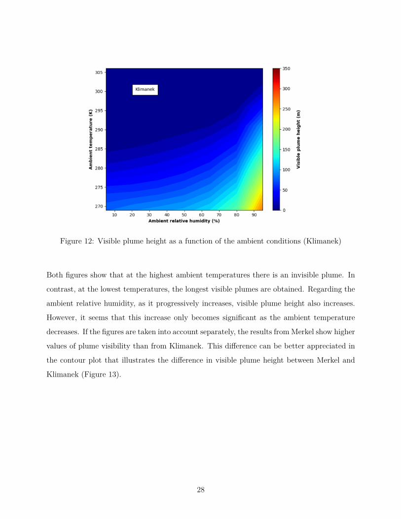
Figure 12: Visible plume height as a function of the ambient conditions (Klimanek)

Both figures show that at the highest ambient temperatures there is an invisible plume. In

contrast, at the lowest temperatures, the longest visible plumes are obtained. Regarding the

ambient relative humidity, as it progressively increases, visible plume height also increases.

However, it seems that this increase only becomes significant as the ambient temperature

decreases. If the figures are taken into account separately, the results from Merkel show higher

values of plume visibility than from Klimanek. This difference can be better appreciated in

the contour plot that illustrates the difference in visible plume height between Merkel and

Klimanek (Figure 13).

28

Figure 13: Difference in visible plume height considering Merkel minus Klimanek methods.

The comparison shows that the biggest differences between methods is located at low ambi-

ent temperature. The highest difference is at minimum ambient temperature and maximum

relative humidity. These differences can be explained through the disparities between output

values of the cooling tower solution, which are used for solving the plume, i. e., T0 and RH0.

Merkel assumes 100% for RH0, while Klimanek calculates RH0. Thus, Merkel can’t predict

either subsaturated or supersaturated cases. Even though Figure 15 shows subsaturation at

the higher ambient temperatures and it is expected a high difference between methods, in

reality this differences are nearly 0. This can be due to the high source temperatures (shown

in Figure 14) that promotes plume abatement to a large extend. Regarding the negative and

positive differences, following the same reasoning, could be due to, firstly, higher source tem-

peratures in Klimanek and, then, largely higher source temperatures in Merkel. This abrupt

increase of temperature at low ambient temperatures and the wrong and recurrent allocation

of 100% relative humidity show Merkel method inaccuracy at supersaturated conditions as

well as subsaturated conditions. Therefore, since Klimanek model is able to provide better

predictions for the outlet air temperature and relative humidity, it is the method likely to

29

provide more accurate predictions for plume visibility.

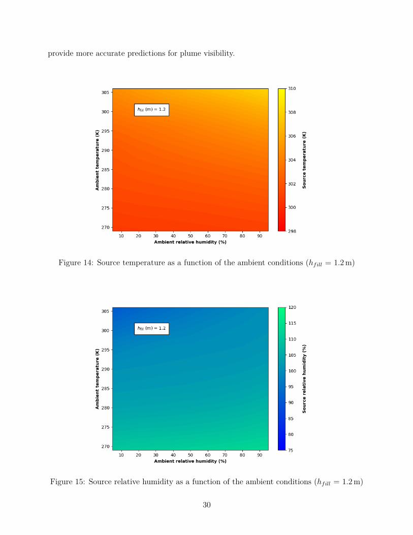
Figure 14: Source temperature as a function of the ambient conditions (hfill = 1.2 m)

Figure 15: Source relative humidity as a function of the ambient conditions (hfill = 1.2 m)

30

4.2 Parametric study of the fill height (hfill) for plume abatement

As Klimanek has been argued to be the more accurate method, as it is valid for super-

saturation and subsaturation conditions, in this section all simulations have been carried

out only using this model. These simulations take into account the same ambient conditions

range; however, this time a specific operating parameter which has direct relation with plume

visibility (and keeping all the other constant) has been varied: the fill height. Because the

base case used to compare results against the Merkel solution only takes into account a fixed

fill height (particularly, 1.2 m), it was decided to test two more cases: one with a height

value above and another with the value below (see Table 3) in order to study the effect of

the evaporation reduction/increase.

Table 3: Fill height test cases

hfill (m) 0.6 1.2 1.8

Following the same procedure as in the comparison of methods, the plume visibility height

has been obtained and illustrated for the three cases, shown in Figures 16, 17 and 18.

Figure 16: Visible plume height as a function of the ambient conditions (hfill = 0.6 m)

31

Figure 17: Visible plume height as a function of the ambient conditions (hfill = 1.2 m)

Figure 18: Visible plume height as a function of the ambient conditions (hfill = 1.8 m)

32

The figures show that as the fill height is increased, higher values for visible plume height are

obtained. Similarly, it is appreciated that the starting points where visible plume is obtained

appear earlier, at higher ambient temperatures. This phenomena can be related with the

physical meaning of reducing or increasing the fill height, i.e. decreasing/increasing outlet

RH0.

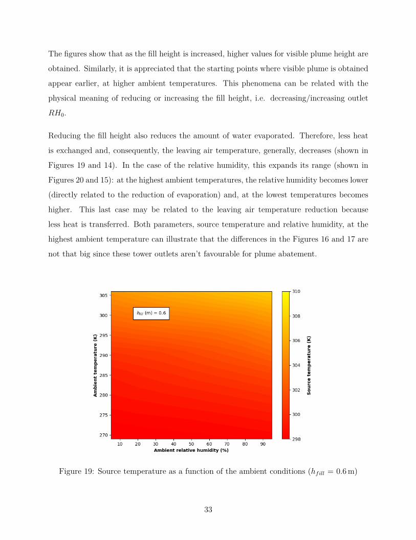
Reducing the fill height also reduces the amount of water evaporated. Therefore, less heat

is exchanged and, consequently, the leaving air temperature, generally, decreases (shown in

Figures 19 and 14). In the case of the relative humidity, this expands its range (shown in

Figures 20 and 15): at the highest ambient temperatures, the relative humidity becomes lower

(directly related to the reduction of evaporation) and, at the lowest temperatures becomes

higher. This last case may be related to the leaving air temperature reduction because

less heat is transferred. Both parameters, source temperature and relative humidity, at the

highest ambient temperature can illustrate that the differences in the Figures 16 and 17 are

not that big since these tower outlets aren’t favourable for plume abatement.

Figure 19: Source temperature as a function of the ambient conditions (hfill = 0.6 m)

33

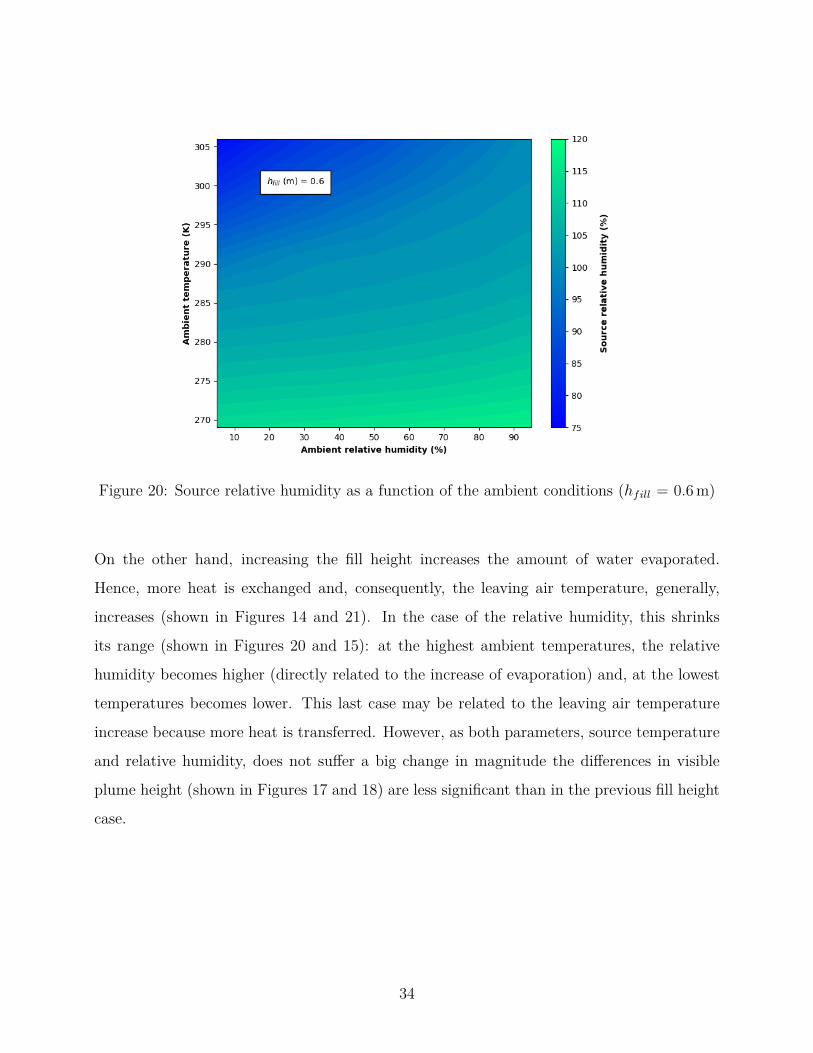
Figure 20: Source relative humidity as a function of the ambient conditions (hfill = 0.6 m)

On the other hand, increasing the fill height increases the amount of water evaporated.

Hence, more heat is exchanged and, consequently, the leaving air temperature, generally,

increases (shown in Figures 14 and 21). In the case of the relative humidity, this shrinks

its range (shown in Figures 20 and 15): at the highest ambient temperatures, the relative

humidity becomes higher (directly related to the increase of evaporation) and, at the lowest

temperatures becomes lower. This last case may be related to the leaving air temperature

increase because more heat is transferred. However, as both parameters, source temperature

and relative humidity, does not suffer a big change in magnitude the differences in visible

plume height (shown in Figures 17 and 18) are less significant than in the previous fill height

case.

34

Figure 21: Source temperature as a function of the ambient conditions (hfill = 1.8 m)

Figure 22: Source relative humidity as a function of the ambient conditions (hfill = 1.8 m)

35

4.3 Parametric study of the L/G ratio for plume abatement

The purpose of this set of simulations is to study how the plume visibility changes as the

L/G ratio is varied. The economical viability is also taken into account too as increasing

G will abate the plume at the expense of increasing fan power consumption. The impact of

varying the L/G ratio on the fan consumption has been quantified while trying to keep an

acceptable cooling range. Therefore, three cases are proposed in addition to a base L/G ratio

shown in Table 4. In all of them, the mass flow rate of water, L, has been kept constant at

the base case value, 1000 kg/s, while the air flow rate, G, has been varied.

Table 4: L/G ratio test cases

L/G 2 1 1/2 1/4

Following this procedure, the visible plume height has been obtained for the four cases,

Figures 23, 24, 25 and 26. This time, though, besides the contour plots, the visible plume

height against the L/G ratio has been represented for four specific cases (Figure 27). This

cases are build varying the parameters of ambient relative humidity and temperature inside

the ranges of the contour plot (Table 5).

Table 5: Ambient conditions test cases

Case 1 Case 2 Case 3 Case 4

Ta (K) 296 296 274 274RHa (%) 20 80 20 80

36

Figure 23: Visible plume height as a function of the ambient conditions (L/G = 2)

Figure 24: Visible plume height as a function of the ambient conditions (L/G = 1)

37

Figure 25: Visible plume height as a function of the ambient conditions (L/G = 0.5)

Figure 26: Visible plume height as a function of the ambient conditions (L/G = 0.25)

38

Figure 27: Visible plume height as a function of the L/G ratio

The figures show that as the L/G ratio is decreased, the visible plume height decreases.

However, the changes between L/G = 2 and L/G = 1 are smaller than in the rest of the

cases. Similarly, the starting points where the visible plume appears, occur later, at colder

temperatures. This behaviour of the plume can be explained through the parameters of

relative humidity and temperature. Their variation is illustrated in the following contour

plots and plots of the cases shown in Table 5.

39

Figure 28: Source temperature as a function of the ambient conditions (L/G = 2)

Figure 29: Source relative humidity as a function of the ambient conditions (L/G = 2)

40

Figure 30: Source temperature as a function of the ambient conditions (L/G = 1)

Figure 31: Source relative humidity as a function of the ambient conditions (L/G = 1)

41

Figure 32: Source temperature as a function of the ambient conditions (L/G = 0.5)

Figure 33: Source relative humidity as a function of the ambient conditions (L/G = 0.5)

42

Figure 34: Source temperature as a function of the ambient conditions (L/G = 0.25)

Figure 35: Source relative humidity as a function of the ambient conditions (L/G = 0.25)

43

Figure 36: Source temperature as a function of the L/G ratio

Figure 37: Source relative humidity as a function of the L/G ratio

44

The increase in air mass flux leads to the effluent leave the tower colder (as shown in Figures

28, 30, 32 and 34). Figure 36 shows that the higher is the ambient relative humidity and

temperature, the higher is the output temperature, specially at lower L/G ratios. In addition

(as shown in Figures 29, 31, 33, 35 and 37), at hot ambient conditions, by reducing the L/G

ratio, the exhaust air can achieve subsaturation and its source relative humidity can be cut

down significantly. However, the opposite effect occurs at lower ambient temperatures: as the

L/G ratio is decreased, the source relative humidity increases. This effect is less appreciable

than in high ambient temperatures. Therefore, source relative humidity and temperature

tendency matches with the visible plume tendency, Figure 27, previously mentioned.

Conversely, while increasing the L/G ratio and taking the base case as a reference, the values

of source temperature and relative humidity does not suffer a big change. Regarding the

temperatures (Figures 28, 30 and 36), although there is a clear decrease, it is smaller than

in the previous cases when the L/G ratio was decreased. Regarding the relative humidities

(Figures 29, 31 and 37), the difference between them is almost negligible. This behaviour of

temperature and relative humidity explains the main reason why, while increasing the L/G

ratio, the visible plume heights between the L/G = 1 and L/G = 2 cases do not suffer a

significant increase as expected.

Moreover, this mass flow rate of air variation must be studied also in terms of the force that

allows it, in other words, the fan power consumption. This fan power consumption, Pcf , is

obtained using,

Pcf = ∆PT · Vaηf · ηc

, (33)

where Va is the volumetric flow rate of air, ∆PT is the total pressure drop between the inlet

and outlet of the cooling tower, and ηf and ηc are the fan and conversion efficiencies which

have been considered 0.75 and 0.96, respectively.

45

Fan power consumption is shown in Figure 38. Contour plots are not shown because fan

power appears to be insensitive to the ambient conditions used. Figure 38 shows the impact

of varying the L/G ratio on cooling tower consumption. Decreasing the L/G ratio increases

power consumption exponentially: the case with highest L/G ratio computes power values

of the order of kilowatts, while the one with the lowest L/G ratio shows values of the order

of megawatts. This is due to the previous fan power formulation (Equation (33)) where the

total pressure drop and the volumetric flow rate of air are directly related to the air velocity,

i.e. L/G ratio. Therefore, plume abatement come with a heavy expense.

Figure 38: Fan power consumption as a function of the L/G ratio

Besides the results of visible plume height and fan power consumption, in order to choose

the best scenario, it has to be also taken into account its viability through the cooling range

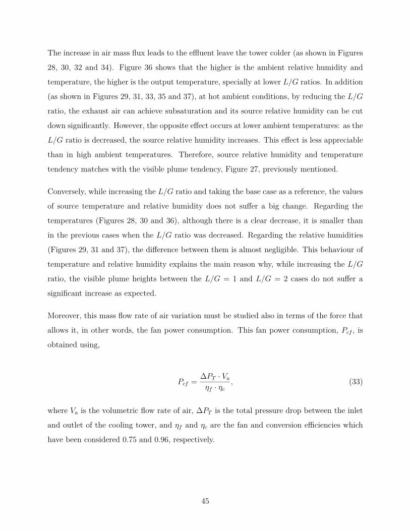
keeping acceptable operating conditions (Figures 39, 40, 41, 42 and 43).

46

Figure 39: Cooling range as a function of the ambient conditions (L/G = 2)

Figure 40: Cooling range as a function of the ambient conditions (L/G = 1)

47

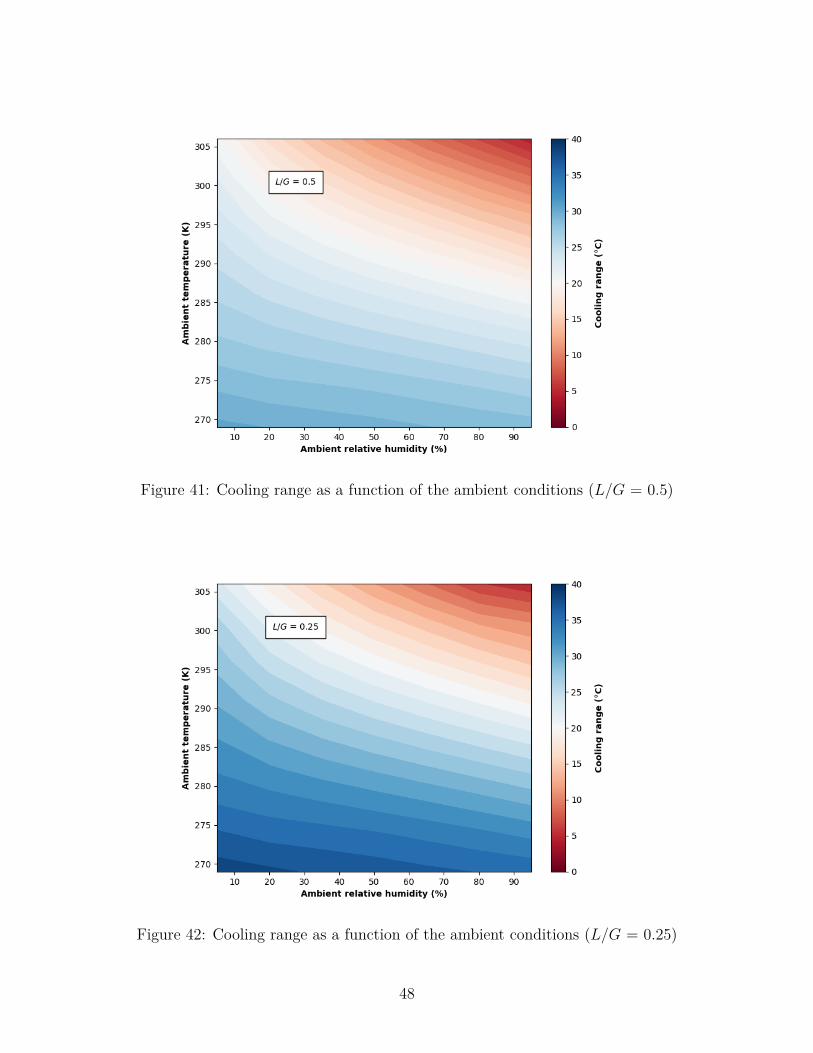
Figure 41: Cooling range as a function of the ambient conditions (L/G = 0.5)

Figure 42: Cooling range as a function of the ambient conditions (L/G = 0.25)

48

Figure 43: Cooling range as a function of the L/G ratio

The figures show that, as the L/G ratio decreases, the cooling range increases. In addition,

in the Figure 43, the cases with the lowest ambient temperature have the widest cooling

range with a low sensitivity to the ambient relative humidity. On the other hand, at the

highest ambient temperatures, the cooling range is lower and more sensitive to the ambient

relative humidity variation. Although the highest L/G case may seem to be the best a priori

in terms of energy consumption and plume visibility (as there isn’t a big change compared to

the base case), it is quickly discarded while seeing their cooling ranges (Figure 43). Taking

a reasonable operating requirement of 20°C for the cooling range, it can be appreciated that

this L/G = 2 case is unsuitable since none of the cases accomplish it. On the other hand,

the base case with L/G = 1 only satisfies this criterion for the coldest ambient temperatures,

while for the other two cases, with L/G ratio equal to 0.5 and 0.25, fulfills it partially and

almost fully, respectively.

49

5 Conclusions

A numerical software has been developed to analyze the effects of cooling tower ambient

and operating conditions on plume visibility. To do so, a theoretical steady-state plume

model adapted from the work of Wu and Koh (1978) [20] and Ali Moradi and M. R. Flynn et

al. [1] has been implemented into CoolIT, a Python-based, object-oriented code for solving

cooling towers. Subsequently, this turbulent plume model was coupled to two wet cooling

tower models, Merkel and Klimanek which represent the most common and advanced model

in literature. As a final step of this merging, a new tab for the plume study has been added

to the CoolIT user graphical interface. Finally, the implementation has been verified by

comparing the plume results obtained from CoolIT with the ones obtained from the Matlab-

based source plume code.

The analysis of the plume behaviour has been divided into three studies. The first study

compared the effects of the two wet cooling tower methods, Klimanek and Merkel, on plume

behaviour predictions. It is concluded that Klimanek model is able to provide better predic-

tions for the outlet air temperature and humidity and, therefore, it is likely to provide more

accurate predictions for plume visibility. Then, a parametric study varying the fill height

has been carried out. Although the fill height reduction leads to an improvement in plume

abatement, it is not feasible as it also leads to a reduction of the cooling tower performance.

Finally, a parametric study is carried by varying the L/G ratio. Although the increase of

the mass flux of air leads to a great increase in the fan power consumption, it is favourable

since improves the plume abatement as well as the process performance, the cooling range

becomes wider.

Proper design and operation of a cooling tower must take into account performance and

plume abatement. The variation of the operating conditions, specifically the L/G ratio,

has proven to be a good mechanism for reducing plume visibility. It is observed that at

low ambient temperatures and high ambient relative humidities, it is more likely to observe

plume visibility. Hence, during these conditions, fan power consumption must be increased.

A control system can be implemented to do so efficiently. The amount of energy spent to

50

increase the mass flux of air would depend on the legal regulations in plume abatement for

location and level of hazard.

51

6 References

[1] SHUO LI, ALI MORADI, BRAD VICKERS AND M.R. FLYNN. “Cooling tower plume

abatement using a coaxial plume structure”. International Journal of Heat and Mass

Transfer. Edmonton, Canada, Volume 120, Pages 178-193, May 2018.

[2] SPX COOLING TECHNOLOGIES, INC. “Cooling Tower Fundamentals”- second edi-

tion, Kansas, USA, 2009.

[3] EPA CONTRACT No. 68-DO-0137. “Development Of Particulate Emission Factors For

Wet Cooling Towers”, Kansas, September 1991.

[4] K. HOOMAN, Z. GUAN, H. GURGENCI. “Advances in dry cooling for concentrating

solar thermal (CST) power plants”, Queensland, Australia.

[5] PAUL LINDAHL, KEN MORTENSEN AND SPX COOLING TECHNOLOGIES.

“Plume Abatement - The next generation”, Houston, Texas, February 2010.

[6] J.P. JENSEN, B. CONRAD, U. SCHUETZ, F.R. ULLRICH, A. WANNING. “Hybrid

dry coolers in cooling systems of high energy physics accelerators”, Lucerne, Switzerland,

2004.

[7] G.J. KOSTEN. “Wet, dry and hybrid system, a comparison of thermal performance”, St

Petersburg, Florida, August/September, 1994.

[8] A. STRENG. “Combined wet/dry cooling towers of cell type construction”, Energy Eng.

124, 104 - 121, 1998.

[9] ASHRAE. “Systems and Equipment of Cooling Towers”, 2008.

[10] K. TAKATA, T. MICHIOKA AND R. KUROSE. “Prediction of a Visible Plume from a

Dry and Wet Combined Cooling Tower and Its Mechanism of Abatement”, Japan, 2016.

[11] MCKELVEY, K. K., AND BROOKE, M. “The Industrial Cooling Tower”, Elsevier,

Amsterdam, 1959.

[12] MERKEL, F. “Verdunstungskuhlung”, VDI-Zeitchrift, Vol. 70, pp. 123 – 128, 1925.

52

[13] JABER, H., AND WEBB, R. L. “Design of Cooling Towers by the Effectiveness - NTU

Method”, ASME J. Heat Transfer, 111, pp. 837 – 843, 1989.

[14] POPPE, M., AND ROGENER, H. “Berechnung von Ruckkuhlwerken”, VDI - Warmeat-

las, pp. Mi 1–Mi 15, 1991.

[15] A. KLIMANEK AND R.A. BIALECKI. “Solution of heat and mass transfer in counter-

flow wet-cooling tower”, International Communications in Heat and Mass Transfer, 36,

No. 6, pp. 547-553, 2009.

[16] TYAGI SK, WANG SW, MA ZJ. Prediction, potential and control of plume from wet

cooling tower of commercial buildings in Hong Kong: a case study. Int J Energy Res.

31:778–95, 2007.

[17] XU X, WANG S, ZHENJUN M. Evaluation of plume potential and plume abatement of

evaporative cooling towers in a subtropical region. Appl Therm Eng. 28:1471–84, 2008.

[18] WANG SW, TYAGI SK, SHARMA A, KAUSHIK SC. Application of solar collectors

to control the visible plume from wet cooling towers of a commercial building in Hong

Kong: a case study. Appl Therm Eng. 27:1394–404, 2007.

[19] TYAGI SK, WANG SW, PARK SR, SHARMA A. Economic considerations and cost

comparisons between the heat pumps and solar collectors for the application of plume

control from wet cooling towers of commercial buildings. Renew Sust Energy Rev.

12:2194–210, 2008.

[20] F.H. WU AND R.C. KOH. “Mathematical model for multiple cooling tower plumes”,

volume 1, Environmental Protection Agency, Office of Research and Development, En-

vironmental Research Laboratory, 1978.

[21] J.C. KLOPPERS AND D.G. KROGER. “Cooling Tower Performance Evaluation:

Merkel, Poppe, and e-NTU Methods of Analysis”, Journal of Engineering for Gas Tur-

bines and Power, ASME, Vol. 127 / 7, South Africa, 2005.

[22] BOSNJACOVIC, F. “Technische Thermodinmik”, Theodor Steinkopf, Dresden, 1965.

53

[23] MORTON, B. R., TAYLOR, G. I., AND TURNER, J. S. ”Turbulent gravitational con-

vection from maintained and instantaneous sources”. Proc. Roy. Soc. Lon. A, 234:1–32,

1956.

[24] J.C. KLOPPERS AND D.G. KROGER. “The Lewis factor and its influence on the per-

formance prediction of wet-cooling towers”, International Journal of Thermal Sciences,

44(9): 879–884, 2005.

[25] EMANUEL K.A. “Atmospheric Convection”, Oxford University Press, New York, 580

pp, 1994.

54