Multi-objective optimization of a cooling tower assisted vapor compression refrigeration system
14
Multi-objective optimization of a cooling tower assisted vapor compression refrigeration system Hoseyn Sayyaadi*, Mostafa Nejatolahi Faculty of Mechanical Engineering-Energy Division, K.N. Toosi University of Technology, P.O. Box 19395-1999, No. 15-19, Pardis Str., Mollasadra Ave., Vanak Sq., Tehran 1999 143344, Iran article info Article history: Received 23 December 2009 Received in revised form 24 July 2010 Accepted 30 July 2010 Available online 6 August 2010 Keywords: Refrigeration system Cooling tower Exergy Economy Optimization abstract A cooling tower assisted vapor compression refrigeration machine has been considered for optimization with multiple criteria. Two objective functions including the total exergy destruction of the system (as a thermodynamic criterion) and the total product cost of the system (as an economic criterion), have been considered simultaneously. A thermody- namic model based on energy and exergy analyses and an economic model according to the Total Revenue Requirement (TRR) method have been developed. Three optimized systems including a single-objective thermodynamic optimized, a single-objective economic optimized and a multi-objective optimized are obtained. In the case of multi- objective optimization, an example of decision-making process for selection of the final solution from the Pareto frontier has been presented. The exergetic and economic results obtained for three optimized systems have been compared and discussed. The results have shown that the multi-objective design more acceptably satisfies generalized engineering criteria than other two single-objective optimized designs. ª 2010 Elsevier Ltd and IIR. All rights reserved. Optimisation d’un syste ` me frigorifique a ` compression de vapeur dote ´ d’une tour de refroidissement mene ´e avec plusieurs objectifs Mots cle ´s : Syste ` me frigorifique ; Tour de refroidissement ; Exergie ; E ´ conomie ; Optimisation 1. Introduction In selection, design and optimization of energy systems, several and commonly conflicting criteria might be consid- ered. For example, for optimization of a vapor compression refrigeration system, a designer may consider one or more of the thermodynamic, economic and environmental criteria as the objective function. If only the thermodynamic criterion is considered, the system will be an ideal system from thermo- dynamic point of view, but it might not be able to pass the economic criterion. On the other hand, by considering only the economic criterion, the system will be the cheapest one, but this system might not be a well designed system from thermodynamic and environmental points of view e say * Corresponding author. Tel.: þ98 21 8867 4841-8x2212; fax.: þ98 21 8867 4748. E-mail addresses: [email protected] (H. Sayyaadi), [email protected] (M. Nejatolahi). www.iifiir.org available at www.sciencedirect.com journal homepage: www.elsevier.com/locate/ijrefrig international journal of refrigeration 34 (2011) 243 e256 0140-7007/$ e see front matter ª 2010 Elsevier Ltd and IIR. All rights reserved. doi:10.1016/j.ijrefrig.2010.07.026
Transcript of Multi-objective optimization of a cooling tower assisted vapor compression refrigeration system
i n t e rn a t i o n a l j o u r n a l o f r e f r i g e r a t i o n 3 4 ( 2 0 1 1 ) 2 4 3e2 5 6
www. i ifi i r .org
ava i lab le at www.sc iencedi rec t . com
journa l homepage : www.e lsev ier . com/ loca te / i j r e f r ig
Multi-objective optimization of a cooling tower assisted vaporcompression refrigeration system
Hoseyn Sayyaadi*, Mostafa Nejatolahi
Faculty of Mechanical Engineering-Energy Division, K.N. Toosi University of Technology, P.O. Box 19395-1999, No. 15-19, Pardis Str.,
Mollasadra Ave., Vanak Sq., Tehran 1999 143344, Iran
a r t i c l e i n f o
Article history:
Received 23 December 2009
Received in revised form
24 July 2010
Accepted 30 July 2010
Available online 6 August 2010
Keywords:
Refrigeration system
Cooling tower
Exergy
Economy
Optimization
* Corresponding author. Tel.: þ98 21 8867 48E-mail addresses: [email protected] (H
0140-7007/$ e see front matter ª 2010 Elsevdoi:10.1016/j.ijrefrig.2010.07.026
a b s t r a c t
A cooling tower assisted vapor compression refrigeration machine has been considered for
optimization with multiple criteria. Two objective functions including the total exergy
destruction of the system (as a thermodynamic criterion) and the total product cost of the
system (as an economic criterion), have been considered simultaneously. A thermody-
namic model based on energy and exergy analyses and an economic model according to
the Total Revenue Requirement (TRR) method have been developed. Three optimized
systems including a single-objective thermodynamic optimized, a single-objective
economic optimized and a multi-objective optimized are obtained. In the case of multi-
objective optimization, an example of decision-making process for selection of the final
solution from the Pareto frontier has been presented. The exergetic and economic results
obtained for three optimized systems have been compared and discussed. The results have
shown that the multi-objective design more acceptably satisfies generalized engineering
criteria than other two single-objective optimized designs.
ª 2010 Elsevier Ltd and IIR. All rights reserved.
Optimisation d’un systeme frigorifique a compression devapeur dote d’une tour de refroidissement menee avecplusieurs objectifs
Mots cles : Systeme frigorifique ; Tour de refroidissement ; Exergie ; Economie ; Optimisation
1. Introduction
In selection, design and optimization of energy systems,
several and commonly conflicting criteria might be consid-
ered. For example, for optimization of a vapor compression
refrigeration system, a designer may consider one or more of
the thermodynamic, economic and environmental criteria as
41-8x2212; fax.: þ98 21 88. Sayyaadi), hoseynsayyaier Ltd and IIR. All rights
the objective function. If only the thermodynamic criterion is
considered, the system will be an ideal system from thermo-
dynamic point of view, but it might not be able to pass the
economic criterion. On the other hand, by considering only
the economic criterion, the system will be the cheapest one,
but this system might not be a well designed system from
thermodynamic and environmental points of view e say
67 [email protected] (M. Nejatolahi).reserved.
Nomenclature
A Heat transfer area (m2), Approach (�C)a1ea6 Constants in computing the purchased equipment
cost (PEC) of the cooling tower
BBY Balance at the beginning of the year
BD Book depreciation
BL Book life
C Constant coefficient
CC Carrying charge
CELF The constant escalation levelization factor
COP Coefficient of performance
CRF Capital-recovery factor
Celect Electricity price ($ kW�1 h�1)
CP Heat Capacity (J kg�1 K�1)_CP Total product cost ($ h�1)_C�P Normalized form of _CP
Cw The cost of cooling water ($ m�3)_E Rate of exergy (kW)
EV Expansion valve
FC Fuel cost ($ h�1)
f Objective function
g Gravity acceleration (m s�2)
h Enthalpy (kJ kg�1)
H0 Height relative to the ground surface (m)_I Irreversibility rate (kW)_I�
Normalized form of _I
ieff Interest rate (%)
j jth year of the system operation
K Number of objective functions
k Number of operating year; Component kth
LD Tube length to shell diameter ratio_m Mass flow rate (kg s�1)
n Number of years; Number of decision variables
OMC Operating and maintenance cost ($)
P Pressure (kPa)
PEC Purchase equipment cost ($)_Q Heat transfer rate (kW)
R Temperature range in the cooling tower (�C)ROI Return on investment
rFC Annual escalation rate for the cost of the electricity
rW Annual escalation rate for the cost of the cooling
water
rOMC Annual escalation rate for the operating and
maintenance cost
s Specific entropy (kJ kg�1)
T Temperature (�C or K)
TCR Total capital-recovery
TNI Total net investment
TRR Total revenue requirement
U0 Velocity relative to the ground surface (m s�1)_V Volumetric flow rate (m3 s�1)_W Power (kW)
WC Water cost ($ h�1)
x A decision variable vector
x* An optimum decision variable vector_Z Cost rate associated with the capital investment
and OMC ($ h�1)
DHct Height difference between the cooling tower inlet
and outlet water conduits
DP Pressure deference
DT Temperature deference
I, II States I, II on the vapor compression refrigeration
system
1, 2, ., 11 States 1, 2, ., 11 on the vapor compression
refrigeration system
Greek Letters
r Density (kg m�3)
h Efficiency (%)
s Number of operating hours in a year (h)
3 Specific exergy (kJ kg�1)
Subscripts
act Actual
comp Compressor
cond Condenser
ct Cooling tower
desired Desired
elect Electrical
evap Evaporator
fan Fan
i Inlet
io Inlet/outlet difference
isen Isentropic
elect Electrical
L Levelized
Loss Loss
net Net
mech Mechanical
OMC Operating and maintenance cost
o Outlet
pump Pump
ref Refrigerant
R Rational
s Isentropic
sub Subcooled
sup Superheated
tot Total
used Used
w Water
wb Wet bulb
0 Dead state; Related to the first year of the system
operation
Superscripts
CI Capital investment
Ch Chemical
i Inlet
K Kinetic
OMC Operating and maintenance cost
o Outlet
P Potential
Ph Physical
Q Heat
W Work
i n t e r n a t i o n a l j o u r n a l o f r e f r i g e r a t i o n 3 4 ( 2 0 1 1 ) 2 4 3e2 5 6244
i n t e rn a t i o n a l j o u r n a l o f r e f r i g e r a t i o n 3 4 ( 2 0 1 1 ) 2 4 3e2 5 6 245
a system that consumes lots of energy or emits a lot of
pollutants into the environment. Both of these systems are
not acceptable from a comprehensive engineering point of
view. Thus it seems that simultaneous consideration of all or
some of these criteria might provide better option for engi-
neers. This goal can be obtained by multi-objective optimi-
zation techniques. In this way, we will have a system that
satisfies all of the optimization criteria as much as possible
simultaneously. Thermodynamic criteria are usually the first
law (energetic) and the second law (exergetic) criteria. In this
paper the second law criterion (the total exergy destruction of
the system) is considered as the thermodynamic objective
function which has been proven that it better considers
thermodynamic criterion than the first law optimization. The
economic objective function is the total product cost of the
system that is developed according to the total revenue
requirement (TRR) method. These two criteria are considered
in a multi-objective optimization of a cooling tower assisted
vapor compression refrigeration system as an example of
energy systems.
As a powerful thermodynamic tool, the exergy analysis
(availability or second law analysis) presented in this study is
well suited for furthering the goal of more effective energy
resource use, for it enables the location, cause, and true
magnitude and waste and loss of exergy to be determined.
Such information can be used in the design of new energy-
efficient systems and for increasing the efficiency of the
existing system (Bejan et al., 1996). There have been several
studies on the exergy analysis of different types of refrigera-
tion and heat pump systems. Leidenfrost et al. (1980) used
exergy analysis to investigate performance of a refrigeration
cycle working with R-12 as the refrigerant. Dincer et al. (1996)
investigated the thermal performance of a solar powered
absorption refrigeration system. Meunier et al. (1997) studied
the performance of adsorptive refrigeration cycles using the
second law analysis. Nikolaidis and Probert (1998) utilized the
exergy method in order to simulate the behavior of a two-
stage compound compression-cycle with flash inter-cooling
running with R-22 as the refrigerant. The effects of tempera-
ture changes in the condenser and evaporator on the irre-
versibility rate of the cycle were determined. Bouronis et al.
(2000) studied the thermodynamic performance of a single-
stage absorption/compression heat pump using the ternary
working fluid trifluoroethanolewateretetraethyleneglycol
dimethylether for upgrading waste heat. Goktun and Yavuz
(2000) investigated the effects of thermal resistances and
internal irreversibilities on the performance of combined
cycles for cryogenic refrigeration. Chen et al. (2001) studied
the optimization of a multistage endoreversible combined
refrigeration system. Kanoglu (2002) presented amethodology
for the exergy analysis of multistage cascade refrigeration
cycle and obtained the minimum work relation for the lique-
faction of natural gas. Yumrutas‚ et al. (2002) presented
a computational model based on the exergy for the investi-
gation of the effects of the evaporating and condensing
temperatures on the pressure losses, exergy losses, second
law efficiency, and the coefficient of performance (COP) of
a vapor compression refrigeration cycle. Kanoglu et al. (2004)
developed a procedure for the energy and exergy analyses of
open-cycle desiccant cooling systems and applied it to an
experimental unit operating in ventilation mode with natural
zeolite as the desiccant. Kopac and Zemher (2006) presented
a computational study based on the exergy analysis for the
investigation of the effects of the saturated temperatures of
the condenser and the evaporator on the efficiency defects in
each of the components of the plant, the total efficiency defect
of the plant, the second law efficiencies and the values of COP
of a vapor compression refrigeration plant for NH3, HFC-134a,
R-12 and R-22. Ozgener and Hepbasli (2007) reviewed the
energy and exergy analyses of solar assisted heat pump
systems that many of them were in the category of solar
assisted ground source heat pump systems.
On the other side, there have been several studies on the
economic or thermoeconomic analysis of refrigeration and
heat pump systems. Wall (1991) presented a pioneering work
in application of thermoeconomic optimization of heat pump
systems. In that study, the objective function was the total life
cycle cost including the electricity and the capital costs. The
Lagrange multipliers method was utilized for minimization of
the objective function. Cammarata et al. (1997) presented an
economicmethod for optimizing a thermodynamic cycle of an
air conditioning system. Global optimum values were found
using the directmathematicalmethod. d’Accadia and de Rossi
(1998) investigated thermoeconomic optimization of a vapor
compression refrigerator using the exergetic cost theory
method. Dingec and Ileri (1999) carried out the optimization of
a domestic R-12 refrigerator. The structural coefficient
method was used in this optimization procedure. Their
objective was to minimize the total life cycle cost, which
includes both the electricity and capital costs, for a given
cooling demand and system life. Tyagi et al. (2004) investi-
gated the thermoeconomic optimization of an irreversible
Stirling cryogenic refrigerator cycle. Al-Otaibi et al. (2004) used
thermoeconomics to study a vapor compression refrigeration
system. The efficiencies of the compressor, condenser, evap-
orator, and electric motor were also studied as the decision
variables with cost parameters. Sanaye and
Malekmohammadi (2004) presented a new method of
thermal and economical optimum design of air conditioning
units with vapor compression refrigeration system. Soylemez
(2004) presented a thermoeconomic optimization analysis
yielding a simple algebraic formula for estimating the
optimum operating temperature for refrigeration systems,
which utilizes energy recovery applications. In their work the
method used is known as the P1�P2 method, used with the
usage factor and simplified wall gain load factors. Selbas‚ et al.,
2006 applied an exergy-based thermoeconomic optimization
application to a subcooled and superheated vapor compres-
sion refrigeration system. All calculationsweremade for three
refrigerants: R-22, R-134a, and R-407c. Misra et al. (2003, 2005)
investigated thermoeconomic optimization of single and
double effect H2O/LiBr vapor-absorption refrigeration
systems. Sanaye and Niroomand (2009) investigated the
thermal-economic modeling and optimization of a vertical
ground source heat pump.
According to the above-mentioned paragraphs, there are
comprehensive investigations in the field of exergy and
economic analyses and optimization of refrigeration and heat
pump systems, especially on vapor compression refrigeration
systems. But as mentioned previously, by considering only
i n t e r n a t i o n a l j o u r n a l o f r e f r i g e r a t i o n 3 4 ( 2 0 1 1 ) 2 4 3e2 5 6246
one of the exergetic or economic criteria as the objective
function of optimization, the systems would not satisfactory
pass the other criteria. Thus it seems that a multi-objective
optimization is required. Multi-objective optimization is
developed to deal with different and often competing objec-
tives is an optimization problem (e.g. see Fonseca and
Fleming, 1997; Van Veldhuizen and Lamont, 2000; Deb, 2001
and Konak et al., 2006). Multi-objective optimization of
energy systems has been paid attention by researchers
nowadays (e.g. Toffolo and Lazzaretto, 2002, 2004). Moreover,
Sayyaadi et al. (2009) and Sayyaadi and Amlashi (in press)
performed multi-objective optimization for GSHP systems in
cooling mode. Objective functions were the total product cost
of the system and the total exergy destruction. They
compared the results of exergy and thermoeconomic analyses
of the base case, two single-objective optimized, and the
multi-objective optimized systems.
Thiswork has been presented here as an attempt formulti-
objective optimization of a cooling tower assisted vapor
compression refrigeration system. Objectives are the total
exergy destruction and the total product cost of the system.
Product in the refrigeration system is defined as refrigeration
effect of the evaporator, hence in our study, the cost of the
system product is defined as the unit cost of refrigeration
effect in the evaporator. Three optimization scenarios
including the thermodynamic single-objective, the thermoe-
conomic single-objective and multi-objective optimizations
are performed in this work. All optimization scenarios are
conducted using an artificial intelligence technique known as
evolutionary algorithm (EA). The output of themulti-objective
optimization is a Pareto frontier that yields a set of optimal
points. In the case of multi-objective optimization scenario,
an example of decision-making process for selection of the
final solution from the Pareto frontier is presented here. The
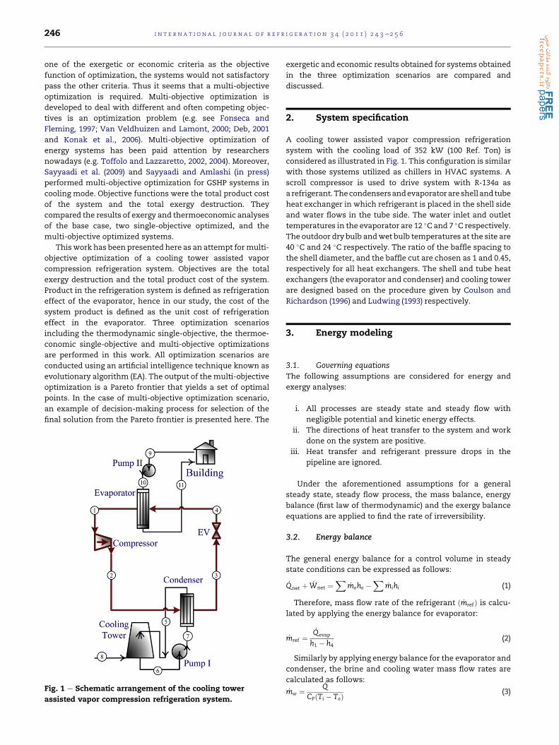
Fig. 1 e Schematic arrangement of the cooling tower
assisted vapor compression refrigeration system.
exergetic and economic results obtained for systems obtained
in the three optimization scenarios are compared and
discussed.
2. System specification
A cooling tower assisted vapor compression refrigeration
system with the cooling load of 352 kW (100 Ref. Ton) is
considered as illustrated in Fig. 1. This configuration is similar
with those systems utilized as chillers in HVAC systems. A
scroll compressor is used to drive system with R-134a as
a refrigerant.Thecondensersandevaporatorareshell and tube
heat exchanger in which refrigerant is placed in the shell side
and water flows in the tube side. The water inlet and outlet
temperatures in the evaporator are 12 �C and 7 �C respectively.
The outdoor dry bulb andwet bulb temperatures at the site are
40 �C and 24 �C respectively. The ratio of the baffle spacing to
the shell diameter, and the baffle cut are chosen as 1 and 0.45,
respectively for all heat exchangers. The shell and tube heat
exchangers (the evaporator and condenser) and cooling tower
are designed based on the procedure given by Coulson and
Richardson (1996) and Ludwing (1993) respectively.
3. Energy modeling
3.1. Governing equationsThe following assumptions are considered for energy and
exergy analyses:
i. All processes are steady state and steady flow with
negligible potential and kinetic energy effects.
ii. The directions of heat transfer to the system and work
done on the system are positive.
iii. Heat transfer and refrigerant pressure drops in the
pipeline are ignored.
Under the aforementioned assumptions for a general
steady state, steady flow process, the mass balance, energy
balance (first law of thermodynamic) and the exergy balance
equations are applied to find the rate of irreversibility.
3.2. Energy balance
The general energy balance for a control volume in steady
state conditions can be expressed as follows:
_Qnet þ _Wnet ¼X
_moho �X
_mihi (1)
Therefore, mass flow rate of the refrigerant ð _mrefÞ is calcu-
lated by applying the energy balance for evaporator:
_mref ¼_Qevap
h1 � h4(2)
Similarly by applying energy balance for the evaporator and
condenser, the brine and cooling water mass flow rates are
calculated as follows:
_mw ¼_Q
(3)
CPðTi � ToÞ
i n t e rn a t i o n a l j o u r n a l o f r e f r i g e r a t i o n 3 4 ( 2 0 1 1 ) 2 4 3e2 5 6 247
The type of compressor considered in this study is Copeland
scroll compressor. The compressor power is given according
to the following equation:
_Wact;comp ¼ _mrefðh2;s � h1Þhisen;comp
(4)
Where hisen is the compressor isentropic efficiency.
By applying the energy balance for the entire cycle, heat
load of the condenser is calculated as:
_Qcond ¼ _Qevap þ _Wcomp (5)
The pumping power requirements for each pump in the
system as per Fig. 1 are:
_Wpump;I ¼ _VwðrwgDHct þ DPcondÞ=hpump (6)
_Wpump;II ¼ _VwDPevap=hpump (7)
Where DHct is equal to the difference between the height of
cooling towerwater inlet and outlet connections of the cooling
tower and _V is volumetric flow rate (m3/s).
The total consumed electrical power of the system is as
follows:
_Wtot ¼ _Wcomp þ _Wpump;I þ _Wpump;II þ _Wfan (8)
Where _Wfan is the consumed power by the cooling tower fan
that is calculated according to procedure given by Ludwing
(1993).
Table 1 e Exergy balance equations for each componentof the cooling tower assisted vapor compassionrefrigeration system (Fig. 1).
_Ipump;I ¼ ð _E6 � _E7Þ þ _Wpump;I
_Ipump;II ¼ ð _E9 � _E10Þ þ _Wpump;II
_Icond ¼ ð _E7 � _E5Þ þ ð _E2 � _E3Þ_Ievap ¼ ð _E10 � _E11Þ þ ð _E4 � _E1Þ_IEV ¼ ð _E3 � _E4Þ_Ict ¼ ð _E5 � _E6Þ þ _Wfan þ _E8
_Icomp ¼ ð _E1 � _E2Þ þ _Wcomp
_Itot ¼ ð _E9 � _E11Þ þ _Wpump;I þ _Wpump;II þ _Wfan þ _Wcomp þ _E8
4. Exergy analysis
An exergy analysis provides, among others, the exergy of each
stream in a system as well as the real “energy waste” i.e., the
thermodynamic inefficiencies (exergy destruction and exergy
loss), and the exergetic efficiency for each system component
(Bejan et al., 1996) Thermodynamic processes are governed by
the laws of conservation of the mass and energy. However,
exergy is not generally conserved but is destroyed by irre-
versibilities within a system. Furthermore, exergy is lost, in
general, when the energy associated with amaterial or energy
stream is rejected to the environment.
The general form of the exergy balance for a control
volume in steady state conditions is:
_I ¼ _Ei � _E
o þ _EQ þ _E
W(9)
Where _I is the total exergy destruction or irreversibility. The _EQ
is the exergy flow associated with the heat transfer through
the control volume boundaries and is calculated as follow:
_EQ ¼ _Qð1� T0=TÞ (10)
Because work is an ordered energy, its associated exergy
flow is equal to the amount of that work. Thus
_EW ¼ _W (11)
The _Eiand _E
oare the exergies of the control volume inlet and
outlet streams of matter and are given by:
_E ¼ _m3 (12)
Where 3 is the specific exergy of a steam of matter that
includes kinetic (3K), potential (3P), physical (3Ph) and chemical
(3Ch) exergies:
3 ¼ 3K þ 3P þ 3Ch þ 3Ph (13)
3K ¼ U20=2 (14)
P
3 ¼ gH0 (15)The kinetic and potential exergies are ignored in this work.
Further, since most material steams of the system are not
associated with any kind of chemical reaction, therefore, the
chemical exergy terms will be canceled out in the balance
equation. Thus, the exergy of flow in this work (Eq. (13)) (except
in the cooling tower thatwater changes phase and the chemical
exergy terms are not canceled out) are comprised only from the
physical component. The physical specific exergy is given by:
3Ph ¼ ðh� T0sÞ � ðh0 � T0s0Þ (16)
Where the subscript 0 is referred to the environmental
conditions (restricted equilibrium with the environmental).
The specific chemical exergy for liquid and vapor forms of the
water are equal to 2.4979 and 0 kJ kg�1, respectively (Bejan
et al., 1996).
By applying the exergy balance for a control volume that
encloses the entire system, the total exergy destruction is
evaluated as follow:
_Itot ¼�_E9 � _E11
�þ _Wpump;I þ _Wpump;II þ _Wfan þ _Wcomp þ _E8 (17)
Different ways of formulating exergetic efficiency proposed
in the literature have been given in detail elsewhere (Bejan
et al., 1996). Among these, the rational efficiency or the over-
all rational efficiency is defined by as the ratio of the desired
exergy output to the exergy used, namely
hR ¼_Edesired
_Eused
(18)
Where _Edesired is the sum of all exergy transfer rates from the
system, which must be regarded as constituting the desired
output, plus any by product that is produced by the system,
while _Eused is the required rate of input exergy for the process
to be performed. For the vapor compression refrigeration
system, these two terms are determined as follows:
_Eused ¼ _Wpump;I þ _Wpump;II þ _Wfan þ _Wcomp þ _E8 (19)
_Edesired ¼ �� _E9 � _E11
�(20)
i n t e r n a t i o n a l j o u r n a l o f r e f r i g e r a t i o n 3 4 ( 2 0 1 1 ) 2 4 3e2 5 6248
From Eqs. (18)e(20), the rational efficiency is obtained as
follows:
hR ¼ �ð _E9 � _E11Þ_Wpump;I þ _Wpump;II þ _Wfan þ _Wcomp þ _E8
(21)
Application of the exergy balance equation (Eq. (9)) for each
component of the vapor compression refrigeration system
(Fig. 1) leads to the balancing equations mentioned in Table 1.
5. Economic models
The economic model takes into account the cost of the
components, including amortization and maintenance, the
cost of fuel consumption and the cost of water consumption.
In order to define a cost function, which depends on the
optimization parameters of interest, component costs have to
be expressed as functions of thermodynamic variables. These
relationships can be obtained by statistical correlations
between costs and the main thermodynamic parameters of
the component performed on the real data series.
The following sections illustrate the total revenue require-
ment method (TRR method ) which is based on procedures
adopted by the Electric Power Research Institute in their tech-
nical assessment guide (TAG�, 1993). Based on the estimated
total capital investment and assumptions for economic,
financial, operating, and market input parameters, the total
revenue requirement is calculated on a year-by-year basis.
Finally, the non-uniform annual monetary values associated
with the investment, operating (excluding fuel and water),
maintenance, water and the fuel costs of the system being
analyzed are levelized; that is, they are converted to an
equivalent series of constant payments (annuities) (Bejan et al.,
1996). The annual total revenue requirement (TRR, total product
cost) for a system is the revenue that must be collected in
a given year through the sale of all products to compensate the
system operating company for all expenditures incurred in the
same year and to ensure sound economic system operation
(Bejan et al., 1996).
The series of annual costs associated with the carrying
charges CCj and expenses (FCj and OMCj) for the jth year of
a system operation is not uniform. In general, carrying charges
decrease while fuel costs increase with increasing years of
operation (Bejan et al., 1996). A levelized value for the total
annual revenue requirement, TRRL, can be computed by
applying a discounting factor and the capital-recovery factor
CRF:
TRRL ¼ CRFXn1
TRRj�1þ ieff
�j (22)
In applying Eq. (22), it is assumed that each monetary
transaction occurs at the end of each year. The capital-
recovery factor CRF is given by:
CRF ¼ ieff�1þ ieff
�n�1þ ieff
�n�1(23)
TRRj is the total revenue requirement in the jth year of
system operation, ieff is the average annual effective discount
rate (cost of money), and n denotes the system economic life
expressed in years.
In the case of the cooling tower assisted vapor compression
refrigeration system, the annual total revenue requirement is
equal to the sum of the following five annual amounts
including the total capital-recovery (TCR); minimum return on
investment (ROI ); fuel costs (FC ); water costs (WC ); and the
operating and maintenance cost (OMC ):
TRRj ¼ TCRj þ ROIj þ FCj þWCj þ OMCj (24)
The calculation method for TCRj and ROIj is given by Bejan
et al. (1996), the extension of TCRj and ROIj for a cooling
system is developed by Sayyaadi et al. (2009) and Sayyaadi and
Amlashi (in press). FCj,WCj and OMCj and their corresponding
levelized values are obtained using the following procedure.
If the series of payments for the annual fuel cost FCj is
uniform over the time except for a constant escalation rFC (i.e.,
FCj ¼ FC0 (1 þ rFC)j), then the levelized value FCL of the series
can be calculated by multiplying the fuel expenditure FC0 at
the beginning of the first year by the constant escalation
levelization factor CELF:
FCL ¼ FC0CELF ¼ FC0kFC
�1� kn
FC
�ð1� kFCÞ CRF (25)
Where,
kFC ¼ 1þ rFC1þ ieff
and rFC ¼ constant (26)
The terms rFC and CRF denote the annual escalation rate for
the fuel cost and the capital-recovery factor (Eq. (23)), respec-
tively. The levelized value WCL is calculated the same as FCL.
Accordingly, the levelized annual operating and mainte-
nance costs (OMCL) are given as follows:
OMCL ¼ OMC0CELF ¼ OMC0kOMC
�1� kn
OMC
�ð1� kOMCÞ (27)
With
kOMC ¼ 1þ rOMC
1þ ieffand rOMC ¼ constant (28)
The term rOMC is the nominal escalation rate for the oper-
ating and maintenance costs.
Finally, the levelized carrying charges CCL are obtained
from the following equation:
CCL ¼ TRRL � FCL �WCL � OMCL (29)
The annual carrying charges or capital investment
(superscript CI ) and operating and maintenance costs
(superscript OMC ) of the total system can be apportioned
among the system components according to the contribu-
tion of the kth component to the purchased equipment cost
for the overall system ðPECtotal ¼P
k PECkÞ:
_ZCI
k ¼ CCL
sPECkPk PECk
(30)
_ZOMC
k ¼ OMCL
sPECkPk
PECk(31)
Here, PECk and s denote the purchased equipment cost of the
kth system component and the total annual time (in hours) of
i n t e rn a t i o n a l j o u r n a l o f r e f r i g e r a t i o n 3 4 ( 2 0 1 1 ) 2 4 3e2 5 6 249
system operation at full load, respectively. PECk equations for
various components of the cooling tower assisted vapor
compression refrigerationsystemaregiven inAppendixA.The
term _Zk represents the cost rate associated with the capital
investment and operating and maintenance expenses:
_Zk ¼ _ZCI
k þ _ZOMC
k (32)
The annual fuel and cooling water costs for the first year of
the system operation are given as follows respectively:
FC0 ¼ Celect$s$ _Wtot (33)
WC0 ¼ Cw$s$ _mw;loss � 36001000
(34)
Inwhich,Celect is the electricity price per kWh,Cw is thewater
price perm3, s is annual operating hours in coolingmode, _Wtot is
the total powerconsumptionof thesystem (Eq. (8)), and _mw;loss is
themassflowrateofmakeupwaterof thecooling tower (lit s�1).
The electricity and water prices are local prices in Iran that
considered as 0.075 $ kW�1 h�1 and 0.0368 $ m�3 respectively.
The operating life of the system is assumed as 15 years. The
total annual operating time of the system in cooling mode is
considered as 1800 h. In this study, the magnitude of other
economic constant such as rFC, rWC, ieff and rOMC are assumed
0.06, 0.06, 0.12 and 0.05, respectively (Bejan et al., 1996).
The levelized cost rates of the expenditures for electricity
and cooling water supplied to the system are respectively
given as follows:
_Zelect ¼ FCL
s(35)
_Zw ¼ WCL
s(36)
Levelized costs, such as _ZCI
k ;_ZOMC
k ; _Zelect and _Zw are used as
input data for the economic analysis.
6. Objective function, decision variables andconstraints
Optimization problem usually involves with these elements:
objective functions, decision variables and constraints.
Following sections describe the element of optimization
problem for the proposed cooling tower assisted vapor
compression refrigeration system.
6.1. Objective functions
Objective functions for single-objective and multi-objective
optimizations in this study are the thermodynamic and
economic objective functions denoted by Eqs. (37) and (38),
respectively. In the single-objective thermodynamic optimiza-
tion, the aim isminimizing the total irreversibility of the cooling
tower assisted vapor compression refrigeration system. In the
single-objective economic optimization, the total product cost
of the vapor compression refrigeration system is minimized.
The product in this system is defines as a cooling load (refrig-
eration effect) that should be provided in the evaporator. The
economic objective is denoted by Eq. (38).
Thermodynamic : _Itot ¼X
_Ik (37)
economic : _CP ¼ _Zelect þ _Zw þX
_Zk (38)
6.2. Decision variables
The following eight decision variables are chosen in this work:
1. Tcond: the condenser saturation temperature
2. Tevap: the evaporator saturation temperature
3. Tw,i,ct: the water inlet temperature of the cooling tower
4. Tw,o,ct: the water outlet temperature of the cooling tower
5. LDcond: ratio of the tube length to the shell diameter for the
condenser
6. LDevap: ratio of the tube length to the shell diameter of the
evaporator
7. DTsub: the magnitude of sub-cooling in the condenser
8. DTsup: the magnitude of super-heating in the evaporator
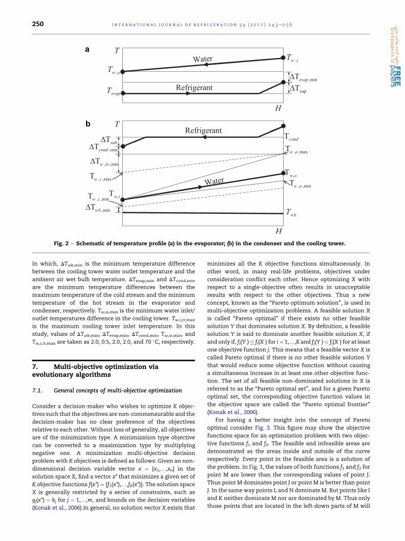
Fig. 2 shows a schematic for temperature profiles in the
evaporator, and the condenser and cooling tower. This figure
can be considered as a guideline to recognize some of above-
mentioned decision variables and their constraints.
6.3. Constraints
In engineering application of the optimization problem, there
are usually constraints on the trading-off of decision vari-
ables. In this case, some limitations are emanating from the
technical view points. For example, the allowable water
velocity in the tube sides of a shell and tube heat exchanger
should be within the range of 1e3 m/s to prevent fouling and
erosion, respectively. The recommended good practice value
for LD (ratio of the tube length to the shell diameter) for the
evaporator and condenser is a number between 5 and 15. The
recommended values of DTsub and DTsup are something
between 1 �C and 10 �C. Due to having several tube passes in
the evaporator and condenser, in order to prevent the
temperature cross problem in these exchangers, the
maximum temperature of the cold stream is always lower
than the minimum temperature of the hot stream. Using
Fig. 2, the limitations on the maximum and minimum ranges
of decision variables 1e4 can be obtained as follows:
Tcond;max ¼ 65�C (39)
Tcond;min ¼ Twb þ DTwb;min þ DTcond;min þ DTsup þ DTw;io;min (40)
Tevap;max ¼ Tw;i � DTsup � DTevap;min (41)
Tevap;min ¼ �5�C (42)
Tw;i;ct;max ¼ min
�Tcond � DTcond;min � DTsub
Tct;max(43)
Tw;o;ct;max ¼ Tw;i;ct;max � DTw;io;min (44)
Tw;o;ct;min ¼ Twb þ DTwb;min (45)
Tw;i;ct;min ¼ Tw;o;ct þ DTw;io;min (46)
a
b
Fig. 2 e Schematic of temperature profile (a) in the evaporator; (b) in the condenser and the cooling tower.
i n t e r n a t i o n a l j o u r n a l o f r e f r i g e r a t i o n 3 4 ( 2 0 1 1 ) 2 4 3e2 5 6250
In which, DTwb,min is the minimum temperature difference
between the cooling tower water outlet temperature and the
ambient air wet bulb temperature. DTevap,min and DTcond,min
are the minimum temperature differences between the
maximum temperature of the cold stream and the minimum
temperature of the hot stream in the evaporator and
condenser, respectively. Tw,io,min is the minimum water inlet/
outlet temperatures difference in the cooling tower. Tw,i,ct,max
is the maximum cooling tower inlet temperature. In this
study, values of DTwb,min, DTevap,min, DTcond,min, Tw,io,min, and
Tw,i,ct,max are taken as 2.0, 0.5, 2.0, 2.0, and 70 �C, respectively.
7. Multi-objective optimization viaevolutionary algorithms
7.1. General concepts of multi-objective optimization
Consider a decision-maker who wishes to optimize K objec-
tives such that the objectives are non-commensurable and the
decision-maker has no clear preference of the objectives
relative to each other.Without loss of generality, all objectives
are of the minimization type. A minimization type objective
can be converted to a maximization type by multiplying
negative one. A minimization multi-objective decision
problemwith K objectives is defined as follows: Given an non-
dimensional decision variable vector x ¼ {x1,.,xn} in the
solution space X, find a vector x* that minimizes a given set of
K objective functions f(x*) ¼ {f1(x*),.,fK(x*)}. The solution space
X is generally restricted by a series of constraints, such as
gj(x*) ¼ bj for j ¼ 1,.,m, and bounds on the decision variables
(Konak et al., 2006).In general, no solution vector X exists that
minimizes all the K objective functions simultaneously. In
other word, in many real-life problems, objectives under
consideration conflict each other. Hence optimizing X with
respect to a single-objective often results in unacceptable
results with respect to the other objectives. Thus a new
concept, known as the “Pareto optimum solution”, is used in
multi-objective optimization problems. A feasible solution X
is called “Pareto optimal” if there exists no other feasible
solution Y that dominates solution X. By definition, a feasible
solution Y is said to dominate another feasible solution X, if
and only if, fi(Y )� fi(X ) for i¼ 1,.,K and fj(Y )< fj(X ) for at least
one objective function j. This means that a feasible vector X is
called Pareto optimal if there is no other feasible solution Y
that would reduce some objective function without causing
a simultaneous increase in at least one other objective func-
tion. The set of all feasible non-dominated solutions in X is
referred to as the “Pareto optimal set”, and for a given Pareto
optimal set, the corresponding objective function values in
the objective space are called the “Pareto optimal frontier”
(Konak et al., 2006).
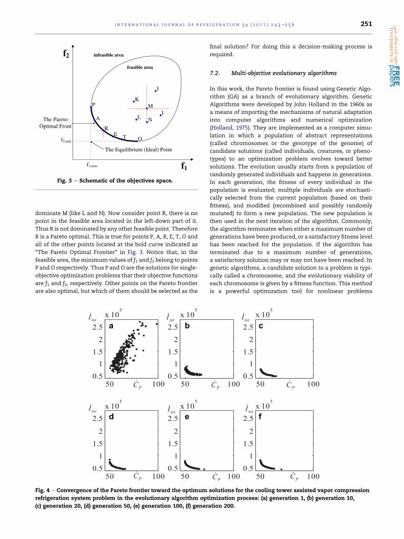
For having a better insight into the concept of Pareto
optimal consider Fig. 3. This figure may show the objective
functions space for an optimization problem with two objec-
tive functions f1 and f2. The feasible and infeasible areas are
demonstrated as the areas inside and outside of the curve
respectively. Every point in the feasible area is a solution of
the problem. In Fig. 3, the values of both functions f1 and f2 for
point M are lower than the corresponding values of point J.
Thus point M dominates point J or point M is better than point
J. In the sameway points L and N dominate M. But points like I
and K neither dominate M nor are dominated by M. Thus only
those points that are located in the left-down parts of M will
J
MK
IL
P
O
feasible area
infeasible area
f1,min
f2,min
The Equilibrium (Ideal) Point
The Pareto Optimal Front
A
E T
1
2
N
R
Fig. 3 e Schematic of the objectives space.
i n t e rn a t i o n a l j o u r n a l o f r e f r i g e r a t i o n 3 4 ( 2 0 1 1 ) 2 4 3e2 5 6 251
dominate M (like L and N). Now consider point R, there is no
point in the feasible area located in the left-down part of it.
Thus R is not dominated by any other feasible point. Therefore
R is a Pareto optimal. This is true for points P, A, R, E, T, O and
all of the other points located at the bold curve indicated as
“The Pareto Optimal Frontier” in Fig. 3. Notice that, in the
feasible area, theminimum values of f1 and f2 belong to points
P and O respectively. Thus P and O are the solutions for single-
objective optimization problems that their objective functions
are f1 and f2, respectively. Other points on the Pareto frontier
are also optimal, but which of them should be selected as the
a b
d e
Fig. 4 e Convergence of the Pareto frontier toward the optimum
refrigeration system problem in the evolutionary algorithm opt
(c) generation 20, (d) generation 50, (e) generation 100, (f) gener
final solution? For doing this a decision-making process is
required.
7.2. Multi-objective evolutionary algorithms
In this work, the Pareto frontier is found using Genetic Algo-
rithm (GA) as a branch of evolutionary algorithm. Genetic
Algorithms were developed by John Holland in the 1960s as
a means of importing the mechanisms of natural adaptation
into computer algorithms and numerical optimization
(Holland, 1975). They are implemented as a computer simu-
lation in which a population of abstract representations
(called chromosomes or the genotype of the genome) of
candidate solutions (called individuals, creatures, or pheno-
types) to an optimization problem evolves toward better
solutions. The evolution usually starts from a population of
randomly generated individuals and happens in generations.
In each generation, the fitness of every individual in the
population is evaluated; multiple individuals are stochasti-
cally selected from the current population (based on their
fitness), and modified (recombined and possibly randomly
mutated) to form a new population. The new population is
then used in the next iteration of the algorithm. Commonly,
the algorithm terminates when either a maximum number of
generations have been produced, or a satisfactory fitness level
has been reached for the population. If the algorithm has
terminated due to a maximum number of generations,
a satisfactory solution may or may not have been reached. In
genetic algorithms, a candidate solution to a problem is typi-
cally called a chromosome, and the evolutionary viability of
each chromosome is given by a fitness function. This method
is a powerful optimization tool for nonlinear problems
c
f
solutions for the cooling tower assisted vapor compression
imization process: (a) generation 1, (b) generation 10,
ation 200.

Table 2 e The tuning parameters in MOEA optimizationprogram.
Tuning parameters value
Population size 300
Maximum No. of generations 200
Probability of crossover 0.7
Probability of mutation 0.01
Selection process Roulette wheel
Table 3 e The values and normalized values of objectivefunctions for three optimized designs.
_CPð$$hr�1Þ _ItotðkWÞ _C�P
_I�tot
Economic Optimized 49.86 81.32 0.0 1.0
Multi-Objective Optimized 55.03 54.60 0.26 0.27
Thermodynamic Optimized 69.85 44.570 1.0 0.0
i n t e r n a t i o n a l j o u r n a l o f r e f r i g e r a t i o n 3 4 ( 2 0 1 1 ) 2 4 3e2 5 6252
(Holland, 1975; Goldberg, 1989). For more information about
Multi-Objective Evolutionary Algorithms (MOEAs) see (Konak
et al., 2006).
Fig. 4 presents the trend of convergence for the Pareto fron-
tier in this optimization process from the beginning to genera-
tion number 200. This figure reveals that between generations 1
and10, thepopulationsuddenly converges to the left-downpart
of the objective functions space. Convergence continues in the
next generations. After 50 generations, the trend of Pareto
optimal solutions is converged to a curve namely as the Pareto
frontier. Finally, the result of generationnumber200 isassumed
to be the final Pareto frontier in this study.
8. Results and discussion
The proposed model for the cooling tower assisted vapor
compression refrigeration system schematically shown in
Fig. 1 including eight decision variables and their constraints
(introduced in Section 6.2) is optimized using the evolutionary
algorithm with the tuning parameters that are mentioned in
Table 2. Three optimization scenarios including thermody-
namic single-objective, economic single-objective and multi-
objective optimizations are performed.
Fig. 5a presented the normalized form of the Pareto frontier
obtained inmulti-objective optimization scenario. Commonly,
it is better to work with the normalized data of the Pareto
frontier instead of the real values. The horizontal and vertical
Fig. 5 e (a) Normalized form of Pareto frontier and schematic of
distance of each point on the Pareto frontier from the equilibriu
axes in Fig. 5a are the normalized form of the objective func-
tions that defined as follow respectively:
_C�P ¼
_CP � _CP;min
_CP;max � _CP;min
(47)
and
_I�tot ¼
_Itot � _Itot;min
_Itot;max � _Itot;min
(48)
Where _CP;min and _CP;max are the minimum and maximum
values of _CP in the Pareto frontier. In the same way _Itot;min and_Itot;max are the minimum and maximum values of _Itot in the
Pareto frontier. Obviously _CP;min and _Itot;min belong to the
economic optimized and the thermodynamic optimized
designs, respectively. In this case, and commonly in most of
the cases, the shape of the Pareto frontier is such that _CP;mam
and _Itot;max belong to the thermodynamic optimized and the
economic optimized designs, respectively. Using Eqs. (47) and
(48), the values of _C�P and _I
�tot for the economic single-objective
optimized design are 0 and 1, respectively. Similarly, _C�P and _I
�tot
in the thermodynamic single-objective optimized design are 1
and 0, respectively (see Fig. 5a).
In multi-objective optimization scenario, selection of the
final solution among optimum points exist on the Pareto
frontier needs a process of decision-making. The process of
decision-making performed using definition of an ideal point
on Pareto frontier namely as the equilibrium point as shown
on Figs. 3 and 5a. At this equilibrium point, both objective
functions ð _CP and _ItotÞ have their minimum value and thus
the decision-making process, (b) the graph that shows the
m point.

Table 4 e The values of decision variables in the variousoptimization scenarios.
Decisionvariables
Basecase
Economicoptimized
Thermodynamicoptimized
Multi-objectiveoptimized
Tcond
(�C)50.25 43.45 32.33 36.27
Tevap
(�C)0.10 2.78 5.50 5.07
Tw,i,ct
(�C)30.80 32.84 29.33 32.13
Tw,o,ct
(�C)27.48 26.97 26.00 26.02
LDcond 10.00 12.85 5.00 13.05
LDevap 10.00 12.54 5.00 11.68
DTsub
(�C)5.50 8.56 1.00 1.83
DTsup
(�C)3.00 1.00 1.00 1.01
i n t e rn a t i o n a l j o u r n a l o f r e f r i g e r a t i o n 3 4 ( 2 0 1 1 ) 2 4 3e2 5 6 253
both of _C�P and _I
�tot are zero. It is clear that this point is not
existing in real world and is not located on the Pareto frontier
as is clear from Fig. 5a. Thus this point is not a possible design
of a system and is only an ideal point. In this decision-making
process, the point of Pareto frontier that has shortest distance
from the equilibrium point is selected as a final optimum
solution. This solution is not only located on the Pareto fron-
tier but also it archives the minimum possible values for both
objectives (Sayyaadi et al., 2009 and Sayyaadi and Amlashi,
2010). The presented data for the optimum solution of the
multi-objective optimization scenario reveals the corre-
sponding data for this selected solution as described in Fig. 5a,
hereinafter. Hence, values of _C�P and _I
�tot for the selected final
optimal solution in the multi-objective optimized design are
0.26 and 0.27, respectively.
Fig. 5a graphically shows the variation of the distance
between the equilibrium point and points located on the
Pareto frontier in Fig. 5a. This distance is equal toffiffiffiffiffiffiffiffiffiffiffiffiffiffiffiffiffiffi_C�P þ _I
�tot
q. It
can be seen from this figure that the minimum value of this
distance belongs to the selected multi-objective optimized
point. This distance is equal to its maximum value, 1, for both
of the single-objective economic optimized ð _C�P ¼ 0:0 and _I
�tot ¼
1:0Þ and the single-objective thermodynamic optimized ð _C�P ¼
1:0 and _I�tot ¼ 0:0Þ designs. It should be mentioned that for
Table 5 e The results of energy analysis the various optimizat
Base case Economic optimiz
Total refrigerant flow rate (kg s�1) 2.56 2.32
CT water flow rate (kg s�1 s) 34.25 17.79
CT make up water flow rate (kg s�1) 0.38 0.25
Evaporator water flow rate (kg s�1) 16.84 16.84
Compressor power (kW) 126.60 86.24
CT pump power (kW) 29.36 6.57
Evaporator pump power (kW) 3.47 2.67
CT fan power (kW) 6.33 4.61
Evaporator heat load (kW) 352.00 352.00
Condenser heat load (kW) 478.60 438.24
Thermodynamic cycle COP 2.78 4.08
Heat pump COP 2.12 3.52
points close to the minimum point, the slope of the graph is
near zero. Hence one of these points, instead of the selected
point, could be selected as a final solution in the multi-
objective optimization problemwithout significant increase in
the distance to the equilibrium point. The selection of the final
solution point depends on the decision-maker opinion. For
example a decision-maker could select a point that has a value
of _C�P about 0.05 (19.23%) less than the corresponding values of
_C�P for selected multi-objective final optimal solution at the
cost of a 0.056 (20.74%) increasing in the value of _I�tot. In this
new selected point the distance to the equilibrium point is
increased only 0.0147 (4%) from the corresponding value of
selected final optimal solution in themulti-objective scenario.
In Fig. 5b a part of the Pareto frontier that are located on the
left hand side of the minimum of the curve have better
economic sound however the right hand side points are better
in thermodynamic point of view.
The values of _CP; _Itot; _C�P and _I
�tot for three optimization
scenarios are listed in Table 3.
Table 4 indicates the magnitude of decision variables for
the base case design and corresponding magnitudes obtained
in the three optimization scenarios.
Table 5 indicates the results of energy analysis for various
designs including the base case, economic optimized, ther-
modynamic optimized and multi-objective optimized
systems. Some useful data are listed in this table, such as flow
rates, heat loads, electrical works, and COPs.
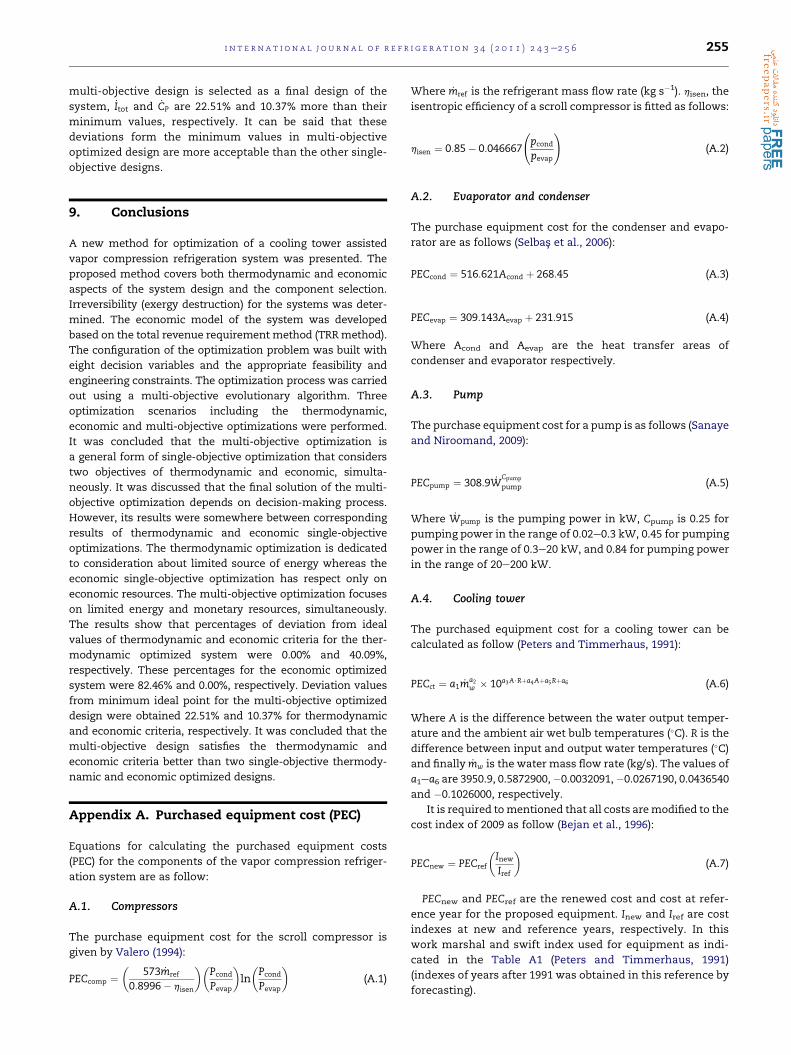
Fig. 6 shows the results of exergy analysis for the base case
design and three optimized designs. This figure indicates that
the thermodynamic optimized design has minimum total
exergy destruction equal to 44.57 kW. The next exergy
destructive designs are the multi-objective optimized, the
economic optimized and the base case designs that have
exergy destructions equal to 54.60 kW, 81.32 kW and
147.30 kW. These values are 22.51%, 82.46% and 230.48%more
than total exergy destruction for the thermodynamic design
respectively.
Fig. 6 also indicates that for all of the three optimized
designs, the most exergy destruction occurs in the
compressor, condenser and cooling tower.
The results of economic analysis for three optimized
systems and the base case system are given in Fig. 7. This
figure indicates that the minimum purchased equipment
ion scenarios.
ed Thermodynamic optimized Multi-objective optimized
2.22 2.29
28.89 16.18
0.32 0.24
16.84 16.84
52.35 63.24
3.49 4.48
0.15 1.10
7.19 4.60
352.00 352.00
404.35 415.23
6.72 5.57
5.57 4.79
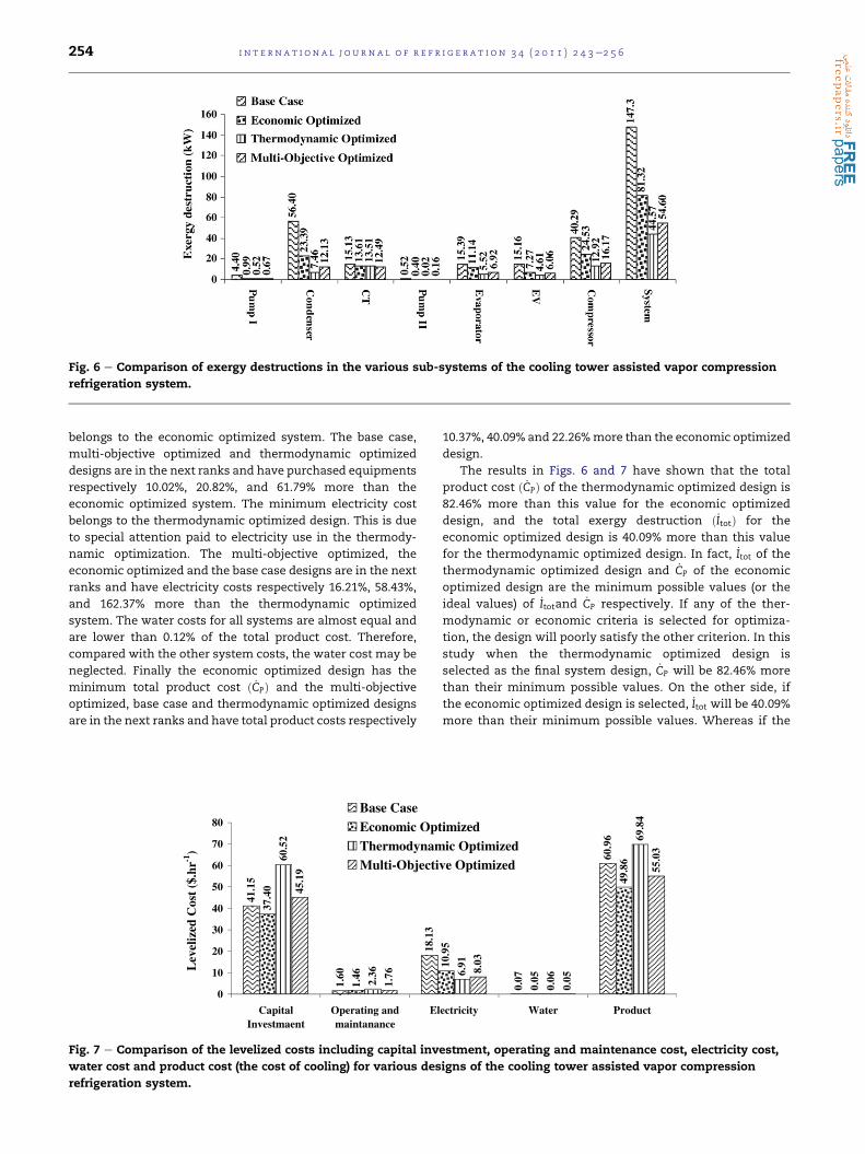
Fig. 6 e Comparison of exergy destructions in the various sub-systems of the cooling tower assisted vapor compression
refrigeration system.
i n t e r n a t i o n a l j o u r n a l o f r e f r i g e r a t i o n 3 4 ( 2 0 1 1 ) 2 4 3e2 5 6254
belongs to the economic optimized system. The base case,
multi-objective optimized and thermodynamic optimized
designs are in the next ranks and have purchased equipments
respectively 10.02%, 20.82%, and 61.79% more than the
economic optimized system. The minimum electricity cost
belongs to the thermodynamic optimized design. This is due
to special attention paid to electricity use in the thermody-
namic optimization. The multi-objective optimized, the
economic optimized and the base case designs are in the next
ranks and have electricity costs respectively 16.21%, 58.43%,
and 162.37% more than the thermodynamic optimized
system. The water costs for all systems are almost equal and
are lower than 0.12% of the total product cost. Therefore,
compared with the other system costs, the water cost may be
neglected. Finally the economic optimized design has the
minimum total product cost ð _CPÞ and the multi-objective
optimized, base case and thermodynamic optimized designs
are in the next ranks and have total product costs respectively
51.14
06.1
31.81
04.73
64.1
25.06
63.2
91.54
67.1
0
10
20
30
40
50
60
70
80
CapitalInvestmaent
Operating andmaintanance
El
rh.$(tso
Cdezileve
L1-)
Base CaseEconomic OptThermodynamMulti-Objecti
Fig. 7 e Comparison of the levelized costs including capital inv
water cost and product cost (the cost of cooling) for various des
refrigeration system.
10.37%, 40.09% and 22.26%more than the economic optimized
design.
The results in Figs. 6 and 7 have shown that the total
product cost ð _CPÞ of the thermodynamic optimized design is
82.46% more than this value for the economic optimized
design, and the total exergy destruction ð_ItotÞ for the
economic optimized design is 40.09% more than this value
for the thermodynamic optimized design. In fact, _Itot of the
thermodynamic optimized design and _CP of the economic
optimized design are the minimum possible values (or the
ideal values) of _Itotand _CP respectively. If any of the ther-
modynamic or economic criteria is selected for optimiza-
tion, the design will poorly satisfy the other criterion. In this
study when the thermodynamic optimized design is
selected as the final system design, _CP will be 82.46% more
than their minimum possible values. On the other side, if
the economic optimized design is selected, _Itot will be 40.09%
more than their minimum possible values. Whereas if the
70.0
69.06
59.01
50.0
68.94
19.6 60.0
48.96
30.8 50.0
30.55
ectricity Water Product
imizedic Optimized
ve Optimized
estment, operating and maintenance cost, electricity cost,
igns of the cooling tower assisted vapor compression
i n t e rn a t i o n a l j o u r n a l o f r e f r i g e r a t i o n 3 4 ( 2 0 1 1 ) 2 4 3e2 5 6 255
multi-objective design is selected as a final design of the
system, _Itot and _CP are 22.51% and 10.37% more than their
minimum values, respectively. It can be said that these
deviations form the minimum values in multi-objective
optimized design are more acceptable than the other single-
objective designs.
9. Conclusions
A new method for optimization of a cooling tower assisted
vapor compression refrigeration system was presented. The
proposed method covers both thermodynamic and economic
aspects of the system design and the component selection.
Irreversibility (exergy destruction) for the systems was deter-
mined. The economic model of the system was developed
based on the total revenue requirement method (TRRmethod).
The configuration of the optimization problem was built with
eight decision variables and the appropriate feasibility and
engineering constraints. The optimization process was carried
out using a multi-objective evolutionary algorithm. Three
optimization scenarios including the thermodynamic,
economic and multi-objective optimizations were performed.
It was concluded that the multi-objective optimization is
a general form of single-objective optimization that considers
two objectives of thermodynamic and economic, simulta-
neously. It was discussed that the final solution of the multi-
objective optimization depends on decision-making process.
However, its results were somewhere between corresponding
results of thermodynamic and economic single-objective
optimizations. The thermodynamic optimization is dedicated
to consideration about limited source of energy whereas the
economic single-objective optimization has respect only on
economic resources. The multi-objective optimization focuses
on limited energy and monetary resources, simultaneously.
The results show that percentages of deviation from ideal
values of thermodynamic and economic criteria for the ther-
modynamic optimized system were 0.00% and 40.09%,
respectively. These percentages for the economic optimized
system were 82.46% and 0.00%, respectively. Deviation values
from minimum ideal point for the multi-objective optimized
design were obtained 22.51% and 10.37% for thermodynamic
and economic criteria, respectively. It was concluded that the
multi-objective design satisfies the thermodynamic and
economic criteria better than two single-objective thermody-
namic and economic optimized designs.
Appendix A. Purchased equipment cost (PEC)
Equations for calculating the purchased equipment costs
(PEC) for the components of the vapor compression refriger-
ation system are as follow:
A.1. Compressors
The purchase equipment cost for the scroll compressor is
given by Valero (1994):
PECcomp ¼�
573 _mref
0:8996� hisen
��Pcond
Pevap
�ln
�Pcond
Pevap
�(A.1)
Where _mref is the refrigerant mass flow rate (kg s�1). hisen, the
isentropic efficiency of a scroll compressor is fitted as follows:
hisen ¼ 0:85� 0:046667
pcond
pevap
!(A.2)
A.2. Evaporator and condenser
The purchase equipment cost for the condenser and evapo-
rator are as follows (Selbas‚ et al., 2006):
PECcond ¼ 516:621Acond þ 268:45 (A.3)
PECevap ¼ 309:143Aevap þ 231:915 (A.4)
Where Acond and Aevap are the heat transfer areas of
condenser and evaporator respectively.
A.3. Pump
The purchase equipment cost for a pump is as follows (Sanaye
and Niroomand, 2009):
PECpump ¼ 308:9 _WCpump
pump (A.5)
Where _Wpump is the pumping power in kW, Cpump is 0.25 for
pumping power in the range of 0.02e0.3 kW, 0.45 for pumping
power in the range of 0.3e20 kW, and 0.84 for pumping power
in the range of 20e200 kW.
A.4. Cooling tower
The purchased equipment cost for a cooling tower can be
calculated as follow (Peters and Timmerhaus, 1991):
PECct ¼ a1 _ma2w � 10a3A$Rþa4Aþa5Rþa6 (A.6)
Where A is the difference between the water output temper-
ature and the ambient air wet bulb temperatures (�C). R is the
difference between input and output water temperatures (�C)
and finally _mw is the water mass flow rate (kg/s). The values of
a1ea6 are 3950.9, 0.5872900,�0.0032091,�0.0267190, 0.0436540
and �0.1026000, respectively.
It is required tomentioned that all costs aremodified to the
cost index of 2009 as follow (Bejan et al., 1996):
PECnew ¼ PECref
�InewIref
�(A.7)
PECnew and PECref are the renewed cost and cost at refer-
ence year for the proposed equipment. Inew and Iref are cost
indexes at new and reference years, respectively. In this
work marshal and swift index used for equipment as indi-
cated in the Table A1 (Peters and Timmerhaus, 1991)
(indexes of years after 1991 was obtained in this reference by
forecasting).
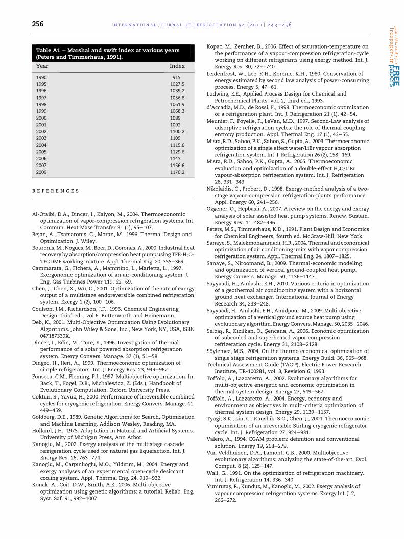
Table A1 e Marshal and swift index at various years(Peters and Timmerhaus, 1991).
Year Index
1990 915
1995 1027.5
1996 1039.2
1997 1056.8
1998 1061.9
1999 1068.3
2000 1089
2001 1092
2002 1100.2
2003 1109
2004 1115.6
2005 1129.6
2006 1143
2007 1156.6
2009 1170.2
i n t e r n a t i o n a l j o u r n a l o f r e f r i g e r a t i o n 3 4 ( 2 0 1 1 ) 2 4 3e2 5 6256
r e f e r e n c e s
Al-Otaibi, D.A., Dincer, I., Kalyon, M., 2004. Thermoeconomicoptimization of vapor-compression refrigeration systems. Int.Commun. Heat Mass Transfer 31 (1), 95e107.
Bejan, A., Tsatsaronis, G., Moran, M., 1996. Thermal Design andOptimization. J. Wiley.
Bouronis,M., Nogues,M., Boer, D., Coronas, A., 2000. Industrial heatrecovery byabsorption/compressionheat pumpusingTFE-H2O-TEGDME working mixture. Appl. Thermal Eng. 20, 355e369.
Cammarata, G., Fichera, A., Mammino, L., Marletta, L., 1997.Exergonomic optimization of an air-conditioning system. J.Eng. Gas Turbines Power 119, 62e69.
Chen, J., Chen, X., Wu, C., 2001. Optimization of the rate of exergyoutput of a multistage endoreversible combined refrigerationsystem. Exergy 1 (2), 100e106.
Coulson, J.M., Richardson, J.F., 1996. Chemical EngineeringDesign, third ed.., vol 6. Butterworth and Heinemann.
Deb, K., 2001. Multi-Objective Optimization Using EvolutionaryAlgorithms. John Wiley & Sons, Inc., New York, NY, USA, ISBN047187339X.
Dincer, I., Edin, M., Ture, E., 1996. Investigation of thermalperformance of a solar powered absorption refrigerationsystem. Energy Convers. Manage. 37 (1), 51e58.
Dingec, H., Ileri, A., 1999. Thermoeconomic optimization ofsimple refrigerators. Int. J. Energy Res. 23, 949e962.
Fonseca, C.M., Fleming, P.J., 1997. Multiobjective optimization. In:Back, T., Fogel, D.B., Michalewicz, Z. (Eds.), Handbook ofEvolutionary Computation. Oxford University Press.
Goktun, S., Yavuz, H., 2000. Performance of irreversible combinedcycles for cryogenic refrigeration. Energy Convers. Manage. 41,449e459.
Goldberg, D.E., 1989. Genetic Algorithms for Search, Optimizationand Machine Learning. Addison Wesley, Reading, MA.
Holland, J.H., 1975. Adaptation in Natural and Artificial Systems.University of Michigan Press, Ann Arbor.
Kanoglu, M., 2002. Exergy analysis of the multistage cascaderefrigeration cycle used for natural gas liquefaction. Int. J.Energy Res. 26, 763e774.
Kanoglu, M., Carpınlıoglu, M.O., Yıldırım, M., 2004. Energy andexergy analyses of an experimental open-cycle desiccantcooling system. Appl. Thermal Eng. 24, 919e932.
Konak, A., Coit, D.W., Smith, A.E., 2006. Multi-objectiveoptimization using genetic algorithms: a tutorial. Reliab. Eng.Syst. Saf. 91, 992e1007.
Kopac, M., Zemher, B., 2006. Effect of saturation-temperature onthe performance of a vapour-compression refrigeration-cycleworking on different refrigerants using exergy method. Int. J.Energy Res. 30, 729e740.
Leidenfrost, W., Lee, K.H., Korenic, K.H., 1980. Conservation ofenergy estimated by second law analysis of power-consumingprocess. Energy 5, 47e61.
Ludwing, E.E., Applied Process Design for Chemical andPetrochemical Plants. vol. 2, third ed., 1993.
d’Accadia, M.D., de Rossi, F., 1998. Thermoeconomic optimizationof a refrigeration plant. Int. J. Refrigeration 21 (1), 42e54.
Meunier, F., Poyelle, F., LeVan, M.D., 1997. Second-Law analysis ofadsorptive refrigeration cycles: the role of thermal couplingentropy production. Appl. Thermal Eng. 17 (1), 43e55.
Misra,R.D., Sahoo, P.K., Sahoo, S., Gupta,A., 2003.Thermoeconomicoptimization of a single effect water/LiBr vapour absorptionrefrigeration system. Int. J. Refrigeration 26 (2), 158e169.
Misra, R.D., Sahoo, P.K., Gupta, A., 2005. Thermoeconomicevaluation and optimization of a double-effect H2O/LiBrvapour-absorption refrigeration system. Int. J. Refrigeration28, 331e343.
Nikolaidis, C., Probert, D., 1998. Exergy-method analysis of a two-stage vapour-compression refrigeration-plants performance.Appl. Energy 60, 241e256.
Ozgener, O., Hepbasli, A., 2007. A review on the energy and exergyanalysis of solar assisted heat pump systems. Renew. Sustain.Energy Rev. 11, 482e496.
Peters, M.S., Timmerhaus, K.D., 1991. Plant Design and Economicsfor Chemical Engineers, fourth ed. McGraw-Hill, New York.
Sanaye, S.,Malekmohammadi,H.R., 2004. Thermal andeconomicaloptimization of air conditioning units with vapor compressionrefrigeration system. Appl. Thermal Eng. 24, 1807e1825.
Sanaye, S., Niroomand, B., 2009. Thermal-economic modelingand optimization of vertical ground-coupled heat pump.Energy Convers. Manage. 50, 1136e1147.
Sayyaadi, H., Amlashi, E.H., 2010. Various criteria in optimizationof a geothermal air conditioning system with a horizontalground heat exchanger. International Journal of EnergyResearch 34, 233e248.
Sayyaadi, H., Amlashi, E.H., Amidpour, M., 2009. Multi-objectiveoptimization of a vertical ground source heat pump usingevolutionaryalgorithm.EnergyConvers.Manage. 50, 2035e2046.
Selbas‚ , R., Kızılkan, O., S‚ encana, A., 2006. Economic optimizationof subcooled and superheated vapor compressionrefrigeration cycle. Energy 31, 2108e2128.
Soylemez, M.S., 2004. On the thermo economical optimization ofsingle stage refrigeration systems. Energy Build. 36, 965e968.
Technical Assessment Guide (TAG�), Electric Power ResearchInstitute, TR-100281, vol. 3, Revision 6, 1993.
Toffolo, A., Lazzaretto, A., 2002. Evolutionary algorithms formulti-objective energetic and economic optimization inthermal system design. Energy 27, 549e567.
Toffolo, A., Lazzaretto, A., 2004. Energy, economy andenvironment as objectives in multi-criteria optimization ofthermal system design. Energy 29, 1139e1157.
Tyagi, S.K., Lin, G., Kaushik, S.C., Chen, J., 2004. Thermoeconomicoptimization of an irreversible Stirling cryogenic refrigeratorcycle. Int. J. Refrigeration 27, 924e931.
Valero, A., 1994. CGAM problem: definition and conventionalsolution. Energy 19, 268e279.
Van Veldhuizen, D.A., Lamont, G.B., 2000. Multiobjectiveevolutionary algorithms: analyzing the state-of-the-art. Evol.Comput. 8 (2), 125e147.
Wall, G., 1991. On the optimization of refrigeration machinery.Int. J. Refrigeration 14, 336e340.
Yumrutas‚ , R., Kunduz, M., Kanoglu, M., 2002. Exergy analysis ofvapour compression refrigeration systems. Exergy Int. J. 2,266e272.