New Sensing Techniques for Structural Health Monitoring of Hydraulic Hose, Composite Panels, and

Biodegradable Metal Implants

A Thesis submitted to the

Graduate School

of the University of Cincinnati

in partial fulfillment of the

requirements for the degree of

Master of Science

in the Department of Mechanical Engineering

of the College of Engineering

by

Surya Narayanan Sundaramurthy

B.E. in Mechanical Engineering (Sandwich)

PSG College of Technology

June 2007

Committee Chair: Dr. Mark J Schulz

ii

Abstract

The development of new sensing techniques for in-situ continuous monitoring systems is one of

the most interesting research topics in the area of Structural Health Monitoring (SHM). The

primary difficulties related to putting health monitoring systems in applications are

implementation costs, reliability of the sensor system, and having the expertise required to use

these techniques. Hence there is a need to develop innovative, low cost sensor systems that are

simple, rugged, reliable and user friendly. This thesis makes a contribution in that direction by

developing low cost sensor systems for health monitoring of various mechanical components.

The novel sensing techniques evaluated as a part of this thesis include;

A new sensor concept based on electrical impedance technology called a ‘sensor skin’ for

surface SHM that detects small initiating damage over large areas,

A clip-on sensor module designed using a commercially available low cost piezo film

sensor for local damage detection and strain monitoring of the structure,

A continuous sensor developed using advanced, high performance, lightweight carbon

nanotube sensor thread, and an impedance based carbon nanotube sensor thread for crack

and strain sensing, and surface damage detection,

An eddy current based sensing technique for monitoring corrosion behavior, and a

feedback control device using the cathodic protection principle for prevention of

corrosion in structural/biomedical systems.

In the thesis, three different application scenarios were considered; health monitoring of

hydraulic hose used in machinery, damage detection in composite panels used in aerospace

applications, and monitoring the corrosion of biodegradable metal implants. The new sensing

iii

techniques were evaluated for these applications. One of the significant advantages of using the

new sensing approaches is the large reduction in the number of channels of data acquisition and

reduction in computational needs for health monitoring. Composite materials in particular can

benefit from these new sensing techniques using carbon nanotubes and the sensor skin. Also, the

use of carbon nanotube sensor thread opens the possibility of continuously monitoring large

structures like aircraft, ships, and other large vehicles with a small number of data acquisition

channels. The research in this thesis was performed in the Nanoworld Laboratory at University

of Cincinnati.

iv

v

Acknowledgements

First and foremost, I would like to thank my advisor Dr. Mark J. Schulz for his excellent

guidance, continuous support and patience during the course of this thesis. I thank Dr. Jay Lee,

Dr. Vesselin N. Shanov and Dr. David Thompson for agreeing to be in my thesis committee.

I would like to thank Dr. Yun for his assistance during the course of my thesis. Also, I would like

to thank Dr. John Yin, Dr. Heineman and his students Amos, Julia and Xuefei for their help in

the corrosion project. I appreciate the support shown to me by my colleagues from the

Nanoworld Lab.

I would also like to thank Dr. Xiangdong (Dawn) Zhu for her guidance, Wenyu and David from

the IMS center for their help in the hose project.

My sincere thanks to Chandrika for her huge support and encouragement and being with me

through the good and bad times at University of Cincinnati. I would like to appreciate the

support given by my friends Sanu, Rajiv, Devi, Hema and a special thanks to all of them for

presenting me with a model of Ferrari F10. I also thank all my other friends in Cincinnati and

back home.

Finally, I thank my parents Sundaramurthy and Saraswathi, my brother Jai, sister-in-law Rashi,

my sister Gayathri, brother-in-law Prakash for being there for me.

vi

Table of Contents

Abstract ........................................................................................................................................... ii

Acknowledgements ......................................................................................................................... v

Chapter 1 Introduction .................................................................................................................... 1

1.1 Problem Statement ................................................................................................................ 1

1.2 Structural Health Monitoring System ................................................................................... 2

1.3 Thesis Organization............................................................................................................... 5

Chapter 2 Structural Health Monitoring of Hydraulic Hose ........................................................... 9

2.1 Introduction ........................................................................................................................... 9

2.1.1 Need for SHM of hydraulic hose .................................................................................. 11

2.1.2 Current technologies to monitor health of hose ............................................................ 12

2.1.3 Sensor road map ........................................................................................................... 14

2.1.4 Test Bed Setup .............................................................................................................. 18

2.2 Cycle Counters .................................................................................................................... 19

2.2.1 Electrical Counter – Pedometer .................................................................................... 19

2.3 Strain Gage .......................................................................................................................... 20

2.3.1 Strain Gage as a damage prediction sensor .................................................................. 20

2.3.2 Strain Gage as a damage detection sensor .................................................................... 22

2.4 Piezoelectric Sensors for Hose Health Monitoring ............................................................. 25

2.4.1 Introduction .................................................................................................................. 25

2.4.2 Design 1: Attaching the PVDF sensor using adhesive ................................................. 27

2.4.3 Design 2: Clip-on PVDF Sensor Module Using Hose Clamps .................................... 30

2.4.4 Design 3: Improved Clamp Design for Clip-on PVDF Sensor .................................... 36

2.4.5 Design 4: Clip-on Sensor using Long Flexible PVDF Sensors .................................... 41

2.4.6 Design 5: Piezo Cable for Hose Health Monitoring ..................................................... 42

2.4.7 Design 6: Rugged Clip-on Sensor Design .................................................................... 47

2.5 Damage detection using wave propagation ......................................................................... 51

2.5.1 Experimental Setup and Results ................................................................................... 51

Chapter 3 Sensor Skin for Surface Structural Health Monitoring ................................................ 55

vii

3.1 Introduction ......................................................................................................................... 55

3.2 Sensor Skin Concept ........................................................................................................... 56

3.2.1 Design Considerations for Sensor Skin ........................................................................ 59

3.2.2 Damage Modeling for Sensor Skin .............................................................................. 59

3.2.3 Initial Validation of Concept ........................................................................................ 60

3.3 Testing of Sensor Skin Materials ........................................................................................ 64

3.3.1 Sensor Skin Material Table .......................................................................................... 65

3.3.2 Load Testing of Sensor Skin ........................................................................................ 66

3.3.3 Impact Testing .............................................................................................................. 72

3.4 Application of Sensor Skin ................................................................................................. 73

3.4.1 Sensor Skin on Hose ..................................................................................................... 75

Chapter 4 Carbon Nanotube Sensor Yarn for Structural Health Monitoring ............................... 93

4.1 Introduction ......................................................................................................................... 93

4.1.1 Carbon Nanotubes (CNT) ............................................................................................. 94

4.2 Electrical Impedance Measurement of CNT based Materials ............................................. 97

4.2.1 CNT Ribbon ................................................................................................................. 98

4.2.2 CNT Thread/Yarn ....................................................................................................... 105

4.3 Application of Carbon Nanotubes ..................................................................................... 109

4.3.1 Current SHM Techniques for Composite Structures .................................................. 109

4.3.2 CNT based Sensor for SHM of Composite Structures ............................................... 111

Chapter 5 Corrosion Monitoring and Control of Biodegradable Metal Implants ....................... 126

5.1 Introduction ....................................................................................................................... 126

5.1.1 Biomaterials ................................................................................................................ 127

5.1.2 Need for Biodegradable Implants ............................................................................... 129

5.1.3 Magnesium as Biodegradable Material ...................................................................... 129

5.1.4 Corrosion Behavior..................................................................................................... 131

5.1.5 Importance of Corrosion Monitoring and Control of Biodegradable Implants .......... 132

5.2 Corrosion Monitoring of Magnesium Implants ................................................................ 133

5.2.1 Eddy Current Methodology to Monitor Corrosion ..................................................... 133

5.2.2 Corrosion Monitoring of Mg Plate ............................................................................. 135

5.2.3 Corrosion Monitoring of a Mg Screw ........................................................................ 141

viii

5.2.4 Conclusion and Future Work Based on Corrosion Testing ........................................ 145

5.3 Corrosion Control of Magnesium Implants ...................................................................... 148

5.3.1 Corrosion Control using Impressed Current Cathodic Protection System ................. 150

5.3.2 Experimental Setup and Procedure............................................................................. 152

5.3.3 Results and Discussion of Corrosion Control Study .................................................. 158

5.3.4 Corrosion Control Feedback Algorithm using LabVIEW .......................................... 164

5.3.5 Conclusion and Future Work for using Cathodic Protection of Implants .................. 171

Chapter 6 Conclusions and Future Work .................................................................................... 173

6.1 Health Monitoring of Hydraulic Hose .............................................................................. 173

6.2 Sensor Skin for Structural Health Monitoring .................................................................. 175

6.3 CNT Sensor Yarn for Health Monitoring of Composite Structures.................................. 176

6.4 Corrosion Health Monitoring and Control of Implants for Biomedical Applications ...... 178

6.5 Future Work ...................................................................................................................... 179

6.5.1 Health monitoring of hydraulic hose .......................................................................... 179

6.5.2 Sensor skin for structural health monitoring .............................................................. 180

6.5.3 CNT sensor yarn for health monitoring of composite structures ............................... 181

6.5.4 Corrosion health monitoring of implants for biomedical applications ....................... 181

6.5.5 Corrosion control of implants for biomedical applications ........................................ 181

References ................................................................................................................................... 185

ix

List of Figures Figure 2.1 Basic construction of hydraulic hose [Image courtesy of google.com]. ..................... 10 Figure 2.2 Schematic of Smart Hose Safety system [[14], [22] Courtesy http://www.smarthose.com] .......................................................................................................... 12 Figure 2.3 Low molecular weight organic liquid detection sensor in shape of a wire [19].......... 13 Figure 2.4 Safety hose section view [20]. ..................................................................................... 14 Figure 2.5 Hose-bending test bed [13], [22]. ................................................................................ 18 Figure 2.6 Sensor allocations at UC test bed [13], [22]. ............................................................... 18 Figure 2.7 Life Fitness HJ-720ITLF pedometer used for cycle counting. .................................... 19 Figure 2.8 Experimental setup with strain gage attached to the hose. .......................................... 20 Figure 2.9 Strain Gage data from a fixed end sensor [22]. ........................................................... 21 Figure 2.10 Strain gages “folding” due to cycling of the hose [22]. ............................................ 21 Figure 2.11 Miniature strain gage [24] ......................................................................................... 22 Figure 2.12 Strain gage bonded to the spiral hose ........................................................................ 23 Figure 2.13 Crack induced in the spiral hose. ............................................................................... 23 Figure 2.14 Strain signal from the spiral hose when bent............................................................. 24 Figure 2.15 Experimental Setup: (a)PVDF sensors attached to the hose using adhesive; (b) PVDF sensor used in this setup;(c) close up image of PVDF sensor mounted to the rubber. ................. 27 Figure 2.16 PVDF sensor signal from fixed half of hose [22]...................................................... 28 Figure 2.17 PVDF sensor signal from moving end of the hose [22]. ........................................... 29 Figure 2.18 PVDF sensor signals placed at either end of the hose [22]. ...................................... 29 Figure 2.19 Clip-on sensor design using PVDF sensor [29]. ....................................................... 31 Figure 2.20 Experimental setup with two clip-on PVDF sensors. ................................................ 32 Figure 2.21 Amplitude response from PVDF clip on sensor: (a) Raw data; (b) Filtered data. .... 32 Figure 2.22 Experimental setup with six clip-on PVDF sensors attached to the hose [29]. ......... 33 Figure 2.23 Easy-to-Install bolt clamp and belleville washer. ...................................................... 37 Figure 2.24 PVDF sensor mounted on the hose. .......................................................................... 38 Figure 2.25 Experimental setup using hydraulic pump. ............................................................... 38 Figure 2.26 PVDF signal response when the hand pump is pressurized from 0 to 2000psi. ....... 39 Figure 2.27 Voltage responses from the sensor due to gradual application of pressure. .............. 40 Figure 2.28 Long flexible PVDF sensor. ...................................................................................... 41 Figure 2.29 Slot machined to take the lead of the sensor out. ...................................................... 41 Figure 2.30 Piezo cable [31]. ........................................................................................................ 43 Figure 2.31 Experimental setup using piezo cable. ...................................................................... 44 Figure 2.32 Signal strength vs. Number of clamps. ...................................................................... 45 Figure 2.33 Comparison between spiral and longitudinal orientation (without voltage divider). 45 Figure 2.34 Comparison between spiral and longitudinal orientation (with voltage divider). ..... 46 Figure 2.35 Mylar silicone splicing tape used to develop rugged clip-on sensor. ........................ 47 Figure 2.36 Rugged clip-on PVDF sensor. ................................................................................... 48

x

Figure 2.37 Amplitude responses from rugged clip-on sensor due to bending cycle of the hose. 49 Figure 2.38 Experimental setup using rugged clip-on sensor [Picture by Wenyu]. ..................... 50 Figure 2.39 Schematic of wave propagation experimental setup. ................................................ 51 Figure 2.40 Experimental setup of wave propagation in a hydraulic hose. .................................. 52 Figure 2.41 Voltage vs. time comparison of input and output wave for healthy hose sample. .... 52 Figure 2.42 Voltage vs. time comparison for healthy, rubber layer damage and wire damage hose. .............................................................................................................................................. 53 Figure 3.1 Basic configuration of the Sensor Skin (skin thickness exaggerated for clarity). ....... 56 Figure 3.2 Different designs of sensor skin: (a) piezoresistive; (b) spikes that stay attached to the opposite electrode when damage occurs; (c) an auxetic material to enhance collapsing of the insulating layer when damage occurs; (d) intermediate wire [37] ................................................ 58 Figure 3.3 Sensor skin developed for this experiment: (a) rubber sheet on which the electrode is attached; (b) sensor skin with two aluminum electrodes and a dielectric attached to the structure........................................................................................................................................................ 61 Figure 3.4 Experimental setup showing infinite resistance when no load is applied. .................. 61 Figure 3.5 Experimental setup displaying zero resistance when electrodes were damaged. ........ 62 Figure 3.6 Thin Aluminum electrodes with a pin-hole damage induced in it. ............................. 63 Figure 3.7 Change in electrical resistance of the sensor skin when load is applied. .................... 64 Figure 3.8 Experimental Setup for Load Testing; (a) Hydraulic press used for testing the sensor skin; (b) close-up image of indentation of sensor skin in the press; (c) spherical indenters of diameters: 0.187, 0.374, and 0.55 in., respectively; (d) Kapton film used as a dielectric; (e) optical image of the sensor skin after indentation (0.374 in.). ...................................................... 67 Figure 3.9 Variation of resistance of the sensor skin due to loading. ........................................... 68 Figure 3.10 Impact Testing of Sensor Skin: (a) Experimental Setup, (b) Optical image of the sensor skin after impact testing, (c) Variation in resistance due to impact testing. ...................... 73 Figure 3.11 Development of Sensor Skin: (a) Inside rubber layer, (b) First conductive layer attached to hose, (c) Insulating layer attached, (d) Second conductive layer attached to the hose, (e) Rubber layer placed to cover the sensor skin. ......................................................................... 76 Figure 3.12 Sensor Skin on the outside of hose: (a) Along the length, (b) Circumferential. ....... 78 Figure 3.13 Sensor skin between the inner rubber and steel layer................................................ 79 Figure 3.14 Experimental setup. ................................................................................................... 80 Figure 3.15 Change in resistance due to damage of the sensor skin............................................. 81 Figure 3.16 Carbon rubber electrodes and insulator patch. .......................................................... 83 Figure 3.17 (a) Sensor skin developed using carbon rubber medical electrodes; (b) Side view of the sensor skin. .............................................................................................................................. 84 Figure 3.18 (a) Sensor skin developed using medical soft white foam electrodes; (b) Side view of the sensor skin. .............................................................................................................................. 84 Figure 3.19 Insulted tips used to create pinhole damage. ............................................................. 85 Figure 3.20 Experimental setup with medical soft white foam electrodes: (a) No Damage; (b) Drop in resistance due to pinhole damage. ................................................................................... 86

xi

Figure 3.21 Experimental setup with carbon rubber electrodes: (a) No Damage; (b) Drop in resistance due to pinhole damage. ................................................................................................ 86 Figure 3.22 Damage in the sensor skin: (a) medical soft white foam electrodes; (b) Carbon rubber electrodes. .......................................................................................................................... 87 Figure 3.23 PVDF as a charging device. ...................................................................................... 89 Figure 3.24 Sensor skin outside the hose ...................................................................................... 90 Figure 3.25 Sensor skin between inner rubber layers. .................................................................. 91 Figure 3.26 Sensor Skin on outside and inside hose (Image from [39])....................................... 92 Figure 4.1 Single Wall Carbon Nanotube [54]. ............................................................................ 94 Figure 4.2 Carbon nanotubes: (a) SWCNT (b) MWCNT [54]. .................................................... 95 Figure 4.3 Manufacturing of CNT materials: (a) Long CNT forest (>1 cm) on a 4 inch wafer; (b) CNT Array; (c) CNT Thread; (d) CNT Yarn (two threads twisted together); (e) CNT Ribbon [59], [102]. .................................................................................................................................... 98 Figure 4.4 CNT array and ribbon: (a) CNT array; (b) drawing the ribbon from the array onto a spool; (c) TEM image of the ribbon with a 5 micron scale bar. ................................................... 99 Figure 4.5 Experimental setup: (a) Solartron Impedance Gain-Phase Analyzer connected to the Device under Test (CNT Ribbon), (b) Bode plot obtained from the analyzer. .......................... 100 Figure 4.6 CNT Ribbon (7cm long) wound between 2 copper posts. ........................................ 100 Figure 4.7 Impedance Plot for open and short correction measurement: (a) Magnitude of impedance by opening electrodes without any sample (Open Correction). (b) Magnitude of impedance by directly connecting the electrodes together without any sample (Short Correction)...................................................................................................................................................... 101 Figure 4.8 Magnitude vs. Frequency for CNT ribbon without epoxy. ....................................... 103 Figure 4.9 Phase vs. Frequency for CNT ribbon without epoxy. ............................................... 103 Figure 4.10 Magnitude vs. Frequency for CNT ribbon with epoxy. .......................................... 104 Figure 4.11 Phase vs. Frequency for CNT ribbon with epoxy. .................................................. 105 Figure 4.12 SEM Images of Carbon Nanotube Thread: (a) SEM Image of a single CNT thread. (b) SEM Image showing two threads twisted together [102]. .................................................... 105 Figure 4.14 Magnitude vs. Frequency for CNT thread without epoxy. ...................................... 106 Figure 4.15 Phase vs. Frequency for CNT thread without epoxy. .............................................. 107 Figure 4.16 Magnitude vs. Frequency for CNT thread with epoxy. ........................................... 108 Figure 4.17 Phase vs. Frequency for CNT thread with epoxy. ................................................... 108 Figure 4.18 Carbon nanotube thread bonded on the surface along the length of the composite beam [22], [36]............................................................................................................................ 113 Figure 4.19 Microscopic images of the carbon nanotube thread used in this experiment: (a) Microscopic image of the nanotube thread used in the experiment; (b) Microscopic image of the nanotube thread attached to the fiberglass beam by a nonconductive epoxy [22], [36]. ............ 113 Figure 4.20 Testing CNT thread on a cantilever beam: (a) cantilever beam in undeformed stage with no load applied; (b) cantilever beam in the deformed stage after the application of load [22]...................................................................................................................................................... 114

xii

Figure 4.21 Change in resistance of the carbon nanotube thread vs. applied load. .................... 115 Figure 4.22 Crack Propagation Experiment: (a) Microscopic image of CNT thread before crack propagation; (b) Microscopic image of CNT thread after crack propagation [22]. .................... 116 Figure 4.23 Sensing and anti/de-icing system. ........................................................................... 119 Figure 4.24 Sensor configurations: (a) Two electrode CNT thread Impedance Sensor; (b) Distributed CNT thread array network. ...................................................................................... 122 Figure 4.25 Experimental setup for testing CNT thread to detect ice and water. ....................... 123 Figure 4.26 CNT thread Impedance Sensor: (a) Test sample with water between CNT thread; (b) Test sample with ice between CNT thread. ................................................................................ 123 Figure 4.27 Bode Plot for three cases of clean surface, water and ice between CNT sensor thread...................................................................................................................................................... 124 Figure 5.1 Eddy Current Method (Image courtesy: http://www.olympus-ims.com/en/eddycurrenttesting). ................................................................................................. 134 Figure 5.2 Eddy current coil; (a) Two coil flexible eddy current sensor; (b) Close-up view of the inter-wound coils. ....................................................................................................................... 135 Figure 5.3 Corrosion monitoring of Mg plate: (a) Mg-Y alloy plate; (b) Mg-Y alloy plate placed in a beaker containing 10X PBS (Phosphate Buffer Saline) solution with the flexible coil sensor wrapped around it. ...................................................................................................................... 136 Figure 5.4 Schematic of experimental setup. .............................................................................. 137 Figure 5.5 Corrosion monitoring of Mg plate. ............................................................................ 138 Figure 5.6 Corrosion Monitoring Diagram for Mg-Y 4% alloy plate in a highly corrosive 10x concentrated PBS solution. ......................................................................................................... 139 Figure 5.7 Corrosion monitoring of Mg screw: (a) Mg screw; (b) Mg screw placed in a beaker containing 10X PBS solution with the flexible coil sensor wrapped around it. ......................... 141 Figure 5.8 Corrosion monitoring of Mg plate. ............................................................................ 142 Figure 5.9 Corrosion degradation of Mg screw every 24 hours over a period of 17 days. ........ 143 Figure 5.10 Corrosion monitoring diagram for Mg screw in a highly corrosive 10x PBS solution...................................................................................................................................................... 144 Figure 5.11 Schematic of Cathodic protection system (Image courtesy: http://www.aaawelldrilling.com/Cathodic%20Protection.html). ............................................... 150 Figure 5.12 Schematic of the corrosion control experimental setup. ......................................... 154 Figure 5.13 Mg implant with the epoxy layer removed due to corrosion................................... 155 Figure 5.14 Mg implant prepared using Buehler Epokwick fast cure epoxy. ............................ 156 Figure 5.15 Electrodes used for corrosion control experiment: (a) Aluminium Electrode, (b) Cut Mg pellet, (c) Mg pellet coated with non-conductive epoxy. ..................................................... 156 Figure 5.16 Corrosion control experimental setup: (a) Control Case; (b) No control Case. ...... 157 Figure 5.17 Change in weight of Mg for a period of 25 days when there is no corrosion control...................................................................................................................................................... 159 Figure 5.18 Change in weight of Mg when using Al as counter electrode at different applied potential for a period of 25 days. ................................................................................................ 160

xiii

Figure 5.19 Change in weight of Al electrode at different applied potential for 25 days. ......... 161 Figure 5.20 Change in weight of Mg when using Zn as counter electrode at different applied potential for a period of 25 days. ................................................................................................ 162 Figure 5.21 Change in weight of Zn electrode at different applied potential for 25 days. ......... 163 Figure 5.22 Schematic of automated corrosion control experiment developed using LabVIEW...................................................................................................................................................... 165 Figure 5.23 LabVIEW front panel window for the automated corrosion control. ..................... 167 Figure 5.24 Front panel displaying the condition when 1 V Potential is applied to Zn electrode...................................................................................................................................................... 168 Figure 5.25 LabVIEW window when potential to Zn electrode is increased to 5 V. ................. 169 Figure 5.26 LabVIEW window when control algorithm automatically reduces the output potential from 5 V to 1 V. ........................................................................................................... 169 Figure 5.27 LabVIEW window when potential to Zn electrode is reduced to 0.5 V. ................ 170 Figure 5.28 LabVIEW window when control algorithm automatically increases the output potential from 0.5 V to 1 V. ........................................................................................................ 170

xiv

List of Tables

Table 2-1 Sensor Evaluation Summary Chart .............................................................................. 17 Table 2-2 Design methodologies adopted for using PVDF sensors for hose health monitoring. . 26 Table 2-3 Amplitude response level from PVDF sensors located at 3, 4 and 5. .......................... 34 Table 3-1 Conductive Skin Material Properties............................................................................ 65 Table 3-2 Dielectric Material Properties ....................................................................................... 66 Table 3-3 Load to failure of sensor skin due to different spherical indenters. ............................. 68 Table 3-4 Diameter of indentation on the composite for the three spherical indenters. ............... 69 Table 3-5 Variation in electrical properties with Kapton film as a dielectric due to loading (spherical indenter diameter: 0.187 in.). ....................................................................................... 71 Table 3-6 Variation in electrical properties with wax paper as a dielectric due to loading (spherical indenter diameter: 0.187 in.). ....................................................................................... 71 Table 3-7 Variation in electrical properties with Kapton film as a dielectric (spherical indenter diameter: 0.374 in.). ...................................................................................................................... 72 Table 3-8 Variation in electrical properties with wax paper as a dielectric. ................................. 72 Table 3-9 Two different types of medical electrode used for sensor skin. ................................... 83 Table 4-1 Comparison of the approximate strength and conductivity of various materials [56]. 96 Table 4-2 Comparison of Mechanical Properties of various materials [57], [102]. ..................... 97 Table 5-1 Common biomaterials and its applications [86], [88]. ............................................... 128 Table 5-2 Open circuit potential measurement between magnesium and counter electrodes. ... 152 Table 5-3 Open circuit potential measurement between magnesium and counter electrodes. ... 153 Table 5-4 Corrosion control experimental parameters. .............................................................. 158 Table 5-5 Control Algorithm Table. ........................................................................................... 166

1

Chapter 1

Introduction

1.1 Problem Statement

Structural Health Monitoring (SHM) techniques refers to the process of developing and

implementing a damage identification, detection and characterization strategy to monitor the

health and condition of diverse structures ranging from aerospace, civil, biomedical and

mechanical engineering infrastructures [1]. Several health and condition monitoring techniques

have been developed to tackle very complex problems that are economically justified or needed

based on safety and reliability of structures. Large scale monitoring systems have significant

costs in terms of sensors, data acquisition, processing, and expertise and hence the solution

becomes quite complicated and time consuming. Hence, there arises a need for a low cost sensor

system which is generic, flexible, inexpensive, and easy to implement.

The performance and safety of large structures and advanced structures is dependent

mainly on the reliability of composite materials and heterogeneous materials that are used to

build the structure. The difficulty to define ‘damage’ in the structure increases as materials

themselves contain imperfections. In general, the damage to the structure can be attributed to the

changes occurring to the material and geometric properties of the structural system that adversely

affect the performance of the structure [2], [22]. The damage occurring in some of these

materials may be difficult to track and can propagate fast during operation of the vehicle or

structure. For instance, in aircraft industries wherein composite materials are being widely used

for their superior mechanical properties, the damage detection is difficult mainly due to the

2

initiation of damage in these composite materials which usually occurs inside the material unlike

regular metals [3]. In this case, conventional nondestructive testing techniques and several other

sensing techniques based on periodic inspection may not be adequate for the timely detection of

damage in novel structure designs. In much of the current research in SHM, the emphasis is on

designing a system that is simple, compact and autonomous and it should be scalable to complex

real-life structures [4]. Therefore, a specific sensor system must be developed for SHM that will

be required to capture a wide variety of damage and failure modes as described above and in

some cases combination of more than one kind of failure [5]. This thesis is focused on the

development of low cost sensor system for a wide variety of applications ranging from

mechanical, aerospace and biomedical applications.

1.2 Structural Health Monitoring System

Typically, SHM involves the following steps;

Data Acquisition: Observing and recording the system parameters over a period of time

using an array of sensors like piezoelectric polymers, strain gages, etc.

Data Processing: Processing the data to eliminate noise signals and extracting features

from those measurements that are related to the health of the system.

Damage Analysis: Performing analysis on the extracted features to determine the health

and current condition of the structure.

The process is performed continuously and the output is updated frequently to provide

reliable information regarding the integrity of the structure. Using SHM information, it is

possible to estimate the remaining useful life of a component and perform condition-based

maintenance [6].

3

The data acquisition stage is the first and the important stage in SHM for any application.

The excitation methods, parameters that need to be measured, sensor types, number and locations

of sensors on the structure, data acquisition (DAQ) hardware, sampling rate of the DAQ device,

etc., needs to be decided and each of these parameters will be application specific. Before

extracting the significant features from the collected data, data processing needs to be carried

out. Any sources of variability in the data acquisition process need to be identified and

minimized to the extent possible to get accurate information of the health of the system [7].

The data processing stage includes normalizing the data in order to offset any changes

caused by operational changes, unwanted noise signals in the collected data, environmental

conditions. Also, data cleansing is performed wherein any data that are unrelated to the health of

the system being monitored are removed from the feature extraction process. For instance, if the

application is temperature independent, i.e., if the system performance is not going to be affected

due to variations in temperature, then any data that corresponds to the temperature of the system

is not required and hence can be filtered from the feature extraction process. In the feature

extraction stage, the main goal is to identify the properties that vary with damage and allows the

user to distinguish between the damage and healthy state of the system. The significant

properties affecting the system performance is specific to the application. Sometimes, usage of

analytical tools such as finite element models can be a great asset in this process. Also,

accelerated damage testing is performed to identify appropriate features wherein significant

structural components are degraded by subjecting them to realistic loading conditions. Insight

into the appropriate features can be gained from several types of analytical and experimental

studies which are useful in the feature extraction process [7].

4

Damage analysis is the final stage in SHM where algorithms that utilize the extracted

features are developed using statistical tools in MATLAB, LabVIEW, etc., to quantify the

damage in a structure. Typically, the algorithms developed fall into two categories; supervised

and unsupervised learning. Supervised learning is when the quantification of damage is done

using data from both the undamaged and damaged states. Some examples of supervised learning

include group classification and regression analysis. In unsupervised learning, the quantification

of damage is done using data from only the undamaged state [7], [22].

The development of SHM that started with vibration based monitoring of structures has

expanded considerably widely to other areas like aerospace, biomedical, etc., over the last couple

of decades. The advances in the fields of sensor systems, data acquisition hardware, wireless

sensors have increased the variety and types of structures that can be monitored. Also, advances

in materials like carbon nanotubes (CNTs) have made integrated sensing possible wherein the

CNT are embedded into the structure to detect damage.

However, the overall costs are still high. Also, in a situation wherein large number of

sensors is used to collect huge amount of data, data acquisition and feature extraction becomes

more complicated [22]. The associated wiring, instrumentation, amplification, multiplexing, and

computational resources required to implement these methods on a large scale will be prohibitive

in terms of cost, added weight, and reliability. Hence there is a need to select a sensor system

that requires very few data channels and simpler data processing to determine the health of the

structure. The goal of this thesis is to develop such low cost sensor systems that continuously

monitor the health of the structure under study for different SHM applications including

mechanical structures, composite structures used in aircraft industries and magnesium implants

5

used in biomedical applications. An overview of each of these applications is given in the next

sections and is discussed in detail in the subsequent chapters of this thesis.

1.3 Thesis Organization

Chapter 2 Health Monitoring of Hydraulic Hose describes the low cost sensor system that is

developed for the health monitoring of hydraulic hose for structural applications. The chapter

contains a brief introduction about the hydraulic hose, requirement for the health monitoring of

hose, literature review of the current technologies being used and the sensor road map developed

to detect damage and predict the remaining life of the hose.

The purpose of the hydraulic hose is to transfer fluids from one place to another.

Typically, they are a composite assembly made of steel wire mesh and polymer materials and are

used in a variety of industries like oil & gas drilling, agricultural, construction, heavy machinery,

etc. Hoses fail due to various factors like external damage, operating conditions, etc [8]. The

failure can lead to serious injury and cause adverse damage to the surroundings and

environments. The cost incurred due to failure of the hose is more than the cost incurred in

replacing the hose. The solutions designed to address these issues and to predict/detect the

damage in the hose using multitude of sensors like low cost piezoelectric sensors that extracts

significant features from the hose before the actual occurrence of the failure are discussed in this

work. Also, a new sensing technique is proposed to detect damage in the hose that is low cost,

reliable, requires very few data channels and simple data processing.

Chapter 3 Sensor Skin for Surface Structural Health Monitoring proposes a new

sensing technique called ‘Sensor Skin’ for damage detection. This technique is primarily used for

surface SHM. This chapter describes the concept of sensor skin followed by development and

6

validation of the concept by performing experimental testing. Finally, couple of applications is

described in which the sensor skin can be used to detect damage.

Chapter 4 Carbon Nanotube Sensor Yarn for Structural Health Monitoring describes

the new and innovative sensor developed based on advanced material like the carbon nanotubes

(CNT). The chapter gives a brief introduction about the structure, properties and possible

applications of CNT. In this work, the CNT based sensors developed for different applications

are presented.

Health monitoring of composite is difficult compared to regular metals because of the

occurrence of damage inside the composite materials. [3]. Most common types of damage in

composite materials are delamination. Though damage detection is difficult, composite materials

offer a significant advantage wherein the damage sensors can be embedded in the structure. The

damage sensors developed to monitor the health of the composite structures are based on carbon

nanotube (CNT) materials. It is known from the literature that the carbon nanotubes possess

remarkable mechanical, thermal, electrical properties. Also, CNTs are best suited for sensor

applications as they are piezoresistive in nature. The CNTs that are embedded into the structures

not only enhances its bulk properties but also aids in damage detection by continuously

monitoring the health of the CNTs. In this thesis, experimental work conducted to detect damage

in a composite structure is discussed. Also, yet another application of CNT based sensors are

discussed in this thesis which involves the detection of ice on the surface of the aircraft

structures. Impedance measurement based CNT sensor was developed for this work and are

discussed in detail in chapter 4 of this thesis.

7

Chapter 5 Corrosion Monitoring and Control of Biodegradable Metal Implants focuses

on developing a corrosion health monitoring system for biomedical applications. It gives a brief

introduction about the implants, implant materials, magnesium as implant material, corrosion of

magnesium implants, corrosion monitoring system developed to continuously monitor the

corrosion rate of the implant and the corrosion control device developed to control the corrosion

of the implant as per the requirements.

Implants are biomedical devices that are primarily used for replacing a missing biological

structure, supporting a damaged biological structure or enhancing an existing biological

structure. For instance, in orthopedic surgery, the implant devices are placed over or within

bones to hold the fractured bone while they heal. The biomaterials that are used to make these

implant devices must have good mechanical, electrical, physical, thermal and chemical

properties. Different biomaterials are selected for different applications. For instance, in

orthopedic applications, the implants are primarily structural members that transmit loads.

Hence, mechanical properties like ultimate strength, elastic modulus, fracture toughness, etc.,

becomes an important criterion. In recent years, the research and development of biodegradable

implant materials has become one of the most important and interesting topics in the biomaterials

field. The primary reason for choosing biodegradable implants over conventional permanent

metal implants like stainless steel is to avoid a second surgery to remove the stainless steel

implants from the body and hence prevent any risk of re-fracture, discomfort to the patient and

also eliminate the cost involved in performing a second surgery. Whereas these biodegradable

implants dissolve and absorb in the human body after a period of time. Magnesium has been

discovered as a potential replacement and this thesis will mainly focus on the usage of

magnesium as an effective biodegradable material for implants. However, one of the main issues

8

with magnesium is the rapid rate of corrosion as it is an active material and rapid corrosion is an

intrinsic response of magnesium and its alloys to chloride containing solutions including the

human body fluid. Apart from producing Mg2+ ions that can be tolerated by the human body, the

rapid corrosion of magnesium results in the formation of hydrogen gas bubbles and hydroxides

that are undesirable to the human body [9]. Hence there is need to understand the corrosion

behavior of the implant and to develop a corrosion health monitoring system that continuously

monitors and controls the corrosion rate of the magnesium according to the requirements.

Chapter 5 of this thesis will discuss the innovative methods developed to address the above

mentioned issues.

Chapter 6 Conclusions and Future Work gives the overall conclusion of this research work and

scope for future work.

9

Chapter 2

Structural Health Monitoring of Hydraulic Hose

2.1 Introduction

Hydraulic hose transfers fluids under pressure from one place to another [22]. In general, hoses

are made from one or a combination of many different materials. The material of the hose being

used largely depends on the application and the performance needed from the hose. Some of the

common materials include nylon, polyurethane, polyethylene, PVC or synthetic or natural

rubbers. In order to achieve a better pressure resistance, hoses can be reinforced with fibers or

stainless steel wires. Some of the commonly used reinforcement methods include braiding,

spiraling, knitting and wrapping [10]. Variations in hose can be due to its size, rated temperature,

weight, numbers of reinforcement layers, type of reinforcement layers, rated working pressure,

flexibility and economics.

The hydraulic hose described in this chapter are steel reinforced rubber hoses [22]. A

hydraulic hose can be described as a composite structure primarily made of alternate layers of

rubber and steel as shown in Figure 2.1. Each hose consists primarily of three layers namely;

Tube, Reinforcement and Cover [11].

10

Figure 2.1 Basic construction of hydraulic hose [Image courtesy of google.com].

The tube is the innermost layer of the hose. The tube is made from different rubber

compounds and composites in order to chemically resist the fluid being conveyed. The inside

diameter of the tube is the key indicator of hose size. Typically, for an SAE specification hose,

the smaller diameter tube can handle higher pressures [11], [12].

The intermediate steel plies are called as reinforcement layer and is the muscle of all

hydraulic hoses. The working pressure of the hose is determined by the reinforcement layer.

They can be braided across the length for higher strength or spirally wrapped along the length

and can be made of natural fibers, synthetic materials or steel wire [11], [12].

The outermost layer is called as the cover and its primary purpose is to protect the other

two layers from heat, abrasion, corrosion and environmental deterioration [11]. The cover can be

made from different materials like synthetic rubber, fiber depending on the application [11], [12].

Hydraulic hose can be grouped based on the operating pressure [11], [22] as follows;

Extremely high pressure hose

High pressure hose

Medium pressure hose

Low pressure hose

11

2.1.1 Need for SHM of hydraulic hose

Hydraulic hoses are used in a variety of industries like oil & gas drilling, agricultural,

construction, mining equipment, heavy-machinery, household appliances, etc. Hydraulic hoses

fail due to various factors like pulling, abrasion, twisting of wire layers due to multi plane

bending, operating conditions, etc. The operating conditions of the hose determine its service

life. For instance, extremes in temperature accelerate aging, frequent and extreme pressure

fluctuations accelerate fatigue life of hose.

Hose failure can lead to serious injury or death of an operator [22] and can also cause

adverse damage to the surroundings and environments. The cost incurred due to failure of the

hose is more than the cost incurred in replacing the hose. Additional costs might be due to the

collateral damage caused to other components, damage caused by the ingression of

contaminants, etc. It is difficult to predict the life of the hose because of its inhomogeneity

wherein the hose characteristics change with aging and environmental conditions [13], [22].

Most of the current maintenance scheme is mainly based on preventive or Fail-and-Fix (FAF)

methods. A higher level of maintenance, Predict-and-Prevent (PAP) is needed to achieve near-

zero down maintenance, which in turn will increase productivity and safety [13].

Research work is being conducted at Nanoworld Lab and IMS center in University of

Cincinnati (UC) to address these issues and to come up with a solution to predict and/or detect

damage in the hose before the occurrence of the failure. This chapter presents some of the

solutions designed to predict/detect the damage in the hose using multitude of sensors that

extracts significant features from the hose that show anomalous characteristics of the signal

which might be a precursor to failure (Work in this chapter was part of teamwork for an industry

12

project where several students worked together and each reported our individual results from the

experiments).

2.1.2 Current technologies to monitor health of hose

A literature search was conducted to find the methodologies currently available in the

market to monitor condition of a hose and based on the findings, a detailed road map for the

project was formulated which will be described in the next section. A brief overview of some of

the important patent and literature survey carried out are presented below;

a) Smart Hose Safety

The "Smart-Hose™ Safety" system (Philadelphia) shuts-off the flow instantly whenever hose

coupling ejection, hose stretching or hose separation occurs [22]. Smart-Hose™ includes a

coated cable that acts as a compression spring. It is connected to valve plungers, wedges or

flappers [14]. The cable holds the valve open by giving thrust. Whenever the thrust is eliminated

due to any failure, the valves release and instantly seat, stopping flow in both directions [14],

[22]. The schematic is shown in Figure 2.2.

Figure 2.2 Schematic of Smart Hose Safety system [[14], [22] Courtesy

http://www.smarthose.com]

13

b) Abrasive material transport hose with wear detecting sensors - US Patent 6386237

The useful life can be increased if the first sign of internal wear is spotted and remedied [22].

This is accomplished by disposing at least two wear sensing elements each at a specified distance

from the innermost surface of the inner tube, and monitoring a condition indicative of wear of

the hose. When the innermost wear sensing element implies wear, the position of the hose can be

changed to extend the useful life until the outermost wear sensing element indicates wear

requiring replacement of the hose [15], [22].

c) Sensor Coil or Thin Film That Changes Resistance

A Low Molecular Weight Organic Liquid Detection Sensor in the shape of a wire was designed

and used for leakage detections such as underground oil tank leak detection. One of the sensor

designs is shown in Figure 2.3. The sensor is in a shape of wire and is comprised of two layers, a

conductive layer and a conductor core. An isolation coating is applied between the two layers to

prevent electrical connectivity. The conductive layer is made of a special conductive material

which absorbs a very small amount of low molecular weight organic liquid and swells and

therefore changes its resistance. An oil leakage can thus be detected by monitoring the resistance

change [19].

Figure 2.3 Low molecular weight organic liquid detection sensor in shape of a wire [19].

2-Conductive layer 3,3’-Electrodes11-Conductor12-Insolation coating33,34,35-Lead wiresR-Measuring instrument

14

d) Safety Hose with Leakage Sensor

The safety hose was originally designed for logging practice to prevent injury to human

operators due to hose failure. Figure 2.4 shows a section view of the safety hose [20]. The hose

is comprised of an inner primary hydraulic pressure hose (38) and an outer secondary hose or

tube (40). There is an annular passageway (42) between the two layers. When inner hose breaks,

hydraulic fluid is pushed into the annular passageway between inner and outer hoses, and

dissipated from bleed holes (62) at the end fitting section at lower pressure. The bleed holes are

positioned outside of the coupling of the inner hose to prevent direct exposure of high pressure

fluid in case the inner hose fail at the end right beneath the bleed holes.

Figure 2.4 Safety hose section view [20].

2.1.3 Sensor road map

The goal of the project is to determine the most appropriate sensors, understand the

reasons behind hose failure and to be able to predict the failure enough in advance that the hose

can be retired from service. A Responsive Hose/Smart Hose concept is thought to be a possible

solution to prevent failure of hoses by notifying the operator that the hose needs replacement.

This approach is called condition based maintenance wherein the component is replaced when its

useful life has ended and not after a prescribed time or number of load cycles [13], [22].

30-Hydraulid safety hose38-Primary hydraulic pressure hose40-Outer secondary hose or tube42-Annular passageway44-Nylon core tube45-Synthetic fiber braid layer46-Polyurethane outer jacket50-Hydraulic connector fitting52-Threaded outer end56-Enlarged hexagonal wrenching boss62-bleed holes64-Annular ring

15

The sensors would measure features from the hose that shows anomalous characteristics

of the signal that are a precursor of failure. They may also measure a relationship among hose

system parameters which are a precursor of failure. Beyond indicating damage, it is necessary to

understand the root cause of damage and failure in hose. Understanding the failure modes would

allow redesign and also design of the most appropriate sensor to detect damage [22].

One of the objectives of the study is to perform a root cause analysis and to find the

parameter of the hose that is the most sensitive indicator of the damage. Damage could occur due

to a combination of causes such as turbulent flow in the hose, aging rubber, foreign objects in the

oil or dirty or degraded oil, loose connections, leaks at seals, shift in the braid angle in moving

hoses, fretting wear, corrosion, shear between the wire layers, and cracking of the wire and

reduction in the effective wall thickness of the hose [21], [22].

The sensor selection was categorized into two following approaches:

To predict the damage using a cycle counting method to count the number of cycles

To devise a method to detect damage

Damage Prediction: Hoses are tested in custom made rigs before being released into the market

[22]. The hoses are tested till failure and the operator would know the minimum number of

cycles that particular hose will last. In such circumstances, it is possible to predict the failure

with a cycle counter wherein number of cycles exhausted by the hose is measured based on

which the remaining useful life of the hose can be calculated. But the damage propagation in a

hose can be rapid and hence the time taken for the hose to develop failure from initial crack is

very minimal. In such cases, prediction methods cannot detect this premature damage scenario

16

[22]. The counting can be done using cycle counter, piezoelectric film or strain gage. In later

sections of this chapter, each of these sensing methods is discussed in detail.

Damage Detection: When hose fails prematurely, the prediction method may not be the best and

hence the need is to devise a method to detect damage in a hose. Premature failure of a hose may

be due to misuse of the hose like when they are subjected to use beyond their limitations. The

damage occurs near end-fittings and midway. The approaches used to detect damage are

described in detail in the later sections (Work in this section was part of a teamwork for an

industry project where several students worked together and each reported our individual results

from the experiments).

Table 2-1 gives a brief summary of the various sensors that were evaluated as a potential sensor

approach to predict/detect damage in the hose. Each of these sensors will be discussed in detail.

17

Table 2-1 Sensor Evaluation Summary Chart

Function Sensor Type Advantages Disadvantages Results

Clip-on Sensor

PVDF Piezoelectric

(PZT) Polymer

Flexible, Long Life, Cost $10,

No bonding required

Low operating temperature,

Leads make it hard to build- in

On-line counter built using LabVIEW

MEMS Accelerometer

Long, Life Cheap, Cost

$15 Same as above Same as above

Novel Sensor for In situ

Monitoring

Eddy Current (Foil Sensors) Non-contact Not for rubber Detects surface damage

Strain Gage Local

Monitoring at hot spots

Short lifetime, Bonding,

Debonded due to surface unevenness

Carbon Nanotube

Thread

Strong, Light weight, sensitive, multi-functional

In developmental stages

New Concept : Works by making rubber

conductive and also reinforcing it

Wave Propagation

Need Ceramic PZT make it

hard to build-in Not repeatable Can detect surface

damage

Electrical Impedance

Measurement

Simple measurements

Hose needs to be electrically insulated

Can detect discontinuities and pinhole damages

Novel Sensors for

Manufacturing Quality

Control and On site testing

X-Ray Clear Images Damages in

rubber yet to be identified

Images obtained

Eddy current (Cylindrical

Probe) Non-contact Time

consuming Detects surface damage

Ultrasonic Sensitive to metal

Rubber damages hard to

identify

Can detect surface damages

18

2.1.4 Test Bed Setup

A test bed with pneumatic cylinder shown in Figure 2.5 is used to simulate hose bending cycles.

One end of the hose is fixed and the other end is moved back and forth from fixed end. The test

bed is provided by Parker Hannifin. A sketch of sensor allocation is shown in Figure 2.6 [13],

[22].

Figure 2.5 Hose-bending test bed [13], [22].

Figure 2.6 Sensor allocations at UC test bed [13], [22].

Compound insulator

Moving end

Fixed end

Pedometer

Strain gage

Piezoelectric sensor mounted

Piezoelectric sensor taped

Resistance

Fixed and electrically insolated end

Moving end

19

2.2 Cycle Counters

As discussed in the previous section, cycle count is an important measure of hose life. By design,

every type of hose must deliver normal performance with high pressure fluid for at least a

specific number of cycles before any incipient failures can happen [13], [22]. There are two

types of motion that hose is being subjected to during operation, namely bending and pulse.

Bending is caused by the mechanical movement whereas pulse is caused when high speed fluid

passes the hose. With only mechanical motion, the hose is unlikely to fail. However explosion

and fixture failure can happen due to local stress concentration [22]. In this section, we will

evaluate the possibility to apply different techniques for hose cycle monitoring.

2.2.1 Electrical Counter – Pedometer

Electrical counter uses piezoelectric sensor for motion detection [22]. Figure 2.7 shows one of

the products for fitness application that was employed to count the cycles of the hose.

Figure 2.7 Life Fitness HJ-720ITLF pedometer used for cycle counting.

The bending cycle was simulated using the test rig with the pedometer attached to the

hose. The pedometer incremented by one count after every bending cycle and the readings were

recorded. The pedometer can detect multiple directions of motion therefor there is no limitation

on its orientation. Also, the pedometer memory is organized by day [22], [23].

powered by a CR2032 batter 5-digit counting scale up to 4-day storage data downloadable to computer

20

2.3 Strain Gage

Strain gage was used as one of the sensor approach for both prediction and damage detection as

described below;

2.3.1 Strain Gage as a damage prediction sensor

2.3.1.1 Experimental Setup

Strain gages were used as one of the sensor material to count the number of cycles. The cycling

of the hose being a repetitive motion causes cyclic strain in the hose [22]. The strain gages were

purchased from Vishay Micromeasurements Inc. [24]. The strain gages used for cycle counter

had a resistance of 350 Ohms. The data was acquired using a NI-DAQ module designed for

strain gages. Two strain gages were attached to the ends of the hose as show in Figure 2.8. The

hose was cycled in the pneumatic test bed and data acquired using the NI-9215 DAQ module

[22].

Figure 2.8 Experimental setup with strain gage attached to the hose.

21

2.3.1.2 Results and Conclusions

Figure 2.9 shows the filtered data from the strain gage mounted near the fixed end. The data

showed consistency with less noise after filtering. The test rig cycles the hose at a frequency of 1

Hz. As seen from the plot, the cycle is repetitive and is consistent with the cycling frequency of

the hose. From the plot, it is possible to count the number of cycles the hose is subjected and

from it, the useful life of the hose can be determined. Thus, strain gage was able to fulfill its

purpose by providing a method for counting cycles [22].

Figure 2.9 Strain Gage data from a fixed end sensor [22].

The major difficulty experienced in this experiment was the adhesion of the strain gages

to the hose surface. The adhesives were not very efficient during cycling as the strain gages

underwent “folding” as shown in Figure 2.10 [22].

Figure 2.10 Strain gages “folding” due to cycling of the hose [22].

22

2.3.2 Strain Gage as a damage detection sensor

2.3.2.1 Concept

Strain gage was used as a sensor to detect the damage in the wire layers in the hose. The concept

was that the spiral strain gage bonded to a continuous wire layers in the spiral hose will give a

continuous strain signal. If there is damage in the wire layer, it will disrupt the continuity of the

wire layers. The discontinuity will affect the strain in the hose; as a result the strain signal from

the damage layer will be comparatively different from the healthy condition. So by monitoring

the strain signal of the hose, it is possible to identify the onset of any damage in the wire layer in

a spiral hose.

2.3.2.2 Experimental Setup and Results

In this experiment, a miniature strain gage was used as shown in Figure 2.11. Strain gage was

purchased from Vishay Inc.

Strain Gage Parameters: Gage Series EA Gage Resistance 12

Ω Gage Length 0.031” Overall Pattern Length 0.140” Grid Width 0.032” Overall Pattern Width 0.032” Matrix Length 0.27” Matrix Width 0.12”

Figure 2.11 Miniature strain gage [24]

The miniature strain gage was bonded to the spiral hose using a non-conductive epoxy. It

was bonded in the direction that is parallel to the orientation of the steel layers in the hose as

shown in Figure 2.12.

23

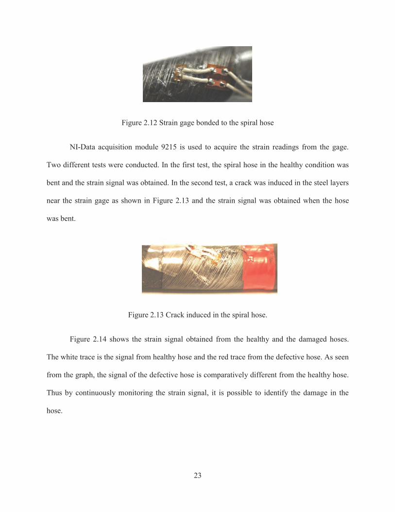
Figure 2.12 Strain gage bonded to the spiral hose

NI-Data acquisition module 9215 is used to acquire the strain readings from the gage.

Two different tests were conducted. In the first test, the spiral hose in the healthy condition was

bent and the strain signal was obtained. In the second test, a crack was induced in the steel layers

near the strain gage as shown in Figure 2.13 and the strain signal was obtained when the hose

was bent.

Figure 2.13 Crack induced in the spiral hose.

Figure 2.14 shows the strain signal obtained from the healthy and the damaged hoses.

The white trace is the signal from healthy hose and the red trace from the defective hose. As seen

from the graph, the signal of the defective hose is comparatively different from the healthy hose.

Thus by continuously monitoring the strain signal, it is possible to identify the damage in the

hose.

24

Figure 2.14 Strain signal from the spiral hose when bent.

2.3.2.3 Conclusions and Future Work using Strain Gages

From the experiments conducted, it can be concluded that the discontinuities in the continuous

spiral windings can be detected due to change in load transfer. Also, when the strain gages are

bonded at the critical locations in the hose, where the failure is more predominant, any damage

occurring to the steel layers can be detected in those areas by continuously monitoring the strain

signals. This enables the local monitoring at hot spots possible in a spiral hose. The main

disadvantage of this method is the possibility of the strain gage failing before the actual failure of

the hose. In order to tackle this disadvantage, more testing is to be conducted in the actual

working conditions to determine the suitability of this sensor under different working conditions.

25

2.4 Piezoelectric Sensors for Hose Health Monitoring

2.4.1 Introduction

A piezoelectric sensor is a device that uses the piezoelectric effect to measure pressure, strain or

force by converting them to an electrical signal. Piezoelectricity is the ability of certain materials

to accumulate charge in response to applied mechanical strain. Some of the materials that exhibit

piezoelectricity include naturally occurring crystals like quartz, topaz, etc., man-made ceramics

like lead zirconate titanate (PZT), lead titanate, etc., polymers like polyvinylidene fluoride

(PVDF) [25], [26], [27].

Hydraulic hose is normally subjected to bending or pulsing motion during its operating

conditions which causes mechanical strain in the hose. Hence, attaching a piezoelectric sensor to

the hose will cause a strain in the piezoelectric material thereby generating voltage. By

continuously monitoring the voltage generated from the sensor, strain in the hose can be

monitored. If there is any failure to the hose, the strain in the hose will differ thus changing the

voltage signal characteristics from the piezoelectric sensor compared to the healthy condition.

The signals from the sensor have to be processed to remove the noise signals and significant

features that indicate the health of the hose needs to be extracted from the filtered signal. Thus,

by monitoring the signal characteristics from the sensor, the health of the hose can be monitored

and any failure occurring to the hose can be immediately sensed and the hose can be replaced

without causing any damage to the other components, surrounding and environments.

An attempt has been made in the project to use the piezoelectric sensor as a sensor device

that monitors the health of the hose. For this work, PVDF piezoelectric sensor was selected as

they are flexible and can easily conform to hose surface [22]. In general, the PVDF sensor is a

26

flexible component comprising an extremely thin layer of piezoelectric PVDF polymer film with

screen-printed Ag-ink electrodes (in the order of 28 μm), laminated to a polyester substrate (in

the order of 0.125 mm). These PVDF sensors are attached to different locations in the hose and

as the piezoelectric film is displaced from the mechanical neutral axis due to the motion of the

hose, bending creates very high strain within the piezopolymer and generating high voltages.

Different designs for the sensor module were tried and tested that includes testing different types

of PVDF sensors, different types of clamping methods to attach the sensor onto the hose, etc., in

order to find the optimal sensor design as shown in Table 2-2. These designs will be described in

the next sections of this chapter.

Table 2-2 Design methodologies adopted for using PVDF sensors for hose health monitoring.

Design Function Improvement 1 Used adhesive to attach the PVDF

sensor to the hose First Design

2 Used hose clamps to hold the PVDF sensor to the hose

Adhesives were not effective; Used clamps to hold the sensor to the surface of the hose

3 Improved clamp design to hold the PVDF sensor

Clamp force in hose clamp was difficult to control leading to variations in signals from sensor; Used a constant pressure clamp that applies constant pressure to the sensor and eliminates any variations due to the clamp force.

4 Used long flexible PVDF sensors Taking leads out from short film PVDF sensors and connecting to NI-DAQ module to acquire data were difficult; Used long flexible PVDF sensor to improve the data acquisition.

5 Used Piezo cable Long flexible PVDF sensors were limited in temperature range and ruggedness; Used Piezo cable that is rugged.

6 Customized long flexible PVDF sensor to withstand high temperature

Piezo cables were not effective compared to flexible PVDF sensor and were difficult to install. Improved temperature capability and ruggedness of the flexible PVDF sensor by attaching an additional layer of insulation tape (Mylar tape - strong and high temperature resistant capability) to the sensor.

27

2.4.2 Design 1: Attaching the PVDF sensor using adhesive

2.4.2.1 Experimental Setup and Results

The PVDF film sensors (LDT0 PVDF sensor) were purchased from Measurement Specialties

Inc. [28]. The sensors were glued with a commercially available adhesive called Contact Cement

sold by Permatex. The PVDF sensors were placed on four locations on the hose; two near end-

fittings are labeled as A and D and two more at midpoint labeled as B and C as shown in Figure

2.15a. The leads from the sensor are coupled with 1 MΩ to avoid impedance mismatch. The test

rig is used to simulate the hose bending cycles. The voltage across the resistance is measured

while bending and acquired using NI-Data Acquisition 9215 module [22]. Figure 2.15c shows

the close up image of the mounting of PVDF sensor to the hose.

Figure 2.15 Experimental Setup: (a)PVDF sensors attached to the hose using adhesive; (b) PVDF

sensor used in this setup;(c) close up image of PVDF sensor mounted to the rubber.

a

b

c

A

B C

D

28

Figure 2.16 shows the plot of amplitude response from the two PVDF sensors attached on

near the fixed end D) and the other placed closed to the center (C). It can be seen that the peak

from D is higher compared to C because of the jerk motion near the fixed end[22].

Figure 2.16 PVDF sensor signal from fixed half of hose [22].

Figure 2.17 shows the plot of amplitude response from the two PVDF sensors attached on

near the moving end (A) and the other one placed closed to the center (B). It can be seen that

both A and B are in phase and amplitude of A is higher compared to B.

29

Figure 2.17 PVDF sensor signal from moving end of the hose [22].

Figure 2.18 compares the amplitude response from the fixed end (A) and moving end (D)

of the hose. The signals are of same amplitude but there is a difference in phase. A phase

difference between peaks can be because of hose cycling.

Figure 2.18 PVDF sensor signals placed at either end of the hose [22].

30

2.4.2.2 Conclusions from using the Piezo Sensor

The output voltage from the piezo sensors at the ends are about 5V peak-to-peak and are around

3V for sensors placed near the center. The peaks seem to be lower as jerk reaction is mitigated

along the length due to the structure’s mechanical resistance. The amplitudes responses from the

sensors clearly indicate a cycling process [22]. This indicates that the signals from the sensor can

be processed and algorithms such as derivative based slope counting method, zero crossing

counting method can be employed to count the number of cycles.

The disadvantage with using the adhesive to glue the sensor to the hose was the

possibility of the glue coming off. Also, it was found that the glue damps out some energy and

hence the voltage signal from the sensor is not the accurate signal from the sensor. Hence, an

improved sensor design was proposed and will be discussed in the next section.

2.4.3 Design 2: Clip-on PVDF Sensor Module Using Hose Clamps

The clip-on sensor design is shown in Figure 2.19. The PVDF piezoelectric sensing element is

placed inside a hose clamp and the hose clamp is firmly attached to the hose structure. Also,

there is a rubber cushion layer between the hose clamp and the sensing device. Since the entire

design incorporates clamp that can be easily attached or detached from the hose structure, it is

called as a clip-on sensor. The leads from the sensor are connected to the NI-DAQ module for

data acquisition. Using this clip-on design, the PVDF sensor can be placed either in the

circumferential orientation or in the longitudinal direction along the hose.

31

Figure 2.19 Clip-on sensor design using PVDF sensor [29].

2.4.3.1 Experimental Setup and Results using the Clip-On Sensor

Bending test was carried out to measure the signals from the PVDF sensors using the clip-on

method. The initial experiments can be seen as a way to determine whether this method of

clipping on the sensor can provide an indicative signal of the bending or pressure cycle exerted

on the hose, as well as whether this sensor is suitable for determining the number of cycles the

hose experiences. The overall experimental setup is shown in Figure 2.20. There are two PVDF

sensors mounted using the clip on method, with one placed on the top of the hose and the other

placed on the moving end near the end fitting. The bending test rig uses compressed air to bend

and cycle the attached hose, with the mounted hose being cycled at an approximate rate of

1cycle/sec. NI 9221 DAQ module is used to acquire the voltage signal from each sensor and the

LabVIEW software is used in conjunction with the DAQ module to perform the data collection,

filtering and processing of the data.

32

Figure 2.20 Experimental setup with two clip-on PVDF sensors.

Figure 2.21a shows the unfiltered amplitude response from the two PVDF sensors. A

Finite Impulse Response (FIR) band-pass filter with a lower cutoff frequency of 0.5Hz and an

upper cutoff frequency of 1.5Hz was used to smooth the raw time signal. Figure 2.21b shows the

filtered signal wherein much of the noise in the raw signal has been removed.

Figure 2.21 Amplitude response from PVDF clip on sensor: (a) Raw data; (b) Filtered data.

As shown in Figure 2.21, the response from the sensor near the end-fitting (blue curve) is

much larger and this would indicate that there is more strain and stress placed on the hose under

33

bending at this location when compared to the top of the hose where the other sensor is located.

Also, the 1Hz bending of the hose is represented by the 1Hz cyclic wave that can be seen in both

sensor output signals and this shows that a counting method like zero crossing or slope based

method can be applied to count cycles.

Since the clip-on sensor method gave a good indicating signal of the bending motion of

the hose, next set of experiments were carried out to find an optimal placement of the sensors on

the hose that gives a best response. For this experiment, six PVDF sensors were placed on

multiple locations on the hose as shown in Figure 2.22. Also, the six sensors were placed in

either longitudinal or circumferential orientations in order to find the best possible orientation for

the bending test. The sensors numbered as 1, 2, 3 and 6 are placed in the circumferential

orientation and sensors numbered as 4 and 5 are placed in the longitudinal orientation.

Figure 2.22 Experimental setup with six clip-on PVDF sensors attached to the hose [29].

The amplitude responses from all the six sensors were recorded simultaneously using NI-

DAQ module. The amplitude response was similar to the plot shown in Figure 2.21. The signal

34

response at locations 1, 2 and 6 has a higher level of noise compared to the other three signals.

The response at locations 3, 4 and 5 have a higher signal to noise ratio and a comparison between

the amplitude of the signals are shown below in Table 2-3. From this experiment, the best

response was found to be at location 4 and 5. For the bending motion, the longitudinal

orientation for the PVDF sensor provides the best signal. Also, the sensor closer to the moving

end has a larger response.

Table 2-3 Amplitude response level from PVDF sensors located at 3, 4 and 5.

Sensor Location Amplitude Response Level (V)

3 0.08

4 0.45

5 0.50

After finding optimal location of the sensor and orientation, next set of experiments were

conducted to understand the amplitude response signals and extract significant features from the

signals that might give an indication of the health of the hose. For this experiment, three clip-on

PVDF sensors were placed in the longitudinal direction along the hose with one near the fixed

end, one in the middle of the hose and one near the moving end. The bending test-rig was used

and data was collected for a 1-hour time span from a healthy hose. The sensor was removed from

the hose and then put back again and the test was conducted. Same procedure was repeated for

three times to check for repeatability and also to check for any variability in data due to the

removal and reattachment of the sensor.

Based on the data collected from the three tests, it was found that the maximum

amplitude of the waveform or other indicators of the sensor signal change over time during the

35

testing and this effect might be due to a variation in the clamping force that is used to attach the

sensor to the hose surface. Also the hose clamps are not rigid and are easily bent; hence it is

difficult to put the same clamping force every time.

2.4.3.2 Conclusions from using the Clip-On PVDF Sensor

The clip-on sensor design of attaching the sensor to the hose surface using hose clamps was

found to be a better method compared to the previous method of using an adhesive to glue the

sensor to the hose. From the experiments conducted using clip-on sensors, new developments

have been made that include analysis on determining the best sensor location for the largest

amplitude signal and the signal with the best signal to noise ratio. It was determined that for the

bending motion of the hose, the longitudinal PVDF sensor orientation provides the signal with

the best signal to noise ratio and the sensor located closest to the moving end has the largest

amplitude response. However for a pressure pulse or other excitations it might be necessary to

use the circumferential direction or sensing elements placed in both orientations. Also further

understanding on what locations provide the best signal as well as an understanding at what

location might be best to detect degradation of the hose at the earliest stage is also a

consideration for deciding on the optimum placement of the clip-on sensor module.

The major conclusion that can be drawn from this clip-on design is the importance of

maintaining constant pressure and load on the sensing element so that the sensor response is

repeatable and does not change due to operating or environmental conditions. If the sensor

amplitude changes due to slight wear of the outer surface of the rubber hose, or a change in

temperature, or change in operating pressure, the sensor response will change and this change

may be interpreted as damage. As shown in the testing, the maximum amplitude of the sensor

36

signal changed over time due to a variation in the clamping force and this gives a possibility of

false positive indication of damage. Thus an improved clip-on sensor approach is proposed in the

next section that has the ability to maintain constant contact force between the hose and PVDF

sensor element.

2.4.4 Design 3: Improved Clamp Design for Clip-on PVDF Sensor

Previous testing has shown that false positive indications of damage may occur due to

variation in the clamping force of the clip-on sensor. For strain and piezoelectric sensor where

shear and normal forces are transferred between the hose and sensor, maintaining a constant

contact force and interface condition is very important. The following are the design changes that

were incorporated to maintain constant contact force between the hose and the sensor element;

Replacement of hose clamp with bolt clamp

Usage of Belleville spring that acts like a spring

The bolt clamp used in this improved clamp design is easy to install and also stronger

than the hose clamp. Belleville washers were used to maintain constant interface conditions

between the hose and sensor. The washers act like a long spring and they are compressed so that

a near constant force is applied to clamps. Washer adjusts the clamp diameter to compensate for

any change in operating or environmental conditions. When a long spring is compressed to a

nominal length, a further small variation in compression of the spring will not change the force

much due to the low spring constant, i.e. F=k(x0 + xv), where the spring force F is proportional to

the spring stiffness k and initial displacement x0 and variation in displacement xv (due to thermal

expansion or pressure in the hose or other factors). Since x0>>xv, the contact force and pressure

37

on the PVDF will be nearly constant. The bolt clamp and belleville washer are shown in Figure

2.23.

Figure 2.23 Easy-to-Install bolt clamp and belleville washer.

2.4.4.1 Experimental Setup and Results

Experiments were conducted to determine whether this method of clipping on the sensor

provides a good and repeatable signal compared to the previous design. The sensor response

signal was compared with different pre-load values from 5 to 50 in-lb and the pre-load value that

gives the highest signal to noise ratio and the most repeatable and consistent signal was

determined. The experimental setup is shown in Figure 2.24. PVDF sensor is mounted near the

center of the hose. NI 9221 DAQ module is used to acquire the voltage signal from the sensor. It

was found that 35 in-lb was the nominal pre-load value to the bolt clamp that gave a consistent

and good signal from the sensor.

38

Figure 2.24 PVDF sensor mounted on the hose.

In order to find the sensitivity of the PVDF sensor to pressure pulse, a hydraulic hand

pump was used. The hydraulic hand pump was provided by Parker Hannifin. The hose was

attached to hydraulic pump. The experimental setup is shown in Figure 2.25. As before, NI-DAQ

was used to collect the data from the sensor. Initial experiments were carried out to find the

optimal orientation of the sensor. It was found that the response signal from the longitudinal

orientation was very small, when pressure was applied. Circumferential orientation gave a clear

signal which shows that for pressure pulse, circumferential orientation is more suited.

Figure 2.25 Experimental setup using hydraulic pump.

Clip-on PVDF Sensor

Adjustable Torque Wrench Gauge

39

Next, the amount of clamping force that needs to be given in order to get a good and

consistent signal from the sensor was determined and found to be 30 inlb. Figure 2.26 shows the

amplitude response plot from the PVDF sensor. In this case, the hand pump was quickly pumped

to pressurize the hose to 2000 psi and then the pressure was quickly released. As the pressure in

the hose increases, the voltage from the PVDF sensor also increases and ramps up to 10 V and

then it slowly declines as the pressure is released. Also noticeable from the plot is the drop in the

response signal to -10V when the valve is open and fluid goes the other way.

Figure 2.26 PVDF signal response when the hand pump is pressurized from 0 to 2000psi.

Figure 2.27 shows the plot of the voltage response from the sensor when the pressure was

gradually and periodically increased to 1500 psi and then released. It can be seen that the

pressure dynamics are clearly captured by the PVDF sensor and also the quick decline in the

pressure is shown by the decrease in the voltage response.

0 5 10 15 20 25 30 35 40-15

-10

-5

0

5

10

15

Time (s)

PV

DF

Pre

ssur

e S

igna

l

PVDF Signal for 0-2000psi ramp up and down, Pre-load of 30in-lb

40

Figure 2.27 Voltage responses from the sensor due to gradual application of pressure.

2.4.4.2 Conclusions from the Clip-on Sensor Design Study

Improved clip-on design using bolt clamp and belleville washer gave a consistent and

repeatable sensor signal. Also, the nominal value for the clamping force that gives a good signal

was determined for both bending and pressure tests. It was observed that too tight of clamping

might cause adverse effect on the hose life and the readings from the sensor might not be

accurate. And if the clamp is loose, the sensor was not able to capture the signal and the obtained

signal was too noisy. Pressure test was conducted using a hydraulic hand pump and was found

that the pressure dynamics was captured accurately by the PVDF sensor and the circumferential

orientation was more suited for the pressure test compared to the longitudinal orientation.

0 5 10 15 20 25 30 35 40-2

-1

0

1

2

3

4

5

Time (s)

PV

DF

Pre

ssur

e S

igna

l

PVDF Signal for pumping pressure up to 1500psi and than release, pre-load of 30in-lb

41

2.4.5 Design 4: Clip-on Sensor using Long Flexible PVDF Sensors

2.4.5.1 Experimental Setup and Results

The PVDF sensors used are short in length (about 1” long). Hence longer connecting

wires are needed to connect from the sensor to the NI-DAQ module. These long wires are not

desirable because of the possibility of the wires from different sensors coming in contact and

getting intertwined while the hose is in operation. Also noise signals from these wires need to be

filtered while performing data processing which is complicated. To overcome the shortcomings

of short length PVDF sensor, long flexible PVDF sensors are used as shown in Figure 2.28.

Long flexible PVDF sensors called as FDT series elements with lead attachment was procured

from Measurement Specialties [30]. The length of the sensor is 10”.

Figure 2.28 Long flexible PVDF sensor.

In order to assemble PVDF sensors, a rectangular slot was machined on the clamp. This

avoided the possibility of any positioning error of the sensor as shown in Figure 2.29.

Figure 2.29 Slot machined to take the lead of the sensor out.

42

Testing was performed with the new sensor using both the bending and pressure test rig.

Main advantage of using this sensor was the reduction in the noise signals. Also, the connecting

wires were not coming in contact with each other and this eliminated the possibility of

intertwining of wires.

2.4.5.2 Conclusion from using the Long PVDF Sensor

Long flexible PVDF sensor proved as a good alternative to the short PVDF film sensor used. It

had the same functionality as the previous one but because of its longer length, the issues with

the connecting wires were negated. The two main disadvantages of both the long and short

PVDF film sensors were limited operating range of temperature and were not very rigid.

Generally, the hydraulic hose are subjected to extreme conditions. The PVDF sensor used might

not be suitable to operate under those conditions as there is a high possibility that these sensors

can fail before the actual failure of the hose. This also gives rise to the possibility of false

positive indications of damage as the damage of the sensor might be thought of as damage to the

hose itself. For lab testing at UC, these PVDF sensors were well suited but in real time

application, there is a need for sensors that are strong and have the capability to withstand higher

temperatures.

2.4.6 Design 5: Piezo Cable for Hose Health Monitoring

In order to address the issues encountered in the previous section, piezo cable was selected as an

alternate sensor material to long flexible PVDF sensor. Piezo Cable is another form of Piezo

polymer sensors. Designed as a coax cable, the Piezo polymer is the “dielectric” between the

center core and the outer braid as shown in Figure 2.30. When the cable is compressed or

43

stretched, a charge or voltage is generated proportional to the stress. The main features of piezo

cable include;

Self-shielded, allowing its use in a high EMI environment

Extremely rugged

Ideal for monitoring large areas [31]

Figure 2.30 Piezo cable [31].

2.4.6.1 Experimental Setup and Results

Various tests were conducted to find the suitability of piezo cable for the monitoring the health

of the hose. Similar to the previous tests, piezo cable was placed at longitudinal direction and

also wrapped spirally over the hose. Also different length of piezo cable was tested. The

experimental setup using piezo cable is shown in Figure 2.31.

Standard Center core

Piezo Copolymer Copper Braid

Polyethylene Outer Cover

44

Figure 2.31 Experimental setup using piezo cable.

Hand pump was used to pressurize the hose. Piezo cable was attached to the hose using

clamps. The first test performed was to compare the signal response due to the number of

clamps. For this test, piezo cable was placed in the longitudinal orientation. Test was varied from

using zero clamps to six clamps and the response in the signal was compared. Each test was

repeated for three trials and the average minimum peak value for the number of clamping points

are plotted in Figure 2.32. The minimum peak value is obtained when the valve is released. As

seen from the plot, the minimum peak value increases as the number of clamping points are

increased.

Piezo cable

45

Figure 2.32 Signal strength vs. Number of clamps.

Figure 2.33 compares the signal obtained from longitudinal and spiral orientation. It

shows that the spiral orientation gives larger response under similar input condition. The flat line

that comes beyond the 10V in the plot indicates that the NI-DAQ module used in this setup has

the maximum input capability of 10V and any voltage beyond 10V is shown as a flat line as the

module was not able to measure it.

Figure 2.33 Comparison between spiral and longitudinal orientation (without voltage divider).

0 1 2 3 4 5 60

1

2

3

4

5

6

7

8

9

10

Clamp #

Mag

nitu

de o

f Neg

ativ

e P

eak

whe

n V

alve

is re

leas

ed

Signal Strength vs. Number of Clamping Points

0 5 10 15 20 25 30 35 40-15

-10

-5

0

5

10

15

Time (s)

Vol

tage

Res

pons

e fro

m P

iezo

-Cab

le

LongitudinalSpiral

46

Hence a voltage divider circuit was placed to limit the voltage signal from the sensor. The

sensor was connected to the voltage divider circuit and the output from the circuit is given to the

NI-DAQ module. The same plot with the voltage divider circuit is shown in Figure 2.34. From

this plot, it can be seen that positive peak look similar for both the orientations but the spiral

orientation has a greater negative peak compared with the longitudinal orientation.

Figure 2.34 Comparison between spiral and longitudinal orientation (with voltage divider).

2.4.6.2 Conclusion from testing using Piezo Cable

Piezo cable was more rugged and had a better operating temperature range compared to the long

flexible PVDF sensor. Based on the initial test result, spiral orientation was more suited than the

longitudinal orientation for the piezo cable tested for pressure pulse. But the piezo cable was

difficult to install onto the hose and the response obtained from the sensor contained more noise

and hence data filtering was complicated. Also the orientation with the piezo cable was difficult.

Though the piezo cable was able to monitor large areas, there was a need to clamp the sensor at

more number of spots in order to get a good signal from the sensor. Based on the results, it can

be concluded that the piezo cable is not suited for monitoring the health of the hose.

0 2 4 6 8 10 12 14 16 18-5

-4

-3

-2

-1

0

1

Time (s)

Vol

tage

Res

pons

e fro

m P

iezo

-Cab

le

LongitudinalSpiral

11.35 11.4 11.45 11.5 11.55 11.6 11.65-4.5

-4

-3.5

-3

-2.5

-2

-1.5

-1

-0.5

0

Time (s)

Vol

tage

Res

pons

e fro

m P

iezo

-Cab

le

LongitudinalSpiral

47

2.4.7 Design 6: Rugged Clip-on Sensor Design

Since the piezo cable was not matching the requirements for the hose health monitoring, we went

back to using long flexible PVDF sensors. A customized approach was proposed that would

improve the ruggedness and the temperature capability of the PVDF sensors. The proposed

approach was to incorporate an additional layer to the film sensor using an insulated tape

material that is strong and has higher temperature resistant capability. The material selected for

this purpose is called as Mylar which is a trade name for biaxially-oriented polyethylene

terephthalate (BOPET) polyester film. The significant features of the Mylar film are its high

tensile strength, ability to withstand high temperatures, chemical and dimensional stability,

transparency and electrical insulation. Mylar Silicone Splicing Tape shown in Figure 2.35 was

procured from 3M.

Figure 2.35 Mylar silicone splicing tape used to develop rugged clip-on sensor.

Figure 2.36 shows the parts required to construct a rugged clip-on sensor. A layer of

Mylar tape is attached to both sides of the long flexible PVDF film sensor. This enables the

PVDF film sensor to become more strong and rugged. Then, the rugged PVDF film sensor is

placed in the clamp and the lead from the sensor is taken out from the slot machined on the

clamp to avoid the positioning error of the sensor. Then, the rubber strip is placed on top of

sensor so that after the clamp is installed, the rubber strip will act as a protection between PVDF

48

sensor and the outer surface of the hose. The completed construction of the rugged clip-on sensor

is shown in Figure 2.36.

Figure 2.36 Rugged clip-on PVDF sensor.

2.4.7.1 Experimental Setup and Results

Rugged clip-on sensor was attached near the moving end of the hose in the bending test rig. NI-

DAQ 9215 module was used to acquire the data and LabVIEW software was used to store, filter

and process the data. A Finite Impulse Response (FIR) band-pass filter with a lower cutoff

frequency of 0.5Hz and an upper cutoff frequency of 1.5Hz was used to smooth the raw time

signal. Figure 2.37 shows the filtered amplitude response signal from the sensor. As seen from

the plot, the signal looks smooth and it is in correspondence with the bending cycle of the hose.

Thus the data can be processed to count the number of cycles which will indicate the current

health of the hose. By knowing the total number of cycles that particular hose can be subjected,

49

the remaining useful life of the hose can be determined using this cycle counting method. This

method of monitoring the health of the hose is called as usage monitoring.

Figure 2.37 Amplitude responses from rugged clip-on sensor due to bending cycle of the hose.

Also, the data can be processed to extract significant features that might indicate at the

earliest stage any damage to the hose. Features like maximum amplitude, RMS signal, kurtosis,

FFT, etc., can be obtained for the healthy hose and can be saved as the reference signature. Hose

can then be monitored continuously and any deviation in features from their reference signature

can serve as an effective indicator of any damage in the hose and that particular hose can be

inspected and replaced, if necessary.

2.4.7.2 Conclusion using Rugged Clip-on Sensor

A strong and temperature resistant insulated tape material was attached to the PVDF film sensor

to make a rugged sensor design. The readings from the sensor show a good and consistent signal

due to the application of bending cycle for a long period of time using the bending test rig at UC.

The sensor showed good consistency to the pressure applied using the hydraulic hand pump at

50

UC. Also, the sensor was exposed to extreme operating conditions at Parker Hannifin test lab

facility wherein the hose was subjected to pressure pulse with high temperature fluid passing

through and the test was run until the hose failed. The experimental setup is shown in Figure

2.38. The work was conducted by Wenyu Zhao from the IMS center.

Figure 2.38 Experimental setup using rugged clip-on sensor [Picture by Wenyu].

The result showed promising trend for the rugged sensor design as all the sensors gave

consistent readings and were in good working condition even after the failure of the hose. Based

on the results, it can be concluded that the rugged sensor design is the optimal design for the

clip-on sensor. More testing needs to be carried both in the lab at UC and at Parker facilities to

improve the test setup and modify the algorithms developed to count the cycles and to detect

damage in the hose. Also, additional sensing elements, discussed in the chapter 3 of this thesis,

can be attached to the hose that can be used in parallel with the clip-on sensor to detect

predict/damage in the hose.

51

2.5 Damage detection using wave propagation

2.5.1 Experimental Setup and Results

The schematic of the experimental setup is shown in Figure 2.39. The actuators were pulsed

using Agilent Function generator 33200A. A burst signal with 5 cycles burst every second of

sine wave with frequency range from 25 to 40 kHz and amplitude of 40V was generated. The

generated signal was then amplified using Trek Amplifier PZD350. The amplified output was

sent to PZT actuators that are attached to the structure. Waves propagate through the structure

and the propagated wave is measured using the PVDF film sensors. The output of the sensor is

captured using Le Croy Oscilloscope LT 344 [22].

Figure 2.39 Schematic of wave propagation experimental setup.

A healthy hydraulic hose sample was taken and attached to the bending rig in order to fix

the position of the hose throughout the experiment. Two sensors were attached to each end of the

hose. The sensor to which the alternation signal is given will act as an actuator and will

propagate the wave through the hose and the other sensor will receive this propagated signal. The

proposed idea is to make measurements and record the output values using a healthy hose sample

and artificially induce damage to the hose and perform the same measurements and record the

output values of the damaged hose and compare the waveform of the healthy and damaged hoses

for any possible indication of damage using wave propagation method. Two stages of damage

Function Generator Amplifier Oscilloscope

Device under Test

Actuator (Ceramic PZT)

Sensor (PVDF Film)

Input Output

52

was induced in the hose sample; first was to remove the protective rubber layer and the next was

to expose the outer wire reinforcement ply with approximately 10% of the wires cut in the

middle of the hose assembly. Figure 2.40 shows the experimental setup for the wave propagation

experiment.

Figure 2.40 Experimental setup of wave propagation in a hydraulic hose.

Figure 2.41 Voltage vs. time comparison of input and output wave for healthy hose sample.

Hydraulic hose with sensors attached

Oscilloscope

Signal Generator

Amplifier

53

Figure 2.41 shown above plots a waveform between the input and output amplitude

response on a healthy hose. As seen from the plot, a chirp signal with 40 V input wave is given

to the actuator using the signal generator via the piezo amplifier. The actuator is attached to one

end of the hose and the propagated hose is received using another sensor placed on the other end

of the hose. The plot indicates that there is a large level of attenuation of the signal as the output

amplitude response received from the sensor is only in the range of 2.5 V compared to 20 V

input amplitude. The primary reason that might be attributed to this high level of attenuation is

the presence of the rubber layer in the hose that attenuated the signal a great deal and the

difficulty of propagating the wave through the multiple layers of the hose.

The experiment was repeated and was results were found to be repeatable. Then, damage

was induced artificially by first removing the rubber layer and then cutting about 10% of the

wires in the middle of the hose assembly. Figure 2.42 compares the output waveform for the

healthy, rubber layer damage and wire damage hose.

Figure 2.42 Voltage vs. time comparison for healthy, rubber layer damage and wire damage

hose.

54

As seen from the plot, there is a difference of about 2 V between the healthy hose and the

damaged hose for the same input conditions. The amplitude response for the healthy hose was in

the range of 2.5 V but for the damaged hose, the amplitude response was less than 0.5 V. For the

rubber layer damage, the response was found to be 0.5 V and for the wire layer damage, it was

around 0.28 V. This graph shows a clear indication that any damage occurring to the hose like

rubber layer damage or wire damage will inhibit and attenuate the propagation of wave through

the hose even further resulting in a reduced amplitude response compared to the healthy hose.

2.5.1.1 Conclusion for Wave Propagation Study

Initial experiments have shown that by monitoring the wave propagated through the hose, it is

possible to indicate the damage occurring to the hose. However, it was found that the rubber

attenuates the signal a great deal and it is very difficult to send a wave through the layers of the

hose without a larger level of actuation. The experiments needs to be repeated for different types

of damages and different hose specimens to see if similar waveform results. Better equipment

that is capable of generating a high input signal at a very high frequency in the range of MHz is

needed to get better and more accurate results but that will increase the cost substantially. Also,

the wave propagation experiment is performed when the hose is at fixed position or at rest.

Hence, this method cannot be applied when the hose is in running condition. The hose needs to

be taken out and maintained at a fixed position and tests needs to be conducted. Hence,

continuous monitoring is not possible using this method but the hose can be tested at periodic

intervals of time using this method for possible damage detection.

55

Chapter 3

Sensor Skin for Surface Structural Health Monitoring

3.1 Introduction

Structural health monitoring (SHM) relies on continuously monitoring the state of the component

or structure for damage or degradation using in-situ sensors [32]. One of the longstanding

barriers in the field of SHM has been to detect small damage on large structures. Non

Destructive techniques like acoustic and ultrasonic approaches of propagating waves and looking

for changes in the transmisson and reflection of the wave can be used to identify damage [33],

[35]. This method is expensive and not practical most of the time because small damage cannot

be detected on large structures. There is also a need for too many sensors and actuators and a

complex data acqusition system to acquire and process the data from the multitude of sensors

and actuators. Another approach, acoustic emission moitoring, uses high bandwidth sensors to

listen for waves produced by damage propagating [34]. This method is also expensive and

complicated to implement although a continuous sensor concept improves the sensitivity of the

technique while using fewer channels of data acquisition [22], [36], [40].

In this chapter, a new sensing technique called ‘Sensor Skin’ is proposed for damage

detection [37]. Previous chapter showed the concept of using conventional sensors like

piezoelectric, strain gages for SHM of hydraulic hose wherein the data acquired from these

sensors were processed and features were extracted and analzed using different damage detection

algorithms in MATLAB. These data acquisition and feature extraction might be tedious and time

56

consuming when multitude of sensors and actuators are employed [22]. A new approach for

damage detection without the need for complex data analysis is proposed in this chapter. The

‘sensor skin’ technique can be used in situations where the damage needs to be monitored and

detected at a low cost with the need for very few data channels and much simpler data processing

[22]. Also, the new approcah needs little supervision, fewer signals to monitor and also fully

capable of warning the user without the need of an expert to interpret the data [37].

3.2 Sensor Skin Concept

The sensor skin is an electrical impedance approach to detect small initiating damage over large

surfaces. A sensor skin consists of two electrodes separated by a dielectric material thereby

forming a capacitor. A schematic of the sensor skin is shown in Figure 3.1.

Figure 3.1 Basic configuration of the Sensor Skin (skin thickness exaggerated for clarity).

The sensor skin is thin (10-1000 microns thick) and can be attached or sprayed onto the

surface of a structure. Electrical impedance measuements are used to detect damage to the sensor

skin due to impact or high pressure, or cracking of the structure underneath the skin. This

damage will puncture the dielectric medium, thereby resulting in contact of the two electrodes.

This contact will cause the electrical impedance of the sensor skin to change from initially the

Load Monitor Impedance Z

Structure

Top Electrode

Bottom Electrode with Tips

57

M-ohm range to near zero. Thus, initiating damage can be identified early and the component

can be repaired or taken out of service before it fails.

Advantages of the sensor skin are that it can detect small damage over very large areas

that may have complex structural shapes and features and only one or a small number of

channels of data acquisition are needed to monitor the impedance. The sensor skin can be very

low cost and tailored to each application. No damage from external loading can occur to the

structure without first being detected by the change in impedance of the sensor skin or by

damage to the sensor skin.

The type of dielectric (e.g., silicone rubber, epoxy, nanotube elastomer, plastic,

honeycomb, polymer nanocomposite, etc) will allow use of the sensor skin for different

structural and component applications including flexible components like hoses, tires and belts,

rigid structures like concrete, and stiff composite components and structures like aircraft and

spacecraft. Many variations of the electrode material, thickness, size of protrusions (e.g. contact

points), and the dielectric material and thickness are possible. Different electrode configurations

are possible for use with the sensor skin including deformable (e.g. ductile like aluminum)

metals in which the thickness of the electrode can vary so that damage would cause the outer

electrode to deform into, and remain attached to the inner electrode thus shorting the sensor.

Carbon nanotube arrays on one electrode surface, carbon nanotubes dispersed in the dielectric or

insulator matererial, and different shape electrode surfaces could be built using nanotube

synthesis on different substrates, dispersion of nanotubes in polymer and elastomers, and

magnetron sputtering or other thin film deposition systems can be used to put patterns on the

58

electrodes. A few designs of sensor skin are shown in Figure 3.2.

Auxetics are materials which, when stretched, become thicker perpendicularly to the

applied force. That is, they have a negative Poisson's ratio. This occurs because they contain

hinge-like structures which flex when stretched. Such materials are expected to have interesting

mechanical properties such as high energy absorption and fracture resistance. This may be useful

in applications such as body armor, packing material, knee and elbow pads, robust shock

absorbing material, and sponge mops.

Figure 3.2 Different designs of sensor skin: (a) piezoresistive; (b) spikes that stay attached to the

opposite electrode when damage occurs; (c) an auxetic material to enhance collapsing of the

insulating layer when damage occurs; (d) intermediate wire [37]

59

3.2.1 Design Considerations for Sensor Skin

The sensor skin can be customized for different applications. A general guidance is that the

mechanical impedance of the sensor skin must roughly match the impedance of the structure or

component being sensed. For monitoring compostie materials, a stiffer and thinner sensor skin is

appropriate because the displacements and strains may be small and the loads may be large such

as due to impact. For applications like SHM of hydraulic hose, the sensor skin should be softer

because the displacements and strains are larger and the loads are lower. The sensor skin could

also be used as an integrating load sensor or as a damage sensor. For the load sensor, the sensor

skin might use a piezoresistive dielectric layer like carbon nanotubes dispersed in a polymer or

elastomer. For a damage sensor, thicker deformable electrodes are used so that if the sensor skin

is impacted, the two electrode layers contact each other and the electrical impedance Z goes from

infinte to zero. The sensor skin could be segmented into individual sensors and the segments

could be multiplexed to provide information on the occurrance and location of damage. Also,

many variations of the sensor skin design are possible such as using a piezoresistive dielectric

and deformable electrodes.

3.2.2 Damage Modeling for Sensor Skin

The response of the sensor skin can be modeled. For instance, if a piezoresistive nanocomposite

material is used between the electrodes, the loading of nanotubes in the polymer could be close

to the percolation level which provides high sensitivity to load but the sensitivity is highly

nonlinear. If a dielectric material is used for the insulating center layer in the skin, a capacitance

model is appropriate. The overall impedance model is given in Equation 3.1.

60

CjeRZ t

x

o

11

(3.1)

where CtxRo ,,,,, are the initial resistance of the insulating layer, a constant that depends on

the piezoresistive property such as from the percent loading of carbon nanotubes in the polymer,

comporssion displacement of the sensor, separation of the electrodes, frequency of the

interrogation electrical isgnal, and capacitance, respectively, and tx . The capacitance is given

in Equation 3.2.

xtkAC

(3.2)

where xtAk ,, are the dielectric constant, area of the electrodes, and the separation of the

electrodes, respectively. These models will be verified and used to design sensor skin for

different applicaitons and for modeling the response of a component to damage.

3.2.3 Initial Validation of Concept

In this experiment, a simple configuration of materials for the sensor skin was selected and tested

to validate the proof of concept. A rubber sheet was chosen as the structure that the sensor skin

would monitor for damage, as shown in Figure 3.3a. The sensor skin in this experiment consists

of two thin aluminium electrodes as shown in Figure 3.3b, and a dielectric medium (paper in this

case to form a capacitor). Electrical alligator clamps shown in Figure 3.3b are attached to the two

aluminium electrodes and are also connected to the measurement device (a multimeter).

61

Figure 3.3 Sensor skin developed for this experiment: (a) rubber sheet on which the electrode is

attached; (b) sensor skin with two aluminum electrodes and a dielectric attached to the structure.

Initially, the electrical resistance of the sensor skin was infinite, as there was no contact

between the two electrodes as shown in Figure 3.4. A probe which is an rod about 1/10 inch in

diameter with a rounded tip that is electrically insulated by a polymer film was used as the tool to

produce damage in the sensor skin.

Figure 3.4 Experimental setup showing infinite resistance when no load is applied.

(a) (b)

Structure (Rubber Sheet)

Aluminum Electrode

Structure Dielectric medium

Thin Aluminium electrodes

Electrode tips

62

When the load and damage was applied the outer electrode, the electrical resistance and

capacitance changed as the distance between the two electrodes reduced. The load was applied

continuously until damage (similar to a pin hole) occured to the outer electrode. This damage

penetrated the dielectric medium and resulted in the contact of the two aluminium electrodes.

This caused the electrical impedance properties (resistance and capacitance) of the sensor skin to

immediately go from infinte to zero as shown in Figure 3.5.

Figure 3.5 Experimental setup displaying zero resistance when electrodes were damaged.

Figure 3.6 shows the damage that was induced in the outer electrode which penetrated

through the dielectric medium and eventually damaged the inner electrode.

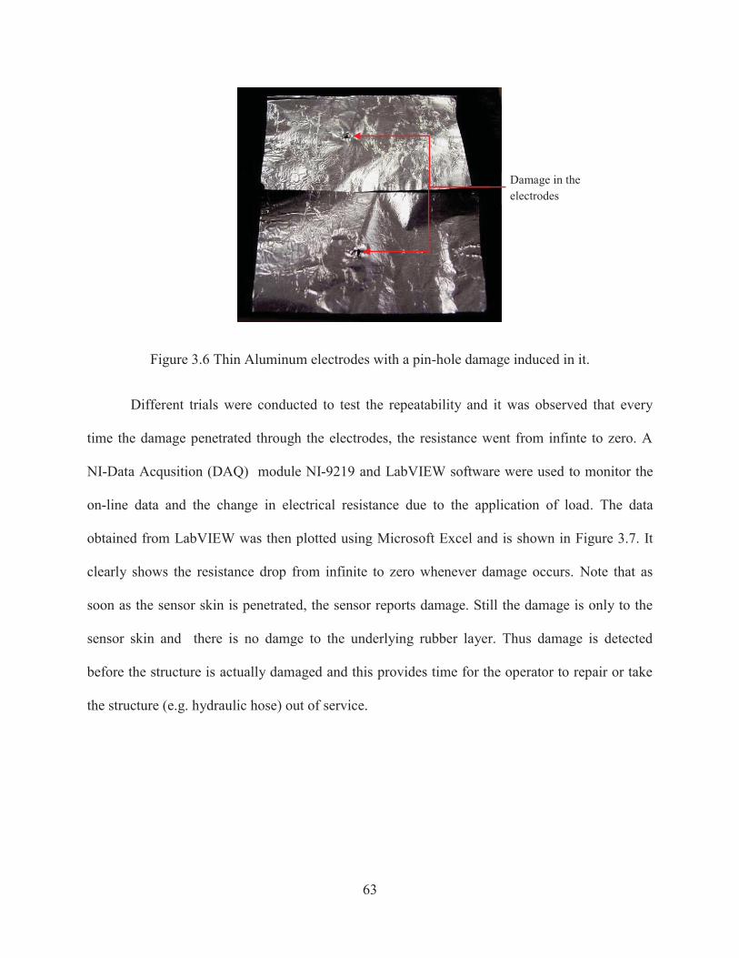
63

Figure 3.6 Thin Aluminum electrodes with a pin-hole damage induced in it.

Different trials were conducted to test the repeatability and it was observed that every

time the damage penetrated through the electrodes, the resistance went from infinte to zero. A

NI-Data Acqusition (DAQ) module NI-9219 and LabVIEW software were used to monitor the

on-line data and the change in electrical resistance due to the application of load. The data

obtained from LabVIEW was then plotted using Microsoft Excel and is shown in Figure 3.7. It

clearly shows the resistance drop from infinite to zero whenever damage occurs. Note that as

soon as the sensor skin is penetrated, the sensor reports damage. Still the damage is only to the

sensor skin and there is no damge to the underlying rubber layer. Thus damage is detected

before the structure is actually damaged and this provides time for the operator to repair or take

the structure (e.g. hydraulic hose) out of service.

Damage in the electrodes

64

Figure 3.7 Change in electrical resistance of the sensor skin when load is applied.

3.3 Testing of Sensor Skin Materials

In this section, different materials that can be considered for conductive electrodes and for

dielectric layers are listed. Also, results obtained from performing load testing, impact testing on

the sensor skin material is described. Some of the major criteria for selecting sensor skin

materials for different application include:

Material must be able to withstand high temperature

Material must be strong and flexible in order to withstand bending stress and pressure cycle

Electrode must be highly conductive

Material must not fail before the failure of the structure

Material must be able to operate at extreme operating and environmental conditions

0

2000

4000

6000

8000

10000

12000

0 5 10 15 20

Res

ista

nce

(Ω)

Time (s)

Resistance

65

3.3.1 Sensor Skin Material Table

Table 3-1 shows the list of materials that can be considered for the conductive electrodes and

their significant mechanical, electrical and thermal properties. Each of these materials can be

used for different applications.

Table 3-1 Conductive Skin Material Properties

Material Elastic

Modulus

(GPa)

Temperature

Range (°C)

Electrical

Resistivity

(Ωm)

Thermal

Conductivity

(W/mK)

Density

(g/cm3)

Flexibility

Aluminium 70 54 to 316 2.82×10−8 237 2.70 Yes

Medical

Electrodes

(Carbon based

material coated on

the electrode for

conductivity)

Properties will vary based on the conducting material being used for the electrode. For

instance, if carbon black is used, the electrical and mechanical properties of the medical

electrodes will be similar to carbon black.

Yes

Carbon nanotube

thread

20 - TBD Up to 250 2×10-4 - 5×10-

5

30 1 – 1.4 Yes

Conducting

polymer

Properties will depend on the type of the conducting polymer being used. Yes

Graphite 8-15 -240 to 400 2.5-5.0×10−6 25-470 1.3-1.95 Flexible graphite

sheets are available

Steel 190-210 -40 to 125 1.18 × 10-7 11.2-36.7 7.85 Less flexible

compared to medical

electrodes

Table 3-2 shows the list of materials that can be considered for the dielectric layer and

their significant mechanical, electrical and thermal properties. Each of these materials can be

used for different applications.

66

Table 3-2 Dielectric Material Properties

Material Tensile Strength

(MPa)

Temperature

Range (°C)

Density (g/cm3) Flexibility

Duct Tape - Up to 93 - Yes

Wax Paper - Up to 55 0.47-0.78 Yes

Plastics (Nylon, for

instance)

86 100 1.13 Yes

Fiberglass 3450MPa -29 to 150 2.57 Less flexible

Kapton Film - -273 to 400 - Yes

3.3.2 Load Testing of Sensor Skin

Load testing of the sensor skin was conducted to determine the load carrying capacity of the

sensor skin. In this experiment, a sensor skin for use on composite materials was fabricated using

a Kapton film sheet between two aluminum film electrodes (0.016 mm thick), which is one way

that a dry capacitor is formed and the test was carried out.

Load testing was performed to validate the proof of concept of the sensor skin using a

hydraulic press as shown in Figure 3.8a, b. Figure 3.8c shows three different spherical indenters

with diameters 0.187”, 0.374”, 0.55” used in the experiment to apply load and induce damage in

the skin. Figure 3.8d shows a sensor skin with dimensions 3” by 2”. In this experiment, the

sensor skin is placed on the loading station in the hydraulic press. The spherical indenter is

attached to the top of the loading station as shown in Figure 3.8b. The load was gradually applied

until the sensor skin was damaged. Figure 3.8e shows the damage pattern created by the

spherical indenter.

67

The electrical impedance of the sensor skin was monitored continuously using NI-DAQ

9219 module and data were saved in the computer. It was observed that the electrical resistance

of the sensor skin changed from infinite to zero as the damage penetrated the dielectric medium

and resulted in the contact of the two electrodes in the sensor skin. At the sensor, the composite

plate showed indentation damage with the diameter of indentation measured to be 0.33”.

Figure 3.8 Experimental Setup for Load Testing; (a) Hydraulic press used for testing the sensor

skin; (b) close-up image of indentation of sensor skin in the press; (c) spherical indenters of

diameters: 0.187, 0.374, and 0.55 in., respectively; (d) Kapton film used as a dielectric; (e)

optical image of the sensor skin after indentation (0.374 in.).

The response of the sensor skin versus loading for three different indenter sizes is shown

in Figure 3.9. The graph shows change in the resistance of the skin due to loading with the

applied load shown in the x-axis and resistance of the skin shown on the y-axis.

a b

c

d

a b

c

d

e

68

Figure 3.9 Variation of resistance of the sensor skin due to loading.

It can be seen from the plot that the electrical resistance of the skin was large (10,500Ω)

in the beginning and the resistance suddenly dropped to zero as the skin was damaged due to

loading due to contact of the two electrodes. It should be noted that the resistance seen in the plot

is the maximum resistance that can be measured using NI-DAQ 9219 module. It is also observed

that as the diameter of the spherical indenter was increased, the load at which the resistance of

the sensor skin changed from infinite to zero also increased as shown in Table 3-3.

Table 3-3 Load to failure of sensor skin due to different spherical indenters.

Diameter of Spherical Indenter (inch) Load to Failure of Sensor Skin (klbs)

0.187 1.25

0.374 4.00

0.55 8.50

From the table, it can be concluded that the sensor skin is sensitive to any size of damage.

For instance, the sensor skin will be sensitive to small damage like pin holes or large damage

from impact with large particles. Having sensitivity to different size of damage is explained by

considering the stress applied to the skin. The diameter of indentation on the composite for the

69

three spherical indenters is measured as shown in Table 3-4.

Table 3-4 Diameter of indentation on the composite for the three spherical indenters.

Diameter of Spherical Indenter (inch) Diameter of Indentation on the Composite (inch)

0.187 0.128

0.374 0.23

0.55 0.33

The stress applied to the skin was then calculated by knowing the area of indentation (A)

and the force applied (F) to the sensor skin based on the Equation 3.3.

The applied stress on the skin due to damage was found using the above formula to be

around 680MPa for all three spherical indenters. With a small diameter sphere, the area of

indentation is small and the sensor skin fails at a small load. With a larger diameter sphere, the

area of indentation is larger and a larger load is required to cause the skin to fail. However, it was

observed that the stress is similar for all cases.

The surface of the fiberglass panel also sustained minor localized spherical shaped

damage but the damage area was smaller than the area of indentation in the sensor skin. Also, the

depth to which the damage was penetrated through the composite plate was measured for all

three cases and was found be only around 0.0134”. From this experiment, it can be concluded

that the sensor skin had been used as a protective layer to prevent excessive damage due to

continuous loading in the composite plate because the damage in the composite plate was limited

to only 0.0134” even at a very high stress level.

70

A computational model can also be developed to predict the stress and impact energy

applied to the structure based on the change in resistance of the sensor skin for different loading

geometries, e.g. spherical, distributed pressure and non-spherical loading. Damage in the

composite can be characterized and correlated with the change in resistance of the sensor skin.

The damage in the composite can then be related to the residual strength for simple prognostics

analysis.

Also, an experimental study was conducted to compare different dielectric materials.

Here, two different configurations of sensor skin were fabricated and attached to the composite;

Kapton film sheet between two aluminium film electrodes (0.016 mm thick)

Wax paper attached between the two aluminium electrodes

Continuous load was applied to the composite structure until the sensor skin failed using

the hydraulic press and the electrical properties (resistance and capacitance) of the sensor skin

were monitored using a RLC meter. In order to check for repeatability, three trials were

conducted.

Table 3-5 and Table 3-6 show the variation in electrical properties of the sensor skin due

to loading developed using Kapton film and wax paper respectively. The diameter of the

spherical indenter used is 0.187”. As expected, the sensor skin developed using Kapton film is

much stronger and was able to withstand higher load compared to the sensor skin with wax paper

as the dielectric layer. The failure of the sensor skin can be observed with the sudden change in

the electrical properties. The sensor skin with Kapton as dielectric failed at 1250lbs whereas

sensor skin with wax paper failed much earlier at 500 lbs.

71

Table 3-5 Variation in electrical properties with Kapton film as a dielectric due to loading

(spherical indenter diameter: 0.187 in.).

Load Applied (Pounds)

Resistance (Ω) Capacitance (nF) Trial 1 Trial 2 Trial 3 Trial 1 Trial 2 Trial 3

No Load Infinite Infinite Infinite 3 2 2 250 Infinite Infinite Infinite 3 2 2 350 Infinite Infinite Infinite 3 2 2 500 Infinite Infinite Infinite 3 2 2 750 Infinite Infinite Infinite 3 2 2

1000 Infinite Infinite Infinite 3 2 2 1250 10 0.5 8 Infinite Infinite Infinite 1750 7 0.4 7 Infinite Infinite Infinite

Table 3-6 Variation in electrical properties with wax paper as a dielectric due to loading

(spherical indenter diameter: 0.187 in.).

Load Applied (Pounds)

Resistance (Ω) Capacitance (nF) Trial 1 Trial 2 Trial 3 Trial 1 Trial 2 Trial 3

No Load Infinite Infinite Infinite 4 3 4 250 10 Infinite Infinite 10 3 5 350 1.8 Infinite Infinite Infinite Infinite Infinite 500 0.8 0.5 0.8 Infinite Infinite Infinite 750 0.3 0.5 0.4 Infinite Infinite Infinite

Similarly, Table 3-7 and Table 3-8 show the variation in electrical properties of the

sensor skin due to loading developed using Kapton film and wax paper respectively wherein the

diameter of the spherical indenter used is 0.374”. As with the previous case, the failure of the

sensor skin can be observed with the sudden change in the electrical properties. The sensor skin

with Kapton as dielectric failed at 4000 lbs whereas sensor skin with wax paper failed much

earlier at 1500 lbs.

72

Table 3-7 Variation in electrical properties with Kapton film as a dielectric (spherical indenter

diameter: 0.374 in.).

Load Applied (Pounds)

Resistance (Ω) Capacitance (nF) Trial 1 Trial 2 Trial 3 Trial 1 Trial 2 Trial 3

No Load Infinite Infinite Infinite 1 2 1 500 Infinite Infinite Infinite 1 2 1 1000 Infinite Infinite Infinite 1 2 1 1500 Infinite Infinite Infinite 1 2 1 2000 Infinite Infinite Infinite 1 2 1 2500 Infinite Infinite Infinite 1 2 1 3000 Infinite Infinite Infinite 1 2 1 3500 Infinite Infinite Infinite 1 2 1 4000 0.5 0.3 0.4 Infinite Infinite Infinite 4500 0.3 0.3 0.3 Infinite Infinite Infinite

Table 3-8 Variation in electrical properties with wax paper as a dielectric.

Load Applied (Pounds)

Resistance (Ω) Capacitance (nF) Trial 1 Trial 2 Trial 3 Trial 1 Trial 2 Trial 3

No Load Infinite Infinite Infinite 2 4 2 250 Infinite Infinite Infinite 2 4 2 350 Infinite Infinite Infinite 2 4 2 500 Infinite Infinite Infinite 2 4 2 750 Infinite Infinite Infinite 2 4 2 1000 Infinite Infinite Infinite 2 4 2 1250 Infinite Infinite Infinite Infinite Infinite Infinite 1500 0.6 0.4 0.8 Infinite Infinite Infinite 1750 0.3 0.3 0.4 Infinite Infinite Infinite

3.3.3 Impact Testing

An experiment was conducted to study the feasibility of the sensor skin to detect impact damage.

A fiberglass panel was simply supported on two angle sections as shown in Figure 3.10. A

spherical indenter (steel ball) was dropped from a certain height onto the sensor skin and the

variation in the resistance of the skin was monitored online using a NI-DAQ 9219 device and

73

LabVIEW software. Figure 3.10a show the experimental setup and Figure 3.10b show the optical

image of the sensor skin after impact testing. It was observed that the resistance of the skin

dropped from M-Ohm range to zero as the impact resulted in the contact of the two electrodes as

shown in Figure 3.10c. This experiment shows that the sensor skin can detect dynamic loading

and impact damage.

3.4 Application of Sensor Skin

The sensor skin can find applications in aerospace fields like aircraft, satellites,

unmanned vehicles, missiles, etc. The damage to these structures from external sources like

lightning, debris, and large pressure loading can be detected. The sensor skin’s thinness makes it

suitable for such applications. The sensor skin can be made of different materials to meet the

demands of the application such as high or low temperature, abrasion, electrical conductivity,

and corrosion resistance.

a

b

c

Figure 3.10 Impact Testing of Sensor Skin: (a) Experimental Setup, (b) Optical image of the

sensor skin after impact testing, (c) Variation in resistance due to impact testing.

74

The sensor skin can be applied on the surface of structures to detect external damage. The

main advantages of the skin are its light weight and high damage sensitivity. It can be installed

on any structure with ease. Also, sensor skin can also be used to protect the spacecraft against

orbital debris impact damage. The electrodes of the sensor skin can be made of a material that

complies with the requirements of a spacecraft.

Sensor skin can also be used as an effective barrier to protect critical aircraft and

spacecraft components against fragment impact; for instance, it can be used to protect the aircraft

component against fragments resulting from failure of a turbine engine, etc. The sensor skin can

sense the damage and offer protection which is critical to the health of the structure.

In general, any structure that is embedded with a sensor skin cannot be damaged by

impact without first damaging the sensor skin. Thus, the sensor skin foremost provides safety

and reliability for systems. The sensor skin material can be designed for the specific application

and be compatible with most manufacturing process that might have different temperature and

mechanical handling and strain conditions. The sensor skin can also be integrated into the

interior of materials such as composites to detect internal damage that might occur due to

overstress or causes other than impact to the surface.

In this section, a specific case wherein the concept of sensor skin can be applied is

described in detail;

Sensor skin on hydraulic hose for damage detection

75

3.4.1 Sensor Skin on Hose

A hydraulic hose, as described in the previous chapter, is a composite structure primarily made

of rubber and steel reinforcement. As described in detail in the previous chapter, one of the

current works at University of Cincinnati involves building a clip-on module using piezoelectric

sensors to detect damage in the hose. The clip-on module might be sensitive to only local

damage, i.e., damage directly beneath the clip-on sensor and it might not detect damage

occurring elsewhere. Hence, there is a need to incorporate another sensing approach like ‘sensor

skin’ that could be used in parallel with the clip-on sensor to detect small initiating damage over

large areas.

The concept of sensor skin was extended to the hose application. Initial experiments were

conducted to determine the feasibility of having an external sensor on the hose that could

indicate the damage like pin holes, oil leak, etc. Two different designs were conceptualized for

the hose application;

Design 1: Sensor skin on the outer layer of the hose.

Design 2: Sensor skin between the innermost rubber layer and steel layer (inside the hose).

In this section, two different sensor skin materials are considered;

Sensor skin using aluminium as conductive electrode and Kapton/Wax Paper as dielectric

Sensor skin using medical electrodes as conductive layer and duct tape as dielectric

76

3.4.1.1Development of Sensor Skin using Aluminium Electrode

The following section describes the process involved in the development of sensor skin.

For demonstration purpose, a section of hose was cut (~15cm) and a layer of sensor skin

was developed on it. First, the innermost rubber layer was cut as shown in Figure 3.11a. Next, an

insulating layer was glued to the innermost steel layer with an adhesive. On top of it, first layer

of conductive aluminium was attached along the length of the hose as shown in Figure 3.11b.

After that, an insulating layer (wax paper or Kapton film) was put on top of the first conductive

layer as shown in Figure 3.11c. Second conductive aluminium layer was then added on top of the

insulating layer thereby forming the sensor skin as shown in Figure 3.11d. Finally, the innermost

a b c

d e

Figure 3.11 Development of Sensor Skin: (a) Inside rubber layer, (b) First conductive

layer attached to hose, (c) Insulating layer attached, (d) Second conductive layer

attached to the hose, (e) Rubber layer placed to cover the sensor skin.

77

rubber layer was attached on top of the sensor skin as shown in Figure 3.11e. Lead wires were

attached to the conductive layers for impedance measurements.

Design 1: Sensor skin on the outer layer of the hose:

The design utilizes the concept of developing a sensor skin layer on the outside of the hose. This

concept can also be visualized as putting an external sensor on the hose like the sensor sleeve.

The sensor sleeve can be manufactured as a separate product and can be placed on top of the

outer layer of the hose. The significant advantage is the simplicity of this design as it is likely

that there would be no modification to the hose itself. The sensor skin can be protected from the

outside environment by covering the sensor skin with a protective rubber layer probably like the

same polymer material as that of the outer layer of the hose. By this protective layer, it is

possible to prevent any damage to the sensor skin from any environmental conditions and might

prevent any false positive alarms from the sensor skin.

This design might not prevent damage happening to the hose because the sensor skin is

going to identify the damage only after the hose has failed. But this design will prevent damage

penetrating from the hose to the outside environment and causing damage to the environment.

The entire system can be modeled in such a way that the moment the signal from the sensor skin

deviates from the nominal value, an alarm can be activated and the entire system can be shut

down and the hose can be replaced. This design thus prevents any significant damage to the

outside environment.

A prototype of this concept was constructed and tested. It used aluminium as the

conductive material and either kapton film or wax paper as the insulating material. As described

in the previous section, first layer of aluminium was attached to the outer layer of the hose

78

followed by the insulating layer and another conductive aluminium layer on top of the insulating

layer. All the layers were attached to each other using commercially available adhesive. Lead

wires were taken out from the first and second conductive layers. The electrical impedance

between the two layers could then be measured.

Two different orientations of sensor skin were tested; sensor skin placed along the length

of the hose shown in Figure 3.12a and the other placed circumferentially shown in Figure 3.12b.

For the second case, it can be visualized as having a sensor skin tape that can be attached

circumferentially along the entire length of the hose.

Figure 3.12 Sensor Skin on the outside of hose: (a) Along the length, (b) Circumferential.

Design 2: Sensor skin between the inner rubber and steel layer

This design utilizes the concept of putting a layer of sensor skin on the inside of the hose. The

sensor skin can be built between the innermost rubber layer and first reinforcement layer. The

significant advantage of this design is that it is going to prevent the damage in the hose as any

damage to the hose will have to penetrate the sensor skin, hence causing failure of the sensor

skin. Thus, any damage like pin holes, oil leak, etc., beyond the innermost rubber layer can be

prevented from occurring and the hose can be inspected and replaced, if necessary.

a b

79

This design will be simple, ideal solution to predict and prevent damage from occurring

to the hydraulic hoses. However, on the downside, there are challenges like how to take the

connecting leads of the sensor skin from inside the hose. Also, since the sensor skin has to be put

inside the hose, the manufacturing process should be altered and it is going to be expensive. And

finally, the possibility of having the sensor skin in contact with each other due to crimping in the

end fitting area needs to be addressed.

In order to prove the concept, a prototype was developed and tested. In this experiment, a

portion of the inner rubber layer (~15cm) was cut thus exposing the steel reinforcement layer.

Then, as described earlier, the layers of the sensor skin were attached in the proper sequence

using the adhesive. The thickness of the entire sensor skin comprising of two conductive layers

and insulating layer was only between 10-1000 microns. Finally, the rubber layer was glued back

to its initial position as shown in Figure 3.13. Lead wires were taken out from the first and

second conductive layers and the electrical impedance between the two layers was measured.

The sensor skin was placed in the longitudinal orientation. For this experiment, there was no end

fitting in the hose being tested. Hence, there was no issue of the sensor skin coming in contact

with each other due to crimping.

Figure 3.13 Sensor skin between the inner rubber and steel layer.

80

Test procedure and results

The experimental setup is shown in Figure 3.14. NI-DAQ 9219 module was used as the data

acquisition system to monitor the impedance (electrical resistance) of the sensor skin. Lead wires

were attached to the NI-DAQ 9219. Program was created in LabVIEW to automatically store the

data from the sensor skin and indicate the damage occurring to the sensor skin by activating a

LED signal.

Figure 3.14 Experimental setup.

Two experiments were conducted; first was to simulate the pinhole damage and second

was to simulate the oil leak. In the first experiment, pinhole damage was simulated using a sharp

pointed tool and the electrical resistance was monitored continuously. The moment the pinhole

damage penetrated through the inner rubber layer and hit the sensor skin, the resistance dropped

NI-DAQ 9219 Module

Sensor Skin

LabVIEW indicating the condition of sensor skin

81

from infinite (10.5kΩ – maximum resistance capability for NI-DAQ 9219) to zero and activating

the LED signal, thus indicating the damage to the hose. It can be observed that the damage has

not penetrated to the steel reinforcement layer, thus reiterating the advantage the sensor skin has

in predicting and preventing the damage to the hose.

In the second experiment, oil leak was simulated by injecting oil using syringe into the

hose until damage occurred. Approximately, 0.5 to 1cc of oil was injected to the hose. Similar to

the previous experiment, the resistance dropped from infinite to zero and activated the LED

signal, indicating the damage to the hose. However, it was difficult to measure the exact amount

of oil injected in the inner rubber layer. But, the experiments were repeated for several times and

the response was repeatable.

The change in resistance of the sensor skin is shown in Figure 3.15. It can be seen that the

resistance of the sensor skin is consistent when the hose is in the healthy condition. The sharp

drop in resistance can be seen when the damage occurred to the hose. Similar result was

observed for both pinhole damage and oil leak situations.

Figure 3.15 Change in resistance due to damage of the sensor skin.

82

Conclusion using Aluminium Electrode

Initial studies and experiments have proven that the new sensing technique to monitor the health

of the hose works. In general, sensor skin shows a lot of promise as a new sensing technique for

SHM. Laboratory experiments have shown that sensor skin can detect small initiating damage

like pin holes and oil leaks over large areas utilizing single channel of data acquisition.

3.4.1.2 Sensor Skin Using Medical Electrodes

The medical electrodes are flexible, durable and usually consist of a conducting gel or paste.

Hence, they were selected as the conductive electrodes for the sensor skin. These electrodes are

capable of working for long periods of bending, pulsing cycle under extreme conditions and will

not fail before the actual failure of the hose. The medical electrodes are also light weight and

very thin (approximately 1mm); hence will not affect the mechanical integrity of the hose. Two

different types of medical electrodes were chosen for the sensor skin;

1. Medical Soft White Foam Electrodes

2. Carbon Rubber Electrodes

The following Table 3-9 describes some of the main features of these electrodes.

83

Table 3-9 Two different types of medical electrode used for sensor skin.

Medical Soft White Foam Electrodes

Carbon Rubber Electrodes

Self-Adhering, Reusable Self- Adhering , Reusable Comfortable White Foam Backing Electrodes are used with conductive gel

and secured with tape patches or used with conductive pads.

Development of sensor skin using medical electrodes

The following section describes the process involved in the development of sensor skin using

medical electrodes. Figure 3.16 shows the two carbon rubber electrodes which act as the two

conductive surfaces for the sensor skin and a duct tape which acts as an insulator patch. The

carbon rubber electrode has a coating of carbon black on its surface, which makes the electrode

conductive.

Figure 3.16 Carbon rubber electrodes and insulator patch.

84

The sensor skin is developed by gluing the insulator patch between the two conductive

surfaces as shown in Figure 3.17a. Figure 3.17b shows the side view of the developed sensor

skin. It is clear that the thickness of the entire skin is only around 2 mm and can further be

reduced, if necessary by reducing the thickness of the electrodes.

Figure 3.17 (a) Sensor skin developed using carbon rubber medical electrodes; (b) Side view of

the sensor skin.

Figure 3.18a shows another configuration of the sensor skin developed using medical soft

white foam electrodes. These electrodes have conductive gel that adheres to the surface. Figure

3.18b shows the side view of the developed sensor skin using these electrodes.

Figure 3.18 (a) Sensor skin developed using medical soft white foam electrodes; (b) Side view of

the sensor skin.

Test Procedure and Results

Initial experiments were conducted to validate the concept of using these medical electrodes for

the sensor skin. To simulate pin hole defect, insulted tips (non-conductive epoxy was applied on

the surface of those pins) of different sizes were taken as shown in Figure 3.19. Fluke Multimeter

a b

a b

85

was used to monitor the impedance (electrical resistance) of the sensor skin. The lead wires from

the sensor skin were attached to the multimeter.

Figure 3.19 Insulted tips used to create pinhole damage.

Experiments were conducted on both the electrode configurations several times to check

for repeatability. Figure 3.20a show the experiment conducted on the medical soft white foam

electrodes. Electrical resistance was monitored continuously. As seen from Figure 3.20a, the

resistance of the skin was infinite (40MΩ – maximum capability of the multimeter). Pinhole was

simulated using the insulated tip. The moment the damage penetrated the skin layers, the

resistance dropped from infinite to few kΩ ranges, thus indicating the damage to the sensor skin.

The drop in resistance is shown in Figure 3.20b. Similar result was observed, when different

sizes of insulted tip were used to create pin hole in the sensor skin.

86

Figure 3.20 Experimental setup with medical soft white foam electrodes: (a) No Damage; (b)

Drop in resistance due to pinhole damage.

Figure 3.21 shows the experiment conducted using carbon rubber electrodes. Similar to

the previous case, the resistance dropped from infinite to few kΩ ranges when the damage

penetrated the carbon rubber electrodes, thus indicating the damage to the sensor skin.

Figure 3.21 Experimental setup with carbon rubber electrodes: (a) No Damage; (b) Drop in

resistance due to pinhole damage.

a b

a b

87

Figure 3.22 shows the damage to the sensor skin for these two different configurations.

The difference between the two configurations is the sensitivity to the damage. From the

experiment, it was observed that the carbon rubber electrodes were much more sensitive to the

small pinhole damages while the medical soft foam electrodes were sensitive to large size of

damage. This can be attributed to the level of conductivity of these electrodes. And the

sensitivity can be tuned for different hose applications and each of these electrodes can be used

for different type of hose applications.

Figure 3.22 Damage in the sensor skin: (a) medical soft white foam electrodes; (b) Carbon

rubber electrodes.

Conclusions using Medical Electrodes

Laboratory experiments have shown that sensor skin developed using medical electrodes can

detect small initiating damage like pin holes over large areas utilizing single channel of data

acquisition.

3.4.1.3 Advantages

The major advantage of having a sensor skin on the hose is that the hose cannot leak without first

damaging the sensor skin, thus providing foremost safety and reliability of systems. It is light

weight, extremely thin, has high damage sensitivity and can be easily embedded to the structures.

Also, the only parameter to monitor is the change in the electrical impedance of the sensor skin;

Damage to the medical electrodes

88

hence, there is limited or no need for any signal processing, algorithm, data extraction,

comparison, etc.

3.4.1.4 Challenges and Future Work in Sensor Skin Development

If the sensor skin is put inside the hose, then the manufacturing process is to be altered and it is

going to be expensive. Also, the major challenge is to find a way to bring the electrical

connections of the sensor skin from inside the hose.

Different conductive electrode materials need to be identified whose mechanical

impedance closely matches the hose in order to maintain the structural integrity. Aluminium was

used during the initial testing phase as the conductive material but this material might not be the

best suited material for the hose applications. The material chosen must be flexible, durable,

must be able to withstand high temperatures, etc. and must not fail before the actual failure of the

hose. The material for the insulating layer needs to be identified.

Different configurations of conducting and insulating layers can be tested like having the

adhesive that glues the conducting surfaces act as the insulating layer (idea suggested by Dawn),

coating only one side of the surface with a conductive material so that the other side acts as a

insulation, thereby eliminating the need for an extra insulation layer. Material and impact testing

of the new sensor skin configuration need to be tested.

Further testing needs to be carried out with sensor skin attached to the hose. Also, a

prototype of the sensor skin can be made at Parker Hannifin facility with the skin attached to the

outside of the hose. To begin with, sensor skin can be attached to the outside of the hose at

critical locations on the hose like the end fitting, as shown in Figure 3.24 and sensor skin can be

subjected to bending and pressure cycles at Parker Hannifin facility. NI-DAQ 9219 module can

89

be used as the data acquisition system to monitor the electrical resistance of the skin

continuously.

Proposed Ideas for sensor skin on hose:

The following section proposes some ways to minimize the challenges addressed above;

• Possibility of using PVDF sensor as a charging device to light up LED or give a buffer

signal: This method involves using the PVDF sensor from the clip-on module as a charging

device. The PVDF sensor currently being used for the clip-on module is going to be charged due

to the bending and pressure cycles of the hose. This charge can be used to light up LED or give a

buffer signal to the operator when the hose is damaged. Figure 3.23 show the schematic of the

connection for the proposed method.

Figure 3.23 PVDF as a charging device.

When the hose is in healthy condition, the sensor skin will not touch each other; hence

the circuit will be open condition and the charge from the PVDF sensor will not do anything.

But if the hose is damaged, the sensor skin will fail, thus causing the two conductive electrodes

to come in contact with each other. This condition will immediately make a closed circuit and

LED Piezo Buffer

RFID Wireless

PVDF

Clip on Sensor

Sensor Skin

Hose

90

the charge from PVDF sensor will now light up LED or give a buffer signal to the operator to

replace the hose, if necessary. This method thus employs both the sensor skin concept as well as

clip-on module to work in parallel with each other.

• Possibility of developing a hose with built-in sensor skin either inside/outside hose at

UC/Parker: This method involves developing a hose with built-in sensor skin inside or outside

the hose after the new material for the sensor skin been identified and tested.

Outside the hose: Figure 3.24 shows a proposed method of putting a sensor skin on the outside of

the hose. It can also be visualized as putting in a separate product like sensor sleeve on the

outside of the hose. The sensor sleeve consists of the sensor skin covered with a insulting layer,

probably with the same polymer material as the outside layer of the hose. By this way, the sensor

skin can be prevented from any outside envirnmental damage and hence false positive alarm can

be eliminated or minimized. Since one of the most common failure modes of the hose is near the

end fitting, the sensor sleeve can be attached only near the end fitting as shown or the sensor

sleeve can be place along the entire length of the hose.

Figure 3.24 Sensor skin outside the hose

91

Inside the hose: To put the sensor skin inside the hose, the ideal location would be inbetween the

innermost rubber and reinforcement layer. By this way, any damage to the reinforcement

material could be prevented and the damage will not penetrate the innermost rubber layer. But

the sensor skin can be placed in any locations. Figure 3.25 shows one proposed method of

putting the sensor skin inside the hose. As seen from the figure, the sensor skin is placed beween

the inner rubber layers. The two major challenges that needs to be addressed are the means to

take the electrical connections from the sensor skin and prevent the sensor skin from damage

during the crimping operation in the end fitting. The proposed method addresses the second

problem. In this method, the sensor skin does not run along the entire length of the hose. The

sensor skin is not put in the place where crimping is done to fix the end fitting as shown in

Figure 3.25. This eliminates the problem of having sensor skin coming in contact with each other

during crimping.

Figure 3.25 Sensor skin between inner rubber layers.

Figure 3.26 shows a schematic of the combined form of all the different ideas mentioned

above. It shows the sensor skin connected to the PVDF sensor so that charge from PVDF sensor

can sound an alarm, if the sensor skin fails due to damage in the hose. Also, the configuration of

sensor skin inside the hose is also shown in the Figure 3.26. As seen from the figure, the

electrical connections from the sensor skin to the PVDF sensor are achieved with the help of

92

coated Carbon Nanotube (CNT) yarn. CNT yarn are very light, strong, thin (micron in diameter)

and have remarkable electrical and mechanical properties, which will be discussed in detail in

the next chapter. These CNT material can be used as a effective conductor to transfer the

electrical signal from the sensor skin to the PVDF sensor. Coating the CNT yarn will provide the

necessary insulation and prevent the CNT yarn from any unwanted electrical error signals.

Figure 3.26 Sensor Skin on outside and inside hose (Image from [39]).

93

Chapter 4

Carbon Nanotube Sensor Yarn for Structural Health

Monitoring

4.1 Introduction

Research and technology development at the nanoscale level has been to provide a fundamental

understanding of phenomena and materials at the nanoscale and to create and use structures,

devices and systems that have novel properties and functions because of their small and/or

intermediate size. Nanotechnology is the space at the nanoscale (i.e. one billionth of a meter),

which is smaller than “micro” (one millionth of a meter) and larger than “pico” (one trillionth of

a meter). However, due to a number of scientific principles becoming dominant at the nanoscale,

nanomaterials can have very different properties than bulk materials. This includes materials that

are stronger, lighter, more electrically conductive, super paramagnetic, tunable optical emission,

more porous, better thermal insulating, and less corrosive. The applications being imagined

today for nanotechnologies will have wide spread impact on manufacturing, medicine,

chemistry, computing, energy, and security [45]-[48].

Carbon in the form of diamond is the hardest substance known to mankind, but in recent

times other forms of carbon, known as carbon nanotubes, have been discovered that are harder

than diamond. Carbon Nanotubes (CNT) is one of the unique nanostructures with remarkable

electrical and mechanical properties [49]. They have attracted great attention both in applications

and research because of their unique properties. They were discovered in 1991 by Japanese

electron microscopist Sumio Iijima [50]. Harnessing the unique physical, mechanical and

94

electrical properties of carbon nanotubes in materials applications has yet to be fully realized.

Improvement of these properties has been one of the major topics of research in the 21st century.

More about carbon nanotubes and their remarkable properties will be dealt with in the next

section.

4.1.1 Carbon Nanotubes (CNT)

Carbon Nanotubes are thin cylinders of carbon exhibiting remarkable physical, mechanical,

electrical properties which are unique for their size and shape. Brief details about the structure,

properties and applications of carbon nanotubes are given below;

4.1.1.1 Structure of the CNT

The basic structure of CNT can be thought of as cylinders formed through rolling of graphite

sheets as shown in Figure 4.1. Graphite, one of the most abundant forms of pure carbon on earth,

is composed of sheets of trigonally bonded carbon atoms arranged in hexagonal sheets called

graphene layers. Graphite is a soft, grey solid with high electrical conductivity along the

direction of its graphene layers. The structure of CNTs can be of three types namely armchair,

zigzag, chiral depending on the way in which graphite sheet is rolled [53], [102].

Figure 4.1 Single Wall Carbon Nanotube [54].

95

Carbon nanotubes can be further classified as single wall nanotubes (SWCNT) and multi

wall nanotubes (MWCNT) as shown in Figure 4.2. A SWCNT can be described as single

graphene sheet rolled into a cylindrical shape so that the structure is one dimensional with axial

symmetry and in general exhibiting a spiral conformation called chirality. A MWCNT consists

of coaxial tubes of graphene sheets forming a tube like structure. MWCNTs are easier and less

expensive to produce because current synthesis methods for SWCNTs result in major

concentrations of impurities that require removal by acid treatment. But MWCNTs have higher

occurrence of structural defects, which diminishes their useful properties. SWCNTs have no such

defects and their properties are consequently stronger [51], [55].

Figure 4.2 Carbon nanotubes: (a) SWCNT (b) MWCNT [54].

4.1.1.2 Properties of CNT

The huge research interests in CNTs are attributed to their excellent mechanical and electrical

properties.

Table 4-1 shows a comparison of approximate strength, electrical and thermal conductivity of

carbon nanotube and other materials. The properties of CNT are dependent on their diameter,

length, and chirality, or twist [102].

96

Table 4-1 Comparison of the approximate strength and conductivity of various materials [56].

Some of the significant properties of CNT are described below;

Mechanical properties: CNTs exhibit extraordinary mechanical properties that make them

interesting and potentially useful. Comparison of mechanical properties between CNT and other

materials are shown in Table 4-2.

Carbon nanotubes have very high stiffness, high strength, high aspect ratio, low density.

They are the strongest and most flexible molecular material because of the c-c covalent

bonding and seamless hexagonal network architecture.

Buckling rather than fracture is a common phenomenon in nanotubes. It is observed that

the thicker wall tubes tend to get buckled while the thinner tubes tend to collapse or fracture.

Material

Density (g/cm3)

Strength (GPa)

Specific Strength

(GPa/g/cm3)

Elastic Modulus

(GPa)

Specific Modulus

(GPa/g/cm3)

Ult. Strain

%

Electrical Conductivity

(S/cm)

Specific Electrical

Conductivity (S/cm/g/cm3)

Current Density

(A/cm^2)

Specific Current Density

(A/cm2/g/cm3)

Thermal Conductivity

(W/m K)

Specific Thermal Conductivity

(W/m K/g/cm3)

IM8 PAN Carbon Fiber

1.8 6.1 3.4 305 169 1.8 1 x 103 556 NA NA 500 278

Copper 8.9 0.15Y, 0.34U

0.017Y, 0.039U 119 13 3-60 59 × 106 6.6 x 106 6 x 102 67 400 45

Individual CNT 1.4 100 71 1000 714 10 1 x 106 0.7 x 106 1 x 109 0.7 x 109 3,000 2,143

CNT Yarn Experiment 1.3 1 0.77 NA NA NA 0.8 x 106 0.6 x 106 1 x 109 0.7 x 109 30 23

CNT Yarn Theory 1.4 70 50 NA NA NA NA NA NA NA NA NA

97

Table 4-2 Comparison of Mechanical Properties of various materials [57], [102].

Material Young’s Modulus

(GPa)

Tensile Strength

(GPa)

Density

(g/cm3)

SWCNT 1054 150 1.4

MWCNT 1200 2.6 2.6

Steel 208 .4 7.8

Epoxy 3.5 .0005 1.25

wood 16 .0008 .6

Electrical conductivity: Depending on their chiral vector, carbon nanotubes with small

diameters are either semi-conducting or metallic. The differences in conducting properties are

caused by the molecular structure that results in a different band structure and thus a different

band gap [58]. CNTs can behave as both metals and semiconductors based on how the sheets are

rolled. They behave as metals when their hexagons line up straight along the tube’s axis (arm

chair) and as semiconductors when the sheet is rolled on the diagonal so that the hexagons spiral

along the axis (zigzag).

4.2 Electrical Impedance Measurement of CNT based Materials

One of the major research focuses at the Nanoworld Lab at University of Cincinnati is to produce

quality carbon nanotube materials and primary work involves developing various techniques to

improve the quality and properties of carbon nanotube materials by minimizing the defects

during the manufacturing of carbon nanotubes [59]. Different types of carbon nanotubes are

produced at Nanoworld Lab that includes CNT array, CNT ribbon, CNT thread and CNT yarn as

shown in Figure 4.3. Each of these materials has their own properties and is being investigated

for improving their properties and developing potential applications using them. This section of

98

the chapter will focus on CNT ribbon, CNT thread and yarn and the impedance measurements

performed to characterize the electric properties like resistance, inductance and capacitance of

these materials.

Figure 4.3 Manufacturing of CNT materials: (a) Long CNT forest (>1 cm) on a 4 inch wafer; (b)

CNT Array; (c) CNT Thread; (d) CNT Yarn (two threads twisted together); (e) CNT Ribbon

[59], [102].

4.2.1 CNT Ribbon

CNT arrays or forests are synthesized and drawn into ribbon as shown in Figure 4.4. Ribbon is

drawn by grasping the edge of the array with tweezers or tape and pulling out a section of ribbon

and attaching the end of the ribbon to a spool. A motor rotates the spool and continuously winds

the ribbon. Ribbon can be pulled from the array at a high linear velocity. The ribbon is sticky due

to van der Waals forces and the ribbon must be wound onto Teflon to enable unwinding.

Otherwise thicker ribbon can be produced by winding layer onto layer. A single layer of ribbon

is almost transparent. Adding layers eventually makes the ribbon dark black. The nanotubes in

the array are double wall or triple wall with outer diameter about 20 nm. There are about 10

billion nanotubes per square cm in the array. The ribbon is about 200 nm thick and the width can

be from mm to cm depending on how wide of a section is initially pulled from the array. Because

the ribbon is thin, hundreds of meters of ribbon can be pulled from an array depending on the

Aa b c d e

99

size of the array.

Figure 4.4 CNT array and ribbon: (a) CNT array; (b) drawing the ribbon from the array onto a

spool; (c) TEM image of the ribbon with a 5 micron scale bar.

CNT ribbons can be used to make electrical fiber and smart materials for actuation and

SHM sensors. There is already significant research using CNT ribbon for actuation. Researchers

at Tsinghua University used CNT ribbon to build loud speakers [60]. Because of its high strain

and high stress under relatively low voltage, CNT ribbon provides new properties for electronic

actuators like artificial muscle [61], [62].

Understanding the properties of ribbon is still a subject of research. In perfect single wall

carbon nanotubes (SWCNT) that are short, defect free, and have armchair chirality, the

conductance is in theory ballistic [63] and the CNT can carry a huge current. There is no Joule

heating (i2R loss) for conductance along the length of the SWCNT but there is a contact

resistance at the ends between the nanotube and a metal conductor. If the properties of individual

SWCNT could be scaled up to a macro-size ribbon, the ribbon would be a revolutionary new

material. However, in practice, the ribbon has multi-wall nanotubes with various chiralities, there

are defects in the nanotubes, and there are trillions of interfaces or overlap junctions between

adjacent nanotubes aligned in the ribbon. The defects in the nanotubes increase resistance, and

a b c

100

the interfaces increase resistance and create capacitance in the ribbon. Thus the ribbon has lower

conductance than SWCNT and significant energy loss. An attempt has been made to characterize

and help understand the electrical properties of CNT ribbon from an engineering viewpoint so

the ribbon can be put into applications.

4.2.1.1 Impedance Measurement of CNT Ribbon

Experimental Setup and Procedure:

Experiments were conducted to measure the impedance properties of the CNT ribbon. The

impedance is measured using Solartron Impedance Gain-Phase analyzer as shown in Figure 4.5.

Figure 4.5 Experimental setup: (a) Solartron Impedance Gain-Phase Analyzer connected to the

Device under Test (CNT Ribbon), (b) Bode plot obtained from the analyzer.

CNT ribbon was pulled out from an array and wrapped between 2 copper posts as shown

in Figure 4.6. The distance between the 2 copper posts is 7 cm.

Figure 4.6 CNT Ribbon (7cm long) wound between 2 copper posts.

a b

101

The ends of the copper posts were connected to the Solartron Impedance Gain-Phase

analyzer to measure the electrical impedance properties of the ribbon. Prior to mounting the CNT

ribbon onto the analyzer, the impedance of the analyzer and the wiring are determined by

performing open and short corrections. Open and short corrections will eliminate any

inaccuracies arising from the impedance data due to the effects of the analyzer internal circuit

and the external wires. For the open circuit correction measurement, the two leads were kept

open and were fixed at 7 cm distance apart from each other. After fixing the distance, the

equipment is not altered and Solartron impedance analyzer was run from 10 Hz till 10MHz to

record and save the open circuit correction measurement. The magnitude of impedance for open

correction is shown in Figure 4.7a. Similarly for the short circuit correction, a copper foil is

placed between the two leads thereby forming a short circuit. After placing the copper foil, the

analyzer was run from 10Hz to 10MHz and the data was saved. The magnitude of impedance for

short correction is shown in Figure 4.7b.

Figure 4.7 Impedance Plot for open and short correction measurement: (a) Magnitude of

impedance by opening electrodes without any sample (Open Correction). (b) Magnitude of

impedance by directly connecting the electrodes together without any sample (Short Correction).

a b

102

The open and short correction data were then fed into the instrument setup before

measuring the impedance of the CNT ribbon. During the actual measurement, device under test

(CNT ribbon) was connected to the analyzer and the equipment setup is not altered during the

measurement. The analyzer applies a 3V voltage to the sample and scans the frequency from

10Hz to 10MHz and the experiment is repeated for 3 trials. All the parameters including the real

part and imaginary part of impedance can be obtained in one measurement. The impedance data

was saved and later exported to excel and plotted. The impedance results CNT ribbon are

discussed next.

Results and Discussion:

Figure 4.8 shows the magnitude of the impedance plotted versus the frequency. Experiments

were repeated for 3 times to check for repeatability of data. As seen from the graph, the data

were repeatable and consistent. The magnitude of the impedance was about 6100Ω and did not

alter much and was consistent throughout the frequency range (10 Hz to 10MHz). CNT ribbon

exhibits higher impedance because the cross-sectional area of the ribbon is small, the length of

the ribbon is long and there are many junctions.

103

Figure 4.8 Magnitude vs. Frequency for CNT ribbon without epoxy.

Figure 4.9 shows the phase plotted versus the frequency and all trials closely matched

each other. At higher frequency (10MHz) the phase of the CNT ribbon was around -3.24° and as

the frequency reduced to around 1MHz, the phase also gradually reduced to 0° and stayed

constant at 0° till 10 Hz. This effect indicates that the ribbon might show a capacitive behavior at

high frequencies.

Figure 4.9 Phase vs. Frequency for CNT ribbon without epoxy.

1

10

100

1000

10000

1.00E+01 1.00E+02 1.00E+03 1.00E+04 1.00E+05 1.00E+06 1.00E+07

│Z│

Frequency (Hz)

CNT Ribbon without Epoxy - Trial 1

CNT Ribbon without Epoxy - Trial 2

CNT Ribbon without Epoxy - Trial 3

-10

-8

-6

-4

-2

0

2

1.00E+01 1.00E+02 1.00E+03 1.00E+04 1.00E+05 1.00E+06 1.00E+07

Phas

e

Frequency (Hz)

CNT Ribbon without Epoxy - Trial 1CNT Ribbon without Epoxy - Trial 2CNT Ribbon without Epoxy - Trial 3

104

For the previous experiment, the CNT ribbon was wrapped around the copper posts. In

order to get better conductivity and to improve the test setup, conductive epoxy was applied in

the copper posts. This enabled better conductance between the copper post and CNT ribbon. The

experiment was repeated for 3 times as before and the data is plotted. Figure 4.10 shows the

magnitude of the impedance plotted versus the frequency. It can be seen that the data were

repeatable and consistent. The magnitude of the impedance was about 6350Ω and did not alter

much and was consistent throughout the frequency range (10 Hz to 10MHz). The difference

between the impedance values before and after applying the epoxy was only 250Ω.

Figure 4.10 Magnitude vs. Frequency for CNT ribbon with epoxy.

Figure 4.11 shows the phase plotted versus the frequency and all trials closely matched

each other. At higher frequency (10MHz) the phase of the CNT ribbon was around -3.04° and as

the frequency reduced to around 1MHz, the phase also gradually reduced to 0° and stayed

constant at 0° till 10 Hz. When compared with previous result, the phase degree was slightly

lower but showed the similar trend.

1

10

100

1000

10000

1.00E+01 1.00E+02 1.00E+03 1.00E+04 1.00E+05 1.00E+06 1.00E+07

|Z|

Frequency (Hz)

CNT Ribbon with Epoxy - Trial 1CNT Ribbon with Epoxy - Trial 2CNT Ribbon with Epoxy - Trial 3

105

Figure 4.11 Phase vs. Frequency for CNT ribbon with epoxy.

4.2.2 CNT Thread/Yarn

CNT threads are yarns formed from spinning CNT arrays. A single long yarn spun from CNT

array is called as CNT thread and CNT yarn is formed when two threads are twisted as shown in

Figure 4.12. Also, when more than two threads are twisted, multi-ply yarns are obtained.

Figure 4.12 SEM Images of Carbon Nanotube Thread: (a) SEM Image of a single CNT thread.

(b) SEM Image showing two threads twisted together [102].

4.2.2.1 Impedance Measurement of CNT Thread

Experimental Setup and Procedure:

-10

-8

-6

-4

-2

0

2

1.00E+01 1.00E+02 1.00E+03 1.00E+04 1.00E+05 1.00E+06 1.00E+07

Phas

e

Frequency (Hz)

CNT Ribbon with Epoxy - Trial 1CNT Ribbon with Epoxy - Trial 2CNT Ribbon with Epoxy - Trial 3

106

The experimental setup and procedure to measure the impedance of the CNT thread is

similar to that of CNT ribbon. CNT thread with a length of 7 cm was wrapped between 2 copper

posts. The ends of the copper posts were connected to the Solartron Impedance Gain-Phase

analyzer to measure the impedance properties of the thread. The analyzer applies a 3V voltage to

the sample and scans the frequency from 10Hz to 10MHz and the experiment is repeated for 3

trials. The impedance data was saved and later exported to excel and plotted. The impedance

results CNT thread are discussed next.

Results and Discussion:

Figure 4.13 shows the magnitude of the impedance plotted versus the frequency. Experiments

were repeated for 3 times to check for repeatability of data. As seen from the graph, the data

were repeatable and consistent. The magnitude of the impedance was about 5600Ω and did not

alter much and was consistent throughout the frequency range (10 Hz to 10MHz).

Figure 4.13 Magnitude vs. Frequency for CNT thread without epoxy.

1

10

100

1000

10000

1.00E+01 1.00E+02 1.00E+03 1.00E+04 1.00E+05 1.00E+06 1.00E+07

│Z│

Frequency (Hz)

CNT Thread without epoxy - Trial 1

CNT Thread without epoxy - Trial 2

CNT Thread without epoxy - Trial 3

107

Figure 4.14 shows the phase plotted versus the frequency and all trials closely matched

each other. At higher frequency (10MHz) the phase of the CNT ribbon was around -3.1° and as

the frequency reduced to around 1MHz, the phase also gradually reduced to 0° and stayed

constant at 0° till 10 Hz. This effect indicates that the ribbon might show a capacitive behavior at

high frequencies.

Figure 4.14 Phase vs. Frequency for CNT thread without epoxy.

Similar to CNT ribbon, conductive epoxy was applied in the copper posts which enabled

better conductance between the copper post and CNT thread. The experiment was repeated for 3

times as before and the data is plotted. Figure 4.15 shows the magnitude of the impedance

plotted versus the frequency. It can be seen that the data were repeatable and consistent. The

magnitude of the impedance was about 5900Ω and did not alter much and was consistent

throughout the frequency range (10 Hz to 10MHz). The difference between the impedance

values before and after applying the epoxy was only 300Ω.

-3.5

-3

-2.5

-2

-1.5

-1

-0.5

0

0.5

1.00E+01 1.00E+02 1.00E+03 1.00E+04 1.00E+05 1.00E+06 1.00E+07

Phas

e

Frequency (Hz)

CNT Thread without epoxy - Trial 1

CNT Thread without epoxy - Trial 2

CNT Thread without epoxy - Trial 3

108

Figure 4.15 Magnitude vs. Frequency for CNT thread with epoxy.

Figure 4.16 shows the phase plotted versus the frequency and all trials closely matched

each other. At higher frequency (10MHz) the phase of the CNT thread was around -2.75° and as

the frequency reduced to around 1MHz, the phase also gradually reduced to 0° and stayed

constant at 0° till 10 Hz. When compared with previous result, the phase degree was slightly

lower but showed the similar trend.

Figure 4.16 Phase vs. Frequency for CNT thread with epoxy.

1

10

100

1000

10000

1.00E+01 1.00E+02 1.00E+03 1.00E+04 1.00E+05 1.00E+06 1.00E+07

│Z│

Frequency (Hz)

CNT Thread with wpoxy - Trial 1

CNT Thread with epoxy - Trial 2

CNT Thread with epoxy - Trial 3

-3

-2.5

-2

-1.5

-1

-0.5

0

0.5

1.00E+01 1.00E+02 1.00E+03 1.00E+04 1.00E+05 1.00E+06 1.00E+07

Phas

e

Frequency (Hz)

CNT Thread with epoxy - Trial 1CNT Thread with epoxy - Trial 2CNT Thread with epoxy - Trial 3

109

4.3 Application of Carbon Nanotubes

Carbon nanotubes are being proposed to be used in many potential applications. Their negligible

weight and high mechanical properties shows their potential to be used in aerospace applications

such as in low weight composite structures. Some industries wherein CNT can be used are

sporting goods industry, medical devices, automobile and some civil applications. The excellent

electrical properties give them the potential to be used in developing nanoelectronic devices and

also replacing copper in electric motor, cables, etc [102].

This section will primarily focus on using CNT in Structural Health Monitoring

applications, specifically SHM of composite structures. An overview of the various SHM

methodology related to composite structures currently adopted in the industry is described in the

next section. Later part of the section proposes the idea of using CNT based sensors to monitor

the health of the composites.

4.3.1 Current SHM Techniques for Composite Structures

Composite Structure Health Monitoring is difficult compared to regular metals because in

composite materials, the damage occurs inside the materials [102]. Failure in a composite

laminate may be caused by failure of individual lamina or plies within the laminate (intra-

laminar failure) or by separation of contiguous lamina or layers (inter-laminar failure) [66],

[102]. Unlike metals, where the damage is known to stem from the initiation and growth of a

single dominant crack, in composite materials the damage is characterized by the multiplication

of cracks, which differ with the kind of laminate. Most common types of damage in composite

materials are delamination which might occur due to fiber breakage, matrix micro cracking, and

fiber debonding from the matrix and ply separation [102]. However, composite materials offers

110

an advantage that damage sensors can be embedded which is not possible with most of the

conventional metals available. In Composite structures, real time prognostics health management

system should be able to detect the presence, location, and extent of local and global failure

modes such as fiber failure, compression crippling, delamination, and large matrix structural

cracking, and predict the remaining life and stability of the composite structure [67].

The following describes some of the current SHM techniques used for monitoring the

health of the composite structure;

Visual Inspection: Current airframe inspection practices in aircraft industry mainly depend upon

periodic visual inspection for detecting surface damages. Visual inspection is conducted with

naked eye. Impact sensitive coatings, liquid penetrants and magnetic particles are the techniques

used to enhance the resolution and sensitivity of inspection. However visual inspection is limited

to identifying the flaws lying near to the surface [68], [102].

Strain gage methods: Strain gages are piezoresistive foil gages that can only be used on the

surface of the structures. These devices are relatively small, inexpensive and simple to

implement and data acquisition is very straight forward. However, a large number of strain gages

need to be attached to the structure since a single strain gage can only cover a small region. This

makes the data acquisition and analysis complicated [69].

Eddy Current: Eddy Current testing is one of the common methods used for Non-destructive

evaluation (NDE) of Composites. This method is based on electro-magnetic induction

phenomenon. Eddy currents are simple but their usage is limited to electrically conducting

materials, require large amount of power and data produced is difficult to interpret [69], [70],

[102].

111

Acoustic Emission: Acoustic emission is another NDE method which is based on the release of

energy in the form of transitory elastic waves within the material having dynamic deformation

processes. This is a passive method in which piezo-electric sensors are bonded on or embedded

in a structure. The surface vibration is collected by a piezo-electric sensor and amplified to

produce the acoustic emission signal. The frequencies of AE are often in the range of 100 KHz to

1 MHz [102]. AE method is capable to detect matrix cracking, fiber breakage, fiber pullout and

delamination in composite materials. The limitations include background noise, such as

vibration-induced noise, electromagnetic interference and transient noise and noise signals needs

to be filtered before processing and interpreting the data [40], [68], [69], [102].

4.3.2 CNT based Sensor for SHM of Composite Structures

CNTs are tough, strong, lightweight, durable, electrically conductive and microns in diameter.

The toughness means CNT can be bent 180 degrees and return to their original straight

configuration. In tension, CNT can strain 9% before failure. Toughness and flexibility together

are an extremely important property combination that other materials like carbon fiber and

copper do not possess. The greatest advantage of CNT may be their suite of multiple properties.

All nanotubes are good thermal conductors along the tube due to ballistic conduction, and are

good insulators laterally to the tube axis. Perfect CNT can transmit about 3,000Wm-1K-1 at room

temperature. This is better than copper which transmits 400Wm-1K-1. The temperature stability of

carbon nanotubes is about 2800°C in vacuum and about 500°C in air based on testing performed

using CNTs produced at UC [59], [75]. Thermal conductivity is crucial for many aerospace

applications where high temperature electronics and systems need to pipe heat away from the

source efficiently and without excessive weight. Graphitic materials have found success, but the

mechanical durability of CNTs combined with their thermal and electrical capabilities makes

112

them a stronger solution.

The piezoimpedance property of the CNT material will be helpful in identifying any

structural defects like delamination or micro cracks. Piezoimpedance means that the resistance,

capacitance, and inductance of yarn/ribbon change with pressure (which causes strain) acting on

the material. As the CNT thread/yarn is strained, its piezoimpedance changes, which can be used

to sense strain, damage, or chemical concentration changes such as moisture absorption in the

material. This property can be used to build continuous strain or damage sensors that can indicate

the health of the structure. An array of long continuous carbon nanotube threads can be

embedded on or into a structure to provide a continuous strain signal which can be processed to

detect high strains and damage in the structure [22], [36].

In this section, the research work conducted at the Nanoworld Lab to validate the concept

of using CNT threads for SHM applications are described. Two specific applications wherein

there is a high potential of using CNT threads are presented; (1) using CNT thread as a

continuous sensor to detect damage and to monitor the health of a composite structure and (2)

using CNT thread as impedance based sensor to detect ice accretion on the surface of the aircraft

structures.

4.3.2.1 Damage Detection for Composite Panel

Experimental Procedure and Results:

Initial experiments were conducted to determine the feasibility of using carbon nanotube thread

as a continuous sensor to detect damage in the composite structure. In this experiment, a single

long continuous carbon nanotube thread of length 14 cm, and a diameter of 32 microns was

taken and embedded into a fiberglass beam as shown in Figure 4.17 using nonconductive epoxy

113

resin. Lead wires were taken from the two ends of the nanotube thread using conductive epoxy.

Figure 4.18 shows the microscopic image of the CNT thread used in the experiment [22], [36].

Figure 4.17 Carbon nanotube thread bonded on the surface along the length of the composite

beam [22], [36].

Figure 4.18 Microscopic images of the carbon nanotube thread used in this experiment: (a)

Microscopic image of the nanotube thread used in the experiment; (b) Microscopic image of the

nanotube thread attached to the fiberglass beam by a nonconductive epoxy [22], [36].

When the continuous nanotube threads are placed along the entire length of the structure,

any high strains or damage to the structure will cause damage to the nanotube threads, which

leads to a considerable change in the resistance of the nanotube thread. This can be an effective

indicator for the damage in the structure. Also, these continuous nanotube threads need only one

channel of data acquisition; this eliminates the need for a large number of wires and data

acquisition devices to monitor the health of the structure [22].

a b

114

A simple experiment was conducted wherein a fiberglass beam was placed like a

cantilever beam fixed at one end and a load was applied at the free end as shown in Figure 4.19.

A two probe resistance measurement device was used to measure the resistance of the nanotube

thread. Prior to applying any load, the resistance of the carbon nanotube thread was measured

and found to be 102.317kΩ [22].

Figure 4.19 Testing CNT thread on a cantilever beam: (a) cantilever beam in undeformed stage

with no load applied; (b) cantilever beam in the deformed stage after the application of load [22].

Figure 4.20 shows the plot of change in resistance versus the applied load for the carbon

nanotube thread on the beam. As seen from the plot, the resistance increases linearly with the

application of the load. Three experiments were conducted to check for repeatability of the

sensor. It can be observed that the results match each other closely [22].

ba

115

Figure 4.20 Change in resistance of the carbon nanotube thread vs. applied load.

The small size of the nanotube thread and the unique electrical and piezoresistive

properties they exhibit provide an advantage in developing a continuous structural health

monitoring sensor which can be embedded throughout the length of the structures for damage

detection. A crack propagation experiment was performed on the fiberglass beam to understand

the reaction of the sensor to cracks or any other form of damage on structures. A crack was

artificially created in the beam and was allowed to propagate across the structure. The crack

propagation across the fiberglass beam was observed carefully for changes in the resistance

value from the piezoresistive thread. With time, the crack spread across the nanotube thread

sensor embedded in the beam thus damaging it as shown in Figure 4.21. This renders the sensor

nonconductive indicated by a large jump in resistance from a few kilo ohms to infinity [22].

0

10

20

30

40

50

60

0 100 200 300 400 500 600

Cha

nge

in R

esis

tanc

e ,Δ

R (Ω

)

Load (Grams)

1st Trial

2nd Trial

3rd Trial

116

Figure 4.21 Crack Propagation Experiment: (a) Microscopic image of CNT thread before crack

propagation; (b) Microscopic image of CNT thread after crack propagation [22].

Conclusion and Future Work:

Initial experiments have proven that CNT threads can be used as an effective continuous sensor

material and shows a lot of promise for structural health monitoring. The concept can be used to

develop a continuous sensor by embedding arrays of carbon nanotube threads thus detecting high

strains, cracking or other damage in the structure including delamination and moisture absorption

[22]. Carbon nanotube threads can be used as a material for sensor skin (described in Chapter 3)

as they are conductive in nature. Carbon nanotubes can be coated / sprayed on to any one side of

the surface of any metal, thus making that particular surface conductive. Similarly, the carbon

nanotube particles can be sprayed on to another surface of the second metal, thereby producing

two conductive surfaces. These two conductive surfaces can act as the two electrodes for the

sensor skin. The other two surfaces which are not coated with carbon nanotube can act as the

insulting layer. This eliminates the need for any external insulting layer. This carbon nanotube

based sensor skin can be embedded throughout the length of the structure for damage detection.

117

4.3.2.2 Icing Accretion Detection for Aircraft Structures

The need for the combination of light weight and high strength is driving the use of composite

materials for aircraft and rotorcraft structural components. Despite the use of composite

materials to improve the aerodynamic performance of aircraft, ice accretion is still a major

problem. The impact of super-cooled droplets freezing on the aerodynamic surface causes an

uneven flow of air thereby affecting the performance of the aircraft and causing serious safety

issues. Ice accretion on aircraft aerodynamic surfaces can lead to a number of aerodynamic

penalties like decreased lift, increased drag, changes in the pressure distribution, vibration, and

reduced controllability, and consequently ice causes a serious safety problem. Current anti/de-

icing systems are based on resistive heating, blowing warm air over the leading edge, pumping

anti-freeze over the surface, infrared heating, inflatable rubber bladders, graphite foil heating

elements, impact or vibration of the leading edge, and these methods are complex, expensive or

can cause overheating of composite materials resulting in delamination or micro-cracking

damage to the composite structure. Current anti/de-icing systems also utilize materials like

tungsten that add weight to the structure, increase the cost, and potentially affect the integrity of

the structure. Carbon fiber is also used for anti/de-icing but the fiber is brittle and susceptible to

impact damage on leading edges and carbon fiber is not an optimal electrical conductor.

Moreover, the approach of spraying anti-freeze coatings on aircraft before flight is expensive and

not always effective [76] - [80].

A successful sensing/detection approach needs to be able to detect the presence of ice as

well as other contaminants like any foreign object damage, snow, etc., and at the same time,

monitor the health and condition of the entire composite structure and detect damage that might

occur to the structure such as delamination and micro-cracking. It must also be effective in

118

removing the ice layer from the surface if the ice build-up becomes potentially dangerous. One

feasible sensing approach is to incorporate CNT sensory materials on/into the composite. The

sensor material will be very light at the same time be strong, tough and sensitive to detect ice and

damage.

There are significant advantages to using CNT yarn for heating to replace metals. Metals

can generate a large amount of heat but have limitations of being heavy, difficult to bend around

a sharp radius without causing cracking in the wire, wires cannot be made smaller than about 75

microns in diameter, and metals can oxidize which shortens their life. CNT are an ideal black

body structure and can be used as a heating element that has high thermal stability and thermal

radiation efficiency. CNT are also electrically conductive, oxidization resistant, have high fatigue

resistance, high toughness and impact resistance, corrosion resistance, UV resistance, low heat

capacity per unit area (less than 2x10-4 J/m2K) which allows fast heating and cooling and CNT

have a large surface area to volume ratio which also allows fast heating of the ice. CNT have a

current density about one hundred times greater than copper and thus CNT can be used at higher

power levels than an equivalent copper wire of the same cross-sectional area and the CNT are

much lighter than metal wires. Researchers at Nanoworld Lab compared CNT yarn with tungsten

as a light bulb and the CNT nanobulb produces about 25% more light in a side by side

comparison with tungsten at the same power level.

CNT thread/yarn can be woven in any specific pattern and incorporated either on the

surface of the composite leading edge or embedded within the body of the composite structure.

CNT ribbon can be laminated on the composite to provide distributed sensing and heating to

avoid localized overheating during ice melting. CNT ribbon/yarn when powered by a DC or AC

voltage act as micro heaters [81] generating sufficient heat to prevent ice formation on the

119

composite leading edge. The composite structure with incorporated CNT ribbon/yarn thus

becomes self-sensing and can detect damage or faults without affecting the integrity of the

structure.

Figure 4.22 shows a schematic of the proposed self-monitoring anti/de-icing system using

CNT yarn or ribbon. The CNT yarn/ribbon may be integrated within the composite or applied as

a thin laminate system like a tape bonded to any surface of an aircraft where icing might become

a problem.

Figure 4.22 Sensing and anti/de-icing system.

Experimental Procedure and Results:

Micron-diameter CNT thread embedded in the composite structure will be monitored using a

Solartron SI 1260 Impedance/Gain Phase analyzer. The impedance analyzer is used to

interrogate the sensors to detect the presence of ice and also detect any structural damage. The

CNT thread can be bonded or embedded to form a sensor network that extends throughout the

leading edge of the composite. Ice formation on the surface of the CNT thread electrodes forms

CNT yarn Ice Detection System

CNT yarn De-icing System

120

an RLC circuit and changes the impedance of the CNT thread, which will be measured by the

impedance analyzer. Based on the impedance change for different conditions, an impedance

range graph can be established which enables distinguishing the presence of ice from other

contaminants like ice, rain, snow, etc. As shown in the previous section, damage in the structure

like delamination and cracking will result in breaking of the CNT thread which will result in a

sudden impedance increase to infinity.

Sensor Design: An impedance-based sensor using CNT thread will be used to detect the

presence of ice and damage in leading edge of the composite aerodynamic structure in a non-

intrusive manner. Each CNT thread has electrical impedance Z and depending on the

environment the CNT thread is subjected, the impedance will vary accordingly, which will be

monitored using the impedance analyzer. Before installing the CNT thread in the composite, the

morphology and baseline LCR (inductance, capacitance, resistance) properties of the thread are

determined. Once the CNT thread are embedded on the composite structure, the LCR properties

of the sensors are again measured and used as reference data for the healthy condition of the

composite structure. The reference data can allow greater sensitivity of the sensor.

The length, arrangement, and distribution of the CNT thread/yarn and ribbon will depend

on the needed coverage area for icing detection. Two different configurations of CNT thread or

ribbon are proposed: a simple two electrodes CNT thread impedance sensor and CNT thread

array network consisting ‘n’ rows and columns. A schematic of the proposed setup for the sensor

configuration is shown in Figure 4.23.

Two electrodes CNT thread impedance sensor: The impedance sensor consists of two

conductive CNT thread electrodes attached to an impedance analyzer as shown in Figure 4.23a.

121

They can be embedded or incorporated in the leading edge of the composite structure. This

enables the conductive electrodes to come in direct contact with ice as it starts to build up along

the leading edge. The electrodes can be attached lengthwise or chordwise along the entire

structure. They can be attached on any flat or curved leading edge. This also provides

redundancy if one sensor is damaged. In order to increase the coverage area, the sensor can be

placed in multiple locations along the leading edge.

CNT thread and ribbon array network: The CNT thread array network consists of individual

CNT threads arranged in a grid pattern consisting of ‘n’ rows and columns, distributed in a

specific pattern along the leading edge of the composite to form a configuration as shown in

Figure 4.23b. The array network can be laminated or embedded to the leading edge of the

composite structure. The length and arrangement of the CNT threads will depend on the

coverage area needed. This configuration enables location of ice build-up and also detects other

defects like any foreign object damage, any structural defects like delamination or cracks. For

instance, if there is ice build-up on the surface of the CNT thread at electrodes R2 and C3 as

shown Figure 4.23b, there will be impedance change corresponding to threads R2 and C3 while

the rest of CNT threads are unaffected. If delamination or crack develops in some other area/spot

in the material under the array network, for instance near R4 and C4, one or more CNT threads

located in that region will lose continuity and their impedance will increase or go to infinity,

which is monitored using the impedance analyzer. Using CNT thread is a very simple approach

to SHM, but CNT thread must be highly distributed to detect small damage over large areas.

Using long arrays of interconnected threads woven into fabric will allow monitoring large areas

using a small number of electrical connections [82], [83].

122

Figure 4.23 Sensor configurations: (a) Two electrode CNT thread Impedance Sensor; (b)

Distributed CNT thread array network.

Testing CNT thread to detect water and damage: Ice build-up on the surface of the CNT

thread electrodes adds a loading effect and changes the impedance which is monitored through

impedance analyzer. Similarly, other materials that touch the electrode surface will change the

impedance. An impedance range graph will be determined for each of these conditions from

which we can distinguish the presence of ice from other materials. Also, other foreign object

damage like a bird strike or excessive erosion on helicopter blades will result in breakage of

CNT threads thereby increasing the total impedance monitored using the impedance analyzer.

Preliminary experiments were conducted to demonstrate the feasibility of CNT sensor

thread to detect ice and water. Two electrode CNT sensor thread was attached to a composite

fiber glass plate (7.8 * 7.8 * 3 mm). Conductive epoxy was applied to the ends of the CNT

threads and the electrodes were connected to the Solartron SI 1260 Impedance/Gain Phase

Analyzer. The experimental setup is shown in Figure 4.24.

123

Figure 4.24 Experimental setup for testing CNT thread to detect ice and water.

Three cases were simulated for the experiment;

Electrode surface free from any contaminants,

Layer of water on the electrode surface as shown in Figure 4.25a

Layer of ice on the electrode surface as shown in Figure 4.25b

Figure 4.25 CNT thread Impedance Sensor: (a) Test sample with water between CNT thread; (b)

Test sample with ice between CNT thread.

For the first case, impedance of the CNT thread was measured which simulated the clean

surface of the composite with no contaminants. Next, water was poured between the two CNT

124

threads and the impedance was measured. Then the test sample was kept inside the refrigerator

for a certain period of time until ice formed on the surface and impedance was measured. Each of

the experiment was performed three times to check for repeatability. Figure 4.26 shows the bode

plot obtained for three difference cases.

Figure 4.26 Bode Plot for three cases of clean surface, water and ice between CNT sensor thread.

Clean surface represents the condition when there is no water or ice formed on the

electrode surface. The impedance of the sensor yarn was infinite. It can be seen that the

magnitude of the impedance dropped from infinite to around 104, when water was present

between the two electrodes. And the phase angle went into negative direction indicating the

double layer capacitive effect of the CNT thread because of the presence of ions in water. The

magnitude of the impedance drop due to presence of ice between the CNT thread is shown in the

bode plot. From the magnitude plot, the difference in impedance drop due to water and ice can

125

be clearly seen. The impedance drop due to ice is measured to be in the order of 105 and it is

significantly less compared to water.

An impedance range graph can be plotted from the above plot for these different

conditions. During the actual measurement, the raw signal can be compared with the impedance

range graph to differentiate the presence of ice from other conditions like water, snow and any

foreign object damage such as bird strike. This result shows the feasibility of using CNT thread

to detect ice and water formed over the composite material and shows that CNT thread, being

extremely light weight, micron-size, tough, can effectively be used as a sensor material to detect

ice, water and other conditions.

126

Chapter 5

Corrosion Monitoring and Control of Biodegradable Metal

Implants

5.1 Introduction

Medical implants are man-made devices that are manufactured to fulfill any or all of the

following functionalities; to replace a missing biological structure, support a damaged biological

structure or to enhance an existing biological structure. Sometimes, implants contain electronic

devices like artificial pacemaker, etc., or they are made to carry implantable pills for

subcutaneous drug delivery devices. Pins, screws, plates and rods are some of the common types

of medical implants that are used to support a damaged bone while they heal [84].

Implants can be categorized into different types based on their applications like

electrically powered implants, bio-implants, dental and orthopedic implants. Generally, the

energy for the electrically powered implants are provided by the lithium-ion batteries and one of

the most common examples is the artificial pacemaker which helps in regulating heart rhythms

[85]. Bio-implants are biomaterials that are surgically implanted in a person's body to replace

damaged tissue. Most common applications for the implants are in orthopedic surgery wherein

the implant devices are placed over or within bones to hold the fractured bone while they heal.

Whenever the bone fractures, the fragments lose their alignments and the purpose of the implants

is to aid in the process of re-alignment of the fractured bone to their normal position. Generally,

these orthopedic implants are commercially available for hip, knee, shoulder and elbow fractures

[84]. This chapter focuses on medical implants that are made for orthopedic applications.

127

5.1.1 Biomaterials

The development of new and improved implant materials is one of the important areas in

medical science. The materials that are used to manufacture implants for wide range of

applications are called as biomedical materials or biomaterials. The functional requirement of an

implant material will vary depending on the applications and may be of physical, mechanical,

electrical or chemical origin. For instance, in orthopedics applications, the implants are primarily

structural members that transmit loads which may be high, fluctuating loads with varying strain

rate and also may involve sliding contact at surfaces. Hence, mechanical properties like ultimate

strength, elastic modulus, fracture toughness, wear and fatigue resistance, etc., becomes an

important consideration while choosing the biomaterial. Likewise there are applications wherein

the physical, chemical properties of the implant must be taken into consideration [86].

The two important properties required of a biomaterial are that it should not illicit an

adverse reaction on the patient leading to re-surgery to remove the implant or an adverse effect

on the implant that causes failure to continue to function in the required manner. The most

important fundamental cause for the failure of implants can be attributed to the interaction

between the implant and physiological environment [86]. Based on the interaction between the

implant and environment, biomedical materials can be divided into three main types; inert, active

and degradable materials. Inert materials are those that have no or minimal interaction with the

environment. Active materials, on the other hand, aid in bonding to surrounding tissue with, for

instance, new bone growth being stimulated and degradable materials can be gradually dissolved

and absorbed completely after a period of time. Some of the common biomaterials that are being

used are metals, ceramics, polymers, composite materials and silicone. Metallic biomaterials are

typically inert, ceramic materials can be inert, active or degradable and polymer materials can be

128

inert or degradable. Metallic biomaterials are generally used for load bearing applications and

hence must possess sufficient fatigue strength, tensile strength, etc., to endure the rigors of daily

activity. Ceramics are generally used for their hardness and wear resistance while polymers are

usually used for their flexibility and stability [87], [88]. Table 5-1 shows some of the

biomaterials commercially available and its applications.

Table 5-1 Common biomaterials and its applications [86], [88].

Biomaterial Applications

Metals and

alloys

316 L Stainless steel Orthopedic fracture plates, joint replacement

prostheses

Cobalt-Chromium alloys Orthopedic fracture plates, joint replacement

prostheses, denture bases, heart valve

Titanium and its alloys Orthopedic fracture plates, dental implants, cranial

plates

Platinum Electrodes

Magnesium and its alloys Orthopedic fracture plates

Ceramic Alumina Joint replacement prostheses

Carbon Heart valves, dental implants, percutaneous

implants

Ion-leachable glasses Dental cement, coatings for orthopedic prostheses

Polymer Polyethylene Joint replacement prostheses

Polypropylene Finger joint prostheses, heart valves, sutures

Polymethylmethacrylate Dentures, cement for fixation of orthopedic

prostheses, ophthalmic implants and contact lenses

129

5.1.2 Need for Biodegradable Implants

In recent years, the research and development of biodegradable implant materials has become

one of the most important and interesting topics in the biomaterials field. Traditional methods for

surgical bone implants for orthopedic surgery use metallic biomaterials like stainless steel or

titanium. These durable metal implants represent a foreign body thereby enduring the risk of

local inflammation. Also, metal implants permanently protect the healing bone against

mechanical exposure called as stress shielding which obstructs the stabilization of bone tissue

that needs mechanical loads to obtain and maintain its rigidity. Hence there is a need to perform

a second surgery to remove the implants from the body after healing and this might cause a risk

of re-fracture, additional days of after-treatment and discomfort to the patient. Also, the cost

involved in performing a second surgery is high [89], [90].

Thus, a more cost effective and appropriate solution to overcome these difficulties would

be use degradable, biocompatible implants that dissolves and absorbs in the human body after a

period of time. Theoretically, an implant made of biodegradable material should have a

controllable dissolution rate wherein in must be able to fully function before surgical bone heals

and then, the implant should be capable of being gradually dissolved and absorbed in the human

body. Compared with a traditional permanent implant, a biodegradable material will not cause

permanent physical irritation or chronic inflammatory discomfort [91].

5.1.3 Magnesium as Biodegradable Material

Metallic biodegradable materials are receiving greater focus lately because of available

techniques that improves biocompatibility of metals, and especially because biodegradable

metals are expected to provide cost savings and better healing for several applications in the area

130

of regenerative medicine. Currently biodegradable implants are mainly made of polymers such

as poly-L-Lactic acid [92]. However, these polymer based implants usually have an

unsatisfactory mechanical strength and therefore limited applications [91].

Magnesium (Mg) has been discovered as a potential replacement for metallic materials

and this chapter will mainly focus on the usage of magnesium as an effective biodegradable

material for implants. Some of the significant advantages of using Mg are its biocompatibility,

non-toxicity, good mechanical, physical and chemical properties. The significant property of Mg

is its non-toxicity to the human body. Mg2+ is an essential element and is present in large amount

in the human body. The human body usually contains approximately 35g of Mg per 70kg body

weight and the human body’s daily intake of Mg for a normal adult is about 300-400 mg. Also,

redundant magnesium cations can be harmlessly and efficiently excreted from the human body

[91], [93].

The density of magnesium is 1.74 g/cm3 which are 1.6 times less dense than aluminum

and 4.5 less dense than steel [94]. Also, the fracture toughness of magnesium is greater than

ceramic biomaterials such as hydroxyapatite. The mechanical properties of Mg are superior to

ceramic, polymer biomaterials but still inferior to steel or titanium alloys [89]. The elastic

modulus of Mg (41-45 GPa) and compressive yield strength of magnesium are closer to those of

natural bone (3-20 GPa) compared to the commonly used biomaterials, for instance, Ti alloys,

Co–Cr alloys and stainless steels have a density > 4 g/cm3 and a modulus > 110 GPa; synthetic

hydroxyapatite has a density > 3 g/cm3 and modulus > 70 GPa). Hence in orthopedic

applications, Mg and its alloys are particularly superior to any other metallic or polymer implants

in terms of the physical and mechanical properties because the dissimilarity in elastic modulus

between an implant and natural bone can result in stress shielding effects, leading to

131

concentration of stress at the interface between the bone and implant, consequently, reducing

stimulation of new bone growth and decreasing implant stability [95].

5.1.4 Corrosion Behavior

One of the problems with biodegradable implants is the understanding of its corrosion behavior

while it is corroding in the body. This is important because the implant should not degrade or

fracture before the healing of the body has taken place. Magnesium is an active material and

rapid corrosion is an intrinsic response of magnesium and its alloys to chloride containing

solutions including the human body fluid or blood plasma [95] and hence magnesium corrodes at

a faster rate when there is an interaction between the magnesium implant and the chemical

environment. As mentioned in the precious section, magnesium is an essential element to human

body and present in large amount in the human body. Corrosion of magnesium results in the

formation of Mg2+ ions. Even if there is excess of Mg2+ ions in the human body that exceeds the

daily intake limit, any side effects of Mg2+ overdose on the human body has not been found yet

[91]. Hence biocompatibility is not an issue and the magnesium implant in the human body fluid

is acceptable from a physiological point of view.

However, Mg2+ is not the only corrosion product of magnesium in a chemical

environment like simulated body fluid, saline solution, etc. Equation 5.1 shows that hydrogen is

also an important corrosion product of magnesium.

The generation of hydrogen molecule during the corrosion process causes hydrogen gas

bubbles in the human body that are detrimental to health. For instance, if magnesium implant is

used for bone fracture, there is a high possibility that the rapidly generated hydrogen bubbles will

132

lead to formation of significant subcutaneous bubbles that may hinder the healing process and

also cause discomfort to patients. If the implant is used in stent application, the hydrogen gas

bubbles might block the flowing blood in the circulating system that is detrimental to the health

of the patient. The hydroxide formed during the corrosion process causes alkalization that results

in the local increase in pH value of the body fluid adjacent to the magnesium implant. As a

result, it might affect the physiological balances in the human body which is not desirable [91],

[95].

5.1.5 Importance of Corrosion Monitoring and Control of Biodegradable Implants

Even though Mg is biocompatible and the excess amount of Mg2+ can be tolerated in the human

body, the other corrosion products namely the generation of hydrogen gas bubbles and

hydroxides are not desirable in the human body. Rapid corrosion of magnesium causes rapid

formation of these undesirable corrosion products that could cause serious problems to the health

of the patient. Hence there is need to understand the corrosion behavior of the implant and to

control the corrosion rate of the magnesium according to the requirements.

A suitable corrosion rate is critical to a biodegradable magnesium implant. Controlling

the corrosion rate of magnesium in body fluid is an important issue in development of

magnesium implants. For instance, during the initial stages, the implant must carry load and

allow the injury to heal slowly. As the injury heals, the implant should gradually degrade and

transfer increasing load to the body until the body fully recovers or heals. After healing, the

implant should be fully consumed in the body. Additionally, the corrosion rate should be slow

enough so that the concentration of the corrosion by-products will not exceed the limit that the

human body can tolerate. Thus there is a need to continuously monitor and control the corrosion

133

rate of the magnesium implant. In the next sections, the research efforts that are focused on

developing innovative methods to monitor the corrosion behavior of the implant and to control

the corrosion rate of the implant are discussed.

5.2 Corrosion Monitoring of Magnesium Implants

As described in the previous section of this chapter, monitoring magnesium implant while it is

corroding in the body can help to understand the corrosion process in a specific environment and

also verify that the implant is not degrading too quickly or too slowly. Ideally, the implant should

follow an optimal dissolution response. It is vital to understand the corrosion behavior of

magnesium under specific conditions and also to devise ways to slow the corrosion rate of the

implant. In this section, an innovative technique for monitoring the corrosion of a simulated Mg

implant is presented. The major benefit of this technique is that the corrosion of the implant can

be continuously monitored wirelessly from outside the body using a safe eddy current technique.

5.2.1 Eddy Current Methodology to Monitor Corrosion

In the field of non-destructive testing, the eddy current method is used to find small defects like

cracks, etc., measure thickness, presence of corrosion in materials. Generally, the transducers

used for eddy current measurement measures the material’s response to the electromagnetic

fields over frequency range, typically from a few kHz to several MHz. Electrical conductivity

and magnetic permeability are the two main properties that are directly measured using the eddy

current transducers. Hence this method can be employed only to those materials that are

conductive in nature. Thus for monitoring the corrosion of magnesium implants, eddy current

method can be employed as magnesium is conductive.

Eddy current methods rely on the principle of magnetic induction to interrogate the

134

materials under test. They operate on the principle of applying an alternating current to a primary

coil which generates a magnetic field in and around it. When an electrical conductor comes in

close proximity to this magnetic field, electrical currents called ‘eddy currents’ are induced in the

conductor [96]. Figure 5.1 shows the schematic of eddy current testing method. In accordance

with Lenz law, the direction of the induced eddy currents, and consequently the secondary field

generated by these currents is such as to oppose the change in the primary field. And the flux

linkage associated with the coil decreases because of the opposing nature of the primary and

secondary fields. As the flux linkage decreases, the self-inductance of the coil decreases. Also

the resistance of the coil increases. The effect of the eddy current can be measured by winding a

secondary coil (output) within the primary coil (input). Coupling between the two coils is

reduced when another conductor comes within the magnetic field.

Figure 5.1 Eddy Current Method (Image courtesy: http://www.olympus-

ims.com/en/eddycurrenttesting).

Some of the typical applications of the eddy current method include finding cracks in

135

aluminum aircraft or monitoring corrosion in steel pipelines by mapping the eddy current probe

over the surface of the component. In this research, the proven technique of monitoring the

corrosion is applied to the biomedical application wherein the flexible eddy current coils are used

to monitor the condition of an electrically conductive material such as Mg implants [97]. One

nice advantage of using magnetic fields for sensing for the biomedical application is that the

magnetic field is not harmful to the human body.

In the next section, a couple of specific cases wherein the concept of using eddy current

method to monitor the corrosion of Mg implant are described in detail;

Corrosion monitoring of Mg plate

Corrosion monitoring of Mg screw

5.2.2 Corrosion Monitoring of Mg Plate

5.2.2.1Experimental Setup

An experiment is performed to simulate how corrosion of an implant in the human body could be

monitored. The eddy current coil sensor used in the experiment is shown in Figure 5.2.

Figure 5.2 Eddy current coil; (a) Two coil flexible eddy current sensor; (b) Close-up view of the

inter-wound coils.

136

As seen from Figure 5.2, the eddy current sensor is thin, flexible and contains two coils

that are inter-wound; a primary coil wherein alternating current is applied that generates a

magnetic field around it and a secondary coil that picks up the induced eddy currents from the

sample. Because of its flexibility, the coil sensor can be attached onto different structures.

Therefore, for biomedical application, to monitor the corrosion of the plate/screw attached in the

knee of the human body, the coil sensor can be flexed and made to wound around the knee

region of the human body. In this in vitro experiment, the coil sensor is made to conform to the

shape of the beaker. The flexible coil sensor is placed outside the beaker to simulate how the

measurement would be made in practice.

An Mg plate 25.4 by 15.8 by 3.2 mm made from Mg-Y (Magnesium – Yttrium) alloy

which contains 4% by weight of Y was used in this study as shown in Figure 5.3a. The plate was

polished smooth with sandpaper and weighed. The plate was then immersed in a beaker

containing 40mL of phosphate buffered saline (PBS) solution as shown in Figure 5.3b. A 10x

concentration of PBS was used to accelerate the corrosion process and shorten the experimental

time. The electrolyte is about 10 times more concentrated than a typical simulated body fluid.

Figure 5.3 Corrosion monitoring of Mg plate: (a) Mg-Y alloy plate; (b) Mg-Y alloy plate placed

in a beaker containing 10X PBS (Phosphate Buffer Saline) solution with the flexible coil sensor

wrapped around it.

137

The experimental method involves using a function generator to produce a sinusoidal

signal at an input peak voltage of 2.5V and a frequency of 500 kHz driving the primary coil. The

coil is flexible and is wrapped around the beaker generating a magnetic field that couples to the

Mg implant. Since the implant is electrically conductive, the alternating magnetic field acting on

the implant produces eddy currents in the implant that will generate their own magnetic field

which is in the direction to oppose the magnetic field that produced the current in the implant.

The output voltage of the secondary coil was measured using an oscilloscope. The schematic of

the experimental set-up is shown in Figure 5.4.

Figure 5.4 Schematic of experimental setup.

The distance between the coil and center of the implant was maintained constantly at 10

mm. When there is no implant, the output voltage of the secondary coil is a maximum. When the

Mg plate is first put into the electrolyte, the maximum electrical conductivity and eddy currents

occur in the plate and the output voltage of the secondary coil is the smallest. As the implant

corrodes, the voltage of the output coil gradually increases because the size of the implant is

decreasing and hence producing a smaller eddy current. The maximum voltage occurs when the

implant is completely dissolved, which is almost the same voltage as the initial value of the

AC

10x PBSMg

Oscilloscope

Eddy CurrentCoil Sensor

138

output voltage when there was no implant in the beaker.

The steps involved in performing the experiment are shown below;

Turn on the sine wave excitation voltage to the primary coil using function generator

Record the peak voltage in the secondary or output coil using oscilloscope

Turn off the excitation voltage

Remove the implant from the beaker and weigh the implant

Place the implant at the same location in the beaker

Replace the 10 X PBS solution and maintain at the same level

Data was recorded once a day. The experimental setup is shown in Figure 5.5.

Figure 5.5 Corrosion monitoring of Mg plate.

139

5.2.2.2 Results and Discussion from Corrosion Testing

The voltage and weight change of the Mg plate were measured over a period of 12 days. The

voltage change versus the reduction in weight of the implant, and the voltage change versus time

are graphed in Figure 5.6. It was observed that the weight of the implant increases slightly at the

beginning of the test. This was attributed to the build-up of the oxide or hydroxide layer and

water adsorption on the Mg surface. After 2 days the weight of the Mg plate began decreasing.

The change in voltage (ΔV) was obtained by subtracting the output voltage at the beginning of

the experiment (Vstart) from the output voltage measured each day during the test (Vout), i.e., ΔV

= Vout – Vstart. In this experiment, the initial output voltage was 1.25V. The correlation between

voltage and corrosion of the implant shows good sensitivity in Figure 5.6.

Figure 5.6 Corrosion Monitoring Diagram for Mg-Y 4% alloy plate in a highly corrosive 10x

concentrated PBS solution.

140

The 10x concentration is used to shorten the test time for sensor development. The

change in voltage of the sensor is plotted on the y-axis. The percent reduction in weight of the

implant is plotted on the lower x-axis. The number of days is plotted on the upper x-axis. The

curve for voltage versus percent reduction in weight is black. The black dotted line is the

approximate curve using 2 end points. The curve for voltage versus number of days is red. The

sample is shown at the beginning and the end of the test. The test was run for 12 days and

stopped at about 80% weight loss of the plate.

When the weight loss of the Mg plate increases due to corrosion, the voltage of the output

coil also increases. As an example of using the corrosion monitoring diagram in Figure 5.6, if a

change in voltage of 0.2 V is measured, projecting from the y-axis to the black line and down to

the lower x-axis (see black arrows), the percent reduction in weight of the implant is about 30%,

and projecting from the y-axis to the red line and up to the upper x-axis (see red arrows), the

number of days the sample has been corroding is about 7.5 days. Also from the curve we can say

that the implant will be about 80% reduced in weight or dissolved in another 4.5 days. When the

implant is used in the body, these curves can be used to approximately determine the percentage

of the implant that has dissolved by measuring the voltage of the output coil at any time.

There is also a simple way to approximate the corrosion curve without running the full

experiment. Measurement of the output voltage with no implant will be approximately equal to

the final output voltage when the implant is completely dissolved. Thus an approximate curve of

the corrosion behavior for different sizes of implants and corrosion conditions can be obtained by

just measuring the output voltage with and without the implant in the beaker. The two point

quadratic approximation to the change in voltage versus change in weight curve is shown as the

dotted line in Figure 5.6. Once the experiment is run for a specific condition say 25mm distance

141

between the implant and the coil using a specific electrolyte, material and implant size, the

implant can be used in the human body and voltage data recorded, and the corrosion of the

implant can be determined. Also, any abnormality like fast or slow corrosion or fracture of the

implant might be detected. The remaining life of the implant can also be predicted based on the

corrosion profile. The accuracy of this approach depends on how well the in vitro simulation

matches the environment in the body.

5.2.3 Corrosion Monitoring of a Mg Screw

5.2.3.1 Experimental Setup

An Mg screw as shown in Figure 5.7 was used in this study. The screw was polished smooth

with sandpaper and weighed. The screw was then immersed in a beaker containing 60mL of

phosphate buffered saline (PBS) solution. A 10x concentration of PBS was used to accelerate the

corrosion process and shorten the experimental time.

Figure 5.7 Corrosion monitoring of Mg screw: (a) Mg screw; (b) Mg screw placed in a beaker

containing 10X PBS solution with the flexible coil sensor wrapped around it.

142

The experimental setup is similar to the previous experiment wherein a function

generator to produce a sinusoidal signal at an input peak voltage of 2.5V and a frequency of 500

kHz driving the primary coil. The coil is flexible and is wrapped around the beaker generating a

magnetic field that couples to the Mg screw. The output voltage of the secondary coil was

measured using an oscilloscope. The setup is shown in Figure 5.8.

Figure 5.8 Corrosion monitoring of Mg plate.

When the Mg screw is first put into the electrolyte, the maximum electrical conductivity

and eddy currents occur in the screw and the output voltage of the secondary coil is the smallest.

As the implant corrodes, the voltage of the output coil gradually increases because the size of the

implant is decreasing and hence producing a smaller eddy current. The maximum voltage occurs

when the implant is completely dissolved, which is almost the same voltage as the initial value of

the output voltage when there was no implant in the beaker. Data was recorded once a day.

143

5.2.3.2 Results and Discussion

The voltage and weight change of the Mg screw were measured over a period of 17 days. The

corrosion photos of the screw are taken every 24 hours and the corrosion degradation of the Mg

screw over the period of 17 days is shown in Figure 5.9. It can be seen that the screw degrades

rapidly under a highly corrosive environment (10 X PBS solution) and the material also becomes

weaker and disintegrates into small chunks after a period of time. The white color substances in

these images of the Mg screw are the hydroxide layers formed due to the corrosion.

Figure 5.9 Corrosion degradation of Mg screw every 24 hours over a period of 17 days.

144

The voltage change versus the reduction in weight of the implant, and the voltage change

versus time are graphed in Figure 5.10. It was observed that the weight of the implant increases

slightly at the beginning of the test. This was attributed to the build-up of the oxide or hydroxide

layer and water adsorption on the Mg surface. The change in voltage (ΔV) was obtained by

subtracting the output voltage at the beginning of the experiment (Vstart) from the output voltage

measured each day during the test (Vout), i.e., ΔV = Vout – Vstart.

Figure 5.10 Corrosion monitoring diagram for Mg screw in a highly corrosive 10x PBS solution.

The change in voltage of the sensor is plotted on the y-axis. The percent reduction in

weight of the implant is plotted on the lower x-axis. The number of days is plotted on the upper

x-axis. The curve for voltage versus percent reduction in weight is black. The curve for voltage

versus number of days is red. The sample is shown at the beginning and the end of the test. The

test was run for 17 days and stopped at about 75% weight loss of the screw.

145

In this experiment, the initial output voltage was 1.45V. It can be seen that the weight

loss of the Mg screw increases due to corrosion corresponds to the increase in the voltage of the

output coil. For instance, using the corrosion monitoring diagram in Figure 5.10, if a change in

voltage of 0.08 V is measured, projecting from the y-axis to the black line and down to the lower

x-axis (see black arrows), the percent reduction in weight of the implant is about 40%, and

projecting from the y-axis to the red line and up to the upper x-axis (see red arrows), the number

of days the sample has been corroding is about 11 days. Also from the curve we can say that the

implant will be about 75% reduced in weight or dissolved in another 5 days. When the implant is

used in the body, these curves can be used to approximately determine the percentage of the

implant that has dissolved by measuring the voltage of the output coil at any time.

5.2.4 Conclusion and Future Work Based on Corrosion Testing

In vitro experiments carried out to monitor the corrosion of the Mg implant (plate and screw)

using eddy current inspection method proves to be a successful and reliable method. Based on

the corrosion profile obtained by monitoring the output voltage picked up by the secondary coil,

the remaining life of the implant can be predicted. Also, any abnormality like fast or slow

corrosion or fracture of the implant might be detected. One of the main advantages of using this

method for biomedical application is that the magnetic field is not harmful to the human body.

5.2.4.1 Need for Better Eddy Current Coil Design

A major limitation of using this eddy current method for biomedical applications is that the coils

may be separated from the implant which reduces their sensitivity because magnetic flux density

is inversely proportional to the distance from the coil. The current system of measurement works

properly if the eddy current sensor and the implant are placed at a close distance (about 10 mm).

146

But the application requires the sensor to be placed at least 30-40 mm away from the implant.

The problem with placing the sensor at a greater distance is that the magnetic field strength from

the sensor is not able to generate sufficient eddy currents in the implant material, hence the

sensitivity completely reduces and measurement of the any induced voltage from the pickup coil

becomes impossible. Therefore, the important goal to overcome this limitation is to optimize the

eddy current coil design by modifying the input frequency and voltage, the coil geometry

parameters such as number of turns, and increasing the current to improve the sensitivity of

corrosion measurement and also to perform the measurement when the implant is placed deeper

in the body without affecting/minimizing the sensitivity. Some of the factors that need to be

taken into consideration while designing the coil include [96];

Lift-off – Distance between the sensor and the test material.

Skin effect – the distance to which eddy currents penetrate the material is called the depth

of penetration. The standard depth of penetration can be calculated as

where , are the standard depth of penetration, electrical conductivity, magnetic

permeability and test frequency of the material.

The total magnetic flux increases in proportion with the square of the coil diameter.

The inductance of a test coil is approximately proportional to the square of the product of

diameter and number of turns.

For a given input power, the size of the magnetic field surrounding an eddy current coil is

147

directly proportional to the diameter of the coil.

The axial field projection distance is directly proportional to the diameter of the exciting

coil and can be increased by increasing the number of turns of the coil.

Small diameter coils project their fields axially for very short distances whereas large

diameter coils project their fields to correspondingly greater distances. In general, a

relatively strong magnetic field exists within an axial distance on the order of one tenth of

the coil diameter. At an axial distance equal to one third of coil diameter, the field is

typically about 50% of its strength at the coil face. At an axial distance equal to the coil

diameter, the magnetizing field intensity is only about 10% of that near coil surface. Such

low magnetizing fields produce very small eddy current test signals.

Typically, the intensity of the eddy current flow is greatest at the excited surface of the

test parts and decreases exponentially with depth below the surface. The voltage amplitude

provided by the pickup coil is proportional to the test frequency, so, if the test is operated at a

very low frequency, the signal can become too low to detect in the presence of normal noise

signals. Increasing the spacing between the test coil and test material reduces the magnitude of

induced eddy currents and the sensitivity if the eddy current test. If the eddy current test requires

large probe lift-off, it may be necessary to use a large diameter coil winding which can project a

reasonably strong field to the test material and ensure adequate signal levels. However, the area

of the test material inspected by large coils is increased in proportion to the coil diameter, which

eventually reduces test sensitivity to small discontinuities. Therefore to provide adequate field

strength to induce eddy currents with detectable reaction effects, the driving power to the coil

must be increased by increasing the current or the number of turns [96], [98].

148

5.2.4.2 Future Work in Corrosion Measurement

Further research in the area of corrosion measurement will focus on further optimizing

the eddy current coil design. Vic-3d, commercially available NDE software specifically meant

for designing and modeling of eddy current coil sensor will be used to model an eddy current

coil sensor capable of sensing at larger lift-off distances. Based on the simulation results from

those designs, the best design will be chosen and coil sensor will be fabricated and then in vitro

experiments will be performed. Evaluating the corrosion monitoring technique for different alloy

implants, porous implants, and different coatings on implants is also important.

5.3 Corrosion Control of Magnesium Implants

Typically, the corrosion of a piece of metal can be explained as the change from the metal to the

metal ion or the loss of one or more electrons from the metallic atom. In case of pure

magnesium, there are two electrons that are lost from each atom thereby forming magnesium

ions as shown in Equation 5.4 [99]. Pure magnesium is an active material and the corrosion

mechanism of pure magnesium in aqueous solution results in an electrochemical reaction with

water thereby producing magnesium hydroxide and hydrogen gas. Magnesium goes into the

solution as magnesium ions and the metal assumes a negative charge from the excess electrons

that remain in it. The overall reaction for corrosion of pure magnesium given by Equation 5.3

can be split into anodic and cathodic partial reactions as shown in Equation 5.4 and 5.5.

Formation of hydroxide film layer on the surface of the magnesium is given in Equation 5.6 [91].

(5.3)

(5.4)

149

(5.5)

(5.6)

As described in the previous sections, the generation of hydrogen gas bubbles and

hydroxides are not desirable in the human body. Also, rapid corrosion of magnesium causes

rapid formation of these undesirable corrosion products that could cause serious problems to the

health of the patient. Hence there is need to control the corrosion rate of the magnesium

according to the requirements. A suitable corrosion rate is critical to a biodegradable magnesium

implant. For instance, during the initial stages, the implant must carry load and allow the injury

to heal slowly and hence the corrosion should be controlled. After some time when the injury has

been healed, the corrosion can be speed up so that the implant can gradually degrade and fully

consumed in the body. Additionally, the corrosion rate should be slow enough so that the

concentration of the corrosion by-products will not exceed the limit that the human body can

tolerate. Thus there is a need to develop a method that can effectively control the corrosion rate

of the magnesium implant.

Typically, adding different alloying elements increases the corrosion resistance of the

magnesium. Some examples of magnesium alloys that are commonly used for these applications

include AZ31, AZ91 magnesium alloys. Also, techniques like anadoziation, etc., are employed to

increase the corrosion resistance of the magnesium implant. In the next section, an innovative

method called as “Impressed Current Cathodic Protection Technique” is proposed to control the

corrosion rate of the implant. The method can be employed to pure magnesium as well as

different alloys of magnesium. Also, the technique proposed can be proven to be an effective

150

method to either slow down the corrosion or speed up the corrosion of the implant according to

the requirements.

5.3.1 Corrosion Control using Impressed Current Cathodic Protection System

Cathodic protection is one of the most effective means for controlling the corrosion rate of

metals. Cathodic protection technique is used to control the corrosion by making the corroding

metal as the cathode of an electrochemical cell [101] . Cathodic protection is accomplished by

supplying external current to the corroding metal due to which the corrosion is reduced virtually

to zero and the metal surface can be maintained in a corrosive environment without degradation

for as long as the current is applied [99]. The schematic of a typical cathodic protection system is

shown in Figure 5.11.

Figure 5.11 Schematic of Cathodic protection system (Image courtesy:

http://www.aaawelldrilling.com/Cathodic%20Protection.html).

As shown in Figure 5.11, the cathodic protection system requires a direct current source

and another metal to act as an anode of the electrochemical cell. In an electrochemical cell, the

metal electrode through which the current flows from the metal into the electrolyte is called as

151

the anode and the metal electrode where the flow of current is from the electrolyte to the metal is

called as the cathode. Hence, in a cathodic protection system the structure to be protected is

called as cathode which receives external current from the anode to stop it from corrosion. In

general, the DC source is connected with its positive terminal to the anode and the negative

terminal to the structure to be protected thereby the flow of current will be from the anode

through the electrolyte to the structure. Current from the DC source leaves the auxiliary anode

and enters both the anodic and cathodic areas of the corrosion cell and then returns to the source

of the DC current. When the cathodic areas are polarized by the external current to the open-

circuit potential of the anodes, all the metal surfaces will be at the same potential and as a result

local-action current causing the corrosion of the metal will no longer flow. Therefore, the metal

cannot corrode as long as the external current is maintained [99], [100].

Cathodic protection systems using impressed current cathodic protection technique are

employed in a wide range of applications to control and protect corrosion of metallic structures

in different environments. Some of the common applications include corrosion control of steel

structures in sea water or fuel pipelines (shown in Figure 5.11), ships, boats, steel structures used

in offshore oil platforms, metal reinforcement bars in concrete buildings and structures, etc. One

of the main advantages of incorporating cathodic protection system is its simplicity and the

system can be continuously monitored. Cathodic protection can be applied to pure metals and

also applied to a coated structure to provide corrosion control to region where the coating may be

damaged. It can also be used to prolong the life of the existing structure.

In the next section, the research effort focused on developing a cathodic protection

system for the biomedical application wherein the corrosion of the magnesium implant needs to

be controlled are discussed.

152

5.3.2 Experimental Setup and Procedure

5.3.2.1 Counter Electrode Selection

For the corrosion control experiment using impressed current cathodic protection system, the

important criterion is the selection of the counter electrodes. Initially, electrode materials that are

inert to the corrosion were selected as counter electrodes. The rationale behind this selection was

to select an electrode material that will not corrode in the electrolyte solution, last longer and will

control the corrosion of magnesium. Two electrode materials that were selected based on these

criterions were Platinum and Stainless Steel. Before setting up the control experiment, open

circuit potential between magnesium and counter electrodes were measured using a multimeter.

This measurement gave an idea of the difference in electric potential between the two electrodes

when there is no external load connected. Table 5-2 shows the potential between the two

electrodes.

Table 5-2 Open circuit potential measurement between magnesium and counter electrodes.

Open Circuit Potential between Mg & Counter Electrodes Potential (V)

Potential between Mg & Stainless Steel -1.29

Potential between Mg & Pt -1.43

In order to control or slow down the corrosion of magnesium (cathode), the applied

voltage to the anode (counter electrode) must be at least equal or greater than the open circuit

potential. This implies that at least 1.5 V DC needs to be applied when Platinum is used as

counter electrode or around 1.3 V DC when stainless steel is used. Even though the corrosion can

be controlled at these voltages, the side effect will be the generation of hydrogen ions. Under

153

normal conditions, the electrolysis of water takes place at around 1.2 V wherein hydrogen ions

are produced. This ionic hydrogen will combine at the metal surface to create hydrogen gas

which is undesirable and unsafe to the human body. Generation of hydrogen gas is one of the

huge concerns as one does not want any hydrogen gas formed under the surface of human skin.

The effect of hydrogen gas generation was experimentally observed when 2V DC

potential was applied to the Platinum electrode placed in a beaker containing Phosphate buffer

solution (10 X Concentration). Even though the corrosion of magnesium was slowed down, the

hydrogen gases that were created formed bubbles at the surface of magnesium and platinum

electrodes. Also, from the experiment, it was found that the 2 V was not sufficient to completely

control the corrosion of magnesium and at least 3-4 V needs to be applied for effective cathodic

protection.

One of the solutions to counteract the hydrogen ion formation is to select different

counter electrodes whose open circuit potential will be significantly less than the potential

required to produce hydrogen ions in the electrolyte solution. Hence, more active electrode

materials like Aluminium and Zinc that are also prone to corrosion were considered for the

counter electrode. These electrode materials had a much lesser open circuit potential, as shown in

Table 5-3 compared to the Platinum and Stainless steel.

Table 5-3 Open circuit potential measurement between magnesium and counter electrodes.

Open Circuit Potential between Mg & Counter Electrodes Potential (V)

Potential between Mg & Zn -0.64

Potential between Mg & Al -0.85

Theoretically, the voltage potential needed to control the corrosion using Aluminium and

Zinc electrodes will be around 1 V which is lesser than the potential needed for the hydrogen ion

154

formation. This minimizes or eliminates the possibility of generation of hydrogen ions in the

solution. The tradeoff in using Aluminium and Zinc electrodes compared to Platinum is the fact

that Al, Zn electrode will also corrode and ions of Al and Zn will be generated in the solution.

Too much concentration of Zn/Al ions in the human body might be toxic and undesirable. Hence

the applied voltage must be optimized to avoid formation of higher concentrations of Zn/Al ions.

5.3.2.2 Experimental setup

This section describes the experimental setup for the corrosion control. The schematic is shown

in Figure 5.12. Positive terminal of the DC source is connected to the anode, which in our case is

either Al or Zn. Negative terminal is connected to the cathode which is the magnesium implant.

Both the electrodes are placed inside a beaker containing 100mL of phosphate buffer saline

(PBS) solution with 10X concentration. 10X concentration are chosen so as to accelerate the

experimental conditions. As seen from the schematic, the current flows from the Al/Zn through

the electrolyte to the Mg implant, thereby controlling the corrosion of the implant.

Figure 5.12 Schematic of the corrosion control experimental setup.

155

Magnesium pellets (Diameter: 8mm, length: 6mm) was machined from 99.99% pure Mg

rod. After machining, copper wire is connected to one surface of the pellet using conductive

epoxy. The sample is kept in the oven at 120° C for 20 min for curing. After curing, the Mg

pellets were coated with non-conductive epoxy on all but one surface using two methods;

- Using quick setting epoxy

- Using Buehler Epokwick fast cure epoxy

The exposed surface is prone to corrosion. Next, sample preparation was carried out by

cleaning the exposed surface with sand paper and washing with acetone. Different grades of sand

paper from coarse to fine were used to clean the surface.

Initial experiments were carried out using the quick setting epoxy. The epoxy was easy to

use and a thin layer of the epoxy was applied to all but one surface of the implant and cured at

room temperature. Immersion testing was performed by placing the sample in the electrolyte

solution to determine the effectiveness of the epoxy. It was found that the epoxy coating came

off after 2-3 days due to the corrosion of the implant as shown in Figure 5.13. This showed that

the quick setting epoxy is not strong enough to hold the implant for a long period of time. The

interfacial layer between the epoxy and the implant became weak as the implant began to

corrode near it. The corrosion progressed at a rapid rate near the interface and eventually the

epoxy layer came off from the implant.

Figure 5.13 Mg implant with the epoxy layer removed due to corrosion.

156

Therefore, a stronger non-conductive epoxy was chosen which will be able to hold the

implant. Buehler Epokwick fast cure epoxy was used. The mg implant sample was kept inside a

mold. The resin and the hardener were mixed in 1:5 ratio and the mixture was poured into the

mold. The mold was cured at room temperature for 24 hours and the sample was removed from

the mold after curing. Figure 5.14 shows the mg implant prepared using this method. Immersion

test were performed and it was found that the epoxy was strong enough to hold the implant for a

long period of time and it did not come out like the previous one.

Figure 5.14 Mg implant prepared using Buehler Epokwick fast cure epoxy.

Based on the open circuit potential measurements described in the previous section,

Aluminium and Zinc were chosen as counter electrodes. Aluminium electrode (30mm*

8mm*1mm) was cut and the surface were cleaned using sand paper and washed with acetone.

Similar procedure was carried out for Zn electrode. Figure 5.15 shows the electrodes used in the

corrosion control experiment.

Figure 5.15 Electrodes used for corrosion control experiment: (a) Aluminium Electrode, (b) Cut

Mg pellet, (c) Mg pellet coated with non-conductive epoxy.

157

Weight loss measurement is used as the measurement technique to determine the

corrosion rate of the Mg pellet. The corrosion control experimental setup using impressed current

cathodic protection system is shown in Figure 5.16. Voltage is applied to the counter electrode

using the DC power supply. The weight loss measurement is taken every 24 hours. During the

measurement, Mg pellet and the counter electrode were taken from the beaker, cleaned with

chromic solution to remove oxide layer, washed with deionized water, dried and then weighed.

Also, the electrolyte solution was changed every 24 hours so that there are no corrosion products

or Zn/Al ions in the electrolyte solution that might affect the measurement. The total duration of

each experiment was around 20-25 days.

Figure 5.16 Corrosion control experimental setup: (a) Control Case; (b) No control Case.

The experiment was setup in such a way that four different experiments can be carried

out simultaneously. By this way, different parameters like applied potential, counter electrode

can be used and the effect of each of these parameters can be found out. Also, to compare the

control case with the no control case, four Mg pellets were put in separate beaker solutions and

158

weight measurement were taken using the procedure mentioned above. Eight experiments were

conducted so far. Four experiments using Aluminium as counter electrode and four were using

Zinc as counter electrode. The applied potential was varied from 1.5 V, 1 V, 0.75 V and 0.5 V

DC. Table 5-4 shows the parameters for the experiments carried out. The results from these

experiments are discussed in the next section.

Table 5-4 Corrosion control experimental parameters.

Experiment

Set

Without Control With Control

Counter Electrode Potential Applied (V)

1 1 Trial 1 Al 1.5

2 Trial 2 Al 1

3 Trial 3 Zn 1.5

4 Trial 4 Zn 1

2 1 Trial 1 Al 0.75

2 Trial 2 Al 0.5

3 Trial 3 Zn 0.75

4 Trial 4 Zn 0.5

5.3.3 Results and Discussion of Corrosion Control Study

This section describes the results obtained from the corrosion control experiments. Figure 5.17

shows the plot of change in weight of Mg pellets over time when placed in the electrolyte

solution without any corrosion control for a period of 25 days. This simulates the case of no

control wherein the Mg pellets are allowed to undergo corrosion in their natural state. As seen

159

from the plot, each sample corrodes differently due to its own characteristics. On an average,

there is 35% weight loss in the sample. Only 2 samples (No Control Case 7 and Case 6) corroded

a lot more compared to others. Case 7 had a weight loss of 78% of its original weight and case 6

had 51% weight loss. The reason might be due to the way these samples were prepared, surface

morphology, and strength of the sample. It was observed experimentally that a pit forms on the

surface of the sample during the initial days of experiment and the corrosion develops from those

pits. Case 7 shows the case where the pit is formed near the interface between the sample and

non-conductive epoxy. The adhesive surface becomes a lot weaker and electrolyte solution

penetrates the adhesive layer and corrosion increases. Hence, weight loss is much more when

compared to other cases.

Figure 5.17 Change in weight of Mg for a period of 25 days when there is no corrosion control.

-10

0

10

20

30

40

50

60

70

80

90

100

0 5 10 15 20 25

Chan

ge in

Wei

ght o

f Mg

(%)

Days

No Control Case 1No Control Case 2No Control Case 3No Control Case 4No Control Case 5No Control Case 6No Control Case 7No Control Case 8

160

Aluminium as the counter electrode:

Figure 5.18 shows the plot of corrosion control of Mg pellet sample when using Al as the counter

electrode at different applied potential for a period of 25 days. Four different potentials were

applied to see the effect of corrosion control at each of these cases. It can be seen that there is

virtually no or very little corrosion in the range of 2% happening for the cathodic protected

samples when 1 or 1.5 V DC potential is applied to Al electrode. But when the applied potential

is lowered to 0.75 V DC, there is about 20% corrosion of Mg sample which indicates that 0.75 V

is not sufficient to control the corrosion. When the applied potential is even lowered to 0.5 V, the

corrosion of Mg sample went up to 88%. This indicates that 0.5 V is not suitable for slowing

down the corrosion. But this experiment shows the possibility of speeding up the corrosion of the

sample when needed. Thus, by applying different voltage potential, corrosion can be either speed

up or slowed down depending on the requirement.

Figure 5.18 Change in weight of Mg when using Al as counter electrode at different applied

potential for a period of 25 days.

-20

0

20

40

60

80

100

0 5 10 15 20 25

Cha

nge

in W

eigh

t of M

g (%

)

Days

With Control (Al Electrode at 1.5 VPotential)With Control (Al Electrode at 1 V Potential)

With Control (Al Electrode at 0.75 VPotential)With Control (Al Electrode at 0.5 VPotential)

161

Figure 5.19 shows the weight loss of Al electrode for a period of 25 days. As can be seen

from the plot, the weight loss of the Al electrode is less. At higher potential (1.5 V), there is 7 %

weight loss of electrode and at 1 V, it is only around 3%.

Figure 5.19 Change in weight of Al electrode at different applied potential for 25 days.

Zinc as the counter electrode:

Figure 5.20 shows the plot of corrosion control of Mg pellet sample when using Zn as the

counter electrode at different applied potential for a period of 25 days. Similar to the previous

experiment, four different potentials were applied to see the effect of corrosion control at each of

these cases. It can be seen that there is virtually no corrosion for the cathodic protected samples

when 1 or 1.5 V DC potential is applied to Zn electrode. But when the applied potential is

lowered to 0.75 V DC, there is about 13% corrosion of Mg sample which indicates that 0.75 V is

not sufficient to control the corrosion. When the applied potential is even lowered to 0.5 V, the

corrosion of Mg sample went up to 97%. This indicates that 0.5 V is not suitable for slowing

0

5

10

15

20

0 5 10 15 20 25

Chan

ge in

wei

ght o

f Al E

lect

rode

(%)

Days

Al Electrode at 1.5 V PotentialAl Electrode at 1 V PotentialAl Electrode at 0.75 V PotentialAl Electrode at 0.5 V Potential

162

down the corrosion. The results obtained show similar trend to results obtained by using Al as

the counter electrode. From this experiment, it can be observed that by applying different voltage

potential, corrosion can be either speed up or slowed down depending on the requirement.

Figure 5.20 Change in weight of Mg when using Zn as counter electrode at different applied

potential for a period of 25 days.

Figure 5.21 shows the weight loss of Zn electrode for a period of 25 days. As can be seen

from the plot, the weight loss of the Zn electrode is less or negligible at lower potential. But at 1

V potential, there is 32 % weight loss of electrode and at 1.5 V, there is 43% weight loss of Zn

electrode. This is strikingly different compared to Al electrode wherein the weight loss is much

lesser. The probable reason might be due to the fact that Zn is more corrosive in the electrolyte

environment compared to Al electrode.

-20

0

20

40

60

80

100

0 5 10 15 20 25

Chan

ge in

Wei

ght o

f Mg

(%)

Days

With Control (Zn Electrode at 1.5 V Potential)

With Control (Zn Electrode at 1 V Potential)

With Control (Zn Electrode at 0.75 V Potential)

With Control (Zn Electrode at 0.5 V Potential)

163

Figure 5.21 Change in weight of Zn electrode at different applied potential for 25 days.

Initial results show a promising trend in using Al/Zn as a counter electrode to control the

corrosion of the implant. The results indicate that as long as the applied potential is maintained at

a certain level, the corrosion can be controlled to almost zero corrosion for a long period of time.

Also, the corrosion can be slowed down or accelerated depending on the requirements. The

previous experiments were conducted using a constant DC power source wherein the output

potential is maintained constant throughout the duration of the experiment. But, when there is a

need to alter the potential to either slow down or speed up the corrosion, the present setup needs

to be manually changed every time. Therefore, a better method would be to automate the entire

corrosion control experiment that alters the output potential automatically according to the needs.

The next section discusses the new method developed to automatically control the corrosion of

the magnesium implant using LabVIEW software using a feedback control algorithm that

continuously monitors the conditions of the implant using sensors like hydrogen sensor, pH

sensor, etc., and alters the output potential to effectively control the corrosion of the implant.

0

10

20

30

40

50

60

70

0 5 10 15 20 25

Chan

ge in

wei

ght o

f Zn

Elec

trod

e (%

)

Days

Zn Electrode at 1.5 V PotentialZn Electrode at 1 V PotentialZn Electrode at 0.75 V PotentialZn Electrode at 0.5 V Potential

164

5.3.4 Corrosion Control Feedback Algorithm using LabVIEW

5.3.4.1 Corrosion Control Algorithm Description

Based on the previous experimental results with constant DC Power supply, following three

conditions have been observed;

1 V potential to Zn electrode works well for corrosion control (Optimal)

5 V generates huge amount of hydrogen gas bubbles (Extreme Case 1)

0.5 V speeds up the corrosion (Extreme Case 2)

To verify the proof of concept of the corrosion control, a feedback control algorithm was

developed using LabVIEW. For preliminary experiments, hydrogen sensor is used to monitor the

level of hydrogen gas generation. Based on the level of hydrogen gas generation, the output

potential will be altered and maintained at optimal value for efficient corrosion control.

LabVIEW is programmed to include all the three cases during different phases of the experiment

to simulate the real operating conditions of the implant. For instance, during the initial stages,

optimal voltage is maintained to effectively control the corrosion which simulates the condition

wherein the corrosion should be controlled until the bone heals. After the healing, the implant

can be allowed to degrade in the body. To simulate this condition, the LabVIEW is programmed

to accelerate the corrosion of the implant by altering the potential supplied to the anode.

In future, the control algorithm will be modified to take into account the sensor readings

from hydrogen sensor, Mg ion sensor, pH sensor and Zn ion concentration sensor. Also, the

current density will be monitored. The output potential will be altered based on these input

values for efficient corrosion control. For this initial experiment, the feedback control

continuously monitors the level the hydrogen gas potential by measuring the potential difference

165

between Pt and Ag/AgCl reference electrode using NI-DMM (Digital Multimeter Module). And

based on the control law, LabVIEW gives the required output potential to the Zn electrode using

NI-9263 Analog Output Data Acquisition (DAQ) module as shown in Figure 5.22.

Figure 5.22 Schematic of automated corrosion control experiment developed using LabVIEW.

The control law in LabVIEW is designed in a way that it takes into account all the three

cases described above. During the initial phase of the experiment, LabVIEW maintains a

constant supply of 1 V to the Zn electrode because 1 V seems to be the optimal voltage required

for corrosion control of Mg implant. If the potential is increased beyond 1.5 V, hydrolysis takes

place and hydrogen gas bubbles increases and this is measured using the hydrogen sensor. This is

simulated in the LabVIEW program by automatically increasing the output potential to 5 V after

some time, say after x hours. Any value from 2 to 10 V will cause the hydrogen bubbles to

increase to a large extent. The hydrogen sensor measures and monitors this increase and feeds

the value to the control algorithm. As a result, the control algorithm automatically decreases the

LabVIEW Control Algorithm

Beaker containing electrolyte solution

NI-Output DAQ Module

Zinc Plate (Counter Electrode)

Mg pellet sample

NI-Input DAQ Module

Pt Electrode

Ag/AgCl Reference Electrode

166

output potential to the Zn electrode until the hydrogen gas potential comes to normal level.

Similarly, to simulate the effect of speeding up the corrosion, the output potential is decreased to

0.25-0.5 V. Again, hydrogen sensor monitors sudden change in the measurement and feeds the

data to the control algorithm. The control algorithm immediately increases the output potential to

Zn electrode until the hydrogen gas potential reaches the nominal value. Finally, during the final

phase of the experiment, when there is a need to increase the corrosion rate to speed up the

corrosion, the control algorithm reduces the potential to 0.25-0.5 V and maintains the potential at

that level to speed up the corrosion. Table 5-5 summarizes the control algorithm developed using

LabVIEW for feedback control.

Table 5-5 Control Algorithm Table.

State Condition Operation Time

Expected Reaction

Control Algorithm Coded in LabVIEW

1 Optimal Potential at 1 V

t = 0 to x hours Ex: 0 to 24 hours

Efficient Corrosion Control

Maintain the potential at 1 V till t = x hours.

2 Extreme Case 1: High Potential at 2-12 V

t = x to xn hours Ex: 24 to 48 hours

High generation of Hydrogen gas bubbles; High Current; Not desirable

Reduce the potential and go to State 1. Continuously monitor the hydrogen sensor and maintain the potential at 1 V so that hydrogen gas bubble does not increase.

3 Extreme Case 2: Low Potential at 0.25-0.5 V

t = y to yn hours Ex: 24 to 48 hours

Speeds up the corrosion; Not desirable during the initial phase of the experiment

Increase the potential and go to State 1. Continuously monitor the hydrogen sensor and maintain potential at 1 V.

4 Final Phase of experiment: Potential at 0.25-0.5 V

t = z to end Ex: 20 days to end of experiment

Speeds up the corrosion for degradation of the Mg implant.

Reduce the potential to 0.25-0.5 V and maintain the potential.

167

5.3.4.2 Results and Discussion

Preliminary experiments were conducted to validate the feedback algorithm developed using

LabVIEW. The results from these experiments are presented in this section.

Figure 5.23 shows the front panel window for the corrosion control feedback program

developed using LabVIEW software.

Figure 5.23 LabVIEW front panel window for the automated corrosion control.

As seen from Figure 5.23, the front panel window is like a user interface that contains all

the necessary information about the corrosion control program. The graph window is the input

from the hydrogen sensor that displays the hydrogen gas potential continuously during the

experiment. The output parameter is the output potential applied to the Zn electrode based on the

input conditions, in this case, the input from the hydrogen sensor. The radio buttons and their

corresponding text buttons indicate the current state of the experiment. The current date and time

168

are displayed in the date and time history window and entire time history is stored and can be

viewed by clicking the ‘VIEW TIME HISTORY’ button. The program can be stopped at any

point in time using the ‘PROGRAM STOP’ button.

Figure 5.24 shows the front panel when 1 V Potential is applied to Zn electrode for

effective corrosion control. Radio and text buttons corresponding to this state are highlighted.

Also, the waveform displays the hydrogen gas potential measured using the hydrogen sensor.

Based on the condition of the hydrogen gas potential, the output potential is maintained at 1V.

Figure 5.24 Front panel displaying the condition when 1 V Potential is applied to Zn electrode.

Figure 5.25 shows the LabVIEW window when potential to Zn electrode is increased

thereby causing an increase in the hydrogen gas potential. It can be seen that the warning sign is

turned ON displaying the message: “Warning: High potential causing hydrogen gas bubbles”.

Whenever this signal is activated, the control law reads the input potential from the hydrogen

sensor and gives the signal to reduce the output potential to 1V. Figure 5.26 shows the LabVIEW

169

window wherein the control algorithm automatically reduces the output potential from 5 V to 1

V. The input waveform shows the subsequent reduction in hydrogen gas potential thereby

indicating that the conditions are back to normal. Also, the ‘Warning’ Dialog box is not

highlighted anymore indicating the system is back in normal operating condition.

Figure 5.25 LabVIEW window when potential to Zn electrode is increased to 5 V.

Figure 5.26 LabVIEW window when control algorithm automatically reduces the output

potential from 5 V to 1 V.

170

Figure 5.27 shows the condition wherein the output potential is only 0.5 V which causes

the corrosion to increase. As in the previous case, the ‘Warning’ dialog box is activated

displaying the message: “Warning: Very low potential causing corrosion to increase”. After

reading this current state, the control algorithm immediately sends the signal to the output

module to increase the potential from 0.5 to 1V as shown in Figure 5.28.

Figure 5.27 LabVIEW window when potential to Zn electrode is reduced to 0.5 V.

Figure 5.28 LabVIEW window when control algorithm automatically increases the output

potential from 0.5 V to 1 V.

171

5.3.5 Conclusion and Future Work for using Cathodic Protection of Implants

Based on the experimental results using the constant DC power source, it can be concluded that

cathodic protection technique using different electrodes like Al and Zn is a possible method to

control the corrosion of the Mg implant. Results show that there is virtually no corrosion over the

period of 25 days using cathodic protection technique. Also, a potential of 1 V is sufficient to

control the corrosion. It can be concluded that based on the requirements, the corrosion can be

speed up or slowed down. During the initial days, a higher potential can be applied in the order

of 1 V to control the corrosion and after the certain period of time, when the Mg implant is no

longer needed, the applied potential can be lowered which speeds up the corrosion. Also, the

experiments shows that using Al or Zn as counter electrode reduces the cathodic potential needed

to control the corrosion compared to Pt and stainless steel electrode. Previous experiments

conducted using Pt electrode showed that at least 4 V DC is needed to control the corrosion. But,

with Al or Zn electrode, 1.5 V or 1 V is sufficient.

Future work includes conducting EDAX on the Mg samples to analyze the different

constituent present on the surface of the sample. Cathodic protection experiments using Pt, Zn

and Al electrodes needs to be repeated to optimize the potential required to control the corrosion

and also to check for repeatability.

The proof of concept for the corrosion control using feedback control algorithm

developed using LabVIEW was verified. The preliminary results show a promising trend in

using the feedback control for efficient corrosion control of the implant. Presently, the feedback

control relies on the data from the hydrogen sensor to give an appropriate output potential to the

anode to control the corrosion. In future, various other sensors like pH sensor, Mg ion sensor,

172

etc., will also be incorporated and the output potential will be altered based on these input values

for efficient corrosion control. A compact portable corrosion control system will be developed

using USB powered NI-DAQ module (NI-USB 6281 module) that is capable of both acquiring

inputs from various sensors and also providing analog output potential to the anode.

173

Chapter 6

Conclusions and Future Work

A medley of sensors was investigated in this thesis for health monitoring of various mechanical

components. The different results described relate to the health monitoring of structures like

hydraulic hose used in machines, composite structures used in aerospace applications, corrosion

monitoring and control of implants used in biomedical applications are summarized. In this

chapter, conclusions drawn from all the experiments described in the previous chapters are listed

by topic. Also, the scope for future work is also presented.

6.1 Health Monitoring of Hydraulic Hose

Chapter 2 of this thesis dealt in detail with an interesting problem of health monitoring of

hydraulic hoses wherein several sensing techniques to predict or detect damage in the hose were

presented. Current techniques in the market do not have a universal solution to detect damage.

The major focus of this work was to devise a set of sensing methodologies that can detect the

initial occurrence of damage and prevent the damage from propagating any further.

The laboratory experimentation was performed using a pneumatic test rig. Hose was

fixed to this test rig and sensors were attached to the hose. The sensors extracted significant

features from the hose that show anomalous characteristics of the signal which might be a

precursor to failure. The following are the summary drawn from the experimental studies

described in chapter 2;

174

Cycle count is an important measure of hose life. Laboratory experimentation have

shown that commercially available low cost electrical counters like pedometers can be used to

record and count the bending cycles of the hose in the test rig.

Strain gages were used to count the number of cycles as the bending motion caused

cyclic strains that can be captured by strain gages. The experimental data were consistent and

corresponded to the cyclic frequency of the hose. But the adhesion of the gages was the primary

problem as the gages underwent “folding” and debonded from the hose after a few cycles.

Also, a strain gage was used to detect damage in the wire layers of the spiral hose by

continuously monitoring the strain signals. The experiments showed that any discontinuities

arising due to cracking in the wire layers results in a strain signal that differs from a healthy

signal. The main disadvantage is the possibility of the strain gage failing before the actual failure

of the hose. Hence, more testing is to be conducted in the actual conditions to determine its

suitability.

A clip-on sensor module was developed using piezoelectric sensors. Different designs for

the sensor module were tested that included testing different types of PVDF sensors, different

clamping methods to attach the sensor to the hose and an optimal clip-on sensor module was

designed that can be used to count the cycles and also to detect any local damage.

The readings from the piezoelectric sensors showed good sensitivity and a consistent

signal for both the application of bending cycling using a bending test rig and application of a

pressure pulse using a hydraulic pump. Algorithms were developed to count the number of

cycles based on the amplitude response from the sensors. Also, post processing of the data was

performed to extract significant features that might indicate at the earliest stage any damage to

the hose.

175

Also the sensor was exposed to extreme operating conditions at the Parker Hannifin test

lab wherein the hose was subjected to pressure pulsing with high temperature fluid passing

through the hose and the test was run until the hose failed. The result showed a promising trend

as the sensors gave consistent readings and were in good working condition even after the failure

of the hose.

Other NDE techniques like wave propagation were tested to determine the feasibility of

detecting damage. Initial experiments show that by monitoring the wave propagated through the

hose, it is possible to indicate the damage occurring to the hose. However, rubber attenuates the

signal a great deal and it is very difficult to send a wave through the layers of the hose without a

larger level of actuation. The experiments needs to be repeated for different types of damages

and different hose specimens to see if similar waveform results.

6.2 Sensor Skin for Structural Health Monitoring

Chapter 3 proposed a new sensing technique called ‘Sensor Skin’ for damage detection.The

sensor skin is an electrical impedance approach that consists of two electrodes separated by a

dielectric material thereby forming a capacitor. It can be attached or sprayed onto the surface of a

structure. Any damage to the structure will have to first damage the sensor skin and this damage

will puncture the dielectric medium, thereby resulting in contact of the two electrodes that causes

the electrical impedance of the sensor skin to change from infinte to near zero. Thus, initiating

damage can be identified early and the component can be repaired or taken out of service. Sensor

skin can be used in situations where the damage needs to be monitored and detected at a low cost

and there is a requirement for very few data channels and much simpler data processing.

176

The major focus of this chapter was to devise experimental setups to validate the proof of

concept. A specific application for the sensor skin dealing with health monitoring of hydraulic

hose was described in detail in Chapter 3. Two differnt designs were conceptualized for hose

application; sensor skin on the outer layer of the hose and sensor skin inside the hose. Different

conductive electrode materials like alumnium, medical electrodes, etc., and dielectric materials

like kapton film, wax paper, duct tape, etc., were tested. Initial experiments indicated the new

sensing technique to monitor the health of the hose works and it can detect small initiating

damage like pin holes and oil leaks over large areas utilizing single channel of data acquisition.

One of the main challenges when embedding the sensor skin when it is put inside the hose is the

need to alter the manufacturing process of hose to incorporate the sensor skin. Another major

challenge is to find a way to bring the electrical connections of the sensor skin from inside the

hose. The experiments performed in Chapter 3 are a first step in this direction and there is a need

to perform more testing aimed at tackling these challenges and to take the concept of sensor skin

to the next level and build applications using sensor skin.

6.3 CNT Sensor Yarn for Health Monitoring of Composite Structures

A new sensor approach using carbon nanotube based materials was discussed in Chapter 4 of this

work. Carbon nanotubes with their unique physical, electrical and mechanical properties have

attracted great attention and are being proposed to be used in many potential applications like

aerospace, medical devices, automobiles, civil, structural, nanoelectronic devices, replacing

copper in electric motors, cables, etc. In this work, research was conducted to validate the

concept of using carbon nanotube threads/yarns for structural health monitoring applications,

specifically related to the health monitoring of composite structures for aerospace applications.

Two applications were presented; (1) using CNT thread as a continuous sensor to detect damage

177

and to monitor the health of a composite structure, and (2) using CNT thread as impedance based

sensor to detect ice accretion on the surface of the aircraft structures.

For damage detection, a single long continuous carbon nanotube thread was embedded in

a fiberglass beam. Because of the piezoresistive nature of the carbon nanotube threads, any high

strains or damage to the structure will cause damage to the CNT threads, which leads to a

considerable change in the resistance of the nanotube thread that can indicate damage in the

structure. Initial experiments have validated the concept and CNT based sensor material shows

promise for structural health monitoring. The concept can be developed further to build a

continuous sensor by embedding arrays of carbon nanotube threads thus detecting high strains,

cracking or other damage in the structure including delamination and moisture absorption.

For the second application, an impedance sensor consisting of two conductive CNT

threads was developed for detection of ice accretion on aircraft structures. For concept

validation, a micron-diameter CNT thread was embedded in the composite structure and was

monitored using a Solartron SI 1260 Impedance/Gain Phase analyzer. Ice formation on the

surface of the CNT thread electrodes formed an RLC circuit and changed the impedance of the

CNT thread, which was measured by the impedance analyzer. Three cases were simulated for the

experiment; electrode surface free from any contaminants, layer of water on the electrode

surface, and layer of ice on the electrode surface. Based on the impedance change for these three

conditions, an impedance range graph was established that enabled distinguishing the presence

of ice from other contaminants. The experimental results have demonstrated the feasibility of

using CNT thread to detect ice and water formed over the composite material and showed that

CNT thread, being extremely light weight, micron-size, and tough, can effectively be used both

as a sensor material to detect ice, water and also used for damage detection.

178

6.4 Corrosion Health Monitoring and Control of Implants for Biomedical Applications

A new sensing approach using flexible eddy current foil to detect the corrosion of biodegradable

magnesium implants used in biomedical applications was proposed in the first part of Chapter 5

of this work. Initial in vitro experiments were performed with the flexible eddy current coil

sensor wrapped around the beaker containing 10X concentration of phosphate buffer saline

solution that acts as electrolyte solution. Two experiments were conducted one using Mg plate

and the other using Mg screw which were immersed in the beaker solution. The experimental

method involved using a function generator that produced a sinusoidal signal at an input peak

voltage of 2.5V and a frequency of 500 kHz driving the primary coil. Since the implant is

electrically conductive, the alternating magnetic field acting on the implant produced eddy

currents in the implant which was measured using an oscilloscope. The voltage and weight

change of the Mg implant were measured over a period of time and were plotted. These in vitro

experiments using eddy current inspection method proved to be a successful and reliable method.

The corrosion profile obtained by monitoring the output voltage picked up by the secondary coil

was used to predict the remaining life of the implant. Also, any abnormality like fast or slow

corrosion or fracture of the implant might be detected.

An innovative methodology to develop a corrosion control medical device was proposed

in the second part of Chapter 5. The proposed method involved using impressed current cathodic

protection technique wherein external current supplied to the corroding metal reduces the

corrosion and the metal surface can be maintained in a corrosive environment without

degradation for as long as the current is applied. In vitro experiments were conducted to validate

the methodology. The experimental method involved using a DC power source that supplies

external current to counter electrodes (aluminum, zinc) that controls the corrosion of the

179

magnesium implant. Both the magnesium implant and the counter electrode were immersed in a

beaker containing phosphate buffer saline solution with 10X concentration that acts as

electrolyte. Experimental results have shown that cathodic protection technique using different

electrodes like Al and Zn is a possible method to control the corrosion of the Mg implant and

there is virtually no corrosion over the period of 25 days when a potential of 1 V is applied. Also,

the corrosion can be sped up or slowed down depending on the requirements. Hence, during the

initial days, a higher potential can be applied in the order of 1 V to control the corrosion and after

a certain period of time, when the Mg implant is no longer needed, the applied potential can be

lowered which speeds up the corrosion. The proof of concept for the corrosion control using

feedback control algorithm developed using LabVIEW was also verified. The feedback control

relied on the data from the hydrogen sensor to give an appropriate output potential to the anode

to control the corrosion. The preliminary results show a promising trend in using the feedback

control for efficient corrosion control of the implant.

6.5 Future Work

Primary research involved developing new sensing techniques for the wide variety of

applications considered in this work. Each of these techniques and ideas can be improved and

polished further and made into real products for industry. Below are some of the

recommendations for the future work listed by the different topics covered in this work:

6.5.1 Health monitoring of hydraulic hose

Initial testing with miniature strain gage and crack sensor showed that any damage

occurring to the steel layers in the hose can be detected by continuously monitoring the

180

strain signals. But more testing is to be conducted in the actual working conditions to

determine the suitability of this sensor under different working conditions.

More testing needs to be carried with clip-on sensor module both in the lab at UC and at

Parker facilities to improve the test setup and modify the algorithms developed to count

the cycles and to detect damage in the hose. A prototype can be built using the optimized

sensor design and tested under real conditions.

Wave propagation showed promising results but cannot be applied for hose applications

as there is a lot of attenuation. But this technique can be extended to other applications

like tubes, etc.

Also advanced, light weight, high strength nanomaterials like carbon nanotubes, carbon

nanotube threads can be embedded to the structure that will act as reinforcement and also

as a sensor.

6.5.2 Sensor skin for structural health monitoring

The concept of sensor skin needs to be extended to other applications like composites.

Different conductive and insulating materials need to be identified and tested based on

the applications.

Different configurations of conducting and insulating layers can be tested like coating

only one side of the surface with a conductive material so that the other side acts as a

insulation, thereby eliminating the need for an extra insulation layer, etc.

For the hydraulic hose application, a prototype can be made at Parker Hannifin facility

with the skin attached to the outside of the hose. The ideas were described in Chapter 3.

181

6.5.3 CNT sensor yarn for health monitoring of composite structures

The concept of using CNT yarn sensor can be developed further by building continuous

sensor using arrays of carbon nanotube threads that can detect high strains, cracks or

other damage in the structure including delamination.

CNT threads can be used as a material for sensor skin. It can be coated / sprayed on to

metal surface in order to make the surface conductive. These CNT based sensor skin can

be embedded throughout the length of the structure for damage detection.

6.5.4 Corrosion health monitoring of implants for biomedical applications

Optimize the eddy current coil design by modifying the input frequency and voltage, the

coil geometry parameters such as number of turns, and increasing the current to improve

the sensitivity of corrosion measurement and also to perform the measurement when the

implant is placed deeper in the body without affecting the sensitivity.

Commercially available NDE software like Vic-3d will be used to model an eddy current

coil sensor capable of sensing at larger lift-off distances.

More testing needs to be carried out to evaluate the corrosion monitoring technique for

different alloy implants, porous implants, and different coatings on implants.

6.5.5 Corrosion control of implants for biomedical applications

Cathodic protection experiments using Pt, Zn and Al electrodes needs to be repeated to

optimize the potential required to control the corrosion and also to check for repeatability.

For corrosion control feedback control using LabVIEW, various other sensors like pH

sensor, Mg ion sensor, hydrogen sensor, etc., needs to be incorporated and the output

potential can be altered based on these input values for efficient corrosion control.

182

A compact portable corrosion control system will be developed using USB powered NI-

DAQ module (NI-USB 6281 module) that is capable of both acquiring inputs from

various sensors and also providing analog output potential to the anode.

183

References

[1] Keith Worden et al., “The fundamental axioms of structural health monitoring,” Proc. R.

Soc. A (2007) 463, pp.1639–1664.

[2] S. W. Doebling et al, "Summary Review of Vibration-Based Damage Identification

Methods," The Shock and Vibration Digest, vol. 30, pp. 91-105, Mar. 1998.

[3] Jandro Abot et al., "Delamination Detection with CNT Thread in Self-Sensing Composite

Materials," Composites Sci. Technol., vol. 70, no. 7, pp. 1113-1119, July 2010.

[4] Sundaresan et al., “A Neural System for Structural Health Monitoring,” SPIE 8th Intl.

Symp. on Smart Materials and Structures, Mar. 4-8, 2001.

[5] Y. Zou et al., “Vibration-based model-dependent damage (delamination) identification

and health monitoring for composite structures - a review,” Journal of Sound and

Vibration, vol. 230, pp. 357 – 378, 2000.

[6] Brian Dawson, “Vibration condition monitoring techniques for rotating machinery,” in

The Shock and Vibration Digest, London, 1976. doi: 10.1177/058310247600801203.

[7] H. Sohn et al., “A Review of Structural Health Monitoring Literature: 1996–2001,”

Report Number LA-13976-MS, Los Alamos National Laboratory, Los Alamos, NM,

2004.

[8] [Online]. Available: http://www.insidersecretstohydraulics.com/hydraulic-hose.html

[9] Guangling Song and Shizhe Song, “A Possible Biodegradable Magnesium Implant

Material,” Advanced Engineering Materials, vol. 9, No. 4, pp. 298-302, Apr. 2007.

[10] [Online]. Available: http://en.wikipedia.org/wiki/Hose

[11] Gates Professional Development Series, “Introduction to Hydraulics,” The Gates Rubber

Company, Denver, CO, Tech. Rep. 428-7172, Aug. 1999.

184

[12] Gates Professional Development Series, “Introduction to Hydraulic Hose and Fittings,”

Gates Corporation, Denver, CO, Tech. Rep. 428-7155, Dec. 2005.

[13] Xiangdong Zhu et al., “Smart Hose Project Report,” Parker Hannifin Corporation, Tech.

Rep. May 2008.

[14] Smart-Hose Technologies, Smart-Hose Technology, [Online]. Available:

http://www.smarthose.com/technology.htm

[15] Chevalier et al., “Abrasive material transport hose with wear detecting sensors,” US

Patent 6386237, May 14, 2002.

[16] Eric Ronald Whiteley, “Wear indicator and detector for hoses,” US Patent 20040065377,

Apr. 8, 2004.

[17] Aaron Don Deckard, “Hydraulic hose with life-sensing capability and method therefor,”

US Patent 2006/0196252, Sep. 7, 2006.

[18] Aaron Don Deckard, “Hydraulic hose with life-sensing capability and method therefor,”

US Patent 7555936 B2, Jul. 7, 2009.

[19] Toshio Kudo et al., “Low molecular weight organic liquid detection sensor in the shape

of a wire and detector using this sensor,” US Patent 5378995, Jan. 3, 1995.

[20] Ray Silvey, “Hydraulic safety hose,” US Patent 4349049, Sep. 14, 1982

[21] “A Guide for Hose Failure Analysis,” Parker Hannifin Corporation, Wickliffe, OH, Tech.

Rep. Feb. 1998.

[22] Sai Lalitya Mullapudi, “New Techniques in Structural Health Monitoring using

Continuous Sensors,” M.S. thesis, Dept. Mech. Eng., University of Cincinnati,

Cincinnati, OH, 2010.

[23] Nobuo Kubo, “Body Motion Detector,” US Patent 6700499, Mar. 2, 2004.

185

[24] “Strain Gage Selection: Criteria, Procedures, Recommendations,” Vishay Micro-

Measurements Inc., Tech. Rep. Document Number: 11055, Apr. 9, 2007.

[25] Gautschi, G. Piezoelectric sensorics, Springer Berlin, Heidelberg, New York, 2002.

[26] "Piezoelectric sensors," [Online] Available:

http://www.piezocryst.com/piezoelectric_sensors.php, Retrieved 2006-06-02.

[27] Karki, James, "Signal Conditioning Piezoelectric Sensors," Texas Instruments. [Online]

Available: http://focus.ti.com/lit/an/sloa033a/sloa033a.pdf, September 2000.

[28] “Piezo Sensors – LDT Series,” Measurement Specialties Inc., [Online] Available:

http://www.meas-spec.com/product/t_product.aspx?id=2484.

[29] Xiangdong Zhu et al., “Parker Hannifin Smart Hose Development Project - Phase I Final

Report,” Tech. Rep. Mar. 2009.

[30] “Piezo Sensors – FDT Series,” Measurement Specialties Inc., [Online] Available:

http://www.meas-spec.com/product/t_product.aspx?id=2482.

[31] “Piezo Sensor - Polymer Coaxial Cable,” Measurement Specialties Inc., [Online]

Available: http://www.meas-spec.com/product/t_product.aspx?id=2476.

[32] Chang, F., “Structural Health Monitoring: demands and challenges,” SPIE 7th Intl. Symp.

on SSM, Keynote Paper 3990-17, Mar. 5-9, 2000.

[33] Ness, S., Sherlock, C.N., “Nondestructive Testing Handbook (10) Nondestructive Testing

Overview,” ASNT, 1996.

[34] R.K.Miller and P.McIntire, Eds., Nondestructive Testing Handbook, Vol. 5, Second

Edition, Acoustic Emission Testing, American Society for Nondestructive Testing, 1987.

[35] Komsky, I.N., Achenbach, J.D., “Ultrasonic imaging of corrosion and fatigue crack in

multilayered airplane structures,” SPIE, vol.2945, Jan. 1996.

186

[36] Surya Sundaramurthy et al., “New continuous sensors for condition monitoring of

machines and structures”, Proc. of 2009 Conf. of Society for Machinery Failure

Prevention Technology, Dayton, OH, 2009.

[37] Mark Schulz et al., “Sensor Skin for Structural Health Monitoring of Surfaces,” Invention

Disclosure, UC 109-058, Feb 19, 2009.

[38] Ian Radtke et al., “Design of Power-Transmitting Hydraulic Hose with Integrated

Controller Area Network and Life-Sensing Capability”, Proc. of 2005 ASAE Agricultural

Equipment Technology Conf., Kentucky, USA, 2005.

[39] Jason Stark, Eaton Corporation, “Hose with Fault Detection Capability”, US Patent No:

2010/0007325, Cleveland, OH, 2010.

[40] Goutham Kirikera, “A Structural Neural System for Health Monitoring of Structures,”

Ph.D. Dissertation, University of Cincinnati, Cincinnati, August 2006.

[41] Shneiderman, B., “Touch screens now offer compelling uses,” IEEE Software vol. 8, No.

2, pp. 93–94, 1991, doi:10.1109/52.73754.

[42] [Online]. Available: http://computer.howstuffworks.com/question716.htm.

[43] Mark Patschon, “Acoustic touch technology adds a new input dimension,” Computer

Design. pp. 89–93, Mar. 1988.

[44] Robert Kable, “Electrographic Apparatus,” US Patent 4,600,807, Jul. 15, 1986.

[45] N. Taniguchi, “On the Basic Concept of 'Nano-Technology,” Proc. Intl. Conf. Prod.

London, Part II British Society of Precision Engineering, 1974.

[46] Fritz Allhoff et al., What is nanotechnology and why does it matter?: from science to

ethics, pp.3-5, John Wiley and Sons, 2010.

[47] "Basic Concepts of Nanotechnology”, [Online] Available: http://www.inanot.com/

187

[48] Ramanand R. Kumar Gollapudi, “Synthesis of carbon nanotubes by chemical vapor

deposition and processing of epoxy carbon nanocomposites,” M.S. thesis, Dept. Mech.

Eng., University of Cincinnati, Cincinnati, OH, 2006.

[49] R Saito et al., Physical Properties of Carbon Nanotubes, Imperial College Press, London,

1999.

[50] Sumio Iijima, “Helical microtubules of graphitic carbon,” Nature, vol. 354, pp. 56 – 58,

Nov. 7, 1991; doi: 10.1038/354056a0.

[51] "Physical properties of carbon nanotubes," [Online] Available:

http://www.pa.msu.edu/cmp/csc/ntproperties/.

[52] X Wang et al., “Fabrication of Ultra long and Electrically Uniform Single-Walled Carbon

Nanotubes on Clean Substrates,” NanoLetters, vol. 9, No. 9, pp. 3137–3141, 2009.

[53] P. Harris “Carbon nanotube science and technology,” [Online] Available:

http://www.personal.reading.ac.uk/~scsharip/tubes.htm.

[54] “Nanotubes and Bucky Balls,” [Online] Available: http://www.nanotech-

now.com/nanotube-buckyball-sites.htm.

[55] Jennifer Ouellette “Building the Nanofuture with Carbon Tubes,” The Industrial

Physicist, vol. 8, pp. 18-21, Dec. 2002.

[56] Jayasinghe, C et al., “Nanotube responsive materials,” MRS Bulletin, vol. 35, No. 9, pp.

682-692,2010.

[57] “Strength of nanotubes,” [Online] Available:

http://nanopedia.case.edu/NWPage.php?page=nanotube.strength.

[58] Sander Tans et al., “Individual single-wall carbon nanotubes as quantum wires,” Nature

(London) vol. 386, pp. 474-477, 1997.

188

[59] “Nanoworld and Smart Materials and Devices Lab,” [Online] Available:

www.min.uc.edu/nanoworldsmart.

[60] Lin Xiao et al.,” Flexible, Stretchable, Transparent Carbon Nanotube Thin Film

Loudspeakers,” Nano Letters, vol. 8, No.12, pp. 4539-4545, 2008.

[61] R. H. Baughman et al. “Carbon Nanotube Actuators,” Science, Vol. 284, No. 5418, pp.

1340-1344, 1999.

[62] G. M. Spinks et al., “Pneumatic Carbon Nanotube Actuators,” Adv. Mater, Vol. 14, No.

23, pp. 1728- 1732, Dec. 2002.

[63] A Bachtold et al., “Scanned probe microscopy of electronic transport in carbon

nanotubes,” Physical Review Letters, Vol. 84, pp. 6082-6085, 2000.

[64] N Mallik et al., “Study on Carbon Nano-Tube Spun Thread as Piezoresistive Sensor

Element,” Advanced Materials Research, Vol. 67, pp. 155-160, 2009.

[65] Brad Edwards, The Space Elevator. BC Edwards, 2003. ISBN 0974651710

[66] M. I. Daniel et al., Engineering Mechanics of Composite Materials, Oxford University

Press New York, 2006.

[67] Jandro Abot et al., “Delamination detection with carbon nanotube thread in self-sensing

composite materials,” Compos. Sci. Technol. Vol. 70, No. 7, pp. 1113-1119, 2010.

[68] K Diamanti and C Soutis, “Structural health monitoring techniques for aircraft composite

structures,” Progress in Aerospace Sciences, Vol. 46, No. 8, pp. 342-352, Nov. 2010.

[69] S. S. Kessler, “Piezoelectric-Based in-Situ Damage Detection of Composite Materials for

Structural Health Monitoring Systems,” Ph.D. Thesis, Department of Aeronautics and

Astronautics, Massachusetts Institute of Technology, 2002.

189

[70] H. A. Sodano, “Development of an Automated Eddy Current Structural Health

Monitoring Technique with an Extended Sensing Region for Corrosion

Detection,” Structural Health Monitoring, vol. 6, No. 2, pp. 111-119, 2007.

[71] “Basic principles of ultrasonic testing,” [Online] Available: http://www.ndt-

ed.org/EducationResources/CommunityCollege/Ultrasonics/Introduction/description.htm.

[72] C. J. Lissenden and J. L. Rose, “Structural health monitoring of composite laminates

through ultrasonic guided wave forming,” NATO Applied Vehicle Technology Symp. on

Military Platform Ensured Availability Proc., RTO-MP-AVT-157, p1-13, 2008.

[73] Wei Fan and Pizhong Qiao, “Vibration-based damage Identification Methods: A Review

and Comparative Study,” Structural Health Monitoring, Apr. 20, 2010. DOI:

10.1177/1475921710365419.

[74] C. White et al., “Damage detection in repairs using frequency response techniques,”

Composite Structures, Vol. 87, No. 2, pp. 175-181, 2009.

[75] M. J. Schulz et al., Nanoengineering of structural, functional, and smart materials, CRC

Press, Boca Raton, 2006.

[76] Botura, Galdemir and Alan Fahrner, “Icing detection system – conception, development,

testing and applicability to UAVs,” Goodrich Corporation, AIAA, Sep. 2003.

[77] Claude Hubert and Daniel Christy, “Composite Ice protection heater and method of

producing same” US Patent 7291815 B2, Nov. 6, 2007.

[78] Paul Stoner et al., “Low-Power, pulsed, electro-thermal ice protection system,” US Patent

7246773 B2, Jul. 24, 2007.

[79] Jeffrey Moe et al., “Method and apparatus for noise abatement and ice protection of an

aircraft engine nacelle inlet lip,” US Patent 7588212 B2, Sep. 15, 2009.

190

[80] Christopher Gilmore et al., “Ice protection of aerodynamic surfaces,” US Patent 0099617

A1, May 1, 2008.

[81] Vesselin Shanov et al., “De-Icing of Solid Structures by Surface Heating Through CNT

Thread and Ribbon,” Invention Disclosure UC 109-076, University of Cincinnati, Apr. 9,

2009.

[82] M. J. Sundaresan et al., “Sensor array system,” US Patent 6,399,939 B1, Jun. 2002.

[83] Goutham Kirikera, “A Structural Neural System for Health Monitoring of Structures,”

Ph.D Thesis, University of Cincinnati, Cincinnati, OH, August 2006.

[84] “Medical Implants,” [Online] Available: http://en.wikipedia.org/wiki/Implant_(medicine)

[85] Mahdi Rasouli, S Phee, “Energy sources and their development for application in medical

devices,” Expert Review of Medical Devices, Vol. 7, No. 5, pp. 693-709, Sep.2010.

[86] David. F. Williams, “Corrosion of implant materials,” Annu. Rev. Mater. Sci., Vol. 6, pp.

237–65, 1976.

[87] J. Czenuszka, “Biomaterials under the microscope,” Material World, Vol. 4, pp. 452-53,

1996.

[88] “Biomaterials” [Online] Available: http://www.azom.com/Details.asp?ArticleID=108,

Feb 26, 2001.

[89] B. Denkena et al., “Degradable implants made of magnesium alloys,” Proc. Of 5th euspen

Intl. Conf., Montpellier, France, May 2005.

[90] G. O. Hofmann., “Biodegradable implants in orthopedic surgery – a review on the state

of the art,” Clin. Materials, Vol. 10, pp. 75-80, 1992.

[91] Guangling Song and Shizhe Song, “A Possible Biodegradable Magnesium Implant

Material,” Advanced Engineering Materials, Vol. 9, No. 4, pp. 298-302, 2007.

191

[92] H. Tamai et al., “Initial and 6-month results of biodegradable poly-L-lactic acid coronary

stents in humans,” Circulation, Vol. 102, pp. 399–404, 2000.

[93] J. Vormann, “Magnesium: nutrition and metabolism,” Mol. Aspects Med., Vol. 24, pp.

27-37, 2003.

[94] M. P. Staiger et al., “Magnesium and its alloys as orthopedic biomaterials: a

review,” Biomaterials, Vol. 27, pp.1728-1734, 2006.

[95] Guangling Song, “Control of biodegradation of biocompatible magnesium alloys,”

Corrosion Science, Vol. 49, pp. 1696-1701, 2007.

[96] Peter J. Shull, “Nondestructive Evaluation: Theory, Techniques and Applications,”

Marcel Dekker, Inc., New York, 2002.

[97] Mark. J. Schulz et al., “Corrosion Measurement for Metal Implants,” Invention

Disclosure UC 109-085, University of Cincinnati, Cincinnati, OH, Apr. 30, 2009.

[98] Robert C. McMaster et al., “Nondestructive Testing Handbook: Electromagnetic testing :

eddy current, flux leakage and microwave nondestructive testing,” 2nd Edition, Vol. 4,

American Society for Nondestructive Testing, Columbus, OH, 1986.

[99] John Morgan, “Cathodic Protection,” NACE publication, Houston, Texas, 1987.

[100] Herbert H. Uhlig and R. Winston Revie, “Corrosion and Corrosion Control,” John Wiley

& Sons, New York, 1985.

[101] “Impressed current cathodic protection systems,” [Online] Available:

http://en.wikipedia.org/wiki/Cathodic_protection#cite_note-9.

[102] Maruthi Amardeep Sri Vatsavaya, “Electrical Resistance based Damage Detection in

Composite Materials using Carbon Nanotube Threads as Sensors: An Experimental

Study,” M.S. thesis, Dept. Mech. Eng., University of Cincinnati, Cincinnati, OH, 2010.