�����������������

Citation: Chua, Z.-W.; Kuleshov, Y.;

Watkins, A.B.; Choy, S.; Sun, C. A

Comparison of Various Correction

and Blending Techniques for

Creating an Improved

Satellite-Gauge Rainfall Dataset over

Australia. Remote Sens. 2022, 14, 261.

https://doi.org/10.3390/rs14020261

Academic Editor: Silas Michaelides

Received: 4 December 2021

Accepted: 3 January 2022

Published: 7 January 2022

Publisher’s Note: MDPI stays neutral

with regard to jurisdictional claims in

published maps and institutional affil-

iations.

Copyright: © 2022 by the authors.

Licensee MDPI, Basel, Switzerland.

This article is an open access article

distributed under the terms and

conditions of the Creative Commons

Attribution (CC BY) license (https://

creativecommons.org/licenses/by/

4.0/).

remote sensing

Article

A Comparison of Various Correction and Blending Techniquesfor Creating an Improved Satellite-Gauge Rainfall Datasetover AustraliaZhi-Weng Chua 1, Yuriy Kuleshov 1,2,*, Andrew B. Watkins 1, Suelynn Choy 2 and Chayn Sun 2

1 Bureau of Meteorology, Melbourne, VIC 3008, Australia; zhi-weng.chua@bom.gov.au (Z.-W.C.);andrew.watkins@bom.gov.au (A.B.W.)

2 School of Mathematical and Geospatial Sciences, Royal Melbourne Institute of Technology (RMIT) University,Melbourne, VIC 3000, Australia; suelynn.choy@rmit.edu.au (S.C.); chayn.sun@rmit.edu.au (C.S.)

* Correspondence: yuriy.kuleshov@bom.gov.au

Abstract: Satellites offer a way of estimating rainfall away from rain gauges which can be utilised toovercome the limitations imposed by gauge density on traditional rain gauge analyses. In this study,Australian station data along with the Japan Aerospace Exploration Agency’s (JAXA) Global SatelliteMapping of Precipitation (GSMaP) and the Bureau of Meteorology’s (BOM) Australian GriddedClimate Dataset (AGCD) rainfall analysis are combined to develop an improved satellite-gaugerainfall analysis over Australia that uses the strengths of the respective data sources. We investigateda variety of correction and blending methods with the aim of identifying the optimal blended dataset.The correction methods investigated were linear corrections to totals and anomalies, in addition toquantile-to-quantile matching. The blending methods tested used weights based on the error varianceto MSWEP (Multi-Source Weighted Ensemble Product), distance to the closest gauge, and the errorfrom a triple collocation analysis to ERA5 and Soil Moisture to Rain. A trade-off between away-from-and at-station performances was found, meaning there was a complementary nature between specificcorrection and blending methods. The most high-performance dataset was one corrected linearly tototals and subsequently blended to AGCD using an inverse error variance technique. This datasetdemonstrated improved accuracy over its previous version, largely rectifying erroneous patches ofexcessive rainfall. Its modular use of individual datasets leads to potential applicability in otherregions of the world.

Keywords: satellite precipitation estimates; rainfall blending; satellite rainfall; gauge analysis

1. Introduction

Rainfall is a fundamental part of the water cycle that brings freshwater to Earth’ssurface. The estimation of the amount of rainfall that has fallen is crucial for quantificationsof water availability. This is important for many facets of society, including populationhealth [1], disaster risk management [2], economic decisions [3], scientific modelling [4],and the protection of ecosystems [5]. Rain gauges offer a direct way of measuring rainfallthat reaches the surface. Although gauges are considered the most accurate of rainfallestimates [6], they are still subject to their own biases, such as those from wind, evaporation,wetting and splashing effects, as well as those induced from the instrument and observer [7].

Another crucial limitation of rain gauges is that they offer a point-based measurement,whereas a gridded product is valuable for climate monitoring over large scales as wellas for use in scientific models [8]. Point-based observations can be converted into a gridvia objective analysis methods but there can be significant deficiencies where rain gaugedensity is low [9] and when short time scales are concerned [10]. This is because rainfall isa variable that can exhibit high spatiotemporal variation. In [11], the correlation of adjacentrain gauges in the USA was evaluated, finding that at distances of 5 km the correlation was

Remote Sens. 2022, 14, 261. https://doi.org/10.3390/rs14020261 https://www.mdpi.com/journal/remotesensing

Remote Sens. 2022, 14, 261 2 of 21

already less than 0.5. Using this observation, in [12] it was estimated that less than 1% ofthe Earth’s surface could be reliably represented daily by rain gauges.

Expansion of the current rain gauge network is difficult due to both economical andphysical constraints, with much of the remaining unobserved area in the world being eitherremote or over oceans [12]. There are also issues with how well gridded datasets canrepresent variability. In [13] it was found that although gridded annual totals were closeto the rain gauge values, the frequency of low-precipitation events was greatly increased,while both the amount and frequency of heavy precipitation were significantly reduced.These effects are natural given that the rainfall is being spread over an area, and haveimplications for the representation of extreme events.

To utilise the superior performance of gauge data where spatial density is adequate [8]whilst giving more credence to non-gauge datasets in poorly observed areas, numerouscorrected and blended datasets have been developed which have better performance overthat of their comprising datasets, e.g., [6,14,15]. Correction refers to the calibration of anon-gauge dataset to gauge data while blending refers to the merging of a gauge datasetwith one or more datasets.

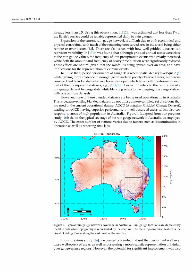
However, none of these blended datasets are being used operationally in Australia.This is because existing blended datasets do not utilise a more complete set of stations thatare used in the current operational dataset AGCD (Australian Gridded Climate Dataset),leading to AGCD having superior performance in well-observed areas which also cor-respond to areas of high population in Australia. Figure 1 (adapted from our previousstudy [16]) shows the typical coverage of the rain gauge network in Australia, as employedby AGCD. The exact number of stations varies due to factors such as discontinuities inoperation as well as reporting time lags.

Remote Sens. 2022, 14, x FOR PEER REVIEW 2 of 22

rainfall is a variable that can exhibit high spatiotemporal variation. In [11], the correlation

of adjacent rain gauges in the USA was evaluated, finding that at distances of 5 km the

correlation was already less than 0.5. Using this observation, in [12] it was estimated that

less than 1% of the Earth’s surface could be reliably represented daily by rain gauges.

Expansion of the current rain gauge network is difficult due to both economical and

physical constraints, with much of the remaining unobserved area in the world being ei-

ther remote or over oceans [12]. There are also issues with how well gridded datasets can

represent variability. In [13] it was found that although gridded annual totals were close

to the rain gauge values, the frequency of low-precipitation events was greatly increased,

while both the amount and frequency of heavy precipitation were significantly reduced.

These effects are natural given that the rainfall is being spread over an area, and have

implications for the representation of extreme events.

To utilise the superior performance of gauge data where spatial density is adequate

[8] whilst giving more credence to non-gauge datasets in poorly observed areas, numer-

ous corrected and blended datasets have been developed which have better performance

over that of their comprising datasets, e.g., [6,14,15]. Correction refers to the calibration of

a non-gauge dataset to gauge data while blending refers to the merging of a gauge dataset

with one or more datasets.

However, none of these blended datasets are being used operationally in Australia.

This is because existing blended datasets do not utilise a more complete set of stations that

are used in the current operational dataset AGCD (Australian Gridded Climate Dataset),

leading to AGCD having superior performance in well-observed areas which also corre-

spond to areas of high population in Australia. Figure 1 (adapted from our previous study

[16]) shows the typical coverage of the rain gauge network in Australia, as employed by

AGCD. The exact number of stations varies due to factors such as discontinuities in oper-

ation as well as reporting time lags.

Figure 1. Typical rain gauge network coverage in Australia. Rain gauge locations are depicted by

the blue dots while topography is represented by the shading. The main topographical feature is

the Great Dividing Range along the east coast of the country.

In our previous study [16], we created a blended dataset that performed well over

these well-observed areas, as well as possessing a more realistic representation of rainfall

over gauge-sparse regions. However, the potential for significant improvement was also

Figure 1. Typical rain gauge network coverage in Australia. Rain gauge locations are depicted bythe blue dots while topography is represented by the shading. The main topographical feature is theGreat Dividing Range along the east coast of the country.

In our previous study [16], we created a blended dataset that performed well overthese well-observed areas, as well as possessing a more realistic representation of rainfallover gauge-sparse regions. However, the potential for significant improvement was also

Remote Sens. 2022, 14, 261 3 of 21

identified, especially regarding the correction process used, which occasionally generatedsubstantial positive bias.

This paper aims to develop an optimal configuration for the correction and blendingof satellite data with gauge data on a monthly timescale, improving upon a previousdataset [16]. The term ‘correction’ will be used instead of ‘adjustment’ to align withconvention as well as to reflect the idea that the corrected dataset is of greater quality thanthe original version. To achieve this, the following objectives are set:

1. Several new methods of correction and blending of satellite data to gauge data willbe explored. The correction techniques evaluated will be linear correction- to-totalsand correction-to-anomalies methods (the former being the original technique), aswell as the use of quantile-to-quantile matching. The use of Empirical BayesianKriging (EBK) and Empirical Bayesian Kriging Regression Prediction (EBKRP) willalso be investigated to find if they offer improvements on Ordinary Kriging (OK).These corrected datasets will be blended with the gauge analysis using the originalmethod of inverse error variance (IEV), in addition to a method that explicitly includesdistance and another where the weights come from a triple collocation analysis (TCA);

2. The efficacy of datasets built from a combination of all these techniques will beevaluated, along with an analysis of their respective advantages and disadvantages.Performance close to stations will be determined through comparison to station data,while a comparison to MSWEP along with a triple collocation analysis (TCA) willestablish performance away from stations.

2. Materials and Methods2.1. Validation

Traditional validation compares datasets against a known reference, typically onebased on rain gauges. However, rain gauges (and more generally, any dataset) are subjectto their own biases which conflate validation. Additionally, large parts of the world havepoor coverage where the use of rain gauges as a reference would bear a great deal ofuncertainty [12]. Triple collocation analysis (TCA) provides an alternative method ofvalidation where the error [17] and correlation statistics [18] of three independent datasets(known as the triplet) can be estimated against an ‘unknown’ truth.

It was first utilised to estimate the error characteristics of wind data [17]; subsequently,it was first adapted for rainfall in [19]. Following [19], later studies (e.g., [20,21]) havedemonstrated the technique is capable of providing realistic error estimates for rainfall,being especially valuable over gauge-sparse areas.

A short overview of the technique is presented below, for full details refer to [21].The proper use of TCA relies on the key assumptions of: (1) stationarity of the data (noautocorrelation); (2) orthogonality of errors (their expected sum is zero); (3) the datasetsused are linearly related; and (4) there is no correlation amongst the errors of the datasets,as well as with the truth [21].

First, the datasets in the triplets can be related to the truth using an additive model(Equation (1)):

Xi = X′i + εi = αi + βit + εi (1)

where t is the truth, Xi (i = 1, 2, 3) are the triplet data which can be linearly related to the truthusing the ordinary least squares intercepts αi and slopes βi, and εi are their random errors.Using one of the datasets as a reference along with the assumptions stated, the equationscan be rearranged to provide an estimation of the residual errors, σε ,i (Equation (2)), as wellas the correlation of the datasets to the truth, ρt,Xi (Equation (3)).

σε,1 =√

Q11 − Q12Q13Q23

σε,2 =√

Q22 − Q12Q23Q13

σε,3 =√

Q33 − Q13Q23Q12

(2)

Remote Sens. 2022, 14, 261 4 of 21

ρt,X1 =√

Q12Q13Q11Q23

ρt,X2 = sign(Q13Q23)√

Q12Q23Q13Q22

ρt,X3 = sign(Q12Q23)√

Q13Q23Q12Q33

(3)

Qij denotes the covariances of the datasets with each other and there is a sign ambiguityfor ρt,X; however, in practice, the datasets can be assumed to be positively correlated to thetruth in almost all cases [18]. Intuitively, the equations depict the error for a dataset beingsmaller if it possesses a smaller variance and when it has strong correlations to the otherdatasets. The degree to which the required assumptions are satisfied by the datasets usedin this study, and hence the appropriateness of this technique for this study, is exploredin Appendix A. For validation, the triplet is comprised of the dataset to be verified, SoilMoisture to Rain (SM2R), and ERA5.

Three validation methods are used in this study. Performance at rain gauges wascaptured by validation against point station data. TCA and a gridded comparison againstMSWEP (Multi-Source Weighted-Ensemble Precipitation) [6] provided additional methodsof ranking the datasets, with a particular focus on performance away from rain gauges.All data were bilinearly interpolated to a resolution of 0.1 degrees (the native resolutionfor the blended datasets), with any negative values from the interpolation process set tozero. In the case of the point station comparison, the station value is compared to a griddedaverage centred at the location of the station. Consequently, a spatial representative error isexpected but as it would be constant amongst the datasets, a comparison can still be made.

For the gauge and MSWEP comparisons, the mean bias (MB), root-mean-squared-error(RMSE) and Pearson correlation coefficient (R) were computed for each dataset while theTCA yielded the aforementioned error variance (σ) and correlation (ρ). These metrics wereaveraged over the Australian domain and a study period of 2001 to 2020.

For each verification, a dataset’s ranking was determined through ranking the meanranking of its error and correlation statistics. This meant equal rankings could occur (suchas when two datasets had the same rankings but for opposite metrics). These individualverification rankings were then averaged with the mean forming a summary statistic. Thisfacilitated an easy-to-understand summary statistic with a focus on the relative ranking ofthe datasets.

2.2. Datasets

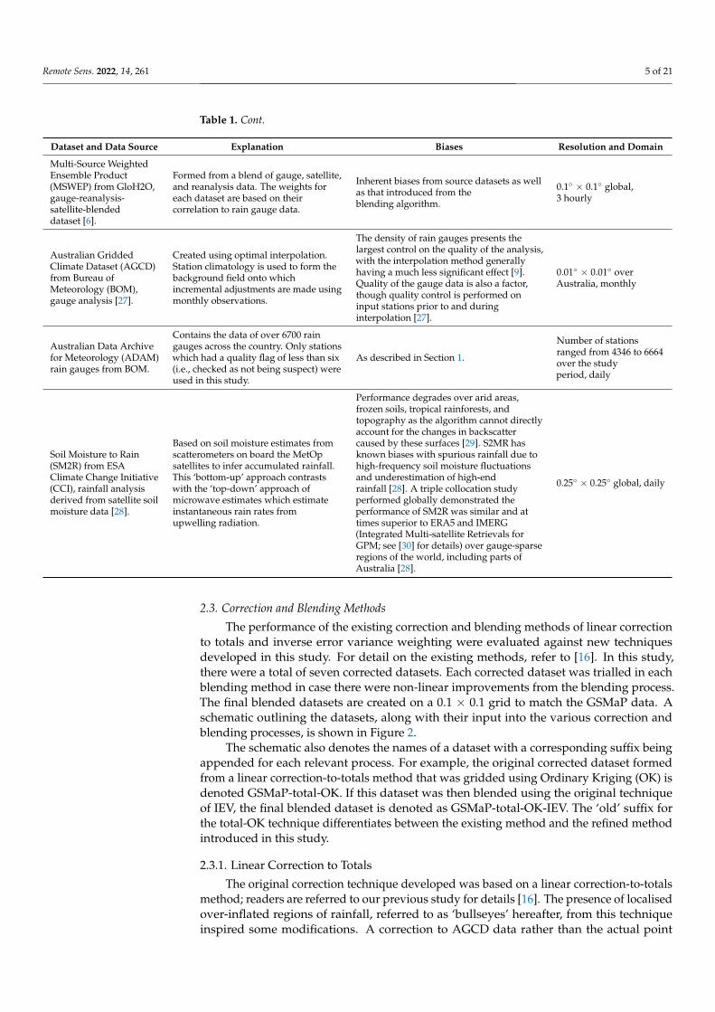
Datasets used for the development of the blended satellite datasets or its subsequentvalidation are described briefly below in Table 1.

Table 1. Details on datasets used in this study for creation of the blended dataset, as well asfo validation.

Dataset and Data Source Explanation Biases Resolution and Domain

Global Satellite Mappingof Precipitation (GSMaP)from Japan AerospaceExploration Agency(JAXA), microwave-basedestimates fromsatellites [22].

A rain rate is estimated from theemission and change in the scattering ofmicrowaves due to precipitation. Thesemicrowave estimates are advected usingcloud motion vectors to increase theirspatiotemporal coverage.

Measurement error from the sensors and thereliance on algorithms to obtain a rain rate.The algorithms are known to have adeficiency over topography and coastalboundaries. The detection of light rain fromwarm clouds [23] and sub-cloudevaporation of rainfall in aridenvironments [24] are also known problems.

0.1◦ × 0.1◦ global from60◦ S to 60◦ N, hourly

ERA5 from the EuropeanCentre forMedium-Range Forecast(ECMWF), modelreanalysis [25].

Created using 4D-Var assimilation ofobservations into their weather forecastmodel, the Integrated Forecast System(IFS). Assimilation does not includerainfall from gauges butgauge-corrected radar over the UnitedStates of America (US) as well assatellite radiances and atmosphericmotion vectors are ingested.

Biases arise from the observations ingested,as well as from the assimilation andmodelling processes with reducedobservations leading to a deterioration inquality [26]. In line with other reanalyses,ERA5 has reduced variability, with spuriouslow-end rainfall being a contributingfactor [6].

0.1◦ × 0.1◦ global, hourly

Remote Sens. 2022, 14, 261 5 of 21

Table 1. Cont.

Dataset and Data Source Explanation Biases Resolution and Domain

Multi-Source WeightedEnsemble Product(MSWEP) from GloH2O,gauge-reanalysis-satellite-blendeddataset [6].

Formed from a blend of gauge, satellite,and reanalysis data. The weights foreach dataset are based on theircorrelation to rain gauge data.

Inherent biases from source datasets as wellas that introduced from theblending algorithm.

0.1◦ × 0.1◦ global,3 hourly

Australian GriddedClimate Dataset (AGCD)from Bureau ofMeteorology (BOM),gauge analysis [27].

Created using optimal interpolation.Station climatology is used to form thebackground field onto whichincremental adjustments are made usingmonthly observations.

The density of rain gauges presents thelargest control on the quality of the analysis,with the interpolation method generallyhaving a much less significant effect [9].Quality of the gauge data is also a factor,though quality control is performed oninput stations prior to and duringinterpolation [27].

0.01◦ × 0.01◦ overAustralia, monthly

Australian Data Archivefor Meteorology (ADAM)rain gauges from BOM.

Contains the data of over 6700 raingauges across the country. Only stationswhich had a quality flag of less than six(i.e., checked as not being suspect) wereused in this study.

As described in Section 1.

Number of stationsranged from 4346 to 6664over the studyperiod, daily

Soil Moisture to Rain(SM2R) from ESAClimate Change Initiative(CCI), rainfall analysisderived from satellite soilmoisture data [28].

Based on soil moisture estimates fromscatterometers on board the MetOpsatellites to infer accumulated rainfall.This ‘bottom-up’ approach contrastswith the ‘top-down’ approach ofmicrowave estimates which estimateinstantaneous rain rates fromupwelling radiation.

Performance degrades over arid areas,frozen soils, tropical rainforests, andtopography as the algorithm cannot directlyaccount for the changes in backscattercaused by these surfaces [29]. S2MR hasknown biases with spurious rainfall due tohigh-frequency soil moisture fluctuationsand underestimation of high-endrainfall [28]. A triple collocation studyperformed globally demonstrated theperformance of SM2R was similar and attimes superior to ERA5 and IMERG(Integrated Multi-satellite Retrievals forGPM; see [30] for details) over gauge-sparseregions of the world, including parts ofAustralia [28].

0.25◦ × 0.25◦ global, daily

2.3. Correction and Blending Methods

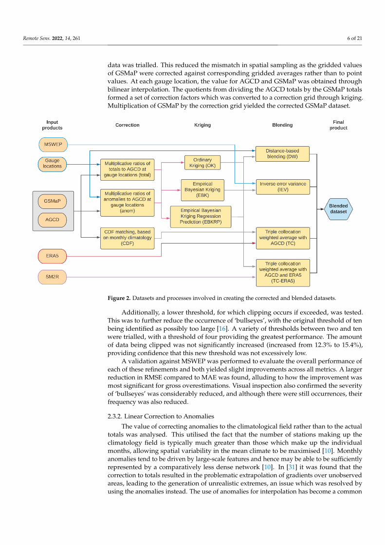
The performance of the existing correction and blending methods of linear correctionto totals and inverse error variance weighting were evaluated against new techniquesdeveloped in this study. For detail on the existing methods, refer to [16]. In this study,there were a total of seven corrected datasets. Each corrected dataset was trialled in eachblending method in case there were non-linear improvements from the blending process.The final blended datasets are created on a 0.1 × 0.1 grid to match the GSMaP data. Aschematic outlining the datasets, along with their input into the various correction andblending processes, is shown in Figure 2.

The schematic also denotes the names of a dataset with a corresponding suffix beingappended for each relevant process. For example, the original corrected dataset formedfrom a linear correction-to-totals method that was gridded using Ordinary Kriging (OK) isdenoted GSMaP-total-OK. If this dataset was then blended using the original techniqueof IEV, the final blended dataset is denoted as GSMaP-total-OK-IEV. The ‘old’ suffix forthe total-OK technique differentiates between the existing method and the refined methodintroduced in this study.

2.3.1. Linear Correction to Totals

The original correction technique developed was based on a linear correction-to-totalsmethod; readers are referred to our previous study for details [16]. The presence of localisedover-inflated regions of rainfall, referred to as ‘bullseyes’ hereafter, from this techniqueinspired some modifications. A correction to AGCD data rather than the actual point

Remote Sens. 2022, 14, 261 6 of 21

data was trialled. This reduced the mismatch in spatial sampling as the gridded valuesof GSMaP were corrected against corresponding gridded averages rather than to pointvalues. At each gauge location, the value for AGCD and GSMaP was obtained throughbilinear interpolation. The quotients from dividing the AGCD totals by the GSMaP totalsformed a set of correction factors which was converted to a correction grid through kriging.Multiplication of GSMaP by the correction grid yielded the corrected GSMaP dataset.

Remote Sens. 2022, 14, x FOR PEER REVIEW 6 of 22

were a total of seven corrected datasets. Each corrected dataset was trialled in each blend-

ing method in case there were non-linear improvements from the blending process. The

final blended datasets are created on a 0.1 × 0.1 grid to match the GSMaP data. A schematic

outlining the datasets, along with their input into the various correction and blending

processes, is shown in Figure 2.

The schematic also denotes the names of a dataset with a corresponding suffix being

appended for each relevant process. For example, the original corrected dataset formed

from a linear correction-to-totals method that was gridded using Ordinary Kriging (OK)

is denoted GSMaP-total-OK. If this dataset was then blended using the original technique

of IEV, the final blended dataset is denoted as GSMaP-total-OK-IEV. The ‘old’ suffix for

the total-OK technique differentiates between the existing method and the refined method

introduced in this study.

Figure 2. Datasets and processes involved in creating the corrected and blended datasets.

2.3.1. Linear Correction to Totals

The original correction technique developed was based on a linear correction-to-to-

tals method; readers are referred to our previous study for details [16]. The presence of

localised over-inflated regions of rainfall, referred to as ‘bullseyes’ hereafter, from this

technique inspired some modifications. A correction to AGCD data rather than the actual

point data was trialled. This reduced the mismatch in spatial sampling as the gridded

values of GSMaP were corrected against corresponding gridded averages rather than to

point values. At each gauge location, the value for AGCD and GSMaP was obtained

through bilinear interpolation. The quotients from dividing the AGCD totals by the

GSMaP totals formed a set of correction factors which was converted to a correction grid

through kriging. Multiplication of GSMaP by the correction grid yielded the corrected

GSMaP dataset.

Additionally, a lower threshold, for which clipping occurs if exceeded, was tested.

This was to further reduce the occurrence of ‘bullseyes’, with the original threshold of ten

being identified as possibly too large [16]. A variety of thresholds between two and ten

were trialled, with a threshold of four providing the greatest performance. The amount of

Figure 2. Datasets and processes involved in creating the corrected and blended datasets.

Additionally, a lower threshold, for which clipping occurs if exceeded, was tested.This was to further reduce the occurrence of ‘bullseyes’, with the original threshold of tenbeing identified as possibly too large [16]. A variety of thresholds between two and tenwere trialled, with a threshold of four providing the greatest performance. The amountof data being clipped was not significantly increased (increased from 12.3% to 15.4%),providing confidence that this new threshold was not excessively low.

A validation against MSWEP was performed to evaluate the overall performance ofeach of these refinements and both yielded slight improvements across all metrics. A largerreduction in RMSE compared to MAE was found, alluding to how the improvement wasmost significant for gross overestimations. Visual inspection also confirmed the severityof ‘bullseyes’ was considerably reduced, and although there were still occurrences, theirfrequency was also reduced.

2.3.2. Linear Correction to Anomalies

The value of correcting anomalies to the climatological field rather than to the actualtotals was analysed. This utilised the fact that the number of stations making up theclimatology field is typically much greater than those which make up the individualmonths, allowing spatial variability in the mean climate to be maximised [10]. Monthlyanomalies tend to be driven by large-scale features and hence may be able to be sufficientlyrepresented by a comparatively less dense network [10]. In [31] it was found that thecorrection to totals resulted in the problematic extrapolation of gradients over unobservedareas, leading to the generation of unrealistic extremes, an issue which was resolved byusing the anomalies instead. The use of anomalies for interpolation has become a common

Remote Sens. 2022, 14, 261 7 of 21

technique and is employed in other datasets, such as the Precipitation Reconstruction(PREC) [32] and AGCD [27].

In this study, the anomaly method involved finding the ratio between the anomalies(in contrast to totals as in Section 2.3.1) of both the satellite data and the station data at eachstation, with respect to their own climatology. As in Section 2.3.1, this was converted into agrid through kriging, which was then applied to the original data to correct the satelliteanomalies. The anomalies were then added back onto the climatology to obtain the valuefor each month. Clip values between ±3 and ±15 were trialled with ±8 providing thebest performance.

2.3.3. Quantile to Quantile Matching

An alternative to linear correction using ratios is the use of quantile-to-quantile match-ing, with cumulative distribution frequency (CDF) matching being a common technique,e.g., [33,34]. CDF matching involves fitting the data from the two sources to a statisticaldistribution. This yields CDFs from which a transfer function can be generated to rescalethe values from the original distribution to the target distribution [35]. The best-fittingdistribution can be highly dependent on the spatiotemporal domain and so it was perti-nent for this study to perform its own fitting. A gamma distribution has seen traditionalusage, e.g., [35,36], though more contemporary studies have noted the superiority of otherdistributions, such as the Pearson III, e.g., [37,38], log-Pearson III, e.g., [39], generalisedextreme value (GEV), e.g., [40], and even non-parametric distributions [41].

In this study, the gamma distribution was revealed to be most appropriate (seeAppendix B). Thus, both the satellite and gauge observations (using AGCD as a proxy) ateach grid point were fitted to gamma distributions, allowing their CDFs to be determined.Using the CDFs, the satellite observations were rescaled so that their percentile matchedthat of AGCD.

Two methods were trialled, basing the CDF on the last 30 months, as well as on theclimatology for each month for the maximum record of the satellite data (20 years). Thelatter yielded better results and so was chosen for this study.

2.3.4. Distance-Based Weighting Methods

Distance-based weighting methods vary the influence of gauge data based on thedistance to the closest rain gauge. It is a common technique with contemporary examplesincluding the Global Precipitation Climatology Project’s (GPCP) rain gauge analysis [42]and the Climate Hazards Group Infrared Precipitation with Stations (CHIRPS) dataset [43].Typically, the influence of gauge data decreases until it ceases to influence at a point wherethe correlation to rain gauges is considered to be negligible. In [27], it was noted thecorrelation of stations decreased below a significant level at around an order of 300 to500 km. The Multi-Source Weighted-Ensemble Precipitation (MSWEP) Version 2 datasetuses an empirical function based on an exponential function where the weight given tostations in the blended dataset is less than 0.1 after distances greater than 93 km [6].

In this study, a blended dataset was formed through a weighted average of correctedGSMaP and AGCD, with the weights being based on the distance of that grid cell from theclosest station. The equation used was:

w = exp(− D

D0

)(4)

D denotes the distance of a grid cell from the closest station in kilometres, whileD0 represents how quickly the influence diminishes with greater values, resulting in thegauge possessing greater influence for a given distance. There is an exponential decreaseof influence away from a gauge. By testing a range of D0 values between 50 and 400incremented by 50, a D0 of 100 was identified to be optimal in terms of providing thehighest correlation for an extremely dry and wet month. For this D0, the weighting for the

Remote Sens. 2022, 14, 261 8 of 21

gauge data reduces to 0.1 at around 230 km, which is in line with the correlation lengthscales obtained in [27].

2.3.5. Kriging Variants

Kriging methods rely on forming an estimate based on the weighted average of knownvalues in the neighbourhood, which minimises the estimation variance [44]. The originalmethod employed Ordinary Kriging (OK) assumed a constant mean and variogram acrossthe entire domain. Numerous other more complex kriging techniques exist based onwhat assumptions of the stationarity and stochastic properties of the field are made [45].However, the added complexity does not always result in better performance. Variousstudies have compared OK to other kriging methods and results have not been conclusive.For example, Ref. [46] compared OK to ordinary cokriging (OCK) and kriging with anexternal drift (KED) over the Hawaiian Islands and found that OK performed best, whileRef. [47] compared the same three methods over two Victorian catchments and foundthat OCK was the superior technique. OCK aims to create a better spatial relationshipby utilising additional covariates, while KED uses an external trend to account for non-stationarity [46].

Empirical Bayesian Kriging (EBK) attempts to overcome some limitations of classicalkriging by using an ensemble of variograms that are applied to subsets of the data. Foreach subset, a variogram ensemble is iteratively generated by using the original estimatedvariogram to produce new data values which are then used to produce new variograms [48].EBK allows non-stationarity as well as uncertainty in the variogram estimation to bebetter accounted for [48]. EBK Regression Prediction (EBKRP) builds on EBK by usinginformation provided by additional explanatory variables. In [49], it was found a rainfallanalysis created using EBK was able to outperform OK over Northwest India, while EBKRPfollowed closely by EBK yielded the best performance in a study over Pakistan [45].

In this study, an exponential variogram was used, along with the default parametersfor EBK and EBKRP (maximum local points of 100, an overlap factor of 1, and number ofsemivariograms of 100). For the EBK method, an empirical transformation was applied tothe data.

2.3.6. TCA Blend

The error statistics from the TCA can also be used as a basis for blending. Twotechniques were used. The first merged corrected GSMaP and AGCD, while the secondmerged corrected GSMaP, AGCD, and ERA5. Inverse error variance blending was usedagain, with the weights being derived from the fractional RMSEs obtained from TCA.The fractional RMSE (fRMSE) is obtained by dividing σε by the standard deviation tostandardise the RMSEs between the datasets.

For AGCD to be used in the blended product, the TCA employed to obtain the weightscomprised of uncorrected GSMaP, AGCD, and ERA5. Even though corrected GSMaP isused in the blended product, it could not be used to derive the weights given that itsdependency on AGCD violates the assumption of independence amongst the TCA triplet.

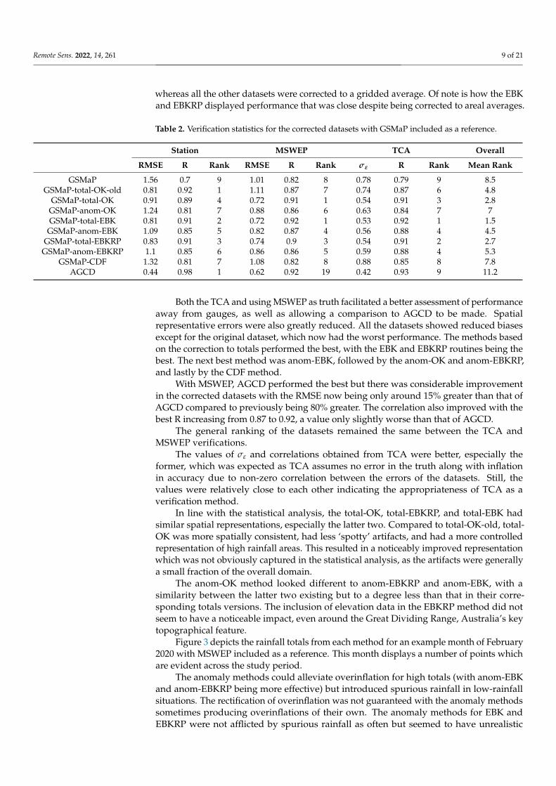
3. Results3.1. Corrected Datasets

The results for the corrected datasets are shown in Table 2. Examining the averageRMSE and R across the corrected datasets, it was evident that the linear correction-to-totalsmethods performed the best with average RMSEs between 0.69 to 0.72 and average Rvalues of 0.91. This was followed by the linear correction-to-anomaly methods, with theEBK and EBKRP having a larger edge over OK than what was obtained with a correctionto totals. The CDF method was last, but it still outperformed the uncorrected GSMaP.

Using stations as truth, the original method obtained the highest performance. This isexpected as this was the only dataset that was corrected to the actual point stations values

Remote Sens. 2022, 14, 261 9 of 21

whereas all the other datasets were corrected to a gridded average. Of note is how the EBKand EBKRP displayed performance that was close despite being corrected to areal averages.

Table 2. Verification statistics for the corrected datasets with GSMaP included as a reference.

Station MSWEP TCA Overall

RMSE R Rank RMSE R Rank σε R Rank Mean Rank

GSMaP 1.56 0.7 9 1.01 0.82 8 0.78 0.79 9 8.5GSMaP-total-OK-old 0.81 0.92 1 1.11 0.87 7 0.74 0.87 6 4.8

GSMaP-total-OK 0.91 0.89 4 0.72 0.91 1 0.54 0.91 3 2.8GSMaP-anom-OK 1.24 0.81 7 0.88 0.86 6 0.63 0.84 7 7GSMaP-total-EBK 0.81 0.91 2 0.72 0.92 1 0.53 0.92 1 1.5

GSMaP-anom-EBK 1.09 0.85 5 0.82 0.87 4 0.56 0.88 4 4.5GSMaP-total-EBKRP 0.83 0.91 3 0.74 0.9 3 0.54 0.91 2 2.7

GSMaP-anom-EBKRP 1.1 0.85 6 0.86 0.86 5 0.59 0.88 4 5.3GSMaP-CDF 1.32 0.81 7 1.08 0.82 8 0.88 0.85 8 7.8

AGCD 0.44 0.98 1 0.62 0.92 19 0.42 0.93 9 11.2

Both the TCA and using MSWEP as truth facilitated a better assessment of performanceaway from gauges, as well as allowing a comparison to AGCD to be made. Spatialrepresentative errors were also greatly reduced. All the datasets showed reduced biasesexcept for the original dataset, which now had the worst performance. The methods basedon the correction to totals performed the best, with the EBK and EBKRP routines being thebest. The next best method was anom-EBK, followed by the anom-OK and anom-EBKRP,and lastly by the CDF method.

With MSWEP, AGCD performed the best but there was considerable improvementin the corrected datasets with the RMSE now being only around 15% greater than that ofAGCD compared to previously being 80% greater. The correlation also improved with thebest R increasing from 0.87 to 0.92, a value only slightly worse than that of AGCD.

The general ranking of the datasets remained the same between the TCA andMSWEP verifications.

The values of σε and correlations obtained from TCA were better, especially theformer, which was expected as TCA assumes no error in the truth along with inflationin accuracy due to non-zero correlation between the errors of the datasets. Still, thevalues were relatively close to each other indicating the appropriateness of TCA as averification method.

In line with the statistical analysis, the total-OK, total-EBKRP, and total-EBK hadsimilar spatial representations, especially the latter two. Compared to total-OK-old, total-OK was more spatially consistent, had less ‘spotty’ artifacts, and had a more controlledrepresentation of high rainfall areas. This resulted in a noticeably improved representationwhich was not obviously captured in the statistical analysis, as the artifacts were generallya small fraction of the overall domain.

The anom-OK method looked different to anom-EBKRP and anom-EBK, with asimilarity between the latter two existing but to a degree less than that in their corre-sponding totals versions. The inclusion of elevation data in the EBKRP method did notseem to have a noticeable impact, even around the Great Dividing Range, Australia’s keytopographical feature.

Figure 3 depicts the rainfall totals from each method for an example month of February2020 with MSWEP included as a reference. This month displays a number of points whichare evident across the study period.

The anomaly methods could alleviate overinflation for high totals (with anom-EBKand anom-EBKRP being more effective) but introduced spurious rainfall in low-rainfallsituations. The rectification of overinflation was not guaranteed with the anomaly methodssometimes producing overinflations of their own. The anomaly methods for EBK andEBKRP were not afflicted by spurious rainfall as often but seemed to have unrealistic

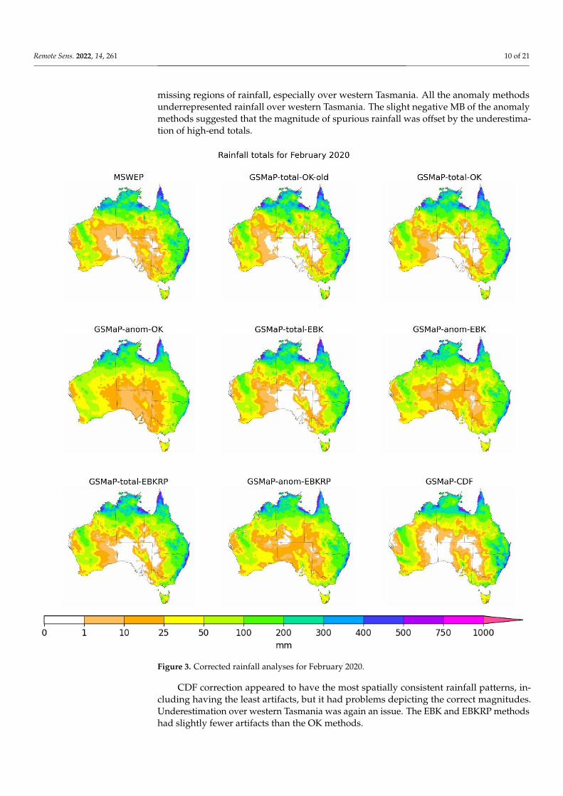
Remote Sens. 2022, 14, 261 10 of 21

missing regions of rainfall, especially over western Tasmania. All the anomaly methodsunderrepresented rainfall over western Tasmania. The slight negative MB of the anomalymethods suggested that the magnitude of spurious rainfall was offset by the underestima-tion of high-end totals.

Remote Sens. 2022, 14, x FOR PEER REVIEW 11 of 22

Figure 3. Corrected rainfall analyses for February 2020.

Table 3. Verification statistics for blended datasets with AGCD included as a reference.

Station MSWEP TCA Overall

RMSE R Rank RMSE R Rank σε R Rank Rank (Mean)

GSMaP-total-OK-IEV-old 0.62 0.96 9 0.57 0.94 7 0.44 0.93 16 10.3

GSMaP-total-OK-IEV 0.66 0.95 12 0.54 0.95 2 0.40 0.94 1 6.2

GSMaP-anom-OK-IEV 0.69 0.95 13 0.54 0.95 1 0.40 0.94 2 6.7

GSMaP-total-EBK-IEV 0.64 0.95 10 0.55 0.94 3 0.42 0.94 3 6.8

GSMaP-anom-EBK-IEV 0.72 0.94 18 0.57 0.94 4 0.40 0.93 6 10.5

GSMaP-total-EBKRP-IEV 0.64 0.95 11 0.56 0.94 5 0.41 0.94 3 8.2

GSMaP-anom-EBKRP-IEV 0.72 0.94 17 0.57 0.94 8 0.40 0.93 3 10.7

GSMaP-total-OK-DW 0.60 0.96 4 0.60 0.94 9 0.45 0.93 9 9.3

GSMaP-total-OK-TC 0.72 0.94 18 0.60 0.94 10 0.44 0.93 7 13.2

GSMaP-total-OK-TC-ERA5 1.28 0.76 26 1.23 0.68 24 0.32 0.92 8 21.0

AGCD 0.44 0.98 1 0.62 0.92 19 0.42 0.93 9 11.2

Figure 3. Corrected rainfall analyses for February 2020.

CDF correction appeared to have the most spatially consistent rainfall patterns, in-cluding having the least artifacts, but it had problems depicting the correct magnitudes.Underestimation over western Tasmania was again an issue. The EBK and EBKRP methodshad slightly fewer artifacts than the OK methods.

Remote Sens. 2022, 14, 261 11 of 21

3.2. Blended Datasets

A key result was that the ranking of the corrected datasets could change after theblending process and between blending processes, justifying the decision to trial eachblending method with all the corrected datasets, rather than just the best-performing ones.

Importantly, even though the total-EBK had the best overall ranking out of the cor-rected datasets, the best blended dataset was total-OK-IEV, with total-EBK-IEV comingsecond. Total-OK-IEV had the best ranking in the MSWEP and the TCA verifications. In thestation verification, it was outperformed by the DW-blended datasets as well as by total-EBK-IEV and total-EBKRP-IEV. This suggests it demonstrated the best away-from-stationperformance in addition to having strong at-station accuracy.

The inverse error variance method yielded the best results, followed by the DWmethod and then the TCA method. For brevity, only the subset of results for the datasetsbased on the OK-total and/or IEV methods is shown in Table 3—the full configurationcan be found in Appendix C, Table A3. This subset was chosen based on the result ofthe total-OK-IEV method being the best, along with the variance between the blendingtechniques and the input-corrected dataset largely being unsubstantial. There is an indirectinclusion of MSWEP in the IEV datasets which would lead to some degree of skill inflationin the MSWEP validation; however, the substitution of MSWEP for ERA5 in the IEV methoddid not change the result of IEV datasets performing the best in the MSWEP validation.

Table 3. Verification statistics for blended datasets with AGCD included as a reference.

Station MSWEP TCA Overall

RMSE R Rank RMSE R Rank σε R Rank Rank (Mean)

GSMaP-total-OK-IEV-old 0.62 0.96 9 0.57 0.94 7 0.44 0.93 16 10.3GSMaP-total-OK-IEV 0.66 0.95 12 0.54 0.95 2 0.40 0.94 1 6.2

GSMaP-anom-OK-IEV 0.69 0.95 13 0.54 0.95 1 0.40 0.94 2 6.7GSMaP-total-EBK-IEV 0.64 0.95 10 0.55 0.94 3 0.42 0.94 3 6.8

GSMaP-anom-EBK-IEV 0.72 0.94 18 0.57 0.94 4 0.40 0.93 6 10.5GSMaP-total-EBKRP-IEV 0.64 0.95 11 0.56 0.94 5 0.41 0.94 3 8.2

GSMaP-anom-EBKRP-IEV 0.72 0.94 17 0.57 0.94 8 0.40 0.93 3 10.7GSMaP-total-OK-DW 0.60 0.96 4 0.60 0.94 9 0.45 0.93 9 9.3GSMaP-total-OK-TC 0.72 0.94 18 0.60 0.94 10 0.44 0.93 7 13.2

GSMaP-total-OK-TC-ERA5 1.28 0.76 26 1.23 0.68 24 0.32 0.92 8 21.0AGCD 0.44 0.98 1 0.62 0.92 19 0.42 0.93 9 11.2

The various blending techniques all had a harmonising effect on the corrected datasets,with the similarity in the blended products for each technique being relatively high. Thedegree of harmonisation was less for the TCA blending.

In terms of similarity based on the input dataset, the CDF-corrected dataset yieldedthe greatest dissimilarity to the others with other methods being fairly similar. The krigingtechnique matters less than whether correction to totals or anomalies was used.

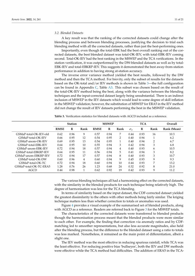
Figure 4 provides a visual example of the summarised set of blended products, alongwith AGCD as a reference. Readers are referred back to Figure 3 for the MSWEP totals.

The characteristics of the corrected datasets were transferred to blended productsthough the harmonisation process meant that the blended products were more similarto each other. For example, the finding that correction via anomaly ratios and by CDF-matching led to smoother representations, but also less accurate magnitudes, also heldafter the blending process, but the difference to the blended dataset using a ratio to totalswas less marked. Nonetheless, it remained as the main point of differentiation, albeit aslight one.

The IEV method was the most effective in reducing spurious rainfall, while TCA wasthe least effective. For reducing positive bias ‘bullseyes’, both the IEV and DW methodswere effective while the TCA method had difficulties. The addition of ERA5 in the TCA-

Remote Sens. 2022, 14, 261 12 of 21

blended method did not necessarily improve results. Only the σε metric from the TCAvalidation was improved.

Remote Sens. 2022, 14, x FOR PEER REVIEW 13 of 22

Figure 4. Blended rainfall analyses for February 2020. Figure 4. Blended rainfall analyses for February 2020.

Remote Sens. 2022, 14, 261 13 of 21

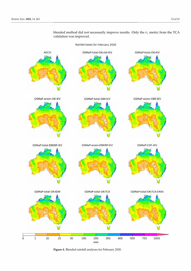
Figure 5 shows the period-averaged correlations obtained from the TCA for all thecorrected datasets, and the total-OK- and/or IEV-blended variants. GSMaP and AGCDare included for reference. It allows identification of where the correction and blendingmethods were most effective.

Remote Sens. 2022, 14, x FOR PEER REVIEW 14 of 22

Figure 5. Correlations obtained using triple collocation analysis for corrected and blended datasets.

4. Discussion

4.1. Correction Techniques

The use of cell-to-cell correction instead of point-to-cell correction was important in

removing stray bullseye artifacts that were a result of large discrepancies due to incon-

sistent spatial sampling. This was especially true for cases where a gauge value was much

higher than its gridded average.

Figure 5. Correlations obtained using triple collocation analysis for corrected and blended datasets.

Remote Sens. 2022, 14, 261 14 of 21

The anom-OK and CDF correction methods were not so effective in the interior ofWestern Australia, where the gauge network is sparse. The CDF method also did notperform well over central parts of the eastern coastline. The improvement of total-OK overtotal-OK-old is also clear, especially over the northern coastline. The regions where themethod is the weakest appears to be towards the centre of Western Australia, as well asaround East Arnhem in Northern Territory.

The similarity of the blending methods is evident. From a glance, only the total-OK-TC-ERA5 method displayed noticeable differences, having slightly weaker correlationsacross the country than the other blended products. The blending methods improvedcorrelations to a level that was similar to AGCD, with the patch of lower correlation in thecentre of Western Australia present in both AGCD and the blended satellite datasets. Thisis a region of very low gauge density, alluding to the possibility that the blended satellitedataset is still limited, at least to some extent, by the quality of the gauge analysis and itsunderlying network.

4. Discussion4.1. Correction Techniques

The use of cell-to-cell correction instead of point-to-cell correction was important inremoving stray bullseye artifacts that were a result of large discrepancies due to inconsistentspatial sampling. This was especially true for cases where a gauge value was much higherthan its gridded average.

Correction to totals was generally the best at creating a product where the satellitetotals were most similar to the observed ones. However, it was also the most prone toartifacts. As described in [16], if GSMaP contained isolated patches of elevated rainfallthat were not also present in AGCD, over areas with low rain gauge densities this couldlead to incorrect adjustment. If GSMaP totals were less than what were observed atthe closest, albeit still faraway gauges, the elevated rainfall patch would end up beinggreatly exaggerated.

The correction to anomalies dealt better with high totals and also resulted in lessartifacts. However, this method struggled with low rainfall totals, generating the greatestamount of spurious light rainfall. This was likely because the final product still containedrainfall from the climatological background. Furthermore, the representation of extremeanomalies could be lost when these anomalies were over poorly observed areas. In thesecases, the adjustment was again based on faraway stations where GSMaP and station datawere more aligned, resulting in some little adjustments so that the final product resembledthe climatology rather than the anomaly.

The CDF method has proved to be effective in past studies, e.g., [50,51]. It createdthe most realistic-looking representations and was least prone to the incorrect adjustmentof isolated anomalies over gauge-sparse areas. This can be attributed to how under thisscenario, the other two methods would utilise a faraway station-based adjustment whilethe CDF method was matched based on the local distributions. Even though the datasetsmay have been quite different locally in an absolute sense, they could be similar in theirrelative frequency, reducing the susceptibility of extreme adjustment errors.

However, the CDF method underestimated rainfall during very-low-total scenarios.For dry areas where many totals are zero, the gamma distribution may not be appropriateas zero values have to be excluded during fitting. Sometimes, a lack of adjustment alsooccurred, including underrepresentation of elevated totals over western Tasmania. Itis possible that this was due to the satellite value having a very similar position in itsdistribution to its station equivalent, resulting in little adjustment. If there was a longerrecord, this method would likely perform better, as having only 20 years of data canconstrain the robustness of the fit, especially for extremes. In [33], the authors increasedthe amount of data available for fitting by utilising daily data as well as consideringsurrounding grid cells, likely improving the accuracy derived from this method. However,

Remote Sens. 2022, 14, 261 15 of 21

the method being developed in this study is intended to be limited to monthly data,reducing the resource requirement, and increasing simplicity of use.

The CDF method does not have to rely on the gauge analysis having correct totals, butrather on the frequency of the gauges being more correct. Considering that the representa-tion was relatively similar to that obtained from the linear correction methods, the CDFmethod could be advantageous for regions with sparser rain gauge networks where theability to create an accurate rain gauge analysis is more difficult.

The result of a linear correction performing the best has been observed in the literature,including contemporary studies, e.g., [52]. There appears to be a trade-off between bettermatching at stations and an increased likelihood of artifacts away from stations.

The small amount of variance between the different kriging techniques suggests theassumption of a constant variogram used across the whole domain in OK was generallyacceptable. There was not a clear superior variant, with a dependence on the validationdataset used. This can be reconciled with [45], which found EBKRP to be the superiordataset, albeit with only a slight difference to EBK and OK. The differences between EBKand EBKRP did not tend to occur over topography, which was unexpected given elevationwas the extra parameter used in EBKRP.

4.2. Blending Techniques

An important result is that the three blending techniques produced a similar repre-sentation of rainfall. Considering that all three were derived from considerably differentmethods (error variance from MSWEP, error variance from a TCA using AGCD and ERA5,and adjustment using distance from stations), this provides confidence that an optimalresult (particularly within the technique but also across techniques) was being achieved. Italso suggests that obtaining a marked improvement via the use of other blending techniquesmay be difficult.

The scenario where there was the most difference in the blending techniques was whenthere was a strong difference in the underlying corrected dataset over a region with sparserain gauge coverage. The DW-blended method retained this difference, while the other twoblended techniques would adjust this difference towards AGCD. The DW method functionsas intended in this sense as AGCD should be considered less dependable in these areasand thus weighed less, but at times the corrected satellite dataset contained its own biaseswhich outweighed the effect of reduced reliance on AGCD. As described in Section 4.1,the most problematic scenario for the most performant-corrected dataset (total-OK-IEV)was over-adjusted bullseyes in gauge-sparse regions. The DW method would incorrectlyamplify or retain these artifacts, while the other two techniques were able to resolve them.

It was also not a guarantee that the best corrected dataset would result in the bestblended dataset—the effect of blending was non-linear. In general, the corrected datasetsusing a linear correction to totals yielded the best blended dataset with the choice of krigingtechnique between OK, EBK, and EBKRP not having much effect in this study.

The inclusion of ERA5 data in the TCA-blended dataset did not generally improveperformance. The only metric that improved was the σε from the TCA validation, whichwas expected as the weights were formed from the optimisation of fRMSE. It should also benoted that the TC-ERA5 datasets are more likely to violate the assumption of independencerequired for TCA, and so the fact that they yielded the lowest TCA error statistics, butworse statistics otherwise, suggests that their TCA results are suspect. A possible reasonwhy performance was not improved could be the introduction of spurious minute rainfallfrom the use of a greater number of component rainfall datasets, which has a more adverseimpact on the correlation metrics than the error ones. The use of additional datasets doesnot necessarily improve accuracy and requires greater nuance, including the use of asensible method for determining rain/no-rain cells.

As seen amongst the correction techniques, there was also a trade-off of performanceat stations and away from stations among the blending techniques. This is reflected in thevalidation technique used as well. The station-based verification favoured the DW method

Remote Sens. 2022, 14, 261 16 of 21

due to its explicit inclusion of station data. The MSWEP and TCA validations indicatedthat the IEV method was the best. Considering that the MSWEP and TCA validationsare more generalised and evaluate performance both at and away from stations, theyare likely a better indicator of the overall performance of datasets. The IEV-blendingmethod also performed relatively well in the station validation, being the best non-DWmethod evaluated.

5. Conclusions

Gauge analyses possess high uncertainty in gauge-sparse regions and while alterna-tive data sources like satellites can provide estimates for these areas, their indirect formof estimation means their accuracy is less than gauge analyses where stations exist. Bycombining satellite and gauge data, a better dataset that takes advantage of the complemen-tary nature of both sources can be produced. This study evaluated the efficacy of variousconfigurations of correction and blending techniques. The correction techniques trialledwere linear correction to totals, linear correction to anomalies, and CDF matching. Theblending techniques tested were based on inverse error variance using MSWEP as truth,a distance-weighted approach, and a triple collocation analysis-weighting scheme usingGSMaP, AGCD, and ERA5. The main findings are as follows:

1. The most performant correction technique in this study was a linear correction tototals. The choice of kriging technique did not have a strong impact, with EBK slightlyoutperforming EBKRP and OK;

2. The most performant blending technique was an inverse error variance blending tech-nique using a GSMaP dataset linearly corrected to totals. All the blending techniquestested were able to improve the underlying corrected dataset, having a harmonisingeffect that greatly reduced the differences between the corrected datasets. The im-provement was non-linear, resulting in the total-OK-IEV-blended dataset performingthe best generally;

3. The validation technique used is important, as station-based validation favouredDW-blended datasets while the more general TCA and MSWEP validations favouredthe IEV-blended datasets. Triple collocation analysis using satellite data, SM2R, andERA5 as the triplet yielded results consistent with a traditional comparison to MSWEP,highlighting the versatility of the technique;

4. The trade-off between at-station and away-from-station performance was clear. Forthe correction techniques, the CDF method traded at-station performance for away-from-station performance. For the blending techniques, the DW method traded away-from-station performance for at-station performance. This made them complementaryto each other. Likewise, the linear correction methods were complementary to the IEVblending methods.

The results of having three different blending techniques yield a similar representationof rainfall, suggesting that the blended result obtained in this study is close to beingoptimal. When both at-station and away-from-station performance is considered, total-OK-IEV performed the best. The effectiveness of this method over a domain with much fewerrain gauges is an important future research topic as the rain gauge analysis is an importantingredient in this method.

Author Contributions: Conceptualisation, Z.-W.C., Y.K., A.B.W., S.C. and C.S.; methodology, Z.-W.C.and Y.K.; software, Z.-W.C.; validation, Z.-W.C.; formal analysis, Z.-W.C.; investigation, Z.-W.C.;resources, Z.-W.C.; data curation, Z.-W.C.; writing—original draft preparation, Z.-W.C.; writing—review and editing, Z.-W.C., Y.K., A.B.W., S.C. and C.S.; visualisation, Z.-W.C., supervision, Z.-W.C.,Y.K., A.B.W., S.C. and C.S.; project administration, Z.-W.C. and Y.K. All authors have read and agreedto the published version of the manuscript.

Funding: This research was supported by the World Meteorological Organization through “Weatherand Climate Early Warning System for Papua New Guinea (CREWS-PNG)” project 20170888.

Remote Sens. 2022, 14, 261 17 of 21

Data Availability Statement: GSMaP data were provided by EORC, JAXA. CMORPH data wereprovided by CPC, NOAA. AGCD and station gauge data were provided by the Bureau of Meteorology.Contains modified Copernicus Climate Change Service Information (2019). Neither the EuropeanCommission nor ECMWF is responsible for any use that may be made of the Copernicus Informationor Data it contains. MSWEP data were provided by GloH2O.

Acknowledgments: We are grateful to colleagues from the Climate Monitoring and Long-RangeForecasts sections of the Bureau of Meteorology for their helpful advice and guidance. Threeanonymous reviewers provided valuable comments which helped us to improve the quality of theinitial manuscript.

Conflicts of Interest: The authors declare no conflict of interest.

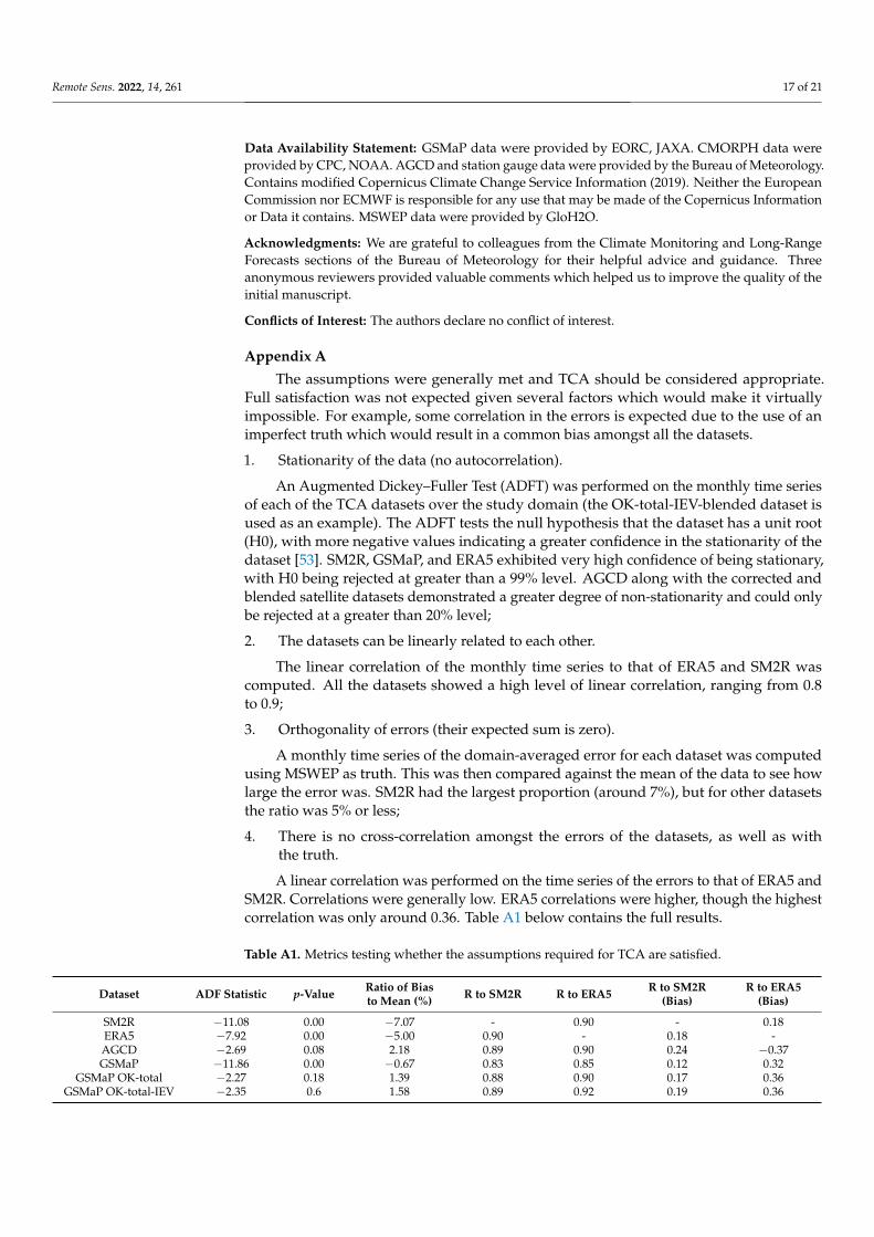
Appendix A

The assumptions were generally met and TCA should be considered appropriate.Full satisfaction was not expected given several factors which would make it virtuallyimpossible. For example, some correlation in the errors is expected due to the use of animperfect truth which would result in a common bias amongst all the datasets.

1. Stationarity of the data (no autocorrelation).

An Augmented Dickey–Fuller Test (ADFT) was performed on the monthly time seriesof each of the TCA datasets over the study domain (the OK-total-IEV-blended dataset isused as an example). The ADFT tests the null hypothesis that the dataset has a unit root(H0), with more negative values indicating a greater confidence in the stationarity of thedataset [53]. SM2R, GSMaP, and ERA5 exhibited very high confidence of being stationary,with H0 being rejected at greater than a 99% level. AGCD along with the corrected andblended satellite datasets demonstrated a greater degree of non-stationarity and could onlybe rejected at a greater than 20% level;

2. The datasets can be linearly related to each other.

The linear correlation of the monthly time series to that of ERA5 and SM2R wascomputed. All the datasets showed a high level of linear correlation, ranging from 0.8to 0.9;

3. Orthogonality of errors (their expected sum is zero).

A monthly time series of the domain-averaged error for each dataset was computedusing MSWEP as truth. This was then compared against the mean of the data to see howlarge the error was. SM2R had the largest proportion (around 7%), but for other datasetsthe ratio was 5% or less;

4. There is no cross-correlation amongst the errors of the datasets, as well as withthe truth.

A linear correlation was performed on the time series of the errors to that of ERA5 andSM2R. Correlations were generally low. ERA5 correlations were higher, though the highestcorrelation was only around 0.36. Table A1 below contains the full results.

Table A1. Metrics testing whether the assumptions required for TCA are satisfied.

Dataset ADF Statistic p-Value Ratio of Biasto Mean (%) R to SM2R R to ERA5 R to SM2R

(Bias)R to ERA5

(Bias)

SM2R −11.08 0.00 −7.07 - 0.90 - 0.18ERA5 −7.92 0.00 −5.00 0.90 - 0.18 -AGCD −2.69 0.08 2.18 0.89 0.90 0.24 −0.37GSMaP −11.86 0.00 −0.67 0.83 0.85 0.12 0.32

GSMaP OK-total −2.27 0.18 1.39 0.88 0.90 0.17 0.36GSMaP OK-total-IEV −2.35 0.6 1.58 0.89 0.92 0.19 0.36

Remote Sens. 2022, 14, 261 18 of 21

Appendix B

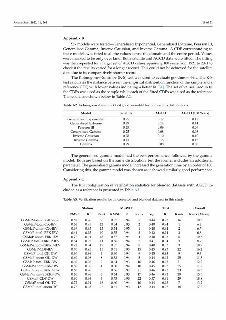
Six models were tested—Generalised Exponential, Generalised Extreme, Pearson III,Generalised Gamma, Inverse Gaussian, and Inverse Gamma. A CDF corresponding tothese models was fitted to all the values across the domain and the entire period. Valueswere masked to be only over land. Both satellite and AGCD data were fitted. The fittingwas then repeated for a larger set of AGCD values, spanning 100 years from 1921 to 2021 tocheck if the results varied for a longer record. This could not be achieved for the satellitedata due to its comparatively shorter record.

The Kolmogorov–Smirnov (K-S) test was used to evaluate goodness-of-fit. The K-Stest calculates the distance between the empirical distribution function of the sample and areference CDF, with lower values indicating a better fit [54]. The set of values used to fitthe CDFs was used as the sample while each of the fitted CDFs was used as the reference.The results are shown below in Table A2.

Table A2. Kolmogorov–Smirnov (K-S) goodness-of-fit test for various distributions.

Model Satellite AGCD AGCD (100 Years)

Generalised Exponential 0.25 0.17 0.17Generalised Extreme 0.29 0.14 0.14

Pearson III 0.25 0.09 0.09Generalised Gamma 0.25 0.08 0.08

Inverse Gaussian 0.28 0.10 0.10Inverse Gamma 0.43 0.15 0.15

Gamma 0.29 0.08 0.08

The generalised gamma model had the best performance, followed by the gammamodel. Both are based on the same distribution, but the former includes an additionalparameter. The generalised gamma model increased the generation time by an order of 100.Considering this, the gamma model was chosen as it showed similarly good performance.

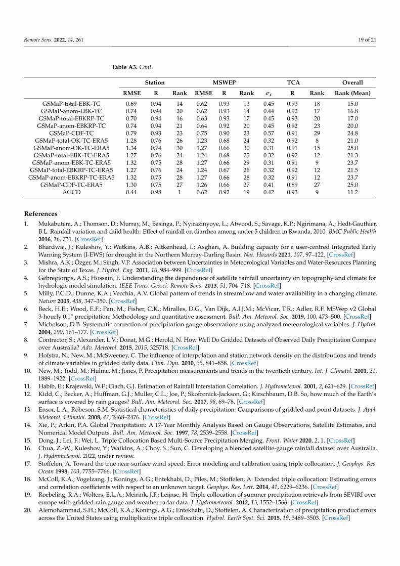
Appendix C

The full configuration of verification statistics for blended datasets with AGCD in-cluded as a reference is presented in Table A3.

Table A3. Verification results for all corrected and blended datasets in this study.

Station MSWEP TCA Overall

RMSE R Rank RMSE R Rank σε R Rank Rank (Mean)

GSMaP-total-OK-IEV-old 0.62 0.96 9 0.57 0.94 7 0.44 0.93 16 10.3GSMaP-total-OK-IEV 0.66 0.95 12 0.54 0.95 2 0.40 0.94 1 6.2

GSMaP-anom-OK-IEV 0.69 0.95 13 0.54 0.95 1 0.40 0.94 2 6.7GSMaP-total -EBK-IEV 0.64 0.95 10 0.55 0.94 3 0.42 0.94 3 6.8GSMaP-anom-EBK-IEV 0.72 0.94 18 0.57 0.94 4 0.40 0.93 6 10.5

GSMaP-total-EBKRP-IEV 0.64 0.95 11 0.56 0.94 5 0.41 0.94 3 8.2GSMaP-anom-EBKRP-IEV 0.72 0.94 17 0.57 0.94 8 0.40 0.93 3 10.7

GSMaP-CDF-IEV 0.70 0.95 15 0.61 0.93 15 0.45 0.93 22 16.2GSMaP-total-OK-DW 0.60 0.96 4 0.60 0.94 9 0.45 0.93 9 9.3

GSMaP-anom-OK-DW 0.60 0.96 8 0.58 0.94 5 0.44 0.92 25 11.3GSMaP-total-EBK-DW 0.60 0.96 2 0.64 0.93 16 0.46 0.93 21 12.2

GSMaP-anom-EBK-DW 0.60 0.96 4 0.60 0.94 10 0.45 0.92 25 11.7GSMaP-total-EBKRP-DW 0.60 0.96 3 0.66 0.92 21 0.46 0.93 23 14.3

GSMaP-anom-EBKRP-DW 0.60 0.96 6 0.64 0.93 17 0.46 0.92 28 15.5GSMaP-CDF-DW 0.60 0.96 6 0.75 0.90 22 0.57 0.91 29 18.8

GSMaP-total-OK-TC 0.72 0.94 18 0.60 0.94 10 0.44 0.93 7 13.2GSMaP-total-anom-TC 0.77 0.93 22 0.61 0.93 12 0.44 0.92 18 17.2

Remote Sens. 2022, 14, 261 19 of 21

Table A3. Cont.

Station MSWEP TCA Overall

RMSE R Rank RMSE R Rank σε R Rank Rank (Mean)

GSMaP-total-EBK-TC 0.69 0.94 14 0.62 0.93 13 0.45 0.93 18 15.0GSMaP-anom-EBK-TC 0.74 0.94 20 0.62 0.93 14 0.44 0.92 17 16.8

GSMaP-total-EBKRP-TC 0.70 0.94 16 0.63 0.93 17 0.45 0.93 20 17.0GSMaP-anom-EBKRP-TC 0.74 0.94 21 0.64 0.92 20 0.45 0.92 23 20.0

GSMaP-CDF-TC 0.79 0.93 23 0.75 0.90 23 0.57 0.91 29 24.8GSMaP-total-OK-TC-ERA5 1.28 0.76 26 1.23 0.68 24 0.32 0.92 8 21.0

GSMaP-anom-OK-TC-ERA5 1.34 0.74 30 1.27 0.66 30 0.31 0.91 15 25.0GSMaP-total-EBK-TC-ERA5 1.27 0.76 24 1.24 0.68 25 0.32 0.92 12 21.3

GSMaP-anom-EBK-TC-ERA5 1.32 0.75 28 1.27 0.66 29 0.31 0.91 9 23.7GSMaP-total-EBKRP-TC-ERA5 1.27 0.76 24 1.24 0.67 26 0.32 0.92 12 21.5

GSMaP-anom-EBKRP-TC-ERA5 1.32 0.75 28 1.27 0.66 28 0.32 0.91 12 23.7GSMaP-CDF-TC-ERA5 1.30 0.75 27 1.26 0.66 27 0.41 0.89 27 25.0

AGCD 0.44 0.98 1 0.62 0.92 19 0.42 0.93 9 11.2

References1. Mukabutera, A.; Thomson, D.; Murray, M.; Basinga, P.; Nyirazinyoye, L.; Atwood, S.; Savage, K.P.; Ngirimana, A.; Hedt-Gauthier,

B.L. Rainfall variation and child health: Effect of rainfall on diarrhea among under 5 children in Rwanda, 2010. BMC Public Health2016, 16, 731. [CrossRef]

2. Bhardwaj, J.; Kuleshov, Y.; Watkins, A.B.; Aitkenhead, I.; Asghari, A. Building capacity for a user-centred Integrated EarlyWarning System (I-EWS) for drought in the Northern Murray-Darling Basin. Nat. Hazards 2021, 107, 97–122. [CrossRef]

3. Mishra, A.K.; Özger, M.; Singh, V.P. Association between Uncertainties in Meteorological Variables and Water-Resources Planningfor the State of Texas. J. Hydrol. Eng. 2011, 16, 984–999. [CrossRef]

4. Gebregiorgis, A.S.; Hossain, F. Understanding the dependence of satellite rainfall uncertainty on topography and climate forhydrologic model simulation. IEEE Trans. Geosci. Remote Sens. 2013, 51, 704–718. [CrossRef]

5. Milly, P.C.D.; Dunne, K.A.; Vecchia, A.V. Global pattern of trends in streamflow and water availability in a changing climate.Nature 2005, 438, 347–350. [CrossRef]

6. Beck, H.E.; Wood, E.F.; Pan, M.; Fisher, C.K.; Miralles, D.G.; Van Dijk, A.I.J.M.; McVicar, T.R.; Adler, R.F. MSWep v2 Global3-hourly 0.1◦ precipitation: Methodology and quantitative assessment. Bull. Am. Meteorol. Soc. 2019, 100, 473–500. [CrossRef]

7. Michelson, D.B. Systematic correction of precipitation gauge observations using analyzed meteorological variables. J. Hydrol.2004, 290, 161–177. [CrossRef]

8. Contractor, S.; Alexander, L.V.; Donat, M.G.; Herold, N. How Well Do Gridded Datasets of Observed Daily Precipitation Compareover Australia? Adv. Meteorol. 2015, 2015, 325718. [CrossRef]

9. Hofstra, N.; New, M.; McSweeney, C. The influence of interpolation and station network density on the distributions and trendsof climate variables in gridded daily data. Clim. Dyn. 2010, 35, 841–858. [CrossRef]

10. New, M.; Todd, M.; Hulme, M.; Jones, P. Precipitation measurements and trends in the twentieth century. Int. J. Climatol. 2001, 21,1889–1922. [CrossRef]

11. Habib, E.; Krajewski, W.F.; Ciach, G.J. Estimation of Rainfall Interstation Correlation. J. Hydrometeorol. 2001, 2, 621–629. [CrossRef]12. Kidd, C.; Becker, A.; Huffman, G.J.; Muller, C.L.; Joe, P.; Skofronick-Jackson, G.; Kirschbaum, D.B. So, how much of the Earth’s

surface is covered by rain gauges? Bull. Am. Meteorol. Soc. 2017, 98, 69–78. [CrossRef]13. Ensor, L.A.; Robeson, S.M. Statistical characteristics of daily precipitation: Comparisons of gridded and point datasets. J. Appl.

Meteorol. Climatol. 2008, 47, 2468–2476. [CrossRef]14. Xie, P.; Arkin, P.A. Global Precipitation: A 17-Year Monthly Analysis Based on Gauge Observations, Satellite Estimates, and

Numerical Model Outputs. Bull. Am. Meteorol. Soc. 1997, 78, 2539–2558. [CrossRef]15. Dong, J.; Lei, F.; Wei, L. Triple Collocation Based Multi-Source Precipitation Merging. Front. Water 2020, 2, 1. [CrossRef]16. Chua, Z.-W.; Kuleshov, Y.; Watkins, A.; Choy, S.; Sun, C. Developing a blended satellite-gauge rainfall dataset over Australia.

J. Hydrometeorol. 2022, under review.17. Stoffelen, A. Toward the true near-surface wind speed: Error modeling and calibration using triple collocation. J. Geophys. Res.

Ocean 1998, 103, 7755–7766. [CrossRef]18. McColl, K.A.; Vogelzang, J.; Konings, A.G.; Entekhabi, D.; Piles, M.; Stoffelen, A. Extended triple collocation: Estimating errors

and correlation coefficients with respect to an unknown target. Geophys. Res. Lett. 2014, 41, 6229–6236. [CrossRef]19. Roebeling, R.A.; Wolters, E.L.A.; Meirink, J.F.; Leijnse, H. Triple collocation of summer precipitation retrievals from SEVIRI over

europe with gridded rain gauge and weather radar data. J. Hydrometeorol. 2012, 13, 1552–1566. [CrossRef]20. Alemohammad, S.H.; McColl, K.A.; Konings, A.G.; Entekhabi, D.; Stoffelen, A. Characterization of precipitation product errors

across the United States using multiplicative triple collocation. Hydrol. Earth Syst. Sci. 2015, 19, 3489–3503. [CrossRef]

Remote Sens. 2022, 14, 261 20 of 21

21. Massari, C.; Crow, W.; Brocca, L. An assessment of the performance of global rainfall estimates without ground-based observations.Hydrol. Earth Syst. Sci. 2017, 21, 4347–4361. [CrossRef]

22. Mega, T.; Ushio, T.; Matsuda, T.; Kubota, T.; Kachi, M.; Oki, R. Gauge-Adjusted Global Satellite Mapping of Precipitation. IEEETrans. Geosci. Remote Sens. 2019, 57, 1928–1935. [CrossRef]

23. Ebert, E.E.; Janowiak, J.E.; Kidd, C. Comparison of near-real-time precipitation estimates from satellite observations and numericalmodels. Bull. Am. Meteorol. Soc. 2007, 88, 47–64. [CrossRef]

24. Dinku, T.; Ceccato, P.; Cressman, K.; Connor, S.J. Evaluating detection skills of satellite rainfall estimates over desert locustrecession regions. J. Appl. Meteorol. Climatol. 2010, 49, 1322–1332. [CrossRef]

25. Hersbach, H.; Bell, B.; Berrisford, P.; Hirahara, S.; Horányi, A.; Muñoz-Sabater, J.; Nicolas, J.; Peubey, C.; Radu, R.; Schepers, D.;et al. The ERA5 global reanalysis. Q. J. R. Meteorol. Soc. 2020, 146, 1999–2049. [CrossRef]

26. Bosilovich, M.G.; Chen, J.; Robertson, F.R.; Adler, R.F. Evaluation of global precipitation in reanalyses. J. Appl. Meteorol. Climatol.2008, 47, 2279–2299. [CrossRef]

27. Evans, A.; Jones, D.; Smalley, R.; Lellyett, S. An Enhanced Gridded Rainfall Dataset Scheme for Australia; Bureau of Meteorology:Melbourne, Australia, 2020; ISBN 978-1-925738-12-4.

28. Brocca, L.; Filippucci, P.; Hahn, S.; Ciabatta, L.; Massari, C.; Camici, S.; Schüller, L.; Bojkov, B.; Wagner, W. SM2RAIN-ASCAT (2007–2018): Global daily satellite rainfall data from ASCAT soil moisture observations. Earth Syst. Sci. Data 2019, 11,1583–1601. [CrossRef]

29. Wagner, W.; Hahn, S.; Kidd, R.; Melzer, T.; Bartalis, Z.; Hasenauer, S.; Figa-Saldaña, J.; De Rosnay, P.; Jann, A.; Schneider, S.;et al. The ASCAT soil moisture product: A review of its specifications, validation results, and emerging applications. Meteorol.Zeitschrift 2013, 22, 5–33. [CrossRef]

30. Huffman, G.J.; Bolvin, D.T.; Braithwaite, D.; Hsu, K.L.; Joyce, R.J.; Kidd, C.; Nelkin, E.J.; Sorooshian, S.; Stocker, E.F.; Tan, J.; et al.Integrated Multi-satellite Retrievals for the Global Precipitation Measurement (GPM) Mission (IMERG). In Advances in GlobalChange Research; Springer: Berlin/Heidelberg, Germany, 2020; Volume 67, pp. 343–353.

31. Rudolf, B.; Hauschild, H.; Rueth, W.; Schneider, U. Terrestrial Precipitation Analysis: Operational Method and Required Densityof Point Measurements. In Global Precipitations and Climate Change; Springer: Berlin/Heidelberg, Germany, 1994; pp. 173–186.

32. Chen, M.; Xie, P.; Janowiak, J.E. Global land precipitation: A 50-yr monthly analysis based on gauge observations. J. Hydrometeorol.2002, 3, 249–266. [CrossRef]

33. Xie, P.; Xiong, A.Y. A conceptual model for constructing high-resolution gauge-satellite merged precipitation analyses. J. Geophys.Res. Atmos. 2011, 116, D21106. [CrossRef]

34. Mastrantonas, N.; Bhattacharya, B.; Shibuo, Y.; Rasmy, M.; Espinoza-Dávalos, G.; Solomatine, D. Evaluating the benefits ofmerging near-real-time satellite precipitation products: A case study in the Kinu basin region, Japan. J. Hydrometeorol. 2019, 20,1213–1233. [CrossRef]

35. Piani, C.; Haerter, J.O.; Coppola, E. Statistical bias correction for daily precipitation in regional climate models over Europe. Theor.Appl. Climatol. 2010, 99, 187–192. [CrossRef]

36. Ines, A.V.M.; Hansen, J.W. Bias correction of daily GCM rainfall for crop simulation studies. Agric. For. Meteorol. 2006, 138,44–53. [CrossRef]

37. Pombo, S.; de Oliveira, R.P. Evaluation of extreme precipitation estimates from TRMM in Angola. J. Hydrol. 2015, 523,663–679. [CrossRef]

38. Alam, M.A.; Emura, K.; Farnham, C.; Yuan, J. Best-fit probability distributions and return periods for maximum monthly rainfallin Bangladesh. Climate 2018, 6, 9. [CrossRef]

39. Yue, S.; Hashino, M. Probability distribution of annual, seasonal and monthly precipitation in Japan. Hydrol. Sci. J. 2007, 52,863–877. [CrossRef]

40. Mamoon, A.A.; Rahman, A. Selection of the best fit probability distribution in rainfall frequency analysis for Qatar. Nat. Hazards2017, 86, 281–296. [CrossRef]

41. Enayati, M.; Bozorg-Haddad, O.; Bazrafshan, J.; Hejabi, S.; Chu, X. Bias correction capabilities of quantile mapping methods forrainfall and temperature variables. J. Water Clim. Chang. 2021, 12, 401–419. [CrossRef]

42. Becker, A.; Finger, P.; Meyer-Christoffer, A.; Rudolf, B.; Schamm, K.; Schneider, U.; Ziese, M. A description of the global land-surface precipitation data products of the Global Precipitation Climatology Centre with sample applications including centennial(trend) analysis from 1901-present. Earth Syst. Sci. Data 2013, 5, 71–99. [CrossRef]

43. Funk, C.; Peterson, P.; Landsfeld, M.; Pedreros, D.; Verdin, J.; Shukla, S.; Husak, G.; Rowland, J.; Harrison, L.; Hoell, A.; et al.The climate hazards infrared precipitation with stations—A new environmental record for monitoring extremes. Sci. Data 2015,2, 150066. [CrossRef]

44. Wackernagel, H. Multivariate Geostatistics: An Introduction with Applications; Multivar. geostatistics an Introd. with Appl; Springer:Berlin/Heidelberg, Germany, 1995. [CrossRef]

45. Ali, G.; Sajjad, M.; Kanwal, S.; Xiao, T.; Khalid, S.; Shoaib, F.; Gul, H.N. Spatial–temporal characterization of rainfall in Pakistanduring the past half-century (1961–2020). Sci. Rep. 2021, 11, 6935. [CrossRef] [PubMed]

46. Frazier, A.G.; Giambelluca, T.W.; Diaz, H.F.; Needham, H.L. Comparison of geostatistical approaches to spatially interpolatemonth-year rainfall for the Hawaiian Islands. Int. J. Climatol. 2016, 36, 1459–1470. [CrossRef]

Remote Sens. 2022, 14, 261 21 of 21

47. Adhikary, S.K.; Muttil, N.; Yilmaz, A.G. Cokriging for enhanced spatial interpolation of rainfall in two Australian catchments.Hydrol. Process. 2017, 31, 2143–2161. [CrossRef]

48. Gribov, A.; Krivoruchko, K. Empirical Bayesian kriging implementation and usage. Sci. Total Environ. 2020, 722, 137290.[CrossRef] [PubMed]

49. Gupta, A.; Kamble, T.; Machiwal, D. Comparison of ordinary and Bayesian kriging techniques in depicting rainfall variability inarid and semi-arid regions of north-west India. Environ. Earth Sci. 2017, 76, 512. [CrossRef]

50. Valdés-Pineda, R.; Demaría, E.; Valdés, J.; Wi, S.; Serrat-Capdevilla, A. Bias correction of daily satellite-based rainfall estimates forhydrologic forecasting in the Upper Zambezi, Africa. Hydrol. Earth Syst. Sci. Discuss. 2016, 1–28. [CrossRef]

51. Katiraie-Boroujerdy, P.S.; Naeini, M.R.; Asanjan, A.A.; Chavoshian, A.; Hsu, K.L.; Sorooshian, S. Bias correction of satellite-based precipitation estimations using quantile mapping approach in different climate regions of Iran. Remote Sens. 2020,12, 2102. [CrossRef]

52. Gumindoga, W.; Rientjes, T.H.M.; Tamiru Haile, A.; Makurira, H.; Reggiani, P. Performance of bias-correction schemes forCMORPH rainfall estimates in the Zambezi River basin. Hydrol. Earth Syst. Sci. 2019, 23, 2915–2938. [CrossRef]

53. Chatfield, C.; Fuller, W.A. Introduction to Statistical Time Series. J. R. Stat. Soc. Ser. A 1977, 140, 379. [CrossRef]54. Massey, F.J. The Kolmogorov-Smirnov Test for Goodness of Fit. J. Am. Stat. Assoc. 1951, 46, 68–78. [CrossRef]