EM 1110-2-2907 1 October 2003

US Army Corps of Engineers ENGINEERING AND DESIGN

Remote Sensing

ENGINEER MANUAL

CECW-EE

Manual No. 111 0-2-2907

DEPARTMENT OF THE ARMY US Army Corps of Engineers Washington, DC 20314-1000

Engineering and Design REMOTE SENSING

EM 1110-2-2907

1 October 2003

1. Purpose. This EM is intended to promote effective use of remotely sensed data by all USACE divisions and districts.

2. Applicability. This EM applies to all HQUSACE elements and USACE commands responsible for integrating remotely sensed and geospatial data into Civil Works Projects.

3. Distribution. Approved for public release, distribution is unlimited.

4. References. References are listed in Appendix A.

5. Discussion. The theory, practice, and use of remote sensing are comprehensively presented in this EM. Focus is placed on the U.S. Army Corps of Engineers 9- Civil Works Business Practice Areas.

FOR THE COMMANDER:

9 Appendices (See Table of Contents) Colonel, C s of Engineers

ChiefofS ff

This manual supersedes Engineer Pamphlet 70-1-1, Remote Sensing Applications Guide, Planning and Management Guidance, dated October 1979.

DEPARTMENT OF THE ARMY EM 1110-2-2907 U. S. Army Corps of Engineers CECW-EE Washington, D.C. 20314-1000 Engineer Manual No. 1110-2-2907 1 October 2003

Engineering and Design REMOTE SENSING

Table of Contents

Subject Paragraph Page CHAPTER 1 Introduction to Remote Sensing Purpose of this Manual............................................................................ 1-1 1-1 Contents of this Manual .......................................................................... 1-2 1-1 CHAPTER 2 Principles Of Remote Sensing Systems Introduction ...............................................................................................2-1 2-1 Definition of Remote Sensing ...................................................................2-2 2-1 Basic Components of Remote Sensing......................................................2-3 2-1 Component 1: Electromagnetic Energy Is Emitted From A Source ..........................................................................................2-4 2-2 Component 2: Interaction of Electromagnetic Energy with Particles in the Atmosphere .....................................................................................2-5 2-14 Component 3: Electromagnetic Energy Interacts with Surface and Near Surface Objects.................................................................................2-6 2-20 Component 4: Energy is Detected and Recorded by the Sensor ...............2-7 2-29 Aerial Photography....................................................................................2-8 2-42 Brief History of Remote Sensing ..............................................................2-9 2-44 CHAPTER 3 Sensors and Systems Introduction ...............................................................................................3-1 3-1 Corps 9—Civil Works Business Practice Areas .......................................3-2 3-2 Sensor Data Considerations.......................................................................3-3 3-3 Value Added Products...............................................................................3-4 3-7 Aerial Photography....................................................................................3-5 3-8 Airborne Digital Sensors ...........................................................................3-6 3-8 Airborne Geometries .................................................................................3-7 3-9 Planning Airborne Acquisitions ................................................................3-8 3-9 Bathymetric and Hydrographic Sensors....................................................3-9 310 Laser Induced Fluorescence ......................................................................3-10 3-10 Airborne Gamma.......................................................................................3-11 3-11 Satellite Platforms and Sensors .................................................................3-12 3-11 Satellite Orbits...........................................................................................3-13 3-12

EM 1110-2-2907 1 October 2003

Subject Paragraph Page Planning Satellite Acquisitions .................................................................3-14 3-13 Ground Penetrating Radar Sensors............................................................3-15 3-14 Match to the Corps 9—Civil Works Business Practice Areas ..................3-16 3-15 CHAPTER 4 Data Acquisition and Archives Introduction ............................................................................................. 4-1 4-1 Specifications for Image Acquisition ..................................................4-2 4-2 Satellite Image Licensing ........................................................................ 4-3 4-3 Image Archive Search and Cost .............................................................. 4-4 4-3 Specifications for Airborne Acquisition.................................................. 4-5 4-6 Airborne Image Licensing....................................................................... 4-6 4-7 St. Louis District Air-Photo Contracting................................................. 4-7 4-7 CHAPTER 5 Processing Digital Imagery Introduction ............................................................................................. 5-1 5-1 Image Processing Software ..................................................................... 5-2 5-1 Metadata .................................................................................................. 5-3 5-1 Viewing the Image .................................................................................. 5-4 5-2 Band/Color Composite ............................................................................ 5-5 5-2 Information About the Image .................................................................. 5-6 5-2 Datum...................................................................................................... 5-7 5-2 Image Projections .................................................................................... 5-8 5-3 Latitude.................................................................................................... 5-9 5-3 Longitude ................................................................................................ 5-10 5-4 Latitude/Longitude Computer Entry ....................................................... 5-11 5-4 Transferring Latitude/Longitude to a Map .............................................. 5-12 5-4 Map Projections....................................................................................... 5-13 5-5 Rectification ............................................................................................ 5-14 5-6 Image to Map Rectification..................................................................... 5-15 5-7 Ground Control Points (GCPs)................................................................ 5-16 5-7 Positional Error........................................................................................ 5-17 5-7 Project Image and Save ........................................................................... 5-18 5-11 Image to Image Rectification .................................................................. 5-19 5-12 Image Enhancement ................................................................................ 5-20 5-12 CHAPTER 6 Remote Sensing Applications in USACE Introduction ............................................................................................. 6-1 6-1 Case Studies ............................................................................................ 6-2 6-1 Case Study 1............................................................................................ 6-3 6-1 Case Study 2............................................................................................ 6-4 6-5 Case Study 3............................................................................................ 6-5 6-8 Case Study 4............................................................................................ 6-6 6-10 Case Study 5............................................................................................ 6-7 6-12 Case Study 6............................................................................................ 6-8 6-14

ii

EM 1110-2-2907 1 October 2003

Subject Paragraph Page

Case Study 7............................................................................................ 6-9 6-15

Case Study 8............................................................................................ 6-10 6-17 Case Study 9............................................................................................ 6-11 6-19 Case Study 10.......................................................................................... 6-12 6-22 APPENDIX A References APPENDIX B Regions of the Electromagnetic Spectrum and Useful TM Band Combinations APPENDIX C Paper Model of the Color Cube/Space APPENDIX D Satellite Sensors APPENDIX E Select Satellite Platforms and Sensors APPENDIX F Airborne Sensors APPENDIX G TEC’s Imagery Office (TIO) SOP APPENDIX H Example Contract - Statement of Work (SOW) APPENDIX I Example Acquisition – Memorandum of Understand (MOU) GLOSSARY

iii

EM 1110-2-2907 1 October 2003

LIST OF TABLES

Table Page 2-1 Different scales used to measure object temperature. ................................................ 2-4 2-2 Wavelengths of the primary colors of the visible spectrum ....................................... 2-9 2-3 Wavelengths of various bands in the microwave range ........................................... 2-10 2-4 Properties of radiation scatter and absorption in the atmosphere ............................. 2-18 2-5 Digital number value ranges for various bit data ..................................................... 2-30 2-6 Landsat Satellites and sensors .................................................................................. 2-35 2-7 Minimum image resolution required for various sized objects. ............................... 2-41 5-1 Effects of shadowing ................................................................................................ 5-21 5-2 Variety in 9-matix kernel filters used in a convolution enhancement ...................... 5-25 5-3 Omission and commission accuracy assessment matrix .......................................... 5-34 6-1 Detection Matrix for objects at various GSDS........................................................... 6-7 6-2 Factors Important in Levee Stability ........................................................................ 6-19

LIST OF FIGURES

Figure Page 2-1 The satellite remote sensing process .......................................................................... 2-2 2-2 Photons are emitted and absorbed by atoms............................................................... 2-3 2-3 Propagation of the electromagnetic and magnetic field ............................................. 2-4 2-4 Wave morphology ...................................................................................................... 2-5 2-5 High and low frequency wavelengths. ....................................................................... 2-5 2-6 Wave frequency.......................................................................................................... 2-6 2-7 Electromagnetic spectrum .......................................................................................... 2-6 2-8 Visible spectrum......................................................................................................... 2-7 2-9 Electromagnetic spectrum on a vertical scale............................................................. 2-8 2-10 Spectral intensity for different temperatures ............................................................ 2-13 2-11 Sun and Earth spectral emission diagram................................................................. 2-14 2-12 Various radiation obstacles and scatter paths ........................................................... 2-15 2-13 Moon rising in the Earth’s horizon. From the moon showing the Earth rising. ....... 2-16 2-14 Non-selective scattering ........................................................................................... 2-17 2-15 Atmospheric windows diagram................................................................................ 2-17 2-16 Atmospheric windows related to the emitted energy supplied by the sun and the Earth ............................................................................................................ 2-19

iv

EM 1110-2-2907 1 October 2003

Figure ....................................................................................................... Page 2-17 Absorbed, reflected, and transmitted radiation......................................................... 2-21 2-18 Specular reflection and diffuse reflection................................................................. 2-23 2-19 Diffuse reflection of radiation .................................................................................. 2-23 2-20 Spectral reflectance diagram of snow....................................................................... 2-25 2-21 Spectral reflectance diagram of healthy vegetation.................................................. 2-25 2-22 Spectral reflectance diagram of soil ......................................................................... 2-26 2-23 Spectral reflectance diagram of water ...................................................................... 2-26 2-24 Spectral reflectance of grass, soil, water, and snow ................................................. 2-27 2-25 Reflectance spectra of five soil types ....................................................................... 2-29 2-26 Data conversion: Analog to digital........................................................................... 2-30 2-27 Raster image ............................................................................................................. 2-32 2-28 Brightness levels relative to radiometric resolutions................................................ 2-33 2-29 Raster array and accompanying digital number values ............................................ 2-33 2-30 Landsat MSS band 5 data ......................................................................................... 2-34 2-31 Digital numbers identified in each spectral band ..................................................... 2-37 2-32 Landsat imagery band combinations: 3/2/1, 4/3/2, and 5/4/3.................................. 2-39 2-33 In this Landsat TM band 4 image, and false color composite .................................. 2-40 2-34 Aerial photograph of an agricultural area................................................................. 2-43 3-1 Image mosaic with “holidays”.................................................................................... 3-6 3-2 Satellite in Geostationary Orbit ................................................................................ 3-12 3-3 Satellite Near Polar Orbit ......................................................................................... 3-13 5-1 True color versus false color composite ..................................................................... 5-2

5-2 Geographic projection ................................................................................................ 5-4 5-3 A rectified image ........................................................................................................ 5-6 5-4 GCP selection display modules ................................................................................ 5-10 5-5 Illustration of a llinear stretch................................................................................... 5-12 5-6 Example image of a linear contrast stretch............................................................... 5-13 5-7 Pixel DN histograms illustrating enhancement stretches ......................................... 5-15 5-8 Landsat TM with accompanying image scatter plots ............................................... 5-16 5-9 Band 4 image with low-contrast data ....................................................................... 5-17 5-10 Landsat image of Denver area .................................................................................. 5-19 5-11 Landsat composite of bands 3, 2, 1 .......................................................................... 5-20 5-12 Change detection with the use of NDVI................................................................... 5-23 5-13 Landsat image and accompanying spectral plot ....................................................... 5-27 5-14 Spectral variance between two bands....................................................................... 5-28 5-15 Five images of Morro Bay, California...................................................................... 5-30

v

EM 1110-2-2907 1 October 2003

Figure ....................................................................................................... Page 5-16 Landsat image and its corresponding thematic map with 17 thematic classes......... 5-29 5-17 Training data are selected with a selection tool........................................................ 5-31 5-18 Classification training data of 35 landscape classification features ......................... 5-32 5-19 Minimum mean distance, parallelepiped, and maximum likelihood........................ 5-33 5-20 Unsupervised and supervised classification ............................................................. 5-36 5-21 Image mosaic............................................................................................................ 5-38 5-22 Image mosaic of Western US ................................................................................... 5-39 5-23 Image subset ............................................................................................................. 5-40 5-24 Digital elevation model (DEM)................................................................................ 5-42 5-25 Hyperspectral classification image of the Kissimmee River in Florida ................... 5-43 5-26 Atlantic Gulf Stream................................................................................................. 5-44 5-27 Radarsat image ......................................................................................................... 5-45 5-28 False color composite of forest fire burn.................................................................. 5-48 5-29 Landsat image with bands 5, 4, 2 (RGB) ................................................................. 5-49 5-30 Mining activities in Nevada...................................................................................... 5-49 5-31 AVIRIS cryptogamic soil mapping .......................................................................... 5-51 5-32 MODIS image of a plankton bloom in the Gulf of Maine ....................................... 5-52 5-33 Karst topography in Orlando, Florida....................................................................... 5-53 5-34 Landsat image of Mt. Etna eruption ......................................................................... 5-54 5-35 Forest Fires in Arizona ............................................................................................. 5-54 5-36 Grounded barges in the Mississippi River delta ....................................................... 5-55 5-37 Saharan dust storm over the Mediterranean ............................................................. 5-55 5-38 Oil Trench Fires in Baghdad .................................................................................... 5-59 5-39 Mosaic of three Landsat images ............................................................................... 5-57 5-40 GIS/remote sensing map........................................................................................... 5-59

vi

EM 1110-2-2907 1 October 2003

Chapter 1 Introduction to Remote Sensing

1-1 Purpose of this Manual.

a. This manual reviews the theory and practice of remote sensing and image

processing. As a Geographical Information System (GIS) tool, remote sensing provides a cost effective means of surveying, monitoring, and mapping objects at or near the surface of the Earth. Remote sensing has rapidly been integrated among a variety of U.S. Army Corps Engineers (USACE) applications, and has proven to be valuable in meeting Civil Works business program requirements.

b. A goal of the Remote Sensing Center at the USACE Cold Regions Research Engi-

neering Laboratory (CRREL) is to enable effective use of remotely sensed data by all USACE divisions and districts.

c. The practice of remote sensing has become greatly simplified by useful and afford-able commercial software, which has made numerous advances in recent years. Satellite and airborne platforms provide local and regional perspective views of the Earth’s sur-face. These views come in a variety of resolutions and are highly accurate depictions of surface objects. Satellite images and image processing allow researchers to better under-stand and evaluate a variety of Earth processes occurring on the surface and in the hydro-sphere, biosphere, and atmosphere. 1-2 Contents of this Manual.

a. The objective of this manual is to provide both theoretical and practical information to aid acquiring, processing, and interpreting remotely sensed data. Additionally, this manual provides reference materials and sources for further study and information.

b. Included in this work is a background of the principles of remote sensing, with a focus on the physics of electromagnetic waves and the interaction of electromagnetic waves with objects. Aerial photography and history of remote sensing are briefly dis-cussed.

c. A compendium of sensor types is presented together with practical information on obtaining image data. Corps data acquisition is discussed, including the protocol for se-curing archived data through the USACE Topographic Engineering Center (TEC) Image Office (TIO).

d. The fundamentals of image processing are presented along with a summary of map projection and information extraction. Helpful examples and tips are presented to clarify concepts and to enable the efficient use of image processing. Examples focus on the use of images from the Landsat series of satellite sensors, as this series has the longest and most continuous record of Earth surface multispectral data.

1-1

EM 1110-2-2907 1 October 2003

e. Examples of remote sensing applications used in the Corps of Engineers mission

areas are presented. These missions include land use, forestry, geology, hydrology, geog-raphy, meteorology, oceanography, and archeology.

f. A glossary of remote sensing terms is presented at the end of this manual, also see http://rst.gsfc.nasa.gov/AppD/glossary.html.

g. The Remote Sensing GIS Center at CRREL supports new and promising remote sensing and GIS (Geographical Information Systems) technologies. Introductory and ad-vanced remote sensing and GIS PROSPECT courses are offered through the Center. For more information regarding the Remote Sensing GIS Center, please contact Andrew J. Bruzewicz, Director, or Timothy Pangburn, Branch Chief of Remote Sensing GIS and Water Resources, at 603-646-4372 and 603-646-4296.

h. This manual represents the combined efforts of individuals from Science and Technology Corporation (STC), Dartmouth College, and USACE-ERDC-CRREL. Principal contributors include Lorin J. Amidon (STC), Emily S. Bryant (Dartmouth College), Dr. Robert L. Bolus (ERDC-CRREL), and Brian T. Tracy (ERDC-CRREL).

1-2

EM 1110-2-2907 1 October 2003

Chapter 2 Principles Of Remote Sensing Systems 2-1 Introduction. The principles of remote sensing are based primarily on the proper-ties of the electromagnetic spectrum and the geometry of airborne or satellite platforms relative to their targets. This chapter provides a background on the physics of remote sensing, including discussions of energy sources, electromagnetic spectra, atmospheric effects, interactions with the target or ground surface, spectral reflectance curves, and the geometry of image acquisition. 2-2 Definition of Remote Sensing.

a. Remote sensing describes the collection of data about an object, area, or phenome-non from a distance with a device that is not in contact with the object. More commonly, the term remote sensing refers to imagery and image information derived by both air-borne and satellite platforms that house sensor equipment. The data collected by the sen-sors are in the form of electromagnetic energy (EM). Electromagnetic energy is the en-ergy emitted, absorbed, or reflected by objects. Electromagnetic energy is synonymous to many terms, including electromagnetic radiation, radiant energy, energy, and radiation.

b. Sensors carried by platforms are engineered to detect variations of emitted and re-flected electromagnetic radiation. A simple and familiar example of a platform carrying a sensor is a camera mounted on the underside of an airplane. The airplane may be a high or low altitude platform while the camera functions as a sensor collecting data from the ground. The data in this example are reflected electromagnetic energy commonly known as visible light. Likewise, spaceborne platforms known as satellites, such as Landsat Thematic Mapper (Landsat TM) or SPOT (Satellite Pour l’Observation de la Terra), carry a variety of sensors. Similar to the camera, these sensors collect emitted and reflected electromagnetic energy, and are capable of recording radiation from the visible and other portions of the spectrum. The type of platform and sensor employed will control the im-age area and the detail viewed in the image, and additionally they record characteristics of objects not seen by the human eye.

c. For this manual, remote sensing is defined as the acquisition, processing, and analysis of surface and near surface data collected by airborne and satellite systems. 2-3 Basic Components of Remote Sensing.

a. The overall process of remote sensing can be broken down into five components. These components are: 1) an energy source; 2) the interaction of this energy with parti-cles in the atmosphere; 3) subsequent interaction with the ground target; 4) energy re-corded by a sensor as data; and 5) data displayed digitally for visual and numerical inter-pretation. This chapter examines components 1–4 in detail. Component 5 will be discussed in Chapter 5. Figure 2-1 illustrates the basic elements of airborne and satellite remote sensing systems.

2-1

EM 1110-2-2907 1 October 2003

b. Primary components of remote sensing are as follows:

• Electromagnetic energy is emitted from a source. • This energy interacts with particles in the atmosphere. • Energy interacts with surface objects. • Energy is detected and recorded by the sensor. • Data are displayed digitally for visual and numerical interpretation on a computer.

Figure 2-1. The satellite remote sensing process. A—Energy source or illumination (electromagnetic energy); B—radiation and the atmosphere; C—interaction with the target; D—recording of energy by the sensor; E—transmission, reception, and processing; F—interpretation and analysis; G—application. Modified from http://www.ccrs.nrcan.gc.ca/ccrs/learn/tutorials/fundam/chapter1/chapter1_1_e.html, cour-tesy of the Natural Resources Canada. 2-4 Component 1: Electromagnetic Energy Is Emitted From A Source.

a. Electromagnetic Energy: Source, Measurement, and Illumination. Remote sensing data become extremely useful when there is a clear understanding of the physical princi-ples that govern what we are observing in the imagery. Many of these physical principles have been known and understood for decades, if not hundreds of years. For this manual, the discussion will be limited to the critical elements that contribute to our understanding of remote sensing principles. If you should need further explanation, there are numerous works that expand upon the topics presented below (see Appendix A).

2-2

EM 1110-2-2907 1 October 2003

b. Summary of Electromagnetic Energy. Electromagnetic energy or radiation is de-rived from the subatomic vibrations of matter and is measured in a quantity known as wavelength. The units of wavelength are traditionally given as micrometers (µm) or na-nometers (nm). Electromagnetic energy travels through space at the speed of light and can be absorbed and reflected by objects. To understand electromagnetic energy, it is necessary to discuss the origin of radiation, which is related to the temperature of the matter from which it is emitted.

c. Temperature. The origin of all energy (electromagnetic energy or radiant energy) begins with the vibration of subatomic particles called photons (Figure 2-2). All objects at a temperature above absolute zero vibrate and therefore emit some form of electro-magnetic energy. Temperature is a measurement of this vibrational energy emitted from an object. Humans are sensitive to the thermal aspects of temperature; the higher the temperature is the greater is the sensation of heat. A “hot” object emits relatively large amounts of energy. Conversely, a “cold” object emits relatively little energy.

Figure 2-2. As an electron jumps from a higher to lower energy level, shown in top figure, a photon of energy is released. The absorption of photon energy by an atom allows electrons to jump from a lower to a higher energy state.

d. Absolute Temperature Scale. The lowest possible temperature has been shown to

be –273.2oC and is the basis for the absolute temperature scale. The absolute temperature scale, known as Kelvin, is adjusted by assigning –273.2oC to 0 K (“zero Kelvin”; no de-

2-3

EM 1110-2-2907 1 October 2003

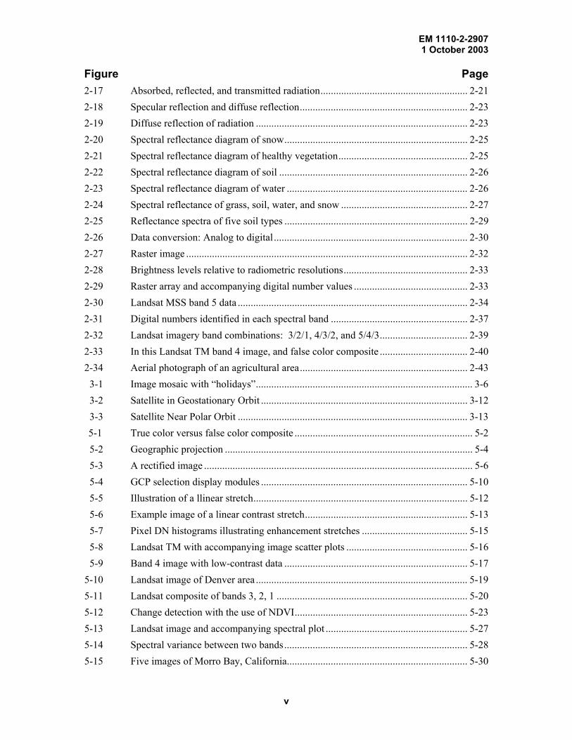
gree sign). The Kelvin scale has the same temperature intervals as the Celsius scale, so conversion between the two scales is simply a matter of adding or subtracting 273 (Table 2-1). Because all objects with temperatures above, or higher than, zero Kelvin emit elec-tromagnetic radiation, it is possible to collect, measure, and distinguish energy emitted from adjacent objects.

Table 2-1 Different scales used to measure object temperature. Conversion formulas are listed below.

Object Fahrenheit (oF) Celsius (oC) Kelvin (K) Absolute Zero –459.7 –273.2 0.0 Frozen Water 32.0 0.0 273.16 Boiling Water 212.0 100.0 373.16 Sun 9981.0 5527.0 5800.0 Earth 46.4 8.0 281.0 Human body 98.6 37.0 310.0

Conversion Formulas: Celsius to Fahrenheit: F° = (1.8 x C°) + 32 Fahrenheit to Celsius: C° = (F°- 32)/1.8 Celsius to Kelvin: K = C° + 273 Fahrenheit to Kelvin: K = [(F°- 32)/1.8] + 273

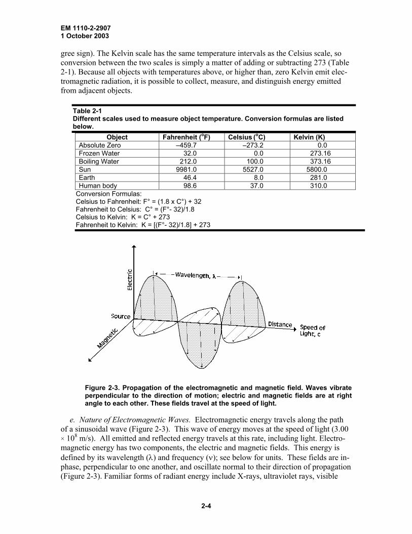
Figure 2-3. Propagation of the electromagnetic and magnetic field. Waves vibrate perpendicular to the direction of motion; electric and magnetic fields are at right angle to each other. These fields travel at the speed of light.

e. Nature of Electromagnetic Waves. Electromagnetic energy travels along the path of a sinusoidal wave (Figure 2-3). This wave of energy moves at the speed of light (3.00 × 108 m/s). All emitted and reflected energy travels at this rate, including light. Electro-magnetic energy has two components, the electric and magnetic fields. This energy is defined by its wavelength (λ) and frequency (ν); see below for units. These fields are in-phase, perpendicular to one another, and oscillate normal to their direction of propagation (Figure 2-3). Familiar forms of radiant energy include X-rays, ultraviolet rays, visible

2-4

EM 1110-2-2907 1 October 2003

light, microwaves, and radio waves. All of these waves move and behave similarly; they differ only in radiation intensity.

f. Measurement of Electromagnetic Wave Radiation.

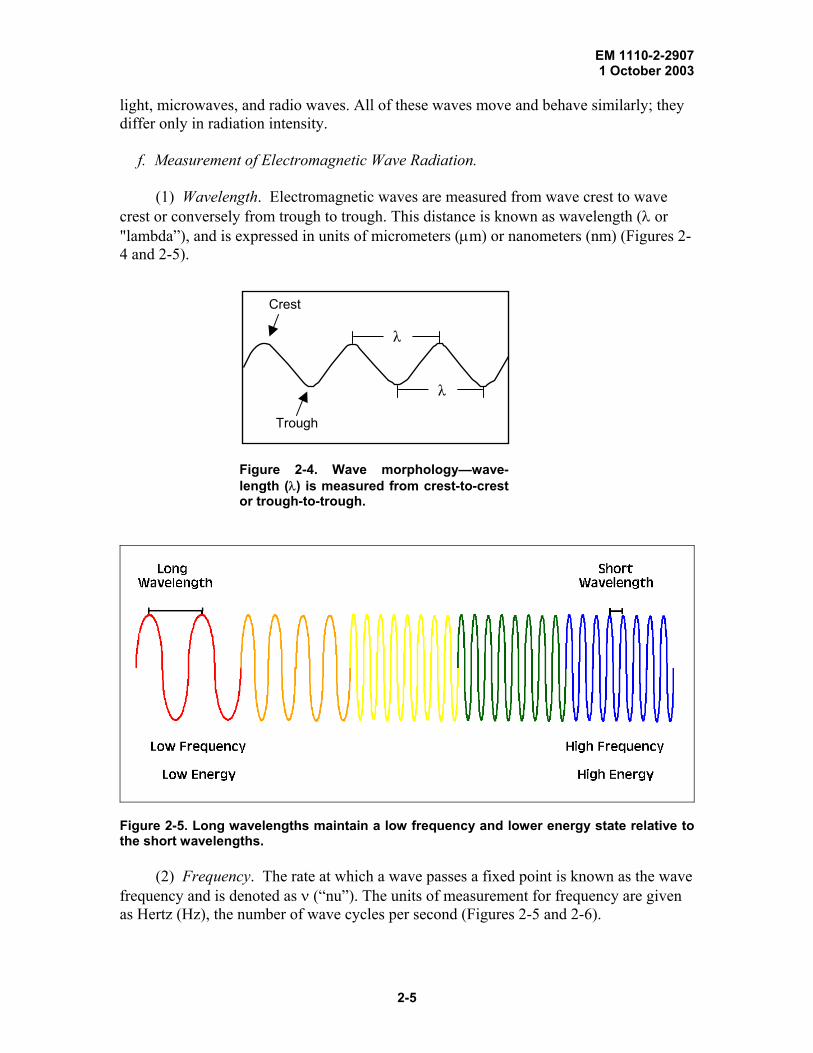
(1) Wavelength. Electromagnetic waves are measured from wave crest to wave crest or conversely from trough to trough. This distance is known as wavelength (λ or "lambda”), and is expressed in units of micrometers (µm) or nanometers (nm) (Figures 2-4 and 2-5).

λ

λ

Crest

Trough

Figure 2-4. Wave morphology—wave-length (λ) is measured from crest-to-crest or trough-to-trough.

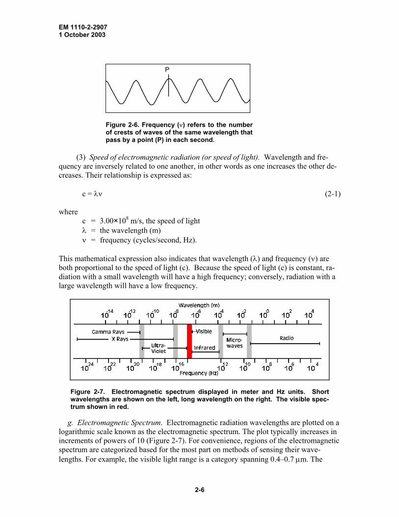
Figure 2-5. Long wavelengths maintain a low frequency and lower energy state relative to the short wavelengths.

(2) Frequency. The rate at which a wave passes a fixed point is known as the wave frequency and is denoted as ν (“nu”). The units of measurement for frequency are given as Hertz (Hz), the number of wave cycles per second (Figures 2-5 and 2-6).

2-5

EM 1110-2-2907 1 October 2003

P

Figure 2-6. Frequency (ν) refers to the number of crests of waves of the same wavelength that pass by a point (P) in each second.

(3) Speed of electromagnetic radiation (or speed of light). Wavelength and fre-

quency are inversely related to one another, in other words as one increases the other de-creases. Their relationship is expressed as:

c = λν (2-1) where

c = 3.00×108 m/s, the speed of light λ = the wavelength (m) ν = frequency (cycles/second, Hz).

This mathematical expression also indicates that wavelength (λ) and frequency (ν) are both proportional to the speed of light (c). Because the speed of light (c) is constant, ra-diation with a small wavelength will have a high frequency; conversely, radiation with a large wavelength will have a low frequency.

Figure 2-7. Electromagnetic spectrum displayed in meter and Hz units. Short wavelengths are shown on the left, long wavelength on the right. The visible spec-trum shown in red.

g. Electromagnetic Spectrum. Electromagnetic radiation wavelengths are plotted on a

logarithmic scale known as the electromagnetic spectrum. The plot typically increases in increments of powers of 10 (Figure 2-7). For convenience, regions of the electromagnetic spectrum are categorized based for the most part on methods of sensing their wave-lengths. For example, the visible light range is a category spanning 0.4–0.7 µm. The

2-6

EM 1110-2-2907 1 October 2003

minimum and maximum of this category is based on the ability of the human eye to sense radiation energy within the 0.4- to 0.7-µm wavelength range.

(1) Though the spectrum is divided up for convenience, it is truly a continuum of

increasing wavelengths with no inherent differences among the radiations of varying wavelengths. For instance, the scale in Figure 2-8 shows the color blue to be approxi-mately in the range of 435 to 520 nm (on other scales it is divided out at 446 to 520 nm). As the wavelengths proceed in the direction of green they become increasingly less blue and more green; the boundary is somewhat arbitrarily fixed at 520 nm to indicate this gradual change from blue to green.

Figure 2-8. Visible spectrum illustrated here in color.

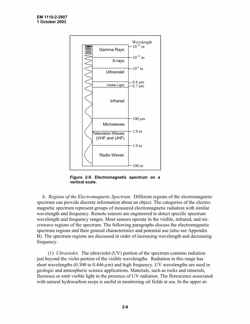
(2) Be aware of differences in the manner in which spectrum scales are drawn. Some authors place the long wavelengths to the right (such as those shown in this man-ual), while others place the longer wavelengths to the left. The scale can also be drawn on a vertical axis (Figure 2-9). Units can be depicted in meters, nanometers, micrometers, or a combination of these units. For clarity some authors add color in the visible spectrum to correspond to the appropriate wavelength.

2-7

EM 1110-2-2907 1 October 2003

Wavelength

Gamma Rays

X-rays

Ultraviolet

Visible Light

Infrared

Microwaves

Television Waves(VHF and UHF)

Radio Waves

0.7 µm 0.4 µm

100 m

1.0 m

1.0 m

100 µm

10-9 m

10-19 m

10-13 m

Figure 2-9. Electromagnetic spectrum on a vertical scale.

h. Regions of the Electromagnetic Spectrum. Different regions of the electromagnetic

spectrum can provide discrete information about an object. The categories of the electro-magnetic spectrum represent groups of measured electromagnetic radiation with similar wavelength and frequency. Remote sensors are engineered to detect specific spectrum wavelength and frequency ranges. Most sensors operate in the visible, infrared, and mi-crowave regions of the spectrum. The following paragraphs discuss the electromagnetic spectrum regions and their general characteristics and potential use (also see Appendix B). The spectrum regions are discussed in order of increasing wavelength and decreasing frequency.

(1) Ultraviolet. The ultraviolet (UV) portion of the spectrum contains radiation just beyond the violet portion of the visible wavelengths. Radiation in this range has short wavelengths (0.300 to 0.446 µm) and high frequency. UV wavelengths are used in geologic and atmospheric science applications. Materials, such as rocks and minerals, fluoresce or emit visible light in the presence of UV radiation. The florescence associated with natural hydrocarbon seeps is useful in monitoring oil fields at sea. In the upper at-

2-8

EM 1110-2-2907 1 October 2003

mosphere, ultraviolet light is greatly absorbed by ozone (O3) and becomes an important tool in tracking changes in the ozone layer.

(2) Visible Light. The radiation detected by human eyes is in the spectrum range aptly named the visible spectrum. Visible radiation or light is the only portion of the spectrum that can be perceived as colors. These wavelengths span a very short portion of the spectrum, ranging from approximately 0.4 to 0.7 µm. Because of this short range, the visible portion of the spectrum is plotted on a linear scale (Figure 2-8). This linear scale allows the individual colors in the visible spectrum to be discretely depicted. The shortest visible wavelength is violet and the longest is red.

(a) The visible colors and their corresponding wavelengths are listed below (Table 2-2) in micrometers and shown in nanometers in Figure 2.8.

Table 2-2 Wavelengths of the primary colors of the visible spectrum

Color Wavelength Violet 0.4–0.446 µm Blue 0.446–0.500 µm

Green 0.500–0.578 µm Yellow 0.578–0.592 µm Orange 0.592–0.620 µm

Red 0.620–0.7 µm

(b) Visible light detected by sensors depends greatly on the surface reflection characteristics of objects. Urban feature identification, soil/vegetation discrimination, ocean productivity, cloud cover, precipitation, snow, and ice cover are only a few exam-ples of current applications that use the visible range of the electromagnetic spectrum.

(3) Infrared. The portion of the spectrum adjacent to the visible range is the infra-red (IR) region. The infrared region, plotted logarithmically, ranges from approximately 0.7 to 100 µm, which is more than 100 times as wide as the visible portion. The infrared region is divided into two categories, the reflected IR and the emitted or thermal IR; this division is based on their radiation properties.

(a) Reflected Infrared. The reflected IR spans the 0.7- to 3.0-µm wavelengths. Reflected IR shares radiation properties exhibited by the visible portion and is thus used for similar purposes. Reflected IR is valuable for delineating healthy verses unhealthy or fallow vegetation, and for distinguishing among vegetation, soil, and rocks.

(b) Thermal Infrared. The thermal IR region represents the radiation that is

emitted from the Earth’s surface in the form of thermal energy. Thermal IR spans the 3.0- to 100-µm range. These wavelengths are useful for monitoring temperature variations in land, water, and ice.

(4) Microwave. Beyond the infrared is the microwave region, ranging on the spec-trum from 1 µm to 1 m (bands are listed in Table 2-3). Microwave radiation is the longest

2-9

EM 1110-2-2907 1 October 2003

wavelength used for remote sensing. This region includes a broad range of wavelengths; on the short wavelength end of the range, microwaves exhibit properties similar to the thermal IR radiation, whereas the longer wavelengths maintain properties similar to those used for radio broadcasts.

Table 2-3 Wavelengths of various bands in the microwave range Band Frequency (MHz) Wavelength (cm)

Ka 40,000–26,000 0.8–1.1 K 26,500–18,500 1.1–1.7 X 12,500–8000 2.4–3.8 C 8000–4000 3.8–7.5 L 2000–1000 15.0–30.0 P 1000–300 30.0–100.0

(a) Microwave remote sensing is used in the studies of meteorology, hydrology,

oceans, geology, agriculture, forestry, and ice, and for topographic mapping. Because mi-crowave emission is influenced by moisture content, it is useful for mapping soil mois-ture, sea ice, currents, and surface winds. Other applications include snow wetness analy-sis, profile measurements of atmospheric ozone and water vapor, and detection of oil slicks.

(b) For more information on spectrum regions, see Appendix B.

i. Energy as it Relates to Wavelength, Frequency, and Temperature. As stated above, energy can be quantified by its wavelength and frequency. It is also useful to measure the intensity exhibited by electromagnetic energy. Intensity can be described by Q and is measured in units of Joules.

(1) Quantifying Energy. The energy released from a radiating body in the form of a vibrating photon traveling at the speed of light can be quantified by relating the en-ergy’s wavelength with its frequency. The following equation shows the relationship between wavelength, frequency, and amount of energy in units of Joules:

Q = h ν (2-2)

Because c = λν, Q also equals Q = h c/λ where

Q = energy of a photon in Joules (J) h = Planck’s constant (6.6 × 10–34 J s) c = 3.00 × 108 m/s, the speed of light λ = wavelength (m) ν = frequency (cycles/second, Hz).

2-10

EM 1110-2-2907 1 October 2003

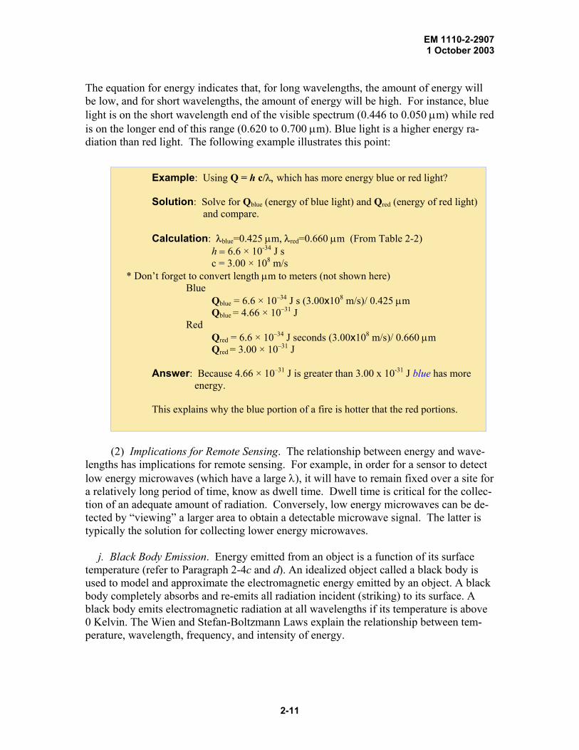
The equation for energy indicates that, for long wavelengths, the amount of energy will be low, and for short wavelengths, the amount of energy will be high. For instance, blue light is on the short wavelength end of the visible spectrum (0.446 to 0.050 µm) while red is on the longer end of this range (0.620 to 0.700 µm). Blue light is a higher energy ra-diation than red light. The following example illustrates this point:

Example: Using Q = h c/λ, which has more energy blue or red light? Solution: Solve for Qblue (energy of blue light) and Qred (energy of red light)

and compare. Calculation: λblue=0.425 µm, λred=0.660 µm (From Table 2-2)

h = 6.6 × 10-34 J s c = 3.00 × 108 m/s

* Don’t forget to convert length µm to meters (not shown here) Blue

Qblue = 6.6 × 10–34 J s (3.00x108 m/s)/ 0.425 µm Qblue = 4.66 × 10–31 J

Red Qred = 6.6 × 10–34 J seconds (3.00x108 m/s)/ 0.660 µm Qred = 3.00 × 10–31 J

Answer: Because 4.66 × 10–31 J is greater than 3.00 x 10-31 J blue has more

energy.

This explains why the blue portion of a fire is hotter that the red portions.

(2) Implications for Remote Sensing. The relationship between energy and wave-

lengths has implications for remote sensing. For example, in order for a sensor to detect low energy microwaves (which have a large λ), it will have to remain fixed over a site for a relatively long period of time, know as dwell time. Dwell time is critical for the collec-tion of an adequate amount of radiation. Conversely, low energy microwaves can be de-tected by “viewing” a larger area to obtain a detectable microwave signal. The latter is typically the solution for collecting lower energy microwaves.

j. Black Body Emission. Energy emitted from an object is a function of its surface temperature (refer to Paragraph 2-4c and d). An idealized object called a black body is used to model and approximate the electromagnetic energy emitted by an object. A black body completely absorbs and re-emits all radiation incident (striking) to its surface. A black body emits electromagnetic radiation at all wavelengths if its temperature is above 0 Kelvin. The Wien and Stefan-Boltzmann Laws explain the relationship between tem-perature, wavelength, frequency, and intensity of energy.

2-11

EM 1110-2-2907 1 October 2003

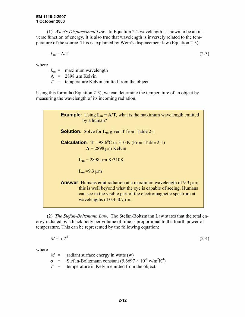
(1) Wien's Displacement Law. In Equation 2-2 wavelength is shown to be an in-

verse function of energy. It is also true that wavelength is inversely related to the tem-perature of the source. This is explained by Wein’s displacement law (Equation 2-3):

Lm = A/T (2-3) where

Lm = maximum wavelength A = 2898 µm Kelvin T = temperature Kelvin emitted from the object.

Using this formula (Equation 2-3), we can determine the temperature of an object by measuring the wavelength of its incoming radiation.

Example: Using Lm = A/T, what is the maximum wavelength emitted by a human?

Solution: Solve for Lm given T from Table 2-1 Calculation: T = 98.6oC or 310 K (From Table 2-1)

A = 2898 µm Kelvin

Lm = 2898 µm K/310K Lm =9.3 µm

Answer: Humans emit radiation at a maximum wavelength of 9.3 µm;

this is well beyond what the eye is capable of seeing. Humans can see in the visible part of the electromagnetic spectrum at wavelengths of 0.4–0.7µm.

(2) The Stefan-Boltzmann Law. The Stefan-Boltzmann Law states that the total en-

ergy radiated by a black body per volume of time is proportional to the fourth power of temperature. This can be represented by the following equation:

M = σ T4 (2-4) where

M = radiant surface energy in watts (w) σ = Stefan-Boltzmann constant (5.6697 × 10-8 w/m2K4) T = temperature in Kelvin emitted from the object.

2-12

EM 1110-2-2907 1 October 2003

This simply means that the total energy emitted from an object rapidly increases with only slight increases in temperature. Therefore, a hotter black body emits more radiation at each wavelength than a cooler one (Figure 2-10).

1000 2000 3000 40000

Wavelength (λ) nm

Spe

ctra

l Int

ensi

ty

Yellow = 6000 K Green = 5000K Brown = 4000 K

Figure 2-10. Spectral intensity of different emitted tempera-tures. The horizontal axis is wavelength in nm and the verti-cal axis is spectral intensity. The vertical bars denote the peak intensity for the temperatures presented. These peaks indicate a shift toward higher energies (lower wavelengths) with increasing temperatures. Modified from http://rst.gsfc.nasa.gov/Front/overview.html.

(3) Summary. Together, the Wien and Stefan-Boltzmann Laws are powerful tools.

From these equations, temperature and radiant energy can be determined from an object’s emitted radiation. For example, ocean water temperature distribution can be mapped by measuring the emitted radiation; discrete temperatures over a forest canopy can be de-tected; and surface temperatures of distant solar system objects can be estimated.

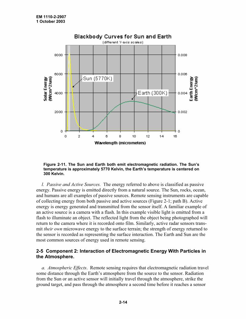
k. The Sun and Earth as Black Bodies. The Sun's surface temperature is 5800 K; at that temperature much of the energy is radiated as visible light (Figure 2-11). We can therefore see much of the spectra emitted from the sun. Scientists speculate the human eye has evolved to take advantage of the portion of the electromagnetic spectrum most readily available (i.e., sunlight). Also, note from the figure the Earth’s emitted radiation peaks between 6 to 16 µm; to “see” these wavelengths one must use a remote sensing detector.

2-13

EM 1110-2-2907 1 October 2003

Figure 2-11. The Sun and Earth both emit electromagnetic radiation. The Sun’s temperature is approximately 5770 Kelvin, the Earth’s temperature is centered on 300 Kelvin.

l. Passive and Active Sources. The energy referred to above is classified as passive

energy. Passive energy is emitted directly from a natural source. The Sun, rocks, ocean, and humans are all examples of passive sources. Remote sensing instruments are capable of collecting energy from both passive and active sources (Figure 2-1; path B). Active energy is energy generated and transmitted from the sensor itself. A familiar example of an active source is a camera with a flash. In this example visible light is emitted from a flash to illuminate an object. The reflected light from the object being photographed will return to the camera where it is recorded onto film. Similarly, active radar sensors trans-mit their own microwave energy to the surface terrain; the strength of energy returned to the sensor is recorded as representing the surface interaction. The Earth and Sun are the most common sources of energy used in remote sensing. 2-5 Component 2: Interaction of Electromagnetic Energy With Particles in the Atmosphere.

a. Atmospheric Effects. Remote sensing requires that electromagnetic radiation travel some distance through the Earth’s atmosphere from the source to the sensor. Radiation from the Sun or an active sensor will initially travel through the atmosphere, strike the ground target, and pass through the atmosphere a second time before it reaches a sensor

2-14

EM 1110-2-2907 1 October 2003

(Figure 2-1; path B). The total distance the radiation travels in the atmosphere is called the path length. For electromagnetic radiation emitted from the Earth, the path length will be half the path length of the radiation from the sun or an active source.

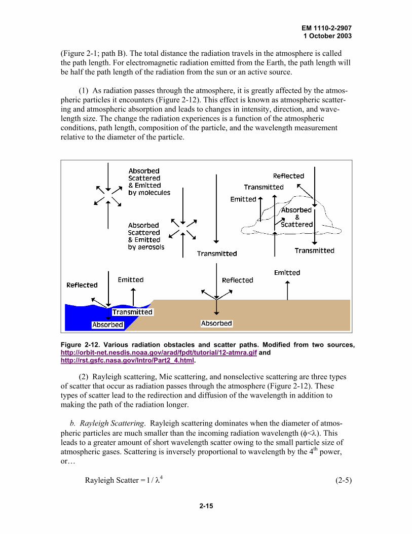
(1) As radiation passes through the atmosphere, it is greatly affected by the atmos-pheric particles it encounters (Figure 2-12). This effect is known as atmospheric scatter-ing and atmospheric absorption and leads to changes in intensity, direction, and wave-length size. The change the radiation experiences is a function of the atmospheric conditions, path length, composition of the particle, and the wavelength measurement relative to the diameter of the particle.

Figure 2-12. Various radiation obstacles and scatter paths. Modified from two sources, http://orbit-net.nesdis.noaa.gov/arad/fpdt/tutorial/12-atmra.gif and http://rst.gsfc.nasa.gov/Intro/Part2_4.html.

(2) Rayleigh scattering, Mie scattering, and nonselective scattering are three types of scatter that occur as radiation passes through the atmosphere (Figure 2-12). These types of scatter lead to the redirection and diffusion of the wavelength in addition to making the path of the radiation longer.

b. Rayleigh Scattering. Rayleigh scattering dominates when the diameter of atmos-pheric particles are much smaller than the incoming radiation wavelength (φ<λ). This leads to a greater amount of short wavelength scatter owing to the small particle size of atmospheric gases. Scattering is inversely proportional to wavelength by the 4th power, or…

Rayleigh Scatter = 1/ λ4 (2-5)

2-15

EM 1110-2-2907 1 October 2003

where λ is the wavelength (m). This means that short wavelengths will undergo a large amount of scatter, while large wavelengths will experience little scatter. Smaller wave-length radiation reaching the sensor will appear more diffuse.

c. Why the sky is blue? Rayleigh scattering accounts for the Earth’s blue sky. We see predominately blue because the wavelengths in the blue region (0.446–0.500 µm) are more scattered than other spectra in the visible range. At dusk, when the sun is low in the horizon creating a longer path length, the sky appears more red and orange. The longer path length leads to an increase in Rayleigh scatter and results in the depletion of the blue wavelengths. Only the longer red and orange wavelengths will reach our eyes, hence beautiful orange and red sunsets. In contrast, our moon has no atmosphere; subsequently, there is no Rayleigh scatter. This explains why the moon’s sky appears black (shadows on the moon are more black than shadows on the Earth for the same reason, see Figure 2-13).

Figure 2-13. Moon rising in the Earth’s horizon (left). The Earth’s atmosphere appears blue due to Rayleigh Scatter. Photo taken from the moon’s surface shows the Earth rising (right). The Moon has no atmosphere, thus no atmospheric scatter. Its sky appears black. Images taken from: http://antwrp.gsfc.nasa.gov/apod/ap001028.html, and http://antwrp.gsfc.nasa.gov/apod/ap001231.html.

d. Mie Scattering. Mie scattering occurs when an atmospheric particle diameter is equal to the radiation’s wavelength (φ = λ). This leads to a greater amount of scatter in the long wavelength region of the spectrum. Mie scattering tends to occur in the presence of water vapor and dust and will dominate in overcast or humid conditions. This type of scattering explains the reddish hues of the sky following a forest fire or volcanic eruption.

e. Nonselective Scattering. Nonselective scattering dominates when the diameter of at-mospheric particles (5–100 µm) is much larger than the incoming radiation wavelength (φ>>λ). This leads to the scatter of visible, near infrared, and mid-infrared. All these wavelengths are equally scattered and will combine to create a white appearance in the sky; this is why clouds appear white (Figure 2-14).

2-16

EM 1110-2-2907 1 October 2003

Figure 2-14. Non-selective scattering by larger atmospheric particles (like water droplets) affects all wavelengths, causing white clouds.

Figure 2-15. Atmospheric windows with wavelength on the x-axis and percent transmission measured in hertz on the y-axis. High transmission corresponds to an “atmospheric win-dow,” which allows radiation to penetrate the Earth’s atmosphere. The chemical formula is given for the molecule responsible for sunlight absorption at particular wavelengths across the spectrum. Modified from http://earthobservatory.nasa.gov:81/Library/RemoteSensing/remote_04.html.

f. Atmospheric Absorption and Atmospheric Windows. Absorption of electromagnetic radiation is another mechanism at work in the atmosphere. This phenomenon occurs as molecules absorb radiant energy at various wavelengths (Figure 2-12). Ozone (O3), car-bon dioxide (CO2), and water vapor (H2O) are the three main atmospheric compounds that absorb radiation. Each gas absorbs radiation at a particular wavelength. To a lesser extent, oxygen (O2) and nitrogen dioxide (NO2) also absorb radiation (Figure 2-15). Be-

2-17

EM 1110-2-2907 1 October 2003

low is a summary of these three major atmospheric constituents and their significance in remote sensing.

g. The role of atmospheric compounds in the atmosphere.

(1) Ozone. Ozone (O3) absorbs harmful ultraviolet radiation from the sun. Without this protective layer in the atmosphere, our skin would burn when exposed to sunlight.

(2) Carbon Dioxide. Carbon dioxide (CO2) is called a greenhouse gas because it greatly absorbs thermal infrared radiation. Carbon dioxide thus serves to trap heat in the atmosphere from radiation emitted from both the Sun and the Earth.

(3) Water vapor. Water vapor (H2O) in the atmosphere absorbs incoming long-wave infrared and shortwave microwave radiation (22 to 1 µm). Water vapor in the lower atmosphere varies annually from location to location. For example, the air mass above a desert would have very little water vapor to absorb energy, while the tropics would have high concentrations of water vapor (i.e., high humidity).

(4) Summary. Because these molecules absorb radiation in very specific regions of the spectrum, the engineering and design of spectral sensors are developed to collect wavelength data not influenced by atmospheric absorption. The areas of the spectrum that are not severely influenced by atmospheric absorption are the most useful regions, and are called atmospheric windows.

h. Summary of Atmospheric Scattering and Absorption. Together atmospheric scatter

and absorption place limitations on the spectra range useful for remote sensing. Table 2-4 summarizes the causes and effects of atmospheric scattering and absorption due to at-mospheric effects.

i. Spectrum Bands. By comparing the characteristics of the radiation in atmospheric

windows (Figure 2-15; areas where reflectance on the y-axis is high), groups or bands of wavelengths have been shown to effectively delineate objects at or near the Earth’s sur-face. The visible portion of the spectrum coincides with an atmospheric window, and the maximum emitted energy from the Sun. Thermal infrared energy emitted by the Earth corresponds to an atmospheric window around 10 µm, while the large window at wave-lengths larger than 1 mm is associated with the microwave region (Figure 2-16).

Table 2-4 Properties of Radiation Scatter and Absorption in the Atmosphere

Atmospheric Scattering

Diameter (φ) of particle relative to incoming

wavelength (λ) Result

Rayleigh scattering φ<λ Short wavelengths are scattered Mie scattering φ=λ Long wavelengths are scattered Nonselective scattering

φ>>λ All wavelengths are equally scattered

Absorption No relationship CO2, H20, and O3 remove wavelengths

2-18

EM 1110-2-2907 1 October 2003

Figure 2-16. Atmospheric windows related to the emitted energy supplied by the sun and the Earth. Notice that the sun’s maximum output (shown in yellow) coincides with an atmos-pheric window in the visible range of the spectrum. This phenomenon is important in optical remote sensing. Modified from http://www.ccrs.nrcan.gc.ca/ccrs/learn/tutorials/fundam/chapter1/chapter1_4_e.html.

j. Geometric Effects. Random and non-random error occurs during the acquisition of

radiation data. Error can be attributed to such causes as sun angle, angle of sensor, ele-vation of sensor, skew distortion from the Earth’s rotation, and path length. Malfunctions in the sensor as it collects data and the motion of the platform are additional sources of error. As the sensor collects data, it can develop sweep irregularities that result in hun-dreds of meters of error. The pitch, roll, and yaw of platforms can create hundreds to thousands of meters of error, depending on the altitude and resolution of the sensor. Geometric corrections are typically applied by re-sampling an image, a process that shifts and recalculates the data. The most commonly used re-sampling techniques include the use of ground control points (see Chapter 5), applying a mathematical model, or re-sam-pling by nearest neighbor or cubic convolution.

k. Atmospheric and Geometric Corrections. Data correction is required for calculat-ing reflectance values from radiance values (see Equation 2-5 below) recorded at a sensor and for reducing positional distortion caused by known sensor error. It is extremely im-portant to make corrections when comparing one scene with another and when perform-ing a temporal analysis. Corrected data can then be evaluated in relation to a spectral data library (see Paragraph 2-6b) to compare an object to its standard. Corrections are not nec-essary if objects are to be distinguished by relative comparisons within an individual scene.

2-19

EM 1110-2-2907 1 October 2003

l. Atmospheric Correction Techniques. Data can be corrected by re-sampling with the

use of image processing software such as ERDAS Imagine or ENVI, or by the use of specialty software. In many of the image processing software packages, atmospheric cor-rection models are included as a component of an import process. Also, data may have some corrections applied by the vendor. When acquiring data, it is important to be aware of any corrections that may have been applied to the data (see Chapter 4). Correction models can be mathematically or empirically derived.

m. Empirical Modeling Corrections. Measured or empirical data collected on the ground at the time the sensor passes overhead allows for a comparison between ground spectral reflectance measurements and sensor radiation reflectance measurements. Typi-cal data collection includes spectral measurements of selected objects within a scene as well as a sampling of the atmospheric properties that prevailed during sensor acquisition. The empirical data are then compared with image data to interpolate an appropriate cor-rection. Empirical corrections have many limitations, including cost, spectral equipment availability, site accessibility, and advanced preparation. It is critical to time the field spectral data collection to coincide with the same day and time the satellite collects ra-diation data. This requires knowledge of the satellite’s path and revisit schedule. For ar-chived data it is impossible to collect the field spectral measurements needed for devel-oping an empirical model that will correct atmospheric error. In such a case, a mathematical model using an estimate of the field parameters must complete the correc-tion.

n. Mathematical Modeling Corrections. Alternatively, corrections that are mathe-matically derived rely on estimated atmospheric parameters from the scene. These pa-rameters include visibility, humidity, and the percent and type of aerosols present in the atmosphere. Data values or ratios are used to determine the atmospheric parameters. Subsequently a mathematical model is extracted and applied to the data for re-sampling. This type of modeling can be completed with the aid of software programs such as 6S, MODTRAN, and ATREM (see http://atol.ucsd.edu/~pflatau/rtelib/ for a list and descrip-tion of correction modeling software).

2-6 Component 3: Electromagnetic Energy Interacts with Surface and Near Surface Objects.

a. Energy Interactions with the Earth's Surface. Electromagnetic energy that reaches a target will be absorbed, transmitted, and reflected. The proportion of each depends on the composition and texture of the target’s surface. Figure 2-17 illustrates these three in-teractions. Much of remote sensing is concerned with reflected energy.

2-20

EM 1110-2-2907 1 October 2003

Transmitted

Reflected

Absorbed

Emitted

Figure 2-17. Radiation striking a target is reflected, ab-sorbed, or transmitted through the medium. Radiation is also emitted from ground targets.

(1) Absorption. Absorption occurs when radiation penetrates a surface and is in-

corporated into the molecular structure of the object. All objects absorb incoming inci-dent radiation to some degree. Absorbed radiation can later be emitted back to the atmos-phere. Emitted radiation is useful in thermal studies, but will not be discussed in detail in this work (see Lillisand and Keifer [1994] Remote Sensing and Image Interpretation for information on emitted energy).

(2) Transmission. Transmission occurs when radiation passes through material and exits the other side of the object. Transmission plays a minor role in the energy’s interac-tion with the target. This is attributable to the tendency for radiation to be absorbed be-fore it is entirely transmitted. Transmission is a function of the properties of the object.

(3) Reflection. Reflection occurs when radiation is neither absorbed nor transmit-ted. The reflection of the energy depends on the properties of the object and surface roughness relative to the wavelength of the incident radiation. Differences in surface properties allow the distinction of one object from another.

(a) Absorption, transmission, and reflection are related to one another by

EI = EA + ET +ER (2-6) where

EI = incident energy striking an object EA = absorbed radiation ET = transmitted energy ER = reflected energy.

2-21

EM 1110-2-2907 1 October 2003

(b) The amount of each interaction will be a function of the incoming wave-

length, the composition of the material, and the smoothness of the surface.

(4) Reflectance of Radiation. Reflectance is simply a measurement of the percent-age of incoming or incident energy that a surface reflects

Reflectance = Reflected energy/Incident energy (2-7) where incident energy is the amount of incoming radiant energy and reflected energy is the amount of energy bouncing off the object. Or from equation 2-5:

EI = EA + ET +ER

Reflectance = ER/EI (2-8) Reflectance is a fixed characteristic of an object. Surface features can be distinguished by comparing the reflectance of different objects at each wavelength. Reflectance com-parisons rely on the unchanging proportion of reflected energy relative to the sum of in-coming energy. This permits the distinction of objects regardless of the amount of inci-dent energy. Unique objects reflect differently, while similar objects only reflect differently if there has been a physical or chemical change. Note: reflectance is not the same as reflection.

Specular and diffuse reflection The nature of reflectance is controlled by the wavelength of the radiation relative to the surface texture. Surface texture is defined by the roughness or bumpiness of the surface relative to the wavelength. Objects display a range of reflectance from diffuse to specular. Specular reflectance is a mirror-like reflection, which occurs when an object with a smooth surface reflects in one direction. The incoming radiation will reflect off a surface at the same angle of incidence (Figure 2-18). Diffuse or Lambertian reflectance reflects in all directions owing to a rough surface. This type of reflectance gives the most information about an object.

2-22

EM 1110-2-2907 1 October 2003

Figure 2-18. Specular reflection or mirror-like reflection (left) and diffuse reflection (right).

(5) Spectral Radiance. As reflected energy radiates away from an object, it moves in a hemi-spherical path. The sensor measures only a small portion of the reflected radia-tion—the portion along the path between the object and the sensor (Figure 2-19). This measured radiance is known as the spectral radiance (Equation 2-9).

I = Reflected radiance + Emitted radiance 2-9 where I = radiant intensity in watts per steradian (W sr–1). (Steradian is the unit of cone angle, abbreviated sr, 1 sr equals 4π. See the following for more details on steradian.) http://whatis.techtarget.com/definition/0%2C%2Csid9_gci528813%2C00.html

Figure 2-19. Diffuse reflection of radiation from a single target point. Radiation moves outward in a hemispherical path. Notice the sensor only samples radiation from a single vector. Modified after http://rst.gsfc.nasa.gov/Intro/Part2_3html.html.

2-23

EM 1110-2-2907 1 October 2003

(6) Summary. Spectral radiance is the amount of energy received at the sensor per

time, per area, in the direction of the sensor (measured in steradian), and it is measured per wavelength. The sensor therefore measures the fraction of reflectance for a given area/time for every wavelength as well as the emitted. Reflected and emitted radiance is calculated by the integration of energy over the reflected hemisphere resulting from dif-fuse reflection (see http://rsd.gsfc.nasa.gov/goes/text/reflectance.pdf for details on this complex calculation). Reflected radiance is orders of magnitude greater than emitted ra-diance. The following paragraphs, therefore, focus on reflected radiance.

b. Spectral Reflectance Curves.

(1) Background.

(a) Remote sensing consists of making spectral measurements over space: how much of what “color” of light is coming from what place on the ground. One thing that a remote sensing applications scientist hopes for, but which is not always true, is that sur-face features of interest will have different colors so that they will be distinct in remote sensing data.

(b) A surface feature’s color can be characterized by the percentage of incoming electromagnetic energy (illumination) it reflects at each wavelength across the electro-magnetic spectrum. This is its spectral reflectance curve or “spectral signature”; it is an unchanging property of the material. For example, an object such as a leaf may reflect 3% of incoming blue light, 10% of green light and 3% of red light. The amount of light it reflects depends on the amount and wavelength of incoming illumination, but the per-cents are constant. Unfortunately, remote sensing instruments do not record reflectance directly, rather radiance, which is the amount (not the percent) of electromagnetic energy received in selected wavelength bands. A change in illumination, more or less intense sun for instance, will change the radiance. Spectral signatures are often represented as plots or graphs, with wavelength on the horizontal axis, and the reflectance on the vertical axis (Figure 2-20 provides a spectral signature for snow).

(2) Important Reflectance Curves and Critical Spectral Regions. While there are too many surface types to memorize all their spectral signatures, it is helpful to be famil-iar with the basic spectral characteristics of green vegetation, soil, and water. This in turn helps determine which regions of the spectrum are most important for distinguishing these surface types.

(3) Spectral Reflectance of Green Vegetation. Reflectance of green vegetation (Figure 2-21) is low in the visible portion of the spectrum owing to chlorophyll absorp-tion, high in the near IR due to the cell structure of the plant, and lower again in the shortwave IR due to water in the cells. Within the visible portion of the spectrum, there is a local reflectance peak in the green (0.55 µm) between the blue (0.45 µm) and red (0.68 µm) chlorophyll absorption valleys (Samson, 2000; Lillesand and Kiefer, 1994).

2-24

EM 1110-2-2907 1 October 2003

Figure 2-20. Spectral reflectance of snow. Graph developed for Prospect (2002 and 2003) using Aster Spectral Library (http://speclib.jpl.nasa.gov/) data

Figure 2-21. Spectral reflectance of healthy vegetation. Graph developed for Prospect (2002 and 2003) using Aster Spectral Library (http://speclib.jpl.nasa.gov/) data

(4) Spectral Reflectance of Soil. Soil reflectance (Figure 2-22) typically increases

with wavelength in the visible portion of the spectrum and then stays relatively constant in the near-IR and shortwave IR, with some local dips due to water absorption at 1.4 and 1.9 µm and due to clay absorption at 1.4 and 2.2 µm (Lillesand and Kiefer, 1994).

2-25

EM 1110-2-2907 1 October 2003

Figure 2-22. Spectral reflectance of one variety of soil. Graph developed for Prospect (2002 and 2003) using Aster Spectral Library (http://speclib.jpl.nasa.gov/) data

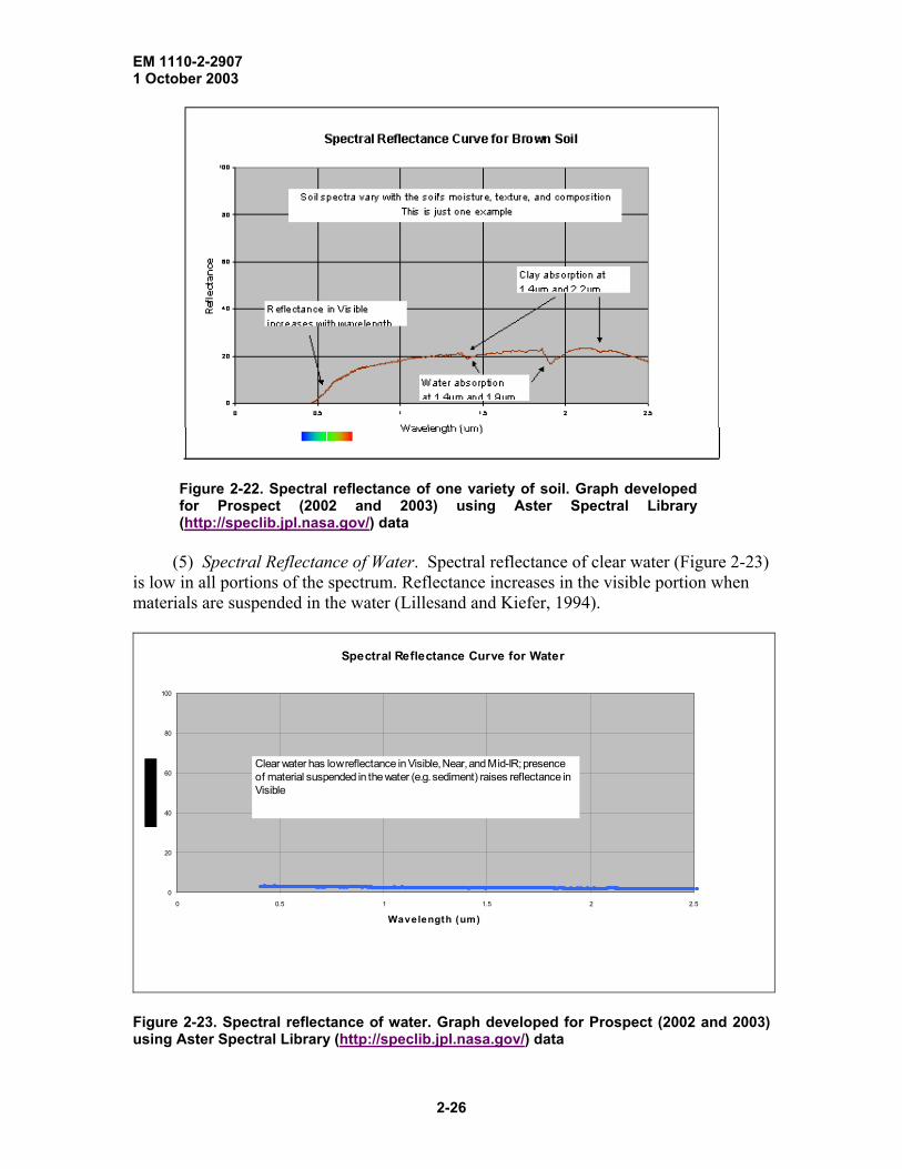
(5) Spectral Reflectance of Water. Spectral reflectance of clear water (Figure 2-23) is low in all portions of the spectrum. Reflectance increases in the visible portion when materials are suspended in the water (Lillesand and Kiefer, 1994).

Spectral Reflectance Curve for Water

0

20

40

60

80

100

0 0.5 1 1.5 2 2.5

Wavelength (um)

Clear water has low reflectance in Visible, Near, and Mid-IR; presence of material suspended in the water (e.g. sediment) raises reflectance in Visible

Figure 2-23. Spectral reflectance of water. Graph developed for Prospect (2002 and 2003) using Aster Spectral Library (http://speclib.jpl.nasa.gov/) data

2-26

EM 1110-2-2907 1 October 2003

(6) Critical Spectral Regions. The spectral regions that will be most useful in a remote sensing application depend on the spectral signatures of the surface features to be distinguished. The figure below (Figure 2-24) shows that the visible blue region is not very useful for separating vegetation, soil, and water surface types, since all three have similar reflectance, but visible red wavelengths separate soil and vegetation. In the near-IR (refers to 0.7 to 2.5 µm), all three types are distinct, with vegetation high, soil inter-mediate, and water low in reflectance. In the shortwave IR, water is distinctly low, while vegetation and soil exchange positions across the spectral region. When spectral signa-tures cross, the spectral regions on either side of the intersection are especially useful. For instance, green vegetation and soil signatures cross at about 0.7 µm, so the 0.6- (visi-ble red) and 0.8-µm and larger wavelengths (near IR) regions are of particular interest in separating these types. In general, vegetation studies include near IR and visible red data, water vs. land distinction include near IR or SW IR. Water quality studies might include the visible portion of the spectrum to detect suspended materials.

Figure 2-24. Spectral reflectance of grass, soil, water, and snow. Graph developed for Prospect (2002 and 2003) using Aster Spectral Library (http://speclib.jpl.nasa.gov/) data

(7) Spectral Libraries. As noted above, detailed spectral signatures of known ma-terials are useful in determining whether and in what spectral regions surface features are distinct. Spectral reflectance curves for many materials (especially minerals) are avail-able in existing reference archives (spectral libraries). Data in spectral libraries are gath-ered under controlled conditions, quality checked, and documented. Since these are re-

2-27

EM 1110-2-2907 1 October 2003

flectance curves, and reflectance is theoretically an unvarying property of a material, the spectra in the spectral libraries should match those of the same materials at other times or places.

(a) If data in spectral libraries are not appropriate, reflectance curves can be ac-quired using a spectrometer. The instrument is aimed at a known target and records the radiance reflected from the target over a fixed range of the spectrum (the 0.4- to 2.5-µm range is relatively common). The instrument must also measure the radiance coming in to the target, so that the reflected radiance can be divided by incoming radiance at each wavelength to determine spectral reflectance of the target. Given the time and expense of gathering spectra data, it is best to check spectral libraries first.

(b) Two major spectral libraries available on the internet (where spectra can be downloaded and processed locally if needed) include:

• US Geological Survey Digital Spectral Library (Clark et al. 1993) http://speclab.cr.usgs.gov/spectral-lib.html “Researchers at the Spectroscopy lab have measured the spectral reflectance of hundreds of materials in the lab and have compiled a spectral library. The libraries are used as ref-erences for material identification in remote sensing images.”

• ASTER Spectral Library (Jet Propulsion Laboratory, 1999) http://speclib.jpl.nasa.gov/ “Welcome to the ASTER spectral library, a compilation of almost 2000 spectra of natural and man made materials.”

(c) The ASTER spectral library includes data from three other spectral libraries: the Johns Hopkins University (JHU) Spectral Library, the Jet Propulsion Laboratory (JPL) Spectral Library, and the United States Geological Survey (USGS—Reston) Spec-tral Library.”

(8) Real Life and Spectral Signatures. Knowledge of spectral reflectance curves is useful if you are searching a remote sensing image for a particular material, or if you want to identify what material a particular pixel represents. Before comparing image data with spectral library reflectance curves, however, you must be aware of several things.

(a) Image data, which often measure radiance above the atmosphere, may have to be corrected for atmospheric effects and converted to reflectance.

(b) Spectral reflectance curves, which typically have hundreds or thousands of spectral bands, may have to be resampled to match the spectral bands of the remote sensing image (typically a few to a couple of hundred).

(c) There is spectral variance within a surface type that a single spectral library

reflectance curve does not show. For instance, the Figure 2-25 below shows spectra for a number of different soil types. Before depending on small spectral distinctions to separate

2-28

EM 1110-2-2907 1 October 2003

surface types, a note of caution is required: make sure that differences within a type do not drown out the differences between types.

(d) While spectral libraries have known targets that are “pure types,” a pixel in a

remote sensing image very often includes a mixture of pure types: along edges of types (e.g., water and land along a shoreline), or interspersed within a type (e.g., shadows in a tree canopy, or soil background behind an agricultural crop).

Figure 2-25. Reflectance spectra of five soil types: A—soils having > 2% organic matter content (OMC) and fine texture; B— soils having < 2% OMC and low iron content; C—soils having < 2% OMC and medium iron content; D—soils having > 2% OMC, and coarse tex-ture; and E— soil having fine texture and high iron-oxide content (> 4%). 2-7 Component 4: Energy is Detected and Recorded by the Sensor. Earlier paragraphs of this chapter explored the nature of emitted and reflected energy and the in-teractions that influence the resultant radiation as it traverses from source to target to sen-sor. This paragraph will examine the steps necessary to transfer radiation data from the satellite to the ground and the subsequent conversion of the data to a useable form for display on a computer.

a. Conversion of the Radiation to Data. Data collected at a sensor are converted from a continuous analog to a digital number. This is a necessary conversion, as electromag-netic waves arrive at the sensor as a continuous stream of radiation. The incoming radia-tion is sampled at regular time intervals and assigned a value (Figure 2-26). The value given to the data is based on the use of a 6-, 7-, 8-, 9-, or 10-bit binary computer coding scale; powers of 2 play an important role in this system. Using this coding allows a com-puter to store and display the data. The computer translates the sequence of binary num-bers, given as ones and zeros, into a set of instructions with only two possible outcomes (1 or 0, meaning “on” or “off”). The binary scale that is chosen (i.e., 8 bit data) will de-pend on the level of brightness that the radiation exhibits. The brightness level is deter-mined by measuring the voltage of the incoming energy. Below in Table 2-5 is a list of select bit integer binary scales and their corresponding number of brightness levels. The ranges are derived by exponentially raising the base of 2 by the number of bits.

2-29

EM 1110-2-2907 1 October 2003

Vol

tage

(ν);

reco

rded

as a

co

ntin

uous

stre

am o

f dat

a

Time Dashed lines denote the sampling interval. DN value is given above the sampled point.

0

255

Digital N

umber (D

N)

54

68

92 103

112

9995

192

150

138

204

121 118

Figure 2-26. Diagram illustrates the digital sampling of continuous analog voltage data. The DN values above the curve represent the digital output values for that line segment.

Table 2-5 Digital number value ranges for various bit data

Number of bits Exponent of 2 Digital Number (DN) Value Range 6 26 64 0–63 8 28 256 0–255 10 210 1024 0–1023 16 216 65536 0–65535

b. Diversion on Data Type. Digital number values for raw remote sensing data are

usually integers. Occasionally, data can be expressed as a decimal. The most popular code for representing real numbers (a number that contains a fraction, i.e., 0.5, which is one-half) is called the IEEE (Institute of Electrical and Electronics Engineers, pro-nounced I-triple-E) Floating-Point Standard. ASCII text (American Standard Code for Information Interchange; pronounced ask-ee) is another alternative computing value sys-

2-30

EM 1110-2-2907 1 October 2003

tem. This system is used for text data. You may need to be aware of the type of data used in an image, particularly when determining the digital number in a pixel.

c. Transferring the Data from the Satellite to the Ground. The transfer of data stored in the sensor from the satellite to the user is similar to the transmission of more familiar signals, such as radio and television broadcasts and cellular phone conversations. Every-thing we see and hear, whether it is a TV program with audio or a satellite image, origi-nates as a form of electromagnetic radiation. To transfer satellite data from the sensor to a location on the ground, the radiation is coded (described in Paragraph 2-7a) and attached to a signal. The signal is generally a high frequency electromagnetic wave that travels at the speed of light. The data are instantaneously transferred and detected with the use of an appropriate antenna and receiver.

d. Satellite Receiving Stations.

(1) Satellite receiving stations are positioned throughout the world. Each satellite program has its own fleet of receiving stations with a limited range from which it can pick up the satellite signal. For an example of locations and coverage of SPOT receiving stations go to http://www.spotimage.fr/home/system/introexp/station/welcome.htm.

(2) Satellites can only transmit data when in range of a receiving station. When outside of a receiving range, satellites will store data until they fly within range of the next receiving station. Some satellite receiving stations are mobile and can be placed on airplanes for swift deployment. A mobile receiving station is extremely valuable for the immediate acquisition of data relating to an emergency situation (flooding, forest fire, military strikes).

e. Data is Prepared for User. Once transmitted the carrier signal is filtered from the data, which are decoded and recorded onto a high-density digital tape (HDDT) or a CD-ROM, and in some cases transferred via file transfer protocol (FTP). The data can then undergo geometric and radiometric preprocessing, generally by the vendor. The data are subsequently recorded onto tape or CD compatible for a computer.

f. Hardware and Software Requirements. The hardware and software needed for sat-ellite image analysis will depend on the type of data to be processed. A number of free image processing software programs are available and can be downloaded from the inter-net. Some vendors provide a free trial or free tutorials. Highly sophisticated and powerful software packages are also available for purchase. These packages require robust hard-ware systems to sustain extended use. Software and hardware must be capable of man-aging the requirements of a variety of data formats and file sizes. A single satellite image file can be 300 MB prior to enhancement processing. Once processed and enhanced, the resulting data files will be large and will require storage for continued analysis. Because of the size of these files, software and hardware can be pushed to its limits. Regularly save and back up your data files as software and hardware pushed to its limits can crash,

2-31

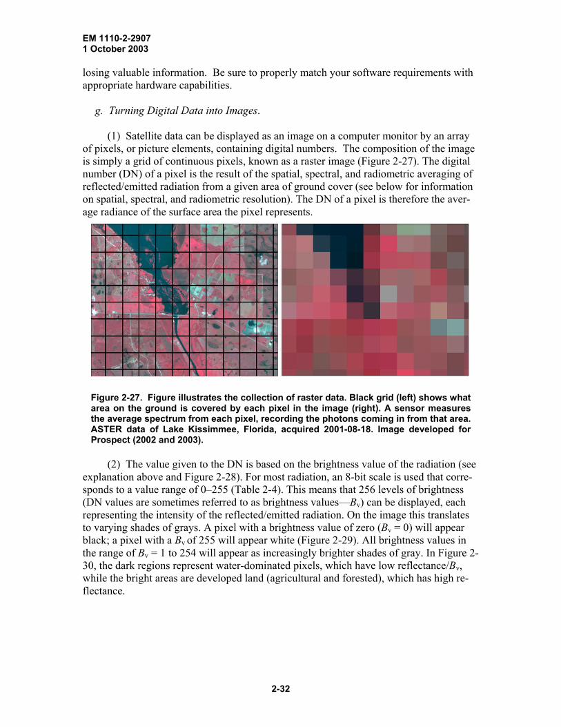
EM 1110-2-2907 1 October 2003

losing valuable information. Be sure to properly match your software requirements with appropriate hardware capabilities.

g. Turning Digital Data into Images.

(1) Satellite data can be displayed as an image on a computer monitor by an array of pixels, or picture elements, containing digital numbers. The composition of the image is simply a grid of continuous pixels, known as a raster image (Figure 2-27). The digital number (DN) of a pixel is the result of the spatial, spectral, and radiometric averaging of reflected/emitted radiation from a given area of ground cover (see below for information on spatial, spectral, and radiometric resolution). The DN of a pixel is therefore the aver-age radiance of the surface area the pixel represents.

Figure 2-27. Figure illustrates the collection of raster data. Black grid (left) shows what area on the ground is covered by each pixel in the image (right). A sensor measures the average spectrum from each pixel, recording the photons coming in from that area. ASTER data of Lake Kissimmee, Florida, acquired 2001-08-18. Image developed for Prospect (2002 and 2003).

(2) The value given to the DN is based on the brightness value of the radiation (see

explanation above and Figure 2-28). For most radiation, an 8-bit scale is used that corre-sponds to a value range of 0–255 (Table 2-4). This means that 256 levels of brightness (DN values are sometimes referred to as brightness values—Bv) can be displayed, each representing the intensity of the reflected/emitted radiation. On the image this translates to varying shades of grays. A pixel with a brightness value of zero (Bv = 0) will appear black; a pixel with a Bv of 255 will appear white (Figure 2-29). All brightness values in the range of Bv = 1 to 254 will appear as increasingly brighter shades of gray. In Figure 2-30, the dark regions represent water-dominated pixels, which have low reflectance/Bv, while the bright areas are developed land (agricultural and forested), which has high re-flectance.

2-32

EM 1110-2-2907 1 October 2003

256 brightness levels (8 bits)

2 brightness levels (1 bit)

4 brightness levels (2 bits)

16 brightness levels (4 bits)

Figure 2-28. Brightness levels at different radiometric resolutions. Im-age developed for USACE Prospect #196 (2002).

Figure 2-29. Raster array and accompanying digital number (DN) values for a single band image. Dark pixels have low DN values while bright pixels have high values. Modified from Natural Resources Canada image http://www.ccrs.nrcan.gc.ca/ccrs/learn/tutorials/fundam/chapter1/chapter1_7_e.html.

2-33

EM 1110-2-2907 1 October 2003

Figure 2-30. Landsat MSS band 5 data of San Francisco, California. The black pixels represent water; the various levels of gray to bright pixels represent dif-ferent vegetation and ground cover types across the landscape. Image taken from http://sfbay.wr.usgs.gov/access/change_detect/Satellite_Images2.html.

h. Converting Digital Numbers to Radiance. Conversion of a digital number to its cor-responding radiance is necessary when comparing images from different satellite sensors or from different times. Each satellite sensor has its own calibration parameter, which is based on the use of a linear equation that relates the minimum and maximum radiation brightness. Each spectrum band (see Paragraph 2-7i) also has its own radiation minimum and maximum.

2-34

EM 1110-2-2907 1 October 2003

(1) Information pertaining to the minimum and maximum brightness (Lmin and Lmax

respectively) is usually found in the metadata (see Chapter 5). The equation for deter-mining radiance from the digital number is:

L = (Lmax – Lmin)/255 × DN + Lmin (2-10) where

L = radiance expressed in Wm-2 sr-1 Lmin = spectral radiance corresponding to the minimum digital number Lmax = spectral radiance corresponding to the maximum digital number DN = digital number given a value based on the bit scale used.

(2) This conversion can also be used to enhance the visual appearance of an image

by reassigning the DN values so they span the full gray scale range (see Paragraph 5-20).

i. Spectral Bands.

(1) Sensors collect wavelength data in bands. A number or a letter is typically as-signed to a band. For instance, radiation that spans 0.45 to 0.52 µm is designated as band 1 for Landsat 7 data; in the microwave region radiation spanning 15 to 30 cm is termed the L-band. Not all bands are created equally. Landsat band 1 (B1) does not represent the same wavelengths as SPOT’s B1.

(2) Band numbers are not the same as sensor numbers. For instance Landsat 4 does not refer to band 4. It instead refers to the fourth satellite sensor placed into orbit by the Landsat program. This can be confusing, as each satellite program has a fleet of satellites (in or out of commission at different times), and each satellite program will define bands differently. Two different satellites from the same program may even be collecting radia-tion at a slightly difference wavelength range for the same band (Table 2-6). It is, there-fore, important to know which satellite program and which sensor collected the data.

Table 2-6 Landsat Satellites and Sensors The following table lists Landsat satellites 1-7, and provides band information and pixel size. The band numbers for one sensor does not necessarily imply the same wavelength range. For example, notice that band 4 in Landsat 1-2 and 3 differ from the band 4 in Landsat 4-5 and Landsat 7. Source: http://landsat.gsfc.nasa.gov/guides/LANDSAT-7_dataset.html#8.

Satellite Sensor Band number Band wavelengths Pixel Size

1) 0.45 to 0.57 80 2) 0.58 to 0.68 80

RBV

3) 0.70 to 0.83 80 4) 0.5 to 0.6 79 5) 0.6 to 0.7 79 6) 0.7 to 0.8 79

Landsats 1-2

MSS

7) 0.8 to 1.1 79

Landsat 3 RBV 1) 0.45 to 0.52 40

2-35

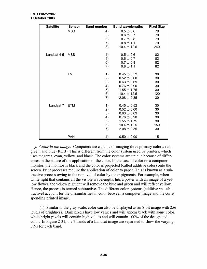
EM 1110-2-2907 1 October 2003

Satellite Sensor Band number Band wavelengths Pixel Size

4) 0.5 to 0.6 79 5) 0.6 to 0.7 79 6) 0.7 to 0.8 79 7) 0.8 to 1.1 79

MSS

8) 10.4 to 12.6 240

4) 0.5 to 0.6 82 5) 0.6 to 0.7 82 6) 0.7 to 0.8 82

MSS

7) 0.8 to 1.1 82

1) 0.45 to 0.52 30 2) 0.52 to 0.60 30 3) 0.63 to 0.69 30 4) 0.76 to 0.90 30 5) 1.55 to 1.75 30 6) 10.4 to 12.5 120

Landsat 4-5

TM

7) 2.08 to 2.35 30

1) 0.45 to 0.52 30 2) 0.52 to 0.60 30 3) 0.63 to 0.69 30 4) 0.76 to 0.90 30 5) 1.55 to 1.75 30 6) 10.4 to 12.5 150

ETM

7) 2.08 to 2.35 30

Landsat 7

PAN 4) 0.50 to 0.90 15

j. Color in the Image. Computers are capable of imaging three primary colors: red,

green, and blue (RGB). This is different from the color system used by printers, which uses magenta, cyan, yellow, and black. The color systems are unique because of differ-ences in the nature of the application of the color. In the case of color on a computer monitor, the monitor is black and the color is projected (called additive color) onto the screen. Print processes require the application of color to paper. This is known as a sub-tractive process owing to the removal of color by other pigments. For example, when white light that contains all the visible wavelengths hits a poster with an image of a yel-low flower, the yellow pigment will remove the blue and green and will reflect yellow. Hence, the process is termed subtractive. The different color systems (additive vs. sub-tractive) account for the dissimilarities in color between a computer image and the corre-sponding printed image.

(1) Similar to the gray scale, color can also be displayed as an 8-bit image with 256 levels of brightness. Dark pixels have low values and will appear black with some color, while bright pixels will contain high values and will contain 100% of the designated color. In Figure 2-31, the 7 bands of a Landsat image are separated to show the varying DNs for each band.

2-36

EM 1110-2-2907 1 October 2003

Figure 2-31. Individual DNs can be identified in each spectral band of an image. In this ex-ample the seven bands of a subset from a Landsat image are displayed. Image developed for Prospect (2002 and 2003).

(2) When displaying an image on a computer monitor, the software allows a user to assign a band to a particular color (this is termed as “loading the band”). Because there are merely three possible colors (red, green, and blue) only three bands of spectra can be displayed at a time. The possible band choices coupled with the three-color combinations creates a seemingly endless number of possible color display choices.

(3) The optimal band choice for display will depend of the spectral information needed (see Paragraph 2-6b(7)). The color you designate for each band is somewhat ar-bitrary, though preferences and standards do exist. For example, a typical color/band designation of red/green/blue in bands 3/2/1 of Landsat displays the imagery as true-color. These three bands are all in the visible part of the spectrum, and the imagery ap-pears as we see it with our eyes (Figure 2-32a). In Figure 2-32b, band 4 (B4) is displayed in the red (called “red-gun” or “red-plane”) layer of the bands 4/3/2, and vegetation in the agricultural fields appear red due to the infrared location on the spectrum. In Figure 2-32c, band 4 (B4) is displayed as green. Green is a logical choice for band 4 as it repre-sents the wavelengths reflected by vegetation.

2-37

EM 1110-2-2907 1 October 2003

a. The true color image appears with these bands in the visible part of the spectrum.

b. Using the near infra-red (NIR) band (4) in the red gun, healthy vegetation appears red in the imagery.

2-38

EM 1110-2-2907 1 October 2003

c. Moving the NIR band into the green gun and adding band 5 to the red gun changes the vegetation to green. Figure 2-32. Three band combinations of Landsat imagery of 3/2/1, 4/3/2, and 5/4/3 in the RGB. Images developed for Prospect (2002 and 2003).

k. Interpreting the Image. When interpreting the brightness of a gray scale image (Figure 2-33), the brightness simply represents the amount of reflectance. For bright pix-els the reflectance is high, while dark pixels represent areas of low reflectance. By exam-ple, in a gray scale display of Landsat 7 band 4, the brightest pixels represent areas where there is a high reflectance in the wavelength range of 0.76 to 0.90 µm. This can be inter-preted to indicate the presence of healthy vegetation (lawns and golf courses).

(1) A color composite can be somewhat difficult to interpret owing to the mixing of color. Similar to gray scale, the bright regions have high reflectance, and dark areas have low reflectance. The interpretation becomes more difficult when we combine different bands of data to produce what is known as false-color composites (Figure 2-33).

(2) White and black are the end members of the band color mixing. White pixels in a color composite represent areas where reflectance is high in all three of the bands dis-played. White is produced when 100% or each color (red, green, and blue) are mixed in equal proportions. Black pixels are areas where there is an absence of color due to the low DN or reflectance. The remaining color variations represent the mixing of three band DNs. A magenta pixel is one that contains equal portions of blue and red, while lacking green. Yellow pixels are those that are high in reflectance for the bands in the green and red planes. (Go to Appendix C for a paper model of the color cube/space.)

2-39

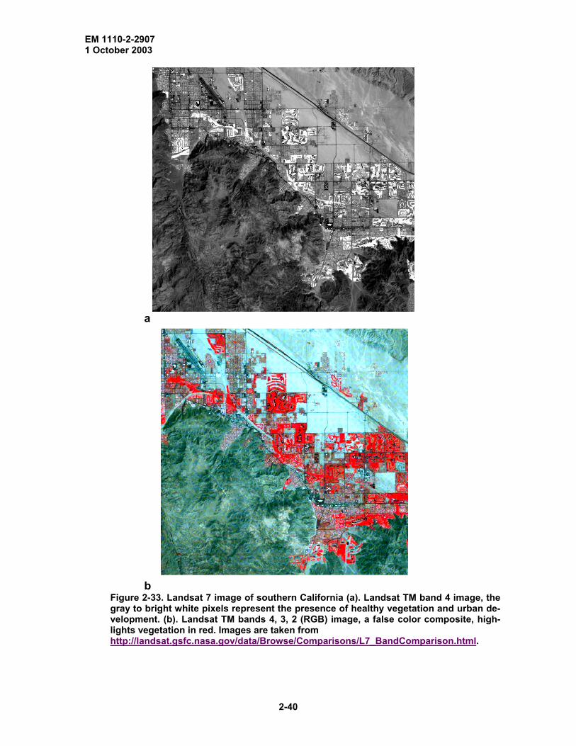
EM 1110-2-2907 1 October 2003

a

b

Figure 2-33. Landsat 7 image of southern California (a). Landsat TM band 4 image, the gray to bright white pixels represent the presence of healthy vegetation and urban de-velopment. (b). Landsat TM bands 4, 3, 2 (RGB) image, a false color composite, high-lights vegetation in red. Images are taken from http://landsat.gsfc.nasa.gov/data/Browse/Comparisons/L7_BandComparison.html.

2-40

EM 1110-2-2907 1 October 2003

l. Data Resolution. A major consideration when choosing a sensor type is the defini-

tion of resolution capabilities. “Resolution” in remote sensing refers to the ability of a sensor to distinguish or resolve objects that are physically near or spectrally similar to other adjacent objects. The term high or fine resolution suggests that there is a large de-gree of distinction in the resolution. High resolution will allow a user to distinguish small, adjacent targets. Low or coarse resolution indicates a broader averaging of radiation over a larger area (on the ground or spectrally). Objects and their boundaries will be difficult to pinpoint in images with coarse resolution. The four types of resolution in remote sensing include spatial, spectral, radiometric, and temporal.

(1) Spatial Resolution.

(a) An increase in spatial resolution corresponds to an increase in the ability to resolve one feature physically from another. It is controlled by the geometry and power of the sensor system and is a function of sensor altitude, detector size, focal size, and system configuration.

(b) Spatial resolution is best described by the size of an image pixel. A pixel is a two-dimensional square-shaped picture element displayed on a computer. The dimen-sions on the ground (measured in meters or kilometers) projected in the instantaneous field of view (IFOV) will determine the ratio of the pixel size to ground coverage. As an example, for a SPOT image with 20- ×20-m pixels, one pixel in the digital image is equivalent to 20 m square on the ground. To gauge the resolution needed to discern an object, the spatial resolution should be half the size of the feature of interest. For exam-ple, if a project requires the discernment of individual tree, the spatial resolution should be a minimum of 15 m. If you need to know the percent of timber stands versus clearcuts, a resolution of 30 m will be sufficient.

Table 2-7 Minimum image resolution required for various sized ob-jects.

Resolution (m)

Feature Object (m)

0.5 1.0 1.0 2.0 1.5 3.0 2.0 4.0 2.5 5.0 5.0 10.0

10.0 20.0 15.0 30.0 20.0 40.0 25.0 50.0

(2) Spectral Resolution. Spectral resolution is the size and number of wavelengths,

intervals, or divisions of the spectrum that a system is able to detect. Fine spectral resolu-tion generally means that it is possible to resolve a large number of similarly sized wavelengths, as well as to detect radiation from a variety of regions of the spectrum. A

2-41

EM 1110-2-2907 1 October 2003

coarse resolution refers to large groupings of wavelengths and tends to be limited in the frequency range.

(3) Radiometric Resolution. Radiometric resolution is a detector’s ability to distin-guish differences in the strength of emitted or reflected electromagnetic radiation. A high radiometric resolution allows for the distinction between subtle differences in signal strength.

(4) Temporal Resolution.

(a) Temporal resolution refers to the frequency of data collection. Data collected on different dates allows for a comparison of surface features through time. If a project requires an assessment of change, or change detection, it is important to know: 1) how many data sets already exist for the site; 2) how far back in time the data set ranges; and 3) how frequently the satellite returns to acquire the same location.

(b) Most satellite platforms will pass over the same spot at regular intervals that range from days to weeks, depending on their orbit and spatial resolution (see Chapter 3). A few examples of projects that require change detection are the growth of crops, defor-estation, sediment accumulation in estuaries, and urban development.

(5) Determine the Appropriate Resolution for the Project. Increasing resolution tends to lead to more accurate and useful information; however, this is not true for every project. The downside to increased resolution is the need for increased storage space and more powerful hardware and software. High-resolution satellite imagery may not be the best choice when all that is needed is good quality aerial photographs. It is, therefore, im-portant to determine the minimum resolution requirements needed to accomplish a given task from the outset. This may save both time and funds. 2-8 Aerial Photography. A traditional form of mapping and surface analysis by re-mote sensing is the use of aerial photographs. Low altitude aerial photographs have been in use since the Civil War, when cameras mounted on balloons surveyed battlefields. Today, they provide a vast amount of surface detail from a low to high altitude, vertical perspective. Because these photographs have been collected for a longer period of time than satellite images, they allow for greater temporal monitoring of spatial changes. Roads, buildings, farmlands, and lakes are easily identifiable and, with experience, sur-face terrain, rock bodies, and structural faults can be identified and mapped. In the field, photographs can aid in precisely locating target sites on a map.

a. Aerial photographs record objects in the visible and near infrared and come in a va-riety of types and scales. Photos are available in black and white, natural color, false color infrared, and low to high resolution.

b. Resolution in aerial photographs is defined as the resolvable difference between adjacent line segments. Large-scale aerial photographs maintain a fine resolution that

2-42

EM 1110-2-2907 1 October 2003

allows users to isolate small objects such as individual trees. Photographs obtained at high altitudes produce a small-scale, which gives a broader view of surface features.

c. In addition to the actual print or digital image, aerial photographs typically include information pertaining to the photo acquisition. This information ideally includes the date, flight, exposure, origin/focus, scale, altitude, fiducial marks, and commissioner (Figure 2-34). If the scale is not documented on the photo, it can be determined by taking the ratio of the distance of two objects measured on the photo vs. the distance of the same two objects calculated form measurements taken from a map.

Photo scale = photo distance/ground distance = d/D (2-11)

Figure 2-34. Aerial photograph of a predominately agricultural area near Modesto, Califor-nia. Notice the ancillary data located on the upper and right side margins. These data pro-vide information regarding the location and acquisition of the photo.

2-43

EM 1110-2-2907 1 October 2003

d. The measurement is best taken from one end of the photo to the other, passing through the center (because error in the image increases away from the focus point). For precision, it is best to average a number of ratios from across the image.

e. Photos are interpreted by recognizing various elements in a photo by the distinction of tone, texture, size, shape, pattern, shadow, site, and association. For instance, airport landing strips can look like roads, but their large widths, multiple intersections at small angles, and the positioning of airport hangers and other buildings allow the interpreter to correctly identify these “roads” as a special use area.

f. Aerial-photos are shot in a sequence with 60% overlap; this creates a stereo view when two photos are viewed simultaneously. Stereoscopic viewing geometrically corrects photos by eliminating errors attributable to camera tilt and terrain relief. Images are most easily seen in stereo by viewing them through a stereoscope. With practice it is possible to see in stereo without the stereoscope. This view will produce a three-dimensional im-age, allowing you to see topographic relief and resistant vs. recessive rock types.

g. To maintain accuracy it is important to correlate objects seen in the image with the actual object in the field. This verification is known as ground truth. Without ground truth you may not be able to differentiate two similarly toned objects. For instance, two very different but recessive geologic units could be mistakenly grouped together. Ground truth will also establish the level of accuracy that can be attributed to the maps created based solely on photo interpretations.

h. For information on aerial photograph acquisition, see Chapter 4. Chapter 5 presents a discussion on the digital display and use of aerial photos in image processing. 2-9 Brief History of Remote Sensing. Remote sensing technologies have been built upon by the work of researchers from a variety of disciplines. One must look further than 100 years ago to understand the foundations of this technology. For a timeline his-tory of the development of remote sensing see http://rst.gsfc.nasa.gov/Intro/Part2_8.html. The chronology shows that remote sensing has matured rapidly since the 1970s. This ad-vancement has been driven by both the military and commercial sectors in an effort to effectively model and monitor Earth processes. For brevity, this overview focuses on camera use in remote sensing followed by the development of two NASA programs and France’s SPOT system. To learn more about the development of remote sensing and de-tails of other satellite programs see http://rst.gsfc.nasa.gov/Front/tofc.html.

a. The Camera. The concept of imaging the Earth’s surface has its roots in the devel-opment of the camera, a black box housing light sensitive film. A small aperture allows light reflected from objects to travel into the black box. The light then “exposes” film, positioned in the interior, by activating a chemical emulsion on the film surface. After exposure, the film negative (bright and dark are reversed) can be used to produce a posi-tive print or a visual image of a scene.

2-44

EM 1110-2-2907 1 October 2003

b. Aerial Photography. The idea of mounting a camera on platforms above the

ground for a “birds-eye” view came about in the mid-1800s. In the 1800’s there were few objects that flew or hovered above ground. During the US Civil War, cameras where mounted on balloons to survey battlefield sites. Later, pigeons carrying cameras were employed (http://www2.oneonta.edu/~baumanpr/ncge/rstf.htm), a platform with obvious disadvantages. The use of balloons and other platforms created geometric problems that were eventually solved by the development of a gyro-stabilized camera mounted on a rocket. This gyro-stabilizer was created by the German scientist Maul and was launched in 1912.

c. First Satellites. The world’s first artificial satellite, Sputnik 1, was launched on 4

October 1957 by the Soviet Union. It was not until NASA’s meteorological satellite TIROS –1 was launched that the first satellite images were produced (http://www.earth.nasa.gov/history/tiros/tiros1.html). Working on the same principles as the camera, satellite sensors collect reflected radiation in a range of spectra and store the data for eventual image processing (see above, this chapter).

d. NASA’s First Weather Satellites. NASA’s first satellite missions involved study of the Earth’s weather patterns. TIROS (Television Infrared Operational Satellite) missions launched 10 experimental satellites in the early 1960’s in an effort to prepare for a per-manent weather bureau satellite system known as TOS (TIROS Operating System). TIROS-N (next generation) satellites currently monitor global weather and variations in the Earth’s atmosphere. The goal of TIROS-N is to acquire high resolution, diurnal data that includes vertical profile measurements of temperature and moisture.

e. Landsat Program. The 1970’s brought the introduction of the Landsat series with the launching of ERTS-1 (also known as Landsat 1) by NASA. The Landsat program was the first attempt to image whole earth resources, including terrestrial (land based) and marine resources. Images from the Landsat series allowed for detailed mapping of land-masses on a regional and continental scale.

(1) The Landsat imagery continues to provide a wide variety of information that is highly useful for identifying and monitoring resources, such as fresh water, timberland, and minerals. Landsat imagery is also used to assess hazards such as floods, droughts, forest fire, and pollution. Geographers have used Landsat images to map previously un-known mountain ranges in Antarctica and to map changes in coastlines in remote areas.

(2) A notable event in the history of the Landsat program was the addition of TM (Thematic Mapper) first carried by Landsat 4 (for a summary of Landsat satellites see http://geo.arc.nasa.gov/sge/landsat/lpsum.html). The Thematic Mapper provides a resolu-tion as low as 30 m, a great improvement over the 70-m resolution of earlier sensors. The TM devise collects reflected radiation in the visible, infrared (IR), and thermal (IR) re-gion of the spectrum.

(3) In the late 1970’s, the regulation of Landsat was transferred from NASA to NOAA, and was briefly commercialized in the 1980s. The Landsat program is now oper-

2-45

EM 1110-2-2907 1 October 2003

ated by the USGS EROS Data Center (US Geological Survey Earth Resources Observa-tion Systems; see http://landsat7.usgs.gov/index.html).

(4) As government sponsored programs have become increasingly commercialized and other countries develop their own remote sensors, NASA’s focus has shifted from sensor development to data sharing. NASA’s Data Acquisition Centers serves as a clear-ing-house for satellite data; these data can now be shared via the internet.

f. France’s SPOT Satellite System. As a technology, remote sensing continues to ad-vance globally with the introduction of satellite systems in other countries such as France, Japan, and India. France’s SPOT (Satellite Pour l’Observation de la Terra) has provided reliable high-resolution (20 to 10 m resolution) image data since 1986.

(1) The SPOT 1, 2, and 3 offer both panchromatic data (P or PAN) and three bands of multispectral (XS) data. The panchromatic data span the visible spectrum without the blue (0.51-0.73 µm) and maintains a 10-m resolution. The multispectral data provide 20-m resolution, broken into three bands: Band 1 (Green) spans 0.50–0.59 µm, Band 2 (Red) spans 0.61–0.68 µm, and Band 3 (Near Infrared) spans 0.79–0.89 µm. SPOT 4 also sup-plies a 20-m resolution shortwave Infrared (mid IR) band (B4) covering 1.58 to 1.75 µm. SPOT 5, launched in spring 2002, provides color imagery, elevation models, and an im-pressive 2.5-m resolution. It houses scanners that collect panchromatic data at 5 m reso-lution and four band multispectral data at 10-m resolution (see Appendix D-“SPOT” file).

(2) SPOT 3 was decommissioned in 1996. SPOT 1, 2, 4, and 5 are operational at the time of this writing. For information on the SPOT satellites go to http://www.spotimage.fr/home/system/introsat/seltec/welcome.htm.

g. Future of Remote Sensing. The improved availability of satellite images coupled with the ease of image processing has lead to numerous and creative applications. Re-mote sensing has dramatically brought about changes in the methodology associated with studying earth processes on both regional and global scales. Advancements in sensor resolution, particularly spatial, spectral, and temporal resolution, broaden the possible applications of satellite data.

(1) Government agencies around the world are pushing to meet the demand for re-liable and continuous satellite coverage. Continuous operation improves the temporal data needed to assess local and global change. Researchers are currently able to perform a 30-year temporal analysis using satellite images on critical areas around the globe. This time frame can be extended back with the incorporation of digital aerial photographs.

(2) Remote sensing has established itself as a powerful tool in the assessment and management of U.S. lands. The Army Corps of Engineers has already incorporated this technology into its nine business practice areas, demonstrating the tremendous value of remote sensing in civil works projects.

2-46

EM 1110-2-2907 1 October 2003

Chapter 3 Sensors and Systems 3-1 Introduction. Remotely sensed data are collected by a myriad of satellite and air-borne systems. A general understanding of the sensors and the platforms they operate on will help in determining the most appropriate data set to choose for any project. This chapter reviews the nine business practice areas in USACE Civil Works and examines the leading questions to be addressed before the initiation of a remote sensing project. Airborne and satellite sensor systems are presented along with operational details such as flight path/orbits, swath widths, acquisition, and post processing options. Ground-based remote sensing GPR (Ground Penetrating Radar) is also introduced. This chapter con-cludes with a summary of remote sensing and GIS matches for each of the nine civil works business practice areas.

a. Industry Perspective on Image Acquisition. In the past 30 years, selection of re-motely sensed imagery was confined by system constraints and only provided by a few vendors. Imagery that was available from archive, or that would become available due to orbital frequency, maintained numerous constraints; consequently ground coverage, rather than image resolution, was the primary concern. Additionally, minor consideration was given to the spectral characteristics of the target and the spectral bands available, as there were a limited number of imaging platforms. To an extent projects had to be tai-lored to fit the limitations of the data. This is no longer the case however, with signifi-cant technologic improvements and numerous product choices. Creative researchers are finding new applications in the on-going advancement of remote sensing.

b. Image Improvements. Satellite sensor system developers continue to improve im-age cost, resolution, spectral band choices, spectral data library sets, and value-added products or post-processing methods. Improvements in sensor development and afforda-bility can be attributed to the commercialization and subsequent expansion of the remote sensing industry. NASA, other US governmental agencies, and foreign space agencies, such as those in Canada, France, India, and Japan, progressively enhance the industry by furthering current technologic advances in the remote sensing field. Consequently, the resolution constraints on data that existed 20 or more years ago are no longer an obstacle with the addition of these affordable higher resolution systems. Listed here are just a few examples of airborne and satellite data costs:

• AVHRR scene at 1 km GSD for < $50 • Landsat TM scene at 30 m GSD for $625 • Landsat ETM scene can be acquired for $800 • ERS-1 SAR scene at 25 m GSD for $2000 • ERS-2 SAR scene at 25 m GSD for $1500. • Vendors of high-resolution satellite imaging systems products (such as

IKONOS or QUICKBIRD or other products with <4 m GSD [ground sampling distance is the spatial resolution measurement]) charge on a per area basis. The minimum area is 11 km2 for approximately $2000.

3-1

EM 1110-2-2907 1 October 2003

c. Archive Imagery. This can be accessed and purchased at a reduced rate. Some im-

aging systems can acquire new imagery at reasonable rates as well. It is now possible to tailor acquisitions to meet the specific needs of Corps projects. Costs presented in this manual will fluctuate, but generally become more affordable over time. The downward trend in cost applies to all aspects of remote sensing - data acquisition and the required software and hardware. 3-2 Corps 9—Civil Works Business Practice Areas. The spatial, spectral, and temporal requirements set by the goals in a Corps business practice area should be bal-anced with the economic limits of the project. To achieve this result, it is helpful to con-sider a few preliminary steps when planning an image data acquisition. Below is a review of the Corps 9 Civil Works Business Practice Areas. The steps that should be taken to determine the specific data requirements follow each business practice. A list of vendor services is presented along with details on the various platforms (airborne, satellite, and ground penetrating radar). The nine business practice areas in Civil Works of the Corps of Engineers and a listing of their operations follows:

a. Navigation. • Responsible for navigation channels. • Dredging for specified width and depth. • Maintenance of 12,000 miles of inland waterways. • Maintenance of 235 locks. • 300 commercial harbors. • 600 smaller harbors.

b. Flood Damage Reduction.

• Build and maintain levees. • Maintenance of 383 dams and reservoirs. • Advice on zoning, regulations and flood warning systems. • Shore protection—protection from hurricane and coastal storms. • Construction of jetties, seawalls, and beach sand renourishment. • Responsibility for dam safety—inspection of Corps and other’s dams

c. Environmental Missions.

• Ecosystem restoration—many small ecosystem restoration projects, and the larger Florida Everglades hydrologic restoration project.

• Environmental stewardship—protect forest and wildlife habitat; monitor water quality at reservoirs; operate several fish hatcheries; support national goal of “no net loss of wetlands”; and projects on conservation, preservation, restora-tion and wetland creation.

• Radioactive site cleanup—FUSRAP (Formerly Used Sites Remedial Action Program).

d. Wetlands and Waterways Regulation and Permitting.

• Support Clean Water Act.

3-2

EM 1110-2-2907 1 October 2003

• Authority over dumping, dredging and filling in Waters of the US (WoUS). • Determine areas for protection as wetlands (under guidelines of 1987 Wetland

Delineation Manual), and permitting for land use. • Water supply—Washington DC aqueduct operation, manage water supply

from Corps reservoirs and water use for agriculture in arid regions of South-western US

• Hydroelectric power—Corps operates 75 hydroelectric power plants.

e. Real Estate. • Full range of services to Army and Air Force. • Manage Contingency Real Estate Support Team (CREST). • DOD agent for Recruiting Facilities Program, Homeowners Assistance Pro-

gram and Defense National Relocation Program.

f. Recreation. • Operate and maintain 2500 recreation areas at 463 lakes. • Rangers are Dept. of Army employees. • Corps is active in National Water Safety Program.

g. Emergency Response.

• Response to hurricanes, tornadoes, flooding, and natural disasters. • Support to FEMA when activated by Federal Response Plan (FRP). • Under FRP Corps has lead for public works and engineering missions.

h. Research and Development.

ERDC is composed of seven research laboratories for military, civil works and civilian infrastructure applications:

TEC—Topographic Engineering Center CERL—Construction Engineering and Research Laboratory CRREL—Cold Regions Research and Engineering Laboratory WES-GSL—Waterways Experiment Station-Geotechnical and Structures

Laboratory WES-EL—Waterways Experiment Station-Environmental Laboratory WES-CHL—Waterways Experiment Station-Coastal Hydraulics

Laboratory WES –ITL—Waterways Experiment Station-Information Technology

Laboratory

i. Support to Others. This includes engineering and water resources support to state and Federal agencies, and to foreign countries.

3-3 Sensor Data Considerations (programmatic and technical).

a. Below is a list of preliminary steps and questions to consider when planning an im-age data acquisition. Answer these questions in light of the Corps Civil Works 9 Business Practice Areas before proceeding.

3-3

EM 1110-2-2907 1 October 2003

• What is the primary goal of the project?

Define the problem. How can remote sensing be applied to assist in solving the problem?

• What spatial resolution is need?

Determine the minimum, maximum, and/ or optimal GSD (ground sampling distance).

• What is the target or what is being mapped?

High-resolution panchromatic (black and white) aerial photography may be sufficient. Define what spectral bands are needed.

• Will field work be included in the project budget? What detail is needed from the imagery?

• What spectral resolution is needed?

Set bandwidth and proximity. • Determine timing and temporal resolution requirements.

Select season(s) and time frequencies. • How urgent is the data needed?

To capture an emergency event or temporal phenomena an airborne system may need to be promptly employed.

• What repeat cycle do we need?

Each sensor system operates on a different cycle. • When will ground truth data be collection?

Image data acquisition ideally coincides with ground truth data collection. • What are the weather and light conditions?

Select radar or optical imagery or adjust acquisition timing to accommodate for variable atmospheric conditions.

• What level of processing will be performed by the vendor?

For example, choose basic processes such as radiometric, atmospheric, and geo-metric corrections should be considered.

• What accuracy do we want?

Set vertical and horizontal limits. • Where is the project geographically located?

Specify upper left/ lower right hand corner Latitudes and Longitudes.

3-4

EM 1110-2-2907 1 October 2003

• What is the funding situation?

Chose a system and methods that will allow you to cost-effectively follow through on a project.

• Do we need new or archived data?

Avoid wasting resources by soliciting imagery data that already exists. Contact TEC Image Office (TIO) to determine image data availability and purchasing procedures.

b. Here are some ancillary decisions to be made based on answers to the above

questions. • What field of view is needed?

Specify image overlap if one image is not sufficient. Be aware that aircraft and flight line paths control image overlap. Should either be altered then the overlap could be negatively affected (Figure 3-1).

• What acquisition look direction?

Radar imagery taken in mountainous regions can have layover distortion and shadow regions; whereas nadir looking airborne imagery has less of that effect, so that equal amounts of backscatter and transmission are collected on both sides of the feature.

• Are commercial analytical services needed?

Will post-processing of the imagery be accomplished in-house, or does this re-quire external expertise — an example is the processing of radar IFSAR into ele-vation data, which is a very special technique done by dedicated software on dedicated hardware and not generally done in-house. Below are examples of vendor post-processing services.

3-5

EM 1110-2-2907 1 October 2003

Figure 3-1. In this CAMIS image a decrease in aircraft altitude (due to cir-cumstances beyond the operators control) reduced the pixel size and sub-sequently decreased the image scene. After mosaicing the individual scenes the side overlaps created “holidays” or gaps in the data. Taken from Campbell (2003).

3-6

EM 1110-2-2907 1 October 2003

3-4 Value Added Products. Examples of post-processing done on imagery are listed here with URLs to some of the companies that do the work (sometimes called level 2 or value added products).

• Earthsat Corporation http://www.earthsat.com/ip/prodsvc/ offers geocoding, orthorectification, seamless mosaics, data fusion, and spectral transforms including simulated true color, minimum noise fraction (MNF), vegetation suppression, and decor-relation stretch. They offer hyperspectral processing such as atmospheric correction, automatic endmember selection, pixel unmixing, vegetation stress mapping, and aircraft motion compensation.

• The SPOT Corporation http://www.spot.com/home/proser/welcome.htm of-fers SPOTView (image map product), land use/land cover (thematic product), eleva-tion/terrain mapping (3-D products), and vegetation products.

• Vectorization Services http://www.vectorizationservices.com/services.htm of-fers rectification and orthorectification, enhancement, mosaicing, fusion and image inter-pretation.

• Agricast http://www.agricast.com/ offers value-added products for precision farming, agriculture, and range management.

• Science Applications International Corporation (SAIC) http://www.saic.com/imagery/remote.html offers many value added products for indus-tries from agriculture to utilities. See their web site for the complete list.

• Emerge http://www.emergeweb.com/Public/info/productsPage.asp offers digi-tal ortho products and mosaics from airborne imagery.

• The J.W. Sewall Company http://www.jws.com/pages/core_sevices.html of-fers photogrammetric mapping, cadastral mapping, municipal GIS development, energy and telecommunications services, and natural resources consulting.

• Analytical Imaging and Geophysics http://www.aigllc.com/research/intro.htm offers analysis of multispectral, hyperspectral and SAR imagery with map production and field verification.

• Spectral International, Inc. http://www.pimausa.com/services.html offers analytical services, consulting and hyperspectral image processing.

• Earthdata http://www.earthdata.com/index2.htm offers digital orthophotos, to-pographic maps, planimetric maps, and LIDAR 3-D elevation data.

• Intermap Technologies http://www.intermaptechnologies.com/products.htm offers IFSAR DEMs, DSMs, DTMs, and orthorectified radar images.

• 3Di http://www.3dicorp.com/rem-products.html offers LIDAR DEMs, orthorectified imagery, contour mapping, wetlands mapping, vegetation mapping, 3D perspective image drapes, and volumetric analysis.

• Terrapoint http://www.terrapoint.com/Products2.htm offers LIDAR elevation data sets, DTMs, DEMs, canopy DTMs, building heights, land records, and floodmaps.

• i-cubed http://www.i3.com offers information integration and imaging • Leica Geosystems http://www.gis.leica-geosystems.com offers GIS and map-

ping. • PhotoScience, Inc. http:// www.photoscience.com offers aerial photography,

photogrammetry, GPS survey, GIS services, image processing

3-7

EM 1110-2-2907 1 October 2003

3-5 Aerial Photography. Aerial photography is a highly useful mapping tool and maintains the highest spatial resolution of any of the remote sensing systems. Standard 9-in. (22.9 cm) aerial photos used for mapping and site identification are collected and made available through commercial companies. USGS generates digital elevation model (DEM) data and stereo classification of ground cover from aerial photography. These data are derived from the National Aerial Photography Program (NAPP), formally the National High Altitude Program (NHAP). The NAPP products are quarter quad-centered photographs of the entire contiguous US, acquired every 5 years over 2-year intervals since 1990. NAPP photography is acquired at 20,000 ft (~600 m) above mean terrain with a 6-in. (~15 cm) focal length lens. The flight lines are quarter quad-centered on the 1:24,000-scale USGS maps. NAPP photographs have an approximate scale of 1:40,000, and collect black-and-white or color infrared, as specified by state or Federal require-ments. The St. Louis District of the Corps has several airborne contracts in place as well.

a. Softcopy photogrammetry is the semi-automatic processing of aerial photos after they have been digitally scanned into files and transferred into a computer. Once in digi-tal form, the processes of stereo imaging, stereo compilation, aerial triangulation, topog-raphic mapping, ortho-rectification, generation of DEMs, DTMs, and DSMs and digital map generation can be carried out.

b. Aerial photos are geometrically corrected using the fiducial marks and a camera model and projected into the ground coordinates. Images within a stereo overlap are ad-justed using a triangulation algorithm so that they fit within the constraints of the ground control point information. At the end of the triangulation, individual stereo models are mathematically defined between stereo images. Topographic information is extracted from the images using autocorrelation techniques that match image patterns within a de-fined radius. By using parallax created by the different angle shots, elevation is measured from the distance of matching pixels. A terrain model is used to create an ortho-rectified image from the original photo that is precision geocoded and an ancillary Digital Surface Model (DSM) is available.

c. Some of the companies that contract with USACE for aerial photography include:

• Highland Geographic Inc. http://www.highlandgeographic.com • James W. Sewall Company http://www.sewall.com • Alcor Technologies Limited http://www.alcortechnologies.com • Aero-Metric Inc. http://www.aerometric.com • PhotoScience, Inc. http://www.photoscience.com

3-6 Airborne Digital Sensors. The advancement of airborne systems to include high resolution digital sensors is becoming available through commercial companies. These systems are established with onboard GPS for geographic coordinates of acquisitions, and real time image processing. Additionally, by the time the plane lands on the ground, the data can be copied to CDROM and be available for delivery to the customer with a basic level of processing. The data at this level would require image calibration and additional

3-8

EM 1110-2-2907 1 October 2003

processing. The data at this level would require image calibration and additional proc-essing. See Appendix F for a list of airborne system sensors. 3-7 Airborne Geometries. There are several ways in which airborne image geometry can be controlled. Transects should always be flown parallel to the principle plane to the sun, such that the BRDF (bi-directional reflectance distribution function) is symmetrical on either side of the nadir direction. The pilot should attempt to keep the plane level and fly straight line transects. But since there are always some attitude disturbances, GPS and IMU (inertial measuring unit) data can be used in post-processing the image data to take out this motion. The only way of guaranteeing nadir look imagery is to have the sensor mounted on a gyro-stabilized platform. Without this, some angular distortion of the im-agery will result even if it is post-processed with the plane’s attitude data and an eleva-tion model (i.e., sides of buildings and trees will be seen and the areas hidden by these targets will not be imaged). Shadow on one side of the buildings or trees cannot be elimi-nated and the dynamic range of the imagery may not be great enough to pull anything out of the shadow region. The only way to minimize this effect is to acquire the data at or near solar noon. 3-8 Planning Airborne Acquisitions.

a. Planning airborne acquisitions requires both business and technical skills. For ex-ample, to contract with an airborne image acquisition company, a sole source claim must be made that this is the only company that has these special services. If not registered as a prospective independent contractor for a Federal governmental agency, the company may need to file a Central Contractor Registration (CCR) Application, phone (888-227-2423) and request a DUNS number from Dun & Bradstreet, phone (800-333-0505). After this, it is necessary for the contractee to advertise for services in the Federal Business Opportu-nities Daily (FBO Daily) http://www.fbodaily.com. Another way of securing an airborne contractor is by riding an existing Corps contract; the St. Louis District has several in place. A third way is by paying another governmental agency, which has a contract in place. If the contractee is going to act as the lead for a group acquisition among several other agencies, it may be necessary to execute some Cooperative Research and Develop-ment Agreements (CRDAs) between the contractee and the other agencies. As a word of caution, carefully spell out in the legal document what happens if the contractor, for any reason, defaults on any of the image data collection areas. A data license should be spelled out in the contract between the parties.

b. Technically, maps must be provided to the contractor of the image acquisition area. They must be in the projection and datum required, for example Geographic and WGS84 (World Geodetic System is an earth fixed global reference frame developed in 1984). The collection flight lines should be drawn on the maps, with starting and ending coordinates for each straight-line segment. If an area is to be imaged then the overlap between flight lines must be specified, usually 20%. If the collection technique is that of overlapping frames then both the sidelap and endlap must be specified, between 20 and 30%. It is a good idea to generate these maps as vector coverages because they are easily changed when in that format and can be inserted into formal reports with any caption desired later.

3-9

EM 1110-2-2907 1 October 2003

The maximum angle allowable from nadir should be specified. Other technical consid-erations that will affect the quality of the resulting imagery include: What sun angle is allowable? What lens focal length is allowable? What altitude will the collection be flown? Will the imagery be flown at several resolutions or just one? Who will do the orthorectification and mosaicing of the imagery? Will DEMs, DTMs, or DSMs be used in the orthorectification process? How will unseen and shadow areas be treated in the final product? When planning airborne acquisitions, these questions should be part of the deci-sion process. 3-9 Bathymetric and Hydrographic Sensors.

a. The Scanning Hydrographic Operational Airborne Lidar Survey (SHOALS http://shoals.sam.usace.army.mil/default.htm) system is used in airborne lidar bathymet-ric mapping. The Joint Airborne Lidar Bathymetry Technical Center of Expertise (JALBTCX) is a partnership between the South Atlantic Division, US Army Corps of Engineers (USACE), the Naval Meteorology and Oceanography Command and Naval Oceanographic Office and USACE's Engineer Research and Development Center. JALBTCX owns and operates the SHOALS system. SHOALS flies on small fixed wing aircraft, Twin Otter, or on a Bell 212 helicopter. The SHOALS system can collect data on a 4-m grid with vertical accuracy of 15 cm. In clear water bathymetry can be collected at 2–3 times Secchi depth or 60 m. It does not work in murky or sediment-laden waters.

b. The Corps uses vessels equipped with acoustic transducers for hydrographic sur-veys. The USACE uses multibeam sonar technology in channel and harbor surveys. Mul-tibeam sonar systems are used for planning the depth of dredging needed in these shallow waters, where the accuracy requirement is critical and the need for correct and thorough calibration is necessary. USACE districts have acquired two types of multibeam trans-ducers from different manufacturers, the Reson Seabat and the Odom Echoscan multi-beam. The navigation and acquisition software commonly in use by USACE districts is HYPACK and HYSWEEP, by Coastal Oceanographics Inc. For further information see the web site at https://velvet.tec.army.mil/access/milgov/fact_sheet/multibea.html (due to security restrictions this site can only be accessed by USACE employees). 3-10 Laser Induced Fluorescence.

a. Laser fluorosensors detect a primary characteristic of oil, namely their characteris-tic fluorescence spectral signature and intensity. There are very few substances in the natural environment that fluoresce, those that do, fluoresce with sufficiently different spectral signatures and intensities that they can be readily identified. The Laser Environ-mental Airborne Fluorosensor (LEAF) is the only sensor that can positively detect oil in complex environments including, beaches and shorelines, kelp beds, and in ice and snow. In situations where oil contaminates these environments, a laser fluorosensor proves to be invaluable as a result of its ability to positively detect oil http://www.etcentre.org/home/water_e.html.

3-10

EM 1110-2-2907 1 October 2003

b. Other uses of laser fluorosensors are to detect uranium oxide present in facilities,

abandoned mines, and spill areas that require remediation. See Special Technologies Laboratory of Bechtel, NV, http://www.nv.doe.gov/business/capabilities/lifi/. 3-11 Airborne Gamma.

a. An AC-500S Aero Commander aircraft is used by the National Operational Hy-drologic Remote Sensing Center (NOHRSC) to conduct aerial snow survey operations in the snow-affected regions of the United States and Canada. During the snow season (January–April), snow water equivalent measurements are gathered over a number of the 1600+ pre-surveyed flight lines using a gamma radiation detection system mounted in the cabin of the aircraft. During survey flights, this system is flown at 500 ft (152 m) above the ground at ground speeds ranging between 100 and 120 knots (~51 to 62 m/s). Gamma radiation emitted from trace elements of potassium, uranium, and thorium radio-isotopes in the upper 20 cm of soil is attenuated by soil moisture and water mass in the snow cover. Through careful analysis, differences between airborne radiation measure-ments made over bare ground are compared to those of snow-covered ground. The radia-tion differences are corrected for air mass attenuation and extraneous gamma contamina-tion from cosmic sources. Air mass is corrected using output from precision temperature, radar altimeter, and pressure sensors mounted on and within the aircraft. Output from the snow survey system results in a mean areal snow water equivalent value within ±1 cm. Information collected during snow survey missions, along with other environmental data, is used by the National Weather Service (NWS), and other agencies, to forecast river lev-els and potential flooding events attributable to snowmelt water runoff (http://www.aoc.noaa.gov/_).

b. Other companies use airborne gamma to detect the presence of above normal gamma ray count, indicative of uranium, potassium, and thorium elements in the Earth’s crust (for example, Edcon, Inc., http://www.edcon.com, and the Remote Sensing Labora-tory at Bechtel, Nevada). The USGS conducted an extensive survey over the state of Alaska as part of the National Uranium Resource Evaluation (NURE) program that ran from 1974 to 1983, http://edc.usgs.gov/. 3-12 Satellite Platforms and Sensors.

a. There are currently over two-dozen satellite platforms orbiting the earth collecting data. Satellites orbit in either a circular geo-synchronous or polar sun-synchronous path. Each satellite carries one or more electromagnetic sensor(s), for example, Landsat 7 sat-ellite carries one sensor, the ETM+, while the satellite ENVISAT carries ten sensors and two microwave antennas. Some sensors are named after the satellite that carries them, for instance IKONOS the satellite houses IKONOS the sensor. See Appendices D and E for a list of satellite platforms, systems, and sensors.

b. Sensors are designed to capture particular spectral data. Nearly 100 sensors have been designed and employed for long-term and short-term use. Appendix D summarizes details on sensor functionality. New sensors are periodically added to the family of ex-

3-11

EM 1110-2-2907 1 October 2003

isting sensors while older or poorly designed sensors become decommissioned or de-funct. Some sensors are flown on only one platform; a few, such as MODIS and MSS, are on-board more than one satellite. The spectral data collected may span the visible (optical), blue, green, microwave, MIR/SWIR, NIR, Red, or thermal IR Sensors can de-tect single wavelengths or frequencies and/or ranges of the EM spectrum. 3-13 Satellite Orbits.

a. Remote sensing satellites are placed into different orbits for special purposes. The weather satellites are geo-stationary, so that they can image the same spot on the Earth continuously. They have equatorial orbits where the orbital period is the same as that of the Earth and the path is around the Earth’s equator. This is similar to the communication satellites that continuously service the same area on the Earth (Figure 3-2).

Figure 3-2. Satellite in Geostationary Orbit. Courtesy of the Natural Resources Canada.

b. The remaining remote sensing satellites have near polar orbits and are launched

into a sun synchronous orbit (Figure 3-3). They are typically inclined 8 degrees from the poles due to the gravitational pull from the Earth’s bulge at the equator; this allows them to remain in orbit. Depending on the swath width of the satellite (if it is non-pointable), the same area on the Earth will be imaged at regular intervals (16 days for Landsat, 24 days for Radarsat).

3-12

EM 1110-2-2907 1 October 2003

Figure 3-3. Satellite Near Polar Orbit, Courtesy of the Natural Resources Canada.

3-14 Planning Satellite Acquisitions. Corps satellite acquisition must be arranged through the Topographic Engineering Center (TEC) Imagery Office (TIO). It is very easy to transfer the cost of the imagery to TEC via the Corps Financial Management System (CFMS). They will place the order, receive and duplicate the imagery for entry into the National Imagery and Mapping Agency (NIMA) archive called the Commercial Satellite Imagery Library (CSIL), and send the original to the Corps requester. They buy the im-agery under a governmental user license contract that licenses free distribution to other government agencies and their contractors, but not outside of these. It is important for Corps personnel to adhere to the conditions of the license. Additional information con-cerning image acquisition is discussed in Chapter 4 (Section 4-1).

a. Turn Around Time. This is another item to consider. That is the time after acquisi-tion of the image that lapses before it is shipped to TEC-TIO and the original purchaser. Different commercial providers handle this in different ways, but the usual is to charge an extra fee for a 1-week turn around, and another fee for a 1 to 2 day turn around. For ex-ample, SPOT Code Red programmed acquisition costs an extra $1000 and guarantees shipment as soon as acquired. The ERS priority acquisition costs an extra $800 and guar-antees shipment within 7 days, emergency acquisition cost $1200 and guarantees ship-ment within 2 days, and near real time costs an extra $1500 and guarantees shipment as soon as acquired. Also arrangement may be made for ftp image transfers in emergency situations. Costs increase in a similar way with RADARSAT, IKONOS, and QuickBird satellite imaging systems.

3-13

EM 1110-2-2907 1 October 2003

b. Swath Planners.

• Landsat acquired daily over the CONUS, use DESCW swath planner on PC

running at least Windows 2000 for orbit locations. http://earth.esa.int/services/descw/ • ERS, JERS, ENVISAT—not routinely taken, use DESCW swath planner on

PC running at least Windows 2000 for orbit locations. http://earth.esa.int/services/descw/ • RADARSAT—not routinely acquired, contact the TEC Imagery Office

regarding acquisitions of Radarsat data. • Other commercial imaging systems, contact the TEC Imagery Office regard-

ing acquisitions. 3-15 Ground Penetrating Radar Sensors. Ground penetrating radar (GPR) uses electromagnetic wave propagation and back scattering to image, locate, and quantita-tively identify changes in electrical and magnetic properties in the ground. Practical plat-forms for the GPR include on-the-ground point measurements, profiling sleds, and near-ground helicopter surveys. It has the highest resolution in subsurface imaging of any geo-physical method, approaching centimeters. Depth of investigation varies from meters to several kilometers, depending upon material properties. Detection of a subsurface feature depends upon contrast in the dielectric electrical and magnetic properties. Interpretation of ground penetrating radar data can lead to information about depth, orientation, size, and shape of buried objects, and soil water content.

a. GPR is a fully operational Cold Regions Research and Engineering Laboratory (CRREL) resource. It has been used in a variety of projects: e.g., in Antarctica profiling for crevasses, in Alaska probing for subpermafrost water table and contaminant path-ways, at Fort Richardson probing for buried chemical and fuel drums, and for the ice bathymetry of rivers and lakes from a helicopter.

b. CRREL has researched the use of radar for surveys of permafrost, glaciers, and river, lake and sea ice covers since 1974. Helicopter surveys have been used to measure ice thickness in New Hampshire and Alaska since 1986. For reports on the use of GPR within cold region environments, a literature search from the CRREL website (http://www.crrel.usace.army.mil/) will provide additional information. Current applica-tions of GPR can be found at http://www.crrel.usace.army.mil/sid/gpr/gpr.html.

c. A radar pulse is modulated at frequencies from 100 to 1000 MHz, with the lower frequency penetrating deeper than the high frequency, but the high frequency having better resolution than the low frequency. Basic pulse repetition rates are up to 128 Hz on a radar line profiling system on a sled or airborne platform. Radar energy is reflected from both surface and subsurface objects, allowing depth and thickness measurements to be made from two-way travel time differences. An airborne speed of 25 m/s at a low al-titude of no more than 3 m allows collection of line profile data at 75 Hz in up to 4 m of depth with a 5-cm resolution on 1-ft (30.5 cm)-grid centers. Playback rates of 1.2 km/min. are possible for post processing of the data.

3-14

EM 1110-2-2907 1 October 2003

d. There are several commercial companies that do GPR surveys, such as Blackhawk

Geometrics and Geosphere Inc., found on the web at http://www.blackhawkgeo.com, and http://www.geosphereinc.com.

3-16 Match to the Corps 9—Civil Works Business Practice Areas. Match to the Corps business practice areas presupposes that everything about remote sensing for a particular ground or water parameter is known or works. However, this is not the case. Mapping for the amount of visible detail for a particular business area can be and has been readily listed in the National Imagery Interpretability Rating Scale (NIIRS). An ap-proximate match between NIIRS level and GSD is given in the following.

a. Navigation Needs—lock and dam modification and construction, harbor facilities construction, channel dredging.

(1) How can remote sensing help in the maintenance, dredging, and planning for new construction?

(2) Remote sensing match:

• Hydrographic surveys creating maps of underwater depth and obstructions. • Maps of original land and water area to be converted. • Elevation profiles of the areas. • Maps of the surrounding area to meet requirement of no net loss of wetlands. • See Paragraph 3-3.

b. Flood Damage Reduction Needs—levee, dam, jetty, and seawall construction and

beach sand re-nourishment projects, installation of flood warning systems.

(1) How can remote sensing help in planning for construction, for beach sand re-nourishment projects, and for the installation of flood warning systems?

(2) Remote sensing match:

• Maps of construction and surrounding areas. • Elevation profiles of the areas. • Beach maps and elevation profiles and near shore bathymetry. • Levee top elevations for flood warning systems. • See Paragraph 3-3.

c. Environmental Mission Needs—ecosystem restorations, protection of forest and

wildlife habitat, water quality monitoring, wetland creation, radioactive and abandoned mine lands (AML) cleanup.

(1) How can remote sensing help in planning for ecosystem restorations, monitor-ing forest and wildlife habitat and water quality, and for wetland creation and AML cleanup?

3-15

EM 1110-2-2907 1 October 2003

(2) Remote sensing match:

• Maps of current ecosystem, wetlands, rivers, streams, aquifers, natural vegetation. • Maps of forest types and vegetation communities. • Map chlorophyll and sediments in lakes and reservoirs. • Map mine sites, polluted drainage and stream and watershed areas. • See “Sensor Data Considerations (programmatic and technical).”

d. Wetlands and Waterways Needs—authority over dumping, dredging, and filling in Waters of the US, delineate wetlands, monitor water quality of water supplies, planning conservation of water in the arid southwest.

(1) How can remote sensing help in delineating wetlands and issuing permits for dumping, dredging, and filling, monitoring water quality of water supplies, and in man-agement of water in arid and agricultural regions of the west and southwest?

(2) Remote sensing match:

• Maps delineating wetlands. • Maps of water quality and sedimentation of water supplies. • Maps of snow/ water equivalency and reservoir capacity and agriculture demand. • See Paragraph 3-3.

e. Real Estate Needs—locations and types.

(1) How can remote sensing help in planning real estate location and type?

(2) Remote sensing match:

• Mapping urban, suburban and city locations for entry into a GIS. • see “Sensor Data Considerations (programmatic and technical).”

f. Recreation—maintain 2500 recreation areas.

(1) How can remote sensing help in maintenance and operation of recreation areas?

(2) Remote sensing match:

• Mapping and classification of forests and habitat in parks and monitoring water quality of lakes and reservoirs.

• See Paragraph 3-3. g. Emergency Response—response to hurricanes and natural disasters.

(1) How can remote sensing help in response to natural disasters?

3-16

EM 1110-2-2907 1 October 2003

(2) Remote sensing match:

• Immediate mapping of disaster area. • High resolution mapping to determine extent of personal damage (houses) and

temporary roofing capability (FEMA regulated at 50 % roof rafters still in place). • See Paragraph 3-3.

h. Research and Development—Seven research laboratories and support to the Nation’s civil works sector.

(1) How can remote sensing help in the work carried out by the seven research laboratories and support the nation’s civil works sector?

(2) Remote sensing match:

• Mapping and classification in mission areas and specific projects. • Development of new methods and techniques of remote sensing and processing. • See Paragraph 3-3.

i. Support to Others—other state and Federal agencies, foreign countries, and reimburs-able work done.

(1) How can remote sensing help in work done for other state and federal agencies, foreign countries and in reimbursable work done?

(2) Remote sensing match:

• Mapping, remote sensing and GIS training, and classification in ongoing projects • See Paragraph 3-3.

3-17

EM 1110-2-2907 1 October 2003

Chapter 4 Data Acquisition and Archives 4-1 Introduction.

a. USACE Image Acquisition Standard Operating Procedure. Image data should be acquired following the established protocol developed by ERDC’s TEC Imaging Office (TIO)*. The protocol allows for efficient monitoring of image ac-quisition and archival practice. There are numerous advantages in using TIO’s image procedure. The most significant advantage in using TIO’s protocol is cost savings. This savings is the result of on-going contracts between satellite data vendors and the federal government. In addition to a reduced cost, TIO is able to broaden the image-share licensing allowing USACE full access to previously pur-chased data. The image-share licensing agreement is funded by NIMA who in turn allows all DoD and Title 50 Intelligence members full use of imagery data. In other words, once a USACE researcher has acquired imagery all other USACE districts can legally access these data at no charge. These data are also available to contractors working under a USACE contract.

b. SOP. The standard operating procedure (SOP) for acquiring new data is de-

fined by the EM 1110-1-2909 (Appendix I), which states that no imagery shall be purchased from a commercial vendor without first coordinating with TIO (Appendix G). TIO has streamlined image data purchases and provides quick and efficient turn-around. The only exception to this SOP is in the case of acquiring free imagery downloaded from the Internet. A handful of governmental and commercial agencies (such as NASA and SpaceImaging) have made select satellite images available at no cost. These sites may require a login and can provide software for viewing data free of charge.

Ordering Commercial Satellite Imagery “No imagery shall be purchased from a commercial vendor without first coordinating with the TIO. Any U.S. Army organization with commercial satellite imagery requirements must forward their commercial satellite imagery requirements to TEC for research, acquisition, and distribution of the data.” Contact TEC’s Imagery Office, using one of the following methods: Web Site: WWW.tec.army.mil/tio/index.htm Email: TIO@tec.army.mil

ERDC (Engineer Research and Development Center) includes the seven Corps of Engineers research

laboratories. TEC (Topographic Engineering Center) serves the Corps of Engineers and the Department of Defense. TIO (TEC Imaging Office) monitors and coordinates all USACE image requirements with commercial

vendors and public data libraries.

4-1

EM 1110-2-2907 1 October 2003

c. Placing Image Orders. Commercial imagery and aerial photo requests can be placed via email, memorandum, fax, or phone. The following image requirements should be determined prior to contacting TIO.

1. Geographic area of interest in latitude/longitude coordinates in de-grees and minutes (or path/row if known).

2. Acceptable date range for data coverage; cloud cover and quality restrictions.

3. Satellite system/sensor. 4. Desired end product (digital or hard copy and preferred media). 5. Mailing and electronic address and phone number.

Consider the timing requirements for the project. For projects not involving emergencies or hazards satellite data may be delivered by regular mail. TIO can also deliver data by FEDEX and FTP. The TIO performs an image data search through the CSIL (Commercial Satellite Image Library). When data is available in the CSIL, the TIO receives a CD of the data, and copies the data for the cus-tomer.

DO

Verify your geo-coordinates. Review imagery for accuracy and quality make sure the imagery covers your area of interest. You may call a commercial satellite vendor to discuss technical problems encountered after you receive the imagery from the TEC Imagery Office (i.e.: accuracy and quality problems).

DO NOT

Contact the vendors on your own without first communicating with the TIO. During the acquisition stage, do not consult the vendor’s technical staff to have additional work done that is not stated in the written proposal.

d. Points of Contact (as of September 2003). • Army Commercial Imagery Acquisition Program Manager—Mary Pat

Santoro, 703-428-6903 • TIO Team Leader—Mary Brenke, 703-428-6909 • TIO Team Member—Alana Hubbard, 703-428-6717

4-2 Specifications for Image Acquisition. The TEC Imagery Office (TIO) is the first stop for obtaining imagery for the USACE, contact Mary Brenke (703-428-6909) or Alana Hubbard (703-428-6717). But, before contacting them, some basic information about what is wanted should be put together. A list follows:

4-2

EM 1110-2-2907 1 October 2003

• Geographic coordinates—upper left and lower right corner

latitude–longitude coordinates or, if known, the path/row of a Landsat scene, the K/J of a SPOT scene; the orbit and frame number for a SAR image from ERS, Radarsat, JERS, or Envisat.

• Acceptable coverage dates. • Acceptable percentage of cloud cover, image quality, and off nadir

angle limit. • Satellite sensor or sensors. • Image format—digital tape, CDROM, projection wanted, projec-

tion parameters, tar (tape archive retrieval is a compression file format), satellite format, compression or uncompressed.

• Your name, phone, FAX, e-mail, mailing address. • Payment—TIO will determine the correct cost for the imagery,

which will be purchased for you by the USGS Eros Data Center (EDC). You will have to do a Military Interdepartmental Purchase Request (MIPR) of the money to EDC, EDC will send the imagery to the TIO for duplication and archiving in CSIL at NIMA, the original image will be forwarded to you. 4-3 Satellite Image Licensing. The license for satellite imagery is extended to a no cost duplication of the data for any DOD agencies and their contractors when the imagery is bought through the TEC-TIO contract with NIMA and the USGS EROS Data Center. Beyond that, the license specifically states that no other duplication of the unprocessed data is allowed. 4-4 Image Archive Search and Cost. The following is a compilation of ar-chive search sources, along with web site addresses and the approximate cost of imagery. Data costs reflect new purchases and archive data rates at the time of the release of this manual.

a. USGS EROS Data Center. http://earthexplorer.usgs.gov

LANDSAT (MSS, TM4 & 5) $ 425 - 2700.00 LANDSAT7 (ETM) $ 600

DOQQ First Image $ 45.00 Additional images: $ 7.50 – Pan $ 15.00 - Color

Full Orbit AVHRR $ 50 DEMs and DLGs no cost ALI (Landsat mimic 37km by 42km) $ 500 – 2800 http://eo1.usgs.gov/ Hyperion (hyperspectral 7.7km by 42km) $ 500 - 2800

4-3

EM 1110-2-2907 1 October 2003

b. Space Imaging Corp. http://www.spaceimaging.com

IRS $ 2700.00 IKONOS $ 18 - 200.00 per sq km

c. SPOT Image Corp. http://www.spot.com

SPOT Pan and Multi-spectral $ 750.00 - 2500.00 RADARSAT and ERS $ 1500.00 - 4500.00

d. RADARSAT INC. http://www.rsi.ca

$ 1500.00 - 3,000.0

e. NOAA—Satellite Active Archive. http://www.saa.noaa.gov AVHRR full swath limited Mbyte size no cost

f. Earth Satellite Corporation. http://www.geocover.com

Landsat scenes & mosaics $ 250 - see price list

g. Digital Chart of the World. http://www.maproom.psu.edu/dcw/

Penn State University Library GIS themes including DEMs no cost

h. AVIRIS Home Page. http://makalu.jpl.nasa.gov Archived or new AVIRIS scenes $500.00 or $ 30k to 60k new data

i. Eurimage Home Page. http://www.eurimage.com

Europe Landsat TM 4, 5,7, IKONOS, Quickbird, ERS, IRS Radarsat, Envisat, Resurs-01 see price list

j. AIGLLC home page. http://www.aigllc.com

HyMap hyperspectral (2.3km x 20km) $ 5000

k. ESA Home Page. http://earthnet.esrin.esa.it

Mideast Envisat, ERS, IRS, Landsat, AVHRR SeaWiFs, MODIS see price list

4-4

EM 1110-2-2907 1 October 2003

l. ALOS Home Page. http://www.alos.nasda.go.jp

PRISM, AVNIR-2, PALSAR see price list

m. DigitalGlobe home page. http://www.digitalglobe.com

Quickbird $6,000 - see price list

n. EOS DAAC. http://edcdaac.usgs.gov

MODIS, ASTER, Landsat 7 free - $600 - see price list

o. Geostationary Satellite Server. http://www.goes.noaa.gov

GOES, Meteosat weather satellite data free

p. Espatial Home Page. http://www.espatialweb.com

Emerge electronic camera $11k for 50 sq mi mission

q. Positive Systems Home Page. http://www.possys.com

ADAR digital camera quote on request

r. Flight Landata Inc. http://www.flidata.com

DMSV, variable filter hyperspectral quote on request

s. Earth Search Sciences Inc (ESSI). http://www.earthsearch.com

Probe-1 hyperspectral quote on request

t. EarthData. http://www.earthdata.com

LIDAR elevation data quote on request

u. University of Florida. http://www.alsm.ufl.edu

LIDAR elevation & airphoto data quote on request (25km by 1km elev. and air photo) $ 75k

v. SHOALS Home Page. http://shoals.sam.usace.army.mil

LIDAR bathymetry quote on request

4-5

EM 1110-2-2907 1 October 2003

w. Intermap. http://www.intermaptechnologies.com

IFSAR elevation quote on request Archive tile (7.5min x 7.5min x 5m posting) $2000

x. Aeromap U.S. http://www.aeromap.com

Orthophotography, imagery, DEMs quote on request

y. TerraSystems Inc. http://www.terrasys.com

TS-1 DMSV & TS-3 electronic quote on request

z. DLR (German aerospace center). http://www.dfd.dlr.de

MOS ocean color data & others see price list

aa. NASA Goddard DAAC. http://daac.gsfc.nasa.gov

CZCS, MODIS, OCTS, SeaWiFs Ocean color sensors & others see price list

bb. ENVISAT home page. http://envisat.esa.int

MERIS ocean color data & others see price list DESCW swath planner free

cc. Alaska SAR Facility. http://www.asf.alaska.edu

Radarsat mosaic of Antarctica free Alaska High Altitude Air Photo Program (AHAP)

dd. ITRES Research Limited. http://www.itres.com CASI (hyperspectral) quote on request

4-5 Specifications for Airborne Acquisition. Maps must be provided to the con-tractor of the image acquisition area. They must be in the projection and datum required, for example Geographic and WGS84. The collection flight lines should be drawn on the maps with starting and ending coordinates for each straight-line segment. If an area is to be imaged, then the overlap between flight lines must be specified, usually 20%. If the collection technique is that of overlapping frames, then both the sidelap and endlap must be specified, between 20 and 30%.

4-6

EM 1110-2-2907 1 October 2003

4-6 Airborne Image Licensing. Licenses for data collected by aircraft vary. The contractor must read and agree to the terms. Some state that there are no con-ditions, some state that the data can be passed or resold to others after a certain period of time, some state the contractor is the sole owner of the data and that they can never be passed without their written permission. 4-7 St. Louis District Air-Photo Contracting. The St. Louis District has an extensive Geodesy, Cartography, and Photogrammetry (GC&P) Section. Photo-grammetrists as certified by the American Society of Photogrammetry and Re-mote Sensing (ASPRS) have many years of experience in aerial photography, surveying, mapping and in the A-E Contracting of these services. The GC&P sec-tion is currently responsible for the technical management of all aerial photogra-phy and mapping projects within the St. Louis District. They provide contracting services for all photogrammetric mapping projects for other government agencies, as well as other Corps of Engineers Districts.

a. Their experts in photogrammetry can provide assistance in developing con-tracts, scopes of work, government estimates or negotiation assistance. Technical guidance is provided in the development, acquisition, accuracy, and utilization of base topographic and planimetric mapping. They also provide advice on remote sensing data, environmental data sets, and engineering data to be incorporated into Geographic Information Systems (GIS) to assist engineers and scientists in Corps of Engineers project work.

b. The Point of Contact at the St. Louis District is Dennis Morgan (314)-331-8373. Appendices H and I include example contracts of a Statement of Work (SOW) and a Memorandum of Understanding (MOU).

4-7

EM 1110-2-2907 1 October 2003

Chapter 5 Processing Digital Imagery 5-1 Introduction. Image processing in the context of remote sensing refers to the management of digital images, usually satellite or digital aerial photographs. Image processing includes the display, analysis, and manipulation of digital image computer files. The derived product is typically an enhanced image or a map with accompanying statistics and metadata. An image analyst relies on knowledge in the physical and natural sciences for aerial view interpretation combined with the knowledge of the nature of the digital data (see Chapter 2). This chapter will explore the basic methods employed in image processing. Many of these processes rely on concepts included in the fields of ge-ography, physical sciences, and analytical statistics. 5-2 Image Processing Software.

a. Imaging software facilitates the processing of digital images and allows for the manipulation of vast amounts of data in the file. There are numerous software programs available for image processing and image correction (atmospheric and geometric cor-rections). A few programs are available as share-ware and can be downloaded from the internet. Other programs are available through commercial vendors who may provide a free trial of the software. Some vendors also provide a tutorial package for testing the software.

b. The various programs available have many similar processing functions. There may be minor differences in the program interface, terminology, metadata files (see be-low), and types of files it can read (indicated by the file extension). There can be a broad range in cost. Be aware of the hardware requirements and limitations needed for running such programs. An on-line search for remote sensing software is recommended to ac-quire pertinent information concerning the individual programs. 5-3 Metadata.

a. Metadata is simply ancillary information about the characteristics of the data; in other words, it is data about the data. It describes important elements concerning the ac-quisition of the data as well as any post-processing that may have been performed on the data. Metadata is typically a digital file that accompanies the image file or it can be a hardcopy of information about the image. Metadata files document the source (i.e., Landsat, SPOT, etc.), date and time, projection, precision, accuracy, and resolution. It is the responsibility of the vendor and the user to document any changes that have been applied to the data. Without this information the data could be rendered useless.

b. Depending on the information needed for a project, the metadata can be an invalu-able source of information about the scene. For example, if a project centers on change detection, it will be critical to know the dates in which the image data were collected. Numerous agencies have worked toward standardizing the documentation of metadata in an effort to simplify the process for both vendors and users. The Army Corps of Engi-neers follows the Federal Geographic Data Committee (FGDC) standards for metadata

5-1

EM 1110-2-2907 1 October 2003

(go to http://geology.usgs.gov/tools/metadata/standard/metadata.html). The importance of metadata cannot be overemphasized. 5-4 Viewing the Image. Image files are typically displayed as either a gray scale or a color composite (see Chapter 2). When loading a gray scale image, the user must choose one band for display. Color composites allow three bands of wavelengths to be displayed at one time. Depending on the software, users may be able to set a default band/color composite or designate the band/color combination during image loading. 5-5 Band/Color Composite. A useful initial composite (as seen in Figure 5-1a) for a Landsat TM image is Bands 3, 2, 1 (RGB). This will place band 3 in the red plane, band 2 in the green plane, and band 1 in the blue plane. The resultant image is termed a true-color composite and it will resemble the colors one would observe in a color photo-graph. Another useful composite is Bands 4, 3, 2 (R, G, B), known as a false-color com-posite (Figure 5-1b). Similar to a false-color infrared photograph, this composite dis-plays features with color and contrast that differ from those observed in nature. For instance, healthy vegetation will be highlighted by band 4 and will therefore appear red. Water and roads may appear nearly black.

a. True-color Landsat TM composite 3, 2, 1 (RGB respectively). Figure 5-1. Figure 5-1a is scene in which watebright. Figure 5-1b is a composite that highlights with little sediment appears black. Images develo 5-6 Information About the Image. Once thbecome familiar with the characteristics of the dain a separate metadata file or as a header file embnote the pixel size, the sensor type, data, the proj 5-7 Datum.

a. A geographic datum is a spherical or ellipsnate system. Datums approximate the shape and t

5-2

b. False color composite 4, 3, 2.

r, sediment, and land surfaces appear healthy vegetation (shown in red); water ped for USACE Prospect #196 (2002).

e image is displayed it is a good idea to ta file. This information may be found edded with the image file. Be sure to

ection, and the datum.

oidal model used to reference a coordi-opography of the Earth. Numerous

EM 1110-2-2907 1 October 2003

datums have evolved, each developed by the measurement of different aspects of the Earth’s surface. Models are occasionally updated with the use of new technologies. For example, in 1984 satellites carrying GPS (global position systems) refined the World Geodetic System 1927 (WGS-27); the updated datum is referred to as WGS–84 (World Geodetic System–1984). Satellite data collected prior to 1984 may have coordinates linked to the WGS-27 datum. Georeferencing coordinates to the wrong datum may re-sult in large positional errors. When working with multiple images, it is therefore im-portant to match the datum for each image.

b. Image processing software provide different datums and will allow users to con-vert from one datum to another. To learn more about geodetic datums go to http://www.ngs.noaa.gov/PUBS_LIB/Geodesy4Layman/geo4lay.pdf.

5-8 Image Projections.

a. Many projects require precise location information from an image as well as geo-coding. To achieve these, the data must be georeferenced, or projected into a standard coordinate system such as Universal Transverse Mercator (UTM), Albers Conical Equal Area, or a State Plane system. There are a number of possible projections to choose from, and a majority of the projections are available through image processing software. Most software can project data from one map projection to another, as well as unpro-jected data. The latter is known as rectification. Rectification is the process of fitting the grid of pixels displayed in an image to the map coordinate system grid (see Paragraph 5-14).

b. The familiar latitude and longitude (Lat/Long) is a coordinate system that is ap-plied to the globe (Figure 5-2). These lines are measured in degrees, minutes, and sec-onds (designated by o, ', and " respectively). The value of one degree is given as 60 min-utes; one minute is equivalent to 60 seconds (1o = 60'; 1'= 60"). It is customary to present the latitude value before the longitude value. 5-9 Latitude. Latitude lines, also known as the parallels or parallel lines, are perpen-dicular to the longitude lines and encircle the girth of the globe. They are parallel to one another, and therefore never intersect. The largest circular cross-section of the globe is at the equator. For this reason the origin of latitude is at the equator. Latitude values in-crease north and south away from the equator. The north or south direction must be re-ported when sighting a coordinate, i.e., 45oN. Latitude values range from 0 to 90o, therefore the maximum value for latitude is 90o. The geographic North Pole is at 90oN while the geographic South Pole is at 90oS

5-3

EM 1110-2-2907 1 October 2003

Figure 5-2. Geographic projection.

5-10 Longitude. The lines of longitude pass through the poles, originating at Green-wich, England (0o longitude) and terminating in the Pacific (180o). Because the Earth’s spherodal shape approximates a circle, its degree measurement can be given as 360o. Therefore, to travel half way around the world one must move 180o. The degrees of lon-gitude increase to the east and west, away from the origin. The coordinate value for lon-gitude is given by the degree number and the direction from the origin, i.e., 80oW or 130oE. Note: 180oW and 180oE share the same line of longitude. 5-11 Latitude/Longitude Computer Entry. Software cannot interpret the north/south or east/west terms used in any coordinate system. Negative numbers must be used when designating latitude coordinates south of the Equator or longitude values west of Greenwich. This means that for any location in North America the latitude coordinate will be positive and the longitude coordinate will be given as a negative number. Coor-dinates north of the equator and east of Greenwich will be positive. It is usually not nec-essary to add the positive sign (+) as the default values in most software are positive numbers. The coordinates for Niagara Fall, New York are 43o 6' N, 79 o 57' W; these values would be recorded as decimal degrees in the computer as 43.1o, –79.95 o. Notice that the negative sign replaces the “W” and minutes were converted to decimal degrees (see example problem below). Important Note: Coordinates west of Greenwich Eng-land are entered into the computer as a negative value. 5-12 Transferring Latitude/Longitude to a Map. Satellite images and aerial photographs have inherent distortions owing to the projection of the Earth’s three-di-mensional surface onto two-dimensional plane (paper or computer monitor). When the Latitude/Longitude coordinate system is projected onto a paper plane, there are tremen-dous distortions. These distortions lead to problems with area, scale, distance, and direc-tion. To alleviate this problem cartographers have developed alternative map projec-tions.

5-4

EM 1110-2-2907 1 October 2003

Problem: The Golden Gate Bridge is located at latitude 37o 49' 11" N, and longitude 122 o 28' 40" W. Convert degrees, minutes, and seconds (known as sexagesimal system) to decimal degrees and format the value for computer entry.

Solution: The whole units of degrees will remain the same (i.e., the value will begin with 37). Minutes and seconds must be converted to degrees and added to the whole number of degrees.

Calculation: Latitude: 37o = 37o 49' = 49'(1o /60') = 0.82 o 11" =11" (1'/60")(1o /60') = 0.003o 37o + 0.82 o + 0.003o = 37.82o 37o 49' 11" N = 37.82o

Longitude: 122o = 122o

28' = 28'(1o /60') = 0.47 o 40" =40" (1'/60")(1o /60') = 0.01 o 122o + 0.47 o +0.01 o = 122.48 o 122 o 28' 40" W = 122.48 o

Answer: 37.82o, –122.48 o

5-13 Map Projections.

a. Map projections are attempts to render the three-dimensional surface of the earth onto a planar surface. Projections are designed to minimize distortion while preserving the accuracy of the image elements important to the user. Categories of projections are constructed from cylindrical, conic, and azimuthal planes, as well as a variety of other techniques. Each type of projection preserves and distorts different properties of a map projection. The most commonly used projections are Geographical (Lat/Lon), Universal Transverse Mercator (UTM), and individual State Plane systems. Geographic (Lat/Lon) is the projection of latitude and longitude with the use of a cylindrical plane tangent to the equator. This type of projection creates great amounts of distortion away from the poles (this explains why Greenland will appear larger than the US on some maps).

5-5

EM 1110-2-2907 1 October 2003

b. The best projection and datum to use will depend on the projection of accompa-

nying data files, location of the origin of the data set, and limitations on acceptable pro-jection distortion. 5-14 Rectification.

a. Image data commonly need to be rectified to a standard projection and datum. Rectification is a procedure that distorts the grid of image pixels onto a known projec-tion and datum. The goal in rectification is to create a faithful representation of the scene in terms of position and radiance. Rectification is performed when the data are unpro-jected, needs to be reprojected, or when geometric corrections are necessary. If the analysis does not require the data to be compared or overlain onto other data, corrections and projections may not be necessary. See Figure 5-3 for an example of a rectified im-age.

Figure 5-3. A rectified image typically will appear skewed. The rectification cor-rection has rubber-sheeted the pixels to their geographically correct position. This geometric correction seemingly tilts the image leaving black margins were there are no data.

5-6

EM 1110-2-2907 1 October 2003

b. There are two commonly used rectification methods for projecting data. Image

data can be rectified by registering the data to another image that has been projected or by assigning coordinates to the unprojected image from a paper or digital map. The fol-lowing sections detail these methods. A third method uses newly collected GIS refer-ence points or in-house GIS data such as road, river, or other Civil Works GIS informa-tion. 5-15 Image to Map Rectification. Unprojected images can be warped into projec-tions by creating a mathematical relationship between select features on an image and the same feature on a map (a USGS map for instance). The mathematical relationship is then applied to all remaining pixels, which warps the image into a projection. 5-16 Ground Control Points (GCPs). The procedure requires the use of prominent features that exist on both the map and the image. These features are commonly referred to as ground control points or GCPs. GCPs are well-defined features such as sharp bends in a river or intersections in roads or airports. Figure 5-4 illustrates the selection of GCPs in the image-to-image rectification process; this process is similar to that used in image to map rectification. The minimum number of GCPs necessary to calculate the transformation depends upon the order of the transformation. The order of transforma-tion can be set within the software as 1st, 2nd, or 3rd order polynomial transformation. The following equation (5-1) identifies the number of GCPs required to calculate the transformation. If the minimum number is not met, an error message should inform the user to select additional points. Using more that the minimum number of GCPs is rec-ommended. (t + 1)(t + 2) = minimum number of GCPs 5-1 2 where t = order of transformation (1st, 2nd, or 3rd ).

a. To begin the procedure, locate and record the coordinate position of 10 to 12 fea-tures found on the map and in the image. Bringing a digital map into the software pro-gram will simplify coordinate determination with the use of a coordinate value tool. When using a paper map, measure feature positions as accurately as possible, and note the map coordinate system used. The type of coordinate system used must be entered into the software; this will be the projection that will be applied to the image. Once pro-jected, the image can be easily projected into a different map projection.

b. After locating a sufficient number of features (and GCPs) on the map, find the same feature on the image and assign the coordinate value to that pixel. Zooming in to choose the precise location (pixel) will lower the error. When selecting GCPs, it is best to choose points from across the image, balancing the distribution as much as possible; this will increase the positional accuracy. Once the GCP pixels have been selected and given a coordinate value, the software will interpolate and transform the remaining pix-els into position. 5-17 Positional Error. The program generates a least squares or “Root Mean Square” (RMS) estimation of the positional accuracy of the mathematical transforma-

5-7

EM 1110-2-2907 1 October 2003

tion. The root mean square estimates the level of error in the transformation. The esti-mate will not be calculated until three or four GCPs have been entered. Initial estimates will be high, and should decrease as more GCPs are added to the image. A root mean square below 1.0 is a reasonable level of accuracy. If the RMS is higher that 1.0, simply reposition GCPs with high individual errors or delete them and reselect new GCPs. With an error less than 1.0 the image is ready to be warped to the projection and saved.

a. The scene appearance of the GCP selection module may look similar to this scene capture. Each segment of the function is presented individually below.

5-8

EM 1110-2-2907 1 October 2003

b. This scene represents the original, unprojected data file

c. This geo-registered image is used to match sites within the unprojected data file. Projected images such as this are often available on-line.

5-9

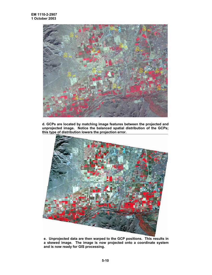
EM 1110-2-2907 1 October 2003

d. GCPs are located by matching image features between the projected and unprojected image. Notice the balanced spatial distribution of the GCPs; this type of distribution lowers the projection error.

e. Unprojected data are then warped to the GCP positions. This results in a skewed image. The image is now projected onto a coordinate system and is now ready for GIS processing.

5-10

EM 1110-2-2907 1 October 2003

f. RMS error for each GCP is recorded in a matrix spreadsheet. A total RMS error of 0.7742 is provided in the upper margin of Figure 5-4a.

Figure 5-4. GCP selection display modules. 5-18 Project Image and Save. The last procedure in rectification involves re-sam-pling the image using a “nearest neighbor” re-sampling technique. The software easily performs this process. Nearest neighbor re-sampling uses the value of the nearest pixel and extracts the value to the output, or re-sampled pixel. This re-sampling method pre-serves the digital number value (spectral value) of the original data. Additional re-sam-pling methods are bilinear interpolation and cubic convolution, which recalculate the spectral data. The image is projected subsequent to re-sampling, and the file is ready to be saved with a new name.

Recommendation: Naming altered data files and documenting

procedures

Manipulating the data alters the original data file. It is therefore a good idea to save data files with different names after performing major alterations to the data. This practice creates reliable data backup files. Because of the number of data files an analysis can create, it is best to clearly name the altered image files with the procedure name performed on the image (i.e., “TmSept01warped” indicates Thematic Mapper data collected September 2001, warped by user). Be sure to document your procedures and parameters used in a journal or a text file. Include the name of the altered file, changes applied to the data, the date, and other useful information.

5-11

EM 1110-2-2907 1 October 2003

5-19 Image to Image Rectification.

a. Images can also be rectified to a second projected digital image. The procedure is similar to that performed in image to map rectification. Simply locate common, identifi-able features in both images, match the locations, and assign GCPs. Adjust GCPs until RMS error is less than 1.0. Enter the coordinate system that will be used and designate a re-sampling method (Figure 5-4).

b. Rectified images can easily be converted from one coordinate system to another. Projected images can readily be superimposed onto other projected data and used for georeferencing image features. 5-20 Image Enhancement. The major advantage of remote sensing data lies in the ability to visually evaluate the data for overall interpretation. An accurate visual inter-pretation may require modification of the output brightness of a pixel in an effort to im-prove image quality. Here are a number of methods used in image enhancement. This paragraph examines the operations of 1) contrast enhancement, 2) band ratio, 3) spatial filtering, and 4) principle components. The type of enhancement performed will depend on the appearance of the original scene and the goal of the interpretation.

a. Image Enhancement #1: Contrast Enhancement.

(1) Raw Image Data. Raw satellite data are stored as multiple levels of brightness known as the digital number (DN). Paragraph 2-7a explained the relationship between the number of brightness levels and the size of the data storage. Data stored in an 8-bit data format maintain 256 levels of brightness. This means that the range in brightness will be 0 to 255; zero is assigned the lowest brightness level (black in gray- and color-scale images), while 255 is assigned the highest brightness value (white in gray scale or 100% of the pigment in a color scale). The list below summarizes the brightness ranges in a gray scale image.

0 = black 50 = dark gray 150 = medium gray 200 = light gray 255 = white

(a) When a satellite image is projected, the direct one-to-one assignment of

gray scale brightness to digital number values in the data set may not provide the best visual display (Figures 5-5 and 5-6). This will happen when a number of pixel values are clustered together. For instance, if 80% of the pixels displayed DNs ranging from 50–95, the image would appear dark with little contrast.

5-12

EM 1110-2-2907 1 October 2003

Figure 5-5. A linear stretch involves identifying the minimum and maximum brightness values in the image histogram and applying a transformation to stretch this range to fill the full range across 0 to 255.

Figure 5-6. Contrast in an image before (left) and after (right) a linear con-trast stretch. Taken from http://rst.gsfc.nasa.gov/Sect1/Sect1_12a.html.

(b) The raw data can be reassigned in a number of ways to improve the contrast needed to visually interpret the data. The technique of reassigning the pixel DN value is known as the image enhancement process. Image enhancement adds contrast to the data by stretching clustered DNs across the 0–255 range. If only a small part of the DN range is of interest, image enhancement can stretch those values and compress the end values to suppress their contrast. If a number of DNs are clustered on the 255 end of the range,

5-13

EM 1110-2-2907 1 October 2003

it is possible that a number of the pixels have DNs greater than 256. An image en-hancement will decompress these values, thereby increasing their contrast.

Data Analysis Histograms

Image processing software can chart the distribution of digital number values within a scene. The distribution of the brightness values is displayed as a histogram chart. The horizontal axis shows the spread of the digital numbers from 0 to the maximum DN value in the data set. The vertical axis shows the frequency or how many pixels in the scene each value has (Figure 5-7). The histogram allows an analyst to quickly access the type of distribution maintained by the data. Types of distribution may be normal, bimodal, or skewed (Figure 5-7). Histograms are particularly useful when images are enhanced.

Lookup Tables

A lookup table (LUT) graphs the intensity of the input pixel value relative to the output brightness observed on the screen. The curve does not provide information about the frequency of brightness, instead it provides information regarding the range associated with the brightness levels. An image enhancement can be modeled on a lookup table to better evaluate the relationship between the unaltered raw data and the adjusted display data.

Scatter plots

The correlation between bands can be seen in scatter plots generated by the software. The scatter plots graph the digital number value of one band relative to another (Figure 5-8). Bands that are highly correlated will produce plots with a linear relationship and little deviation from the line. Bands that are not well correlated will lack a linear relationship. Digital number values will cluster or span the chart randomly. Scatter plots allow for a quick assessment of the usefulness of particular band combinations.

5-14

EM 1110-2-2907 1 October 2003

Figure 5-7. Pixel population and distribution across the 0 to 255 digital number range. All three plots show the pixel dis-tribution before and after a linear stretch function (white de-notes pre-stretch distribution and colored elements denote stretched pixel distribution). The stretched histogram shows gaps between the single values due to the discrete number of pixel values in the data set. The top histogram (red) has a bimodal distribution. The middle (green) maintains a skewed distribution, while the last histogram (blue) reveals a normal distribution. The solid black line superimposed in each im-age indicates the maximum and minimum DN value that is stretched across the entire range. Notice the straight lines that join the linear segment. Image taken from Prospect (2002 and 2003).

5-15

EM 1110-2-2907 1 October 2003

Figure 5-8. Landsat TM band 345 RGB color composite with accompanying image scatter plots. The scatter plots map band 3 relative to bands 4 and 5 onto a feature space graph. The data points in the plot are color coded to display pixel population. The table provides the pixel count for five image features in band 3, 4, and 5. A is agricultural land, B is deep (partially clear) water, C is sediment laden water, D is undeveloped land, E fallow fields. Image developed for Prospect (2002 and 2003).

(2) Enhancing Pixel Digital Number Values. Images can enhance or stretch the visual display of an image by setting up a different relationship between the DN and the brightness level. The enhancement relationship created will depend on the distribution of pixel DN values and which features need enhancement. The enhancement can be applied to both gray- and color-scale images.

(3) Contrast Enhancement Techniques. The histogram chart and lookup table are useful tools in image enhancement. Enhancement stretching involves a variety of tech-niques, including contrast stretching, histogram equalization, logarithmic enhancement, and manual enhancement. These methods assume the image has a full range of intensity (from 0–255 in 8-bit data) to display the maximum contrast.

(4) Linear Contrast Stretching. Contrast stretching takes an image with clustered intensity values and stretches its values linearly over the 0–255 range. Pixels in a very

5-16

EM 1110-2-2907 1 October 2003

bright scene will have a histogram with high intensity values, while a dark scene will have low intensity values (Figure 5-9). The low contrast that results from this type of DN distribution can be adjusted with contrast stretching, a linear enhancement function performed by image processing software. The method can be monitored with the use of a histogram display generated by the program.

Figure 5-9. Unenhanced satellite data on left. After a default stretch, image contrast is increased as the digital number values are distributed over the 0–255 color range. The resulting scene (shown on the right) has a higher contrast.

(a) Contrast stretching allocates the minimum and maximum input values to 0

and 255, respectively. The process assigns a gray level 0 to a selected low DN value, chosen by the user. All DNs smaller than this value are assigned 0 as well, grouping the low input values together. Gray level 255 is similarly assigned to a selected high DN value and all higher DN values. Intermediate gray levels are assigned to intermediate DN values proportionally. The resulting graph looks like a straight line (shown in Figure 5-7 as the black solid-line plot superimposed onto the three DN histograms), while the corresponding histogram will distribute values across the range, leaving an increase to the image contrast (Figure 5-9). The stretched histogram shows gaps between the single values due to the discrete number of pixel values in the data set (Figure 5-7). The pro-portional brightness gives a more accurate appearance to the image data, and will better accommodate visual interpretation.

(b) The linear enhancement can be greatly affected by a random error that is particularly high or low in brightness values. For this reason, a non-linear stretch is sometimes preferred. In non-linear stretches, such as histogram equalization and loga-rithmic enhancement, brightness values are reassigned using an algorithm that exagger-ates contrast in the range of brightness values most common in that image.

5-17

EM 1110-2-2907 1 October 2003

(5) Histogram Equalization. Low contrast can also occur when values are spread

across the entire range. The low contrast is a result of tight clustering of pixels in one area (Figure 5-10a). Because some pixel values span the intensity range it is not possible to apply the contrast linear stretch. In Figure 5-10a, the high peak on the low intensity end of the histogram indicates that a narrow range of DNs is used by a large number of pixels. This explains why the image appears dark despite the span of values across the full 0–255 range.

(a) Histogram equalization evenly distributes the pixel values over the entire intensity range (see steps below). The pixels in a scene are numerically arranged ac-cording to their DN values and divided into 255 equal-sized groups. The lowest level is assigned a gray level of zero, the next group is assigned DN 1, …, the highest group is assigned gray level 255. If a single DN value has more pixels than a group, gray levels will be skipped. This produces gaps in the histogram distribution. The resultant shape of the graph will depend on the frequency of the scene.

(b) This method generally reduces the peaks in the histogram, resulting in a flatter or lower curve (Figure 5-10b). The histogram equalization method tends to en-hance distinctions within the darkest and brightest pixels, sacrificing distinctions in mid-dle-gray. This process will result in an overall increase in image contrast (Figure 5-10b).

(6) Logarithmic Enhancement. Another type of enhancement stretch uses a loga-

rithmic algorithm. This type of enhancement distinguishes lower DN values. The high intensity values are grouped together, which sacrifices the distinction of pixels with higher DN.

(7) Manual Enhancement. Some software packages will allow users to define an arbitrary enhancement. This can be done graphically or numerically. Manually adjusting the enhancement allows the user to reduce the signal noise in addition to reducing the contrast in unimportant pixels. Note: The processes described above do not alter the spectral radiance of the pixel raw data. Instead, the output display of the radiance is modified by a computed algorithm to improve image quality.

b. Image Enhancement #2: Band Arithmetic

(1) Band Arithmetic. Spectral band data values can be combined using arithmetic

to create a new “band.” The digital number values can be summed, subtracted, multi-plied, and divided (see equations 5-1 and 5-2). Image software easily performs these op-erations. This section will review only those arithmetic processes that involve the divi-sion or ratio of digital band data.

(2) Band Ratio. Band ratio is a commonly used band arithmetic method in which one spectral band is proportioned with another spectral band. This simple method re-duces the effects of shadowing caused by topography, highlights particular image ele-ments, and accentuates temporal differences (Figure 5-11).

5-18

EM 1110-2-2907 1 October 2003

b. After histogram equalization stretch the

pixels are reassigned new values and spread out across the entire value range. The data maximum is subdued while the histogram leading and trailing edges are amplified, the resulting image has an overall increase in contrast.

a. Image and its corresponding DN histogram show that the majority of pixels are clustered together (cen-tering approximately on DN value of 100).

Figure 5-10. Landsat image of Denver area.

5-19

EM 1110-2-2907 1 October 2003

Landsat bands 3, 2, 1

Band ratio 3/1 highlights hematite

Band ratio 1/7 highlights aluminum ore

Band ratio 7/5 highlights clays

Band ratio 4/2 highlights biomass Figure 5-11. NASA Landsat images from top to bottom: Color composite bands 3, 2, 1, band ratio 3/1 highlights iron oxide minerals, band ratios 7/5 and 1/7 re-veals the presence of water in minerals—appropriate for mapping clay miner-als or aluminum ore, and band ratio 4/2 allows for biomass determination.

5-20

EM 1110-2-2907 1 October 2003

(3) Shadow Removal from Data. The effect of shadowing is typically caused by a combination of sun angle and large topographic features (i.e., shadows of mountains). Table 5-1 lists the pixel digital number values for radiance measured from two different objects for two bands (arbitrarily chosen) under differing lighting conditions. Pixel data representing the radiance reflecting off deciduous trees (trees that lose their leaves annu-ally) is consistently higher for non-shadowed objects. This holds true as shadowing ef-fectively lowers the pixel radiance. When the ratio of the two bands is taken (or divided by one another) the resultant ratio value is not influenced by the effects of shadowing (see Table 5-1). The band ratio therefore creates a more reliable data set.

Table 5-1 Effects of shadowing

Tree type Light conditions Band A (DN)

Band B (DN)

Band A/B (ratio) (DN)

Deciduous Trees In sunlight 48 50 0.96 In shadow 18 19 0.95 Coniferous Trees In sunlight 31 45 0.69 In shadow 11 16 0.69

(4) Emphasize Image Elements. A number of ratios have been empirically devel-

oped and can highlight many aspects of a scene. Listed below are only a few common band ratios and their uses. When choosing bands for this method, it is best to consider bands that are poorly correlated. A greater amount of information can be extracted from ratios with bands that are covariant.

B3/B1 – iron oxide B3/B4 – vegetation B4/B2 – vegetation biomass B4/B3 – known as the RVI (Ratio Vegetation Index) B5/B2 – separates land from water B7/B5 – hydrous minerals B1/B7 – aluminum hydroxides B5/B3 – clay minerals

(5) Temporal Differences. Band ratio can also be used to detect temporal changes

in a scene. For instance, if a project requires the monitoring of vegetation change in a scene, a ratio of band 3 from image data collected at different times can be used. The newly created band file may have a name such as “Band3’Oct.98/Ban3’Oct.02.” When the new band is loaded, the resulting ratio will highlight areas of change; these pixels will appear brighter. For areas with no change, the resulting pixel values will be low and the resulting pixel will appear gray.

(a) One advantage of the ratio function lies in its ability to not only filter out the effects of shadowing but also the effects attributable to differences in sun angle. The sun angle may change from image to image for a particular scene. The sun angle is con-trolled by the time of day the data were collected as well as the time of year (seasonal effects). Processing images collected under different sun angle conditions may be un-

5-21

EM 1110-2-2907 1 October 2003

avoidable. Again, a ratio of the bands of interest will limit shadowing and sun angle ef-fects. It is therefore possible to perform a temporal analysis on data collected at different times of the day or even at different seasons.

(b) A disadvantage of using band ratio is the emphasis that is placed on noise in the image. This can be reduced, however, by applying a spatial filter before employing the ratio function; this will reduce the signal noise. See Paragraph 5-20c.

(6) Create a New Band with the Ratio Data. Most software permits the user to perform a band ratio function. The band ratio function converts the ratio value to a meaningful digital number (using the 256 levels of brightness for 8-bit data). The ratio can then be saved as a new band and loaded onto a gray scale image or as a single band in a color composite.

(7) Other Types of Ratios and Band Arithmetic. There are a handful of ratios that highlight vegetation in a scene. The NDVI (Normalized Difference Vegetation Index; equations 5-1and 5-2) is known as the “vegetation index”; its values range from –1 to 1.

NDVI = NIR-red/NIR + red (5-1) where NDVI is the normalized difference vegetation index, NIR is the near infrared, and red is the band of wavelengths coinciding with the red region of the visible portion of the spectrum. For Landsat TM data this equation is equivalent to:

NDVI = Band 4- Band 3/ Band 4+ Band 3 (5-2) In addition to the NDVI, there is also IPVI (Infrared Percentage Vegetation Index), DVI (Difference Vegetation Index), and PVI (Perpendicular Vegetation Index) just to name a few. Variation in vegetation indices stem from the need for faster computations and the isolation of particular features. Figure 5-12 illustrates the NDVI.

5-22

EM 1110-2-2907 1 October 2003

Figure 5-12. Top: True color CAMIS image. Bottom: NDVI mask isolating vegetated pixels. This mask will be useful during the classification process, which will subsequently classify only the vegetation in the scene while disregarding water and urban features. Taken from Campbell (2003).

5-23

EM 1110-2-2907 1 October 2003

c. Image Enhancement #3: Spatial Filters. It is occasionally advantageous to reduce

the detail or exaggerate particular features in an image. This can be done by a convolu-tion method creating an altered or “filtered” output image data file. Numerous spatial filters have been developed and can be automated within software programs. A user can also develop his or her own spatial filter to control the output data set. Presented below is a short introduction to the method of convolution and a few commonly used spatial filters.

(1) Spatial Frequency. Spatial frequency describes the pattern of digital values observed across an image. Images with little contrast (very bright or very dark) have zero spatial frequency. Images with a gradational change from bright to dark pixel val-ues have low spatial frequency; while those with large contrast (black and white) are said to have high spatial frequency. Images can be altered from a high to low spatial fre-quency with the use of convolution methods.

(2) Convolution.

(a) Convolution is a mathematical operation used to change the spatial fre-quency of digital data in the image. It is used to suppress noise in the data or to exagger-ate features of interest. The operation is performed with the use of a spatial kernel. A kernel is an array of digital number values that form a matrix with odd numbered rows and columns (Table 5-2). The kernel values, or coefficients, are used to average each pixel relative to its neighbor across the image. The output data set will represent the av-eraging effect of the kernel coefficients. As a spatial filter, convolution can smooth or blur images, thereby reducing image noise. In feature detection, such as an edge en-hancement, convolution works to exaggerate the spatial frequency in the image. Kernels can be reapplied to an image to further smooth or exaggerate spatial frequency.

(b) Low pass filters apply a small gain to the input data (Table 5-2a). The re-sulting output data will decrease the spatial frequency by de-emphasizing relatively bright pixels. Two types of low pass filters are the simple mean and center-weighted mean methods (Table 5-2a and b). The resultant image will appear blurred. Alterna-tively, high pass frequency filters (Table 5-2c) increase image spatial frequency. These types of filters exaggerate edges without reducing image details (an advantage over the Laplacian filter discussed below).

(2) Laplacian or Edge Detection Filter.

(a) The Laplacian filter detects discrete changes in spectral frequency and is used for highlighting edge features in images. This type of filter works well for deline-ating linear features, such as geologic strata or urban structures. The Laplacian is calcu-lated by an edge enhancement kernel (Table 5-2d and e); the middle number in the ma-trix is much higher or lower than the adjacent coefficients. This type of kernel is sensitive to noise and the resulting output data will exaggerate the pixel noise. A smoothing convolution filter can be applied to the image in advance to reduce the edge filter's sensitivity to data noise.

5-24

EM 1110-2-2907 1 October 2003

The Convolution Method Convolution is carried out by overlaying a kernel onto the pixel image and centering its middle value over the pixel of interest. The kernel is first placed above the pixel located at the top left corner of the image and moved from top to bottom, left to right. Each kernel position will create an output pixel value, which is calculated by multiplying each input pixel value with the kernel coefficient above it. The product of the input data and kernel is then averaged over the array (sum of the product divided by the number of pixels evaluated); the output value is assigned this average. The kernel then moves to the next pixel, always using the original input data set for calculating averages. Go to http://www.cla.sc.edu/geog/rslab/Rscc/rscc-frames.html for an in-depth description and examples of the convolution method. The pixels at the edges create a problem owing to the absence of neighboring pixels. This problem can be solved by inventing input data values. A simpler solution for this problem is to clip the bottom row and right column of pixels at the margin.

(b) The Laplacian filter measures the changes in spectral frequency or pixel in-tensity. In areas of the image where the pixel intensity is constant, the filter assigns a digital number value of 0. Where there are changes in intensity, the filter assigns a posi-tive or negative value to designate an increase or decrease in the intensity change. The resulting image will appear black and white, with white pixels defining the areas of changes in intensity. Table 5-2 Variety in 9-Matix Kernel Filters Used in a Convolution Enhancement. Each graphic shows a kernel, an example of raw DN data array, and the resultant enhanced data array. See http://www.cee.hw.ac.uk/hipr/html/filtops.html for further information on kernels and the filtering methods.

a. Low Pass: simple mean kernel. 1 1

1 1 1 1 1

1 1 1 1 1 1

1

1

1 1 1 1 1 1 1 11 1 1 1 1 1 1 1 1 1 1 1 1 11 1 1 1 1 1 1 1 1 2 2 2 1 11 1 1 10 1 1 1 1 1 2 2 2 1 11 1 1 1 1 1 1 1 1 2 2 2 1 11 1 1 1 1 1 1 1 1 1 1 1 1 11 1 1 1 1 1 1 1 1 1 1 1 1 1

Raw data Output data

5-25

EM 1110-2-2907 1 October 2003

b. Low Pass: center weighted mean kernel. 1 1 1 1 2 1 1 1 1 1 1 1 1 1 1 1 1 1 1 1 1 1 1 1 1 1 1 1 1 1 1 1 1 1 1 1 1 1 1 1 1 1 1 1 1 1 2 2 2 1 1 1 1 1 10 1 1 1 1 1 2 3 2 1 1 1 1 1 1 1 1 1 1 1 2 2 2 1 1 1 1 1 1 1 1 1 1 1 1 1 1 1 1 1 1 1 1 1 1 1 1 1 1 1 1 1 1 Raw data Output data

c. High Pass kernel. -1 -1 -1 -1 8 -1 -1 -1 -1 10 10 10 10 10 10 10 0 0 0 0 0 0 0 10 10 10 10 10 10 10 0 0 0 0 0 0 0 10 10 10 10 10 10 10 0 0 -5 -5 -5 0 0 10 10 10 15 10 10 10 0 0 -5 40 -5 0 0 10 10 10 10 10 10 10 0 0 -5 -5 -5 0 0 10 10 10 10 10 10 10 0 0 0 0 0 0 0 10 10 10 10 10 10 10 0 0 0 0 0 0 0 Raw data Output data

d. Direction Filter: north-south component kernel. -1 2 -1 -2 1 -2 -1 2 -1 1 1 1 2 1 1 1 0 0 -4 8 -4 0 0 1 1 1 2 1 1 1 0 0 -4 8 -4 0 0 1 1 1 2 1 1 1 0 0 -4 8 -4 0 0 1 1 1 2 1 1 1 0 0 -4 8 -4 0 0 1 1 1 2 1 1 1 0 0 -4 8 -4 0 0 1 1 1 2 1 1 1 0 0 -4 8 -4 0 0 1 1 1 2 1 1 1 0 0 -4 8 -4 0 0 Raw data Output data

e. Direction Filter: East-west component kernel. -1 -2 -1 2 4 2 -1 -2 -1 1 1 1 2 1 1 1 0 0 0 0 0 0 0 1 1 1 2 1 1 1 0 0 0 0 0 0 0 1 1 1 2 1 1 1 0 0 0 0 0 0 0 1 1 1 2 1 1 1 0 0 0 0 0 0 0 1 1 1 2 1 1 1 0 0 0 0 0 0 0 1 1 1 2 1 1 1 0 0 0 0 0 0 0 1 1 1 2 1 1 1 0 0 0 0 0 0 0 Raw data Output data

5-26

EM 1110-2-2907 1 October 2003

d. Image Enhancement #4: Principle Components. The principle component analy-

sis (PCA) is a technique that transforms the pixel brightness values. This transformation compresses the data by drawing out maximum covariance and removes correlated ele-ments. The resulting data will contain new, uncorrelated data that can be later used in classification techniques.

(1) Band Correlation. Spectral bands display a range of correlation from one band to another. This correlation is easily viewed by bringing up a scatter plot of the digital data and plotting, for instance, band 1 vs. band 2. Many bands share elements of information, particularly bands that are spectrally close to one another, such as band 1 and 2. For bands that are highly correlated, it is possible to predict the brightness out-come of one band with the data of the other (Figure 5-13). Therefore, bands that are well correlated may not be of use when attempting to isolate spectrally similar objects.

Figure 5-13. Indian IRS-1D image and accompanying spectral plot. Representative pixel points for four image elements (fluvial sediment in a braided channel, water, agriculture, and forest) are plotted for each band. Plot illustrates the ease by which each element can be spectrally separarted. For example, water is easily distinguishable from the other elements in band 2.

(2) Principle Component Transformation. The principle component method ex-tracts the small amount of variance that may exist between two highly correlated bands and effectively removes redundancy in the data. This is done by “transforming” the ma-jor vertical and horizontal axes. The transformation is accomplished by rotating the horizontal axis so that it is parallel to a least squares regression line that estimates the data. This transformed axis is known as PC1, or Principle Component 1. A second axis, PC2, is drawn perpendicular to PC1, and its origin is placed at the center of the PC1 range (Figure 5-14). The digital number values are then re-plotted on the newly transformed axes. This transformation will result in data with a broader range of values. The data can be saved as a separate file and loaded as an image for analysis.

5-27

EM 1110-2-2907 1 October 2003

Band A Brightness Value

Ban

d B

Brig

htne

ss V

alue

PC1 PC2

0 0 255

255

Figure 5-14. Plot illustrates the spectral variance between two bands, A and B. PC1 is the line that captures the mean of the data set. PC2 is orthogonal to PC1. PC1 and PC2 be-come the new horizontal and vertical axis; brightness values are redrawn onto the PC1 and PC2 scale.

c. Transformation Series (PC1, PC2, PC3, PC4, PC5, etc.). The process of transform-ing the axis to fit the maximum variance in the data can be performed in succession on the same data set. Each successive axis rotation creates a new principal component axis; a series of transformations can then be saved as individual files. Band correlation is greatly reduced in the first PC transformation, 90% of the variance between the bands will be isolated by PC1. Each principle component transformation extracts less and less variance, PC2, for instance, isolates 5% of the variance, and PC3 will extract 3% of the variance, and so on (Figure 5-15). Once PC1 and PC2 have been processed, approxi-mately 95% of the variance within the bands will be extracted. In many cases, it is not useful to exact the variance beyond the third principle component. Because the principle component function reduces the size of the original data file, it functions as a pre-proc-essing tool and better prepares the data for image classification. The de-correlation of band data in the principle component analysis is mathematically complex. It linearly

5-28

EM 1110-2-2907 1 October 2003

transforms the data using a form of factor analysis (eigen value and eigen vector matrix). For a complete discussion of the technique see Jensen (1996).

Figure 5-15. PC-1 contains most of the variance in the data. Each succes-sive PC-transformation isolates less and less variation in the data. Taken from http://rst.gsfc.nasa.gov/start.html.

d. Image Classification. Raw digital data can be sorted and categorized into thematic maps. Thematic maps allow the analyst to simplify the image view by assigning pixels into classes with similar spectral values (Figure 5-16). The process of categorizing pix-els into broader groups is known as image classification. The advantage of classification is it allows for cost-effective mapping of the spatial distribution of similar objects (i.e., tree types in forest scenes); a subsequent statistical analysis can then follow. Thematic maps are developed by two types of classifications, supervised and unsupervised. Both types of classification rely on two primary methods, training and classifying. Training is the designation of representative pixels that define the spectral signature of the object class. Training site or training class is the term given to a group of training pixels. Clas-sifying procedures use the training class to classify the remaining pixels in the image.

5-29

EM 1110-2-2907 1 October 2003

Figure 5-16. Landsat image (left) and its corresponding thematic map (right) with 17 the-matic classes. The black zigzag at bottom of image is the result of shortened flight line over-lap. (Campbell, 2003).

(1) Supervised Classification. Supervised classification requires some knowledge about the scene, such as specific vegetative species. Ground truth (field data), or data from aerial photographs or maps can all be used to identify objects in the scene.

(2) Steps Required for Supervised Classification.

(a) Firstly, acquire satellite data and accompanying metadata. Look for infor-mation regarding platform, projection, resolution, coverage, and, importantly, meteoro-logical conditions before and during data acquisition.

(b) Secondly, chose the surface types to be mapped. Collect ground truth data with positional accuracy (GPS). These data are used to develop the training classes for the discriminant analysis. Ideally, it is best to time the ground truth data collection to coincide with the satellite passing overhead.

(c) Thirdly, begin the classification by performing image post-processing tech-niques (corrections, image mosaics, and enhancements). Select pixels in the image that are representative (and homogeneous) of the object. If GPS field data were collected, geo-register the GPS field plots onto the imagery and define the image training sites by outlining the GPS polygons. A training class contains the sum of points (pixels) or poly-gons (clusters of pixels) (see Figures 5-17 and 5-18). View the spectral histogram to in-spect the homogeneity of the training classes for each spectral band. Assign a color to represent each class and save the training site as a separate file. Lastly, extract the re-

5-30

EM 1110-2-2907 1 October 2003

maining image pixels into the designated classes by using a discriminate analysis routine (discussed below).

Figure 5-17. Landsat 7 ETM image of central Australia (4, 3, 2 RGB). Lin-ear features in the upper portion of the scene are sand dunes. Training data are selected with a selection tool (note the red enclosure). A similar process was performed on data from Figure 5-16 (the DN values for figure 5-16 are presented in Figure 5-18).

5-31

EM 1110-2-2907 1 October 2003

SORT # CLASS NAME COLOR TRAINING CLASSIFIED % TOTAL % DATA

1 Unclassified 25,207,732 68.86% 2 ROAD Red1 77 0 0.00% 0.003 AG Green1 1642 0 0.00% 0.004 LP Red1 4148 2,164,089 5.91% 19.535 LPO Blue1 5627 1,562,180 4.27% 14.106 LPH Maroon1 4495 2,170,395 5.93% 19.587 MHW-low Aquamarine 888 329,360 0.90% 2.978 CUT Chartreuse 1219 1,055,063 2.88% 9.529 MHW-high Sienna1 3952 1,566,698 4.28% 14.14

10 MORT Green3 1703 4,651 0.01% 0.0412 juncus-low-density Red1 52 37,808 0.10% 0.3413 juncus-high-density Blue1 65 102,174 0.28% 0.9213 juncus-panicum-mix Cyan1 53 0 0.00% 0.0014 juncus-mixed-clumps-field Magenta1 29 3 0.00% 0.0016 g1=hd-scol+background+w Green1 32 610,283 1.67% 5.5117 g2=md-scol+background Yellow1 29 952 0.00% 0.0118 g4=md-scol+spartina+mud Maroon1 36 0 0.00% 0.0019 g3=md-scol+spartina+background Purple1 50 0 0.00% 0.0020 g5=ld-scol+mud Aquamarine 56 617 0.00% 0.0121 g1=md-spal+w Red1 66 4,789 0.01% 0.0422 g2=hd-spal+w Green1 52 141,060 0.39% 1.2723 g3=hd-spal+w+sppa Cyan1 29 803,145 2.19% 7.2524 g4=md-spal+w+sppa Magenta1 44 0 0.00% 0.0025 g5=hd-spal+mud Red1 25 25 0.00% 0.0026 g6=mixed-spal Chartreuse 28 6,555 0.02% 0.0626 g7=md-spal+lit+mud Thistle1 36 6 0.00% 0.0028 g8=md-mixed-spal Blue4 85 0 0.00% 0.0029 g1=hd-sppa+mix Red1 37 74 0.00% 0.0030 g2=hd-sppa+mud Blue1 40 0 0.00% 0.0031 g3=mhd-sppa+spal+background Cyan1 32 939 0.00% 0.0132 g4=lmd-sppa+mix+background Magenta1 160 0 0.00% 0.0033 g9-ld-sppa+spal+mud Blue4 28 520,290 1.42% 4.6934 g10=ld-sppa+mix+background Cyan3 45 0 0.00% 0.0035 g11=ld-sppa+w+mix Green2 32 1,255 0.00% 0.0137 11082411.00

Figure 5-18. Classification training data of 35 landscape classification features. “Training” pro-vides the pixel count after training selection; classification provides the image pixel count after a classification algorithm is performed. This data set accompanies Figure 5-16, the classified image. (Campbell, 2003).

(3) Classification Algorithms. Image pixels are extracted into the designated classes by a computed discriminant analysis. The three types of discriminant analysis algorithms are: minimum mean distance, maximum likelihood, and parallelepiped. All use brightness plots to establish the relationship between individual pixels and the training class (or training site).

(a) Minimum Mean Distance. Minimum distance to the mean is a simple com-putation that classifies pixels based on their distance from the mean of the training class.

5-32

EM 1110-2-2907 1 October 2003

It is determined by plotting the pixel brightness and calculating its Euclidean distance (using the Pythagorean theorem) to the unassigned pixel. Pixels are assigned to the training class for which it has a minimum distance. The user designates a minimum dis-tance threshold for an acceptable distance; pixels with distance values above the desig-nated threshold will be classified as unknown.

(b) Parallelepiped. In a parallelepiped computation, unassigned pixels are grouped into a class when their brightness values fall within a range of the training mean. An acceptable digital number range is established by setting the maximum and minimum class range to plus and minus the standard deviation from the training mean. The pixel brightness value simply needs to fall within the class range, and is not based on its Euclidean distance. It is possible for a pixel to have a brightness value close to a class and not fall within its acceptable range. Likewise, a pixel may be far from a class mean, but fall within the range and therefore be grouped with that class. This type of classification can create training site overlap, causing some pixels to be misclassified.

(c) Maximum Likelihood. Maximum Likelihood is computationally complex. It establishes the variance and covariance about the mean of the training classes. This algo-rithm then statistically calculates the probability of an unassigned pixel belonging to each class. The pixel is then assigned to the class for which it has the highest probability. Figure 5-19 visually illustrates the differences between these supervised classification methods.

Figure 5-19. From left to right, minimum mean distance, parallelepiped, and maximum likelihood. Courtesy of the Department of Geosciences at Murray State University.

(4) Assessing Error. Accuracy can be qualitatively determined by an error matrix

(Table 5-3). The matrix establishes the level of errors due to omission (exclusion error), commission (inclusion error), and can tabulate an overall total accuracy. The error ma-trix lists the number of pixels found within a given class. The rows in Table 5-2 list the pixels classified by the image software. The columns list the number of pixels in the reference data (or reported fro m field data). Omission error calculates the probability of

5-33

EM 1110-2-2907 1 October 2003

a pixel being accurately classified; it is a comparison to a reference. Commission deter-mines the probability that a pixel represents the class for which it has been assigned. The total accuracy is measured by calculating the proportion correctly classified pixel rela-tive to the total tested number of pixels (Total = total correct/total tested).

Table 5-3 Omission and Commission Accuracy Assessment Matrix. Taken from Jensen (1996).

Reference Data Classification Residential Commercial Wetland Forest Water Raw Total Residential 70 5 0 13 0 88 Commercial 3 55 0 0 0 58 Wetland 0 0 99 0 0 99 Forest 0 0 4 37 0 41 Water 0 0 0 0 121 121 Column Total 73 60 103 50 121 407 Overall Accuracy = 382/407=93.86%

Producer’s Accuracy (measure of omission error) Residential= 70/73 = 96–4% omission error Commercial= 55/60 = 92–8% omission error Wetland= 99/103 = 96–4% omission error Forest= 97/50 = 74–26% omission error Water= 121/121 = 100–0% omission error

User’s Accuracy (measure of commission error) Residential= 70/88 = 80–20% omission error Commercial= 55/58 = 95–5% omission error Wetland= 99/99 = 100–0% omission error Forest= 37/41 = 90–10% omission error Water= 121/121 = 100–0% omission error

Example error matrix taken from Jensen (1986). Data are the result of an accuracy assessment of Landsat TM data.

Classification method summary

Image classification uses the brightness values in one or more spectral bands, and classifies each pixel based on its spectral information The goal in classification is to assign remaining pixels in the image to a designated class such as water, forest, agriculture, urban, etc. The resulting classified image is composed of a collection of pixels, color-coded to represent a particular theme. The overall process then leads to the creation of a thematic map to be used to visually and statistically assess the scene.

5-34

EM 1110-2-2907 1 October 2003

(5) Unsupervised Classification. Unsupervised classification does not re-quire prior knowledge. This type of classification relies on a computed algorithm that clusters pixels based on their inherent spectral similarities.

(a) Steps Required for Unsupervised Classification. The user designates 1) the number of classes, 2) the maximum number of iterations, 3) the maximum number of times a pixel can be moved from one cluster to another with each it-eration, 4) the minimum distance from the mean, and 5) the maximum standard deviation allowable. The program will iterate and recalculate the cluster data until it reaches the iteration threshold designated by the user. Each cluster is chosen by the algorithm and will be evenly distributed across the spectral range maintained by the pixels in the scene. The resulting classification image (Figure 5-20) will approximate that which would be produced with the use of a minimum mean dis-tance classifier (see above, “classification algorithm”). When the iteration thresh-old has been reached the program may require you to rename and save the data clusters as a new file. The display will automatically assign a color to each class; it is possible to alter the color assignments to match an existing color scheme (i.e., blue = water, green = vegetation, red = urban) after the file has been saved. In the unsupervised classification process, one class of pixels may be mixed and as-signed the color black. These pixels represent values that did not meet the re-quirements set by the user. This may be attributable to spectral “mixing” repre-sented by the pixel.

(b) Advantages of Using Unsupervised Classification. Unsupervised

classification is useful for evaluating areas where you have little or no knowledge of the site. It can be used as an initial tool to assess the scene prior to a supervised classification. Unlike supervised classification, which requires the user to hand select the training sites, the unsupervised classification is unbiased in its geo-graphical assessment of pixels.

(c) Disadvantages of Using Unsupervised Classification. The lack of in-formation about a scene can make the necessary algorithm decisions difficult. For instance, without knowledge of a scene, a user may have to experiment with the number of spectral clusters to assign. Each iteration is time consuming and the final image may be difficult to interpret (particularly if there is a large number of unidentified pixels such as those in Figure 5-19). The unsupervised classification is not sensitive to covariation and variations in the spectral signature to objects. The algorithm may mistakenly separate pixels with slightly different spectral val-ues and assign them to a unique cluster when they, in fact, represent a spectral continuum of a group of similar objects.

(6) Evaluating Pixel Classes. The advantages of both the supervised and unsupervised classification lie in the ease with which programs can perform sta-tistical analysis. Once pixel classes have been assigned, it is possible to list the exact number of pixels in each representative class (Figure 5-17, classified col-umn). As the size of each pixel is known from the metadata, the metric area of each class can be quickly calculated. For example, you can very quickly deter-

5-35

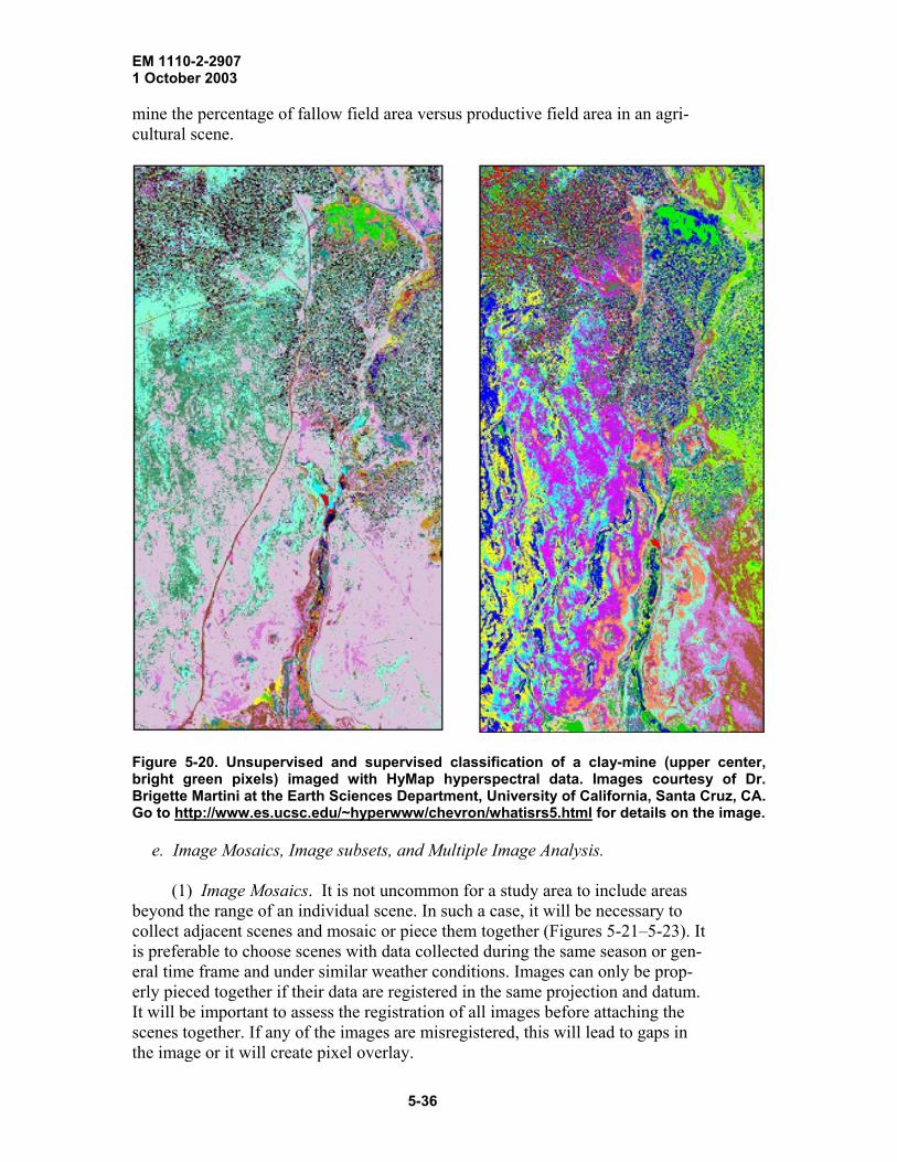
EM 1110-2-2907 1 October 2003

mine the percentage of fallow field area versus productive field area in an agri-cultural scene.

Figure 5-20. Unsupervised and supervised classification of a clay-mine (upper center, bright green pixels) imaged with HyMap hyperspectral data. Images courtesy of Dr. Brigette Martini at the Earth Sciences Department, University of California, Santa Cruz, CA. Go to http://www.es.ucsc.edu/~hyperwww/chevron/whatisrs5.html for details on the image.

e. Image Mosaics, Image subsets, and Multiple Image Analysis.

(1) Image Mosaics. It is not uncommon for a study area to include areas beyond the range of an individual scene. In such a case, it will be necessary to collect adjacent scenes and mosaic or piece them together (Figures 5-21–5-23). It is preferable to choose scenes with data collected during the same season or gen-eral time frame and under similar weather conditions. Images can only be prop-erly pieced together if their data are registered in the same projection and datum. It will be important to assess the registration of all images before attaching the scenes together. If any of the images are misregistered, this will lead to gaps in the image or it will create pixel overlay.

5-36

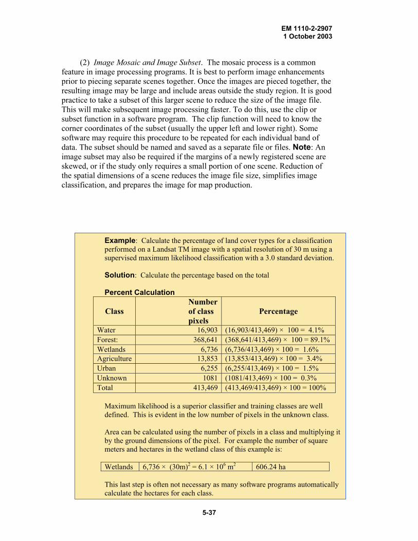
EM 1110-2-2907 1 October 2003

5-37

(2) Image Mosaic and Image Subset. The mosaic process is a common

feature in image processing programs. It is best to perform image enhancements prior to piecing separate scenes together. Once the images are pieced together, the resulting image may be large and include areas outside the study region. It is good practice to take a subset of this larger scene to reduce the size of the image file. This will make subsequent image processing faster. To do this, use the clip or subset function in a software program. The clip function will need to know the corner coordinates of the subset (usually the upper left and lower right). Some software may require this procedure to be repeated for each individual band of data. The subset should be named and saved as a separate file or files. Note: An image subset may also be required if the margins of a newly registered scene are skewed, or if the study only requires a small portion of one scene. Reduction of the spatial dimensions of a scene reduces the image file size, simplifies image classification, and prepares the image for map production.

Example: Calculate the percentage of land cover types for a classification performed on a Landsat TM image with a spatial resolution of 30 m using a supervised maximum likelihood classification with a 3.0 standard deviation. Solution: Calculate the percentage based on the total Percent Calculation

Class

Number of class pixels

Percentage

Water 16,903 (16,903/413,469) × 100 = 4.1%

Forest: 368,641 (368,641/413,469) × 100 = 89.1%

Wetlands 6,736 (6,736/413,469) × 100 = 1.6%

Agriculture 13,853 (13,853/413,469) × 100 = 3.4%

Urban 6,255 (6,255/413,469) × 100 = 1.5%

Unknown 1081 (1081/413,469) × 100 = 0.3%

Total 413,469 (413,469/413,469) × 100 = 100%

Maximum likelihood is a superior classifier and training classes are well defined. This is evident in the low number of pixels in the unknown class. Area can be calculated using the number of pixels in a class and multiplying it by the ground dimensions of the pixel. For example the number of square meters and hectares in the wetland class of this example is: Wetlands 6,736 × (30m)2 = 6.1 × 106 m2

606.24 ha This last step is often not necessary as many software programs automatically calculate the hectares for each class.

EM 1110-2-2907 1 October 2003

Figure 5-21. Multiple Landsat TM images, shown on the left (some sub-scenes are not shown here) were pieced together to create the larger mosaic image on the right. The seams within the mosaic image (right) are virtually invisible, an indication of the accuracy of the projection. Taken from Prospect (2002 and 2003).

5-38

EM 1110-2-2907 1 October 2003

Figure 5-22. Multi-image mosaic of Western United States centered on the state of Utah. Mosaic seams are invisible in this scene, an indication of good radiometric and geometric corrections. The skewed and curved margins are an artifact of the rectification and mosaic process. Taken from http://www.jpl.nasa.gov/images/earth/usa/misr_020602_2.html.

5-39

EM 1110-2-2907 1 October 2003

Figure 5-23. Landsat 7 Image of the Boston, Massachusetts area. Image on the right shows red box outlining the boundaries of the subset scene on the right. Taken from http://landsat.gsfc.nasa.gov/education/l7downloads/index.html.

(3) Multiple-image Temporal Analysis. It is possible to combine bands from different images or data sets. This allows a user to perform a change detec-tion analysis. The process of “layering” multi-temporal data involves loading a composite of bands from different images of the same scene. For example, a study assessing urban development in a forested area would benefit from examining a band combination that included band 3 data in the red plane, and band 3 data of a later image in the green plane. If the spectral signature of the scene has changed and is detectable within the resolution of the data, then changes in the scene will be highlighted. This image can then be classified and the areas of change can be statistically assessed. To perform this task accurately, it is important that both im-ages are registered properly. Misregistration will lead to an offset in the image, which leaves brightly colored lines of pixels. Be sure to choose images whose data were collected under similar conditions, such as the same season, time of day, and prevailing weather, i.e., minimum cloud cover.

f. Remote Sensing and Geospatial Information. Remote sensing data are eas-ily integrated with other digital data, such as vector data used in a GIS (Geo-graphical Information System). Vector data can be incorporated into a raster sat-ellite image by overlaying the data onto an image scene. Conversely, a raster image can be saved as a .jpeg or .tiff file and exported to a vector software proc-essing program. Remote sensing data files can provide land cover and use infor-mation as well as digital elevation models (DEMs), and a number of geo-physical and biophysical parameters. Satellite images coupled with GIS data can be used to create original maps. The use of remote sensing in this type of application can drastically cut costs of GIS database development. It also provides data for inac-cessible areas.

(1) Digital Orthoquadrangle (DOQs). A digital orthoquadrangle (DOQ) is a digital image of an aerial photograph that has had ground relief removed and is

5-40

EM 1110-2-2907 1 October 2003

geometrically corrected. The removal of ground relief adds to the accuracy meas-urement of distances on the ground. DOQs are available over the internet through the USGS or state level natural resources and environmental agencies. They come in black and white and color infrared. These digital aerial photographs come in a variety of scales and resolutions (often 1-m GSD). Due to the ortho-correc-tion process, DOQs are typically in UTM, Geographic, or State Plane Projection. The images typically have 50 to 300 m overlap. This overlap simplifies the mo-saic process. DOQs work well in combination with GIS data and may aid in the identification of objects in a satellite scene. It is possible to link a DOQ with a satellite image and a one-to-one comparison can be made between a pixel on the satellite image and the same geographic point on the DOQ.

(2) Digital Elevation Models (DEM). A Digital Elevation Model (DEM) is a digital display of cartographic elements, particularly topographic features. DEMs utilize two primary types of data, DTM (digital terrain model) or DSM (digital surface model). The DTM represents elevation points of the ground, while DSM is the elevation of points at the surface, which includes the top of buildings and trees, in addition to terrain. The DEM incorporates the elevation data and projects it relative to a coordinate reference point. (See http://www.ipf.tuwien.ac.at/fr/buildings/diss/node27.html for more information on DEM, DTM, and DEMs.

(3) DEM Generation. Elevation measurements are sampled at regular in-tervals to form an array of elevation points within the DEM. The elevation data are then converted to brightness values and can be displayed as a gray scale image (Figure 5-24). The model can be viewed in image processing software and su-perimposed onto satellite image data. The resulting image will appear as a “three-dimensional” view of the image data.

(a) DEMs come in a variety of scales and resolutions. Be sure to check the date and accuracy of the DEM file. DEMs produced before 2001 have as much a 30 m of horizontal error. As with other files, the DEM must be well reg-istered and in the same projection and datum as other files in the scene. Check the metadata accompanying the data to verify the projection.

(b) The primary source of DEM data is digital USGS topographic maps and not satellite data. Spaceborne elevation data will be more readily available with the processing and public release of the Shuttle Radar Topography Mission (SRTM) data. Some of this data is currently available through the Jet Propulsion Laboratory (http://www.jpl.nasa.gov/srtm/) and USGS EROS Data Center (http://srtm.usgs.gov/index.html).

5-41

EM 1110-2-2907 1 October 2003

Figure 5-24. Digital elevation model (DEM). The brightness values in this image represent elevation data. Dark pixels cor-respond to low elevations while the brightest pixels represent higher elevations. Taken from the NASA tutorial at http://rst.gsfc.nasa.gov/Sect11/Sect11_5.html.

(c) DEMs can be created for a study site with the use of a high resolution

raster topographic map. The method involved in creating a DEM is fairly ad-vanced; see http://spatialnews.geocomm.com/features/childs3/ for information on getting starting in DEM production.

(4) Advanced Methods in Image Processing. Remote sensing software fa-cilitates a number of advanced image processing methods. These advanced meth-ods include the processing of hyperspectral data, thermal data, radar data, spectral library development, and inter-software programming.

(a) Hyperspectral Data. Hyperspectral image processing techniques manage narrow, continuous bands of spectral data. Many hyperspectral systems maintain over 200 bands of spectral data. The narrow bands, also known as chan-nels, provide a high level of detail and resolution. This high resolution facilitates the identification of specific objects, thereby improving classification (Figure 5-24). The advantage of hyperspectral imaging lies in its ability to distinguish indi-vidual objects that would be otherwise grouped in broadband multi-spectra im-agery. Narrow bands are particularly useful for mapping resources such as crop and mineral types. The narrow, nearly continuous bands create large data sets, which require advance software and hardware to store and manipulate the data.

5-42

EM 1110-2-2907 1 October 2003

Figure 5-25. Hyperspectral classification image of the Kis-simmee River in Florida (Image created by Lowe Engineers - LLC and SAIC, 2003). Classifications of 28 vegetation com-munities are based on a supervised classification.

(b) Thermal Data. Thermal image processing techniques are used to im-

age objects by the analysis of their emitted energy (Figure 5-26). The thermal band wavelength ranges are primarily 8 to 14 µm and 3 to 5 µm. The analysis of thermal data is typically used in projects that evaluate surface temperatures, such as oceans and ice sheets, volcano studies, and the emission of heat from man-made objects (e.g., pipelines).

5-43

EM 1110-2-2907 1 October 2003

Figure 5-26. Close-up of the Atlantic Gulf Stream. Ocean temperature and current mapping was performed with AVHRR thermal data. The temperatures have been classified and color-coded. Yellow = water 23oC (73oF), green = 14Co (57oF), blue = 5oC (41oF). Taken from http://www.osdpd.noaa.gov/PSB/EPS/EPS.html.

(c) Radar. Radar (radio detection and ranging) systems are able to penetrate cloud cover in certain wavelengths. This technology is useful for imag-ing day or night surface features during periods of intense cloud cover, such as storms, smoke from fire, or sand and dust storms (Figure 5-27).

5-44

EM 1110-2-2907 1 October 2003

Figure 5-27. Radarsat image, pixel resolution equals 10 m. Image is centered over the Illinois River (upper left), Mississippi River (large channel in center), and the Missouri River (smaller channel in center. Chapter 6 case study 3 details the analysis of this scene. Taken from Tracy (2003).

g. Customized Spectral Library. Many software programs allow users to build

and maintain a customized spectral library. This is done by importing spectra sig-natures from objects of interest and can be applied to identify unknown objects in an image.

h. Internal Programming.

(1) Image processing software allows users to develop computing tech-niques and unique image displays by programming from within the software package. Programming gives the user flexibility in image manipulation and in-formation extraction. The users’ manual and online help menus are the best re-sources for information on how to program within particular software.

(2) New applications in image processing and analysis are rapidly being developed and incorporated into the field of remote sensing. Other advanced uses in image processing include the modification of standard methods to meet indi-vidual project needs and improving calibration methods. Go to http://www.techexpo.com/WWW/opto-knowledge/IS_resources.html for more

5-45

EM 1110-2-2907 1 October 2003

information on advanced and specialized hardware and software and their appli-cations.

i. The Interpretation of Remotely Sensed Data. There are four basic steps in processing a digital image: data acquisition, pre-processing, image display and enhancement, and information extraction. The first three steps have been intro-duced in this and previous chapters. This section focuses on information extrac-tion and the techniques used by researchers to implement and successfully com-plete a remote sensing analysis. The successful completion of an analysis first begins with an assessment of the project needs. This initial assessment is critical and is discussed below.

(1) Assessing Project Needs. Initiating a remote sensing project will require a thorough understanding of the project goals and the limitations accompanying its resources. Projects should begin with an overview of the objectives, followed by plans for image processing and field data collection that best match the objec-tives.

(a) An understanding of the customer resources and needs will make all aspects of the project more efficient. Practicing good client communication throughout the project will be mutually beneficial. The customer may need to be educated on the subject of remote sensing to better understand how the analysis will meet their goals and to recognize how they can contribute to the project. This can prevent false expectations of the remotely sensed imagery while laying down the basis for decisions concerning contributions and responsibilities. Plan to dis-cuss image processing, field data collection, assessment, and data delivery and support.

(b) The customer may already have the knowledge and resources needed for the project. Find out which organizations may be in partnership with the cus-tomer. Are there resources necessary for the project that can be provided by ei-ther? It is important to isolate the customer’s ultimate objective and learn what his or her intermediate objectives may be. When assessing the objectives, keep in mind the image classification needed by the customer and the level of error they are willing to accept. Consider the following during the initial stages of a project:

• What are the objectives? • Who is the customer and associated partners? • Who are the end users? • What is the final product? • What classification system is needed? • What are the resolution requirements? • What is the source of image data? • Does archive imagery exist? • Is season important? • What image processing software will be used? Is it adequate? • What type of computer hardware is available? Is it adequate? • Is there sufficient memory storage capacity for the new imagery?

5-46

EM 1110-2-2907 1 October 2003

• Are hardware and software upgrades needed? Who will finance upgrades? • Are plotters/printers available for making hardcopy maps? • Can the GIS import and process output map products? (c) Field considerations: • What are the ecosystem dynamics? What type of field data will be re-

quired? • Will the field data be collected before, after, or during image acquisition? • Who will be collecting the field data? • What sampling methods will be employed? • What field data analysis techniques will be required? • Who will be responsible for GPS/survey control? • Who will pay for the field data collection? • Is the customer willing to help by providing new field data, existing

field data, or local expertise?

(2) Visualization Interpretation.

(a) Remotely sensed images are interpreted by visual and statistical analyses. The goal in visualization is to identify image elements by recognizing the relationship between pixels and groups of pixels and placing them in a mean-ingful context within their surroundings. Few computer programs are able to mimic the adroit human skill of visual interpretation. The extraction of visual in-formation by a human analyst relies on image elements such as pixel tone and color, as well as association. These elements (discussed in Chapter 2) are best per-formed by the analyst; however, computer programs are being developed to ac-complish these tasks.

(b) Humans are proficient at using ancillary data and personal knowl-edge in the interpretation of image data. A scientist is capable of examining im-ages in a variety of views (gray scale, color composites, multiple images, and various enhancements) and in different scales (image magnification and reduc-tion). This evaluation can be coupled with additional information such as maps, photos, and personal experience. The researcher can then judge the nature and importance of an object in the context of his or her own knowledge or can look to interdisciplinary fields to evaluate a phenomena or scene.

(3) Information Extraction. Images from one area of the United States will appear vastly different from other regions owing to variations in geology and bi-omes across the continent. The correct identification of objects and groups of ob-jects in a scene comes easily with experience. Below is a brief review of the spectral characteristics of objects that commonly appear in images.

(a) Vegetation. Vegetation is distinguished from inorganic objects by its absorption of the red and blue portions of the visible spectrum. It has high reflec-tance in the green range and strong reflectance in the near infrared. Slight vari-ability in the reflectance is ascribable to differences in vegetation morphology,

5-47

EM 1110-2-2907 1 October 2003

such are leaf shape, overall plant structure, and moisture content. The spacing or vegetation density and the type of soil adjacent to the plant will also create varia-tions in the radiance and will lead to “pixel mixing.” Vegetation density is well defined by the near infrared wavelengths. Mid-infrared (1.5 to 1.75 µm) can be used as an indication of turgidity (amount of water) in plants, while plant stress can be determined by an analysis using thermal radiation. Field observations (ground truth) and multi-temporal analysis will help in the interpretation of plant characteristics and distributions for forest, grassland, and agricultural fields. See Figures 5-28 and 5-29.

Figure 5-28. Forest fire assessment using Landsat imagery (Denver, Colorado). Image on the left, courtesy of NASA, was collected in 1990; image on the right was collected in 2002 (taken from http://landsat7.usgs.gov/gallery/detail/178/). Healthy vegetation such as forests, lawns, and agricultural areas are depicted in shades of green. Burn scares in the 2002 im-age appear scarlet. Together these images can assist forest managers in evaluating extend and nature of the burned areas.

(b) Exposed Rock (Bedrock). Ground material such as bedrock, regolith

(unconsolidated rock material), and soil can be distinguished from one another and distinguished from other objects in the scene. Exposed rock, particularly hy-drothermally altered rock, has a strong reflectance in the mid-infrared region spanning 2.08 to 2.35 µm. The red portion of the visible spectrum helps delineate geological boundaries, while the near infrared defines the land–water boundaries. Thermal infrared wavelengths are useful in hydrothermal studies. As discussed in earlier sections, band ratios such as band 7/band 5, band 5/band 3, and band 3/band 1 will highlight hydrous minerals, clay minerals, and minerals rich in fer-rous iron respectively. See Figure 5-30.

(c) Soil. Soil is composed of loose, unconsolidated rock material com-bined with organic debris and living organisms, such as fungi, bacteria, plants, etc. Like exposed rock, the soil boundary is distinguished by high reflectance in

5-48

EM 1110-2-2907 1 October 2003

the red range of the spectrum. Near infrared wavelengths highlight differences between soil and crops. The thermal infrared region is helpful in determining moisture content in soil. See Figure 5-31.

Figure 5-29. Landsat scene bands 5, 4, 2 (RGB). This composite highlights healthy vegetation, which is indicated in the scene with bright red pixels. Taken from http://imagers.gsfc.nasa.gov/ems/infrared.html.

5-49

EM 1110-2-2907 1 October 2003

Figure 5-30. ASTER (SWIR) image of a copper mine site in Nevada. Red/pink = kaolinite, green = limestones, and blue-gray = unaltered volcanics. Courtesy of NASA/GSFC/METI/ERSDAC/JAROS, and U.S./Japan ASTER Science Team.

(d) Water (Water, Clouds, Snow, and Ice). As previously mentioned, the near infrared defines the land–water boundaries. The transmittance of radiation by clear water peaks in the blue region of the spectrum. A ratio of band 5/band 2 is useful in delineating water from land pixels. Mid-infrared wavelengths in the 1.5- to 1.75-mm range distinguishes clouds, ice, and snow. See Figure 5-32.

(e) Urban Settings. Objects in an urban setting include man-made fea-tures, such as buildings, roads, and parks. The variations in the materials and size of the structure will greatly affect the spectral data in an urban scene. These fea-tures are well depicted in the visible range of the spectrum. Near infrared is also useful in distinguishing urban park areas. Urban development is well defined in false-color and true color aerial photographs, and in high resolution hyperspectral data. The thermal infrared range (10.5 to 11.5 µm) is another useful range owing to the high emittance of energy. A principal components analysis may aid in highlighting particular urban features. See Figure 5-33.

5-50

EM 1110-2-2907 1 October 2003

Figure 5-31. AVIRIS image, centered on Arches National Park, produced for the mapping of cryptogamic soil coverage in an arid environment. Taken from http://speclab.cr.usgs.gov/PAPERS.arches.crypto.94/arches.crypto.dri.html.

5-51

Arches National

Park

Microbiotic Soils Map

Kokaly, Qark, and Swayze 1993

USGS mbandmap product

SOUTH

80% "micro" 20% "veg"

72% "micro" 10% "sand" 18% "veg"

1164% "micro" 20% "sand" 16% "veg"

1140% "micro" 20% "sand" 40% "veg"

1120% "micro" 80% "sand"

11 100% "sand"

Note: "sand"= sand, or rock

EM 1110-2-2907 1 October 2003

Figure 5-32. MODIS image of a plankton bloom in the Gulf of St. Lawrence near Newfoundland, Canada. Ground pixel size is 1 km. In this image, water and clouds are easily distinguishable from land (green pixels at top left of scene). Taken from http://rapidfire.sci.gsfc.nasa.gov/gallery/?2003225-0813/Newfoundland.A2003225.1440.1km.jpg.

5-52

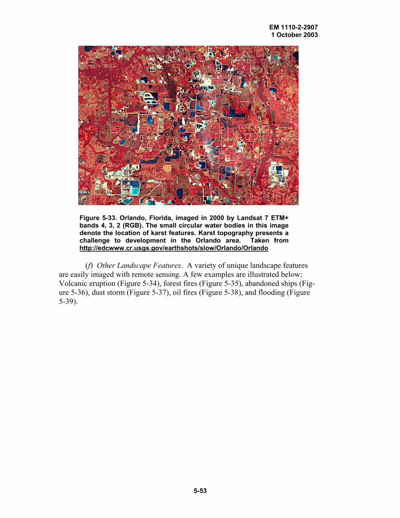
EM 1110-2-2907 1 October 2003

Figure 5-33. Orlando, Florida, imaged in 2000 by Landsat 7 ETM+ bands 4, 3, 2 (RGB). The small circular water bodies in this image denote the location of karst features. Karst topography presents a challenge to development in the Orlando area. Taken from http://edcwww.cr.usgs.gov/earthshots/slow/Orlando/Orlando

(f) Other Landscape Features. A variety of unique landscape features

are easily imaged with remote sensing. A few examples are illustrated below: Volcanic eruption (Figure 5-34), forest fires (Figure 5-35), abandoned ships (Fig-ure 5-36), dust storm (Figure 5-37), oil fires (Figure 5-38), and flooding (Figure 5-39).

5-53

EM 1110-2-2907 1 October 2003

Figure 5-34. Landsat image of Mt. Etna eruption of July 2001. Bands 7, 5, 2 (RGB) reveal the lava flow (or-ange) and eruptive cloud (purple). Taken from http://www.usgs.gov/volcanoes/etna/.

Figure 5-35. Forest Fires in Arizona may assist for-est managers in fire-fighting strategies and pre-vention. Meteorologist also use such images to evaluate air quality. Image taken from http://rst.gsfc.nasa.gov/Front/overview.html.

5-54

EM 1110-2-2907 1 October 2003

Figure 5-36. Grounded barges at the delta of the Mississippi River are indicated by the yellow circle. Taken from http://www.esa.ssc.nasa.gov/rs_images_display.asp?name=prj_image_arcvip.5475.1999.101916538330.jpg&image_program=&image_type=&image_keywords=&offset=312&image_back=true.

Figure 5-37. July 2001 Saharan dust storm over the Medi-terranean. Taken from http://rapidfire.sci.gsfc.nasa.gov/gallery/.

5-55

EM 1110-2-2907 1 October 2003

Figure 5-38. Oil trench fires and accompa-nying black smoke plumes over Baghdad, Iraq (2003). This image was acquired by Landsat 7 bands 3, 2, 1 (RGB). Urban areas are gray, while the agricultural areas ap-pear green. Taken from http://landsat7.usgs.gov/gallery/detail/220/.

5-56

EM 1110-2-2907 1 October 2003

Figure 5-39. The mosaic of three Landsat images dis-plays flooding along the Mississippi River, March 1997.

j. Statistical Analysis and Accuracy Assessment. Accuracy assessment means the correctness or reliability in the data. Error is inherent in all remote sensing data. It is important to establish an acceptable level of error and to work within the resolution of the image. Working within the means of the resolution of an im-age is important for maintaining the desired accuracy. Attempting to extract in-formation from an image for which objects are not clearly resolvable will likely lead to incorrect assumptions. Error can be introduced during acquisition by the sensor and while performing geometric and radiometric correction and image en-hancement processes. Another major source of error lies in the misidentification and misinterpretation of pixels and groups of pixels and their classification.

5-57

EM 1110-2-2907 1 October 2003

(1) Resolution and RMS (Root Mean Squared). Some errors are simple to

quantify. For instance, the image pixel in a TM image represents the average radi-ance from a 30- × 30-m area on the ground. So, measurements within a TM scene will only be accurate to within 30 m. Positional accuracy may be established by a comparison with a standard datum giving an absolute uncertainty value. The RMS (root mean squared) error is automatically calculated during image rectification. This error can be improved while designating GCPs (Ground Control Points; see Paragraph 5-17).

(2) Overall Accuracy. Overall accuracy can be established with “Ground truth.” Ground truth is site-specific and measures the accuracy by sampling a number of areas throughout a scene. Overall accuracy of an image is then calcu-lated by modeling the difference between the observed pixel DN signature and known object on the ground.

(3) Error Matrices. Assessing classification error is more involved. Solv-ing for this type of error requires a numerical statistical analysis. Some software incorporates accuracy assessment within the classification function. For instance, classification error assessment compares an image classification matrix with a reference matrix. See Paragraph 5-20d(4) for information on classification accu-racy. In this type of assessment, the reference data are assumed correct. Pixels are assessed in terms of their mistaken inclusion or exclusion from an object class; this is known as commission and omission (see Congalton and Green, 1999). All known error should be noted and included in any assessment. Review Congalton and Green (1999) for further information on the practice of error assessment.

k. Presenting the Data. Once a visual and statistical evaluation has been per-formed, the analysis must be presented in a manner that best communicates the information needed. The information may be presented as a hardcopy printout of the image or presented as a map (Figure 5-40). The information may also be dis-played as a statistical database, which includes data tables and graphs. Knowledge of GIS, cartography, and spatial analysis is helpful in choosing and executing the manner in which the data will be presented. For instance, a number of GIS soft-ware programs are capable of displaying the image in a map format with a linked data set. Be sure to keep in mind the final product needed by the client.

5-58

EM 1110-2-2907 1 October 2003

Figure 5-40. The final product may be displayed as a digital image or as a high quality hard copy. Taken from Campbell (2003).

5-59

EM 1110-2-2907 1 October 2003

Chapter 6. Remote Sensing Applications in USACE 6-1 Introduction. Remote Sensing is currently used by Corps scientists and engineers at the seven research and development laboratories as well as at the Districts and Divisions. Remote sensing has proven to be a cost effective means of spatially analyzing the environ-ment and is particularly usefully in regions with limited field access. A vast amount of lit-erature covering remote sensing applications in environmental and engineering projects has been published and much of it is available through the ERDC and USACE library system. This chapter only touches the surface of the material that describes the variety of applica-tions and products in use. Some of the references listed in Appendix A also have internet web sites providing more in-depth information on the subject of remote sensing and current research. 6-2 Case Studies.

a. Each study presented below uses remote sensing tools and data. Special emphasis have been placed on Corps works and contracted work related to civil projects. Non-Corps projects, such as NASA works, are also presented in an effort to provide broader examples of the potential use of remote sensing and to aid in the implementation of remote sensing into existing and future US Army Corps of Engineers projects. This chapter 1) reviews the capabilities of sensors, 2) illustrates the value of remote sensing data analysis and integra-tion into spatial data management systems, and 3) communicates recent studies to promote cooperation between Corps Districts, local government, and the general public.

b. The following topics are presented in this chapter:

• Water Quality. • Wetland mitigation. • Archeology. • Engineering. • Soil science—sediment transport. • Forestry. • Agriculture. • Environmental projects. • DEM generation. • Applications in snow and ice. • Emergency Management.

6-3 Case Study 1: Kissimmee River Restoration Remote Sensing Pilot Study Project Final Report

• Subject Area: Environmental Assessment. • Purpose: To evaluate the vegetative response to the restoration of the Kissimmee

River floodplain ecosystem using hyperspectral data. • Data Set: Hyperspectral Airborne.

6-1

EM 1110-2-2907 1 October 2003

a. Introduction. Historically, the Kissimmee River meandered 103 miles (~166 km), connecting Lake Kissimmee to Lake Okeechobee. The river and its floodplain supported diverse wetland communities including aquatic and terrestrial plants and animals. The Kis-simmee River was hydrologically unique owing to prolonged and extensive flood inunda-tion. During the 1960s, the river and its 1- to 2-mile (1.6- to 3.2-km) wide floodplain was channelized and drained in an effort to control flooding. Canal excavation eliminated one-third of the channel, and drainage destroyed two-thirds the floodplain. This Corps of Engi-neers project lead to a significant decrease in waterfowl, wading bird, and fish populations.

(1) An environmental restoration plan is underway in an attempt to restore the pre-1960 ecosystem in the Kissimmee River floodplain. The USACE Jacksonville District and the South Florida Water Management District are jointly responsible for this 3000- square mile (7770 km2) restoration project. The primary goal of the restoration project is to re-es-tablish a significant portion of the natural hydrologic connectivity between Lake Kissimmee and Lake Okeechobee. With the natural hydrologic conditions in place, the objective of the project is to rebuild the wetland plant communities and restore the local biological diversity and functionality.

(2) The study reviewed here represents a pilot study conducted by SAIC (Science Ap-plications International Corporation) to establish a baseline for environmental monitoring of the Kissimmee Restoration Project. Their study explored the utility of hyperspectral image data in aiding vegetative mapping and classification. The hyperspectral remote sensing data demonstrated themselves to be highly useful in delineating complex plant communities. Continued use of such a data set will easily aid in the management of the Kissimmee River Restoration Project.

b. Description of Methods. The test area within the restoration site was chosen by USACE. Preliminary field studies conducted in1996, established approximately 70 plant communities, a handful of which were not present during the study of interest (conducted in 2002). It was determined that the rapid changes in hydrologic conditions had altered the plant community structure during the interim between studies; in places, some plant species and groups had entirely disappeared. Researchers monitoring the vegetation restoration at the Kissimmee site were concerned with the establishment of native versus non-native inva-sive and exotic plant species. The colonization by non-native plant species, such as Brazil-ian Pepper and Old World Climbing Fern, are of interest because of their potential affect on other revitalization efforts; those focusing on fauna restoration, for instance. The spectral analysis of heterogeneous plant species communities is difficult owing to the commonality of plant chemistry and morphology. The spectral difference between native and non-native plants is therefore narrow, and difficulties in distinguishing them are compounded by their mixing (or sharing of habitat). Additionally, the domination by one plant species in many places added to the problem of accurately classifying the plant communities. See below for vegetation classes established for this study.

(1) Examples of vegetation classes include:

• Aquatic vegetation.

6-2

EM 1110-2-2907 1 October 2003

• Broadleaf marsh. • Miscellaneous wetland vegetation. • Upland forest. • Upland herbaceous. • Upland shrub. • Wetland forest. • Wetland shrub. • Wet prairie. • Vines

(2) Geological constrains did not aid in the identification of the vegetation classes.

Geologic constrains tend to be more useful in mapping plant communities in areas with a more mature ecosystem or were there is significant variation in the substrate or soil. Choosing a sensor capable of delineating healthy vegetation versus stressed vegetation was another consideration that needed to be addressed by the researchers. This would allow land use managers the opportunity to closely monitor the decline and rise of various species throughout the duration of the wetland restoration.

c. Field Work.

(1) Airborne hyperspectral data were collected in conjunction with 146 ground-truth data points (also known as training sites); this collection was made on-foot and by airboat. Fieldwork was done and data collected during a flood by a botanist and a GIS specialist. In the field, SAIC’s hand held spectrometer was used to collect the spectral data associated with mixed plant communities from within the Kissimmee River floodplain. These ground-control points were then used to test the accuracy of the vegetation map developed from the hyperspectral data.

(2) Problems arose using the plant classes defined by the 1996 field study. Classes were subsequently altered to better suit the dechannelized ecology. A supervised classifica-tion was applied to the data and two vegetation maps were produced denoting 68 vegetation communities and 12 plant habitat types (Figure 5-25). The hyperspectral map was then compared to the existing vegetation map produced in 1996.

d. Hyperspectral Sensor Selection. Researchers on this project had the opportunity to choose between AVIRIS and HyMap. HyMap was eventually chosen for its accuracy, spectral capabilities, and reasonable expense. HyMap, a hyperspectral sensor (HSI), was placed on board a HyVista aircraft. HyMap maintains 126 bands across the 15- to 20-nm range. The error in HyMap data was found to be at ±3 m, equivalent to the accuracy of the on board GPS unit. To learn more about HyMap and HyVista view http://www.hyvista.com/main.html.

(1) For this project, the hyperspectral (HSI) data maintained clear advantages over other sensor data. HSI’s high spectral resolution allows for the distinction of spectrally similar vegetation and had the potential to monitor vegetation health status. The shortwave infrared (SWIR) wavelengths where found to be most sensitive to the non-photosynethic

6-3

EM 1110-2-2907 1 October 2003

properties in the vegetation. This further helped to discriminate among the vegetation classes.

(2) HyVista pre-processed the digital data. Pre-processing included a smoothing algo-rithm to reduce the signal to noise ratio (SNR) across the scene, to an impressive >500:1. The data were geographically rectified using ground control points identified on a geo-reg-istered USGS orthophoto. The geo-positional accuracy was determined to be within ± 3 pix-els across 95% of the scene. This was established by comparing the image with a high-resolution orthophoto. A digital orthophoto was then over laid on top of the digital hyper-spectral data to verify geo-positional accuracy.

e. Study Results. Analyst used KHAT (Congalton, 1991), a classification statistic used to test the results of supervised versus unsupervised classification (Equation 6-1). KHAT con-siders both omission and commission errors. Statistically it is “a measure of the difference between the actual agreement between reference data and the results of classification, and the chance agreement between the reference data and a random classifier” (see http://www.geog.buffalo.edu/~lbian/rsoct17.html to learn more on accuracy assessment). KHAT values usually range from 0 to 1. Zero indicates the classification is not better than a random assignment of pixels; one indicates that the classification maintains a 100% im-provement from a random assignment. KHAT values equaled 0.69 in this study, well within the 0.6 to 0.8 range that describes the class designation to be “very good” (≥ 0.8 is “excel-lent”). For this study, KHAT indicated good vegetative mapping results with the supervised classification for distinguishing plant species and for mapping surface water vegetation. The KHAT also verified the potential value of image classification to map submerged aquatic vegetation using HIS data.

observed accuracy chance agreement

1 chance agreementk −

=−

(6-1)

1 1( )

r r

i iN S xii S xi x i

= =− + × +

12 ( )

r

ik N S xi x i

== − + × +

where

r = number of rows in the error matrix xii = number of observations in row i and column i (the diagonal) xi+ = total observations of row i x+i = total observations of column i N = total of observations in the matrix .

The estimated time savings of the mapping project as compared with the manual analysis using color infrared was calculated to be a factor of 10 or better. Additional benefits include a digital baseline for change detection and managing restoration. The study did not establish under which conditions HSI did not work. HSI processing and analyses was shown to be a generally valuable tool in a large-scale riparian restoration.

6-4

EM 1110-2-2907 1 October 2003

f. Conclusions. HSI’s advantages over aerial panchromatic and color infrared include its ability to automate data processing rapidly; this will be highly useful for change detection if the hyperspectral data are collected over time. This data can then be easily coupled with other useful GIS data when researchers attempt to combine hydrographic and wildlife data. Wetland hyperspectral imaging paired with advanced data processing and analysis capabili-ties were shown to be a valuable tool in supporting large-scale programs, such as the Com-prehensive Everglades Restoration Program (CERP). For continued successful management of the Kissimmee Restoration Project, the Corps’ Jacksonville District and the South Florida Water Management District will have to decide on a mapping method that provides the de-tail needed to monitor plant community evolution while balancing this need with budget constraints. Point of Contact: Wiener Cadet, Project Manager, Phone: (904) 232-1716 6-4 Case Study 2: Evaluation of New Sensors for Emergency Management

• Subject Area: Emergency Management. • Purpose: To test the resolvability of high-resolution imaging to evaluate roof

condition. • Data Set: Visible and infrared.

a. Introduction.

(1) Emergency response and management efforts are best facilitated with timely and accurate information. Typically, these data include an enormous amount of geo-spatial in-formation detailing the extent and condition of damage, access to emergency areas or sup-port services, and condition of urban infrastructure. Remotely sensed imagery has the capa-bility of delivering this type of information, but it is best combined with geo-spatial data when they are rectified and pre-processed in a way that allows for easy visual and algorithm analysis. The amalgamation of geo-spatial data into one comprehensive map will aid emer-gency management organizations in their effort to coordinate and streamline their response.

(2) Understanding the utility and limitations of a sensor is highly valuable to emer-gency response workers. This study evaluated the effectiveness of Emerge, a new airborne sensor that collects visible and infrared radiation. Emerge was tested in relation to four pri-mary requirements, listed below.

• Ground sampling distance (GSD). • Capability for storing large volumes of digital data. • Pre-processing and the vendors ability to orthorectify up to “500 single frames of

imagery in 12 hours or less” and save these data onto a CD-ROM or ftp for fast delivery.

• Indexing system for all resolutions collected, allowing for easy determination of image location.

6-5

EM 1110-2-2907 1 October 2003

b. Description of Methods. Originally, this study intended to evaluate roof damage

caused by an actual emergency. In the absence of such an emergency, alternate imagery was collected over a housing development under construction in Lakeland, Florida, located 30 miles (48 km) northeast of Tampa, Florida. The different phases of housing construction provided an analog to roof damage during an event such as strong winds or a hurricane. The different structural states of both residential and commercial roofs included exposed rafters, exposed plywood, and plywood covered by tarpaper or shingles.

c. Field Work. Initially, field reconnaissance established the appropriateness of using two neighboring test areas in Lakeland, Florida. Roof conditions at individual buildings were evaluated and geo-referenced. After the first flight, an assessment of the ground sampling distance (GSD) and sensor data determined that a finer resolution would be required to ade-quately examine roof condition. Two additional flights were then acquired, resulting in a collection of data gathered at resolutions of 3, 2, and 1 ft (91.4-, 61-, and 30.5- cm respec-tively), and 8-in (20.3 cm). Landscaping features, such as tree type and leaf on/off state, were also documented with digital photos. This information was later used to establish the feasibility in mapping vegetation using the Emerge system.

d. Sensor Data Acquisition. The two test sites, occupying 8 square miles (~21 km2), were surveyed at several resolutions using Emerge imagery (see http://www.directionsmag.com/pressreleases.php?press_id=6936 for more details on the Emerge System). Multiple resolutions were collected over a 2-month period. As a result, a one-to-one comparison of the effect of resolution on image analysis was difficult, as house construction in some areas was completed during the 2-month interval. The volume of data collected was equivalent to that required for a 60 square mile (~155 km2) area, with ap-proximately 25% image overlap (at a single resolution). This volume of data totaled 5 giga-bits.

e. Study Results. Evaluation of the imagery showed that roof rafters were best resolved at a 1-ft and 8-in. (30.5 and 20.3 cm) resolution. At this resolution, plywood can be distin-guished from other construction materials and individual rafters can be observed. Tarpaper was not distinguishable from shingles owing to their spectral similarities.

(1) Despite the functionality of the 1-ft and 8-in (30.5 and 20.3 cm). resolutions, in places with bright spectral response, saturation on the high end of the intensity scale low-ered the resolvability of rafters relative to the flooring material. This was the result of a high gain set for radiation detection within the sensor. Over-saturation lowers the contrast be-tween rafters and the flooring, making it difficult to fully evaluate the condition of the roof. Lowering radiation saturation requires collecting data during low to medium sun angle. This may, however, delay data acquisition.

(2) Sun angle controls image contrast in two ways. First, a low sun angle may in-crease shadowing, leading to a loss in target radiation data. Secondly, a high sun angle may over-saturate the sensor. Both extremes were shown to lower contrast in this study, making roof analysis difficult.

(3) A scatter plot breakdown of band 1 relative to band 2 was performed to evaluate the possibility of automating an analysis that would delineate intact roofs and damaged

6-6

EM 1110-2-2907 1 October 2003

roofs. A preliminary analysis suggests that this is possible because of the strong covariance displayed by roofs shingled with monochromatic materials. Any automated process devel-oped would need to address the limitations posed by non-monochromatic shingles (which would appear spectrally mixed and indistinguishable from damaged roofs).

(4) A vegetation analysis was also explored to test the resolution required to accu-rately describe tree type and condition. At the 1-ft (30.5 cm) resolution, researchers were able to determine leaf on/off conditions (data were collected in February). However, at this resolution it was not possible to delineate any details regarding leaf morphology. At the 8-in (20.3 cm). resolution, palms were distinguishable, although it was not possible to differenti-ate broad versus narrow leaves.

f. Conclusions. Evaluation of the Emerge sensor led to the development of a detection matrix. This matrix reviews the capabilities of the sensor at various spatial resolutions for all objects studied (see Table 6-1). This study determined that Emerge could adequately meet the requirements of emergency management systems. High-resolution data can be acquired within 4 hours of the plane’s landing. This includes the time needed for pre-processing (orthorectification and the production of geo-TIFF files for CD-ROM and ftp). Shingles and tarpaper are not resolvable, though rafters and plywood are at the 2-ft (~61 cm) resolution. For high-resolution images, a medium sun angle increased roof detail. Palm trees and leaf on/off conditions can be visually identified at the 8-in (20.3 cm). resolution; however, broad-leafed trees cannot be distinguished from narrow-leafed trees. The only limitations placed on these data centered on over-saturation and sensor inability to distinguish tree types. The covariance displayed by band 1 relative to band 2 indicates the potential success for developing an automated algorithm to locate and count damaged roofs.

Table 6-1 Detection Matrix for Objects at Various GSDS

Objects/GSD 3-ft (91.4) 2-ft (61 cm) 1-ft (30.5 cm) 8-in. (20.3 cm) Roof rafters Not visible Barely visible Often visible Visible

Shingles/tarpaper (other) vs. plywood

Can sometimes separate

Can often separate

Can determine wood vs. other cover

Can determine wood vs. other cover

Rafters in 3-band saturation

Causes rafter detail loss

Causes rafter detail loss

Causes rafter detail loss

Causes rafter detail loss

Broad-leaf vs. narrow-leaf

Cannot separate

Can determine leaf on/off

Can determine leaf on/off

Palms are always visible

All in cloud shadow Degrades image

Some info recoverable

Some info recoverable

Some info recoverable

Roofs as a function of sun zenith angle

Best detail, near zero angle, overhead sun

Best detail, medium angle, shadow casting

Best detail, medium angle, shadow casting

Best detail, medium angle, shadow casting

All in 1, 2, 3 RGB, 2∑ stretch

Enhances imagery

Enhances imagery

Enhances imagery Enhances imagery

Point of Contact: Robert Bolus, Phone: (603) 646-4307

6-7

EM 1110-2-2907 1 October 2003

6-5 Case Study 3: River Ice Delineation with RADARSAT SAR

• Subject Area: Ice monitoring • Purpose: To evaluate the concentration and condition of river ice. • Data Set: RADARSAT SAR

a. Introduction. Remote sensors operating in the microwave region of the spectrum have

the advantage of seeing through clouds and atmospheric haze. RADARSAT SAR (synthetic aperture radar) collects spectral data in the microwave region and is capable of imaging ground targets during adverse weather conditions, such as storms. Additionally, RADARSAT SAR collects 10-m pixel sized data, a high spatial resolution well suited for studies examining ice in narrow river channels. The study reviewed here explored RADARSAT SAR’s potential in delineating and monitoring ice and ice floes in rivers ranging in stream widths of 160 to 1500 m. A better estimate of ice conditions along large streams will allow for better navigation planning and will provide river dam regulators the information needed to plan and prepare for ice breakup and floes.

b. Description of Methods. Three rivers of varying widths were evaluated for ice cover over the course of two winters (2002 and 2003). The first winter was relatively mild with partial river ice development at the three sites. Winter 2003 possessed a number of below freezing days and was an ideal time for examining river ice in the northern mid-west. The rivers chosen for this study were the Mississippi River near St. Louis, Missouri, the Mis-souri River at Bismarck, North Dakota, and the Red Lake River in Grand Forks, North Da-kota. Each site offered unique contributions to the study. The Mississippi River represented a stream with heavy navigation use, the Missouri River site included a hydropower dam, while the Red Lake River had extensive ice jam and flood records. Coordinated efforts among CRREL researchers, the local Corps Districts, and the RADARSAT International (RSI) aided in the acquisition and timing of satellite data collection.

(1) Stream channels were subset and isolated for river ice classification. To accom-plish this, a band ratio was applied to Landsat TM data. They were then classified by an un-supervised process and extracted for mask overlay onto the radar data. This sufficiently out-lined the land/water boundaries and isolated the stream in images with wide river channels. This process omitted vegetation and islands from the resultant image. The subsequent SAR subset did not include mixed pixels (land/water/ice).

(2) Images with narrow channels required hand-digitization and a textural analysis, followed by a supervised classification (to further eliminate land pixels). The hand-digitiza-tion proved less successful than the Landsat TM overlay and extraction method. Hand-dig-itization did not thoroughly omit pixels with mixed water, vegetation, and land (i.e., river islands).

(3) In the SAR images, only the channel reaches were analyzed for ice conditions us-

ing an unsupervised classification. The classification mapped brash ice (accumulated float-ing ice fragments), river channel sheet ice, shore ice, and open water.

6-8

EM 1110-2-2907 1 October 2003

c. Field Work. Direct field observations were not necessary as a web-camera mounted on

a bridge provided the visual documentation of ice conditions in the river. At the Missouri River site, web-cameras have been strategically placed in a variety of locations in the US by ERDC/CRREL. To view the Missouri River images used in this study, as well as other river web-camera images, go to http://webcam.crrel.usace.army.mil. Study sites without a web-camera relied on District contacts for field information. At Red Lake River near Grand Forks, North Dakota, field reconnaissance ice surveys were conducted by the Corps St. Paul, Minnesota, District office.

d. Sensor Selection and Image Post-Processing.

(1) As stated above, RADARSAT SAR data was chosen for this study. Radar data have already proven their utility in sea ice mapping and monitoring (Carsey, 1989). Radar can aid in determining ice concentration, classification, ice motion monitoring, and ice fea-ture changes. The study reviewed here adapted methods used to study large ice sheets to the evaluation of smaller more temporal river ice.

(2) The acquired radar images were visually analyzed and classified using an unsu-pervised classification to delineate open water, moving ice floes, and stationary ice covers. The delineation of river channels was undertaken by two methods, described above (hand-digitization and TM extraction and overlay).

e. Study Results. The following description summarizes the ice condition results stem-ming from each river surveyed:

“In the Mississippi River imagery near St. Louis, Missouri, the wide channel width (500–2000 meters) contributed to identifying river ice with RADARSAT imagery. In the 2002 image it was determined that 30% of the channel had ice in the flow, and in the 2003 image, it was deter-mined that there was 100% ice cover. Additionally, this ice cover was separated into forms of ice; brash ice and border ice. In the 2003 image it is believed that the brash ice formed as a re-sult of navigation ice-breaking activities.

(1) In the Missouri River imagery near Bismarck, North Dakota, the channel width

(400–1000 m) was suitable, and river ice was determined from the RADARSAT imagery. The 2002 image showed that 77% of the channel had ice in the flow, and in the 2003 image, only 21% of the channel had ice. The 2003 imagery was acquired before full icing condi-tions, and a small amount of ice was interpreted to exist.

(2) In the Red Lake River imagery near the confluence with the Red River of the North at Grand Forks, North Dakota, the river channel is narrow (40–75 m). The narrowness of the channel limited the process of delineating the channel boundary on the imagery. As a result of the narrow channel width, river ice was not determined by this process. However, ice surveys were conducted by the US Army Corps of Engineers during the time of image acquisitions, and an ice cover was recorded in both 2002 and 2003.

f. Conclusions. RADARSAT SAR data were able to detect ice on rivers with widths ranging from 400 to 2000 m. Despite RADARSAT’s 10-m resolution, this data set was un-able to detect the present of ice on the narrower Red Lake River, with a width of 40–75 m. RADARSAT’s overall suitability for detecting river ice and ice conditions was shown to be

6-9

EM 1110-2-2907 1 October 2003

of potential use. The method presented here details an important tool that may aid in haz-ardous wintertime navigation and assist dam regulators on decisions regarding stream flow and reservoir levels. Point of Contact: Brian Tracy, Phone: (603) 646-4739 6-6 Case Study 4: Tree Canopy Characterization for EO-1 Reflective and Thermal Infrared Validation Studies in Rochester, New York

• Subject Area: Forestry and climate change • Purpose: To collect forest canopy structure and temperature data. • Data Set: Multispectral and hyperspectral

a. Introduction. Tree and forest structure respond strongly to environmental conditions

and change. Subsequently, studies have successfully shown the utility of remote sensing in monitoring environmental conditions through the analysis of vegetation. The study reviewed here surveyed a mixed forest in northern New York State in an attempt to better understand the interaction between solar radiation and tree/forest structure. An additional objective of this study was to validate the Earth Observing satellite (EO-1, launched in 2000). The vali-dation was performed by comparing the EO-1 satellite data with that of the Landsat-7 ETM+ data. The EO-1 satellite acquired data at the same orbit altitude as Landsat-7 while flying approximately 1 minute behind. EO-1 reflective bands were combined with the Land-sat-7 ETM+ thermal infrared bands to estimate canopy temperature. The 1-minute delay in synchronization between the two sensors was evaluated to test the effects of separating the thermal and reflective measurements in time. Relating scene exitance (the radiative flux leaving a point on a surface, moving in all directions) and reflectance to the landscape pro-vided insight to prevailing environmental characteristics for the region.

b. Description of Methods. Ground and tree canopy data were collected from mature healthy forest stands at a site in Durant-Eastman Park in Rochester, New York. Characteri-zation of the forest included a stem and trunk survey, tree structure geometry measurements, regional meteorology, and leaf area index (LAI) measurements (see http://www.uni-giessen.de/~gh1461/plapada/lai/lai.html for more information on LAI). Two smaller field sites, Ballard Ridge and Smith Grove, were selected for detailed study from within the lar-ger forested area. Tree heights for both sites averaged 20–30 m. Ballard Ridge consisted of a dense mature stand of maple, cottonwood, elm, and oak trees. The Smith Grove consisted of a dense mature stand of locust trees and cottonwood. Thermal and reflective spectral meas-urements were made on leaves, tree bark, leaf litter, soil, and grass.

c. Field Work. Leaf area index (LAI) was calculated in the field with the use of a non-imaging instrument, which measures vegetation radiation in the spectrum of 320–490 nm. Leaf area index is a ratio of the foliage area in a forest canopy relative to the ground surface area. It estimates the photosynthetic capability of a forest. The measured light intensity was used to calculate the average LAI for each location within the field site. High-resolution hemispherical photographs were collected at each site using a digital camera with a fisheye lens (148° field-of-view). The digital photographs were taken during the early morning and

6-10

EM 1110-2-2907 1 October 2003

late evening hours to reduce the effects of atmospheric haze. The digital hemispherical photographs were later analyzed using a specialized forestry software, which measures both LAI and canopy leaf structure. LAI calculations based on the computed hemispherical digi-tal images compared favorably with the LAI measurements from the meter instrument.

d. Sensor System.

(1) Satellite data were collected with the use of Landsat MTI, Hyperion, and ALI (Advanced Land Imager) on 25 August 2001. The ALI sensor has nine spectral bandwidths plus a panchromatic band. Three bands where analyzed for this study 773.31 nm, 651.28 nm, and 508.91 nm. The forested areas appear bright red, urban areas are gray-blue, and the water is depicted by the dark blue regions.

(2) The sensor radiance was converted with the use of 6S, an atmospheric corrections model that converts sensor radiance to estimated surface reflectance. The differences and consistencies in the two sensors were then easily compared with the spectral data collected in the field. Then, a more detailed study of the forest site was made, using measured geo-metric and optical parameters as input to the SAIL multi-layer canopy reflectance model. The ETM+ and ALI data were then compared with the SAIL (Scattering by Arbitrarily In-clined Leaf) reflectance model and the high resolution Hyperion, a hyperspectral imaging instrument (see http://eo1.usgs.gov/instru/hyperion.asp for details).

e. Study Results. A comparison of the panchromatic ETM+ and ALI data show dramatic differences. The ALI data provided better definition of the marina and pier area as well as natural water features (urban and water targets). Relative to the ETM+ images the ALI data maintained a reduced DN value for all forest pixels, increasing the contrast in the forest re-gion. The authors suggested the higher resolution and the narrow bandwidths accounted for the dramatic contrasts between the image data sets.

(1) Spectral plot comparisons of the multispectral bands for different ground targets (grass, water, urban features, and forest) illustrating the relationship between reflectance and wavelength indicated a close match between the two sensors. The spectral plots were cre-ated by the selection of training pixels for each target group. ALI spectral values were closer in value than those seen in the ETM+ data; again, this is a result of the narrow bandwidths and higher resolution. The only notable difference in the spectral response between the two sensors was evident in band 5 for grass and urban features. These targets had up to 20% variation in signal response between the sensors. Specifically, the ALI band 5 with a reflec-tance of 0.35 µm is ~20% higher than the ETM+ value of 0.29 µm.

(2) The combined spectral plot of data from ETM+, ALI, Hyperion, and the empiri-cally derived SAIL show overall an excellent agreement. The three satellite data sets closely match one another, with slightly different values recorded in the SAIL model data. SAIL values best matched those of the sensors in the visible portion of the spectrum.

f. Conclusions. The authors of this study were able to establish a simple, multi-layer canopy reflectance model using measured parameters from the site to compare the ETM+ and ALI spectra. Hyperspectral data were also compared against the satellite and ground data. Additional work is needed to establish the relationship between leaf area index (LAI)

6-11

EM 1110-2-2907 1 October 2003

and satellite data. The potential use of ALI and hyperspectral Hyperion for studies of forests in remote locations and forests at risk may greatly enhance forest management and lower the costs associated with ecological monitoring. Accurate estimates of LAI based on satellite imagery have the potential to support forest biomass monitoring, and hence forest health and changes in canopy structure attributable to pollution and climate change. The ability to esti-mate LAI with remote sensing techniques is, therefore, a valuable tool in modeling the eco-logical processes occurring within a forest and in predicting ecosystem responses. Point of Contact: Jerry Ballard, Phone: (601) 634-2946 6-7 Case Study 5: Blended Spectral Classification Techniques for Mapping Water Surface Transparency and Chlorophyll Concentration

• Subject Area: Water quality • Purpose: To establish water clarity and algal growth in a dam reservoir • Data Set: Landsat TM - Visible and infrared

a. Introduction.

(1) An accurate portrayal of water clarity and algal growth in dynamic water bodies can be difficult owing to the heterogeneity of water characteristics. Heterogeneity can stem from the spatial distribution of sediments delivered to a lake by a tributary. Water turbidity associated with tributary sediment load controls water clarity and subsequently will impact algae growth. Additionally, algal growth will influence water clarity by reducing water transparency during times of algal blooms. Both algal growth and sediment turbidity are controlled by such factors as water depth, flow rate, and season.

(2) To better monitor the water quality at dam reservoirs, a spatial estimate of both water clarity and algal chlorophyll over a broad area is required. To accurately capture these properties a large number of water samples must be taken, a task that may not be feasible for most studies. Remote sensing lends itself well to the assessment of water quality testing at a variety of spectral scales due to the response of suspended sediment in the visible and ther-mal spectrum. Chlorophyll, produced by algae, can also be detected by its visible and infra-red emission. The study reviewed here developed a classification algorithm to predict water clarity and chlorophyll concentrations. The algorithm was based on a correlation between spectral data and the empirical field data. Previous studies attempting to classify water clar-ity and chlorophyll required field sampled training sites. The goal of this study was to de-velop an algorithm based on empirical data that would illuminate the need for such test training sites. Thus, researchers testing for water quality would then need only the Landsat TM data to monitor water quality at a fresh water lake.

b. Field Work. Secchi Disk measurements and water samples were collected at a dam reservoir in conjunction with a Landsat fly-over at West-Point Lake, Georgia. Water sam-ples were frozen and stored in a dark room to preserve the algae populations. These samples where later analyzed for chlorophyll (Ca) concentrations. Water clarity was measured in situ with a Secchi Disk (Sd). This 20-cm disk estimates water clarity by measuring the depth to

6-12

EM 1110-2-2907 1 October 2003

which the disk is visible. Remote sensors generally detect water clarity to 20–50% of the Sd measurement. Sampling sites were chosen evenly across the reservoir and adjacent tribu-taries. A global positioning unit was used to locate 109 sample sites. Drift during sampling occurred but was compensated for with the use of a 3×3 kernel during image classification. Samples and data were collected during two periods—summer and fall of 1991.

c. Sensor System. Two Landsat TM data sets separated in time were used to develop a linear-logarithmic cluster analysis. Visible, near, and middle infrared radiation band ratio was employed with a stratified sampling technique. Using a variety of band ratio, the work-ers were able to accurately develop a blended classification scheme, which is detailed be-low.

d. Study Results. The authors adapted multivariate density estimation with the use of an algorithm k-NN density estimator. This was used to group spectrally similar pixels. The spectral classes and class structures (or groupings that separated the spectral classes) were developed using an unsupervised classification. Within each of the two scenes, 16 unique classes were determined. These classes were combined with the empirical data, leaving four logarithmic algorithms. Applying a 3×3 kernel to the data compensated for the drift that oc-curred during data collection. This placed the positional accuracy to within ±30 m.

(1) The average spectral value was determined by a log estimation of the band ratio for the given pixel within the kernel (Equation 6-2). Combinations of band ratios were tested. A middle infrared ratio against the visible red showed the largest correlation with Sd and Ca. Visible green versus near infrared also provided a good separation of the spectral response for estimating Sd and Ca.

3 3

1 1 x,y

1 (mid IIR ln9 (visible red)x y= =

= ∑ ∑ R) 6-2

(2) Observed versus predicted Sd and Ca were well correlated with the use of this log

estimate. Focused sampling and spectral blending led to the development of an accurate un-supervised classification with a 95% confidence interval. Sampling positions near tributar-ies were overestimated at only five sampling sites (relative to 109 sampling sites).

e. Conclusions. A strong correlation was made between the Landsat TM middle IR and the empirical Secchi Disk and chlorophyll concentrations. Chlorophyll was shown to have increased from 12.64 to 17.03 mg/m3, contributing to a decline in water clarity. The appli-cation of this log estimate now eliminates the need to collect empirical water quality data, likely reducing the cost in a water quality survey. Point of Contact: Robert Bolus, Phone: (603) 646-4307

6-13

EM 1110-2-2907 1 October 2003

6-8 Case Study 6: A SPOT Survey of Wild Rice in Northern Minnesota

• Subject Area: Agriculture • Purpose: To estimate the percentage of wild rice in a wetland environment • Data Set: Visible and near infrared

a. Introduction.

(1) A vegetation survey of natural wild rice surrounding three neighboring lakes 200 miles (518 km) south of St. Paul, Minnesota, was conducted to provide a base map for pol-lutant and water level monitoring. The study presented here utilized standard supervised classification, based on ground-truth, of high-resolution SPOT data. Wild rice is a natural marsh grass that is sensitive to water level changes and to changes in phosphorous concen-trations; increases in phosphorous and water levels can significantly destroy wild rice com-munities. This is of concern as this important grass is a staple in the Chippewa Indian diet and is consumed by migratory birds.

(2) The researchers in this study were tasked with mapping and estimating the acreage of wild rice surrounding three lakes in Minnesota. Three spectral classes where developed with the use of a supervised classification to delineate the grass and its varying substrate.

b. Description of Methods. Ground truth data were collected simultaneously with SPOT over flight. The ground truth data included information regarding vegetation and substrate type as well as the sites corresponding UTM (global position in the Universal Transverse Mercator coordinate system).

c. Field Work. In the field, 18 ground control points (GCPs) were collected for rectifi-cation of the SPOT image and an additional 132 ground truth points were collected for the supervised classification algorithm. This data collection coincided with the SPOT over flight.

d. Sensor System. SPOT was chosen for its optimal detection of vegetation in the pres-ence of inorganic ground cover (i.e., water). Vegetation absorbs both red and blue radiation, while reflecting green and near infrared (NIR) because of chlorophyll production. This matched well with the spectrum data provided by SPOT (which maintains green, red, and NIR bands among others).

e. Study Results. (1) Prior to the classification process, it had been predicted that the wild rice would

dominate one spectral class, as wild rice is spectrally distinct from other vegetation. Open-ings in the grass canopy, however, contributed to the spectral mixing observed in the image scene. Three spectrally distinct populations were noted, likely because of the heterogeneity of the background reflectance, varying crop canopy, and varying water content in the sub-strate.

6-14

EM 1110-2-2907 1 October 2003

(2) A histogram plot of the digital number value assigned to each pixel in the scene

clearly reveals three distinct spectral populations. These three classes were determined to be wild rice growing in the lake, wild rice in marsh, and wild rice in a saturated soil. Wild rice growing in shallow or marsh water produced pixels that overlapped with more than one class. The near-infrared (N-IR) band allowed for better spectral separation by eliminating the effect of varying amounts of water in the substrate.

f. Conclusions.

(1) An estimate of the acreage percent based on a supervised classification determined that 1% of the scene was dominated by wild rice. Habitat was shown to predominately exist along the lakeshore, at inlets, ponds, on banks, and in marsh areas. Wild rice was deter-mined to grow in saturated soil, marsh, and in shallow lake waters. The author recommend 200 ground truth points be collected per class (100 for spectral determinations and 100 for classification designation). Application of the ground truth data to a SPOT scene collected 5 days after the ground truth data did not produce an accurate classification. This test reveals the limitations on the usefulness of SPOT data for surveying vegetation—ground truth must be collected at the time of data acquisition.

(2) A detailed map of the distribution of wild rice will allow land managers to better predict the impact of changes in water level and phosphorous input on the natural produc-tion of wild rice.

Point of Contact: Robert Bolus, Phone: (603) 646-4307 6-9 Case Study 7: Duration and Frequency of Ponded Water on Arid Southwestern Playas

• Subject Area: Hydrology. • Purpose: To delineate playa inundation frequency and duration. • Data Set: Multispectral/thermal (Landsat 4, 5, and 7 and MTI – Multi-spectral Thermal

Imager).

a. Introduction.

(1) Playas are ephemeral shallow lakes found in the arid southwest United States. Their hydrology is dominated by rainfall and runoff in the wet season and evaporation throughout most of the year. Surface hydrology, particularly frequency and duration, is poorly understood in the playa environment. US waters, including playa water, are Federally regulated under article 33 CFR 328.3 [a] of the Clean Water Act. Water bodies are deline-ated to their outermost extent termed their “Ordinary High Water” (OHW). OHW is defined by the presence of physical hydrological features representing the ordinary reaches of high water in its bed or basin.

(2) Playas exhibit tremendous temporal variation, as they may not pond at all during a particular year or may remain ponded for several years. The extent to which water remains

6-15

EM 1110-2-2907 1 October 2003

on the surface is influenced by the ambient climate, surface properties, evaporation rate, sa-linity, and infiltration or discharge of groundwater. Spatial and temporal factors such as in-undation, evaporative rate, relocation of brine pools by winds, and desiccation of surface water hinder the ability to approximate the duration and frequency of ponding necessary to accurately model flood events or to determine whether certain Federal environmental regulations apply. This study attempted to model the frequency and duration of playa inundation in an effort to better delineate playas for regulations.

b. Description of Methods.

(1) For this study, three playa lakes on the Edwards Air Force Base were examined with the use of 20 years of historical Landsat and MTI imagery. These data were coupled with 59 years of precipitation records collected on the base. Rogers Lake (114 km2) and Rosamond Lake (53 km2) occupy the eastern and western region of the study area, respectively. Smaller playa lakes separate Rogers and Rosamond Lakes, including Buck-land (5 km2). The playa lakes are located on a Pleistocene glacial lakebed; the Pleistocene features dwarf the present geologic structures. Chenopod vegetation and saltbush plant communities dominate the terrestrial plain surrounding the playa.

(2) The playas remain dry for most of the year; however, winter rainstorms and sum-mer thunderstorms cause water to periodically inundate playas. The duration of flooding de-pends on the magnitude and location of precipitation and ambient prevailing climate. Sig-nificant flooding is also associated with El Niño events in the Pacific Ocean, which leads to above-normal precipitation in the Southwestern US. Precipitation records maintained at Edwards Air Force Base provided precipitation data for the years 1942 to 2001. The average annual precipitation was calculated to be 13 cm/year with an estimated 280cm/year evapo-ration rate.

c. Sensor System. The department of energy on collected visible and near infrared data with the use of a Multi-spectral Thermal Imager (MTI) from February through May of 2001 Two sequential daily MTI images were acquired at 16-day intervals. This was done to en-sure the capture of water that may exist at any time throughout the course of 31 days. The acquisition of multiple scenes eliminated the lack of data due to cloud coverage. Seven years of data were analyzed for this inundation study.

d. Study Results.

(1) The visible bands were not useful in visually delineating ponded water. Ponded water was best defined by a band ratio technique of B5/B2, which evaluated the proportion of reflective energy to input energy. The ratio values for each pixel were consistently greater than 1.0 for non-water objects and less than 1.0 for water objects. This ratio method was then followed by a classification that grouped pixels with values less than 1.0. Workers then assigned a DN value of 0 for objects displaying a ratio value of less than 1.0, thereby color-ing all water bodies black in the scene. This ratio technique aided the image analysis by eliminating the problems caused by sun angle, sun intensity, and seasons—problems intrin-sic to multi-temporal image analysis.

6-16

EM 1110-2-2907 1 October 2003

(2) The average precipitation was calculated to be 8.28 cm/year. These data, coupled

with the image data, established the inundation frequency to be 51% of the time. This sug-gests that the playas are inundated, on average, every other year.

e. Conclusions. Results indicate that ponding that persists 16 days or longer occurred approximately every other year. The average precipitation needed to initiate ponding is es-timated at 8.29 cm. Duration of ponding was shown to range from 1 to 32 weeks, with a di-rect relationship between length of inundation and total seasonal rainfall. Playa inundation, duration, and frequency can be determined from precipitation data and satellite imagery. The authors suggest the addition of contributing factors such as soil type and geometry may lead to a more robust hydrologic model of the playa system. A thorough understanding of the playa hydrologic regime may one day lead to new land use regulations. Point of Contact: Robert Lichvar, Phone: (603) 634-4657 6-10 Case Study 8: An Integrated Approach for Assessment of Levees in the Lower Rio Grande Valley

• Subject Area: Engineering. • Purpose: To detect weak areas within levees prior to flood events. • Data Set: LIDAR.

a. Introduction. A series of levees were constructed along the Lower Rio Grande in

Texas and Mexico in the 1930s. Local farmers, working with the county government, con-structed the levee system to prevent flood damage to crops in low-lying areas near the river. The levees were constructed of sediment and soil materials obtained locally. The Federal government later completed the levee system in the 1940s and continued expansion and re-pairs through the 1940s. The US Army Engineer Research and Development (ERDC), working recently with the International Boundary and Water Commission, developed a GIS database to catalog levee condition. Knowledge of levee conditions prior to a flood is help-ful in determining where repair and rebuilding are necessary on these man-made structures. A visual display of the levee and detail on the location of potential structural failure could then be used to prioritize levee repair and reconstruction.

b. Description of Methods.

(1) This study maintained four primary objectives. The first was to survey the levee system of the Lower Rio Grande River. The information compiled during the course of this survey was organized into a GIS database. The second was to extensively evaluate levee condition. The third was to compare the results of the airborne survey with those obtained from ground-based surveys. This objective tested the validity of implementing a remote sensing survey. Fourth, ground-truth locations were selected based on LIDAR data, and at these locations soil and subsurface strata were mapped using a cone penetrometer.

(2) In the course of developing the GIS database, ERDC developed a 10-point crite-rion for evaluating the condition of the levee system. Traditional geophysical tools were

6-17

EM 1110-2-2907 1 October 2003

then merged with remote sensing methods to proceed with the levee assessment. Levee to-pology was assessed with the use of LIDAR, digital video, aerial photographs, soil maps, and geological maps. Topographic deviations of 6 in (15.2 cm). or more along the centerline of the levee were then targeted for detailed seismic field studies. In addition to targeting segments with an undulating topography, several stretches of the levee (on the US side) were seismically surveyed.

c. Field Work.

(1) Ground surveys were conducted at five sites ranging in length from 3000 to 5000 ft (0.91 to 1.5 km). Electrical resistivity, EM, and magnetic surveys were collected in con-junction with the airborne EM and magnetic survey. The ground-based geophysical sites were geo-referenced with the use of a global position unit.

(2) Much of the data acquired for the GIS database were collected from previous sources. Information was taken from state and Federal survey maps, and from new and old aerial photographs. Digital photography and aerial photographs were used to map Holocene and Pleistocene deposits and geomorphologic structures. In areas with recent urban devel-opment, older images dating to the 1930s were used to evaluate the underlying geology.

d. Sensor Data Acquisition. LIDAR was utilized to survey levee elevation to determine deviations from the original design. Deviations in height indicate segments with potential damage attributable to seepage or sediment voids. Floodwater overtopping, slope failure, and seepage all potentially compromise levee stability. Seepage can create void spaces in the sediment and soil, resulting in subsequent levee collapse.

e. Study Results.

(1) The levee was then mapped and tagged with a conditional assessment of good, marginal, acceptable, or high-risk zones. The assessment was based on a numerical measure of 10 features deemed important in determining levee stability. These 10 features were cho-sen by agreement among Corps experts specializing in levee construction and repair. Table 6-2 lists the 10 features ranked in order of importance.

(2) Low scores in any one of the 10 features could result in a poor rating for a given levee segment. The levee was divided into segments based on conductivity measurements (shown to be controlled by levee material make-up); each segment was then given a numeri-cal value based on a weighted measure of the 10 features. Segment ratings were color coded and presented as a layer within the GIS database. The color-coded maps provided an easy to interpret assessment of levee condition.

6-18

EM 1110-2-2907 1 October 2003

Table 6-2 Factors Important in Levee Stability Performance history (under flood stage) Construction history (original or upgraded) Visual inspection apparent condition (on-site observation) Material type (sand [worst] transition to clay [best]; (from EM, borings, soil maps) Topographic irregularity (swags, erosion) (from LIDAR) Potential slope stability (material type, relation to flow) Man-made intrusions (utilities, bridges, pump stations, etc.) Geology (old stream beds, river deposits) Proximity of borrow area (size, depth, distance, side of levee) Anomalies (unexplained radical conductivity “spots”)

List is modified from Dunbar et al. (2003)

f. Conclusions. LIDAR, accurate to within 2 to 3 in (5.1 to 7.6 cm), was beneficial in economically mapping the surface morphology of the Lower Rio Grande Valley levee sys-tem. The merged remote sensing and geophysical data onto a GIS database facilitated easy retrieval of information for individual segments and can continue to aid in the management of the levee system. The authors view this study as a success and acknowledge that the ap-plication of these techniques to other geographical regions, while potentially of benefit, may not hold true for levee projects in other regions. Point of Contact: Joseph Dunbar, Phone: (601) 634-3315 6-11 Case Study 9 : From Wright Flyers to Aerial Thermography—The 1910 Wright Brother’s Hangar at Huffman Prairie

• Subject Area: Archeology • Purpose: To review developing NASA products and detail their use in Corps

works • Data Set: Airborne CAMS

a. Introduction.

(1) The Huffman Prairie Flying Field, a National Historic Landmark located at

Wright-Patterson Air Force Base, was surveyed using a variety of ground and airborne sen-sors in an effort to locate the forgotten Wright Brother’s hanger. This hangar, in use from 1910 to 1916, was the training and testing site for the Wright Aeronautical Company activi-ties. The hanger was demolished during the 1940’s with no record of its precise location.

(2) In the early 1990s, CERL researchers investigated the Huffman Prairie Flying Field using traditional and common archeological methods, such as excavation, magnetic and electromagnetic surveys, and ground penetrating radar (GPR). NASA aided CERL’s effort with the addition of thermal data collected from an airborne platform. The airborne

6-19

EM 1110-2-2907 1 October 2003

data isolated a rectangular footprint, which corresponded with the location of the Wright hangar. Later ground truth data collection and excavation works unearthed well-preserved wall posts constructed of wood. This project exemplifies the technological methods cur-rently being adopted by archeologists. Geographic Information Systems (GIS) practices are now in wide use among archeologists, who take advantage of the utility of spatially related data.

b. Description of Methods. This study had two objectives; the first was to locate the pre-cise position of the Wright hangar. In archeological terms, the site and the history centering on the Wright Brother’s and their activities is well documented. The historical record con-tains many photographs and aerial photographs that trace the approximate location of the Wright buildings. In 1994 an architectural firm established the dimensions and structural details of the Wright hangar with the use of these photographs. They determined that the hangar was approximately 70 by 49 ft (21.3 by 14.9 m). Knowing the approximate dimen-sions and location of the building would seemingly make the archeological work a simple task. The second objective of the study was to determine if traditional and modern archeo-logical work could add insightful information to the already well-documented site, and thereby further detail the history of early American aviation.

(1) The authors describe the general area surrounding the Huffman Prairie Wright Brothers field as being relatively undisturbed despite the growth and development of the Wright-Patterson Air Force Base neighboring the site. The prairie had been subject to burn-ing, but not plowing. The task in locating the hanger included fieldwork, near surface geo-physical work, and aerial remote sensing. The initial excavation made it apparent that identi-fying remains of the hangar would require either a significant amount of additional excavation or the use of technologically sophisticated, noninvasive methods. Further exca-vation was deemed too destructive for the site, leading to the decision to employ near-surface and aerial remote sensing.

(2) The geophysical work included magnetic, electromagnetic, and ground penetrating radar (GPR). Combining multiple geophysical techniques is a good practice, as one instru-ment may easily pick up features not identified by another. Geophysical survey methods typically involve data collection in a grid pattern across the study site. Anomalies in the sub-surface potentially indicate natural phenomena or anthropogenic disturbances in the strata. Some anomalies may then be excavated for ground-truth data collection. It is generally good practice to conduct some ground-truth to verify the geophysical interpretations. c. Field Work.

(1) Fieldwork, prior to collecting the remote sensing, began in 1990. The researchers hoped to find underground building remnants or surface features, such as the hanger’s foot-ings or drip lines that paralleled the absent roofline. Long trenches were hand-excavated un-earthing 60% industrial debris, 2% domestic articles; the remaining material consisted of wood debris and other uncategorized items. Excavation did not identify any intact architec-tural remains of the actual building, and did not locate the precise position of the hanger.

(2) Additional fieldwork verifying the geophysical results uncovered three features.

Feature 1 was a well-preserved, intact wood post—possibly one of the hangar's major wall

6-20

EM 1110-2-2907 1 October 2003

posts. Features 2 and 3 were pits filled with artifacts and debris. Feature 2 fill included nails, a shell casing, and flat glass. The function of this pit was undetermined. Feature 3 contained wood, glass, nails, and roofing fragments. It was assumed that this was a posthole pit exca-vated in 1924 during the remodel and repair of the hanger. The posthole was subsequently back filled with reconstruction debris. These three features were not evenly spaced nor in a parallel or perpendicular orientation relative to the predicted location of the hanger. The authors did assert that possibly two of these features represented intact hangar posts.

d. Sensor Data Acquisition. The airborne remote sensing study conducted by NASA in-corporated a calibrated airborne multispectral sensor (CAMS), which collects data in the visible, infrared, and thermal bands. A hand held inframetrics thermal scanner was also used.

e. Study Results.

(1) The geophysical survey results indicated that a rectangular area defined by the conductivity, magnetic, and GPR anomalies most likely encompassed the hangar location, which was initially indicated by the 1924 air photo. The airborne hand held inframetrics confirmed the shape and location of the hanger. An explanation for the distinct thermal re-sponse remains unclear. The authors suggested that soil compaction and heat retention re-lated to spilled petroleum products may account for the unique thermal signature at the han-gar site. The field research led to the collection of over 6000 individual samples; the majority of which were buried industrial artifacts. The authors stated that with “no historical records, it might have been very difficult to infer the primary function of the hangar build-ing” from the collected fragments.

(2) All artifacts were georeferenced and a GIS map was generated to indicate the dis-tribution of materials relative to the hangar and other building units. The majority of artifact categories are concentrated on the northern portion of the hanger as a result of demolition processes. The inframetrics was useful in locating the hanger footprint and delineated gul-lies adjacent to the road. The CAMS detected the actual roadbed.

f. Conclusions. This study demonstrates how remote sensing technologies can further traditional research efforts in the area of archeology and history. The amalgamation of GIS with airborne and ground remote sensing methods proved highly successful in providing additional information on the already well-documented site. The distribution mapping of artifacts indicated that the building had been demolished by a bulldozer, differing from the theory that the building had simply collapsed on its own accord. Even though the hangar may have been demolished using a bulldozer, its archaeological evidence maintained some integrity and was easily detected by the thermal sensor. Thermal sensors are thus likely to join the growing array of near surface geophysical and aerial remote sensing techniques that can enhance researchers ability to detect and study archaeological sites. Point of Contact: Michael Hargrave, Phone: (217) 352-6511, x7325

6-21

EM 1110-2-2907 1 October 2003

6-12 Case Study 10: Digital Terrain Modeling and Distributed Soil Erosion Simulation/Measurement for Minimizing Environmental Impact of Military Training

• Subject Area: DEM generation and soil erosion modeling • Purpose: To adequately model soil erosion and transport for land use

management • Data Set: Digital Elevation Models (DEM)

a. Introduction.

(1) The conservation of soil on military land is a priority among land use managers, second only to the protection of threatened and endangered species. A realistic model of soil erosion and subsequent transport will provide managers the information required to better plan military activities, such as training. A better model of the various factors that contribute to soil loss will give insight into the best temporal and spatial use of military land.

(2) The optimal soil loss model incorporates information regarding the diurnal, sea-sonal, and temporary elements influencing soil properties, as well as incorporating terrain details. Prior to this 1997 study, soil loss models tended to measure soil loss along a linear slope, calculated as the average slope across the study area. Models with these simple slope inputs do not consider the dynamic nature of slope terrain and its consequential control on soil erosion, transport, and deposition. The study summarized here attempted to improve upon existing soil erosion models by incorporating details associated with an undulating sur-face. The model extracted high resolution terrain information from a digital elevation model (DEM) to better mimic erosional provenance and sediment sinks within a watershed.

b. Description of Methods. This study applied three sediment erosion/deposition models to 30- and 10-m DEM data. The models included CASC2D, a two-dimensional rain-fall/runoff model, USPED, an improved Universal Soil Loss Equation model, and SIMWE (SIMulated Water Erosion), a landscape scale erosion/deposition model. All models at-tempted to simulate watershed response to military training scenarios.

(1) The first model, the CASC2D is a two-dimensional rainfall-runoff model that simulates spatially variable surface runoff. This modeling process can be found in GIS/remote sensing software packages (http://www.engr.uconn.edu/~ogden/casc2d/casc2d_home.html). Model inputs include run-off hydrographs, and water infiltration rate and depth, surface moisture, surface runoff depth, and channel runoff depth.

(2) The second model, the Revised Universal Soil Loss Equation (RUSLE; see equa-tion 6-3), is the most widely used empirical erosion model, and is best applied to homoge-neous, rectangular agricultural fields. The equation quantifies major factors that affect ero-sion by water. The LS (slope length factor) accounts for only the steepness of the terrain over a given area. The authors of this study developed an LS analog for the RUSLE and refined the soil loss equation creating the Unit Stream Power Erosion and Deposition

6-22

EM 1110-2-2907 1 October 2003

(USPED) model. This model increases the accuracy of erosion and deposition prediction on uneven terrain.

A = R×K×LS×C×P 6-3 where

A = estimated average soil loss in tons per acre per year R = rainfall-runoff erosivity factor K = soil erodibility factor LS = slope length factor C = cover-management factor P = support practice factor.

(3) See http://www.iwr.msu.edu/rusle/about.htm for details on the Revised Universal

Soil-Loss Equation.

(4) The two models described above use statistical averages of hill slope segments for the entire watershed, leading to inaccurate outputs. The SIMulated Water Erosion (SIMWE) model, the third model used in this study, overcomes these shortcomings by adding a conti-nuity equation. SIMWE is based on the solution of the continuity equation (solved by Green’s function Monte Carlo Method) that describes the flow of sediment over the land-scape area. The factors included in the SIMWE model include measurements relating to steady-state water flow, detachment and transport capacities, and properties of soil and ground cover. The primary advantage of this model is its ability to predict erosion and depo-sition on a complex terrain on a landscape-scale, thereby improving land use assessments.

c. Remotely Sensed DEM Data. In an effort to minimize environmental impacts at mili-tary training sites, CERL scientists evaluated the effectiveness of applying standard soil loss equations with the use of DEM at varying resolutions. The optimal pixel size for landscape level erosion and deposition modeling ranges from 5 to 20 m. Most readily available DEM data is at the 30-m resolution. Higher resolution DEM data are slowly becoming more available ; for older DEM data sets and the easily accessible Landsat data, it is possible to interpolate the low resolution data and resample the data at a finer resolution. For this study the authors converted 30-m resolution data to 10-m resolution data by applying a regular-ized spline with tension (RST) method, a spatial interpolation tool included in some GIS software. The method is a smoothing function, which interpolates the resampled data from scattered data (RST was developed by Lubos Mitas at North Carolina State University).

d. Study Results. The authors illustrated the issues associated with modeling soil loss over a large area by evaluating a mountainous, 3000-km2 region in Fort Irwin, California. Topographic inputs into the models served as both a tool in evaluating erosion potential and in determining the quality of the DEM. Low quality DEMs hold a high proportion of noise in the data. The noise in the data creates two related problems: 1) the signals could easily be interpreted as landscape features, and 2) large terrain features could be obscured by the noise. Resampling and smoothing techniques using the RST reduced the noise and produced a 10-m resolution DEM. This process better highlighted prominent topographic features.

(1) The potential for net erosion/deposition was calculated using two different resolu-tions (the 30-m DEM and a 10-m DEM developed by the resampling of the 30-m data).

6-23

EM 1110-2-2907 1 October 2003

These calculations provided the test required to determine the effectiveness of the smooth-ing and resampling techniques. The visual analysis of the image overlaid onto the 10-m resolution DEM revealed little noise. The USPED model is described as being “very sensi-tive to artifacts in a DEM as it is a function of second order derivatives (curvatures) of the elevation surface.” With the reduced noise in the data, the USPED model is predicted to ac-curately assess soil erosion and deposition.

(2) Sediment flow rates were calculated for a subset area from within a 36-km2 area of Fort McCoy, Wisconsin. The rate was determined with the use of the SIMWE, which solves for the continuity of mass equation. The results indicated high sediment flow rates in valley centers and varying flow rates in adjacent areas. The SIMWE model compared well with the USPED model results

(3) The USPED and SIMWE models were also compared in an analysis of soil trans-port in the Fort McCoy, Wisconsin, area. Topographic potential for erosion and deposition were estimated with the USPED model using a 30-m and a 10-m DEM. The 10-m data were again derived from the 30-m data by a smoothing and resampling technique.

(4) The GIS map is based on the 10-m data denoting areas of high potential for soil erosion, typically shown to be hilly areas adjacent to streams. This landscape model showed areas of temporary deposition, where soil and sediment resided before entering the main stream. The map created with the 30-m data inadequately predicted the areas of soil loss; it was suggested this was the result of concentrated flow in valleys. Furthermore, artificial waves of erosion and deposition were shown in flat areas. This was due to the vertical reso-lution of up to 1 m in the 30-m pixel size DEM. The 10-m data maintains a lower 0.1-m vertical resolution.

(5) When the 10-m resolution DEM was used with the USPED model, intense erosion was predicted in the hilly regions adjacent the main streams and tributaries. Deposition con-tinued to be evident in the concave areas. Distinct from the map derived with 30-m DEM, the 10-m resolution DEM GIS map indicated high erosion in areas with concentrated flow that could reach the main streams. The artificial pattern of erosion/deposition along nearly flat contours was not depicted in the 10-m GIS data.

e. Conclusions. The CASC2D, USPED, and SIMWE soil erosion models significantly advanced the simulation of runoff, erosion, and sediment transport and deposition. With the application of factors relating to three dimensions, these models better predict the spatial distribution and motion of soil and sediments in a watershed. The 10-m resolution was shown to be most advantageous in revealing the detail required to model soil erosion and deposition. The 10 m resolution was easily developed from 30-m pixel sized data with the use of software resampling tools followed by a smoothing algorithm. In summary, this work potentially improves land management and should reduce land maintenance and restoration costs. Point of Contact: Steven Warren; swarren@cemml.colostate.edu

6-24

EM 1110-2-2907 1 October 2003

Appendix A References

a. Government Sources. Ballard, J. R. and J. A. Smith (2002) Tree Canopy Characterization for EO-1 Reflective and

Thermal Infrared Validation Studies: Rochester, New York. ERDC/EL TR-02-33, U.S. Army Engineer Research and Development Center, Vicksburg, MS.

Bolus, Robert L. (1994) A SPOT Survey of Wild Rice in Northern Minnesota. Journal of

Imaging Science and Technology, 38 (6): 594-597. Bolus, Robert L. and A. Bruzewicz (2002) Evaluation of New Sensors for Emergency

Management, Cold Regions Research and Engineering Laboratory, ERDC/CRREL TR-02-11.

Campbell, Michael V. and Robert L. Fisher (2003) Utilization of High Spatial Resolution Digital

Imagery, ERDC TEC report, pending publication. Clark, R.N., G.A. Swayze, A.J. Gallagher, T.V.V. King, and W.M. Calvin (1993), The U.S.

Geological Survey, Digital Spectral Library: Version 1: 0.2 to 3.0 microns, U.S. Geological Survey Open File Report 93-592: 1340, http://speclab.cr.usgs.gov. Version 4 of the spectral library was available as of 2002.

Dunbar, Joseph, B., J. Stefanov, M. Bishop, L. Peyman-Dove, J.L. Lloopis, W.L. Murphy,

R.F. Ballard (2003) An Integrated Approach for Assessment of Levees in the Lower Rio Grande Valley, ERDC, Vicksburg, MS, pending publication.

Hargrave, Michael, John Simon Isaacson, and James A. Zeidler (1998), Archeological

Investigations at the Huffman prairie Flying Field Site: Archeological, Geophysical, and Remote Sensing Investigations of the 1910 Wright Brother’s Hangar, Wright-Patterson Air Force Base, Ohio, Report Number 98/98.

Jet Propulsion Laboratory (1999) ASTER Spectral Library, California Institute of

Technology, Pasadena, CA, available on the Internet at: http://speclib.jpl.nasa.gov/. LaPotin, Perry, Robert Kennedy, Timothy Pangburn, and Robert Bolus (2001), Blended

Spectral Classification Techniques for Mapping Water Surface Transparency and Chlorophyll Concentration, Photogrammetric engineering and Remote Sensing, 67 (9):1059-1065.

Lichvar, Bob, Greg Gustina, and Robert L. Bolus (2002) Duration and Frequency of Ponded

Water on Arid Southwestern Playas, Wetlands Regulatory Assistance Program, ERDC TN –WRAP –02-02.

A-1

EM 1110-2-2907 1 October 2003

Lowe Engineers LLC, and SAIC (2003) Kissimmee River Restoration Remote Sensing Pilot

Study Project Final Report, generated in support by USACE Jacksonville District and the South Florida Water Management District, unpublished contract report.

U.S. Army Corps of Engineers, Civilian and Commercial Imagery Office (2003) In

Geospatial Manual, Engineering Manual 1110-01-2909, Appendix I, publication anticipated for October 2003.

U.S. Army Corps of Engineers (1979) Remote Sensing Applications Guide, Parts 1-3,

Planning and Management Guidance, Engineer Pamphlet 70-1-1. Tracy, Brian, Dr. Robert L. Bolus, and Emily S. Bryant (2002 and 2003) U.S. Army Corps

of Engineers, Remote Sensing Fundamentals, PROSPECT No. 196. Tracy, Brian T. and Steven F. Daly (2003) River Ice Delineation with RADARSAT SAR,

Committee on river Ice Processes and the Environment (CGU-HS) report, Abstracts of the 12th Workshop on the Hydraulics of Ice Covered Rivers, Edmonton, AB, 18 – 20 June, 10p.

Warren, Steven (1998) Digital Terrain Modeling and Distributed Soil Erosion

Simulation/Measurement for Minimizing Environmental Impact of Military Training, USACERL Interim Report 99/12.

Websites used in the production of the manual: http://rst.gsfc.nasa.gov/start.html http://rst.gsfc.nasa.gov/Sect3/Sect3_1.html (NASA-vegetation interpretation) http://speclab.cr.usgs.gov/spectral.lib04/spectral-lib04.html http://www.saj.usace.army.mil/dp/Kissimmee/Kissimmee2.html

b. Non-government Sources. American Society of Photogrammetry (1983) Manual of Remote Sensing Volumes 1 & 2, 2nd

Edition, Editor in Chief: Robert N. Colwell, 2440 pp. Carsey, F. (1989) Review and Status of Remote Sensing of Sea Ice. IEEE J. Oceanic Engineering,

14 (2): 127-138. Congalton, R. and K. Green. (1999) Assessing the Accuracy of Remotely Sensed Data:

Principles and Practices. CRC/Lewis Press, Boca Raton, FL. Congalton, R. (1991) A review of assessing the accuracy of classifications of remotely

sensed data. Remote Sensing of Environment. 37: 35-46. Jensen, J. R. (1996) Introductory Digital Image Processing: A remote sensing perspective,

2nd Edition. NJ: Prentice-Hall.

A-2

EM 1110-2-2907 1 October 2003

Kriebel, K.T. (1976), Remote Sensing of Environment, 4: 257-264. Lillesand and Kiefer, 1994, Remote sensing and Image Interpretation, Third Edition, John

Wiley and Sons, Inc. New York, 750pp. Lillesand and Kiefer, 1994, Remote sensing and Image Interpretation, Third Edition, New

York: John Wiley and Sons, Inc. Pedelty, Jeffrey A., Jeffrey Morisette, James A. Smith (2002) Comparison of EO1 Landsat-

7 ETM+ and EO-1 Ali images over Rochester, New York. In Proceeding of SPIE Algorithms and Technologies for Multispectral, Hyperspectral, and Ultraspectral Imagery VIII, Sylvia S. Shen; Paul E. Lewis Editors vol. 4725, p. 357-365.

Sabins, F. F. (2000) Remote Sensing: Principles and Interpretation. NY: W.H. Freeman and

Company. Stoner, E.R., and M.F. Baumgardner (1981) Characteristic variations in reflectance of

surface soils, Soil Science American Journal, 45: 1161-1165. S.A. Drury (1990) A Guide to Remote Sensing. Oxford, 199 pp. Websites used in the production of the manual: http://crssa.rutgers.edu/courses/remsens/remsensing9/- unsupervised classification http://www.cla.sc.edu/geog/rslab/rsccnew/Figure%202 http://www.colorado.edu/geography/gcraft/notes/mapproj/mapproj_f.html (map projections) Peter H. Dana, Department of Geography, University of Texas at Austin, 1995. http://www.nrcan-rncan.gc.ca/inter/index.html http://www.shef.ac.uk/~bryant/211lectures/2001/211L11_2001.rtf -supervised classification http://www.geog.buffalo.edu/~lbian/rsoct17.html http://www.directionsmag.com/pressreleases.php?press_id=6936 http://dipin.kent.edu/secchi.htm Recommended Web sites: http://emma.la.asu.edu/~stefanov/research.html soils http://www.ghcc.msfc.nasa.gov/archeology/remote_sensing.html archeology http://www.learnremotesensing.org/modules/image_classification/index.php?case=nrv&targ

et=appearance_training_data_poly http://www.frw.ruu.nl/nicegeo.html#gis http://rst.gsfc.nasa.gov/Front/overview.html http://www.cla.sc.edu/geog/rslab/Rscc/rscc-frames.html

A-3

EM 1110-2-2907 1 October 2003

Appendix B Regions of the Electromagnetic Spectrum and Useful TM Band Combinations

Spectrum Region Wavelength range Use UV 0.300 − 0.446 µm Florescent materials such as hydrocarbons and rocks. Monitor

ozone in stratosphere Visible - blue 0.446 − 0.500 µm Soil/vegetation discrimination, ocean productivity,

cloud cover, precipitation, snow, and ice cover Visible - green 0.500 − 0.578 µm Corresponds to the green reflectance of healthy

vegetation and sediment in water.

Urban features

Visible - red 0.579 − 0.7 µm Helpful in distinguishing healthy vegetation, plant species, and soil/geological boundary mapping

0.7 − 0.80 µm Delineates healthy verses unhealthy or fallow vegetation, vegetation biomass, crop identification (near infrared) soil, and rocks

Near infrared (NIR)

0.80 − 1.10 µm Delineates vegetation, penetrating haze and water/land boundary mapping

Surface water, snow, and ice

1.60 − 1.71 µm (SWIR)

Soil and leaf moisture; can discriminate clouds, snow, and ice. Used to remove the effects of thin clouds and smoke

Mid-infrared

2.01 − 2.40 µm Geologic mapping and plant and soil moisture, particularly useful for mapping hydrothermally altered rocks

3.0 − 100 µm Monitoring temperature variations in land, water, ice, and forest fires (and volcanic fire)

6.7 − 7.02 µm Upper-tropospheric water vapor

Thermal IR

10.4 − 12.5 µm Vegetation classification, and plant stress analysis, soil moisture and geothermal activity mapping, cloud top and sea surface temperatures.

Microwave 1 µm to 1 m Useful for mapping soil moisture, sea ice, currents, and surface winds, snow wetness, profile measurements of atmospheric ozone and water vapor, detection of oil slicks

Color Plane Applications Red Green Blue

3 2 1 True Color. Water depth, smoke plumes visible 4 3 2 Similar to IR photography. Vegetation is red, urban areas appear

blue. Land/water boundaries are defined but water depth is visible as well.

4 5 3 Land/water boundaries appear distinct. Wetter soil appears darker. 7 4 2 Algae appear light blue. Conifers are darker than deciduous 6 2 1 Highlights water temperature. 7 3 1 Helps to discriminate mineral groups. Saline deposits appear white,

rivers are dark blue. 4 5 7 Mineral differentiation. 7 2 1 Useful for mapping oil spills. Oil appears red on a dark background.

Land

sat T

M B

and

Com

bina

tion

7 5 4 Identifies flowing lava as red/yellow. Hot lava appears yellow. Outgassing appears as faint pink.

B-1

EM 1110-2-2907 1 October 2003

Appendix C Paper model of the color cube/space

To generate the color cube/space cut along perimeter and fold at horizontal and vertical lines. Cube edges will need to be adhered with tape.

C-1

EM 1110-2-2907 1 October 2003

Appendix D: Satellite Sensors Satellites and sensors are commissioned and deployed annually. The list presented here is an attempt to briefly review the utility of only a few sensors. This list, though not fully com-prehensive, is a good starting point in referencing sensors. For an extensive list of satellite sensors (acronyms and full names) see http://ioc.unesco.org/oceanteacher/resourcekit/M3/Data/Measurements/Instrumentation/gcmd_sensors.htm.

Sensor Spatial Resolution (metric)

Band/Wavelength or Frequency Detection

Application URL

AATSR 1000m 0.555µm (green), 0.659µm (red), 0.865µm (NIR), 1.6µm (SWIR), 3.7µm (TIR), 10.85µm (TIR), 12.0µm (TIR)

Atmosphere, forest, vegetation, oceans, coasts, weather & climate

http://telsat.belspo.be/satellites/satelliteresult.asp?var=56

AC 250 0.89-1.58µm Used to atmospherically correct high-spatial, low-spectral resolution multispectral sensors

http://eo1.gsfc.nasa.gov/Technology/AtmosCorr.htm

ACE-FTS 0.02-1cm 4km vertical resolution

2-13 µm (infrared) Measures the temperature, vertical distribution of trace gases and aerosols an thin clouds

http://www.space.gc.ca/asc/eng/csa_sectors/space_science/atmospheric/scisat/fts.asp

AIRS Measures 2,300 spectral channels: 0.4 - 1.7 µm and 3.4 - 15.4 µm

Weather, climate, O3, and greenhouse gasses

http://telsat.belspo.be/satellites/satelliteresult.asp?var=92

ALI 30 m (10 m – panchromatic)

10 bands across 0.433-2.35 µm

Land use studies, mineral resource assessment, coastal processes research and climate change studies

http://eo1.gsfc.nasa.gov/miscPages/TechForum3.html

AMI (SAR and wind Scattometer)

30 m 37.5 – 77 mm Ocean surface winds and mean sea level

http://www.eoc.nasda.go.jp/guide/satellite/sendata/ami_e.html

AMSR 5 to 50km depending on frequency band

8 frequency bands from 6.9GHz to 89GHz bands respectively

Water vapor content, precipitation, sea surface temperature, sea surface wind, sea ice, and clouds (detectable night and day)

http://www.eoc.nasda.go.jp/guide/satellite/sendata/amsr_e.html

D-1

EM 1110-2-2907 1 October 2003

AVHRR 2/3 1 6m Pan – 8m

0.42 - 0.50mm 0.52 - 0.60mm 0.61 - 0.69mm 0.76 - 0.89mm Pa : 0.52 - 0.69mm

Land and coastal zone monitoring of such phenomena as: desertification, deforestation, coastal zone pollution, resource exploration, land use, fire detection (and temperature), and vegetation indices.

http://edcdaac.usgs.gov/1KM/avhrr_sensor.html

AVNIR 16 km Band1 : 0.42 - 0.50mm

For precise land coverage observation

http://www.eoc.nasda.go.jp/guide/satellite/sendata/avnir_e.html

AVNIR-2 10 m Band1 : 0.42 - 0.50 Band2 : 0.52 - 0.60 Band3 : 0.61 - 0.69 Band4 : 0.76 - 0.89

Land-use classification http://www.eoc.nasda.go.jp/guide/satellite/sendata/avnir2_e.html

EROS 1.8m 0.5 - 0.9µm Very high resolution imagery

http://www.ccrs.nrcan.gc.ca/ccrs/data/satsens/eros/erostek_e.html

ERS 5.8m 0.5 - 0.75 µm + NIR, and mid IR

High resolution imagery http://www.spaceimaging.com/products/irs/irs_technical_overview.htm

GEROS V, N, & S, IR- 250m Infrared - 1km

23 visible and near-infrared bands 6 short-wave length infrared bands 7 middle & thermal infrared bands

Land, ocean, clouds sensitive to chlorophyll, dissolved organic substance, surface temperature, vegetation distribution, vegetation biomass, distribution of snow and ice, and albedo of snow and ice

http://www.oso.noaa.gov/goes/goes-calibration/index.htm

HYPERION 30 m 250 bands with in the 0.4 - 2.5 µm range

Measures ice sheet mass balance, cloud and aerosol heights, minute land topography changes, and vegetation characteristics

http://eo1.usgs.gov/

IKONOS 1m and 4m Visible and infrared Very high resolution imagery

http://www.spaceimaging.com/products/ikonos/index.htm

ILAS 1km Stratosphere monitoring

7.14 - 11.76mm 2 - 8mm 12.80 - 12.83mm 753 - 784nm

Measures the vertical profiles of O3, NO2, aerosols, H2O, CFC11, CH4, N2O, CIONO2, temperature, & pressure

http://www.eoc.nasda.go.jp/guide/satellite/sendata/ilas2_e.html

IRS 5.8 – 70 m 0.52 - 0.59 0.62 - 0.68 0.77 - 0.86 1.55 – 1.70 Pan: 0.5 – 0.75

Vegetation (forest and agriculture), water, and urban features

http://www.fas.org/spp/guide/india/earth/irs.htm

D-2

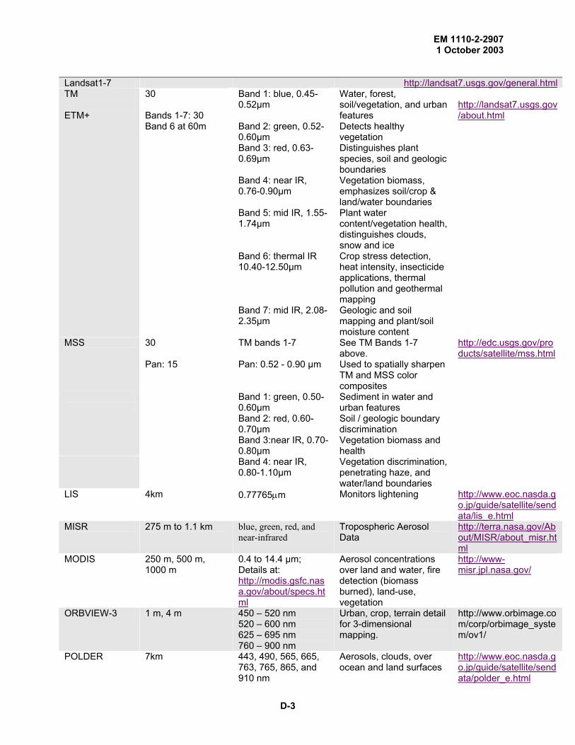
EM 1110-2-2907 1 October 2003

Landsat1-7 Band 1: blue, 0.45-0.52µm

Water, forest, soil/vegetation, and urban features

Band 2: green, 0.52-0.60µm

Detects healthy vegetation

Band 3: red, 0.63-0.69µm

Distinguishes plant species, soil and geologic boundaries

Band 4: near IR, 0.76-0.90µm

Vegetation biomass, emphasizes soil/crop & land/water boundaries

Band 5: mid IR, 1.55-1.74µm

Plant water content/vegetation health, distinguishes clouds, snow and ice

Band 6: thermal IR 10.40-12.50µm

Crop stress detection, heat intensity, insecticide applications, thermal pollution and geothermal mapping

TM ETM+

30 Bands 1-7: 30 Band 6 at 60m

Band 7: mid IR, 2.08-2.35µm

Geologic and soil mapping and plant/soil moisture content

http://landsat7.usgs.gov/about.html

30 TM bands 1-7 See TM Bands 1-7 above.

http://edc.usgs.gov/products/satellite/mss.html

MSS

Pan: 15 Pan: 0.52 - 0.90 µm Used to spatially sharpen TM and MSS color composites

Band 1: green, 0.50-0.60µm

Sediment in water and urban features

Band 2: red, 0.60-0.70µm

Soil / geologic boundary discrimination

Band 3:near IR, 0.70-0.80µm

Vegetation biomass and health

Band 4: near IR, 0.80-1.10µm

Vegetation discrimination, penetrating haze, and water/land boundaries

LIS 4km 0.77765µm Monitors lightening http://www.eoc.nasda.go.jp/guide/satellite/sendata/lis_e.html

MISR 275 m to 1.1 km blue, green, red, and near-infrared

Tropospheric Aerosol Data

http://terra.nasa.gov/About/MISR/about_misr.html

MODIS 250 m, 500 m, 1000 m

0.4 to 14.4 µm; Details at: http://modis.gsfc.nasa.gov/about/specs.html

Aerosol concentrations over land and water, fire detection (biomass burned), land-use, vegetation

http://www-misr.jpl.nasa.gov/

ORBVIEW-3 1 m, 4 m 450 – 520 nm 520 – 600 nm 625 – 695 nm 760 – 900 nm

Urban, crop, terrain detail for 3-dimensional mapping.

http://www.orbimage.com/corp/orbimage_system/ov1/

POLDER 7km 443, 490, 565, 665, 763, 765, 865, and 910 nm

Aerosols, clouds, over ocean and land surfaces

http://www.eoc.nasda.go.jp/guide/satellite/sendata/polder_e.html

http://landsat7.usgs.gov/general.html

D-3

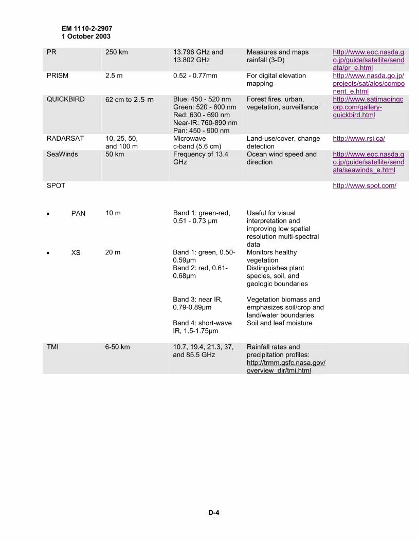
EM 1110-2-2907 1 October 2003

PR 250 km 13.796 GHz and

13.802 GHz

PRISM 0.52 - 0.77mm For digital elevation mapping

http://www.nasda.go.jp/projects/sat/alos/component_e.html

Measures and maps rainfall (3-D)

http://www.eoc.nasda.go.jp/guide/satellite/sendata/pr_e.html

2.5 m

QUICKBIRD 62 cm to 2.5 m Blue: 450 - 520 nm

Green: 520 - 600 nm Red: 630 - 690 nm Near-IR: 760-890 nm Pan: 450 - 900 nm

Forest fires, urban, vegetation, surveillance

http://www.satimagingcorp.com/gallery-quickbird.html

RADARSAT 10, 25, 50, and 100 m

Microwave c-band (5.6 cm)

Land-use/cover, change detection

http://www.rsi.ca/

SeaWinds 50 km Frequency of 13.4 GHz

Ocean wind speed and direction

http://www.eoc.nasda.go.jp/guide/satellite/sendata/seawinds_e.html

SPOT

• PAN 10 m Band 1: green-red, 0.51 - 0.73 µm

Useful for visual interpretation and improving low spatial resolution multi-spectral data

http://www.spot.com/

• XS 20 m Band 1: green, 0.50-0.59µm

Monitors healthy vegetation

Band 2: red, 0.61-0.68µm

Distinguishes plant species, soil, and geologic boundaries

Band 3: near IR, 0.79-0.89µm

Vegetation biomass and emphasizes soil/crop and land/water boundaries

Band 4: short-wave IR, 1.5-1.75µm

Soil and leaf moisture

TMI 6-50 km 10.7, 19.4, 21.3, 37, and 85.5 GHz

Rainfall rates and precipitation profiles: http://trmm.gsfc.nasa.gov/overview_dir/tmi.html

D-4

EM 1110-2-2907 1 October 2003

Appendix E Satellite Platforms and sensors Satellite On board sensors URL ALI Hyperion http://eo1.usgs.gov/instru/ali.asp ALOS PRISM

AVNIR-2 PALSAR

http://www.nasda.go.jp/projects/sat/alos/index_e.html

ADEOS AVNIR OCTS NSCAT TOMS POLDER IMG ILAS RIS

http://www.eorc.nasda.go.jp/ADEOS/

ADEOS-II AMSR GLI SeaWinds POLDER ILAS-2

http://www.eoc.nasda.go.jp/guide/satellite/satdata/adeos2_e.html

AQUA AMSR-E AIRS AMSU CERES HSB MODIS

http://aqua.nasa.gov/

ERS-1 AMI SCAT RA ATSR-M LRR PRARE

http://earth.esa.int/ers/

ERS-2 Above plus: AMI/SAR ATSR GOME MWS RA

http://earth.esa.int/ers/

JERS-1 SAR OPS

http://www.eorc.nasda.go.jp/JERS-1/

LANDSAT ETM+ MSS TM

http://geo.arc.nasa.gov/sge/landsat/landsat.html

MOS-1/1b MESSR http://www.restec.or.jp/eng/data/satelite/mos.html NOAA-11 thru -17

VTIR MSR Amsu

http://www.noaa.gov/satellites.html

RADAR SAT

Avhrr HIRS/3 POES SAR

http://www.space.gc.ca/asc/eng/csa_sectors/earth/radarsat1/radarsat1.asp

E-1

EM 1110-2-2907 1 October 2003

SPOT HRVIR

HRV http://www.spot.com/

TERRA ASTER CERES MISR MODIS MOPITT PR

http://terra.nasa.gov/About/

TRMM VIRS TMI CERES LIS

http://trmm.gsfc.nasa.gov

E-2

EM 1110-2-2907 1 October 2003

Appendix F Airborne Sensors Presented here is a short list of common airborne sensors and their general performance capabilities. For an larger list of airborne sensors (acronyms and full names) see http://carstad.gsfc.nasa.gov/Topics/instrumentlist.htm and http://ioc.unesco.org/oceanteacher/resourcekit/M3/Data/Measurements/Instrumentation/gcmd_sensors.htm.

Sensor Spatial Resolution (metric)

Band/ Wavelength or Frequency

Application General Information

AC 250 0.89-1.58µm Used to atmospherically correct high-spatial, low-spectral resolution multispectral sensors

http://eo1.gsfc.nasa.gov/Technology/AtmosCorr.htm

ACE-FTS 0.02–1cm 4km vertical resolution

2-13 µm (infrared) Measures the temperature, vertical distribution of trace gases and aerosols an thin clouds

http://www.space.gc.ca/asc/eng/csa_sectors/space_science/atmospheric/scisat/fts.asp

ATM 10- to 20-cm vertical resolution

LIDAR-based sensor (microwave)

Beach topography, ice mapping, sea-surface elevation, and wave morphologies

http://aol.wff.nasa.gov/ATMindex.html

AVIRIS 4 – 20 m 400 - 2500 nm Aerosols, ice, and water quality mapping and ecologic and geologic applications

http://popo.jpl.nasa.gov/html/aviris.overview.html and http://popo.jpl.nasa.gov/html/aviris.freedata.html

CAMIS 26 – 156 cm 450, 550, 650 and 800 nm

Terrestrial and oceanographic applications

http://www.flidata.com/prod02.htm

CASI 0.5 – 10 m 400 – 1000nm Environmental monitoring, forestry, pipeline engineering, military, agriculture, and water quality

http://www.itres.com/

EMERGE 0.3 – 0.6 m Visible and infrared Land use and agricultural surveys

http://www.emergeweb.com/

HYDICE 400 - 2500 nm Agriculture, forestry, environmental, mapping, disaster management, and surveillance

http://www.oss.goodrich.com/HyperspectralDigitalImageryCollectionExperiment.shtml

HYMAP 2 – 10 m VIS,NIR, SWIR, MIR and TIR

Agriculture, forestry, environmental, urban, geologic, and soil mapping

http://www.intspec.com/

IFSAR Can at collect <1 m Microwave region Topography JPL Airsar

100 m Microwave region All-weather terrain imager. Can penetrate forest canopy

http://airsar.jpl.nasa.gov/index.html

SHOALS 4 – 8 m Visible and infrared Bathymetry http://shoals.sam.usace.army.mil/

TIMS ~1 – 50 m Thermal infrared (8-12 µm)

Mineral mapping and archeologic applications

http://www.dfrc.nasa.gov/airsci/ER-2/tims.html

F-1

EM 1110-2-2907 1 October 2003

Appendix G TEC’s Imagery Office (TIO) The following is taken from Appendix I of the Geospatial Engineer Manual (EM 1110-1-2902), which outlines the procedures for acquiring image data. G-1 Development of TEC’s Imagery Office (TIO).

a. To help Army agencies/organizations avoid duplicating commercial and civil imagery purchases, the Office of the Assistant Chief of Engineers designated TEC in 1990 to act as the U.S. Army Commercial and Civil Imagery (C2I) Acquisition Program Manager. To accomplish this task, the TIO was initiated with the added focus on educating the soldier on the uses, types, and availability of commercial satellite imagery. As Army use of this imagery increased and as the number of satellites increased, the TIO has grown to keep up with the demand. Currently, TIO provides thousands of dollars of imagery support to its customers, and is an active participant in National Imagery and Mapping Agency’s Commercial Imagery Strategy.

b. TIO is the designated repository of selected commercial satellite imagery data pertaining to terrain analysis and water resources operations worldwide. These data support worldwide military applications and operations. TIO executes the Commercial Imagery Program for TEC and the Army. The current revision of Army Regulation 115-11, “Geospatial Information and Services,” strengthens the role of TIO as the point of contact for acquisition of commercial satellite imagery in the Army. G-2 How to Order Commercial Satellite Imagery.

a. USACE Commands are required to first coordinate with TIO before purchasing satellite imagery from a commercial vendor. USACE organizations with requirements for commercial satellite imagery must forward requests to TIO for research, acquisition, and distribution of the data. The requests can be submitted as follows:

TIO@tec.army.mil Telephone: 703-428-6909

Fax: 703-428-8176 Online Request Form

www.tec.army.mil/forms/csiform1.html

b. Each request should include the following information:

• Geographic area of interest. Please provide Upper Left and Lower Right coordinates (e.g., 27 00 00N 087 00 00W) and path/row, if known.

• Acceptable date range for data coverage (e.g., 5 January 1999 to 3 March 2000).

• Cloud cover and quality restrictions (e.g., less than 10 percent cloud cover, no haze, 10 degrees off nadir).

G-1

EM 1110-2-2907 1 October 2003

• Satellite system/sensor. (For basic satellite information, access

www.tec.army.mil/TIO/ satlink.htm.)

• Desired end product (digital or hard copy and preferred media type; e.g., CD-ROM).

• Point of contact, mailing and electronic address, and telephone number.

c. Purchased Commercial Satellite Imagery Submission to the Commercial Satellite

Imagery Library (CSIL)

d. Commercial satellite imagery that the TIO purchases for customers is disseminated upon receipt to the requestor as well as to the CSIL. This provides data access for DoD/Title 50 users.

G-2

EM 1110-2-2907 1 October 2003

Appendix H Example Contract - Statement of Work (SOW)

Laser Fluorescence Oil Spill Surveillance

Statement of Work 2/14/96

To: DOE/NV Remote Sensing Laboratory From: RSGISC, U. S. Army Corps of Engineers

1.0 Purpose The purpose of this SOW is to demonstrate proof-of-concept of an airborne fluorescence imaging system capable of sensing oil on land and in wetlands. These are issues of concern to the Corps. 2.0 Background The U.S. Coast Guard Research and Development Center (R&D Center) and Environment Canada have sponsored experiments with a Laser Environmental Airborne Fluorimeter (LEAF) spot sensor for the detection of oil on water in land-locked pools. The tests successfully demonstrated that oils fluoresce with distinct spectral signatures when excited by a laser source. In order to develop the fluorescence concept into a practical field instrument for supporting oil spill response operations, an upgrade to an imaging sensor is necessary. The EG&G, Santa Barbara, Special Technologies Laboratory (STL) is prototyping an airborne Laser Induced Fluorescence Imager (LIFI) which can be applied to the detection of oil spills on land and in wetlands. 3.0 Objectives/ Scope The DOE/NV Remote Sensing Laboratory (RSL) and STL will design and perform measurements to test airborne LIFI technology for the detection of oil-on-land and in wetlands. 1. Acquire laboratory and ground fluorescence spectra of several types of spilled oil on land and in wetlands in the presence of both organic and inorganic background materials. This can be used to define the source intensity needed for required signal levels and resolve major technical issues such as spatial resolution, swath width, aircraft altitude, and speed. 2. Acquire imagery from airborne LIFI over oiled targets for proof of concept. 4.0 Requirements Task 1

H-1

EM 1110-2-2907 1 October 2003

A series of laboratory measurements will be collected to measure the fundamental

fluorescence properties of the oils and background materials. Optimal sensing specification for oils depend on the fluorescence efficiency of the oil as well as the spectral and spatial resolution required for the application. Task 2 Outdoor laser range measurements will be made for up to 20 target/background combinations. These should include crude, diesel and home heating oils, on sand, gravel, soil and vegetation organic backgrounds. Measurements will address the fluorescence efficiency, emission spectra, duration and the effects of oil aging over a period of up to six weeks. The effects of the wetness of the backgrounds on the emission efficiency, duration and spectra will be addressed. Task 3 When the STL LIFI system becomes airborne, imagery from flight tests over oil targets will be collected. It is planned to operate at an altitude of 300 ft agl and provide a swath of 60 ft., 512 pixels wide or about 1.4 in. per pixel in the cross track direction. The spectral range will be 300nm with 128 channels covering the visible portion of the spectrum. Excitation will be at 355nm. 5.0 Schedule The STL shall coordinate its airborne data collection schedule to coincide with its other sponsored flight test programs. All ground data will be collected preliminary to airborne testing. All reports and deliverables will be completed within six months of data collection. 6.0 Deliverables Deliverable 1 - Presentation at Oil Spill Program Review Test planning will be presented at the Oil Spill Program review and meetings required by the Oil Spill Program Manager [FY96]. Deliverable 2 - Technical Report A written summary report will be delivered to the Oil Spill Program Manager NLT six months after acquisition of the data. Deliverable 3 - Distribution of Data All laboratory, ground and airborne data will become the property of and be transmitted to the RS/GIS Center in digital computer compatible format.

H-2

EM 1110-2-2907 1 October 2003

Appendix I Example Acquisition – Memorandum of Understanding (MOU)

CONDITIONS FOR DATA ACQUISITION DURING

THE 1999 AIG HYMAP USA GROUPSHOOT CAMPAIGN

This Memorandum of Understanding, Conditions for Data Acquisition During the 1999

AIG HyMap USA Groupshoot Campaign (MOU) is entered into between Analytical Imaging and Geophysics LLC (“AIG”) a limited liability company, with its principal place of business located at 4450 Arapahoe Avenue, Suite 100, Boulder, Colorado, 80303, USA, and (“Sponsor”), a corporation, with its principal place of business located at .

WHEREAS, AIG is acting as the coordinator for various Sponsors for the acquisition of HyMap data, the 1999 AIG/HYVISTA North American Group Shoot (“Group Shoot”), and the Sponsor is will to acquire data using the HyMap sensor system.

WHEREAS, this MOU outlines the conditions for HyMap data acquisition as part of the Group Shoot. It establishes the guidelines for AIG and HyVista Corporation (“HyVista”) efforts to acquire data using the HyMap sensor system for sponsor-specified flight locations.

NOW, THEREFORE, in consideration of the premises and the agreements and covenants of the parties set forth in this Agreement, the parties hereto agree as follows:

DEFINITIONS As used in this Agreement, the following terms have the following meanings:

“Individual Site” means: a 2.3 kilometer wide x 20 kilometer long area.

"Scene" means: an image cube of an Individual Site (2.3 kilometers by 20 kilometers) at 5 meter spatial resolution and 126 spectral bands.

“Research Mode” means: Scenes acquired which may be available to anyone.

“Proprietary Mode” means: Scenes acquired which are only available to the Sponsor ordering acquisition.

OBLIGATIONS OF AIG AIG shall use its best efforts to perform the services and deliver the

group Scene and the Sponsor’s Scene(s), listed in Exhibit A, within 8 weeks after completion of the mission. All work shall be performed in a workmanlike and professional manner to industry standards. All work will be performed using AIG facilities,

I-1

EM 1110-2-2907 1 October 2003

excepting HyMap data acquisition and items below indicated by (HyVista), which will be performed by HyVista Corporation.

AIG agrees to supply the following for each Scene either on CDs or tape:

• Image data in units of radiance (µW/cm-2/nm/sr); BIL format data files with corresponding ENVI header files (HyVista)

• GPS positions of the plane during data acquisition (HyVista) • Dark current measurements (HyVista) • Spectral calibration parameters: band centers and band shape (HyVista) • Image data corrected to apparent reflectance using an atmospheric model;

BIL format data files with corresponding ENVI header files • A single-band image of precision geocorrected data • Geocorrection information sufficient to precision geocode other bands/results

OBLIGATIONS OF SPONSOR

Sponsors shall supply the start and finish coordinates of each Individual Site in latitude/longitude pairs (decimal degrees using the WGS84 datum). Larger areas can be covered at an incremental cost. If such areas are to be covered, in order to provide uninterrupted coverage of adjacent data strips, a 20% overlap for each strip with its neighbor should be allowed. AIG and HyVista Corporation accept no responsibility for sponsors supplying incorrect coordinates for survey sites; sponsors will be charged in full for the full data acquisition fee in these instances.

DATA ACQUISITION Data will be acquired at a date nominated by AIG and HyVista with input

from the Sponsor. Data will be acquired in weather conditions to the satisfaction of AIG and HyVista. Sponsor will be notified of proposed acquisition of data from an elected study site not less than 24 hours prior to acquisition. AIG and HyVista reserve the right to omit data acquisition for a Sponsor’s chosen site if adverse weather conditions preclude the acquisition of data to corporate quality standards.

DATA QUALITY All data presented to Sponsor shall bear full 126-channel coverage. To keep

turbulence effects to a minimum the scanner is mounted on a stabilized platform the Jena SM 2000. The geometric integrity of the data therefore will be within the platform performance characteristics as supplied by the manufacturers and the operators will endeavor to keep turbulence effects to a minimum or abort the line if the motion is too great. Cloud cover will be less than 10 percent total for a named study area. Spatial accuracy of the data is limited by the on-board GPS of the aircraft.

Should a sponsor be dissatisfied with the data quality, the following procedure will be followed: The data in question will be supplied for a quality control assessment to 2 impartial experts, one selected by each

I-2

EM 1110-2-2907 1 October 2003

party. The impartial experts will have no professional or financial interest in their selector’s organization. The impartial experts will assess the data quality, and judge whether the data is supplied in accordance to HyVista’s specifications for the survey. Should the experts judge that data meets or exceeds HyVista’s quoted data quality specifications, then the data will be supplied and the sponsor will be liable to pay agreed data acquisition costs, and all costs incurred in the data assessment. Should the experts judge that the supplied data does not meet HyVista’s quoted data quality specifications, then the data will not be supplied.

PAYMENT The cost of a Research Mode Scene is Five Thousand US Dollars

($5,000.00). The cost of a Proprietary Mode Scene is Ten Thousand US Dollars ($10,000.00). The Group Shoot Scene is also delivered to the Sponsor at no additional cost. Custom acquisitions and larger areas can be covered at an incremental cost and volume discounts may be applied. These additional Scenes shall be listed in Appendix E.

Invoices will be issued upon signature of this MOU and payment is net 30 days. In instances where AIG and HyVista acquire only a portion of a requested block of data due to adverse weather conditions or other unforeseen circumstances, AIG and HyVista will refund a portion of the fee at a rate proportional to the agreed fee for full data coverage. In the event that no Sponsor data are acquired AIG will refund Sponsor all payments received.

I-3

EM 1110-2-2907 1 October 2003

POINTS OF CONTACT

Dr. Fred A. Kruse is designated as the AIG point of contact for this program.

AIG Sponsor:

Fred A. Kruse Contact:

Senior Research Scientist Title:

Analytical Imaging and Geophysics LLC Address:

4450 Arapahoe Ave, Suite 100 Address:

Boulder, CO 80303 Address:

Phone: 303-499-9471 Phone:

FAX: 303-665-6090 FAX:

Email: kruse@aigllc.com Email:

TERM AND TERMINATION

The Agreement shall enter into force on the Effective Date and shall continue until terminated as provided in this Section 8. After all Scenes have been delivered to Sponsor and payment received this Agreement shall terminate.

CONFIDENTIALITY Both Sponsor and AIG acknowledge and agree that both parties own

confidential, proprietary and secret information related to various aspects of Sponsor’s and AIG’s respective business and technology.

As used in this Agreement, “Confidential Information” consists of (i) any information designated by either party as confidential, and (ii) any information relating to either party’s product plans, client lists, product designs, product costs, product prices, product names, finances, marketing plans, business opportunities, personnel, research, development or know-how, except such information which the parties agree in writing is not confidential. Each party shall use the other party’s Confidential Information solely for implementing its obligations under this Agreement. Confidential Information shall not include information that (i) is known to each at the time of disclosure to the other party, (ii) has become publicly known through no wrongful act of the other party, (iii) has been rightfully received from a third party authorized to make such disclosure without restriction, or (iv) has been approved for release by written authorization of the other party.

Each party will not use in any way for its own account or the account of any third party, nor disclose to any third party (excepting HyVista), any such Confidential Information revealed to it by the other party. Each party agrees to protect any Confidential

I-4

EM 1110-2-2907 1 October 2003

Information from disclosure to others with at least the same degree of care as that which is accorded to its own proprietary information, but in no event with less than reasonable care. In the event of termination of this Agreement, there shall be no use or disclosure by either party of any Confidential Information.

Each party agrees to notify the other party promptly in the event of any breach of confidentiality or security under conditions in which it would appear that any Confidential Information was disclosed in violation of this Agreement, prejudiced or exposed to loss. Each party shall, upon request of the other party, take all reasonable steps necessary to recover any compromised trade secrets disclosed to or placed in the possession of the other party by virtue of this Agreement.

Each party agrees to use Confidential Information under carefully controlled conditions for the purposes set forth in this Agreement, and to inform all persons who are given access to Confidential Information by either party that such materials are confidential trade secrets of the other party. Each party expressly agrees it shall be fully responsible for the conduct of all its employees, contractors, agents and representatives who may in any way breach this Agreement.

Each party acknowledges that any breach of any of its obligations under this Section 7 is likely to cause or threaten irreparable harm to the other party, and, accordingly, each party agrees that in such event, the other party shall be entitled to equitable relief to protect its interest therein, as well as money damages.

WARRANTY AND INDEMNIFICATION Sponsor shall defend, indemnify and hold harmless AIG from and

against all claims, liability, losses, damages and expenses (including attorneys’ fees and court costs) arising from or in connection with the use or application of AIG’s work by Sponsor or any direct or indirect purchaser or licensee of Sponsor.

AIG SHALL NOT BE LIABLE TO SPONSOR FOR ANY DIRECT, INDIRECT, SPECIAL, AND/OR CONSEQUENTIAL DAMAGES WHATSOEVER, WHETHER CAUSED BY AIG’S NEGLIGENCE, ERRORS, OMISSIONS, STRICT LIABILITY, BREACH OF CONTRACT, BREACH OF WARRANTY OR OTHER CAUSE OR CAUSES WHATSOEVER INCLUDING BUT NOT LIMITED HYVISTA CORPORATIONS INABILITY TO GATHER THE HYMAP DATA SCENES.

GENERAL PROVISIONS No Assignability. The parties agree that this Agreement is not

assignable or transferable by AIG without the prior written consent of Sponsor.

No Agency Relationship. This Agreement does not establish any agency, joint venture, or partnership relationship between the

I-5

EM 1110-2-2907 1 October 2003

parties, and neither party can bind the other by any contract or representation.

Notices. All notices provided for in this Agreement shall be in writing and will be deemed effective when either served by personal delivery or sent by express, registered or certified mail, postage prepaid, return receipt requested, to the other party at the corresponding mailing address set forth on the first page hereof or at such other address as such other party may hereafter designate by written notice in the manner aforesaid.

Modification. The parties acknowledge and agree that this Agreement may only be modified by the mutual written agreement of the parties.

Entire Agreement. The written terms and provisions in this Agreement constitute the entire agreement and understanding between the parties relating to the subject matter hereof and supersede all previous communications, proposals, representations, and understandings, whether oral or written, relating thereto. This Agreement may be executed in two or more counterparts, each of which shall be deemed an original and all of which together shall constitute one instrument.

Governing Law. This Agreement shall be governed by and construed and enforced in accordance with the laws of the State of Colorado, U.S.A., without regard to the conflict of laws provisions thereof. Both AIG and Sponsor agree and consent to personal jurisdiction and venue in the state and federal courts in the State of Colorado, U.S.A. All actions relating to or arising out of this Agreement may be brought only in federal or state courts in the State of Colorado, U.S.A.

Binder. This Agreement is binding on and inures to the benefit of the parties, their respective heirs, assigns, and legal representatives.

Severability. In case any one or more of the provisions contained in this Agreement shall, for any reason, be held to be invalid, illegal, or unenforceable in any respect, such invalidity, illegality, or unenforceability shall not affect any other provisions of this Agreement, and this Agreement shall be construed as if such valid, illegal, or unenforceable provision had never been contained herein.

Binding Agreement. Each party agrees and acknowledges that it has read this Agreement, understands it, and agrees to be bound by the terms and conditions herein.

IN WITNESS WHEREOF, this Agreement is executed by and between the parties as of the Effective Date.

I-6

EM 1110-2-2907 1 October 2003

AIG SPONSOR: By: By: Name: James M. Young Name: Title: Contracts Manager Title: Date: Date:

I-7

EM 1110-2-2907 1 October 2003

Glossary This glossary was compiled from Internet Sites at the USGS, NASA, Goddard Space Center, Canadian Center for Remote Sensing, and the ASPRS DISCLAIMER: Any use of trade, product, or firm names is for descriptive purposes only and does not imply endorsement by the U.S. Government. A

Absolute temperature Temperature measured on the Kelvin scale, whose base is absolute zero, i.e. -273 °C (0 °C is expressed as 273 °K).

Absorptance A measure of the ability of a material to absorb EM energy at a specific wavelength.

Absorption band Wavelength interval within which electromagnetic radiation is absorbed by the atmosphere or by other substances.

Absorptivity Capacity of a material to absorb incident radiant energy. Achromatic vision The perception by the human eye of changes in brightness, often used

to describe the perception of monochrome or black and white scenes. Active remote sensing Remote sensing methods that provide their own source of

electromagnetic radiation to illuminate the terrain. Radar is one example.

Acuity A measure of human ability to perceive spatial variations in a scene. It varies with the spatial frequency, shape, and contrast of the variations, and depends on whether the scene is colored or monochrome.

Additive primary colors Blue, green, and red. Filters of these colors transmit the primary color of the filter and absorb the other two colors.

Adiabatic cooling Refers to decrease in temperature with increasing altitude. Advanced very high resolution radiometer (AVHRR)

Crosstrack multispectral scanner on a NOAA polar-orbiting satellite that acquires five spectral bands of data (0.55 to 12.50 µm) with a ground resolution cell of 1.1 by 1.1 km.

Aerial magnetic survey Survey that records variations in the earth's magnetic field. Aeromagnetic Aeromagnetic is descriptive of data pertaining to the Earth's magnetic

field which has been collected from an airborne sensor. AGL Above ground level. Air base Ground distance between optical centers of successive overlapping

aerial photographs. Airborne imaging spectrometer (AIS)

Along-track multispectral scanner with spectral bandwidth of 0.01 µm.

Airborne visible and infrared imaging spectrometer (AVIRIS)

Experimental airborne along-track multispectral scanner under development at JPL to acquire 224 images in the spectral region from 0.4 to 2.4 µm.

AID--Agency for International Development

The United States Federal agency for international development projects.

Albedo (A) Ratio of the amount of electromagnetic energy reflected by a surface to the amount of energy incident upon it.

Albers Equal Area Projection

The Albers Equal Area projection is a method of projection on which the areas of all regions are shown in the same proportion of their true areas. The meridians are equally spaced straight lines converging at a common point, which is normally beyond the pole. The angles between them are less than the true angles. The parallels are unequally spaced concentric circular arcs centered on the point of convergence of the meridians. The meridians are radii of the circular arcs. The poles are normally circular arcs enclosing the same angle as that enclosed by the

Glossary-1

EM 1110-2-2907 1 October 2003

other parallels of latitude for a given range of longitude. Albers Equal Area is frequently used in the ellipsoidal form for maps of the United States in the National Atlas of the United States, for thematic maps, and for world atlases. It is also used and recommended for equal-area maps of regions that are predominantly east-west in extent.

Along-track scanner Scanner with a linear array of detectors oriented normal to flight path. The IFOV of each detector sweeps a path parallel with the flight direction.

Alteration Changes in color and mineralogy of rocks surrounding a mineral deposit that are caused by the solutions that formed the deposit. Suites of alteration minerals commonly occur in zones.

Amplitude For waves, the vertical distance from crest to trough. Analog display A form of data display in which values are shown in graphic form, such

as curves. Differs from digital displays in which values are shown as arrays of numbers.

Analogue image An image where the continuous variation in the property being sensed is represented by a continuous variation in image tone. In a photograph, this is achieved directly by the grains of photosensitive chemicals in the film; in an electronic scanner, the response in millivolts is transformed to a display on a cathode-ray tube where it may be photographed.

Angular beam width In radar, the angle subtended in the horizontal plane by the radar beam.

Angular field of view Angle subtended by lines from a remote sensing system to the outer margins of the strip of terrain that is viewed by the system.

Angular resolving power Minimum separation between two resolvable targets, expressed as

angular separation. Anomaly An area on an image that differs from the surrounding, normal area. For

example, a concentration of vegetation within a desert scene constitutes an anomaly.

Antenna Device that transmits and receives microwave and radio energy in radar systems.

Aperture Opening in a remote sensing system that admits electromagnetic radiation to the film in radar systems.

APL Applied Physics Laboratory of John Hopkins University. Apollo U.S. lunar exploration program of satellites with crews of three

astronauts. Apparent thermal inertia (ATI)

An approximation of thermal inertia calculated as one minus albedo divided by the difference between daytime and nighttime radiant temperatures.

ARC Export EXPORT creates an ARC/INFO interchange file to transfer coverages, INFO data files, text files, and other ARC/INFO files between various computer systems. An interchange file contains all coverage information and appropriate INFO file information in a fixed length, ASCII format. It can be fully or partially compressed as well as uncompressed ASCII depending upon the given EXPORT option.

ARC SECOND 1/3600th of a degree (1 second) of latitude or longitude. ARC/INFO ARC/INFO is a geographic information system (GIS) used to automate,

manipulate, analyze, and display geographic data in digital form. ARC/INFO is a proprietary system developed and distributed by the Environmental Systems Research Institute, Inc., in Redlands, California

ArcUSA Designed by ESRI, ArcUSA is a general-purpose database used to generate thematic maps of the conterminous United States at the State and county levels. The database contains cartographic information, tabular information, and indices and is designed for a wide range of applications.

Glossary-2

EM 1110-2-2907 1 October 2003

Areal Relating to or involving an area. Artifact A feature on an image, which is produced by the optics of the system or

by digital image processing, and sometimes masquerades as a real feature.

ASA index Index of the American Standards Association designating film speed, or sensitivity to light. Higher values indicate higher sensitivity. The ASA index has been replaced by the ISO index.

Ascending node Direction satellite is traveling relative to the Equator. An ascending node would imply a northbound Equatorial crossing.

ATI Apparent Thermal Inertia. Atmosphere Layer of gases that surrounds some planets. Atmospheric correction Image-processing procedure that compensates for effects of selectivity

scattered light in multispectral images. Atmospheric shimmer An effect produced by the movement of masses of air with different

refractive indices, which is most easily seen in the twinkling of stars. Atmospheric window Wavelength interval within which the atmosphere readily transmits

electromagnetic radiation. Attributes Attributes, also called feature codes or classification attributes, are

used to describe map information represented by a node, line, or area. For example, an attribute code for an area might identify it to be a lake or swamp; an attribute code for a line might identify a road, railroad, stream, or shoreline.

Attitude Angular orientation of remote sensing system with respect to a geographic reference system.

AVHRR Advanced Very High Resolution Radiometer, a multispectral imaging system carried by the TIROS-NOAA series of meteorological satellites.

AVIRIS Airborne visible and infrared imaging spectrometer. Azimuth Geographic orientation of a line given as an angle measured in degrees

clockwise from north. Azimuth direction In radar images, the direction in which the aircraft is heading. Also

called flight direction. Azimuth resolution In radar images, the spatial resolution in the azimuth direction. B

Background Area on an image or the terrain that surrounds an area of interest, or target.

Backscatter In radar, the portion of the microwave energy scattered by the terrain surface directly back toward the antenna.

Backscatter coefficient A quantitative measure of the intensity of energy returned to a radar antenna from the terrain.

Band A wavelength interval in the electromagnetic spectrum. For example, in Landsat images the bands designate specific wavelength intervals at which images are acquired.

Bandwidth The total range of frequency required to pass a specific modulated signal without distortion or loss of data. The ideal bandwidth allows the signal to pass under conditions of maximum AM or FM adjustment. (Too narrow a bandwidth will result in loss of data during modulation peaks. Too wide a bandwidth will pass excessive noise along with the signal.) In FM, radio frequency signal bandwidth is determined by the frequency deviation of the signal.

Base height ratio Air base divided by aircraft height. This ratio determines vertical exaggeration on stereo models.

Glossary-3

EM 1110-2-2907 1 October 2003

Batch processing Method of data processing in which data and programs are entered into

a computer that carries out the entire processing operation with no further instructions.

Bathymetry Configuration of the seafloor. Beam A focused pulse of energy. BIA--Bureau of Indian Affairs, Department of the Interior

The BIA serves Indian and Alaska Native tribes living on or near reservations. The BIA administers and manages approximately 52 million acres of land held in trust for Indians by the United States and works with local tribal governments on issues including road construction and maintenance, social services, police protection, and economic development.

BIL (Band-Interleaved-by-Line)

BIL is a CCT tape format that stores all bands of satellite data in one image file. Scanlines are sequenced by interleaving all image bands. The CCT header appears once in a set.

Bilinear The term bilinear is referring to a bilinear interpolation. This is simply an interpolation with two variables instead of one.

Bin One of a series of equal intervals in a range of data, most commonly employed to describe the divisions in a histogram.

Binary Based upon the integer two. Binary Code is composed of a combination of entities that can assume one of two possible conditions (0 or 1). An example in binary notation of the digits 111 would represent (1 X 2) + (1 X 2) + (1 X 2) = 4 + 2 + 1 = 7.

Bit Contraction of binary digit, which in digital computing represents an exponent of the base 2.

BIP--Band-Interleaved-by-Pixel

When using the BIP image format, each line of an image is stored sequentially, line 1 all bands, line 2 all bands, etc. For example, the first line of a three-band image would be stored as p1b1, p1b2, p1b3, p2b1, p2b2, p2b3, where p1b1 indicates pixel one, band one, p1b2 indicates pixel one, band two, etc.

Blackbody An ideal substance that absorbs the entire radiant energy incident on it and emits radiant energy at the maximum possible rate per unit area at each wavelength for any given temperature. No actual substance is a true blackbody, although some substances, such as black lamps, approach this property.

Blind spot The point of the optic nerve to the retina where no radiation is detected by the eye.

BLM--Bureau of Land Management, Department of the Interior

Under the Federal Land Policy and Management Act of 1976, the BLM administers and manages approximately 300 million acres of public lands primarily located in the western half of the lower 48 States and Alaska. Public lands in the U.S. contain mineral and timber reserves, support habitat for a host of wildlife, and provide recreational opportunities.

BOR--Bureau of Reclamation, Department of the Interior

The BOR was chartered in 1902 with the responsibility to reclaim arid lands in the western U.S. for farming by providing secure, year-around water supplies for irrigation. The BOR's responsibilities since have expanded to include generating hydroelectric power; overseeing municipal and industrial water supplies, river regulation, and flood control; enhancing fish and wildlife habitats; and researching future water and energy requirements.

BPI--Bits Per Inch The tape density to which the digital data were formatted. Brightness Magnitude of the response produced in the eye by light. Brute Force Radar See real-aperture radar. BSQ--Band Sequential BSQ is a CCT tape format that stores each band of satellite data in one

image file for all scanlines in the imagery array. The CCT headers are recorded on each band.

Byte A group of eight bits of digital data.

Glossary-4

EM 1110-2-2907 1 October 2003

C

Calibration Process of comparing an instrument's measurements with a standard. Calorie Amount of heat required to raise the temperature of 1g of water by 1

°C. Camouflage detection photographs

Another term for IR color-photograph.

Cardinal point effect In radar, very bright signatures caused by optimally oriented corner reflectors, such as buildings.

Cartographic Pertaining to cartography, the art or practice of making charts or maps. Cathode ray tube (CRT) A vacuum tube with a phosphorescent screen on which images are

displayed by an electron beam. C band Radar wavelength region from 3.8 to 7.5 cm. CCD Charge-coupled detector. CCT Computer-compatible tape. CD-ROM--Compact Disc-Read Only Memory

CD-ROM is a computer peripheral that employs compact disc technology to store large amounts of data for later retrieval. The capacity of a CD-ROM disk is over 600 megabytes, the equivalent of over 250,000 typewritten pages.

Centerpoint The optical center of a photograph. Change-detection images An image prepared by digitally comparing scenes acquired at different

times. The gray tones or colors of each pixel record the amount of difference between the corresponding pixels of the original images.

Channels A range of wavelength intervals selected from the electromagnetic spectrum.

Charge-coupled detector (CCD)

A device in which electrons are stored at the surface of a semiconductor.

Chlorosis Yellowing of plant leaves resulting from an imbalance in the iron metabolism caused by excess concentrations of copper, zinc, manganese, or other elements in the plant.

Chromatic vision The perception by the human eye of changes in hue. CIR Color infrared. Circular scanner Scanner in which a faceted mirror rotates about a vertical axis to sweep

the detector IFOV in a series of circular scan lines on the terrain. Classification Process of assigning individual pixels of an image to categories,

generally based on spectral reflectance characteristics. Coastal zone color scanner (CZCS)

A satellite-carried multi-spectral scanner designed to measure chlorophyll concentrations in the oceans.

Coherent radiation Electromagnetic radiation whose waves are equal in length and are in phase, so that waves at different points in space act in unison, as in laser and synthetic aperture radar.

Color composite image Color image prepared by projecting individual black-and-white multispectral images, each through a different color filter. When the projected images are superposed, a color composite image results.

Color ratio composite image

Color composite image prepared by combining individual ratio images for a scene using a different color for each ratio image.

Complementary colors Two primary colors of light (one additive and the other subtractive) that produce white light when added together. Red and cyan are complimentary colors.

Computer-compatible tape (CCT)

The magnetic tape on which the digital data for Landsat MSS and TM images are distributed.

Conduction Transfer of electromagnetic energy through a solid material by molecular interaction.

Cones Receptors in the retina, which are sensitive to color. There are cones sensitive to the red, green, and blue components of light.

Glossary-5

EM 1110-2-2907 1 October 2003

Contact print A reproduction from a photographic negative in direct contact with

photosensitive paper. Context The known environment of a particular feature on an image. Contrast The ratio between the energy emitted or reflected by an object and its

immediate surroundings. Contrast enhancement Image-processing procedure that improves the contrast ratio of images.

The original narrow range of digital values is expanded to utilize the full range of available digital values.

Contrast ratio On an image, the reflectance ratio between the brightest and darkest parts of an image.

Contrast stretching Expanding a measured range of digital numbers in an image to a larger range, to improve the contrast of the image and its component parts.

Convection Transfer of heat through the physical movement of matter. Corner reflector Cavity formed by two or three smooth planar surfaces intersecting at

right angles. Electromagnetic waves entering a corner reflector are reflected directly back toward the source.

Corps US Army Corps of Engineers (USACE) COSMIC Computer Software Management and Information Center, University of

Georgia. This facility distributes computer programs developed by U.S. government-funded projects.

Cross polarized Describes a radar pulse in which the polarization direction of the return

is normal to the polarization direction of the transmission. Cross-polarized images may be HV (horizontal transmit, vertical return) or VH (vertical transmit, horizontal return).

Cross track scanner Scanner in which a faceted mirror rotates about a horizontal axis to sweep the detector IFOV in a series of parallel scan lines oriented normal to the flight direction.

CRT Cathode ray tube. Cubic convolution A high order resampling technique in which the brightness value of a

pixel in a corrected image is interpolated from the brightness values of the 16 nearest pixels around the location of the corrected pixel.

Cut off The digital number in the histogram of a digital image, which is set to zero during contrast stretching. Usually this is a value below which atmospheric scattering makes a major contribution.

CWA Clean Water Act Cycle One complete oscillation of a wave. CZCS Coastal Zone color scanner. D

Dangling ARC An arc having the same polygon on both its left and right sides and having at least one node that does not connect to any other arc. See dangling node.

Dangling node The dangling endpoint of a dangling arc. Often identifies that a polygon does not close properly, that arcs do not connect properly, or that an arc was digitized past its intersection with another arc. In many cases, a dangling node may be acceptable. For example, in a street centerline map, cul-de-sacs are often represented by dangling arcs.

Data collection system (DCS)

On Landsats 1 and 2, the system that acquired information from seismometers, flood gauges, and other measuring devices. These data were relayed to ground receiving stations.

Glossary-6

EM 1110-2-2907 1 October 2003

Datum In surveying, a reference system for computing or correlating the

results of surveys. There are two principal types of datums: vertical and horizontal. A vertical datum is a level surface to which heights are referred. In the United States, the generally adopted vertical datum for leveling operations is the national geodetic vertical datums of 1929 (differing slightly from mean sea level). The horizontal datum, used as a reference for position, is defined by: the latitude and longitude of an initial point, the direction of a line between this point and a specified second point, and two dimensions which define the spheroid. In the United States, the initial point for the horizontal datum is located at Meade’s Ranch in Kansas.

Defense Meteorological Satellite Program (DMSP)

A U.S. Air Force meteorological satellite program with satellites circling in sun-synchronous orbit. Imagery is collected in the visible- to near-infrared band (0.4 to 1.1 micrometers) and in the thermal-infrared band (about 8 to 13 micrometers) at a resolution of about three kilometers. While some of the data is classified, most unclassified data is available to civilian users.

DEM--Digital Elevation Models

The U.S. Geological Survey produces five primary types of digital elevation model data. They are:

• 7.5-minute DEM (30- x 30-m data spacing, cast on Universal Transverse Mercator (UTM) projection or 1- x 1-arc-second data spacing). Provides coverage in 7.5- x 7.5-minute blocks. Each product provides the same coverage as a standard USGS 7.5-minute map series quadrangle. Coverage: Contiguous United States, Hawaii, and Puerto Rico.

• Degree DEM (3- x 3-arc-second data spacing). Provides coverage in 1- x 1-degree blocks. Two products (three in some regions of Alaska) provide the same coverage as a standard USGS 1-x 2-degree map series quadrangle. The basic elevation model is produced by or for the Defense Mapping Agency (DMA), but is distributed by USGS in the DEM data record format. Coverage: United States

• 30-minute DEM (2- x 2-arc-second data spacing). Consists of four 15- x 15-minute DEM blocks. Two 30-minute DEMs provide the same coverage as a standard USGS 30- x 60-minute map series quadrangle. Saleable units will be 30- x 30-minute blocks, that is, four 15- x 15-minute DEMs representing one half of a 1:100,000-scale map. Coverage: Contiguous United States, Hawaii.

• 15-minute Alaska DEM (2- x 3-arc-second data spacing, latitude by longitude). Provides coverage similar to a 15-minute DEM, except that the longitudinal cell limits vary from 20 minutes at the southernmost latitude of Alaska to 36 minutes at the northern most latitude limits of Alaska. Coverage of one DEM will generally correspond to a 1:63,360-scale quadrangle.

• 7.5-minute Alaska DEM (1- x 2-arc-second data spacing, latitude by longitude). Provides coverage similar to a 7.5-minute DEM, except that the longitudinal cell limits vary from 10 minutes at the southernmost latitude of Alaska to 18 minutes at the northernmost latitude limits of Alaska.

Densitometer Optical device for measuring the density of photographic transparencies.

Density, of images Measure of the opacity, or darkness, of a negative or positive transparency.

Density, of materials (r) Ratio of mass to volume of a material, typically expressed as grams per cubic centimeter.

Glossary-7

EM 1110-2-2907 1 October 2003

Density slicing Process of converting the continuous gray tones of an image into a

series of density intervals, or slices, each corresponding to a specific digital range. The density slices are then displayed either as uniform gray tones or as colors.

Depolarized Refers to a change in polarization of a transmitted radar pulse as a result of various interactions with the terrain surface.

Depression angle (y) In radar, the angle between the imaginary horizontal plane passing through the antenna and the line connecting the antenna and the target.

Descending Node Direction satellite is traveling relative to the Equator. A descending node would imply a southbound Equatorial crossing.

Detectability Measure of the smallest object that can be discerned on an image. Detector Component of a remote sensing system that converts electromagnetic

radiation into a recorded signal. Developing Chemical processing of an exposed photographic emulsion to produce

an image. Dielectric constant Electrical property of matter that influences radar returns. Also referred

to as complex dielectric constant. Difference image Image prepared by subtracting the digital values of pixels in one image

from those in a second image to produce a third set of pixels. This third set is used to form the difference image.

Diffuse reflector Surface that reflects incident radiation nearly equally in all directions. Digital display A form of data display in which values are shown as arrays of numbers. Digital image An image where the property being measured has been converted from

a continuous range of analogue values to a range expressed by a finite number of integers, usually recorded as binary codes from 0 to 255, or as one byte.

Digital image processing Computer manipulation of the digital-number values of an image. Digital number (DN) Value assigned to a pixel in a digital image. Digitization Process of converting an analog display into a digital display. Digitizer Device for scanning an image and converting it into numerical format. Directional filter Mathematical filter designed to enhance on an image those linear

features oriented in a particular direction. Distortion On an image, changes in shape and position of objects with respect to

their true shape and position. Diurnal Daily. DLG--Digital Line Graph A DLG is line map information in digital form. The DLG data files

include information about planimetric base categories, such as transportation, hydrography, and boundaries.

DMA--Defense Mapping Agency

The DMA was established in 1972, when mapping, charting, and geodesy functions of the Defense Community were combined into this joint Department of Defense agency. The mission of the Agency is to: produce and distribute to the Joint Chiefs of Staff, unified and specified commands, military departments, and other department of defense users, timely and uniquely tailored mapping, charting, and geodetic products, services, and training; provide nautical charts and marine navigational data to worldwide merchant marine and private vessel operators; and maintain liaison with civil agencies and other national and international scientific and other organizations engaged in mapping, charting, and geodetic activities. The above activities were handled by the DMA Combat Support Center until the Center was disbanded in 1995 and responsibilities were transferred to the National Imagery Mapping Agency (NIMA)

Doppler principle Describes the change in observed frequency that electromagnetic or other waves undergo as a result of the movement of the source of waves relative to the observer.

Glossary-8

EM 1110-2-2907 1 October 2003

Doppler radar The weather radar system that uses the Doppler shift of radio waves to

detect air motion that can result in tornadoes and precipitation, as previously-developed weather radar systems do. It can also measure the speed and direction of rain and ice, as well as detect the formation of tornadoes sooner than older radars.

Doppler shift A change in the observed frequency of EM or other waves caused by the relative motion between source and detector. Used principally in the generation of synthetic-aperture radar images.

DOQQ Digital ortho-quarter quadrangle Drainage Basin Geographic area or region containing one or more drainage areas that

discharge run-off to a single point. DTM--Digital Terrain Model

A DTM is a land surface represented in digital form by an elevation grid or lists of three-dimensional coordinates.

Dwell time Time required for a detector IFOV to sweep across a ground resolution cell.

E

Earth Observing System (EOS)

A series of small- to intermediate-sized spacecraft that is the centerpiece of NASA's Mission to Planet Earth (MTPE). Planned for launch beginning in 1998, each of each of the EOS spacecraft will carry a suite of instruments designed to study global climate change. MTPE will use space-, aircraft-, and ground-based measurements to study our environment as an integrated system. Designing and implementing the MTPE is, of necessity, an international effort. The MTPE program involves the cooperation of the U.S., the European Space Agency (ESA), and the Japanese National Space Development Agency (NASDA). The MTPE program is part of the U.S. interagency effort, the Global Change Research Program.

EDAC--Earth Data Analysis Center

EDAC, also known as the Technology Applications Center (TAC), has served as a NASA center since 1964. EDAC operates under the objective of transferring Earth-observing technologies to the user community. It supports and works directly with industries developing technologies related to space science and collaborating with them to enhance and encourage the user community to adopt the new technologies. EDAC also supports and works with public agencies, private citizens, educational organizations, and volunteer groups to ensure ready accessibility to NASA generated space imagery.

EDC EROS Data Center. Edge A boundary in an image between areas with different tones. Edge enhancement Image-processing technique that emphasizes the appearance of edges

and lines. Ektachrome A Kodak color positive film. Electromagnetic radiation Energy propagated in the form of and advancing interaction between

electric and magnetic fields. All electromagnetic radiation moves at the speed of light.

Electromagnetic spectrum Continuous sequence of electromagnetic energy arranged according to wavelength or frequency.

Glossary-9

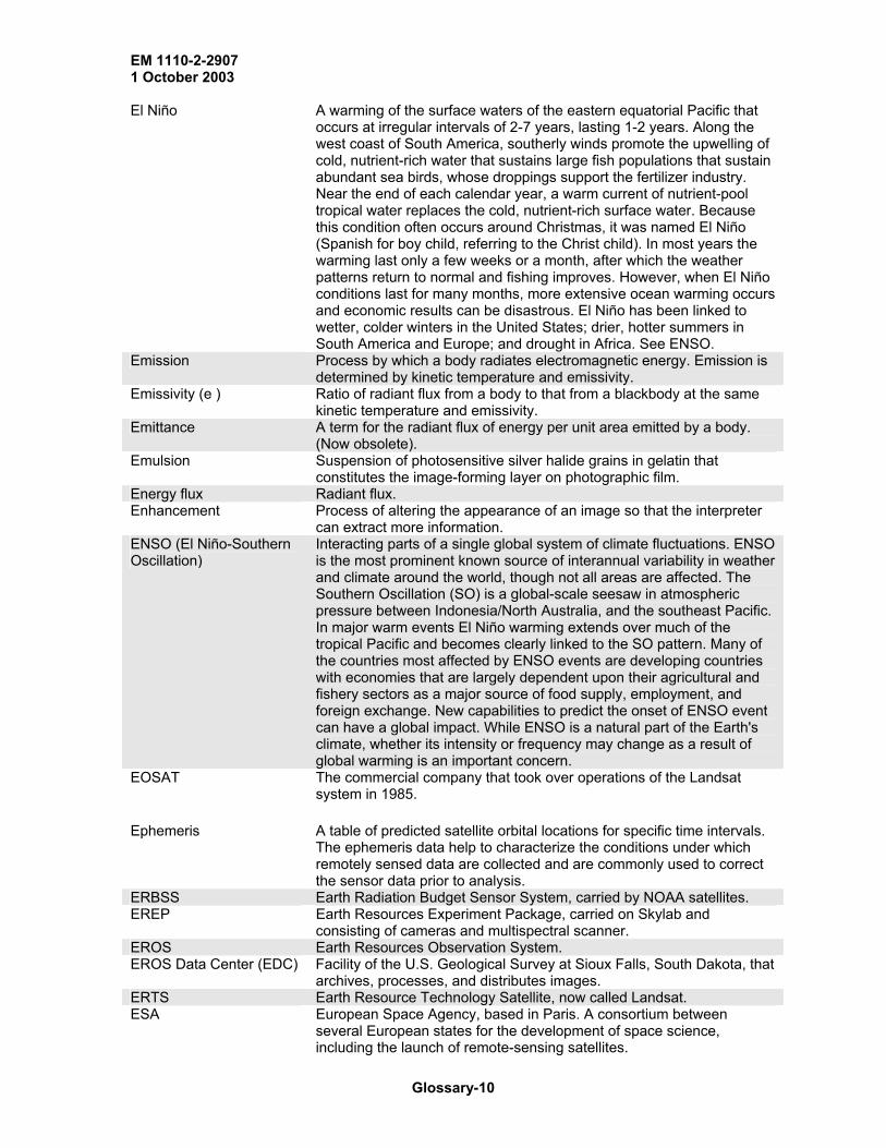
EM 1110-2-2907 1 October 2003

El Niño A warming of the surface waters of the eastern equatorial Pacific that

occurs at irregular intervals of 2-7 years, lasting 1-2 years. Along the west coast of South America, southerly winds promote the upwelling of cold, nutrient-rich water that sustains large fish populations that sustain abundant sea birds, whose droppings support the fertilizer industry. Near the end of each calendar year, a warm current of nutrient-pool tropical water replaces the cold, nutrient-rich surface water. Because this condition often occurs around Christmas, it was named El Niño (Spanish for boy child, referring to the Christ child). In most years the warming last only a few weeks or a month, after which the weather patterns return to normal and fishing improves. However, when El Niño conditions last for many months, more extensive ocean warming occurs and economic results can be disastrous. El Niño has been linked to wetter, colder winters in the United States; drier, hotter summers in South America and Europe; and drought in Africa. See ENSO.

Emission Process by which a body radiates electromagnetic energy. Emission is determined by kinetic temperature and emissivity.

Emissivity (e ) Ratio of radiant flux from a body to that from a blackbody at the same kinetic temperature and emissivity.

Emittance A term for the radiant flux of energy per unit area emitted by a body. (Now obsolete).

Emulsion Suspension of photosensitive silver halide grains in gelatin that constitutes the image-forming layer on photographic film.

Energy flux Radiant flux. Enhancement Process of altering the appearance of an image so that the interpreter

can extract more information. ENSO (El Niño-Southern Oscillation)

Interacting parts of a single global system of climate fluctuations. ENSO is the most prominent known source of interannual variability in weather and climate around the world, though not all areas are affected. The Southern Oscillation (SO) is a global-scale seesaw in atmospheric pressure between Indonesia/North Australia, and the southeast Pacific. In major warm events El Niño warming extends over much of the tropical Pacific and becomes clearly linked to the SO pattern. Many of the countries most affected by ENSO events are developing countries with economies that are largely dependent upon their agricultural and fishery sectors as a major source of food supply, employment, and foreign exchange. New capabilities to predict the onset of ENSO event can have a global impact. While ENSO is a natural part of the Earth's climate, whether its intensity or frequency may change as a result of global warming is an important concern.

EOSAT The commercial company that took over operations of the Landsat system in 1985.

Ephemeris A table of predicted satellite orbital locations for specific time intervals.

The ephemeris data help to characterize the conditions under which remotely sensed data are collected and are commonly used to correct the sensor data prior to analysis.

ERBSS Earth Radiation Budget Sensor System, carried by NOAA satellites. EREP Earth Resources Experiment Package, carried on Skylab and

consisting of cameras and multispectral scanner. EROS Earth Resources Observation System. EROS Data Center (EDC) Facility of the U.S. Geological Survey at Sioux Falls, South Dakota, that

archives, processes, and distributes images. ERTS Earth Resource Technology Satellite, now called Landsat. ESA European Space Agency, based in Paris. A consortium between

several European states for the development of space science, including the launch of remote-sensing satellites.

Glossary-10

EM 1110-2-2907 1 October 2003

ETC Earth-terrain camera. Evaporative cooling Temperature drop caused by evaporation of water from a moist

surface. Exitance The radiant flux. F

False color image A color image where parts of the non-visible EM spectrum are expressed as one or more of the red, green, and blue components, so that the colors produced by the Earth's surface do not correspond to normal visual experience. Also called a false-color composite (FCC). The most commonly seen false-color images display the very-near infrared as red, red as green, and green as blue.

False color photograph Another term for IR color photograph. Far range The portion of a radar image farthest from the aircraft or spacecraft

flight path. Fiducial Marks A set of four marks located in the corners or edge-centered, or both, of

a photographic image. These marks are exposed within the camera onto the original film and are used to define the frame of reference for spatial measurements on aerial photographs. Opposite fiducial marks connected, intersect at approximately the image center of the aerial photograph.

Film Light-sensitive photographic emulsion and its base. Film speed

Film Types Photographic products for use in image interpretation are commonly generated from the following film types:

Filter, digital Mathematical procedure for modifying values of numerical data. Filter, optical A material that, by absorption or reflection, selectivity modifies the

radiation transmitted through an optical system.

Measure of the sensitivity of photographic film to light. Larger numbers indicate higher sensitivity.

•

• Black-and-White Infrared (BIR): With some exceptions, this film is sensitive to the spectral region encompassing 0.4 micrometers

Black-and-White Panchromatic (B&W): This film primarily consists of a black-and-white negative material with a sensitivity range comparable to that of the human eye. It has good contrast and resolution with low graininess and a wide exposure range.

to 0.9 micrometers. It is sometimes referred to as near-infrared film because it utilizes only a narrow portion of the total infrared spectrum (0.7 micrometers to 0.9 micrometers).

• Conventional Color: This film contains three emulsion layers that are sensitive to blue, green, and red (the three primary colors of the visible spectrum). This film replicates colors as seen by the human eye and is commonly referred to as normal or natural color. Color film is a valuable image interpretation tool because the human eye can discern a greater variety of color tones than gray tones.

• Color Infrared (CIR): This film, originally referred to as camouflage-detection film because of its warfare applications, differs from conventional color film because its emulsion layers are sensitive to green, red, and near-infrared radiation (0.5 micrometers to 0.9 micrometers). Used with a yellow filter to absorb the blue light, this film provides sharp images and penetrates haze at high altitudes. Color-infrared film also is referred to as false-color film.

Glossary-11

EM 1110-2-2907 1 October 2003

Flight path Line on the ground directly beneath a remote sensing aircraft or

spacecraft. Also called flight line. Fluorescence Emission of light from a substance following exposure to radiation from

an external source. F-number

Focal length In cameras, the distance from the optical center of the lens to the plane at which the image of a very distant object is brought into focus.

Foreshortening A distortion in radar images causing the lengths of slopes facing the antenna to appear shorter on the image than on the ground. It is produced when radar wave fronts are steeper than the topographic slope.

Format Size of an image Forward overlap The percent of duplication by successive photographs along a flight

line. Fovea The region around that point on the retina intersected by the eye's optic

axis, where receptors are most densely packed. It is the most sensitive part of the retina.

Frequency (v ) The number of wave oscillations per unit time or the number of wavelengths that pass a point per unit time.

F-stop Focal length of a lens divided by the diameter of the lens’s adjustable diaphragm. Smaller numbers indicate larger openings, which admit more light to the film.

G

GAC--Global Area Coverage

This is a unit of magnetic intensity. GCP

U.S. program of two-man earth-orbiting spacecraft in 1965 and 1966. Geodetic

The accuracy with which geographic position and elevation of features on the Earth's surface are mapped. This accuracy incorporates information in which the size and shape of the Earth has been taken into account.

Geographic information system (GIS)

Geometric correction Image-processing procedure that corrects spatial distortions in an image.

Representation of the speed of a lens determined by the focal length divided by diameter of the lens. Smaller numbers indicate faster lenses.

GAC data are derived from a sample averaging of the full resolution AVHRR data. Four out of every five samples along the scan line are used to compute one average value and the data from only every third scan line are processed, yielding 1.1 km by 4 km resolution at the subpoint.

Gamma Ground-control point. GCPs are physical points on the ground whose positions are known with respect to some horizontal coordinate system and/or vertical datum. When mutually identifiable on the ground and on a map or photographic image, ground control points can be used to establish the exact spatial position and orientation of the image to the ground. Ground control points may be horizontal control points, vertical control points, or both.

Gemini Of or determined by geodesy; that part of applied mathematics which deals with the determination of the magnitude and figure either of the whole Earth or of a large portion of its surface. Also refers to the exact location points on the Earth's surface.

Geodetic accuracy

A data-handling and analysis system based on sets of data distributed spatially in two dimensions. The data sets may be map oriented, when they comprise qualitative attributes of an area recorded as lines, points, and areas often in vector format, or image oriented, when the data are quantitative attributes referring to cells in a rectangular grid usually in raster format. It is also known as a geobased or geocoded information system.

Glossary-12

EM 1110-2-2907 1 October 2003

Georegistered

Refers to satellites traveling at the angular velocity at which the earth rotates; as a result, they remain above the same point on earth at all times.

Geostationary Operational Environmental Satellite (GOES)

a NOAA satellite that acquires visible and thermal IR images for meteorological purposes such as:

GOES observes the U.S. and adjacent ocean areas from vantage points 35,790 km (22,240 miles) above the equator at 75 degrees west and 135 degrees west. GOES satellites have an equatorial, Earth-synchronous orbit with a 24-hour period, a visible resolution of 1 km, an IR resolution of 4 km, and a scan rate of 1864 statute miles in three minutes. See geostationary. The transmission of processed weather data (both visible and infrared) by GOES is called weather facsimile (WEFAX). GOES WEFAX transmits at 1691+ mhz and is accessible via a ground station with a satellite dish antenna.

Geostationary orbit An orbit at 41 000 km in the direction of the Earth's rotation, which matches speed so that a satellite remains over a fixed point on the Earth's surface. Synchronous with respect to the rotation of the Earth. See geostationary.

An image that has been geographically referenced or rectified to an Earth model, usually to a map projection. Sometimes referred to as geocoded or geometric registration.

Geostationary

• Provide continuous day and night weather observations; • Monitor severe weather events such as hurricanes,

thunderstorms, and flash floods; • Relay environmental data from surface collection platforms to a

processing center; • Perform facsimile transmissions of processed weather data to

low-cost receiving stations; • Monitor the Earth's magnetic field, the energetic particle flux in

the satellite's vicinity, and x-ray emissions from the sun; • Detect distress signals from downed aircraft and ships.

GOES carries the following five major sensor systems: 1. The imager is a multispectral instrument capable of sweeping

simultaneously one visible and four infrared channels in a north-to-south swath across an east-to-west path, providing full disk imagery once every thirty minutes.

2. The sounder has more spectral bands than the imager for producing high quality atmospheric profiles of temperature and moisture. It is capable of stepping one visible and eighteen infrared channels in a north-to-south swath across an east-to-west path.

3. The Space Environment Monitor (SEM) measures the condition of the Earth's magnetic field, the solar activity and radiation around the spacecraft, and transmits these data to a central processing facility.

4. The Data Collection System (DCS) receives transmitted meteorological data from remotely located platforms and relays the data to the end-users.

5. The Search and Rescue Transponder can relay distress signals at all times, but cannot locate them. While only the polar-orbiting satellite can locate distress signals, the two types of satellites work together to create a comprehensive search and rescue system.

Geosynchronous (aka GEO)

Glossary-13

EM 1110-2-2907 1 October 2003

Geothermal Refers to heat from sources within the earth. Goddard Space Flight Center (GSFC)

The NASA facility at Greenbelt, Maryland, that is also a Landsat ground receiving station.

GMT Greenwich mean time. This international 24-h system is used to designate the time at which Landsat images are acquired. Geostationary Operational Environmental Satellite.

Gossan Surface occurrence of iron oxide formed by the weathering of metallic sulfide ore minerals.

GPS--Global Positioning System

The GPS is a worldwide satellite navigation system that is funded and supervised by the U.S. Department of Defense. GPS satellites transmit specially coded signals. These signals are processed by a GPS receiver that computes extremely accurate measurements, including 3-dimensional position, velocity, and time on a continuous basis

Granularity Graininess of developed photographic film that is determined by the texture of the silver grains.

GRASS--Geographic Resources Analysis Support System

GRASS is a product of the U.S. Army Corps of Engineers Construction Engineering Research Laboratories (USACERL) in Champaign, Illinois. It is an integrated set of programs designed to provide digitizing, image processing, map production, and geographic information system capabilities to its users.

Gray scale The result of interpolation from values of a variable measured at irregularly distributed points, or along survey lines, to values referring to square cells in a rectangular array. It forms a step in the process of contouring data, but can also be used as the basis for a raster format to be displayed and analyzed digitally after the values have been rescaled to the 0-255 range.

Ground-control point A geographic feature of known location that is recognizable on images and can be used to determine geometric corrections.

Ground range On radar images, the distance from the ground track to an object. Ground-range image Radar image in which the scale in the range direction is constant.

Facility that records data transmitted by a satellite, such as Landsat. Ground resolution cell Area on the terrain that is covered by the IFOV of a detector. Ground swath Width of the strip of terrain that is imaged by a scanner system. GSFC Goddard Space Flight Center

Harmonic Refers to waves in which the component frequencies are whole- number multiples of the fundamental frequency.

HCMM Heat Capacity Mapping Mission, the NASA satellite launched in 1978 to observe thermal properties of rocks and soils. It remained in orbit for only a few months. Ratio of heat absorbed or released by a material to the corresponding temperature rise or fall. Expressed in calories per gram per degree centigrade. Also called thermal capacity.

Heat Capacity Mapping Mission (HCMM)

NASA satellite orbited in 1978 to record daytime and nighttime visible and thermal IR images of large areas. Areas of bright tone on an image.

High-pass filter A spatial filter that selectively enhances contrast variations with high spatial frequencies in an image. It improves the sharpness of images and is a method of edge enhancement.

HIRIS-High Resolution Imaging Spectrometer

Possibly to be carried by the Space Shuttle.

HIRS-High Resolution Infrared Spectrometer

Carried by NOAA satellites.

GOES

A sequence of gray tones ranging from black to white. Grid format

Ground receiving station

H

Heat capacity-(c)

Highlights

Glossary-14

EM 1110-2-2907 1 October 2003

Histogram A means of expressing the frequency of occurrence of values in a data

set within a series of equal ranges or bins, the height of each bin representing the frequency at which values in the data set fall within the chosen range. A cumulative histogram expresses the frequency of all values falling within a bin and lower in the range. A smooth curve derived mathematically from a histogram is termed the probability density function (PDF). Transmission of microwaves so that the electric lines of force are horizontal, while the magnetic lines of force are vertical.

HRPT--High Resolution Picture Transmission

HRPT data are full resolution image data transmitted to a ground station as they are collected. The average instantaneous field-of-view of 1.4 milliradians yields a HRPT ground resolution of approximately 1.1 km at the satellite nadir from the nominal orbit altitude of 833 km (517 mi).

HRV--High Resolution Visible Imaging Instrument

The HRV instrument is a multispectral radiometer designed for SPOT spacecraft. The HRV instrument provides for high-resolution imaging in the visible and near-infrared portions of the electromagnetic spectrum. The first three SPOT satellites carry twin HRVs that operate in a number of viewing configurations and in different spectral modes. Some of those viewing configurations and spectral modes include one HRV only operating in a dual spectral mode (i.e., in both panchromatic mode and multispectral mode); two HRVs operating in the twin-viewing configuration (i.e., one HRV in panchromatic mode and one HRV in multispectral mode); and two HRVs operating independently of each other (i.e., not in twin-viewing configuration).

Hue In the IHS system, represents the dominant wavelength of a color. HYDROLOGY

The scientific study of the Earth's topologic configuration above sea level, especially the measurement and mapping of land elevation.

I

IFOV Instantaneous field of view. IHS Intensity, hue, and saturation system of colors. Image Pictorial representation of a scene recorded by a remote sensing

system. Although image is a general term, it is commonly restricted to representations acquired by non-photographic methods.

Image dissection The breaking down of a continuous scene into discrete spatial elements, either by the receptors on the retina, or in the process of capturing the image artificially.

Image striping A defect produced in line scanner and push-broom imaging devices produced by the non-uniform response of a single detector, or amongst a bank of detectors. In a line-scan image the stripes are perpendicular to flight direction, but parallel to it in a push-broom image.

Image swath See ground swath. Incidence angle In radar, the angle formed between an imaginary line normal to the

surface and another connecting the antenna and the target. Incident energy Electromagnetic radiation impinging on a surface.

HORIZONTAL POLARIZATION

Scientific study of the waters of the Earth, especially with relation to the effects of precipitation and evaporation upon the occurrence and character of ground water.

HYPSOGRAPHY

Glossary-15

EM 1110-2-2907 1 October 2003

Index of refraction (n) Ratio of the wavelength or velocity of electromagnetic radiation in a

vacuum to that in a substance. Instantaneous field of view (IV or IFOV)

Solid angle through which a detector is sensitive to radiation. In a scanning system, the solid angle subtended by the detector when the scanning motion is stopped.

Intensity In the IHS system, brightness ranging from black to white. Method of image processing in which the operator views preliminary results and can alter the instructions to the computer to achieve desired results.

Interpretation The process in which a person extracts information from an image. Characteristic or combination of characteristics that enable an interpreter to identify an object on an image.

IR Infrared region of the electromagnetic spectrum that includes wavelengths from 0.7µm to 1 mm.

IR color photograph Color photograph in which the red-imaging layer is sensitive to photographic IR wavelengths, the green-imaging layer is sensitive to red light, and the blue-imaging layer is sensitive to green light. Also known as camouflage detection photographs and false-color photographs.

ISO index Index of the International Standards Organization, designating film speed in photography. Higher values indicate higher sensitivity.

Isotherm Contour line connecting points of equal temperature. Isotherm maps are used to portray surface-temperature patterns of water bodies.

Japanese National Space Development Agency (NASDA)

The agency reports to the Japanese Ministry of Science and Technology.

JNC--Jet Navigation Chart The JNC series provides worldwide coverage at a scale of 1:2,000,000. The information on these charts are suitable for aeronautical long-range, high-altitude, high-speed travel; map features include cities, roads, railroads, lakes, principal drainage, and permanent snow/ice areas. The polar regions are in a Transverse Mercator projection. All other regions are presented in the Lambert Conformal Conic projection.

Johnson Space Flight Center

A NASA facility in Houston, Texas.

JPL Jet Propulsion Laboratory, a NASA facility at Pasadena, California, operated under contract by the California Institute of Technology.

K

Ka band Radar wavelength region from 0.8 to 1.1 cm. Kelvin Units A Kelvin Unit refers to a thermometric scale in which the degree

intervals are equal to those of the Celsius scale and in which zero (0) degrees equals -273.15 degrees Celsius (absolute zero)

Kernel Two-dimensional array of digital numbers used in digital filtering. Kinetic energy The ability of a moving body to do work by virtue of its motion. The

molecular motion of matter is a form of kinetic energy. Kinetic temperature Internal temperature of an object determined by random molecular

motion. Kinetic temperature is measured with a contact thermometer. Kodachrome A Kodak color positive film. L

LAC--Local Area LAC are full resolution data recorded on an onboard tape recorder for

Interactive processing

Interpretation key

J

Glossary-16

EM 1110-2-2907 1 October 2003

Coverage subsequent transmission during a station overpass. The average

instantaneous field-of-view of 1.4 milliradians yields a LAC ground resolution of approximately 1.1 km at the satellite nadir from the nominal orbit altitude of 833 km.

LACIE Large Area Crop Inventory Experiment Lambert Azimuthal Equal Area Projection

Azimuthal projections are formed onto a plane, which is usually tangent to the globe at either pole, the Equator, or any intermediate point. The Lambert Azimuthal Equal Area projection is a method of projecting maps on which the azimuth or direction from a given central point to any other point is shown correctly and also on which the areas of all regions are shown in the same proportion of their true areas. When a pole is the central point, all meridians are spaced at their true angles and are straight radii of concentric circles that represent the parallels. This projection is frequently used in one of three aspects: The polar aspect is used in atlases for maps of polar regions and of the Northern and Southern Hemispheres; the equatorial aspect is commonly used for atlas maps of the Eastern and Western Hemispheres; and the oblique aspect is used for atlas maps of continents and oceans.

Lambert Conformal Conic Projection

To minimize and distribute scale errors, the two standard parallels are chosen to enclose two-thirds of the north to south map area. Between these parallels, the scale will be too small, and beyond them, too large. If the north to south extent of the mapping is limited, maximum scale errors will rarely exceed one percent. Area exaggeration between and near the standard parallels, is very slight; thus, the projection provides good directional and shape relationships for areas having their long axes running in an east to west belt.

LANDSAT (formerly ERTS)

The Landsat program, first known as the Earth Resources Technology Satellite (ERTS) Program, is a development of the National Aeronautics and Space Administration (NASA) in association with NOAA, USGS, and the Space Imaging. The activities of these combined groups led to the concept of dedicated Earth-orbiting satellites, the defining of spectral and spatial requirements for their instruments, and the fostering of research to determine the best means of extracting and using information from the data. The first satellite, ERTS 1, was launched on 7/23/72. The second satellite was launched on 1/22/75. Concurrently the name of the satellites and program was changed to emphasize its prime area of interest (land resources). The first two satellites were designated as Landsats 1 and 2. Landsat 3 was launched on 3/5/78. Landsat 4 was launched on 7/16/82. Landsat 5 (launched 3/1/84) is currently in service providing selected data to worldwide researchers.

Laplacian filter A form of nondirectional digital filter. Large-format camera (LFC)

An experiment first carried on the Space Shuttle in October 1984.

Laser Light artificially stimulated electromagnetic radiation: a beam of coherent radiation with a single wavelength.

Latitude (aka the geodetic latitude)

The angle between a perpendicular at a location, and the equatorial plane of the Earth.

The Lambert Conformal Conic Projection is derived by the projection of lines from the center of the globe onto a simple cone. This cone intersects the Earth along two standard parallels of latitude, both of which are on the same side of the equator. All meridians are converging straight lines that meet at a common point beyond the limits of the map. Parallels are concentric circles whose center is at the intersection point of the meridians. Parallels and meridians cross at right angles, an essential of conformality.

Glossary-17

EM 1110-2-2907 1 October 2003

Latent image Invisible image produced by the photochemical effect of light on silver

halide grains in the emulsion of film. The latent image is not visible until after photographic development.

Layover In radar images, the geometric displacement of the objects toward the near range relative to their base. Radar wavelength region from 15 to 30 cm.

Lens One or more pieces of glass or other transparent material shaped to form an image by refraction of light. Level 1b is considered raw quality controlled data configured into discrete data sets and to which Earth location and calibration information have been appended, but not applied.

LFC Large-format camera. The LFC was a high altitude aerial mapping camera scaled up to operate from the Space Shuttle in Earth-orbital altitudes. LFC specifications included:

LIDAR Light intensity detection and ranging, which uses lasers to stimulate fluorescence in various compounds and to measure distances to reflecting surfaces.

Light Electromagnetic radiation ranging from 0.4 to 0.7µm in wavelength that is detectable by the human eye.

Light meter Device for measuring the intensity of visible radiation and determining the appropriate exposure of photographic film in a camera.

Lineament Linear topographic or tonal feature on the terrain and on images, maps, and photographs that may represent a zone of structural weakness.

Linear Adjective that describes the straight line-like nature of features on the terrain or on images and photographs.

Lineation The one-dimensional alignment of internal components of a rock that cannot be depicted as an individual feature on a map.

Line drop out

Line-pair Pair of light and dark bars of equal widths. The number of such line-pairs aligned side by side that can be distinguished per unit distance expresses the resolving power of an imaging system.

Line scanner

Look angle The angle between the vertical plane containing a radar antenna and the direction of radar propagation. Complementary to the depression angle.

Look direction

A mathematical formula used to convert one distribution of data to another, most conveniently remembered as a conversion graph.

Longitude The angular distance from the Greenwich meridian (0 degree), along the equator. This can be measured either east or west to the 180th meridian (180 degrees) or 0 degree to 360 degrees W.

Low-sun-angle photograph

Aerial photograph acquired in the morning, evening, or winter when the sun is at a low elevation above the horizon.

L band

LEVEL 1b

• Film Format Size: 9 x 18 inches (23 x 46 cm) • Lens Aperture: F/6.0 -Lens Focal Length: 12 inches (30.5 cm) • Exposure Interval: 7.5 sec. • Exposure Range: 1/250 to 1/31.25 seconds • Ground Resolution: 20 meters at 160 nautical miles • Ground Coverage: 120 x 240 nautical miles at 160 nm

The loss of data from a scan line caused by malfunction of one of the detectors in a line scanner.

An imaging device, which uses a mirror to sweep the ground surface normal to the flight path of the platform. An image is built up as a strip comprising lines of data.

Direction in which pulses of microwave energy are transmitted by a radar system. The look direction is normal to the azimuth direction. Also called range direction.

Look-up table (LUT)

Glossary-18

EM 1110-2-2907 1 October 2003

Luminance

M

Mach band An optical illusion of dark and light fringes within adjacent areas of contrasted tone. It is a psychophysiological phenomenon, which aids human detection of boundaries or edges.

Median filter A spatial filter, which substitutes the median value of DN from surrounding pixels for that recorded at an individual pixel. It is useful for removing random noise.

Mercator Projection Mercator is a conformal map projection, that is, it preserves angular relationships. Mercator was designed and is recommended for navigational use and is the standard for marine charts. Mercator is often and inappropriately used as a world map projection in atlases and for wall charts where it presents a misleading view of the world because of the excessive distortion of area in the higher latitude areas.

Mercury U.S. program of one-man, earth-orbiting spacecraft in 1962 and 1963. Microwave Region of the electromagnetic spectrum in the wavelength range of 0.1

to 30 cm. Mid-infrared (MIR) The range of EM wavelengths from 8 to 14 µm dominated by emission

of thermally generated radiation from materials; also known as thermal infrared.

Mie scattering The scattering of EM energy by particles in the atmosphere with comparable dimensions to the wavelength involved.

Minimum ground separation

Minimum distance on the ground between two targets at which they can be resolved on an image.

Minus-blue photographs Black-and-white photographs acquired using a filter that removes blue wavelengths to produce higher spatial resolution.

Mixed pixel A pixel whose DN represents the average energy reflected or emitted by several types of surface present within the area that it represents on the ground; sometimes called a mixel.

Modular optoelectric multispectral scanner (MOMS)

An along-track scanner carried on the Space Shuttle that recorded two bands of data.

Modulate To vary the frequency, phase, or amplitude of electromagnetic waves. Modulation transfer function (MTF)

A method of describing spatial resolution.

MOMS Modular optoelectric multispectral scanner. MOS-1 Marine Observation Satellite, launched by Japan in 1987. Mosaic Composite image or photograph made by piecing together individual

images or photographs covering adjacent areas. MSS Multispectral scanner system of Landsat that acquires images of four

wavelength bands in the visible and reflected IR regions. Multiband camera System that simultaneously acquires photographs of the same scene at

different wavelengths. Multispectral classification Identification of terrain categories by digital processing of data acquired

by multispectral scanners. Multispectral scanner Scanner system that simultaneously acquires images of the same

scene at different wavelengths. N

NAD27--North American Datum of 1927

NAD27 is defined with an initial point at Meads Ranch, Kansas, and by the parameters of the Clarke 1866 ellipsoid. The location of features on USGS topographic maps, including the definition of 7.5-minute quadrangle corners, are referenced to the NAD27.

Quantitative measure of the intensity of light from a source.

Glossary-19

EM 1110-2-2907 1 October 2003

NAD83--North American Datum of 1983

NAD83 is an Earth-centered datum and uses the Geodetic Reference System 1980 (GRS 80) ellipsoid, unlike NAD27, which is based on an initial point (Meade’s Ranch, Kansas). Using recent measurements with modern geodetic, gravimetric, astrodynamic, and astronomic instruments, the GRS 80 ellipsoid has been defined as a best fit to the worldwide geoid. Because the NAD83 surface deviates from the NAD27 surface, the position of a point based on the two reference datums will be different.

Nadir Point on the ground directly in line with the remote sensing system and the center of the earth.

NAPP--National Aerial Photography Program

NAPP was established to coordinate the collection of aerial photography covering the 48 contiguous States and Hawaii every five years. NAPP's goals are to ensure that photography with uniform scale, quality, and cloud-free coverage be made available to meet the requirements of several Federal and State agencies. The program was initiated in 1980 as the National High Altitude Photography (NHAP) program. In 1987, the program was renamed to NAPP when the flying height for the program changed from 40,000 feet to 20,000 feet. NAPP photography is available in black and white, and in most cases, color-infrared. The program is administered by the U.S. Geological Survey's National Mapping Division. NAPP imagery is used by the USGS for photo revision and land use land cover characterization work on the standard series maps at 1:24,000; 1:100,000 and 1:250,000 scales.

NASA National Aeronautical and Space Administration. The NDVI is computed by calculating the ratio of the VI (vegetation index, i.e., the difference between Channel 2 and 1) and the sum of Channels 2 and 1. Thus NDVI = (channel 2 - channel 1) / (channel 2 + channel 1).

Nearest Neighbor Resampling

When correcting image data points, the nearest neighbor technique assigns for each new pixel that pixel value which is closest in relative location to the newly computed pixel location.

Near infrared (NIR) The shorter wavelength range of the infrared region of the EM spectrum, from 0.7 to 2.5 µm. It is often divided into very-near infrared (VNIR) covering the range accessible to photographic emulsions (0.7 to 1.0m), and the short-wavelength infrared (SWIR) covering the remainder of the NOR atmospheric window from 1.0 to 2.5m.

Near range Refers to the portion of a radar image closest to the aircraft or satellite flight path.

Negative photograph

NESDIS--National Environmental Satellite, Data and Information Service

NESDIS is the element in NOAA that is responsible for establishing a digital archive of data collected from the current generation of NOAA operational polar orbiting satellites

NHAP National High Altitude Photography program of the U.S. Geological Survey. National Oceanic and Atmospheric Administration.

Noise Random or repetitive events that obscure or interfere with the desired information.

Nondirectional filter Mathematical filter that treats all orientations of linear features equally. Non-selective scattering The scattering of EM energy by particles in the atmosphere which are

much larger than the wavelengths of the energy, and which causes all wavelengths to be scattered equally.

Non-spectral hue A hue which is not present in the spectrum of colors produced by the analysis of white light by a prism of diffraction grating. Examples are brown, magenta, and pastel shades.

NDVI--Normalized Difference Vegetation Index

Photograph on film or paper in which the relationship between bright and dark tones is the reverse of that of the features on the terrain.

NOAA

Glossary-20

EM 1110-2-2907 1 October 2003

Nonsystematic distortion Geometric irregularities on images that are not constant and cannot be

predicted from the characteristics of the imaging system. Normal color film Film in which the colors are essentially true representations of the

colors of the terrain. NSSDC National Space Science Data Center. O

Oasis A spot in a desert made fertile by water, which normally originates as groundwater.

Oblique photograph Photograph acquired with the camera intentionally directed at some angle between horizontal and vertical orientations.

OMS Orbital maneuvering system. ONC--Operational Navigation Chart

The ONC series covers most of the world landmass areas at 1:1,000,000 scale. At this scale it takes 62 charts to cover the conterminous United States. Information on these charts includes cities and landmarks, drainage, and relief (shown by shading and contours). International and State boundaries are shown, but not county boundaries.

Orbit Path of a satellite around a body such as the earth, under the influence of gravity.

Orthophotograph A vertical aerial photograph from which the distortions due to varying elevation, tilt, and surface topography have been removed, so that it represents every object as if viewed directly from above.

Orthophotoscope An optical-electronic device, which converts a normal vertical aerial photograph to an orthophotograph.

Ortho-correction Correction applied to satellite imagery to account for terrain-induced distortion.

Overlap Extent to which adjacent images or photographs cover the same terrain, expressed as a percentage.

P

Black and white film that is sensitive to all visible wavelengths. Parallax Displacement of the position of a target in an image caused by a shift in

the observation system. The difference in the distance on overlapping vertical photographs between two points, which represent two locations on the ground with different elevations.

Parallel-polarized Describes a radar pulse in which the polarization of the return is the same as that of the transmission. Parallel-polarized images may be HH (horizontal transmit, horizontal return) or VV (vertical transmit, vertical return).

Pass In digital filters, refers to the spatial frequency of data transmitted by the filter. High-pass filters transmit high-frequency data; low-pass filters transmit low-frequency data.

Passive microwaves

Remote sensing of energy naturally reflected or radiated from the terrain.

Path-and-row index System for locating Landsat MSS and TM images. Pattern Regular repetition of tonal variations on an image or photograph. Periodic line dropout Defect on Landsat MSS or TM images in which no data are recorded

for every sixth or sixteenth scan line, causing a black line on the image.

Panchromatic film

Parallax difference

Radiation in the 1 mm to 1 m range emitted naturally by all materials above absolute zero.

Passive remote sensing

Glossary-21

EM 1110-2-2907 1 October 2003

Periodic line striping Defect on Landsat MSS or TM images in which every sixth or sixteenth

scan line is brighter or darker than the others. Caused by the sensitivity of one detector being higher or lower than the others.

Photodetector Device for measuring energy in the visible-light band. Photogeology Mapping and interpretation of geologic features from aerial

photographs. Photograph- Representation of targets on film that results from the action of light on

silver halide grains in the film's emulsion. Photographic IR Short-wavelength portion (0.7 to 0.9 µm) of the IR band that is

detectable by IR color film or IR black-and-white film. Photographic UV Long-wavelength portion of the UV band (0.3 to 0.4 µm) that is

transmitted through the atmosphere and is detectable by film. Photomosaic Photon Minimum discrete quantity of radiant energy. Photopic vision Picture element In a digitized image, the area on the ground represented by each digital

number. Commonly contracted to pixel. Pitch Rotation of an aircraft about the horizontal axis normal to its longitudinal

axis that causes a nose-up or nose-down attitude. Pixel Contraction of picture element. Planck's Law An expression for the variation of emittance of a blackbody at a

particular temperature as a function of wavelength. Point spread function (PSF)

The image of a point source of radiation, such as a star, collected by an imaging device. A measure of the spatial fidelity of the device.

Polarization The direction of orientation in which the electrical field vector of electromagnetic radiation vibrates.

Polar orbit An orbit that passes close to the poles, thereby enabling a satellite to pass over most of the surface, except the immediate vicinity of the poles themselves.

Polarized radiation

Positive photograph Photographic image in which the tomes are directly proportional to the terrain brightness.

Precision Precision is a statistical measurement of repeatability that is usually expressed as a variance or standard deviation, root mean square or RMS, of repeated measurements. These are expressed as x, y coordinates of arcs, label points, and tics in either single or double precision in ARC/INFO. Single-precision coordinates have up to seven significant digits of precision. This allows for a level of accuracy of approximately 10 meters for a region whose extent is 1,000,000 meters across. Double-precision coordinates have up to 15 significant digits; this allows for the precision necessary to represent any desired map accuracy at a global scale.

Previsual symptom A vegetation anomaly that is recognizable on IR film before it is visible to the naked eye or on normal color photographs. It results when stressed vegetation loses its ability to reflect photographic IR energy and is recognizable on IR color film by a decrease in brightness of the red hues.

Primary colors A set of three colors that in various combinations will produce the full range of colors in the visible spectrum. There are two sets of primary colors, additive and subtractive.

Principal component analysis

The analysis of covariance in a multiple data set so that the data can be projected as additive combinations on to new axes, which express different kinds of correlation among the data.

Mosaic composed of photographs.

Vision under conditions of bright illumination.

Electromagnetic radiation in which the electrical field vector is contained in a single plane, instead of having random orientation relative to the propagation vector. Most commonly refers to radar images.

Glossary-22

EM 1110-2-2907 1 October 2003

Principal-component (PC) image

Digitally processed image produced by a transformation that recognizes maximum variance in multispectral images.

Principal point Optical center of an aerial photograph. Printout Display of computer data in alphanumeric format. Probability density function (PDF)

A function indicating the relative frequency with which any measurement may be expected to occur. In remote sensing it is represented by the histogram of DN in one band for a scene.

Projection Orderly system of lines on a plane representing a corresponding system of imaginary lines on an adopted terrestrial or celestial datum surface. Also, the mathematical concept of such a system. For maps of the Earth, a projection consists of (1) a graticule of lines representing parallels of latitude and meridians of longitude or (2) a grid.

Pulse Short burst of electromagnetic radiation transmitted by a radar antenna. Pulse length Duration of a burst of energy transmitted by a radar antenna, measured

in microseconds. Pushbroom scanner An alternate term for an along-track scanner Pushbroom system

Q

Quantum The elementary quantity of EM energy that is transmitted by a particular wavelength. According to the quantum theory, EM radiation is emitted, transmitted, and absorbed as numbers of quanta, the energy of each quantum being a simple function of the frequency of the radiation.

Radar Acronym for radio detection and ranging. Radar is an active form of remote sensing that operates in the microwave and radio wavelength regions.

Radar altimeter A non-imaging device that records the time of radar returns from vertically beneath a platform to estimate the distance to and hence the elevation of the surface; carried by Seasat and the EAS-ERS-1 platforms.

Radar cross section A measure of the intensity of backscattered radar energy from a point target. Expressed as the area of a hypothetica surface, which scatters radar equally in all directions and which would return the same energy to the antenna.

Radar scattering coefficient

A measure of the back-scattered energy from a target with a large area. Expressed as the average radar cross section per unit area in decibels (db). It is the fundamental measure of the radar properties of a surface. A non-imaging device that records radar energy backscattered from terrain as a function of depression angle.

Radar shadow Dark signature on a radar image representing no signal return. A shadow extends in the far-range direction form an object that intercepts the radar beam.

Radial relief displacement The tendency of vertical objects to appear to learn radially away from the center of a vertical aerial photograph. Caused by the conical field of view of the camera lens.

Radian Angle subtended by an arc of a circle equal in length to the radius of the circle 1 rad = 57.3¡.

An imaging device consisting of a fixed linear array of many sensors, which is swept across an area by the motion of the platform, thereby building up an image. It relies on sensors whose response and reading is nearly instantaneous, so that the image swathe can be segmented into pixels representing small dimensions on the ground.

R

Radar scatterometer

Glossary-23

EM 1110-2-2907 1 October 2003

Radiance Measure of the energy radiated by an object. In general, radiance is a

function of viewing angle and spectral wavelength and is expressed as energy per solid angle.

Radiant energy peak Wavelength at which the maximum electromagnetic energy is radiated at a particular temperature.

Radiant flux Rate of flow of electromagnetic radiation measured in watts per square centimeter.

Radiant temperature Concentration of the radiant flux from a material. Radiant temperature is the kinetic temperature multiplied by the emissivity to the one-fourth power.

Radiation Propagation of energy in the form of electromagnetic waves. Device for quantitatively measuring radiant energy, especially thermal radiation.

Random line dropout In scanner images, the loss of data from individual scan lines in a nonsystematic fashion.

Range In radar usage this is the distance in the direction of radar propagation, usually to the side of the platform in an imaging radar system. The slant range is the direct distance from the antenna to the object, whereas the distance from the ground track of the platform to the object is termed the ground range.

Range direction See look direction. Range resolution In radar images, the spatial resolution in the range direction, which is

determined by the pulse length of the transmitted microwave energy. Raster The scanned and illuminated area of a video display, produced by a

modulated beam of electrons sweeping the phosphorescent screen line by line from to bottom at a regular rate of repetition.

Raster format A means of representing spatial data in the from of a grid of DN, each line of which can be used to modulate the lines of a video raster.

Raster pattern Pattern of horizontal lines swept by an electron beam across the face of a CRT that constitute the image display.

Ratio image An image prepared by processing digital multi-spectral data as follows: for each pixel, the value for one band that is divided the value of another. The resulting digital values are displayed as an image.

Rayleigh criterion In radar, the relationship between surface roughness, depression angle, and wavelength that determines whether a surface will respond in a rough or smooth fashion to the radar pulse.

Rayleigh scattering Selective scattering of light in the atmosphere by particle that is small compared with the wavelength of light.

RBV Return-beam vidicon. Real-aperture radar Radar system in which azimuth resolution is determined by the

transmitted beam width, which is in turn determined by the physical length of the antenna and by the wavelength.

Real time Refers to images or data made available for inspection simultaneously with their acquisition.

Recognizability Ability to identify an object on an image. Rectilinear Refers to images with no geometric distortion in which the scales in the

horizontal and vertical directions are identical. Redundancy Information on an image, which is either not, required for interpretation

or cannot be seen. Redundancy may be spatial or spectral. The term also refers to multispectral data where the degree of correlation between bands is so high that one band contains virtually the same information as all the bands. Ratio of the radiant energy reflected by a body to the energy incident on it. Spectral reflectance is the reflectance measured within a specific wavelength interval.

Radiometer

Reflectance

Glossary-24

EM 1110-2-2907 1 October 2003

Reflected energy peak Wavelength (0.5 µm) at which maximum amount of energy is reflected

from the earth's surface. Electromagnetic energy of wavelengths from 0.7 µm to about 3 µm that consists primarily of reflected solar radiation.

Reflectivity Ability of a surface to reflect incident energy. Refraction Bending of electromagnetic rays as they pass from one medium into

another when each medium has a different index of refraction. Registration Process of superposing two or more images or photographs so that

equivalent geographic points coincide. Relief Vertical irregularities of a surface. Relief displacement Geometric distortion on vertical aerial photographs. The tops of objects

appear in the photograph to be radially displaced from their bases outward from the photograph's center point.

Remote sensing Collection and interpretation of information about an object without being in physical contact with the object.

Resampling The calculation of new DN for pixels created during geometric correction of a digital scene, based on the values in the local area around the uncorrected pixels. Pattern of small crosses added to photographs.

Resolution Ability to separate closely spaced objects on an image or photograph. Resolution is commonly expressed as the most closely spaced line-pairs per unit distance that can be distinguished. Also called spatial resolution.

Resolution target Series of regularly spaced alternating light and dark bars used to evaluate the resolution of images or photographs.

Resolving power A measure of the ability of individual components. And of remote sensing systems, to separate closely spaced targets.

Reststrahlen band In the IR region, refers to absorption of energy as a function of silica content.

Return In radar, a pulse of microwave energy reflected by the terrain and received at the radar antenna. The strength of a return is referred to as return intensity. A system in which images are formed on the photosensitive surface o a vacuum tube; the image is scanned with an electron beam and transmitted or recorded. Landsat 3 used a pair of RBV's to acquire images.

Ringing Fringe-like artifacts produced at edges by some forms of spatial-frequency filtering.

Rods The receptors in the retina that are sensitive to brightness variations. Roll Rotation of an aircraft that causes a wing-up or wing-down attitude. Roll compensation system

Rough criterion In radar, the relationship between surface roughness, depression angle, and wavelength that determines whether a surface will scatter the incident radar pulse in a rough or intermediate fashion.

Roughness In radar, the average vertical relief of a small-scale irregularities of the terrain surface. Also called surface roughness

RMSE (Root Mean Square Error)

The RMSE statistic is used to describe accuracy encompassing both random and systematic errors. The square of the difference between a true test point and an interpolated test point divided by the total number of test points in the arithmetic mean. The square root of this value is the root mean square error.

S

SAMII Stratospheric Aerosol Measurement experiment, carried by Nimbus-7.

Reflected IR

Reseau marks

Return-beam vidicon (RBV)

Component of an airborne scanner system that measures and records the roll of the aircraft. This information is used to correct the imagery for distortion due to roll.

Glossary-25

EM 1110-2-2907 1 October 2003

SAMS Stratospheric and Mesospheric Sounder, carried by Nimbus-7. SAST (Scientific Assessment and Strategy Team)

SAST is an interdisciplinary team of senior scientists and engineers from various Federal Government agencies assigned to assess and report on the damage caused by the flood of 1993 and to provide assistance and advice to Federal officials responsible for making decisions with respect to the flood recovery in the Upper Mississippi and Missouri River basin.

Satellite An object in orbit around a celestial body. Saturation In the IHS system, represents the purity of color. Saturation is also the

condition where energy flux exceeds the sensitivity range of a detector. SBUV Solar Back-scatter Ultraviolet Instrument, carried by NOAA satellites. Scale Ratio of distance on an image to the equivalent distance on the ground. Scan line Narrow strip on the ground that is swept by IFOV of a detector in a

scanning system. Scanner An imaging system in which the IFOV of one or more detectors is swept

across the terrain. Scanner distortion Geometric distortion that is characteristic of cross-track scanner

images. Scan skew Distortion of scanner images caused by forward motion of the aircraft or

satellite during the time required for scanning completion. Scattering Multiple reflections of electromagnetic waves by particles or surfaces. Scattering coefficient curves

Display of scatterometer data in which relative backscatter is shown as a function of incidence angle.

Scatterometer Nonimaging radar device that quantitatively records backscatter of terrain as a function of incidence angle.

Scene Scotopic vision Vision under conditions of low illumination, when only the rods are

sensitive to light. Visual acuity under these conditions is highest in the blue part of the spectrum.

Seasat NASA unmanned satellite that acquired L-band radar images in 1978. Sensitivity Degree to which a detector responds to electromagnetic energy

incident on it. Sensor Device that receives electromagnetic radiation and converts it into a

signal that can be recorded and displayed as either numerical data or an image.

Shaded relief Shading added to an image that makes the image appear to have three-dimensional aspects. This type of enhancement is commonly done to satellite images and thematic maps utilizing digital topographic data to provide the appearance of terrain relief within the image.

Shuttle imaging radar (SIR)

L-band radar system deployed on the Space Shuttle.

Sidelap Extent of lateral overlap between images acquired on adjacent flight lines.

Side-looking airborne radar (SLAR)

An airborne side scanning system for acquiring radar images.

Side-scanning sonar- Active system for acquiring images of the seafloor using pulsed sound waves. A system that acquires images of a strip of terrain parallel with the flight or orbit path but offset to one side.

Signal Information recorded by a remote sensing system. Signal to noise radio (S/N) The ratio of the level of the signal carrying real information to that

carrying spurious information as a result of defects in the system. Silver halide Silver salts that are especially sensitive to visible light and convert to

metallic silver when developed. SIR Shuttle Imaging Radar, synthetic-aperture radar experiments carried

aboard the NASA Space Shuttle in 1981 and 1984.

Area on the ground that is covered by an image or photograph.

Side-scanning system-

Glossary-26

EM 1110-2-2907 1 October 2003

Skylab U.S. Earth-orbiting workshop that housed three crews of three

astronauts in 1973 and 1974. Skylight Component of light that is strongly scattered by the atmosphere and

consists predominantly of shorter wavelengths. Slant range In radar, an imaginary line running between the antenna and the target. Slant-range distance Distance measured along the slant range. Slant-range distortion Geometric distortion of a slant-range image. Slant-range image In radar, an image in which objects are located at positions

corresponding to their slant-range distances from the aircraft path. On slant-range images, the scale in the range direction is compressed in the near-range region

SLAR Side-looking airborne radar. SMIRR Shuttle Multispectral Infrared Radiometer, a non-imaging

spectroradiometer carried by the NASA Space Shuttle covering ten narrow wavebands in the 0.5-2.4 m range.

SMMR Scanning Multichannel Microwave Radiometer, carried by Nimbus-7. Smooth criterion In radar, the relationship between surface roughness, depression

angle, and wavelength that determines whether a surface will scatter the incident radar pulse in a smooth or intermediate fashion.

Software Programs that control computer operations. Sonar Acronym for sound navigation ranging. Sonar is an active form of

remote sensing that employs sonic energy to image the seafloor. Space Shuttle U.S. manned satellite program in the 1980s, officially called the Space

Transportation System (STS). Space Station A planned series of three polar-orbiting, sun-synchronous satellites to

be launched by NASA, the European Space Agency, and the Japanese Space Agency in the 1990s. They will carry a large range of remote-sensing devices.

Spatial-frequency filtering The analysis of the spatial variations in DN of an image and the separation or suppression of selected frequency ranges.

Specific heat The ratio of the heat capacity of unit mass of a material to the heat capacity of unit mass of water.

Spectral hue A hue that is present in the spectral range of white light and is analyzed by a prism or diffraction grating.

Spectral reflectance Reflectance of electromagnetic energy at specified wavelength intervals.

Spectral sensitivity Response, or sensitivity, of a film or detector to radiation in different spectral regions.

Spectral vegetation index An index of relative amount and vigor of vegetation. The index is calculated from two spectral bands of AVHRR imagery. Device for measuring intensity of radiation absorbed or reflected by a materiel as a function of wavelength.

Spectroradiometer A device that measures the energy reflected or radiated by materials in narrow EM wavebands.

Spectrum Continuous sequence of electromagnetic energy arranged according to wavelength or frequency.

Specular Refers to a surface that is smooth with respect to the wavelength of incident energy.

SPOT Systeme Probatoire d'Observation del la Terre. Unmanned French remote sensing satellite orbiting in the late 1980s.

Stefan-Boltzmann constant

5.68 x 10 -12 W . Cm-2 .K-4.

Stefan-Boltzmann law States that radiant flux of a blackbody is equal to the temperature to the fourth power times the Stefan-Boltzmann constant.

Stereo base Distance between a pair of correlative points on a stereo pair that are oriented for stereo viewing.

Spectrometer

Glossary-27

EM 1110-2-2907 1 October 2003

Stereo model Three-dimensional visual impression produced by viewing a pair of

overlapping images through a stereoscope. Stereo pair Two overlapping images or photographs that may be viewed

stereoscopically. Stereopsis The ability for objects to be perceived in three dimensions as a result of

the parallax differences produced by the eye base. Stereoscope Binocular optical device for viewing overlapping images or diagrams.

The left eye sees only the left image, and the right eye sees only the right image.

SSU Stratosphere Sounding Unit, carried by NOAA-series satellites. Subscene A portion of an image that is used for detailed analysis. Subtractive primary colors Yellow, magenta, and cyan. When used as filters for white light, these

colors remove blue, green and red light, respectively. Sunglint Bright reflectance of sunlight caused by ripples on water. Sun-synchronous Earth satellite orbit in which the orbit plane is nearly polar and the

altitude is such that the satellite passes over all places on earth having the same latitude twice daily at the same local sun time.

Sun-synchronous orbit

Supervised classification Digital-information extraction technique in which the operator provides training-site information that the computer uses to assign pixels to categories.

Surface phenomenon Interaction between electromagnetic radiation and the surface of a material.

Surface roughness See roughness. Synthetic-aperture radar (SAR)

Radar system in which high azimuth resolution is achieved by storing and processing data on the Doppler shift of multiple return pulses in such a way as to give the effect of a much longer antenna.

Synthetic stereo images Stereo images constructed through digital processing of a single image. Topographic data are used to calculate parallax.

System Combination of components that constitute an imaging device. Systematic distortion Geometric irregularities on images that are caused by known and

predictable characteristics. T

Target Object on the terrain of specific interest in a remote sensing investigation.

TDRS Tracking and Data Relay Satellite Telemeter To transmit data by radio or microwave links. Terrain Surface of the earth. Texture

Thematic data layers in a data set are layers of information that deal with a particular theme. These layers are typically related information that logically go together. Examples of thematic data would include a data layer whose contents are roads, railways, and river navigation routes.

Thematic Mapper (TM) A cross-track scanner deployed on Landsat that records seven bands of data from the visible through the thermal IR regions.

Thermal capacity (c ) See heat capacity. Thermal conductivity (K) Measure of the rate at which heat will pass through a material,

expressed in calories per centimeter per second per degree Centigrade. On a plot of radiant temperature versus time, the point at which temperature curves for two different materials intersect.

Thermal diffusivity (k) Governs the rate at which temperature changes within a substance, expressed in centimeters squared per second.

A polar orbit where the satellite always crosses the Equator at the same local solar time.

Frequency of change and arrangement of tones on an image. Thematic Data

Thermal crossover

Glossary-28

EM 1110-2-2907 1 October 2003

Thermal inertia (P) Measure of the response of a material to temperature changes,

expressed in calories per square centimeter per square root of second. Thermal IR

Thermal IR image Image acquired by a scanner that records radiation within the thermal IR band.

Thermal IR multispectral scanner (TIMS)

Airborne scanner that acquires multispectral images within the 8-to-14mm band of the thermal IR region.

Thermal model Mathematical expression that relates thermal and other physical properties of a material to its temperature. Models may be used to predict temperature for given properties and conditions. Medical applications of thermal IR images. Images of the body, called thermograms, have been used to detect tumors and monitor blood circulation.

THIR Temperature-Humidity Infrared Radiometer, carried by Nimbus-7. A point on the ground, which is common to two images. Several are used in the co-registration of images.

TIMS Thermal IR multispectral scanner. TM Thematic Mapper. Tone Each distinguishable shade of gray from white to black on an image.

An optical illusion that may occur on images with extensive shades. Ridges appear to be valleys, and valleys appear to be ridges. The illusion is corrected by orienting the image so that the shadows trend from the margin of the image to the bottom.

Topographic reversal A geomorphic phenomenon in which topographic lows coincide with structural highs and vice versa. Valleys are eroded on crests of anticlines to cause topographic lows, and synclines form ridge, or topographic highs. TIROS Operational Vertical Sounder.

Tracking and Data Relay Satellite (TDRS)

Geostationary satellite used to communicate between ground receiving stations and satellite such as Landsat.

Training area A sample of the Earth's surface with known properties; the statistics of the imaged data within the area are used to determine decision boundaries in classification.

Trade-off As a result of changing one factor in a remote sensing system, there are compensating changes elsewhere in the system; such a compensating change is known as a trade-off.

Training site

Transmissivity Property of a material that determines the amount of energy that can pass through the material.

Transpiration Expulsion of water vapor and oxygen by vegetation. Travel time In radar, the time interval between the generation of a pulse of

microwave energy and its return from the terrain. Tristimulus color theory A theory of color relating all hues to the combined effects of three

additive primary colors corresponding to the sensitivities of the three types of cone on the retina.

U

Digital information extraction technique in which the computer assigns pixels to categories with no instructions from the operator.

IR region from 3 to 14 µm that is employed in remote sensing. This spectral region spans the radiant power peak of the earth.

Thermography

Tie-point

Topographic inversion

TOVS

Area of terrain with known properties or characteristics that is used in supervised classification.

Transparency Image on a transparent photographic material, normally a positive image.

Unsupervised classification

Glossary-29

EM 1110-2-2907 1 October 2003

UTM--Universal Transverse Mercator Projection

UTM is a widely used map projection that employs a series of identical projections around the world in the mid-latitude areas, each spanning six degrees of longitude and oriented to a meridian. This projection is characterized by its conformality; that is, it preserves angular relationships and scale plus it easily allows a rectangular grid to be superimposed on it. Many worldwide topographic and planimetric maps at scales ranging between 1:24,000 and 1:250,000 use this projection. Ultraviolet region of the electromagnetic spectrum ranging in wavelengths from 0.01 to 0.4m.

V

Variance A measure of the dispersion of the actual values of a variable about its mean. It is the mean of the squares of all the deviations from the mean value of a range of data.

VAS Atmospheric Sounder, carried by GEOS satellites Vector Any quantity, which has both magnitude and direction, as opposed to

scalar that has only magnitude. Vector Data Vector data, when used in the context of spatial or map information,

refers to a format where all map data is stored as points, lines, and areas rather than as an image or continuous tone picture. These vector data have location and attribute information associated with them.

Vector format The expression of points, lines, and areas on a map by digitized Cartesian coordinates, directions, and values.

Vegetation anomaly Deviation from the normal distribution or properties of vegetation. Vegetation anomalies may be caused by faults, trace elements in soil, or other factors.

Vertical exaggeration In a stereo model, the extent to which the vertical scale appears larger than the horizontal scale.

Vertical Positional Accuracy

Vertical positional accuracy is based upon the use of USGS source quadrangles, which are compiled to meet National Map Accuracy Standards (NMAS). NMAS vertical accuracy requires that at least 90 percent of well defined points tested be within one half contour interval of the correct value. Comparison to the graphic source is used as control to assess digital positional accuracy.

Vidicon An imaging device based on a sheet of transparent material whose electrical conductivity increases with the intensity of EM radiation falling on it. The variation in conductivity across the plate is measured by a sweeping electron beam and converted into a video signal. Now largely replaced by cameras employing arrays of charge-coupled devices (ccds).

Vignetting A gradual change in overall tone of an image from the center outwards, caused by the imaging device gathering less radiation from the periphery of its field of view than from the center. Most usually associated with the radially increasing angel between a lens and the Earth's surface, and the corresponding decrease in the light-gathering capacity of the lens.

Visible radiation Energy at wavelengths from 0.4 to 0.7mm that is detectable by the human eye.

Visual dissonance The disturbing effect of seeing a familiar object in an unfamiliar setting or in an unexpected color.

VISSR Visible Infrared Spin-Scan Radiometer carried by the GOES satellites. Volume scattering In radar, interaction between electromagnetic radiation and the interior

of a material.

UV

Glossary-30

EM 1110-2-2907 1 October 2003

Glossary-31

W

Watt (W) Unit of electrical power equal to rate of work done by one ampere under a potential of one volt.

Wavelength Distance between successive wave crests or other equivalent points in a harmonic wave.

Wien's displacement law Describes the shift of the radiant power peak to shorter wavelengths as temperature increases.

WRS--Worldwide Reference System

The WRS is a global indexing scheme designed for the Landsat program based on nominal scene centers defined by path and row coordinates.

X

X band Radar wavelength region from 2.4 to 3.8 cm. Y

Yaw Rotation of an aircraft about its vertical axis so that the longitudinal axis deviates left or right from the flight line.

Z

ZENITH Zenith is the point on the celestial sphere vertically above a given position or observer.

Zephyr A Mediterranean term for any soft, gentle breeze.