USE OF .GIS .& REMOTE SENSING TECHNIQUES FOR ...

USE OF .GIS .& REMOTE SENSING TECHNIQUES FOR ASSESSING RAINWATER HARVESTING POTENTIAL

A DISSERTATION. Submitted in partial fulfilment of the

requirements for the award of the degree of

MASTER OF TECHNOLOGY in

HYDROLOGY

By SANJAY ICUMAR GUPTA

DEPARTMENT OF HYDROLOGY INDIAN INSTITUTE OF TECHNOLOGY ROORKEE

ROORKEE-247 667 (INDIA) JUNE, 2006

~• INDIAN INSTITUTE OF TECHNOLOGY ROORKEE

ROORKEE-247667

CANDIDATE'S DECLARATION

I hereby certify that the work which is being presented in dissertation entitled "USE

OF GIS & REMOTE SENSING TECHNIQUES FOR ASSESSING RAINWATER

HARVESTING POTENTIAL" in partial fulfillment of the requirement for the award

of the Degree of Masters of Technology in Hydrology, submitted to the Department

of Hydrology (DOH), Indian Institute of Technology, Roorkee, Uttaranchal, is an

authentic record of my work carried out during the period from July 2005 to June

2006 under the supervision and guidance of Dr. RANVIR SINGH and Dr. P.K.

GARG.

The matter embodied in this dissertation has not been submitted by me for the award

of any other degree.

Date: June 30, 2006

Place: Roorkee SANJAY KUMAR GUPTA

This is to certify that the above declaration given by the candidate is correct to the

best of our knowledge.

Dr. P.K. GARG Professor,

Civil Engineering Department, Indian Institute of Technology

Roorkee, India

Dr. RA VIR SINGH Professor

- Department of Hydrology Indian Institute of Technology

Roorkee, India

i

ACKNOWLEDGMENT

I take this opportunity to express deep gratitude to Dr Ranvir Singh, Professor,

Department of Hydrology and Dr. P.K. Garg Department of Civil Engineering, Indian

Institute of Technology, Roorkee for encouraging, inspiring and motivating me and

providing valuable guidance and help throughout during the preparation and completion

this dissertation. I am highly indebted to both my guides for providing me full

cooperation and valuable suggestion from time to time, with out which, the dissertation

of mine presented as such would have come to such shape

I am greatly thankful to Dr. N.K. Goel Professor, Head of Department of

Hydrology Dr. D. K Shrivastava DRC chairman and other faculty members of

Department of Hydrology for their cordial cooperation and valuable suggestions

I extend my thanks to Authorities of Geomatics lab, Department of Civil

Engineering, Indian Institute of Technology, Roorkee for providing necessary facilities

during the study period.

I wish to express my deep sense of gratitude towards Mahesh Kumar Jat,

Research Scholar, Department of Civil Engineering, Indian Institute of Technology,

Roorkee, for his invaluable continuous guidance and persistent encouragement during the

preparation of this work.

I extend my thanks to N. Rama Rao, K.Venkateshwarlu, Uppaluri Sirisha, and

Mili Ghosh, Research Scholars Department of Civil Engineering IIT Roorkee for their

time to time suggestion and cooperation during the completion of this work.

Acknowledgement is also extended to the H.P. Uniyal, Director of Jal Bhawan,

Dehradun and Dr (Mrs.) Laxmi Rawat Forest Research Institute, Dehradun for providing

me the required data of the project area.

I am also thankful to all my friend & trainee officers of 33 d̀ batch and staff

member of Hydrology Dept, for their cooperation and friendship in the last the two years

stay here at IIT Roorkee.

SANJAY KUMAR GUPTA

33`dBatch

ABSTRACT Assessing, managing and planning of water resources for sustainable use has

become a crucial issue in recent times. There is an obvious need for proper understanding

of the hydrological processes in the watershed. Rainfall-runoff relationship plays an

important role in understanding the dynamic aspects of the hydrological processes that

take place in any region. Harvesting of available runoff at a micro-level for storage and

recycling is necessary for better utilization of rainfall, control of erosion and providing

life saving irrigation to crops during dry spells in the monsoon season and also for

growing a second crop in the Rabi season.

In areas under rain fed agriculture, a small additional increment of harvesting

water can dramatically increase crop yields and lower the risk of crop failure. Sometimes,

it can make a difference between crop and no crop in drought prone areas. The objective

and technologies of rain water harvesting are highly location specific and an appropriate

technology developed for a particular region cannot be used as such for other areas due to

physiographic, environmental, technical and socio-economic reasons. As far as water

harvesting is concerned, technologies are not based on annual rainfall only, but terrain,

soil permeability, landuse and its variation in space and time also play an important role

in determining the sites. Integration of Remote Sensing and Geographical Information

System (GIS) Techniques provides reliable, accurate and up-to-date database on land and

water resources, which is a pre-requisite for an integrated approach in identifying

potential runoff zones and suitable sites for water harvesting structures such as check

dams, farm ponds, percolation tanks and bandies etc

Hydrologic information is needed for watershed management planning, analysis

and design of water resource projects and for making landuse impact assessment.

Sometimes adequate hydrologic, meteorological and biophysical data are not available at

locations of interest and even when data are available, deciding the most appropriate

method to use can be difficult. Selecting the appropriate hydrological method requires careful

consideration of following:

1. The type and accuracy of information and data available

2. The physical and bio-geological characteristics of watershed.

3. The technical capabilities of the individual performing the study

4. The time and economic constraints

The watershed selected for present study is Dehradun watershed in Dehradun district, the interim

capital of the new-born state of Uttaranchal, where the burgeoning population pressure is posing

ever-increasing water demands. The results indicate that Rajpur and MDDA park are amongst the

areas with potential recharge capabilities. Details of roof top water harvesting plan are also

indicated.

iv

CONTENTS

Title

Page

CANDIDATE'S DECLARATION i ACKNOWLEDGMENT ii

ABSTRACT iii

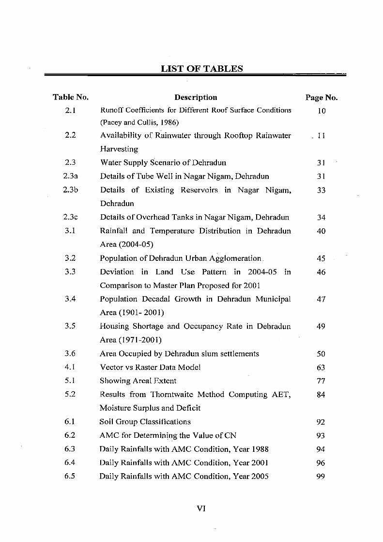
LIST OF TABLES• VI

LIST OF FIGURES VIII

CHAPTER ONE: INTRODUCTION

1.0 Introduction 1

1.1 Rainwater harvesting and its utility( 2

1.2 Need of GIS in Rainwater Harvesting 2

1.3 Scope of the Study 3

1.4 Objectives of the Study 3

1.5 Methodology used in this study 4

1.6 Organization of the thesis 6

CHAPTER TWO: LITERATURE REVIEW

2.1 General 7

2.2 Classification of Rainwater Harvesting 7

2.2.1 Rooftop Rainwater Harvesting 7

2.1.2 Rainwater Harvesting from Open Areas 14

2.2 Case studies 16

2.3 Present Scenario 27

2.3.1 Critical reviews of the present status and water supply 27

2.3.2 Water supply 27

2.3.3 Growing Demand of water 29

2.3.4 Tariff for Domestic and Non-Domestic Consumers 30

2.3.5 Springs 31

CHAPTER THREE: THE STUDY AREA

3.0 Location 35

3.1 Historical Background 36

I

3.2 Physiography 38 3.3 Climate 39

3.3.1 Temperature 39 3.3.2 Rainfall 40 3.3.3 Humidity 41 3.3.4 Prevailing Winds 41

3.4 Environmental Status 42 3.5 Trends of Urbanisation 44

3.7 Population Characteristics 47 3.8 Socio-Economic Profile 48

CHAPTER FOUR: BASIC GIS CONCEPT

4.0 GIS and Decision Making 52 4.1 GIS Components 53

4.1.1 The Hardware 53 4.1.2 The Software 53

4.1.3 Data, Dataset and Database 55 4.1.3.1 Primary data and secondary data 56

4.1.3.2 Geospatially Data 57 4.1.3.3 Spatial Data 58 4.1.3.4 Modeling 59 4.1.3.5 Spatial Elements 60

4.2.4 Basic data Models 61 4.3 Data Analysis and Modelling 63

4.3.1 Analysis; Functions 64

4.3.2 Retrieval, Reclassification and Measurement Operations 64 4.3.3 Overlay Operation 65 4.3.4 Neighborhood Operation 65

4.3.5 Connectivity Functions 66 4.4 Coordinate System and Map Projection 67 4.5 GIS and Decision Support System 69 4.6 Remote Sensing Concept 70

4.6.1 Spectral Reflectance Curves 72

4.6.2 Digital Remote Sensing Image Analysis 73

II

CHAPTER FIVE: WATER AVAILABILITY

5.0 General 75 5.1 The Water Balance Equation 75

5.1.1 Definition of Parameters in the Water Balance 75 5.1.2 Equation for Water Availability76

5.2 Areal Extent 77 5.3 Precipitation 77 5.4 Evapotranspiration 78

5.4.1 Estimation of Potential Evapotranspiration 78 5.4.2 Results 83

5.4.2 Estimation of Actual Evapotranspiration 83 5.4.2.1 Results85

5.5 Available Water Today 85 5.5.1 Annual and Monthly Surplus 86

5.5.2.1 Results 86 5.5.2 Water Received from Neighboring Watersheds 86 5.5.3 Total Water Availability 86

CHAPTER SIX: RAINFALL RUNOFF MODELLING IN GIS

ENVIRONMENT

6.0 Introduction 86

6.1 Soil Conservation Service (SCS) Model 86 6.1.1. Runoff Curve Number Equation 87 6.1.2. Estimation of S 89 6.1.3. Determination of Curve Number 90

6.2.3.1. Soil Group Classification 90

6.1.3.2. Hydrologic Soil Cover Complexes 91

6.1.3.3. Antecedent Moisture Condition 91

6.1.3.4. Selection of CN 92

6.1.4. Assumptions of SCS-CN method 92 6.1.5. Limitation of SCS-CN method 93

6.2 Rainfall Patterns 93 6.3 Runoff using GIS 99

III

6.4 Conclusion 109

CHAPTER SEVEN: SITE SUITABILITY ANALYSIS FOR RAIN WATER

HARVESTING

7.0 Introduction 110 7.1 Terrain Parameters used in this study. 111

7.1.1 Geological Impact 111 7.1.2 Landuse / Landcover 112 7.1.3 Soil Type 121

7.1.4 Terrain Slope 122

7.1.5 Drainage order 123

7.1.6 Settlement Buffer 123

7.3. Methodology for Site Suitability Analysis 125 7.4. Results and Discussion 133

CHAPTER 8 :ANALYSIS AND DESIGN OF ROOFTOP RAINWATER

HARVESTING

8.0 Introduction 135

8.1 Design Parameters 135 8.1.1 Roof Area 135

8.1.2Maximum Rainfall 137 8.1.3 Efficiency 138

8.1.4 Potential of Rooftop Rainwater Harvesting 138 8.2 Estimate of Rainwater Harvesting

8.3 Roof top Rainwater Harvesting 139 8.3.1 Site Assessment 139 8.3.2 Estimating the size of the required systems 140 8.3.3 General Design Features 140

8.3.3.1 Main System Components 141 8.3.4 Design of Storage Tanks 0 142

8.3.5 Design of Filters 142 8.4 Concluding Remark 143

CHAPTER NINE: CONCLUSIONS AND RECOMMENDATIONS

IV

LIST OF TABLES

Table No. Description Page No. 2.1 Runoff Coefficients for Different Roof Surface Conditions 10

(Pacey and Cullis, 1986) 2.2 Availability of Rainwater through Rooftop Rainwater 11

Harvesting

2.3 Water Supply Scenario of Dehradun 31 2.3a Details of Tube Well in Nagar Nigam, Dehradun 31

2.3b Details of Existing Reservoirs in Nagar Nigam, 33 Dehradun

2.3c Details of Overhead Tanks in Nagar Nigam, Dehradun 34 3.1 Rainfall and Temperature Distribution in Dehradun 40

Area (2004-05)

3.2 Population of Dehradun Urban Agglomeration. 45 3.3 Deviation in Land Use Pattern in 2004-05 in 46

Comparison to Master Plan Proposed for 2001 3.4 Population Decadal Growth in Dehradun Municipal 47

Area (1901- 2001)

3.5 Housing Shortage and Occupancy Rate in Dehradun 49 Area (1971-2001)

3.6 Area Occupied by Dehradun slum settlements 50 4.1 Vector vs Raster Data Model 63 5.1 Showing Areal Extent 77 5.2 Results from Thorntwaite Method Computing AET, 84

Moisture Surplus and Deficit

6.1 Soil Group Classifications 92 6.2 AMC for Determining the Value of CN 93 6.3 Daily Rainfalls with AMC Condition, Year 1988 94 6.4 Daily Rainfalls with AMC Condition, Year 2001 96 6.5 Daily Rainfalls with AMC Condition, Year 2005 99

VI

6.6 Runoff generated on year in Dehradun Watershed 110

7.1 Rain Water harvesting for Ground Recharge 125

7.2 Surface Rainwater harvesting 129

8.1 Projected Roof Area for the Year 2001 135

8.2 Variation of rainfall year to year 1 137

8.3 Classification of Roof Area 139

VII

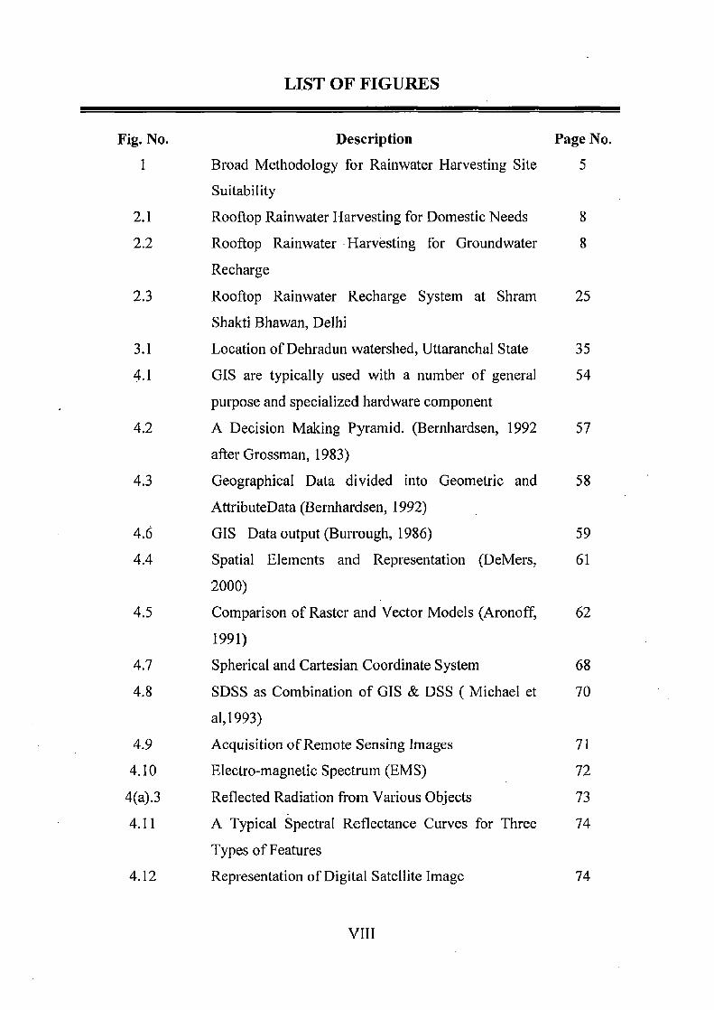
LIST OF FIGURES

Fig. No. Description Page No. 1 Broad Methodology for Rainwater Harvesting Site 5

Suitability

2.1 Rooftop Rainwater Harvesting for Domestic Needs 8

2.2 Rooftop Rainwater - Harvesting for Groundwater 8

Recharge

2.3 Rooftop Rainwater Recharge System at Shram 25

Shakti Bhawan, Delhi

3.1 Location of Dehradun watershed, Uttaranchal State 35

4.1 GIS are typically used with a number of general 54

purpose and specialized hardware component

4.2 A Decision Making Pyramid. (Bernhardsen, 1992 57

after Grossman, 1983)

4.3 Geographical Data divided into Geometric and 58

AttributeData (Bernhardsen, 1992)

4.6 GIS Data output (Burrough, 1986) 59

4.4 Spatial Elements and Representation (DeMers, 61

2000)

4.5 Comparison of Raster and Vector Models (Aronoff, 62

1991)

4.7 Spherical and Cartesian Coordinate System 68

4.8 SDSS as Combination of GIS & DSS ( Michael et 70

al,1993)

4.9 Acquisition of Remote Sensing Images 71

4.10 Electro-magnetic Spectrum (EMS) 72

4(a).3 Reflected Radiation from Various Objects 73

4.11 A Typical Spectral Reflectance Curves for Three 74

Types of Features

4.12 Representation of Digital Satellite Image 74

VIII

5.1 Areal Extent of Dehradun Watershed 77

5.2 Linear Relationships between Average Monthly 82

Potential Evapotranspiration Values Calculated by

Penman and Thorntwaite between 1967 and 2005

5.3 Monthly Average Potential Evapotranspiration in 83

Dehradun based on Data between 1960 and 2005

5.4 Monthly AET and PET in Dehradun based on 85

Monthly Average Data between 1960 and 2005

5.5 Monthly Water Availability in Dehradun based on 86

Monthly Average Data between 1960 and 2005

6.1 Daily rainfall in Dehradun watershed (Year1988) 95

6.2 Daily rainfall in Dehradun watershed (2001) 97

6.4 Daily rainfall in Dehradun watershed (Year2005) 99

6.4 Curve No.1 (AMC I) and Potential Maximum Retention I (1988) 100

6.4 Curve No.2 (AMC 1I) and Potential Maximum Retention II 100

(1988)

6.5 Curve No.3 (AMC III) and Potential Maximum Retention 101

III(1988)

6.8 Daily Runoff Image (1988) 101

6.8 Curve No.1 (AMC I) and Potential Maximum Retention 1 (2001) 102

6.9 Curve No.2 (AMC 1I) and Potential Maximum Retention II 102

(2001)

6.10 Curve No.3 (AMC III) and Potential Maximum Retention III 103

(2001)


6.12 Curve No.1 (AMC I) and Potential Maximum Retention I (2005) 104

6.13 Curve No.1 (AMC II) and Potential Maximum Retention II 104

(2005)

6.14 Curve No.3 (AMC III) and Potential Maximum Retention III 105

(2005)


IX

6.8 Total Runoff Generation in mm (1988) 106



7.1 Geological map 112

7.2 LISS III FCC Image 1988 115

7.3 LISS III FCC Image 2001. 116

7.4 LISS III FCC Image 2005 117

7.5 Classified Image 1988. 118

7.6 Classified Image 2001 119

7.7 Classified Image 2005 120

7.8 Soil Map 121

7.9 Slope Map (in percentage) 122

7.10 Drainage Map (Order) 123

7.11 Settlement Buffer 124

7.13 Parameter Conditions for rain water harvesting 127

(Ground water)

7.14 Suitable Site for Ground Water Recharge 128

7.15 Field Photos: Identified Ground Recharge Sites in 129

the Study Area (Rajpur)

7.16 Rainwater Harvesting Model for New Site selection 131

(surface water)

7.17 Parameter Conditions for Rainwater Harvesting 131

(Surface Water)

7.18 Suitable Site for Surface Water Storage (MDDA 132

Park)

7.19 Field Photos: Identified Surface Water Storage Sites 133

in the Study Area (MDDA Park)

8.1 Building Map of Dehradun City 136

8.2 Rainfall Variations 137

8.3 Cross Section of 1000 litre Traditional Filter 144

8.4 Cross Section of 500 litre Traditional Filter 145

X

CHAPTER ONE

INTRODUCTION

1.0 General Inspite of astonishing achievements in the field of science and technology, nature remains

to be a mystery for human beings. Though water is being obtained through desalination,

artificial rain by cloud seeding etc. the shortage of water even for drinking purpose is a

perpetual phenomenon throughout the world, especially in developing and

underdeveloped countries.

In most of the cities, the water supply sector is facing a number of problems and

constraints. The pace of watershed (urban & rural) development and the increase in

population in the watershed have resulted in exploitation of water resources to the

extremes. Fresh water sources are being heavily exploited to meet the demands of

watershed populace. Failure of monsoon makes the situation even worse. As surface

water sources fail to meet the ever increasing demands, ground water reserves are tapped,

often to unsustainable levels. Also fast rate of urbanization reduces the availability of

open spaces for natural re-charge of rain water. Some city (like Chennai) and its suburban

areas often get affected with water scarcity during the periods of low rainfall. As the

dependence of ground water increases during such periods the ground water table

depletes faster than normal rate resulting in dry wells. In addition to quantity, we also

face problems of water quality is also faced due to over extraction of ground water.

Unplanned and uncontrolled extraction of ground water would disturbs the hydrological

balance along the coastal areas which results in possible sea water intrusion. Hence, it is

necessary to take up measures to conserve and augment the renewable water resources in

all possible ways. Ground water recharge by rain water harvesting (RWH) is the simple

and-cost effective way.

Rainwater harvesting can not only provide a source of water to increase water

supplies but also involves the public in water management, making water management

everybody's business. It will reduce the demand of the institutions to meet water needs of

the people. It would also help everyone to internalize the full costs of their water

I

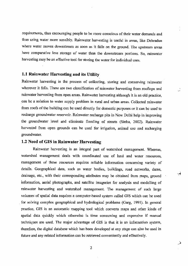
requirements, thus encouraging people to be more conscious of their water demands and

thus using water more sensibly. Rainwater harvesting is useful in areas, like Dehradun

where water moves downstream as soon as it falls on the ground. The upstream areas

have comparative less storage of water than the downstream portions. So, rainwater

harvesting may be an effective tool for storing the water for individual uses.

1.1 Rainwater Harvesting and its Utility

Rainwater harvesting is the process of collecting, storing and conserving rainwater

wherever it falls. There are two classification of rainwater harvesting from rooftops and

rainwater harvesting from open areas. Rainwater harvesting although it is an old practice,

can be a solution to water supply problem in rural and urban areas. Collected rainwater

from roofs of the building can be used directly for domestic purposes or it can be used to

recharge groundwater reservoir. Rainwater recharge pits in New Delhi help in improving

the groundwater level and eliminate flooding of streets (Sinha, 2002). Rainwater

harvested from open grounds can be used for irrigation, animal use and recharging

groundwater.

1.2 Need of GIS in Rainwater Harvesting

Rainwater harvesting is an integral part of watershed management. Whereas,

watershed management deals with coordinated use of land and water resources,

management of these resources requires reliable information concerning variety of

details. Geographical data, such as water bodies, buildings, road networks, dams,

drainage, etc., with their corresponding attributes may be obtained from maps, ground

information, aerial photographs, and satellite imageries for analysis and modelling of

rainwater harvesting and watershed management. The management of such large

volumes of spatial data requires a computer-based system called GIS which can be used

for solving complex geographical and hydrological problems (Garg, 1991). In general

practice, GIS is an automatic mapping tool which converts maps and other kinds of

spatial data quickly which otherwise is time consuming and expensive if manual

techniques are used. The major advantage of GIS is that it is an information system,

therefore, the digital database which has been developed at any stage can also be used in

future and any related information can be retrieved conveniently and effectively.

0)

1.3 Scope of the Study The scope of the study is limited to assess rainwater harvesting potential through

rooftop for domestic use. For conceptual understanding, some of the basic principles of

GIS are reviewed and the basic principles are discussed. A highlight of present trend of

GIS as management tool and the possibilities of integrating resources models with GIS

through Decision Support System (DSS) are also discussed. The reports collected from

Jal Sansthan and Jal Nigam, Dehradun, topographic maps and guide map obtained from

Survey of India served as the main data input for the present study.

Considering the existing water system of the study area, water sources, population,

water demand, rainfall data and water deficit are assessed. The final results of the

analysis are presented in the form of images and tables along with concluding remarks.

Detailed design of water harvesting structures based on various classification and

criteria being developed along with economical consideration is also incorporated in

this dissertation.

1.4 Objectives of the Study The emergent GIS technology has been gaining popularity in its wide range of

application and capability of organizing, storing, editing, analyzing and displaying large

volume of information which is referenced to geographic location and its attributes. The

recent effort trying to integrate GIS and resource models into tight-coupled system in a

way where both can interact directly, laid a ground for better resource planning and

management decision-making. To attain the desired benefits from this new technology, it

requires the conceptual understanding of the system.

The objectives of this study are:

(i) To show the potential capabilities of GIS in general, for rainwater

harvesting.

(ii) To show how predictive runoff can be modelled in GIS.

(iii) To assess the runoff producing potential and accumulation of runoff for

different land use/land cover.

3

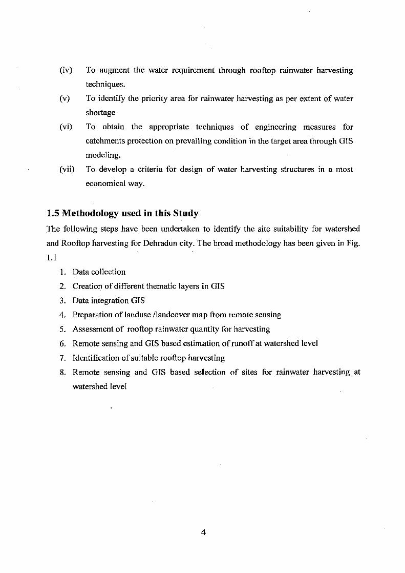
(iv) To augment the water requirement through rooftop rainwater harvesting

techniques.

(v) To identify the priority area for rainwater harvesting as per extent of water

shortage

(vi) To obtain the appropriate techniques of engineering measures for

catchments protection on prevailing condition in the target area through GIS

modeling.

(vii) To develop a criteria for design of water harvesting structures in a most

economical way.

1.5 Methodology used in this Study The following steps have been 'undertaken to identify the site suitability for watershed

and Rooftop harvesting for Dehradun city. The broad methodology has been given in Fig.

1.1

1. Data collection

2. Creation of different thematic layers in GIS

3. Data integration GIS

4. Preparation of landuse /landcover map from remote sensing

5. Assessment of rooftop rainwater quantity for harvesting

6. Remote sensing and GIS based estimation of runoff at watershed level

7. Identification of suitable rooftop harvesting

8. Remote sensing and GIS based selection of sites for rainwater harvesting at

watershed level

2

FLOW CHART OF METHODOLOGY

SOI TOPOSHEET METEOROLOGICAL DATA SATELLITE IMAGERY

RAINFALL LANDUSE I ANDCOVER TEMPERATURE WIND VELOCITY URBON AR A MAPPING

CREATION OF GIS DATA BASE

RELATIVE HUMIDITY II • CONTOUR SUNSHINE HOUR II

• SLOPE EVAPORATION ________ _j • LOCATION OF STUDY AREA

• ZONE MAP ii IMPERVIOUS • POPULATION MAP ii URBAN AREA • ROAD NETWORK MAP • WATER DEMAND MAP • WATER SUPPLY MAP • BUILDING MAP RUNOFF ESTIMATION ROOFTOP RUNOFI • OPEN AREA MAP OF WATERSHED ESTIMATION • WATER SHORTAGE MAP • ROOFTOP RAINWATER

HARVESTING POTENTIAL MAP

ANALYSIS IN GIS

SELECTION OF SUITABLE SITE FOR

SELECTION OF ROOFTOP WATER RAINWATER HARVESTING AT HARVESTING SYSTEM WATERSHED LEVEL

Fig. 1 Broad Methodology for Rainwater Harvesting Site Suitability

5

1.7 Organization of the thesis

Chapter 2 deals with the literature review; it highlights the discussion of different water

harvesting techniques-and various methods of rainwater harvesting techniques.

Chapter 3 deals with the details of study area of the Dehradun watershed. It covers

historical background, physiographic, climate, temperature, urbanization and socio

economic growth etc.

Chapter 4 describes briefly the salient features of GIS study area.

Chapter 5 Deal with the water availability senior of Dehradun

Chapter 6 Deals with GIS study of rainwater harvesting, methodology, software used

and data analysis.

Chapter 7 Deals with the site suitability analysis

Chapter 8 deals with analysis and design criteria of rooftop rainwater harvesting

structures.

Chapter 9 covers the discussion, conclusions and scope of future work.

Z

CHAPTER TWO

LITERATURE REVIEW

2.1 General

Water is most precious natural and universal asset. Water provides life support

system for human being, vegetation and animals. It is also a vital part of socio-economic

system. Rainwater harvesting, though an old age practice, is an emerging paradigm in

water resource development and management. Both government and non-government

organizations have recently stepped up their efforts in water harvesting and watershed

management activities following participatory approach. Rainwater harvesting systems

are relatively more equitable and environmentally sound. Water resources generated

locally provide benefits to the local community and minimize social conflicts.

Participatory management of harvested water resources ensures effective utilization of

the system.

2.2 Classification of Rainwater Harvesting

The rainwater harvesting can be classified into two ways:

2.2.1 Rooftop Rainwater Harvesting

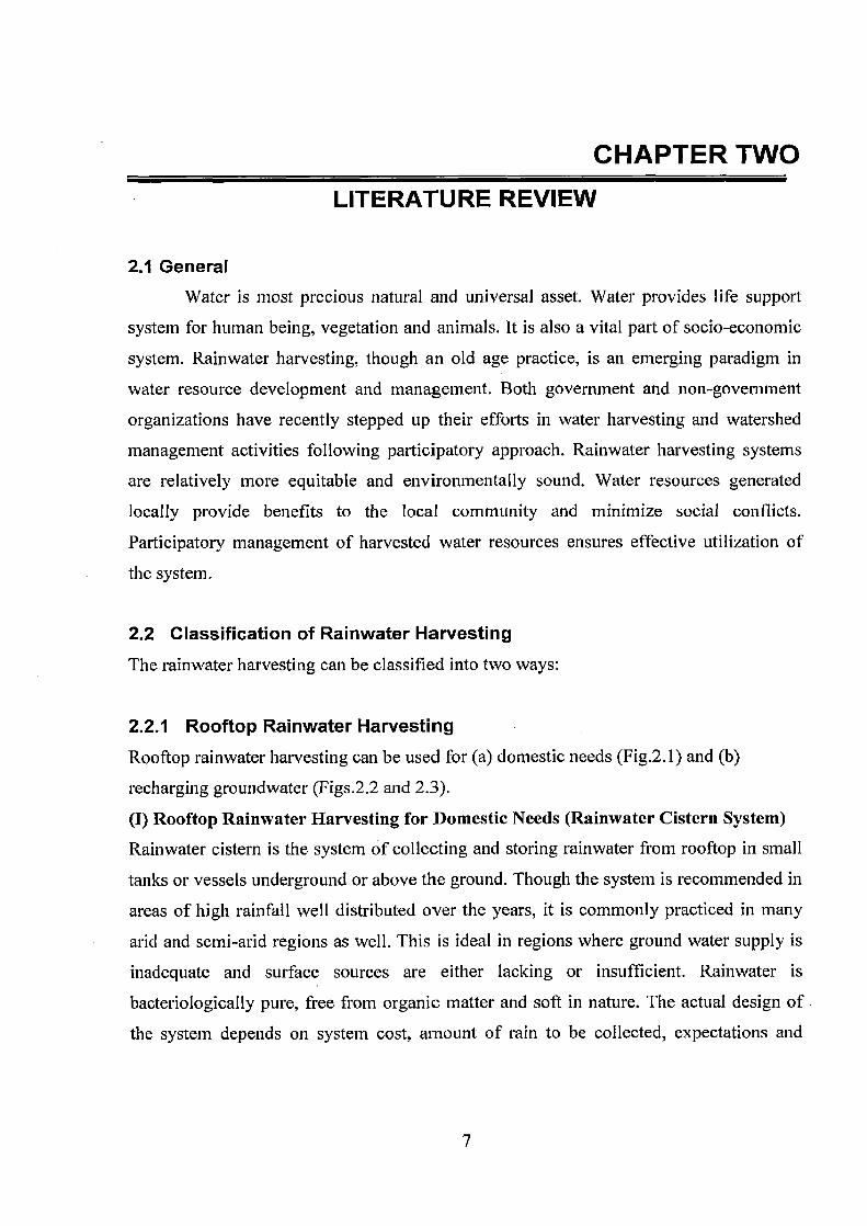
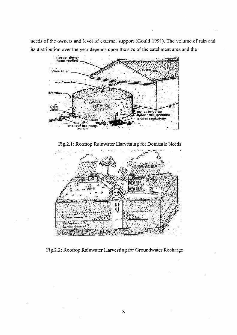
Rooftop rainwater harvesting can be used for (a) domestic needs (Fig.2.1) and (b)

recharging groundwater (Figs.2.2 and 2.3).

(I) Rooftop Rainwater Harvesting for Domestic Needs (Rainwater Cistern System)

Rainwater cistern is the system of collecting and storing rainwater from rooftop in small

tanks or vessels underground or above the ground. Though the system is recommended in

areas of high rainfall well distributed over the years, it is commonly practiced in many

arid and semi-arid regions as well. This is ideal in regions where ground water supply is

inadequate and surface sources are either lacking or insufficient. Rainwater is

bacteriologically pure, free from organic matter and soft in nature. The actual design of

the system depends on system cost, amount of rain to be collected, expectations and

needs of the owners and level of external support (Gould 1991). The volume of rain and

its distribution over the year depends upon the size of the catchment area and the

'plastic--tile or • n ear.rocfing,

IntakE. filtr: • g

• . _ _ . .-,. -.:- .:: it

vorflow• 4 L '

. vlve: - ,~~#?; sar f~

outlet {may ̀6e piped Into dw8111n`g)

_ : gravel soakaway . - ,

ShiliOw draertage '- .. . -

Trench - . -- f~

Fig.2. 1: Rooftop Rainwater Harvesting for Domestic Needs

.%" ` ` ry t..

- ir ,+' r + r +t •`"`T't 7/'F^EGi'P'Ra«4 ~~.r .

- IJIIL

H~nwv re a ~:,eeYi~„~ ~ •r s'.,`I ~ ~ e. 1~, 64~ TLti ~ w '+ 5

r ~• f, i eta Lr uiY~-n ALb A.+w~+ Yr ~ra.rr +~ r 4 D 1iw 1~lef fi YC'Itn+ rl ~ • A „ ~

•~ dd r TAIL ~rKri S= . • ~r5~ W/ N~IYr L14i1 ~ ~ti

y T I Z 't t L LCD ~ S 3 T, a •. +j..' s t 2'r) `ka~•~t 1s t 1' • r tip: rr 1 .e.. S{5;`- ri - i v

Fig.2.2: Rooftop Rainwater Harvesting for Groundwater Recharge

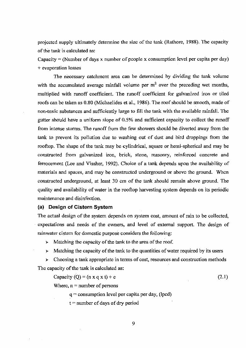
projected supply ultimately determine the size of the tank (Rathore, 1988). The capacity

of the tank is calculated as: Capacity = (Number of days x number of people x consumption level per capita per day)

+ evaporation losses The necessary catchment area can be determined by dividing the tank volume

with the accumulated average rainfall volume per m2 over the preceding wet months,

multiplied with runoff coefficient. The runoff coefficient for galvanized iron or tiled

roofs can be taken as 0.80 (Michaelides et al., 1986). The roof should be smooth, made of

non-toxic substances and sufficiently large to fill the tank with the available rainfall. The

gutter should have a uniform slope of 0.5% and sufficient capacity to collect the runoff

from intense storms. The runoff from the few showers should be diverted away from the

tank to prevent its pollution due to washing out of dust and bird droppings from the

rooftop. The shape of the tank may be cylindrical, square or hemi-spherical and may be

constructed from galvanized iron, brick, stone, masonry, reinforced concrete and

ferrocement (Lee and Vissher, 1992). Choice of a tank depends upon the availability of

materials and spaces, and may be constructed underground or above the ground. When

constructed underground, at least 30 cm of the tank should remain above ground. The

quality and availability of water in the rooftop harvesting system depends on its periodic

maintenance and disinfection.

(a) Design of Cistern System

The actual design of the system depends on system cost, amount of rain to be collected,

expectations and needs of the owners, and level of external support. The design of

rainwater cistern for domestic purpose considers the following:

Matching the capacity of the tank to the area of the roof.

Matching the capacity of the tank to the quantities of water required by its users

Choosing a tank appropriate in terms of cost, resources and construction methods

The capacity of the tank is calculated as:

Capacity (Q) _ (n x q x t) + e (2.1)

Where, n = number of persons

q = consumption level per capita per day, (lpcd)

t = number of days of dry period

0

e = evaporation losses from storage, (liters)

Runoff per unit roof area can be computed by multiplying total average rainfall over the

preceding wet months or monsoon with the runoff coefficient (f) (0.80-0.90). The runoff

coefficient for a hard roof is taken as 0.80. Table 2.1 gives the values for different roofing

material. Availability of rainwater from different roof top area for a range of rainfall is

given in Table 2.2, assuming runoff coefficient as 0.80. The required roof catchment area

can be determined by dividing the tank volume (Q) with runoff volume per m2.

Required roof catchment area (m2) A = Q/(f x P)

(2.2)

Where, P is rainfall in metrer

Types of Catchment Coefficients Roof Catchment

Tiles - Corrugated metal sheet 0.80 - 0.90

0.70 - 0.90 Ground Surface Coverings Concrete Plastic sheeting (gravel covered) 0.60 - 0.80 Butyl rubber 0.70 - 0.80

- Brick pavement 0.80 - 0.90 0.50 -0.60

Treated Ground Catchment Compacted and smoothed soil Clay/cow-dung threshing floors 0.30 - 0.50 Silicone-treated soil 0.50 - 0.60 Soil treated with sodium salts 0.50 - 0.80 Soil treated with paraffin wax 0.40 - 0.70

0.60 - 0.90 Untreated Ground Catchment Soil on slopes less than 10 percent Rocky natural catchment - 0.30

0.20 -0.50 Table 2.1: Runoff Coefficients for Different Roof Surface Conditions (Pacey and Cullis, 1986)

(b) Components of Rooftop Rainwater Harvesting System

Gutter: Gutter collects the rainwater runoff from the roof and conveys the water to the

down pipe. Gutter may be constructed from plain galvanized iron sheets or of local

material, such as bamboo, wood, etc. All gutters should have a mild slope (say around

0.50%) to avoid the formation of stagnant pools of water. Gutters with semi-circular

10

cross-section of 60 mm radius are sufficiently large enough to carry away most of the inter-monsoon rainfall.

Table 2.2: Availability of Rainwater through Rooftop Rainwater Harvesting

Rainfall

(mm) 100 200 300 400 600 800 1000 1200 1400 1600 1800 2000

Rooftop

Area (m2) Harvested Water from Rooftop (m3)

20 1.6 3.2 4.8 6.4 9.6 12.8 16 19.2 22.4 25.6 28.8 32

30 2.4 4.8 7.2 9.6 14.4 19.2 24 28.8 33.6 38.4 43.2 48

40 3.2 6.4 9.6 12.8 19.2 25.6 32 38.4 44.8 51.2 57.6 64

50 4 8 12 16 24 32 40 48 56 64 72 80

60 4.8 9.6 14.4 19.2 28.8 38.4 48 57.6 67.2 76.8 86.4 96

70 5.6 11.2 16.8 22.4 33.6 44.8 56 67.2 78.4 89.6 101 112

80 6.4 12.8 19.2 25.6 38.4 51.2 64 76.8 89.6 102 115 128

90 7.2 14.4 21.6 28.8 43.2 57.6 72 86.4 101 115 130 144

100 8 16 24 32 48 64 80 96 112 128 144 160

150 12 24 36 48 72 96 120 144 168 192 216 240

200 16 32 48 64 96 128 160 192 224 256 288 320

250 20 40 60 80 120 160 200 240 280 320 360 400

300 24 48 72 96 144 192 240 288 336 384 432 480

400 32 64 96 128 192 256 320 384 448 512 576 640

500 40 80 120 160 240 320 400 480 560 640 720 800

1000 80 160 240 320 480 640 800 960 1120 1280 1440 1600

2000 160 320 480 640 960 1280 1600 1920 2240 2560 2880 3200

3000 240 480 720 960 1440 1920 2400 2880 3360 3840 4320 4800

Down pipe: A vertical down pipe of 100 to 150mm diameter may be required to convey

the harvested rainwater to the storage tank. An inlet screen (wire mesh) to prevent entry

of dry leaves and other debris into down pipe should be fitted.

11

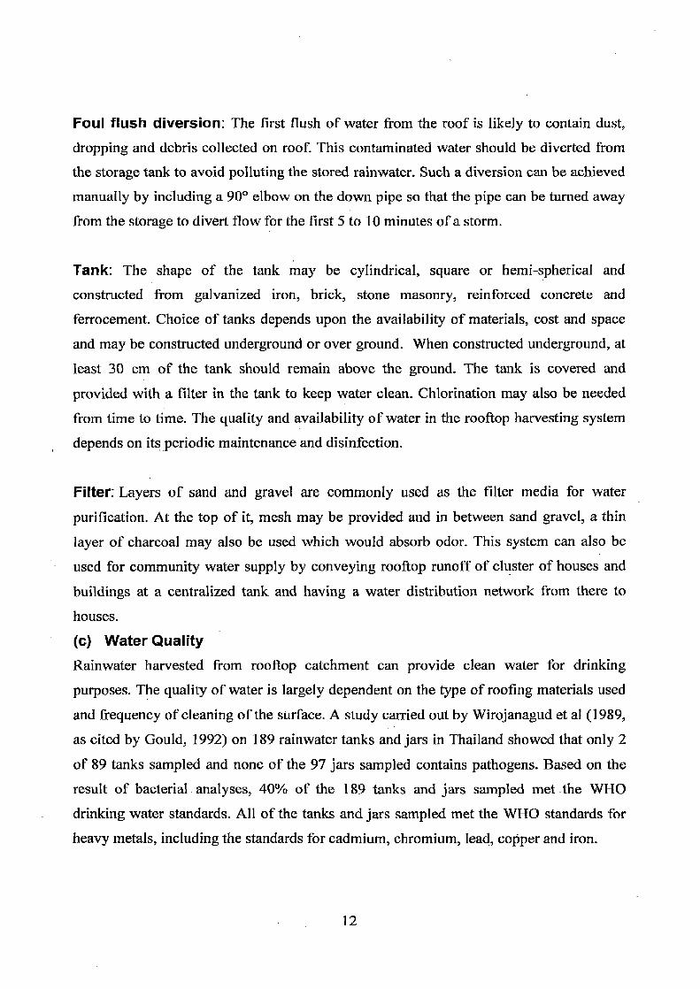
Foul flush diversion: The first flush of water from the roof is likely to contain dust,

dropping and debris collected on roof. This contaminated water should be diverted from

the storage tank to avoid polluting the stored rainwater. Such a diversion can be achieved

manually by including a 900 elbow on the down pipe so that the pipe can be turned away

from the storage to divert flow for the first 5 to 10 minutes of a storm.

Tank: The shape of the tank may be cylindrical, square or hemi-spherical and

constructed from galvanized iron, brick, stone masonry, reinforced concrete and

ferrocement. Choice of tanks depends upon the availability of materials, cost and space

and may be constructed underground or over ground. When constructed underground, at

least 30 cm of the tank should remain above the ground. The tank is covered and

provided with a filter in the tank to keep water clean. Chlorination may also be needed

from time to time. The quality and availability of water in the rooftop harvesting system

depends on its periodic maintenance and disinfection.

Filter: Layers of sand and gravel are commonly used as the filter media for water

purification. At the top of it, mesh may be provided and in between sand gravel, a thin

layer of charcoal may also be used which would absorb odor. This system can also be

used for community water supply by conveying rooftop runoff of cluster of houses and

buildings at a centralized tank and having a water distribution network from there to

houses.

(c) Water Quality Rainwater harvested from rooftop catchment can provide clean water for drinking

purposes. The quality of water is largely dependent on the type of roofing materials used

and frequency of cleaning of the surface. A study carried out by Wirojanagud et al (1989,

as cited by Gould, 1992) on 189 rainwater tanks and jars in Thailand showed that only 2

of 89 tanks sampled and none of the 97 jars sampled contains pathogens. Based on the

result of bacterial analyses, 40% of the 189 tanks and jars sampled met .the WHO

drinking water standards. All of the tanks and jars sampled met the WHO standards for

heavy metals, including the standards for cadmium, chromium, lead, copper and iron.

12

(II) Rooftop Rainwater Harvesting for Recharging Groundwater

Rooftop rainwater recharge of ground water can be achieved by conveying harvested

rainwater through following methods:

Abandoned dug well

Abandoned/running hand pump

Recharge pit

Recharge trench

v Gravity head recharge well

Recharge shaft

Abandoned Dug Well: The recharge water is conveyed through a pipe to the bottom

of well or below a water level to avoid scouring of the bottom and entrapment of air

bubbles in the aquifer. It is suitable for large buildings having roof area more than 1000

m2.

Abandoned 1 Running Hand Pump: The water is diverted from rooftop to the hand

pump through pipe of 50 to 100 mm diameter. The structure is suitable for small building

having roof area up to 150 m2.

Recharge Pit: These are constructed generally by excavating 1 to 2 m wide and 2 to 3

m deep, circular, square or rectangular shape, and refilled with pebbles and boulders. It is

suitable for small building having roof area up to 100 m2.

Recharge Trench: It is constructed in permeable strata of adequate thickness and the

trench is shallow depth filled with pebbles and boulders. The trench may be 0.5 to I m

wide, 1 to 1.5 m deep and 10 to 20 m long depending the availability of land and rooftop

area. These are constructed across the land slope. It is suitable for buildings having roof

area of 200 to 300 m2.

Gravity Head Recharge Well: The rooftop rainwater harvesting is channelised into

the well and recharges under gravity flow condition and suitable for roof area about 500-

1500 m2 suitable for areas where ground water levels are deep.

13

Recharge Shaft: It is constructed where the shallow aquifer is located below surface.

The diameter of shaft varies from 0.5 to 3m and the depth varies from 10 to 15 m. The shaft is backfilled with boulders, gravels and coarse sand.

2.2.2 Rainwater Harvesting from Open Areas

The major water harvesting systems prevalent in and and semi-arid regions of India are as follows:

(a) Nadis, Tanka, Khadin and percolation tanks in Rajastan

(b) Bandharas in Maharashtra

(c) Bundhis in Madya Pradesh and Uttar Pradesh, and

(d) Ahars in Bihar

Tanka: Tanka is the most common rainwater harvesting system in the Indian and zone,

and is local name given to a covered underground tank, generally constructed for storage

of surface runoff. The first known construction of Tanka in the Indian and and semi-arid

region can be traced back during the year 1607 in village Vadi Ka Melan near Jodhpur.

The Tanka is constructed by digging a circular hole 3.00 to 4.25 m in diameter and

plastering the base and sides with 6 mm thick lime mortar or 3 mm thick cement mortar

(Vangani et al, 1988). An Improved Tanka of 21 m3 capacities has been designed by

Vangani et al, (1988) to provide adequate drinking water for a family of six persons

through out the year.

Nadis: Nadis are excavated or embanked village pond for harvesting meager

precipitation to mitigate the scarcity of drinking water in desert regions. This is the most

important ancient practice of water harvesting in and and semi 'arid region, and the first

recorded masonry Nadi was constructed in 1520 near Jodhpur. A Nadi is generally

located in areas with lowest elevation to have the benefit of natural drainage and

minimum excavation of earth. It consists of two components; catchment area and water

storage. The Nadis range from 1.5 to 12 m in depth, 400 to 700,000 m3 in capacity, and have various shapes and sizes (8 to 2,000 ha).

14

Khadin: Khadin is a system of growing crops on harvested and stored water by

constructing an earthen bund across the gentle slope of the farm in the valley bottom

(Kolarkar et al, 1980). It was innovated during 15th century for runoff farming by Paliwal

Brahmin Community in Jaisalmer area. They are generally practiced in areas receiving

less than 100 mm average annual rainfall.

Anicut, Check Dam and Percolation Tank: These are constructed across the

ephemeral streams to intercept runoff from local catchments and store it for optimum

utilization (Khan, 1992). The stored water from behind is used for drinking, irrigation and

recharging the downstream wells. These structures are suitable in hilly and uneven

topography, where ephemeral streams are available in catchments with runoff

characteristics, and are widely adopted in hard rock and basaltic terrain of south-east

Rajasthan, Gujarat, Maharashtra, Madya Pradesh and in Deccan Plateau (Anon, 1988).

The design of two major components i.e. earthen embankments and masonry spillway is

based upon 50 years return period. A thorough and detailed knowledge of geological,

hydrological and morphological features of the area is necessary while selecting the site.

An anicut constructed on an ephemeral stream in western Rajasthan has been

found to enhance the ground water recharge by 35% over a period of three years (Sharma

and Kalla, 1980). An anicut is a structure or masonry wall, built across a river, by means

of which the water level on the upstream side is raised up to the crest level before it can

pass down the river

A percolation tank in basaltic formation influences about 1.5 to 2.0 km2 area and

recharge about (0.15 x 106 m3) of runoff during the normal rainfall years. The enhanced

recharge is variable, ranging from 0.032 x 106 m3 to 0.0182 x 106 m3 which is about 50%

of the storage capacity (Anon, 1988).

Ahars and Bundies: These are similar to Khadins, and are widely practiced in Bihar

and U.P. The basic principle is to allow runoff water to collect behind an earthen bund

usually 3 metres in height and running along contour over sizeable distance and hooked

up at appropriate points. The length of bunds varies from 100 m to 10 kms or more,

15

depending upon rainfall, watershed area and requirement of communities and individuals.

The submergence area may vary from 1 to 500 ha or more with stored water varying from

0.50 to 100 ha-m. The Ahars are constructed in on a very gentle gradient to facilitate large

inundation. The bund is of uniform soil without clay core or cut-off trench and usually

has 1:2 upstream and downstream slopes. Spillway is provided to release excess water.

The crest of spillway is 1 m lower than the top of the bund. Sluice gates are provided in

masonry structures to empty out Ahars quickly at time of sowing. Concrete or cast iron

pipes 150-300 mm in diameter are embedded in the bund at intervals of 50-100 m to

release water for irrigation.

Bandharas: Bandhara is a Marathi term for weir with vents. The vents have removable

shutters held in grooves in pipes. The vents are kept open during floods to carry away

heavy silt. The Bandharas catch the flow of streams and utilize it to provide irrigation to

crops. In many cases the water is pumped out of the bandharas and conveyed to higher

grounds.

Dams/ Reservoir: Earth dams can be built in those regions where the flow is perennial.

They consist of earthen embankments, 2 to 5 m in height, mostly with clay core and

downstream stone apron. Spillway is provided to drain of excess runoff. The storage

capacity generally ranges from 1000 to 50,000 m3. In and zone, Luni basin forms the

major drainage system, in which, there are 865 minor to major medium reservoirs

constructed with a total storage capacity of 1096.63 x 106 m3 (Anon,1990). The storage

water caters to the domestic and livestock requirements in addition to irrigation demand.

2.2 Case Studies (1.) Gupta and Tamhane (2004) applied GIS as tool for watershed analysis. The work has

been carried out are in the following manner:

i. District level resource mapping creation was done using 1: 50,000 Survey of India

Toposheets keeping in view the project objectives.

16

2. IRS—ID, LISS-III digital satellite data of 23.5 metres resolution were procured from

NRSA, Hyderabad for two seasons (i.e. Rabi and Kharif cropping seasons) for land

cover mapping and updating the information/data gathered from the base maps

generated from 1:50,000 Survey of India Toposheets.

3. Digital Image processing of satellite data using standard software packages was done

for data merging, enhancement of relevant features, digital classification and

conversion to thematic maps bringing the processed data into GIS environment for

water resource mapping from satellite imagery.

4. By combining the remote sensing information with adequate field data, based on the

status of water resources development and irrigated areas (through remote sensing),

artificial recharge structures such as check dams, nala bonds etc were recommended

upstream of irrigated areas to recharge downstream areas so as to augment

groundwater resources.

(2.) Sarangi et, al (2004) developed user interface in ArcGIS for watershed management,

the developed interface is a useful tool for integrated watershed management. This also

endorse the use of advanced computer assisted technology applied to the management of

natural resources on a watershed basis. The interface provides the inexperienced or new

user with an entry point to a powerful GIS without any detailed training in hydrological

modelling. The interface command buttons perform a series of inherent GIS instructions

and displays the results in a user-friendly format. The link of the developed interface with

Watershed and Stream Delineation Tool (WSDT) for watershed delineation and stream

network generation assists the user to start watershed management activities from a

DEM, without looking for digitization of topological information. The intent of this study

was to link the geospatial database with the interpretive routines for estimation of

morphological parameterson watersheds.

The Visual Basics for Applications (VBA) programming Ianguage and the ArcObjects

technology used in this interface are an emerging fields in GIS based applications. The

flexibility of the interface for further modification and updation is an added advantage

with the interface. This technique will further assist the linkage of hydrologic simulation

17

models for prediction of real time sediment and runoff estimations on watersheds. This

interface on watershed morphology estimation within ArcGIS environment is first of its

kind and is a useful tool for watershed prioritization and prediction of hydrologic responses.

(3.) Adhikari (2003) developed GIS - Remote Sensing compatible rainfall-surface runoff

model for regional level planning. In the broad sense, the term hydrological modelling

implies rainfall-runoff modeling, which helps in simulating and forecasting the flow from

a catchment and in determining the inflow series for the ungauged catchments. Efforts

have been made for the spatial distributed nature of the watershed properties by

introducing GIS for spatial discretisation of watershed into interlinked systems of

triangles and development of a physically based rainfall-surface runoff model for

simulating flood hydrographs in a user-friendly interface (GUI). The model is compatible

with both the GIS database and remote sensing data, although interactive option is

provided to the user for modifying the database, if necessary. GIS has also been used to

describe the various thematic layers such as physiography, landuse, soil etc. in the study.

Terrain modelling is a pre-requisite to hydrologic simulation of the rainfall-runoff

process. Algorithms have been used in the present study to extract watershed features,

such as overland flow cascades, channel network, confluence points, ridges etc., for a

given digital elevation data using Triangulated Irregular Network (TIN). The overland

flow is modelled as one-dimensional sheet flow over cascades of overland "flow planes"

contributing as lateral inflow to the channels flowing in the valley. Both the overland and

channel flows are simulated using the kinematic wave approximation of fluid flow and

solved through explicit finite difference routines. The main input to the watershed is

taken as the rainfall. The usage of the model for regional level planners is demonstrated

for tasks such as determination of waterways for small bridges and culverts, design of

spillways of small dams, construction of flood protection levees, agriculture, site planning for micro hydels etc

(4.) Hadi and Hamid (2003) worked for the sediment yield potential estimation of

Kashmar urban watershed using MPSIAC model in the GIS framework, with due

18

attention to the relatively suitable compatibility of MPSIAC model with the and and

semi-arid conditions of Iran and lack of hydrometric station in region, in order to

estimating of sediment yield and providing sediment yield and erosion intensity map in

this watershed, we used modified PSIAC model. At first to enter the available raw data

into the GIS framework, they digitized topography, geology, geomorphology, land

capability, soil hydrologic groups and plant cover maps using on-screen method. In the

second stage, digitized maps were encoded based on the values of geology, soil

erodibility, climate, land cover, land use, present status of erosion and channel erosion

and sediment transport factors. Using the DEM layer, slope and rain (using the rain

gradient equation) maps were provided and consequently topographic and runoff (using

the logical method) factors maps were prepared. Then these maps were summed together

and finally sedimentation score map was provided.

(5.) Pandey and Sahu (2002), worked for generation of curve number using remote

sensing and GIS. For ungauged watersheds, accurate prediction of the quantity of runoff

from land surface into rivers and streams requires much effort and time. But this

information is essential in dealing with watershed development and management

problems. Conventional methods of runoff measurements are not easy for inaccessible

terrain of Arunachal Pradesh. Remote sensing technology can augment the conventional

method to a great extent in rainfall-runoff studies. Many researchers (Ragan and Jackson,

1980; Slack and Welch, 1980, Tiwari et al., 1991) have been utilized the satellite data to

estimate the USDA soil conservation Services (SCS) Runoff Curve Number (CN). In this

study SCS Curve Number (CN) technique modified for Indian condition has been used

for generation of CN for Remi watershed, which is located in the East Siang district of

Arunachal Pradesh under Pasighat circle. The area of watershed is 210.00 Km2. The

watershed area lies in the Survey of India (SOI) topo-sheet No. 82 P/4, 82P/8, 83M/1 and

83M/5 It is located between 27° 50'to 28° 05' N latitude and 95° 05' to 95° 25' E

longitude.

(6.) Sharma et. al. (1999) developed micro-watershed plans using remote sensing and

GIS for a part of Shetrunji river basin, Bhavnagar district, Gujarat. Micro-watershed

19

level planning requires a host of inter-related information to be generated and studied in

relation to each other. Remotely sensed data provides valuable and up-to-date spatial

information on natural resources and physical terrain parameters. GIS with its capability

of integration and analysis of spatial, aspatial, multi-layered information obtained in a

wide variety of formats both from remote sensing and other conventional sources has

proved to be an effective tool in planning for micro-watershed development. In this

study, an approach using remote sensing and GIS has been applied to identify the natural

resources problems and to generate locale specific micro-watershed development plans

for a part of Shetrunji river basin in Bhavnagar district, Gujarat. Study of multi-date

satellite data has reveled that the main land use /land cover in the area is rainfed

agriculture, wasteland with/without scrubs. in the plains and undulating land and scrub

forests with forest blanks on the hills. Due to paucity of ground water for irrigation, the

rain fed agriculture area lacks sufficient soil and moisture to support good agriculture.

(7.) Baruah,(2002) used GIS as tool in watershed hydrology and irrigation water

management, this powerful tool holds a very large potential in the field of regional and

micro-level spatial planning, particularly in micro-watershed planning and management.

A GIS can helpful together various types of disparate data such as remote sensing data,

census data, records from different administrative bodies, topographical data and field

observations to assist researchers, planners, project officers and decision-makers in

resource management. Creation of a spatial database is the first step in micro-level

planning. This is followed by spatial analysis to help identify problem areas and, finally,

the steps towards planning to mitigate problems are taken by marking out action areas.

Taking a watershed as the spatial unit of study, appropriate physiographic and

morphometric parameters can be taken into account to enable proper micro-watershed

management.

(8.) Sarangi et.al (2004) used GIS tool in watershed hydrology and irrigation water

management. Watershed hydrology plays a significant role in generation and

quantification of runoff and sediment loss from watersheds. With an aim to asses runoff

and soil loss, GIS tool was used to assist in data base development which acted as input

20

to a developed conceptual model (Small Watershed Runoff Generation Model,

SWARGEM). The input to the model was in the form of data tables and digitized maps

comprising of soil parameters, topological information and land use features of Banha

watershed under Damodar Valley Corporation, Bihar, India. The topological information

indicated the elevations of corners of square grid array. The model used 4-point pour-

point technique to route surface flow from one grid to the other in an overlaid grid array

of the Banha watershed. The digitised watershed topology and square grid array was

created using ARC/INFO GIS tool . Manning's formulae was used to route water over the

entire watershed coupled with water budgeting technique corresponding to rainfall

events. The output of the model generated event based Direct Runoff Hydrographs

(DRH) for the watershed. The non-parametric statistical analysis (Wilcoxon's matched

pair signed rank test) performed on the predicted value and observed runoff rate at the

outlet of the watershed revealed that there is no significant difference between the

observed and predicted values at 0.05 probability level. The topological information

extracted using GIS was also used to obtain the geomorphological parameters of the

watershed. The hypsometric analysis which is under geologic geomorphological

component was performed using GIS tool. The analysis showed the erosion status of

watershed, which is moderately prone to erosion and is at equlibrium stage.

(9.) Sah et.al. (1997) worked for subwatershed prioritization for watershed management

using remote sensing and GIS. Delineating the wathershed area into subwatershed for

priority based conservation work is essential and appropriate for the developing countries

like Nepal. Considering its drainage system can do such delineation. The delineated

subwatersheds were used for prioritization. Prioritization can be done by considering

their forest loss, soil loss and land sensitivity, which is defined as the locational

relationship between forest loss and soil loss. These factors were used to extract the DSI,

SI and PC, which were considered as the condition indicator of the subwatershed. Using

these condition indicators, a new method of prioritization for conservation work was

proposed by the qualitative matrix analysis. Based on prioritization, subwatershed

conservation management activities were proposed. Finally, it can be said that remote

21

sensing and GIS in combination with USLE model can be used as appropriate tools for

sub wathershed prioritization.

(10.) Greenfield et. al (2004) developed watershed erosion and sediment load estimation

tool, The watershed erosion and sediment load estimation tool is an ArcView-based

system that can be used to estimate soil erosion and sediment loads from watersheds. The

potential erosion from each source (grid) cell in the watershed is calculated using the

Universal Soil Loss Equation (USLE) in which the USLE factors, such as K, LS, C and P

are automatically calculated based on spatial data layers such as soil, Digital Elevation

Map (DEM), land use, road network, and management practices. The potential sediment

load to user-specified assessment points in the watershed is estimated by using one of

three alternative methods for computing sediment delivery ratio. The user is provided

with the capability to easily and quickly prepare alternative scenarios to determine the

effects of land use changes, best management practices (BMPs), and road management

practices on the erosion and sediment estimates. BMPs that affect the source of the

erosion (e.g., tillage practices) and the sediment pathways (e.g., ponds, buffer strips) are

considered separately. Other features, such as grouping the estimates by source,

automatic report generation, and scenario tracking are also provided.

(11.) Samad et.al (1997) applied GIS and remote sensing for soil erosion and

hydrological study of the Bakun Dam catchment area, Sarawak. The USLE was applied

to predict annual soil loss in the study area, using the integration of satellite remote

sensing GIS technologies. Parameters of the USLE used to generate the relevant raster

layers for soil erosion spatial modelling in the GIS are - (i) rainfall erosivity, (ii) slope

length/gradient, (iii) cover- conservation method and (iv) soil erodibility. The analysis

was done in MICSIS (Micro-computer Spatial Information System), an image processing

and GIS software package developed specifically for erosion modeling under the Malaysian-China cooperation.

(12.) A case study of a rooftop water harvesting system in village Satengal, district Tehri

Garhwal under "SWAJAL" project carried out by District Project Management Unit,

22

Dehradun with local NGO-Rural Litigation and Entitlement Kendra as a support

organization, is presented to illustrate an example that followed a participatory approach

(Dobhal, 2000). After detailed deliberation with the community, the community finally

selected the ferrocement type storage tank. Following design parameters were taken into

account:

Average number of persons per household n = 5

Average water consumption for drinking purpose q = 5 1pcd

Average annual rainfall p = 2000 mm

Dry period t = 270 days

Runoff coefficient, f

For corrugated galvanized iron sheets (CGI) = 0.80

For RCC roofs = 0.70

For slate roofs = 0.60

Water demand per household during dry period was calculated as:

Q=nxqxt=5x5x270=6750 liters

Considering water storage tank of 7k1 capacity per household.

Roof catchment area

Required area A = Q/(f x p)

For GI sheet roof A = 7/( 0.80 x 2) = 4,375, say 5m2

For RCC roofs A = 7/( 0.70 x 2) = 5 m2

For slate roofs A = 7/ (0.60 x 2) = 6 m2

These requisite roof areas were easily available with the village houses. After this initial

feasibility of rooftop rainwater harvesting system, the various technical proposals were

discussed with the community. The water storage tanks proposed were of RCC,

brick/stone masonry, galvanized iron sheets, synthetic polymer and ferrocement. After

detailed deliberation with the community, the community finally selected the ferrocement

type storage tank due to the following reasons:

Low cost

• Ease of construction

A Ease of maintenance

Lesser area required than brick/stone masonry tank

23

Temperature control

13. Rathore, (1988), carried out a study related to rooftop rainwater harvesting in village

Jaislan in Nagaur district, western Rajastan. The study area is located in the saline ground

water track. The village has geographical area of 868 ha with 879 inhabitants living in

133 households. Drinking water is always a problem in the region since the settlement of

the village 250 years ago. The villagers used to transport the drinking water from the nearby village 3 km away. During 1906, a villager tried to rooftop water harvesting in his

house. An underground water storage tank was linked through drain pipes with the roof.

This was a successful experiment and became an important non-saline potable water

source in the village. Inspired by this, more rooftop rainwater harvesting systems were

constructed between 1923 and 1926. The water was supplied to entire village during

summer when acute scarcity of water was felt. The number increased to about 100 and

the structures have been working successfully in the village. The entire village has

become self-sufficient in meeting out

the drinking water needs on sustainable basis.

14. Study carried out by the Center for Science and Environment (CSE) has found a rise

in water table of some areas in New Delhi, where water harvesting structures were

installed. Rainwater collected from roof of buildings was conveyed to recharge pit

installed in different parts of the city. This water harvesting system is the solution to the

depleting water table and water log areas (Sinha, 2002). It was reported to have a

significant rise in water table in the following areas: Panchseel Park (92.4 to 87.1 ft),

Jamia Hamdard University (148.5 to 132 ft), Janki Devi Memorial College in Ranjinder

Nagar (118.14 to 72.93 ft) and Sriram School, Vasant Vihar (119.8 to 115.5 ft).

15. In many states such as Delhi, Maharashtra, Gujarat, Chandigarh (UT), Punjab,

Haryana, Rajasthan, Tamil Nadu, Meghalaya, etc., rooftop runoff from housing

complexes and institutional buildings is being used to recharge ground water. Chennai

Metro Water Board has made rooftop rainwater harvesting mandatory under the city's

building regulations. At Shram Shakti Bhawan, New Delhi, artificial recharge structures

24

t!1L!I.. v- ~A

'emu/!

1pc .R

Ci~11c4L t i :Y 5.bi:. Y. , I L. }r N CU _._ •• p, .i lFGtr v ;. ate: ;

~e SOL SLCf [lr — 1 M isL1+ -P9

CM ~>'fl 7R

n CrC YLi _ .. _ r 5'FC.7J.~}S b1. lord..

Fig 2.3: Rooftop Rainwater Recharge System at Shram Shakti Bhawan, Delhi

are installed Fig. 2.3. The roof area is 3110 m2 and receiving the average annual rainfall

of 712mm. It is found that there is a rise of water table from 0.62 to 1.37 m.

16. Raju (1994) carried out work on sub-surface. water harvesting in Kutchh district of

Gujarat. Due to over exploitation of ground water in the study area, the water table has

gone down drastically in many years. Many open wells have dried up and sea water had

intruded into the coastal aquifers. The total area affected by sea water intrusion has been

estimated as 15,500 ha in 244 villages. Shree Vivekanand Research and Training Institute

constructed water harvesting system since 1987 with the assistance of voluntary

organizations and State Government. In all 58 check dams, 48 percolation tanks, two-

surface dam, 39 recharge wells and 42 storage tanks were constructed till July 1993.

Total capacity of the recharge structures was 1.44 x 106 m3, which can accommodate two

to three floods in normal rainfall year, thus increasing recharge capacity to about 3 x 106

m3 in a year of good rainfall. The area likely to be benefited is of the order of 3301 ha in

20 villages. The rise in water table over a period of 6 years is of the order of 6 m and

maximum decline of salts is of the order of 920 ppm. This water harvesting structure has

25

given encouraging results and proved the effectiveness of recharge wells and sub-surface

dams as recharge structure.

17. A study has been conducted for identification of suitable sites for water harvesting

structures in upper Betwa watershed of Betwa basin using "WARTS" package developed

over Arc/INFO GIS. The present study uses decision support system "WARTS" for

identification of suitable sites for water harvesting structures. It covers an area of 1384.61

km2 and falls in parts of Bhopal and Raisen districts in Madhya Pradesh. Theme layers

viz, landuse / landcover, soil, slope, hydrogeomorphology, etc., which affect the

identification of sites were generated in Arc/INFO environment (Bothale, et al, 2002).

Following structures were suggested after identification of suitable sites:

Anicut: For anicut sites buffer of 1 km was constructed around 2nd to 3rd order

streams. Medium slope areas between 2 to 8% were taken. Favorable soils were

given weights to allow storage of water. A total of 10 sites were marked in the

area.

Nala bund: Nearly plain, (up to 2%), upper reach, catchments greater than 40 ha,

permeable soils were the criteria according to which the weights were decided.

After the analysis 16 sites were marked which are suitable for nala bund.

Farm pond: Flat topography, low permeability, absence of faults, joints were the

criteria for site suitability.

Dug cum bore well: Lineament map pertaining to study area was studied and 9

suitable sites were marked on the output.

18. TWAD Board in association with UNICEF launched a pilot project during the year

1994 to study the effectiveness of rainwater harvesting structures constructed in a micro

watershed. An evaluation conducted recently indicates that the rainwater harvesting

structures contributed considerably to the groundwater regime enhancing both quality and

quantity parameters. It has been found out that all the target wells in the project area

became sustainable after the intervention of the project.

19. TWAD Board in association with the Anna University undertook an exercise to

identify optimum locations for the construction of rainwater harvesting structures

throughout the State, using remote sensing technology. The study has identified 13,357

structures that need to be constructed/improved. The details of these structures are:

Desilting of tanks (5,266), Check dams (6055), Percolation ponds (1,201), Recharge pits

(684), Subsurface dykes (82) and Nala bunds (69).

20. The Government proposes to enlist the participation of the Public and Non

Governmental Organization (NGOs) in propagating and installing rainwater harvesting

structures. Every household can construct and benefit from rainwater harvesting. Every

rooftop and any open space is a potential catchment area for rainwater harvesting

(Ramalingam et al, 2002).

2.3 PRESENT SCENARIO In the present study, critical review of the existing water sources have been made, which

are described below:

2.3.1 Critical reviews of the present status and water supply (a) Drinking water supply and source available (surface and ground water)

(b) Suitability of existing sources for drinking water

(c) Adequacy of these sources

(d) Existing operational systems/policy of drinking water supply

(e) Existence and conditions of springs

(f) Working out demand, availability and deficiency for present & future

(g) Strata charts/stratification- details of formations

(h) Soil and infiltration characteristics

2.3.2 Water Supply No city can exist without an adequate water supply of safe water that is fit for human

consumption. In urban contest besides drinking, water has other purposes, such as

27

washing, industrial uses, fire fighting & air conditioning, irrigating lawns and public

parks etc. The most concerned public facilities of all large cities have been with their

water supplies.

The larger cities during their expansion found the local sources from wells,

springs and brooks that were inadequate to meet the drinking and sanitary demands of

growing population. Construction of aqueducts that could bring the water from distance

was the solution to fulfill the demand.

Generally, the water supply schemes of this kind are constructed and operated by

the municipals corporation. Dehradun city is no longer different than the other cities. In

olden days, people met their demands from dug wells, natural springs and canals. Later as

the city grew, pipelines were introduced connecting the perennial springs to meet the

demand. Subsequently the surface water was brought from river Bandal through gravity

main and with this, a proper water works department with facilities of filtration came in

to existence at Dila Ram Bazar. Pipelines were also laid for conveying water to the

town's population.

Under the status and the existing set-ups and until few of the Jal Sansthan (Water

and Sewage Boards) came up with power to levy water and drainage tax, its realization

and also the responsibility of establishing a protected water supply vested with the local

bodies representing the community. Obviously the responsibilities of establishing a water

supply and promotion of protected water supply in Dehradun, because of the

responsibility of the Dehradun Municipality.

2.3.3 Growing Demand of water With the urbanization and industrial growth the demand started increasing unprecedently.

The new areas on all sides of town were inhabited and so the limits of Dehradun across

Municipality extended demanding the civic facilities to newly formed settlements. The

existing water supply from springs and rivers became inadequate and tapping new

sources for augmentation for water needs and also extension of distribution system to the

new colonies became essential.

Water supply of Dehradun city is managed by Jal Sansthan. According to data

provided, it is known that the total population of Dehradun is 5,78,646 (On year 2003

basis). As per design criteria, the total water demand of the city is 89.69 mld (@155 1pcd)

and the institutional demand is 10.00 mid. Thus the total demand is 99.69 mld. But

presently supply is being done @ 200 1pcd. Therefore total demand according to 200 1pcd

for the present population is 115.73 mld - and after including institutional demand it

reaches to 125.73 mid. But the total water supplied from various sources is unable to

make the demand.

Total water supply for the city is 102.32 mld (On year 2003 basis). Tube wells are

the main source of water supply in Dehradun city. Total amount of water supplied from

these tube wells is 83.95 mld while rest of the amount i.e. 18.37 mld water is supplied

from the natural resources. Table 4.1 shows the present supply and demand statement of

the city. Presently there is shortage of about 23.41 mld and the gap is expected to widen

in the next decade. Hence corrective measures are necessary to fill this gap. Rainwater if

harvested may be used to bridge the gap.

About 82% of total water supply of the city is met from the 52 tubewells that are

scattered almost all over in the city. There are 26 overhead tanks of varying capacity in

order to supply the elevated areas. Tables 2.3a, 2.3b & 2.3c show the list of tubewells and

overhead tanks. The ground water level varies from 20-90 m.

The present water supply scheme of the capital city is catering the need of 5.79 lakh

people (on year 2003 basis). Besides this permanent population it also serves the tourists

and the students who are considered to be the floating population.

For the efficient running of a water works system and equal distribution the water

supply department works from four zones within the city viz. Upper zone, Rajender

Nagar zone, Dharampur zone and Niranjanpur zone. Out of 46,221 connections, there are

36,115 domestic connections, 6,465 non-domestic and 1789 are commercial metered

connections. There are 134 bulk connections given for industrial and institutional

requirements. To the economically weaker sections of the society, there are 1758

connections given by water works through stand post, which are unmetered. Table 2.4

shows the total no. of registered connection with Water Works Department (W. W. D).

Despite there being a supply of 102.32 mid, the supply situation became grim in

every summer. Except the few areas though rest of the city has problem in getting

drinking water. The areas facing the shortage of water supply are Clock Tower, Hathi

I

Barkala, Rest Camp, Tyagi Road, Chander Road, Kaulagarh Road and Genaral Mahadeo

Singh Road. The water scarcity in these areas is due to rapid commercialization,

construction of new shopping complexes etc., so the demand of water is suddenly

increased. The water demand- project doesn't include the need of this population. The

storage capacity of the overhead tanks and number of tube wells within the city are less in

number to meet the demands. Table 2.5 shows the deficiency in storage for the city.

The problem of water pressure in the pipes remains in the areas of higher

elevation. This problem clearly indicates the lack of research during the planning for

constructing the overhead tanks. Apart from the above reason, the limited economic

resources, the cost involved in drilling tube well (approx. 18-20 lakhs) and the shortage of

man power are also strong reasons for the crippled operational system of water works.

Summing up the above issues, it was inferred that a holistic study needs to locate new

potential sites, keeping in mind the future requirements of the growing population.

2.3.4 Tariff for Domestic and Non-Domestic Consumers Water is sold to the domestic consumers @ Rs. 2.50 per thousand liters and non-domestic

rate of supplying water is @ Rs. 12 per, thousand liters. Besides the existing tariff rate of

consumption of water, a minimum service charge of Rs.12.50 plus Rs. 2.00 for meter rent

is collected monthly. This however holds good for consumers who are drawing water

through metered connections, but there is a section of people who do not have either

metered or unmetered connection on flat rates, but enjoy and draw water from Municipal

Mains. To extend the tax basis to this section of population and also to have a minimum

assured income from the water supply system, a water tax @12.5 % of the rental value of

the property is levied on all houses and properties except houses belonging to the weaker

sections of the society, irrespective of whether that property has a water connection or not

and also whether or not water is consumed at such premises. However all those properties

which are having metered water connections enjoy a monthly fixed non chargeable

quantity of water in lieu of water tax paid, but all consumption over the fixed monthly

limits all chargeable. If in any case the monthly consumption- fall short of the non-

chargeable limit the balance is not carried forward and it lapse. The tariff structure for

water consumption is presented in Table 2.6

30

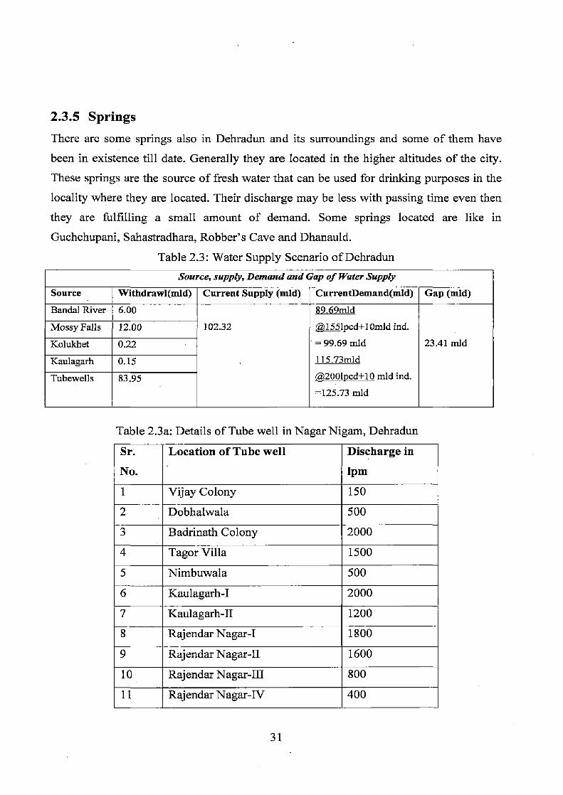
2.3.5 Springs

There are some springs also in Dehradun and its surroundings and some of them have

been in existence till date. Generally they are located in the higher altitudes of the city.

These springs are the source of fresh water that can be used for drinking purposes in the

locality where they are located. Their discharge may be less with passing time even then

they are fulfilling a small amount of demand. Some springs located are like in

Guchchupani, Sahastradhara, Robber's Cave and Dhanauld.

Table 2.3: Water Supply Scenario of Dehradun Source, supply, Demand and Gap of Water Supply

Source Withdrawl(mld) Current Supply (mld) CurrentDemand(mld) Gap (mld)

Bandal River 6.00

102.32

89.69m1d

1551pcd+l Omld ind.

= 99.69 mld

115.73m1d

g2001pcd+10 mld ind.

=125.73 mld

23.41 mld Mossy Falls 12.00

Kolukhet 0.22

Kaulagarh 0.15

Tubewells 83.95

Table 2.3a: Details of Tube well in Nagar Nigam, Dehradun

Sr. No.

Location of Tube well Discharge in 1pm

1 Vijay Colony 150

2 Dobhalwala 500

3 Badrinath Colony 2000

4 Tagor Villa 1500

5 Nimbuwala 500

6 Kaulagarh-I 2000

7 Kaulagarh-II 1200

8 Rajendar Nagar-I 1800

9 Rajendar Nagar-II 1600

10 Rajendar Nagar-III 800

11 Rajendar Nagar-IV 400

31

12 Vijay Park 1200

13 Govind Garh 2500

14 Khurbura 1600

15 Panditwadi 1200

16 Basant Vihar-I 2200

17 Basant Vihar-II 1200

18 Indira Nagar-I 1600

19 Indira Nagar-II 2000

20 Maharani Bag 2200

21 Engineer Enclave 2200

22 Patel Nagar 2200

23 Niranjanpur-I 2500

24 Niranjanpur-II 2200

25 Niranjanpur-III 2200

26 Niranjanpur-IV 2500

27 Rest Camp 2500

28 Race Course 2500

29 Nehru Colony-I 2200

30 Nehru Colony-Il 2400

31 Nehru Colony-III 1800

32 Nehru Colony-IV 2200

33 Nehru Colony-V 2500

34 Nehru Colony-VI 2200

35 . Dharampur 2000

36 Sanjay Colony 2500

37 Curzon Road 1500

38 Survey Chowk 1600

39 Parade Ground 800

40 Tibati Market 1600

41 Gandhi Park 2200

32

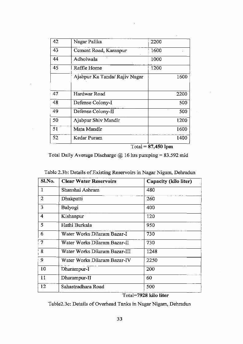
42 Nagar Palika 2200

43 Cement Road, Karanpur 1600

44 Adhoiwala 1000

45 Raffle Home 1200

Ajabpur Ka Tanda/ Rajiv Nagar 1600

47 Hardwar Road 2200

48 Defense Colony-I 500

49 Defense Colony-II 500

50 Ajabpur Shiv Mandir 1200

51 Mata Mandir 1600

52 Kedar Puram 1400

Total = 87,450 1pm

Total Daily Average Discharge @ 16 hrs pumping = 83.592 mid

Table 2.3b: Details of Existing Reservoirs in Nagar Nigam, Dehradun

S1.No. Clear Water Reservoirs Capacity (kilo liter)

1 Shanshai Ashram 480

2 Dhakpatti 260

3 Balyogi 400

4 Kishanpur 120

5 Hathi Burkala 950

6 Water Works Dilaram Bazar-I 730

7 Water Works Dilaram Bazar-II 730

8 Water Works Dilaram Bazar-III 1248

9 Water Works Dilaram Bazar-IV 2250

10 Dharampur-I 200

11 Dharampur-II 60

12 Sahastradhara Road 500

Total=7928 kilo liter

Table2.3c: Details of Overhead Tanks in Nagar Nigam, Dehradun

33

Sr. No. Overhead Tanks Capacity(Kilo liter)

1 Water Works Dilaram Bazar-V 1800

2 Parade Ground-I 900

3 Parade Ground-II 2500

4 Nagar Nigam Compound (City Board 900

5 Prem Kunj, Nimbuwala 225

6 Kaulagarh 450

7 Rajendar Nagar 850

8 Dobhalwala 1250

9 Vijay park near ONGC 550

10 Khurbura 1800

11 Jhanda Mohalla 900

12 Basant Vihar 450

13 Indira Nagar 500

14 Engineer Enclave 100

15 Laxman Chowk/Kanvali Road 900

16 Patel Nagar 2500

17 Indira Puram 600

18 Race Course 1250

19 Nehru Colony-I 2500

20 NEHRU COLONY-II 225

21 Ajabpur 300

22 Adhoiwala 450

23 Raffle Home 100

24 Rajiv Nagar 500

25 Defense colony 200

26 Kedar Puram 600

Total = 23,380 kilo liter

11

CHAPTER THREE

THE STUDY AREA

3.0 Location

The Dehradun city, the capital of newly formed Uttaranchal state, is situated in the south

central part of Dehradun District, and is one of the major urban center of the region. It is

located 250 km. north of New Delhi. The study area lies between 77° 57 24' E to 78° 07

44' E and 30006 27'N to 30027 40' N latitude (Fig. 3.1).

Fig 3.1 Location of Dehradun watershed, Uttaranchal State

35

Surrounded by lush green forests and hills, Dehradun has always been a favorite

destination with the tourists. It is endowed with a pleasant, moderate, climate and is well

connected with other important places such as Delhi, Haridwar. Dehradun is a gateway

and base camp for tourists and pilgrims headed for Gangotri- Jamunotri- Kedarnath-

badrinath- valley of flowers and famous hill queen Mussoorie.

Dehradun is one of the beautiful towns in the northern India. It boasts of a number

of reputed educational institutions such as the Forest Research Institute, Wildlife Institute

of India, Forest Survey of India, Indian Military Academy, The Doon School etc. The

entire Dehradun Valley has numerous places of scenic beauty and picnic spots such as

Robbers Cave, Rajaji National Park, etc.

Dehradun is strategically located in the foothills of the Himalayas in the north, the

Shiwalik hills in the south, the Ganga in the east and Yamuna River in the west. The

Doon valley is a longitudinal valley, which extends about 80 km in the length and 20 km

in width, lie between the rivers Ganga and Yamuna. The pre-tertiary rocks of the mid

Himalayan range rise up to 2200 m. above MSL bounded the north and the Shiwalik

range, which rises up to 900 m above MSL, bound Doon valley in the south.

3.1 Historical Background

The name of the city is composed of two words "Dehra" and "Doon". "Dehra" was

derived from 'dera' signifying a temporary abode or camp of a religious saint cum

preacher. "Doon" or "dun", in Sanskrit and Hindi means an elongated valley, hence the

name "Dehradun". The Oxford dictionary defined it as "Valley in Shiwalik Hills".

Among the number of large and small valleys between the Lesser Himalaya and Shiwalik

Hills, Dehradun is one of the largest and best known of them all.

36

There are a number of myths related to the naming of "Dehradun" city. According

to Skanda Purana,- an ancient text, "Dun" formed part of the region called "Kedar

Khand". It was included in the kingdom of Lord Ashoka by the end of the 3rd century

B.C. History reveals that for centuries the region formed part of Garhwal kingdom with

some interruption from Rohillas.

However, most popular myth is that the city derived its name from the local

tradition. During the 17th century, the Sikh guru Ram Rai, (a sent in Udasi fakir sect) took

up his residence iii the Dun. History connects the event with Guru Har Rai, the leader of

the famous Sikh sect who died in 1661 leaving behind two sons, Ram Rai and Har

Kishan. After the death of Guru Har Rai, emperor Aurangzeb,.confirmed the election of

guru Har Kishan and direct Ram Rai to retire to the wilderness of the Dun. In obedience

to the emperor's command, Ram Rai retired to the Dun at Kandli on the river Tons. Later

on he moved from the Dun and settled down in Khurbura, now included in the city of

Dehradun. Guru Ram Rai built a temple at the village Dhamanwala, which became the

nucleus of the present city and even today his Darbar Saheb is the heart of the city's

cultural and spiritual life.

For about two decades till 1815 the city was under the occupation of the Gorkhas.

In April 1815, Gorkha rulers were ousted from Garhwal and Garhwal was annexed by the

British. In the decades that followed, the British Government felt that the material

progress of Dehradun and adjoining hill towns of Mussoorie and Landour was dependent

upon colonization and reclamation of the wastelands. This led the government to

encourage capitals. The growth of tea industry and the extended operations of forest

department, the establishment of two military Cantonments (in 1872 and 1908),

37

increasing popularity of Mussoorie and Landour, as a retreat of well to do pensioners and

opening of the railway in 1900 have all contributed towards growth of Dehradun.

Later on, the construction of 1.6 km long Paltan Bazar (from Clock Tower to

Gurudwara) led to the trade transaction and thus led to a very rapid growth of the city.

This development was further aggravated after the second world war, through the

establishment of new Cantonment, Ordinance Factory, Indian Institute of Petroleum,

Indian Photo Interpretation Institute (renamed as Indian Institute of Remote Sensing), Oil

and Natural Gas Corporation, Survey of India, Doon School and many other institution,

offices and the growth of ancillary activities and other infrastructure facilities have

contributed considerably to the growth and physical expansion of the city.

Thus, this unprecedented growth of institutions, offices, large and small scale

industries, time based industries at Dehradun have triggered the problems of congestion

in the central core of the city and crippled the transportation system have resulted in

overall environmental degradation. However, till 1960, there was no effort to channelise

the haphazard growth of the city. Under this circumstances the city at present is suffering

from a number of problems of uncontrolled and haphazard development, severe traffic

congestion, rapid growth of slums on low lands, particularly at the beds of the seasonal

streams and encroach of commercial activities.

3.2 Physiography

The general physiography of Dehradun city is located on a gentle undulating

intermountain valley at an average altitude of 1350 m above mean sea level. The lowest

altitude is 419 m. in the southern part, whereas highest altitude is 2280 m on the northern

part. The northern slope (south facing), at the base of Mussorie hills, has gentle gradient

38

of about 8° which mostly comprises of coarse detritus boulders, pebbles, gravels derived

mainly from Pre-Tertiary and Siwalik rocks with top soil and silt /sand. The north facing

southern slope of Siwalik hill range is steeper in gradient of about 100 formed mainly of

reworked Upper Siwalik boulders and gravels with sand and silt. The drainage of the city

is borne by two rivers namely: Bindal Rao and Rispana Rao. The direction of flow of

these seasonal streams and nalas in the eastern part is north to south and western part it is

north to southwest. The whole area is heavily dissected by a number of seasonal streams

and nalas, which are locally known as "Khalas". Dense patches of forests exist along the

north and in the outer limit of regulated areas.

3.3 Climate In general, the climatic conditions of the study area are subtropical to temperate.

Dehradun experiences four seasons, namely, winter, summer, rainy and post monsoon

seasons. The period from November to February is the winter season. The summer

season followed continues up to the end of June. The rainy season is from July to about

third week of September. The following period, till the middle of November is the post

monsoon or transition period.

3.3.1 Temperature

The maximum average temperature is 36± 6 °C and the minimum is 5 ± 2 °C. In

summers, maximum temperature i.e. 36 ± 6° C and the minimum temperature is 16 ±7° C

whereas in winters it varies from 23± 4° C and 5 ± 2° C respectively. In summers, the

heat is often so intense and on individual day, the maximum temperature rises to over 42°

C. January is generally the coldest month and the maximum temperature sometimes falls

down to about a degree below freezing point of water. Inversion of temperature is a

conspicuous phenomenon, owing to the location of the city in the valley.

Table 3.1: Rainfall and Temperature Distribution in Dehradun Area (2004-05)

Year

Month

2004 2005

Rainfall

(mm)

Mean Max

Temp °C

Mean Min

Temp °C

Rainfall

(mm)

Mean Max

Temp °C

Mean Min

Temp °C

January 60.6 18.8 5.1 39.3 19.5 4.5

February 107.6 19.0 5.1 3.1 24.8 5.3

March 67.8 26.1 9.4 23.4 28.5 8.9

April 45.2 34.8 13.8 32.2 33.2 14.2

May 108.2 36.5 20.7 49.8 35.9 20.3

June 214.8 31.9 23.0 301.2 31.7 22.8

July 544.2 29.8 24.1 664.0 31.0 24.6

August 215.0 31.1 24.1 307.3 31.3 24.1

September 156.7 31.2 24.4 16.4 32.6 20.5

October 0.0 31.7 15.2 0.9 32.2 16.0

November 1.2 27.0 9.7 2.4 27.4 8.6

December 0.0 22.9 3.6 8.4 22.5 5.0

(Source: Forest Research Institute Annual Report, Dehradun)

3.3.2 Rainfall

The average annual rainfall of Dehradun watershed is 2183.5 mm. About 87% of the

rainfall is through monsoon, and is received during the months from June to September,

July and August being the rainiest months. The table 3.1 shows the monthly total rainfall

(mm) and monthly mean minimum and maximum temperature (°C) during the year 2004

and 2005.

3.3.3 Humidity

The relative humidity is high during the monsoon season normally exceeding 70% on an

average in the city of Dehradun. The mornings are generally more humid than the

afternoons. The driest part of the year is during the summer season, with the relative

humidity becoming less than 45%.

3.4.3 Prevailing Winds

In Doon valley, winds are mostly from direction between south-west and north-west

throughout the year except in October and November. The annual wind speed is 3.2 km /

hour. Mountain and valley winds are common throughout the year.

3.4 Other Characteristics of City Cities are attached with intangible values like status, character and function. Activities of

the city dwellers, which emerge from the city functions, are manifested in the physical

development of the city. A harmonious integration of the function and the activity can

lead to a healthy and orderly development of the city. These are the major functions of

Dehradun city —

(a) Administrative: Administration is one of its important functions of Dehradun being

the interim capital of state. In addition, district headquarters and headquarters of a

number of all India organizations are also located in the city.

(b) Educational and Institutional: Dehradun, besides being seat for prestigious

educational institutions (e.g. Doon school) and _other technical institutes, is famous for

national level institutes such as Forest Research. Institute, Wadia Institute of Himalayan

41

Geology, Oil and Natural Gas Corporation, Wild Life Institute, Indian Institute of

Remote Sensing and many others. I

(c) Commercial: Dehradun is the largest service center in Uttranchal State. It meets the

trade and commerce requirements of this region. With the establishment of national level

institutes and offices and the expansion of Cantonment area, the commercial activity has

gained momentum.

(d) Industrial: Establishment of Industries based mainly on Limestone and Forests have

attracted ancillary industrial units and other industries. Development of industries is

likely to play a vital role in building a sound economic base of the city.

(e) Tourism: Dehradun is endowed with immense potentialities to be place of tourist

attraction besides being gateway to Mussoorie. There are number of tourist places and

recreational spots within short distance of the city, which are developed and landscaped

for tourist attractions.

(f) Defense: Dehradun is the headquarters of Indian Military Academy. A number of

other Defense establishments viz., Doon Cantonment, Clement Town, Ordinance Factory,

Indo-Tibet Border Police, President's Body-Guard etc. are located in Dehradun. The

defense function has played a vital role in shaping the development of the city and it will

continue to influence the future development and economy of the town.

3.5 Environmental Status

Large-scale ecological degradation has taken place in urban Dehradun triggered by

human activities. Increase in population pressure, forest clearing, unplanned stone

mining, lack of planning and other uncontrolled environmental impacts have lead to

mentally stressful life in the city and threaten the very existence of life in Dehradun City.

42

The air is thick with smoke and pollutants from over 200 lime kilns (Dehradun District).

One of the major contributors to air and noise pollution is a cheap public transport, a

three-wheeled, diesel operated vehicle, commonly named as 'Vikram'.

The secondary data compiled on the present environmental conditions prevailing

in the city is enumerated below —

o Dust concentration (SPM) was found ranging from 266 µg /m3 to 972 µg /m3' where as permissible limit of 100 µg /m3.

o Sulphur Dioxide concentration ranging from 8 µg /m3 to 60 µg /m3, against the

pern 1 issible limit of 30 µg /m3. o Nitrogen oxide concentration ranging from 4 gg /m3 to 102 gg /m3, against the

permissible standard of 30 µg /m3. o Drinking water data compiled revealed acceptable hardness but fecal coliform

contamination varying from 240-9080 /100 ml, against a standard tolerable limit

of10/100mI.

o During summers water supply situation becomes grim with demand increasing as

much as 15 gallons/day/capita than the average supply of 30 gallons/ day / capita.

o Some of the disturbing facts are-

o Dust concentration is 3 to 10 times higher than permissible limits.

o SO2 and NO2 are two to three times higher than acceptable levels.

o Alarmingly poor quality of water whim hosts 24-900 times high of fecal coliform

o Drastic reduction in water availability during summers often only a third.

The problem of water contamination occurs due to lack of adequate chlorination.

The fecal coliform counts found to be higher during the rainy season, as the rainy water

brings in all sullage and unwanted things in the surface streams. The growth of algae in

the distribution line as well as the tube well walls may also lead to the increase of

pathogens in the water.

43

Dehradun used to be regarded as a green lung but now it is fast converting in to

black lung. During the last few decades there is a frightening increase of various stress

related disorders, hypertension, coronary artery disease, duodenal ulcer etc. Gastro-

intestinal disorders are on rise. There is an ever-increasing incidence of throat irritation,

infection, allergy, bronchial asthma and bronchitis with emphysema. The rate of

incidence of Enteric fever and jaundice are also recorded to be high.

3.6 Trends of Urbanisation

The past heritage of Dehradun, concentration of national and regional level institutions,

economic activities and availability of infrastructure will invite further influx of

population from the valley and outside, in addition to its own natural growth. Also the

regional linkages by rail and road, the climate and feasibility of spatial expansion of

Dehradun will be instrumental in stimulating future growth. The rural growth centers

within the valley and close to the vicinity of Dehradun city, which though not fully

urbanized but are very much likely to merge. Rural-urban migration due to relatively

more employment opportunities will also add to its expansion.

Dehradun is the second most populated district of Uttaranchal after Haridwar and

accommodates 15.08% of state population. It is also second highly urbanized district

consists 9 cities and towns after Udham Singh Nagar. Increase in population density at

district level is also an indication of urbanization. According to Census of India 2001,

population density of Dehradun district increased to 414 persons/km2 in comparison to

332 persons/km2 in 1991. With successive physical growth, Dehradun has been

developed into a group of townships belonging to different periods. The parent township

along with its urban out- growths and the cantonment; forms an urban agglomeration

(Table 3.2).

Table 3.2- Population of Dehradun Urban Agglomeration

Name of Development Population Dehradun Municipal Corporation 4,26,674

Dehradun (C.B.) 53,675 Forest Reserch Institute 5,424 Clement Town (C.B.) 19,569

Rajpur (CT) 24,921 Doiwala (N.P.) 8,043

Total (Source: Census of India, 2001)

To conceive and develop a functional and integrated city structure for Dehradun,

it is necessary to understand the existing land use pattern or disposition of various

activities in all its intent, growth trends and physical limitation etc. Physical expansion or

Dehradun has been strictly governed by the physiography of its site. Existence of a

number of seasonal streams, dissected- topography, hills in the north, east and north-west

and other undulations have resulted in a sporadic growth especially in the northern parts.

This topography has not only influenced the direction of growth but also conditioned the

shape of the city. The main city sand witched between Bindal river and Rispana Rao,

spreads around the Gurudwara and the clock tower. Restricted ribbon growth has resulted

along Rajpur Road and Sahastradhara road. During the past decade the city has been

expanding towards Haridwar road, Saharanpur road and Chakrata road where terrain is

relatively plain and accessibility is easier. In general, the development of the city will

have to be guided in such a manner that it fits in the topography of the city and enhances

the scenic beauty provided by rivers, streams, hillocks and forests.

The quality of urban life and functional efficiency of a city is dependent on proper

disposition of activities, the -inter-relationship it establishes between the work centers,

living areas, community facilities and recreational areas. The inter-relationship among

various land uses suffers from a break-down because of piece-meal and unrelated growth

of the city. The wholesale and retail trades have mixed up in a haphazard manner causing

45

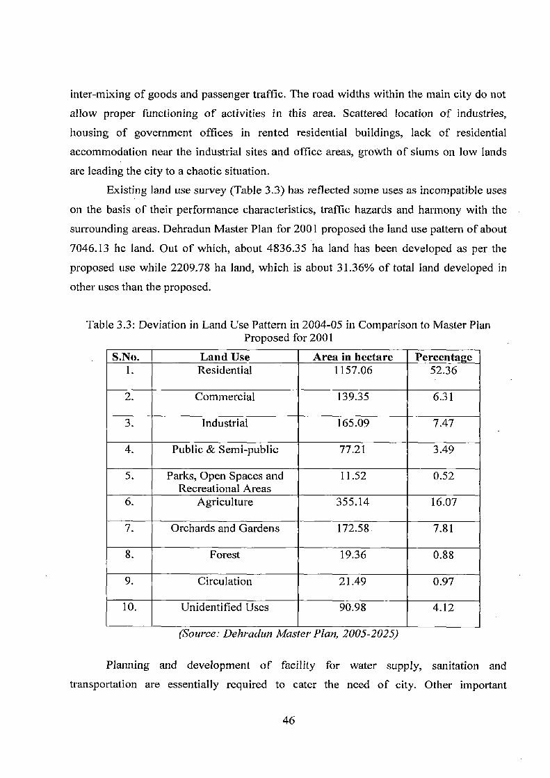
inter-mixing of goods and passenger traffic. The road widths within the main city do not

allow proper functioning of activities in this area. Scattered location of industries,

housing of government offices in rented residential buildings, lack of residential

accommodation near the industrial sites and office areas, growth of slums on low lands

are leading the city to a chaotic situation.

Existing land use survey (Table 3.3) has reflected some uses as incompatible uses

on the basis of their performance characteristics, traffic hazards and harmony with the

surrounding areas. Dehradun Master Plan for 2001 proposed the land use pattern of about

7046.13 he land. Out of which, about 4836.35 ha land has been developed as per the

proposed use while 2209.78 ha land, which is about 31.36% of total land developed in

other uses than the proposed.

Table 3.3: Deviation in Land Use Pattern in 2004-05 in Comparison to Master Plan Proposed for 2001

S.No. Land Use Area in hectare Percentage 1. Residential 1157.06 52.36

2. Commercial 139.35 6.31

3. Industrial 165.09 7.47

4. Public & Semi-public 77.21 3.49

5. Parks, Open Spaces and Recreational Areas

11.52 0.52

6. Agriculture 355.14 16.07

7. Orchards and Gardens 172.58 7.81

8. Forest 19.36 0.88

9. Circulation 21.49 0.97

10. Unidentified Uses 90.98 4.12

(Source: Dehradun Master Plan, 2005-2025)

Planning and development of facility for water supply, sanitation and

transportation are essentially required to cater the need of city. Other important

infrastructure facilities, which require careful study and attention for finding proper

solution in the present context, are parks, playground, parking space, drainage etc. for

aesthetical value of the city.

3.7 Population Characteristics

The population of Dehradun was 2,100 in 1817. During 1981-91, its population has

increased from 2,11,838 to 2,70,159. Taking this figure on an average, everyday 17

persons were assumed to be added to Dehradun Municipal Board population during last

decade. The growth at this rate, population predicted for Dehradun Municipal Board to

4,20,271 by the year 2011. While population of Dehradun Municipal Corporation reached

to 4,26,674 in 2001 census itself. The following table 3.4 shows the absolute figures of

population; increase of population and the percentage increase for each decade from

1901-2001 for Dehradun Municipal Area.

Dehradun is the largest and capital city of Uttaranchal State. During the census

year 1931, the population figure showed a decrease due to the outbreak of Plague. The

migration of people from west Punjab after the partition in the late 40's was the main

reason for the sudden increase in population (95.52 %). Since early 60's, the

establishments of many government agencies, prestigious research and educational

institutions and public schools have increased the population.

Table 3.4: Population Decadal Growth in Dehradun Municipal Area (1901- 2001)

Year Population Decadal Variation % age Decadal Growth

1901 30,995 ---

1911 42,568 + 11,573 +37.34

1921 50,858 + 8,290 + 19.47

1931 43,206 - 7,652 - 15.05

47

1941. 59,535 + 16,329 + 37.79

1951 1,16,404 +56,869 +95.52

1961 1,29,764 + 13,360 + 11.48

1971 1,69,827 + 40,063 + 30.87

1981 2,11,416 +41,589 +29.86

1991 2,70,159 +58,743 +27.78

2001 4,26,674 + 156,515 + 57.93

(Source: Census of hidia)

3.8 Socio-Economic Profile

Density Pattern

A study of density enables us to understand various aspects such as intensity of the use of

urban land, problem of overcrowding arising out of congestion and high occupancy rate,

adequacy and inadequacy of open space etc. Gross density within Dehradun Municipal

area is 7,109 persons/km2 according to 2001 census. Presently the average population

density of Dehradun Municipal area 133 persons per hectare.

Housing

Housing areas, which cover large portion of an urban settlement, influence the quality of

urban life, which in turn attacks, the efficiency of the settlements. The main housing

areas are Govindpur, Rest Camp, Dharampur, Dalanwala, Karanpur, Rajpur, and

relatively new colonies like Satya Bihar, Rajendra Nagar etc. Though in the localities like

Jhanda Mohalla, Dandipur, Dhamawala, Balliwala, Kishanpur etc., most of the housing

areas especially in the central core of the city have zigzag narrow roads, which are

difficult to be widened, and there is a general lack of parks and open spaces. The

relatively new housing areas are in the form of developed colonies which are located

along Haridwar Road, Mussoorie Road and Chakrata Road. The areas beyond Bindal

River are relatively better planned like Vasant Vihar.

Housing Shortage

According to 1971 Census figures, the total number of housing shortage within Dehradun

area was 10605, which decreases to 7371 persons in 1981 Census and 880 in 1991

Census (Table 3.5). While, housing shortage increases to 3288 in 2001 Census. There are

1.4 households per residential house, i.e. more than one family is living in one house,

which implies high occupancy rate. Household size while related to number of habitable

rooms gives an idea about occupancy ratio and the degree of congestion. It is helpful in

estimating future housing requirements of the city. On an average, there are 5

members/household.

Table 3.5: Housing Shortage and Occupancy Rate in Dehradun Area (1971-2001) Year Household Size Housing Shortage Occupancy rate

1971 5.34 10605 0.74

1981 5.22 7371 0.87

1991 5.10 880 0.98

2001 5.11 3288 0.97

(Source: Dehradun Master Plan 2005-2025)

49

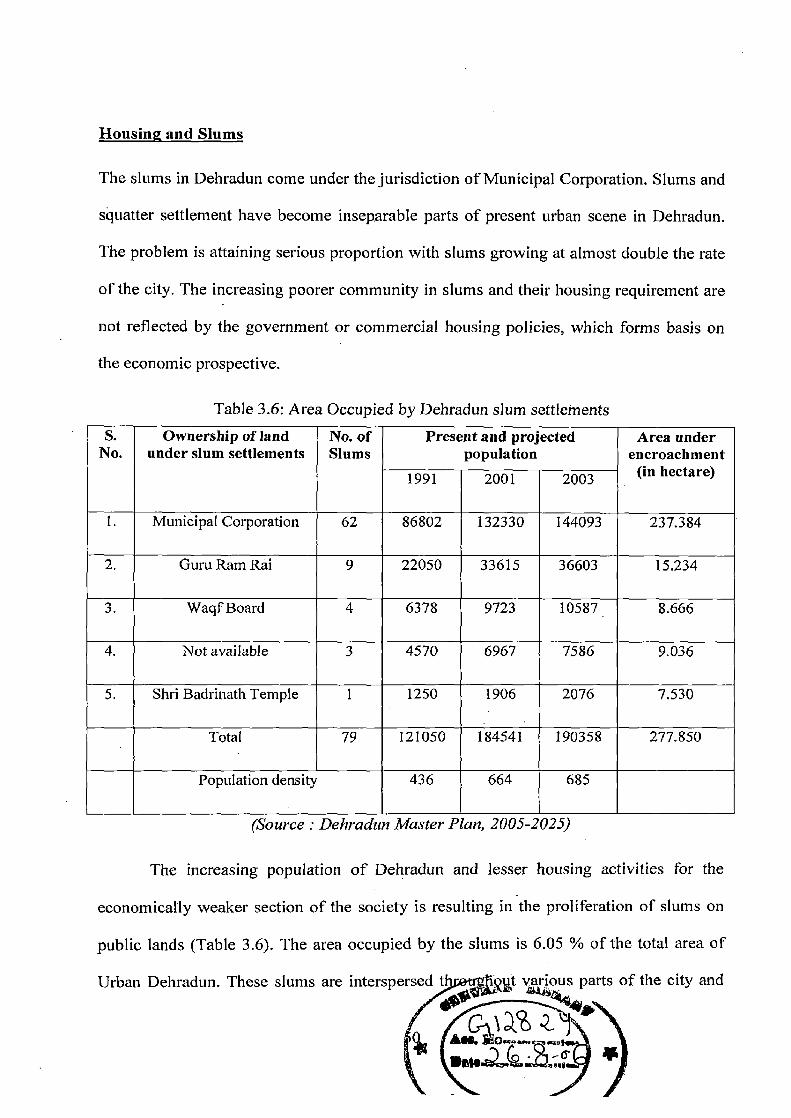
Housing and Slums

The slums in Dehradun come under the jurisdiction of Municipal Corporation. Slums and

squatter settlement have become inseparable parts of present urban scene in Dehradun.

The problem is attaining serious proportion with slums growing at almost double the rate

of the city. The increasing poorer community in slums and their housing requirement are

not reflected by the government or commercial housing policies, which forms basis on

the economic prospective.

Table 3.6: Area Occupied by Dehradun slum settlements S.

No. Ownership of land

under slum settlements No. of Slums

Present and projected population

Area under encroachment

(in hectare) 1991 2001 2003

1. Municipal Corporation 62 86802 132330 144093 237.384

2. Guru Ram Rai 9 22050 33615 36603 15.234

3. Waqf Board 4 6378 9723 10587 8.666

4. Not available 3 4570 6967 7586 9.036

5. Shri Badrinath Temple 1 1250 1906 2076 7.530

Total 79 121050 184541 190358 277.850

Population density 436 664 685

(Source : Dehradun Master Plan, 2005-2025)

The increasing population of Dehradun and lesser housing activities for the

economically weaker section of the society is resulting in the proliferation of slums on

public lands (Table 3.6). The area occupied by the slums is 6.05 % of the total area of

Urban Dehradun. These slums are interspersed utrtiout various parts of the city and

have grown mostly on the beds of Bindal river and other small seasonal streams, low

lying areas and vacant parts of the city. Insanitary conditions, lack of drainage, water

supply, paved streets and poor lighting facilities are the major problems prevailing in the

slums

51

CHAPTER FOUR BASIC GIS CONCEPT

4.0 GIS and Decision Making GIS can be defined as a computerized system that deals with spatial data in terms

of their collection, storage, management, retrieval, conversion, analysis, modeling, and

display/output. It evolved as means of assembling and analyzing diverse spatial data. The

development of GIS is the result linking parallel developments of several other spatial

data processing disciplines, such as cartography, computer aided design, remote sensing

technology, surveying and. photogrammetry. Due to increasing complexity of the real

world situations, more challenges emerge in knowing about the precious earth, and also

in planning and decision making processes. Today, GIS is considered as an important

tool in planning and decision-making. It has been found applied in many fields, such as

cadastral mapping, land use planning, forestry, wildlife management, infrastructure

planning, zoning, military, environmental monitoring, network planning, facility

selecting, including socio-economic applications (taxation, census, marketing, health

planning).

The success with which a GIS can be used is determined by several factors

that can be grouped as follows:

The Dataset — We cannot use the data if we do not have. Getting the relevant

data is important for an efficient GIS and the most cost effective data collection would be

to collect only the data we need. The optimum data quality is the minimum level of

quality that can be satisfactorily used for intended purpose.

Data Organization — Data, is of no value unless the right data can be in the

right place at the right time.

The Model — A good model is the simplest model that correctly and

consistently predicts the behavior of the real world for the phenomena of interest.

The Criteria — The criteria used should be such that is understandable to a

same level by all involved, such as analyst, decision-makers, other stakeholders, etc.

52

4.1 GIS Components A GIS is comprised of hardware, software, data, humans, and a set of

organizational protocols. These components must be well integrated for effective use of

GIS, and the development and integration of these components is an iterative, ongoing

process. The selection and purchase of hardware and software is often the easiest and

quickest step in the development of a GIS. Data collection and organization, personnel

development, and the establishment of protocols for GIS use are often more difficult and

time-consuming endeavors.

4.1.1 The Hardware A fast computer, large data storage capacities, and a high-quality, large

display form the hardware foundation of most GIS (Fig. 4.1). A fast computer is required

because spatial analyses are often applied over large areas and/or at high spatial

resolutions. Calculations often have to be repeated over tens of millions of times,

corresponding to each space we are analyzing in our geographical analysis. Even simple

operations may take substantial time if sufficient computing capabilities are not present,

and complex operations can be unbearably long-running. While advances in computing

technology during the 1990s have substantially reduced the time required for most spatial

analyses, computation times are still unacceptably long for a few applications.

While most computers and other hardware used in GIS are general purpose

and adaptable for a wide range of tasks, there are also specialized hardware components

that are specifically designed for use with spatial data. Many non-GIS endeavors require

the entry of large data volumes, including inventory control in large markets, parcel

delivery, and bank transactions. However, GIS is unique in the volume of coordinate data

that must be entered.

4.1.2 The Software GIS software provides the tools to manage, analyze, and effectively display

and disseminate, spatial data and spatial information. GIS by necessity involves the

collection and manipulation of the coordinates we use to specify location. We must

collect qualitative or quantitative information on the non-spatial attributes of our

geographic features of interest. We need tools to view and edit these data, manipulate

53

Coordinate and text input Large, high High-quality hard-

devices copy graphic and text resolution output devices

Display

Rapid acces Digital mass storage media

High-speed

Computer omputer

Storage

output

Network and web data communication

Figure 4.1 GIS are typically used with a number of general purpose and specialized

hardware component.

them to generate and extract the information we require, and produce the materials to communicate the information we have developed. GIS software provides the specific

tools for some or all of these tasks.

There are many public domain and commercially available GIS software.

packages, and many of the commercial packages originated at academic or government-

funded research laboratories. The Environmental Systems Research Institute (ESRI) line

of products, including Arc/Info, is a good example. Much of the foundation for Arc/Info

was developed during the 1960s and 1970s at Harvard University in the Laboratory of Computer Graphics and Spatial Analysis. Alumni from Harvard carried these concepts

with them to Redlands, California when forming ESRI, and included them in their commercial products.

The function commonly provided by GIS software are:

Data entry Analysis manual coordinate capture spatial query

attribute capture attribute query digital coordinate capture interpolation data import connectivity Editing proximity

54

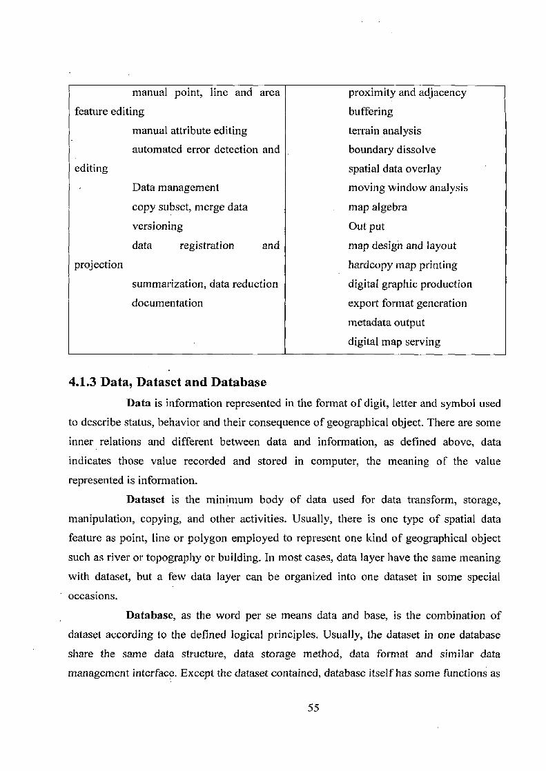
manual point, line and area

feature editing

manual attribute editing

automated error detection and

editing

Data management

copy subset, merge data

versioning

data registration and

projection

summarization, data reduction

documentation

proximity and adjacency

buffering

terrain analysis

boundary dissolve

spatial data overlay

moving window analysis

map algebra

Out put

map design and layout

hardcopy map printing

digital graphic production

export format generation

metadata output

digital map serving

4.1.3 Data, Dataset and Database Data is information represented in the format of digit, letter and symbol used

to describe status, behavior and their consequence of geographical object. There are some

inner relations and different between data and information, as defined above, data

indicates those value recorded and stored in computer, the meaning of the value

represented is information.

Dataset is the minimum body of data used for data transform, storage,

manipulation, copying, and other activities. Usually, there is one type of spatial data

feature as point, line or polygon employed to represent one kind of geographical object

such as river or topography or building. In most cases, data layer have the same meaning

with dataset, but a few data layer can be organized into one dataset in some special

occasions.

Database, as the word per se means data and base, is the combination of

dataset according to the defined logical principles. Usually, the dataset in one database

share the same data structure, data storage method, data format and similar data

management interface. Except the dataset contained, database itself has some functions as

55

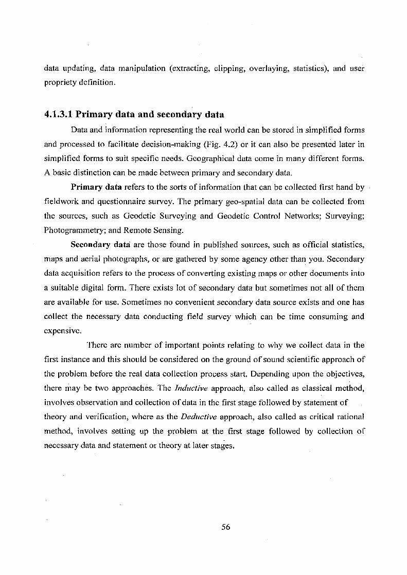
data updating, data manipulation (extracting, clipping, overlaying, statistics), and user

propriety definition.

4.1.3.1 Primary data and secondary data Data and information representing the real world can be stored in simplified forms

and processed to facilitate decision-making (Fig. 4.2) or it can also be presented later in

simplified forms to suit specific needs. Geographical data come in many different forms.

A basic distinction can be made between primary and secondary data.

Primary data refers to the sorts of information that can be collected first hand by

fieldwork and questionnaire survey. The primary geo-spatial data can be collected from

the sources, such as Geodetic Surveying and Geodetic Control Networks; Surveying;

Photogrammetry; and Remote Sensing.

Secondary data are those found in published sources, such as official statistics,

maps and aerial photographs, or are gathered by some agency other than you. Secondary

data acquisition refers to the process of converting existing maps or other documents into

a suitable digital form. There exists lot of secondary data but sometimes not all of them

are available for use. Sometimes no convenient secondary data source exists and one has

collect the necessary data conducting field survey which can be time consuming and

expensive.

There are number of important points relating to why we collect data in the

first instance and this should be considered on the ground of sound scientific approach of

the problem before the real data collection process start. Depending upon the objectives,

there may be two approaches. The Inductive approach, also called as classical method,

involves observation and collection of data in the first stage followed by statement of

theory and verification, where as the Deductive approach, also called as critical rational

method, involves setting up the problem at the first stage followed by collection of

necessary data and statement or theory at later stages.

56

DECISION

STRATEGIC LEVEL

COLLECTION DAT MANAGING

and of

Figure 4.2. A Decision Making Pyramid. (Bernhardsen, 1992 after Grossman, 1983)

4.1.3.2 Geospatial Data Geo-spatial data are also called as Geographical data, Geographic data,

Geographic Information, GIS data, Earth-sciences data or Geo-scientific data, and

spatial data. Geographical data are information that identifies the geographic Iocation

and characteristics of natural or constructed features and boundaries on the earth. The

main difference between geographical data and other data is that the later helps answer

question like, what? or where? as the former answers both what? and where? It is because

that it contains Geometric or Spatial data for spatial elements and Attribute data (Figure

Spatial data is used to describe the location of geographical object, and attribute

data describe the fundamental characteristics of the phenomena involved. For instance,

the objects classified as buildings may have a number stores attributes with legitimate

values of I to 10, etc. Attribute data can in turn be sub-divided into Qualitative and

Quantitative data.

57

Historically, several terms have been used to describe the data in a GIS database,

among them features, objects, or entities. The term feature derives from cartography and

is commonly used to identify ' features shown on a map," while entity and object are

terms from computer science used to identify the elements in a database. The normal

dictionary definitions of these terms are: Object: a thing that can be seen or touched; material thing that occupies space

characterized by type, attribute, geometry, relation and quality.

Entity: a thing that has definite, individual existence in reality (e.g. house number) Feature: the make, shape, form or appearance of a person or thing (e.g. circle, linear)

GEOGRAPHICAL DATA

GEOMETRI A TRIBUTE

;;-Geometry _______ Oualitativ

/1 \ __________ _________ Oualitativ

Point Line Area

Ordinal Ratio

Interval

Fig. 4.3. Geographical Data divided into Geometric and AttributeData (Bernhardsen, 1992)

4.1.3.3 Data output: Data output is the operation of presenting the results of data manipulation in a

form that is understandable to a user or in a form that allows data transfer to another computer system. The basic output formats from a GIS are hard copy, soft copy, am)

electronic outputs (Fig. 3.6). Maps and historical tabulations are output in the hard copy

format by the help of hard copy output devices such as dot matrix pi-inters, ink jet plotters, pen plotters, matrix camera, color laser printer, etc.

58

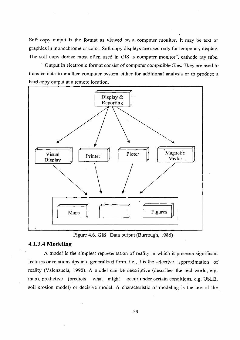
Soft copy output is the format as viewed on a computer monitor. It may be text or

graphics in monochrome or color. Soft copy displays are used only for temporary display.

The soft copy device most often used in GIS is computer monitor", cathode ray tube.

Output In electronic format consist of computer compatible files. They are used to

transfer data to another computer system either for additional analysis or to produce a

hard copy output at a remote location.

Maps Figures

Figure 4.6. GIS Data output (Burrough, 1986)

4.1.3.4 Modeling A model is the simplest representation of reality in which it presents significant

features or relationships in a generalized form, i.e., it is the selective approximation of

reality (Valenzuela, 1990). A model can be descriptive (describes the real world, e.g.

map), predictive (predicts what might occur under certain conditions, e.g. USLE,

soil erosion model) or decisive model. A characteristic of modeling is the use of the

59

attribute data, i.e., each map has one or several tables that include a specific single datum

(attribute) of the pertinent map.

4.1.3.5 Spatial Elements Spatial objects in the real world can be thought of as occurring as four easily

identifiable types: Points, Lines, Areas, and Surfaces (Figure 4.4). Collectively, they can

represent most of the tangible natural and human phenomena that we encounter on an

everyday basis. In general, points, lines, and areas are used to explicitly represent real-

world objects, where as surfaces are mostly used for volumetric representation, such as to

represent hills, valleys. Thus, all data can be considered to be explicitly spatial.

Point features are spatial phenomena each of which occurs at one location in

space. Each feature is said to be discrete in that it can occupy only a given point in space

at any time and considered to have no spatial dimension — no width or length. Example of

such feature would be a house or a village. But a village can be represented by point

feature or area feature as well depending upon the resolution of data.

Line features are conceptualized as occupying only a single dimension in

coordinate space. They are represented as the series of single coordinates connected to

each other. Roads, rivers, are the examples of linear features. The resolution or scale of

given dataset once again places a fundamental limitation to conceive them as having any

width. Linear features, unlike point features, allow us to measure their spatial

extent/length.

Area features have two dimensions both length and width dimensions. Area

is composed of series of lines that begin and end at the same location. We can describe

their shapes and orientations, and the amount of territory occupied as well. In database,

the term polygon is often used instead of area. Again, physical size in relation to the scale

determines whether an object is represented by an area or by a point.

It is often that area is divided into regular squares or rectangles so that all

objects are described in terms of areas. This entire data structure is called ;a grid. Each

square or rectangular is known as a cell and represents a uniform value. Adding the

dimension of height to area features allows us to observe and record the existence of

Surfaces. Surfaces have three dimensions — length, width, and height. For instance, hills,

valleys, and ridges can be described by citing their locations, amount of area they occupy,

how they are oriented, and by noting their heights.

Sp t1AI Elomcnts and Repro»enta

P4lnt IJI Am surface rupmenLLiMr represetk#ton represenaf on rtprasentatlorf

t i ritra ! 1 !' M

In t1°~ tit

hlgar n itp~ e

ti►wv srrr=aan r! density

cr~arrrk~ spill ~i~ Y r $

newsLidi~! n

river _ rI1Iiiu

/4 t river Aete•9ed W vualer

Fig 4.4 Spatial Elements and Representation (DeMers, 2000)

4.2 Basic data Models Spatial elements can be represented in two models: Vector and Raster/Grid

(Figure 4.5). In the vector model, the spatial locations of features are defined on the basis

of coordinate pairs. These can be discrete, taking the form of points (POINT or NODE

data); linked together to form discrete sections of line (ARC or LINE data); linked

together to form closed boundaries encompassing an area (AREA or POLYGON data).

Attribute data pertaining to the individual spatial features is maintained in an external

database. The data model used by the software, like Arc/Info, AreView is Vector model.

In raster model, one or group of cell/grid/pixel depending upon the grid

resolution represents spatial elements. Most of raster models adhere strictly to a single

attribute per cell structure although some raster models support the assignment of values

to multiple attributes per discrete cell.

vii

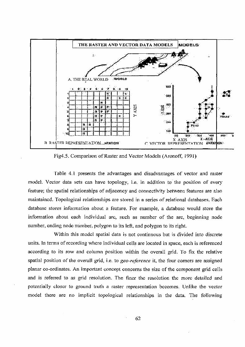
THE RASTER AND VECTOR DATA MODELS INUOO L

A. THE REAL WORLD f

i +ii.:

X AXIS C. VECTOR RRPRERF.NTATIfIN R RASTFR REPRESENTATION _l TA1100:

Fig4.5. Comparison of Raster and Vector Models (Aronoff, 1991)

Table 4.1 presents the advantages and disadvantages of vector and raster

model. Vector data sets can have topology, i.e. in addition to the position of every

feature; the spatial relationships of adjacency and connectivity between features are also

maintained. Topological relationships are stored in a series of relational databases. Each

database stores information about a feature. For example, a database would store the

information about each individual arc, such as number of the arc, beginning node

number, ending node number, polygon to its left, and polygon to its right.

Within this model spatial data is not continuous but is divided into discrete

units. In terms of recording where individual cells are located in space, each is referenced

according to its row and column position within the overall grid. To fix the relative

spatial position of the overall grid, i.e. to geo-reference it, the four corners are assigned

planar co-ordinates. An important concept concerns the size of the component grid cells

and is referred to as grid resolution. The finer the resolution the more detailed and

potentially closer to ground truth a raster representation becomes. Unlike the vector

model there are no implicit topological relationships in the data. The following

information should always be recorded when assembling, compiling and utilizing raster

data:

Grid size (number of rows and columns)

Grid resolution

Geo-referencing information, e.g. corner co-ordinate, source projection

Table 4.1. Vector vs Raster Data Model

Vector s i jT

Raster S. Y S s

Advantages

Compact data structure (less data volume) Simple data structure

Efficient topology encoding, good for Easier and efficient overlay operation

operations, such as network analysis High spatial variability is efficiently

Better graphics forprecise expression represented

Efficient in manipulation and enhancement

of digital images

Disadvantages

Complex data structure Large data volume (data compression

Implementation of overlay operations is technique can overcome this problem)

difficult Difficult to represent topological

Inefficient representation of high spatial relationships

variability Less aesthetic graphic output

Not effective for manipulation and Not good for some operations, such as

enhancement of digital images network analysis

4.3 Data Analysis and Modelling The most significant characteristics of GIS are the provision of the

capabilities for data analysis and spatial modeling. These functions use the spatial and

non-spatial attribute data of the GIS database to answer questions about the real world.

The database in GIS is the model of the real world that can be used to simulate certain

aspects of reality. A model may be represented in words, m mathematical equations or as

a set of spatial relationships displayed on a map. The general problem in data analysis

is: users query -* database link -X• output.

63

The user has particular specification, constraints or query. The database

contains information in the form of maps that can be used to answer the users query. All

that is necessary is to establish a link between database and output that will provide the

answer the form of a map, table, or figure. The link is any function that can be used to

convert data from one or more inputmaps, into an output.

4.3.1 Analysis; Functions: The power of GIS lies in its ability to analyze spatial and attribute data together. A large

range of analysis procedure/ functions have been divided in to four categories: retrieval,

red classification and measurement overlay; Distance and connectivity; and

neighborhood.

4.3.2 Retrieval, Reclassification and Measurement Operations In these functions retrieval of both spatial and attribute data are made and

only attribute data are modified. Creation of new spatial elements is not made.

Retrieval operations: This involves the selective search and manipulation and output of

data. Retrieval operation includes the retrieval of data using:

- Geometric classification,

- Symbolic specifications,

- A name of code of an attribute,

- Conditional and logical statement.

Reclassification procedures: This procedure involves the operation that reassign

thematic values to the categories of a existing .map as a function of the initial value, the

position size or shape of the spatial configuration associated with each category (for

instance a soil map reclassified into erodibility map). In raster based GIS, numerical

values are often used for indicate classes. A cell might be assigned the value to indicate

classes. Classification is done using simple data layers as well as with multiple data

layers as part of an overlay operation.

Measurement operations: Spatial data measurement includes: calculation of

distance, length of lines, areas and perimeter of polygons, and volumes. Measurements

involving points are: distance from a point to a point, a line, a polygon, enumeration of

the total number as well as the enumeration of points falling within the polygon.

4.3.3 Overlay Operation Overlay operation creates a new data set containing new polygons formed

from intersection of the boundaries of the two or more sets of separate polygonal layers.

There are two common overlay operations: arithmetic and logical. Arithmetic overlay

includes operation such as addition, subtraction, division and multiplication of each

value in a data layer by the value in the corresponding location in the second data layer.

Logical overlay involves the selection of an area where a set of conditions are satisfied.

The logical overlay operation is done using the rules of Boolean logic. Boolean algebra

uses the operations of AND, OR, XOR, NOT to see whether a particular condition is

true or false .

4.3.4 Neighborhood Operation This involves the. creation of new data based on the consideration of roving

window of neighboring points about selected target locations. They evaluate

characteristics of an area surrounding spatial location. In all neighborhood operations, it

is necessary to indicate one or more target locations, the neighborhood considering each

target and the type of function to be executed The typical neighborhood operation in

most GIS's are; search topographic functions and interpolation.

Search functions:

This constitutes one of the most commonly use neighborhood function. Value

assignment to each target feature is made on the basis of some characteristics of its

neighborhood. The basic parameters required to be defined in a neighbor search are

targets, the neighborhood, and the functions to be applied to the neighborhood to generate

neighborhood value. The search area is usually square, rectangular or circular whose size

is determine by the analyst.

65

Topographic functions:

Topography refers to surface characteristics such as the slope, relief and

form of the area. The topography of a surface can be presented in a digital elevation

model (DEM). DEM represents a topographic surface terms of a set of elevation values

measured at a finite number, o points, and contains terrain features of geo

morphological importance such as valleys and ridges, peaks and pits (Valenzuela 1990).

Topographic functions are used to calculate values that describe the topography of an

area. The most common transformations working with elevation data are the slope

and aspect - slope face direction.

Interpolation:

This procedure predicts unknown values at any sampled sites using the known

values of existing observations neighboring locations. Point and aerial interpolation

involve variety of methods such as polynomial regression, kriging , splines , trend

surface analysis, Fourier- series and moving averages (Burrough, 1986; Valenzuela,

1990). The quality of interpolation results is a function of the precision, accuracy,

number and distribution of the known points used in the, calculation and the manner in

which the mathematical function models reality. The unknown values are the n

calculated according to this function.

4.3.5 Connectivity Functions Connectivity operation is those that estimate values (quantitative or

qualitative) by accumulating them over the area that is being traversed. These

operations require the specification of the manner in which the spatial elements arc

interconnected, specification of the rules that control the movements allowed along

the spatial elements and the unit of measurements. Connectivity functions are

grouped in to contiguity, proximity, and network and spread operation.

Contiguity:

Contiguity measures characterized spatial units that are connected. A contiguous

area is formed by a group of spatial units that have one or more common characteristics

and constitute a unit. Common measures of contiguity are the size of the contiguous

area and the shortest and the longest straight line distance across the area.

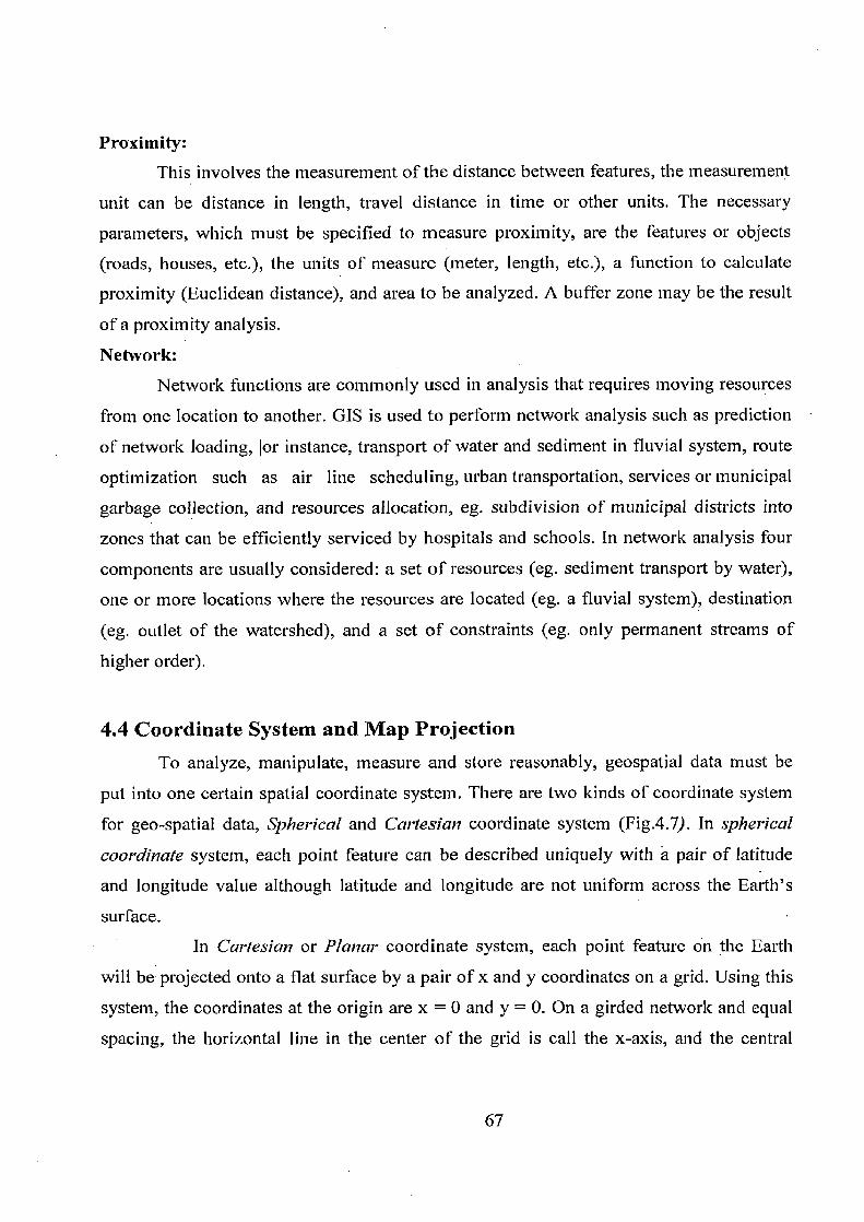
Proximity: This involves the measurement of the distance between features, the measurement

unit can be distance in length, travel distance in time or other units. The necessary

parameters, which must be specified to measure proximity, are the features or objects

(roads, houses, etc.), the units of measure (meter, length, etc.), a function to calculate

proximity (Euclidean distance), and area to be analyzed. A buffer zone may be the result

of a proximity analysis.

Network: Network functions are commonly used in analysis that requires moving resources

from one location to another. GIS is used to perform network analysis such as prediction

of network loading, bor instance, transport of water and sediment in fluvial system, route

optimization such as air line scheduling, urban transportation, services or municipal

garbage collection, and resources allocation, eg. subdivision of municipal districts into

zones that can be efficiently serviced by hospitals and schools. In network analysis four

components are usually considered: a set of resources (eg. sediment transport by water),

one or more locations where the resources are located (eg. a fluvial system), destination

(eg. outlet of the watershed), and a set of constraints (eg. only permanent streams of

higher order).

4.4 Coordinate System and Map Projection To analyze, manipulate, measure and store reasonably, geospatial data must be

put into one certain spatial coordinate system. There are two kinds of coordinate system

for geo-spatial data, Spherical and Cartesian coordinate system (Fig.4.7). In spherical

coordinate system, each point feature can be described uniquely with a pair of latitude

and longitude value although latitude and longitude are not uniform across the Earth's

surface.

In Cartesian or Planar coordinate system, each point feature on the Earth

will be projected onto a flat surface by a pair of x and y coordinates on a grid. Using this

system, the coordinates at the origin are x = 0 and y = 0. On a girded network and equal

spacing, the horizontal line in the center of the grid is call the x-axis, and the central

Origin

vertical is call y-axis. Therefore, coordinate value; measures of length, angle and area are

uniform in this coordinate system.

0

• y axi g d} 1 q, ~ p~~ L

w

55°N 500E

fl-I'-.-f4.*2.'l- -ç' -• Ldtuth2 Latitude

1iEi IMlIgitltde

I(

IF

Fig. 4.7 Spherical and Cartesian Coordinate System

The main co-ordinate reference systems for describing a geographic position

mathematically are geodetic reference systems and map projections. Geodetic reference

systems are used for describing the figure of the Earth and positions on it: ellipsoids (and

the sphere) are used for describing the horizontal position. The shape of an ellipsoid, is

defined by a Semi-major and Semi-minor axis, and there are several spheroids available

for use in different parts of the world. Each of them assume different semi-major and

semi-minor axis. Geoids are the gravity related model for referencing the elevation.

Geodetic reference systems have a datum, which defines the position of the spheroid

relative to center of the earth. It defines the origin and orientation of latitude and

longitude lines. There are two types of datum. The latitude and longitude of a point, the

azimuth of a line from that point, and the two radii needed to define the geometric

reference surface that best approximates the surface of the earth in the region of the survey define horizontal datum. Vertical datum ensures that elevation and depth

measurements are held to a common vertical standard.

When we try to transform the location information on three-dimensional

earth surface onto a two-dimensional map, projection is needed. In other words, Map

projections are used to map the curved surface of an ellipsoid to a plane. This achieved

by transforming the values with mathematical expressions. There are three major

projection types, namely Planar (also know as Azimuthal), Conic, and Cylindrical

projections depending on the shape of the developable surface (Fig. 3.8).

Azimuthal projections, points are projected from the surface of the Earth to

the plane. A commonly used projection of this type is the stereographic conformal

projection. This type of projection includes Gnomonic, Stereographic, Orthographic,

Azimuthal Equal Area, Azimuthal Equidistant, and Globular projection. Planar or

Azimuthal Projections are used most often to map Polar Regions.

Conic projections result from conceptually transferring the earth's

coordinates onto a cone. This family of projection includes Simple Conic, Two-Standard

Parallel Conic, Lambert's Conformal, Albert's Equal Area, Conic Equidistant, Polyconic,

and Bonne Projection.

Cylindrical projections are a family of projections resulting from

conceptually transferring the earth's coordinates onto a cylinder. Cassini or Cassini-

Soldner, Gall's Cylindrical, Mercator, Lambert's Cylindrical Equal-Area, and Transverse

Mercator projection. Universal Transverse Mercator (UTM) projection system is one of

the commonly used projection systems.

The two most commonly used projection system are polyconic and world

geodetic system 1984 (WGS 84). These coordinate systems can successfully be used in

the context of GMS countries.

4.5 GIS and Decision Support System The successful operational applications of GIS require institutional setting

and must support the management of resources or some problem solving processes.

Furthermore, it must exist within an organizational setting that is capable of providing it

with proper support.

The recent development of decision support system (DSS) brought a new concept of

integrating GIS and resource models into a tightly-coupled system in that the systems

more likely to be used to aid decision making. Out of the combination of DSS and GIS

emerges an entirely new system called spatial decision support system (SDSS). SDSSs

are new classes of computer systems that combine the technologies of GISs and DSSs to

aid decision makers with problems that have spatial dimension. Fig. 4.8 presents the

melding of GIS and DSS into SDSS.

SDSSs are oriented towards the decision makers and offers one unifying

framework for integrating GIS and DSS including the models within the DSS, i.e, the

SDSS framework offers a means to increase the utility of both GISs and DSSs to

assist decision makers.

Figure 4.8 SDSS as Combination of GIS & DSS (Michael et al,1993)

4.6 Remote Sensing Concept

Remote sensing is a technology for sampling electromagnetic radiation to acquire and

interpret non-immediate geospatial data to extract information about features, objects,

and classes on the Earth's land surface, oceans, and atmosphere. Generally, remote

sensing refers to the activities of recording/observing/perceiving (sensing) objects or

70

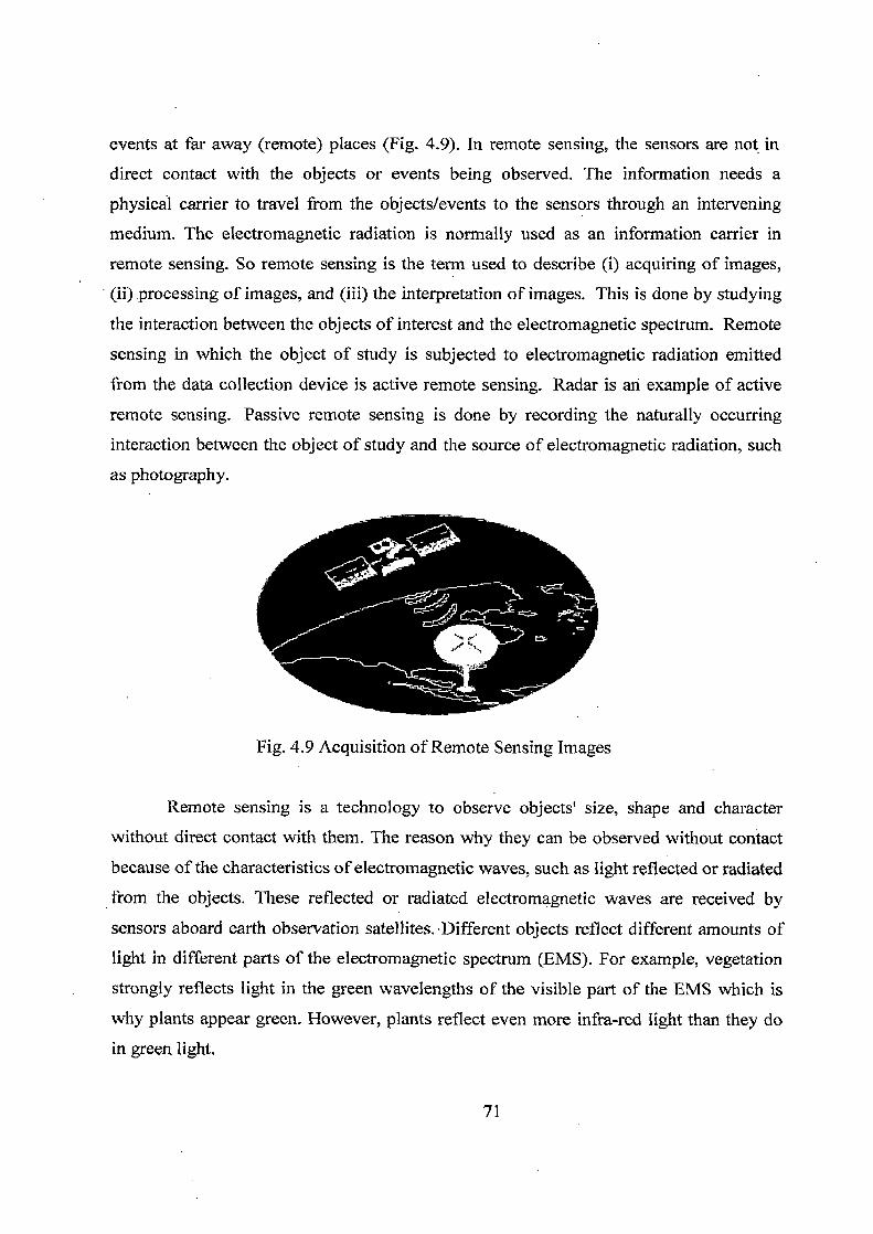
events at far away (remote) places (Fig. 4.9). In remote sensing, the sensors are not in direct contact with the objects or events being observed. The information needs a

physical carrier to travel from the objects/events to the sensors through an intervening medium. The electromagnetic radiation is normally used as an information carrier in remote sensing. So remote sensing is the term used to describe (i) acquiring of images, (ii) .processing of images, and (iii) the interpretation of images. This is done by studying

the interaction between the objects of interest and the electromagnetic spectrum. Remote

sensing in which the object of study is subjected to electromagnetic radiation emitted from the data collection device is active remote sensing. Radar is an example of active

remote sensing. Passive remote sensing is done by recording the naturally occurring interaction between the object of study and the source of electromagnetic radiation, such as photography.

Fig. 4.9 Acquisition of Remote Sensing Images

Remote sensing is a technology to observe objects' size, shape and character without direct contact with them. The reason why they can be observed without contact

because of the characteristics of electromagnetic waves, such as light reflected or radiated

from the objects. These reflected or radiated electromagnetic waves are received by sensors aboard earth observation satellites. , Different objects reflect different amounts of light in different parts of the electromagnetic spectrum (EMS). For example, vegetation

strongly reflects light in the green wavelengths of the visible part of the EMS which is

why plants appear green. However, plants reflect even more infra-red light than they do in green light.

71

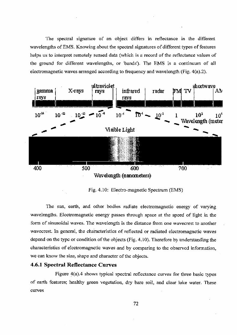
400 500 600 700

The spectral signature of an object differs in reflectance in the different

wavelengths of EMS. Knowing about the spectral signatures of different types of features

helps us to interpret remotely sensed data (which is a record of the reflectance values of the ground for different wavelengths, or 'bands'). The EMS is a continuum of all

electromagnetic waves arranged according to frequency and wavelength (Fig. 4(a).2).

ultraviolet shortwave gamma X-rays rays infrared radar 1FM TV I Al r s r s

II

10"i¢ 10'11 10 -"' 10 1 10 101 1 10, 101 - Wavelength (meter

4,0 'r V sibl a Light

Wavelength (nanometers)

Fig. 4.10: Electro-magnetic Spectrum (EMS)

The sun, earth, and other bodies radiate electromagnetic energy of varying

wavelengths. Electromagnetic energy passes through space at the speed of light in the

form of sinusoidal waves. The wavelength is the distance from one wavecrest to another

wavecrest. In general, the characteristics of reflected or radiated electromagnetic waves

depend on the type or condition of the objects (Fig. 4.10). Therefore by understanding the

characteristics of electromagnetic waves and by comparing to the observed information, we can know the size, shape and character of the objects.

4.6.1 Spectral Reflectance Curves Figure 4(a).4 shows typical spectral reflectance curves for three basic types

of earth features; healthy green vegetation, dry bare soil, and clear lake water. These curves

72

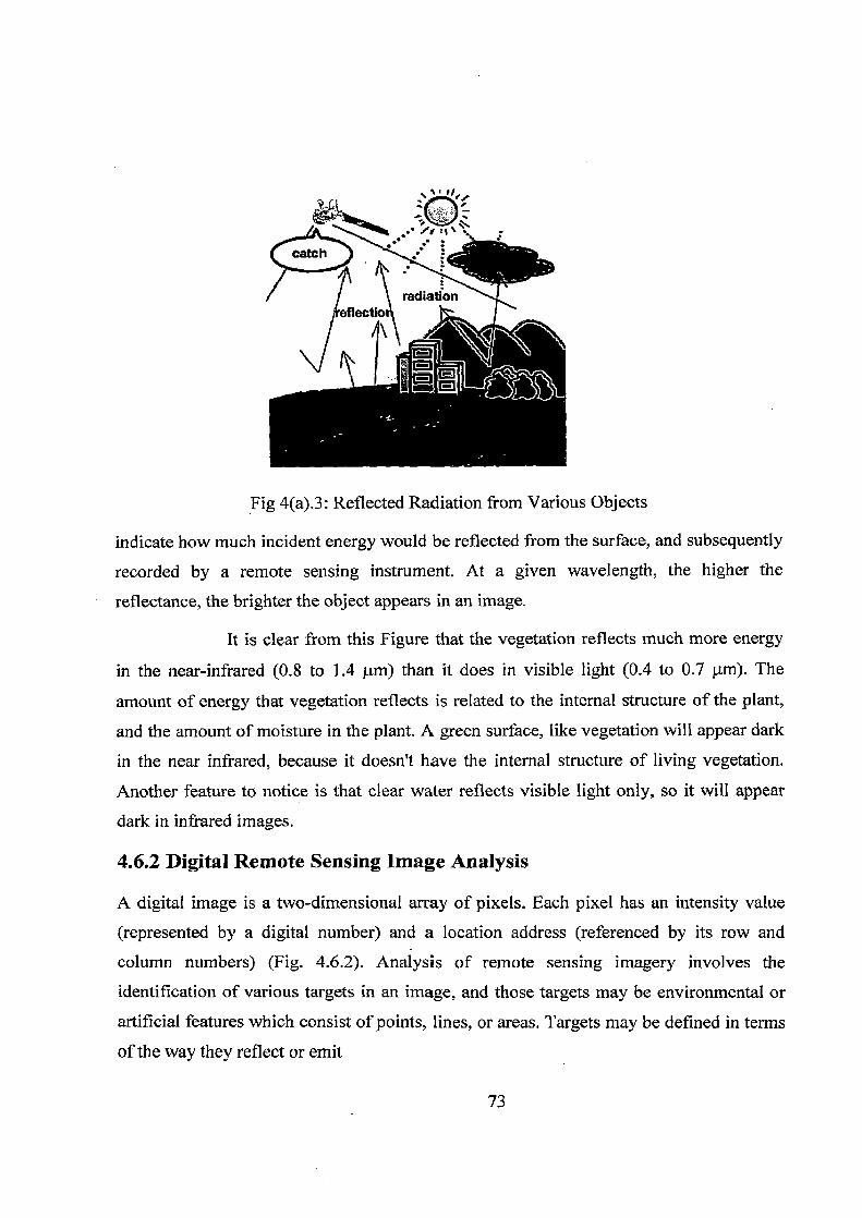
catch

Uectio

fr''' ;

radiation

Fig 4(a).3: Reflected Radiation from Various Objects

indicate how much incident energy would be reflected from the surface, and subsequently

recorded by a remote sensing instrument. At a given wavelength, the higher the

reflectance, the brighter the object appears in an image.

It is clear from this Figure that the vegetation reflects much more energy

in the near-infrared (0.8 to 1.4 }im) than it does in visible light (0.4 to 0.7 µm). The

amount of energy that vegetation reflects is related to the internal structure of the plant,

and the amount of moisture in the plant. A green surface, like vegetation will appear dark

in the near infrared, because it doesn't have the internal structure of living vegetation.

Another feature to notice is that clear water reflects visible light only, so it will appear

dark in infrared images.

4.6.2 Digital Remote Sensing Image Analysis

A digital image is a two-dimensional array of pixels. Each pixel has an intensity value (represented by a digital number) and a location address (referenced by its row and

column numbers) (Fig. 4.6.2). Analysis of remote sensing imagery involves the

identification of various targets in an image, and those targets may be environmental or

artificial features which consist of points, lines, or areas. Targets may be defined in terms

of the way they reflect or emit

73

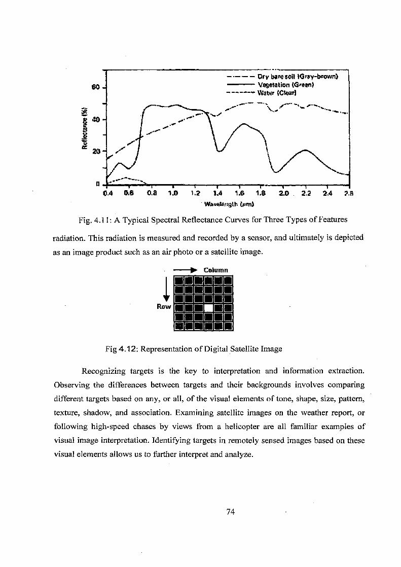
7

_ .— _ pry bare soil lGroy-brown) Vegetation (Green)

----4 Water CCk r3 1. ~ ~, ... ... r~+`. _ .-.

0.4 06 0.8 1.0 1,2 1.4 1.6 1.8 2.0 . 2.2 2.4 ?.E~ Wavalpngth (Nm~

Fig. 4.11: A Typical Spectral Reflectance Curves for Three Types of Features

radiation. This radiation is measured and recorded by a sensor, and ultimately is depicted

as an image product such as an air photo or a satellite image.

10 Column

Row

Fig 4.12: Representation of Digital Satellite Image

Recognizing targets is the key to interpretation and information extraction.

Observing the differences between targets and their backgrounds involves comparing

different targets based on any, or all, of the visual elements of tone, shape, size, pattern,

texture, shadow, and association. Examining satellite images on the weather report, or

following high-speed chases by views from a helicopter are all familiar examples of visual image interpretation. Identifying targets in remotely sensed images based on these

visual elements allows us to further interpret and analyze.

74

CHAPTER FIVE

WATER AVAILABILITY 5.0 General: In this chapter, a water balance will be set up. The purpose of the water balance is to

quantify the water availability in the watershed, Q available, today. The water availability is the amount of water supplied from natural processes, such as rainfall. Not all the

rainfall will become available since losses occur in the form of evapotranspiration.

The chosen watershed is the area that at present supplies the city with the majority of

its water supply. The amount of water coming from neighboring watersheds which

adds to Dehradun's water supply is also included in Q available, only small amounts of

water are at present taken from neighboring watersheds.

The estimated water availability will be compared to the total water

production for domestic and industrial use in Dehradun in chapter seven to see how

large proportion of the available water that is used at present. This will also indicate to

what extent the supplies can be increased to satisfy the demand by using water

available within the watershed as effectively as possible.

5.1 The Water Balance Equation The watershed can be viewed as a three dimensional piece of land, see Figure 5.1.

Based on geological and hydrological information of the area, the water inputs and

outputs can be defined and the water balance can be set up as the following: Water balance: Inputs = Outputs + changes in storage

P = AET + Qs,,,.ace + Qg,.o,,,,d ± AST (5.1)

5.1.1 Definition of Parameters in the Water Balance Precipitation (P) is the amount of rain that falls over the watershed. The rainfall is

assumed to be evenly distributed over the watershed. It is also assumed to be equal to

that measured at the New Forest Meteorological Observatory, which is located just outside the watershed Infiltration (I) affects the water balance on a monthly basis, since some of the infiltrated rainfall will add to the soil moisture storage (A ST) and some will add to the groundwater flow (Qgiou„d) after deep percolation. AST is positive in the water

- 75

balance equation when it adds to the actual evapotranspiration due to withdrawal from the soil moisture storage during soil moisture utilization and negative when it adds to

the soil moisture storage due to soil moisture recharge. The amount of water stored as

soil moisture varies in a cyclic way over a year. Per definition it can van" between the wilting point of the plants and field capacity' of the soil (Devi 1992). The differences

in stored amount are generally cancelled out over a year, so that the annual difference

becomes approximately zero, A ST = 0.

Surface water (Qsurface) within the watershed consists of the two seasonal

rivers, the Rispana and the Bindal river mentioned in chapter three. These are

supplied by water mainly from springs in the north of the watershed. Only the

northern pan of Rispana and the southern pan of Bindal river have a flow all year

round. The main pans of the rivers are dry and there is only a great amount of flow

during a few days of the monsoon season each year, following days of heavy rainfall

(Chopra 2003a).

Groundwater (Qgro,,nd) flow within the watershed follows the topography and

is in north-south direction The size of the aquifers is not estimated in the water

balance. It is assumed for the water balance study that the water divide is the same for

both surface water and groundwater.

Actual evapotranspiration of the watershed (A ET) is water that evaporates back to

the atmosphere either through direct evaporation or transpiration from plants. When

the soil is not at field capacity, the actual evapotranspiration will be less than the

potential evapotranspiration. The soil moisture content changes over the year

depending on rainfall, vegetation growth as well as on other factors.

5.1.2 Equation for Water Availability The purpose of the water balance is to estimate the water available in the watershed

due to rainfall. The water balance equation is as previously mentioned:

Q ground + Q sinface = P- AET f A ST (5.2)

The total water availability includes the water coming from neighboring watersheds.

The surface water supply from the Bindal River is such a source as well as

groundwater from 8 tube-wells. Hence the total water availability can be written:

Q available = Q ground + Q surface + Q neighbor =P- AET + A ST+ Q neighbor (5.3)

76

monsoon season each year, following days of heavy rainfall (Chopra 2003a).

Groundwater (Qground) flow within the watershed follows the topography and is in north-south direction according to the map in appendix 12.4. The size of the aquifers is not estimated in the water balance. It is assumed for the water balance study that the

water divide is the same for both surface water and groundwater. Actual evapotranspiration of the watershed (A ET) is water that evaporates back to the atmosphere either through direct evaporation or transpiration from plants. When

the soil is not at field capacity, the actual evapotranspiration will be less than the

potential evapotranspiration. The soil moisture content changes over the year depending on rainfall, vegetation growth as well as on other factors.

5.1.2 Equation for Water Availability The purpose of the water balance is to estimate the water available in the watershed

due to rainfall. The water balance equation is as previously mentioned:

Q ground + Q surface = P- AET ± A ST

(5.2)

The total water availability includes the water coming from neighboring watersheds.

The surface water supply from the Bindal River is such a source as well as

groundwater from 8 tube-wells. Hence the total water availability can be written: f

Q available = Q ground + Q surface + Q neighbor=P- AET ± A ST+ Q neighbor (5.3)

5.2 Areal Extent of Watershed The areal extent of the watershed, the city and the part of the city that is within the watershed were estimated from the map

Table 5.1 Showing Areal Extent

Area Estimated Area km2] Watershed 327

City boundary 114 City area within watershed 60

■ Watershed

■ City boundary

o City area within watershed

77

5.4 Evapotranspiration Evapotranspiration is the process where water evaporates back to the atmosphere as

vapor either through direct land evaporation or through the plants metabolic process called transpiration. The potential evapotranspiration (PET) is defined as "the -amount

of water that will be lost from a surface completely covered with vegetation if there is sufficient water in the soil at all times for the use of the vegetation" (Thorntwaite

1955). Hence, potential evapotranspiration assumes an infinite supply of water.

According to the water balance (Q ground + Q surface P - AET ± A ST), the

actual evapotranspiration (AET) needs to be estimated. Actual evapotranspiration is

dependent on the soil moisture and is less than or equal to the potential

evapotranspiration. When the soil is saturated with water, evapotranspiration proceeds

at the potential rate so the actual evapotranspiration equals the potential

evapotranspiration. As the soil moisture content decreases it becomes increasingly

difficult for water to be lost by evaporation or transpiration, since the suction pressure

of the soil increases (FAO, 2004). Therefore, the rate of actual evapotranspiration will

decrease as the soil moisture content decreases.

5.4.1 Estimation of Potential Evapotranspiration Potential evapotranspiration needs to be estimated as a first step in the estimation of

actual evapotranspiration, which can be achieved using data of meteorological variables. The variables affecting evaporation losses include (Garg 2000);

• Vapor pressure

• Wind speed

• Temperature

• Solar radiation.

The Penman Formula for Calculating Potential Evapotranspiration

In 1948, Penman developed a formula to calculate the evaporation from a free water

surface. It was a combination of the energy budget and the mass transfer method. In

1963 it was modified in a new publication by Penman to apply for the potential

evapotranspiration (PET) from vegetated areas (Shaw 1994). The equations used for the calculations are based on those given in Shaw (1994), which are the standard

equations used by the hydro-meteorological branch of the United Kingdom

78

Meteorological Office with an amendment of the original Penman for the blackbody radiation of vegetation (Grindley 1970).

The Penman equation for potential evapotranspiration from a vegetated surface is given by:

PET (Penman) = ( A/ y)H + Eat (5.4) (A/y)+1

PET. (Penman) Potential evapotranspiration [mm] A . Slope of the curve of saturated vapor pressure plotted against

temperature [mm Hg °C-i] y

The hygrometric constant, depending on the atmospheric pressure [mm Hg°C-' }

H Net radiation [mm of evaporable water day-'] E., Mass transfer [nun of evaporable water day-']

Equation for net radiation (If):

The net radiation is the net incoming solar (shortwave) radiation minus the net outgoing (long wave) radiation:

H=R; -R0 (5.5) R. Net incoming (shortwave) radiation [mm of evaporable water day-1)

Ro Net outgoing (long wave) radiation [mm of evaporable water day-]

The net incoming radiation (R1 ):

The solar radiation has been calculated using the Angstrom formula, which relates

solar radiation to extraterrestrial radiation and relative sunshine duration:

Rs =(a+b N)RQ RE Solar or shortwave radiation [mm of evaporable water day']

n Actual duration of sunshine [hours] N

N Maximum possible duration of sunshine or daylight hours [hours] n n Relative sunshine duration N Ra Extraterrestrial radiation [mm of evaporable water day']

a Regression constant expressing the fraction of extraterrestrial radiation

(5.6)

79

reaching the earth on overcast days (when n=0)

a + b Fraction of extraterrestrial radiation reaching the earth on clear day (when

n=N). The Angstrom values a and b vary with atmospheric condition

(Humidity, dust) and declination (latitude and time of the year).

Accounting for the albedo (the reflection coefficient) of the area, with an assumed

albedo of 0.25 for grass-covered land taken from Garg (2000), the net incoming radiation can be expressed:

R; = (1-r) RS (5.7) R. Net incoming (shortwave) radiation [mm of evaporable watet day-1]

r the albedo [-]

The net outgoing (long wave) radiation (R0):

The Stefan-Boltzman law expresses the quantitative long wave energy emission from the earth as the absolute temperature of the earth surface raised to the fourth power.

The net energy flux leaving the earth's surface is less due to absorption and downward

radiation from the atmosphere. Green house gases, water vapor and dust are

responsible for the absorption and emission of long wave radiation. These factors

have been corrected for in the equation for outgoing (long wave) radiation, where the

second term expresses a correction for air humidity and the third the effect of

cloudiness. A correction factor of 0.95 has been multiplied to the equation to account for the fact that vegetation does not radiate as a perfect black body:

Ro = 0.95 or T4 (0.56 - 0.092 eQ ) (0.10 + 0.90 N) (5.8)

Ro Net outgoing (long wave) radiation [mm of evaporable water day

6 Stefan-Bolzman constant [2.01 * 10-9 mm day-']

Ta Mean air temperature [K]

ea Actual vapor pressure [mm Hg] ,n N

relative sunshine duration [-]

The final equation for the net radiation (H):

Putting together the values of R. and Ro gives the equation:

80

H= Rs (1 – r) -- 0.956T 4 0.56– 0.092eQ 5 )(0.10 + 0.90-p- (5.9)

Mass transfer equation (Eat ) The empirical mass transfer equation derived by Penman and later modified to apply

for evapotranspiration over a vegetated land surface is related to wind speed and the saturation deficit and is given by:

Ea, = 0.35(1+---)(ea –es ) (5.10)

it, Wind speed measured at 2 m above the ground surface [km day-']

ea – es The vapor pressure deficit which is the difference between the saturated .

vapor pressure at the temperature of the evaporative land surface and the

actual vapor pressure of the air above [mm Hg]

Correlation with Thomtwaite for Longer Time Series

For the time period 1960-1967, only . temperature data were available and other

necessary parameters for using the Penman formula were missing. In order to get a

complete time series of PET data between 1960 and 2002 using Penman, a linear

relationship between Thorntwaite's empirical formula and Penman was found by

plotting the PET values calculated by Thomthwatie and Penman against each other.

Thorntwaite's formula is simpler than the Penman formula, only taking into account

the mean temperature and an adjustment factor for the number of daylight hours. The

Throntwaite formula was taken from Shaw (1994).

The first step was to calculate PET values with Thornthwatie's empirical formula

between the years 1967-2002. Thorntwaite's empirical formula is expressed as:

PET (Thornthwaite) =16N,,, ( 107 "') ° (5.11)

PET(Thornwaite) Potential evapotranspiration [mm] Monthly adjustment factor related to hours of daylight calculated from N/12, where N is the mean monthly value of possible sunshine hours/day for each month for 30 degrees north latitude. For N values Monthly mean temperature ['Cl

I Heat index for the year for m = Jan... .Dec [-] a A third grade polynom

51

Heat index equation (I):

Third grade polynom (a):

a=6.7*10-'1' –7.7*10-5 I2 +1.8*10-2 I+0.49 (5.12)

In the. second step the monthly average PET values from the Penman calculations for

the years 1967-2005 was plotted against monthly average PET values from the

Thorntwaite calculations for the same time period. A linear relationship, see Figure 5.2,

was found with determination coefficient of R2 = 0.85.

LINEAR RELATIONSHIP

200 y= 0.7681 x + 23.426 R2 = 0.8519

150 E d 100 C.

0. 50

9

0 50 100 150 200

PET (Thornwaite)

Fig. 5.2 Linear Relationships between Average Monthly Potential Evapotranspiration Values Calculated by Penman and Thorntwaite between 1967 and 2005.

The relationship can be expressed as:

PET (Penman) = 0.77 * PET (Thornivaite) + 23.43

From this relationship PET (Penman) was extrapolated and calculated for the time

period 1960-1967 using the linear relationship.

Equations and Variables for the PET Calculations

Tables and constants for the Penman equations come from Garg (2000) and are

presented in Appendix 12.2. The equations used were based on Shaw (1994). Also,

for the PET calculations using Thorntwaite's empirical formula, Shaw (1994) was used.

82

5.4. 2 Results

The monthly potential evapotranspiration is based on an average for the years 1960-

2002. As previously mentioned, the potential evapotranspiration is mostly dependent

on temperature, wind speed, actual vapor pressure, and solar radiation (sunshine

hours). It is evident from Figure 5.3 that the potential evapotranspiration is highest

during the warmest months when sunshine hours are many and the wind speed is quite

high. The potential evapotranspiration decreases with the onset of the south-west

monsoon when the solar radiation decreases because of the formation of clouds and

the high vapor content of the air. During the winter the potential evapotranspiration is

low mostly because of low temperatures.

180 160

Fig5.3 Monthly Average Potential 140

Evapotranspiration in Dehradun E 120

based on Data between 1960 and ti 80 0 60

2005. 40 20 0

J F M A M J J A S 0 N D

MONTH

5.4.2 Estimation of Actual Evapotranspiration The estimation of actual evapotranspiration takes into account not only the

meteorological parameters as those used for estimating the potential

evapotranspiration, but also takes into account the fact that the soil moisture storage is

different during different times of the year. The soil moisture influences the actual

evapotranspiration since the rate of evapotranspiration becomes less when the soil is

not at field capacity

Estimation of AET using Thomtwaite's Method In order to compute the monthly actual evapotranspiration as well as the soil

moisture deficit and surplus according to Thomtwaite's method it is necessary to have:

• Mean monthly air temperatures

• Mean monthly rainfall

• Necessary conversion and computational tables

• Information on the water holding capacity of the depth of soil for which the balance

is to be computed

83

Mean monthly air temperature and mean monthly rainfall from FRI for the years 1960-2002 has been used. The water holding capacity of the soil is assumed to be 50

nun, which is equivalent to brown hill soils and a vegetation of temperate forest type

that is typical for the Doon valley (Anandeshwari 1995). The conversion and

computational tables are published in Thorntwaite and Mather (1957). The

computational approach involves a step to estimate the PET. Instead of this step, the calculated values of PET from the previous section have been used.

5.4.2.1 Results Following the steps in Thorntwaite and Mather (1957) produces the results presented

in Table 5.2 below.

Table 5.2 Results from Thorntwaite Method Computing AET, Moisture Surplus and Deficit.

Parameter J F' M A M J J A S 0 N D YEAR PET [mm] 32 48 86 126 15" 148 120 109 105 84 45 29 1089 P [mm] 45 57 51 26 49 223 568 620 258 36 8 24 1965 P-PET [mm] 13 9 -35 - -108 75 448 511 153 -48 -37 -5 876 AWL[mm] -35 - -243 -48 -85 -90 ST [mm] 20 29 24 3 1 50 50 50 50 18 8 7 AST [mm] +13 +9 -5 -21 -) +49 0 0 0 -32 -10 -1 0 AET [mm] 32 48 56 47 51 148 120 109 105 68 18 25 827 D Immi 0 0 30 79 106 0 0 0 0 16 27 4 262 S [mm] 0 0 0 0 (1 26 448 511 1530 0 0 1138 PET the potential evapotranspiration as estimated in the previous section

P the monthly average rainfall

P-PET the potential water surplus or deficit

AWL the accumulated potential water loss, which is the accumulated sum of the

negative- P-PET. ST for positive AWL values, ST is the moisture storage compared to previous

month (P-PET+ST previous month), 50 mm being the soil moisture holding capacity and hence the highest possible storage. Values for negative

AWL are found in Appendix 12.3. A ST the change in soil moisture storage as. compared with the previous month AET the actual evapotranspiration (P-AST when AST has a negative value

otherwise AET = PET) D the soil moisture deficit (PET-AET)

84

S the soil moisture surplus (P-AET-AST)

In Figure 5.4 the monthly AET calculated using Thorntwaite and Mather (1957) is

plotted together with the PET calculated in chapter 5.4.1. The actual

evapotranspiration is equal to the potential evapotranspiration during the south-west

monsoon season (June-September) when the excess of rainfall is high and the soil

moisture content is equal to the moisture holding capacity.

180 Figure5.4 Monthly AET and PET 160

in Dehradun based on Monthl 140 Monthly ° 120

Average Data between 1960 and Z 100 80

2005. o 60 a

40 20 0

J F MA M J J A SO ND

5.5 Available Water

5.5.1 Annual and Monthly Surplus The soil moisture surplus from the AET calculations is defined as the water which

could become runoff in the form of either surface or groundwater flow (Thornwaite

and Mather 1957). On an annual basis, the change in soil moisture storage is assumed

to be zero and surplus water is equal to:

Sannual = Qgrou d + Qs«,face = P — AET (5.14)

The rainfall greatly exceeds the actual evapotranspiration on an annual basis

and therefore the watershed has an annual water surplus.

For monthly values of available water it is necessary to consider the change in

soil moisture storage for each month. Following months of prolonged drought, a water

deficit may occur due to vegetation utilization of soil moisture (which becomes AET)

and when rain falls again, recharge will take place before there will be an actual

surplus. The monthly surplus is therefore equal to:

S,,,0„,nry = Q + = = P — AET ± AST (5.15)

85

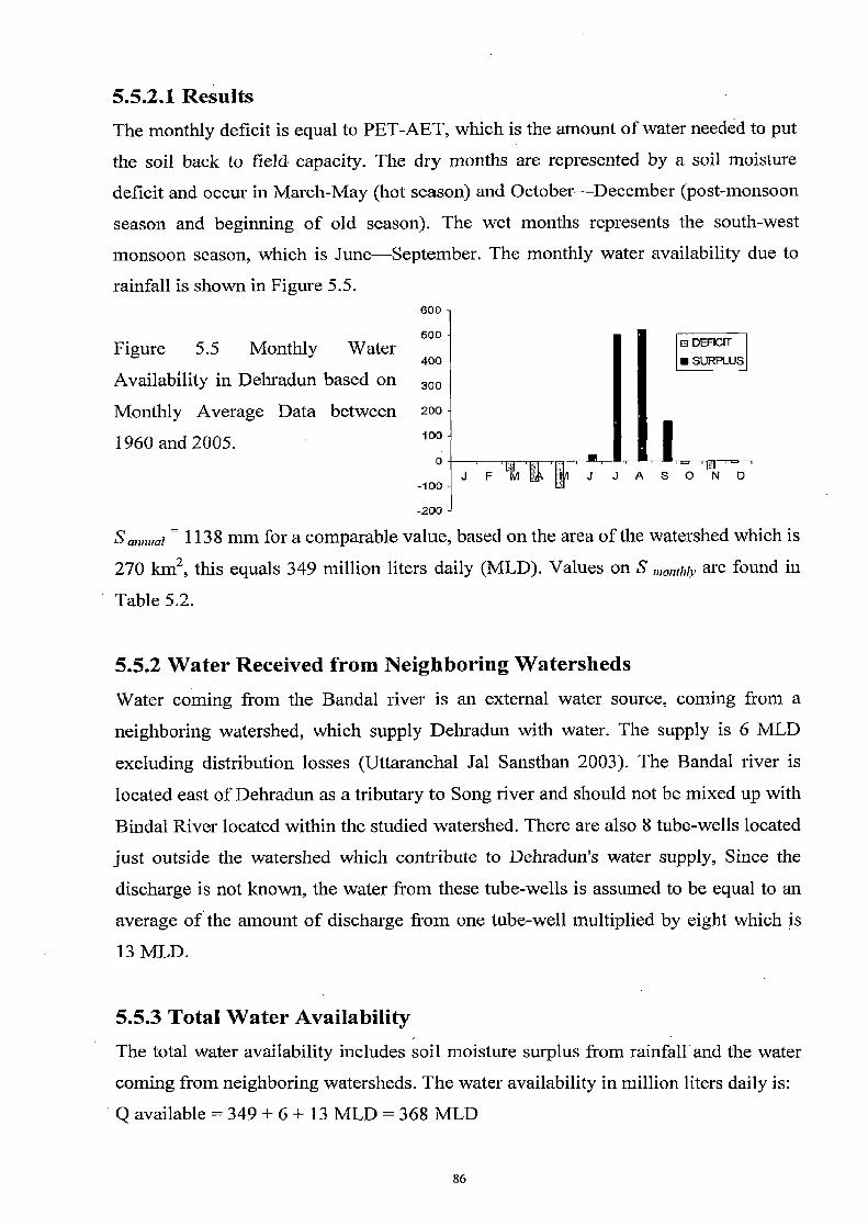
5.5.2.1 Results The monthly deficit is equal to PET-AET, which is the amount of water needed to put

the soil back to field capacity. The dry months are represented by a soil moisture deficit and occur in March-May (hot season) and October—December (post-monsoon

season and beginning of old season). The wet months represents the south-west

monsoon season, which is June—September. The monthly water availability due to

rainfall is shown in Figure 5.5. 600

500 Figure 5.5 Monthly Water

400

Availability in Dehradun based on 300

Monthly Average Data between 200

1960 and 2005. 100

0

-100

-200

S annual = 1138 mm for a comparable value, based on the area of the watershed which is

270 km2, this equals 349 million liters daily (MLD). Values on S ,,,o,,,w j' are found in

Table 5.2.

5.5.2 Water Received from Neighboring Watersheds Water coming from the Bandal river is an external water source, coming from a

neighboring watershed, which supply Dehradun with water. The supply is 6 MLD

excluding distribution losses (Uttaranchal Jal Sansthan 2003). The Bandal river is

located east of Dehradun as a tributary to Song river and should not be mixed up with

Bindal River located within the studied watershed. There are also 8 tube-wells located

just outside the watershed which contribute to Deluadun's water supply, Since the

discharge is not known, the water from these tube-wells is assumed to be equal to an

average of the amount of discharge from one tube-well multiplied by eight which is

13 MLD.

5.5.3 Total Water Availability The total water availability includes soil moisture surplus from rainfall and the water

coming from neighboring watersheds. The water availability in million liters daily is:

Q available = 349 + 6 + 13 MLD = 368 MLD

86

CHAPTER SIX RAINFALL RUNOFF MODELLING IN GIS ENVIRONMENT

6.0 Introduction: The Soil Conservation Service (SCS) runoff equation which came into use in the mid-

50's is the product of more than 20 years of studies of rainfall-runoff relationships from

small rural agricultural watershed areas. The procedure which is basically empirical was

developed to provide a rational basis for estimating the effects of land treatment and land

use changes upon runoff resulting from storm rainfall. It was initially used by SCS in

project planning for the small watershed program. Because of its simplicity, however; its

use has spectrum of hydrologic application by the hydrologists. The procedure is reliable

when used in situation for which it was designed but it is not adequate for solving all

types of hydrologic problems.

6.1 Soil Conservation Service (SCS) Model The Soil Conservation Services procedure, which came into common use in the year

1954, is the product of more than 20 years of studies of rainfall runoff relationships for

small rural watershed areas. Thousands of infiltrometer tests were carried out by SCS in

the late 1930s and early 1940s. The intent was to develop basic data to evaluate the

effects of watershed treatment and soil conservation measures on the rainfall-runoff

process. The procedure which is basically empirical was. developed to provide a rational

basis for estimating the effects of land treatment and land use changes upon runoff

resulting from storm rainfall. Because of its simplicity, its use has spread through the

spectrum of hydrologic application of Agriculturists, Hydrologists and Soil Conservation

Engineers.

The SCS developed an index, which is called the runoff curve number (CN) to

represent the combined hydrologic effect of Soil, Land use, agricultural land treatment

class, hydrologic condition and antecedent soil moisture. The SCS has also developed a

soil classification system that consists of four hydrologic groups according to their

minimum infiltration rate, which is obtained for a bare soil after prolonged wetting. The

soil groups are identified by the letters A, B, C and D.

The SCS has also used an antecedent moisture to estimate three conditions (AMC

I — dry, AMC II — normal and AMC III — wet). The relationship between rainfall and

runoff for these three conditions is expressed as curve number. Each storm in a rainfall

series is assigned one of the three curve numbers according to antecedent moisture

condition.

6.1.1. Runoff Curve Number Equation The fundamental hypotheses of the SCS - CN method are

(i) Runoff starts after an initial abstraction Ia has been satisfied. This abstraction

consists principally of interception, surface storage, and infiltration.

(ii) The ratio of actual retention of rainfall to the potential maximum retention S is

equal to rainfall minus initial abstraction.

Mathematically,

F_ Q (6.1)

Where, F = actual retention = P - Q

S = potential maximum retention.

Q = runoff volume uniformly distributed over the drainage

basin.

P = mean rainfall over the drainage basin.

Ia = initial abstraction.

The value of P, Q and S are given in depth dimensions. While the original method

was developed in U.S. customary units (inches), an appropriate conversion to SI units

(cm) is possible. Rainfall P is the total depth of storm rainfall. Runoff Q is the total depth

of direct runoff resulting from storm rainfall P. Potential retention S is the maximum

depth of storm rainfall that could potentially be abstracted by a given site.

In a typical case, a certain amount of rainfall, referred to as "initial abstraction", is

abstracted as interception, infiltration, and surface storage before runoff begins. In the

CN method the initial abstraction Ia is subtracted from rainfall P in (1) to yield

EMI

P—IQ —Q Q S P —h

(6.2)

Solving for Q in (6.2) yields,

Q— (P —la)z (6.3) (P—I,,)+S

Which is valid for P > 1a, that is, after runoff begins; and Q = 0 otherwise. Eq. (6.3)

has two parameters: S and Ia. To remove the necessity for an independent estimation of

initial abstraction, a linear relationship between Ia and S was suggested by SCS (1985).

Ia = ?..S (6.4)

Where ?. = initial abstraction ratio. Eq. (6.4) was justified on the basis of

measurements in watersheds less than 10 acres in size (SCS 1985). According to NEH-4

50% of the data points lay within the limits 0.095 0.38 [SCS (1985)]. This led SCS

to adopt a standard value of the initial abstraction ratio X = 0.2. With X = 0.2 in (6.4), Eq.

(6.3) becomes

Q— (P-0.2S)2 P + 0.8S

Which is the rainfall-runoff relation used in the SCS method of estimating direct

runoff from storm rainfall.

Now,

Equation (6.5) can be re arranged as

Q = P — S (1.2 - S ) (P + 0.8S)

(6.6)

Clearly, this is a one-parameter model containing S as the parameter.

Equation (6.6) is a form of the hydrologic budget, (an elementary expression of

conservation of mass).

i.e. Q=P—L

in which L accounts for losses expressed as

L=S [1.2- S ] (P + 0.85)

These losses fall into five categories:

(6.5)

E:f j

1. Interception storage in a rural setting, by vegetation foliage, stems, by cultural

features of the landscape.

2. Surface storage in ponds, puddles and other usually small temporary storage

locations.

3. Infiltration to the subsurface to feed and replenish soil moisture, interflow, and

ground-water flow.

4. Evaporation from water bodies such as lake, reservoirs, streams, and rivers as

well as from moisture on bare ground.

5. Evapotranspiration from all types of vegetation.

Of these five types of hydrologic abstractions, infiltration is the most important for

storm analysis (short term). Evaporation and evapotranspiration are the most important

for seasonal or annual yield evaluations (long term). The remaining two losses

(interception and surface storage) are usually of secondary importance.

It is important to note that if P > 0.2S than only runoff will occur, otherwise runoff be

assumed as Zero. So the above formula (6.5) is valid only when P > 0.2S.

6.1.2. Estimation of S The parameter S depends upon characteristics of the soil- vegetation-land

use (SVL) complex and antecedent soil-moisture conditions in a watershed. For each

SVL complex, there is a lower limit and an upper limit of S. The soil conservation service

expressed S as a function of curve number (CN) as

CN = 1000 5+10

or, S = 1000 CN - 10; (6.7)

S is in inches.

Where CN is the curve number, it is a relative measure of retention of water by a

given SVL complex and takes on values from 0 to 100. A CN= 100 represents a

condition of zero potential retention (S=0), that is, an impermeable watershed.

Conversely, a CN=0 represents a theoretical upper bound to the potential retention (S =

oo), that is, an infinitely abstracting watershed.

Substituting (6.7) into (6.5), yields

(P-200 +2)2 CN

(P+8- -8) CN

__ [CN(P + 2) — 200] z or, Q (6.8)

CN[CN(P — 8) + 800]

In this equation, CN is the only parameter to be determined.

6.1.3. Determination of Curve Number The CN value is determined from (a) Soil type and (b) Antecedent moisture conditions.

6.2.3.1. Soil Group Classification The soils are classified on the basis of intake of water at the end of long duration storms

occurring after prior wetting and opportunity for swelling without the protective effects

of vegetation.

The hydrologic soil groups as defined by SCS are classified into four groups.

Group A — Soil in this group have a low runoff potential (high-infiltration rates)

even when thoroughly wetted. e.g. - Deep sand or Gravels, deep loess.

Group B -~ Soils in this group have moderate infiltration rates when thoroughly

wetted and consist chiefly of moderately deep to deep well drained to moderately

well drained soils. e.g.- sandy loam soil with shallow loess.

Group C -~ Soils have slow infiltration rates when thoroughly wetted and consist

chiefly of soils with a layer that impedes the downward movement of water.

These soils have a slow rate of water transmission. e.g. - clay loam.

Group D --4 Soils have a high-runoff potential (very slow infiltration rates) when

thoroughly wetted. These soils consist chiefly of clay soils with high swelling

potential.

TABLE 6.1 SOIL GROUP CLASSIFICATIONS

Group Soil Characteristics. Minimum infiltration

rate(in/hr)/cm/hr

A. Deep sand, deep loess and aggregated 0.3 — 0.45 / 7.6 — 11.4

silts.

B. Shallow loess and sandy loam 0.15 — 0.30 / 3.8 — 7.6

C. Clay loams, shallow sandy loam, soils in

organic content, and soils usually high in 0.05-0.15 / 1.3-3.8

clay

D. Soils that swell upon wetting, heavy

plastic clays, and certain saline soils 0 — 0.05 / 0 — 1.3

6.1.3.2. Hydrologic Soil Cover Complexes . SCS has considered the following parameters to assign curve number in hydrologic soil

cover complex.

- Hydrologic soil group

- Land use or land cover

- Treatment class

- Hydrologic condition

The curve number has been assigned for watershed condition with AMC II and Ia

= 0.2S. The numbers show the relative value of the complexes as direct run off. The

higher the CN, the greater the amount of direct runoff to be expected from a

storm.Hydrologic condition may be poor, fair or good depending upon percentage of

ground cover present.

Poor — heavily grazed land

Fair — moderate cover

Good — heavy or dense cover

(50% under ground cover)

(50% - 75%)

(> 75% under ground cover)

6.1.3.3. Antecedent Moisture Condition The amount of rainfall in a period of 5 days prior to a particular storm starts, is termed as

AMC. Also, it refers to the water content present in the soil at a given time.

91

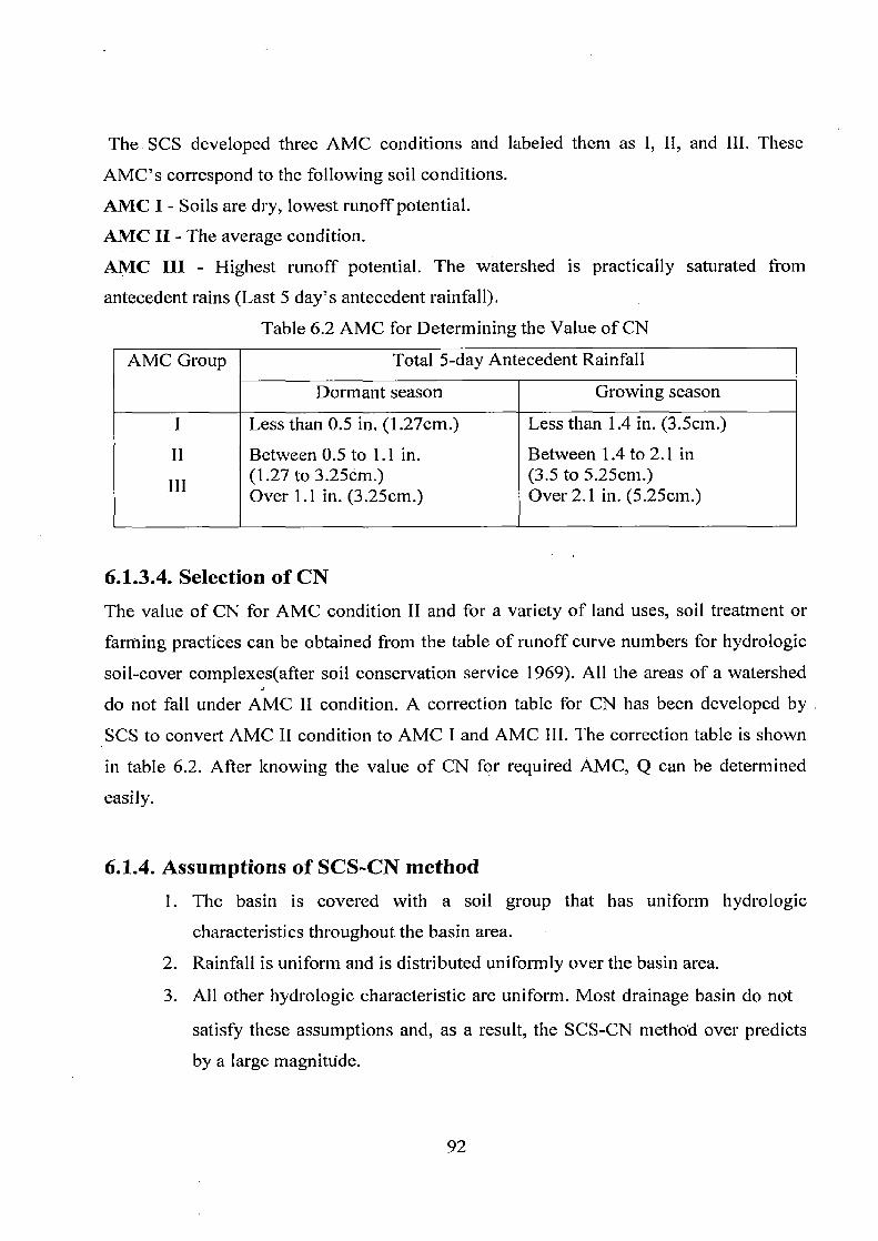
The-SCS developed three AMC conditions and labeled them as I, II, and III. These

AMC's correspond to the following soil conditions.

AMC I - Soils are dry, lowest runoff potential.

AMC II - The average condition.

AMC III - Highest runoff potential. The watershed is practically saturated from

antecedent rains (Last 5 day's antecedent rainfall).

Table 6.2 AMC for Determining the Value of CN

AMC Group Total 5-day Antecedent Rainfall

Dormant season Growing season

I Less than 0.5 in. (1.27cm.) Less than 1.4 in. (3.5cm.)

II Between 0.5 to 1.1 in. Between 1.4 to 2.1 in

III (1.27 to 3.25cm.) (3.5 to 5.25cm.) Over 1.1 in. (3.25cm.) Over 2.1 in. (5.25cm.)

6.1.3.4. Selection of CN The value of CN for AMC condition II and for a variety of land uses, soil treatment or

farming practices can be obtained from the table of runoff curve numbers for hydrologic

soil-cover complexes(after soil conservation service 1969). All the areas of a watershed

do not fall under AMC II condition. A correction table for CN has been developed by

SCS to convert AMC II condition to AMC I and AMC III. The correction table is shown

in table 6.2. After knowing the value of CN for required AMC, Q can be determined

easily.

6.1.4. Assumptions of SCS-CN method 1. The basin is covered with a soil group that has uniform hydrologic

characteristics throughout the basin area.

2. Rainfall is uniform and is distributed uniformly over the basin area.

3. All other hydrologic characteristic are uniform. Most drainage basin do not

satisfy these assumptions and, as a result, the SCS-CN method over predicts

by a large magnitude.

92

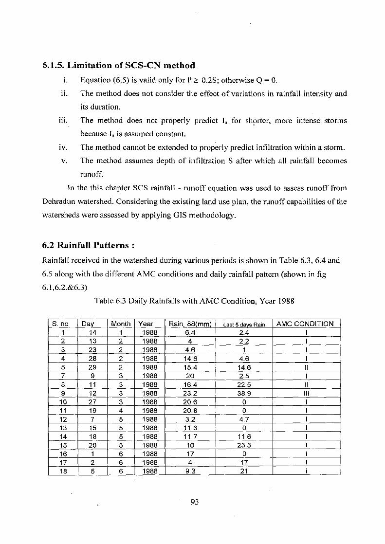
6.1.5. Limitation of SCS-CN method i. Equation (6.5) is valid only for P >_ 0.2S; otherwise Q = 0.

ii. The method does not consider the effect of variations in rainfall intensity and

its duration.

iii. The method does not properly predict Ia for shorter, more intense storms

because Ia is assumed constant.

iv. The method cannot be extended to properly predict infiltration within a storm.

v. The method assumes depth of infiltration S after which all rainfall becomes

runoff.

In the this chapter SCS rainfall - runoff equation was used to assess runoff from

Dehradun watershed. Considering the existing land use plan, the runoff capabilities of the

watersheds were assessed by applying GIS methodology.

6.2 Rainfall Patterns : Rainfall received in the watershed during various periods is shown in Table 6.3, 6.4 and

6.5 along with the different AMC conditions and daily rainfall pattern (shown in fig

6.1,6.2.&6.3)

Table 6.3 Daily Rainfalls with AMC Conditiol3, Year 1988

S. no Day Month Year Rain 88 mm Last 5 days Rain AMC CONDITION 1 14 1 1988 6.4 2.4 2 13 2 1988 4 2.2 3 23 2 1988 4.6 1 4 28 2 1988 14.6 4.6 5 29 2 1988 15.4 14.6 II 7 9 3 1988 20 2.5 8 11 3 1988 16.4 22.5 II 9 12 3 1988 23.2 38.9 III

10 27 3 1988 20.6 0 11 19 4 1988 20.8 0 12 7 5 1988 3.2 4.7 13 15 5 1988 11.6 0 14 18 5 1988 11.7 11.6 15 20 5 1988 10 23.3 16 1 6 1988 17 0 i 17 2 6 1988 4 17 I 18 5 6 1988 9.3 21 i

93

19 14 6 1988 8.3 1.3 1 20 15 6 1988 18 9.6 21 18 6 1988 9.7 28.6 22 22 6 1988 21 10.7 23 24 6 1988 46.6 24.6 24 25 6 1988 35.9 70.2 III 25 27 6 1988 3.6 106.5 III 26 28 6 1988 15.1 89.1 II 27 29 6 1988 13.6 101.6 111

28 30 6 1988 4.7 68.6 III 29 2 7 1988 23 39.4 II

30 4 7 1988 7.6 45.1 II 31 5 7 1988 21.8 39.1 II 32 6 7 1988 28 56.2 III 34 10 7 1988 4.8 57 III 35 12 7 1988 17.4 12 36 13 7 1988 10 22.6 37 14 7 1988 23.8 32.2 38 15 7 1988 3 56 III 39 17 7 1988 10.7 54.6 III 40 20 7 1988 5.9 17.1 41 21 7 1988 .11 20 42 22 7 1988 13.2 30.6 43 • 23 7. 1988 22.5 33.1 44 24 7 1988 12.6 55.2 III 45 25 7 1988 7 65.2 III 46 26 7 1988 9.2 66.3 III 47 27 7 1988 45.5 64.5 II! 48 31 7 1988 62.4 60.1 III 49 1 8 1988 46 113.3 III 50 2 8 1988 38.7 113.8 Iii 51 3 8 1988 31 150.7 III 52 6 8 1988 48 117.2 III 53 7 8 1988 15.1 119.2 Ill 54 8 8 1988 29.6 95.6 III 55 10 8 1988 12.1 97 III 56 12 8 1988 56 59.9 III 57 14 8 1988 22.8 71.2 III 58 15 8 1988 68 91.2 III 59 16 8 1988 20.5 147.1 III 60 17 8 1988 18.4 167.3 III 61 19 8 1988 9.4 130.5 III 62 24 8 1988 62.2 13.1 63 27 8 1988 10.8 67.1 111 64 4 9 1988 6.5 0 1 65 6 9 1988 14 6.5 66 9 9 1988 4.6 20.9 I 67 16 9 1988 18.6 0 I

68 19 9 1988 24.9 18.6 69 22 9 1988 13.9 24.9 I 70 23 9 1988 32.1 38.8 Ii 71 24 9 1988 17 70.9 III 72 25 9 1988 95.9 63 III 73 27 9 1988 13 158.9 III 74 23 12 1988 18.2 1.8 1 75 24 12 1988 8.8 20 II 76 25 12 1988 4.4 28.8 II 77 26 12 1988 18.5 32 II

Rain_88(m m)

120

100

80

60 o Rain_88(mm)

40

20 .LnbDLnI. ,qk. • 0

1 5 9 13 17 21 25 29 33 37 41 45 49 53 57 61 65 69 73

Fig.6.1 Daily rainfall in Dehradun watershed (Year1988)

Table 6.4 Daily Rainfalls with AMC Condition, Year 2001

S.No. Day Month Year Rain 01 Last 5 days Rain AMC

CONDITION 1 2 1 2001 25.5 1

2 20 1 2001 20.2 0 1

3 21 3 2001 4.6 0 1

4 29 3 2001 16 0 1

5 31 3 2001 17.3 16 I

6 14 4 2001 7 0 1

7 18 4 2001 27.6 11.7 1

8 16 5 2001 33.2 0.9 1

9 17 5 2001 12 34.1 II

95

10 19 5 2001 36 46.1 II

11 28 5 2001 15 2.5 1

12 2 6 2001 109.8 16.7 I

13 3 6 2001 13.3 111.5 III

14 4 6 2001 11.2 123.1 III

15 7 6 2001 22 134.3 III

16 12 6 2001 4.4 22 I

17 14 6 2001 52.2 4.4 1

18 15 6 2001 11.9 56.6 III

19 19 6 2001 12.4 72.8 III

20 21 6 2001 14.5 21.1 1

21 25 6 2001 6.8 21.1 I

22 26 6 2001 20.5 27.9 I

23 27 6 2001 3.4 33.9 i

24 28 6 2001 27 35.3 11

25 29 6 2001 14.5 59.5 III

26 30 6 2001 20 72.2 III

27 1 7 2001 19.2 85.4 III

28 2 7 2001 45.4 84.1 III

29 5 7 2001 11.6 86.4 III

30 6 7 2001 61.2 78 III

31 11 7 2001 7.5 66.4 III

32 13 7 2001 9.5 11.8 I

33 14 7 2001 15.6 17.5 I

34 15 7 2001 94.4 32.6 I

35 16 7 2001 32 127 Ill

36 17 7 2001 43.8 151.5 III

37 18 7 2001 4.5 195.3 III

38 20 7 2001 7.5 174.7 Hi

39 21 7 2001 72 87.8 III

40 22 7 2001 12.2 127.8 III

41 23 7 2001 10.2 96.2 111

42 25 7 2001 13.5 101.9 III

43 26 7 2001 32 107.9 III

44 27 7 2001 32 67.9 111

45 28 7 2001 35.4 87.7 III

46 _ 29 7 2001 22.4 112.9 III

47 31 7 2001 6.7 122.3 111

48 3 8 2001 6.5 29.6 I

49 4 8 2001 12.8 13.7 I

50 6 8 2001 44 19.3 1

51 7 8 2001 8 63.3 111

52 8 8 2001 4.2 71.3 III

53 9 8 2001 11 69 III

54 10 8 2001 4.6 67.2 Itt

55 12 8 2001 30.6 28.3 I

56 13 8 2001 44.4 50.9 II

57 14 8 2001 74.7 91.1 III

58 18 8 2001 75 121.1 III

59 19 8 2001 93.8 151.7 111

60 21 8 2001 45.2 171.3 111

61 22 8 2001 5.3 216.5 III

62 23 8 2001 2.5 221.8 III

63 29 8 2001 15.5 2.7 1

64 30 8 2001 24.4 18.2 1

65 31 8 2001 52.8 42.6 11

66 1 9 2001 15.5 93.2 III

67 4 9 2001 33.2 92.7 111

68 10 9 2001 19 0 1

69 13 9 2001 14.8 19.5 1

70 15 9 2001 4.8 35.1 11

71 30 9 2001 36.6 0 1

Rain Year 2001

120

100 11

80 0 Ii H __________

60 D Rain 01

40 II

20

0

1 6 11 16 21 26 31 36 41 46 51 56 61 66 71

Fig.6.2 Daily rainfall in Dehradun watershed (2001)

97

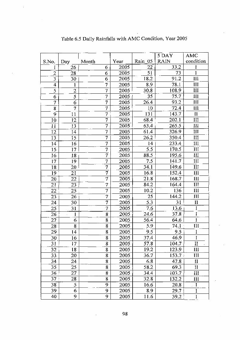
Table 6.5 Daily Rainfalls with AMC Condition, Year 2005

S.No. Day Month Year Rain 05 5DAY RAIN

AMC condition

1 26 6 2005 22 33.2 I 2 28 6 2005 51 73 I 3 30 6 2005 18.2 91.2 III 4 1 7 2005 8.9 78.1 III 5 2 7 2005 30.8 108.9 III 6 5 7 2005 35 75.7 111 7 6 7 2005 26.4 93.2 III 8 7 7 2005 10 72.4 III 9 11 7 2005 131 143.7 II

10 12 7 2005 68.4 202.1 III Il 13 7 2005 63.4 265.5 11I 12 14 7 2005 61.4 326.9 III 13 15 7 2005 26.2 350.4 III 14 16 7 2005 14 233.4 III 15 17 7 2005 5.5 170.5 III 16 18 7 2005 88.5 195.6 I11 17 19 7 2005 7.5 141.7 III 18 20 7 2005 34.1 149.6 III 19 21 7 2005 16.8 152.4 III 20 22 7 2005 21.8 168.7 III 21 23 7 2005 84.2 164.4 I1I 22 25 7 2005 10.2 136 III 23 26 7 2005 25 144.2 III 24 30 7 2005 5.3 31 II 25 31 7 2005 7.6 13.6 I 26 1 8 2005 24.6 37.8 1 27 6 8 2005 56.4 64.6 I 28 8 8 2005 5.9 74.1 III 29 14 8 2005 9.5 9.5 I 30 16 8 2005 37.4 46.9 I 31 17 8 2005 57.8 104.7 II 32 18 8 2005 19.2 123.9 III 33 20 8 2005 36.7 153.7 III 34 24 8 2005 6.8 47.8 II 35 25 8 2005 58.2 69.3 II 36 27 8 2005 34.4 103.7 III 37 28 8 2005 32.8 132.2 III 38 5 9 2005 16.6 20.8 I 39 6 9 2005 8.9 29.7 I 40 9 9 2005 11.6 39.2 I

41 10 9 2005 3.9 26.5 II 42 11 9 2005 14.5 32.1 I 43 13 9 2005 6.5 36.5 I 44 14 9 2005 7.5 32.4 II 45 17 9 2005 20.7 39.6 I •46 18 9 2005 57.4 90.5 II 47 19 9 2005 4.8 87.8 III 48 24 9 2005 52 58.9 I 49 25 9 2005 74 132.9 III 50 26 9 2005 14.5 147.4 III

Fig.6.4 Daily rainfall in Dehradun watershed (Year2005)

6.3 Runoff using GIS In this chapter SCS rainfall - runoff equation was used to assess runoff from Dehradun

watershed. Considering the existing land use plan, the runoff capabilities of the

watersheds was assessed by implementing NRCS approach in GIS.

Results obtained by GIS are in the form of maps or tabular form (attributes of the map).

Runoff maps obtained from the daily rainfall storm received in Dehradun watersheds are

given in the above table. The various input maps such as rainfall, curve number, S value

etc. map which has been used to get the runoff maps are shown in the Figs. 6.5 to 6.18.

The maps are self explanatory and properly classified as per the runoff depth classes in

the particular colour coded areas.

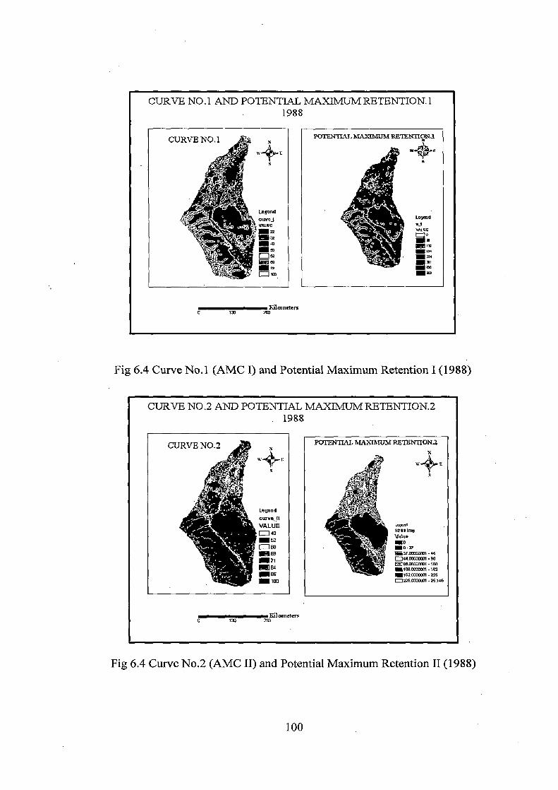
CURVE NO.1 AND POTENTIAL 1988

MAXIX4UM RETENTION. I

CURVE NO. I "' P AL MA [MUM RETENTION.1

w+e e R~ rs

i':. Legend =f atcft j Lid

e 7 VALUE22 ~~, VALUE Mo

3z

lo w r~ 'et

IVlolnctel -A U 13U 260

Fig 6.4 Curve No.I (AMC I) and Potential Maximum Retention I (1988)

CURVE NO.2 AND POTENTIAL MAXIMUM RETENTION.2 . 1988

CURVE NO? PAL MIA I XtJM RE'IBNTION.2

W F. U' Q

t , SV~YYTT!

Legend . _ t-n,1a1r. c~n•ve_ll VALUE °

~- Vatue 7u ter. Meg ~37AOOWWI -k6 _ ~1 Oaa-m000o01 -98

®84 ~samaaoaoi -1 oa

m es 18zm00001 - 225 =10 O 225DOOOOUM - 25,146

Kilometers 0 260

Fig 6.4 Curve No.2 (AMC II) and Potential Maximum Retention II (1988)

100

CURVE NO3 AND POTENTIAL MAXIMUM RETENTION.3 1988

F.1lo71 ews 0 130 260

POTENTIAL MAXIMUM REIENTION3 N

f

i ±_

~d

L s3 B8_otnJing Value

-13 -

:13 ~?~~`•" -16 16-44

'J-•;✓ 1.44.67 t 67 - 98 ` X98-162 = 162. 25.146

Fig 6.5 Curve No.3 (AMC III) and Potential Maximum Retention 1II(1988)

DAILY RUNOFF IMAGE 1988

4 ii~nL.WB V1tw

~WI

u v Vax ~t• ~e.o

iiµ

• day

o~i •E ©°

5025 0 30 100 150 200 Kilometers

Fig. 6.8 Daily Runoff Image (1988)

101


MIAXIIvIUI\M1 RETENTION. I

CURVE NO.1 POTEN1I4L MAXIMUM RETENTIoN.1

. w 111 ft ~ w'~e -

•~+a~ T ~j̀ i~ Legend

VALUE ®0 a Ot outimg `28 V®lue

• =32 C]0 ®40 0-114

Zi `45 : 114.225 ®W ®225- 244 =52 =244.298 ®68 0 298 - 365 -t om 365-621

=621-25,146

I~iLaueters 0 130 2W

Fig 6.8 Curve No.1 (AMC I) and Potential Maximum Retention 1(2001)

CURVE NO.2 AND POTENTIAL MAXIMUM RETENTION.2 2001

CURVE NO.2 PO1AL MAX'Wunl RETEN IION.2

4S ;

Legend

curve II VALUE r_ 521mg

Value X52 C7o [~60 ~0-44

=44-98 O88-tOB

=71 1D 108- 162

~ 84 D 162 - 225 ® 10

225-276

D 275 - 25,146

KV10Rletern


102


MAXIMUM RETENTION.3

CURVE NO.3 POTENTIAL AL MN-W ~I RETENTION.3

F y'tp,

Lepend A CURVE NO.III ~~ d

VALUE

j;jj

S31mg

M67 Value =71 00 =76 M0-16

~i~;"+ _62 1♦ 16-37 ®84 ~l37-44 _66 M44-52 ®93 1= 52 - 67

100 X67-119 X119-25.146

Riloinotcis 0 130 260

Fig 6.10 Curve No.3 (AMC III) and Potential Maximum Retention III (2001)

DAILY RUNOFF IMAGE 2001

tea. ... ~~..

. yl

__

ou-n - e+-.. s.a 19-'1

Q=

.o : tee..

50 23 0 30 100 150 200 Kilomelera

Fig. 6.11 Daily Runoff Image (2001)

103

CURVE NO.1 AND POTENTIAL MAXIMUM RETENTION. 1 2005

CURVE NO .1 PAL BVIGN RIA1 RETENnON1

cV~F. 1t~E

i S ~

1.1;t'r3 Legend r- curve no_1 S

VALUE si

=28 VALUE 32

~ 5•y' X40 ®018

®52 =310 M 68 X381 -1w —s39

—3

Kilometers 0 133 260

Fig 6.12 Curve No.1 (AMC I) and Potential Maximum Retention T (2005)


MAXIMUM RETENTION.2

CURVE NO? POTENHAL I IJMI2HTENUON2

n• - c 1 ~Y E S

Legend CURVE NO. N SZ VALUE 1 Value X47 X52

OQ-14

• • O6O =14.29

43 =65 X43-58

l69 '58-72 = 71 IM72-87 =84 087-101 =100 =101-116

116- 130

' iloinUars o 530 2E0


104

CURVE NO.3 AND POTENTIAL MAXIMUM RETENTION.3 2005

CURVE NO.3

w±t

Legend CURVE NO. In VALUE

07

84

60

pOTENUAL MAXIMUM RETENIION3

ç L.

63

— - - Kilolnder5

0 130 260

Fig 6.14 Curve No.3 (AMC III) and Potential Maximum Retention III (2005)

• DAILY RUNOFF IMAGE 2005

J.

WA

vsw

73

4 £

:it to 4, .24-27 •. . i .I -. . . 4

3025 0 30 100 ISO 260 0o2tr

Fig. 6.15 Daily Runoff Image (2001

105

N

WE

S

7.5 3.75

Legend

Total Runoff genration 1988 Value

95- 120

® 120-205

205-256 7_5 Kilometers

Fig. 6.8 Total Runoff Generation in mm (1988)

Runoff 2001 N

WE

S

Legend

Total Runoff genration 2001 Value ____'a

0-74

74- 120

(120-205

205-269 7.5 3.75 0 7.5 Kilometers


107

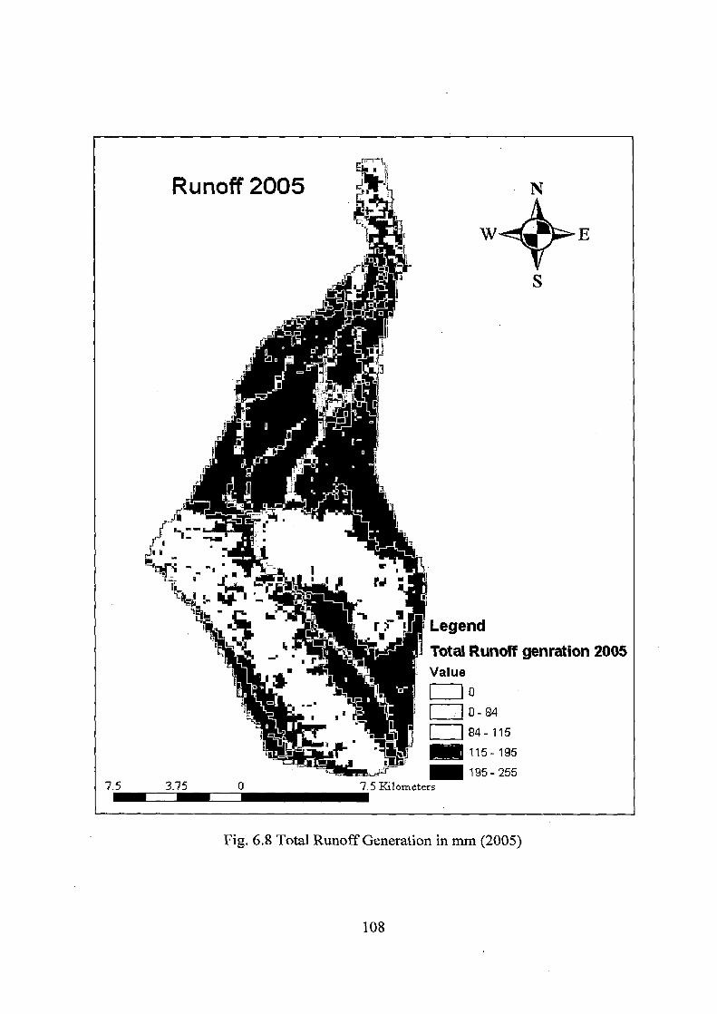
N

WE

S

7.5 3.75

Legend Total Runoff genration 2005 Value

10 D 0-84

1 84- 115 ® 115-125

195-255 7.5 Kilometers


108

Table — 6.6 Runoff generated on year in Dehradun Watershed

Year Area (in km2.) Runoff Depth (in km.) Runoff (Ha-m.)

1988 317.3 0.58932 18699123.6 2001 315.7 0.66275 20923017.5 2005 327.2 0.582681 19065322.32

6.4 Conclusion The runoff curve number method gaining its popularity among hydrology

practioners to its simplicity, predictability, and stability. The method is a conceptual

model of hydrologic abstraction of storm rainfall, supported by empirical data. Its

objective is to estimate direct runoff volume from storm rainfall depth, based on a curve

number CN. The method does not take into account the spatial and temporal variability of

infiltration and other abstractive losses; rather it aggregates these into a calculation of the

total depth loss for a given storm event and drainage areas.

The runoff was generated by analysis of three years satellite data. from analysis it was

observed that in 1988 the runoff is 18699123.6 Ha-m, in 2001 the runoff is 20923017.5

HA-m and in the year 2005 the runoff is 19065322.32 HA-m.

109

CHAPTER SEVEN

SITE SUITABILITY ANALYSIS FOR RAIN WATER

HARVESTING

7.0 Introduction Unprecedented and continued urban expansion in developing countries, however

inevitable, could be planned optimally through controlled growth of future expansion

areas. While the past cannot be erased, proper planning of future expansion becomes

undoubtedly the most important function of urban management. Optimal management

of cities requires a careful planning of their future expansion. While in the past, the

management system suffered due to lack of appropriate data, inadequate resources, fast

growth and poor knowledge of the consequences of such expansion, remote sensing

information available today have facilitated orderly expansion of cities to ensure a

reasonable quality of life in the cities. Evaluation of the suitability of land for different

purposes to identify areas for locating Industries, residential complexes and green belts

based on soil depth, soil texture, slope, relief, flood and erosion proneness, availability

of drinking water, drainage characteristics and wind pattern has resulted in arriving at

suitable strategy for optimal land use pattern to cater to the futuristic requirements of

the new cities. Urban land use mapping seems to be a most sought-for activity for dealing with

the dynamic cities and their growth areas The rapid urbanization of the Dehradun

requires the development of new growth areas that can eventually absorb the greater

demands for space and resources from an increasing population. The exponential

population growth and the consequent expansion of urban conglomerations being an

inevitable reality, the challenge of today lies in understanding the population dynamics

and realising the effective utilisation of high technology tools as that of space

technology for optimal and 'sustainable management of urban environments.

Identification of suitable land for water harvesting is one of the critical issues of

planning. The assessment of suitability conditions of a terrain for developing a new area

based on evaluation of terrain parameters like geology, geomorphology, slope, ground

water prospects, land use, soil, natural hazards like floods and earthquakes etc. and

110

proximity of roads and railways can be done effectively using geoinformatics. While in

the past, time consuming and expensive detailed land and aerial surveys were the

inhibiting factors preventing optimal planning of urban expansion, availability of high

resolution space imageries combined with parallel technological developments such as

GIS and GPS have overcome this problem.

The ability to identity different classes of land use and land cover and providing

estimates of the areas under each land use such as agricultural lands, forest cover, built

up land etc, together with its capability to provide information on natural resources

including underground water, makes remote sensing a unique tool for urban

management Major parameters for developing the urban environment should naturally

include physiography, land use pattern, geology, water resources, soil and drainage

pattern apart from the effects of human usage of land.

Geological, soil slope, aspect , and landuse/ landcover information can be extracted

from remote sensing data and were used to elaborate maps of land use suitability with

respect to ground and surface recharge purpose, areas for urban expansion and areas

with risks of natural or human induced hazard. This information, associated with land

use/land cover maps and socio-economic diagnosis, allowed the elaboration of maps to

provide guidelines for regional land use policies.

7.1 Terrain Parameters used in this Study The planning of developing a new harvesting site in a geodynamically unstable and

environmentally fragile domain of watershed region require assessment of various

terrain parameters in order to safeguard the life and property of the inhabitants due to

recurrent natural calamities and human induced hazards caused by unplanned

development of the city. The key parameters used in this study are geology,

landuse/landcover, soil texture, slope, drainage density, and, relief required to be

accessed for sustainable development of a new harvesting site are described below:

7.1.1 Geological features The geological realm in the area is dominated by alluvium in the flat terrain and rocks

in the hilly terrain. The lithological formation exposed in the hilly terrain primarily

111

x W E

S

Legend

Geological map ntime

Blaini, Kral Damta,Sircra, Chakrata Saknidhar

- Siwalik

Subathu

Tal

5to

30'1

309

consists of various types of shale, slate, limestone and quartzites. The rocks types, like

shale because of their splintery nature and limestone due to high weathering rates are

less suitable for infrastructure development as compared to massive slates and hard

quartzites. On the contrary, Shiwalik range dominated terrains have ideal conditions for

development of harvesting site. The building stone resources of the rocky terrain can

be harnessed for the construction material. The natural hazards like landslide and

earthquake impact are more prevalent and disastrous in hilly region whereas land

hazards caused by flood inundation and water logging can pose serious threat to healthy

geoenvironment in plain regions. In this the study the geology map is prepared by using

Are GIS software. The geological map has been given in Fig. 7.1.

GEOLOGICAL MAP

9 4.5 0 9Ki1®ehrc

Fig.7.1 Geological map

7.1.2 Landuse / Landcover Land is becoming a scarce commodity due to the immense agricultural and

demographic pressure. The information on land resources and possibilities for their

112

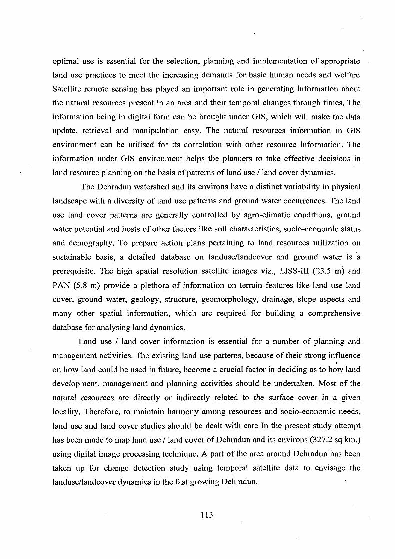
optimal use is essential for the selection, planning and implementation of appropriate

land use practices to meet the increasing demands for basic human needs and welfare

Satellite remote sensing has played an important role in generating information about

the natural resources present in an area and their temporal changes through times, The

information being in digital form can be brought under GIS, which will make the data

update, retrieval and manipulation easy. The natural resources information in GIS

environment can be utilised for its correlation with other resource information. The

information under GIS environment helps the planners to take effective decisions in

land resource planning on the basis of patterns of land use / land cover dynamics.

The Dehradun watershed and its environs have a distinct variability in physical

landscape with a diversity of land use patterns and ground water occurrences. The land

use land cover patterns are generally controlled by agro-climatic conditions, ground

water potential and hosts of other factors like soil characteristics, socio-economic status

and demography. To prepare action plans pertaining to land resources utilization on

sustainable basis, a detailed database on landuse/landcover and ground water is a

prerequisite. The high spatial resolution satellite images viz., LISS-III (23.5 m) and

PAN (5.8 m) provide a plethora of information on terrain features like land use land

cover, ground water, geology, structure, geomorphology, drainage, slope aspects and

many other spatial information, which are required for building a comprehensive

database for analysing land dynamics.

Land use / land cover information is essential for a number of planning and

management activities. The existing land use patterns, because of their strong influence

on how land could be used in future, become a crucial factor in deciding as to how land

development, management and planning activities should be undertaken. Most of the

natural resources are directly or indirectly related to the surface cover in a given

locality. Therefore, to maintain harmony among resources and socio-economic needs,

land use and land cover studies should be dealt with care In the present study attempt

has been made to map land use / land cover of Dehradun and its environs (327.2 sq km.)

using digital image processing technique. A part of the area around Dehradun has been

taken up for change detection study using temporal satellite data to envisage the

landuse/landcover dynamics in the fast growing Dehradun.

113

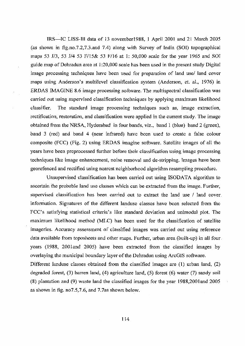
IRS—IC LISS-Ill data of 13 november1988, 1 April 2001 and 21 March 2005

(as shown in fig.no.7.2,7.3.and 7.4) along with Survey of India (SOI) topographical

maps 53 J/3, 53 J/4 53 F/15& 53 F/16 at 1: 50,000 scale for the year 1965 and SOI

guide map of Dehradun area at 1:20,000 scale has been used in the present study Digital

image processing techniques have been used for preparation of land use/ land cover

maps using Anderson's multilevel classification system (Anderson, et. al., 1976) in

ERDAS IMAGINE 8.6 image processing software. The multispectral classification was

carried out using supervised classification techniques by applying maximum likelihood

classifier. The standard image processing techniques such as, image extraction,

rectification, restoration, and classification were applied in the current study. The image

obtained from the NRSA, Hyderabad in four bands, viz., band 1 (blue) band 2 (green),

band 3 (red) and band 4 (near infrared) have been used to create a false colour

composite (FCC) (Fig. 2) using ERDAS imagine software. Satellite images of all the

years have been preprocessed further before their classification using image processing

techniques like image enhancement, noise removal and de-stripping. Images have been

georefenced and rectified using nearest neighborhood algorithm resampling procedure.

Unsupervised classification has been carried out using ISODATA algorithm to

ascertain the probable land use classes which can be extracted from the image. Further,

supervised classification has been carried out to extract the land use / land cover.

information. Signatures of the different landuse classes have been selected from the

FCC's satisfying statistical criteria's like standard deviation and unimodal plot. The

maximum likelihood method (MLC) has been used for the classification of satellite

imageries. Accuracy assessment of classified images was carried out using reference

data available from toposheets and other maps. Further, urban area (built-up) in all four.

years (1988, 2001and 2005) have been extracted from the classified images by

overlaying the municipal boundary layer of the Dehradun using ArcGIS software.

Different landuse classes obtained from the classified images are (1) urban land, (2)

degraded forest, (3) barren land, (4) agriculture land, (5) forest (6) water (7) sandy soil

(8) plantation and (9) waste land the classified images for the year 1988,2001 and 2005

as shown in fig. no7.5,7.6, and 7.7as shown below.

114

N

W" ' E

S

°250

6'0"1

0100°h

30°250N

30°200" N

30°15'0"N

30°100N

77005'0"E 78°600E 7806'0"E 78°10'0E

DEHRADUN WATERSHED 1988

7.5 3.75 0 7.5 Kilometers 30°5'0"N I0IIN

77055'0E 78°600E 7806'0"E 780100E

Fig 7.2: LISS III FCC Image 1988.

115

77°G5'0"E 78°60'0E 70°5'0"E . 78°100E

30°25'0N

30°20'0"N

30°150N

30°100N

30°5'0"N


N

E

~a✓l Fyi.. 7 ~i P 'y

e4'4 ~4I ~.b5ti1

V •rr~r

7.5 3.75 0 7.5 Kilometers

770550"E 78°600"E 78°5'0"E 78°100E

Fig. 7.3: LISS III FCC Image 2001.

116

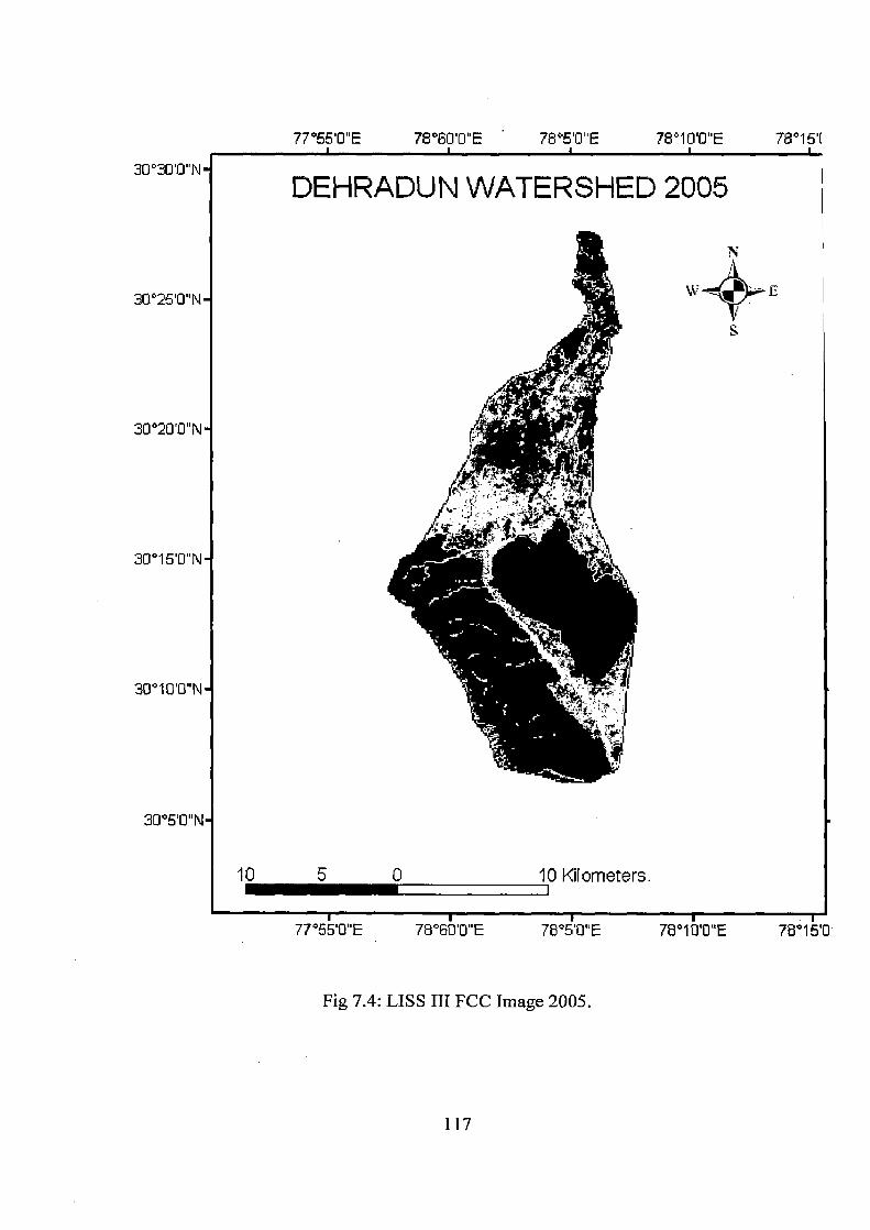
77°660E 780600"E 78°60"E 78°1010"E 780161

30°300"N

30°26'0"N

30 °20'0"N

30°150N

30°100"N

30°5'0"N

1

s ~

s P

r . i~ • y t`

1 1 1 •

77066'0E 7806010E 7805101 E 78°1010 1E

78°15'0'

Fig 7.4: LISS III FCC Image 2005.

117

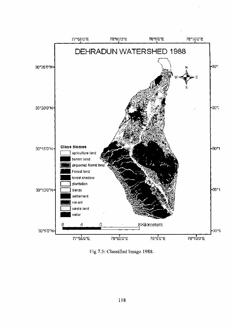
30°2550N

30 °20'0"N

30°15'0N Class Names

I I agriculture land

barren land degraded forest It

® Forest land

M forest shadow Q plantation

30°100N II Sandy settlement

vacant

waste land water

N

S

°1

77°550E 78°60'0E 780E 78°100E


8 4 0 8Kilometers k006 30°5'0"N '

77°55'0"E T8°60'0"E 78°55'0"E 78°100"E

Fig 7.5: Classified Image 1988.

118

30°200"N

30°150"N Class Names

agriculture I

barren land

degraded fc

® forest land

plantation

30°10'0"N Qriver bed

ettllement

Undassifiec

} vas#e land

w ter

N

E r S

78°100"E

DEHRADUN WATERSHED 2001 30°250"N

30°5'0°N1 8 4 0 8 Kilometers

77°5501 E 780600"E 78°6'0"E


119

77°60'0"E

77°560"E 78°600E 78°5'0"E 78°100E 78°160"E

30°3D'O"N


30°250N

30°200"N

30°15'0"N Class Names 0 agriculture land

degraded forest la forest

® forest shadow

30°100 N plantation

II river bed

settlement

[I vacant land

II waste land

30°5'0"N ® water

°26'0~~ r W

r

S

°20'0°l

15'0"h

1001%

°6,0„ N

10 5 0 10 Kilometers

77°500E 77°550E 78°600"E 78°5'0"E

r#IuY7fLW#:iiiN~~~L:


120

7.1.3 Soil Type Assessment of soil texture and soil depth constitutes a prerequisite for planning any

developmental activity The uneven compaction of soil during post construction period

can pose danger to the overlying structure Presence of fine loamy and sandy soils with

high bulk densities is better suited for road foundations and building sites as compared

to coarse loamy and skeletal soils heavy structures require deeper foundation and

therefore require regions with deep soils Shallow soils with rocky basement incur

problems during construction and poses heavy risk during earthquakes The deeper soils

are met towards the southwestern portion of the area over alluvial planes are best suited

for developing new township in view of the location of the area in Zone IV of the

earthquake hazards and its vicinity to seismically active Delhi-Hardwar Ridge.The soil

map was prepared using arc GIS software (Fig. 7.8)

SOIL MAP

301 15'0"N

SOIL r1AP 11..M

W. 10'0"N coarse loa /,mode rte sna oo&eroslon, steep

Mse loamr,de¢D .rve0drains ghterosbn

- 0. loaw sandy,deep ,wall dram,gertle sbpa

_dne loamp.deep .rvd d,aln.genff slope

= One loamq,deep ,..I drain,ligM in

=d ne Inamp,mshallo eii drained Steepslope

Nary y.maderde deep erosion &lOpeyaen Grain

10-W..odeta0¢ SMll .en dramed, sta¢p

loamyshallow,well drained bamp,shanobu,well drelnad ve ry steep

_ loanryverysh.11aowel1 drained

10 5 0 10 Xilrmteters

Fig. 7.8: Soil Map

121

r r

W ~- E

s

Legend

RANGE ®0.1

1-3 3-5

= 5.10 10-15 15-35 >35

3001

3001

7.1.4 Terrain Slope Terrain slope is an important factor for the distribution of utilities-facilities in a planned

development site Lower the slope easier would he the activities involved in

infrastructure development The cost of development in hilly regions is also very high as

compared to flat regions Terrain slopes in hilly tracts of the area are generally were then

25 and have very little flat areas for development of township The plain areas have

suitable slopes of less than 5 which is recommended for ideal development of a medium

size township in the area The slope map was prepared using arc GIS software the Fig.

no.7.9 as shown below

SLOPE MAP

10 5 0 10 Kilmneters

. Fig. 7.9: Slope Map (in percentage)

122

N

W ~' E

S

Legend

DRAINAGE ORDER — 1 —2 —3 —4 —5

I:

34°1

300130 V

7.1.5 Drainage order Natural drainage provides escape routes for the turbulent surface flow to move down

slope, thereby reducing soil erosion and danger to the surrounding infrastructure. They

also act as recharge zone for ground water Higher costs are envisaged in developing

infrastructure without disturbing the natural drainage of the region Therefore areas with

higher drainage density should be avoided while infrastructure development The

drainage order map was prepared using are GIS software the Fig. no.8.10 as shown

below

DRAINAGE MAP

10 5 a 10Ki1anetess

Drainage Map (Order)

'0"N

123

7.1.6 SETTLEMENT BUFFER Settlement buffer was generated using ARCGIS software. The buffer distance around

the settlement was taken 500m.in the settlement region all surface is impervious so it

most unsuitable water harvesting Fig. no.8.11 as shown below

SETTLEMENT BUFFER MAP

lr

30°25,0. E

S

ilr

30°150 Legend t-3O°150"N

BUFFER = >S00M

7 3.5 0 7 Ki1am eters

Fig.7.11: Settlement Buffer

124

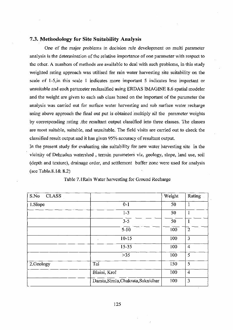
7.3. Methodology for Site Suitability Analysis One of the major problems in decision rule development on multi parameter

analysis is the determination of the relative importance of one parameter with respect to

the other. A numbers of methods are available to deal with such problems, in this study

weighted rating approach was utilised for rain water harvesting site suitability on the

scale of 1-5,in this scale I indicates more important 5 indicates less important or

unsuitable and each parameter reclassified using ERDAS IMAGINE 8.6 spatial modeler

and the weight are given to each sub class based on the important of the parameter the

analysis was carried out for surface water harvesting and sub surface water recharge

using above approach the final out put is obtained multiply all the parameter weights

by corresponding rating the resultant output classified into three classes. The classes

are most suitable, suitable, and unsuitable. The field visits are carried out to check the

classified result output and it has given 95% accuracy of resultant output.

In the present study for evaluating site suitability for new water harvesting site in the

vicinity of Dehradun watershed , terrain parameters viz, geology, slope, land use, soil

(depth and texture), drainage order, and settlement buffer zone were used for analysis

(see Table.8.1 & 8.2)

Table 7.1 Rain Water harvesting for Ground Recharge

S.No CLASS Weight Rating

1.Slope 0-1 50 1

1-3 50 1

3-5 50 1

5-10 100 2

10-15 100 3

15-35 100 4

>35 100 5

2.Geology TaI 150 5

Blaini, Krol 100 4

Damta,Simla,Chakrata,Saknidhar 100 3

125

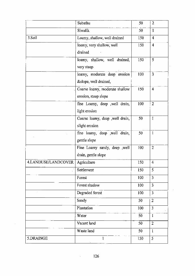
Subathu 50 2

Siwalik 50 1

3.Soil Loamy, shallow, well drained 150 4

loamy, very shallow, well

drained

150 4

loamy, shallow, well drained,

very steep

150 5

loamy, moderate deep erosion

&slope, well drained,

100 3

Coarse loamy, moderate shallow

erosion, steep slope

150 4

fine Loamy, deep well drain,

light erosion

100 2

Coarse loamy, deep well drain,

slight erosion

50 1

fine loamy, deep well drain,

gentle slope

50 1

Fine Loamy sandy, deep well

drain, gentle slope

100 2

4.LANDUSE/LANDCOVER Agriculture 150 4

Settlement 150 5

Forest 100 3

Forest shadow 100 3

Degraded forest 100 3

Sandy 50 2

Plantation 100 3

Water 50 1

Vacant land 50 2

Waste land 50 1

5.DRAINGE 1 150 5

126

2 150 4

3 50 1

4 50 2

5 100 3

6. SETTLEMENT BUFFER 0 100 0

1 150 5

n7_s a.bddyndex

Fig 7.12: Rainwater Harvesting Model for New Site Selection (Ground water)

Fig 7.13: Parameter Conditions for rain water harvesting (Ground water)

127

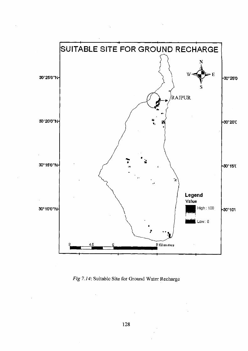
15'(

gend Iue

High : 100 30°101

Low: 0

30"25.0"

30°

30°15

30°

f -C r S

250

UITABLE SITE FOR GROUND RECHARGE

9 4.55 0 9 Kilometers

Fig 7.14: Suitable Site for Ground Water Recharge

128

Fig 7.15: Field Photos: Identified Ground Recharge Sites in the Study Area (Rajpur)

Table 8.2: Surface Rainwater harvesting

S.No Class Reclassifications Weight Rating

1. Slope 0-1 50 1

1-3 50 1

3-5 50 1

5-10 100 2

10-15 100 3

15-35 100 4

>35 100 5

2. Geology Tal 150 1 Blaini, Krol 100 2

Damta,Simla,Chakrata,Saknidhar 100 3

129

Subathu 50 4

Siwalik 50 5

3. Soil Loamy, shallow, well drained 2

loamy, very shallow, well drained 100 2

loamy, shallow, well drained, very steep

50 1

loamy, moderate deep erosion &slope, well drained,

100 2

Coarse Ioamy, moderate shallow erosion, steep slope

150 4

fine Loamy, deep well drain, light

erosion 100 3

Coarse loamy, deep well drain, slight erosion

150 5

fine loamy, deep well drain, gentle slope

150 5

Fine Loamy sandy, deep ,well drain,

gentle slope 150 4

4. Landuse/Landcover Agriculture 150 4

Settlement 150 5

Forest 100 3

Forest shadow 100 3

Degraded forest 100 3

Sandy 50 2

Plantation 100 3

Water 50 1

Vacant land 50 2

Waste land 50 1

5. Drainage 1 150 5

2 150 4

3 50 1

130

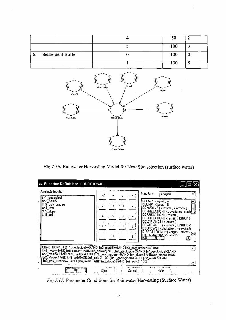
4 50 2

5 100 3

6. Settlement Buffer 0 100 0

1 150 5

n7_atiebnyv~Eex

Fig 7.16: Rainwater Harvesting Model for New Site selection (surface water)

Available Inputs: JJJ:J J-1JJ ~JJJJ JJ-1 ~1 JJJJ

Functions: Analysis

CLUMP (<layer> .4) CLUMP (<layer> .8) CONVOLVE (<raster> , <kernel> ) CORRELATION (<covariance matrit CORRELATION (<raster>) CORRELATION (<raster> , IGNORE' COVARIANCE (<raster> ) COVARIANCE (<raster> .IGNORE < DELFIOWS (<dsctable> , <sievetable DIRECT LOOKUP (<argl> , <table> FMPIQ d18TRIX,f tmarrivl l

CONDITIONAL { ($nl_geological==5 AND $n2_mar05==1AND $n3_poly_uraban==0 AND $n4 river-=3AND$n5 slope==1AND$nB soil==5) 50. ($nl_geological<5 AND $n1_geological>2ALAD $n2 mar05>1 AND $n2 mar05<4AND $n3 poly_uraban==O AND $n4_river<3AND$n5_slope>1AND $r _slope<4 AND $n8_soil< AND$nB_soil>2)100 ,($n1_geological<3 AND $n2_mar05>3 AND $n3_poly_uraban==1 AND $n4 river>3 AND$n5 slope>3 AND $n8 soil<3)150} Vf

Cf Clear Cancel Help

Fig 7.17: Parameter Conditions for Rainwater Harvesting (Surface Water)

131

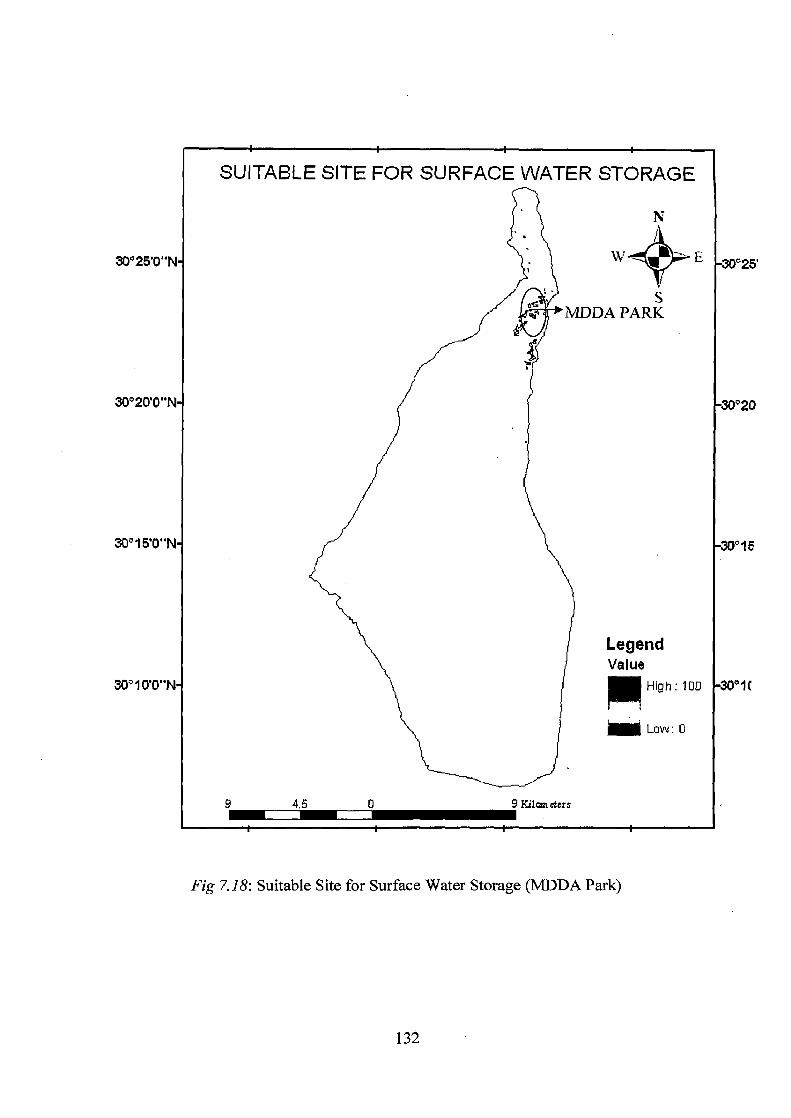
N 1

W ~- e 1 S

IDDA PARK

Legend Value

High: 100

Low: 0

20

15

30°250'

30°200

30°1 5O

30°1 OO•

SUITABLE SITE FOR SURFACE WATER STORAGE

9 4.5 0 9 Ki1om eters

Fig 7.18: Suitable Site for Surface Water Storage (MDDA Park)

132

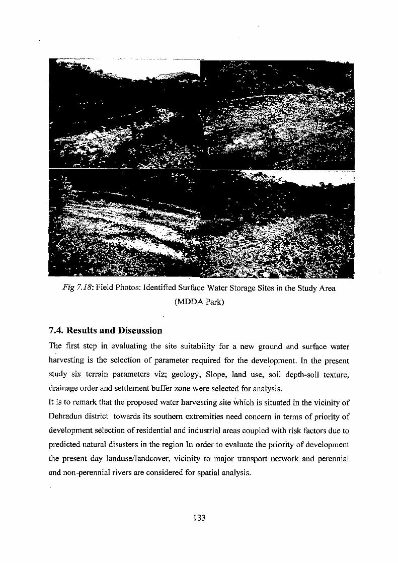
Fig 7.18: Field Photos: Identified Surface Water Storage Sites in the Study Area

(MDDA Park)

7.4. Results and Discussion The first step in evaluating the site suitability for a new ground and surface water

harvesting is the selection of parameter required for the development. In the present

study six terrain parameters viz; geology, Slope, land use, soil depth-soil texture,

drainage order and settlement buffer zone were selected for analysis.

It is to remark that the proposed water harvesting site which is situated in the vicinity of

Dehradun district towards its southern extremities need concern in terms of priority of

development selection of residential and industrial areas coupled with risk factors due to

predicted natural disasters in the region In order to evaluate the priority of development

the present day landuse/Iandcover, vicinity to major transport network and perennial

and non-perennial rivers are considered for spatial analysis.

133

Adopting this approach, the said parameters were analyzed with respect to the final

suitability map for demarcation of areas suitable for surface and ground water

harvesting purpose.

134

CHAPTER 8 ANALYSIS AND DESIGN OF ROOFTOP RAINWATER

HARVESTING

8.0 Introduction The present chapter deals with the development of criteria for the design of

storage/recharging structures for a particular roof area based on the inputs available

from GIS analysis. Various parameters based on the available data collected from

different sources as well as ground reality information through site visits to Dehradun

city are considered.

8.1 Design Parameters Various design parameters are considered for approximating the tank capacity for

storage or recharging structures, which are briefly discussed below:

8.1.1 Roof Area Roof areas of the buildings are digitized from IKONOS IMAGE at lm resolution,

obtained from NRSA Hyderabad and stored in GIS database (Fig.8.1). The total

number of buildings and projected roof areas for 2001 are given in Table 8.1.

Maximum and minimum roof areas are considered in the design analysis.

Table 8.1: Projected Roof Area for the Year 2001

Classification Number Perce - Roof Area (m2)

of Area of ntage Total Min. Max. Mean

Buildings

<lOOm2 5,034 11.89 1,79,411.76 4.26 93.91 35.64

I00m2 -200 mz 21,798 51.50 37,518,71.76 101.03 196.44 172.12

200m2 -500 m2 11,715 27.68 47,08,844.25 200.63 499.99 401.95

500m2-1000 mz 2,207 5.21 14,11,795.83 500.00 999.67 639.69

>1000m2 1,573 3.72 34,33,481.48 1000.64 47463.16 2182.76

Total 42,327 100 1,34,85,405.08

135

r f

Kl

A

rI

Sahaspw

• y•• ;~•~,afa `

~ f

W r~

Z: Raw Ih ° t o

f, r

Fe 1 4

r

p4m

F a

S.

i

ti ti

INDEX Bound

Roof Area In SO Meter ®pion

11ob Crtd c21i

lb1 surd KCB ®> SOD an: d 1 QGQ ® 101 1 i om

Murz pIaI Eowi y

Fig. 8.1 Building Map of Dehradun City

136

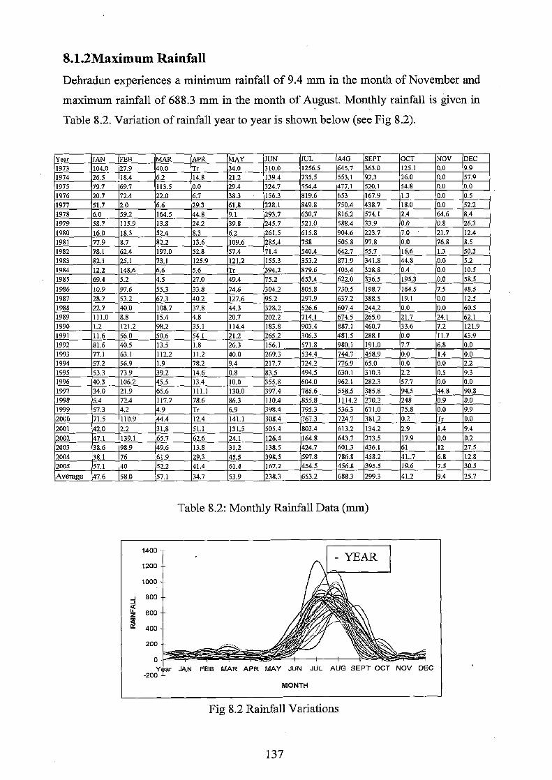
8.1.2Maximum Rainfall Dehradun experiences a minimum rainfall of 9.4 mm in the month of November and

maximum rainfall of 688.3 mm in the month of August. Monthly rainfall is given in

Table 8.2. Variation of rainfall year to year is shown below (see Fig 8.2).

Year JAN FEB MAR APR MAY JUN JUL A4G SEPT OCT NOV DEC 1973 104.0 27.9 40.0 Tr 34.0 310.0 1256.5 645.7 363.0 125.1 0.0 9.9 1974 26.5 18.4 6.2 14.8 21.2 139.4 735.5 553.1 92.3 26.0 0.0 57.9 1975 79.7 69.7 113.5 0.0 29.4 324.7 554.4 477.1 520.1 54.8 0.0 0.0 1976 20.7 72.4 22.0 6.7 38.3 156.3 819.6 653 167.9 1.3 0.0 0.5 1977 51.7 2.0 6.6 29.3 61.8 228.1 849.8 750.4 438.7 18.0 0.0 52.2 1978 6.0 59.2 164.5 44.8 9.1 293.7 630.7 816.2 574.1 2.4 64.6 8.4 1979 58.7 115.9 13.8 24.2 39.8 245.7 521.0 588.4 33.9 0.0 0.8 26.3 1980 16.0 18.3 52.4 8.3 6.2 261.5 615.8 904.6 223.7 7.0 21.7 12.4 1981 77.9 8.7 82.2 13.6 109.6 285.4 758 505.8 97.8 0.0 76.8 8.5 1982 78.1 62.4 197.0 52.8 57.4 71.4 540.4 642.7 55.7 16.6 1.3 50.3 1983 82.1 25.1 73.1 125.9 121.2 155.3 353.2 871.9 341.8 44.8 0.0 5.2 1984 I2.2 148.6 6.6 5.6 Ti 394.2 879.6 403.4 328.8 0.4 0.0 10.5 1985 69.4 5.2 4.5 27.0 49.4 75.2 653.4 622.0 336.5 195.3 0.0 58.5 1986 10.9 97.6 55.3 33.8 74.6 304.2 805.8 730.5 198.7 164.5 7.5 48.5 1987 28.7 53.2 67.3 40.2 127.6 95.2 297.9 637.2 388.5 19.1 0.0 12.5 1988 22.7 40.0 108.7 37.8 44.3 328.2 526.6 607.4 244.2 0.0 0.0 60.5 1989 111.0 8.8 15.4 4.8 20.7 202.2 714.1 674.5 265.0 21.7 24.1 62.1 1990 1.2 121.2 98.2 35.1 114.4 183.8 903.4 887.1 460.7 33.6 7.2 121.9 1991 11.6 56.0 50.6 54.1 21.2 265.2 306.3 481.5 288.1 0.0 11.7 43.9 1992 81.6 40.5 13.5 1.8 26.3 156.1 571.8 980.1 191.0 7.7 6.8 0.0 1993 77.1 63.1 112.2 11.2 40.0 269.3 534.4 744.7 458.9 0.0 1.4 0.0 1994 57.2 56.9 1.9 78.2 9.4 217.7 724.2 776.9 65.0 0.0 0.0 2.2 1995 53.3 73.9 39.2 14.6 0.8 83.5 494.5 630.1 310.3 2.2 0.5 9.3 1996 40.3 106.2 45.5 13.4 10.0 355.8 604.0 962.1 282.3 57.7 0.0 0.0 1997 34.0 21.9 65.6 111.1 130.0 397.4 785.6 558.5 385.8 94.5 44.8 90.8 1998 5.4 72.4 117.7 78.6 86.3 110.4 855.8 1114.2 270.2 248 0.9 0.0 1999 57.3 4.2 4.9 Tr 6.9 398.4 795.3 536.3 671.0 75.8 0.0 9.9 2000 71.5 110.9 44.4 12.4 141.1 308.4 767.3 724.7 381.2 0.2 Ti 0.0 2001 42.0 2.2 31.8 51.1 131.5 505.4 803.4 613.2 134.2 2.9 1.4 9.4 2002 47.1 139.1 65.7 62.6 24.1 126.4 164.8 643.7 273.5 17.9 0.0 0.2 2003 38.6 98.9 49.6 13.8 31.2 138.5 424.7 601.3 436.1 61 12 27.5 2004 38.1 76 61.9 29.3 45.5 398.5 597.8 786.8 458.2 41..7 6.8 12.8 2005 57.1 40 52.2 41.4 61.4 167.2 454.5 456.8 395.5 19.6 7.5 30.5 Average 47.6 58.0 57.1 34.7 53.9 238.3 653.2 688.3 299.3 41.2 9.4 25.7

Table 8.2: Monthly Rainfall Data (mm)

1400 - YEAR 1200

1000

800

Y ar JAN FEB MAR APR MAY JUN JUL AUG SEPT OCT NOV DEC -200

MONTH

Fig 8.2 Rainfall Variations

137

8.1.3 Efficiency Efficiency is one of the important factors in computing the runoff generated from

rooftops. The type of roof would affect the quantity of rainwater harvesting. It has

been observed during site visits that most of the roofs are flat and made of re-inforced

concrete. Runoff coefficient for re-inforced concrete is about 0.70-0.90 (Pacey and

Cullis, 1986). Another factor that affects the quantity of water harvested from roofs

are evaporation and wastage due to flushing during initial rains. In this analysis,

efficiency of 0.80 is used considering the evaporation losses and wastage.

8.1.4 Potential of Rooftop Rainwater Harvesting: The total roof area of the buildings in Dehradun is 13.48 Mme, which is 13.48 km2.

The planning for the above area has to be done under different categories of buildings.

To understand the potential of Rooftop Rainwater Harvesting, let us consider the

normal rainfall of Dehradun, which is 2183 mm.

Total Roof Area = 13.48 Mme

Normal rainfall = 2.18 m

Volume of water available at rooftop = 29.44 Mm3

Runoff Coefficient

1 :1

Volume of water that can be used for storage/recharge =23550 M liters

= 5233.33 M Gallons

=14.33 MLD

8.2 Estimate of Rainwater Harvesting For rainwater harvesting at the first stage Rooftop Rainwater Harvesting would be

appropriate. The total roof area of the buildings is 1,23,85,405 m2. The average cost

of installation of Rooftop Rainwater Harvesting system is about Rs 125/- per m2. The

estimated cost is the average of the cost for installation including cost of pipe

assembly, filters and tanks, whenever necessary. The estimated cost for the Rooftop

Rainwater Harvesting is given in Table-8.3.

138

Table 8.3: Classification of Roof Area

Classification of

Area

Average

Roof Area

(m)

Number

of

Buildings

Total (m2)

Rate

(Rs/

sq m)

Amount

(Rs. in lacs)

ROOF TOP RAIN WATER HARVESTING

(Direct Method)

< 100 m 5,034 1,79,411.76 125 224.265

100 m2 -200 m 150 21,798 37,518,71.76 125 4689.840

200m2 -500m2 350 11,715 47,08,844.25 125 5886.055

500m2-1000m2 750 2,207 14,11,795.83 125 1764.745

>1000 m 1,573 34,33,481.48 125 4291.852

Total 1,34,85,405.08 16856.757

8.3 Roof top Rainwater Harvesting Rooftop catchment tanks are storage containers installed to receive runoff water from

the roof of a house, a shed or a public building via a gutter and a down pipe. The most

suitable roofs for the purpose are those covered with iron sheet, tiles and fiberglass-

sheet. Existing asbestos sheets can also be used (because the health hazards from

inhaling and ingesting asbestos fibre is only related to the production and construction

process). Thatched roofs too have been used, particularly for the traditional systems

but they give a much lower yield and often produce coloured water (Handbook on

Rainwater Harvesting-Rajiv Gandhi Drinking Water Mission).

8.3.1 Site Assessment Assessing the site conditions together with future tank owners is the first step towards

a sound system design. The five main site conditions to be assessed are:

Availability of suitable roof catchment

Foundation characteristics of soil near the house

Location of trees

Estimated runoff to be captured per unit area of the roof;

Availability and location of construction.

139

8.3.2 Estimating Size of the Required Systems The actual size of the system will depend on various factors. Primarily, the size will

be influenced by the cost of the system, the amount of rainwater to be collected,

expectations and needs of tank owners and the level of external support.

The key to the solution here lies in matching the supply and demand to the

satisfaction of the user(s) at the lowest cost possible. The amount of rain and its

distribution over the year, the size of the tank. Usually the worst scenario will present

itself during the longest dry spell. The size of the catchment area and tank should be

enough to supply sufficient water for the users during this period. Assuming a full

tank at the beginning of the dry season (and knowing the average length of the dry

season and the average water use), the volume of the tank can be calculated by the

following formula:

V= (t X n X q) + et

(8.1)

Where V = volume of the tank (litres)

t = length of the dry season (days)

n = Number of people using the tank

q = consumption per capita per day (litres)

et = evaporation loss during the dry period

8.3.3 General Design Features Rooftop water harvesting systems can provide good quality potable water if

the design features outlined below are followed:

The substances that go into the making of the roof should be non-toxic in

nature.

Roof surfaces should be smooth, hard and dense since they are easier to clean

and are less likely to be damaged and release materials/ fibres into the water.

Roof painting is not advisable since most paints contain toxic substances and

may peel off.

No overhanging trees should be left near the roof.

The nesting of birds on the roof should be prevented.

140

s All gutters ends should be fitted with a wire mesh screen to keep out leaves,

etc.

A first-flush rainfall capacity, such as a detachable downpipe section, should

be installed.

A hygienic soakaway channel should be built at water outlets and a screened

overflow pipe should be provided.

The storage tank should have a tight fitting roof that excludes light, a manhole

cover and a flushing pipe at the base of the tank (for standing tanks).

There should be a reliable sanitary extraction device such as a gravity tap or a

hand pump to avoid contamination of the water in the tank.

There should be no possibility of contaminated wastewater flowing into the

tank (especially for tanks installed at ground level).

Water from other sources, unless it is a reliable source, should not be emptied

into the tank through pipe containers or the manhole cover.

8.3.3.1 Main System Components A rooftop catchment system has the three main components, viz, - a roof, a guttering

and first flush device and a storage tank.

(a) Roof: The roof should be smooth, made of non-toxic substances and sufficiently

large to fill the tank with the available rainfall conditions. Existing roofs of houses

and public buildings can be used for a rooftop catchment system. In some cases

enlarged or additional roofed structures can be built.

(b) Guttering and first-flush device: Guttering is intended to protect the building by

collecting the water running off the roof and direct it, via a down pipe, to the storage

tank. Gutters should have a uniform slope of 0.5 % large enough to collect the heavy

runoff from high-intensity rain.

(C)Tank: Water tanks using Ferro cement technology come in different designs with

volumes ranging between two and 200 m3. For example, a freestanding cylindrical

tank can be built in sizes between 10 and 30 m3, while a capacity of upto 200 m3 is

141

possible with sub-surface covered tanks. The latter is most economical when the

capacity exceeds 50 m3. Even PVC tanks can be used for this purpose.

8.3.4 Design of Storage Tanks Storage tanks in accordance with the volume of water expected to be collected at 2.5

and 5.0 cm/hr have been proposed. The volume of the proposed storage tanks range

from 2500 liter to 50,000 liter. The cost of the rainwater harvesting arrangements in

the buildings of Dehradun has been worked out (Table 9.3) at the rate of Rs. 50/- per

square meter.

8.3.5 Design of Filters The purpose of filters is to purify the water. In case of rooftop rainwater harvesting

filters are being provided as a purification device in the way of rainwater collected

from rooftop to the recharging structures in vicinity. Filters of-different capacities are

in use-1000, 500 and the 200 liters.

(a) Details of 1000 litre Capacity Tank

This normally comprises of a Syntax tank of capacity 1000 litre. Having an internal

diameter 110 cm and height 115 cm, the over flow is provided at 10 cm above the top

layer.

Arrangement of filter media: (Top to Bottom)

- Sand

- Charcoal

- Pebbles and gravel

One nylon mesh is also provided between the aggregate and charcoal for

protection of clogging. On the top of sand layer one piece of sand stone is placed for

protection of sand layer due to the high pressure of rainwater on it. But it reduce the

total surface area and the position of sand stone is not proper and due to it the

effective depth of sand is reduce at that point, which ultimately effect the rate of

filtration and turbidity removal efficiency of filter. (Fig 9.1) shows its cross section.

This filter can be used for roof areas greater than 500 m2.

142

(b) Details of 500 Liter Filter Here the internal diameter is of 92 cm and the height 98 cm. The overflow is provided

10cm. above the top layer (Fig 9.2), which can be used for medium size roof i.e. 200-500 m2.

Arrangement of filter media is (top to bottom)

- Sand

- Charcoal

- Pebbles and gravel

(c) Details of 200 litre Filter

The tank is Syntax tank of capacity 200 liter with internal diameter of 64 cm and

height 70 cm (Fig 9.3). The overflow is provided at 10 cm above the top layer. The

arrangement of the different layers is the same as the other filters cited above. This

can be used for roof area upto 200 m2.

The details of the filters and the schematic diagrams are given through figures.

8.4 Concluding Remark

As discussed in the previous sections, there is enough potential of rainwater

harvesting in Dehradun. Since more than 80% of water supply is met by groundwater

alone, it is the necessary to augment the groundwater storage through rainwater

harvesting and artificial recharging. The rooftop rainwater harvesting can be taken up

with the different kind of recharging schemes as given in this chapter. It is

recommended that the filters be installed with utmost care so that there is no

possibility of pollution from the recharged water. The drains flowing within the city

should not be used for recharge purpose as their conditions are very poor.

143

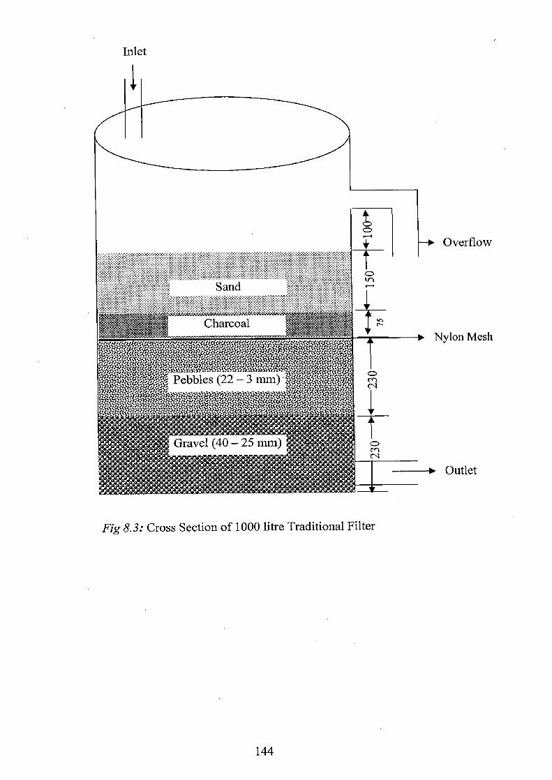
Overflow

Nylon Mesh

Outlet

Inlet

Fig 8.3: Cross Section of 1000 litre Traditional Filter

144

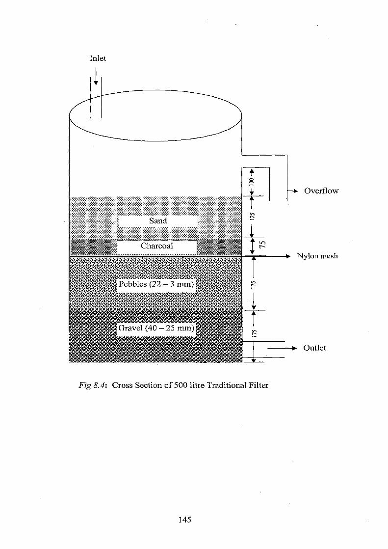
Overflow

Nylon mesh

Outlet

Inlet


145

Overflow

Nylon mesh

Outlet

Inlet


146

cc z

I C oc

CHAPTER NINE

CONCLUSIONS AND RECOMMENDATIONS

9.0 Conclusions Development plans relevant to small and medium water harvesting require acquisition

of basic information regarding geoenvironment of the area, location of existing utilities-

facilities, and their accessibility and development trends in relation to socio-economic

structure of the Watershed.

Geoinformatics with its powerful tools of Remote Sensing, and GIS has

emerged as a State of art technology for the policy maker, planners, urban

administrators and related professional concerned with the development and regulation

of urban I regional activities for better planning and judicious management.

Various spatial database layers related to meteorological and geological parameters

have been created and analyzed in GIS environment.

Using this spatial database, the SCS rainfall-runoff was evaluated and then runoff

estimation was created.

The silent features of the study are:

i) Calculation of runoff is done by SCS modified model using remote sensing and

GIS

ii) Identification of rainwater harvesting suitable site

The total water availability includes soil moisture surplus from rainfall and the

water coming from neighboring watersheds. The water availability in million liters daily

was found to be 368 MLD The runoff curve number method gaining its popularity among hydrology

practioners to its simplicity, predictability, and stability. The method is a conceptual

model of hydrologic abstraction of storm rainfall, supported by empirical data. Its

objective is to estimate direct runoff volume from storm rainfall depth, based on a curve

number CN. The method does not take into account the spatial and temporal variability

of infiltration and other abstractive losses; rather it aggregates these into a calculation of

the total depth loss for a given storm event and drainage areas

TLS

The runoff was generated by analysis of three years satellite data. It has been observed

that during 1988, 2001, and 2005, the runoff was 18699123.6 Ha-m, 20923017.5 Ha-m

and 19065322.32 Ha-m respectively.

The identified water harvesting site which is situated in the vicinity of Dehradun district

towards its southern extremities need concern in terms of priority of development of

residential and industrial areas coupled with risk factors due to predicted natural

disasters in the region. There is enough potential of rainwater harvesting in Dehradun.

Since more than 80% of water supply is met by groundwater alone, it is the necessary to

augment the groundwater storage through rainwater harvesting and artificial recharging.

The rooftop rainwater harvesting can be taken up with the different kind of recharging

schemes as given in this chapter. It is recommended that the filters be installed with

utmost care so that there is no possibility of pollution from the recharged water. The

drains flowing within the city should not be used for recharge purpose as their conditions are very poor.

9.1 Recommendations

The present gap between the demand and supply in Dehradun city is about 20%

in spite of the large number of tubewells constructed by the government departments.

The demand for drinking water of the city is met more than 80% by groundwater

through tubewells. This has resulted in lowering of groundwater table in general.

The existing tubewells and/or abandoned wells may also be used for recharge, for this purpose.

Existing springs especially Sahastradhara, Gucchu-Pani, Nala Pani etc., needs

immediate attention, as they are still the main source in some rural areas. Their

recharge areas to be increased by soil and water conservation practices.

Soil and water conservation techniques in grassland in the catchment of springs

are required in the form of controlled grazing or fencing to avoid degradation of existing vegetation with the catchments of springs.

150

Depending upon the suitability/availability of space, contour trenches can be

constructed to check the runoff and increase the recharge of the springs.

Gully control structures i.e. check dams, brushwood check dam, loose

boulder/rock dam, gabions etc., in the catchment of springs need to be

constructed to check the runoff and soil erosion at the same time will recharge

the springs.

It is recommended that for the drains passing through the city, government

should consider for an alternate system of waste disposal. In addition to that

cleaning of these drains would be required to check the pollution.

Rooftop rainwater harvesting should be made mandatory for all the new

construction with the municipal limit of Dehradun.

9.3 Scope of Future Work Efforts should be made for identification of potential rainwater harvesting sites

in open areas, particularly for those zones having a shortage of water.

Extension of the study area and methods to cover recharging capacity of spring

sources.

High resolution satellite image (e.g. IKONOS) may be used to get the accurate

surface feature information and identifications of potential rain harvesting site at

large scale.

r-

151

REFERENCES

1. Agarwal, C.S. and Garg P.K., 2002. Textbook on Remote Sensing in Natural

Resources Monitoring and Management. A.H. Wheeler and Co. Ltd., New Delhi.

pp 164-184

2. Anonymous, Texas Department of Transportation, Hydraulic design Manual,

Revised march 2004

3. Anonymous, The Study on Comprehensive Management Plan. for The Water

Resources of Brantas River Basin, in The Republic of Indonesia (1998). Nippon

Koei Co, Ltd and Nikken Consultant INC

4. Anonymous, Final Report Identification Study and Detailed Design of Small

Ponds, Review of Water Resources Development Study for Water Supply in

Brantas River Basin under Wonorejo Multipurpose Dam Construction Project

5. Aronoff (1991), Geographic information System, WDLP Publication P.O bax

585, Station B Ottawa, Ontario KIP SP 7 Canada

6. Husain S.K., 1976, Textbook of Water Supply and Sanitary Engineering, 2"a

Edition, Oxford & IBH Publishing Co. 66 Janpath, New Delhi, 3 pp 69-84.

7. Pandey Ashish and Sahu A. K., Generation of curve number using Remote

Sensing and Geographic Information System, Map Asia 2002Anonymous, 1988.

Seminar on Water Harvesting System & Management, National Drinking Water

Mission, Bangalore.

8. Anonymous, 1990. Inventory of Irrigation Tanks in Western Rajasthan,

Department of Irrigation, Jodhpur.

9. Aronoff, S.,1989. Geographic Information System, WOLP Publications, P.O. Box

585, Station B. Ottawa, Ontario KIP 5P7, Canada. 294 p.

10. Prasad Bhuwneshwar. Honda Sah Kiyoshi & Shunji Mural, Subwatershed

Prioritization for Watershed Management using Remote Sensing and GIS, ACRS

1997

11. Burrough, P.A., 1986. Principles of Geographic Information systems for Land

Resources Assesment, Clarendon Press, Oxford, U.K.

152

12. Central Ground Water Board-undated. Roof top Rainwater Harvesting for

Augmenting Groundwater Storage in NCT, Delhi.

13. CGWB 2000, Guide on Artificial Recharge to Ground Water. CGB, Ministry of

Water Resources, Gov't. of India, New Delhi. 93 p.

14. Chiradeep Adhikari, A GIS - Remote Sensing compatible rainfall-surface runoff

model for regional level planning, Map India 2003

15. Dhobal, A., 2000. Roof top Rainwater harvesting- A case study of SWAJAL

Village 'Satingal', Proc. Intl. Conf. RUWATSS, Roorkee, pp 316-331.

16. Dirbude D.G.,Jat M.K.,Kumar G.S., "Site Suitability Analysis for Rainwater

Harvesting Structures In Hire Watershed using Remote Sensing and GIS

Techniques" July 2001

17. Garg P.K. 2000. Appropriate Technologies for Surveying and mapping The

Features Related to Drinking Water. International Innovative Technologies for

Rural Water Supply and Environment Sanitation-2000, Roorkee, India October

12-13, pp 263-267.

18. Geleta M.T. (1993) Application of Geographic Information System in Watershed

Management. M.Tech Dissertation, WRDTC, U.O.R., Roorkee, 2, pp 5-35.

19. Gould, 1992. Sourcebook of Alternative Technologies for Freshwater

Augmentation in Some Countries in Asia. Rainwater Harvesting in the

Philippines. http://www.unep.or.jp/ietc/TechPublications.

20. Gould, J.E., 1991. Rainwater Catchment System for Household Water Supply,

Environmental Sanitation Review No. 32, Asian Institute of Technology,

Bangkok.

21. Katyal J.K., Singh R.P., Sharma Shriniwas, Das S.K., Padmanabhan M.V. and

Mishra P.K., 1995, Field Manual on Watershed Management. Central Research

Institute for Dryland Agriculture, Hyderabad, 2& 3, pp 4-85.

22. Kancharla V.S.A.V. Prasad, 2001. A GIS Study To Assess the Impact of

Urbanization on Runoff. M. Tech. Dissertation, Civil Engg. Dept. IIT Roorkee.

23. Khare D ,Garg P K ,Chaube U.0 Project Report on "Augmentation of Source,

Water Conservation & Recharge for Dehradun & Almora Cities in Uttaranchal"

153

Submitted to Uttaranchal Peyjal Sansadhan Vikash Evam Nirman

Nigam(Government of Uttaranchal)

24. Khare Deepak, Aug.2001, Project Report on Performance Evaluation Studies of

Filters And Its Economic Analysis (For Rainwater Harvesting) under Research

and Development for Indore Municipal Corporation, Indore.

25. Khan, M.A. 1992. Development of Surface Water Resources, In: Rehabilitation of

Degraded Arid Ecosystem (ed. A.S. Kolarkar, D.C. Joshi and K.D. Sharma) pp

136-143 Scientific Publication, Jodhpur.

26. Kolarkar, A.S., Murthy, K.N.K. and Singh, N. 1980. Water Harvesting & Runoof

Farming in Arid Rajasthan, Indian J. of Soil Cons. 8:113-119.

27. Lee, M.D. & Visscher, J.T. 1992. Water Harvesting — A Guide for Planners &

Project managers, IRC International Water & Sanitation Centre, The Hague.

28. Marble, D.F. and Donna J. Peuquet, 1990. Introductory Reading in GIS, London,

Tylor and Francis.

29. Michaelides, G., Allybokus M. and Young, R.J., 1986. 'Optimized Design and

Water Quality Studies of Rooftop Rainwater Catchment Project in Mauritius

Water Supply, 4; 117-122.

30. National Academy of Sciences, USA 1974. More Water for Arid Lands, pp 73-80.

31. Pacey and Cullis, A., 1986. Rainwater harvesting- The Collection of Rainfall and

Runoff in Rural Areas. Intermediate Tech. Publications, London. 216 p.

32. Rajashree V. Bothale, Vinod M. Bothale, G. Srinivasan and R.J. Sharma. , 2002.

Identification of Suitable Sites for Water harvesting Structures in Upper Betwa

Watershed through WARIS. http://www.gisdevelopment.net

33. Rathore, M.S. 1988. Traditional Drinking Water in Rajasthan- A Case Study of

Underground Tanks. In: Development Ecology and Rural Drinking Water Supply

in the Rajasthan Dessert; Aspects and Alternatives (ed. P.S. Shekhawat), pp 287-

311. Institute of Development Studies, Jaipur.

34. Sharma A. K. and Navalgund R. R., Pandey A. K. and Rao K. K., Micro-

watershed development plans using Remote Sensing and GIS for a part of

Shetrunji river basin, Bhavnagar district, Gujarat, Map India 1999

154

35. Sarangi A., Enright P., Madramootoo C.A., Development of User Interface in

ArcGIS for Watershed Management, Map India 2004

36. Sarangi A., Enright P., Madramootoo C.A., Development of User Interface in

ArcGIS for Watershed Management, Map India.2004

37. Sarangi A., Rao N.H., Sheena M. Brownee, Singh A.K., Use of Geographic

Information System (GIS) tool in watershed hydrology and irrigation water

management, Map India 2004

38. Sharma, K.D. and Kala A.K., 1980. Effects of Nala Bunding on Vindhyan

Sandstone Aquifer in Western Rajasthan, Indian J. Soil Cons. 8:44-49.

39. Sinha Saurabh, Sept. 30, 2002. Harvesting Does Wonders for Water Table, Times

of India, New Delhi.

40. Tideman E.M., 1996, Watershed Management, Guidelines for Indian Conditions.

41. Twort A.C., Law F.M., Crowley F.W. and Ratnayaka D.D., 1994. Textbook on

Water Supply, 4"' Edition, Estimating Water Demand,Edward Arnold 338 Euston

Road, London NWI 3BH, pp 22-26.

42. ' Valenzuela, C.R., 1990. Introduction to Geographic Information System. ITC

Publication No. 22 ITC, Enschede, The Netherlands.

43. Vangani,N.S., Sharma, K.D. and Chatterji, P.C. 1988. Tanka -A Reliable System

of Rainwater Harvesting in Indian Desert. Technical Bulletin No.33 Central Arid

Zone Research Institute, Johdpur.

155

LIST OF PUBLICATIONS.

Publications:

Gupta S.K, Garg P.K., Singh Ranvir, (2006). Meeting water demand through Rainwater harvesting, Uttaranchal state council for Science and Technology (USCST) (accepted)

Gupta S.K, Garg P.K., Singh Ranvir,(2006) Rainwater Harvesting Concept-Using Remote Sensing And GIS Application, Indo-Australian international conference on Information technology in civil engineering (IAC-ITCE) Page no.94-95

Gupta S.K, Jat M.K., Garg P.K., Singh Ranvir,(2006) Urban growth change detection through Remote Sensing and GIS Techniques,"Geo-informatics for Rural Development—Achieving Synergy between Technical and Social Systems"(ICORG 2006) Page no.65

Gupta S.K, Jain Sadhana, Kanayinl 0. Teshebaeva,(2006) Optimisation of Health Facility Location for Osh City, Kyrgyzstan Internet Publication (Review)

156

USE OF .GIS .& REMOTE SENSING TECHNIQUES FOR ...

Documents

Transcript of USE OF .GIS .& REMOTE SENSING TECHNIQUES FOR ...