57Geocarto International, Vol. 19, No. 2, June 2004 E-mail: geocarto@geocarto.comPublished by Geocarto International Centre, G.P.O. Box 4122, Hong Kong. Website: http://www.geocarto.com

Global Land Ice Measurements from Space (GLIMS): RemoteSensing and GIS Investigations of the Earth’s Cryosphere

Wilfried Haeberli, Andreas Kääb and Frank PaulDepartment of Geography, University of ZurichCH-8057 Zurch, Switzerland

Dorothy K. HallHydrological Sciences Branch, code 974, NASA/GoddardSpace Flight CenterGreenbelt, Maryland 20771 U.S.A.

Jeffrey S. KargelU.S. Geological Survey, 2255 N. Gemini Dr.Flagstaff, Arizona 86001 U.S.A.

Bruce F. Molnia926A National Center, U.S. Geological SurveyReston, Virginia 20192 U.S.A.

Dennis C. TrabantU.S. Geological Survey, 3400 Shell St.Fairbanks, Alaska 99701 U.S.A.

Rick WesselsAlaska Volcano Observatory, U.S. Geological SurveyAnchorage, Alaska 99508 U.S.A.

Abstract

Concerns over greenhouse-gas forcing and global temperatures have initiated research into understandingclimate forcing and associated Earth-system responses. A significant component is the Earth’s cryosphere, asglacier-related, feedback mechanisms govern atmospheric, hydrospheric and lithospheric response. Predicting thehuman and natural dimensions of climate-induced environmental change requires global, regional and localinformation about ice-mass distribution, volumes, and fluctuations. The Global Land-Ice Measurements from Space(GLIMS) project is specifically designed to produce and augment baseline information to facilitate glacier-changestudies. This requires addressing numerous issues, including the generation of topographic information, anisotropic-reflectance correction of satellite imagery, data fusion and spatial analysis, and GIS-based modeling. Field andsatellite investigations indicate that many small glaciers and glaciers in temperate regions are downwasting andretreating, although detailed mapping and assessment are still required to ascertain regional and global patterns ofice-mass variations. Such remote sensing/GIS studies, coupled with field investigations, are vital for producingbaseline information on glacier changes, and improving our understanding of the complex linkages betweenatmospheric, lithospheric, and glaciological processes.

Michael P. Bishop, Jeffrey A. Olsenhollerand John F. ShroderDepartment of Geography/GeologyUniversity of Nebraska at OmahaOmaha, NE 68182 U.S.A.

Roger G. Barry and Bruce H. RaupNational Snow/Ice Data CenterUniversity of ColoradoBoulder, Colorado 80309 U.S.A.

Andrew B. G. Bush and Luke CoplandDepartment of Earth/Atmos. SciencesUniversity of AlbertaEdmonton, Alberta T6G 2E3 Canada

John L. DwyerScience Applications International Corp.USGS EROS Data CenterSioux Falls, South Dakota 57198 U.S.A.

Andrew G. FountainDepartment of Geography/GeologyPortland State UniversityPortland, Oregon 97207 U.S.A.

Global Land-ice Measurements from Space (GLIMS) project.By necessity, only a sample of some key geographic areascan be presented, as well as a few other regions where moreplentiful glacier information is available. Specifically, weaddress the significance of understanding ice-mass

Introduction

The purpose of this article is to demonstrate the role ofremote sensing and GIS in an international science projectdesigned to assess the worlds’ glaciers from space; the

58

fluctuations, describe the role of remote sensing and GISinvestigations in glaciological research, address uniquechallenges for accurate information extraction from satelliteimagery, and provide preliminary results based upon fieldinvestigations and remote sensing/GIS studies.

Concerns over greenhouse-gas forcing and warmertemperatures have initiated research into understandingclimate forcing and associated Earth-system responses.Considerable scientific debate occurs regarding climateforcing and landscape response, as complex geodynamicsregulate feedback mechanisms that couple climatic, tectonicand surface processes (Molnar and England, 1990; Ruddiman,1997; Bush, 2000; Zeitler et al., 2001; Bishop et al., 2002).A significant component in the coupling of Earth’s systemsinvolves the cryosphere, as glacier-related feedbackmechanisms govern atmospheric, hydrospheric andlithospheric response (Bush, 2000; Shroder and Bishop,2000; Meier and Wahr, 2002). Specifically, glaciers partiallyregulate atmospheric properties (Henderson-Sellers andPitman, 1992; Kaser, 2001), sea level variations (Meier,1984; Haeberli et al., 1998; Lambeck and Chappell, 2001;Meier and Wahr, 2002), surface and regional hydrology(Schaper et al., 1999; Mattson, 2000), erosion (Hallet et al.,1996; Harbor and Warburton, 1992, 1993), and topographicevolution (Molnar and England, 1990; Brozovik et al., 1997;Bishop et al., 2002). Consequently, scientists have recognizedthe significance of understanding glacier fluctuations andtheir use as direct and indirect indicators of climate change(Kotlyakov et al., 1991; Seltzer, 1993; Haeberli and Beniston,1998; Maisch, 2000). In addition, the international scientificcommunity now recognizes the need to assess glacierfluctuations at a global scale, in order to elucidate thecomplex, scale-dependent interactions involving climateforcing and glacier response (Haeberli et al., 1998; Meierand Dyurgerov, 2002). Furthermore, it is essential that weidentify and characterize those regions that are changingmost rapidly and having a significant impact on sea level,water resources, and natural hazards (Haeberli, 1998).

High-latitude and mountain environments are known fortheir complexity and sensitivity to climate change (Beniston,1994; Mysak et al., 1996; Meier and Dyurgerov, 2002). Inaddition to the continental ice masses, several geographicregions have been identified as “critical regions” and includeAlaska, Patagonia and the Himalaya (Haeberli, 1998; Meierand Dyurgerov, 2002). Although smaller in extent, alpineglaciers are thought to be very sensitive to climate forcingdue to the altitude range and/or the variability in debris cover(Nakawo et al., 1997). Furthermore, such high-altitudegeodynamic systems are considered to be the direct result ofclimate forcing (Molnar and England, 1990; Bishop et al.,2002), although climatic versus tectonic causation is stillbeing debated (e.g., Raymo et al., 1988; Raymo andRuddiman, 1992). Central to various geological andglaciological arguments is obtaining a fundamentalunderstanding of the feedbacks between climate forcing andglacier response (Hallet et al., 1996; Dyurgerov and Meier,2000). This requires detailed information about glacier

distribution and ice volumes, annual mass-balance, regionalmass-balance trend, and landscape factors that controlablation. From a practical point-of-view, the extremelyrapidly changing glaciological, geomorphological andhydrological conditions in the cryosphere, present to manyregions of the world, a “looming crisis”, in terms of adecreasing water supply, increased hazard potential, and insome instances, geopolitical destabilization.

Scientific progress in understanding these remoteenvironments, however, has been slow due to logistics,complex topography, paucity of field measurements, andlimitations associated with information extraction fromsatellite imagery. Problems include the paucity and/or qualityof information on: (1) enumeration and distribution ofglaciers; (2) glacier mass-balance gradients and regionaltrends; (3) estimates of the contribution of glacial meltwaterto the observed rise in sea level; and (4) natural hazards andthe imminent threat of landsliding, ice and moraine dams,and outburst flooding caused by rapid glacier fluctuations.

McClung and Armstrong (1993) have indicated thatdetailed studies of a few well-monitored glaciers do notpermit characterization of regional mass-balance trends, theadvance/retreat behavior of glaciers, or global extrapolation.Given our current rate of collecting glacier information, it isexpected that far too many glaciers will be entirely gonebefore we can measure and understand them. This time-sensitive issue requires us to continue to acquire global andregional coverage of glaciers via satellite imagery beforethey disappear. As time is of the essence, a certain level ofautomation is required, although numerous challenges remainregarding information extraction and validation.Consequently, an integrated approach to studying thecryosphere must be accomplished using remote sensing andGIS investigations to improve our understanding of climateforcing and glacier fluctuations (Haeberli et al., 1998, 2004).

Background

Climate ForcingThe spatio-temporal dynamics that govern the coupled

atmosphere-ocean-cryosphere system are only beginning tobe exposed through a series of observational, theoretical,and numerical studies. With the increasing availability ofglobal satellite data, however, a barrage of statistical analyses(e.g., empirical orthogonal functions, cross-correlationanalysis, singular-value decomposition) has identified theclimatic signatures of a number of oscillations to which thiscoupled system is subject. These oscillations act across avery broad range of timescales, from seasonal to decadaland, invoking results from numerical climate models, alsoextend into the centennial to millenial range. Observedclimatic oscillations have very well-defined spatial signaturesin meteorological variables such as surface temperature,pressure, or precipitation. They therefore affect, quitefundamentally, cryospheric processes at the Earth’s surface.

The best example of annual variability is, of course, theseasonal cycle of incoming solar radiation. It determines the

59

latitudinal distribution of temperature and the mean locationat which the westerly jet streams occur during any givenmonth (Barry and Carleton, 2001). Internal variability withinthe climate system, however, causes the seasonal cycle to beslightly different from year to year. The resulting latitudinalvacillations of the westerly jets are believed to be ultimatelyresponsible for the North and South Annular Modes (e.g.,Thompson and Wallace, 2000), the former of which hasbeen linked to the North Atlantic/Arctic Oscillation (e.g.,Limpasuvan and Hartmann, 2000) and hence influencesArctic sea ice (e.g., Venegas and Mysak, 2000).

The best example of interannual variability is the El NiñoSouthern Oscillation (ENSO), a coupled atmosphere-oceanphenomenon whose internal workings are relatively wellunderstood and predictable within approximately 6-8 months.ENSO appears to be fundamentally correlated to the southAsian monsoon and hence to snow and ice accumulation inthe Himalaya (Bush, 2002). In addition, correlation of ENSOwith sea ice concentration in the Arctic (e.g., Mysak et al.,1996) demonstrates that even tropical climate variabilityinfluences high-latitude cryospheric processes.

On longer timescales, the Pacific Decadal Oscillation andcentennial climate variability also appear to have significantglobal signatures in temperature and precipitation, and willalso play a role in crysopheric dynamics at the Earth’s surface.

The global nature of many of these oscillations demandsthat any observational network that attempts to explain thembe global, or at least hemispheric, in extent. Therefore,satellite remote sensing is an integral component to researchon climate variability. In addition, those geographic regionsthat are particularly susceptible to such variability shouldhave additional monitoring. Those locations that compriseEarth’s cryosphere are prime examples of such sensitiveregions. The high-latitudes and high-mountain regions havebeen flagged as the “canary in the coal mine” of climatechange because of the cryosphere’s rapid response to climateperturbations. In addition, interannual and decadal variabilityis exhibited in the low-latitude high-altitude cryosphere ofthe Himalaya and the Andes.

The responses of ocean and atmospheric circulationpatterns to changes in the cryosphere, and the feedbacksprevailing in such interactions, are new and emerging themesof climate research. Historically considered dynamic ononly very slow timescales, the Earth’s cryosphere is rapidlyproving itself to be a major player in climate oscillations onevery timescale.

Water ResourcesThe global hydrologic cycle of the Earth is absolutely

critical for sustaining the biosphere, and its components arequantitatively measured and accounted for in hydrologic, ormass-balance, water-flow budgets. Rational watermanagement should be founded upon a thoroughunderstanding of water availability and movement (Haeberliet al., 1998), which requires monitoring of all the essentialelements. The most significant elements of the hydrologiccycle are: (1) the volumes of solid, liquid, and gas within the

subsystems; (2) residence times during which a unit remainswithin a subsystem reservoir; and (3) paths of motion fromone system to another. Fresh water in the form of iceconstitutes about 80 percent of the water that is not inoceans, which is far greater than any other stored source, andalso about 2 percent of the total water on the planet. Most icein the cryosphere occurs in the ice sheets covering Greenlandand Antarctica, where it may reside for thousands to millionsof years before returning as icebergs and meltwater to thesea, or as vapor to the atmosphere.

On the other hand, the snow- and ice-covered mountainsof the world constitute the water towers of vital supply forhundreds of millions of the world’s people. In some places,however, such as Afghanistan, glacier-ice resources havebeen dramatically reduced in the past few decades of droughtand increased melt, and downstream water discharges havebeen reduced catastrophically (Shroder, 2004a). In manyplaces though, each annual melt of snow and ice resourcesrecharges the river basins and reservoirs of the world. Butworld-water use per person has also doubled in the pastcentury, and is expected to become an increasingly scarceand ever-more contentious commodity in coming years(Gleick, 2001; Aldous, 2003). Furthermore, climate changecould bring hydrological chaos, even with an averagetemperature rise of only a few degrees C over the comingcentury, which is expected to bring more rain, less snow, andmore and earlier melting. This may halve snowpack volumesand increase flood and landslide hazards, especially in winterand spring seasons (Gleick, 2003). It is thus essential toestablish a better means to measure, model, and plan forfuture climates.

Asrar and Dozier (1994) have noted that understanding ofhow global change may influence world-wide water balanceswill require information about spatial and temporal variationsin storage of water in its various reservoirs, and magnitudeof transfers between reservoirs. Most important will beworking out the best methods to determine interannualvariability of global hydrologic processes, from naturalvariability and the seasonal cycle, to infer mechanisms andmagnitudes of climate change. Newly developed continental-and regional-scale surface hydrologic models include explicittreatment of precipitation, runoff, soil moisture, and snowand ice dynamics over the land (Asrar and Dozier, 1994).

Kump (2002) has pointed out, however, that the lack of anadequate ancient analogue for future climates means that weultimately must use and trust climate models evaluated againstmodern observations of existing climates and water storagesand discharges, using the best geologic records of warm andcold climates of the past. Armed with an elevated confidencein the models, more reliable predictions can then be made ofthe Earth’s response to risky human inputs into the climatesystem. In addition, the hydrologic cycle in deep-time climateproblems is presently the target of intensive research(Pierrehumbert, 2002) to better understand whatever difficultworld-water situation we are going to face in the future. Thisincludes the expected highly problematic, sea-level rise asthe cryosphere continues to melt (Lambeck et al., 2002).

60

In fact, ice-mass changes in the cryosphere are among thesafest or most reliable natural evidence of ongoing changesin the energy balance at the Earth’s surface and, hence, canbe considered as essential information for early detection ofclimate warming from human or natural causes in the nearfuture (Haeberli, 1998). The many problems of logistics,funding, maintenance of long-term monitoring, lack of trulyrepresentative field coverage, as well as quite limited coverageof any kind in many third world areas, means that remotesensing and GIS investigations, coupled with field controlwhere possible, are vital to maintaining adequate informationon the water-storage resources of snow and ice in theheadwater basins of many of the world’s great watersheds.

Natural HazardsExtreme natural events occur in seasonal, annual, or

secular fluctuations of processes that constitute hazard tohumans, to the extent that their adjustments to the frequency,magnitude, or timing of the natural extremes are based uponimperfect knowledge (White, 1974). Many natural hazardsare subject to assessment and prediction through the use ofremote sensing and GIS technology. The GLIMS project isideally suited to provide essential information for certainnatural hazards that are of increasing concern to people inmany parts of the world (Huggel et al., 2002).

Hazards in the cryosphere represent a continuous andgrowing threat to human lives and infrastructure, especiallyin high-mountain regions. In the future, however, the threatmay also be from rapid surge or massive calving of polar icecaps and catastrophic rise of sea level world-wide, whichwould drown port cities and even eliminate some islandnations entirely. At the present time, cryosphere-relateddisasters (e.g., glacial-lake outburst floods, glacial surges,debris flows, landslides, avalanches) in mountains can killhundreds or even thousands of people at once and causedamage with costs on the order of $ 100 million annually.Present-day trends in climatic warming especially affectterrestrial systems where surface and subsurface ice areinvolved. Changes in glacier and permafrost equilibria areshifting hazard zones beyond historical experience orknowledge, which makes prediction more difficult.Furthermore, as world populations increase, humansettlements and activities are being extended towardsendangered zones. As a consequence, empirical knowledgewill have to be increasingly replaced by improvedunderstanding of process.

The recently accelerated retreat of glaciers in nearly allmountain ranges of the world has led to the development ofnumerous potentially dangerous lakes (Mool et al., 2001a,b),which can break out in devastating floods (Coxon et al.,1996; Shroder et al., 1998; Cenderelli and Wohl, 2001). In2002, the United Nations Environment Program (UNEP),therefore, launched a high-level warning system in view ofthe dramatic growth of gigantic glacier lakes in the Himalaya.At the present time, the main hazards from the cryosphererecognized in mountain regions are: (1) the outburst ofglacier lakes, causing floods and debris flows; (2) avalanche/

landslide-induced wave impacts on glacial-lake dams; (3)ice break-offs and subsequent ice avalanches from steepglaciers; (4) stable and unstable (surge-type) glacier lengthvariations; (5) destabilization of frozen or unfrozen debrisslopes; (6) destabilization of rock walls, as related to glacialand periglacial activity; (7) adverse effects of rock glaciers;and (8) combinations or complex chain reactions of theseprocesses.

In addition, increasing recognition of these hazards hasled to a new proposal for the establishment of an inter-divisional Working Group of the International Commissionon Snow and Ice (ICSI) within the International Associationof Hydrological Sciences (IAHS) of the International Unionof Geodesy and Geophysics to address glacier and permafrosthazards in high mountains. The Working Group plans toaddress issues dealing with: (1) processes involved information of glacier and permafrost hazards; (2) techniquesand strategies for mapping, monitoring, and modeling; (3)methods of hazard vulnerability and risk assessment; (4)methods of hazard mitigation, including styles andeffectiveness of remedial works; and (5) raising awarenessof protocols for hazard assessment and remediation. In thisfashion, the ICSI Working Group aims to improveinternational scientific communications on cryospherichazards to government agencies, and the media, as well as toprovide up-to-date advice and information to other relevantgroups. GLIMS will contribute to the process with newsatellite-based observations.

Glacier ObservationsFluctuations of glaciers and ice caps have been

systematically observed for more than a century in variousparts of the world (Williams and Ferrigno, 1989; Haeberli etal., 1998; Williams and Ferrigno, 2002b) and are consideredto be highly reliable indications of worldwide warmingtrends (e.g., Fig. 2.39a in IPPC, 2001). Mountain glaciersand ice caps are, therefore, key variables for early-detectionstrategies in global climate-related observations. Within theframework of the global, climate-related, terrestrial-observingsystems, a Global Hierarchical Observing Strategy (GHOST)was developed to be used for all terrestrial variables.According to a corresponding system of tiers, the regional toglobal representativeness in space and time of the recordsrelating to glacier mass and area should be assessed by morenumerous observations of glacier-length and thicknesschanges, as well as by compilations of regional glacierinventories repeated at time intervals of a few decades - thetypical dynamic response time of mountain glaciers (Haeberliet al., 2000). The individual tier levels are as follows:• Tier 1 (multi-component system observation across

environmental gradients).Primary emphasis is on spatial diversity at large(continental-type) scales or in elevation belts of high-mountain areas. Special attention should be given tolong-term measurements. Some of the already observedglaciers (for instance, those in the American Cordillerasor in a profile from the Pyrenees through the Alps and

61

Scandinavia to Svalbard) could later form part of Tier 1observations along large-scale transects.

• Tier 2 (extensive glacier mass balance and flow studieswithin major climatic zones for improved processunderstanding and calibration of numerical models).Full parameterization of coupled numerical energy/massbalance and flow models is based on detailed observationsfor improved process understanding, sensitivityexperiments and extrapolation to areas with lesscomprehensive measurements. Ideally, sites should belocated near the center of the range of environmentalconditions of the zone that they are representing. Theactual locations will depend more on existinginfrastructure and logistical feasibility rather than onstrict spatial guidelines. Site locations should represent abroad range of climatic zones (such as tropical, subtropical,monsoon-type, midlatitude maritime/continental,subpolar, polar).

• Tier 3 (determination of regional glacier volume changewithin major mountain systems using cost-savingmethodologies).Numerous sites exist that reflect regional patterns of ice-mass change within major mountain systems, but theyare not optimally distributed (Cogley and Adams, 1998).Observations with a limited number of strategicallyselected index stakes (annual time resolution) combinedwith precision mapping at about decadal intervals (volumechange of entire glaciers) for smaller ice bodies or withlaser altimetry/kinematic GPS (Arendt et al., 2002) forlarge glaciers constitute optimal possibilities for extendingthe information into remote areas of difficult access.Repeated mapping and altimetry alone provide importantdata at lower time resolution (decades).

• Tier 4 (long-term observation data of glacier-length changewithin major mountain ranges for assessing therepresentativity of mass balance and volume changemeasurements).At this level, spatial representativeness is the highestpriority. Locations should be based on statisticalconsiderations (Meier and Bahr, 1996) concerning climatecharacteristics, size effects and dynamics (calving, surge,debris cover etc.). Long-term observations of glacier-length change at a minimum of about 10 sites within eachof the mountain ranges should be measured either in-situor with remote sensing at annual, to multi-annualfrequencies.

• Tier 5 (glacier inventories repeated at time intervals of afew decades by using satellite remote sensing).Continuous upgrading of preliminary inventories andrepetition of detailed inventories using aerial photographyor, in most cases satellite imagery, should enable globalcoverage and permit validation of climate models(Beniston et al., 1997). The use of digital terraininformation and GIS technology greatly facilitatesautomated procedures of image analysis, data processingand modeling/interpretation of newly availableinformation (Haeberli and Hoelzle, 1995; Bishop et al.,

1998a, 2000; Kääb et al., 2002; Paul et al., 2002).Preparation of data products from satellite measurementsmust be based on a long-term program of data acquisition,archiving, product generation, and quality control.This integrated and multi-level strategy aims at integrating

in-situ observations with remotely sensed data, processunderstanding with global coverage, and traditionalmeasurements with new technologies. Tiers 2 and 4 mainlyrepresent traditional methodologies that remainfundamentally important for deeper understanding of theinvolved processes, as training components in environment-related educational programs and as unique demonstrationprojects for the public. Tiers 3 and 5 constitute newopportunities for the application of remote sensing and GIS.

A network of 60 glaciers representing Tiers 2 and 3 wasestablished. This step closely corresponds to the datacompilation published so far by the World Glacier MonitoringService with the biennial Glacier Mass Balance Bulletin andalso guarantees annual reporting in electronic form. Such asample of reference glaciers provides information onpresently-observed rates of change in glacier mass,corresponding acceleration trends and regional distributionpatterns. Long-term changes in glacier length must be usedto assess the representativity of the small sample of valuesmeasured during a few decades with the evolution at a globalscale and during previous time periods. This can be done by:(1) intercomparison between curves of cumulative, glacier-length change from geometrically similar glaciers; (2)application of continuity considerations for assumed stepchanges between steady-state conditions reached after thedynamic response time (Hoelzle et al., 2003); and (3) dynamicfitting of time-dependent flow models to present-daygeometries and observed long-term length change (Oerlemanset al., 1998). New detailed glacier inventories are now beingcompiled in areas not covered so far in detail or, forcomparison, as a repetition of earlier inventories. This taskhas been greatly facilitated by the implementation of theinternational GLIMS project (Kieffer et al., 2000). Remotelysensed data at various scales (satellite imagery,aerophotogrammetry) and GIS technologies must becombined with topographic information (Hall et al., 1992,2000; Bishop et al., 2000, 2001; Kääb et al., 2002; Paul etal., 2002) in order to overcome the difficulties of earliersatellite-derived preliminary inventories (area determinationonly) and to reduce the cost and time of compilation. In thisway, it should be feasible to reach the goals of globalobserving systems in the years to come.

International GLIMS Project

The international GLIMS project is a global consortiumof universities and research institutes, coordinated by theUnited States Geological Survey (USGS) in Flagstaff,Arizona, whose purpose is to assess and monitor the Earth’sglaciers. Glaciers play a significant role in Earth systemdynamics, and control the natural resource potential formany regions of the world. Specifically, GLIMS objectives

62

are to ascertain the extent and condition of the world’sglaciers so that we may understand a variety of Earth surfaceprocesses and produce information for resource managementand planning. These scientific, management and planningobjectives are supported by the monitoring and informationproduction objectives of the United States government andUnited Nations scientific organizations, and are central tothe ongoing economic and geopolitical discussions aboutresource availability and geopolitical stability.

GLIMS entails: (1) comprehensive satellite multispectraland stereo-image acquisition of land ice on an annual basis;(2) use of satellite imaging data to measure inter-annualchanges in glacier length, area, boundaries, and snowlineelevation; (3) measurement of glacier ice-velocity fields; (4)assessment of water resource potential; (5) development of acomprehensive digital database to inventory the world’sglaciers, with pointers to other data and relevant scientificpublications; and (5) rigorous validation of the GLIMS glacierdatabase. This work and the global image archive will beuseful for a variety of scientific and planning applications.

GLIMS’s objectives are being achieved through: (1)involvement in observation planning of satellite data; (2) useof a liberal data distribution policy to disseminate satelliteimages to GLIMS collaborators; (3) development of aninternational consortium of research institutes (RegionalCenters), where image analysis and modeling for glacierstatus and changes can be conducted; (4) reliance on otherglaciological and remote sensing institutes, such as theNational Snow and Ice Data Center (Boulder, CO) and theEROS Data Center (Sioux Falls, SD) to provide criticalservices lacking elsewhere in the GLIMS structure; and (5)creation of a robust and publicly accessible database forstorage and manipulation of the glaciological data to bederived by consortium members. The GLIMS web-site (http://www.glims.org) provides additional information about theproject.

GLIMS will primarily utilize multispectral imaging forassessment of glacier state and dynamics (e.g. ASTER data).Various approaches and techniques have producedimpressive, ground-validated results, while other approachesremain to be rigorously validated, while others are still in anexploratory phase of development. We can identify, however,some critical limitations of multispectral imaging even withforeseen advances in sensors, data and methods.Consequently, GLIMS will increasingly utilize the integrationof solar reflective, thermal and microwave remote sensing toassist in glacier analysis to address the limitations ofmultispectral approaches which include: 1) difficulty indifferentiating subpixel mixtures of ice, water and rock; 2)multi-scale topographic effects on sensor response; 3)difficulty in assessing small-magnitude glacier surfacedisplacements given spatial resolution and short-termtemporal coverage; 4) image coregistration issues givenhigher spatial resolution sensors; 5) DEM errors due toreflectance saturation and technical issues related to particularmethods of computing parallax and transforming parallaxinto surface relief; 6) atmospheric effects; 7) daylight

imaging; and 8) lack of internal information regarding icedepth, flow and deformation (i.e. supraglacial versus englacialand basal information).

Thermal, microwave, and light detecting and ranging(LIDAR) sensors can compensate for some, though not all,of these limitations. These systems have their own limitations,but an integrated approach to glacier analysis is more robust.This is a key future direction of the GLIMS project.

Synthetic aperture radar (SAR) imaging andInterferometric SAR (InSAR) analysis have producedrevolutionary advances in remote sensing of glaciers. SARand InSAR can compensate for a number of theaforementioned limitations. SAR systems have all-weatherand day/night acquisition capabilities. The dielectricproperties of snow, ice, and rock are such that SAR enablesdifferentiation of those materials in glacier areas, permittingmapping of the recession of snow, rock abundance, surfacewetting, and shallow ice structure. Multi-band SAR hasproven itself for accurate mapping of rock-size distributions,and facilitates the mapping of snow, ice and firn facies.Consequently, it can be used to map the transient melting-altitude line. Ice-penetrating radar is also able to map internalfeatures, such as horizons of volcanic ash and other icelayers and basal topography.

InSAR can provide short-term glacier displacements andinterannual changes in glacier surface height continuouslyover an entire glacier. In a remarkable complementaryfashion, InSAR can assess short-term ice-velocity vectorfields of glaciers (over periods of days to months, dependingon flow speeds) but not long-term changes, whilemultispectral approaches can assess long-term ice-velocityvector fields and other glacier fluctuations (over months toyears, depending on flow speeds).

EROS Data CenterThe USGS EROS Data Center (EDC) is the host institution

for the Land Processes Distributed Active Archive Center(LP DAAC) that is funded by NASA to support its EarthObserving System (EOS) Mission. The LP DAAC isresponsible for the archive and distribution of MODIS landdata products, and it is the primary archive, processing, anddistribution facility for ASTER data. In addition, the LPDAAC archives Level-0R data acquired by the Landsat 7enhanced thematic mapper plus (ETM+) instrument and isco-located at the EDC with the Landsat 7 ground station andprocessing systems. Given the mission responsibilities andthe systems capabilities in place, the EDC has been in aposition to assist the GLIMS project in data acquisitionscheduling, data processing, and data access and distribution.

The LP DAAC receives ASTER data from the grounddata system (GDS) in Japan, where the data are processed toLevel-1A (radiometric and geometric calibration coefficientsappended) and Level-1B (radiometric and geometriccalibration coefficients have been applied). Depending oncloud cover and scene quality, a variable number of theLevel-1A data are routinely processed to Level-1B. Thealgorithms used to quantify cloud cover extent are particularly

63

challenged over glacier environments because of the need todiscriminate between snow, ice, and various types of cloudcover. In fact, clouds are a critical factor by which theASTER GDS determines which scenes to process to Level-1B. Consequently, the amount of Level-1B data availableover many glaciers remains low. Accurate radiometriccalibration, co-registration of the 14 spectral bands, andgeographic referencing of the data are required in order toperform quantitative image analysis and generate higher-level data products.

In order to monitor the status of data acquisition requests(DARs) submitted by the GLIMS project relative to thescenes that were actually acquired, as well as the level towhich they had been processed by the ASTER GDS, the LPDAAC provided regular metadata exports from the ASTERinventory database to the GLIMS Coordination Center inFlagstaff. This included attributes such as scene-id, acquisitiondate and time, scene coordinates, percent cloud cover, DAR-id, and gain settings. These metadata were incorporated intoa project database that enabled graphic display of thegeographic coverage of ASTER data and the ability to querymetadata attributes (http://www.glims.org/astermap.html).

For glaciers where ASTER Level-1B data wereunavailable, Landsat 5 thematic mapper (TM) and Landsat 7ETM+ scenes were acquired to fill gaps in the ASTERcoverage. More than 100 Landsat 7 ETM+ and Landsat 5thematic mapper (TM) scenes were purchased and madeavailable to GLIMS investigators. The LP DAAC establisheda suite of online data directories allowing ftp access toETM+ and ASTER scenes acquired for the project. Thesedata directories are organized by Regional Center (http://www.glims.org/icecheck.html) and contain subdirectoriesfor each instrument. The subdirectories for the ETM+ andTM data are organized by path/row of the World ReferenceSystem 2 (WRS-2).

Recently, the LP DAAC completed local testing of theASTER GDS Level-1B processing algorithms and systemperformance in the event that selective Level-1B processingwould be required in the future. NASA and the ASTER GDSagreed to allow the LP DAAC to process 2800 scenes forGLIMS as part of the performance testing. We are currentlyin the process of manually assessing the cloud cover andscene quality of these Level-1B data. A spreadsheet containingASTER scene information (database-ID, filename, acquisitiondate & time, scene center latitude & longitude) and the resultsfrom manual assessment (cloud-cover percent, scene qualitycomments) are maintained, and reduced resolution JPEGimages are also being created. As the individual ASTERLevel-1B scenes are examined, cloud-cover extent is estimatedand entered into the spreadsheet along with other relevantcomments on data quality anomalies, and the JPEG imagesare created. Groups of 40 JPEG images are archived andcompressed into a Winzip file and are stored along with themost current version of the spreadsheet on the FTP server.The ASTER Level-1B data files are placed under theappropriate GLIMS Regional Center ASTER subdirectoryfor access by GLIMS investigators.

Unique events/emergencies may require immediate dataacquisitions, such as the Kolka Glacier collapse (Kääb et al.,2003), and ASTER data acquisition requests can be scheduled.Once the data have been acquired by the instrument anddown-linked to NASA Goddard Space Flight Center, theyare delivered electronically to the LP DAAC for expeditedprocessing and staged for FTP access. ASTER expediteddata are typically available within 6 hours of acquisition bythe instrument. In other cases, such as monitoring fracturedevelopment on the Amery Ice Shelf, out-of-cycle Landsat 7ETM+ acquisitions have been scheduled. If necessary, theETM+ acquisitions can be written to the solid state recorderonboard the spacecraft for direct down-link to the groundstation at EDC, enabling the data to be processed and madeavailable in less than 24 hours after acquisition.

National Snow & Ice Data CenterComplete regional databases and incomplete global

databases of Earth’s glaciers exist, however, there arecurrently no geographically complete, global-glacierdatabases. A major task of GLIMS is to produce acomprehensive global database so that scientists caninvestigate local, regional and global changes andinterrelationships.

The results of glacier analysis done by GLIMS RegionalCenters, including thematic/spatial information (e.g., landcover, glacier outlines, snowlines, centerlines) and basicscalar attributes (e.g., glacier length, width, and flow speed),are sent to the National Snow and Ice Data Center (NSIDC)for archiving in the GLIMS Glacier Database. NSIDC hasimplemented a relational database designed to permitinformation storage regarding glaciers, base imagery, relevantliterature references, and supporting spatial data such asDEMs (see http://www.glims.org/ for a complete description).The database is also designed to store information about thecomplex relationships between different glaciers. Forexample, as glaciers melt, glaciers that formerly wereconnected as one ice mass may separate and become distinctice masses. The database permits storage of such ‘parent-child’ relationships.

Database information can be searched and retrieved overthe World Wide Web. Database queries can be constrainedgeographically, temporally, or by establishing glacier-attribute magnitude limits. For example, a typical querymight be, “itemize all the glaciers in the southern hemispherethat move faster than 50 meters per year, and which calveicebergs”. In the near future, NSIDC plans to augment thisinterface to enable graphical map-based searches as well.This work will include the implementation of a Web-MapServer and Web-Coverage Server, both interfaces specifiedby the OpenGIS Consortium (http://www.opengis.org).

The GLIMS Glacier Database will allow detailed analysisof global trends and patterns of change that transcend regionalscope (e.g., Dyurgerov and Meier, 1997; Dyurgerov andBahr, 1999; McCabe et al., 2000; Dyurgerov and Meier,2000; Meier and Dyurgerov, 2002). The importance of thisglobal-glacier database lies in its ability to answer queries

64

across all regions, enabling researchers to identifyglobal patterns related to the cryosphere/climatesystems.

Digital Terrain Data

Within GLIMS, orthorectification of satelliteimagery, retrieval of three-dimensional glacierparameters and other procedures and correctionsrequire the use of topographic information (i.e.,DEMs) covering large glacierized areas. ForDEM-generation, GLIMS presently focuses onstereoscopic satellite imagery, but will uponavailability, increasingly consider data from theShuttle Radar Topographic Mission (SRTM) andother spaceborne, synthetic-aperture, radarinterferometry, missions.

Stereo satellite imagery is either recorded fromrepeated imaging of the terrain with differentview angles, i.e., from different satellite tracks(cross-track stereo), or during one overflight bynadir, forward and/or backward looking along-track stereo channels. Multi-temporal SPOT datafrom different pointing-angles have been widelyused for DEM generation over mountainous terrain(e.g., Al-Rousan and Petrie, 1998; Bishop et al.,2000; Zomer et al., 2002).

If available, along-track stereo is preferablefor most applications in glaciology, since the dataare obtained within one overflight, during whichterrain changes are minor. Over the much longertime spans between the stereo partners of cross-track stereo imagery (up to months and years),the terrain conditions might change significantlyand complicate image correlation, for instance,by snow-fall or melt. Within GLIMS, DEMs areprimarily computed from ASTER along-trackstereo (Figure 1) (Kääb, 2002; Kääb et al., 2002;Hirano et al., 2003).

For generating DEMs from ASTER data, eithercorrected level 1B data are applied, or level 1Adata, which are destriped using the respectiveparameters provided by the image headerinformation. Orientation of the 3N and accordant3B band (Figure 1) from ground control points(GCP), transformation to epipolar geometry,parallax-matching, and parallax-to-DEMconversion is, for instance, done using the softwarePCI Geomatica Orthoengine or other tools. Inareas with no sufficient ground control available,such information is directly computed from thegiven satellite position and rotation angles. Insuch cases, the line-of-sight for an individualimage point is intersected with the Earth ellipsoid.The resulting position on the ellipsoid is correctedfor the actual point elevation, which in turn, isestimated from the 3N-3B parallax of the selected

GCP. Such GCPs may, then be imported into, for instance, PCIGeomatica for bundle adjustment (Kääb, 2002; Kääb et al., 2002).

A number of comparisons to aero-photogrammetrical DTMs wereperformed to evaluate ASTER DTMs. It turned out that under difficulthigh-mountain conditions with high relief, steep rock walls, deepshadows and snow-fields without contrast, severe errors of up to severalhundred meters occur in the ASTER DEM, especially for sharp peakswith steep northern slopes. These errors are, to some extent not surprising,keeping in mind that such northern slopes are heavily distorted (or eventotally hidden) in the 27.6 back-looking band 3B, and lie, at the sametime, in shadow. The RMS error for such terrain is in the order ofseveral tens of meters. For more moderate mountainous terrain, RMSerrors on the order of 10 - 30 m were achieved, i.e. in the order of thespatial resolution of applied ASTER VNIR data (Figure 2) (Kääb et al.,2002).

The availability of SRTM DEMs provides an additional source oftopographic information that may be used in some regions. Stereomethods are needed above 60º latitude. In high-relief alpine regions,SRTM spatial coverage may be limited due to radar shadows. In thewestern Himalaya, for example, SRTM spatial coverage accounts forapproximately 75 percent of the needed coverage. This potentiallyreduces the effective use of SRTM data in some mountain areas. Inaddition, some regions exhibit rapid topographic changes due tocatastrophic processes and high-magnitude surface processes. Glaciersurface changes also occur. Consequently, the lack of SRTM repeatcoverage represents another limitation that can be overcome usingstereo methods.

Laser altimetry is a relatively new approach for acquisition ofaccurate topographic information. Unfortunately, rugged alpine

Figure 1 ASTER stereo geometry and timing of the nadir-band 3N and the back-looking sensor 3B. An ASTER nadir scene of approximately 60 km length,and a correspondent scene looking back by 27.6º off-nadir angle andacquired about 60 seconds later, form, together, a stereo scene. AfterERSDAC (1999a, b) and Hirano et al. (2003).

65

anisotropic-reflectance correction (ARC) ofsatellite imagery is required to accurately mapnatural resources and estimate important land-surface parameters (Yang and Vidal, 1990; Colbyand Keating, 1998; Bishop et al., 2003; Bush etal., 2004).

Research into this problem has been ongoingfor about twenty years. To date, an effective ARCmodel to study anisotropic reflectance in mountainenvironments has yet to emerge (Bishop andColby, 2002; Bishop et al., 2003).

Various approaches have been used to reducespectral variability caused by the topography. Theyinclude: 1) spectral-feature extraction – varioustechniques are applied to satellite images andnew spectral-feature images are used forsubsequent analysis; 2) semi-empirical modeling– the influence of the topography on spectralresponse is modeled by using a DEM; 3) empiricalmodeling – empirical equations are developed bycharacterizing scene-dependent relationshipsbetween reflectance and topography, and; 4)physical radiative transfer models – variouscomponents of the radiative transfer process areparameterized and modelled using the laws ofphysics.

The different approaches have their advantagesand disadvantages with respect to computation,radiometric accuracy, and application suitability.Spectral-feature extraction and the use of spectral-band ratios and principal components analysishave been widely used (Conese et al., 1993b;Ekstrand, 1996).

For many applications, spectral-band ratioingis most frequently used to reduce the topographiceffect. It is important, however, to account foratmospheric effects such as the additive path-radiance term before ratioing (Kowalik et al.,1983). This dictates that DN values should beconverted to radiance, and atmospheric-correctionprocedures accurately account for optical-depthvariations (Hall et al., 1989). The altitude-atmosphere interactions are almost neverconsidered, and information may be lost in areaswhere cast shadows are present because the diffuseirradiance and adjacent-terrain irradiance are notaccounted for. One might also expect that ratioingusing visible bands may not be effective due tothe influence of the atmosphere at thesewavelengths. Ekstrand (1996) found this to be thecase and indicated that the blue and green regionsof the spectrum should not be used for ratioing toreduce the topographic effect. Furthermore, land-surface estimates cannot be directly derived fromrelative transformed values.

Other investigators have attempted to correctfor the influence of topography by accounting for

Figure 2 Cumulative histogram of absolute deviations between areo-photogrammetricreference DTMs and ASTER L1A or L1B derived DTMs. For the ASTERL1B derived DTM of the Gruben area, for instance, 63 percent of the pointsshow a deviation of ±15 m or smaller, the ASTER VNIR pixel size. TheGruben site shows extreme high-mountain characteristics with high relief(1500-4000 m a.s.l.), sharp peaks and ridges, and steep flanks. The areacontains only a small fraction of glacier-accumulation areas. The glaciertongues are usually debris-covered. Both facts result in a comparable highoptical contrast in the applied imagery. The second test site, the Gries area,is a more moderate mountain area. Optical contrast is, however, worse dueto large snow-covered and clean ice areas. Gross errors for the Gries areaASTER DTM are, therefore, reduced but the overall accuracy is worsecompared to the Gruben area. Both test sites are situated in the Swiss Alps.

environments create limitations. Future satellite laser systems, however,promise great improvements in obtaining altimetry, surface albedo, andother biophysical information.

Anisotropic-Reflectance Correction

Earth scientists working with satellite imagery in rugged terrainmust correct for the influence of topography on spectral response(Smith et al., 1980; Proy et al., 1989; Bishop and Colby, 2002). Theliterature refers to this as the removal or reduction of the topographiceffect in satellite imagery, and it is generally referred to as topographicnormalization (e.g., Civco, 1989; Colby, 1991; Conese et al., 1993a;Gu and Gillespie, 1998). Numerous environmental factors such as theatmosphere, topography and biophysical properties of matter governthe magnitude of the surface irradiance and upward radiance. Otherfactors such as solar and sensor geometry are critical, such that themagnitude of the radiant flux varies in all directions (anisotropicreflectance).

From a perspective of physical modeling, the problem is one ofcharacterizing anisotropic-reflectance variations, as environmentalfactors govern the irradiant flux and the bi-directional reflectancedistribution function (BRDF). From an applications point-of-view,

66

the nature of surface reflectance (Lambertian or non-Lambertian) and the local topography (Colby, 1991; Ekstrand,1996; Colby and Keating, 1998). Semi-empirical approachesinclude Cosine correction (Smith et al., 1980), Minnaertcorrection (Colby, 1991), the c-correction model (Teillet etal., 1982), and other empirical corrections that make use of aDEM to account for pixel illumination conditions. Thesemodels have been widely applied over small areas of limitedtopographic complexity, given their relative simplicity andease of implementation.

Research indicates that these approaches may work, onlyfor a given range of topographic conditions (Smith et al.,1980; Richter, 1997), and they all have similar problems(Civco, 1989). For example, the Cosine-correction modeldoes not work consistently. Smith et al. (1980) producedreasonable results for terrain where slope and solar-zenithangles were relatively low. Numerous investigators havefound that this approach “over-corrects” and cannot be usedin complex topography (Civco, 1989; Bishop and Colby,2002).

The Minnaert-correction procedure has been usedfrequently because it does not assume Lambertian reflectance.It relies on the use of a globally-derived Minnaert “constant”(k), to characterize the departure from Lambertian reflectance.Ekstrand (1996) found the use of one fixed k value to beinadequate in a study in southwestern Sweden, and previouswork has suggested that local k values may be needed (Colby,1991). Over-correction can still be a problem, and thisprompted Teillet et al. (1982) to propose the c-correctionmodel, where c represents an empirical-correction coefficientthat lacks any exact physical explanation. Other empiricalmodels, which are based upon the relationship betweenradiance and the direct irradiance, have similar problems andare not usable for some applications (Gu and Gillespie, 1998).

Given the popularity of the Minnaert-correction model,Bishop and Colby (2002) tested it in the western Himalayaand found the implementation to be inadequate for largeareas exhibiting topographic complexity, because high r2

values are required for the computation of k. Instead, theyused multiple Minnaert coefficients to characterizeanisotropic reflectance caused by topography and land cover.Furthermore, they found that ARC can alter the spatially-dependent variance structure of reflectance in satelliteimagery.

The aforementioned problematic issues are the result ofignoring the primary scale-dependent topographic effects(Proy et al., 1989; Giles, 2001). Previous research has notprovided an adequate linkage between topographic,atmospheric and BRDF modeling. Furthermore, the degreeof reflectance anistropy is wavelength dependent (Greuelland de Ruyter de Wildt, 1999), and most models do notenable investigation of this important surface property.

It is evident from the literature that a landscape-scaletopographic solar-radiation transfer model that enables ARCof satellite imagery and the prediction of parameters of thesurface energy budget is needed for glaciologicalinvestigations. Furthermore, this GIS-based modeling is

required to make progress on automated glacier assessmentand mapping from space.

Glacier Mapping

ArcticThe glaciers and ice caps of the Canadian Arctic Islands

cover an area of approximately 150,000 km2 (Ommanney,1970; Williams and Ferrigno, 2002a). This is the largest areaof ice outside of the Antarctic and Greenland ice sheets, andcomprises ~ 5 percent of the Northern Hemisphere’s icecover (Koerner, 2002). Of this area, approximately 40,000km2 of ice exists on Baffin and Bylot Islands (Andrews,2002). The Penny and Barnes Ice Caps are the largest onBaffin Island, and are thought to be the final remnants of theLaurentide Ice Sheet. Further to the north, the Queen ElizabethIslands contain approximately 110,000 km2 of ice amongst 8large ice caps and many smaller glaciers on Devon, Ellesmereand Axel Heiberg Islands. The only ice that exists in thewestern part of the Canadian Arctic Islands are a few smallice caps on Melville Island which total < 160 km2 in size. Afull review of the distribution of glaciers in the CanadianArctic Islands and history of scientific studies in this regionmay be found in Williams and Ferrigno (2002b).

The large areas of ice in the Canadian Arctic Islandspresent a challenge for glacier mapping. To enable efficientdetermination of ice-covered areas, recent work has focusedon evaluating automated techniques to map glacier outlinesin Landsat 7 imagery. Techniques developed for other regionsare not necessarily directly transferable to the Canadian Arcticdue to the lack of vegetation, rare occurrence of debris-covered glaciers, and dominance of large ice caps in this area.

To prepare the imagery for classification, the Landsat 7ETM+ scenes were first orthorectified using ground controlpoints determined from published 1:250,000 scale mapsand 100 m resolution DEMs provided by GeomaticsCanada. Once orthorectified, the Landsat scenes weremosaicked to provide a single image of each ice cap in thestudy area. Late summer imagery from the same or similaracquisition dates was used for this mosaicking, with mostscenes coming from July and August 1999. Areas ofsurrounding sea ice were clipped from these orthomosaics,and three automated classification methods were evaluatedfor their ability to differentiate ice from non-ice areas inthe imagery:1. Thresholded band 4/band 5 ratio image. This method has

been chosen as the core algorithm for the new Swissglacier inventory (Kääb et al., 2002), and has providedgood results in some alpine regions. This method providedgenerally good results for the Canadian High Arctic, exceptin deeply shadowed areas on glaciers which were oftenmisclassified as being non-ice. In addition, the scheme didnot work well for areas with light cloud cover.

2. Unsupervised classification of Landsat 7 band 8(panchromatic) imagery (Vogel, 2002). Similarly, thismethod worked well for most areas, but had the problemof misclassifying deeply shadowed areas on glaciers as

67

non-ice, and also had a tendency to classify small snowpatches (e.g., in gullies) as ice. This resulted in veryuneven glacier outlines with many small patches. Thismethod, however, was slightly better at classifying ice inareas of light cloud cover than the band 4/band 5 ratiomethod.

3. Unsupervised classification using the normalized-difference snow index (NDSI) (Dozier, 1984):

band2 - band5NDSI = ––––––––––––––––––––– (1)band2 + band5

This method utilizes the brightness of snow and ice in thevisible band 2 versus the low reflectivity in the near-infrared band 5 (Vogel, 2002). It performed the best ofthe three techniques in our study area, successfullyclassifying most areas that were in shadow, whileexcluding the small snow patches that were a problemwith method 2 (Figure 3a&b). It was also generallyeffective through areas of thin cloud, and was thereforechosen as the best technique for our needs.

To create the final glacier outlines for GLIMS, theclassified raster output from the NDSI method was firstpassed through an eliminate filter to remove small patchesless than 0.1 km2 in size. It was then passed through despeckleand sharpen filters to remove noise, and manually checkedagainst the original Landsat 7 imagery. Although NDSIprovided the best results of the three methods, it was stillnecessary to correct the ice-covered areas in some areaswhere there was heavy shadowing or the surface waswaterlogged. The final, cleaned raster image was convertedto vector shapefiles in ArcView (Figure 3c). The ice-capoutlines were then subdivided into individual drainage basinsusing the DEM discussed above. These form the basic unitof input to the GLIMS database, and facilitate the derivationof characteristics for individual basins such as length,hypsometry, area, etc.

Future work will involve an assessment of the changes inice extent over the last 40 years. A complete set of highresolution aerial photographs was flown over the CanadianArctic in 1959/60, which will provide a basis for quantifyingglacier changes when compared with the present day Landsat7 imagery. Initial calculations suggest that small ice capssuch as those on Melville Island have reduced in area by asmuch as 20 percent over this time, although the percentagearea changes are much lower on the large ice caps.

AlaskaMore than 95 percent of the estimated 100,000 glaciers in

Alaska have retreated since the late nineteenth century. Therate of glacier-volume decrease has been accelerating, withthe recent rate of volume loss about three times greaterduring the period since 1995, compared with the period 1950to 1995 (Arendt et al., 2002). This accelerating rate of losshas made Alaska glaciers the largest single glaciologicalcontributors to rising sea level during the past 50 years(Arendt et al., 2002). Glacier volume losses in Alaska are

Figure 3 John Evans Glacier, Ellesmere Island (79º40'N, 74º30'W): (a)Original Landsat 7 imagery; (b) Imagery classified into ice andnon-ice areas using the NDSI classification method; (c) Finalice outlines superimposed on the original Landsat 7 imagery.

linked to climate warming during the past several decades(IPPC, 2001) with complications added by surging andcalving dynamics. Deglaciated terrains present new hazardsby exposed steep valley walls that are susceptible to massfailures and by forming new glacier-dammed lakes thatalmost invariably outburst and flood downstream valleys.

Volume changes of only 67 glaciers in Alaska have been

68

evaluated; all from laser profiling data (Arendt et al., 2002).Long-term mass balance studies on 5 of these glaciers (Hodgeet al., 1998;Rabus and Echelmeyer, 1998; Pelto and Miller,1990; Miller and Pelto, 1999) corroborate the acceleratingrates of mass loss during the past decade. On GulkanaGlacier, in the central Alaska Range, a photogrammetricvolume change (geodetic) analysis for the periods 1974-93and 1993-1999 (Figure 4) confirmed both the laser-profileand cumulative surface mass balance (glaciologic) results.The two periods of analysis show that the glacier-wide rateof loss increased from 0.3 meters of water per year between1974 and 1993, to 0.9 meters of water per year between 1993and 1999. Gulkana Glacier is one of two benchmark basinsin Alaska that serve as reference data for remote sensing andGIS analyses. Most of the rest of the trend in glacier-volumereduction has been deduced from geologic evidence ofterminus changes, discovery-era mapping, and more recentlyfrom early terrestrial and aerial photographic documentation.Remote sensing and GIS inventorying and analysis ofglaciological trends is underway.

An example of Alaskan glacier mapping in the area ofupper College Fiord, Prince William Sound, has beenconducted (Figure 5). Supervised classification was usedwith five categories of training sites including water,vegetated slopes, bare bedrock, moraine-covered and debris-covered ice, and exposed ice (Figure 6). This preliminarywork was designed to compare ground-based and aerialobservations of the imaged area with the ASTERclassification to determine classification accuracy.

The classified area has been studied and photographed onmany occasions during the past 30 years. Near-vertical aerialphotographs of two locations, the terminus and lower reachesof Smith Glacier (Figure 7), and the terminus and lowerreaches of Yale Glacier (Figure 8) were selected forcomparison with the classified image.

For the Smith Glacier, from southwest to northeast, theclassified image of the terminus and lower reaches of theglacier (Figure 6) shows an apron of debris-covered ice, thena triangle of bare rock, a band of debris-covered ice, a bandof exposed ice, a second band of debris-covered ice, asecond band of exposed ice, a third band of debris-coveredice, an irregularly-shaped area of bare bedrock, and a fourththin band of debris-covered ice. All of these are sandwichedbetween two vegetated slopes.

The September 3, 2002 oblique aerial photograph of theterminus and lower reaches of Smith Glacier (Figure 7),shows a different and more complicated picture. Much of theapron of debris-covered ice is actually glacially-derivedsediment suspended in the surface waters of College Fiordand pieces of floating brash ice. In other places, what isclassified as debris-covered ice is till and glacial-fluvialsediment. The triangle of bare rock (Figure 7) is a large areaof till and glacial-fluvial sediment, a braided stream and itsdelta, and a crescent-shaped wedge of vegetation. The bandof debris-covered ice, the band of exposed ice, the secondband of debris-covered ice, the second band of exposed ice,and the third band of debris-covered ice are correctly

Figure 4 Cumulative surface mass-balance measurements of volumechange (the glaciologic series) on Gulkana Glacier, in thecentral Alaska Range, Alaska, agrees within a few percent ofthe geodetic determinations of the change in glacier volumemeasured between 1974 and 1993 and between 1993 and1999. Glaciologic measurements on Gulkana Glacier beganduring 1962.

classified. Far more bare ice is present, however, than isindicated by the classification. The irregularly-shaped areaof bare bedrock does correspond to a recently exposedbedrock barren zone, but it also includes a large area of tilland glacial-fluvial sediment. The fourth thin band of debris-covered ice is actually a continuation of the large area of tilland glacial-fluvial sediment.

For the Yale Glacier, the classified image of the terminusand lower reaches (Figure 6) is far more complicated than theclassified image of the terminus and lower reaches of SmithGlacier. From southwest to northeast, the image shows avegetated slope, a band of debris-covered ice, an irregularly-shaped mass of bare rock with several linear areas of debris-covered ice, a band of debris-covered ice with a linear area ofvegetation, a large band of exposed ice, and an area of firn.

As was the case with Smith Glacier, the September 3,2002 oblique aerial photograph of the terminus and lowerreaches of Yale Glacier (Figure 8), shows different andmore complicated patterns. From southwest to northeast,the image depicts a vegetated slope, then a triangular-shaped lake filled with suspended-sediment-laden waterrather than a large band of debris-covered ice. To its east isan irregularly-shaped mass of hummocky bedrock with anumber of blue-water lakes and several areas of vegetativecover, but no debris-covered ice. To its east is a narrowband of debris-covered ice and then a large band of exposedice. Its eastern side is heavily crevassed and bordered by aband of debris-covered ice. No area of firn is present on theeastern margin.

The data indicate that the supervised classificationsuccessfully recognizes many large general classes offeatures, but has a difficult time discriminating detail beyondthe limits of the spatial resolution of the sensor and betweensimilarly-reflective features. Perhaps selection of morenarrowly defined training sites and the use of additionalspectral and spatial features may produce better classification

69

accuracies. Therefore, additional information and/orapproaches to image classification of Alaskan glaciers areneeded to address spectral similarities associated withsupraglacial debris cover (Bishop et al., 2000, 2001; Kääb etal., 2002).

American WestScientific study of the glaciers in the American West

(exclusive of Alaska) did not begin until September 1871when glaciers were first “discovered” on Mt. Shasta,California by the King Expedition sponsored by the War

Department (King, 1871). On that same expedition separateparties identified glaciers further north on Mt. Hood inOregon and Mt. Rainier in Washington.

Glaciers in the American West span the latitude of 37º to49º N and longitude from 105º to 124º W. They occur in thestates of Colorado, Wyoming, Montana, Idaho, Utah, Nevada,Idaho, California, Oregon, and Washington. Only six stateshave appreciable glacier cover (Colorado, Wyoming,Montana, California, Oregon, and Washington), whereas theothers have dubious claims to glaciers that may be perennialsnow patches (Figure 9). According to Meier and Post (1975),

Figure 5 ASTER VNIR false-color composite (321 RGB) image ofupper College Fiod, Prince William Sound, Alaska. Shownon the image are the lower reaches of the advancing HarvardGlacier, the retreating Yale Glacier, and most of Smith, BrynMawr, and the northern part of Vasser Glaciers. Fivecategories of training sites are shown: water, vegetated slopes,bare bedrock, moraine-covered and debris-covered ice, andexposed ice.

Figure 6 A supervised classification of the ASTER data presented inFigure 5. The black lines shows the direction and extent ofphotography (Figures 7 & 8) being compared to theclassification results.

70

glaciers cover about 587.4 km2 of the American West as ofabout 1960, of which about 71 percent are located inWashington State and are small alpine glaciers. The largestis Emmons Glacier on Mt. Rainier, at 11.2 km2. The averagesize of a glacier (those that exceed 0.1 km2) in the NorthCascades National Park, one of the most heavily glaciatedregions of the west, is 0.37 km2 (Granshaw, 2001).

Glacier altitudes rise with decreasing latitude with warmerclimates to the south (Meier, 1961). Glacier altitudes alsorise with distance from moisture sources. For example, Postet al. (1971) and Granshaw (2001) showed that for the NorthCascades of Washington, average glacier elevation increaseseastward away from the Pacific Ocean. Generally speakingthe glaciers in the northwestern part of the US West are morenumerous and exist at lower elevations( ~ 2000 m) compared to glaciated areas in the drier regionsto the southeast (Wyoming, Colorado) and the warmer regionsto the south (California), ~ 3000 m. Montana, which is drierand cooler than the Northwest, has glaciers at altitudes ~2500 m. Consequently, the Northwest hosts true valley

glaciers, particularly on the stratovolcanoes, which presentsome of the highest accumulation zones in the region. Glaciersin the other regions tend to be more mountain glaciers wherethe ice terminates on the mountainside, never making it tothe valley below. In the southern regions of California andColorado the glaciers are largely cirque glaciers.

In the past few decades the glaciers have been receding(Marston et al., 1991; McCabe and Fountain, 1995;Dyurgerov and Meier, 2000; Hall and Fagre, 2003),continuing a trend from the Little Ice Age (Davis, 1988;O’Connor et al., 2001). The magnitude of area shrinkage

Figure 7 September 3, 2002, oblique aerial photograph of the terminusand lower reaches of Smith Glacier. Photograph by Bruce F.Molnia.

Figure 8 September 3, 2002, oblique aerial photograph of the terminusand lower reaches of Yale Glacier. Photograph by Bruce F.Molnia.

Figure 9 Bar chart showing the total glacier-covered area in each state(Meier and Post, 1975).

Figure 10 Photograph of Middle Cascade Glacier, North CascadesRange, Washington.

71

varies. For the North Cascades National Park (Washington),between 1957 and 1997 the shrinkage of 321 glaciers averaged7 percent (Granshaw, 2001). For about the same period oftime in Glacier National Park (Montana) the shrinkage fortwo glaciers was about 33 percent (Hall and Fagre, 2003).This range in values seems to be broadly consistent withchanges elsewhere in the west.

Detailed measurements of glacier mass balance areavailable only from South Cascade Glacier, located in theNorth Cascades of Washington (Figure 10). Variations innet mass balance are positively correlated with the massbalance of other glaciers in the region although the amplitudeof the change may differ (Granshaw, 2001). South Cascadehas been generally losing mass and retreating since 1958(Krimmel, 1999). The mass loss accelerated starting in 1976due to a change in atmospheric circulation patterns whichreduced winter snow accumulation (McCabe and Fountain,1995). This trend is reflected in the global trend of massbalance variation (Dyurgerov and Meier, 2000) and wepresume the variations in glacier mass of the American Westis similar. One notable exception to this trend is the rapidlygrowing glacier in the crater of Mt. St. Helens. It has gained900 percent in area (0.1 to 1.0 km2) in 5 years (Schilling etal., 2004). This unusual exception is due to the eruption ofMt St. Helens in 1980, which created a deep north-facingcrater, ideal conditions for collecting and protecting a seasonalsnow cover.

Assessment of glacier change in the American West hasbeen sporadic since the start of scientific observations in the1930’s. Part of the challenge has been the inaccessible natureof the glaciers, which makes repeated observations difficultover sustained periods. In the late 1950’s, a series of massbalance programs were initiated at Blue Glacier (Armstrong,1989) and South Cascade Glacier (Meier and Tangborn,1965). Since that time other programs measuring variousglacier variables have come and gone. It is essential tomaintain mass-balance programs in this region to validateremote sensing/GIS glacier studies before South CascadeGlacier and others disappear.

The glaciers of the AmericanWest are distributed acrossthousands of kilometers, consequently glacier information isalso widely distributed. To help organize this information,we are developing an additional regional GIS database forassessing glacier distribution and glacier change. Our GISrelies on historic topographic maps (1:63,360 or 1:24,000)to populate the database with one complete depiction (extentand topography) of each glacier in the west. The maps wereproduced by the US Geological Survey, based on aerialphotography of the late 1950’s. Where available, glacierextents and topography from other historic maps are added.Some federal agencies have conducted special mappingefforts and/or arranged long-term glacier monitoring efforts(e.g., National Park Service). Current and future updates tothe database will be derived from satellite imagery. Animportant attribute of this database is that it is available viathe World Wide Web (www.glaciers.us).

The GIS database is only part of a glacier-monitoring

strategy that includes detailed ground-based, mass-balancemeasurements at a few glaciers and less detailedmeasurements at other glaciers (Fountain et al., 1997). Takentogether, the GIS database provides a regional to continental-scale context of glacier change, whereas the detailed surface-based measurements provide specific information on thephysical processes and seasonality controlling glacier change.

The future of assessing glacier change in the west willrely on satellite remote sensing. Accurate mapping andassessment, however, is a challenge given the small size ofthe glaciers (e.g., 0.37 km2 in the North Cascades) andmapping limitations because of spatial resolution. Therelatively coarse systems of the past were not suitable formonitoring glacier changes. The more recent systems, suchas SPOT, Ikonos, ASTER, and Landsat-7 ETM+, providespatial resolutions of 15m or less and are better suited for theglaciers of the west. Unfortunately, in many situations aroundthe world, the spatial resolution may be too coarse, whichprecludes tracking the small glaciers or glacier changes overshort time intervals. With the recent advent of high-resolutionimagery (Ikonos), the problem of spatial resolution is solved,however, the added spectral variability poses new problems.

SwitzerlandLandsat TM data have widely been used for glacier

mapping using a variety of different methods (Williams andHall, 1998; Gao and Liu, 2001). Apart from manual glacierdelineation by on-screen cursor tracking, most methods utilizethe low reflectance of ice and snow in the middle-infraredpart of the spectrum for glacier classification. The methodsused range from thresholded ratio images (Bayr et al., 1994;Jacobs et al., 1997), to unsupervised (Aniya et al., 1996) andsupervised (Li et al., 1998) classification, to principalcomponents (Sidjak and Wheate, 1999) and approaches usingfuzzy set theory (Binaghi et al., 1997; Bishop et al., 1999).Comparisons for the same test region suggest that thresholdedTM4 / TM5 ratio images using original digital number (DN)values, produce reasonable results with respect to accuracy(Hall et al., 1989; Paul, 2001). Moreover, band ratioing canalso be used with other satellite data with similar spectralbands (e.g., ASTER, IRS-1C/D, SPOT 4/5). Consequently,the method was chosen as the core algorithm for the newSwiss glacier inventory (Kääb et al., 2002).

Thresholding ratio images is most sensitive in regionswith ice in cast shadow, where the threshold value (in generalaround 2.0) should be selected. Application of a medianfilter to the final glacier map reduces noise considerably.Turbid lakes and vegetation in cast shadow are alsomissclassified as glacier ice from TM4 / TM5. They can,however, be excluded from the glacier map by performing aseparate classification and doing overlay GIS operations. Atlow sun elevations (high latitudes or late autumn) TM3 /TM5 gives better results for glacier areas in shadow, butmore turbid lakes are incorrectly mapped. A hierarchical,ratio-based method (Wessels et al., 2002) can be used as analternative for mapping supraglacial lakes. For icecaps (i.e.,no cast shadows) which are covered by a thin volcanic ash

72

layer (e.g., Vatnajökull), the thermal infrared band TM6 canbe used instead of TM5.

The main problem for rapid, automatic glacier mapping isdebris cover on ice, because supraglacial debris typically hasthe same spectral properties as the surrounding terrain (lateralmoraines, glacier forefields, etc.) and must frequently bedelineated manually. Paul et al., 2004 proposed a method formapping debris-covered glaciers by combining multispectraland DEM classification techniques using GIS-basedprocessing. For the new Swiss glacier inventory, TM-derivedglacier maps are converted from raster to vector format, andindividual glaciers are obtained by intersection with manuallydigitized glacier basins. Three-dimensional glacier parametersare derived from DTM fusion (Figure 11) .

Remote sensing and GIS investigations of the Swiss Alpsindicate the following general findings:• Changes in glacier geometry are highly individual and

non-uniform. Thus, only a large sample of investigatedglaciers reveals ongoing changes with a sufficientconfidence level.

• Relative changes in glacier area depend mostly on glaciersize with an increasing scatter towards smaller glaciers.Thus, the size classes used for area change assessmentshave to be noted.

• The area of ice-mass loss has been found to be due toseparation of formerly connected tributaries and emergingrock outcrops and shrinkage along the entire glacierperimeter (including accumulation area), rather than dueto classical glacier tongue retreat. These facts clearlypoint to a strong down-wasting trend of the Swiss glaciers.

• The way of calculating new glacier parameters afterchanges in geometry or length is not yet defined. Thus,the definition of new and GIS-adapted standards isrequired in the future.More specific results of glacier change for the Swiss Alps

are derived from the 1973 inventory (Figure 12) and LandsatTM imagery:

• The relative loss in glacier area from 1973-1998/9 isabout -20 percent, with only little changes until 1985 (-1percent) and a loss of about -10 percent for each period1985-1992 and 1992-1998/9.

• Glaciers smaller than 1 km2 contribute about 40 percentto the total loss of area from 1973 to 1998/9, althoughthey cover only 15 percent of the total area in 1973.

• The highest absolute loss of area with elevation is foundwhere most glaciers are located (around 2800 m asl),while highest relative changes occur at lower elevations(below 2000m asl).The experience gained from the new satellite-data derived

Swiss glacier inventory suggests that inventory of globalglaciers from TM or ASTER data in a GIS environment ispossible and able to generate new insights in the characteristicsof land-ice distribution and its changes with time. Carefulpre-processing such as orthorectification or delineation ofdebris-covered ice is required to ensure quality results.

Western HimalayaThe Himalaya represents a significant region which

includes central Asia, Afghanistan, Pakistan, and the Indianand Nepalese Himalaya. This “critical region” is thought tocontribute 16 percent of the water transferred to the world’soceans (Haeberli, 1998). Little is known about the glaciersin the western Himalaya and Hindu Kush, although amongthe first remote sensing and glacial geomorphological studieswere conducted by Shroder (1980, 1989); Bishop et al.(1995, 1998a,b, 1999); Shroder and Bishop (2000); Shroder(2004a,b). The western Himalaya and Hindu Kush regionlacks fundamental and reliable glaciological information,although a number of workers in recent decades havecontributed essential fieldwork and surveys of availableliterature (Horvath, 1975; Mercer, 1975b,a; Mayewski andJeschke, 1979; Mayewski et al., 1980; Goudie et al., 1984;Hewitt and Young, 1990).

Our field investigations and remote sensing analyses

Figure 11 A ratio image (left) obtained from TM4 / TM5 is converted to a glacier map by thresholding. GIS-basedintersection with digitized glacier basins (middle) extracts individual glaciers, which are combined witha DTM to obtain 3-D glacier parameters (right).

73

indicate that many of the glaciers are retreating anddownwasting. It is not currently known, however, whatthe regional mass-balance trend is, like many otherregions, although field evidence currently suggests anegative mass-balance trend corroborated by massbalance estimates within the larger Himalaya region(e.g., Cao, 1998; Aizen et al., 1997; Fujita et al., 1997;Bhutiyani, 1999; Meier et al., 2003). We do not, however,know the exact number of alpine glaciers within thisregion, the size distribution, regional ice volume,modern-day and historical spatial-distribution patterns,or the sensitivity of these heavily debris-covered glaciersnearly as well as the eastern Himalaya (e.g., Mool et al.,2001a,b). This information is critical for understandingthe variability in climate and ice-volume fluctuations,as this region has experienced significant climaticvariations and glacial fluctuations (Phillips et al., 2000;Shroder and Bishop, 2000; Bishop et al., 2002).

Numerous studies have indicated the difficulty ofaddressing the problem of glacier mapping in thepresence of supraglacial debris cover (e.g., Bishop etal., 1995, 2000, 2001; Williams et al., 1997; Kääb etal., 2002). As we have already indicated, the use ofspectral features and per-point classification algorithmsis problematic, and this has prompted many toinvestigate the use of topographic information, as manyalpine glaciers exhibit unique topography andboundaries that can be delineated using a DEM.

In the Himalaya, the common topographic complexitydictates a sophisticated treatment of spectral andtopographic analysis in order to map glaciers (Bishop etal., 2000, 2001). This has led to the development andtesting of an object-oriented glacier mapping model thatuses data modeling and analysis of the topography tocharacterize and map debris-covered alpine glaciers.

First- and second-order geomorphometric parameters(i.e., slope, slope aspect, curvature) serve as the basis ofthis approach. Using a topology of elementary forms,which is based upon the integration of the terrainparameters, elemental terrain-form objects can begenerated (Bishop et al., 2001). The geometric attributesand 3-D spatial topological relationships for, and among,these terrain-form objects are then computed. Followinghierarchy theory, terrain-form objects are aggregated toidentify terrain-feature objects, which are subsequentlyaggregated to generate landform-feature objects, thatcan be aggregated to generate other landform-objects.

Bishop et al. (2001) discussed the importance ofcharacterizing the hierarchical nature of mountaintopography as it relates to surface processes and glaciermapping. They also demonstrated the ability torecognize and characterize process-form relationships,and were able to accurately delineate and map alpineglaciers using a DEM. The hierarchical modeling of thetopography in the Himalaya is an important step inunderstanding topographic forcing on surface processes,and in identifying the operational scale of glaciation on

the landscape (Bishop et al., 2001). The advanced analysis enablesmorphometric, and morphogenetic information to be accountedfor, and this type of mapping model works very well for complexdebris-covered glaciers in the Himalaya (Figure 13). Additionalwork is required to address the subtle variations in topographicform to better delineate some parts of a glaciers terminus orboundaries where smooth elevation transitions exist. The additionof shape analysis and 3-D topological analysis is expected toimprove the accuracy.

Ultimately, object-oriented analysis of image-derived, land-cover and terrain-objects should enable accurate mapping ofdebris-covered glaciers. Accurate area estimates are essential forthe production of ice volume estimates, as scaling analysis andmass and momentum conservation equations show that glaciervolumes are related by a power law to easily measured glacier

Figure 12 Glacier retreat from 1973 (white) to 1999 (black) is highly individualand non-uniform (exemplified here for the Rheinwald group, SwissAlps). Also the scatter plot depicts the high variability of relativearea changes for glaciers smaller than 1 km2, as well as an increasingrelative area loss towards smaller glaciers if distinct area classes areused.

74

surface areas (Bahr et al., 1997). Consequently, scalingfunctions can be used to estimate total ice volume andchanges in ice volume.

Mapping ErrorAs satellite sensors become more sophisticated and the

resolution of the resulting imagery increases, the accuracy ofmeasuring glacier changes from space has increased (Hall etal., 2003). This applies both to the measurement of changesin glacier terminus and area as well as to the measurement ofthe glacier facies. The measurement accuracy depends onthe registration technique (if the data are not geocoded), andthe pixel resolution of the sensor when two satellite imagesare used.

It is sometimes difficult to measure accurately the positionof a glacier terminus from space as was demonstrated byWilliams et al. (1997), in a study of outlet glacier changes ofVatnajökull, Iceland, using Landsat data. When a glacier isin recession, debris may collect on the surface of part, or allof the glacier tongue, and the glacier will have a spectralreflectance similar to the surrounding moraine. This canmake the exact terminus difficult to locate, using spectraland topographic data. On the ground, the terminus positioncan usually be determined by digging into the top layers ofthe debris to detect ice below, but this is a very labor-intensive activity. Even if ice is found, it may not be part ofthe glacier and this stagnant ice, unconnected to the glaciertongue, may further confuse the determination of the terminus.

Advancing glaciers, and other receding glaciers, such astidewater glaciers with clean termini, are generally easier tomeasure from space (Sturm et al., 1991; Hall et al., 1995).Even, however, on receding glaciers with copious amountsof surficial morainal material, such as occurs on the PasterzeGlacier, Austria, good results can still be obtained. Forexample, in a study of the Pasterze Glacier, between 1976and 2001, Landsat-derived measurements show a recessionof the terminus of the Pasterze Glacier of 479 ± 136 m whilemeasurements from the ground showed a recession of 428 ±1 m (Hall et al., 2003). Figure 14 shows a Landsat imagefrom 2001 with the 1976 and 2001 positions of the Pasterze

Glacier terminus shown as derived from Landsatmeasurements. Though part of the terminus was debris-covered, the calculated uncertainty (±136 m) of the satellitemeasurement was greater than the difference between thesatellite and ground measurement.

The Landsat database, beginning in 1972, enables decadal-scale glacier changes to be measured with increasing detail,and is an important resource for measuring glacier changesand correlating those changes with regional climate changesin most glacierized areas on the Earth. With the 1999 launchof the Landsat-7 satellite with the Enhanced Thematic MapperPlus (ETM+) on board, the resolution available from theLandsat sensors ranged from 80 m (from the earlyMultispectral Scanner (MSS) sensors) to 30 m (from theThematic Mapper (TM) and ETM+ sensors) and even 15 m(with band 8 (0.52 - 0.9µm) on the ETM+). The regularly-acquired data from the Landsat series (Bindschadler et al.,2001) are especially valuable for studying glacier changesfor climate studies.

Figure 13 Geomorphometric parameters and object-oriented glacier mapping for the Raikot Glacierat Nanga Parbat. The images from left to right are: 1) slope-angle map, 2) profile-curvature map, 3) tangential-curvature map, 4) automated, glacier-delineation map.Geomorphometric parameters can be used to delineate debris-covered glaciers, and themapping model does a reasonable job in identifying and delineating the majority of theablation zone. Problem segments of the glacier boundary can be addressed using advanced3-D spatial analysis.

Figure 14 ETM+ band 5 (1.55-1.75 m) image from August 23, 2001,showing changes in the position of the exposed ice part of thePasterze Glacier tongue from 1976 (yellow line), to 2001 (redline) (Hall et al., 2003).

75

The ASTER sensor onboard Terra has acquired 15-mresolution multispectral data since early 2000 (Bishop et al.,2000; Raup et al., 2000). The ability to produce a DEMusing data from the ASTER sensor makes it even morevaluable for studies of some glaciers, as topographic data isuseful for accurate determination of boundaries of debris-covered glaciers (Bishop et al., 2000, 2001; Paul et al.,2004). Ikonos data, geocoded and with 4-m and 1-mresolution, provide the capability for studying changes withgreater precision between years, and are especially suited fordetailed mapping of the glacier tongue. Table 1 shows theimprovement in accuracy using increasingly advancedsatellite-borne sensors and geocoded imagery from theLandsat MSS in 1972, to the present (Hall et al., 2003).

High-quality aerial photographs represent additionalimportant information for measuring glacier changes,however, accurate registration and quantitative comparisonof aerial photographs and satellite imagery are often difficult,making the associated errors large or unknown. In addition,when an old topographic map and a satellite image are co-registered, it is useful to infer the changes in terminus positionand areal extent over time, but it is not possible to determinethe accuracy if the accuracy of the original map is unknown.Also, topographic maps can be used to infer present and pastpositions of the equilibrium-line altitude (Leonard andFountain, 2003).

Because extensive use is made of the three-decade longLandsat database, and data from other, more-recentmultispectral sensors, it is imperative to know the accuracyof determining interannual glacier changes. Measurementerrors are getting increasingly smaller as the satellite imagesare geocoded, and as the resolution of the images improvesover time.

Glacier Ice-Velocity Determination

A highly efficient method for measuring terraindisplacements consists of comparing multitemporal imagery.If the original imagery is used, the obtained displacementshave to be rectified using the respective sensor model andorientation parameters (Kääb et al., 1997; Kääb and Funk,1999). If ortho-images are used, the image comparisondirectly delivers the horizontal components of the surface-displacement vector.

The digital comparison between multi-temporal (ortho-)images may be accomplished by block matching techniques,or feature matching techniques. Block matching comparescomplete image sections to each other, feature matchingcompares geometric forms such as edges or polygons thatare extracted from the imagery beforehand through pre-processing. Block matching techniques include two-dimensional cross-correlation, least-square matching ormatching of interpolated Fourier functions (e.g., Scambos etal., 1992; Lefauconnier et al., 1994; Frezzotti et al., 1998;Kääb and Vollmer, 2000; Evans, 2004; Kaufmann andLadstädter, 2003). Before the basic matching, it might beuseful to apply filters to the raw imagery such as edge

enhancements, interest operators, or global and regionalradiometric adjustments.

Here, the horizontal displacements of individual terrainfeatures are derived from multi-temporal digital ortho-imagesusing the software Correlation Image Analyser, CIAS (Kääband Vollmer, 2000). Measuring an individual horizontaldisplacement vector basically follows two steps (Figure 15):1. In the orthophoto of time 1, an image section (so-called

‘reference-block’) with sufficient optical contrast ischosen. The ground coordinates of its central pixel areknown from the orthophoto geo-reference.

2. The corresponding image section (so-called ‘test-block’)is searched for in a sub-area (so-called ‘test-area’) of theorthophoto of time 2. If successfully found, the differencesin central pixel coordinates directly give the horizontaldisplacement between time 1 and 2 (Figures 16 & 17).The sizes of the reference- and test-block has to be chosenaccording to the textural characteristics of the groundsurface. If the reference-block size is too small, the two-dimensional correlation function has no clear maximum;if the reference-block size is too large, computing timeincreases drastically. As a consequence of the ratio betweentypical sizes of terrain features, such as rocks and crevasses,and the spatial image resolution, we use small block sizesfor satellite imagery (e.g., 7 × 7 pixels).Matching blunders are detected and eliminated from

analysis of correlation coefficients and from applyingconstraints such as expected ranges for flow speed anddirection. In case of coherent displacement fields, additionalspatial filters may be applied such as median or RMSthresholds. Glaciers usually show such a coherent velocityfield due to the stress-transferring properties of ice.

In order to avoid distortions between the multi-temporalproducts, all imagery are adjusted as one image blockconnected by tie-points. For the multi-temporal modelconnection, these tiepoints are placed on stable terrain. Fromcomparison with ground measurements and analyticalphotogrammetry, and from the noise within coherent flowfields, we found an accuracy of 0.5 to 1 pixel sizes of theapplied imagery for the horizontal displacementmeasurements. It is important to note that the accuracy ofsuch image matching is often restricted by terrain properties

Table 1 Errors derived in measuring glacier termini when using maps orsatellite images (from Hall et al., 2003). ETM+ error does notrefer to band 8 data.

Map or Image Error

Map to Satellite Unknown errorMSS to TM1 ±136 mTM2 to TM3 ±5 m

TM4 to ETM+ ±54 mETM+ to ETM+ ±40 m

ASTER to ASTER ±21 m4-m Ikonos to 4-m Ikonos ±5.7 m1-m Ikonos to 1-m Ikonos ±1.4 m

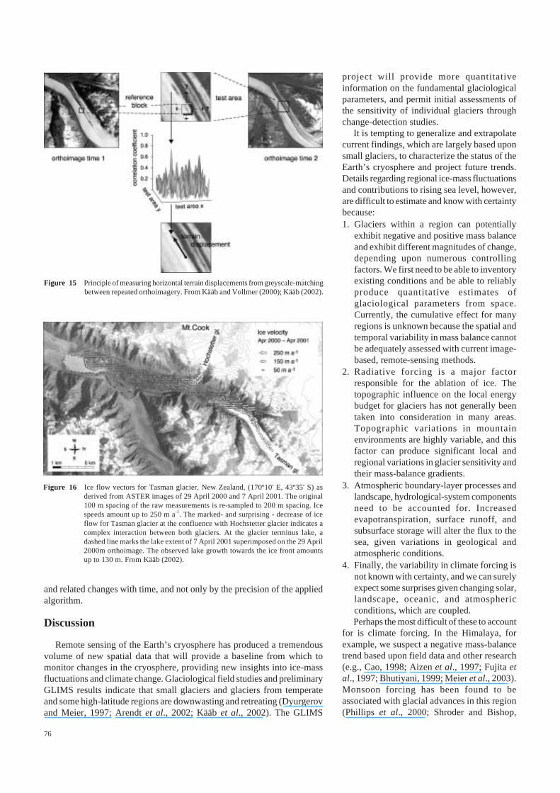
76

project will provide more quantitativeinformation on the fundamental glaciologicalparameters, and permit initial assessments ofthe sensitivity of individual glaciers throughchange-detection studies.

It is tempting to generalize and extrapolatecurrent findings, which are largely based uponsmall glaciers, to characterize the status of theEarth’s cryosphere and project future trends.Details regarding regional ice-mass fluctuationsand contributions to rising sea level, however,are difficult to estimate and know with certaintybecause:1. Glaciers within a region can potentially

exhibit negative and positive mass balanceand exhibit different magnitudes of change,depending upon numerous controllingfactors. We first need to be able to inventoryexisting conditions and be able to reliablyproduce quantitative estimates ofglaciological parameters from space.Currently, the cumulative effect for manyregions is unknown because the spatial andtemporal variability in mass balance cannotbe adequately assessed with current image-based, remote-sensing methods.

2. Radiative forcing is a major factorresponsible for the ablation of ice. Thetopographic influence on the local energybudget for glaciers has not generally beentaken into consideration in many areas.Topographic variations in mountainenvironments are highly variable, and thisfactor can produce significant local andregional variations in glacier sensitivity andtheir mass-balance gradients.

3. Atmospheric boundary-layer processes andlandscape, hydrological-system componentsneed to be accounted for. Increasedevapotranspiration, surface runoff, andsubsurface storage will alter the flux to thesea, given variations in geological andatmospheric conditions.

4. Finally, the variability in climate forcing isnot known with certainty, and we can surelyexpect some surprises given changing solar,landscape, oceanic, and atmosphericconditions, which are coupled.Perhaps the most difficult of these to account

for is climate forcing. In the Himalaya, forexample, we suspect a negative mass-balancetrend based upon field data and other research(e.g., Cao, 1998; Aizen et al., 1997; Fujita etal., 1997; Bhutiyani, 1999; Meier et al., 2003).Monsoon forcing has been found to beassociated with glacial advances in this region(Phillips et al., 2000; Shroder and Bishop,

Figure 15 Principle of measuring horizontal terrain displacements from greyscale-matchingbetween repeated orthoimagery. From Kääb and Vollmer (2000); Kääb (2002).

Figure 16 Ice flow vectors for Tasman glacier, New Zealand, (170º10' E, 43º35' S) asderived from ASTER images of 29 April 2000 and 7 April 2001. The original100 m spacing of the raw measurements is re-sampled to 200 m spacing. Icespeeds amount up to 250 m a-1. The marked- and surprising - decrease of iceflow for Tasman glacier at the confluence with Hochstetter glacier indicates acomplex interaction between both glaciers. At the glacier terminus lake, adashed line marks the lake extent of 7 April 2001 superimposed on the 29 April2000m orthoimage. The observed lake growth towards the ice front amountsup to 130 m. From Kääb (2002).

and related changes with time, and not only by the precision of the appliedalgorithm.

Discussion

Remote sensing of the Earth’s cryosphere has produced a tremendousvolume of new spatial data that will provide a baseline from which tomonitor changes in the cryosphere, providing new insights into ice-massfluctuations and climate change. Glaciological field studies and preliminaryGLIMS results indicate that small glaciers and glaciers from temperateand some high-latitude regions are downwasting and retreating (Dyurgerovand Meier, 1997; Arendt et al., 2002; Kääb et al., 2002). The GLIMS

77

2000). Monsoons are ultimately driven by the seasonalland-sea temperature contrast, which is induced by thedifferent heat capacities of land and sea.

A wealth of proxy data indicate that the south Asianmonsoon was once much stronger than it is today, both interms of wind speed and precipitation (Prell, 1984; Street-Perrott and Harrison, 1985). Because wind speed impactsevaporation over the Arabian Sea, as well as inlandpenetration of the monsoon jet, the strength of the monsoon(both summer and winter) plays a crucial role in regulatingHimalayan precipitation and snow accumulation (Benn andOwen, 1998; Richards et al., 2000).

Impacts of early-mid Holocene solar insolation on themonsoon have been studied in numerical simulations usinggeneral circulation models. Such experiments have confirmedthe link between solar forcing and strength of the Asianmonsoon (Kutzbach and Otto-Bliesner, 1982; Kutzbach andGuetter, 1984; Prell and Kutzbach, 1992). In addition, theconnection between tropical sea surface temperatures andthe strength of the monsoon has been shown to potentiallydominate orbital forcing (Bush, 2001) and that, in the lateQuaternary, a combination of these factors likely played arole in regulating the spatio-temporal extent of Himalayansnow accumulation (Bush, 2002).

Future snow accumulation and ice and sediment flux inthe Himalaya will be severely impacted by increasingamounts of atmospheric carbon dioxide, but competingeffects make it unclear which process – ice expansion orablation – will dominate. Under a global warming scenario,it is important to note that, for the monsoon, it is thetemperature gradient that is important, and not the actualvalues of temperature. For example, if temperatures were toincrease uniformly everywhere, this would have littledynamical impact on the strength of the winds. It would,however, dramatically impact the hydrological componentof the monsoon by increasing evaporation over the ArabianSea and precipitation in the Himalaya. It could be the casethat an increase in melting caused by warmer temperaturesmay be offset by an increase in snow accumulation causedby increased moisture flux into the Himalaya.

Climate simulations, coupled with remote sensing andGIS investigations, could provide us with new understandingsof how glaciers in the Himalaya and elsewhere might respondto greenhouse-gas forcing. Simulations that account for highertemperatures produce an increase in the temperature gradient.Similarly, greater moisture flux into the Himalaya andprecipitation could cause glaciers to exhibit positive massbalance. An increase in latent heat and glacier area couldenhance the strength of the monsoon and produce more snowaccumulation (Bush, 2000). This regional scenario is oppositeto our current understanding of higher temperatures causingincreased ablation and therefore glacial retreat.

To characterize the state of the Earth’s ice massdistribution, remote sensing provides the only practical meansto assess and monitor glaciers, by providing thematic andbiophysical information at frequent intervals (Kieffer et al.,2000; Bishop et al., 2000). Furthermore, remote sensing and

Figure 17 Landsat ETM+ image accquired 2001-1-14, showing UpsalaGlacier, South Patagonia. All velocity vectors obtained fromcross-correlation based, feature tracking between October 2000to March 2001 are overlaid as white line segments, and asubset of these are overlaid as black arrows for clarity. Icesurface speed ranges up to just under 2000 m a-1. The fast-moving calving front is approximately 2 km wide.

GIS investigations can play a critical role in studying climateforcing and glacier response (Bush et al., 2004). Scale-dependent (spatio-temporal) information extracted fromsatellite remote sensing and DEMs, coupled with detailed,field-calibration investigations, have the potential to greatlyimprove our ability to understand and monitor glacier process-structure and climate-glacier feedback relationships (Bishopet al., 1998a; Bush et al., 2004).

Multispectral analysis of debris-covered glaciers, whichare characteristic of many regions of the world, still representsa problem that has not been thoroughly investigated (Bishopet al., 1995, 1998a, 1999, 2001). Quantitative remote-sensingstudies are needed to examine and characterize supraglacialcharacteristics. Consequently, a comprehensive approach toinformation extraction and glaciological characterization ofglaciers from space is sorely needed.

In complex environments, information extraction fromsatellite imagery is complicated by the relatively low-to-highfrequency, spatial-reflectance variations caused by theatmosphere, topography and biophysical variations of matteron the landscape. Numerous investigators have developedand tested algorithms for normalizing reflectance variationsrelated to the atmosphere and topography (e.g., Dozier andFrew, 1981; Colby, 1991; Vermote et al., 1997; Bishop et al.,1998b; Bishop and Colby, 2002), so that radiometrically

78

calibrated data can be used to produce more accurate thematicand biophysical information. Many other investigators havefound, however, that anisotropic-reflectance correction andcalibration issues are not the only problems that must beaddressed for extracting reliable information, as spectral,spatial and topographic information (i.e., spectral features,spatial features, geomorphometric parameters), are essentialfor quantification and mapping of complex patterns in theseenvironments (Allen and Walsh, 1996; Gong, 1996; Bishopet al., 1998a,b, 1999; Kääb et al., 2002). Despite theseadvances in using additional information, results aredependent upon the complexity of the terrain, data qualityand measurement scale, ability to integrate multi-sourcedata, spatial-analysis approaches, and pattern-recognitionalgorithms. Furthermore, increased spectral-reflectancevariability from high-resolution imagery has been found tocause problems, as traditional classification methods havenumerous limitations (Gong, 1996). This has been empiricallydemonstrated by Franklin and Wilson (1992), where theydeveloped and tested a new three-stage classifier to overcomeextreme spectral variability in a complex environment.

Attempting to assess and map glaciers via ASTER andETM+ data using traditional approaches will permit theproduction of baseline information that allows change-detection studies. The use of various techniques and brute-force classification algorithms, however, do not produceconsistently high-quality results (Bishop et al., 1999), andquality information production often requires significantpre-analysis steps and a priori knowledge of the study area.Consequently, the GLIMS consortium is developing newapproaches to address classification and assessment problems,as new technologies and approaches have considerablepotential for information extraction from remotely senseddata and spatial data in GIS data bases.

Given the various uncertainties associated with spatialdata and standard, information-extraction approaches/algorithms, caution is warranted in terms of interpretingremote sensing results. Although the advantages of remotesensing and GIS investigations are widely recognized,numerous issues need to be addressed, and these require thesophisticated use of remote sensing science and geographicinformation technology. More research into the followingtopics is necessary to reduce the level of uncertaintyassociated with assessing the Earth’s glaciers from space:• Topographic solar-radiation transfer (TSRT) modeling.

Improved mapping of glaciers and change detection usingsatellite multispectral imagery will require operationalARC to radiometrically calibrate imagery and reduce theatmospheric and topographic effects. Accounting formulti-scale topographic effects in modeling the irradiantand radiant flux should permit effective “topographicnormalization” based on our preliminary modeling results.Accurate DEM generation capabilities are essential inthis effort.

• Landscape BRDF modeling. Field BRDF measurementsof supraglacial facies are required to validate BRDFmodeling results. Furthermore, it is necessary to establish

the nature of the relationship between reflectance anistropyand surface properties, solar geometry, viewing geometry,and wavelength dependence. This is essential for TSRTmodeling to accurately estimate the surface irradiance,and in making use of an asymmetry parameter (e.g.,Hapke, 1981) that will enable investigation of usingreflectance anistropy for glacier mapping and delineationof supraglacial facies.

• Integration of topographic information. Debris-coveredglaciers are difficult to map using spectral data alone.Research indicates that mapping results can besignificantly improved by using topographic informationin manual or computer-assisted approaches. Per-pointanalysis of spectral and topographic data, however, isgenerally not very effective for mapping debris-coveredglaciers due to scale-dependent supraglacial features andhighly variable glacier topography. Consequently, newapproaches to GIS-based data modeling and spatialanalysis, which address the issue of scale and topology,need to be further investigated, as our preliminary resultsindicate that this approach may significantly improveglacier mapping and permit semi-automated analysis(Bishop et al., 2001; Paul et al., 2004).

• Scientific visualization. Visualization of spatial data setshas progressed significantly over the years, such that 3-Dperspectives of satellite images are now routine. Greaterinteractivity and control of visualizing imagery, analysisand classification results are warranted, so that Earthscientists can better assess the accuracy of results incontext with other characteristics of the landscape.

• GIS-based physical models. GIS-based physical modelsthat utilize information from imagery and databases arerequired to better estimate glaciological parameters. Forexample, the integration of a TSRT model with surfaceenergy-budget modeling and spatial data can be used toestimate ablation rates, the mass-balance gradient and theequilibrium line altitude (ELA). This type of modeling issorely needed as the influence of the topography onradiative forcing is not always accounted for, and theglacier distribution and debris-cover spatial variation anddepth can be mapped and estimated using satellite imageryand field data. This approach might also be useful forestimating the sensitivity of glaciers to climate forcing,as the mass-balance gradient and glacial topography arestrongly related to changing atmospheric and flowconditions (Dyurgerov and Dwyer, 2000).These and other aspects of GLIMS research should

improve the quality of information about the Earth’s icemasses and establish a foundation for automated analysis inthe future. This will be accomplished by multidisciplinaryresearch involving Earth scientists and information scientists.Technically, progress is being made through the integrationof spectral analysis, spatial analysis, geomorphometricanalysis and physical modeling. This type of research isrequired to accurately assess the Earth’s cryosphere andreduce the uncertainties associated with improving ourunderstanding of climate forcing and glaciation, and

79

predicting the impact of global warming on the human andnatural dimensions of environmental change.

Conclusions

The international Global Land Ice Measurements FromSpace project is a USGS-led consortium of more than fortyuniversities and research institutes, whose purpose is to assessand monitor the Earth’s glaciers. Remote sensing and GIStechnology play an important role in assessing complex andremote environments as well as in the quantitative analysisand modeling of radiation transfer, surface energy budgets,glacier ablation and mass-balance estimates and climatesimulations. To date, preliminary remote sensing and GISinvestigations coupled with field data indicate that smallglaciers and glaciers in temperate regions are generallydownwasting and retreating, although detailed informationregarding glacier mass-balance gradients and regional trendshas yet to be determined from space. These and ongoingstudies have identified numerous issues associated withaccurate mapping and assessment of glaciers from space.GLIMS-related research will address these issues and developand implement new approaches to information extractionfrom spatial data. Our findings indicate the need to establishan integration of field studies with remote sensing and GISinvestigations, and develop new GIS-based physical modelsthat make use of satellite imagery and DEMS to account forspatial variation of phenomena and serve as constraints inmodeling efforts. Such remote sensing/GIS studies are vitalfor producing baseline information on glacier changes, andimproving our understanding of the complex linkages betweenatmospheric, lithospheric, and glaciological processes.

Acknowledgements

Bishop and Shroder would like to thank the UniversityCommittee on Research at the University of Nebraska atOmaha, the University of Nebraska Foundation, the NationalScience Foundation (EAR 9418839, EPS-9720643, and BCS-0242339), NASA (OES-2 grant) and the USGS. Bushgratefully acknowledges support from Canada’s NaturalSciences and Engineering Research Council Discovery Grant194151 and the Earth System Evolution Program of theCanadian Institute for Advanced Studies. Copland wouldlike to thank the CRYSYS program of the MeteorologicalService of Canada and the Canadian Space Agency forfunding. The University of Alberta Glims Regional Center.Fountain would like to thank the National Park Service andNASA (OES-2 grant). Additional support was provide by aNASA Earth Science Enterprise grant to the USGS/Flagstaff,NSIDC/boulder and EROS Data Center/Sioux Falls. NSIDCmembers (Barry, Raup, Armstrong, Scharfen, Khalsa)acknowledge support from NASA (grant NAG5-9722,REASoN CAN grant, 2 OES-2 grants). Kargel alsoacknowledges support from a NASA OES-2 grant and theUSGS. Haeberli, Kääb and Paul were supported by the

Swiss National Science Foundation (Grant no. 21-54073.98).We would also like to acknowledge the contributions ofNASA/METI, USGS, the ASTER Science Team, andregional center chiefs and staff, who have contributedsignificantly to various aspects of the GLIMS project. TheWorld Glacier Monitoring Service (WGMS) of theInternational Commission on Snow and Ice (ICSI/IAHS) isone of the services of the Federation of Astronomical andGeophysical Data Analysis Services (FAGS/ICSU) and runsthe Global Terrestrial Network on Glaciers (GTN-G) withinthe Global Terrestrial Observing System (GTOS/GCOS) ofFAO, ICSU, UNEP, UNESCO, and WMO.

References

Aizen, V. B., Aizen, E. M., Dozier, J., Melack, J. M., Sexton, D. D.,and Nesterov, V. N. (1997). Glacial regime of the highest TienShan mountain, Pobeda-Khan Tengry massif. Journal of Glaciology,33:503–512.

Al-Rousan, N. and Petrie, G. (1998). System calibration, geometricaccuracy testing and validation of DEM and orthoimage dataextracted from SPOT stereopairs using commercially availableimage processing systems. International Archives ofPhotogrammetry and Remote Sensing, 34(4):8–15.

Aldous, P. (2003). The world’s forgotten crisis. Nature, 422:251.

Allen, T. R. and Walsh, S. J. (1996). Spatial and compositional patternof alpine treeline, Glacier National Park, Montana. PhotogrammetricEngineering and Remote Sensing, 62(11):1261–1268.

Andrews, J. T. (2002). Glaciers of Baffin Island. In Williams andFerrigno (2002b), pages J165–J198.

Aniya, M., Sato, H., Naruse, R., Skvarca, P., and Casassa, G. (1996).The use of satellite and airborne imagery to inventory outlet glaciersof the southern Patagonia icefield, South America. PhotogrammetricEngineering and Remote Sensing, 62(12):1361–1369.

Arendt, A., Echelmeyer, K., Harrison, W. D., Lingle, G., and Valentine,V. (2002). Rapid wastage of Alaska glaciers and their contributionto rising sea level. Science, 297:382–386.

Armstrong, R. L. (1989). Mass balance history of Blue Glacier,Washington, USA. In Oerlemans, J., editor, Glacier Fluctuationsand Climatic Change, pages 183–192. Kluwer Academic Publishers,Dordrecht.

Asrar, G. and Dozier, J. (1994). Science Strategy for the Earth ObservingSystem (EOS). American Institute of Physics, Woodbury, NY.

Bahr, D. B., Meier, M. F., and Peckham, S. D. (1997). The physicalbasis of glacier volume-area scaling. Journal of GeophysicalResearch, 102:20,355–20,362.

Barry, R. G. and Carleton, A. M. 2001. Synoptic and Dynamicclimatology, Routledge, London and New York..

Bayr, K. J., Hall, D. K., and Kovalick, W. M. (1994). Observations onglaciers in the eastern Austrian Alps using satellite data.International Journal of Remote Sensing, 15(9):1733–1742.

Beniston, M., editor (1994). Mountain Environments in ChangingClimates. Routledge, London.

Beniston, M., Haeberli,W., Hoelzle, M., and Taylor, A. (1997). On thepotential use of glacier and permafrost observations for verificationof climate models. Annals of Glaciology, 25:400–406.

80

Benn, D. I. and Owen, L. A. (1998). The role of the Indian summermonsoon and the midlatitude westerlies in Himalayan glaciation:Review and speculative discussion. Journal of the GeologicalSociety, 155(2):353–363.

Bhutiyani, M. R. (1999). Mass-balance studies on Siachen Glacier inthe Nubra valley, Karakoram Himalaya, India. Journal ofGlaciology, 45:112–118.

Binaghi, E., Madella, P., Montesano, M. P., and Rampini, A. (1997).Fuzzy contextual classification of multisource remote sensingimages. IEEE Transactions on Geoscience and Remote Sensing,GE-35(2):326–339.

Bindschadler, R., Dowdeswell, J., Hall, D., and Winther, J. G. (2001).Glaciological applications with Landsat-7 imagery: Earlyassessments. Remote Sensing of Environment, 78(147):163–179.

Bishop, M. P., Bonk, R., Kamp, Jr., U., and Shroder, Jr., J. F. (2001).Terrain analysis and data modeling for alpine glacier mapping.Polar Geography, 24(4):257–276.

Bishop, M. P. and Colby, J. D. (2002). Anisotropic reflectancecorrection of SPOT-3 HRV imagery. International Journal ofRemote Sensing, 23(10):219–222.

Bishop, M. P., Kargel, J. S., Kieffer, H. H., MacKinnon, D. J., Raup,B. H., and Shroder, Jr., J. F. (2000). Remote sensing science andtechnology for studying glacier processes in high Asia. Annals ofGlaciology, 31:164–170.

Bishop, M. P. and Shroder, Jr., J. F., editors (2004). GeographicInformation Science and Mountain Geomorphology. Springer-Praxis, Chichester.

Bishop, M. P., Shroder, Jr., J. F., Bonk, R., and Olsenholler, J. (2002).Geomorphic change in high mountains: A western Himalayanperspective. Global and Planetary Change, 32:311–329.

Bishop, M. P., Shroder, Jr., J. F., and Colby, J. D. (2003). Remotesensing and geomorphometry for studying relief production in highmountains. Geomorphology, 55:345–361.

Bishop, M. P., Shroder, Jr., J. F., and Hickman, B. L. (1999). Highresolution satellite imagery and neural networks for informationextraction in a complex mountain environment. GeocartoInternational, 14(2):17–26.

Bishop, M. P., Shroder, Jr., J. F., Hickman, B. L., and Copland, L.(1998a). Scale dependent analysis of satellite imagery forcharacterization of glacier surfaces in the Karakoram Himalaya.Geomorphology, 21:217–232.

Bishop, M. P., Shroder, Jr., J. F., Sloan, V. F., Copland, L., and Colby,J. D. (1998b). Remote sensing and GIS technology for studyinglithospheric processes in a mountain environment. GeocartoInternational, 13(4):75–87.

Bishop, M. P., Shroder, Jr., J. F., and Ward, J. L. (1995). SPOTmultispectral analysis for producing supraglacial debris-load estimatesfor Batura Glacier, Pakistan. Geocarto International, 10(4):81–90.

Brozovik, N., Burbank, D. W., and Meigs, A. J. (1997). Climatic limitson landscape development in the northwestern Himalaya. Science,276:571–574.

Bush, A. B. G. (2000). A positive feedback mechanism for Himalayanglaciation. Quaternary International, 65-6:3–13.

Bush, A. B. G. (2001). Pacific sea surface temperature forcing dominatesorbital forcing of the early Holocene monsoon. QuaternaryResearch, 55:25–32.

Bush, A. B. G. (2002). A comparison of simulated monsoon circulationsand snow accumulation in Asia during the mid-Holocene and at theLast Glacial Maximum. Global and Planetary Change, 32:331–347.

Bush, A. B. G., Prentice, M. L., Bishop, M. P., and Shroder, Jr., J. F.(2004). Modeling global and regional climate systems: Climateforcing and topography. In Bishop and Shroder (2004).

Cao, M. S. (1998). Detection of abrupt changes in glacier mass balancein the Tien Shan Mountains. Journal of Glaciology, 44(147):352–358.

Cenderelli, D. A. and Wohl, E. E. (2001). Peak discharge estimates ofglacial lake outburst floods, and “normal” climatic floods in theMount Everest region, Nepal. Geomorphology, 40:57–90.

Civco, D. L. (1989). Topographic normalization of landsat thematicmapper digital imagery. Photogrammetric Engineering and RemoteSensing, 55(9):1303–1309.

Cogley, J. G. and Adams,W. P. (1998). Mass balance of glaciers otherthan the ice sheets. Journal of Glaciology, 44:315–325.

Colby, J. D. (1991). Topographic normalization in rugged terrain.Photogrammetric Engineering and Remote Sensing, 57(5):531–537.

Colby, J. D. and Keating, P. L. (1998). Land cover classification usingLandsat TM imagery in the tropical highlands: The influence ofanisotropic reflectance. International Journal of Remote Sensing,19(8):1479–1500.

Conese, C., Gilabert, M. A., Maselli, F., and Bottai, L. (1993a).Topographic normalization of tm scenes through the use of anatmospheric correction method and digital terrain models.Photogrammetric Engineering and Remote Sensing, 59(12):1745–1753.

Conese, C., Maracchi, G., and Maselli, F. (1993b). Improvement inmaximum likelihood classification performance on highly ruggedterrain using principal components analysis. International Journalof Remote Sensing, 14(7):1371–1382.

Coxon, P., Owen, L. A., and Mitchell, W. A. (1996). A Late Quaternarycatastrophic flood in the Lahul Himalayas. Journal of QuaternaryScience, 11:495–510.

Davis, P. T. (1988). Holocene glacier fluctuations in the AmericanCordillera. Quaternary Science Reviews, 7(2):129–157.

Dozier, J. (1984). Snow-reflectance from Landsat-4 Thematic Mapper.IEEE Transactions on Geoscience & Remote Sensing, GE-22(3):323–328.

Dozier, J. and Frew, J. (1981). Atmospheric corrections to satelliteradiometric data over rugged terrain. Remote Sensing ofEnvironment, 11:191–205.

Dyurgerov, M. and Dwyer, J. (2000). The steepness of glacier massbalance gradients with northern hemisphere warming. Zeitschriftfür Gletscherkunde und Glazialgeologie, 36:107–118.

Dyurgerov, M. B. and Bahr, D. B. (1999). Correlations betweenglacier properties: Finding appropriate parameters for global glaciermonitoring. Journal of Glaciology, 45(149):9–16.

Dyurgerov, M. B. and Meier, M. F. (1997). Year-to-year fluctuationsof global mass balance of small glaciers and their contribution tosea-level changes. Arctic and Alpine Research, 29(4):392–402.

Dyurgerov, M. B. and Meier, M. F. (2000). Twentieth century climatechange: Evidence from small glaciers. Proceedings of the NationalAcademy of Science, 97(4):1406–1411.

Ekstrand, S. (1996). Landsat TM-based forest damage assessment:Correction for topographic effects. Photogrammetric Engineeringand Remote Sensing, 62(2):151–161.

ERSDAC (1999a). ASTER User’s Guide. Part I(2). Earth RemoteSensing Data Analysis Center, Tokyo, Japan.

81

ERSDAC (1999b). ASTER User’s Guide. Part II(2). Earth RemoteSensing Data Analysis Center, Tokyo, Japan.

Evans, A. N. (2004). Glacier surface motion computation from digitalimage sequences. IEEE Transactions on Geoscience and RemoteSensing, page in press.

Field, W. O., editor (1975). Mountain Glaciers of the NorthernHemisphere, volume 1. Cold Regions Research and EngineeringLaboratory, Hanover, NH.

Fountain, A. G., Krimmel, R. M., and Trabant, D. C. (1997). AStrategy for Monitoring Glaciers. Number 1132 in Circular. UnitedStates Geological Survey, Reston.

Franklin, S. E. and Wilson, B. A. (1992). A three-stage classifier forremote sensing of mountain environments. PhotogrammetricEngineering and Remote Sensing, 58(4):449–454.

Frezzotti, M., Capra, A., and Vittuari, L. (1998). Comparison betweenglacier ice velocities inferred from GPS and sequential satelliteimages. Annals of Glaciology, 27:54–60.

Fujita, K., Nakawo, M., Fujii, Y., and Paudyal, P. (1997). Changes inglaciers in Hidden Valley, Mukut Himal, Nepal Himalayas, from1974 to 1994. Journal of Glaciology, 43:583–588.

Gao, J. and Liu, Y. (2001). Applications of remote sensing, GIS andGPS in glaciology: A review. Progress in Physical Geography,25(4):520–540.

Giles, P. T. (2001). Remote sensing and cast shadows in mountainousterrain. Photogrammetric Engineering and Remote Sensing,67(7):833–839.

Gleick, P. (2001). Making every drop count. Scientific American,284:41–45.

Gleick, P. (2003). Atlas of a thirsty planet. Nature, 422:252–253.

Gong, P. (1996). Integrated analysis of spatial data from multiplesources: Using evidential reasoning and artificial neural networktechniques for geological mapping. Photogrammetric Engineeringand Remote Sensing, 62(5):513–523.

Goudie, A. S., Brunsden, D. N., Collins, D. N., Derbyshire, E., Ferguson,R. I., Hashmet, Z., Jones, D. K. C., Perrot, F. A., Said, M., Waters,R. S., and Whalley, W. B. (1984, Vol. II). The geomorphology ofthe Hunza Valley, Karakoram Mountains, Pakistan. In Miller, K.J., editor, The International Karakoram Project, pages 359–410.Cambridge University Press, Cambridge.

Granshaw, F. C. (2001). Glacier Change in the North Cascades NationalPark Complex, Washington State, USA, 1958-1998. PhD thesis,Portland State University, Portland, Oregon.

Greuell, W. and de Ruyter de Wildt, M. (1999). Anisotropic reflectionby melting glacier ice: Measurements and parametrizations inLandsat TM bands 2 and 4. Remote Sensing of the Environment,70:265–277.

Gu, D. and Gillespie, A. (1998). Topographic normalization of LandsatTM images of forest based on subpixel sun-canopy-sensor geometry.Remote Sensing of the Environment, 64:166–175.

Haeberli,W. (1998). Historical evolution and operational aspects ofworldwide glacier monitoring. In Haeberli et al. (1998), pages 35–47.

Haeberli, W., Barry, R., and Cihlar, J. (2000). Glacier monitoringwithin the Global Climate Observing System. Annals of Glaciology,31:241–246.

Haeberli, W. and Beniston, M. (1998). Climate change and its impactson glaciers and permafrost in the Alps. Ambio, 27(4):258–265.

Haeberli, W., Benz, C., Gruber, U., Hoelzle, M., Kääb, A., and Schaper,J. (2004). GIS applications for snow and ice in high-mountainareas: Examples from the Swiss Alps. In Bishop and Shroder(2004).

Haeberli, W. and Hoelzle, M. (1995). Application of inventory datafor estimating characteristics of and regional climate-change effectson mountain glaciers: A pilot study with the European Alps. Annalsof Glaciology, 21:206–212.

Haeberli, W., Hoelzle, M., and Suter, S., editors (1998). Into theSecond Century of Worldwide Glacier Monitoring: Prospects andStrategies. UNESCO, Paris.

Hall, D. K., Bayr, K. J., Schöner,W., Bindschadler, R. A., and Chien,J. Y. L. (2003). Consideration of the errors inherent in mappinghistorical glacier positions in Austria from the ground and space(1893 - 2001). Remote Sensing of Environment, 86(4):566–577.

Hall, D. K., Benson, C. S., and Field, W. O. (1995). Changes ofglaciers in Glacier Bay, Alaska, using ground and satellitemeasurements. Physical Geography, 16(1):27–41.

Hall, D. K., Chang, A. T. C., Foster, J. L., Benson, C. S., and Kovalick,W. M. (1989). Comparison of in situ and Landsat derived reflectanceof Alaskan glaciers. Remote Sensing of the Environment, 28:23–31.

Hall, D. K., Williams, R. S., Barton, J. S., Sigurdsson, O., Smith, L. C.,and Garvin, J. B. (2000). Evaluation of remote sensing techniquesto measure decadal-scale changes of Hojsjökull ice cap, Iceland.Journal of Glaciology, 46(154):375–388.

Hall, D. K., Williams, R. S., and Bayr, K. J. (1992). Glacier recessionin Iceland and Austria. EOS Transactions of the AmericanGeophysical Union, 73(12):129,135,141.

Hall, M. H. P. and Fagre, D. B. (2003). Modeled climate-inducedglacier change in Glacier National Park, 1850-2100. BioScience,53(2):131–140.

Hallet, B., Hunter, L., and Bogen, J. (1996). Rates of erosion andsediment evacuation by glaciers: A review of field data and theirimplications. Global and Planetary Change, 12:213–235.

Hapke, B. W. (1981). Bidirectional reflectance spectroscopy - 1.Theory. Journal of Geophysical Research, 86:3039–3054.

Harbor, J. and Warburton, J. (1992). Glaciation and denudation rates.Nature, 356:751.

Harbor, J. and Warburton, J. (1993). Relative rates of glacial andnonglacial erosion in alpine environments. Arctic and AlpineResearch, 25:1–7.

Henderson-Sellers, A. and Pitman, A. (1992). Land surface schemesfor future climate models: Specification, aggregation, andheterogeneity. Journal of Geophysical Research, 97:2687–2696.

Hewitt, K. and Young, G. J. (1990). Snow and ice hydrology project:Upper Indus basin. Overall report, Canadian Centre.

Hirano, A., Welch, R., and Lang, H. (2003). Mapping from ASTERstereo image data: DEM validation and accuracy assessment. ISPRSJournal of Photogrammetry and Remote Sensing, page in press.

Hodge, S. M., Trabant, D. C., Krimmel, R. M., Heinrichs, T. A.,March, R. S., and Josberger, E. G.(1998). Climate variations andchanges in mass of three glaciers in western North America. Journalof Climate, 11(9):2161–2179.

Hoelzle, M., Haeberli, W., Dischl, M., and Peschke, W. (2003). Secularglacier mass balances derived from cumulative glacier lengthchanges. Global and Planetary Change, 36(4):77–89.

82

Horvath, E. (1975). Hindu Kush. In Field (1975), pages 361–370.

Huggel, C., Kääb, A., Haeberli, W., Teysseire, P. and Paul, F., (2002).Remote sensing based assessment of hazards from glacier lakeoutbursts: a case study in the Swiss Alps. Canadian GeotechnicalJournal, 39 (a): 316-330.

IPPC (2001). Climate Change 2001 - The Scientific Basis. Contributionof Working Group I to the Third Assessment Report of theIntergovernmental Panel on Climate Change. Cambridge UniversityPress, New York.

Jacobs, J. D., Simms, E. L., and Simms, A. (1997). Recession of thesouthern part of Barnes Ice Cap, Baffin Island, Canada, between1961 and 1993, determined from digital mapping of Landsat TM.Journal of Glaciology, 43(143):98–102.

Kääb, A. (2002). Monitoring high-mountain terrain deformation fromair- and spaceborne optical data: Examples using digital aerialimagery and ASTER data. ISPRS Journal of Photogrammetry andRemote Sensing, 57(1-2):39–52.

Kääb, A. and Funk, M. (1999). Modelling mass balance usingphotogrammetric and geophysical data: A pilot study atGriesgletscher, Swiss Alps. Journal of Glaciology, 45(151):575–583.

Kääb, A., Haeberli, W., and Gudmundsson, G. H. (1997). Analysingthe creep of mountain permafrost using high precision aerialphotogrammetry: 25 years of monitoring Gruben Rock Glacier,Swiss Alps. Permafrost and Periglacial Processes, 8(4):409–426.

Kääb, A., Paul, F., Maisch, M., Hoelzle, M., and Haeberli, W. (2002).The new remote sensing derived Swiss glacier inventory: II. Firstresults. Annals of Glaciology, 34:362–366.

Kääb, A., R. Wessels, W. Haeberli, C. Huggel, J. S. Kargel, S. J. S.Khalsa, 2003, Rapid ASTER imaging facilitates timely assessmentof glacier hazards and disasters. EOS, Transacting AmericanGeophysical Union. 84 (13) 117 & 121.

Kääb, A. and Vollmer, M. (2000). Surface geometry, thickness changesand flow fields on creeping mountain permafrost: Automaticextraction by digital image analysis. Permafrost and PeriglacialProcesses, 11:315–326.

Kaser, G. (2001). Glacier-climate interaction at low latitudes. Journalof Glaciology, 47:195–204.

Kaufmann, V. and Ladstädter, B. (2003). Spatio-temporal analysis ofthe dynamic behaviour of the Hochebenkar rock glaciers (OetztalAlps, Austria) by means of digital photogrammetric methods. InProceedings, 6th International Symposium on High Mountain RemoteSensing Cartography, volume 37, pages 119–139, Ethiopia, Kenya,Tanzania. Grazer Schriften der Geographie und Raumforschung.

Kieffer, H., Kargel, J., Barry, R., Bindschadler, R., Bishop, M. P.,MacKinnon, D., Ohmura, A., Raup, B., Antoninetti, M., Bamber,J., Braun, M., Brown, I., Cohen, D., Copland, L., DueHagen, J.,Engeset, R., Fitzharris, B., Fujita, K., Haeberli, W., Hagen, J., Hall,D., Hoelzle, M., Johansson, M., Kaeaeb, A., Koenig, M., Konovalov,V., Maisch, M., Paul, F., Rau, F., Reeh, N., Rignot, E., Rivera, A.,de Ruyter de Wildt, M., Scambos, T., Schaper, J., Scharfen, G.,Shroder, J., Solomina, O., Thompson, D., van der Veen, K.,Wohlleben, T., and Young, N. (2000). New eyes in the sky measureglaciers and ice sheets. EOS Transactions, 81(24).

King, C. (1871). On the discovery of actual glaciers on the mountainsof the Pacific Slope. American Journal of Science and Arts,24(3):157–167.

Koerner, R. M. (2002). Glaciers of the High Arctic Islands. In Williamsand Ferrigno (2002b), pages J111–J146.

Kotlyakov, V. M., Serebrjanny, L. R., and Solomina, O. N. (1991).Climate change and glacier fluctuations during the last 1,000 yearsin the southern mountains of the USSR. Mountain Research andDevelopment, 11:1–12.

Kowalik, W. S., Lyon, R. J. P., and Switzer, P. (1983). The effects ofadditive radiance terms on ratios of Landsat data. PhotogrammetricEngineering and Remote Sensing, 49(5):659–669.

Krimmel, R. M. (1999). Analysis of difference between direct andgeodetic mass balance measurements at South Cascade Glacier,Washington. Geografiska Annaler, 81A(4):653–658.

Kump, L. R. (2002). Reducing uncertainty about carbon dioxide as aclimate driver. Nature, 419:188–190.

Kutzbach, J. E. and Guetter, P. J. (1984). The sensitivity of monsoonclimates to orbital parameter changes for 9000 years B.P.:Experiments with the NCAR general circulation model. In Berger,A., Imbrie, J., Hays, J. D., Kukla, G. J., and Saltzman, B., editors,Milankovitch and Climate, pages 801–820. Publishing Company.

Kutzbach, J. E. and Otto-Bliesner, B. L. (1982). The sensitivity of theAfrican-Asian monsoonal climate to orbital parameter changes for9000 years B.P. in a low-resolution general circulation model.Journal of the Atmospheric Sciences, 39:1177–1188.

Lambeck, K. and Chappell, J. (2001). Sea level change through the lastglacial cycle. Science, 292:679–686.

Lambeck, K., Tezer, M. E., and Potter, E. K. (2002). Links betweenclimate and sea levels for the past three million years. Nature,419:199–206.

Lefauconnier, B., Hagen, J. O., and Rudant, J. P. (1994). Flow speedand calving rate of Kronebreen Glacier, Svalbard, using SPOTimages. Polar Research, 13(1):59–65.

Leonard, K. C. and Fountain, A. G. (2003). Map-based methods forestimating glacier equilibrium line altitudes. Journal of Glaciology,page in press.

Li, Z., Sun, W., and Zeng, Q. (1998). Measurements of glacier variationin the Tibetan Plateau using Landsat data. Remote Sensing ofEnvironment, 63:258–264.

Limpasuvan, V. and Hartmann, D. L. (2000). Wave-maintained annularmodes of climate variability. Journal of Climate, 13:4414–4429.

Maisch, M. (2000). The longterm signal of climate change in the SwissAlps: Glacier retreat since the end of the Little Ice Age and futureice decay scenarios. Geografia Fisica e Dinamica Quaternaria,23(2):139–151.

Marston, R. A., Pochop, L. O., Kerr, G. L., Varuska, M. L., andVeryzer, D. J. (1991). Recent glacier changes in the Wind RiverRange, Wyoming. Physical Geography, 12(2):115–123.

Mattson, L. E. (2000). The influence of a debris cover on the mid-summer discharge of Dome Glacier, Canadian Rocky Mountains.In Nakawa, M., Raymond, C. F., and Fountain, A., editors, DebrisCovered Glaciers, number 264 in Proceedings and Reports, pages25–33. IAHS Press.

Mayewski, P. A. and Jeschke, P. A. (1979). Himalayan and trans-Himalayan glacier fluctuations since AD 1812. Arctic and AlpineResearch, 11: 267–287.

Mayewski, P. A., Pergent, G. P., Jeschke, P. A., and Ahemad, N.(1980). Himalayan and Trans-Himalayan glacier fluctuations andthe south Asian monsoon record. Arctic and Alpine Research,12:171–182.

McCabe, G. J. and Fountain, A. G. (1995). Relations betweenatmospheric circulation and mass balance of South Cascade Glacier,Washington, U.S.A. Arctic and Alpine Research, 27(3):226.

83

McCabe, G. J., Fountain, A. G., and Dyurgerov, M. (2000). Variabilityin winter mass balance of northern hemisphere glaciers and relationswith atmospheric circulation. Arctic, Antarctic, and Alpine Research,32(1):64–72.

McClung, D. M. and Armstrong, R. L. (1993). Temperate glacier timeresponse from field data. Journal of Glaciology, 39(132):323–326.

Meier, M. F. (1961). Distribution and variations of glaciers in theUnited States exclusive of Alaska. International Association ofScientific Hydrology, 47:420–429.

Meier, M. F. (1984). Contribution of small glaciers to global sea level.Science, 226:1418–1421.

Meier, M. F. and Bahr, D. B. (1996). Counting glaciers: Use of scalingmethods to estimate the number and size distribution of the glacierson the world. In Colbeck, S. C., editor, Glaciers, Ice Sheets andVolcanoes: A Tribute to Mark F. Meier, number 96-27, pages 1–120. CRREL Special Report.

Meier, M. F. and Dyurgerov, M. B. (2002). How Alaska affects theworld. Science, 297:350–351.

Meier, M. F., Dyurgerov, M. B., and McCabe, G. J. (2003). The healthof glaciers: Recent changes in glacier regime. Climate Change,0:1–13.

Meier, M. F. and Post, A. (1975). Glaciers: A Water Resource. UnitedStates Geological Survey, Reston.

Meier, M. F. and Tangborn, W. V. (1965). Net budget and flow ofSouth Cascade Glacier, Washington. Journal of Glaciology,5(41):547–566.

Meier, M. F. and Wahr, J. M. (2002). Sea level is rising: Do we knowwhy? Proceedings of the National Academy of Science,99(10):6524–6526.

Mercer, J. H. (1975a). Himalaya. In Field (1975), pages 411–448.

Mercer, J. H. (1975b). Karakoram. In Field (1975), pages 371–410.

Miller, M. M. and Pelto, M. S. (1999). Mass balance measurements onthe Lemon Creek Glacier, Juneau Icefield, Alaska 1953-1998.Geografiska Annaler, 81A(4):671–681.

Molnar, P. and England, P. (1990). Late Cenozoic uplift of mountainranges and global climate change: Chicken or egg? Nature, 346:29–34.

Mool, P. K., Bajracharya, S. R., and Joshi, S. P. (2001a). Inventory ofGlaciers, Glacial Lakes and Glacial Lake Outburst Floods, Nepal.International Center for Integrated Mountain Development,Kathmandu, Nepal.

Mool, P. K.,Wangda, D., Bajracharya, S. R., Kunzang, K., Gurung, D.R., and Joshi, S. P. (2001b). Inventory of Glaciers, Glacial Lakesand Glacial Lake Outburst Floods, Bhutan. International Centerfor Integrated Mountain Development, Kathmandu, Nepal.

Mysak, L. A., Ingram, R. G., Wang, J., and vanderBaaren, A. (1996).The anomalous sea-ice extent in Hudson Bay, Baffin Bay and theLabrador Sea during three simultaneous NAO and ENSO episodes.Atmosphere-Ocean, 34:313–343.

Nakawo, M., Fujita, K., Ageta, U., Shankar, K., Pokhrel, P. A., andTandong, Y. (1997). Basic studies for assessing the impacts of theglobal warming on the Himalayan cryosphere. Bulletin of GlacierResearch, 15:53–58.

O’Connor, J. E., Hardison III, J. H., and Costa, J. E. (2001). DebrisFlows from Failures of Neoglacial-Age Moraine Dams in theThree Sisters and Mount Jefferson Wilderness Areas, Oregon.Number 1606 in Professional Paper. United States GeologicalSurvey, Reston.

Oerlemans, J., Anderson, B., Hubbard, A., Huybrechts, P., Johannesson,T., Knap, W. H., Schmeits, M., Stroeven, A. P., van de Wal, R.S.W.,Wallinga, J., and Zuo, Z. (1998). Modelling the response ofglaciers to climate warming. Climate Dynamics, 14:267–274.

Ommanney, S. (1970). The Canadian glacier inventory. In Glaciers,Proceedings of Workshop Seminar, pages 23–30. Ottawa CanadianNational Committee. The International Hydrological Decade.

Paul, F. (2001). Evaluation of different methods for glacier mappingusing Landsat TM. In EARSeL Workshop on Remote Sensing ofLand Ice and Snow, volume 1, pages 239–245, Dresden. EARSeLProceedings, CD-ROM.

Paul, F. (2004). The New Swiss Glacier Inventory 2000 - Applicationof Remote Sensing and GIS. PhD thesis, University of Zurich,Zurich, Switzerland.

Paul, F., Kääb, A., Maisch, M., Kellenberger, T., and Haeberli,W.(2002). The new remote sensing derived Swiss glacier inventory: I.Methods. Annals of Glaciology, 34:355–361. 4th InternationalSymposium on Remote Sensing in Glaciology.

Paul, F., Huggel, C., and Kääb, A. (2004). Combining SatelliteMultispectral image data and a digital elevation model for mappingof debris-covered glaciers, Remote Sensing of Environment, 89 (4):510-518.

Pelto, M. S. and Miller, M. M. (1990). Mass balance of the TakuGlacier, Alaska from 1946-1986. Northwest Science, 64:121–130.

Phillips, W. M., Sloan, V. F., Shroder, Jr., J. F., Sharma, P., Clarke, M.L., and Rendell, H. M. (2000). Asynchronous glaciation at NangaParbat, northwestern Himalaya Mountains, Pakistan. Geology,28:431–434.

Pierrehumbert, R. T. (2002). The hydrologic cycle in deep-time climateproblems. Nature, 419:191–198.

Post, A., Richardson, D., Tangborn, W. V., and Rosselot, F. L. (1971).Inventory of Glaciers in the North Cascades Washington. Number705-A in Professional Paper. United States Geological Survey, Reston.

Prell, W. L. (1984). Monsoonal climate of the Arabian Sea during thelate Quaternary: A response to changing solar radiation. In Berger,A., Imbrie, J., Hays, J. D., Kukla, G. J., and Saltzman, B., editors,Milankovitch and Climate, pages 349–366. Publishing Company.

Prell, W. L. and Kutzbach, J. E. (1992). Sensitivity of the Indianmonsoon to forcing parameters and implications for its evolution.Nature, 360:647–652.

Proy, C., Tanre, D., and Deschamps, P. Y. (1989). Evaluation oftopographic effects in remotely sensed data. Remote Sensing of theEnvironment, 30:21–32.

Rabus, B. T. and Echelmeyer, K. E. (1998). The mass balance ofMcCall Glacier, Brooks Range, Alaska, U.S.A.; Its regionalrelevance and implications for climate change in the Arctic. Journalof Glaciology, 44(147):333–351.

Raup, B. H., Kieffer, H. H., Hare, T. M., and Kargel, J. S. (2000).Generation of data acquisition requests for the ASTER satelliteinstrument for monitoring a globally distributed target: Glaciers.IEEE Transactions on Geoscience and Remote Sensing, 38(2):1105–1112.

Raymo, M. E. and Ruddiman,W. F. (1992). Tectonic forcing of thelate Cenozoic climate. Nature, 359:117–122.

Raymo, M. E., Ruddiman, W. F., and Froelich, P. N. (1988). Influenceof late Cenozoic mountain building on geochemical cycles. Geology,16:649–653.

84

Richards, B. W., Owen, L. A., and Rhodes, E. J. (2000). Timing ofLate Quaternary glaciations in the Himalaya of northern Pakistan.Journal of Quaternary Science, 15:283–297.

Richter, R. (1997). Correction of atmosphere and topographic effectsfor high spatial resolution satellite imagery. International Journalof Remote Sensing, 18(5):1099–1111.

Ruddiman, W. F., editor (1997). Tectonic Uplift and Climate Change.Plenum Press, New York.

Scambos, T. A., Dutkiewicz, M. J., Wilson, J. C., and Bindschadler, R.A. (1992). Application of image cross-correlation to themeasurement of glacier velocity using satellite image data. RemoteSensing of Environment, 42(3):177–186.

Schaper, J., Martinec, J., and Seidel, K. (1999). Distributed mappingof snow and glaciers for improved runoff modelling. HydrologicalProcesses, 13(12-13):2023–2031.

Schilling, S. P., Carrara, P. E., Thompson, R. A., and Iwatsubo, E. Y.(2004). Post-eruption glacier development within the crater ofMount St. Helens, Washington, USA. Quaternary Research, pagein press.

Seltzer, G. O. (1993). Late-Quaternary glaciation as a proxy for climatechange in the central Andes. Mountain Research and Development,13:129–138.

Shroder, Jr., J. F. (1980). Special problems of glacial inventory inAfghanistan. In World Glacial Inventory Proceedings ReideralpWorkshop, September 1978, number 126 in Hydrological SciencesBulletin, pages 142–147. IAHS-AISH Press.

Shroder, Jr., J. F. (1989). Glacierized areas of Afghanistan. In Haeberli,W., Bosch, H., Scherler, K., Østrem, G., and Wallen, C. C., editors,World Glacial Inventory, Status 1988, pages C39–C40. IAHS(ICSI)-UNEP-UNESCO, Teufen, Switzerland.

Shroder, Jr., J. F. (2004a). Satellite glacier inventory of Afghanistan.In Williams and Ferrigno (2004).

Shroder, Jr., J. F. (2004b). Satellite-image analysis of glaciers ofnorthern Pakistan. In Williams and Ferrigno (2004).

Shroder, Jr., J. F. and Bishop, M. P. (2000). Unroofing of the NangaParbat Himalaya. In Khan, M. A., Treloar, P. J., Searle, M. P., andJan, M. Q., editors, Tectonics of the Nanga Parbat Syntaxis and theWestern Himalaya, number 170 in Special Publication, pages 163–179. Geological Society, London.

Shroder, Jr., J. F., Bishop, M. P., and Scheppy, R. (1998). Catastrophicflood flushing of sediment, western Himalaya, Pakistan. In Kalvoda,J. and Rosenfeld, C. L., editors, Geomorphological Hazards inHigh Mountain Areas, pages 27–48. Kluwer Academic Publishers,Dordrecht.

Sidjak, R. W. and Wheate, R. D. (1999). Glacier mapping of theIllecillewaet icefield, British Columbia, Canada, using LandsatTM and digital elevation data. International Journal of RemoteSensing, 20(2):273–284.

Smith, J. A., Lin, T. L., and Ranson, K. J. (1980). The Lambertianassumption and Landsat data. Photogrammetric Engineering andRemote Sensing, 46(9):1183–1189.

Street-Perrott, F. A. and Harrison, S. P. (1985). Lake levels andclimate reconstruction. In Berger, A., editor, Paleoclimate Analysisand Modeling, pages 291–340. John Wiley and Sons, New York.

Sturm, M., Hall, D. K., Benson, C. S., and Field,W. O. (1991). Non-climatic control of glacier terminus fluctuations in the Wrangelland Chugach Mountains, Alaska, USA. Journal of Glaciology,37:347–356.

Teillet, P. M., Guindon, B., and Goodenough, D. G. (1982). On theslope-aspect correction of multispectral scanner data. CanadianJournal of Remote Sensing, 8(2):733–741.

Thompson, D. W. J. and Wallace, J. M. (2000). Annular modes in theextratropical circulation. Part I: Month-to-month variability. Journalof Climate, 13:1000–1016.

Venegas, S. A. and Mysak, L. A. (2000). Is there a dominant timescaleof natural climate variability in the Arctic? Journal of Climate,13:3412–3434.

Vermote, E. F., Tanré, D., Deuzé, J. L., Herman, M., and Morcrette, J.(1997). Second simulation of the satellite signal in the solarspectrum, 6S: An overview. IEEE Transactions on Geoscience andRemote Sensing, 35 (3):675–686.

Vogel, S. W. (2002). Usage of high-resolution Landsat 7 band 8 forsingle-band snow-cover classification. Annals of Glaciology, 34:53–57.

Wessels, R., Kargel, J. S., and Kieffer, H. H. (2002). ASTERmeasurements of supraglacial lakes in the Mount Everest region ofthe Himalaya. Annals of Glaciology, 34:399–408.

White, G. F. (1974). Natural hazards research: Concepts, methods, andpolicy implications. In White, G. F., editor, Natural Hazards:Local, National, Global, pages 3–5. Oxford Press, Oxford.

Williams, R. S. and Ferrigno, J. G., editors (1989). Satellite ImageAtlas of Glaciers of the World. U.S. Geological Survey, Denver.

Williams, R. S. and Ferrigno, J. G., editors (2004). Satellite ImageAtlas of Glaciers. Number 1386-F in Professional Paper. U.SGeological Survey.

Williams, Jr., R. S. and Ferrigno, J. G. (2002a). Introduction. InWilliams and Ferrigno (2002b), pages J1–J26.

Williams, Jr., R. S. and Ferrigno, J. G., editors (2002b). SatelliteImage Atlas of Glaciers of the World. Glaciers of North America -Glaciers of Canada. Number 1386-J in Professional Paper. UnitedStates Geological Survey.

Williams, Jr., R. S. and Hall, D. K. (1998). Use of remote-sensingtechniques. In Haeberli et al. (1998), pages 97–111.

Williams, Jr., R. S., Hall, D. K., Sigurdsson, O., and Chien, J. Y. L.(1997). Comparison of satellitederived with ground-basedmeasurements of the fluctuations of the margins of Vatnajökull,Iceland, 1973-92. Journal of Glaciology, 24:72–80.

Yang, C. and Vidal, A. (1990). Combination of digital elevationmodels with SPOT-1 HRV multispectral imagery for reflectancefactor mapping. Remote Sensing of the Environment, 32:35–45.

Zeitler, P. K., Meltzer, A. S., Koons, P. O., Craw, D., Hallet, B.,Chamberlain, C. P., Kidd, W. S., Park, S. K., Seeber, L., Bishop,M. P., and Shroder, Jr., J. F. (2001). Erosion, Himalayangeodynamics, and the geomorphology of metamorphism. GSAToday, 11:4–8.

Zomer, R., Ustin, S., and Ives, J. (2002). Using satellite remotesensing for DEM extraction in complex mountainous terrain:Landscape analysis of the Makalu Barun National Park of easternNepal. International Journal of Remote Sensing, 23(1):125–143.