A Decade of Variability on Jakobshavn Isbrae - The Cryosphere

1

A Decade of Variability on Jakobshavn Isbrae: Ocean Temperatures Pace Speed Through Influence on Mélange Rigidity Ian Joughin1, David E. Shean2, Benjamin E. Smith1, Dana Floricioiu3 1Applied Physics Laboratory, University of Washington, Seattle, 98105, USA 5 2Department of Civil and Environmental Engineering, University of Washington, Seattle, 98185, USA 3German Aerospace Center (DLR), Remote Sensing Technology Institute, SAR Signal Processing, Muenchenerstr. 20, 82230 Wessling, Germany

1Department example, University example, city, postal code, country 10 2Laboratory example, city, postal code, country

Correspondence to: Ian Joughin ([email protected])

Abstract. The speed of Greenland’s fastest glacier, Jakobshavn Isbrae, has varied substantially since its speedup in the late

1990s. Here we present observations of surface velocity, mélange rigidity, and surface elevation to examine its behaviour over

the last decade. Consistent with earlier results, we find a pronounced cycle of summer speedup and thinning followed by winter 15

slowdown and thickening. There were extended periods of rigid mélange in the winters of 2016–17 and 2017–18, concurrent

with terminus advances ~6 km farther than in the several winters prior. These terminus advances to shallower depths caused

slowdowns, leading to substantial thickening, as has been noted elsewhere. The extended periods of rigid mélange coincide

well with a period of cooler waters in Disko Bay. Thus, along with the relative timing of the seasonal slowdown, our results

suggest that the ocean’s dominant influence on Jakobshavn Isbrae is through its effect on winter mélange rigidity, rather than 20

summer submarine melting. The elevation time series also reveals that in summers when the area upstream of the terminus

approaches flotation, large surface depressions can form, which eventually become the detachment points for major calving

events. It appears that as elevations near flotation, basal crevasses can form, which initiates a necking process that forms the

depressions. The elevation data also show that steep cliffs often evolve into short floating extensions, rather than collapsing

catastrophically due to brittle failure. Finally, summer 2019 speeds are slightly faster than the prior two summers, leaving it 25

unclear whether the slowdown is ending.

1 Background

Except for a few brief intervals, Jakobshavn Isbrae (see location in Fig. 1) has been the fastest and largest (by discharge

volume) glacier in Greenland over the last several decades (Mouginot et al., 2019). In the mid 1990s, it thickened slightly

after slowing down relative to the 1980s (Joughin et al., 2004; Thomas et al., 2003). By the late 1990s and early 2000s, 30

https://doi.org/10.5194/tc-2019-197Preprint. Discussion started: 4 September 2019c© Author(s) 2019. CC BY 4.0 License.

2

however, it began to speed up as its floating ice tongue disintegrated (Joughin et al., 2004; Krabill et al., 2004; Luckman and

Murray, 2005). Although the glacier maintained a steady speed year round in the 1980s (Echelmeyer and Harrison, 1990),

following its speedup, a strong seasonal variation in speed developed in response to the annual advance and retreat of its

calving terminus (Joughin et al., 2008a; 2008b). The increased extension during the summer speedup produced near-terminus

thinning of ~30 m/yr, which was partially offset by ~15 m/yr of thickening as the glacier slowed over the winter (Joughin et 35

al., 2012b). While the speed peaked in the summer of 2012, strong speedups continued over the next several summers (Joughin

et al., 2018; 2014). Over the winter of 2016-2017, however, the terminus began to slow (Lemos et al., 2018), leading to a peak

speed the summer of 2017 that was comparable to the minimum speeds for several of the previous winters (Joughin et al.,

2018).

40

With this slowdown, the terminus region transitioned from ~15 m/yr of net annual thinning to ~15 m/yr of thickening

(Khazendar et al., 2019). This slowdown coincided with a period of increased surface mass balance and cooler atmospheric

and ocean temperatures (Joughin et al., 2018; Khazendar et al., 2019; Mouginot et al., 2019). While it is clear that seasonal

variation modulates Jakobshavn Isbrae’s flow speed, the causal links to underlying atmospheric and oceanic forcing remain

poorly understood. Here we investigate the nature of the recent changes and investigate potential links to recent climate 45

variability.

While surface velocity is reasonably well sampled over the last decade, past studies have been limited by sparse spatial and

temporal sampling of the large and rapid changes in Jakobshavn Isbrae’s surface geometry. To help fill this gap, we assembled

a substantial collection of digital elevation models (DEMs) from several optical and radar sensors. Together, the velocity and 50

elevation data sets provide a detailed look at the evolution of Jakobshavn Isbrae’s terminus region over the last decade.

2 Methods

We used data from a variety of radar and optical sensors to determine surface velocity, elevation, and other conditions in the

fjord over the last decade.

2.1 SAR Derived Velocity, Terminus Position, and the Presence of Rigid Mélange 55

We determined surface velocity over the fast moving region of Jakobshavn Isbrae for the period from January 2009 through

mid-August 2019 by applying standard speckle-tracking methods (Joughin, 2002) to stripmap TerraSAR-X and TanDEM-X

synthetic aperture radar (SAR) data provided by the German Aerospace Center (DLR). We also applied these algorithms to

several Cosmo-SkyMed images from the summer of 2019, which were provided by the Italian Space Agency (ASI).

60


3

The formal errors are small (~< 10 m/yr) relative to the speeds we examine here (>1000 m/yr), so the precision is good with

respect to points collected using the same imaging geometry and general time period. Because we make the measurements

assuming the flow is parallel to the surface (Joughin et al., 1998), however, errors in the surface slope can introduce absolute

errors of ~0.5–3%. With the relatively accurate DEMs we used, the errors should tend toward the low end of this range in most

instances. Exceptions may occur where large temporal fluctuations in slope occur near the terminus as discussed below. 65

Although we generally update the DEM annually, large intra-annual changes can introduce geolocation errors so that the

correct velocity is reported at the wrong location (~50 m displacement error). These absolute geolocation errors can introduce

relative geolocation errors of ~100 m between maps created with substantially differing imaging geometries (e.g., from

ascending and descending passes). Thus, location errors can lead to large velocity errors (>100 m/yr) in areas with high strain

rates, such that the correct velocity is reported at the wrong location. Given the fast speeds we examine, however, the magnitude 70

of such errors has little impact on the analysis described below.

In addition to the glacial ice, the speckle tracker was also applied to the regions in the fjord where an ice mélange (mixture of

sea ice and icebergs) is often present. When the mélange is rigid and moves within the bounds of the tracking algorithm (i.e.,

at speeds similar to the terminus), a successful velocity estimate is returned. In such cases, the velocity is indicative of rigid 75

mélange that is being pushed down the fjord by the advancing terminus (Joughin et al., 2008b). Absence of an estimate usually

indicates non-rigid motion in which there is substantial relative motion within the ~200-m dimensions of the tracking window,

yielding little correlation between image patches acquired several days apart. Alternatively, the trackers failure to produce a

result could indicate strong rotation or extremely fast rigid translation down the fjord (e.g., large calving event or wind-driven

advection) at rates beyond what tracker was designed to accommodate (i.e., much faster than the terminus). For the remainder 80

of the text, when we refer to “rigid mélange,” we mean a mélange that is being coherently advected at a rate similar to the flow

speed at the terminus.

2.2 Terminus Position Data

Using several hundred TerraSAR-X images with ~20-m resolution, we manually digitized the points where the profile shown

in Fig. 1 crosses the terminus, as a proxy for the overall terminus position. Because of the rapidly changing elevations relative 85

to the static DEM used for geolocation, the absolute geolocation errors of points at the terminus could be as large as ~100 m.

Since we used images acquired from both ascending and descending orbits, the relative error could be nearly twice as large

between images, because a given height error will induce geolocation error in opposite directions (i.e., the terminus could

appear up to nearly 200 m apart in images acquired at the same time from ascending and descending orbits, even though

individually each would be in error by 100 m). Thus, these data are used to examine the overall seasonal pattern of advance 90

and retreat, rather than to identify the calving of individual icebergs, which are typically about 100–200 m in the along-flow

dimension (Amundson et al., 2010).


4

2.3 Terminus Elevation Data

We used elevation data from a number of sources including both optical and radar sensors. All elevations are given as meters

above the EGM2008 geoid, which approximates mean sea level. All DEMs were up- or down-sampled to a consistent 25-m 95

posting for analysis.

We generated DEMs from DigitalGlobe WorldView-1/2/3 (WV) and GeoEye-1 (GE) imagery acquired between June 2008

and May 2015 using the NASA Ames Stereo Pipeline (Beyer et al., 2018) and methods outlined in Shean et al. (2016). The

DEMs were co-registered to available ground control points (GCPs from NASA’s ICESat, LVIS and ATM lidars) over static 100

control surfaces (e.g., exposed bedrock) using a rigid-body iterative closest-point algorithm to determine the translation that

minimized the elevation difference between the DEMs and GCPs (Shean et al., 2015). After co-registration, the residual error

of each DEM was estimated using the normalized median absolute deviation (NMAD; Hoehle and Hoehle, 2009) of all GCP-

DEM differences (Shean, 2016), with values for WV DEMs of 0.52 m.

105

We used ArcticDEM strips also derived from WV/GE imagery acquired between 2016–2019 (Porter et al., 2018), generated

using the SETSM processing workflow (Noh and Howat, 2017). The WV/GE DEMs are posted at 2 m, with a swath that is

~13-17 km wide and ~13-110 km long, depending on sensor and acquisition mode. The elevation of each DEM was adjusted

by adding constant to produce a self-consistent set of results that minimized biases in regions of overlap on bedrock. After this

procedure, comparison with several thousand independent lidar point measurements yielded a median bias of 1.2 m with 110

median standard deviation of 0.9 m.

We included DEMs from SAR images acquired between 2011–2013 in bistatic, stripmap mode as part of DLR’s TandDEM-

X mission and processed using the Integrated TanDEM-X Processor (ITP) (Rossi et al., 2012). The DEM posting was 5 m

with a ~35 km wide and ~50-60 km long footprint. Absolute elevation offsets from baseline-dependent interferometric SAR 115

(InSAR) height ambiguities were corrected by adjusting the absolute phase offset during InSAR processing. We further

improved the accuracy by applying horizontal and vertical adjustments constrained by ground control points with a similar

procedure to that applied to the WorldView data described above (Shean, 2016), yielding accuracy of 1.2 m.

We obtained four DEMs produced by the Glacier and Land Ice Surface Topography Interferometer (GLISTIN) collected in 120

each spring from 2016 to 2019, which are publicly available from the JPL Uninhabited Aerial Vehicle SAR (UAVSAR)

website (http://uavsar.jpl.nasa.gov). The GLISTIN system uses Ka-Band to limit penetration in ice and has meter-scale

accuracy (Moller et al., 2011), which is comparable to the other DEMs we used.


5

2.4 Flotation Height

We computed the flotation height, ℎ", equal to the maximum height that the surface of a column of floating ice could have 125

without its bottom touching the bed, using standard methods and assuming densities of 910 and 1028 kg/m3 for ice and sea

water, respectively (Cuffey and Paterson, 2010). The bed data used in this calculation are from BedMachine Version 3

(Morlighem et al., 2017). Estimated bed elevation uncertainty for this region is up to ~100 m, which translates to an uncertainty

of 13 m in ℎ".

3 Results 130

As described throughout this section, we have assembled a comprehensive set of velocity, elevation, and terminus position

data that provide a detailed view of Jakobshavn Isbrae’s behaviour over the last decade.

3.1 Velocity and Terminus Position

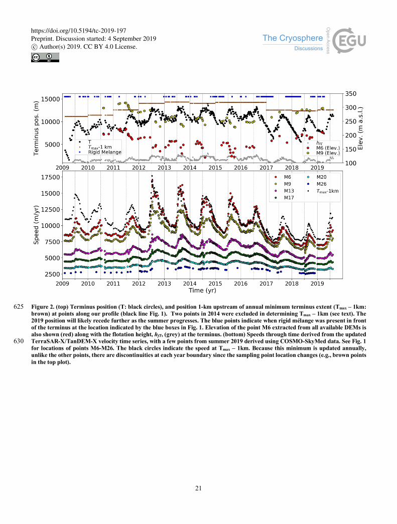
The top panel in Fig. 2 shows the terminus position (black) along our profile (Fig. 1) as a function of time. Also shown are the

points along the profile located 1-km behind the point of maximum annual terminus retreat for each year (Tmax-1km; brown). 135

In determining Tmax-1km for 2014, we excluded two anomalous points associated with rapid retreat and re-advance, which

appear to have been from an area that was floating and had little impact on the speed. As in similar time series (Joughin et al.,

2014), these data show seasonal variation in terminus extent by more than 2 km, with the terminus retreating farther inland

each year through 2012. From 2012 through 2016, the extent of maximum retreat was similar each summer as indicated by the

Tmax-1km positions (brown lines Fig. 2). The seasonal transition from advance to retreat typically occurred around March, but 140

it started as early as January (2010) and as late as June (2011). Peak retreat generally occurred in late summer/early fall.

In the winter of 2008–09, a several-kilometre long transient ice tongue advanced, as was the case for the prior winters following

the breakup of the more extensive ice tongue (Joughin et al., 2012b). This pattern altered for the 2009-10 through 2015-16

winters when there was no substantial ice tongue advance, although, as described below, the terminus was floating at times. 145

The pattern changed again when a floating tongue 4–5 km in length advanced during the winter of 2016–17 (see Fig. 2), with

an even longer ice tongue advancing the following winter. A similar ice tongue advanced in the 2018–19 winter, but it was

less extensive than those from the prior two winters.

3.2 Mélange Extent

We sampled the mélange in a static, 1 km x 1 km region just outside the point of maximum terminus advance for 2010–2019. 150

Because the extent of the floating ice tongue was so much greater in 2009, we moved the sampling region for the 2008–09

winter farther down the fjord (see blue boxes Fig. 1). The blue symbols in the top panel of Fig. 2 indicate the times when rigid


6

mélange was detected in front of the terminus. This detection of rigid mélange is relatively robust, hence there should be few

false detections. Missed detections could result if the speckle-tracker fails due to poor correlation despite the presence of rigid

mélange. We examined the individual maps by hand, and there appear to be few, if any, instances of missed detections. As 155

plotted, a gap in coverage would also indicate a lack of mélange. Such gaps are indicated by a corresponding lack of velocity

data in the lower panel of Fig. 2 (e.g., gap in Fall 2010).

The duration of periods with rigid mélange varies substantially from year to year. The longest periods of rigid mélange occurred

during the 2016–17 through 2018–19 winters, which coincide well with the periods when a more extended floating ice tongue 160

developed. Similarly, there was extensive mélange in the 2008-2009 winter when a floating tongue also advanced (only 2009

is shown in Fig. 2). For other years the mélange generally was less frequent and more sporadic. Mélange was particularly

sparse in both 2011 and 2012, which are the years when the greatest retreat occurred. In all summers there was a mélange-free

period of at least a few months, which tends to line up well with the periods of summer speedup. In general, extended periods

where rigid mélange exists coincide well with periods of terminus advance, which is consistent with similar data from the 165

period from 2005 to 2007 (Joughin et al., 2008b).

3.3 Velocity

The lower portion of Fig. 2 shows the speed at several points along the main trunk, which represents an update to earlier

records (Joughin et al., 2014; 2018). For consistency, we use the same locations and naming schemes (M6–M26) as earlier

work (Joughin et al., 2008b; 2014). We also include the speed at the point 1-km upstream of the point of maximum annual 170

terminus retreat (Tmax-1km; see brown Fig. 2 top), which provides speed relative to the evolving terminus position rather than

a fixed point. As noted elsewhere (Joughin et al., 2014), when the terminus migrates inland along a reverse bed slope, the

speed at a fixed point should increase due both to a thicker calving front and to the reduced proximity to its steep face (Joughin

et al., 2014). Thus, the Tmaxn-1km time series is much faster than the M6 data in the early part of the record when the terminus

was more advanced, but the speeds for the two points begin to converge as the terminus migrates inland. From 2012–2016 the 175

speeds at these two points are nearly identical, consistent with their similar proximity to terminus, with separation by ~1-km

in the cross-flow direction (see Fig. 1).

Figure 2 indicates that the slowdown that began in the winter of 2016–17 (Joughin et al., 2018; Lemos et al., 2018) continued,

with the slowest summer speeds for the 2009–2019 period occurring in 2018. Although the 2018–19 winter speeds were similar 180

to the previous winter, the terminus retreated rapidly beginning in late April with an accompanying increase in speed. By mid-

August 2019, the maximum speed was slightly greater than the maximums for the prior two summers. Since the seasonal peak

can occur later in the summer or even early fall, further speedup may still occur.


7

3.4 Elevation

We assembled a total of 84 DEMs spanning the period from 2010 to 2019 that incorporates data from ASP- (50) and SETSM- 185

(19) processed WorldView stereo pairs, TanDEM-X acquisitions (11), and GLISTIN (4) airborne campaigns. Figure 2 (top)

shows the full time series at points M6 and M9. At these points, surface was highest in late spring 2011 after winter thickening

recovered some of the loss that occurred the prior summer. The surface then lowered by ~30 m during the 2011 summer, but

thickened moderately (~10 m) during the subsequent winter. As the terminus retreated in summer 2012, the surface at M6

dropped by nearly 40 m between June 10 and July 20, coincident with the most extreme speedup event in the entire record. 190

From summer 2012 to summer 2016, there was a fairly consistent annual cycle with the terminus thickening by 35-50 m each

winter, and thinning by a similar amount each summer, bringing M6 to near or at flotation in 2013–2015. The record is sparser

for 2016, but it is sufficient to indicate that increased thickening occurred during the winter of 2016-17 as the ice tongue

advanced and the glacier slowed. As a result, just prior to the summer speedup in 2017, the terminus region was ~35 meter

higher than the previous summer (see also Khazendar et al., 2019). Winter thickening continued to outpace summer thinning 195

so that by March 2019, surface elevations near the terminus were only 10 to 20 m lower than those observed during spring of

2011.

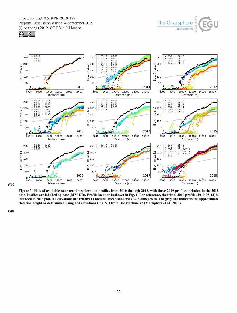
Figure 3 shows the surface elevation time series along the profile shown in Fig. 1 along with the flotation height (ℎ" ; solid

grey) computed using BedMachine v3 data (Fig. S1; Morlighem et al., 2017). For reference, the first profile (August 12, 2010) 200

is plotted (black circles) for comparison with each year. The plot for 2018 also includes 3 March 2019 profiles that are nearly

identical to the August 2010 profile, indicating some degree of recovery in response to recent slowdown and thickening

(Joughin et al., 2018; Khazendar et al., 2019).

The data reveal a variety of terminus geometries. Several of the profiles in Fig. 3 show a relatively steep calving face in mid 205

to late summer (e.g., August 17, 2010). Another common configuration involves the area ~0.5–2km upstream of the terminus

floating, with elevation well below ℎ". At times when the terminus was afloat, there were cases when the elevation tapered

smoothly to the water surface with little or no terminal cliff (e.g., August 12, 2010). In many other cases, particularly in many

of the early spring profiles, the downstream part of the floating region was relatively flat with a relatively steep calving front.

210

Between 2012 and 2015 in late summer there were often ~1–2 km transverse width depressions with surface heights tens of

meters below flotation a kilometre or more upstream of the well-grounded terminus. There are insufficient data to determine

whether such depressions formed in 2016, though depressions that remain above flotation were present in the March through

July 2016 profiles. Similar features did not appear in the 2017 and 2018 data, which appear similar to the 2010 and 2011

summers when the surface also was well above flotation. When they are present, these depressions advect downstream with 215

the ice flow, as is the case for similar features that have been observed elsewhere (James et al., 2014; Joughin et al., 2008c).


8

To provide a better picture of the spatial pattern of terminus variation, Fig. 4 shows a subset of the DEMs. In addition to the

colour scale to represent elevation, the 100- (white) and 150-m (black) contours are also shown. Below ~100 m, most of the

ice in the main trunk should be fully afloat, and above 150 m it should be fully grounded. The region between these contours 220

represents the transition from grounded to floating ice, including the grounding line. As with the profile data, the map-view

data reveal periods when the terminus is an abrupt grounded cliff, often indicated by areas where the 100-m contour tracks the

terminus. At other times, a heavily crevassed but generally intact floating extension is clearly visible. In particular, the extended

tongues that formed during the 2016–17 and 2017–18 winters are still visible in the respective early spring DEMs.

225

The DEMs in Fig. 4 indicate complex spatial and temporal variations in the near terminus geometry. There is a persistent

depression that forms in the lee of what appears to be a bed constriction on the north side of the main channel just upstream of

the closed white contour in the August 2010 DEM (see Fig. 4). Relatively little thinning occurs on the steep slope immediately

upstream of this feature, leading to little variation in the position of 100 and 150-m contours. Towards the centre of the main

trunk, however, these contours migrate back and forth ~2.5 km over the observation period, which is consistent with the point 230

data shown in Fig. 2. This variation can yield large changes in the near terminus slope. For example, in July 2012 DEM, the

two contours are separated by less than 500 m. By contrast, in the April 2014 DEM the 150 m contour intersects the profile at

nearly the same point (diamond in Fig. 4), but the 100-m contour is located nearly 2-km farther downstream. On the south side

of the fjord, there is a ridge (e.g., December 2011) that separates a pair of local topographic lows. Over the course of the record,

this area evolves substantially as the surface elevation varies by several 10s of meters. There are times when the upstream 235

depression extends inland so that the south side of the channel appears to reach, or at least approach, flotation while the centre

and north side remain well grounded. Toward the centre of the main trunk, the ephemeral surface depressions mentioned

above are visible in the September 2013 and August 2014 DEMs (see closed contours between the diamond and star in Fig.

4). For many other times, instead of a depression, this region represents a cross-flow high for the main trunk.

4 Discussion 240

The results described above provide a detailed view of the evolution of the terminus region of Jakobshavn Isbrae over the last

decade. Here we provide additional interpretation, including discussion of the relation between speed and bed topography;

how ocean temperature may influence the seasonal speedup through its control on mélange rigidity; the processes that produce

surface depressions and related calving events; and ice cliff stability.

4.1 Relation Between Speed and Terminus Position 245

As with previous work on Jakobshavn Isbrae (Joughin et al., 2012b), Fig. 2 reveals a strong correlation between seasonal

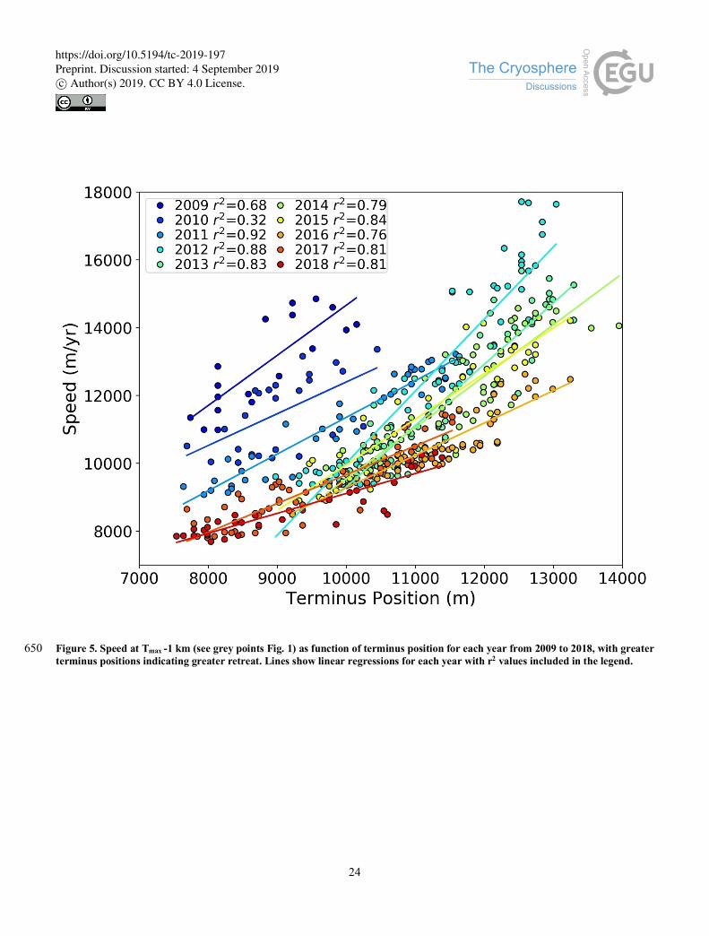
speedup and terminus position. To investigate further, Fig. 5 shows year-by-year linear regressions of terminus speed (Tmax-1


9

km) against terminus position. Here we have limited the regressions to positions along the profile >7500 m, which excludes

many of the locations where the terminus was clearly floating and providing little resistance. For all but 2009 and 2010, a

linear relation between the two explains >75% of the variance (r2=0.76–0.92). The lowest correlation occurs in 2010 (r2=0.32), 250

which was a year when there was relatively little retreat and corresponding speedup, hence other factors may dominate.

If we consider the terminus position as a proxy for the grounded terminus depth during retreat/advance along a retrograde

slope, then the results in Fig. 5 are consistent with increasing terminus thickness producing speedups during periods of retreat,

and vice versa during advance. While this relation should be non-linear (Howat et al., 2005; Thomas, 2004), it appears to be 255

relatively linear over the scale of the annual perturbations (~2 km) as indicated by the r2 values. Despite the good agreement,

it is important to note that there is still significant variation not accounted for by terminus position. In particular, some of the

calving events likely occur from a floating or lightly grounded terminus, which should yield little or no speedup (Cassotto et

al., 2019). For example, the brief period of retreat and rapid re-advance in the autumn of 2014 with no corresponding speedup

was likely due to calving from a floating ice tongue. In addition, variation in the width of the channel and local bed topography 260

should also influence speed as the terminus retreats inland.

Both the slope and intercept of the regressions vary substantially over time. The variation in slope to some extent may reflect

the expected non-linearity noted above, with increasing sensitivity as the terminus retreats into deeper water. Faster speeds at

less retreated positions in the earlier period (2009–2011) may be due to the generally thicker terminus region (see M6 and M9 265

elevations in Fig. 2), which should yield a greater surface slope and driving stress in the region upstream of the terminus.

4.2 Role of Ocean Temperature and Mélange

Figure 6 shows ocean temperature (similar to that from Khazendar et al., 2019) and winter air temperature anomalies for the

period from 1980 to the most recent observations. The strong summer speedups from 2012–2015 (Fig. 2) coincide with periods

when the water in Disko Bay was relatively warm (>3oC). Conversely, the slowdown that began in Fall 2016 took place when 270

the water in Disko Bay was relatively cool (~1.5oC). Based on this relation, it has been argued that enhanced melting of the

terminus produced greater calving, retreat, and speedup, particularly in summer when buoyant subglacial meltwater plumes

should enhance circulation at the terminus (Khazendar et al., 2019). While water temperature in the fjord should undoubtedly

modulate melt, it is less clear that this correlation establishes a causal relation between enhanced melt at the terminus and

speedup/thinning. 275

Maximum melt rates for 2012 to 2015 are estimated to be ~8-10 m/yr for concentrated plumes with limited spatial extent, or

about a factor 3 less if the melt water emerges with a uniform distribution from beneath the grounded ice (Khazendar et al.,

2019). Whether concentrated or evenly distributed, the factor-of-3 reduction should roughly represent the average melt rate

across the terminus. Thus, scaling the plume rates from Khazendar et al. (2019) by a factor of 3 yields approximate average 280


10

melt between ~3.5 m/yr during the summers with warmest water and ~1.9 m/yr during the summers when the water was

coolest. It is also important to note that much of the oceanic heat in the fjord goes into melting icebergs (Moon et al., 2018),

so these values may be biased high. During the summer, the terminus advances at ~30-45 m/day, so that ice is replenished far

faster than it is removed via submarine melting at these rates (Joughin et al., 2012a). While we cannot entirely rule out melt

serving in some way as a “catalyst” (e.g., by undercutting the front) to accelerate calving, a shift in average melt rate from 3.5 285

to 1.9 m/yr over a few months of the year should not drastically alter the rate of retreat and speedup.

In contemplating whether submarine melt, particularly in summer, might drive the observed retreat and speedup, it is important

to consider the relative timing of the recent changes. Although submarine melt should have been substantially reduced in the

summer of 2016 (Khazendar et al., 2019), the maximum retreat was virtually identical to that of the four prior years and speeds 290

were only slightly reduced, suggesting melt is not directly controlling retreat. Unlike prior years in that decade, however, rigid

mélange formed early that fall and was uninterrupted for more than 6 months. Over the 2016–17 winter the terminus advanced

~6 km farther than any winter since 2008–09 (Fig. 2), and an even greater re-advance occurred the following winter, which

had similar mélange conditions. The additional buttressing from this partially grounded and partially floating extension likely

produced much slower summer and winter speeds, which in turn produced the observed thickening (Fig. 3; see also Khazendar 295

et al. 2019). The winter of 2018-2019 yielded a more extended than normal period of rigid mélange, but less so than the

previous two winters. In this case, the winter advance fell between the extremes of 2011–2016 and 2016–2018 periods.

Collectively, these observations are consistent with earlier work indicating that the presence of rigid mélange can suppress

calving (Amundson et al., 2010; Joughin et al., 2008b).

300

Time series of Sentinel 1A/B SAR imagery from 2015-2016 reveal regular flushing of the mélange within the fjord (see movie

in Supplement) throughout the summer, consistent with the lack of rigid mélange at the terminus (Fig. 2). By contrast, for most

of the winter the mélange moves down much of the fjord at the rate at which it is pushed by the terminus. While not as regular

as in the summer, there were several flushing events in the winter of 2015–16, during which a large portion of the mélange

was rapidly advected through and cleared from the fjord. In the 2016–17 and 2017-18 cold seasons, however, the first flushing 305

events did not occur until April and May, respectively, consistent with an indication of more rigid mélange shown in Fig. 2.

It is well established that rigid mélange is most prevalent in winter when surface air temperatures are low (Cassotto et al.,

2015), which agrees with the results in Fig. 2. Nearby weather station data (Fig. 6) indicate that the 2016–17 and 2017–18

winters were colder than normal for the decade, but so was the 2014–15 winter that was followed by a large summer speedup, 310

suggesting that air temperatures are not the only control. As noted above, 250-m water temperatures in Disko Bay were ~1.5oC

cooler for 2016-2017 (Fig. 6 and Khazendar et al., 2019), and this cold ocean layer should extend across the sill at the mouth

of the fjord (Gladish et al., 2015a). A reasonable assumption is that this colder water facilitated more rapid winter freeze up

and greater mélange rigidity in the winter of 2016–17, with similar behavior the subsequent winters. By contrast, the warmer


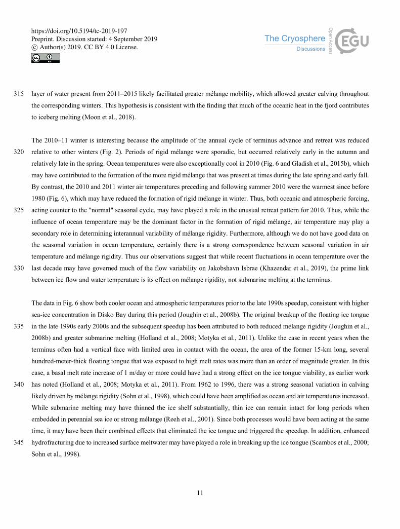
11

layer of water present from 2011–2015 likely facilitated greater mélange mobility, which allowed greater calving throughout 315

the corresponding winters. This hypothesis is consistent with the finding that much of the oceanic heat in the fjord contributes

to iceberg melting (Moon et al., 2018).

The 2010–11 winter is interesting because the amplitude of the annual cycle of terminus advance and retreat was reduced

relative to other winters (Fig. 2). Periods of rigid mélange were sporadic, but occurred relatively early in the autumn and 320

relatively late in the spring. Ocean temperatures were also exceptionally cool in 2010 (Fig. 6 and Gladish et al., 2015b), which

may have contributed to the formation of the more rigid mélange that was present at times during the late spring and early fall.

By contrast, the 2010 and 2011 winter air temperatures preceding and following summer 2010 were the warmest since before

1980 (Fig. 6), which may have reduced the formation of rigid mélange in winter. Thus, both oceanic and atmospheric forcing,

acting counter to the "normal" seasonal cycle, may have played a role in the unusual retreat pattern for 2010. Thus, while the 325

influence of ocean temperature may be the dominant factor in the formation of rigid mélange, air temperature may play a

secondary role in determining interannual variability of mélange rigidity. Furthermore, although we do not have good data on

the seasonal variation in ocean temperature, certainly there is a strong correspondence between seasonal variation in air

temperature and mélange rigidity. Thus our observations suggest that while recent fluctuations in ocean temperature over the

last decade may have governed much of the flow variability on Jakobshavn Isbrae (Khazendar et al., 2019), the prime link 330

between ice flow and water temperature is its effect on mélange rigidity, not submarine melting at the terminus.

The data in Fig. 6 show both cooler ocean and atmospheric temperatures prior to the late 1990s speedup, consistent with higher

sea-ice concentration in Disko Bay during this period (Joughin et al., 2008b). The original breakup of the floating ice tongue

in the late 1990s early 2000s and the subsequent speedup has been attributed to both reduced mélange rigidity (Joughin et al., 335

2008b) and greater submarine melting (Holland et al., 2008; Motyka et al., 2011). Unlike the case in recent years when the

terminus often had a vertical face with limited area in contact with the ocean, the area of the former 15-km long, several

hundred-meter-thick floating tongue that was exposed to high melt rates was more than an order of magnitude greater. In this

case, a basal melt rate increase of 1 m/day or more could have had a strong effect on the ice tongue viability, as earlier work

has noted (Holland et al., 2008; Motyka et al., 2011). From 1962 to 1996, there was a strong seasonal variation in calving 340

likely driven by mélange rigidity (Sohn et al., 1998), which could have been amplified as ocean and air temperatures increased.

While submarine melting may have thinned the ice shelf substantially, thin ice can remain intact for long periods when

embedded in perennial sea ice or strong mélange (Reeh et al., 2001). Since both processes would have been acting at the same

time, it may have been their combined effects that eliminated the ice tongue and triggered the speedup. In addition, enhanced

hydrofracturing due to increased surface meltwater may have played a role in breaking up the ice tongue (Scambos et al., 2000; 345

Sohn et al., 1998).


12

4.3 Depressions Leading to Calving Events

Beginning in 2012 and extending through at least 2015, a series of transverse depressions developed behind the terminus prior

to several late summer and autumn calving events (Fig. 3). The bottoms of some of these depressions extend more than 50 m

below flotation, and appear to eventually serve as the detachment points for large calving events. Downstream of these 350

depressions, the area immediately upstream of the terminus can reach heights of 25 m or more above flotation. Similar features

have been observed on Helheim and Kangerdlugssuaq glaciers (Howat et al., 2007; James et al., 2014; Joughin et al., 2008c),

and the development of one on Jakobshavn Isbrae was captured with a terrestrial radar interferometer in August 2012 (Cassotto

et al., 2019). These features, which develop over weeks, are distinctly different than the depressions that can form as the

terminus rises above flotation for tens of minutes prior to large calving events (Parizek et al., 2019). 355

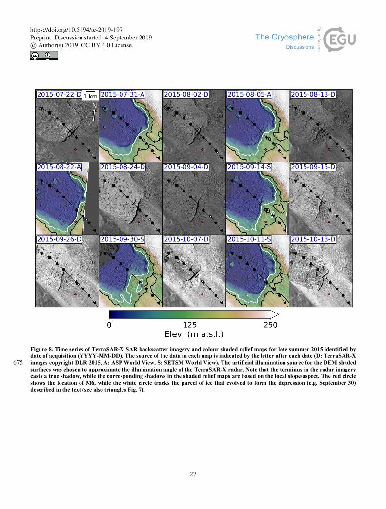
To better examine the evolution of one of these depressions in 2015, Figs. 7 and 8 show a time series of elevations in profile-

and map-view, respectively. To improve temporal sampling, Fig. 8 also shows several TerraSAR-X images. The imaging

geometry for these acquisitions was such that a prominent radar shadow is visible when there is a steep, high terminus, (e.g.,

August 24). In addition, sufficiently well-developed depressions are distinguishable in the SAR data (e.g. September 26). The 360

general pattern of brightening with time in the SAR image time series is due to the transition from summer melting to fall

freeze-up. To track the evolution of the parcel of ice that evolves to form the bottom of a large depression, we used the average

velocity field for this period to estimate its location through time, which is shown with coloured triangles in Fig. 7 and white

dots in Fig. 8.

365

In the July 31 and August 5 DEMs, a minor depression near flotation was apparent (Fig. 7), which is difficult to identify in the

SAR images from this period (Fig. 8). These first two DEMs and the SAR data reveal a nearly vertical calving face ~120–140

m high. By August 13, the less pronounced shadow in the SAR image indicates a less sheer terminus and the development of

several large crevasses or, potentially, through-going rifts. By August 22 a large calving event, which appears to have extended

through the bottom of the minor depression, produced a steep new calving face ~130 m high. Although the August 22 DEM 370

is limited in extent, there is a shallow back slope at the upstream end that suggests the presence of a nascent depression, which

is not yet distinguishable in the radar image from 2 days later. By September 4, however, there is a subtle indication of this

depression in the radar data (see area around white circle for September 4 in Fig. 8). The September 14 elevation data show

that the bottom of the depression was ~40-m below flotation (Figs. 7&8). Over the next 16 days, this feature advected

downstream, deepening to ~65 meters below flotation. Although the spatial scale is such that the area below flotation is not 375

fully in hydrostatic equilibrium, its depth suggests thinning by up to several hundred meters.

Depressions below flotation that develop through-going rifts and form detachment points for icebergs represent one mode of

calving (James et al., 2014; Joughin et al., 2008c). One mechanism that has been proposed to explain this evolution involves


13

a grounded glacier advancing down a prograde (forward) slope, driving the terminus downward, causing buoyant flexure that 380

lifts the front above flotation but depresses the region upstream below flotation (James et al., 2014; Wagner et al., 2016). This

process does not seem to apply here because both the available bed topography and the observed speed as function of terminus

position (e.g., Fig. 5) are consistent with a retrograde rather than prograde bed slope. Moreover, the glacier surface is above

flotation both upstream and downstream of the depression, which means if it was purely the result of downward flexure of ice

initially above flotation then its base would have to dip below the bed. Alternatively, flow models illustrate that reverse surface 385

slopes can develop near the terminus of an outlet glacier, but these features are generally tied to the underlying topography

and do not advect downstream as do the depressions shown in Figs. 7 and 8 (Vieli et al., 2002).

In general, the depressions we observe tend to develop after summer thinning yields a surface near flotation in the region a

few kilometres upstream of the terminus. Strong extension near the terminus and an ice column that is at or near flotation 390

should facilitate the development of basal crevasses (Van Der Veen, 1998). Once a basal crevasse develops, the thinner ice

above it must support the same column-integrated longitudinal stress, leading to greater extension. As a result, a necking

process likely would commence, causing sustained localized thinning that would create depressions like those shown in Figs.

3, 7, and 8 (Bassis and Ma, 2015). Consistent with this hypothesis, the observed depressions have width/thickness ratios (~1:1)

similar to modelled results (Bassis and Ma, 2015). Furthermore, Fig. 7 shows the velocity gradient steepening over the areas 395

where the depressions occur, which is consistent with that increased strain rates and thinning that forms them.

As the depressions develop, the elevation downstream of the depression and ~1 km upstream of the terminus remains tens of

meters above flotation (Figs. 7 and 8). While similar high spots have been attributed to buoyant flexure on Helheim (James et

al., 2014), in the examples presented here, the downstream high spot seems to be advected downstream faster than it can thin 400

to flotation (see progression of high spot from August 22 to September 30). After it attains a peak value, strong extension

produces thinning so that the last few hundred meters of the heavily rifted terminus regions are afloat.

The development of depressions like those just described occurred over several weeks, culminating in large calving events

involving a kilometre or more of ice (e.g., August 22 to October 11 in Figs. 7 and 8). Such events seem to occur in late summer 405

to early fall and did not start until 2012. As Fig. 3 indicates, in 2010 and 2011 the near-terminus region was relatively steep,

rising quickly above flotation, making it less likely that basal crevasses will form upstream of the terminus at these times. The

more intense summer speedups that began in 2012, however, produced shallower late-summer calving fronts, with elevations

near flotation extending several kilometres upstream of the terminus, which were favourable to basal crevasse formation that

could seed the formation of these depressions. Thus, this mode of calving appears generally to occur in late summer after 410

strong speedups have produced conditions favourable to the formation of basal crevasses that can evolve to form surface

depressions. Since full-thickness calving requires a terminus near flotation (Amundson et al., 2010), the development of the

high spot downstream of the depression may suppress calving long enough to give these features more time to develop.


14

4.4 Terminus Elevation and Cliff Instability

The depressions that lead to the calving events described above represent just one of a variety of failure modes that can cause 415

calving. Recent work has raised concern about ice cliff instability contributing to rapid ice-sheet collapse (DeConto and

Pollard, 2016). With ice cliffs more than 130 m above the waterline at times, Jakobshavn Isbrae provides an interesting case

study for understanding the effect of such potential instabilities. In actuality, however, ice sheet or glacier instability arises

when the calving and discharge rates fall out of sync (Amundson and Truffer, 2010), rather from the actual failures (i.e.,

calving events). Whether it initiates above or below the water line, it is important to note that some kind of material failure 420

must occur to produce calving events even in steady state. It is also important to consider that while the terminus is advancing

at 40 m/day and calving in ~100 m slabs, any ice cliff has a limited lifespan (~2.5 days on average, though clustering of calving

events may keep some cliffs intact up to weeks). Here we examine evolution of the front, following the formation of steep

calving faces.

425

Figure 7 illustrates the evolution of what begins as an initially ~130-m high sheer ice front (see August 22 in Fig. 7). Rather

than a brittle failure event leading to a rapid collapse, the strong extension near the terminus instead causes evolution from a

sheer grounded cliff to a heavily crevassed floating tongue with a ~5% slope (see September 30 in Fig. 7). In some sense this

represents the failure of the cliff, but as a process that evolves over weeks likely involving multiple small failures (e.g., crevasse

events) rather than a single catastrophic failure. Furthermore, the stability of the floating extension depends on environmental 430

factors. As our data suggest, cooler ocean temperatures, perhaps supplemented by colder air temperatures, could allow such a

tongue to advance over the colder part of the year. Conversely, when more summer-like conditions prevail, such a tongue

should disintegrate far more rapidly as was the case for the transient tongue shown in shown in Figs. 7 and 8. Thus, stability

likely is governed more by environmental conditions than by a single height-dependent mechanical failure criterion that could

yield rapid collapse (Parizek et al., 2019). 435

Our data also reveal that once the summer speedup commences, near terminus surface thinning rates can exceed 50 m over the

course of a few months (see M6 elevations in Fig. 2). Thus, even without cliff failure, the high stretching rates associated with

an unbuttressed terminus on a retrograde bed slope can cause rapid thinning to flotation, which, if unabated, will lead to further

calving and rapid retreat. Were it not for the seasonal cycle that facilitates re-advance and winter thickening (see Figs. 2 and 440

3), the terminus of Jakobshavn Isbrae would have receded far deeper inland than it has thus far, even without ice cliff collapse

as such.

Finally, it is important to note that to the best of our knowledge, Jakobshavn Isbrae has the deepest unbuttressed calving face

in Greenland or Antarctica, leading to the fastest marine terminating glaciers speeds (Joughin et al., 2014). As such, it has been 445

out of balance at times by more than a factor of 3 seasonally (Joughin et al., 2014) and a factor of 2 annually (Mouginot et al.,


15

2019). Nearly all glaciers in Greenland and Antarctica have steady-state speeds well below that of Jakobshavn Isbrae. Thus,

given that speed scales non-linearly with terminus depth (Schoof, 2007), any glacier that evolves to the point where the height

of its unbuttressed calving face rivals that of Jakobshavn Isbrae will already be well out of balance, yet likely will maintain

heights well below those needed to exceed a material failure criterion (~200 m) that would lead to rapid brittle failure (Parizek 450

et al., 2019). Our point is not that cliff failure is irrelevant, but rather that any glacier that reaches terminus heights where cliff

failure may be a significant effect, must already be in a state of rapid retreat. Far more important to long-term outlet glacier

stability is how seasonal variability and oceanographic/atmospheric trends influence the calving rates of grounded glacier

termini. In Antarctica and northern Greenland there are additional atmospheric temperature sensitivities (e.g., meltwater

ponding and hydrofracture) that influence ice-shelf stability (Scambos et al., 2000). In summary, while brittle failure cliff 455

instability may be important in some circumstances, it is far more likely to play a role in a late stage retreat than to serve as

the process that would initiate such a retreat.

5 Conclusions

We have assembled and produced a comprehensive time series of surface flow velocity, surface elevation, and mélange rigidity

for Jakobshavn Isbrae over the last decade. The data show a strong degree of variability, including a potentially brief slowdown 460

that coincided with cooler ocean temperatures (see also Khazendar et al., 2019). The time series of elevation provides an

unprecedented level of detail, which clearly shows a pattern of summer thinning partially offset by winter thickening in

response to seasonal changes in flow speed. These data also provide observational evidence to support theoretical development

describing how necking proceeds as basal crevasses form (Bassis and Ma, 2015). They also show that although Jakobshavn

Isbrae likely has the highest unbuttressed ice cliffs on Earth, at this point they do not appear to be subject to catastrophic brittle 465

failure. Most importantly, our observations reinforce earlier findings on the influence of mélange rigidity on calving

(Amundson et al., 2010; Joughin et al., 2008b), and help establish a connection to ocean temperature. Water temperatures are

expected to rise over the next century (Stocker et al., 2013), which will likely produce further retreat of Jakobshavn Isbrae.

Superimposed on any trend for the last century, however, there is substantial multi-decadal scale variability of ocean

temperatures in Disko Bay that correlate well with the Atlantic Multidecadal Oscillation (AMO) Index, which has been linked 470

to past changes on Jakobshavn Isbrae (Lloyd et al., 2011). Thus, whether Jakobshavn Isbrae can stabilize, at least temporarily,

likely depends on whether a cycle similar to that of the last century produces an extended period of cooler waters in Disko

Bay.

Acknowledgements

The National Aeronautics and Space Administration (NASA) supported contributions by I.J. (NNX17AH04G), D.S. (NESSF 475

fellowship award NNX12AN36H), and B.S. (NNX13AP96G ). Resources supporting this work were provided by the NASA


16

High-End Computing (HEC) Program through the NASA Advanced Supercomputing (NAS) Division at Ames Research

Center. The TerraSAR-X and TanDEM-X data were provided by DLR (project HYD0754 and XTI_GLAC0400). The Cosmo-

SkyMed data were delivered under an ASI licence to use. The bed data were provided by the BedMachine project at UC Irvine

and archived at NSIDC (https://nsidc.org/data/IDBMG4). Ocean temperature date were provided by the Ocean Melting 480

Greenland Project (OMG) and the International Council for the Exploration of the Sea Oceanography. Weather station data

were provided by the Goddard Institute for Space Studies GISTEMP Team. We acknowledge Claire Porter, Paul Morin, and

others at the Polar Geospatial Center (NSF ANT-1043681) who managed tasking, ordering, and distribution of the L1B

commercial stereo imagery under the NGA NextView license. DEMs provided by the Polar Geospatial Center under NSF-

OPP awards 1043681, 1559691, and 1542736. Comments by M. Maki improved the manuscript. 485

References

Amundson, J. M. and Truffer, M.: A unifying framework for iceberg-calving models, J Glaciol, 56(199), 822–830, 2010.

Amundson, J. M., Fahnestock, M., Truffer, M., Brown, J., Luethi, M. P. and Motyka, R. J.: Ice melange dynamics and implications for terminus stability, Jakobshavn Isbrae Greenland, J Geophys Res-Earth, 115, F01005, 490 doi:10.1029/2009JF001405, 2010.

Bassis, J. N. and Ma, Y.: Evolution of basal crevasses links ice shelf stability to ocean forcing, Earth Planet Sc Lett, 409, 203–211, doi:10.1016/j.epsl.2014.11.003, 2015.

Beyer, R. A., Alexandrov, O. and McMichael, S.: The Ames Stereo Pipeline: NASA's Open Source Software for Deriving and Processing Terrain Data, Earth and Space Science, 5(9), 537–548, doi:10.1029/2018EA000409, 2018. 495

Cassotto, R., Fahnestock, M., Amundson, J. M., Truffer, M. and Joughin, I.: Seasonal and interannual variations in ice melange and its impact on terminus stability, Jakobshavn Isbrae, Greenland, J Glaciol, 61(225), 76–88, doi:10.3189/2015JoG13J235, 2015.

Cassotto, R., Fahnestock, M., Amundson, J. M., Truffer, M., Boettcher, M. S., la Pena, de, S. and Howat, I.: Non-linear glacier response to calving events, Jakobshavn Isbrae, Greenland, J Glaciol, 65(249), 39–54, doi:10.1017/jog.2018.90, 2019. 500

Cuffey, K. M. and Paterson, W.: The Physics of Glaciers, 4 ed., Amsterdam. 2010.

DeConto, R. M. and Pollard, D.: Contribution of Antarctica to past and future sea-level rise, Nature, 531(7596), 591–597, doi:10.1038/nature17145, 2016.

Echelmeyer, K. and Harrison, W. D.: Jakobshavns Isbræ, West Greenland: Seasonal variations in velocity-or lack thereof, J Glaciol, 36(122), 82–88, 1990. 505

GISTEMP Team 2019: GISS Surface Temperature Analysis (GISTEMP), version 4, [online] Available from: https://data.giss.gov/gistemp, 2019.


17

Gladish, C. V., Holland, D. M. and Lee, C. M.: Oceanic Boundary Conditions for Jakobshavn Glacier. Part II: Provenance and Sources of Variability of Disko Bay and Ilulissat Icefjord Waters, 1990-2011, J Phys Oceanogr, 45(1), 33–63, doi:10.1175/JPO-D-14-0045.1, 2015a. 510

Gladish, C. V., Holland, D. M., Rosing-Asvid, A., Behrens, J. W. and Boje, J.: Oceanic Boundary Conditions for Jakobshavn Glacier. Part I: Variability and Renewal of Ilulissat Icefjord Waters, 2001-14, J Phys Oceanogr, 45(1), 3–32, doi:10.1175/JPO-D-14-0044.1, 2015b.

Hoehle, J. and Hoehle, M.: Accuracy assessment of digital elevation models by means of robust statistical methods, ISPRS Journal of Photogrammetry and Remote Sensing, 64(4), 398–406, doi:10.1016/j.isprsjprs.2009.02.003, 2009. 515

Holland, D. M., Thomas, R. H., De Young, B., Ribergaard, M. H. and Lyberth, B.: Acceleration of Jakobshavn Isbrae triggered by warm subsurface ocean waters, Nat Geosci, 1(10), 659–664, doi:10.1038/ngeo316, 2008.

Howat, I. M., Joughin, I. and Scambos, T.: Rapid Changes in Ice Discharge from Greenland Outlet Glaciers, Science, 315(5818), 1559–1561, doi:10.1126/science.1138478, 2007.

Howat, I. M., Joughin, I., Tulaczyk, S. and Gogineni, S.: Rapid retreat and acceleration of Helheim Glacier, east Greenland, 520 Geophys Res Lett, 32(22), L22502, doi:10.1029/2005GL024737, 2005.

James, T. D., Murray, T., Selmes, N., Scharrer, K. and O'Leary, M.: Buoyant flexure and basal crevassing in dynamic mass loss at Helheim Glacier, Nat Geosci, 7(8), 594–597, doi:10.1038/NGEO2204, 2014.

Joughin, I.: Ice-sheet velocity mapping: A combined interferometric and speckle-tracking approach, Ann Glaciol, 34, 195–201, 2002. 525

Joughin, I. R., Kwok, R. and Fahnestock, M. A.: Interferometric estimation of three-dimensional ice-flow using ascending and descending passes, IEEE T Geosci Remote, 36(1), 25–37, 1998.

Joughin, I., Abdalati, W. and Fahnestock, M.: Large fluctuations in speed on Greenland's Jakobshavn Isbræ glacier, Nature, 432(7017), 608–610, doi:10.1038/nature03130, 2004.

Joughin, I., Alley, R. B. and Holland, D. M.: Ice-sheet response to oceanic forcing, Science, 338(6111), 1172–1176, 530 doi:10.1126/science.1226481, 2012a.

Joughin, I., Das, S. B., King, M. A., Smith, B. E., Howat, I. M. and Moon, T.: Seasonal speedup along the western flank of the Greenland Ice Sheet, Science, 320(5877), 781–783, doi:10.1126/science.1153288, 2008a.

Joughin, I., Howat, I. M., Fahnestock, M., Smith, B., Krabill, W., Alley, R. B., Stern, H. and Truffer, M.: Continued evolution of Jakobshavn Isbrae following its rapid speedup, J Geophys Res-Earth, 113, F04006, doi:10.1029/2008JF001023, 535 2008b.

Joughin, I., Howat, I., Alley, R. B., Ekstrom, G., Fahnestock, M., Moon, T., Nettles, M., Truffer, M. and Tsai, V. C.: Ice-front variation and tidewater behavior on Helheim and Kangerdlugssuaq Glaciers, Greenland, J Geophys Res-Earth, 113, –, doi:10.1029/2007JF000837, 2008c.

Joughin, I., Smith, B. E. and Howat, I.: Greenland Ice Mapping Project: ice flow velocity variation at sub-monthly to decadal 540 timescales, The Cryosphere, 12(7), 2211–2227, doi:10.5194/tc-12-2211-2018, 2018.


18

Joughin, I., Smith, B. E., Howat, I. M., Floricioiu, D., Alley, R. B., Truffer, M. and Fahnestock, M.: Seasonal to decadal scale variations in the surface velocity of Jakobshavn Isbrae, Greenland: Observation and model-based analysis, J Geophys Res, 117(F2), F02030, doi:10.1029/2011JF002110, 2012b.

Joughin, I., Smith, B. E., Shean, D. E. and Floricioiu, D.: Brief Communication: Further summer speedup of Jakobshavn 545 Isbrae, The Cryosphere, 8(1), 209–214, doi:10.5194/tc-8-209-2014, 2014.

Khazendar, A., Fenty, I. G., Carroll, D., Gardner, A., Lee, C. M., Fukumori, I., Wang, O., Zhang, H., Seroussi, H., Moller, D., Noel, B. P. Y., Van Den Broeke, M. R., Dinardo, S. and Willis, J.: Interruption of two decades of Jakobshavn Isbrae acceleration and thinning as regional ocean cools, Nat Geosci, 12(4), 277–+, doi:10.1038/s41561-019-0329-3, 2019.

Krabill, W., Hanna, E., Huybrechts, P., Abdalati, W., Cappelen, J., Csatho, B., Frederick, E., Manizade, S., Martin, C., 550 Sonntag, J., Swift, R., Thomas, R. and Yungel, J.: Greenland Ice Sheet: Increased coastal thinning, Geophys Res Lett, 31(24), L24402, doi:10.1029/2004GL021533, 2004.

Lemos, A., Shepherd, A., McMillan, M., Hogg, A. E., Hatton, E. and Joughin, I.: Ice velocity of Jakobshavn Isbræ, Petermann Glacier, Nioghalvfjerdsfjorden, and Zachariæ Isstrøm, 2015–2017, from Sentinel 1-a/b SAR imagery, The Cryosphere, 12(6), 2087–2097, doi:10.5194/tc-12-2087-2018, 2018. 555

Lloyd, J., Moros, M., Perner, K., Telford, R. J., Kuijpers, A., Jansen, E. and McCarthy, D.: A 100 yr record of ocean temperature control on the stability of Jakobshavn Isbrae, West Greenland, Geology, 39(9), 867–870, doi:10.1130/G32076.1, 2011.

Luckman, A. and Murray, T.: Seasonal variation in velocity before retreat of Jakobshavn Isbrae, Greenland, Geophys Res Lett, 32(8), L08501, doi:10.1029/2005GL022519, 2005. 560

Moon, T., Sutherland, D. A., Carroll, D., Felikson, D., Kehrl, L. and Straneo, F.: Subsurface iceberg melt key to Greenland fjord freshwater budget, Nat Geosci, 11(1), 49–54, doi:10.1038/s41561-017-0018-z, 2018.

Morlighem, M., Williams, C. N., Rignot, E., An, L., Arndt, J. E., Bamber, J. L., Catania, G., Chauche, N., Dowdeswell, J. A., Dorschel, B., Fenty, I., Hogan, K., Howat, I., Hubbard, A., Jakobsson, M., Jordan, T. M., Kjeldsen, K. K., Millan, R., Mayer, L., Mouginot, J., Noel, B. P. Y., O'Cofaigh, C., Palmer, S., Rysgaard, S., Seroussi, H., Siegert, M. J., Slabon, P., 565 Straneo, F., van den Broeke, M. R., Weinrebe, W., Wood, M. and Zinglersen, K. B.: BedMachine v3: Complete Bed Topography and Ocean Bathymetry Mapping of Greenland From Multibeam Echo Sounding Combined With Mass Conservation, Geophys Res Lett, 44(21), 11051–11061, doi:10.1002/2017GL074954, 2017.

Motyka, R. J., Truffer, M., Fahnestock, M., Mortensen, J., Rysgaard, S. and Howat, I.: Submarine melting of the 1985 Jakobshavn Isbrae floating tongue and the triggering of the current retreat,, 116(F1), –n–a, doi:10.1029/2009JF001632, 570 2011.

Mouginot, J., Rignot, E., Bjork, A. A., van den Broeke, M., Millan, R., Morlighem, M., Noël, B., Scheuchl, B. and Wood, M.: Forty-six years of Greenland Ice Sheet mass balance from 1972 to 2018, P Natl Acad Sci USA, 116(19), 9239–9244, doi:10.1073/pnas.1904242116, 2019.

Noh, M.-J. and Howat, I. M.: The Surface Extraction from TIN based Search-space Minimization (SETSM) algorithm, 575 ISPRS Journal of Photogrammetry and Remote Sensing, 129, 55–76, doi:10.1016/j.isprsjprs.2017.04.019, 2017.

Parizek, B. R., Christianson, K., Alley, R. B., Voytenko, D., Vankova, I., Dixon, T. H., Walker, R. T. and Holland, D. M.: Ice-cliff failure via retrogressive slumping, Geology, 47(5), 449–452, doi:10.1130/G45880.1, 2019.


19

Porter, C., Morin, P., Howat, I., Noh, M.-J., Bates, B., Peterman, K., Keesey, S., Schlenk, M., Gardiner, J., Tomko, K., Willis, M., Kelleher, C., Cloutier, M., Husby, E., Foga, S., Nakamura, H., Platson, M., Wethington, M. J., Williamson, C., 580 Bauer, G., Enos, J., Arnold, G., Kramer, W., Becker, P., Doshi, A., D'Souza, C., Cummens, P., Laurier, F. and Bojesen, M.: ArcticDEM,, (2018-09-26), 2018–09–26, doi:10.7910/DVN/OHHUKH, 2018.

Reeh, N., Thomsen, H., Higgins, A. and Weidick, A.: Sea ice and the stability of north and northeast Greenland floating glaciers, Ann Glaciol, 33, 474–480, 2001.

Scambos, T., Hulbe, C., Fahnestock, M. and Bohlander, J.: The link between climate warming and break-up of ice shelves in 585 the Antarctic Peninsula, J Glaciol, 46(154), 516–530, 2000.

Schoof, C.: Ice sheet grounding line dynamics: Steady states, stability, and hysteresis, J Geophys Res-Earth, 112(F3), F03S28, doi:10.1029/2006JF000664, 2007.

Shean, D. E.: Quantifying ice-shelf basal melt and ice-stream dynamics using high-resolution DEM and GPS time series, PhD Thesis University of Washington, Seattle, 9 June. 2016. 590

Shean, D. E., Moratto, Z. M., Alexandrov, O., B, S., I, J., C, P. and P, M.: An automated, open-source pipeline for mass production of digital elevation models from very-high-resolution commerical stereo satellite imagery, SPRS Journal of Photogrammetry and Remote Sensing, doi:in review, 2015.

Sohn, H. G., Jezek, K. C. and Van der Veen, C. J.: Jakobshavn Glacier, West Greenland: 30 years of spaceborne observations, Geophys Res Lett, 25(14), 2699–2702, 1998. 595

Stocker, T. F., Qin, D., Plattner, G. K., Tignor, M., Allen, S. K., Boschung, J., Nauels, A., Xia, Y., Bex, V. and Midgley, P. M.: Climate Change 2013 - The Physical Science Basis, edited by Intergovernmental Panel on Climate Change, T. F. Stocker, Q. Ding, G. K. Plattner, M. Tignor, S. K. Allen, J. Boschung, A. Nauels, Y. Xia, V. Bex, and P. M. Midgley, Cambridge University Press, Cambridge. 2013.

Thomas, R. H.: Force-perturbation analysis of recent thinning and acceleration of Jakobshavn Isbræ, Greenland, J Glaciol, 600 50(168), 57–66, 2004.

Thomas, R. H., Abdalati, W., Frederick, E., Krabill, W., Manizade, S. and Steffen, K.: Investigation of surface melting and dynamic thinning on Jakobshavn Isbrae, Greenland, J Glaciol, 49(165), 231–239, 2003.

Van Der Veen, C.: Fracture mechanics approach to penetration of bottom crevasses on glaciers, Cold Reg Sci Technol, 27(3), 213–223, 1998. 605

Wagner, T. J. W., James, T. D., Murray, T. and Vella, D.: On the role of buoyant flexure in glacier calving, Geophys Res Lett, 43(1), 232–240, doi:10.1002/2015GL067247, 2016.

610


20

615

Figure 1: Surface elevation (colour) over shaded surface derived from the GIMP DEM for the region near the terminus of Jakobshavn Isbrae (see inset for location). The black box shows location of images shown in Figs. 4 and 8 and the blue box indicates area used to sample mélange as described in the text. The solid black line shows the location of the profile shown in Figs. 3 and BB, with the dashed section used to show the full extent. White markers with assorted symbols denote 1-km intervals along the profile 620 between 6- and 17-km. Coloured markers (M6-M26) show where velocity is sampled in Fig. 2 at points consistent with earlier work (Joughin et al., 2008b; 2012b; 2014).


21

Figure 2. (top) Terminus position (T: black circles), and position 1-km upstream of annual minimum terminus extent (Tmax – 1km: 625 brown) at points along our profile (black line Fig. 1). Two points in 2014 were excluded in determining Tmax – 1km (see text). The 2019 position will likely recede further as the summer progresses. The blue points indicate when rigid mélange was present in front of the terminus at the location indicated by the blue boxes in Fig. 1. Elevation of the point M6 extracted from all available DEMs is also shown (red) along with the flotation height, hfT, (grey) at the terminus. (bottom) Speeds through time derived from the updated TerraSAR-X/TanDEM-X velocity time series, with a few points from summer 2019 derived using COSMO-SkyMed data. See Fig. 1 630 for locations of points M6-M26. The black circles indicate the speed at Tmax – 1km. Because this minimum is updated annually, unlike the other points, there are discontinuities at each year boundary since the sampling point location changes (e.g., brown points in the top plot).


22

635 Figure 3. Plots of available near-terminus elevation profiles from 2010 through 2018, with three 2019 profiles included in the 2018 plot. Profiles are labelled by date (MM-DD). Profile location is shown in Fig. 1. For reference, the initial 2010 profile (2010-08-12) is included in each plot. All elevations are relative to nominal mean sea-level (EGS2008 geoid). The grey line indicates the approximate flotation height as determined using bed elevations (Fig. S1) from BedMachine v3 (Morlighem et al., 2017).

640


23

Figure 4. Color shaded relief maps for of a subset of DEMs, excluding maps for 2015, which are included in Fig. 8. Elevation contours of 150 (black) and 100 (white) meters bound the approximate transition from grounded to floating ice. The letter after the date-string (YYYY-MM-DD) indicates the DEMs source (A: ASP World View, T: TanDEM-X, S: SETSM World View, and G: GLISTIN). The profile with 1-km symbols is the same as shown in Fig. 1 and the red dot shows the location of M6. 645


24

Figure 5. Speed at Tmax -1 km (see grey points Fig. 1) as function of terminus position for each year from 2009 to 2018, with greater 650 terminus positions indicating greater retreat. Lines show linear regressions for each year with r2 values included in the legend.


25

Figure 6. (top) Ocean temperatures at 250 m depth in Disko bay (all available casts for: -68.6o < latitude < 69.4o, -54o < longitude < 52o), which is based on a similar figure by Khazendar et al. (2019). Small differences exist based on the sampling region and 655 averaging scheme. The ocean temperatures for 2015-2018 are extracted from the Ocean Melting Greenland data set (https://doi.org/10.5067/OMGEV-AXCTD) and the International Council for the Exploration of the Sea Oceanography (http://www.ices.dk/marine-data/data-portals/Pages/ocean.aspx).To obtain estimates representative of 250 m depth, we averaged temperatures from 225 to 275 m depth. The bars indicate uncertainty in the mean based on the number of points in the sampling region. We take the mean intra-annual standard deviation averaged over the full record as the intrinsic uncertainty for a single 660 point (i.e., how representative a point measurement is for the entire region). We then scale this value by 1/sqrt(number of points) to determine the plotted bar for each annual mean. (bottom) Winter 2-m air temperature (D-J-F) anomalies from weather stations in Egsminde and Illulisat (GISTEMP Team 2019, 2019).

665


26

Figure 7. Elevation and velocity profiles for summer 2015 illustrating evolution of advecting transverse surface depressions. The legends give the nominal dates (MM-DD) in 2015. As in Fig. 3, grey line indicates nominal height of flotation. The triangles show the estimated locations (see text) of parcel of ice that evolved to form the bottom of the depression (see also white circles in Fig. 8) that served as a detachment point for a calving event(s) that occurred between September 30 and October 11. 670


27

Figure 8. Time series of TerraSAR-X SAR backscatter imagery and colour shaded relief maps for late summer 2015 identified by date of acquisition (YYYY-MM-DD). The source of the data in each map is indicated by the letter after each date (D: TerraSAR-X images copyright DLR 2015, A: ASP World View, S: SETSM World View). The artificial illumination source for the DEM shaded 675 surfaces was chosen to approximate the illumination angle of the TerraSAR-X radar. Note that the terminus in the radar imagery casts a true shadow, while the corresponding shadows in the shaded relief maps are based on the local slope/aspect. The red circle shows the location of M6, while the white circle tracks the parcel of ice that evolved to form the depression (e.g. September 30) described in the text (see also triangles Fig. 7).


A Decade of Variability on Jakobshavn Isbrae - The Cryosphere

Documents

Transcript of A Decade of Variability on Jakobshavn Isbrae - The Cryosphere