Empirical Relations Between the Earth's Radiation Budget ...
Upload
independentCategory
view
0download
0
FLUID FLOW NEAR THE SURFACE OF EARTH'S OUTER CORE
Jeremy Bloxham and Andrew Jackson Department of Earth and Planetary Sciences Harvard University Cambridge, Massachusetts
Abstract. Maps of the fluid flow at the core surface are important for a number of reasons: foremost they may provide some insight into the workings of the geodynamo and may place useful constraints on geodynamo models; from the flow, the force balance at the top of the core can, at least in part, be deduced; the flow can provide short- term predictions of the secular variation; the flow is important in understanding changes in the length of day; and constraints on lateral temperature variations and topography at the core-mantle boundary may be derived. Unlike the case of mantle convection, only very small
lateral variations in core density are required to drive the flow; these density variations are too small (by several orders of magnitude) to be imaged seismically, so instead we use the geomagnetic secular variation to infer the flow. Despite considerable recent progress in mapping the core flow, substantial differences exist between maps produced by different researchers. Here we examine the possible underlying reasons for these differences, paying particular attention to the inherent problems of nonuniqueness. We focus on the aspects of the flow which do seem to be well determined and discuss their geophysical implications.
1. INTRODUCTION
It is almost 300 years since Halley [1692] first sug- gested that the geomagnetic secular variation, in particular the westward drift, implies mass motion within the Earth's interior. Nowadays much effort is concentrated on trying to use our knowledge of the geomagnetic secular variation to determine these motions, with the expectation that they might provide insight into the dynamo process responsible for the origin and maintenance of the field, as well as aid our understanding of a range of geophysical phenomena including changes in the length of day on the period of decades. In Halley's day, knowledge of the structure of the Earth's interior was extremely crude, and this, combined with an equally crude understanding of electromagnetism, limited Halley's attempts to infer these motions to the realms of gross speculation (although he did infer, somewhat fortuitously, the presence of a solid inner core immersed in a fluid outer core).
Today we have a much more complete understanding of electrodynamics and hydrodynamics, and of the structure of the Earth's interior, to bring to bear on the problem: this review is concerned with recent attempts at extracting information on the pattern of fluid flow near the surface of the outer core from the geomagnetic secular variation. Ideally, of course, in our bid to understand the geodynamo we should like to be able to determine fluid flow through- out the core; since mapping the flow requires knowledge of
the magnetic field, and our knowledge of the magnetic field does not extend into the core (on account of the high electrical conductivity of the core), we are restricted to mapping the flow just beneath the core-mantle boundary (CMB). This presupposes that we know the magnetic field at, or rather just beneath, the CMB; this issue is discussed at greater length in section 2, but for now we comment that provided we assume that the mantle is an electrical insulator, then we can take surface or satellite observations of the magnetic field and infer the magnetic field at the CMB.
It is only relatively recently that attempts have been made to map the flow pattern. The groundwork was laid almost a half century ago by Alfvdn [1942], who showed that in a moving fluid in the limit of perfect electrical conductivity, magnetic field lines become frozen in the fluid, so that changes in the magnetic field are due entirely to advection of field by the flow, with the field lines thus acting as tracers for the flow. A closely analogous theorem is Kelvin's circulation theorem in inviscid fluid dynamics, whereby vortex lines are frozen in the fluid. The frozen flux theory was applied to the Earth's core some 25 years ago by Roberts and Scoa [1965], who argued that over the length scales (some thousands of kilometers) and time scales (a few decades) of interest in the core, the core acts as a perfect conductor. The first attempts at applying this theory, however, failed to take adequate account of the inherent nonuniqueness in using the geomagnetic secular
Copyright 1991 by the American Geophysical Union.
8755-1209/91/90RG-02470 $05.00 .97.
Reviews of Geophysics, 29, 1 / February 1991 pages 97-120
Paper number 90RG02470
98 ß Bloxham and Jackson: FLUID FLOW AT EARTH'S CORE SURFACE 29, 1 /REVIEWS OF GEOPHYSICS
variation to map the core flow. This nonuniqueness, which implies that many different flows may be found which generate the same secular variation, arises because we are unable to identify and label individual field lines, regard- less of how precisely we know the magnetic field. A simple example illustrates how this can be a problem. Consider a simple axial dipole field: then any purely zonal fluid motion (a motion entirely along lines of constant latitude) will not change the field observed outside the core, and so is invisible. But the nonuniqueness is more insidious than this simple example, and much of the recent progress has been concerned with resolving the problems that it poses.
Besides these considerable theoretical obstacles, our incomplete knowledge of the magnetic field has also been thought to impose a limitation. The availability of high-quality magnetic field data from the Magsat satellite has provided a recent stimulus, leading to renewed attempts at mapping the fluid flow at the core surface and to recent theoretical advances resulting in at least a partial resolution of the nonuniqueness problem. However, the results obtained have not always been entirely consistent with those obtained by others, and since these maps are now being used in other geophysical studies (such as investigating core-mantle coupling), a review and, in particular, an assessment of the various flows are called for.
This paper is structured as follows. The mathematical details are largely confined to sections 2 and 3, in which we review the frozen flux theory of the secular variation and the core motions inverse problem, respectively. As we have already mentioned, the frozen flux theory of the secular variation forms the foundation of all attempts at determining the fluid flow; without an understanding of this theory and its limitations we cannot hope to assess the resulting maps of the flow. But understanding the forward problem of how the action of the fluid flow near the CMB on the magnetic field generates the secular variation is only part of the problem; we must also examine the inverse problem of taking our knowledge of the magnetic field and secular variation and inverting for the fluid flow. The difficulties encountered in this inverse problem are common to many areas of geophysics.
In section 4 we present a range of maps of the fluid flow from a number of investigators and seek to determine which aspects of the flow, if any, are well determined. In section 5 we consider the broader geophysical implications of the flows. Sections 2 and 3 could be omitted by a reader interested more in the results and their implications; however, we would caution that in order to understand the
equivocal nature of the results the reader should not pass over these rather more theoretical sections.
In this review we restrict our attention to attempts at mapping the large-scale, global fluid flow near the CMB. We note that particular methods also exist for estimating the flow at single points or on curves on the core surface [Backus, 1968; Benton, 1979, 1981; Whaler, 1982;
Gubbins, 1982; Barraclough et al., 1989]. These methods, as has been noted by some of the authors cited, suffer from the serious shortcoming that they require estimates of the secular variation either at points or along curves on the CMB; such estimates are subject to great uncertainty. We note that the maps of the secular variation produced by Gubbins [1983] have unbounded errors on point estimates, while differencing the main field models of Gubbins and Bloxharn [1985] produces a signal-to-noise ratio in point estimates of the secular variation over a 10-year period of less than 0.5; clearly, even with the rather strong assump- tions implicit in the error analyses of Gubbins [1983] and Gubbins and Bloxharn [1985], point estimates of the secular variation are, for practical purposes, meaningless. Hence we restrict our attention to attempts at mapping the large-scale flow near the core surface, rather than the pointwise flow, although, as we shall see, even the large-scale flow may not be well determined.
We also consider the use of the horizontal component of the induction equation in addition to the radial component. Lloyd and Gubbins [1990] have used both the radial and the horizontal components of the field to determine purely toroidal flows (flows with no upwelling or downwelling), and Jackson and Bloxham [1991] have derived general flows based on two components of the field. This recent work enables us to estimate the radial shear (i.e., the rate of change of the velocity with radius) at the CMB in addition to the flow.
2. THE FROZEN FLUX THEORY OF THE SECULAR VARIATION
2.1. Preliminaries
Our starting point is the magnetic induction equation
OB/Ot = V ̂ (u^B)+ 11V2B (1)
where B is the magnetic field, u the fluid velocity, and •1 = 1/(g0o) the magnetic diffusivity, with go the magnetic permeability and o the electrical conductivity of the core fluid (assumed constant). The magnetic induction equation shows how the time rate of change of magnetic field is due to the effects of magnetoadvection and magnetic diffusion.
The dynamics of flow in the core is described by the Boussinesq Navier-Stokes equation [e.g., Gubbins and Roberts, 1987]
P0 (• +u.Vu4-211^u) =- Vp + p'g + J^B + P0 vV2u (2)
where P0 and p' are the hydrostatic density and departure from hydrostatic density, respectively, 11 is the Earth's rotation vector, p is the nonhydrostatic part of the pressure, g is the acceleration due to gravity, v is the kinematic viscosity, and J is the current density. Although we shah

29, 1 / REVIEWS OF GEOPHYSICS Bloxham and Jackson: FLUID FLOW AT EARTH'S CORE SURFACE ß 99
consider the dynamics in more detail later, our primary concern is with the kinematics of flow in the core, and
particularly with using (1) to determine u. In order to reduce (1) to a more useful form, we
introduce the toroidal-poloidal decomposition of the magnetic field B, defined by
B = BT + Bp = V^(T•) + V^V^(P •) (3)
where T(r, 0, tp) and P(r, 0, tp) are the toroidal and poloidal scalars, respectively, defining the toroidal B r and poloidal B t, ingredients of B. Any solenoidal vector field (a vector field with zero divergence) can be decomposed in this manner; for a very complete discussion of this decomposi- tion, see Backus [1986]. This decomposition is common- place in geophysics, being employed, for example, extensively in low-frequency seismology and in studies of mantle convection.
In spherical polar coordinates (r, 0, t•) the toroidal and poloidal ingredients may be written in terms of the toroidal and poloidal scalars in the form
1 3T 1 3T) (4) BT = 0, r sin 0 •--•'- 7 •
L2p 1 32P 1 32P ) Bt, = r 2 ' r r3r 30' r sin 0 3r 30 (5) where L is the angular momentum operator of quantum mechanics, defined by
sin0 • sin0 +sin 20 302 (6) The fluid flow u in the core can also be split into
toroidal and poloidal components if we assume incompres- sibility so it too is solenoidal. Throughout this paper we will use the symbols T and P to represent the magnetic toroidal and poloidal scalars and the symbols 'T and P for the flow scalars.
Considering first the magnetic field, using Aml•re's law we can deduce that the current density J satisfies
goJ = V^B = V^B? + V^Bt,
= V^V^(T•)+ V^V^V^(P •)
= V^V^(r•) + V^[(-V2p)•] (7)
Comparing this expression for the current with our definition of the toroidal-poloidal decomposition, it is clear that poloidal field results from toroidal currents, and toroidal field from poloidal currents. If J = 0, as in an insulator, then B? = 0, while B e does not necessarily vanish, although P must satisfy V2p = 0 (in which case we call it a potential field).
Because the atmosphere at the Earth's surface is an extremely poor conductor of electricity, B r _- 0 there. Hence we observe only the poloidal field at the Earth's
surface. In principle, we can find the toroidal field within the mantle from measurements of the electric field at the
sea bottom [e.g., Runcorn, 1955; Lanzerotti et al., 1985], but the electric field from the toroidal field from the core is
likely to be small compared with the field from other sources, especially that from ocean currents.
Thus our knowledge is restricted to the poloidal field at the Earth's surface. If we assume that the electrical
conductivity of the mantle is known, then we can deter- mine the poloidal field at the CMB. In fact, for a reason- able range of mantle conductivities, the effect of mantle conductivity on the poloidal field is small and can safely be neglected. Of course, if the lowermost mantle were a perfect insulator, then we would also know the toroidal field, since then it would have to be zero, but the lower- most mantle is certainly a moderate conductor and may, on account of reaction with the core, have a conductivity comparable to that of the core [Knittle and Jeanloz, 1986]. Thus our knowledge of the magnetic field at the CMB is fundamentally incomplete. This might appear to preclude the possibility of deducing the flow u, since the observed rate of change of poloidal field could possibly result from the effects of the flow u on the unknown toroidal field at the CMB.
Let us temporarily assume that the CMB is a free-slip boundary. Then at the CMB, u.r = 0, but u = u n •- 0). Then following Bullard and Gellman [ 1954], we can show that
[V^(uh - [V^(un (8)
from which we obtain the poloidal induction equation at the CMB,
3Bt,/3t = [VA(HhABp )]p + •IV2B•, (9)
This possibly rather surprising result shows that at the CMB the observed rate of change of poloidal field comes entirely from the poloidal field itself. It is worth noting that the toroidal induction equation does not separate so easily: the rate of change of toroidal field depends on both the toroidal field and the poloidal field. This is a corollary of the important result in dynamo theory that the produc- tion of toroidal field from poloidal field does not require any radial motion, while closing the dynamo circuit by producing poloidal field from toroidal field does require radial motions.
As mentioned, this analysis is incomplete. We assumed that the CMB is a free-slip boundary; in fact, it is a rigid boundary, so that u = 0 there. But a large part of the observed secular variation results from advection by a nonzero velocity; this must be the velocity at the top of the free stream, immediately beneath a boundary layer at the CMB. Strictly, therefore, we need to know the field at the base of this boundary layer, rather than at the CMB, and so we must consider how the field changes as we descend through the boundary layer.
100 ß Bloxham and Jackson: FLUID FLOW AT EARTH'S CORE SURFACE 29, 1 /REVIEWS OF GEOPHYSICS
2.2. The Frozen Flux Hypothesis The induction equation (1) shows that the time rate of
change of the magnetic field (the secular variation) depends upon both magnetoadvection and diffusion. We can associate time scales x. and xa with these two processes. Let us consider a region of characteristic length scale L in which the fluid has characteristic velocity U. Then
'c,, ~ L/U (10)
'•,, ~ L2/q (11)
For the Earth' s core, L - 106 m, U• 5 x 10 -4 m s -•, and T I _- I m 2 s -•, giving '•a -- 60 years and '•a '" 3 x 10⁴ years, showing that the time scale of advection is comparable to the time scale of the geomagnetic secular variation and much shorter than the time scale of diffusion. Our
estimate of U may be obtained by inferring the velocity of the core fluid based on the westward drift rate of the
magnetic field of roughly 0.2 ø yr -•, although such an inference itself relies implicitly upon the frozen flux hypothesis.
Equivalently, we can express the ratio of the mag- netoadvection and diffusion terms as the magnetic Reynolds number
Rm - •:a UL IV^(u^B)I ~ 500 (12) -•:-•= q ~ •iV2Bi
This all suggests that we should be able to neglect the diffusion term, at least over time scales short compared with '•a, and to consider the reduced equation
3B/3t = VA(UAB) (13)
However, as has been pointed out by Moffatt [1978] and Bloxharn [1988a], such an argument may be misleading. We have assumed that the velocity field and magnetic field both vary on the length scale L. The magnetic field may vary over a much shorter length scale. Indeed, the magnetoadvection calculations of Weiss [1966] suggest that the magnetic field will be concentrated into boundary layers of thickness/5 ~ R•mL in which magnetoadvection and diffusion are balanced. These are not idle concerns, and we shall consider them further later in this review. For
now, however, in order to develop the theory, we shall adopt the frozen flux approximation and so neglect diffusive effects.
Having chosen to neglect the effects of magnetic diffusion, at least in the main body of the core, we now consider the effects of viscosity. The kinematic viscosity in the core is extremely poorly determined, though generally estimates close to v = 10 -6 m 2 s -• are favored. We can gauge the relative importance of viscous effects by the Ekman number, the ratio of viscous forces to the Coriolis force, given by
E = v/flL 2 (14)
where fl is the rotation rate. We find E ~ 10 -•s, indicating that viscous effects are negligible in the main body of the core.
But this model of zero magnetic diffusivity and zero kinematic viscosity cannot hold throughout the core, otherwise we would be unable to satisfy the boundary conditions to the CMB. As is well known, the problem is resolved by the existence of a boundary layer near the CMB in which the free-s•eam solutions adjust to match the boundary conditions, within which the effects of diffusion cannot be disregarded. This returns the discus- sion to the problem raised earlier: how is the magnetic field at the CMB, or, more accurately, immediately above the CMB, related to the field at the top of the free stream, i.e., immediately beneath the boundary layer?
We adopt the notation IX] to represent the jump in the quantity X across the boundary layer. Then using V.B = 0 and the fact that within the boundary layer
a/3r >> V, (15)
we find that [B,] = 0 and so maps of the radial component of field immediately above the CMB also represent the radial component of magnetic field at the top of the free stream.
The effect of the boundary layer on B n is more compli- cated, requiring a more detailed boundary layer analysis, which has been studied by a number of authors [Stewartson, 1960; Roberts and Scott, 1965; Roberts, 1967; Backus, 1968; Gilman and Benton, 1968; Hide and Stewartson, 1972; Braginsky, 1984]. Following Hide and Stewartson [1972], we have
[Bn] ~ B•_•U (•.•)« (16) giving [B s] _- 20 nT, which is insignificant. However, we should bear in mind that some models of the dynamo, notably Braginsky's model-Z [Braginsky, 1978], can result in a larger jump in B n across the boundary layer, further- more, other boundary layer analyses have reached different conclusions from that of Hide and Stewartson. The change in B n across the boundary layer cannot be considered to be a well-resolved issue.
A further complica}ion must be considered. We have used the condition u.r = 0 at the CMB to show that the
poloidal induction equation separates fully from the full induction equation at the CMB. However, at the base of the boundary layer, u.•' need not necessarily vanish because of Ekman suction. Then, we would have
u'•' IBL- '" UE u2 (17)
We are concerned with the conversion of toroidal field into
poloidal field. As has been emphasized by Bloxharn [1988b], toroidal flux can be concentrated near the CMB,
29, 1 / REVIEWS OF GEOPHYSICS Bloxham and Jackson: FLUID FLOW AT EARTH'S CORE SURFACE ß 101
t•3/2 t> Comparing the rate of reaching an amplitude B ~ tx m o•,. production of poloidal field from poloidal field, Ppop with the rate of production of poloidal field from toroidal field Ptor' we then have
Ppd ~ U B •, 1 ~ ~ 3 x 10 4 (18) Ptor U E mR3m/2B•, •t2 3t2 E R m
indicating that conversion of toroidal field into poloidal field by Ekman suction is likely to be small, even when we take an extreme value for the strength of the toroidal field at the base of the boundary layer. Thus our separation of the poloidal component of the induction equation appears reasonable.
However, the incomplete nature of the boundary layer analysis, and possibly a failure to recognize this separation of the induction equation, has meant that most work, at least until very recently, has focused on using the radial component of the field alone to map the fluid flow immediately beneath the boundary, though, as we shall discuss later, a recent study by Barraclough et aL [1989] has shown that use of the horizontal field is permissible, and its use has been adopted by Lloyd and Gubbins [1990] and Jackson and Bloxham [1991].
One further approximation is made. In order to use measurements of the magnetic field made at or above the Earth's surface to infer the field at the CMB the mantle is
usually approximated as an insulator. As mentioned, this approximation, when taken in its strictest sense, is at variance with the discussion earlier concerning our lack of knowledge of the toroidal field at the CMB, for in the limit of vanishing mantle conductivity the toroidal field at the CMB is precisely zero. For spherically symmetric mantle conductivity profiles, the poloidal field can, in principle, be corrected for mantle conductivity, using the diffusion equation. This correction is usually not applied for two reasons: first, mantle conductivity is very poorly deter- mined, especially below depths of about 2000 km where induction studies [e.g., Banks, 1969, 1972] lose resolution, so that the correction that should be applied is very uncertain; and second, Benton and Whaler [1983] show that for a reasonable range of proposed mantle conduc- tivity profiles the correction to the insulating limit is only a few percent anyway. Thus we adopt the potential field as our model of the more general poloidal field at the CMB.
2.3. Testing the Frozen Flux Hypothesis Before proceeding further we seek to test the frozen flux
approximation. Using the radial component of the frozen flux magnetic induction equation, Backus [1968] derived a set of necessary conditions for frozen flux, namely,
l•3Br --3T dS =0 (19)
where the patch S on the CMB is chosen so that 3S is a contour of B r = 0 (a null-flux curve). Equivalently [Bloxham and Gubbins, 1986], we have the set of conditions
• B r dS--O (20)
Typical maps of the radial field at the CMB have between 6 and 10 such patches, providing a test of the frozen flux approximation. As noted by Hide and Malin [1981], these conditions imply the simpler, but less powerful, condition
d• alc dt= • •m [Brim - 0 (21)
where • is termed the unsigned flux integral. Rather few attempts have been made to test these
conditions in any rigorous manner. This is not entirely surprising: given that maps of B r at the CMB are necessar- ily based upon inadequate data and so are imperfect, any test must ultimately reduce to a statistical hypothesis test. Unfortunately, the statistics of maps of B r are poorly known, and so great uncertainty always attends such tests.
The strongest tests are obviously those based on the full set of conditions (19) or (20). Booker [1969] was the first to attempt a test: he found the decay of the dipole to be inconsistent with flux conservation, a finding later corroborated by Gubbins [1983], although Gubbins and Bloxham [1985] suggested that the dipole decay is consistent with flux conservation. Later, B loxham and Gubbins [1986], looking at individual flux patches over a 20-year period, did find evidence of flux diffusion.
However, their result depends very critically upon their estimates of the errors in the field maps; these error estimates have recently been challenged by Backus [1988a, b], and any evidence of flux diffusion found in that study is certainly not robust to the type of error analysis advocated by Backus. Rigorous estimates of the uncertainty in estimating the magnetic field at the CMB, as advocated by Backus, are exceedingly pessimistic, since to achieve rigor, only rigorous bounds can be placed on the space of acceptable models; in the case of modeling the Earth's magnetic field the only known rigorous bound is that the magnetic field energy may not exceed the rest mass of the universe. Less rigorous bounds, such as the heat flux bound (that the Ohmic heating in the core should not exceed the surface heat flux), are still of little use if we wish to determine core motions. Even the grossly optimistic bounds of Gubbins and Bloxham predict a signal-to-noise ratio of only 0.5 for the secular variation over a decade time period. Clearly, if we wish to use our observations to infer flow in the core, we must be willing to accept very optimistic bounds, in fact unjustifiably optimistic bounds, on models of the magnetic field at the CMB.
This discussion assumes that we wish to construct maps of the flow which we can then plot and examine. If, on the other hand, we wish only to test particular hypotheses concerning the nature of the flow, then a better approach would be to fit the magnetic field observations directly: if with a particular hypothesis we are able to fit the observa- tions, then we have no grounds to reject that hypothesis, even if we cannot necessarily believe the details of the
102 ß Bloxham and Jackson: FLUID FLOW AT EARTH'S CORE SURFACE 29, 1 /REVIEWS OF GEOPHYSICS
resulting solution. However, as we shall mention again later, the issue of deciding what constitutes an adequate fit to the original data is not necessarily any less difficult than deciding what constitutes an adequate fit to a field model.
Returning to the frozen flux hypothesis, the rather equivocal results of Bloxham and Gubbins [1986] were later bolstered by Bloxham and Gubbins [1985], who found very much stronger evidence of flux diffusion, concentrated in the first quarter of this century, seemingly providing almost incontrovertible evidence of flux diffusion.
Other tests have concentrated on using the weaker condition (21). Hide and Malin [1981] used the unsigned flux integral to determine the core radius, by seeking the radius which best satisfies (21). They obtain discrepancies between this magnetically determined radius and the much better seismically determined radius as small as 2%; they conclude that this provides support for the frozen flux hypothesis. Voorhies and Benton [1982] reach the same conclusion; further such tests, again reaching the same conclusion, are reported by Benton and Voorhies [1987]. However, none of these studies attempts a statistical test of the hypothesis.
The importance of testing the condition statistically cannot be overstressed: typically, field models are based on up to 50,000 observations, from which about 100 parameters are estimated; imposing the condition (21) only reduces the number of degrees of freedom by one, so the attendant increase in misfit need only be very small indeed to suggest that the condition (21) is not satisfied at a very high confidence level.
We should consider a little further what these tests
mean. On the one hand, the rather weak evidence of magnetic diffusion presented by Bloxham and Gubbins [1986] should be taken as implying at the very most that recent geomagnetic field maps, or more accurately the data on which they are based, are sufficient to detect the effects of diffusion. By any argument the effects of diffusion in the period (1960-1980) studied by Bloxham and Gubbins [1986] are small. Other examinations of the flux condi- tions over this period have tended to suggest that diffusion cannot be detected. As Bloxham [1989] has argued, these tests do not in any case necessarily address the issue of whether we can use the frozen flux approximation to map the core flow; they merely address the issue of whether the effects of diffusion, which must be present, can be detected. This distinction seems, surprisingly, to have become surrounded in considerable confusion in the
literature.
The episode of rapid flux diffusion detected by Bloxham and Gubbins [1985] (but also inferred by Bullard [1954]) in the first quarter of this century is of more importance, for then diffusion appears, at least in a region beneath southern Africa, to be the dominant ingredient of the secular variation. There core flow maps based on the frozen flux approximation might be expected to be misleading.
These frozen flux conditions can be extended to the case
where we assume continuity of the horizontal field across the CMB and the boundary layer. Backus [1968] first derived this further set of consistency conditions; they have recently been rederived using an intuitively appealing geometrical argument by H. K. Moffatt (personal com- munication, 1990) and applied by Barraclough et al. [1989]. Barraclough et al. consider the set of conditions
d •• Qodl = 0 (22) • s
where
Q = (r^B)B-V(r-B) (23)
Barraclough, et al. test these conditions, which they call the "extended frozen flux conditions," using a sequence of field models from Bloxham et al. [1989] consmined to satisfy the "restricted frozen flux conditions" (20). Barraclough et al. find no compelling evidence that the extended frozen flux conditions are violated, indicating that the data are not inconsistent with the conditions.
Both these tests are implicitly also tests of the insulating mantle approximation, for in both cases we have used maps of the magnetic field at the CMB obtained by downward continuation of the potential field inferred at the Earth's surface. If this downward continuation is in great error on account of mantle conductivity, then we might ex- pect failure of the tests. The fact that the determination of the core radius by means of (21) yields results similar to those obtained seismically [Hide and Malin, 1981; Voor- hies and Benton, 1982; Bloxham et al., 1989] provides an intuitively appealing demonstration that the insulating mantle approximation is not totally unreasonable.
2.4. The Forward Problem
We have the frozen flux poloidal magnetic induction equation
-37- = [V^(un ^Be )]•, (24)
The gradient operator in (24) implies that the poloidal secular variation depends on both the flow un and its radial derivative, the shear u/, = 3un/3r.
Before considering how to determine un and u/, given B e and its time rate of change, an inverse problem, we first consider the forward problem, i.e., how to calculate the time rate of change of B t, given B•,, un, and u•. We follow very closely the development of Jackson and Bloxham [1991] and adopt their notation. Other authors have used very similar formalisms for determining the flow from the radial component of the induction equation.
We represent the potential magnetic field as the gradient of a scalar magnetic potential
B(r, 0, {, 0 = -V(I)(r, 0, {, 0 (25)
29, 1 / REVIEWS OF GEOPHYSICS Bloxham and Jackson: FLUID FLOW AT EARTH'S CORE SURFACE ß 103
which we expand in surface spherical harmonics
o• I 1+1
(I)(r,O,dp,t)=a • • (r a-) /=I m=0
ß (g? (t) cos m•) + h? (t) sin m•)) P? (cos 0) (26) where a is the radius of the Earth's surface (nominally 6371.2 km), the {g• (t), h•' (t)} are the Gauss geomagnetic coefficients, and the P•(cos 0) are associated Legendre polynomials, normalized so that
• (Pt) 2 sin 2 m. df•=• (Pt) 2 cos 2 m. df• • 4n (27) = (Ptø) 2dfl=2l+l
and
rh = Er t + (3rS
•(Erø •r) (øt'ø) S
= Hrq (36)
(37)
We divide the velocity u into toroidal and poloidal ingredients:
U = U T + Up = VA{q"•) + VAVA{P•) (28)
which, since u = u h, we can write in the form
u = Uh = V/x{ T•) + Vh $ (29)
where •)P
$ = ar (30)
The representation of the shear u/• follows from (28) and involves two extra scalars; we find
= (% s, T; s') (31)
where the prime represents radial derivatives. We expand the potentials T, 5, T ', and 5' in surface spherical harmonics
T= E E (ct•(t)cosm½+ st•(t) sinmq))P•(cos O) (32) !---O m--O
oo l
S = • • (cs•' (t) cos m4) + ss• (t) sin me)P? (cos 0) (33) l--0 m--0
T'= E E (cti"'(t) cos mOO+ •tim(t) sin m•))P•(cos O) !--O m-O
(34) oo l
$ '= • • (cS[" (t) cos m• + ss["' (t) sin m•)P• (cos 0) l--0 m--0
(35)
Using t to represent the vector with elements t•, s to m
represent the vector with elements s t , t' to represent the .m
vector with elements t t , s' to represent the vector with .m
elements st , and m to represent the vector with elements m
gt;h•, and substituting into (24), we can obtain, after some manipulation, the closed-form matrix equations
for the radial and horizontal components of (24), respec- tively, where q = (t: s) and q' = (t': s').
We omit the derivation of the matrix elements of M r and Hh; they are derived by Jackson and Bloxham [1991], who use generalized spherical harmonics and the complex canonical basis of Burridge [1969] and Phinney and Burridge [1973]. It is particularly noteworthy that the horizontal component of (24) (a vector equation in two scalar components) yields just one additional equation, namely (37).
An alternative formalism is given by Lloyd and Gubbins [1990], who derive the matrix elements corresponding to a purely toroidal flow using a discrete vector spherical transform, an approach which should yield some comput- ational advantage.
3. THE CORE MOTIONS INVERSE PROBLEM
Our aim then is to invert one or both of (36) and (37) either for q or for q and q'. As with all inverse problems, we must consider problems of uniqueness of solution in addition to the practical problem of constructing solutions.
3.1. Uniqueness The fundamental nonuniqueness of the geomagnetic
core motions problem was first recognized by Roberts and Scott [1965] and formalized by Backus [1968]. Informally, the nonuniqueness is apparent from the form of the induction equation. Let us first consider the radial induction equation
OtBr + Vh ß (UhBr) = 0 (38)
We have a single scalar equation but wish to solve for the two-vector Uh; i.e., at each point on the CMB we have one equation in two unknowns. Obviously, the determination of U h from OtBr and B r is nonunique. What if we also include the horizontal components of the induction

104 ß Bloxham and Jackson: FLUID FLOW AT EARTH'S CORE SURFACE 29, 1 /REVIEWS OF GEOPHYSICS
equation? As we have seen, the horizontal poloidal components of the induction equation yield only one additional equation but introduce two additional un- knowns, namely the two components of the shear u•.
This nonuniqueness has been studied more formally by Backus [1968]; he shows that if u 0 is any velocity field consistent with the observed B r and 3fir, then any velocity u where
Br u = Br u0 - •AgZh (39)
will also be consistent with the observed B r and •?r' If the horizontal poloidal and toroidal fields are also known, then some additional information is provided about the flow around null flux curves (curves on which B r = 0), but the basic ambiguity remains, for it is still possible to choose • arbitrarily (subject to certain matching conditions) at points where B r •: O. An intriguing similarity arises when the nonuniqueness of the shear is considered. It is possible to show that if u• is any shear consistent with the observed B•, and/}tB•,, then any shear u' where
Br u' = B r u• -- •A•7h •
will also be consistent [Jackson and Bloxham, 1991]. The nonuniqueness in the shear is determined by the morphol- ogy of the radial poloidal field in the same way as is that part of the flow. We discuss methods of reducing the nonuniqueness in the shear in section 3.3.
3.2. Resolving the Nonuniqueness in Velocity In order to resolve the nonuniqueness, additional
assumptions must be made about the nature of the flow. Three different assumptions have been introduced over the last 10 years and have been used either individually or in combination to construct solutions.
3.2.1. Steady motions. Gubbins [1982] first recog- nized that unique solutions could be obtained by assuming the flow to be steady over some finite time interval. This idea was formalized and extended by Voorhies and Backus [1985], who showed that if the flow is assumed to be the same at three separate points in time, then, with the exception of certain degenerate cases, the flow can be determined uniquely. A particularly appealing proof of this theorem is given by Voorhies and Backus based on the simple requirement of making the equation for the flow fully determined.
The steady motions theorem relies upon the changing geometry of the field to resolve the nonuniqueness. Clearly, if the field geometry were to remain unchanged throughout the time interval over which we assume the flow to be steady, then the nonuniqueness would not be resolved. A simple example is the case of a steady axial dipole: any purely zonal flow is undetermined.
An important question is, by how much must the field geometry change if we are to be able to resolve the
nonuniqueness? We can approach this question using a result from Voorhies and Backus; they require
A= • . [Br(t 1 )(VhBr(t2)AVhBr(t3 )) -I- B r (t 2 )(V h B r (t 3 )A•7h B r (tz ))
+ Br(t3 )(VhBr(tl )^VhBr(t2))] •0
where (tl, t2, t3) are the three points in time at which the flow is assumed identical. Then the solution can be
determined analytically in the form
u, = A -z •^d (42)
where
d•
VhBr(tl ) VhBr(t2) VhBr(t3 )
Br (t• ) Br (t2 ) Br (t3 )
•r (tl) •r (t2) •r (t3) (43)
and by
Vh ø Uh = A-1 • ø [Br(tl )(VhBr(t2)AVhBr(t3 )
+ •r(t2)(VhBr(t3 )AVhBr(tl )
+ •r(t3)(VhBr(tl )^VhBr(t2)] (44)
From (42) and (44) the formal requirement that A • 0 is obvious. However, if A is small, then u n will be very poorly determined.
We wish to derive a requirement on A. An obvious requirement is that A be much greater than the error in A, i.e., that A be significantly nonzero. We assess the error in A using a simple Monte Carlo simulation: for each of the three times (t 1, t 2, t3) we calculate the field using the time-varying model described by B loxham and Jackson [1989] and calculate A at a grid of points on the CMB. We then recalculate A repeatedly, adding noise chosen randomly from a normal distribution with standard deviation the lesser of 5 nT and 5% of the coefficient
value, calculate the standard deviation of these perturbed estimates of A about the original estimate, and calculate the ratio
A
r = var (A) (45) Clearly, we desire r >> 1. Unfortunately, we find that the average r over the CMB does not exceed 1 for intervals less than 50 years. The seemingly obvious conclusion that we should choose t I - t 3 to be large does not necessarily follow: first, our error model does not reflect the fact that older models are subject to larger errors, and second, as the time interval is increased, then the assumption that the flow is steady becomes progressively less valid.
29, 1 / REVIEWS OF GEOPHYSICS Bloxham and Jackson: FLUID FLOW AT EARTH'S CORE SURFACE ß 105
We must consider whether there is any a priori justifica- tion for assuming the motions to be steady. Maps of the magnetic field at the CMB (see, for example, Bloxharn et al. [1989]) suggest that the field in most regions changes systematically over time periods of centuries. Indeed, B loxham et al. are able to identify many common femmes in the field in maps spanning almost 300 years and to trace their motion over that time interval, suggesting that much of the flow pattern is steady over that interval. On the other hand, short-period phenomena such as the magnetic jerk in 1969 suggest that the flow is unsteady on quite short time scales, although the amplitude of the jerk is very small compared with the large-scale secular variation (not surprisingly, the jerk cannot be identified in a sequence of field maps spanning 1969).
Further evidence of unsteadiness comes from considera-
tion of the angular momentum balance of the coupled core-mantle system. The length of day (the period for the mantle to rotate through 2• radians) changes on a variety of time scales. The shortest-period changes are due to transfer of angular momentum between the atmosphere and the Earth; changes over very long time scales (primarily, the secular deceleration) are due to tidal torques, i.e., exchanges of angular momentum between the Earth and the moon and Sun. Between these lie the so-called decade
changes in the length of day: although these may have contributions from exchanges of angular momentum between the oceans and the Earth, and from changes in the Earth's inertia tensor from changes in groundwater, they are thought to derive primarily from exchanges of angular momentum between the core and mantle.
Four mechanisms may lead to exchanges of angular momentum between the core and mantle: pressure (topographic) coupling between the flow in the core and topography at the CMB; electromagnetic coupling due to an electrically conducting mantle; gravitational coupling between density inhomogeneities in the mantle and core; and viscous coupling from shear flow at the CMB. Of these, only the last seems certain to be negligible. However, the mechanism need not concem us; our concern is with the plausibility of exchanges of angular momentum between the core and mantle on decade time scales. In
particular, we note that the decade changes in the length of day imply an unsteady exchange of angular momentum. Given such time-varying exchanges of angular momentum, then the flow in the core immediately beneath the CMB must change on that same time scale (provided we accept the frozen flux approximation on decade time scales).
This seems to provide rather strong evidence against steady flow. However, the unsteadiness could be confined to short length scales, so the assumption of steadiness may be reason- able if we restrict our attention to large-scale flow, though there is little reason to believe this to be the case. As we will
discuss later, the steady motions constraint may be required in practice, since we cannot resolve the "instantaneous" flow near the core surface. The steady ingredient of the flow may well be all we can reasonably expect to obtain.
3.2.2. Geostrophic motions. The geostrophic motions constraint, proposed by Hills [1979] and inde- pendently by LeMou•l [1984], is based on the hypothesis that the Coriolis force dominates the force balance in the
core fluid near the CMB. This hypothesis is based on a comparison of terms in equation (2) from which the geostrophic momentum equation is obtained in the form
2p0 (11^u)=- Vp + p'g (46)
Curling this equation, we obtain the thermal wind equation
2p0 (fi ß V)u = g^Vp' (47)
The radial component gives the so-called geostrophic constraint
cos 0)= 0 (48)
Note that we have derived this constraint by taking the radial component of the thermal wind equation, which was obtained by curling the momentum equation. The net result of these operations amounts only to using horizontal derivatives of the momentum equation, so we only require that the Coriolis force dominate the force balance on the
surface on which we determine the flow.
We must justify the neglect of the other terms in the momentum equation. The neglect of the viscosity has been justified above. The Rossby number
u 0_7 Ro = r•E ~ 4 x 1 (49)
compares the two inertial terms on the left-hand side of (2) with the Coriolis term, and the Ekman number compares the viscous term on the extreme right-hand side of (2) with the Coriolis term. We can see that they are negligible in comparison with the Coriolis term.
Consideration of the Lorentz force is less straightfor- ward. We write it in the form
1 (V^B)^B J^B = • = 1 • [-« VB2 +(B'V)B] (50)
so that the horizontal momentum equation is reduced to the horizontal magnetostrophic momentum equation
1
2p0(ll^u)n + Vn•= •(B.V)Bn (51) where p = p + (1/2g0)VB2; i.e., p is the nonhydrostatic pressure modified to include the magnetic pressure. For geostrophy we require that
I(B'V)Bnl M = 2g0 P0 E2U << 1 (52)

106 ß Bloxham and Jackson: FLUID FLOW AT EARTH'S CORE SURFACE 29, 1 / REVIEWS OF GEOPHYSICS
There are two contributions to (B-V)Bh: 3Ba
By • (Bt, -Vt,)Bn (53)
We need to estimate IBnl and I•Bn/•rl. LeMougl [1984] argues that if the toroidal field is small at the CMB (if the mantle is a perfect insulator, it must vanish) and its radial gradient is small, then these terms are of the order of By 2/L, where B•, is the size of the poloidal field at the CMB (_- 5 x 10 -4 T), giving M _- 10 -3.
However, are the toroidal field and its radial derivative small at the CMB? First, we consider the strength of the toroidal field inside the core. Both kinematic and dynamic arguments can be used to estimate the strength B r of the toroidal field in the core. Kinematically, if the toroidal field is produced by differential rotation from the poloidal field, we expect
BT '"'RmBp (54)
which for R m ~ 102 and B t, ~ 5 x 10⁻⁴ T gives B r ~ 5 x 10 -2 T. Dynamically, requiring a balance between Coriolis and Lorentz forces yields
BT ~ (21.10 P00..LU )1/2 (55)
which gives B r ~ 3 x 10 -2 T. These two similar estimates may be misleading. A class of weak field dynamo models exists in which there is little differential rotation and a
geostrophic balance throughout the core, though Roberts [1987] provides rather convincing arguments against such models.
Obviously, if the toroidal field at the CMB is as strong as it is within the core, then M -_ 1, since the above dynamical argument is based on precisely the assumption of mangetostrophic balance. However, if the lowermost mantle at the CMB is an insulator, then the toroidal field must vanish there. But the conductivity of the lower mantle is very poorly determined: although there are disagreements on the conductivity of a pure perovskite lower mantle, the more serious issue for lowermost mantle conductivity comes from uncertainties over composition. Recent work has suggested that iron may become incorpo- rated into the mantle at the CMB [Knittle and Jeanloz, 1986], leading to greatly enhanced conductivity, compara- ble with that of the core. In that case the toroidal field at
the CMB could indeed be comparable with that within the core.
LeMougl et al. [1987] considered the case where the toroidal field is purely axisymmetric and noted that the Lorentz force from the self-interaction of the toroidal field
can then be written in terms of an equivalent magnetic pressure and temperature, thus retaining the geostrophic balance. Two lines of reasoning suggest that this con- figuration is unlikely: first, the surface poloidal field is sufficiently complicated that the toroidal field produced from it by differential rotation is most unlikely to be
axisymmetric, and second, such axisymmetric fields would decay with time, since they cannot be sustained by dynamo action [Cowling, 1934].
The argument just given is particular to the case of a highly conducting lower mantle. However, a mag- netostrophic balance may be expected even if the mantle is very poorly conducting, since the term B•3Bn/3r may be large. Upwelling motions in the core concentrate field near the CMB into regions of thickness d ~ R2•/2L [Weiss, 1966]. Using this length scale to estimate the radial derivative, and the kinematic scaling for B r within the core, we have
2 3/2
[ I BpBT BpRm B•-37- ~ a ~ L (56)
which for R m = 102 gives M _- 1. These arguments suggest that the force balance is likely
to be magnetostrophic rather than goestrophic near the CMB. Several possibilities still exist under which a geostrophic balance is possible: strong toroidal fields may not exist anywhere in the core, so that the core is every- where geostrophic; the mantle may be a near insulator, so that B n is small at the CMB and, additionally, poloidal motions may not extend to near the CMB so that the radial derivatives are also small; or the mantle is a near insulator, and the magnetic Reynolds number is much smaller than supposed.
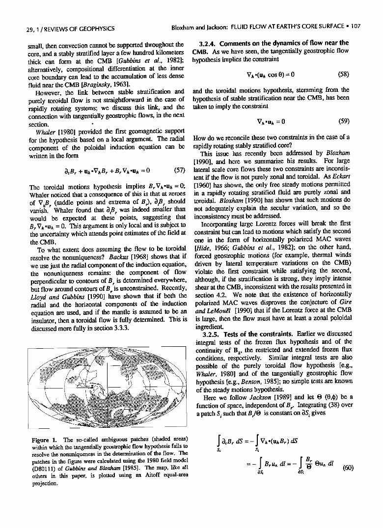
These arguments for magnetostrophy are equivocal, and the hypothesis of tangentially geostrophic flow merits further consideration, in particular since it serves to reduce the nonuniqueness in the flow. This has been addressed, for the use of the radial poloidal induction equation, by Hills [1979] and Backus and LeMougl [1986]. Backus and LeMougl show that the nonuniqueness is resolved fully in certain regions but incompletely elsewhere. The regions where the nonuniqueness is resolved incompletely are determined by the morphology of the magnetic field; they dub these regions ambiguous patches. In Figure 1 we plot the ambiguous patches for the 1980 main field model of Gubbins and Bloxham [1985]; they account for 41% of the area of the CMB. Within these patches, only one component of the flow is known everywhere, but else- where, i.e., over almost 60% of the core surface, the flow is fully determined.
3.2.3. 1oroidal motions. A third dynamical hypothe- sis is that the flow at the CMB is purely toroidal, i.e., that there is no upwelling or downwelling of fluid at the CMB. The dynamical motivation for the hypothesis derives from the possibility that the core is stably stratified within a layer beneath the CMB, a suggestion first made by Higgins and Kennedy [1971] on the basis of the properties of core materials at very high pressure and temperature. Although more recent determinations of these properties have cast doubt on the assertion of Higgins and Kennedy, the idea of a stably stratified layer near the CMB has persisted.
A stably stratified layer can arise through two mechanisms. If the cooling rate of the core is sufficiently
29, 1 /REVIEWS OF GEOPHYSICS Bloxham and Jackson: FLUID FLOW AT EARTH'S CORE SURFACE ß 107
small, then convection cannot be supported throughout the core, and a stably stratified layer a few hundred kilometers thick can form at the CMB [Gubbins et al., 1982]; alternatively, compositional differentiation at the inner core boundary can lead to the accumulation of less dense fluid near the CMB [Braginsky, 1963].
However, the link between stable stratification and purely toroidal flow is not straightforward in the case of rapidly rotating systems; we discuss this link, and the connection with tangentially geostrophic flows, in the next section. ß
Whaler [1980] provided the first geomagnetic support for the hypothesis based on a local argument. The radial component of the poloidal induction equation can be written in the form
•}tBr q- Uh ø•7hBr q- t•r Vh øUh -- 0 (57)
The toroidal motions hypothesis implies Br•7høUh--0; Whaler noticed that a consequence of this is that at zeroes of VnB r (saddle points and extrema of B•), •tBr should vanish. Whaler found that •tBr was indeed smaller than would be expected at these points, suggesting that Br •7n oun - 0. This argument is only local and is subject to the uncertainty which attends point estimates of the field at the CMB.
To what extent does assuming the flow to be toroidal resolve the nonuniqueness? Backus [1968] shows that if we use just the radial component of the induction equation, the nonuniqueness remains: the component of flow perpendicular to contours of B r is determined everywhere, but flow around contours of B r is unconstrained. Recently, Lloyd and Gubbins [1990] have shown that if both the radial and the horizontal components of the induction equation are used, and if the mantle is assumed to be an insulator, then a toroidal flow is fully determined. This is discussed more fully in section 3.3.3.
3.2.4. Comments on the dynamics of flow near the CMB. As we have seen, the tangentially geostrophic flow hypothesis implies the constraint
cos 0) = 0 (58)
and the toroidal motions hypothesis, stemming from the hypothesis of stable stratification near the CMB, has been taken to imply the constraint
Vn-un =0 (59)
How do we reconcile these two constraints in the case of a rapidly rotating stably stratified core?
This issue has recently been addressed by Bloxham [1990], and here we summarize his results. For large lateral scale core flows these two constraints are inconsis- tent if the flow is not purely zonal and toroidal. As Eckart [1960] has shown, the only free steady motions permitted in a rapidly rotating stratified fluid are purely zonal and toroidal. B loxham [1990] has shown that such motions do not adequately explain the secular variation, and so the inconsistency must be addressed.
Incorporating large Lorentz forces will break the first constraint but can lead to motions which satisfy the second one in the form of horizontally polarized MAC waves [Hide, 1966; Gubbins et al., 1982]; on the other hand, forced geostrophic motions (for example, thermal winds driven by lateral temperature variations on the CMB) violate the first constraint while satisfying the second, although, if the stratification is strong, they imply intense shear at the CMB, inconsistent with the results presented in section 4.2. We note that the existence of horizontally polarized MAC waves disproves the conjecture of Gire and LeMou•'l [1990] that if the Lorentz force at the CMB is large, then the flow must have at least a zonal poloidal ingredient.
3.2.5. Tests of the constraints. Earlier we discussed integral tests of the frozen flux hypothesis and of the continuity of B n, the restricted and extended frozen flux conditions, respectively. Similar integral tests are also possible of the purely toroidal flow hypothesis [e.g., Whaler, 1980] and of the tangentially geostrophic flow hypothesis [e.g., Benton, 1985]; no simple tests are known of the steady motions hypothesis.
Here we follow Jackson [1989] and let !9 (0,•) be a function of space, independent of B r. Integrating (38) over a patch S i such that B,/O is constant on •Si gives
Figure 1. The so-called ambiguous patches (shaded areas) within which the tangentially geostrophic flow hypothesis fails to resolve the nonuniqueness in the determination of the flow. The patches in the figure were calculated using the 1980 field model (D80111) of Gubbins and Bloxham [1985]. The map, like all others in this paper, is plotted using an Aitoff equal-area projection.
l •tBr dS = - I Vh ø(Uh Br) as si
=lBrundl-I Br - - • Ou, dl (60)

108 ß Bloxham and Jackson: FLUID FLOW AT EARTH'S CORE SURFACE 29, 1 /REVIEWS OF GEOPHYSICS
where we have used Green's theorem in the plane to convert the surface integral into a line integral, and u,, is the component of u, normal to 3S/. Rearranging and reapplying Green's theorem gives
f •}tBr d$ =- • f Vh'(Uh O) dS Br
V Si '•- = const on OSi (61)
time-varying field model of B loxharn and Jackson [ 1989]. Summarizing his results, he finds little evidence to question the purely toroidal motions hypothesis, but rather stronger, though by no means unequivocal, evidence that the tangential geostrophy conditions are not satisfied.
Although we might draw the conclusion that there is stronger support for the toroidal motions hypothesis than for the tangential geostrophy hypothesis, such a conclusion must be tentative. More complicated models of the magnetic field could yield a different result.
Obviously, we can choose O in a number of ways. First consider O = const; then it follows that we must choose S i such that •}S i is a contour of B r. We then have
l atB r dS = - Br I •7, ø(Uh ) dS (62)
The restricted frozen flux conditions follow in the special case of B r = 0 on 3S i.
Recalling that the hypothesis of purely toroidal motions implies V,.u h = 0, we obtain the set of conditions
I 3tBr dS = 0 V Si :Br = const on 3Si (63) Si
We call these the "toroidal motions conditions."
Alternatively, consider the choice t9 = cos 0. Recall- ing that the tangential geostrophy hypothesis implies V h.(u h cos 0) = 0, we obtain the set of conditions
3tBr dS = 0 V Si ' • = cos 0 = const on aS/ (64) Si
3.3. Resolving the Nonuniqueness in Shear In section 3.1 we showed that when only the poloidal
components of field are known at the CMB, the shear is subject to exactly the same type of ambiguity as that which plagues the determination of flow from the radial compo- nent of secular variation, namely a toroidal ambiguity in the field u'B r. In section 3.2 we discussed three pos- sibilities for circumventing the nonuniqueness in the flow; in this section we state the corresponding results for circumventing the nonuniqueness in the shear.
3.3.1. Steady shear. A trivial extension of the steady motions theorem for velocity described by Jackson and Bloxharn [1991] shows that if the shear is steady over a certain interval of time, then measurement of B and 3tB at three different times will serve to resolve the shear
uniquely (with the exception of some special cases similar to those for steady flow).
3.3.2. Geostrophic flow and shear. Section 3.2.2 discussed the likelihood of a geostrophic regime of core flow. Here we consider the case where Lorentz forces are
negligible in the dynamics of the shear. Let œ = J^B represent the Lorentz force. The flow
must satisfy
We call these the "tangential geostrophy conditions." We note that a special case of these conditions is the choice 0 = •/2 so that the patches correspond to the northern and southern hemispheres.
Jackson [ 1989] shows that we can rewrite the conditions in the form
d-7 B• dS = 0 (65)
Whaler [1984] attempted to test the toroidal motions conditions using inverse theory but did not reach any firm conclusion, owing to the large uncertainties involved and poor resolution of the individual patches. Benton et al. [1987] and Benton and Voorhies [1987] evaluated the tangential geostrophy conditions for the special case 0 = n/2; they found that secular variation models (at least when not truncated at too low degree) satisfy the constraint well; however, they did not attempt any statistical test of the hypothesis.
Jackson [1989] evaluated both the toroida! motions conditions and the tangential geostrophy conditions using a
u cos 0 = A1 q + Ur• - (290 f•) -1 (66)
where • = •,A1 = •^Vh and q = p/(2Pof•r ). At the CMB, u r = 0 and geostrophy requires that the term in œ be small. What is the constraint on u'? The derivative of
(66) shows that u' must obey
u' cos 0 = A t q + u• t + (2p0 fi)-I •^[a k- 0r • ] (67)
where the prime represents differentiation with respect to r, a = P•/P0, and q* =[p'-p/r-qp]/(2pof•r). To compare sizes of terms in (67), we need to estimate the size of lu'l. The only estimate available to us is that obtained from prior core velocity studies using the radial component of the induction equation, which supply u•. We shall find later that this quantity is badly determined and can vary between zero for toroidal flows to u• ~ 10 -2 yr -• for other flows. Taking this to be a representative value for the shear, and with lul - 10 km yr -•, we find that the length scale for shear L is roughly 1000 km. In this case, Lq* - q and the term otœ can be neglected. The size of the term 3 r œ is particularly difficult to estimate, since even in
29, 1 / REVIEWS OF GEOPHYSICS Bloxham and Jackson: FLUID FLOW AT EARTH'S CORE SURFACE ß 109
the case of an insulating manfie (B r = 0 at r = c) it involves terms of the form
•}L •}Br •}Bh •}2 Bh • ~ -37- •7- + B,, /}ra (68)
is large, the requirement that the toroidal field vanish may not permit the horizontally polarized MAC wave solutions invoked by B loxham [1990] to explain the dynamics of the secular variation if the motions are purely toroidal. This last point requires further examination.
Provided these terms are sufficiently small, we find that the shear is coupled to the flow and satisfies
Vh'(U' cos 0)= Vh'('•/ sin 0t•) (69)
where U = V h.u is the upwelling. In this case we can show that the shear can be deter-
mined uniquely everywhere except within the same ambiguous patches previously encountered when consider- ing the flow [Jackson and B loxham, 1991]. If the mantle is insulating, then the proof of Lloyd and Gubbins [1990] can be adapted to the geostrophic case, and the flow and shear are uniquely determined everywhere provided the field satisfies certain conditions (D. Lloyd and D. Gubbins, personal communication, 1990).
3.3.3. Ioroidal flow. As mentioned above, Lloyd and Gubbins [1990] show that if the radial and horizontal components of the field are used, and if the mantle is assumed to be insulating (in which case the toroidal field at the CMB vanishes), then the flow and shear are determined uniquely provided the field satisfies a consistency condition. The condition that the toroidal field vanish at
the CMB is crucial to their restfit: it provides an additional equation, since it requires that the production of toroidal field due to the action of the toroidal flow and shear on the
poloidal field should be zero. The consistency condition on the field is
(•A•7hB r )ø•7 h (B'•7hBr ) :/: 0 (70)
As Lloyd and Gubbins remark, this condition will fail everywhere if the field is axisymmetric. However, for the geomagnetic field, which is nonaxisymmetric, failure will be restricted to lines on the CMB. This failure is much
less insidious than that encountered with tangentially geostrophy, where the resolution of the nonuniqueness fails within patches, rather than along lines. Given the fact that at best we can resolve only the large-scale ingredient of the flow, failure along lines is likely to be of little concern, but failure within patches of dimension compara- ble to the length scale of the flow is of considerable concem.
How likely is the field and flow regime. required by Lloyd and Gubbins? They require that the toroidal field vanish at the CMB and that the flow be purely toroidal there. As discussed earlier, Bloxham [1990] has argued that for the flow to be purely toroidal, Lorentz forces must be important in the dynamical balance at the CMB. Although, as has also been discussed earlier, large Lorentz forces may arise at the CMB even if the toroidal field there vanishes, provided that the radial gradient of toroidal field
3.4. Constructing Solutions The problems of nonuniqueness discussed above must
be taken into consideration when constructing solutions. Recent solutions have used one or more of the three
dynamical hypotheses to resolve the nonuniqueness. However, as we have seen, the extent to which the nonuniqueness is actually resolved remains uncertain: steady motions are dynamically unproven and only resolve the nonuniqueness if the flow is steady over substantial time intervals (at least 50 years); tangential geostrophy is based on assumptions which may not hold even at the core surface, and even if true does not fully resolve the nonuniqueness over the whole core surface; and the toroidal motions hypothesis is plausible only if the core is both stratified and has substantial Lorentz forces at the
core surface, and only resolves the nonuniqueness if we use both the radial and the horizontal components of the induction equation, and then only if the mantle is an insulator at the CMB. The situation is obviously less than ideal.
Uniqueness proofs are applicable to the case of perfect data: instead, we have imperfect data which do not precisely satisfy any of the foregoing hypotheses. We obtain solutions by regularized least squares procedures which necessarily yield unique solutions but represent only one of a large class of solutions compatible with the data.
A closely related issue is that of nuncation of the model v•tors, since the problem as posed is infinite dimensional. Two approaches can be taken to truncation: the first is to truncate at or below some level at which we believe the
data still have adequate resolution; the second is to damp the inversion to obtain a solution with some particular property (such as smoothness), and nuncate the expansions only on the basis of numerical convergence. The second approach is to be preferred, since with a suitable choice of regularization (damping) we can construct solutions which do not contain any spurious detail.
These issues of regularization and truncation (of course nuncation in the first case is really just an extreme example of regularization) apply equally well to the construction of the field model which we treat here as the
data; we refer the reader to Grubbins and Bloxharn [1985] for a discussion of field modeling.
Most model regularizations can be written as quadratic norms
•{. = qrNq (71)
where N is a positive-definite damping matrix. Two choices of • have been used in recent studies: Madden and LeMougl [1982] introduced the minimum energy norm
110 ß Bloxham and Jackson: FLUID FLOW AT EARTH'S CORE SURFACE 29, 1 / REVIEWS OF GEOPHYSICS
•= •c•t•lun I • dS (72) and B loxham [1988a] the norm
9(2 = •ca4• [(V•2uø) 2+ (V•2u*) 2] dS (73) 9• ensures that the solution obtained has, for a given fit to the magnetic field, the minimum surface kinetic energy density; 9• 2 is a stronger regularization condition which minimizes the roughness of the flow, as measured by the second spatial derivatives.
Models of the magnetic field typically lose resolution around degree 12 as a result of the effects of crustal fields. To fit the secular variation to degree 12 (and using a magnetic main field to degree 12) in principle requires harmonics to degree 24, on account of the triangle rule [Bullard and Gellman, 1954]. However, good fits can be obtained with flow models which converge by degree 12; typically, the velocity expansion is truncated by degree 14.
The simplest problem consists of constructing flows which fit the observed instantaneous secular variation
given an instantaneous model of the magnetic field. Voorhies [1986a] extended this linear problem by solving at all points in a finite time interval by introducing time-averaged data and assuming the flow to be steady through the time interval. This extension is important for two reasons: first, it provides a method of implementing the steady motions hypothesis; and second, all methods involve some assumption of steadiness of the flow, and Voorhies' method makes this assumption explicit. This last point requires some explanation. Any model of the instantaneous time rate of change of field is really a time average rather than an instantaneous model; the averaging time is certainly no shorter than 1 year (since most information on the time derivative of the field comes from
observatory annual means) and most probably at least 5 years on account of the effects of mantle conductivity and the necessary averaging required with noisy data.
In further work, Voorhies [1986b] recognized that the problem is more completely posed as a nonlinear problem, that of matching the temporal evolution of the observed main field over a finite time interval. Voorhies did not
solve this nonlinear problem, restricting himself to a linearization of the full problem.
Bloxham [1988a] and Bloxham et al. [1989] solved the nonlinear problem for the case where the field is known at a discrete number of points in time (such as from a discrete time sequence of main field models); Bloxham [1988b] extended the formalism to the case where the field is
known as a continuous function of time.
4. MAPS OF THE CORE FLOW
4.1. Maps Based on the Radial Component In this section we seek to compare maps of the core
flow derived using different subsets of these constraints.
We begin by considering maps based on the radial component equation alone. Although the first attempts at determining maps of the core flow were made almost 25 years ago [Kahle et al., 1967], the vast majority have appeared in the last 5 years, and our attention is largely restricted to this recent work. The earlier solutions took
inadequate account of the nonuniqueness which is so pervasive in this subject; however, we do not wish to diminish their value, since more recent solutions are based on approximations whose applicability is not unques- tionable and which do not necessarily guarantee global uniqueness anyway.
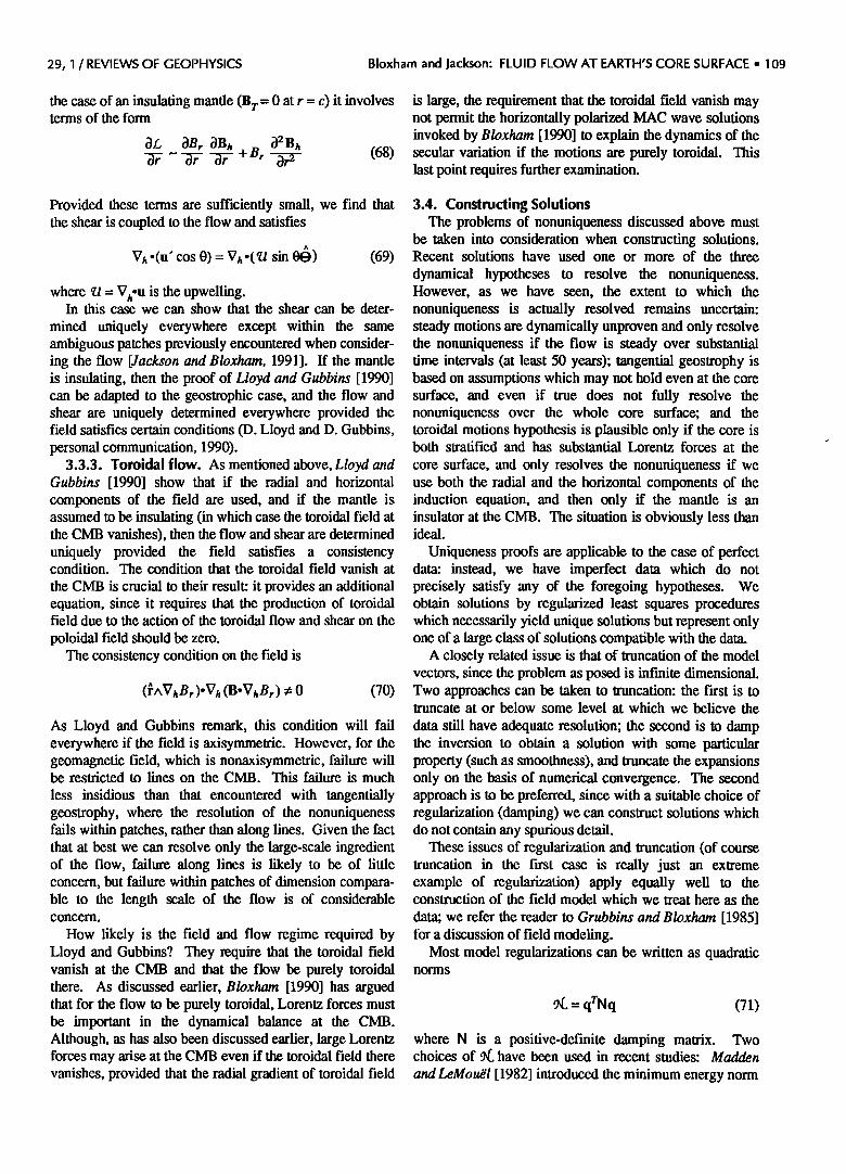
We begin by considering steady flows. The first global steady flow maps were produced by Voorhies [1986a, b]; other solutions have been produced by Bloxham [1988a, b, 1989],Bloxham et al. [ 1989] and Whaler and Clarke [1988]. The solutions of Bloxham are all constmctexl by solving the nonlinear problem, and those of the other authors by solving the linear problem. In Figure 2 we show two steady solu- tions: Figure 2a shows the flow Ia of Bloxham [1989] for the period 1975-1980, and Figure 2b shows flow C4 of Voorhies [1986a] for the period 1960-1980.
--• 20km/yr a _4x10-2 4x10 -2
b -4x10 -2 4x10 -2
Figure 2. Steady unconstrained flows. (a) Flow Ia from Bloxham [1989] for the imerval 1975-1980. (b) Flow C4 from Voorhies [1986a] for the interval 1960-1980. The vectors show the speed and direction of the flow near the core surface, and the grey scale shows the intensity of the horizontal divergence (upwelling and downwelling) of the flow. The sign of the horizontal divergence can be determined from the flow vectors using the fact that the flow is incompressible.
29, 1 / REVIEWS OF GEOPHYSICS Bloxham and Jackson: FLUID FLOW AT EARTH'S CORE SURFACE ß 111
Similarities, and differences, between these two flows are evident; many of the salient features have been identi- fied and described by Voorhies [1986a], Whaler and Clarke [1988], and Bloxham [1988a, 1989]. Most promi- nent are two counterrotating (in map view) circulations north and south of the geographic equator from 90øE westward to 90øW (though less pronounced north of the equator); viewed as a solid boundary rotation, we can very roughly approximate this flow as a cylindrical rotation about an axis parallel to the Earth's rotation axis through approximately _+45 ø latitude and 0 ø longitude. The west- ward drift component of these flows is largely confined to equatorial regions. Both flows have some evidence of a similar circulation south of the equator in the opposite hemisphere. Cross-equatorial flow is present in both flows, especially beneath equatorial South America. However, beneath Indonesia, where there are also indica- tions of cross-equatorial flow, these flows differ; Bloxham and Gubbins [1985] have suggested that the secular varia- tion is complex there and might be the result of a wave in the core, which large-scale flows such as these would not resolve adequately. They also differ beneath the northern Pacific, Figure 2a having very weak flow there, which is consistent with the observation of low secular variation at the CMB in this region [Bloxham and Gubbins, 1985]. However, the possibility remains that there is flow in the re- gion aligned with contours of B r which has not been re- solved because the time interval of 20 years is too short to resolve this ambiguity. We note that for each of these flows, approximately 75% of the surface kinetic energy density is concentrated in the toroidal ingredient of the flow.
The first attempts at constructing tangentially geostrophic flows were made by Hills [1979]. Later, LeMoub'l et al. [1985] derived tangentially geostrophic flows by solving the linear problem for the flow at 1970 and at 1980, but as Bloxham [1988b] has pointed out, these flows (and the flows of Hills) are not in fact tangentially geostrophic, mostly owing to the presence of substantial ageostrophic components at degree Lm,x/2 and above (where Lm, x is the truncation level).
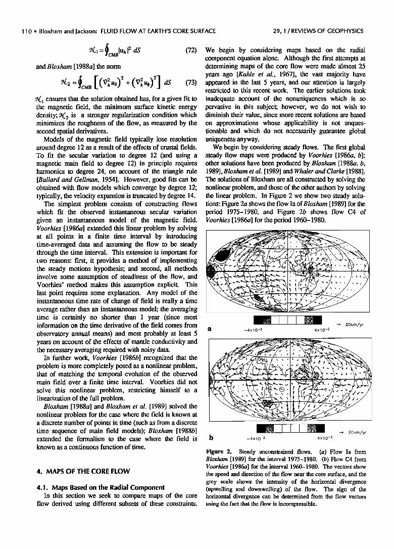
More recently, tangentially geostrophic flow maps have been given by Bloxham [1989] and by Gire and LeMoub'l [1990]. In Figure 3 we plot these solutions: Figure 3a shows flow IIa for 1975-1980 from Bloxham [1989], and Figure 3b shows the 1980 flow from Gire and LeMoub'l [1990]. These flows are substantially different from each other; Figure 3b is more complicated than Figure 3a, with much more small-scale flow. Comparing the large-scale aspects of these solutions, both, in common with the flows in Figure 2, have westward flow near the equator in the region from 90øE westward to 90øW; Figure 3a also has the circulation south of the equator present in the flows in Figure 2; evidence for the corresponding circulation north of the equator is rather weak in both these flows, but perhaps stronger in Figure 3b. Figure 3a has a fairly strong circulation south of the equator in the opposite hemisphere, a feature identified rather weakly in Figure 2.
The pattern of upwelling and downwelling differs greatly (we emphasize the change in scale from Figure 2; the upwellings and downwellings in Figure 3 are weaker than those in Figure 2). Figure 3b has a number of upwellings and downwellings near the geographic equator, considerably more complicated than simply a main upwelling underneath the equatorial Indian Ocean and a main downwelling area west of Peru as described by Gire and LeMo•'l [1990].
_2x10-2 2x10 -2 • 20km/yr
Figure 3. Tangenfially geoslxophic flows. (a) Flow IIa from Bloxham [1989], a steady solution for the period 1975-1980. (b) A flow from Gire and LeMougl [1990] at 1980. The sign of the horizontal divergence is readily deduced: flow toward the equator corresponds to positive divergence (upwelling), and flow away from the equator to negative divergence (downwelling). Note the change in scale of the horizontal divergence from Figure 2.
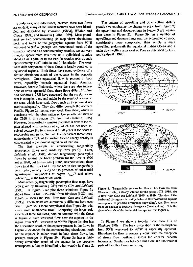
In Figure 4 we show a toroidal flow, flow IIIa of Bloxham [1989]. The basic circulation in the hemisphere from 90øE westward to 90øW is especially apparent. Elsewhere the flow is generally weak, with the exception of strong flow northward across the equator beneath Indonesia. Similarities between this flow and the toroidal
parts of the other flows are strong.

112 ß Bloxham and Jackson: FLUID FLOW AT EARTH'S CORE SURFACE 29, 1 / REVIEWS OF GEOPHYSICS
What are the causes of the differences between these
flows? The flows are based on different models of the
magnetic field and secular variation which undoubtedly accounts for some of the differences; the different constraints applied obviously account for some of the differences as well, but it is likely that different regulariza- tions are also an important source of difference between these solutions. The solutions of Voorhies are regularized by truncation; the solutions of Gire and LeMou8l by weakly minimizing the surface kinetic energy density; and
4.2. Maps Based on the Radial and Horizontal Components
In this section we consider flows derived using both the radial and the horizontal components of the induction equation. In Figures 5, 6, and 7 we show steady solutions for the period 1960-1980 derived using the same field model as the flows given by Bloxham [1989] but based on both the radial and the horizontal components of the field (for details, see Jackson and Bloxham [1991]). The flow in Figure 5 is steady but otherwise unconstrained, the flow
the solutions of B loxham by minimizing the spatial complexity.
20km/yr -2x10⁻² 2x10 -2
--• 20km/yr
Figure 4. Toroidal flow. Flow Ilia from Bloxham [1989], a steady solution for the period 1975-1980.
It is immediately apparent that the pattern of upwelling and downwelling shows little similarity between any of the flows considered here. Indeed, Bloxham [1989] has argued that the poloidal ingredient of the flow is much less well determined than the toroidal ingredient: these flows certainly seem consistent with that view. We note, however, that Madden and LeMougl [1982] reached exactly the opposite conclusion, even claiming to have shown that purely poloidal flow can be determined uniquely: we find no support for their conjecture. Two possible approaches can be adopted given that only the toroidal flow is well determined: either we can seek to
determine the toroidal flow alone, or we can constrain the poloidal flow by adopting the tangential geostrophy constraint. In connection with this last point, it is worth highlighting that given any purely toroidal flow, we can construct a tangentially geostrophic flow by adding suitable poloidal terms, without changing any of the toroidal terms. In other words, we may view the toroidal motions constraint as a means of determining the poorly determined poloidal flow by assuming it to be zero, and the tangentially geostrophic constraint as a way of determining the poloidal terms by assuming that they are such as to make the flow tangentially geostrophic. In both cases, given a toroidal flow, we determine the poloidal component uniquely.
'-• c40km/yr -2x10 -2 2x10⁻²
b
Figure 5. Steady unconstrained (a) flow and (b) shear for the interval 1960-1980. To relate the shear to flow, the shear is multiplied by the radius of the CMB, and the scale of the arrows is changed.
in Figure 6 is constrained to be tangentially geostrophic, and the flow in Figure 7 is constrained to be purely toroidal. In Figure 8 we show the solution CV70 from Lloyd and Gubbins [1990], a purely toroidal solution. Compared with the flows based on just the radial com- ponent, the similarity of the toroidal components of these flows is now especially apparent. In fact, the basic pattern of toroidal flow described above is apparent particularly clearly in these flows. However, the pattern of upwelling and downwelling is still poorly determined, Figures 5 and 6 exhibiting substantially different patterns.

29, 1 / REVIEWS OF GEOPHYSICS Bloxham and Jackson: FLUID FLOW AT EARTH'S CORE SURFACE ß 113
--* 20km/yr --• c40km/yr -2x10 -2 2x10 -2 -2x10 -2 2x10 -2
a b
Figure 6. Steady fully geostrophic (a) flow and (b) shear for the interval 1960-1980.
a --. 20km/yr
--• c40km/yr
Figure 7. Steady toroidal (a) flow and (b) shear for the interval 1960-1980.
Figures 5-8 also show the shear, the radial derivative of the flow immediately beneath the CMB. We have multiplied the shear by the core radius so that it has the same dimensions as the flow. Then, if the flow and shear at some point are identical (i.e., equal in magnitude and direction), it indicates that the flow diminishes with depth, but without rotating, at such a rate so as to reach zero at the Earth's center. We see that the toroidal shear is relatively insensitive to the assumptions (though this case is weakest for the unconstmined solution). A tendency for the shear
to be either parallel (indicating flow weakening with depth) or antiparallel (indicating flow strengthening with depth) to the flow is apparent. This is most clearly apparent for the circulation centered on 45øS latitude and 0 ø longitude, where the ratio of the flow to the shear is approximately half the core thickness (as would be expected for a convection cell extending over the entire core thickness), suggesting that this circulation is an expression of flow extending very deep into the core.
a --• 20km/yr
--• c40km/yr
Figure 8. Toroidal (a) flow and (b) shear from Lloyd and Gubbins [1990] at 1970.
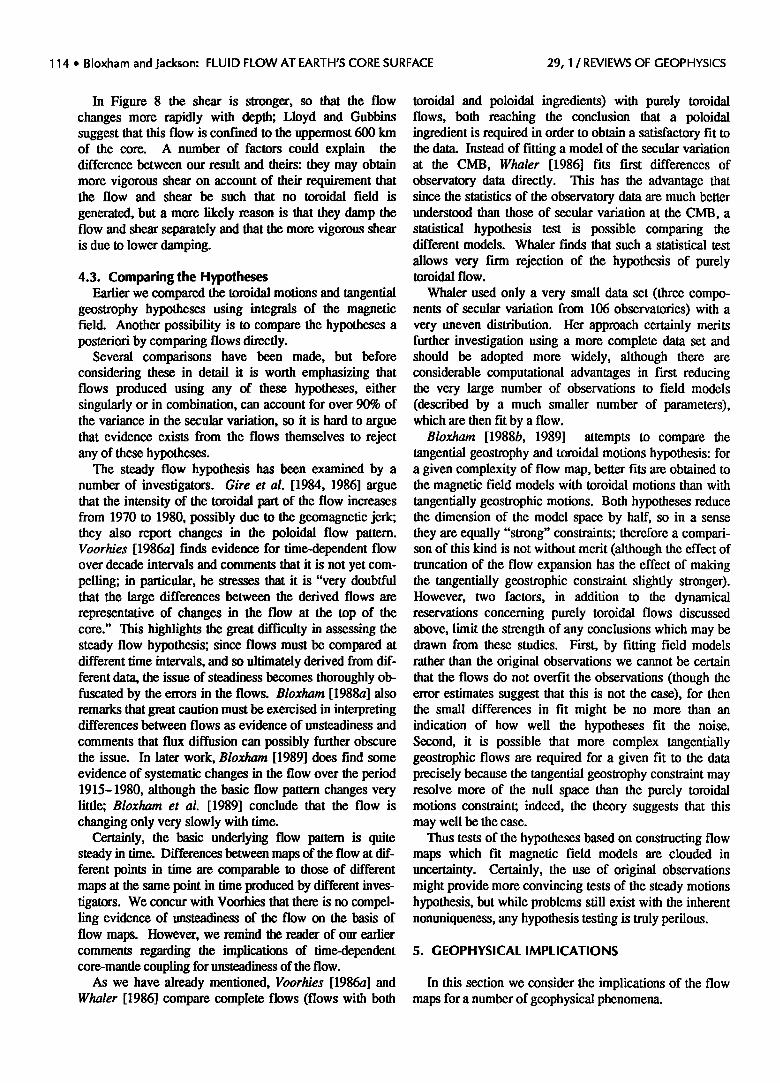
114 ß Bloxham and Jackson: FLUID FLOW AT EARTH'S CORE SURFACE 29, 1 / REVIEWS OF GEOPHYSICS
In Figure 8 the shear is stronger, so that the flow changes more rapidly with depth; Lloyd and Gubbins suggest that this flow is conf'med to the uppermost 600 km of the core. A number of factors could explain the difference between our result and theirs: they may obtain more vigorous shear on account of their requirement that the flow and shear be such that no toroidal field is
generated, but a more likely reason is that they damp the flow and shear separately and that the more vigorous shear is due to lower damping.
4.3. Comparing the Hypotheses Earlier we compared the toroidal motions and tangential
geostrophy hypotheses using integrals of the magnetic field. Another possibility is to compare the hypotheses a postefiofi by comparing flows directly.
Several comparisons have been made, but before considering these in detail it is worth emphasizing that flows produced using any of these hypotheses, either singularly or in combination, can account for over 90% of the variance in the secular variation, so it is hard to argue that evidence exists from the flows themselves to reject any of these hypotheses.
The steady flow hypothesis has been examined by a number of investigators. Gire et al. [1984, 1986] argue that the intensity of the toroidal part of the flow increases from 1970 to 1980, possibly due to the geomagnetic jerk; they also report changes in the poloidal flow pattern. Voorhies [1986a] finds evidence for time-dependent flow over decade intervals and comments that it is not yet com- pelling; in particular, he stresses that it is "very doubtful that the large differences between the derived flows are representative of changes in the flow at the top of the core." This highlights the great difficulty in assessing the steady flow hypothesis; since flows must be compared at different time intervals, and so ultimately derived from dif- ferent data, the issue of steadiness becomes thoroughly ob- fuscated by the errors in the flows. Bloxham [1988a] also remarks that great caution must be exercised in interpreting differences between flows as evidence of unsteadiness and
comments that flux diffusion can possibly further obscure the issue. In later work, B loxham [1989] does find some evidence of systematic changes in the flow over the period 1915-1980, although the basic flow pattern changes very little; Bloxham et al. [1989] conclude that the flow is changing only very slowly with time.
Certainly, the basic underlying flow pattern is quite steady in time. Differences between maps of the flow at dif- ferent points in time are comparable to those of different maps at the same point in time produced by different inves- tigators. We concur with Voorhies that there is no compel- ling evidence of unsteadiness of the flow on the basis of flow maps. However, we remind the reader of our earlier comments regarding the implications of time-dependent core-mantle coupling for unsteadiness of the flow.
As we have already mentioned, Voorhies [1986a] and Whaler [1986] compare complete flows (flows with both
toroidal and poloidal ingredients) with purely toroidal flows, both reaching the conclusion that a poloidal ingredient is required in order to obtain a satisfactory fit to the data. Instead of fitting a model of the secular variation at the CMB, Whaler [1986] fits first differences of observatory data directly. This has the advantage that since the statistics of the observatory data are much better understood than those of secular variation at the CMB, a statistical hypothesis test is possible comparing the different models. Whaler finds that such a statistical test
allows very firm rejection of the hypothesis of purely toroidal flow.
Whaler used only a very small data set (three compo- nents of secular variation from 106 observatories) with a very uneven distribution. Her approach certainly merits further investigation using a more complete data set and should be adopted more widely, although there are considerable computational advantages in first reducing the very large number of observations to field models (describexl by a much smaller number of parameters), which are then fit by a flow.
Bloxham [1988b, 1989] attempts to compare the tangential geostrophy and toroidal motions hypothesis: for a given complexity of flow map, better fits are obtained to the magnetic field models with toroidal motions than with tangentially geostrophic motions. Both hypotheses reduce the dimension of the model space by half, so in a sense they are equally "strong" constraints; therefore a compari- son of this kind is not without merit (although the effect of truncation of the flow expansion has the effect of making the tangentially geostrophic constraint slightly stronger). However, two factors, in addition to the dynamical reservations concerning purely toroidal flows discussed above, limit the strength of any conclusions which may be drawn from these studies. First, by fitting field models rather than the original observations we cannot be certain that the flows do not overfit the observations (though the error estimates suggest that this is not the case), for then the small differences in fit might be no more than an indication of how well the hypotheses fit the noise. Second, it is possible that more complex tangenfially geostrophic flows are required for a given fit to the data precisely because the tangential geostrophy constraint may resolve more of the null space than the purely toroidal motions constraint; indeed, the theory suggests that this may well be the case.
Thus tests of the hypotheses based on constructing flow maps which fit magnetic field models are clouded in uncertainty. Certainly, the use of original observations might provide more convincing tests of the steady motions hypothesis, but while problems still exist with the inherent nonuniqueness, any hypothesis testing is truly perilous.
5. GEOPHYSICAL IMPLICATIONS
In this section we consider the implications of the flow maps for a number of geophysical phenomena.
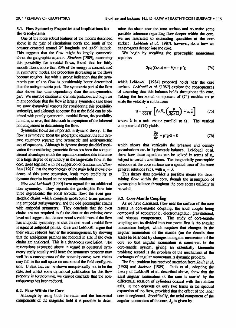
29, 1 / REVIEWS OF GEOPHYSICS Bloxham and Jackson: FLUID FLOW AT EARTH'S CORE SURFACE ß 115
5.1. Flow Symmetry Properties and Implications for the Geodynamo
One of the more robust features of the models describexl
above is the pair of circulations north and south of the equator centered around 0 ø longitude and +_45 ø latitude. This suggests that the flow might be largely symmetric about the geographic equator. B loxham [1989], examining this possibility for toroidal flows, found that for fairly smooth flows, more than 80% of the energy is concentratext in symmetric modes, the proportion decreasing as the flows become rougher, but with a strong indication that the sym- metric part of the flow is considerably better determined than the antisymmetric part. The symmetric part of the flow also shows less time dependency than the antisymmetric part. We must be cautious in our interpretation: although we might conclude that the flow is largely symmetric (and there are some dynamical reasons for considering this possibility seriously), and although adequate fits to the field can be ob- tained with purely symmetric, toroidal flows, the possibility remains, as ever, that this result is a symptom of the inherent nonuniqueness in determining the flow.
Symmetric flows are important in dynamo theory. If the flow is symmetric about the geographic equator, the full dyn- amo equations separate into symmetric and antisymmetric sets of eq, at_ions. Although in dynamo theory the chief moti- vation for considering symmetric flows has been the comput- ational advantages which the separation renders, this inference of a large degree of symmetry in the large-scale flow in the core, taken together with the suggestion of Gubbins and Blox- ham [1987] that the morphology of the main field shows evi- dence of this same separation, lends more credibility to dynamo theories based on the separable solutions.
Gire and LeMou•l [1990] have argued for an additional flow symmetry. They separate the geostrophic flow into three ingredients: the zonal toroidal flow; the even geo- strophie chains which comprise geostrophic terms possess- ing antitxxtal antisymmetry; and the odd geostrophic chains with antiIxxlal symmetry. They conclude that the even chains are not required to fit the data at the existing error level and suggest that the non-zonal-toroidal part of the flow has antitxxtal symmetry, so that the non-zonal-toroidal flow is equal at antipodal points. Gire and LeMou•l argue that their result reduces further the nonuniqueness, by showing that the ambiguous patches are reduced in size if the even chains are neglected. This is a dangerous conclusion. The reservations expressed above in regard to equatorial sym- metry apply equally well here: the symmetry property may well be a consequence of the nonuniqueness; even chains may fall in the null space on account of the field configura- tion. Unless that can be shown unequivocally not to be the case, and unless some dynamical justification for this flow property is forthcoming, we cannot conclude that the non- uniqueness has been reduced.
5.2. Flow Within the Core
Although by using both the radial and the horizontal components of the magnetic field it is possible to deter-
mine the shear near the core surface and so make some
possible inference regarding flow deeper within the core, we are restricted to estimating quantifies at the core surface. LeMou•'l et al. [1987], however, show how we can progress deeper into the core.
We begin by recalling the geostrophic momentum equation
200 (s•^u):- V/, + p • (?4)
which LeMo•'l [1984] proposed holds near the core surface. LeMo•'l et al. [1987] explore the consequences of assuming that this balance holds throughout the core. Taking the horizontal component of (74) enables us to write the velocity u in the form
= t, •.] (75) 1 ['^V, (2poll) + Ur u cos 0
where • is a unit vector parallel to l•. The vertical component of (74) yields
•- + p'g-•. = 0 (76)
which shows that vertically the pressure and density perturbations are in hydrostatic balance. LeMou•l et al. show how these equations can be solved in terms of u r, subject to certain conditions. The tangentially geostrophic solutions at the core surface are a special case of the more general solutions (75), with u r = O.
This theory thus provides a possible means for deter- mining flow within the core, though the assumption of geostrophic balance throughout the core seems unlikely to be valid.
5.3. Core-Mantle Coupling As we have discussed, flow near the surface of the core
results in core-mantle coupling, the total couple being composed of topographic, electromagnetic, gravitational, and viscous components. The study of core-mantle coupling can be divided into two parts: first is the angular momentum budget, which requires that changes in the angular momentum of the mantle (on the decade time scale) be balanced by changes in angular momentum of the core, so that angular momentum is conserved in the core-mantle system, giving an essentially kinematic problem; second is the problem of the mechanism of the exchanges of angular momentum, a dynamic problem.
The first problem has received attention from Jault et al. [1988] and Jackson [1989]. Jault et al., adopting the theory of LeMou•l et al. describexl above, show that the axial angular momentum of the core is carded by the differential rotation of cylinders coaxial with the rotation axis. It then depends on only two terms in the spectral expansion of the flow, provided that the effect of the inner core is neglected. Specifically, the axial component of the angular momentum of the core, J,, is given by

116 ß Bloxham and Jackson: FLUID FLOW AT EARTH'S CORE SURFACE 29, 1 / REVIEWS OF GEOPHYSICS
where t? and t• are coefficients from the expansion (32). This then provides a simple means for calculating
changes in the an•ular momentum of the core from changes in t? and t]. The resulting change in angular momentum of the core should balance the changes in angular momentum of the mantle calculated from length of day observations. Jault et al. obtain an impressive agreement over the period 1969-1985; similar agreement is found for this period by Jackson [1989], and over the last century the calculated changes are in reasonable agreement with the length of day observations, although the agreement degrades back in time. This suggests rather strongly that the angular momentum of the core is well represented by these two terms in the velocity expansion: the extent to which this then implies that the force balance is everywhere geostrophic requires further examination.
This then leads to the second problem in core-mantle coupling, the examination of the mechanism of coupling. Of the mechanisms mentioned, viscous coupling is likely to be insubstantial; electromagnetic coupling does not de- pend directly on the flow and will not be considered fur- ther in this review. The remaining two contributions, the topographic couple due to the action of the flow on topog- raphy and the CMB, and the gravitational couple due to the gravitational coupling between density inhomogeneities in the mantle and those in the core, have been considered in detail by Jault and LeMou•l [1989]. As they point out, the calculation of the gravitational couple requires the den- sity throughout the core, which is unknown.
Topographic coupling, arising from the action of pressure gradients near the core surface on topography at the CMB, was first proposed by Hide [1967]. Hide [1989] and Jault and LeMou•'l [1989] describe the theory for calculating the topographic couple; the calculation requires that the flow be tangentially geostrophic, so that the pressure can be determined from the flow, and that the topography of the CMB be known.
We have discussed at some length the validity of the first of these requirements. However, it is worth emphasiz- ing that the topographic couple depends only on the poloidal ingredient of the flow, which we have seen to be especially poorly determined. Furthermore, in order to explain the time-dependent couple we must resolve time dependency in the poloidal flow: this seems very far beyond our current capabilities.
Concern is also raised by the other requirement, namely that we know the CMB topography. A number of recent studies in seismology have attempted to map the topog- raphy of the CMB; maps have been published by Craeger and Jordan [1986], Morelli and Dziewonski [1987], Doornbos and Hilton [1989], Gudmundsson [1989], and Li [1990]. These maps differ considerably, suggesting that the topography is not sufficiently well determined to calculate the resultant couple (see, in particular, Gud- mundsson [1989]).
Jault and LeMoub'l [1990], using the flow of Gire and LeMou•l [1990] and the topography of Morelli and Dziewonski [1987], find torques which are two orders of magnitude larger than required. Repeating the calculation at different epochs (1970, 1980, and 1985), they obtain similar torques; but repeating the calculations with perturbed topography models (using perturbations within the errors given by Morelli and Dziewonski), they f'md a large range of torques. They conclude that the greatest uncertainties come from the topography rather than the flow, although they comment that the calculation of the torque is likely to be seriously affected by truncation. We concur but argue that the uncertainties in our knowledge of the time-dependent poloidal flow and uncertainties in the validity of the tangential geostrophy hypothesis are sufficiently large in themselves to render such calculations exceedingly unreliable.
Various possibilities which could give rise to a small couple are discussed by Jault and LeMou•l [1990]: the topography at the CMB may be much smaller than currently inferred seismically (studies based on the free core nutation [Gwinn et al., 1986] and on the orientation of the mantle rotation axis [Wahr, 1987] suggest that this may be the case); the effective topography could be smaller owing to the presence of a stable layer separating the mantle from the core (as suggested by Craeger and Jordan [1986] and Hide [1989]); or gravity torques may oppose the topographic torque [see Jault and LeMou•'l, 1989]). Roberts [1989] discusses the dynamical feasibility of large topographic torques and favors electromagnetic coupling.
The possibility of a stably stratified layer, highly differentiated from the bulk core (perhaps differing in density by a few percent from the bulk core), up to a few tens of kilometers thick immediately beneath the CMB does offer a possible solution to these seemingly irrecon- cilable observations. The secular variation could permeate the layer (as magnetic waves); undulations in the interface of the layer with the bulk core owing to undulations in the geoid (the gravitational equipotential surface) can lead to lateral density heterogeneities in the core as envisaged by Wahr and de Vries [1989] (although such lateral density heterogeneities seem unlikely to be detectable seismically); and Earth rotational constraints on CMB topography could be relaxed if the effective top of the free stream in the core is at the interface of the stable layer and the bulk core. Substantial topography of the CMB could then be tolerated.
5.4. Lateral Temperature Variations at the CMB In this section we consider what we can learn about the
pattern of density variations which drive flow near the CMB. By interpreting such density variations as being due to thermal expansion, we can derive the pattern of lateral temperature variations immediately beneath the CMB [see Bloxham and Jackson, 1990].
We begin by neglecting Lorentz forces, in the momen- tum equation, an approximation which we have argued is

29, 1 / REVIEWS OF GEOPHYSICS Bloxham and Jackson: FLUID FLOW AT EARTH'S CORE SURFACE ß 117
certainly less than ideal but, as we have seen, departures from geostrophy are not so large as to be egregious. We assume further that this balance holds in the vicinity of the CMB, so that we can use the thermal wind equation (47), which we rewrite in the form
2p0 (gl.V)un = - g Vn ̂(p'•) (78)
Immediately beneath the CMB we can calculate the left-hand side provided we know the flow and the shear. To find p', we seek the toroidal scalar corresponding to the toroidal part of the left-hand side. For a geostrophic flow and shear the left-hand side is purely toroidal also; for ageostrophic flows we find the toroidal scalar of the left-hand side by a least squares procedure. Hence we obtain the density p' to within a constant of integration.
Assuming a relation of the form
P = P0 (1 - 0[{9) (79)
where O is the nonadiabatic part of the temperature and o[ the coefficient of thermal expansion, we can readily derive the temperature (again to within a constant of integration) from the density.
In Figures 9 and 10 we show the temperature variations for the two flows in Figures 6 and 7. A large degree 1 component is apparent: the region beneath the Pacific hemisphere is on average cooler than the region beneath the Atlantic, although the amplitude of the pattern is greater for the toroidal flow (Figure 10) than for the geostrophic flow (Figure 9). This difference in amplitude and the differences in pattern result from the different assumptions used to derive the flow maps. Figure 9 is a self-consistent calculation: the assumptions used to derive the temperature map are consistent with those used to derive the flow. Figure 10, on the other hand, is not self-consistent and represents a least squares solution.
An important issue is, to what extent is this pattern of lateral temperature or density variations due to the
-2xlO -3 temperoture 2xlO -3
Figure 9. Lateral temperature variations at the CMB calculated from the flow in Figure 6.
underlying process of core convection and to what extent does it represent lateral temperature variations at the CMB due to the mantle? Thermodynamic arguments by Frazer [1973] suggest that the temperature variations associated with the convective flow necessary to account for the heat flux at the CMB are substantially smaller than those inferred by Bloxham and Gubbins [1986] as likely to result from core-mantle interactions, suggesting that the pattern may be dominated by the mantle. This argument is overly simplistic; the problem of convection with laterally varying boundary conditions is very far from being understood.
-2x10 -3 temperoture 2x10 -3
Figure 10. Lateral temperature variations at the CMB calculated from the flow in Figure 7.
5.5. Sudace Helicity Density Given the flow and the shear, we can also calculate the
surface helicity density. The helicity density is defined as
H = u'V^u (80)
Helicity is an important component of dynamo theories [Moffatt, 1978]. Any dynamo theory must account for the generation of toroidal field from poloidal field and for the generation of poloidal field from tomidal field. The first of these is readily accomplished by differential rotation; the second may be accomplished by cyclonic flows (flows with nonzero helicity) as first envisaged by Parker [1955].
For flows with small-scale turbulence, mean field dynamo theory shows that mean helicity of the turbulent velocity field may result in a nonzero •, where {z is a pseudotensor relating the mean magnetic field to the mean electromotive force. This should be contrasted with
laminar flow, for which the induction equation shows that the electromotive force is always perpendicular to the magnetic field.
Here, of course, we are restricted to looking at the large-scale flow. Just beneath the CMB where u r = 0, the surface helicity density is given by
H = u,. - u, -37- (81)
118 ß Bloxham and Jackson: FLUID FLOW AT EARTH'S CORE SURFACE 29, 1 / REVIEWS OF GEOPHYSICS
In Figures 11 and 12 we show the helicity calculated for the flows in Figures 6 and 7. Foremost is the concentration of helicity into the region beneath the Atlantic hemisphere, with little helicity beneath the Pacific hemisphere. The patterns of helicity show a rather weak tendency toward symmetry about the geographical equator; these maps only depict large scales, and so this does not necessarily imply that the small-scale helicity (and hence et) has any tendency toward equatorial symmetry. Simple kinematic turbulent dynamo models usually assume that et is antisymmetric.
-500 helicity +500
Figure 11. Surface helicity density at the CMB calculated from the flow in Figure 6.
6. CONCLUDING REMARKS
Clearly the determination of flow in the core near the CMB is a very poorly determined problem. We see that flows produced using different assumptions and different field models differ considerably. None of the three constraints used to decrease the extent of nonuniqueness (but not necessarily eliminate it) are particularly satisfactory.
However, despite this rather obfuscated view of the flow, the steady large-scale toroidal part of the flow does appear to be well resolved; poloidal flow and the time dependency of the flow are much less well resolved. We are forced to resort either to setting the poloidal flow to be identically zero or to determining it by requiring the flow to be tangentially geostrophic. Both approaches are less than ideal.
By using the horizontal component of the induction equation we are able to determine the shear in addition to the flow. In general, the horizontal poloidal field cannot improve the determination of the flow except through regularization effects, although the fully geostrophic case considered does couple the flow and shear. In addition, although the kernels for the flow and the shear are the same, the data which are required to compute the shear are apt to be more noisy than those for the flow, because they depend on horizontal gradients of secular variation.
-500 hellcity +500
Figure 12. Surface helicity density at the CMB calculated from the flow in Figure 7.
We conclude by highlighting an important issue, the vertical length scale of the flow. The results of Jackson and Bloxham [1991] suggest that it is comparable to half the depth of the outer core, whilst Lloyd and Gubbins [1990] favor a length scale of about 600 km. This difference is important: the result of Jackson and Bloxham suggests that the dynamo and the secular variation may be intimately linked, with the secular variation representing the natural time dependency of the dynamo process; on the other hand, the finding of Lloyd and Gubbins might indicate a situation with the dynamo operating deep in the core and with the secular variation operating in the upper few hundred kilometers of the core. These dichotomous views of the dynamo process demand resolution.
ACKNOWLEDGMENTS. This work was supported by NSF and NASA. The authors are grateful to a number of people for useful discussions, including David Gubbins, Jean-Louis LeMou/51, David Lloyd, and Kathy Whaler. Jean-Louis LeMouE1, Camille Gire and Dominique Jault, and David Gubbins and David Lloyd all kindly provided preprims of work prior to publication.
Jack Jacobs was the editor responsible for this paper. He thanks David Gubbins for serving as a technical referee and Marcia Neugebauer and J. Cogley for serving as cross- disciplinary referees.
REFERENCES
Alfv6n, H., On the existence of electromagnetic-hydromagnetic waves, Arkiv. Mat. Astron. Fys. 29B(2)7, 1942.
Backus, G. E., Kinematics of geomagnetic secular variation in a perfectly conducting core, Philos. Trans. R. Soc. London, Ser. A, 263, 239-266, 1968.
Backus, G. E., Poloidal and toroidal fields in geomagnetic field modeling, Rev. Geophys., 24, 75-109, 1986.
Backus, G. E., Bayesian inference in geomagnetism, Geophys. J., 92, 125-142, 1988a.
Backus, G. E., Comparing hard and soft bounds in geophysical inverse problems, Geophys. J., 94, 249-261, 1988b.
29, 1 / REVIEWS OF GEOPHYSICS Bloxham and Jackson: FLUID FLOW AT EARTH'S CORE SURFACE ß 119
Backus, G. E., and J.-L. LeMouE1, The region on the core-mantle boundary where a geostrophic velocity field can be deter- mined from frozen-flux magnetic data, Geophys. J.R. Astron. Soc., 85, 617-628, 1986.
Banks, R. J., Geomagnetic variations and the electrical conduc- tivity of the upper mantle, Geophys. J.R. Astron. Soc., 17, 457-487, 1969.
Banks, R. J., The overall electrical conductivity distribution of the Earth, J. Geomagn. Geoelectr., 24, 337-351, 1972.
Barraclough, D. R., D. Gubbins, and D. Kerridge, On the use of horizontal components of magnetic field in determining core motions, Geophys. J. Int., 98, 293-299, 1989.
Benton, E. R., Magnetic probing of planetary interiors, Phys. Earth Planet. Inter., 20, 111-118, 1979.
Benton, E. R., Inviscid, frozen-flux velocity components at the top of Earth's core from magnetic observations at Earth's surface, 1, A new methodology, Phys. Earth Planet. Inter., 18, 157-174, 1981.
Benton, E. R., On the coupling of fluid dynamics and electromagnetism at the top of the Earth's core, Geophys. Astrophys. Fluid Dyn., 33, 315-330, 1985.
Benton, E. R., and C. V. Voorhies, Testing recent geomagnetic field models via magnetic flux conservation at the core-mantle boundary, Phys. Earth Planet. Inter., 48, 350-357, 1987.
Benton, E. R., and K. A. Whaler, Rapid diffusion of the poloidal magnetic field through the weakly conducting manfie: A perturbation solution, Geophys. J. R. Astron. Soc., 75, 77-100, 1983.
Benton, E. R., R. H. Estes, and R. A. Langel, Geomagnetic field modeling incorporating constraints from frozen-flux electro- magnetism, Phys. Earth Planet. Inter., 48, 241-264, 1987.
Bloxham, J., The determination of fluid flow at the core surface from geomagnetic observations, in Mathematical Geophysics, A Survey of Recent Developments in Seismology and Geodynamics, edited by N.J. Vlaar et al., pp. 189-208, D. Reidel, Hingham, Mass., 1988a.
Bloxham, J., The dynamical regime of fluid flow at the core surface, Geophys. Res. Lett., 15, 585-588, 1988b.
Bloxham, J., Simple models of fluid flow at the core surface derived from geomagnetic field models, Geophys. J. Int., 99, 173-182, 1989.
Bloxham, J., On the consequences of strong stable stratification at the top of Earth's outer core, Geophys. Res. Lett., 17, 2081-2084, 1990.
Bloxham, J., and D. Gubbins, The secular variation of Earth's magnetic field, Nature, 317, 777-781, 1985.
Bloxham, J., and D. Gubbins, Geomagnetic field analysis, IV, Testing the frozen-flux hypothesis, Geophys. J. R. Astron. Soc., 84, 139-152, 1986.
Bloxham, J., and A. Jackson, Simultaneous stochastic inversion for geomagnetic main field and secular variation, 2, 1820-1980, J. Geophys. Res., 94, 15,753-15,769, 1989.
Bloxham, J., and A. Jackson, Lateral temperature variations at the core-mantle boundary deduced from the magnetic field, Geophys. Res. Lett., 17, 1997-2000, 1990.
Bloxham, J., D. Gubbins, and A. Jackson, Geomagnetic secular variation, Philos. Trans. R. Soc. London, Ser. A, 329, 415-502, 1989.
Booker, J. R., Geomagnetic data and core motions, Proc. R. Soc. London, 309, Ser. A, 27-40, 1969.
Braginsky, S. I., Smacture of the F layer and reasons for convection in the Earth's core (in Russian), Dokl. Akad. Nauk SSSR, 149, 8-10, 1963.
Braginsky, S. I., Nearly axisymmetric model of the hydromag- netic dynamo of the Earth, Geomagn. Aeron., Engl. Transl., 18, 225-231, 1978.
Braginsky, S. I., Short-period geomagnetic secular variation, Geophys. Astrophys. Fluid Dyn., 30, 1-78, 1984.
Bullard, E. C., The secular change in the Earth's magnetic field, Mon. Not. R. Astron. Soc., Geophys. Suppl., 5, 248-257, 1954.
Bullard, E. C., and H. Gellman, Homogeneous dynamos and terrestrial magnetism, Philos. Trans. R. Soc. London, Ser. A, 247, 213-278, 1954.
Burridge, R., Spherically symmetric differential equations, the rotation group, and tensor spherical functions, Proc. Cambridge Philos. Soc., 65, 157-175, 1969.
Cowling, T. G., The magnetic field of sunspots, Mon. Not. R. Astron. Soc., 94, 39-48, 1934.
Craeger, K. C., and T. H. Jordan, Aspherical structure of the core mantle boundary from PKP travel times, Geophys. Res. Lett., 13, 1497-1500, 1986.
Doornbos, D. J., and T. Hilton, Models of the core-mantle boundary and the travel times of internally reflected core phases, J. Geophys. Res., 94, 15,741-15,751, 1989.
Eckart, C., Hydrodynamics of Oceans and Atmospheres, Pergamon, New York, 1960.
Frazer, M. C., Temperature gradients and the convective velocity in the Earth's core, Geophys. J. R. Astron. Soc., 34, 193-201, 1973.
Gilman, P. A., and E. R. Benton, Influence of an axial magnetic field on the steady linear Ekman boundary layer, Phys. Fluids, 11, 2397-2401, 1968.
Gire, C., and J.-L. LeMouE1, Tangentially geostrophic flow at the core-mantle boundary compatible with the observed geomag- netic secular variation: The large-scale component of the flow, Phys. Earth Planet. Inter., 59, 259-287, 1990.
Gire, C., J.-L. LeMou•l, and T. Madden, The recent westward drift rate of the geomagnetic field and the body drift of external layers of the core, Ann Geophys., 2, 37-46, 1984.
Gire, C., J.-L. LeMouE1, and T. Madden, Motions at the core surface derived from SV data, Geophys. J. R. Astron. Soc., 84, 1-29, 1986.
Gubbins, D., Finding core motions from magnetic observations, Philos. Trans. R. Soc. London, Ser. A, 306, 247-254, 1982.
Gubbins, D., Geomagnetic field analysis, I, Stochastic inversion, Geophys. J. R. Astron. Soc., 73, 641-652, 1983.
Gubbins, D., and J. Bloxham, Geomagnetic field analysis, 111, Magnetic fields on the core-mantle boundary, Geophys. J. R. Astron. Soc., 80, 695-713, 1985.
Gubbins, D., and J. Bloxham, Morphology of the geomagnetic field and implications for the geodynamo, Nature, 325, 509-511, 1987.
Gubbins, D., and P. H. Roberts, Magnetohydrodynamics of the Earth's core, in Geomagnetism, vol. 2, edited by J. A. Jacobs, pp. 1-183, Academic, San Diego, Calif., 1987.
Gubbins, D., C. J. Thomson, and K. A. Whaler, Stable regions in the Earth's liquid core, Geophys. J. R. Astron. Soc., 68, 241-251, 1982.
Gudmundsson, O., Some problems in global tomography: Modeling the core-mantle boundary and statistical analysis of travel time data, Ph.D. thesis, Calif. Inst. of Technol., Pasadena, 1989.
Gwinn, C. R., T. A. HenSng, and I. I. Shapiro, Geodesy by radio interferome•,,,: Studies of the forced nutations of the Earth, 2, Interpretation, J. Geophys. Res., 91, 4755-4765, 1986.
Halley, E., An account of the cause of the change of the variation of the magnetical needle, with an hypothesis of the structure of the internal parts of the Earth, Philos. Trans. R. Soc. London, 16, 563-578, 1692.
Hide, R., Free hydromagnetic oscillations of the Earth's core and the theory of the geomagnetic secular variation, Philos. Trans. R. Soc. London, Ser. A, 259, 615-650, 1966.
Hide, R., Motions of the Earth's core and mantle and variations of the main geomagnetic field, Science, 157, 55-56, 1967.
Hide, R., Fluctuations in the Earth's rotation and the topography of the core-mantle interface, Philos. Trans. R. Soc. London, Ser A, 328, 351-363, 1989.

120 ß Bloxham and Jackson: FLUID FLOW AT EARTH'S CORE SURFACE 29, 1 /REVIEWS OF GEOPHYSICS
Hide, R., and S. R. C. Malin, On the determination of the size of the Earth's core from observations of the geomagnetic secular variation, Proc. R. Soc. London, Ser. A, 374, 15-33, 1981.
Hide, R., and K. Stewartson, Hydromagnetic oscillations of the Earth's core, Rev. Geophys., 10, 579-598, 1972.
Higgins, G., and G. C. Kennedy, The adiabatic gradient and the melting point gradient in the core of the Earth, J. Geophys. Res., 76, 1870-1878, 1971.
Hills, R. G., Convection in the Earth's mantle due to viscous shear at the core-mantle interface and due to large-scale buoyancy, Ph.D. thesis, N.M. State Univ., Las Cruces, 1979.
Jackson, A., The Earth's magnetic field at the core-mantle boundary, Ph.D. thesis, Univ. of Cambridge, Cambridge, England, 1989.
Jackson, A., and J. Bloxham, Mapping the fluid flow and shear near the core surface using the radial and horizontal compo- nents of the magnetic field, Geophys. J. Int., in press, 1991.
Jault, D., and J.-L. LeMou•l, The topographic torque associated with a tangentially geostrophic motion at the core surface and inferences on the flow inside the core, Geophys. Astrophys. Fluid Dyn., 48, 273-296, 1989.
Jault, D., and J.-L. LeMouEl, Core-mantle boundary shape: Constraints inferred from the pressure torque acting between the core and the mantle, Geophys. J. Int., 101,233-241, 1990.
Jault, D., C. Gire, and J.-L. LeMou•l, Westward drift, core motions and exchanges of angular momentum between core and mantle, Nature, 333, 353-356, 1988.
Kahle, A. B., E. H. Vestinc, and R. H. Ball, Estimated surface motions of the Earth's core, J. Geophys. Res., 72, 1095-1108, 1967.
Knittie, E., and R. Jeanloz, High-pressure metallization of FeO and implications for Earth's core, Geophys. Res. Lett., 13, 1541-1544, 1986.
Lanzerotti, L. J., L. V. Medford, C. G. Maclennan, D. J. Thompson, A. Meloni, and G. P. Gregori, Measurements of the largescale direct-current Earth potential and possible implications for the geomagnetic dynamo, Science, 229, 47-49, 1985.
LeMou•l, J.-L., Outer core geostrophic flow and secular variation of Earth's magnetic field, Nature, 311,734-735, 1984.
LeMouEl, J.-L., C. Gire, and T. Madden, Motions at the core surface in geostrophic approximation, Phys. Earth Planet. Inter., 39, 270-287, 1985.
LeMouEl, J.-L., D. Jault, and C. Gire, Sur la forme des mouve- ments lents anitaant le fluide du noyau terrestre, C. R. Acad. Sci. Paris, 305, 619-624, 1987.
Li, X. D., The asphericity of the Earth from free oscillations, Ph.D. thesis, Harvard Univ., Cambridge, Mass., 1990.
Lloyd, D., and D. Gubbins, Toroidal fluid motion at the top of Earth's core, Geophys. J. Int., 100, 455-467, 1990.
Madden, T., and J.-L. LeMou•l, The recent secular variation and the motions at the core surface, Philos. Trans. R. Soc. London, Set. A, 306, 271-280, 1982.
Moffatt, H. K., Magnetic Field Generation in Electrically Conducting Fluids, Cambridge University Press, New York, 1978.
Morelli, A., and A.M. Dziewonski, Topography of the core- manfie boundary and lateral homogeneity of the liquid core, Nature, 325, 678-683, 1987.
Parker, E. N., Hydromagnetic dynamo models, Astrophys. J., 122, 293-314, 1955.
Phinney, R. A., and R. Burridge, Representation of the elasto- gravitational excitation of a spherical Earth model by generalized spherical harmonics, Geophys. J. R. Astron. Soc., 34, 451-487, 1973.
Roberts, P. H., An Introduction to Magnetohydrodynamics, Elsevier, New York, 1967.
Roberts, P. H., Orig/n of the main field: Dynamics, Ln Geomag- netism, vol. 2, edited by J. A. Jacobs, pp. 251-306, Academic, San Diego, Calif., 1987.
Roberts, P. H., on topographic core-mantle coupling, Geophys. Astrophys. Fluid Dyn., 44, 181-187, 1989.
Roberts, P. H., and S. Scott, On the analysis of the secular variation, 1, A hydromagnetic constraint: Theory, J. Geomagn. Geoelectr., 17, 137-151, 1965.
Runcorn, S. K., The electrical conductivity of the Earth's mantle, Eos Trans. AGU, 36, 191-198, 1955.
Stewartson, K., On the motion of a non-conducting body through perfectly conducting fluid, J. Fluid Mech., 8, 82-96, 1960.
Voorhies, C. V., Steady flows at the top of Earth's core derived from geomagnetic field models, J. Geophys. Res., 91, 12,444-12,466, 1986a.
Voorhies, C. V., Steady surficial core motions: An alternate method, Geophys. Res. Lett., 13, 1537-1540, 1986b.
Voorhies, C. V., and G. E. Backus, Steady flows at the top of the core from geomagnetic field models: The steady motions theorem, Geophys. Astrophys. Fluid Dyn., 32, 163-173, 1985.
Voorhies, C. V., and E. R. Benton, Pole strength of the field from Magsat and magnetic determination of the core radius, Geophys. Res. Lett., 9, 258-261, 1982.
Wahr, J., The Earth's C• and S• gravity coefficients and the rotation of the core, Geophys. J. R. Astron. Soc., 88, 265-276, 1987.
Wahr, J., and D. de Vries, The possibility of lateral structure inside the core and its implications for nutation and Earth tide observations, Geophys. J. Int., 99, 511-520, 1989.
Weiss, N. O., The expulsion of magnetic flux by eddies, Proc. R. Soc. London, $er.A, 293, 310-328, 1966.
Whaler, K. A., Does the whole of the Earth's core convect?, Nature, 287, 528-530, 1980.
Whaler, K. A., Geomagnetic secular variation and fluid motion at the core surface, Philos. Trans. R. Soc. London, Ser. A, 306, 235-246, 1982.
Whaler, K. A., Fluid upwelling at the core-mantle boundary--Resolvability from surface geomagnetic data, Geophys. J. R. Astron. Soc., 78, 453-473, 1984.
Whaler, K. A., Geomagnetic evidence for fluid upwelling at the core-mantle boundary, Geophys. J. R. Astron. Soc., 86, 563-588, 1986.
Whaler, K. A., and S. O. Clarke, A steady velocity field at the top of the Earth's core in the frozen-flux approximation, Geophys. J., 94, 143-155, 1988.
J. Bloxham and A. Jackson, Department of Earth and Planetary Sciences, Harvard University, Cambridge, MA 02138.
Copyright © 2022 FDOKUMEN


![Pobrezje near Maribor [2014]](https://static.fdokumen.com/doc/165x107/632193418a1d893baa0d239f/pobrezje-near-maribor-2014.jpg)