Svensk Kärnbränslehantering ABSwedish Nuclear Fueland Waste Management Co

Box 250, SE-101 24 Stockholm Phone +46 8 459 84 00

Technical Report

TR-13-22

Prototype RepositoryOpening and retrieval of outer section of Prototype Repository at Äspö Hard Rock Laboratory

Summary report

Christer Svemar, Lars-Erik Johannesson, Pär Grahm, Daniel Svensson Svensk Kärnbränslehantering AB

Ola Kristensson, Margareta Lönnqvist, Ulf Nilsson Clay Technology AB

January 2016

Tänd ett lager: P, R eller TR.

Prototype RepositoryOpening and retrieval of outer section of Prototype Repository at Äspö Hard Rock Laboratory

Summary report

Christer Svemar, Lars-Erik Johannesson, Pär Grahm, Daniel Svensson Svensk Kärnbränslehantering AB

Ola Kristensson, Margareta Lönnqvist, Ulf Nilsson Clay Technology AB

ISSN 1404-0344SKB TR-13-22ID 1364827

January 2016

Keywords: Prototype repository, Retrieval, Outer section, Plug, Backfill, Buffer, Electrical heater, Instrumentation, Copper corrosion.

A pdf version of this document can be downloaded from www.skb.se.

© 2016 Svensk Kärnbränslehantering AB

SKB TR-13-22 3

Summary

The Prototype Repository is a full-scale field experiment in crystalline rock at a depth of 450 m in the Äspö Hard Rock Laboratory (Äspö HRL). The experiment aims to simulate conditions that are largely relevant to the Swedish/Finnish KBS-3V disposal concept for spent nuclear fuel. The 64 m long experimental tunnel at the very end of the main access ramp of the Äspö HRL contains six deposition holes and as many full-scale copper canisters surrounded by MX-80 bentonite buffer. This part of the access ramp was excavated by a tunnel boring machine (TBM) and the test-tunnel was divided into two separate sections. The inner section, with four deposition holes, has been operated since 2001 and the outer section, with two deposition holes, since 2003. Each section was backfilled with a mixture of bentonite (30% by weight) and crushed rock (70% by weight) and finally sealed by reinforced concrete dome plugs. One inner plug separates the inner section from the outer section and one outer plug separates the Prototype Repository from the rest of the Äspö HRL. The canisters contain electrical heaters to simulate the decay heat from spent nuclear fuel. The original intentions for the Prototype Repository were to operate the inner section for approximately 20 years in order to support the operational permit for the final repository for spent fuel with as accurate information and data as possible, and to operate the outer section for approximately five years in order to demonstrate the feasibility of the KBS-3V method in conjunction with the license application. Due to the different objectives the two sections were differently instrumented; the inner section more sparsely and the outer section more intensively.

In accordance to the intents the outer plug was opened and the outer section (23 meter long) was retrieved after about seven years of operation (this project is termed “Project” with capital “P” in this report). The overall objective with the retrieval was to study the actual conditions of canister, buffer, backfill and the surrounding rock after being subjected to natural groundwater inflow and heating for a considerable time. The work commenced in 2010 by a joint venture between SKB/Sweden and Posiva/Finland. Later six additional international parties joined the project’s organization: NDA (RMW)/United Kingdom, Andra/France, NUMO/Japan, BMWi/Germany, NWMO/Canada and Nagra/Switzerland.

This summary report describes the synthesis of experience and overall conclusions from the Project’s activities in which a 200 ton concrete plug, 900 tons of backfill, 50 tons of buffer and two copper canisters were retrieved, sampled and examined. Additionally, extensive thermal (T), termo-hydrau-lic (TH) and termo-mechanical (TM) modeling were performed, the rock mass in and around the emptied deposition holes was studied in detail and furthermore the retrieved sensors from different positions in the outer section were checked. The report also condenses the experience gained into recommendations on how the work on opening and retrieval of the inner section can be carried out.

The project planning was carried out during six months of 2010, while excavation and retrieval took more than a year. The field work began in November 2010 and was completed in December 2011. It was conducted in strict compliance with the time schedule despite significant challenges such as additional tasks added to the project scope and a very difficult working environment in the field.

During the field work, approximately 9,300 samples were collected for instant determination of den-sity and water content. These analyses were performed within 48 hours in the Äspö Geolaboratory. The management of samples functioned flawlessly according to the plans. Further, a large number of buffer material samples were collected, carefully packed and stored before being sent to the respec-tive laboratory for targeted and extensive laboratory analyses. The laboratory program was carried out in a total of 18 months, from January 2012 until summer 2013. Most of the analyses, such as microbiological conditions and hydro-mechanical properties, were completed within the original schedule, while certain analyses were delayed a few months due to the requirement for specific equipment and the need to wait for specialist performance of consulting firms.

The outcome of the Project confirms that both the originally addressed experimental purposes and the specific objectives of the retrieval of the outer section have been successfully completed. The overall scientific result can be summarized into that the engineered barrier systems (plug, backfill, buffer and canister) have performed as expected and evolved consistently with the established under-standing and available modeling capabilities.

4 SKB TR-13-22

The laboratory examinations of the backfill and buffer samples have detected changes of contents and material properties during the seven years of exposure to the underground rock environment, which was expected from experiences made in other experiments in the Äspö HRL The changes were either of the nature of supporting already established knowledge or of the nature of contributing to improved knowledge. None of the changes were of such magnitude that they had any significant impact on the safety functions of the EBS. The installed instruments provided reliable readings and indicated a true state of conditions at the time of opening and retrieval. One type of sensors (pressure sensors in backfill and buffer), however, gave reliable readings first when a more correct interpretation of the sensor data was applied (polynomial instead of linear equation). The backfill was completely saturated, while the buffer was partly saturated with scattered distribution of degree of saturation in both deposition holes. The influence of the hydraulic characteristics of the rock on the saturation process thus became obvious. No significant chemical alterations of the montmorillonite content in the bentonite have occurred and no significant changes of its repository performance have been observed beyond the ones predicted. It was, however, found that the bentonites brittleness had increased proportionately much, but not to a level that it affects SKB’s standard calculation of the canister stability against rock shear across the deposition hole. A study of Fe(II)/Fe(III) ratio, which had not been part of the characterization of bentonite samples from earlier experiments in the Äspö HRL, showed reduction of Fe(III) but not the corresponding reductant. Copper corrosion products were not abundant in such quantities that copper could have acted as the reducing agent. While the environ-ment was reducing with respect to trivalent iron the corrosion potential of copper was close to the Cu/Cu2O boundary. The temperature peaked at the predicted level, which occurred earlier than the time the problems with heating started. Mechanically the Prototype Repository rock mass responded largely as an elastic continuum to excavation and heating. No spalling was observed in the deposi-tions holes, which was in agreement with the modeling results. The displacements of the buffer in the deposition holes were in line with expected movements, but not that the main part of the dis-placement occurred in the top buffer block. But the displacement above the canisters was larger than what is accepted by current demands for density reduction in the buffer. This fact underscores the rationale for choosing of a stiffer backfill material in the reference design of backfill in a KBS-3V deposition tunnel.

Remaining work of scientific interest is the development of discrete images of the hydraulic properties in the rock that can fit better the measured and observed variation of buffer saturation in the two deposition holes respectively, the mechanism of iron reduction in the bentonite buffer and if such reduction could possibly have any implications for the buffer performance. Disturbances during the operational phase of the Prototype Repository have been problems with heaters and forced changes of water pressure as well as nearby tunnel excavations and grouting. A source of data is now available for support of further analyzing and development of understanding of their impact and importance. The experience gained by the Project is good and the recommendations for opening and retrieval of the inner section are basically to do it in the same way, but with considerations of some details that can be improved. There are also issues that are considered to be valuable to compare with the out-come in the Project with the objective to study the trend during the seven years of exposure with the trend during the extended time of exposure that will be the case when the inner section is opened and the components available for sampling.

SKB TR-13-22 5

Sammanfattning

Prototypförvaret är ett fullskaligt fältförsök i kristallint berg på ett djup av 450 meter i Äspölabora-toriet (Äspö HRL). Experimentet syftar till att efterlikna förhållanden som i hög grad är relevanta för det svenska/finska KBS-3V-konceptet för slutförvaring av använt kärnbränsle. Den 64 meter långa experimenttunneln, som finns i slutet av Äspölaboratoriets nedfartsramp, innehåller sex deponerings-hål och lika många fullskaliga kopparkapslar, vilka omges av MX-80 bentonitbuffert. Denna del av stamtunneln tillreddes med en tunnelborrmaskin (TBM) och själva försökstunneln delades upp i två separata delar: en inre sektion med fyra deponeringshål, som togs i drift 2001, och en yttre sektion med två deponeringshål, som togs i drift 2003. De två sektionerna återfylldes med en blandning av bentonit (30 viktsprocent) och krossat berg (70 viktsprocent) och förseglades med armerade valv-pluggar. Den innersta pluggen separerade den inre sektionen från den yttre, medan den yttre pluggen separerade Prototypförvaret från resten av Äspölaboratoriet. Kapslarna innehåller elektriska värmare för att simulera resteffekten från använt kärnbränsle. De ursprungliga intentionerna för Prototyp-förvaret var att driva den inre delen i cirka 20 år för att stödja drifttillståndet för slutförvaret för använt bränsle med så korrekt information och data som möjligt, och den yttre delen i ungefär fem år för att demonstrera ändamålsenligheten av KBS-3V-metoden i samband med tillståndsansökan för uppförande av förvaret. På grund av den skilda målbilden för de två sektionerna är de instrument-erade på olika sätt: den inre sektionen glesare och den yttre sektionen tätare.

I enlighet med de ursprungliga projektmålen öppnades den yttre pluggen för återtag av den yttre sektionen (23 meter lång) efter ungefär sju års drift (detta projekt kallas ”Project” med stort ”P” i denna rapport). Det övergripande målet med återtaget var att studera de faktiska förhållandena hos kapsel, buffert, återfyllning och det omgivande berget efter att ha exponerats för naturligt grund-vatteninflöde och värme under lång tid. Arbetet påbörjades 2010 i form av ett samarbetsprojekt mellan SKB/Sverige och Posiva/Finland. Senare anslöt ytterligare sex internationella parter till projektets organisation: NDA (RMW)/Storbritannien, Andra/Frankrike, NUMO/Japan, BMWi/Tyskland, NWMO/Kanada och Nagra/Schweiz.

Denna sammanfattande rapport beskriver samlade erfarenheter och övergripande slutsatser från projektets aktiviteter där en 200 tons betongplugg, 900 ton återfyllning, 50 ton buffert och två kop-parkapslar återtagits, provtagits och undersökts. Dessutom gjordes termiska (T), termo-hydrauliska (TH) och termo-mekaniska (TM) modelleringar. Bergmassan i och runt de två tömda deponerings-hålen studerades. Givare samlades in från olika positioner i den yttre sektionen för efterkontroller. I denna rapport sammanställs också en rad erfarenheter och rekommendationer om hur arbetet med att öppna och återta den inre sektionen kan utföras.

Projektplaneringen genomfördes under sex månader 2010, medan utgrävningen och återtaget tog mer än ett år. Fältarbetet påbörjades i november 2010 och avslutades i december 2011. Det genom-fördes i strikt överensstämmelse med tidsplanen trots betydande utmaningar så som att ytterligare arbetsuppgifter lades till och att arbetsmiljön i fält var mycket besvärlig.

Under fältarbetet samlades cirka 9 300 prover in för omgående bestämning av densitet och vatten-kvot. Dessa analyser utfördes inom 48 timmar av det lokala geolaboratoriet vid Äspö. Hanteringen av prover fungerade felfritt i enlighet med de planerade aktivitetsplanerna. Vidare samlades ett stort antal buffertmaterialprover in, som omsorgsfullt förpackades och lagrades innan de skickades vidare till respektive laboratorium för målinriktade analyser inom det omfattande programmet. Laboratorie-programmet genomfördes under totalt 18 månader, från januari 2012 fram till sommaren 2013. De flesta analyserna, såsom mikrobiologiska förhållanden och hydromekaniska egenskaper, utfördes inom den ursprungliga tidsplanen, medan vissa analyser försenades några månader på grund av krav på särskild utrustning och behov av att vänta på specialistutförande av konsultföretag.

Projektetresultaten bekräftar att både det ursprungliga experimentsyftet och de särskilda målen för återtaget av den yttre delen hade uppnåtts. Det övergripande vetenskapliga resultatet kan sammanfat-tas i att de ingenjörstekniska barriärsystemen (plugg, återfyllning, buffert och kapsel) har presterat enligt förväntan och utvecklats i överensstämmelse med den etablerade förståelsen och den tillgäng-liga modelleringsförmågan.

6 SKB TR-13-22

Laboratorieundersökningar gjorda på prover tagna från återfyllningen och bufferten visar på vissa förändringar av både innehållet och egenskaperna hos dem efter sju års exponering för miljön som rådde i experimentet. Erfarenheter och resultat från andra experiment utförda på Äspölaboratoriet visar att man kunde förvänta dessa förändringar. Inga av de observerade förändringarna var av sådan typ eller omfattning att de har någon betydande inverkan på ingenjörsbarriärernas säkerhetsfunk-tioner. De installerade givarna genererade tillförlitliga värden och gav en bra bild av förhållandet i försöket vid tidpunkten för brytningen. En typ av givare (totaltyckstryckgivare i återfyllningen och bufferten) gav emellertid tillförlitliga värden först efter en mer korrekt tolkning av signalen från givarna (polynom i stället för linjär omräkning). Återfyllningen var vid brytningen helt vattenmättad, medan vattenmättnadsgraden för bufferten uppvisade stora variationer i de båda deponeringshålen. Inverkan av de hydrauliska egenskaperna hos berget i deponeringshålen på buffertens mättnadsför-lopp var tydlig. Inga signifikanta förändringar av montmorilloniten i bentoniten har observerats och inte heller några stora förändringar i bentonitens egenskaper, förutom de förväntade. Undersökning-arna visade dock på att buffertens styvhet hade ökat (töjningen vid brott hade minskat) på grund av exponeringen. Förändringen bedöms dock inte vara så stor att den påverkar kapseln stabilitet mot bergskjuvning över deponeringshålet. Den utförda undersökningen av Fe(II)/Fe(III) förhål-landet i bufferten, som inte har varit en del av karakteriseringen av bentoniten från tidigare utförda och brutna försök på Äspölaboratoriet, visade på en reduktion av Fe(III) men inget motsvarande reduktionsmedel kunde identifieras. Korrosionsprodukter från koppar fanns inte i sådana mängder att koppar kan ha agerat som reduktionsmedel. Medan miljön var reducerande med avseende på järn, var korrosionspotentialen för koppar nära gränsen för Cu/Cu2O. Den maximala uppnådda tempera-turen var enligt förväntningarna och den uppnåddes före tidpunkten då problemen med uppvärmning började. Bergmassan runt försöket uppförde sig mekaniskt i stort sätt som ett elastiskt kontinuum-material vid borrningen av deponeringshålen och vid uppvärmning. Ingen spjälkning kunde observe-ras, vilket var i överensstämmelse med modelleringsresultaten. De uppmätta deformationerna av buf-ferten i deponeringshålen var i linje med de förväntade, men inte att huvuddelen av deformationen inträffade i det övre buffertblocket. Deformationen av bufferten ovanför kapslarna var större än vad som accepteras enligt dagens krav. Detta faktum understryker den logiska grunden för att välja ett styvare material i referensutformningen för återfyllningen i KBS-3V-metodens deponeringstunnlar.

Återstående arbete av vetenskapligt intresse är utvecklingen av en diskret modell för de hydrauliska förhållandena i berget som bättre kan korreleras till uppmätta och observerade variationer av buffertens vattenupptag i de två deponeringshålen samt mekanismen för reduktion av trevärt järn i bentoniten och om denna reduktion möjligen kan ha någon påverkan på buffertens funktion. Störningsmoment under den operativa fasen av Prototypförvaret har varit problemen med värmarna i kapslarna, dräneringen av försöket och uttaget av en näraliggande tunnel för prov av injekterings-teknik. Data är nu tillgängligt så att ytterligare analyser för en ökad förståelse av hur detta har påverkat försöket kan göras.

Erfarenheterna från brytningen av den yttre sektionen är goda och rekommendationen för brytningen av den inre sektionen är att man bör genomföra den i princip på samma sätt, men med förbättringar av vissa detaljer. Det bedöms också värdefullt att jämföra utvecklingen under de sju första åren med utvecklingen under den ytterligare tid som gått när den inre sektionen öppnas och prover kan tas.

SKB TR-13-22 7

Contents

1 Introduction 111.1 Final disposal concept 111.2 Prototype Repository 121.3 Opening and retrieval of the outer section – the “Project” 131.4 Document outline 13

2 Prototype Repository 152.1 Prototype Repository background 152.2 Prototype Repository objectives 152.3 Technical constraints of Prototype Repository 16

2.3.1 Experimental constraints 162.3.2 Deviations compared to today’s design 17

2.4 Prototype Repository site conditions 182.5 Prototype Repository layout, excavation, components manufacturing and

installation 182.5.1 Layout 182.5.2 Deposition holes 212.5.3 Canister with heater elements 252.5.4 Buffer and buffer protection sheet 262.5.5 Backfill 302.5.6 Plug 322.5.7 Instrumentation 342.5.8 Geological conditions 362.5.9 Rock stress conditions 372.5.10 Geothermal conditions 372.5.11 Geohydraulic conditions 372.5.12 Hydrochemical conditions 372.5.13 Microbial conditions 37

2.6 Prototype Repository monitoring 382.6.1 Monitored parameters 382.6.2 Operation history 392.6.3 Events during operation with possible impacts on EBS evolution 402.6.4 Canister 412.6.5 Buffer 452.6.6 Backfill 522.6.7 Rock 532.6.8 Gas and water samples from buffer, backfill and rock 622.6.9 Plug 632.6.10 Copper corrosion 632.6.11 Performance of instrumentation 642.6.12 Code development 64

3 Purpose and management of the Project 653.1 Participating parties 653.2 Objectives 653.3 Organization of work 663.4 Work breakdown structure 673.5 Predicted outcome 68

4 Opening and retrieval of outer section 714.1 Planning of field work 71

4.1.1 Objectives 714.1.2 Planning and work break down structure 71

4.2 Opening of outer plug 724.2.1 Objectives 724.2.2 Testing of water tightness of plug 73

8 SKB TR-13-22

4.2.3 Sampling of concrete-rock interface 734.2.4 Breaching of plug 744.2.5 Observations 74

4.3 Removal and sampling of tunnel backfill 754.3.1 Objectives 754.3.2 Removal of tunnel backfill 764.3.3 Sampling of tunnel backfill 764.3.4 Removal and sampling of deposition hole backfill 774.3.5 Observations 78

4.4 Sampling and removal of buffer 784.4.1 Objectives 784.4.2 Sampling of buffer 784.4.3 Displacements of buffer and canister 804.4.4 Observations 83

4.5 Retrieval of canisters and cables and sampling of copper 844.5.1 Objectives 844.5.2 Retrieval of canisters 844.5.3 Sampling of cables 884.5.4 Observations 88

4.6 Retrieval of copper electrodes 894.6.1 Objectives 894.6.2 Measurement of in situ corrosion potential 894.6.3 Retrieval methodology 894.6.4 Observations 89

4.7 Rock examinations 904.7.1 Objectives 904.7.2 Damage to the rock wall in the deposition holes 904.7.3 Damage to the rock close to the deposition holes 904.7.4 Inflows to tunnel and deposition holes 91

4.8 Retrieval of sensors 914.8.1 Objectives 924.8.2 Sensors in backfill 924.8.3 Sensors in buffer 924.8.4 Sensors in rock 934.8.5 Total number of retrieved sensors 93

5 Laboratory program and examinations 955.1 Density and water content in backfill and buffer 95

5.1.1 Objectives 955.1.2 Procedure 955.1.3 Backfill 955.1.4 Buffer 98

5.2 Chemical and mineralogical characterization of backfill and buffer 1035.2.1 Objectives 1035.2.2 Sampling and marking of samples 1045.2.3 Chemical and mineralogical analyses of buffer bentonite 1045.2.4 Chemical and mineralogical characterization of tunnel backfill

bentonite 1165.3 Hydro-mechanical analyses on buffer bentonite 119

5.3.1 Objective 1195.3.2 Analysis methodology 1195.3.3 Hydraulic conductivity and swelling pressure 1205.3.4 Triaxial tests 1235.3.5 Unconfined compression tests 126

5.4 Microbiological analysis 1285.4.1 Objective 1295.4.2 Analytical methods 1295.4.3 Backfill 1305.4.4 Buffer 130

SKB TR-13-22 9

5.4.5 Canister surface 1315.5 Laboratory examination of canisters 132

5.5.1 Objectives 1325.5.2 Measurements of canister diameter 1325.5.3 Measurement of canister length 1345.5.4 Examination of canister surfaces 1345.5.5 Examination of corrosion products on canister surfaces 1345.5.6 Examination of hydrogen content 135

5.6 Examination of copper electrodes 1365.6.1 Objectives 1365.6.2 Electrochemical measurements of corrosion potential 1365.6.3 Laboratory examination of electrode “Black” 1375.6.4 Observations 140

5.7 Laboratory examination of heater cables 1415.7.1 Objectives 1425.7.2 Measurement on cabling 1425.7.3 Measurement on cables 142

5.8 Sensor validation and credibility of data 1465.8.1 Objectives 1465.8.2 Pressure sensors in buffer and backfill 1465.8.3 Geoelectrical sensors in buffer and backfill 1495.8.4 Sensors in rock 151

6 Modeling 1576.1 Thermal, hydraulic and mechanical modeling of buffer evolution 157

6.1.1 Objectives 1576.1.2 Modeling methodology 1576.1.3 General problem formulation 1576.1.4 Governing conditions and important events 1586.1.5 Solution strategy 1586.1.6 PR-1: Global H modeling before installation 1606.1.7 PR-2: Global T/H/TH modeling after installation 1636.1.8 PR-3: Local TH modeling after installation 1716.1.9 Observations 181

6.2 Thermal and thermo – mechanical evaluation of the rock 1826.2.1 Objectives 1826.2.2 Thermal evolution 1826.2.3 Thermal and thermo-mechanical modelling approach: Comparison

between Code_Bright and 3DEC 1846.2.4 Thermo-mechanical evolution 185

7 Experimental experiences and lessons learnt 1957.1 Breaching of plug 1957.2 Removal and sampling of backfill 1957.3 Sampling and removal of buffer 1967.4 Retrieval of canisters 1967.5 Experiences from monitoring during operation 197

7.5.1 Instruments in rock 1977.5.2 Instruments in buffer and backfill 198

7.6 Retrieval and re-calibration of sensors 1997.7 Thermal, hydraulic and mechanical modeling of buffer and backfill evolution 2007.8 Thermal and thermo-mechanical modeling of rock mass 201

7.8.1 Modeling and interpretation of data 2017.8.2 Thermal and thermo-mechanical evolution of rock mass 202

7.9 Project planning and performances 203

8 Results and conclusions 2058.1 Relevance of Project 2058.2 Fulfillment of objectives 206

8.2.1 Image of final density and water saturation 206

10 SKB TR-13-22

8.2.2 Interface between buffer and backfill 2068.2.3 Interface between rock and backfill 2068.2.4 Buffer material properties 2068.2.5 Water and gas samples 2078.2.6 Rock mass around the deposition holes 2078.2.7 THM modeling 2078.2.8 Current position of canister 2078.2.9 Deformation of canisters 2078.2.10 Copper corrosion 2088.2.11 Damages to concrete dome and conditions of interface between

concrete and rock 2088.2.12 Impact of concrete on bentonite in backfill material 2088.2.13 No harmful impact on the inner section 208

8.3 Opening and retrieval 2098.3.1 Preparatory work 2098.3.2 Field work 2098.3.3 Laboratory work 209

8.4 Comparison of predictions and real conditions after seven years of operation 2108.4.1 Water flow through plug 2108.4.2 Backfill saturation in tunnel 2108.4.3 Backfill saturation in upper part of deposition holes 2118.4.4 Buffer saturation in deposition holes 2118.4.5 Hydro-mechanical properties of buffer bentonite 2128.4.6 Geochemical composition of buffer bentonite 2138.4.7 Presence of microbes 2148.4.8 Presence of copper in buffer material 2148.4.9 Copper corrosion 2158.4.10 Deformation of canisters 2158.4.11 Displacement of canisters 2168.4.12 Thermal deformation of rock 2168.4.13 Water supply from rock for saturation of buffer 2178.4.14 Validation of sensor credibility 2178.4.15 Conditions of electrical cables to heaters 218

8.5 Additional significant results 2188.5.1 Examination of interface between plug concrete and rock 2188.5.2 Geochemical composition of the backfill bentonite close to the plug 218

8.6 Modeling achievements 218

9 Recommendations for opening and retrieval of inner section 2219.1 Structure of work 2219.2 Objectives and issues 222

9.2.1 Testing and removal of plug 2229.2.2 Removal and sampling of backfill 2229.2.3 Removal and sampling of backfill in deposition hole 2229.2.4 Removal and sampling of buffer 2229.2.5 Retrieval and sampling of canister 2239.2.6 Analyses of rock in tunnel and deposition holes 2239.2.7 Density and water content in backfill and buffer 2239.2.8 Chemical, mineralogical and hydro-mechanical laboratory analyses

of backfill and buffer 2239.2.9 Microbiological analysis 2239.2.10 Laboratory examination of canisters 2249.2.11 Testing of sensors and validation of data 224

Acknowledgements 225

References 227

Appendix Acronyms and explanations of terms used 235

SKB TR-13-22 11

1 Introduction

1.1 Final disposal conceptSKB’s reference concept for final disposal of spent nuclear fuel – the KBS-3V method with copper canisters emplaced in a vertical mode – has been developed through studies of different parts, in different scales since 1976, when the first outline of an in-hole placement concept deep down in the Swedish bedrock was presented (SKBF/KBS 1977, 1978). An improved design with a copper canister surrounded by a bentonite buffer in a vertical deposition hole placed in crystalline rock at a depth of approximately 500 m, and with carefully backfilled deposition tunnels – the KBS-3 method (SKBF/KBS 1983) – was in 1983 approved by the Swedish Government to fulfill the then applicable Swedish law (Nuclear Activities Act) as “a method for final disposal of spent nuclear fuel, which can be accepted with respect to safety and radiation protection”. This approval was one requirement set forth by the Government to authorize the two utilities Swedish State Power Board and Sydkraft (now E.ON) to charge the two Swedish nuclear power units Forsmark III and Oskarshamn III with nuclear fuel. The general design of this KBS-3V method is illustrated in Figure 1-1.

The development work following the Governmental approval continued with laboratory research, underground research laboratory (URL) tests and system analyses having the objective of decreasing uncertainties in prediction of long-term evolution and performance, as well as of establishing robust engineering practice for manufacturing and deposition technologies.

Figure 1-1. Illustration of the KBS-3V method at a depth of about 500 m in the Swedish bedrock. To the left: layout of deposition tunnels. To the right: layout of a deposition hole. (The vertical (V) emplacement mode was distinguished from the horizontal (H) emplacement mode first in the early 2000ies.)

12 SKB TR-13-22

1.2 Prototype Repository Testing underground in realistic crystalline rock environment was first started in the Stripa Mine, where an experimental area was established in the 1970ies hosting among several tests the Buffer Mass Test in half-scale (Gray 1993). In 1995 the successor to the Stripa Mine, the Äspö Hard Rock Laboratory (Äspö HRL), was ready to host large-scale demonstration experiments aiming to test canister deposition and retrieval techniques, buffer, backfill and plug construction at full scale, as well as long-term physical/chemical testing of buffer, backfills and plugs.

One of these experiments was the Prototype Repository, which was located to the very end of the Äspö HRL ramp, at 450 m depth below ground surface. It was designed as a replica of a part of a KBS-3V repository and represented an up-scaling of the Stripa Mine Buffer Mass Test. The Proto-type Repository included studies of individual engineered barriers (EB) as well as their combined engineered barrier system (EBS) and their interaction with groundwater and surrounding rock.

Figure 1-2 shows an artist’s view of the Prototype Repository. It covers 64 m of the Äspö HRL ramp, a part which was excavated with a TBM and has two sections, one inner section with four deposition holes and one outer section with two deposition holes. The two sections are separated from each other by a stiff and watertight concrete plug, and the whole Prototype Repository is separated from the rest of the Äspö HRL by a cast plug of the same design as the inner one.

The design, construction and initial observations were part of an international European Commission supported project (EC-Contract FIKW-CT-2000-00055).

Figure 1-2. Artist’s view of the Prototype Repository. The adjacent tunnel to the right in the figure (denoted G-tunnel in Figure 2-2) contains the instrument panels. Bright steaks between the Prototype Repository tunnel and the G-tunnel denote lead-through pipes. In total 32 lead-through pipes were required in order to host all cables from the Prototype Repository. In addition, two lead-through pipes were installed in the outer plug in order to facilitate on-line sampling of gas and water from the outer section.

SKB TR-13-22 13

1.3 Opening and retrieval of the outer section – the “Project”This report addresses the project “Opening and retrieval of the outer section of the Prototype Repository” (hereafter termed “Project” with capital “P”) having the overall objective of studying the actual conditions of canister, buffer, backfill and surrounding rock after more than seven years of natural groundwater inflow to the deposition holes and the sealed deposition tunnel. Through a careful sampling of clay materials, retrieval of canisters and examination of installed sensors the Prototype Repository evolution could be established and compared with prediction based on numerical modeling and information from the selected places where instruments were placed.

1.4 Document outlineThe following chapters present premises, work conducted, results and conclusions.

Chapter 2 presents premises of the Prototype Repository at the Äspö HRL.

Chapter 3 describes the purpose and objectives of the Project.

Chapter 4 provides description of opening, sampling and retrieval activities regarding plug, backfill, buffer, canisters, heater cables and sensors.

Chapter 5 presents the laboratory program in general as well as laboratory examinations in particular.

Chapter 6 presents the work on development of numerical codes for thermo-hydraulic (TH) processes in the buffer, and on applying thermo-mechanical (TM) codes on the monitored evolution of the TM processes in the rock.

Chapter 7 describes lessons learnt.

Chapter 8 summarizes results and conclusions.

Chapter 9 presents recommendations to the opening and retrieval of the inner section.

Explanation of acronyms and specific terms used in the report are listed in an Appendix in addition to the explanation in the text, which only is presented the first time respective acronym or term is used.

SKB TR-13-22 15

2 Prototype Repository

2.1 Prototype Repository backgroundThe first draft layout of the Prototype Repository was made in the early 1990ies in conjunction with the planning of all the essential tests and experiments, which were to be considered in the final layout of the Äspö HRL. One important opinion was that the site for the experiment should be located as close to 500 m depth as possible. At that time the whole ramp was assumed to be excavated by the Drill & Blast (D&B) method. The Prototype Repository was designed to include modelling of the evolution of the experiment and associated code development. Eventually opening and retrieval activities would be needed in order to support interpretation of instrument readings at specific sections with real observations of the state-of-condition in the whole experiment. The detail planning of the experimental set-up started when the access ramp had been finished in 1995 and the last 400 m of the 3,600 m long ramp in reality had been excavated by a TBM. Still the preferential location of the Prototype Repository was considered to be the last 100 m of the ramp, which eventu-ally also became the final location.

2.2 Prototype Repository objectivesThe main objective of the Prototype Repository was to simulate a part of a future KBS-3 repository to the extent possible with respect to geometry, design, materials, construction and rock environment, except that radioactive waste was to be simulated by electrical heaters. By that a full scale reference would be provided for predictive numerical modeling concerning individual components as well as the complete repository system, and for demonstration of sufficient understanding of the important processes that take place in the EBS and the host rock,

Additional objectives were:

• To simulate appropriate parts of a KBS-3V repository design and construction processes.

• To develop, test and demonstrate engineering standards and construction and quality assurance method.

• To test and demonstrate the integrated function of a KBS-3V repository components under realistic conditions in full scale.

• To compare results with models and assumptions.

The operational objective was to observe the evolution of different components until opening and retrieval, which was set to twenty years for the inner section and to five years for the outer section. These time spans were mirroring the assumption that a license application for the final repository would need data after about five years and that a final license for taking the repository into operation would need data after about twenty years.

The aim of the outer section of the Prototype Repository was in particular to capture the following processes and phenomena:

• Temperature evolution in canister, buffer, backfill and rock.

• Copper corrosion.

• Hydraulic conductivity and hydraulic head of the near-field rock.

• Stresses and displacements in the near-field rock.

• Coupled hydraulic and stress regimes in the rock.

• Wetting of buffer and backfill.

• Evolution of pore pressure in buffer, backfill and rock.

• Evolution of swelling pressure and displacement in buffer and backfill.

16 SKB TR-13-22

• Deformation and displacement of canisters.

• Gas accumulation and composition in the buffer and backfill.

• Chemical composition of the backfill and buffer pore waters and the water in the near-field rock.

• Salt accumulation in the buffer.

• Mineral alteration in the buffer.

• Bacterial growth and migration in the buffer.

• Cellulose alteration in high pH environment.

• Strains and deformations in plug during curing.

2.3 Technical constraints of Prototype Repository2.3.1 Experimental constraintsBesides the already mentioned use of electrical heaters for simulation the thermal emission from spent fuel, the following design features in the experiment deviated from the design elements applied in the design of the final repository, which was presented in the license application in March 2011:

• As the tunnel was excavated by a tunnel boring machine (TBM) the consequent tunnel section was circular while the reference deposition tunnel in the KBS-3V repository is horseshoe-shaped and excavated by the D&B method. The differences of importance to the long-term performance are the hydraulic conditions in the rock wall and the height of the tunnel above the deposition holes. The hydraulic conditions are determined by the extent of the excavation disturbed zone (EDZ) that is developed in the rock closest to the tunnel wall. And the TBM method is known to produce an EDZ with less extension into the rock wall than the D&B method, as concluded by Emsley et al. in the Zedex (zone of excavation disturbance experiment) project in the Äspö HRL (Emsley et al. 1997). The different properties induced by the two excavation methods have theoretically been assumed to be of importance to radionuclide migration along the deposition tunnel, in case of a defective canister, and less to an even distribution of water around the backfill during saturation. The first mention difference is not a concern for the Prototype Repository as radio nuclide migration is not studied. The second mentioned difference affects the up-swelling distance of the buffer as the swelling pressure of the buffer compacts the backfill. But the difference in tunnel height above deposition holes is small – 5 m in the TBM tunnel and 4.8 m in the reference horseshoe-shaped tunnel – and is only expected to lead to a proportionately larger up-swelling of the buffer. Comment on observations made in the Project is provided in Section 4.4.3.

• Plastic sheets were mounted in the roof of the tunnel at places were the water inflow and drip-ping was so high that it would jeopardize the possibility to install buffer and backfill with the requested quality. The water was diverted to the walls of the tunnel, which consequently would remove the possibility to observe any even distribution of water in the EDZ around the tunnel. However, observations during mapping of the tunnel wall and during marking of spots needing protection against dripping water supported the expert judgment of uneven distribution of water inflow, although, of course, only during atmospheric pressure in the tunnel. The consequence for the saturation of the backfill, that the sheets might have caused, has not yet been subject to analysis in the progressing modelling work (Section 6.1.8).

• There were some but minor problems with removing the plastic buffer protection sheets in the deposition holes (Section 2.5.4 describes their installation). A small piece (about 0.25 m2) in deposition hole No 5 could not be removed since it was stuck between the power cable and the rock in-between a depth of 1.5 and 1.7 m below the top bentonite block. The same problem with the plastic buffer protection sheet was encountered in deposition hole No 6, and a 0.5–1 m2 piece of plastic was caught between the power cables and the rock, also between a depth of 1.5 and 1.7 m below the top bentonite block (Johannesson et al. 2004). These remaining pieces of plastic were not deemed to cause observable effects on the buffer saturation process. They have conse-quently not been subject to analysis in the progressing modelling work presented in Section 6.1.

SKB TR-13-22 17

• The plugs in the Prototype Repository were simulating “Temporary plugs” in a final repository, which at the time of installation of the Prototype Repository had the following requirements (SKB 1998) to: – hold buffer and backfill material in the closed-off area in place, and – prevent or reduce water transport from this closed-off area to the open area outside.

The design in the Prototype Repository was made in order to fulfil these requirements. At the time the Prototype Repository was constructed the proven technology could provide pumpable, self-com-pacting concrete (SCC) but with conventional reinforcement and with a relatively high pH in the leachate. In addition laboratory machines, equipment and methods were used in the installation of the Prototype Repository as well as more time-extended installation sequences due to the nature of the experimental set-up versus an industrial operation. These types of differences have, however, not affected the planned design of the experiment or the intended initial state, i.e. the state when no further engineering measure will be taken (see SKB 2010a for a more detailed definition of “initial state”). The machines and methods used have solely contributed to the fulfilment of the intended geometrical result of the installation and the quality of the installed EBs. The reader, who wants to study in detail the differences in machines, equipment and methods is referred to the Prototype Repository installation report on the outer section (Johannesson et al. 2004) and the Repository Production Report (SKB 2010a) as well as the final repository Production Line Reports for Canister (SKB 2010b), Underground Openings (SKB 2010c), Buffer (SKB 2010d) and Backfill and Plug (SKB 2010e).

2.3.2 Deviations compared to today’s designBackfillThe used backfill consisted of a mixture of Milos soda activated bentonite (30% by weight) and crushed rock (70% by weight), with the crushed rock made of TBM muck from the Äspö HRL. It was emplaced and compacted in inclined layers in situ at a slop of approximately 35° (lower than the material’s angle of repose) (Johannesson et al. 2004) with the same method as was used in the Backfill and Plug Test at the 420 m level (Gunnarsson et al. 2001b). The selected mixture had by Johannesson et al. (1999) and Gunnarsson et al. (2001a) been shown to have the appropriate prop-erties to meet the required functions of the tunnel backfill at the time the Prototype Repository was installed, see Section 2.4.6.

But quantitative values of properties that meet the functional requirements have been revised since then, and the 30/70 mixture has been considered to perform poorer than other alternatives (Johan-nesson and Nilsson 2006, SKB 2010e). The 30/70 mixture was actually found to perform poorer than the revised requirements for the final repository, see Section 5.1.3. Today one of the alternative backfill materials has been chosen as reference material – a swelling clay that is emplaced in the form of pre-compacted blocks (SKB 2010e). Data from the backfill in the Prototype Repository are consequently today of less interest in the context of the Swedish final repository concept, but still of interest in the context of final repositories for low-and intermediate level waste.

PlugThe design of the plug has been improved in some details since the Prototype Repository plugs were constructed. Today the dome plug design specification for the final repository requires pumpable, low-pH SCC without reinforcement (Malm 2012). And, the plug structure shall be as watertight as possible after saturation of the buffer and backfill. The latter requirement has been addressed by adding a layer with bentonite behind the concrete dome (Malm 2012). The basis for the new detailed specifications is the hard restriction on amount of bentonite buffer that may leave the deposition holes together with flowing water. This was not a quantified issue when the Prototype Repository was designed and installed.

18 SKB TR-13-22

2.4 Prototype Repository site conditionsThe TBM tunnel was not specifically excavated to host the Prototype Repository but, as the end part of the access ramp was considered to be the most favorable location in the Äspö HRL work was focused on characterization of the site with respect to important conditions for studies of EBs’ and EBS’ performance.

This characterization was made in several phases, which adapted to the excavation, installation and monitoring stages of the Prototype Repository (Patel et al. 1997), and addressed:

• Geology.

• Rock mechanics.

• Geothermal conditions.

• Geohydrology.

• Hydrochemistry.

• Microbial conditions.

Following characterization of the rock from the tunnel ten approximately 8.5 m deep core holes were drilled with a center-to center distance of 6 m, see Figure 2-1, for further investigation of the rock characteristics. The center distance of 6 m was the same distance between deposition holes, as in the reference final repository layout, and Jansson and Koukkanen (1999) showed in calculations with data from the Prototype Repository tunnel that a 6 m spacing of heaters would not exceed the temperature limit for the bentonite in the Prototype Repository. Later six of these holes were selected for reaming to full deposition hole size and use in the Prototype Repository.

2.5 Prototype Repository layout, excavation, components manufacturing and installation

2.5.1 LayoutThe Prototype Repository is located at approximately 450 m depth below ground surface, where the 5 m diameter TBM ramp is oriented approximately east to west (278° from magnetic north), see Figure 2-2. Figure 2-3 shows the tunnel with roadbed before installation.

Additional openings were excavated north and south of this end part of the access ramp in order to make room for other experiments. Figure 2-2 shows, in addition to the location of the Prototype Repository, an overview of the location of different experiments in the Äspö HRL at the time when the Prototype Repository was installed. Figure 2-4 shows the present day overview of the Äspö HRL experimental areas.

Figure 2-1. Positions of the pilot holes. They were slightly inclined towards west in order to pass vertical fractures at as high an angle as possible. In KA XXXX G “K” denotes “Kärnborrhål” (Core hole in English), “A” denotes the tunnel where the boring took place, in this case the main access ramp, see Figure 2-2, “nnnn” denotes the chainage, i.e. the distance in meters from the ramp portal at ground surface and “G” (“Golv” – Floor in English) denotes the position of the drill collaring in the tunnel. The six holes at chainages 3,587 m, 3,581 m, 3,575 m, 3,569 m, 3,551 m and 3,545 m were reamed to full deposi-tion hole size.

Chainage3,600 3,550

TBM tunnel

SKB TR-13-22 19

Figure 2-3. Prototype Repository tunnel with installed roadbed.

N

G-tunnel

A-tunnel

J-tunnel

Figure 2-2. Location of different experiments in the Äspö HRL in the late 1990ies. The Prototype Repos-itory tunnel strikes close to the E-W direction with an exact strike of 278° from the magnetic north. The Prototype Repository tunnel is the last part of the A-tunnel. The adjacent tunnels are termed “G-tunnel” and “J-tunnel”. A current date overview of the experimental areas is shown in Figure 2-4.

20 SKB TR-13-22

The Prototype Repository occupies the last 64 m of the access ramp and has six 1.75 m diameter and approximately 8.5 m deep deposition holes. They are separated into two sections: one inner with four holes and one outer with two holes. A concrete dome plug separated the two sections and a similar plug separated the Prototype Repository from the rest of the Äspö HRL. The layout is shown in Figure 2-5.

The guiding criterion for the center to center distance between the holes was the maximum accept-able temperature on the surface of the canisters – 100°C – that is required for long-term safety reasons. By a series of calculations with a fixed center-to-center distance between deposition holes of 6.0 m, a thermal load of 1,800 W per canister, bentonite blocks with an initial relatively high degree of water content (weight of water divided by weight of solid particles) and parameter values for rock, bentonite and backfill, as shown in Table 2-1, Jansson and Koukkanen (1999) showed that the conditions giving the highest calculated temperature were dry air in the gap between the canister and buffer block, pellets in the slot between the buffer block and rock wall with air-filled pores, dry rock and slow saturation of the bentonite. The highest temperature on the surface of the canisters – 90.3°C – was found on the canister in deposition hole No 3, see the canister position in Figure 2-5. Canisters in deposition holes No 5 and No 6 were estimated to exhibit a maximum temperature of 83°C and 82°C respectively. The temperatures were judged to comply with the 90°C limit for design, which has been set in order to provide a robust design that never exceeds the absolute limit of 100°C. Consequently, the center to center distance between deposition holes in the generic reference design of a KBS-3V final repository – 6 m – was decided to be appropriate to apply in the Prototype Repository.

Figure 2-4. Present day view of experiment sites from –220 m to –460 m level, which includes additional experiments that are referred to in this report, The tunnel that hosted the three experiments “Alternative Buffer Materials” (ABM), “Caps” (Counterforce applied to prevent spalling) and “Apse” (Äspö Pillar Stability Experiment) is termed “Tasq” (“T”unnel, “as”po and “q” for the tunnel in alphabetical order). The tunnel in the figure that is denoted “System design of Backfilling Deposition Tunnels, full-scale test” is “Tass” (“T”unnel, “as”po and “s” for the tunnel in alphabetical order), which hosted the experiment “Sealing of Tunnel at Great Depth” during its excavation phase.

SKB TR-13-22 21

Table 2-1. Thermal properties used in the calculation of temperature distribution in conjunction with the designing of the Prototype Repository. (Jansson and Koukkanen 1999)

Parameter Value at 14°C Value at 100°C

RockThermal conductivity 2.60 W/mK 2.45 W/mKHeat capacity 2.22 MJ/m3K 2.45 MJ/m3K

Inner gap – air-filledThermal conductivity 0.057 W/mK1) 0.096 W/mK1)

BentoniteThermal conductivity – dependent on degree of saturation 0.8–1.25 W/mK 0.8–1.25 W/mKHeat capacity 2.2 MJ/m3K 2.2 MJ/m3K

Outer gap filled with pelletsThermal conductivity – dependent on degree of saturation 0.8–1.25 W/mK 0.8–1.25 W/mKHeat capacity 2.2 MJ/m3K 2.2 MJ/m3K

Backfill in tunnelThermal conductivity 1.1 W/mK –Heat capacity 1.75 MJ/m3K –

1) 4.544·10–4·T+5.046·10–2 W/mK at 100% humid air.

2.5.2 Deposition holesExcavationThe deposition holes were full-face bored by a Shaft Boring Machine (SBM) with a diameter of 1.75 m. Criteria regarding nominal borehole diameter, deviation between start and end center points, surface roughness and performance of the machine were set up according to the KBS-3V design and were fulfilled with a fair margin (Andersson and Johansson 2002).

Acoustic emission Acoustic emission (AE) registerd the noise that was made when fractures were formed, or existing ones widened, sheared or propagated. In order to capture this noise, sensors were, prior to boring, installed in the rock around the decided positions of the two deposition holes in the outer section with the prime aim to observe the micro-seismicity during boring of the deposition holes (Pettitt et al.1999a). Figure 2-6 shows the result. AE activity around deposition hole No 6 was much more frequent than around deposition hole No 5. This difference was likely to be dependent upon the pre-existence of a greater number of fractures. These fractures may have been preferentially located in the side wall of the deposition hole or preferentially orientated to the in situ stress field. Breakout fracturing was observed with AE distributed mainly in regions orthogonal to the direction of the maximum principal stress. AEs, and hence micro-crack damage, are shown to locate in clusters down the deposition hole and not as a continuous ‘thin skin’. These clusters were assumed to be associated with weaknesses in the rock mass generated by boring through the pre-existing fractures. The AE

Figure 2-5. Schematic view of the layout of the Prototype Repository and deposition holes.

13 m 6 m 6 m 6 m 9 m 9 m 6 m 8 m

Section I Section II

1 2 3 4 5 6

22 SKB TR-13-22

results showed that damage in the side wall of the deposition holes depended significantly on these pre-existing features. The in situ stress field was a contributing factor in that induced stresses were sufficiently high to create damage in these weakened regions although not sufficiently high to create significant damage in the rock mass as a whole.

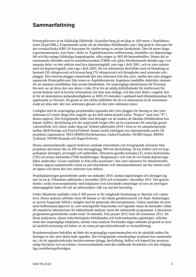
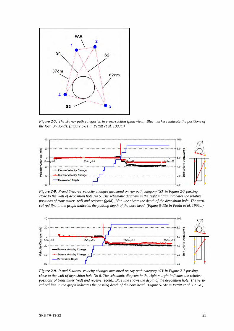
Ultrasonic surveyUltrasonic sound travels with a velocity that is determined by the medium it passes. In crystalline rock the speed is highest in the homogeneous rock and lowest in parts with fractures. Sensors for this type of measurement were as well installed in the rock around the two deposition holes in the outer section with the prime objective to register any change in the rock a few centimeters away from the wall when the boring progressed, but also in the rock between the two deposition holes (Pettitt et al. 1999a). The ultrasonic velocity (UV) system measured velocity changes between transmitter-receiver pairs. For each deposition hole the array geometry was such that in plan view there were six possible ray path categories, as illustrated in Figure 2-7. Three of these ray path categories ‘skimmed’ the deposition hole wall at approximately 20–30 mm. Two sets of ray paths pass at greater distances, approximately 400 and 600 mm away, and one ray passed at a very far distance, approximately 2.6 m. The P-and S-waves’ velocity changes in longitudinal direction in the ray paths passing closest to the deposition hole walls are shown in Figure 2-8 for deposition hole No 5 and Figure 2-9 for deposition hole No 6. (The P-wave is a pressure wave, which moves through alternating compressions and rarefactions and consequently is longitudinal in nature. The S-wave is a shear wave, which moves through motion perpendicular to the direction of wave propagation and consequently is transverse in nature). Very consistent velocity changes were observed during boring of the two deposition holes. This agreed well with earlier observations from the deposition hole boring in the Canister Retrieval Test (CRT) tunnel (Pettitt et al. 1999b)

Figures 2-8 and 2-9 show that there was little velocity change until the deposition hole passed the ray path (vertical red line) where after an abrupt change of between –10 to –30 m/s occurred. This indicated a progressive opening of fractures along the ray path as the bore head passed. Both P- and S-waves showed similar trends in velocity change although the magnitude often differed somewhat. No similar change was observed in any of the other ray paths.

Figure 2-6. All AE positions obtained from monitoring of both deposition holes No 5 (A in figure) and No 6 (B in figure) in the Prototype Repository tunnel. Events are color scaled to their magnitude. Left plot is in plan, right plot is in cross-section. Black markers indicate transducer positions in the rock around the two deposition holes. (Figure 5-4 in Pettitt et al. 1999a.)

SKB TR-13-22 23

Figure 2-8. P-and S-waves’ velocity changes measured on ray path category ‘S3’ in Figure 2-7 passing close to the wall of deposition hole No 5. The schematic diagram in the right margin indicates the relative positions of transmitter (red) and receiver (gold). Blue line shows the depth of the deposition hole. The verti-cal red line in the graph indicates the passing depth of the bore head. (Figure 5-13a in Pettitt et al. 1999a.)

Figure 2-9. P-and S-waves’ velocity changes measured on ray path category ‘S3’ in Figure 2-7 passing close to the wall of deposition hole No 6. The schematic diagram in the right margin indicates the relative positions of transmitter (red) and receiver (gold). Blue line shows the depth of the deposition hole. The verti-cal red line in the graph indicates the passing depth of the bore head. (Figure 5-14c in Pettitt et al. 1999a.)

Figure 2-7. The six ray path categories in cross-section (plan view). Blue markers indicate the positions of the four UV sonds. (Figure 5-11 in Pettitt et al. 1999a.)

24 SKB TR-13-22

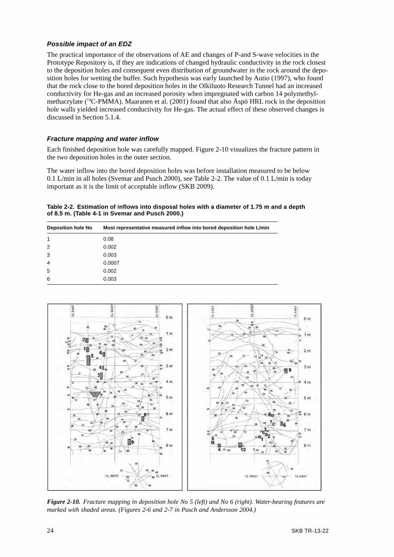
Possible impact of an EDZThe practical importance of the observations of AE and changes of P-and S-wave velocities in the Prototype Repository is, if they are indications of changed hydraulic conductivity in the rock closest to the deposition holes and consequent even distribution of groundwater in the rock around the depo-sition holes for wetting the buffer. Such hypothesis was early launched by Autio (1997), who found that the rock close to the bored deposition holes in the Olkiluoto Research Tunnel had an increased conductivity for He-gas and an increased porosity when impregnated with carbon 14 polymethyl-methacrylate (14C-PMMA). Maaranen et al. (2001) found that also Äspö HRL rock in the deposition hole walls yielded increased conductivity for He-gas. The actual effect of these observed changes is discussed in Section 5.1.4.

Fracture mapping and water inflowEach finished deposition hole was carefully mapped. Figure 2-10 visualizes the fracture pattern in the two deposition holes in the outer section.

The water inflow into the bored deposition holes was before installation measured to be below 0.1 L/min in all holes (Svemar and Pusch 2000), see Table 2-2. The value of 0.1 L/min is today important as it is the limit of acceptable inflow (SKB 2009).

Table 2-2. Estimation of inflows into disposal holes with a diameter of 1.75 m and a depth of 8.5 m. (Table 4-1 in Svemar and Pusch 2000.)

Deposition hole No Most representative measured inflow into bored deposition hole L/min

1 0.082 0.0023 0.003 4 0.00075 0.002 6 0.003

Figure 2-10. Fracture mapping in deposition hole No 5 (left) and No 6 (right). Water-bearing features are marked with shaded areas. (Figures 2-6 and 2-7 in Pusch and Andersson 2004.)

SKB TR-13-22 25

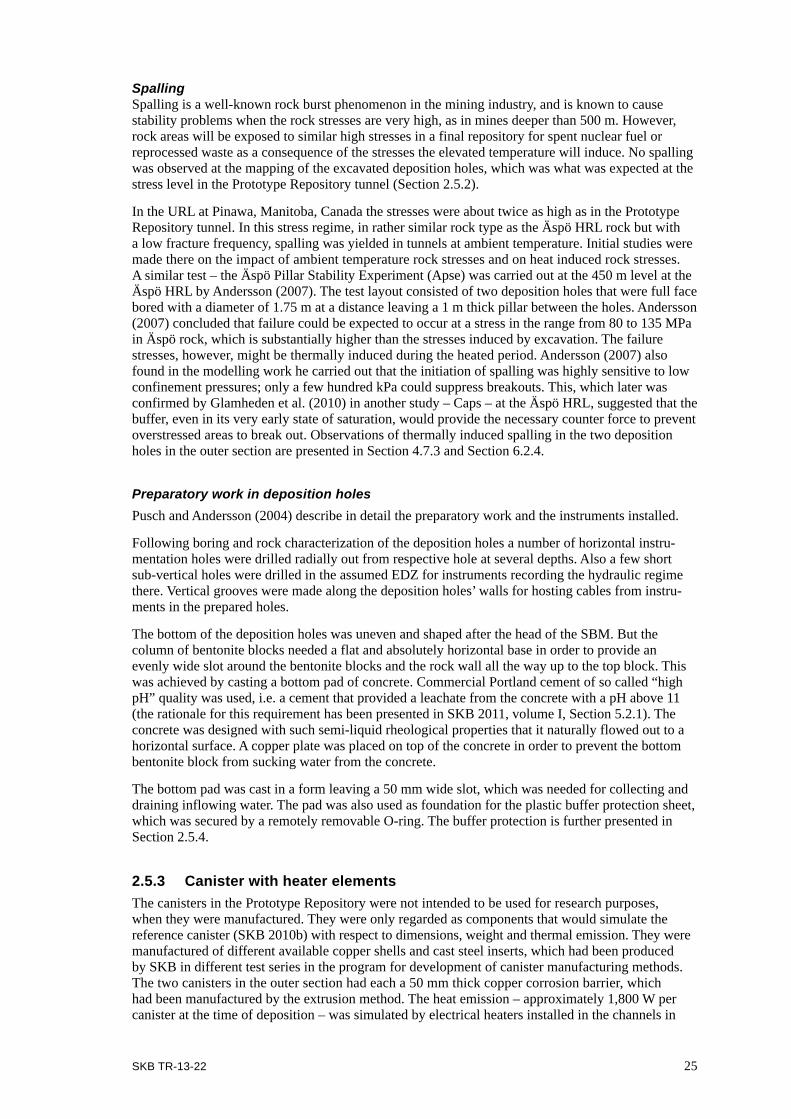
SpallingSpalling is a well-known rock burst phenomenon in the mining industry, and is known to cause stability problems when the rock stresses are very high, as in mines deeper than 500 m. However, rock areas will be exposed to similar high stresses in a final repository for spent nuclear fuel or reprocessed waste as a consequence of the stresses the elevated temperature will induce. No spalling was observed at the mapping of the excavated deposition holes, which was what was expected at the stress level in the Prototype Repository tunnel (Section 2.5.2).

In the URL at Pinawa, Manitoba, Canada the stresses were about twice as high as in the Prototype Repository tunnel. In this stress regime, in rather similar rock type as the Äspö HRL rock but with a low fracture frequency, spalling was yielded in tunnels at ambient temperature. Initial studies were made there on the impact of ambient temperature rock stresses and on heat induced rock stresses. A similar test – the Äspö Pillar Stability Experiment (Apse) was carried out at the 450 m level at the Äspö HRL by Andersson (2007). The test layout consisted of two deposition holes that were full face bored with a diameter of 1.75 m at a distance leaving a 1 m thick pillar between the holes. Andersson (2007) concluded that failure could be expected to occur at a stress in the range from 80 to 135 MPa in Äspö rock, which is substantially higher than the stresses induced by excavation. The failure stresses, however, might be thermally induced during the heated period. Andersson (2007) also found in the modelling work he carried out that the initiation of spalling was highly sensitive to low confinement pressures; only a few hundred kPa could suppress breakouts. This, which later was confirmed by Glamheden et al. (2010) in another study – Caps – at the Äspö HRL, suggested that the buffer, even in its very early state of saturation, would provide the necessary counter force to prevent overstressed areas to break out. Observations of thermally induced spalling in the two deposition holes in the outer section are presented in Section 4.7.3 and Section 6.2.4.

Preparatory work in deposition holesPusch and Andersson (2004) describe in detail the preparatory work and the instruments installed.

Following boring and rock characterization of the deposition holes a number of horizontal instru-mentation holes were drilled radially out from respective hole at several depths. Also a few short sub-vertical holes were drilled in the assumed EDZ for instruments recording the hydraulic regime there. Vertical grooves were made along the deposition holes’ walls for hosting cables from instru-ments in the prepared holes.

The bottom of the deposition holes was uneven and shaped after the head of the SBM. But the column of bentonite blocks needed a flat and absolutely horizontal base in order to provide an evenly wide slot around the bentonite blocks and the rock wall all the way up to the top block. This was achieved by casting a bottom pad of concrete. Commercial Portland cement of so called “high pH” quality was used, i.e. a cement that provided a leachate from the concrete with a pH above 11 (the rationale for this requirement has been presented in SKB 2011, volume I, Section 5.2.1). The concrete was designed with such semi-liquid rheological properties that it naturally flowed out to a horizontal surface. A copper plate was placed on top of the concrete in order to prevent the bottom bentonite block from sucking water from the concrete.

The bottom pad was cast in a form leaving a 50 mm wide slot, which was needed for collecting and draining inflowing water. The pad was also used as foundation for the plastic buffer protection sheet, which was secured by a remotely removable O-ring. The buffer protection is further presented in Section 2.5.4.

2.5.3 Canister with heater elementsThe canisters in the Prototype Repository were not intended to be used for research purposes, when they were manufactured. They were only regarded as components that would simulate the reference canister (SKB 2010b) with respect to dimensions, weight and thermal emission. They were manufactured of different available copper shells and cast steel inserts, which had been produced by SKB in different test series in the program for development of canister manufacturing methods. The two canisters in the outer section had each a 50 mm thick copper corrosion barrier, which had been manu factured by the extrusion method. The heat emission – approximately 1,800 W per canister at the time of deposition – was simulated by electrical heaters installed in the channels in

26 SKB TR-13-22

the steel insert. Figure 2-11 shows a canister of SKB’s reference design and Figure 2-12 the top of the Prototype Repository canister design before filling of the voids. An extra cable protective lid was eventually put on top of the canister in order to mechanically protect the cables to the heaters.

2.5.4 Buffer and buffer protection sheetThe buffer consisted of bentonite, which is natural clay that contains the clay mineral montmorillonite of the smectite group. Smectite possesses the property of being able to absorb water and swell, which gives the bentonite a sealing capability. This was early recognized in the development of methods for final disposal of nuclear waste, and bentonite was first suggested as a buffer between canister and rock in the 1970ies. Bentonite from Wyoming in the USA with the trade name MX-80 Volclay has a high content of montmorillonite. Thanks to its good properties and high quality, MX-80 has been used by SKB and Posiva as a reference material from the very start, although several other bentonite types show high content of smectite and equally good properties as MX-80 (SKB 2013, Section 25.4.4). The mineralogical composition of the specific shipment of the MX-80 bentonite that was used in the Prototype Repository is presented in Table 2-3.

Figure 2-11. SKB’s reference canister for boiling water reactor (BWR) spent nuclear fuel with a 50 mm thick outer corrosion barrier of copper and an insert of nodular cast iron. The copper shell is extending below the canister’s central bottom in order to provide for non-disturbing testing of the weld attaching the copper bottom to the copper shell. The heater elements in the Prototype Repository canisters were designed to simulate the weight of BWR fuel assemblies. (From Figure 3-1 in SKB 2010b.)

5 cm copper shell

Estimated weight (kg):Copper canister 7,400Insert 13,600Fuel assembly (BWR) 3,600Total 24,600

4,83

5 m

m

1,050 mm

5 cm copper8.9 g/cm3

Nodular iron7.2 g/cm3

50160

Diameter 949

Diameter 1,050

BWR type

(mm)

Channel tube

SKB TR-13-22 27

Table 2-3. Mineralogical compositions in percent of weight of four reference samples (Ref 1 to 4), representing the MX-80 used for manufacturing the buffer blocks in deposition hole No 5 and No 6, quantified with the Siroquant software (Siroquant 3.0, www.siroquant.com). Smectite and illite contents are adjusted by the potassium content of the clay fraction. For comparison gypsum and calcite, calculated on chemical compositions, are shown in parentheses. (From Tables 3-36 and 3-37 in Olsson et al. 2013.)

Sample Smectite Quartz Plagioclase K-feldspar Cristobalite Hematite Gypsum Illite Calcite Zircon Apatite

Ref 1 90.1 3.1 3.5 1.0 1.3 0.6 (1.2) 0.2 0.2 (0.5) 0.0 0.0Ref 2 86.3 3.5 4.8 2.2 1.0 0.4 1.6 (0.9) 0.1 0.1 (0.5) 0.0 0.0Ref 3 89.2 3.4 4.0 1.1 1.6 0.5 (1.1) 0.1 0.1 (0.4)

Ref 4 89.2 3.3 4.7 0.9 1.2 0.5 (1.1) 0.1 0.0 (0.5) 0.0

The functional requirements on the buffer are in the first place focused on its ability to isolate the waste and retard radionuclides migrating from the waste. In order to do so it shall protect the can-isters from harmful corrosion of the copper by prevent corroding substances to transport to the canister and limit microbial activity, act as a mechanical buffer around the canister in case of rock shear across a deposition hole and provide its protecting shield around the canister in the long-term perspective (SKB 1998, Section 6.1.1, SKB 2010d). These requirements have been expressed as requirements on the buffer’s density after saturation. The minimum acceptable density is determined by the requirement to limit microbial activity, which ceases at a saturated density of 1,950 kg/m3 and above in MX-80 bentonite (SKB 2010d). The maximum acceptable density is determined by the buffer’s shear strength, which has been proven to require a saturated density of 2,050 kg/m3 or less (SKB 2010b, d).

The Prototype Repository buffer was designed to initially develop a saturated density close to the upper limit. The preferred method to achieve such a density was to construct the buffer in the deposition hole with pre-compacted blocks and to fill the gap between blocks and rock wall with bentonite pellets.

Figure 2-12. Connection of power supply cables to the canister lid. Supporting bars were mounted and on top of them a second lid in order to avoid any major swelling pressure on the cables.

28 SKB TR-13-22

Commercial MX-80 bentonite, mixed with tap water to a water content of approximately 17%, was used to manufacture the buffer blocks and the pellets (Johannesson 2002). The blocks were uniaxi-ally compacted in rings, for the area along the canisters, and solid cylinders, for the areas underneath and above the canisters. All blocks were manufactured with an outer diameter of 1.65 m and a height of 0.5 m. The inner diameter of the ring-shaped blocks was 1.07 m. Figure 2-13 shows a photo of this type of block. In order to arrive at similar average buffer density everywhere, including the unfilled slot between rings and canister and the pellets-filled slot between blocks and rock wall, the rings and the cylinders were compacted by different pressures: 100 MPa for rings and 40 MPa for cylinders, The mold had a minor conical shape in order to facilitate the release of compacted blocks. The inner part of the mold for ring-shaped blocks, however, was completely straight. Lubrication oil with trade name “MOLYKOTE BR 2 plus,, consisting of molybdenum sulfide, zinc-dialkyldith-iophosphate and graphite (Olsson et al. 2013, Section 3.2), was used in order to further facilitate the release of the compacted blocks. As a consequence lubrication oil has contaminated the bentonite at the surfaces of the blocks. The possible impact of the lubrication oil is discussed in Sections 5.2.3 and 5.6.4.

The average weight, water content, density, degree of saturation (amount of the total porous volume that is filled with water), void ratio (porous volume divided by volume of solid particles) and com-paction pressure of the rings and cylinders respectively produced for the two deposition holes in the outer section are listed in Table 2-4 (Johannesson et al. 2004).

Table 2-4. Average parameters determined directly after compaction on the blocks for the outer section of the Prototype Repository. (Table 4-1 in Johannesson et al. 2004)

Block type Weight kg

Water content %

Density kg/m3

Degree of saturation

Void ratio Compact load MN

Compact pressure MPa

Ring 1,264 17.3 2,075 0.841 0.571 121 100Cylinder 2,126 17.4 2,012 0.778 0.623 84 40

Prior to emplacement of the buffer, the blocks with instruments were prepared and the sensors installed. This concerned cylindrical blocks underneath and above the canister and ring-shaped blocks at mid height of the canister.

Figure 2-13. The height of the bentonite block was measured at 12 positions around the block. (Figure 2-7 in Johannesson 2002.)

SKB TR-13-22 29

During emplacement the blocks were placed on top of each other in the deposition hole (Johannesson et al. 2004). When the uppermost top ring (R10 in Figure 2-14) was in place the canister was installed in the center of the buffer column. Block R10 ended somewhat higher than the canister lid and the space that was formed was filled with small pre-compacted MX-80 blocks. The remaining buffer cylinders were then emplaced on top. A water tight plastic buffer protection sheet was used in order to isolate the buffer blocks from the humid air in the deposition hole during installation and until the deposition tunnel above was to be backfilled (Johannesson et al. 2004). Then the plastic sheet was totally removed (except for the small pieces left in each hole as described in Section 2.3) and the slot between buffer blocks and rock wall was filled with pre-compacted MX-80 pellets. Figure 2-15 shows the interior of the sheet.

The complete bentonite buffer thus consisted of compacted large blocks, compacted small bricks on top of the canister and compacted pellets in the slot between the blocks and the rock. In Table 2-5 Johannesson et al. (2004) summarize the emplaced weights and water contents of those parts as well as the calculated average values after saturation in deposition holes No 5 and No 6 respectively. The weights are summarized to a total of 24,448 kg (bulk weight) in deposition hole No 5 and 24,821 kg in deposition hole No 6. The calculation of average densities and void ratios after saturation assumes no axial swelling during saturation.

Johannesson et al. (2004) used the values in Table 2-5 for calculating average densities and void ratios at saturation, also under the assumption that no axial selling would take place, in three different sections in the deposition holes. These results are presented in the Table 2-6. “Section A” is underneath the canisters, “Section B” along the canister and “Section C” just above the canister, where the bricks are located. The largest variation in density, between 2,012 kg/m3 and 2,067 kg/m3

,

was calculated for deposition hole No 6.

Figure 2-14. A schematic drawing of a canister hole with bentonite blocks. Each block is slightly tapered (Ø 1,630 mm at top and Ø 1,650 mm at bottom) so that the compacted block could be squeezed out from the mold. The upper ring-shaped block ends 170 mm above the doubled-layered canister lid (canister lid and cable-protecting lid on top). The space above block C4 was filled with backfill material up to the tunnel floor level. A circular groove was machined into the bottom block to accommodate the canister´s extended copper shell. (After Figure 4-1 in Johannesson et al. 2004.)

30 SKB TR-13-22

Table 2-5. The bulk weight and water content of the blocks and pellets installed in the deposition holes and the average saturated density of the buffer. (Table 4-3 in Johannesson et al. 2004.)

Deposition hole Blocks Bricks Pellets Average

Weight kg

Water content %

Weight kg

Water content %

Weight kg

Water content %

Saturated density kg/m3

Void ratio

Deposition hole No 5 21,118 17.3 330 15.1 3,000 13.1*) 2,027 0.734Deposition hole No 6 21,168 17.4 335 13.7 2,870 13.1*) 2,022 0.742

*) Measured at the delivery of the pellets.

Table 2-6. Calculated saturated density and void ratio for different parts of the buffer in the two deposition holes. (Table 4-4 in Johannesson et al. 2004.)

Deposition hole Section A Section B Section C

Saturated density kg/m3

Void ratio

Saturated density kg/m3

Void ratio Saturated density kg/m3

Void ratio

Deposition hole No 5 2,039 0.713 2,017 0.750 2,053 0.690Deposition hole No 6 2,034 0.722 2,012 0.759 2,067 0.668

2.5.5 Backfill The backfill was designed to provide a tunnel fill that would contribute to tunnel stability, hold the bentonite around the canisters in place, prevent or limit the flow of water around the canister positions, not cause deterioration of the quality of the groundwater, and remain chemically stable over a long time (SKB 1998). It consisted of well mixed 30% by weight commercial Milos soda activated ben-tonite, and 70% by weight SKB-produced crushed TBM muck from the Äspö HRL ramp. At the time of installation (2003) the properties to achieve were in quantitative terms a hydraulic conductivity of maximum 10–9 m/s, a swelling pressure of minimum 100 kPa and a compression modulus of not lower than 10 MPa in order to avoid upward swelling of no more than 0.2 m of the interface between the top buffer block and the backfill in the deposition hole (Gunnarsson et al. 2001a). The choice of compression modulus was based on preliminary calculations of displacement, which showed displacement of about 0.08 m with likely values of E-modulus (30 MPa) and of Poisson’s ratio (0.3), corresponding to a compression modulus of 26 MPa.

Figure 2-15. Buffer protection sheet seen from above. The bottom bentonite cylinder and the first ring have already been emplaced. (Figure 1-3 in Wimelius and Pusch 2008.)

SKB TR-13-22 31

The swelling pressure was the most demanding requirement and needed a dry density of 1,600 to 1,800 kg/m3 in the actual mixture of Milos bentonite and crushed TBM muck, when the backfill was saturated with water containing 0.7% by weight of salt (Gunnarsson et al. 2001a). Gunnarsson et al. (2001a) also noticed that very similar results were obtained with both Milos soda activated bentonite and MX-80 bentonite when all other conditions were the same. Later (2006) the quantitative requirements on buffer material were studied in more detail, but only with MX-80 bentonite and crushed rock from drill and blast excavation (Johannesson and Nilsson 2006). A higher salinity in the ground water was assumed (3.5% by weight of salt). The design of the backfill was also to consider a margin of 100 kPa, i.e. to aim at a swelling pressure of minimum 200 kPa, as the measurement of swelling pressure would be made in the small laboratory scale, which might provide values that divert as much as 100 kPa from the real value in the deposition tunnel. The requirement on hydraulic conductivity was decreased one order of magnitude to 10–10 m/s. A new quantitative value was the limit set for compression of the backfilled caused by the swelling of the buffer in the deposition hole. The limit was set as a minimum saturated density of 1,950 kg/m3 in the buffer on top of the canister. Each of these requirements was expressed as a minimum dry density in the backfill with the following result for a 30/70 mixture of MX-80 bentonite and crushed blasted rock (Johannesson and Nilsson 2006):

• Required dry density of 1,850 kg/m3 (saturated density of 2,160 kg/m3) in order to yield a hydraulic conductivity of 10–10 m/s.

• Required dry density of 1,800 kg/m3 (saturated density of 2,130 kg/m3) in order to yield a swelling pressure of 200 kPa.

• Required dry density of 1,700 kg/m3 (saturated density of 2,070 kg/m3) in order to yield rheological properties that limit the expanded buffer to a minimum saturated density of 1,950 kg/m3.

As the swelling pressure requirement formed the dominating design basis for the Prototype Repos-itory and Milos soda activated bentonite provided very similar properties as MX-80 bentonite in a 30/70 mixture (Gunnarsson et al. 2001a) the values concluded by Johannesson and Nilsson (2006) are judged to be applicable to also the backfill mixture used in the Prototype Repository.

In the Prototype Repository the 30/70 mixture was compacted in situ in 10 cm thick horizontal layers in the upper parts of the deposition holes and, in 20 cm thick layers at an inclination of about 35°, in the tunnel (Johannesson et al. 2004). In the deposition holes an ordinary road construction vibrator was used for compaction, while in the tunnel specially designed vibrating compactors were used, one at the roof and one on the slope, both mounted on a boom that gave access to the whole roof and slope areas, see Figure 2-16.

Instruments were placed in the backfill in respective instrumented layer. Sensors and cables were covered with bentonite powder as described by Johannesson et al. (2004).

The density and water content were measured in situ in both the deposition holes and in the tunnel. Samples for determining water content were taken as well. Methods and procedures were described in detail by Johannesson et al. (2004).

Figure 2-16. The roof compactor (left) and the slope compactor (right) during compaction. (Figure 2-15 in Pusch et al. 2004.)

32 SKB TR-13-22

In the tunnel it was not possible to get the tools for measurement close enough to the roof to verify the assumed decrease in dry density close to the roof. In one layer detailed density measurements were made along profiles of which two were directed from the center axis of the tunnel in direction to 10 o’clock and 2 o’clock points in the tunnel roof respectively Along one profile a decrease in dry density was measured at a distance within one meter from the rock, while this trend could not be observed in the measurements made along the other profile. Another observation was that a mass volume estimate of the buffer material brought into the outer section and measurement of the tunnel volume resulted in an average dry density of 1,630 kg/m3, while the average dry density was 1,750 kg/m3 for all measurements made in the center of all layer and outwards as far as the space was enough to host the instrument (Johannesson et al. 2004). The backfill was considered to fulfill the density requirement, after saturation in Äspö groundwater containing 0.7% by weight of salt, stipulated by Gunnarsson et al. (2001a).

The assumed lower density close to the rock raised concern for piping to occur in those regions. As reliable measurements were impossible to make during installation (Johannesson et al. 2004) the assumption on lower dry densities and possible piping close to the rock could not be addressed until samples were taken and analyzed at opening and retrieval, see Section 5.1.3.

The measured average dry density was 1,830 kg/m3 in deposition hole No 5 and 1,770 kg/m3 in deposition hole No 6 (Johannesson et al. 2004).

2.5.6 Plug The outer plug consisted of a cast concrete dome plug and a retaining wall of pre-fabricated concrete beams behind, which held the backfill in place while the dome was cast and the concreted cured, see Figure 2-17. The cast dome was designed to resist a hydraulic pressure of 4.5 MPa and the retaining wall a backfill swelling pressure of 0.1 MPa. The whole structure was designed to provide a seal with negligible leakage of water (Dahlström 2009). No requirement on the leakage was set at the time of installation of the Prototype Repository. Later, in the work with the safety assessment SR-Site (SKB 2011) SKB indicated an acceptable value that would limit the possible amount of bentonite that could migrate out as water slurry through the plug before the repository would be backfilled and the requirements on the performance of the plug would cease. The compliance of the plug to this safety-related value could, however, not be fully tested, as the hydraulic pressure in the rock was too low for applying a test pressure of 4.5 MPa, see result of the test in Section 4.2.2.

Figure 2-17. A schematic drawing of the plug with the cast concrete dome and the prefabricated concrete beams behind, making up the retaining wall. (Left figure in Figure 2-1 in Johannesson and Hagman 2013.)

Retaining wall Concrete

Compacted bentonite

SKB TR-13-22 33

The concrete consisted of conventional cement and rock filler with such rheological properties that the concrete was pumpable and self-compacting. The structural strength was supported by steel reinforcement (Dahlström 2009).

Figure 2-18 shows three photos from the installation of the retaining wall. After completion of the retaining wall the inner part of the reinforcement was installed. Instruments were installed in the slot and on the reinforcement for monitoring of mechanical response. The cooling system was installed to control the heat release during the curing of the concrete. The work continued with installation of the outer reinforcement and installation of instruments to monitor temperatures before the concrete dome was cast (Johannesson et al. 2004). Figure 2-19 shows the finished outer reinforcement.

Two lead-through pipes were placed in the plug with the main objective to minimize the distances from on-line sampling of gas and water to collectors outside the plug (Johannesson et al. 2004). These lead-throughs are shown in Figure 2-17 and on photos in Figure 2-20.

Figure 2-18. The retaining wall of the outer plug. (Figure 4-12 in Dixon et al. 2009.)

(a) Upper Region to be filled with pellets

(b) Installation of blocks and pellets (c) Retaining wall before construction of concrete dome

Figure 2-19. The outer reinforcement of the plug. (Figure 6-4 in Johannesson et al. 2004.)

34 SKB TR-13-22

Such a massive concrete structure as the plug shrinks during curing and a gap was expected to develop in the interface between the concrete dome and the rock in the abutment. This interface could provide preferential pathways for water and prevent the plug to perform as water tight as required. Measures had to be taken to seal these preferential pathways. Dahlström (2009) has described the procedure applied to the outer plug. Before the plug was cast, preparations had been made for post-grouting by installation of tubes against the rock for injection of grout. Once the concrete had cured and hardened the plug was cooled below ambient temperature in order to widen the gap as much as possible. After grouting, when the cooling had ended the plug expanded and tightened up the gaps even further. The grout used was a combination of micro cement and silica sol (suspension of colloidal silica). The result of the post-grouting is presented in Section 4.2.3.

2.5.7 InstrumentationThe canister, buffer, backfill, rock and plug were instrumented for recording the influential processes during the evolution of the barriers in the transient water saturation phase. More than 1,000 instru-ments were installed in the buffer and the backfill, of which 401 were installed in the outer section (Börgesson and Sandén 2003). A further 24 instruments were installed in the outer plug (Dahlström 2009). Hydraulic characterization of the rock around the Prototype Repository tunnel was carried out in more than 100 measurement sections (47 around the outer section) in 39 core holes (15 around the outer section) (Rhén and Forsmark 2001).

Number, positions and installation procedures in the outer section have been reported in detailed by Pettitt et al. (1999b), Rhén and Forsmark (2001), Rhén et al. (2003), Barcena and Garcia-Sineriz (2001), Puigdomenech and Sandén (2001), Collin and Börgesson (2002), Börgesson and Sandén (2003), Rothfuchs et al. (2003), Bono and Röshoff (2003a, b), Pusch and Andersson (2004), Johan-nesson et al. (2004) and Rosborg (2013a).

The two canisters were equipped with fiber optical cables on their surfaces for a close-pattern measurement of the temperature (T) there (Goudarzi 2014). Instruments for measurement of canister displacements were installed in deposition hole No 6 (Barcena and Garcia-Sineriz 2002).

The buffer and backfill in the two deposition holes and the backfill in the tunnel were instrumented with thermal, hydraulic and mechanical (T, H, M) sensors (Collin and Börgesson 2002, Johannesson et al. 2004) as well as with gas and water samplers (C, B) (Puigdomenech and Sandén 2001, Bör-gesson and Sandén 2003, Johannesson et al. 2004). Chains of resistivity sensors were placed in the rock, the buffer and the backfill (H) (Rothfuchs et al. 2003). Electrodes for measurement of copper corrosion on-line were installed in the buffer in deposition hole No 5 (Börgesson and Sandén 2003, Rosborg 2013a). Parcels with concrete and cellulose packages were placed in the backfill (Börgesson and Sandén 2003), but with the objective to provide information on disposal units with cellulose content in repositories for low-and intermediate level waste.

The AE and ultrasonic sound sensors as well as the majority of the rock stress gauges (M), which were installed prior to boring of the deposition holes, remained in place (Pettitt et al. 1999b, Bono

Figure 2-20. Photos of the two lead-through in the plug. (Figure 5-12 in Johannesson et al. 2004.)

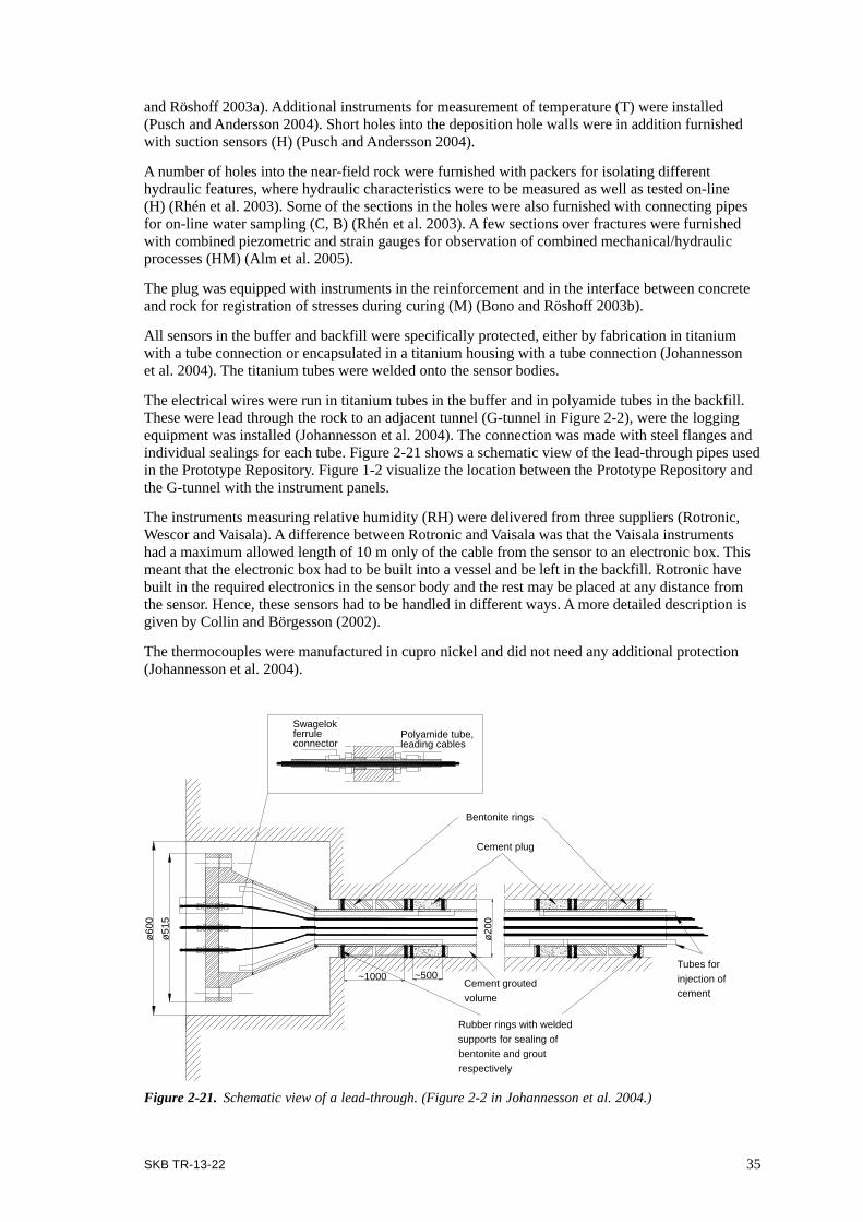
SKB TR-13-22 35

and Röshoff 2003a). Additional instruments for measurement of temperature (T) were installed (Pusch and Andersson 2004). Short holes into the deposition hole walls were in addition furnished with suction sensors (H) (Pusch and Andersson 2004).

A number of holes into the near-field rock were furnished with packers for isolating different hydraulic features, where hydraulic characteristics were to be measured as well as tested on-line (H) (Rhén et al. 2003). Some of the sections in the holes were also furnished with connecting pipes for on-line water sampling (C, B) (Rhén et al. 2003). A few sections over fractures were furnished with combined piezometric and strain gauges for observation of combined mechanical/hydraulic processes (HM) (Alm et al. 2005).

The plug was equipped with instruments in the reinforcement and in the interface between concrete and rock for registration of stresses during curing (M) (Bono and Röshoff 2003b).

All sensors in the buffer and backfill were specifically protected, either by fabrication in titanium with a tube connection or encapsulated in a titanium housing with a tube connection (Johannesson et al. 2004). The titanium tubes were welded onto the sensor bodies.

The electrical wires were run in titanium tubes in the buffer and in polyamide tubes in the backfill. These were lead through the rock to an adjacent tunnel (G-tunnel in Figure 2-2), were the logging equipment was installed (Johannesson et al. 2004). The connection was made with steel flanges and individual sealings for each tube. Figure 2-21 shows a schematic view of the lead-through pipes used in the Prototype Repository. Figure 1-2 visualize the location between the Prototype Repository and the G-tunnel with the instrument panels.

The instruments measuring relative humidity (RH) were delivered from three suppliers (Rotronic, Wescor and Vaisala). A difference between Rotronic and Vaisala was that the Vaisala instruments had a maximum allowed length of 10 m only of the cable from the sensor to an electronic box. This meant that the electronic box had to be built into a vessel and be left in the backfill. Rotronic have built in the required electronics in the sensor body and the rest may be placed at any distance from the sensor. Hence, these sensors had to be handled in different ways. A more detailed description is given by Collin and Börgesson (2002).

The thermocouples were manufactured in cupro nickel and did not need any additional protection (Johannesson et al. 2004).

Figure 2-21. Schematic view of a lead-through. (Figure 2-2 in Johannesson et al. 2004.)

Rubber rings with welded supports for sealing of bentonite and grout respectively

ø200

ø600

Cement grouted volume

Bentonite rings

~1000 ~500

ø515

Tubes for injection of cement

Cement plug

Swagelok ferrule connector

Polyamide tube, leading cables

36 SKB TR-13-22

2.5.8 Geological conditionsRock typeThe dominant rock type identified in the Prototype Repository tunnel is Äspö diorite having a medium- grained porphyritic texture with inclusions of primarily fine-grained granite but also greenstone.

Geological structureFractures were mapped in detail, and the tunnel was in a first phase mapped according to the Äspö standard mapping procedure and in a second phase in more detail with focus on the floor region (Patel et al. 1997). A plot from the standard mapping is shown in Figure 2-22. The projection is folded out from the center line of the roof and shown from above.

The information collected through mapping in the tunnel, and stored in SKB’s data base “Site character ization database ” (SICADA) (initially tunnel mapping system – TMS – data base), has been used for 3D visualization with the “Rock Visualization System (RVS). Figure 2-23 shows a computer added design (CAD) visualization of the major fractures that intersect the Prototype Repository tunnel. The dominant ones are steep and oriented north west/south east and several of them are the most hydraulically active fractures in the tunnel. A few steep-oriented fractures are present and also somewhat inclined and flat lying ones, striking more or less west/east. The latter ones appear in the roof, wall and floor.

Figure 2-22. View of fractures and water-bearing features mapped by standard mapping procedure View of a projection being unfolded from the center line of the roof, and seen from above. The positions of the six deposition holes are indicated by the upper figure. More precisely the deposition holes No 5 and No 6 have their center positions at chainages 3551 m (i.e. at the position 3,551 m from the ramp portal at ground surface) and 3545 m respectively. (From Figure 7-3 in Johannesson 2014.)

Figure 2-23. CAD visualization of different fractures that intersect the Prototype Repository tunnel. (Figure 4-2 in Svemar and Pusch 2000.)

Section I Section II

400 390 380 370 360 340350410

3590 3580 3560 3560 3550 3520353035403600

0 5 10 m

FracturesGroutWater conductiveCalcite

EpoditeOxidized rim

Mylonite or displacement

DisplacementFlowing waterDriping waterMoist

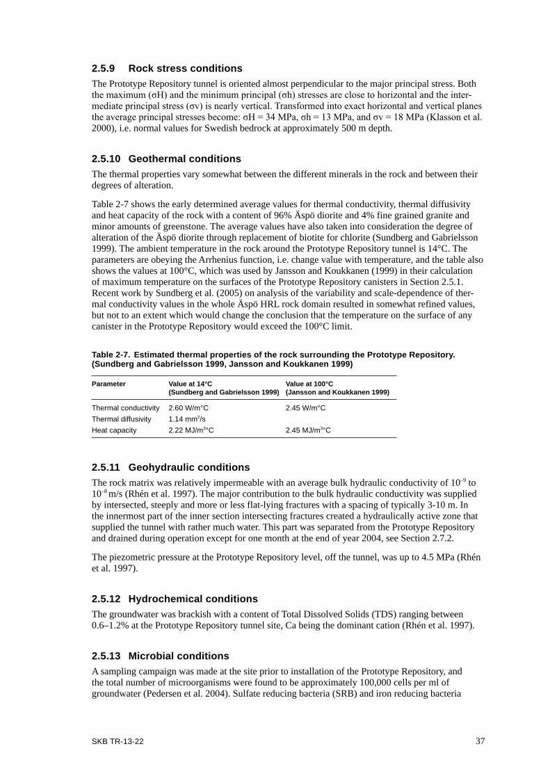
SKB TR-13-22 37

2.5.9 Rock stress conditionsThe Prototype Repository tunnel is oriented almost perpendicular to the major principal stress. Both the maximum (σH) and the minimum principal (σh) stresses are close to horizontal and the inter-mediate principal stress (σv) is nearly vertical. Transformed into exact horizontal and vertical planes the average principal stresses become: σH = 34 MPa, σh = 13 MPa, and σv = 18 MPa (Klasson et al. 2000), i.e. normal values for Swedish bedrock at approximately 500 m depth.

2.5.10 Geothermal conditionsThe thermal properties vary somewhat between the different minerals in the rock and between their degrees of alteration.

Table 2-7 shows the early determined average values for thermal conductivity, thermal diffusivity and heat capacity of the rock with a content of 96% Äspö diorite and 4% fine grained granite and minor amounts of greenstone. The average values have also taken into consideration the degree of alteration of the Äspö diorite through replacement of biotite for chlorite (Sundberg and Gabrielsson 1999). The ambient temperature in the rock around the Prototype Repository tunnel is 14°C. The parameters are obeying the Arrhenius function, i.e. change value with temperature, and the table also shows the values at 100°C, which was used by Jansson and Koukkanen (1999) in their calculation of maximum temperature on the surfaces of the Prototype Repository canisters in Section 2.5.1. Recent work by Sundberg et al. (2005) on analysis of the variability and scale-dependence of ther-mal conducti vity values in the whole Äspö HRL rock domain resulted in somewhat refined values, but not to an extent which would change the conclusion that the temperature on the surface of any canister in the Prototype Repository would exceed the 100°C limit.

Table 2-7. Estimated thermal properties of the rock surrounding the Prototype Repository. (Sundberg and Gabrielsson 1999, Jansson and Koukkanen 1999)

Parameter Value at 14°C (Sundberg and Gabrielsson 1999)

Value at 100°C (Jansson and Koukkanen 1999)

Thermal conductivity 2.60 W/m°C 2.45 W/m°CThermal diffusivity 1.14 mm2/sHeat capacity 2.22 MJ/m3°C 2.45 MJ/m3°C

2.5.11 Geohydraulic conditionsThe rock matrix was relatively impermeable with an average bulk hydraulic conductivity of 10–9 to 10–8 m/s (Rhén et al. 1997). The major contribution to the bulk hydraulic conductivity was supplied by intersected, steeply and more or less flat-lying fractures with a spacing of typically 3-10 m. In the innermost part of the inner section intersecting fractures created a hydraulically active zone that supplied the tunnel with rather much water. This part was separated from the Prototype Repository and drained during operation except for one month at the end of year 2004, see Section 2.7.2.

The piezometric pressure at the Prototype Repository level, off the tunnel, was up to 4.5 MPa (Rhén et al. 1997).

2.5.12 Hydrochemical conditionsThe groundwater was brackish with a content of Total Dissolved Solids (TDS) ranging between 0.6–1.2% at the Prototype Repository tunnel site, Ca being the dominant cation (Rhén et al. 1997).

2.5.13 Microbial conditionsA sampling campaign was made at the site prior to installation of the Prototype Repository, and the total number of microorganisms were found to be approximately 100,000 cells per ml of groundwater (Pedersen et al. 2004). Sulfate reducing bacteria (SRB) and iron reducing bacteria

38 SKB TR-13-22

(IRB) and heterotrophic acetogens dominated among the physiological groups that were cultured. Sparse occurrence of autotrophic microorganisms was also discovered as well as a few heterotrophic methanogens ones.

2.6 Prototype Repository monitoring2.6.1 Monitored parametersData and other information that have been collected during the evolution of different parts of the Prototype Repository have regularly been analyzed and reported together with general observations of disturbances and events, which have made a footprint in the measurement records. The monitoring of the outer section started in May 2003, when the heaters in deposition hole No 5 were switch on. The covered period for the outer section ended in November 2011 when the opening and retrieval of the section started.

The following parameters were recorded during operation:

• Canister:– Thermal power.– Temperature.– Displacement.

• Buffer:– Temperature.– Degree of saturation.– Pore pressure.– Total pressure.– Gas and water composition.

• Backfill:– Temperature.– Degree of saturation.– Pore pressure.– Total pressure.– Gas and water composition.

• Rock:– Temperature.– Stress. – Strain.– Seismic events.– Ultrasonic properties.– Groundwater pressure.– Groundwater composition.– Coupled hydraulic-stress relation.– Suction.

• Plug:– Temperature (in concrete).– Width of contact between concrete and rock in abutment.– Compression of concrete.

• Copper corrosion:– Rate of corrosion.

All observations have been reported in the following way:

• Goudarzi (2014) presents the latest report in a series of sensor data reports on continuous sensor readings with graphs for each sensor that cover the time from start of monitoring up to the time of compiling the report.

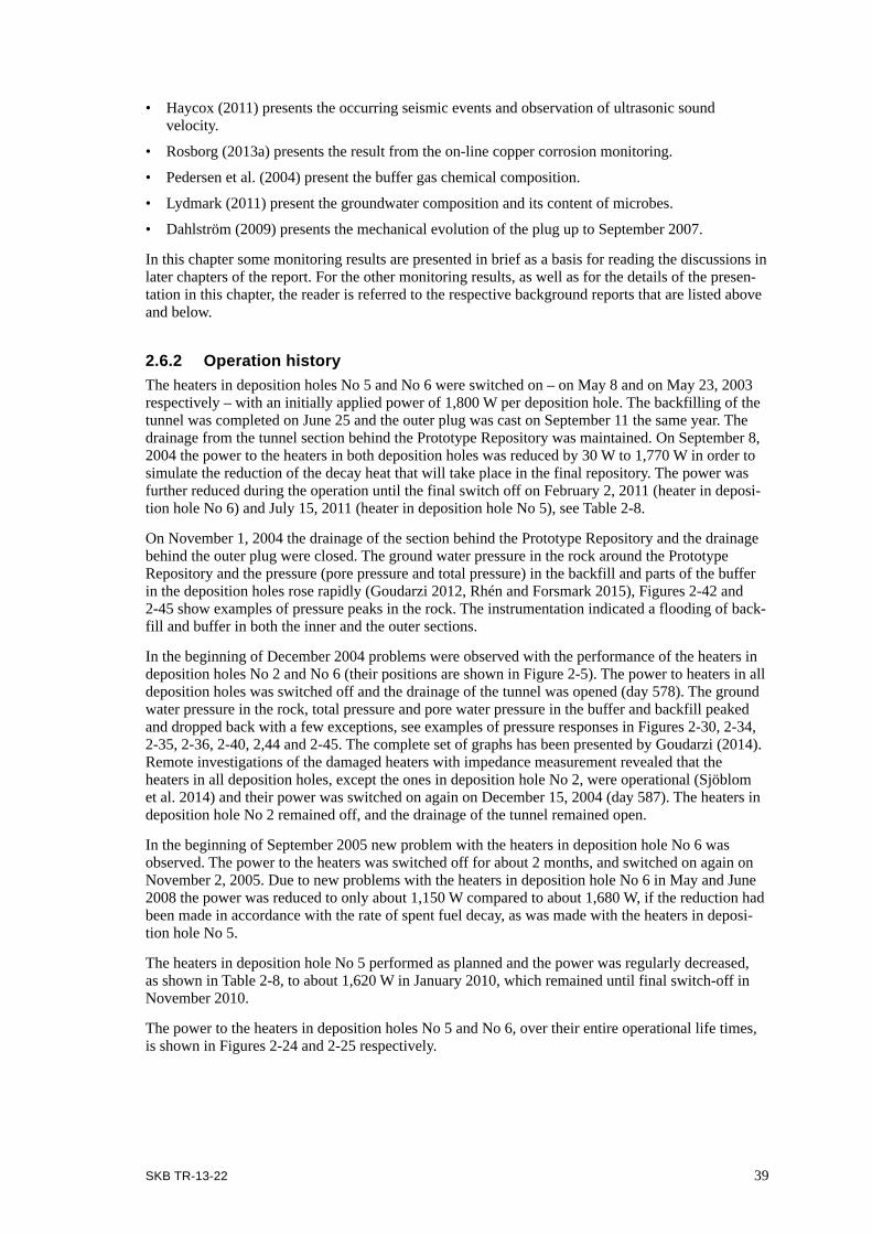
SKB TR-13-22 39

• Haycox (2011) presents the occurring seismic events and observation of ultrasonic sound velocity.

• Rosborg (2013a) presents the result from the on-line copper corrosion monitoring.

• Pedersen et al. (2004) present the buffer gas chemical composition.

• Lydmark (2011) present the groundwater composition and its content of microbes.

• Dahlström (2009) presents the mechanical evolution of the plug up to September 2007.

In this chapter some monitoring results are presented in brief as a basis for reading the discussions in later chapters of the report. For the other monitoring results, as well as for the details of the presen-tation in this chapter, the reader is referred to the respective background reports that are listed above and below.

2.6.2 Operation historyThe heaters in deposition holes No 5 and No 6 were switched on – on May 8 and on May 23, 2003 respectively – with an initially applied power of 1,800 W per deposition hole. The backfilling of the tunnel was completed on June 25 and the outer plug was cast on September 11 the same year. The drainage from the tunnel section behind the Prototype Repository was maintained. On September 8, 2004 the power to the heaters in both deposition holes was reduced by 30 W to 1,770 W in order to simulate the reduction of the decay heat that will take place in the final repository. The power was further reduced during the operation until the final switch off on February 2, 2011 (heater in deposi-tion hole No 6) and July 15, 2011 (heater in deposition hole No 5), see Table 2-8.

On November 1, 2004 the drainage of the section behind the Prototype Repository and the drainage behind the outer plug were closed. The ground water pressure in the rock around the Prototype Repository and the pressure (pore pressure and total pressure) in the backfill and parts of the buffer in the deposition holes rose rapidly (Goudarzi 2012, Rhén and Forsmark 2015), Figures 2-42 and 2-45 show examples of pressure peaks in the rock. The instrumentation indicated a flooding of back-fill and buffer in both the inner and the outer sections.

In the beginning of December 2004 problems were observed with the performance of the heaters in deposition holes No 2 and No 6 (their positions are shown in Figure 2-5). The power to heaters in all deposition holes was switched off and the drainage of the tunnel was opened (day 578). The ground water pressure in the rock, total pressure and pore water pressure in the buffer and backfill peaked and dropped back with a few exceptions, see examples of pressure responses in Figures 2-30, 2-34, 2-35, 2-36, 2-40, 2,44 and 2-45. The complete set of graphs has been presented by Goudarzi (2014). Remote investigations of the damaged heaters with impedance measurement revealed that the heaters in all deposition holes, except the ones in deposition hole No 2, were operational (Sjöblom et al. 2014) and their power was switched on again on December 15, 2004 (day 587). The heaters in deposition hole No 2 remained off, and the drainage of the tunnel remained open.

In the beginning of September 2005 new problem with the heaters in deposition hole No 6 was observed. The power to the heaters was switched off for about 2 months, and switched on again on November 2, 2005. Due to new problems with the heaters in deposition hole No 6 in May and June 2008 the power was reduced to only about 1,150 W compared to about 1,680 W, if the reduction had been made in accordance with the rate of spent fuel decay, as was made with the heaters in deposi-tion hole No 5.

The heaters in deposition hole No 5 performed as planned and the power was regularly decreased, as shown in Table 2-8, to about 1,620 W in January 2010, which remained until final switch-off in November 2010.

The power to the heaters in deposition holes No 5 and No 6, over their entire operational life times, is shown in Figures 2-24 and 2-25 respectively.

40 SKB TR-13-22

Table 2-8. Key dates for the outer section

Activity Date

Start backfilling 29/4 2003Start heating in deposition hole No 5 (1,800 W) 8/5 2003Start heating in deposition hole No 6 (1,800 W) 23/5 2003Finished backfilling 25/6 2003Plug casting 11/9 2003Decreased power to deposition hole No 5 (–30 W) 8/9 2004Decreased power to deposition hole No 6 (–30 W) 8/9 2004Drainage of the tunnel closed 1/11 2004Power to all deposition holes switched off 2/12 2004Drainage of the tunnel opened 6/12 2004Power to all deposition holes switched on 15/12 2004Power to deposition hole No 6 switched off 6/9 2005Power to deposition hole No 6 switched on 2/11 2005Decreased power to deposition hole No 5 (–30 W) 2/12 2005Decreased power to deposition hole No 6 (–30 W) 2/12 2005Decreased power to deposition hole No 5 (–30 W) 21/12 2006Decreased power to deposition hole No 6 (–30 W) 21/12 2006Decreased power to deposition hole No 5 (–30 W) 11/12 2007Decreased power to deposition hole No 6 (–30 W) 11/12 2007Decreased power to deposition hole No 6 (–200 W) due to problems with the heaters

8/4 2008

Decreased power to deposition hole No 6 (–300 W) due to problems with the heaters

5/6 2008

Decreased power to deposition hole No 5 (–30 W) 29/1 2009Decreased power to deposition hole No 5 (–30 W) 21/1 2010Power to deposition hole No 5 switched off for good 15/7 2011Power to deposition hole No 6 switched off for good 16/2 2011Start of dismantling of the outer plug 29/11 2010

2.6.3 Events during operation with possible impacts on EBS evolutionSeveral of the events during the operational period were judged to have a significant impact on the evolution of the Prototype Repository. The most obvious events were:

• Opening and closing of the drainage behind the Prototype Repository.

• Excavation of the Tass tunnel (location is shown in Figure 2-4).

• Boring of the 90 m long horizontal tunnel for the horizontal deposition project (KBS-3H) at the 220 m level right above the Prototype Repository.

• Switching off/on the power to the heaters.

The closing of the drainage had an immediate effect with increased water pressure and flooding of the Prototype Repository, but saturation progressed with the same speed as before, when the drain-age was opened again. The low water pressure thereafter was judged to have the effect of slowing down the saturation process compared to a situation where the water pressure had been higher.

The excavation of the Tass tunnel caused temporary decreases and temporary increases in the water pressure at several occasions during an extended period of time. The activities induced short spike-like responses with no effects on the long-term trends of the water pressure, which was both decreasing in some parts of the rock around the Prototype Repository and increasing in others. The trend around deposition hole No 5 was increasing.

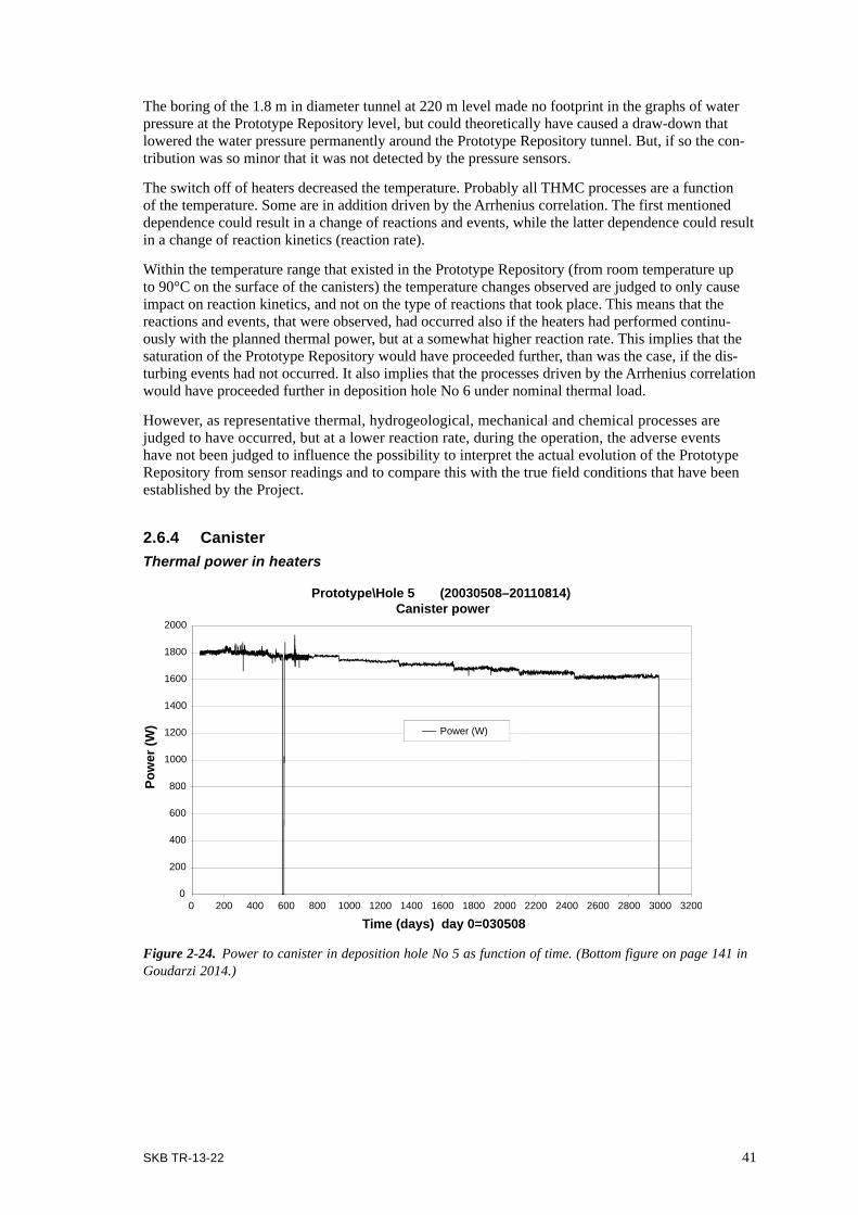
SKB TR-13-22 41

The boring of the 1.8 m in diameter tunnel at 220 m level made no footprint in the graphs of water pressure at the Prototype Repository level, but could theoretically have caused a draw-down that lowered the water pressure permanently around the Prototype Repository tunnel. But, if so the con-tribution was so minor that it was not detected by the pressure sensors.

The switch off of heaters decreased the temperature. Probably all THMC processes are a function of the temperature. Some are in addition driven by the Arrhenius correlation. The first mentioned dependence could result in a change of reactions and events, while the latter dependence could result in a change of reaction kinetics (reaction rate).

Within the temperature range that existed in the Prototype Repository (from room temperature up to 90°C on the surface of the canisters) the temperature changes observed are judged to only cause impact on reaction kinetics, and not on the type of reactions that took place. This means that the reactions and events, that were observed, had occurred also if the heaters had performed continu-ously with the planned thermal power, but at a somewhat higher reaction rate. This implies that the saturation of the Prototype Repository would have proceeded further, than was the case, if the dis-turbing events had not occurred. It also implies that the processes driven by the Arrhenius correlation would have proceeded further in deposition hole No 6 under nominal thermal load.

However, as representative thermal, hydrogeological, mechanical and chemical processes are judged to have occurred, but at a lower reaction rate, during the operation, the adverse events have not been judged to influence the possibility to interpret the actual evolution of the Prototype Repository from sensor readings and to compare this with the true field conditions that have been established by the Project.

2.6.4 CanisterThermal power in heaters

Figure 2-24. Power to canister in deposition hole No 5 as function of time. (Bottom figure on page 141 in Goudarzi 2014.)

0

200

400

600

800

1000

1200

1400

1600

1800

2000

Pow

er (W

)

Time (days) day 0=030508

Prototype\Hole 5 (20030508–20110814) Canister power

Power (W)

0 200 400 600 800 1000 1200 1400 1600 1800 2000 2200 2400 2600 2800 3000 3200

42 SKB TR-13-22

Temperature on canister surfaceThe temperature evolution on the surface of the canisters in deposition holes No 5 and No 6, mea-sured by optical cables attached in grooves into the canisters’ surfaces, was as shown in Figure 2-26 and Figure 2-27 respectively (Goudarzi 2014). The figures show the maximum temperatures, which were measured at mid-height of the canisters, and which were reached within one year after the heaters had been switched on. On the canister in deposition hole No 5 this maximum temperature was 88°C and on the canister in deposition hole No 6 about 93°C, which were higher than the predicted tem-peratures – 82°C and 83°C respectively – the design was based on (Section 2.5.1).

But, the maximum temperatures were below the criterion 100°C that is required for long term safety reasons. Once the first reduction of power to the heaters was made on day 489 (September 8, 2004), in compliance with the actual decrease of spent nuclear fuel, the temperatures on the surfaces of both canisters dropped and then proceeded to lie on values below the peak temperatures.

All four optical cables attached to the canister in deposition hole No 5 had broken around day 1,500 (June 2007) and in deposition hole No 6 around day 1,300 (December 2006).

The sudden decrease in power to the canister in deposition hole No 6 (Figure 2-25) after about 1,850 days (June 2008) from start was due to the heater failure and the consequent decrease of the thermal power below the value that would represent the reference canister in the final repository. The temperature on the canister’s surface (measured by thermocouples attached to the canister’s surface after the optical cables had broken) in deposition hole No 6 dropped to approximately 75°C, while the temperature on the surface of the canister in deposition hole No 5, which had functioning heaters, remained at approximately 80°C (Goudarzi 2014).

Canister displacementDeposition hole No 6 had three sensors positioned in the bottom, under the canister, for observing vertical movements, and three sensors located in Ring R10 and attached to the upper lid of the canister, for measuring horizontal movements. The installation is presented in more detail by Barzena and Garcia-Sineriz (2001).

Figure 2-25. Power to canister in deposition hole No 6 as function of time. (Bottom figure on page 163 in Goudarzi 2014.)

0

200

400

600

800

1000

1200

1400

1600

1800

2000

Pow

er (W

)

Time (days) day 0=030508

Prototype\Hole 6 (20030508-20110405)Canister power

Power (W)

0 200 400 600 800 1000 1200 1400 1600 1800 2000 2200 2400 2600 2800 3000

SKB TR-13-22 43

Figure 2-26. Maximum temperature (at mid-height) on the surface of the canister in deposition hole No 5. (Top figure on page 142 in Goudarzi 2014.)

Figure 2-27. Maximum temperature (at mid-height) on the surface of the canister in deposition hole No 6. (Top figure on page 164 in Goudarzi 2014.)

Prototype\ Hole 5 \Canister (030508–070601)Max. temperature on the canister surface – Optical fiber cables

0

10

20

30

40

50

60

70

80

90

100

110

120

Time (days) day 0=030508

Tem

pera

ture

(°C

)

Cable 1, outlet °C Cable 1, inlet °C Cable 2, outlet °C Cable 2, inlet °C

0 100 200 300 400 500 600 700 800 900 1000 1100 1200 1300 1400 1500 1600

Prototype\ Hole 6 \Canister (030508-070601)Max. temperature on the canister surface – Optical fiber cables

0

10

20

30

40

50

60

70

80

90

100

110

120

Tem

pera

ture

(°C

)

Time (days) day 0=030508

Cable 1, outlet °C Cable 1, inlet °C Cable 2, outlet °C Cable 2, inlet °C

0 100 200 300 400 500 600 700 800 900 1000 1100 1200 1300 1400 1500 1600

44 SKB TR-13-22

The monitoring of the displacements started on May 8, 2003 (Goudarzi 2014). Figure 2-28 shows the measurement results from all the six sensors. Negative values were set to correspond to a retraction of the transducer, i.e. vertical sinking or horizontal movement toward the rock wall, depending on the transducer’s position.

Figure 2-28 shows that that the vertical sensors started to measure upward displacement when the water protecting sheet was removed. The same observation was also made in deposition hole No 3 in the inner section. The cause was considered to be that the bottom blocks started to swell as soon as they got in contact with the humid air in the deposition hole. The copper plate prevented water from entering, and the water inflow was so low that the water table did not rise above the bottom pad before vertical displacements were recorded.

Figure 2-28 also indicates that the effect of closing and opening the tunnel drainage had negligible impact (closed on day 543 – November 1, 2004 – and re-opened on day 578 – December 6, 2004), but that the power switch off to all canisters from day 574 to day 587 – December 2 to December 15, 2004 – gave noticeable movements, see Figure 2-28 for impact on canister in deposition hole No 6.

The graphs show that the vertical sensors have maintained their trends of constant rise of the canister from the start of measurement. Although one of the sensors measured a rise later than the other two, all the three have measured similar values until the first data blackout (on September 25, 2006 – day 871). This indicates that no tilting of the canister had taken place up to that moment. Later two sensors measured a practically constant value of 12 mm. The third one, which dropped below zero during the first data blackout, measured afterwards the same slight increase as the other two sensors. During the last month of the measurement period, all three vertical sensors registered a small but noticeable increase, on the order of hundredths of mm. This indicates that a slightly rising trend still existed when the transducers were switched off on November 1, 2011.

The horizontal sensors showed some fast movement at the very beginning, with elongation of two sensors and retraction of the third one, which indicated a canister movement on the order of 1 mm. Later one of the elongated sensors, at a somewhat higher rate, measured a total displacement of about 11 mm. This was, however, judged to be an artifact as the other two horizontal sensors remained rather constant except for an elongation of about 1 to 2 mm in conjunction with the closure and re-opening of the tunnel drainage in 2004–2005. Two horizontal sensors remained in operation throughout the measurement period and they measured progressing elongations with time at a rate of 12–19 µm/month. The measured horizontal displacement was thus very small and of no significance.

Data plot deposition hole 6

Figure 2-28. Displacements of the canister in deposition hole No 6 in vertical and horizontal directions. Data plots as function of time. (Figure A8.6 from p 176 in Goudarzi 2012.)

SKB TR-13-22 45

2.6.5 BufferSaturationThe saturation evolution was monitored by measurement of total pressure, pore pressure, RH and suction (Goudarzi 2014). The installation is presented in detail by Johannesson et al. (2004). Geo-electrical measurements were in addition made in deposition hole No 5 (Goudarzi 2014). The installa-tion of the geoelectrical sensors is presented in detail by Rothfuchs et al. (2003).

The sensor readings indicated that the buffer was only partly saturated at the time the power to the heaters was switched off. This observation is explained and exemplified by the graphs in this section.

Deposition hole No 5The saturation occurred differently in different parts of the buffer in deposition hole No 5, as indicated by both total pressure and RH sensors (Goudarzi 2014). Figures 2-29 and 2-30 (total pressure sensors) and Figures 2-31, 2-32 and 2-33 (RH sensors) visualize this observation.

Some total pressure sensors from Geokon indicated rather high total pressures (up to almost 11 MPa during the seven years of operation), see Figure 2-29 while others measured low pressures, see Figure 2-30. The reason for the observed differences with the two types of sensors in the same block (block R5) is that the sensors are positioned in different places as is shown in the figures to the right of respective graph. Each sensor was capturing the correct absolute total pressure at the place it was positioned. One sensor, which measured the total pressure in block R5 at the inner slot towards the canister (sensor PB511) started to react strongly around 200 days after start (November 24, 2003), see Figure 2-29, which was considered to be an indication of the time when the inner slot – between canister and buffer blocks – was closed. As the graph shows, this particular sensor failed after about 1,500 days.

Figure 2-29. Total pressure registered by three Geokon sensors in block R5. The fourth sensor in the legend below the graph – sensor PB513 – was out of order from start. The sensors’ names (XXnnn(a.aaa\bb°\0.ccc) are sensor-unique and composed of: “XX” for type of sensor – in this case“PB” for pressure buffer, “nnn” for the number in the PB series, “a.aaa” for the distance in m from the bottom plate below block C1 (z direction in the top figure at right that visualizes the coordinate system), “bb°”the angle in degrees from the tunnel direction AC where A is directed towards the end of the tunnel (α in the top figure at right), and 0.ccc.the distance in m from the center of the deposition hole (r in the top figure at right). (Figure on bottom of page 125 in Goudarzi 2014.)

0,0

2,0

4,0

6,0

8,0

10,0

12,0

Pres

sure

(MPa

)

Prototype\Hole 5\Ring5 (20030508-20110814)Total pressure – Geokon

PB511(3.036\5°\0.685) PB513(3.036\95°\0.635)PB514(3.036\95°\0.785) PB515(3.036\185°\0.635)

0 200 400 600 800 1000 1200 1400 1600 1800 2000 2200 2400 2600 2800 3000 3200

Time (days) day 0=030508

46 SKB TR-13-22

Figure 2-30. Total pressure registered by seven Kulite sensors in blocks C1, R5 and C2. The sensors’ names are explained in the figure caption to Figure 2-29. (Figure at top on p 127 in Goudarzi 2014.)

Figure 2-31. Relative humidity and temperature registered by four Rotronic sensors in block C1. The humidity is shown by the top graphs and the temperature by the bottom ones. The sensors’ names are explained in the figure caption to Figure 2-29, with the exception of “WB” that stands for “water buffer”. (Figure at bottom on p 130 in Goudarzi 2014.)

–0,2

0,3

0,8

1,3

1,8

2,3

2,8

3,3

3,8

4,3

Pres

sure

(MPa

)Prototype\Hole 5 (20030508-20110814)

Total pressure – Kulite

PB503(0.340 \5°\ 0.585) PB504(0.340 \5°\0.685) PB505(0.340 \5°\ 0.785)

PB510(2.876 \10°\ 0.535) PB512(2.876 \5°\ 0.825) PB516(2.876 \190°\ 0.825)

PB518(5.433 \10°\ 0.585) PB519(5.433 \10°\ 0.685) PB520(5.433 \10°\ 0.785)

0 200 400 600 800 1000 1200 1400 1600 1800 2000 2200 2400 2600 2800 3000 3200

Time (days) day 0=030508

10

20

30

40

50

60

70

80

90

100

Rel

ativ

e hu

mid

ity(%

)\Tem

pera

ture

(°C

)

Time(days) day0=030508

Prototyp\Hole 5\Cyl.1 (20030508-20110814)Relative humidity –Rotronic

WB509(0.250\80°\0.785) WB510(0.250\170°\0.585) WB511(0.250\170°\0.685) WB512(0.250\170°\0.785)

0 200 400 600 800 1000 1200 1400 1600 1800 2000 2200 2400 2600 2800 3000 3200

SKB TR-13-22 47

Figure 2-32. RH and temperature registered by four Vaisala sensors in block C1. The humidity is shown by the top graphs and the temperature by the bottom ones. The sensors’ names are explained in the figure caption to Figure 2-31. (Figure at bottom on p 127 in Goudarzi 2014.)

Figure 2-33. RH and temperature registered by five Vaisala sensors in block R5. Two of the sensors in the legend below the graph – WB515 and WB519 – ceased to give data early. The humidity is shown by the top graphs and the temperature by the bottom ones. The sensors’ names are explained in the figure caption to Figure 2-31. (Figure at top on p 128 in Goudarzi 2014.)

0

10

20

30

40

50

60

70

80

90

100R

elat

ive

hum

idity

(%)\T

empe

ratu

re(°

C)

Time(days) day0=030508

Prototype\Hole 5\Cyl.1 (20030508-20110814)Relative humidity – Vaisala

WB504(0.340\350°\0.585) WB505(0.340\350°\0.685) WB506(0.340\350°\0.785) WB507(0.340\80°\0.585)

0 200 400 600 800 1000 1200 1400 1600 1800 2000 2200 2400 2600 2800 3000 3200

10

30

50

70

90

110

130

10

20

30

40

50

60

70

80

90

100

Tem

pera

ture

(°C

)

Rel

ativ

e hu

mid

ity(%

)

Time(days) day0=030508

Prototype\Hole 5\Ring 5 (20030508-20110814)Relative humidity – Vaisala

WB513(2.876\350°\0.585) WB514(2.876\350°\0.685) WB515(2.876\350°\0.785)

WB519(2.876\180°\0.535\In the slot) WB520(2.876\180°\0.685)

0 200 400 600 800 1000 1200 1400 1600 1800 2000 2200 2400 2600 2800 3000 3200

48 SKB TR-13-22

Some RH sensors were measuring RH of ~ 100%, see Figures 2-31 and 2-33, indicating a high degree of saturation of the buffer. In other parts of the buffer most of the sensors indicated low RH and slow wetting of the buffer with time, see Figure 2-32. Although many sensors, but not everyone, reacted just before and after the drainage was closed and open again day 543 (November 1, 2004) and day 578 (December 6, 2004) respectively and connected power switched off and on day 574 (December 2, 2004) and day 587 (December 15, 2004) respectively, the saturation rate, indicated by the sensors, did not changed radically over the time. Many sensors measured lower RH than the 100% that would be yielded at full saturation.

Deposition hole No 6The saturation also evolved differently in different parts of the buffer in deposition hole No 6, as indicated by total pressure, pore pressure and RH sensors (Goudarzi 2014).

The saturation of the buffer was more significantly affected by the quick increase in pressure than the saturation of the buffer in deposition hole No 5, when the drainage of the tunnel was closed between days 543 and 573. This was registered by both total pressure, pore pressure and RH sensors, see Figures 2-34 and 2-35 (total pressure sensors), Figure 2-36 (pore pressure) and Figure 2-37 (RH sensors). The difference to the evolution in deposition hole No 5 is that higher pressures were measured by the sensors and that the RH rose faster. This indicated a larger supply of groundwater to deposition hole No 6 as a consequence of the increased groundwater pressure in the rock. Figure 2-36 (pore pres-sure sensors) indicate that the response in the inner part of the bottom blocks was small.

The total pressure was also affected when the power was switched off again on day 852 (September 6, 2005), see Figures 2-34 and 2-35. The drop in total pressure was very large and rapid and the pressure started to increase before the power to the canister was switched on again on day 909 (November 2, 2005). When the power was switched on the pressure increased very fast to the same level as before the power was switched off. This course of events indicated that the change in total pressure was an effect of the changes in water volume in the bentonite caused by the variation in temperature.

Figure 2-34. Total pressure registered by three Kulite (PB603, PB604 and PB605) and three Geokon (PB606, PB607 and PB608) sensors in blocks C1, R5 and C2. Two Kulite and one Geokon sensors failed before day700. The sensors’ names are explained in the figure caption to Figure 2-29. (Figure at bottom of p 145 in Goudarzi 2014.)

0,00

2,00

4,00

6,00

8,00

10,00

12,00

Pres

sure

(MPa

)

Prototype\Hole 6\Ring1 and Ring 2 (20030508-20110405)Total pressure

PB603(0.770 \10°\ 0.785) PB604(0.770 \80°\ 0.685) PB605(0.770 \170°\ 0.585)PB606(1.534\55°\0.735) PB607(1.534\145°\0.635) PB608(1.284 \215°\ 0.535)

Time (days) day0=0305080 200 400 600 800 1000 1200 1400 1600 1800 2000 2200 2400 2600 2800 3000

SKB TR-13-22 49

Figure 2-35. Total pressure registered by three Kulite (PB610, PB611 and PB612) and four Geokon (PB613, PB61, PB615 and PB616) sensors in blocks R5 and R6. All three Kulite and one Geokon sensors failed before day800. The sensors’ names are explained in the figure caption to Figure 2-29. (Figure at top of p 146 in Goudarzi 2014.)

0,0

1,0

2,0

3,0

4,0

5,0

6,0

7,0

8,0

9,0

10,0Pr

essu

re (M

Pa)

Prototype\Hole 6\Ring 5 and Ring 6 (20030508-20110405)Total pressure

PB610(2.795 \10°\ 0.785) PB611(2.795 \80°\ 0.685) PB612(2.795 \170°\ 0.585)PB613(3.550\55°\0.785) PB614(3.550\145°\0.635) PB615(3.300 \215°\ 0.535)PB616(3.253\325°\0.875)

Time (days) day0=0305080 200 400 600 800 1000 1200 1400 1600 1800 2000 2200 2400 2600 2800 3000

Figure 2-36. Pore pressure registered by four sensors in blocks C1 and R2. The sensors’ names are explained in the figure caption to Figure 2-29 with the exception of “UB” that stands for “water buffer”. (Figure at bottom of p 153 in Goudarzi 2014.)

0,00

0,20

0,40

0,60

0,80

1,00

1,20

1,40

1,60

1,80

2,00

Pres

sure

(MPa

)

Prototype\Hole6 \Cyl.1 and Ring2 (20030508-20110405)Pore pressure

UB601(0.260 \280°\ 0.210) UB603(1.284\225°\0.535) UB605(2.795\190°\0.585) UB604(1.253 \310°\ 0.875)

Time (days) day0=0305080 200 400 600 800 1000 1200 1400 1600 1800 2000 2200 2400 2600 2800 3000

50 SKB TR-13-22

The sensors indicated that some parts, primarily in the C-blocks below and above the canister, were not saturated at the time when the heaters were switch off. In average the sensor readings suggested that the buffer in deposition hole No 6 had accumulated more water during the seven years of opera-tion than the buffer in deposition hole No 5.

Temperature gradientDeposition hole No 5The temperature gradient in deposition hole No 5 over the inner part of the buffer together with the temperature on the canister and the temperature at the radius of 600 mm in the ring shaped block R5 (position of block is shown in Figure 2-14) are plotted as function of time in Figure 2-38 (Goudarzi 2014). The starting date (October 10, 2004) of the plot is after the first reduction of power to the heaters. The shaded part of the plot is representing the time when the power to the heaters was switched off in December 2004. The plot shows that both the temperature and the temperature gradient were affected very little by the switch off/on of the power. The plot also indicates that the temperature gradient decreased after the power had been switched on again.

Deposition hole No 6The temperature gradient in deposition hole No 6, block 5 over the inner slot is shown in Figure 2-39 as function of time (Goudarz1 2014). Also this plot starts at a time when the power to the heaters had been reduced to 1,770 W. The shaded parts of the plot represents the time when the power to the heaters was switched off (December 2004). The plot shows that both the temperatures and the temperature gradient, in contrast to the reaction in deposition hole No 5, were affected very much by the closing/opening of the drainage, which indicates that the inner slot was closed when water entered the slot. The temperatures and the gradient were also affected when the power to the heaters was switched off for the second time (September to November 2005). Both the temperatures and the gradient reached afterwards the same levels as before the power was switched off the second time.

Figure 2-37. RH and temperature registered by four Vaisala and three Rotronic sensors in block R1 and R2. The RH is shown by the top graphs and the temperature by the bottom ones. The sensors’ names are explained in the figure caption to Figure 2-31. (Figure at bottom on p 147 in Goudarzi 2014.)

10

20

30

40

50

60

70

80

90

100

110

Rel

ativ

e hu

mid

ity(%

)\Tem

pera

ture

(°C

)Prototype\Hole 6\Ring 1 and Ring 2 (20030508-20110405)

Relative humidity

WB607(0.770\90°\0.685) WB609(0.770\180°\0.585) WB612(0.770\360°\0.785) WB613(1.284\40°\0.735)WB615(1.284\130°\0.635) WB617(1.284\230°\0.535) WB620(1.253\315°\0.875)

Time (days) day0=0305080 200 400 600 800 1000 1200 1400 1600 1800 2000 2200 2400 2600 2800 3000

SKB TR-13-22 51

The measured temperatures in the buffer were also affected by the two reductions of the power to the heaters with about 200 W and 300 W due to problems with the installed heaters. Many of the sensors installed close to the canister surface have stopped giving reliable values and the temperature on the canister and the gradient over the inner part of the buffer are thus less accurate.

Figure 2-38. The temperature and temperature gradient over the inner part of the buffer plotted as function of the date in deposition hole No 5, block R5 (position of block is shown in Figure 2-14). (Figure 7-3 in Goudarzi 2014.)

Figure 2-39. The temperature and temperature gradient over the inner part of the buffer plotted as function of the date in deposition hole No 6, block R5 (position of block is shown in Figure 2-14). (Figure 7-7 in Goudarzi 2014.)

30

40

50

60

70

80

90

0.0

0.5

1.0

1.5

2.0

2.5

3.0

Tem

pera

ture

(ºC

)

Tem

pera

ture

Gra

dien

t (ºC

/cm

)

DateTemperature gradient over the inner part of buffer Temperature on canister surface Temperature at r = 600 mm

2004-10-10 2005-11-14 2006-12-19 2008-01-23 2009-02-26 2010-04-02 2011-05-07

20

25

30

35

40

45

50

55

60

65

70

75

80

85

90

95

0

5

10

15

20

25Te

mpe

ratu

re (º

C)

Tem

pera

ture

Gra

dien

t (ºC

/cm

)

DateTemperature Gradient over inner slot Temperature on canister surface Temperature on inner surface of

bentonite block (r = 535 mm)

2004-10-10 2005-11-14 2006-12-19 2008-01-23 2009-02-26 2010-04-02 2011-05-07

52 SKB TR-13-22

2.6.6 BackfillSaturationThe pore pressure, measured both with total and pore pressure transducers placed in the backfill, increased fast from a low level when the drainage of the tunnel was closed in November 2004 (Goudarzi 2014). This is exemplified by Figure 2-39, which shows the pore pressure in two positions in the backfill. The fast increase of the pore pressure affected the rate in which the backfill was saturated measured both with soil psychrometers and with resistivity measurements in the backfill (Goudarzi 2014). After the drainage was opened the pore pressure stabilized on a higher level than before the drainage was closed. Both the total pressure and the water pressure continued to increase although the drainage was kept open. Figure 2-39 shows this in a similar way as the other graphs Goudarzi (2014) has presented.

During the measuring period most of the pore pressure and total pressure sensors indicated a relatively constant pressure up to the time work with dismantling of the outer plug started, like the graphs in Figure 2-40 (Goudarzi 2014). Most of the installed soil psychrometers measured very low suction values after the closing/opening of the drainage in November/December 2004, which indicated that the backfill was close to full saturation at that point in time.

The chain of geoelectrical sensors over deposition hole No 6 (Rothfuchs et al. 2003) has shown evolu-tion of increased saturation with time in the backfill (Goudarzi 2014). The central area of higher resis-tivity has decreased continuously in size, and at the end of 2009, resistivity has reached values around 2 Ω m everywhere in the cross section, see Figure 2-41. The backfill in the outer section was considered to be fully saturated at that time. Since then there has been a slight increase in resistivity to a distribution comparable to the one encountered at the end of 2008.

All sensors in the backfill, both soil type of sensors and geoelectrical sensors, have measured high degree of saturation and suggested that the backfill is fully saturated at the time for switching off the heaters.

Figure 2-40. Pore pressure registered by two Geokon sensors in the backfill in the outer section. They are both positioned close to the outer plug. The sensors’ names (XXXnnn(aa\b.b\c\dddd) are sensor-unique and composed of: “XX” for type of sensor – in this case “UFA” for pore water pressure, “nnn” for the number in the UFA series, “aa” for the position in the tunnel in this case E5 means “over” deposition hole No 5 (not correctly visualized in the figure), “b.b” for the horizontal distance from the tunnel axis in m with “-” in direction towards south (see Figure 2-2), “c” for distance from tunnel floor in m, and “dddd” for distance from tunnel portal at ground surface in m (Figure on bottom of page 172 in Goudarzi 2014.)

0,00

0,20

0,40

0,60

0,80

1,00

1,20

1,40

1,60

1,80

Pres

sure

(MPa

)

Prototype\Backfill \Section2 (20101120-20110405)Pore pressure – Geokon

UFA17(E5\-2.3\0\3551) UFA18 (In front of plug\0\0\3539)

0 200 400 600 800 1000 1200 1400 1600 1800 2000 2200 2400 2600 2800 3000

SKB TR-13-22 53

TemperatureThe temperature in the backfill ranged from 20 to 31°C (Goudarzi 2014). The highest temperature was, as expected, measured just above the buffer in deposition hole No 5. When the power to the heaters in deposition hole No 6 was switched off at the beginning of September 2005 the tempera-ture in the backfill close to the upper surface of the buffer in deposition hole No 6 dropped with about 2°C, but increased when the power was switched on again. A decrease in temperature was also recorded during this measuring period due to the reduction of the power to the heaters in deposition hole No 6.

2.6.7 RockSaturationSeven out of totally nine sensors installed in the rock wall in deposition hole No 6 measured suction in the rock from the start of the measurements (Goudarzi 2014), which indicated unsaturated condi-tions in the rock wall of the deposition hole.

Geoelectrical monitoring in rock between deposition holes No 5 and No 6The resistivity distributions along the three electrode chains installed in the rock (Rothfuchs et al. 2003) were quite similar to each other and showed no significant variation in time until April 2003 (Goudarzi 2014). Close to the electrodes, the resistivity ranges around 200 Ωm. This value is characteristic for the water-saturated concrete used for backfilling the electrode boreholes. Further away from the boreholes, the resistivity values were 2,000 to 7,000 Ωm, which is characteristic for water-saturated granite (Wieczorek et al. 2014).

From April 2003 on, there was a slight decrease in resistivity in the rock near deposition hole No 5. This coincided with installation of the buffer, which ended when the pumping of water from the open

Figure 2-41. Left: Tomogram showing the degree of saturation of the backfill in the outer section on September 30, 2009. Blue color shows high water content, and the tomogram suggests that the backfill was fully saturated at this point in time. (From figure on page 193 in Goudarzi 2014). Right: The electrode arrangement in the backfill in the outer section (from Figure 5-2 in Wieczorek et al. 2014).

double cross aray in the backfill

3 chains in the rock between boreholes 5 and 6

ELOCAB Cable

3 chains in buffer at top of borehole 5, 1 chain in the rock

25 m

Section IILead ThroughBorehole

Lead ThroughBorehole

Backfill

Canister

Buffer

(2D) 28 Jan 2010

x/m-5

-4

-3

-2

-1

0

1

2

3

4

5

z/m

rho09113050.036.226.319.013.810.07.25.33.82.82.0

x

ooooooo

ooo

o

o

ooo

o

oooooooooxoooooo

ooo

(2D) 28 Jan 2010

03-90-9002

-3 -2 -1 0 1 2 3

54 SKB TR-13-22

deposition hole stopped, and caused a slight de-saturation of the rock. The resistivity increased again from February 2004. This became very visible from May 2006 onwards. The cause was probably drying of the concrete backfill in the electrode holes and drying of the surrounding rock (Wieczorek et al. 2014).

Near the deposition hole No 6, no such effect was detected. In 2010 the resistivity near deposition hole No 5 decreased notably at a depth around 5.7 m below the tunnel floor. The cause to this event was never identified (Wieczorek et al. 2014).

AE and UV measurementsThe AE measurement results around deposition hole No 6 during operation are summarized in Figure 2-42. The figure also includes the measurement results during boring of the deposition hole, as supplementary information. The time period from switching on (May 23, 2003) to switching off (February 16, 2011) the heaters is separated into three measurement periods:

• Heating phase from start of heating through to April 1, 2007.

• From April 1, 2007 through to March 31, 2010.

• From March 31, 2010 through to September 30, 2010.

The majority of the events after the heaters had been switched on were located in the NE and SW quadrants, which are regions subjected to increased compressive stresses, as identified from the in situ stress field by Pettitt et al. (1999a). The events occurring during the last measurement period were interpreted as occurring along the same structures as during the preceding two measurement periods in Figure 2-42.

These events could be a continuation of activity in the EDZ, created either by movement on pre-exist-ing micro-cracks or as a result of extension or formation of new micro-cracks in the existing damaged region.

Haycox (2013) has reported the observations made by ultrasonic measurements and the induced impact different events have had on the rock mass. In particular Haycox connects the changes in P- and S-wave to different events in thermally induced stresses (switching off and switching on heaters), the closing and opening of the drainage in the second period and the activities that took place in the adjacent Tass tunnel (see location of the tunnel in Figure 2-4).

One of the results from the ultrasonic survey of the rock mass surrounding deposition hole No 6 is presented in Figure 2-43. The figure shows changes in the P-and S-wave velocities along the S3 category, which is the same category as for which the change in the P-and S-wave velocities were exemplified during boring of the deposition hole in this report, see Figure 2-9. The direction of the S3 category is shown in Figure 2-7. Changes along the other ray direction categories have, as well, been presented by Haycox (2011). He distinguished five different measuring periods following the switched on of the heaters. These periods are marked in Figure 2-43. The measurement results during each period were interpreted in the following way. For a more detailed presentation of the results and their interpreted impact, the reader is referred to Haycox (2011).

Period 1-from May 25, 2003 through to October 31, 2004 (Initial heating)The S3 category ray-paths pass through a rock mass that is unloaded and hence experiences low compres-sive stresses. This rock mass responds more rapidly to thermal stresses because existing micro-fractures are initially unloaded and hence more open than micro-fractures in the compressive region.

In the first few months of heating, another effect was superimposed onto the rock’s response to thermal stresses. This was measured as a reduction in the P-wave velocities compared to the S-wave velocities in the first few months of heating. This was particularly noticeable on other ray path categories than the S3 category (Haycox 2011). A de-saturation occurred along all ray-path categories other than S3. This was judged to be caused by a drying of the rock mass in the zones experiencing high compressive stresses in the cause of heating, i.e. both temperature and pressure acted to expel moisture. In the low-compressed, or tensile, region (the EDZ) saturation increases during this period. This might be caused by hot fluids expanding into the open micro-fracture fabric.

SKB TR-13-22 55

Figure 2-42. Plan view of total AEs positioned around deposition hole No 6 (middle) and density plane plan view (left) during boring of the deposition hole and three subsequent measurement periods following the switch on of the heaters. The red arrows mark the orientation of the principle stresses. (From Figure 3-15 in Haycox 2011.)

Figure 2-43. Changes in rock properties and velocity along the ray path category S3. Average P-and S-wave velocity change shown with temperature and total pressure measurements. Periods representing five consecutive similar environmental conditions are separated by vertical blue lines. (Top graph in Figure 4-3 in Haycox 2011.)

Phase of boring the deposition hole

Heating phase from start of heating through to April 1, 2007

From April 1, 2007 through to March 31, 2010

From March 31, 2010 through to September 30, 2010

(a)

(b)

(c)

(d)

56 SKB TR-13-22

Period 2-from November 1, 2004 through to September 4, 2005 (Closure and opening of drainage)Pressure rose rapidly when the drainage of the tunnel was closed. The power to the canister was temporarily switched off. The temperature around the deposition hole dropped rapidly, but increased again after 13 days, when the power to the canister was switched on again. Significant changes to the character of many recorded ultrasonic wave forms were observed as significant increases in signal quality (Haycox 2011). This suggested that as pressure increased in the rock surrounding the deposi-tion hole, attenuation of the ultrasonic waves was significantly reduced meaning that they could pass more efficiently through the rock medium.

The pressure increase was interpreted as an increase in stiffness of the rock with a corresponding decrease in crack density. The magnitude of increase is greater for S3 than for other categories because the volumes through which they pass are close to the deposition hole and contain a higher proportion of micro-fractures in the EDZ. The pressure increase was judged to act as a confining pressure on the rock mass leading to a closure of the pre-existing micro-crack fabric and therefore a reduction in crack density.

Another effect during the period was a rapid cooling of the rock when the power to the canister was switched off followed by warming as the rock was re-heated. The majority of the ray path categories did not show any significant change in the P-or S-wave except category S3, which exhibited a decrease in the P-and S-wave velocities followed by an increase that mirrored the rate at which the temperature changed. The explanation was that when the rock cooled, thermal stresses acting in the rock with low compressive (or slightly tensile) stresses were reduced causing unloading of the micro-cracks. Micro-cracks closed again when the rock was re-heated and thermal stresses increased.

Period 3-from September 5, 2005 through to November 2, 2005 (Opening of additional drainage)In September 2005 additional drainage from a permeable mat placed on the inner surface of the outer plug was opened, and heaters were switched off. This resulted in cooling and de-pressurization in the deposition hole. Neither temperature nor pressure reduced to the background level. The decrease in velocity on most raypaths was generally low compared to the increases observed in earlier periods.

At the start of the period a sudden (over a few days), but relatively small changes in velocity was observed, superimposed on the longer-term trends. It was believed that these changes were related to rapid changes in fluid pressure; a corresponding increase was observed at the end of the period (start of Period 4).

Period 4-from November 3, 2005 through to April 13, 2007 (Pressure increase in buffer and tunnel)During the fourth period, power to the heaters was switched on once more causing temperature around the deposition hole to increase. Pressure increased rapidly again, probably caused by changes in the buffer temperature (changes in water volume caused by the temperature in combination with low hydraulic conductivity) (Goudarzi and Johannesson 2006). Velocity increased rapidly at first, then at a constant rate, following a similar pattern to the temperature and pressure.

When temperature and pressure increased the stiffness of the rock increased. This was accompanied by a reduction in crack density. The associated increase in stiffness and decrease in crack density was interpreted as the closing of existing micro-fractures and pore spaces as observed previously. This effect continued until closing for the opening and retrieval work.

Period 5-from April 14, 2007 through to September 30, 2010 (Steady-state conditions)During the fifth response period the excavation of the Tass tunnel took place. The pressure in the Prototype Repository tunnel backfill increased through the period (by ~ 1.7 MPa), while the tempera-ture remained extremely stable (maximum change of only 1–2°C). Conditions in the buffer surrounding the canister remained fairly stable with the exception of two sudden drops in both temperature and pressure. The first occurred on October 21, 2007, when temperature dropped by ~ 5°C and pressure by ~ 8 MPa. These changes coincided with decreases in P-and S-wave velocity and amplitude. The second occurred on June 10, 2008, at a time when no ultrasonic survey data was captured. As tem-

SKB TR-13-22 57

perature and pressure decreased, stresses reduced in the rock mass causing micro-cracks to re-open, resulting in an increase in fracture density and reduced stiffness of the rock. During the remaining period small changes in P-and S-wave amplitude and velocity, comparable with similarly smaller changes in rock properties, were observed (Haycox 2011).

Comments of UV measurementsThe method has registered a number of events, of which some are of major importance to the buffer saturation procedure and have been detected by other sensors. However, some has only been regis-tered by the UV method. Although the causes of these events have been fairly accurately identified they cannot be characterized as events of importance to the how the saturation of the buffer took place. From UV measurements only it would be difficult to select those of importance to the buffer saturation from those with insignificant impact on that process.

Stress and strain in the rockThe mechanical behavior of the rock was observed already during boring of the two deposition holes in the outer section. Instrument holes were drilled in the vicinity of the planned positions of the deposition holes and instrumented, as has been presented in detail by Bono and Röshoff (2003a). These instruments were maintained during the measurement period up to the time when opening and retrieval started. They are referred to as “primary”. When the deposition holes were completed instrument holes were drilled from the inside of the holes and instrumented, as also is presented by Bono and Röshoff (2003a). These instruments are termed “complementary”.

All sensor designs are based on vibrating wire technique, which requires knowledge of the tempera-ture around respective sensor. All sensors are consequently also furnished with devices for registra-tion of the temperature in parallel with measurement of rock mechanics parameters.

The measurement results have been presented graphically for each of the sensors by Goudarzi (2014). The measurement results with different type of sensors have been are summarized in the following way.

Stress changes in the rock adjacent to deposition holesThe initial measurements with biaxial stress meters showed a maximum stress increase and a maximum stress reduction around deposition hole No 5 within the range of 5–15 MPa (Goudarzi 2014). Around deposition hole No 6 the measurements showed a somewhat lower change, between 1 and 5 MPa. These levels have thereafter been maintained and only no or small changes have been noticed by any of the sensors. Given the uncertainty of the instrument with vibrating wire (Section 4.8.4), like these, are the absolute values highly uncertain, while the trend may be assumed to be realistic.

The early difference between the two deposition holes is consistent with the AE and UV measure-ments (see above), as by those methods the fracture density was measured to be greater around depo-sition hole No 6 than around deposition hole No 5. And, when being subject to increased pressure the fractures closed and the pressure in the rock with the greatest fracture density increased the slowest.

However, no sensor was retrieved and post-calibrated due to the strong belief that the actual rock stress was difficulty to capture when the temperature increased and its impact on reading values went beyond the manufacturers established calibration curve. This suggests that any reading during the heating phase could not be verified and thus had to be considered as unreliable.

Changes of deposition hole diametersThe initial measurements of stress changes with soft inclusion stress cells indicated stress increases which corresponded to a reduction in deposition hole diameter ranging from 0.005 mm to 0.014 mm in the approximately 1,750 mm diameter boreholes. Thereafter no or negligible stress changes were measured around neither deposition hole (Goudarzi 2014).

58 SKB TR-13-22

Extension measurements in vertical “primary” boreholesThe deformation gages installed in vertical boreholes measured an increased elongation of 0.1 to 0.7 mm over the gage length (up to 1.9 m). The measured elongations were associated with mea-sured increases in temperature. Thereafter the measurements in boreholes around deposition hole No 5 as well as around deposition hole No 6 showed no or very insignificant changes, which also was the result of the continuing temperature measurements (Goudarzi 2014).

Extension measurements in horizontal “complementary” boreholesThe deformation measurements in the horizontal holes bored from the deposition holes as well showed elongations of the sensors with increasing temperature. The deformations in the rock adjacent to deposition hole No 5 were measured from negligible values up to 0.4 mm over the length of the gages (up to 1.2 m) during the period of temperature increase. The corresponding measurements in the rock around hole No 6 yielded extension values from 0.1 mm to 0.4 mm over the length of the gages (up to 1.2 m). Stable readings were recorded thereafter with very small changes (Goudarzi, 2014).

Strain measurements in “complementary” boreholesAt start the strain measurements, made in the two boreholes extending from the bottom of the two deposition holes, showed extension strains of 19 to 27 µm with increasing temperatures from 14°C up to 26°C. In the long run the measurements remained stable and showed no or very small changes. The temperature remained constant. But one gage in the borehole beneath deposition hole No 6 recorded during the second half of 2006 a compression of almost 20 microstrain (Goudarzi 2014).

Water pressure in the rock Groundwater pressures and inflows into the Prototype Repository tunnel and the tunnel system around were measured before the Prototype Repository was constructed and installed (Rhén and Forsmark 2001). This groundwater measuring system was then complemented during the cause of progress in the Prototype Repository construction (Rhén et al. 2003, Alm et al. 2005). Graphs and discussions on events and their consequences have been presented in detail by Goudarzi (2014).

Sections close to the Prototype Repository tunnel wall had lower pressure than sections further out into the rock, both in short holes and in long holes (Rhén and Forsmark 2015). The trend of mea-sured pressures with time showed both decreasing and increasing levels. The graphs in Figure 2-44 represent the pressure measurements in two holes, which extend from the Prototype Repository tunnel out into the rock a bit away from the tunnel, while the two graphs in Figure 2-45 represent measurements in two investigation holes drilled vertically downwards on both sides and close to deposition hole No 5. In the first mentioned two graphs the trend is decreasing while in the secondly mention graphs the trend is increasing. The trend in the two similarly located boreholes along depo-sition hole No 6 is as well increasing (Rhén and Forsmark 2015).

The graphs show spikes and minor changes in the small scale but none of the events causing these reactions provide any change in trend, only shorter interruptions in the pressure development trend. Most of these interruptions are caused by malfunctions of sensors or packer, hydraulic testing in different sections or impact from other projects in the adjacent rock mass, such as the grouting project (Sealing of Tunnel at Great Depth in Figure 2-4) in 2009 and the excavation of the tunnel hosting this experiment, the Tass tunnel, in 2009–2010. There were also pressure change events, which have not been explained yet. Some of the interruptions were short and made no footprint in the shown graphs in Figures 2-44 and 2-45.

One event, which is seen in all graphs is the closure of the drainage of the inner highly conductive part behind the inner section (in November 2004) and the consequent opening of the drainage about one month later.

SKB TR-13-22 59

Figure 2-44. Pressure measurements in KA3539G and KA3542G02 as function of time. “K” denotes “kärnborrhål”, which in English is core borehole, “A” denotes the main tunnel, i.e. the tunnel the Proto-type Repository is situated in, “nnnn” denotes the position of the core borehole collar in the tunnel in m from the A-tunnel portal at ground surface, “G” denotes “golv”, which in English is floor, and “01” the order of holes the hole represents at that particular place. Day 1 is September 17, 2001, the day the power to the heaters in deposition hole No 1 was switched on. The blue bar shows the duration of the excavation and grouting in the Tass tunnel. (Top figure from figure on p A15 in Rhén and Forsmark (2015) and bottom figure on p 259 in Goudarzi (2012). Bottom: figure from bottom figure on p 260 in Goudarzi (2012).)

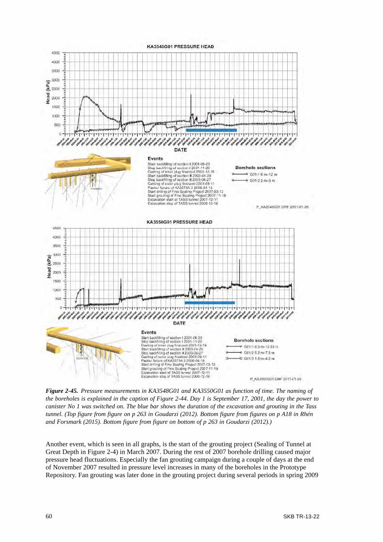
60 SKB TR-13-22

Figure 2-45. Pressure measurements in KA3548G01 and KA3550G01 as function of time. The naming of the boreholes is explained in the caption of Figure 2-44. Day 1 is September 17, 2001, the day the power to canister No 1 was switched on. The blue bar shows the duration of the excavation and grouting in the Tass tunnel. (Top figure from figure on p 263 in Goudarzi (2012). Bottom figure from figures on p A18 in Rhén and Forsmark (2015). Bottom figure from figure on bottom of p 263 in Goudarzi (2012).)

Another event, which is seen in all graphs, is the start of the grouting project (Sealing of Tunnel at Great Depth in Figure 2-4) in March 2007. During the rest of 2007 borehole drilling caused major pressure head fluctuations. Especially the fan grouting campaign during a couple of days at the end of November 2007 resulted in pressure level increases in many of the boreholes in the Prototype Repository. Fan grouting was later done in the grouting project during several periods in spring 2009

SKB TR-13-22 61

without major immediate impact on the pressure in the rock around the Prototype Repository. In the final end of the measuring period the pressure drops significantly in all graphs. This is most probably caused by the preparations for the opening and retrieval work.

A general drawdown of the ground water pressure was also observed in the Äspö HRL during the operation period. Except construction of the nearby Tass tunnel there were two more major campaigns that contributed to increased trend in draw-down in observational drillholes above and south of the Prototype Repository area. In spring 2003 excavation was carried out for the Tasq tunnel further east of the Prototype Repository (see location in Figure 2-4) as well as excavation of a niche 230 m above that area, Nasa1619 (Niche “as”pö “a”-tunnel at chainage 1619). Late in 2004 a 90 m long 1.8 m diameter tunnel was bored horizontally out over the Prototype Repository area from the Nasa1619 (see location of “Horizontal Deposition” in Figure 2-4). These activities coincided with slightly increased gradient in groundwater pressure decrease in many drillholes, especially at the 220 m level above the Prototype Repository.

Flow measurements in front of the outer plugSeveral weirs were located in the Prototype Repository tunnel and in other tunnels in the area. Figure 2-46 shows the flows collected by the weir closest to the outer plug at 3,535 m from the ramp portal. The measurements started in April 2004.

Manual measurements made in December 2003 showed a flow rate for MA3535G (see position of the weir and explanation to the weir’s name in Figure 2-46) of 0.4 L/min. The increase of flow during October 2004 was likely caused by the final grouting that was done around the outer plug on October 8, 2004. The flow rates thereafter decreased. At the end of the period the flow to the weir was on the order of 0.01–0.05 L/min (Goudarzi 2012).

Figure 2-46. Measured water flow to weir MA3535G. “M” denotes “mätvall”, which in English is weir, “A” denotes the main tunnel, i.e. the tunnel the Prototype Repository is situated in, “nnnn” denotes the position for the weir in the tunnel in m from the A-tunnel portal at ground surface, “G” denotes “golv”, which in English is floor. (Figure on p 278 in Goudarzi 2012.)

62 SKB TR-13-22

Temperature in rockThe maximum temperature in the rock near both deposition holes No 5 and No 6 was measured to 54°C. The position of these measurements was in both holes close to the rock wall at mid-height of the holes (Goudarzi 2012).

All the sensors located close to deposition hole No 6 measured a drop in temperature when the power was switched off at three occasions since the start of the test. After the two latest reductions of the power with 200 and 300 W respectively the temperature measured by the sensor, which were located at mid height of the canister in deposition hole No 6 and at the surface of the deposition hole No 6 dropped with about 8°C to a maximum temperature of about 45°C (Goudarzi 2012).

2.6.8 Gas and water samples from buffer, backfill and rockSamples from buffer and backfillSamples have occasionally been taken from the sampling points in the backfill and buffer for analyses on gas components, microbial existence and chemical composition (Pedersen et al. 2004). In addition, groundwater from boreholes in the rock surrounding the Prototype repository was analyzed regard-ing its gas composition, microbiology and chemistry (Eriksson 2007, Lydmark 2011).

It was indicated in the early phase (2004) that there was a significant gas exchange going on between the Prototype Repository and the surrounding tunnels resulting in a release of groundwater gases in the Prototype Repository that pushed away the air trapped in the Prototype Repository during installation.

Later it was discovered by Eriksson (2007) that many of the hydrochemical sampling points differ quite remarkably from each other. This was still the case at the last sampling campaign in 2011 prior to start of the opening and retrieval of the outer section (Lydmark 2011). Seven groups of samples with similar properties were recognized. The properties of one sampling group resembled those of the groundwater, while a second one differed in microbial composition, salinity, sulfate content, pH, and the concentrations of calcium, potassium, magnesium, sodium, and many dissolved metals, actinides, and lanthanides. A third sampling group contained samples that seemed to have been in contact with tunnel air. A fourth sampling group contained samples from points near the canisters in the buffer with very little pore water with high pH and a high salt content. A fifth group represented samples from sampling point in the backfill, which showed no groundwater in the May 2007 sam-pling campaign but did so in the November 2010 sampling campaign. This pore water had properties resembling those of the groundwater.

The gas composition in the sampling groups was uniform in that the proportion of nitrogen in the extracted gas increased and the oxygen content decreased with time. In most sampling groups, the oxygen content in the pore water had decreased from 3–7% in 2007 to 0.6–4% in 2009 (Lydmark 2011). This can also be compared with the oxygen content of 10–18% in the gas phase in 2005 (Eriksson 2007). Hydrogen, methane, helium, and carbon dioxide concentrations varied, especially in the sampling groups with extractable pore water. Some sampling points did not produce any extractable water during the operational time period, especially those in the buffer in the outer section.

Lydmark (2011) demonstrated with ATP (i.e. the biovolume) analyses that the biomass in the Pro-totype Repository was high compared to the surrounding groundwater. The microbiological results indicated that aerobic microbes, such as methane-oxidizing bacteria (MOB) and cultivable hetero-trophic aerobic bacteria (CHAB), thrived in the aerobic Prototype Repository environment.

The chemistry data indicated differences between the sampling groups: pH and concentrations of Na and K were higher in the Prototype Repository pore water than in the groundwater outside, while Ca and sometimes Mg concentrations were lower than in the groundwater. Obviously, cation exchange in the montmorillonite interlayers had occurred (Lydmark 2011).

At sampling points containing active microbes, however, Rb, Cs, V, and U were enriched up to 225 times the groundwater level (Lydmark 2011). Microbes were likely responsible for the dissolu-tion of these substances by the excretion of compound-specific ligands.

SKB TR-13-22 63

Overall, the observations supported the hypothesis that oxygen was consumed by bacteria within a short period of time (i.e. weeks to years), as opposed to the long period associated with abiotic pro-cesses (i.e. many years) (Lydmark 2011). The gas data generally indicated that oxygen disappeared and that MOB were responsible for at least some of the oxygen decrease. The microbes also affected the chemistry in the Prototype Repository, both indirectly (by being active and changing redox and pH) and possibly directly (via compound-specific ligands).

2.6.9 PlugThe prime focus for the monitoring program was the conditions at the interface between the plug and the rock in the abutment, which was considered to be the paths for water seepage through the plug. But, the monitoring program also included observations of the stress build-up in the concrete structure (Dahlström 2009).

Measurements across and parallel to the concrete-rock interface with joint meters, measuring the width, and strain gages, measuring the compression of the concrete, showed that at the end of 2007 the three instruments installed perpendicular to the rock surface all showed an increase of the inter-face width from start, with a maximum increase of 0.24 mm on the north side of the plug. The left side showed an increase of joint width of 0.15 mm. These measured values were in well agreement with predicted results (Dahlström 2009). The gap was expected to be filled and sealed by grout, which also was confirmed in the Project, see Section 4.2.3.

The measurements of the strains in the plug showed that the maximum stress perpendicular to the tunnel axis was approximately –4.9 MPa, and that the whole plug was under compression at the end of 2007. When the plug was designed, stresses, strain and deformations were estimated by numerical calculation. The plug was assumed to be subject to a pressure of 4.5 MPa from backfill and ground-water, for which the predicted maximum load became –9 to –16 MPa depending on rock properties. However, due to the low groundwater pressure – the open drainage – the plug was exposed to an outer pressure of no more than 1.6 MPa. Still, it could be verified that the whole plug would become under compression, which was the purpose of its design.

2.6.10 Copper corrosionReal time corrosion monitoring by means of electrochemical methods was applied in the Prototype Repository in order to measure corrosion rate of copper on copper electrodes during the whole operational period, which would mean observation during the initial oxidizing conditions. Anoxic conditions were considered probable to occur before opening and retrieval of the inner section according to the predictions made prior to the installation (Karnland et al. 2009, 2011), and not likely to occur before opening and retrieval of the outer section, see Section 3.5. For the purpose three nominally identical copper electrodes were installed, in bentonite block C3 in deposition hole No 1 and in block C4 in deposition hole No 5 (see position of the blocks in Figure 2-14), before respective heater was switched on, on September 17, 2001 and on May 8, 2003 respectively. Two cables were connected to each of the electrodes. They had black, yellow-green and red insulation respectively in order to keep track of the electrodes.

The in situ corrosion rate was measured at several occasions (Rosborg 2013a). The first time was in January 2004, and then periodically in 2005, 2006, 2008, and most recently in the end of 2010 just before work to open the outer section was started. The temperature of the copper electrodes had been around 30°C in deposition hole No 1 and somewhat below 35°C in deposition hole No 5.

The recorded corrosion rates were below 1 µm/year (using a default value of n=2 in the software to convert the corrosion current density to a penetration rate by means of Faraday’s law, and with no correction applied for the used measuring frequency of 0.01 Hz; also disregarding highly scattered data obtained for the copper electrodes in deposition hole No 1 during 2010). While the recorded rates on the electrodes in deposition hole No 5 first increased from about 0.2 µm/year in 2004 up to a maximum of 1.3 µm/year a year later (the drainage of the inner and outer sections was temporary closed in the end of 2004), and then gradually decreased to 0.7 µm/year in the end of 2010, the recorded rates on the electrodes in deposition hole No 1 showed a quite different picture. The recorded rates were in the range 0.4–0.7 µm/year and did not reflect any obvious decrease. However,

64 SKB TR-13-22

it is anticipated that similar time dependence as observed for the electrodes in deposition hole No 5 could have been present early on in the exposure, as the electrodes were installed in 2001 and that the first measurements were not made until 2004. Also, saturation of the bentonite was, according to instrument readings, faster in deposition hole No 1 than in deposition hole No 5.

Since the major corrosion product formed on the copper electrodes is cuprite (Cu2O), see Section 5.8, it would have been more appropriate to use n=1 as a default value in the software to convert the corrosion current density to a penetration rate. Furthermore, electrochemical impedance spectro-scopy (EIS) on pure copper electrodes in Äspö groundwater open to air has shown that an applied measuring frequency of 0.01 Hz underestimates the polarization resistance with a factor of 4, and thus overestimates the corrosion rate with the same amount (Rosborg 2013a). Applying these correc-tions of the corrosion, estimated rates were below 0.4 µm/year in 2010. Assuming that the correction for the measuring frequency is correct this is the highest possible corrosion rate; the actual corrosion rate could in fact be lower due to parallel reduction-oxidation reactions.

The estimated corrosion rates on the copper electrodes in the Prototype Repository were lower than the rate estimated for the copper electrodes in test parcel A2 of the Long Term Test of Buffer Material (LOT) – about 0.4 compared to 0.8 µm/year after six years exposure respectively (Rosborg 2013a). Different operating conditions might have been the reason for this. The average corrosion rate obtained from weight measurements of copper coupons in LOT test parcel A2 was found to be less than 0.5 µm/year (Rosborg 2013a), suggesting that the real-time corrosion monitoring have provide conservative corrosion rates.

2.6.11 Performance of instrumentationThe performance of the instrumentation is presented in detail by Goudarzi (2014). A summary of experiences and lessons learnt is discussed in Section 7.5.

2.6.12 Code developmentThe data from the continuous reading of sensors in the Prototype Repository have been widely used for calibration of different numerical codes on THM processes in the bentonite buffer. At first code calibration was a Work Package of its own in the EU-supported project “Proto-type Repository-FIKW-CT-2000-00055”. Progress of work was presented by Alonso and Ledesma (2005) Summary of results was reported by Pusch (2004). Following the completion of the EU project the code development continued in the Äspö Task Force on Engineered Barriers (EBS-TF). One example of the presently ongoing work in this EBS-TF is presented in this report in Section 6.1. Because the work is in progress the presentation is only capable of showing a “snapshot” of what can be expected when the work will be completed.

SKB TR-13-22 65

3 Purpose and management of the Project

3.1 Participating partiesThe Project was initiated jointly by SKB and Posiva in early 2010. Another six international end users – NDA (RWM), Andra, NUMO, BMWi, NWMO and Nagra – joined the Project in order to follow the work closely, acquire early results and learn about experiences and lessons of such full-scale experiment. In addition, two organizations (GRS and ASC) that participated in the installation of the Prototype Repository (holders of certain installed sensors) also took part in the retrieval phase. Thus, the Project organization consisted of the following parties:

• SKB Sweden.

• Posiva Finland.

• NDA (RWM.) United Kingdom.

• Andra France.

• NUMO Japan.

• BMWi Germany.

• NWMO Canada.

• Nagra Switzerland.

• GRS Germany.

• ASC England.

3.2 Objectives The purpose of the Project was to contribute with data and knowledge to support SKB’s and Posiva’s arguments on safe disposal with the KBS-3V method and also to provide a basis for the iterative updating of the reference design of a final repository.

In detail the objectives were to specifically address the following:

• To produce an image of the final density and water saturation of the buffer and backfill, after more than seven years of natural wetting through sampling and analyzing, and comparing the results with the density and saturation the buffer and backfill had at the time of installation.

• To study how the interfaces between the buffer and backfill and between the rock and backfill appeared during progress of the retrieval.

• To sample and to test the buffer material properties, and to compare the results with similar tests conducted on reference samples (of the original material), in order to identify any changes in the geochemical or hydro-mechanical properties of the buffer.

• To take and analyze water and gas samples in order to check the results obtained from analyses of biological and chemical activities in samples taken during the operation.

• To study the rock mass around the deposition holes in order to observe any changes that possibly had taken place (a visual inspection to confirm or reject measurement indications).

• To perform THM modeling of the experiment in order to compare the modeling results with the results from measurements of the density and water content of the buffer and backfill.

• To examine the canisters’ current position at the retrieval and their possible deformation due to exposure to high swelling pressure from the buffer.

• To measure copper corrosion by electric potential measurements of the installed copper electrodes in deposition hole No 5 and by sampling of the bentonite closest to the canister surface.

66 SKB TR-13-22

• To study possible damages to the concrete dome as well as to inspect the conditions of the inter-faces between the concrete and the rock (the performed contact grouting).

• To examine how the concrete material has affected the bentonite in the backfill material near the inner plug.

An important constrain on the Project was to not cause any harmful impact on the continued opera-tion of the inner section, other than the fact that the outer section would be removed.

3.3 Organization of workThe project was carried out by the organization shown in Figure 3-1.

The Client has been Anders Sjöland, SKB Nuclear Fuel Department (B), throughout the Project.

Project Managers have been Lars-Erik Johannesson, Clay Technology (Technical Leader) and Pär Grahm, SKB (Executive Leader) throughout the Project. Christer Svemar, SKB, who supervised the installation of the Prototype Repository in 2000–2003, also joined the Project with the aim to compile conclusions as the head-writer of the present summary report.

Project support was managed by Karin Nilsson, SKB, at the Äspö HRL.

The International Steering Committee consisted of representatives from each participating partner (see Section 3.1) and the teamwork was coordinated by Johanna Hansen, Posiva.

Opening and retrieval activities were organized as six Sub-projects as outlined in Figure 3-1. Also the Sub-project Managers have remained the same throughout the project:

SP1 Field work and sampling Patrik Hagman, SKB.

SP2 Laboratory examinations Daniel Svensson, SKB.

SP3 Modeling Ola Kristensson, Clay Technology.

SP4 Canister retrieval Mikael Hedin, ÅF Industry.

SP5 Sensor inspections Ulf Nilsson, Clay Technology.

SP6 Rock examination Rolf Christiansson, SKB.

Figure 3-1. Project organization.

InternationalSteering Committee(Reference group)

SKBControl group

Client

Project Manager

Retrieval

RemovalField work

Laboratoryexaminations Modeling Canister

retrievalSensor

inspectionsRock

examination

Operation

Project support

SKB TR-13-22 67

In addition to SKB’s Quality Management System, a separate Quality Plan and a Project Plan were developed for the Project. Furthermore, for each Sub-project a detailed sub-project Plan was pro-duced as a basis for the resource planning and orders of consultants and other services.

The continued operation of the Prototype Repository has been managed by the Project Managers and operations have been reduced in scope as the outer section was excavated. The operation of the inner section will continue until about 2020.

3.4 Work breakdown structureThe practical implementation of the Project was strategically divided into 25 different activities, as listed in Table 3-1.

Table 3-1. Activity Plans that have been conducted within the project.

Äspö HRL Id No. (AP TD – )

Description of work

KBP1001-10-042 Electric potential measurements on copper electrodes in deposition hole No 5, phase 1

KBP1001-10-047 Tightness testing of the outer concrete plugKBP1001-10-050 Breaching and sampling of the outer concrete domeKBP1001-10-051 Analyses of gas and microbiology before opening of the

outer sectionKBP1001-10-056 Analysis of water before opening of the outer sectionKBP1001-10-063 Sampling and removal of the backfill in the outer sectionKBP1001-11-010 Electric potential measurements on copper electrodes in

deposition hole No 5, phase 2KBP1001-11-013 Sampling and removal of the backfill inside (the top of)

deposition holes No 5 and 6KBP1001-11-014 Sampling and removal of the buffer in deposition hole No 6KBP1001-11-016 Retrieval of the canister from deposition hole No 6KBP1001-11-034 Microbiology analysis of the copper canister surfaces KBP1001-11-039 Gas sampling inside the canister in deposition hole No 6KBP1001-11-047 Microbiology analysis of the backfill materialKBP1001-11-056 Hydro-mechanical and chemical characterization of bentonite

material from dep. hole No 6KBP1001-11-057 Sampling and removal of the buffer in deposition hole No 5KBP1001-11-059 Electrochemical measurements on copper electrodes in

deposition hole No 5, before retrievalKBP1001-11-068 Gas sampling inside the canister in deposition hole No 5KBP1001-11-069 Gas analysis of buffer cores from deposition hole No 5KBP1001-11-088 Retrieval of the canister from deposition hole No 5KBP1001-11-091 Microbiology analysis of the buffer material from deposition

ole No 5KBP1001-12-012 Hydro-mechanical and chemical characterization of bentonite

material from dep. hole No 5KBP1001-12-040 AE system re-calibration (an attempt to reconnect the

system)KBP1001-12-041 Chemical characterization of the backfill materialKBP1001-12-068 Inflow measurements into deposition hole No 6 and No 5. KBP1001-13-058 XANES and XRD investigation on buffer samples from

deposition hole No 6

Primary data and other results from these activities are registered in the SKB database Sicada.

68 SKB TR-13-22

3.5 Predicted outcomeIn December 2010, before the plug was breached, SKB sent a letter of notification to the Swedish Radiation Safety Authority (SSM). The translated version of the attached Memo was entitled “Forecast of anticipated status prior to opening the Prototype Repository” (Johannesson 2011). The purpose was to make a short statement in advance about the overall results that were expected to be obtained by the Project. The results were also aimed to contribute to increased confidence in SKB’s and Posiva’s standpoint that it is possible to understand the processes that initially take place in the EBs and the surrounding bedrock in a complete final repository system.

As a follow up of the notification letter, a one-day briefing was arranged at the Äspö HRL for SSM and the Finnish Radiation and Nuclear Safety Authority (STUK) in late April 2011.

In short, the prediction (Johannesson 2011) concluded that:

• The water flow through the plug was expected to be low. The measurements had shown low values (Figure 2-44) although the water pressure behind the plug had been low due to the drainage of the section behind the Prototype Repository. An increased water pressure was not expected to change the through-flow in any significant way. The Project’s findings are presented in Section 4.2.2.

• The backfill was expected to be saturated at a mean dry density of 1,750 kg/m3 (Section 2.5.5). A lower density was expected close to the tunnel walls, roof and floor. Traces of piping might be seen due to the exposure of high water pressure during one month in 2004 (Section 2.5.5). Piping might also be seen because of water flows along cables to sensors. The Project’s findings are presented in Section 5.1.3.

• Backfill in the upper part of the deposition holes was expected to be saturated as well at a mean dry density of 1,750 kg/m3 based on the result measured during installation (Section 2.5.5). Traces of piping through the filling might be seen as well as some deformation caused by upward swelling of the bentonite buffer. This was expected to be more apparent in deposition hole No 6 as the buffer in this deposition hole indicated a higher degree of water saturation. The Project’s findings are presented in Section 5.1.3.

• The buffer in deposition hole No 5 was not expected to be fully saturated (Section 2.6.5). The highest level of saturation was expected to be found about three meters from the bottom of the deposition hole, i.e. at the middle section of the canister. The canister is expected to be in full contact with the buffer. The Project’s findings are presented in Section 5.1.4.

• The buffer in the rings around the canister in deposition hole No 6 was expected to be close to fully saturated, while the cylinders below and above the canister were expected to be saturated in the outer periphery but not in the center (Section 2.6.5). The canister was expected to have moved somewhat axially (Section 2.6.4). The Project’s findings are presented in Sections 5.1.4 (buffer conditions) and 4.4.3 (canister displacement).

• The explanation to the difference in saturation between deposition hole No 5 and deposition hole No 6 was not clear. The cause was expected to be found in either different saturation properties of the buffer or different water supply conditions in the deposition holes. The Project’s findings are presented in Section 5.1.4.

• The hydro-mechanical properties of the buffer were expected to show no detectable change with respect to hydraulic conductivity and swelling pressure after the more than seven years of expo-sure to heat from the canister and water from the bedrock at Äspö (Dueck et al. 2011). The buffer material, however, was expected to be somewhat more brittle (Dueck et al. 2011). In general, similar results to those found in the CRT (Kristensson and Börgesson 2015) were anticipated, even though the maximum temperature in the Prototype Repository buffer – 93°C (Section 2.6.4) – had been reported by Goudarzi et al. (2006) to be 100°C in CRT. The Project’s findings are presented in Section 5.3.

• Geochemical compositions of the buffer were not expected to have changed significantly. Similar results to those found in the CRT (Dueck et al. 2011) were anticipated, even though the tempera-ture in the Prototype Repository buffer had been somewhat lower than in the CRT buffer. The Project’s findings are presented in Section 5.2.

SKB TR-13-22 69

• Microbiological analyses were expected to yield existence of oxygen-consuming bacteria and SRB, but in negligible numbers (Section 2.6.8) as was the case in the buffer of the CRT (Lydmark and Pedersen 2011). The Project’s findings are presented in Section 5.4.

• Analysis of copper content in the buffer nearest the canister was expected to show existence of copper (Dueck et al. 2011, Karnland et al. 2011). The Project’s findings are presented in Section 5.2.3.

• The actual surface of the canister was expected to have a thin layer of copper (I) and copper (II) compounds caused by reaction between the canister surface and oxygen enclosed during installa-tion as was the case in LOT (Karnland et al. 2009, 2011). The Project’s findings are presented in Section 5.5.5.

• Deformation of the shape of both canisters was anticipated, similar to those observed in the CRT. The Project’s findings are presented in Section 5.5.2.

• Upward movement of both canisters was expected, as indicated by Figure 2-26. The Project’s findings are presented in Section 4.4.3.

• Thermal deformation of the rock was expected to be of elastic nature only (i.e. deformed revers-ibly), and not to have resulted in spalling (Section 2.5.2). No new microscopic fractures were expected to have developed (Section 2.5.2). The Project’s findings are presented in Section 4.7.3.

• Small movements of fractures or clogging of existing ones at the rock wall in the deposition holes causing changed patterns of inflowing water could not be ruled out but it was judged highly improbable that such changes would be possible to detect (Johannesson 2011). The Project’s findings are presented in Section 4.7.2.

• Validation of sensors installed in the Prototype Repository was expected to give the same results as validation of the sensors in Temperature Buffer Test (TBT) (Åkesson 2012) and CRT (Kristiansson and Börgesson 2011). The Project’s findings are presented in Section 5.8.

• The same type of damage to electrical cables to heaters, as seen in the CRT (Eng 2008), was anticipated to have occurred in the Prototype Repository. The Project’s findings are presented in Section 5.7.

SKB TR-13-22 71

4 Opening and retrieval of outer section

In this section the field work carried out at the Äspö HRL, starting in November 2010 and ending in December 2011, is described in a summary manner. More detailed information is found in the background report by Johannesson and Hagman (2013).

The mission of the field work was to breach the 200-ton concrete plug to the outer section of the Prototype Repository and carry out adequate sampling during excavation of the backfill (900 tons) and buffer (40 tons). Location and vertical swelling of each bentonite block was to be determined for comparison with the height and location at installation. The two copper canisters were to be retrieved from their deposition holes and to be inspected at the Canister Laboratory in Oskarshamn. All installed sensors that could be recovered were to be collected for an initial assortment, where sensors in appropriate condition were to be sent to laboratories for further inspection. Finally, visual inspections of the rock walls in the emptied tunnel and deposition holes were to be performed with focus on the inside and surroundings of the deposition holes.

4.1 Planning of field workThe retrieval of samples from the outer section was predicted to be a very extensive work. The plan-ning was carried out during six months of 2010, while the actual excavation, sampling and retrieval activities were considered to take about 14 months (including a total of six weeks of holidays with paused activities in the field).

To meet requests from the modelers and to fulfill the laboratory scope it was decided that the field work team should collect almost 8,000 samples on the buffer and about 1,300 samples of the backfill for immediate determination (within 48 hours) of density and water content in the local Geolabora-tory at the Äspö HRL. Furthermore, a large number of buffer material samples should be collected for more extensive laboratory examinations.

4.1.1 ObjectivesThe objective of the preparatory work was to provide a detailed guidance to how the different activities should be carried out in order to meet the overall objectives. The plans and procedures addressed:

• How the opening and retrieval should be carried out.

• Time needed for the excavation, sampling and all their associated tasks.

• Necessary resources in the form of machines, equipment and staff required.

• Costs involved.

4.1.2 Planning and work break down structureA Project Plan, a Quality Management Plan and six Sub-project Plans were developed by the project team, as described in Section 3.3, and a work breakdown structure with 25 Activity plans was estab-lished according to Section 3.4.

Below is a list of how the field activities were planned in chronologic order:

• Switching off the heaters in deposition hole No 6.

• Testing of the tightness of the outer plug.

• Breaching and removal of the outer plug.

• Sampling and excavation of the backfill to a section behind deposition hole No 6.

• Construction of a protective and retaining wall for the remaining backfill.

72 SKB TR-13-22

• Excavation of the backfill inside (the top of) deposition hole No 6.

• Sampling and removal of the bentonite Block C4-C2 and R10-R1 in deposition hole No 6 (block positions are shown in Figure 2-14).

• Sampling of gas inside the first canister (after removal of block R10).

• Retrieval of the canister in deposition hole No 6.

• Sampling and removal of the bentonite Block C1 in deposition hole No 6. (Block position is shown in Figure 2-14).

• Switching off the heaters in deposition hole No 5.

• Summer holidays 2011.

• Removing the temporary retaining wall.

• Continuing of the sampling and excavation of the backfill to the inner plug.

• Excavation of the backfill inside (the top of) deposition hole No 5.

• Sampling and removal of the bentonite Block C4-C2 and R10-R1 in deposition hole No 5 (Block positions are shown in Figure 2-14).

• Sampling of gas inside the second canister (after removal of block R10).

• Retrieval of the canister in deposition hole No 5.

• Sampling and removal of the bentonite Block C1 in deposition hole No 5. (Block position is shown in Figure 2-14).

• Rock inspection.

Each activity of the work breakdown structure (Table 3-1) was described as detailed as possible in a corresponding Activity Plan, including the sampling and excavation methods to use, which machines or equipment that were needed, responsible staff, means of documentation by texts and photographs, and how and where obtained material should be filed in SKB’s electronic systems for documents and data, e.g. the data base Sicada.

In addition each Activity Plan presented a risk analysis on safety, health and environment with grading of each identified risk and means of preventing them to occur. The guiding rule was that the Activity Plan had to be complete and approved according to SKB’s Quality Assurance System before the activity was allowed to start. Once a plan had been approved and put into operation every adverse event had to be reported, its impact analyzed and the change approved according to SKB’s applied non-compliance system.

A central practical part of the fieldwork planning were the identification of such methods to use that would provide representative samples and representative observations of the hydro-mechanical situation in the surrounding rock without jeopardizing the continuing operation of the inner section.

4.2 Opening of outer plug The actual dismantling operation began with the removal of the concrete plug. Before this, a simple test of the water tightness of the plug was made, and samples were taken from the interface between the plug and the rock in the recess.

4.2.1 ObjectivesThe removal of the plug was carried out with the following objectives:

• Determine the water tightness of the plug.

• Determine the quality obtained by the contact grouting of the interface between the concrete plug and the rock wall in the recess.

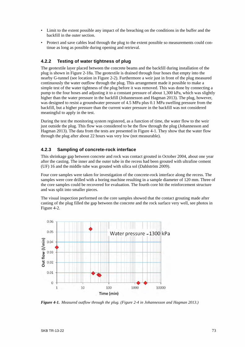
SKB TR-13-22 73

• Limit to the extent possible any impact of the breaching on the conditions in the buffer and the backfill in the outer section.

• Protect and save cables lead through the plug to the extent possible so measurements could con-tinue as long as possible during opening and retrieval.

4.2.2 Testing of water tightness of plugThe geotextile layer placed between the concrete beams and the backfill during installation of the plug is shown in Figure 2-18a. The geotextile is drained through four hoses that empty into the nearby G-tunnel (see location in Figure 2-2). Furthermore a weir just in front of the plug measured continuously the water outflow through the plug. This arrangement made it possible to make a simple test of the water tightness of the plug before it was removed. This was done by connecting a pump to the four hoses and adjusting it to a constant pressure of about 1,300 kPa, which was slightly higher than the water pressure in the backfill (Johannesson and Hagman 2013). The plug, however, was designed to resist a groundwater pressure of 4.5 MPa plus 0.1 MPa swelling pressure from the backfill, but a higher pressure than the current water pressure in the backfill was not considered meaningful to apply in the test.

During the test the monitoring system registered, as a function of time, the water flow to the weir just outside the plug. This flow was considered to be the flow through the plug (Johannesson and Hagman 2013). The data from the tests are presented in Figure 4-1. They show that the water flow through the plug after about 22 hours was very low (not measurable).

4.2.3 Sampling of concrete-rock interfaceThis shrinkage gap between concrete and rock was contact grouted in October 2004, about one year after the casting. The inner and the outer tube in the recess had been grouted with ultrafine cement (UF) 16 and the middle tube was grouted with silica sol (Dahlström 2009).

Four core samples were taken for investigation of the concrete-rock interface along the recess. The samples were core drilled with a boring machine resulting in a sample diameter of 120 mm. Three of the core samples could be recovered for evaluation. The fourth core hit the reinforcement structure and was split into smaller pieces.

The visual inspection performed on the core samples showed that the contact grouting made after casting of the plug filled the gap between the concrete and the rock surface very well, see photos in Figure 4-2.

Figure 4-1. Measured outflow through the plug. (Figure 2-4 in Johannesson and Hagman 2013.)

74 SKB TR-13-22

4.2.4 Breaching of plugThe technique used to breach the plug was to first core drill through the outer part of the plug towards the retaining wall, see Figure 4-3. The boreholes were placed in an overlapping cross-like pattern, as shown by Figure 4-4. After the drilling, the breaching continued by mechanical demoli-tion using a hydraulic breaker and a hydraulic hammer. The hydraulic breaker was vibrated into the concrete and then hydraulically expanded in order to create fractures in the concrete dome. After fracturing the plug was further demolished with the hydraulic hammer. When reinforcement became visible it was cut off by the use of a cutting blowpipe. Finally, the remaining of the plug was trans-ported out from the tunnel with a front loader.

The retaining wall, consisting of several prefabricated and reinforced concrete beams, was then removed by first cutting off the mounts for the beams on the rock wall and then by mechanical demolition with the hydraulic hammer.

4.2.5 Observations The initial plan of the removal was based on core drilling through both the concrete plug and the wall of prefabricated beams (retaining wall in Figure 2-17) placed behind the plug. During core drilling through the plug the backfill material, however, was pressed out through the drilled hole and a modification of the plan for the removal was required. Thus core drilling was made only through the concrete plug towards the beams.

The concrete structure was found to be harder than expected to breach and the removal method was changed from chiseling technique to technique with hydraulic hammer.

After removal of the concrete plug the retaining wall could be easily removed.

Figure 4-2. Close up pictures of the cores taken from the interface between concrete plug and rock. The yellow grouting tubes are embedded in grout. (Figure 2-6 in Johannesson and Hagman 2013.)

SKB TR-13-22 75

4.3 Removal and sampling of tunnel backfillThe backfill material was first installed by in situ compaction in the upper one m of the deposition hole (on top of the buffer) with the use of a vibrating road compactor. The backfill was thereafter installed by in situ compaction in inclined layers in the tunnel with the use of a vibrating slope com-pactor attached to a backhoe loader. Material and backfill processes are described in Section 2.5.5 and in more detail by Johannesson et al. (2004).

4.3.1 ObjectivesThe backfill was removed with the following objectives:

• Empty the tunnel.

• Uncover the buffer.

Figure 4-3. The rig used for core drilling through the concrete dome. (Figure 2-5 in Johannesson and Hagman 2013.)

Figure 4-4. Left: The cross-like pattern of the core drilled holes through the plug. Right: The machine used for demolition of the concrete plug. (Figure 2-2 in Johannesson and Hagman 2013.)

76 SKB TR-13-22

• Sample the backfill material in a way that would provide representative samples from the deposi-tion hole and tunnel cross sections.

• Retrieve installed sensors to the extent possible and with a condition that made them fit for post-examination and re-calibration.

The samples were to be handled properly with respect to coming examinations, and sent to surface laboratories for determination of density and degree of saturation.

4.3.2 Removal of tunnel backfillThe removal of the tunnel backfill started immediately after the first beams from the retaining wall had been removed and took place during two periods. At the first period (March 2011), the excava-tion was made to a section approximately 3 m behind deposition hole No 6. A retaining wall of wood was then placed in front of the backfill to ensure that the rest of the backfill was in place during sampling and removal of backfill, buffer and canister in deposition hole No 6. The excavation of the tunnel backfill continued when deposition hole No 6 became empty (August – September 2011). The total amount of backfill removed from the tunnel and deposition holes was about 900 tons, i.e. about the same amount that once had been installed. The removal was, as planned, made with a backhoe loader in inclined layers, but with a steeper slope angle to the tunnel floor (average 45°) than the angle applied during the in situ compaction (35°). Different bucket designs were tested before one was chosen. The concern was that the bucket teeth might damage sensors while they also would be needed in order to tear loose parts of the backfill.

During removal particular account was taken to the eleven lead-through pipes located on the north side of the tunnel and to the two lead-through pipes in the concrete plug. It was deemed important that these sensors provided accurate readings for as long as possible so the cool-down process could be observed after switching off the heaters in the canister in deposition hole No 6.

4.3.3 Sampling of tunnel backfillThe removal stopped every second meter and samples were taken for determination of the water content and density of the backfill material, see Figure 4-5. In order to be able to stand on the surface of the backfill, when taking samples, steel rods were pushed into the backfill and platforms were placed on them. Samples (about 100 from each of the investigated eleven sections) were taken from the surface with the use of an angle grinder. The position of each sample was determined by geodetic surveying. In total about 1,000 samples of this kind were obtained.

The samples were wrapped in plastic and transported to the laboratory for determining of water content and density. The determination of the water content and density was made within 48 hours after the samples had been taken from the site. The results from the measurements were described and presented in a separate report by Johannesson (2014). A summary of the results is presented in this report in 5.1.3.

Besides the samples taken for determining the water content samples were taken also close to the inner concrete plug for chemical and mineralogical examinations. These tests were described by Olsson et al. (2013). The results are summarized in this report in Section 5.2.4.

Samples were taken also for analysis of occurring microorganisms. A total of 143 backfill samples were taken along a profile starting from the floor level of tunnel chainage 3,551.154 m (i.e. at the position 3,551.154 m from the ramp portal at ground surface) and ending at the roof level at chain-age 3,556.241 m, see position of chainages in Figure 2-1). These samples were individually vacu-um-packaged and sent to the Microbial laboratory. Some 63 samples were randomly selected out of the 143 ones to provide an overview of the backfill material. The result from the analyses were also described and presented in a separate report (Arlinger et al. 2013). A summary of the results is presented in this report in Section 5.4.

SKB TR-13-22 77

4.3.4 Removal and sampling of deposition hole backfillThe backfill material placed inside the two deposition holes above the last installed buffer block in each of the deposition holes were removed by hand, after the material was loosened with a pneumatic hammer. Some samples were also taken from this part of the tunnel backfill on which the water con-tent and the density were measured and the occurrence of microorganisms analyzed, see Figure 4-6.

Figure 4-5. Top left: Sampling of the backfill material. Top right: Geodetic surveying of the position of the taken samples. Bottom left: An example of data from the geodetic surveying. The eleven sections, which were sampled, are marked with different colors. Section No 1 is blue (to the right) and section No 11 is black (to the left). Bottom right: Samples were placed in plastic bags before being transported to the laboratory. (Figure 3-3 in Johannesson and Hagman 2013.)

Figure 4-6. Samples taken from the tunnel backfill inside a deposition hole together with an installed sensor. (Figure 3-6 in Johannesson and Hagman 2013.)

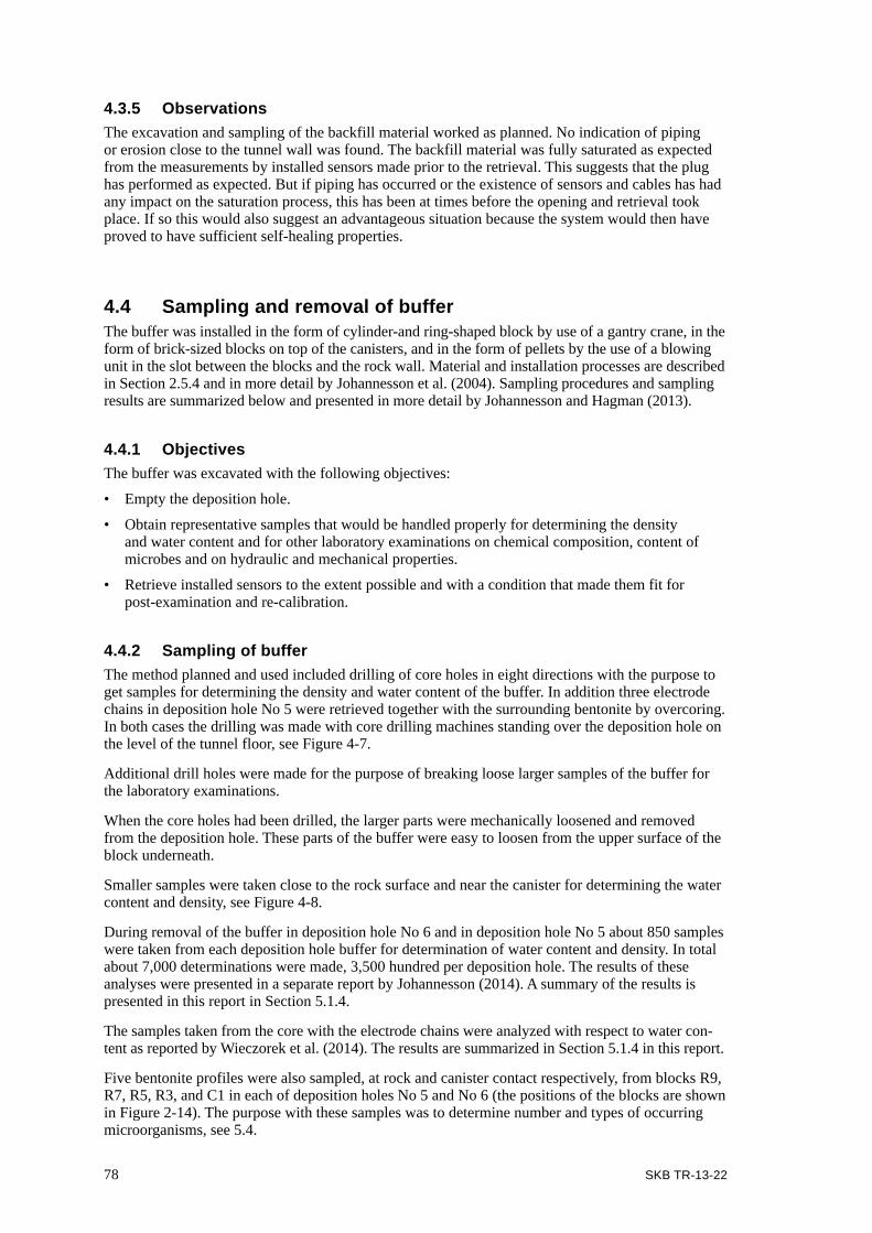
78 SKB TR-13-22

4.3.5 ObservationsThe excavation and sampling of the backfill material worked as planned. No indication of piping or erosion close to the tunnel wall was found. The backfill material was fully saturated as expected from the measurements by installed sensors made prior to the retrieval. This suggests that the plug has performed as expected. But if piping has occurred or the existence of sensors and cables has had any impact on the saturation process, this has been at times before the opening and retrieval took place. If so this would also suggest an advantageous situation because the system would then have proved to have sufficient self-healing properties.

4.4 Sampling and removal of bufferThe buffer was installed in the form of cylinder-and ring-shaped block by use of a gantry crane, in the form of brick-sized blocks on top of the canisters, and in the form of pellets by the use of a blowing unit in the slot between the blocks and the rock wall. Material and installation processes are described in Section 2.5.4 and in more detail by Johannesson et al. (2004). Sampling procedures and sampling results are summarized below and presented in more detail by Johannesson and Hagman (2013).

4.4.1 ObjectivesThe buffer was excavated with the following objectives:

• Empty the deposition hole.

• Obtain representative samples that would be handled properly for determining the density and water content and for other laboratory examinations on chemical composition, content of microbes and on hydraulic and mechanical properties.

• Retrieve installed sensors to the extent possible and with a condition that made them fit for post-examination and re-calibration.

4.4.2 Sampling of bufferThe method planned and used included drilling of core holes in eight directions with the purpose to get samples for determining the density and water content of the buffer. In addition three electrode chains in deposition hole No 5 were retrieved together with the surrounding bentonite by overcoring. In both cases the drilling was made with core drilling machines standing over the deposition hole on the level of the tunnel floor, see Figure 4-7.

Additional drill holes were made for the purpose of breaking loose larger samples of the buffer for the laboratory examinations.

When the core holes had been drilled, the larger parts were mechanically loosened and removed from the deposition hole. These parts of the buffer were easy to loosen from the upper surface of the block underneath.

Smaller samples were taken close to the rock surface and near the canister for determining the water content and density, see Figure 4-8.

During removal of the buffer in deposition hole No 6 and in deposition hole No 5 about 850 samples were taken from each deposition hole buffer for determination of water content and density. In total about 7,000 determinations were made, 3,500 hundred per deposition hole. The results of these analyses were presented in a separate report by Johannesson (2014). A summary of the results is presented in this report in Section 5.1.4.

The samples taken from the core with the electrode chains were analyzed with respect to water con-tent as reported by Wieczorek et al. (2014). The results are summarized in Section 5.1.4 in this report.

Five bentonite profiles were also sampled, at rock and canister contact respectively, from blocks R9, R7, R5, R3, and C1 in each of deposition holes No 5 and No 6 (the positions of the blocks are shown in Figure 2-14). The purpose with these samples was to determine number and types of occurring microorganisms, see 5.4.

SKB TR-13-22 79

Each profile covered two bentonite blocks, one in contact with the canister surface and another in contact with the rock boundary layer. In total about 50 samples were taken for this purpose, equally many from each deposition hole. The results of these analyses were presented in a separate report by Arlinger et al. (2013). A summary of the results is presented in this report in Section 5.4.

Five core samples were taken from deposition hole No 5 for analysis of gas content in the bentonite and its composition. The work with these was reported by Arlinger et al. (2013). As the nature of that work was focused on evaluating methods to measure the role of microorganisms in the process of decreasing the content of oxygen in gas (before the buffer becomes saturated), no summary of result from this activity was included in this report.

Microbial and molecular samples were taken also from the canister surfaces in deposition holes No 5 and No 6, (Arlinger et al. 2013). Two different methods were used: scraping off with a sterile scalpel and swabbing off with deoxyribonucleic acid /ribonucleic acid (DNA/RNA)-free cotton swabs soaked in sterile phosphate buffered saline (PBS). Figure 4-9 shows the sampling. The results of these analyses have been presented by Arlinger et al. (2013). A summary of the results is presented in Section 5.4.

Figure 4-7. Left: The core drilling machines standing on the tunnel floor. Right: Holes from cores taken from a buffer block. Wooden templates were used to position the drill bit. (Figure 4-1 in Johannesson and Hagman 2013.)

Figure 4-8. Left: The cores taken for determination of the density and water content of the buffer. Middle: The extra cores (red) drilled to loosen the buffer inside the deposition hole. Right: The large samples (green) taken from the buffer for further investigations in the laboratory and the samples (blue) taken for determining the water content and density close to the canister and the rock. (Figure 4-2 in Johannesson and Hagman 2013.)

30°

45°

15°

30°

45°15° 30°

45°

15°

30°45°

15°

B, 90°

A, 0°

C, 180°

D, 270°

R875R825R77

5

R725

R675R625

R575

R52

5

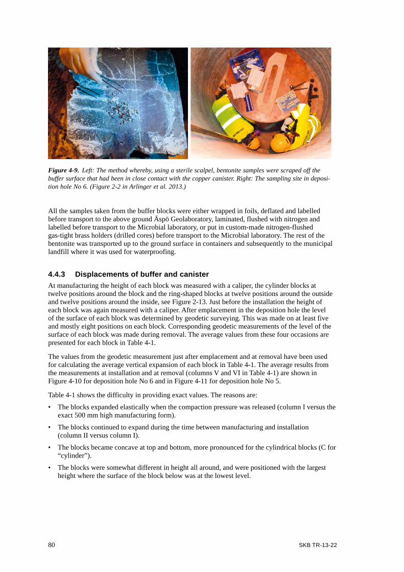
80 SKB TR-13-22

All the samples taken from the buffer blocks were either wrapped in foils, deflated and labelled before transport to the above ground Äspö Geolaboratory, laminated, flushed with nitrogen and labelled before transport to the Microbial laboratory, or put in custom-made nitrogen-flushed gas-tight brass holders (drilled cores) before transport to the Microbial laboratory. The rest of the bentonite was transported up to the ground surface in containers and subsequently to the municipal landfill where it was used for waterproofing.

4.4.3 Displacements of buffer and canisterAt manufacturing the height of each block was measured with a caliper, the cylinder blocks at twelve positions around the block and the ring-shaped blocks at twelve positions around the outside and twelve positions around the inside, see Figure 2-13. Just before the installation the height of each block was again measured with a caliper. After emplacement in the deposition hole the level of the surface of each block was determined by geodetic surveying. This was made on at least five and mostly eight positions on each block. Corresponding geodetic measurements of the level of the surface of each block was made during removal. The average values from these four occasions are presented for each block in Table 4-1.

The values from the geodetic measurement just after emplacement and at removal have been used for calculating the average vertical expansion of each block in Table 4-1. The average results from the measurements at installation and at removal (columns V and VI in Table 4-1) are shown in Figure 4-10 for deposition hole No 6 and in Figure 4-11 for deposition hole No 5.

Table 4-1 shows the difficulty in providing exact values. The reasons are:

• The blocks expanded elastically when the compaction pressure was released (column I versus the exact 500 mm high manufacturing form).

• The blocks continued to expand during the time between manufacturing and installation (column II versus column I).

• The blocks became concave at top and bottom, more pronounced for the cylindrical blocks (C for “cylinder”).

• The blocks were somewhat different in height all around, and were positioned with the largest height where the surface of the block below was at the lowest level.

Figure 4-9. Left: The method whereby, using a sterile scalpel, bentonite samples were scraped off the buffer surface that had been in close contact with the copper canister. Right: The sampling site in deposi-tion hole No 6. (Figure 2-2 in Arlinger et al. 2013.)

SKB TR-13-22 81

Table 4-1 shows that the variation in height at manufacturing was minor for cylindrical blocks (3 mm) than for ring-shaped blocks (13 mm). This is consistent with the variation measured just before emplacement of the blocks, although the individual blocks show variation in the proportional expansion on a mm scale. The caliper method applied, however, has not such an accuracy that these small variations can be used for any conclusion on block evolution. At the time of removal of the buffer the variation in height of the individual blocks was larger, from minus 2 mm in the bottom part to plus 70 mm at the interface between the buffer and the backfill. Different blocks thus have evolved differently and the vertical swelling differs between 0,1% of the height after emplacement in the bottom part to 14% in the top part. This variation of vertical expansion of the individual blocks

Figure 4-10. Left: Relative displacement of the upper surface of the blocks in deposition hole No 6 at the excavation (red) compared to the position at the installation (green) in mm. The shown measure for each block is the average measure from eight different points at the surface of the block. Right: measured deformation of the individual blocks – measured height of block at retrieval minus height at installation (red) together with the accumulated deformation (blue) for the 14 installed bentonite blocks in deposition hole No 6. Positive values indicate vertical displacement upwards. For individual blocks positive values indicate increased height. Blocks R5 and R7 show compression, which is unlikely. This is most probably a measurement error. (Figures 4-5 and 4-6 in Johannesson and Hagman 2013.)

Figure 4-11. Left: Relative displacement of the upper surface of the blocks in deposition hole No 5 at the excavation (red) compared to the position at the installation (green) in mm. The shown measure for each block is the average measure from eight different points at the surface of the block. Right: Measured deformation of the individual blocks – measured height of block at retrieval minus height at installation (red) together with the accumulated deformation (blue) for the 14 installed bentonite blocks in deposition hole No 5. Positive values indicate vertical swelling upwards. For individual blocks positive values indicate increased height. Blocks R5 and R1 show compression, which is unlikely. This is most probably a measure-ment error. (Figures 5-3 and 5-4 in Johannesson and Hagman 2013.)

R9R10C2C3C4

3236

234357

8117

6

R8R7

2730

R6 2936

3432

28 9

R5R4R3R2R1C1

–0.02

0.00

0.02

0.04

0.06

0.08

0.10

0.12

0.14

0.16

0.18

Def

orm

atio

n (m

)

Total deformationIndividual block deformation

C4 C3 C2 R10 R9 R8 R7 R6 R5 R4 R3 R2 R1 C1

R9R10C2C3C4

3654

83

R8R7R6R5

4

153

6

R4R3R2R1C1

1531

2620

1614

1513

6

–0.02

0.00

0.02

0.04

0.06

0.08

0.10

0.12

0.14

0.16

0.18

Def

orm

atio

n (m

)

Total deformationIndividual block deformation

C4 C3 C2 R10 R9 R8 R7 R6 R5 R4 R3 R2 R1 C1

82 SKB TR-13-22

is shown by Figure 4-10 and Figure 4-11. The two figures also present the accumulated vertical displacement at the upper surface of each block and visualize the information in Table 4-1, that the vertical displacements of the blocks at mid-height of the canisters were very small compared to the deformation of cylinder blocks above and underneath the canisters. Positive values show vertical dis-placements upwards. For each individual block a positive value shows increased height. Two blocks in deposition hole No 5 – R5 and R7 – and two blocks in deposition hole No 6 – R1 and R5 – have according to Table 4-1 been compressed, which is considered unlikely and most probably due to measurement errors. The measured values are within the measurement accuracy of the geodetic method when also considering the difficulty in finding the exact interface between blocks in a 350 mm wide slot (canister still in place) in the deposition hole during buffer removal, especially at the bottom part. The measured vertical displacements have been developed in the TBM tunnel with a diameter of 5 m. In the reference shoe-shaped tunnel with a height of 4.8 m the displacements would be expected to be very similar, because the backfill close to the tunnel roof had the lowest density and would conse-quently be the part of the backfill that would be more compacted by the swelling buffer than the core of the backfill. And this roof layer of backfill can be expected to be equally thick in both tunnel cases.

Table 4-1. Height of individual blocks in deposition holes No 5 and No 6 measured at three differ-ent occasions. The values are average values from measurements on four to eight positions on each block. Values in columns I and II have been measured with calipers and values in columns III and IV with geodesy.

I II III IV V VIBlock in deposition hole No 6

Height at manufacturing

Caliper, mm

Height before installation

Caliper, mm

Height after emplacement

Geodesy, mm

Height at removal

Geodesy, mm

IV-III

Vertical swelling, mm

Accumulated vertical displace-ment, mm

C4 502.9 507.0 507.2 603.6 96.4 177.1C3 499.6 501.3 507.2 530.4 23.2 80.7C2 500.6 503.5 509.6 524.8 15.2 57.5R10 510.8 514.3 514.5 520.1 5.6 42.3R9 505.7 509.3 510.0 514.9 4.9 36.8R8 509.4 510.8 512.2 518.0 5.7 31.9R7 508.0 512.3 511.8 507.4 –4.4 26.2R6 501.8 506.8 504.8 506.1 1.4 30.6R5 504.2 510.0 509.7 502.6 –7.1 29.2R4 495.7 499.5 498.5 500.0 1.5 36.3R3 500..9 503..8 503.5 506.9 3.4 34.8R2 509.2 514.5 513.2 516.5 3.2 31.4R1 507.2 510.8 511.1 530.0 18.9 28.2C1 502.9 507.0 510.1 519.4 9.3 9.3

Block in deposition hole No 5

C4 499.1 501.3 505.4 574.9 69.5 152.9C3 501.1 502.3 505.2 534.8 29.6 83.4C2 408.4 501.4 507.5 525.4 17.9 53.8R10 503.2 508.8 506.8 511.3 4.6 35.8R9 505.3 510.0 510.5 515.3 4.8 31.3R8 512.3 514.3 514.3 520.9 6.6 26.5R7 511.9 516.5 515.0 518.7 3.8 19.9R6 504.0 508.5 507.8 509.8 2.0 16.1R5 504.0 508.6 508.2 507.5 –0.8 14.1R4 501.5 505.8 504.5 506.1 1.6 14.9R3 507.1 512.0 507.8 515.4 7.6 13.2R2 506.2 511.0 510.0 511.5 1.5 5.6R1 500.4 504.5 305.2 503.5 –1.8 4.1C1 496.9 500.0 500.5 506.4 5.9 5.9

SKB TR-13-22 83

The level of the canister lid was measured in five positions with small deviances between the measure ments. They showed that the canister has moved upwards with about 23 mm in deposition hole No 6 after the installation. Corresponding value for deposition hole No 5 is 15 mm. Further-more the measurements showed that the lids in the two deposition holes had a horizontal position which indicates that no tilting of the canister has occurred during the saturation phase. This is in con-trast to the registered displacement of 12 mm of the canister in deposition hole No 6 (Section 2.6.4). The cause of the difference is discussed in Section 4.4.4.

4.4.4 Observations The sampling and retrieval of the buffer in the two deposition holes worked as planned. No gap between the canister and the buffer was observed. This was also true for the drier parts of the buffer. Although the pellets-filled the outer slot and the outermost part of the blocks were saturated, the interface between the blocks and the pellets was visible thus the buffer had not homogenized during the more than seven years of saturation. In addition, the interfaces between the blocks were visible. No signs of piping or erosion were found in the buffer and no signs of water transport along cables to sensors. If such events have taken place this has been at times before opening and retrieval took place.

The upward swelling of the buffer was large but not larger than expected and most of the swelling had occurred in the upper parts of the buffer.

The measured upward movement of the canister’s lid in deposition hole No 6 (23 mm) can be compared with the instrument readings of the upward movement of the canister’s bottom (~ 12 mm in Section 2.6.4). This upward movement is fairly close to the measured upward movement of the bottom block (9 mm in Figure 4-10). The difference between the values from the two measurements can be explained in one of three ways: the canister has been extended ~ 10 mm, the canister has been displaced upwards during removal of the backfill and the buffer, or one or both measurements are incorrect.

Extension of the canister is probable, as reported in Section 5.5.3, and is, if so, a consequence of the decreased diameter at mid-height (Hernelind 2014). But the indication in Section 5.5.3 for the canister in deposition hole No 6 is no more than 3.4 mm, a value which is rather similar to the measured extension of the canister in the CRT. The value of 3.4 mm (extension from nominal value at manufacturing) is, however, very uncertain as the real length of the canister at installation was not measured.

The second alternative explanation, canister displacement in the course of removal, was examined during removal of the backfill and the buffer above in deposition hole No 5. The reason was that the problem of non-conforming measurements in deposition hole No 6 was of high priority to understand. Another approach was taken in deposition hole No 5, where the top of the canister was measured through a hole drilled from the tunnel before the removal of the backfill and the buffer in the deposition hole started. This approach discovered no upward displacement during the course of successive removal of the material on top of the canister, and was not assessed as a probable event in deposition hole No 6 either. It was also concluded that the displacement sensors, which were attached to the bottom of the canister should have indicated such an extension of the bottom block (unless the sensor system had been damaged during the removal of the backfill and the buffer on top of the canister).

The third alternative explanation is coupled to the accuracy of the measurement methods. The applied geodetic survey method was based on laser beams and is very accurate, but the surface it rebounds back from – buffer block surfaces – may be uneven and irregularly shaped. Analyses of the measurements made and the possible errors in positions of laser equipment and conditions of measured surfaces indicate that a variation of ± 3 mm may be realistic.

The sensors that were attached to the bottom were calibrated before the installation but not after-wards. The accuracy of their readings is dependent on a good and remaining performance of the glue that was used for attachment of sensors to the canister bottom. These attachments could not be investigated after removal of the canisters as they were destroyed when the canister was pulled up. Another small measurement error may have occurred at the measurement of the canister’s length (the canister was standing on a floor with uncertain evenness, see Section 5.5.3).

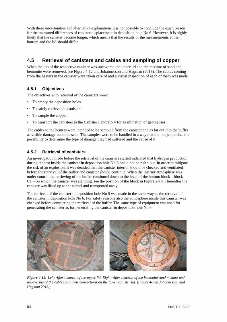
84 SKB TR-13-22

With these uncertainties and alternative explanations it is not possible to conclude the exact reason for the measured differences of canister displacement in deposition hole No 6. However, it is highly likely that the canister become longer, which means that the results of the measurements at the bottom and the lid should differ.

4.5 Retrieval of canisters and cables and sampling of copperWhen the top of the respective canister was uncovered the upper lid and the mixture of sand and bentonite were removed, see Figure 4-12 and Johannesson and Hagman (2013). The cables coming from the heaters in the canister were taken care of and a visual inspection of each of them was made.

4.5.1 ObjectivesThe objectives with retrieval of the canisters were:

• To empty the deposition holes.

• To safely retrieve the canisters.

• To sample the copper.

• To transport the canisters to the Canister Laboratory for examination of geometries.

The cables to the heaters were intended to be sampled from the canister and as far out into the buffer as visible damage could be seen. The samples were to be handled in a way that did not jeopardize the possibility to determine the type of damage they had suffered and the cause of it.

4.5.2 Retrieval of canistersAn investigation made before the retrieval of the canisters started indicated that hydrogen production during the test inside the canister in deposition hole No 6 could not be ruled out. In order to mitigate the risk of an explosion, it was decided that the canister interior should be checked and ventilated before the retrieval of the buffer and canister should continue. When the interior atmosphere was under control the retrieving of the buffer continued down to the level of the bottom block – block C1 – on which the canister was standing, see the position of the block in Figure 2-14. Thereafter the canister was lifted up to the tunnel and transported away.

The retrieval of the canister in deposition hole No 5 was made in the same way as the retrieval of the canister in deposition hole No 6. For safety reasons also the atmosphere inside this canister was checked before completing the retrieval of the buffer. The same type of equipment was used for penetrating the canister as for penetrating the canister in deposition hole No 6.

Figure 4-12. Left: After removal of the upper lid. Right: After removal of the bentonite/sand mixture and uncovering of the cables and their connections on the lower canister lid. (Figure 4-7 in Johannesson and Hagman 2013.)

SKB TR-13-22 85

Gas sampling inside canistersThe reason for assessing the risk of explosion imminent was that Eng (2008) had reported the finding of hydrogen gas inside a canister in a test specially performed to investigate the evolution of the atmosphere inside a canister heated by electrical heater elements as well as in the canister in the CRT. The gas inside the tested canister contained 6.6% by volume of hydrogen gas while the CRT canister contained less than 2.5% by volume of hydrogen gas. Eng (2008) described that the hydrogen gas probably was produced by the corrosion of the iron inside the canister in a humid atmosphere. The source of water was probably the installed heater elements and the cabling inside the canister. He underpinned this assumption by reporting results from a study on moisture measure-ments inside six heater elements from the CRT canister after its retrieval. Samples had been analyzed from top, bottom and middle of the elements. The result was that all heater elements had small amounts of moisture inside. In the most extreme case one heater element had a moisture content of 0.29% by weight in the bottom and 0.91% by weight in the top. He also refereed to earlier studies, which had shown that the average value for a used heater of the type installed in the CRT canister was a moisture content of 0.58% by weight. Precautions had been taken before the CRT canister had been assembled and each heater element had been dried. As the CRT heater elements still had remaining moisture inside it was decided to check the atmosphere inside the canisters in deposition holes No 5 and No 6 in the Prototype Repository before retrieval, and in practice as soon as the canister tops were uncovered. The “hot tap” device, see Figure 4-13, selected for the investigation allowed both sampling of the gas and exchange of the atmosphere inside the canister before the retrieval continued. With the device a hole was drilled through the canister lid and a valve mounted in a pressurized container in a way that prevented leakages of gas from the canister. This type of device is used when installing valves in gas or gasoline pipes without the need to stop the flow inside the pipe. The procedure followed in the Prototype Repository is described in detail by Johannesson and Hagman (2013).

Once the “hot-tap” device was in place on the canister in deposition hole No 6, the contact with the inner atmosphere of the canister revealed that the pressure inside was below atmospheric pressure. The first samples taken with a vacuum vessel turned out to have similar composition as the air in the tunnel, which indicated that the used technique was not suitable for taking samples inside the can-ister when the pressure is below atmospheric pressure. Overpressure was applied inside the canister by the use of argon gas and new gas samples were taken. They resulted in up to 20% by volume of hydrogen but small content of oxygen, below the content for providing an explosive oxy-hydrogen gas mixture. But in open air an explosive composition would be formed, if the dilution would not be large enough. After repeated ventilation cycles with nitrogen gas the hole for the “hot-tap” device was plugged and the retrieval procedure continued.

Figure 4-13. A schematic drawing and a photo of a “hot-tap” device. (Figure 4-9 in Johannesson and Hagman 2013.)

The drill with a smooth surface to get a good seal with the o-rings

The o-rings for sealing the drill

Valve

Threads used for mounting on the canister lid

86 SKB TR-13-22

For the canister in deposition hole No 5 the interior atmosphere was measured to have a small over-pressure, about 0.16 bar. But the gas content was mainly nitrogen gas with a small amount of argon and only traces of hydrogen and oxygen. It turned out that the canister had been filled with nitrogen gas after the installation of the heater elements but before the lid was attached. This, however, had not been reported in a way that made this fact obvious to the staff involved with the retrieval of the canister. The canister was ventilated with nitrogen gas in a similar way as the canister in deposition hole No 6 before the “hot-tap” device was plugged and the excavation of the buffer was continued.

Retrieval of canistersThe canisters were removed from the deposition holes with the same device as was used during installation, i.e. the unshielded deposition machine, which was developed for the large-scale tests at the Äspö HRL. The retrieval procedure was to place the deposition machine with the frame and the plate for the canister over the deposition hole and reverse the deposition procedure. This was done by transporting the deposition machine to the deposition hole on a trailer pulled by a truck (right bottom photo in Figure 4-14 shows the deposition machine on the trailer with a retrieved canister). The trailer was moved away and the lifting plate with two chains was attached to the lid of the canis-ter, and the canister was lifted vertically upward from the deposition hole and placed horizontally on the plate in the frame of the deposition machine through steps of simultaneous tilting the canister and moving of the frame in both horizontal and vertical directions. When the canister had been retrieved the trailer was placed under the deposition machine and pulled out from the tunnel with the truck. Figure 4-14 shows some steps in the procedure.

Figure 4-14. Top left: Canister lifted vertically up from the deposition hole. Top right: Canister tilted horizontally. Bottom left: Canister placed on the deposition machine. Bottom right: Deposition machine with canister placed on a trailer. (Figure 4-10 in Johannesson and Hagman 2013.)

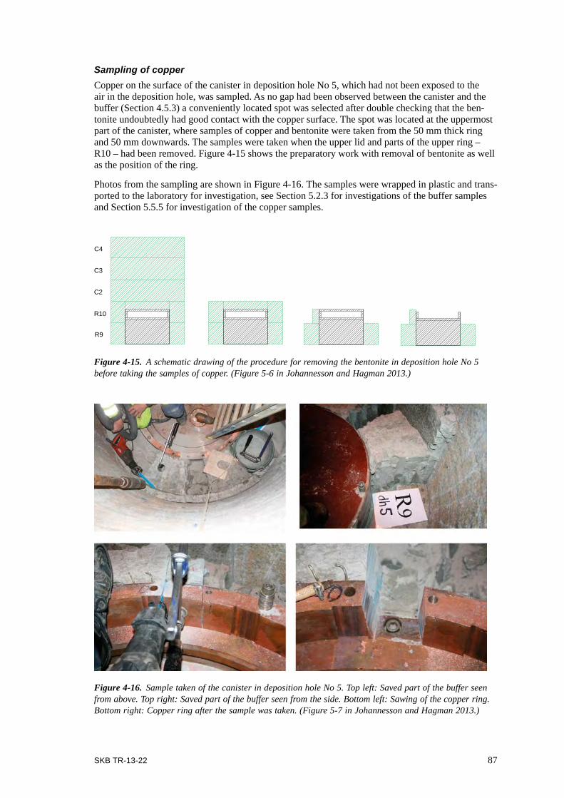
SKB TR-13-22 87

Sampling of copperCopper on the surface of the canister in deposition hole No 5, which had not been exposed to the air in the deposition hole, was sampled. As no gap had been observed between the canister and the buffer (Section 4.5.3) a conveniently located spot was selected after double checking that the ben-tonite undoubtedly had good contact with the copper surface. The spot was located at the uppermost part of the canister, where samples of copper and bentonite were taken from the 50 mm thick ring and 50 mm downwards. The samples were taken when the upper lid and parts of the upper ring – R10 – had been removed. Figure 4-15 shows the preparatory work with removal of bentonite as well as the position of the ring.

Photos from the sampling are shown in Figure 4-16. The samples were wrapped in plastic and trans-ported to the laboratory for investigation, see Section 5.2.3 for investigations of the buffer samples and Section 5.5.5 for investigation of the copper samples.

Figure 4-15. A schematic drawing of the procedure for removing the bentonite in deposition hole No 5 before taking the samples of copper. (Figure 5-6 in Johannesson and Hagman 2013.)

Figure 4-16. Sample taken of the canister in deposition hole No 5. Top left: Saved part of the buffer seen from above. Top right: Saved part of the buffer seen from the side. Bottom left: Sawing of the copper ring. Bottom right: Copper ring after the sample was taken. (Figure 5-7 in Johannesson and Hagman 2013.)

R9

R10

C2

C3

C4

88 SKB TR-13-22

Once the canisters had been retrieved, they were transported to the Canister Laboratory in Oskarshamn. Besides surface sampling of films on the copper metal, core samples were taken at six positions on each canister. Figure 4-17 shows the core drilling machine attached to one of the canisters. The drill-ing penetrated the full 50 mm thickness of the copper shell.

4.5.3 Sampling of cablesThe damaged parts of the cables were taken care of and sent to the laboratory for examination. The results of these examinations are presented in Section 5.7.

4.5.4 Observations The surfaces of the copper canisters were observed to be partly covered with corrosion products. This was expected with respect to the existence of oxygen and sulfur in combination with micro-organisms (Lydmark 2011). Sampling and later laboratory analysis verified that this was correct (Sections 5.5.5 and 5.6.3).

The problem with the heaters, especially the heater elements in the canister in deposition hole No 6, had puzzled the project staff. When freeing the top part of this particular canister the large damage observed on the cables close to the canister, e.g. see Figure 4-18, became the most likely cause of the problem. There the cables had been stretched and bent to their breakpoint and so heavily damaged that their isolation had been broken at several places, where water could have access in to the electrical wires and shorting them. The water could then also flow along the conductors into the canister. Burns showed that some wires had come too close together, probably by stretching, and been shorted.

Figure 4-17. Sampling of the canister in deposition hole No 6 by drilling of 28 mm cores through the 50 mm thick copper shell. (Figure 2-2 in Taxén et al. 2012.)

SKB TR-13-22 89

4.6 Retrieval of copper electrodesThree nominally identical copper electrodes had been installed in block C4 in deposition hole No 5 (see position of the block in 2-16). The purpose was to measure copper corrosion on them on-line during operation, see Section 2.6.10 and Rosborg (2013a).

4.6.1 ObjectivesThe electrodes were uncovered and retrieved with the objectives to first check the prevailing cor-rosion environment around the electrodes and then retrieve them for analyses of possible extent of corrosion and type of corrosion products that had been formed on their surfaces.

4.6.2 Measurement of in situ corrosion potential When part of the concrete plug to the outer section of the repository had been removed the corrosion potential was measured. A second measurement was made when the backfill in the tunnel had been removed. Further measurements were made in the laboratory after retrieval of the package with the electrodes embedded in the bentonite (the retrieval is described in Section 4.6.3). The results from all these measurements are presented in Section 5.6.

4.6.3 Retrieval methodologyThe retrieval was made by seam drilling, i.e. drilling small diameter holes close to each other in the bentonite around the three electrodes. When the drilling had been completed the whole block of bentonite with the electrodes was broken loose by bending and lifted up to the tunnel floor, see Figure 4.19, and immediately packed in triplicate evacuated tri-laminate bags.

The retrieved package of electrodes and surrounding buffer (see Figure 4-19) was sent to the laboratory, where further measurement were made on corrosion potential (Section 5.6.2) before the bentonite was removed and the electrodes’ surfaces examined (Section 5.6.3).

4.6.4 Observations The retrieved block with electrodes surrounded by bentonite was in good shape, and the contact with the three electrodes were excellent.

Figure 4-18. Left: Damages observed close to the periphery of the canister. Right: Damages observed where the cables were going through the lower canister lid. (Figure 4-8 in Johannesson and Hagman 2013.)

90 SKB TR-13-22

4.7 Rock examinationsThe tunnel and deposition holes were inspected after excavation of backfill respectively buffer with respect to visible damages and water inflows.

4.7.1 ObjectivesThe objective with the inspection was to determine if any spalling had occurred in the deposition holes and if the pattern of water bearing fractures and total water inflow rates had changed during the seven years of operation.

4.7.2 Damage to the rock wall in the deposition holes The inspection revealed that no visible damage to the rock had happened along the deposition holes’ walls or in the uppermost part of the deposition holes at the tunnel floor.

4.7.3 Damage to the rock close to the deposition holes It was concluded based on thermo-mechanical (T-M) modeling that the risk for stress induced spall-ing during the thermal phase was very small, but that the maximum tangential stresses were close to the limit to induce spalling (Section 6.2.4). The concentration of AE events (Figure 2-42) or change in UV at the perimeter of the deposition holes during the heating phase (Haycox 2011) could not be correlated to spalling. The deposition hole wall in the areas with “high” frequency of acoustic events showed solid rock. The highest density of events was in the order of a few events per dm3. It was not possible to correlate the position of events to any of the mapped fractures in deposition holes and

Figure 4-19. Removal of the copper electrodes installed in block C4 in deposition hole No 5. Position of the block is shown in Figure 2-14. Top left: Core used for the drilling. Top right. Seam drilling around the electrodes. Bottom left: Electrodes together with the bentonite lifted up from the deposition hole. Bottom right: Bentonite and electrodes wrapped in plastic. (Figure 5-2 in Johannesson and Hagman 2013.)

SKB TR-13-22 91

in the tunnel. The resolution in either the fracture mapping or the source location capability might be too low, or the events occurred as small micro-cracks in solid rock with more localized stress concentration.

The small possibility of finding spalling made it doubtful to be able to verify that spalling actually had taken place by sampling the rock for observation of micro-cracks. There was an obvious risk that core drilling into high-stress areas around the deposition hole would cause as much damage to the rock as the heating. This condition led to the decision not to take any rock samples.

4.7.4 Inflows to tunnel and deposition holes Inflow to tunnel in outer sectionIt was easy to identify water bearing fractures in the tunnel directly after removal of the backfill. There was a dusty layer of clay from the backfill on the tunnel contour. This clay absorbed and spread out the seepage over an area around the fractures. However, this made it difficult to com-pare the distribution of inflow along individual fractures to the observations directly after tunnel excavation. It was concluded that the distribution of flowing fractures that intersect the tunnel was unchanged, but the distribution of inflow along individual fractures was difficult to assess. It should, however, be noticed that the tunnel was excavated and mapped in 1995 and the installation of the backfill was made 2003. And there was no re-mapping of the inflow distribution close to backfilling of the tunnel.

Inflow to deposition holes No 5 and No 6.It was not possible to observe any visible inflow to the deposition holes after removal of the buffer. One likely cause could have been that the rather extensive ventilation required, when working down in the deposition holes, dried out the rock. Other causes could have been that bentonite was pressed into open fractures, or that the swelling pressure closed fractures. The total inflow to the deposition holes was estimated by measuring the inflow to a dry deposition hole. The holes were pumped dry and inflow was allowed for a week. The height of the water table from the deposition hole bottom was measured and the inflow was calculated based on that reading and the known diameter of the deposition holes. This value was compared to the volume pumped out. The process was repeated three times and the mean value of three readings was used.

The results are presented in Table 4-2 and compared with the measurements made in year 2000, see also Table 2-2. The reason for the decrease is unknown. The processes in the deposition holes such as THM-induced closure of fractures or clogging of swelling bentonite in the deposition holes may be possible explanations. But, it was also noticed that the excavation and grouting project in the nearby Tass tunnel (see location in Figure 2-4), that was started in March 2007, had an influence on all hydro-monitored drill holes around the Prototype Repository (Rhén and Forsmark 2015) see examples in Figures 2-44 and 2-45. (See also discussion in Section 6.1.8.)

Table 4-2. Inflow to the deposition holes before and after seven years of operation.

Borehole March 2000 L/min January 2013 L/min

DA3551G01 (#5) 0.0015 0DA3545G01 (#6) 0.0027 0.0005

4.8 Retrieval of sensorsSensors had been installed in the rock, the buffer and the backfill as described in Section 2.5.7, and they were intended to be retrieved during removal and sampling of the backfill and the buffer. But, the retrieval of them got a low priority when the Project actually was planned. The final result is described by Nilsson (2014) and Wieczorek et al. (2014), and summarized below in this section.

92 SKB TR-13-22

4.8.1 ObjectivesThe objective was:

• To remove as many of the installed sensors in the outer section as possible.

• To harm the sensors as little as possible during retrieval.

• To send the retrieved sensors to surface laboratories for examination of damages and checking of the reliability of the data the sensors had delivered.

• To obey the premises that the efficient removal and sampling of backfill and buffer had priority over the retrieval of sensors.

4.8.2 Sensors in backfillIn total 89 sensors and two geoelectric arrays with 72 electrodes had been installed in the backfill for measurement of water content and backfill density, see Table 4-3. Out of the 89 sensors only 21 could be retrieved because heavy equipment was used for the removal of the backfill as explained in Section 4.3.2. Of these 21 only 16 were in the shape needed for the validation test (Section 5.8). The result from these tests has been reported by Nilsson (2014) and is summarized in this report in Section 5.8.2.

Some of the installed electrodes for measuring the resistivity in the backfill (Rothfuchs et al. 2003) were retrieved from the backfill on top of deposition hole No 6 by manual freeing them from the swollen backfill. The backfill electrodes were sent to GRS’s laboratory for inspection. The results from this work have been reported by Wieczorek et al. (2014) and summarized in this report in Section 5.8.3. The opening and retrieval did not disturb the performance of the electrode array in the inner section, which continues to provide on-line data from the backfill state of saturation.

Although the priority at the excavation was to remove the backfill as fast as possible and in a safe way, some effort was made to take care of the installed sensors. Of special importance was the small cups installed in the backfill. Three out of four installed were found. The cups were retrieved with some backfill material in order to secure that the collected water would not leak from the cup. The samples were then analyzed in the laboratory. The results from these analyses have been described by Arlinger et al. (2013).

4.8.3 Sensors in bufferIn total 173 sensors and two geoelectric arrays had been installed in the buffer for measurement of water content and buffer density, see Table 4-3. Out of the 173 sensors only 52 could be retrieved. The reason for this was that all the cables from the sensors were led through titanium tubes. These tubes had to be cut as the work with the sampling and removal of the buffer progressed, which damaged some of the sensors. The core drilling through the bentonite blocks also caused damages on the sensors. Of the 52 retrieved sensors only 27 were in the shape needed for the validation test (Section 5.8). They were saved and checked afterwards. None of the installed RH sensors could be checked. There were several reasons for that. One was that once water has entered the sensor, i.e. the RH has reached 100%, it stopped functioning. Another reason was that for one type of sensors (Vaisala) some of its electronic components were installed some 10 meters from the sensor, i.e. in the backfill in a water tight vessel. It became obvious at the retrieval of the vessels that some of them were not watertight and thus water inside the vessel had caused failure of the sensor. The result of the examination of the retrieved sensors has been reported by Nilsson (2014) and is summarized in Section 5.8.2.

Two of the electrode chains in the upper part of deposition hole No 5 were retrieved by overcoring. In connection with this work samples were also taken for determining the water content and density of the material close to the electrodes. Sections of the buffer cores were sent to GRS’s laboratory for inspection. The result from these tests has been reported by Wieczorek et al. (2014) and is summa-rized in Section 5.8.3.

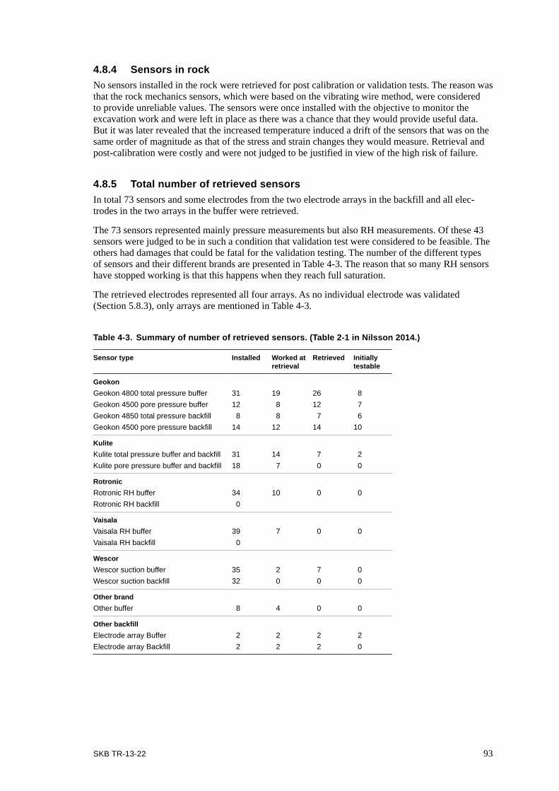
SKB TR-13-22 93

4.8.4 Sensors in rockNo sensors installed in the rock were retrieved for post calibration or validation tests. The reason was that the rock mechanics sensors, which were based on the vibrating wire method, were considered to provide unreliable values. The sensors were once installed with the objective to monitor the excavation work and were left in place as there was a chance that they would provide useful data. But it was later revealed that the increased temperature induced a drift of the sensors that was on the same order of magnitude as that of the stress and strain changes they would measure. Retrieval and post-calibration were costly and were not judged to be justified in view of the high risk of failure.

4.8.5 Total number of retrieved sensorsIn total 73 sensors and some electrodes from the two electrode arrays in the backfill and all elec-trodes in the two arrays in the buffer were retrieved.

The 73 sensors represented mainly pressure measurements but also RH measurements. Of these 43 sensors were judged to be in such a condition that validation test were considered to be feasible. The others had damages that could be fatal for the validation testing. The number of the different types of sensors and their different brands are presented in Table 4-3. The reason that so many RH sensors have stopped working is that this happens when they reach full saturation.

The retrieved electrodes represented all four arrays. As no individual electrode was validated (Section 5.8.3), only arrays are mentioned in Table 4-3.

Table 4-3. Summary of number of retrieved sensors. (Table 2-1 in Nilsson 2014.)

Sensor type Installed Worked at retrieval

Retrieved Initially testable

GeokonGeokon 4800 total pressure buffer 31 19 26 8Geokon 4500 pore pressure buffer 12 8 12 7Geokon 4850 total pressure backfill 8 8 7 6Geokon 4500 pore pressure backfill 14 12 14 10

KuliteKulite total pressure buffer and backfill 31 14 7 2Kulite pore pressure buffer and backfill 18 7 0 0

Rotronic Rotronic RH buffer 34 10 0 0Rotronic RH backfill 0

Vaisala Vaisala RH buffer 39 7 0 0Vaisala RH backfill 0

WescorWescor suction buffer 35 2 7 0Wescor suction backfill 32 0 0 0

Other brandOther buffer 8 4 0 0

Other backfillElectrode array Buffer 2 2 2 2Electrode array Backfill 2 2 2 0

SKB TR-13-22 95

5 Laboratory program and examinations

The performance and the results of the laboratory examinations are described in this chapter. The scope of the work was to determine the actual density and water content of the backfill and the buffer, characterize the chemical environment in the buffer and backfill, investigate whether any chemical/mineralogical or hydro-mechanical changes had taken place in the buffer and backfill materials, and study the occurrence of microorganisms. The laboratory work program also included studies of the changes of the canister geometries, conditions and causes of failure of cables to heaters and the reliability of the sensor readings made during the seven years of operation.

Furthermore, inspections and laboratory examinations were performed on the two retrieved canisters, on 33 selected sensors, on some selected geoelectric electrodes, on one copper electrode from inside a buffer block in deposition hole No 5 and on the heater cables.

5.1 Density and water content in backfill and buffer 5.1.1 ObjectivesThe samples taken during removal of the backfill and buffer were sent to the Äspö Geolaboratory on the surface at the Äspö HRL with the objective to determine water content and density under known and controlled atmospheric condition.

5.1.2 ProcedureThe determination of the water content and density of samples taken from both the backfill and the buffer was made within 48 hours after the sample had been taken from the site in order to minimize the risk of drying the sample and changing its water content and density. The water content (w) was determined by drying the samples in an oven at a temperature of 105°C for 24 hours. The bulk density (ρbulk) was determined by weighing the samples in air and submerged in paraffin oil with known density. The two methods have been described in detail by Johannesson and Hagman (2013). From the determined water content and bulk density the dry density (ρdry), the degree of saturation (Sr) and the void ratio (e) could be determined, see equation 5-1 to 5-3.

)1( wbulk

dry += ρρ (5-1)

bulks

wsbulkr w

wSρρ

ρρρ−+×

××=)1(

/ (5-2)

rwbulk

bulks

Se

×−−=

ρρρρ

(5-3)

The calculations of the parameters were made with the assumption that the solid bentonite particles had a density of 2,780 kg/m3 and the crushed rock particles a solid density of 2,650 kg/m3 (solid density of sand).

5.1.3 BackfillIn tunnelDry density and degree of saturation of the backfill in the tunnel were calculated with the data from the measurement of water content and density (the measurements are presented in Section 5.1.3). About 100 determinations of water content and density were made in each of the eleven investigated sections of the tunnel (the determinations are presented in Section 4.3). The results were plotted as contour plots, as shown in Figure 5-1 for section No 9 (section position is shown in Figure 4-5). The data from all eleven sections have been presented by Johannesson (2014). The plots indicate that the backfill had a low density and high water content close to the rock surface, especially close to the roof. The plots of the degree of saturation indicate that there were some spots which had a divergent value compared to surrounding parts.

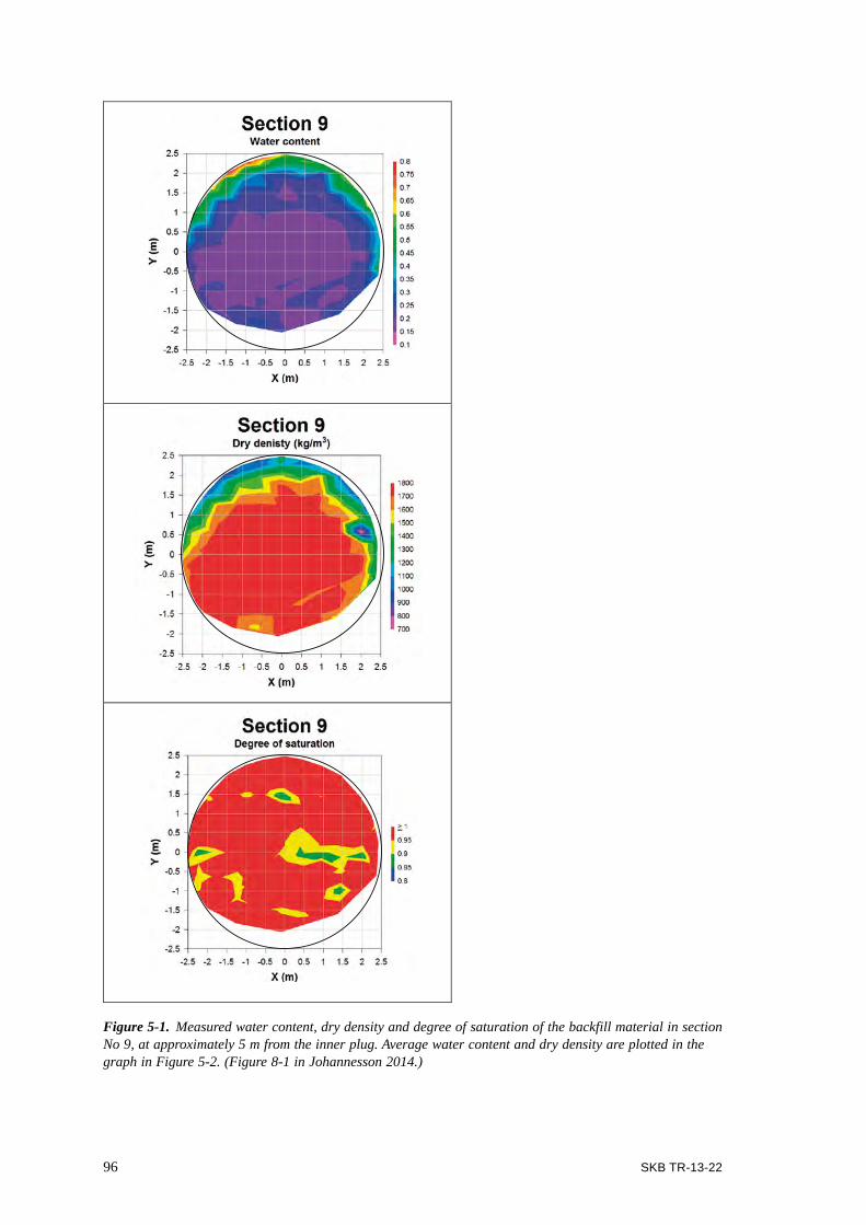
96 SKB TR-13-22

Figure 5-1. Measured water content, dry density and degree of saturation of the backfill material in section No 9, at approximately 5 m from the inner plug. Average water content and dry density are plotted in the graph in Figure 5-2. (Figure 8-1 in Johannesson 2014.)

SKB TR-13-22 97

This can be explained by the fact that the backfill material at removal was rather heterogeneous and the degree of saturation was calculated from the measurement of water content and density, which were determined on two different samples although they both were taken from the same spot in the backfill.

From the measurements on the investigated sections (see Figure 4-5) average density, water content and degree of saturation were calculated. The data from these calculations are shown in Table 5-1 and Figure 5-2. They indicate that the backfill was fully saturated on average and that there was a tendency of increased dry density towards the outer plug, which also was observed during the installation (Johannesson et al. 2004). Furthermore, the average dry densities were significantly lower than the density measured at the installation (Johannesson et al. 2004). A probable explanation to this is that the density was not measured directly at the installation. Instead a nuclear gauge probe and a penetrometer were used for interpretation of the density of the filling. These instruments and how they were used have been described by Johannesson et al. (2004).

The dry densities measured close to the roof were low (< 1,000 kg/m3), see the example in Figure 5-1. This low density was not expected from the determinations made during the installation, because the density could at that time only be measured as close as about 0.5 m from the tunnel wall. It is there-fore possible that the low density close to the roof also was present at the installation. No evidence of piping and erosion was observed in any part of the backfill at the retrieval, as commented on in Section 4.3.5.

When comparing these results with the required properties in a final repository (Section 2.5.5) it is obvious that the Prototype Repository material, installed with in situ compaction technique, did not meet the minimum dry density criterion of 1,850 kg/m3 for providing a sufficiently low hydraulic conductivity. The margin to the acceptable level is too large for any other interpretation of the result obtained by the Project. The upwards swelling of the top bentonite block, however, has not exceeded the stipulated 2, which is commented on in Section 2.5.5.

Figure 5-2. Average density and water content of the backfill material as function of the distance from the inner plug. (Figure 8-2 in Johannesson 2014.)

1,500

1,550

1,600

1,650

1,700

0.20

0.25

0.30

0.35

0 5 10 15 20

Dry

Den

sity

(kg/

m3 )

Ave

rage

wat

er c

onte

nt (–

)

Distance from inner plug (m)

Water content

Dry density

98 SKB TR-13-22

Table 5-1. Average water content, dry density, void ratio and degree of saturation for the eleven investigated sections and the backfill towards the two plugs. The averages are based on about 100 determinations in each section. (Layer No 7 was located above deposition hole No 6 and was only sampled up to the chainage just passed the deposition hole; consequently its center point was marked closer to the outer plug than that of the layer No 6. The last layer, No 11, hit the inner plug half way up; consequently this layer got its center point marked further away from the plug than that of the layer No 10.) (Table 8-2 in Johannesson 2014.)

Section No Average distance from the inner plug

m

Water content

weight %

Dry density

kg/m3

Void ratio Degree of saturation

%

Plug 2 20.0 0.23 1,690 0.62 1001 18.0 0.24 1,653 0.65 992 17.0 0.26 1,623 0.68 1013 16.0 0.27 1,581 0.74 984 14.5 0.24 1,655 0.65 1005 12.5 0.25 1,639 0.67 1006 10.0 0.26 1,593 0.72 987 10.5 0.23 1,666 0.62 998 7.0 0.28 1,583 0.75 989 5.0 0.29 1,567 0.77 10010 3.0 0.28 1,575 0.78 9911 4.0 0.26 1,591 0.71 99Plug 1 0.0 0.30 1,570 0.80 99

In deposition holes

At the installation of the Prototype Repository, the upper one meter of the deposition holes (see Figure 2-14) was filled with backfill material. At the retrieval samples were taken of also this part of the backfill. The mean values and standard deviations of the density and water content of the backfill inside the two deposition holes both at the installation and at the retrieval are summarized in Table 5-2. The filling inside the deposition holes had an initial height of about one m. From the measured average density it was possible to make a rough calculation of the compression of the backfill inside the deposition holes caused by the upward swelling of the buffer. The outcomes from these calculations are also shown in Table 5-2.

The figures indicate that the deformations of the backfill inside the two deposition holes were small compared to the observed deformation of the upper surface of the bentonite (153 mm in deposition hole No 5 and 176 mm in deposition hole No 6, as shown in Figures 4-10 and 4-11). Thus most of the compression of the backfill was located to the backfill in the tunnel.

Table 5-2. The mean values (Mean) and standard deviation (Stdev) of the dry density and water content of backfill material inside the two deposition holes in the outer section. (Table 8-1 in Johannesson 2014.)

At installation At retrieval

Deposition hole Dry density (kg/m3)

Water content Dry density (kg/m3)

Water content Deformation

Mean Stdev Mean Stdev Mean Stdev Mean Stdev

DA3545G01 (Dh 6) 1,770 84 0.150 0,018 1,796 57 0.180 0.019 ~ 14 mmDA3551G01 (Dh 5) 1,830 82 0.128 0,015 1,814 70 0.178 0.023 0 mm

5.1.4 BufferThe measurements of the water content and density of the buffer in the two deposition holes have been described in detail by Johannesson (2014) and Wieczorek et al. (2014). Johannesson (2014)

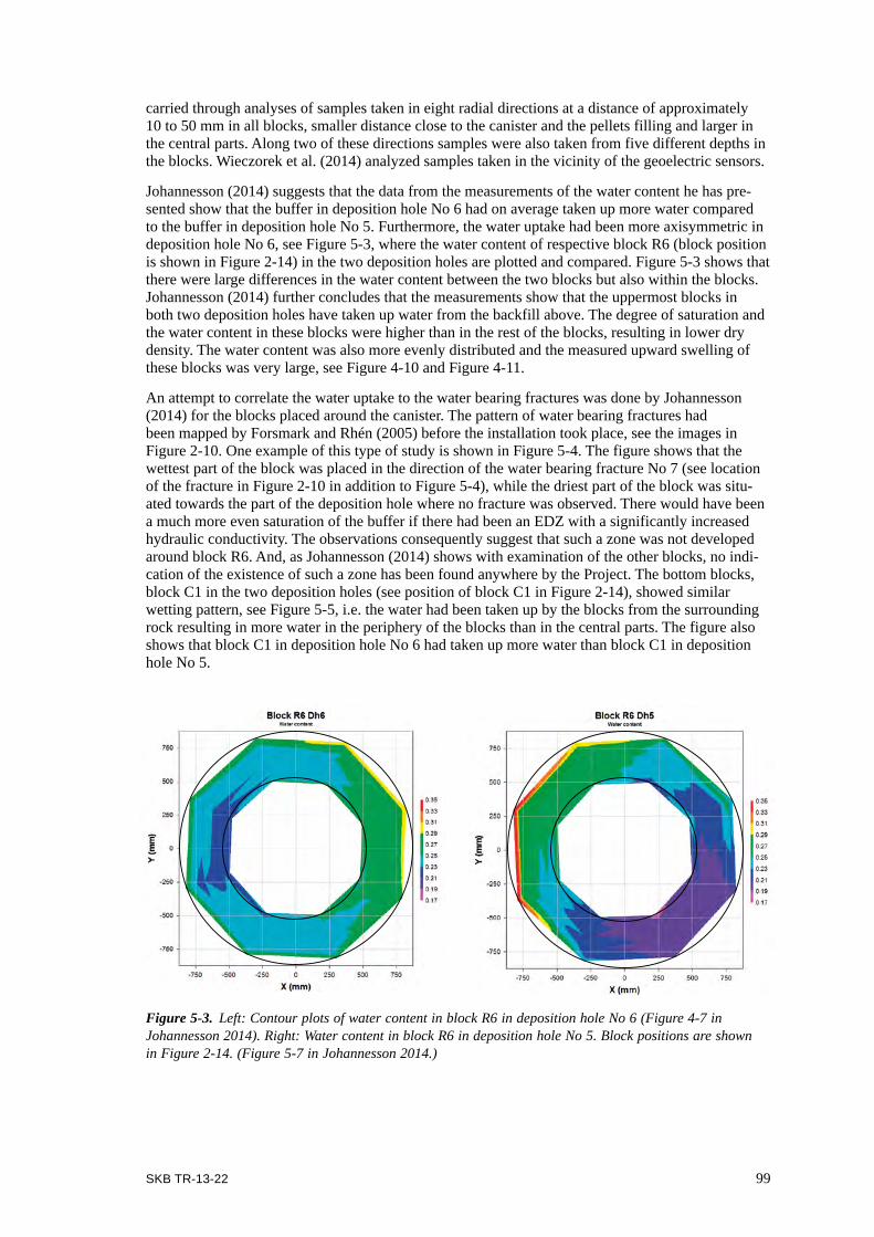
SKB TR-13-22 99

carried through analyses of samples taken in eight radial directions at a distance of approximately 10 to 50 mm in all blocks, smaller distance close to the canister and the pellets filling and larger in the central parts. Along two of these directions samples were also taken from five different depths in the blocks. Wieczorek et al. (2014) analyzed samples taken in the vicinity of the geoelectric sensors.

Johannesson (2014) suggests that the data from the measurements of the water content he has pre-sented show that the buffer in deposition hole No 6 had on average taken up more water compared to the buffer in deposition hole No 5. Furthermore, the water uptake had been more axisymmetric in deposition hole No 6, see Figure 5-3, where the water content of respective block R6 (block position is shown in Figure 2-14) in the two deposition holes are plotted and compared. Figure 5-3 shows that there were large differences in the water content between the two blocks but also within the blocks. Johannesson (2014) further concludes that the measurements show that the uppermost blocks in both two deposition holes have taken up water from the backfill above. The degree of saturation and the water content in these blocks were higher than in the rest of the blocks, resulting in lower dry density. The water content was also more evenly distributed and the measured upward swelling of these blocks was very large, see Figure 4-10 and Figure 4-11.

An attempt to correlate the water uptake to the water bearing fractures was done by Johannesson (2014) for the blocks placed around the canister. The pattern of water bearing fractures had been mapped by Forsmark and Rhén (2005) before the installation took place, see the images in Figure 2-10. One example of this type of study is shown in Figure 5-4. The figure shows that the wettest part of the block was placed in the direction of the water bearing fracture No 7 (see location of the fracture in Figure 2-10 in addition to Figure 5-4), while the driest part of the block was situ-ated towards the part of the deposition hole where no fracture was observed. There would have been a much more even saturation of the buffer if there had been an EDZ with a significantly increased hydraulic conductivity. The observations consequently suggest that such a zone was not developed around block R6. And, as Johannesson (2014) shows with examination of the other blocks, no indi-cation of the existence of such a zone has been found anywhere by the Project. The bottom blocks, block C1 in the two deposition holes (see position of block C1 in Figure 2-14), showed similar wetting pattern, see Figure 5-5, i.e. the water had been taken up by the blocks from the surrounding rock resulting in more water in the periphery of the blocks than in the central parts. The figure also shows that block C1 in deposition hole No 6 had taken up more water than block C1 in deposition hole No 5.

Figure 5-3. Left: Contour plots of water content in block R6 in deposition hole No 6 (Figure 4-7 in Johannesson 2014). Right: Water content in block R6 in deposition hole No 5. Block positions are shown in Figure 2-14. (Figure 5-7 in Johannesson 2014.)

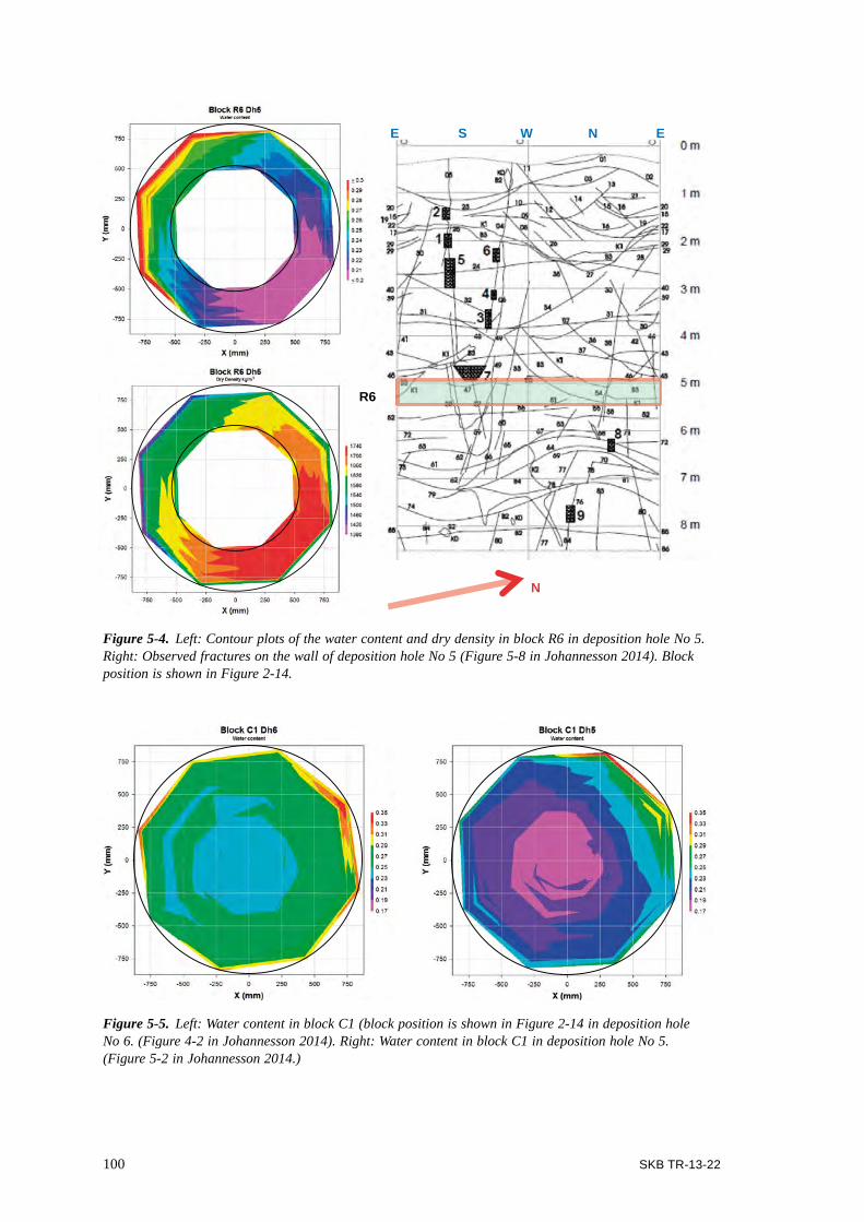
100 SKB TR-13-22

Figure 5-4. Left: Contour plots of the water content and dry density in block R6 in deposition hole No 5. Right: Observed fractures on the wall of deposition hole No 5 (Figure 5-8 in Johannesson 2014). Block position is shown in Figure 2-14.

Figure 5-5. Left: Water content in block C1 (block position is shown in Figure 2-14 in deposition hole No 6. (Figure 4-2 in Johannesson 2014). Right: Water content in block C1 in deposition hole No 5. (Figure 5-2 in Johannesson 2014.)

R6

E EW NS

N

SKB TR-13-22 101

The different rock conditions indicated by AE and UV measurements in Section 2.5.2 suggested an increased fracturing of the rock around deposition hole No 6, but not around deposition hole No 5. This could be one part of the explanation why the buffer in deposition hole No 6 has a higher degree of saturation than the buffer in deposition hole No 5, if the global water supply to both holes was equal. The uneven wetting of the buffer that Johannesson (2014) found, however, suggests that the water uptake was correlated to the position of fractures by the clear difference between buffer saturation close to fractures and buffer saturated far away from fractures. This finding underpins the comment on the insignificant importance some events that AE and UV measures had on the wetting process of the buffer and the backfill (Section 2.6.7).

Wieczorek et al. (2014) reports that buffer core samples were taken at different positions, as indicated in Figure 5-6. The water content of the samples was determined by drying at 105°C. The measured water content is shown color coded in Figure 5-6; the actual values are given in Table 5-3. All results were in the range between 21.5% by weight and 23.7% by weight of water. The core close to the deposition hole wall was somewhat wetter than the central core, which would be expected if the buffer was saturated from the deposition hole wall.

The results are in good agreement with the result of the water content analyses performed by Johannesson (2014), whose results for the upper buffer of deposition hole No5 are summarized in Figure 5-7. The results presented by Wieczorek et al. (2014) of around 22% by weight of water in the center (marked with a small blue circle in Figure 5-7) blend in very well. The same holds for the values around 23 % by weight of water close to the deposition hole wall (blue oval in Figure 5-7), taking into account that the core originates from 180° azimuth.

While water content was very inhomogeneous around the deposition hole perimeter, the values for 180° azimuth are in good agreement with Johannesson’s (2014) results for 205°.

Figure 5-6. Positions of samples for water content analysis with color coded results. (Figure 8.5 in Wieczorek et al. 2014.)

Central core sample Core sample near borehole wall

Water content in wt.%

W1

W2W3

W4

W5

W6

C1

C2

C3

C4

C5

C6

C7

C8

102 SKB TR-13-22

Table 5-3. Measured water content of buffer core samples. Sample positions are shown in Figure 5-6. (Table 8.1 in Wieczorek et al. 2014).

Buffer core Sample Water content [% by weight]

Near borehole wall W1 23.7W2 23.3W3 23.2W4 22.0W5 23.2W6 22.4

Near Center C1 22.0C2 22.7C3 22.7C4 21.5C5 22.3C6 22.2C7 22.2C8 21.8

Figure 5-7. Johannesson’s (2014) results for water content and saturation of the upper buffer of deposition hole No 5, with supplement of Wieczorek et al.’s water content values for the buffer cores. (Figure 8.6 in Wieczorek et al. 2014.)

Water uptake in block C2 Dh5

0.10

0.15

0.20

0.25

0.30

0.35

0.40

0.45

0 200 400 600 800 1,000

Wat

er c

onte

nt (–

)

Radius (mm)

2570115160205250295340Initial condition

Dh5 Block C2

Rock

Pellets

0.70

0.75

0.80

0.85

0.90

0.95

1.00

0 200 400 600 800 1,000

Deg

ree

of s

atur

atio

n (–

)

Radius (mm)

2570115160205250295340Initial condition

Dh5 Block C2

Rock

Pellets

B, 90° D, 270°

A, 0°

C, 180°

25°

45°

20°

25°

45°

20° 25°

45°

20°

25°

45°

20°

SKB TR-13-22 103

5.2 Chemical and mineralogical characterization of backfill and buffer

The development of the chemical environment in buffer and backfill is mainly determined by the type of saturating groundwater, microbial activity and the chemical/mineralogical processes in the bentonite. This development is reflected by the chemical composition of pore water and gases in the rock, buffer and backfill. Their combined impact on the bentonite’s safety function properties is important to know as they may affect key properties such as: hydraulic conductivity, swelling pressure, unconfined compressive strength and shear strength. The properties and especially the long term assessment of them were examined more indirectly by studying the bentonite’s chemical and mineralogical composition.

5.2.1 ObjectivesSeveral aspects, relevant for the long term safety of the final repository, were identified in the Prototype Repository’s Test Plan by Puigdomenech and Pedersen (1999). They considered that the following issues were of importance in an opening and retrieval project:

• Mineralogical and chemical sampling of bentonite buffer.

• Comparison of CEC and the mineralogy at start and end of the test.

• Analysis of salt deposits as a result of the thermal gradient.

• The redox components: Fe(II)/Fe(III) ratio in clay, organic material and pyrite oxidation.

• Determination of migration of copper into the bentonite and possible formation of secondary copper mineral.

• (Evaluation of possible tracer migration experiments carried out.)

• Characterization of the surface of the copper canister: Evidence of local corrosion.

• Analysis of survival for naturally present, and possibly added, microorganisms.

• (Evaluation of the cellulose degradation test.)

• Analysis of possible sulfate reduction.

• Analysis of the concrete plug dissolution and pH gradients in the bentonite caused by the concrete.

Most of these issues have been addressed in the Project. Some issues (the ones within parenthesis) have been considered to be of no or low interest and have instead been replaced by other more important investigations. No tracers were installed, so no work on this topic could be performed. The degradation of the cellulose packages was initiated by work on low and intermediate level waste, and was consequently not of interest to any work supporting a high-level waste repository. Also no work on the degradation of the concrete plug was done. However, the bentonite in contact with the plug was tested. Investigation of the hydro-mechanical properties of the bentonite buffer was added, due to the direct importance of both the swelling pressure and hydraulic conductivity on the bentonite’s barrier properties.

A strategy during the excavation was to make some very early analysis by SKB staff of some of the main identified issues serving as a guideline for the upcoming work. The mineralogical content, identification of salt precipitates and the Fe-redox chemistry were selected. On May 13, 2011 the first buffer sample in contact with the canister in deposition hole No 6 was excavated.

These samples were analyzed for iron and copper redox properties within the following five days in Lund, and the mineralogical content and salt precipitates were analyzed within the next three weeks. The early iron redox results made it possible to add additional analysis to the analytical program (e.g. wet chemical analysis of Fe(II) in bentonite). They also had an impact on the design of the Alternative Buffer Material packages 4-6 (ABM45) experiment (SKB 2012) that was installed in November 2012 (by the addition of copper inserts), and on the latest SKB research and demonstra-tion program (SKB 2013), with increased focus on bentonite properties connected to the iron redox conditions. More detailed results are present in the report focusing only on bentonite analysis of buffer and backfill (Olsson et al. 2013).

104 SKB TR-13-22

5.2.2 Sampling and marking of samplesThe main part of the analyses was performed on samples obtained by dividing selected “large sectors” (see Sections 4.3 and 4.4 on removal and sampling of backfill and buffer), which were sawn horizontally into five approximately 100 mm thick samples labelled A (at the top) to E (at the bottom). These pieces were thereafter cut along the block radius into approximately 20 mm thick samples, which were marked and recorded. In order to increase the resolution, samples proximal to the canister were divided into thinner sub-samples.

Block material for Mössbauer and X-ray absorption near edge structure (XANES) analyses required handling and sampling under oxygen-free conditions and was packed in vacuum-sealed aluminum-polymer bags as rapidly as possible after the sampling. Further sampling was done in inert atmosphere in a glove box, where the exposed block surfaces were removed before the samples for analyses were taken.

Samples for the hydro-mechanical tests were cored from the “large sectors”. Most of these samples had a diameter of 35 mm, but samples taken close to the canister had a diameter of 20 mm.

The denomination of a sample (center of a volume) was made in accordance to the following example:

P5R06 032A 535b where:

P5 material from Prototype Repository deposition hole No 5,

R06 block number (R for ring-shaped blocks, C for massive cylinders),

032 azimuth direction (degrees),

A vertical level in the block (A at the top, E at the bottom),

535 radial distance in mm from the center of the canister,

b bulk material (alt. c=the fine clay fraction).

Reference material (non-compacted bentonite saved in conjunction with manufacturing) for a specific block was labeled according to the following example:

P5R06 Rb where:

P5 Prototype Repository deposition hole No 5,

R06 block number,

R reference material,

b bulk material (alt. c=the fine clay fraction).

5.2.3 Chemical and mineralogical analyses of buffer bentonite Visual appearance of the samplesMost of the compacted bentonite was fully intact with no visual cracks. The surface facing the copper canister had a dark discoloration. Sometimes a white precipitate could be seen as a powder or small hair-like crystals (Figure 5-8). The innermost 5–10 mm of the bentonite was darker, and this difference irreversibly disappeared upon drying in air for 13 days (Figure 5-9).

Soluble salts, EC, CEC and chemical composition Two of the objectives (Section 5.2.1) were comparison of CEC and analysis of salt deposits as a result of the thermal gradient. The CEC is an important indicator of montmorillonite content, hence indirectly an important parameter for the long-term safety function of the bentonite buffer. Accu-mulation of salt (e.g. gypsum from the bentonite starting material) is expected to occur in the early stage of the repository and is expected to equilibrate with the surrounding natural water with time. In original bentonite several more or less water soluble salts are normally present, typically as sulfates and carbonates (Karnland et al. 2006). During the water saturation the bentonite interacted with the Äspö groundwater (Table 5-4), hence transporting water soluble phases towards the copper canister,

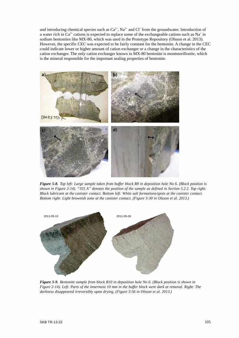
SKB TR-13-22 105

and introducing chemical species such as Ca2+, Na2+ and Cl– from the groundwater. Introduction of a water rich in Ca2+ cations is expected to replace some of the exchangeable cations such as Na+ in sodium bentonites like MX-80, which was used in the Prototype Repository (Olsson et al. 2013). However, the specific CEC was expected to be fairly constant for the bentonite. A change in the CEC could indicate lower or higher amount of cation exchanger or a change in the characteristics of the cation exchanger. The only cation exchanger known in MX-80 bentonite is montmorillonite, which is the mineral responsible for the important sealing properties of bentonite.

Figure 5-8. Top left: Large sample taken from buffer block R8 in deposition hole No 6. (Block position is shown in Figure 2-14). “355 A” denotes the position of the sample as defined in Section 5.2.2. Top right: Black lubricant at the canister contact. Bottom left: White salt formations/spots at the canister contact. Bottom right: Light brownish zone at the canister contact. (Figure 3-30 in Olsson et al. 2013.)

2011-05-262011-05-13

Figure 5-9. Bentonite sample from block R10 in deposition hole No 6. (Block position is shown in Figure 2-14). Left: Parts of the innermost 10 mm in the buffer block were dark at removal. Right: The darkness disappeared irreversibly upon drying. (Figure 3-56 in Olsson et al. 2013.)

106 SKB TR-13-22

Chloride was found to increase in all the bentonite samples in both deposition hole No 5 and depo-sition hole No 6 (Olsson et al. 2013) as shown in Figure 5-10. This was expected as the monitored chemistry of the corresponding Äspö water (Olsson et al. 2013, Table 1-1) shows high chloride levels (approximately 200 mM). Before the experiment the amount of chloride in the bentonite was low, about 0.016% by weight, and after the experiment 0.06% by weight (Figure 5-10). In sample P6R6 the installed bentonite had a dry density of 1,772 kg/m3 and a bulk density of 2,077 kg/m3 (Johannesson 2014). The porosity was 36%, hence for 1 m3 of bentonite 360 L of water was needed for saturation of which 305 L were present already at installation (85% saturation; Johannesson 2014, p.15). Hence only 360–305 = 55 L of water was needed to be added from the groundwater for saturation. Additionally the 1 m3 of bentonite expanded its volume with about 90 L filling gaps and spaces in the experiment. Hence a total of 55 + 90 = 145 L was approximately added per 1 m3 of bentonite. Based on the chloride concentration in the groundwater 110 L are needed to explain the observed chloride content. Hence, the increased amount of chloride corresponds approximately to the chloride present in the Äspö water needed for the water saturation and swelling of the bentonite buffer. The small difference may be due to the variations in data and the approximations in the calculations.

Table 5-4. Main composition of the groundwater in borehole HG0038B01 in 2002, 2006, 2007, 2008, and 2010. (Table 1-1 in Olsson et al. 2013.)

Date Na mM

K mM

Ca mM

Mg mM

HCO3

mMCl mM

SO4

mMBr mM

F mM

Si mM

pH E.C. mS/m

2002-09-17 92.6 0.26 49.9 2.00 0.63 195.0 4.78 0.554 0.08 0.18 7.42 1,9072006-05-19 106.1 0.27 58.9 1.89 0.24 213.8 5.28 0.621 0.08 0.16 7.62 2,1102006-10-02 98.7 0.26 56.6 1.90 0.21 219.2 5.57 0.617 0.08 0.21 7.62 2,1702007-10-03 114.8 0.26 69.1 2.06 0.18 249.9 5.70 0.741 0.07 0.20 7.64 2,3802008-09-16 – – – – 0.19 225.9 5.54 0.582 0.09 0.00 7.79 2,2302010-11-30 106.1 0.23 63.9 1.76 0.16 231.6 5.60 0.703 0.10 0.20 7.40 2,261

Sulfate was present in the original bentonite in the form of gypsum, which is a water soluble phase. During the water saturation process this sulfate was transported towards the copper canister. Also carbonate (inorganic carbon) had a similar trend (Olsson et al. 2013), see Figure 5-10.

The exchangeable cations (EC) of the bulk bentonite were determined by extraction into alcoholic ammonium chloride solution according to a procedure originally recommended for CEC determina-tions of gypsiferous/calcareous soils (see Belyayeva 1967, Jackson 1975). An alcoholic solution was used to minimize dissolution of gypsum and calcite, which are soluble in aqueous solutions. Ideally, i.e. when there is a minimum of easily soluble salts such as chlorides and carbonates of alkali metals, the sum of extracted cations should be equivalent to the CEC of the sample.

A small increase of Ca2+ towards the copper canister and minor general decrease in Mg2+ were found among the EC (Olsson et al. 2013). Hence very little cation exchange seems to have occurred (Figure 5-11). This was likely due to the rather small amount of water that had circulated in the deposition holes, as the cation exchange reaction is very fast itself. In contrast, recent work on a much smaller scale of bentonite experiments at Äspö, ABM 1 (Svensson et al. 2011) showed exten-sive cation exchange reactions. Consequently, cation exchange is expected with time, however, the large scale of the Prototype Repository made these reactions very slow.

CEC was determined by three laboratories (Clay Technology, B+Tech and BGR). The CEC of the bulk materials and of the clay fractions (< 0.5 μm) were determined by exchange with copper(II)triethylenetetramine following the procedure of Meier and Kahr (1999), modified according to Ammann et al. (2005) to ensure complete exchange. CEC of some of the bulk samples possibly showed a small decrease in CEC compared to the reference samples (Olsson et al. 2013), see Figure 5-12 with data from Clay Technology’s laboratory. The maximum difference seems to be approximately 3 cmol(+)/100 g, i.e. about 3.5% lower. The difference between the field and refer-ence samples was somewhat different between the different laboratories involved in the analytical work. In the work at Clay Technology and B+Tech, the difference was very small and within the

SKB TR-13-22 107

level of the uncertainty of the method. At the BGR laboratory, however, the difference was some-what larger (Dohrmann 2014, personal communication). The observed differences are on the level of method variation and further analysis would be needed in order to draw any further conclusions.

Figure 5-10. Radial distribution of chloride (Cl), sulfate (SO4-S) and carbonate (inorganic carbon) in pro-files P5R06 050 and P6R05 165. (These profile denominations are explained in Section 5.2.2). Reference samples are plotted in green on the right axis. (Figure 3-2 in Olsson et al.2013.)

Figure 5-11. Left: Relative distribution of exchangeable Ca, K, Mg and Na in profiles P5R06 050. Right: Relative distribution of exchangeable Ca, K, Mg and Na in profiles P6R05 165. Denomination of samples is explained in Section 5.2.2. “Ref” denotes reference sample taken from the delivered bentonite lot. (Figure 3-4 in Olsson et al. 2013.)

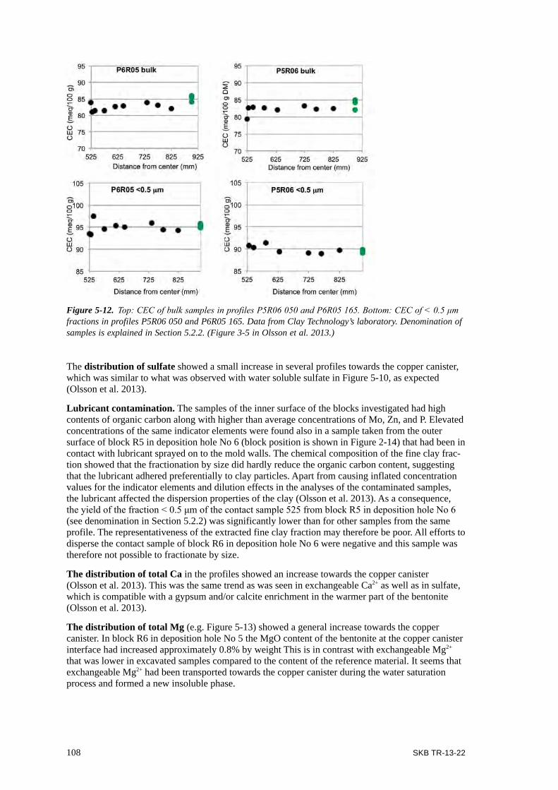
108 SKB TR-13-22

The distribution of sulfate showed a small increase in several profiles towards the copper canister, which was similar to what was observed with water soluble sulfate in Figure 5-10, as expected (Olsson et al. 2013).

Lubricant contamination. The samples of the inner surface of the blocks investigated had high contents of organic carbon along with higher than average concentrations of Mo, Zn, and P. Elevated concentrations of the same indicator elements were found also in a sample taken from the outer surface of block R5 in deposition hole No 6 (block position is shown in Figure 2-14) that had been in contact with lubricant sprayed on to the mold walls. The chemical composition of the fine clay frac-tion showed that the fractionation by size did hardly reduce the organic carbon content, suggesting that the lubricant adhered preferentially to clay particles. Apart from causing inflated concentration values for the indicator elements and dilution effects in the analyses of the contaminated samples, the lubricant affected the dispersion properties of the clay (Olsson et al. 2013). As a consequence, the yield of the fraction < 0.5 μm of the contact sample 525 from block R5 in deposition hole No 6 (see denomination in Section 5.2.2) was significantly lower than for other samples from the same profile. The representativeness of the extracted fine clay fraction may therefore be poor. All efforts to disperse the contact sample of block R6 in deposition hole No 6 were negative and this sample was therefore not possible to fractionate by size.

The distribution of total Ca in the profiles showed an increase towards the copper canister (Olsson et al. 2013). This was the same trend as was seen in exchangeable Ca2+ as well as in sulfate, which is compatible with a gypsum and/or calcite enrichment in the warmer part of the bentonite (Olsson et al. 2013).

The distribution of total Mg (e.g. Figure 5-13) showed a general increase towards the copper canister. In block R6 in deposition hole No 5 the MgO content of the bentonite at the copper canister interface had increased approximately 0.8% by weight This is in contrast with exchangeable Mg2+ that was lower in excavated samples compared to the content of the reference material. It seems that exchangeable Mg2+ had been transported towards the copper canister during the water saturation process and formed a new insoluble phase.

Figure 5-12. Top: CEC of bulk samples in profiles P5R06 050 and P6R05 165. Bottom: CEC of < 0.5 μm fractions in profiles P5R06 050 and P6R05 165. Data from Clay Technology’s laboratory. Denomination of samples is explained in Section 5.2.2. (Figure 3-5 in Olsson et al. 2013.)

SKB TR-13-22 109

The distribution of total Cu in the bentonites (e.g. Figure 5-14) indicates that Cu originating from the copper canister (Block R5 in deposition hole No 6 and R6 in deposition hole No 5) was almost in all cases very locally present at the innermost approximately 1–3 mm. However, in block R10 in deposition hole No 5 the Cu distribution curve looks different from the others, and the penetration was in this profile deeper, approximately 10 mm. The concentrations were in the range of ~ 80 ppm in block R5 in deposition hole No 6 to 670 ppm in block R6 in deposition hole No 5. The latter block had the maximum Cu concentration of all blocks analyzed by digestion of whole samples. However, parallel spot and area analyses on a micrometer scale – 50 μm × 50 μm – of the inner mil-limeter of the blocks by use of scanning electron microscopy (SEM) with energy dispersive X-ray spectroscopy (SEM-EDX) showed that the copper content ranged from background concentrations in some areas up to a few % by weight in other, nearby areas, suggesting that the copper distribution was much more irregular and random than indicated in analyses representing the average for the whole sample volume. Microanalyses using SEM was done both by Clay Technology and BGR, and both observed bright white spots, i.e. high electron density phases in samples from the vicinity of the copper canister. BGR found locally significant amounts of a Cu-Fe-sulfide (e.g. chalcopyrite). The high-resolution series of the innermost 30 mm of the blocks showed that the concentration gradient was steep in the innermost millimeters at the canister/bentonite interface in block R6 in deposition hole No 5 and block R5 in deposition hole No 6, while appearing smoothed over the innermost 10 mm in block R10 in deposition hole No 6. This difference is most probably caused by the sampling procedure. The block R10 in the deposition hole No 6 and the corresponding part of the canister were detached in one piece by sawing. Saw dust had probably contaminated the bentonite as copper saw dust was visually observed in some of the scraping samples taken from the canister, and hence compromised the value of the samples.

The Na-converted, purified < 0.5 μm fraction of the contact sample from block R5 in deposition hole No 6 had almost the same copper concentration as the bulk sample (the contact sample from block R6 from deposition hole No 5 was not fractionated due to poor dispersion), which again suggests that copper, other than saw dust, existed in a water-insoluble, non-exchangeable form.

Figure 5-13. Top: Radial distribution of total Mg (on ignited basis) in bulk samples and < 0.5 μm fractions of profiles P5R06 050 and P6R05 165 (<0.5 μm fraction of P5R6 525 is missing). Bulk samples were taken of both the inner and outer block surface of P6R05. Bottom: Distribution of magnesium in bulk samples from the innermost 30 mm of blocks P5R06, P6R05 and P5R10. Reference samples plotted in green on the right axis. Data from Clay Technology’s laboratory. Denomination of samples is explained in Section 5.2.2. (Figure 3-12 in Olsson et al. 2013.)

110 SKB TR-13-22

Mineral phase studiesExamination of the mineralogical content of the bentonite buffer was one of the identified objectives (Section 5.2.1), as the content and its changes are indicators of changes in the buffer’s safety func-tion properties. The most powerful method for mineralogical analysis is powder X-ray diffraction (XRD) and that is the core in this part of the investigation. The key factors are montmorillonite con-tent and observation of any indications of montmorillonite transformation. Additionally precipitates such as gypsum (CaSO4 2 H2O) or calcite (CaCO3) can be studied with this method.

Powder XRD data was collected by a total of four laboratories (SKB, Clay Technology, B+Tech and BGR). The analyses they performed have been presented in detail by Olsson et al. (2013). A sporadic increase in the smectite basal spacing (001) reflection was observed in several samples. The basal spacing is the distance between each montmorillonite platelet and increases with increased water content/swelling (hydration). BGR data showed lower spacings for the excavated smectite. This difference was, however, due to the drying of the samples. The increase in basal spacing of air-dried samples is either a possible indicator of a cation exchange reaction towards more divalent cations or due to variations in the RH during the measurements, or due to incomplete drying of the field samples.

Other differences were a general increase of gypsum in samples from the vicinity of the copper canister, see Figure 5-15ab. This is compatible with the chemical analysis that showed a general increase of Ca and S towards the canister by Olsson et al. (2013). Minor amounts of anhydrite were also found by one team (Olsson et al. 2013). Anhydrite (CaSO4) is a dehydrated form of gypsum, and is easily formed by drying at elevated temperatures.

No change in the position of the 060 reflection was observed (Olsson et al. 2013), see Figure 5-15c. The 060 reflection distinguishes dioctahedral smectites (such as montmorillonite) from trioctahedral smectites (such as saponite). Dioctahedral smectites have a 060 reflection at 1.49–1.50 Å, while trioctahedral smectites has an 060 reflection of 1.52 Å or larger. Purified and oriented clay fractions showed no indications of any new non-smectitic clay minerals or any change in the properties between field and reference samples (Figure 5-16).

Figure 5-14. Top: Radial distribution of total Cu in bulk and < 0.5 μm fractions of profiles P5R06 050 and P6R05 165 (<0.5 μm fraction P5R06 525 missing). Bulk samples were taken of both the inner and outer block surface of P6R05. Bottom: Distribution of copper in bulk samples from the innermost 30 mm of blocks P5R06, P6R05 and P5R10. Reference samples plotted in green on the right axis. Data from Clay Technology’s laboratory. Denomination of samples is explained in Section 5.2.2. (Figure 3-8 in Olsson et al. 2013.)

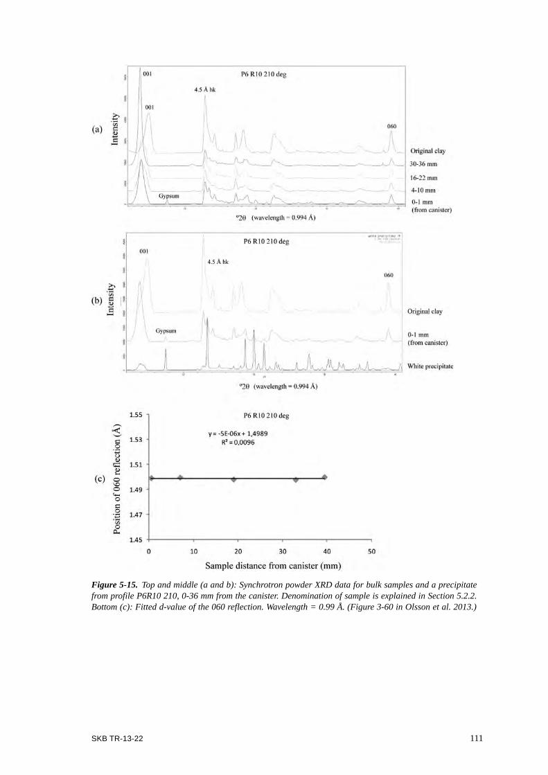
SKB TR-13-22 111

Figure 5-15. Top and middle (a and b): Synchrotron powder XRD data for bulk samples and a precipitate from profile P6R10 210, 0-36 mm from the canister. Denomination of sample is explained in Section 5.2.2. Bottom (c): Fitted d-value of the 060 reflection. Wavelength = 0.99 Å. (Figure 3-60 in Olsson et al. 2013.)

112 SKB TR-13-22

No new phase was identified in the XRD or Fourier transform infrared spectroscopy (FTIR) data explaining the increase in MgO in Figure 5-15 (Olsson et al. 2013). A crystalline phase in the range of 0.8% by weight is, however, far from trivial to identify with XRD. The MgO was likely not pres-ent as a phase itself; more likely the Mg was included in a carbonate, sulfate or silicate (Olsson et al. 2013). It could also be the case that the formed phase was hidden behind one already present. Such a case would be formation of a smectite that would have all major reflections hidden by the dominant montmorillonite phase (Olsson et al. 2013). E.g. stevensite is a trioctahedral smectite known to be easily formed, and can be synthesized by hydrothermal reaction of amorphous silica and magnesium carbonate at basic conditions and 100°C in 0.5 to 20 hours (Ogawa et al. 1991).

In the MX-80 bentonite the Mg source could be interlayer exchangeable Mg2+ and the silicon source could possibly be cristobalite. If present in stevensite, 0.8% by weight of MgO would correspond to approximately 3% by weight of stevensite (24% by weight of MgO). The only difference in the XRD pattern between montmorillonite and stevensite can be found in the 060 reflection at about 1.5 Å. No such change was seen in the XRD data by any laboratory, however, the montmorillonite content in MX-80 is approximately 80% by weight; hence any stevensite 060 reflection would have approximately 3/83 = 4% of the intensity of montmorillonite 060 reflection. To detect such a phase would require major improvements in the signal/noise ratio and/or resolution compared with currently available data. The innermost part of the bentonite was, as stated before, contaminated and hence diluted by the lubricant. A dilution of the bentonite would be expected to lower the smectite content (Olsson et al. 2013), while in the XRD results the smectite content was somewhat higher at the copper interface (91% by weight compared to the average of 88% by weight of the two reference samples (R1b and R2b), see Table 5-5). The difference is perhaps not significant, but anyway com-patible with the possibility of a 3% by weight formation of an Mg-smectite mineral from the accessory minerals. Formation of trioctahedral phases has, however, been seen in bentonite field experiments with iron heaters (Svensson and Hansen 2013).

Å

Figure 5-16. Close up of the 060 region in the XRD patterns of samples. Left: From profile P5:R06 250B (Figure 3-46 in Olsson et al. 2013). Right: From profile P6:R08 355 A (Figure 3-49 in Olsson et al. 2013). Denomination of samples is explained in Section 5.2.2.

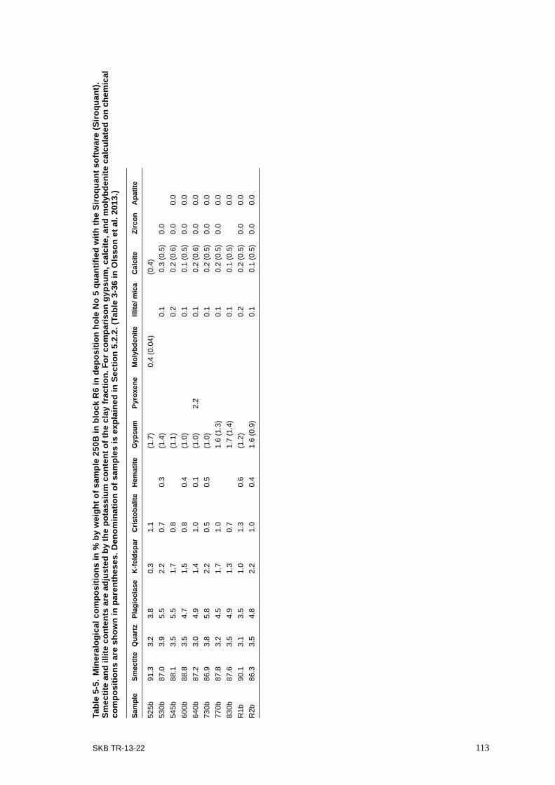
SKB TR-13-22 113

Tabl

e 5-

5. M

iner

alog

ical

com

posi

tions

in %

by

wei

ght o

f sam

ple

250B

in b

lock

R6

in d

epos

ition

hol

e N

o 5

quan

tifie

d w

ith th

e Si

roqu

ant s

oftw

are

(Siro

quan

t).

Smec

tite

and

illite

con

tent

s ar

e ad

just

ed b

y th

e po

tass

ium

con

tent

of t

he c

lay

frac

tion.

For

com

paris

on g

ypsu

m, c

alci

te, a

nd m

olyb

deni

te c

alcu

late

d on

che

mic

al

com

posi

tions

are

sho

wn

in p

aren

thes

es. D

enom

inat

ion

of s

ampl

es is

exp

lain

ed in

Sec

tion

5.2.

2. (T

able

3-3

6 in

Ols

son

et a

l. 20

13.)

Sam

ple

Smec

tite

Qua

rtz

Plag

iocl

ase

K-fe

ldsp

arC

risto

balit

eH

emat

iteG

ypsu

mPy

roxe

neM

olyb

deni

teIll

ite/ m

ica

Cal

cite

Zirc

onA

patit

e

525b

91.3

3.2

3.8

0.3

1.1

(1.7

)0.

4 (0

.04)

(0.4

)53

0b87

.03.

95.

52.

20.

70.

3(1

.4)

0.1

0.3

(0.5

)0.

054

5b88

.13.

55.

51.

70.

8(1

.1)

0.2

0.2

(0.6

)0.

00.

060

0b88

.83.

54.

71.

50.

80.

4(1

.0)

0.1

0.1

(0.5

)0.

00.

064

0b87

.23.

04.

91.

41.

00.

1(1

.0)

2.2

0.1

0.2

(0.6

)0.

00.

073

0b86

.93.

85.

82.

20.

50.

5(1

.0)

0.1

0.2

(0.5

)0.

00.

077

0b87

.83.

24.

51.

71.

01.

6 (1

.3)

0.1

0.2

(0.5

)0.

00.

083

0b87

.63.

54.

91.

30.

71.

7 (1

.4)

0.1

0.1

(0.5

)0.

0R

1b90

.13.

13.

51.

01.

30.

6(1

.2)

0.2

0.2

(0.5

)0.

00.

0R

2b86

.33.

54.

82.

21.

00.

41.

6 (0

.9)

0.1

0.1

(0.5

)0.

00.

0

114 SKB TR-13-22

FTIR performed by B+Tech and BGR showed no indications of any formation of any 680 cm–1 absorption band that would have been indicative for a newly formed trioctahedral smectite (Olsson et al. 2013). Compared to the reference samples an increase in intensity of organic impurities was observed in samples closest to the canister (525b and 530b). These organic impurities appeared at wave numbers of 2,930 cm–1 and 2,855 cm–1. This is most likely from the lubricant used for compaction. The chemical and mineralogical compositions, indicated that the carbonate content was higher towards the heater (Olsson et al. 2013), hence it seems that the carbonate distribution was sporadically increased, however, unevenly distributed. No significant differences of differential ther-mal analysis (DTA) measurements at BGR on four different samples indicate as well any significant change in the clay mineral content or properties (Olsson et al. 2013).

Optical microscopy was performed by B+Tech as a complementary technique for mineral identifi-cation, and identified minor phases such as feldspars, hematite, mica, zircon, carbonates and apatite, but did not show any change between the excavated samples compared to the reference samples (Olsson et al. 2013).

Redox studies using XANES, Mössbauer and wet chemistryRedox chemistry in the bentonite buffer was one of the identified objectives (Section 5.2.1). Prob-ably the most widely used method for redox analysis of bentonite is Mössbauer spectroscopy. As redox chemistry is very difficult to analyze with bentonites. Mössbauer has been combined with Fe and K XANES and wet chemical analysis, as each technique has its own strengths and weaknesses. The redox chemistry of iron in bentonite is important for several reasons. One being as a potential redox marker, giving information about the redox conditions present in the experiment. Another reason is that montmorillonite is susceptible for redox changes, hence the iron in montmorillonite may change back and forth from Fe(III) to Fe(II), at least within some limits. As the montmorillonite layer charge depends on the balance between positive and negative cations, the change between trivalent to divalent iron also may impact the montmorillonite layer charge and hence potentially some of its properties and performance. No similar measurements have previously been performed on samples from Cu – bentonite field experiments.

Quantitative determination of Fe(II) in bentonite is difficult. One reason is that the samples are air sensitive, and may easily oxidize during the excavation, sample handling or the measurement (Svensson and Hansen 2013). The other reason is that subtle changes only can be captured if the methods are highly reproducible. Here different samples (profiles) were analyzed with different methods. This made it difficult to compare the methods or the samples directly between each other. However, some trends were seen that seemed to be general. With all methods, and with all samples, a higher Fe(II)/Fe total ratio was found in bentonite in contact with the canister compared to the ratio of the reference samples (Olsson et al. 2013). The largest contrast was seen with XANES, see Figure 5-17, where an increase from 21 to 48% was observed. The reproducibility of the XANES method was evaluated on a natural clay stone material (with similar Fe(II) content compared to exposed Prototype Repository bentonite) and the variation was found to have a standard deviation in the range of 0.9–2.4%, which was smaller than the variation in the material itself that was in the range of 3.0–4.2% (Svensson and Hansen 2013). Svensson and Hansen (2013) found that with Mössbauer, the increase was 30 to 48%, and with wet chemical analysis the increase was from 27 to 35%. In the XANES data the samples further out from the canister were deemed to be some-what lower in Fe(II)/Fe total. In the Mössbauer data the difference was much smaller, and with wet chemical analysis all the samples further out were lower in Fe(II) even compared to the reference samples. The scattering between the reference samples were smallest with wet chemical analysis and largest with XANES. But the wet chemical analysis showed what was deemed to be a higher scatter among the field samples compared to the other methods. The reference bentonites had a Fe(II)/Fe total content of 21% with XANES, 27% with wet chemical analysis and 30% using Mössbauer spectroscopy. The lowering of Fe(II) in the field test, indicated by wet chemical analysis, was in contrast to the other methods. Oxidation of pyrite in the bentonite could be the explanation. Possibly oxidation of pyrite occurred in all samples together with reduction of the Fe(III) in the montmorillo-nite, both processes masking each other. The wet chemical samples may have re-oxidized, and hence only the trace of pyrite oxidation was observed. The most likely source for oxidation of pyrite is oxygen from the air trapped inside the bentonite buffer. This process was seen in the pyrite rich Callovo-Oxfordian-clay in ABM1 (Svensson and Hansen 2013). The difference between the methods

SKB TR-13-22 115

and samples was an effect of the complexity of both Fe(II) determinations in bentonite and the differences derived from the field experiment itself. The XANES data showed indications of a max-imum Fe(II)-content at the canister interface followed by a drop, while Mössbauer indicated a more general increase. Visual observations during sample oxidation agreed best with the XANES data (Figure 5-17). This increase at the canister surface indicated that the reduction of Fe(III) to Fe(II) in the bentonite could possibly have been a redox reaction with the copper material. However, 10–20% of the total Fe seems to have been reduced. Based on 3.5% of total Fe and 2000 kg of bentonite per block that corresponds to 7–14 kg of Fe(II) produced per block. Only 100 ppm of Cu was observed in the innermost 5 mm, and this small amount cannot reduce 14 kg of Fe based on mass-balance calculations.

The Fe- redox chemistry in different smectites is affected differently by the external redox potential. Both XANES and Mössbauer spectroscopy indicated approximately 50% Fe(II)/Fe total at the canister interface (Figure 5-17). According to Gorski et al. (2013) this corresponds for Wyoming montmorillonite to a redox potential of approximately –50 mV SHE. This is very close to the corrosion potential measured on the three copper electrodes installed in the Prototype Repository (deposition hole No 5) that showed values in the range of –60 to –30 mV SHE (Rosborg 2013a) see Section 5.6.2. Hence the bentonite seems to have adapted to the surrounding redox conditions. Possibly the redox change in the bentonite was a function of the surrounding redox potential as well as the temperature distribution in the block with the highest temperature close to the canister affect-ing the kinetics of the Fe(III) reduction.

Figure 5-17. The Fe(II)/Fe total content as a function of the distance from the canister in different profiles using different methods (XANES, Mössbauer and wet chemical analysis). Denomination of samples is explained in Section 5.2.2. (Figure based on results in Olsson et al. 2013.)

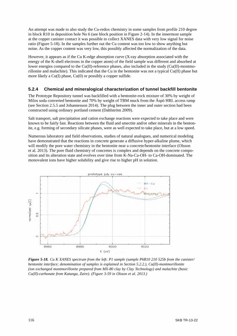
116 SKB TR-13-22

An attempt was made to also study the Cu-redox chemistry in some samples from profile 210 degree in block R10 in deposition hole No 6 (see block position in Figure 2-14). In the innermost sample at the copper canister contact it was possible to collect XANES data with very low signal for noise ratio (Figure 5-18). In the samples further out the Cu content was too low to show anything but noise. As the copper content was very low, this possibly affected the normalization of the data.

However, it appears as if the Cu K-edge absorption curve (X-ray absorption associated with the energy of the K-shell electrons in the copper atom) of the field sample was different and absorbed at lower energies compared to the Cu(II)-reference phases, also included in the study (Cu(II)-montmo-rillonite and malachite). This indicated that the Cu in the bentonite was not a typical Cu(II) phase but more likely a Cu(I) phase, Cu(0) or possibly a copper sulfide.

5.2.4 Chemical and mineralogical characterization of tunnel backfill bentonite The Prototype Repository tunnel was backfilled with a bentonite-rock mixture of 30% by weight of Milos soda converted bentonite and 70% by weight of TBM muck from the Äspö HRL access ramp (see Section 2.5.5 and Johannesson 2014). The plug between the inner and outer section had been constructed using ordinary portland cement (Dahlström 2009).

Salt transport, salt precipitation and cation exchange reactions were expected to take place and were known to be fairly fast. Reactions between the fluid and smectite and/or other minerals in the benton-ite, e.g. forming of secondary silicate phases, were as well expected to take place, but at a low speed.

Numerous laboratory and field observations, studies of natural analogues, and numerical modeling have demonstrated that the reactions in concrete generate a diffusive hyper-alkaline plume, which will modify the pore water chemistry in the bentonite near a concrete/bentonite interface (Olsson et al. 2013). The pore fluid chemistry of concretes is complex and depends on the concrete compo-sition and its alteration state and evolves over time from K-Na-Ca-OH- to Ca-OH-dominated. The monovalent ions have higher solubility and give rise to higher pH in solution.

Figure 5-18. Cu K XANES spectrum from the left: P1 sample (sample P6R10 210 525b from the canister/bentonite interface; denomination of samples is explained in Section 5.2.2.), Cu(II)-montmorillonite (ion exchanged montmorillonite prepared from MX-80 clay by Clay Technology) and malachite (basic Cu(II)-carbonate from Katanga, Zaire). (Figure 3-59 in Olsson et al. 2013.)

SKB TR-13-22 117

Soluble salts, CE, CEC and elemental composition The amount of chloride had increased significantly in the Prototype Repository backfill (Olsson et al. 2013), see Figure 5-19. This is the same behavior as seen in the buffer bentonite. The sulfate content in the excavated backfill was slightly lowered. This small change can probably be explained by a very small dilution from particles from the crushed TBM muck. The proportion of EC or less unaffected, however, a small increase in Na and K was seen in relation to Mg and Ca that decreased, see Figure 5-20. CEC of the < 1 mm fraction showed no sign of any change, see Figure 5-21. Greene-Kelly tests using Li-saturation followed by heating to 250°C showed a scatter in the results and no unambiguous conclusions could be drawn. Clay was dispersed in water and the pH was mea-sured after 1 h and 4 days. The results were rather ambiguous, but indicated a small increase in pH in the innermost sample towards the plug – pH 9 versus 8.5. The amount of acid soluble carbon was found to be rather stable. Most importantly, Mg did not change towards the plug. However, the ratio of exchangeable (soluble) Mg / Mg total decreased, see Figure 5-22. Hence, the soluble Mg was transformed into an Mg-phase, possibly in a similar way as seen in the buffer bentonite. In contrast, the ratio between exchangeable Na and total increased towards the plug, while K was unaffected.

Figure 5-19. Distribution of Cl– and SO4-S (mg/g dry mass) in the < 1 mm fraction of the backfill bentonite 0–160 mm from the concrete plug plotted versus the distance from the concrete plug. The concentrations in the reference sample 1 m from the concrete are plotted in green on the right axis. (Figure 5-2 in Olsson et al. 2013.)

Figure 5-20. Relative proportions of the EC extracted by exchange against NH4+ in ethanol solution. PBF (Prototype BackFill) + distance from inner concrete plug in mm. (Figure 5-4 in Olsson et al. 2013.)

118 SKB TR-13-22

Mineral phase studies using XRD Powder XRD data showed that the separated fraction of ≤ 1 mm was a mixture of crushed rock and original bentonite (Olsson et al. 2013), see Figure 5-23. In the original bentonite various minerals were identified such as smectite, calcite, dolomite, quartz, gypsum (Table 2-3) and pyrite. In the crushed rock minerals such as quartz, plagioclase, K-feldspar, chlorite, biotite and amphibole were found. The smectite basal spacing 001 reflection was at 12.5 Å, which is expected for a Na-smectite with one-water-layer at ~ 50% RH. The 060 reflection that separated dioctahedral smectite from trioctahedral smectite showed no signs of any change. However, sporadically a small reflection was seen at 1.53 Å that may correspond to a trioctahedral phyllosilicate, e.g. biotite, chlorite or smectite, or possibly calcite that also have a reflection in the vicinity. Increase in calcite was seen in samples ~ 0–40 mm from the plug. This also correlated to a decrease in dolomite (Mg-Ca-carbonate). In PBF10 (Prototype BackFill at a distance of 10 mm from the inner plug) a weak reflection of halite (NaCl) was seen. The oriented, Mg and ethylene glycol saturated samples showed no indication of transformation of the smectite. No sign of any neo-formed Mg-phase was observed.

Figure 5-22. Distribution of total and non-exchangeable MgO, Na2O and K2O in the < 1 mm fraction of the backfill 0-160 mm from the concrete plug. The concentrations of the reference backfill sample 1 m from the concrete are plotted in green on the right axis. (Figure 5-11 in Olsson et al. 2013.)

Figure 5-21. CEC of the < 1 mm fractions plotted versus the distance from the concrete plug. Value for the reference backfill sample from one m is plotted in green on the right axis. (Left figure in Figure 5-5 in Olsson et al. 2013.)

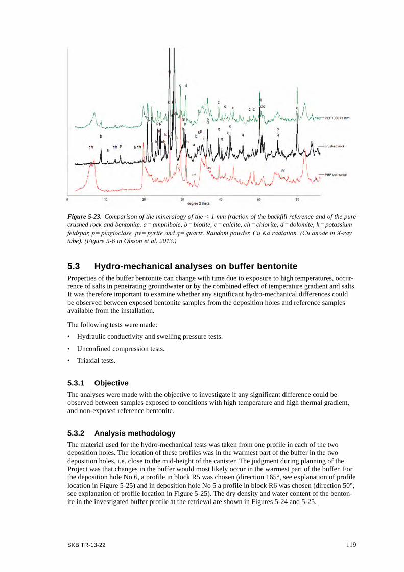
SKB TR-13-22 119

5.3 Hydro-mechanical analyses on buffer bentoniteProperties of the buffer bentonite can change with time due to exposure to high temperatures, occur-rence of salts in penetrating groundwater or by the combined effect of temperature gradient and salts. It was therefore important to examine whether any significant hydro-mechanical differences could be observed between exposed bentonite samples from the deposition holes and reference samples available from the installation.

The following tests were made:

• Hydraulic conductivity and swelling pressure tests.

• Unconfined compression tests.

• Triaxial tests.

5.3.1 ObjectiveThe analyses were made with the objective to investigate if any significant difference could be observed between samples exposed to conditions with high temperature and high thermal gradient, and non-exposed reference bentonite.

5.3.2 Analysis methodologyThe material used for the hydro-mechanical tests was taken from one profile in each of the two deposition holes. The location of these profiles was in the warmest part of the buffer in the two deposition holes, i.e. close to the mid-height of the canister. The judgment during planning of the Project was that changes in the buffer would most likely occur in the warmest part of the buffer. For the deposition hole No 6, a profile in block R5 was chosen (direction 165°, see explanation of profile location in Figure 5-25) and in deposition hole No 5 a profile in block R6 was chosen (direction 50°, see explanation of profile location in Figure 5-25). The dry density and water content of the benton-ite in the investigated buffer profile at the retrieval are shown in Figures 5-24 and 5-25.

Figure 5-23. Comparison of the mineralogy of the < 1 mm fraction of the backfill reference and of the pure crushed rock and bentonite. a = amphibole, b = biotite, c = calcite, ch = chlorite, d = dolomite, k = potassium feldspar, p = plagioclase, py = pyrite and q = quartz. Random powder. Cu Kα radiation. (Cu anode in X-ray tube). (Figure 5-6 in Olsson et al. 2013.)

120 SKB TR-13-22

One series of tests from each deposition hole was run. In every series three types of samples were tested;

• Material saved at the block production was compacted aiming at the densities 1,900, 1,950, 2,000, 2,050, 2,100 and 2,150 kg/m3 at full water saturation. These were denoted “references”.

• Retrieved samples by core drilling from removed larger buffer pieces were trimmed to fit the sample holders and thus having a density close to the field value.

• Block samples were air-dried and ground to a grain size similar to the original MX-80 powder and re-compacted to a density of 2,000 kg/m3.

5.3.3 Hydraulic conductivity and swelling pressureA swelling pressure device was used to determine hydraulic conductivity and swelling pressure. The device is shown in Figure 5-26. The samples were confined by a cylinder ring with a diameter of 35 mm or 20 mm and stainless steel filters at the top and bottom. The smallest cylinder was used

Figure 5-24. Water content and dry density of block R6 in deposition hole No 5. (Block position is shown in Figure 2-14.) (Figures from Appendix 24 in Johannesson 2014.)

Figure 5-25. Water content and dry density of block R5 in deposition hole No 6. (Block position is shown in Figure 2-14) (Figures from Appendix 9 in Johannesson 2014.)

50° 50°

SKB TR-13-22 121

for the samples taken close to the canister surface in order to get a sample, which was representative of the buffer very close to the canister. The test volume was sealed by O-rings placed between the bottom plate and the cylinder ring and between the piston and the cylinder ring. At test start the height of the test sample was approximately 15 mm.

A load cell placed between the piston and the upper lid measured the axial force from the samples. The displacement of the piston due to transducer deformation is 25 µm at maximum force, corre-sponding to 0.17% of the sample height, which was considered insignificant.

The samples were saturated or re-saturated after preparation by introducing water to the bottom and top side simultaneously. Water was added after evacuation of air from filters and tubes by a vacuum pump. For all samples groundwater from the Prototype Repository site was used. During the satura-tion a small water pressure of approximately 5 kPa was applied. The swelling pressure was measured continuously until full saturation was reached. A more detailed description of test procedures has been presented by Olsson et al. (2013).

The data from the measurements of swelling pressure and hydraulic conductivity are summarized in Figures 5-27 and 5-28.

Based on the results from investigations of field-exposed material with results from investigations of reference material it was found that there were no large variations in swelling pressure between the reference samples and the samples of field-exposed material although there was a small tendency that the swelling pressures of the field-exposed material was somewhat lower i.e. all the green dia-mond and the red squares in Figure 5-27 plot under the solid line representing the swelling pressure of the reference samples.

Estimation of the variation in the measurement of the swelling pressure was made by analyzing the sample of ground and compacted material from deposition hole No 6, see red circles in Figure 5-27. Five of these samples had similar dry density and the average measured swelling pressure with these samples was 4,975 kPa with a standard deviation of 747 kPa.

The hydraulic conductivity of the trimmed samples taken from the Prototype Repository was some-what lower than that of the reference samples, especially at higher densities, see Figure 5-28.

Estimation of the variation in the measurement of the hydraulic conductivity was made in the same way as for the swelling pressure, see Figure 5-28. The average measured hydraulic conduc-tivity and the standard deviation for the ground and compacted samples were 8.23·10–14 m/s and 1.00· 10–14 m/s, respectively.

Figure 5-26. A photo and a schematic drawing of the swelling pressure device. (Figure 2-1 in Olsson et al. 2013.)

Load cell

Water inlet

Water inlet

Filter

Specimen

Filter

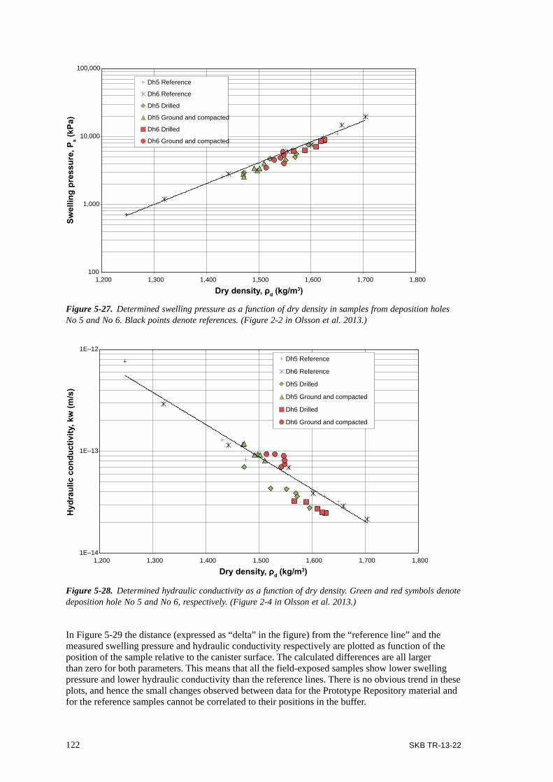
122 SKB TR-13-22

In Figure 5-29 the distance (expressed as “delta” in the figure) from the “reference line” and the measured swelling pressure and hydraulic conductivity respectively are plotted as function of the position of the sample relative to the canister surface. The calculated differences are all larger than zero for both parameters. This means that all the field-exposed samples show lower swelling pressure and lower hydraulic conductivity than the reference lines. There is no obvious trend in these plots, and hence the small changes observed between data for the Prototype Repository material and for the reference samples cannot be correlated to their positions in the buffer.

Figure 5-28. Determined hydraulic conductivity as a function of dry density. Green and red symbols denote deposition hole No 5 and No 6, respectively. (Figure 2-4 in Olsson et al. 2013.)

1E–14

1E–13

1E–12

1,200 1,300 1,400 1,500 1,600 1,700 1,800

Hyd

raul

ic c

ondu

ctiv

ity, k

w (m

/s)

Dry density, ρd (kg/m3)

Dh5 Reference

Dh6 Reference

Dh5 Drilled

Dh5 Ground and compacted

Dh6 Drilled

Dh6 Ground and compacted

Figure 5-27. Determined swelling pressure as a function of dry density in samples from deposition holes No 5 and No 6. Black points denote references. (Figure 2-2 in Olsson et al. 2013.)

100

1,000

10,000

100,000

1,200 1,300 1,400 1,500 1,600 1,700 1,800

Swel

ling

pres

sure

, Ps (

kPa)

Dry density, ρd (kg/m3)

Dh5 Reference

Dh6 Reference

Dh5 Drilled

Dh5 Ground and compacted

Dh6 Drilled

Dh6 Ground and compacted

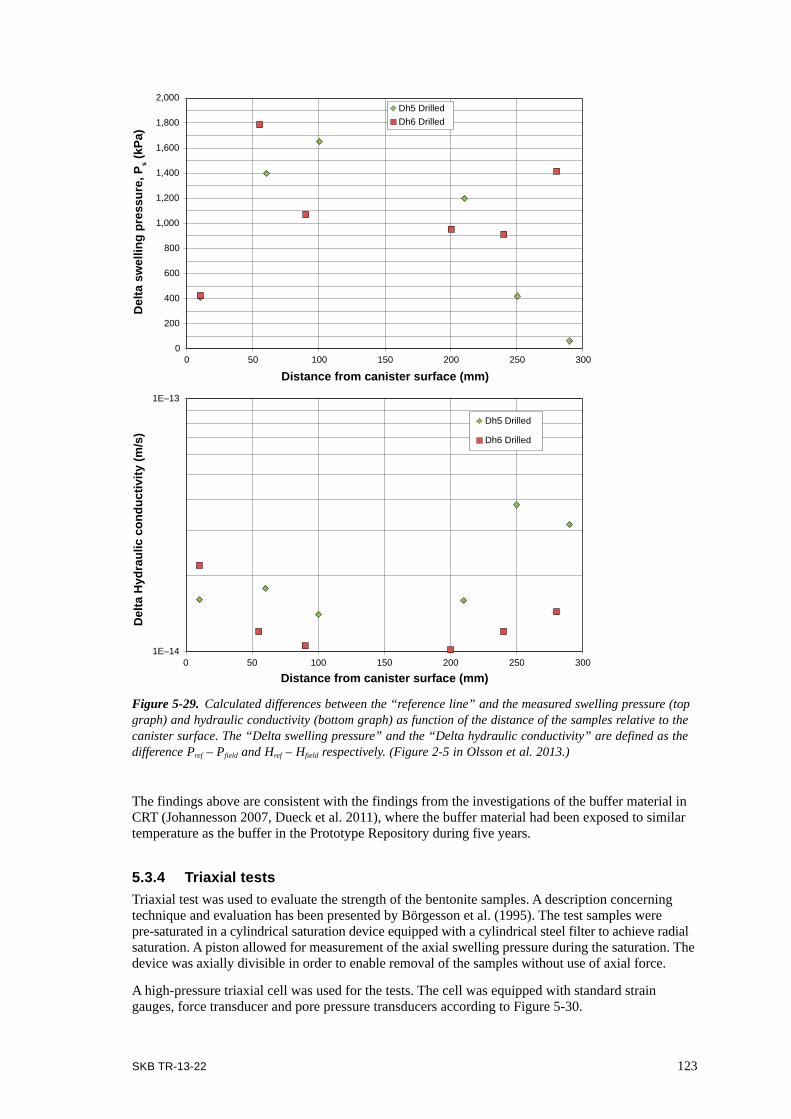
SKB TR-13-22 123

The findings above are consistent with the findings from the investigations of the buffer material in CRT (Johannesson 2007, Dueck et al. 2011), where the buffer material had been exposed to similar temperature as the buffer in the Prototype Repository during five years.

5.3.4 Triaxial testsTriaxial test was used to evaluate the strength of the bentonite samples. A description concerning technique and evaluation has been presented by Börgesson et al. (1995). The test samples were pre-saturated in a cylindrical saturation device equipped with a cylindrical steel filter to achieve radial saturation. A piston allowed for measurement of the axial swelling pressure during the saturation. The device was axially divisible in order to enable removal of the samples without use of axial force.

A high-pressure triaxial cell was used for the tests. The cell was equipped with standard strain gauges, force transducer and pore pressure transducers according to Figure 5-30.

Figure 5-29. Calculated differences between the “reference line” and the measured swelling pressure (top graph) and hydraulic conductivity (bottom graph) as function of the distance of the samples relative to the canister surface. The “Delta swelling pressure” and the “Delta hydraulic conductivity” are defined as the difference Pref – Pfield and Href – Hfield respectively. (Figure 2-5 in Olsson et al. 2013.)

0

200

400

600

800

1,000

1,200

1,400

1,600

1,800

2,000

0 50 100 150 200 250 300

Del

ta s

wel

ling

pres

sure

, Ps (

kPa)

Distance from canister surface (mm)

Dh5 DrilledDh6 Drilled

1E–14

1E–13

0 50 100 150 200 250 300

Del

ta H

ydra

ulic

con

duct

ivity

(m/s

)

Distance from canister surface (mm)

Dh5 Drilled

Dh6 Drilled

124 SKB TR-13-22

The technique requires relatively large test samples and is resource consuming, both concerning time and active work. The two test series were therefore limited to two samples each: one from the field experiment and one reference sample. The field samples from deposition holes No 5 and No 6 were taken from Ring 6 and Ring 5 close to the canisters, see Figure 2-14 for positions of blocks in the deposition holes. The references were given the same dimensions and water saturated in the same device as the field samples.

The samples were mounted in the triaxial cell, shown in Figure 5-30, after about four weeks of water saturation. A cell pressure corresponding to the swelling pressure during the saturation was applied and the pore pressure in the samples was measured with the pedestal valve closed. In order to help the pore pressure to equalize over the sample, filter paper drains were attached vertically.

During the tests the following parameters were measured: the cell pressure (σ3), the pore pressure (u), the deviator stress (q) and the deformation of the sample (Δl).

The deviator stress was calculated from:

)(0

0

0 lll

AFq ∆−= (5-4)

where A0 is the sample’s initial cross section area and l0 the initial length of the sample.

The vertical total stress σ1 was calculated from:

31 σσ += q (5-5)

The average effective stress p’ was calculated from:

)32(31' 31 up −+= σσ (5-6)

The strain ε was calculated from:

0ll∆=ε (5-7)

Figures 5-31 and 5-32 show the deviator stress plotted versus strain and effective mean stress, respectively.

The stiffness of all the samples was similar at the beginning of the tests i.e. up to a strain of about 2%, see Figure 5-32. At failure, however, the strain of the samples with field-exposed material was smaller compared with the strain of the samples of reference material.

Figure 5-30. Triaxial test equipment used in combination with a mechanical press. (Figure 2-10 in Olsson et al. 2013.)

load

load cell

piston

top cap

drainage foils

rubber membrane

filterbase pedestal

cell water pressure

sample

steel cylinder

strain gauge

SKB TR-13-22 125

Figure 5-31. Deviator stress versus strain resulting from the triaxial tests. The dotted lines represent data from tests made on reference samples (P5R06 R and P6R05 R). Denomination of samples is explained in Section 5.2.2. (Figure 2-11 in Olsson et al. 2013.)

Figure 5-32. Stress paths plotted as deviator stress versus mean effective stress. The dotted lines represent data from tests made on reference samples (P5R06 R and P6R05 R). Denomination of samples is explained in Section 5.2.2. (Figure 2-12 in Olsson et al. 2013.)

0

500

1,000

1,500

2,000

2,500

3,000

3,500

4,000

4,500

0 5 10 15 20 25

Dev

iato

r str

ess,

q (k

Pa)

Strain, ε(%)

P5R06 050C 545

P5R06 R

P6R05 165A 547

P6R05 R

0

500

1,000

1,500

2,000

2,500

3,000

3,500

4,000

4,500

0 2,000 4,000 6,000 8,000 10,000 12,000 14,000 16,000

Dev

iato

r str

ess,

q (k

Pa)

Effective mean stress, p (kPa)

P5R06 050C 545P5R06 RP6R05 165A 547P6R05 RBörgesson et al. 1995

126 SKB TR-13-22

Since only a small number of tests were made on bentonite samples from the Prototype Repository, the data were compared with previously made triaxial test on MX-80 (Börgesson et al. 1995), see Figure 5-32. The deviator stresses were larger at failure in all tests compared to the previously made tests and there was a small tendency that this was more pronounced for the field-exposed samples than for the reference samples, see Figure 5-32. The impact strength can have, is if it affects the shearing of the canister. Figure 5-32 shows a significantly higher deviator stress (up to 3,800 kPa) than was measured in earlier tests, a stress that is about the same that Börgesson et al. (2010) measured for Deponit Can (4,000 kPa); and the property of Deponit Can is used as reference in the calculations of canister shear scenarios.

Consequently this is not any reason for reconsideration of the bentonite model that is used in the can-ister shear scenarios. But the issue should be under observation and studied when samples become available from the decommissioning of the inner section. The objective should be to investigate if the exposure time affects the strength.

5.3.5 Unconfined compression testsIn the unconfined compression test the cylindrical samples were compressed axially to shear failure with a constant rate of strain with no radial confinement or external radial stress. The shear strength was determined on tall samples with a height equal to double the size of the diameter to allow for the shear failure to develop without boundary effects from the end surfaces. Tests were also performed on short samples with a height equal to the diameter in order to study relative changes between different samples.

Before the compression tests the samples were saturated and then placed in a mechanical press according to Figure 5-33 where a constant rate of strain was applied.

Three main test series from each deposition hole were run, two series with short samples and one series with long samples. The diameters of all samples were 20 mm and the short ones had equal height as the diameter aiming at relative changes between samples. The heights of the tall samples were twice the size of the diameter aiming at determination of the shear strength. All samples were fully saturated, except for two short series, which were sheared directly after sampling.

The samples retrieved from the Prototype Repository were prepared by drilling and trimming cylin-drical samples while the references were compacted to cylindrical samples from material saved from block production. The tall reference samples were assembled by two short samples put on top of each other in the saturation device before the saturation. The dimension of the test samples was mini-mized in order to increase the spatial resolution of the test parcel and to ensure full water saturation.

Groundwater from the Prototype Repository site was used for the saturation of the drilled and com-pacted samples, which was done in a specially designed saturation device where water was applied to the samples after evacuation of air from the tubes and filters. The short and tall samples were saturated for 2 and 8 weeks respectively.

During shearing the samples were surrounded by a protective plastic sheet to minimize evaporation. After failure the water content and density were determined.

The deviator stress and the strain were calculated, see Johannesson (2014) for calculation details. An example of a plot of deviator stress versus strain for one series of tests is shown in Figure 5-34. The legends denote the distance from canister center (mm) or the references density (kg/m3).

The results, plotted as maximum deviator stress and corresponding strain versus dry density, are shown in Figure 5-35 and Figure 5-36. Samples from deposition hole No 5 are marked with green symbols whereas red symbols denote samples from deposition hole No 6. The lines in the figures are calculated from the tests made on the reference samples.

The stress at failure increased for the reference sample as well as for the samples retrieved from the Prototype Repository with increasing dry density. Although the scatter in strength was large, especially at higher densities, no large differences in strength could be seen between the reference samples and the samples from the Prototype Repository, see Figure 5-35. The strength was also independent of the height of the samples.

SKB TR-13-22 127

loadframe

specimen

load cell

deformationtransducer

top capandbase pedestalwithlubricatedends

constant rate of strain

Figure 5-33. Set-up for the unconfined compression tests. (Figure 2-15 in Olsson et al. 2013.)

Figure 5-34. Deviator stress versus strain for tall saturated samples from deposition hole No 5. The labels show the distance in mm from canister center and the references initial dry density in kg/m3 respectively. (Figure 2-19 in Olsson et al. 2013.)

0

500

1,000

1,500

2,000

2,500

3,000

3,500

4,000

0 5 10 15 20

Dev

iato

r str

ess,

q (k

Pa)

Strain, ε (%)

Dh5 40 mm sat535575615a615b735775805R_1400R_1550R_1675

Figure 5-35. Maximum deviator stress versus dry density for test series with short and tall saturated samples. (Figure 2-25 in Olsson et al. 2013.)

0

1,000

2,000

3,000

4,000

5,000

6,000

1,350 1,400 1,450 1,500 1,550 1,600 1,650 1,700 1,750

Max

imum

dev

iato

r str

ess,

q m

ax (k

Pa)

Dry density, ρd (kg/m3)

ReferenceDh5 20 mmDh5 40 mmDh6 20 mmDh6 40 mm

128 SKB TR-13-22

The strain at failure of the samples depends on the dry density as shown in Figure 5-36. A higher density results, as expected, in lower strain at failure i.e. a more brittle behavior. The strain at failure also depends on the height of the samples i.e. the higher samples had smaller strain at failure. Although there was a large scatter in the evaluated strain at failure for the samples from the Prototype Repository, especially at higher densities, the differences between the reference samples and the samples from the Prototype Repository were small but significant. All the samples from the Prototype Repository, however, plot below the lines representing the strain for the reference samples, implying that material from the Prototype Repository was somewhat more brittle than the reference samples. This would become alarming, if the rate of change during the seven years of exposure continues for a long time, which, however, has been ruled out as unlikely by Dueck (2010) in the detailed study of the conditions that favor development of brittleness. Dueck (2010) only detected increased brittleness in saturated samples that had a high saturated density (ρ ≥ 2,060 kg/m3) or had been exposed to a high temperature (T ≥ 150°C), i.e. conditions outside the conditions in a KBS-3 repository. Brittle failure behavior was also seen on unsaturated specimens with a degree of satura-tion less than Sr < 90%. Failure at reduced strain was seen on specimens exposed to T = 150°C, on specimens having a water content of wi = 0% before saturation, on specimens with a final degree of saturation of Sr ≤ 97%, i.e. conditions during the transient period. In Figure 5-37 the distance from the lines evaluated from the reference samples and the measured strain at maximum deviator stress from Figure 5-36 are plotted as function of the position of the samples relative the canister surface. The trend in the plot indicated that the deviation from the reference line increased with decreasing distance from the canister i.e. the higher the temperature the greater the brittleness of the material from the Prototype Repository. The results obtained by the Project are consistent with the findings in the examination of the CRT buffer material (Dueck et al. 2011). The issue should be further studied when samples will become available from the decommissioning of the inner section of the Prototype Repository.

5.4 Microbiological analysis Some microorganisms can catalyze reactions that have an impact on the long-term performance of the final repository such as sulfate reduction, methane oxidation (in which oxygen is consumed) and iron reduction. This section describes the work on determining the proliferation of microbes, their survival and their mobility, in both buffer and backfill.

Figure 5-36. Strain at maximum deviator stress versus dry density for test series with short and tall, saturated samples. (Figure 2-26 in Olsson et al. 2013.)

0

2

4

6

8

10

12

1,350 1,400 1,450 1,500 1,550 1,600 1,650 1,700 1,750

Stra

in a

t max

imum

dev

iato

r str

ess,

ε (%

)

Dry density, ρd (kg/m3)

Reference 20 mmReference 40 mmDh5 20 mmDh5 40 mmDh6 20 mmDh6 40 mm

SKB TR-13-22 129

5.4.1 ObjectiveSpecial samples were taken from the backfill, the buffer, and at the canisters’ surfaces (see Sections 4.3, 4.4 and 4.5) with the objectives:

• To study microbial presence and number.

• To investigate if microorganisms such as IRB and SRB, which occur in the groundwater surrounding the Prototype Repository (Eriksson 2007), also would occur in the backfill and the buffer.

• To study indications of microbe mobility in the buffer towards the canister.

• To prove the possible occurrence of biofilm on the surfaces of the canisters.

5.4.2 Analytical methodsThe procedures used are described by Arlinger et al. (2013). Below follows a brief summary.

The number of CHAB was determined by using petri dishes (shallow cylindrical lidded dish) con-taining agar (jelly-like substance) with nutrients. The dishes were prepared as described by Hallbeck and Pedersen (2008).

The most probable number (MPN) of microorganisms was determined using anoxic media as described by Hallbeck and Pedersen (2008). The media were prepared by a modified procedure described by Widdel and Bak (1992). Five tubes were used for each ten-times dilution, resulting in an approximate 95% confidence interval lower limit of 1/3 of the obtained value and an upper limit of three times the value (Greenberg et al. 1992).

Total genomic DNA was extracted from swab samples that were taken from the copper surface using the PowerSoil DNA isolation kit (cat. no. 12888) and from samples of bentonite clay using the PowerMax Soil DNA isolation kit (cat. no 12988), both from MO BIO Laboratories, Carlsbad, CA, USA, according to the manufacturer’s protocol. For all DNA extracts, polymerase chain reaction (PCR) screening was conducted using the universal 16S ribosomal RNA (16S rRNA) primer set 27f and 1492r (Lane 1991), numbers corresponding to positions in Escherichia coli Brosius (Brosius et al. 1978). Furthermore, the adenosine-5’-phosphosulfate (APS)7f and APS8r primer set specific to the APS reductase alpha sub-unit gene (apsA) – a gene specific to SRB – was used for screening SRB swab DNA extracts (Friedrich 2002).

Figure 5-37. Calculated differences between the “reference line” and the measured strain at maximum deviator stress as function of the distance of the samples to the canister surface. (Figure 2-27 in Olsson et al. 2013.)

–0.5

0.0

0.5

1.0

1.5

2.0

2.5

3.0

3.5

0 50 100 150 200 250 300

Del

ta S

trai

n, ε

(%)

Distance from canister surface (mm)

Dh5 H = 20 mmDh6 H = 20 mm

130 SKB TR-13-22

5.4.3 BackfillAll but one of the 63 randomly chosen backfill samples exhibited bacterial growth to various extents when inoculated on agar plates. The samples that exhibited the most bacterial growth were found in the upper half and around the edges of the backfill material bordering on the tunnel wall, as shown in Figure 5-38.

From the 63 backfill samples analyzed for CHAB, five were randomly chosen for MPN analysis. The results indicated that the best position for bacterial growth seems to be the boundary between the tunnel roof and the backfill material, where the highest bacterial numbers, i.e. both MPN and CHAB, were observed. This is consistent with the lowest backfill densities, and consequent lowest bentonite densities, measured in that region (see Section 5.1.3), The backfill–rock boundary area was also found to favor SRB over IRB, possibly because sulfate-rich, anaerobic groundwater (Arlinger et al. 2013) seeps through cracks in the rock and comes into contact with the upper backfill layer, creating a favorable milieu for SRB. The correlation between higher numbers of CHAB and SRB at the same sites could furthermore be explained by the fact that CHAB are responsible for the decrease in oxygen levels that creates the beneficial anaerobic habitats for SRB present at the same sites.

5.4.4 Buffer The numbers of SRB and CHAB were below their detection limit in all 20 samples analyzed. Three samples cultured in IRB media could be cultivated to a level of 10,300, 13,100 and 245 cells gww−1 (cells per gram wet weight), respectively. All three samples were cultured at 40°C and came from the warmest region, which was block R5 in deposition hole No 6 (see position of block in Figure 2-14),

Figure 5-38. Plot showing the CHAB results for 63 backfill samples in a profile starting from the floor level of tunnel chainage 3/551.154 m (i.e. at the position 3,551.154 m from the ramp portal at ground surface) and ending at the roof level at chainage 3/556.241 m. The chainages’ positions are shown in Figure 2-1. Bacterial numbers are according to the intervals shown in the legend (CFU gww–1: abbrevi-ation for colony-forming unit per gram wet weight). Numbers < 103 CFU gww–1 (turquoise in legend) are considered to be below detection. (Figure 3-1 in Arlinger et al. 2013.)

SKB TR-13-22 131

the first two from near the rock boundary layer and the last one from within the bulk. A notable fact is that this block was measured to have a high water saturation and a low dry density (Johannesson 2014), i.e. good conditions for finding active microorganisms, if any in the buffer. To obtain informa-tion on the species that had been cultivated in the IRB MPN cultures from the block, the 16S rDNA gene was cloned, which generated database matches of ~ 90% to known thermophilic bacteria. Clon-ing and sequencing revealed a total of six clones from the bulk and 11 from the rock boundary layer. The species found represent the phylum Firmicutes and classes Clostridia and Bacilli. Each genus was 87–100% similar to database records in Genbank (as of 2012-09-21). Sequences not exhibiting a 100% match to database records were submitted to Genbank and assigned individual accession numbers. All accession numbers have been listed by Arlinger et al. (2013, Table 3-2).

The results are consistent with previous findings regarding thermophilic bacteria in bentonite clay (Eriksson 2007, personal communication). Since the buffer in a repository will be exposed to increased high temperature for several thousand years, the abundance of thermophilic bacteria is important, since this group of bacteria could persist for a long time in the buffer under those conditions. Furthermore, the classes found were Clostridia and Bacillus belonging to the phylum Firmicutes, many of which have the potential to form a dormant endospore structure. Endospores are resistant to high temperatures and to radiation and can withstand a lack of nutrients and water. As soon as the environment becomes more favorable, the endospore switches to a vegetative state. This implies that endospores may be present at the site (Arlinger et al. 2013). If conditions change and become more favorable, they may become viable bacteria. Most of the genera found were anaerobes associated with bacteria found in sediments, some of which are syntrophic with IRB. The findings of IRB DNA support this hypothesis and suggest that IRB microbes have been dormant (as spores) since the formation of the bentonite blocks and became viable, when the appropriate growing conditions were formed. No comparison was made between quantitative abundance in the delivered bentonite and the sampled species.

5.4.5 Canister surfaceSRB naturally occur in bentonite and groundwater, as demonstrated by previous studies (Eriksson 2007). Previous studies have also shown that microbial activities that consume oxygen will decrease the oxygen level with time (Lydmark 2011). Consequently, the occurrence of this type of microor-ganisms is helpful in reducing the corrosion rate of copper during the transient saturation period. A compound that contributes to copper corrosion is sulfide and sulfide may be produced by the reduction of sulfate by SRB. This bacterial group has been found in groundwater from environments surrounding the Prototype Repository (Eydal et al. 2009) as well as in the bentonite clay (Masurat et al. 2010a).

The concentration of such bacteria should be low in the buffer, if the proposed and tested model with use of bentonite with a high swelling pressure for depressing bacterial activities in the buffer, espe-cially at the interface between buffer and copper canister (Masurat et al. 2010a, Persson et al. 2011), could be confirmed in the Prototype Repository. The boundary between the bentonite and the copper canister could, however, have been a less harsh environment for SRB, and could perhaps even have been a suitable place for biofilm formation (Persson et al. 2011). But in that case SRBs had to stay viable in the bentonite and/or migrate through it from the groundwater to reach high enough numbers to produce sulfide concentrations at a harmful level for the canisters.

One question, when opening and retrieving the outer section of the Prototype Repository, was whether these SRBs had survived in the boundary between the buffer and the copper canister and whether biofilm formation could be observed on the canister surface. One hypothesis was that SRBs from the surrounding groundwater had migrated through the backfill and buffer towards the canister during the saturation phase and existed there in abundant number. However, the low cultivable numbers of these bacteria in the center of the backfill and in the buffer suggested that migration from outside groundwater had not occurred to any significant extent. Further analysis of the growth of SRB, as indicated by the presence of their metabolic product of sulfide, did not find sulfide concen-trations high enough to signify harmful SRB activity at the copper canister surface.

This low cultivability indicated that microbial activity most probably was insignificant in the sample. But the low cultivability could also hypothetically be explained by that not enough material

132 SKB TR-13-22

was sampled given the low bacterial numbers or even dormant populations to allow the culturing methods to recover the SRB. Further work would be needed in order to definitely rule out other explanations than insufficient existence of microorganism at or close to the copper canister surface.

Since cultivation could only barely detect viable bacteria at the site, molecular techniques were used for their potential to detect not only viable bacteria, but bacterial residues as well by targeting the 16S rDNA gene. Furthermore, by targeting apsA it was possible to also specifically detect SRB at the site. These results indicated that bacterial cells, potentially D. aespoeensis, were present but not cultivable, since only SRB were detected on the canister in deposition hole No 5, when using molecular methods but not when using microbial cultivation methods. SRB have been reported by Persson et al. (2011) to form biofilms on copper surfaces, although to a lesser extent than other known biofilm systems. This suggests that, if SRB can find their optimal conditions and become viable, they could produce sulfide. But this also suggests that the buffer did not provide for their optimal conditions, and did prevent them from migrating through the buffer during the seven years of operation.

5.5 Laboratory examination of canistersThe canister in the final repository is expected to get an hourglass-like shape as a result of the bentonite swelling pressure, which closes the one millimeter gap between the copper shell and the steel insert at mid-height of the canister, but not at the ends, similar to the changed shape of the canister in the CRT.

At the time of installation of the canisters in the Prototype Repository there was no intension to study the geometrical change of the canister, and the canisters’ geometries were only documented in a way that supported manufacturing, transportation and installation.

Neither were preparations made on the copper canisters’ surfaces, like polishing or microscopic examination, in order to establish precise surface conditions at the time of installation.

5.5.1 ObjectivesExaminations of the canisters were made with the following objectives:

• To find out if any change of the diameter along the canisters had taken place during the seven years of operation.

• To find out if any change of the canisters’ lengths had taken place during the seven years of operation.

• To investigate if any change of the topographies of the two canisters’ copper surfaces’ could be detected and verified to be caused by corrosion processes.

5.5.2 Measurements of canister diameter The two retrieved canisters from the outer section were examined by the Swedish SP Technical Research Institute to determine their diameters (and lengths, see Section 5.5.3). A point laser measurement method was applied with 400 points evenly distributed around the canister periphery (including top and bottom positions, see Section 5.5.3). The method had a measurement accuracy of ± 0.08mm. Table 5-6 summarizes the result of diameter measurements. The nominal diameter at manufacturing of the two canisters was 1,050 mm.

Table 5-6. Summary of diameters from point laser measurements. (From Table in Jonsson 2015.)

Canister in Deposition hole No

Calculated diameter for best fitted cylinder based on the measurements at 400 point

mm

Largest deviations from calculated diameter

mm

5 1,048.0 5.1826 1,047.6 2.700

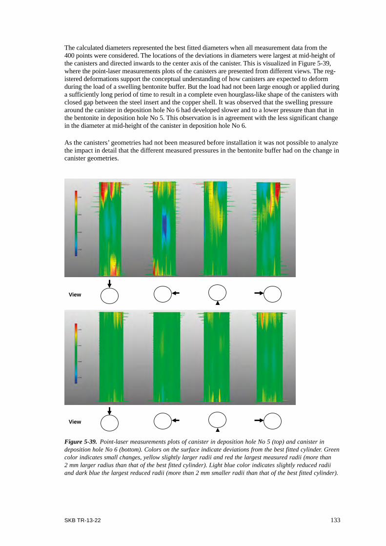
SKB TR-13-22 133

The calculated diameters represented the best fitted diameters when all measurement data from the 400 points were considered. The locations of the deviations in diameters were largest at mid-height of the canisters and directed inwards to the center axis of the canister. This is visualized in Figure 5-39, where the point-laser measurements plots of the canisters are presented from different views. The reg-istered deformations support the conceptual understanding of how canisters are expected to deform during the load of a swelling bentonite buffer. But the load had not been large enough or applied during a sufficiently long period of time to result in a complete even hourglass-like shape of the canisters with closed gap between the steel insert and the copper shell. It was observed that the swelling pressure around the canister in deposition hole No 6 had developed slower and to a lower pressure than that in the bentonite in deposition hole No 5. This observation is in agreement with the less significant change in the diameter at mid-height of the canister in deposition hole No 6.

As the canisters’ geometries had not been measured before installation it was not possible to analyze the impact in detail that the different measured pressures in the bentonite buffer had on the change in canister geometries.

Figure 5-39. Point-laser measurements plots of canister in deposition hole No 5 (top) and canister in deposition hole No 6 (bottom). Colors on the surface indicate deviations from the best fitted cylinder. Green color indicates small changes, yellow slightly larger radii and red the largest measured radii (more than 2 mm larger radius than that of the best fitted cylinder). Light blue color indicates slightly reduced radii and dark blue the largest reduced radii (more than 2 mm smaller radii than that of the best fitted cylinder).

View

View

134 SKB TR-13-22

5.5.3 Measurement of canister lengthThe top lid was removed before measurements took place. The upper level was determined by direct measurement of the outer ring at 400 points around the canister (Jonsson 2015). The lower level could not be accessed directly as the canister were standing directly on the floor, and the measure-ments were made on the floor around the canister and immediately adjacent to the canister. As a consequence, possible procedural irregularities on the floor were included in the results of the mea-surements of the lower level. The numerical results are presented in Table 5-7. The nominal length at manufacturing of the two copper shells was 4,835 mm. The length, however, was not measured just before installation, so the exact original length was not known. The available data would suggest that both canisters have been longer during the seven years in the Prototype Repository. And, elongation was expected. Calculations made by SKB have revealed that an elongation of 5 mm would be realistic when the swelling pressure of the buffer decreases the diameter at mid-height (Rydén H 2015, personal communication). At an assumed worst case with uneven wetting the elongation was estimated to become 12 mm. Although it would be logical to assume that the canisters in deposition holes No 5 and no 6 have been longer, there are no conclusive facts that justify such an assumption.

Table 5-7. Summary of canister lengths from point laser measurements. D1 denotes the largest distance between the canister top and the floor the canister stood on, D2 denotes the shortest distance. (Table in Jonsson 2015.)

Canister in Deposition hole No

Measured length based on the measure-ments of top and bottom positions mm

5 D1 4838.140 D2 4836.030

6 D1 4838.797 D2 4837.988

5.5.4 Examination of canister surfacesWhen the canisters had been retrieved and transported to the Canister Laboratory, the first ocular examination showed that the canister had some damage caused by the handling, in addition to the manmade grooves for the fiber optics that measured the surface temperature.

The examination made by the Swedish SP Technical Research Institute showed that major damage or surface defects could not be detected by high density laser scanning or geodetic method.

The examinations made by Taxén (2013) on the surfaces of the two canisters used a more sophis-ticated method. Core samples were taken across the total copper shell thickness at six different positions on each canister (Figure 5-40). The surface profiles were measured from SEM images of cross-sections through the cores. Observation of the maximum pit depth was done at 20 different locations per sample and the measured values of pit depths were treated with extreme value analysis. The results were relatively consistent for both examined canisters and showed that the sample from the bottom plate exhibited the greatest pit depths with a maximum observed depth of ~ 7 µm. The sample from the mid-height of the canisters exhibited the minimum pit depths and the sample from the lid, which had not been exposed to the compacted bentonite, showed an intermediate pit depth. The canister from deposition hole No 6 exhibited slightly deeper pits than the canister in deposition hole No 5. The difference is of the order of 20%. Taxén (2013) points out that the results of his examination cannot be used as a basis for an assessment of morphology evolution over time, as the canisters’ surface conditions had not been examined before the canisters were installed.

5.5.5 Examination of corrosion products on canister surfacesThe sample taken from the upper part of the canister in deposition hole No 5 (Figure 4-16) was cut into smaller samples for various analyses (Taxén 2013). The samples taken from the canister in deposition hole No 6 were never used for corrosion examinations, only metallographic documenta-tion, see Section 5.5.4.

SKB TR-13-22 135

Examination methodsAttenuated Total Reflectance (ATR)-FTIR microscopy was used directly on the copper surface for identification of corrosion products, which were not fully crystallized and ATR-FTIR analysis and KBr-transmissions analysis on powder scraped off the copper surface. XRD was used directly on the copper surface for identification of crystalline compounds. SEM was used to provide micrographs and distribution of different elements locally on the surfaces.

Examination of corrosion productsThe surface profiles measured after cleaning and pickling showed clear traces of the machining during manufacturing. The grooves had a height of about 10 µm and were relatively sharp. This suggested that in these areas had only slight corrosion occurred and that the corrosion had been relatively smooth.

Small and unquantifiable amounts of the corrosion products malachite – Cu(II) compound – and likely cuprite – Cu(I) compound – were identified on the surface by FTIR. XRD showed cuprite but not malachite. The difference may be that the FTIR measurements made more locally and to a signal from a local presence of malachite did not show up in the mean value over the area covered by XRD.

Elemental analysis of the surface by SEM showed, in addition to copper, substances believed to come from the bentonite: oxygen, magnesium, silicon, aluminum, potassium and calcium. Sulfur might have come from several sources: sulfate and sulfide from bentonite and groundwater.

A relatively strong correlation between the presence of molybdenum and sulfur was found suggest-ing that some of the sulfur content came from molybdenum sulfide, which was used as a lubricant when the bentonite block was manufactured.

5.5.6 Examination of hydrogen contentA total of six samples of copper were analyzed. Their size was about 5 × 5 × 5 mm and mass about 1.3 grams each. Two of the samples were taken from the canister surface, and had thus been in contact with the bentonite. Two were taken just inside the former, further inwards in the copper shell. The last two were taken just inside the latter two, at a depth of 10 mm into the copper shell.

The purpose was to look for evidence that the hydrogen content in the copper had increased, which would suggest that copper had corroded under production of hydrogen gas.

Examination methodAll samples were melted in a graphite crucible. Released gases were caught up in an atmosphere of inert gas and the content of hydrogen gas was determined. The exact temperature at which the hydrogen left could be inferred from the method. The analysis covered all hydrogen that was released at a temperature of 2,500°C. A reference analysis of a sample with known hydrogen content was made in direct connection to the canister sample analyzes. This reference sample consisted of 6 ppm of hydrogen in steel and was used for calibration. Before and after copper analyzes were made, reference analyzes were made of hydrogen in titanium. These reference analyzes showed no sign of abnormal drift of the instrument calibration during the time the copper analyzes were made. A detailed description of the analytical method has been presented by Taxén et al. (2012).

Examination of hydrogen in copperMelting analysis of hydrogen content at three different depths into the copper metal did not indicate that hydrogen was absorbed during exposure in the Prototype Repository. The hydrogen content in the material was homogeneous, on this scale, with a mean value of about 0.43 ppm. This value is consistent with the analytical data for the copper ingots that specified a range of between 0.3 and 0.8 ppm hydrogen (SKB 2010b).

136 SKB TR-13-22

5.6 Examination of copper electrodesReal time corrosion monitoring was applied in the Prototype Repository in order to measure corro-sion rate of copper during the whole operational period, see Section 2.6.10. For the purpose three copper electrodes had been installed in the buffer block C4 in the upper part of deposition hole No 5 (Section 2.6.10). In the cause of opening and retrieval the in situ corrosion potential was measured before the electrodes were retrieved and sent to the laboratory (Section 4.6) for further examination.

5.6.1 ObjectivesThe electrodes were uncovered and retrieved with the objectives to:

• Supplement the on-line measurement with in situ measurement of the corrosion potential, which would be possible when part of the concrete plug to the outer section had been removed.

• Perform laboratory measurements of the corrosion potential.

• Examine the corrosion products on the surface of the electrodes.

5.6.2 Electrochemical measurements of corrosion potentialMeasurements during opening and retrievalThe corrosion potential of the copper electrodes was first measured in early 2011 when part of the outer concrete plug was removed and it became possible to drill a hole through the remaining wall of the prefabricated concrete beams and place a reference electrode in contact with the backfill (Rosborg 2013b).

The corrosion potential was measured to –40 mV Standard Hydrogen Electrode (SHE) in February 2011. The corrosion potential was again measured in September 2011 when reference electrodes could be placed in the remaining backfill just above the copper electrodes. About 850 mm backfill still remained on top of bentonite block C4. The corrosion potential at this time was measured to 25 mV SHE. This value was interpreted as a sign of air ingress to the electrode/bentonite interface. The two measurement values are shown in Table 5-8.

Table 5-8. Measured corrosion potential of examined copper electrodes from bentonite block C4 in deposition hole No 5. (After Table 3-1 in Rosborg 2013b.)

Occasion of measurement Measured corrosion potential mV SHE

April 2011 when plug had been breached. –40September 2011 when backfill had been removed. +25November 2011 just before retrieval of electrode “Black” from the small removed bentonite block that was seamed drilled from block C4.

+165

Measurements after opening and retrievalFinal electrochemical measurements were performed in the laboratory on the three electrodes, when they still were embedded in the bentonite in the retrieved package (the retrieval is described in Section 4.6.2). The measurements comprised measurements of the corrosion potential and EIS.

The corrosion potentials, measured for one of the three electrode labeled “Black” (after the color of the insulation of its cables), were given as a back-up for the post-test examination of the electrodes. Real-time corrosion monitoring with the SmartCET® instrumentation, as performed at Äspö before retrieval (see Section 2.6.10) and also intended for the final measurements turned out to be impossible as the corrosion potentials of the copper electrodes had at that point in time drifted apart too much.

The test set-up comprised two reference electrodes and one thermometer installed in the bentonite block as shown in Figure 5-40. Holes were drilled in the bentonite block to a depth of about 5 cm and some Äspö HRL groundwater was poured into the holes before installing the reference electrodes in them. The measurements were then performed in the following order:

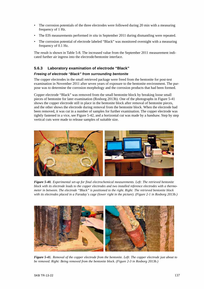
SKB TR-13-22 137

• The corrosion potentials of the three electrodes were followed during 20 min with a measuring frequency of 1 Hz.

• The EIS measurements performed in situ in September 2011 during dismantling were repeated.

• The corrosion potential of electrode labeled “Black” was monitored overnight with a measuring frequency of 0.1 Hz.

The result is shown in Table 5-8. The increased value from the September 2011 measurement indi-cated further air ingress into the electrode/bentonite interface.

5.6.3 Laboratory examination of electrode “Black”Freeing of electrode “Black” from surrounding bentoniteThe copper electrodes in the small retrieved package were freed from the bentonite for post-test examination in November 2011 after seven years of exposure to the bentonite environment. The pur-pose was to determine the corrosion morphology and the corrosion products that had been formed.

Copper electrode “Black” was removed from the small bentonite block by breaking loose small pieces of bentonite for later examination (Rosborg 2013b). One of the photographs in Figure 5-41 shows the copper electrode still in place in the bentonite block after removal of bentonite pieces, and the other shows the electrode during removal from the bentonite block. When the electrode had been removed, it was cut in a number of samples for further examination. The copper electrode was tightly fastened in a vice, see Figure 5-42, and a horizontal cut was made by a handsaw. Step by step vertical cuts were made to release samples of suitable size.

Figure 5-40. Experimental set-up for final electrochemical measurements. Left: The retrieved bentonite block with its electrode leads to the copper electrodes and two installed reference electrodes with a thermo-meter in between. The electrode “Black” is positioned to the right. Right: The retrieved bentonite block with its electrodes placed in a Faraday´s cage (lower right in the picture). (Figure 2-1 in Rosborg 2013b.)

Figure 5-41. Removal of the copper electrode from the bentonite. Left: The copper electrode just about to be removed. Right: Being removed from the bentonite block. (Figure 2-3 in Rosborg 2013b.)

138 SKB TR-13-22

Examination of electrode “Black”Identification of corrosion productsXRD measurements, FTIR spectroscopy, and Raman spectroscopy were employed by Rosborg (2013b) to identify corrosion products on the copper electrode. Corrosion products for XRD measurements and FTIR spectroscopy were scraped off from two surface areas of the copper electrode “Black”, see Figure 5-43. One area (termed “H”) contained mainly brownish, and one area (termed V) mainly blue-green corrosion products. FTIR and Raman spectroscopy were also applied on corrosion products remaining on the surface of electrode “Black”.

MicroscopyA USB microscope (digital microscope which connects to a computer via a USB port) was used to examine the surface on the copper electrode (seen in Figure 5-43) at a magnification of about 50x. Some areas were also viewed at a higher magnification. SEM was used to examine areas of the surface in more detail. A Nova 600 NanoLab DualBeam™ SEM/FIB instrument was used to prepare a few “micro-cross sections” through the electrode surface by means of focused ion beam milling to examine and characterize the corrosion product layer on the electrode (Rosborg 2013b).

Appearance of electrode after exposureRosborg (2013b) suggested from the appearance of the copper electrode, when part of the surround-ing bentonite had been removed, see Figure 5-44, that both Cu(I) and Cu(II) corrosion products existed on the electrode surface and that they had been formed during the seven years of exposure. The blue-green corrosion material, suggested to be Cu(II) products, was unevenly distributed on the surface of the electrode (electrode “Black”). They were more abundant on some parts of the electrode. Corrosion products were also found on the adjacent bentonite after removal of the copper electrode from the bentonite block, see Figure 5-44, thus revealing a better adherence to the benton-ite on that part of the surface. Four photographs of the electrode, after it had been removed from the bentonite block, are shown in Figure 5-45.

Corrosion productsThe XRD measurements verified the presence of cuprite, Cu2O (Cu(I) compound), and malachite, Cu2(OH)2CO3 (Cu(II) compound), (Rosborg 2013b). Paratacamite, Cu2(OH)3Cl (Cu(II) compound), was not found contrary to the finding on copper coupons in LOT test parcel A2 (Karnland et al. 2009), where only paratacamite was observed and nomalakite. This difference was explained by Rosborg (2013b) to be caused by the difference in chemical composition of the water in the bentonite.

The performed FTIR and Raman spectroscopy confirmed the observation (Rosborg 2013b). The FTIR spectra from the KBr transmission measurements on corrosion products from sample areas “V” and “H” (see explanation to labels “V” and “H” in caption to Figure 5-43) were dominated by bands from bentonite, but the spectra had also bands from malachite and cuprite. Malachite was

Figure 5-42. Left: Cutting out samples from the copper electrode “Black”. Right: Temporary storage of samples from the copper electrode “Black”. (Figure 2-4 in Rosborg 2013b.)

SKB TR-13-22 139

Figure 5-43. The two photographs show where corrosion products were scraped off from copper electrode “Black”. Left: the sample area termed “H” where mainly brownish corrosion products existed. Right: the sample area termed “V” was mainly blue-green corrosion products were sampled. (Figure 2-5 in Rosborg 2013b.)

Figure 5-44. Corrosion products still remaining on adjacent bentonite after removal of the electrode. (Figure 3-1 in Rosborg 2013b.)

Figure 5-45. Appearance of copper electrode “Black” immediately after removal from the bentonite block. The top pictures show the two sample areas termed “H” (left) and “V” (right) in Figure 5-43. (Figure 3-2 in Rosborg 2013b.)

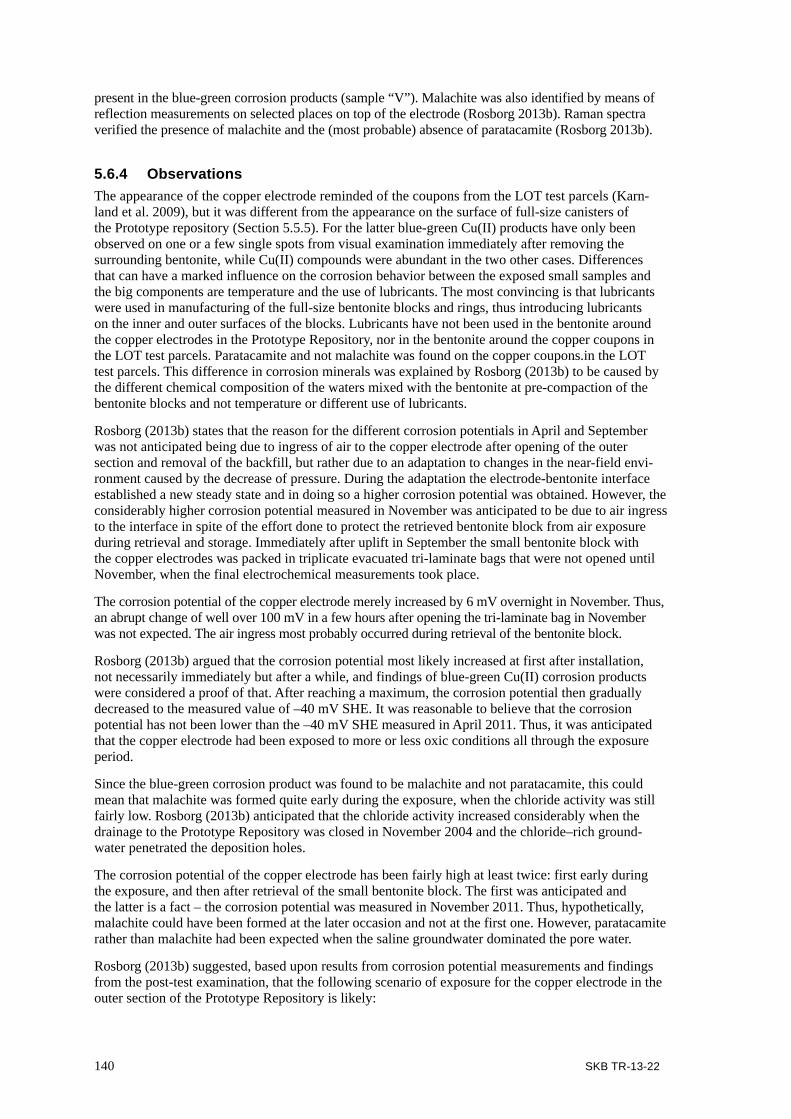
140 SKB TR-13-22

present in the blue-green corrosion products (sample “V”). Malachite was also identified by means of reflection measurements on selected places on top of the electrode (Rosborg 2013b). Raman spectra verified the presence of malachite and the (most probable) absence of paratacamite (Rosborg 2013b).

5.6.4 ObservationsThe appearance of the copper electrode reminded of the coupons from the LOT test parcels (Karn-land et al. 2009), but it was different from the appearance on the surface of full-size canisters of the Prototype repository (Section 5.5.5). For the latter blue-green Cu(II) products have only been observed on one or a few single spots from visual examination immediately after removing the surrounding bentonite, while Cu(II) compounds were abundant in the two other cases. Differences that can have a marked influence on the corrosion behavior between the exposed small samples and the big components are temperature and the use of lubricants. The most convincing is that lubricants were used in manufacturing of the full-size bentonite blocks and rings, thus introducing lubricants on the inner and outer surfaces of the blocks. Lubricants have not been used in the bentonite around the copper electrodes in the Prototype Repository, nor in the bentonite around the copper coupons in the LOT test parcels. Paratacamite and not malachite was found on the copper coupons.in the LOT test parcels. This difference in corrosion minerals was explained by Rosborg (2013b) to be caused by the different chemical composition of the waters mixed with the bentonite at pre-compaction of the bentonite blocks and not temperature or different use of lubricants.

Rosborg (2013b) states that the reason for the different corrosion potentials in April and September was not anticipated being due to ingress of air to the copper electrode after opening of the outer section and removal of the backfill, but rather due to an adaptation to changes in the near-field envi-ronment caused by the decrease of pressure. During the adaptation the electrode-bentonite interface established a new steady state and in doing so a higher corrosion potential was obtained. However, the considerably higher corrosion potential measured in November was anticipated to be due to air ingress to the interface in spite of the effort done to protect the retrieved bentonite block from air exposure during retrieval and storage. Immediately after uplift in September the small bentonite block with the copper electrodes was packed in triplicate evacuated tri-laminate bags that were not opened until November, when the final electrochemical measurements took place.

The corrosion potential of the copper electrode merely increased by 6 mV overnight in November. Thus, an abrupt change of well over 100 mV in a few hours after opening the tri-laminate bag in November was not expected. The air ingress most probably occurred during retrieval of the bentonite block.

Rosborg (2013b) argued that the corrosion potential most likely increased at first after installation, not necessarily immediately but after a while, and findings of blue-green Cu(II) corrosion products were considered a proof of that. After reaching a maximum, the corrosion potential then gradually decreased to the measured value of –40 mV SHE. It was reasonable to believe that the corrosion potential has not been lower than the –40 mV SHE measured in April 2011. Thus, it was anticipated that the copper electrode had been exposed to more or less oxic conditions all through the exposure period.

Since the blue-green corrosion product was found to be malachite and not paratacamite, this could mean that malachite was formed quite early during the exposure, when the chloride activity was still fairly low. Rosborg (2013b) anticipated that the chloride activity increased considerably when the drainage to the Prototype Repository was closed in November 2004 and the chloride–rich ground-water penetrated the deposition holes.

The corrosion potential of the copper electrode has been fairly high at least twice: first early during the exposure, and then after retrieval of the small bentonite block. The first was anticipated and the latter is a fact – the corrosion potential was measured in November 2011. Thus, hypothetically, malachite could have been formed at the later occasion and not at the first one. However, paratacamite rather than malachite had been expected when the saline groundwater dominated the pore water.

Rosborg (2013b) suggested, based upon results from corrosion potential measurements and findings from the post-test examination, that the following scenario of exposure for the copper electrode in the outer section of the Prototype Repository is likely:

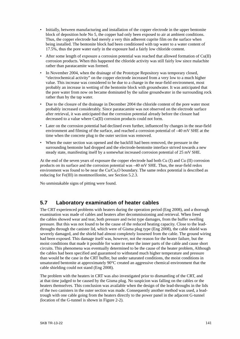
SKB TR-13-22 141

• Initially, between manufacturing and installation of the copper electrode in the upper bentonite block of deposition hole No 5, the copper had only been exposed to air at ambient conditions. Thus, the copper electrode had merely a very thin adherent cuprite film on the surface when being installed. The bentonite block had been conditioned with tap water to a water content of 17.5%, thus the pore water early in the exposure had a fairly low chloride content.

• After some length of exposure a corrosion potential was reached that allowed formation of Cu(II) corrosion products. When this happened the chloride activity was still fairly low since malachite rather than paratacamite was formed.

• In November 2004, when the drainage of the Prototype Repository was temporary closed, “electro chemical activity” on the copper electrode increased from a very low to a much higher value. This increase was considered to be due to a change in the near-field environment, most probably an increase in wetting of the bentonite block with groundwater. It was anticipated that the pore water from now on became dominated by the saline groundwater in the surrounding rock rather than by the tap water.

• Due to the closure of the drainage in December 2004 the chloride content of the pore water most probably increased considerably. Since paratacamite was not observed on the electrode surface after retrieval, it was anticipated that the corrosion potential already before the closure had decreased to a value where Cu(II) corrosion products could not form.

• Later on the corrosion potential had declined even further, influenced by changes in the near-field environment and filming of the surface, and reached a corrosion potential of –40 mV SHE at the time when the concrete plug to the outer section was removed.

• When the outer section was opened and the backfill had been removed, the pressure in the surrounding bentonite had dropped and the electrode-bentonite interface strived towards a new steady state, manifesting itself by a somewhat increased corrosion potential of 25 mV SHE.

At the end of the seven years of exposure the copper electrode had both Cu (I) and Cu (II) corrosion products on its surface and the corrosion potential was –40 mV SHE. Thus, the near-field redox environment was found to be near the Cu/Cu2O boundary. The same redox potential is described as reducing for Fe(III) in montmorillonite, see Section 5.2.3.

No unmistakable signs of pitting were found.

5.7 Laboratory examination of heater cablesThe CRT experienced problems with heaters during the operation period (Eng 2008), and a thorough examination was made of cables and heaters after decommissioning and retrieval. When freed the cables showed wear and tear, both pressure and twist type damages, from the buffer swelling pressure. But this was not found to be the cause of the reduced heating capacity. Close to the lead-throughs through the canister lid, which were of Gisma plug type (Eng 2008), the cable shield was severely damaged, and the shield had almost completely loosened from the cable. The ground wiring had been exposed. This damage itself was, however, not the reason for the heater failure, but the moist conditions that made it possible for water to enter the inner parts of the cable and cause short circuits. This phenomena was eventually determined to be the cause of the heater problem, Although the cables had been specified and guaranteed to withstand much higher temperature and pressure than would be the case in the CRT buffer, but under saturated conditions, the moist conditions in unsaturated bentonite at approximately 90°C created an aggressive chemical environment that the cable shielding could not stand (Eng 2008).

The problem with the heaters in CRT was also investigated prior to dismantling of the CRT, and at that time judged to be caused by the Gisma plug. No suspicion was falling on the cables or the heaters themselves. This conclusion was available when the design of the lead-throughs in the lids of the two canisters in the outer section was made. Consequently another method was used, a lead-trough with one cable going from the heaters directly to the power panel in the adjacent G-tunnel (location of the G-tunnel is shown in Figure 2-2).

142 SKB TR-13-22

When the information of the cause of the heater problem in the CRT became available and the indi-cations in the Prototype Repository were very similar, with low resistance in the systems, the Project initiated a survey of the installation of cabling/canister in the outer section.

5.7.1 ObjectivesThe survey of cables, lead-throughs through the canister lids and heaters inside the canisters was made with the objectives:

• To make visual inspections of the cables during freeing of them and after their retrieval.• To measure the cables’ insulation (resistance between wire and earth).• To open the canisters and examine the cables and heaters inside.

5.7.2 Measurement on cablingEach cable was cut at 3–4 meters distance from the canister and a first visual inspection indicated extensive damage because of the major deformation and external damage to the insulation, see Figure 5-51 (left picture). The insulation was stripped at the ends so that the wires could be identified and then measured for each pair of earth resistance and insulation, see Figure 5-46 (right picture). The grounding wire was oxidized which also was a result of the damaging of the outer insulation.

5.7.3 Measurement on cablesAfter the first measurement the cables were cut close to the canister and each wire was tested with respect to continuity and insulation. The cases of interruptions that were found could be attributed to damage from drilling, see Figure 5-47 (left picture). One exception was a short-circuit that had led to emission of heat so that nearby wires’ isolations had been affected by the woven reinforcement. This had occurred during operation, see Figure 5-47 (right picture).

Measurements inside canistersCanister in deposition hole No 5The canister was opened and inspected for damage to the lids, seals and penetrations. No visible damage to the lid or its seals was observed. Figure 5-48 shows an electrical wire penetration in good condition. The electric grommet was not damaged either. Discoloration of the surface copper/copper was assumed to come from the inside and reached only to the first seal. Damages and/or leakages through the sealing compound around the individual wires were not tested.

Figure 5-46. Damaged cable in deposition hole No 6.

Deformed cable from canister in deposition hole No 6. Stripped cable from canister in deposition hole No 6 with exposed wires.

SKB TR-13-22 143

Figure 5-47. Examples of damaged that have occurred on cables in deposition hole No 6.

Drill damage on cable from canister in deposition hole No 6. Melted insulation in cable from canister in deposition hole No 5. The cause is probably short-circuiting, which has caused local heating. The photo shows how the woven reinforcement has affected the surface of the wires.

Figure 5-48. “Nose” for electrical wire penetrations. Corrosion products were found only inside the first O-ring.

The canister in deposition hole No 5 was dry and measurements on its heater elements showed good results. No sign of humidity or corrosion was detected. All heater elements were in good condition. Figure 5-49 (left picture) shows a photo of the open lid and Figure 5-49 (right picture) the interior behind the inner lid in the canister in deposition hole No 5.

Canister in deposition hole No 6Canister in deposition hole No 6 was humid and water poured out of the canister when it was opened. Figure 5-50 shows the opened canister after removal of the copper lid. The extent of corrosion on the lid provided an indication of the amount of water that had leaked in to the canister. As the canister had been stored in horizontal position after retrieval and been laying in two different directions, two areas

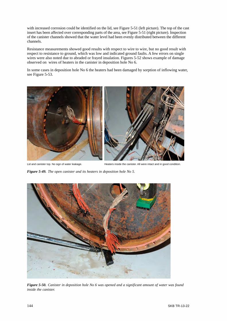
144 SKB TR-13-22

with increased corrosion could be identified on the lid, see Figure 5-51 (left picture). The top of the cast insert has been affected over corresponding parts of the area, see Figure 5-51 (right picture). Inspection of the canister channels showed that the water level had been evenly distributed between the different channels.

Resistance measurements showed good results with respect to wire to wire, but no good result with respect to resistance to ground, which was low and indicated ground faults. A few errors on single wires were also noted due to abraded or frayed insulation. Figures 5-52 shows example of damage observed on wires of heaters in the canister in deposition hole No 6.

In some cases in deposition hole No 6 the heaters had been damaged by sorption of inflowing water, see Figure 5-53.

Figure 5-49. The open canister and its heaters in deposition hole No 5.

Figure 5-50. Canister in deposition hole No 6 was opened and a significant amount of water was found inside the canister.

Lid and canister top. No sign of water leakage. Heaters inside the canister. All were intact and in good condition.

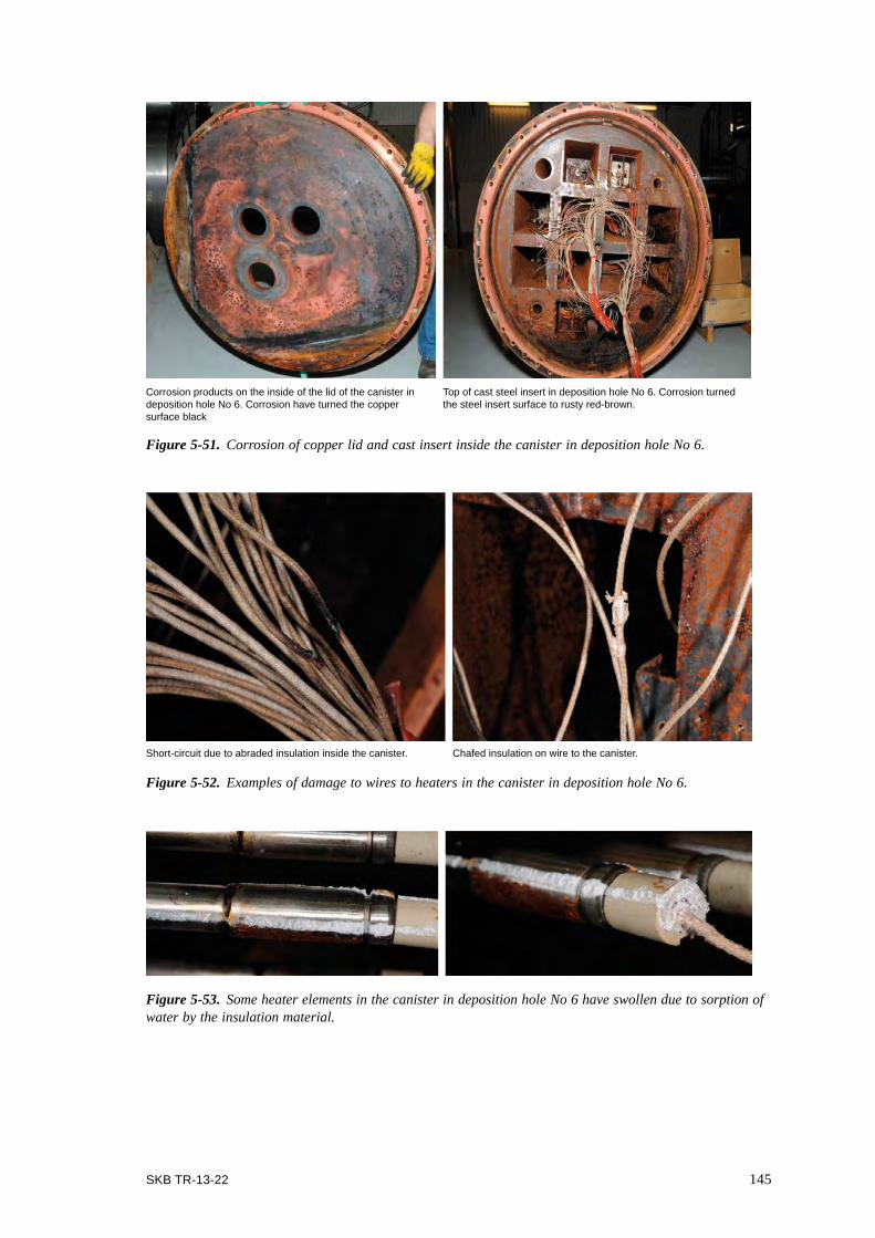
SKB TR-13-22 145

Figure 5-51. Corrosion of copper lid and cast insert inside the canister in deposition hole No 6.

Corrosion products on the inside of the lid of the canister in deposition hole No 6. Corrosion have turned the copper surface black

Top of cast steel insert in deposition hole No 6. Corrosion turned the steel insert surface to rusty red-brown.

Figure 5-52. Examples of damage to wires to heaters in the canister in deposition hole No 6.

Figure 5-53. Some heater elements in the canister in deposition hole No 6 have swollen due to sorption of water by the insulation material.

Short-circuit due to abraded insulation inside the canister. Chafed insulation on wire to the canister.

146 SKB TR-13-22

5.8 Sensor validation and credibility of data The result of the retrieval of sensors is presented in Section 4.8. This Section 5.8 presents the validation work carried out with the retrieved sensors having a condition considered appropriate for yielding accurate results. The work has been reported in detail by Nilsson (2014) and Wieczorek et al. (2014), and the following summarizes their findings.

5.8.1 ObjectivesThe objective with the laboratory examination and testing of the retrieved sensors were:

• To get feedback and information about which of the installed sensors functioned as planned. This is not least important as input for the planning of instrumentation of upcoming tests.

• To get information whether any of the calibration values have changed during the water uptake phase and thus affected the interpretation of the recorded data.

5.8.2 Pressure sensors in buffer and backfillFirst sorting of sensors to be validatedWhen the sensors arrived in the laboratory, a first sorting was made where several sensors could be directly excluded due to the damage seen such as missing cables or missing parts, which made validation impossible. Pressure sensor surfaces, which were used for sealing towards the test cell, had to be without severe damages. Otherwise, leakage could prevent the water pressure from being maintained in the cell during the validation test.

This first sorting revealed that some of the observed damages were likely to have occurred during dismantling of the test while others were likely to have occurred during the operation or the installa-tion of the Prototype Repository.

In total 33 sensors out of retrieved 73 in the buffer and backfill were judged to be in a sufficiently good condition for the validation work. They were pressure sensor only as shown in Table 4-3. Nilsson (2014) has presented the reasons for excluding sensors in more detail.

Work with GRS geoelectric sensors is presented in Section 5.8.3.

Testing methodologyGeokonTotal pressure cells (type: 4800 positioned in the in buffer, see Table 4-3) were immersed in a pres-sure vessel and the tube with the wire was led through the lid, see Figure 5-54a. A Swagelok 8 mm coupling was used to seal the tube, which was the reason why sensors with short or damaged tubes could not be tested. The maximum pressure the vessel could stand was 4.5 MPa, which exceeded the maximum reading for all but three sensors. Those showed a maximum pressure of about 6 MPa. Complementary testing, where a mechanical force was applied on the total pressure cell, was also carried out. These tests were made in a hydraulic press with rubber pads for transferring the load to the cell, see Figure 5-54b.

Total pressure cells (type: 4850 positioned in the backfill, see Table 4-3) were placed in a hydraulic press with heavy rubber padding for distributing the load from the load frame to the sensors, see Figure 5-54c. Steel plates were used to distribute the pressure over the rubber pad. Since this test set-up is not ideal, it can be seen more as an indicative test of the sensor function.

A number of different tests with rubber and wood padding were made to investigate the method. The repeatability within the same set up was good but different set-up gave different results. This means that the results can only be used to test whether the sensors function and whether the signal is linear to the load but not to check absolute values.

Pore pressure cells (type: 4500 positioned in both the backfill and the buffer, see Table 4-3) were tested in a another pressure vessel where the sensor tip was led through the lid implying that only the active parts were immersed into the vessel, see 5-54d. The front part of the housing with the filter was thus excluded.

SKB TR-13-22 147

KuliteThe sensors were tested in the same way as the Geokon sensors (total immersion). The applied power supply and resistive load were the same as in the original manufacturer’s test.

ObservationsThe results from the testing of the sensors were presented as the measured/calculated value as a func-tion of the applied pressure. Linear regression analyses were made. Ideally, the regression should be Y = X. However, in most cases, the results from the regression was in the form of Y = A * X + B where A is the slope and B is the offset error. Sensors with slope within ± 2% deviation from A=1 and an offset of ≤ 0,2MPa were considered to have given reliable values during the operation of the Prototype Repository. This is against the background that the manufacturer specifies an interval of ± 1% devia-tion of the newer sensors.

Figure 5-54. Test cells used for validation of total pressure sensors. (Figures 3-1, 3-2, 3-3 and 3-4 in Nilsson 2014.)

a) Test cell with a total pressure sensor before immersion into water.

b) Total pressure sensor tested with mechanical force and a rubber pad.

c) Total pressure sensorsunder testing, the sensorwas installed in thebackfill.

d) The lid of the test cell with a pore pressure sensor installed.

148 SKB TR-13-22

The majority of the pore pressure sensors and the total pressure sensors, placed in the backfill, were tested. They show deviation from the applied pressure within ± 2% with one exception. This sensor had a deviation of –4%. The data from these types of installed sensors can thus be trusted as long as readings were acquired.

Of the retrieved 26 total pressure sensors in the buffer (all of type Geokon 4800 in Table 4-3) 8 were tested. All of the validated sensors worked correctly, but an error in the evaluation of the Geokon sensors was identified. The evaluation of the obtained frequency signal from the sensor was during operation made with an equation (out of two) given in a calibration protocol. When using the linear equation (which is normal) the error appeared to be more than 30% above applied pressure.

Figure 5-55 shows one example from the validation were the re-calculated pressure (Y-axis) is com-pared to the actually applied pressure (X-axis).

The graph shows a strong disagreement of pressures (more than 30%) below a pressure of 5 MPa. After a number of additional tests, also with new sensors, the discrepancy remained.

A comparison between the results with the two different equations was therefore made. In Figure 5-56 the results from both the linear equation (blue diamonds) and the polynomial equation (red boxes) are presented. When using the linear and the polynomial equations on the same raw data the discrepancy was explained. The polynomial equation provided a sensor deviation of only 1% from the ideal line Y=X and is thus the equation that should have been used. Since the values are in the low range for the senor the difference between the two calculations is quite large. In practice it means that the total pressure values registered prior to opening and retrieval should be recalcu-lated with the correct equation. A check of the calibration data for the rest of the sensors showed that the difference between linear and polynomial equation was large for only this batch of model variant 4800, which had been specially design for SKB. Goudarzi has in the latest sensor data report (2014) made the necessary adjustments.

Since no Kulite sensor could be tested no conclusions could be drawn regarding their readings. The GRS geoelectrical sensors described in Section 5.8 3 gave correct readings if not suffering from strained cables.

Figure 5-55. Linear equation applied to values from sensor PB526 (total pressure sensor in deposition hole No 5). (Figure 4-1 in Nilsson 2014.)

y = 1,3479x + 0,048

R² = 0,9995

0

1

2

3

4

5

6

0 1 2 3 4 5

Cal

cula

ted

pres

sure

[MPa

]

Applied Standard Pressure [MPa]

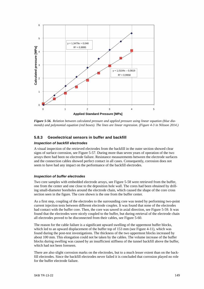
SKB TR-13-22 149

5.8.3 Geoelectrical sensors in buffer and backfillInspection of backfill electrodesA visual inspection of the retrieved electrodes from the backfill in the outer section showed clear signs of surface corrosion, see Figure 5-57. During more than seven years of operation of the two arrays there had been no electrode failure. Resistance measurements between the electrode surfaces and the connection cables showed perfect contact in all cases. Consequently, corrosion does not seem to have had any impact on the performance of the backfill electrodes.

Inspection of buffer electrodesTwo core samples with embedded electrode arrays, see Figure 5-58 were retrieved from the buffer, one from the center and one close to the deposition hole wall. The cores had been obtained by drill-ing small-diameter boreholes around the electrode chain, which caused the shape of the core cross section seen in the figure. The core shown is the one from the buffer center.

As a first step, coupling of the electrodes to the surrounding core was tested by performing two-point current injection tests between different electrode couples. It was found that none of the electrodes had contact with the buffer core. Then, the core was sawed in axial direction, see Figure 5-59. It was found that the electrodes were nicely coupled to the buffer, but during retrieval of the electrode chain all electrodes proved to be disconnected from their cables, see Figure 5-60.

The reason for the cable failure is a significant upward swelling of the uppermost buffer blocks, which led to an upward displacement of the buffer top of 153 mm (see Figure 4-11), which was found during the post-test investigations. The thickness of the two uppermost blocks increased by about 100 mm. This elongation could not be taken by the cables. The volume increase of the buffer blocks during swelling was caused by an insufficient stiffness of the tunnel backfill above the buffer, which had not been foreseen.

There are also slight corrosion marks on the electrodes, but to a much lesser extent than on the back-fill electrodes. Since the backfill electrodes never failed it is concluded that corrosion played no role for the buffer electrode failure.

Figure 5-56. Relation between calculated pressure and applied pressure using linear equation (blue dia-monds) and polynomial equation (red boxes). The lines are linear regression. (Figure 4-3 in Nilsson 2014.)

y = 1,0104x – 0,0819

R² = 0,9958

y = 1,3479x + 0,048R² = 0,9995

0

1

2

3

4

5

6

0 1 2 3 4 5

Cal

cula

ted

pres

sure

[MPa

]

Applied Standard Pressure [MPa]

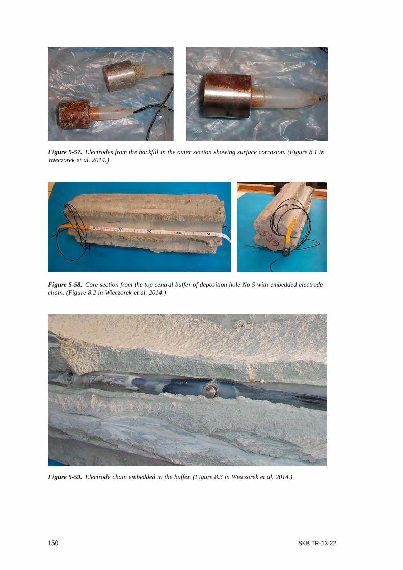
150 SKB TR-13-22

Figure 5-57. Electrodes from the backfill in the outer section showing surface corrosion. (Figure 8.1 in Wieczorek et al. 2014.)

Figure 5-58. Core section from the top central buffer of deposition hole No 5 with embedded electrode chain. (Figure 8.2 in Wieczorek et al. 2014.)

Figure 5-59. Electrode chain embedded in the buffer. (Figure 8.3 in Wieczorek et al. 2014.)

SKB TR-13-22 151

5.8.4 Sensors in rockThe sensors installed in the rock are presented in Section 2.5.7. None were retrieved for laboratory testing or re-calibration.

The temperature sensors were considered to work well as their readings gave the same results as the temperature readings by other supplementary installed thermocouples in sensors for observation of other parameters, like rock stresses.

The Geokon rock stress sensors, however, provided unexpected readings, which were judged to be wrong. The sensors were namely designed to be used at ambient rock temperature, but were during operation exposed to elevated temperatures outside the known calibration curve. These elevated temperatures were found to affect the readings more than the absolute values that were intended to be observed. Retrieval and re-calibration were not judge to make the readings completely reliable, and it became consequently of no added value to retrieve the sensors.

The credibility of measurement data from the rock mechanical sensors was instead assessed by com-parison with results from numerical models (Lönnqvist and Hökmark 2015). General conclusions from these analyses are presented below.

Credibility of rock mechanical sensorsFour types of rock mechanical instruments were installed around deposition holes No 5 and No 6:

• Biaxial stressmeter.

• Soft inclusion stress cell.

• Deformation meter.

• Strain gage.

Each type was analyzed.

Figure 5-60. Retrieved electrode chain. (Figure 8.4 in Wieczorek et al. 2014.)

152 SKB TR-13-22

Biaxial stress metersMonitoring of changes in stress by use of biaxial stress meters took place both during the drilling of deposition holes 5 and 6 and during the subsequent heated phase. The biaxial stress meters monitored the change in stress from a reference state to a new state. In the following, these changes in stress are denoted stress increments.

Monitored stress additions caused by the construction of the deposition holes were compared with corresponding stress additions obtained from a set of linear elastic models with uniform properties and different assumptions regarding magnitudes and orientations of the in situ stresses. The results were qualitatively similar. At all monitored points, the major and minor principal components of the stress addition tensor were an increase and a reduction in compression, respectively, see Figure 5-61, left.

With regard to stress magnitudes, the models and measurements were found to agree reasonably at some points, but disagreed by about ± 50% at others. However, it should be noted that the biaxial stress meters are designed to monitor compressive stresses only (Geokon 2010a) and may give unre-liable results when monitoring decreasing compressive stresses (Bono and Röshoff 2003a).

Assessment was also made of the impact by a schematic reconstruction of a deterministic fracture network established by Curtis (2011, personal communication) for the outer section of the Prototype Repository. In the model, stress increases as well as reductions of at maximum 10 MPa were observed, see Figure 5-61, right. It was also indicated that, although the anomalies observed in some

Figure 5-61. Left: Comparison between measurements (plot symbols) and numerically obtained stresses around deposition hole 5 (lines). Cases 1 to 8 represent different assumptions regarding the initial state of stress, see Table 6-11 for details. Right: Example of difference between the major horizontal component of the stress addition tensor after excavation in a model with a fracture network and in a corresponding elastic model. Contours in MPa where blue colors represent a reduction in compression compared with the elastic model and red colors correspond to an increase in compression compared with the elastic model. (Modified after Figures 6-19 and 8-9 in Lönnqvist and Hökmark 2015.)

SKB TR-13-22 153

of the measurement data were of the same order of magnitude as the stress concentrations and relaxations in the models with fractures, the numerical models probably overestimated the impact of the fracture network. Therefore, the differences between models and measurements should probably not be attributed entirely to stress disturbances caused by shear displacements along fractures inter-secting the measurement region. No further conclusions regarding the reliability or accuracy of the measurement data could be drawn from the comparison between measurements and calculations.

During the heated phase, there was significant scattering of data at the beginning of the measure-ment period and many of the sensors started malfunctioning when the power to all canisters was switched off in December 2004 (day 1,172), see Figure 5-62. It was shown that the major horizontal stress could be reproduced reasonable well assuming rock properties consistent with “intact rock” prior to that time.

The agreement between the monitored and modelled minor horizontal stress component, however, was poor; the modelled stress increased whereas the monitored stress decreased in contrast to the possible explanation for the anomalies observed during construction phase. It was also considered unlikely that the fracture network had caused the systematic reduction (5–10 MPa) registered in the minor horizontal thermal stress component. Lönnqvist and Hökmark (2015) also concluded that the impact of the swelling pressure within the deposition holes could not explain the differences in results. Consequently, the reasons for the inconsistent results could not be specified. Several possi-bilities were suggested that may have caused the sensors to malfunction, e.g. a partial loss of contact between sensors and borehole walls during the three-year-period between excavation and heated phase, temperature and chemical disturbances or calibration errors.

Figure 5-62. Biaxial stress monitoring by A5:Bi (see position in right figure). Comparison between measure ments and modelling results for “rock mass” properties (top) and “intact rock” properties (bottom), respectively. ‘1–3’ represents measurements evaluated using vibrating wires 1, 2 and 3. ‘4–6’ represents corresponding measurements evaluated using vibrating wires 4, 5 and 6. P5 and P1 are 3DEC models with “rock mass” and “intact rock” properties, respectively. (Figure 6-21 in Lönnqvist and Hökmark 2015.)

154 SKB TR-13-22

Soft inclusion stress cellsMonitoring of changes in borehole diameter by use of soft inclusion stress cells took place both during the drilling of deposition holes No 5 and No 6 and during the subsequent heated phase. However, no clear description of the orientations of the vibrating wires was given by Bono and Röshoff (2003a). Lönnqvist and Hökmark (2015) judged that the wires were oriented as shown in Figure 5-63, i.e., devices labelled ‘SSR’ (soft inclusion stress cell radial) were oriented tangential to the deposition hole and devices labelled ‘SST’ (soft inclusion stress cell tangential) were oriented radial to the deposition hole based on comparison of measurements to modelling results from the construction phase.

The soft inclusion stress cells were located symmetrically around each deposition hole, see Figure 5-63. Therefore, if the rock mass were a homogenous linear elastic continuum, the measured changes in borehole diameter at symmetrically placed sensors would be identical. This, however, was found not to be the case. The conclusion was that the measurements must be disturbed either by fractures or other inhomogeneities, or by performance or installation errors.

Lönnqvist and Hökmark (2015) also made analytical estimates of the change in borehole diameter based on stresses obtained from a set of numerical 3DEC models. Because of the proximity to the stress boundary, i.e. the tunnel, plane stress conditions was found to be the most relevant approxi-mation. For this approximation, a reasonable fit of modelling results to measurements was found for intact rock properties and for all tested in situ stress assumptions, see Figure 5-65. However, even if the qualitative agreement was the same at all instrument positions (sense of variation around the borehole perimeter, order of magnitude) there were differences between results from symmetrically positioned instruments that must be explained by stress disturbances caused by intersecting fractures, see Figure 5-61 right, or by instrument errors.

During the heated phase, the measurements showed a borehole diameter reduction of similar magni-tude in the radial and in the tangential directions, whereas the model results showed an insignificant change in the radial direction at all measurement positions, see Figure 5-65.

The measured reduction in the tangential direction is also more rapid than predicted by the models. It was suggested that since the thermal stress additions around the uppermost parts of the deposition holes (i.e. where the soft stress cells were installed) were rather small, the impact of the swelling pressure developed in the buffer and backfill may have been sufficient to mask the thermal stress impact at the positions of the soft stress cells. However, at present there is no model of the evolu-tion of the swelling pressure that can be used as input to the 3DEC models. Consequently it was concluded impossible to draw any firm conclusions regarding the reliability of the measurements made by the soft stress cells during the heated phase.

Figure 5-63. Positions of soft inclusion stress cells and assumed orientations of vibrating wire. (Modified from Figure 6-29 in Lönnqvist and Hökmark 2015.)

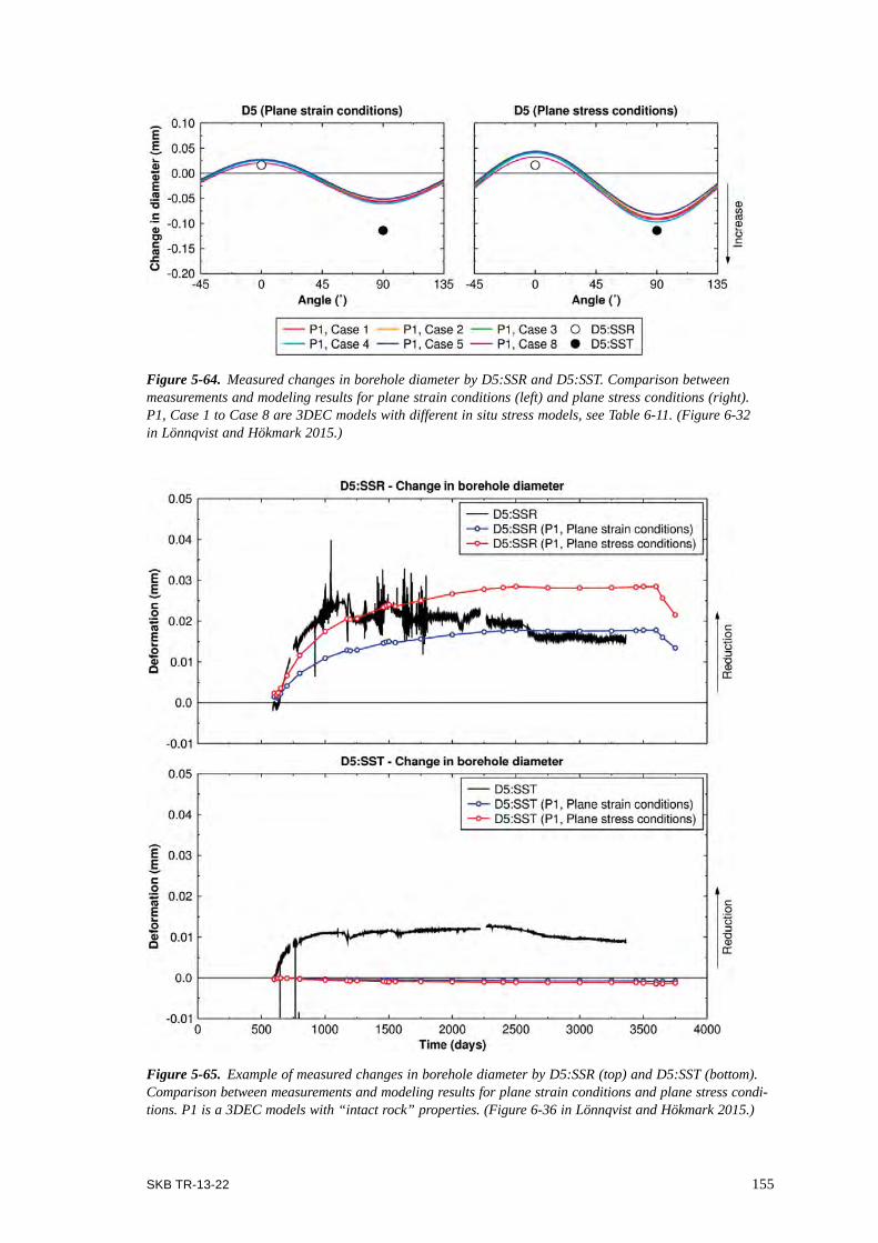
SKB TR-13-22 155

Figure 5-64. Measured changes in borehole diameter by D5:SSR and D5:SST. Comparison between measurements and modeling results for plane strain conditions (left) and plane stress conditions (right). P1, Case 1 to Case 8 are 3DEC models with different in situ stress models, see Table 6-11. (Figure 6-32 in Lönnqvist and Hökmark 2015.)

Figure 5-65. Example of measured changes in borehole diameter by D5:SSR (top) and D5:SST (bottom). Comparison between measurements and modeling results for plane strain conditions and plane stress condi-tions. P1 is a 3DEC models with “intact rock” properties. (Figure 6-36 in Lönnqvist and Hökmark 2015.)

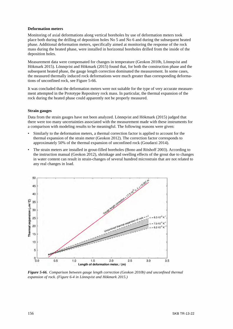
156 SKB TR-13-22

Deformation metersMonitoring of axial deformations along vertical boreholes by use of deformation meters took place both during the drilling of deposition holes No 5 and No 6 and during the subsequent heated phase. Additional deformation meters, specifically aimed at monitoring the response of the rock mass during the heated phase, were installed in horizontal boreholes drilled from the inside of the deposition holes.

Measurement data were compensated for changes in temperature (Geokon 2010b, Lönnqvist and Hökmark 2015). Lönnqvist and Hökmark (2015) found that, for both the construction phase and the subsequent heated phase, the gauge length correction dominated the measurement. In some cases, the measured thermally induced rock deformations were much greater than corresponding deforma-tions of unconfined rock, see Figure 5-66.

It was concluded that the deformation meters were not suitable for the type of very accurate measure-ment attempted in the Prototype Repository rock mass. In particular, the thermal expansion of the rock during the heated phase could apparently not be properly measured.

Strain gaugesData from the strain gauges have not been analyzed. Lönnqvist and Hökmark (2015) judged that there were too many uncertainties associated with the measurement made with these instruments for a comparison with modeling results to be meaningful. The following reasons were given:

• Similarly to the deformation meters, a thermal correction factor is applied to account for the thermal expansion of the strain meter (Geokon 2012). The correction factor corresponds to approximately 50% of the thermal expansion of unconfined rock (Goudarzi 2014).

• The strain meters are installed in grout-filled boreholes (Bono and Röshoff 2003). According to the instruction manual (Geokon 2012), shrinkage and swelling effects of the grout due to changes in water content can result in strain-changes of several hundred microstrain that are not related to any real changes in load.

Figure 5-66. Comparison between gauge length correction (Geokon 2010b) and unconfined thermal expansion of rock. (Figure 6-4 in Lönnqvist and Hökmark 2015.)

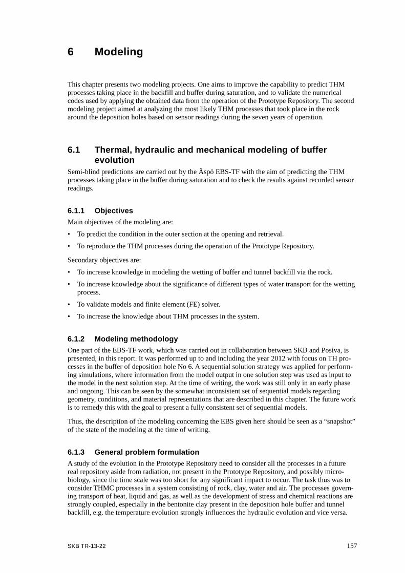
SKB TR-13-22 157

6 Modeling

This chapter presents two modeling projects. One aims to improve the capability to predict THM processes taking place in the backfill and buffer during saturation, and to validate the numerical codes used by applying the obtained data from the operation of the Prototype Repository. The second modeling project aimed at analyzing the most likely THM processes that took place in the rock around the deposition holes based on sensor readings during the seven years of operation.

6.1 Thermal, hydraulic and mechanical modeling of buffer evolution

Semi-blind predictions are carried out by the Äspö EBS-TF with the aim of predicting the THM processes taking place in the buffer during saturation and to check the results against recorded sensor readings.

6.1.1 ObjectivesMain objectives of the modeling are:

• To predict the condition in the outer section at the opening and retrieval.

• To reproduce the THM processes during the operation of the Prototype Repository.

Secondary objectives are:

• To increase knowledge in modeling the wetting of buffer and tunnel backfill via the rock.

• To increase knowledge about the significance of different types of water transport for the wetting process.

• To validate models and finite element (FE) solver.

• To increase the knowledge about THM processes in the system.

6.1.2 Modeling methodologyOne part of the EBS-TF work, which was carried out in collaboration between SKB and Posiva, is presented, in this report. It was performed up to and including the year 2012 with focus on TH pro-cesses in the buffer of deposition hole No 6. A sequential solution strategy was applied for perform-ing simulations, where information from the model output in one solution step was used as input to the model in the next solution step. At the time of writing, the work was still only in an early phase and ongoing. This can be seen by the somewhat inconsistent set of sequential models regarding geometry, conditions, and material representations that are described in this chapter. The future work is to remedy this with the goal to present a fully consistent set of sequential models.

Thus, the description of the modeling concerning the EBS given here should be seen as a “snapshot” of the state of the modeling at the time of writing.

6.1.3 General problem formulationA study of the evolution in the Prototype Repository need to consider all the processes in a future real repository aside from radiation, not present in the Prototype Repository, and possibly micro-biology, since the time scale was too short for any significant impact to occur. The task thus was to consider THMC processes in a system consisting of rock, clay, water and air. The processes govern-ing transport of heat, liquid and gas, as well as the development of stress and chemical reactions are strongly coupled, especially in the bentonite clay present in the deposition hole buffer and tunnel backfill, e.g. the temperature evolution strongly influences the hydraulic evolution and vice versa.

158 SKB TR-13-22

Thus, to properly model the evolution in the Prototype Repository a theory and a numerical tool, which can represent those processes and their mutual couplings accurately, are needed.

The modeling presented here was restricted to only consider T/H/TH processes explicitly. Implicitly, chemistry will be considered by incorporating and selecting retention relations. Mechanics will be accounted for by using two density distributions, one initial and one radially homogenized, in order to evaluate the effect from mechanical processes on the hydraulic evolution.

The models, in 3D except otherwise stated, were designed for and solved by the FE-solver Code_Bright, developed for geomechanical applications.

6.1.4 Governing conditions and important eventsOne obvious condition affecting the evolution in the Prototype Repository was the character of the natural wetting from the rock. The heterogeneous flow properties of the host rock, in terms of water bearing fractures and highly permeable rock volumes, gave rise to inhomogeneous/asymmetric wetting of the EBS.

The effect of large-scale hydraulic processes was also connected to the natural wetting by the rock. Two adjacent tunnels were situated close to the Prototype Repository, one pre-existing – the G-tun-nel – and one that was excavated during the operational phase – the Tass tunnel. (see the locations of these two tunnels in Figure 2-4). Both of these had a strong effect on measured water pressures. Another large-scale hydraulic process that influences the water pressures was the global drainage of the Äspö HRL.

The opening/closing of the drainage behind the Prototype Repository, had a significant influence on the measured inflow and on the collected sensor data.

The water pressure in the host rock was measured in borehole sections that were sealed off using packers. Failure of any of these immediately changed conditions in parts of the Prototype Repository surroundings, which was observed on a few occasions.

The influence from changing heater power was another obvious governing condition within the Prototype Repository.

The change in the rock’s state of stress during the seven years, indicated by UV changes (Section 2.6.7) did not give measurable indications on the groundwater pressure graphs – Figures 2-44 and 2-45. This effect was therefore judged to be negligible and has not been considered in the modeling work.

6.1.5 Solution strategyThe modeling is performed using a solution strategy, which utilized a sequence of simulations. In the sequence the complexity was gradually increased and results from the preceding simulations form the basis for those that follow. To verify that the strategy was able to produce relevant results a somewhat “simplified” batch of models was first developed. After the first sequence of simplified simulations had been completed, refined models were developed where necessary and the solution steps were updated.

The motivation for using such a sequential solution strategy was the estimated computational costs of the problem. In the end THM-processes in the buffer and in the deposition holes were intended to be studied at a high level of detail. In order to account for the significant large-scale effects on the wetting process, a considerable part of the Prototype Repository’s host rock had to be included in the model. So, as a result, if using a “monolithic” solution strategy of the problem, solving for THM processes in a sufficiently detailed and geometrically large enough model, the computational demand was estimated to be too high for the available numerical tools (hardware and software).

The adopted solution strategy consisted of three steps, where the analysis in each step was found to be interesting to study on its own. It is, however, the last step that will produce the results that are aimed for in the main objectives. The models associated with the first two steps considered the entire

SKB TR-13-22 159

Prototype Repository on a global scale, whereas the last step’s model will act on a local scale around a single deposition hole. The three solution steps were:

• Global scale H modeling of the water flow into the “open” Prototype Repository before installation.

• Global scale modeling of the T and H processes during the operational phase after installation.

• Local scale modeling of the THM processes in deposition hole No 6 after installation and predic-tion of the state at the excavation that took place during 2011.

The improvement when using the sequential approach, in terms of computational demand, will come from:

• Decoupling of the processes in the large scale models, which will give fewer degrees of freedom to solve for simultaneously.

• Using significantly coarser discretization in the first two global-scale models as compared to the local scale models in the last solution step.

• Only solving the detailed coupled THM problem in the smaller geometry of the local model in PR-3.

Below follows a more detailed description of the solution steps, the results they produced, and how they connected with each other.

Solution step PR-1: Global H modeling before installationA hydraulic model with an empty tunnel and empty deposition holes was developed. In this model, significant water-conducting structures – cracks/highly permeable volumes – were represented and water transport in the host rock around the “open” Prototype Repository before installation was simulated. Calibration of the host rock properties and validation of the model was made by compari-sons with the measured inflows of water in the tunnel/deposition holes and measured water pressures in the host rock respectively. The developed geometry and calibrated material properties of the rock were used as a point of departure for PR-2.

Solution step PR-2: Global T/H/TH modeling after installation.The hydraulic model from PR-1 was here equipped with simplified representations of tunnel backfill and buffer to enable simulations of the hydraulic processes during operation. The obtained solutions were compared with experimental data in order to evaluate the capability of the model to reproduce significant overall features in the “behavior” of the Prototype Repository. When the solution was judged to be sufficiently close to the Prototype Repository data, the model results were used to pro-vide hydraulic boundary conditions for subsequent TH/THM models in PR-3.

A thermal model of the Prototype Repository had already been developed before this project. The only alteration to this was to extend the simulated time in order to obtain thermal boundary conditions up to the time of opening and retrieval for subsequent TH/THM models in PR-3.

Solution step PR-3: Local TH, HM, THM-modeling after installationLocal TH-models of a single deposition hole were developed to obtain a detailed and coupled representation of the conditions in the deposition hole at the time of opening and retrieval. “Global” thermal and hydraulic material properties and boundary conditions were motivated by analyses of the models in PR-1 and PR-2. “Local” hydraulic properties were calibrated against deposition hole inflow measurements. The model responses were compared with sensor data and the evolution in PR-1 and PR-2. Once the model was adequately calibrated, it was used to predict the state of the bentonite buffer at retrieval.

In the continuing work models also incorporate mechanics, i.e. HM and THM models. Then, mechan-ically related properties such as; density distribution, canister displacement, pressure distribution and buffer upward swelling can be studied and evaluated against sensor data and data obtained at the excavation.

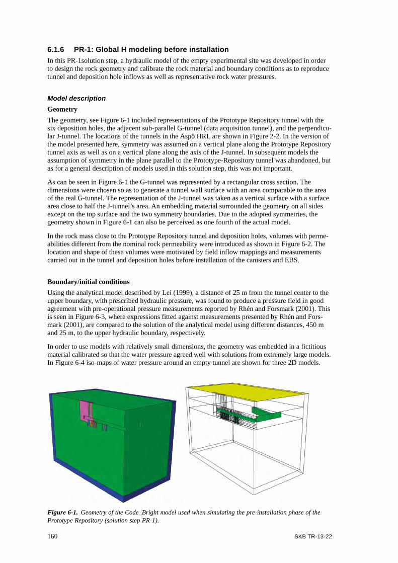
160 SKB TR-13-22

6.1.6 PR-1: Global H modeling before installationIn this PR-1solution step, a hydraulic model of the empty experimental site was developed in order to design the rock geometry and calibrate the rock material and boundary conditions as to reproduce tunnel and deposition hole inflows as well as representative rock water pressures.

Model descriptionGeometryThe geometry, see Figure 6-1 included representations of the Prototype Repository tunnel with the six deposition holes, the adjacent sub-parallel G-tunnel (data acquisition tunnel), and the perpendicu-lar J-tunnel. The locations of the tunnels in the Äspö HRL are shown in Figure 2-2. In the version of the model presented here, symmetry was assumed on a vertical plane along the Prototype Repository tunnel axis as well as on a vertical plane along the axis of the J-tunnel. In subsequent models the assumption of symmetry in the plane parallel to the Prototype-Repository tunnel was abandoned, but as for a general description of models used in this solution step, this was not important.

As can be seen in Figure 6-1 the G-tunnel was represented by a rectangular cross section. The dimensions were chosen so as to generate a tunnel wall surface with an area comparable to the area of the real G-tunnel. The representation of the J-tunnel was taken as a vertical surface with a surface area close to half the J-tunnel’s area. An embedding material surrounded the geometry on all sides except on the top surface and the two symmetry boundaries. Due to the adopted symmetries, the geometry shown in Figure 6-1 can also be perceived as one fourth of the actual model.

In the rock mass close to the Prototype Repository tunnel and deposition holes, volumes with perme-abilities different from the nominal rock permeability were introduced as shown in Figure 6-2. The location and shape of these volumes were motivated by field inflow mappings and measurements carried out in the tunnel and deposition holes before installation of the canisters and EBS.

Boundary/initial conditionsUsing the analytical model described by Lei (1999), a distance of 25 m from the tunnel center to the upper boundary, with prescribed hydraulic pressure, was found to produce a pressure field in good agreement with pre-operational pressure measurements reported by Rhén and Forsmark (2001). This is seen in Figure 6-3, where expressions fitted against measurements presented by Rhén and Fors-mark (2001), are compared to the solution of the analytical model using different distances, 450 m and 25 m, to the upper hydraulic boundary, respectively.

In order to use models with relatively small dimensions, the geometry was embedded in a fictitious material calibrated so that the water pressure agreed well with solutions from extremely large models. In Figure 6-4 iso-maps of water pressure around an empty tunnel are shown for three 2D models.

Figure 6-1. Geometry of the Code_Bright model used when simulating the pre-installation phase of the Prototype Repository (solution step PR-1).

SKB TR-13-22 161

Figure 6-2. Rock volumes used for representing the host rock of the Prototype Repository when modeling the pre-installation phase (solution step PR-1). The hydraulic parameters used to describe the materials are shown in Table 6-1.

Figure 6-3. Effect from the upper boundary position on water pressure in the rock.

Figure 6-4. The effect from using a calibrated embedment material. Left: Cutout from an extremely large model. Middle: A model without embedment. Right: A model with embedment.

Rock 1

Frac tunnel section 2

Rock 2

Frac tunnel section 3

DH1DH2

DH3DH4

DH5DH6

1 10 1000

100

200

300

400

500

Radal distance from tunnel center (m)

Wat

er p

ress

ure

(m)

1 10 1000

100

200

300

400

500

Radal distance from tunnel center (m)

Wat

er p

ress

ure

(m)

Thin lines: Expressions fitted against experimentThick lines: Analytical solution (in different directions)

Hydraulic pressure 450 m above tunnel center Hydraulic pressure 25 m above tunnel center

Extremely large Without embedment With embeddment

162 SKB TR-13-22

The two models without and with embedment had similar cross section dimensions as compared to the 3D model shown in Figure 6-1 The effect from using a calibrated embedding material is clearly seen in Figure 6-4.

The pre-installation conditions were:

• A water pressure of 0.1 MPa representing “open” tunnel/deposition hole walls.

• A water pressure of 4.35 MPa representing the hydraulic pressure at 425 m depth, which was prescribed on the top boundary.

• A zero flux prescribed on all other boundary surfaces.

The initial conditions were:

• A hydrostatic liquid pressure.

• A constant temperature of 15°C.

• A constant gas pressure of 0.1 MPa.

• A porosity of 0.3% by volume.

Material representationsWhen calibrating the basic rock conductivity the analytical model of Lei (1999) was used again; this time for obtaining a relation between an estimated tunnel inflow and the rock conductivity. The rela-tion was compared to the measured inflow in six sections of the Prototype repository tunnel (Rhén and Forsmark 2001), see Figure 6-5, and the conductivity, K = 1·10–10 m/s, which gave an inflow comparable to the lower measurements, was taken as the nominal value.

When calibrating the permeabilities of the volumes with high flow, a simple Newton-Raphson based iteration scheme administrated in Excel was used. In the scheme the residual between simulated and measured inflows were minimized according to:

The obtained permeabilities are shown in Table 6-1 together with other material representations.

Table 6-1. Material laws and parameter values of the rock materials used in solution step PR-1.

Material Retention curve Sl (-) = Intr. perm. k (m2) =

Relative perm. krl (-) =

λλ −−

−+

)1/(1

0

1p

pp lg ( )2/1 )1(1 λλll SS −−

P0

(MPa)λ(-)

Rock 1

1.74 0.6

1.03·10–17

Rock 2 4.16·10–16

Frac tunnel section 2 4.36·10–15

Frac tunnel section 3 4.59·10–15

Deposition hole No 1 2.98·10–16

Deposition hole No 2 1.76·10–18

Deposition hole No 3 1.17·10–18

Deposition hole No 4 1.75·10–19

Deposition hole No 5 3.11·10–19

Deposition hole No 6 5.74·10–19

Embedment 1.00·10–16

SKB TR-13-22 163

Results and discussionAt the final step of the iteration scheme described above, the obtained and by Rhén and Forsmark (2001) measured inflows into tunnel and deposition holes were as shown in Figure 6-6. The permeabilities of the volumes surrounding the deposition holes were calibrated against the diffuse inflow, estimated from studying the total deposition hole inflow and measured local inflows in each deposition holes. The obtained permeabilities are given in Table 6-1.

To evaluate whether the model was good enough to use for generating input to the following solution steps, the calculated pressures were compared to the measured pressures reported by Rhén and Forsmark (2001). In Figure 6-7 water pressures from the measurements and simulation are shown. Simulated pressures are shown along lines aligned with the boreholes directed from the tunnel floor and downwards against north. It can be seen that the model produced somewhat low pressures for the pre-installation state, but they were judged to be good enough to allow for proceeding to the next step in the solution scheme.

6.1.7 PR-2: Global T/H/TH modeling after installationIn this second solution step – PR-2 – a previously existing thermal model of the Prototype Reposi-tory with some additions was used to produce thermal BCs, and the hydraulic pre-installation model developed in the previous solution step PR-1 was further developed as to incorporate the installation and operational phases.

T-model descriptionThe thermal model, which was used as a starting point, is described by Kristensson and Hökmark (2007) The only addition to this original model was to extend the simulated time to also include the end of the operational phase and the cooling of the system after the heaters in the canisters in the outer section were turned off.

0

0.05

0.1

Conductivity exponent

Tunn

el in

flow

(kg/

min

/m)

1.666×10–10

1.242×10–10

9.81×10–11

0

0.05

0.1

Conductivity exponent

Tunn

el in

flow

(kg/

min

/m)

8.821×10–11

3.634×10–11

2.999×10–12

–13 –12 –11 –10 –9 –8 –13 –12 –11 –10 –9 –8 –13 –12 –11 –10 –9 –8

–13 –12 –11 –10 –9 –8–13 –12 –11 –10 –9 –8–13 –12 –11 –10 –9 –8

0

0.05

0.1

Conductivity exponent

Tunn

el in

flow

(kg/

min

/m)

1.47×10–10

4.904×10–11

0

0

0.05

0.1

Conductivity exponent

Tunn

el in

flow

(kg/

min

/m)

10find_exp(col) =

1.617×10–9

1.005×10–9

5.881×10–10

0

0.05

0.1

Conductivity exponent

Tunn

el in

flow

(kg/

min

/m)

10find_exp(col) =

10find_exp(col) =10find_exp(col) =

10find_exp(col) =

1.176×10–9

6.175×10–10

1.47×10–10

0

0.05

0.1

Conductivity exponent

Tunn

el in

flow

(kg/

min

/m)

10find_exp(col) =

1.772×10–9

1.654×10–9

1.573×10–9

Red line: Analytical solution, Ground surface 25 m above tunnel center.Other lines: Mean, max and min of the measured diffuse tunnel inflows

A B C

D E F

”Basic” conductivity k ≈ H 1·10–10 m/s

Figure 6-5. Measured and calculated tunnel section inflow as a function of permeability.

164 SKB TR-13-22

T-model results and discussionIn Figure 6-8 the modelled temperature evolution in the host rock is shown together with correspond-ing sensor data (Goudarzi and Johannesson 2010) at multiple positions, indicated in the drawing above each of the graphs. Sensor data is represented with thin black, green and dark blue lines. Two variations of the simulated responses are given for the points closest to the deposition holes, indicated with the red ring in the schematic drawing above the graphs. The red lines indicate unaltered simula-tion results and the light blue lines “cooled” variants where the unaltered data have been subtracted by 0.2°C/year to simulate global cooling of the experimental site from the time of installation.

Figure 6-6. Top: Measured and simulated tunnel inflow. Bottom: Measured and simulated deposition hole inflow. The deposition hole No 1 inflow should be read on the left scale and the others on the right scale. The simulated deposition hole inflows, indicated by empty rectangles, were calibrated against the diffuse inflow estimated from measurements, indicated by filled circles.

Figure 6-7. Left: Water pressures in the rock as measured in the field (open squares) and from the model presented here (black dots). Right: Diagram indicating in red the boreholes for which the comparison is made.

0.00

0.05

0.10

0.15

0.20

0.25

0.30

0.35

0 10 20 30 40 50 60 70 80

Inflo

w p

er le

ngth

uni

t (l/m

in/m

)

Horizontal distance from tunnel end-wall (m)

Sim.

1997

1999

2000

0.000

0.001

0.002

0.003

0.004

0.000

0.025

0.050

0.075

0.100

0 1 2 3 4 5 6

Inflo

w (

l/min

)

Deposition hole no.

Exp. tot.

Exp. diff.

Sim.

0

1

2

3

4

0 5 10 15 20 25 30 35 40 45

Exp.Sim.

Pres

sure

[MPa

]

Radius [m]

Exp.Sim.

N

SKB TR-13-22 165

Figure 6-8. Measured and calculated temperatures at indicated positions in the host rock. Sensor data are represented with the black, green and dark blue lines. Two variations of the simulated responses are given for the points closest to the deposition holes, indicated with the red ring in the schematic drawing above the graphs. The red lines indicate unaltered simulation results and the light blue lines “cooled” variants, where the unaltered data have been subtracted by 0.2°C/year to simulate global cooling of the Prototype Repository site from the time of installation.

10

15

20

25

30

35

40

45

50

10

15

20

25

30

35

40

45

50

10

15

20

25

30

35

40

45

50

10

15

20

25

30

35

40

45

50

5 65

5 66

10

15

20

25

30

35

40

45

50

0 200 400 600 800 1000 1200 1400 1600 1800 2000 2200 2400 2600 2800 3000 32010

15

20

25

30

35

40

45

50

0 200 400 600 800 1000 1200 1400 1600 1800 2000 2200 2400 2600 2800 3000

Tem

pret

ure

(°C

)

Tem

pret

ure

(°C

)

Tem

pret

ure

(°C

)

Tem

pret

ure

(°C

)

Tem

pret

ure

(°C

)

Tem

pret

ure

(°C

)

0 200 400 600 800 1,000 1,200 1,400 1,600 1,800 2,000 2,200 2,400 2,600 2,800 3,000 3,200 3,400 3,600 3,8000 200 400 600 800 1,000 1,200 1,400 1,600 1,800 2,000 2,200 2,400 2,600 2,800 3,000 3,200 3,400 3,600 3,800

0 200 400 600 800 1,000 1,200 1,400 1,600 1,800 2,000 2,200 2,400 2,600 2,800 3,000 3,200 3,400 3,600 3,800 0 200 400 600 800 1,000 1,200 1,400 1,600 1,800 2,000 2,200 2,400 2,600 2,800 3,000 3,200 3,400 3,600 3,800

Time(days) day 0=030508 Time(days) day 0=030508

Time(days) day 0=010917Time(days) day 0=010917

Time(days) day 0=010917

166 SKB TR-13-22

The overall trends in the rock temperature are well reproduced as well as the temperature values. The results are considered good enough to be used when designing boundary conditions for the local model.

H model descriptionGeometryThe pre-installation model geometry described in Section 6.1.6 was further developed when modeling the operational phase.

Figure 6-9 shows the asymmetric geometry where the Tass tunnel south of the Prototype Repository tunnel also has been incorporated (see also Figure 2-4, which shows an overview of the extended Äspö HRL). The excavation of the Tass tunnel had a clear effect on the water pressure in the rock around the Prototype Repository as shown in Figures 6-11 and 6-12.

This event was therefore incorporated in the model. As the excavation process has not yet been included in the modeling the Tass tunnel has been treated as being occupied by intact rock in all models presented in this report.

A new permeable zone indicated to the left in Figure 6-9 (denoted Frac tunnel section 1 in Table 6-3) was included at approximately the position of the outer plug to represent a local inflow, clearly seen in Figure 6-6 between 60 and 70 m from the tunnel end wall. This zone was not considered in the pre-in-stallation model described earlier.

The drainage sump inside of deposition hole No 1 was in the presented model geometrically repre-sented by an empty cylinder, while the outer plug drainage was handled by prescribing a boundary condition at the “end surface” of the tunnel backfill.

In addition to the described alterations, EBS elements have been added to the model. These are:

• Buffer: the material in the deposition holes from the bottom up to about 1 m from the tunnel floor.

• Backfill: the material in the tunnel and 1 m down in the deposition holes.

• Crushed rock: the material in the tunnel inside of deposition hole No 1.

• Plug1: the material separating the two tunnel sections.

Figure 6-9. Left: A 3D-view of the geometry for a hydraulic post-installation model (belonging to solution step PR-2. Right: A vertical cut along the tunnel axis.

Asymmetric geometry

G-tunnelS-tunnel

New permeable zone

Drainage representations

No. of nodes ≈ 26500

No. of elements ≈ 150000

SKB TR-13-22 167

Initial/boundary condition.The model initially consisted of an empty excavated Prototype Repository tunnel with deposition holes having the same conditions as in the pre-installation model in order to obtain representative water pressure conditions at installation. The pre-installation and initial conditions were the same as presented in Section 6.1.6 “Boundary/initial conditions”. Once the model had reached steady state, the EBS-materials were introduced by using the construction/excavation functionality available in Code_Bright. The prescribed initial conditions are listed in Table 6-2.

In order to account for the global drainage of the Äspö HRL around the Prototype Repository the water pressure prescribed at the top surface, initially set to 4.35 MPa, was decreased linearly in time by 0.19 MPa/year. In the model described here, the drainage of the inner and outer section was represented by prescribing 0.1 MPa at the surface of the drainage sump and of the end surface of the tunnel backfill.

Table 6-2. Initial conditions of the materials representing the EBS.

Material Porosity (-) Liquid pressure (MPa)

Buffer 0.332 –46.00Backfill 0.367 –2.23Crushed rock 0.180 –0.90Plug1 0.003 –2.23

Material representations

As Table 6-3 shows, the representation of the rock materials differed from the pre-installation model described previously. Both the retention parameters and the values of the intrinsic permeability were changed. These changes came from:

• A new retention parameterization, made available specifically for Äspö rock.

• The inclusion of a new highly permeable volume near the outer plug.

• The material representations of the EBS materials are listed in Table 6-4.

Table 6-3 Hydraulic properties of materials representing the host rock.

Material Retention curve Sl (-) = Intr. perm. k (m2) =

Relative perm. krl (-) =

λλ −−

−+

)1/(1

0

1p

pp lg ( )2/1 )1(1 λλll SS −−

P0

(MPa)λ(-)

Rock 1 0.6 0.24 1.00·10–17

Rock 2 4.02·10–16

Frac tunnel section 1 1.00·10–15

Frac tunnel section 2 4.33·10–15

Frac tunnel section 3 4.57·10–15

Deposition hole No 1 2.60·10–16

Deposition hole No 2 1.51·10–18

Deposition hole No 3 9.34·10–19

Deposition hole No 4 1.36·10–19

Deposition hole No 5 2.11·10–19

Deposition hole No 6 3.66·10–19

Embedment 1.74 0.6 1.00·10–16

168 SKB TR-13-22

Table 6-4 Hydraulic properties of materials representing the EBS.

Material Retention curve Sl (-) = Intr. perm. k (m2) =

Relative perm. krl (-) =

λλ −−

−+

)1/(1

0

1p

pp lg ASlδ

P0

(MPa)λ (-)

A (-)

δ (-)

Buffer 15.19 0.25 4.20·10–21 1 3Backfill 0.332 0.23 5.00·10–18 1 3Crushed rock 0.03 0.6 1.00·10–15 1 0

λλ −−

−+

)1/(1

0

1p

pp lg ( )2/1 )1(1 λλll SS −−

P0

(MPa)λ (-)

Plugg1 0.6 0.24 1.00·10–17

H-model results and discussion

Below, the performance of the hydraulic model was studied from different viewpoints. First, the effect of using an asymmetric model in contrast to symmetrical models is shown by comparing pres-sure maps for the different type of models. Then, to evaluate the asymmetric model, comparisons between measured and simulated rock pressures were shown. Also, the simulated outflow from the drainage systems and character of the tunnel backfill wetting process were compared with measure-ments and briefly discussed.

In Figure 6-10, iso-maps of the water pressure in the rock 42 days after installation of the inner section are shown.

Studying the upper maps, the influence from the open G-tunnel is clearly seen for both types of models. The appearance of the pressure field is very similar for the two models around the Prototype Repository geometry for the horizontal cut. As for the vertical cut shown in the maps at bottom, however, the symmetrical and asymmetric models did not agree as well, and the benefits from using an asymmetric geometry becomes clear, if water pressure boundary conditions are to be extracted from the pressure field in the host rock.

In the rock around the Prototype Repository the water pressure in the rock was measured in sealed off sections of boreholes (Goudarzi 2014). These measurements have been compiled together with rock water pressures obtained in the model at the position of the sealed section mid-point. In Fig-ures 6-11 and 6-12 the measurements from the Prototype Repository are identified by the lines with markers and the simulation results are given by the colored lines.

The overall features of the measured water pressures in the rock were reproduced by the simulation sufficiently well to extract boundary conditions for the local models in the following solution step. The magnitudes of water pressure were reasonable and the relative difference in water pressure between different borehole sections are similar to what is found in the Prototype Repository rock.

There were, however, several hydraulic events that were not captured in the model, such as the closure and subsequent opening of the drainage systems in both tunnel sections in November 1 and Decem-ber 6, 2004 respectively, the failure of the packer in section 3 of borehole KA3573A on April 18, 2006, and work on the construction of the neighboring Tass tunnel that started on April 13, 2007.

SKB TR-13-22 169

Moreover, when comparing the calculated outflow from the drainage system in the inner section with measurements reported in Goudarzi and Johannesson (2010), it is found that the model severely underestimates the outflow. When using improved representations of the drainage system, however, much improved levels of outflow were obtained.

One more issue that remains to be discussed is the wetting process of the tunnel backfill, which was much quicker in the model as compared to measured data (Goudarzi 2014).

The most plausible explanation for this discrepancy was the effect from plastic mats installed at the tunnel roof and sides, stretching from between deposition hole No 2 and deposition hole No 3 and inwards, which were not accounted for in the present model. It should be noted that these plastic mats most probably have been ruptured somewhat during installation of the tunnel backfill, but to what extent it is uncertain. The effect of these plastic mats has not yet been incorporated in the models.

Despite the discussed differences between model response and experimental data, it is still believed that the model produces water pressures in the rock of good enough “quality” so as to be used when constructing a first set of hydraulic boundary conditions for the local models in the following solution step.

Figure 6-10. Left: Water pressure iso-maps for symmetrical model. Right: Water pressure iso-maps for asymmetric model. At the top the iso-maps are shown on a horizontal cut through the tunnel axis and below on a vertical cut perpendicular to the tunnel through deposition hole No 6. Identical color scales are used in all contour maps.

Symmetrical models Asymmetric model

170 SKB TR-13-22

Figure 6-11. Measured (black lines) and simulated (colored lines) water pressure in the rock (Borehole KA3554G01).

Figure 6-12. Measured (black lines) and simulated (colored lines) water pressure in the rock (Borehole KA3554G02).

12345

12345

SKB TR-13-22 171

6.1.8 PR-3: Local TH modeling after installationModel descriptionUsing the results from the large-scale models of the Prototype Repository presented above, it was possible to construct a high-resolution, three dimensional local-scale model of deposition hole No 6 including only the deposition hole, tunnel backfill and a small volume of surrounding rock.

GeometryAn overview of the geometry, with assigned materials, is shown in Figure 6-13. Also included in the geometry, but not seen in the figure, is a column of air, thick, between the heater and bentonite rings. The smaller geometry allowed the use of a grid of higher quality and with a higher resolution in the deposition hole as compared to the global models. The model was meshed with hexahedral elements, with a total of approximately 58,000 nodes, out of which about 20,000 nodes were placed in the deposition-hole buffer material. To ensure that the solution was grid independent, a model with twice as high mesh density was constructed, which showed negligible differences in the result.

Two variations of the geometry of the buffer were simulated, see Figure 6-14. One of these rep-resented the state of the buffer immediately after installation, and one represent the buffer in an idealized final state, where it has fully homogenized in the radial direction. The geometry shown in Figure 6-13 represented the installation state models. In the homogenized models the cylinder/pellets was replaced by a material representing homogenized cylinders, and the rings/pellets/air column was replaced by a material representing homogenized rings.

Material propertiesTo represent the situation in the deposition hole just after installation as well as after radial homoge-nization seven different materials were required. The rock was divided into three main parts:

• Deposition hole rock.

• Fractured rock.

• Rock TX.

The thermal properties of these materials are tabularized in Table 6-5 and the hydraulic properties in Table 6-6 and Table 6-7.

Figure 6-13. The local-scale model, with all different materials, except for the column of air between the heater and bentonite rings depicted.

172 SKB TR-13-22

Table 6-5 Thermal and solid phase properties, Sl denotes liquid saturation.

Material ρsolid [kg/m3]

cs [J kg–1 K–1]

Thermal Conductivity λsat [W mK–1]

λdry [W mK–1]

Rings 2,780 800

λ(Sr ) = λsatSl + λdry(1 – Sl)

0.7 1.3Cylinders 2,780 800 0.7 1.3Pellets 2,780 800 0.7 1.3Hom. rings 2,780 800 0.7 1.3Hom. cylinders 2,780 800 0.7 1.3Canister 8,930 390 390 390Tunnel backfill 2,500 780 1.3 1.7DH rock 2,770 770 2.685 2.685Rock 2,770 770 2.685 2.685Rock T1 2,770 1,500 1.0 1.0Rock T2 2,770 15,000 60.0 60.0

Table 6-6. Hydraulic properties

Material Retention curve P0

[MPa]λ [-]

Intr. perm. [m2]

Relative perm.Sl = krl = A δ

Rings

(1 + )–λ

(Ψ)

P0

1 1–λ

67.2 0.48 1.2·10–21

ASlδ

1 3Cylinders 43.5 0.38 2.0·10–21 1 3Pellets 0.508 0.26 6.0·10–21 1 –2.402Hom. rings 8.93 0.22 6.0·10–21 1 3Hom. cylinders 15.2 0.25 4.2·10–21 1 3Canister 0.01 0.6 1.0·10–29 10–20 3Tunnel backfill 0.332 0.23 5.0·10–18 1 3DH Rock 0.6 0.24 *1)

√Sl [1 – (1 – Sl1/λ)λ]

2 – –Rock/Rock T1/Rock T2

0.6 0.24 1.0·10–17

– –

*1) The permeabilities used in the “DH rock” material are shown in Table 6-7.

Figure 6-14. The void ratios prescribed in the deposition hole bentonite buffer when modeling deposition hole No 6.

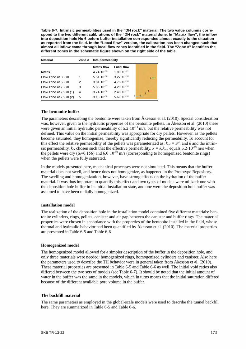
SKB TR-13-22 173

Table 6-7. Intrinsic permeabilities used in the “DH rock” material. The two value columns corre-spond to the two different calibrations of the “DH rock” material done. In “Matrix flow”, the inflow into deposition hole No 6 before buffer installation corresponded almost exactly to the situation as reported from the field. In the “Local flow” version, the calibration has been changed such that almost all inflow came through local flow zones identified in the field. The “Zone #” identifies the different zones in the schematic figure shown on the right side of the table.

Material Zone # Intr. permeability

Matrix flow Local flowMatrix 4.74·10–19 1.00·10–21

Flow zone at 3.2 m 1 5.51·10–18 3.27·10–18

Flow zone at 6.2 m 2 3.81·10–17 4.78·10–16

Flow zone at 7.2 m 3 5.86·10–17 4.20·10–16

Flow zone at 7.9 m (1) 4 3.74·10–18 2.40·10–17

Flow zone at 7.9 m (2) 5 3.18·10–18 5.69·10–18

The bentonite bufferThe parameters describing the bentonite were taken from Åkesson et al. (2010). Special consideration was, however, given to the hydraulic properties of the bentonite pellets. In Åkesson et al. (2010) these were given an initial hydraulic permeability of 5.2·10–19 m/s, but the relative permeability was not defined. This value on the initial permeability was appropriate for dry pellets. However, as the pellets become saturated, they homogenize, thereby significantly reducing the permeability. To account for this effect the relative permeability of the pellets was parameterized as: krel = Sl

δ, and δ and the intrin-sic permeability, k0, chosen such that the effective permeability, k = k0krel, equals 5.2·10–19 m/s when the pellets were dry (Sl=0.156) and 6.0·10–21 m/s (corresponding to homogenized bentonite rings) when the pellets were fully saturated.

In the models presented here, mechanical processes were not simulated. This means that the buffer material does not swell, and hence does not homogenize, as happened in the Prototype Repository. The swelling and homogenization, however, have strong effects on the hydration of the buffer material. It was thus important to quantify this effect and two types of models were utilized: one with the deposition hole buffer in its initial installation state, and one were the deposition hole buffer was assumed to have been radially homogenized.

Installation modelThe realization of the deposition hole in the installation model contained five different materials: ben-tonite cylinders, rings, pellets, canister and air gap between the canister and buffer rings. The material properties were chosen in accordance with the properties of the bentonite installed in the field, whose thermal and hydraulic behavior had been quantified by Åkesson et al. (2010). The material properties are presented in Table 6-5 and Table 6-6.

Homogenized modelThe homogenized model allowed for a simpler description of the buffer in the deposition hole, and only three materials were needed: homogenized rings, homogenized cylinders and canister. Also here the parameters used to describe the TH behavior were in general taken from Åkesson et al. (2010). These material properties are presented in Table 6-5 and Table 6-6 as well. The initial void ratios also differed between the two sets of models (see Table 6-7). It should be noted that the initial amount of water in the buffer was the same in the models, which in turns means that the initial saturation differed because of the different available pore volume in the buffer.

The backfill materialThe same parameters as employed in the global-scale models were used to describe the tunnel backfill here. They are summarized in Table 6-5 and Table 6-6.

174 SKB TR-13-22

The surrounding rock – Uncertainties in field inflow measurementsNear the deposition hole (r = 1 m) a material called “DH rock”, see Figure 6-15, which separated high and low-flow zones was used. Further out from the deposition hole, a homogeneous material, simply called “fractured rock”, was used to describe the flow on larger scale, where separating high and low-flow zones was not needed.

The “DH rock” material was used to describe the rock near the deposition hole. To accurately rep-resent the flow paths into the deposition hole at a fine scale, the rock in this volume was separated into rock matrix and local zones with higher permeability. Before installation of the Prototype Repository, the inflows into the tunnel and deposition holes were carefully measured (see Rhén and Forsmark 2001). In deposition hole No 6 three different methods were used:

• Total inflow into the deposition hole by measuring the water table with time.

• Local inflow measurements of high-flowing zones on the deposition hole wall using plastic bags glued onto the wall and measurement of the collected water.

• Using diapers to absorb water and create an inflow map of the entire deposition hole wall.

How the water enters into the deposition hole was not clearly understood from the measurements, although the total volume of inflowing water per unit time was rather well determined. Combining the total inflow with the plastic bag measurements suggested that about 20% of the inflow came from local zones, while the rest was more evenly distributed over the deposition hole wall. However, looking at the results from the diaper measurements, the inflow was suggested to be highly localized, with water coming from local zones with high inflow.

To account for this uncertainty in the models two calibrations of the “DH rock” volume was done:

• Matrix (High) and Local Flow (Low): This calibration represented the plastic bag measurements, where 80% of the inflow was matrix flow and 20% was through local zones.

• Matrix (Low) and Local Flow (High): This calibration represented the diaper measurements, where the matrix flow was reduced to close to zero in the open deposition hole in the model, and the inflow (whose total volume was kept constant) was directed through the local zones. The flow ratios between the local zones are taken from the plastic bag measurements.

Further out from the deposition hole, the rock was treated as a single material that represented both the flow through large-scale fractures, as well as the matrix flow. This material was called “fractured rock” in the model.

Figure 6-15. The rock near the deposition hole (called “DH rock”) was divided into several parts (right panel) to accurately represent the flow paths identified in the field (left panel). The permeabilities of the different volumes are calibrated to match the inflows measured in the field.

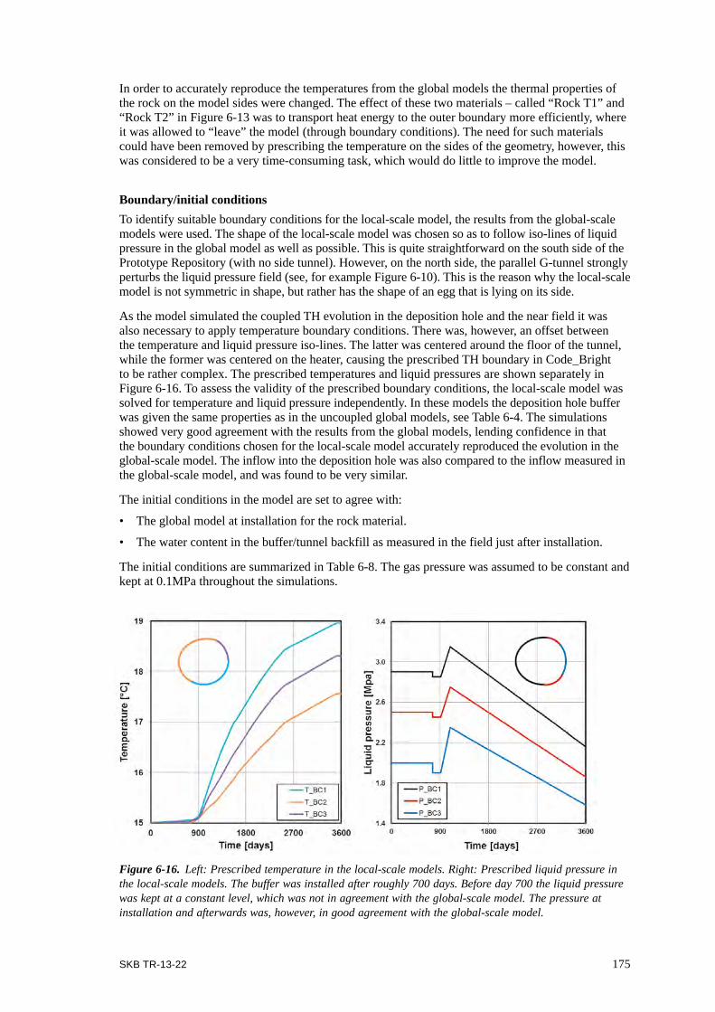
SKB TR-13-22 175

In order to accurately reproduce the temperatures from the global models the thermal properties of the rock on the model sides were changed. The effect of these two materials – called “Rock T1” and “Rock T2” in Figure 6-13 was to transport heat energy to the outer boundary more efficiently, where it was allowed to “leave” the model (through boundary conditions). The need for such materials could have been removed by prescribing the temperature on the sides of the geometry, however, this was considered to be a very time-consuming task, which would do little to improve the model.

Boundary/initial conditionsTo identify suitable boundary conditions for the local-scale model, the results from the global-scale models were used. The shape of the local-scale model was chosen so as to follow iso-lines of liquid pressure in the global model as well as possible. This is quite straightforward on the south side of the Prototype Repository (with no side tunnel). However, on the north side, the parallel G-tunnel strongly perturbs the liquid pressure field (see, for example Figure 6-10). This is the reason why the local-scale model is not symmetric in shape, but rather has the shape of an egg that is lying on its side.

As the model simulated the coupled TH evolution in the deposition hole and the near field it was also necessary to apply temperature boundary conditions. There was, however, an offset between the temperature and liquid pressure iso-lines. The latter was centered around the floor of the tunnel, while the former was centered on the heater, causing the prescribed TH boundary in Code_Bright to be rather complex. The prescribed temperatures and liquid pressures are shown separately in Figure 6-16. To assess the validity of the prescribed boundary conditions, the local-scale model was solved for temperature and liquid pressure independently. In these models the deposition hole buffer was given the same properties as in the uncoupled global models, see Table 6-4. The simulations showed very good agreement with the results from the global models, lending confidence in that the boundary conditions chosen for the local-scale model accurately reproduced the evolution in the global-scale model. The inflow into the deposition hole was also compared to the inflow measured in the global-scale model, and was found to be very similar.

The initial conditions in the model are set to agree with:

• The global model at installation for the rock material.

• The water content in the buffer/tunnel backfill as measured in the field just after installation.

The initial conditions are summarized in Table 6-8. The gas pressure was assumed to be constant and kept at 0.1MPa throughout the simulations.

Figure 6-16. Left: Prescribed temperature in the local-scale models. Right: Prescribed liquid pressure in the local-scale models. The buffer was installed after roughly 700 days. Before day 700 the liquid pressure was kept at a constant level, which was not in agreement with the global-scale model. The pressure at installation and afterwards was, however, in good agreement with the global-scale model.

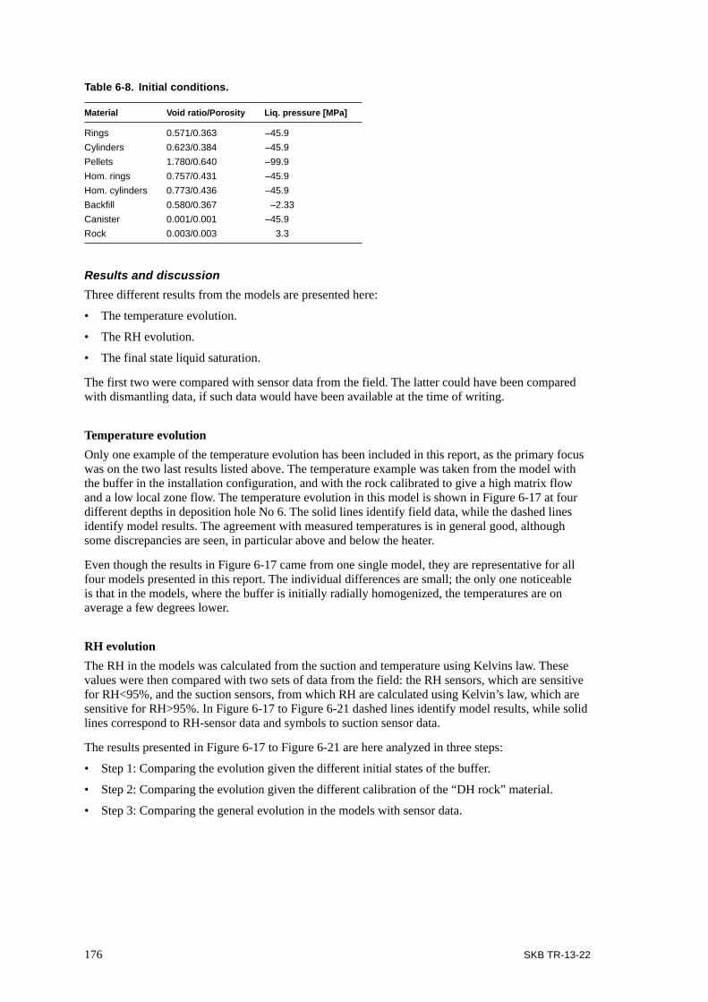
176 SKB TR-13-22

Table 6-8. Initial conditions.

Material Void ratio/Porosity Liq. pressure [MPa]

Rings 0.571/0.363 –45.9Cylinders 0.623/0.384 –45.9Pellets 1.780/0.640 –99.9Hom. rings 0.757/0.431 –45.9Hom. cylinders 0.773/0.436 –45.9Backfill 0.580/0.367 –2.33Canister 0.001/0.001 –45.9Rock 0.003/0.003 3.3

Results and discussionThree different results from the models are presented here:

• The temperature evolution.

• The RH evolution.

• The final state liquid saturation.

The first two were compared with sensor data from the field. The latter could have been compared with dismantling data, if such data would have been available at the time of writing.

Temperature evolutionOnly one example of the temperature evolution has been included in this report, as the primary focus was on the two last results listed above. The temperature example was taken from the model with the buffer in the installation configuration, and with the rock calibrated to give a high matrix flow and a low local zone flow. The temperature evolution in this model is shown in Figure 6-17 at four different depths in deposition hole No 6. The solid lines identify field data, while the dashed lines identify model results. The agreement with measured temperatures is in general good, although some discrepancies are seen, in particular above and below the heater.

Even though the results in Figure 6-17 came from one single model, they are representative for all four models presented in this report. The individual differences are small; the only one noticeable is that in the models, where the buffer is initially radially homogenized, the temperatures are on average a few degrees lower.

RH evolutionThe RH in the models was calculated from the suction and temperature using Kelvins law. These values were then compared with two sets of data from the field: the RH sensors, which are sensitive for RH<95%, and the suction sensors, from which RH are calculated using Kelvin’s law, which are sensitive for RH>95%. In Figure 6-17 to Figure 6-21 dashed lines identify model results, while solid lines correspond to RH-sensor data and symbols to suction sensor data.

The results presented in Figure 6-17 to Figure 6-21 are here analyzed in three steps:

• Step 1: Comparing the evolution given the different initial states of the buffer.

• Step 2: Comparing the evolution given the different calibration of the “DH rock” material.

• Step 3: Comparing the general evolution in the models with sensor data.

SKB TR-13-22 177

Figure 6-18. Relative-humidity evolution in buffer block C1 in the four different models presented here. The dashed lines identify model results, while solid lines correspond to RH-sensor data and symbols to suction sensor data.

Figure 6-17. The temperature evolution in the buffer from the model with the buffer in the installation state and with high matrix flow/low local flows. The solid lines correspond to temperature sensors in the field, while the dashed lines identify model results. The model results did not vary significantly between the different realizations, except that in the models with a homogenized buffer the measured temperatures were on average a few degrees lower.

178 SKB TR-13-22

Figure 6-20. RH evolution in buffer blocks R8 and R9 in the four different models presented here. The dashed lines identify model results, while solid lines correspond to RH sensor data and symbols to suction sensor data.

Figure 6-19. Relative humidity evolution in buffer blocks R2 and R3 in the four different models presented here. The dashed lines identify model results, while solid lines correspond to RH sensor data and symbols to suction sensor data.

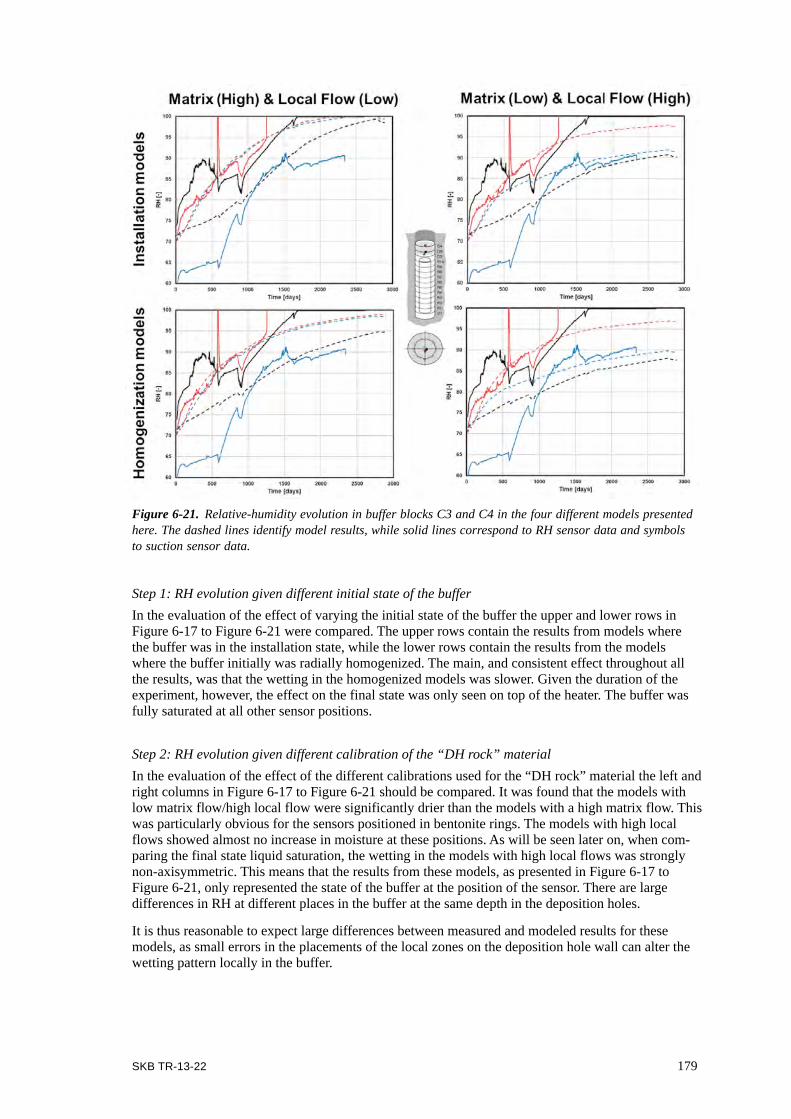
SKB TR-13-22 179

Step 1: RH evolution given different initial state of the bufferIn the evaluation of the effect of varying the initial state of the buffer the upper and lower rows in Figure 6-17 to Figure 6-21 were compared. The upper rows contain the results from models where the buffer was in the installation state, while the lower rows contain the results from the models where the buffer initially was radially homogenized. The main, and consistent effect throughout all the results, was that the wetting in the homogenized models was slower. Given the duration of the experiment, however, the effect on the final state was only seen on top of the heater. The buffer was fully saturated at all other sensor positions.

Step 2: RH evolution given different calibration of the “DH rock” materialIn the evaluation of the effect of the different calibrations used for the “DH rock” material the left and right columns in Figure 6-17 to Figure 6-21 should be compared. It was found that the models with low matrix flow/high local flow were significantly drier than the models with a high matrix flow. This was particularly obvious for the sensors positioned in bentonite rings. The models with high local flows showed almost no increase in moisture at these positions. As will be seen later on, when com-paring the final state liquid saturation, the wetting in the models with high local flows was strongly non-axisymmetric. This means that the results from these models, as presented in Figure 6-17 to Figure 6-21, only represented the state of the buffer at the position of the sensor. There are large differences in RH at different places in the buffer at the same depth in the deposition holes.

It is thus reasonable to expect large differences between measured and modeled results for these models, as small errors in the placements of the local zones on the deposition hole wall can alter the wetting pattern locally in the buffer.

Figure 6-21. Relative-humidity evolution in buffer blocks C3 and C4 in the four different models presented here. The dashed lines identify model results, while solid lines correspond to RH sensor data and symbols to suction sensor data.

180 SKB TR-13-22

Step 3: Comparing the “general” RH evolution with sensor dataWith regards to the general RH evolution, it is seen in Figure 6-17 to Figure 6-21 that the model results, obtained from assuming a high matrix flow, were in closer agreement with the Prototype Repository data. The buffer rings were, for example, much too dry in the models with high local flows, suggesting that these are incorrect. It should be noted, however, that one important event was neglected in the models. Approximately 700 days after installation, the drainage in the inner part of the Prototype Repository tunnel, as well as in the outer plug, was temporarily closed. This led to a quick rise in the pore pressure in the tunnel backfill, and to a strong reaction in the RH sensors in the deposition hole buffer rings, whose RH values spiked to levels close to 100%.

Perhaps, the closing of the drainage led to water being pushed in between the blocks, filling up the inner column, as well as saturating all the RH sensors. While it is unclear exactly what happened, the RH sensors in the rings can most likely not be trusted after this event. Nevertheless, data from the suction sensors suggested that the RH in the rings shortly after the event was rather high, which is in agreement with the models with a high matrix flow.

Final state – liquid saturation in the deposition hole bufferThe best choice of validation of the models was to compare the liquid saturation in the buffer material, as measured during excavation, with the prediction from the models. The final state for all four models is shown in Figure 6-22 and Figure 6-23. The overall trend was very similar to what was seen from the RH evolution. The models with high matrix flow, see Figure 6-22, were close to full saturation everywhere except on top of the heater, while the models with high local flows and hence low matrix flow, see Figure 6-23, were considerably drier.

Furthermore, the saturation was rather axisymmetric in the models with high matrix flow, which was not the case when the flow came mostly through local zones.

Matrix (High) and Local Flow (Low)

Installation model Homogenized model

Figure 6-22. Final liquid saturation in the models with high matrix flow and low local flows. The buffer was close to full saturation everywhere except on top of the heater. The two plots have different ranges, due to that the homogenized model was significantly drier than the installation model just above the heater.

SKB TR-13-22 181

Retrieval data showed that the buffer rings were almost fully saturated, while the buffer just below and above the canister – blocks C1 and C2 – was still somewhat dry (Section 5.1.4). As such, it was concluded that the homogenized model with low matrix flow did not represent the field evolution. It was, however, not possible to rank the remaining three models with the data currently available. The small pieces of plastic that were left in the holes (Section 2.3.4) had no measurable impact on this conclusion.

6.1.9 ObservationsThe modeling of the Prototype Repository, at the state of writing this report, showed that:

• The stepwise solution strategy, using models at different scales and level of detail in a sequential approach, seemed to work satisfactory.

• The hydraulic processes in the host rock around the Prototype Repository were quite complex to model. Strongly heterogeneous water transport properties had to be used in order to mimic hydraulic measurements available in positions around tunnel and deposition holes.

• The uncertainties in the measured inflows to the deposition holes were too large to make a precise calibration of the rock surrounding the deposition holes.

• The buffer wetting process was sensitive to the calibration of the rock surrounding the deposition holes.

• Based on the RH evaluation, “reality” was expected to be somewhere between the two consid-ered representations of water transportation in the rock close to the deposition hole.

Matrix (Low) and Local Flow (High)

Installation model Homogenized model

Figure 6-23. Final liquid saturation in the models with low matrix flow and high local flows. The buffer far from fully saturated, in particular the homogenized model. Furthermore the saturation was highly non-axisymmetric, owing to that the inflow was so highly localized.

182 SKB TR-13-22

6.2 Thermal and thermo – mechanical evaluation of the rock Thermal and thermo-mechanical modelling of the Prototype Repository host rock was undertaken by Lönnqvist and Hökmark (2015) in connection with the opening and retrieval of the outer section.

6.2.1 ObjectivesThe objective was:

• To assess the response of the rock mass to changes in mechanical and thermal conditions during the construction phase and during the subsequent heated phase.

6.2.2 Thermal evolutionThermal models of the Prototype Repository had previously been developed by Sundberg et al. (2005) who derived thermal properties for the rock based on inverse modeling, see Chapter 2, and by Kristensson and Hökmark (2007) who modelled the first 1,400 days of heating. Lönnqvist and Hökmark (2015) extended the model by Kristensson and Hökmark (2007) to the first 3,800 days of heating, i.e. beyond the time when the heaters in the outer section were switched off for good. Although results from previous modeling work indicated that the temperature at some of the mea-surement positions was influenced by water movements, Lönnqvist and Hökmark (2015) assumed that the heat transport took place exclusively by linear thermal conduction in their analyses with the finite-element code Code_Bright, (CIMNE 2004).

Code_Bright modelThe thermal model was represented by a 200 m × 200 m × 200 m block of rock in which the tunnel and six deposition holes were explicitly represented, see Figure 6-24. The geometry of the tunnel and deposition holes was based on the description given by Goudarzi (2012, Figures 1-1 and 4-3) and was the same as in the study by Kristensson and Hökmark (2007).

As the aim of the modeling work was to reproduce the measurements, close attention was paid to replicating the heat output from each canister, see Figure 6-25.

Thermal properties were assigned to each material in the models, i.e. to canisters, buffer, backfill, plugs and rock. The tunnel plugs were assumed to have the same thermal properties as the rock. For the rock, four different thermal conductivity values in the range 2.52–2.72 W/mK were tested, see Table 6-9.

Figure 6-24. Left: Outline of Code_Bright model. In order to reduce the size of the model, advantage was taken of the vertical symmetry plane through the tunnel axis. Right: Close-up of Code_Bright model. (From Figures 4-2 and 4-4 in Lönnqvist and Hökmark 2015).

200 m

200 m 100 m

Tunnel plugsBackfill

CanistersBuffer

Rock

Rock in tunnel floor region

SKB TR-13-22 183

Table 6-9. Model map and data used in the thermal assessment, after Lönnqvist and Hökmark (2015).

Parameter Unit Rock mass and plugs Backfilld Bufferd Canisterd

CB1a CB2b CB3b CB4c

Thermal conductivity W/mK 2.685 (3.5) 2.72 2.65 2.52 1.5 1.0 390Specific heat J/kgK 770 770 770 770 780 800 390Solid phase density kg/m3 2,770 2,770 2,770 2,770 2,500 2,780 8,930

a. Best-estimate thermal conductivities obtained in the study by Kristensson and Hökmark (2007). Value within brackets is used in the floor of the tunnel, cf. Figure 6-24 right. b. Based on inverse modelling using sensors in the inner section (Sundberg et al. 2005).c. Based on laboratory measurements of samples taken from both sections (Sundberg et al. 2005).d. Same as in the study by Kristensson and Hökmark (2007).

Comparison with temperature measurementsIn total, 85 sensors were installed with 37 sensors in the inner section and 48 sensors in the outer section. Their positions are shown in Figure 6-26. The comparison of measurement data from all installed instruments with model results showed that the measured temperatures in the outer section could be reproduced well using homogeneous, isotropic and global rock thermal conductivities in the range 2.52–2.72 W/mK, see Figure 6-26c and d. The observed differences between measured and calculated temperatures were judged to be the results of a number of factors such as spatial varia-tions in rock thermal properties, effects of water movements, temperature dependence and conditions in the interior of the holes. It was found that, at some distance from the heaters where the tempera-tures were determined by heat transport properties averaged over large volumes, the value 2.72 W/mK appeared to reproduce the measured temperatures slightly better than the tested lower values of the thermal conductivity. Therefore, this value was chosen as reference value for the further thermal and thermo-mechanical modeling work with the distinct element code 3DEC (Itasca 2007).

Lönnqvist and Hökmark (2015) concluded that the measured temperatures in the inner section were affected by water movements associated with the changes in drainage initiated some 1,000 days after test start. The calculated temperatures were generally significantly overestimated at late times and particularly at positions close to the tunnel floor for all tested values of the thermal conductivity, see Figure 6-26 a and b. When assuming that the thermal conductivity range that was established for the outer section also was relevant for the inner section, the water outflow reported for the inner section by Goudarzi (2014) was found to be sufficient to match a power loss equivalent that would explain the differences between measured and calculated temperatures.

Figure 6-25. Power evolution of the heater in Hole 5 (left) and in Hole 6 (right) used in Code_Bright model (red) and measured power from Figures 2-24 and 2-25 (black). Time ‘0’ represents the time when the heater in deposition hole No 1 was switched on. Note that where the graphs indicate values below 1 kW, the power was, in fact, zero. (Modified from Figure 4-3 in Lönnqvist and Hökmark 2015).

184 SKB TR-13-22

6.2.3 Thermal and thermo-mechanical modelling approach: Comparison between Code_Bright and 3DEC

The built-in thermal logic in 3DEC is based on an analytical solution of the temperature evolution due to individual point sources or grids of point sources (line sources) in an infinite medium with homogeneous and isotropic thermal properties (Itasca 2007). Given that the thermal properties of heaters, deposition holes and backfilled tunnels cannot be accounted for, Lönnqvist and Hökmark (2015) tested the adequacy of the thermal logic in the 3DEC code by comparing results from that code with results from the Code_Bright analyses.

Figure 6-26. Examples of measured (black curves) and modeled temperatures (colored curves) for instruments located around deposition hole No 1 (sub-figures a and b) and around deposition hole No 5 (sub-figures c and d). (Modified after Figures 4-5, 4-7 and A-3 in Lönnqvist and Hökmark 2015.)

SKB TR-13-22 185

Hökmark and Fälth (2003) have showed that a superposition of two line sources of different lengths (so-called compound line-sources) could be used to approximate the heat output from a real canister which has higher surface heat flux at the top and bottom. This approach was used to represent the heaters in the outer section. The heaters in the inner section were represented by simple line sources. The heat output from each canister was given by a step-function approximation of the power evolution applied in the Code_Bright model, see Figure 6-24. A good agreement between the rock temperatures as calculated by the two codes was found. Ignoring the low-conductivity backfill gave an insignificant temperature underestimate just below the tunnel floor and a corresponding small overestimate just above the tunnel roof, see Figure 6-27. Corresponding calculations of the thermally induced stresses in the rock were generally in good agreement except at points located at heater mid-height close to the deposition holes. It was concluded that the Code_Bright results were influenced by the coarse discretization of the interior of the deposition holes, which appeared to cause an overestimation of the radial stress at the buffer-rock interface. Since the 3DEC results agreed with the Code_Bright results at all other points, it was judged that the 3DEC results were correct and consistent with the input assumption.

6.2.4 Thermo-mechanical evolutionContinued study of the mechanical and thermo-mechanical evolution of the rock in the outer section of the Prototype Repository was made by use of 3DEC version 5.00. The objectives of this modeling work were:

• To compare model results with mechanical measurements made in the rock. Assess the potential for spalling in the walls of the deposition hole walls.

• To study the impact of a simplistic fracture network on stresses around the deposition holes.

• To assess the stability and normal stress variations of selected fracture planes intersecting the repository openings.

Figure 6-27. Comparison between 3DEC and Code_Bright (CB2) at points above the tunnel (Pt. 1), below the tunnel (Pt. 2) and at canister mid-height between deposition holes No 5 and No 6 (Pt. 3). (Modified after Figure 5-4 in Lönnqvist and Hökmark 2015.)

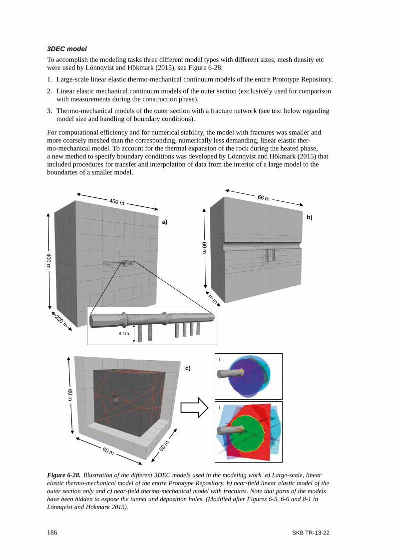
186 SKB TR-13-22

3DEC modelTo accomplish the modeling tasks three different model types with different sizes, mesh density etc were used by Lönnqvist and Hökmark (2015), see Figure 6-28:

1. Large-scale linear elastic thermo-mechanical continuum models of the entire Prototype Repository.

2. Linear elastic mechanical continuum models of the outer section (exclusively used for comparison with measurements during the construction phase).

3. Thermo-mechanical models of the outer section with a fracture network (see text below regarding model size and handling of boundary conditions).

For computational efficiency and for numerical stability, the model with fractures was smaller and more coarsely meshed than the corresponding, numerically less demanding, linear elastic ther-mo-mechanical model. To account for the thermal expansion of the rock during the heated phase, a new method to specify boundary conditions was developed by Lönnqvist and Hökmark (2015) that included procedures for transfer and interpolation of data from the interior of a large model to the boundaries of a smaller model.

Figure 6-28. Illustration of the different 3DEC models used in the modeling work. a) Large-scale, linear elastic thermo-mechanical model of the entire Prototype Repository, b) near-field linear elastic model of the outer section only and c) near-field thermo-mechanical model with fractures. Note that parts of the models have been hidden to expose the tunnel and deposition holes. (Modified after Figures 6-5, 6-6 and 8-1 in Lönnqvist and Hökmark 2015).

b)a)

8.1m

c)I

II

SKB TR-13-22 187

For both types of models, i.e. continuum models and models with a fracture network, the rock mass (or intact rock between the fractures) was assumed to be a linear thermo-elastic material. The ther-mal parameter values were the same as in the Code_Bright model CB 2, see Table 6-9. Parameter values for the mechanical and thermo-mechanical rock properties were chosen from the range estab-lished for the Apse test site, see Figure 2-4 (Staub et al. 2004, Andersson 2007). For the fractures, an idealized elasto-plastic material model was chosen with constant normal and shear stiffnesses, zero tensile strength and a Mohr-Coulomb shear strength criterion. The selected base case fracture parameter values were consistent with average laboratory-scale values obtained in the Laxemar site-investigation (Hakami et al. 2008). All input parameters to the 3DEC models are listed in Table 6-10.

Table 6-10. Material properties used in the modelling work.

Component* Parameter Unit Base case value Alternative values

Rock Thermal conductivity W/mK 2.72 –Thermal diffusivity m2/s 1.275·10–6 –Density kg/m3 2,770 –Young’s modulus GPa 76 (intact rock) 55 (rock mass)Poisson’s ratio – 0.25 –Coefficient of thermal expansion K–1 7·10–6 6.2·10–6; 8.3·10–6 Spalling strength MPa 121 –

Fractures** Friction angle ° 35 20, 25, 30, 40, 45Cohesion MPa 0 –Tensile strength MPa 0 –Normal stiffness GPa/m 700 –Shear stiffness GPa/m 40 –

Fictitious fractures properties***

Friction angle ° 63 –Cohesion MPa 500 –Tensile strength MPa 500 –Normal stiffness GPa/m 70,000 –Shear stiffness GPa/m 4,000 –

* The concrete plugs were judged to have an insignificant influence on the stresses and deformations around the deposition holes and were therefore not included in the models.** Properties assigned to a circular area of the selected fracture planes, i.e. to the fractures. *** Properties assigned to fracture planes outside the circular areas.

Six different in situ stress models were considered, see Table 6-11. The differences between the six stress fields are not large. The reason for analyzing the models with this dense case coverage was mainly to ensure that the poor agreement between measured and calculated stress changes and deformations was not a result of disregarding possible nuances in the in situ stress model. For further details of the six stress models, see Lönnqvist and Hökmark (2015).

Table 6-11. In situ stress models. Magnitudes in MPa. Trend in degrees in the Swedish national RT90 system; Plunge in degrees from horizontal.

Model name σ1 σ2 σ3Mag. Trend Plunge Mag. Trend Plunge Mag. Trend Plunge

Case 1 (base case) 28 304 0 14 214 0 12.8 – 90909090900

Case 2 28 294 0 14 204 0 12.8 –Case 3 28 314 0 14 224 0 12.8 –Case 4 30 304 0 13 214 0 12.8 –Case 5 26 304 0 15 214 0 12.8 –Case 8 (Apse) 30 298.2 0 15 – 90 10 208.2

188 SKB TR-13-22

No account was taken for any pore pressure disturbances or variations around the Prototype Repository due to e.g. the excavation of the tunnel and the deposition holes, the subsequent changes in the degree of saturation of the buffer and backfill materials or to any large-scale trends at the Äspö HRL in general. Instead, bounding estimates of any fracture pore pressure effects were obtained by considering two simple cases as shown in Figure 6-29.

The response of the rock mass to changes in mechanical and thermal conditions was subsequently assessed in five general steps: 1) establishment of a primary equilibrium, 2) excavation of the tunnel, 3) excavation of the deposition holes, 4) excavation of the plug slots and 5) application of the thermal load.

Evaluation of rock mechanical measurementsThe mechanical response of the rock mass surrounding the Prototype Repository was extensively moni-tored throughout the experiment by use of instruments monitoring AE events, stresses, deformations and strain as reported by Goudarzi (2014) and Haycox (2011). Lönnqvist and Hökmark (2015) analyzed the measurement data and compared the results with numerical 3DEC models. Example results and conclu-sions from their study are presented in Section 5.8.3 and are not discussed further here.

Stresses in deposition hole walls: potential for spalling Linear elastic models were used to assess the potential for spalling in the walls of the deposition holes. Spalling is thus not explicitly modeled, but assumed to be initiated when the tangential stress in the wall of a borehole is equal to, or exceeds, the nominal spalling strength (Andersson 2007, Hökmark et al. 2010). As discussed by Hökmark et al. (2010), such a model cannot be used to predict the depth or the shape of the spalled region but gives an indication of the intervals along the borehole walls where spalling may be expected.

Lönnqvist and Hökmark (2015) assumed in all models that the holes were unsupported, i.e. the impact of swelling pressure from the bentonite was ignored, which overestimates the tangential stress in the walls of the deposition holes. Using this approach, results from all linear elastic models indicated that the spalling strength would not be exceeded other than locally at the top of the deposition holes. This is in keeping with the visual observations, i.e. that no spalling had occurred (see Section 4.7.2). It should, however, be remembered that there is a possibility that also very small support pressures provided by the pellet-filled slot between the bentonite blocks and the rock walls probably could have been sufficient to suppress the spalling process (Glamheden et al. 2010). Not observing spalling during the heated phase may, therefore, be an uncertain indication of whether or not the tangential stresses exceeded the nominal spalling strength.

Figure 6-29. Schematic view of the two pore pressure models: constant hydrostatic pore pressure (model F1a) and reduced pore pressure at the beginning of the excavation phase (model F1b) together with two examples of measured groundwater pressures during the heated phase. (Modified after, Figure 8-3 in Lönnqvist and Hökmark 2015). Inset shows the positions of groundwater pressure measurements (from Goudarzi 2014).

SKB TR-13-22 189

For the models with base case material properties, see Table 6-10, model P1, and in situ stresses, see Table 6-11, Case 1, the largest tangential stresses were found just below the tunnel floor, see Figure 6-30, where this stress was close to the nominal spalling strength in small regions already after excavation. Not observing spalling at any position in the unsupported deposition hole walls at this time was judged to be a reasonably safe indication that the tangential stresses did not reach the nominal spalling strength, and, consequently, that the in situ stress magnitudes have not been under estimated. By considering models with different proportions of “intact rock” and “rock mass” properties it was observed that the properties assigned to a local rock volume surrounding the depo-sition holes determined the magnitude of the tangential stress with very little influence of properties assigned to the surrounding rock mass, see Figure 6-31a. Assuming intact rock properties such as in models P1 to P4 (see Lönnqvist and Hökmark (2015) for details) was likely to overestimate the calculated tangential stresses. Increasing the coefficient of thermal expansion, see Figure 6-31b, or the in situ stress anisotropy, see Figure 6-31c, Case 4, was found to increase the tangential stress by about 5 MPa at stress maximum. Although Lönnqvist and Hökmark (2015) could not make a rigorous quan-titative verification of the stress magnitudes, the results described above indicated that the models probably did not underpredict the stresses during the heated phase by any significant amounts.

Figure 6-30. Top: Temporal development of the major principal stress at –0.5 m depth and at canister mid-height (–5 m) in deposition hole No 5. Grey area represents pre-thermal time with 1) initial state of stress, 2) excavation of tunnel, 3) excavation of deposition holes and 4) excavation of plug slots. Bottom: Contour plots of the major principal stress after excavation (left) and after 2,000 days of heating (right). Contours in MPa. Dashed rectangles represent the areas used to evaluate the stresses in the upper figure. (Figure 7-6 in Lönnqvist and Hökmark 2015).

190 SKB TR-13-22

Results from the models with fractures showed that a combination of elastic and plastic shear dis-placements along the intersecting fractures perturbed the stress field in the walls of the deposition holes quite significantly, see Figure 6-32. Stress concentrations above the nominal spalling strength were formed at the tips of the intersections of steeply dipping fractures already after excavation of the holes. Since there was no evidence of any systematic stress induced damage to the walls of the deposition holes after the dismantling of the outer section, see Section 4.7.2, it was concluded that the schematic perfectly planar fracture geometry applied in the models probably overestimated the impact of the fractures. The latter observation is in line with findings by Hökmark et al. (2006), who concluded that “small regions of structurally controlled stress concentrations should not be considered relevant for spalling risk estimates, meaning that the elastic approximations should be sufficient”.

Fracture deformationsFourteen fractures intersecting the deposition holes or the tunnel from the Prototype Repository fracture model were selected for inclusion in the numerical model. Following the modelling approach made by e.g., Hökmark et al. (2010) all fractures, regardless of shape in the fracture model, were approximated to be circular, see Figure 6-28c. In 3DEC, this was accomplished by assigning actual fracture properties to a circular area of the fracture plane and fictitious high-strength/high-stiffness properties to the remaining parts of the plane, see e.g. Fälth et al. (2010, Appendix B) for details.

For the base case in situ stress and shear strength properties of the fractures, Lönnqvist and Hökmark (2015) found all fractures in the 3DEC model to be initially stable and under high compression. Only four of these fractures were found to have shear displacements exceeding a few millimeters over any significant area at any point in time during the excavation phase or during the subsequent heated phase, see Figure 6-33. These fractures formed the boundaries of blocks with large displacements located in the tunnel floor. Accounting for the lower pore pressure close to the tunnel by reducing the pore pressure in all fractures from 4.4 MPa to 0 MPa during excavation was shown to stabilize these blocks and reduced the maximum shear displacements very efficiently, see Figure 6-34 right.

Since fracture 265 had the largest shear displacements for both pore pressure models, results for this fracture were used as examples. Figure 6-34 (left column) shows the cumulative shear displacement after excavation of the tunnel and at the end of the modelling period. Shear displacements exceeding 1 mm were only found in the most stress-disturbed region close to the tunnel. For the majority of the surface area, the maximum shear displacement was only fractions of a millimeter. Some distance away from the openings, the shear displacements are small for all friction angles considered in Table 6-10. Based on the modeling results, it appeared that most of the displacements took place during the excava-tion with very little additional movements during the heated phase, (see Figure 6-35 left).

Figure 6-31. Temporal development of the major principal stress at canister mid-height (–5 m) in Hole 5 for a) base case in situ stresses but different proportions of “rock mass” properties and “intact rock” prop-erties, b) base case material properties and in situ stresses but different values of the coefficient of thermal expansion and c) base case material properties but different in situ stress models. Grey area represents pre-thermal time with 1) initial state of stress, 2) excavation of tunnel, 3) excavation of deposition holes and 4) excavation of plug slots. (Modified after Figures 7-9, 7-12 and 7-14 in Lönnqvist and Hökmark 2015).

SKB TR-13-22 191

Regions of low normal stress were found where the fractures intersected the repository openings or were approximately parallel to them, see Figure 6-34 right column. Given the simplistic fracture network considered by Lönnqvist and Hökmark (2015), additional regions of low normal stress were formed at the boundaries of the blocks with large displacements in the floor of the tunnel due to the schematic assignment of pore pressure within the fractures. Accounting for the lower pore pressure close to the tunnel by reducing the pore pressure in all fractures from 4.4 MPa to 0 MPa during excavation was shown to stabilize these blocks. During the heated phase, compression generally increased on all fractures, see Figure 6-35 right.

Figure 6-32. Left: Example of stress redistribution effects after excavation due to intersecting fractures in deposition hole No 5. Contours in MPa. Right: Difference in stress magnitudes compared with a linear elastic model. Contours in MPa where blue colors represent a reduction in compression compared with the elastic model and red colors correspond to an increase in compression compared with the elastic model. (Modified after Figures 8-6 and 8-8 in Lönnqvist and Hökmark 2015).

Figure 6-33. Maximum fracture area with shear displacement equal to, or exceeding, given value for each fracture in the fracture model. From Lönnqvist and Hökmark (2015, Figure 8-12).

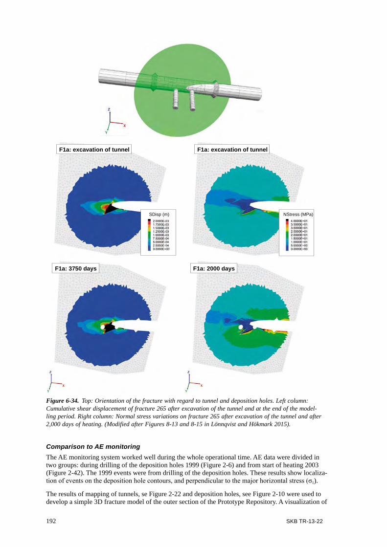
192 SKB TR-13-22

Comparison to AE monitoringThe AE monitoring system worked well during the whole operational time. AE data were divided in two groups: during drilling of the deposition holes 1999 (Figure 2-6) and from start of heating 2003 (Figure 2-42). The 1999 events were from drilling of the deposition holes. These results show localiza-tion of events on the deposition hole contours, and perpendicular to the major horizontal stress (σ1).

The results of mapping of tunnels, se Figure 2-22 and deposition holes, see Figure 2-10 were used to develop a simple 3D fracture model of the outer section of the Prototype Repository. A visualization of

F1a: excavation of tunnel

F1a: 3750 days

SDisp (m)

F1a: excavation of tunnel

F1a: 2000 days

NStress (MPa)

Figure 6-34. Top: Orientation of the fracture with regard to tunnel and deposition holes. Left column: Cumulative shear displacement of fracture 265 after excavation of the tunnel and at the end of the model-ling period. Right column: Normal stress variations on fracture 265 after excavation of the tunnel and after 2,000 days of heating. (Modified after Figures 8-13 and 8-15 in Lönnqvist and Hökmark 2015).

SKB TR-13-22 193

AE event positions together with position of mapped fractures are given in Figure 6-36. Many events are located close to the deposition hole No 6, the installation was such that it screened deposition hole No 6 best. The red circle shows clusters that have occurred within a short period of time, indicating a possible spalling. The black circles represent clusters that occurred rather late in the heating phase, and were shallow under the tunnel floor. It was not possible to inspect the nature of these areas after excavation of the backfill, because these areas were under the cast concrete support for the steel road bed used during installation of the experiment. A hypothesis is that something happened in the interface concrete – rock.

The modelled fractures and the 3D distribution of the AE events were used to explore the possibility that more distant events from the deposition holes indicated movements along existing fracture planes. But, no clear indication of events located close to or in the vicinity of fractures was found. It seems rather that the events are localized in areas of more intact rock between the mapped fractures. This might likely also be the areas were localized highest stresses are concentrated.

No spalling was found in the deposition holes (se Section 4.7.2) and no clear indication of AE events in the fractures mapped in them.

Figure 6-35. Temporal development of the shear displacement (left) and effective normal stress (right) at selected points on Fracture 265 (top figure) for Model F1a. Grey area represents pre-thermal time with 1) initial state of stress, 2) excavation of tunnel, 3) excavation of deposition holes and 4) excavation of plug slots. (Modified after Figures 8-14 and 8-16 in Lönnqvist and Hökmark 2015).

Figure 6-36. Positions of AE events relative to mapped fractures in the tunnel and in the deposition holes. Left: Top view. Right: Side view.

Fracture #265

Pt 1Pt 3

Pt 2

Pt 4

SKB TR-13-22 195

7 Experimental experiences and lessons learnt

7.1 Breaching of plugThe breaching and dismantling of the plug was conducted as planned. The chosen technique (core drilling through the plug followed by mechanical demolition of the reinforced concrete dome) functioned well in practice. However, a hydraulic breaker, which at the planning of the work was not included, was deemed necessary in order to finish the work within the given time frame. A faster and perhaps more efficient way of breaching the plug might have been to use careful blasting together with mechanical demolition. This technique was under consideration but was rejected since there was a strong wish that the cables, which were led through the plug, should be saved and that would be a mission impossible if explosives were to be used. Another feasible method for breaching the plug was wire-sawing. This method was considered, however, to be too expensive, although less time consuming.

For future full-scale experiments, it is suggested to design the plug for a coming removal by avoiding leading cables and tubes through the plug. It might also be possible to prepare the plug in advance for the breaching, if such design can be introduced without disturbing the reference design of a repository plug.

7.2 Removal and sampling of backfillThe removal of the backfill with a backhoe loader and manual sampling on freed and inclined sur-faces worked well. By making an extensive sampling in pre-determined regular patterns and an effi-cient surveying of the sample positions, it was possible to get a good picture of the variation in water content and density of the backfill. The management of samples e.g. the way they were marked, packed and stored, contributed to the good quality of the examination of the backfill material. Also the minimized time of interim storage of samples before the determinations of water content and density in the Äspö Geolaboratory was essential to the good results. The following disadvantages were, however, also observed during the work:

1. It was difficult to retrieve all the sensors installed in the backfill, since the excavation was not made with the same inclination as the inclination at the installation and thus the sections with installed sensors were cut off at the excavation. Furthermore heavy machinery was used and it was not possible to have personnel in front of the excavator, for occupational safety reasons. This made it impossible to make a systematic retrieval of the sensors. In order to retrieve more sensors, smaller machines should be used and the excavation should be made in thinner layers with the same inclination as used during installation. This would, however, greatly extend the schedule for excavation and potentially jeopardize the feasibility of sampling.

2. It was not possible to collect samples, for measuring of water content and density, close to the floor of the tunnel, mainly due to the chosen inclination of the backfill sample sections. Further-more, water coming into the tunnel was collected close to the floor and thus made the material wet and not representative.

The work environment in the Prototype Repository tunnel was poor. The work spaces were narrow, it was slippery to walk on the backfill material and muddy underfoot when sampling from the backfill layers. Many cables were in the way and made the job difficult. An aerial platform could not be used since it would be impossible to cut out backfill samples from such an angle. Noisy environment and poor air quality occurred when the excavator operated in the tunnel. Additional ventilation was organized but that was quickly found out to be detrimental to the backfill material as it began to dry before the sampling. Thanks to the applied risk management and the implemented safety standard in work performance no safety-related incidents occurred.

196 SKB TR-13-22

7.3 Sampling and removal of bufferThe chosen technique for taking samples and excavating the buffer in the two deposition holes had been previously used at the Äspö HRL in retrievals of the CRT (Johannesson 2007) and TBT (Johan-nesson 2010) with good results. Also, for the purpose of excavating the two outer deposition holes in the Prototype Repository, this technique worked well. During planning of the sampling and removal of the buffer it was confirmed that the buffer was not saturated and that there was a large variation in water content and density between different parts of the buffer.

In order to capture this variation the sampling of the buffer was done systematically in eight directions in each bentonite block. This extensive sampling made it possible to obtain a detailed picture of the water content and density of the buffer. The management of samples e.g. the way they were marked, packed and stored, contributed to the good quality in the examination of the buffer. Also the minimized time of interim storage of sample before determinations of the water content and density in the Äspö Geolaboratory was essential to the good results. Some disadvantages were observed, however, during the work:

1. At the retrieval of the buffer it was found that too little information was available of the blocks’ original positions. A more precise positioning of the buffer blocks at the installation and at the retrieval would have been beneficial.

2. It was difficult to retrieve all the sensors installed in the buffer, in particular the thermocouples. The reason for this is that the thermocouples were exposed over their entire length and it was almost impossible to keep them intact during the excavation, which is vital if they shall be tested.

It was generally a very dusty and noisy environment during drilling in the buffer blocks. Vacuum clean-ers were powerful but still not enough to keep all the dust away. Masks and other protective equipment were therefore used to obtain acceptable working conditions. It was also very difficult for the field staff to climb down and up in the deposition holes with only 3 space between the canister and the rock.

Some important suggestions for improvement of the work conditions were discussed with the staff:

• A headset on the helmets would have facilitated communication. It was hard to hear each other from the bottom of the deposition hole to tunnel floor level, especially when the vacuum cleaners were operating. The use of headsets could in addition reduce safety hazards.

• Fall protection equipment should be mounted directly above the deposition holes instead of from the sides in order to facilitate their use without facing the risk of being caught or trip.

7.4 Retrieval of canistersThe canisters were removed by reversing the emplacement method. This technique had earlier been used in removal of the CRT canister and worked as planned in the Project. The following problems were associated with the work:

1. A more precise positioning of the canister both at the installation and at the retrieval would have been favorable. Furthermore, accurate measurements of the dimensions of the canisters are required both before and after the test in order to determine any changes of the shape of the canister during the test. The geometry of the canister was, however, not an issue at the time the canister was fabri-cated and no such measurements were considered; all focus was on the buffer and the backfill.

2. The actual atmosphere inside the canisters at the time of retrieval was unknown. One scenario, based on experience from previous retrieved canisters, was that corrosions inside the canister had produced an explosive gas mixture of hydrogen, which potentially could result in occupational hazard.

At the retrieval of the first canister this hazard was considered highly probable, and a method was specially developed to remotely puncture the canister before sampling and possibly changing its gas content. The analyses of the gas showed that the first canister contained hydrogen and low levels of oxygen. The second canister contained only nitrogen. It would have facilitated the analysis of the interior gas composition, if the canisters had been equipped with a valve for sampling and changing of the atmosphere before emplacement. For occupational safety reasons it is also suggested that the atmosphere inside is changed to an inert atmosphere before emplacement.

SKB TR-13-22 197

3. The electrical cables from the installed heaters had major damages. The cable winding material had become brittle and cracked during stretching and bending. The cables were guaranteed to withstand a temperature of 400°C and the pressure of swollen bentonite in a saturated environ-ment. It was obvious that an environment had formed, different from the expected one, with only semi-saturated conditions, which led to embrittlement of the winding material. It is likely that the damages on the cables were the reason for the problems with the heaters, which were observed during the operational phase. Damages to the cables were also observed to have been due to the displacements caused by the swelling buffer. It is obvious that for future experiments, another type of cable or cable protection is required.

7.5 Experiences from monitoring during operation7.5.1 Instruments in rockThe instrumentation installed in the surrounding rock measured temperature, water pressure, strain, stress, AE and UV.

1. Temperature. The temperature in the surrounding rock was measured with thermocouples installed in holes drilled from the two deposition holes. These thermocouples are deemed to have given reliable values. The temperature was also measured by other sensors installed for measur-ing stresses and strains in the rock (thermistors). Also these sensors are deemed to have given reliable values of the temperature.

The majority of the temperature sensors installed in the rock performed well throughout the experiment. In the outer section, a good agreement with modeling results was generally obtained. Although there was a poorer agreement between models and measurements in the inner section, the differences in results appear to be well correlated to the measured groundwater outflow from this section.

2. Water pressure. A large number of boreholes in the surrounding rock were instrumented with one or several packers. In all packed-off sections, the water pressure was measured. Each borehole section was connected to a tube of polyamide that, via lead-through holes, ends in the nearby tunnel – G-tunnel in Figure 1-1. All pressure transducers were placed in the nearby tunnel to facilitate easy calibration and exchange of transducers that were out of order. This system has given reliable values trough out the test period.

3. Strain and stress. The sensors were installed in holes drilled both from the tunnel floor and from the walls of the deposition holes. At the installation the sensors were grouted into the drilled holes. The measuring principle was vibrating wire.

These types of sensors did not function properly (except for the temperature measurements). The reason for this is unclear but it is most likely related to the high temperature in the rock which the readings from the sensors were not properly compensated for. Another possible reason for the unreliable readings might be problems related to the grouting around the sensors. A conclusion from this investigation is that for future experiments with this type of measurements (stresses and strain in the rock) a new measuring system is required. Furthermore, the function of the system should be tested before installation in a similar environment (temperature, pressure water salinity etc) as expected in the test.

4. AE and UV. All instruments of these types performed well during both excavation and operation. The AE readings were judged to be very accurate, and the data indicated a correct direction of maximum and minimum stress directions.

However, the cables to the sensors were accidentally cut off during removal of the backfill, and the UV changes during the cooling phase were not recorded. The cables were re-connected later for a last velocity reading, indicating that the small increase in velocity, recorded during the early heating phase, had almost decreased to the initial value. This indicated an elastic behavior of the rock mass.

None of the installed rock mechanical instruments performed satisfactorily throughout the opera-tional 7-year period. The poor performance was considered to be attributed to several factors such as loss of contact between sensors and borehole walls during the three-year-period between the

198 SKB TR-13-22

construction phase and heated phase, temperature and chemical disturbances, calibration errors, operation – at least partly – outside their intended measurement range, and the fact that some instruments turned out to be less suitable for the type of measurements they were intended to per-form in the Prototype Repository. This is particularly true for the instruments that were installed to measure changes of rock properties during boring of the deposition holes, but maintained in operation also afterwards during installation and operation of the complete Prototype Repository.

Vibrating wire sensors were before the installation assumed to cause calibration problems at elevated temperature, if they were maintained in their positions after deposition hole excavation, because of the expected thermal extension of the wire. This was found to be the case and the experience indicated the need for a more robust sensor system for stress and strain measurements in rock at elevated temperature.

5. Groundwater pressure. The ground water pressure system with transducers placed in the G-tunnel (see location of tunnel in Figure 2-1) and having hydraulic connections via tubes to packed-off sections in the different boreholes worked well. A crucial contributing factor to the good perfor-mance was the access to calibration of transducers and replacement of transducers that failed.

6. Hydro-mechanical instruments. Although the instrumentation worked well and measurements were successful, the deformation measurements were difficult. The deformations are small and anchors need to be fixed to the rock wall in order to provide accurate information. The sensors (strain gauge and temperature) in the equipment should withstand the environment (temperature and water pressure) in the borehole. In the future improvement of instruments in these matters are desirable.

7. Hydro-mechanical instruments over fractures. The specially developed instruments for simul-taneous measurement of changes in fracture aperture and water flow provided steady readings during the operational period. They showed no thermally induced change in the fractures’ hydraulic characteristics in the eight observed borehole sections during the period.

7.5.2 Instruments in buffer and backfillThe instrumentation in buffer and backfill measured temperature, pore pressure, total pressure, RH and water content. The temperature sensors had a cover of cupronickel while the rest of the sensors had housing of titanium.

1. Temperature. The temperature in the buffer and backfill was measured with thermocouples installed in holes drilled into the buffer and backfill. These thermocouples were deemed to have given reliable values. In addition, temperature gauges were included in the RH sensors and the pressure gauges of vibrating wire type. Also these sensors were deemed to have given reliable values on the temperature. Temperature was also measured on the surface of the canisters with optical fiber cables. The optical cables, two for each canister, with protection tube of Inconel 625 were placed in grooves on the surface of the canister. With this system it was possible to measure the variation of the temperature over the length of the canister. The system gave reliable values for the first three and a half years of the test, after which they failed. The reason for the failure is unclear but it is likely that the tubes of Inconel were broken due to the occurred displacements of both the canister and the buffer, since water was observed dripping from the tube at the connec-tion to the data acquisition system in the G-tunnel.

2. Pore pressure. The pore pressure (water pressure) in the buffer and the backfill was measured with pore pressure sensors from two different suppliers with different measuring principles: Geocon (vibrating wire) and Kulite (piezo-resistive). Both types of sensors have been functioning well during the whole operational phase.

3. Total pressure. The total pressure in the buffer and the backfill was measured with pressure sensors also from two different suppliers with different measuring principles: Geocon (vibrating wire) and Kulite (piezo-resistive). A general problem with the sensors from Kulite was that the connection between the housing of the sensor and the tube, through which the cable from the sensor was led, was a mechanically weak point. Either handling of the sensor at the installation or the swelling pressure from the buffer caused fractures there through which water could enter into the sensor and thereby causes its failure.

SKB TR-13-22 199

4. RH. The RH in the buffer and backfill was measured with two different measuring principles. One type was capacitive sensors for measuring RH between 0–100% RH, and the other one was soil psychrometers for measuring RH above 95%. Two suppliers of capacitive sensors were used: Vaisala and Rotronic. The sensors from Vaisala were installed with a vessel in which some electrical devices were protected from high water pressure. It was found out at the retrieval that water had entered into some of the vessels and thus caused failure of these sensors. The soil psychrometers (Wescor) were used mainly in the backfill. Some of the psychrometers were also installed in the buffer in deposition hole No 6 and in the surrounding rock close to this deposition hole.

About half of the sensors in the outer section, which had ceased to provide reliable values when the plug was breached, were RH sensors. Common for all types of the used RH sensors was that they ceased to give reliable values once the RH reached 100%. Some ceased to provide reliable readings before the RH in the surrounding material reached the 100%, because water entered the sensor via its cables when they broke due to displacements in the swelling buffer. These two factors were judged to be the main explanation why the sensor stopped working properly.

The possibility of breaking cables was a known risk and the alternative sensor type, the Time Domain Reflectometry (TDR) sensor, which continues to operate also after reaching 100% RH, was considered but rejected because of its large size and high cost.

5. Geoelectrical arrays. The electrode arrays for monitoring water content in the backfill and buffer (as well as in the rock) in the outer section worked well during the whole operational period and delivered reliable data. Several of the arrays’ electrodes, however, failed during the seven years of operation, the reason later found to be the swelling of the buffer blocks, which stretched the chains beyond their breaking point.

6. Instrument cables. Cable designs with cables in titanium tubes that would provide both mechani-cal and water tight protection, did not work to satisfaction.

7. Gas and water sample collectors. Collectors and the tubes leading out through the plug were operative until being retrieved. The collectors in the buffer, though, had not, after seven years in place, been filled with water.

About 2/3 of the sensors for T-H-M measurements in the buffer and the backfill in the outer section were in operation at the time of breaching the plug About half of the sensors, which provided no or not reliable data, were RH sensors, which were designed to stop working when full saturation was reached. Those, which had been in operation for different long periods of time, and the ones still in operation at the time of starting opening and retrieval, had given intended details of T-H-M evolution of the buffer and backfill, and provided needed data for comparison of modeling capabilities and for building confidence in the understanding of buffer and backfill evolution under prescribed THM conditions in the surrounding rock mass.

The cables from the sensors placed in the buffer were led through titanium tubes in the buffer and polyamide tubes in the backfill in order to protect the cables and to make a secure sealing when they passed through the head flange at the wall of the deposition tunnel. At retrieval, damages were observed both in the titanium tubes close to the actual sensors and at the connector between the tita-nium tube and the plastic tube. One way to avoid this type of damages in the future is to separate the mechanical protection of the cable from the protection from high water pressure. This is considered possible by using a cable which can withstand high water pressure and on the outside thread has a mechanical protection, which is not necessarily water tight.

7.6 Retrieval and re-calibration of sensorsDue to the management decision to prioritize the time plan for removal and sampling of the backfill and the buffer before the retrieval of sensors, most sensors or their cabling were damaged by the removal equipment. Only 73 sensors and some electrodes from four electrode arrays were retrieved, and of them only 33 sensors and some electrodes were considered to be in such a condition that they could fulfill the criteria for successful post mortem control. Only pressure sensors were re-calibrated and they showed minimal operational deviations and thus indicated that the measurements of total

200 SKB TR-13-22

pressure in all operating sensors throughout the operational period were reliable, as expected from comparison of obtained field data with results from laboratory analyses of sampled buffer and backfill.

During the post mortem re-calibration of the tested 8 out of the 26 retrieved SKB’s specially designed Geokon total pressure sensor (type Geokon 4800 in Table 4-3) it was discovered that there was a much better agreement between observed and calibrated data when the polynomial instead of linear equation was used. This suggested that although the sensors provided accurate information with their emitted signals, the transformation to pressure values gave to low pressures. As a result of this, correc-tion was introduced in the applicable parts of the latest sensor data report (Goudarzi 2014).

The accuracy of the information sent by the other sensors, which could not be tested by re-calibration, was instead determined indirectly by comparing the readings with the state-of-conditions that was established through analyses and examinations in the Project. In the case of the rock mechanical sensors detailed mathematical calculations were made (Section 6.2). The result was positive with respect to the feasibility to make such a study. But, the result was less positive in factual information as sharp conclusions on the evolution of stresses in the rock during different events were vague.

7.7 Thermal, hydraulic and mechanical modeling of buffer and backfill evolution

The main goals of the modeling are to predict the THM-state at the retrieval of the outer section and to capture the THM-processes during operation. The THM modeling of the deposition-hole buffer and tunnel backfill is to be performed using the finite element solver Code_Bright. The solution strategy utilizes models at different scales and level of detail in three subsequent steps:

1. Global modeling has been made of hydraulic processes prior to the installation, i.e. the inflow into the open tunnel and open deposition holes and the water pressure in the rock, in order to calibrate the hydraulic conductivities in the rock and determine the applied boundary conditions for the next step. The measurements of inflow to the tunnel and to the deposition holes, as well as the water pressure measurements in the surrounding rock were essential for this part of the modeling.

2. Global modeling has been made of thermal and hydraulic processes in the experiment after instal-lation, i.e. during the operational phase of the test. The outcome of this step was representative thermal and hydraulic boundary conditions for the subsequent THM-models on a smaller (local) scale. Temperature sensor data, water pressure sensor data in the surrounding rock and the tunnel backfill, as well as suction/RH sensor data, obtained during the operational phase of the test, were essential for this part of the modeling.

3. TH-processes in deposition hole No 6 have been modeled in order to support the final modeling step of modeling the coupled THM-processes. Characteristics and magnitude of the inflow into the deposition hole as measured before the installation of the buffer were essential input for this modeling. Furthermore, temperature data and suction/RH measurements in the buffer during the operational phase and the measured water content and density of the buffer obtained at the retrieval of the test were essential for this part of the modeling.

The measurements obtained before installation, during operation and at the opening and retrieval of the outer section were used in a proficient way for this modelling task. The stepwise solution strategy, using “connected” models at different scales and level of detail, was deemed to have worked well. The results of the modeling made so far has shown that the wetting of the buffer was sensitive to the hydraulic properties of the rock close to the deposition hole, which confirmed the results from the blind predictive modeling that was conducted before the installation started. The combination of the model’s high sensitivity to the deposition hole inflow characteristics and the uncertainty in the data from the inflow measurements meant that it was not possible to calibrate the model using the exper-imental data and obtain predictions with a high accuracy. The information describing the hydraulic properties of the rock mass and their development during the operational time is not precise enough to provide constraints enabling a detailed representation of the water flow conditions around each deposition hole.

Based on the experience gained during the modeling work it is recommended that the work continues in the following way:

SKB TR-13-22 201

• Further developments are necessary for the global H model in order to obtain satisfactory agreement with the Prototype Repository data concerning drainage outflow, water pressure in the rock, and the evolution of the tunnel backfill wetting. Some possible improvements to start with are: a) Improve drainage representation in the inner section (represent partially penetrated plastic mats), b) Incorporate documented initial density heterogeneity of the tunnel backfill and c) Incor-porate the excavation of the S-tunnel.

• Development of the local-scale TH model of deposition hole No 5 by determining which of the two “DH rock” material calibrations that best represent the conditions in the field, following the same strategy as utilized for deposition hole No 6.

• To include mechanical processes in the models. In order to accurately describe the behavior of the buffer, it is necessary to represent the interface between buffer/canister and buffer/rock. To do this, while at the same time accurately represent the flow conditions in the rock, wall friction between surfaces in 3D have to be included. This is, however, not available in Code_Bright at the time of writing this report. As fully coupled THM models generally are computationally challenging, this modeling will be done in two steps: HM models and THM models.

7.8 Thermal and thermo-mechanical modeling of rock mass7.8.1 Modeling and interpretation of dataNone of the installed rock mechanical instruments performed satisfactorily throughout the experiment.

• The biaxial stress meters were designed to monitor compressive stresses only (Geokon 2010a) and were installed prior to boring of the deposition holes in an environment with ambient temperature. They were left in place in order to be used also during operation with due awareness of the lack of calibration data at elevated temperature. It was also later discovered that the vibrating wire could have non reversible thermally induced elongation properties. Calibration of the thermal range foreseen in the Prototype Repository during the thermal phase was no option due to cost reasons – order of magnitude higher than the cost for the sensors. Consequently the risk existed that the biaxial stress meters might give unreliable results when monitoring decreasing compressive stresses in the Prototype Repository (Bono and Röshoff 2003a). After the drilling of the deposition holes, the major horizontal component of the stress addition tensor was compressive whereas the corresponding minor horizontal component was tensile. The fact that the instruments were partly operated outside their calibrated range of measurement is likely one main factor behind the quantitative disagreement between monitored and modeled stresses during the construction phase. Although the stress concentrations and relaxations in the models with fractures were of the same order of magnitude as the anomalies observed in some of the measurement data, the impact of the fracture network was probably overestimated in the models. Therefore, it is unlikely that the differ-ences between models and measurements could be explained entirely by stress disturbances caused by shear displacements along fractures intersecting the measurement region. During the heated phase, both qualitative and quantitative differences between models and measurements were observed. Several instruments started to malfunction when the power to all canisters was switched off in December 2004. The causes of the malfunctioning and the qualitatively and quantitatively different behavior compared with the modeling results are unknown but could be related to e.g. a partial loss of contact between sensors and borehole walls during the three-year-period between excavation and heated phase, temperature and chemical disturbances and calibration errors.

• The soft inclusion stress cells appear to have performed reasonably well during the construction phase. However, even though there was a qualitative agreement at all instrument positions (sense of variation around the borehole perimeter and order of magnitude of the change in borehole diam-eter), differences were observed at symmetrically positioned instruments that could be explained either partly by stress disturbances caused by intersecting fractures or by instrument errors. During the heated phase, both qualitative and quantitative differences between models and measurements were observed. It is not known if these differences were caused by instrument errors or by other factors. Since the instruments were located close to the top of the deposition holes, where the ther-mal stress additions were reasonably small, it is possible that the measurements were influenced by the swelling pressure from the bentonite buffer and/or backfill.

202 SKB TR-13-22

• The deformation meters had a temperature correction that invalidated all measurements. During the construction phase, the deformations caused by the drilling of the deposition holes were too small to be measured properly. The monitored deformations were dominated by the correction for the fluctuations in temperature during the measurement period. Since the coefficient of thermal expansion of the deformation meters was significantly higher than that of the rock, deformations relating to thermal expansion of the rock during the heated phase could not be determined from these measurements.

• The measurement data from the strain gauges were judged to be too uncertain for a comparison with modeling results to be meaningful. Firstly, these instruments had a large thermal correction factor that corresponded to about 50% of unconfined thermal expansion of the rock.

Secondly, shrinkage and swelling effects of the grout within the instrumentation boreholes due to changes in water content could result in strain changes of several hundred microstrain that are not related to any real changes in load (Geokon 2012).

The poor performance of these instruments has highlighted the importance of a more systematic approach regarding instrumentation and evaluation of measurements:

• Detailed scoping calculations should be performed for each phase of the experiment. For example, model results could be used to select measurement positions and to check whether a given instrument would be suitable for a particular measurement.

• While the instrumentation in the Prototype Repository provided data at a large number of different positions within the rock, the results from the Prototype Repository showed that it can be very difficult to distinguish between genuine spatial variations and measurement errors, when measurement points are scattered in space. It is recommended that several measurements should be made at positions where conditions are expected to be similar, i.e. the strategy for positioning of instruments should be decided with the potential need for back-up in mind.

• Evaluations of measurement data should be performed at regular intervals during each phase in order, for example, to make decisions regarding continued monitoring with existing instruments or to make decisions on calculations that may be required to judge on the relevance of the measurements.

7.8.2 Thermal and thermo-mechanical evolution of rock massThe temperature measurements in the outer section could be reproduced well using models with homogeneous and isotropic properties and heat transport exclusively by means of thermal conduc-tion. In the inner section, a poorer agreement between models and measurements was obtained. Particularly at positions close to the tunnel floor, the temperatures were generally overestimated compared with the measurements. However, the differences in results appear to correlate well to the measured outflow from the inner section (see e.g. Goudarzi 2014). It can be concluded that the influence of convection in the inner section is not sufficiently small to be ignored.

Since the majority of the rock mechanical measurements were concluded to be unreliable, a full quantitative assessment of the input data to the mechanical and thermo-mechanical models could not be performed. Instead, a qualitative assessment was made regarding the relevance of the modeling approach and the input data:

• Positions of AE events during the drilling of the deposition holes coincided with modeled regions of high compressive stress around the holes. The range in trend of the major horizontal in situ stress established in previous stress evaluation campaigns appears to be well constrained.

• Due to the lack of reliable monitoring data from the drilling of the deposition holes, a rigorous quantification of in situ stress magnitudes was not possible. However, the absence of any observ-able damage to the walls of the deposition holes in combination with modeled stresses that were close to the nominal spalling strength locally at the top of the deposition holes suggests that the in situ stress magnitudes used as input to the models were not underestimated.

• In the models with a fracture network, stress redistribution effects due to shear displacements along fractures intersecting the deposition holes caused stress concentrations that locally were

SKB TR-13-22 203

above the nominal spalling strength. Since there was no visible damage to the walls of the deposi-tion holes, it appears that these stress redistribution effects in reality were more modest than in the models. This suggests that the planar fracture surface geometry implemented in the 3DEC models is a too schematic approximation of the real rock fractures in the Prototype Repository.

• The modeled stress magnitudes in the walls of the depositions holes were below the nominal spall-ing strength at all times during the heated phase except locally at the top of the holes. This is con-sistent with the visual observations after the experiment that spalling had not occurred. However, the lack of disagreement between models and observations does not constitute a real verification of the stress magnitudes in the model as a small support-pressure provided by the pellets during the heated phase may be sufficient to suppress the initiation of spalling (Glamheden et al. 2010).

7.9 Project planning and performancesA vital basis for the planning of the Project was the installation report for the outer section of the Prototype Repository, where Johannesson et al. (2004) in a detailed and clear way had documented the initial condition of the buffer, canister backfill, plug and installed sensors.

During the 8-month pre-study phase of the project the project management developed a comprehen-sive plan which was supplemented with details up until the plug to the outer section was breached and the retrieval could begin. The planning involved people with great expertise and experience from similar work together with those responsible for the tasks. This resulted in an experienced-based and well anchored schedule. However, some critical operations had to be added to the scope later on, e.g. the need to analyze gas content inside the canisters. This required that double shifts were introduced for a few weeks in order to pick up the lost time in the time-critical activities in the timetable.

The field work was decided to be divided into several activities, which each were described in detail in separate Activity Plans. This way of organizing the work was afterwards considered to be one contributing factor to the favorable implementation of the field work. A continuous follow-up of the field activities, on a daily basis, made it possible to adjust the planning of the coming work with short notice. Very few resources were involved in the field activities and they carried large responsibilities for the work performance. Furthermore, the staff had experience from similar tasks. Some persons had for instance been involved in the installation of the experiment.

The field work was possible to implement in strict compliance with the original time schedule despite significant challenges like additional tasks added to the examination scope and a very difficult work-ing environment. A significant reason for this was that the project was able to retain its intimate field organization throughout the period and that the leadership in the meantime was deeply involved in all tasks, solved current problems immediately and made frequent follow-ups and adjustments to comply with the planning. In addition, a close coordination with other activities at the Äspö HRL could give the project a high logistic priority when it was most needed.

The management of samples functioned flawlessly by the planned Activity Plans.

Overall, the careful planning of the field work and the sampling plan made it possible to manage the 14-month opening and retrieval task on a weekly basis and end it before Christmas 2011, just as planned. Thanks to responsible individuals, engaged activity leaders and proactive project manage-ment all objectives of time, budget, quality and avoidance of injuries, could be achieved during the field work at the Äspö HRL.

The subsequent laboratory program was recognized as a very comprehensive mission and the ability to cope with the timetable was largely dependent on the availability of consulting firms. Throughout the project, the analytical tasks were mainly performed within the original schedule, but the need to involve special experts, with large workload, for certain analyzes meant that certain determinations were delayed. Some additional analyses were also introduced very late in the project due to comments from reviewers of the public reports (the reports that provide the basis for this summary report).

The reporting of the work was very extensive and the need to coordinate the results of various studies became a major challenge.

204 SKB TR-13-22

The report from the laboratory investigations was delayed a few months, which in turn affected the delivery date of this summary report. Consequently this caused a delay of the termination of the project. In retrospect it is believed that a few things could have been done with greater efficiency, but more time than expected was needed and should have been budgeted for the reporting phase. Also a more precise follow-up by the project management in this part of the project could have identified, at an earlier stage that several new scientific issues were raised and would affect the total duration of the Project.

SKB TR-13-22 205

8 Results and conclusions

The Project has addressed a set of objectives (Section 3.2), and addressed them in way that made it possible to compare the true conditions in the outer section (Chapters 4 and 5) with the predicted conditions based on sensor readings (Section 3.5). A modelling work was started, but not completed before this report was published, with the aim to reproduce the THM processes that had taken place in the buffer and backfill and resulted in the field conditions found by the Project (Section 6.1).

In this chapter the main conclusions from these activities are summarized and commented on with focus on the answers they provide on the Project’s priority tasks (Section 3.2). Implications of the results on the final repository have not been the task of the Project, and those that are raised in Chapters 4, 5 and 6 are therefore not further elaborated in this chapter, but left to subsequent studies to analyze.

8.1 Relevance of ProjectWhen the Prototype Repository was constructed it simulated the reference design of a KBS-3V repository of that time (2003) with two exceptions: a TBM tunnel instead of a D&B tunnel, and electrical heaters instead of spent nuclear fuel. The location at 450 m depth was close enough to the approximately 500 m depth assumed in the reference design. The dimension and form of the TBM tunnel (5 m diameter) provided insignificant difference in performance compared to the performance of the reference tunnel design (horse-shoe shaped with a height of 4.8 m and a width of 4.2 m in the Swedish case, and a height of 4.7 to 5.1 m due to different lengths of canisters and a width of 4.1 m in the Finnish case).

The aim (Section 2.2) was that the ground water pressure and the canisters’ thermal emission would simulate the expected conditions in the final repository. This became impossible when the drainage was decided to be kept open during the whole operational period (Section 2.6.2) and when several heater elements in deposition hole No 6 failed in 2008 (Section 2.6.2) resulting in a reduced thermal load below the nominal value in the real situation. In addition the excavation and grouting of two nearby tunnels (KBS-3H and Tass led to irregular ground water pressure and groundwater flow in the rock mass around the Prototype Repository.

All of this influenced the evolution of the Prototype Repository in comparison with the evolution under the final repository conditions. The importance to the Project is the impact these irregular operational conditions had when the modelers with mathematical codes reproduced the processes that had taken place. But it had no influence on the comparison of the true and predicted field condi-tions at the opening and retrieval. As is shown in Chapters 4 and 5 it has been possible to demonstrate that the true conditions were fairly accurately predicted beforehand (Section 3.5) by use of sensor readings, on-line gas and water sample analyses, and experience from large scale experiments at the Äspö HRL.

The Project is consequently deemed relevant for prediction of EBS evolution by sensor readings and comparison of this result with actual conditions established during opening and retrieval.

Since the installation of the Prototype Repository the reference designs of the backfill and of the plug have been changed (backfill: pre-compacted blocks of bentonite, and plug: bentonite seal behind the concrete dome). The Prototype Repository is consequently not a replica that includes all components of the present day KBS-3V method and cannot claim to mirror the combined perfor-mance of the EBs in the final repository. This, however, does not reduce the relevance of the Project of predicting the evolution of installed EBs by using sensor readings.

The following summarizes the results achieved by the Project.

206 SKB TR-13-22

8.2 Fulfillment of objectivesThe Project objectives are presented in Section 3.2.

8.2.1 Image of final density and water saturation ObjectiveThe objective was to produce an image of the final density and water saturation of the buffer and backfill through sampling and analyzing, and comparing the results with the density and saturation the buffer and backfill had at the time of installation.

Project activitiesDensity and degree of saturation of buffer as well as of backfill was determined in detail during production of the components and during installation. The results are summarized in Section 2.5.4 (buffer) and Section 2.5.5 (backfill).

During removal of the backfill and buffer samples were taken in pre-planned patterns, and analyzed shortly after the sampling. Procedures and results are presented in Sections 4.3 and 5.1.3 (backfill), and in Sections 4.4 and 5.1.4 (buffer). The results are also summarized in Sections 8.4.2 and 8.4.3 (backfill) and Section 8.4.4 (buffer).

8.2.2 Interface between buffer and backfillObjectiveThe objective was to study how the interfaces between the buffer and backfill appeared during the retrieval.

Project activitiesThe interface was studied in both deposition holes both by the naked eye and by geodetic measure-ments of the position of the interfaces in relation to the positions at installation. Procedures and results are presented in Sections 4.4.3 and 4.4.4. The results are also summarized in Section 8.4.4.

8.2.3 Interface between rock and backfillObjectiveThe objective was to study how the interfaces between the rock and the backfill appeared during progress of the retrieval.

Project activitiesThis interface was studied by the naked eye and by sampling the backfill close to the rock walls. Procedures and results are presented in Section 4.3.5. The results are also summarized in Section 8.4.2.

8.2.4 Buffer material properties ObjectiveThe objective was to sample and to test the buffer material properties, and to compare the results with similar tests conducted on reference samples (of the original material), in order to identify any changes in the geochemical or hydro-mechanical properties of the buffer.

Project activitiesDifferent laboratory analyses have been made by several laboratories. Different Project participants have contributed to the work and results. Procedures and results are presented in Sections 5.2 and 5.3. The results are also summarized in Sections 8.4.5 and 8.4.6.

SKB TR-13-22 207

8.2.5 Water and gas samples ObjectiveThe objective was to take and analyze water and gas samples in order to check the results obtained from analyses of biological and chemical activities in samples taken during the operation.

Project activitiesSamples were taken from dedicated spots in the buffer and the backfill, and analyzed. Special cups had been installed for the purpose of collecting water that would represent the current water chemistry at each particular position at retrieval. However, only cups in the backfill contained water. All cups in the bentonite were dry. Procedures and results are presented in Section 2.6.8.

8.2.6 Rock mass around the deposition holes ObjectiveThe objective was to study the rock mass around the deposition holes in order to observe any changes that possibly had taken place (a visual inspection to confirm or reject measurement indications).

Project activitiesThe rock mass was first instrumented to observe the rock response to excavation. Later the instrumen-tation was complemented with instruments for observing changes during the thermal load. At removal of the buffer the deposition hole walls were observed by the naked eye and mapped with respect to fractures and water bearing features. Procedures and results are presented in Sections 2.5.2 and 4.7. The results are also summarized in Sections 8.4.12 and 8.4.13.

8.2.7 THM modeling ObjectiveThe objective was to perform THM modeling of the experiment in order to compare the modeling results with the results from measurements of the density and water content of the buffer and backfill.

Project activitiesTHM modelling was performed by a SKB-Posiva team within the frame of the Äspö EBS-TF. The work was and is adapted to the time plan of this EBS-TF, and was not planned to be completed before this summary report would be published. Only results from two steps (T and TH modeling) out of three (THM) are available now. Procedures and results are presented in Chapter 6. The results are also summarized in Section 8.6.

8.2.8 Current position of canisterObjectiveThe objective was to examine the canisters’ current position at the retrieval.

Project activitiesThe position of the canisters was observed by instruments during operation (deposition hole No 6) and geodetic survey at retrieval. Procedures and results are presented in Sections 4.4.3 and 4.4.4. The results are also summarized in Section 8.4.

8.2.9 Deformation of canistersObjectiveThe objective was to examine the possible deformation of the canisters due to exposure to high swell-ing pressure from the buffer.

208 SKB TR-13-22

Project activitiesThe canisters’ geometries were measure by laser after retrieval and their unevenness was estab-lished. No baseline measurement existed for comparison. Procedures and results are presented in Sections 5.5.2 and 5.5.3. The results are also summarized in Section 8.4.10.

8.2.10 Copper corrosion ObjectiveThe objective was to measure copper corrosion by electric potential measurements of the installed copper electrodes in deposition hole No 5 and by sampling of the bentonite closest to the canister surface.

Later the objective was extended to also cover corrosion analyses on samples taken from the upper part of the canister in deposition hole No 5 and hydrogen analyses on samples taken from the surface of the same canister.

Project activitiesCopper corrosion was measured on line during operation and the electrical potential in the course of opening and retrieval. Samples were taken and analyzed from the surface of one electrode and from the buffer close to the electrode. Procedures and results are presented in Sections 2.6.1, 2.6.10, 4.6.2 and 5.6.

Analyses of corrosion products on the canister’s surface were made on samples that had been in contact with the bentonite. Samples for hydrogen analyses were taken from the same areas at the top of the canister, some though somewhat deeper into the copper wall. Procedures and results of these activities are presented in Sections 5.5.5 and 5.5.6.

The results from all copper corrosion studies are also summarized in Section 8.4.9.

8.2.11 Damages to concrete dome and conditions of interface between concrete and rockObjectiveThe objective was to study possible damages to the concrete dome as well as to inspect the conditions of the interfaces between the concrete and the rock (the performed contact grouting).

Project activitiesThe interface between the concrete dome and the rock wall was inspected by core drilling through the interface and examination of the cores. Procedures and results are presented in Sections 4.2.3 and 4.2.4. No damage could be seen on the dome front and as a consequence no formal investigation of damage was initiated.

8.2.12 Impact of concrete on bentonite in backfill materialObjectiveThe objective was to examine how the concrete material has affected the bentonite in the backfill material near the inner plug.

Project activitiesSamples of backfill was taken close to the inner plug and analyzed. Procedures and results are presented in Sections 5.2.4. The results are also summarized in Section 8.5.2.

8.2.13 No harmful impact on the inner sectionObjectiveAn important constrain on the Project was to not cause any harmful impact on the continued operation of the inner section, other than the fact that the outer section would be removed.

SKB TR-13-22 209

Project activitiesNo formal activity was initiated. Sensor readings in the inner section continued to deliver data in the same way and with no interruptions after completed decommissioning of the outer section as before the Project started (Goudarzi 2014).

8.3 Opening and retrieval8.3.1 Preparatory workThe planning with using Activity Plans was advantageous because the field work became possible to manage on a weekly basis and was possible to complete within time and budget. Only incremental addition of new critical activities had to be added once the work had started.

Another important contributing factor to the favorable outcome was that several members of the staff were experienced with URL tests and some also had taken part in the installation work. This fact together with the application of SKB’s standard risk management system also made it possible to avoid personnel injuries at work.

Also in the laboratory program the system with Activity Plans was advantageous. However, as some additional analyses were introduced very late and the needed personnel resources had not been booked in advance and the project had to compete for the same resources with other SKB activities, which resulted in time delays, but not in compromises on quality of work. This was especially recog-nized in reporting.

8.3.2 Field workThe breaching of the plug was made with the expected quality of the result, although a more efficient but less tested method was applied. Pipes and cables through the plug created an obstacle during removal.

The manual sampling from the surface of inclined and freed sections worked well and delivered samples of very good quality for analyses. However, high quality samples were difficult to take close to the tunnel floor because of the disturbance the inflowing water hade on the backfill before sam-ples could be taken. The steep angle and working conditions made it difficult to retrieve instruments.

The bentonite sampling technique also worked to satisfaction. Samples for analyses could be taken with very good quality. A difficulty was to verify the original position of each sample. Another diffi-culty was to retrieve sensors with long cables, in particular thermocouples, as not enough time was allocated for this activity.

The canisters were removed successfully as well. A drawback was the lack of available documen-tation from the commissioning of the canisters, especially the atmosphere inside – nitrogen gas or air. This caused the risk management to alarm and to request a late addition of activities in order to minimize the risk of causing an oxyhydrogen explosion.

8.3.3 Laboratory workThe methods used for determining the density and water content of both the buffer and backfill have been applied in a number of projects and worked well also in the Project, as expected.

The laboratory program for determining the hydro-mechanical properties and the geochemical composition of the buffer material used similar methods that have been applied in previous retrieved large scale tests. These methods provided good and reliable results also in the Project.

The very good quality and reliability of the laboratory results made it feasible to study any changes in the properties and the composition of the material after about seven years of exposure by compar-ing the results of the tests made on field material with tests made on the original reference material. The measured differences are judged to represent real differences.

210 SKB TR-13-22

8.4 Comparison of predictions and real conditions after seven years of operation

8.4.1 Water flow through plugPredictionThe water flow through the plug was predicted to be low (Section 3.5).

ResultsAt the pre-breaching test with increased pressure – 1.3 MPa – in the filter compartment just behind the concrete structure, no measurable flow outside the plug was obtained during a 22 hour-period (Section 4.2.2). However, the plug was designed to provide its tightness up to a water pressure of 4.5 MPa, but for reasons explained in Section 4.2.2 this pressure could not be applied in the test. But simple relationship between water flow and water pressure suggests that the plug would have been found to be sufficiently watertight also under such test conditions.

The plug’s tightness was supported by the visual inspection of sampled cores from the interface between concrete and rock in the recession (Section 4.2.3). The post-grouting was judged to have efficiently sealed any gap between them.

The true conditions of tightness are judged to have been fairly accurately captured by the prediction prior to opening and retrieval.

Today the design used in the Prototype Repository has been further developed and provided with additional filters for facilitating the installation and enhancing the function of preventing water leakage (Malm 2012).

8.4.2 Backfill saturation in tunnelPredictionThe backfill was predicted to be saturated at a mean dry density of 1,750 kg/m3 (Section 3.5). A lower density was expected close to the tunnel walls, roof and floor. Traces of piping were judged to be possible to see due to the exposure of high water pressure during one month in 2004. Piping was also judged to be possible to see in case water had flowed along cables to sensors (Section 3.5).

ResultsAt the retrieval the analyzed samples showed full saturation (Section 5.1.3). The dry density was about 1,600 kg/m3 with a variation between 1,567 and 1,690 kg/m3 in the eleven sections that were sampled. Low density in the backfill nearest the rock was expected as a result of the installation method used in 2003, which experienced difficulties in compacting the backfill close to the rock wall, especially in the roof area, where the Project measured dry densities lower than 1,000 kg/m3. This result did not match the target dry density of 1,600 to 1,800 kg/m3 (Section 2.5.5), nor the predicted dry density of 1,750 kg/m3.

The difference to the prediction was that the areas close to the rock wall were not possible to mea-sure during installation, while the average values in the rest of the layers, that were measured, had an average dry density of approximately 1,750 kg/m3 (Section 2.5.5).

Already before the outer section was opened and retrieved, the designers had changed the in situ compaction method with a method based on installation of pre-compacted blocks of bentonite with bentonite pellets filling of the gap between the blocks and the rock wall (SKB 2010e). The results from the Project, which came after this decision, confirmed that the change was motivated.

No sign of piping along the tunnel walls or channeling along sensor cables were observed. If such events had happened they had occurred before the opening and retrieval took place (Section 4.3.5). This suggests that piping and erosion, if occurred, had insignificant impact on the THM evolution of the backfill.

SKB TR-13-22 211

The true conditions of degree of water saturation were judged to have been accurately captured by the prediction prior to opening and retrieval, while the dry densities were poorly captured and much lower in reality. The difference was markedly large in the areas closest to the tunnel wall.

8.4.3 Backfill saturation in upper part of deposition holesPredictionBackfill in the upper part of the deposition holes was also predicted to be saturated at a mean dry density of 1,750 kg/m3 (Section 3.5). Traces of piping through the filling might be seen as well as some deformation caused by upward swelling of the bentonite buffer. This was expected to be more apparent in deposition hole No 6 as the buffer in this deposition hole indicated a higher degree of water saturation (Section 3.5).

ResultsThe Project found that the average dry densities in the two deposition holes were 1,796 kg/m3 (depo-sition hole No 6) and 1,814 kg/m3 (deposition hole No 5) (Section 5.1.3). This was higher than the prediction and higher than the quality requirement set on the material (Section 2.5.5).

No remaining traces of piping/erosion were found in the backfill in the deposition holes during the removal and sampling work. If channels had been formed, they had self-healed (Section 4.3.5). The conclusion is the same as for the backfill in the tunnel; if occurred, piping and erosion had insignifi-cant impact on the THM evolution of the backfill.

The true conditions of saturation and dry density were judged to have been fairly well captured by the prediction prior to opening and retrieval. The backfill was fully saturated but the dry densities were about the same as those measured at installation, and higher than those predicted. The predicted risk of finding piping or erosion never became a reality.

Still the in situ compaction method has been changed in the reference design, also for this backfill-ing, to the method based on installation of pre-compacted bentonite blocks (SKB 2010e).

8.4.4 Buffer saturation in deposition holesPredictionThe buffer in deposition hole No 5 was predicted to be not fully saturated (Section 3.5). The highest level of saturation was expected to be found about three meters from the bottom of the deposition hole, i.e. at the middle section of the canister. The canister was expected to be in full contact with the buffer (Section 3.5). The buffer in the rings around the canister in deposition hole No 6 was pre-dicted to be close to fully saturated, while the cylinders below and above the canister were predicted to be saturated in the outer periphery but not in the center (Section 3.5).

The canister was expected to have moved somewhat axially (Section 3.5).

The explanation to the difference in saturation between deposition hole No 5 and deposition hole No 6 was expected to be found in either different saturation properties of the buffer or different water supply conditions in the deposition holes (Section 3.5).

Results and conclusionsNone of the buffers in deposition holes No 5 or No 6 were fully saturated, as expected (Section 5.1.4). The buffer in deposition hole No 6 had in average taken up more water than the buffer in deposition hole No 5 (Section 5.1.4). The reason for this is not clear, and is suggested to be dependent on local inflow of water, the access of water from the backfilled tunnel and the water pressure in the rock and its variation with time. The AE and ultrasonic measurements indicated a more fractured rock around depo-sition hole No 6 than around deposition hole No 5 (Section 2.5.2), which could indicate a difference in supply of ground water locally. Another reason could be that the saturation of the buffer in deposition hole No 6 was affected by the quick increase in pressure when the drainage of the tunnel was closed in

212 SKB TR-13-22

November 2004. The total pressure was also affected when the power was switched off again in the beginning of September 2005. The drop in total pressure was very large and rapid and the pressure started to increase before the power to the canister was switched on again.

When the power was switched on, the pressure increased very rapidly to the same level as before the power was switched off.

This course of events indicated that the change in total pressure was an effect of the changes in water volume in the bentonite caused by variation in temperature.

The saturation of the buffer in deposition hole No 5, as indicated by both RH sensors and total pres-sure sensors, was inhomogeneous. Some total pressure sensors indicated rather high total pressures while others measured very low pressures. This finding contradicts the possible interpretation of the UV measurement results that the deposition hole after excavation would be surrounded by a rock zone with a higher hydraulic conductivity (Section 2.5.2 ) that would distribute and supply the ground water evenly all around the buffer. But, the most probable conclusion of the findings in the Project is that water primarily is supplied by fractures and that the contact between inflowing water and the bentonite is at those interfaces where the deposition hole has contact with fractures. The findings by the modelers, so far, challenge this conclusion as the findings suggest that the best fitted model is the one with a high matrix flow of water around the deposition hole (Section 6.1.8). Although Section 6.1.8 also notices that this flow model is not supported by the RH sensor readings.

A visual inspection of the rock walls in the two deposition holes after retrieval of buffer and canister shed no light on the reason for the different saturation processes to take place. The walls were covered with clay dust and no visible fracture displacement, clogged fractures or inflow points were detected.

Nor did the laboratory investigations on the buffer material indicate any difference in saturation prop-erties between the two deposition holes that could explain the different water uptake (Section 5.1.4).

The gap between buffer blocks and canister were closed as well as the gap filled with pellets between the buffer blocks and the rock (Section 4.4.4). Interfaces between blocks were visible as well as interface between buffer blocks and pellets filling (Section 4.4.4). This was in good agreement with the predicted conditions.

An effect of saturation and development of swelling pressure was a volumetric expansion of the buffer upwards into the backfill. The interface between the upper buffer block and backfill in the deposition holes moved 176 mm upwards in deposition hole No 6 and 153 mm in deposition hole No 5. This is less than the 200 mm that was the ceiling value in the design specification for the backfill material (Section 2.5.5). The greatest displacement in the field occurred in the uppermost block (Section 4.4.3), while the displacement in the design specification assumed even expansion of all three blocks on top of the canister. This suggests that the difference between the presumption and the outcome in the outer section made the displacement measured by the Project unacceptable (the density of the upper block C4 drops below the required density). Furthermore, it was observed that the compaction of the backfill in the deposition hole on top of the buffer was only a fraction of the total displacement and that the major part of the compaction occurred in the backfill in the tunnel (Section 5.1.3). This observation is supported by the measured high dry density of the backfill in the deposition hole. And it supports the replacement of the backfill method used in the Prototype Repository with the method based on pre-compacted blocks and bentonite pellets in the gap between the blocks and the rock wall.

8.4.5 Hydro-mechanical properties of buffer bentonitePredictionThe hydro-mechanical properties of the buffer were predicted to show no detectable change with respect to hydraulic conductivity and swelling pressure after the more than seven years of exposure to heat from the canister and water from the bedrock at Äspö (Section 3.5). The buffer material, however, was expected to be somewhat more brittle (Section 3.5). In general, similar results to those found in the CRT were anticipated, even though the maximum temperature in the Prototype Reposi-tory buffer (93°C) had been somewhat lower than the 100°C in the CRT (Section 3.5).

SKB TR-13-22 213

Results and conclusionsThe laboratory analyses of the buffer properties: hydraulic conductivity (Section 5.3.3), swelling pressure (Section 5.3.3), brittleness (Section 5.3.4) and unconfined compression (Section 5.3.5) showed no major difference between reference samples (taken during manufacturing of the blocks) and field-exposed samples, just as expected based on the results from similar tests on buffer in CRT, LOT and TBT.

The small differences identified were that the field-exposed material tended to have a lower swelling pressure than the reference samples and a lower hydraulic conductivity. The lower hydraulic conduc-tivity was most clearly indicated at higher densities. These trends were not coupled to any particular position in the buffer, and were thus not related to temperature.

The unconfined compression tests found no clear difference between the stress at failure for reference samples and field exposed samples. The scatter of data was fairly large at higher densities, but that was the same situation for both reference and field samples. The results from measurements of strain at failure (brittleness) showed the same pattern and small differences between reference samples and field samples. The trend seen was that the field samples showed somewhat lower strain at failure, i.e. had a more brittle behavior than the reference samples. A trend of increased brittleness with increased temperature was also indicated, as the brittleness increased towards the canisters.

None of the identified differences have any significant importance for the buffer in the long term.

8.4.6 Geochemical composition of buffer bentonitePredictionGeochemical compositions of the buffer were predicted not to have changed significantly (Section 3.5). Similar results to those found in the CRT were anticipated, even though the temperature in the Pro-totype Repository buffer (up to about 93°C) had been somewhat lower than in the CRT buffer (up to almost 100°C) (Section 3.5).

Results and conclusionsGeochemical studies used the conventionally applied methods for investigation of: content of soluble salts, chemical composition, EC, CEC, mineral phases and redox chemistry. The results show, as expected, increases in the levels of copper, magnesium and gypsum in the buffer material closest to the canister (Section 5.2.3).

Due to the wetting with groundwater the chloride concentration had increased (Section 5.2.3). Gypsum but also calcite in one profile, had been redistributed and re-precipitated close to the canister (Section 5.2.3). The chloride and sulfate concentrations in the “driest” investigated profile had remained at the low concentrations of the reference bentonite (Section 5.2.3).

The major change in the EC cation pool was a small but general loss in magnesium compared to the reference concentration in the outer and middle parts of all four profiles investigated (Section 5.2.3).

Non-exchangeable magnesium in bulk samples had increased from the reference level in the inner parts of all four profiles investigated (Section 5.2.3). The magnesium phase could not be identified, but the Mg-bearing phase was of low solubility, and the magnesium content was elevated also in the Na-converted < 0.5 µm fraction of the samples (Section 5.2.3).

FTIR and XRD data, and the calculated structural smectite formulae, together with the CEC properties of purified, Na-converted < 0.5 µm fractions provided no evidence of any structural changes in the montmorillonite (Section 5.2.3). All formulae calculations were, however, based on the assumption that all magnesium in the chemical analyses was in the octahedral sheet of the smectite.

There are indications that the bulk CEC may have been somewhat lower for field samples than for the reference samples (Section 5.2.3).

No change in the swelling mineral montmorillonite was observed and no indications of neo-formation of illite were found. These findings were in line with the results from the earlier retrieved tests of CRT, LOT and TBT and consistent with current understanding.

214 SKB TR-13-22

XANES, Mössbauer and wet chemical analyses indicated an increase of Fe(II) in some or all of the field-exposed bentonite, indicating reduction of trivalent iron under field conditions (Section 5.2.3). The results were rather similar between the methods, but chemical analysis indicated the opposite that some samples instead had oxidized (Section 5.2.3). This was the first time the Fe(III)/Fe(II) ratio was analyzed in depth for a field experiment with a copper heater, and appropriate time was not available in the Project for establishing the reducing source, which so far is unknown. However, copper was excluded as the source, as too small amounts of copper were found in the bentonite (Section 5.2.3), while pyrite in the bentonite was considered to possibly have been the electron source, as parts of the bentonite appears to have oxidized according to the wet chemical analysis (Section 5.2.3). Studies will continue on the processes taken place and if the reduction possibly could have any implication on the buffer performance in the long run.

The small-scale changes in hydro-mechanical properties of the bentonite and the main geochemical reactions highlighted in the investigation of the buffer are in most respects qualitatively analogous to those observed in other field tests with buffers of MX-80 bentonite and heaters/canisters of copper, as predicted prior to opening and retrieval. The reduction of Fe(III) has not been studied in the earlier retrieval projects with copper heater and there is consequently no reference to compare with. Besides the new issue of Fe(III)/Fe(II) ratio the results agree well with the predictions.

The reduction mechanism for Fe(III) could not be identified and studies will continue on the process taken place and if the reduction possibly could have any implication on the buffer performance.

8.4.7 Presence of microbesPredictionMicrobiological analyses were expected to yield existence of oxygen-consuming bacteria and sulfate reducing bacteria, but in negligible numbers (Section 3.5) as was the case in the buffer of the CRT (Lydmark and Pedersen 2011).

Results and conclusionsAll but one of the about 60 backfill samples exhibited bacterial growth after cultivation. The growth was greatest in the parts with lowest densities (Section 5.4.3).

The number of SRB and CHAB in the buffer was below detection limit in all the taken samples (Section 5.4.4). Three out of 20 samples could be cultivated in IRB media (Section 5.4.4). Two of these three samples were taken close to the rock, while one was taken in the bulk of the buffer. None was found close to the canister.

SRB naturally occurs in groundwater, and their existence at the Prototype Repository was indirectly confirmed (Section 5.4.5). But no evidence was found that the bacteria had migrated into the backfill or through the buffer to the canister (Section 5.4.5). Furthermore, there was no evidence that SRB existed at the surface of the canister.

The findings are consistent with the findings in earlier retrieved tests, e.g. the CRT and also consis-tent with the prediction.

8.4.8 Presence of copper in buffer materialPredictionAnalysis of copper content in the buffer nearest the canister was expected to show existence of copper (Section 3.5).

Results and conclusionsSamples of the canister/bentonite interface (~1 mm thick samples) showed elevated copper concentrations in all blocks, but the maximum concentration in the profiles was variable, ranging from 35 to 670 ppm Cu (Section 5.2.3). Area analyses (50 μm x50 μm) performed on the canister/bentonite interface to a depth of ~ 1 mm by use of SEM EDX showed that copper was irregularly

SKB TR-13-22 215

distributed – the copper content ranged from background values up to a few % by weight in nearby areas (Section 5.2.3). Copper existed mainly in an insoluble, non-exchangeable form and, according to Cu K-edge XANES spectra, copper was probably present as Cu(0), Cu(I) or as a copper sulfide.

The result agrees well with the prediction.

8.4.9 Copper corrosionPredictionThe actual surface of the canister was expected to have a thin layer of Cu(I) and Cu(II) com-pounds caused by reaction between the canister surface and oxygen enclosed during installation (Section 3.5).

Results and conclusionsThe copper surface in contact with bentonite at the top of the canister in deposition hole No 5 showed small amounts of corrosion products (Section 5.5.5). Malachite Cu2(OH)2CO3 and Cu2O were identified, but the amounts were too small to be quantified. The relatively sharp grooves after machining of the canister before installation and exposure to the environment in the deposition hole indicated that the corrosion generally was low.

The profile on the copper surface was, aside from the tracks after machining, relatively smooth (Section 5.5.4). No tendency to local corrosion was detected by optical microscopy. Scanning elec-tron microscopy, however, showed that pits of different shape existed: hemispherical, branching and pinholes. Taxén (2013) points out that the results of his examination cannot be used as a basis for an assessment of morphology evolution over time, as the canisters’ surface conditions had not been examined before they were installed.

Analysis of hydrogen by melting some surface copper metal showed no elevated hydrogen content (Section 5.5.6). The hydrogen detected was homogeneously distributed in the copper, at least in the examined scale. If copper corrosion under conditions had occurred, a situation with highest hydrogen content in the surface copper and lowest content further into the copper material would have been an indication that such process had existed. The finding in the Project, however, is no evidence that such process did not occur.

Copper corrosion was also measures on line on copper electrodes mounted in the bentonite buffer. The electrochemical real-time measurements of the corrosion during operation showed that the corrosion rate was lower than an average of 1 µm/year. Previous experience with the measurement method and correction for the oxidation state of the actual corrosion products (mainly Cu(I) com-pound as stated in Section 2.6.9) suggests that the actual corrosion rate was about 0.4 µm/year. Post analysis of a copper electrode installed in the bentonite in deposition hole No 5 showed that cuprite (Cu2O was the primary corrosion product indicating that the chemical near-field environment was mildly oxidizing during a major part of the exposure period. Consequently the measured corrosion rate was judged to greatly exaggerate the corrosion rate in the final repository.

The copper electrode showed no clear sign of pitting corrosion (Section 5.6.4). The analyses of canisters’ surfaces, however, revealed the presence of up to 7 µm deep pits, which could be local corrosion (Section 5.5.4). This was, however, a highly uncertain conclusion because the canister material was not characterized prior to deposition. The present characterization may, however, serve as a reference for analyses of the copper surface on the canisters that were deposited in the inner section of the Prototype Repository.

8.4.10 Deformation of canistersPredictionDeformation of the shape of both canisters was predicted, similar to those measured on the canister in the CRT (Section 3.5).

216 SKB TR-13-22

Results and conclusionsDetailed studies of the two canisters’ geometries after retrieval showed that they both had a smaller diameter at mid-height than at bottom and top, i.e. an hourglass-like shape (Section 5.5.2), as was the case for the CRT canister. Since neither canister was measured in the same detailed manner before installation as in the Project there is no accurate basis for comparison and consequently not for making any conclusion on the impact the swollen bentonite might have had on the geometries.

The lengths of the canisters were also measured after retrieval. They were found to be 1 to 4 mm longer than the nominal length aimed at during manufacturing (Section 5.5.3). However, any com-parative measurements from the canister manufacturing were not available for the Project.

8.4.11 Displacement of canistersPredictionBoth canisters were predicted to have moved upwards (Section 3.5).

Results and conclusionsThe canisters had moved 23 mm upward in deposition hole No 6 and 15 mm in deposition hole No 5 according to the geodetic measurements on the canisters’ lids (Section 4.4.3). In deposition hole No 6 the installed displacement sensors, attached to the bottom of the canister’, registered a vertical displacement of 12 mm before the heaters were switched off (Section 2.6.4). Three possibilities for this difference between different observations have been analyzed in Section 4.4.3: a) the canister was displaced upwards during removal of backfill and buffer on top of the canister, b) the canister was extended as a consequence of the reduced radius (hourglass-like shape), and c) one or both measurement methods were incorrect. Section 4.4.3 concludes that a) is less likely as this phenom-enon was investigated during retrieval of the canister in deposition hole No 5 without finding any displacement in the assumed way. Possibility b) is very likely as an extension (3 mm) was measured on the canister in the CRT. Also c) is likely and a variation of ± 3 mm is considered possible. And, the condition of attachments of the bottom displacement sensors on the canister’s bottom was not possible to examine after retrieval as they were destroyed when the canister was pulled up. Conse-quently there was no verified explanation found for the total difference in measured displacement.

Still, the result agrees well with the prediction that only stated “upward displacement”.

8.4.12 Thermal deformation of rockPredictionThermal deformation of the rock was predicted to be of elastic nature only (i.e. deformed reversibly), and not to have resulted in spalling (Section 3.5. No new microscopic fractures were expected to have developed (Section 3.5).

Results and conclusionsThe maximum temperature in the outer section never exceeded 54°C in the rock (Section 2.6.7)during the seven years of operation, and a high temperature was maintained for a longer period of time in deposition hole No 5 than in deposition hole No 6 (Goudarzi 2014). The temperature mea-surements could be reproduced well using models with homogeneous and isotropic properties and heat transport exclusively by means of thermal conduction.

Mechanically the Prototype Repository rock mass responded largely as an elastic continuum to excavation and heating, with little disturbances of spatial variations in thermal properties and with no distinct and quantifiable effects of the fractures intersecting the central parts of the outer section (Section 6.2.4). Because of the poor performance of the rock mechanical instruments, it was not meaningful to attempt any rigorous quantitative validation of the in situ stress model or the material model.

SKB TR-13-22 217

For the in situ stress model it was possible, though, to verify reasonably well the assumed orientation of the horizontal stresses by comparing the positions of the modeled stress concentrations around the two deposition holes with the reported patterns of AE events.

No spalling was observed, which was in agreement with the modeling results, although high stresses in the uppermost part of the deposition holes indicated a high possibility for such events (Section 6.2.4). Also concentration of AE events could have been indications of spalling. The conclusion was that the models did not underestimate the risk.

The deposition hole walls showed solid rock in the areas with high frequency of AE events (Section 2.5.2). The highest density of events was in the order of a few events per dm3, and it was not possible to correlate the positions of the events to any of the mapped fractures in the deposition holes and in the tunnel. The resolution in either the fracture mapping or the source location capability might have been too low, or the events occurred as small micro-cracks in solid rock with more localized stress concentration.

8.4.13 Water supply from rock for saturation of bufferPredictionSmall movements of fractures or clogging of existing ones at the rock wall in the deposition holes causing changed patterns of inflowing water could not be ruled out but it was predicted highly improb-able that such changes would be possible to detect (Section 3.5).

Results and conclusionsThe hydro mechanical tests started in May 2003 and the observed deformations and transmissivity changes during the operational period were small. This was expected as the initial rock stresses before heating were rather high around the Prototype Repository tunnel. In addition, the temperature gradient away from the deposition holes was steep thus inducing only small thermo-mechanical effects. The transmissivity decreased by 10% at one observation position just outside a deposition hole while the decrease was less in all other observation positions near or distant from the deposition holes.

The water pressure around the deposition tunnels did not increase as planned due to the draining of the section behind the Prototype Repository.

The deformation due to the thermal load was limited, and the observed small deformations may just have been due to long term pressure changes.

8.4.14 Validation of sensor credibilityPredictionValidation of sensors installed in the Prototype Repository was predicted to give the same results as validation of the sensors in TBT (Åkesson 2012) and CRT (Eng 2008).

Results and conclusionsDue to priority of timely sampling only 73 sensors and some electrodes in the electrode arrays in the buffer and backfill were retrieved for post mortem control. They were mostly pressure sensors but also RH sensors and geoelectrical sensors (Section 4.8.5). Of these 33 pressure sensors plus the electrodes were tested. They all showed minimal operational deviations, which indicated that all pressure sensors and electrode arrays had provided reliable data, also those that were not operative at the time of open-ing and retrieval (Section 5.8), as expected from comparison of obtained field data with results from laboratory analyses of sampled buffer and backfill.

During the post mortem calibration of 8 of SKB’s specially designed Geokon total pressure sensor it was discovered that there was a much better agreement between observed and calibrated data when the polynomial instead of linear equation was used for transferring the raw instrument data into pressure values (Section 5.8.2). As a result of this, correction was introduced in the applicable parts of the latest sensor data report (Goudarzi 2014).

218 SKB TR-13-22

8.4.15 Conditions of electrical cables to heatersPredictionThe same type of damage to electrical cables to heaters, as seen in the CRT – (Eng 2008), was pre-dicted to have occurred in the Prototype Repository (Section 3.5).

Results and conclusionsThe heaters inside the canister in deposition hole No 6 have been damaged by leaking water. Most likely, the water came in through battered cables. In both two canisters in the outer section a specific design was used where cables were made in one piece going from the canister interior to the electri-cal panel outside the Prototype Repository. In the deposition hole No 6 the cable damage was found to be very strong due to exposure to high temperature humid air and mechanical stress from the swelling and displacement of the buffer.

No water had entered the canister in deposition hole No 5.

8.5 Additional significant results8.5.1 Examination of interface between plug concrete and rockConcrete shrinks during the curing process that can result in an open gap for water flow between the concrete and rock in the recess. In order to prevent this source of water leakage the gap was after curing grouted with UF16 and silica sol (Section2.5.6). Before the plug was demolished four cores were drilled through the interface (Section 4.2.3),

Three cores were inspected and the post-grouting was judged to have been well conducted. The gap was filled and no visible gap was detected between the plug concrete and grout or grout and rock. This suggests that the applied design and method are reliable.

8.5.2 Geochemical composition of the backfill bentonite close to the plugThe investigations of the backfill material, sampled within the interval 0–160 mm from the inner concrete plug, did not identify any alteration of the montmorillonite, however, as the bentonite was mixed with crushed rock the interpretation of trioctahedral mica traces was not unambiguous (Section 5.2.4).

The exchangeable magnesium and calcium had been replaced primarily by sodium in the vicinity of the concrete.

Neo-formed calcite and an unidentified Mg-phase of low solubility had precipitated in the innermost centimeters from the plug. XRD-data for the < 1 mm fractions indicated that the increase in calcite in the innermost centimeters from the plug coincided with dissolution of dolomite. No secondary phases were detected in the < 0.5 µm fractions.

CEC of < 0.5 µm fraction had increased by 10 meq (milliequivalent)/100 g in the sample at the concrete. Tests of the expansion behavior and of the charge distribution in the smectite, however, provided no clear evidence of any structural changes of the smectite. The cation exchange properties of the secondary Mg-phase is not known and other, undetected, secondary phases with exchange capacity might have been formed.

The chloride concentration had increased in a similar way as in the buffer (Section 5.2.4).

SKB TR-13-22 219

8.6 Modeling achievementsThe modeling work is ongoing and the results presented so far (Section 6.1) are characterized as a “snapshot” of the state of the modeling at the time this report was written. The work has been done on different scales with an aim of capturing the conditions in detail in deposition hole No 6 during different times. This was achieved by using the finite element solver Code_Bright. The result of the work done up to the time of writing this report indicates that the stepwise solution strategy, using models at different scales and level of detail in a sequential approach, works satisfactory.

It also shows that the hydraulic processes in the host rock around the Prototype Repository are quite complex to model. Strongly heterogeneous water transport properties have to be used in order to mimic hydraulic measurements available in positions around tunnel and deposition holes. The uncer-tainties in the measured inflows to the deposition holes are too large to make a precise calibration of the rock surrounding the deposition holes. Consequently, the buffer wetting process is sensitive to the calibration of the rock surrounding the deposition holes.

Based on the RH evaluation, “reality” is expected to be somewhere between the two considered representations of water transportation in the rock close to the deposition hole.

SKB TR-13-22 221

9 Recommendations for opening and retrieval of inner section

9.1 Structure of workThe retrieval of the inner section should be preceded with an extensive planning and risk analyses of all the different parts included in the work. And, the work is recommended to be divided into the following activities:

• Testing of the plug.

• Removal of the plug.

• Removal and sampling of backfill to a section inside deposition hole No 4.

• Removal and sampling of backfill and buffer in deposition hole No 4.

• Retrieval and sampling of canister in deposition hole No 4.

• Removal and sampling of backfill to a section inside deposition hole 3.

• Removal and sampling of backfill, canister and buffer in deposition hole 3.

• Retrieval and sampling of canister in deposition hole No 3.

• Removal and sampling of backfill to a section inside deposition hole 2.

• Removal and sampling of backfill, canister and buffer in deposition hole 2.

• Retrieval and sampling of canister in deposition hole No 2.

• Removal and sampling of backfill to the end of the tunnel.

• Removal and sampling of backfill, canister and buffer in deposition hole 1.

• Retrieval and sampling of canister in deposition hole No 1.

• Analyses of the rock in the tunnel and the deposition holes.

• Density and water content in backfill and buffer.

• Chemical and mineralogical laboratory analysis of backfill and buffer.

• Hydro-mechanical analysis of backfill and buffer.

• Microbiological analysis.

• Laboratory examination of canisters.

• Testing of sensors and validation of data.

For each of these activities it is recommended that an activity plan is written where the work is described in detail, and where the risks are analyzed.

Some of the laboratory tests i.e. the determination of density and water content of the buffer and backfill should be made in conjunction with the removal, while the geochemical and hydro-mechan-ical investigations of bentonite and buffer, measurement of canister geometries and studies of copper corrosion can be made in parallel or after the completion of all the retrieval activities.

It would also be favorable, if the expected outcome of the opening and retrieval could be presented in a document before the work starts. Furthermore, pre-modeling (THM-modeling) of the test is recommended to be made, and to be used as guidance in selecting places where special interest can be found to take samples for analysis and investigation. At this modeling it is essential to use the “up to date” models for rock, buffer and backfill.

222 SKB TR-13-22

9.2 Objectives and issues The experience obtained in the Project suggests that the following objectives and issues are addressed in the future activities on opening and retrieval of the inner section.

9.2.1 Testing and removal of plugThe plug is recommended to be examined and tested before the breaching. This test is suggested to include:

• Examination of the outer surface of the plug.

• Pressurization of the plug by increasing the pore pressure inside the plug to a pressure of 5 MPa during continuously measuring of water outflow and deformations of the plug.

• Sampling of the concrete.

• Sampling of the interface between the concrete and the rock.

• Consideration of careful blasting in combination with mechanical demolishing for removal of the plug.

9.2.2 Removal and sampling of backfillFor removal and sampling of the backfill a similar procedure is recommended to use as was used for the outer section, including the following:

• Use a tractor at the excavation. The excavation is recommended to be made in sections with lengths of about 2 m with a rather steep front. The objective is to minimize the upward swelling of the buffer during sampling and removal of the backfill by ensuring that there is a vertical pressure on the buffer in the deposition hole until the excavation of the buffer starts.

• Despite the fact that many of the installed sensors in the backfill have stopped giving reliable read-ings, efforts should be made to retrieve as many as possible for laboratory testing.

• In order to get a good picture of the variation of water content and density in the backfill it is recommended to use the same method and take the same number of samples as was done in sam-pling and removal of the outer section i.e. about 100 samples per excavated section.

9.2.3 Removal and sampling of backfill in deposition holeThe excavation and sampling of the backfill is recommended to be done in the same way as in the outer section. A more extensive sampling of the backfill, compared to the one made in the outer section would be preferable. The objective would be to possibly evaluate any compression of the material that has been caused by the upward swelling of the buffer.

9.2.4 Removal and sampling of bufferThe inner section consists of four deposition holes. The heating in deposition hole No 2 has failed and the heaters in deposition hole 1 are running with reduced power. The water inflow in deposition hole No 1 is much higher than in the other deposition holes in the Prototype Repository (Table 2-2). Sampling and removal in all four deposition holes in the inner section will most probably be very time consuming and costly. A priority among the four holes might be necessary, and the recommendation is to give deposition hole No 1 the top priority, as the buffer there can be assumed to have reached the highest degree of saturation. Deposition hole No 2 is recommended to be given the lowest priority due to the lack of power to the heaters and the consequent low temperature in the buffer.

For sampling and removal of the buffer a similar procedure is recommended to be used as was used for the outer section, including the used sampling technique, the number of samples from each deposition hole buffer and their spatial distribution. It would be favorable, if a more precise system for deter-mining the position of the blocks, the canisters and the sensors could be used (more accurate geodetic survey than used in the outer section).

During sampling and removal prioritization of determination of the thickness of the pellets filled slot is recommended.

SKB TR-13-22 223

9.2.5 Retrieval and sampling of canisterUpon retrieval of the canisters it cannot be ruled out that there is an explosive mixture of gas inside the canisters (mixture of oxygen and hydrogen) and thus the procedure used for evacuating the gas in the outer section is recommended to be used for the canisters in the inner section, including remote drilling of holes for ventilating the canister.

The canister in deposition hole No 3 has displacement sensors connected to its bottom in the same way as the canister in deposition hole No 6. It is therefore recommended that a careful geodetic measurement of the canister’s position is made in this particular hole with the objective to compare the agreement between the two displacement measurement methods.

The cables to the heaters inside the canisters are of another design than those to the heaters inside the canisters in the outer section. Gisma plugs are placed in the canister lids to which the cables are connected on the outside. Although the cables are of another design it is likely that similar problems with stretched cables in the outer section caused the problems with the heating in the inner section. It is recommended that the retrieved canisters are opened for inspection afterwards to see whether water has entered the canisters, and that the cables are inspected with the objective to determine the cause of heating failure and compare the outcome with the result from inspections made by the Project and by the CRT.

9.2.6 Analyses of rock in tunnel and deposition holesAfter the removal of the buffer it is recommended that investigation of signs and possible appearance of spalling of the rock inside the deposition holes is made. The focus is recommended to be on the upper part of the deposition holes, which is the most likely location for spalling to occur.

It is very likely that the water inflow both into the tunnel and into the deposition holes has changed over the operational period. How it has changed is of great importance to the modelers, and it is recommended that measuring of the water inflow both to the tunnel and to the deposition holes is made when the backfill and buffer materials have been removed.

9.2.7 Density and water content in backfill and bufferDensity and water content of samples from backfill and buffer were determined directly on site (Äspö Geolaboratory) after the samples had been taken. The same procedure is recommended to apply also on samples from the inner section.

9.2.8 Chemical, mineralogical and hydro-mechanical laboratory analyses of backfill and buffer

Chemical, mineralogical and hydro-mechanical properties of backfill and buffer were determined in laboratory on samples from the outer section. Conventional methods and instruments were used. The same procedures are recommended to be used also on samples from the inner section. The objectives are to compare results with analyses of the reference samples, and to compare trends of detected changes from start of heating. Special issues are:

• Fe(III)/Fe(II) ratio and causes of Fe(III) reduction.

• Change of brittle behavior of the buffer bentonite with the objective to examine the conclusion of the Project that the change occurred primarily during the heating phase and then not at all.

• Lubricant’s impact on the saturation of buffer blocks.

9.2.9 Microbiological analysisThe existence of microbes on the surface of the canisters and the buffer bentonite close to the canis-ters was examined by the Project without finding proof of microbe migration from the groundwater around the Prototype Repository through the buffer to the canister surface during seven years of operation. Similar analyses are recommended to be made with the objective to determine the situa-tion after the extended operational time of the inner section.

224 SKB TR-13-22

9.2.10 Laboratory examination of canistersThe swelling pressure of the buffer caused deformations of the canisters in the outer section as well as of the canister in the CRT. The canisters got an hourglass-like shape, a deformation that also, according to modeling work as well as actual measurements on the canisters, resulted in an elongation of the canisters. It is recommended that the geometries of the canisters are measured after the retrieval with the objectives to determine the actual geometries (diameter and length) of the canisters after the expo-sure to swelling pressure during the operational time period of the inner section. Compare, if possible, any determined difference in shape between the canisters in the inner section and the canisters in the outer section, and relate the differences to the difference in pressure situations. Both canisters in the outer section had a copper shell with a nominal thickness of 50 mm. Three of the canisters in the inner section have a copper shell with the same thickness. The fourth canister, the canister in deposition hole No 4, has a thickness of 30 mm. The investigation of changes of canister geometries is recommended to prioritize changes in the geometry of the canister in deposition hole No 4 with the changes in the geometry of the other canisters.

Corrosion products with both Cu(I) and Cu(II) compounds were found on the surface of the canisters in the outer section. Similar investigations are recommended to be made on canisters from the inner section with the objectives to establish any difference in type and amount of corrosion products between the inner and outer sections, and to relate any such difference to the chemical environment.

The morphology of the canister surfaces was studied in the Project and a similar study is recom-mended to do of the surfaces of the canisters from the inner section with the objectives to identify any changes related to the operational time length and to prevailing chemical environment.

The hydrogen content in the copper shell was analyzed in the Project. Similar analyses of the canisters in the inner section are recommended to do with the objective to identify any change in the spatial distribution of hydrogen in the canisters from the inner section with the spatial distribution determined in the Project.

9.2.11 Testing of sensors and validation of data Drifting of sensors’ output of data with time is vital to know when comparing actual conditions with conditions indicated by sensor readings, and when developing mathematical codes for describing the evolution of the EBS. The sensors’ accuracy may be tested with sensors retrieved from backfill and buffer during the removal and sampling activities and retrieved from the rock when access to instrumented holes is possible. Representative sensors among the retrieved ones are recommended to be investigated, with the same methods that were used in the Project, with the objective to establish the accuracy of the recorded data collected during the operation.

SKB TR-13-22 225

Acknowledgements

The project partners – Posiva NDA (RWM.), Andra, NUMO, BMWi, NWMO, Nagra, GRS and ASC – are acknowledged with much appreciation for their support, contributions and valuable expert comments in scientific details.

The geoelectrical measurements and the GRS work in the frame of the Prototype Repository opening and retrieval have been funded by the German Bundesministerium für Wirtschaft und Technologie (BMWi) under support codes 02 E 9279 (until 2004) and 02 E 9944 (since August 2004).

SKB TR-13-22 227

References

SKB’s (Svensk Kärnbränslehantering AB) publications can be found at www.skb.se/publications. References to SKB’s unpublished documents are listed separately at the end of the reference list. Unpublished documents will be submitted upon request to document@skb.se.

Alm P, Forsmark T, Rhén I, 2005. Äspö Hard Rock Laboratory. Prototype repository. Installations for measurements of flow into tunnels, water pressure in rock and hydro mechanical responses in boreholes during operation phase. SKB IPR-05-04, Svensk Kärnbränslehantering AB.

Alonso E, Ledesma A (eds), 2005. Advances in understanding engineered clay barriers: proceedings of the International Symposium on Large Scale Field Tests in Granite, Sitges, Barcelona, Spain, 12–14 November 2003. Leiden: Balkema.

Andersson C J, 2007. Äspö Hard Rock Laboratory. Äspö Pillar Stability Experiment, Final report. Rock mass response to coupled mechanical thermal loading. SKB TR-07-01, Svensk Kärnbränslehantering AB.

Andersson C, Johansson Å, 2002. Boring of full scale deposition holes at the Äspö Hard Rock Laboratory. Operational experiences including boring performance and a work time analysis. SKB TR-02-26, Svensk Kärnbränslehantering AB.

Ammann L, Bergaya F, Lagaly G, 2005. Determination of the cation exchange capacity of clays with copper complexes revisited. Clay Minerals 40, 441–453.

Arlinger J, Bengtsson A, Edlund J, Eriksson L, Johansson J, Lydmark S, Rabe L, Pedersen K, 2013. Prototype repository – Microbes in the retrieved outer section. SKB P-13-16, Svensk Kärnbränslehantering AB.

Autio J, 1997. Characterization of the excavation disturbance caused by boring of the experi-mental full scale deposition holes in the Research Tunnel at Olkiluoto. SKB TR 97-24, Svensk Kärnbränslehantering AB.

Barcena I, Garcia-Sineriz J-L, 2001. Äspö Hard Rock Laboratory. Prototype Repository. System for Canisters Displacement Tracking. SKB IPR-02-06, Svensk Kärnbränslehantering AB.

Belyayeva N I, 1967. Rapid method for the simultaneous determination of the exchange capacity and content of exchangeable cations in solonetzic soils. Soviet Soil Science, 1409–1413.

Bono N, Röshoff K, 2003a. Äspö Hard Rock Laboratory. Prototype repository. Instrumentation for stress, strain and displacement measurements in rock. SKB IPR-03-19, Svensk Kärnbränslehantering AB.

Bono N, Röshoff K, 2003b. Prototype Repository. Instrumentation of the outer plug to monitor trains and deformation. SKB IPR-03-44, Svensk Kärnbränslehantering AB .

Brosius J, Palmer M L, Kennedy P J, Noller H F, 1978. Complete nucleotide sequence of a 16S ribosomal RNA gene from Escherichia coli. Proceedings of the National Academy of Sciences 75, 4801–4805.

Börgesson L, Sandén T, 2003. Äspö Hard Rock Laboratory. Prototype Repository. Instrumentation of buffer and backfill in Section II. SKB IPR-03-21, Svensk Kärnbränslehantering AB.

Börgesson L, Johannesson L-E, Sandén T, Hernelind J, 1995. Modelling of the physical behaviour of water saturated clay barriers. Laboratory tests, material models and finite element application. SKB TR 95-20, Svensk Kärnbränslehantering AB.

Börgesson L, Dueck A, Johannesson L-E, 2010. Material model for shear of buffer – evaluation of laboratory test results. SKB TR-10-31, Svensk Kärnbränslehantering AB.

CIMNE, 2004. Code_Bright. Version 2.2 users guide. Departemento de Ingenieria del Terreno, Cartográfica y Geofísica. Universidad Politécnica de Cataluña, Spain.

228 SKB TR-13-22

Collin M, Börgesson L, 2002. Äspö Hard Rock Laboratory. Prototype Repository. Instru-mentation of buffer and backfill for measuring THM processes. SKB IPR-02-03, Svensk Kärnbränslehantering AB.

Dahlström L-O, 2009. Experiences from the design and construction of plug II in the Prototype Repository. Prototype Repository. SKB R-09-49, Svensk Kärnbränslehantering AB.

Dixon D A, Börgesson L, Gunnarsson D, Hansen J, 2009. Plugs for deposition tunnels in a deep geologic repository in granitic rock. Concepts and experience. SKB R-09-50, Svensk Kärnbränslehantering AB.

Dueck A, 2010. Thermo-mechanical cementation effects in bentonite investigated by unconfined compression tests. SKB TR-10-41, Svensk Kärnbränslehantering AB.

Dueck A, Johannesson L-E, Kristensson O, Olsson S, 2011. Report on hydro-mechanical and chemical-mineralogical analyses of the bentonite buffer in Canister Retrieval Test. SKB TR-11-07, Svensk Kärnbränslehantering AB.

Emsley S, Olsson O, Stenberg L, Alheid H.J, Falls S, 1997. ZEDEX – A study of damage and disturbance from tunnel excavation by blasting and tunnel boring. SKB TR 97-30, Svensk Kärnbränslehantering AB.

Eng A, 2008. Äspö Hard Rock Laboratory. Canister Retrieval Test. Retrieval phase. Project report. SKB IPR-08-13, Svensk Kärnbränslehantering AB.

Eriksson S, 2007. Äspö Hard Rock Laboratory. Prototype Repository. Analysis of microorgan-isms, gases, and water chemistry in buffer and backfill, 2004–2007. SKB IPR-08-01, Svensk Kärnbränslehantering AB.

Eydal H S C, Jägevall S, Hermansson M, Pedersen K, 2009. Bacteriophage lytic to Desulfovibrio aespoeensis isolated from deep groundwater. The ISME Journal 3, 1139–1147.

Forsmark T, Rhén I, 2005. Äspö Hard Rock Laboratory, Prototype Repository, Hydrogeology – diaper measurements in DA3551G01 and DA3545G01, flow measurements in section II and tunnel G, past grouting activities. SKB IPR-05-03, Svensk Kärnbränslehantering AB.

Friedrich M W, 2002. Phylogenetic analysis reveals multiple lateral transfer of adenosine-5’– phos-phosulfate reductase genes among sulfate-reducing microorganisms. Journal of Bacteriology 184, 278–289.

Fälth B, Hökmark H, Munier R, 2010. Effects of large earthquakes on a KBS-3 repository. Evalu-ation of modelling results and their implications for layout and design. SKB TR-08-11, Svensk Kärnbränslehantering AB.

Geokon, 2010a. Instruction manual. Model 4350BX. Biaxial stressmeter. Lebanon, NH: Geokon, Inc.

Geokon, 2010b. Instruction manual. Model 4430. VW deformation meter. Lebanon, NH: Geokon, Inc.

Geokon, 2012. Instruction manual. Model 4200 Series. Vibrating wire strain gages. Lebanon, NH: Geokon, Inc.

Glamheden R, Fälth B, Jacobsson L, Harrström J, Berglund J, Bergkvist L, 2010. Äspö Hard Rock Laboratory. Counterforce applied to prevent spalling. SKB TR-10-37, Svensk Kärnbränslehantering AB.

Gorski C, Klüpfel L, Voegelin A, Sander M, Hofstetter T B, 2013. Redox propeties of structural Fe in clay minerals: 3 . Relationships between smectite redox and structural properties. Environmen-tal Science & Technology 47, 13477–13485.

Goudarzi R, 2012. Prototype Repository – Sensor data report (period 010917–110101). Report no 24. SKB P-12-12, Svensk Kärnbränslehantering AB.

Goudarzi R, 2014. Prototype Repository – Sensor data report (period 010917–130101). Report No 25. SKB P-13-39, Svensk Kärnbränslehantering AB.

Goudarzi R, Johannesson L-E, 2006. Äspö Hard Rock Laboratory. Prototype Reposi-tory. Sensors data report (period 010917–060601). Report no:15. SKB IPR-06-26, Svensk Kärnbränslehantering AB.

SKB TR-13-22 229

Goudarzi R, Johannesson L-E, 2010. Äspö Hard Rock Laboratory. Sensor data report No 23. SKB IPR-10-18, Svensk Kärnbränslehantering AB.

Goudarzi R, Börgesson L, Röshoff K, Edelman M, 2006. Äspö Hard Rock Laboratory. Canister Retrieval Test. Sensors data report (Period 001026–060501) Report No:12. SKB IPR-06-35, Svensk Kärnbränslehantering AB.

Gray M, 1993. OECD/NEA International Stripa Project 1980–1992. Overview Volume III. Engi-neered barriers. OECD/NEA.

Greenberg A E, Clesceri L S, Eaton A D (eds), 1992. Standard methods for the examination of water and wastewater. Estimation of bacterial density. 18th ed. Washington, DC: American Public Health Association.

Gunnarsson D, Johannesson L-E, Börgesson L, 2001a. Äspö Hard Rock Laboratory. Prototype Repository. Backfill of the tunnel in the Prototype Repository. Results of pre-tests. Design of material, production, technique and compaction technique. SKB IPR-01-11, Svensk Kärnbränslehantering AB.

Gunnarsson D, Börgesson L, Hökmark H, Johannesson L-E, Sandén T, 2001b. Äspö Hard Rock Laboratory. Report on the installation of the Backfill and Plug Test. SKB IPR-01-17, Svensk Kärnbränslehantering AB.

Hakami E, Fredriksson A, Lanaro F, Wrafter J, 2008. Rock mechanics Laxemar. Site descriptive modelling, SDM-Site Laxemar. SKB R-08-57, Svensk Kärnbränslehantering AB.

Hallbeck L, Pedersen K, 2008. Characterization of microbial processes in deep aquifers of the Fen-noscandian Shield. Applied Geochemistry 23, 1796–1819.

Haycox J, 2011. Acoustic emission and ultrasonic monitoring results from deposition hole DA3545G01 in the Prototype Repository between April 2010 and September 2010. SKB P-11-22, Svensk Kärnbränslehantering AB.

Hökmark H, Fälth B, 2003. Thermal dimensioning of the deep repository. Influence of canister spacing, canister power, rock thermal properties and nearfield design on the maximum canister surface temperature. SKB TR-03-09, Svensk Kärnbränslehantering AB.

Hökmark H, Fälth B, Wallroth T, 2006. T-H-M couplings in rock. Overview of results of impor-tance to the SR-Can safety assessment. SKB R-06-88, Svensk Kärrnbränslehantering AB.

Hökmark H, Lönnqvist M, Fälth B, 2010. THM-issues in repository rock. Thermal, mechanical, thermo-mechanical and hydro-mechanical evolution of the rock at the Forsmark and Laxemar sites. SKB TR-10-23, Svensk Kärnbränslehantering AB.

Itasca, 2007. 3DEC – 3-Dimensional Distinct Element Code. User’s guide. Minneapolis, MN: Itasca Consulting Group, Inc.

Jackson M L, 1975. Soil chemical analysis: advanced course. 2nd ed. Madison, WI: University of Wisconsin.

Jansson P, Koukkanen M, 1999. Äspö Hard Rock Laboratory. Prototype Repository. Finite ele-ment analyses of heat transfer and temperature distribution in buffer and rock. SKB IPR-01-07, Svensk Kärnbränslehantering AB.

Johannesson L-E, 2002. Äspö Hard Rock Laboratory Manufacturing of bentonite buffer for the Prototype Repository. SKB IPR-02-19, Svensk Kärnbränslehantering AB.

Johannesson L-E, 2007. Äspö hard rock Laboratory. Canister Retrieval Test. Dismantling and sampling of the buffer and determination of density and water ratio. SKB IPR-07-16, Svensk Kärn-bränslehantering AB.

Johannesson L-E, 2010. Temperature Buffer Test. Measurements of water content and density of the excavated buffer material. SKB P-12-05, Svensk Kärnbränslehantering AB.

Johannesson L-E, 2014. Prototype Repository. Measurements of water content and density of the excavated buffer material form deposition hole 5 and 6 and the backfill in the outer section of the Prototype Repository. SKB P-13-14, Svensk Kärnbränslehantering AB.

230 SKB TR-13-22

Johannesson L-E, Hagman P, 2013. Prototype Repository. Method for opening and retrieval of the outer section. SKB P-13-15, Svensk Kärnbränslehantering AB.

Johannesson L-E, Nilsson U, 2006. Deep repository – engineered barrier systems. Geotechnical behaviour of candidate backfill materials. Laboratory tests and calculations for determining perfor-mance of the backfill. SKB R-06-73, Svensk Kärnbränslehantering AB.

Johannesson L-E, Börgesson L, Sandén T, 1999. Äspö Hard Rock Laboratory. Backfill materials based on crushed rock (part 2). Geotechnical properties determined in laboratory. SKB IPR-99-23, Svensk Kärnbränslehantering AB.

Johannesson L-E, Gunnarsson D, Sandén T, Börgesson L, Karlzén R, 2004. Äspö Hard Rock Laboratory. Prototype Repository. Installation of buffer, canisters, backfill, plug and instruments in Section II. SKB IPR-04-13, Svensk Kärnbränslehantering AB.

Karnland O, Olsson S, Nilsson U, 2006. Mineralogy and sealing properties of various bentonites and smectite-rich clay materials. SKB TR-06-30, Svensk Kärnbränslehantering AB.

Karnland O, Olsson S, Dueck A, Birgersson M, Nilsson U, Hernan-Håkansson T, Pedersen K, Nilsson S, Eriksen T E, Rosborg B. 2009. Long term test of buffer material at the Äspö Hard Rock Laboratory, LOT project. Final report on the A2 test parcel. SKB TR-09-29, Svensk Kärnbränslehan-tering AB.

Karnland O, Olsson S, Sandén T, Fälth B, Jansson M, Eriksen T E, Svärdström E, Rosborg B, Muurinen A, 2011. Long term test of buffer material at the Äspö HRL, LOT project. Final report on the A0 test parcel. SKB TR-09-31, Svensk Kärnbränslehantering AB.

Klasson H, Persson M, Ljunggren C, 2000. Äspö Hard Rock Laboratory. Overcoring rock stress measurements at the Äspö HRL Prototype Repository: borehole KA3579G (revised data) and K-tunnel: borehole KK0045G01. SKB IPR-01-67, Svensk Kärnbränslehantering AB.

Kristensson O, Börgesson L, 2015. Canister Retrieval Test. Final report. SKB TR-14-19, Svensk Kärnbränslehantering AB.

Kristensson O, Hökmark H, 2007. Prototype Repository. Thermal 3D modeling of Äspö Prototype Repository. SKB IPR-07-01, Svensk Kärnbränslehantering AB.

Lane D J, 1991. 16S/23S rDNA sequencing. In Stackebrandt E, Goodfellow M (eds). Nucleic acid techniques in bacterial systematics. Chichester: Wiley, 115–175.

Lawrenz D, Hawkins J, 2012. Simultaneous oxygen, nitrogen and hydrogen determination of metals. St Joseph, MI: LECO Corporation. Available at: http://www2.leco.com/resources/application notes/pdf/analytical_tips/O-N-H Determination 209-141-004.pdf [2012-12-12].

Lei S, 1999. An analytical solution for steady flow into a tunnel. Groundwater 37, 23–26.

Lydmark S, 2011. Äspö Hard Rock Laboratory. Prototype Repository. Analyses of micro-organisms, gases, and water chemistry in buffer and backfill, 2010. SKB P-11-16, Svensk Kärnbränslehantering AB.

Lydmark S, Pedersen K, 2011. Äspö Hard Rock Laboratory. Canister Retrieval Test. Microorgan-isms in buffer from the Canister Retrieval Test – numbers and metabolic diversity. SKB P-11-06, Svensk Kärnbränslehantering AB.

Lönnqvist M, Hökmark H, 2015. Thermal and thermo-mechanical evolution of the Äspö Prototype Repository rock mass. Modelling and assessment of sensors data undertaken in connection with the dismantling of the outer section. SKB R-13-10, Svensk Kärnbränslehantering AB.

Maaranen J, Lehtioksa J, Timonen J, 2001. Äspö Hard Rock Laboratory. Determination of porosity, permeability and diffusivity of rock samples from Äspö HRL using the helium gas method. SKB IPR-02-17, Svensk Kärnbränslehantering AB.

Malm R, 2012. Low-pH concrete plug for sealing the KBS-3V deposition tunnels. SKB R-11-04, Svensk Kärnbränslehantering AB.

SKB TR-13-22 231

Masurat P, Eriksson S, Pedersen K, 2010. Evidence of indigenous sulphate-reducing bacteria in commercial Wyoming bentonite MX-80. Applied Clay Science 47, 51–57.

Meier L P, Kahr G, 1999. Determination of the cation exchange capacity (CEC) of clay minerals using the complexes of copper(II) ion with triethylenetetraamine and tetraethylenepentamine. Clays and Clay Minerals 47, 386–388.

Nilsson U, 2014. Prototype Repository. Validation of retrieved sensors from the Prototype experi-ment at Äspö Hard Rock laboratory. SKB P-13-31, Svensk Kärnbränslehantering AB.

Ogawa M, Sato T, Takahashi N, Tanaka M, 1991. Synthetic stevensite and process for preparation thereof. U.S. Patent 5,004,716 A, filed April 2, 1990, and published April 2, 1991.

Olsson S, Jensen V, Johannesson L-E, Hansen E, Karnland O, Kumpulainen S, Svensson D, Hansen S, Lindén J, 2013. Prototype Repository. Hydromechanical, chemical and mineralogical characterization of the buffer and backfill material from the outer section of the Prototype Reposi-tory. SKB TR-13-21, Svensk Kärnbränslehantering AB.

Patel S, Dahlström L-O, Stenberg L, 1997. Äspö Hard Rock Laboratory. Characterisation of the rock mass in the Prototype Repository at Äspö HRL Stage 1. SKB Progress Report HRL-97-24, Svensk Kärnbränslehantering AB.

Pedersen K, Kennedy C, Nederfeldt K-G, Bergelin A, 2004. Äspö Hard Rock Laboratory. Pro-totype Repository. Chemical measurements in buffer and backfill; sampling and analyses of gases. SKB IPR-04-26, Svensk Kärnbränslehantering AB.

Persson J, Lydmark S, Edlund J, Pääjärvi J, Pedersen K, 2011. Microbial incidence on copper and titanium embedded in compacted bentonite clay. SKB R-11-22, Svensk Kärnbränslehantering AB.

Pettitt W, Baker C, Young P, 1999a. Äspö Hard Rock Laboratory. Prototype Repository. Acoustic emission and ultrasonic monitoring during the excavation of deposition holes in the Prototype Repository. SKB IPR-01-01, Svensk Kärnbränslehantering AB.

Pettitt W, Baker C, Young P, 1999b. Äspö Hard Rock Laboratory. Acoustic emission and ultrasonic monitoring during the excavation of deposition holes in the Canister Retrieval test. SKB IPR-01-02, Svensk Kärnbränslehantering AB.

Puigdomenech I, Pedersen K, 1999. Äspö Hard Rock Laboratory. Prototype Repository. Test plan for subtask Sampling and monitoring of microbial activities and chemical conditions during 20 years of operation. SKB IPR-99-34, Svensk Kärnbränslehantering AB.

Puigdomenech I, Sandén T, 2001. Äspö Hard Rock Laboratory. Prototype Repository. Instrumenta-tion for gas and water sampling in buffer and backfill. Tunnel Section I. SKB IPR-01-62, Svensk Kärnbränslehantering AB.

Pusch R, 2004. Äspö Hard Rock Laboratory. Prototype Repository. Comparison of results from THMCB modelling of buffer, backfill and rock with measured data from Prototype Repository . SKB IPR-04-11, Svensk Kärnbränslehantering AB.

Pusch R, Andersson C, 2004. Äspö Hard Rock Laboratory. Prototype Repository. Preparation of deposition holes prior to emplacement of buffer and canisters in Section II. SKB IPR-04-21, Svensk Kärnbränslehantering AB.

Pusch R, Börgesson L, Svemar C (eds), 2004. Äspö Hard Rock Laboratory. Prototype Repository. Final report (Deliverable D36). SKB IPR-04-27, Svensk Kärnbränslehantering AB.

Rhén I, Forsmark T, 2001. Äspö Hard Rock Laboratory. Prototype Repository. Hydrogeol-ogy. Summary report of investigations before the operation phase. SKB IPR-01-65, Svensk Kärnbränslehantering AB.

Rhén I, Forsmark T, 2015. Prototype Repository. Hydro-mechanical measurements during opera-tion phase 2003-05-01 – 2010-02-01. SKB R-12-12, Svensk Kärnbränslehantering AB.

Rhén I, Gustafson G, Wikberg P, 1997. Results from pre-investigations and detailed site charac-terization. Comparison of predictions and observations. Hydrogeology, groundwater chemistry and transport of solutes. SKB TR 97-05, Svensk Kärnbränslehantering AB.

232 SKB TR-13-22

Rhén I, Forsmark T, Magnusson J, Alm P, 2003. Äspö Hard Rock Laboratory. Prototype Reposi-tory. Hydrogeological, hydrochemical, hydromechanical and temperature measurements in boreholes during the operation phase of the Prototype Repository Tunnel Section II. SKB IPR-03-22, Svensk Kärnbränslehantering AB.

Rosborg R, 2013a. Recorded corrosion rates on copper electrodes in the Prototype Repository at the Äspö HRL. SKB R-13-13, Svensk Kärnbränslehantering AB.

Rosborg R, 2013b. Post-test examination of a copper electrode from deposition hole 5 in the Proto-type Repository. SKB R-13-14, Svensk Kärnbränslehantering AB.

Rothfuchs T, Hartwig L, Komischke M, Miehe R, Wieczorek K, 2003. Äspö Hard Rock Labora-tory. Prototype Repository. Instrumentation for resistivity measurements in buffer, backfill and rock in Section II. SKB IPR-03-48, Svensk Kärnbränslehantering AB.

Sjöblom R, Hermansson H-P, Ramqvist G, 2014. Elektrisk integritet i testkapslar. SKB R-13-09, Svensk Kärnbränslehantering AB. (In Swedish.)

SKB, 1998. RD&D-Programme 98. Treatment and final disposal of nuclear waste. Programme for research, development and demonstration of encapsulation and geological disposal. Svensk Kärnbränslehantering AB.

SKB, 2009. Design premises for a KBS-3V repository based on results from the safety assessment SR-Can and some subsequent analyses. SKB TR-09-22, Svensk Kärnbränslehantering AB.

SKB, 2010a. Design and production of the KBS-3 repository. SKB TR-10-12, Svensk Kärnbränslehantering AB.

SKB, 2010b. Design, production and initial state of the canister. SKB TR-10-14, Svensk Kärnbränslehantering AB.

SKB, 2010c. Design, construction and initial state of the underground openings. SKB TR-10-18, Svensk Kärnbränslehantering AB.

SKB, 2010d. Design, production and initial state of the buffer. SKB TR-10-15, Svensk Kärnbränslehantering AB.

SKB, 2010e. Design, production and initial state of the backfill and plug in deposition tunnels. SKB TR-10-16, Svensk Kärnbränslehantering AB.

SKB, 2011. Long-term safety for the final repository for spent nuclear fuel at Forsmark. Main report of the SR-Site project. SKB TR-11-01, Svensk Kärnbränslehantering AB.

SKB, 2012. Äspö Hard Rock Laboratory. Annual report 2012. SKB TR-13-10, Svensk Kärnbränslehantering AB.

SKB, 2013. RD&D Programme 2013. Programme for research, development and demonstra-tion of methods for the management and disposal of nuclear waste. SKB TR-13-18, Svensk Kärnbränslehantering AB.

SKBF/KBS, 1977. KBS 1 – Handling of spent nuclear fuel and final storage of vitrified high level reprocessing waste. Volumes I–IV. Svensk Kärnbränsleförsörjning AB (SKBF).

SKBF/KBS, 1978. KBS 2 – Handling and final storage of unprocessed spent nuclear fuel. Volumes I–II. Svensk Kärnbränsleförsörjning AB (SKBF).

SKBF/KBS, 1983. KBS 3 – Final storage of spent nuclear fuel. Volumes I–IV. Svensk Kärnbränsle-försörjning AB (SKBF).

Staub I, Andersson J C, Magnor B, 2004. Äspö Pillar Stability Experiment. Geology and mechani-cal properties of the rock in TASQ. SKB R-04-01, Svensk Kärnbränslehantering AB.

Sundberg J, Gabrielsson A, 1999. Äspö Hard Rock Laboratory. Laboratory and field measure-ments of thermal properties of the rocks in the Prototype Repository at Äspö HRL. SKB IPR-99-17, Svensk Kärnbränslehantering AB.

Sundberg J, Back P-E, Hellström G, 2005. Scale dependence and estimation of rock thermal con-ductivity. Analysis of upscaling, inverse thermal modelling and value of information with the Äspö HRL prototype repository as an example. SKB R-05-82, Svensk Kärnbränslehantering AB.

SKB TR-13-22 233

Svemar C, Pusch R, 2000. Äspö Hard Rock Laboratory. Prototype Repository. Project description. FIKW-CT-2000-00055. SKB IPR-00-30, Svensk Kärnbränslehantering AB.

Svensson P D, Hansen S, 2013. Redox chemistry in two iron-bentonite field experiments at Äspö Hard Rock Laboratory, Sweden: an XRD and Fe K-edge XANES study. Clays and Clay Minerals 61, 567–580.

Svensson D, Dueck A, Nilsson U, Olsson S, Sandén T, Lydmark S, Jägerwall S, Pedersen K, Hansen S, 2011. Alternative buffer material. Status of the ongoing laboratory investigation of refer-ence materials and test package 1. SKB TR-11-06, Svensk Kärnbränslehantering AB.

Taxén C, 2013. Ytprofiler på kopparkapslar från deponeringshål 5 och 6 i försöksserien Prototyp. (Surface profiles of copper canisters fron deposition holes 5 and 6 in the test series Prototype). SKB P-13-50, Svensk Kärnbränslehantering AB. (In Swedish.)

Taxén C, Lundholm M, Persson D, Jakobsson D, Sedlakova M, Randelius M, Karlsson O, Rydgren P, 2012. Analyser av koppar från prototypkapsel 5 och 6 (Analysis of copper from the Prototype Repository canisters 5 and 6). SKB P-12-22, Svensk Kärnbränslehantering AB. (In Swedish.)

Widdel F, Bak F, 1992. Gram-negative, mesophilic sulphate-reducing bacteria. In Balows A, Truper H G, Dworkin M, Harder W, Schleifer K-Z (eds). The prokaryotes: a handbook on the biology of bacteria. Vol 4. New York: Springer, 3352–3378.

Wieczorek K. Komischke M, Miehe R, Moog H, 2014. Geoelectric monitoring of bentonite barrier resaturation in the Äspö Prototype Repository. Final report. GRS-352, Gesellschaft für Anlagen- und Reaktorsicherheit (GRS) gGmbH.

Wimelius H, Pusch R, 2008. Buffer protection in the installation phase. SKB R-08-137, Svensk Kärnbränslehantering AB.

Åkesson M, 2012. Temperature buffer test. Final report. SKB TR-12-04, Svensk Kärnbränslehante-ring AB.

Åkesson M, Börgesson L, Kristensson O, 2010. SR-Site Data report. THM modeling of buffer, backfill and other system components. SKB TR-10-44, Svensk Kärnbränslehantering AB.

Unpublished documentsHernelind J, 2014. Analysis of canister with unfavourable pressure load. SKBdoc 1419643 ver 1.0, Svensk Kärnbränslehantering AB.

Johannesson L-E, 2011. Forecast of anticipated status prior to opening the Prototype Repository. SKBdoc 1260797 ver 1.0, Svensk Kärnbränslehantering AB.

Jonsson M, 2015. Surface inspection of copper components using laser-based methods. SKBdoc 1442182 ver 1.0. Svensk Kärnbränslehantering AB.

SKB TR-13-22 235

Appendix

Acronyms and explanations of terms used

Acronyms

Acronym Explanation

16S rDNA 16S ribosomal deoxyribonucleic acid, a gene sequencing for bacterial identification.16S rRNA 16S ribosomal ribonucleic acid, a component of the 30S small subunit of prokaryotic

ribosomes. The genes coding for it are referred to as 16S rRNA and are used in reconstructing phylogenies.

ABM Alternative Buffer MaterialsABM1 Alternative Buffer Material package 1ABM45 Alternative Buffer Material package 4–6AE Acoustic emissionAPS Adenosine-5’-phosphosulfate, an intermediate in the reduction of sulfate to sulfite.aps Alpha submit geneApse Äspö Piller Stability ExperimentCAD Computer aided designCaps Counterforce applied to prevent spallingCEC Cation exchange capacityCFU gww–1 Colony-forming unit per gram wet weightCHAB Cultivable heterotrophic aerobic bacteriaCRT Canister Retrieval TestD&B Drill and blast excavationDNA Deoxyribonucleic acidDTA Differential thermal analysis EB Engineered barrierEBS Engineered barrier systemEBS-TF Task Force on Engineered BarriersEC Exchangeable cationsEDZ Excavation damaged/disturbed zone. The rock around a rock excavation where irreversible

changes have taken place.EIS Electrochemical impedance spectroscopyFTIR Fourier transformed infrared spectroscopyinorg. carbon CarbonateIRB Iron-reducing bacteriaKBS KärnBränsleSäkerhet (Nuclear Fuel Safety in English)

Also a department within SKBF under the name “Handling and Final Storage of Nuclear Power Waste”.

KBS-3V KärnBränsleSäkerhet (Nuclear Fuel Safety in English), third version of vertical (V) emplace-ment mode

meq MilliequivalentMPN Most probable numberNasa Niche Aspo at A-tunnel (Äspö’s tunnels are denoted in alphabetical order)P-wave Pressure wave, which moves through alternating compressions and rarefactions and is

longitudinal in nature.PBF Prototype BackFillPCR Polymerase chain reactionProject The project on “Opening and Retrieval of the Outer Section of the Prototype Repository”.Prototype Repository The project on a full-scale replica of a KBS-3V repository at the Äspö HRL.RH Relative humidityRNA Ribonucleic acidRVS Rock visualization system S-wave Shear wave, which moves through motion perpendicular to the direction of wave propagation,

is transverse in nature.SBM Shaft Boring MachineSCC Self Compacting ConcreteSEM Scanning Electron Microscopy

236 SKB TR-13-22

Acronym Explanation

SHE Standard Hydrogen ElectrodeSicada Site characterization database Silica sol Silica-based liquid that cure when mixed with salt (NaCl)Siroquant Curve fitting programSKB Svensk Kärnbränslehantering AB (Swedish Nuclear Fuel and Waste Management Company in

English)SKBF Svensk KärnbränsleFörsörjning (Swedish Nuclear Fuel Supply Company in English). Now

SKBSO4–S SulfateSRB Sulfur reducing bacteriaSSR Soft inclusion stress cell radialSST Soft inclusion stress cell tangentialSTUK Finnish Radiation and Nuclear Safety Authority SSM Swedish Radiation Safety Authority Tasq Tunnel Aspo Q-tunnel (Äspö’s tunnels are denoted in alphabetical order)Tass Tunnel Aspo S-tunnel (Äspö’s tunnels are denoted in alphabetical order)TBM Tunnel boring machineTBT Temperature Buffer TestTDR Time Domain ReflectometryTDS Total Dissolved Solids THM Thermo-hydro-mechanicalTMS Tunnel mapping systemUF Ultrafine (cement)URL Underground rock laboratoryUSB microscope Digital microscope which connects to a computer via a USB portUV Ultrasonic velocityXANES Fe K and Cu K X-ray absorption spectroscopy XRD X-ray diffraction analysisZedex Zone of Excavation Disturbance ExperimentÄspö HRL Äspö Hard Rock Laboratory

Explanation of terms

Term Explanation

Agar A jelly-like substance, obtained from algae.APS adenosine 5’-phosphosulfate, an intermediate in the reduction of sulfate to sulfite.Degree of saturation Amount of total porous volume that is filled with water.Petri dish Shallow cylindrical glass or plastic lidded dish that is used to culture cells.Void ratio Porous volume divided by the volume of the solid particles.Water content Weight of water divided by weight of dry solid particles.