Assessing land cover and soil quality by remote sensing and geographical information systems (GIS)

Catena 104 (2013) 77–92

Contents lists available at SciVerse ScienceDirect

Catena

j ourna l homepage: www.e lsev ie r .com/ locate /catena

Review

Assessing land cover and soil quality by remote sensing andgeographical information systems (GIS)

Vincent de Paul Obade ⁎, Rattan LalThe Ohio State University, Carbon Management and Sequestration Center, School of Environment and Natural Resources, 2021 Coffey Road, Columbus, OH, United States

⁎ Corresponding author. Tel.: +1 614 292 5678; fax:E-mail addresses: [email protected] (V. de Paul Obad

0341-8162/$ – see front matter © 2012 Elsevier B.V. Allhttp://dx.doi.org/10.1016/j.catena.2012.10.014

a b s t r a c t
a r t i c l e i n f o
Article history:Received 28 May 2012Received in revised form 30 September 2012Accepted 22 October 2012

Keywords:Land managementRemote sensingSoil organic carbonSoil quality

Precise soil quality assessment is critical for designing sustainable agriculture policies, restoring degradedsoils, carbon (C) modeling, and improving environmental quality. Although the consequences of soil qualityreduction are generally recognized, the spatial extent of soil degradation is difficult to determine, because nouniversal equation or soil quality prediction model exists that fits all ecoregions. Furthermore, existing soilorganic C (SOC) models generate estimates with uncertainties that may exceed 50%. Therefore it is possiblethat drastic changes in soil quality may be occurring in sites which are not identifiable on existing maps. Soilquality can either be directly inferred from SOC concentration, or through the assessment of the soil physical,chemical and biologic properties. Assessing the spatial distribution of SOC over large areas requires the cali-bration and development of models derived from laboratory or field based techniques. However, mappingSOC concentration in all soils is logistically challenging by using normal standard survey techniques. Theavailability of new generations of remotely sensed datasets and geographical information system (GIS)models (i.e. GEMS, RothC, and CENTURY) provides new opportunities for predicting soil properties and qual-ity at different spatial scales. This article discusses the current approaches, identifies gaps and proposes im-provements in techniques for measuring soil quality within agricultural fields.

© 2012 Elsevier B.V. All rights reserved.

Contents

1. Introduction . . . . . . . . . . . . . . . . . . . . . . . . . . . . . . . . . . . . . . . . . . . . . . . . . . . . . . . . . . . . . . . 781.1. Principle land uses and relation to soil quality . . . . . . . . . . . . . . . . . . . . . . . . . . . . . . . . . . . . . . . . . . . 78

1.1.1. Croplands . . . . . . . . . . . . . . . . . . . . . . . . . . . . . . . . . . . . . . . . . . . . . . . . . . . . . . . . 791.1.2. Pastureland . . . . . . . . . . . . . . . . . . . . . . . . . . . . . . . . . . . . . . . . . . . . . . . . . . . . . . . 791.1.3. Forest . . . . . . . . . . . . . . . . . . . . . . . . . . . . . . . . . . . . . . . . . . . . . . . . . . . . . . . . . . 791.1.4. Mine soils . . . . . . . . . . . . . . . . . . . . . . . . . . . . . . . . . . . . . . . . . . . . . . . . . . . . . . . . 791.1.5. Urban . . . . . . . . . . . . . . . . . . . . . . . . . . . . . . . . . . . . . . . . . . . . . . . . . . . . . . . . . . 79

2. Development of methods for SOC estimation . . . . . . . . . . . . . . . . . . . . . . . . . . . . . . . . . . . . . . . . . . . . . . . 802.1. Laboratory methods . . . . . . . . . . . . . . . . . . . . . . . . . . . . . . . . . . . . . . . . . . . . . . . . . . . . . . . . 802.2. Field based methods . . . . . . . . . . . . . . . . . . . . . . . . . . . . . . . . . . . . . . . . . . . . . . . . . . . . . . . 822.3. Aerial and satellite measurements . . . . . . . . . . . . . . . . . . . . . . . . . . . . . . . . . . . . . . . . . . . . . . . . . 822.4. Upscaling and data fusion . . . . . . . . . . . . . . . . . . . . . . . . . . . . . . . . . . . . . . . . . . . . . . . . . . . . . 83

2.4.1. Spatial interpolation . . . . . . . . . . . . . . . . . . . . . . . . . . . . . . . . . . . . . . . . . . . . . . . . . . . 832.4.2. Machine learning . . . . . . . . . . . . . . . . . . . . . . . . . . . . . . . . . . . . . . . . . . . . . . . . . . . . . 832.4.3. Generic models for SOC determination . . . . . . . . . . . . . . . . . . . . . . . . . . . . . . . . . . . . . . . . . . . 84

2.5. Validation . . . . . . . . . . . . . . . . . . . . . . . . . . . . . . . . . . . . . . . . . . . . . . . . . . . . . . . . . . . . 842.6. Challenges in SOC estimation . . . . . . . . . . . . . . . . . . . . . . . . . . . . . . . . . . . . . . . . . . . . . . . . . . . 852.7. Examining the sensitivity of spectral response to soil quality . . . . . . . . . . . . . . . . . . . . . . . . . . . . . . . . . . . . . 85

2.7.1. Methods . . . . . . . . . . . . . . . . . . . . . . . . . . . . . . . . . . . . . . . . . . . . . . . . . . . . . . . . . 852.7.2. Results . . . . . . . . . . . . . . . . . . . . . . . . . . . . . . . . . . . . . . . . . . . . . . . . . . . . . . . . . 86

3. Case studies . . . . . . . . . . . . . . . . . . . . . . . . . . . . . . . . . . . . . . . . . . . . . . . . . . . . . . . . . . . . . . . 87

+1 614 292 7432.e), [email protected] (R. Lal).

rights reserved.

http://dx.doi.org/10.1016/j.catena.2012.10.014

mailto:[email protected]

mailto:[email protected]

http://dx.doi.org/10.1016/j.catena.2012.10.014

http://www.sciencedirect.com/science/journal/03418162

http://crossmark.crossref.org/dialog/?doi=10.1016/j.catena.2012.10.014&domain=pdf

78 V. de Paul Obade, R. Lal / Catena 104 (2013) 77–92

4. Researchable priorities . . . . . . . . . . . . . . . . . . . . . . . . . . . . . . . . . . . . . . . . . . . . . . . . . . . . . . . . . . 895. Conclusion . . . . . . . . . . . . . . . . . . . . . . . . . . . . . . . . . . . . . . . . . . . . . . . . . . . . . . . . . . . . . . . . 89Acknowledgments . . . . . . . . . . . . . . . . . . . . . . . . . . . . . . . . . . . . . . . . . . . . . . . . . . . . . . . . . . . . . . . 89References . . . . . . . . . . . . . . . . . . . . . . . . . . . . . . . . . . . . . . . . . . . . . . . . . . . . . . . . . . . . . . . . . . 89

1. Introduction

Soil quality refers to the “capacity of the soil to function within nat-ural or managed ecosystem boundaries to sustain biological productiv-ity, maintain water and air quality, and support human habitation”(Doran and Zeiss, 2000; NRCS, 2012). Soil organic carbon (SOC) is acritical indicator of soil quality (Lal, 2004a,b; Sa and Lal, 2009; Stevenset al., 2008). Tan et al. (2007) argued that the spatial variation in soilquality is the result of changes in SOC concentration. Soil C sequestra-tion is the net removal and storage of atmospheric CO2 securely in thesoil so that it is not remitted into the atmosphere (Lal, 2004b,c). TheSOC concentration can be used as a proxy for soil quality and directlyused to inform policy makers, develop strategies for agricultural sus-tainability, and monitor the environmental impact of development(Bellon-Maurel and McBratney, 2011; Cerri et al., 2007; Deininger andByerlee, 2012; Lal, 2001b, 2004a,c, 2006; UNEP, 2007).

The SOC pool is a large andmost dynamic reservoir of C in the globalC cycle, having twice the amount of C in the biosphere and atmospherecombined (Batjes, 1996; Bellamy et al., 2005; Wang et al., 2009). It is amajor component of soil organic matter (SOM), and determinant ofthe soil chemical, physical and biological properties, which influencesoil productivity (Lal, 2001b; Rossi et al., 2009; Sombroek et al., 1993).Higher SOC concentration therefore indicates higher soil quality, andvice versa. Although SOC is a constituent of SOM, hereafter both areused interchangeably. Lal (2009) described soil degradative processeswhich are directly related to the depletion of SOM pool by acceleratederosion, decline in soil structure, acidification, elemental imbalance,and salinization. Other than being a reservoir of SOC, soils are also relat-ed to gaseousfluxes ofmethane (CH4) and nitrous oxides (N2O) (Batjes,2008; Luo et al., 2010). The increase in atmospheric concentration ofgreenhouse gasses (GHGs) such as CO2, CH4 and N2O associated withclimate change is partially attributed to the decline in soil quality (IPCC,2000; Lal, 2009; Lal and Bruce, 1999; Phachomphon et al., 2010; Ussiriet al., 2009; Wielopolski et al., 2011). The United Nations FrameworkConvention on Climate Change (UNFCCC) categorizes CO2 as the mostsignificant GHG (UNFCCC, 1997).

The release and sequestration of C from soil may be substantially al-tered depending on the land use, parentmaterial, soil drainage, texture,nutrient availability, soilmanagement practices and climate (Bellamy etal., 2005; FAO, 2007; Hughes et al., 2002; Lal, 2003a; Perez et al., 2007;Rutunga et al., 2007; Sachs and Reid, 2006; Sombroek et al., 1993). Perezet al. (2007) postulated that high temperatures in Sub Saharan Africa(SSA) and elsewhere in the tropics accelerate SOM decompositionthereby minimizing C sequestration. In general, anaerobic soils whichare characteristically cool and wet should accumulate C compared toaerobic soils which are generally warm and dry (Sinsabaugh, 2010).Other than temperature and moisture variation, activities of soil biotamay also influence C sequestration, for example plants release CO2 dur-ing respiration, and assimilate C in their tissues during photosynthesis(Dungait et al., 2012b; Liu et al., 2004a). The SOMpool can be enhancedthrough applying soil amendments, increasing the amount of landunder permanent grassland or forest vegetation, using complex crop ro-tations, and reducing the frequency and intensity of tillage (Lal, 2003a,2004c, 2005).

The SOC has been recognized as a pivotal variable in the KyotoProtocolwhich requires signatory countries tomonitor changes and im-plement measures to mitigate or adapt to climate changes caused byatmospheric abundance of GHGs (IPCC, 2000; Lal, 2003a; Steffen et al.,1998). Initiatives for mitigating GHG emission such as the Clean

Development Mechanism (CDM) within the UNFCCC encourage tradein C credits, which allows a country that emits C above the agreed limitsto purchase C offsets from another country that sequesters C throughbiologic means (IPCC, 2000). However, determining the amounts orchanges in SOC is difficult because of analytical data mismatches inspatial and temporal resolution, the spatial variability and complexityin soils, and absence of data for example of bulk density (Cao et al.,2001; Dungait et al., 2012b; Wielopolski et al., 2011). Furthermore,the precise quantities of SOC at regional or global scale remain unclearbecause current approaches for estimating the spatial distribution ofSOC are fragmented and generate inconsistent results (Eswaran et al.,1993; Liu et al., 2004b; Mulder et al., 2011; Reeves, 2010; Sombroeket al., 1993). Thus, innovativemethods are required to quantify the spa-tiotemporal dynamics of C sources and sinks at the local, regional, andglobal scales, to understand the processes, and driving forces that influ-ence the current and future CO2 exchange between the land and theatmosphere (Liu et al., 2004a).

The SOC can be estimated by laboratory based measurements or insitu. The need to devise inexpensive, precise and efficient methods formonitoring soil quality over large areas has generated interest on thepotential of technologies such as remote sensing and geographicalinformation systems (GIS). Remote sensing has the capability of synop-tic view, large area repeat coverage, and continuous spatial dataset,whereas GIS integrates spatially referenced datasets for purposes ofmodeling and informative decision making. As such remote sensing/GIS may play a crucial role in the establishment of national C inventorydatasets, and monitoring change in C pools. This review article collatesand synthesizes information on the current approaches involving re-mote sensing/GIS tools, and identifies the knowledge gaps and futureresearchable areas for quantifying soil quality.

1.1. Principle land uses and relation to soil quality

Land cover refers to all the natural, physical and man-made fea-tures that cover the earth's immediate surface such as vegetation,urbanization, water, ice, bare rock or sand surfaces. Conversely, landuse refers to the human activity that is associated with a specificland-unit, in terms of utilization, impacts, or management practices(Anderson et al., 2001; Jansen and Di Gregorio, 2002; Thompson,1996). Land use is, therefore, based upon function, where a specificuse can be “defined in terms of a series of activities undertaken toproduce one or more goods or services” (Jansen and Di Gregorio,2002). Change in land cover can impact on the range of potential landuses in a given area, whereas a change in land use can physically alterthe land cover. Thus, there can only be one land cover type associatedwith a location on the earth's surface, but this can be associated withseveral land uses, for example grassland may be used for pastoralismwithin a conservancy area. The data in Table 1 show the distributionof cropland and pasture land uses for different biomes in the World(Ramankutty et al., 2008), whereby pasture is categorized as the domi-nant land use especially within the savannah/grassland and shrublandbiomes. Total land area for all biomes combined is 13.03×109ha, ofwhich 11.5% is under cropland (1.5×109ha), and 21.6% under pastureland use (2.81×109ha) (Table 1).

Land use and cover change may impact the SOC pool with resul-tant effect on the quantity and quality of biomass returned to thesoil, water and energy budgets, and variations in soil and atmospherictemperatures (Cerri et al., 2007; Eswaran et al., 1993; Lal, 2003a). Forexample, land use conversion from forest to agricultural systems

Table 1Global areas of cropland and pasture by biome.a

Recalculated from Ramankutty et al. (2008).

Biome Land area

Cropland,area in109 ha

% of thebiome thatis cropland

Pasture,area in109ha

% of thebiome thatis pasture

Forest 0.71 12.86 0.52 9.41Savanna/grassland 0.58 17.21 1.37 41.02Shrubland 0.19 10.82 0.71 39.32Other land 0.02 0.72 0.21 9.04Total 1.50 2.81

a Total land area for all biomes combined is 13.03×109ha.

79V. de Paul Obade, R. Lal / Catena 104 (2013) 77–92

depletes the SOC pool (Lal, 2005). However, appropriate manage-ment can enable agricultural soils to be a net sink of C and otherGHGs (Ussiri and Lal, 2005). Management practices such as newcrop varieties, deep rooting crops, efficient use of organic amend-ments (e.g. compost and manure), improved crop rotations, im-proved internal drainage system and fertilization can enhance SOCpools (Cerri et al., 2007; Liu et al., 2011; Smith, 2004). For example,fertilization with N and P can be effective in enhancing agriculturalproduction, and might increase the SOC pool or at least minimizethe decrease brought about by tillage, harvesting and other agricul-tural management practices. However, fertilizers not only have po-tential to pollute the soil and water but are also one of the largestsources of GHG (e.g., N2O) emission (Reiners et al., 2002). Land appli-cation of plant residues can enhance SOC pool. The residue amountremaining in the agricultural field depends on the soil tillage prac-tices, equipment, soil moisture regime, water and wind erosionhazards (Graham et al., 2007). The Conservation Technology Informa-tion Center (CTIC, 2004) defines tillage practice according to the pro-portion of surface residue cover. For example, conservation tillage is atillage system that maintains at least 30% of the soil surface coveredby residues, whereas conventional tillage has less than 30% cover.Soil tillage practices may vary spatially and temporally dependingon the economic and environmental conditions (Daughtry et al.,2006). The next sub-section illustrates some problems encounteredwhen assessing soil quality within agricultural lands which is thefocus of this article, and then briefly discuses soil quality concernswithin other land cover or land uses.

Table 2Global area estimates (×107 ha) of major land cover classes.Modified from Zhu and Waller (2003).

Forest Other landcover class

Water

Africa 114.37 182.67 2.98Australia and tropical Asia 35.66 72.44 0.54Europe and temperate/subtropical Asia 186.75 317.79 18.39North America 101.65 140.31 8.30South America 123.07 51.94 2.61Global 561.45 765.15a 32.83

a The estimate excludes the area of Antarctica.

1.1.1. CroplandsA comprehensive map of individual crops under different manage-

ment practices (e.g. no till and conventional) may provide criticalinformation for assessing soil quality. However, mapping crops is dif-ficult because they have similar spectral reflectance with other natu-ral vegetation cover types such as grassland. Furthermore, multipleuses of agricultural land within a year can make mapping crops diffi-cult (Ramankutty et al., 2008). There exists several SOC estimationtechniques and tools (i.e., in situ and ex situ) to measure spatial andtemporal variations of SOC in agricultural lands (Chatterjee et al.,2009; Lal and Bruce, 1999; Liu et al., 2011; Luo et al., 2010; Mora-Vallejo et al., 2008). However, these techniques generate estimateswith large uncertainties because of: (i) the specific experimental ap-proach, (ii) variation of SOC with soil depths, (iii) temporal changesin SOC, (iv) land use change, (v) soil texture gradients, and (vi) climaticvariation (Grunwald, 2009; Mulder et al., 2011). The SOC dynamicswithin agricultural fields is difficult to map because soil properties arecontinuously modified by internal factors, climate and anthropogenicimpacts or land management (Grunwald, 2009). Yet, there exists noneor little information about the difference between fallow versus contin-uous cultivation on C dynamics at regional scale (Liu et al., 2004a).

1.1.2. PasturelandThe definition of pastureland or grazing land is problematic (FAO,

2012; Ramankutty et al., 2008), because grazing lands may havemultiple land cover or uses. For mapping purposes, pasturelands aregenerally categorized as grassland, although livestock may graze inshrub lands, and woodlands, or a mixture of these land cover types.Therefore, it is difficult to produce reliable maps of pasturelandswhich may be used to assess the spatial and temporal variations inSOC, because no clear definition of pastureland exists. Some workershave suggested that pasturelands be defined based on the density oflivestock (Ramankutty et al., 2008). In essence, pasturelands are ex-pected to have more SOC concentration attributed to the livestockwaste (Dungait et al., 2012a).

1.1.3. ForestForest ecosystems cover approximately 40% (Table 2) of the total

land surface on earth, although the estimate may vary depending onthe definition of forest (FAO, 2003). Forest plantations are the mainsupplier of timber products, which are used as energy source, papermanufacture, or for construction purposes. Forests play a significantrole in the global C cycle (Baritz et al., 2010; Cerri et al., 2007), ab-sorbing amounts of CO2 from the atmosphere via photosynthesis,and losing C to the atmosphere through respiration (Davidson et al.,2002). vanNoordwijk et al. (1997) postulate that conversion of forest,for example, to agriculture leads to a reduction in ecosystem C storagedue to the immediate removal of aboveground biomass. Pearce andBrown (1994) estimated the economic damage resulting from globalwarming caused by tropical deforestation alone to be in the range ofbetween US $ 1.4 and 10.3 billion per year. Knowledge on the SOCconcentration in forest soils remains unclear. Reliable approachesfor SOC accounting in forest soils would therefore be valuable.

1.1.4. Mine soilsMine soils are those soils that have been reclaimed after mining

activity. Mining is the process or activity aimed at removing the de-sired minerals (e.g., coal, gold, iron, or other metals) from its naturalplacement inside the Earth. Surface mining operations remove andstockpile soil materials thereby adversely affecting the soil quality,disturbing the soil properties, and damaging the ecosystem (Shresthaand Lal, 2006; Ussiri and Lal, 2005). The high spatial variability of SOCin mine soils (Ussiri and Lai, 2008) may be indicative of the high vari-ability of soil quality at different locations and depths.

1.1.5. UrbanUrban or built-up land is an area of intensive use largely covered

by structures e.g., cities, towns, and shopping centers (Anderson etal., 2001). As a result of the rapid urban expansion, more than halfof the planet's population now lives in cities (Pickett et al., 2011).UNFPA (2007) estimates that by 2030, approximately 5 billion peopleare expected to live in urban areas, or 60% of the projected global pop-ulation of 8.3 billion, with developed nations (e.g., USA) having a


majority of the population residing within urban areas. The rapidpopulation rise has repercussions such as enhanced risks of climatechange effects, excessive use of energy resources, water scarcity, pol-lution, loss of wildlife and agricultural land, and lack of employmentor underemployment among others. Due to heterogeneity in landcover and sealing of soil surface, the SOC estimates within urban en-vironments are unknown, or are difficult to measure. The massiveSOC losses from urban soils (Lal, 2003a,b), will require accurate SOCestimation to make science driven decisions aimed at conservingthe soil and water resources (Platt, 1994).

2. Development of methods for SOC estimation

Laboratory methods such as the Walkley and Black (1934), andthe dry combustion (DC) (Kalembasa and Jenkinson, 1973; Nelsonand Sommers, 1982) have been the standard approaches for SOC de-termination. The SOC pool can also be quantified in situ, for examplethrough the Inelastic Neutron Scattering (INS) method (Wielopolskiet al., 2011). However, determination of SOC using laboratory orfield based methods may be expensive and time consuming especiallyfor C inventory over large spatial extents. Remote sensing technologyis emerging as a promising tool for environmental and public sectorapplications, given the availability of historical data, the reduction indata cost, and increased resolution from satellite platforms (GOFC-GOLD, 2012; Rowland et al., 2007). Remote sensing exploits the factthat objects on the earth's surface reflect, absorb, and emit electromag-netic radiation in a different way (i.e., each object has a specific spectralresponse) depending on their molecular composition, texture, size andshape. A major limitation in most remote sensors especially when usedto acquire information in-situ is that they provide only spectral re-sponse of objects on the earth's surface. However, analytical spectral de-vices (ASD) e.g., the FieldSpec exist which may be used to acquirespectral reflectance of soils below the earth surface in the laboratory.

Remotely sensed data may be acquired using ground, aerial orspace based sensors. Ground based systems although applicable forsmall area assessments are not only accurate, but have relativelyless atmospheric errors due to decreased atmospheric path length,compared with aerial or satellite sensors which in turn are suitablefor regional mapping. Ground based sensors are useful for calibratingairborne or satellite sensor data. Table 3 provides some examples ofthe relative instrumentation cost of ground based sensors e.g., the

Table 3Estimated acquisition cost for remotely sensed data.

Ground sensor (spatial resolution dependson height of sensor above ground)

Wavelengthrange (nm)

Purchase pricefor sensor(US $)

ASD Fieldspec Pro JRa 350–2500 42,000–70,000Apogee/StellarNet SPEC-PAR/NIR 350–950 3600StellarNet EPP2000-NIR-InGaAs 580–1700 17,000Cropscan 16 MSR 450–1750 3000Airborne sensorsb Spatial

resolution (m)Imagery cost(US $ km−2)

Aerial photo (scanned, non rectified) 1 4000–5000Aerial photo (orthorectified) 1 10,000–15,000Satellite sensorsb

Very high resolution b4 3000–10,000High resolution passive optical b20 120–400Medium resolution optical 20–250 0.08Coarse resolution passive optical >250 0

a Analytical spectral device (ASD). Source: http://www.usu.edu/cpl/PDF/Comparison%20of%20Spectrometers.pdf.

b Modified from Hyde (2005), Rogan and Chen (2004), and http://land.umn.edu/documents/FS3.pdf. Prices do not include pre-flight (e.g. transportation or GPS) costsor post-flight processing (optical airborne and satellite sensors acquire data in spectralbands between 400 and 2500 nm wavelength range).

ASD FieldSPec (350–2500 nm) and CropScan 16 handheld multispec-tral radiometer (MSR), airborne and satellite sensors, all of whichvary depending on the spatial, spectral or temporal resolution specifica-tions (Ben-Dor et al., 2008; Chang et al., 2005; Reeves, 2010; Rossel etal., 2009). Coarse spatial resolution satellite data are generally less ex-pensive than higher resolution, exception include the moderate spatialresolution satellite sensors such as Landsat which are currently free(Roy et al., 2008).

Dependingon the energy sources involved in thedata acquisition, re-mote sensing imaging instruments may be classified as active (i.e. emitsand detects own energy, to and from target), or passive (i.e. sun is theenergy source). The use of passive optical remotely sensed spectralband data from the visible and near infra-red is being proposed tocharacterize soil quality (Bricklemyer and Brown, 2010; Croft et al.,2012; McCarty et al., 2002; Stevens et al., 2008). However, among theprincipal limitations of individual spectral bands are that they are notonly highly correlated, but also vary with solar zenith, and topographicslope (Holben and Justice, 1981; Huete, 1987; Huete and Tucker, 1991).An alternative would be to use spectral indices which are neither highlycorrelated nor influenced by solar zenith (Haboudane et al., 2004; Hueteet al., 1994). Spectral indices are computed from a combination ofindividual spectral bands from at least two different regions within theelectromagnetic spectrum.

The SOC, a proxy of soil quality may be measured in the laboratoryor field and upscaled to cover large spatial extents using aerial or sat-ellite data (Fig. 1). This can be undertaken for example, by measuringthe spectral reflectance of surface and sub-surface soils in the labora-tory, and then developing models that relate SOC concentration atdifferent depths with reflectance. These developed models can thenbe applied directly on to the satellite data to extrapolate over largespatial extents. Alternately, the temporal variability in crop yield mayalso be a useful indicator of soil quality variability across space and time.

Validation of remotely sensed products with actual field measure-ments may be conducted through statistical analysis, for example byregression analysis or analysis of variance (ANOVA). If a large disagree-ment exists betweenmodeled estimates and actual measurements, thealgorithm ormodel is modified and re-applied to generate another SOCestimate which is evaluated, and the process of model and product de-velopment repeated until satisfactory results are achieved. The accuracyof the final SOC values is noted for comparison, or reference. A discus-sion of themethods applied tomeasure SOC an indicator of soil quality,and limitations are provided in the next sub-section and summarized inTable 4.

2.1. Laboratory methods

The Walkley and Black (1934) method is a chemical oxidationprocedure for measuring SOC concentration. Although the Walkley–Black procedure is simple, rapid with minimal equipment needs, theresults may vary depending on the land uses, soil depth, and soil tex-ture (De Vos et al., 2007). On the other hand, the dry combustion (DC)instruments e.g., the Vario Max CN analyzer (Nelson and Sommers,1996), give the C/N ratios, and determine the SOC concentration ofair-dried and sieved soils (e.g., through 2 mm diameter) at 900 °C. Al-ternately, the weight loss on ignition method is a DC approach thatgravimetrically determines SOC from soil samples heated in a furnaceat 430 °C, for 24 h (Chatterjee et al., 2009). The Walkley–Black, andthe weight loss on ignition method provide SOC estimates that varywidely with soil depths. Tivet et al. (2012) demonstrated that theDC method provides less uncertainty in SOC estimates for differentland uses and depth compared withWalkley–Black, and proposed con-version equations from Walkley–Black to DC.

Laboratory methods such as the DC compute SOC as mass fractionby weight (g kg−1) (Smith and Tabatabai, 2004a). For estimating thespatial variation in SOC, it is important to initially determine the soil

http://land.umn.edu/documents/FS3.pdf




ANOVA: Analysis of VarianceIDW: Inverse distance weighting1INS Inelastic Neutron Scattering2LIBS Laser Induced Breakdown Spectroscopy3DRIFTS Diffuse Reflectance Fourier Transform infra-red Spectroscopy4EDCM Erosion Depositional Carbon model5GEMS General Ensemble biogeochemical Modeling System6IPCC Intergovernmental Panel on Climate Change7RothC Rothamsted carbon model

Validation (compare measured with predicted): error matrix, correlation analysis, coefficient of determination, mean square error, mean absolute error.

Further improvementsTechnological advancement in tools requiring new calibration

Product distribution

SOC map, Soil quality maps

Accuracy

assessmentTraining and

ancillary data

Upscaling

Spatial Interpolation: Regressions, IDW, trend surface modeling,local spatial average, proximity polygons, geostatistics. Machine learning: classification (parametric, non parametric), sub-pixel mapping GIS models: CENTURY, 4EDCM, 5GEMS, 6IPCC, 7RothC

Data collectionTraditional: wet oxidation and dry combustionNew methods: 1INS, 2LIBS, 3DRIFTS

SOC prediction model development(i.e. calibration)Statistical analysis: e.g. regression, ANOVA, and conversion parameters (e.g. wet to dry)

Fig. 1. Flowchart of steps involved in mapping soil quality at regional scales.

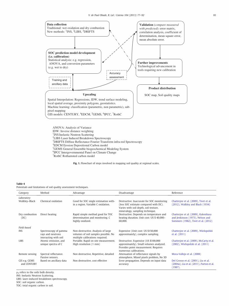
Table 4Potentials and limitations of soil quality assessment techniques.

Category Method Advantage Disadvantage Reference

LaboratoryWalkley–Black Chemical oxidation Good for SOC single estimation with-

in a region. Variable C oxidation.Destructive. Inaccurate for SOC monitoring(less SOC estimate compared with DC).Varies with soil depth, soil texture,mineralogy, sampling technique.

Chatterjee et al. (2009), Tivet et al.(2012), Walkley and Black (1934)

Dry combustion(DC)

Direct heating Rapid simple method good for TOCdetermination and monitoring. Chighly oxidized.

Destructive. Depends on temperature andheating duration. Unit cost: US $ 40,000–60,000.

Chatterjee et al. (2009), Kalembasaand Jenkinson (1973), Nelson andSommers (1982), Tivet et al. (2012)

Field-basedINS Spectroscopy of gamma

rays and neutronsinteracting with soil

Non-destructive. Analysis of largevolumes of soil samples possible. Nomultiple calibrations required.

Expensive (Unit cost: US $150,000approximately), complex sampling.

Chatterjee et al. (2009), Wielopolskiet al. (2011)

LIBS Atomic emission, andunique spectra of C

Portable. Rapid on site measurement.High resolution (1 mm)

Destructive. Expensive (US $100,000approximately). Small volumes analyzed.Provides point measurement. Requiresnumerous calibrations.

Chatterjee et al. (2009), McCarty et al.(2002), Wielopolski et al. (2011)

Remote sensing Spectral reflectance.Passive sensors.

Non destructive, Repetitive, detailed Attenuation of reflectance signals byatmosphere, Mixed pixels problem, No 3D

Mora-Vallejo et al. (2008)

GIS e.g. GEMSand CENTURY

Based on ancillary data Non destructive, cost effective Error propagation. Depends on input dataaccuracy

Del Grosso et al. (2001), Liu et al.(2004a), Liu et al. (2011), Parton et al.(1987).

ρb refers to the soils bulk density.INS: Inelastic Neutron Scattering.LIBS: laser-induced breakdown spectroscopy.SOC: soil organic carbon.TOC: total organic carbon in soil.



bulk density (ρb), so as to express C on volume basis (g m−2 orMg ha−1). The requirement to analyze SOC and evaluate ρb is timeconsuming, and labor intensive (Chatterjee et al., 2009; Lal, 2006).Soil ρb can be rapidly estimated in situ using near infra red (NIR) ormid infra red (MIR) spectrometry, or other sensors such as the gammaprobe, or directly using volumetric concentration of C (Bellon-Maureland McBratney, 2011). Laboratory determination of SOC generally in-volves destructive sampling,with initial processing conducted to reduceheterogeneity in the soil samples. The SOC from the homogenized soilsamples can then be extrapolated using approaches such as geostatistics(Webster, 2007; Wielopolski et al., 2011).

Spectroscopic techniques have been applied to assess SOC in the lab-oratory (Croft et al., 2012; Rossel et al., 2006). Spectroscopic methodspermit a rapid and non-destructive means for quantifying SOC withhigh precision, reduced cost and processing times (Cohen et al., 2007),although considerable sample preparation (collection, grinding, sieving,and drying) is still required (Stevens et al., 2008). Laboratory spectros-copy may be useful for calibration of aerial and satellite reflectancemeasurements (Stevens et al., 2008), and for investigating the relation-ship between SOC decomposition processes and soil reflectance.

2.2. Field based methods

The determination of SOC directly in the field may not only be costeffective, but appropriate in circumstances where a laboratory is notreadily available (Reeves, 2010). Lal (2002) outlined 10 steps in theassessment of SOC at a field scale. The SOC pool can be determinedin situ by the INS approach (Wielopolski et al., 2011) which operatesby inducing fast thermal neutrons that interact with nuclei of the el-ements in soil. The output gamma ray spectra are registered by anarray of detectors, and the net peak intensities (or counts) analyzed.The INS system is non-destructive, supports multi-elemental analy-ses, can analyze large soil volumes, does not require multiple calibra-tion of the soil's ρb, and can be operated in static and scanning modes(Chatterjee et al., 2009; Wielopolski et al., 2011). In contrast, othermethods such as the DC, laser-induced breakdown spectroscopy (LIBS)(Ebinger et al., 2006), and diffuse reflectance Fourier Transform infra-red spectroscopy (DRIFTS) (McCarty et al., 2002), are destructive andprovide only point measurement.

Sensors can be mounted on tractors to provide “on-the-go” SOC es-timates or rapid data acquisition (Croft et al., 2012). Bricklemyer andBrown (2010) argued that “on the go” spectroscopy could not capturedetailed SOC variability within small areas. However, Stevens et al.(2008) reported that with statistical calibration conducted before eachfield campaign, the portable spectroscopy provided SOC valueswith ac-curacy similar to that by laboratory techniques e.g., by Walkley andBlack (1934). Morgan et al. (2009) attributed the scanning measure-ment errors for “on the go” sensors to soil smearing, varying soil surfaceroughness asmacro-aggregates are disturbed, and the spatial averagingof the reflectance data.

2.3. Aerial and satellite measurements

The application of sensors mounted on aerial or satellite platformsfor measuring SOC is still at its infancy (Ben-Dor et al., 2009; Croft etal., 2012; Mora-Vallejo et al., 2008). Although airborne and satellite-derived reflectance data may provide spatially continuous SOC mapsat high temporal resolutions, issues such as data acquisition costs, pre-processing requirements, and technical complexity have hamperedtheir development (Croft et al., 2012; Hansen et al., 2008; Moran et al.,1997; Roy et al., 2006). In addition, the aerial and satellite borne remotesensors only detect the surface reflectance, which is correlated toSOC. Subsurface SOC may need to be computed indirectly from modelsrelating surface to subsurface SOC. Other issues to contend with whendetermining SOC with air and satellite borne sensors include variablesoil moisture for different localities, and vegetation which may obscure

the remote sensors from acquiring soil reflectance. However, for crop-ping systems, air or space borne sensors may be used to measure thesoil reflectance during the times of the year when the crops are absentfrom the field, or begun growing. The SOCmodeled using data from op-tical sensors mounted on aerial platforms have yielded strong correla-tion with the ground data (Croft et al., 2012; Stevens et al., 2008). Incontrast, Gomez et al. (2008) reported a weaker correlation betweenHyperion satellite modeled SOC, and ground or laboratory determinedSOC, which was attributed to the low signal/noise ratio.

Spectral reflectance datamust be processed to reduce noise or errors(Coppin et al., 2004; Moran et al., 1997). Atmospheric, radiometric andgeometric errors in sensor data are caused by Rayleigh, Mie, non-selective scattering, cloud cover, the bidirectional reflectance distribu-tion function (BRDF), sensor drift in space and time, andmis-registrationerrors (Coppin et al., 2004; Moran et al., 1997; Stevens et al., 2010).Cloud cover can be masked out, although this creates data gaps. Roy etal. (2008) demonstrated a gap filling approach whereby scan gaps onthe Landsat satellite imagery, and data gaps left aftermasking out cloudswere filled using data acquired by other remote sensing systems. Simpleatmospheric correction methods that do not use radiative transferinclude the dark object subtraction, histogramminimization, regressionline method, and empirical line correction method. The complex radia-tive transfer models include the second simulation of satellite signalin solar spectrum (6 s), MODTRAN/LOWTRAN, SMAC etc. Simple atmo-spheric correction methods are only applicable for narrow field of viewinstruments, and are not feasible when processing a large number ofsatellites on a systematic basis. In addition, simple atmospheric correc-tionmethods require assumptions of a Lambertian surface (i.e. equal re-flectance in all directions), large homogeneous area, and that the surfacebeing studied is pseudo-invariant (Roy et al., 2008).

The histogramminimization and dark object subtraction are empir-ical atmospheric correction methods, whereby the lowest digital num-ber or reflectance value is subtracted from all the pixels within eachspectral band, under the assumption that the pixels with the lowestreflectance values are from shadows, water or dark colored surfaceswhich should have zero values. Therefore, any existing values in thewater bodies or dark colored surfaces are presumably errors due to at-mospheric effects. On the contrary, the regression and empirical linesassume the offsets to be the result of atmospheric errors. Errors suchas BRDF occur in circumstances where the study area encompassingmore than one satellite imagery has variation in illumination. In suchsituations, normalization may be conducted on the satellite imageryto minimize the BRDF effects (Roy et al., 2008). In the normalizationprocess the sensed digital numbers recorded on the satellite sensordata, are initially converted to spectral radiance by using sensor calibra-tion gain and bias coefficients retrieved from the metadata. After that,the spectral radiance is converted to the top of atmosphere reflectance,so as tominimize errors introduced through variations in the earth–sundistance, solar geometry, and atmospheric solar irradiance arising fromspectral band differences (Chander et al., 2009). Masek et al. (2006) ar-gued that conversion of radiance sensed at the reflectivewavelengths toreflectance (unitless) has physical meaning, and should enable bettercomparison of satellite data with ground based measurements, modeloutputs, and data from other sensors.

Geometric correction and image registration of data are essentialin mapping land use or cover change analysis. Although geometriccorrection and data registration are undertaken concurrently, geomet-ric correction is a procedure that involves the creation of an orthogo-nal map projection, whereas image registration is done through theprecise matching of two or more corrected or non-geometricallycorrected datasets using selected identical locations. Generally, a poly-nomial model is applied to merge selected points on the satellite im-agery or aerial photograph with ground reference points of knownaccuracy. Accurate geometric correction can ascertain to the user thatthe change identified is accurate, and not an artifact of the image pro-cessing procedure. Geometric correction minimizes positional errors


present in remotely sensed data, created by random distortions relatedto the sensor system attitude and altitude. Tucker et al. (2004) docu-mented the standard procedure for geometric correction.

2.4. Upscaling and data fusion

Upscaling or downscaling the spatial and temporal changes in SOCpools from points to regions or vice versa, is a critical step toward im-proving the basic understanding of the dynamics of C sources andsinks over varying spatial extents (Liu et al., 2011; Pohl and vanGenderen, 1998). The upscaling process may utilize models to predictvalues for unsampled locations based on accurately measured pointsamples. For amodel to be effective itmust: (i) describe the data as sim-ply as possible, and (ii) predict unobserved data (De'ath and Fabricius,2000). In the next section, various approaches for predicting unsampledlocations are discussed.

2.4.1. Spatial interpolationInterpolation techniques have been used to upscale SOC estimates

at a range of scales for different soil environments (Goovaerts, 1999;Ping and Dobermann, 2006). Because the SOC field data are acquiredfrom specific sampled point locations, interpolation techniques suchas the regression, proximity polygons, local spatial average, inverse dis-tance weighting (IDW), trend surface modeling, or kriging (Goovaerts,1999; Phachomphon et al., 2010) have been used to predict unsampledlocations. The inverse distance weighting (IDW) computes the variableat unknown points using weights based on the distance betweenthe prediction and measured/observed points; whereas trend surfacemodels predict unknown points using polynomial regression modelsgenerated from spatially referenced points. In contrast, geostatisticalmethods (e.g. kriging) predict unknown points using both the distanceand the degree of variation between the sample pairs based on avariogram. Some examples of kriging methods include the ordinary,simple, and universal (Goovaerts, 1999).

Hybrid approaches which combine geostatistics and environmen-tal variables have been documented (Goovaerts, 1999; Simbahan andDobermann, 2006). The secondary predictor variables in hybrid inter-polators are normally highly correlated to the original predictor vari-able. Examples of secondary predictor variables are relief, climate, orsoil types. Hybrid interpolation techniques (e.g., co-kriging) may en-hance precision of prediction in situations of incomplete or missingdata. Hybrid approachesmay improve SOC estimates when the second-ary variable is at a finer sample spacing (Ladoni et al., 2010), and alsoprovide more accurate local predictions than ordinary kriging or theother univariate predictors (Simbahan and Dobermann, 2006).

2.4.2. Machine learningManual handling of remotely sensed data for mapping does not

only provide inconsistent results but is also a formidable task e.g.,due to iterative nature of processing required (Mulder et al., 2011;Singh, 1989). Remote sensing applications have benefitted from ad-vancements in computer technology, and increased availability of al-gorithms (De Fries et al., 1998; Hansen et al., 1996, 2000). Machinelearning is a technique for data partitioning and categorization (Camps-Valls, 2009; Lippit et al., 2008; Petropoulos et al., 2012) based on theidea of “learning” patterns in datasets. Classified map products from au-tomated processing of remotely sensed imagery, or machine learningtechniques are useful inputs in GIS based models for assessing SOCover large spatial extents. Applyingmodels derived from point measure-ments of SOC and correlated with spectral reflectance on remotelysensed imagery, provides complete datasets for extrapolating/estimatingSOC values in unsampled locations, because of the spatial continuity insatellite remotely sensed datasets, unlike other point data interpolationtechniques e.g., kriging. Image classification, whether parametric or nonparametric is based on the operational concept of machine learning,and utilizes a statistical routine to sort the pixels in an image into discrete

spectral categories or themes. Supervised andunsupervised classificationprocedures are the major digital spectral oriented techniques for map-ping surface cover, based on the concept of machine learning. In the su-pervised classification, the image analyst specifies descriptors of interestor training areas from the site that are present in the scene, to “train” theclassifier to categorize similar classes within the imagery using the com-puter algorithm (Lillesand and Kiefer, 2000).

The unsupervised classification circumvents the need for trainingdataset by directly clustering the image spectral data to produce amap of spectrally similar classes, based on natural groupings presentin the image values. The principle is that values within a given covertype should be close together in measurement space, whereas data indifferent classes should be comparatively separated. The spectral clas-ses or outcome from the unsupervised classifications can then be relat-ed to measured values at the same sites (e.g., SOC and salinity).

2.4.2.1. Parametric. Parametric techniques assume that the samplesare normally distributed, have a homogeneous variance, and the dataare independent of each other, such as in the Gaussian distribution. Ex-amples of parametric supervised classification approaches include the:(i) maximum likelihood classifier which evaluates the variance, and co-variance of the spectral response patternswhen classifying anunknownpixel. Here, the probability density functions are used to classify anunidentified pixel by computing the probability of the pixel value be-longing to each category, (ii) parallelepiped classifier which considersthe range of values in each category training set. The ranges are definedby the highest, and the lowest digital number values in each band nor-mally represented as a rectangular area. An unknown pixel is classifiedaccording to the decision region or category range in which it lies, or as“unknown” if it lies outside all regions, and (iii) minimum distance tomeans classifier, which classifies based on the distance between apixel value, and the category mean value of a class. Here, the unknownpixel is assigned to the closest class (Lillesand and Kiefer, 2000).

2.4.2.2. Non parametric. The non parametric technique also known as“distribution free” methods, does not make any statistical assumptionsin modeling distributions, and can characterize non linear relationships(Breiman et al., 1984). Examples of non parametricmethods include thek-nearest neighbor, decision tree, and the neural network (Mulder etal., 2011). Decision trees mimic the human abstraction process throughhierarchical categorization, whereas neural networks mimic the brainstructure of neurons and linkages (Lippit et al., 2008). The decisiontree can process either categorical data (classification trees), or contin-uous data (regression trees).

Currently, the regression trees are the state of the art approach indigital classification of remotely sensed imagery (Hansen et al., 2008,2011; Lawrence et al., 2006). The regression tree repeatedly splits thedata into two mutually exclusive subsets (or groups), thereby mini-mizing the sum of squares within groups, and creating homogeneousgroups (Breiman et al., 1984). This process is iterated until all subsetsare either pure, or there are not enough data to conduct an additionalsplit. In the regression tree, the input or independent parameters canbe environmental variables that are used to predict the variable of in-terest. Regression trees have been used to generate accurate vegeta-tion maps from remotely sensed data (De Fries et al., 1998; Hansenet al., 1996, 2000, 2002a,b; Michaelsen et al., 1994). Alternately, theaccuracy of the regression tree can be enhanced by generating severaltrees from training data, and averaging their predictions, a techniquecalled “bagging” (Breiman, 1996). Pittman et al. (2010) utilized a bag-ging methodology with variables derived from MODIS bands, NDVI(Normalized Difference Vegetation Index), and thermal data to mapglobal cropland extent. The study found that the MODIS layer accu-rately mapped the regions of intensive crop production, whereas re-gions with minimal agricultural intensification, such as Africa, hadlower map accuracies. The Random forest approach which uses a dif-ferent random subset of training data to grow multiple trees, and


averages their predictions, is based on a similar concept to regressiontree (Breiman, 2001).

2.4.3. Generic models for SOC determinationGeneral or generic models are designed using a set of model param-

eters that are expected to provide accurate SOC estimates over largespatial extents. Quantifying SOC precisely on a regular basis may be dif-ficult because SOC varies along the soil profile depending on the rate ofmicrobial degradation (Liu et al., 2011). Baker et al. (2007) mentioneddrainage as another factor influencing SOC dynamics in croplands. Poor-ly drained environments favor SOC accumulation,whereaswell drainedenvironments enhance the decomposition of SOC and emission of C(Tan et al., 2004).

Mapping SOC directly through remote sensing may be challengingespecially in locations where the soil surface is partially or whollycovered (e.g., by other vegetation or buildings). For scenarios of par-tial coverage of the soil surface, SOC may be modeled through a com-bination of field, remotely sensed datasets, and analyzed through aGIS. Examples of GIS based models for quantifying SOC at variousscales include the General Ensemble biogeochemical Modeling Sys-tem (GEMS), CENTURY, DayCent (Daily Century model), RothamstedCarbon Model (RothC), and the Erosion Depositional Carbon Model(EDCM) (Del Grosso et al., 2001; Liu et al., 2004a, 2011; Tan et al.,2009; Wielopolski et al., 2011). CENTURY is an entire ecosystemmodel with a plant productivity sub-model (Parton et al., 1987). Bio-geochemical modeling using the CENTURY model requires a detailedspecification of cropping practices on agricultural land, including cropspecies and management practices. The CENTURY model was origi-nally developed for use in North American grassland (Parton et al.,1987).

GEMS and EDCM are process based modeling systems developedfrom the CENTURY to simulate C, N, and P dynamics in a diverse rangeof ecosystems. EDCM was developed to characterize SOC dynamicswithin the soil profile, and evaluate the impacts of soil erosion and

SOC: Soil Organic Carbon

C: Carbon

NPP: Net Primary Production

ρb:Bulk density

Climate data e.g.precipitation, temperatures

Inputs

Outputs

ModeCENTURY, G

Grain y

Soil properties e.g.textures, ρb, moisture, drainage

NPP

Fig. 2. Schematic diagram of inputs and

deposition (Liu et al., 2011; Zhao et al., 2010), whereas GEMS wasdesigned to simulate C dynamics in vegetation and soils at different spa-tial scales (Tan et al., 2009). The RothC model is a soil decompositionmodel that requires plant productivity parameters as input (Colemanand Jenkinson, 1996). The Intergovernmental Panel on Climate Change(IPCC) facilitated the creation of an empirical method, referred to as theIPCC which computes the spatial and temporal variations of SOC (IPCCet al., 1997). Other SOC prediction models include the EnvironmentalPolicy Integrated Climate (EPIC), and CQUESTER (Lal, 2009).

Generic models can integrate data such as management practices,land cover, climate and soils (Liu et al., 2004a, 2008; Ojima et al., 1994;Parton et al., 2004; Zhao et al., 2010). The common model inputs(Fig. 2) include monthly precipitation, monthly maximum and mini-mum temperatures, soil texture, ρb, drainage, initial SOC level, waterholding capacity, cropping system, cultivation, atmospheric N deposi-tion, fertilization, harvesting, grazing, tree removal, land cover data,and natural disturbances such as erosion or fire (Dieye et al., 2012; Liuet al., 2008; Parton et al., 2004). The major output variables are NPP,grain yield, C decomposition, C exchange rates between ecosystemsand atmosphere, biomass removal by harvesting, and the C pool in veg-etation and soils. Genericmodels also provide the uncertainty of predict-ed variables in space and time (Liu et al., 2004a, 2008).

2.5. Validation

Validation quantifies the product accuracy by comparing the knowndata ormeasured reference datawith the predicted data (Robinson andMetternicht, 2006). In validation, a portion of the dataset is set aside formodel fitting and the remainder to check the accuracy of the fittedmodel (Davis, 1987). In practical situations, validation requires compro-mises that minimize costs without sacrificing the precision. Remotelysensed products are validated through the computation of commission,omission, producer's accuracy, user's accuracy, and the overall accuracybased on the contingency table, or error matrix. In the contingency

l e.g.EMS, RothC

SOC and vegetation C poolsield

InitialSOC level

Management i.e. land usee.g. crop type and cover types from satellite or aerial data, topographic map etc., fertilizer inputs

outputs in the SOC generic models.


table, the number of rows should equal the number of columns, withthe diagonal representing correctly classified pixels. The overall accura-cy of classified maps is computed by dividing the sum of correctly clas-sified pixels, by the total number of classified pixels (Congalton et al.,1983). Another accuracy assessment technique, the kappa statistics,produces a range of values between−1 and+1,with a value of zero in-dicating that chance agreement equaled the effect of the classifier,whereas +1 indicates a perfect classification with no contributionfrom chance agreement, and negative values represent very poor classi-fication in which chance agreement is more important than classifica-tion. Kappa values of 0.75 or greater indicate very good to excellentclassification performance (Monserud and Leemans, 1992). The errormatrix requires the perfect coregistration of datasets, and the descrip-tion of the field sampling design (Foody, 2002).

Cross validation which is a more elaborate validation approach isperformed through the following steps: (i) removal of one observa-tion from the dataset, (ii) estimation of the value of the variable atthe location the variable was removed using the remaining observa-tions, (iii) computation of error based on the difference between theobserved and predicted variable, and (iv) the process is repeated forall the remaining observations (Davis, 1987; Robinson and Metternicht,2006). The degree of agreement between measured and interpolated orpredicted values can be evaluated through a correlation analysis, themean square error, or mean absolute error, whereby the mean error isexpected to be zero, if the interpolation approach is not biased. The com-putedmean error, however, depends on the sampling points considered,and the scale of the data (Robinson and Metternicht, 2006). A drawbackof quantitative accuracy measures is that they may not indicate if theproduct is relevant for qualitative applications, or better than an alterna-tive non-remote sensing source of information.

2.6. Challenges in SOC estimation

Developing accurate, rapid and systematic approaches for estimat-ing SOC over large spatial scales constitutes a significant challenge.For example, the requirement of a high sampling density with pointdata and the high spatial variability of ρb influence interpolation accu-racy (Moran et al., 1997; van Wesemael et al., 2011). Unlike withpoint data, interpolation based on remotely sensed satellite data hasthe advantage of continuity of data in space and time (Duveiller andDefourny, 2010). In practice, secondary data related to the nature ofthe ecosystem may be utilized in situations of limited data to makepredictions (D'Acqui et al., 2007).

In highly variable environment mixed pixels, which represent aweighted average of spectral reflectance signals of the different landcover types within a pixel may occur (Foody, 2000). Approaches suchas the sub-pixel mapping can minimize the mixed pixel problem(Roberts et al., 1993). Subpixel mapping methods may be performedthrough methods such as the regression tree, spectral mixture analysis,or a combination of both. Regression tree conceptwas earlier introducedin this article, under the subsection dealing with non-parametric classi-fication. Spectral Mixture Analysis (SMA) technique uses informationfrom all the spectral reflectance bands, to divide each ground resolutionelement into its constituent materials through decomposing the DN,or reflectance values into fraction images or components using end-members (Dennison and Roberts, 2003; Garcia-Haro et al., 1999).Endmembers are spectral reflectance generated frompure target surfaceclasses. The relative contribution of a given endmember to amixed spec-trum of a pixel is equivalent to the surface abundance of the respectiveland cover class in that pixel (Peddle and Smith, 2005; Smith et al.,1990). The SMA technique has been used to characterize the spatialdistribution of surface crop residue cover which is a major source ofSOM (Bannari et al., 2006; Obade et al., 2011). It does not detect non-linear mixing (Fan et al., 2009; Roberts et al., 1998), even though non-linear mixing which results from multiple scattering by vegetation, soil

surfaces, and variation in illumination can be significant (Ray andMurray, 1996; Van der Meer and De Jong, 2000).

Mismatches between spatial, spectral and temporal resolution ofremotely sensed data also create difficulty in the remote sensingbased assessment of SOC changes (Lobell, 2010). For example, therate of change in SOC for specific locations within the terrestrial eco-systems may be small, making temporal SOC change detection overlarger areas difficult (Smith, 2004). To minimize errors attributed todiffering spatial resolution between sensors, an approach that is res-olution independent should be used in map comparisons. Methodssuch as Mapcurves can be useful for comparing maps having differentspatial resolutionswithout necessarily conducting rigorous georeferenc-ing. Mapcurves graphically and quantitatively evaluate the degree of fitamong any number of maps (Hargrove et al., 2006). Mapcurves tech-nique are category-based (polygon) rather than cell based, therefore,the goodness of fit measures are resolution independent (Hargrove etal., 2006).

The spectral reflectance of soil varies depending on the chemicalor physical factors, such as soil mineralogy, soil moisture, SOM con-tent, soil texture, and particle size (Croft et al., 2012; Wielopolski etal., 2011), which makes it difficult to acquire the pure spectral reflec-tance signals of SOC. The drawback of generic models such asCENTURY, GEMS is that they operate effectively for only soil systemson which they were created, and require historic datasets which arerare as part of the inputs (Dieye et al., 2012; Dungait et al., 2012b;Liu et al., 2011). An investigation on the impacts of agricultural man-agement on SOC by Ogle et al. (2007) illustrated that the CENTURYmodel generated a higher statistical precision at regional than localscale. Furthermore, the secondary data utilized in the generic modelsmay enhance uncertainty in SOC estimates (Jones et al., 2007; Stevenset al., 2010). The knowledge on variation of SOC with depth is alsolimited, because most SOC inventories focus on the first 1 m belowthe soil surface, although a substantial amount of C can occur at great-er depths (Batjes, 2008; Jobbagy and Jackson, 2000; Lorenz and Lal,2009; Schwartz and Namri, 2002).

2.7. Examining the sensitivity of spectral response to soil quality

2.7.1. MethodsA field experiment was conducted to investigate the sensitivity of

spectral reflectance on management induced differences in soil qual-ity. A total of 72 soil samples from 2 soil types, were collected fromselected corn fields and forest. The field data was collected duringMay and July, 2012 at Preble (39° 41′ 45″ N, 84° 40′ 36″ W) andAuglaize (40° 27′ 34.5″ N, 84° 26′ 14.8″ W) counties, within the stateof Ohio. For each site, soil samples for different management systemsi.e., conventional tillage (CT), no-tillage (NT), natural vegetation (NV)or forest were obtained at similar landscape position, and 2 depthsi.e., surface (0 to 10 cm), and at 40–60 cm, general rooting depth. Foreach of the soil samples, the corresponding soil types were identifiedfrom the USDA web soil survey (http://websoilsurvey.nrcs.usda.gov/app/HomePage.htm). The SOC content and soil moisture were deter-mined in the laboratory through the gravimetric method, but the spec-tral reflectance for each soil sample was measured outdoors. The SOCconcentration of air-dried and sieved (2 mm) samples was analyzedthrough the dry combustion at 900 °C with a Vario Max CN analyzer(Nelson and Sommers, 1996). The sieved soils were put on 10 cm cruci-bles to a soil depth of approximately 4 cm in each crucible, and 3 scanstaken with an ASD FieldSpec 3 Spectroradiometer on an outdoor envi-ronment on a flat surface on clear sunny days i.e., minimal cloudcover. Although the focus of this article is on the link between soil qual-ity and remote sensing measurements, corn residue cover which influ-ences SOC inputs was manually applied to cover 50% of each of thecrucibles, and reflectancemeasurements taken again on all the samples.The hypothesis is that no difference exists in spectral reflectance fromsoils under similar management system because of similar SOC input/

http://websoilsurvey.nrcs.usda.gov/app/HomePage.htm

http://websoilsurvey.nrcs.usda.gov/app/HomePage.htm


output dynamics. Models developed relating SOCwith specificmanage-ment practice may provide information on whether the soil quality isincreasing or decreasing, by comparingwith SOC in e.g., natural vegeta-tion such as forest. The moisture content for the dry corn residue coverwas 2–7%, whereas that of the dry soil was 5 to 14% and the soil wettedwith approximately 5 ml of water between 17 and 25%.

2.7.2. ResultsThe results are shown in Fig. 3 and Table 5. The highest C/N ratio

was measured for soils under NV for both soil types (Table 5). Inboth soil depths sampled, the NT had a higher C/N ratio than CT forthe Pewamo silty clay loam soils, although the reverse was true with

0.00

0.10

0.20

0.30

0.40

0.50

250 1000 1750 2500

% R

efle

ctan

ce

nanometers

a) CT

0.00

0.10

0.20

0.30

0.40

0.50

250 1000 1750 2500

% R

efle

ctan

ce

nanometers

c) NV

0.00

0.10

0.20

0.30

250 1000 1750 2500

% R

efle

ctan

ce

Wavelength in nanometers

e) NT

Fig. 3. Spectral response for Pewamo silty clay loam (i.e., a, c, e), and Crosby Celina silt loam(NT) management in Ohio, USA. The effect of atmospheric water vapor which is prominentthese wavelengths.

the Crosby Celina silty loams. For surface soils i.e., 0 to 10 cm the % Cwas highest in the NV, followed by NT, and lastly CT. However, forthe sub surface soil i.e., 40 to 60 cm depth, the % C was highest in NVfor Crosby Celina silty loam soils, and at NT for Pewamo silty clayloam soils. The differences between sites may be attributed to differ-ences in soil type, management, and duration since adoption of NT.

Fig. 3 provides the median spectral response from 2 different sam-pled soils under different management, at the 2 counties within thestate of Ohio, USA. In both sites and under all themanagement practices,the surface soils that were wet and bare (0% residue cover) consistentlyhad the least reflectance across all wavelengths. In Auglaize county, thedry surface soils under conventional tillage that had partial residue

0.00

0.10

0.20

0.30

0.40

250 1000 1750 2500

% R

efle

ctan

ce

nanometers

b) CT

0.00

0.05

0.10

0.15

0.20

0.25

250 1000 1750 2500

% R

efle

ctan

ce

nanometers

d) NV

0.00

0.05

0.10

0.15

0.20

0.25

250 1000 1750 2500

% R

efle

ctan

ce

nanometers

f) NT

surface soil, 0 % residue, wet soil

surface soil, 0 % residue, dry soil

surface soil, 50 % residue, dry soil

surface soil, 50 % residue, wet soil

40 to 60 cm, dry soil

(i.e., b, d, f) soils under conventional tillage (CT), natural vegetation (NV), and no tillat 1500, 1750 and 2500 nm is shown by the sporadic reflectance pattern observed at

Table 5Sampling locations, averaged % C, and soil Carbon (C)/Nitrogen (N) ratio's for soil at depths 0 to 10 cm, and 40 to 60 cm under different management practices within the state ofOhio, USA. CT is conventional tillage, NT is no-till, and NV is natural vegetation. Soil type description follows the USDA soil classification system.

Site Preble (39° 41′ 45″ N, 84° 40′ 36″ W) Auglaize (40° 27′ 34.5″ N, 84° 26′ 14.8″ W)

Soil types CtA (Crosby Celina silt loams) Pw (Pewamo silty clay loam)

Management CT NT NV CT NT NV

% C (0 to 10 cm) 1.05 1.09 1.31 2.50 2.55 3.80% C (40 to 60 cm) 1.50 1.76 2.21 1.83 2.31 1.33C/N ratio (0 to 10 cm) 10.13 9.29 9.89 9.11 9.55 11.21C/N ratio (40 to 60 cm) 10.34 9.06 11.80 9.78 9.98 11.12

Table 6SOC estimates (Pg) per biome.Modified from Jenkinson et al. (1991), Jobbagy and Jackson (2000), and Post et al. (1982).

References Time 1 (B) Time 2 (A) % change

BiomeBoreal forest 181.9 150 −18Crops 167.5 248 48Deserts 84 208 148Temperate forest 104.3 262 151Tropical forest 184.5 816 342Tundra 191.8 144 −25Tropical grassland/savanna 129.6 345 166Temperate grassland 149.3 172 15Total SOC 1192.9 2345 97

A: Jobbagy and Jackson (2000). This is the source of data for Time 2 (i.e., year 2000).B: Post et al. (1982), and Jenkinson et al. (1991). Source of data for Time 1 (i.e., 1982similar to 1991).% change=SOC estimates from (A−B)/(A)×100.Pg is equivalent to estimated value (×1015g).


cover (i.e., 50%) had the highest spectral reflectance recorded across the350 to 2500 nmwavelength range, followed by the dry sub surface soil,bare surface soils, and the wet surface soil with partial residue cover.The NV had the highest reflectance with the dry surface soil partiallycovered with residue, the dry sub surface soil, the wet surface soilwith residue, and then the dry bare surface soil, respectively. Alternate-ly, the reflectance magnitude for soils under NT management inAuglaize ranged from dry surface soil with partial residue cover, drybare surface soil, dry sub surface soil, wet partially residue coveredsurface soil, and then the wet bare surface soil, respectively. However,the results from Preble county were slightly different from those atAuglaize. For example, under the conventional tillage, the subsurfacesoils had the largest spectral reflectance, followed by the dry surfacesoils having partial residue cover, and the dry bare soil. Interestingly,the wet soil with and without residue cover had similar least reflec-tance. Soils in the NV had the subsurface soils with the largest reflec-tance, followed by the dry bare soil; dry and wet partially residuecovered which alternated in magnitude of reflectance across the wave-lengths. Similarly, the NT had the dry subsurface soil with the highestreflectance, dry surface bare soil, after which similar response was ob-served for the dry and wet soils with partial residue cover.

The dry bare surface and subsurface Pewamo silty clay loam soilsunder CT and NT management with lower C/N ratios had relativelyhigher % reflectance between 350 and 2500 nm compared with NV.The dry subsurface Crosby Celina silt loam soils gave similar observa-tions. Slightly different results were observed with the dry bare surfaceCrosby Celina silt loam soils whereby the CT although having a high C/Nratio, had the least reflectance compared with NT and NV. Because ofthe differences in spectral reflectance data for soils with differentproperties at different depths, convertible equations relating soil reflec-tance to soil quality are required. Other than SOC, which highly influ-ences the soil quality (Lal, 2001a,b, 2002, 2004b; Rossi et al., 2009; Saand Lal, 2009; Sombroek et al., 1993), the spectral response of soilsunder different management in Fig. 3, may be explained by the numer-ous variables that can determine soil properties at different depths, be-ginning with soil mineralogy, structure, and texture. For example theproportion of solid, air, and water may be variable in soils. In addition,the effect of other factors e.g., soil ρb, and the type of bonding on reflec-tance need further investigation. Effective modeling of soil quality inreal time using reflectance data may require rigorous statistical testingof these parameters, to determine which ones significantly influencereflectance.

3. Case studies

Modification or changes in land use and covermay have significantimpact on SOC. Comparing the global SOC within different biomes(Table 6) computed by Jobbagy and Jackson (2000) to those byJenkinson et al. (1991) or Post et al. (1982) shows a disparity of 97%suggesting that the global SOC increased over time. The tropical forest,tropical grassland/savanna, temperate forest and desert biomes allhad an increase in SOC of 342%, 166%, 151%, and 148% respectively,which implied that the soil quality improved within these biomes.High agricultural production is expected in locations with high soil

quality in the absence of other limiting plant growth factors such aswater. On the other hand, boreal forest and tundra biomes had a re-duced SOC of 18% and 25%, respectively. In a different study conductedin Brazil, vanNoordwijk et al. (1997) documented a gradual decline ofSOC originating from the forest system, and its partial replacement bySOMderived from inputs of sugarcane (Saccharum officinarum) withinthe first fifty years of cultivation. These results revealed that forestconversion to well managed grasslands may lead to an increased SOCstorage, in the long run. However without information on the land usehistory, no simple explanation exists for the SOC variability e.g., be-tween tree plantations with different species (Usuga et al., 2010).Kumar and Lal (2011) conducted a geostatistical analysis with 920 soilprofiles to estimate the SOC in Pennsylvania, USA. The soil clay content,ρb, total N content, pH, Ca2+, Na+, extractable acidity, and cation ex-change capacity (CEC) were used as covariates. The geographicallyweighted regression kriging produced the best estimate for the SOCpool.

Liu et al. (2004b) modeled SOC dynamics in the SoutheasternPlains ecoregion using the General Ensemble Biogeochemical Model-ing System (GEMS). The study reported an increase in C sequestrationwhich was attributed to the afforestation. In another study, Liu et al.(2011) simulated SOC dynamics within 0–1 m depth of soils acrossthe state of Iowa in the USA using GEMS, and extrapolated the find-ings to regional scale. The soils within a depth of 1 m were found tobe an SOC source, which was attributed to either the drainage systemincreasing SOC circulation from the deep soil layers, or the crop rotation.It is important to note that SOCdynamics are significantly dependent onthe initial SOC levels i.e. soils with higher SOC levels tend to be Csources, whereas those with lower levels tend to be C sinks (Lal,2001a,b). The SOC sequestration can be enhanced through slowing de-forestation, and restoring degraded lands (Glenday, 2006; Lal, 2003a;Sachs and Reid, 2006; Zhang and Justice, 2001; Zhang et al., 2002).

Africa is the second largest continent, approximating 20% of theEarth's land area. Africa has a range of ecoregions comprising forest,grasslands, savannah, and desert. Much of the ecosystems in Africa


have been degraded due to non-sustainable management practices andland use conversion (UNEP, 2007). Lal (2009) stated that erosion in-duced decline in soil quality ismore serious in developing than in devel-oped countries. The knowledge on the severity of soil quality reductioncaused by SOC pool changes attributed to land use conversion in Africais limited, despite the abundance of technological options for monitor-ing the SOC (Batjes, 1996, 2008; Birch-Thomsen et al., 2007; Schwartzand Namri, 2002; Thomas et al., 2008; Williams et al., 2007). For exam-ple,Wang et al. (2009) studied the spatial heterogeneity of the SOCpool

Table 7Some notable studies of SOC mapping with key findings and limitations.

Country Technique Key finding

Australia Multi-sensor satellite data, and global climatemodels

Lack of prec

Africa, Americas, Asia,Europe, and U.S.A.

Boosted regression trees (BRT), Partial LeastSquares (PLS) regression, and visible andnear-infrared (VNIR) diffuse reflectancespectroscopy.

Strong correperformed bfor calibraticalibration m

Burundi, DemocraticRepublic of Congo,and Rwanda

SOTER (Soil and Terrain database)Scale of 1: 2 millionDepth of 1 m

SOC contenthe warm srial, soil drasecondary d

Brazil GEFSOC soil carbon (C) model, and SOTER Declining truse changes

China Environmental Policy Integrated Climate (EPIC)agro-ecosystem simulation, and HadCM3 globalClimate model

SOC sequestwheat–corn

Ethiopia Multiple regression model Poor correlareflectance'and woodla

Italy Regression, and Ordinary Kriging (OK) Improved reration of enmulti-senso

Japan Rothamsted carbon model (RothC) The RothC sdecreased funreliable b

Kenya Regression Kriging The digital m

Kenya Global Environment Facility Soil Organic Carbon(GEFSOC) Modelling System

ConversionSoil C losses

Laos Ordinary kriging (OK), inverse distance weighting(IDW), regularized spline with tension (RST),co-kriging (OCK)

OCK yieldedattributed t

Senegal Classification tree approach Poor modelwere geomo

Senegal Geostatistical techniques for SOC. Soil sampling at0 to 40 cm depth.

Semivariogrtocorrelatiolevels than

South Africa Visible near infrared soil spectroscopy (VNIRS)and partial least square regression (PLSR). Depthsof 0–5 mm, and 0–200 mm

Study foundSOC. There ifor SOC pre

Tanzania Kriging Sampling st

Tropics Reviewed application of pedotransfer functions(PTF) for predicting soil properties

Soils in thehigher bulkin soil textudistribution

Uganda Reflectance values, vegetation indices, spectralmixture modeling fractions with SPOT satellite,and SRTM.

Significant csaturation, p

U.S.A. Dry combustion, and kriging. Depths of 0–100 cm, and 0–180 cm

Regressionsoil depth, l

U.S.A. Visible and Near-Infrared (VNIR) reflectance.Partial Least Squares (PLS) regression modeling.

SOC predictsuccessful (selected and

U.S.A. Near infrared reflectance spectroscopy (NIRS),and mid infrared reflectance spectroscopy(MIRS).

Results demmeasures, a

Review artiregion, spatcovariates, p

Near infrared reflectance spectroscopy (NIRS),and mid infrared reflectance spectroscopy (MIRS)

Review articby moisturedent verific

within the savanna ecosystem of the Kalahari desert in the southernpart of Africa on wet and dry sites, using the isotope method, andfound contrasting results on the contributions of C3 and C4 vegetationto the SOC pools on thewet and dry sites. At the dry site, approximately40% of the SOC was derived from C3 vegetation, whereas the wet sitehad 90% of the SOC originating from C3 vegetation. These results wereamong the first quantitative information on SOC spatial distributionsunder different moisture regimes. Other notable studies on SOC assess-ments for purposes of evaluating the soil quality are outlined in Table 7.

and limitations References

ision in rangeland C sequestration estimates. Dean et al.(2012)

lation between VNIR and SOC. Boosted regression trees (BRT)etter than PLS regression. Large datasets (sample size) is requiredon and validation. Multi-sensor technology, supplemented by localay improve SOC prediction.

Brown et al.(2006)

t was high in cool humid mountains due to volcanic rocks and low inavannah region. SOC highly correlated with texture of parent mate-inage conditions, land use vegetation. Uncertainties attributed toatabase (SOTER).

Batjes (2008)

end in SOC pool observed. Validation data needed on effects of landon SOC dynamics.

Cerri et al.(2007)

ration rates higher for continuous wheat under no tillage practice, ordouble cropping. Validation required.

Thomson etal. (2006)

tion between SOC pool and vegetation index or IR and green bands. SOC pool significantly differed between cultivated, grazing land,nd.

Nyssen et al.(2008)

sults with combined OK and regression models. Proposed incorpo-vironmental factors, such as topography, soil types and the use ofr remote sensing for improved accuracy.

D'Acqui et al.(2007)

imulations found that the region's soil C pool, across all soils, hadrom the year 1970 to 2010. Predictions of SOC pools to year 2050 isecause of large uncertainties of model outputs

Koga et al.(2011)

ap of SOC had low accuracy attributed to the low sampling density. Mora-Vallejoet al. (2008)

of natural vegetation to annual crops led to the greatest soil C losses.were large from 1990 to 2030.

Kamoni et al.(2007)

the most accurate predictions. The low interpolation accuracy waso limited data points.

Phachomphonet al. (2010)

performance with large errors. Factors influencing SOC distributionrphology, topography, vegetation, and land use. Validation required.

Stoorvogel etal. (2009)

ams of soil C showed moderate spatial dependence and spatial au-n at short lags. Shrub canopies had higher correlation with soil Ctrees

Lufafa et al.(2008)

that combining soil spectroscopy and PLSR accurately predicteds potential for future application of satellite-born hyperspectral datadictions

Nocita et al.(2011)

rategy important for estimating SOC in heterogeneous landscapes Rossi et al.(2009)

tropics have higher clay content, lower cation exchange capacity,density, lower water content than temperate regions. The differencere between the tropics, and temperate regions affects SOC.

Minasny andHartemink(2011)

lass differences in soil texture, color, organic carbon (SOC), baseH, effective cation exchange capacity (ECEC), and clay mineralogy

Hansen et al.(2009)

kriging performed better than block kriging. Total soil C varies withand use, soil type, and soil drainage class.

Vasques et al.(2010)

ion at new locations by extrapolation to regional scale was partially67% success). Proposed the use of independent, larger randomlygeographically diverse datasets for calibration, and validation.

Brown et al.(2005)

onstrated that accurate calibrations for a wide variety of soil Cre feasible using MIR.

Reeves et al.(2006)

cle. Discussed effect of soil properties, sampling, soil geographicial scale, historic data, methods/model type, environmentaledological knowledge on SOC estimation

Grunwald(2009)

le. MIRS more accurate than NIRS, but mid-IR spectra more affectedand sample preparation than NIR. Field calibrations and indepen-

ations of findings are yet to be done.

Reeves (2010)


4. Researchable priorities

Credible determination of soil quality depends on the accuracy ofthe soil property maps or those of the models and ancillary datasuch as soil ρb, used to compute the SOC pool. Land use practicesand change influence SOC dynamics. Soil quality is directly relatedto SOC which in turn varies with the soil texture, for example sandysoils tend to have less SOC compared with clay soil (Chhabra et al.,2003). The feasibility of the cap and trade markets depends on the ef-fectiveness of the C measuring and monitoring schemes (Perez et al.,2007). However, limited monitoring of SOC is currently the situationin most developing countries (Birch-Thomsen et al., 2007). Otherthan climate and soil quality, the major factors affecting agriculturalproductivity are crop diseases, weeds and the resilience of croppests. Remedial management measures such as no-till, intercroppingand complex rotations may reduce the need for fertilizer input, andimpact of pests. However, bibliographic studies and reviews on thepotential of intercropped fields to sequester C are scarce, because pro-ducing maps of intercropped fields is difficult, even with remotelysensed data due to the similarity in spectral signature between differ-ent crops. Hyperspectral remotely sensed data, rigorous calibration,data preprocessing coupled with advanced GIS models may generaterepresentative maps for intercropped fields or other heterogeneoussurfaces. Other than the land use and SOC mapping issues, some im-portant questions that may guide future research on soil quality are:

o What is the correlation between various land use practices andSOC pool changes?

o How to quantify at regional scale the variation of SOC with soildepths at different soil moisture regimes?

o If SOC is changing, what is the management strategy and time forachieving a steady state of SOC?

o How to validate historical soil quality map products?o Simulate using remotely sensed data the link between soil quality,

and climatic patterns.

5. Conclusion

The literature reviewed supports the following conclusions:

1. The protection of the environment and agricultural sustainability re-quires a dedicated team of experts to develop innovative approachesfor monitoring soil quality, especially at large spatial scales.

2. Soil quality can be assessed by geostatistical approaches which notonly account for spatial variation across a landscape, but are alsouseful for determining optimal sampling strategies. However, geo-statistical approaches require field data with high sampling densityfor completeness and accuracy.

3. Remote sensing technology offers the potential to rapidly, repeat-edly and inexpensively assess soil quality at various scales. Howev-er, the variation of spectral response of soils with depth and soiltype, and the mismatch in spatial, spectral and temporal resolu-tions of different sensors may require intensive data processing,and complex models.

4. A hybrid approach that combines laboratory data, field data, andremotely sensed map products is a viable option for soil qualityassessment.

5. The absence of historical data and the utilization of secondary dataas proxy may generate additional uncertainty, for example whenassessing changes in soil quality.

6. The potential of active remote sensors such as radio detecting andranging (RaDAR), and light detecting and ranging (LiDAR) to deter-mine soil quality requires further research. RaDAR has the capabilityto penetrate the ground, whereas LiDAR can measure vegetationheights (e.g., canopy heights) although at a small spatial scale.

Acknowledgments

The authors wish to thank Dr. Izaya Numata of the Geographic In-formation Science Center of Excellence, South Dakota State Universi-ty, Dr. Gyanesh Chander of the United States Geological Survey EROSdata center, and the 2 anonymous reviewers for their helpful com-ments, and suggestions.

References

Anderson, J., Hardy, E., Roach, J., Witmer, R., 2001. A land use and land cover classifica-tion system for use with remote sensor data. A Revision of the Land Use Classifica-tion System as Presented in U.S. Geological Survey Professional Paper 964:Geological Survey circular, 671.

Baker, J.M., Ochsner, T.E., Venterea, R.T., Griffis, T.J., 2007. Tillage and soil carbonsequestration—what do we really know? Agriculture, Ecosystems and Environment118, 1–5.

Bannari, A., Pacheco, A., Staenz, K., McNairn, H., Omari, K., 2006. Estimating and map-ping crop residues cover on agricultural lands using hyperspectral and IKONOSdata. Remote Sensing of Environment 104, 447–459.

Baritz, R., Seufert, G., Montanarella, L., Van Ranst, E., 2010. Carbon concentrations andstocks in forest soils of Europe. Forest Ecology and Management 260, 262–277.

Batjes, N.H., 1996. Total carbon and nitrogen in the soils of the world. European Journalof Soil Science 47, 151–163.

Batjes, N.H., 2008. Mapping soil carbon stocks of Central Africa using SOTER. Geoderma146, 58–65.

Bellamy, P.H., Loveland, P.J., Bradley, R.I., Lark, R.M., Kirk, G.J.D., 2005. Carbon lossesfrom all soils across England and Wales 1978–2003. Nature 437, 245–248.

Bellon-Maurel, V., McBratney, A., 2011. Near-infrared (NIR) and mid-infrared (MIR)spectroscopic techniques for assessing the amount of carbon stock in soils—criticalreview and research perspectives. Soil Biology and Biochemistry 43, 1398–1410.

Ben-Dor, E., Heller, D., Chudnovsky, A., 2008. A novel method of classifying soil profiles inthe field using optical means. Soil Science Society of America Journal 72, 1113–1123.

Ben-Dor, E., et al., 2009. Using Imaging Spectroscopy to study soil properties. RemoteSensing of Environment 113, S38–S55.

Birch-Thomsen, T., Elberling, B., Fog, B., Magid, J., 2007. Temporal and spatial trends insoil organic carbon stocks following maize cultivation in semi-arid Tanzania, EastAfrica. Nutrient Cycling in Agroecosystems 79, 291–302.

Breiman, L., 1996. Bagging predictors. Machine Learning 24, 123–140.Breiman, L., 2001. Random forests. Machine Learning 45, 5–32.Breiman, L., Friedman, J.H., Olshen, R.A., Stone, C.J., 1984. Classification and Regression

Trees. Chapman and Hall, Boca Raton, FL.Bricklemyer, R.S., Brown, D.J., 2010. On-the-go VisNIR: potential and limitations for

mapping soil clay and organic carbon. Computers and Electronics in Agriculture70, 209–216.

Brown, D.J., Bricklemyer, R.S., Miller, P.R., 2005. Validation requirements for diffuse re-flectance soil characterization models with a case study of VNIR soil C prediction inMontana. Geoderma 129, 251–267.

Brown, D.J., Shepherd, K.D., Walsh, M.G., Mays, M.D., Reinsch, T.G., 2006. Global soil char-acterization with VNIR diffuse reflectance spectroscopy. Geoderma 132, 273–290.

Camps-Valls, G., 2009. Machine learning in remote sensing data processing, MachineLearning for Signal Processing, 2009. MLSP 2009. IEEE International Workshopon, pp. 1–6.

Cao, M.K., Zhang, Q.F., Shugart, H.H., 2001. Dynamic responses of African ecosystemcarbon cycling to climate change. Climate Research 17, 183–193.

Cerri, C.E.P., et al., 2007. Predicted soil organic carbon stocks and changes in the BrazilianAmazon between 2000 and 2030. Agriculture, Ecosystems & Environment 122,58–72.

Chander, G., Markham, B.L., Helder, D.L., 2009. Summary of current radiometric calibra-tion coefficients for Landsat MSS, TM, ETM+, and EO-1 ALI sensors. Remote Sensingof Environment 113, 893–903.

Chang, J., Clay, S.A., Clay, D.E., 2005. Clouds influence precision and accuracy of ground-based spectroradiometers. Communications in Soil Science and Plant Analysis 36,1799–1807.

Chatterjee, A., Lal, R., Wielopolski, L., Martin, M.Z., Ebinger, M.H., 2009. Evaluation ofdifferent soil carbon determination methods. Critical Reviews in Plant Sciences28, 164–178.

Chhabra, A., Palria, S., Dadhwal, V.K., 2003. Soil organic carbon pool in Indian forests.Forest Ecology and Management 173, 187–199.

Cohen, M., Mylavarapu, R.S., Bogrekci, I., Lee, W.S., Clark, M.W., 2007. Reflectance spec-troscopy for routine agronomic soil analyses. Soil Science 172, 469–485.

Coleman, K., Jenkinson, D.S., 1996. RothC-26.3—a model for the turnover of carbon insoil. In: Powlson, D.S., Smith, P., Smith, J.U. (Eds.), Evaluation of Soil Organic MatterModels using existing long-term datasets. Springer Berlin, pp. 237–246.

Congalton, R.G., Oderwald, R.G., Mead, R.A., 1983. Assessing Landsat classification accura-cy using multivariate-analysis statistical techniques. Photogrammetric Engineeringand Remote Sensing 49, 1671–1678.

Coppin, P., Jonckheere, I., Nackaerts, K., Muys, B., Lambin, E., 2004. Digital change detec-tion methods in ecosystem monitoring: a review. International Journal of RemoteSensing 25, 1565–1596.

Croft, H., Kuhn, N.J., Anderson, K., 2012. On the use of remote sensing techniques formonitoring spatio-temporal soil organic carbon dynamics in agricultural systems.Catena 94, 64–74.


CTIC, 2004. Conservation Technology Information Center, CTIC. West Lafayette, IN.(http://www.ctic.purdue.edu/resourcedisplay/322/).

D'Acqui, L.P., Santi, C.A., Maselli, F., 2007. Use of ecosystem information to improve soilorganic carbon mapping of a Mediterranean Island. Journal of Environmental Quality36, 262–271.

Daughtry, C.S.T., et al., 2006. Remote sensing of crop residue cover and soil tillage in-tensity. Soil & Tillage Research 91, 101–108.

Davidson, E.A., et al., 2002. Belowground carbon allocation in forests estimated fromlitterfall and IRGA-based soil respiration measurements. Agricultural and ForestMeteorology 113, 39–51.

Davis, B.M., 1987. Uses and abuses of cross-validation in geostatistics. MathematicalGeology 19, 241–248.

De Fries, R.S., Hansen, M., Townshend, J.R.G., Sohlberg, R., 1998. Global land cover classifi-cations at 8 km spatial resolution: the use of training data derived from Landsat imag-ery in decision tree classifiers. International Journal of Remote Sensing 19, 3141–3168.

De Vos, B., Lettens, S., Muys, B., Deckers, J.A., 2007. Walkley–Black analysis of forest soilorganic carbon: recovery, limitations and uncertainty. Soil Use and Management23, 221–229.

Dean, C., Wardell-Johnson, G.W., Harper, R.J., 2012. Carbon management of commercialrangelands in Australia: major pools and fluxes. Agriculture, Ecosystems & Environ-ment 148, 44–64.

De'ath, G., Fabricius, K.E., 2000. Classification and regression trees: a powerful yet sim-ple technique for ecological data analysis. Ecology 81, 3178–3192.

Deininger, K., Byerlee, D., 2012. The rise of large farms in land abundant countries: dothey have a future? World Development 40, 701–714.

Del Grosso, S.J., Parton, W.J., Mosier, A.R., Hartman, M.D., Brenner, J., Ojima, D.S.,Schimel, D.S., 2001. Simulated interaction of carbon dynamics and nitrogen tracegas fluxes using the DAYCENT model. In: Schaffer, M., Ma, L., Hansen, S. (Eds.),Modeling carbon and nitrogen dynamics for soil management. CRC Press, BocaRaton, Florida, pp. 303–332.

Dennison, P.E., Roberts, D.A., 2003. Endmember selection for multiple endmemberspectral mixture analysis using endmember average RMSE. Remote Sensing ofEnvironment 87, 123–135.

Dieye, A.M., et al., 2012. Sensitivity analysis of the GEMS soil organic carbon model toland cover land use classification uncertainties under different climate scenariosin Senegal. Biogeosciences 9, 631–648.

Doran, J.W., Zeiss, M.R., 2000. Soil health and sustainability: managing the biotic com-ponent of soil quality. Applied Soil Ecology 15, 3–11.

Dungait, J.A.J., et al., 2012a. Advances in the understanding of nutrient dynamics andmanagement in UK agriculture. Science of the Total Environment 434, 39–50.

Dungait, J.A.J., Hopkins, D.W., Gregory, A.S., Whitmore, A.P., 2012b. Soil organic matter turn-over is governedby accessibility not recalcitrance. Global Change Biology 18, 1781–1796.

Duveiller, G., Defourny, P., 2010. A conceptual framework to define the spatial resolu-tion requirements for agricultural monitoring using remote sensing. Remote Sens-ing of Environment 114, 2637–2650.

Ebinger, M.H., Cremers, D.A., Meyer, C.M., Harris, R.D., 2006. Laser induced breakdownspectroscopy and applications for soil carbon measurement. In: Lal, R., Cerri, C.C.,Bernoux, M., Etchveers, J., Cerri, E. (Eds.), Carbon Sequestration in Soils of LatinAmerica. Food Products Press, Binghamton, NY, pp. 407–421.

Eswaran, H., Vandenberg, E., Reich, P., 1993. Organic-carbon in soils of the world. SoilScience Society of America Journal 57, 192–194.

Fan, W.Y., Hu, B.X., Miller, J., Li, M.Z., 2009. Comparative study between a newnonlinear model and common linear model for analysing laboratory simulated-forest hyperspectral data. International Journal of Remote Sensing 30, 2951–2962.

FAO, 2003. Definitions related to planted forests. In: Organization U.N.F.a.A. (Ed.), FAOForestry Paper, No. 79. (FAO) Food and Agriculture Organization, Rome.

FAO, I., UG., 2007. Soil and terrain database for central Africa (Burundi and Rwanda 1:1million scale; Democratic Republic of Congo 1: 2 million scale)., Land and WaterDigital Media Series 33, Food and Agricultural Organization of the United Nations.ISRIC-World Soil Information and Universiteit Gent, Rome.

FAO, 2012. FAOSTAT. http://faostat.fao.org/site/375/default.aspx.Foody, G.M., 2000. Estimation of sub-pixel land cover composition in the presence of

untrained classes. Computers & Geosciences 26, 469–478.Foody, G.M., 2002. Status of land cover classification accuracy assessment. Remote

Sensing of Environment 80, 185–201.Garcia-Haro, F.J., Gilabert, M.A., Melia, J., 1999. Extraction of endmembers from spectral

mixtures. Remote Sensing of Environment 68, 237–253.Glenday, J., 2006. Carbon storage and emissions offset potential in an East African trop-

ical rainforest. Forest Ecology and Management 235, 72–83.GOFC-GOLD, 2012. Global Observations of Forest Cover–Global Observations of Land

Cover Dynamics, Regional Networks.Gomez, C., Rossel, R.A.V., McBratney, A.B., 2008. Soil organic carbon prediction by

hyperspectral remote sensing and field vis–NIR spectroscopy: an Australian casestudy. Geoderma 146, 403–411.

Goovaerts, P., 1999. Geostatistics in soil science: state-of-the-art and perspectives.Geoderma 89, 1–45.

Graham, R.L., Nelson, R., Sheehan, J., Perlack, R.D., Wright, L.L., 2007. Current and poten-tial US corn stover supplies. Agronomy Journal 99, 1–11.

Grunwald, S., 2009. Multi-criteria characterization of recent digital soil mapping andmodeling approaches. Geoderma 152, 195–207.

Haboudane, D., Miller, J.R., Pattey, E., Zarco-Tejada, P.J., Strachan, I.B., 2004. Hyperspectralvegetation indices and novel algorithms for predicting green LAI of crop canopies:modeling and validation in the context of precision agriculture. Remote Sensing ofEnvironment 90, 337–352.

Hansen, M., Dubayah, R., DeFries, R., 1996. Classification trees: an alternative to tradition-al land cover classifiers. International Journal of Remote Sensing 17, 1075–1081.

Hansen, M.C., Defries, R.S., Townshend, J.R.G., Sohlberg, R., 2000. Global land cover clas-sification at 1 km spatial resolution using a classification tree approach. Interna-tional Journal of Remote Sensing 21, 1331–1364.

Hansen, M.C., DeFries, R.S., Townshend, J.R.G., Marufu, L., Sohlberg, R., 2002a. Develop-ment of a MODIS tree cover validation data set for Western Province, Zambia.Remote Sensing of Environment 83, 320–335.

Hansen, M.C., et al., 2002b. Towards an operational MODIS continuous field of percenttree cover algorithm: examples using AVHRR and MODIS data. Remote Sensing ofEnvironment 83, 303–319.

Hansen, M.C., et al., 2008. A method for integrating MODIS and Landsat data for sys-tematic monitoring of forest cover and change in the Congo Basin. Remote Sensingof Environment 112, 2495–2513.

Hansen, M.K., Brown, D.J., Dennison, P.E., Graves, S.A., Bricklemyer, R.S., 2009. Induc-tively mapping expert-derived soil-landscape units within Dambo wetland cate-nae using multispectral and topographic data. Geoderma 150, 72–84.

Hansen, M.C., et al., 2011. Continuous fields of land cover for the conterminous UnitedStates using Landsat data: first results from the Web-Enabled Landsat Data (WELD)project. Remote Sensing Letters 2, 279–288.

Hargrove, W.W., Hoffman, F.M., Hessburg, P.F., 2006. Mapcurves: a quantitative methodfor comparing categorical maps. Journal of Geographical Systems 8, 187–208.

Holben, B., Justice, C., 1981. An examination of spectral band ratioing to reduce the to-pographic effect on remotely sensed data. International Journal of Remote Sensing2, 115–133.

Huete, A.R., 1987. Soil and sun angle interactions on partial canopy spectra. InternationalJournal of Remote Sensing 8, 1307–1317.

Huete, A.R., Tucker, C.J., 1991. Investigation of soil influences in AVHRR red and Near-Infrared Vegetation Index Imagery. International Journal of Remote Sensing 12,1223–1242.

Huete, A., Justice, C., Liu, H., 1994. Development of vegetation and soil indexes forMODIS-EOS. Remote Sensing of Environment 49, 224–234.

Hughes, R.F., Kauffman, J.B., Cummings, D.L., 2002. Dynamics of aboveground and soilcarbon and nitrogen stocks and cycling of available nitrogen along a land-use gra-dient in Rondonia, Brazil. Ecosystems 5, 244–259.

Hyde, P., 2005. Measuring and Mapping Forest Wildlife Habitat Characteristics UsingLIDAR Remote Sensing and Multi-sensor Fusion. University of Maryland, 877 CollegePark Maryland MD.

IPCC, 2000. Land Use, Land-use Change, and Forestry. Cambridge University Press,Cambridge, UK.

IPCC, UNEP, OECD, IEA, 1997. Revised 1996 IPCC Guidelines for National GreenhouseGas Inventories, Intergovernmental Panel on Climate Change; United Nations Envi-ronment Programme, Organization for Economic Cooperation and Development.International Energy Agency, Paris, France.

Jansen, L.J.M., Di Gregorio, A., 2002. Parametric land cover and land-use classificationsas tools for environmental change detection. Agriculture, Ecosystems & Environment91, 89–100.

Jenkinson, D.S., Adams, D.E., Wild, A., 1991. Model estimates of CO2 emissions from soilin response to global warming. Nature 351, 304–306.

Jobbagy, E.G., Jackson, R.B., 2000. The vertical distribution of soil organic carbon and itsrelation to climate and vegetation. Ecological Applications 10, 423–436.

Jones, J.W., et al., 2007. Integrating stochastic models and in situ sampling for monitoringsoil carbon sequestration. Agricultural Systems 94, 52–62.

Kalembasa, S.J., Jenkinson, D.S., 1973. Comparative study of titrimetric and gravimetricmethods for determination of organic carbon in soil. Journal of the Science of Foodand Agriculture 24, 1085–1090.

Kamoni, P.T., et al., 2007. Predicted soil organic carbon stocks and changes in Kenya be-tween 1990 and 2030. Agriculture, Ecosystems & Environment 122, 105–113.

Koga, N., et al., 2011. Estimating net primary production and annual plant carbon in-puts, and modelling future changes in soil carbon stocks in arable farmlands ofnorthern Japan. Agriculture, Ecosystems & Environment 144, 51–60.

Kumar, S., Lal, R., 2011. Mapping the organic carbon stocks of surface soils using localspatial interpolator. Journal of Environmental Monitoring 13, 3128–3135.

Ladoni, M., Bahrami, H.A., Alavipanah, S.K., Norouzi, A.A., 2010. Estimating soil organiccarbon from soil reflectance: a review. Precision Agriculture 11, 82–99.

Lal, R., 2001a.Managingworld soils for food security and environmental quality. Advancesin Agronomy 74 (74), 155–192.

Lal, R., 2001b. World cropland soils as a source or sink for atmospheric carbon. In: Sparks,D.L. (Ed.), Advances in Agronomy, Vol 71, pp. 145–191.

Lal, R., 2002. Soil carbon dynamics in cropland and rangeland. Environmental Pollution116, 353–362.

Lal, R., 2003a. Offsetting global CO2 emissions by restoration of degraded soils and in-tensification of world agriculture and forestry. Land Degradation & Development14, 309–322.

Lal, R., 2003b. Soil erosion and the global carbon budget. Environmental International29, 437–450.

Lal, R., 2004a. Soil C sequestration impacts on global climate change and food security.Science 304, 1623–1627.

Lal, R., 2004b. Carbon emission from farm operations. Environment International 30,981–990.

Lal, R., 2004c. Soil carbon sequestration to mitigate climate change. Geoderma 123, 1–22.Lal, R., 2005. Forest soils and carbon sequestration. Forest Ecology and Management

220, 242–258.Lal, R., 2006. Bulk density measurements for assessment of soil carbon pools. In: Lal, R.

(Ed.), Carbon Sequestration in Soils of Latin America. Food Products Press, BinghamtonNY, pp. 491–516.

Lal, R., 2009. Challenges and opportunities in soil organic matter research. EuropeanJournal of Soil Science 60, 158–169.

http://www.ctic.purdue.edu/resourcedisplay/322/

http://faostat.fao.org/site/375/default.aspx


Lal, R., Bruce, J.P., 1999. The potential of world cropland soils to sequester C and miti-gate the greenhouse effect. Environmental Science & Policy 2, 177–185.

Lawrence, R.L., Wood, S.D., Sheley, R.L., 2006. Mapping invasive plants using hyper-spectral imagery and Breiman Cutler classifications (RandomForest). Remote Sensingof Environment 100, 356–362.

Lillesand, T.M., Kiefer, R.W., 2000. Remote Sensing and Image Interpretation, 4th ed.John Wiley and Sons, Inc., New York.

Lippit, C.O., et al., 2008. Mapping selective logging in mixed deciduous forest: a compar-ison of machine learning algorithms. Photogrammetric Engineering and RemoteSensing 74, 1201–1211.

Liu, S., Kaire, M., Wood, E., Diallo, O., Tieszen, L.L., 2004a. Impacts of land use andclimate change on carbon dynamics in south-central Senegal. Journal of AridEnvironments 59, 583–604.

Liu, S.G., Loveland, T.R., Kurtz, R.M., 2004b. Contemporary carbon dynamics in terrestrialecosystems in the Southeastern Plains of the United States. Environmental Manage-ment 33, S442–S456.

Liu, J.X., Liu, S.G., Loveland, T.R., Tieszen, L.L., 2008. Integrating remotely sensed landcover observations and a biogeochemical model for estimating forest ecosystemcarbon dynamics. Ecological Modelling 219, 361–372.

Liu, S.G., Tan, Z.X., Li, Z.P., Zhao, S.Q., Yuan, W.P., 2011. Are soils of Iowa USA currently acarbon sink or source? Simulated changes in SOC stock from 1972 to 2007. Agricul-ture, Ecosystems & Environment 140, 106–112.

Lobell, D.B., 2010. Remote sensing of soil degradation: introduction. Journal of Environ-mental Quality 39, 1–4.

Lorenz, K., Lal, R., 2009. Biogeochemical C and N cycles in urban soils. EnvironmentalInternational 35, 1–8.

Lufafa, A., et al., 2008. Carbon stocks and patterns in native shrub communities ofSenegal's Peanut Basin. Geoderma 146, 75–82.

Luo, Z.K.,Wang, E.L., Sun, O.J., 2010. Soil carbon change and its responses to agricultural prac-tices in Australian agro-ecosystems: a review and synthesis. Geoderma 155, 211–223.

Masek, J.G., et al., 2006. A Landsat surface reflectance dataset for North America, 1990–2000. IEEE Geoscience and Remote Sensing Letters 3, 68–72.

McCarty, G.W., Reeves, J.B., Reeves, V.B., Follett, R.F., Kimble, J.M., 2002. Mid-infraredand near-infrared diffuse reflectance spectroscopy for soil carbon measurement.Soil Science Society of America Journal 66, 640–646.

Michaelsen, J., Schimel, D.S., Friedl, M.A., Davis, F.W., Dubayah, R.C., 1994. Regressiontree analysis of satellite and terrain data to guide vegetation sampling and surveys.Journal of Vegetation Science 5, 673–686.

Minasny, B., Hartemink, A.E., 2011. Predicting soil properties in the tropics. Earth-ScienceReviews 106, 52–62.

Monserud, R.A., Leemans, R., 1992. Comparing global vegetation maps with the Kappastatistic. Ecological Modelling 62, 275–293.

Moran, M.S., Inoue, Y., Barnes, E.M., 1997. Opportunities and limitations for image-based remote sensing in precision crop management. Remote Sensing of Environ-ment 61, 319–346.

Mora-Vallejo, A., Claessens, L., Stoorvogel, J., Heuvelink, G.B.M., 2008. Small scale digitalsoil mapping in Southeastern Kenya. Catena 76, 44–53.

Morgan, C.L.S., Waiser, T.H., Brown, D.J., Hallmark, C.T., 2009. Simulated in situ charac-terization of soil organic and inorganic carbon with visible near-infrared diffuse re-flectance spectroscopy. Geoderma 151, 249–256.

Mulder, V.L., de Bruin, S., Schaepman, M.E., Mayr, T.R., 2011. The use of remote sensingin soil and terrain mapping—a review. Geoderma 162, 1–19.

Nelson, D.W., Sommers, L.E., 1982. Total carbon, organic carbon, and organic matter. In:Page, A.L., Miller, R.H., Keeney, D.R. (Eds.), Methods of Soil Analysis. Part 2.American Society of Agronomy, Madison, Wisconsin, USA, pp. 539–580.

Nelson, D.W., Sommers, L.E., 1996. Total carbon, organic carbon, and organic matter. In:Sparks, D.L., et al. (Ed.), Am. Soc. of Agron. SSA, Madison, WI, pp. 961–1010.

Nocita, M., et al., 2011. Predictions of soil surface and topsoil organic carbon contentthrough the use of laboratory and field spectroscopy in the Albany Thicket Biomeof Eastern Cape Province of South Africa. Geoderma 167–68, 295–302.

NRCS, 2012. Soil quality concept, Natural Resources Conservation Service (NRCS).Nyssen, J., et al., 2008. Spatial and temporal variation of soil organic carbon stocks in a

lake retreat area of the Ethiopian Rift Valley. Geoderma 146, 261–268.Obade, V.P., et al., 2011. Estimating Nonharvested Crop Residue Cover Dynamics Using

Remote Sensing, Progress in Biomass and Bioenergy Production. InTech, pp. 325–332.Ogle, S.M., Breidt, F.J., Easter, M., Williams, S., Paustian, K., 2007. An empirically based

approach for estimating uncertainty associated with modelling carbon sequestra-tion in soils. Ecological Modelling 205, 453–463.

Ojima, D.S., Schimel, D.S., Parton, W.J., Owensby, C.E., 1994. Long-term and short-termeffects of fire on nitrogen cycling in tallgrass prairie. Biogeochemistry 24, 67–84.

Parton, W.J., Schimel, D.S., Cole, C.V., Ojima, D.S., 1987. Analysis of factors controllingsoil organic-matter levels in great-plains grasslands. Soil Science Society of Amer-ica Journal 51, 1173–1179.

Parton, W., Tappan, G., Ojima, D., Tschakert, P., 2004. Ecological impact of historical andfuture land-use patterns in Senegal. Journal of Arid Environments 59, 605–623.

Pearce, D.W., Brown, K., 1994. Saving the World's Tropical Forests. In: Pearce, D.W.,Brown, K. (Eds.), University College London Press Limited London, pp. 1–26.

Peddle, D.R., Smith, A.M., 2005. Spectral mixture analysis of agricultural crops:endmember validation and biophysical estimation in potato plots. InternationalJournal of Remote Sensing 26, 4959–4979.

Perez, C., Roncoli, C., Neely, C., Steiner, J.L., 2007. Can carbon sequestration marketsbenefit low-income producers in semi-arid Africa? Potentials and challenges. Agri-cultural Systems 94, 2–12.

Petropoulos, G.P., Arvanitis, K., Sigrimis, N., 2012. Hyperion hyperspectral imageryanalysis combined with machine learning classifiers for land use/cover mapping.Expert Systems with Applications 39, 3800–3809.

Phachomphon, K., Dlamini, P., Chaplot, V., 2010. Estimating carbon stocks at a regionallevel using soil information and easily accessible auxiliary variables. Geoderma155, 372–380.

Pickett, S.T.A., et al., 2011. Urban ecological systems: scientific foundations and a de-cade of progress. Journal of Environmental Management 92, 331–362.

Ping, J.L., Dobermann, A., 2006. Variation in the precision of soil organic carbon mapsdue to different laboratory and spatial prediction methods. Soil Science 171,374–387.

Pittman, K., Hansen, M.C., Reshef, I.B., Potapov, P.V., Justice, C.O., 2010. Estimating glob-al cropland extent with multi-year MODIS data. Remote Sensing 2, 1844–1863.

Platt, R.H., 1994. The Ecological City: Introduction and Overview. In: Platt, R.H.,Rowntree, R.A., Muick, P.C. (Eds.), University of Massachusetts Press, Amherst,pp. 1–17.

Pohl, C., van Genderen, J.L., 1998. Multisensor image fusion in remote sensing: concepts,methods and applications. International Journal of Remote Sensing 19, 823–854.

Post, W.M., Emanuel, W.R., Zinke, P.J., Stangenberger, A.G., 1982. Soil carbon pools andworld life zones. Nature 298, 156–159.

Ramankutty, N., Evan, A.T., Monfreda, C., Foley, J.A., 2008. Farming the planet: 1. Geo-graphic distribution of global agricultural lands in the year 2000. Global Biogeo-chemical Cycles 22.

Ray, T.W., Murray, B.C., 1996. Nonlinear spectral mixing in desert vegetation. RemoteSensing of Environment 55, 59–64.

Reeves III, J.B., 2010. Near- versus mid-infrared diffuse reflectance spectroscopy for soilanalysis emphasizing carbon and laboratory versus on-site analysis: where are weand what needs to be done? Geoderma 158, 3–14.

Reeves III, J.B., Follett, R.F., McCarty, G.W., Kimble, J.M., 2006. Can near ormid-infrared dif-fuse reflectance spectroscopy be used to determine soil carbon pools? Communica-tions in Soil Science and Plant Analysis 37, 2307–2325.

Reiners, W.A., Liu, S., Gerow, K.G., Keller, M., Schimel, D.S., 2002. Historical and future landuse effects on N(2)O and NO emissions using an ensemble modeling approach: CostaRica's Caribbean lowlands as an example. Global Biogeochemical Cycles 16.

Roberts, D.A., Smith, M.O., Adams, J.B., 1993. Green vegetation, non photosynthetic veg-etation, and soils in AVIRIS data. Remote Sensing of Environment 44, 255–269.

Roberts, D.A., et al., 1998. Mapping chaparral in the Santa Monica Mountains usingmultiple endmember spectral mixture models. Remote Sensing of Environment65, 267–279.

Robinson, T.P., Metternicht, G., 2006. Testing the performance of spatial interpolationtechniques for mapping soil properties. Computers and Electronics in Agriculture50, 97–108.

Rogan, J., Chen, D.M., 2004. Remote sensing technology for mapping and monitoringland-cover and land-use change. Progress in Planning 61, 301–325.

Rossel, R.A.V., Walvoort, D.J.J., McBratney, A.B., Janik, L.J., Skjemstad, J.O., 2006. Visible,near infrared, mid infrared or combined diffuse reflectance spectroscopy for simul-taneous assessment of various soil properties. Geoderma 131, 59–75.

Rossel, R.A.V., Cattle, S.R., Ortega, A., Fouad, Y., 2009. In situ measurements of soil col-our, mineral composition and clay content by vis–NIR spectroscopy. Geoderma150, 253–266.

Rossi, J., et al., 2009. Spatial structures of soil organic carbon in tropical forests—a casestudy of Southeastern Tanzania. Catena 77, 19–27.

Rowland, J., Wood, E., Tieszen, L.L., 2007. Review of Remote Sensing Needs and Appli-cations in Africa. US Geological Survey Earth Resources Observation and ScienceCenter, p. 124.

Roy, D.P., Lewis, P., Schaaf, C.B., Devadiga, S., Boschetti, L., 2006. The global impact ofclouds on the production of MODIS bidirectional reflectancemodel-based compositesfor terrestrial monitoring. IEEE Geoscience and Remote Sensing Letters 3, 452–456.

Roy, D.P., et al., 2008. Multi-temporal MODIS-Landsat data fusion for relative radiomet-ric normalization, gap filling, and prediction of Landsat data. Remote Sensing ofEnvironment 112, 3112–3130.

Rutunga, V., Janssen, B.H., Mantel, S., Janssens, M., 2007. Soil use and managementstrategy for raising food and cash output in Rwanda. Journal of Food Agriculture& Environment 5, 434–441.

Sa, J.C.d.M., Lal, R., 2009. Stratification ratio of soil organic matter pools as an indicatorof carbon sequestration in a tillage chronosequence on a Brazilian Oxisol. Soil &Tillage Research 103, 46–56.

Sachs, J.D., Reid, W.V., 2006. Environment. Investments toward sustainable develop-ment. Science 312, 1002.

Schwartz, D., Namri, M., 2002. Mapping the total organic carbon in the soils of theCongo. Global and Planetary Change 33, 77–93.

Shrestha, R.K., Lal, R., 2006. Ecosystem carbon budgeting and soil carbon sequestrationin reclaimed mine soil. Environmental International 32, 781–796.

Simbahan, G.C., Dobermann, A., 2006. Sampling optimization based on secondary in-formation and its utilization in soil carbon mapping. Geoderma 133, 345–362.

Singh, A., 1989. Review Article Digital change detection techniques using remotely-sensed data. International Journal of Remote Sensing 10, 989–1003.

Sinsabaugh, R.L., 2010. Phenol oxidase, peroxidase and organic matter dynamics of soil.Soil Biology and Biochemistry 42, 391–404.

Smith, P., 2004. Carbon sequestration in croplands: the potential in Europe and theglobal context. European Journal of Agronomy 20, 229–236.

Smith, K.A., Tabatabai, M.A., 2004a. Automated instruments for the determination oftotal carbon, nitrogen, sulfur, and oxygen. In: Smith, K.A.e.a (Ed.), Soil and Environ-mental Analysis: Modern Instrumental Techniques. Marcel Dekker, NY, pp. 235–282.

Smith, M.O., Ustin, S.L., Adams, J.B., Gillespie, A.R., 1990. Vegetation in deserts: I. Aregional measure of abundance from multispectral images. Remote Sensing ofEnvironment 31, 1–26.

Sombroek, W.G., Nachtergaele, F.O., Hebel, A., 1993. Amounts, dynamics and sequester-ing of carbon in tropical and subtropical soils. Ambio 22, 417–426.


Steffen, W., et al., 1998. The terrestrial carbon cycle: implications for the Kyoto Protocol.Science 280, 1393–1394.

Stevens, A., et al., 2008. Laboratory, field and airborne spectroscopy for monitoring or-ganic carbon content in agricultural soils. Geoderma 144, 395–404.

Stevens, A., et al., 2010. Measuring soil organic carbon in croplands at regional scaleusing airborne imaging spectroscopy. Geoderma 158, 32–45.

Stoorvogel, J.J., Kempen, B., Heuvelink, G.B.M., de Bruin, S., 2009. Implementation andevaluation of existing knowledge for digital soil mapping in Senegal. Geoderma149, 161–170.

Tan, Z.X., Lal, R., Smeck, N.E., Calhoun, F.G., 2004. Relationships between surface soilorganic carbon pool and site variables. Geoderma 121, 187–195.

Tan, Z., Liu, S., Li, Z., Loveland, T.R., 2007. Simulated responses of soil organic carbonstock to tillage management scenarios in the Northwest Great Plains. Carbon Bal-ance Management 2, 7.

Tan, Z., Tieszen, L.L., Tachie-Obeng, E., Liu, S., Dieye, A.M., 2009. Historical and simulat-ed ecosystem carbon dynamics in Ghana: land use, management, and climate.Biogeosciences 6, 45–58.

Thomas, A.D., Hoon, S.R., Linton, P.E., 2008. Carbon dioxide fluxes from cyanobacteriacrusted soils in the Kalahari. Applied Soil Ecology 39, 254–263.

Thompson, M., 1996. A standard land-cover classification scheme for remote-sensingapplications in South Africa. South African Journal of Science 92, 34–42.

Thomson, A.M., Izaurralde, R.C., Rosenberg, N.J., He, X.X., 2006. Climate change impactson agriculture and soil carbon sequestration potential in the Huang-Hai Plain ofChina. Agriculture, Ecosystems & Environment 114, 195–209.

Tivet, F., et al., 2012. Soil carbon inventory by wet oxidation and dry combustionmethods: effects of land use, soil texture gradients, and sampling depth on the lin-ear model of C-equivalent correction factor. Soil Science Society of America Journal76, 1048–1059.

Tucker, C.J., Grant, D.M., Dykstra, J.D., 2004. NASA's global orthorectified landsat dataset. Photogrammetric Engineering and Remote Sensing 70, 313–322.

UNEP, 2007. Global Environmental Outlook: Environment for Development (GEO-4).United Nations Environment Programme (UNEP), Nairobi.

UNFCCC, 1997. Kyoto Protocol to the United Nation Framework Convention on ClimateChange (UNFCCC).

UNFPA, 2007. State of the world population 2007. In: (UNFPA) U.N.P.F. (Ed.), Unleashingthe Potential of Urban Growth.

Ussiri, D.A.N., Lai, R., 2008. Method for determining coal carbon in the reclaimedminesoils contaminated with coal. Soil Science Society of America Journal 72,231–237.

Ussiri, D.A.N., Lal, R., 2005. Carbon sequestration in reclaimed minesoils. Critical Reviewsin Plant Sciences 24, 151–165.

Ussiri, D.A.N., Lal, R., Jarecki, M.K., 2009. Nitrous oxide and methane emissions fromlong-term tillage under a continuous corn cropping system in Ohio. Soil & TillageResearch 104, 247–255.

Usuga, J.C.L., Toro, J.A.R., Alzate, M.V.R., Tapias, A.J., 2010. Estimation of biomass andcarbon stocks in plants, soil and forest floor in different tropical forests. ForestEcology and Management 260, 1906–1913.

Van der Meer, F., De Jong, S.M., 2000. Improving the results of spectral unmixing ofLandsat Thematic Mapper imagery by enhancing the orthogonality of end-members. International Journal of Remote Sensing 21, 2781–2797.

van Wesemael, B., et al., 2011. How can soil monitoring networks be used to improvepredictions of organic carbon pool dynamics and CO2 fluxes in agricultural soils?Plant and Soil 338, 247–259.

vanNoordwijk, M., Cerri, C., Woomer, P.L., Nugroho, K., Bernoux, M., 1997. Soil carbondynamics in the humid tropical forest zone. Geoderma 79, 187–225.

Vasques, G.M., Grunwald, S., Comerford, N.B., Sickman, J.O., 2010. Regional modellingof soil carbon at multiple depths within a subtropical watershed. Geoderma 156,326–336.

Walkley, A., Black, I.A., 1934. An examination of the Degtjareff method for determiningsoil organic matter, and a proposed modification of the chromic acid titrationmethod. Soil Science 37, 29–38.

Wang, L., Okin, G.S., Caylor, K.K., Macko, S.A., 2009. Spatial heterogeneity and sources ofsoil carbon in southern African savannas. Geoderma 149, 402–408.

Webster, R., 2007. Analysis of variance, inference, multiple comparisons and samplingeffects in soil research. European Journal of Soil Science 58, 74–82.

Wielopolski, L., Chatterjee, A., Mitra, S., Lal, R., 2011. In situ determination of soil carbonpool by inelastic neutron scattering: comparison with dry combustion. Geoderma160, 394–399.

Williams, C.A., et al., 2007. Africa and the global carbon cycle. Carbon balance and man-agement 2, 3.

Zhang, Q., Justice, C.O., 2001. Carbon emissions and sequestration potential of CentralAfrican ecosystems. Ambio 30, 351–355.

Zhang, Q.F., Justice, C.O., Desanker, P.V., 2002. Impacts of simulated shifting cultivationon deforestation and the carbon stocks of the forests of central Africa. Agriculture,Ecosystems & Environment 90, 203–209.

Zhao, S., Liu, S., Li, Z., Sohl, T.L., 2010. Federal landmanagement, carbon sequestration, andclimate change in the Southeastern U.S.: a case study with Fort Benning. Environ-mental Science and Technology 44, 992–997.

Zhu, Z.L., Waller, E., 2003. Global forest cover mapping for the United Nations Food andAgriculture Organization Forest Resources Assessment 2000 program. Forest Science49, 369–380.

Assessing land cover and soil quality by remote sensing and geographical information systems (GIS)

Documents

Transcript of Assessing land cover and soil quality by remote sensing and geographical information systems (GIS)