Journal of Forestry Research (2010) 21(1): 1−12 DOI 10.1007/s11676-010-0001-7

Improved strategy for estimating stem volume and forest biomass using moderate resolution remote sensing data and GIS

Arief Wijaya • Sandi Kusnadi • Richard Gloaguen • Hermann Heilmeier

Received: 2009-06-08; Accepted: 2009-08-01 © Northeast Forestry University and Springer-Verlag Berlin Heidelberg 2010

Abstract : This study presents the utility of remote sensing (RS), GIS and field observation data to estimate above ground biomass (AGB) and stem volume over tropical forest environment. Application of those data for the modeling of forest properties is site specific and highly uncertain, thus further study is encouraged. In this study we used 1460 sampling plots collected in 16 transects measuring tree diameter (DBH) and other forest properties which were useful for the biomass assessment. The study was carried out in tropical forest region in East Kalimantan, Indo-nesia. The AGB density was estimated applying an existing DBH – bio-mass equation. The estimate was superimposed over the modified GIS map of the study area, and the biomass density of each land cover was calculated. The RS approach was performed using a subset of sample data to develop the AGB and stem volume linear equation models. Pear-son correlation statistics test was conducted using ETM bands reflectance, vegetation indices, image transform layers, Principal Component Analy-sis (PCA) bands, Tasseled Cap (TC), Grey Level Co-Occurrence Matrix (GLCM) texture features and DEM data as the predictors. Two linear

The online version is available at http://www.springerlink.com

Arief Wijaya • Richard Gloaguen Remote Sensing Group, Institute for Geology, TU-Bergakademie, B. von-Cottastr. 2, 09599 Freiberg, Germany

Arief Wijaya ( ) Faculty of Agricultural Technology, Gadjah Mada University, Jl. Sosio Yustisia 1, Bulaksumur, Yogyakarta, 55281, Indonesia Phone: +49-(0)3731-444167; Fax: +49-(0)3731-393599; Email : Arief.Wijaya@student.tu-freiberg.de; boeaja.yk@gmail.com

Sandi Kusnadi Business Tech. Center Network, Indonesian Ministry of Res. and Tech., BPPT Building II, 8th Floor; Jl. M.H. Thamrin 8, Jakarta 10340, Indone-sia

Hermann Heilmeier Interdisciplinary Ecological Centre, Biology/Ecology Unit, TU-Bergakademie, Leipzigerstr. 29, 09599 Freiberg, Germany

Responsible editor: Chai Ruihai

models were generated from the significant RS data. To analyze total biomass and stem volume of each land cover, Landsat ETM images from 2000 and 2003 were preprocessed, classified using maximum likelihood method, and filtered with the majority analysis. We found 158±16 m3·ha-1 of stem volume and 168±15 t·ha-1 of AGB estimated from RS approach, whereas the field measurement and GIS estimated 157±92 m3·ha-1 and 167±94 t·ha-1 of stem volume and AGB, respectively. The dynamics of biomass abundance from 2000 to 2003 were assessed from multi temporal ETM data and we found a slightly declining trend of total biomass over these periods. Remote sensing approach estimated lower biomass abundance than did the GIS and field measurement data. The earlier approach predicted 10.5 Gt and 10.3 Gt of total biomasses in 2000 and 2003, while the later estimated 11.9 Gt and 11.6 Gt of total bio-masses, respectively. We found that GLCM mean texture features showed markedly strong correlations with stem volume and biomass.

Keywords: above ground biomass, stem volume, remote sensing, GIS, field observation data Introduction Current information on above ground biomass (AGB) is impor-tant to estimate carbon accumulation over a forest region and it is required to study the impacts of forest disturbance on total bio-mass. The AGB can be estimated using different data and ap-proaches, namely using field observation data (Brown and Lugo 1984; Brown, Gillespie et al. 1989; Brown and Lugo 1992), re-mote sensing (RS) data (Roy and Ravan 1996; Barbosa et al. 1999; Steininger 2000; Foody 2003; Thenkabail et al. 2004), and GIS (Brown, Iverson et al. 1994; Brown and Gaston 1995). Field observation approach is known to be the best and the most accu-rate method, but it is costly and time-consuming as destructive sampling data is required (De Gier 2003; Lu 2006). RS and GIS approaches recently become more popular as huge areas can be covered with less efforts and time, with regard to different sensor characteristics and limitations (Houghton et al. 2001; Lu 2005; Lu 2006). Estimation of AGB is still a challenging task since the utility of RS and GIS for the biomass modeling is site specific

RESEARCH PAPER

Journal of Forestry Research (2010) 21(1): 1−12

2

and is highly uncertain (Houghton et al. 2001; Foody et al. 2003). Performance of RS data and combination of field data – GIS in estimating the AGB is presented in this work.

The application of remote sensing data and techniques for AGB prediction have been widely studied, employing optical sensor (Lu 2005), SAR data (Hajnsek et al. 2005) or LIDAR data (Lefsky et al. 2002). These studies found that state of the art LIDAR data could provide the most accurate result as it allows a deep penetration through forest canopy (Lu 2006). The utility of polarimetric interferometry SAR data (PolinSAR) for biomass estimation is also widely studied (Hajnsek et al. 2005). This data provides useful information on digital surface model, which can easily be converted into biomass using some inversion models (Isola and Cloude 2001; Hajnsek et al. 2005; Cloude et al. 2008). Unfortunately, the potential of these data cannot be demonstrated here due to data unavailability. Alternatively, moderate resolu-tion of Landsat ETM data coupled with vegetation indices, image transform layers, PCA, Tasseled caps, Grey Level Co-occurrence Matrix (GLCM) texture features and SRTM DEM were consid-ered.

Different forest disturbance and harvesting regimes could have occurred over a forest area. Once these disturbances were over, forest regenerating processes are started. The intensity of these processes is different for each forest region depending on climate, terrain conditions, soil fertility and nutrient contents, characteris-tics of pioneer vegetation species, etc. In natural secondary for-

ests, a mixture of different forest physiognomy, e.g. young forest, regenerating forest, old secondary forest, etc., is easily noticed. This study has objectives to estimate AGB and stem volume over different forest succession stages. Because recent studies arrived at different conclusions on the biomass assessment when RS data were applied (Ketterings et al. 2001; Foody et al. 2003; Rahman, et al. 2005), thus it is important to conduct further study on this topic. Study area descriptions

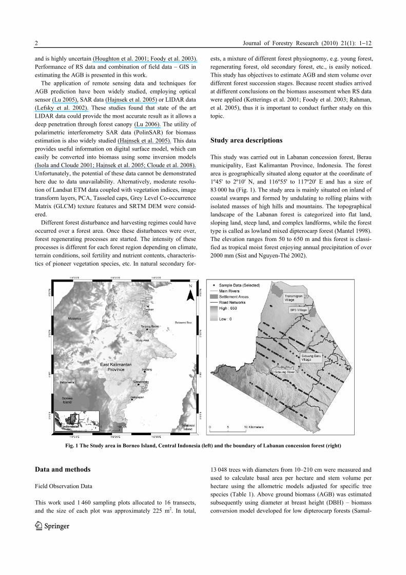
This study was carried out in Labanan concession forest, Berau municipality, East Kalimantan Province, Indonesia. The forest area is geographically situated along equator at the coordinate of 1º45' to 2º10' N, and 116º55' to 117º20' E and has a size of 83 000 ha (Fig. 1). The study area is mainly situated on inland of coastal swamps and formed by undulating to rolling plains with isolated masses of high hills and mountains. The topographical landscape of the Labanan forest is categorized into flat land, sloping land, steep land, and complex landforms, while the forest type is called as lowland mixed dipterocarp forest (Mantel 1998). The elevation ranges from 50 to 650 m and this forest is classi-fied as tropical moist forest enjoying annual precipitation of over 2000 mm (Sist and Nguyen-Thé 2002).

Fig. 1 The Study area in Borneo Island, Central Indonesia (left) and the boundary of Labanan concession forest (right)

Data and methods Field Observation Data This work used 1 460 sampling plots allocated to 16 transects, and the size of each plot was approximately 225 m2. In total,

13 048 trees with diameters from 10–210 cm were measured and used to calculate basal area per hectare and stem volume per hectare using the allometric models adjusted for specific tree species (Table 1). Above ground biomass (AGB) was estimated subsequently using diameter at breast height (DBH) – biomass conversion model developed for low dipterocarp forests (Samal-

Journal of Forestry Research (2010) 21(1): 1−12

3

ca 2007). The stem volume varied from 1.73–628.62 m3·ha-1 and the

mean volume was 156±92 m3·ha-1. Similar with stem volume, the AGB also showed highly variable values and the mean AGB was 167±94 t·ha-1. These variations are common for natural forests especially those which are occupied by secondary and regener-

ating forests. Tree regenerating processes take place following the completion of forest harvesting, forest burning, and other types of forest disturbance. These processes which can continue for over 30 years are affected by various dependent and inde-pendent aspects, e.g. anthropogenic factors, drought, disease, etc.

Table 1. Descriptions of sampling plots describing parameters of different forest physiognomies

Forest physi-ognomies

Number of Stems (stems·ha-1)

DBH (cm)

Basal Area (m2·ha-1)

Stem Volume (m3·ha-1)

Biomass (t·ha-1)

Number of plots (n = 1460)

Descriptions

Shrub (Sh) 219.2 25.7 8.9 92.4 105.4 58 Mixture of pioneer species, low to medium tree size and shrubs, canopy cover < 50%, currently disturbed, shows noticeable marks of forest burning and clearing

Riparian forest (RF)

290.6 26.7 11.8 121.5 139.0 24 Sparse forest dominated with slim and tall vegetation, canopy cover < 50%, located adjacent to the streams

Dense forest (DF)

224.5 34.1 12.3 142.5 152.4 885 Dense forest (canopy cover 50%−70%), logged over < 10 years, located in flat and moderate slope

Very dense forest (VDF)

319.3 32.7 16.6 189.4 200.4 455 Very dense forest (canopy cover 70%−80%), logged over between 10 - 20 years, located in moderate and highly steep regions

Mature forest (MF)

262.2 54.1 18.2 221.1 234.2 38 Advanced forest stucture, closed canopy (over 80%), logged over > 20 years, located mostly in highly steep region

Images Acquisition and Preprocessing Two sets of Landsat 7 ETM+ images with 30 meter spatial reso-lution were used. The first Landsat image was acquired on Au-gust 26, 2000 under hazy and cloud conditions, and the second image, acquired on May 31, 2003, showed clear atmospheric conditions with no apparent clouds. The satellite data were or-thorectified into WGS 84 datum and projected on Zone 50N using Universal Transverse Mercator (UTM) projection. Pre-processing of ETM images were conducted for correcting the atmospheric and topographic effects to minimize the artifacts caused by the atmospheric attenuations, e.g. haze and irradiance scattering, and the terrain effects. Moreover, calculation of vege-tation indices required the surface reflectance rather than digital number (DN) values or top of atmosphere reflectance, thus the corrections on the images were required.

Atmospheric corrections were applied on the ETM data using dark object substraction (DOS) method proposed by Chavez (Chavez Jr. 1988). According to a study conducted by Song et al. (2001), different variations of DOS technique are available. We experienced the COST-DOS technique offered more preferable results with regard to the spectral responses of vegetated areas. Topographic corrections were implemented using C-Correction procedure assuming Lambertian effects on the earth surface (Riaño et al. 2003). Hereafter, we refer the satellite images to the corrected ETM data.

Digital Elevation Model (DEM) of the area was obtained from the Shuttle Radar Topography Mission (SRTM) data. The DEM originally 90 meter resolution was orthorectified with the ETM data and resampled using nearest neighborhood method into 30 meter spatial resolution to fit with the resolution of the ETM image. Slope angle and aspect were computed from the resam-pled DEM and applied as ancillary input for AGB and stand

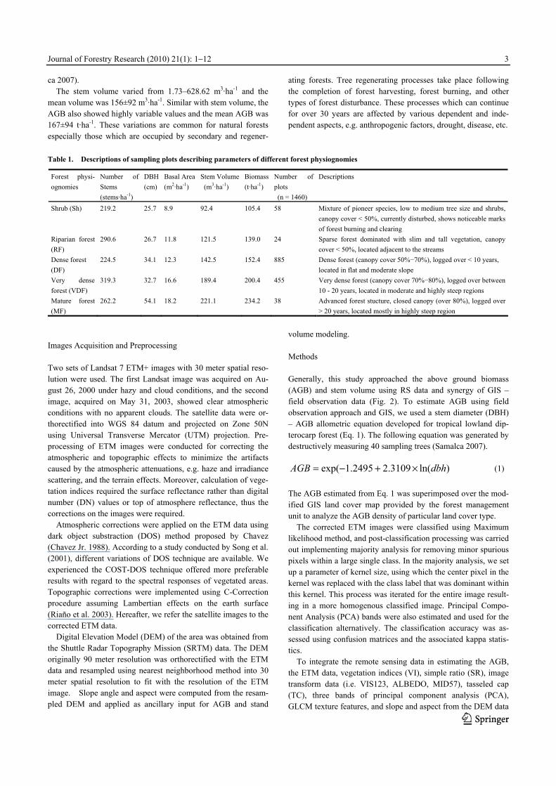
volume modeling. Methods Generally, this study approached the above ground biomass (AGB) and stem volume using RS data and synergy of GIS – field observation data (Fig. 2). To estimate AGB using field observation approach and GIS, we used a stem diameter (DBH) – AGB allometric equation developed for tropical lowland dip-terocarp forest (Eq. 1). The following equation was generated by destructively measuring 40 sampling trees (Samalca 2007).

)ln(3109.22495.1exp( dbhAGB ×+−= (1)

The AGB estimated from Eq. 1 was superimposed over the mod-ified GIS land cover map provided by the forest management unit to analyze the AGB density of particular land cover type.

The corrected ETM images were classified using Maximum likelihood method, and post-classification processing was carried out implementing majority analysis for removing minor spurious pixels within a large single class. In the majority analysis, we set up a parameter of kernel size, using which the center pixel in the kernel was replaced with the class label that was dominant within this kernel. This process was iterated for the entire image result-ing in a more homogenous classified image. Principal Compo-nent Analysis (PCA) bands were also estimated and used for the classification alternatively. The classification accuracy was as-sessed using confusion matrices and the associated kappa statis-tics.

To integrate the remote sensing data in estimating the AGB, the ETM data, vegetation indices (VI), simple ratio (SR), image transform data (i.e. VIS123, ALBEDO, MID57), tasseled cap (TC), three bands of principal component analysis (PCA), GLCM texture features, and slope and aspect from the DEM data

Journal of Forestry Research (2010) 21(1): 1−12

4

were statistically correlated with the biomass data following the Pearson correlation test procedure. The biomass data was care-fully selected using GLCM mean texture feature as the reference, as we obtained this texture feature had the highest correlation coefficient compared to other RS data. The modeling of the AGB and stem volume equations was conducted using SPSS version 11.5 software applying a stepwise multi-linear regression method. The modeling used a subset of sample data, and was validated

with the complete dataset. Biomass density and total biomass of each land cover class was predicted overlaying the AGB estimate with the land cover maps of 2000 and 2003. Subsequently, the total biomass change during this period was calculated. Dynam-ics of the estimated forest properties assessed from RS and com-bination of GIS–field observation approaches, and substantial correlation between GLCM mean texture and the AGB are dis-cussed.

PCA & TC Simple Ratio & VI

Image transform

Field data

Field data selectionPearson

correlation

RS based biomass

modeling

GLCM Texture

ETM 00

ETM 03

Image classification

Post-classification

process

Field data

GIS land cover map

Biomass modeling using allometric

equation

Biomass density and total biomass

estimates

RS based biomass change (00 – 03)

Field data & GIS based biomass

change (00 – 03)

Remote Sensing (RS) Based Biomass Estimate Field Data & GIS Based Biomass

Estimate

Fig. 2 Workflow of the study describes two main approaches for estimating the AGB, using remote sensing method (left shaded box) and com-bination of field data and GIS method (right shaded box). The middle part of the workflow (non shaded area) explains the classification proce-

dure of multi-temporal ETM images (2000 and 2003) performed in this study Vegetation indices generation and land cover Classification Various vegetation indices may be computed from the satellite data. These vegetation indices were proposed for different appli-cations, such as soil moisture, vegetation monitoring, mineral deposits mapping, etc (Jensen 1996). Vegetation indices gener-ated from certain satellite image bands are sensitive to character-ize green vegetation/forested regions from other objects on the ground. In vegetated regions, the cells in plant leaves are very effective scatterers of light because of the high contrast in the index of refraction between the water-rich cell contents and the intercellular air spaces. Vegetation is very dark in the visible bands (400–700 nm) because of the high absorption of pigments in leaves (chlorophyll, protochlorophyll, xanthophyll, etc.). There is a slight increase in reflectivity around 550 nm (visible green band) because the pigments are least absorptive in this range. In the spectral range of 700-1300 nm plants are very bright because this is a spectral no-man's land between the elec-tronic transitions, providing absorption in the visible and mo-lecular vibrations that absorb in longer wavelengths. There is no strong absorption in this spectral range, but the plant scatters

strongly. From 1300 nm to about 2500 nm vegetation is rela-tively dark, primarily because of the absorption by leaf water. Cellulose, lignin, and other plant materials are also absorbed in this spectral range (Lillesand and Kiefer 1994).

This study, moreover, demonstrated the utility of vegetation indices, especially those proposed for vegetation monitoring, for estimating the AGB and stand volume (Table 2).

Besides those indices explained above, we also computed three bands of principal component analysis (PCA) and three bands of tasseled cap (TC), i.e. brightness (TC1), greenness (TC2) and wetness (TC3). Another attempt to include more ETM features was to calculate the Gray Level Co-Occurrence Matrix (GLCM) texture features. Eight GLCM texture computed using second derivatives of mean (GLCM_MEAN), variance (GLCM_VAR), homogeneity (GLCM_HOMO), contrast (GLCM_CONT), dissimilarity (GLCM_DISS), entropy (GLCM_ENTR), second moment (GLCM_SECM), and correla-tion (GLCM_CORR) were generated. We analyzed the variance matrix of ETM bands and found substantial variance of forested lands from ETM band 5 (Wijaya, Marpu et al. 2008). This band was ultimately selected for generating the texture features using 5×5 moving window. The texture layers were calculated to each

Journal of Forestry Research (2010) 21(1): 1−12

5

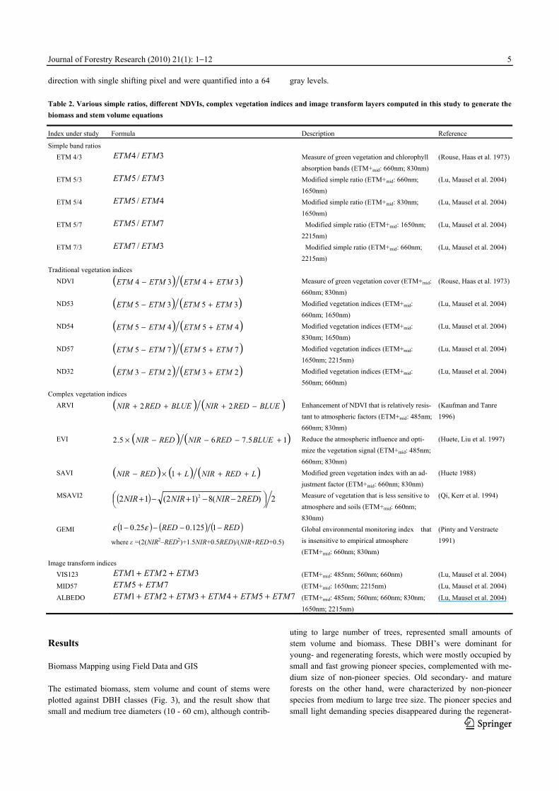
direction with single shifting pixel and were quantified into a 64 gray levels. Table 2. Various simple ratios, different NDVIs, complex vegetation indices and image transform layers computed in this study to generate the biomass and stem volume equations

Index under study Formula Description Reference

Simple band ratios ETM 4/3 3/4 ETMETM Measure of green vegetation and chlorophyll

absorption bands (ETM+mid: 660nm; 830nm) (Rouse, Haas et al. 1973)

ETM 5/3 3/5 ETMETM Modified simple ratio (ETM+mid: 660nm; 1650nm)

(Lu, Mausel et al. 2004)

ETM 5/4 4/5 ETMETM Modified simple ratio (ETM+mid: 830nm; 1650nm)

(Lu, Mausel et al. 2004)

ETM 5/7 7/5 ETMETM Modified simple ratio (ETM+mid: 1650nm; 2215nm)

(Lu, Mausel et al. 2004)

ETM 7/3 3/7 ETMETM Modified simple ratio (ETM+mid: 660nm; 2215nm)

(Lu, Mausel et al. 2004)

Traditional vegetation indices NDVI ( ) ( )3434 ETMETMETMETM +− Measure of green vegetation cover (ETM+mid:

660nm; 830nm) (Rouse, Haas et al. 1973)

ND53 ( ) ( )3535 ETMETMETMETM +− Modified vegetation indices (ETM+mid: 660nm; 1650nm)

(Lu, Mausel et al. 2004)

ND54 ( ) ( )4545 ETMETMETMETM +− Modified vegetation indices (ETM+mid: 830nm; 1650nm)

(Lu, Mausel et al. 2004)

ND57 ( ) ( )7575 ETMETMETMETM +− Modified vegetation indices (ETM+mid: 1650nm; 2215nm)

(Lu, Mausel et al. 2004)

ND32 ( ) ( )2323 ETMETMETMETM +− Modified vegetation indices (ETM+mid: 560nm; 660nm)

(Lu, Mausel et al. 2004)

Complex vegetation indices ARVI ( ) ( )BLUEREDNIRBLUEREDNIR −+++ 22 Enhancement of NDVI that is relatively resis-

tant to atmospheric factors (ETM+mid: 485nm; 660nm; 830nm)

(Kaufman and Tanre 1996)

EVI ( ) ( )15.765.2 +−−−× BLUEREDNIRREDNIR Reduce the atmospheric influence and opti-mize the vegetation signal (ETM+mid: 485nm; 660nm; 830nm)

(Huete, Liu et al. 1997)

SAVI ( ) ( ) ( )LREDNIRLREDNIR +++×− 1 Modified green vegetation index with an ad-justment factor (ETM+mid: 660nm; 830nm)

(Huete 1988)

MSAVI2 ( ) 2)2(8)12(12 2 ⎟⎠⎞⎜

⎝⎛ −−+−+ REDNIRNIRNIR Measure of vegetation that is less sensitive to

atmosphere and soils (ETM+mid: 660nm; 830nm)

(Qi, Kerr et al. 1994)

GEMI ( ) ( ) ( )REDRED −−−− 1125.025.01 εε

where ε =(2(NIR2–RED2)+1.5NIR+0.5RED)/(NIR+RED+0.5)

Global environmental monitoring index that is insensitive to empirical atmosphere (ETM+mid: 660nm; 830nm)

(Pinty and Verstraete 1991)

Image transform indices VIS123 321 ETMETMETM ++ (ETM+mid: 485nm; 560nm; 660nm) (Lu, Mausel et al. 2004)

MID57 75 ETMETM + (ETM+mid: 1650nm; 2215nm) (Lu, Mausel et al. 2004)

ALBEDO 754321 ETMETMETMETMETMETM +++++ (ETM+mid: 485nm; 560nm; 660nm; 830nm; 1650nm; 2215nm)

(Lu, Mausel et al. 2004)

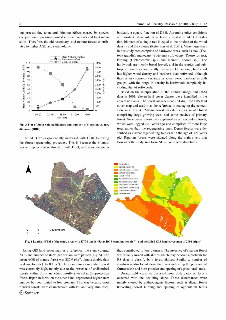
Results Biomass Mapping using Field Data and GIS The estimated biomass, stem volume and count of stems were plotted against DBH classes (Fig. 3), and the result show that small and medium tree diameters (10 - 60 cm), although contrib-

uting to large number of trees, represented small amounts of stem volume and biomass. These DBH’s were dominant for young- and regenerating forests, which were mostly occupied by small and fast growing pioneer species, complemented with me-dium size of non-pioneer species. Old secondary- and mature forests on the other hand, were characterized by non-pioneer species from medium to large tree size. The pioneer species and small light demanding species disappeared during the regenerat-

Journal of Forestry Research (2010) 21(1): 1−12

6

ing process due to natural thinning effects caused by species competition in pursuing limited nutrient contents and light inten-sities. Therefore, the old secondary- and mature forests contrib-uted to higher AGB and stem volume.

010

203040

5060

708090

100110

10-20 21-40 41-80 81-100 >100DBH (cm)

Stem

Vol

ume

(m3 ·h

a-1) /

Bio

mas

s (t·h

a-1)

0500

100015002000

25003000

350040004500

50005500

Cou

nt o

f ste

ms

Stem Volume (m³/ha)Biomass (ton/ha)Count of stems

Fig. 3 Plot of Stem volume/biomass and number of stems/ha vs. tree diameter (DBH)

The AGB was exponentially increased with DBH following the forest regenerating processes. This is because the biomass has an exponential relationship with DBH, and stem volume is

basically a square function of DBH. Assuming other conditions are constant, stem volume is linearly related to AGB. Besides that, biomass of a single tree is equal to the product of the wood density and the volume (Ketterings et al. 2001). Many large trees in our study area comprise of hardwood trees, such as teak (Tec-tona grandis), mahogany (Swietenia sp.), ebony (Diospyros sp.), keruing (Dipterocarpus sp.), and meranti (Shorea sp.). The hardwoods are mostly broad-leaved, and in the tropics and sub-tropics these trees are usually evergreen. On average, hardwood has higher wood density and hardness than softwood, although there is an enormous variation in actual wood hardness in both groups, with the range in density in hardwoods completely in-cluding that of softwoods.

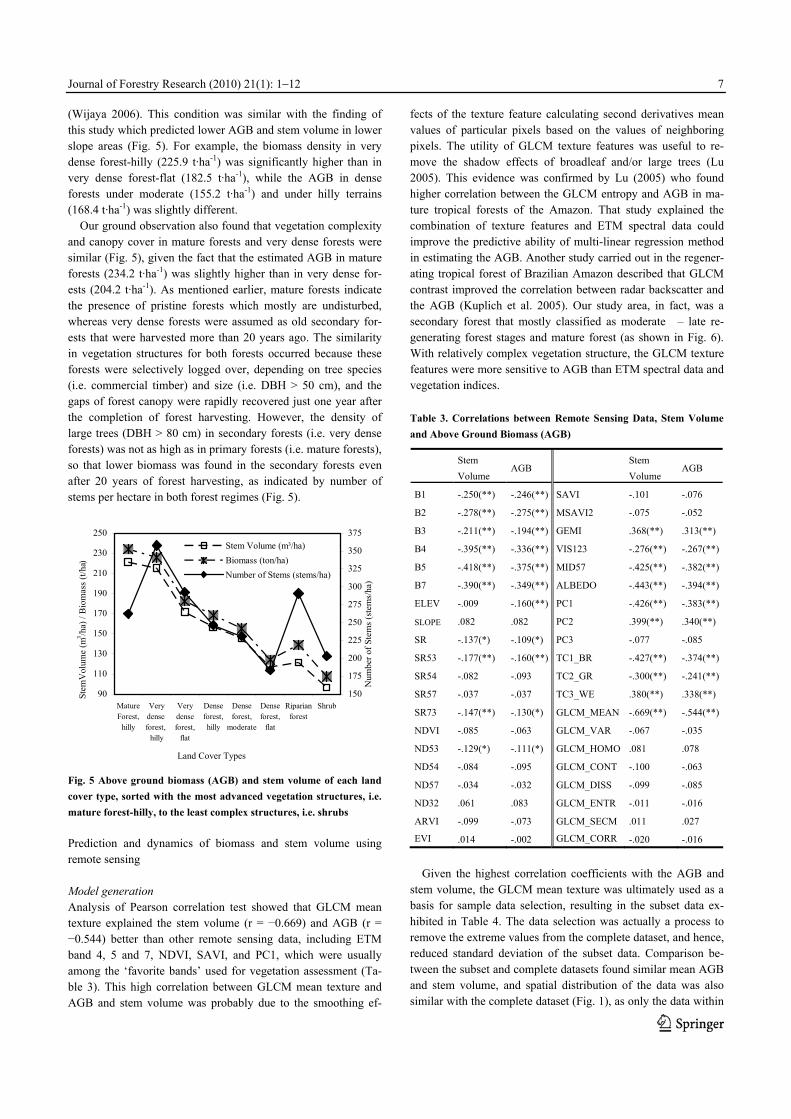
Based on the interpretation of the Landsat image and DEM data in 2001, eleven land cover classes were identified in the concession area. The forest management unit digitized GIS land cover map and used it as the reference in managing the conces-sion area (Fig. 4). Mature forest was defined as an old forest comprising large growing trees and some patches of primary forest. Very dense forests was explained as old secondary forest, which were logged >20 years ago and comprised of more large trees rather than the regenerating ones. Dense forests were de-scribed as current regenerating forests with the age of <20 years old. Riparian forests were situated along the main rivers that flow over the study area from NE – SW to west directions.

Fig. 4 Landsat ETM of the study area with ETM bands 453 as RGB combination (left), and modified GIS land cover map of 2001 (right)

Using GIS land cover map as a reference, the stem volume,

AGB and number of stems per hectare were plotted (Fig. 5). The mean AGB of mature forest was 287.9 t·ha-1, almost double than in dense forests (149.8 t·ha-1). The stem number in mature forest was extremely high, mainly due to the presence of undisturbed forests within this class which mostly situated in the protection forest. Riparian forest on the other hand, represented higher stem number but contributed to low biomass. This was because most riparian forests were characterized with tall and very slim trees,

thus contributed to less biomass. The presence of riparian forest was usually mixed with shrubs which may become a problem for RS data to classify both forest classes. Similarly, number of shrubs was also found along the rivers indicating the presence of former slash and burn practice and opening of agricultural lands.

During field work, we observed more disturbance on forests occurred with the declining slope. These disturbances were mainly caused by anthropogenic factors, such as illegal forest harvesting, forest burning and opening of agricultural farms

Journal of Forestry Research (2010) 21(1): 1−12

7

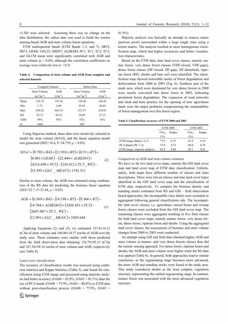
(Wijaya 2006). This condition was similar with the finding of this study which predicted lower AGB and stem volume in lower slope areas (Fig. 5). For example, the biomass density in very dense forest-hilly (225.9 t·ha-1) was significantly higher than in very dense forest-flat (182.5 t·ha-1), while the AGB in dense forests under moderate (155.2 t·ha-1) and under hilly terrains (168.4 t·ha-1) was slightly different.

Our ground observation also found that vegetation complexity and canopy cover in mature forests and very dense forests were similar (Fig. 5), given the fact that the estimated AGB in mature forests (234.2 t·ha-1) was slightly higher than in very dense for-ests (204.2 t·ha-1). As mentioned earlier, mature forests indicate the presence of pristine forests which mostly are undisturbed, whereas very dense forests were assumed as old secondary for-ests that were harvested more than 20 years ago. The similarity in vegetation structures for both forests occurred because these forests were selectively logged over, depending on tree species (i.e. commercial timber) and size (i.e. DBH > 50 cm), and the gaps of forest canopy were rapidly recovered just one year after the completion of forest harvesting. However, the density of large trees (DBH > 80 cm) in secondary forests (i.e. very dense forests) was not as high as in primary forests (i.e. mature forests), so that lower biomass was found in the secondary forests even after 20 years of forest harvesting, as indicated by number of stems per hectare in both forest regimes (Fig. 5).

90

110

130

150

170

190

210

230

250

MatureForest,

hilly

Verydense forest,

hilly

Verydenseforest,

flat

Denseforest,hilly

Denseforest,

moderate

Denseforest,

flat

Riparianforest

Shrub

Land Cover Types

Stem

Vol

ume

(m3 /h

a) /

Bio

mas

s (t/

ha)

150

175

200

225

250

275

300

325

350

375

Num

ber o

f Ste

ms (

stem

s/ha

)

Stem Volume (m³/ha)Biomass (ton/ha)Number of Stems (stems/ha)

Fig. 5 Above ground biomass (AGB) and stem volume of each land cover type, sorted with the most advanced vegetation structures, i.e. mature forest-hilly, to the least complex structures, i.e. shrubs Prediction and dynamics of biomass and stem volume using remote sensing Model generation Analysis of Pearson correlation test showed that GLCM mean texture explained the stem volume (r = −0.669) and AGB (r = −0.544) better than other remote sensing data, including ETM band 4, 5 and 7, NDVI, SAVI, and PC1, which were usually among the ‘favorite bands’ used for vegetation assessment (Ta-ble 3). This high correlation between GLCM mean texture and AGB and stem volume was probably due to the smoothing ef-

fects of the texture feature calculating second derivatives mean values of particular pixels based on the values of neighboring pixels. The utility of GLCM texture features was useful to re-move the shadow effects of broadleaf and/or large trees (Lu 2005). This evidence was confirmed by Lu (2005) who found higher correlation between the GLCM entropy and AGB in ma-ture tropical forests of the Amazon. That study explained the combination of texture features and ETM spectral data could improve the predictive ability of multi-linear regression method in estimating the AGB. Another study carried out in the regener-ating tropical forest of Brazilian Amazon described that GLCM contrast improved the correlation between radar backscatter and the AGB (Kuplich et al. 2005). Our study area, in fact, was a secondary forest that mostly classified as moderate – late re-generating forest stages and mature forest (as shown in Fig. 6). With relatively complex vegetation structure, the GLCM texture features were more sensitive to AGB than ETM spectral data and vegetation indices. Table 3. Correlations between Remote Sensing Data, Stem Volume and Above Ground Biomass (AGB)

Stem Volume

AGB Stem Volume

AGB

B1 -.250(**) -.246(**) SAVI -.101 -.076

B2 -.278(**) -.275(**) MSAVI2 -.075 -.052

B3 -.211(**) -.194(**) GEMI .368(**) .313(**)

B4 -.395(**) -.336(**) VIS123 -.276(**) -.267(**)

B5 -.418(**) -.375(**) MID57 -.425(**) -.382(**)

B7 -.390(**) -.349(**) ALBEDO -.443(**) -.394(**)

ELEV -.009 -.160(**) PC1 -.426(**) -.383(**)

SLOPE .082 .082 PC2 .399(**) .340(**)

SR -.137(*) -.109(*) PC3 -.077 -.085

SR53 -.177(**) -.160(**) TC1_BR -.427(**) -.374(**)

SR54 -.082 -.093 TC2_GR -.300(**) -.241(**)

SR57 -.037 -.037 TC3_WE .380(**) .338(**)

SR73 -.147(**) -.130(*) GLCM_MEAN -.669(**) -.544(**)

NDVI -.085 -.063 GLCM_VAR -.067 -.035

ND53 -.129(*) -.111(*) GLCM_HOMO .081 .078

ND54 -.084 -.095 GLCM_CONT -.100 -.063

ND57 -.034 -.032 GLCM_DISS -.099 -.085

ND32 .061 .083 GLCM_ENTR -.011 -.016

ARVI -.099 -.073 GLCM_SECM .011 .027

EVI .014 -.002 GLCM_CORR -.020 -.016

Given the highest correlation coefficients with the AGB and

stem volume, the GLCM mean texture was ultimately used as a basis for sample data selection, resulting in the subset data ex-hibited in Table 4. The data selection was actually a process to remove the extreme values from the complete dataset, and hence, reduced standard deviation of the subset data. Comparison be-tween the subset and complete datasets found similar mean AGB and stem volume, and spatial distribution of the data was also similar with the complete dataset (Fig. 1), as only the data within

Journal of Forestry Research (2010) 21(1): 1−12

8

±1.SD were selected. Assuming there was no change on the data distribution, the subset data was used to build the remote sensing-based AGB and stem volume linear equations.

ETM multispectral bands (ETM Bands 1-5, and 7), SR53, SR73, GEMI, VIS123, MID57, ALBEDO, PC1, TC1, TC2, TC3, and GLCM mean were significantly correlated with AGB and stem volume (ρ < 0.05), although the correlation coefficients on average were relatively low (r < 0.5)

Table 4. Comparison of stem volume and AGB from complete and selected datasets

Complete Dataset Subset Data

Stem Volume

(m3·ha-1) AGB

(t·ha-1) Stem Volume

(m3·ha-1) AGB

(t·ha-1)

Mean 156.79 167.36 156.60 166.82 Min 1.73 4.69 59.95 60.85 Max 628.62 663.35 221.97 234.03 SD 92.15 94.16 24.69 27.12 %SD 59% 56% 16% 16% N 1460 388

Using Stepwise method, these data were iteratively selected to

model the stem volume (StVol), and the linear equation model was generated (SEE=18.4, F=34.719, ρ < 0.05).

( ) ( ) ( )( ) ( )( ) ( )( ) 511.1192_595.15

_3412.2541699.4214444.22001.0

751.85910.114703.9

+×

−×−×

+×−×

+×+×+×=

MEANGLCWETCPC

ALBEDOGEMIBBBStVol

(2)

Similar to stem volume, the AGB was estimated using combina-tion of the RS data for predicting the biomass linear equation (SEE=22.7, F=21.44, ρ < 0.05).

( ) ( ) ( )( ) ( )( )( ) 644.1029_991.12

_3087.26471451.3430784.14

7366.95198.144569.6

+×

−×

−×+×

−×−×−×=

MEANGLC

WETCPCALBEDO

BBBAGB

(3)

Applying Equations (2) and (3), we estimated 157.8±16.12

m3/ha of stem volume and 168.06±14.57 ton/ha of AGB over the study area. These estimates were similar with those predicted from the field observation data obtaining 156.79±92.15 m3/ha and 167.36±94.16 ton/ha of stem volume and AGB, respectively (see Table 4). Land cover classification The accuracy of classification results was assessed using confu-sion matrices and Kappa Statistics (Table 5), and found the clas-sification using ETM image and processed using majority analy-sis had better accuracy (OA00 = 82.8%, OA03 = 85.1%) than the use of PCA bands (OA00 = 75.9%, OA03 = 80.8%) or ETM data without post-classification process (OA00 = 77.9%, OA03 =

81.9%). Majority analysis was basically an attempt to remove minor

spurious pixels surrounded within a large single class using a kernel matrix. The analysis resulted in more homogenous classi-fication map, which had higher accuracies and better visualiza-tion characteristics.

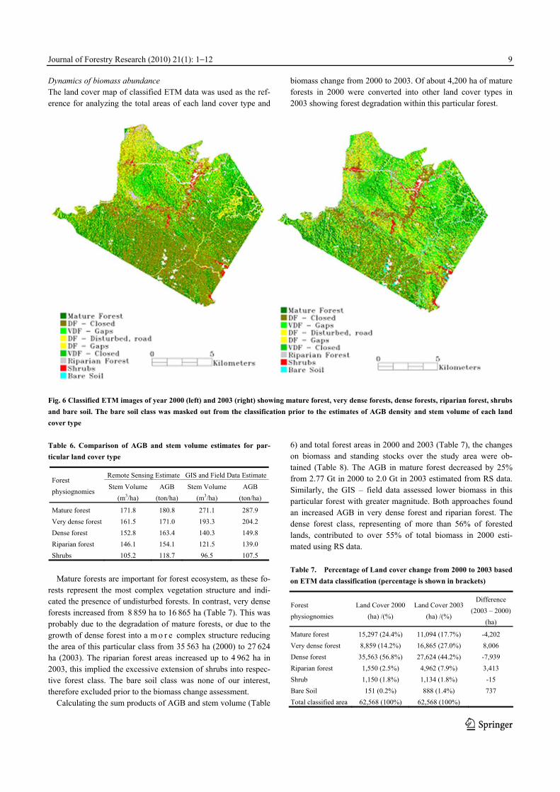
Based on the ETM data, nine land cover classes, namely ma-ture forest, very dense forest classes (VDF-closed, VDF-gaps), dense forest classes (DF-closed, DF-gaps, DF-disturbed), ripar-ian forest (RF), shrubs and bare soil were classified. The classi-fication map showed noticeable marks of forest degradation and deforestation from 2000 to 2003 (Fig. 6). Southern part of the study area, which were dominated by very dense forests in 2000 were mostly converted into dense forest in 2003, indicating prominent forest degradation. The expansion of road networks and slash and burn practice for the opening of new agriculture lands were the major problems compromising the sustainability of forest management over this forest region.

Table 5. Classification Accuracy of ETM 2000 and 2003

ETM 2000 ETM 2003 OA00 (%)

Kappa OA03 (%)

Kappa

ETM image (Band 1-5,7) 77.9 0.75 81.9 0.79 PCA Bands (PC 1-3) 75.9 0.73 80.8 0.78 ETM image, majority analysis 82.8 0.80 85.1 0.83

Comparison of AGB and stem volume estimates We have so far two land cover maps, namely the GIS land cover map and land cover map of ETM data classification. Unfortu-nately, both maps have different number of classes and class descriptions. There were eleven classes and nine land cover types identified in the GIS land cover map and the classification of ETM data, respectively. To compare the biomass density and standing stocks estimated from RS and GIS – field observation based approaches; the incompatible class labels were excluded or aggregated following general classification rule. The incompati-ble land cover classes, i.e. agriculture, mixed forest and swamp forest classes were excluded from the GIS land cover map. The remaining classes were aggregated resulting in five final classes for both land cover maps, namely mature forest, very dense for-est, dense forest, riparian forest and shrubs. Using the aggregated land cover classes, the assessments of biomass and stem volume changes from 2000 to 2003 were conducted.

An attempt using GIS and field data obtained higher AGB and stem volume in mature- and very dense forests classes than did the remote sensing approach. For dense forest, riparian forest and shrubs, the AGB and stem volume were higher when the RS data was applied (Table 6). In general, both approaches lead to similar conclusion, as the regenerating stage becomes more advanced, the more AGB and standing stocks were found in the study area. This study considered shrubs as the least complex vegetation structure, representing the earliest regenerating stage. In contrast, mature forest was associated with the most advanced vegetation structure.

Journal of Forestry Research (2010) 21(1): 1−12

9

Dynamics of biomass abundance The land cover map of classified ETM data was used as the ref-erence for analyzing the total areas of each land cover type and

biomass change from 2000 to 2003. Of about 4,200 ha of mature forests in 2000 were converted into other land cover types in 2003 showing forest degradation within this particular forest.

Fig. 6 Classified ETM images of year 2000 (left) and 2003 (right) showing mature forest, very dense forests, dense forests, riparian forest, shrubs and bare soil. The bare soil class was masked out from the classification prior to the estimates of AGB density and stem volume of each land cover type Table 6. Comparison of AGB and stem volume estimates for par-ticular land cover type

Remote Sensing Estimate GIS and Field Data EstimateForest physiognomies

Stem Volume (m3/ha)

AGB (ton/ha)

Stem Volume (m3/ha)

AGB (ton/ha)

Mature forest 171.8 180.8 271.1 287.9 Very dense forest 161.5 171.0 193.3 204.2 Dense forest 152.8 163.4 140.3 149.8 Riparian forest 146.1 154.1 121.5 139.0 Shrubs 105.2 118.7 96.5 107.5

Mature forests are important for forest ecosystem, as these fo-

rests represent the most complex vegetation structure and indi-cated the presence of undisturbed forests. In contrast, very dense forests increased from 8 859 ha to 16 865 ha (Table 7). This was probably due to the degradation of mature forests, or due to the growth of dense forest into a m o r e complex structure reducing the area of this particular class from 35 563 ha (2000) to 27 624 ha (2003). The riparian forest areas increased up to 4 962 ha in 2003, this implied the excessive extension of shrubs into respec-tive forest class. The bare soil class was none of our interest, therefore excluded prior to the biomass change assessment.

Calculating the sum products of AGB and stem volume (Table

6) and total forest areas in 2000 and 2003 (Table 7), the changes on biomass and standing stocks over the study area were ob-tained (Table 8). The AGB in mature forest decreased by 25% from 2.77 Gt in 2000 to 2.0 Gt in 2003 estimated from RS data. Similarly, the GIS – field data assessed lower biomass in this particular forest with greater magnitude. Both approaches found an increased AGB in very dense forest and riparian forest. The dense forest class, representing of more than 56% of forested lands, contributed to over 55% of total biomass in 2000 esti-mated using RS data. Table 7. Percentage of Land cover change from 2000 to 2003 based on ETM data classification (percentage is shown in brackets)

Forest physiognomies

Land Cover 2000 (ha) /(%)

Land Cover 2003(ha) /(%)

Difference (2003 – 2000)

(ha)

Mature forest 15,297 (24.4%) 11,094 (17.7%) -4,202 Very dense forest 8,859 (14.2%) 16,865 (27.0%) 8,006 Dense forest 35,563 (56.8%) 27,624 (44.2%) -7,939 Riparian forest 1,550 (2.5%) 4,962 (7.9%) 3,413 Shrub 1,150 (1.8%) 1,134 (1.8%) -15 Bare Soil 151 (0.2%) 888 (1.4%) 737 Total classified area 62,568 (100%) 62,568 (100%)

Journal of Forestry Research (2010) 21(1): 1−12

10

In overall, there was a slightly declining trend in total biomass from 2000–2003. This indicates continuous degradation and deforestation within the forest region and consequently reduced

the total abundance of biomass and the volume of standing stocks.

Table 8. Dynamics of Forest Biomass (AGB) and Stem Volume (Vol) from 2000 to 2003

Remote Sensing data estimate 2000 2003 Differences (2003–2000)Forest physiog-

nomies Vol. (m3) (%)

AGB (Gton)

(%) Vol. (m3) (%) AGB

(Gton) (%) Vol. (m3) AGB (Gton)

Mature forest 2,627,681 26.7% 2.766 26.4% 1,905,789 19.7% 2.006 19.5% -721,893 -0.760

Very dense forest 1,430,454 14.5% 1.515 14.5% 2,723,228 28.1% 2.884 28.0% 1,292,774 1.369

Dense forest 5,435,006 55.2% 5.812 55.5% 4221747 43.5% 4.515 43.8% -1,213,260 -1.298

Riparian forest 226,391 2.3% 0.239 2.3% 725,013 7.5% 0.765 7.4% 498,621 0.526

Shrub 120,894 1.2% 0.136 1.3% 119,295 1.2% 0.135 1.3% -1,599 -0.002

Total 9,840,427 100% 10.469 100.0% 9,695,071 100.0% 10.304 100.0% -145,356 -0.164

GIS and field data estimate 2000 2003 Differences (2003–2000)

Forest type

Vol. (m3) (%) AGB

(Gton) (%) Vol. (m3) (%)

AGB (Gton)

(%) Vol. (m3) AGB (Gton)

Mature forest 4,147,107 37.2% 4.403 37.1% 3,007,788 27.7% 3.194 27.6% -1,139,319 -1.210

Very dense forest 1,712,045 15.4% 1.809 15.2% 3,259,308 30.0% 3.444 29.7% 1,547,262 1.635

Dense forest 4,987,952 44.7% 5.329 44.9% 3,874,489 35.7% 4.139 35.7% -1,113,463 -1.189

Riparian forest 188,261 1.7% 0.215 1.8% 602,902 5.6% 0.690 6.0% 414,641 0.474

Shrub 110,976 1.0% 0.124 1.0% 109,508 1.0% 0.122 1.1% -1,468 -0.002

Total 11,146,342 100.0% 11.880 100.0% 10,853,995 100.0% 11.588 100.0% -292,347 -0.292

Carbon accumulation over this period definitely was reduced,

and more carbon was released into the atmosphere. Remote sensing approach in general calculated lower biomass abundance and stem volume than those from GIS–field data. The earlier approach predicted 10.45 Gt and 10.3 Gt of total biomasses in 2000 and 2003, while the later estimated 11.9 Gt and 11.6 Gt of total biomasses, respectively. Discussion Prediction Results Assessment This study successfully predicted the above ground biomass (AGB) and stem volume over a tropical forest region using re-mote sensing and GIS–field data approaches. Estimation of stem volume is important for mapping of standing stock and for forest inventory purpose, as it provides initial prediction on timber amount that could be commercially harvested. The biomass on the other hand is important for indicating carbon accumulation in a forest region over time, and information on total AGB esti-mated for each land cover type is useful to assess how different regeneration stages could have an effect on the forest as a source of carbon sink.

Remote sensing based estimates have potential to predict the dynamics of forest biomass and stem volume over large forest region with less efforts, time and cost than field based estimate. However, the accuracy of the estimates is somehow questionable,

as it depends on the quality of remote sensing data and its rela-tionship with field observation data being modeled. Several at-tempts to estimate AGB from remote sensing data found high uncertainties which were around 30%–40% (Sales, Souza Jr. et al. 2007). This study confirmed this high error estimate in as-sessing the AGB using RS data and found slightly lower error estimate (Table 9), and the result might be used as an initial pre-diction of AGB over the study area. To elevate the estimate pre-cision, correlation analysis between the RS data and biomass can be separately implemented for different land cover, and it should be considered for further study.

An attempt to estimate the AGB using remote sensing (RS) tends to underestimate the result due to the saturation of the ETM spectral values and vegetation indices. The RS data satu-rated at higher AGB and stem volume, reducing the coefficient correlation with the measured forest properties. In order to re-duce the saturation problem, we masked the extreme values out from RS data to get better correlation with the forest properties under study. The present study as well as previous studies con-firmed that reflectance of Landsat data and NDVI were saturated at higher biomass density (Steininger 2000; Lu 2005). Several underlying factors may cause this problem, namely the size of sampling plot that was not designed to be related to spaceborne data, or the saturation from dense leaf canopies that restricts the AGB estimates into a low level when passive sensors, such Landsat ETM, are used (Anaya et al. 2009). Nevertheless, the utility of moderate resolution of satellite data, such as ETM im-

Journal of Forestry Research (2010) 21(1): 1−12

11

age, is the only alternative to predict the AGB and stem volume in this particular forest due to the lack of active sensors, e.g. SAR and Lidar, or high spatial resolution satellite imagery, e.g. Ikonos and Quickbird.

The biomass estimates of this study were compared with those computed using another allometric model generated with de-structive sampling and developed for similar forest environment. Assuming the similarity of forest structure and vegetation com-positions, those models were implemented in this study for esti-mating the AGB using available sample dataset. Our estimates (AGBGIS and AGBRS) were similar with the results of FAO model (FAO 1997) and Brown and Lugo study (Brown, Gilles-pie et al. 1989). However, Ketterings model (Ketterings et al. 2001) estimated significantly lower biomass than did other mod-els (Table 9). This was probably due to the forest composition in Sumatra, the site where this particular model was developed, did not represent the forest in the Labanan, although both forests were geographically located in one country. The AGB models developed for general tropical forest (Brown et al. 1989; Brown 1997) are more suitable for our study site. The Brown & Lugo model (Brown et al. 1989) was generated collecting tree sample from Brazil, Cambodia and Indonesia. Similarly, the FAO model (Brown 1997) was developed for tropical moist forest environ-ment in general. Table 9. Above ground biomass estimates computed in this study using different allometric equations developed for tropical forest environment

AGBGIS (This study)

AGBRS (This study)

FAO Model (1997)

Brown & Lugo (1992)

Ketter-ings, et.al. (2001)

AGB Estimate (t·ha-1)

167.4 166.8 164 155.7 88.46

SD (t·ha-1) 94.2 27.1 91.8 94.5 47.5

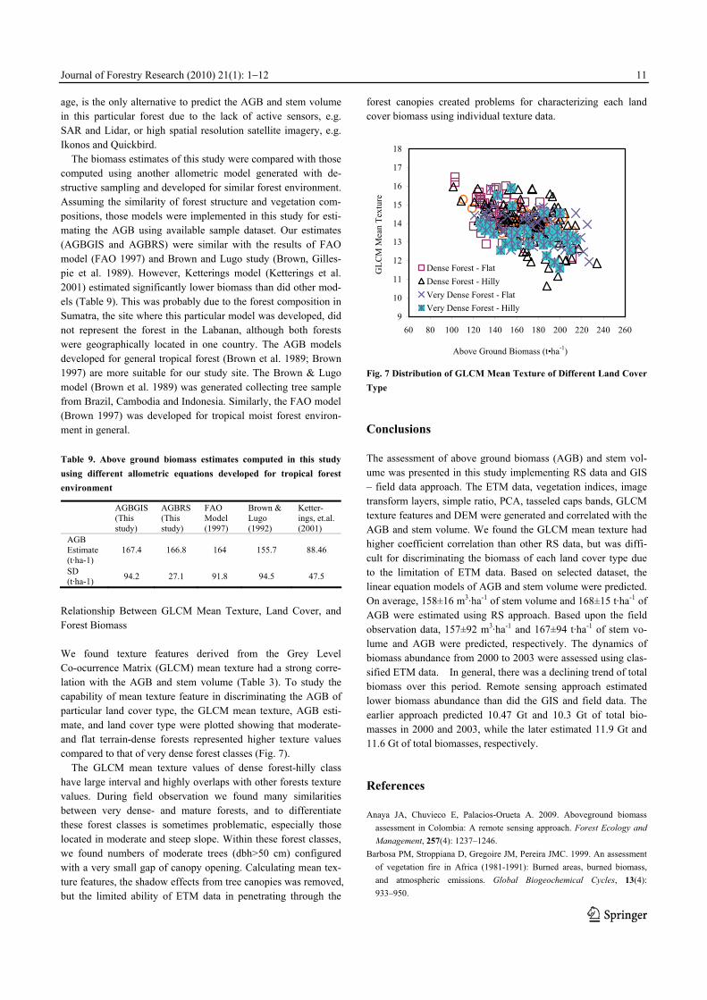
Relationship Between GLCM Mean Texture, Land Cover, and Forest Biomass We found texture features derived from the Grey Level Co-ocurrence Matrix (GLCM) mean texture had a strong corre-lation with the AGB and stem volume (Table 3). To study the capability of mean texture feature in discriminating the AGB of particular land cover type, the GLCM mean texture, AGB esti-mate, and land cover type were plotted showing that moderate- and flat terrain-dense forests represented higher texture values compared to that of very dense forest classes (Fig. 7).

The GLCM mean texture values of dense forest-hilly class have large interval and highly overlaps with other forests texture values. During field observation we found many similarities between very dense- and mature forests, and to differentiate these forest classes is sometimes problematic, especially those located in moderate and steep slope. Within these forest classes, we found numbers of moderate trees (dbh>50 cm) configured with a very small gap of canopy opening. Calculating mean tex-ture features, the shadow effects from tree canopies was removed, but the limited ability of ETM data in penetrating through the

forest canopies created problems for characterizing each land cover biomass using individual texture data.

9

10

11

12

13

14

15

16

17

18

60 80 100 120 140 160 180 200 220 240 260

Above Ground Biomass (t•ha-1)

GLC

M M

ean

Text

ure

Dense Forest - FlatDense Forest - HillyVery Dense Forest - FlatVery Dense Forest - Hilly

Fig. 7 Distribution of GLCM Mean Texture of Different Land Cover Type Conclusions The assessment of above ground biomass (AGB) and stem vol-ume was presented in this study implementing RS data and GIS – field data approach. The ETM data, vegetation indices, image transform layers, simple ratio, PCA, tasseled caps bands, GLCM texture features and DEM were generated and correlated with the AGB and stem volume. We found the GLCM mean texture had higher coefficient correlation than other RS data, but was diffi-cult for discriminating the biomass of each land cover type due to the limitation of ETM data. Based on selected dataset, the linear equation models of AGB and stem volume were predicted. On average, 158±16 m3·ha-1 of stem volume and 168±15 t·ha-1 of AGB were estimated using RS approach. Based upon the field observation data, 157±92 m3·ha-1 and 167±94 t·ha-1 of stem vo-lume and AGB were predicted, respectively. The dynamics of biomass abundance from 2000 to 2003 were assessed using clas-sified ETM data. In general, there was a declining trend of total biomass over this period. Remote sensing approach estimated lower biomass abundance than did the GIS and field data. The earlier approach predicted 10.47 Gt and 10.3 Gt of total bio-masses in 2000 and 2003, while the later estimated 11.9 Gt and 11.6 Gt of total biomasses, respectively. References Anaya JA, Chuvieco E, Palacios-Orueta A. 2009. Aboveground biomass

assessment in Colombia: A remote sensing approach. Forest Ecology and Management, 257(4): 1237–1246.

Barbosa PM, Stroppiana D, Gregoire JM, Pereira JMC. 1999. An assessment of vegetation fire in Africa (1981-1991): Burned areas, burned biomass, and atmospheric emissions. Global Biogeochemical Cycles, 13(4): 933–950.

Journal of Forestry Research (2010) 21(1): 1−12

12

Brown S. 1997. Estimating Biomass and Biomass Change of Tropical Forests: a Primer. Rome: FAO - Food and Agriculture Organization of the United Nations.

Brown S, Gaston G. 1995. Use of forest inventories and geographic informa-tion systems to estimate biomass density of tropical forests: Application to tropical Africa. Environmental Monitoring and Assessment, 38(2-3): 157–168.

Brown S, Gillespie AJR, Lugo AE. 1989. Biomass estimation methods for tropical forests with applications to forest inventory data. Forest Science, 35(4): 881–902.

Brown S, Iverson LR, Lugo AE. 1994. Land-use and biomass changes of forests in Peninsular Malaysia from 1972 to 1982: GIS approach. New York: Springer

Brown S, Lugo AE. 1984. Biomass of tropical forests - a new estimate based on forest volumes. Science, 223(4642): 1290–1293.

Brown S, Lugo AE. 1992. Aboveground biomass estimates for tropical moist forests of the Brazilian Amazon. Interciencia, 17: 8–18.

Chavez Jr. PS. 1988. An improved dark-object subtraction technique for atmospheric scattering correction of multispectral data. Remote Sensing of Environment, 24: 459–479.

Cloude S, Chen E, Li Z, Tian X, Pang Y, Li S, Pottier E, Ferro-Famil L, Neumann M, Hong W, Cao F, Wang YP, Papathanassiou KP. 2008. Forest structure estimation using space borne polarimetric radar: An ALOS PALSAR case study. In European Space Agency, (Special Publication) ESA SP, Beijing.

De Gier A. 2003. A new approach to woody biomass assessment in wood-lands and shrublands. In: P. Roy (ed.), Geoinformatics for Tropical Eco-systems, pp. 161–198, India.

FAO. 1997. State of the world's forests, Vol. 2006. Food and Agriculture Organization of the United Nations.

Foody GM. 2003. Remote sensing of tropical forest environments: towards the monitoring of environmental resources for sustainable development. International Journal of Remote Sensing, 24(20): 4035–4046.

Foody GM, Boyd DS, Cutler MEJ. 2003. Predictive relations of tropical forest biomass from Landsat TM data and their transferability between regions. Remote Sensing of Environment, 85(4): 463–474.

Hajnsek I, Kugler F, Papathanassiou K, Horn R, Scheiber R, Moreira A, Hoekman D, Davidson M. 2005. INDREX II - Indonesian airborne radar experiment campaign over tropical forest in L- and P-band: First results. In International Geoscience and Remote Sensing Symposium (IGARSS), Vol. 6, pp. 4335–4338, Seoul.

Houghton RA, Lawrence KT, Hackler JL., Brown S. 2001. The spatial distri-bution of forest biomass in the Brazilian Amazon: A comparison of esti-mates. Global Change Biology, 7(7): 731–746.

Huete AR. 1988. A Soil-Adjusted Vegetation Index (SAVI). Remote Sensing of Environment, 25: 295–309.

Huete AR., Liu H, Batchily K, Leeuwen WV. 1997. A comparison of vegeta-tion indices over a global set of TM images for EOS-MODIS. Remote Sensing of Environment, 59(3): 440–451.

Isola M, Cloude SR. 2001. Forest height mapping using space-borne po-larimetric SAR interferometry. In International Geoscience and Remote Sensing Symposium (IGARSS), Vol. 3, pp. 1095–1097, Sydney, NSW.

Jensen JR. 1996. Introductory Digital Image Processing: A remote Sensing Perspective, Second Edition edn. Prentice Hall.

Kaufman YJ, Tanre D. 1996. Strategy for direct and indirect methods for correcting the aerosol effect on remote sensing: from AVHRR to EOS-MODIS. Remote Sensing of Environment, 55: 65–79.

Ketterings QM, Coe R, Van Noordwijk M, Ambagau Y, Palm CA. 2001. Reducing uncertainty in the use of allometric biomass equations for pre-dicting above-ground tree biomass in mixed secondary forests. Forest Ecology and Management, 146(1–3): 199–209.

Kuplich TM, Curran PJ, Atkinson PM. 2005. Relating SAR image texture to

the biomass of regenerating tropical forests. International Journal of Re-mote Sensing, 26(21): 4829–4854.

Lefsky MA, Cohen WB, Harding DJ, Parker GG, Acker SA, Gower ST. 2002. Lidar remote sensing of above-ground biomass in three biomes. Global Ecology and Biogeography, 11(5): 393–399.

Lillesand TM, Kiefer RW. 1994. Remote Sensing and Image Interpretation, Third Edition edn. John Wiley & Sons, Inc.

Lu D. 2005. Aboveground biomass estimation using Landsat TM data in Brazilian Amazon. International Journal of Remote Sensing, 26(12): 2509–2525.

Lu D, Mausel P, Brondizio E, Moran E. 2004. Relationships between forest stand parameters and Landsat TM spectral responses in the Brazilian Ama-zon Basin. Forest Ecology and Management, 198(1–3): 149–167.

Lu DS. 2006. The potential and challenge of remote sensing-based biomass estimation. International Journal of Remote Sensing, 27(7): 1297–1328.

Mantel S. 1998. Soil and Terrain of the Labanan Area: Development of an environmental framework for the Berau Forest Management Project. Berau Forest Management Project, Berau.

Pinty B, Verstraete MM. 1991. GEMI: a non-linear index to monitor global vegetation from satellites. Vegetation, 101: 15–20.

Qi J, Kerr Y, Chehbouni A. 1994. External Factor Consideration in Vegeta-tion Index Development. In Proceeding of Physical Measurements and Signatures in Remote Sensing, ISPRS, pp. 723–730.

Rahman MM, Csaplovics E, Koch B. 2005. An efficient regression strategy for extracting forest biomass information from satellite sensor data. Inter-national Journal of Remote Sensing, 26(7): 1511–1519.

Riaño D, Chuvieco E, Salas J, Aguado I. 2003. Assessment of different to-pographic corrections in Landsat-TM data for mapping vegetation types. IEEE Transactions on Geoscience and Remote Sensing, 41(5): 1056 – 1061.

Rouse JW, Haas RH, Schell JA, Deering DW. 1973. Monitoring vegetation systems in the great plains with ERTS. . In: Third ERTS Symposium, NASA SP-351 I, Vol. I, pp. 309–317.

Roy PS, Ravan SA. 1996. Biomass estimation using satellite remote sensing data - An investigation on possible approaches for natural forest. Journal of Biosciences, 21(4): 535–561.

Sales MH, Souza Jr CM, Kyriakidis PC, Roberts DA, Vidal E. 2007. Improv-ing spatial distribution estimation of forest biomass with geostatistics: A case study for Rondonia, Brazil. Ecological Modelling, 205(1–2): 221–230.

Samalca I. 2007. Estimation of Forest Biomass and its Error: A case in Kali-mantan, Indonesia. Unpublished MSc. Thesis, ITC the Netherlands, En-schede.

Sist P, Nguyen-Thé N. 2002. Logging damage and the subsequent dynamics of a dipterocarp forest in East Kalimantan (1990–1996). Forest Ecology and Management, 165(1–3): 85–103.

Song C, Woodcock CE, Seto KC, Lenney MP, Macomber SA. 2001. Classi-fication and change detection using Landsat TM data: When and how to correct atmospheric effects? Remote Sensing of Environment, 75(2): 230–244.

Steininger M. 2000. Satellite estimation of tropical secondary forest above-ground biomass: data from Brazil and Bolivia. International Journal of Remote Sensing, 21(6 & 7): 1139–1157.

Thenkabail PS, Stucky N, Griscom BW, Ashton MS, Diels J, Van der Meer B, Enclona E. 2004. Biomass estimations and carbon stock calculations in the oil palm plantations of African derived savannas using IKONOS data. In-ternational Journal of Remote Sensing, 25(23): 5447–5472.

Wijaya A. 2006. Comparison of soft classification techniques for forest cover mapping. Journal of Spatial Science, 51(2): 7–18.

Wijaya A, Marpu PR, Gloaguen R. 2008. Geostatistical texture classification of tropical rainforest in Indonesia. In：J.S. Alfred Stein, and Wietske Bijker (eds.), Quality Aspect in Spatial Data Mining, pp. 199–210. CRC Press Inc.