Assessing Crop Water Demand by Remote Sensing and GIS for the Pontina Plain, Central Italy
28
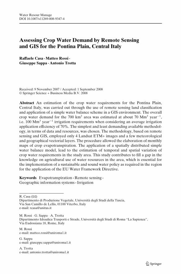
Water Resour Manage DOI 10.1007/s11269-008-9347-4 Assessing Crop Water Demand by Remote Sensing and GIS for the Pontina Plain, Central Italy Raffaele Casa · Matteo Rossi · Giuseppe Sappa · Antonio Trotta Received: 9 November 2007 / Accepted: 1 September 2008 © Springer Science + Business Media B.V. 2008 Abstract An estimation of the crop water requirements for the Pontina Plain, Central Italy, was carried out through the use of remote sensing land classification and application of a simple water balance scheme in a GIS environment. The overall crop water demand for the 700 km 2 area was estimated at about 70 Mm 3 year −1 , i.e. 100 Mm 3 year −1 irrigation requirements when considering an average irrigation application efficiency of 70%. The simplest and least demanding available methodol- ogy, in terms of data and resources, was chosen. The methodology, based on remote sensing and GIS, employed only 4 Landsat ETM+ images and a few meteorological and geographical vectorial layers. The procedure allowed the elaboration of monthly maps of crop evapotranspiration. The application of a spatially distributed simple water balance model, lead to the estimation of temporal and spatial variation of crop water requirements in the study area. This study contributes to fill a gap in the knowledge on agricultural use of water resources in the area, which is essential for the implementation of a sustainable and sound water policy as required in the region for the application of the EU Water Framework Directive. Keywords Evapotranspiration · Remote sensing · Geographic information systems · Irrigation R. Casa (B ) Dipartimento di Produzione Vegetale, Università degli Studi della Tuscia, Via San Camillo de Lellis, 01100 Viterbo, Italy e-mail: [email protected] M. Rossi · G. Sappa · A. Trotta Dipartimento Idraulica Trasporti e Strade, Università degli Studi di Roma “La Sapienza”, Via Eudossiana 18, Rome, Italy M. Rossi e-mail: [email protected] G. Sappa e-mail: [email protected] A. Trotta e-mail: [email protected]
Transcript of Assessing Crop Water Demand by Remote Sensing and GIS for the Pontina Plain, Central Italy
Water Resour ManageDOI 10.1007/s11269-008-9347-4
Assessing Crop Water Demand by Remote Sensingand GIS for the Pontina Plain, Central Italy
Raffaele Casa · Matteo Rossi ·Giuseppe Sappa · Antonio Trotta
Received: 9 November 2007 / Accepted: 1 September 2008© Springer Science + Business Media B.V. 2008
Abstract An estimation of the crop water requirements for the Pontina Plain,Central Italy, was carried out through the use of remote sensing land classificationand application of a simple water balance scheme in a GIS environment. The overallcrop water demand for the 700 km2 area was estimated at about 70 Mm3 year−1,i.e. 100 Mm3 year−1 irrigation requirements when considering an average irrigationapplication efficiency of 70%. The simplest and least demanding available methodol-ogy, in terms of data and resources, was chosen. The methodology, based on remotesensing and GIS, employed only 4 Landsat ETM+ images and a few meteorologicaland geographical vectorial layers. The procedure allowed the elaboration of monthlymaps of crop evapotranspiration. The application of a spatially distributed simplewater balance model, lead to the estimation of temporal and spatial variation ofcrop water requirements in the study area. This study contributes to fill a gap in theknowledge on agricultural use of water resources in the area, which is essential forthe implementation of a sustainable and sound water policy as required in the regionfor the application of the EU Water Framework Directive.
Keywords Evapotranspiration · Remote sensing ·Geographic information systems · Irrigation
R. Casa (B)Dipartimento di Produzione Vegetale, Università degli Studi della Tuscia,Via San Camillo de Lellis, 01100 Viterbo, Italye-mail: [email protected]
M. Rossi · G. Sappa · A. TrottaDipartimento Idraulica Trasporti e Strade, Università degli Studi di Roma “La Sapienza”,Via Eudossiana 18, Rome, Italy
M. Rossie-mail: [email protected]
G. Sappae-mail: [email protected]
A. Trottae-mail: [email protected]
R. Casa et al.
1 Introduction
Knowledge of the temporal and spatial pattern of irrigation water withdrawals at aregional scale is enormously important for aquifer management purposes, but severalmethodological difficulties exist and for several important areas in Italy no accuraterecent figures are yet available (Bàrberi et al. 2000).
Land use in Italy is still largely dominated by agriculture: recent estimates showthat about 19 million ha are occupied by agricultural activities, covering more than60% of the whole country area (ISTAT 2000).
Estimates from one of the few nation-wide water resources surveys (Passino et al.1999) indicates that, in Central Italy, 970 Mm3 of water are used in agriculture outof a total of 4,142 Mm3 freshwater withdrawals (i.e. about 23%). However, largeuncertainties exist for these and other figures at different scales (Passino et al. 1999;Bàrberi et al. 2000).
Most of the water used in agriculture is employed for irrigation when rainfall is notenough to satisfy crop water needs, as it is mostly the case for spring–summer growncrops in Central Italy, where a Mediterranean climate with dry summers prevails.
Groundwater withdrawals for irrigation are therefore highest during the driestmonths of the year.
Concerning the Latium Department in Central Italy, the lack of data about spatialcrop distribution, causes difficulties for the implementation of sustainable watermanagement policies in the agricultural sector. In facts, the first step for a soundwater resources planning would be the knowledge of agricultural land use and theavailability of reliable estimates on the spatial and temporal distribution of cropwater requirements.
For the Pontina Plain, one of the most intensively cropped coastal plains ofCentral Italy, no detailed information about crop spatial distribution is currentlyavailable, since the existing land use classification data (Piemontese and Perotto2004) are not really suitable for an accurate assessment of the spatial distributionof crop water requirements.
For these reasons, in the context of the European Union Water FrameworkDirective (European Commission 2000), the Regional Watershed Authority of theLatium Department started a preliminary study to achieve an estimation of cropspatial distribution and their monthly water requirements in the Pontina Plain area.
The main objective was that of providing some first indications on the currentspatial and seasonal pattern of irrigation water withdrawals in the area, for aquifermanagement purposes. In facts, at the present time, the reclamation consortium“Agro Pontino”, which supplies water to most of the farmers in the area, is notequipped to provide disaggregated and spatially distributed data on irrigation vol-umes used by farmers.
Furthermore, although specific information is lacking due to the absence ofmonitoring, it is suspected that most of the irrigation water is withdrawn by anunknown number of private wells similarly to what happens in other parts of Italy(Todorovic and Steduto 2003).
Thus, uncontrolled and excessive use of groundwater by farmers frequently causeslowering of the groundwater table and intrusion of seawater which leads to serioussalinization problems in the area (Sappa et al. 2005). Particularly during the driestmonths of the year critical conditions for the aquifers, already stressed for climatic
Crop water demand by remote sensing and GIS for the Pontina Plain
conditions, have been reported (Sappa et al. 2005), thus triggering irreversiblechanges (Coviello et al. 2005).
It was therefore considered important to set up a methodology capable of pro-viding some estimates of the spatial and temporal distribution of irrigation waterrequirements in the area, under the current crop pattern, in order to make availablethis information for subsequent hydrogeological studies and evaluate the possibledynamic and temporal evolution of aquifer stress caused by agricultural activities.
Given the extension of the area of about 700 km2, it was considered that remotesensing would offer several advantages for such a task. Its potential for monitoringwater resources are well known and there is a large number of successful applicationsin operative contexts in the last decades (e.g. FAO 1995; Belmonte et al. 1999; Shultzand Engman 2000; D’Urso 2001; Stehman and Milliken 2007). A review of availableremote sensing approaches to water resources estimation was provided by Schmuggeet al. (2002). Considering the estimation of crop water use, i.e. evapotranspiration,several methodologies are available. Many are based on the determination, throughthe use of thermal infrared bands, of radiometric surface temperature, then em-ployed in solving simplified energy balance equations (see e.g. Moran et al. 1990;Sugita and Brutsaert 1992; Kustas and Norman 1996). This type of approaches havebeen developed into more sophisticated procedures, integrating remotely senseddata into vegetation–atmosphere transfer models (e.g. Bastiaanssen et al. 1998; Allenet al. 2005). However, these methods effectively lead to the estimation of a ‘snap shot’of the actual evapotranspiration at the moment of satellite overpass, at best extendedto daily values and needing interpolation procedures for the estimation of monthly orseasonal values. In this respect, two alternative strategies are used, both adopting theFAO approach (Allen et al. 1998), in which crop evapotranspiration is obtained bymultiplying reference crop evapotranspiration by a specific crop coefficient (Kc). Itshould be noted that although the FAO approach has been universally accepted andwidely applied following its original proposition more than 30 years ago (Doorenbosand Pruitt 1977), it leads to the estimation of evapotranspiration of crops underoptimal agronomic conditions, i.e. in the absence of any biotic or abiotic stress, whichis not realistic under the current farming practice. Moreover it has been shown thatcrop coefficients are site-specific (Hanks 1985) and should be determined locally,implying the need of dedicated experimental activities. Therefore the accuracy ofthe estimates decreases whenever farming or environmental factors cause limitationsto crop growth and where local data on crop coefficients are missing. While thisinaccuracy can sometimes cause inconveniences when the method is used for irri-gation management or scheduling, the FAO approach can be considered adequatefor planning purposes or deriving indications on the spatial and temporal evolutionof crop water requirements, such as for the present study.
The simplest method available for the spatial estimation of evapotranspirationfollowing the FAO approach, is to derive through remote sensing a crop classificationmap. Then monthly crop coefficient (Kc) values are associated to each crop classand a reference evapotranspiration map, e.g. derived from meteorological data,is used in order to estimate crop evapotranspiration in a GIS environment (e.g.Stehman and Milliken 2007). This is the procedure followed in the present study.As an alternative, Kc values can be directly estimated from remote sensing using:(1) empirical relationships with vegetation indices (e.g. Ray and Dadhwal 2001);(2) analytical approaches exploiting the relationships existing between vegetation
R. Casa et al.
spectral reflectance and some parameters like albedo, leaf area, canopy surfaceroughness, by which Kc is influenced (e.g. D’Urso 2001), or (3) deriving the Kcfrom the ratio of actual ET, estimated through remotely sensed surface energybalance models, and reference evapotranspiration (e.g. Tasumi and Allen 2007). Theadvantage of the first strategy is that, assuming an average seasonal trend of cropdevelopment, it is possible to estimate seasonal or monthly Kc values for the wholestudied area. However, when only class specific Kc trends are defined, an assumptionis made of simultaneous crop development and homogeneity between and withinfields under the same crop.
The second strategy can therefore provide more realistic estimates of Kc and takeinto account its spatial variability. However, providing a static estimate of Kc forthe date in which remote sensing data are available, and lacking the knowledge onthe type of crops present in each field, it does not allow to extrapolate to seasonaltrends unless remote sensing data are available for several dates throughout thegrowing season: for example Tasumi and Allen (2007) employed 12 cloud-freeLandsat images for 1 year. Moreover, regional evapotranspiration mapping, basedon crop classification, derived from the first strategy, can be more valuable forsubsequent planning and scenario studies, where hypotheses on the evolution ofcropping systems can be compared. For these reasons this strategy, which is alsothe least expensive in terms of remote sensing data requirements, was selected in thepresent study. Indeed this process allows to increase the land use knowledge and tounderstand the correlations with local aquifer stress conditions helping to identifysensible land use policy solutions.
2 Description of the Study Area
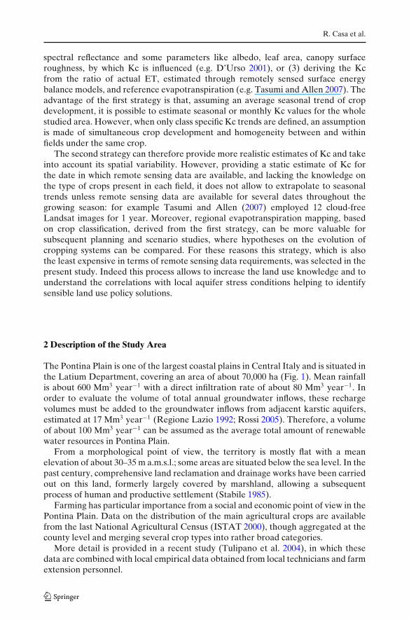
The Pontina Plain is one of the largest coastal plains in Central Italy and is situated inthe Latium Department, covering an area of about 70,000 ha (Fig. 1). Mean rainfallis about 600 Mm3 year−1 with a direct infiltration rate of about 80 Mm3 year−1. Inorder to evaluate the volume of total annual groundwater inflows, these rechargevolumes must be added to the groundwater inflows from adjacent karstic aquifers,estimated at 17 Mm3 year−1 (Regione Lazio 1992; Rossi 2005). Therefore, a volumeof about 100 Mm3 year−1 can be assumed as the average total amount of renewablewater resources in Pontina Plain.
From a morphological point of view, the territory is mostly flat with a meanelevation of about 30–35 m a.m.s.l.; some areas are situated below the sea level. In thepast century, comprehensive land reclamation and drainage works have been carriedout on this land, formerly largely covered by marshland, allowing a subsequentprocess of human and productive settlement (Stabile 1985).
Farming has particular importance from a social and economic point of view in thePontina Plain. Data on the distribution of the main agricultural crops are availablefrom the last National Agricultural Census (ISTAT 2000), though aggregated at thecounty level and merging several crop types into rather broad categories.
More detail is provided in a recent study (Tulipano et al. 2004), in which thesedata are combined with local empirical data obtained from local technicians and farmextension personnel.
Crop water demand by remote sensing and GIS for the Pontina Plain
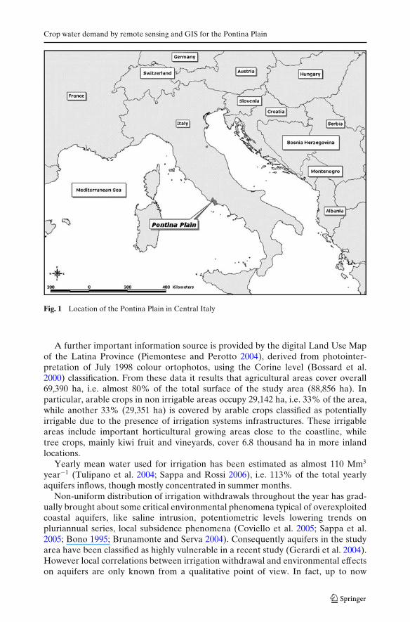
Fig. 1 Location of the Pontina Plain in Central Italy
A further important information source is provided by the digital Land Use Mapof the Latina Province (Piemontese and Perotto 2004), derived from photointer-pretation of July 1998 colour ortophotos, using the Corine level (Bossard et al.2000) classification. From these data it results that agricultural areas cover overall69,390 ha, i.e. almost 80% of the total surface of the study area (88,856 ha). Inparticular, arable crops in non irrigable areas occupy 29,142 ha, i.e. 33% of the area,while another 33% (29,351 ha) is covered by arable crops classified as potentiallyirrigable due to the presence of irrigation systems infrastructures. These irrigableareas include important horticultural growing areas close to the coastline, whiletree crops, mainly kiwi fruit and vineyards, cover 6.8 thousand ha in more inlandlocations.
Yearly mean water used for irrigation has been estimated as almost 110 Mm3
year−1 (Tulipano et al. 2004; Sappa and Rossi 2006), i.e. 113% of the total yearlyaquifers inflows, though mostly concentrated in summer months.
Non-uniform distribution of irrigation withdrawals throughout the year has grad-ually brought about some critical environmental phenomena typical of overexploitedcoastal aquifers, like saline intrusion, potentiometric levels lowering trends onpluriannual series, local subsidence phenomena (Coviello et al. 2005; Sappa et al.2005; Bono 1995; Brunamonte and Serva 2004). Consequently aquifers in the studyarea have been classified as highly vulnerable in a recent study (Gerardi et al. 2004).However local correlations between irrigation withdrawal and environmental effectson aquifers are only known from a qualitative point of view. In fact, up to now
R. Casa et al.
no detailed studies were carried out in order to evaluate the spatial and temporalvariability in irrigation water requirements at regional scale for this area.
3 Methodology
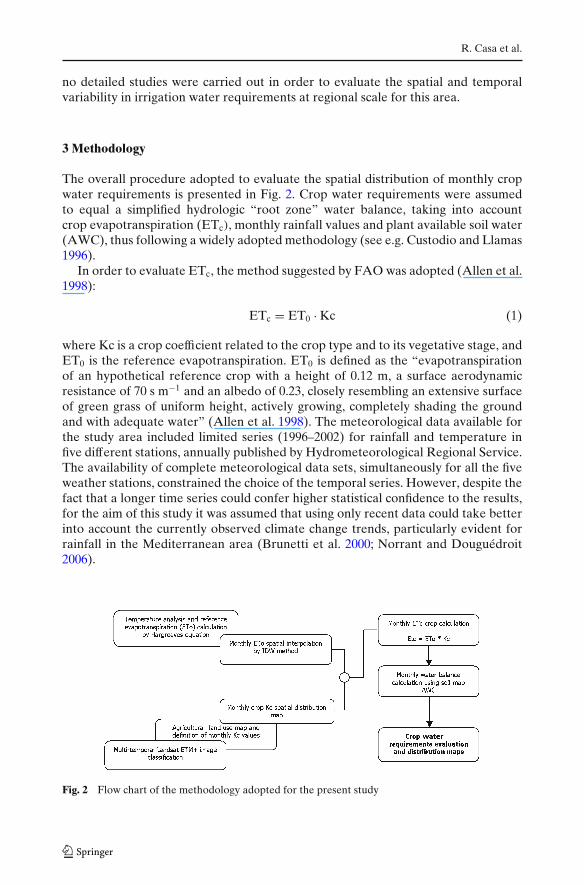
The overall procedure adopted to evaluate the spatial distribution of monthly cropwater requirements is presented in Fig. 2. Crop water requirements were assumedto equal a simplified hydrologic “root zone” water balance, taking into accountcrop evapotranspiration (ETc), monthly rainfall values and plant available soil water(AWC), thus following a widely adopted methodology (see e.g. Custodio and Llamas1996).
In order to evaluate ETc, the method suggested by FAO was adopted (Allen et al.1998):
ETc = ET0 · Kc (1)
where Kc is a crop coefficient related to the crop type and to its vegetative stage, andET0 is the reference evapotranspiration. ET0 is defined as the “evapotranspirationof an hypothetical reference crop with a height of 0.12 m, a surface aerodynamicresistance of 70 s m−1 and an albedo of 0.23, closely resembling an extensive surfaceof green grass of uniform height, actively growing, completely shading the groundand with adequate water” (Allen et al. 1998). The meteorological data available forthe study area included limited series (1996–2002) for rainfall and temperature infive different stations, annually published by Hydrometeorological Regional Service.The availability of complete meteorological data sets, simultaneously for all the fiveweather stations, constrained the choice of the temporal series. However, despite thefact that a longer time series could confer higher statistical confidence to the results,for the aim of this study it was assumed that using only recent data could take betterinto account the currently observed climate change trends, particularly evident forrainfall in the Mediterranean area (Brunetti et al. 2000; Norrant and Douguédroit2006).
Fig. 2 Flow chart of the methodology adopted for the present study
Crop water demand by remote sensing and GIS for the Pontina Plain
3.1 Mapping Reference Evapotranspiration (ET0)
Though FAO recommends the Penman–Monteith equation for the estimation of ET0
(Allen et al. 1998), the unavailability of complete sets of meteorological parametersfor the study area hindered its application. Therefore the Hargreaves equation wasused (Hargreaves 1994) since it only requires temperature and extraterrestrial solarradiation and it has been shown to provide accurate estimates for monthly time steps(Allen et al. 1998; Droogers and Allen 2002).
The Hargreaves equation is the following:
ET0 = 0.0023 · (Tm + 17.8) · (Tmax − Tmin)0.5 · Ra (2)
where ET0 is the daily reference evapotranspiration (millimeter per day), Tm, Tmax
and Tmin are respectively the daily mean, maximum and minimum air temperature(◦C) and Ra is the extraterrestrial solar radiation (millimeter per day). Monthlytemperature data available for five weather stations located inside the study areawere used to calculate ET0 punctually. To obtain ET0 monthly values, monthly meantemperatures were assumed to correspond to that of an average monthly day, sothat Eq. 2 could be applied and the result multiplied by the number of days of therespective month.
For the spatial interpolation of ET0, the Inverse Distance Weight (IDW) methodwas chosen (Burrough and McDonnell 1998; Matheron 1962), since it had alreadybeen applied in similar situations (e.g. Ray and Dadhwal 2001). In fact, because of thescarce quantity of meteorological stations, all with an elevation close to the sea level,other more complex and effective methods like cokriging (Kurtzman and Kadmon1999; Li et al. 2003) or the inclusion of the elevation parameter in IDW method(Zimmerman et al. 1999) gave unsatisfactory results. The operation led to monthlymaps of the spatial distribution of ET0, on grid layers with a 30 m mesh in agreementwith the resolution of land classification (see the following section).
3.2 Mapping Crop Coefficients (Kc) Monthly Distribution
The methodology chosen for obtaining monthly maps of Kc values was the simplestavailable, i.e. that of developing a crop classification map, identifying homogeneouscrop classes in terms of water use and assigning to each class a monthly Kc value.As already mentioned, a digital land use map (Piemontese and Perotto 2004) wasalready available for the study area. However, insufficient detail was provided formost agricultural crops, grouping them into very broad classes. For example, all thefield crops plus horticultural crops were included in only two classes, based on thepresence or not of irrigation infrastructures as observed from ortophotos. Therefore,it was decided to use additional remote sensing data in order to better discriminatebetween the different crop classes. As a reference year for this study the 2001–2002 growing season was chosen. LANDSAT ETM+ images were acquired for thefollowing dates: 9th June 2001, 2nd December 2001, 4th February 2002 and 15thAugust 2002. The images were already orthorectified and geometrically corrected bythe suppliers using digital terrain models and ground control points, with a declaredRoot Mean Squared Error ranging between <25 m (June image) and 250 m (Augustimage). All images were resampled to a pixel size of 30 m for the multispectral bands
R. Casa et al.
and geometric co-registration of all the images to the June 2001 image was carriedout, as the latter had the highest georeference accuracy. Radiometric normalisationof all the images was carried out using the method of “invariant points” (e.g. Furbyand Campbell 2001). Subsequent preprocessing operations included the building ofmasks for excluding clouds and their shadows (occurring only in the December 2001and August 2002 images), using ISODATA unsupervised classification. A mask wasalso built, using the land use map (Piemontese and Perotto 2004), in order to excludenon-agricultural areas from further processing.
In order to carry out multitemporal classification of the images, a training setof ground control points was obtained. For permanent tree crops it was assumedthat they had remained in the same plots between satellite image acquisition dates(years 2001–2002) and the time this study was carried out (spring 2005). Therefore,a field survey was carried out in April 2005, identifying 80 ground truth pointswhich were digitised and georeferenced in site, using a laptop with digital ortophotosand topographic maps. For the non-permanent crops the information was extractedfrom the databases of farmers’ declarations for eligibility to Common AgriculturalPolicy (CAP) and Structural Funds subsidies, maintained by the Italian state agencyAGEA. The agency, in addition to the databases, holds a GIS including ortophotosof the entire Italian territory, used for checking the truthfulness of the declarations,therefore a high reliability of the databases was assumed. Several databases (CAP,Structural funds, Vineyards Cadastre, Olives Cadastre) for the years 2001 and 2002were obtained and were used for the identification and delineation, using cadastralinformation included in the database, of 2,209 polygons comprising 46 crop types.These ground truth points were chosen by extracting a sample of 59 Cadastre sheetshomogeneously distributed across the study area and including the widest cropdiversification. The polygons layer was used to obtain the regions of interest (ROI)to use for multitemporal supervised classification carried out using ENVI 4.0 (RSI,Boulder Colorado, USA). To this end, for each crop type, ROIs were analysedcomparing false colour images, Tasseled Cap Transformation (TCT) images (Cristand Cicone 1984) and digital ortophotos, in order to verify the compatibility to thedeclared crop and to select only pure pixels. Image classification was then carriedout using a mix of strategies, employing decision-trees based on TCT greennessdifferences between dates and testing several supervised classification algorithms.The results were assessed in terms of overall accuracy using error matrices in orderto select the best strategy for each crop type. Finally a classification map including 17crop types was obtained.
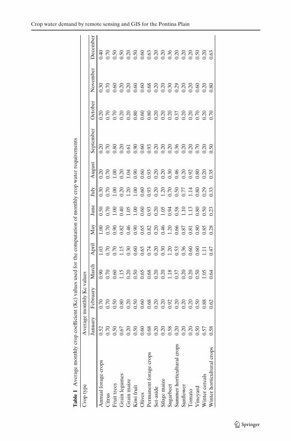
The monthly Kc values assigned to each crop class were obtained from Allenet al. (1998) and Ravelli and Rota (1999). Average Kc monthly values wereestimated, based on farming practices of the study area (Table 1). Informationon the timing of farming operations, particularly planting and harvesting dates,were obtained from a field survey and interviews of farmers and extension servicepersonnel, while information on development phases of crops were obtained mainlyfrom a phenological atlas (Borin et al. 2003). A Kc value of 0.2 was assumed for themonths in which herbaceous crops were not actively vegetating (presence of baresoil or crops residues), while for tree crops this value was increased accordingly tothe crop type in order to take into account soil vegetation cover.
Crop water demand by remote sensing and GIS for the Pontina Plain
Tab
le1
Ave
rage
mon
thly
crop
coef
fici
ent(
Kc)
valu
esus
edfo
rth
eco
mpu
tati
onof
mon
thly
crop
wat
erre
quir
emen
ts
Cro
pty
peA
vera
gem
onth
lyK
cva
lues
Janu
ary
Feb
ruar
yM
arch
Apr
ilM
ayJu
neJu
lyA
ugus
tSe
ptem
ber
Oct
ober
Nov
embe
rD
ecem
ber
Ann
ualf
orag
ecr
ops
0.52
0.70
0.90
1.03
1.00
0.50
0.30
0.20
0.20
0.20
0.30
0.40
Cit
rus
0.70
0.70
0.70
0.70
0.70
0.70
0.70
0.70
0.70
0.70
0.70
0.70
Fru
ittr
ees
0.50
0.50
0.60
0.70
0.90
1.00
1.00
1.00
0.80
0.70
0.60
0.50
Gra
inle
gum
es0.
670.
801.
151.
150.
820.
400.
200.
200.
200.
200.
200.
50G
rain
mai
ze0.
200.
200.
200.
300.
461.
051.
201.
040.
610.
200.
200.
20K
iwif
ruit
0.50
0.50
0.50
0.60
0.90
1.00
1.00
0.90
0.90
0.80
0.60
0.50
Oliv
es0.
600.
600.
650.
650.
650.
600.
600.
600.
600.
600.
600.
60P
erm
anen
tfor
age
crop
s0.
680.
680.
680.
740.
820.
930.
930.
930.
930.
800.
680.
63Se
t-as
ide
0.20
0.20
0.20
0.20
0.20
0.20
0.20
0.20
0.20
0.20
0.20
0.20
Sila
gem
aize
0.20
0.20
0.20
0.30
0.46
1.05
1.20
0.20
0.20
0.20
0.20
0.20
Suga
rbee
t0.
580.
921.
181.
201.
200.
940.
700.
300.
200.
200.
300.
36Su
mm
erho
rtic
ultu
ralc
rops
0.20
0.20
0.37
0.53
0.66
0.58
0.50
0.46
0.36
0.37
0.29
0.20
Sunfl
ower
0.20
0.20
0.20
0.36
0.87
1.10
0.77
0.20
0.20
0.20
0.20
0.20
Tom
ato
0.20
0.20
0.20
0.60
0.81
1.13
1.14
0.92
0.20
0.20
0.20
0.20
Vin
eyar
d0.
500.
500.
500.
600.
800.
800.
800.
800.
700.
700.
600.
50W
inte
rce
real
s0.
570.
881.
051.
110.
850.
500.
290.
200.
200.
200.
200.
20W
inte
rho
rtic
ultu
ralc
rops
0.58
0.62
0.64
0.47
0.28
0.23
0.33
0.35
0.50
0.70
0.80
0.63
R. Casa et al.
3.3 Mapping Crop Evapotranspiration (ETc) and Estimation of Monthly IrrigationRequirements
Using GIS functionality, Eq. 1 was applied and the pixel-wise product of ET0
monthly maps by monthly Kc maps yielded monthly ETc maps.These ETc maps represent the crop evapotranspiration under standard conditions,
i.e from disease-free, well-fertilized crops, grown in large fields, under optimum soilwater conditions, and achieving full production under the given climatic conditions(Allen et al. 1998).
But in order to estimate irrigation requirements, soil water availability needs tobe taken into account, because theoretically only when the plant-available water isinsufficient it would be necessary to supplement this amount with irrigation.
Many methods used in literature make use of the “effective rainfall” concept,using different estimation procedures (Dastane 1974). A widely adopted one is theUSDA Soil Conservation Service method (see e.g. Tsanis et al. 2002; Tsanis andNaoum 2003; Loukas et al. 2007).
Nevertheless, this highly empirical procedure seems not much linked to soilhydraulic conditions and can only be used as a first approximation (Dastane 1974).Therefore, a procedure was chosen which takes into account the nature of the soilsin the study area, more in agreement with hydrogeological studies.
The methodology was based on the knowledge of soil available water content(AWC) distribution throughout the study area and by the implementation of asimplified soil water balance, in order to estimate crop water demand.
AWC, defined as the range of plant available water storable in the upper layer ofthe soil (root zone), is obviously strongly dependent on the soil type (Richards andWadleigh 1952).
By linking, in a GIS environment, pedological classes distribution data (Provinciadi Latina 2003) with corresponding reference AWC values, as found in the literature(Sevink et al. 1991), a digital cartography for the AWC spatial distribution wasobtained.
In order to estimate soil water content the following equation was then used:
Ue = Us − ETc + P (3)
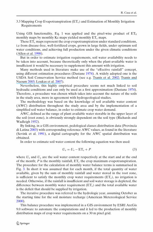
where Us and Ue are the soil water content respectively at the start and at the endof the month; P is the monthly rainfall, ETc the crop maximum evapotranspiration.The procedure for the calculation of monthly water balance terms is summarised inFig. 3. In short it was assumed that for each month, if the total quantity of wateravailable, given by the sum of monthly rainfall and water stored in the root zone,is sufficient to satisfy the monthly crop water requirements (ETc), no irrigation isneeded. Otherwise, if the rainfall is insufficient and soil water storage is depleted, thedifference between monthly water requirement (ETc) and the total available wateris the deficit that should be supplied by irrigation.
The iterative procedure was referred to the hydrologic year, assuming October asthe starting time for the soil moisture recharge (American Metereological Service2000).
This balance procedure was implemented in a GIS environment by ESRI ArcGis9.0 software to automate the computations and it led to the production of monthlydistribution maps of crop water requirements on a 30 m pixel grid.
Crop water demand by remote sensing and GIS for the Pontina Plain
Fig. 3 Monthly water balance calculation algorithm. Us = soil water content at the start of themonth; Ue = soil water content at the end of the month; AWC = available water content; D =soil water deficit, assumed equal to the irrigation requirement; P = rainfall; ETc = maximum cropevapotranspiration; ETr = actual crop evapotranspiration
4 Results and Discussion
4.1 Reference Evapotranspiration (ET0)
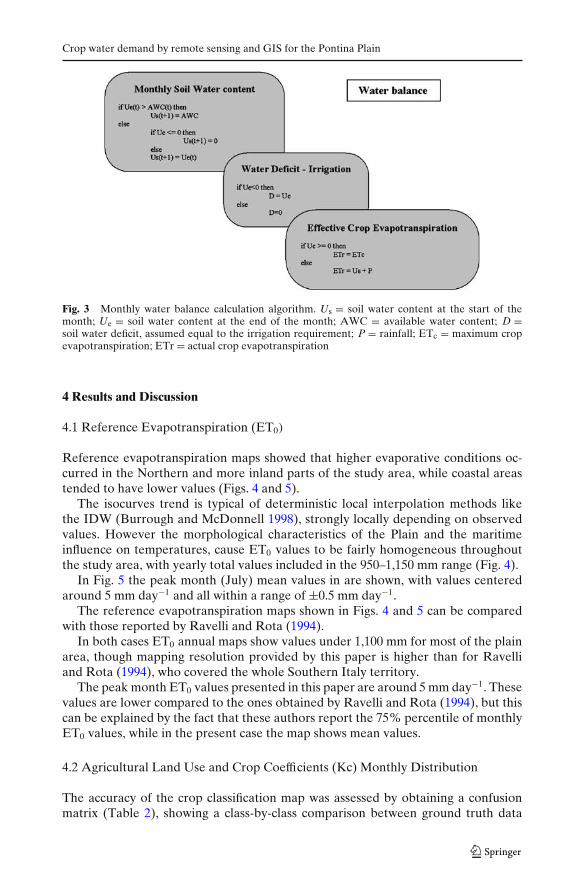
Reference evapotranspiration maps showed that higher evaporative conditions oc-curred in the Northern and more inland parts of the study area, while coastal areastended to have lower values (Figs. 4 and 5).
The isocurves trend is typical of deterministic local interpolation methods likethe IDW (Burrough and McDonnell 1998), strongly locally depending on observedvalues. However the morphological characteristics of the Plain and the maritimeinfluence on temperatures, cause ET0 values to be fairly homogeneous throughoutthe study area, with yearly total values included in the 950–1,150 mm range (Fig. 4).
In Fig. 5 the peak month (July) mean values in are shown, with values centeredaround 5 mm day−1 and all within a range of ±0.5 mm day−1.
The reference evapotranspiration maps shown in Figs. 4 and 5 can be comparedwith those reported by Ravelli and Rota (1994).
In both cases ET0 annual maps show values under 1,100 mm for most of the plainarea, though mapping resolution provided by this paper is higher than for Ravelliand Rota (1994), who covered the whole Southern Italy territory.
The peak month ET0 values presented in this paper are around 5 mm day−1. Thesevalues are lower compared to the ones obtained by Ravelli and Rota (1994), but thiscan be explained by the fact that these authors report the 75% percentile of monthlyET0 values, while in the present case the map shows mean values.
4.2 Agricultural Land Use and Crop Coefficients (Kc) Monthly Distribution
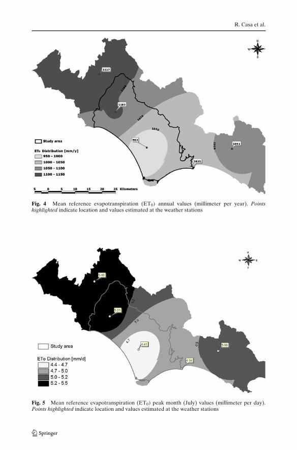
The accuracy of the crop classification map was assessed by obtaining a confusionmatrix (Table 2), showing a class-by-class comparison between ground truth data
R. Casa et al.
Fig. 4 Mean reference evapotranspiration (ET0) annual values (millimeter per year). Pointshighlighted indicate location and values estimated at the weather stations
Fig. 5 Mean reference evapotranspiration (ET0) peak month (July) values (millimeter per day).Points highlighted indicate location and values estimated at the weather stations

Crop water demand by remote sensing and GIS for the Pontina Plain
and classification results (Lillesand and Kiefer 1999). Commission error, representingthe number of pixels belonging to other classes and erroneously assigned to a givenclass, ranged from quite small values, e.g. for winter cereals and horticultural crops, torather high values such as for perennial forage crops and fruit trees (Table 3). Overallthe high commission error found is largely due to a great abundance of mixed pixels,i.e. including more than one crop class. This is due to the spatial resolution of thesatellite data (30 m pixel size) and the agricultural land fragmentation structure inthe study area, in which small fields (less than 0.5 ha) are particularly abundant.
Omission error, taking into account pixels really belonging to a given class thatwere wrongly assigned to another class, was particularly high for grain maize andagain permanent forage crops. Producer accuracy, indicating the probability that agiven pixel belonging to a class is really assigned to that class, was reasonably highfor most classes with the exception of grain maize and permanent forage crops. Useraccuracy, indicating the probability that a pixel classified as belonging to a classreally belongs to it, was high for some classes such as winter cereals, horticulturalcrops, vineyards and sunflower, while rather low values were found for permanentforages and tree crops. Inspection of the confusion matrix (Table 2) revealed that aproblem occurring with these two classes was that high percentages of their pixelsin the training set remained unclassified (57% for permanent forage crops and 39%for fruit trees), because these fell into areas that were covered by clouds in two ofthe four images available. In summary the overall classification accuracy, calculatedfrom the confusion matrix, had a value of 62.5% and a kappa coefficient of 0.59(Jensen 1986).
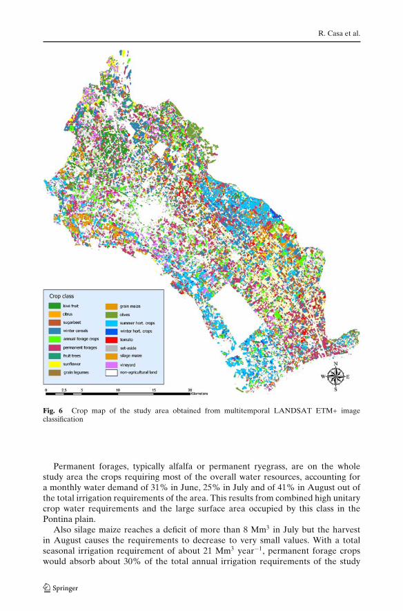
The truthfulness of the classification results was assessed by comparing, on acounty basis, total surface areas attributed to the different crop classes by the presentstudy, with results from the last National Agricultural Census (ISTAT 2000) andby the data reported in a previous study (Tulipano et al. 2004). For tomato thedata used were those provided by the AGEA database, considered more reliable.The crop classification map (Fig. 6) shows that kiwi fruit and other tree cropsare mostly located in the North–West part of the study area, horticultural cropsare mainly along the coastline, while maize and other extensive field crops areespecially abundant in the central part of the Pontina plain. The classification resultswere overall in agreement with crop area statistics reported by ISTAT (2000) ona county basis, although classification provided higher crop area estimates in mostcases (Fig. 7). Analysis of the data revealed that for some counties the total croparea estimated exceeded the used agricultural surface area reported by ISTAT.This suggests that non cropped areas (i.e. hedges, roadsides, woodlots etc. . . ) wereerroneously attributed to the crops, thus contributing to the commission error. Itshould be noted that ISTAT (2000) data are provided in a form aggregated at thewhole county level, while the study area considered here included only partially thecounty of Sezze. This explains an outlier in Fig. 7, where ISTAT data for Sezze reporta much higher surface area for permanent forage crops than the present study, whichonly considered about half of the total county area (i.e. only the flatland).
From an overall crop area estimates comparison (Table 4) it appears that thelargest discrepancies appear for horticultural crops, for which this study estimatesan area almost double than that reported by ISTAT, but still largely smaller that theestimate from Tulipano et al. (2004). Also for other crops these estimates seem tofall in between the values reported by ISTAT (2000) and by Tulipano et al. (2004).
R. Casa et al.
Tab
le2
Con
fusi
onm
atri
xof
the
clas
sific
atio
nre
sult
sus
ing
grou
ndco
ntro
lpoi
nts:
colu
mns
repo
rtth
epe
rcen
tage
sof
grou
ndtr
uth
pixe
lsas
sign
edto
the
vari
ous
clas
ses
(row
s)
Cla
ssG
roun
dtr
uth
(per
cent
)
Win
ter
Kiw
iC
itru
sSu
garb
eet
Fru
itA
nnua
lP
eren
nial
Sunfl
ower
Gra
inG
rain
Sila
geO
lives
Tom
ato
Vin
eyar
dH
orti
cult
ural
Set-
asid
eT
otal
cere
als
frui
ttr
ees
fora
gefo
rage
legu
mes
mai
zem
aize
crop
scr
ops
crop
s
Unc
lass
ified
15
32
390
571
77
61
424
110
13W
inte
rce
real
s96
00
01
20
10
10
00
10
2415
Kiw
ifru
it0
780
04
00
110
00
00
70
06
Cit
rus
00
850
00
00
00
00
00
00
0Su
garb
eet
00
081
03
01
03
80
00
00
4F
ruit
tree
s0
00
046
00
00
00
20
110
04
Ann
ualf
orag
ecr
ops
20
00
082
414
701
140
111
017
7P
eren
nial
fora
gecr
ops
05
123
011
2412
022
30
576
54
9Su
nflow
er0
00
00
02
560
10
10
20
04
Gra
inle
gum
es0
00
30
00
121
10
00
00
01
Gra
inm
aize
00
00
30
10
030
40
10
00
3Si
lage
mai
ze0
00
122
010
00
1545
02
63
210
Oliv
es0
00
00
21
00
00
960
10
07
Tom
ato
00
00
00
00
03
30
100
00
1V
iney
ard
09
00
30
00
01
40
034
00
8H
orti
cult
ural
crop
s0
00
00
00
11
44
016
180
05
Set-
asid
e1
10
02
00
11
118
00
60
544
Tot
al10
010
010
010
010
010
010
010
010
010
010
010
010
010
010
010
010
0
Crop water demand by remote sensing and GIS for the Pontina Plain
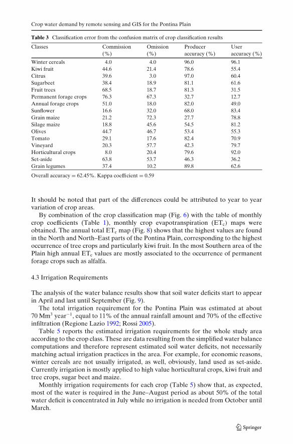
Table 3 Classification error from the confusion matrix of crop classification results
Classes Commission Omission Producer User(%) (%) accuracy (%) accuracy (%)
Winter cereals 4.0 4.0 96.0 96.1Kiwi fruit 44.6 21.4 78.6 55.4Citrus 39.6 3.0 97.0 60.4Sugarbeet 38.4 18.9 81.1 61.6Fruit trees 68.5 18.7 81.3 31.5Permanent forage crops 76.3 67.3 32.7 12.7Annual forage crops 51.0 18.0 82.0 49.0Sunflower 16.6 32.0 68.0 83.4Grain maize 21.2 72.3 27.7 78.8Silage maize 18.8 45.6 54.5 81.2Olives 44.7 46.7 53.4 55.3Tomato 29.1 17.6 82.4 70.9Vineyard 20.3 57.7 42.3 79.7Horticultural crops 8.0 20.4 79.6 92.0Set-aside 63.8 53.7 46.3 36.2Grain legumes 37.4 10.2 89.8 62.6
Overall accuracy = 62.45%. Kappa coefficient = 0.59
It should be noted that part of the differences could be attributed to year to yearvariation of crop areas.
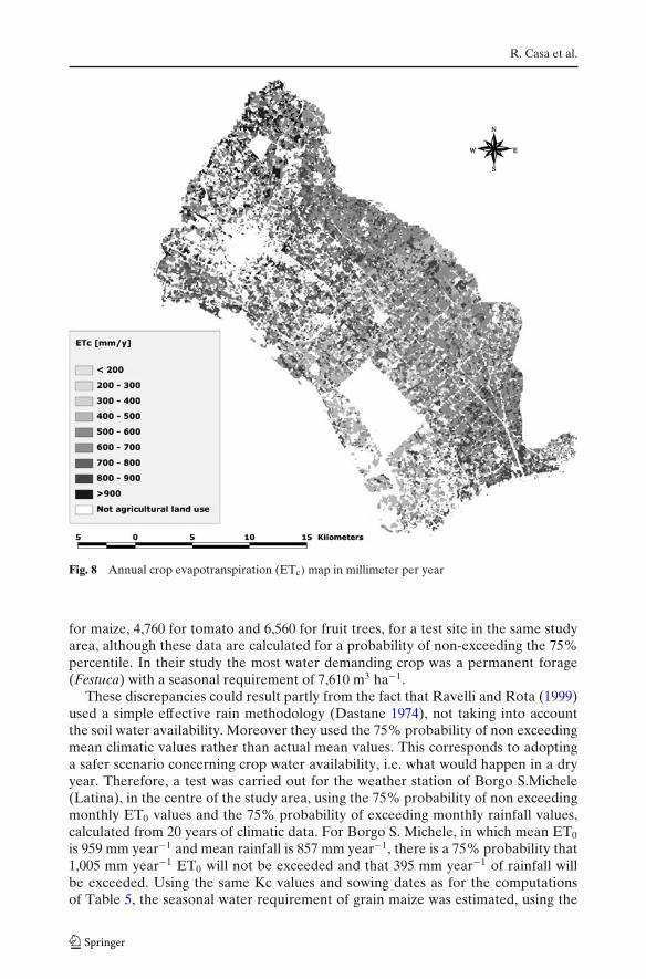
By combination of the crop classification map (Fig. 6) with the table of monthlycrop coefficients (Table 1), monthly crop evapotranspiration (ETc) maps wereobtained. The annual total ETc map (Fig. 8) shows that the highest values are foundin the North and North–East parts of the Pontina Plain, corresponding to the highestoccurrence of tree crops and particularly kiwi fruit. In the most Southern area of thePlain high annual ETc values are mostly associated to the occurrence of permanentforage crops such as alfalfa.
4.3 Irrigation Requirements
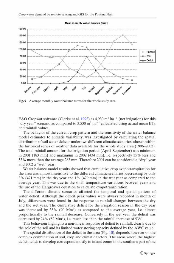
The analysis of the water balance results show that soil water deficits start to appearin April and last until September (Fig. 9).
The total irrigation requirement for the Pontina Plain was estimated at about70 Mm3 year−1, equal to 11% of the annual rainfall amount and 70% of the effectiveinfiltration (Regione Lazio 1992; Rossi 2005).
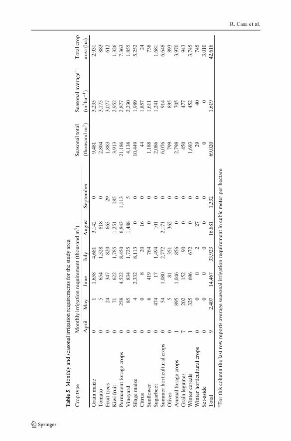
Table 5 reports the estimated irrigation requirements for the whole study areaaccording to the crop class. These are data resulting from the simplified water balancecomputations and therefore represent estimated soil water deficits, not necessarilymatching actual irrigation practices in the area. For example, for economic reasons,winter cereals are not usually irrigated, as well, obviously, land used as set-aside.Currently irrigation is mostly applied to high value horticultural crops, kiwi fruit andtree crops, sugar beet and maize.
Monthly irrigation requirements for each crop (Table 5) show that, as expected,most of the water is required in the June–August period as about 50% of the totalwater deficit is concentrated in July while no irrigation is needed from October untilMarch.
R. Casa et al.
Fig. 6 Crop map of the study area obtained from multitemporal LANDSAT ETM+ imageclassification
Permanent forages, typically alfalfa or permanent ryegrass, are on the wholestudy area the crops requiring most of the overall water resources, accounting fora monthly water demand of 31% in June, 25% in July and of 41% in August out ofthe total irrigation requirements of the area. This results from combined high unitarycrop water requirements and the large surface area occupied by this class in thePontina plain.
Also silage maize reaches a deficit of more than 8 Mm3 in July but the harvestin August causes the requirements to decrease to very small values. With a totalseasonal irrigation requirement of about 21 Mm3 year−1, permanent forage cropswould absorb about 30% of the total annual irrigation requirements of the study

Crop water demand by remote sensing and GIS for the Pontina Plain
Fig. 7 Comparison betweencrop area estimates obtainedfrom LANDSAT ETM+multitemporal imageclassification (present study)and those provided by ISTAT(2000) on per crop and percounty basis
area, followed by silage maize with more than 10 Mm3 year−1, i.e. about 15% of thetotal for the area.
The most water demanding crops grown in the study area were found to be grainmaize, tomato, fruit trees and kiwi fruit, with seasonal requirements in the order of3,000 m3 ha−1. These values are considerably lower than those reported elsewhere.For example Ravelli and Rota (1999) report water deficit values of 5,430 m3 ha−1
Table 4 Comparison between crop surfaces estimated by the present study (through LANDSATETM+ classification), ISTAT (2000) and Tulipano et al. (2004) for the Pontina Plain territory
Crop type Present study (ha) ISTAT (2000) (ha) Tulipano et al. (2004) (ha)
Kiwi fruit 3,456 22,147 5,115Citrus 26 29 –Sugarbeet 1,897 1,670 1,151Winter cereals 5,121 4,683 6,239Annual forage crops 4,882 4,131 –Permanent forage crops 9,318 8,470 6,264Fruit trees 1,081 646 1,795Sunflower 1,352 854 –Grain legumes 1,392 674 –Grain maize 3,734 2,692 5,972Olives 1,420 1,354 603Horticultural crops 8,280 4,653 11,924Tomato 950 706 1,376Set-aside 4,210 3,144 –Silage maize 5,668 4,863 –Vineyard 3,507 2,322 1,603Total 56,296 43,038 42,042
R. Casa et al.
Fig. 8 Annual crop evapotranspiration (ETc) map in millimeter per year
for maize, 4,760 for tomato and 6,560 for fruit trees, for a test site in the same studyarea, although these data are calculated for a probability of non-exceeding the 75%percentile. In their study the most water demanding crop was a permanent forage(Festuca) with a seasonal requirement of 7,610 m3 ha−1.
These discrepancies could result partly from the fact that Ravelli and Rota (1999)used a simple effective rain methodology (Dastane 1974), not taking into accountthe soil water availability. Moreover they used the 75% probability of non exceedingmean climatic values rather than actual mean values. This corresponds to adoptinga safer scenario concerning crop water availability, i.e. what would happen in a dryyear. Therefore, a test was carried out for the weather station of Borgo S.Michele(Latina), in the centre of the study area, using the 75% probability of non exceedingmonthly ET0 values and the 75% probability of exceeding monthly rainfall values,calculated from 20 years of climatic data. For Borgo S. Michele, in which mean ET0
is 959 mm year−1 and mean rainfall is 857 mm year−1, there is a 75% probability that1,005 mm year−1 ET0 will not be exceeded and that 395 mm year−1 of rainfall willbe exceeded. Using the same Kc values and sowing dates as for the computationsof Table 5, the seasonal water requirement of grain maize was estimated, using the
Crop water demand by remote sensing and GIS for the Pontina Plain
Fig. 9 Average monthly water balance terms for the whole study area
FAO Cropwat software (Clarke et al. 1992) as 4,930 m3 ha−1 (net irrigation) for this“dry year” scenario as compared to 3,530 m3 ha−1 calculated using actual mean ET0
and rainfall values.The behavior of the current crop pattern and the sensitivity of the water balance
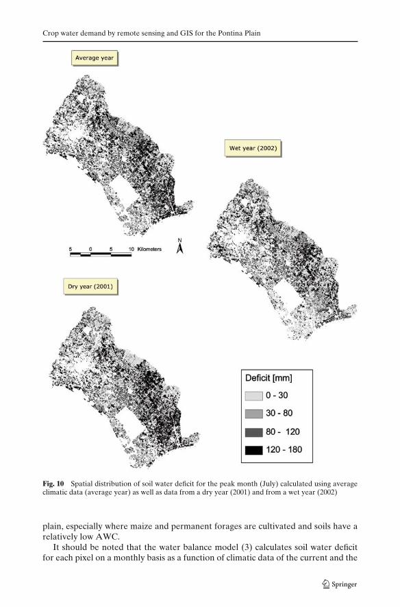
model estimates to climatic variability, was investigated by calculating the spatialdistribution of soil water deficits under two different climatic scenarios, chosen withinthe historical series of weather data available for the whole study area (1996–2002).The total rainfall amount for the irrigation period (April–September) was minimumin 2001 (183 mm) and maximum in 2002 (434 mm), i.e. respectively 35% less and53% more than the average 283 mm. Therefore 2001 can be considered a “dry” yearand 2002 a “wet” year.
Water balance model results showed that cumulative crop evapotranspiration forthe area was almost insensitive to the different climatic scenarios, decreasing by only3% (471 mm) in the dry year and 1% (479 mm) in the wet year as compared to theaverage year. This was due to the small temperature variations between years andthe use of the Hargreaves equation to calculate evapotranspiration.
The different climatic scenarios affected the temporal and spatial pattern ofwater deficit. Although the deficit peak values were always recorded in month ofJuly, differences were found in the response to rainfall changes between the dryand the wet year. The cumulative deficit for the irrigation season in the dry yearwas increased by 35% (90 Mm3) as compared to the average year, i.e. almostproportionally to the rainfall decrease. Conversely in the wet year the deficit wasdecreased by 24% (52 Mm3), i.e. much less than the rainfall increase of 53%.
This behaviour highlights a non-linear response of deficit to rainfall, clearly due tothe role of the soil and its limited water storing capacity defined by the AWC value.
The spatial distribution of the deficit in the area (Fig. 10), depends however on thecomplex combination of soil, crop and climatic factors. The areas where the highestdeficit tends to develop correspond mostly to inland zones in the southern part of the
R. Casa et al.
Tab
le5
Mon
thly
and
seas
onal
irri
gati
onre
quir
emen
tsfo
rth
est
udy
area
Cro
pty
peM
onth
lyir
riga
tion
requ
irem
ent(
thou
sand
m3)
Seas
onal
tota
lSe
ason
alav
erag
eaT
otal
crop
Apr
ilM
ayJu
neJu
lyA
ugus
tSe
ptem
ber
(tho
usan
dm
3)
(m3ha
−1)
area
(ha)
Gra
inm
aize
01
1,65
84,
681
3,14
20
9,48
13,
235
2,93
1T
omat
o0
565
41,
328
818
02,
804
3,17
588
3F
ruit
tree
s0
2434
782
066
329
1,88
33,
077
612
Kiw
ifru
it0
7162
21,
785
1,25
118
53,
913
2,95
21,
326
Per
man
entf
orag
ecr
ops
025
84,
522
8,45
06,
843
1,11
321
,186
2,87
77,
363
Vin
eyar
d0
8583
41,
725
1,48
85
4,13
82,
230
1,85
5Si
lage
mai
ze0
42,
332
8,11
30
010
,449
1,98
95,
252
Cit
rus
00
820
160
441,
857
24Su
nflow
er0
641
976
40
01,
188
1,61
173
8Su
garb
eet
047
417
1,49
410
10
2,08
61,
241
1,68
1Su
mm
erho
rtic
ultu
ralc
rops
054
1,08
02,
772
2,17
10
6,07
691
46,
648
Oliv
es0
581
351
362
079
989
589
3A
nnua
lfor
age
crop
s1
895
1,04
685
60
02,
798
705
3,97
0G
rain
legu
mes
720
215
290
00
450
477
943
Win
ter
cere
als
132
569
667
20
01,
693
452
3,74
5W
inte
rho
rtic
ultu
ralc
rops
00
02
270
2940
745
Set-
asid
e0
00
00
00
03,
010
Tot
al9
2,40
714
,467
33,9
2316
,881
1,33
269
,020
1,61
942
,618
a For
this
colu
mn
the
last
row
repo
rts
aver
age
seas
onal
irri
gati
onre
quir
emen
tin
cubi
cm
eter
per
hect
are
Crop water demand by remote sensing and GIS for the Pontina Plain
Fig. 10 Spatial distribution of soil water deficit for the peak month (July) calculated using averageclimatic data (average year) as well as data from a dry year (2001) and from a wet year (2002)
plain, especially where maize and permanent forages are cultivated and soils have arelatively low AWC.
It should be noted that the water balance model (3) calculates soil water deficitfor each pixel on a monthly basis as a function of climatic data of the current and the
R. Casa et al.
previous month, as well as monthly Kc and AWC. Even keeping constant the lattertwo factors, a wide range of responses to climate is possible, for example becauseof different temporal and spatial rainfall distribution patterns, making a thoroughmodel sensitivity analysis a rather complex task.
4.4 Comparison with Previous Estimates for the Study Area
The water balance results from the present study have been compared with theinformation collected in the Pontina Plain from specific focus groups organisedwith different stakeholders and farmer associations (Tulipano et al. 2004). The dataavailable include mean water amounts used for irrigation and the techniques used inthe Pontina Plain (Tulipano et al. 2004; Sappa and Rossi 2006).
Although the methodology of data collection and the spatial data aggregationscale is very different, these data are the only ones available concerning spatial andtemporal distribution of agricultural water use in the Pontina Plain. The total amountof water used for irrigation in the whole area amounts to 110 Mm3 year−1 accordingto Tulipano et al. (2004), a value much higher than the one obtained in the presentstudy (about 70 Mm3 year−1).
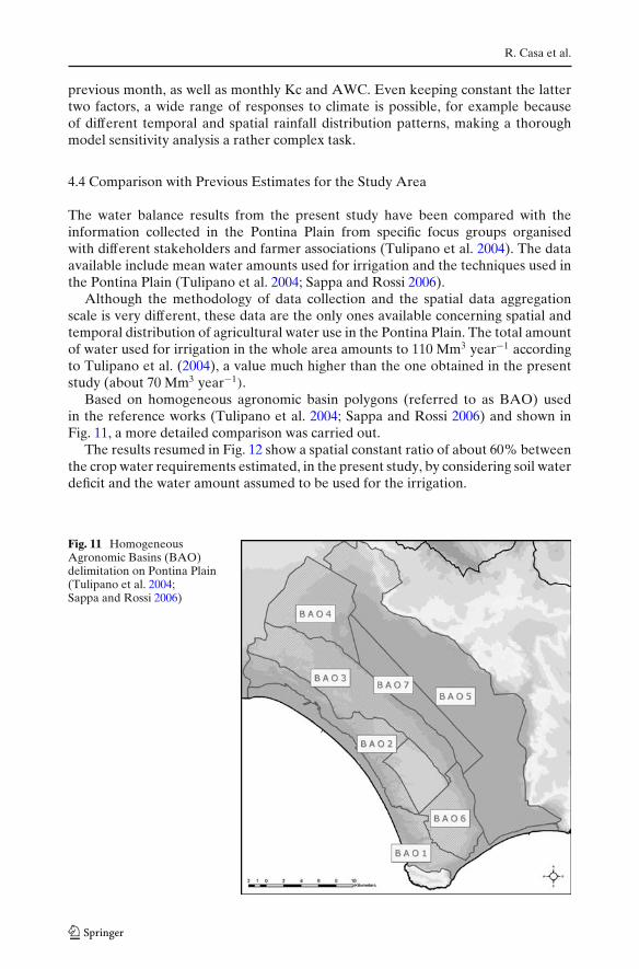
Based on homogeneous agronomic basin polygons (referred to as BAO) usedin the reference works (Tulipano et al. 2004; Sappa and Rossi 2006) and shown inFig. 11, a more detailed comparison was carried out.
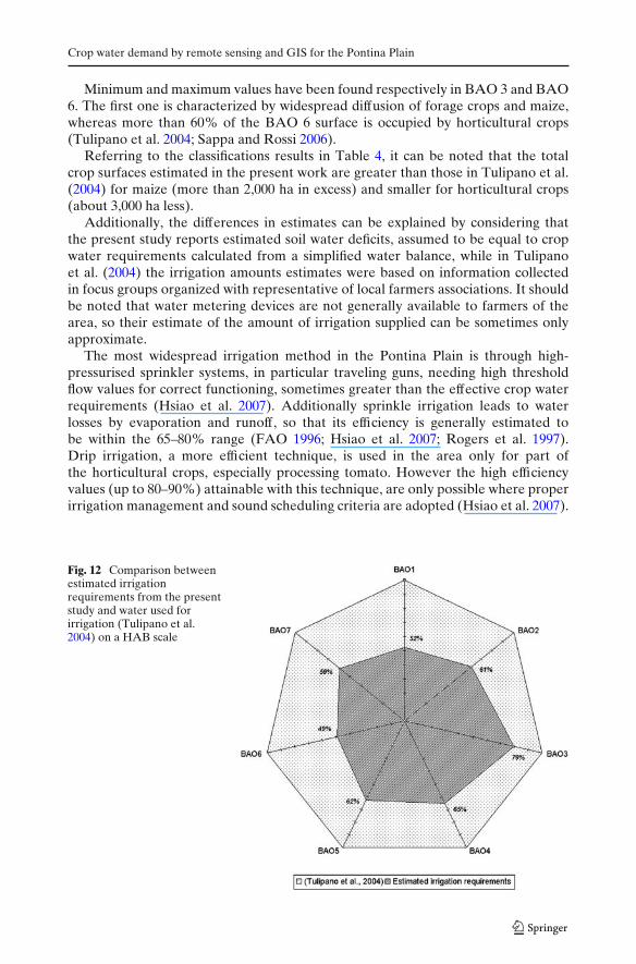
The results resumed in Fig. 12 show a spatial constant ratio of about 60% betweenthe crop water requirements estimated, in the present study, by considering soil waterdeficit and the water amount assumed to be used for the irrigation.
Fig. 11 HomogeneousAgronomic Basins (BAO)delimitation on Pontina Plain(Tulipano et al. 2004;Sappa and Rossi 2006)
Crop water demand by remote sensing and GIS for the Pontina Plain
Minimum and maximum values have been found respectively in BAO 3 and BAO6. The first one is characterized by widespread diffusion of forage crops and maize,whereas more than 60% of the BAO 6 surface is occupied by horticultural crops(Tulipano et al. 2004; Sappa and Rossi 2006).
Referring to the classifications results in Table 4, it can be noted that the totalcrop surfaces estimated in the present work are greater than those in Tulipano et al.(2004) for maize (more than 2,000 ha in excess) and smaller for horticultural crops(about 3,000 ha less).
Additionally, the differences in estimates can be explained by considering thatthe present study reports estimated soil water deficits, assumed to be equal to cropwater requirements calculated from a simplified water balance, while in Tulipanoet al. (2004) the irrigation amounts estimates were based on information collectedin focus groups organized with representative of local farmers associations. It shouldbe noted that water metering devices are not generally available to farmers of thearea, so their estimate of the amount of irrigation supplied can be sometimes onlyapproximate.
The most widespread irrigation method in the Pontina Plain is through high-pressurised sprinkler systems, in particular traveling guns, needing high thresholdflow values for correct functioning, sometimes greater than the effective crop waterrequirements (Hsiao et al. 2007). Additionally sprinkle irrigation leads to waterlosses by evaporation and runoff, so that its efficiency is generally estimated tobe within the 65–80% range (FAO 1996; Hsiao et al. 2007; Rogers et al. 1997).Drip irrigation, a more efficient technique, is used in the area only for part ofthe horticultural crops, especially processing tomato. However the high efficiencyvalues (up to 80–90%) attainable with this technique, are only possible where properirrigation management and sound scheduling criteria are adopted (Hsiao et al. 2007).
Fig. 12 Comparison betweenestimated irrigationrequirements from the presentstudy and water used forirrigation (Tulipano et al.2004) on a HAB scale
R. Casa et al.
In the Pontina Plain, irrigation applications are usually based on simple observa-tions of meteorological conditions or by visual assessment of crop and soil waterstatus and no proper irrigation management based on water balance scheduling(FAO 1996) is practiced in the area (Tulipano et al. 2004).
Therefore, assuming an average irrigation efficiency of 70% for the whole studyarea, the irrigation requirement would be of around 100 Mm3 year−1, from theestimated crop water needs of about 70 Mm3 year−1.
5 Conclusions
The present work aimed at providing a preliminary estimate of irrigation waterrequirements for the Pontina Plain, useful for inferring the temporal and spatialpatterns of groundwater withdrawals due to agricultural use, to be employed infurther hydrological studies. Considering the importance of agricultural water useon the hydrological balance of the area, and given the present economic and timeconstraints of regional institutions, this study was aimed at identifying and testing aninexpensive and rapid methodology for this task.
For this reasons a simple and economic approach, in terms of data and resources,based on remote sensing and GIS, was chosen.
Employing only 4 Landsat images and a few meteorological and geographicalvectorial layers, the integrated use of GIS allowed the elaboration of monthly mapsof crop evapotranspiration for an area of about 700 km2. The application of aspatially distributed water balance model, allowed the estimation of temporal andspatial variation of crop water requirements in the study area.
The accuracy of the estimates provided in the present study is influenced byseveral factors.
Classification error can have an impact on crop evapotranspiration mapping,especially when crops having contrasting water use behaviour are confused (Stehmanand Milliken 2007). A particular problem encountered in the study area was thewidespread occurrence of small sized fields, causing high commission errors in theclassification. Increased accuracy would be achieved by using a per-field rather thana pixel-based classification method (De Wit and Clevers 2004), should digitised fieldboundaries become available for the study area.
Another source of error in crop evapotranspiration maps was the assumption ofstandardized Kc seasonal curves throughout the study area, though the reasonablyuniform climatic and soil conditions of the Pontina Plain entail a fairly homogeneousfarming practices calendar, as confirmed by interviews with local farmers and exten-sion service personnel (Tulipano et al. 2004).
The use of an extremely simplified root-zone water balance adopted in this study,although an improvement compared to the simpler effective rain methodologies,still introduced some gross approximations by not considering in detail severalterms of the water balance, such as drainage and runoff, and ignoring even basiccrop growth terms such as the root uptake of readily available soil moisture andwater stress related evapotranspiration reduction. On the other hand considerablemore information would have been required in order to adopt more detailed agro-hydrological models (Boegh et al. 2004), considering the temporal constraints andthe spatial scale of the present application.
Crop water demand by remote sensing and GIS for the Pontina Plain
Nevertheless, the results provided by this work make available to further hy-drological modelling activities, more detailed and accurate spatial data, on waterrequirements of the existing cropping pattern, than those which are usually employedin similar planning studies (e.g. Bonomi 1995; Capelli et al. 2005).
Actually the crop classification work carried out to build Kc maps, contributed im-portant information on agricultural land use, potentially useful to elaborate differentscenarios in subsequent studies for the definition of sustainable water managementpolicies.
It was not within the scope of the present work to explore possible alternative cropallocation patterns in the area, aimed at minimizing water deficit, or alternativelyprovide the highest economic net benefit. However the results provided by this studycould be used, for example, as inputs of spatially distributed linear optimisationmodels, capable of providing suggestions for planning authorities on more suitablecropping patterns for the conservation of water resources while safeguarding farm-ers’ income.
The increasing availability of high resolution remote sensing data and the recentset-up of a comprehensive network of weather stations in the Latium Department,gives the Regional Watershed Authority powerful tools for updating and improvingthe accuracy of the present work, for an efficient monitoring and planning of waterresources use.
The present study estimated crop water demand for the whole area to be about70 Mm3 year−1, i.e. 100 Mm3 year−1 irrigation requirements when considering anaverage irrigation application efficiency of 70%. A previous estimate of currentirrigation amounts used in the area, though following very different methodologies(Tulipano et al. 2004), reported a figure of 110 Mm3 year−1, suggesting scopefor substantial irrigation water savings. Improvements are expected to stem fromthe diffusion of water metering devices and sound water balance based irrigationscheduling criteria (FAO 1996), or by policies encouraging less water demandingcropping systems.
It should be noted that the calculation of irrigation requirements from thesimplified water balance implemented in the present study, allows plant uptake of thewhole available water content, implying the possibility of occurrence of crop waterstress and yield reduction. Full irrigation scheduling criteria would, more cautiously,allow depletion of only the fraction of readily available soil water (Allen et al. 1998;Clarke et al. 1992).
For these reasons, the overall irrigation water requirement for the Pontina Plain,estimated in this work, can be considered as an absolute minimum net amount ofwater resources necessary for allowing current farming practices to be sustained.
Acknowledgements The authors gratefully acknowledge the funding for this study from RegionalWatershed Authority of Latium Department. The support of AGEA, through provision of CAPdatabases, was essential for the classification work. The contribution of farmers, extension personnel,and officials of farmers union Coldiretti, for providing information on local practices is alsoacknowledged.
References
Allen RG, Pereira LS, Raes D, Smith M (1998) Crop evapotranspiration guidelines for computingcrop water requirements. FAO irrigation and drainage paper 56, Rome, Italy
R. Casa et al.
Allen RG, Tasumi M, Morse A, Trezza R (2005) A Landsat-based energy balance and evapotranspi-ration model in Western US water rights regulation and planning. Irrig Drain Syst 19:251–268.doi:10.1007/s10795-005-5187-z
American Metereological Service (2000) Glossary of metereology, 2nd edn. http://amsglossary.allenpress.com/glossary. Cited 20 Oct 2007
Bàrberi P, Casa R, Lo Cascio B, Arletti E, Lamaddalena N, Steduto P, Lacirignola C (2000)PolAgWat project country outline report: Italy. INCO-DC European Commission IV FP, therelationship between sectoral policies and agricultural water use in mediterranean countries(PolAgWat)
Bastiaanssen WGM, Menenti M, Feddes RA, Holtslag AAM (1998) A remote sensing surfaceenergy balance algorithm for land (SEBAL) 1. Formulation. J Hydrol (Amst) 212–213:198–212.doi:10.1016/S0022-1694(98)00253-4
Belmonte AC, Gonzalez JM, Mayorga AV, Fernandez SC (1999) GIS tools applied to the sustainablemanagement of water resources—application to the aquifer system 08-29. Agric Water Manage40:207–220. doi:10.1016/S0378-3774(98)00122-X
Boegh E, Thorsen M, Butts MB, Hansen S, Christiansen JS, Abrahamsen P, Hasager CB, JensenNO, van der Keur P, Refsgaard JC, Schelde K, Soegaard H, Thomsen A (2004) Incorporat-ing remote sensing data in physically based distributed agro-hydrological modelling. J Hydrol(Amst) 287:279–299. doi:10.1016/j.jhydrol.2003.10.018
Bono P (1995) The sinkhole of Doganella (Pontina Plain, Central Italy). Environ Geol 26:48–52.doi:10.1007/BF00776031
Bonomi T (1995) Gestire le acque sotterranee. SIT per la valutazione del bilancio del sistemaidrogeologico milanese. Fondazione Lombardia per l’Ambiente, Milano, Italy, 146 pp
Borin M, Bigon E, Caprera P (2003) Atlante fenologico: il mutevole aspetto di alcune specie agrariedurante il loro ciclo biologico. Ed.Agricole, Italy
Bossard M, Feranec J, Otahel J (2000) Corine land cover technical guide—addendum 2000. Technicalreport 40, European Environmental Agency, Copenhagen, Denmark
Brunamonte F, Serva L (2004) Natural processes vs human impact in the subsidence history ofthe Pontina Plain (Central Italy). Paper presented at the 32th international geological congress,Florence, Italy, 20–28 Aug 2004
Brunetti M, Maugeri M, Nanni T (2000) Variations of temperature and precipitation in Italy from1866 to 1995. Theor Appl Climatol 65:165–174. doi:10.1007/s007040070041
Burrough PA, McDonnell R (1998) Principles of geographical information systems. OxfordUniversity Press, UK
Capelli G, Mazza R, Gazzetti C (2005) Strumenti e strategie per la tutela e l’uso compatibile dellarisorsa idrica nel Lazio—Gli acquiferi vulcanici. Pitagora Editrice, Bologna
Clarke D, Smith M, El-Askari K (1992) CROPWAT—a computer program for irrigation planningand management. FAO irrigation and drainage paper 46, Rome, Italy
Coviello MT, Rossi M, Sappa G (2005) The groundwater overexploitation of a coastal aquifer: amultidisciplinary approach. In: Proceedings of the 7th hellenic hydrogeology conference, Athens,Greece, 5–6 Oct 2005
Crist EP, Cicone RC (1984) A physically-based transformation of Thematic Mapper data—the TMTasseled Cap. IEEE T Geosci Remote GE 22:256–263. doi:10.1109/TGRS.1984.350619
Custodio G, Llamas MR (1996) Hidrologia Subterranea. Ed. Omega, SpainDastane NG (1974) Effective rainfall in irrigated agriculture. FAO irrigation and drainage paper 25,
Rome, ItalyDe Wit JW, Clevers JGPW (2004) Efficiency and accuracy of per-field classification for operational
crop mapping. Int J Remote Sens 25:4091–4112. doi:10.1080/01431160310001619580Doorenbos J, Pruitt WO (1977) Crop water requirements. FAO irrigation and drainage, paper
no. 24, Rome, Italy, 144 ppDroogers P, Allen RG (2002) Estimating reference evapotranspiration under inaccurate data condi-
tions. Irrig Drain Syst 16:33–45. doi:10.1023/A:1015508322413D’Urso G (2001) Simulation and management of on-demand irrigation systems: a combined
agrohydrological and remote sensing approach. PhD Dissertation, Wageningen University,The Netherlands
European Commission (2000) Water framework directive 2000/60. http://ec.europa.eu/environment/water/water-framework/index_ en.html. Cited 13 Dec 2006
FAO (1995) Use of remote sensing techniques in irrigation and drainage. FAO water report n.4.Cemagref-FAO, Montpellier, France
Crop water demand by remote sensing and GIS for the Pontina Plain
FAO (1996) Irrigation scheduling: from theory to practice. Water reports 8. In: Proceedings ofICID/FAO workshop on irrigation scheduling, Rome, 12–13 Sept 1995
Furby SL, Campbell NA (2001) Calibrating images from different dates to ‘like-value’ digital counts.Remote Sens Environ 77:186–196. doi:10.1016/S0034-4257(01)00205-X
Gerardi A, Catalano G, Gallozzi PL, Di Loreto E, Liperi L, Meloni F, Sericola A, Toccacieli M,Tonelli V, Zizzari P (2004) Carta della vulnerabilità integrata degli acquiferi della regione Lazio.Paper presented at ESRI Italian user conference, Rome, Italy, 21–22 Apr 2004
Hanks RJ (1985) Crop coefficients for transpiration. In: Advances in evapotranspiration. Proceed-ings of national conference on advances in evapotranspiration, Chicago, ASAE, St. Joseph, MI,USA, pp 431–438
Hargreaves GH (1994) Defining and using reference evapotranspiration. J Irrig Drain E-ASCE120:1132–1139. doi:10.1061/(ASCE)0733-9437(1994)120:6(1132)
Hsiao T, Steduto P, Fereres E (2007) A systematic and quantitative approach to improve water useefficiency in agriculture. Irrig Sci 25:209–231. doi:10.1007/s00271-007-0063-2
ISTAT (2000) Quinto Censimento Generale dell’Agricoltura. Italian National Statistics Institute(ISTAT), Rome, Italy
Jensen JR (1986) Introductory digital image processing. Prentice-Hall, New JerseyKurtzman D, Kadmon R (1999) Mapping of temperature variables in Israel: a comparison of differ-
ent interpolation methods. Clim Res 13:33–43. doi:10.3354/cr013033Kustas WP, Norman JM (1996) Use of remote sensing for evapotranspiration monitoring over land
surfaces. Hydrol Sci J 41:495–516Lillesand TM, Kiefer RW (1999) Remote sensing and image interpretation, 4th edn. Wiley,
New YorkLi S, Tarboton DG, McKee M (2003) GIS-based temperature interpolation for distributed modelling
of reference evapotranspiration. Paper presented at the 23rd AGU hydrology days, Fort Collins,Colorado, 31 Mar–03 Apr 2003
Loukas A, Mylopoulos N, Vasiliades L (2007) A modeling system for the evaluation of waterresources management strategies in Thessaly, Greece. Water Resour Manage 21:1673–1702.doi:10.1007/s11269-006-9120-5
Matheron G (1962) Traité de Géostatistique appliquée. Editions Technip, Paris, FranceMoran MS, Jackson RD, Raymond LH, Gay LW, Slater PN (1990) Mapping surface energy balance
components by combining Landsat TM and ground-based meteorological data. Remote SensEnviron 30:77–87. doi:10.1016/0034-4257(89)90049-7
Norrant C, Douguédroit A (2006) Monthly and daily precipitation trends in the Mediterranean(1950–2000). Theor Appl Climatol 83:89–106. doi:10.1007/s00704-005-0163-y
Passino R, Benedini M, Dipinto AC, Pagnotta R (1999) Un futuro per l’acqua in Italia. IRSA/CNRReport No 109, Rome, Italy
Piemontese L, Perotto C (2004) Carta della Copertura del Suolo della Provincia di Latina. Latina,Italy
Provincia di Latina (2003) General Territorial Management Plan—SN4: geopedological subsystem.Latina, Italy
Ravelli F, Rota P (1994) Carta frequenziale dell’evapotraspirazione mensile di riferimento irriguodelle pianure litoranee del Mezzogiorno d’Italia. Irrigazione Drenaggio XLI:5–97. Bologna, Italy
Ravelli F, Rota R (1999) Monthly frequency maps of reference crop evapotranspiration and cropwater deficits in Southern Italy. http://www.francoravelli.it. Cited 14 Feb 2007
Ray SS, Dadhwal VK (2001) Estimation of crop evapotranspiration of irrigation command area usingremote sensing and GIS. Agric Water Manage 49:239–249. doi:10.1016/S0378-3774(00)00147-5
Regione Lazio (1992) Studies on South Latium water resources. Monographs on Latium Hydrogeo-logical Units. Technical Reports of Conv.767/87 rep.6191, Rome, Italy
Richards LA, Wadleigh CH (1952) Soil water and plant growth. In: Shaw BT (ed) Soil physicalconditions and plant growth, vol II. Academic, New York, pp 74–251
Rogers DH, Lamm FR, Alam M, Trooien TP, Clark GA, Barnes PL, Mankin K (1997) Efficienciesand water losses of irrigation systems. Irrigation Management Series MF2243, Kansas StateUniversity, US
Rossi M (2005) Modello di supporto alla gestione di un acquifero sottoposto ad elevata pressioneantropica. PhD Dissertation, University of Rome “La Sapienza”, Rome, Italy
Sappa G, Rossi M (2006) Data shared elaboration to irrigation water needs evaluation supportedby GIS. Proceedings of the 5th European congress on regional geological cartography andinformation systems, Barcelona, Spain, 13–16 June 2006
R. Casa et al.
Sappa G, Coviello MT, Rossi M (2005) Environmental effects of aquifer overexploitation in thePontina Plain. In: Proceedings of the IV national meeting on groundwater management andprotection, Parma, Italy, 21–23 Sept 2005
Sevink J, Duivenvoorden J, Kamermans H (1991) The soils of Agro Pontino. The Agro PontinoSurvey Project, Studeisn in Prea- and Protphistorie 6:31–48, Universiteit van Amsterdam, TheNetherlands
Shultz GA, Engman ET (2000) Remote sensing in hydrology and water management. Springer, NewYork
Schmugge TJ, Kustas WP, Ritchie JC, Jackson TJ, Rango A (2002) Remote sensing in hydrology.Adv Water Resour 25:1367–1385. doi:10.1016/S0309-1708(02)00065-9
Stabile T (1985) Dalle paludi una provincia. Ed. Archimio, Latina, ItalyStehman SV, Milliken JA (2007) Estimating the effect of crop classification error on evapotranspira-
tion derived from remote sensing in the lower Colorado River basin, USA. Remote Sens Environ106:217–227. doi:10.1016/j.rse.2006.08.007
Sugita M, Brutsaert W (1992) Landsat surface temperature and radio sounding to obtain regionalsurface fluxes. Water Resour Res 28:1675–1679. doi:10.1029/92WR00468
Tasumi M, Allen RG (2007) Satellite-based ET mapping to assess variation in ET with timing of cropdevelopment. Agric Water Manage 88:54–62. doi:10.1016/j.agwat.2006.08.010
Todorovic M, Steduto P (2003) A GIS for irrigation management. Phys Chem Earth 28:163–174Tsanis IK, Naoum S (2003) The effect of spatially distributed meteorological parameters on irrigation
water demand assessment. Adv Water Resour 26:311–324. doi:10.1016/S0309-1708(02)00100-8Tsanis IK, Naoum S, Boyle SJ (2002) A GIS interface method based on reference evapotranspiration
and crop coefficients for the determination of irrigation requirements. Water Int 27:233–242Tulipano L, Sappa G, Rossi M (2004) Stima dei fabbisogni irrigui nel settore irriguo e zootecnico nel
territorio della Pianura Pontina. Tech. Rep. 2-04 of Latium Dept. and DITS Agreement, Rome,Italy
Zimmerman D, Pavlik C, Ruggles A, Armstrong M (1999) An experimental comparison ofordinary and universal kriging and inverse distance weighting. Math Geol 31–4:375-390.doi:10.1023/A:1007586507433