Compressive Coherence Sensing

Daniel L. MarksThe Duke Imaging and Spectroscopy Program, Department ofElectrical and Computer Engineering, Duke University, 130

Hudson Hall, Durham NC 27708

Ashwin WagadarikarThe Duke Imaging and Spectroscopy Program, Department ofElectrical and Computer Engineering, Duke University, 130

Hudson Hall, Durham NC 27708

David J. BradyThe Duke Imaging and Spectroscopy Program, Department ofElectrical and Computer Engineering, Duke University, 130

Hudson Hall, Durham NC 27708

Abstract

The coherence function [1] of a stationary, ergodic electromagnetic fieldis the complete description of its second-order statistics [2, 3]. In a two-dimensional aperture, this function comprises the correlations between allpairs of points, so that the coherence is a four-dimensional function. Whilecoherence is a rich source of sensing data, it is almost always impracti-cal to measure the entire four-dimensional function. Compressive sens-ing [4, 5, 6] is a means by which one may accurately reconstruct an imagesampling only a small fraction of the coherence samples. This is accom-plished by imposing a sparsity constraint on the possible reconstructedimages. If the data is such that the reconstructed image satisfies thesparsity constraint, the object can be reconstructed with an exceedinglysmall probability of error given a sufficient amount of data is sampled.This approach may enable new coherence instruments that infer objectproperties without exhaustive coherence data sampling. In this paper theframework of compressed coherence sensing is presented, and an experi-mental demonstration of compressed coherence sensing of a simple objectthrough turbulence is presented.

1. COHERENCE SENSING

Partial coherence is a seldom exploited property of the electromagnetic field forremote sensing and image formation. Most instruments are imaging instrumentsand treat the formed image as incoherent and do not attempt to infer coherenceproperties of the source from the image. However, coherence is a potentiallyrich source of information that could be used for imaging, for example imag-ing through turbulence. The coherence function is the complete description ofthe second-order statistics of the electromagnetic field. In a two-dimensionalaperture, the coherence is a four-dimensional function comprising the correla-tions between every pair of points in the aperture. Unfortunately, the size ofthe coherence function is often an impediment to its use in image formation,as in general a large portion of this function must be measured to produce an

1

accurate image. If the amount of coherence data necessary for quality imageformation could be reduced, coherence-sensing instruments might be more prac-tical. We propose compressive sensing as a means of inferring accurate imagesfrom limited coherence data. Compressive sensing succeeds because the imageis restricted by sparsity constraints to possible images that are accurately re-constructed by a minimum of coherence samples. To demonstrate the utilityof our approach with an experiment, we reconstruct using compressive sens-ing techniques an incoherent object through synthetic turbulence by samplingthe coherence using an interferometer. Our demonstration shows that, withinlimits, it is possible to reconstruct an object from a limited set of coherencesamples.

The coherence of the electromagnetic field in the scalar approximation isdescribed by the cross-spectral density

W (x1, y1, x2, y2, ω) = 〈E(x1, y1, ω)∗E(x2, y2, ω)〉 (1)

where E(x, y) is a quasimonochromatic stochastic electromagnetic field centeredaround frequency ω . From the van Cittert-Zernike theorem [7, 8] we can derivethe following propagation law of the field radiated from an incoherent source ofspectral density S(r, ω):

W (x′

1, y′

1, x′

2, y′

2, ω) =∫

dx dy S(x,y,ω)iz2

exp[

−2iωc

(

(x′

2 − x′

1)xz + (y′

2 − y′

1)yz

)] (2)

Simply stated, the two-dimensional Fourier transmission of the power spectraldensity is the cross-spectral density in the far field as a function of the differencebetween the two coordinates that are correlated. To recover the spectral densityof the source, the remote cross-spectral density may be measured as a function ofspatial coordinate differences x′

2 −x′

1 and y′

2− y′

1 about a central point using aninterferometer and then inverse Fourier transformed to find the power spectraldensity.

If isoplanatic turbulence with an optical path delay d(x′, y′) is present be-tween the source and receiver, the cross-spectral density becomes

W (x′

1, y′

1, x′

2, y′

2, ω) = exp[

iωc (d(x′

1, y′

1) − d(−x′

2,−y′

2))]

∫

dx dy S(x,y,ω)iz2 exp

[

−2iωc

(

(x′

2 − x′

1)xz + (y′

2 − y′

1)yz

)] (3)

The phase introduced into the cross-spectral density distorts the resulting imageif the van Cittert-Zernike theorem is used to inverse the cross-spectral density.Unlike a conventional image of an object in turbulence using a lens, the cross-spectral density measurement contains phase data that includes the turbulencephase.

We use an instrument called the rotational shearing interferometer (RSI)[9, 10, 11, 12, 13, 14] to measure the cross-spectral density, as presented inFig. 1. This interferometer consists of a beams plitter and two folding mirrors.The beam splitter divides the wavefront to be sampled into two. Each of thesplit fields is reflected and rotated by the roof prism, so that the recombinedfields have a relative rotation. The superimposed fields are measured on a sensorarray. The delay of one arm of the interferometer is varied to allow phase-shiftingto find the phase-resolved cross-spectral density.

2

sensor array

folding mirror

folding mirror

beam splitter

input aperture

dithertranslation

stage

Figure 1: The rotational shearing interferometer.

If we consider a stochastic field E(x′, y′) incident on the rotational shearinginterferometer, the cross-spectral density W ′(η, ξ, ω) sampled at a position η, ξon the sensor is given by

W ′(η, ξ, ω) = 〈E(η cos θ + ξ sin θ,−η sin θ + ξ cos θ)∗

E(η cos θ − ξ sin θ, η sin θ + ξ cos θ)∗〉 =W (η cos θ + ξ sin θ,−η sin θ + ξ cos θ, η cos θ − ξ sin θ, η sin θ + ξ cos θ)

(4)given that one arm of the interferometer rotates the field +θ radians and theother arm rotates the field −θ radians. Expressing Eq. 3 as a function of η andξ this becomes

W ′(η, ξ, ω) =exp

[

iωc (d(η cos θ + ξ sin θ,−η sin θ + ξ cos θ)−

d(η cos θ − ξ sin θ, η sin θ + ξ cos θ))]∫

dx dy S(x,y,ω)iz2 exp

[

4iωc

(

ξ sin θ xz − η sin θ y

z

)]

(5)

Disregarding the turbulence d(x′, y′), the cross-spectral density measured by theRSI is the Fourier transform of the source intensity, rotated by 90 degrees andscaled by 1/2 sin θ. Because of this, the RSI is an ideal interferometer to use toreconstruct incoherent sources. The turbulence adds an extra phase term to themeasurement that distorts the estimate of the source intensity. However, thecross-spectral density in the absence of turbulence has Hermitian symmetry, thatis W ′(η, ξ, ω) = W ′(−η,−ξ, ω)∗ being the Fourier transform of a real function,the spectral density of the source. If the angle θ 6= π/2, the turbulence does notnecessarily have Hermitian symmetry. Because of this disparity, the turbulencephase can be distinguished from the phase due to the source itself. Compressivesensing techniques are used to find the turbulence phase and the source spectraldensity, partially based on this distinction.

3

2. COMPRESSIVE SENSING

As previously mentioned, the coherence function is four-dimensional being thecorrelations of every pair of 2-D points in an aperture, while the RSI samplesonly a two-dimensional subset of this coherence function. The previous sectionpresented a model for the coherence function of an incoherent source in thepresence of turbulence. To infer the source spectral density [15, 16, 17, 18] andthe turbulence from this subset of the coherence [19, 20], we employ algorithmsused in compressive sensing, modifying them for improved performance in thepresence in turbulence.

The conventional compressive sensing problem is framed as: find the solutionthat minimzes ‖ y − Ax ‖2 +τ ||x| |0. In this context, y is a measurementvector, x is the data vector to be inferred, and A is a linear transformationbetween the data and measurement vectors. The constraint ‖ y − Ax ‖2 is aconventional least-squares constaint that ensured that the data conforms to themeasurements. The other constraint that minimizes ||x| |0 simply counts thenumber of nonzero elements in the vector x. This is a sparsity constraint basedon the 0-norm (`0) that strongly restricts the possible solutions. This constraintmight be useful, for example, if x represents image samples and it is desired tohave the minimum number of pixels be nonzero. Unfortunately as posed thisproblem is NP so that the computational effort is too great for any resonablysized image.

Rather than solve the `0 problem we can pose it as a different problem basedon the `1-norm: minimizing ‖ y − Ax ‖2 +τ ||x| |1. The `1-norm is a convexnorm, and the sum of these norms is likewise a convex functional. Thereforemany convex optimization methods are available that can find the minimumsolution which is unique. One of the basic results of compressive sensing is thatminimizing `1 always provides the same answer that minimizing `0 would selectgiven that the number of measurements is sufficient and the forward operatorsatisfied certain conditions [21, 22]. This result makes certain compressive sens-ing computations practical and allows analysis of the reconstruction of sparsedata vectors.

For coherence sensing, y is a vector of measured coherence samples, x isa desired image to estimate, and A is a linear transformation that describesthe propagation of partially coherent light, in this case the van Cittert-Zerniketheorem including turbulence. Conventional reconstruction of an image mightminimize the 2-norm of the vector x which is Tikhonov regularization. Unfortu-nately this constraint tends to produce poor images when little data is availablebecause `2-norm restricts only the total energy in the image and not the con-centration of this energy throughout the image. On the other hand, typicalimages do not consist of power distributed randomly over the image, but ratherof discrete objects and surfaces that tend to have features that cluster in certainpixels. The `1-norm tends to produce these images as it concentrates the energyof the image into discrete points. Therefore the `1-norm can produce interestingand useful imagery under more realistic constraints as well as be practical tocompute.

There are many procedures for finding the minimum of the `1-norm compres-sive sensing problem. The algorithm used here is two-step iterative shrinking

4

and thresholding [23] (TwIST). Each iteration this algorithm alternates betweena shrinking step that reduces the least-squares penalty and a thresholding thatreduces the `1-norm. When the minimum is reached to a particular accuracy,the directions of the correction gradient for the least-squares and the `1 normoppose as is needed in any Lagrange multiplier constrained problem, and theiteration may be terminated.

Geometrically, this process has an appealing interpretation. The surface ofa constant squared-error is a hypersphere. On the other hand, the surface ofconstant `1 is the surface of a polytope bounded by hyperplanes called the `1

ball. The solution is typically the intersection between the hypersphere and acorner of the `1 ball. Because the corners of the `1 ball are sharp, small errorsin the data tend to not change which elements of the vector x are nonzero, asthis would involve switching the solution to another corner where the `1 balltouches the sphere. Therefore the sparsity constraint is robust against error.

A block diagram of the modified TwIST algorithm is presented in Fig. 2. Theleast-squares constraint is enforced using gradient-descent. The `1 constraint isenforced by soft-thresholding the elements of x that places the solution on acorner of the `1 ball. However, without modification the algorithm does notaccount for the turbulence phase. The turbulence phase effectively modifies thepropagation operator A. Therefore each iteration both the image and turbu-lence phase are estimated. The first step is a shrinking step that applies theleast-squared constraint to the Fourier transform of the data. The current es-timate of the phase is applied to the Fourier data estimate, and the data isconverted to the spatial domain using the inverse Fourier transform to form animage estimate. The estimated intensity of the spatial-domain image is soft-thresholded to apply the sparsity constraint. The Fourier transform returns thespatial-domain image to the Fourier domain data. The phases of the sparselyconstrained image and the current turblence-aberrated image are subtracted toform a new turbulence phase estimate. The data is then underrelaxed to sta-bilize the iterations. Iteration continues until the iterations produce a minimalchange.

3. AN EXPERIMENTAL DEMONSTRATION

To demonstrate the use of compressive sensing to correct turbulence, we observelight emitting diodes through an aberrating phase screen using the rotationalshearing interferometer, as detailed in Fig. 3. The LEDs emitted wavelengthsin the yellow region of the spectrum, and has their plastic lenses sanded off tonearly the LED chip die to produce isotropic and incoherent radiation. TheseLEDs were collimated by a lens to place their image at infinity as would occur forstellar imaging. An iris eliminates vignetting effects from the collimation lens.A phase distortion plate is placed behind the iris to produce an instance of thephase distortion caused by turbulence. This plate was constructed by drippingpolydimethylsiloxane (Sylgard 184) silicone onto a microscope slide and thenheating with with a heat gun to cure it quickly before the surface became moreuniformly flat. A second lens relays the partially coherent aberrated field to theentrance of the RSI. The RSI collected the intensity interferograms as the delaybetween the two arms of the interferometer was varied. The interferograms at

5

Start with the measured coherence

data, an image estimate, and a null

turbulence phase screen

Shrinking step to enforce fit

of image estimate to

coherence data

Inverse Fourier transform

to image domain using

turbulence phase screen

from last iteration

Soft-threshold intensity

to obtain L1 image

estimate in the absence

of turbulence

TwIST = Two-step iterative shrinking and thresholding

Use under-relaxation to

stabilize iterations

Error in

estimate

below

threshold?

No

Yes

End iterations

Fourier transform to

coherence domain

Compute and store phase

difference between current

coherence estimate and image

estimate to find current

turbulence phase screen

Figure 2: A block diagram of the compressive sensing algorithm used to findthe unaberrated image and a turbulence estimate.

four delays I0,Iπ/2,Iπ ,I3π/2 with phases separated by π/2 were summed to findthe coherence estimate using the formula W = I0 + iIπ/2 − Iπ − iI3π/2. Themodified TwIST algorithm was applied to the coherence estimate. The constantτ was chosen to be the average intensity of all the points in the image with anintensity more than 10% of the maximum intensity in the image. This ensuredthat the image would be sharpened with the soft-thresholding, but not overlyso as to remove significant features from the data. The forward operator of theTwIST algorithm was weighted to favor low frequencies in the image as theseare less affected by turbulence.

The results of the experiment are in Fig. 4. The image of the LEDs assumingno distortion is present is in part (c). The aberration substantially distorts theimage. The estimate of the coherence function without the turbulence is part(a). The real part of the complex phase of the estimated phase screen of thedistortion is part (b). This shows that the phase screen and the object canbe jointly estimated. Part (d) is the estimated object. The algorithm clearlyimproves the quality of the image, whereas it would be hard to discern the threeLEDs from the original aberrated image.

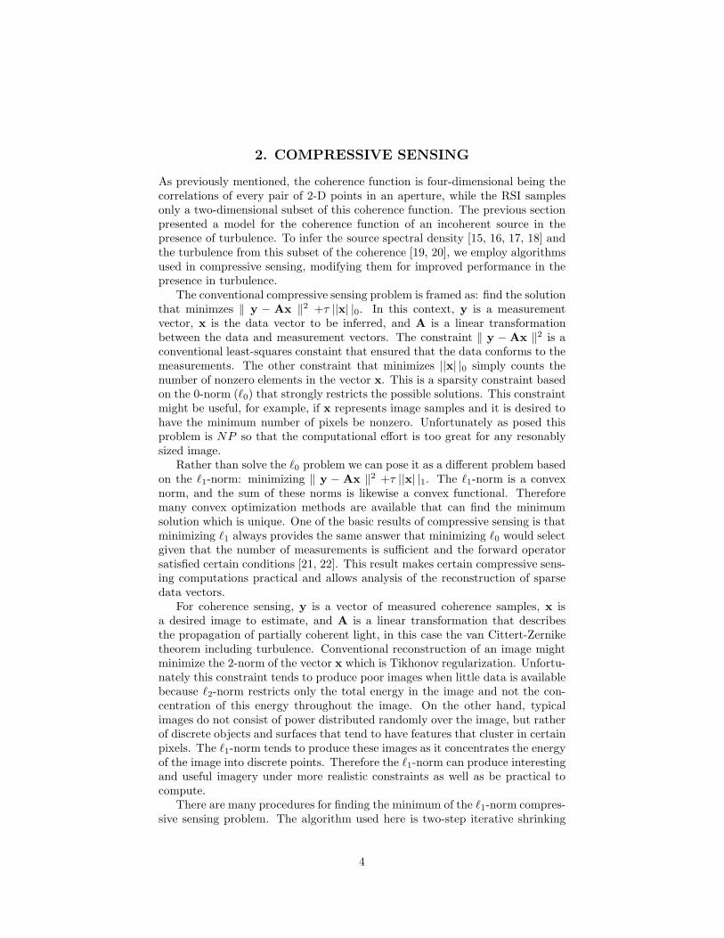
As a control experiment, we performed the same imaging but without aphase distortion plate as shown in Fig. 5. Part (a) is the reconstructed coherencefunction without turbulence, which resembles that of Fig. 4. The phase of thedistortion is estimated to be almost zero in part (b). Part (c) is the image ofthe LEDs directly computed from the unchanged sampled coherence data. Part(d) is the image produced by the algorithm. Because of the L1 constraint, thealgorithm improves the image of the LEDs slightly, sharpening the points. Thecontrol experiment suggests that the algorithm does not merely deconvolve the

6

LEDsIris

(spatial

filter)Distortion

7”

7” 2.5”Old LED holder

14”

Experimental setup

RSI

Afocal telescope to image

beam splitter to CCD

CCD

7” 2.5”Old LED holder

Separation of bottom 2 LEDs

= 20 mm

Separation of top LED from

bottom 2 LEDs = 9.14 mm

New LED holder

Closest possible separation

between LEDs = 6.5 mm

A little larger separation =

11.258 mm

4.5”

Figure 3: Diagram of the setup to measure the cross-spectral density from LEDswith a phase distortion.

Distance in RSI interferogram (mm)

Dis

tanc

e in

RS

I int

erfe

rogr

am(m

m)

Distance in phase estimate (mm)

Dis

tanc

e in

pha

se e

stim

ate

(mm

)

(a) (b)

Distance in object space (mm)

Dis

tanc

e in

obj

ect s

pace

(m

m)

Dis

tanc

e in

obj

ect s

pace

(m

m)

Distance in object space (mm)(c) (d)

Figure 4: Results of compressive sensing reconstruction of three LEDs aberratedby turbulence. (a) The reconstructed coherence function of the LEDs withoutturbulence. (b) The estimated phase of the aberration. (c) The image neglectingturbulence, showing the distortion produced by turbulence. (d) The estimateof the source intensity without turbulence.

7

-10 -5 0 5 10

-10

-5

0

5

10

-10 -5 0 5 10

-10

-5

0

5

10

Distance in RSI interferogram (mm)D

ista

nce

in R

SI i

nter

fero

gram

(mm

)Distance in phase estimate (mm)

Dis

tanc

e in

pha

se e

stim

ate

(mm

)

(a) (b)

0 5 10 15

-50

-45

-40

-355 10 15

-50

-45

-40

-35

Distance in object space (mm)

Dis

tanc

e in

obj

ect s

pace

(m

m)

Dis

tanc

e in

obj

ect s

pace

(m

m)

Distance in object space (mm)(c) (d)

Figure 5: Results of a control experiment of compressive sensing reconstructionof three LEDs not aberrated by turbulence. (a) The reconstructed coherencefunction of the LEDs. (b) The estimated phase of the aberration, which isclose to null because no turbulence is present. (c) The image of the originalsource. (d) The estimate of the source intensity, which improves the imagequality because the L1 constraint sharpens the points slightly.

image directly, but actually estimates the phase and applies this phase to thesampled coherence to produce an improved image.

References

[1] D. J. Brady, Optical Imaging and Spectroscopy. New York: Wiley, 2009.

[2] L. Mandel and E. Wolf, Optical Coherence and Quantum Optics. Cam-bridge: Cambridge University Press, 1995.

[3] J. Goodman, Statistical Optics. New York: John Wiley & Sons, 1985.

[4] D. L. Donoho, “Compressed sensing,” IEEE Trans. Inf. Theory, vol. 52,no. 4, pp. 1289–1306, 2006.

[5] E. J. Candes and T. Tao, “Near-optimal signal recovery from random pro-jections: Universal encoding strategies?” IEEE Trans. Inf. Theory, vol. 52,no. 12, pp. 5406–5426, 2006.

8

[6] E. J. Candes, J. K. Romberg, and T. Tao, “Stable signal recovery from in-complete and inaccurate measurements,” Comm. Pure Appl. Math., vol. 59,pp. 1207–1223, 2006.

[7] P. H. Van Cittert, “Die wahrscheinliche schwingungsventeilung in einer voneiner lichtquelle direkt oder mittels einer linse beleuchten ebene,” Physica,vol. 1, pp. 201–208, 1934.

[8] F. Zernike, “The concept of degree of coherence and its application tooptical problems,” Physica, vol. 5, pp. 785–796, 1938.

[9] M. Murty and E. Hagerott, “Rotational-shearing interferometry,” Appl.Opt., vol. 5, no. 4, pp. 615–619, 1966.

[10] F. Roddier, C. Roddier, and J. Demarcq, “A rotation shearing interfer-ometer with phase-compensated roof prisms,” J. Opt. (Paris), vol. 11, pp.149–152, 1978.

[11] C. Roddier, F. Roddier, and J. Demarcq, “Compact rotational shearinginterferometer for astronomical applications,” Opt. Eng., vol. 28, no. 1, pp.66–70, 1989.

[12] C. Roddier and F. Roddier, “High angular resolution observations of AlphaOrionis with a rotation shearing interferometer,” Astrophys. J., vol. 270,pp. L23–L26, 1983.

[13] F. Roddier, “Interferometric imaging in optical astronomy,” Physics Re-ports, vol. 17, pp. 97–166, 1988.

[14] E. Ribak, C. Roddier, F. Roddier, and J. B. Breckinridge, “Signal to noiseconsiderations in white-light holography,” Appl. Opt., vol. 27, pp. 1183–1186, 1988.

[15] K. Itoh and Y. Ohtsuka, “Interferometric imaging of a thermally luminoustwo-dimensional object,” Opt. Comm., vol. 48, no. 2, pp. 75–79, 1983.

[16] K. Itoh, T. Inoue, and Y. Ichioka, “Interferometric spectral imaging andoptical three-dimensional Fourier transformation,” Jap. J. Appl. Phys.,vol. 29, pp. 1561–1564, 1990.

[17] K. Itoh, T. Inoue, T. Yoshida, and Y. Ichioka, “Interferometric multispec-tral imaging,” Appl. Opt., vol. 29, pp. 1625–1630, 1990.

[18] K. Itoh and Y. Ohtsuka, “Fourier-transform spectral imaging: retrieval ofsource information from three-dimensional spatial coherence,” J. Opt. Soc.Am. A, vol. 3, pp. 94–100, 1986.

[19] R. G. Paxman, T. J. Schulz, and J. R. Fienup, “Joint estimation of objectand aberrations using phase diversity,” J. Opt. Soc. Am. A, vol. 9, pp.1072–1085, 1992.

[20] J. Primot, G. Rousset, T. Marais, and J. C. Fontanella, “Deconvolutionof turbulence-degraded images from wavefront sensing,” Proc. SPIE, vol.1130, pp. 29–32, 1989.

9

[21] A. Juditsky and A. S. Nemirovski, “On verifiable sufficient condi-tions for sparse signal recovery via l1 optimization,” 2008, availablehttp://www.citebase.org/abstract?id=oai:arXiv.org:0809.2650.

[22] K. Lee and Y. Bresler, “Computing performance guarantees for compressedsensing,” in International Confererence on Acoustics, Speech and SignalProcessing, 2008., Apr 2008, pp. 5129–5132.

[23] J. M. Bioucas-Dias and M. A. T. Figueiredo, “A new twist: two-step it-erative shrinkage/thresholding algorithms for image restoration,” IEEE.Trans. Image Proc., vol. 16, no. 12, pp. 2992–3004, Dec. 2007.

10