arX

iv:1

211.

1137

v1 [

cs.IT

] 6

Nov

201

21

Wireless Compressive Sensing for Energy

Harvesting Sensor Nodes

Gang Yang, Vincent Y. F. Tan, Chin Keong Ho, See Ho Ting, and Yong Liang Guan

Abstract

We consider the scenario in which multiple sensors send spatially correlated data to a fusion center

(FC) via independent Rayleigh-fading channels with additive noise. Assuming that the sensor data is sparse

in some basis, we show that the recovery of this sparse signalcan be formulated as a compressive sensing

(CS) problem. To model the scenario in which the sensors operate with intermittently available energy

that is harvested from the environment, we propose that eachsensor transmits independently with some

probability, and adapts the transmit power to its harvestedenergy. Due to the probabilistic transmissions,

the elements of the equivalent sensing matrix are not Gaussian. Besides, since the sensors have different

energy harvesting rates and different sensor-to-FC distances, the FC has different receive signal-to-noise

ratios (SNRs) for each sensor. This is referred to as theinhomogeneityof SNRs. Thus, the elements of the

sensing matrix are also not identically distributed. For this unconventional setting, we provide theoretical

guarantees on the number of measurements for reliable and computationally efficient recovery, by showing

that the sensing matrix satisfies the restricted isometry property (RIP), under reasonable conditions. We then

compute an achievable system delay under an allowable mean-squared-error (MSE). Furthermore, using

techniques from large deviations theory, we analyze the impact of inhomogeneity of SNRs on the so-called

k-restricted eigenvalues, which governs the number of measurements required for the RIP to hold. We

conclude that the number of measurements required for the RIP is not sensitive to the inhomogeneity of

SNRs, when the number of sensorsn is large and the sparsity of the sensor data (signal)k grows slower

than the square root ofn. Our analysis is corroborated by extensive numerical results.

Index Terms

Wireless compressive sensing, Energy harvesting, Restricted isometry property, Compressive sensing,

Wireless sensor networks, Rayleigh-fading channels, Large deviations

G. Yang, S. H. Ting and Y. L. Guan are with the School of Electrical and Electronic Engineering, Nanyang TechnologicalUniversity, Singapore (e-mail:yang0305@e.ntu.edu.sg;{shting, eylguan}@ntu.edu.sg). G. Yang is supported in part by the AdvancedCommunications Research Program DSOCL06271, a research grant from the Directorate of Research and Technology (DRTech),Ministry of Defence, Singapore.

V. Y. F. Tan and C. K. Ho are with the Institute for Infocomm Research, A⋆STAR, Singapore (e-mail:{tanyfv, hock}@i2r.a-star.edu.sg). V. Y. F. Tan is also with the Department of Electrical and Computer Engineering, National University of Singapore.

November 7, 2012 DRAFT

2

I. INTRODUCTION

The lifetimes of conventional wireless sensor networks (WSNs) are limited by the total energy

available in the batteries. It is inconvenient to replace batteries periodically, or even impossible

when sensors are deployed in harsh conditions, e.g., in toxic environments or inside human bodies.

Energy harvesting of ambient energy such as solar, wind, thermal and piezoelectric energy, appears

as a promising alternative to a fixed-energy battery, to prolong the lifetime and offer potentially

maintenance-free operation for WSNs [1], [2]. Compared to limited but reliable power supply from

conventional batteries, energy harvesters provide a virtually perpetual but unreliable energy source.

Moreover, the sensors typically have differentenergy harvesting rates, due to varying harvesting

conditions such as the spread of sunlight and difference in wind speeds.

This paper addresses the problem of data transmission in energy harvesting WSNs (EH-WSNs).

We assume that energy harvesting sensors are deployed to monitor some physical phenomenon

in space, e.g., temperature, toxicity of gas. Data collected from sensors are sent to the fusion

center (FC). The data are typically correlated, and well approximated by a sparse vector in an

appropriate transform (e.g., the Fourier transform). Recent developments in compressive sensing

(CS) theory provide efficient methods to recover sparse signals from limited measurements [3]. CS

theory states that if the sensing matrix satisfies the restricted isometry property (RIP), a small number

of measurements (relative to the length of the data vector) is sufficient to accurately recover the

sparse data. This advantage of CS potentially allows us to reduce the total number of transmissions,

and this is particularly important for data transmission inbandwidth-limited wireless channels.

The accurate estimation of the sensor data by the FC has recently been addressed by using

CS techniques in the literature. In [4], Hauptet. al presented a sensing scheme based on phase-

coherent transmissions for all sensors. However, [4] made two practically limiting assumptions.

First, it assumed that there was no channel fading, and path losses for all sensors were identical.

Second, the transmissions from all sensors were synchronized such that signals arrived in phase

at the FC. In [5], Aeronet. al derived information theoretic bounds on sensing capacity of sensor

networks under a fixed signal-to-noise ratio (SNR) for all sensors. In contrast, [6] proposed a sparse

approximation method in non-fading channels, which adapted a sensor’s sensing activity according

to its energy availability. In [7], Xueet. al successively applied CS in the spatial domain and the

time domain, under a fixed SNR for all sensors. In [8], Fazelet. al proposed a random access

scheme in underwater sensor networks. Each activated sensor picked a uniformly-distributed delay

November 7, 2012 DRAFT

3

to transmit. By simply discarding the colliding data packets from concurrent medium access, the

FC used a CS decoder to recover the sensor data based only on the successfully received packets.

Thus, the scheme did not exploit packet collisions for data recovery.

Since sensors are placed at different locations, it is commonly assumed that the sensors transmit

data over independent but nonidentical channels with different fading conditions. Different energy

harvesting rates also lead to different transmit powers andhence different (receive) SNRs. We refer

to this generally as theinhomogeneityof SNRs. The application ofwireless compressive sensingto

the scenario of inhomogeneous SNRs has, to the best of our knowledge, not been studied in the

literature. We define thesystem delayas the number of concurrent sensor-to-FC transmissions (or

channel uses) for estimating one data vector (among sensors). We aim to reduce the system delay,

while ensuring a target estimation accuracy. Surprisingly, we observe that the required number of

measurements for accurate recoverym is not overly sensitive to the inhomogeneity of SNRs provided

that the number of sensorsn is large and the sparsity of the data vectork grows slower than√n.

This motivates us to further investigate the impact of inhomogeneity of SNRs, based on the recovery

performance in terms of RIP.

The three main contributions are summarized as follows.

1) We first present an efficient transmission scheme, which features probabilistic transmission by

sensor nodes. In each time slot, every sensor locally decides to transmit with some probability,

and adjusts the transmit power according to its energy availability. The FC thus receives a linear

combination of signals that are transmitted from a random subset of sensors. The transmissions

over successive time slots result in a sensing matrix which is effectively achieved through the

mixing of signals in wireless channels.

2) Second, we prove that the FC can recover the data accurately, if the total number of trans-

missions (or measurements)m exceeds

O

(kρmax(k)

ρmin(k)log

n

k

), (1)

wheren is the number of sensors,k is the sparsity of the sensor data, andρmax(k) andρmin(k)

are respectively the maximum and minimumk-restricted eigenvalues (see definition in (15)) of

a Gram matrix which depend on the inhomogeneity of SNRs. Different from previous works

on CS, our bound depends explicitly on the ratioρmax(k)/ρmin(k), which is thek-restricted

condition number of the Gram matrix. Based on this result, wealso compute the achievable

November 7, 2012 DRAFT

4

system delay subject to a desired recovery accuracy.

3) Third, we analyze the impact of inhomogeneity of SNRs on the required number of mea-

surements, in terms ofρmax(k) and ρmin(k). We model the signal powers of the sensors as

independent truncated Gaussians. By using the theory of large deviations, we show that both

ρmax(k) and ρmin(k) concentrate around one (for all constantk) in largen regime, and the

rate of convergence to one depends on the inhomogeneity of SNRs. This allows us to explain

the observation that the inhomogeneity of SNRs does not significantly affect the number of

measurements required for the RIP to hold.

This remainder of this paper is organized as follows: Section II provides a description of the

system model. Section III presents a new wireless compressive sensing scheme. Section IV details

the main results on the RIP, the achievable system delay and investigates the impact of inhomogeneity

of SNRs. Section V provides the simulation results. SectionVI concludes this paper. The proofs

for the RIP result and the result on the impact of inhomogeneity of SNRs are given in Section VII.

We adopt the following set of notation in this paper: lower case letters denotes deterministic

scalars, and lower case Greek letters for constants or angles. Boldface upper case and boldface

lower case refer to matrices and (column) vectors, respectively. We use upper case letters to denote

random variables. Sets are denoted with calligraphic font (e.g.,V). The cardinality of a finite setVis denoted as|V|. Then-order identity matrix is denoted byIn. We also useRn andCn to denote

the n-dimensional real and complex Euclidean spaces respectively.

II. SYSTEM MODEL

Consider a wireless sensor network that consists ofn energy harvesting sensor nodes and a FC.

Sensors transmit their data to the FC via a shared multiple-access channel (MAC). We consider

slotted transmissions by first considering a single snapshot of the spatial-temporal field. Assuming

the sensor datas is compressible, we can model it as being sparse with respectto (w.r.t.) to a fixed

orthonormal basis{ψj ∈ Cn : j = 1, . . . , n}, i.e.,

s = Ψx =

n∑

j=1

ψjxj , (2)

wherex ∈ Cn has at mostk < ⌊n/2⌋ non-zero components and⌊·⌋ is the floor operation.

We assume a flat-fading channel with complex-valued channelcoefficientshij, where1 ≤ i ≤ m

denotes the slot index and1 ≤ j ≤ n denotes the sensor index. The channel remains constant in each

November 7, 2012 DRAFT

5

✲

✲

✲

✒✑✓✏

✒✑✓✏

✒✑✓✏

×

×

×

❄

❄

❄

s

φi1s1

φi2s2

φinsn

...

hi1

hi2

hin

∑

❅❅❅❅❅❘✲

�����✒

✲yi✒✑

✓✏❄+

ei

✲ FusionCenter

Fig. 1. The MAC communication structure for WSNs in thei-th time slot. The signals that are concurrently transmitted fromsensors to the FC are linearly combined over the air.

slot. We further assume a Rayleigh-fading channel, hence the channel coefficients for different slots

are independent and identically distributed (i.i.d.) according to the complex Gaussian distribution.

We propose that sensors concurrently transmit to the FC in a probabilistic manner, such that the

signals from sensors are linearly combined over the air. Sensor j multiplies its datumsj by some

random amplitudeφij (to be defined in (4)), then transmits in thei-th time slot. The FC thus receives

yi =

n∑

j=1

hijφijsj + ei,

where ei is a noise term (not necessarily Gaussian). Afterm time slots, the FC receives the

measurement vector

y = (H⊙Φ)s+ e = Zs + e = ZΨx + e, (3)

where the matrixZ = H⊙Φ, and the operation⊙ is the element-wise product of two matrices. We

assume all noise components are independent, zero mean and have varianceσ2. The signal model

over one slot is illustrated in Fig. 1.

From the perspective of signal recovery, we want to estimatex or equivalentlys, from y, such

that themean-squared-error(MSE) E‖x− x‖22 does not exceed some thresholdǫ. Also, we would

like to estimate the sparse vector using minimum network resources (i.e., channel uses), due to

limited channel resources. Thus, given a fixed number of sensors n and anǫ, our objective is to

design a transmission scheme that minimizes the number of sensor-to-FC transmissionsm.

November 7, 2012 DRAFT

6

Different from [6], [9], we consider Rayleigh-fading channels, and adopt concurrent transmissions

in a probabilistic manner. Moreover, the SNRs of different sensors are considered to be different,

compared to the fixed SNR case in the literature [5], [7], [9].

III. ENERGY-AWARE WIRELESSCOMPRESSIVESENSING

In Section III-A, we first provide a CS perspective for the signal model in (3). Then in Section

III-B, we present an energy-aware wireless compressive sensing scheme. By taking into account the

inhomogeneity of SNRs, we also derive the probability distribution function (pdf) of elements in

the random matrixZ in Section III-C, which will be used to show the RIP in SectionIV-A.

A. A Compressive Sensing Perspective

Since we assume the data vectorx is sparse in some basis, it seems natural to adopt a CS method

to recoverx. The over-the-air combination via the channel matrixH contributes to the effective

equivalent sensing matrixZ in (3). However, there are two differences from the conventional CS

setup that make the analysis more challenging.

• Due to probabilistic transmissions, the elements of the sensing matrixZ are not Gaussian.

• Since sensors have different energy harvesting rates and different sensor-to-FC distances, the

FC has different receive SNRs for all sensors. Thus, the elements of the sensing matrixZ are

also not identically distributed.

The proposed transmission scheme calls for the analysis of non-Gaussian non-i.i.d. sensing matrices.

Hence, we need to analyze the system performance in a more intricate way that differs from

conventional CS problems. The key technique we employ is to show that the elements of the

sensing matrixZ are sub-Gaussian, and make use of new results on sub-Gaussian random matrices.

B. Energy-Aware Wireless Compressive Sensing

We consider only the energy consumption for wireless transmissions, by assuming the energy

consumption on sensing is negligible. The energy harvesting rate varies over sensors. For simplicity,

we assume that each sensor allocates the same power for all slots. Let Ej be the accumulated

harvested energy that is available for sensorj to transmit in each slot. We perform energy-aware

wireless transmissions taking into account the different available energy. It is noted that acausal

November 7, 2012 DRAFT

7

energy constraintthat comes from energy harvesting should be satisfied, i.e.,energy that is consumed

for transmissions can not exceed the energy available in each slot.

Set a probabilityp ∈ (0, 1] and a squared-amplitudebj > 0 . LetΦ in (3) be aselection-and-weight

(SW) matrix, whose elements are independently generated according to the random variable

φij =

+√bj w.p. p/2

0 w.p. 1− p, ∀ i = 1, 2, . . . , m.

−√

bj w.p. p/2

(4)

That is, the sensorj transmits with probabilityp with an amplitude of√

bj , and the actual value is

positive or negative with equal probability. Given available energyEj , we choosebj such that1

pbj ≤ Ej , ∀j = 1, 2, . . . , n. (5)

Clearly, each entryφij is zero mean and has variancepbj . The causal energy constraint is satisfied

in expectation, i.e.,E(φ2ij) = pbj ≤ Ej. This allows us to save energy to be used for future

transmissions. The energy-saving feature can be crucial inthe scenario where the energy harvesting

rates are fluctuating over several snapshots of the spatial-temporal field. It is, however, beyond the

scope of this paper to optimize for thebj ’s.

In [6], all sensors consume the same amount of energy for transmissions. In contrast, each

sensor here adapts the transmit power to its available energy via the above-designed SW matrix.

Furthermore, the SW matrix randomly selects the sensors to transmit, and weighs the data according

to the sensors’ harvested energy. In each time slot, a subsetof sensors are selected at random to

perform transmissions and over-the-air combination. The selections are performed in a distributed

manner at each sensor node, since each node separately decides the slots that it transmits in. We

couple random sensor selection and energy-aware transmission by the choice of the SW matrix.

Recall the signal model in (3), i.e.,y = ZΨx+ e. With the knowledge2 of the matrixZ and the

sparsity-inducing basisΨ, the FC can implement CS decoding to recover sparse coefficients x and

obtain the estimated data vectors = Ψx.

1The quantitybj can be written more generally asbi,j , which means the transmit powers for different slots are different. To reducethe complexity of processing, we allocate the same power to all the slots.

2The assumption that the FC knowsZ andΨ is reasonable, because the FC can perform channel estimation from preambles, andobtain the information on the amount of harvested energy viafeedback. The channel and energy information is used for generatingSW matrix from a predefined set of SW matrices. The global parameters likem andp can be broadcasted to all sensors.

November 7, 2012 DRAFT

8

C. Probability Distribution Analysis and Equivalent Normalized Signal Model

Consider the signal model in (3). Denote each element inZ asZij = hijφij = ZRij + jZI

ij, where

ZRij , hR

ijφij, andZIij , hI

ijφij. Note that elements of the matrixH are assumed to be independent,

and each elementhij has independent real and imaginary components. Also the matrix Φ consists

of independent elements. All elements of matrixZ are thus independent, and have independent real

and imaginary components. As such, it suffices to analyze theprobability distribution of the real

component, since the analysis is similar for the imaginary component. The marginal pdf ofZRij can

be shown to be

fZR

ij(z) =

1√bjfHR

j

(z√bj

)· p2+

1√bjfHR

j

(− z√

bj

)· p2

+ (1− p) · δ(z), (6)

wherefHR

j(·) is the pdf of channel coefficient of sensorj, andδ(·) is the Dirac delta function. For

the sake of brevity, we define a new pdf as follows.

Definition 1. A random variableX follows a mixed Gaussiandistribution, denoted asX ∼N (µ, ν2, p), if its pdf has the following form

fX(x) = p1√2πν2

exp

(−(x− µ)2

2ν2

)+ (1− p)δ(x), (7)

wherep ∈ (0, 1] is the mixing parameter. The corresponding complex mixed Gaussian distribution,

assuming the real and imaginary components are independent, is denoted asNc(µ, ν2, p).

Assuming Rayleigh-fading channels, all elements in the channel matrixH are independent, zero

mean and follow Gaussian distributions. Note that due to different fading channels for the sensors,

the matrixH has column-dependent variances, where thej-th column follows a Gaussian distribution

with variancesν2j . From (6) and (7), the marginal pdf ofZR

ij can be expressed as

fZR(z) = p1√πν2

j bjexp

(− z2

ν2j bj

)+ (1− p)δ(z). (8)

Thus, we haveZR ∼ N(0, ν2

j bj/2, p)

.

Recall thatZ = H ⊙ Φ. Let H = HΓH andΦ = ΦΓΦ, whereΓH = diag{ν1, ν2, . . . , νn} and

ΓΦ = diag{√pb1,√pb2, . . . ,

√pbn}. Then we can decompose the matrixZ as follows

Z =√mZΓ, (9)

November 7, 2012 DRAFT

9

where we denoteZ = H ⊙ Φ and Γ = ΓHΓΦ. Let Γ = diag{√γ1,√γ2, . . . ,

√γn}, where the

receive signal power of sensorj is3 γj = pbjν2j . We term the diagonal elements ofΓ a signal power

pattern. Theγj ’s are generally all different (i.e., inhomogeneous signalpowers), and this directly

leads to the inhomogeneous (receive) SNRs. We note that all elements of the matrixZ are i.i.d.

mixed Gaussian random variables, i.e.,Z ∼ Nc (0, 1/(pm), p) and ZR ∼ N (0, 1/(2pm), p).

Using the equivalent expression in (9), we rewrite the signal model in (3) as

y =√mZΓΨx + e, (10)

where the matrixΨ is a unitary matrix. The distinct signal powers inΓ are spread along sparsity-

inducing basis vectors (i.e., columns ofΨ).

A matrix (or more correctly, asequenceof matrices) is said to bestandard column regularif all

elements are uniformly bounded by some constant [10]. For analytical convenience, we normalize

the matrixΓΨ to be standard column regular. The normalization constant is ‖ΓΨ‖F/√n =

√Pave,

wherePave =∑n

j=1 pbjν2j /n denotes the average (receive) signal power in one time slot.Then the

normalized matrix

Σ = ΓΨ/√

Pave (11)

has bounded spectral norm. By dividing both sides of (10) by√mPave, we obtain the normalized

signal model

y = ZΣx+ e = Ax+ e, (12)

where all noise components are independent, zero mean and have normalized varianceσ2 ,

σ2/(mPave). The average SNR is defined as

SNRave ,Pave

σ2=

p

nσ2

n∑

j=1

bjν2j . (13)

IV. M AIN RESULTS

Having derived the probability distribution of elements ofthe matrixZ in Section III-C, we

recall the definition of RIP [11] and state our main result, that is Theorem 1, in Section IV-A.

The engineering implication of Theorem 1, and in particularthe tradeoff between the achievable

3The receive signal power depends on both the channel condition (i.e., the variance of fading coefficientsν2

j and the averagetransmit powerpbj) that is governed by the accumulated harvested energy.

November 7, 2012 DRAFT

10

system delay and the allowable MSE, will be discussed in IV-B. Finally we analyze the effect of

inhomogeneity of SNRs on RIP and the required number of measurements in Section IV-C.

A. Restricted Isometry Property

It is well established in CS theory that a sufficient condition for accurate and efficient recovery

(via convex optimization) is that the sensing matrix satisfies the RIP. A matrixA is said to satisfy

RIP of orderk, if there exists aδk ∈ (0, 1) such that

(1− δk)‖x‖22 ≤ ‖Ax‖22 ≤ (1 + δk) ‖x‖22 (14)

holds for allk-sparse vectorsx. The smallest constantδk satisfying (14) is known as therestricted

isometry constant(RIC) [11]. When the sensing matrixA is random, the inequality should hold

with overwhelming probability that approaches one asn grows. Many families of random matrices,

e.g., i.i.d. Gaussian random matrices and Bernoulli randommatrices are known to satisfy the RIP

[11], [12]. As a result, to evaluate the recovery performance, all we have to show is that the sensing

matrix A in our scheme also obeys RIP with overwhelming probability.

The RIP requires that the sensing matrixA preserves the Euclidean norm of sparse vectors

well. For the signal model in (12), the entries inZ are i.i.d.sub-Gaussianrandom variables (See

Definition 6 in Section VII-A). It is known that random matrices (with sufficiently many rows and)

with i.i.d. sub-Gaussian entries approximately preserve the Euclidean norm of sparse vectors with

high probability [13]. SinceA = ZΣ, we need to analyze the norm-preserving property ofΣ. To

do so, we define thek-restricted extreme eigenvaluesof the Gram matrixΣ∗Σ as

ρmax(k) = maxv:‖v‖0≤k,‖v‖2=1

‖Σv‖22,

ρmin(k) = minv:‖v‖0≤k,‖v‖2=1

‖Σv‖22,(15)

wherev ∈ Cn, and the “l0-norm” ‖v‖0 refers to the number of non-zero elements ofv. The extreme

eigenvalues will be used to understand how the inhomogeneous SNRs affects the RIP.

Lemma1. The following bounds onρmax(k) andρmin(k) hold:

1 ≤ ρmax(k) ≤ k, 0 ≤ ρmin(k) ≤ 1. (16)

Proof: Fix a vectorv ∈ Cn such that‖v‖2 = 1 and ‖v‖0 = k. Let T ⊂ {1, . . . , n} with

November 7, 2012 DRAFT

11

|T | ≤ k be the support ofv. Let ΣT ∈ Cn×|T | be the submatrix ofΣ with column indicesT .

Denote the eigenvalues of the Gram matrixΣ∗T ΣT by λ1 ≥ . . . ≥ λk ≥ 0. Due to the normalization

in (11), the trace ofΣ∗T ΣT is

∑kj=1 λj = k. This implies that the largest eigenvalue is at least one

and at mostk. Similarly, the smallest eigenvalue is no larger than one.

We note that the sparsity levelk is usually much smaller than the number of sensorsn in

large-scale WSNs. We further assumeρmax(k) ∈ [1, 2] in the following. This simplifies some of the

mathematical arguments. We analytically and numerically verify this claim in Section IV-C. To state

our main theoretical result cleanly, we define two quantities that depend onΣ andk as follows

ξk(Σ) , max {1− ρmin(k), ρmax(k)− 1} ,

ζk(Σ) , max

{0,

2− ρmax(k)− ρmin(k)

ρmax(k)− ρmin(k)

}.

(17)

Sinceρmax(k) ∈ [1, 2], we have4 ξk, ζk ∈ [0, 1]. Let ϑk = (1 + ζk)ρmax(k) − 1. Given δk ∈ (ξk, 1),

for convenience, we mapδk to a “modified RIC” via a piecewise linear mapping as follows

βk(δk,Σ) ,

1− (1− δk)/ρmin(k), δk ∈ (ξk, ϑk)

(1 + δk)/ρmax(k)− 1, δk ∈ (ϑk, 1).(18)

Let ςk = 2/ρmax(k)− 1. The inverse ofβk(δk,Σ) is denoted as

δk(βk,Σ) ,

1− (1− βk)ρmin(k), βk ∈ (0, ζk)

(1 + βk)ρmax(k)− 1, βk ∈ (ζk, ςk).(19)

In the sequel, we assume that the quantityξk(Σ) is a small positive number and it measures the

inhomogeneity of the eigenvalues ofΣ∗T ΣT for |T | ≤ k. This impliesζk is small, and the deviation

betweenβk and δk is also small. The validity of this assumption will be shown both analytically

and numerically in Section IV-C.

Recall that the sensing matrixA = ZΣ in (12), where all elements of them × n matrix Z are

i.i.d. mixed Gaussian random variables,Σ is defined in (11), andn is the number of sensors. We

now state our main theoretical result.

4The arguments of some quantities are sometimes omitted for notational convenience.

November 7, 2012 DRAFT

12

Theorem 1. Let c1, c2 > 0 be some universal constants. Given a sparsity levelk < ⌊n/2⌋, a transmit

probability p ∈ (0, 1] and a numberδk ∈ (ξk, 1), if the number of measurements satisfies

m >c1kρmax(k)

p2β2kρmin(k)

log5en

k, (20)

whereβk = βk(δk,Σ) is defined in(18), then for any vectorx with support of cardinality of at

mostk, we have that the RIP in(14) holds with probability at least

1− exp(−c2mp2β2

k/4). (21)

Proof: See Section VII-A.

Remark1 (Specialization to the homogeneous case). Clearly, the lower bound on the required number

of measurements isO( kρmax(k)β2

kρmin(k)

log nk). For the homogeneous signal power pattern (i.e., the matrix

Γ is a multiple of the identity matrixIn), we haveρmax(k) = ρmin(k) = 1 and βk = δk. Thus

the lower bound reduces toO( kδ2k

log nk), which coincides with the known results for i.i.d. random

sensing matrices. See Theorem 5.2 in [12] and Section 1.4.4 in [13].

Remark2 (Contribution to the RIP analysis). Due to the inhomogeneous signal power pattern, the

rowsai of the sub-Gaussian sensing matrixA arenon-isotropic. To the best of our knowledge, little

is known about the RIP of non-isotropic sub-Gaussian randommatrices. The only relevant result is in

Remark5.40 in [13] which gives a concentration inequality of non-isotropic random sensing matrices

in terms of the upper bound on the spectral norm. However, theauthors did not demonstrate how

the inhomogeneity affects the RIP, nor did they investigatethe number of measurements required

to satisfy the RIP. Theorem 1 fills this gap.

Remark3. Theorem 1 is proved in Section VII-A by leveraging Theorem 2.1 of [14], which states

that a sufficient condition for the approximate preservation of the Euclidean norm upon random

linear mapping is that the number of measurements is proportional to the fourth power of the sub-

Gaussian norm. In our scenario, as shown in Lemma 6, the sub-Gaussian norm bounded above by

1/√p. In addition, Lemma 6 shows (using the Chernoff-bound) thatthe sub-Gaussian tail probability

is bounded above bype−pt2/2. Note that the sub-Gaussian norm is the smallest constant > 0 for

which the sub-Gaussian tail probability is2e−t2/(22) (Definition 6). In view of the fact that the

pre-factor in our bound isp (and not2), there is some degradation with respect top in Theorem 1.

For largerp, the degradation is reduced.

November 7, 2012 DRAFT

13

B. Achievable System Delay

The performance of wireless compressive sensing scheme is characterized by two quantities, i.e.,

the MSE and the system delay. The MSE performance under bounded noise is studied in the CS

literature [3], [15], [16]. Note that there is often a trade-off between the two quantities. Under an

allowable MSEǫ > 0, we thus analyze theachievable system delayD(ǫ), which is defined as

D(ǫ) , minm

m subject to E‖x− x‖22 ≤ ǫ. (22)

Corollary 1. Let p,m, n, k,Σ, ξk, ϑk be as in Theorem 1. Letǫth , 1/(0.0942 × SNRave). Given

an allowable MSEǫ > ǫth, with overwhelming probability (exceeding(21)), the achievable system

delay is

D(ǫ) =c1kρmax(k)

p2(βk)2ρmin(k)log

5en

k, (23)

where

βk(Σ, ǫ) ,

1− 0.693 + 1/√ǫSNRave

ρmin(k), δk ∈ (ξk, ϑk),

1.307− 1/√ǫSNRave

ρmax(k)− 1, δk ∈ (ϑk, 1).

(24)

Proof: We start the proof by leveraging on the following lemma.

Lemma2 (Theorem 3.2 of [15]). Let y = Ax+ e, wherex is a k-sparse vector inCn, e ∈ Cm is a

zero mean, white random vector whose entries have varianceσ2. If the A satisfies the RIP with RIC

δk < 0.307, then the solutionx to the ℓ1-minimization problem in CS decoder [3], [13] satisfies

E‖x− x‖22 ≤σ2

Pave(0.307− δk)2. (25)

Recall the definition ofSNRave in (13). From Lemma 2, to achieve a MSEǫ, it suffices to ensure

the RIC satisfiesδ∗k = 0.307 − 1/√ǫSNRave. From Theorem 1, the required minimum number of

measurements such that the RIP holds with overwhelming probability is

mmin =c1kρmax(k) log

5enk

p2(β∗k)

2ρmin(k)(26)

whereβk is given in (24). The definition of the achievable system delay establishes Corollary 1.

Remark4. Note that Corollary 1 applies only to the case where the MSEǫ is greater than the

thresholdǫth. If ǫ ≤ ǫth, then from (25), simple algebra reveals thatδk = 0, which implies that

November 7, 2012 DRAFT

14

the sensing matrixA is a perfect isometry. SinceA is random, and the entries are governed by a

density that is absolutely continuous w.r.t. the Lebesgue measure, this occurs with probability zero,

implying that the constraint in (22) is almost surely not satisfied. Thus, in this case, we define the

system delay to be∞.

Remark5. As eitherǫ or SNRave increases,βk increases, and thus the system delayD(ǫ) decreases.

More importantly, we note from Corollary 1 that the key measure for the inhomogeneity of SNRs is

the ratior(k) , ρmax(k)/ρmin(k) ∈ [1,∞). The system delay increases asr(k) increases from one.

We hence analyze the impact of inhomogeneity of SNRs on the deviation of ρmax(k) andρmin(k)

from unity in Section IV-C. In addition, the system delay decreases asp increases, sinceSNRave

defined in (13) increases asp increases. Thus, there is an inherent tradeoff between system delay and

energy consumption because largep implies high transmit energy. Thus, it is always advantageous

to transmit with as high a probability as possible subject tothe causal energy constraint.

Example1. Let the number of sensorsn = 500, the sparsity levelk = 5 and the transmit probability

p = 0.8. These parameters implyρmax(k) = 1.09, ρmin(k) = 0.88 (See Section IV). We plot the

achievable system delayD(ǫ) against the allowable MSEǫ, for different average SNRs in Fig. 2.

We observe that beyond the MSE threshold (that depends on theaverage SNR), the system delay

D(ǫ) decreases as eitherǫ or SNRave increases, which is is expected.

Remark6. We considered the scenario in which the FC collects one data vector from all sensors

in one frame. As a generalization of our setup, one can seek tominimize the total number of slots

for collecting multiple data vectors. By adjusting the transmit probability in each frame, one can

allocate different powers for different frames, such that both the recovery accuracy and the causal

energy constraint is guaranteed. Details of this possible extension are beyond the scope of this paper.

C. Effect of Inhomogeneity

This section investigates the impact of inhomogeneity of (receive) SNRs on the number of

measurements needed to satisfy the RIP. Without loss of generality, we assume all sensors have

the same noise power, hence, it suffices to analyze the impactof inhomogeneity of receive signal

powers. We focus on the asymptotic scenario where the numberof sensorsn tends to infinity

and, for the ease of analysis,k is kept constant. To make the dependence onn clear, we denote

ρmax(k) (resp.ρmin(k)) asρmax(k, n) (resp.ρmin(k, n)). It will be shown that bothρmax(k, n) and

November 7, 2012 DRAFT

15

0 0.05 0.1 0.15 0.2 0.25 0.3 0.35 0.40

50

100

150

200

250

300

350

MSE

Sys

tem

Del

ay

Ave. SNR=35dBAve. SNR=30dBAve. SNR=25dB

εth

2εth

1

εth

3

Fig. 2. Plot of achievable system delay against allowable MSE. Beyond the MSE threshold, the achievable system delay increasesas either the allowable MSE or the average SNR increases.

ρmin(k, n) concentrate around one whenn is large, and the rate of convergence to one depends

on the inhomogeneity of SNRs. This implies that the recoveryperformance (the required number

of measurements and the probability that the RIP holds in Theorem 1) is not sensitive to the

inhomogeneity of SNRs whenn is large.

Let w = Σv, where the unit-norm,k-sparse vectorv is supported on the setT , {s1, . . . , sk} ⊂{1, . . . , n} and lets1 < . . . < sk. To obtain further insights, we letΨ be then-point discrete Fourier

transform (DFT) matrix. Then the squaredℓ2-norm ofw can be expressed as follows

‖w‖22 =1

nPave

n∑

i=1

γi

(1 +

k∑

q=1

k∑

l=1,l<q

2Re

{vsqv

∗slexp

(−j2π(i− 1)(sq − sl)

n

)}). (27)

Since‖w‖22 is strongly influenced by the inner summation terms, we analyze the behavior of these

terms more carefully in the sequel. When the signal power pattern is homogeneous, i.e.,Γ =

diag(√γ, . . . ,

√γ), we have‖w‖22 = ‖Σv‖22 = 1, henceρmax(k, n) = ρmin(k, n) = 1 for all k, n.

We are interested to know howρmax(k, n) andρmin(k, n) vary with different signal powersγi’s.

Thus, we consider a model in which theγi’s are i.i.d. random variables following an approximate

Gaussian distribution. By varying the variance of this distribution, we are in fact varying the

inhomogeneity of the signal powers. Specifically, to deal with the fact that the signal powers cannot

November 7, 2012 DRAFT

16

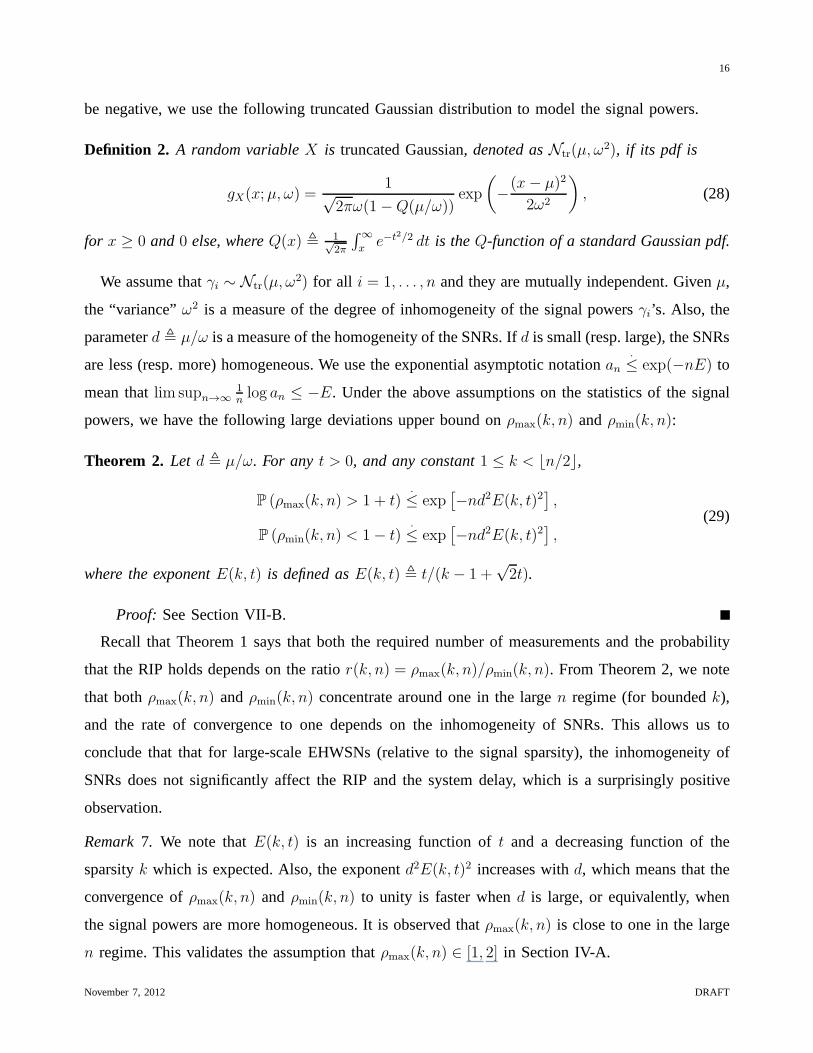
be negative, we use the following truncated Gaussian distribution to model the signal powers.

Definition 2. A random variableX is truncated Gaussian, denoted asNtr(µ, ω2), if its pdf is

gX(x;µ, ω) =1√

2πω(1−Q(µ/ω))exp

(−(x− µ)2

2ω2

), (28)

for x ≥ 0 and0 else, whereQ(x) , 1√2π

∫∞x

e−t2/2 dt is theQ-function of a standard Gaussian pdf.

We assume thatγi ∼ Ntr(µ, ω2) for all i = 1, . . . , n and they are mutually independent. Givenµ,

the “variance”ω2 is a measure of the degree of inhomogeneity of the signal powers γi’s. Also, the

parameterd , µ/ω is a measure of the homogeneity of the SNRs. Ifd is small (resp. large), the SNRs

are less (resp. more) homogeneous. We use the exponential asymptotic notationan.≤ exp(−nE) to

mean thatlim supn→∞1nlog an ≤ −E. Under the above assumptions on the statistics of the signal

powers, we have the following large deviations upper bound on ρmax(k, n) andρmin(k, n):

Theorem 2. Let d , µ/ω. For any t > 0, and any constant1 ≤ k < ⌊n/2⌋,

P (ρmax(k, n) > 1 + t).≤ exp

[−nd2E(k, t)2

],

P (ρmin(k, n) < 1− t).

≤ exp[−nd2E(k, t)2

],

(29)

where the exponentE(k, t) is defined asE(k, t) , t/(k − 1 +√2t).

Proof: See Section VII-B.

Recall that Theorem 1 says that both the required number of measurements and the probability

that the RIP holds depends on the ratior(k, n) = ρmax(k, n)/ρmin(k, n). From Theorem 2, we note

that bothρmax(k, n) andρmin(k, n) concentrate around one in the largen regime (for boundedk),

and the rate of convergence to one depends on the inhomogeneity of SNRs. This allows us to

conclude that that for large-scale EHWSNs (relative to the signal sparsity), the inhomogeneity of

SNRs does not significantly affect the RIP and the system delay, which is a surprisingly positive

observation.

Remark7. We note thatE(k, t) is an increasing function oft and a decreasing function of the

sparsityk which is expected. Also, the exponentd2E(k, t)2 increases withd, which means that the

convergence ofρmax(k, n) and ρmin(k, n) to unity is faster whend is large, or equivalently, when

the signal powers are more homogeneous. It is observed thatρmax(k, n) is close to one in the large

n regime. This validates the assumption thatρmax(k, n) ∈ [1, 2] in Section IV-A.

November 7, 2012 DRAFT

17

Remark8. In the preceding analysis, and particularly in Theorem 2, weassumed thatk does not

grow with n. Close examination of the proof shows that ifk = ⌊n1/2−λ⌋ for anyλ ∈ (0, 1/2], then

the probability that{ρmax(k, n) > 1+t} still goes to zero albeit at a slower rate of≈ exp(−n2λd2t2)

(not exponential inn). More precisely, we can verify that

lim supn→∞

1

n2λlog P(ρmax(k, n) > 1 + t) ≤ −d2t2, (30)

and analogously for{ρmin(k, n) < 1− t}. Inequality (30) is a so-calledmoderate-deviationsresult

[17, Sec. 3.7]. Notice that the dependencies on the homogeneity d = µ/ω andt are similar to (29).

Remark9. One may wonder whether Theorem 2 depends strongly onΨ being the DFT matrix. In

fact, the only property of the DFT that we exploit in the proofof Theorem 2 is its circular symmetry,

i.e., each basis vector of the DFT (containing elements thatare powers of then-th root of unity) is

uniformly distributed over the circle in the complex plane.Hence, certain Cesaro-sums converge to

zero and the proof goes through. See (44) in Section VII-B. Thus, Theorem 2 also applies for other

sparsity-inducing bases whose basis vectors have the circular symmetric property, e.g., the discrete

cosine transform (DCT) or the Hadamard transform.

V. SIMULATION RESULTS

We now numerically validate our results. We set the number ofsensorsn = 500 and transmit

probability p = 0.8. We use the truncated Gaussian distribution withµ = 0.2 to model the receive

signal powers, and use the basis pursuit de-noising (BPDN) algorithm [18] as the CS decoder.

First, we fix d = 2, which impliesω = µ/d = 0.1. Fig. 3 plots the MSE against the number

of measurements (or transmissions)m for different sparsitiesk and different average SNRs. As

expected, the MSE decreases as eitherk decreases or the average SNR increases. Consider the

MSE level 2 × 10−3. When the average SNR is25 dB, the wireless compressive sensing scheme

achieves a smaller system delay ofD = 68 for k = 5 compared toD = 115 for k = 10. When

the sparsityk = 5, the scheme achieves a smaller system delay ofD = 39 for SNRave = 30dB

compared toD = 68 for SNRave = 25dB.

Second, we fixd = 2 and the average SNR to be25dB. Fig. 4 compares the MSEs of the

inhomogeneous SNR and the homogeneous SNR scenarios, for the sparsity levelsk = 5, 10, 20.

It is observed that in the inhomogeneous scenario, the MSE performance is slightly worse than

that of the homogeneous-SNR scenario. Note that the degradation becomes larger as the sparsityk

November 7, 2012 DRAFT

18

20 40 60 80 100 120 140 160 180 20010

−4

10−3

10−2

10−1

100

Number of measurements: m

Mea

n S

quar

ed E

rror

SNR=20dB, k=5SNR=20dB, k=10SNR=25dB, k=5SNR=25dB, k=10SNR=30dB, k=5SNR=30dB, k=10

Fig. 3. Plot of MSE against the number of measurements. The MSE decreases ask decreases, or the average SNR increases.

20 40 60 80 100 120 140 160 180 20010

−4

10−3

10−2

10−1

100

Number of measurements: m

Mea

n S

quar

ed E

rror

Inhomo. SNR, k=5Inhomo. SNR, k=10Inhomo. SNR, k=20Homo. SNR, k=5Homo. SNR, k=10Homo. SNR, k=20

Fig. 4. Plot of MSE against the number of measurements. The MSE performance for the inhomogeneous scenario is slightly worsethan that of the homogeneous-SNR scenario.

increases. This is because the convergence rate forρmax(k) andρmin(k) to one is faster ifk is small

relative ton. This corroborates the observation in Section IV-C.

Third, we setd = 1, 2 andk = 5, 10. Fig. 5 shows the cumulative distribution function (CDF) of

November 7, 2012 DRAFT

19

1 1.1 1.2 1.3 1.4 1.50

0.5

1

ρmax

(k,500)C

DF

0.5 0.6 0.7 0.8 0.9 10

0.5

1

ρmin

(k,500)

CD

F

d=2, k=5d=2, k=10d=1, k=5d=1, k=10

d=2, k=5d=2, k=10d=1, k=5d=1, k=10

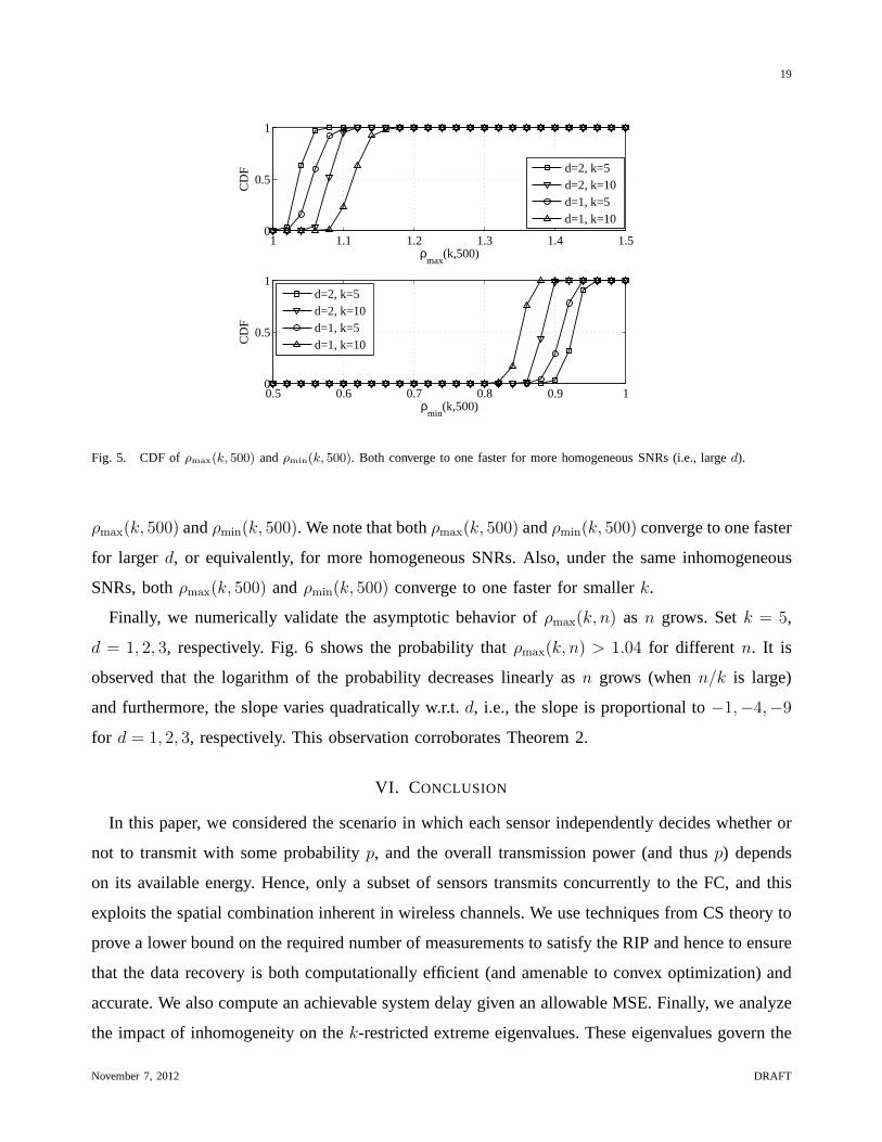
Fig. 5. CDF ofρmax(k, 500) andρmin(k, 500). Both converge to one faster for more homogeneous SNRs (i.e., larged).

ρmax(k, 500) andρmin(k, 500). We note that bothρmax(k, 500) andρmin(k, 500) converge to one faster

for larger d, or equivalently, for more homogeneous SNRs. Also, under the same inhomogeneous

SNRs, bothρmax(k, 500) andρmin(k, 500) converge to one faster for smallerk.

Finally, we numerically validate the asymptotic behavior of ρmax(k, n) as n grows. Setk = 5,

d = 1, 2, 3, respectively. Fig. 6 shows the probability thatρmax(k, n) > 1.04 for different n. It is

observed that the logarithm of the probability decreases linearly asn grows (whenn/k is large)

and furthermore, the slope varies quadratically w.r.t.d, i.e., the slope is proportional to−1,−4,−9

for d = 1, 2, 3, respectively. This observation corroborates Theorem 2.

VI. CONCLUSION

In this paper, we considered the scenario in which each sensor independently decides whether or

not to transmit with some probabilityp, and the overall transmission power (and thusp) depends

on its available energy. Hence, only a subset of sensors transmits concurrently to the FC, and this

exploits the spatial combination inherent in wireless channels. We use techniques from CS theory to

prove a lower bound on the required number of measurements tosatisfy the RIP and hence to ensure

that the data recovery is both computationally efficient (and amenable to convex optimization) and

accurate. We also compute an achievable system delay given an allowable MSE. Finally, we analyze

the impact of inhomogeneity on thek-restricted extreme eigenvalues. These eigenvalues govern the

November 7, 2012 DRAFT

20

200 300 400 500 600 700 800 900 1000

10−4

10−3

10−2

10−1

100

Number of sensors: n

Prob.(ρ

max>

1.04)

d= 1, Analyticald= 1, Monte Carlod= 2, Analyticald= 2, Monte Carlod= 3, Analyticald= 3, Monte Carlo

Slope ∝ −9, −4, −1

Fig. 6. Plot of the probability ofρmax(k, n) > 1.04 against the number of sensors. The logarithm of the probability decreaseslinearly asn grows, and the slope varies quadratically w.r.t.d.

number of measurements required for the RIP to hold. In large-scale EH-WSNs, we showed using

large deviation techniques that the recovery accuracy and the system delay are not sensitive to the

inhomogeneity of SNRs.

VII. PROOFS OFMAIN RESULTS

A. Proof of Theorem 1

Proof: Recall the signal model in (12), i.e.,y = ZΣx+ e = Ax+ e. The proof involves three

steps. In step 1 and step 2, we prove the desired result when all quantities are real; and in step 3, we

extend the result to the complex case. For the real case, we show that the matrixZ acts as isometry

on the images of the sparse vector under matrixΣ, i.e., on the set{Σv : ‖v‖0 ≤ k,v ∈ Rn}.

By showing the rows ofZ are isotropic sub-Gaussian and by exploiting the so-called“restricted

eigenvalue property” ofΣ, we derive an RIP for the matrixA in step 2. Before step 1, we start

with the following preliminaries. Letd(u,v) be the Euclidean distance inRn.

Definition 3 (Nets, covering numbers [13]). Consider a metric space(U , d) with U ⊂ Rn and a

positive numberǫ. A subsetNǫ ⊂ U is called anǫ-netof U if every pointu ∈ U can be approximated

to within ǫ by some pointv ∈ Nǫ, i.e.,d(u,v) ≤ ǫ. Thecovering numberN (U , ǫ) is the cardinality

of the smallestǫ-net ofU .

November 7, 2012 DRAFT

21

Definition 4 (Set of sparse vectors). Let Sn−1 be the unit sphere inRn and 1 ≤ k ≤ n. Define

Uk , {u ∈ Sn−1 : ‖u‖0 ≤ k},

also define the subset of the Euclidean unit ballBn2 with (at most)k-sparse vectors as

Uk , {u ∈ Bn−12 : ‖u‖0 ≤ k}.

Lemma3 (Upper bound on covering numbers, Lemma 2.3 in [14]). Let 0 < ǫ < 1 and1 ≤ k ≤ n.

There exists anǫ-net of Uk, namelyNǫ, whose cardinality can be upper bounded as

|Nǫ| ≤(

5

2ǫ

)k (n

k

).

Definition 5 (Complexity measure [14]). Thecomplexityof a setV ⊂ Rn is defined as

ℓ∗(V) , E

[supv∈V

|〈v,u〉|],

where〈·, ·〉 denotes inner product inRn, u ∼ N (0, I) is a standard Gaussian random vector, and

the supremum is over all vectorsv ∈ V.

Given a subsetV ⊂ Rn, we aim to measure the complexity ofW(V), which is the image set of

the setV under a fixed linear mappingΣ. More precisely, we define

W(V) , {w ∈ Rn : w = Σv, for some v ∈ V}. (31)

Define the complexity ofW(V) as ℓ∗ (W(V)) , E [supv∈V |〈v,Σu〉|] .

Lemma4 (Upper bound on complexity measure, Lemma B.6 in [19]). Let N 1

2,k be a 1

2-net of Uk

provided by Lemma 3. Then for all1 ≤ k ≤ n, it holds that

ℓ∗

(W(N 1

2,k))≤ 3

√kρmax(k) log

5en

k,

ℓ∗ (W(Uk)) ≤ 2ℓ∗

(W(N 1

2,k)), (32)

whereρmax(k) is thek-restricted maximum eigenvalue ofΣ∗Σ defined in (15).

Define the set

Ek , {v ∈ Rn : ‖Σv‖2 = 1, ‖v‖0 = k}, (33)

November 7, 2012 DRAFT

22

then forV = Ek, the complexity measure of the setW(Ek) is bounded in the following Lemma.

Lemma5. The complexity measure of the setW(Ek) is upper bounded as

ℓ∗ (W(Ek)) ≤ 6

√kρmax(k)

ρmin(k)log

5en

k, (34)

whereρmax(k) andρmin(k) are defined in (15).

Proof: For any vectorv ∈ Ek and any random vectoru ∈ Rn, we have with probability one

that

|〈u,Σv〉| = |〈v,Σu〉| = ‖v‖2∣∣∣∣⟨

v

‖v‖2,Σu

⟩∣∣∣∣ ≤ ‖v‖2 supr∈Uk

|〈r,Σu〉| , (35)

where the inequality follows from the definition of the set{ v

‖v‖2 : v ∈ Ek} ⊂ Uk. From Lemma 4,

E

[supv∈Ek

|〈u,Σv〉|]

(a)

≤ supv∈Ek

‖v‖2E[supr∈Uk

|〈r,Σu〉|]

(b)

≤ 6

√kρmax(k)

ρmin(k)log

5en

k. (36)

where(a) comes from (35) and(b) follows from Lemma 4 and the definitions in (15).

Step 1: Isometry on the images of sparse vectors.We consider the case in which the sensor

data and all matrices are real. In this step, we first show thatall row vectors in matrixZ are isotropic

sub-Gaussian (see Definition 7 below) in Lemma 6. Then we use Lemma 5 to obtain an isometry

on the images of sparse vectors.

Definition 6 (sub-Gaussian random variables [13]). Let X be a zero mean random variable that

has unit variance. It issub-Gaussianif for any t ≥ 0, there exist a positive number such that

P (|X| ≥ t) ≤ 2 exp

(− t2

22

).

Thesub-Gaussian norm‖X‖ψ2is the smallest number for which the above inequality holds.

Definition 7 (Isotropic sub-Gaussian random vectors [13]). Let u be a random vector inRn. If

E[uuT ] = In, thenu is called isotropic. The random vectoru is sub-Gaussianwith constantα if

supr∈Rn:‖r‖2=1

‖〈u, r〉‖ψ2< α.

November 7, 2012 DRAFT

23

Lemma6. Let u ∈ Rn be a random vector with i.i.d. elements, each distributed asN (0, 1/p, p).

Thenu is isotropic sub-Gaussian with constantα = c0/√p, wherec0 is an absolute constant.

Proof: Since all elements inu are independent zero mean random variables, and has unit

variance, we haveE[uuT ] = In. Let X ∼ N (0, 1/p, p) be a mixed Gaussian random variable with

pdf defined in (7). Then, we have for everyt ≥ 0 that

P(|X| > t) = 2

∫ ∞

√pt

p · 1√2π

· exp(−x2

2)dx

(a)

≤ pe−pt2/2

(b)

≤ 2e−pt2/2,

where(a) follows from the Chernoff bound on GaussianQ-function, and(b) from p ∈ (0, 1]. Hence,

the sub-Gaussian norm ofX is bounded above by1/√p. From Lemma5.24 in [13], we have that

the vectoru is sub-Gaussian with constantα = c0/√p, wherec0 is an absolute constant.

Recall that the signal model isy = ZΣx+ e. We note that all elements in matrixZ are i.i.d. with

distributionN (0, 1/(mp), p). Then Lemma 6 implies that all row vectors of scaled matrix√mZ are

independent, and isotropic sub-Gaussian with constantα = c0/√p. The key idea to prove Theorem

1 is to apply one result in [14], which is given without proof as follows.

Lemma7 (Theorem 2.1 in [14]). Set1 ≤ m ≤ n and0 < β < 1. Let b be an isotropic sub-Gaussian

random vector onRn with constantα ≥ 1. Let b1,b2, . . . ,bn be independent copies ofb. Let the

random matrixB have rowsb1,b2, . . . ,bn. Let V ⊂ Sn−1. If m satisfies

m >c′α4

β2ℓ∗(V)2,

then with probability at least1− exp (−cβ2m/α4), for all v ∈ V, we have

1− β ≤ ‖Bv‖22m

≤ 1 + β,

wherec′, c are positive absolute constants.

Recall the definitions in (31) and (33), and setV = W(Ek). Then from Lemma 5, Lemma 6 and

Lemma 7, we obtain the following result: if the number of measurements

m >c1kρmax(k)

p2β2ρmin(k)log

5en

k, (37)

November 7, 2012 DRAFT

24

then with probability at least1− exp (−c2β2p2m/4), for all v ∈ Ek, we have

1− β ≤ ‖ZΣv‖22 ≤ 1 + β, (38)

wherec1 , 36c′c40 andc2 , c/c40 are positive absolute constants.

Furthermore, by replacingv with theΣ-normalized vectorv/‖Σv‖2 in (38), we obtain

(1− β)‖Σv‖22 ≤ ‖ZΣv‖22 ≤ (1 + β)‖Σv‖22 (39)

holds with probability at least1− exp (−c2β2p2m/4).

Step 2: Restricted Isometry Property.From (39) and the definitions of thek-restricted extreme

eigenvalues in (15), for anyk-sparse vectorx, we obtain that the following inequality

(1− β)ρmin(k)‖x‖22 ≤ ‖ZΣx‖22 ≤ (1 + β)ρmax(k)‖x‖22, (40)

holds with probability at least1− exp (−c2mp2β2/4).

Recall the definitions of the parametersξk, ζk, ϑk, βk, andδk defined prior to Theorem 1. As in

(40), the LHS and the RHS may have different deviations from one. Hence, the maximum operation

and piecewise linear mappings are used in those definitions,such that after some simple substitutions

and algebraic manipulations, the following inequality

(1− δk)‖x‖22 ≤ ‖ZΣx‖22 ≤ (1 + δk)‖x‖22 (41)

holds with probability at least1 − exp (−c2mp2β2k/4). Collecting the results in (37) and (41), we

obtain Theorem 1 for the real case.

Step 3: Generalization to the complex case.We generalize the above RIP result to the complex

case. First, we show that the matrixZΣ satisfies the RIP for the complex datax = xR + jxI. With

probability at least1− exp (−c2mp2β2k/4), we have

(1− δk)‖xR‖22 ≤ ‖ZΣxR‖22 ≤ (1 + δk)‖xR‖22,

(1− δk)‖xI‖22 ≤ ‖ZΣxI‖22 ≤ (1 + δk)‖xI‖22.

Combining the above two equations yields

(1− δk)‖x‖22 ≤ ‖ZΣx‖22 ≤ (1 + δk)‖x‖22.

November 7, 2012 DRAFT

25

Second, we show that when the sensing matrixA in our scheme is complex random matrix, it

still satisfies the RIP. LetA = AR + jAI. It is assumed that the real partAR and the imaginary

partAI are independent, and have the same probability distribution. Recall that the sensing matrix

A = ZΣ. For anyk-sparse complex vectorx, we have

1

2(1− δk)‖x‖22 ≤ ‖ARx‖22 ≤

1

2(1 + δk)‖x‖22,

1

2(1− δk)‖x‖22 ≤ ‖AIx‖22 ≤

1

2(1 + δk)‖x‖22.

Combining the above two equations yields the RIP in (14) for the general complex case.

B. Proof of Theorem 2

Proof: Clearly, we haveρmax(1, n) = ρmin(1, n) = 1 so the bounds are satisfied fork = 1. We

will first prove Theorem 2 for the casek = 2. Subsequently, we generalize the result to arbitrary

2 ≤ k < ⌊n/2⌋. Let the two non-zero elements bevs1 = A1ejθ1 andvs2 = A2e

jθ2 , whereA21+A2

2 = 1

(because‖v‖2 = 1). Then from (27), and the fact thatPave =∑n

i=1 γi/n, we obtain

‖w‖22 =1

nPave

n∑

i=1

γi +2A1A2

nPave

n∑

i=1

γi cos

(θ +

2π(i− 1)∆

n

)

= 1 + 2A1A2

∑ni=1 aiγi∑ni=1 γi

, (42)

whereθ , θ1−θ2 ∈ (0, 2π], ∆ , s2−s1 ∈ {1, . . . , n−1}, and ai , cos(θ+2π(i− 1)∆/n). We now

setXi = γi to emphasize that the signal powers are random variables. Recall that the distributions

of Xi’s are truncated Gaussian, denoted byNtr(µ, ω). We consider the random variable

Sn ,

∑ni=1 aiXi∑ni=1Xi

. (43)

We define the Cesaro-sum of theai’s as

an ,1

n

n∑

i=1

ai =1

n

n∑

i=1

cos

(θ +

2π(i− 1)∆

n

), (44)

and note that asn → ∞, the Cesaro-sum converge. Indeed, we have

an → a =1

2π∆

∫ 2π∆

0

cos (θ +∆t) dt = 0. (45)

November 7, 2012 DRAFT

26

We now bound the probability thatSn exceeds somet > 0 by considering the chain of inequalities

P (Sn > t) = P

(∑ni=1 aiXi∑ni=1Xi

> t

)

(a)= P

(n∑

i=1

aiXi > t

n∑

i=1

Xi

)

(b)

≤ P

({n∑

i=1

aiXi > t

n∑

i=1

Xi

}∩{1

n

n∑

i=1

Xi > τµ

})+ P

(1

n

n∑

i=1

Xi ≤ τµ

)

(c)

≤ P

({1

n

n∑

i=1

aiXi > tτµ

}∩{1

n

n∑

i=1

Xi > τµ

})+ P

(1

n

n∑

i=1

Xi ≤ τµ

)

≤ P

(1

n

n∑

i=1

aiXi > tτµ

)+ P

(1

n

n∑

i=1

Xi ≤ τµ

), (46)

where(a) is due to the fact thatXi’s are nonnegative random variables, (b) follows from the fact

P(A) = P(A∩B) +P(A∩Bc) ≤ P(A∩B) +P(Bc) and(c) comes from monotonicity of measure.

In the following, we bound the two terms in (46) using the theory of large deviations [17].

Define t′ , tτµ and lets be an arbitrary non-negative number. Then from Markov’s inequality,

the first term in (46) can be upper bounded as follows

P

(1

n

n∑

i=1

aiXi > t′

)≤ exp(−nst′)E

[exp

(n∑

i=1

saiXi

)], (47)

which implies by the independence of theXi’s that

1

nlogP

(1

n

n∑

i=1

aiXi > t′

)≤ −st′ +

1

n

n∑

i=1

logE[exp(saiXi)]. (48)

To bound the sum in (48), we find the cumulant-generating function (CGF) ofX ∼ Ntr(µ, ω2) in

terms of a Gaussian with meanµ and varianceω2. By simple algebraic manipulations, we have

logE[exp(sX)] = µs+1

2ω2s2 + ϕ(µ, ω, s), (49)

whereϕ(µ, ω, s) , log (1−Q (µ/ω + ωs)) − log (1−Q (µ/ω)). We note that given that(µ, ω) is

a positive pair of numbers,s 7→ ϕ(µ, ω, s) for s ≥ 0 is concave, becauses 7→ −Q(µ/ω + ωs) (for

µ/ω > 0) andt 7→ log(1 + t) are both concave and the latter function is non-decreasing.Moreover,

s 7→ ϕ(µ, ω, s) is continuous for each positive(µ, ω) pair, because every concave function on an

open set is continuous. Note thatϕ(µ, ω, 0) = 0.

November 7, 2012 DRAFT

27

Substituting the CGF of the truncated Gaussian distribution in (49) into (48) yields

1

nlog P

(1

n

n∑

i=1

aiXi > t′

)

≤ −st′ + µsan +ω2s2

2n

n∑

i=1

a2i +1

n

n∑

i=1

ϕ(µ, ω, ais)

(a)= −st′ + µsan +

ω2s2

4+

ω2s2

4n

n∑

i=1

cos

(2θ +

4π∆(i− 1)

n

)+

1

n

n∑

i=1

ϕ(µ, ω, ais)

(b)

≤ −st′ + µsan +ω2s2

4+

ω2s2

4n

n∑

i=1

cos

(2θ +

4π∆(i− 1)

n

)+ ϕ

(µ, ω,

s

n

n∑

i=1

ai

), (50)

where (a) comes from the definition ofai and the double-angle formula for the cosine, and(b)

follows the factϕ(µ, ω, s) is concave ins for any positive(µ, ω) pair.

Taking the limsup on both sides of (50) and using the definition of an yields

lim supn→∞

1

nlog P

(1

n

n∑

i=1

aiXi > t′

)

(a)

≤ −st′ +ω2s2

4+

ω2s2

16π∆

∫ 4π∆

0

cos (2θ + t) dt+ lim supn→∞

ϕ (µ, ω, ans)

(b)= −st′ +

ω2s2

4+ lim sup

n→∞ϕ (µ, ω, ans)

(c)= −st′ +

ω2s2

4, f(s), (51)

where (a) follows from Riemann sums, (b) comes from the fact cosine has zero mean over an integer

number of periods (note∆ ∈ Z) and (c) follows from the continuity ofϕ(µ, ω, s) and (45). Note

that the minimumf(s) in (51) is f(s∗) = −τ 2d2t2 (attained ats∗ = 2t′/ω2). Hence,

P

(1

n

n∑

i=1

aiXi > t′

).≤ exp

[−nτ 2d2t2

]. (52)

The second term in (46) can be bounded using standard techniques from the large deviations

theory [17] (Cramer’s theorem) and along the same lines as the derivation above. As such we have

P

(1

n

n∑

i=1

Xi ≤ τµ

)(a)

≤ exp[−n(sµ(1− τ)− ω2s2/2− ϕ(µ, ω,−s)

)]

(b)

≤ exp[−n(sµ(1− τ)− ω2s2/2

)],

November 7, 2012 DRAFT

28

where(a) follows from using the CGF ofXi in (49), and(b) follows from the fact thatϕ(µ, ω,−s) ≤0 for all s ≥ 0. Hence, settings , µ(1− τ)/ω2, we have

P

(1

n

n∑

i=1

Xi ≤ τµ

).≤ exp

[−n(1 − τ)2d2/2

]. (53)

Combining the two terms in (46), we have from (52) and (53) andthe largest-exponent-dominates

principle that

P(Sn > t).≤ exp

[−nmin

{τ 2d2t2, (1− τ)2d2/2

}](54)

Sinceτ > 0 is a free parameter, we can set it to beτ ∗ , 11+

√2t

. Substitutingτ ∗ into (54) yields

P (Sn > t).≤ −nd2t2. (55)

where t , t/(1 +√2t). By symmetry, we can also conclude that

P (Sn < −t).

≤ −nd2t2. (56)

Recall thatρmax(k, n) is the maximum value of‖w‖22 = ‖Σv‖22 over all unit-normk-sparse

vectorsv. From (42),‖w‖22 depends only onA1A2. Note that0 < A1A2 ≤ 1/2 because√A1A2 ≤

(A1 + A2)/2. We setA1A2 = 1/2, whence‖w‖2 attains its maximum value. From (42),

P (ρmax(2, n) > 1 + t).

≤ exp[−nd2t2

],

P (ρmin(2, n) < 1− t).≤ exp

[−nd2t2

].

(57)

Having proved the result for thek = 2 case, we now generalize it to the case wherek > 2.

Set the non-zero elements of the vectorv to be vsq = Aqejθq , q = 1, . . . , k, where

∑kq=1A

2q = 1.

Equation (27) can be written as

‖w‖22 =1

nPave

n∑

i=1

γi

(1 +

k∑

q=1

k∑

l=1,l 6=qAqAl cos

(θq,l +

j2π(i− 1)∆q,l

n

))

= 1 +

k∑

q=1

k∑

l=1,l 6=qAqAl

k∑

i=1

cos

(θq,l +

2π(i− 1)∆q,l

n

),

= 1 +

k∑

q=1

k∑

l=1,l 6=qAqAlS

q,ln , 1 +Bn, (58)

whereSq,ln is defined as in (43) but involving theq-th and thel-th nonzero elements ofv, i.e.,

November 7, 2012 DRAFT

29

θq,l = θq − θl, and∆q,l = sl − sq. On the other hand, we can boundB2n as follows

B2n

(a)

≤(

k∑

q=1

k∑

l=1,l 6=qA2qA

2l

)(k∑

q=1

k∑

l=1,l 6=q(Sq,ln )2

)

=

(

k∑

q=1

A2q

)2

−k∑

q=1

A4q

(

k∑

q=1

k∑

l=1,l 6=q(Sq,ln )2

)

(b)

≤

1− 1

k

(k∑

q=1

A2q

)2(

k∑

q=1

k∑

l=1,l 6=q(Sq,ln )2

)

=k − 1

k

k∑

q=1

k∑

l=1,l 6=q(Sq,ln )2, (59)

where (a) comes from the Cauchy-Schwartz inequality and (b)comes from the basic inequality

relating the arithmetic and quadratic means, namely1/M∑M

j=1 αj ≤ (1/M∑M

j=1 α2j )

1/2.

Now, given anyt > 0, we can bound the probability that|Bn| exceedst as follows:

P (|Bn| > t) = P(B2n > t2

)

(a)

≤ P

(k∑

q=1

k∑

l=1,l 6=q(Sq,ln )2 >

kt2

k − 1

)

≤ P

(maxl 6=q

(Sq,ln )2 >t2

(k − 1)2

)

(b)

≤k∑

q=1

k∑

l=1,l 6=qP

((Sq,ln)2

>t2

(k − 1)2

)

=k∑

q=1

k∑

l=1,l 6=qP

(Sq,ln >

t

k − 1

), (60)

where (a) comes from (59) and monotonicity of measure and (b)comes from the union bound.

Applying the result fork = 2 in (57) to (60), we have

P (|Bn| > t).≤ k(k − 1) exp

[−nd2E(k, t)2

], (61)

where the exponent isE(k, t) , t/(k− 1 +√2t). Recall the definition ofρmax(k, n) in (15). From

(58) and (61), we conclude that

P (ρmax(k, n) > 1 + t).≤ exp

[−nd2E(k, t)2

]. (62)

November 7, 2012 DRAFT

30

The analysis ofP (ρmin(k, n) < 1− t) proceedsmutatis mutandis. This completes the proof.

REFERENCES

[1] A. Kansal, J. Hsu, S. Zahedi, and M. B. Srivastava, “Powermanagement in energy harvesting sensor networks,”ACM Trans.

Embed. Comput. Syst., vol. 6, Sept. 2007.

[2] C. K. Ho and R. Zhang, “Optimal energy allocation for wireless communications with energy harvesting constraints,”IEEE

Trans. Signal Process., vol. 60, pp. 4808–4818, Sept. 2012.

[3] E. J. Candes and M. B. Wakin, “An introduction to compressive sampling,” IEEE Signal Process. Mag., vol. 25, pp. 21–30,

Mar. 2008.

[4] J. D. Haupt and R. D. Nowak, “Signal reconstruction from noisy random projections,”IEEE Trans. Inf. Theory, vol. 52,

pp. 4036–4048, Sept. 2006.

[5] S. Aeron, M. Zhao, and V. Saligrama, “Information theoretic bounds to sensing capacity of sensor networks under fixedSNR,”

in IEEE Inf. Th. Workshop, (Lake Tahoe, CA, USA), pp. 84–89, Sept. 2007.

[6] R. Rana, W. Hu, and C. T. Chou, “Energy-aware sparse approximation technique (EAST) for rechargeable wireless sensor

networks,” inEuropean Conf. on Wireless Sensor Networks, (Coimbra, Portugal), pp. 306–321, Feb. 2010.

[7] T. Xue, X. Dong, and Y. Shi, “A multiple access scheme based on multi-dimensional compressed sensing,” inIEEE Int. Conf.

on Commun. (ICC), (Ottawa, Canada), pp. 3832–3836, Jun. 2012.

[8] F. Fazel, M. Fazel, and M. Stojanovic, “Random access compressed sensing for energy-efficient underwater sensor networks,”

IEEE J. Sel. Areas Commun., vol. 29, pp. 1660–1670, Sept. 2011.

[9] W. Bajwa, New information processing theory and methods for exploiting sparsity in wireless systems. PhD thesis, University

of Wisconsin-Madison, 2009.

[10] A. M. Tulino and S. Verdu,Random matrix theory and wireless communications. Hanover, MA, USA: now Publishers Inc.

Press, 2004.

[11] E. J. Candes and T. Tao, “Decoding by linear programming,” IEEE Trans. Inf. Theory, vol. 51, pp. 4203–4215, Dec. 2005.

[12] R. Baraniuk, M. Davenport, R. D. Vore, and M. Wakin, “A simple proof of the restricted isometry property,”Constr. Approx.,

vol. 28, no. 3, pp. 253–263, 2008.

[13] Y. C. Eldar and G. Kutyniok,Compressed sensing: Theory and applications. Cambridge Univ. Press, 2012.

[14] S. Mendelson, A. Pajor, and N. T. Jaegermann, “Uniform uncertainty principle for Bernoulli and sub-Gaussian ensembles,”

Constr. Approx., vol. 28, pp. 277–289, 2008.

[15] T. T. Cai, M. Wang, and G. Xu, “New bounds for restricted isometry constants,”IEEE Trans. Inf. Theory, vol. 56, pp. 4388–4394,

Sept. 2010.

[16] M. A. Davenport, “The pros and cons of compressive sensing for wideband signal acquisition: Noise folding versus dynamic

range,” IEEE Trans. Signal Process., vol. 60, pp. 4628–4642, Sept. 2012.

[17] A. S. Dembo and O. Zeitouni,Large deviation techniques and applications. Springer Press, 1998.

[18] E. V. D. Berg and M. P. Friedlander, “Probing the Pareto frontier for basis pursuit solutions,”Proc. of Soc. Ind. Appl. Math.,

vol. 31, no. 2, pp. 890–912, 2008.

[19] S. Zhou, “Restricted eigenvalue conditions on sub-Gaussian random matrices.” Website, 2009. http://arxiv.org/abs/0912.4045v2.

November 7, 2012 DRAFT