Graduate Theses, Dissertations, and Problem Reports

1999

Compressive strength prediction for composite unmanned aerial Compressive strength prediction for composite unmanned aerial

vehicles vehicles

Edward Albert Wen West Virginia University

Follow this and additional works at: https://researchrepository.wvu.edu/etd

Recommended Citation Recommended Citation Wen, Edward Albert, "Compressive strength prediction for composite unmanned aerial vehicles" (1999). Graduate Theses, Dissertations, and Problem Reports. 982. https://researchrepository.wvu.edu/etd/982

This Thesis is protected by copyright and/or related rights. It has been brought to you by the The Research Repository @ WVU with permission from the rights-holder(s). You are free to use this Thesis in any way that is permitted by the copyright and related rights legislation that applies to your use. For other uses you must obtain permission from the rights-holder(s) directly, unless additional rights are indicated by a Creative Commons license in the record and/ or on the work itself. This Thesis has been accepted for inclusion in WVU Graduate Theses, Dissertations, and Problem Reports collection by an authorized administrator of The Research Repository @ WVU. For more information, please contact researchrepository@mail.wvu.edu.

brought to you by COREView metadata, citation and similar papers at core.ac.uk

provided by The Research Repository @ WVU (West Virginia University)

Compressive Strength PredictionFor Composite Unmanned

Aerial Vehicles

Edward A. Wen

Thesis Submitted to theCollege of Engineering And Mineral Resources

At West Virginia Universityin Partial Fulfillment of the Requirements for the

Degree of

Master of Sciencein

Aerospace Engineering

Ever Barbero, Ph.D., Chair and AdvisorJohn Loth, Ph.D.

Gary Morris, Ph.D.

Department of Mechanical/Aerospace Engineering

Morgantown, West Virginia University1999

Keywords: Composites, Compression, Prediction, Testing

Abstract

Compressive Strength Prediction for Composite

Unmanned Aerial Vehicles

Edward A. Wen

A rational methodology is presented to predict the compressive strength ofcarbon/epoxy compression specimens and prototype production parts using the modelpresented by Barbero in the Journal of Composite Materials, Vol. 32, No.5/1998. Theexperimental technique is an adaptation of the optical method first proposed by Yurgartis(1987) and can be directly applied to actual development, quality control or failureinvestigation programs. There is very good agreement between actual and predictedcompressive strength at –125F and room temperature. At 180F, the predicted strength isconservative. Aurora Flight Sciences provided the prototype production parts and partialfunding under the “Material Characterization Study for UAV Wing Development”contract. The results of the material characterization study of two carbon/epoxy prepregspresented to Aurora Flight Sciences are also shown here. An extension of the methodpresented by Barbero is also proposed for laminates with average global misalignment,αG, in [+αG]n or [-αG]n stacking sequence.

iii

Acknowledgement

I would like to express tremendous thanks to my advisor, Dr. Ever Barbero, for

his guidance and support throughout this project. There were many difficult moments

encountered in the testing program that could not be solved without Dr. Barbero’s help.

Dr. Barbero drew upon many of his resources in order that we could complete the testing

program.

I would also like to thank Aurora Flight Sciences of West Virginia for allowing

WVU MAE to take on the Material Characterization portion of the NASA program,

“Structures Technology Development for Wings of Unmanned Aerial Vehicles”.

Specifically, I thank Les Montford, Randy Tatman, Clint Church and Alistair Wroe for

their support. I also would like to thank another member of industry, Joseph Noyes of the

Kestrel Aircraft Company, for his advice on testing methods and techniques.

The success of this project is has been facilitated by the work of many WVU

students. Peter Cooke did a superb job of cutting the samples and quantifying the fiber

misalignment to our compressed schedule. I am indebted to Bill Carenbauer who

generously volunteered his time to help set-up and optimize our surface grinding

operation. Additionally, I am grateful to Bill Briers, Tom Damiani, Matt Fox for their

assistance, to Drs. Stiller and Plucinsky (Chem E) for the helium pycnometer density

tests and to Somjai Kajorncheappungam (Chem E) for the TMA and DSC tests.

Last but not least, I would like to thank my mother, Amy Wen, and Tory Platt for

their patience, understanding and support throughout the project.

iv

Table of Contents

Title Page i

Abstract ii

Acknowledgements iii

Table of Contents iv

List of Tables vii

List of Figures viii

Nomenclature xi

Chapter 1: Introduction and Literature Review 1

1.1 Introduction 1

1.2 Literature Review 3

Chapter 2: Theoretical Modeling 9

2.1 Composite Shear Response 9

2.2 Fiber Misalignment 10

2.3 Imperfection Sensitivity 11

2.4 Continuum Damage Model 12

2.5 Explicit Equation 13

2.6 Global Misalignment 15

Chapter 3: Material Characterization and Beam Testing 24

v

3.1 Compression/Shear Test Selection 25

3.2 Compression/Shear Specimen Preparation 25

3.3 Data Normalization 26

3.4 Difficulties in Obtaining F1c 27

3.4.1 Sanding 28

3.4.2 Peel Ply and Caul Plates 28

3.4.3 Surface Ground / Solid Compression Head 29

3.4.4 Bolt Torque 29

3.4.5 Bond Tabs at High Temperatures 30

3.5 Experimental Results 30

3.6 Beam Preparation 31

3.7 Beam Testing 32

3.8 Beam Test Results 32

Chapter 4: Prediction of Compressive Strength 52

4.1 Optical Technique 52

4.2 Modification to Optical Technique 54

4.3 Preparation 55

4.4 Data Reduction and Interpretation 56

4.5 Fiber Volume Correction 57

4.6 Confidence Intervals on Measured Data 58

4.7 Confidence Intervals on Predicted Data 60

vi

Chapter 5: Prediction Results 68

5.1 Normal Distribution 68

5.2 Predicted Strength 68

Chapter 6: Summary and Conclusions 80

Chapter 7: Recommendations 82

References 83

Appendicies 85

Appendix A – Test Methods/Panel History 85

Appendix B – Phase I Test Results 91

Appendix C – Phase II Test Results 99

vii

List of Tables

Chapter 3

3.1 Aurora Flight Sciences Test Matrix 33

3.2 Phase I Test Results 34

3.3 Highlights of Compression Testing 35

3.4 Phase II Test Results, Page 1 36

3.5 Phase II Test Results, Page 2 37

3.6 Phase II Test Results, Page 3 38

Chapter 4

4.1 Fiber Diameters 61

4.2 Average Angle and Skew, 949/M30GC Compression Specimens 61

4.3 Average Angle and Skew, 948A1/M40J Compression Specimens 61

4.4 Average Angle and Skew, 949/M30GC Beam 1 Samples 62

4.5 Average Angle and Skew, 948A1/M40J Beam 2 Samples 62

4.6 G12, F6, F1c Confidence Intervals 949/M30GC 62

4.7 G12, F6, F1c Confidence Intervals 948A1/M40J 63

4.8 Standard Deviation of Misalignment Angle ConfidenceIntervals, 948A1/M40J 63

4.9 Standard Deviation of Misalignment Angle ConfidenceIntervals, 949/M30GC 64

Chapter 5

5.1 Actual vs. Predicted Compressive Strength 71

viii

List of Figures

Chapter 1

1.1 Modes of Fiber Buckling 8

1.2 Building Block Approach to Testing 8

Chapter 2

2.1 Range of Shear Stiffness when using Quadratic Polynomial 18

2.2 Representative Volume Element 18

2.3 Equilibrium States for Various Values of Misalignment 19

2.4 Imperfectiom Sensitivity Plot 19

2.5 F1c at Maximum of Applied Stress 20

2.6 Representative Volume Element with Global Misalignment 20

2.7 Numerical Integration and Quadratic Polynomial Function 21

2.8 Probability Density Function at 0, 1.0 Average Global Misalignment 21

2.9 Probability Density Function at Average Global Misalignments 22

2.10 Cumulative Distribution Function 22

2.11 Applied Stress at Different Global Misalignments 23

2.12 949/M30GC F1c vs. Average Global Misalignment 23

Chapter 3

3.1 IITRI Test Set-up 39

3.2 Compression Specimen Dimensions 39

3.3 SACMA Compression Test Set-up 40

3.4 Shear Specimen Dimensions 41

ix

3.5 Shear Test Set-up 41

3.6 Lay-up Sequence 42

3.7 Significant Change in Slope at Max. Shear Load 42

3.8 No Significant Change in Slope at Max. Shear Load 42

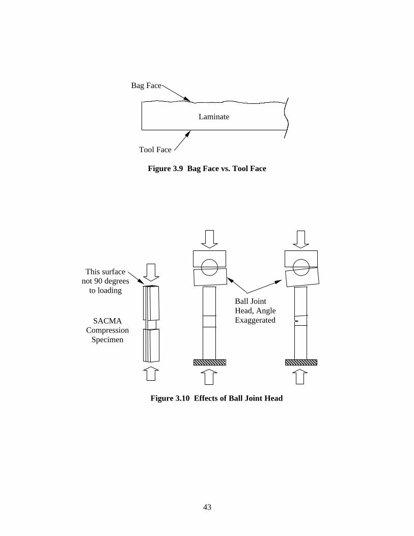
3.9 Bag Face vs. Tool Face 43

3.10 Effects of Ball Joint Head 43

3.11 Void Content Increase with Ply/Debulk Increase 44

3.12 Longitudinal Compressive Strength vs. Temperature 45

3.13 Longitudinal Compressive Modulus vs. Temperature 45

3.14 In-Plane Shear Strength vs. Temperature 46

3.15 In-Plane Shear Modulus vs. Temperature 46

3.16 Longitudinal Tensile Strength vs. Temperature 47

3.17 Longitudinal Tensile Modulus vs. Temperature 47

3.18 C-Beam Dimensions 48

3.19 C-Beam Cross Sectional Views 48

3.20 Four-Point Bending Test 49

3.21 Teflon Spacers to Allow Deflection 49

3.22 Beam 1 Test Results 50

3.23 Beam 2 Test Results 50

3.24 Beam Void Content Increase with Location 51

Chapter 4

4.1 Calculation of Fiber Angle 65

x

4.2 Specimen Skew Example 65

4.3 Reducing Skew by Combination of Distributions 66

4.4 Specimen Polishing Procedure 66

4.5 Beam Sample Polishing Procedure 67

4.6 Measurement of Ellipses That Intersect Selection Line 67

Chapter 5

5.1 Cumulative Distribution Function for Specimen with Lowest Skew 72

5.2 Cumulative Distribution Function for Specimen with Highest Skew 72

5.3 Cumulative Distribution Function of 948A1/M40J 73

5.4 949/M30GC Actual vs. Predicted Compressive Strength 73

5.5 948//M40J Actual vs. Predicted Compressive Strength 74

5.6 949/M30GC Beam 1 & 2 Actual vs. Predicted Compressive Strength 74

5.7 Formula vs. Experimental, Literature Data 75

5.8 949/M30GC RTA Sensitivity to ΩΩ, G12, F6 75

5.9 949/M30GC RTA Maximum Compressive Strength 76

5.10 949/M30GC RTA Normalized Maximum Compressive Strength 76

5.11 948A1/M40J RTA Maximum Compressive Strength 77

5.12 948A1/M40J Normalized RTA Maximum Compressive Strength 77

5.13 949/M30GC RTA Compressive Strength vs. Ave. Global Misalignment 78

5.14 948A1/M40J RTA Compressive Strength vs. Ave. Global Misalignment 78

5.15 949/M30GC RTA F1c vs. Ave. Global Misalignment , ΩΩ 79

5.16 948A1/M40J RTA F1c vs. Ave. Global Misalignment, ΩΩ 79

xi

Nomenclature

1C

6

12

f

( ) = Probability density function, PDFF( ) = Cumulative distribution function, CDFFV = Fiber volumeF = Longitudinal compressive strength

F = In-plane shear strength

G = In-pl

G

g

ane shear modulus

W = Potential energy = Angle of local misalignment, or simply "misalignment"

= Average angle of global misalignment

= Angle of global misalignment

=

αααΩ

f v

Standard deviation of local misalignment angle = Compression stress = Shear stress = Shear strain

= Volume fraction of fibers

στγ

1

Chapter 1: Introduction and Literature Review

1.1 Introduction

In the last 25 years, composite materials have proven themselves to be a cost

effective alternative to metals. Starting from aerospace applications, designers are

continually expanding their use into other industries such as marine, infrastructure, sports

recreation and medical instruments. Despite extensive experience with composites, a

large amount of testing is required (compared to metals) to have confidence in a

particular design. In the next decade, composite manufacturers and engineers will be

challenged to reduce the amount of testing required by improving manufacturing quality

and analysis techniques.

While the tensile strength of composite materials is very well understood, the

compressive strength of composites may still have significant variations from expected

values [1]. The main factors affecting compression strength are:

• Matrix properties

• Local/Global misalignment of fibers

• Void content

• Moisture and other contamination

When the direction of a fiber is not the intended direction, the angle difference is called

global misalignment. Local misalignment or just “misalignment”, is the angle at which

individual fibers vary from the average fiber direction. In the case of a single ply of

preimpregnated composite material, prepreg, misalignment is an inherent property of the

2

material and cannot be improved upon by the shop worker or tape laying machine.

However when two or more plys are in a lay-up, the misalignment will either remain

constant or get worse. Obviously, the shop worker or tape-laying machine will affect the

amount of global misalignment when making a lay-up.

Because of the possible reductions to compressive strength caused by the items

above, the aerospace industry uses a fixed ultimate compression strain allowable that

provides a margin of safety for variations in the material. Depending on the design,

extensive testing is required to validate the compression.

Ideally, compression strength could be measured from production parts without

costly test fixtures and without destroying the part. This investigation strives to reach

this ideal by showing that a compression strength model [2] and optical examination

technique [3] can predict strength of unidirectional composites in a production setting.

Fiber misalignment and matrix properties on compressive strength are measured and

input into the theoretical model. Although they are not active parameters in this study,

global misalignment and void content are measured and recorded. Moisture and

contamination effects are minimized since the tests were done in ambient conditions and

in a relatively clean workshop. Additionally, this study proposes an alternative method to

predict the compressive strength of composites with average global misalignment αG in a

[+αG]n or [-αG]n schedule. This method is an extension of the model proposed in [2].

Aurora Flight Sciences of West Virginia partly sponsored this research for the

purpose of determining properties of two material systems under investigation,

949/M30GC and 948A1/M40J. These materials were being evaluated for possible use on

3

an Unmanned Aerial Vehicle (UAV). Two beams were constructed and tested at Aurora

Flight Sciences were also used to determine the accuracy of this technique.

1.2 Literature Review

There is an enormous body of literature on the subject of prediction of

compression strength of unidirectional, 0 degree composites from basic material

properties in the time period 1965 to 1999. A brief review is shown here.

Rosen first proposed an analytical model to predict compressive strength

laminates in 1965 [4]. Rosen modeled a composite with straight fibers and assumed

linear material properties. Using energy methods in his derivation, he assumed that fiber

buckling was the mode of failure and found that in the limit, compressive strength equals

the elastic shear modulus. Microbuckling could be one of two types: In-phase (shear)

mode or Out-of-phase (extensional) mode as shown in Figure 1.1. The shear mode

required lower stress for failure but his predictions were two to three times higher than

actual values. Only when the shear stiffness was linearly varied to account for inelastic

behavior, did the results come closer to the actual values.

An important refinement of Rosen’s model was made in 1978 by Wang [5] which

included initial fiber misalignment, non-linear shear stiffness and non-linear analysis.

The misalignment factor was determined by fitting predicted and experimental data and

the non-linear shearing stiffness was modeled by piecewise linear segments. Using high

and low temperature tests, Wang found good agreement between predicted and actual

values.

4

In 1981, Maewal [6] modeled the buckling behavior using stability theory based

on Koiter’s theory of elastic stability. The results were very unexpected. When using

linear material properties, such as shear stiffness, fiber buckling was found to be

insensitive to initial misalignment and not expected to significantly reduce microbuckling

stress. This contradicted the results found by [5].

In the same year, Martinez and Piggott [7] devised a modified pultrusion

technique to study the effects of misaligned fibers in compression. By twisting tows of

fibers before introducing them into the resin, the authors claim to have added an average

misalignment angle of θ. Their data showed that up to θ = 10 degrees misalignment,

there was no significant effect on strength. More than likely, the “misalignment” induced

by this technique was similar to the case of a balanced, symmetric lay-up with [+θ/-θ]s.

The strength of this type lay-up is given by the stress transformation [8] and results in a

cosine square term applied to F1c. Thus at 10 degrees, the reduction in strength is only

3%. The authors also investigated the fiber matrix interface and concluded that poor

adhesion between fibers and matrix also had a detrimental effect on strength. Separately,

Piggott [9] concluded in 1981 that “in order to make a composite with good compressive

properties, the fiber should be hard, as straight as possible and well bonded to the matrix.

The matrix should have a high yield stress, tensile strength and compressive strength.”

This statement seems to contradict the earlier study since “straight” fibers imply low

misalignment.

A different approach to predicting compression failure was introduced by

Budiansky in 1983 [10]. Rather than microbuckling, Budiansky studied the mechanics of

fiber kinking. By assuming straight fibers and linear material properties, he found that a

5

zero-degree kink angle could reproduce Rosen’s results. As was well known, the kink

band angle is usually 30-40 degrees and so Budiansky modified the approach to include

non-linear material properties.

In 1987, Tang, Lee, and Springer [11] studied the effects of cure pressure on void

content in a lay-up. By adjusting pressure during the cure cycle, they were able to change

the void content, which they measured optically. In compression strength and

interlaminar shear strength tests, they found that decreasing the void content helps these

properties up to a point. Below 3-4% void content, the strengths do not improve

significantly. One questionable area in this report is the high void content 10%, 6%, 5%

reported for cure pressures 20, 55, 80 psig respectively. This may be due to calibration of

the optical method used. Nevertheless, the authors did establish a relationship between

compressive strength and other key parameters, such as void content.

In the same year, Yurgartis [3] developed an important optical technique to

measure the initial fiber misalignment allowing it to be measured for the first time. This

opened the way for researchers in the late 80’s and early 90’s to quantify and deepen the

analysis of compression. Using the optical technique, Mrse and Piggott [12], Yurgartis

and Sternstein [13], Barbero and Tomblin [14], Lagoudas and Saleh [15], Haberle [1]

found that higher initial fiber misalignment did, in fact, reduce compression strength.

Among these, [13], [16] added more evidence about the direct relationship between

compressive strength and shear stiffness. Furthermore, Steif [17] proposed that the

tangent hyperbolic function could be used to characterize shear stiffness because it

successfully captured the antisymmetric nature of shear stiffness. Previously, piecewise

6

continuous linear segments or truncated polynomials were adequate but were very

cumbersome when used in stability analysis.

Shuart [18] studied the effects of global misalignment on [±θ]s laminates in a

paper published in 1989. Shuart proposed three different failure mechanisms depending

on θ. For 0<θ<15 degrees, interlaminar shear was the dominant failure mode. For

15<θ<50, it was in-plane matrix shearing and for 50<θ<90, matrix compression was the

failure mode. His model included non-linear analysis and initial fiber waviness. The

strength predictions were very good for 50<θ<90, but for 0<θ<50 they were generally

conservative by a 0 to 30% margin.

In 1997, Tomblin, Godoy and Barbero [19] used stability theory to show that fiber

buckling was sensitive to initial misalignment when non-linear shear stiffness (tangent

hyperbolic) was used. When linear shear stiffness was used, fiber buckling was found to

be insensitive to initial misalignment as [6] had proposed 15 years earlier. Later, [14]

combined the continuous damage mechanics work of Kachanov [20] and a statistical

approach to fiber misalignment to arrive at a numerical solution to the prediction of

compressive strength. In 1998, Barbero [2] derived an explicit equation for compression

strength which utilized the continuous damage mechanics and statistical approaches used

in [14].

Despite the large body of work focused on correlating compressive strength with

other basic material properties, the majority of studies use empirical parameters to

correlate strength. Only a few studies base the prediction of compression specimen

strength on actual measured properties of the specimen [1], [14], [21]. To date, there is

7

no known study that correlates compressive strength of production parts with basic

material properties (shear stiffness and strength, but excluding compressive strength).

In industry, the compressive strength of production parts is predicted by finite

element analysis using a database of material properties. Later, compressive strength and

other design parameters are confirmed with a testing program. In the May 1999 ASTM

Symposium on Composite Structures, [22] presented the “Building Block” structural

qualification program for the RAH-66 Comanche Attack Helicopter as shown in Figure

2.2. As can be seen, structural qualification is composed of several levels of testing to

gain confidence in the material allowables and analysis methods. Many times this is

because the performance of a material as a laboratory specimen is better than as a

production part. Lab specimens are fabricated under ideal conditions and tested in very

controlled circumstances whereas production parts are open to the many variables in

manufacturing and testing.

Because the full “Building Block” testing program is costly and time consuming,

efforts are underway to use a “Modified Building Block” approach when possible [23]

and reducing testing in the areas shown in Figure 1.2. In this process, the amount of

testing is reduced to the minimum required based on previous testing experience and

engineering judgement. The minimum required tests will usually involve one or more of

the following: compressive strength, compressive strength after impact, shear strength

and compression-shear interaction.

Industry has signaled a clear need to better predict the strength of composites to

reduce development time and cost. At the same time, the literature shows that studies in

the 90’s have made practical compressive strength prediction more and more a reality.

8

In-Phase (Shear) ModeOut-of-Phase

(Extensional) Mode

Figure 1.1 Modes of Fiber Buckling

FullScale

Testing

Sub-ComponentsTesting

Structural Elements Testing

Determination of Design Allowables

Material Properties Testing

Figure 1.2 Building Block Approach to Testing

Area forpossiblereductionof testing

9

Chapter 2: Theoretical Modeling

The theoretical model presented by Barbero in [2], [14] draws upon many of the

references cited in the literature review. Fundamentally, it is a unique approach because

it integrates a statistical representation of the composite with a continuum damage

mechanics model to arrive at an explicit equation for compressive strength in terms of

measured properties, shear modulus G12, shear strength F6 and the standard deviation of

the fiber misalignment angle, Ω.

2.1 Composite Shear Response

The shear stress-strain relationship for polymer-matrix composites is not linear

and can be represented as

γ=τ

6

12 6 F

GtanhF (2.1)

or a quadratic polynomial such as

.C-G 2212 γγ=τ (2.2)

The hyperbolic tangent function nicely represents the anti-symmetric nature of the shear

response. The quadratic polynomial has the advantage of being easier to manipulate than

the hyperbolic tangent expression but must be used where the fit is good. Consequently,

the tangent hyperbolic was used when finding the exact but implicit solution that is

solved by numerical methods in [14], and the quadratic polynomial was used when

deriving an explicit solution in [2]. The derivation of the explicit solution is shown here.

10

The constant C2 can be found solving the above two equations for C2 and

restricting γ to not exceed γlim.

12

6lim G

F2=γ

(2.3)

( )6

212

2 4F

GC −= (2.4)

where γlim is an upper bound to the shear strain at which most composite materials,

carbon-epoxy and glass-polyester, fail in compression. A comparison is shown in Figure

2.1 between the two equations and experimental results for 949/M30GC using the ASTM

5379 shear test.

Other micromechanical models that use in-situ properties, such as shear modulus of

the matrix, Gm, were purposely avoided. This is because it would be very difficult to

verify if the compression strength prediction was correct since the in-situ properties are

very difficult to measure and could be different than properties in the bulk matrix.

2.2 Fiber Misalignment

Since the misalignment of fibers is very small, a microscope is used to measure this

misalignment in the cross-section. The technique is described in detail in Chapter 4.

Experimentally, the distribution of angles has been shown to be Gaussian or normal,

hence the probability is given by

∞<α<−∞

Ωα−

πΩ=α ,

22

1)(

2

2

ef (2.5)

11

where Ω is the standard deviation, α is the misalignment angle and f(α) is the probability

density function. The probability of getting an angle between -α and α is given by the

integral

( ) ( ') 'F f dα

α

α α α−

= ∫ (2.6)

Changing to the normalized misalignment variable z, defined as

2 zΩ

α= (2.7)

the cumulative distribution function can now be described as a “folded” function as

below

')'exp(2

erf(z)F(z)0

2 dzzz

∫ −π

== (2.8)

Since the integral of a transcendental equation is difficult to manipulate later, it is

approximated by a quadratic polynomial,

267z0.34555809-8z1.17964385 F(z) = (2.9)

for the interval 0<α<3Ω, which is sufficiently broad to model the problem at hand [2].

2.3 Imperfection Sensitivity Equation

The relationship between buckling stress and misalignment is called the imperfection

sensitivity curve. Unlike equilibrium based models that compute shear strain only at the

inflection points of the given fiber shape, the shear strain energy of the entire

12

Representative Volume Element, RVE, is modeled in the equation. This model assumes

that all fibers are misaligned at the same angle as shown in Figure 2.2.

The model uses the principle of total potential energy and assumes axial effects can

be neglected. In this one dimensional case, an expression can be written where only the

shear energy is considered in the total potential energy

lPdAdxdWl

∆−γ= ∫ ∫ ∫γ

0 A 06F (2.10)

where P is the end load; ∆l is the end shortening; τ and γ are the shear stress and strain; l

and A are the length and area of the RVE. Using the shear stress as described in equation

(2.2), equation (2.9) can be solved for the equilibrium stress as

πα+γγ

+α+γ

γ=γασ

)(3

C

3

8G),(

2212 (2.11)

This equilibrium equation produces a family of curves for 949/M30GC as in Figure

2.3. Thus for every angle α, there is a maximum value of compression strength before

buckling occurs. The curve that joins all the maxima is

2 2 12 212

2 2 12

4 2 ( 8 3 ) 16( )

33 ( 8 3 )

C C G CG

C C G

α α π ασ αππ α α π

− += − +

− − +(2.12)

2.4 Continuum Damage Model

At any time during the loading of the specimen, the applied stress is equal to the

effective stress in the composite times the area that remains unbuckled

)](1)[( αω−ασ=σ (2.13)

13

In this equation, 0 ≤ ω(α) ≤ 1 is the area of the buckled fibers per unit of initial composite

area. For any value of effective stress, all fibers having more than the corresponding

value of misalignment given in Figure 2.4 have buckled. The area of the composite with

buckled fibers ω(α) is proportional to the area under the normal distribution located

beyond the misalignment angle ±α. Therefore ω(α) is given by:

∫ ∫α

α−

∞

α

αα=αα−=αω ')'(2')'(1)( dfdf (2.14)

Substituting into equation (2.13) the compressive strength of a composite can be found as

1c max [ ( ) ( ') ']F f dα

α

σ α α α−

= ∫ (2.15)

Graphically, F1c can be seen as the maximum of the applied stress curve in Figure 2.5.

2.5 Explicit Equation

Substituting equation (2.9) for the integral in equation (2.15), the applied stress

equation (2.13) becomes

).()()( zFzz σ=σ (2.16)

which simplifies subsequent derivations.

To find the maximum explicitly, equation (2.16) is expanded into a truncated

polynomial about α = Ω (or z = (1/2)1/2 ), which is an adequate range for a broad class of

materials [2]. The root of the derivative can then be found explicitly as

14

2 3 3 4 2 212 2 2 12 2

1 2 2 2 312 2 12 2

3 2 2 2 22 12 2 12 2

2 22 12 2 12

1019.011 375.3162 845.7457

(282.113 148.1863 132.6943 )

457.3229C 660.77 22.43143

(161.6881 138.3753 61.38939

c

G C C G CF

g G C G C

G C G C

g C G C G

Ω − Ω − Ω=

+ Ω − Ω − Ω

Ω − Ω − Ω×

+ Ω − Ω − 2,

)

(2.17)

where g is the following

).424778.90.8( 1222 GCCg −ΩΩ= (2.18)

Substituting C2 and g, equation (2.4) and (2.18), into (2.17), the following

expression can be written:

1 3

12 4

2 4 33

22 3

23 2

4

24

103961 C -10979.6-8432.03 19037.205 124.653

64

(12191.07 1881.87 176.286 7979.978 ) 2.3562

C ( 7.146 41.298 5.608 )2

cF CG C

χπ

χ χ χ χ

χχ χ χ χ

χχ χ χ

=

= − − −

+ + + + +

= − − + +

22

12

6

2.356

(10.106 34.594 61.389) 2.3562

G

F

χ

χχ χ χ

χ

+ + − +

Ω=

(2.19)

15

Taking into account that the dimensionless compression strength, F1c/G12,can be

modeled in terms of a dimensionless number, χ, the following numerical approximation

can be made of the ungainly equation (2.19) as follows:

1

12

1

.21

.69

cb

FG a

a

b

χ = +

== −

(2.20)

Constants a and b are found by using a full factorial design within the range

12

6

0.5075 Msi 1.160 Msi

5.8 ksi F 23.2 ksi

1 3.5

G< << <

° < Ω < °

This gives n = 33 = 27 points for which the dimensionless compression strength can be

computed using equation (2.19) to find constants a and b.

2.6 Global Misalignment

When a lay-up has average global misalignment αG and is balanced and

symmetric [±αG]s, the maximum compressive stresses can be found by stress

transformation [8]. The compressive stress is given by (F1c) x (cosine2(αG)). There is

good agreement with the data for 0<αG<10 degrees [18]. However, there exists no

known method for estimating the strength of laminates with average global misalignment

and [+αG]n or [-αG]n stacking schedule.

16

When there is global misalignment, the representative volume element is as

shown in Figure 2.6. The potential energy (2.9) and equilibrium (2.11) equations still

apply but the distribution of fiber angles (2.5) and normalized misalignment variable

(2.7) are shifted by the average angle, αG.

2

2

( )1( , ) ,

22G

Gf eα αα α α

π − −

= −∞ < < ∞ ΩΩ (2.21)

2 z

Ω

α−α= G (2.22)

The probability density function from 0 to ∞ is no longer the probability density function

(2.8) because there is no symmetry about zero. Therefore, the quadratic polynomial

approximation (2.9) cannot be used. Instead, the function can be integrated numerically

as shown in Figure 2.7 which is for the case of 0 degree average global misalignment and

fixed value of Ω = 1.15 degrees. Notice that there are slight differences between the

previous quadratic polynomial approximation and the discrete numerical integration

within the range of 0 < α < 3Ω for which equation (2.9) is valid. To illustrate the

integration, Figure 2.8 shows the case of 1.0 degree average global misalignment. The

function is folded about zero and the two distributions are added together. For

comparison, the probability density function for 0 degree average global misalignment is

shown too.

Using this technique, a family of probability density functions at various average

global misalignment angles can be determined as shown in Figure 2.9. Figure 2.10

shows the integration of these curves (2.21) to obtain the cumulative distribution function

at these angles of average global misalignment. When multiplied by the effective stress

17

(2.12), the resulting applied stress curves are shown in Figure 2.11. The maximum of

each curve represents the compressive strength at the given average global misalignment

angle with Ω = 1.15 degrees. This technique is informally called the “Method of Shifted

Distributions”.

Note that Figure 2.7 through 2.11 were for a fixed value of Ω. If Ω was taken at

different values, it would produce a family of curves for F1c as a function of Ω and αG.

Figure 2.12 shows the compressive strength F1c as a function of αG when the standard

deviation of fiber misalignment is fixed at various values. An individual curve represents

a part fabricated with a prepreg lay-up that has Ω and oriented with an average global

misalignment of αG with respect to the nominal direction.

18

NTP-4-9 Experimental vs. Curve Fit Shear Stress

0

2000

4000

6000

8000

10000

12000

0 0.01 0.02 0.03 0.04 0.05 0.06 0.07 0.08 0.09 0.1

Shear Strain [rad]

Sh

ear

Str

ess

[psi

] Experimental

Tangent Hyperbolic

Quadratic Polynomial

Area of Approximation,0 < γ < 2F6/G12

Figure 2.1 Range of Shear Stiffness when using Quadratic Polynomial

RVE

α = αmax

e

Q

L

x, u

z, u

α = 0

wi

wt

A

Figure 2.2 Representative Volume Element

σ

19

949/M30GC Stress vs. Shear Strain, Misalignment

0

100

200

300

400

500

600

700

0 0.01 0.02 0.03 0.04 0.05 0.06

Shear Strain [rad]

Co

mp

ress

ive

Str

ess

[ks

i]α = 0.01 Ωα = 0.1 Ωα = 0.5 Ωα = 1.0 Ωα = 2.0 ΩMaxima

Ω = 1.15 deg

Figure 2.3 Equilibrium States for Various Values of Misalignment

949/M30GC Compressive Stress vs. Misalignment

0

100

200

300

400

500

600

700

-10 -5 0 5 10

Misalignment [degree]

Str

ess

[ksi

]

Figure 2.4 Imperfection Sensitivity Plot

20

Figure 2.6 Representative Volume Element with Global Misalignment

α = αmax

e

Q

L

x, u

z, u

α = 0

wi

wt

RVE

A

αG

Combined Buckling/Misalignment for 949/M30GC

0.00

0.10

0.20

0.30

0.40

0.50

0.60

0.70

0.80

0.90

1.00

0.00 0.50 1.00 1.50 2.00 2.50 3.00

Normalized Misalignment α/Ωα/Ω

No

rmal

ized

Str

ess

F6

/ G12 Normalized Effective Stress

Normalized Applied SressProbability Density FunctionF(z)

Max Value = .271Max at 1.52

Figure 2.5 F1c at Maximum of Applied Stress

σ

21

Numerically Integrated CDF

0

0.1

0.2

0.3

0.4

0.5

0.6

0.7

0.8

0.9

1

0 1 2 3 4 5

Misalignment [degree]

Cu

mu

lati

ve D

istr

ibu

tio

n F

un

ctio

n, C

DF

Probability Distribution Function

Quadratic Polynomial CDF

Numerically Integrated CDF

Figure 2.7 Numerical Integration and Quadratic Polynomial Function

Shifted Probability Density Function

0

0.1

0.2

0.3

0.4

0.5

0.6

0.7

0.8

0 1 2 3 4 5

Global Misalignment [degree]

Pro

bab

ility

Den

sity

Fu

nct

ion

[1/

deg

]

0 Deg Ave Global Misalignment

1 Deg Ave. Global Misalignment

1 Deg Ave. Global Misalignment, Folded

1 Deg Ave. Global Misalignment, Combined

a

b

a+b

Figure 2.8 Probability Density Function at 0, 1.0 Ave. Global Misalignment

22

F(z) by using Excel discrete sums

0

0.1

0.2

0.3

0.4

0.5

0.6

0.7

0.8

0 1 2 3 4 5Global Misalignment [degree]

Pro

bab

ility

Den

sity

Fu

nct

ion

[1/

deg

] 0.0 Deg Ave. Global Misalignment0.5 Deg Ave. Global Misalignment1.0 Deg Ave. Global Misalignment2.0 Deg Ave. Global Misalignment3.0 Deg Ave. Global Misalignment

Figure 2.9 Probability Density Functions at Ave. Global Misalignments

F(z) by using Excel discrete sums

0

0.1

0.2

0.3

0.4

0.5

0.6

0.7

0.8

0.9

1

0 1 2 3 4 5

Global Misalignment [degree]

Cu

mu

lati

ve D

istr

ibu

tio

n F

un

ctio

n

0.0 Deg Ave. Global Misalignment

0.5 Deg Ave. Global Misalignment

2.0 Deg Ave. Global Misalignment

1.0 Deg Ave. Global Misalignment

3.0 Deg Ave. Global Misalignment

Figure 2.10 Cumulative Distribution Functions

23

Applied Stress vs. shift

0

100

200

300

400

500

600

700

0.00 1.00 2.00 3.00 4.00 5.00

Global Misalignment [degree]

Co

mp

ress

ive

Str

ess

[ksi

]

Effective Stress0.0 Deg Ave., Applied Stress0.5 Deg Ave., Applied Stress1.0 Deg Ave., Applied Stress2.0 Deg Ave., Applied Stress3.0 Deg Ave., Applied StressMaximums

Figure 2.11 Applied Stress at Different Global Misalignments

0

100

200

300

400

500

600

700

0 2 4 6 8 10

Average Global Misalignment [degree]

Co

mp

ress

ive

Str

eng

th [

ksi]

Ω = 0.0Ω = 1.15Ω = 3.0Ω = 10.0

Figure 2.12 949/M30GC F1c vs. Average Global Misalignment

24

Chapter 3: Material Characterization and Beam Testing

The matrix of tests requested by Aurora Flight Sciences to characterize the Cytech

Fiberite 949 HYE/M30GC and the 948A1 HYE/M40J material systems at –125F, RTA,

180F is shown in Table 3.1. The first material, 949 HYE/M30GC, is a carbon/epoxy

prepreg commonly used for golf club shafts and tennis rackets. The second material,

948A1 HYE/M40J, is also a carbon/epoxy prepreg that has an intermediate modulus fiber

and a relatively stiffer matrix.

Phase I tests were arranged to study the effects of “debulking” on void sensitive

properties. For example, to debulk a lay-up of 100 plys of prepreg, the lay-up is vacuum

bagged every 10 plys to reduce voids or air pockets that occur in the process. This study

looked at 5, 10 and 20 plys/debulk in the hope of finding the “knee” in the curve where

increasing the number of plys/debulk had diminishing improvement in material

properties. In Phase I, the compression tests were contracted to Touchstone Research

Laboratories.

Phase II tests were intended to study the effects of temperature on mechanical

properties. Phase II high and low temperature tests were contracted to Orange County

Material Test Labs (OCM). All the results of the material characterization program are

shown here but only the compression and shear tests are discussed in detail.

25

3.1 Compression/Shear Test Selection

Initially, the ASTM D3410 “IITRI” test was used for Phase I compression testing.

It utilizes a shear loaded specimen as shown in Figure 3.1. Since the IITRI test gave low

values of compression strength as in Table 3.2, the SACMA SRM-1R-94 procedure was

selected for all subsequent compression tests (Figures 3.2, 3.3). Because of its end

loaded specimen, this test typically provides compressive strengths 5% better than the

D3410 “IITRI” method. The SACMA test also allowed easier comparison with

manufacturer’s data because composite parts manufacturer’s and prepreg producers use it

more often.

To measure shear strength and modulus, the D5379 “Iosipescu” method was

selected (Figures 3.4 and 3.5). MicroMeasurements Shear Gages N2P-08-C032A-500

were used since they average the shear strain over the entire region between the notches

of the specimen. Modulus data was taken between 1000-6000 microstrains from back-to-

back shear gages and the results from each side were averaged together. A detailed

description of the test methods can be found in Appendix A.

3.2 Compression/Shear Specimen Preparation

The prepregs were laid up by hand and cured in an oven at 275 deg F for 90

minutes with approximately 27 in. Hg vacuum bag pressure. A 7 ply [0 deg] panel was

26

made for the compression specimens and a 20 ply [0 deg] panel was used for the shear

modulus and shear strength specimens. The 7 ply panel was cured with peel ply and caul

plates on both sides of the panel so that the surface would have very little waviness and

the thickness would be relatively uniform (Figure 3.6). To achieve low global

misalignment, great care was taken to align the 7 plies of the prepreg to the manufactured

edge of the tape. The 20 ply panel was cured without caul plates or peel ply because the

variations in thickness were judged to be small when compared to the total thickness.

Panel sizes were 12” X 18-24”. The manufacturing history of each panel made in this

study can be found in Appendix A.

The specimen tabs were bonded to the panels using technique similar to the one

outlined in [1]. A room temperature cure paste adhesive, Magnabond 6380, was used to

bond prefabricated glass/carbon tabs to a panel before cutting. A tile saw was used to

rough cut the specimen panel to size. A surface grinder installed with a diamond blade

was then used to make the final cuts. The surface grinder mounted with an 80 grit wheel

was used to grind the surfaces square. A diamond bit on a milling machine ground the

notches in the shear specimen.

3.3 Data Normalization

The panel thickness for the fiber driven property tests was very small –

approximately 0.040 inches. Since local variations in thickness could cause big changes

in the final results, the thicknesses were normalized to an average value. This method is

consistent with MIL-HDBK-17-E practices.

27

The nominal thickness was found by taking the average thickness of several specimens

that were sanded with 50 strokes of 400 grit sandpaper in the gage section prior to

bonding strain gages.

Since the panel thickness for the matrix driven properties was much larger,

approximately 0.125 inches, local variations in thickness were not judged to cause a

strong effect on the results. Therefore, the data reported was the raw data and was not

normalized. In-plane shear strength, F6, was taken where there was a significant change

in the slope of the load-displacement plot (Figure 3.7). In some cases, especially with the

tougher resin 949, there was no significant change and so F6 was taken at the slight dip

between the initial curved section and the linear section of the load-displacement plot

(Figure 3.8).

At the customer’s request, the material properties were reported at the fiber

volumes (FV) in which they were tested and not normalized to a constant FV value (i.e.

60% FV). In order to predict strength with G12 and F6, these values are normalized to

the FV of F1c for the compressive strength specimens as is shown in Chapter 4.

3.4. Difficulties in Obtaining F1c

Compression is by far the most difficult of the tests shown in the test matrix

because it requires a high level of precision in the specimen and very good test set-up.

Thickness Nominal

ThicknessSpecimen ValueTest Value Normalized ×=

28

Many attempts were made to get the final values reported in the previous tables.

Highlights of the compression tests are shown in Table 3.3.

3.4.1 Sanding

Initially, the specimen panels were made without peel ply or caul plates because

peel ply and caul plates they were used only selectively for fabrication of actual parts

made at Aurora Flight Sciences. This produced a panel with a rough, wavy surface on

the bag face and a smooth surface on the tool face (Figure 3.9).

The panels were sanded on the bag face to make a smooth surface for the tabs and

to get a uniform thickness for measurement of thickness. Tests No. 1 and 2 in Table 3.3

showed that the sanding had reduced the strength from 170 to 140 ksi. Sanding had

effectively removed one ply from the panel. However, even without sanding, the strength

values were low compared to manufacturer’s values and it would not be clear what

thickness to use for comparison of strength.

3.4.2 Peel Ply & Caul Plates

In order to remove the waviness on the bag face and to straighten the fibers to

increase the strength, peel ply and caul plates were used on both sides of the lay-up.

These were used on the manufacturer’s panel when they produced their specimen but

again, were only selectively used in the shop at Aurora Flight Sciences. Tests No. 2,3 in

29

Table 3.3 showed that the peel ply/caul plates did improve strength, but still not to the

level of the manufacturer.

3.4.3 Surface Ground/Solid Compression Head

Originally, the edges of the compression specimen were cut with a diamond saw

blade mounted on a modified grinding table. This cut the edges smoothly but at a slight

angle. To compensate for this angle, it was believed that a ball joint head would adjust

the compression head to fit the exact angle of the end specimen. In truth, the adjustable

head was most likely causing a premature failure of the specimen by concentrating the

load in the area when the collapse first takes place (Figure 3.10).

To solve this problem, a surface grinder was purchased to grind accurate, square

ends on the specimen after being cut by the diamond saw. The test fixture was modified

from a ball joint head to a solid head. Tests No. 3,4 in Table 3.3 showed that these

changes increased the compression strength significantly.

3.4.4 Bolt Torque

Bolt torque on the fixture made a significant difference on final strength as in Test

No. 4, 5 in Table 3.3. The SACMA standard does call out a range of bolt torques but

other similar standards such as the modified D695 call for hand tight bolts. After

discovering this fact, bolts were held to a constant torque on the WVU tests to

approximately 5 in-lbs.

30

3.4.5 Bond Tabs at High Temperature

There was a concern that because the two testing labs used film adhesives cured at

250 F, it would cause a post-cure to this material system (which is cured at 275F). This

would artificially increase their strength values. WVU used a room temperature cure

adhesive throughout the program but Tests No. 6,7 in Table 3.3 showed that there was no

noticeable improvement in strength from the post-cure of WVU’s own specimens. If

there was an effect, it was small compared to other aspects of the testing.

3.5 Experimental Results

The test results summary from Phase I is shown on Table 3.2. The details of

Phase I results are in Appendix B. The effects of debulking were not clear from the

Phase I results. It is expected that voids increase with increasing plys/debulk and

therefore mechanical properties (excluding density) decrease with increasing plys/debulk.

Indeed in the “Delta” column of the table, many of the properties show a small decrease

in properties. However, the two most important properties, Longitudinal Compressive

Strength and In-Plane Shear Strength, are increasing with increasing plys/debulk. This

brings into question the validity of the entire Phase of this study.

More than likely, the panels (1 foot by 2 foot) made were too small to show any

effect of voids and larger panels, e.g. 20 feet long, would show a meaningful difference.

As shown in Figure 3.11, the void content at the center of a 20 ply panel with 5

plys/debulk is 1.066%. On the same size panel but with 20 plys/debulk, the void content

31

is 1.736%. This is a 63% increase in void content but the absolute value is still below

2%, which is considered to be low. Thus, the differences in material properties were

probably hidden by the variations in test specimen preparation, test set-up, etc.

Fortunately, the effect of temperature on mechanical properties is clear in the

Phase II results. Higher temperatures are expected to lower the material properties and

the Tables 3.4, 3.5, 3.6 confirm these expectations. The details of Phase II results are in

Appendix C. Graphs of these trends are shown in Figures 3.12 through 3.17. It is

important to note there is a sharp decrease in shear modulus when going from RTA to

180 F (Figure 3.15).

3.6 Beam Preparation

Two C-section beams were made at Aurora Flight Sciences of West Virginia.

These beams were made of the 949 HYE/M30GC and were relatively thick hand lay-ups

cured at 275F with 27 in Hg vacuum pressure (Figure 3.18). The beam caps were much

thicker towards the ends and thinner in the test section in the center. In Beam 1, the test

section caps consisted of 60 plys of 0 deg and ±45 deg on top and bottom. In Beam 2, the

test section had 56 plys with one ±45 deg ply every 8 plys of 0 deg. The shear web at the

test section was made of a honeycomb core with ±45 deg plies for shear stiffness and 90

deg plies for transverse stiffness. Twenty eight total strain gages were placed on the

beam with twelve gages on the test section as shown in Figure 3.19.

32

3.7 Beam Testing

Two C-section beams were tested in four point bending at Aurora Flight Sciences

(Figure 3.20). These beams were restrained at their ends and pulled at two points roughly

¼ of the length from the ends. Teflon pieces were used to separate the loading fixture

from the beam table to allow it to displace in the transverse direction. Roller pins

allowed the loading fixture to move along the table (Figure 3.21).

3.8 Beam Test Results

The strain gage data shown in Figure 3.22 and 3.23 show that the highest

compressive strain experienced on Beam 1 was 7500 microstrains and on Beam 2 was

7772 microstrains. From visual inspection, it was confirmed that compression (and not

shear) was the most likely mode of failure because of the presence of kink bands at the

damaged area. There was also a significant void content tested in Beam 1. Figure 3.24

shows the increase in voids from 2.679% at the end of the beam, to 4.636% close to the

middle. Nevertheless, the ultimate strain capability of the beams were very close to the

8043 microstrains ultimate capability of the 949/M30GC compression specimens.

33

Phase I Phase II 949/M30GC 949/M30GC 948A1/M40J Ply/ Debulk Ply/ Debulk Ply/ Debulk

Test Property Temp [F] 5 7 10 20 7 or 20 7 or 20

+180 - - - - 5 10

RTA 3 (5) a 4 3 - (20)

-125 - - - - 5 5

+180 - - - - - -RTA 5 - 5 - - (6)

-125 - - - - - -+180 - - - - 5 5

RTA (5) - (5) (5) - (5)

-125 - - - - 5 5

+180 - - - - - 5

RTA - - - - (6) (6)

-125 - - - - - 5

+180 - - - - - -RTA (5) - (5) (5) - (5)

-125 - - - - - -

Density D 792-91 Bulk Density w/Pycnometer RTA (10) - (5) (10) (20) (5)

Void Content Theor.&Bulk Density w/Pycno. RTA (10) - (5) (10) (20) (5)

Glass Transition D 3418-97 Tg w/DSC @ Tg - - - - (2) (2)

Long/Trans CTE E831-93 -125 to +180 - - - - 3 3

Note a: "( )" denotes number of tests done by WVU. If # of strength tests differ from # of modulus tests, the # of strength tests are shown here. Touchstone Research Labs performed all tests in Phase I not done by WVU. Orange County Materials Test Labs performed all tests in Phase II not done by WVU.

Longitudinal Compressive Modulus & Ultimate Strength:

E1C, F1C

Transverse Compressive Modulus & Ultimate Strength:

E2C, F2C

Compression SRM-1R-94 (SACMA)

& D3410-95 (IITRI)

Shear Modulus & Ultimate Shear Strength:

G12, F12

ShearD 5379-93(Iosipescu)

Longitudinal Tensile Modulus, Ultimate Strength &

Longitudinal Poisson's Ratio: E1T, F1T, v12

Trans. Tensile Modulus, Ult. Strength & Transverse

Poisson's Ratio: E2T, F2T, v21

Tension

D 3039-95a

Long./Trans. αT w/DTA

Table 3.1 Aurora Flight Sciences Test Matrix

34

Average Values Delta Retest Fiberite5 10 20 5 to 20 ply 7 Values

Property Notation Units plys/debulk plys/debulk plys/debulk [%] plys/debulk

1. Long. Compressive Strength F1C [ksi] 112.0 1 130.5 1 135.2 120.7% 185.0 2 195.8 2,3

2. Long. Compressive Modulus E1C [Msi] 18.18 4 17.97 4 17.96 4-1.21% 23.0 5 low 20's 6

3. Trans. Compressive Strength F2C [ksi] 24.9 24.6 - -1.20% - -

4. Trans. Compressive Modulus E2C [Msi] 1.070 1.028 - -3.93% - -

5. In-Plane Shear Strength F12 [ksi] 9.80 10.04 10.06 2.61% - 9.72 7,8

6. In-Plane Shear Modulus G12 [Msi] 0.576 9 0.541 9 0.537 9-6.77% - -

7.Trans. Tensile Strength F2T [ksi] 4.68 4.69 4.76 1.71% - -

8.Trans. Tensile Modulus E2T [Msi] 1.059 1.040 1.008 -4.82% - -

Minor Poisson's Ratio v21 - 0.00903 0.00894 0.00762 -15.61% - -

9. Apparent (Bulk) Density rhoa [gm/cc] 1.4848 1.4833 1.4788 -0.40% - -

Void Content: Near Edge 10 Void [%] 1.857 1.781 2.092 12.65% - -

Void Content: Near Center 10 Void [%] 1.066 - 1.736 62.85% - -Notes: 1. IITRI D3410-95, fiber volume 54.13%. 8. Inter-laminar Shear Strength used, no In-Plane 2. SACMA SRM-1R-94, fiber volume 61.45%. Strength provided. 3. Fiberite fiber volume adjusted to 61.45%. 9. Revised with correct usage of shear gage data. 4. Fiber volume 54.13%, using SACMA SRM-1R-94. 10. Panel length 22", width 12", thickness .120". 5. Fiber volume 61.45%, using SACMA SRM-1R-94. 6. Fiberite said reasonable to get low 20's [Msi]. 7. Fiberite fiber volume adjusted to 54.13%.

Table 3.2 Phase I Test Results

35

No. Panel Sanded Unsanded Peel Ply & Surface w/ 250 F Ball Joint Solid Bolts Bolts 948A1/M40J 949/M30GC

NTP- Caul Plate Ground Post Cure Head Head Hand Tight Tight [ksi] [ksi]

1. 8,7 Y Y Y 140 1 139

2. 8 Y Y Y 170 1 ----

3. 11,15 Y Y Y Y 182 143

4. 17,15 Y Y Y Y Y 194 185

5. 17 Y Y Y Y Y 216 ----

6. 16 Y Y Y Y Y Y 204 ----

7. 16 Y Y Y Y Y 219 ----

Average of Dashed Box Values 208

Notes: 1. Used .039" sanded thickness for stress calculation.

Table 3.3 Highlights of Compression Testing

36

948A1 HYE/M40J 949 HYE/M30GCProperty Notation Units Temp Mean FV% Cv Mean FV% Cv

1. Longitudinal Compressive Strength F1C [ksi] 180 F 194 59 9.83 149 61 2.92

RTA 208 59 5.83 185 61 9.34

-125 F 223 59 6.76 226 61 4.13

2. Longitudinal Compressive Modulus E1C [Msi] 180 F 24.8 59 4.00 21.0 61 0.83

RTA 28.8 59 4.34 23.0 61 0.92

-125 F 41.7 59 5.13 41.8 61 8.48

3. Transverse Compressive Strength F2C [ksi] RTA 27.2 52 5.06 24.9 54 3.29

4. Transverse Compressive Modulus E2C [Msi] RTA 1.15 52 7.63 1.07 54 3.49

5. In-Plane Shear Strength F12 [ksi] 180 F 8.93 52 1.12 6.07 54 5.40

RTA 11.35 52 1.59 9.80 54 5.07

-125 F 14.28 52 5.72 16.01 54 4.58

6. In-Plane Shear Modulus G12 [Msi] 180 F 0.439 52 6.23 0.365 54 5.64

RTA 0.625 52 1.56 0.576 54 3.67

-125 F 0.676 52 4.65 0.627 54 2.51

7. Longitudinal Tensile Strength F1T [ksi] 180 F 368 59 2.03 ---- 61 ----

RTA 336 59 5.99 451 61 5.55

-125 F 290 59 11.27 ---- 61 ----

8. Longitudinal Tensile Modulus E1T [Msi] 180 F 33.0 59 6.44 ---- 61 ----

RTA 32.5 59 1.74 24.7 61 1.65

-125 F 31.7 59 2.42 ---- 61 ----

Table 3.4 Phase II Test Results, Page 1

37

948A1 HYE/M40J 949 HYE/M30GCProperty Notation Units Temp Mean FV% Cv Mean FV% Cv

9. Major Poisson Ratio v12 [ ] 180 F 0.310 59 9.96 ---- 61 ----

RTA 0.288 59 11.31 0.275 61 11.05

-125 F 0.277 59 13.26 ---- 61 ----

10. Minor Poisson Ratio v21 [ ] RTA 0.01024 52 47.43 0.00903 54 11.54

11. Transverse Tensile Strength F2T [ksi] RTA 5.47 52 6.81 4.68 54 7.28

12. Transverse Tensile Modulus E2T [Msi] RTA 1.00 52 2.93 1.06 54 4.40

13. Panel Apparent Density: Edge, t = ~.125" ρ [gm/cc] RTA 1.5043 52 0.02 1.4788 54 0.03

14. Panel Void Content A: Edge, t = ~.125" Void [%] RTA 2.019 52 n/a 2.092 54 n/a

Panel Void Content B: Center, t = ~.125" Void [%] RTA ---- --- n/a 1.736 54 n/a

Panel Void Content C: Center, t = ~.041" Void [%] RTA ---- --- n/a 1.468 61 n/a

15. Beam Void Content A: End, Near Web Void [%] RTA ---- --- n/a 2.679 --- n/a

Beam Void Content B: Center, Near Web Void [%] RTA ---- --- n/a 4.267 --- n/a

Beam Void Content C: Center, Near Edge Void [%] RTA ---- --- n/a 4.636 --- n/a

16. Glass Transition Temperature Tg [F] n/a 303 59 n/a 254 61 n/a

17. Long. Coeff. of Thermal Expansion αLm [µin/inF] n/a -0.80 52 27.43 -1.10 54 81.24

18. Trans. Coeff. of Thermal Expansion αTm [µin/inF] n/a 20.0 52 2.26 18.6 54 4.41

"----": Not Scheduled for Testing

"n/a": Not Applicable

Table 3.5 Phase II Test Results, Page 2

38

948A1 HYE/M40J 949 HYE/M30GCProperty Notation Units Temp Mean FV% Cv Mean FV% Cv

19. Longitudinal Compressive Ult. Strain ε1C [µin/in] 180 F 7823 59 n/a 7095 61 n/a

RTA 7222 59 n/a 8043 61 n/a

-125 F 5348 59 n/a 5407 61 n/a

20. Longitudinal Tensile Ult. Strain ε1T [µin/in] 180 F 10578 59 n/a ---- 61 n/a

RTA 9821 59 n/a 16854 61 n/a

-125 F 8736 59 n/a ---- 61 n/a

"----": Not Scheduled for Testing

"n/a": Not Applicable

Table 3.6 Phase II Test Results, Page 3

39

Figure 3.1 IITRI Test Set-Up

A

B

C

D

Specimen A B C DIITRI 6.00 0.50 0.75 0.12

SACMA 3.19 0.50 0.19 0.041

Notes: 1. All dimensions in inches2. Tolerance as follows0.X 0.XX 0.XXX+/- 0.1 +/- 0.03 +/- 0.013. All angles have atolerance of +/- 0.5 degree.4. Ply orientation +/-0.5 degree.

Tabs (four total)

Carbon/epoxy

Figure 3.2 Compression Specimen Dimensions

40

Anti-bucklingPlates

Specimen

SpecimenGageSection

ClampingBolts(four)

Figure 3.3 SACMA Compression Test Set-Up

41

3.0

.750 .450

45 °

.12

Notes: 1. All dimensions in inches2. Tolerance as follows0.X 0.XX 0.XXX+/- 0.1 +/- 0.03 +/- 0.013. All angles have atolerance of +/- 0.5 degree.4. Ply orientation +/-0.5 degree.

Figure 3.4 Shear Specimen Dimensions

Figure 3.5 Shear Test Set-Up

42

Caul PlatesPeel Plys

CarbonPrepreg

Tool

Vacuum Bag

Figure 3.6 Lay-Up Sequence

0

100

200

300

400

500

600

700

20 40 60 80 100 120 140 160

Stroke [.001in]

Lo

ad [

lbs]

load

Max Load = 488 lbs

Figure 3.7 Significant Change in Slope at Max. Shear Load

0

100

200

300

400

500

600

700

0 20 40 60 80 100 120

Stroke [.001]

Lo

ad [

lbs]

load

Max Load = 551 lbs

Figure 3.8 No Significant Change in Slope at Max. Shear Load

43

Tool Face

Bag Face

Laminate

Figure 3.9 Bag Face vs. Tool Face

This surfacenot 90 degrees

to loading

SACMACompression

Specimen

Ball JointHead, AngleExaggerated

Figure 3.10 Effects of Ball Joint Head

44

Void Content A:1.736 %

24 in.

12 in.

20 Plys/Debulk20 Plys Thick

Void Content A:1.066%

24 in.

12 in.

5 Plys/Debulk20 Plys Thick

Figure 3.11 Void Content Increase with Ply/Debulk Increase.

45

Longitudinal Compressive Strength vs. Temperature

194185

149

208223

226

0

50

100

150

200

-140 -100 -60 -20 20 60 100 140 180 220

Temperature [F]

Str

eng

th [

ksi]

948949

Figure 3.12 Longitudinal Compressive Strength vs. Temperature

Longitudinal Compressive Modulus vs. Temperature

21.0

28.8

24.8

41.7

23.0

41.8

0.0

5.0

10.0

15.0

20.0

25.0

30.0

35.0

40.0

45.0

50.0

-140 -100 -60 -20 20 60 100 140 180 220Temperature [F]

Mo

du

lus

[Msi

]

948949

Figure 3.13 Longitudinal Compressive Modulus vs. Temperature

46

In-Plane Shear Strength vs. Temperature

8.93

16.01

6.07

11.35

14.28

9.80

0.00

2.00

4.00

6.00

8.00

10.00

12.00

14.00

16.00

18.00

-140 -100 -60 -20 20 60 100 140 180 220

Temperature [F]

Str

eng

th [

ksi]

948949

Figure 3.14 In-Plane Shear Strength vs. Temperature

In-Plane Shear Modulus vs. Temperature

0.676

0.625

0.439

0.6270.576

0.365

0.000

0.100

0.200

0.300

0.400

0.500

0.600

0.700

0.800

-140 -100 -60 -20 20 60 100 140 180 220

Temperature [F]

Mo

du

lus

[Msi

]

948949

Figure 3.15 In-Plane Shear Modulus vs. Temperature

47

Longitudinal Tensile Strength vs. Temperature

368

290

336

0

50

100

150

200

250

300

350

400

-140 -100 -60 -20 20 60 100 140 180 220

Temperature [F]

Str

eng

th [

ksi]

948

Figure 3.16 Longitudinal Tensile Strength vs. Temperature

Longitudinal Tensile Modulus vs. Temperature

333233

0

5

10

15

20

25

30

35

40

-140 -100 -60 -20 20 60 100 140 180 220

Temperature [F]

Mo

du

lus

[Msi

]

948

Figure 3.17 Longitudinal Tensile Modulus vs. Temperature

48

B

B

A

A

Honeycomb Section

Figure 3.18 C-Beam Dimensions

96 in.

5 in.

Beam Cap

Shear Web±45 Plys

A-A B-BTest Section

Beam Cap

Shear Web±45, 90 Plys

HoneycombCore

Strain Gage

Figure 3.19 C-Beam Cross Sectional Views

49

Figure 3.20 Four Point Bending Test

Figure 3.21 Teflon Spacers to Allow Deflection

50

Beam 1 Strain vs. Load

-10000

-8000

-6000

-4000

-2000

0

2000

4000

6000

0 2000 4000 6000 8000 10000 12000

Load [lbs]

Str

ain

[u

in/in

]

gage 1

gage 2

gage 3

gage 4

gage 5

gage 12

gage 13

gage 14

gage 15

gage 16

Beam Cap

Shear Web±45, 90 Plys

HoneycombCore

1 2 3

5 4

16 15

12 13 14

Figure 3.22 Beam 1 Test Results

Beam 2 Strain vs. Load

-10000

-8000

-6000

-4000

-2000

0

2000

4000

6000

0 2000 4000 6000 8000 10000 12000

Load [lbs]

Str

ain

[u

in/in

]

gage1

gage2

gage3

gage4

gage5

gage12

gage13

gage14

gage15

gage16

Beam Cap

Shear Web±45, 90 Plys

HoneycombCore

1 2 3

5 4

16 15

12 13 14

Figure 3.23 Beam 2 Test Results

51

Void Content A: 2.68%

Void Content B: 4.27%

Void Content C: 4.64%

42 in.

Figure 3.24 Beam Void Content Increase with Location

52

Chapter 4: Prediction of Compression Strength

With the material characterization and beam compression tests complete, the work

turned to predicting the compression strengths. Two of the three parameters required,

shear strength and modulus, were already captured in the experimental portion of the

program. The only remaining parameter was the standard deviation of the fiber

misalignment, Ω.

4.1 Optical Technique

An optical technique first proposed by Yurgartis [3] can be used to measure the

misalignment angle of each fiber in the cross section. The technique consist of cutting

the composite at a known angle and measuring under microscope the major axis of the

ellipse formed by the intersection of a cylindrical fiber with the cutting plane. The

misalignment angle is computed from the major axis length, l, the fiber diameter, d, and

the angle of the cutting plane φ, as shown in Figure 4.1.

This technique assumes that (1) fibers are straight over short sections and that (2)

fibers have equal diameters. The first assumption has been shown to be reasonable in [1],

[3]. The fiber diameters were roughly equal and were averaged for each material system.

The fiber diameters for both materials were found to be lower than those reported by the

manufacturer, Toray. Approximately forty points of data were taken on each specimen

and the coefficient of variation is about 10% as shown in the Table 4.1. As in [1], [21],

the effect of fiber diameter variation was not included in the study.

53

The angle of the sectioning plane should be chosen so that most of the misaligned

fibers can be captured. At the same time, the angle should not be set such that the ellipse

formed at the plane of intersection is very long since the assumption of straight segments

is less likely to be fulfilled. Practically speaking, a low viewing magnification would be

required to measure long ellipses. This would reduce accuracy when taking

measurements manually. The angle to cut the composite was chosen at 5 deg since [1],

[3] obtained good results with carbon/epoxy at this angle. Later, the results would show

it was a good choice.

When laying down the unidirectional prepreg at 0 degrees, it was assumed that the

global misalignment tolerance was ±0.25 degrees for the compression specimen panels

and ±0.5 degree for the prototype production beams. A ±0.25 degree tolerance was

assumed when cutting and polishing the specimens and beam samples. Summing the

tolerances, a ±0.50 degree total tolerance was expected on the angles produced from the

compression specimen samples and a ±0.75 degree total tolerance was expected on the

beam samples.

It is reasonable to expect a symmetric distribution of fiber angles but this

technique typically shows a distribution of angles that is skewed as shown in Figure 4.2.

This shows more fibers counted with positive angles. Statistically, skew can be

quantified as,

3

1( 1)( 2)

nj

j

x xnskewness

n n s=

−= − −

∑ (4.1)

54

where

j

= number of data points

= sample standard deviation

x = sample average

x = th sampled data point.

n

s

j

Positive skewness indicates a distribution with an asymmetric tail extending toward more

positive values. Negative skewness indicates a distribution with an asymmetric tail

extending toward more negative values [24].

One explanation of why there is a skew is that fibers that have angles less than –5

degrees get “flipped” back into the distribution [1], [21]. For example, if α= -6 deg, it

would be recorded as α= -4 deg, α= -7 deg as α= -3 deg, etc. However, this does not

explain the phenomenon that was observed in this study. The technique had a tendency to

show more frequency on the side of the distribution where the fiber lengths are shorter.

Also, it seems unlikely that fibers with angles greater than –5 degrees are getting

“flipped” back into the distribution because most of the fibers never went beyond –4

degrees. One would have expected more frequency leading up to – 5 degrees in order to

believe significant frequency beyond –5 degrees.

4.2 Modifications to Optical Technique

Because there is inherent skew in this technique, researchers have proposed

different methods of adjusting the curve to make it a normal or Gaussian distribution. In

[21], the negative side of the curve was discarded and assumed to be a mirror image of

the positive side. In [1], the values were first shifted to make the mean equal 0 degrees,

55

and then the positive values were added to the negative values to get a “folded”

distribution.

In this investigation, another method is proposed with the intent of changing the

original data as little as possible. Data was taken on a +5 and –5 degree cut surface so

that two oppositely skewed distributions would be obtained. If the average angles of the

distributions were within the tolerances caused by cutting/polishing and global

misalignment, then it was judged to be reasonable to shift the distributions to have an

average of zero degrees. The distributions were then added to get a single distribution

with skewness closer to zero (Figure 4.3).

4. 3 Preparation

After the compression specimens were broken, the two halves of the specimens

were carefully ground to regain parallel edges. This is possible since the damage from

the compression failure is around the gage section and the end of the specimen can still

be used to establish a reference surface. A 5 degree cut was made on each of the

compression specimen halves so that one side would have +5 degree cut and the other

side would have a –5 degree cut as shown in Figure 4.4. Each side was cut into three

pieces so that they could be potted in small circular acrylic cylinders with the ± 5 degree

surfaces on top. These cylinders were installed in a carousel that could handle 3 or 6

cylinders at one time and the carousel was installed in the Buehler Ecomet 2 polishing

machine. These surfaces were then polished at 240, 400, 600, 800 grit sandpaper and

with 1 micron alumina polishing compound.

56

In the case of the beams, a piece was cut from the compression caps as near as

possible to the location of the failure as shown in Figure 4.5. A piece cut in this manner

had two faces that were against the tool and therefore could be taken as reference

surfaces when performing the subsequent grinding to square up the specimen. Again, the

pieces were sectioned into thirds and then potted in acrylic

To quantify fiber misalignment, the major and minor axes of the fiber ellipse were

measured with a conventional microscope and a graphics software program, OPTIMAS.

The major axis was measured at 200X magnification for 1512 fibers on each specimen

and the minor axis of the fiber was measured at 500X magnification for 40 points on each

specimen.

As pointed out in [1], [3], there is a tendency to pick the fibers with a major axis

of smaller length and neglect the fibers with a longer length. To make the selection as

random as possible, a line was drawn on the screen as shown in Figure 4.6 and all fibers

crossing the line were measured. The line was kept so that it started from the top of the

specimen and ended at the bottom. Additional lines of data were taken until the required

number of points had been achieved.

4.4 Data Reduction and Interpretation

Tables 4.2, 4.3, 4.4, 4.5 show the average angle before shifting to zero and the

skew for all the specimens. (Note the “Left Side” was cut at –5 degrees and the “Right

Side” was cut at +5 degrees.) The average angle is very small - less than ± 0.5 deg with

only a few exceptions. As mentioned before, this is caused by cutting, polishing and

57

global misalignment errors. Hence, it is reasonable to disregard these average angles and

shift to zero degrees in each case. As expected, the combined skew is reduced by adding

the “Left Side” and “Right Side” angles.

4.5 Fiber Volume Correction

As noted in Chapter 3.3, the material properties were reported at the fiber

volumes in which they were tested and not normalized as in Table 4.6 and 4.7. In order

to make the compressive strength comparisons, the data for F6 and G12 was normalized

to the same fiber volume fraction of F1c by the following equations.

1212

f

f

v GG

v≅ (4.2)

66

f

f

v FF

v≅ (4.3)

For the 949/M30GC material, G12 and F6 were reported at 54.13% and F1c at 61.45%.

For the 948A1/M40J material, G12 and F6 were reported at 52.02% and F1c at 59.41%.

Therefore the correction factor was 1.135 for 949/M30GC and 1.142 for 948A1/M40J.

It should be noted that these are approximate equations and the relationships

could be more refined. From the inverse rule of mixtures, G12 does not have a linear

relationship with fiber volume. However, in the range of fiber volumes of this study,

52% to 61%, the relationship is essentially linear and can be written as above.

1212 12

1

1f f

f f

v v GG G

v v

−= ≅ −

(4.3)

58

4.6 Confidence Intervals on Measured Data

The confidence interval on the mean of a normal distribution with the population

variance unknown, is given by [25],

/ 2, 1 / 2, 1n nt s t sx x

n nα αµ− −− ≤ ≤ + (4.5)

where

12 6 1c

/2,n-1

population mean for G , F , F

x sample mean

s sample standard deviation

probability

n number of data points

t t distribution at /2, n-1.α

µ

α

α

=====

=

Thus, there is a 100(1 - α) percent confidence that the population mean, µ, lies between

the above two values, which form the confidence interval. This equation was used for

F6, G12, and the experimental values of F1c. The confidence intervals are shown in

Table 4.6 and 4.7.

The confidence interval on the standard deviation of a normal distribution with

the population variance unknown, is given by [25],

2 2

2 2/ 2, 1 1 / 2, 1

( 1) ( 1)

n n

n s n s

α αχ χ− − −

− −≤ Ω ≤ (4.6)

where

59

2

2 2/2,n-1

2 21 /2,n-1

population standard deviation

s sample standard deviation

s sample variance

probability

n number of data points

chi distribution at /2, n-1

chi distribution at 1- /2,

α

α

α

χ α

χ α−

Ω ==

===

=

= n-1.

The results of the confidence interval on Ω are shown in the “chi-squared”

column of Table 4.8 and 4.9 with α = 0.05, or a 95% confidence level. Since 1512 fibers

per sample were measured (n=1512), the confidence intervals were very narrow.

However, as can be seen for the samples with identification NTP-15-XX, the confidence

intervals of the four samples do not overlap. The same is true of the other three types of

samples. This means that Ω changes from point to point in the same panel (i.e. NTP-11-

XX) or from panel to panel. Because of this, the values of Ω were treated as point

estimates, or samplings, of the standard deviation of the misalignment angle at different

locations in the panels instead representing the population standard deviation of the

misalignment angle. The standard deviation was then calculated as

2 2 2 21 2 3 ns s s s

n+ + + ⋅⋅ ⋅ ⋅+

Ω = (4.7)

where

2

population standard deviation

s sample standard deviation

s sample variance

n number of data points 4.

Ω ==

== =

The confidence interval was calculated as

60

/ 2, 1 / 2, 1n nt SV t SVV V

n nα α− −− ≤ Ω ≤ + (4.8)

where

/2,n-1

population standard deviation

V sample variance

SV standard deviation of sample variance

probability

n number of data points

t t distribution at /2, n-1.α

α

α

Ω ==

===

=

The values of Ω and the confidence intervals are shown in the “t-dist.” column of Tables

4.8 and 4.9.

4.7 Confidence Intervals on Predicted Data

Because the three terms in the compression formula (2.20) all have their own

confidence interval, the predicted compression strength will have its associated

confidence interval. Using a binomial expansion for the terms in compression formula, it

shows that the highest value of F1c occurs when G12 and F6 are at their highest value

and Ω is at its lowest. The lowest values of F1c occur when the values take the opposite

extremes, which is consistent with intuition.

( )612 12

6 61 12

1

1 11

b

C

FG G

a F aFF G

aa

χχ

χ

∆ ± ± Ω∆ ± ∆Ω = + + +

(4.8)

61

949/M30GC 948A1/M40JFiber Diameter Fiber Diameter

[microns] [microns]Average 5.02 4.85Standard Dev. 0.41 0.52Cv 8.16 10.67

No. of pts n 238 320

Table 4.1 Fiber Diameters

Left Side Right Side Combined949/M30GC α 1 Skew α 1 Skew α 1 Skew

Specimen [deg] [ ] [deg] [ ] [deg] [ ]NTP-15-1 -1.22 0.424 -0.12 -0.168 -0.67 -0.022NTP-15-84 -0.47 -0.167 -0.02 -0.064 -0.24 -0.113NTP-15-86 -0.36 0.413 0.02 -0.328 -0.17 -0.010NTP-15-21 0.26 -0.118 0.10 -0.173 0.18 -0.145Average -0.45 0.138 0.00 -0.183 -0.23 -0.072Standard Dev. 0.61 0.32 0.09 0.11 0.35 0.07Note 1: Angles before shifting to zero.

Table 4.2 Average Angle and Skew, 949/M30GC compression specimens

Left Side Right Side Combined948A1/M40J α 1 Skew α 1 Skew α 1 Skew

Specimen [deg] [ ] [deg] [ ] [deg] [ ]NTP-11-1 -0.14 0.328 0.18 -0.100 0.02 0.105NTP-17-7 0.35 0.405 -0.41 -0.193 -0.03 0.099NTP-16-5 0.78 0.750 -0.50 -0.259 0.14 0.221NTP-11-21 0.37 -0.064 0.26 -0.332 0.32 -0.218Average 0.34 0.355 -0.12 -0.221 0.11 0.052Standard Dev. 0.38 0.33 0.39 0.10 0.15 0.19Note 1: Angles before shifting to zero.

Table 4.3 Average Angle and Skew , 948A1/M40J compression specimens

62

Left Side Right Side Combined949/M30GC α 1 Skew α 1 Skew α 1 SkewBeam 1 Sample [deg] [ ] [deg] [ ] [deg] [ ]B1-1 0.31 0.346 0.14 -0.133 0.23 0.035B1-L1R1 -0.02 0.176 -0.12 -0.470 -0.07 -0.207B1-L2R2 -0.38 0.429 -0.28 -0.264 -0.33 0.113B1-L3R3 -0.01 -0.086 -0.13 -0.017 -0.07 -0.046Average -0.03 0.216 -0.10 -0.221 -0.06 -0.026Standard Dev. 0.28 0.23 0.17 0.19 0.23 0.14Note 1: Angles before shifting to zero.

Table 4.4 Average Angle and Skew, 949/M30GC Beam 1 Samples

Left Side Right Side Combined949/M30GC α 1 Skew α 1 Skew α 1 SkewBeam 2 Sample [deg] [ ] [deg] [ ] [deg] [ ]B2-1 0.30 0.082 -0.07 -0.585 0.12 -0.260B2-L1R1 0.30 0.082 -0.01 -0.728 0.15 -0.310B2-L2R2 -0.38 0.388 -0.29 -0.253 -0.34 -0.022B2-L3R3 0.25 0.835 -0.95 -0.325 -0.35 0.306Average 0.12 0.347 -0.33 -0.473 -0.11 -0.072Standard Dev. 0.33 0.36 0.43 0.22 0.27 0.28

Note 1: Angles before shifting to zero.

Table 4.5 Average Angle and Skew, 949/M30GC Beam 2 Samples

Table 4.6 G12, F6, F1c Confidence Intervals, 949/M30GC

Material Temp. G12 95% F6 95% F1c 95%(Fib. Vol. Confidence (Fib. Vol. Confidence (Fib. Vol. Confidence54.13%) Interval 54.13%) Interval 61.45%) Interval

(t-dist.) (t-dist.) (t-dist.)[F] [Msi] [Msi] [ksi] [ksi] [ksi] [ksi]180 0.365 + .026 6.07 + .410 149 + 5.41

- .026 - .410 - 5.41949/M30GC RTA 0.576 + .026 9.80 + .621 185 + 21.4

- .026 - .621 - 21.4-125 0.627 + .020 16.01 + .906 226 + 11.6

- .020 - .906 - 11.6

63

Type I.D. Standard 95% Modified 95%

of Deviation Confidence Standard Confidence

Sample Interval Deviation Interval

Ωn=1512 (Chi2 dist.) n=4 (t - dist.)[deg] [deg] [deg] [deg]

NTP-11-1 1.129 + .040- .039

948A1/M40J NTP-17-7 1.164 + .041SACMA - .040 1.205 + .157

Compression - .181Specimen NTP-16-5 1.163 + .041

- .040

NTP-11-21 1.352 + .048- .047

Table 4.8 Standard Deviation of Misalignment Angle Confidence Intervals,948A1/M40J

Table 4.7 G12, F6, F1c Confidence Intervals, 948A1/M40J

Material Temp. G12 95% F6 95% F1c 95%(Fib. Vol. Confidence (Fib. Vol. Confidence (Fib. Vol. Confidence52.02%) Interval 52.02%) Interval 59.41%) Interval

(t-dist.) (t-dist.) (t-dist.)[F] [Msi] [Msi] [ksi] [ksi] [ksi] [ksi]180 0.439 + .034 8.93 + .124 194 + 13.6

- .034 - .124 - 13.6948A1/M40J RTA 0.625 + .012 11.40 + .223 208 + 5.68

- .012 - .223 - 5.68-125 0.676 + .039 14.30 + 1.02 223 + 18.6

- .039 - 1.02 - 18.6

64

Type I.D. Standard 95% Modified 95%

of Deviation Confidence Standard Confidence

Sample Interval Deviation Interval

Ωn=1512 (Chi2 dist.) n=4 (t - dist.)[deg] [deg] [deg] [deg]

NTP-15-1 1.236 + .046- .043

949/M30GC NTP-15-84 1.123 + .042SACMA - .039 1.150 + .091

Compression - .099Specimen NTP-15-86 1.129 + .042

- .039

NTP-15-21 1.109 + .041- .038

B1-1 1.342 + .0500- .046

B1-L1R1 1.328 + .049949/M30GC - .046 1.313 + .091

Beam 1 - .097B1-L2R2 1.223 + .045

-. 042

B1-L3R3 1.355 + .050- .047

B2-1 1.158 + .043- .040

B2-L1R1 1.134 + .042949/M30GC - .039 1.125 + .055

Beam 2 - .058B2-L2R2 1.074 + .040

- .370

B2-L3R3 1.133 + .042- .039

Table 4.9 Standard Deviation of Misalignment Angle Confidence Intervals,949/M30GC

65

α

fiber

φ

ω

ld

=ω

φ−ω=α

sin

sectioningplane

Figure 4.1 Calculation of Fiber Angle

NTP-15-86 Left Side Angles

0 0 0 1 4 614

58

92

108

83

50

24

104 3 1 0 0

147150

0

20

40

60

80

100

120

140

160

-5 -4 -3 -2 -1 0 1 2 3 4 5

Angle [Degree]

Fre

qu

ency Skewness +0.413

Figure 4.2 Specimen Skew Example

66

Negative skew Positive skew Combined distributions

Figure 4.3 Reducing Skew by Combination of Distributions

-5°

+5°

1.

2.

3.

4.

Figure 4.4 Specimen Polishing Procedure

Variable

FrequencyFrequencyFrequency

67

1.

2.

4.

3.

Figure 4.5 Beam Sample Polishing Procedure

Selection Line

Figure 4.6 Measurement of Ellipses That Intersect Selection Line

68

Chapter 5: Prediction Results

5.1 Normal Distribution

The plots of cumulative distribution show that they are very close to a normal

cumulative distribution. The lowest and highest skew for all the specimens was in

949/M30GC samples and is shown in Figures 5.1 and 5.2. Figure 5.3 shows a typical

one-sided skew for the 948A1M40J material. These figures compare the analytical

normal cumulative distribution function (CDF) with the experimental CDF. Hence, it was

reasonable to use the normal distribution in the derivation of the compressive strength.

5.2 Predicted Strength

Actual vs. predicted compressive strengths of the SACMA specimens and four-

point beam bending specimens are shown in Figure 5.4 for the 949/M30GC, Figure 5.5

for the 948/M40J and Figure 5.6 for the 949/M30GC Beam 1 and 2. For a full

breakdown of the data, see Table 5.1. The formula predicted the compressive strength of

the RTA and –125 F compression specimens very well. The averages are within 8%.

However, the 180 F specimen strength predictions were low even when using the full

extent of the confidence interval. The predictions at this temperature are conservative by

a 25% margin. The discrepancy is believed to be due in part to the large changes in shear

modulus that occur at high temperature. One can see from Figure 3.11 and Figure 3.12,

shear strength is almost linear in the –125F to 180F temperature range while shear

69

modulus has a large decrease between RTA and 180F. Residual stresses from curing the

part in manufacturing may also play a role in the discrepancy.

Actual vs. predicted strengths on the beam data was also very good as can be seen

in Figure 5.6. On beam 2, the value was within a percentage point of the experimental

values. Plotted against other data from the literature [1], [21] in Figure 5.7, the

experimental data falls along the line of predicted values vs. the non-dimensional

parameter, χ.

The sensitivity plot for 949/M30GC at room temperature in Figure 5.8 confirms

the trends expected by intuition. Increases in G12 and F6 increase compressive strength

F1c, and increases in Ω decrease F1c. On a percentage basis, F6 is most powerful in

reducing F1c and Ω is the most powerful in increasing F1c.

In Figure 5.9, the combined buckling/misalignment plot for 949/M30GC at room

temperature shows the maximum strength of 177 ksi at the point of zero slope on the

σ applied curve. This point corresponds to a misalignment of approximately 1.75

degrees which means that fibers with angles greater than 1.75 degrees have already

buckled by the time compression failure occurs. The percentage of fibers that had not

buckled before compression failure was approximately 87%. A normalized version of

this data in Figure 5.10, shows that the failure occurs at only 27% of the theoretical

maximum (F1c = G12) and at 1.5 times the standard deviation, Ω. Interestingly, other

than the different absolute values of compressive strength, similar values were obtained

in the normalized version for 948A1/M40J as shown in Figure 5.11, 5.12.

The strength values for global misalignment of 949/M30C and 948A1/M40J at

room temperature are shown in Figures 5.13 and 5.14 using the method of shifted

70

distributions described in section 2.6. As can been seen, this method shows that the drop

in strength caused by global misalignment occurs much faster than the stress

transformation factor of cosine squared αG. “Carpet plots” of compressive strength vs. Ω

and average global misalignment, αG, are shown on Figures 5.15 and 5.16. According to

this, composites with high misalignment Ω (i.e. fiberglass Ω = 3-4 degrees), are quite

insensitive to global misalignment.

71

Type Temperature Predicted 95% Actual 95% % Diff.of Compressive Confidence Compressive Confidence (Actual

Sample Strength Interval Strength Interval Base)F1c F1c (t-dist.)

[F] [ksi] [ksi] [ksi] [ksi] [%]180 111 + 14 149 + 5 -26%

- 12 - 5949/M30GC

SACMA RTA 177 + 20 185 + 21 -4%Compression - 17 - 21Specimens

-125 243 + 24 226 + 12 8%- 21 - 12

949/M30GC RTA 160 + 17 169 N/A -5%Beam 1 - 15

949/M30GC RTA 176 + 16 175 N/A 1%Beam 2 - 14

180 147 + 21 194 + 14 -24%- 16 - 14

948A1/M40JSACMA RTA 196 + 23 208 + 6 -6%

Compression - 17 - 6Specimens

-125 231 + 39 223 + 19 4%- 30 - 19

Table 5.1 Actual vs. Predicted Compressive Strength

72

NTP-15-86 Cumulative Distribution Function

0.00

0.25

0.50

0.75

1.00

-5 -4 -3 -2 -1 0 1 2 3 4 5

Angle [Degree]

CD

F

Normal CDFActual CDF

Figure 5.1 Cumulative Distribution Function for Specimen with lowest skew.

Skewness = -0.010

0.00

0.25

0.50

0.75

1.00

-5 -4 -3 -2 -1 0 1 2 3 4 5

Angle [Degree]

CD

F

Normal CDFActual CDF

Skewness = -0.310

Figure 5.2 Cumulative Distribution for Specimen with highest skew.

73

949/M30GC SACMA Predicted vs. Actual F1c

226

185

243

177

111

149

0

50

100

150

200

250

300

-150 -125 -100 -75 -50 -25 0 25 50 75 100 125 150 175 200 225

Temperature [F]

Str

eng

th [

ksi]

Prediction

Actual

Figure 5.4 949/M30GC Actual vs. Predicted Compressive Strength

NTP-17-7 Cumulative Distribution Function

0.00

0.25

0.50

0.75

1.00

-5 -4 -3 -2 -1 0 1 2 3 4 5

Angle [Degree]

CD

F

Normal CDFActual CDF

Skewness = +0.099

Figure 5.3 Cumulative Distribution Function of 948A1/M40J specimen.

74

948A1/M40J SACMA Predicted vs. Actual F1c

223208

194

231

196

147

0

50

100

150

200

250

300

-150 -125 -100 -75 -50 -25 0 25 50 75 100 125 150 175 200 225

Temperature [F]

Str

eng

th [

ksi]

ActualPrediction

Figure 5.5 948A1/M40J Actual vs. Predicted Compressive Strength

Beam 1 & 2 Predicted vs. Actual F1c

160

169

176 175

100

110

120

130

140

150

160

170

180

190

200

63 68 73 78 83Temperature [F]

Str

eng

th [

ksi]

Beam 1 Prediction

Beam 1 Actual

Beam 2 Prediction

Beam 2 Acutal

Notes:

1. Material is 949/M30GC.2. All tests done at 73.4 F.3. No range data available for Beam 1 & 2 Actual F1c.

146

177

161

191

Figure 5.6 949/M30GC Beam 1&2 Actual vs. Compressive Strength

75

Formula vs. Experimental, Literature Data

0

0.2

0.4

0.6

0.4 0.9 1.4 1.9

χχ = G12 ΩΩ /F6

F1c

/ G

12

Formula

Literature Data

Experimental Data

948 180F949 180F

Beam 1

949 -125F

948 -125FBeam 2

948 RTA

949 RTA

Figure 5.7 Formula vs. Experimental, Literature Data

949/M30GC Sensitivity

0.900

0.925

0.950

0.975

1.000

1.025

1.050

1.075

1.100

0.9 0.95 1 1.05 1.1

Omega/Ave Omega, G12/Ave G12, F6/ Ave F6

F1c

/Ave

F1c

Omega/(Ave Omega)G12/(Ave G12)F6/(Ave F6)

Figure 5.8 949/M30GC RTA Sensitivity to Ω, Ω, G12, F6

76

Combined Buckling/Misalignment for 949/M30GC

0

100

200

300

400

500

600

700

0.00 1.00 2.00 3.00 4.00 5.00

Misalignment [degree]

Str

ess

[ksi

]

0

0.1

0.2

0.3

0.4

0.5

0.6

0.7

0.8

0.9

1

Effective StressApplied StressProbability DensityCumulative Distribution

Failure at 177 ksi.Fibers greaterthan 1.75 degreeshave already buckled.

1.75 degrees

87%

Figure 5.9 949/M30GC RTA Maximum Compressive Strength

Combined Buckling/Misalignment for 949/M30GC

0.00

0.10

0.20

0.30

0.40

0.50

0.60

0.70

0.80

0.90

1.00

0.00 0.50 1.00 1.50 2.00 2.50 3.00

Normalized Misalignment α/Ωα/Ω

No

rmal

ized

Str

ess

F6

/ G12 Normalized Effective Stress

Normalized Applied SressProbability Density FunctionF(z)

Max Value = .271Max at 1.52

Figure 5.10 949/M30GC RTA Normalized Maximum Compressive Strength

77

Combined Buckling/Misalignment for 948A1/M40J

0

100

200

300

400

500

600

700

800

0.00 1.00 2.00 3.00 4.00 5.00

Misalignment [degree]

Str

ess

[ksi

]

0

0.1

0.2

0.3

0.4

0.5

0.6

0.7

0.8

0.9

1

Effective StressApplied StressProbability DensityCumulative Distribution

Failure at 196 ksi.Fibers greaterthan 1.875 degreeshave already buckled.

1.875degrees

88%

Figure 5.11 948A1/M40J RTA Maximum Compressive Strength

Combined Buckling/Misalignment for 948A1/M40J

0.00

0.10

0.20

0.30

0.40

0.50

0.60

0.70

0.80

0.90

1.00

0.00 0.50 1.00 1.50 2.00 2.50 3.00

Normalized Misalignment α/Ωα/Ω

No

rmal

ized

Str

ess

F6

/ G12 Normalized Effective Stress

Normalized Applied SressProbability Density FunctionF(z)

Max Value = .275Max at 1.55

Figure 5.12 948A1/M40J Normalized RTA Maximum Compressive Strength

78

Figure 5.13 949/M30GC RTA Compressive Strength vs. Ave. Global Misalignment

152

122

103

79

51

176170

178

50

70

90

110

130

150

170

190

0 1 2 3 4 5 6 7 8 9 10

Average Global Misalignment [degree]

Co

mp

ress

ive

Str

eng

th [

ksi]

Method of Shifted Distribution

Method of Stress Transformation

Figure 5.14 948/M40J RTA Compressive Strength vs. Ave. Global Misalignment

168

137

116

90

58

195

188

197

50

70

90

110

130

150

170

190

0 1 2 3 4 5 6 7 8 9 10

Average Global Misalignment [degree]

Co

mp

ress

ive

Str

eng

th [

ksi]

Method of Shifted Distributions

Method of Stress Transformation

79

Figure 5.15 949/M30GC RTA F1c vs. Ave. Global Misalignment, ΩΩ

Figure 5.16 948A1/M40J RTA F1c vs. Ave. Global Misalignment, ΩΩ

0

100

200

300

400

500

600

700

0 2 4 6 8 10

Average Global Misalignment [degree]

Co

mp

ress

ive

Str

eng

th [

ksi]

Ω = 0 . 0

Ω = 1 . 1 5

Ω = 3 . 0

Ω = 1 0 . 0

0

100

200

300

400

500

600

700

0 2 4 6 8 10

Average Global Misalignment [degree]

Co

mp

ress

ive

Str

eng

th [

ksi] Ω = 0.0

Ω = 1.21Ω = 3.0Ω = 10.0

80

Chapter 6: Summary and Conclusions

This study has shown very good agreement between actual and predicted values

of compressive strength in compression specimens. At the higher temperatures, the

prediction method is conservative which suggests that there are other effects that may not

have been considered. These include errors in reading the shear stiffness and strength in

the shear test because of the significant increase in temperatures.

The prototype-beam actual strengths were also very close to the predicted.

Interestingly, the misalignment Ω of beam 1 was the highest and beam 2 the lowest of all

samples tested. While it is expected that production parts would have higher

misalignment Ω than test specimens, beam 2 shows that Aurora Flight Sciences can make

production parts with very low misalignment and, when doing so, will gain a benefit in

ultimate compressive strength capability.

Void content was very low on the specimen panels (1-2%) and thus did not effect

material properties in Phase I. The void content on the beams was considerably higher

(2-4%) but did not seem to be a factor affecting compressive strength since the

predictions were very close. This agrees with the results from [11].

Despite some conservatism, the technique outlined here could be practical in

some production environments. Already there are some production parts that are made

slightly longer so that the excess can be cut for density and void content tests. Likewise,

if a segment of the compression portion of the part could be lengthened, it too could be

cut and polished to take fiber misalignment data. The measurement of fiber

81

misalignment does not have to be done manually. Commercial equipment is available

that automate the polishing and the acquisition of the fiber data [26]. This would greatly

reduce the time required for this process.

Undoubtedly, this technique has application to “post-mortem” investigation. For

example, a part that failed (i.e. wing spar) could be examined to find the fiber

misalignment Ω and, with shear properties, a compressive strength capability could be

determined. The investigators could then deduce if the reason for failure was lower than

expected strength capability. The alternative is much more difficult. Cutting the

damaged part to get a specimen for compression tests causes micro-defects in the

material that greatly reduce strength.

Lastly, the technique proposed to predict the compression strength of composites

with average global misalignment in a [+αG]n or [-αG]n stacking schedule also holds

promise. Test fixtures will need to be devised to stabilize this type of laminate up to

compressive failure stress in order to confirm the predictions.

82

Chapter 7: Recommendations

Due to the time and budget restraints of this study, there are some areas that could

not be explored and would be excellent candidates for future investigations.

• Determine the mechanism that allows compressive strength to be higher than

predicted at 180F and incorporate into explicit equation.

• Test commercially available software [26] that measures fiber misalignment in an

actual case to predict compressive strength of a production part.

• Determine the minimum number of data points necessary to get Ω on a production

part by checking variation in Ω at different points in the production part.

• Generalize the explicit equation by incorporating effects of global misalignment and

void content.

• Demonstrate effectiveness of this technique on an actual Quality Control and “Post-

Mortem” studies.

83

References

1. Haberle, J.G. 1991. “Strength and Failure Mechanisms of Unidirectional CarbonFibre-Reinforced Plastics Under Axial Compression,” Ph.D. Thesis, Imperial College,London, U.K.

2. Barbero, E.J. 1998.”Prediction of Compression Strength Of Unidirectional PolymerMatrix Composites,” Journal of Composite Materials, 32(5):483-502.

3. Yurgartis, S.W. 1987. “Measurement of Small Angle Fiber Misalignment InContinuous Fiber Composites,” Composite Science and Technology, 30:279-293.

4. Rosen, B.W. 1965. Chapter 3 in “Fiber Composite Materials,” Metals Park, OH:American Society for Metals.

5. Wang, A.S.D. 1978. “A Non-Linear Microbuckling Model Predicting theCompressive Strength of Unidirectional Composites,” ASME Winter Annual Meeting.ASME Paper 78-WA/Aero-I.

6. Maewal, A. 1981. “Post Buckling Behavior of a Periodically Laminated Medium inCompression,” International Journal of Solids and Structures. 17:335-344.

7. Martinez, G.M., M.R. Piggott, D.M.R. Bainbridge and B. Harris. 1981. “TheCompression Strength of Composites with Kinked, Misaligned and Poorly AdheringFibres,” Journal of Materials Science. 16: 2831-2836.

8. Barbero, E.J. 1999. “Introduction to Composite Materials Design,” Taylor andFrancis, Philadelphia, PA.

9. Piggot, M.R. 1981. “A theoretical framework for the compressive properties ofaligned fibre composite,” Journal of Materials Science. 16: 2837-2845.

10. Budiansky, B. 1983. “Micromechanics,” Computers and Structures. 16: 3-12.

11. Tang, J.M., W.I. Lee and G.S. Springer. 1987. “Effects of Cure Pressure on ResinFlow, Voids, and Mechanical Properties,” Journal of Composite Materials. 21:421-440.

12. Mrse, A. and Piggott. 1990. “Relation between Fibre Divagation and CompressiveProperties of Fibre Composites,” 35th International SAMPE Symposium, April 2-5,pp. 2236-2244.

13. Yurgartis, S. W. and S.S. Sternstein. 1992. “Experiments to reveal the role of matrixproperties and Composite Microstructure in Longitudinal Compression Strength,”

84

ASTM Symposium on Compression Response of Composite Structures. November16-17.

14. Barbero, E.J. and J.S. Tomblin, 1996. “A Damage Mechanics Model forCompression Strength of Composites,” Int. J. Solid Structures. 33(29):4379-4393.

15. Lagoudas, D.C. and A.M. Saleh. 1993. “Compressive Failure Due to Kinking ofFibrous Composites,” Journal of Composite Materials,” 27:83-106.

16. Crasto, A.S. and R.Y. Kim, 1992. “The Effects of Constituent Properties on theCompression Strength of Advanced Composites,” ASTM Symposium onCompression Response of Composite Structures. November 16-17.

17. Steif, P.S. 1990. “A Model for Kinking in Fiber Composites-Part I Fiber Breakagevia Micro-buckling,” 26:549-561, and “II Kink Band Formation,” Int. JJ. SolidStructures. 26:563-569.

18. Shuart, M.J. 1989.”Failure of Compression-Loaded Multidirectional CompositeLaminates,” AIAA Journal. 27:1274-1279.

19. Tomblin, J.S., L.A. Godoy, and E.J. Barbero. 1997. “Imperfection Sensitivity ofFiber Micro-buckling in Elastic-Nonlinear Polymer Matrix Composites,” Int. J. SolidStructures. 34(13):1667-1679.

20. Kachanov, L.M. 1990. “Introduction to Continuum Damage Mechanics,” KluwerAcademic Publishers, Hingham, MA.

21. Tomblin, J.S. 1994. “Compressive Strength Models for Pultruded Glass FiberReinforced Composites,” Ph.D. Thesis, West Virginia University, Morgantown, WV.

22. Dobyns, A., B. Barr, and J. Adelmann. 1999. “RAH-66 Comanche Building BlockStructural Qualification Program,” ASTM Symposium on Composite Structures:Theory And Practice, May 17-18.

23. Anderson, T.C. 1999. “The Interaction Between CAI and BVID as It Applies to theDevelopment of a Thermoplastic Tailboom,” ASTM Symposium on CompositeStructures: Theory And Practice, May 17-18.

24. Sachs, L. 1982. “Applied Statistics: A Handbook of Techniques,” Springer-Verlag,New York, New York.

25. Montgomery, D.C. and G.C. Runger. 1994. “Applied Statistics and Probability forEngineers,” John Wiley and Sons, New York, New York.

26. Buehler Enterprises. 41 Waukegan Rd, Lake Bluff, IL.

85

Appendix A:

Testing Methods/Panel History

86

Property: Longitudinal Compressive Strength Property: Longitudinal Compressive StrengthLongitudinal Compressive ModulusTransverse Compressive StrengthTransverse Compressive Modulus

Tested by: Touchstone Research Laboratories Tested by: Touchstone Research Laboratories, WVU, OCMTest Specification: ASTM D3410-95 Test Specification: SACMA SRM 1R-94Method: Procedure B, "IITRI", with tabs Method: StandardSpecimen Material:Cytech Fiberite Carbon Tape Specimen Material:Cytech Fiberite Carbon TapeProduct Code: HYE 949/M30GC, HYE948A1/M40J Product Code: HYE 949/M30GC, HYE948A1/M40JLength: 6.0 in Length: 3.18 inWidth: 0.5 in Width: 0.5 inDepth: .110-.115 in Depth: .037-.044 and .110-.115Tab Material: E-glass, plain weave Tab Material: Alternating carbon/E-glass panel, McMaster-CarrTab Depth: .062 in Tab Depth: .090 inAdhesive: 275 deg F, 90 min. cure Adhesive: AF163, 250 deg F, 60 min. cure, Magnabond 6380Rate of Cross-head:~1.5mm/min Rate of Cross-head:~1.0 mm/minStrain Measurement:none Strain Measurement:extensometer, EA-06-125AC-350,-120 strain gagesTest Humidity: Ambient Test Humidity: AmbientTest Environment: Lab Air Test Environment: Lab AirTest Temperature: ~65 deg F Test Temperature: ~65 deg F

Notes: 1. Tabs protruded .1" from end of grips. Notes: 1. Touchstone used extensometer and found 2. 3-4 samples tested of each material type. modulus in 1000-3000 microstrain range.

2. WVU used strain gages and found modulus in 0-1000 microstrain range. This was because specimens buckled 1500 microstrain and above.3. WVU used surface grinder to square off four of six faces of specimens.

87

Property: In-Plane Shear Strength Property: Longitudinal Tensile StrengthIn-Plane Shear Modulus Longitudinal Tensile Modulus

Transverse Tensile StrengthTransverse Tensile Modulus

Tested by: WVU, OCM Tested by: WVUTest Specification: ASTM D5379-93 Test Specification: ASTM D3039-95aMethod: With tabs Method: With tabsSpecimen Material:Cytech Fiberite Carbon Tape Specimen Material:Cytech Fiberite Carbon TapeProduct Code: HYE 949/M30GC, HYE948A1/M40J Product Code: HYE 949/M30GC, HYE948A1/M40JLength: 3.0 in Length: 10.0 in., 7.0 inWidth: .75 in Width: 0.5 in., 1.0 inDepth: .110-.115 in Depth: .041in, .110-.115 inTab Material: Alternating carbon/E-glass panel, McMaster-Carr Tab Material: Alternating carbon/E-glass panel, McMaster-CarrTab Depth: .062 in Tab Depth: .062 inAdhesive: DP460, EPI 1559A/B,Magnabond 6380,OCM film adhesiveAdhesive: DP460, EPIBOND 1559A/B, Magnabond 6380Rate of Cross-head:.05 in/min Rate of Cross-head:.05 in/minStrain Measurement:MicroMeasurements Shear Gages Strain Measurement:EA-06-125TM-120 strain gagesTest Humidity: 50% Relative Humidity Test Humidity: 45% Relative HumidityTest Environment: Lab Air Test Environment: Lab AirTest Temperature: 23 deg C Test Temperature: 24 deg C

Notes: 1. Back-to-back shear gages used. Notes: 1. Transverse Chord Modulus taken over 2. Over 3% twist occured in some tests, 1000-2500 microstrains. Longitudinal Chordcause unknown, values are averaged from Modulus taken over 1000-3000 microstrains.both gages 2. MTS 810 material system used for 3. Shear Chord Modulus taken over modulus tests.1000-6000 microstrains. 3. Instron 1000 with manually tightened,

self-aligning grips, used for Transverse strength testing.4. Transverse strength specimens taken from modulusspecimens with tabs removed. Specimenlength = 5.0 in.5. Emery cloth used at grips.

88

Property: Apparent Density Property: Theoretical DensityVoid Content

Tested by: WVU Tested by: WVUTest Specification: ASTM D 792-91, Helium Pycnometer Method Test Specification: Procedure from MicromeriticsMethod: Method B for D792-91 Method: Micromeitics Accu Pyc 1330 StandardSpecimen Material:Cytech Fiberite Carbon Tape Specimen Material:Cytech Fiberite Carbon Tape, Intermediate ModulusProduct Code: HYE 949/M30GC, HYE 948A!/M40J Product Code: HYE 949/M30GC, HYE 948A1/M40JLength: 38 mm Length: 2.75-5.25 cc, ground to pass 30 mesh sieveWidth: 11 mm Width: 2.75-5.25 cc, ground to pass 30 mesh sieveDepth: .110-.115 in Depth: 2.75-5.25 cc, ground to pass 30 mesh sieveTab Material: none Tab Material: noneTab Depth: none Tab Depth: noneAdhesive: none Adhesive: noneRate of Cross-head:none Rate of Cross-head:noneStrain Measurement:none Strain Measurement:noneTest Humidity: 50% Relative Humidity Test Humidity: 45% Relative HumidityTest Environment: Lab Air Test Environment: Lab AirTest Temperature: 20 deg C Test Temperature: 20 deg C

Notes: 1. Both liquid displacement and helium Notes: 1. Differences in theoretical density mostpycnometer used for tests. likely caused by variations in grinding.2. 4 samples for each material type used with D 792-91.3. 5 samples used for each material type with pyncometer.

89

Property: Glass Transition Temperature Property: Longitudinal Coefficient of Thermal ExpansionTransverse Coefficient of Thermal Expansion

Tested by: WVU Tested by: OCMTest Specification: Cytech Fiberite Test Method T16 Test Specification: ASTM E-831Method: Max Value of tan(δ) Method: TMASpecimen Material:Cytech Fiberite Carbon Tape Specimen Material:Cytech Fiberite Carbon TapeProduct Code: HYE 949/M30GC, HYE 948/M40J Product Code: HYE 949/M30GCLength: 5.5 mm Length: .25"Width: 1.1 mm Width: .25"Depth: .042"-.043" Depth: .120"-.127"Tab Material: none Tab Material: noneTab Depth: none Tab Depth: noneAdhesive: none Adhesive: noneRate of Cross-head:none Rate of Cross-head:noneStrain Measurement:none Strain Measurement:noneTest Humidity: 50% Relative Humidity Test Humidity: 45% Relative HumidityTest Environment: Lab Air Test Environment: Lab AirTest Temperature: 20 deg C Test Temperature: 20 deg C

Notes: Notes: 1. Tested in temperature range -125 F to 180 F.

90

Panel Material Len Wid Approx Thick # Plys Plys/ Manufacturing Method Notes

ID Unsanded Debulk Caul Peel Perf. Bleeder/

NTP- [in] [in] [in] Plates Ply Ply Breather

1 949/M30GC 22 12 0.120 20 5 --- --- P7 Yes Cured to 240F,post cured to 275F.

2 949/M30GC 22 12 0.120 20 10 --- --- P7 Yes Cured to 240F,post cured to 275F.

3 949/M30GC 22 12 0.120 20 20 --- --- P7 Yes Cured to 240F,post cured to 275F.

4 949/M30GC 22 12 0.124 20 5 --- --- CT Yes

5 949/M30GC 20 4 CT 20 5 --- --- CT Yes

6 949/M30GC 20 4 CT 20 10 --- --- P3 Yes

7 949/M30GC 12 24 0.046 7 7 --- --- P7 Yes

8 948A1/M40J 12 24 0.046 7 7 --- --- P7 Yes

9 948A1/M40J 18 12 0.124 20 20 --- --- P7 Yes Cracked when removed from tool.

10 948A1/M40J 23.5 12 0.042 7 7 .5" Alum Yes --- --- Discarded,suspected lint contamination.

11 948A1/M40J 23.5 12 0.042 7 7 .5" Alum Yes --- ---

12 948A1/M40J 22 12 0.127 20 20 --- --- P7 Yes Discarded, creases caused by rel. film.

13 Not Used

14 948A1/M40J 22 12 0.124 20 20 --- --- P7 Yes

15 949/M30GC 23.5 12 0.041 7 7 .5" Alum Yes --- ---

16 948A1/M40J 23.5 12 0.042 7 7 .5" Alum Yes --- ---

17 948A1/M40J 23.5 12 0.042 7 7 .5" Alum Yes --- ---

Notes:"CT": Cannot Trace this information.

91

Appendix B:

Phase I Test Results

92

Touchstone Tests:

1. Longitudinal Compressive Strength

5 ply/debulk 10 ply/debulk 20 ply/debulkSpecimen Ult. LoadUlt. Stress Specimen Ult. LoadUlt. Stress Specimen Ult. LoadUlt. Stress

[lb] [ksi] [lb] [ksi] [lb] [ksi]NTP-4-26 6860 123.6 NTP-6-3 7309 131.7 NTP-3-28 6693 120.6NTP-4-30 5905 106.4 NTP-6-5 6699 120.7 NTP-3-26 7670 138.2NTP-4-25 5883 106.0 NTP-6-4 7526 135.6 NTP-3-22 8147 146.8

NTP-6-6 7426 133.8Ave 6216 112.0 Ave 7240 130.5 Ave 7504 135.2St Dev 558 10.05 St Dev 371 6.69 St Dev 741 13.36Cv 8.97 8.97 Cv 5.13 5.13 Cv 9.88 9.88

Ave + StD 6774 122.0 Ave + StD 7611 137.1 Ave + StD 8245 148.6Ave - StD 5658 102.0 Ave - StD 6869 123.8 Ave - StD 6762 121.8

2. Longitudinal Compressive Modulus

5 plys/debulk 10 plys/debulk 20 plys/debulkSpecimen Modulus Specimen Modulus Specimen Modulus

[Msi] [Msi] [Msi]1L-2S 18.46 2L-2S 18.23 3L-1M 17.471L-3S 18.71 2L-3S 17.78 3L-2M 17.751L-4S 17.86 2L-4S 17.87 3L-3M 17.801L-5S 17.50 2L-5S 18.63 3L-4M 18.041L-XS 18.35 2L-XS 17.36 3L-5M 18.75Ave 18.18 Ave 17.97 Ave 17.96St Dev 0.488 St Dev 0.482 St Dev 0.487Cv 2.69 Cv 2.68 Cv 2.71

Ave + StD 18.66 Ave + StD 18.46 Ave + StD 18.45Ave - StD 17.69 Ave - StD 17.49 Ave - StD 17.48

93

3. Transverse Compressive Strength

5 ply/debulk 10 ply/debulkSpecimen Ult. LoadUlt. Stress Specimen Ult. LoadUlt. Stress

[lb] [ksi] [lb] [ksi]1T-4M 1464 24.6 2T-4M 1498 25.41T-5M 1494 25.3 2T-5M 1493 25.31T-6M 1535 23.6 2T-6M 1458 24.41T-7M 1520 25.4 2T-7M 1400 23.71T-9M 1520 25.6 2T-8M 1423 24.4Ave 1507 24.9 Ave 1454 24.6St Dev 28.0 0.819 St Dev 42.9 0.709Cv 1.86 3.29 Cv 2.95 2.88

Ave + StD 1535 25.7 Ave + StD 1497 25.3Ave - StD 1479 24.1 Ave - StD 1412 23.9

4. Transverse Compressive Modulus

5 ply/debulk 10 ply/debulkSpecimen Modulus Specimen Modulus

[Msi] [Msi]1T-6S 1.083 2T-4S 1.0451T-7S 1.030 2T-5S 1.0581T-8S 1.047 2T-6S 1.0341T-9S 1.064 2T-7S 1.0131T-XS 1.127 2T-8S 0.992Ave 1.070 Ave 1.028St Dev 0.0374 St Dev 0.0262Cv 3.49 Cv 2.55

Ave + StD 1.108 Ave + StD 1.055Ave - StD 1.033 Ave - StD 1.002

94

WVU Tests

1. Longitudinal Compression Strength

7 ply/debulkSpecimen Ult. Load Ult. Stress

[lb] [ksi]NTP-15-82 3426 184NTP-15-83 3941 211NTP-15-84 3510 187NTP-15-85 3057 164NTP-15-86 3276 177Ave 3442 185St Dev 328 17Cv 9.52 9.32

Ave + StD 3770 202Ave - StD 3114 167

2. Longitudinal Compressive Modulus

7 plys/debulkSpecimen Mod 1 Mod 2 Ave. Mod.

[Msi] [Msi] [Msi]NTP-15-52 23.2 23.1 23.2NTP-15-53 21.3 24.7 23.0NTP-15-54 21.9 24.0 22.9NTP-15-55 23.6 21.8 22.7NTP-15-56 21.8 24.6 23.2Average 22.3 23.6 23.0St Dev 0.99 1.22 0.21Cv 4.44 5.14 0.92

Ave + StD 23.3 24.8 23.2Ave - StD 21.3 22.4 22.8

95

5. In-Plane Shear Strength

5 Ply/Debulk 10 Ply/Debulk 20 Ply/DebulkSpecimen Ult. Load Ult Stress Specimen Ult. Load Ult Stress Specimen Ult. Load Ult Stress

[lb] [psi] [lb] [psi] [lb] [psi]NTP-4-9 513 9950 NTP-2-9 518 10380 NTP-3-9 498 9770NTP-4-10 552 10590 NTP-2-11 515 10360 NTP-3-11 513 10060NTP-4-11 488 9440 NTP-2-15 491 9940 NTP-3-12 513 10040NTP-4-14 483 9360 NTP-2-16 474 9680 NTP-3-14 527 10300NTP-4-16 493 9680 NTP-2-17 483 9830 NTP-3-17 510 10120Ave 506 9804 Ave 496 10038 Ave 512 10058St Dev 28 496 St Dev 20 317 St Dev 10 191Cv 5.58 5.06 Cv 3.93 3.16 Cv 2.02 1.90Ave + StD 534 10300 Ave + StD 516 10355 Ave + StD 523 10249Ave - StD 478 9308 Ave - StD 477 9721 Ave - StD 502 9867

6. In-Plane Shear Modulus

5 Ply/Debulk 10 Ply/Debulk 20 Ply/DebulkSpecimen [Msi] Specimen [Msi] Specimen [Msi]

NTP-4-9 Mod 1 0.492 NTP-2-9 Mod 1 0.543 NTP-3-9 Mod 1 0.5174Mod 2 0.601 Mod 2 0.47 Mod 2 0.5895Ave Mod 0.5465 Ave Mod 0.5065 Ave Mod 0.55345Twist 9.97% Twist 7.21% Twist 6.51%

[Msi] [Msi] [Msi]NTP-4-10 Mod 1 0.604 NTP-2-11 Mod 1 0.498 NTP-3-11 Mod 1 0.498

Mod 2 0.584 Mod 2 0.586 Mod 2 0.570Ave Mod 0.594 Ave Mod 0.542 Ave Mod 0.534Twist 1.68% Twist 8.12% Twist 6.70%

[Msi] [Msi] [Msi]NTP-4-11 Mod 1 0.504 NTP-2-15 Mod 1 0.564 NTP-3-12 Mod 1 0.414

Mod 2 0.622 Mod 2 Not Avail. Mod 2 0.598Ave Mod 0.563 Ave Mod 0.564 Ave Mod 0.506Twist 10.48% Twist Not Avail. Twist 18.12%

96

5 Ply/Debulk 10 Ply/Debulk 20 Ply/DebulkSpecimen [Msi] Specimen [Msi] Specimen [Msi]

NTP-4-14 Mod 1 0.557 NTP-2-16 Mod 1 0.554 NTP-3-14 Mod 1 0.548Mod 2 0.634 Mod 2 0.564 Mod 2 0.549Ave Mod 0.596 Ave Mod 0.559 Ave Mod 0.549Twist 6.47% Twist 0.90% Twist 0.09%

NTP-4-16 Mod 1 0.531 NTP-2-17 Mod 1 0.478 NTP-3-17 Mod 1 0.508Mod 2 0.634 Mod 2 0.593 Mod 2 0.579Ave Mod 0.583 Ave Mod 0.535 Ave Mod 0.543Twist 8.84% Twist 10.78% Twist 6.54%

Ave Mod 0.576 Ave Mod 0.541 Ave Mod 0.537St Dev 0.021 St Dev 0.023 St Dev 0.019Cv 3.67 Cv 4.19 Cv 3.49

Ave + StD 0.597 Ave + StD 0.564 Ave + StD 0.556Ave - StD 0.555 Ave - StD 0.519 Ave - StD 0.518

Ave Twist 7.49% Ave Twist 6.75% Ave Twist 7.59%

7. Transverse Tensile Strength5 Ply/Debulk 10 Ply/Debulk 20 Ply/Debulk

Specimen Ult. Load Ult Stress Specimen Ult. Load Ult Stress Specimen Ult. Load Ult Stress[lb] [psi] [lb] [psi] [lb] [psi]

NTP-4-1 561 4963 NTP-2-1 496 4510 NTP-3-2 532 4668NTP-4-2 486 4303 NTP-2-2 493 4445 NTP-3-3 517 4571NTP-4-3 534 4726 NTP-2-6 508 4615 NTP-3-4 562 4929NTP-4-6 496 4354 NTP-2-7 569 5176 NTP-3-5 556 4920NTP-4-8 560 5045 NTP-2-8 526 4696 NTP-3-6 535 4696Mean 527 4678 Mean 518 4688 Mean 540 4757St Dev 35 340 St Dev 31 289 St Dev 19 160Cv 6.62 7.28 Cv 6.02 6.17 Cv 3.43 3.37

Mean+StD 562 5019 Mean+StD 550 4978 Mean+StD 559 4917Mean-StD 493 4338 Mean-StD 487 4399 Mean-StD 522 4596

97

8. Transverse Tensile Modulus and Minor Poisson's Ratio

5 Ply/Debulk 10 Ply/Debulk 20 Ply/DebulkSpecimen E2 v21 Specimen E2 v21 Specimen E2 v21

[Msi] [Msi] [Msi]NTP-4-1 1.069 0.00965 NTP-2-1 1.084 0.00540 NTP-3-1 1.008 0.00880NTP-4-2 1.026 0.00795 NTP-2-2 1.058 0.00882 NTP-3-2 0.978 0.00594NTP-4-6 1.131 0.00980 NTP-2-6 1.025 0.01475 NTP-3-6 1.020 0.00774NTP-4-7 1.011 0.00990 NTP-2-7 1.049 0.00590 NTP-3-7 1.029 0.00975NTP-4-8 1.058 0.00783 NTP-2-8 0.983 0.00984 NTP-3-8 1.004 0.00585Mean 1.059 0.00903 Mean 1.040 0.00894 Mean 1.008 0.00762St Dev 0.047 0.00104 St Dev 0.038 0.00375 St Dev 0.019 0.00172Cv 4.40 11.54 Cv 3.67 41.98 Cv 1.92 22.65

Mean+StD 1.106 0.01007 Mean+StD 1.078 0.01270 Mean+StD 1.027 0.00934Mean-StD 1.012 0.00798 Mean-StD 1.002 0.00519 Mean-StD 0.988 0.00589

9. Density and Void Content at Location A

Density1: Helium Pycnometer, apparent densityDensity2: Liquid Displacement Method, liquid - isopropanol, apparent densityDensity3: Helium Pycnometer, sample ground to 30 mesh sieve, theoretical densityLocation A: 4" from end of panel 12"x22"5 Plys/Debulk 10 Plys/Debulk 20 Plys/Debulk

Apparent Apparent Theoretical Apparent Apparent Theoretical Apparent Apparent TheoreticalDensity1 Density2 Density3 Density1 Density2 Density3 Density1 Density2 Density3

[gm/cc] [gm/cc] [gm/cc] [gm/cc] [gm/cc] [gm/cc] [gm/cc] [gm/cc] [gm/cc]

1.4848 1.4866 1.5129 1.4833 1.4833 1.5102 1.4788 1.4787 1.5104

Void Content 1.857% Void Content 1.781% Void Content 2.092%[volume %] [volume %] [volume %]

98

9. Density and Void Content at Location B

Density1: Helium Pycnometer, apparent densityDensity3: Helium Pycnometer, sample ground to 30 mesh sieve, theoretical density

Location B: At center of panel 12"x22"

5 Plys/Debulk 20 Plys/Debulk

Apparent Theoretical Apparent TheoreticalDensity1 Density3 Density1 Density3

[gm/cc] [gm/cc] [gm/cc] [gm/cc]

1.4846 1.5006 1.4776 1.5037

Void Content 1.066% Void Content 1.736%[volume %] [volume %]

99

Appendix C:

Phase II Test Results

100

Material: 948A1 Material: 949Tested by: OCM Tested by: OCMTemp: 180 Temp: 180# of Plys: 7 # of Plys: 7Sanding: No Sanding: NoBleeder: No Bleeder: NoCaul Plate:.5" Aluminum Caul Plate:.5" AluminumPeel Ply: Both sides Peel Ply: Both sidesModulus: 24.8 ([Msi] Adjusted OCM data) Modulus: 21.0 ([Msi] Adjusted OCM data)

22.6 ([Msi] Original OCM data) 19.4 ([Msi] Original OCM data)

Specimen Width Thick used Load StrengthAdj Thick Adj Str Specimen Width Thick used Load Strength Adj Thick Adj Str[in.] [in] [lbs] [ksi] [in] [ksi] [in.] [in] [lbs] [ksi] [in] [ksi]

NTP-11-1 0.501 0.040 4167 208 0.038 219 NTP-15-1 0.502 0.038 2710 142 0.037 146NTP-11-2 0.502 0.040 4011 200 0.038 210 NTP-15-2 0.503 0.037 2807 151 0.037 151NTP-11-3 0.500 0.040 4077 204 0.038 215 NTP-15-3 0.500 0.037 2779 150 0.037 150NTP-11-4 0.500 0.038 3759 198 0.038 198 NTP-15-4 0.501 0.039 2683 137 0.037 145NTP-11-5 0.498 0.040 3926 197 0.038 207 NTP-15-5 0.500 0.038 2880 152 0.037 156NTP-16-21 0.500 0.040 3074 154 0.038 162NTP-16-22 0.501 0.040 3460 173 0.038 182NTP-16-23 0.501 0.041 3283 160 0.038 172NTP-16-24 0.501 0.040 3492 174 0.038 183NTP-16-25 0.501 0.041 3648 178 0.038 192

Average 0.501 0.040 3690 184 0.038 194 Average 0.501 0.038 2772 146 0.037 149St Dev 0.001 0.001 362 19 0.000 19 St Dev 0.001 0.001 79 6 0.000 4.360Cv 0.22 2.04 9.81 10.45 0.00 9.83 Cv 0.26 2.21 2.84 4.35 0.00 2.92

Ave + StD 0.502 0.041 4052 204 0.038 213 Ave + StD 0.503 0.039 2850 153 0.037 154Ave - StD 0.499 0.039 3328 165 0.038 175 Ave - StD 0.500 0.037 2693 140 0.037 145

Ult Strain Adj Ult Strain Ult Strain Adj Ult Strain[ue] [ue] [ue] [ue]

8180 7823 7531 7095

180 F Longitudinal Compressive Strength

101

Material: 948A1 Material: 949Tested by: WVU Tested by: WVU

Temp: RTA Temp: RTA# of Plys: 7 # of Plys: 7Sanding: Yes, for strain gage only Sanding: Yes, for strain gage onlyBleeder: No Bleeder: NoCaul Plate:.5" Aluminum Caul Plate:.5" AluminumPeel Ply: Both sides Peel Ply: Both sidesModulus: 28.8 ([Msi] WVU data) Modulus: 23.0 ([Msi] WVU data)

Specimen Width Thick used Load Strength Adj Thick Adj Str Specimen Width Thick used Load Strength Adj Thick Adj Str[in.] [in] [lbs] [ksi] [in] [ksi] [in.] [in] [lbs] [ksi] [in] [ksi]

NTP-16-1 0.485 0.040 3588 185 0.038 195 NTP-15-82 0.503 0.038 3426 179 0.037 184NTP-16-2 0.488 0.041 3812 191 0.038 206 NTP-15-83 0.504 0.039 3941 200 0.037 211NTP-16-3 0.479 0.040 3636 190 0.038 200 NTP-15-84 0.506 0.039 3510 180 0.037 187NTP-16-4 0.486 0.0405 3998 203 0.038 216 NTP-15-85 0.503 0.038 3057 160 0.037 164NTP-16-5 0.49 0.041 3810 190 0.038 205 NTP-15-86 0.501 0.038 3276 172 0.037 177NTP-16-6 0.490 0.041 4332 216 0.038 233NTP-16-7 0.492 0.041 4116 204 0.038 220NTP-16-8 0.498 0.041 3860 189 0.038 204NTP-16-9 0.498 0.041 4072 199 0.038 215NTP-16-10 0.495 0.0415 4162 203 0.038 221NTP-17-1 0.502 0.040 3545 177 0.038 186NTP-17-2 0.504 0.040 3721 185 0.038 194NTP-17-3 0.508 0.040 4170 205 0.038 216NTP-17-4 0.509 0.041 4218 202 0.038 218NTP-17-5 0.505 0.041 4134 200 0.038 215NTP-17-6 0.506 0.041 4100 198 0.038 213NTP-17-7 0.509 0.041 4244 204 0.038 220NTP-17-8 0.506 0.040 3792 187 0.038 197NTP-17-9 0.472 0.041 3535 183 0.038 197NTP-17-10 0.425 0.042 3148 176 0.038 195

Average 0.492 0.041 3900 194 0.038 208 Average 0.503 0.038 3442 178 0.037 185St Dev 0.019 0.001 306 10.55 0.000 12.14 St Dev 0.002 0.000 328 14.73 0.000 17.26Cv 3.86 1.41 7.85 5.43 0.00 5.83 Cv 0.38 1.17 9.52 8.25 0.00 9.34

Ave + StD 0.511 0.041 4206 205 0.038 220 Ave + StD 0.505 0.039 3769 193 0.037 202Ave - StD 0.473 0.040 3593 184 0.038 196 Ave - StD 0.501 0.038 3114 164 0.037 168

Adj Ult Strain [ue] 7222 Adj Ult Strain [ue] 8043

RTA Longitudinal Compressive Strength

102

Material: 948A1 Material: 949Tested by: OCM Tested by: OCMTemp: -125 Temp: -125# of Plys: 7 # of Plys: 7Sanding: No Sanding: NoBleeder: No Bleeder: NoCaul Plate:.5" Aluminum Caul Plate: .5" AluminumPeel Ply: Both sides Peel Ply: Both sidesThick.: .042-.043 unsanded Thick.: .041-.042 unsanded

0.038 sanded 0.037 sandedModulus: 41.7 ([Msi] Adjusted OCM data) Modulus: 41.8 ([Msi] Adjusted OCM data)

36.9 ([Msi] Original OCM data) 38.4 ([Msi] Original OCM data)

Specimen Width Thick Load Strength Adj Thick Adj Str Specimen Width Thick Load StrengthAdj Thick Adj Str[in.] [in] [lbs] [ksi] [in] [ksi] [in.] [in] [lbs] [ksi] [in] [ksi]

NTP-11-21 0.501 0.040 4448 222 0.038 234 NTP-15-21 0.498 0.038 4377 231 0.037 238NTP-11-22 0.496 0.039 3812 197 0.038 202 NTP-15-22 0.500 0.037 3997 216 0.037 216NTP-11-23 0.501 0.040 4135 206 0.038 217 NTP-15-23 0.500 0.039 4334 222 0.037 234NTP-11-24 0.499 0.039 4565 235 0.038 241 NTP-15-24 0.501 0.036 4107 228 0.037 222NTP-11-25 0.501 0.040 4176 208 0.038 219 NTP-15-25 0.501 0.039 4091 209 0.037 221

Average 0.500 0.040 4227 214 0.038 223 Average 0.500 0.038 4181 221 0.037 226St Dev 0.002 0.001 294 15 0.000 15 St Dev 0.001 0.001 165 9 0.000 9Cv 0.44 1.38 7 6.87 0.00 6.76 Cv 0.24 3.45 4 3.99 0.00 4.13

Ave + StD 0.502 0.040 4521 228 0.038 238 Ave + StD 0.501 0.039 4346 230 0.037 235Ave - StD 0.497 0.039 3933 199 0.038 208 Ave - StD 0.499 0.036 4016 213 0.037 217

Ult Strain Adj Ult Strain Ult Strain Adj Ult Strain[ue] [ue] [ue] [ue]

5790 5348 5764 5407

-125 F Longitudinal Compressive Strength

103

Material: 948A1 Material: 949Tested by: OCM Tested by: OCMTemp 180 Temp 180# of Plys: 7 # of Plys: 7Sanding: No Sanding: NoBleeder: No Bleeder: NoCaul Plate: .5" Aluminum Caul Plate: .5" AluminumPeel Ply: Both sides Peel Ply: Both sidesThick.: 0.042-.043 unsanded Thick.: 0.041-.042unsanded

0.038 sanded 0.037 sanded

Specimen Thick used Modulus Thick to use Adj. Mod. Specimen Thick used Modulus Thick to use Adj. Mod.[in] [Msi] [in] [Msi] [in] [Msi] [in] [Msi]

NTP-11-11 0.042 22.70 0.038 25.1 NTP-15-11 0.040 19.60 0.037 21.2NTP-11-12 0.042 22.84 0.038 25.2 NTP-15-12 0.040 19.27 0.037 20.8NTP-11-13 0.042 20.93 0.038 23.1 NTP-15-13 0.039 20.02 0.037 21.1NTP-11-14 0.041 23.85 0.038 25.7 NTP-15-14 0.041 18.78 0.037 20.8NTP-11-15 0.042 22.45 0.038 24.8 NTP-15-15 0.040 19.52 0.037 21.1

Average 0.042 22.6 0.038 24.8 Average 0.040 19.4 0.037 21.0St Dev 0.000 1.05 0.00 0.99 St Dev 0.001 0.46 0.00 0.17Cv 1.07 4.67 0.00 4.00 Cv 1.77 2.35 0.00 0.83

Ave + StD 0.042 23.6 0.038 25.8 Ave + StD 0.041 19.9 0.037 21.2Ave - StD 0.041 21.5 0.038 23.8 Ave - StD 0.039 19.0 0.037 20.8

180 F Longitudinal Compressive Modulus

104

Material: 948A1 Material: 949Tested By: WVU Tested By: WVUTemp RTA Temp RTA# of Plys: 7 # of Plys: 7Sanding: Yes, for strain gage only Sanding: Yes, for strain gage onlyBleeder: No Bleeder: NoCaul Plate: .5" Aluminum Caul Plate: .5" AluminumPeel Ply: Both sides Peel Ply: Both sidesThick.: 0.042-.043unsanded Thick.: 0.041-.042unsanded

0.038 sanded 0.037 sandedStrain Range:0 to 1000 ue Strain Range: 0 to 1000 ue

Specimen Thick used Mod 1 Mod 2 Ave. Mod. Specimen Thick used Mod 1 Mod 2 Ave. Mod.[in] [Msi] [Msi] [Msi] [in] [Msi] [Msi] [Msi]

NTP-11-71 0.038 26.64 26.69 26.67 NTP-15-52 0.037 23.23 23.09 23.16NTP-11-72 0.038 27.68 29.81 28.75 NTP-15-53 0.037 21.30 24.65 22.98NTP-11-73 0.038 29.17 29.18 29.18 NTP-15-54 0.037 21.85 24.00 22.93NTP-11-74 0.038 29.51 29.95 29.73 NTP-15-55 0.037 23.56 21.77 22.67NTP-11-75 0.038 32.14 27.10 29.62 NTP-15-56 0.037 21.76 24.62 23.19

Average 0.038 29.0 28.5 28.8 Average 0.037 22.3 23.6 23.0St Dev 0.000 2.09 1.54 1.25 St Dev 0.000 0.99 1.22 0.21Cv 0.00 7.20 5.40 4.34 Cv 0.00 4.44 5.14 0.92

Ave + StD 0.038 31.1 30.1 30.0 Ave + StD 0.037 23.3 24.8 23.2Ave - StD 0.038 26.9 27.0 27.5 Ave - StD 0.037 21.3 22.4 22.8

RTA Longitudinal Compressive Modulus

105

Material: 948A1 Material: 949Tested By: OCM Tested By: OCMTemp -125 Temp -125# of Plys: 7 # of Plys: 7Sanding: No Sanding: NoBleeder: No Bleeder: NoCaul Plate: .5" Aluminum Caul Plate: .5" AluminumPeel Ply: Both sides Peel Ply: Both sidesThick.: 0.042-.043unsanded Thick.: 0.041-.042unsanded

0.038 sanded 0.037 sanded

Specimen Thick used ModulusThick to use Adj. Mod. SpecimenThick used ModulusThick to useAdj. Mod.[in] [Msi] [in] [Msi] [in] [Msi] [in] [Msi]

NTP-11-31 0.043 39.36 0.038 44.5 NTP-15-31 0.041 39.36 0.037 43.6NTP-11-32 0.044 34.28 0.038 39.7 NTP-15-32 0.040 34.27 0.037 37.0NTP-11-33 0.043 38.20 0.038 43.2 NTP-15-33 0.039 42.45 0.037 44.7NTP-11-34 0.043 36.49 0.038 41.3 NTP-15-34 0.041 40.15 0.037 44.5NTP-11-35 0.042 35.98 0.038 39.8 NTP-15-35 0.040 35.99 0.037 38.9

Average 0.043 36.9 0.038 41.7 Average 0.040 38.4 0.037 41.8St Dev 0.001 1.98 0.00 2.14 St Dev 0.001 3.29 0.00 3.54Cv 1.64 5.36 0.00 5.13 Cv 2.08 8.55 0.00 8.48

Ave + StD 0.044 38.8 0.038 43.8 Ave + StD 0.041 41.7 0.037 45.3Ave - StD 0.042 34.9 0.038 39.6 Ave - StD 0.039 35.2 0.037 38.2

-125 F Longitudinal Compressive Modulus

106

Material: 948A1 Material: 949Tested By: WVU Tested By: TouchstoneTemp RTA Temp RTA# of Plys: 20 # of Plys: 20Sanding: 220 grit, lightly sanded Sanding: NoBleeder: Yes Bleeder: YesCaul Plate: no Caul Plate: noPeel Ply: no Peel Ply: noStrain Range: 1000 to 3000 ue Strain Range: 1000 to 3000 ue

Specimen Width Thick used Load Stress Specimen Width Thick used Load Stress[in] [in] [lb] [ksi] [in] [in] [lb] [ksi]

NTP-14-31 0.510 0.120 1665 27.2 1T-4M 0.499 0.119 1464 24.6NTP-14-32 0.505 0.120 1745 28.8 1T-5M 0.494 0.119 1494 25.3NTP-14-33 0.498 0.119 1671 28.2 1T-6M 0.499 0.130 1535 23.6NTP-14-34 0.499 0.119 1478 24.9 1T-7M 0.498 0.120 1520 25.4NTP-14-35 0.500 0.119 1577 26.5 1T-9M 0.497 0.120 1520 25.6NTP-14-37 0.497 0.119 1619 27.4

Average 0.501 0.119 1625 27.2 Average 0.497 0.122 1507 24.9St Dev 0.005 0.001 92 1.37 St Dev 0.002 0.005 28 0.819Cv 1.01 0.43 5.65 5.06 Cv 0.42 3.88 1.86 3.29

Ave + StD 0.507 0.120 1717 28.5 Ave + StD 0.499 0.126 1535 25.7Ave - StD 0.496 0.119 1534 25.8 Ave - StD 0.495 0.117 1479 24.1

RTA Transverse Compressive Strength

107

Material: 948A1 Material: 949Tested By: WVU Tested By: TouchstoneTemp RTA Temp RTA# of Plys: 20 # of Plys: 20Sanding: 220 grit, lightly sanded Sanding: NoBleeder: Yes Bleeder: YesCaul Plate: no Caul Plate: noPeel Ply: no Peel Ply: noStrain Range:1000 to 3000 ue Strain Range:1000 to 3000 ue

Specimen Width Thick Mod 1 Mod 2 Ave. Mod. Specimen Width Thick Mod 1[in] [in] [Msi] [Msi] [Msi] [in] [in] [Msi]

NTP-14-41 0.487 0.123 1.31 1.09 1.20 1T-6S 0.503 0.119 1.08NTP-14-42 0.47 0.126 1.12 1.07 1.09 1T-7S 0.504 0.119 1.03NTP-14-43 0.502 0.127 1.04 1.05 1.04 1T-8S 0.502 0.119 1.05NTP-14-44 0.522 0.121 1.08 1.20 1.14 1T-9S 0.498 0.120 1.06NTP-14-45 0.501 0.126 1.10 1.43 1.27 1T-10S 0.500 0.118 1.13

Average 0.496 0.125 1.13 1.17 1.15 Average 0.501 0.119 1.07St Dev 0.019 0.003 0.10 0.16 0.09 St Dev 0.002 0.001 0.04Cv 3.89 2.01 9.29 13.56 7.63 Cv 0.48 0.59 3.49

Ave + StD 0.516 0.127 1.23 1.33 1.24 Ave + StD 0.504 0.120 1.11Ave - StD 0.477 0.122 1.02 1.01 1.06 Ave - StD 0.499 0.118 1.03

RTA Transverse Compressive Modulus

108

Material: 948A1 Material: 949Tested OCM Tested by: OCMTemp: 180 F Temp: 180 F# of Plys: 20 # of Plys: 20Sanding: 220 grit, very lightly Sanding: 220 grit, very lightlyBleeder: No Bleeder: NoCaul Plate: No Caul Plate: NoPeel Ply: No Peel Ply: No

Specimen Width Thick Ult. Load Strength Modulus Specimen Width Thick Ult. Load Strength Modulus[in] [in] [lbs] [ksi] [Msi] [in] [in] [lbs] [ksi] [Msi]

NTP-14-1 0.445 0.125 499 8.97 0.426 NTP-4-19-1 0.443 0.123 315 5.78 0.351NTP-14-2 0.447 0.124 492 8.88 0.404 NTP-4-19-2 0.444 0.124 334 6.07 0.398NTP-14-3 0.444 0.124 495 8.99 0.433 NTP-4-19-3 0.443 0.125 319 5.76 0.348NTP-14-4 0.446 0.123 496 9.04 0.467 NTP-4-19-4 0.445 0.123 339 6.19 0.356NTP-14-5 0.445 0.124 485 8.79 0.467 NTP-4-19-5 0.438 0.124 356 6.55 0.371

Average 0.445 0.124 493 8.93 0.439 Average 0.443 0.124 333 6.07 0.365St Dev 0.001 0.001 5 0.10 0.027 St Dev 0.003 0.001 16 0.33 0.021Cv 0.26 0.57 1.08 1.12 6.23 Cv 0.61 0.68 4.95 5.40 5.64

Ave+StD 9.03 0.467 Ave+StD 6.40 0.385Ave-StD 8.83 0.412 Ave-StD 5.74 0.344

180 F In-Plane Shear Properties

109

Material: 948A1 Material: 949Tested by: WVU Tested by: WVUTemp: RTA Temp: RTA# of Plys: 20 # of Plys: 20Sanding: 220 grit, very lightly Sanding: 40/80/150 gritBleeder: No Bleeder: NoCaul Plate: No Caul Plate: NoPeel Ply: No Peel Ply: No

Specimen Thick Mod 1 Mod 2 TwistAve Mod Strength Specimen Thick Mod 1 Mod 2 Twist Ave Mod Strength[in] [Msi] [Msi] [%] [Msi] [ksi] [in] [Msi] [Msi] [%] [Msi] [ksi]

NTP-14-21 0.124 0.6117 0.6695 4.51% 0.6406 11.33 NTP-4-9 0.112 0.4919 0.6012 10.00% 0.5466 9.95NTP-14-25 0.122 0.6514 0.6023 3.92% 0.6269 11.31 NTP-4-10 0.113 0.6040 0.5842 1.67% 0.5941 10.59NTP-14-26 0.122 0.6357 0.6094 2.11% 0.6226 11.53 NTP-4-11 0.112 0.5042 0.6216 10.43% 0.5629 9.44NTP-14-27 0.122 0.5889 0.6473 4.72% 0.6181 11.49 NTP-4-14 0.112 0.5569 0.6341 6.48% 0.5955 9.36NTP-14-28 0.122 0.5269 0.7055 ##### 0.6162 11.07 NTP-4-16 0.111 0.5307 0.6342 8.88% 0.5825 9.68

Average 0.122 0.6029 0.6468 5.95% 0.625 11.35 Average 0.112 0.5375 0.6151 7.49% 0.576 9.80St Dev 0.001 0.0487 0.043 4.88% 0.010 0.18 St Dev 0.001 0.0448 0.022 3.60% 0.021 0.50Cv 0.731 8.07 6.62 82.06 1.56 1.59 Cv 0.631 8.34 3.56 48.03 3.67 5.07

Ave+StD 0.635 11.53 Ave+StD 0.597 10.30Ave-StD 0.615 11.16 Ave-StD 0.555 9.31

RTA In-Plane Shear Properties

110

Material: 948A1 Material: 949Tested by: OCM Tested by: OCMTemp: -125 F Temp: -125 F# of Plys: 20 # of Plys: 20Sanding: 220 grit, lightly Sanding: 220 grit, lightlyBleeder: No Bleeder: NoCaul Plate: No Caul Plate: NoPeel Ply: No Peel Ply: No

Specimen Width Thick Ult. Load Strength Modulus Specimen Width Thick Ult. Load Strength Modulus[in] [in] [lbs] [ksi] [Msi] [in] [in] [lbs] [ksi] [Msi]

NTP-14-11 0.445 0.125 761 13.68 0.660 NTP-4-19-11 0.443 0.126 947 16.97 0.646NTP-14-12 0.446 0.124 784 14.18 0.635 NTP-4-19-12 0.445 0.126 900 16.05 0.623NTP-14-13 0.446 0.126 847 15.07 0.672 NTP-4-19-13 0.445 0.127 930 16.46 0.631NTP-14-14 0.445 0.124 735 13.32 0.711 NTP-4-19-14 0.442 0.129 870 15.26 0.603NTP-14-15 0.446 0.123 831 15.15 0.704 NTP-4-19-15 0.444 0.128 871 15.33 0.632

Average 0.446 0.124 792 14.28 0.676 Average 0.444 0.127 904 16.01 0.627St Dev 0.001 0.001 47 0.82 0.031 St Dev 0.001 0.001 35 0.73 0.016Cv 0.12 0.92 5.93 5.72 4.65 Cv 0.29 1.03 3.83 4.58 2.51

Ave+StD 15.10 0.708 Ave+StD 16.74 0.643Ave-StD 13.46 0.645 Ave-StD 15.28 0.611

-125 F In-Plane Shear Properties

111

Material: 948A1Tested By: OCMTemp: 180 F# of Plys: 7Sanding: NoBleeder: NoCaul Plate: .5" AluminumPeel Ply: Both sidesThick.: 0.042-.043unsanded

0.038 sanded

specimen thick used Strength Modulus Poisson Ult Strain thick to use Adj Strength Adj. Modulus[in] [ksi] [Msi] [ ] [ue] [in] [ksi] [Msi]

NTP-11-41 0.040 340.92 29.60 0.317 11070 0.038 358.86 31.2NTP-11-42 0.040 345.25 30.60 0.334 10880 0.038 363.42 32.2NTP-11-43 0.041 346.63 30.50 0.283 10820 0.038 374.00 32.9NTP-11-44 0.041 339.07 29.90 0.343 10860 0.038 365.84 32.3NTP-11-45 0.041 349.30 34.00 0.273 9260 0.038 376.88 36.7

Average 0.041 344.23 30.92 0.310 10578.00 0.038 368 33.0St Dev 0.001 4.19 1.77 0.031 743.05 7.48 2.13Cv 1.35 1.22 5.73 9.96 7.02 2.03 6.44

Ave+StD 11321.05 375 35.2Ave-StD 9834.95 360 30.9

180 F Longitudinal Tensile Properties

112

Material: 948A1 Material: 949Tested by: WVU Tested by: WVUTemp: RTA Temp: RTA# of Plys: 7 # of Plys: 7Sanding: Yes, for strain gage only Sanding: Yes, for strain gage onlyBleeder: No Bleeder: NoCaul Plate: .5" aluminum Caul Plate: .5" aluminumPeel Ply: both sides Peel Ply: both sidesThick: .042-.043 unsanded Thick: .041-.042 unsanded

0.038 sanded 0.037 sanded

Specimen Width Thick Load Strength Mod Poisson Ult. Strain Specimen Width Thick Load Strength Mod Poisson Ult. Strain[in.] [in] [lbs] [ksi] [Msi] [ ] [uin/in] [in.] [in] [lbs] [ksi] [Msi] [ ] [uin/in]

NTP-11-81 0.479 0.038 5418 298 32.3 0.277 8777 NTP-15-61 0.468 0.037 7764 448 24.5 0.238 16895NTP-11-82 0.486 0.038 6278 340 32.2 0.302 10059 NTP-15-62 0.448 0.037 7868 475 25.0 0.296 17114NTP-11-83 0.459 0.038 6008 344 32.2 0.270 10046 NTP-15-63 0.455 0.037 7304 434 24.9 0.262 16577NTP-11-84 0.490 0.038 6294 338 33.3 0.265 9717 NTP-15-64 0.467 0.037 7250 420 24.0 0.290 16052NTP-11-85 0.471 0.038 6026 337 33.2 0.348 9729 NTP-15-65 0.455 0.037 8172 485 24.8 0.248 18054NTP-11-86 0.494 0.038 6710 357 32.0 0.265 10596 NTP-15-66 0.468 0.037 7642 441 25.1 0.316 16430

Average 0.480 0.038 6122 336 32.5 0.288 9821 Average 0.460 0.037 7667 451 24.7 0.275 16854St Dev 0.013 0.000 428 20 0.6 0.033 603 St Dev 0.009 0.000 350 25 0.4 0.030 694Cv 2.72 0.00 7.00 5.99 1.74 11.31 6.14 Cv 1.87 0.00 4.56 5.55 1.65 11.05 4.12

Ave+StD 356 33.1 0.320 10424 Ave+StD 476 25.1 0.305 17548Ave-StD 316 32.0 0.255 9218 Ave-StD 426 24.3 0.245 16160

RTA Longitudinal Tensile Properties

113

Material: 948A1Tested By: OCMTemp: -125 F# of Plys: 7Sanding: NoBleeder: NoCaul Plate: .5" AluminumPeel Ply: Both sidesThick.: 0.042-.043 unsanded

0.038 sanded

specimen thick used Strength Modulus Poisson Ult Strain thick to use Adj Strength Adj. Modulus[in] [ksi] [Msi] [ ] [ue] [in] [ksi] [Msi]

NTP-11-51 0.041 266.59 29.80 0.279 8330 0.038 287.64 32.2NTP-11-52 0.041 286.24 29.70 0.305 9370 0.038 308.84 32.0NTP-11-53 0.041 281.63 29.70 0.299 8990 0.038 303.86 32.0NTP-11-54 0.041 217.13 29.40 0.214 7370 0.038 234.27 31.7NTP-11-55 0.041 291.66 28.10 0.290 9620 0.038 314.69 30.3

Average 0.041 268.65 29.34 0.277 8736.00 0.038 290 31.7St Dev 0.000 30.27 0.71 0.037 905.36 33 0.8Cv 0.00 11.27 2.42 13.26 10.36 11.27 2.42

-125 F Longitudinal Tensile Properties

114

Material: 948A1 Material: 949Tested by: WVU Tested WVUTemp: RTA Temp: RTA# of Plys: 20 # of Plys: 20Sanding: 220 grit, lightly sanded Sanding: 40/80/150 gritBleeder: Yes Bleeder: YesCaul Plate: No Caul Plate: NoPeel Ply: No Peel Ply: No

Specimen Width Thick Load Strength Mod Minor Specimen Width Thick Load Strength Mod Minor[in.] [in] [lbs] [ksi] [Msi] Poisson [in.] [in] [lb] [ksi] [Msi] Poisson

[ ] [ ]NTP-14-51 0.983 0.123 613 5.070 0.9573 0.00292 NTP-4-1 1.000 0.113 561 4.963 1.069 0.00965NTP-14-52 0.995 0.122 736 6.063 ---- ---- NTP-4-2 1.000 0.113 486 4.303 1.026 0.00795NTP-14-53 1.006 0.126 689 5.436 1.0310 0.01650 NTP-4-3 1.000 0.113 534 4.726 ---- ----NTP-14-54 0.999 0.127 ---- ---- 1.0168 0.01068 NTP-4-6 1.000 0.114 496 4.354 1.131 0.00980NTP-14-55 0.993 0.126 691 5.523 0.9872 0.00975 NTP-4-7 1.000 0.116 ---- ---- 1.011 0.00990NTP-14-56 1.000 0.126 664 5.270 1.0146 0.01136 NTP-4-8 1.000 0.111 560 5.045 1.058 0.00783

Average 0.996 0.125 679 5.47 1.00 0.01024 Average 1.000 0.113 527 4.68 1.06 0.00903St Dev 0.008 0.002 45 0.37 0.03 0.00486 St Dev 0.000 0.002 35 0.34 0.05 0.00104Cv 0.78 1.60 6.62 6.81 2.93 47.43 Cv 0.00 1.44 6.62 7.28 4.40 11.54

RTA Transverse Tensile Properties

115

Material # Plys Plys/Debulk Location Apparent Theoretical VoidDensity Density Content[gm/cc] [gm/cc] [%vol]

949 20 5 panel, edge 1.4848 1.5129 1.857%949 20 10 panel, edge 1.4833 1.5102 1.781%949 20 20 panel, edge 1.4788 1.5104 2.092%949 20 5 panel, center 1.4846 1.5006 1.066%949 20 20 panel, center 1.4776 1.5037 1.736%949 7 7 panel, center 1.5172 1.5398 1.468%949 ~89 10 beam, near end,web 1.4931 1.5342 2.679%949 ~65 10 beam: near center,web 1.4649 1.5302 4.267%949 ~65 10 beam, near center,edge 1.4583 1.5292 4.636%

Material # Plys Plys/Debulk Location Apparent Theoretical VoidContent

[gm/cc] [gm/cc] [%vol]948 20 20 panel, edge 1.5043 1.5353 2.019%

Apparent Density and Void Content

116

Apparent Density: Helium PycnometerTheoretical Density: Helium Pycnometer, sample ground to pass through 30 mesh sieve

Panel Locations

Location A: 4" from edge on 12" x 22" x .125" panelLocation B: Center of 12" x 22" x 0.125" panelLocation C: Center of 12" x 22" x 0.042" panel

30 mesh sieve

Beam Locations

Location A: Near Beam End, Near WebLocation B: Near Beam Center (about 42" from end), Near WebLocation C: Near Beam Center (about 42" from end), Near Flange Edge

.59 mmsquareopening

.33 mmwire diameter

Apparent Density and Void Content Continued

117

Glass Transition Temperature

Material: 948A1 HYE/M40J Material: 949 HYE/M30GC

Specimen Maximum Temperature Specimen Maximum TemperatureValue [F] Value [F]Tan(δ) Tan(δ)

NTP-11-91 0.322 302 NTP-15-71 0.358 249NTP-11-92 0.275 303 NTP-15-72 0.516 258

Average 303 Average 254

Longitudinal/Transverse Coefficient of Thermal Expansion

Material: 948A1 HYE/M40J Material: 949 HYE/M30GC

Specimen Longitudinal Specimen Transverse Specimen Longitudinal Specimen TransverseαLm αTm αLm αTm

[µin/in F] [µin/in F] [µin/in F] [µin/in F]NTP-14-71 -0.63 NTP-14-81 19.8 NTP-2-21 -0.55 NTP-2-31 18.1NTP-14-72 -0.71 NTP-14-82 20.5 NTP-2-22 -2.13 NTP-2-32 19.5NTP-14-73 -1.04 NTP-14-83 19.7 NTP-2-23 -0.62 NTP-2-33 18.1

Average -0.80 Average 20.0 Average -1.10 Average 18.6St Dev 0.22 St Dev 0.5 St Dev 0.89 St Dev 0.8Cv 27.43 Cv 2.26 Cv 81.24 Cv 4.41

Glass Transition Temperature and Coefficient of Thermal