
Adsorption on interstellar analog surfaces: from atoms to ...
Upload
khangminh22Category
view
4download
0
Dissertationsubmitted to the
Combined Faculties of the Natural Sciences and Mathematicsof the Ruperto-Carola-University of Heidelberg. Germany
for the degree ofDoctor of Natural Sciences
Put forward byDipl.-Phys. Benedikt Rudekborn in: Rockville/MD/USAOral examination: 2012/05/09


Multiple Ionization of Heavy Atoms
by Intense X-Ray Free-Electron Laser Pulses
Referees: Prof. Dr. Joachim Ullrich
Prof. Dr. Ilme Schlichting


AbstractThe photoionization of heavy atoms, krypton and xenon, by ultra-intense X-raylaser pulses was studied at the novel X-ray free-electron laser (FEL), the Linac Co-herent Light Source (LCLS). Using an ion time-of-flight (TOF) spectrometer, theion charge-state distributions were retrieved at 1.5 and 2 keV photon energies as afunction of the FEL pulse energy, while large X-ray pnCCD detectors simultane-ously recorded the fluorescence spectra. The experimental findings are compared tocalculations by S.-K. Son and R. Santra, that are based on perturbation theory andnumerically solve a large number of coupled rate equations, and to photoionizationprocesses in light atoms observed in previous measurements at LCLS.
For xenon unprecedentedly high charge states, up to Xe36+, are found at 1.5 keVphoton energy, 80 fs pulse length and 2.5 mJ pulse energy, although the ground-stateionization energy exceeds the photon energy starting at Xe26+ already. As directmulti-photon ionization was demonstrated to play a minor role at X-ray energies,a different ionization pathway has to be considered here. Measured fluorescencespectra along with the theoretical analysisindicate that ionization beyond the Xe26+
threshold is enabled by densely spaced excitation resonances which can be hit withina single broadband FEL pulse for several subsequent high charge states generatedduring the ionization process. In contrast to the 1.5 keV case, photoionization at2 keV photon energy only proceeds up to Xe32+, because at higher photon energyaccessible resonances appear at higher charge states, which are not reached withina single shot for the pulse energies used in the present experiment.
In order to demonstrate the general nature of the multiple ionization mechanisminvolving resonances, similar measurements were performed for krypton at 2 keV.Here, combined experimental and theoretical analysis shows that, similar to the caseof xenon at 1.5 keV, the highest observed charge state, Kr21+, can only be explainedby the resonance-enhanced X-ray multi-ionization process.
Based on the experimental data for two exemplary elements and the generalmodel suggested to explain the results, resonance-enhanced photoionization in in-tense X-ray pulses is predicted to be a general phenomenon for heavy atoms. Thus,systems containing heavy atoms with large nuclear charge Z will experience dramat-ically increased photoionization in certain photon energy ranges, which can eitherbe desirable, e.g. for the efficient creation of dense plasmas of high-Z atoms, ordisturbing, e.g. for coherent diffractive imaging, where local radiation damage inthe vicinity of heavy atoms can be significantly enhanced.


ZusammenfassungDie vorliegende Arbeit befasst sich mit der Photoionisation von schweren Ato-men, Krypton und Xenon, durch hoch-intensive Röntgenstrahlung, wie sie erstma-lig durch Freie-Elektronen-Laser (FEL) zur Verfügung steht. Die Messungen wur-den am Röntgen-FEL Linac Coherent Light Source (LCLS) durchgeführt. Mit Hilfeeines Flugzeitspektrometers wurden die in der Photoionisation resultierenden La-dungszustände für Photonenenergien von 1.5 und 2 keV als Funktion der einge-strahlten Pulsenergie bestimmt. Gleichzeitig registrierten energiesensitive pnCCDRöntgen-Detektoren die Fluoreszenzstrahlung der ionisierten Atome. Die Messer-gebnisse werden mit theoretischen Modellen von S.-K. Son und R. Santra, basierendauf Störungsrechnung und numerisch gelösten Ratengleichungen, unterlegt und mitvorangegangenen Photoionisations-Experimenten an leichten Atomen verglichen.
Für Xenon wurde eine Ionisation bis zu Xe36+ beobachtet, was den bis datohöchsten nachgewiesenen Ionisationsgrad durch Photoionisation darstellt. Die dabeigenutzte Strahlung hatte eine Photonenenergie von 1.5 keV, eine Pulslänge von 80 fsund eine Pulsenergie von 2.5 mJ. Da die eingestrahlte Photonenenergie von 1.5 keVjedoch lediglich ausreicht, Xenon bis zum Ladungszustand 28+ direkt zu ionisierenund direkte Multiphotonen-Ionisation bei Röntgenenergien eine vernachlässigbareRolle spielt, wird in dieser Arbeit ein neuer Ionisationspfad vorgeschlagen. Anhandder Fluoreszenzspektren wird gezeigt, dass nach Erreichen der Ionisationsschwelleeines Orbitals mehrere Elektronen dieses Orbitals statt ins Kontinuum resonant ingebundene Zustände angehoben werden, von wo sie auto-ionisieren können. SolcheResonanzen sind sowohl abhängig vom Ladungszustand, der die Bindungsenergieder Elektronen bestimmt, als auch von der gewählten Photonenenergie. Währendbei der Photoionisation von Xenon mit 1.5 keV innerhalb eines Röntgenpulses La-dungszustände erreicht werden, die dicht-liegende Resonanzen aufweisen, treten imFalle von 2 keV Resonanzen erst bei noch höheren Ladungszuständen auf, zu hoch,als dass sie den Ionisationsgrad noch beeinflussen könnten. Für Krypton wieder-um finden sich auch bei 2 keV Photonenenergie Resonanzen, um die sequentielleMultiphotonen-Ionisation effizient verstärken zu können.
Die untersuchten Resonanzmechanismen treten überwiegend bei der Wechselwir-kung von hoch-intensiven Röntgenstrahlen mit schweren Elementen auf, da diesewährend der Ionisation dichte Resonanzen in Valenz- und Rydbergorbitale aufwei-sen. Somit sind die hier nachgewiesenen Prozesse für alle Experimente zu berück-sichtigen, bei denen schwere Elemente intensivem Röntgen-Licht ausgesetzt werden.

Contents
1 Introduction 1
2 Interaction of Light with Matter 7
2.1 Atomic Structure . . . . . . . . . . . . . . . . . . . . . . . . . . . . . 7
2.1.1 The Unperturbed One-Electron Atom . . . . . . . . . . . . . . 7
2.1.2 Multielectron Atoms . . . . . . . . . . . . . . . . . . . . . . . 8
2.2 Photoabsorption and Photoionization Processes in Atoms . . . . . . . 11
2.2.1 An Atom in an Electromagnetic Field . . . . . . . . . . . . . . 12
2.2.1.1 Time-Dependent Perturbation Theory . . . . . . . . 13
2.2.2 Single-Photon Processes in Weak Electromagnetic Fields . . . 15
2.2.2.1 Fermi’s Golden Rule . . . . . . . . . . . . . . . . . . 15
2.2.2.2 Selection Rules . . . . . . . . . . . . . . . . . . . . . 15
2.2.2.3 Resonances and Ionization . . . . . . . . . . . . . . . 16
2.2.2.4 Photoionization in the X-ray Regime . . . . . . . . . 18
2.2.2.5 Decay Mechanism of Inner-Shell Holes . . . . . . . . 19
2.2.3 Multiphoton Processes in Strong Electromagnetic Fields . . . 22
2.2.3.1 Sequential and Direct Multiphoton Ionization . . . . 22
2.2.3.2 Classification of Strong-Field Interactions . . . . . . 25
2.2.3.3 Strong-Field Effects in the Tunneling Regime . . . . 26
2.2.4 Photoionization by Intense X-ray Pulses . . . . . . . . . . . . 28
2.2.4.1 Multiple Ionization of Inner-Shell Electrons . . . . . 28
2.2.4.2 Modeling of X-Ray Photoionization . . . . . . . . . . 29
3 Experimental Setup 31
3.1 The Linac Coherent Light Source . . . . . . . . . . . . . . . . . . . . 31
3.1.1 Electron Acceleration in the Linac . . . . . . . . . . . . . . . . 31
i

3.1.1.1 Electron Sources . . . . . . . . . . . . . . . . . . . . 323.1.1.2 Accelerator . . . . . . . . . . . . . . . . . . . . . . . 32
3.1.2 Light Generation by the Undulators . . . . . . . . . . . . . . . 333.1.3 Diagnostics . . . . . . . . . . . . . . . . . . . . . . . . . . . . 36
3.1.3.1 Photon Energy . . . . . . . . . . . . . . . . . . . . . 363.1.3.2 X-Ray Pulse Length . . . . . . . . . . . . . . . . . . 373.1.3.3 Pulse Energy . . . . . . . . . . . . . . . . . . . . . . 383.1.3.4 The LCLS Gas Monitor Device . . . . . . . . . . . . 393.1.3.5 The ASG Intensity Monitor . . . . . . . . . . . . . . 41
3.1.4 Beamlines . . . . . . . . . . . . . . . . . . . . . . . . . . . . . 463.1.4.1 Focus Size . . . . . . . . . . . . . . . . . . . . . . . . 48
3.2 The CAMP Endstation . . . . . . . . . . . . . . . . . . . . . . . . . . 513.2.1 Gas Jet . . . . . . . . . . . . . . . . . . . . . . . . . . . . . . 523.2.2 Momentum Imaging Charged-Particle Spectrometers . . . . . 54
3.2.2.1 Reaction Microscope . . . . . . . . . . . . . . . . . . 553.2.2.2 Velocity Map Imaging Spectrometer . . . . . . . . . 563.2.2.3 Time and Spatial Resolved Ion Detection . . . . . . 59
3.2.3 Photon Detection . . . . . . . . . . . . . . . . . . . . . . . . . 613.3 Data Acquisition and Analysis . . . . . . . . . . . . . . . . . . . . . . 63
3.3.1 From Analogue Pulses to Digitized Data . . . . . . . . . . . . 633.3.1.1 High-Pass Filter . . . . . . . . . . . . . . . . . . . . 633.3.1.2 Digital Converter . . . . . . . . . . . . . . . . . . . . 633.3.1.3 Analysis Software . . . . . . . . . . . . . . . . . . . . 64
3.3.2 Ion Time-of-Flight Spectra . . . . . . . . . . . . . . . . . . . . 643.3.2.1 Constant Fraction Discriminator . . . . . . . . . . . 653.3.2.2 Calibration of a Time-of-Flight Spectrum . . . . . . 653.3.2.3 Deconvolution of Merged Charge States . . . . . . . 66
3.3.3 Analysis of the Fluorescence Spectra . . . . . . . . . . . . . . 683.3.3.1 Correction Maps created from Dark Frames . . . . . 693.3.3.2 Clustering of Pixels and Pixel Threshold . . . . . . . 70
3.3.4 Machine Data . . . . . . . . . . . . . . . . . . . . . . . . . . . 70
4 Multiple Ionization of Heavy Atoms by Intense X-Ray FEL Pulses 71
4.1 Experimental Parameters . . . . . . . . . . . . . . . . . . . . . . . . . 714.2 Ion Spectra: Charge-State Distribution after X-ray FEL Irradiation . 75
ii

4.2.1 Ion Spectra of Xenon . . . . . . . . . . . . . . . . . . . . . . . 754.2.2 Discussion of the Xenon Charge-State Distribution . . . . . . 784.2.3 Ion Spectra of Krypton . . . . . . . . . . . . . . . . . . . . . . 834.2.4 Discussion of the Krypton Charge-State Distribution . . . . . 84
4.3 Ion Yield vs. Fluence: How Many Photonsare Involved in the Ionization? . . . . . . . . . . . . . . . . . . . . . . 864.3.1 Xenon at 80 fs Pulse Length . . . . . . . . . . . . . . . . . . . 864.3.2 Discussion of the Ion Yields for Xenon . . . . . . . . . . . . . 914.3.3 Krypton at 80 fs Pulse Length . . . . . . . . . . . . . . . . . . 924.3.4 Discussion of the Ion Yield of Krypton . . . . . . . . . . . . . 924.3.5 Photoionization of Krypton at 3 fs Pulse Length . . . . . . . . 934.3.6 Discussion of the Ion Yields for Krypton (3 fs Pulse) . . . . . 95
4.4 Fluorescence Spectra of Xenon:Radiative Transitions During Ionization . . . . . . . . . . . . . . . . . 97
4.5 Tracing back the Xenon Ionization Pathways . . . . . . . . . . . . . . 100
5 Summary and Outlook 107
A Appendix to the Experimental Setup 113
A.1 Free-Electron Laser . . . . . . . . . . . . . . . . . . . . . . . . . . . . 113A.1.1 Microbunching and SASE . . . . . . . . . . . . . . . . . . . . 113A.1.2 Seeding and Resonators . . . . . . . . . . . . . . . . . . . . . 115A.1.3 Determination of the X-Ray Pulse Length . . . . . . . . . . . 116
A.2 The CAMP endstation . . . . . . . . . . . . . . . . . . . . . . . . . . 121A.2.1 A Multi-Purpose Endstation . . . . . . . . . . . . . . . . . . . 121A.2.2 Vacuum System . . . . . . . . . . . . . . . . . . . . . . . . . . 122A.2.3 Estimating the Density and Temperature of the Gas Jet . . . 123A.2.4 Multi Channel Plate (MCP) . . . . . . . . . . . . . . . . . . . 124A.2.5 pn-Junction Charge Coupled Device (pnCCD) . . . . . . . . . 125
Bibliography 128
iii


List of Tables
2.1 Atomic quantum numbers . . . . . . . . . . . . . . . . . . . . . . . . 8
3.1 Measurements of the X-ray pulse duration . . . . . . . . . . . . . . . 383.2 Beamlines and their particular purpose at LCLS . . . . . . . . . . . . 483.3 Isotopic composition of xenon . . . . . . . . . . . . . . . . . . . . . . 67
4.1 Experimental parameters during the beamtimes in 2009 and 2011 . . 714.2 Photoionization cross sections for the individual orbitals in the ground-
state configuration of neutral xenon at 1.5 keV photon energy . . . . 804.3 Exemplary Auger cascade upon 2s photoionization in krypton . . . . 854.4 Minimum number of absorbed photons needed to create a given xenon
charge state . . . . . . . . . . . . . . . . . . . . . . . . . . . . . . . . 874.5 Minimum number of absorbed photons needed to create a given kryp-
ton charge state . . . . . . . . . . . . . . . . . . . . . . . . . . . . . . 92
v


List of Figures
1.1 Peak Brilliance of Synchrotrons and FELs . . . . . . . . . . . . . . . 3
2.1 Schematic atomic absorption spectrum below and above the ioniza-tion threshold . . . . . . . . . . . . . . . . . . . . . . . . . . . . . . . 17
2.2 Decay mechanism of an inner-shell vacancy . . . . . . . . . . . . . . . 20
2.3 Fluorescence yields for the K and L shells . . . . . . . . . . . . . . . 20
2.4 Direct and sequential two-photon two-electron ionization. . . . . . . . 22
2.5 Photoionization processes in the multiphoton regime . . . . . . . . . 23
2.6 Tunneling ionization and high harmonics generation . . . . . . . . . . 27
3.1 LCLS machine layout . . . . . . . . . . . . . . . . . . . . . . . . . . . 33
3.2 Undulator working principle . . . . . . . . . . . . . . . . . . . . . . . 33
3.3 LCLS gain length . . . . . . . . . . . . . . . . . . . . . . . . . . . . . 35
3.4 Light generation in bending magnet, wiggler and undulator . . . . . . 35
3.5 Photon energy bandwidth and energy jitter . . . . . . . . . . . . . . . 37
3.6 The LCLS attenuator system . . . . . . . . . . . . . . . . . . . . . . 39
3.7 The LCLS gas monitor device . . . . . . . . . . . . . . . . . . . . . . 40
3.8 Intensity monitor setup and position . . . . . . . . . . . . . . . . . . 42
3.9 Total cross sections of rare and residual gases . . . . . . . . . . . . . 43
3.10 Xenon TOF spectrum vs. pulse energy in the intensity monitor . . . . 44
3.11 GMD calibration curves . . . . . . . . . . . . . . . . . . . . . . . . . 45
3.12 Xenon ion yield vs. pulse energy measured by the ASG intensity mon-itor . . . . . . . . . . . . . . . . . . . . . . . . . . . . . . . . . . . . 46
3.13 Reflectivity of the Soft X-ray Offset Mirror System (SOMS) . . . . . 47
3.14 The LCLS photon beam line layout with instrument stations . . . . . 47
3.15 Imprint studies in the HFP chamber of the AMO beamline . . . . . . 49
3.16 Overview of the CAMP endstation . . . . . . . . . . . . . . . . . . . 51
vii

3.17 Setup of the supersonic gas jet . . . . . . . . . . . . . . . . . . . . . . 53
3.18 The jet velocity seen in detector-hit positions . . . . . . . . . . . . . 54
3.19 REMI sketch . . . . . . . . . . . . . . . . . . . . . . . . . . . . . . . 55
3.20 Sketches of ASG REMI and VMI spectrometer . . . . . . . . . . . . . 57
3.21 Two modes to run a VMI spectrometer: spatial imaging and focusing 59
3.22 The working principle of the delay line anode . . . . . . . . . . . . . 60
3.23 The mounting of two pnCCD-detector pairs in the CAMP endstation 61
3.24 VMI and reaction microscope mounted in CAMP . . . . . . . . . . . 61
3.25 Circuit of high-pass MCP read-out . . . . . . . . . . . . . . . . . . . 63
3.26 Circuit of anode read-out . . . . . . . . . . . . . . . . . . . . . . . . . 63
3.27 Constant Fraction discriminator . . . . . . . . . . . . . . . . . . . . . 65
3.28 Xenon time-of-flight calibration at 50 V spectrometer voltage . . . . . 67
3.29 Deconvolution of merged xenon time-of-flight peaks . . . . . . . . . . 68
4.1 Determination of beamline transmission by the use of the neon charge-state distribution . . . . . . . . . . . . . . . . . . . . . . . . . . . . . 73
4.2 Xenon ion time-of-flight spectra at 1.5 keV photon energy for threefluences . . . . . . . . . . . . . . . . . . . . . . . . . . . . . . . . . . 75
4.3 Xenon ion time-of-flight spectrum at 1.5 keV and 2 keV photon energy 76
4.4 Xenon charge-state distribution at 1.5 keV and 2 keV photon energy . 77
4.5 Xenon orbital binding energies as a function of the degree of ionization 80
4.6 Xenon 3d single-hole Auger life time and inverse 3d photo-absorptionrate . . . . . . . . . . . . . . . . . . . . . . . . . . . . . . . . . . . . 81
4.7 Krypton ion time-of-flight spectrum at 2 keV photon energy . . . . . 83
4.8 Krypton charge-state distribution at 2 keV photon energy . . . . . . . 84
4.9 Krypton orbital binding energies as a function of the degree of ionization 86
4.10 Determination of the pulse energy dependent ion yield from ion time-of-flight and GMD data . . . . . . . . . . . . . . . . . . . . . . . . . 88
4.11 Experimental and calculated xenon ion yield vs. peak fluence at 1.5 keVand 2 keV photon energy . . . . . . . . . . . . . . . . . . . . . . . . . 90
4.12 Experimental and calculated krypton ion yield vs. peak fluence at2 keV photon energy . . . . . . . . . . . . . . . . . . . . . . . . . . . 93
4.13 Krypton ion time-of-flight spectrum at 2 keV photon energy and 3 fspulse length . . . . . . . . . . . . . . . . . . . . . . . . . . . . . . . . 94
viii

4.14 Experimental and calculated krypton ion yield vs. peak fluence at2 keV photon energy and 3 fs pulse length . . . . . . . . . . . . . . . 95
4.15 Xe fluorescence spectra at 1500 eV photon energy . . . . . . . . . . . 984.16 Diagram of an exemplary pathway leading to Xe36+ . . . . . . . . . . 1004.17 Population of xenon charge states as a function of time during a 80 fs
X-ray pulse . . . . . . . . . . . . . . . . . . . . . . . . . . . . . . . . 1014.18 Calculated photoabsorption cross sections around 1.5 keV photon en-
ergy for Xe21+, Xe26+ and Xe31+ . . . . . . . . . . . . . . . . . . . . . 1024.19 Calculated photoabsorption cross sections around 1.5 keV photon en-
ergy for Xe21+ up to Xe35+ . . . . . . . . . . . . . . . . . . . . . . . . 104
5.1 Xenon binding energy as a function of the ionization level and pre-dicted REXMI region at 6keV photon energy . . . . . . . . . . . . . . 111
A.1 Energy exchange between electron and light wave . . . . . . . . . . . 115A.2 LCLS X-ray pulse length determination via double core hole creation 117A.3 LCLS X-ray pulse length determination via sidebands in a two color
set up . . . . . . . . . . . . . . . . . . . . . . . . . . . . . . . . . . . 118A.4 Pulse length determination by light field streaking . . . . . . . . . . . 119A.5 The working principle of the multi channel plate . . . . . . . . . . . . 124A.6 LCLS Photon beam line layout with instrument stations. . . . . . . . 126
ix

Abbreviations
AMO Atomic, Molecular and Optical Science
ASG Max Planck Advanced Study Group at CFEL
CAMP CFEL-ASG Multi-Purpose endstation
CASS CFEL-ASG-Software-Suite
CCD Charged Coupled Device
CFEL Center of Free-Electron Laser Science at DESY
CFD Constant Fraction Discriminator
DESY Deutsches Elektronen-Synchrotron, research center in Hamburg
FEL Free Electron Laser
FLASH Freie-Elektronen-Laser in Hamburg, the XUV to soft X-ray FEL at DESY
FWHM Full width half maximum (e.g. of a Gaussian distribution)
GMD Gas Monitor Device, pulse energy monitor at LCLS
KB mirror Kilpatrick Baez mirror, X-ray grazing incidence mirror
LCLS Linac Coherent Light Source, the X-FEL facility on the SLAC campus
REMI Reaction Microscope, ion and electron spectrometer
rms root mean square, the quadratic mean
SASE Self Amplified Spontaneous Emission
SLAC Stanford Linear Accelerator Center, an US National Lab in Menlo Park, CA
UV ultraviolet, photon energies from 3.26 eV to 6.2 eV (380 nm to 200 nm)
VMI Velocity Map Imaging (-spectrometer), ion and electron spectrometer
VUV vacuum UV, photon energies from 6.2 eV to 12.4 eV (200 nm to 100 nm)
XUV extreme UV, 12.4 eV up to 124 eV (corresponding to 100 nm to 10 nm)
Constants
ε0 vacuum permittivity, 8.854 · 1012F/m
e elementary charge, 1.602 · 10−19C
h Planck constant, 1.054 · 10−34Js
me mass of the electron, 9.109 · 10−31kg
mp mass of the proton, 1.672 · 10−27kg
x

Chapter 1
Introduction
About hundred years ago, studies of the fundamental processes in light-matter in-teraction have set both, the foundation of modern physics and a starting point forapplications indispensable in many disciplines of natural science today. In 1898,Wilhelm Conrad Röntgen discovered the X-rays [1]; in 1900, Max Planck postulatedthe quantization of emitted electromagnetic energy, E = hω, an assumption incom-patible with classical physics [2]. Albert Einstein seized Planck’s idea to introducelight quanta - now called photons - to explain the photoelectric effect, where elec-trons were emitted from surfaces irradiated by light and their kinetic energy wasfound to be solely dependent on the frequency ω of the incident light but not onits intensity [3]. That also explained why electrons were only emitted when thephoton energy exceeded the work function of the irradiated material independentof the light intensity. In an extension of this experimentally verified model, MariaGöppert-Mayer theoretically discussed the possibility that two photons could beabsorbed simultaneously, adding up the single photon energies to surpass the ion-ization threshold [4]. Because two-photon absorption requires relatively high lightintensities, an experimental demonstration of this process in the optical domain wasnot possible until 1965, when a new technology, the LASER, provided extremelyintense radiation which could, for instance, ionize a xenon atom by combining theenergy of seven 1.78 eV photons to overcome the ionization threshold of 12.13 eV[5]. Since then, multiphoton ionization has become a powerful tool to investigatethe behavior of targets perturbed by the intense laser field, and still remains a hottopic in atomic, molecular and optical physics.
Until recently, the technological and scientific advances in the area of laser science
1

and the applications of X-rays were mostly separate fields. Röntgen’s X-rays werefirst used to capture images of human bone structures [6], which is still the mostfamous application today. In 1912 Max von Laue pointed out the importance of theshort wavelength and the penetration depth of X-rays for structural analysis. Hepredicted that X-ray diffraction in crystals would provide information about the po-sition of the atoms and the arrangement of the chemical bonds. His theory led to theearliest X-ray diffraction experiment on a single crystal [7]. Peter Debye and PaulScherrer extended the approach for powder diffraction [8]. Laue’s model was simpli-fied by William Henry Bragg and William Lawrence Bragg, who proposed a basiccondition for coherent and incoherent scattering from a crystal lattice, now knownas Bragg’s law [9]. Thereupon X-ray diffraction on crystals, X-ray crystallography,became a standard tool for structural analysis in biology, chemistry and materialscience and resulted in more than a dozen Nobel prices. One prominent exampleis the discovery of the helical structure of the DNA [10]. While first experimentswere restricted to broadband X-ray tubes limited in tunability and photon intensity,X-ray crystallography heavily benefited from the development of synchrotron lightsources [11]. Synchrotrons offer much higher peak brilliance (see notes in figure 1.1),which allows for better resolution, and are tunable over a wide range of wavelengths.One of the main factors currently limiting the achievable resolution in X-ray crystal-lography is given by the radiation dose the sample can tolerate before its structureis significantly modified due to the onset of radiation damage.
Moreover it typically requires crystallized samples, where diffraction from differ-ent periodic layers add up to the total signal. Otherwise, even synchrotrons cannotdeliver enough luminosity to gain sufficient structural information. Here extremeintensities and high degree of coherence common to lasers would be needed. Mostlasers, on the other hand, are restricted to the infrared, optical or ultraviolet spectralrange.
With the advent of free-electron lasers (FELs) radiation with unique, laser-likeproperties became available in the extreme-ultraviolet (XUV) and X-ray domains,the spectral range typically covered by synchrotrons. FELs deliver peak brilliancesnine orders of magnitude higher than modern synchrotrons (see figure 1.1), shortenthe pulse length down to a few tens of femtoseconds and even below while providingfull spatial and partial temporal coherence. Thus, the start-up of the first hard X-ray free-electron laser, the Linac Coherent Light Source (LCLS), has sparked intense
2

Chapter 1. Introduction
Black plate (337,1)
at 13.7 nm for the first time. This 13 nm region is important becauseof its relevance to EUV lithography. At saturation, FLASH deliversultrashort pulses with durations as low as 10 fs, and with peak andaverage powers of up to 10 GW and 20 mW, respectively (recordvalues for EUV lasers). FLASH also produces bright emission atthe third harmonic (4.6 nm) and the fifth harmonic (2.75 nm) ofthe fundamental mode. The latter wavelength is shorter than anyproduced so far by plasma-based X-ray lasers, and it lies wellwithin the so-called water window where biological systems can beimaged and analysed in vitro (and potentially in vivo). In addition,the pulse durations of the harmonics decrease with harmonicnumber, so their durations lie in the single-digit femtosecondrange, opening up the possibility of studying deep inner-shellatomic and molecular dynamics on a subfemtosecond timescale.
RESULTS
PRODUCTION OF ELECTRON BUNCHES
FLASH is a SASE FEL that produces EUV radiation during a singlepass of an electron beam through a long periodic magneticundulator7–9. The driving mechanism of a FEL is the radiativeinstability of the electron beam due to the collective interactionof electrons with the electromagnetic field in the undulator24.The amplification process in SASE FELs starts from the shotnoise in the electron beam. When the electron beam enters theundulator, the beam modulation at wavelengths close to theresonance wavelength,
l ¼ lwð1þ K2Þ=ð2g2Þ ð1Þ
initiates the process of radiation emission (here lw is the undulatorperiod, K ¼ eBwlw/2pmec is the undulator parameter, Bw isthe r.m.s. value of the undulator field, g is the relativistic factor, cis the velocity of light and me and e are the mass and chargeof the electron, respectively). The interaction between theelectrons oscillating in the undulator and the radiation that theyproduce, leads to a periodic longitudinal density modulation(microbunching) with a period equal to the resonancewavelength. The radiation emitted by the microbunches is inphase and adds coherently, leading to an increase in the photonintensity that further enhances the microbunching. Theamplification process develops exponentially with the undulatorlength, and an intensity gain in excess of 107 is obtained in thesaturation regime. At this level, the shot noise of the electronbeam is amplified up to the point at which completemicrobunching is achieved and almost all electrons radiate inphase, producing powerful, coherent radiation.
A qualitative estimation of the FEL operating parameter spacecan be obtained in terms of the FEL parameter r (ref. 25).
r ¼ I
IA
A2JJ K
2l2w
32p 2g2s2?
" #1=3
: ð2Þ
Here I is the beam current, IA ¼ 17 kA is the Alfven current, s?is the r.m.s transverse size of the electron bunch, and thecoupling factor is AJJ ¼ 1 for a helical undulator and AJJ ¼[J0(Q) 2 J1(Q)] for a planar undulator, where Q ¼ K2/[2(1 þK2)] and J0 and J1 are the Bessel functions of the first kind.Estimates for the main FEL parameters are as follows: the field gainlength, Lg lw/(4pr), the FEL efficiency in the saturation regimeis approximately equal to r, the spectral bandwidthis approximately 2r, and the coherence time is tc Lgl/(lwc).
The FLASH facility has already been described in detailelsewhere14. A comprehensive description of specific systems, withrelevant references, is presented in the Supplementary Information,(Sections 1–3). Figure 2a shows the schematic layout of theFLASH facility. The electron beam is produced in a radio-frequency gun and brought up to an energy of 700 MeV by fiveaccelerating modules ACC1 to ACC5 (ref. 14). At energies of 130and 380 MeV, the electron bunches are compressed in the bunchcompressors BC1 and BC2. The undulator is a fixed 12-mm gappermanent magnet device with a period length of 2.73 cm and apeak magnetic field of 0.47 T. The undulator system is subdividedinto six segments, each 4.5 m long.
The electron beam formation system is based on the use ofnonlinear longitudinal compression. When the bunch isaccelerated off-crest in the accelerating module, the longitudinalphase space acquires a radio-frequency-induced curvature.Downstream of each bunch compressor, this distortion results ina non-gaussian distribution within the bunch and in a localcharge concentration. It is the leading edge of the bunch, with itshigh peak current, that is capable of driving the high-intensitylasing process (Fig. 2). With proper optimization of thebunch compression system, it is possible to obtain a lowtransverse emittance for the high-current spike, which isabsolutely crucial for the production of high-quality FELbeams. In this regard, it should be noted that collectiveeffects play a significant role in the bunch compression processfor short pulses. In the high-current part of the bunch, withr.m.s length sz and peak current I, coherent synchrotronradiation (CSR) and longitudinal space charge (LSC) effects scaleas I/sz
1/3 and I/sz, respectively. For instance, the LSC-induced
1019
1035
1033
1031
1029
1027
1025
1023
1021
Peak
bril
lianc
e (p
hoto
ns p
er (s
mra
d2 m
m2
0.1%
BW
))
101 102 103 104 105 106
Energy (eV)
EuropeanXFEL
FLASH(seeded) LCLS
FLASH
SLSBESSY
APS
SPring-8PETRA IIIESRF
FLASH (3rd)
FLASH (5th)
Figure 1 Peak brilliance of X-ray FELs in comparison with third-generation
synchrotron-radiation light sources. Blue spots show experimental performance
of the FLASH FEL at DESY at the fundamental, 3rd and 5th harmonics.
ARTICLES
nature photonics | VOL 1 | JUNE 2007 | www.nature.com/naturephotonics 337
Figure 1.1 – Peak brilliance of XUV and X-ray FELs in comparison with third-
generation synchrotron-radiation light sources. Blue spots show the experimental per-
formance of the FLASH XUV FEL at DESY at the fundamental, 3rd and 5th harmon-
ics; the LCLS X-ray FEL performance is drawn in green, the design parameters of the
upcoming European XFEL in red. Lower colored lines refer to various state-of-the-art
synchrotrons as indicated in the figure. For comparison: Standard X-ray tubes have
a bremsstrahlung continuum of about 3 to 30 keV with up to 107 photons/(s mrad2
mm2 0.1%), the copper Kα line lies at 8050 eV with up to three orders of magnitude
higher brilliance than bremsstrahlung. The peak brilliance is defined as number of
photons per time [s], opening angle [millirad] squared, beam area [mm2] and 0.1% of
the bandwidth. It is proportional to the pulse intensity (number of photons times the
photon energy divided by area and time). Image source: W. Ackermann et al. Nature
Photonics 1, 336-342 (2007). Copyright (2007) by the Nature Publishing Group.
3

research activities of a broad scientific community exploiting the unique propertiesof FEL light.
One large portion of research activity at LCLS is related to X-ray scatteringanother to X-ray absorption. X-ray scattering, as described above, is used to retrievestructural information from large molecules and solid samples; X-ray absorptionyields insight about the electronic response of matter to the impinging radiation.
In scattering experiments the unique combination of extreme peak intensity andshort pulse length common for FELs allows one to acquire a sufficiently brightsingle-shot image before the disintegration of the sample blurs out the image [12].Here, single-shot coherent diffractive imaging (CDI) of crystals as well as of non-periodic samples has been demonstrated in proof-of-principle-experiments at LCLS[13, 14]. Moreover, to provide save grounds for this new technique, sample disin-tegration times and impact of radiation damage on the resolution has been startedto be investigated [15, 16], image classification algorithms have been improved [17]and methods have been developed to account for the finite-size effect of nano- tomicrometer-sized crystals used in first experiments [18].
In first X-ray absorption experiments at LCLS the electronic response of smallfew-electron quantum systems, i.e. individual atoms, for example neon [19, 20], andsmall molecules, for example nitrogen [21–23], to X-ray pulses of unprecedentedlyhigh intensity was investigated. Here, multiple photoionization was found to pre-dominantly proceed via sequential single-photon single-electron interactions [19–21],in good agreement with earlier theoretical predictions [24]. Although the signaturesof the direct two-photon processes, where two light-quanta add their energies toremove or excite one electron, were experimentally observed, their contribution wasfound to be rather small [20, 25]. In general, strong-field phenomena playing animportant role in the optical domain, such as "tunneling" and "electron recollision"with the nucleus [26–28], could be neglected, owing to the high photon energy wherein a simple picture the electromagnetic field oscillates too fast to allow for any sig-nificant response by the atomic potential. However, an inherent novel feature of theinteraction with high-intensity pulses at short wavelength is the creation of multipleinner-shell vacancies [19, 21]. These multiple core-hole states occur when the X-rayintensity is high enough to photoionize the inner-shell of the ion a second time be-fore the initial inner-shell vacancy is filled. Here, the energy of the electron liberatedduring an Auger decay into double-core holes was shown to carry information about
4

Chapter 1. Introduction
the chemical environment [22, 23].
While such fundamental experiments on X-ray absorption are of direct impor-tance for the understanding of atomic structure and dynamics, the knowledge ofthe single-atom response to intense X-ray radiation also has considerable impact onvirtually all other scientific applications of X-FELs. In a sense, atomic physics isthe starting point of any approximation needed to describe larger systems. Withneon and nitrogen, the first studies at LCLS focused on light atoms and molecules.Most of the samples in scattering experiments, however, contain at least a few heavyelements, for which different mechanisms of the interactions with light might be ex-pected - given the experience from experiments with heavy atoms at high-intensitylight sources of lower photon energy [29–31].
This thesis deals with the photoionization of heavy atoms, xenon and krypton,by high-intensity, femtosecond X-ray pulses provided by the LCLS. The main goalof this work was to study dominant multiple ionization pathways for systems withhigh atomic number Z, to search for basic differences compared to lighter elements,and to highlight potential features and mechanisms specific for the heavy atoms.
Multiple ionization was experimentally studied using the combination of a time-of-flight (TOF) spectrometer measuring ionic charge-state distributions, and energy-resolving, single-photon counting X-ray detectors simultaneously recording the flu-orescence spectra during the ionization. The simultaneous measurement allows onenot only to define the final charge state of the system, but also to trace signaturesof the inner-shell vacancies from the radiative relaxation of the excited ions. Theexperimental results were compared to calculations (performed by S.-K. Son andR. Santra) based on perturbation theory and numerically solved coupled rate equa-tions. In contrast to the earlier experiments on lighter elements, charge states withionization potentials far exceeding the energetic limit for the sequence of single-photon single-electron ionization steps were observed. Combined experimental andtheoretical analysis of the ion charge-state distributions and correlated fluorescencespectra indicate that this enhanced ionization is caused by intermediate resonanceswhich enable photoionization beyond the direct one-photon photoionization thresh-old. This mechanism, denoted as "resonance-enabled X-ray multiple ionization"(REXMI), is predicted to be a general phenomenon for high-Z atoms irradiated bysufficiently intense X-ray pulses, and is expected to play an important role for manyXFEL application, such as, e.g., the creation of dense plasmas of heavy elements,
5

or local radiation damage in coherent diffractive imaging.The work is structured as follows: In Chapter 2, the description and nomenclature
of the atomic structure and basic photoionization mechanisms at different photonenergies and intensities will be introduced. Chapter 3 describes the LCLS X-ray FELand the experimental apparatus used to simultaneously record ionic and fluorescencespectra. In Chapter 4, the obtained experimental results are presented and discussedin comparison with the outcome of the theoretical model of Son and Santra. Finally,Chapter 5 summarizes the findings of the work and gives an outlook towards futureexperiments.
6
Chapter 2
Interaction of Light with Matter
Multiphoton multiple ionization in the X-ray regime is a new phenomenon and hasonly become accessible at the novel ultra-intense X-ray free-electron laser LCLS atStanford. To put this new kind of light-matter interaction into physical and histor-ical context, atomic photoionization and decay mechanisms in different wavelengthregions and the basics of the underlying theory will be discussed in this chapter.
2.1 Atomic Structure
2.1.1 The Unperturbed One-Electron Atom
In classical mechanics, the equation of motion, Newton’s 2nd law F = p, predicts thetemporal evolution of a mechanical system. In quantum mechanics, the Schrödingerequation, analogue to Newton’s law, describes how the quantum state of a physicalsystem changes in time. In the Schrödinger equation, the wavefunction ψ replacesthe local coordinate in the classical equation of motion. Wavefunctions can also formstanding waves, called stationary states or orbitals. To calculate these orbitals, thetime-independent Schrödinger equation is used. For the hydrogen or hydrogen-like atom, an electron of mass me is interacting with the nucleus, assumed to beinfinitively heavy, through the Coulomb potential. Then, the time-independentSchrödinger equation (in SI units) becomes
Hψ(r, θ, φ) =
(− h2
2me
∇2 − e2
4πε0r
)ψ(r, θ, φ) = Eψ(r, θ, φ) (2.1)
7

2.1. Atomic Structure
Due to the spherical symmetry of the atom, the electron wavefunction ψ is chosento be dependent on its spherical coordinates ψ(r, θ, φ). Here, h is Planck’s constant,e the electron charge, and E its energy Eigenvalues. Expressing the Laplacianoperator ∇2 in spherical coordinates allows to separate ψ into a radial part, Rnl(r),and an angular part, Y m
l (θ, φ):
ψ(r, θ, φ) = Rnl(r)Yml (θ, φ) (2.2)
Solving the time-independent Schrödinger equation with this Ansatz yields, thatthe hydrogen atom can be described by three independent quantum numbers. Thespherical harmonics Y m
l (θ, φ) depend on the angular momentum quantum numberl, and the magnetic quantum number ml. The radial part, which basically is apolynomial multiplied by an exponential, defines the principal quantum number n.n is associated with the energy of the electron, l with the angular momentum andml with its z-projection. The quantum numbers can be summarized as shown intable 2.1. Here, the quantum numbers ms, which represent the z component of theelectron spin angular momentum, is introduced ad hoc, and can only consistentlyderived within a relativistic treatment of the problem. It will be shortly discussedfor multielectron atoms below.
Quantum number Associated physical quantity Range
n principal En = −e28πε0a0n2 1, 2, 3, ...
l angular momentum |L| = h√l(l + 1) 0 ≤ l ≤ n− 1
ml magnetic Lz = mh m = 0,±1,±2...± lms spin ±1
2
Table 2.1 – Atomic quantum numbers
Commonly n is denoted K,L,M, ... for n = 1, 2, 3, ... and l as s, p, d, f, ... forl = 0, 1, 2, 3, ....
2.1.2 Multielectron Atoms
In multielectron atoms the electrons not only experience the attractive Coulombpotential of the nucleus, but also repulsions by the other electrons. To account forthis, electron correlation terms have to be added to the Schrödinger equation; e.g.for helium, the time-independent Schrödinger equation can be written as a sum of
8

Chapter 2. Interaction of Light with Matter
two hydrogen-like Hamiltonians, HH(1) and HH(2), for each individual electron,plus an interelectronic repulsion term e2/(4πε0r12):(
HH(1) +HH(2) +e2
4πε0r12
)ψ(~r1, ~r2) = Eψ(~r1, ~r2) (2.3)
Then an exact solution of the Schrödinger equation is not possible any more. How-ever, approximation methods yield solutions with sufficient accuracy. Widely usedtechniques are perturbation theory, which will be introduced in section 2.2.1.1, andthe variation method. The variational principle says that, if the ground-state wave-function ψ0 is substituted by any other function φ, the eigenvalue Eφ will always begreater than the ground-state energy E0:
Eφ =
∫φ∗Hφdτ∫φ∗φdτ
≥∫ψ∗0Hψ0dτ∫ψ∗0ψ0dτ
= E0 (2.4)
Thus, any trial function φ can be taken to calculate an upper bound of the ground-state energy. This trial function may be dependent on some arbitrary variationalparameters, so that Eφ can be minimized with respect to these variational parametersto get as close as possible to the ground-state energy E0.
Neglecting the interelectronic repulsion term in equation 2.3 for now, the ground-state wavefunction would be a product of the hydrogen wavefunctions of the twoindividual electrons
φ0(~r1, ~r2) = ψ1s(~r1)ψ1s(~r2) with ψ1s(~rj) =
(Z3eff
πa30
)1/2
e−Zeff rj/a0 (2.5)
as calculated from equation 2.2, for the hydrogen ground-state n = 1, m = l = 0and with j = 1 or j = 2. This wavefunction can now serve as trial function withtheeffective nuclear charge Zeff as variational parameter. It is inserted into equation2.4 (with normalized wavefunctions
∫φ∗φdτ = 1), evaluated with the Hamiltonian
in equation 2.3
E(Zeff ) =
∫φ(~r1, ~r2)Hφ(~r1, ~r2)d~r1d~r2 =
mee4
16π2ε20h
(Z2eff −
27
8Zeff
)(2.6)
then minimized with respect to Zeff and yields, now in atomic units (wheree = h = me = 1),
dE(Zeff )
dZeff= 2Zeff −
27
8⇒ Zeff =
27
16(2.7)
9

2.1. Atomic Structure
This result is substituted back into equation 2.6 to give Eφ = −2.8477 for theground-state energy of the helium atom (experimental result −2.9033)[32]. For moreaccurate calculations, a trial function with more than one variational parameter canbe chosen, i.e. in a linear combination φ =
∑Nj=1 cjfj where fj themselves may
contain variational parameters; then, however, minimization of E(cj) has to bedone numerically.
In the illustrative example above, the interelectronic repulsion term was com-pletely neglected, hydrogen ground-state orbitals ψ1s were used, and the Pauli ex-clusion principle did not restrict the electron configuration. Modifications to correctfor these shortcomings are expressed in the Hartree-Fock method [33].
In the Hartree-Fock procedure, the two-electron wavefunction ψ(~r1, ~r2) can bewritten as product of one-electron orbitals, such as in equation 2.5, but with arbi-trary orbitals φ(~r1)φ(~r2) (in practice a linear combination of Slater orbitals is used[34], see below). The potential energy that electron 1 experiences at point r1 due toelectron 2 can be expressed as effective potential
V eff1 (r1) =
∫φ∗(~r2)
1
r12
φ(~r2)d~r2 (2.8)
where the probability distribution of the second electron, φ∗(~r2)φ(~r2)d~r2, is inter-preted as classical charge density (mean field approximation). Because the effectiveone-electron Hamiltonian in the Hartree-Fock equation with the orbital energy ε1 isnow dependent on φ(~r2) via V eff
1 (r1),
Heff1 (~r1)φ(~r1) =
(− h2
2me
∇21 −
e2
4πε0r1
+ V eff1 (r1)
)φ(~r1) = ε1φ(~r1) (2.9)
an iterative approach, the self-consistent field method, is required: first a form ofφ(~r2) is guessed to set a V eff
1 (r1) for the calculation of Heff1 . In turn the resulting
φ(~r1) is used to get better value of φ(~r2). These iterations are repeated until the fieldbecomes self-consistent. The final wavefunctions φ are called Hartree-Fock orbitals.
In quantum mechanics, elementary particles have a characteristic property, i.e.the spin, which has no classical analogon. For electrons the spin is either +1/2
or −1/2. Then their wavefunction consists of two parts, a spatial (e.g. 1s) anda spin (α or β) part. Under the Pauli exclusion principle, all electronic (in gen-eral: fermionic) wavefunctions must be antisymmetric under interchange of any twoelectrons (ψ(2, 1) = −ψ(1, 2)). Therefore, one part in the electronic wavefunctionhas to be symmetric, the other one antisymmetric. For the two indistinguishable
10

Chapter 2. Interaction of Light with Matter
ground-state electrons of helium, the linear combination of all possible labeling ofthe two electrons is ψ = 1sα(1)1sβ(2)− 1sα(2)1sβ(1). The Slater determinant
ψ(1, 2) =1√2!
∣∣∣∣∣ 1sα(1) 1sβ(1)
1sα(2) 1sβ(2)
∣∣∣∣∣ (2.10)
accounts for the indistinguishability of the electrons in accordance with the PauliPrinciple an asymmetric wavefunction as a linear combination of single-electronorbitals. While for the two-electron-system, helium, only the spatial part was con-sidered inHeff
1 , the full Slater determinant has to be used in systems with more thantwo electrons. Then Heff
1 will be substituted by the more complex Fock operator.Up to now, several approximations have been used that can be accounted for
in more sophisticated treatments. The Hartree-Fock method itself is based on thecentral field approximation, where the electrons are considered to move in the meanfield of all other electrons, rather than including the instantaneous repulsion betweenelectrons. If the correlation energy of electrons cannot be neglected, Hartree-Fockorbitals can be treated as zero-order wavefunctions and the correlation energy canbe calculated by perturbation theory [32]. Moreover, a non-relativistic approachwas used, which is not valid for heavy atoms and can be accounted for e.g. bythe relativistic HF approximation. Then, the finite mass of the nucleus has to beconsidered, which can strictly only be done within quantum electrodynamics (QED).Finally, if it comes to precision atomic structure calculations QED effects have tobe taken into account that are particularly important for the inner-shell levels ofhigh-Z atoms due to their ∼Z4 scaling
2.2 Photoabsorption and Photoionization Processes
in Atoms
When an atom or molecule interacts with an electromagnetic field, it can absorb thequantized photon energy hω. Consequently, electrons will either undergo a bound-bound transition between two energy levels, Ei − Ef = h · ω, or, when the photonenergy exceeds the electron binding energy, will be emitted into the continuumcarrying away the excess energy, Ekin = h · ω − Ei ("bound-free" transition). Toquantitatively describe the photon-atom interaction, transition probabilities uponphoton impact can be derived from time-dependent perturbation theory ("Fermi’s
11

2.2. Photoabsorption and Photoionization Processes in Atoms
Golden Rule") as outlined in section 2.2.1. These transition probabilities also implycertain selection rules. Photoionization involving inner-shell electrons represent aninteresting case, since it results in the creation of an inner-shell vacancy, whichis filled either radiatively or non-radiatively, and, thus, is discussed separately insection 2.2.2.4 and 2.2.2.5.
In intense electromagnetic fields, more than one photon can be absorbed to pho-toionize an atom. Here, photoionization has been distinguished [35] to proceedeither via multiphoton absorption [36] or via "tunneling" [26], which are classifiedby photon energy and intensity dependent parameter as described in detail in sec-tion 2.2.3.2. Finally in section 2.2.4.1, photoionization at X-ray energies and highintensities will be put in context to these regimes and modeling approaches, as wellas relaxation mechanisms of core-excited atoms summarized.
2.2.1 An Atom in an Electromagnetic Field
The Hamiltonian for a hydrogen-like atom with nuclear charge Z and mass me withthe electroncoordinate ~r in an electromagnetic field is given by
H(~p, ~r) =1
2m
(~p− q ~A(~r)
)2
− Ze2
4πε0~r(2.11)
In addition to the electrons’ kinetic energy expressed by ~p2/2me, and its potentialenergy in the electric field of the nucleus as described in equation 2.1, the interactionwith the external electromagnetic field is considered via the vector potential ~A(t). Itis related to the magnetic induction field ~B via~B(~r) = ∇× ~A(~r) and to the electric field ~E via ~E = −∇Φ(~r) − ∂ ~A
∂t, where Φ(~r)
is the scalar potential [37, 38].When the Coulomb gauge is chosen, one has ∇ · ~A = 0. Then with ~p = −h∇
(~p− q ~A(~r)
)2
= ~p2 − ~pq ~A− q ~A~p+ q2 ~A2 = ~p2 − q ~A~p+ q2 ~A2 (2.12)
because ~p · ~A = −h∇ · ~A = 0. Equation 2.11 simplifies to
H =~p2
2me
− Ze2
4πε0~r− q
2me
(~A · ~p+ q2 ~A2
)(2.13)
The first two terms represent the field-free Hamiltonian, while the last term is de-pendent on the vector potential. In weak fields ~A2 is small and will, therefore, beneglected.
12

Chapter 2. Interaction of Light with Matter
The vector potential of the electromagnetic field with the polarization vector ~ε isapproximated as plane wave
~A(~r, t) = A0~εei(~k~r−ωt) (2.14)
Then this plane wave is separated into a space- and a time-dependent part andexpanded for the spatial part
~A(~r, t) = A0~ε · ei(~k~r−ωt) = A0~ε · e−iωt · (1 + i~k~r +
(i~k~r)2
2!+ ...) (2.15)
As the wavelength λ = 2π/k is large as compared to the orbit of an electron ofabout 1 Å for most cases where the photon energy is not too high, ~k~r 1 andhigher orders can be neglected. This is called the electric dipole approximation;"electric" because an ~r-independent vector potential discards the magnetic inductionfield ( ~B(~r) = ∇× ~A(t)). The Schrödinger equation then becomes
ih∂
∂tψ(~r, t) = Hψ(~r, t) =
(~p2
2m− Ze2
4πε0~r− q2
me
A0~ε~pe−iωt)ψ(~r, t) (2.16)
which is generalized to
ih∂
∂tψ(~r, t) =
(H0 + ~d · e−iωt
)ψ(~r, t) (2.17)
where H0 is the Hamiltonian of the field-free particle, and (q/me)A0~ε~p was summa-rized as ~d, the dipole operator. Because there is no general analytical solution tothis equation, numerical approaches or approximation methods have to be applied.
2.2.1.1 Time-Dependent Perturbation Theory
If the interaction with the electromagnetic field in equation 2.16 is sufficiently weakto be regarded as small perturbation, which will leave the population of a state "al-most" untouched, the exact solutions of a time-independent, unperturbed systemcan be found, and corrections from the time-dependent Hamiltonian H ′(t), describ-ing the perturbation, can be added.
Here, the general form of perturbation theory is derived [37], and will be appliedfor the special case of a short perturbation by an oscillating electric field in the nextsection.
Equation 2.17 is generalized using the parameter ζ for the order of the perturba-tion as
ih∂
∂t|ψ(t)〉 = (H0 + ζH ′(t))|ψ(t)〉 (2.18)
13

2.2. Photoabsorption and Photoionization Processes in Atoms
The exact solution of a time-independent unperturbed system H0 with eigenfunc-tions |n〉, time-dependent phases e−iωnt and energy eigenvalues E0,n is
ih∂
∂t|n(t)〉 = H0|n(t)〉 with |n(t)〉 = e−iωnt|n〉 and ωn =
E0,n
h(2.19)
so that the perturbed states |ψ(t)〉 can be expanded in a linear combination of theorthonormal, unperturbed and time-independent eigenfunctions with the coefficientscni
|ψ(t)〉 =∑n
cni(t)e−iωnt|n〉 (2.20)
where the index i marks the initial unperturbed state at time zero. Without per-turbation the state does not change - that is expressed by the equation cni(0) = δni.This expansion is inserted in equation 2.18 to investigate if the system changedfrom its initial unperturbed eigenvalue, now denoted as |i0〉, to a final unperturbedeigenvalue |f0〉. With the product rule, subtraction of ωn = E0,n
hand multiplication
with 〈f0|eiωf t (i.e. the projection on state f0) a system of differential equations isobtained
ih∂
∂tcfi(t) =
∑n
〈f0|ζH|n0〉eiωfntcni(t), with ωfn = ωf − ωn (2.21)
For the zeroth order ζ = 0, the system is unperturbed so that cfi = δfi. Thiscoefficient is now inserted into equation 2.21 to calculate the first order. Then,zeroth and first order are used to calculated the second order and so on. Zeroth,first and second order are
cfi(t) = δfi (2.22)
− i
h
∫ t
0
dt′〈f0|H ′(t′)|i0〉eiωfit′
+
(i
h
)2 ∫ t
0
dt′∫ t′
0
dt′′∑n
〈f0|H ′(t′)|n0〉 × 〈n0|H ′(t′)|i0〉eiωfnt′eiωnit
′′
+ ...
Then cfi(t) is interpreted as probability amplitude for a transition from |i0〉 to |f0〉.In any of the individual matrix elements, just a single perturbation by the photonfield is expressed. Thus, in second order, for example, the system is perturbed twice,which means that two photons were involved. The probability for a transition isgiven by the square of the modulus
Wfi = |cfi(t)|2 (2.23)
14

Chapter 2. Interaction of Light with Matter
2.2.2 Single-Photon Processes in Weak Electromagnetic Fields
2.2.2.1 Fermi’s Golden Rule
The perturbation of the light field is described as H ′(t) = ~d · e−iωt = H ′e±iωt
(equation 2.17), where the time dependence is separated from the perturbing Hamil-tonian H ′(t). The first order perturbation then becomes [37]
cfi(t) = − ih
∫ t
0
dt′〈f0|H ′|i0〉ei(ωfi±ω)t = − ih〈f0|H ′|i0〉
ei(ωfi±ω)t − 1
i(ωfi ± ω)(2.24)
with the transition probability as described in equation 2.23
Wfi = |cfi(t)|2 =1
h2 |〈f0|H ′|i0〉|24 sin2[(ωfi ± ω) t
2]
(ωfi ± ω)2(2.25)
Because the term containing ∆ω = ωfi±ω can be approximated for long times (thesystem will be evaluated long time after the perturbation) with
limt→∞
4 sin2[(ωfi ± ω) t2]
(ωfi ± ω)2= 2πtδ(ωfi ± ω) (2.26)
the famous Fermi’s Golden Rule is found defining the transition rate Pfi
Pfi = limt→∞
Wfi(t)
t=
2π
h|〈f0|H ′|i0〉|2 δ(Ef − Ei ± hω) (2.27)
with hωfi = Ef − Ei being the energy difference between final and initial state.The perturbing Hamiltonian H ′ for photo-absorption is, in the dipole approxima-
tion, the dipole operator ~d = A0(q/me)~ε · ~p and, thus, 〈f0|~d|i0〉 is called transitiondipole moment, Mfi. Because the dipole operator is proportional to the field ampli-tude A0, the transition rate |Mfi|2 is proportional to the amplitude squared. Then,since A2
0 ∝ I, the transition rate is linearly proportional to the intensity in first-orderperturbation theory:
P(1)fi = σ1I
1 (2.28)
2.2.2.2 Selection Rules
For a photo-absorption in the dipole approximation, the dipole operator is insertedinto the transition dipole moment Mfi often using the length-form where ~p = ~r, sothat with linear polarized light along the z-direction ~d = A0(q/me)~ε · ~p∝q~r = q~z
Mfi ∝ q
∫〈ψf |z|ψi〉 (2.29)
15

2.2. Photoabsorption and Photoionization Processes in Atoms
In the above section about the atomic structure, ψ was expressed in a radial partand an angular part (equation 2.2). Here, the spherical harmonics are rewritten asY ml (θ, φ) = 1/
√2πΘl
m · eimφ with the associated Legendre functions Θlm so that
ψn,l,ml=
1√2πRn,l(r)Θ
lm(θ)eimφ (2.30)
Then the matrix element becomes with z = r · cos θ
(Mfi)z =1
2π
∫ ∞r=0
RiRfr3dr ·
∫ π
θ=0
Θlfmf Θli
misin θ cos θdθ ·
∫ 2π
φ=0
ei(mf−mi)φdφ (2.31)
From the last factor concerning the the magnetic quantum number following condi-tion has to be fulfilled so that (Mfi)z is non-zero: ∆mif = (mf −mi) = 0, i.e. thez-component of the angular momentum, remains unchanged. An illustrative expla-nation is that the angular momentum of linear polarized light can be expressed as asum of Eigenstates with ±h circular polarization and, thus, its z-component is zeroin average.
The second factor is only non-zero for ∆l = li − lf = ±1, a change by one inthe angular momentum quantum number. Since the photon angular momentum is±h, the quantum number l of the atom has to change by ±h to conserve the totalangular momentum.
Other selection rules, such as for the total angular momentum in many-electronsystems and the spin quantum number, will not be discussed in the context ofthis work. Also note that these selection rules are only valid for electric dipoletransitions, and must be modified for multipole or magnetic transitions. Magneticdipole transitions are typically 105 times less likely than dipole transitions. The nextmultipole transition, the electric quadrupole, is typically 108 times less likely thandipole transitions [39], such that both classes of transitions will be neglected here.There is no selection rule for the principal quantum number n, and all transitionsare allowed, as long as they are energetically possible and in accordance with theselection rules for the other quantum numbers.
2.2.2.3 Resonances and Ionization
Fermi’s Golden Rule describes (electric dipole) transition rates in general, regardlesswhether a photon is absorbed or emitted, or whether the final state is bound or lies inthe continuum. Here, the photoabsorption rate in the vicinity of the photoionization
16

Chapter 2. Interaction of Light with Matter
threshold, that means the border from bound to continuum states, is discussed sinceit relates directly to the experimental situation of this work.
Bound-bound transitions require a discrete photon energy within a small interval∆E around h · ω = Ei − Ef . The energy interval where absorption occurs is calledlinewidth, named after the sharp lines in a continuous absorption energy spectrum.According to the Heisenberg uncertainty principle ∆E∆t ≥ h/2, the linewidth isconnected to the lifetime ∆t of the bound state where the electron is excited to.Because of the limited linewidth, bound-bound transitions are called resonances.
Close to the ionization threshold, the spacing of excited states becomes very dense.These highly excited states, named after Johannes Rydberg, have macroscopic radiimaking them suitable to be described by the Bohr model: Rydberg states can beconsidered as hydrogenic systems, i.e. as nuclei with a single electron in a Coulombpotential. Then, the binding energy is calculated with the Rydberg formula as
En = −Ry ·Z2eff
n2= −13.6eV · (q + 1)2
n2(2.32)
where the Rydberg constant Ry equals the ground-state binding energy of an elec-tron in hydrogen, and the effective charge of the nucleus Zeff is the total charge ofthe nucleus minus the number of shielding electrons. So for neutral atoms Zeff = 1,for ions of charge state q it follows Zeff = q + 1. The linewidth of transitions intoRydberg states is very small due to their long lifetime.
Figure 2.1 – Schematic atomic absorption spectrum below and above the ionization
threshold. Below the threshold photons are absorbed at sharp photon energies to
excite electrons into Rydberg states (sharp red lines with a black envelope illustrating
an actual detector resolution). Above threshold the atom is ionized and electrons are
emitted into the continuum (red area). The two steps in the absorption spectrum
illustrate photoionization of different shells1.
1Source: Demtröder Experimentalphysik 3: Atome, Moleküle und Festkörper [40]
17

2.2. Photoabsorption and Photoionization Processes in Atoms
For n → ∞ the transition rate for resonant excitation into densely-spaced Ryd-berg states, expressed by the dipole moment Mfi, smoothly converges towards thetransition rate into unbound continuous states, as illustrated in figure 2.1.
2.2.2.4 Photoionization in the X-ray Regime
The X-ray regime is classified by a wavelength range between ten nanometer downto about one picometer [41], corresponding to 124 eV to 124 keV. This range is com-monly divide into soft X-rays, with the photon energies up to the argon (2958 eV)K-edge [42], and hard X-rays for higher photon energies, where the wavelength offew Ångström and below becomes comparable to the length of a chemical bond (andhence enabling structure determination with atomic-scale resolution).
Photoionization at X-ray energies proceeds predominantly through single-photonionization of the deepest energetically accessible inner-shell electron. For one-electronatoms and ions the photo-electric cross section σ can be derived (see [43]) as
σ =16√
2π
3α8Z5
(mec
2
hω
)7/2
a20 (2.33)
where α ≈ 1/137 is the fine structure constant and a0 ≈ 0.5 Åthe first Bohr ra-dius of hydrogen. This formula can also (approximately) be applied to inner-shellphotoionization in the X-ray regime, far-off from any absorption edges. The energydependency shows, that photoabsorption rapidly decreases with higher photon en-ergy for a given electronic state. The Z5 term implies, that heavier elements have ahigher X-ray absorption than lighter elements. In addition, since heavier elementshave lower lying shells, i.e. a series of edges (see figure 2.1), absorption is dramati-cally enhanced. So in experiments with molecules consisting of different elements theX-ray photon is preferably absorbed by inner-shell electrons of the high-Z-elements.That means X-ray photon absorption is element-specific which is a crucial featurefor chemical analysis. A review on spectroscopic applications of monochromatic softX-rays can be found in reference [44].
While X-ray photoionization is predominantly a one-photon one-electron process,nevertheless through electron correlation one X-ray photon can ionize two electronssimultaneously with rather low probability (typically less than 1%) [45], e.g. viathe so-called shake-off process. Here, in sudden approximation the electronic wave-function has to adjust after photoionization. Then, the wavefunction of the neutral
18

Chapter 2. Interaction of Light with Matter
initial state is projected onto the ionic final state exhibiting overlap with continuumstates, offering the possibility that the electron is "shaken-off" [46–48].
2.2.2.5 Decay Mechanism of Inner-Shell Holes
Inner-shell photoionization leaves the ion in a highly excited state.
A+ hω → (A+)∗ + e−Photoionization (2.34)
For relaxation, the inner-shell vacancy ("core-hole") is filled with an electron ofan outer shell. The binding energy difference of these shells is dissipated via twocompeting mechanisms:
Fluorescence In a radiative decay, an X-ray photon is emitted. Its energy equalsthe binding energy difference of the inner and outer shell, hω = Eo − Ei:
(A+)∗ → A+ + hωFluorescnece (2.35)
The atom relaxes but the charge state remains. For fluorescent decay, selection rulesapply, see section 2.2.2.2 above.
Auger Decay By Coulomb interaction, the liberated transition energy can betransferred to a second outer-shell electron, which then is emitted carrying the ex-cess energy. The excess energy is the binding energy difference of the inner andouter shell (transition energy) minus the ionization potential of the ejected electron,Ekin = Eexcess = |Ei| − |Eo| − |IP |. When the excess energy is not fully transformedinto kinetic energy of the electron, but also into an additional excitation of an outer-shell electron, the Auger decay is called satellite Auger transition. In a double Augerdecay, the excess energy is sufficient to emit even two electrons at the same time.
Auger decay mediated by intra-shell transitions is called Coster-Kronig-decay. Ifenergetically allowed Coster-Kronig decay is the dominating Auger channel.
The single Auger decay is described by
(A+)∗ → A++ + e−AugerDecay (2.36)
Auger decay increases the ion charge state by one or, with low probability, by two(double Auger). The Auger decay mechanism is non-radiative, so it is not limitedby selection rules.
19

2.2. Photoabsorption and Photoionization Processes in Atoms
Figure 2.2 – Decay mechanism of an inner-shell vacancy.
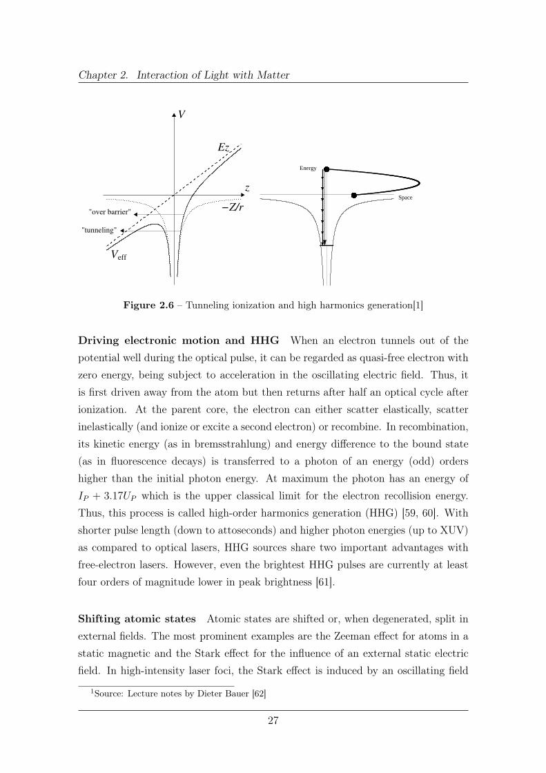
Auger decay and fluorescence decay are illustrated in figure 2.2. In cases wherethe shells above Eo are filled as well, electrons of these shells will fill the Eo vacancy,so that the vacancy successively moves to higher shells until full relaxation. This iscalled decay cascade. If the inner-shell vacancy is created by a resonant excitationinstead of a photoionization, the subsequent Auger decay is called resonant Augerdecay [49], see on the very right in figure 2.2. It will become important when thephoton energy is not sufficient for direct single ionization of a core electron, andwhen resonant bound-bound transitions are energetically possible instead.
Figure 2.3 – Fluorescence yields1
Both decay mechanisms show a Z depen-dence: for a K-shell vacancy, the X-ray fluores-cence rate strongly increases for heavier atoms,∝ Z4, while the Auger rate rises slower thanlinear [38, 50].
In figure 2.3 the fluorescence yield for theK-shell and the average yield for the three L-shells are plotted as a function of the atomicnumber. Accordingly, core-hole relaxation inheavy elements proceeds primarily through ra-diative decay, but becomes less likely for relax-ation of vacancies in outer shells.
The strong Z dependence of the fluorescence
1Source: X-ray data booklet http://xdb.lbl.gov/Section1/Sec_1-3.html
20

Chapter 2. Interaction of Light with Matter
rate is based on a cubic dependence as a function of the emitted photon energy [46].Thus, in a decay cascade, started by a K-shell vacancy, the first decays are predomi-nantly radiative but non-radiative Auger transitions are dominating for outer-shells[38]. When the transition energy during a decay cascade is not sufficient anymoreto liberated an electron, Auger decay is energetically not possible, and the excitedstate relaxes radiatively instead.
21

2.2. Photoabsorption and Photoionization Processes in Atoms
2.2.3 Multiphoton Processes in Strong Electromagnetic Fields
2.2.3.1 Sequential and Direct Multiphoton Ionization
Here, different pathways of photoionization will be discussed proceeding from singleto multiple photoabsorption. They are illustrated in figure 2.4 for the ejection oftwo electrons and in figure 2.5 for one electron ejection.
For a quantitative treatment of processes in the multiphoton regime perturbativetheory can be employed. The first-order perturbation theory describes the inter-action with a single photon, whereas in the n-th order n photons contribute toexcitation or ionization. Because of the iterative approach in the calculation of theexpansion coefficients c(n)
fi (t) (equation 2.22) the transition dipole moment appearsn-times in the calculation of the n-th order coefficient. That means the transitionprobability for an n-th order transition rises with the power of n. As |Mfi|2 ∝ P ∝ I
for single-photon absorption, |Mfi|2n ∝ P n ∝ In is valid for multiphoton absorp-tion. With the generalized cross sections σn the multiphoton transition probabilityis derived as
P(n)fi = σnI
n (2.37)
In the following this result will be discussed for the different pathways of photoion-ization.
Figure 2.4 – Direct and sequential two-
photon two-electron ionization.
When the photon energy exceeds theionization potential of the atom, hω >
Ip, single photon ionization is possibleand the most likely ionization process(pannel a) in figure 2.5). Upon ioniza-tion the Coulomb force of the nucleus isshielded by less electrons and, thus, theremaining electrons are stronger bound.
If the photon energy still exceeds theionization potential of the created ionicstate, a second photon can be absorbedresulting in sequential ionization, de-picted on the right in figure 2.4. In fig-ure 2.4 the direct two photon double ion-ization (TPDI) is illustrated. It has become observable at hih photon intensities in
22

Chapter 2. Interaction of Light with Matter
situations, when the energy of the second photon is not enough to onize the ion(figure 2.4 left), but where the sum of both photon energies exceed the sum of theionization potential of the two electrons. For a detailed description for TPDI in thecase of Helium see [51].
Figure 2.5 – Photoionization processes in the multiphoton regime. The blue arrows
symbolized the photon energy which has to overcome the ionization potential drawn
in black. The energy difference between photon and binding energy is observed in the
electron kinetic energy (in red). The required intensity at a given photon energy is
increasing from left to right, indicated by the grey arrow, with the resonant process as
an exception on the very right.
If the photon energy is smaller than the ionization potential IP , a single photoncannot ionize the atom. Then several photons have to be absorbed simultaneously tofulfill the condition n · hω > Ip (picture b) in figure 2.5). This direct non-sequentialmultiphoton ionization has a small cross section and, thus, requires a high intensity.The probability for multiphoton ionization rises with the intensity to the power n ofsimultaneously absorbed photons, see equation 2.38. For optical lasers, the intensityrange between 1012 W/cm2 and 1014 W/cm2 is called multiphoton regime, as manyphotons can be absorbed simultaneously at these intensities.
If more photons are absorbed than required for ionization, n · hω > Ip + x · hωwith n > x > 1, the electron will carry away the excess energy, which is a multipleof the single photon energy x · hω [52, 53] (picture c) in figure 2.5). Such abovethreshold ionization (ATI) was exploited to calibrate the energy scale of the electron
23

2.2. Photoabsorption and Photoionization Processes in Atoms
spectrometer, described in this work, by analyzing the discrete excess energies in thephotoelectrons created by the simultaneously absorption of photons from a Ti:Salaser in argon (here, the photon energy was 1.5 eV and the ionization potentialfor argon is 15.6 eV. Electrons with ten different energies were resolved. Fromn · 1.5eV > 15.8eV + 10 · 1.5eV , it follows that n=20 photons were absorbed).
In "resonant" multiphoton ionization a resonant bound-bound transition is in-cluded in the photoionization [52, 54] (picture d) in figure 2.5). Resonances sig-nificantly enhance the ionization process, such that it is called resonance enhancedmultiphoton ionization (REMPI). REMPI is widely used in spectroscopy [55, 56].If the resonance is hit with monochromatic light, the probability to excite the atomvia this resonance is close to one. Then, the absorption is saturated, and a furtherincrease in intensity cannot further increase the absorption probability. Hence, theprobability of resonant multiphoton ionization is proportional to In−r, with r as thenumber of involved saturated resonances. However, it is closer to In when the res-onances are not saturated, e.g. because not all photons in a large bandwidth pulsehave the appropriate energy.
The transition rate in equation 2.37 in a photoionization experiment with N0
target atoms is often observed by means of the ion yield dN1/dt.
dN1
dt= N0σ
(n)
(I
hω
)n(2.38)
Here, the intensity is divided by the energy hω to give a dimensionless number ofions when multiplied with the generalized cross section.
The intensity I can be varied by increasing or decreasing the focus size or at-tenuating the laser beam, respectively. Then, a measurement of the ion yield as afunction of the intensity can provide information about the number of absorbed pho-tons. In a double-logarithmic plot of ion yield as a function of intensity, the numberof photons is found as the slope of the yield curve, n = log(dN1/dt)/log(I/hω). Theminimum number of photons necessary for m-fold ionization is the sum of ionizationenergies divided by the photon energy, nmin =
∑m(IP )m/hω.
When the intensity is rising, all neutral target-atoms will be ionized at somepoint. Then, a further increase of the intensity will not lead to a higher ion yieldof singly-ionized charge states any more. The single-photoionization in the targetvolume is saturated; the path to full saturation can be described by an exponentialdecrease of the population of neutral target-atoms. Upon single-photoionization, the
24

Chapter 2. Interaction of Light with Matter
ions in the target volume can absorb another photon. Again this sequential doublephotoionization will saturate as soon as all target-ions are doubly ionized.
For instance, in two-photon double ionization, the ion yield for the sequentialtwo-photon ionization is
dN seq2
dt= N1σ
(1)12
(I
hω
)1
(2.39)
with N1(t) =
∫ t
−∞N0(t′)σ1
01
(I
hω
)1
dt′ (2.40)
Here, σ01 and σ12 are the photoionization cross sections for the first and secondstep, respectively. For completeness it should be noted that two photons may, withmuch lower probability, also be absorbed simultaneously in a non-sequential doublephotoionization [51], depicted in 2.4
dNnonseq2
dt= N1σ
(2)02
(I
hω
)2
(2.41)
(2.42)
So from the number of absorbed photons these pathways cannot be distinguished.
2.2.3.2 Classification of Strong-Field Interactions
The kinetic energy of a free electron driven by an oscillating electromagnetic field isdescribed by the ponderomotive potential. It is defined as
UP (E,ω) =e2E2
4meω2=E2
4ω2=
I
4ω2(2.43)
where E denotes the electric field, ω the radiation frequency and I the field intensity.The two right terms are, for shortness, expressed in atomic units where e = me = 1.Obviously, the ponderomotive potential rises linearly with the pulse intensity, anddecreases quadratically with shorter wavelength, i.e. with higher photon energy.
For distinguishing between of the "multiphoton" and the "tunneling" (strong-field) regime, the so called Keldysh (or adiabatic) parameter γ was introduced [35]
γ =TtunnelingTlaser periode
=
√IP
2UP(2.44)
It compares the time in which tunneling takes place with the time the laser bendsthe atomic potential to enable tunneling. Since the strong field bends the atomic
25

2.2. Photoabsorption and Photoionization Processes in Atoms
potential (see figure 2.6 on the left), this regime is called tunneling regime. In amore practical form, the Keldysh parameter may be written as the ratio betweenthe ionization potential IP and the ponderomotive potential UP . Now, γ has beenwidely used to approximately distinguish between the two regimes by classifying:
γ 1 multiphoton regime
γ 1 tunneling regime
Note that this classification is not very sharp and has been intensively discussedin the literature. Nevertheless, it provides good guidance. To illustrate the ap-proximate border line between these regimes, the intensity leading to γ = 1 forthe hydrogen atom if radiated by an infrared laser is calculated: with an ionizationpotential of 13.6 eV in the focus of a 800 nm laser, the Keldysh parameter becomesone for an intensity of 1.1 1014 W/cm2.
2.2.3.3 Strong-Field Effects in the Tunneling Regime
If the intensity is increased above the multiphoton regime, the ponderomotive forceof the oscillating electromagnetic field is sufficiently large to modify atomic statesand drive electron motions.
Thus, being far away from a "small perturbation", processes in this regime cannotbe treated by perturbation theory anymore. One of the most common theoreticalapproaches to be applied now is the so-called strong-field approximation. Here, in-teractions with the external field are neglected in the initial state and, in the finalstate, interactions with the nucleus are considered to be small, such that essen-tially a free electron is moving in the laser field [57, 58]. Three prominent reactionmechanisms within the tunneling regime should be mentioned.
Bending the potential well and tunneling The oscillating field modifies thepotential well, so that the 1/r symmetry of the Coulomb potential is broken(figure 2.6). If the oscillation of the field is slower than the tunneling time, elec-trons may tunnel trough the lowered potential barrier [26]. If the potential barrieris bend below the energy level of the electron, the ionization is called above thebarrier ionization.
26
Chapter 2. Interaction of Light with Matter3.4. ATOMS IN STRONG, STATIC ELECTRIC FIELDS 51
Veff
V
z
Ez
−Z/r"over barrier"
"tunneling"
Figure 3.4: Effective potential Veff in field direction. The unperturbed Coulomb potential andthe field potential are also shown separately. Depending on the initial (and possibly Stark-shifted)state, the electron may either escape via tunneling or classically via “over-barrier” ionization.
The effective potential Veff describes a tilted Coulomb potential (see Fig. 3.4). A per-turbative treatment of the problem can be found in almost all quantum mechanics oratomic physics text books (Stark effect). In first order (linear Stark effect) the degener-acy with respect to the angular quantum number ` is removed while the degeneracy inthe magnetic quantum number m is maintained. The non-degenerate ground state isonly affected in second order (quadratic Stark effect). It is down-shifted since the poten-tial widens in the presence of the field. In the case of the hydrogen atom (Z = 1) thisdown-shift is given by∆E =−9E2/4.
Let us first point out that, strictly speaking, there exist no discrete, bound statesanymore even for the tiniest electric field. This is because even a very small field givesrise to a potential barrier (see Fig. 3.4) through which the initially bound electron maytunnel. The electric field couples all bound states to the continuum and thus, as we havelearnt in Section 3.3.1, all discrete states become resonances with a finite line width.Mathematically speaking, the spectrum of the Hamiltonian (3.189) is unbound frombelow. However, since the barrier for small fields is far out, the probability for tunnelingis extremely low (note that the tunneling probability goes exponentially down with thedistance to be tunneled) and the states are “quasi-discrete”.
A strong increase in the ionization probability is expected when the electron caneven escape classically, that is, when it does not have to tunnel. In a zeroth order ap-proximation (which, in fact, is wrong for hydrogen-like ions, as will be discussed below)this so-called critical field Ecrit may be estimated as follows: assuming that the initial en-ergy of the electron does not change (i.e., Stark effect negligible), classical over-barrier
3.6. STRONG FIELD APPROXIMATION 95
3.6.6 High harmonic generation
When an intense laser pulse of frequency ω1 impinges on any kind of sample usuallyharmonics ofω1 are emitted. A typical signature of the emission spectrum in the case ofstrongly driven atoms, molecules or clusters is that the harmonic yield does not simplyroll-off exponentially with increasing harmonic order. Instead, a plateau is observed.This is a prerequisite for high order harmonic generation (HOHG) being of practicalrelevance as an efficient short wavelength source. As targets for HOHG one may thinkof single atoms, dilute gases of atoms, molecules, clusters, crystals, or the surface of asolid (which is rapidly transformed into a plasma by the laser). In fact, for all thosetargets HOHG has been observed experimentally. Even a strongly driven two-levelsystem displays nonperturbative HOHG. The mechanism generating the harmonicsand its efficiency, of course, vary with the target-type. In the case of atoms the so-called three step model explains the basic mechanism in the spirit of simple man’s theory:an electron is freed by the laser at a certain time t ′, subsequently it oscillates in thelaser field, and eventually recombines with its parent ion upon emitting a photon offrequency
ω = nω1, n ≥ 1. (3.370)
This process is illustrated in Fig. 3.21. If the energy of the returning electron is E , theenergy of the emitted photon is ω = E + |Ef| where Ef is the energy of the level whichis finally occupied by the electron, for example, the groundstate.
Space
Energy
Figure 3.21: Illustration of the three step model for high harmonic generation. An electronis (i) released, (ii) accelerated in the laser field, and (iii) driven back to the ion. There it mayrecombine upon emitting a single photon which corresponds to a multiple of the photon energyof the incident laser light.
From this simple considerations we conclude that the maximum photon energy onecan expect is ωmax = Emax+ |Ef|. Using (3.363) we obtain at the recombination time trec
Figure 2.6 – Tunneling ionization and high harmonics generation[1]
Driving electronic motion and HHG When an electron tunnels out of thepotential well during the optical pulse, it can be regarded as quasi-free electron withzero energy, being subject to acceleration in the oscillating electric field. Thus, itis first driven away from the atom but then returns after half an optical cycle afterionization. At the parent core, the electron can either scatter elastically, scatterinelastically (and ionize or excite a second electron) or recombine. In recombination,its kinetic energy (as in bremsstrahlung) and energy difference to the bound state(as in fluorescence decays) is transferred to a photon of an energy (odd) ordershigher than the initial photon energy. At maximum the photon has an energy ofIP + 3.17UP which is the upper classical limit for the electron recollision energy.Thus, this process is called high-order harmonics generation (HHG) [59, 60]. Withshorter pulse length (down to attoseconds) and higher photon energies (up to XUV)as compared to optical lasers, HHG sources share two important advantages withfree-electron lasers. However, even the brightest HHG pulses are currently at leastfour orders of magnitude lower in peak brightness [61].
Shifting atomic states Atomic states are shifted or, when degenerated, split inexternal fields. The most prominent examples are the Zeeman effect for atoms in astatic magnetic and the Stark effect for the influence of an external static electricfield. In high-intensity laser foci, the Stark effect is induced by an oscillating field
1Source: Lecture notes by Dieter Bauer [62]
27

2.2. Photoabsorption and Photoionization Processes in Atoms
and, thus, is called AC-Stark effect. In multiphoton ionization, atomic states, notaccessible by an integer number of laser pulses without the presence of an externalfield, may be shifted by the AS-Stark effect so that the difference to the ground-statebecomes an integer multiple of the photon energy. Then, multiphoton ionizationproceeds very efficiently via this resonance to the shifted intermediate state as inREMPI discussed above for non-shifted levels [63].
A broader discussion on light-matter interactions in intense laser fields can befound in the review articles [26–28, 36].
2.2.4 Photoionization by Intense X-ray Pulses
2.2.4.1 Multiple Ionization of Inner-Shell Electrons
In the preceding section, the multiphoton and tunneling regime were introducedto evaluate at which intensity the oscillating field starts to disturb the potentialbarriers and drives the electron motion. Due to the 1/ω2 dependence of the pon-deromotive force, strong-field effects are expected to play a negligible role at X-rayenergies. Whereas the intensity to yield a Keldysh parameter of γ = 1 for the hydro-gen atom irradiated with 800 nm wavelength was calculated to be 1.1 1014 W/cm2
in section 2.2.3.2, at X-ray energies, say 0.8 nm wavelength (about 1500 eV), therequired intensity becomes 1.1 1020 W/cm2, which is still higher than the valuesachieved at any X-ray source currently available, including free-electron lasers. Thisclassification puts X-ray photoionization clearly in the multiphoton regime.
At infrared, optical and ultraviolet energies direct multiphoton processes havebeen discussed in section 2.2.3.1. At X-ray energies, even at high intensities of free-electron lasers, nonlinear X-ray processes are expected to be dominated by sequentialsingle-photon single-electron interactions [20, 24, 25].
In section 2.2.2.5 decay mechanisms upon X-ray inner-shell photoionization havebeen discussed. At high intensities, several sequential photoionization steps mayoccur, before a decay into the first inner-shell vacancy takes place. Then, multipleinner-shell vacancies are created.
Sequential multiphoton ionization leads to high charge states, where the ratio ofthe two competing decay mechanisms, Auger and fluorescence decay, may change:The Auger rate depends on the number of available electrons in higher shells toparticipate in the decay process. Auger decay becomes, therefore, less likely with
28

Chapter 2. Interaction of Light with Matter
increasing charge state during sequential inner-shell ionization. Eventually core-shellexcited ions like C4+ 1s12s02p1 must solely decay radiatively.
2.2.4.2 Modeling of X-Ray Photoionization
At free-electron lasers two important features have to be addressed by theoreticalmodels: the influence of the chaotic photon statistics (see the experimental section),and the high intensity of the radiation. The basic underlying steps of calculating theatomic response to FEL X-ray pulses are briefly outlined in the following providingreferences to detailed descriptions.
To account for the photon statistics, the number of photons in a certain mode(wavevector ~k, polarization λ) has to be considered and defines the field configu-ration. All possible field configurations are summed up in a density matrix, whichis evaluated via the (first order) field correlation function [64, 65]. Eventually, in-tegration of this function yields an average number of photons per unit area andFEL pulse. In this way, possible intensity and coherence spikes are considered frompulse to pulse. The chaoticity of the FEL pulse was found to have limited impact onthe overall ionization process in the sequential regime, but to become important incertain high-intensity ionization pathways [24]. In the calculations presented in thiswork, a simple Gaussian shape was assumed for the photon intensity distribution.
The differential cross sections for one photon ionization is calculated with non-relativistic quantum dynamics using first-order perturbation theory. Each crosssection is multiplied by the average photon number to give the differential probabilityfor single photoionization by the FEL pulse. The new inner-shell electron bindingenergy of the resulting core excited state is then calculated with the Hartree-Fock-Slater (HFS) approach [66]. Within the sudden approximation [67], the ionizationprocess is assumed to happen instantaneously and the two appropriate Hamiltonians,before and after ionization, are independent. Then, the double ionization probabilityis the product of the single-photon ionization cross section of the ground and of thecore-excited state. The latter may also relax via Auger or fluorescence decay, andthe corresponding decay rates have to be considered within the ionization process.As the differential cross section, these decay rates are calculate within perturbationtheory.
Finally, the ionization probabilities and decay rates of intermediate excited statesare put into a set of coupled rate equation, which are numerically solved. Those
29

2.2. Photoabsorption and Photoionization Processes in Atoms
show the temporal evolution of probabilities to find the target in a certain state.Because photoionization and decay mechanisms constantly shift the charge-statedistributions during the FEL pulse, these probabilities are coupled. While the atomicprocesses (ionization, decay) are treated in the perturbative regime, the overallionization and relaxation dynamics, described by the coupled rate equations, arenon-perturbative.
The accuracy of this modeling is limited by several approximations. First, theelectronic structure calculations is based on the Hartree-Fock-Slater method, whichdoes not consider relativistic effects or electron correlation; the difference of theexact and the self-consistent field energy is the correlation energy (CE) [41]. CEcalculations, however, have shown little deviations from the HFS results on thelevel of sophistication needed for the interpretation of the present experiments. Forthe photoionization and fluorescence rate, the dipole approximation is used, forshake-off ionization the sudden-approximation. At soft X-ray energies the dipoleapproximation is still plausible. Shake-off is included for the first photoionizationstep, then the shake-off ratio decreases, and it has no effect on the production ofhigh charge states [68]. Double Auger decay, Auger satellites and impact ionization(such as "knockout" of an outer-shell electron by the inner-shell photoelectron) arenot considered in the theoretical model. In rate equations either one or anotherstate is addressed but a superposition of states is not possible. For the experimentalparameters of this work, the bandwidth (about 15 eV) is too small for a superpositionof different states (about 50 eV apart).
A discussion of this theoretical approach for helium and neon can be found in[24], a general tutorial in [38]. The XATOM toolkit, which was used by S.-K. Sonfor the calculations, related to this work, is described in [69].
30

Chapter 3
Experimental Setup
3.1 The Linac Coherent Light Source
The Linac Coherent Light Source (LCLS), the world-wide first hard X-ray free-electron laser, has started operation in fall 2009 with one beamline operational, the"AMO-beamline" for atomic, molecular and optical science. In December 2011, thelast of six beamlines was being commissioned. LCLS provides coherent X-rays withpulse lengths between 500 fs and below 3 fs at wavelengths ranging from 1.2 to 22 Å.The offered peak brilliance is almost nine orders of magnitude higher than at con-ventional synchrotron sources [70] (see figure 1.1). The following sections cover fourtopics with respect to the design of the LCLS, namely: the electron gun and the ac-celerator section, the lasing process, the photon diagnostics and, finally, the relevantparameters of the beamlines.
3.1.1 Electron Acceleration in the Linac
The lasing process in FELs is based on the collective interaction of relativistically fastelectrons with their own spontaneous emission. For these collective interactions tooccur, the electrons have to be confined in a small volume and with similar momenta,that means the six-dimensional phase-space density has to be sufficiently high. Theaverage spread of particle coordinates in position and momentum phase space iscalled emittance. The lower the electron beam emittance, the higher the photonbeam brilliance (defined in figure 1.1). To account for the required low emittance andhigh beam currents FELs are based on linear accelerators (Linacs) which are single-pass machines. In comparison, synchrotrons consist of a pre-accelerating Linac, a
31

3.1. The Linac Coherent Light Source
circular accelerator and a storage ring [11] where the same electron bunch circulatesfor several days. The FEL was proposed as early as 1971 [71] but the first opticalFEL based on sufficient electron beam emittance could only be realized in 2001 [72].
3.1.1.1 Electron Sources
LCLS uses the accelerator units in the last kilometer of the 3-km-long SLAC Linac.At kilometer two, the electron beam is created 35 off-axis in a photocathode radiofrequency (RF) gun, where a copper cathode is illuminated by 3-ps-long UV pulseswith a 30 to 120 Hz repetition rate which thereby defines the repetition rate of theX-ray pulses. With stabilized irradiation of the copper cathode, the relative electroncharge stability amounts to 1.1% root mean square (rms, the quadratic mean) at1 nC [73]. The injector is typically operating with a lower charge of 0.25 nC and,then, provides a 35 A peak current and a transverse emittance of less than 1 mmrms [70].
Electron Bunch Length Similar to streak cameras (see figure A.4) the electronbunch profile can be derived by directly streaking the electron beam using an RFdeflecting field [73]. In a transverse-deflection cavity (TCAV3 in figure 3.1), locatedafter the second compressor, the electron beam is deflected by S-band RF pulsesonto a phosphor screen [74]. From the spatial distribution the electron bunch lengthcan be measured down to 10 fs [75]. This deflection measurement is very sensitiveto the deflecting field and a precise calibration is essential; for example between twocalibration procedures a shift in the field strength of up to 30% was found [76]. Ifthe field strength was not recalibrated a 30% offset in the electron bunch lengthwould have been measured.
3.1.1.2 Accelerator
At LCLS the electron bunch is accelerated by the S-band (2.856 GHz) Linac, wherethe RF-fields are fed in from klystrons and form a standing wave in the cavities forresonant acceleration. From the injector, the electron beam enters the main Linacaxis with 135 MeV and is further accelerated to 250 MeV before passing the firstbunch compressor chicane (BC1 in figure 3.1), which shortens the bunch and therebymagnifies the peak current. The two bunch compressors combined cause a 100-foldincrease in peak current to 3.5 kA.
32

Chapter 3. Experimental Setup
The maximum emittance and, thus, the compressibility is limited by the pulsecharge. At low-charge mode operation, that is a 20 pC instead of the typical 0.25 nC,the electron bunch can be compressed to a minimum bunch length of few femtosec-onds [77].
© 2010 Macmillan Publishers Limited. All rights reserved.
The LCLS electron accelerator is based on the last kilometre ofthe SLAC 3-km-long linac. This remarkable 42-year-oldmachine22 uses radiofrequency (RF) fields at 2,856 MHz (S-band)to accelerate electrons up to 50 GeV, most prominently for high-energy physics research. The final kilometre of this linac is nowbeing used to drive the FEL. To create the LCLS, the linac was modi-fied to include a new high-brightness electron injector at the 2 kmpoint, and two magnetic bunch compressor chicanes (BC1 andBC2) were added to increase the peak current of the electronbeam in stages, commensurate with the increasing beam energy.A new 350-m-long transport line was built at the end of the linacto deliver the 3.5–15 GeV electrons to the 132-m-long undulatorline, after which the electrons are dumped and the X-ray beam istransported to the X-ray diagnostics, or one of several experimentalstations. The facility has been designed to allow future expansionwith up to eight undulators and separate X-ray beamlines. TheLCLS layout is shown in Fig. 1.
The new injector23 must produce a very bright electron beam in asingle bunch generated at a rate of up to 120 Hz with a charge of0.25 nC (an empirically improved operating point that performsbetter than the 1-nC design), a peak current of 35 A, and anr.m.s. energy-normalized emittance of ,1 mm in each transverseplane. The injector begins with a photocathode RF gun with acopper cathode illuminated by UV light from a frequency tripledpulse from an amplified Ti:Sapphire laser system. Uniform spatialUV shaping is important to generate the low emittance and isaccomplished with a 1.2-mm-diameter over-filled aperture imagedto the cathode. The (less critical) uniform temporal shaping isaccomplished by stacking two 3-ps-long (FWHM) Gaussianbeams separated by 3 ps.
The pair of new bunch compressors shortens the electron bunchand thereby magnifies the peak current from the injector by a factorof 100, for a final peak current of up to 3.5 kA at the end of thelinac. The high peak current is required to efficiently generate andsaturate the shortest X-ray wavelengths. The compressors weredesigned to minimize the effects of coherent synchrotron radiation24
(CSR), a process that can degrade the electron beam brightnessduring the compression process as the very short electron bunchbegins to radiate coherently in the chicane bend magnets. Theeffects of CSR have been measured in both compressors and showreasonably good agreement with available computer modellingcodes25. The electron bunch length is measured using a transverseRF S-band deflecting cavity26 (‘TCAV3’ in Fig. 1), which workslike a femtosecond-resolution streak camera for electrons and iscapable of resolving bunch lengths as short as 25 fs FWHM.
A special ‘laser heater’27,28 is located in the injector at 135 MeV(‘Heater’ in Fig. 1). This unique component adds a small level ofenergy spread (20 keV r.m.s. before bunch compression) to theelectron beam to ‘Landau damp’ a micro-bunching instabilitybefore it potentially breaks up the high-brightness electron beam.The system modulates the energy of the electron bunch using aco-propagating IR-laser (758 nm) in a short undulator (0.5 m),which is enclosed within a four-dipole magnetic chicane. Theenergy modulation is immediately smeared by the last twomagnets of the chicane into an uncorrelated energy spread, whichcontinues to smooth the temporal distribution of the bunch as itpasses through the downstream bunch compressors. The heater isthe first of its kind in a linac-based FEL and has been shown tobe quite effective in suppressing this instability and improvingFEL performance29.
Table 1 | Design and typical measured parameters for both hard (8.3 keV) and soft (0.8–2.0 keV) X-rays. The ‘design’ and‘hard’ values are shown only at 8.3 keV. Stability levels are measured over a few minutes.
Parameter Design Hard Soft Unit
ElectronsCharge per bunch 1 0.25 0.25 nCSingle bunch repetition rate 120 30 30 HzFinal linac e2 energy 13.6 13.6 3.5–6.7 GeVSlice† emittance (injected) 1.2 0.4 0.4 mmFinal projected† emittance 1.5 0.5–1.2 0.5–1.6 mmFinal peak current 3.4 2.5–3.5 0.5–3.5 kATiming stability (r.m.s.) 120 50 50 fsPeak current stability (r.m.s.) 12 8–12 5–10 %
X-raysFEL gain length 4.4 3.5 1.5 mRadiation wavelength 1.5 1.5 6–22 ÅPhotons per pulse 2.0 1.0–2.3 10–20 1012
Energy in X-ray pulse 1.5 1.5–3.0 1–2.5 mJPeak X-ray power 10 15–40 3–35 GWPulse length (FWHM) 200 70–100 70–500 fsBandwidth (FWHM) 0.1 0.2–0.5 0.2–1.0 %Peak brightness (estimated) 8 20 0.3 1032 *Wavelength stability (r.m.s.) 0.2 0.1 0.2 %Power stability (r.m.s.) 20 5–12 3–10 %
*Brightness is photons per phase space volume, or photons s21 mm22 mrad22 per 0.1% spectral bandwidth.†‘Slice’ refers to femtosecond-scale time slices and ‘projected’ to the full time-projected (that is, integrated) emittance of the bunch.
BC24.3 GeV TCAV3BC1
250 MeV
(9 m)L1S
L1X(320 m)L2-linac
(540 m)L3-linac
DL1135 MeV
L0Gun
TCAV0
Heater
DL2 Undulator3.5−14 GeV
Vert.dump(132 m)
μ w
all
Figure 1 | LCLS machine layout. Layout from the electron gun to the main dump, with two bunch compressors, BC1 and BC2, and a 132-m-long undulator.
ARTICLES NATURE PHOTONICS DOI: 10.1038/NPHOTON.2010.176
NATURE PHOTONICS | VOL 4 | SEPTEMBER 2010 | www.nature.com/naturephotonics642
Figure 3.1 – Layout of the LCLS from the electron gun to the main dump, with two
bunch compressors, BC1 and BC2, and a 132 m long undulator1.
3.1.2 Light Generation by the Undulators
A uniformly moving charge creates both, an electric and a magnetic field. In orderto produce an electromagnetic wave, it is necessary to have charge acceleration.The generation of electromagnetic waves by accelerated charges was predicted byMaxwell in 1864 and experimentally demonstrated by Hertz in 1886. In a Hertziandipole antenna, a radio frequency voltage drives a charge oscillation in a conductor,where the electrons move according to the force of the alternating electric field.
Figure 3.2 – Undulator working principle2. An electron beam (2), deflected in an
array of permanent magnets (1) of period λU , is radiating electromagnetic waves (3).
In an undulator, a charge oscillation is induced by an array of permanent magnetswith alternating poles (see figure 3.2), where an electron beam experiences a Lorentz
1Source: P. Emma et al. Nature Photonics 4, 641-647 (2010). Copyright by the Nature Pub-lishing Group.
2Source: Wikipedia: The Free Encyclopedia. Wikimedia Foundation, Inc.
33
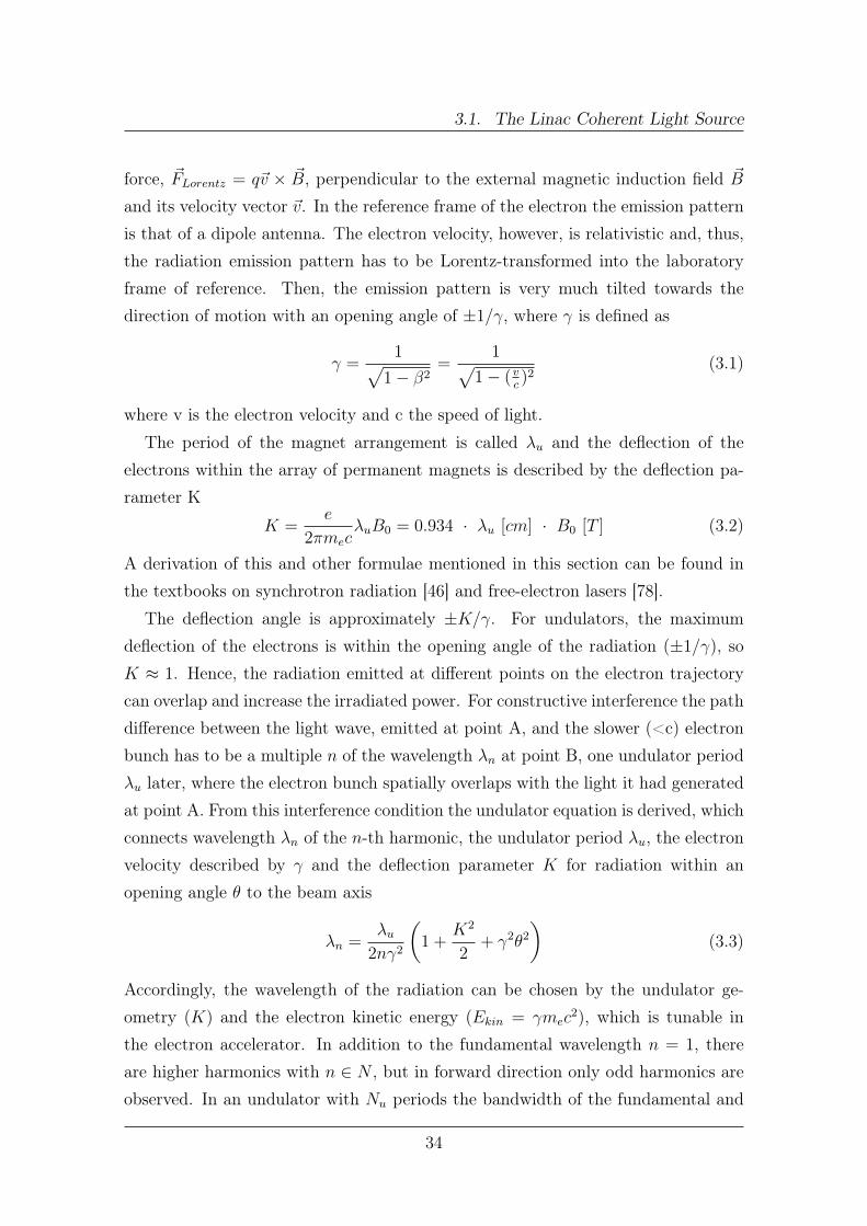
3.1. The Linac Coherent Light Source
force, ~FLorentz = q~v × ~B, perpendicular to the external magnetic induction field ~B
and its velocity vector ~v. In the reference frame of the electron the emission patternis that of a dipole antenna. The electron velocity, however, is relativistic and, thus,the radiation emission pattern has to be Lorentz-transformed into the laboratoryframe of reference. Then, the emission pattern is very much tilted towards thedirection of motion with an opening angle of ±1/γ, where γ is defined as
γ =1√
1− β2=
1√1− (v
c)2
(3.1)
where v is the electron velocity and c the speed of light.
The period of the magnet arrangement is called λu and the deflection of theelectrons within the array of permanent magnets is described by the deflection pa-rameter K
K =e
2πmecλuB0 = 0.934 · λu [cm] · B0 [T ] (3.2)
A derivation of this and other formulae mentioned in this section can be found inthe textbooks on synchrotron radiation [46] and free-electron lasers [78].
The deflection angle is approximately ±K/γ. For undulators, the maximumdeflection of the electrons is within the opening angle of the radiation (±1/γ), soK ≈ 1. Hence, the radiation emitted at different points on the electron trajectorycan overlap and increase the irradiated power. For constructive interference the pathdifference between the light wave, emitted at point A, and the slower (<c) electronbunch has to be a multiple n of the wavelength λn at point B, one undulator periodλu later, where the electron bunch spatially overlaps with the light it had generatedat point A. From this interference condition the undulator equation is derived, whichconnects wavelength λn of the n-th harmonic, the undulator period λu, the electronvelocity described by γ and the deflection parameter K for radiation within anopening angle θ to the beam axis
λn =λu
2nγ2
(1 +
K2
2+ γ2θ2
)(3.3)
Accordingly, the wavelength of the radiation can be chosen by the undulator ge-ometry (K) and the electron kinetic energy (Ekin = γmec
2), which is tunable inthe electron accelerator. In addition to the fundamental wavelength n = 1, thereare higher harmonics with n ∈ N , but in forward direction only odd harmonics areobserved. In an undulator with Nu periods the bandwidth of the fundamental and
34

Chapter 3. Experimental Setup
its harmonics is
∆λnλn
=1
n ·Nu
(3.4)
The interference condition in equation 3.3 is valid for individual electron trajectories,but does not imply coherent radiation of the entire electron bunch. The electronbunch is orders of magnitude longer, i.e. 24 µm (or 80 fs [73]), than the wavelength inthe optical and X-ray regime. To radiate in phase, which amplifies the radiant powerdramatically (∝ N2
electrons instead of ∝ Nelectrons with typically Nelectrons ≈ 109), theelectron bunch has to be sliced into microbunches with elongations in the order ofthe wavelength. This so called microbunching is induced by the interaction of theelectron bunch with its own radiation (see appendix A.1.1). Since the microbunchinghas to be induced by initially uncorrelated, spontaneously emitted photons, sucha light amplification is called self-amplified-spontaneous-emission (SASE). BecauseSASE is based on shot noise, fluctuations in the generated X-ray beam appear fromshot to shot [79–81]. In order to avoid shot-to-shot fluctuations, seeding schemesare planned for future FELs, see appendix A.1.2 for further details. For SASE, theinteraction of the electron beam with the light field must be sufficiently long andintense, so that long undulators and electron beams with high peak current, smallenergy spread and low emittance are required.
© 2010 Macmillan Publishers Limited. All rights reserved.
(time-integrated) emittance values there vary from 0.5 to 1.2 mm,most of the emittance growth is thought to be only in the projection(that is, due to transverse centroid shifts along the bunch). Thetime-sliced emittance measured in the injector (0.4 mm) appearsto be well preserved. The figure shows a measured FEL gain
length of 3.5 m and a saturation length of 60 m (2/3 of the 90-mdesign value), consistent with simulation results where the sliceemittance is taken as 0.4 mm. The FEL gain length at soft X-raywavelengths (15 Å) is measured to be 1.6 m (ref. 36).
To estimate the total FEL energy in the X-ray pulse, the electronenergy loss across the undulator is measured by observing changesof the vertical electron beam position in the dump line after the ver-tical bend magnets (see Fig. 1), where the momentum dispersion islarge. In addition to the FEL process, broadband spontaneous radi-ation and vacuum chamber wakefields can contribute to energy lossin the undulator. However, these non-FEL effects can be isolated byexciting a large horizontal betatron oscillation in the undulator tosuppress the FEL interaction, allowing the FEL-induced energyloss to be precisely determined. This measured average energy lossper electron, multiplied by the electron bunch charge, yields thetotal energy in the FEL X-ray pulse. Using this method, we consist-ently measure X-ray pulse energies from 1 to 3 mJ with ,5% r.m.s.precision for the nominal 250-pC bunch charge throughout theentire operating wavelength range. This electron-based X-ray energymeasurement is also used to calibrate the gas detectors, whichmeasure the relative X-ray pulse energy on each pulse (see below).
Owing to the exceptional electron beam quality and feedbackcontrols, the electron bunch length can easily be varied duringFEL operation, especially with soft X-rays (22 to 6 Å). Figure 5shows the measured X-ray pulse energy at 6 Å (2 keV photonenergy) as a function of the electron bunch length (FWHM) overthe range between 70 and 350 fs (corresponding to a peak currentvariation of 3.5–0.7 kA). The X-ray pulse energy increases withbunch length, probably due to reduced collective effects in thebunch compressors and undulator, but rolls off above 250 fs,because the peak current also drops. To estimate the X-ray peakpower, we divide the X-ray pulse energy by the X-ray pulse length,which is assumed to be the same as the measured electron bunchlength. Figure 5 shows that the X-ray peak power is increased witha shorter pulse length, even where the total pulse energy decreases.
To reach exceptionally short pulse durations, the LCLS has addeda low-charge operating mode (20 pC). The reduced bunch chargeprovides even better transverse emittance from the gun and alsomitigates collective effects in the accelerator, allowing for extreme
−20
0
20
x (μ
m)
1,540 1,560 1,580 1,600 1,620 1,640 1,660 1,680
−20
0
20
y (μ
m)
z (m)
1,540 1,560 1,580 1,600 1,620 1,640 1,660 1,680z (m)
E = 4.30 GeVE = 7.00 GeV
E = 9.25 GeVE = 13.64 GeV
Figure 3 | Electron trajectories through the undulator after beam-based alignment. Both horizontal (top) and vertical (bottom) are shown at four different
electron energies (4.3, 7.0, 9.2 and 13.6 GeV). The trajectory is seen to be highly dispersion-free and therefore well aligned. Error bars represent the r.m.s.
statistical uncertainty in the measured beam position when averaging 50 beam pulses.
0
106
107
108
FEL
pow
er (W
) 109
1010
SimulationMeasured
20 40 60 80 100
−1−0.2
0
0.2
y (m
m)
0.4
0.6
−0.8 −0.6x (mm)
−0.4 −0.2
Undulator magnetic length (m)
λr = 1.5 Å
Ipk = 3.0 kAσE /E0 = 0.01% (slice)
γεx,y = 0.4 μm (slice)
Figure 4 | FEL gain length measurement at 1.5 Å. Measured FEL power (red
points) plotted after continuous insertion of each 3.4-m undulator segment
showing saturation at 60 m and with all 33 undulator segments installed.
Error bars represent the r.m.s. statistical uncertainty in the measured power
when averaging 30 beam pulses. The measured gain length is 3.5 m with a
GENESIS simulation overlaid (blue curve) and with consistent electron beam
parameters shown. The YAG screen image is shown in the inset with
140-mm r.m.s. round X-ray spot size in this early case (April 2009). lr is the
fundamental FEL radiation wavelength; Ipk is the peak current of the electron
beam in the undulator; g is the relativistic Lorentz facotr; 1x,y is the
transverse r.m.s. emittance of the electron beam in the undulator; g1x,y is the
normalized transverse r.m.s. emittance of the electron beam in the
undulator; sE/E0 is the r.m.s. relative energy spread of the electron beam in
the undulator (that is, the r.m.s. energy spread, sE, divided by the mean
electron energy, E0).
ARTICLES NATURE PHOTONICS DOI: 10.1038/NPHOTON.2010.176
NATURE PHOTONICS | VOL 4 | SEPTEMBER 2010 | www.nature.com/naturephotonics644
Figure 3.3 – LCLS gain length1. Figure 3.4 – Synchrotron-light sources2.
35

3.1. The Linac Coherent Light Source
In figure 3.3, the gain length of the LCLS is depicted along with a sketch illus-trating microbunching. The gain length is defined as the distance over which thepower increases by e =2.72 and critically depends on the transverse emittance at theentrance of the undulator. The gain length of LCLS is 3.5 m for hard X-rays (1.5 Å)and 1.6 m for soft X-rays (15 Å), saturation occurs at 60 m [70] (for 1.5 Å) roughlythe 20fold gain-length as predicted by theory [81]. The entire undulator system atLCLS is 132 m long consisting of thirty-three 3.4 m long undulator segments with anundulator period of λU = 3 cm, full gap height of 6.8 mm and a undulator deflectionparameter of K=3.5, corresponding to a magnetic field of 1.5 T [70].
Figure 3.4 schematically compares the magnetic arrays, emission pattern and irra-diated intensity of different synchrotron-light sources. As a result of microbunching,electrons in FEL undulators radiate in phase and the radiated intensity increasesnot only linearly with the number of radiating electrons (as for wigglers and undu-lators from synchrotrons) but quadratically, which gives an enhancement of aboutnine orders of magnitude in peak intensity.
3.1.3 Diagnostics
To date, all four operating short-wavelength FELs, those operating in the extremeultraviolet (XUV) [82, 83] as well as those in the X-ray regime [70, 84], are based onself-amplified spontaneous emission implying significant shot-to-shot fluctuations.To sort the experimental single-shot data, an elaborated photon beam diagnosticsis required.
3.1.3.1 Photon Energy
With a fixed undulator gap, the photon energy is set by the electron energy, ad-justable in the accelerator (see equation 3.3).
At LCLS, the photon energy has a bandwidth of 0.2% to 1% (FWHM) and aphoton energy jitter ("wavelength stability") of 0.2% (rms) [70]. In figure 3.5 thebandwidth is marked in red, the jitter in green. The blue curves illustrate a single-
1Source: P. Emma et al. Nature Photonics 4, 641-647 (2010). Copyright by the Nature Pub-lishing Group. and S.V. Milton et al. Science (New York, N.Y.) 292, 2037-41 (2001). Copyrightby the American Association for the Advancement of Science (AAAS)
2Source http://www.desy.de/forschung/forschungsbereiche/forschung_mit_photonen/
einblick/lichterzeugung, slightly changed
36

Chapter 3. Experimental Setup
Figure 3.5 – Photon energy bandwidth and energy jitter.
shot spectrum, the grey curve the averaged spectrum. The bandwidth is found inevery shot and, e.g., plays a role for energy resolution of photoelectrons and for theaccessibility of narrow transitions (resonances). The jitter shifts the total photonenergy distribution per shot. The jitter is caused by varying start points of SASEin the undulator. It is monitored shot-by-shot and can be eliminated by sortingroutines a posteriori.
Omnipresent spontaneous radiation occurs as surrounding halo of the FEL beam[85]. Higher-energy spontaneous undulator radiation, Bremsstrahlung backgroundradiation and higher harmonics are suppressed by the limited reflectivity of thesteering mirrors to experimental hutches. At the AMO beamline, the second har-monic contributed 0.01% and the third-harmonic content was found to be 1% of thetotal energy over the full tuning range (0.8-2 keV) [20]. The high-harmonic con-tent is very critical for unambiguously identifying very rare nonlinear direct two- ormultiphoton absorption.
3.1.3.2 X-Ray Pulse Length
The X-ray pulse length is varied via the electron bunch length and its measurementprovides an estimate of the former (see section 3.1.1.1). The actual photon pulselength, however, has been found to be shorter does not necessarily match the electronbunch length, as the X-ray pulses are generated in a highly collective process of lasingwithin the electron pulse [86, 87].
Various approaches to determine the FEL-photon-pulse length are summarizedand compared to the nominal value (given by the electron bunch length) in table
37

3.1. The Linac Coherent Light Source
3.1, a description of these approaches is given in the appendix A.1.3.
Measured at LCLS
Measured by Electron bunch length X-ray pulse duration
L. Young et al.[19] 80 fs 40 fs or lessRatio of double- to single-core-hole formation in neon
S. Hau-Riege et al. [88] 300 fs, 150 fs, 70 fs 70 fs, 60 fs, 40 fsStatistical analysis of single-shot photon energy spectra
S. Düsterer et al. [89] 175 fs, 75 fs 120 fs, 40 fsLaser-assisted Auger decay in the X-ray regime (sidebands)
R. Kienberger et al. [90] <10 fs <5 fsNIR streaking (photo-electron momenta)
A. Cavalieri et al. [91] >40fs analysis in progressTHz streaking (photo-electron momenta)
Measured at FLASH and SCSS
Autocorrelation of the split FEL beam in an interferometer [92, 93]
Intensity autocorrelation in non-linear multiphoton-ionization [94–97]
Table 3.1 – Measurements of the X-ray pulse duration
It turns out for various independent measurements, that the X-ray pulse lengthwas found to be at least 40% shorter than the electron bunch.
3.1.3.3 Pulse Energy
Before describing the pulse energy measurement at LCLS, some clear definitionsshould avoid any confusion about three terms, which are often used freely in thecontext of quantifying radiation levels:
Pulse energy is the total energy content of a pulse, i.e. the sum-energy of allindividual photons:
pulse energy = number of photons · energy per photon (3.5)
The maximum pulse energy at LCLS in 2009 to 2011 has been 3 mJ at 2 keVphoton energy (about 1013 photons).
38

Chapter 3. Experimental Setup
Fluence is the total energy delivered per area:
fluence =pulse energy
area(3.6)
Assuming a 3x3 µm2 X-ray focus and 18% beamline transmission at 2.5 mJpulse energy the fluence amounted to 44 µJ/µm2 during the 2011 measure-ments (see section 4.1).
Intensity, also called irradiance or radiative flux, is the energy per area within theperiod of the pulse:
intensity =pulse energy
pulse length · area(3.7)
The intensity with a pulse energy of 2.5 mJ, a pulse length of 100 fs, a 3x3µm2 X-ray focus and 18% transmission is 5 · 1016 W/cm2.
3.1.3.4 The LCLS Gas Monitor Device
At LCLS, two pulse energy detectors to characterize hard X-ray free-electron-laserpulses are permanently installed upstream of the experimental hutches.
Be attenuators are fully retractable, so that the clear aperture isdefined by the larger upstream fixed mask. Two thin Be filters(IF1 Be foil) 10 and 100 mm thick, are added to block visible lightespecially at lower photon energy settings.
The attenuation was measured by comparison between theupstream and downstream gas detectors, illustrated in Fig. 6, as afunction of the beryllium thickness, at a photon energy of 8.3 keV.The measured attenuation length of 3.73 mm is close to thecalculated design value of 4.2 mm. Some degradation of FEL beamimages was observed when using the Be attenuators, which wasattributed to the quality of the Be. An upgrade is planned for thenear future to correct this. The gas attenuator performs reliably inthe soft x-range and still achieves an attenuation of 103 at photonenergies as high as 1500 eV.
3.3. Gas energy detector
Two gas detectors located in the differential pumping sectionsof the gas attenuator, provide non-intrusive FEL energy measure-ment on a pulse-by-pulse basis [5]. The gas detector was notdesigned to provide an absolute intensity measurement, but wasintended to be calibrated with an absolute device such as the totalenergy monitor (see 3.4). The gas detectors measure the N2
fluorescence produced by the FEL beam entering a 30 cm longand 8 cm diameter gas chamber, which is pressurized between0.02–1.2 Torr. The aluminum chamber walls are grooved to sup-press any stray light entering the two perpendicularly-installedphotomultiplier tubes. Magnetic coils around the chamber confinethe photoelectrons and maximize the fluorescence signal. Thenitrogen ionization leads to the emission of photo and Augerelectrons, which deposit their energy in the nitrogen gas until theythermalize or collide with the chamber walls. The exited N2
molecules relax by fluorescence in the near UV, between300–400 nm. The fluorescence yield in air and nitrogen has beenstudied in detail for the detection of highly-energetic cosmic raysand it was found that the fluorescence yield per deposited energy isonly weakly dependent on the energy of the exciting electron [6].Processes such as interaction with the walls, quenching at higherpressures and space charge effects at different FEL energies andoperating pressures may affect the performance and are beingstudied [7].
In conjunction with the photon-based diagnostics anotherenergy measurement of the FEL beam has been developed. Itdetermines the energy loss that electrons suffer in the undulator asthey are kicked on the various orbits leading to varying FEL power.This method has been automated and optimized and gives reliablevalues for the average pulse energy in a matter of only a fewminutes. An example of such an energy loss scan is shown in Fig. 7(left) and a correlation plot with the gas detector signal in Fig. 7(right), which has a relative error typically between 1 to 5% (RMS).
The pulse-by-pulse energy at 8.3 keV, measured with the gasdetector and accumulated over 1000 pulses, is shown in Fig. 8. Thepulse-energy jitter is about 8% (RMS).
Fig. 5. LCLS attenuator system: gas and solid attenuators with differential pumping
sections and integrated gas detector monitors.
Fig. 6. Solid attenuator performance measured with the Gas Detectors as a function
of beryllium attenuator thickness at 8.3 keV.
Fig. 7. Electron energy loss scan (left) and correlation with the gas detector signal (right) at 8.3 keV.
S. Moeller et al. / Nuclear Instruments and Methods in Physics Research A 635 (2011) S6–S11 S9
Figure 3.6 – The LCLS attenuator system1.
They are positioned in the front andin the back of an attenuation chamber,where the incident pulse energy can bereduced, up to an attenuation of 104, ei-ther by adjusting the nitrogen gas pres-sure (up to 16 mbar) within the 4.5 mlong beamline section or by inserting achoice of seven beryllium plates of var-ious thickness (0.5, 0.5, 1, 2, 4, 8 and16 mm) resulting in an adjustable totalthickness of 0 to 32 mm [75]. The solid
attenuators, however, significantly disturb the wavefront of the beam, as imprintstudies have demonstrated [98, 99]. With both detectors working in parallel the
1Source: S. Moeller et al. Nuclear Instruments and Methods in Physics Research Section A:Accelerators, Spectrometers, Detectors and Associated Equipment 635, S6-S11 (2011). Copyrightby Elsevier Ltd.
2Source: S. Hau-Riege et al., PRL, 105, 043003, 2010. Copyright by the American PhysicalSociety.
39

3.1. The Linac Coherent Light Source
incident as well as attenuated pulse energy is monitored simultaneously from shotto shot and their ratio determines the transmission at certain attenuation. Thetransmission can also be calculated from the attenuation (equation 3.8). For thebeamline transmission - the actual transmission in the experimental chamber - seesection 3.1.4.
transmission = exp
(−absorption length · gas pressure
energy dependent constant
)(3.8)
The pulse energy measurement is based on the X-ray induced photoluminescence ofnitrogen in a 30 cm long chamber (figure 3.7). The upper bound for the gas pressureis about 2.5 mbar and is regulated by the gas inlet which competes with pumping.At 8.3 keV photon energy only 0.06% of the photons are absorbed, at lower pho-ton energy a higher cross section increases the absorption and the gas pressure hasto be reduced. Photons are mainly absorbed trough K-shell photoionization whichare rapidly (few fs) followed by Auger relaxations. Both, the photoelectrons andthe Auger electrons, are confined in the 200 G axial magnetic field of an externalsolenoid in order to increase the residence time of the electrons in the nitrogen gas.Thus, their kinetic energy can effectively be transferred to the nitrogen molecules viamolecular excitation and ionization until termination on the chamber walls. Elec-tron impact ionization yields secondary electrons, while molecular excited nitrogenrelaxes under radiative decay of 300 nm to 400 nm [100]. Eventually, the UV lightis detected and amplified by two photo multipliers positioned parallel and perpen-dicular to the polarization vector of the FEL beam and shielded by a near-UV filtertransparent to light between 300 and 390 nm [101, 102].
XFEL beam
magnetic field
30 cm
8 cm
photomultiplier tube vacuum window with EUV filter
nitrogen aluminum liner
Figure 3.7 – Setup of the LCLS gas monitor device2.
The measurement of the UV radiation provides the relative shot-to-shot pulse en-ergy. Thereby gas pressure, magnetic field and photon energy have to be monitoredand stabilized to the recommended operating range. The photon pulse energy is
40

Chapter 3. Experimental Setup
estimated by measuring the electron beam energy loss in the undulator and is takenfor an absolute calibration of the gas detectors.
3.1.3.5 The ASG Intensity Monitor
A second intensity monitor has been installed downstream of the experimental cham-ber as back-up option and to check the LCLS GMD on its linearity. In contrast tothe LCLS luminescence detector, it is based on the photoionization of a gas at alow target density (the same effect is exploited in the DESY gas-detectors designedfor the use at the XUV FEL, FLASH, and the upcoming X-ray FEL, the EuropeanXFEL [103]).
At the Japanese XUV-FEL, SCSS, and X-FEL, SACLA, a third detector type, acryogenic radiometer, is used. It is based on the calorimetric technique, that meansthe temperature rise of a cavity absorber, which corresponds to the radiant powerof the FEL, is measured [104].
The intensity monitor was mounted in a CF63 double cross between the CAMPendstation and the boron carbide (B4C) beam-stop. The gas pressure was kept low(106 mbar) to avoid any gas leakage through the 5 mm aperture into the experimentalchamber. The six ports of the cross were distributed to: the incoming beam, thebeam stop, the intensity monitor, a needle valve for gas inlet, a pressure gauge and aYAG-crystal on a movable linear manipulator to monitor the beam position. Figure3.8 shows the setup and position within the vacuum tubing. The intensity monitoris built as time-of-flight spectrometer, where ion acceleration and drift region arechosen to fulfill the McLarren geometry for optimized time-of-flight resolution [105],also called time focusing geometry. Accordingly charged particles starting from theinteraction point in the middle of the 40 mm acceleration region pass an accelerationlength of 20 mm before they enter the field-free 40 mm long drift region. Differentvoltage regions are separated by copper meshes. The spacing between each electrodeis 7 mm. Ions, extracted with 200 V across the total extraction region i.e. 62 V/mm,are amplified by a commercial1 open MCP detector with two V-stack multi-channelplate and a single metal anode (for a description of MCPs, see section A.2.4 inthe appendix). The amplification is 107 and decoupled MCP signals are furtheramplified by a fast pulse preamplifier2.
1TOPAG MCP Detector MCP-MA33/102Philips scientific fast pulse preamplifier model 6954ds
41

3.1. The Linac Coherent Light Source
acceleration region
drift region
copper mesh
copper mesh MCP detector
Figure 3.8 – Intensity monitor within the CF63 double cross. On the left the time-
of-flight spectrometer in McLarren geometry and V-stack MCP detector is pictured,
on the right the mounting of the intensity monitor.
Located at more than 1m distance from the beam focus in the CAMP endstation,the fluence is estimated to be sufficiently low to suppress any two photon absorption.Thus, the integrated ion yield is anticipated to be linearly proportional to the pulseenergy. Figure 3.10 depicts a scan over the entire available pulse energy. Thetime-of-flight spectra are drawn on the x-axis for pulse energies between 0 mJ and2.75 mJ in steps of 30 µJ on the y-axis. The incident photon energy was set to1200 eV, the pulse length to 150 fs and the working gas pressure in the double crossto 3 10−6 mbar.
Due to its high cross section (see figure 3.9) at X-ray energies, xenon was chosenas target gas. In the charge-state spectrum, singly, doubly and triply charged xenonis nearly absent as M-shell photoionization is followed by a cascade of Auger decayswhich increases the final charge state. In addition, the MCP detection efficiencydecreases for lower charged ions [109]. The depicted spectrum in figure 3.10 startswith the Xe4+ peak at about 4800 ns which, as well as the Xe5+ peak, remainsalmost of constant peak-height throughout the pulse energy scan. The main featurefor Xe6+ and Xe7+ is the significant decrease, which coincides with an increase ofthe neighboring higher-charged ion (also see figure 3.12). The dominant peak in thespectrum is Xe8+, which just depletes with the rise of Xe9+ at the highest pulse
42

Chapter 3. Experimental Setup
0 2 0 0 4 0 0 6 0 0 8 0 0 1 0 0 0 1 2 0 0 1 4 0 0
0 . 1
1
1 0
1 0 0
tot
al cro
ss se
ction [
Mb]
p h o t o n e n e r g y [ e V ]
H y d r o g e n N i t r o g e n O x y g e n N e o n A r g o n K r y p t o n X e n o n
Figure 3.9 – Calculated total cross sections of rare and typical residual gases [106–
108].
energies. No depletion is observed for Xe9+ since the highest charge state, Xe10+,is detected in negligible amounts. In a 44 eV to 1300 eV photon energy scan at theTERAS synchrotron radiation facility, Saito [110] reports a maximum charge stateof Xe8+, which is in agreement with the charge-state distribution measured using theFLASH GMD at the LCLS SXR beamline [111]. In contrast, Carlson [112] showsan ion yield up to Xe10+ for photoionization of 3s, which is accessible at 1200 eVincident photon energy, and Mukoyama [113] measured even small yields of Xe11+
at 4.5 keV, which is still beyond the L-shell ionization threshold.
Thus, charge states above Xe8+ reported here, are attributed to 3s and 3p pho-toionization, which then decays with enhanced double Auger and autoionizationprocesses as compared to 3d ionization at 800eV. Without any focus characteriza-tion and detector efficiency calibration possible during short experimental runs, aquantitative analysis of the individual peak ratios in the time-of-flight spectrum wasnot undertaken.
Residual gas contributes to the spectrum as seen as C1+ (from carbohydrates),N1+ , O1+, O2+, O3+ and H1+. The light peak at the beginning of the spectrum
43
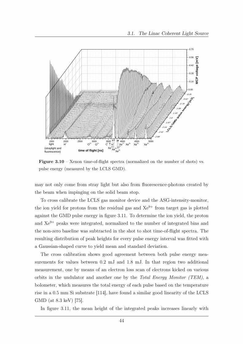
3.1. The Linac Coherent Light Source
1 5 0 0 2 0 0 0 2 5 0 0 3 0 0 0 3 5 0 0 4 0 0 0 4 5 0 0 5 0 0 0
0 . 0 0
- 0 . 1 4
- 0 . 2 8
- 0 . 4 2
- 0 . 5 6
- 0 . 7 0
0 . 2 50 . 5 2
0 . 7 91 . 0 6
1 . 3 31 . 6
1 . 8 72 . 1 4
2 . 4 12 . 6 8
O 1 +N +
t i m e o f f l i g h t [ n s ]
MCP v
oltag
e [mV
]
L CL S
G M D p ul s e
e ne r g
y [ mJ ]
O 2 + X e 4 +X e 5 +X e 6 +X e 7 +
X e 8 +X e 9 +X e 1 0 +C +O 3 +H +
( s t r a y l i g h t a n df l u o r e s c e n c e )
l i g h t
Figure 3.10 – Xenon time-of-flight spectra (normalized on the number of shots) vs.
pulse energy (measured by the LCLS GMD).
may not only come from stray light but also from fluorescence-photons created bythe beam when impinging on the solid beam stop.
To cross calibrate the LCLS gas monitor device and the ASG-intensity-monitor,the ion yield for protons from the residual gas and Xe9+ from target gas is plottedagainst the GMD pulse energy in figure 3.11. To determine the ion yield, the protonand Xe9+ peaks were integrated, normalized to the number of integrated bins andthe non-zero baseline was subtracted in the shot to shot time-of-flight spectra. Theresulting distribution of peak heights for every pulse energy interval was fitted witha Gaussian-shaped curve to yield mean and standard deviation.
The cross calibration shows good agreement between both pulse energy mea-surements for values between 0.2 mJ and 1.8 mJ. In that region two additionalmeasurement, one by means of an electron loss scan of electrons kicked on variousorbits in the undulator and another one by the Total Energy Monitor (TEM), abolometer, which measures the total energy of each pulse based on the temperaturerise in a 0.5 mm Si substrate [114], have found a similar good linearity of the LCLSGMD (at 8.3 keV) [75].
In figure 3.11, the mean height of the integrated peaks increases linearly with
44

Chapter 3. Experimental Setup
pulse energy as indicated by the dark blue lines. The x-scale on top of the graphwas chosen to match both pulse energies in the linear region. However, at about1.8 mJ the ion yield exceeds the interpolated pulse energy. This behavior is in verygood agreement with a previous calibration curve performed by the FLASH GMD(figure 3.11 right side) and proofs a saturation of the LCLS GMD at high pulseenergies. Considering this recalibration, a pulse energy of 2.5 mJ measured by theLCLS GMD becomes 3.5 mJ, 2.75 mJ becomes 4.25 mJ.
0 . 0 00 . 2 50 . 5 00 . 7 51 . 0 01 . 2 51 . 5 01 . 7 52 . 0 02 . 2 52 . 5 02 . 7 5
0 . 0 0 - 0 . 0 4 - 0 . 0 8 - 0 . 1 3 - 0 . 1 7 - 0 . 2 1 - 0 . 2 5 - 0 . 3 0 - 0 . 3 4 - 0 . 3 8 - 0 . 4 2
0 . 0 0 0 . 5 0 1 . 0 0 1 . 5 0 2 . 0 0 2 . 5 0 3 . 0 0 3 . 5 0 4 . 0 0 4 . 5 0 5 . 0 0p u l s e e n e r g y [ m J ] ( i n t e n s i t y m o n i t o r )
m e a n h e i g h t p e r b i n [ m V ]
pulse
energ
y [mJ
] (LCL
S GMD
)
m e a n p r o t o n m e a n X e 9 m e a n b a s e l i n e
0 50 1000
1
2
3
4
5
6
5+/3+4+ / 3+
6+ / 3+
7+ / 3+
Rat
io
Transmission (%)
2+ / 3+
FIG. 5. Ratios of partial cross sections for differently charged Xe ions as a function of the attenuator transmission.
0 0.2 0.4 0.6 0.80
0.5
1.0
1.5
2.0
2.5
3.0
3.5
LCLS
-GM
D (m
J)
FLASH-GMD (mJ)
FIG. 6. Average photon pulse energy measured by the LCLS gas detector versus those obtained with the help of the GMD.
10
Figure 3.11 – Left: Average photon pulse energy measured by the LCLS gas detector
versus the integral of H+ (in green) and Xe+9 (in red) peaks (normalized to the number
of integrated bins). The error bars are derived from the standard deviation of the peaks.
The dark blues line interpolate the linear region of the curves. The upper x-axis-scale
is chosen to match the interpolated line of the Xe+9 curve to the pulse energy scale.
Right: LCLS GMD pulse energy versus the pulse energy measured by the FLASH
GMD [111].
Finally, the baseline-corrected ion yield for all peaks of the spectrum is drawnin a double logarithmic plot with recalibrated pulse energy (figure 3.12). For therecalibration the experimental proton yield is divided by a constant factor so thatthe proton yield-curve has a slope of one, assuming that an proton is liberated uponone-photon absorption. Then, up to 0.3 mJ, all but the Xe+3 curve rise linearly. Asthe ion yield per shot exceeds two units on the y-axis, saturation of the next lowerion charge state occurs. Interestingly, the ion yield does also seem to increase again,when the next higher ion charge state is depleted and falls below the level of twounits on the y-axis.
45

3.1. The Linac Coherent Light Source
S t r a y l i g h t P r o t o n s O 2 +
O 3 +
C +
X e 3 +
X e 4 +
X e 5 +
X e 6 +
X e 7 +
X e 8 + a n d O +
X e 9 + a n d N +
X e 1 0 +
0 . 1 10 . 0 1
0 . 1
1
1 0
Ion yie
ld pe
r sho
t [arbi
trary
units]
P u l s e e n e r g y [ m J ] ( L C L S G M D )Figure 3.12 – Xenon ion yield vs. pulse energy measured by the ASG intensity
monitor. The pulse energy is recalibrated by the recorded proton yield.
3.1.4 Beamlines
The experiment described in this thesis was performed at the AMO beamline. Intable 3.2 all currently available beamlines are listed.
The AMO beamline went online first to gain experience on fundamental pro-cesses in the interaction of the ultra-intense X-FEL light with atoms and molecules.The X-ray beam is reflected into the AMO beamline by three boron-carbide (B4C)coated silicon wafers (SOMS, see figure 3.14) with nominal reflectivity of 0.921,0.931 and 0.898 at 800 eV, 1050 eV and 2000 eV, respectively [19] (figure 3.19), andfocused by a set of Kirkpatrick-Baez parabolic-curved grazing-incidence mirrors ofthe same material. The reflectivity sharply decreases at about 2 keV. So the K-edgeup to neon and the L-edge up to krypton are accessible. High-harmonics are ef-ficiently suppressed by the limited reflectivity, which is favorable when non-linearmultiphoton ionization is investigated.
From the nominal reflectivity R of the five mirrors, the maximum total beamlinetransmissions is calculated to be R5, that is 0.663, 0.699 and 0.584 for the above pho-ton energies, but the measured absolute transmission turned out to be significantly
46

Chapter 3. Experimental Setup
lower:
Figure 3.13 – Reflectivity of the Soft X-
ray Offset Mirror System, that delivers
X-rays to the SXR and AMO beamlines.
the FLASH GMD positioned downstream ofthe AMO endstation showed pulse energiesfrom 12% to 15% of the pulse energy deter-mined by the LCLS gas monitor upstreamof the first steering mirror. This surpris-ingly low value might be due to additionaltransmission losses in the beamline or by apositive offset in the LCLS GMD.
If the focal spot size can be assumed fromother techniques (see next section 3.1.4.1),the transmission can be inferred fromfluence-dependent ion charge-state yields
measured in the main experimental chamber. For neon at 800 eV photon energythe charge-state spectra matched best when a transmission of R5/3 = 20% wasmultiplied to the pulse energy determined by the LCLS GMD [19]. For the CAMPendstation (see section 3.2) a similar approach was undertaken to derive the trans-mission (see figure 4.1).
The other five beamlines at LCLS are summed up in the following table (3.2).The abbreviation is explained, further reading cited and their purpose indicated.Figure 3.14 depicts the beam line layout in the experimental halls and the steeringoptics.
the electron bunch to create a 100 fold increase in peak current to3.5 kA. A transverse-deflection cavity, located after the secondcompressor, allows electron pulse length measurements as short as10 fs. Several feedback loops are implemented to control andstabilize the beam. For example, by controlling the peak current,it is possible to directly control the electron pulse length andtherefore the X-ray pulse length [2].
The undulator is 132 m long and consists of 33 segments. Eachsegment consists of a 3.4 m long planar permanent magnet whichhas a period of 3 cm and a fixed gap of 6.8 mm with a magnetic fieldof 1.25 T, resulting in a k-value of 3.5. The undulators and focusingmagnets sit on a girder system that allow for vertical and horizontalcontrol of five degrees of freedom to submicron level. Each of the 33segments is fully retractable on its girder system. Alignment of theundulator with respect to the electron beam is achieved through abeam based alignment method that measures the electron trajec-tory at various energies. The girder positions are continuouslymonitored to an accuracy of o1 mm with a stretched wire positionmonitoring and a hydrostatic leveling system. Commissioningshowed that saturation at 8 keV could be achieved with only 23undulator segments inserted which is now the typical configura-tion during operation.
After the electron beam dump the FEL beam enters the separateFront End Enclosure (FEE), which houses a suite of components toprepare and characterize the beam before it enters the experi-mental stations in the Experimental Halls. The lay-out of thephoton beam lines is shown in Fig. 1.
A system of grazing-incidence X-ray mirrors, located at thedownstream end of the FEE, splits the beam into soft and hardX-ray branches and distributes the beam into a total of sixexperimental hutches; 3 in each of the experimental halls. Thesoft X-ray branch splits again into the AMO beam line in hutch 1and the SXR beamline ending in hutch 2. The SXR beamline alsocontains a transmission chamber in hutch 1. The hard X-ray linedirects the beam to the XPP station in hutch 3 of the Near Hall and tothe 3 Far Hall experiments: the X-ray Correlation Spectroscopy(XCS) instrument in hutch 4, the Coherent X-ray Imaging (CXI)instrument in hutch 5, and the station for Matter in ExtremeConditions (MEC) in hutch 6. A laser room, equipped with aTi:Sapphire system is located in the Near Hall, with a laser transportpipe leading to each of the 3 hutches for conducting pump-probeexperiments.
3. LCLS photon diagnostics
The main photon diagnostics for LCLS is located in the FEE, a30 m long, separate tunnel located downstream of the electrondump area. The photon diagnostics were designed and fabricatedby Lawrence Livermore National Laboratory (LLNL).
The primary function of the photon diagnostics is to measure,control, and transport the beam for use in the experimental areas.The diagnostics in the FEE were specified for identifying and tuningthe FEL during commissioning, as well as to characterize andoptimize beam properties during operations. It consists of absor-bers, imagers, and intensity monitors. A downstream view of theFEE is shown in Fig. 2. In addition, there is an instrument-specificdiagnostic suite located upstream of each of the hard X-rayinstruments, which permits collimation, attenuation, pulse selec-tion and focusing of the beam as well as measurement of beamprofile, intensity and position. The commissioning of the instru-ment-specific hard X-ray diagnostic package is underway and willbe described elsewhere.
Fig. 3 shows a schematic layout of the diagnostic and opticalcomponents in the FEE. The FEL beam and the spontaneousradiation enter unobstructed through the 2545 mm wide open-ing of the fixed mask into the FEE. Due to the high peak power of theFEL beam, most materials would suffer damage due to melting.Extensive damage studies [3] have shown that boron carbide (B4C)is a suitable candidate to withstand power densities at this locationand therefore a layer of B4C is used to protect all collimators, slits,stoppers, and soft X-ray mirror surfaces. Pop-in cameras are located
Table 1LCLS milestones for commissioning and operation.
Laser gun commissioned 2007
Linac and bunch compressors commissioned 2008
First electron beam through undulator 12/13/2008
21 undulator magnets installed and ready 4/7/2009
First lasing at 1.5 A 4/14/2009
X-ray diagnostics commissioned July–Sept. 2009
Soft X-ray in NEH AMO instrument hutch 1 8/18/2009
Start of user operations 11/1/2009
SXR commissioning/2nd user run May 2010
XPP commissioning start June 2010
3rd user run AMO/SXR/XPP Sept.–Dec. 2010
CXI commissioning start Dec. 2010
XCS commissioning start June 2011
MEC commissioning start 2012
Hutch 4
Hutch 5
Hutch 6Hutch 1 Hutch 2 Hutch 3
Near Experimental Hall Far Experimental Hall
X-Ray Tunnel
FEEElectronDump SH2 S5M1S M2S
M3S1/2 S1
S2
SH1
HorizontalOffset Mirrors
ST1/2
AMO
SXRb
XPP CXIXCS
S2BSXRa
MEC
Fig. 1. LCLS Photon beam line layout with instrument stations.
S. Moeller et al. / Nuclear Instruments and Methods in Physics Research A 635 (2011) S6–S11 S7
Figure 3.14 – The LCLS photon beam line layout with instrument stations1 [75].
47

3.1. The Linac Coherent Light Source
Atomic, Molecular and Optical Science (AMO) [115]Soft X-rays, high resolving electron and ion spectroscopy, CDI and pump-probe
Soft X-ray Research (SXR) [116]Monochromatic or full non-monochromatic soft X-ray beam, various endstations
X-ray Pump Probe (XPP) [117]Optical laser pump, hard X-ray probe; X-ray scattering shows structural changes
Coherent X-ray Imaging (CXI) [118]Image single sub-micron particles in a hard X-ray focus of 0.1 µm diameter
X-ray Correlation Spectroscopy (XCS) [119]Hard X-ray scattering in condensed matter systems; X-ray - X-ray pump-probe
Matter in Extreme Conditions (MEC) [120]High power optical laser beams pump, hard X-ray probe of very dense matter
Table 3.2 – Beamlines and their particular purpose at LCLS [121]
3.1.4.1 Focus Size
Focus size and fluence are crucial parameters for the majority of experiments presentlyperformed at FEL sources. Both parameters directly alter the power density at thetarget. They are strongly influenced by the optical system upstream of the experi-ment due to its focussing and transmission properties. The multi-photon interactioninvestigated in this work is very sensitive to the power density and the focal volume.
The focus size can either be determined in a designated invasive experimentalset-up or traced back from calculated charge-state distributions of small atoms (e.g.Ne), which are fit to data at given focus size. In an intensity scan, the onset ofsaturation of ion yields for low charge states can also provide a direct estimate ofthe focus size [122].
Three invasive methods to characterize the spatial beam profile have been used atFELs so far [123]. In the XUV region a direct imaging of the beam wave-front andintensity distribution through the pinholes of a Hartmann-sensor was possible [124].The pinhole mask in front of a CCD separates the wave-front into evenly spacedpoint sources, where the local tilt of the wave-front across each pinhole can then be
1Source: S. Moeller et al. Nuclear Instruments and Methods in Physics Research Section A:Accelerators, Spectrometers, Detectors and Associated Equipment 635, S6-S11 (2011). Copyrightby Elsevier Ltd.
48

Chapter 3. Experimental Setup
calculated from the position of the spots on the CCD and the intensity distributionfrom the brightness of each spot. This method requires that several pinholes areilluminated and, thus, cannot be applied in the very focus of the FEL beam. AtX-ray energies the lack of commercially available fast CCD cameras has hinderedthis approach so far.
The XUV or X-ray light can be converted to visible wavelengths by luminescencecrystals or phosphorescent coating on a transparent substrate. Then, the spot size,magnified by a microscope, is easily measurable with commercial CCDs. Owing toradiation damage and limited optical resolution, the focus should neither be toointense nor too small.
Figure 3.15 – Imprint studies in the HFP chamber of the AMO beamline [99].
Radiation damage, on the other hand, has been used for an in-focus caustic mea-surement at FLASH [125] and at LCLS. Here a solid sample is inserted into the focusarea to obtain single-shot imprints of the FEL beam at various z positions. Withsimultaneous intensity measurements by the GMD and the spot-size determined exsitu by atomic force microscopy (AFM), the intensity profile can be reconstructedfrom the observed depth under consideration of Lambert-Beer’s law and the sample-specific threshold fluence for ablation. A scan along the FEL propagation directionyields the Rayleigh length, i.e. the distance from the focal point to the place wherethe area of the focal diameter is doubled. The size and possible astigmatism of theincident beam is directly seen in single shot imprints [123].
It should be noted that the standard spot size description by means of the FWHMfails, when the incident beam is distorted or non-homogeneous. Wavefront imper-fections may occur from mirror surface roughness [126] or the light generation byamplified spontaneous emission itself. At LCLS, Bogan et al. found that, while thestructure of each FEL pulse is unique, the average intensity profile deviates consid-
49

3.1. The Linac Coherent Light Source
erably from that of the Gaussian beam [85]. For inhomogeneous beams, the cratersize will rise non-linearly with the pulse energy [98].
50

Chapter 3. Experimental Setup
3.2 The CAMP Endstation
The measurements presented in this report have been performed at the AMO beam-line which was equipped with the CAMP endstation. CAMP is a multi-purposeendstation designed and operated by a collaboration headed by the Max Planck Ad-vanced Study Group at CFEL (thus, CFEL-ASG Multi-Purpose endstation). Thisendstation is described in broad detail in reference [127]. This section presents anddiscusses the main features of CAMP relevant for the measurements described inchapter 4. In the appendix further details about the vacuum system (A.2.2), MCP-detectors (A.2.4) and pnCCD detectors (A.2.5) can be found. Figure 3.21 gives anoverview of the dimensions of the CAMP endstation.
Figure 3.16 – Overview of the CAMP endstation. The FEL entrance is marked by
the yellow arrow. The target gas is injected perpendicular to the FEL beam ("gas
jet", blue arrow). Ion spectrometers are mounted perpendicular to FEL beam and gas
jet via a CF250 port, indicated in orange. The chamber assembly can be remotely
adjusted via translational motions of the inner support (greenish brown) along each of
the three spatial directions and tilt motions along the vertical and horizontal angles
around the pivotal point (marked with the red dot). The base support (blue) remains
fixed [127].
51

3.2. The CAMP Endstation
3.2.1 Gas Jet
During the course of various beamtimes in the CAMP-chamber conducted by col-laborations from different fields of science, a variety of samples and sample-deliverysystems have been employed, such as gas jets for atomic rare gases and rare gas clus-ter, a liquid jet for hydrated bio-samples, an aerosol jet for nano particles, molecularbeams and also solid samples.
In this work a gas jet was used to provide a continuous wave (CW) beam ofatomic rare gases (2011 data) as the target for the photons. In 2009 the beam waspulsed (10 Hz) by a commercial valve3 to reduce the gas load, when the jet wastuned for rare gas cluster. Also, a low-flow metering valve (leak valve) allowed toflood the chamber to increase the target density.
The jet design is optimized for high resolution momentum spectroscopy. Theaverage energy of an atom at room temperature (T =300 K) and with three degreesof freedom is, according to the equipartition theorem, E = 3/2 · kB · T =39 meV,which sets an upper limit of the momentum resolution. To cool the target gas it isexpanded to supersonic speed. In addition, the target volume is reduced to improvethe momentum resolution (Approaches to estimate target density and temperatureare described in the appendix A.2.3).
In the current set-up, the supersonic jet passes four chambers at different vacuumconditions: expansion chamber, skimmer chamber, experimental chamber and dumbchamber, see figure 3.17. Here, the dump chamber was equipped with a residualgas analyzer. Then, the alignment of the gas jet through the various skimmers andapertures can be checked with higher sensitivity.
The target gas is forced through an aperture of 30 µm diameter by a pressure upto 10 bar. To avoid obstruction the gas is cleaned by a Swagelok ceramic particulatefilter with 2 µm pore-size where the gas-line enters the jet. If the pressure beforethe aperture is at least twice as high as after the aperture the gas will expandadiabatically and faster than the speed of sound [128]. For an ideal gas its enthalpy,the sum of internal energy and the product of pressure and volume, will be convertedinto kinetic energy, leaving a fast and cold beam.
H = U + pV =3
2NkBT +NkBT =
5
2NkBT =
1
2m~v2 = Ekin (3.9)
3http://www.parker.com/literature/Literature%20Files/Precision%20Fluidics%
20Division/UpdatedFiles/PulseValves.pdf
52

Chapter 3. Experimental Setup
Figure 3.17 – Setup of the supersonic gas jet (not in scale). In the expansion chamber
a) marks the zone of silence, b) the shock waves and c) the Mach disc. The diameters
of apertures and skimmers are indicated below the drawing as well as the typical gas
pressures in the chambers.
The velocity of an ideal atomic gas jet after expansion would hence amount tovjet =
√5kBT/m, for example for neon (m = 20) vjet =778 m/s. The jet veloc-
ity influences in the spatial distribution of ionization fragments on the detector(figure 3.18).
Additionally to corrections for non-ideal gases, the interaction with the residualgas within the expansion chamber has to be considered. The supersonic jet sends outshock waves where the residual gas is compressed and perturbs the free expansion.Only in an area bordering the gas-inlet-aperture, the so called zone of silence, thegas can expand freely. The form of the zone of silence is close to a cos4 distributionaround the jet axis and several millimeters long. The exact length X up to the Machdisk, that is the end of the zone of silence, is given by
XMach disk =2
3daperture
√pgas
pexpansion(3.10)
where d is the diameter of the aperture, pgas the gas pressure and pexpansion thepressure in the expansion chamber [129]. To take advantage of the cooled beamthe unperturbed inner part has to be cut out before turbulences occur. A skim-mer, that is a thin cone with a small opening on top, is positioned at a distanceX1st skimmer < XMach disk. The skimmer opening-diameter was chosen to be 180 µmand the distance X1st skimmer could be varied between 0 mm and 20 mm. A second
53

3.2. The CAMP Endstation
Hydro-carbon fragments washedout due to Coulomb-explosion
Carbon ring and one Br, singly chargedCarbon ring and one Br, doubly chargeds~tof~sqrt(m/q)s
acc. electric fie
ld
const. jet velocity)Figure 3.18 – The jet velocity is conserved in the ionization fragments, which ex-
perience an additional acceleration by the electric field of a spectrometer (illustrated
on the right). As a result, fragments with different time of flights (TOF) also have
different detector-hit positions (illustrated on the left for a dibromobenzene-target,
a carbon ring with bromine atoms on two opposing sides, recorded on a spatially
resolving detector).
skimmer with a diameter of 400 µm was installed 18 mm downstream to furtherskim the atomic beam and reduce the gas load in the main experimental chamber.The diameter of the atomic beam in the interaction zone is about dtarget =4 mm(FWHM). The shape, however, was recorded not to be fully Gaussian but to havepronounced tails [130].
Additional differential pumping sections and apertures can be implemented toachieve even more confined and dilute targets. Here, an additional differentialpumping section was needed to implement a valve to separate the vacuum of jetand experimental chamber and a bellow for alignment of the jet chambers. (seefigure 3.17)
3.2.2 Momentum Imaging Charged-Particle Spectrometers
When the target gas is ionized, ions and electrons have to be guided by a spectrom-eter to the detectors, so that the momenta and kinetic energies can be retrievedfrom the time and position of the detector-hit. The spectrometer axis is definedby the extraction direction. Two kinds of ion spectrometers have been used in theCAMP endstation to acquire the data discussed in this work: a reaction microscope(REMI) and a velocity map imaging (VMI) spectrometer. The main difference is,that a VMI cannot measure all fragments in coincidence to retrieve the molecular
54

Chapter 3. Experimental Setup
frame. Moreover, as the imaging of electrons is concerned, extraction using just anelectric field (combined electric and magnetic in a REMI) yields very short time-of-flight prohibiting sufficient momentum resolution along the spectrometer axis.Thus, symmetry conditions have to be fulfilled to calculate the 3D momenta fromthe detector images.
3.2.2.1 Reaction Microscope
The development of high-resolution momentum spectrometers started with the in-vestigation of collisions of heavy ions with rare gas targets, where the momentum ofthe recoiling target ion instead of the slightly scattered projectile was measured. Inthis recoil-ion momentum spectroscopy [131] the high-resolved recoil traverse mo-mentum could not only be attributed to the small momentum transfer from theheavy-ion projectile, but also to the ejected electrons. The momentum resolutionwas, however, limited by the thermal motion of the target gas. To resolve the tinymomentum transfer from the electron onto the recoil ion, the target gas had tobe cooled. The implementation of a cool supersonic jet, described above, led to thecold target recoil ion momentum spectroscopy (COLTRIMS) with a high-resolution4π-detection of the recoil-ion.
Simultaneous recoil-ion and electron momentum detection was the final step toreaction-microscopes (see various review articles [132–134]). Here, the electronsare taken to trigger the ion detection and, thus, enable coincident measurements.
Figure 3.19 – REMI sketch1
The electron trajectory is confined by themagnetic field of a pair of solenoids thatis parallel to the detector-axis (Helmholtz-coils). With both, magnetic and electricfields, the electrons are forced on spiral tra-jectories which lead to a time and positionsensitive detector opposite to the ion detec-tor. While the ions are hardly influenced bythe magnetic field and the 4π-detection ofthe recoil-ion is still valid, electrons are si-multaneously detected with close to full solid
1Source: O. Herrwerth et al., New Journal of Physics 10, 025007 (2008). Copyright by theInstitute of Physics
55

3.2. The CAMP Endstation
angle. Thus, kinematically complete experiments are possible, where the vector-momenta of all reaction-products are retrieved. The downturn of such a coincidenceexperiment is the limited single-hit rate. All detector signals from the impingingfragments have to be disentangled and attributed to the individual ionization pro-cess, which becomes impossible for high count rates. Usually that is compensatedfor by high repetition rates of the pulsed incoming beam (up to MHz for ion andelectron beams, several kilohertz for optical lasers). In the case of present FELsources, operated up to 120 Hz, this is a serious limitation.
The actual ASG reaction microscope as used in the CAMP endstation is depictedin figure 3.20. It consist of 30 flat and 16 conical electrodes with an inner diameterof 84 mm and an outer diameter of 130. The electrodes are evenly spaced (8.2 mmdistance at inner diameter) to build up a homogeneous electric field of few volts percentimeter. The electrodes are isolated by ceramic-discs and connected in series via100 kΩ resistors to distribute the voltage. All electrodes are made of aluminum andare gold-plated to avoid voltage-inhomogeneities due to non-conducting aluminumoxide. The opening angle of the conical electrodes are chosen such to provide anunrestricted line of sight from the scattering volume in the interaction center tothe pnCCD detectors (blue vertical lines on the very right in figure 3.20). Thus,the total pnCCD solid angle is covered, while the conical electrodes also suppressscattered stray radiation emerging from outside the interaction center. The circularshape of the electrodes is cut on one side to allow a minimum distance of 59 mmbetween the pnCCDs and the interaction center. Both ion spectrometers, REMIand VMI, are orientated perpendicular to the FEL axis and perpendicular to thetarget jet.
3.2.2.2 Velocity Map Imaging Spectrometer
If more fragments per FEL shot are expected than the reaction microscope candisentangle in a coincidence measurement (several tenth of charged particles), avelocity map imaging spectrometer is preferable. It extracts the fragment with upto several kilovolts per centimeter in a small acceleration region ahead of a field-free drift region of about twice the length (McLaren criterium [105]). Due to thestrong electric fields, electrons can be detected without an additional magnetic field.The covered solid angle depends on the actual voltage setting and electron kineticenergies; for the ASG VMI electrons up to 150 eV can be detected over the full
56
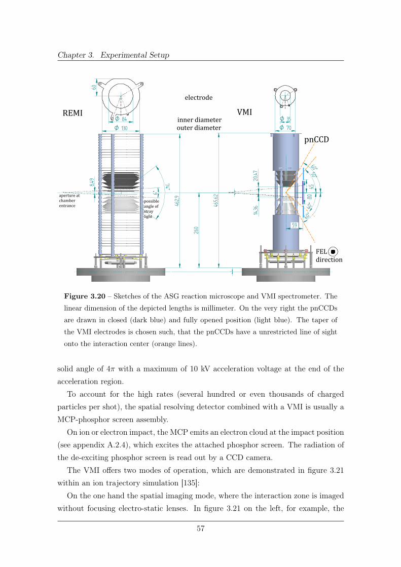
Chapter 3. Experimental Setup
462,9
465,62
00
260
14,36
20,47 50°
60°
40°
60°
8,49
inner diameterouter diameter
FEL
direction
electrode60
O 84
O 130
O 35
O 70
59
4580
6°
74°
aperture at
chamber
entrancepossible
angle of
stray
light
REMI
pnCCD
VMI
Figure 3.20 – Sketches of the ASG reaction microscope and VMI spectrometer. The
linear dimension of the depicted lengths is millimeter. On the very right the pnCCDs
are drawn in closed (dark blue) and fully opened position (light blue). The taper of
the VMI electrodes is chosen such, that the pnCCDs have a unrestricted line of sight
onto the interaction center (orange lines).
solid angle of 4π with a maximum of 10 kV acceleration voltage at the end of theacceleration region.
To account for the high rates (several hundred or even thousands of chargedparticles per shot), the spatial resolving detector combined with a VMI is usually aMCP-phosphor screen assembly.
On ion or electron impact, the MCP emits an electron cloud at the impact position(see appendix A.2.4), which excites the attached phosphor screen. The radiation ofthe de-exciting phosphor screen is read out by a CCD camera.
The VMI offers two modes of operation, which are demonstrated in figure 3.21within an ion trajectory simulation [135]:
On the one hand the spatial imaging mode, where the interaction zone is imagedwithout focusing electro-static lenses. In figure 3.21 on the left, for example, the
57

3.2. The CAMP Endstation
800 nm Ti:sapphire laser ionizes the residual gas along its passage through thespectrometer center and also the krypton in the target gas jet, which is slightlyoffset in the detector image due to its initial momentum. In the spatial imagingmode the time-of-flight is well resolved.
On the other hand, there is the focussing mode, where a non-homogeneous extrac-tion field focuses fragments of different origin but the same initial velocity vector bymeans of open electro-static lenses onto the same point on the detector; the time-of-flight resolution, however, is worse than for the spatial imaging mode (on the right infigure 3.21). The focusing mode is used to retrieve the full 3D momentum vector ofthe fragments via Abel transformation from the measured 2D distribution for sym-metric fragment emission. In a REMI and a low-rate VMI with fast spatial-resolvingdetectors (delay line anodes, see section 3.2.2.3) [136], the molecular frame can betraced back by the 3D coincidence-measurement, where spatial and temporal infor-mation of the detector-hit is available. In a standard VMI, the nanosecond-precisetime information is lost owing to the high extraction field and the millisecond-longintegrating time of phosphor screen and CCD. Then, a coincidence measurement isnot possible and the molecular frame cannot directly be retrieved. Instead of anarbitrarily oriented e.g. molecular ensemble, axial alignment has to be applied withan axis of cylindrical symmetry parallel to the surface of the detector. Then, the3D information can be calculated from the 2D picture via a mathematical inversionprocedure [137, 138]. Velocity map imaging has been employed at the FLASH softX-ray laser and demonstrated that high-resolution momentum distributions can beretrieved at high rate from non-linear FEL ionization processes [139].
The six electrodes of the ASG VMI have smaller inner (35 mm) and outer (70 mm)diameters than the REMI electrodes to provide a higher electric field in the center(figure 3.20). The first generation of VMI spectrometers consisted of a closed re-peller, an open extractor and a grounded drift electrode [140]. Later an open repellerwas chosen to detect either electrons [136] or ions [141] on a second detector as atrigger for the ion time of flight or electron angular distribution, respectively. Here,the VMI is double-sided and symmetric (apart from the first electrode). It has adrift tube on both sides and the extractor electrode of one side works as repellerelectrode for the other side. The symmetric design allows the simultaneous mea-surement of the ion and electron momenta. For instance, the electron diffractionpatterns of photo electrons in a laser aligned molecule could recently be measured
58

Chapter 3. Experimental Setup
-1000V
+1000V+2000V
-2000V-400V
+230V-1000V
+1000V
-1000V-1000V+1000V+1000V
spatial imaging focusing mode Comparison of VMI modes
jetresidual gas
along TiSaH+ O2+N2+ Kr+H+H2O+ H2O+Kr+
MCPphosphor screenopal camera
time-of-flight spectra
2µs2µs 4µs 4µs
repellerelectrodesextractorelectrodesdrift tube
Figure 3.21 – Two modes to run a VMI spectrometer: spatial imaging and focusing.
The detector image (spatial information) and the time-of-flight spectrum is shown
for both modes. Analogue to standard one-side VMIs the electrodes are labeled as
repeller, extractor and drift tube.
on one side while the other side imaged the ion distribution to monitor the degree ofmolecular alignment. The voltage on each electrode is set independently to adjustthe focusing for the expected electron kinetic energy or to change between focusingand spatial imaging mode. The electric field of the spectrometer is defined at theend of the drift tubes by a fine copper mesh with 80% transmission on fixed voltage.An additional unique feature of the ASG VMI are the conical electrodes. With thepnCCDs downstream of the interaction zone (blue vertical lines on the very right infigure 3.20), simultaneous measurements of ion time-of-flight spectra and diffractionpatterns or the fluorescent yields can be performed.
3.2.2.3 Time and Spatial Resolved Ion Detection
The ion signal is amplified by a set of multi-channel plates (MCPs, see appendixA.2.4) by a factor of about 107. While the MCP amplifies the signal of the charged
59

3.2. The CAMP Endstation
particle and provides the time coordinate, an additional anode is required to retrievethe spatial information of a detector hit. Delay line anodes provide high positionresolution over a large area and fast read-out allowing high count-rates [142].
The basic idea is to derive the signal start position on a transmission line of fixedlength from the times the signal needs to propagate to both ends of this line. Thetransmission line, however, is not straight but has a meander-shape causing a timedelay; delayed, that is longer, times are detected with higher accuracy resultingin higher position resolution. By its meander-shape the transmission line coversan area and thereby yields a one dimensional coordinate for all signals starting inthis area. To get a two dimensional position read-out a second delay line is addedperpendicular to the first one.
x2
y2
y1
x1
Figure 3.22 – The working principle of the delay line anode: the position is derived
from signal propagation times (left), meander-shape delay line (middle), two dimen-
sional delay line anode (right).
Although the delay lines form a discrete anode pattern the position read-out iscontinuous. This is achieved by interpolating the center-of-mass of the charge cloudwhich spreads out starting from the impact position of the particle on the MCP andwhich is collected by several wires.
Additionally to the signal transmission line, there is a second so called referenceline on lower voltage relative to the signal line (36 V). The reference line servesas reference to electronic noise which is found on both lines. Moreover, these twoparallel lines form a Lecher line decreasing the impedance for the high-frequencysignals when it runs to the readout.
60
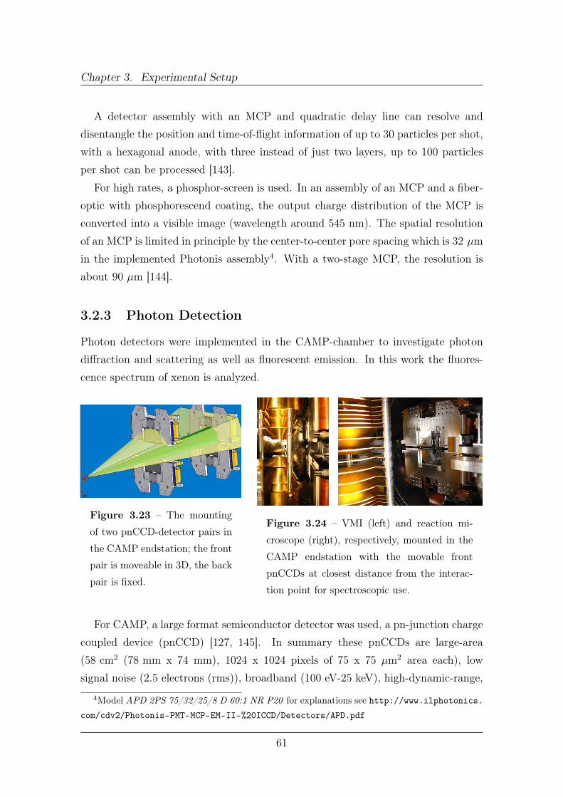
Chapter 3. Experimental Setup
A detector assembly with an MCP and quadratic delay line can resolve anddisentangle the position and time-of-flight information of up to 30 particles per shot,with a hexagonal anode, with three instead of just two layers, up to 100 particlesper shot can be processed [143].
For high rates, a phosphor-screen is used. In an assembly of an MCP and a fiber-optic with phosphorescend coating, the output charge distribution of the MCP isconverted into a visible image (wavelength around 545 nm). The spatial resolutionof an MCP is limited in principle by the center-to-center pore spacing which is 32 µmin the implemented Photonis assembly4. With a two-stage MCP, the resolution isabout 90 µm [144].
3.2.3 Photon Detection
Photon detectors were implemented in the CAMP-chamber to investigate photondiffraction and scattering as well as fluorescent emission. In this work the fluores-cence spectrum of xenon is analyzed.
ARTICLE IN PRESS
limit the motion of pnCCD1. This permits the mounting ofdifferent target jet devices along with lasers for alignment orpump-probe purposes. The middle part of each spectrometerconsists of conically shaped, gold-plated aluminum electrodesthat generate the homogeneous projecting (REMI, Fig. 3a) orinhomogeneous imaging (VMI, Fig. 3b) electric fields. Further
outside, two solid drift tubes (VMI) or equally spaced potentialrings (REMI) guarantee a field-free drift region. The conical shapeof the central electrodes within the solid angle covered by thepnCCD detectors allows unrestricted view into the scatteringvolume. At the same time, the cones excellently suppressscattered stray radiation emerging from outside the interactioncenter.
Since the operation principles of REMI/VMI spectrometershave been described extensively in the literature, only the salientfeatures are briefly outlined in the present contribution. For theREMI configuration, illustrated in Figs. 2a and 3a, the electric fieldforces all ions, independent of their initial momentum, ontoparabolic trajectories (red lines in Fig. 2a) and projects them ontothe detector. The electric field, usually a few V/cm, can in mostcases be adjusted such that all ions of interest are registered.Measuring the time-of-flight (TOF) and the hit position, thetrajectory and, thus, the full three dimensional momentumvector of each individual ion can be reconstructed. Electrons arepushed towards the other hemisphere by the electric field butcannot be efficiently projected onto the detector with moderatefields. Even though their momenta are typically very similar tothose of the ions, the electron energies are several thousand timeslarger, and accordingly, keV projection voltages would berequired, leading to times-of flight of a few nanoseconds. This istoo short to achieve reasonable momentum resolution along theextraction field direction. In a REMI, the dilemma is solved bymaintaining a small electric field but confining the electrons’transverse motion via an additional homogeneous (Helmholtzconfiguration, coil +160 cm) magnetic field (here up to 70Gauss), oriented parallel to the electric field and forcing themonto spiral trajectories as sketched in Fig. 2a (green line). Again,by measuring the TOF and the hit position, the full initialmomentum vector can be retrieved (for details, such as theattainable resolution, see [6]). Both detectors are equipped witheither square or hexagonal delay line anodes (Roentdek HEX80[9]) read out by an eight-channel, 2 GHz digitizer (AcquirisDC822) recording the complete wave form of the signal. Ithas been demonstrated recently at the SCSS test facility that up to150 ions emerging from the interaction of a single EUV-FEL pulsewith a single cluster could be analyzed, with their individual 3Dmomentum vectors [10] determined independently. In principle,the REMI allows for the coincident detection of momentum-resolved ions and electrons emerging from the same reaction. Thisfeature has been used to explore sequential two-photon doubleionization of Ne atoms in a kinematically complete experimentwhere two electrons and the ion have been detected in a triplecoincidence [11]. Meanwhile, specially adapted REMIs have beensuccessfully operated in many experiments at FLASH and the SCSStest facility [12–14] and the present design builds on this previousexperience.
Alternatively, if even more fragments are ejected per FEL shot,the delay line anode can be replaced by a phosphor screencombined with a CCD camera readout, thus recording the imageof electrons and/or ions without the magnetic field and applyingnon-homogeneous imaging voltages generated by the potentialcones depicted in Fig. 3b. In this ‘‘velocity map imaging’’ [7] mode,only two-dimensional (position) images are generated andthe time information is usually lost due to short flight times ofthe electrons resulting from the large imaging electric fields ofup to keV/cm. Still, under certain conditions and/or forlow-energy electrons, three-dimensional images can be retrieved(for details see [15]). Again, the applicability of this method atFELs has been proven recently at FLASH [16]. Since the standardVMI electrode configuration [7] had to be modified for ourapplication, additional lenses are used to provide better spacefocusing [17].
Fig. 4. Artist’s view of the two pnCCD mountings. The two halves of the pnCCD on
the left side (closest to the interaction point), CCD1, can be opened vertically by up
to 90, 45 mm each. Photons scattered under large angles can hence be detected,
while the second (fixed) pnCCD2 records the X-rays under smaller angles. The
distance between the detectors can be changed by moving the CCD1 system up to
250 mm along the beam axis. Moreover, if needed, CCD2 can be placed at any
distance larger than 550 mm away from the interaction zone by simply
introducing fixed spacer tubes of the desired length.
Fig. 3. 3D model of the CAMP reaction microscope (a) and the velocity map
imaging (b) spectrometers. The total length of both devices is 400 mm, and both
are designed for +80 mm detectors. The conically shaped central electrodes are
clearly visible. They provide a free line of sight for the pnCCDs over their complete
active area and, at the same time, suppress stray light, which is, especially effective
for the REMI geometry. For the REMI typical voltages are a few V/cm. The VMI is
operated at kV/cm for full solid-angle imaging of electrons up to 200 eV. With a
magnetic field of up to 70 Gauss for the REMI, electrons emitted with energies of
up to 2 keV into the most unfavourable direction, transverse to the electric
extraction field, are confined to a spiral trajectory with a diameter of about 70 mm
and, thus, are detected with a solid angle of 50% of the full 4p steradiant. Multi-
channel plate detectors are mounted at both ends and can be equipped with delay-
line anodes or phosphor screen CCD camera readout (see text).
L. Struder et al. / Nuclear Instruments and Methods in Physics Research A 614 (2010) 483–496 487
Figure 3.23 – The mounting
of two pnCCD-detector pairs in
the CAMP endstation; the front
pair is moveable in 3D, the back
pair is fixed.
Figure 3.24 – VMI (left) and reaction mi-
croscope (right), respectively, mounted in the
CAMP endstation with the movable front
pnCCDs at closest distance from the interac-
tion point for spectroscopic use.
For CAMP, a large format semiconductor detector was used, a pn-junction chargecoupled device (pnCCD) [127, 145]. In summary these pnCCDs are large-area(58 cm2 (78 mm x 74 mm), 1024 x 1024 pixels of 75 x 75 µm2 area each), lowsignal noise (2.5 electrons (rms)), broadband (100 eV-25 keV), high-dynamic-range,
4Model APD 2PS 75/32/25/8 D 60:1 NR P20 for explanations see http://www.ilphotonics.com/cdv2/Photonis-PMT-MCP-EM-II-%20ICCD/Detectors/APD.pdf
61

3.2. The CAMP Endstation
single-photon-counting X-ray detectors capable of imaging and spectroscopic appli-cations. A detailed description can be found in the appendix, section A.2.5. Forsmall-angle diffractive imaging experiments, one set of pnCCDs is mounted 500 mmdownstream of the interaction point (and can be moved to any longer distance byinserting adaptor tubes). Another set of pnCCDs is moveable along the beam direc-tion over 250 mm and these detectors can be moved vertically (i.e. perpendicularto the beam) by 45 mm for larger scattering angles (see figure 3.23). In the spectro-scopic setting the detectors should be as close as possible to cover the highest solidangle. In figure 3.24 the pnCCDs are moved to the closest distance to the interactionpoint allowed by the ion spectrometer. The resolution at 1500 eV photon energywas found to be 98 eV.
62

Chapter 3. Experimental Setup
3.3 Data Acquisition and Analysis
3.3.1 From Analogue Pulses to Digitized Data
3.3.1.1 High-Pass Filter
Pulses from the MCP-delay-line detector are decoupled through an RC-filter (resistor-capacitor circuit). The bias-voltage is applied on the resistor side, the high-frequencypulses are read out on the capacitor side (fig. 3.25 and 3.26).
Title
Number
ANDRESEN ELECTRONICS LTD.
Date July 1 2008 Size SSheet of Rev File: decoupling_box.Sch
100k
10K
G
to HV supply
to amplifier
4.7nFG
to detector
100
0
4.7nF
10K
Figure 3.25 – High-pass MCP read-out.Title
Number
LBNL
Date July 1 2008 Size SSheet of Rev File: anode readout.Sch
G
6.5nF
6.5nF
to amplifier
1 2
Linear
250
100k
100k
+
+3160
+
+3200high voltagepower supply
G
to anodesignal reference
Figure 3.26 – Differential anode read-
out.
Signal and reference line are connected to the ends of the secondary coil of atransformer. Electric noise is equally distributed on both lines, such that the voltageon both ends of the coil is the same and the transformer does not deliver this DC-likevoltage rise to the primary coil. Due to the slightly higher bias voltage on the signalline, real pulses have a higher amplitude on the signal than on the reference line.Thus, real (AC-like) pulses are transformed to the primary coil.
3.3.1.2 Digital Converter
For the delay line anode, the analogue detector pulses are digitized by an AcqirisADC [146]. It provides four channels with a sampling rate of 2 GHz. That means,the maximum time resolution of a detector signal is 500 ps, when all four channelsare used in parallel, and 125 ps, when only one channel is used. The resolution ofthe pulse height is 10 bit. The Acqiris Digitizer records the complete wave formof the signal and is, therefore, especially capable for multi-hit detection. Any peak
63

3.3. Data Acquisition and Analysis
recognition and filtering is then done on the software site (see sec. 3.3.2.1). Themaximum length of the waveform was limited by the LCLS network speed to 20000data points, such that the waveform was 20 µs long at a 1 ns resolution.
The phosphor screen image is recorded by commercial CCD cameras. LCLSprovided Adimec OPAL-1000 cameras, implemented in their data acquisition system,with megapixel resolution and 120 frames per second acquisition rate [147]. Fornon-LCLS experiments a Pulnix TM-6740CL camera with an acquisition rate of 200frames per second, but a lower resolution of 640 times 480 pixel is used with theASG VMI spectrometer [148].
3.3.1.3 Analysis Software
The LCLC data files (".xtc" file format, "extended tagged container") are ana-lyzed with the C++ based CFEL-ASG Software Suite (CASS) [149]. It handles alldata from the different detectors used in CAMP: from Acqiris analogue-to-digital-converters (ADC) [146], Acqiris time-to-digital-converters (TDC) [150], commer-cially available charge coupled devices (CCD) and pnCCD cameras, and also themachine-related data, i.e. fast shot-to-shot beamline data (e.g. pulse or photonenergy) and slow 1 Hz "epics"-data [151] (e.g. voltage or pressure settings).
Analysis tasks are listed as postprocessors in a text file (".ini file" format). Post-processors are user definable procedures to handle and analyze recorded raw dataof the experiment. They include data operations as, for instance, putting requestedmeasurements from a data file into a user defined spectrum, computing logical andarithmetic values from the dataset or relating different measurements and compu-tations within one FEL event. The resulting 0D, 1D or 2D histograms can eitherbe saved in hdf5 [152] or in root [153] file format. Here, the root format was cho-sen so that histograms could be evaluated further in the ROOT C++ framework.Eventually, histograms have been processed by the analysis software originpro [154]because of its superior graphical presentation and ease of use.
3.3.2 Ion Time-of-Flight Spectra
In a time-of-flight (TOF) spectrometer, the time between the creation of the ion andits detection is proportional to its charge-to-mass-ratio. While the recorded Acqiristrace already comprises the main features of a time-of-flight spectrum, particular
64

Chapter 3. Experimental Setup
peak heights and positions have to be addressed in a more quantitative analysis.
3.3.2.1 Constant Fraction Discriminator
The Acqiris trace depicts the voltage history on the MCP detectors within an ad-justable time window and temporal resolution, here 20 µs and 1 ns, respectively.In a so called counting mode, where the ion rate is intentionally set low to reducethe overlap of signals in the Acqiris trace, the actual pulse shape and amplitude canbe disregarded. The only important information is the (temporal) peak position.For further analysis, it is practical to discretize each peak position. The simplestmethod to find peak positions and suppress noise peaks, is to set a threshold. Thisapproach, however, yields different times for different peak heights as seen in figure3.27 on the left. The determination of the center of mass addresses this issue butfails when neighboring peaks superpose.
Input Signal
Attenuated Input Delay
Delayed and Inverted Input
Constant FractionSignal
Zero Crossing Time
Figure 3.27 – The CFD creates a zero-crossing by adding a delayed and inverted pulse
to a fraction of the original input. This way, the triggering time becomes independent
of the pulse amplitude (right), in contrast to triggering by a threshold (left).
The constant fraction discriminator (CFD), depicted in fig. 3.27, is able to dis-criminate peaks even when they (slightly) superpose. The CFD algorithm delaysthe incoming pulse by few nanoseconds and subtracts it from a fraction, typically60%, of the undelayed pulse:
fCFD(x) = f(x) · fraction− f(x+ delay) (3.11)
3.3.2.2 Calibration of a Time-of-Flight Spectrum
The utilized time-of-flight spectrometer has, except at edges and lenses, a homoge-neous electrostatic field, where the kinetic energy induced on a particle with mass
65

3.3. Data Acquisition and Analysis
m and charge q by the accelerating voltage U is Eel = q · U , thus
Eel = q · U =1
2mv2 = Ekin ⇒ v =
√2qU
m⇒ t = s ·
√m
2qU(3.12)
So at fixed spectrometer voltages, the ion time-of-flight t is specific for a certainm/q value (and specific for the ion momentum along the spectrometer axis). Withthe linear equation √
m
q= a · time of flight + b (3.13)
peaks in a time-of-flight spectrum can be attributed to meaningful values of m andq. Typical ions from residual gas, which can be found in most TOF spectra, arehydrogen,
√mq
= 1, and oxygen singly or doubly charged,√
mq
= 4 or√
mq
= 2.8,respectively. When the peaks of these ions are clearly distinguishable in the TOF,their time-of-flight and
√mq
value serve as calibration points for the whole TOFspectrum.
In the case of the xenon and krypton, irradiated by ultra-intense x-rays, oxygenpeaks were superimposed by target gas ions and the recorded 20 µs Acqiris tracemissed the lowest xenon and krypton charge states, so that simple enumerationalong 1+, 2+, 3+, ... was not possible. Then, the calibration has to be found by thedetermination of the lowest recorded charge state q. The higher charge states canthen be enumerated starting from that q.
In figure 3.28 every time-of-flight peak is attributed to√
mqvalues, assuming that
the lowest recorded charge state at 17.2 µs is either Xe1+ (green), Xe3+ (blue) orXe5+ (red). It turns out that only the blue curve follows the linear equation (3.13),so the peak at 17.2 µs must belong to Xe3+. With the lowest recorded charge stateattributed to Xe3+ the subsequent higher charge states are attributed to q+n. Thisway, the time-of-flight spectrum is calibrated.
3.3.2.3 Deconvolution of Merged Charge States
To determine the precise abundance of each charge state, every peak should beintegrated within TOF adjusted limits. However, for short time-of-flights, due tohigh extraction fields or for highly charges ions, and in the presence of many isotopes,densely spaced peaks may superpose in the averaged spectrum and also in single shotspectra; for example with 50 V extraction voltage 126Xe15+ starts to overlap withthe heavier isotope 136Xe16+, and, at even shorter time of flights, consecutive chargestates increasingly merge.
66

Chapter 3. Experimental Setup
y = 0,0003824x - 0,0157720
0
1
2
3
4
5
6
7
8
4500 6000 7500 9000 10500 12000 13500 15000 16500 18000
Sqrt
(m/q
)
Time-of-flight in nanoseconds
Xenon 5+ Xenon 3+ Xenon 1+ Linear (Xenon 3+)
Figure 3.28 – Xenon time-of-flight calibration at 50 V spectrometer voltage: the√mq ratios are plotted against the TOF. The green, blue and red line assume that
the charge state with the longest time-of-flight is Xe5+, Xe3+ and Xe1+, respectively.
The√
mq values linearly depend on the TOF and as only Xe3+ is described by a linear
function, charge state with the longest time-of-flight must be Xe3+.
To deconvolve the (averaged) spectrum, the height of each individual charge stateis adjusted in a simulated charge-state distribution, until the sum of all simulatedGaussian-shaped peaks matches the experimental data. Three parameters have tobe determined experimentally: the isotopic composition of the target gas as well astime-of-flight dependent peak positions and peak widths. For lower charge states ofxenon, the isotopic composition is resolved. The integral of a Gaussian fit for eachmass yields an isotopic ratio:
Xenon mass in [u] 128 129 130 131 132 134 136Measured percentage 2.26 25.13 4.59 20.76 25.79 11.58 9.89
Literature value 1.91 26.40 4.10 21.29 26.90 10.40 8.90
Table 3.3 – Isotopic composition of xenon
From the equation 3.13 of the calibration, the individual peak position for mergedion signals is derived. The peak width was found to decrease linearly starting from
67

3.3. Data Acquisition and Analysis
Xe11+ and, thus, could be interpolated to higher charge states.
Figure 3.29 – Deconvolution of merged xenon time-of-flight peaks at 1500 eV photon
energy, 80 fs pulse length and 2.5 mJ pulse energy. The height of the individual charge
state peaks (colored) are adjusted so that their sum (red) matches the data (grey).
The deconvolution is manually performed for the experimental spectrum at 2.5 mJpulse energy (fig. 3.29). For a scan over different parameters, in particular differ-ent pulse energies, manual adjustment becomes impractical. Instead, one peak percharge state (i.e. 132Xe instead of all isotopes) is integrated within time-of-flightadjusted limits and merged peaks are weighted according to the overlap with neigh-boring peaks within the limits of integration. For example, the percental contribu-tion in the limits of integration for Xe30+ is: 1.5% Xe29+, 78.5% Xe30+ and 20%Xe31+. These weight factors should be used with care, as they are determined at acertain pulse energy (2.5 mJ), whereas the charge-state distribution and, thus, thepercental contribution will change non linearly at different pulse energies. As thisapproach was limited to a small pulse energy region and few highly charged ions,the effect of changing percental contribution has been neglected.
3.3.3 Analysis of the Fluorescence Spectra
The analysis of spectroscopic pnCCD data requires several calibration steps and acareful choice of readout-parameters. To understand the necessity of these steps, themeasurement process should shortly be summarized (according to reference [155],
68

Chapter 3. Experimental Setup
modified and extended):
Absorption of impinging X-ray Photons The photon energy of a photon im-pinging on the pnCCD detector is converted to electron-hole pairs via the photo-effect, a fraction also into phonons. At X-ray energies 3.6 to 3.7 eV are requiredfor the creation of one electron-hole pair in silicon. Because the electron emissionprocesses are not independent, a statistical uncertainty of this conversion factor,the Fano-noise, has to be considered. Fano-noise describes that it may requireless or more energy to create electron-hole pairs. For silicon the Fano-factor, themeasure of the Fano-noise, is 0.115. The Fano noise is energy dependent, roughly∝√Fano-factor · constant · Energy.
Charge Drift, Diffusion and Distribution over several Pixels As electronsdrift towards the potential minimum 7 µm under the pnCCD readout site (see fig.A.6 in the appendix), the electron cloud widens up due to Coulomb repulsion anddiffusion. This Gaussian shaped cloud may extend over one to four neighboringpixels, so that the total charge may be split in fragments. Charges can be createdthermally or by hot spots in the crystal which is why the pnCCD is cooled down to−50 C and less.
Transfer of Charges to Readout Anode In each readout line, electrons mightbe trapped at crystal defects during the transfer from the pixel-potential well to theanode. They can either catch up with the charge train or be delayed into the chargepackage of a succeeding pixel which smears out the spatial distribution. Charge-transfer efficiency (CTE) is a statistical process and adds noise.
Frontend Electronics The combination of a low capacitance anode and on-chipJFET amplifier provides an excellent signal-to-noise ratio. However, electronic noisemight be added by non-linearities from the output driver of the CAMEX-chips orthe limited bandwidth of the transmission line to the ADCs which themselves mightadd a small digitization noise.
That means for each measurement read noise, gains, charge-transfer efficiencies,charge splitting between neighboring pixels, energy resolution, and bad pixels haveto be determined individually either line or pixel wise.
3.3.3.1 Correction Maps created from Dark Frames
Line and pixel corrections are saved in distinct maps. To avoid "false positives", cor-rections maps are taken as dark maps with all light sources shielded. The following
69

3.3. Data Acquisition and Analysis
correction maps are used:
• Offset Map: Leakage currents may shift the baseline of each pixel. Also thetotal readout channel may show an additional offset.
• Noise Map: To derive the statistically leakage currents of each pixel the stan-dard deviation of 200 sampled frames is taken.
• Common-Mode Correction: Cross talk during the parallel electronic readoutof all channels is addressed in the common mode correction.
• Bad Pixel Map: Bright and noisy pixels are recognized by the offset and noisecorrection. In the analysis settings a noise level can be chosen to automaticallyset pixels as bad-pixel, so that these pixels will be disregarded in the furtheranalysis. Additional bad pixels can be set by the user.
In CASS, common mode, noise and bad pixel correction are individually switchedon and off and read in via the dark calibration file.
3.3.3.2 Clustering of Pixels and Pixel Threshold
In photo frames, the offset map is subtracted, the common-mode correction per-formed and the noise threshold applied. Additional to the pixel coordinates andpulse heights, the frame index and quality value are recorded, which indicates ifan event is in the vicinity of a bad pixel, a border or has an over- or underflow.Charges distributed over neighboring pixels are combined to one event (clustering).At maximum four pixels can be combined, if the resulting pattern is allowed [155](e.g. three pixels in a row are forbidden). Charge-transfer efficiency (CTE) and gaincalibration are loaded from a gain map [156].
3.3.4 Machine Data
Machine data includes fast changing shot-to-shot beamline data (e.g. pulse or pho-ton energy) and slow changing 1 Hz "epics"-data [151] (e.g. voltage or pressuresettings). Here, ion yield curves could be correlated to the pulse energy and thelinearity of pulse energy to attenuation pressure was shown.
70

Chapter 4
Multiple Ionization of Heavy Atoms
by Intense X-Ray FEL Pulses
4.1 Experimental Parameters
The data presented in this work were taken during two beamtimes at the LCLSXFEL using the CAMP endstation at the AMO beamline. The experimental pa-rameters are summarized in table 4.1.
Beamtime December 2009 January 2011
Focus ≈3x3 µm2 ≈3x3 µm2
Rayleigh length 10-20 mm 5-10 mm
Gas jet diameter 2 mm or flooded 4 mmIon detector-acceptance 1 mm, VMI with slit 80 mm, open REMIFluorescence detector-acceptance
38.4 mm x 76.8 mm,67 mm downstream
none
Target Xe Xe KrPulse length 300 fs 80 fs 80, 3 fsPhoton energy 1.5 keV 1.5, 2 keV 2 keVPulse energy 2.5 mJ 2.5 mJ 2.5, 0.4 mJAttenuator transmission 12%, 37%, 100% 0.01-100%, 5 steps
Table 4.1 – Experimental parameters during the beamtimes in 2009 and 2011.
In the beamtime 2009 an aluminum-disk with a 1 mm wide, 20 mm long slit
71

4.1. Experimental Parameters
orientated perpendicular to the FEL direction was inserted into the first electrodeof the VMI spectrometer to confine the detector acceptance to the high-intensitypart of the interaction center.
The pair of front pnCCDs were positioned 67 mm downstream of the interactioncenter. One of the pnCCDs could not be used due to problems with the readoutelectronics. About one third of the analyzed detector area was masked (set as bad-pixel) to disregard pixels with too much stray light and broken pixels after directexposure to the focused beam [157]. Then, the analyzed detector area covered asolid angle of 0.37 sr or 39.3 opening angle, respectively.
With the thin gas jet only, meaningful fluorescence spectra at several pulse ener-gies and for various gas targets could not be recorded within the available beamtime.Besides, at a base pressure of few 10−7 mbar, relatively small time-of-flight signals ofxenon were superimposed with signals from residual gas. Thus, to increase the flu-orescence yield the experimental chamber was flooded with xenon to a gas pressureof 1 · 10−6 mbar. The LCLS gas attenuator was set to three different transmissionsto scan the focus intensity.
In 2011, the ion time-of-flight spectrum of xenon was remeasured under improvedvacuum conditions (10−8 mbar) where contributions from residual gas were negligi-ble in time-of-flight spectra taken with the gas jet only. The intensity was varied infive steps from 0.01-100%. In addition to photon energies of 1.5 keV (correspondingto 0.6 nm wavelength), xenon time-of-flight spectra were measured at 2 keV (corre-sponding to 0.83 nm wavelength). For krypton at 2 keV data for two pulse lengthswere compared, namely 80 fs and < 10 fs, which will hereafter be referred to as 3 fs(3 fs is an estimate, which was used in the calculations. For a discussion of the pulselength determination see section 3.1.3.2).
Here, the REMI, instead of the VMI spectrometer, was used. The total accelera-tion voltage was much lower as compared to the VMI settings in 2009, 50 V insteadof 2 kV, allowing for a much better time-of-flight resolution. With the 80 mm elec-trode opening, the spectrometer was also sensitive to ions created out of focus atlower intensities.
The pulse energy in table 4.1 is given by the LCLS GMD in front of the steer-ing and focusing optics of the AMO beamline. For calculations of the actualphotoionization the fluence at the interaction point has to be estimated consid-ering the AMO beamline transmission and focus size. The experimental beamline
72

Chapter 4. Multiple Ionization of Heavy Atoms by Intense X-Ray FEL Pulses
transmission was reported to be about 20% while the design value is about 60% [19].In reference [19] a focus size of 3 µm2 is assumed for the HFP chamber about 2 mfurther upstream of the CAMP endstation. The focus size in CAMP is larger dueto the larger distance to the KB focusing optics. The smallest measured focus inCAMP so far is about 12 µm2 [158]. Imprint measurements [98] (see section 3.1.4.1)in the CAMP endstation determined an effective focal area of about 45 µm2 in 2009and about 37 µm2 in 2011. However, both measurements were performed at a latertime possibly not reflecting the focal parameters of the actual experiment any more.Besides, with these focal sizes, calculations do not at all reproduce the experimen-tal charge-state distributions suggesting, that the imprint studies overestimate thefocus size.
New Ne calibration with EXP (q=4-9) @ 2000 eV, 80 fs, 2.5 mJ
1.0 1.5 2.0 2.5 3.0 3.5 4.0 4.5
Focal size (µm)
10
20
30
40
50
60
70
Tran
smis
sion
(%)
0
0.01
0.02
0.03
0.04
0.05
0.06
R.m
.s e
rror
Figure 4.1 – Determination of beamline transmission by the use of the neon charge-
state distribution at 2 kV photon energy, 80 fs pulse length, 2.5 mJ pulse energy. On
the left the experimental data (black dots) along with calculations for a 3 µm x 3 µm
FWHM Gaussian-shaped focus size, 4 mm FWHM gas-jet diameter, 80 mm detector
acceptance and several transmissions indicated in the figure are plotted. On the right
the quadratic deviation between data and theory at different sets of focus diameters
and transmissions is shown.
To determine the transmission and focus size during the actual experiment, theexperimental charge-state distribution for a Ne target was compared to theoreticalcalculations that had consistently explained previous measured data [19]. For thispurpose, the experimental charge-state distribution of neon at 2 keV photon energywas taken immediately before the xenon measurement. The deviation between ex-periment and calculation was determined for neon charge states from Ne4+ to Ne9+
neglecting charge states up to Ne3+ which might be created by one photon ioniza-
73

4.1. Experimental Parameters
tion far out of focus. The quadratic mean of these deviations is depicted in figure4.1 on the right for various transmissions and focus sizes. The darkest color marksthe lowest deviation. From the dark-purple diagonal a combination of transmissionand focus size was chosen, which fits within the range of previously reported values:3 µm x 3 µm FWHM Gaussian-shaped focus size and 35% transmission at 2 keVphoton energy (3.5 µm x 3.5 µm and 48%, would fit as well).
With these parameters and a nominal pulse energy of 2.5 mJ, the focal intensitywas 1.2x10¹⁷ W/cm2.
At 1.5 keV photon energy a transmission of 18% and 3 µm x 3 µm focus size wasassumed to fit the calculated intensity-dependent ion yield to the data (see figure4.11; here 35% transmission and a 4.2 µm x 4.2 µm focus size would yield the samefluence). This assumption is based on predictions that the fluence decreases at lowerphoton energies [126]. With the lower transmission at 1.5 keV, the focal intensity is6.3x1016 W/cm2.
74
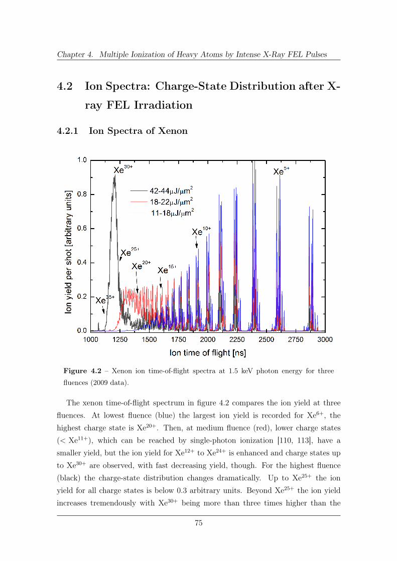
Chapter 4. Multiple Ionization of Heavy Atoms by Intense X-Ray FEL Pulses
4.2 Ion Spectra: Charge-State Distribution after X-
ray FEL Irradiation
4.2.1 Ion Spectra of Xenon
Figure 4.2 – Xenon ion time-of-flight spectra at 1.5 keV photon energy for three
fluences (2009 data).
The xenon time-of-flight spectrum in figure 4.2 compares the ion yield at threefluences. At lowest fluence (blue) the largest ion yield is recorded for Xe6+, thehighest charge state is Xe20+. Then, at medium fluence (red), lower charge states(< Xe11+), which can be reached by single-photon ionization [110, 113], have asmaller yield, but the ion yield for Xe12+ to Xe24+ is enhanced and charge states upto Xe30+ are observed, with fast decreasing yield, though. For the highest fluence(black) the charge-state distribution changes dramatically. Up to Xe25+ the ionyield for all charge states is below 0.3 arbitrary units. Beyond Xe25+ the ion yieldincreases tremendously with Xe30+ being more than three times higher than the
75

4.2. Ion Spectra: Charge-State Distribution after X-ray FEL Irradiation
lower charge states. Here the highest observed charge state is Xe36+. Note that theheight of the peaks in the TOF-spectra for different charge states does not directlyrelate to their respective yields due to the
√q/m compression of the scale towards
shorter TOFs.Due to the high extraction voltages the time-of-flight spectrum is confined on to
just 2 µs, so that the time resolution is rather low and neighboring peaks mergequickly with increasing charge state. For instance, the large peak at Xe30+ is partlydue to contributions from neighboring peaks and, using the deconvolution procedureits height of 0.9 units is actually found to be 0.6 units. Thus, the time-of-flightspectrum of xenon depicted in 4.2 was measured under improved conditions in 2011,see figure 4.3. Note that also other experimental parameters change slightly, seetable 4.1; most notably the detector acceptance was 80 mm in 2011 as comparedto 1 mm in 2009. Hence, not only ions experiencing the highest fluence in theinteraction center are detected, but also ions created by single-photoionization farout of the focus.
Figure 4.3 – Xenon ion time-of-flight spectrum at 1.5 keV (black) and 2 keV (red)
photon energy and 2.4 to 2.6 mJ pulse energy.
In figure 4.3 the xenon time-of-flight spectrum is presented for 1.5 keV (in black)
76

Chapter 4. Multiple Ionization of Heavy Atoms by Intense X-Ray FEL Pulses
and 2 keV (in red) photon energy, integrated over a pulse energy interval of 2.4 mJto 2.6 mJ. This corresponds to a peak fluence of approximately 42-46 µJ/µm2
(1.5 keV) and 82-89 µJ/µm2 (2 keV) at the target.For lower charge states, i.e. long time-of-flights, the REMI spectrometer features
isotope separation with all seven stable isotopes of xenon clearly distinguishable.At Xe15+, mass 126 starts to overlap with mass 136 of Xe16+ and, at even shortertimes, consecutive charge states increasingly merge. To obtain the charge-statedistribution depicted in figure 4.4, a deconvolution procedure was employed forcharge states above Xe23+ by adjusting the height of individual charge states ina simulated distribution until their sum matched the experimental spectrum (seesection 3.3.2.3). Those charge states, where deconvolution becomes necessary, aremagnified in the inset of figure 4.3. To determine the ion yield for the other chargestates the time-of-flight peak for the isotope 132Xe was integrated.
Figure 4.4 – Xenon charge-state distribution at 1.5 keV and 2 keV photon energy.
The data in figure 4.4 is compared to a theoretical model by S.-K. Son andR. Santra. In this model more than a million coupled rate equations -with pho-toionization cross sections and decay rates from non-relativistic Hartree-Fock-Slatercalculations- were numerically solved (see section 2.2.4.2). The sum of each theoreticalcharge-state distribution is normalized to the sum of the corresponding experimentaldistributions; a logarithmic scale is chosen to zoom into low yields of highly chargedions. The calculated yields for the charge states Xe1+ and Xe2+ are not displayedas they were out of range in the experimental time-of-flight spectrum.
In general, the ion yield per X-ray pulse is found to be lower for 2 keV thanfor 1.5 keV photon energy throughout the time-of-flight spectrum. Apparently, thehigher fluence at 2 keV is more than compensated by the lower cross sections for
77

4.2. Ion Spectra: Charge-State Distribution after X-ray FEL Irradiation
M-shell ionization (at 2 keV the L-shell is still out of reach even for two-photonionization). Additionally, the number of photons is lower at higher photon energywhen the same pulse energy is chosen.
For both photon energies the experimental spectra are somewhat smoother thanthe predicted ones if one inspects them in detail on a linear scale. Then in thetheoretical distributions a pronounced minimum at Xe5+ and a maximum at Xe7+
are observable and between Xe10+ and Xe20+ odd-even charge-state alternationsappear. Such alternations have been previously attributed to the disregard of shake-off and double Auger processes by the calculations [19]. Here, the shake-off process(see section 2.2.2.4) is included for 0+ and 1+. Double Auger or Auger satellites(see section 2.2.2.5) are not considered.
The overall trend of the charge-state yields for the 2 keV case is predicted verywell with some divergence in the relative yield between Xe10+-Xe20+, which is exper-imentally found to be lower. For Xe31+ and Xe32+ the relative ion yield is smallerthan 10−3 and the absolute experimental error (indicated as thin black lines) in-creases to the same order of magnitude. For 1.5 keV photon energy, however, theexperimental charge-state distribution deviates drastically from the theory values.The calculations predict a maximum charge state of ∼Xe27+, while the recordeddata show charge states up to Xe36+.
4.2.2 Discussion of the Xenon Charge-State Distribution
Photoionization of xenon at FEL-typical irradiance levels of 1016 W/cm2 has pre-viously been investigated at the Extreme Ultra-Violet (XUV) free-electron laser inHamburg, FLASH [31]. Surprisingly high charge states q up to Xe21+ have beenobserved at 93 eV photon energy, i.e. λ = 13.3 nm. While resonant excitationionization processes have been considered as catalyzers of sequential multiphotonionization, the main contribution to multiple ionization at highest q has been at-tributed to direct multiphoton ionization by up to seven photons [31, 159]. Also,non-perturbative strong-field phenomena [31] and many-electron effects [160] havebeen speculated to play a role.
While pulse intensities here are comparable to those achieved in the FLASHexperiment, much higher photon energies of 1.5 keV and 2.0 keV, respectively, wereused. Due to the 1/ω2 dependence of the ponderomotive force, strong-field effectsare expected to play a negligible role and any non-perturbative effects can be safely
78

Chapter 4. Multiple Ionization of Heavy Atoms by Intense X-Ray FEL Pulses
neglected. Also, direct multiphoton ionization was found to play a minor role [20,24, 25]. At X-ray energies, photoionization in general proceeds predominantly via asequence of single-photon ionization steps of the lowest accessible inner-shell orbitals(see section 2.2.2.4 and 2.2.4.1) and, hereafter, the inner-shell vacancy is filled byouter-shell electrons in a decay cascade (section 2.2.2.5).
The lowest accessible inner-shell orbital is shown in figure 4.5, where the orbitalbinding energy of the electronic ground-states from 3s to 20s orbitals are plottedagainst the xenon charge state. The ground-state configuration of neutral xenon is
1s22s22p63s23p63d104s24d64d105s25p6, (4.1)
hereafter abbreviated as [Ne]3s23p63d104s24d64d105s25p6. To indicate the availablephoton energies dashed red horizontal lines are drawn, which intersect the M-shell(3s, 3p, 3d) binding energies at certain charge states. Sequential single-photonionization implies, that the photoionization will stop as soon as the binding energiesof the not-yet-ionized electrons falls below the respective red line denoting a givenphoton energy.
Accordingly, for 2 keV photon energy single-photon ionization closes at the chargestate Xe32+: With the ground-state configuration [Ne]3s23p63d4, the least-boundelectrons are those in 3d, which have a binding energy of 2018 eV. In the charge-state distribution for 2 keV depicted in figure 4.4 the highest charge state predictedand detected experimentally nicely coincide to be exactly q = 32. Apparently, theunderlying basic process of sequential single-photon ionization is well described bythe theoretical model and no additional processes appear for 2 keV according to theexperimental spectrum.
For 1.5 keV photon energy single-photon ionization closes at the charge stateXe26+ where, in ground-state configuration, all electrons higher than 3d are emitted,[Ne]3s23p63d10. The binding energy for 3d electrons at q = 26 is 1509 eV so that amaximum charge state of Xe26+ is expected.
In striking contrast to these simple considerations as well as to the theoreticalprediction, charge states as high as 36+ are observed at a photon energy of 1.5 keV(figure 4.4). Here, sequential single-photon ionization can not explain the totalionization process and additional pathways have to be considered above Xe26+.
At low charge states (q<18), ionization from the n = 3 core-shell is most efficientas obvious from figure 4.5, blue arrow. Photoionization cross sections for the indi-vidual orbitals in the ground-state configuration of neutral xenon at 1.5 keV photon
79

4.2. Ion Spectra: Charge-State Distribution after X-ray FEL Irradiation
Figure 4.5 – Xenon orbital binding energies as a function of the degree of ionization
calculated with the Hartree-Fock method; the states 8 to 20 are calculated with the
formula for the binding energy of Rydberg levels, equation 2.32. The dashed and
dotted blue lines mark the resonances from 3s, 3p and 3d states at 1.5 keV and 2 keV
photon energy, respectively.
energy are summed up in table 4.2. Upon photoionization, the n=3 vacancies are
Orbital 3d 3p 4d 3s 4p 4sPhotoionization cross section 494 kb 223 kb 63 kb 54 kb 48 kb 14 kb
Table 4.2 – Photoionization cross sections in the ground-state configuration of neutral
xenon at 1.5 keV photon energy [106–108].
filled via Auger decay, which further increases the charge state.Towards q = 24 the 3d-hole Auger lifetime becomes comparable to the average
3d photoionization rate for 1.5 keV photon energy and at a fluence of 50 µJ/µm2,see figure 4.6. For this configuration n = 3 electrons will be ionized faster than theremaining holes can be filled via Auger decay resulting in the creation of multiplecore-holes. M-shell ionization ends at a charge state of 26+, so direct ionizationis closed, but Auger decay of multiple core holes still lead to charge states slightly
80

Chapter 4. Multiple Ionization of Heavy Atoms by Intense X-Ray FEL Pulses
1
10
100
0 5 10 15 20 25 30
Tim
e (fs
)
Charge state
3d hole Auger lifetimeInverse of 3d photoabsorption rate
Figure 4.6 – Xenon 3d single-hole Auger life time and inverse 3d photoabsorption
rate as a function of charge state for a fluence of 50 µJ/µm2.
above Xe26+ as seen in the calculated charge-state distribution in figure 4.4.
The creation of hollow atoms under ultra-intense X-ray irradiation is a well ac-cepted phenomenon at X-FELs. It was predicted even before the first X-FEL wasoperating [24] and has been investigated in detail for small systems such as neon [19]and nitrogen [21–23] since LCLS started operation. While Auger decay into multiplecore holes can indeed push the ionization above the limit for sequential single-photonionization, it cannot account for the strong enhancement of photoionization observedin the recorded xenon time-of-flight spectrum 4.3.
At 26+, an extremely efficient process, that is not included in the calculation,starts boosting multiple ionization as illustrated schematically in figure 4.5. AboveXe18+ electrons can be resonantly excited (red arrows) into Rydberg states (grey).Then subsequently, with increasing charge state, into n = 7, n = 6 and n = 5, whenthe 3s, 3p and 3d orbitals have a 1.5 keV energy difference with those valence states.The resonant excitation stops at around q = 35 due to the large energy gap betweenn = 4 and n = 5.
Auger or autoionizing transitions of these multiple and highly excited hollow-atomstates efficiently deplete the higher shells (green arrows), and, furthermore, refill the3s, 3p and 3d levels continuously. Electrons from refilled 3s, 3p and 3d states maythen again be resonantly excited. Because these resonances enable ionization atcharge states, where direct single-photon ionization is forbidden, this process maybe called resonance-enabled X-ray multiple ionization (REXMI) pathway.
The effectiveness of fast Auger and autoionization decay processes of hollow atoms
81

4.2. Ion Spectra: Charge-State Distribution after X-ray FEL Irradiation
has experimentally been observed [161] and theoretically proven [162] in electronemission and hollow-atom formation occurring when highly charged ions slowly ap-proach insulator and metal surfaces. This effect was first observed by Briand [163]in 1996 and extensively investigated in the following years [164].
Direct photoionization of the n = 4 shells (and above), filled by resonant exci-tation or during Auger decay of resonant excited states, is energetically possibleas well. However, the direct photoionization of Rydberg or valence states imme-diately after resonant excitation has a very low cross section. The highest crosssection is found for 5p valence ionization of Xe35+∗ ([Ne]3s23p65p1) where the ion-ization potential is closest to 1.5 keV. It amounts to 0.01 Mb [165]. In comparison,photoionization of the 3d orbital from neutral xenon has a cross section of about0.5 Mb and bandwidth convolved resonant excitations have cross sections of about1 Mb, see figure 4.18. With the cross section of 0.01 Mb, the fluorescence rate ishigher than the photoionization rate even at the highest fluence of 44 µJ/µm2 [165].Therefore, resonant excited states cannot be regarded as intermediate states in-volved in direct multiphoton ionization, but rather as starting point of Auger decayand autoionization. Thus, the REXMI mechanism is fundamentally different fromresonance-enhanced multiphoton ionization (REMPI), discussed in section 2.2.3.1.
Interestingly, from the level diagram in figure 4.5 one might expect that REXMIbecomes already less effective for charge states larger than about q = 31 whereresonant excitation into n = 6 ends. Resonances into n = 6 enable an efficient two-step ionization pathway with only one additional Auger decay involving n = 4 andnear continuum levels. Indeed, the experimental charge-state distribution in figure4.4 clearly shows a plateau in multiphoton ionization probability until q = 31 witha strong decrease towards q = 36. In ground-state configuration the 3d orbital isdepleted at Xe36+, [Ne]3s23p6, and resonant excitation from the 3d orbital to the5th shell is energetically not possible anymore implying a maximum charge state ofXe36+, as observed in the time-of-flight spectrum.
It should also be mentioned that resonance-enhanced multiple ionization is notlimited to the 1.5 keV case (dashed line in figure 4.4), but is expected for 2 keV pho-ton energy as well, which is indicated with dotted lines in figure 4.4. Nevertheless,with the reduced photon flux and cross section at 2 keV photon energy and the max-imum fluence of 86 µJ/µm2, the charge-state distribution ends already at q = 32just before entering the photon-energy-specific REXMI region (see also figure 4.17).
82
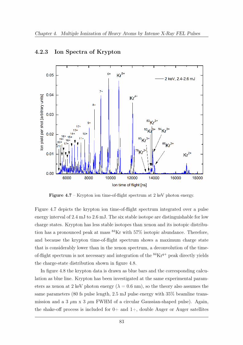
Chapter 4. Multiple Ionization of Heavy Atoms by Intense X-Ray FEL Pulses
4.2.3 Ion Spectra of Krypton
Figure 4.7 – Krypton ion time-of-flight spectrum at 2 keV photon energy.
Figure 4.7 depicts the krypton ion time-of-flight spectrum integrated over a pulseenergy interval of 2.4 mJ to 2.6 mJ. The six stable isotope are distinguishable for lowcharge states. Krypton has less stable isotopes than xenon and its isotopic distribu-tion has a pronounced peak at mass 84Kr with 57% isotopic abundance. Therefore,and because the krypton time-of-flight spectrum shows a maximum charge statethat is considerably lower than in the xenon spectrum, a deconvolution of the time-of-flight spectrum is not necessary and integration of the 84Krq+ peak directly yieldsthe charge-state distribution shown in figure 4.8.
In figure 4.8 the krypton data is drawn as blue bars and the corresponding calcu-lation as blue line. Krypton has been investigated at the same experimental param-eters as xenon at 2 keV photon energy (λ = 0.6 nm), so the theory also assumes thesame parameters (80 fs pulse length, 2.5 mJ pulse energy with 35% beamline trans-mission and a 3 µm x 3 µm FWHM of a circular Gaussian-shaped pulse). Again,the shake-off process is included for 0+ and 1+, double Auger or Auger satellites
83

4.2. Ion Spectra: Charge-State Distribution after X-ray FEL Irradiation
Figure 4.8 – Krypton charge-state distribution at 2 keV photon energy (in blue).
are not considered. For comparison the xenon results are plotted in the background(light red and black).
The experimental charge-state distribution peaks at Kr5+, then decreases forhigher charge states, but shows another local peak at Kr18+. The highest recordedcharge state is Kr21+. With respect to the overall shape, the krypton charge-statedistribution is closer to the Xe 1.5 keV than the Xe 2 keV case. The calculatedcharge-state distribution has three peaks, at Kr4+, Kr8+ and Kr13+. The predictedpeak at 8+ in the theory line appeared for multi- as well as for single-photon ion-ization and was attributed to the lack of relativistic effects in the calculations [166](spin-orbit splitting of the 2p shell could open more decay channels and smoothenthe 8+ peak). After the Kr13+ peak the ion yield constantly decreases. The highestcalculated charge state (in the depicted scale) is Kr18+.
4.2.4 Discussion of the Krypton Charge-State Distribution
At 2 keV photon energy, L-shell ionization for krypton is open and photoionizationof the krypton 2s and 2p shells have the highest cross section. Photoionization isaccompanied by shake-off processes and Auger decay. Single-photon ionization ofthe 2s orbital leads via an Auger cascade to a charge state up to 10+ with the highestyield for Kr7+ according to synchrotron measurements [112] and calculations [167].An exemplary Auger cascade upon 2s photoionization in krypton is shown in table4.3.
As the orbital binding energies increases during the ionization process, the 2sionization channel of krypton is closed at Kr+9 and direct 2p photoionization is
84

Chapter 4. Multiple Ionization of Heavy Atoms by Intense X-Ray FEL Pulses
Transition Name Lifetime
Kr+(2s−1)→Kr2+(2p−13d−1) LLM-Auger τ = 160 asKr2+(2p−13d−1)→Kr3+(3d−3) LMM-Auger τ = 560 as
Kr3+(3d−3)→ Kr4+(3d−24s−14p−1) MMN-Auger τ = 7 fsKr4+(3d−24s−14p−1)→ Kr5+(3d−14s−24p−2) MNN-Auger τ = 18 fs
Kr5+(3d−14s−24p−2)→ Kr6+(4s−24p−4) MNN-Auger τ = 155 fs
Table 4.3 – Exemplary Auger cascade upon 2s photoionization in krypton [68].
closed at Kr+13 at 2 keV photon energy (see dashed red arrow in figure 4.9). Thepeak at q = 13 in the calculated charge-state distribution is mainly due to closingof the direct 2p photoionization, where the photoionization cross section for furtherionization dramatically decreases after q = 13. The higher charge states beyondq = 13 are generated by multiple-core-hole formation, within the current theoreticalmodel. At q = 13 the electronic configuration of krypton in the ground-state is[Ne]3s23p63d5 so that M-shell ionizations may occur but with very low cross sectionscompared to L-shell ionization at lower charge states [166]. That is why the theorycurve rapidly decreases after q = 13. In the experimental spectrum, however, chargestates up to q = 21 are observed.
The ground-state binding energies of the L, M, N, O and P shells for krypton ionsup to a charge state of 22+ are illustrated in figure 4.9. The purple area parallel tothe binding energies of the L-shell mark possible resonances at 2 keV photon energy.At Kr9+, 2s direct photoionization is closed and resonant excitation from 2s intoRydberg orbitals opens instead. Figure 4.9 illustrates that, as for xenon, resonance-enabled X-ray multiple ionization (REXMI) can occur between Kr9+ and Kr20+
at 2 keV photon energy. Within the REXMI region, Auger decay is refueling theongoing ionization after resonant excitation. At 20+ the energy difference between2p and 4s exceeds the available photon energy of 2 keV and resonant excitation isstopped. Auger decay may remove another electron of excited Kr20+ resulting in amaximum charge state of 21+. Again this simple model is in astonishingly goodagreement with the experimental results.
85

4.3. Ion Yield vs. Fluence: How Many Photonsare Involved in the Ionization?
Figure 4.9 – Krypton orbital binding energies as a function of the degree of ionization.
The dotted blue lines mark the resonances from 2s and 2p at 2 keV photon energy.
4.3 Ion Yield vs. Fluence: How Many Photons
are Involved in the Ionization?
4.3.1 Xenon at 80 fs Pulse Length
The minimum number of absorbed photons during the ionization process can easilybe estimated by summing up ground-state binding-energies of ionized orbitals: intable 4.4 the sum is calculated for exemplarily charge states with the binding energiestaken from figure 4.5. This approach assumes that the total energy of an absorbedphoton is used for the ionization process, whereas in an actual photoionization asignificant fraction of the total energy is carried away by the photo- and Auger-electrons. Hence, these numbers can just be regarded as lower limit for the numberof absorbed photons.
In the second chapter (2.2.3.1) multiphoton ionization was treated with pertur-bation theory and it was derived that the multiphoton transition probability is a
86

Chapter 4. Multiple Ionization of Heavy Atoms by Intense X-Ray FEL Pulses
Charge state Sum of binding energies Divided by 1500 eV Divided by 2 keV5 156 eV 0.1 0.110 804 eV 0.5 0.415 2252 eV 1.5 1.120 4610 eV 3.1 2.325 8064 eV 5.4 4.028 12185 eV 8.1 6.130 15785 eV 10.5 7.932 19734 eV 13.2 9.934 24041 eV 16.0 12.036 28794 eV 19.2 14.4
Table 4.4 – Minimum number of absorbed photons needed to create a given charge
state
function of the intensity to the power of n, where n is the number of absorbed pho-tons (see equation 2.37). In the experiment the transition rate is measured by theion yield. To derive the number of photons, the detected ion yield is plotted againstthe pulse energy measured by the GMD in a double logarithmic plot so that theslope of the yield curves implies the number of absorbed photons.
To correlate pulse energy and ion yield, the time-of-flight spectrum is sorted withrespect to the pulse energy for every shot and plotted into a 2D graph with theGMD value on the y- and the time-of-flight spectrum on the x-axis (figure 4.10 onthe left). Then a y-projection, within the time-of-flight window for a particularcharge state, yields its pulse energy dependence of that charge state; for chargestates with coalesced peaks a deconvolution factor is applied (see section 3.3.2.3).
The projection has to be divided by the pulse energy distribution to normalizeon the number of shots at certain pulse energy; here, the binning of both, projec-tion (numerator) and distribution (denominator), has to be coarse enough to avoidnormalization artifacts.
Finally, the linearity of the GMD signal has to be verified by cross calibration withthe measured proton signal as discussed in section 3.1.3.3. For low pulse energies,i.e. high gas pressures in the attenuator, the GMD was found to yield higher pulseenergies than estimated by means of the proton count rate and, thus, the pulseenergy has been recalibrated in this region. Saturation at pulse energies above
87
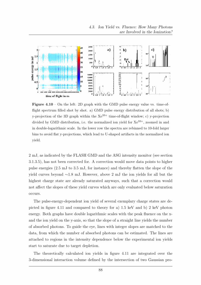
4.3. Ion Yield vs. Fluence: How Many Photonsare Involved in the Ionization?
Figure 4.10 – On the left: 2D graph with the GMD pulse energy value vs. time-of-
flight spectrum filled shot by shot. a) GMD pulse energy distribution of all shots; b)
y-projection of the 3D graph within the Xe33+ time-of-flight window; c) y-projection
divided by GMD distribution, i.e. the normalized ion yield for Xe33+, zoomed in and
in double-logarithmic scale. In the lower row the spectra are rebinned to 10-fold larger
bins to avoid flat y-projections, which lead to U-shaped artifacts in the normalized ion
yield.
2 mJ, as indicated by the FLASH GMD and the ASG intensity monitor (see section3.1.3.5), has not been corrected for. A correction would move data points to higherpulse energies (2.5 mJ to 3.5 mJ, for instance) and thereby flatten the slope of theyield curves beyond ∼1.8 mJ. However, above 2 mJ the ion yields for all but thehighest charge state are already saturated anyways, such that a correction wouldnot affect the slopes of these yield curves which are only evaluated below saturationoccurs.
The pulse-energy-dependent ion yield of several exemplary charge states are de-picted in figure 4.11 and compared to theory for a) 1.5 keV and b) 2 keV photonenergy. Both graphs have double logarithmic scales with the peak fluence on the x-and the ion yield on the y-axis, so that the slope of a straight line yields the numberof absorbed photons. To guide the eye, lines with integer slopes are matched to thedata, from which the number of absorbed photons can be estimated. The lines areattached to regions in the intensity dependence below the experimental ion yieldsstart to saturate due to target depletion.
The theoretically calculated ion yields in figure 4.11 are integrated over the3-dimensional interaction volume defined by the intersection of two Gaussian pro-
88

Chapter 4. Multiple Ionization of Heavy Atoms by Intense X-Ray FEL Pulses
files, the circular Gaussian X-ray beam (3x3 µm2 FWHM) and the circular Gaussiangas jet profile (4 mm FWHM). Due to the large detector acceptance of 80 mm, tailsof the Gaussian gas jet distribution, which reach far into the low-fluence part of theFEL beam, are included in the calculation.
Error bars are calculated including error propagation from the standard deviationof the individual ion yields at certain fluence and the total number of shots at thisfluence, which is used for normalization. The standard deviation of a count rate isthe square root of that count rate.
89

4.3. Ion Yield vs. Fluence: How Many Photonsare Involved in the Ionization?
Figure 4.11 – Experimental (data points) and calculated (solid lines) xenon ion yield
vs. peak fluence at a) 1.5 keV photon energy, and b) 2 keV photon energy. Integer
slopes are added to guide the eye.
90
Chapter 4. Multiple Ionization of Heavy Atoms by Intense X-Ray FEL Pulses
4.3.2 Discussion of the Ion Yields for Xenon
Synchrotron data provides information about the charge-state distribution uponsingle-photon absorption. For xenon single-photon M-shell ionization, charge statesup to 11+ are reported [112, 113]. In these publications the charge-state distributionpeaks at 7+ where the ion yield is more than two orders of magnitude higher thanfor 11+. Consistently, the Xe6+ yield curve follows a line with slope one. In averagethe ionization to Xe9+ requires the absorption of two photons and, thus, is bestfitted by a line with slope two. The number of absorbed photons for Xe15+ is 3, forXe20+ 4, for Xe25+ roughly 5, for Xe28+ about 7; for 30+, 32+ and 36+ the slopessuggest numbers of 10, 13 and 16, however, with large uncertainty.
Within that uncertainty the number of absorbed photons for photoionization at1.5 keV and 2 keV photon energy is about the same. That is reasonable, as ionizationproceeds through M-shell photoionization at both energies with the L-shell far outof reach even at 2 keV. Double ionization processes, which might be enhanced at2 keV by the higher excess energy, are not considered in the calculations and theexperimental statistics is too low to resolve such rare processes.
The calculated yield-curves are in very good agreement with the experimentallydetermined slopes as long as resonances play a minor role: they fit for all chargestates at 2 keV photon energy and up to q = 20 in the 1.5 keV case. For 1.5 keVresonant excitation starts at q = 18 according to figure 4.5. With the very efficientionization through the REXMI pathway, the actual photoionization cross sectionis higher than predicted by the theory. Thus, the experimental yield curves areshifted to lower fluences, as soon as multiple ionization via resonant excitation playsa role. The calculated yield curve for q = 28, in particular, is very much off, since 3pphotoionization is closed at q = 26 and further ionization in the theoretical modelcan just proceed via Auger decay od multiple core-excited states.
The number of absorbed photons, derived from the yield curves, gets closer tothe estimated minimum in table 4.4 with increasing charge state. On one hand theionization potential is closer to the impinging photon energy at high charge statesand less energy is carried away by the photoelectron. Thus the minimum number ofabsorbed photons in table 4.4 is closer to the actual number of photons required forthe ionization. On the other hand resonances may reduce the slope of experimentalyield curves, as discussed in section 2.2.3.1, so that the number of absorbed photons,
91

4.3. Ion Yield vs. Fluence: How Many Photonsare Involved in the Ionization?
derived from the yield curves, is reduced.
4.3.3 Krypton at 80 fs Pulse Length
As described for the case of xenon above, the minimum number of absorbed photonsfor krypton is depicted in table 4.5. Accordingly, ionization by a single photon maylead up to Kr10+, which also was the highest charge state created by L-shell pho-toionization in synchrotron measurements [112]. The average charge state in theseexperiments, however, was 6.7 for 2s photoionization and 5 for 2p photoionization.
Charge state Sum of binding energies Divided by 2 keV5 183 eV 0.110 1000 eV 0.515 3003 eV 1.520 6392 eV 3.2
Table 4.5 – Minimum number of absorbed photons needed to create a given charge
state.
In figure 4.12, the experimental and calculated ion yields for selected kryptoncharge states are plotted as a function of the peak fluence. The theory lines are 3Dvolume-averaged as for xenon and normalized as in the charge-state distribution at2.5 mJ pulse energy (figure 4.8).
4.3.4 Discussion of the Ion Yield of Krypton
While the experimental and calculated slopes fit quite well in general, some curvesdiffer in the absolute ion yield per shot and the position on the fluence axis, forexample Kr14+, Kr16+ and Kr20+.
Moreover, the experimental Kr6+ curves saturates later than predicted. As Kr6+
is created by single-photon ionization, the delayed saturation implies that areasof low-fluence contribute more than assumed by the theory. The theoretical Kr9+
curve is higher for all fluences, probably due to the lack of relativistic effects in thecalculations (as discussed for Kr8+ in section 4.2.4). According to the slope in figure4.12, Kr9+ is created by two-photon ionization.
At 2 keV, the 2s ionization channel of Kr is closed at q = 9 and 2p ionizationis closed at q = 12. Further ionization within the theoretical model is driven by
92

Chapter 4. Multiple Ionization of Heavy Atoms by Intense X-Ray FEL Pulses
Figure 4.12 – Experimental (data points) and calculated (solid lines) krypton ion
yield vs. peak fluence at 2 keV photon energy. Integer slopes are added to guide the
eye.
Auger decay into multiple core holes or valence ionization, which, however, has amuch lower cross section. In the actual experiment, resonances govern the ionizationprocess after closing of the direct L-shell photoionization and enhance the photoion-ization dramatically. Thus, the experimental data is shifted towards lower fluencesdue to higher cross sections as soon as resonant transition play a role in the pho-toionization process, i.e. beyond Kr12+. From the slopes of the ion yield curvesthe number of absorbed photons is 3 for Kr12+, about 4 for Kr14+ and about 6 forKr20+. As the slopes of the experimental and theoretical curves do not significantlydiffer, the resonant transitions do not seem to be saturated, which would result ina reduced slope in the experimental data (see section 2.2.3.1).
4.3.5 Photoionization of Krypton at 3 fs Pulse Length
Figure 4.13 depicts the time-of-flight spectra for krypton at 2 keV photon energy attwo different pulse lengths. To achieve pulses as short as 3 fs the accelerator hadto be operated in low-charge mode [77] (see section 3.1.1.2). Hence, the maximumpulse energy was decreased from 2.5 mJ to 0.5 mJ. In order to compare data with
93

4.3. Ion Yield vs. Fluence: How Many Photonsare Involved in the Ionization?
long and short pulse lengths, the 80 fs pulse length beam was attenuated by gasabsorbers (see section 3.1.3.4) from the maximum pulse energy of 2.5 mJ down toabout 0.5 mJ. In figure 4.13 the short pulse data is drawn in red, the long pulsedata in black. Because the short pulse data was recorded with higher spectrometervoltage, the time-of-flight spectrum is shifted to shorter times. To match short andlong pulse data, both data sets have their own time-of-flight axis (in red and black,respectively).
Figure 4.13 – Krypton ion time-of-flight spectrum at 2 keV photon energy and 0.3
to 0.5 mJ pulse energy for 3 fs pulse length (red) and 80 fs pulse length (black).
In figure 4.14 the ion yields of the 3 fs measurement is plotted as a function ofpulse energy as stars together with the 80 fs data (transparent data points) andtheory curves from figure 4.14 (the same charge states as for the 80 fs data areshown). As seen in the time-of-flight spectrum, figure 4.13, the ion yield per binin the short-pulse data is about twice as high as in the long-pulse data, since thehigher extraction voltage on the spectrometer compresses the time-of-flight peaks tosmaller time intervals.For the 3 fs data, the total time-of-flight peaks are integratedto determine the ion yield while the bounds of integration for the 80 fs data do notinclude the total time-of-flight peak. To account for the higher integrated ion yield,the 3 fs yield curves in figure 4.14 are divided by a constant factor to match the
94

Chapter 4. Multiple Ionization of Heavy Atoms by Intense X-Ray FEL Pulses
80 fs data.
The calculated ion yield curves for 3 fs and 80 fs pulse length did not show anysignificant difference in the investigated pulse energy range, so that only the 80 fsion yield curve is depicted in figure 4.14.
Figure 4.14 – Experimental (data points) and calculated (solid lines) krypton ion
yield vs. peak fluence at 2 keV photon energy. The data for 3 fs pulse length is drawn
as stars, the data for 80 fs pulse length as transparent dots. Integer slopes are added
to guide the eye. The 3 fs data was recorded at one pulse energy setting with a width
from 0.15 to 0.55 mJ. The pulse energy of the 80 fs data was reduced by the gas
attenuator from full 2.5 mJ pulse energy down to three pulse energies a, b and c.
4.3.6 Discussion of the Ion Yields for Krypton (3 fs Pulse)
The photoionization of krypton was measured at two pulse lengths to investigateif it affects the photoionization pathways. When the pulse length is decreased butthe pulse energy is hold constant, the pulse intensity increases (see equation 3.7).A higher intensity could, in principle, lead to direct two-photon absorption or tosaturation of resonant excitation. Direct two-photon absorption would enhancethe creation of highly charged states which cannot be reached with single-photonionization. Saturation of resonances would decrease the slope of the ion yield curves
95

4.3. Ion Yield vs. Fluence: How Many Photonsare Involved in the Ionization?
(sec. 2.2.3.1).
On the other hand, photoionization could be hampered in short pulses of highintensity. When the Auger decay time into an inner-shell hole exceeds the pulseduration, the cross section for total photoionization is reduced ("X-ray inducedtransparency for K-shell holes" [19, 21]) and the creation of highly charged states issuppressed.
In the experimental time-of-flight spectrum (figure 4.13), only charge states upto Kr16+ are observed due to the lower pulse energy of 0.5 mJ as compared to Kr21+
at 2.6 mJ (figure 4.7). The most intense peak is Kr6+, which can be reached in onephotoionization step. The fluence-dependent yield curves in figure 4.14 show, that acharge state up to 10+ can be reached by absorption of two photons of 2 keV photonenergy. With three photons, krypton can be ionized to Kr12+, but the total observedion yield of Kr12+ is already ten times lower than for Kr6+. The time-of-flight spectrafor short and long pulse lengths do not significantly differ and neither do the slopesof the yield curves for 3 fs and 80 fs pulse length in figure 4.14. Apparently, theintensity is still too low for any two-photon ionization or saturation of resonances tooccur. Moreover, no indication of X-ray induced transparency is observed, probablybecause too many electrons are accessible in the L-shell and because the Auger decaytime into L-shell vacancies (see table 4.3) is too short.
The earlier saturation of Kr6+ and Kr9+ for the 3 fs pulses is probably due tothe higher spectrometer voltage, which causes high but narrow time-of-flight peaks.These peaks can saturate the MCP-detector and merged peaks might be counted asone peak by the DAQ (sec. 3.3.2.1).
For the 3 fs data, a pulse energy interval of 0.15 mJ to 0.55 mJ, as measured bythe LCLS GMD, is analyzed in figure 4.14. The width of this interval representsthe stochastic pulse energy distribution due to the SASE process. At 80 fs pulselength a similar width around 0.3 mJ pulse energy is shown by the GMD. Here,however, the data was cross-calibrated with the measured proton signal as discussedin section 3.1.3.3. Due to this cross calibration, the pulse energy distribution of theattenuated data decreased to a small width, illustrated as (b) in figure 4.14 (the otherdata points at 0.15 mJ (a) and 0.5 mJ (c) were measured with a different attenuatorpressure). From the comparison of initial stochastic pulse energy distribution of theFEL beam and the pulse energy distribution after attenuation, it seems that theinitial distribution is somehow lost because of the attenuation by the gas absorber.
96

Chapter 4. Multiple Ionization of Heavy Atoms by Intense X-Ray FEL Pulses
4.4 Fluorescence Spectra of Xenon:
Radiative Transitions During Ionization
The evidence for resonant excitations of electrons from orbitals which are closedfor direct photoionization at 1.5 keV photon energy is further substantiated by thesimultaneous measurement of emitted fluorescence radiation indicating which inner-shell levels are depleted. In figure 4.15 a) the calculated fluorescence spectrum asprovided by S.-K. Son for 1.5 keV photon energy and 50 µJ/µm2, 25 µJ/µm2 and10 µJ/µm2 fluence is shown. Neglecting resonances and, thus, with Xe26+ as thehighest charge state, theory predicts fluorescent decay from 5s,p to 4s,p,d yieldinglines between 100 eV and 400 eV as well as the 4p to 3d transition at around 700 eV.
This is compared to the experimental fluorescence spectrum in figure 4.15 b) withfluences between 11 and 44 µJ/µm2. The spectra are normalize on the stray-lightpeak, i.e. the number of incoming photons, and smoothened by a running averageover 35 eV.
Three general features occur for all fluences: electronic noise from the pnCCDsand its readout electronics below 150 eV (masked area), an oxygen line around500 eV from background gas and the stray-light peak at 1500 eV. In addition, threeclearly intensity-dependent Xe peaks appear centered at (i) 200 eV, (ii) 670 eV,and (iii) above 800 eV indicated in figure 4.15 as yellow, blue and red shaded areas,respectively. In contrast to the calculations, the low energetic 5s-to-4p,d transitions(i) seem to contribute less to the overall spectrum, while the 5p-to-4s fluorescencegives a significant onset to the oxygen Kα line and the 4p-to-3d line (ii) is dominatingat fluences from 18 to 41 µJ/µm2. To explain the unexpected high fluorescence yieldat 200 eV (i) and above 800 eV (iii), higher charge states than 26+ as well as 3p holecreation after the direct 3d photoionization is closed - both missing in the theoreticalmodel - have to be considered.
In figure 4.15 c) the energy of seven radiative decay channels in xenon ions from20+ to 36+ are depicted as a function of charge state. The transition energies arecalculated for ground-states. If other configurations were considered as well, thelines would gain a width of about plus minus 10 eV. Transition energies betweenshells increase with increasing charge state, while they decrease between subshellsas electron repulsion within the ionized subshell is reduced (second Hund’s rule).
97

4.4. Fluorescence Spectra of Xenon:Radiative Transitions During Ionization
Figure 4.15 – Xe fluorescence spectra at 1500 eV photon energy. (a) depicts calculated
spectra for three fluences, (b) is the experimental spectrum and (c) shows fluorescent
transitions in charge states between Xe20+ and Xe36+, for detailed description see text.
98

Chapter 4. Multiple Ionization of Heavy Atoms by Intense X-Ray FEL Pulses
The solid lines are based on the non-relativistic Hartree-Fock-Slater method,whereas the dashed lines were calculated with the Cowan-code including relativisticeffects [168]. According to these calculations in figure 4.15 (c), the fluorescence lineat 200 eV can be attributed to the 3d to 3p transition and the lines above 800 eVto 4s to 3p or 4d to 3p transitions, respectively. The evidence of fluorescence decayinto 3p, which has a binding energy well beyond the available photon energy forxenon ions above 20+, is a clear signature of resonant excitation.
99

4.5. Tracing back the Xenon Ionization Pathways
4.5 Tracing back the Xenon Ionization Pathways
An exemplary ionization pathway up to Xe36+ including the REXMI mechanism issketched in figure 4.16. Up to Xe19+, it is based on the Monte-Carlo-calculationwhich was used for comparison with the experimental charge-state distribution infigure 4.4. For charge states higher than 19+, resonances within a pulse energybandwidth of 15 eV (FWHM) are considered. The Gaussian-shaped pulse with aduration of 80 fs (FWHM) is indicated in light grey. The ionization processes arelimited to 3p and 3d photoionization, fast Auger decays, and resonant excitation tosimplify the sketch. The numbers in front of some transitions indicate that severalresonances are included.
Figure 4.16 – Diagram of an exemplary pathway leading to Xe36+.
The 3p shell is photoionized first which is followed by a five-fold Auger cas-cade. Double Auger decay in the first step after 3d photoionization is reported tocontribute with 10% [169]. Shake-off processes upon 3d or 3p photoionization of
100

Chapter 4. Multiple Ionization of Heavy Atoms by Intense X-Ray FEL Pulses
neutral xenon contribute with 17%, but become less likely for higher charge states,e.g. for Xe6+ (after the Auger cascade of the first photoionization) the shake-off ra-tio is just 5% [68]. In the beginning even direct 3d double ionization is energeticallypossible. With increasing charge state, multi-electron ionization becomes negligibleand Auger cascades shorter, as the number of partner-electrons for Auger decay isreduced.
At 18+ direct 3s ionization is closed for 1.5 keV photon energy and 3s can beresonantly excited into Rydberg orbitals hereafter. According to the calculated time-evolution of the charge state population shown in figure 4.17, charge state 18+ (thickgreen line) is reached at about the middle of the 80 fs pulse leaving enough time forfurther ionization enabled by transient resonances. In the 2 keV case, however,transient resonances at 28+ (thick red line) and above are reached too late in thepulse due to the lower cross section and, thus, cannot significantly contribute to theionization process.
Figure 4.17 – Population of xenon charge states as a function of time during an
80 fs (FWHM) X-ray pulse calculated at 1.5 keV and 2 keV for an X-ray fluence of
50 µmJ/µm2 without inclusion of resonances.
Above Xe20+ the Auger decay time of the 3d hole exceeds the inverse 3d pho-toionization rate, resulting in multiple 3d holes. Direct photoionization of the 3dorbital can proceed until Xe26+, but with multiple 3d holes Auger relaxation canlead up to q = 28, as seen in the charge-state distribution (figure 4.4).
101
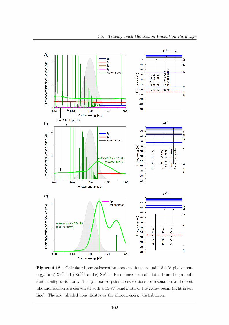
4.5. Tracing back the Xenon Ionization Pathways
Figure 4.18 – Calculated photoabsorption cross sections around 1.5 keV photon en-
ergy for a) Xe21+, b) Xe26+ and c) Xe31+. Resonances are calculated from the ground-
state configuration only. The photoabsorption cross sections for resonances and direct
photoionization are convolved with a 15 eV bandwidth of the X-ray beam (light green
line). The grey shaded area illustrates the photon energy distribution.
102

Chapter 4. Multiple Ionization of Heavy Atoms by Intense X-Ray FEL Pulses
The cross sections for photoabsorption at three exemplary charge states in anenergy window between 1460 eV and 1540 eV are shown in figure 4.18. All threegraphs have the same scales. Resonant bound-bound transitions starting at theground-state are included (dark green). The non-resonant photoabsorption crosssection and cross sections for resonances are convolved with a 15 eV (FWHM) band-width and drawn in light green.
The step-size on the energy axis is 0.01 eV, but resonances can be even nar-rower. Because both, height and width, of the resonances are necessary to evaluatetheir strength, the overall strength of resonances cannot be directly read from thenon-convolved sketch. The density of resonances ought to smoothly merge to thephotoionization threshold of an orbital, here 3p and 3d (see section 2.2.2.3). In theenergy level diagram on the right, possible transitions are indicated with arrows of1500 eV length and the most prominent lines are named.
The selection rule for the angular momentum quantum number explains, why forexample resonant excitation in xenon is possible between the 3p and 7s as well as3p and 7d (for Xe26+ at 1487 eV and 1508 eV, respectively, see figure 4.18), butforbidden between 3p and 7p.
The three exemplary charge states are the following:
• In a), at a charge state of 21+, direct 3d photoionization (red) is open anddirect 3p photoionization (blue) is within the bandwidth of the photon energy(grey shaded area). Direct photoionization from 3d has the highest crosssection, followed by direct the one from 3p; direct 4s and 4p photoionization areboth negligible. Bound-bound-transitions between 3p and Rydberg states or3s and the 7th and 8th-shell are possible as well. The broader width (comparedto the resonances in graph b) and c) for Xe26+ and Xe31+, respectively) is anartefact of the calculations, where Rydberg states are not fully converged andless accurate. The resonance just below the 3p ionization edge at 1507 eV isattributed to the 3s to 8p transition, the resonance above the 3p-edge at 1529eV to the 3s to 9p transition.
• For 26+ in b) direct 3p photoionization is closed, but direct 3d photoioniza-tion is within the bandwidth. In the ground-state configuration 4s and higherorbitals are not occupied at Xe26+, but valence-ionizations would be energet-ically possible for excited states, albeit with a much lower cross section than
103

4.5. Tracing back the Xenon Ionization Pathways
resonant transitions. At photon energies lower than the 3d photoionizationthreshold at 1509 eV an abundance of resonances into Rydberg orbitals ispresent, which enables multi-step ionization processes in a wide range of pho-ton energies. The 3p-7d transition at 1508 eV almost coincides with the 3dionization edge. Above the 3d-edge the 3s to 6p transition appears as isolatedresonance at 1521 eV.
• Finally, for Xe31+ in c) no direct inner-shell photoionization is in reach. Still,however, further ionization is possible through Auger decay following threestrong resonances from 3p and 3d to the n = 5 and n = 6 shells.
The bandwidth-convolved absorption cross sections including direct and resonantchannels for all charge states between 21+ and 35+ are depicted in figure 4.19.Here, the individual shapes of the curves are less important than the fact that thereis a significant photoabsorption cross section for all of these consecutive chargestates because of the resonances within the broad bandwidth. Only for 35+ thecross section appears rather small on this scale (about 0.03 Mb at 1.5 keV photonenergy).
Figure 4.19 – Calculated photoabsorption cross sections around 1.5 keV photon en-
ergy for Xe21+ up to Xe35+. Resonances are calculated from the ground-state config-
uration only and are convolved with a 15 eV bandwidth of the X-ray beam.
104

Chapter 4. Multiple Ionization of Heavy Atoms by Intense X-Ray FEL Pulses
As indicated in the pathway sketch (figure 4.16), more than one resonant ex-citation may occur before the excited state relaxes via Auger decay. In this way,multiple resonances create highly excited states, where not only one, but severalAuger decays may follow. Charge states without resonances within the 15 eV band-width of the photon energy may then not necessarily stop the ionization process,but may appear only in multi-excited electron configuration during the charge-upand, thus, might be simply "ran over" by consecutive Auger decays.
105


Chapter 5
Summary and Outlook
Multiphoton ionization in intense laser fields in the infrared, optical and ultravioletspectral ranges has revolutionized the understanding of strong-field light-mater in-teraction and paved the way for various spectroscopic applications [26–28, 36]. Theadvent of free-electron lasers allowed investigating multiphoton ionization by intenselaser radiation at photon energies reaching even beyond the ultraviolet regime, wherephotoionization pathways are fundamentally different from the strong-field effectsobserved with optical lasers. In the VUV and XUV spectral range of FLASH, mea-surements have been performed on light atoms, such as helium, neon and argon[170, 171], where significant contributions of non-sequential, direct two-photon pho-toionization pathways were found. For heavy atoms such as xenon, non-sequential,direct ionization by up to seven photons was discussed to explain the experimentalspectra with charge states up to Xe21+ [29–31, 159, 160]. At X-ray energies, a lightatom, neon [19, 20], has been studied in detail so far, but only negligible contribu-tions from direct multiphoton photoionization were found in this case [20, 24, 25].For heavier elements, the question arose if similarly high charge states as at FLASHmay occur even though direct multiphoton ionization is much weaker at X-ray en-ergies.
To answer this question, two heavy elements, xenon and krypton, have beeninvestigated at the first X-ray free-electron laser operated world-wide, the LCLS. Ina pioneering measurement in 2009, surprisingly high charge states were found forxenon irradiated with 1.5 keV photon energy. Simultaneously recorded fluorescencespectra showed a sudden increase of the fluorescence yield when highly chargedionic states were created. In order to quantify the charge-state distribution under
107

improved conditions, ion time-of-flight spectra were measured in 2011 with higherresolution and for a more comprehensive set of experimental parameters: The photonenergy was set to 1.5 keV and 2 keV, the pulse energy varied by five different gasattenuator pressures and two pulse lengths could be compared. Additionally to thexenon data, photoionization of krypton was measured.
Confirming the previous findings of 2009, a maximum charge state of Xe36+
was observed at 1.5 keV photon energy or 0.83 nm wavelength, respectively, and6.3x1016 W/cm2 intensity. This maximum charge state compares to previous mea-surements at other energies and intensities as follows: In strong laser fields (1.55 eVphoton energy or 800 nm wavelength and peak intensities up to 1018 W/cm2), thehighest observed charge state so far is Xe20+ [172]; at FLASH (93 eV photon energyor 13.3 nm wavelength and an irradiance level up to 1016 W/cm2), charge states upto Xe21+ have been reported [31]; and ionization by fast heavy-ion impact (highlycharged uranium, U75+, with 15.4 MeV/u kinetic energy) was demonstrated to yieldcharge states up to Xe35+[173]. The charge state reported here thus represents thehighest ever observed for an individual atom exposed to a single pulsed electromag-netic radiation.
For photoionization at 1.5 keV photon energy, a charge state of Xe36+ is unex-pected on the basis of previous theoretical models. Considering sequential directsingle-photon single-electron ionizations only, a maximum charge state of Xe26+ isanticipated, where the binding energy of 3d electrons increases to 1509 eV, thusexceeding the available photon energy. In contrast to the reported photoionizationdata on neon [19], sequential direct single-photon ionization alone can thus not ex-plain at all the ionization process and additional pathways above Xe26+ have to beconsidered.
Simultaneously measured fluorescence spectra show decay from higher states into3d and 3p vacancies for charge states where direct photoionization of these orbitals isalready energetically closed. If direct photoionization is closed, inner-shell vacanciescan only be created by resonant excitation. Such a resonance has been discussed inneon for one single charge state, the special case of K-shell excited Ne7+∗, where theelectron excited to the 5p valence orbital may be photoionized before it is emitted inan Auger decay filling up the K-shell hole [20, 25]. In general, however, resonancesare rare for light atoms at X-ray energies and unimportant at photon energies farabove all absorption edges [19].
108

Chapter 5. Summary and Outlook
Theoretical analysis by Son and Santra of resonances and their cross sections forxenon reveal an abundance of resonant states accessible at 1.5 keV photon energyfor charge states between 20+ and 36+. Hence, even beyond the limit for directphotoionization of Xe26+, further ionization is enabled by densely spaced resonances,which can be excited within a single broadband FEL pulse for several subsequenthigh charge states created during the ionization process. The ionization of outervalence and Rydberg states after multiple resonant excitation of several electronspredominantly proceeds through Auger decays. While resonances in the opticalmultiphoton regime can enhance non-sequential direct multiphoton ionization, adirect photoionization of a resonantly excited state is negligible in the X-ray regimedue to a very small photoionization cross section for Rydberg and outer valencestates.
In contrast to the 1.5 keV case, photoionization at 2 keV photon energy butotherwise the same experimental parameters only proceeds up to Xe32+, where theground-state ionization energy exceeds the photon energy. This qualitatively dif-ferent behavior is due to the fact that at higher photon energy suitable resonancesappear at higher charge states, which are not reached effectively within a single shotfor pulse intensities used in the experiment.
Krypton at 2 keV photon energy illustrates another example of resonant excitationduring X-ray photoionization of heavy atoms. Here, photoionization starts withdirect single-photon ionization of the L-shell electrons. However, the binding energyof the 2s state exceeds the available photon energy at a charge state of 9+ anddirect 2p photoionization closes at 12+ already. At this charge state, 14 electrons inthe M-shell are left which are energetically accessible by the photon energy but thecross section for M-shell photoionization is very small. Instead, further ionizationproceeds through the resonant excitation of L-shell electrons and subsequent Augerdecay into L-shell vacancies. At Kr20+, the energy difference between 2p and 4sstates exceeds the available photon energy of 2 keV and resonant excitation ends.Auger decay may remove another electron of excited Kr20+ resulting in a maximumcharge state of 21+, exactly as recorded in the experimental krypton charge-statedistribution.
In the comparison of krypton time-of-flight spectra and ion yield curves for 3 fsand 80 fs pulse lengths (at the same pulse energy), no significant difference wasfound. At relatively low pulse energy, the shorter pulse length apparently does
109

not sufficiently increases the intensity to cause direct two-photon ionization or tosaturate resonances. For neon [19] and nitrogen [21], X-ray induced transparencywas reported for intense, short X-ray pulses. It occurs when the Auger decay timeis longer than the inverse photoionization rate and inner shell holes are not refilledby Auger decay during the X-ray pulse, such that the photoabsorption is drasticallydecreased. For krypton, no X-ray induced transparency was observed, probablybecause of the ultra-short of Auger decay times (< 1 fs) and the greater number ofelectrons available for photoionization.
The sudden increase of multiple photoionization for heavy atoms at high chargestates and in certain photon-energy ranges is predicted to appear for all systemscontaining high-Z constituents. For imaging experiments, resonance-enhanced pho-toionization should be avoided as increased radiation damage in the vicinity of heavyatoms may appear. On the other hand, this highly efficient ionization process maybe used to efficiently create highly excited, dense plasmas of high-Z atoms. Thestrength of resonance-enhanced multiphoton ionization can be varied by the FELpulse energy, photon energy, and bandwidth.
In this work, the fundamental principle of resonance-enabled X-ray multipho-ton ionization (REXMI) has been demonstrated. Now, a designated experiment toquantitatively investigate this photoionization pathway under newly available evenhigher peak intensities and for higher photon energies is the next logical step.
With imaging experiments taking advantage of the recently commissioned 100 nmfocus at high photon energies (4 to 10 keV) at the coherent X-ray imaging (CXI)beamline at LCLS, an investigation of the REXMI mechanism at these parameters ismost desirable. At 6 keV photon energy, for example, the xenon L-shell is accessiblefor direct photoionization, but closes at Xe30+. At a peak intensity of 1022 W/cm2
(assuming 3 mJ pulse energy, 3 fs pulse length and 0.01µm2 focus size), however,further ionization via the REXMI mechanism is expected to boost charge states upto Xe45+ (see figure 5.1). A measurement under these experimental conditions willclarify if the REXMI region can be reached with the increased intensity of the 100 nmfocus but at reduced photoionization cross sections at high photon energies, and thusif resonance-enhanced ionization plays a role in radiation damage at experimentalparameters typical for many imaging experiments.
For the experimental setup, minor changes are suggested. The pnCCDs should beplaced facing downstream or perpendicular to the beam to avoid direct exposure to
110
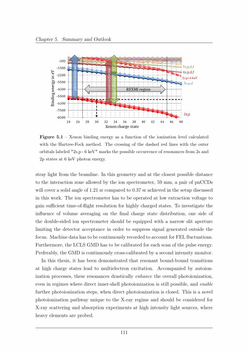
Chapter 5. Summary and Outlook
Figure 5.1 – Xenon binding energy as a function of the ionization level calculated
with the Hartree-Fock method. The crossing of the dashed red lines with the outer
orbitals labeled "2s,p+6 keV" marks the possible occurrence of resonances from 2s and
2p states at 6 keV photon energy.
stray light from the beamline. In this geometry and at the closest possible distanceto the interaction zone allowed by the ion spectrometer, 59 mm, a pair of pnCCDswill cover a solid angle of 1.21 sr compared to 0.37 sr achieved in the setup discussedin this work. The ion spectrometer has to be operated at low extraction voltage togain sufficient time-of-flight resolution for highly charged states. To investigate theinfluence of volume averaging on the final charge state distribution, one side ofthe double-sided ion spectrometer should be equipped with a narrow slit aperturelimiting the detector acceptance in order to suppress signal generated outside thefocus. Machine data has to be continuously recorded to account for FEL fluctuations.Furthermore, the LCLS GMD has to be calibrated for each scan of the pulse energy.Preferably, the GMD is continuously cross-calibrated by a second intensity monitor.
In this thesis, it has been demonstrated that resonant bound-bound transitionsat high charge states lead to multielectron excitation. Accompanied by autoion-ization processes, these resonances drastically enhance the overall photoionization,even in regimes where direct inner-shell photoionization is still possible, and enablefurther photoionization steps, when direct photoionization is closed. This is a novelphotoionization pathway unique to the X-ray regime and should be considered forX-ray scattering and absorption experiments at high intensity light sources, whereheavy elements are probed.
111


Appendix A
Appendix to the Experimental Setup
A.1 Free-Electron Laser
A.1.1 Microbunching and SASE
Microbunching is based on the ponderomotive force which the light field exertson the electrons. It is dependent on the phase difference between the sinusoidalelectron trajectory and the oscillating light-field. The light field at frequencies ωland wavevector kl can be assumed as plane x-polarized electromagnetic wave co-propagating in z with the relativistic electron beam
Ex(z, t) = E0cos(klz − ωlt+ ψ0) with kl = ωl/c = 2π/λl (A.1)
The phase shift ψ0 against the individual electron trajectory accounts for the variouspossible positions of an arbitrary electron within the bunch and will be discussedbelow. Whether the electron gains or looses energy in this field is described by thetime derivative of the electron energy W
dW
dt= ~v · ~F = −e · vx(t)Ex(t) (A.2)
With dW/dt < 0, the electron bunch looses energy and, obeying energy conservation,the light wave gains energy. This is the case when both vectorial factors in the scalarproduct point in the same direction.
Inserting the electric field (equation A.1), into the time derivative (equation A.2)and assuming for the sinusoidal motion of the electrons inside the undulators vx =
113

A.1. Free-Electron Laser
cKγcos(kuz), the following expression is derived
dW
dt= ~v · ~F = −e · vx(t)Ex(t) = −ecK
γcos(kuz)E0cos(klz − ωlt+ ψ0)
= −ecKE0
2γ[cos((kl + ku)z − ωt + ψ0) + cos((kl − ku)z − ωlt+ ψ0)]
= −ecKE0
2γ[cos(ψ)− cos(χ)] (A.3)
where ψ = (kl+ku)z−ωt+ψ0 is called the ponderomotive phase; the fast oscillatingterm χ cancels out. The maximum energy transfer from the electron beam to thelight wave is hence given when ψ = ±n2π. The energy transfer is continuous overthe entire undulator length when ψ is constant, which is only fulfilled at a certainwavelength. Inserting the trajectory equation for z into the condition dψ/dt = 0,this wavelength turns out to be undulator specific wavelength at θ = 0 (equation3.3). So the spontaneous radiation in an undulator is indeed suitable to seed theSASE process.
With this distinct value of the ponderomotive phase ψ, a longitudinal coordinateinside the bunch is defined
ζ =ψ + π/2
kl + ku≈ ψ + π/2
2πλl (A.4)
where ζ0(ψ0 = −π/2) = 0 sets the origin of coordinates at the phase of no energyexchange between electron and light wave.
With the initial bunch-internal coordinate ζ, and the ponderomotive phase ψ0
at the time of entrance to the undulator and equation A.3 for the energy transferbetween the electron beam and the light wave, three cases can be distinguished asseen in figure A.1: at ψ0 = π/2 no energy is transferred between electron and lightwave, for ψ0 < π/2 the electron looses energy to the field, and for π/2 < ψ0 < π itgains energy from the field.
With an initial homogeneous distribution for ζ and ψ0 in the electron bunch,the energy transfer between the electron beam and the light wave results in mi-crobunching: Electrons with ζ > ζ0 lose energy to the field due to ψ0 < π/2, so thelongitudinal velocity decreases, while their transversal amplitude (∝ 1/γ) increases;for electrons with ζ < ζ0 vice versa. For both cases the absolute value of ζ and ψ0
decrease, hence the electrons converge to similar values of ζ and ψ0. As the electrondensity is confined on a pulse length smaller than the wavelength, the radiationbecomes coherent. Thus, not only the intensity but the amplitude of the light fields
114

Appendix A. Appendix to the Experimental Setup
is added. With ongoing microbunching the radiated power of coherently radiatingmicrobunches increases exponentially along the undulator length.
Figure A.1 – Energy exchange between electron and light wave1
However, lasing becomes saturated when further microbunching is hindered bythe internal Coulomb repulsion in the electron bunch, and when the electron energyfalls below critical energy required for constructive interference in the undulatorequation (equation 3.3). The region where increasing microbunching leads to anexponential growth in the radiated power is called linear regime, in contrast tothe saturated regime where additional undulator length does not result in a higherradiated power.
In summary, an electron beam with high peak current, small energy spread andlow emittance is sub-structured into microbunches due to electron-light-field inter-actions in a long undulator. As a result, the electrons radiate in phase, and thus theradiated power increases not only linearly with the number of radiating electrons(as for synchrotrons, see figure 3.4) but quadratically, which gives an enhancementof about nine orders of magnitude.
A.1.2 Seeding and Resonators
The SASE process starts up from spontaneous emission, which is generated stochas-tically by the in space and time randomly distributed electron density of the elec-tron beam. Each of these density fluctuations may radiate spontaneously and seeda SASE process within the undulator bandwidth, where the wavelength fulfills theresonance condition. Ultimately, the resulting radiation pulse consists of a largenumber of independent wavepackets, which give rise to random and uncontrollablespikes in the radiated temporal profile and frequency-domain spectra. Within one
1Source: P. Schmüser et al. Ultraviolet and Soft X-Ray Free-Electron Lasers, Springer-Verlag,2010, Copyright (2010) by Springer-Verlag GmbH
115

A.1. Free-Electron Laser
wavepacket, the radiation is transversely and longitudinally coherent, but the over-all temporal coherence is smaller than anticipated from the electron bunch length[174] (see section A.1.3). To make the SASE-FEL pulses fully coherent and freefrom coherence and intensity spikes, several seeding schemes have been proposed,where SASE is not seeded by stochastically spontaneous emission, but an externaltemporally well defined and coherent light pulse. Optical lasers are best accessi-ble, however, limited in the available wavelength. With high harmonic generation,FEL have been seeded at deep UV [175], and recently pushed to the XUV-region[176]. With HHG a technical issue comes up: the high-harmonic seed light has tosurpass the initial power level of the spontaneous radiation in the SASE-FEL. Asecond approach is to built a multi-segment FEL, where the fundamental or thehigher harmonics (high-gain high harmonics HGHG) of the first undulator segmentis used to seed the SASE-process in the undulators downstream [177]. Both HGHGand HHG schemes are planed for the XUV-FEL update FLASH 2 currently underconstruction.
In contrast to high-gain, single-pass FEL-amplifier a good pulse-to-pulse stabilityand temporal coherence is achieved in FEL-oscillator, where the FEL-light oscillatesin a resonator. In fact the first free-electron laser [178] and succeeding FELs at longwavelength were equipped with an optical resonator, where infrared or microwavelight was amplified with low-gain in an undulator embraced by a pair of mirrors andwith a circulating electron beam passing numerous times [78]. A summary of variousFEL concepts of free-electron lasers can be found in reference [179], "Free-electronlasers: Present status and future challenges".
A.1.3 Determination of the X-Ray Pulse Length
Among one of the first user runs at LCLS, L. Young and coworkers investigated thephotoionization of neon at various photon energies [19]. The K-shell ionization po-tential of neon is 870 eV. Above that energy, at 1050 eV and 2000 eV photon energy,and with a fluence of about 200 µJ/µm2, double core hole formation was observed inelectron spectra. Double core holes are created when the Auger lifetime exceeds theinverse photoionization rate, in other words, the average time until the next pho-toionization event at given beam parameters. For singly charged neon the Augerdecay into a 1s vacancy takes place at 2.4 fs time scale [180], but the Auger lifetimeis rapidly increased during the ionization process; at Ne7+, for instance, it already
116

Appendix A. Appendix to the Experimental Setup
amounts to 23 fs. The Auger lifetime for double core holes is significantly shorter.Due to the impact of Auger lifetimes on observable photoionization processes, the"Auger clock" is a reasonable approach to estimate the X-ray pulse duration.
measured and calculated decay rates37–39. (We note that this is the firstobservation of sequential two-photon production of hollow neonatoms and that the yield, ,10%, is ,303 larger than the 0.3%
yield—observed in synchrotron radiation studies—that naturallyresults from electron correlation in the 1s shell36.) The resulting ratiosof double-to-single core-hole formation for 1,050-eV X-ray pulses ofnominal duration 80 fs are shown in Fig. 5 together with simulations.The simulations for 20 fs and 40 fs form a family from which theobserved double-to-single core-hole ratio can be used to estimate theX-ray pulse duration. As is apparent, the X-ray pulse duration appearsmuch shorter than the nominal 80 fs, in agreement with the ion-charge-state transparency data, Fig. 3a. Thus, two independent methods yieldthe same result—that the nominal ,80-fs mode of operation actuallyproduces X-ray pulses of shorter duration, ,20–40 fs, similar to obser-vations at the FLASH free-electron laser facility40. Our observationsprovide a further example41 of how ultrafast electronic transitionscan be used to characterize X-ray free-electron-laser pulses.
Our observations also provide experimental evidence for the advan-tageous radiation-hardening effect of using ultra-intense X-ray pulses,and thus have positive implications for proposed single-molecule-imaging experiments2. Intense, short X-ray pulses induce transparencyvia photoejection of both 1s electrons to produce hollow atoms. Thehollow-atom configuration can be maintained through the ionizationprocess, as sketched in Fig. 3c. As hollow atoms are nominally trans-parent, the damaging X-ray photoabsorption channel is decreasedrelative to the imaging (coherent scattering) channel. To be quantitat-ive, the photoabsorption cross-section, sphoto, for hollow neon isdecreased 20-fold for 1-A radiation, that is, to 11 barns, to equal thecoherent scattering cross-section, scoh. This trend of increasing scoh/sphoto holds for all hollow atoms. In hollow carbon, scoh/sphoto < 2 for1-A radiation, as opposed to ,0.1 for normal carbon. The ideal case
IonizationNe10+
Ne Time20 fs
1
10
Long
to
shor
t p
ulse
yie
ld r
atio
230 fs to 80 fs model
230 fs to 20 fs model
Experiment
1 2 3 4 5 6 7 8 9 10Neon charge state
1
10
100
1s li
fetim
e (fs
)
Single core holeDouble core hole
P
P
P
P
P
P
A
A
A
A
a c
b
Figure 3 | Intensity-induced X-ray transparency. a, Ratio of charge-stateyield for 230-fs to 80-fs electron bunch durations for 2,000-eV, 2.0-mJ X-raypulses (diamonds). Error bars of 610% are estimated for the observedcharge-state yields. Simulations for 80-fs and 20-fs X-ray pulse durations forthe short pulse are overlaid in green and red, respectively. The comparisonsuggests that the pulse duration of the X-rays generated by the 80-fs electronbunch is less than 80 fs. b, Average lifetimes of the single- and double-core-
hole states in neon as a function of charge state, from ref. 33. The lifetimes ofthe single- and double-core holes increase with charge state. These increasedlifetimes give rise to a decreased absorption cross-section and hence anintensity-dependent X-ray transparency. The double-core-hole lifetimetracks the observed charge-state ratios. c, A scheme leading to high chargestates, for a flux density of 2,000 X-ray photons per A2 per fs, correspondingto that on target for a 2.0-mJ, 2,000-eV, 20-fs X-ray pulse.
300
400
200
100
0
Cou
nts
400350300250
Valencephotoelectrons
Valence 2pphotoelectrons
Single-core-holeAuger
Double-core-holeAuger
Single-core-holeAuger
Double-core-holeAuger
3,000
2,500
2,000
1,500
1,000
500
0
Cou
nts
400350300250
1s photoelectrons
Ne
Ne2+
Ne3+Ne4+
400
300
200
100
0
Cou
nts
400350300250Electron time-of-flight (ns)
θ = 0ºVR = 0 V
θ = 0ºVR = 790 V
θ = 90ºVR = 790 V
a
b
c
Figure 4 | Electron spectra for inner-shell and valence photoelectrons andAuger electrons created by X-ray pulses at a photon energy of 1,050 eV.a, 1s photoelectrons directed along the X-ray polarization axis (h 5 0u) witha photoelectron spectrometer retardation voltage of VR 5 0 V. b, Valenceand Auger electrons at h 5 0u, with VR 5 790 V. c, Valence and Augerelectrons at h 5 90u, VR 5 790 V. Auger electrons from double-core-holestates, the signature of hollow atom formation, are more cleanly measured ath 5 90u (as in c), as background from valence ionization is suppressed. Thestrongest Auger peaks in the double-core-hole and single-core-hole regionsoriginate from the initial PPA and PA ionization sequences, and are used todetermine the double-core-hole to single-core-hole formation ratio.
NATURE | Vol 466 | 1 July 2010 ARTICLES
59Macmillan Publishers Limited. All rights reserved©2010
for biomolecular imaging is an X-ray pulse shorter than the hollow-atom lifetime, such that scattering occurs before further electron ornuclear dynamics. Experiments on atoms are relevant for single-mole-cule imaging because hard X-ray interactions are predominantlyatomic. For example, plasma effects (such as enhanced absorptionvia inverse bremsstrahlung) scale as ln where n . 2 (ref. 42), and arealready unimportant at 33 A (ref. 19) and will be negligible at 1 A. Inaddition, collective effects, such as those resulting from the excitationof giant resonances18, will also be unimportant at photon energies farabove all absorption edges.
Conclusions
Our results represent the first observations of photoabsorptionmechanisms and femtosecond electronic response in a prototypicalatom in the ultra-intense, short-wavelength regime accessed by theLCLS. We find that sequential single-photon absorption dominates,and that with this extreme fluence (105 X-ray photons per A2) anyprocess that is energetically feasible with a single photon is observed.Thus, the target is continually changing during the course of the fem-tosecond-duration X-ray pulse. Atoms become transparent at highX-ray intensity owing to the rapid ejection of inner-shell electrons—a phenomenon we call intensity-induced X-ray transparency. Themultiple Auger clocks that come into play as the pulse progressesthrough the atom cause shorter pulses with equal fluence to produceless damage. This concept of multiple clocks extends the standardnotion in X-ray experiments of internal clocks on the femtosecondtimescale43. The transparency is observable in all atomic, molecular44
and condensed matter systems at high X-ray intensity. Because thisstudy was conducted on the well-characterized neon atom, quantitat-ive comparison with theoretical simulation is possible, and from thiscomparison we derive measures of LCLS pulse duration and fluence.Finally, the successful modelling of the interaction of ultra-intenseX-ray radiation with a free atom using a straightforward rate equationmodel foreshadows extension of this approach to more complexmaterial systems.
METHODS SUMMARY
The X-ray spectral and pulse characteristics were varied by controlling the
electron-bunch energy, charge and compression in the LCLS30,45,46. X-ray pulses
in the 800–2,000 eV range were focused by Kirkpatrick-Baez mirrors to an esti-
mated 1 3 2mm2 FWHM in a neon gas jet centred in the AMO (atomic, molecu-
lar and optical) instrument47. The X-ray pulse energy on target was calculated
using the pulse energy measured in upstream gas detectors22 corrected for the
reflectivities of five B4C mirror surfaces. Ion charge-state spectra were recorded
by a time-of-flight analyser. Electron spectra were recorded with five time-of-
flight analysers positioned at selected polar and azimuthal angles with respect to
the X-ray polarization and propagation directions. Ion charge-state yields were
corrected for microchannel plate detection efficiencies48. No evidence was
observed for charge-changing collisions in ion spectra, nor were space charge
effects observable in the electron spectra. A 1-mm slit in the ion-extraction plate
limited the length of the X-ray beam observed. The electron spectrometerssampled an estimated length of 1.6 mm. Electron spectrometer efficiencies mod-
elled by Monte Carlo simulation showed good agreement with the measured
calibration spectra.
To calculate the atomic response to LCLS pulses, we extended the modeldescribed in ref. 12. Using the Hartree-Slater method49, we determined the sub-
shell photoionization cross-sections for the electron configurations 1si 2sj 2pk of
Neq1. Radiative and non-radiative decay rates were taken from ref. 33. The cross-
sections and decay rates served as input parameters for rate equations for the
populations of the 1si 2sj 2pk configurations. We assumed that on average the
X-ray temporal pulse profile is Gaussian-shaped. The impact of the longitudinal
mode structure is small12 and was neglected. The charge-state distribution and
Auger yields were integrated over the interaction volume, assuming an elliptical
Gaussian beam profile.
Full Methods and any associated references are available in the online version ofthe paper at www.nature.com/nature.
Received 15 February; accepted 10 May 2010.
1. Emma, P. First lasing of the LCLS X-ray FEL at 1.5 A. In Proc. 2009 ParticleAccelerator Conf. (IEEE, in the press).
2. Neutze, R., Wouts, R., van der Spoel, D., Weckert, E. & Hajdu, J. Potential forbiomolecular imaging with femtosecond X-ray pulses. Nature 406, 752–757 (2000).
3. Nagler, B. et al. Turning solid aluminium transparent by intense soft X-rayphotoionization. Nature Phys. 5, 693–696 (2009).
4. Lee, R. W. et al. Finite temperature dense matter studies on next-generation lightsources. J. Opt. Soc. Am. B 20, 770–778 (2003).
5. Gaffney, K. J. & Chapman, H. N. Imaging atomic structure and dynamics withultrafast X-ray scattering. Science 316, 1444–1448 (2007).
6. Stephenson, G. B., Robert, A. & Grubel, G. Revealing the atomic dance. NatureMater. 8, 702–703 (2009).
7. Ostermeier, C. & Michel, H. Crystallization of membrane proteins. Curr. Opin.Struct. Biol. 7, 697–701 (1997).
8. Henderson, R. The potential and limitation of neutrons, electrons and X-rays foratomic resolution microscopy of unstained biological molecules. Q. Rev. Biophys.28, 171–193 (1995).
9. Chapman, H. N. et al. Femtosecond diffractive imaging with a soft-X-ray free-electron laser. Nature Phys. 2, 839–843 (2006).
10. Hau-Riege, S. P. X-ray atomic scattering factors of low-Z ions with a core hole.Phys. Rev. A 76, 042511 (2007).
11. Veigele, W. J. Photon cross sections from 0.1 keV to 1 MeV for elements Z51 toZ594. At. Data Tables 5, 51–111 (1973).
12. Rohringer, N. & Santra, R. X-ray nonlinear optical processes using a self-amplifiedspontaneous emission free-electron laser. Phys. Rev. A 76, 033416 (2007).
13. Augst, S., Strickland, D., Meyerhofer, D. D., Chin, S. L. & Eberly, J. H. Tunnelingionization of noble gases in a high-intensity laser field. Phys. Rev. Lett. 63,2212–2215 (1989).
14. Palaniyappan, S. et al. Ultrastrong field ionization of Nen1 (n # 8): rescatteringand the role of the magnetic field. Phys. Rev. Lett. 94, 243003 (2005).
15. Ackermann, W. et al. Operation of a free-electron laser from the extremeultraviolet to the water window. Nature Photon. 1, 336–342 (2007).
16. Sorokin, A. A. et al. Photoelectric effect at ultrahigh intensities. Phys. Rev. Lett. 99,213002 (2007).
17. Makris, M. G., Lambropoulos, P. & Mihelic, A. Theory of multiphotonmultielectron ionization of xenon under strong 93-eV radiation. Phys. Rev. Lett.102, 033002 (2009).
18. Richter, M. et al. Extreme ultraviolet laser excites atomic giant resonance. Phys.Rev. Lett. 102, 163002 (2009).
19. Bostedt, C. et al. Multistep ionization of argon clusters in intense femtosecondextreme ultraviolet pulses. Phys. Rev. Lett. 100, 133401 (2008).
20. Wabnitz, H. et al. Multiple ionization of atom clusters by intense soft X-rays froma free-electron laser. Nature 420, 482–485 (2002).
21. Ziaja, B., Wabnitz, H., Wang, F., Weckert, E. & Moller, T. Energetics, ionization,and expansion dynamics of atomic clusters irradiated with short intense vacuum-ultraviolet pulses. Phys. Rev. Lett. 102, 205002 (2009).
22. Hau-Riege, S. P., Bionta, R. M., Ryutov, D. D. & Drzywinski, J. Measurement ofx-ray free-electron-laser pulse energies by photoluminescence in nitrogen gas.J. Appl. Phys. 103, 053306 (2008).
0.16
0.14
0.12
0.10
0.08
0.06
0.04
0.02
Rat
io o
f dou
ble
- to
sin
gle-
core
-hol
e yi
eld
1.41.21.00.80.60.40.20.0Pulse energy (mJ)
40 fs
20 fs
Figure 5 | The ratio of double- to single-core-hole formation as a functionof X-ray pulse energy. Red filled circles show experimental data taken withX-rays lasing from an electron bunch of 250 pC charge and 80 fs duration. Agas attenuator was used to reduce the pulse energies. Error bars are statistical(61s) for the Auger yields and measured shot-by-shot X-ray pulse energies.Curves labelled 20 fs (green) and 40 fs (blue) are simulations of the double-to-single core hole formation ratio for two X-ray pulse durations. Thecomparison suggests that the 80-fs electron bunch generates an X-ray pulseof shorter duration, ,20–40 fs.
ARTICLES NATURE | Vol 466 | 1 July 2010
60Macmillan Publishers Limited. All rights reserved©2010
Figure A.2 – LCLS X-ray pulse length determination via double core hole creation1.
On the left the ratio of charge-state yield for 230-fs to 80-fs electron bunch durations is
depicted in (a) (data points and simulation in solid lines at 2 keV, 2.0 mJ X-ray pulses)
and the lifetimes of single and double core hole states as function of neon charge state
in (b) (derived from [181]). On the right the ratio of Auger electron yield into single as
a function to the yield into double core-hole is shown for four pulse energies together
with simulated ratios at 20 fs and 40 fs pulse duration.
The pulse length could independently be retrieved from the ion as well as fromthe electron spectra. The ion yield decreases when long-lived single or even doublecore holes occur, which effectively lower the probability for an additional photoabsorption. For 230 fs pulse length, such core holes can be refilled within the pulseduration, but at nominally 80 fs the pulse length is in the order of the Auger lifetimesand yields for the highest neon charge states are diminished. A comparison of theexperimental and theoretical ratio of ion yields for 230 fs and 80 fs indicates thatthe nominally 80 fs pulse length has actually to be four times lower to explain thedecreased yield for Ne8+, Ne9+ and Ne10+ (see on the left in figure A.2).
This finding is confirmed by pulse length determination from electron spectra:single and double core hole vacancies can easily be differentiated, as Auger electrons
1Source: L. Young et al., Nature 466, 56-61 (2010). Copyright by the Nature Publishing Group.
117

A.1. Free-Electron Laser
from transitions into double core holes are significantly shifted towards higher kineticenergies compared to those from decay into a single core hole. The ratio of doubleto single core holes is specific for a certain pulse energy and pulse length. In thecalculation of this ratio, the radiative decay into core holes [182–184] has also beconsidered. Then, the calculated ratios are compared to ratios derived from theexperimental Auger line intensities. Accordingly, the nominally 80 fs pulse durationis found to be 40 fs or even less (see on the right in figure A.2).
6
Figure 3. Neon Auger electron energy spectra as a function of the relativedelay time τδt between the NIR (τNIR = 100 fs) and the x-ray pulses (τel = 75 fs).Around the relative zero point, the strong depletion and broadening of the mainline corresponds to LAAD.
the final kinetic energy U of an electron introduced into a moderate NIR field (with wavelengthλNIR) with an intensity INIR is given by
U = Ua − sin(φb) cos(θb)√
8UaUp. (1)
φb is the phase of the NIR field at the instant of ionization, θb is the angle between the lightpolarization and the initial velocity of the electron at birth and Ua is the initial kinetic energy.Up is the instantaneous ponderomotive energy at the moment of birth:
Up[eV] = 9.33 × 10⁻¹⁴× λ2
NIR[µm2] × INIR[W cm−2]. (2)
For λNIR = 0.8 µm and INIR = 1.2 × 10¹² W cm−2, Up results in 0.07 eV. This, whensubstituted into equation (1), gives a maximum energy U ' 826 eV or, in other words, theabsorption of about 14 NIR photons from the field. This is in excellent agreement with theexperimental findings shown in figure 3. For a given intensity and wavelength of the NIR laser,U scales with the square root of the initial kinetic energy Ua. Hence, compared with two-colorprocesses previously observed at extreme ultraviolet wavelengths, the large number of sidebandsobserved here at low NIR intensity is a direct consequence of the high kinetic energy of theAuger electron [10, 16].
In figure 4, several single-shot electron spectra, recorded at the nominal maximum temporaloverlap between the x-ray and NIR pulses, are shown. The strong shot-to-shot variation in theLAAD component demonstrates clearly the timing jitter in the synchronization and highlightsthe usefulness of the LAAD effect as a sensitive monitor of the temporal overlap of the pulses.This is even more evident when the experimental line profiles are modeled with a simplifiedanalytical model based on the so-called soft-photon approximation (SPA), allowing us to
New Journal of Physics 13 (2011) 093024 (http://www.njp.org/)
Figure A.3 – LCLS X-ray pulse length determination via sidebands in a two color set
up1 . The neon Auger electron energy spectra are drawn as a function of the relative
delay time (integrated in 50 fs steps) between the NIR (pulse length 100 fs) and the
X-ray pulses (electron pulse length 75 fs). Around the relative zero point, the highest
order of sidebands is observed.
Due to the high requirements on peak fluence for double core hole creation, andthe small angular acceptance of electron time-of-flight spectrometer (0.007 sr), theabove approach is impractical for shot-to-shot on-line diagnostics. By means of amagnetic bottle electron spectrometer with an angular acceptance of approximately0.8 sr and a relatively large focus spot of 60 µm diameter, Düsterer et al. demon-strated a non-invasive technique to obtain the LCLS single shot pulse duration [89].
1Source: S. Düsterer et al., New Journal of Physics 13, 093024 (2011). Copyright by theInstitute of Physics
118

Appendix A. Appendix to the Experimental Setup
To retrieve the pulse duration from the electron spectrum, Auger electrons follow-ing X-ray inner shell ionization of neon were dressed with 100 fs long near-infraredlaser pulses, where their momentum vector was either increased or decreased in in-teraction with the time-dependent laser field (due to the bandwidth of the incidentX-ray beam, which is transferred on the photo-electron energy, the small additionalmomentum contribution cannot be resolved for photo electrons) . The number ofsidebands in the electron kinetic energy spectrum, spaced by the photon energy ofthe NIR laser (1.55 eV, 800 nm), represent the number of absorbed optical photons;the better the temporal overlap of the X-ray pulse and peak intensity of the laserpulse is, the more sidebands are generated. Thus, in a scan of the delay betweenX-ray and optical laser, the number of sidebands reveals the X-ray pulse length[185]. At LCLS this two-color approach determined a pulse length (FWHM) of 120fs for an electron bunch duration of 175 fs and 40 fs for nominally 75 fs long pulse,respectively (figure A.3).
The determination of pulse length via sideband measurements in a two-colorsetup is closely related to light field streaking cameras, which have become an es-tablished diagnosis tool for attosecond HHG sources [186] and XUV FELs [187].
J. Phys. B: At. Mol. Opt. Phys. 44 (2011) 243001 Tutorial
compression scheme used and space-charge effects. This leadsto a linear energy chirp of the XUV pulses [1].
The average pulse duration of FELs can be measuredwith autocorrelation experiments where the pulses are splitinto two parts, which can be delayed with respect to oneanother. At FLASH with such autocorrelation experiments,pulse durations between 29 [30, 31] and 40 fs [10] weremeasured. Furthermore, the autocorrelation measurementsconfirmed the existence of short subpulses [10, 30].
Besides the pulse parameters, also the pulse arrival timefluctuates at FELs which is mainly due to a fluctuation ofthe arrival time of the electron bunches at the undulators.For FLASH, the fluctuations are ∼400 fs full width halfmaximum (FWHM) [32]. Due to these fluctuations,averaged crosscorrelation experiments with visible lasersmainly unravel the jitter and not the pulse duration of theXUV pulses.
3. Streaking electrons with light
In light-field streak cameras, XUV pulses are collinearlyoverlapped with an infrared streaking light field which is usedto accelerate photoelectrons. Let the linearly polarized lightfield be given by Estreak(t) = E0(t) cos(ωstreakt + ϕ). Themomentum change of a photoelectron released at time ti dueto the acceleration in this field is then
p(ti) = e
∫ ∞
ti
Estreak(t′) dt ′ = eAstreak(ti), (1)
where Astreak(t) is the vector potential of the streaking fieldand e is the electron charge. The final momentum of theelectron is then p = p0 +p where p0 is the initial momentumwithout streaking field. This leads to a final kinetic energyWkin. = |p|2/(2me) of
Wkin. = W0 + 2Up cos 2 sin2 ϕi
±√
1 − 2Up
W0sin2 sin2 ϕi
√8W0Up cos sin ϕi, (2)
where is the angle between the final electron velocity andthe polarization direction of the streaking field, ϕi is thephase of the field at ionization time and W 0 is the initialelectron kinetic energy [24, 33]. Up = e2E2
0
/(4meω
2streak
)is the ponderomotive energy of the streaking field with me
being the electron mass. For a final drift velocity parallel orperpendicular to the streaking field, equation (2) reduces to
Wkin.‖ = W0 + 2Up sin2 ϕi ± √8W0Up sin ϕi (3)
Wkin.⊥ = W0 − 2Up sin2 ϕi. (4)
For THz radiation, the second term of (3) and (4) is usuallynegligible, and the electron energy measured perpendicular tothe THz field represents the unperturbed energy. If the XUVpulse is short compared to the streaking field oscillation periodand the delay between the XUV and streak pulse is set suchthat the XUV pulse coincides with a zero crossing of Astreak
(zero crossing of sin ϕi in equation (3)), the electron releasetime is linearly mapped onto energy changes for electronsmeasured parallel to the streaking field (see figure 2). The
Figure 2. Principle of light-field streaking. The XUV pulsegenerates an electron wavepacket with identical temporal profile.The electrons are accelerated by the electric field of the IR streakpulse. The momentum change is given by the IR vector potential atthe ionization time. Thus, the XUV temporal profile is mapped ontochanges of photoelectron momenta.
measured streaked spectrum will consist of a mix of theinitial energy distribution and the streaked pulse structure.If the initial energy distribution is constant in time and smallcompared to the energy shifts due to streaking, the streakedspectrum will directly represent the pulse shape. However,XUV pulses from FELs often have a broad initial spectrumand even a change of the spectrum over the pulse (chirp). Inthis case, a complete reconstruction of the pulse shape fromonly one streaked spectrum is not possible but a set of streakedspectra is necessary [34]. For single-shot experiments, it isdifficult to take spectra at many different phases but it is easilypossible to take spectra in three directions, namely parallel,antiparallel and perpendicular to the THz field. As discussedin the following section, these three spectra are sufficient todetermine relevant temporal characteristics when the XUVpulses are approximated with linearly chirped Gaussian pulses.
Streaking chirped pulses
For linearly chirped XUV pulses, the widths of streaked spectrawill depend on the sign of the streaking field. This is shownin figure 3, where in the first case, the delay between apositively chirped XUV pulse and the streaking field is setsuch that the slope of Astreak is positive. In this case, the slowelectrons generated at the beginning of the pulse will be furtherdecelerated, while the fast electrons generated at the end ofthe pulse will be accelerated. This leads to a streak spectrumbroader than for an unchirped XUV pulse of the same pulseduration. If the slope of Astreak is negative, the streak spectrumwill be narrower than for the unchirped case. This can beemployed to measure the linear chirp rate of XUV pulses.Experimentally, the change of sign can be realized either bychanging the delay between the XUV and streak pulse or bymeasuring with two electron detectors, one parallel and oneantiparallel to the streaking field.
3
Figure A.4 – Pulse length determination by
light-field streaking1.
Here, the XUV or X-ray pulse photoion-izes the target atom, where the tem-poral profile of the generated electronwavepacket resembles the photon pulseshape. Then, the electrons are acceler-ated by the electric field of the opticalstreak pulse. Their momentum changeis given by the vector potential of thedressing field at the ionization time (fig-ure A.4).
By a simultaneous measurement ofthe kinetic energy and angular distribu-tion, the momenta can be recovered andthe temporal profile of the ionizing pulse
reconstructed. The main difference of the sideband and the streaking technique is
1Source: U. Frühling et al. Nature Photonics 3, 523-528 (2009). Copyright by the Institute ofPhysics
119

A.1. Free-Electron Laser
the frequency of the optical dressing laser: for sidebands a high frequency, i.e. highphoton energy, is desirable to distinguish the number of absorbed photons. Owingto the optical pulse duration of several tenth of femtoseconds, the above sidebandapproach is limited to pulse lengths of >40 fs. In contrast the maximum detectablepulse length for light-field streaking cameras is governed by the sub-cycle oscillationof the laser electric field: the X-ray pulse length has to fit into a half single cycle ofthe dressing field to avoid ambiguity. So at 800 nm the longest pulse length measur-able by streaking would be 1.4 fs, which is too small for the estimated pulse length.For short electron pulses at the LCLS, low bunch charge mode, light-field streakinghas been applied with 2.4 µm wavelength, and the X-ray pulse length was found tobe less than five femtoseconds long [90]. To determine longer pulse lengths with thestreaking approach, the wavelength of the dressing laser has to be longer. At FLASHterahertz radiation, which is available from a dedicated THz undulator downstreamof the XUV undulators (thus 9 ns delay to the XUV beam), was employed to deter-mine the XUV pulse length to be 28 fs (FWHM) [188] and, recently, THz radiation(strong IR-laser light frequency converted by a Lithium Niobate (LiNbO3) crystal),was used for light field streaking at LCLS as well [91].
Instead of an additional optical laser, the FEL-light can be split to investigatethe pulse and coherence length in a two-beam single-color experiment. To date,such autocorrelation measurements have been limited to FELs operating up to theXUV region, where beam splitting and guiding optics are better available, but beamsplitters for the X-ray region based on moveable grazing incidence split-mirrors arecurrently developed. Two classes of autocorrelation experiments, based on interfer-ometer or pump-probe multiple-photon ionization, have been carried out at XUV-FELs: At FLASH, a beam splitter and delay stage were employed to determinethe temporal (longitudinal) coherence length via interference patterns produced byoverlapping both partial beams under a small angle and recorded on a XUV sensitiveCCD-camera [92, 93]. Also at FLASH the temporal coherence and pulse length wasinvestigated by means of intensity autocorrelation, where the ion yield from nonlin-ear processes occurring in atoms (two-photon double ionization of He [94, 95], andfour-photon four-fold-ionization of N2 [96]) indicate to which degree the two single-color beams are overlapping; the same technique was employed at SCSS observingthe two-photon single ionization of He [97].
For synchrotron radiation, which is generated by spontaneous emission, the pulse
120

Appendix A. Appendix to the Experimental Setup
length information is delivered in spectral intensity correlations. Its spectrum,shaped by shot noise fluctuations, consists of spikes with widths inversely pro-portional to the bunch length [189]. An intensity interferometry has successfullybeen applied for pulse length determination of synchrotron radiation from a bend-ing magnet [190] and from a wiggler [189]; the statistical temporal properties ofa FEL operating in the self amplified spontaneous emission mode are similar tothose of spontaneous emission, which can be described by a Gaussian process [79].Consequently Hau-Riege et al. derived the pulse length from single shot spectrameasured in the Soft X-ray (SXR) experimental station, which is equipped with amonochromator that can be used as spectrograph [116], and from an assumed pulseshape function. They found the photon pulse length to be 70 fs for 300 fs, 60 fs for150 fs, and 40 fs for 70 fs electron bunch length, respectively [88? ]. It should bementioned, that, vice versa, the averaged spectral shape and the coherence time canbe derived from the averaged pulse duration by the partial-coherence method [191];with both, pulse duration and spectral data at hand, PCM helped to underpin thepulse length measurements at XUV-FELs [96, 97].
A.2 The CAMP endstation
A.2.1 A Multi-Purpose Endstation
Before the experimental setup of the CAMP endstation is discussed, a list of ex-periments performed so far should illustrate the "multi-purpose" as intended in theinitial design:
• simultaneous ion and fluorescence spectra of rare gas atoms [192]
• coulomb explosion imaging of molecular fragmentation
• (time resolved) imaging and ion spectra of X-ray excited clusters
• coherent diffractive imaging of bio-samples [13–16]
• aerosol morphology [85]
• diffractive imaging of oriented molecules in the gas phase
• time-resolved photoelectron diffraction in laser-aligned molecules
121

A.2. The CAMP endstation
• X-ray induced lattice and electron dynamics in graphite [88]
A.2.2 Vacuum System
Ultra high vacuum (UHV) is required for three reasons:
1. some technical devices require vacuum, e.g. the electron multipliers (MCP seebelow) require a vacuum of below 10−5 mbar to avoid sparking
2. photon and ion absorption and scattering should be minimized
3. the target to background signal should be maximized
Vacuum can be reached by a variety of pumping techniques, which classify into threeclasses: a positive displacement pump traps a fixed amount of air and displaces thattrapped volume into the exhaust. They are used to pump from atmospheric pressuredown to pre-vacuum (10−3 mbar). Pressurizing pumps work similarly by generatinga pressure gradient but do not spatially enclose a volume. That is why they hardlywork at atmospheric pressure. Turbo-molecular pumps, for instance, have openrotors, but due to the high rotation speed, a ultra high vacuum down to 10−9 mbarcan be reached. Since gas can be absorbed on a surface, especially water, nitrogenand oxygen are easily trapped on the cold surface of a cryo-pump, which furtherimproves an UHV. All three types of pumps were used in the discussed set-up.
A vacuum in the low 10−8 mbar region is required for any chamber connectingto the AMO beamline. Because this pressure could not be reached in the mainexperimental chamber of CAMP, differential pumping sections were placed betweenthe main chamber and the beamline. In total, three differential pumping sections,separated by apertures of 5 mm diameter, were used to lower the pressure fromat maximum 10−6 mbar in the main chamber to the low 10−8 mbar region. Thepumping section was enclosed by two valves and a bellow between two of the sectionsallowed to move the main experimental chamber for alignment on the actual beamaxis.
The vacuum was created by turbo-molecular pumps connected to the pre-vacuumof several roughing pumps. The main chamber was pumped by four turbo-molecularpumps each with a pumping speed of 700 l/s. The pnCCD detector require cryogeniccooling and expose a large cold area, thus they resemble a cryo-pump; a dedicatedcryo-pump connected to a large copper surface was used as well. Because condensed
122

Appendix A. Appendix to the Experimental Setup
air might rapidly evaporated during warm up and the resulting over-pressure mightpose a hazard to workers and equipment, burst discs which would relieve the pressurewere mandatory.
The vacuum was monitored by several vacuum gauges and could be analyzed bya residual gas analyzer.
A.2.3 Estimating the Density and Temperature of the Gas
Jet
The gas pressure, skimmer opening-diameter and X1st skimmer are the dominatingparameters for the target density in the interaction zone. If all apertures and skim-mers are aligned the pressure in the beam dump, which is a separated chamber topump the gas jet after passing the main experimental chamber, should increase lin-early with the gas pressure. From the pressure in the beam dump, pdump, the targetdensity, ρ, in the interaction zone can be estimated
ρ =NA
22.4· pdumpLdumpvπ(dtarget)2/4
(A.5)
Here NA is the Avogadro constant and Ldump the pumping speed in the jet dump[193]. In contrast to the velocity of an ideal gas derived from the expansion-equation3.9, the velocity v has to be corrected for the temperature Tend which was nottransformed into kinetic energy
5
2NkBT =
1
2m~v2 +
5
2NkBTend ⇒ v =
√5kBm
(T − Tend) (A.6)
The temperature Tend can be derived from the speed-ratio S, the ratio between theaveraged velocity v and the width of the velocity distribution, which is given by thethermic velocity [194]
S =v
vtherm=
v
2kBTend/m=
√5
2
(TendT
)(A.7)
The temperature then becomes Tend = 2.5T/S2. The speed-ratio is empiricallydetermined for given gas pressure and aperture diameter, which can be found intables (e.g. [195]). This relation not only helps to derive the target density, but alsoshows that the temperature Tend after expansion is proportional to the initial gastemperature. Hence, to decrease the internal target motion for a better momentumresolution in the interaction zone, the initial gas temperature should be lowered.
123

A.2. The CAMP endstation
A.2.4 Multi Channel Plate (MCP)
The ion yield is undetectable small and thus has to be amplified to a measurablecurrent. The amplifier has to resolve nanosecond-short timescales but also deliverthe spatial information to the attached position resolving detector. So even thougha simple electron multiplier provides sufficient time resolution, its spatial resolutioncapability is limited by its relative bulky size. A multi channel plate (MCP) can beconsidered as a dense array of thousands of micro-sized electron multiplier, resultingin a spatial resolution determined by their diameter and center-to-center spacing.
In a MCP these micro-sized electron multiplier are semiconductor channels biasedwith a voltage of about 1000 V between thin metal electrodes on both ends. Thechannels are tilted around 8 degree to normal to assure that ions will hit the channelwalls and start a cascade of secondary electrons. The secondary emission process isfed by the bias current flowing through the channel resistance (approx. 30 MΩ) dueto the voltage difference of front and back. As the secondary electrons are strippedfrom this current, a so called strip-current fills up the electron-holes. It can bemeasured as a positive pulse on the MCP.
A single plate yields 103 to 104 electrons, the common array of two plates in achevron (v-like) shape has a gain of 107.
Figure A.5 – Sketch of a MCP and its working principle.1
1Source: http://sales.hamamatsu.com/assets/pdf/catsandguides/MCPassy_
TMCP0001E08.pdf, Copyright by Hamamatsu Corporation.
124

Appendix A. Appendix to the Experimental Setup
The absolute detection efficiency, of a MCP is dependent on the impacting ion-mass and its kinetic energy [109]. To enhance the MCP detection efficiency thecharged particles, which were accelerated in the electric field of the spectrometer,are additionally accelerated in the electric field between a highly transparent thincopper mesh and the MCP front-surface.
A.2.5 pn-Junction Charge Coupled Device (pnCCD)
There are many types of fluorescence detectors available, as a good reference, severalof them can be found in an electron-beam ion trap (EBIT), which is dedicated tofluorescence spectroscopy of highly charged ions and has been employed at VUV andX-ray FELs, FLASH [196] and LCLS: MCPs, semiconductor (Germanium) detec-tor, grazing incident spectrometer and calorimeter. All these devices have specificwavelength-dependent detection efficiencies and energy resolution. For instance,semiconductor detectors have broadband detection efficiency but a low resolution(the EBIT Germanium detector at LCLS1 ≈ FWHM 50 eV resolution), while graz-ing incident spectrometer have high resolution but are limited to a small energyregion and tiny solid angle (for the EBIT spectrometer at LCLS 0.7 eV resolution,60 eV working range). For CAMP, a large format semiconductor detector was used,a pn-junction charge coupled device (pnCCD) [127, 145]. The key idea of CAMPis to measure ion and electron spectra simultaneously with the fluorescence spec-trum in each shot, so that a broadband large-solid-angle detection device was choseninstead of a high resolving one.
The pnCCDs were designed for satellite missions where a wide range of elementshad to be identified by their Kα lines between few hundreds of electronvolts to tenthsof kilo-electronvolt [197]. Thus a broadband (100eV-25keV) optical to hard X-raydetector was required. This energy range and a high quantum efficiency of above90% (>400 eV) could be achieved by a large sensitive depth making use of the fullvolume of the chip to the conversion of the incident X-rays into electron hole pairs.
The underlying technique is the sidewards depletion of a pnp-structure [127, 145,198]: in a 450 µm thick high resistivity (up to 6 kΩ/cm) n-silicon-wafer with p+contacts on both surfaces the pn junctions are reversely biased. The photo-effect
1Combined with the monochromator at the SXR beamline, the Germanium detector could beused as counting detector. Then, the detector count rate during an energy scan by the monochro-mator gives high resolving and fast fluorescence spectrum.
125

A.2. The CAMP endstation
transforms every 3.7 eV of the impinging X-ray energy into an electron-hole pair.With an extraction field of 0.5 V/µm, the holes drift to the p+ -implanted back side,while the electrons drift within few nanoseconds to the potential minimum insidethe n-type silicon (see potential-curve on the right in figure 3.14). The depth ofthis minimum is set by the voltage difference of pnCCD back (X-ray entrance) andfront (electrical readout) side. With a negatively biased back side with respect tothe front side, the voltage is here chosen to set the potential minimum 7 µm underthe front side within an epitaxial layer1 with lower resistivity (40 Ω/cm). Thisdistance is close enough for the electrons to experience a potential well formed bythree transfer registers of two different voltage levels. Each potential well constitutesone pixel. After millisecond-long integration time, the pixel-wise collected electronsare transferred to the readout n+ anode by a simultaneous change of neighboringregister voltages. The benefit of the pnp-structure is that full depletion of thesilicon bulk is achieved at a voltage four times lower than the voltage needed todeplete a simple diode of the same thickness. Hence the capacitance of the n +anode can be kept very small, which yields a superior signal to noise ratio. Each
Of course, the pnCCD is also applied in other projects. Afew examples are the CAST experiment at CERNsearching for solar axions [3], multi-photon experiments[4], transition radiation experiments [5], X-ray microscopy[6] and electron-emission-channeling spectroscopy [7].
The further development of the pnCCD detector wasagain motivated by an X-ray astronomy mission. Roentgensurvey with an imaging telescope array (ROSITA) is aspace telescope proposed by the Max-Planck-Institut furextraterrestrische Physik [8]. It consists of seven Woltertelescopes and seven assigned focal plane detectors.Scientific goals are the detection of new sources in the X-ray sky, and precise measurements of dark-energy anddark-matter density of the universe. The ROSITA CCDhas been tailored according to the requirements of themission.
After an introduction into the frame-store pnCCDconcept, we present the X-ray performance of the newdevice.
In addition to the application for X-ray experiments, theframe-store pnCCD can be used for the detection of near-infrared and optical photons, e.g. as image sensor foroptical telescopes or in the field of adaptive optics. Wedescribe the advantages of the frame-store pnCCD in thiswavelength band and what had to be modified incomparison to its use as X-ray detector.
Finally, the concept of a special pnCCD type isintroduced which allows us to detect single opticalphotons.
2. Concept of the frame-store pnCCD
The 3-phase frame-store pnCCD is a chip with athickness of about 450 mm, which is fully depleted byreverse-biased pn-junctions on front and back sides (seeFig. 1). Back illumination is necessary to obtain a thin andhomogeneous photon entrance window. The relativelydeep transfer of the signal electrons in a depth of about7 mm allows large pixel sizes of 75 75 mm2, which werespecified for the ROSITA project. We minimized the readcapacitance to about 25 fF, and thus achieved a highsignal-to-noise ratio. For each CCD channel, an n-channelJFET is integrated for on-chip signal amplification. It isconnected by wire bond with a dedicated channel of theanalog signal processor. This parallel architecture enablesfast readout of the image, yielding a time resolution in themillisecond range. CCDs for X-ray spectroscopy generallyhave to be cooled to temperatures of about 100 1C inorder to keep the dark-current noise contribution small.Otherwise, dark-current electrons, thermally generated inthe pixel, join the signal electrons resulting in a deteriora-tion of the energy resolution. Our recently produced frame-store pnCCDs, however, can be operated at relatively hightemperatures of about 25 1C due to the following threereasons:
(a) an optimization of the fabrication technology re-sulted in a substantially smaller dark current of thedevices,
ARTICLE IN PRESS
on-chip-electronics
detector depth
- potential
potential maximum
4
50 µ
m
7 µ
m
n--silicon (3-5 kΩ cm)
anode
transfer direction
MIS
photon entrance window
back contact
f u l
l y
d
e p
l e
t e d
pixel 1pixel 2pixel 3pixel 4. . .
X-r
ay p
hoto
n
pixel 1pixel 2pixel 3pixel 4. . .
transfer direction
ϕ3 ϕ2 ϕ1
ϕ3 ϕ2 ϕ1
MIS
image area frame store
shielding against X-rays
X-r
ay p
hoto
n
n-silicon (30 cm)
transfer depth: 7 µm
anode & on-chip transistor
per CCD-channel
Fig. 1. Schematic cross-section through a frame-store pnCCD channel and to the right electric potential in the device vs. depth. The chip thickness of
about 450mm is fully depleted by reverse-biased pn-junctions on the front and back sides of the device. The signal charge is stored and transferred in a
depth of about 7mm below the front side. The frame store of the back-illuminated pnCCD is shielded against radiation. Each transfer channel is equipped
with an anode and a JFET for on-chip signal amplification.
N. Meidinger et al. / Nuclear Instruments and Methods in Physics Research A 565 (2006) 251–257252
Figure A.6 – Schematic cross-section through a frame-store pnCCD channel. On the
right: electric potential in the device vs. depth.2 [199]
1A crystalline overlayer grown on a crystalline substrate with a preferred orientation of theoverlayer.
2Source: N. Meidinger et al. Nuclear Instruments and Methods in Physics Research Section A:Accelerators, Spectrometers, Detectors and Associated Equipment 565, 251-257 (2006). Copyright(2012) by Elsevier Ltd.
126

Appendix A. Appendix to the Experimental Setup
transfer channel depicted in figure 3.14 is coupled to its own on-chip integrated JFETreadout amplifier, where the anode of the pnCCD line is connected to the p+ gateof the n-channel junction gate field-effect transistor (JFET) for signal amplification.The preamplified signal is then fed into a multichannel analog signal amplifier andprocessor (CAMEX) [200], which performs an eightfold sampling of the pixel-signaland the baseline to further improve the signal-to-noise ratio. It also offers to set oneof 16 gain settings. Gain 1 is the maximum gain setting optimal for high resolutionspectroscopy, in gain mode 1/2n additional capacitors are used in the CAMEXchips so that the gain decreases but the dynamic range increases, which enablescounting of scattered X-ray photons at high flux for best imaging. Up to this point,all channels are processed in parallel which ensures a high readout speed of up to200 Hz. Eventually, each of the 16 CAMEX chips performs a multiplexing of allamplified and processed 128 channels to one data stream, which is rapidly (10 MHz)transferred to a 14-bit analog-digital converter and processed by the computer baseddata acquisition system. For X-ray FEL experiments with additional optical pumpor alignment lasers, the pnCCD entrance window was coated with aluminum layer forsuppression of optical light contamination; to avoid deposition of target-fragments, athin foil (e.g. 3 µm polyimide) was used in front of the pnCCD surface [157]. Detailson the actual running, read-out and analysis of the pnCCDs will be presented insection 3.3.3.
127


Bibliography
[1] Röntgen, W. C. Über eine neue Art von Strahlen. Annalen der Physik 300,12–17 (1898). URL http://doi.wiley.com/10.1002/andp.18983000103.
[2] Planck, M. Zur Theorie des Gesetzes der Energieverteilung im Nor-malspektrum. Verhandlungen der Deutschen physikalischen Gesellschaft2, 237 (1900). URL http://www.pro-physik.de/Phy/pdfs/Max_Planck_
DPG-Verhandlungen1900.pdf.
[3] Einstein, A. Über einen die Erzeugung und Verwandlung des Lichtes betref-fenden heuristischen Gesichtspunkt. Annalen der Physik 322, 132–148 (1905).URL http://doi.wiley.com/10.1002/andp.19053220607.
[4] Göppert-Mayer, M. Über Elementarakte mit zwei Quantensprüngen. An-nalen der Physik 401, 273–294 (1931). URL http://doi.wiley.com/10.
1002/andp.19314010303.
[5] Voronov, G. S. & Delone, N. B. Ionization of the xenon atom by the electricfield of ruby laser emission. Journal of Experimental and Theoretical Physics(JETP) Letters 1, 66 (1965). URL http://www.jetpletters.ac.ru/ps/
1590/article_24398.pdf.
[6] Mould, R. F. The early history of x-ray diagnosis with emphasis on the con-tributions of physics 1895-1915. Physics in medicine and biology 40, 1741–87(1995). URL http://www.ncbi.nlm.nih.gov/pubmed/8587931.
[7] Friedrich, W., Knipping, P. & Laue, M. Interferenzerscheinungen bei Rönt-genstrahlen. Annalen der Physik 346, 971–988 (1913). URL http://doi.
wiley.com/10.1002/andp.19133461004.
129

Bibliography
[8] Debye, P. & Scherrer, P. Interferenzen an regellos orientierten Teilchenim Röntgenlicht. I. Physikalische Zeitschrift 17, 277 (1916). URLhttp://www.digizeitschriften.de/dms/img/?PPN=PPN266833020_
0043&DMDID=dmdlog111#.
[9] Bragg, W. L. The Analysis of Crystals by the X-ray Spectrometer. Proceed-ings of the Royal Society A: Mathematical, Physical and Engineering Sciences89, 468–489 (1914). URL http://rspa.royalsocietypublishing.org/cgi/
doi/10.1098/rspa.1914.0015.
[10] Watson, J. D. & Crick, F. H. C. Molecular Structure of Nucleic Acids: AStructure for Deoxyribose Nucleic Acid. Nature 171, 737–738 (1953). URLhttp://www.nature.com/doifinder/10.1038/171737a0.
[11] Wille, K. Synchrotron radiation sources. Reports on Progress in Physics54, 1005–1067 (1991). URL http://stacks.iop.org/0034-4885/54/i=8/
a=001?key=crossref.dc03c82e1b56b9fdb2795980da480ecb.
[12] Neutze, R., Wouts, R., van der Spoel, D., Weckert, E. & Hajdu, J. Potentialfor biomolecular imaging with femtosecond X-ray pulses. Nature 406, 752–757(2000). URL http://www.ncbi.nlm.nih.gov/pubmed/10963603.
[13] Chapman, H. N. et al. Femtosecond X-ray protein nanocrystallography. Na-ture 470, 73–77 (2011). URL http://www.nature.com/doifinder/10.1038/
nature09750.
[14] Seibert, M. M. et al. Single mimivirus particles intercepted and imaged withan X-ray laser. Nature 470, 78–81 (2011). URL http://www.nature.com/
doifinder/10.1038/nature09748.
[15] Barty, A. et al. Self-terminating diffraction gates femtosecond X-ray nanocrys-tallography measurements. Nature Photonics 6, 35–40 (2011). URL http:
//www.nature.com/doifinder/10.1038/nphoton.2011.297.
[16] Lomb, L. et al. Radiation damage in protein serial femtosecond crystallographyusing an x-ray free-electron laser. Physical Review B 84, 214111 (2011). URLhttp://link.aps.org/doi/10.1103/PhysRevB.84.214111.
130

Bibliography
[17] Yoon, C. H. et al. Unsupervised classification of single-particle X-ray diffrac-tion snapshots by spectral clustering. Optics Express 19, 16542 (2011). URLhttp://www.opticsinfobase.org/abstract.cfm?URI=oe-19-17-16542.
[18] Spence, J. C. H. et al. Phasing of coherent femtosecond X-raydiffraction from size-varying nanocrystals. Optics Express 19, 2866(2011). URL http://www.ncbi.nlm.nih.gov/pubmed/22254364http://
www.opticsinfobase.org/abstract.cfm?URI=oe-19-4-2866.
[19] Young, L. et al. Femtosecond electronic response of atoms to ultra-intense X-rays. Nature 466, 56–61 (2010). URL http://www.nature.com/doifinder/
10.1038/nature09177.
[20] Doumy, G. et al. Nonlinear Atomic Response to Intense Ultrashort X Rays.Physical Review Letters 106, 083002 (2011). URL http://link.aps.org/
doi/10.1103/PhysRevLett.106.083002.
[21] Hoener, M. et al. Ultraintense X-Ray Induced Ionization, Dissociation, andFrustrated Absorption in Molecular Nitrogen. Physical Review Letters 104,253002 (2010). URL http://link.aps.org/doi/10.1103/PhysRevLett.
104.253002.
[22] Fang, L. et al. Double Core-Hole Production in N2: Beating the Auger Clock.Physical Review Letters 105, 083005 (2010). URL http://link.aps.org/
doi/10.1103/PhysRevLett.105.083005.
[23] Cryan, J. et al. Auger Electron Angular Distribution of Double Core-HoleStates in the Molecular Reference Frame. Physical Review Letters 105,083004 (2010). URL http://link.aps.org/doi/10.1103/PhysRevLett.
105.083004.
[24] Rohringer, N. & Santra, R. X-ray nonlinear optical processes using aself-amplified spontaneous emission free-electron laser. Physical Review A76, 33416 (2007). URL http://link.aps.org/doi/10.1103/PhysRevA.76.
033416.
[25] Sytcheva, A., Pabst, S., Son, S.-K. & Santra, R. Enhanced nonlinear responseof Ne8+ to intense ultrafast x rays. Phys. Rev. A 85, 023414 (2012). URLhttp://link.aps.org/doi/10.1103/PhysRevA.85.023414.
131

Bibliography
[26] Popov, V. S. Tunnel and multiphoton ionization of atoms and ionsin a strong laser field (Keldysh theory). Physics-Uspekhi 47, 855–885 (2004). URL http://stacks.iop.org/1063-7869/47/i=9/a=R01?key=
crossref.fada7a3507c3603112cd8e21ec3d4bfa.
[27] Protopapas, M., Keitel, C. H. & Knight, P. L. Atomic physics withsuper-high intensity lasers. Reports on Progress in Physics 60, 389–486 (1997). URL http://stacks.iop.org/0034-4885/60/i=4/a=001?key=
crossref.c9efe8743561c1b53a515c06c2e13ca2.
[28] Pukhov, A. Strong field interaction of laser radiation. Reports on Progress inPhysics 66, 47–101 (2003). URL http://stacks.iop.org/0034-4885/66/
i=1/a=202?key=crossref.1b193efe576fde5e6213c8a057c9d7cc.
[29] Wabnitz, H. et al. Multiple ionization of atom clusters by intense soft X-rays from a free-electron laser. Nature 420, 482–485 (2002). URL http:
//www.ncbi.nlm.nih.gov/pubmed/12466837.
[30] Wabnitz, H. et al. Multiple Ionization of Rare Gas Atoms Irradiated withIntense VUV Radiation. Physical Review Letters 94, 023001 (2005). URLhttp://link.aps.org/doi/10.1103/PhysRevLett.94.023001.
[31] Sorokin, A. et al. Photoelectric Effect at Ultrahigh Intensities. Physical Re-view Letters 99, 213002 (2007). URL http://link.aps.org/doi/10.1103/
PhysRevLett.99.213002.
[32] McQuarrie, D. A. & Simon, J. D. Physical Chemistry: A Molecular Approach(University Science Books, 1997).
[33] Hartree, D. R. The Wave Mechanics of an Atom with a Non-Coulomb Cen-tral Field. Part I. Theory and Methods. Mathematical Proceedings of theCambridge Philosophical Society 24, 89 (1928). URL http://www.journals.
cambridge.org/abstract_S0305004100011919.
[34] Slater, J. Atomic Shielding Constants. Physical Review 36, 57–64 (1930).URL http://link.aps.org/doi/10.1103/PhysRev.36.57.
[35] Ionization in the field of a strong electromagnetic wave 20.
132

Bibliography
[36] Mainfray, G. & Manus, G. Multiphoton ionization of atoms.Reports on Progress in Physics 54, 1333–1372 (1991). URLhttp://stacks.iop.org/0034-4885/54/i=10/a=002?key=crossref.
507d1cbda7374fd8b812a25fada68d50.
[37] Wachter, A. & Hoeber, H. Repetitorium Theoretische Physik (Springer-Lehrbuch) (German Edition) (Springer, 2004).
[38] Santra, R. Concepts in x-ray physics. Journal of Physics B: Atomic,Molecular and Optical Physics 42, 169801–169801 (2009). URLhttp://stacks.iop.org/0953-4075/42/i=16/a=169801?key=crossref.
a7edd4b39b6d4d45e87dbb9828e62974.
[39] Fitzpatrick, R. Quantum Mechanics: A graduate level course. lec-ture notes (2006). URL http://farside.ph.utexas.edu/teaching/qm/
lectures/node64.html.
[40] Demtröder, W. Experimentalphysik 3: Atome, Moleküle und Festkörper.Springer-Lehrbuch (Springer, 2010).
[41] Atkins, P. & De Paula, J. Physical Chemistry (Oxford University Press, 2006).
[42] Attwood, D. Soft X-Rays and Extreme Ultraviolet Radiation: Principles andApplications (Cambridge University Press, 2007).
[43] Bransden, B. & Joachain, C. Physics of Atoms and Molecules (Longman PubGroup, 1982).
[44] Ueda, K. High-resolution inner-shell spectroscopies of free atoms andmolecules using soft-x-ray beamlines at the third-generation synchrotron ra-diation sources. Journal of Physics B: Atomic, Molecular and Optical Physics36, R1–R47 (2003). URL http://stacks.iop.org/0953-4075/36/i=4/a=
201?key=crossref.b5a4184768088be9d12aa743766aa6ff.
[45] Southworth, S. et al. Double K-shell photoionization of neon. Physical ReviewA 67, 062712 (2003). URL http://link.aps.org/doi/10.1103/PhysRevA.
67.062712.
[46] Falta, J. & Möller, T. Forschung mit Synchrotronstrahlung (Vieweg-TeubnerVerlag, 2010).
133

Bibliography
[47] Saito, N. & Suzuki, I. H. Shake-off processes in photoionization and Augertransition for rare gases irradiated by soft X-rays. Physica Scripta 49, 80–85 (1994). URL http://stacks.iop.org/1402-4896/49/i=1/a=011?key=
crossref.acb488c749234dd3471c71aa9c2dde74.
[48] Kochur, a. & Popov, V. Shake up and shake off probabilities for L-, M-, andN-electrons in atoms with Z=3 to 60. Radiation Physics and Chemistry 75,1525–1528 (2006). URL http://linkinghub.elsevier.com/retrieve/pii/
S0969806X06002118.
[49] Armen, G. B., Aksela, H., Å berg, T. & Aksela, S. The resonant Augereffect. Journal of Physics B: Atomic, Molecular and Optical Physics 33, R49–R92 (2000). URL http://stacks.iop.org/0953-4075/33/i=2/a=201?key=
crossref.561d62f0e75c83051582880d63fd3c97.
[50] Bambynek, W. et al. X-Ray Fluorescence Yields, Auger, and Coster-KronigTransition Probabilities. Reviews of Modern Physics 44, 716–813 (1972). URLhttp://link.aps.org/doi/10.1103/RevModPhys.44.716.
[51] Kurka, M. Zwei-Photonen-Doppelionisation von Helium und D2-Molekülenam Freie-Elektronen-Laser in Hamburg. Ph.D. thesis, Ruprecht-Karls Uni-versität, Heidelberg (2011). URL http://archiv.ub.uni-heidelberg.de/
volltextserver/volltexte/2011/12345/pdf/PhD_Kurka.pdf.
[52] Freeman, R. et al. Above-threshold ionization with subpicosecond laser pulses.Physical Review Letters 59, 1092–1095 (1987). URL http://link.aps.org/
doi/10.1103/PhysRevLett.59.1092.
[53] Milošević, D. B., Paulus, G. G., Bauer, D. & Becker, W. Above-threshold ionization by few-cycle pulses. Journal of Physics B:Atomic, Molecular and Optical Physics 39, R203–R262 (2006). URLhttp://stacks.iop.org/0953-4075/39/i=14/a=R01?key=crossref.
212b8163f018982d1c4d95988bf902ce.
[54] Dai, B.-N. & Lambropoulos, P. Selective ionization: Effects of power broad-ening, laser bandwidth, and interaction time on selectivity. Physical Review A34, 3954–3961 (1986). URL http://link.aps.org/doi/10.1103/PhysRevA.
34.3954.
134

Bibliography
[55] Johnson, P. M. Molecular multiphoton ionization spectroscopy. Accounts ofChemical Research 13, 20–26 (1980). URL http://www.ncbi.nlm.nih.gov/
pubmed/20234716http://pubs.acs.org/doi/abs/10.1021/ar50145a004.
[56] Johnson, P. M. & Otis, C. E. Molecular Multiphoton Spectroscopy withIonization Detection. Annual Review of Physical Chemistry 32, 139–157(1981). URL http://www.annualreviews.org/doi/abs/10.1146/annurev.
pc.32.100181.001035.
[57] Faisal, F. H. M. Multiple absorption of laser photons by atoms.Journal of Physics B: Atomic and Molecular Physics 6, L89–L92(1973). URL http://stacks.iop.org/0022-3700/6/i=4/a=011?key=
crossref.e8106b936b6411a7642e20c2bf95dbe7.
[58] Reiss, H. Effect of an intense electromagnetic field on a weakly bound system.Physical Review A 22, 1786–1813 (1980). URL http://link.aps.org/doi/
10.1103/PhysRevA.22.1786.
[59] Corkum, P. Plasma perspective on strong field multiphoton ionization. Phys-ical Review Letters 71, 1994–1997 (1993). URL http://link.aps.org/doi/
10.1103/PhysRevLett.71.1994.
[60] Lewenstein, M., Balcou, P., Ivanov, M., L Huillier, A. & Corkum, P. Theoryof high-harmonic generation by low-frequency laser fields. Physical Review A49, 2117–2132 (1994). URL http://link.aps.org/doi/10.1103/PhysRevA.
49.2117.
[61] Smith, R. & Key, M. H. A review of laser and synchrotron based x-ray sources.J. Phys. IV France 11, Pr2–383–Pr2–388 (2001). URL http://dx.doi.org/
10.1051/jp4:2001274.
[62] Bauer, D. Theory of intense laser-matter interaction. lecture notes (2006).
[63] Tang, X., Lyras, A. & Lambropoulos, P. Dynamics of resonances rapidlyshifting under short laser pulses. Physical Review Letters 63, 972–975 (1989).URL http://link.aps.org/doi/10.1103/PhysRevLett.63.972.
135

Bibliography
[64] Agarwal, G. Field-Correlation Effects in Multiphoton Absorption Processes.Physical Review A 1, 1445–1459 (1970). URL http://link.aps.org/doi/
10.1103/PhysRevA.1.1445.
[65] Glauber, R. Coherent and Incoherent States of the Radiation Field. PhysicalReview 131, 2766–2788 (1963). URL http://link.aps.org/doi/10.1103/
PhysRev.131.2766.
[66] Slater, J. A Simplification of the Hartree-Fock Method. Physical Review81, 385–390 (1951). URL http://link.aps.org/doi/10.1103/PhysRev.81.
385.
[67] Cederbaum, L. S. & Domcke, W. Theoretical Aspects of Ionization Potentialsand Photoelectron Spectroscopy: A Green’s Function Approach (John Wiley &Sons, Inc.).
[68] Son, S.-K. Shake-off ratios for xenon ground state 3d and 3p photoionizationfrom q=0+ to q=35+. Private Communications (2012).
[69] Son, S.-K., Young, L. & Santra, R. Impact of hollow-atom formation oncoherent x-ray scattering at high intensity. Physical Review A 83, 033402(2011). URL http://link.aps.org/doi/10.1103/PhysRevA.83.033402.
[70] Emma, P. et al. First lasing and operation of an ångstrom-wavelength free-electron laser. Nature Photonics 4, 641–647 (2010). URL http://www.
nature.com/doifinder/10.1038/nphoton.2010.176.
[71] Madey, J. M. J. Stimulated Emission of Bremsstrahlung in a Periodic MagneticField. Journal of Applied Physics 42, 1906 (1971). URL http://link.aip.
org/link/?JAP/42/1906/1&Agg=doi.
[72] Milton, S. V. et al. Exponential gain and saturation of a self-amplified spon-taneous emission free-electron laser. Science 292, 2037–41 (2001). URLhttp://www.ncbi.nlm.nih.gov/pubmed/11358995.
[73] Emma, P., Frisch, J. & Krejcik, P. A Transverse RF Deflecting Structure forBunch Length and Phase Space Diagnostics. Proceedings 2001 Particle Ac-celerator Conference 18–22 (2001). URL http://www-ssrl.slac.stanford.
edu/lcls/technotes/lcls-tn-00-12.pdf.
136

Bibliography
[74] Bane, K. et al. Measurements and modeling of coherent synchrotron radiationand its impact on the Linac Coherent Light Source electron beam. PhysicalReview Special Topics - Accelerators and Beams 12, 030704 (2009). URLhttp://link.aps.org/doi/10.1103/PhysRevSTAB.12.030704.
[75] Moeller, S. et al. Photon beamlines and diagnostics at LCLS. Nuclear In-struments and Methods in Physics Research Section A: Accelerators, Spec-trometers, Detectors and Associated Equipment 635, S6–S11 (2011). URLhttp://linkinghub.elsevier.com/retrieve/pii/S0168900210024101.
[76] Cavalieri, A. Pulse profile measurements at LCLS. Private Communications(2012).
[77] Ding, Y. et al. Measurements and Simulations of Ultralow Emittance andUltrashort Electron Beams in the Linac Coherent Light Source. Physical Re-view Letters 102, 254801 (2009). URL http://link.aps.org/doi/10.1103/
PhysRevLett.102.254801.
[78] Schmüser, P., Dohlus, M. & Rossbach, J. Ultraviolet and Soft X-Ray Free-Electron Lasers, vol. 229 of Springer Tracts in Modern Physics (Springer-Verlag, 2009), 1 edn.
[79] Saldin, E., Schneidmiller, E. & Yurkov, M. Statistical properties of radia-tion from VUV and X-ray free electron laser. Optics Communications 148,383–403 (1998). URL http://linkinghub.elsevier.com/retrieve/pii/
S0030401897006706.
[80] Bonifacio, R., De Salvo, L., Pierini, P., Piovella, N. & Pellegrini, C. Spectrum,temporal structure, and fluctuations in a high-gain free-electron laser startingfrom noise. Physical Review Letters 73, 70–73 (1994). URL http://link.
aps.org/doi/10.1103/PhysRevLett.73.70.
[81] Huang, Z. & Kim, K.-J. Review of x-ray free-electron laser theory. PhysicalReview Special Topics - Accelerators and Beams 10, 034801 (2007). URLhttp://link.aps.org/doi/10.1103/PhysRevSTAB.10.034801.
[82] Ackermann, W. et al. Operation of a free-electron laser from the extremeultraviolet to the water window. Nature Photonics 1, 336–342 (2007). URLhttp://www.nature.com/doifinder/10.1038/nphoton.2007.76.
137

Bibliography
[83] Shintake, T. et al. A compact free-electron laser for generating coherent radi-ation in the extreme ultraviolet region. Nature Photonics 2, 555–559 (2008).URL http://www.nature.com/doifinder/10.1038/nphoton.2008.134.
[84] Tanaka, T. & Shintake, T. SCSS X-FEL conceptual design report. Tech. Rep.,RIKEN Harima Institute, Hyogo, Japan (2005).
[85] Loh, N., Bogan, M. et al. Morphometry with X-ray Lasers. submitted (2012).
[86] Reiche, S., Musumeci, P., Pellegrini, C. & Rosenzweig, J. Development ofultra-short pulse, single coherent spike for SASE X-ray FELs. Nuclear In-struments and Methods in Physics Research Section A: Accelerators, Spec-trometers, Detectors and Associated Equipment 593, 45–48 (2008). URLhttp://linkinghub.elsevier.com/retrieve/pii/S0168900208006207.
[87] Emma, P. et al. Femtosecond and Subfemtosecond X-Ray Pulses from aSelf-Amplified Spontaneous-Emission-Based Free-Electron Laser. Physical Re-view Letters 92, 074801 (2004). URL http://link.aps.org/doi/10.1103/
PhysRevLett.92.074801.
[88] Hau-Riege, S. et al. Ultrafast disintegration of x-ray-heated solids (2012).Submitted.
[89] Düsterer, S. et al. Femtosecond x-ray pulse length characterization at the LinacCoherent Light Source free-electron laser. New Journal of Physics 13, 093024(2011). URL http://stacks.iop.org/1367-2630/13/i=9/a=093024?key=
crossref.a101f2916caa04161dd7df1533dba70f.
[90] Helm, W., Kienberger, R. et al. Pulse profile measurements with infraredstreaking at LCLS. in preparation (2012).
[91] Grguras, I., Cavalieri, A. et al. Pulse profile measurements with THz streakingat LCLS. in preparation (2012).
[92] Mitzner, R. et al. Spatio-temporal coherence of free electron laser pulses inthe soft x-ray regime. Optics Express 16, 19909 (2008). URL http://www.
opticsinfobase.org/abstract.cfm?URI=oe-16-24-19909.
138

Bibliography
[93] Schlotter, W. F. et al. Longitudinal coherence measurements of an extreme-ultraviolet free-electron laser. Optics Letters 35, 372 (2010). URL http:
//www.opticsinfobase.org/abstract.cfm?URI=ol-35-3-372.
[94] Mitzner, R. et al. Direct autocorrelation of soft-x-ray free-electron-laser pulsesby time-resolved two-photon double ionization of He. Physical Review A80, 025402 (2009). URL http://link.aps.org/doi/10.1103/PhysRevA.80.
025402.
[95] Sorgenfrei, F. et al. The extreme ultraviolet split and femtosecond delay unitat the plane grating monochromator beamline PG2 at FLASH. Review ofScientific Instruments 81, 043107 (2010). URL http://www.ncbi.nlm.nih.
gov/pubmed/20441325.
[96] Jiang, Y. et al. Temporal coherence effects in multiple ionization of N2 viaXUV pump-probe autocorrelation. Physical Review A 82, 3–6 (2010). URLhttp://link.aps.org/doi/10.1103/PhysRevA.82.041403.
[97] Moshammer, R. et al. Second-order autocorrelation of XUV FEL pulsesvia time resolved two-photon single ionization of He. Optics Express 19,21698 (2011). URL http://www.opticsinfobase.org/abstract.cfm?URI=
oe-19-22-21698.
[98] Chalupský, J. et al. Spot size characterization of focused non-gaussian x-ray laser beams. Optics Express 18, 27836 (2010). URL http://www.
opticsinfobase.org/abstract.cfm?URI=oe-18-26-27836.
[99] Krzywinski, J. Imprint Studies in the HFP Chamber at the AMO Beamline.Private Communications (2009).
[100] Lofthus, A. & Krupenie, P. H. The spectrum of molecular nitrogen. Journalof Physical and Chemical Reference Data 6, 113 (1977). URL http://link.
aip.org/link/JPCRBU/v6/i1/p113/s1&Agg=doi.
[101] Hau-Riege, S. P., Bionta, R. M., Ryutov, D. D. & Krzywinski, J. Measurementof x-ray free-electron-laser pulse energies by photoluminescence in nitrogengas. Journal of Applied Physics 103, 053306 (2008). URL http://link.aip.
org/link/JAPIAU/v103/i5/p053306/s1&Agg=doi.
139

Bibliography
[102] Hau-Riege, S. et al. Near-Ultraviolet Luminescence of N2 Irradiated by ShortX-Ray Pulses. Physical Review Letters 105, 3–6 (2010). URL http://link.
aps.org/doi/10.1103/PhysRevLett.105.043003.
[103] Tiedtke, K. et al. Gas detectors for x-ray lasers. Journal of Applied Physics103, 094511 (2008). URL http://link.aip.org/link/JAPIAU/v103/i9/
p094511/s1&Agg=doi.
[104] Saito, N. et al. Radiometric comparison for measuring the absolute radiantpower of a free-electron laser in the extreme ultraviolet. Metrologia 47, 21–23 (2010). URL http://stacks.iop.org/0026-1394/47/i=1/a=003?key=
crossref.42645939dbe205325e4702e8dcd7b103.
[105] Wiley, W. C. & McLaren, I. H. Time-of-Flight Mass Spectrometer with Im-proved Resolution. Review of Scientific Instruments 26, 1150 (1955). URLhttp://link.aip.org/link/RSINAK/v26/i12/p1150/s1&Agg=doi.
[106] Sincrotrone Trieste SCpA. Atomic Calculation of Photoionization Cross-Sections and Asymmetry Parameters (2011). URL http://ulisse.elettra.
trieste.it/services/elements/WebElements.html.
[107] Yeh, J. & Lindau, I. Atomic subshell photoionization cross sections and asym-metry parameters: 1 < z < 103. Atomic Data and Nuclear Data Tables 32,1 – 155 (1985). URL http://www.sciencedirect.com/science/article/
pii/0092640X85900166.
[108] Yeh, J. J. Atomic Calculation of Photoionization Cross-Sections and Asym-metry Parameters (Routledge, 1993).
[109] Fraser, G. The ion detection efficiency of microchannel plates (MCPs). In-ternational Journal of Mass Spectrometry 215, 13–30 (2002). URL http:
//linkinghub.elsevier.com/retrieve/pii/S138738060100553X.
[110] Saito, N. & Suzuki, I. H. Multiple photoionization in Ne, Ar, Kr and Xe from44 to 1300 eV. International Journal of Mass Spectrometry and Ion Processes115, 157–172 (1992). URL http://linkinghub.elsevier.com/retrieve/
pii/0168117692850382.
140

Bibliography
[111] Sorokin, A. et al. Pulse energy monitoring of X-ray FEL beam by gas-monitordetector. DESY Report (2010).
[112] Carlson, T., Hunt, W. & Krause, M. Relative Abundances of Ions Formedas the Result of Inner-Shell Vacancies in Atoms. Physical Review 151, 41–47(1966). URL http://link.aps.org/doi/10.1103/PhysRev.151.41.
[113] Mukoyama, T. et al. Charge distribution of Xe ions as a result ofmultiple photoionisation of Xe atoms between 4.1 and 8.0 keV. Jour-nal of Physics B: Atomic and Molecular Physics 20, 4453–4460 (1987).URL http://stacks.iop.org/0022-3700/20/i=17/a=023?key=crossref.
d4d193dce2aebaacb451608d8189511f.
[114] Yong, G. J. et al. Colossal Magnetoresistive Manganite Based Fast BolometricX-ray Sensors for Total Energy Measurements of Free Electron Lasers. SensorLetters 6, 741–745 (2008). URL http://openurl.ingenta.com/content/
xref?genre=article&issn=1546-198X&volume=6&issue=5&spage=741.
[115] Bozek, J. D. AMO instrumentation for the LCLS X-ray FEL. The Eu-ropean Physical Journal Special Topics 169, 129–132 (2009). URL http:
//www.springerlink.com/index/10.1140/epjst/e2009-00982-y.
[116] Heimann, P. et al. Linac Coherent Light Source soft x-ray materials scienceinstrument optical design and monochromator commissioning. Review of Sci-entific Instruments 82, 093104 (2011). URL http://www.ncbi.nlm.nih.gov/
pubmed/21974570.
[117] Fritz, D. The X-Ray Pump-Probe Instrument at LCLS - OSA TechnicalDigest (CD). In Laser Science XXV, LSMD2 (Optical Society of Amer-ica, 2009). URL http://www.opticsinfobase.org/abstract.cfm?URI=
LS-2009-LSMD2.
[118] Boutet, S. & J Williams, G. The Coherent X-ray Imaging (CXI) instrument atthe Linac Coherent Light Source (LCLS). New Journal of Physics 12, 035024(2010). URL http://stacks.iop.org/1367-2630/12/i=3/a=035024?key=
crossref.ee7b62eb5549902891c671e9eccc3bf3.
[119] Robert, A. The X-Ray Photon Correlation Spectroscopy Instrument at LCLS -OSA Technical Digest (CD). In Laser Science XXV, LSThC1 (Optical Society
141
Bibliography
of America, 2009). URL http://www.opticsinfobase.org/abstract.cfm?
URI=LS-2009-LSThC1.
[120] Stanford National Accelerator Laboratory, Lawrence Livermore National Lab-oratory and PSRI/Science and Technology Facilities Council. Matter inExtreme Conditions Instrument, Conceptual Design Report (2009). URLhttp://www.slac.stanford.edu/cgi-wrap/getdoc/slac-r-934.pdf.
[121] SLAC National Accelerator Laboratory. LCLS User Resources Site (2011).URL http://www-ssrl.slac.stanford.edu/lcls/users/.
[122] Sorokin, A. et al. Method based on atomic photoionization for spot-size mea-surement on focused soft x-ray free-electron laser beams. Applied PhysicsLetters 89, 221114 (2006). URL http://link.aip.org/link/APPLAB/v89/
i22/p221114/s1&Agg=doi.
[123] Chalupsky, J. et al. Comparing different approaches to characterization offocused X-ray laser beams. Nuclear Instruments and Methods in PhysicsResearch Section A: Accelerators, Spectrometers, Detectors and AssociatedEquipment 631, 130–133 (2011). URL http://linkinghub.elsevier.com/
retrieve/pii/S0168900210027816.
[124] Flöter, B. et al. EUV Hartmann sensor for wavefront measurements atthe Free-electron LASer in Hamburg. New Journal of Physics 12, 083015(2010). URL http://stacks.iop.org/1367-2630/12/i=8/a=083015?key=
crossref.65f1d137cb191e60ac8977a379fb4782.
[125] Chalupský, J. et al. Characteristics of focused soft X-ray free-electron laserbeam determined by ablation of organic molecular solids. Optics Express 15,6036–43 (2007). URL http://www.ncbi.nlm.nih.gov/pubmed/19546907.
[126] Barty, A. et al. Predicting the coherent X-ray wavefront focal propertiesat the Linac Coherent Light Source (LCLS) X-ray free electron laser. OpticsExpress 17, 15508–19 (2009). URL http://www.ncbi.nlm.nih.gov/pubmed/
19724548.
[127] Strüder, L. et al. Large-format, high-speed, X-ray pnCCDs combined withelectron and ion imaging spectrometers in a multipurpose chamber for exper-iments at 4th generation light sources. Nuclear Instruments and Methods in
142

Bibliography
Physics Research Section A: Accelerators, Spectrometers, Detectors and Asso-ciated Equipment 614, 483–496 (2010). URL http://linkinghub.elsevier.
com/retrieve/pii/S0168900209023900.
[128] Spielberger, L. Erforschung von Korrelationseffekten in atomarenMehrteilchen-Systemen: Doppel- und Einfachionisation von Helium in-duziert durch hochenergetische Photonen. Ph.D. thesis, Goethe-Universität,Frankfurt am Main (1996). URL http://www.atom.uni-frankfurt.de/
publications/files/LutzSpielberger1996.pdf.
[129] Bergmann, L., Schaefer, C. & Kleinermanns, K. Gase, Nanosysteme, Flüs-sigkeiten. Bergmann-Schaefer Lehrbuch Der Experimentalphysik: Band 5(Gruyter Verlag, 2005), 2 edn.
[130] Beijerinck, H. Absolute intensities and perpendicular temperatures ofsupersonic beams of polyatomic gases. Physica B+C 111, 327–352(1981). URL http://www.ncbi.nlm.nih.gov/pubmed/22302754http://
linkinghub.elsevier.com/retrieve/pii/0378436381901121.
[131] Ullrich, J. et al. Recoil-ion momentum spectroscopy. Nuclear Instruments andMethods in Physics Research Section B: Beam Interactions with Materialsand Atoms 61, 415–422 (1991). URL http://linkinghub.elsevier.com/
retrieve/pii/0168583X91953155.
[132] Ullrich, J. et al. Recoil-ion momentum spectroscopy. Journal ofPhysics B: Atomic, Molecular and Optical Physics 30, 2917–2974 (1997).URL http://stacks.iop.org/0953-4075/30/i=13/a=006?key=crossref.
277731322fcf81426f97a1bedb9f3807.
[133] Dörner, R. et al. Cold Target Recoil Ion Momentum Spectroscopy: a mo-mentum microscope to view atomic collision dynamics. Physics Reports330, 95–192 (2000). URL http://linkinghub.elsevier.com/retrieve/
pii/S037015739900109X.
[134] Ullrich, J. et al. Recoil-ion and electron momentum spectroscopy:reaction-microscopes. Reports on Progress in Physics 66, 1463–1545(2003). URL http://linkinghub.elsevier.com/retrieve/pii/
143

Bibliography
0168583X91953155http://stacks.iop.org/0034-4885/66/i=9/a=203?
key=crossref.4f0ed0c11253bbad6096727290d95871.
[135] Scientific Instrument Services, Inc. (SIS). SIMION Industry standard chargedparticle optics simulation software. . URL http://simion.com/.
[136] Rolles, D. et al. A velocity map imaging spectrometer for electron-ion and ion-ion coincidence experiments with synchrotron radiation. Nuclear Instrumentsand Methods in Physics Research Section B: Beam Interactions with Materialsand Atoms 261, 170–174 (2007). URL http://linkinghub.elsevier.com/
retrieve/pii/S0168583X07009949.
[137] Vrakking, M. J. J. An iterative procedure for the inversion of two-dimensionalion/photoelectron imaging experiments. Review of Scientific Instruments72, 4084 (2001). URL http://link.aip.org/link/RSINAK/v72/i11/p4084/
s1&Agg=doi.
[138] Whitaker, B. J. Imaging in Molecular Dynamics: Technology and Applications(Cambridge University Press, 2003), 1 edn.
[139] Johnsson, P. et al. Velocity map imaging of atomic and molecular processes atthe free electron laser in Hamburg (FLASH). Journal of Modern Optics 55,2693–2709 (2008). URL http://www.tandfonline.com/doi/abs/10.1080/
09500340802393062.
[140] Eppink, A. T. J. B. & Parker, D. H. Velocity map imaging of ions and electronsusing electrostatic lenses: Application in photoelectron and photofragmention imaging of molecular oxygen. Review of Scientific Instruments 68, 3477(1997). URL http://link.aip.org/link/RSINAK/v68/i9/p3477/s1&Agg=
doi.
[141] O’Keeffe, P. et al. A photoelectron velocity map imaging spectrometer forexperiments combining synchrotron and laser radiations. Review of Scien-tific Instruments 82, 033109 (2011). URL http://www.ncbi.nlm.nih.gov/
pubmed/21456720.
[142] Jagutzki, O. Fast position and time-resolved read-out of micro-channelplateswith the delay-line technique for single-particle and photon-detection. In Pro-
144

Bibliography
ceedings of SPIE, vol. 3438, 322–333 (SPIE, 1998). URL http://link.aip.
org/link/?PSI/3438/322/1&Agg=doi.
[143] Motomura, K. et al. Multi-coincidence ion detection system for EUV-FELfragmentation experiments at SPring-8. Nuclear Instruments and Methods inPhysics Research Section A: Accelerators, Spectrometers, Detectors and Asso-ciated Equipment 606, 770–773 (2009). URL http://linkinghub.elsevier.
com/retrieve/pii/S0168900209008882.
[144] Hamamatsu Corporation. MCP and MCP assembly selection guide. URLhttp://sales.hamamatsu.com/assets/pdf/catsandguides/MCPassy_
TMCP0001E08.pdf.
[145] Hartmann, R. et al. Large format imaging detectors for x-ray free-electron-lasers. In Proceedings of the SPIE, vol. 8078, 80780W–80780W–9 (SPIE, 2011).URL http://link.aip.org/link/PSISDG/v8078/i1/p80780W/s1&Agg=doi.
[146] Agilent Technologies. Agilent U1065A – Acqiris High-Speed cPCI Digi-tizers – DC282. URL http://cp.literature.agilent.com/litweb/pdf/
5989-7443EN.pdf.
[147] Adimec. Adimec Opal-1000. URL http://www.adimec.com/en/Service_
Menu/Industrial_camera_products/High_performance_cameras_for_
the_machine_vision_applications/OPAL_series_High_speed_CCD_
cameras/OPAL-1000.
[148] 1stVision Inc. Pulnix TMC-6740CL. URL http://www.1stvision.com/
cameras/JAI/dataman/TM-TMC-6740CL_revAw.pdf.
[149] Foucar, L. et al. CASS - CFEL ASG Software Suite. Submitted to ComputerPhysics Communications, Elsevier.
[150] Agilent Technologies. Agilent U1051A – Acqiris TC890 Time-to-Digital Converter. URL http://cp.literature.agilent.com/litweb/pdf/
5989-7109EN.pdf.
[151] Argonne National Laboratory. Experimental Physics and Industrial ControlSystem. URL http://www.aps.anl.gov/epics/.
145

Bibliography
[152] The HDF Group. Hierarchical Data Format - HDF5. URL http://www.
hdfgroup.org/HDF5/.
[153] Antcheva, I. et al. Root – a c++ framework for petabyte data storage, statisti-cal analysis and visualization. Computer Physics Communications 180, 2499 –2512 (2009). URL http://www.sciencedirect.com/science/article/pii/
S0010465509002550. A celebratory issue focused on quality software for highperformance, grid and novel computing architectures.
[154] OriginLab Corporation. Data Analysis and Graphing Software. URL http:
//www.originlab.com/index.aspx?go=Products/OriginPro.
[155] Andritschke, R., Hartner, G., Hartmann, R., Meidinger, N. & Struder, L. Dataanalysis for characterizing PNCCDS. In 2008 IEEE Nuclear Science Sympo-sium Conference Record, 2166–2172 (IEEE, 2008). URL http://ieeexplore.
ieee.org/lpdocs/epic03/wrapper.htm?arnumber=4774781.
[156] Kimmel, N. et al. Calibration methods and performance evaluation for pnC-CDs in experiments with FEL radiation. In Proceedings of the SPIE, vol.8078, 80780V–80780V–11 (SPIE, 2011). URL http://link.aip.org/link/
PSISDG/v8078/i1/p80780V/s1&Agg=doi.
[157] Weidenspointner, G., Epp, S., Hartmann, A. & Hartmann, R. Practicalexperience from operating the imaging pnCCD detectors of the CAMP in-strument at LCLS. In Proceedings of the SPIE, vol. 8078, 80780U (SPIE,2011). URL http://spiedigitallibrary.org/proceedings/resource/2/
psisdg/8078/1/80780U_1?isAuthorized=no.
[158] Bostedt, C. Focus size in the CAMP endstation. Private Communications(2011).
[159] Makris, M., Lambropoulos, P. & Mihelič, a. Theory of Multiphoton Mul-tielectron Ionization of Xenon under Strong 93-eV Radiation. Physical Re-view Letters 102, 033002 (2009). URL http://link.aps.org/doi/10.1103/
PhysRevLett.102.033002.
[160] Santra, R. & Greene, C. Multiphoton ionization of xenon in the vuv regime.Physical Review A 70, 3–10 (2004). URL http://link.aps.org/doi/10.
1103/PhysRevA.70.053401.
146

Bibliography
[161] Martin, S., Brédy, R., Bernard, J., Désesquelles, J. & Chen, L. Very FastHollow-Atom Decay Processes in Xe30+-C60 Collisions. Physical Review Let-ters 89 (2002). URL http://link.aps.org/doi/10.1103/PhysRevLett.89.
183401.
[162] Karim, K. R., Grabbe, S. R. & Bhalla, C. P. Radiative and Auger de-excitationof hollow argon atoms. Journal of Physics B: Atomic, Molecular and OpticalPhysics 29, 4007–4016 (1996). URL http://stacks.iop.org/0953-4075/
29/i=17/a=021?key=crossref.bba67ae5c1bb8d92a34c711e23d1933e.
[163] Briand, J.-P. et al. Observation of Hollow Atoms or Ions above Insulatorand Metal Surfaces. Physical Review Letters 77, 1452–1455 (1996). URLhttp://link.aps.org/doi/10.1103/PhysRevLett.77.1452.
[164] Briand, J.-P. et al. The interaction of slow highly charged ions on surfaces.Review of Scientific Instruments 71, 627 (2000). URL http://link.aip.
org/link/RSINAK/v71/i2/p627/s1&Agg=doi.
[165] Son, S.-K. Calculated Photoionization Cross Sections of Rydberg States inHighly Charged Xenon. Private Communications (2012).
[166] Son, S.-K. Calculated Photoionization Cross Sections and Charge State Dis-tribution of Kr. Private Communications (2011).
[167] Abdullah, A. H., El-shemi, A. M. & Ghoneim, A. A. Yields of multiply chargedions produced from inner-shell ionization in neutral Ne , Ar and Kr atoms.Radiation Physics and Chemistry 68, 697–705 (2003).
[168] Cowan, R. The Theory of Atomic Structure and Spectra. Los Alamos Seriesin Basic and Applied Sciences (University of California Press, 1981), 1 edn.
[169] Viefhaus, J. et al. Auger cascades versus direct double Auger: relaxationprocesses following photoionization of the Kr 3d and Xe 4d, 3d inner shells.Journal of Physics B: Atomic, Molecular and Optical Physics 38, 3885–3903 (2005). URL http://stacks.iop.org/0953-4075/38/i=21/a=011?
key=crossref.ea0dd0550c766bd887ac46f6effb50ad.
[170] Rudenko, a. et al. Recoil-Ion Momentum Distributions for Two-Photon DoubleIonization of He and Ne by 44 eV Free-Electron Laser Radiation. Physical
147

Bibliography
Review Letters 101, 073003 (2008). URL http://link.aps.org/doi/10.
1103/PhysRevLett.101.073003.
[171] Moshammer, R. et al. Few-Photon Multiple Ionization of Ne and Ar by StrongFree-Electron-Laser Pulses. Physical Review Letters 98, 203001 (2007). URLhttp://link.aps.org/doi/10.1103/PhysRevLett.98.203001.
[172] Yamakawa, K. et al. Many-Electron Dynamics of a Xe Atom in Strong andSuperstrong Laser Fields. Physical Review Letters 92, 123001 (2004). URLhttp://link.aps.org/doi/10.1103/PhysRevLett.92.123001.
[173] Richard, P. et al. The production of highly charged Ar and Xe recoil ions byfast uranium impact. Nuclear Instruments and Methods in Physics ResearchSection A: Accelerators, Spectrometers, Detectors and Associated Equipment240, 532–537 (1985). URL http://linkinghub.elsevier.com/retrieve/
pii/0168900285906771.
[174] DESY. FLASH Brochure (2007). URL http://hasylab.desy.de/
facilities/sr_and_fel_basics/fel_basics/index_eng.html.
[175] Dimauro, L. et al. First SASE and seeded FEL lasing of the NSLS DUV FELat 266 and 400nm. Nuclear Instruments and Methods in Physics ResearchSection A: Accelerators, Spectrometers, Detectors and Associated Equipment507, 15–18 (2003). URL http://linkinghub.elsevier.com/retrieve/pii/
S0168900203008258.
[176] Togashi, T. et al. Extreme ultraviolet free electron laser seeded with high-order harmonic of Ti:sapphire laser. Optics Express 19, 317 (2010). URLhttp://www.opticsinfobase.org/abstract.cfm?URI=oe-19-1-317.
[177] Saldin, E., Schneidmiller, E., Shvydko, Y. & Yurkov, M. X-ray FEL witha meV bandwidth. Nuclear Instruments and Methods in Physics ResearchSection A: Accelerators, Spectrometers, Detectors and Associated Equipment475, 357–362 (2001). URL http://linkinghub.elsevier.com/retrieve/
pii/S016890020101539X.
[178] Deacon, D. et al. First Operation of a Free-Electron Laser. Physical Re-view Letters 38, 892–894 (1977). URL http://link.aps.org/doi/10.1103/
PhysRevLett.38.892.
148

Bibliography
[179] Barletta, W. et al. Free electron lasers: Present status and future challenges.Nuclear Instruments and Methods in Physics Research Section A: Accelerators,Spectrometers, Detectors and Associated Equipment 618, 69–96 (2010). URLhttp://linkinghub.elsevier.com/retrieve/pii/S0168900210005656.
[180] Krause, M. O. Atomic radiative and radiationless yields for K and L shells.Journal of Physical and Chemical Reference Data 8, 307 (1979). URL http:
//link.aip.org/link/JPCRBU/v8/i2/p307/s1&Agg=doi.
[181] Bhalla, C. P., Folland, N. O. & Hein, M. A. Theoretical K-Shell Auger Rates,Transition Energies, and Fluorescence Yields for Multiply Ionized Neon. Phys-ical Review A 8, 649–657 (1973). URL http://link.aps.org/doi/10.1103/
PhysRevA.8.649.
[182] Albiez, A., Thoma, M., Weber, W. & Mehlhorn, W. KL 2,3 ionization inneon by electron impact in the range 1.5-50 keV: cross sections and alignment.Zeitschrift für Physik D: Atoms, Molecules and Clusters 16, 97–106 (1990).URL http://www.springerlink.com/index/10.1007/BF01679570.
[183] Kanngießer, B. et al. Simultaneous determination of radiative and nonradia-tive decay channels in the neon K shell. Physical Review A 62, 014702 (2000).URL http://link.aps.org/doi/10.1103/PhysRevA.62.014702.
[184] Chen, M. Auger transition rates and fluorescence yields for the double-K-holestate. Physical Review A 44, 239–242 (1991). URL http://link.aps.org/
doi/10.1103/PhysRevA.44.239.
[185] Schins, J. et al. Observation of Laser-Assisted Auger Decay in Argon. PhysicalReview Letters 73, 2180–2183 (1994). URL http://link.aps.org/doi/10.
1103/PhysRevLett.73.2180. /link.aps.org/doi/10.1103/PhysRevLett.
73.2180.
[186] Itatani, J. et al. Attosecond Streak Camera. Physical Review Letters 88,173903 (2002). URL http://link.aps.org/doi/10.1103/PhysRevLett.88.
173903.
[187] Frühling, U. Light-field streaking for FELs. Journal of Physics B:Atomic, Molecular and Optical Physics 44, 243001 (2011). URL
149

Bibliography
http://stacks.iop.org/0953-4075/44/i=24/a=243001?key=crossref.
5ae504c47a6f4074370ee8334a24046e.
[188] Frühling, U. et al. Single-shot terahertz-field-driven X-ray streak cam-era. Nature Photonics 3, 523–528 (2009). URL http://www.nature.com/
doifinder/10.1038/nphoton.2009.160.
[189] Catravas, P. et al. Measurement of Electron-Beam Bunch Length and Emit-tance Using Shot-Noise-Driven Fluctuations in Incoherent Radiation. PhysicalReview Letters 82, 5261–5264 (1999). URL http://link.aps.org/doi/10.
1103/PhysRevLett.82.5261.
[190] Krzywinski, J. A new method for ultrashort electron pulse-shape measurementusing synchrotron radiation from a bending magnet. Nuclear Instruments andMethods in Physics Research Section A: Accelerators, Spectrometers, Detectorsand Associated Equipment 401, 429–441 (1997). URL http://linkinghub.
elsevier.com/retrieve/pii/S016890029700987X.
[191] Pfeifer, T., Jiang, Y., Düsterer, S., Moshammer, R. & Ullrich, J. Partial-coherence method to model experimental free-electron laser pulse statistics.Optics Letters 35, 3441 (2010). URL http://www.opticsinfobase.org/
abstract.cfm?URI=ol-35-20-3441.
[192] Rudek, B. et al. Ultra-Efficient Ionization of Heavy Atoms by Intense X-RayFree-Electron Laser Pulses. submitted (2012).
[193] Jahnke, T. Interatomic Coulombic Decay - Experimentelle Untersuchungeines neuartigen, interatomaren Abregungsmechanismus. Ph.D. thesis,Goethe-Universität, Frankfurt am Main (2005). URL http://www.atom.
uni-frankfurt.de/publications/files/TillJahnke2005.pdf.
[194] Toennies, J. P. & Winkelmann, K. Theoretical studies of highly expanded freejets: Influence of quantum effects and a realistic intermolecular potential. TheJournal of Chemical Physics 66, 3965 (1977). URL http://link.aip.org/
link/JCPSA6/v66/i9/p3965/s1&Agg=doi.
[195] Brusdeylins, G., Toennies, J. P. & Vollmer, R. XII. Symposion on MolecularBeams. In Book of Abstracts (1989).
150

Bibliography
[196] Epp, S. Röntgen-Laserspektroskopie hochgeladener Ionen in einerEBIT am Freie-Elektronen-Laser FLASH. Ph.D. thesis, Ruprecht-Karls-Universität, Heidelberg (2007). URL http://archiv.ub.uni-heidelberg.
de/volltextserver/frontdoor.php?source_opus=7493.
[197] Strüder, L. et al. A 36 cm2 large monolythic pn-charge coupled device x-raydetector for the European XMM satellite mission. Review of Scientific Instru-ments 68, 4271 (1997). URL http://link.aip.org/link/RSINAK/v68/i11/
p4271/s1&Agg=doi.
[198] Strüder, L. et al. The MPI/AIT X-ray imager (MAXI) - High speed pn CCDsfor X-ray detection. Nuclear Instruments and Methods in Physics ResearchSection A: Accelerators, Spectrometers, Detectors and Associated Equipment288, 227–235 (1990). URL http://linkinghub.elsevier.com/retrieve/
pii/016890029090490W.
[199] Meidinger, N. et al. pnCCD for photon detection from near-infrared toX-rays. Nuclear Instruments and Methods in Physics Research SectionA: Accelerators, Spectrometers, Detectors and Associated Equipment 565,251–257 (2006). URL http://linkinghub.elsevier.com/retrieve/pii/
S0168900206007662.
[200] Herrmann, S. et al. Mixed signal pnCCD readout ASIC for the future X-Ray astronomy mission eROSITA. 2007 IEEE Nuclear Science SymposiumConference Record 2398–2403 (2007). URL http://ieeexplore.ieee.org/
lpdocs/epic03/wrapper.htm?arnumber=4436626.
151


Selbständigkeitserklärung
Erklärung gemäß §8(3b) der Promotionsordmung darüber, dass die Doktorarbeit aufselbständiger Arbeit beruht.
”Ich versichere hiermit, dass ich die vorliegende Arbeit selbstständig verfasst, kei-ne anderen als die angegebenen Hilfsmittel verwendet und sämtliche Stellen, diebenutzten Werken im Wortlaut oder dem Sinne nach entnommen sind, mit Quellen-bzw. Herkunftsangaben kenntlich gemacht habe.”
Hamburg, 22. März 2012
Benedikt Rudek
153
Copyright © 2022 FDOKUMEN


![Probing molecular symmetry effects in the ionization of N[sub 2] and O[sub 2] by intense laser fields](https://static.fdokumen.com/doc/165x107/6337c3fed102fae1b6078809/probing-molecular-symmetry-effects-in-the-ionization-of-nsub-2-and-osub-2-by.jpg)