lonization potentials and radii of atoms and ions of element 104(unnilquadium) and of hafnium (2 +) derived from multiconfigurationDirac-Fock calculations

Elijah Johnsorr" and B. FrickeDepartment 01Physics, Unioersity 01Kassel, D 3500 Kassel, West Germany

O. L. Keller, Jr., C. W. Nestor, Jr.,b) and T. C. Tuckerb)Chemistry Division, Oak Ridge National Laboratory, Oak Ridge, Tennessee 37831-6375

(Received 11 January 1990; accepted 15 August 1990)

Multiconfiguration relativistic Dirac-Fock (MCDF) values have been computed for the firstfour ionization potentials (IPs) of element 104 (unnilquadium) and of the other group 4elements (Ti, Zr, and Hf). Factors were calculated that allowed correction ofthe systematicerrors between the MCDF IPs and the experimental IPs. Single "experimental" IPs evaluatedin eV (to ± 0.1 eV) for element 104 are: [104(0),6.5]; [104( 1 + ),14.8]; [104(2 + ),23.8];[104(3 + ),31.9]. Multiple experimental IPs evaluated in eV for element 104 are:[(0-2+ ),21.2±0.2]; [(0-3+ ),45.1 ±0.2]; [(0-4+ ),76.8±0.3].OurMCDFresults track 11 of the 12 experimental single IPs studied for group 4 atoms and ions. Theexception is Hf( 2 + ). We submit our calculated IP of 22.4 ± 0.2 eVas much more accuratethan the value of23.3 eV derived from experiment.

I.INTRODUCTION

According to the normal continuation of the PeriodicTable, element104 is expected to be a group 4 element belowTi, Zr, and Hf with a ground state configuration of 6d 27S2.

Early Dirac-Fock computations in the single configurationapproximation1 indicated that indeed the ground state is6d 27s2, butwe now confirm the more recent multiconfigura­tion Dirac-Fock (MCDF) results of Glebov et al,' whichgive the ground state as 6d 7s27p.

TheMCDFvalues for the first four ionization potentials(IPs) ofelement 104 are reported here for the first time. Weuse these MCDF ionization potentials (MCDF IPs) toevaluate "experimental" IPs for the atom and ions of ele­ment 104 and for the poorly measured Hf(2 + ). Radii arealso calculated.

Ourmain objective is to evaluate experimental IPs forelement 104 that are accurate enough to be used in predic­tions of chemical properties. Chemical predictions of thiskind aregenerally based on thermodynamic approaches asoutlined for the transactinides by Cunningham' and by Kel­ler and co-workers." Some quantities needed-such as IPsand atomic radii-will be inaccessible to experiment formany years to come. These quantities now must come fromtheory. Other quantities, such as heats of sublimation" andionic radii,6,7 can be determined by experiment.

Experimental work on transactinide elements is verydifficult becauseof their short half-life (seconds or less) andvery low production rates (one atom at a time) .8 Yet crucialeiperiments have been performed at heavy ion acceleratorsin the D.S., Soviet Union, and Germany where these ele­ments are produced. The chemistry of element 104 was first

.11 Permanent address: Chemistry Division, Oak Ridge National Laborato­ry, P.G.Box 2008, Oak Ridge, Tennessee 37831-6375.

111 Permanent address: Computing and Te1ecommunications Division, OakRidge National Laboratory, P.O. Box 2008, Oak Ridge, Tennessee 37831.

successfully studied by Zvara and co-workers using agasthermochromatography technique they developed." Zvara'sstudies, which used the isotope 259 104 (T1/ 2 = 3.4 s),showed that element 104 behaved like HfCI4. Later Silvaand co-workers carried out aqueous separations10 and Huletand co-workers 11 studied chloride complexation of 104 byion exchange techniques using 261 104 (T1/ 2 = 65 s). Re­cently, Zhuikov and co-workers have established a lowerlimit for the heat of sublimation ofelement 104 from its chro­matographic behavior.'? The results of these later experi­ments confirm the results of Zvara et al" An extensive dis­cussion of the chemistry and physics ofelement 104 has beengiven by Hyde et al. 13 What we know about the chemistry ofelement 104 compared to most other elements is clearly verylimited. Larger targets of 254 Es should become availablefrom the Oak Ridge production facilities in the future. Thenmuch higher production rates of transactinide elements atheavy ion accelerators will allow the development ofa muchbroader know ledge of the chemical properties of these ele­ments."

11. METHOD

The MCDF computer program used is described byDesclaux.!" The general theory is presented, e.g., byGrant,15 and Grant and Quiney.!" The basis functions usedare linear combinations of Slater determinants. Each basisstate (a configuration state function 17 ) is an eigenfunctionof both the square and the z component of the total angularmomentum operators. The single particle wave functionswhich build up the Slater determinants are four componentspinors where each component is a product ofspherical har­monics and radial functions. The Breit interaction was in­cluded by perturbation. The two radial functions (large andsmall components) are obtained by solving the Dirac-Fockequations in an iterative procedure together with the expan­sion coefficients of the configuration state functions such

J. ehern. Phys.93 (11),1 December 1990 0021-9606/90/238041-10$03.00 © 1990 American Institute of Physics 8041

8042 Johnson et al.: Atoms and ions of element 104

that the system is self-consistent. The first iteration wasstarted from the eigenfunctions in the Thomas-Fermipotentia1.

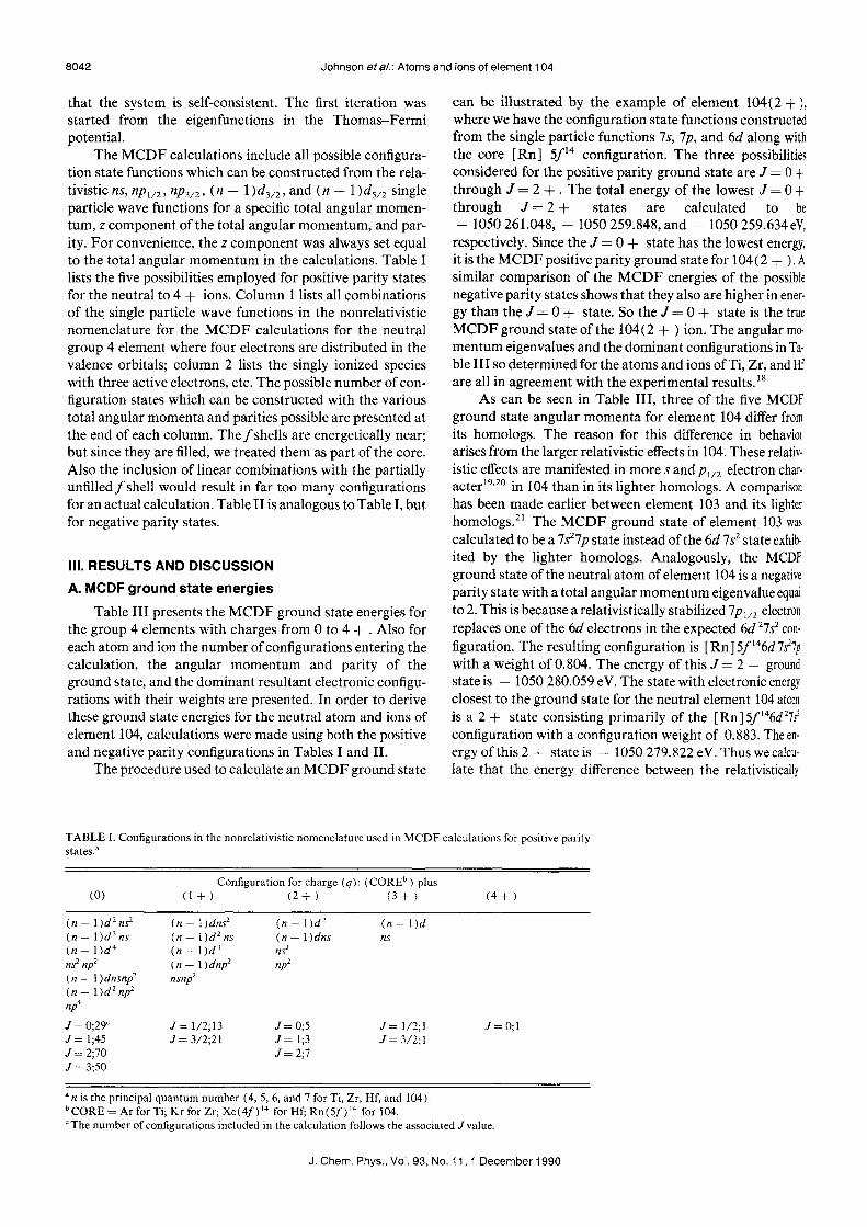
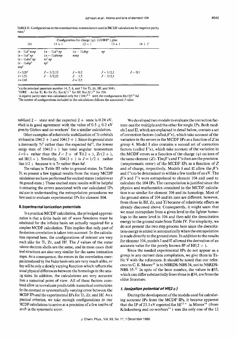
The MCDP calculations include all possible configura­tion state functions which can be constructed from the rela­tivistic ns, npl/2' np3/2' (n - 1)d3/2, and (n - 1)dS/ 2 singleparticle wave functions for a specific total angular momen­tum, z component ofthe total angular momentum, and par­ity. For convenience, the z component was always set equalto the total angular momentum in the ealeulations. Table Ilists the five possibilities employed for positive parity statesfor the neutral to 4 + ions. Column 1 lists all eombinationsof the single particle wave functions in the nonrelativisticnomenclature for the MCDF calculations for the neutralgroup 4 element where four eleetrons are distributed in thevalence orbitals; column 2 lists the singly ionized specieswith three active electrons, etc. The possible number of con­figuration states whieh ean be eonstrueted with the varioustotal angular momenta and parities possible are presented atthe end of each column. The j shells are energetieally near;but since they are filled, we treated them as part ofthe core.Also the inclusion of linear combinations with the partiallyunfilledjshell would result in far too many configurationsfor an actual calculation. Table 11 is analogous to Table I, butfor negative parity states.

111. RESULTS AND DISCUSSION

A. MCDF ground state energies

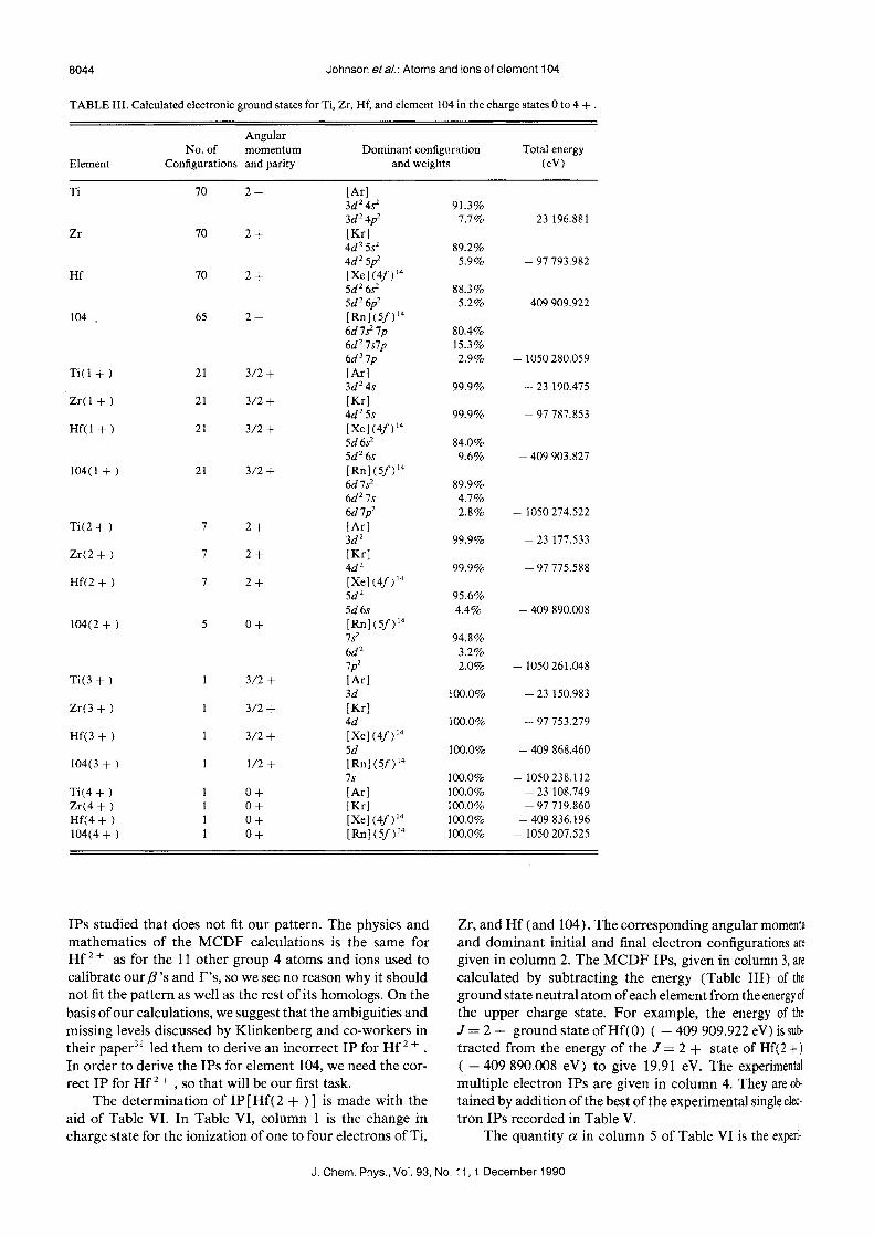
Table 111 presents the MCDF ground state energies forthe group 4 elements with eharges from 0 to 4 + .Also foreach atom and ion the number of configurations entering theealculation, the angular momentum and parity of theground state, and the dominant resultant electronic configu­rations with their weights are presented. In order to derivethese ground state energies for the neutral atom and ions ofelement 104, calculations were made using both the positiveand negative parity configurations in Tables land 11.

The proeedure used to calculate an MCDP ground state

can be illustrated by the example of element 104(2 + ),where we have the configuration state funetions eonstructedfrom the single particle functions 7s, 7p, and 6d along withthe core [Rn] 5j14 configuration. The three possibilitieseonsidered for the positive parity ground state are J = 0 +through J = 2 + . The total energy of the lowest J = 0 +through J = 2 + states are ealculated to be- 1050261.048, - 1050259.848, and - 1050 259.634eV,

respectively. Since the J = 0 + state has the lowest energy,it is the MCDP positive parity ground state for 104(2 + ). Asimilar comparison of the MCDF energies of the possiblenegative parity states shows that they also are higher in ener­gy than the J = 0 + state. So the J = 0 + state is the trueMCDF ground state ofthe 104(2 + ) ion. The angular momentum eigenvalues and the dominant configurations in Ta­ble 111 so determined for the atoms and ions ofTi, Zr, and Hfare all in agreement with the experimental results."

As ean be seen in Table 111, three of the five MCDFground state angular momenta for element 104 differ fromits homologs. The reason for this difference in behaviorarises from the larger relativistic effects in 104.These relativ­istic effects are manifested in more sand Pl/2 electron char­aeter l 9

,20 in 104 than in its lighter homologs. A eomparisonhas been made earlier between element 103 and its lighterhomologs" The MCDP ground state of element 103 wascalculated to be a 7s27pstate instead ofthe 6d 7s2state exhib­ited by the lighter homologs. Analogously, the MCDFground state of the neutral atom of element 104 is a negativeparity state with a total angular momentum eigenvalue equalto 2. This is because a relativistieally stabilized 7pl/2 electronreplaees one of the 6d eleetrons in the expeeted 6d 27S2 con­figuration. The resulting configuration is [Rn] 5f146d7s27pwith a weight of 0.804. The energy of this J = 2 - groundstate is - 1050 280.059 eV. The state with electronic energyelosest to the ground state for the neutral element 104atomis a 2 + state consisting primarily of the [Rn] 5j146d 271configuration with a configuration weight of 0.883. Theen­ergy ofthis 2 + state is - 1050 279.822 eV. Thus wecalcu­late that the energy difference between the relativistically

TABLE I. Configurations in the nonrelativistic nomenclature used in MCDF calculations for positive paritystates."

Configuration for charge (q): (COREb) plus(0) (1+) (2+ ) (3+ ) (4+ )

(n - l)d2ns' (n - 1Ydns' (n - l)d 2 (n -1)d(n - l)d 3 ns (n - l)d 2 ns (n - l)dns ns(n-l)d4 (n - l)d 3 n~

ns' np" (n - l)dnp2 np2(n - 1)dnsnp2 nsnp'(n - l)d 2np'np4

J = 0;29c J = 1/2;13 J=0;5 J = 1/2;1 J=O;1J = 1;45 J = 3/2;21 J= 1;3 J = 3/2;1J= 2;70 J=2;7J = 3;50

anis the principal quantum number (4, 5, 6, and 7 for Ti, Zr, Hf, and 104).bCORE = Ar for Ti; Kr for Zr; Xe(4j) 14 for Hf; Rn(5j) 14 for 104.c The number of configurations included in the calculation follows the associated J value.

J. Chern. Phys., Vol. 93, No. 11, 1 December 1990

Johnson et al.: Atoms and ions of element 104

TAßLE11.Configurations in the nonrelativistic nomenclature used in MCDP calculations for negative paritystates."

8043

(0)Configuration for charge (q): (COREb

) plus(1 + ) (2 + ) (3 + )

(n - 1)d 2 nsnp(n _1)d3 np

(n-l)dnrnp(n _1)dnp3

nsnp3

J= O;20d

J= 1;53J= 2;65

(n - l)d 2 np(n - l)dnsnpns' npnp3

J=I/2;13J = 3/2;22

(n - l)dnpnsnp

J=0;2J= 1;5J= 2;5

np

J = 1/2;1J = 3/2;1

J=O;1

8 nis the principal quantum number (4, 5,6, and 7 forTi, Zr, Hf, and 104).bCORE=ArforTi; Kr for Zr; Xe(4j)14 forHf; Rn(5j)14 for 104.cA negative parity state was calculated only for (104) 4+ with the configuration Rn (5j) 13 6d.dThe number of configurations included in the calculations follows the associated J value.

stabilized 2 - state and the expected 2 + state is 0.24 eV,which is in good agreement with the value of 0.5 ± 0.2 eVgiven by Glebov and co-workers/ for a similar calculation.

Otherexamples of relativistic stabilization of7sorbitalsare found in 104(2 + )and 104(3 + ). Since its ground stateis dominantly 7s2 rather than the expected 6d 2, the lowestenergy state of 104(2 +) has total angular momentumJ=0+ rather than the J = 2 + of Ti(2 + ), Zr(2 + ),and Hf(2 + ). Similarly, 104(3 + ) is J = 1/2 + ratherthan 3/2+ because it is 7s rather than 6d.

Thevalues in Table III refer to ground states. In TableIV, we present a few typical results from the many MCDPcalculations we have performed for excited states (relative tothe ground state.) These excited state results will be helpfulin estimating the errors associated with our calculated IPsand also in understanding the extrapolation procedures wehave used to evaluate experimental IPs for element 104.

B. Experimental ionization potentials

Inapractical MCDP calculation, the principal approxi­mation is that a finite basis set of wave functions must besubstituted for the infinite basis set actually required for acomplete MCDP calculation. This implies that only part oftheelectron correlation is taken into account. In the calcula­tions reported here, the configurations of interest are verymuch alike for Ti, Zr, and Hf. The J values of the outervalence electron shells are the same, and in most cases theirlevel structures are also very similar for the same ionizationstages. As a consequence, the errors in the correlation ener­gies introducedby the finite basis sets are very much alike, orthey will beonly a slowly varying function which reflects theactual physical differences between the homologs in the ana­log states. In addition, the calculations are very accuratefrom a numerical point of view. All of these factors com­bined allow us to evaluate predictable numerical correctionsfor theconstant or systematically varying error between theMCDP IPs and the experimental IPs for Ti, Zr, and Hf. As apractical criterion, we take enough configurations in ourMCDP calculationsto arrive at aprecision ofa few tenths ofan eVin the systematic error.

We developed two models to evaluate the correction fac­tors: one for multiple and the other for single IPs. Both mod­els land 11,which are explained in detail below, contain a setofcorrection factors (calledß 's), which take account ofthevariation in the errors in the MCDP IPs as a function ofZ ingroup 4. Model I also contains a second set of correctionfactors (calIed T's), which take account of the variation inthe MCDP errors as a function ofthe charge (q) on ions ofthe same element (Z). Theß 's and F's then are the precision(unsystematic error) of the MCDP IPs as a function of Zand of charge, respectively. Models land II allow the ß 'sand T's to be determined to within a few tenths ofan eV. Theß 's and T's were extrapolated to element 104 and used tocalculate the 104 IPs. The extrapolation is justified since thephysics and mathematics contained in the MCDP calcula­tion is so similar for element 104 and its homologs. Most ofthe ground states of 104 and its ions are different, however,from those in Hf, Zr, and Ti because of relativistic effects asalready discussed above. Consequently, it might seem thatwe must extrapolate from a given level in the lighter homo­logs to the same level in 104 and then add the deexcitationenergy to the ground state from Table IV. For simplicity, wedo not present the two step process here since the deexcita­tion energy is added in automatically when the extrapolationis made directly to the ground state. In addition to the resultsfor element 104, models land II allowed the derivation ofanaccurate value for the poorly known IP of Hf( 2 + ).

Since the needed experimental IPs do not appear as agroup in any current data compilation, we give them in Ta­ble V with the references. It should be noted that our refer­ence to C. E. Moore." is to NSRDS-NBS 34, not to NSRDS­NBS 35.12 In spite of the later number, the values in #35,which can differ substantially from those in #34, are from theolder literature.

1. lonization potential otHf(2 +)During the development of the models used for calculat­

ing accurate IPs from the MCDP IPs, it became apparentthat the IP of23.3 eV reported for Hf 2 + in Moore" (fromKlinkenberg and co-workers" ) was the only one ofthe 12

J. Chem. Phys., Val. 93, No. 11, 1 December 1990

8044 Johnson et al.: Atoms and ions of element 104

TABLE III. Calculated electronic ground states for Ti, Zr, Hf, and element 104 in the charge states 0 to 4 + .

AngularNo.of momentum Dominant configuration Total energy

Element Configurations and parity and weights (eV)

Ti 70 2+ [Ar]3d 24.r 91.3%3d 24p2 7.7% - 23 196.881

Zr 70 2+ [Kr]4d 25.r 89.2%4d 25p2 5.9% - 97 793.982

Hf 70 2+ [Xe](4j)145d 26.r 88.3%5d 26p2 5.2% - 409 909.922

104 . 65 2- [Rn] (5j)146d7.r 7p 80.4%6d 27s7p 15.3%6d 37p 2.9% - 1050 280.059

Ti( 1 + ) 21 3/2+ [Ar]3d 24s 99.9% - 23 190.475

Zr(1 +) 21 3/2 + [Kr]4d 25s 99.9% - 97 787.853

Hf(1 +) 21 3/2+ [Xe](4j)145d6.r 84.0%5d 26s 9.6% - 409 903.827

104(1 + ) 21 3/2+ [Rn](5j)146d7.r 89.9%6d 27s 4.7%6d7p2 2.8% - 1050274.522

Ti(2 + ) 7 2+ [Ar]3d 2 99.9% - 23 177.533

Zr(2 + ) 7 2+ [Kr]4d 2 99.9% - 97 775.588

Hf(2+ ) 7 2+ [Xe] (4j)145d 2 95.6%5d6s 4.4% - 409 890.008

104(2+ ) 5 0+ [Rn](5j)147.r 94.8%6d 2 3.2%7p2 2.0% - 1050261.048

Ti(3 + ) 3/2 + [Ar]3d 100.0% - 23 150.983

Zr(3 +) 3/2 + [Kr]4d 100.0% - 97 753.279

Hf(3+ ) 3/2 + [Xe] (4j)145d 100.0% - 409 868.460

104(3 + ) 1/2 + [Rn](5j)147s 100.0% - 1050238.112

Ti(4 + ) 0+ [Ar] 100.0% - 23 108.749Zr(4+ ) 0+ [Kr] 100.0% - 97 719.860Hf(4 +) 0+ [Xe] (4j)14 100.0% - 409 836.196104(4 + ) 0+ [Rn](5j)14 100.0% - 1050207.525

IPs studied that does not fit our pattern. The physics andmathematics of the MCDF calculations is the same forHf 2 + as for the 11 other group 4 atoms and ions used tocalibrate our ß 's and r's, so we see no reason why it shouldnot fit the pattern as well as the rest of its homologs. On thebasis ofour calculations, we suggest that the ambiguities andmissing levels discussed by Klinkenberg and co-workers intheir paper" led them to derive an incorrect IP for Hf 2 + .

In order to derive the IPs for element 104, we need the cor­reet IP for Hf 2 + , so that will be our first task.

The determination of IP [Hf( 2 + )] is made with theaid of Table VI. In Table VI, column 1 is the change incharge state for the ionization of one to four electrons of Ti,

Zr, and Hf (and 104). The corresponding angular momentaand dominant initial and final eleetron configurations aregiven in column 2. The MCDF IPs, given in column 3,arecalculated by subtracting the energy (Table 111) of theground state neutral atom ofeach element from the energyofthe upper charge state. For example, the energy of theJ = 2 + ground state of Hf(0) ( - 409 909.922 eV) issub­tracted from the energy of the J = 2 + state of Hf(2 +)

( - 409 890.008 eV) to give 19.91 eV. The experimentalmultiple electron IPs are given in column 4. They are ob­tained by addition ofthe best ofthe experimental single ele­tron IPs recorded in Table V.

The quantity a in column 5 of Table VI is the experi-

J. Chern, Phys., Vol. 93, No. 11, 1 December 1990

Johnson et al.: Atoms and ions of element 104

TAßLE IV. Promotion energies of selected atoms and ions.

Transition between ground MCDF Exp. DifferenceAtom or state and excited energy energy" (MCDF-Exp.)

ion configurations (eV) (eV) (eV)

Ti(2+ ) 3d 2(J = 2 + )_3d2(J = 0 + ) 1.67 1.31 0.36Ti(3 +) 3d(J = 3/2 + )-4s(J = 1/2 + ) 9.72 9.97 - 0.25

Zr(O) 4d 25~ (J = 2 + )_4d 25s2(J = 1 + ) 0.81 0.54 0.27Zr(1 + ) 4d 25s(J = 3/2 + )_4d25s(J =1/2 + ) 0.99 0.71 0.28Zr(2 +) 4d 2 (J = 2 + )_ 4d 2 (J = 0 + ) 1.25 1.00 0.25Zr(3 + ) 4d(J = 3/2 + )-5s(J = 1/2 + ) 4.61 4.74 - 0.13

Hf(O) 5d26~ (J= 2 + )_5d26~ (J= 1 +) 0.89 0.82 0.07Hf(1 + ) 5d6~ (J= 3/2 + )_5d26s(J= 1/2 +) 1.75 1.50 0.25

104(0) 6d 752 7p(J = 2 - ) _ 6d 2 7~ (J = 2 + ) 0.24104(1 + ) 6d7~ (J = 3/2 + )_6d27s(J = 1/2 + ) 3.02104(2 +) 7~(J=0+ )_6d2(J=4+) 3.96104(3 + ) 7s(J = 1/2 + )-6d(J = 3/2 + ) 0.34

aReference 21.

8045

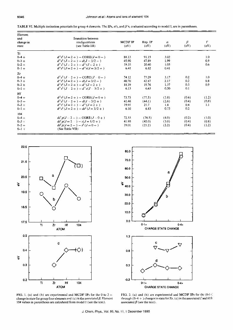
mental IP minus the MCDF IP. Hence ais the total error inthe MCDP IP calculation. It is illustrated in Fig. 1 as therelatively constant distance between the (a) experimentaland (b) MCDF curves for the (0-2 + ) change in state forthe group 4 elements. As can be seen from column 5, a is ofthe order of about 0.5 to 0.8 eV per charge state. This is themagnitude one would expect from an extensive many-con­figuration MCDF calculation of the type we have done.:"Thea's are large in magnitude because they contain the sys­tematic error from two different atomic entities being in­volved in the calculation of an MCDF IP. In contrast, if onetakes thedifferencebetween two configurations which are inthe same atom or ion, as in an excited state calculation, the

TAßLE V.Experimental single ionization potentials for group 4 elements.

IPof Exp.IP Exp.IP ErrorZ(n+ ) (cm- 1

) «vi- (eV) Ref.

Ti(O) 55010 6.820 0.012 236.78 0.02 24

Zr(O) 53 506.0 6.6339 0.0004 256.59 0.07 24

Hf(O) 55047.9 6.82507 0.0004 2654700 6.78 0.07 23

6.52 0.1 24Ti(1 + ) 109494 13.5755 0.0025 27

109500 13.58 0.12 2313.6 0.5 28

Zr(1 + ) 105900 13.13 18Hf(1 + ) 120000 14.9 0.1 23Ti(2+ ) 221 735.6 27.4917 0.0002 29

27.5 0.5 28Zr(2+ ) 186400 23.11 0.06 30

185400 22.99 18Hf(2+ ) 23.3 "a few 0.1 V" 18,31Ti(3 +) 348973.3 43.2672 0.0002 32Zr(3 + ) 277605.8 34.4187 0.0002 33Hf(3 +) 269 150 33.37 0.02 34

269835 33.5 0.1 35268500 33.3 0.1 18

18065.5410 cm -- I = 1 eV.

systematic error is largely removed, and we are left withwhat is essentially an unsystematic error that averages about0.2 eVas can be seen in Table IV. We have developed modelsthat remove the large systematic error from the IPs and leaveus with only the small unsystematic error for use in extrapo­lations to unknown IPs.

The parameter ß in column 6 of Table VI is thedifference in the accuracy of the MCDF calculationfor a given multiple IP in going from one Z to the next higherZ. For example, ß[Zr(O - 4 +), Ti(O - 4 + )]=a[Zr(0-4+)] - a[Ti(0-4+)] = 3.17 - 3.02= 0.2 eV. The ß 's for the (0-2 + ) change in state of the

group 4 elements are plotted in Fig. 1 (curve c). Just as ß isthe variation ofthe MCDF IP calculations as a function of Z(with the charge held constant), so r in column 7 is thevariation of the MCDF IPs as a function of charge (for thesame Z). For example, F[TifO - 4 + ), Ti(O - 3 + )]= 3.02 - 1.99 = 1.0 eV. An illustration of how well the

MCDF IPs track the experimental ones for Zr and its ions isgiven in Fig. 2. The small variation in the T's and ß 's für Zrare shown in curves c and d.

The experimentally determined ß's (Table VI) for Ti,Zr, and Hfare found to fall into the range ofO.1-0.4 eV. TheF's for a given change in charge state in Table VI are alsoseen to vary from each other or from a trend by only a fewtenths ofan eV. The F's for [(0 - 2 + ),(0 - 1 + )] for Ti,Zr, and Hfincrease in the trend 0.6,0.9,1.1 as a function of Z.T'[TifO- 3 + ),Ti(O - 2 + )] and T'[ZrtO- 3 + ),Zr(O - 2 + )] are equal to 0.9 and 0.8, respectively, and theF's for the [(0 - 4 + ), (0 - 3 + )] changes in state for Tiand Zr are both equal to 1.0. As in the case ofthe excitationenergies and the variation of the ß 's, the variation in the F'sindicates an unsystematic error close to 0.2 eV in our MCDFcalculations. Accordingly we will assurne in our calculationof IP[Hf(O - 3 + )] that F[Hf'(O - 3 + ),Rf(O - 2 + )]is 0.8 ± 0.2.

The experimental values for the IPs of Hf(O - 3 + )and Hf(O - 4 + ) are not recorded in Table VI because wediscovered, as noted above, that the IP of Hf(2 + ) of 23.3

J. Chern, Phys., Vol. 93, No. 11, 1 December 1990

8046 Johnson et al.: Atoms and ions of element 104

TABLE VI. Multiple ionization potentials for group 4 elements. The IPs, a's, and ß 's, evaluated according to model I, are in parentheses.

Elementand Transition betweenchangein configurations MCDFIP Exp.IP a ß rstate (see Table 111) (eV) (eV) (eV) (eV) (eV)

Ti0-4+ d 2 1- (J = 2 + ) - CORE(J = 0 + ) 88.13 91.15 3.02 1.00-3 + d 21- (J = 2 + ) - d(J = 3/2 + ) 45.90 47.89 1.99 0.90-2+ d 2 1- (J = 2 + ) - d 2 (J = 2 + ) 19.35 20.40 1.05 0.60-1 + d 2?- (J = 2 + ) - d 2s( J = 3/2 + ) 6.41 6.82 0.41

Zr0-4+ d 2 1- (J = 2 + ) - CORE(J = 0 + ) 74.12 77.29 3.17 0.2 1.00-3 + d 21-(J = 2 + ) - d(J = 3/2 + ) 40.70 42.87 2.17 0.2 0.80-2+ d 2 1- (J = 2 + ) - d? (J = 2 + ) 18.39 19.76 1.37 0.3 0.90-1 + d 21- (J = 2 + ) - d 2s( J = 3/2 + ) 6.13 6.63 0.50 0.1

Hf0-4+ d 2 1- (J = 2 + ) - CORE(J = 0 + ) 73.73 (77.5) (3.8) (0.6) ( 1.2)0-3 + d 2 1- (J = 2 + ) - dt J = 3/2 + ) 41.46 (44.1 ) (2.6) (0.4) (0.8)0-2+ d 2 1- (J = 2 + ) - d 2 (J = 2 + ) 19.91 21.7 1.8 0.4 1.10-1 + d 2 1- (J = 2 + ) - ds' (J = 3/2 + ) 6.10 6.83 0.73 0.2

1040-4+ ds' p(J = 2 - ) - CORE(J = 0 + ) 72.53 (76.5) (4.0) (0.2) ( 1.0)0-3 + ds'p (J = 2 - ) - s( J = 1/2 + ) 41.95 (45.0) (3.0) (0.4) (0.8)0-2+ ds' p (J = 2 - ) - 1-(J = 0 + ) 19.01 (21.2) (2.2) (0.4 ) ( 1.2)0-1 + (See Table VII)

22.5 --------------..--.,

-

c V\1--\1/

I I I I

0-1+ 0-4+CHARGE STATECHANGE

d

/0--0-0o

0.8 -

0.3 ~

-0.2 ------'-------!O__---Io__---L__--J

1.3 r-----------------.

0-1+ 0-4+CHARGE STATECHANGE

0.0 I000-.-_---!o__---10__---L__--'

70.0

80.0

60.0

50.0

20.0

30.0

10.0

>CD 40.0

o'(-0)

Ti Zr Hf 104ATOM

c

O--tO)

/0 -

I I I I

Ti Zr Hf 104ATOM

D a

"0 0

o I'"'"b 0

o

0.5 --------...:.-..---------,

0.3 ....

0.2 '----~--~--"'----~----'

0.4 -

21.5

20.5

17.5 L...-__.&...-__.&...-__..L.--__"'--_~

19.5

18.5

>CI)

>CI)

FIG. 1. (a) and (b) are experimental and MCDF IPs for the 0 to 2 +change in state for group four elements and (c) is the associated ß.Element104 values in parentheses are calculated from model I (see the text).

FIG. 2. (a) and (b) are experimental and MCDF IPs for the (0-1 +)

through (0-4 +) changesinstateforZr. (c) is the associated Pandtdltxassociated ß (see the text).

J. Chern. Phys., Vol. 93, No. 11, 1 December 1990

Johnson et a/.: Atoms and ions of element 104 8047

eV appearing in the Moore tables 18 is inaccurate. The valuesfor IP[Hf(O - 3 + )] and IP[Hf(O - 4 + )] in Table VIare in parentheses to flag that they were evaluated usingmodel I as described below.

Model I is defined by specifying ranges that the ß 's andr's can assurne in the calculation of the unknown IPs fromthe known IPs and the MCDF IPs. We will always let ßrange from plus infinity to minus infinity for the change instate whose IP we are calculating. From this infinite set ofß's, we will select only those IPs that yield T''s in the rangewe havestipulated as described above. All IPs that yield F'soutside the range will be discarded. It will be found that theß'sselectedby model I from the infinite set ofß 's are close tothose found experimentally in Table VI. This approach ofselecting the value ofeachß according to the criterion set forthe associated r rather than specifying the ß 's as weIl as theF's directly serves as a check on the validity of model I.

As a first example, we specify the criterion thatr[Hf(0-3 + ),Hf(0-2 + )] == 0.8 ± 0.2 eV (as justifiedabove) and then apply the above rules for ß and r to evalu­ate IP[Hf(0-3 + )]. The following steps were taken:

(1) For convenience, define a range variable,ßj [HfCD-3 + ),Zr(0-3 + )] that runs from 0.0-0.7 in stepsof 0.1. [It could run from - 00 to + 00, but the actualpossible range for the ßj 's under criterion (3) below will befound to be less than the chosen range ofO.O-o.7.]

(2) Add each ßj to a [Zr(0-3 + )] ( == 2.17) to obtainaset ofaj [Hf(0-3 + )] 'So

(3) Define r j [Hf(0-3 + ),Hf(0-2 + )]={aj [Hf(0-3 + )] - 1.8}, where 1.8 is the experimen­tally knowna[Hf(0-2 + )].

(4) Calculate each (IP) j that satisfies the criterionO.6<rj [Hf(O- 3 + ),Hf(0-2 + )]<1.0.

(5) Calculate the mean IP and the standard deviation.The methodof extrapolation we have developed and appliedhere hasnever appeared in the literature to our knowledge.Onlyß's with values of O. 3 to 0.6 result in IPs that meet the

criterion for the rj 's [item (4) above]. The associated meanvalue of IP [Hf(0-3 + )] is 44.1 ± 0.1 eV. Since the experi­mental." IP[Hf(3 + )] == 33.37, IP[Hf(0-4 + )] == 44.1+ 33.37 == 77.5 ± 0.1 eV. Also IP[Hf(2 + )]==(44.1±0.1)-(21.7±0.1)==22.4±0.2 eV, where

21.7 is the experimental IP of Hf(0-2 + ). These values,along with the ß and r values derived from them, are givenin Table VI in parentheses. The calculated mean ß selectedfrom the infinite set by our calculation is 0.4, a value that fitsin with the experimental values.

As a further check on model I, IP [Hf(0-4 + )] wascalculated independently oflP [Hf(0-3 + )] and the experi­mental value of Hf( 3 + ). The experimentally determinedr's for the [ (0-4 + ), (0-3 + )] change in state ofTi and Zrare both equal to 1.0. As discussed above, our MCDF unsys­tematic error is about 0.2 eV, so we assurne that T'[Hf'(O>4 + ),Hf(0-3 + )] is equal to 1.0 ± 0.2 eV for the model Icalculation. The calculation using this criterion shows thatonly IPs associated with values of ß[Hf(0-4 + ),Zr(O­4 + )] from 0.1 through 0.8 are allowed. The meanIP == 77.4 ± 0.2 eV thus calculated is in excellent agreementwith the value of 77.5 calculated above from IP [Hf(O­3 + )] and the experimental value of IP [Hf( 3 + )] fromSugar. 34

It will be found in the discussion ofTable VII that ourevaluated experimental IP of 22.4 eV for Hf(2 + ) alsoyields a reasonable value for theß for single IPs appropriatefor that table. The fact that the value for the IP of Hf( 2 + )resulting from the multiple ionization calculation is consis­tent with the single ionization table also serves as a check onthe model I calculation.

2. lonization potentials ofelement 104

For the evaluations of the multiple IPs of element 104,we will use the same method (model I type calculation) em­ployed to obtain IP [Hf(0-3 + )] and IP [Hf(0-4 + )]. The

TAßLE VII.Singleionization potentials for group 4 elements. The IPs, a's, and ß 's, evaluated according to model 11,are in parentheses.

Transition betweenChange in Element configurations MCDFIP Exp.IP a ßstate (q) (see Table 111) (eV) (eV) (eV) (eV)

(0)-(1 +) Ti(O) d 2 i2(J = 2 + ) - d 2 S (J = 3/2 + ) 6.41 6.82 0.41Zr(O) d? i2 (J = 2 + ) - d? s(J = 3/2 + ) 6.13 6.63 0.50 0.1Hf(O) d 2 S2 (J = 2 + ) - ds' (J = 3/2 + ) 6.10 6.82 0.72 0.2104(0) ds' p(J = 2 - ) - ds' (J = 3/2 + ) 5.54 (6.5) ( 1.0) (0.3 )

(l +)-(2+) Ti(l +) d 2s(J= 3/2 +) - d? (J= 2 +) 12.94 13.58 0.64Zr(l +) d 2 s( J = 3/2 + ) - d 2 (J = 2 + ) 12.26 13.13 0.87 0.2Hf( 1 + ) ds' (J = 3/2 + ) - d 2 (J = 2 + ) 13.82 14.9 1.1 0.2104( 1 + ) ds' (J = 3/2 + ) - i2(J = 0 + ) 13.47 ( 14.8) (1.3 ) (0.2)

(2+)-(3 + ) Ti(2+ ) d? (J = 2 + ) - dt J = 3/2 + ) 26.55 27.49 0.94Zr(2 + ) d 2 (J = 2 + ) - d (J = 3/2 + ) 22.31 23.11 0.80 -0.1Hf(2 + ) d? (J = 2 + ) - dt J = 3/2 + ) 21.55 (22.4) (0.8) (0.0)104(2 + ) S2 (J = 0 + ) - s(J = 1/2 + ) 22.94 (23.8) (0.9) ( + 0.1)

(3+)-(4 + ) Ti(3 +) d(J= 3/2 +) - CORE(J= 0 +) 42.23 43.27 1.04Zr(3 +) dt J = 3/2 + ) - CORE(J = 0 + ) 33.42 34.42 1.00 0.0Hf(3 + ) d(J=3/2+) -CORE(J=O+) 32.26 33.37 1.11 0.1104(3 + ) s(J = 1/2 + ) - CORE(J = 0 + ) 30.59 (31.9) (1.3 ) (0.2)

J. ehern. Phys., Vol. 93, No. 11,1 December 1990

3 + )] and IP [ 104(0-4 + )] closely parallel those of Hf( 0­3 + )] and Hf(0-4 + ). The experimental multiple IPs forelement 104 thus evaluated with model I are: (0­2 + ) = 21.2 ± 0.1; (0-3 + ) = 45.0 ± 0.2; and (0­

4 + ) = 76.5 ± 0.2. It should be noted that the mean ß'sselected by model I cause the calculated a's and F's to fitperfectly in Table VI as though they had been calculatedwith Table VI rather than by the method that allows them torange from minus infinity to plus infinity. Also, as we shallsee, calculations using another model based on single ratherthan multiple IPs will yield closely similar results. The finalIPs for element 104 will be obtained by averaging the resultsof the two models.

We will now formulate model 11 based on the singleMCDP IPs. This model is embedded in Table VII, which isfor the single IPs of the group 4 elements. In Table VII,column 1is the change in charge state for the one electron IPofthe element or ion in column 2. The corresponding initialand final electron configurations and angular momenta aregiven in column 3. The MCDP IPs, given in column 4, arecalculated by subtracting the energy (Table 111) ofthe Iowercharge state from the upper. The experimental single IP~

given in column 5 are the best values from Table V. The a'~

and ß 's are defined for one electron changes analogously tothose for the multiple IPs in Table VI. The excellent trackintofthe experimental single IPs by the MCDP IPs is illustrated in Fig. 3 for the 3 + and 4 + change in state. The ex·trapolations of the ß 's were so straightforward in Table VIIthat the T's were not needed for further differentiation. Thefollowing i1lustrates how Table VIII was set up: Theß[Zr(o-l + ),Ti(o-l +)] =0.50-0.42=0.1. It is recorded in the Zr(O) line. Our calculated value of 22.4 eVi~

used for the IP of Hf( 2 + ) rather than the value of 23Jderived from experiment (see the discussion above). It i~

seen that the ß = 0.0 for single electron changes resultingfrom the calculated value IP [Hf( 2 + )] = 22.4 from modelI fits nicely with the experimental value of Zr, which equal- 0.1. This close fit supports the correctness of the calculs

tion of IP [Hf( 2 + )] using model I.The ß 's in Table VII give a clear pattern. Although the

extrapolations to element 104 that we selected appear tobe

the only reasonable ones, we assurne that the ß 's can varyfrom this value by ± 0.1 eV. This is equivalent to assuminan error of ± 0.1 eV in the associated IP.

A new set of multiple IPs for element 104 results frornmodel II by adding the single IPs in Table VII. These new

Johnson et al.: Atoms and ions of element 104

a

O~D

:O~D). 0

Ti Zr Hf 104ATOM

-

C (0)0/ -

0/I I I I

Ti Zr Hf 104ATOM

o

8048

44.5

42.5

40.5

38.5>Q)

36.5

34.5

32.5

30.5

28.5

0.3 "'""

-0.1 ---""--------------

>Q) 0.1 -

FIG. 3. (a) and (b) are experimental and MCDF IPs for the 3 + ions ofgroup 4 elements and Ce) is the assoeiated ß. Element 104 values in paren­theses are ealculated from model I (see the text) .

r ranges for the [(0-3 + ),(0-2 + )] and [(0-4 + ),(0­3 + )] changes in state of element 104 are taken to be thesame as for the Hf calculations: {0.6<r[ 104(0-3 + );104(0-2 + )]<1.0}; and {0.8<r[ 104(0-4 + ),104(0-3 + )]< 1.2}. We will also need to set a range for rfor the [ (0-2 + ), (0-1 + )] change in state of 104. In TableVI, the sequence for T's for the (0-2 + ) change in state is0.6 (Ti), 0.9 (Zr), and 1.1 (Hf). A continuation ofthe seriesto 104 gives the probable range {1.I<r[ 104(0­2 + ),104(0-1 + )] < 1.3}. The calculations for IP( 104(0-

TABLE VIII. Evaluated ionization potentials for element 104.

Change instate

Model IIpa

(eV)

Model IIIp b

(eV)

Avg.IP

(eV)

0-1 +0-2+0-3 +0-4+

21.2±0.145.0 ± 0.276.5 ± 0.2

6.5±0.121.3 ± 0.245.1 ±0.377.0 ± 0.4

21.2 ± 0.245.1 ± 0.276.8 ± 0.3

aTable VI.b The sum of single IPs in Table VII.

J. Chem, Phys., Vol. 93, No. 11, 1 December 1990

Johnson et a/.: Atoms and ions of element 104

TAßLE IX. The radius in nanometers of maximum radial charge density (R m ax ) in the outermost shell

(shown in parentheses) of group 4 elements.

Charge \ Element 0 1+ 2+ 3+ 4+

Ti 0.161(4s) 0.150(4s) 0.0523(3d) 0.0494(3d) 0.0469(3p)Zr O.173(5s) 0.163(5s) 0.0834( 4d) 0.0798(4d) 0.0620(4p)Hf 0.161 (6s) 0.149(6s) 0.0872(5d) 0.0831(5d) 0.0626(5p)104 0.178(7p) 0.145(7s) 0.138(7s) 0.135(7s) 0.0706(6p)

8049

multiple IPs are compared in Table VIII to those calculatedby modelI using the multiple IPs approach ofTable VI. Alsoin TableVIII the final IPs for element 104 are obtained as anaverage of the values from models land 11.

Table IX presents the position of the principal maximaRmax in the radial charge density functions of the occupiedorbitals that have the largest values of R m ax and that have asignificantly large configuration weight associated with it forthe group4 elements. The values are taken for the electronicground state configurations. As shown by Slater, the valuesofRmax are useful for estimating atomic and ionic radii. 37,38

IV. CONCLUSION

In all cases considered, the relativistic multiconfigura­tion Dirac-Fock (MCDF) total angular momentum eigen­values and dominant configuration calculated for the lowestenergy state agree with the experimental results. This indi­cates that the MCDF results are reliable at least for these twoproperties. Also MCDP calculations of excited state ener­gies were found to be within about 0.2 eV of the experimentalvalues, an indication that unsystematic errors can be re­duced to an acceptable minimum by taking a large enoughbasis setof wave functions (out of the theoretically requiredinfinite set). An extrapolation method based on MCDP IPshas been developed and applied to obtain chemically usefulIPs for Hf(2 + ) and the atom and ions through the 4 + ofelement 104. The extrapolation procedure necessarily de­pends on the availability of accurate IPs for the lighter ho­mologs in group 4 of element 104. All IPs were availableexcept für Hf(2 + ), which we believe to be inaccuratelymeasured. Wecalculated a new value for the IP ofHf(2 + ).The MCDF ground state electronic configuration found forthe neutral element 104 atom is different from that given byearly predictions,1 but it is in agreement with that found byanother recent MCDP calculation by Glebov et al?

ACKNOWLEDGMENTS

Research sponsored by the Division of Chemical Sei­ences, Office of Basic Energy Sciences, V.S. Department ofEnergy under contract DE-AC05-840R21400 with MartinMarietta EnergySystems, Inc., the Deutsche Forschungsge­meinschaft (DFG), and the Gesellschaft fur Schwerionen­forschung (GSI), Darmstadt. The work was supported bythe Florida State University Supercomputer ComputationsResearch Institute, which is partially funded by the D.S.

Department of Energy through contract DE-FC05-85­ER25000.

1B. Fricke, Struct. Bond. 21, 89 (1975).2V. A. Glebov, L. Kasztura, V. S. Nefedov, and B. L. Zhuikov, Radiochim.Acta 46, 117 (1989).

3B. B. Cunningham, in Proceedings 0/ the Robert A. Welch FoundationConferences on Chemical Research XIII, The Transuranium Elements,edited by W. O. Milligan (R. A. Welch Foundation, Houston, 1970),Chap. XI.

4O. L. Keller, Jr., C. W. Nestor, and B. Fricke, J. Phys. Chem. 78, 1945( 1974).

5S. Hubener and I. Zvara, Radiochim. Acta. 31, 89 (1982).6R. J. Silva, W. J. McDowell, O. L. Keller, Jr., and J. R. Tarrant, Inorg.

Chem. 13,2233 (1974).7W. Bruchle, M. Schadel, U. W. Scherer, J. V. Kratz, K. E. Gregorich, D.

Lee, M. Nurmia, R. M. Chasterler, H. L. Hall, R. A. Henderson, and D.C. Hoffman, Inorg. Chim. Acta. 146,267 (1988).

8 O. L. Keller, Radiochim. Acta. 37, 169 (1984).91. Zvara, V. Z. Belov, L. P. Chelnokov, V. P. Domanov, M. Hussonois,

Yu. S. Korotkin, V. A. Schegolev, and M. R. Shalayevski, Inorg. Nucl.Chem. Lett. 7, 1109 (1971).

10 R. Silva, J. Harris, M. Nurmia, K. Eskola, and A. Ghiorso, Inorg. Nucl.Chem. Lett. 6, 871 (1970).

11 E. K. Hulet, R. W. Lougheed, J. F. Wild, J. H. Landrum, J. M. Nitschke,and A. Ghiroso, J. Inorg. Nucl. Chem. 42,79 (1980).

12 B. L. Zhuikov, Yu. T. Chuburkov, S. N. Timokhin, K. U. Jin, and I.Zvara, Radiochim. Acta 46, 113 (1989).

13 E. K. Hyde, D. C. Hoffman, and O. L. Keller, Jr., Radiochim. Acta 42, 57( 1987).

14J._p. Desc1aux, Comput. Phys. Commun. 9,31 (1975).15 I. P. Grant, Adv. Phys. 19,747 (1970).161.P. Grant and H. M. Quiney, Adv. At. Mol. Phys. 23, 37 (1988).17 C. Froese Fischer, The Hartree-Fock Method for Atoms (Wiley, New

York, 1977).18 Charlotte E. Moore, Ionization Potentials and Ionization Limits Derived

from the Analyses of'OpticalSpectra, NSRDS-NBS 34, SD Catalog No. C13.48:34 (Natl, Stand. Ref. Data Ser., Natl. Bur. Stand., Washington,D.C., 1970).

19 K. S. Pitzer, Ace. Chem. Res. 12, 271 (1979).20p. Pyykko and J.-P. Desc1aux, Ace. Chem. Res. 12,276 (1979).21 J.-P. Desc1aux and B. Fricke, J. Phys. 41,943 (1980).22 Charlotte E. Moore, Atomic Energy Levels, NSRDS-NBS 35, SD Catalog

No. C 13.48:35, (Natl. Stand. Ref. Data Ser., Natl. Bur. Stand., Washing­ton, D.C., 1971).

23 JANAF Thermochemical Tables, 3rd ed., edited by M. W. Chase, C. A.Davies, J. R. Downey, D. J. Frurip, R. A. McDonald, and A. N. Syverud(Natl. Bur. Stand., Washington, D.C., 1985).

24 E. G. Rauh and R. J. Ackermann, J. Chem. Phys. 70, 1004 (1979).25 P. A. Hackett, M. R. Humphries, S. A. Mitchell, and D. M. Rayner, J.

Chem. Phys. 85, 3194 (1986).26C. L. Callender, P. A. Hackett, and D. M. Rayner, J. Opt. Soc. Am. B 5,

1341 (1988).27S. Huldt, S. Johansson, and U. Litzen, Phys. Scr. 25, 401 (1982).28 M. J. Diserens, A. C. H. Smith, and M. F. A. Harrison, J. Phys. B: At.

Mol. Opt. Phys. 21, 2129 (1988).29 B. Edlen and J. W. Swensson, Phys. Scr. 12, 21 (1975).30 Z. A. Khan, M. S. Z. Chaghtai, and K. Rahimullah, Phys. Scr. 23, 29

(1981 ).31 P. F. A. Klinkenberg, Th. A. M. Van Kleef, and P. E. Noorman, Physica

J. Chem, Phys., Vol. 93, No. 11, 1 December 1990

8050 Johnson et al.: Atoms and ions of element 104

27, 1177 (1961).32 J. W. Swensson and B. Edlen, Phys. Sero 9, 335 (1974).33 N. Aequista and J. Reader, J. Opt. Soe. Am. 70, 789 (1980).34 J. Sugar and V. Kaufman, J. Opt. Soe. Am. 64,1656 (1974).35F. G. Meijer, Physiea 72,431 (1974).

36K. Rashid, B. Frieke, J. H. Blanke, and J.-P. Desclaux, Z. Phys. D 11, 99(1989).

37 J. C. Slater, Quantum Theory 01 Moleeules and Solids (MeGraw-Hill,New York, 1965), Vol. 2, Chapter 4.

38 J. C. Slater, J. Chem. Phys. 41, 3199 (1964).

J. Chem, Phys., Vol. 93, No. 11,1 December 1990