DETERMINATION OF PROTON RADII OF NEUTRON-RICHOXYGEN ISOTOPES FROM CHARGE-CHANGING CROSS

SECTION MEASUREMENTS

by

Satbir Kaur

Submitted in partial fulfillment of the requirementsfor the degree of Doctor of Philosophy

at

Dalhousie UniversityHalifax, Nova Scotia

July 2018

c� Copyright by Satbir Kaur, 2018

dedicated to my parents

ii

Table of Contents

List of Tables . . . . . . . . . . . . . . . . . . . . . . . . . . . . . . . . . . . v

List of Figures . . . . . . . . . . . . . . . . . . . . . . . . . . . . . . . . . . x

Abstract . . . . . . . . . . . . . . . . . . . . . . . . . . . . . . . . . . . . . . xi

Acknowledgements . . . . . . . . . . . . . . . . . . . . . . . . . . . . . . . xii

Chapter 1 Introduction . . . . . . . . . . . . . . . . . . . . . . . . . . 1

1.1 Exotic phenomena of neutron-rich nuclei: halos and skin . . . . . . . 41.1.1 Neutron halos . . . . . . . . . . . . . . . . . . . . . . . . . . . 41.1.2 Neutron skin . . . . . . . . . . . . . . . . . . . . . . . . . . . 5

1.2 Motivation to study proton radii of 16-24O . . . . . . . . . . . . . . . 61.2.1 Drip line of oxygen isotopes and 3N forces . . . . . . . . . . . 71.2.2 Proton radii: A test for ab initio approaches . . . . . . . . . . 101.2.3 The shell evolution in oxygen isotopes . . . . . . . . . . . . . 101.2.4 Neutron skin in oxygen isotopes . . . . . . . . . . . . . . . . . 14

1.3 Conventional methods to determine proton radii . . . . . . . . . . . . 141.3.1 Electron scattering . . . . . . . . . . . . . . . . . . . . . . . . 141.3.2 Isotope shift . . . . . . . . . . . . . . . . . . . . . . . . . . . . 161.3.3 Muonic Atom X-Ray Spectroscopy . . . . . . . . . . . . . . . 17

1.4 Charge-changing cross section measurement . . . . . . . . . . . . . . 18

1.5 Finite range Glauber model . . . . . . . . . . . . . . . . . . . . . . . 191.5.1 R

p

determined from �cc

. . . . . . . . . . . . . . . . . . . . . . 20

1.6 This Work . . . . . . . . . . . . . . . . . . . . . . . . . . . . . . . . . 21

Chapter 2 Experiment Description . . . . . . . . . . . . . . . . . . . 22

2.1 The fragment separator . . . . . . . . . . . . . . . . . . . . . . . . . . 22

2.2 Principle of measuring charge-changing cross section . . . . . . . . . . 27

2.3 The detector setup . . . . . . . . . . . . . . . . . . . . . . . . . . . . 282.3.1 Multiple-sample ionization chambers . . . . . . . . . . . . . . 292.3.2 Time projection chambers . . . . . . . . . . . . . . . . . . . . 312.3.3 Plastic scintillators . . . . . . . . . . . . . . . . . . . . . . . . 332.3.4 Veto scintillator . . . . . . . . . . . . . . . . . . . . . . . . . . 33

iii

Chapter 3 Data Analysis . . . . . . . . . . . . . . . . . . . . . . . . . . 35

3.1 Detector calibration . . . . . . . . . . . . . . . . . . . . . . . . . . . . 353.1.1 Calibration of the MUSIC detectors . . . . . . . . . . . . . . . 353.1.2 Time of flight calibration . . . . . . . . . . . . . . . . . . . . . 363.1.3 TPC calibration . . . . . . . . . . . . . . . . . . . . . . . . . . 41

3.2 Particle identification . . . . . . . . . . . . . . . . . . . . . . . . . . . 433.2.1 Location of focal planes . . . . . . . . . . . . . . . . . . . . . 44

3.3 Incident beam selection . . . . . . . . . . . . . . . . . . . . . . . . . . 49

3.4 Z identification after the target . . . . . . . . . . . . . . . . . . . . . 50

3.5 The target position dependence of transmission ratios . . . . . . . . . 52

Chapter 4 Discussion . . . . . . . . . . . . . . . . . . . . . . . . . . . . 55

4.1 The transmission ratios and �cc

. . . . . . . . . . . . . . . . . . . . . 55

4.2 Uncertainty of the measured cross section . . . . . . . . . . . . . . . . 584.2.1 Statistical uncertainty . . . . . . . . . . . . . . . . . . . . . . 594.2.2 Uncertainty from contaminants in the same Z events after the

target . . . . . . . . . . . . . . . . . . . . . . . . . . . . . . . 60

4.3 Secondary beam energies . . . . . . . . . . . . . . . . . . . . . . . . . 61

4.4 MUSIC42 detection e�ciency correction . . . . . . . . . . . . . . . . 62

4.5 Table of charge-changing cross sections . . . . . . . . . . . . . . . . . 64

4.6 Proton radii determination . . . . . . . . . . . . . . . . . . . . . . . . 64

4.7 Discussion of results . . . . . . . . . . . . . . . . . . . . . . . . . . . 664.7.1 Comparison with theory . . . . . . . . . . . . . . . . . . . . . 68

4.8 Neutron skin thickness determination . . . . . . . . . . . . . . . . . . 71

4.9 Summary . . . . . . . . . . . . . . . . . . . . . . . . . . . . . . . . . 72

Bibliography . . . . . . . . . . . . . . . . . . . . . . . . . . . . . . . . . . . 75

iv

List of Tables

Table 2.1 The beam intensity for each fragment setting of the FRS. . . . 26

Table 3.1 The parameters for TAC calibration for the Scintillator detectors. 40

Table 3.2 The position calibration parameters for anodes and delay linesof TPC1�6. . . . . . . . . . . . . . . . . . . . . . . . . . . . . . 43

Table 4.1 The measured �cc

of 16,18-24O with statistical uncertainties. . . . 57

Table 4.2 The energy losses in materials placed between SC41 and thecarbon reaction target at F4. . . . . . . . . . . . . . . . . . . . 62

Table 4.3 The MUSIC42 detection e�ciency corrections to �cc

for 16-18,24O. 63

Table 4.4 The measured �cc

with the uncertainties and secondary beamenergies in front of the target. . . . . . . . . . . . . . . . . . . . 64

Table 4.5 The measured Rcc

p

of 16-18,24O extracted from the measured �cc

.

The R(e�)p

for 16-18O are from Ref. [37]. . . . . . . . . . . . . . . 66

v

List of Figures

Figure 1.1 Mayer-Jensen’s shell model scheme predicted with harmonicoscillator potential and the spin-orbit force [6,7]. Figure adaptedfrom [8]. . . . . . . . . . . . . . . . . . . . . . . . . . . . . . . 2

Figure 1.2 The nuclear landscape where each square represents a nucleus.The valley of stability is shown by black, unstable nuclei are rep-resented by yellow and green region shows theoretically predictedbound nuclei. . . . . . . . . . . . . . . . . . . . . . . . . . . . 3

Figure 1.3 (a) A schematic illustration of neutron skin. (b) �Rrms

as afunction of �E

F

of various isotopes obtained by the RMF Model.The empirical values are shown in shadowed boxes. Right figureadapted from [22]. . . . . . . . . . . . . . . . . . . . . . . . . 6

Figure 1.4 Chiral e↵ective field theory for nuclear forces. The di↵erentcontributions at successive orders are shown diagrammatically.Nucleons and pions are represented by solid and dashed lines,respectively. Figure adapted from [26]. . . . . . . . . . . . . . 8

Figure 1.5 (a) The binding energies (b)Rp

from Ref. [34] using theNNLOsat

interaction (red symbols) and the EM interaction (black symbols)calculated in three di↵erent many-body approaches. The bluestars are R

p

from Ref. [27] calculated using coupled-cluster cal-culations. The experimental R

p

derived from the e� scatteringexperiments [37] are shown by blue open circles. . . . . . . . . 9

Figure 1.6 One-neutron separation energy for di↵erent isospin chains. Fig-ure taken from [39]. . . . . . . . . . . . . . . . . . . . . . . . . 11

Figure 1.7 The shell model scheme of 24O. . . . . . . . . . . . . . . . . . 11

Figure 1.8 (a) The first excited stated of di↵erent isotopes plotted as afunction of the neutron number. Figure taken from [40]. (b)Theone-neutron knockout cross sections and widths of the frag-ment longitudinal-momentum distributions as a function of theneutron number. Figure taken from [47] . . . . . . . . . . . . 13

Figure 1.9 The neutron skin calculated using the calculated Rp

and Rm

.The plusses represent �R calculated using radii with IMSRGmany-body approach with EM interaction (black) and NNLO

sat

interaction (red), taken from Ref. [34]. The stars represent �Rfound from the radii calculated with coupled-cluster calculationsfrom Ref. [27]. . . . . . . . . . . . . . . . . . . . . . . . . . . . 15

vi

Figure 1.10 The radii of point nucleon distribution in (a) Li isotopes (b) Heisotopes (c)Be isotopes. Figures adapted from [68]. . . . . . . 17

Figure 1.11 (a) The measured Rm

(circles) and measured Rcc

p

(triangles) for12-17B (b) The measured R

m

(open circles) and measured Rcc

p

(filled circles) for12-19C. The blue symbols represent the measuredR

p

derived from e� scattering. Figure taken from [82,84]. . . . 21

Figure 2.1 The schematic view of the GSI-FRS facility. Figure from [88]. 22

Figure 2.2 A photograph of FRS at GSI. . . . . . . . . . . . . . . . . . . 23

Figure 2.3 The schematic view of ion optics of the FRS. . . . . . . . . . . 25

Figure 2.4 The position distributions in x of the various isotopes at theF4 using the LISE code (a) without degrader (b) with a wedgedegrader. . . . . . . . . . . . . . . . . . . . . . . . . . . . . . . 26

Figure 2.5 (a) A schematic view of the experimental setup at the FRSwith the detector arrangement at the final focus F4. Fig. takenfrom [82].(b)A flowchart of measurements performed with thedi↵erent detectors. . . . . . . . . . . . . . . . . . . . . . . . . 29

Figure 2.6 The detector setup at F2 and F4 with detector distances. . . . 29

Figure 2.7 A picture of the MUSIC detector (left). Schematic view of theMUSIC detector (right). . . . . . . . . . . . . . . . . . . . . . 30

Figure 2.8 A picture of the detector on the left. A schematic view ofa Time-Projection Chamber (TPC) (right). Figure adaptedfrom [94]. . . . . . . . . . . . . . . . . . . . . . . . . . . . . . 31

Figure 2.9 The control sum distribution using the delay line 1 and anode 1for TPC6. . . . . . . . . . . . . . . . . . . . . . . . . . . . . . 32

Figure 2.10 A photograph of the veto plastic scintillator. . . . . . . . . . . 34

Figure 2.11 The energy loss in left PMT of the veto detector. . . . . . . . 34

Figure 3.1 (a) The uncalibrated MUSIC41 spectrum for the 12C secondarybeam. Each peak is fitted with a Gaussian function (red curve).(b) A linear fit of Z2 versus the mean channel number of thepeaks. (c) The calibrated Z spectrum of the MUSIC41 detector. 36

vii

Figure 3.2 (a) The uncalibrated MUSIC42 spectrum for the 12C setting.Each peak is fitted with a Gaussian function (red curve). (b) Alinear fit of Z2 versus the mean channel number of the peaks.(c) The calibrated Z spectrum of the MUSIC42 detector. . . . 37

Figure 3.3 The TAC spectrum for 10 ns pulses from the TAC calibrator (a)TOF

RR

in channels (RC

) (b) TOFLL

in channels (LC

). . . . . 38

Figure 3.4 (a) The linear fit of Rns

(TOFRR

in ns) versus mean RC

(TOFRR

in channels). (b) The linear fit of Lns

(TOFLL

in ns) versusmean L

C

(TOFLL

in channel). . . . . . . . . . . . . . . . . . 39

Figure 3.5 Linear fit of TOF ⇥ � versus �. The slope of the linear fit isthe TOF o↵set (O) and intercept (S) is the flight path. . . . . 40

Figure 3.6 The scheme of scintillator plastic fibers used for the calibrationof TPCs. . . . . . . . . . . . . . . . . . . . . . . . . . . . . . . 41

Figure 3.7 (a) The TPC delay line 1 spectrum with no condition. (b) Thedelay line spectrum with the scintillator grid coincidence withpeaks fitted with a three-Gaussian function (red curve). (c) Thelinear fit of the mean of the peaks in channels vs. correspondingposition in mm. . . . . . . . . . . . . . . . . . . . . . . . . . . 42

Figure 3.8 The calibrated correlation plot of x (mm) vs. y (mm) of TPC 6showing the structure of scintillator grid. . . . . . . . . . . . . 43

Figure 3.9 The correlation between the angle x (mrad) and the x position(mm) at (a) One meter before the focal plane (b) One meterafter the focal plane (c) At the focal plane at F4 region. . . . . 45

Figure 3.10 (a) The identification plot for the 23O setting. The black circleshows an example of background events. . . . . . . . . . . . . 46

Figure 3.11 The correlation of V etoL

vs. V etoR

for the 23O secondary beam. 47

Figure 3.12 The identification plot for the 23O secondary beam after theveto rejection. . . . . . . . . . . . . . . . . . . . . . . . . . . . 48

Figure 3.13 The correlation of (a) TPC4 energy signal vs MUSIC41 energysignal after the veto rejection. The events inside of the blackcontour represents the selection of good events. . . . . . . . . 48

Figure 3.14 The correlation of (a) MUSIC41 energy signal vs. TPC5 energysignal (b) MUSIC 41 energy signal vs. SC41 energy signal (c)TOF

LL

vs. TOFRR

. The events inside black contour representsthe selection of good events. The spectra show events after vetorejection. . . . . . . . . . . . . . . . . . . . . . . . . . . . . . . 49

viii

Figure 3.15 The identification plot for the 23O before the reaction target.The black contour represents the 23O incident beam selection. 50

Figure 3.16 The MUSIC41 Z spectrum where the blue histogram representsthe 23O selection and the red histogram is the total Z spectrumnormalized for 23O. . . . . . . . . . . . . . . . . . . . . . . . . 50

Figure 3.17 The MUISC42 Z spectrum with the target (red) and withoutthe target (blue) to identify the particles with unchanged Zafter the reaction. . . . . . . . . . . . . . . . . . . . . . . . . . 51

Figure 3.18 (a) The beam x position at the target (Xtarget) (b) Transmis-sion ratio for di↵erent Xtarget positions where green verticallines represent the selection region of constant R. . . . . . . . 52

Figure 3.19 (a) The beam y position at the target (Y target) (b) Transmissionratio for di↵erent Y target positions where green vertical linesrepresent the selection region of constant R. . . . . . . . . . . 52

Figure 3.20 (a) The x angle of the beam at the target in mrad (b) Trans-mission ratio for di↵erent x angles where green vertical linesrepresent the selection region of constant R. . . . . . . . . . . 53

Figure 3.21 (a) The y angle of the beam at the target in mrad (b) Trans-mission ratio for di↵erent y angles where green vertical linesrepresent the selection region of constant R. . . . . . . . . . . 53

Figure 4.1 The transmission ratios for 16,18-24O (a) with the reaction target(R

in

) (b) without the reaction target (Rout

). . . . . . . . . . . 56

Figure 4.2 The �cc

found by varying the x position, y position, x angle andy angle of the beam at the target location for two sets of datafor 24O. . . . . . . . . . . . . . . . . . . . . . . . . . . . . . . 57

Figure 4.3 The measured �cc

of 16-18,24O with statistical uncertainties. . . 58

Figure 4.4 The MUSIC42 detector spectrum for the 23O secondary beam.The red curve shows an exponential function fit of the tail ofthe Z = 7 peak. . . . . . . . . . . . . . . . . . . . . . . . . . . 60

Figure 4.5 The measured velocity ( � ) of the particles at SC41 for the 23Osecondary beam. . . . . . . . . . . . . . . . . . . . . . . . . . 61

Figure 4.6 (a) The TPC detector energy loss vs. SC42 energy loss. Theblack geometric cut represents the selection of oxygen nuclei.(b) The energy loss spectrum of MUSIC after the detector witha selection cut from the left figure. . . . . . . . . . . . . . . . 63

ix

Figure 4.7 The �cc

for 16O calculated using three di↵erent harmonic oscil-lator widths for the density distributions with di↵erent R

p

. Theblue horizontal line represents the central value of the measured�cc

. The black lines represent the uncertainties. The verticallines show the rms proton radii corresponding to the measured �

cc

65

Figure 4.8 The measured point proton radii (Rp

) where the black circles

represent Rcc

p

and the red squares represent R(e�)p

. . . . . . . . 68

Figure 4.9 Rp

from Ref. [34] calculated using NNLOsat

interaction withthree di↵erent many-body approaches compared to the measuredRcc

p

(blue circles). . . . . . . . . . . . . . . . . . . . . . . . . . 69

Figure 4.10 The comparison of the measured Rcc

p

(blue circles) to Rp

fromRef. [34] calculated using the EM interaction with three di↵erentmany-body approaches and R

p

from Ref. [27] computed usingthe coupled-cluster calculation. . . . . . . . . . . . . . . . . . 70

Figure 4.11 The experimental neutron skin (blue circles) determined frommeasured Rcc

p

and the measured Rm

from Ref. [55, 56]. �Rcalculated using IMSRG approach with EM interaction (blacksymbols) and NNLO

sat

interaction (red symbols) from Ref. [34]is shown by plusses and �R calculated using radii from coupled-cluster calculation is shown by blue stars. . . . . . . . . . . . . 72

x

Abstract

The nuclear charge radius is an important bulk property of the nucleus for investigating

nuclear structure. The nuclei lying close to the boundaries of the nuclear chart (the

drip lines) have revealed new exotic features like the halo and skin. Another new

phenomenon that has emerged in the neutron-rich region is the changing or vanishing

of magic numbers. The systematic study of the proton radii along an isotopic chain is

crucial for understanding the halo and skin formation and also the shell evolution in

neutron-rich nuclei near the drip-line. We present the first determination of the proton

radii of neutron-rich oxygen isotopes. The proton radii of 16,18-24O were measured using

the charge-changing cross sections, �cc

, which is the total cross section for the change of

the atomic number of the projectile nucleus due to any interaction with the protons in

the projectile nucleus. The experiment was performed at the fragment separator (FRS)

at GSI, Germany, at a relativistic beam energy of around 900A MeV. The proton radii

were extracted from the measured �cc

using the finite range Glauber model analysis.

The measured proton radii of stable isotopes of oxygen, 16O and 18O, are consistent

with the proton radii derived from the electron scattering experiments. A decrease in

proton radii of 22O and 24O was observed, showing signatures of the unconventional

shell closures at N = 14 and N = 16. This thesis also reports the first determination

of neutron skin thickness (�R) in neutron-rich oxygen isotopes, determined using the

measured proton radii reported in this work and measured matter radii available from

the literature. �R rapidly increases from 22-24O approaching the neutron drip-line,

establishing a thick neutron surface for the neutron-rich oxygen isotopes. We have

compared the measured proton radii to the predictions reported using various ab initio

approaches with di↵erent interactions. The experimental proton radii presented have

challenged these predictions.

xi

Acknowledgements

I would like to thank my supervisor Dr. Rituparna Kanungo for her guidance, ideas,

patience, support and motivation for the work done in this thesis. I consider myself

very fortunate for being able to work with a very considerate and encouraging professor

like her. It was a great learning experience to work under her supervision.

I would like to express my gratitude to my thesis committee members Dr. Scott

Chapman, Dr. Adam Sarty and Dr. David Hornidge for their support during my

research.

Special thanks go to the previous and current collaborators at FRS, GSI Germany.

Working with all of you has been the most educational and enjoyable experience of my

life. I owe my thanks to all of the members of FRS collaboration including physicists,

engineers and technicians who worked hard, day and night, to make the experiment

successful.

I am deeply thankful to Soumya who was always there for helping me out with all

kind of problems with his suggestions and discussions. I would like to thank Preet

and Gurpreet for all the fun times. I would also like to thank my special friends Daisy

and Anwinder.

Thank you Mom and Dad, for all of the unconditional love and encouragement.

This thesis would have been simply impossible without your support. I thank my

siblings Manbir and Taran for their constant support in all phases of my life. I would

like to express my gratitude to Manbir and Gary for answering all my queries whether

it was programming, writing and other aspects like dealing with the stress. A special

thanks to Rajveer for all of the moral support, love and care. It would have been a

lot harder without you to get through this PhD.

In retrospect, there are so many great people to give thanks to. Without them, I

would not have been able to come this far or complete this thesis. Though I cannot

print out all of the names, it is worthy noting that many great people helped me in

di↵erent ways along this journey. I thank them all here. eaaaaaaaaaways along this

journey. eaaaaaaaaaways along this journey. I thank them all hereSatbir Kaur

xii

Chapter 1

Introduction

The discovery of the nucleus goes back to 1909 when Geiger and Marsden irradiated

gold foils with alpha particles and observed the backscattered alpha particles [1].

This led Rutherford to postulate that most of the mass is located in a small, dense

center of the atom, a nucleus. There was a disparity between an element’s atomic

number (protons = electrons) and its atomic mass. Therefore, it seemed there must

be something else in the nucleus, in addition to protons. Chadwick solved the puzzle

about the constituents in the atomic nucleus when he discovered the neutron [2].

However, the fundamental question was: what’s holding the nucleus together

despite the Coulomb repulsion of the protons? In 1935, Yukawa proposed that the

nucleons exchange particles and this mechanism creates the force. He suggested that

according to the uncertainty principle, the exchange particle for the nuclear force

should be a charged particle with rest mass ⇠ 200 MeV [3]. Later, this particle, the

pion, was discovered [4] and its mass was found to be close to the mass predicted by

Yukawa. The mass of the lightest meson observed set the nuclear force range to be ⇠1 fm. As this range is even smaller than the size of the nucleus, the nucleons should

mainly interact with their nearest neighbors. In addition, it was evident from the

measured nuclear binding energies that the nuclear interaction saturates, resulting

in a nearly constant interior nucleon density. On the basis of these properties of the

nuclear force, the nucleus was considered analogous to a drop of a liquid [5]. The liquid

drop model examines the global properties of nuclei, such as binding energies, sizes

and shapes. It provides a good fit to the measured nuclear binding energies to the first

order, however, deviations were observed at certain proton or neutron numbers which

pointed out the existence of closed shells at these numbers. The observed neutron

separation energies with respect to neutron number and the first excited states of

even-even nuclei (even N and even Z) in stable isotopes exhibited discreet jumps at

certain specific nucleon numbers called “magic numbers”. The relative abundance

1

2

of elements with the magic number of protons is higher and they have relatively low

neutron absorption cross sections. These observations provided an evidence for the

shell closures at the following nucleon numbers:

2, 8, 20, 28, 50, 82, 126

On the basis of these observations, the independent particle shell model was proposed,

where each nucleon inside the nucleus was assumed to move independently from the

others in a spherically symmetric potential produced by all of the nucleons. The

Figure 1.1: Mayer-Jensen’s shell model scheme predicted with harmonic oscillatorpotential and the spin-orbit force [6, 7]. Figure adapted from [8].

energy levels predicted by considering a harmonic oscillator (HO) potential are shown

in figure 1.1 in the pink box. Unfortunately, except for the lowest few, these shells

do not correspond to the empirical magic numbers. Mayer [6] independent of Haxel,

Jensen and Suess [7] added a spin-orbit interaction to the HO potential that enabled

it to reproduce the empirical magic numbers. In general, the shell model provides an

excellent reproduction of measured excitation energies, spin/parities for the ground

state and low-energy excited states. However, the shell model could not predict

magnetic dipole moments, electric quadrupole moments and the spectra of excited

3

states for some nuclei. Therefore, various models to account for the collective motion

of nucleons were proposed.

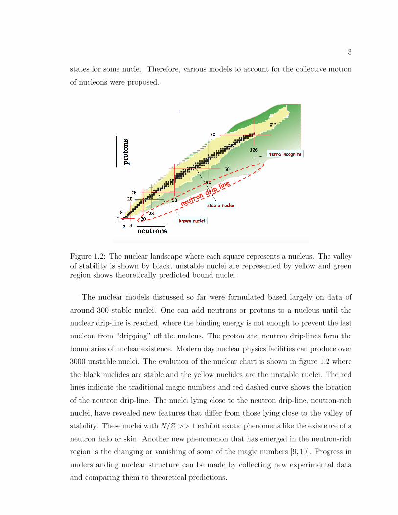
Figure 1.2: The nuclear landscape where each square represents a nucleus. The valleyof stability is shown by black, unstable nuclei are represented by yellow and greenregion shows theoretically predicted bound nuclei.

The nuclear models discussed so far were formulated based largely on data of

around 300 stable nuclei. One can add neutrons or protons to a nucleus until the

nuclear drip-line is reached, where the binding energy is not enough to prevent the last

nucleon from “dripping” o↵ the nucleus. The proton and neutron drip-lines form the

boundaries of nuclear existence. Modern day nuclear physics facilities can produce over

3000 unstable nuclei. The evolution of the nuclear chart is shown in figure 1.2 where

the black nuclides are stable and the yellow nuclides are the unstable nuclei. The red

lines indicate the traditional magic numbers and red dashed curve shows the location

of the neutron drip-line. The nuclei lying close to the neutron drip-line, neutron-rich

nuclei, have revealed new features that di↵er from those lying close to the valley of

stability. These nuclei with N/Z >> 1 exhibit exotic phenomena like the existence of a

neutron halo or skin. Another new phenomenon that has emerged in the neutron-rich

region is the changing or vanishing of some of the magic numbers [9, 10]. Progress in

understanding nuclear structure can be made by collecting new experimental data

and comparing them to theoretical predictions.

4

The charge radius of a nucleus is among the important inputs that are needed to

investigate the nuclear structure and test the newly developing theoretical models.

The evolution of charge radii along an isotopic chain can show signatures of shell

closures as local minima [11]. The proton radii together with the knowledge of the

matter radii (radii of nucleon distribution in nuclei) are also important to deduce the

neutron skin thickness in the neutron-rich nuclei. The neutron-rich oxygen isotopes are

particularly interesting nuclei, with a new magic number (N = 16) [9,10,12,13] at the

neutron drip-line [14–19]. The objective of this dissertation is to determine the proton

radii, Rp

, of 16,18-24O from the charge-changing cross section (�cc

) measurements. Rp

is

defined as the rms radius of proton density distribution inside a nucleus with protons

considered as point particles (henceforth referred to as point proton radii). The point

proton radii of neutron-rich oxygen isotopes (19-24O) have not been measured till date.

The following sections of the introduction start with a brief description of concepts

like neutron halo and skin. After that, the objective of the work is discussed, followed

by a brief discussion on conventional methods that are used to measure the charge

radii and their limitations for measuring the charge radii of neutron-rich nuclei. The

introduction concludes with a description of the charge-changing cross sections and

discussion of the Glauber Model, a theoretical tool used to extract the proton radii

from the measured �cc

.

1.1 Exotic phenomena of neutron-rich nuclei: halos and skin

1.1.1 Neutron halos

The term “nuclear halo” refers to one or two weakly bound neutrons forming an

extended low density surface around a core, which has a compact density with

similar density distributions for protons and neutrons. Nuclear halos are of quantum

mechanical origin and therefore can only be understood by considering the probability

distribution of the least bound nucleon. In a simple model, the interaction potential

between the halo neutron and the core can be assumed as a square well and the wave

function of the neutron outside the potential is written as

(r) =

✓2⇡

◆✓�er

r

◆eR

(1 + R)1/2

�(1.1)

5

where R is the width of the potential and is the slope of the density tail [20].

Using this wavefunction, the density distribution of the neutron is related to the wave

function as

⇢(r) = | (r)|2 (1.2)

and is related to the separation energy of the neutron (Es

) as,

(h̄)2 = 2µEs

(1.3)

where µ is the reduced mass of the core and the neutron. As Es

decreases, decreases

and thus the tail of the distribution becomes longer. However, in addition to a small

separation energy, a small orbital angular momentum of the state is also a necessary

condition for a nucleus to form a halo state. The higher angular momentum provides

an additional centrifugal barrier which lowers the probability of tunneling to a larger

radius, leading to less extension of the wave function. Therefore, the halos are expected

to most likely appear when the valence neutrons are in the s and p states. The presence

of the Coulomb barrier in the proton-rich nuclei makes proton halos less pronounced

than neutron halos.

1.1.2 Neutron skin

A neutron skin is formed when the half density radius of neutrons is greater than

that of the protons with the surface density slope for the neutrons being similar to

the protons. The neutron density actually extends out significantly further than that

of the protons, resulting in a mantle of neutrons as shown in figure 1.3 (a). The

neutron skin thickness (�R = Rn

- RP

) is defined as the di↵erence between the root

mean square radii of the neutron and proton distributions. Recently some studies

have focused on 208Pb, which is a stable nucleus with 126 neutrons and 82 protons.

The observed neutron skin thickness (�R = 0.15± 0.03(stat)± 0.01(sys)fm ) [21] is

relatively small. However, in the case of neutron-rich nuclei (N/Z >> 1), the observed

neutron skins are significantly thicker. For example �R = 0.9 fm was observed in8He from a cluster-type model analysis of the measured interaction cross sections,

the two-neutron removal cross sections, and the four-neutron removal cross section

of 4,6,8He [22]. Matter radii of He isotopes determined in Ref. [22] showed a drastic

6

Figure 1.3: (a) A schematic illustration of neutron skin. (b) �Rrms

as a function of�E

F

of various isotopes obtained by the RMF Model. The empirical values are shownin shadowed boxes. Right figure adapted from [22].

increase from 4He (1.57 ± 0.05 fm) to 6He (2.48 ± 0.03 fm) and 8He (2.52 ± 0.03

fm). The empirically deduced proton and neutron density distributions were well

reproduced by the Relativistic Mean Field (RMF) calculations. The RMF model

calculations were applied to other nuclei near the drip-line and are shown in figure 1.3

(b), which shows the di↵erence in proton and neutron rms radii (�R) as a function of

the di↵erence in Fermi energies of protons and neutrons (�EF

). As shown in figure

1.3 (b), all nuclei with �EF

larger than ⇠ 10 MeV have �R values larger than 0.5 fm.

Therefore, the origin of thick neutron skin in neutron-rich nuclei can be understood to

be arising from a large �EF

which is a consequence of neutrons filling higher shells or

sub-shells. As seen in figure 1.3(b), the most neutron-rich isotope of oxygen, 24O, was

predicted to have a very thick neutron skin based on these calculations. The results,

however, were model-dependent and were therefore somewhat qualitative since no

measurement for the proton distribution of 24O was performed at that time.

1.2 Motivation to study proton radii of 16-24O

Oxygen isotopes with a closed shell of protons (Z = 8) are good candidates to examine

the evolution of shells approaching the neutron drip-line and investigate the e↵ects of

nuclear forces. The most abundant stable isotope of oxygen, 16O, is a doubly magic

7

nucleus with Z = 8 and N = 8 shell closures. In exotic nuclei far away from the region

of stability, a new shell closure (N = 16) at the neutron drip-line has recently been

observed in the oxygen isotopes.

1.2.1 Drip line of oxygen isotopes and 3N forces

Oxygen isotopes are a subject of interest because the neutron drip-line of oxygen

isotopes is found to be at 24O whereas the Nucleon-Nucleon (NN ) potentials predicted

the drip-line to be at 28O (the expected doubly magic nucleus). Oxygen is the heaviest

element for which the neutron drip-line has been confirmed experimentally. The

evidence of neutron drip-line at 24O comes from following measurements. In 1985

Langevin et al. found 25O is unbound [14] and five years later it was found that 26O

is unbound as well [15]. The expected doubly magic nucleus 28O (N = 20) was found

to be unbound by Tarasov et al. indicating the disappearance of conventional shell

closure at N = 20 [16]. The first spectroscopy of 25O was done by Ho↵man et al. who

found that 25O is unbound by 770 keV with a decay width of 172(30) keV [17]. The

upper limit on the ground state energy of 26O was found by Lunderberg et al. who

found that 26O is unbound by less than 200 keV [18]. A recent experiment at the

SAMURAI facility at RIKEN precisely determined the ground state energy of 26O to

be 18 ± 3 keV above the two neutron decay threshold [19]. The energy and width of

the unbound ground state of 25O were also determined precisely in this experiment as

749 ± 10 keV and 88 ± 6 keV, respectively.

The neutron drip-line at N = 16 could not be reproduced using the NN potentials.

Fujita and Miyazawa, considering the fact that nucleons are composite particles,

extended Yukawa’s meson exchange idea to three nucleons (3N) [23]. One example

of the 3N mechanism is an exchange of two pions between three nucleons with one

nucleon virtually exciting a second nucleon to the � resonance, which is de-excited

by scattering o↵ a third nucleon. Otsuka et al. [24] suggested that the drip-line of

oxygen isotopes can be explained by including the contribution from the 3N forces

(3NFs). Otsuka et al. [24] included the 3NFs among two valence neutrons and one

nucleon in the 16O core within the sd�shell model and found that the inclusion of

3NFs lead to the drip-line at N = 16 for the oxygen isotopes in agreement with the

experiments. Three-nucleon interactions arise naturally in the chiral e↵ective field

8

theory (� EFT) [25] which is a systematic approach to derive the nuclear force from

the underlying theory of strong forces, quantum chromodynamics (QCD). At the low

energies relevant to nuclear physics, the QCD coupling constant is large. Therefore,

a perturbative expansion of nuclear processes becomes non-convergent. In � EFT,

nucleons and pions are taken as relevant degrees of freedom. The QCD Lagrangian

is expanded in powers of Q/⇤�

with a momentum Q ⇠ m⇡

and the chiral-symmetry

breakdown scale ⇤�

⇠ m⇢

, which makes Q/⇤�

a small quantity. A diagram of this

expansion of the nuclear interaction is shown in figure 1.4 where LO is the leading order

term, NLO is next-to-leading order term and so on. The hierarchy of nuclear forces,

i.e. NN interactions should be more important than three-nucleon (3N) interactions,

which in turn should be more important than four-nucleon (4N) forces, and so on,

is illustrated in figure 1.4. The high-energy physics is included in the theory via

renormalization and absorbed into coe�cients called low-energy constants. The LECs

are fitted on experimental data; usually nucleon-nucleon phase shifts, binding energies

and other few-body observables.

Figure 1.4: Chiral e↵ective field theory for nuclear forces. The di↵erent contributionsat successive orders are shown diagrammatically. Nucleons and pions are representedby solid and dashed lines, respectively. Figure adapted from [26].

The ab initio models have made tremendous progress where several calculations

have successfully reproduced the neutron drip-line at 24O [27–34]. In Refs. [27,28,31–33]

the ground state energies of oxygen isotopes were calculated with Entem and Machleidt

(EM) interaction [35] using several types of many-body approaches. In EM interaction

9

the NN interaction was taken up to N3LO whereas the three-nucleon interaction

was taken upto NNLO. The low-energy coupling constants (LEC) were derived

from nucleon-nucleon scattering and the properties of the A = 3 and A = 4 nuclei.

The binding energies for the oxygen isotopes obtained with the EM interaction are

consistent with each other and with the experimental data within 1% of the total

binding energies.

V. Lapoux et al. [34] studied the binding energies and Rp

in oxygen isotopes by

performing ab initio calculations with NNLOsat

nuclear interaction [36], which is a

simpler interaction as it includes contributions up to NNLO for both two and three-

nucleon interactions. In NNLOsat

interaction, the NN and 3N forces are optimized

simultaneously in contrast to the EM interaction [35] in which the 3NFs are optimized

subsequently. The determination of the low-energy coupling constants in NNLOsat

interaction includes data on binding energies and radii of 3H, 3,4He, 14C and 16O

isotopes, in addition to the low energy NN data. The binding energies calculated

with the NNLOsat

interaction (red symbols) and the EM interaction (black symbols)

using di↵erent many-body approaches are shown in figure. 1.5 (a). The stars represent

Self Consistent Greens Function (SCGF) calculations by Gorkov (GGF), the triangles

represent the Dyson SCGF (DGF) calculations and the plusses represent the in-medium

similarity renormalization group (IMSRG) calculations. The experimental binding

energies represented by blue symbols agree with these various ab initio approaches.

Figure 1.5: (a) The binding energies (b) Rp

from Ref. [34] using the NNLOsat

interaction (red symbols) and the EM interaction (black symbols) calculated in threedi↵erent many-body approaches. The blue stars are R

p

from Ref. [27] calculated usingcoupled-cluster calculations. The experimental R

p

derived from the e� scatteringexperiments [37] are shown by blue open circles.

10

1.2.2 Proton radii: A test for ab initio approaches

The reliability of various ab initio models depends on their description of other

fundamental observables like charge radius in addition to the binding energies. Figure

1.5(b) shows the proton radii calculated using the NNLOsat

(red symbols) and the

EM interaction (black symbols). The stars represent Dyson SCGF (DGF), the plusses

represent the in-medium similarity renormalization group (IMSRG), and the triangles

represent the Gorkov SCGF (GGF) calculations from Ref. [34]. The Rp

calculated

using the coupled-cluster calculation with EM interaction from Ref. [27] are also shown

in figure 1.5(b) (blue stars). The open circles represent the measured Rp

found using

the charge radius (Rch

) from the e� scattering experiments [37] using the equation:

hR2ch

i = hR2p

i+ hr2p

i+ N

Zhr2

n

i+ 3h̄2

4m2p

c2(1.4)

where rp

and rn

are the charge radii of a proton and a neutron and the last term is

the Darwin-Foldy relativistic correction [38]. As seen in figure 1.5 (b), there is a clear

discrepancy between radii calculated using two di↵erent interactions, the measured Rp

of 16O is closer to Rp

calculated by NNLOsat

, however, it should be considered that

the LEC in NNLOsat

includes the Rch

of 16O. There is no data on the proton radii of

the neutron-rich oxygen isotopes, which is required in order to provide constraints on

these theoretical predictions.

1.2.3 The shell evolution in oxygen isotopes

Another remarkable feature of oxygen isotopes is that there is a new shell closure (N =

16) at the neutron drip-line. The first experimental indication of the N = 16 shell clo-

sure came from a study of the neutron separation energies (Sn

), the amount of energy

needed to remove the outer-most neutron from a nucleus as a function of isospin Tz

=N�Z

Z

[9]. The measured Sn

values for nuclei with odd N and even Z as a function of the

neutron number in an isospin chain are shown in figure 1.6. The Sn

systematics as a

function of neutron number for nuclei with low isospin (Tz

< 5/2) show drops in energy

following the magic numbers N = 8 and 20, indicated by black upward arrows in figure

1.6.

11

Figure 1.6: One-neutron separation energy

for di↵erent isospin chains. Figure taken

from [39].

However, for the neutron-rich nuclei

(Tz

� 5/2) a new break appears at N

= 16 indicated by the brown downward

arrow. The systematic study of beta de-

cay Q values and the energies of the first

excited state also showed sharp discon-

tinuities and confirmed the shell closure

at N = 16 [10]. The sixteen neutrons of

the drip-line nucleus, 24O, should fill the

neutron levels (1s1/21p3/21p1/21d5/22s1/2)

as shown in figure 1.7. The spectroscopic

factor (S), which is the probability to oc-

cupy a final single-particle state when a nucleon is removed from or added to the

target nucleus was measured through the neutron removal reaction of 24O [12]. A

nearly pure 2s1/2 neutron spectroscopic factor of 1.74 ± 0.19 was determined, which

established that the last two neutrons in 24O exhibit single particle behaviour and that

the nature of the shell closure is spherical. A small quadrupole deformation parameter

Figure 1.7: The shell model scheme of 24O.

(�2 =0.15 ± 0.04) of the first 2+ excited state of 24O, determined by proton inelastic

12

scattering [13], also confirmed the spherical nature of this shell closure. The N = 16

shell gap implies an increased energy gap between the 2s1/2 and 1d3/2 orbitals (figure

1.7). A large shell gap was obtained (⇠ 4.8 MeV) in 24O from the excitation energy

of the 2+ state (figure 1.8 (a), black symbols) observed through neutron removal

reactions from 26F to 24O [40].

One proposed mechanism for the emergence of this new magic numbers in neutron-

rich oxygen isotopes is thought to be related to the monopole interaction of the nuclear

force [41, 42]. The tensor component of nuclear interaction is written as

V⌧�

= ⌧ · ⌧� · �f⌧�

(r) (1.5)

with “·00 denoting the scalar product between the isospin (⌧) and spin (�) operators.

f⌧�

(r) is a general function of the interaction distance r. In the long range limit,

f⌧�

(r) = 1 and V⌧�

produces a strong attraction between a spin- and isospin-flip pair

of orbitals i.e. between j>

(l + 1/2) and j<

(l � 1/2) and between the proton and the

neutron orbitals. It should be observed that in figure 1.8 (a) the first excited state

of neon (Z = 10, red symbols) and magnesium isotopes (Z = 12, green symbols) do

not show any increase at N = 16. This is because, for these isotopes the protons

in the 1d5/2 orbital interact strongly with the neutrons in the 1d3/2 orbital, pulling

these orbitals down. However, in oxygen isotopes the proton 1d5/2 orbit is vacant,

thus the attraction is missing which causes the neutron 1d3/2 orbital to remain high

in energy. This creates the shell gap at N = 16. It is observed in figure 1.8 (a)

that the first excited states of the carbon, neon and magnesium isotopes at N =

14 remain relatively constant in contrast to the oxygen isotopes, for which it rises

sharply. The high-lying first excited state in 22O at 3.17 MeV [43,44] suggests that N

= 14 is another possible shell gap in oxygen isotopes. The shell gap between neutron

1d5/2 and 2s1/2 orbitals of 22O was derived from the observation of an unbound 1d5/2

hole state at 2.79(13) MeV in Ref. [45]. This finding was also supported by a small

deformation factor (�) = 0.26(4) for 22O which was derived from the phenomenological

analysis of proton inelastic scattering [46]. The e↵ect of the N = 14 shell closure is

seen in the systematic trend of one-neutron knockout cross sections and widths of

the fragment longitudinal-momentum distributions with increasing neutron number,

shown in figure 1.8 (b). For the oxygen isotopic chain (represented by green symbols),

13

Figure 1.8: (a) The first excited stated of di↵erent isotopes plotted as a function of theneutron number. Figure taken from [40]. (b)The one-neutron knockout cross sectionsand widths of the fragment longitudinal-momentum distributions as a function of theneutron number. Figure taken from [47]

the valence neutrons occupy a 1d5/2 orbit up to N = 14, while for N = 15 and 16,

the valence neutrons occupy the 2s1/2 level (figure 1.7). The observed narrowing of

momentum distribution at N = 15 in figure 1.8 (b) supports the single particle s

orbital occupancy of the valence neutron in 23O. An increase in one-neutron knockout

cross sections observed at N = 15 for oxygen isotopes (shown in figure 1.8 (b) by

green symbols) indicates that the valence neutron occupies 2s1/2 orbital above the

shell gap [47]. The 2s1/2 spectroscopic factor was found to be 0.97(19) in Ref. [48]

from one-neutron knockout of 23O and 0.78(13) from the Coulomb dissociation [49]

indicating a 2s1/2 single particle structure of 23O and therefore a shell gap at N = 14.

The shell gap in oxygen isotopes could be caused by the strong attractive monopole

interaction between the proton 1p1/2 and neutron 1d5/2 which pulls these orbitals

down, thus creating the energy gap. The removal of protons from the 1p1/2 orbital

weakens the N = 14 shell closure, therefore it is less pronounced for nitrogen and

disappears altogether for carbon isotopes [50–54].

The shell gaps can also be visible as local minima in the radii along an isotopic

chain [11]. Therefore, the evolution of the proton radius of neutron-rich oxygen

isotopes with increasing neutron number will help us establish the shell closure at N

= 14 and also understand the cause of its emergence in neutron-rich nuclei.

14

1.2.4 Neutron skin in oxygen isotopes

The proton radii of neutron-rich oxygen isotopes are also important to determine the

neutron skin thickness, �R, which is the di↵erence between the root mean square

radii of the neutron and proton distributions. The root mean square matter radii,

Rm

, are related to the root mean square proton radii, Rp

, and the root mean square

neutron radii, Rn

, according to relation given below

R2m

=

✓N

A

◆R2

n

+

✓Z

A

◆R2

p

(1.6)

where Z = atomic number, A = mass number and N = neutron number.

Rn

and the neutron skin can be determined from the measured matter radii and

proton radii using equation 1.6. The calculated matter and proton radii from Ref. [34]

were used to calculate the neutron skin thickness (�R), which is shown in figure

1.9. The plusses represent the IMSRG calculations with the EM interaction (black

symbols) and the NNLOsat

interaction (red symbols). The calculated (�R) using the

calculated radii with the coupled-cluster approach from Ref. [27] are also shown in

figure 1.9 by the blue symbols. As seen in figure 1.9, a thick neutron skin is expected

in the neutron-rich oxygen isotopes. The predicted skin thickness for 24O shows a

di↵erence between the coupled-cluster and IMSRG calculations. A thick neutron skin

in 24O has also been predicted in Ref. [22]. Therefore, the measurement of Rp

of

neutron-rich oxygen isotopes is needed to determine the neutron skin experimentally.

1.3 Conventional methods to determine proton radii

The matter radii have been determined for a wide range of unstable nuclei [55, 56]

mainly by using the measured interaction cross sections. On the other hand, the data

regarding the proton radii is rather limited for the unstable nuclei. A brief description

of various techniques for measuring the proton radii is given below.

1.3.1 Electron scattering

The scattering of electrons from nuclei has given the most precise information on

nuclear and nucleon structure. Electron scattering avoids the complexity of the strong

interaction between the projectile and the target and provides precise information

15

Figure 1.9: The neutron skin calculated using the calculated Rp

and Rm

. The plussesrepresent �R calculated using radii with IMSRG many-body approach with EMinteraction (black) and NNLO

sat

interaction (red), taken from Ref. [34]. The starsrepresent �R found from the radii calculated with coupled-cluster calculations fromRef. [27].

about the charge distribution in the nucleus. Since the charge distribution of the

nuclei is the subject, only elastic electron scattering is discussed. The di↵erential

cross section for elastic scattering from a spin less nucleus under a Plane-Wave

Impulse-Approximation (PWIA) is given as,

d�

d⌦=

d�Mott

d⌦|F

c

(q)|2 (1.7)

where d�Mott

/d⌦ is the Mott cross section and Fc

(q) is the charge form factor [57].

The Mott cross section is the elastic scattering cross section from a point particle of

charge Z.d�

Mott

d⌦=

(Z↵)2 cos2(✓/2)

4e2 sin4(✓/2)(1.8)

where e is the electron energy, ✓ is the scattering angle and ↵ is the fine-structure

constant. The form factor is a Fourier transform of the charge distribution (⇢c

(r)), for

momentum transfer, q,

Fc

(q) =1

2⇡3/2

Z⇢c

(r)e�i~q.~rrd~r (1.9)

16

One can determine ⇢c

(r) of a target nucleus by an inverse Fourier transformation of

the experimentally determined charge form factor.

Electron scattering has been successfully applied to stable nuclei and the charge

distribution data is compiled in Ref. [58]. Some unstable nuclei have also been studied

by elastic electron scattering, namely 3H and 14C [59,60]. The study of unstable nuclei

with electron scattering require long half-lives to allow preparation of su�ciently thick

radioactive targets. The short-lived nuclei located far from the � stability line have

not been studied so far by electron scattering. The SCRIT (Self-Confining RI Ion

Target) electron scattering facility project has been commissioned at RIKEN RI beam

factory to conduct electron scattering of rare isotopes [61]. The principle is to trap

the target ions along the electron beam axis which reduces the required number of

target nuclei significantly. An experiment has recently been performed in order to

study the nuclear shape of the stable 132Xe [62]. This facility aims to conduct the

electron scattering of the short-lived neutron-rich nuclei in the near future.

1.3.2 Isotope shift

Isotope shift is the change in energy of atomic transition levels when we move from

one isotope to another. The change can be due to the change of mass (mass shift) and

due to change in the charge distribution inside the nucleus (volume shift or the field

shift). The di↵erence in the volume shift of two isotopes determines the di↵erence in

their charge radii. The measurement of charge radii using isotope shift measurements

in Na isotopes provided the first direct evidence of neutron skin [63]. The matter

radii were determined from the interaction cross section measurements. A gradual

growth of neutron skin thickness up to 0.4 fm was observed in neutron-rich � unstable

Na isotopes. However, in the case of light nuclei, the mass-based isotope shift is

10,000 times larger than the volume shift. Therefore, the charge radii of light nuclei,

could not be extracted from isotope shift measurements until the new accurate atomic

calculations of mass shifts together with high precision mass measurements were

made. The charge radii of He [64, 65], Li [66] and Be [67] isotopes determined by this

technique are shown in figure 1.10. The charge radius decreases from 6Li to 9Li and

then increases for 11Li. In the He isotopes, it increases significantly from 4He to 6He

and decreases from 6He to 8He. In Be isotopes, there is an increase in the charge radius

17

Figure 1.10: The radii of point nucleon distribution in (a) Li isotopes (b) He isotopes(c)Be isotopes. Figures adapted from [68].

from 10Be to 11Be. Therefore, it can be concluded that the charge radius increases

when a neutron halo is formed as 11Li, 6He, 11Be are confirmed halo nuclei from study

of the narrow momentum distribution and enhancement of interaction cross-section

measurements [68]. Such an increase may originate from the fact that in the halo

nuclei the valence neutron in the 2s1/2 orbital has extended density distribution. This

causes the center-of-mass (c.m) of the nucleus to be di↵erent from that of the core

leading to c.m motion smearing of the core density and hence a larger proton radius.

The decrease in charge radius in 8He can be explained if the four excess neutrons are

considered to be distributed in a more spherically symmetric fashion around 4He core

and the smearing of the charge in the core is correspondingly less as compared to6He. Recently, charge radii of 41,51,52Ca were measured using isotope shift [69]. The

charge radius of 52Ca is much larger than theoretical predictions and has opened new

intriguing questions on the evolution of nuclear sizes away from stability. However,

the isotope shift measurements have not been extended to other light neutron-rich

isotopes so far because the production of low energy and high intensity beams of

short-lived isotopes of these elements is di�cult. The other main challenge is that the

atomic physics calculations become arduous due to many-body correlations between

the electrons in the atoms.

1.3.3 Muonic Atom X-Ray Spectroscopy

A di↵erent approach to determine the charge distribution inside the nucleus is to

measure the X-ray transition energy of muonic atoms [70]. The muon is 207 times

more massive than the electron. When a negative muon is captured by the nucleus,

18

it can form a muonic atom. The atomic Bohr radius is inversely proportional to the

mass of the orbiting lepton. Therefore, in muonic atoms the negative muon moves

around the nucleus with an atomic Bohr radius about 200 times smaller than in the

corresponding electronic atom. An increase in the energy shift for a muonic atom over

a normal atom can be estimated to be as (mµ

/me

)3 [71]. Muonic X-ray spectroscopy

has been applied to almost all stable elements and the determined charge radii are

available in the Refs. [37, 72]. Since the experimental method requires several tens

of milligrams of target, no muonic X-ray spectroscopic investigation has yet been

performed so far for short-lived nuclei, although researchers start to consider [73] this

opportunity. The idea is to stop both µ� and nuclear beams simultaneously in a solid

deuterium film, followed by the application of the direct muon transfer reaction to

higher Z nuclei to form radioactive muonic atoms.

1.4 Charge-changing cross section measurement

Charge-changing cross section (�cc

) is the cross section for the change in the atomic

number of the projectile nucleus due to any interaction with protons in the projectile

nucleus. �cc

is related to the distribution of protons in a nucleus. It is therefore a

useful method from which the point-proton radius can be derived using the Glauber

model theory. The �cc

of stable isotopes were measured by Webber et al. [74] and

Cummings et al. [75] to interpret the interstellar production of secondary fragments

during cosmic-ray propagation in the galaxy, and so to determine elemental and

isotopic components of cosmic rays. Two years later, Blank et al. [76] measured the

�cc

of neutron-rich lithium isotopes to investigate the proton distribution of these

isotopes by comparing their results to Glauber model calculations. But no attempt to

determine the proton radii was made. Further measurements of �cc

for the light stable

and neutron-rich nuclei (14Be, 10-19B, 12-20C, 14-23N, 16-24O, and 18-27F) were done by

Chulkov et al. [77]. The �cc

values of all the stable nuclei in Ref. [77] are however

greater than those of ref. [74] and also cannot be explained using the proton radii

derived from electron scattering. Therefore, the data of Ref. [77] seems to have some

systematic uncertainty. The proton radii were not determined from the measured

�cc

in Ref. [77]. The proton radii can be extracted from measured charge-changing

cross-sections using the Glauber model framework. In the following section, the finite

19

range Glauber model theory is presented.

1.5 Finite range Glauber model

The proton radii can be extracted from the �cc

using the Glauber model formalism

[78]. The reaction cross section (�R

) for a projectile-target collision is calculated by

integrating the reaction probability with respect to the impact parameter b and is

given by

�R

=

Z[1� T (b)]db (1.10)

where T (b) is the transmission function. It is the probability that, at the impact

parameter b, the projectile will pass through the target without interacting. The

charge changing cross sections, on the other hand, involve the interaction of only the

protons of the projectile nucleus, therefore �cc

is given by

�cc

=

ZdbP

cc

(b). (1.11)

where Pcc

(b) is the probability of charge changing reaction at the impact parameter

b. Pcc

(b) is calculated using Optical Limit Approximation (OLA) [78,79]. This model

assumes that at su�ciently high energies, the nucleons carry su�cient momentum

that they undergo small angle scattering (i.e. nearly undeflected) as the nuclei pass

through each other. According to the Glauber model framework described in [80],

Pcc

(b) is given by

Pcc

(b) = 1� exp

✓� 2

X

N=p,n

ZZdsdtT

(p)P

(s)T (N)T

(t)⇥Re�pN

(b+s-t)

◆(1.12)

where, s is the two dimensional vector of the projectile’s single-particle coordinate, r ,

measured from the projectile’s c.m. coordinate, and t is defined for the target nucleus

in a similar way. T (p)P

(s) is the thickness function of the projectile’s proton density

⇢(p)P

(r),

T(p)P

(s) =

Z 1

�1dz⇢

(p)P

(r)ea; ear = (s , z) (1.13)

20

We evaluated the �cc

with the finite-range profile function �NN

(b) parametrized as [81]

�NN

(b) =1� i↵

NN

4⇡�NN

�tot

NN

exp

✓� b2

2�NN

◆(1.14)

The parameter ↵NN

is the ratio of the real to the imaginary part of the NN scattering

amplitude, �NN

is the slope parameter of the NN elastic di↵erential cross-section

which in other words is the finite range parameter and �tot

NN

is the total cross section

for NN collisions. The values of ↵NN

, �NN

and �tot

NN

are given in Ref. [81] for a wide

range of energies. Hence, the proton radii of the projectile nuclei can be determined

using these measured parameters of nucleon-nucleon cross sections and a target with

a well known density distribution.

1.5.1 Rp

determined from �cc

The proton radii determined from �cc

are denoted by Rcc

p

in what follows. Estrade

et al. [82] deduced the Rcc

p

of 10-17B using a finite-range Glauber model analysis of

�cc

. A thick neutron skin of 0.51 ± 0.11 fm was observed in 17B. A measurement

of the charge-changing cross sections at 300A MeV had been done by Yamaguchi et

al. [83]. In this case, the proton radii of 9-10Be, 14-16C and 16-18O were determined

using the zero range Glauber Model. They had to introduce a universal scaling of

�cc

to reproduce the proton radii from electron scattering measurements. However,

in Ref. [82] no scaling was required to produce proton radii consistent with electron

scattering measurements. The Rcc

p

for 12-14C [84] and 14N [85] determined using the

Glauber Model framework are consistent with point proton radii derived from electron

scattering. These demonstrate the successful use of the finite range Glauber model to

extract radii at 800-900A MeV. The measured Rp

for carbon isotopic chain are shown

in figure 1.11 (b). It is evident from the trend of proton radii determined from this

measurement that there is an evolution of thick neutron surface from ⇠0.5 fm in 15C

to ⇠1 fm in 19C. The halo radius of 19C was determined to be 6.4 ± 0.7 fm, which is

comparable to 11Li. The radii of 13-18C are also consistent with ab initio calculations

based on the chiral nucleon-nucleon and three-nucleon forces.

21

Figure 1.11: (a) The measured Rm

(circles) and measured Rcc

p

(triangles) for 12-17B(b) The measured R

m

(open circles) and measured Rcc

p

(filled circles) for12-19C. Theblue symbols represent the measured R

p

derived from e� scattering. Figure takenfrom [82,84].

1.6 This Work

We have measured the �cc

of 16,18-24O at energies of 800-900A MeV to determine the

proton radii of these isotopes. The experiment was performed at high energy radioactive

ion beam facility, GSI, in Germany. �cc

were measured using the transmission type

measurement. The details of the measurement principle, and the experimental setup

are given in chapter 2.

The analysis of the data is discussed in chapter 3, which begins with the calibration

of detectors followed by a discussion of all the physical observables required for the

determination of �cc

.

The chapter 4 describes the method employed to obtain the �cc

using the measured

physical observables. The extraction of the proton radii from the measured �cc

using

the Glauber model analysis is also discussed in this chapter. The chapter concludes

with a discussion on the observed evolution of the proton radii as a function of the

neutron number.

Chapter 2

Experiment Description

The experiment was performed at the fragment separator (FRS) [86] at GSI to measure

the charge-changing cross sections of the oxygen isotopes [87]. GSI is a high energy

radioactive ion beam facility in Darmstadt, Germany. It consists of a linear accelerator,

UNILAC, coupled to a heavy-ion synchrotron, SIS. The primary beams, 40Ar and22Ne, were accelerated in the UNILAC (2-20A MeV) and then re-accelerated in the

SIS heavy ion synchrotron up to 1A GeV. A schematic view of the GSI-FRS facility

is shown in figure 2.1. The 16-24O secondary beams were produced by fragmentation

Figure 2.1: The schematic view of the GSI-FRS facility. Figure from [88].

reaction (40Ar + 9Be) using a 6.3 g/cm2 thick Be target placed at the entrance of the

Fragment Separator (FRS). The FRS is used to separate and identify the isotope of

interest from the various nuclei produced in the fragmentation reaction. A description

of the separation technique is given in the following section.

2.1 The fragment separator

The FRS is a high-resolution magnetic spectrometer designed to e�ciently separate

projectile fragments in their mass and nuclear charge with a maximum magnetic

22

23

rigidity of 18 Tesla meters (Tm). It consists of four independent stages. Each stage is

comprised of a 30� dipole magnet and a set of quadrupoles placed before and after

the dipoles. The quadrupole magnets in front of the dipole magnets are adjustable to

illuminate the field volume of the dipole magnets to achieve a high resolving power.

The quadrupole magnets following the dipole magnets determine the focusing ion-

optical conditions. Sextuple magnets are placed directly in front of and behind each

dipole magnet to correct for the second-order aberrations. The image of the FRS is

shown in figure 2.2 which shows the magnetic dipoles (green) and the quadrupole

magnets (yellow). The motion of the ions in the magnetic field is governed by the

Figure 2.2: A photograph of FRS at GSI.

Lorentz force. The magnetic fields inside the dipoles are uniform and perpendicular

to the velocity (v) of the fragments. Therefore, the Lorentz force (F ) is given by:

F = qvB =mv2

⇢=�m0v

2

⇢(2.1)

where q is the ionic charge state of the fragment, B is the magnetic field in the

dipole, ⇢ is the radius of the trajectory, m0 is its rest mass, and � =p(1� �2)�1

is the relativistic factor with � = v/c (c is the speed of light). Equation 2.1 can be

rearranged as:m0

q⇡ A

Z=

B⇢

u��c(2.2)

24

where u is the atomic mass unit and charge, q, is equal to Z as we worked with fully

stripped nuclei. The product B⇢ is the magnetic rigidity (�) of a beam, a parameter

defined as following

� = B⇢ =p

q(2.3)

where p is the magnitude of the particle momentum. The ratio of p to q describes the

‘sti↵ness’ of a beam, which can be considered as a measure of how much resistance to

curvature or bending occurs when a particle travels through a given magnetic field.

For a specific magnetic field, the greater the momentum of a particle, the less its path

will be bent as it travels through that field. The greater the charge of a particle, the

more its path will be bent as it travels through a given magnetic field.

The projectile-like fragments that enter the FRS are separated according to their

magnetic rigidities and therefore according to their A/Z ratio. Fragments having

higher velocities (larger A/Z ratio) follow the trajectory with a larger radius than the

fragments having lower velocities according to equation 2.1. The FRS was operated in

the dispersion matched mode where the dispersion of the first stage is matched with

the dispersion of the second stage. The first stage � is set for a particular A/Z and the

second stage � is set to converge the transmitted isotopes back to the same horizontal

position. The combination of both stages becomes an achromatic system. It is useful

to operate the FRS in this mode because rare isotopes have the small production cross

sections, therefore the FRS must be able to capture a large fraction of the angular

and energy range of the selected fragment. The schematics of basic principle of the

FRS in dispersion matched mode is shown in figure 2.3. As the primary beam reacts

with the target, the projectile fragments originate from a small beam spot at the

target. The blue lines show the momentum spread of the fragments in figure 2.3 (top).

The momentum spread of the fragment is dispersed in position at the dispersive focal

plane (F2), which converges back to same horizontal position at achromatic focus

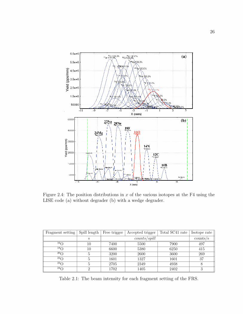
(F4). Figure 2.4 shows the horizontal x position at F4 calculated using LISE code [89]

for FRS centered for 16O. In figure 2.4 (a) all fragments with same A/Z converge at

nearly the same x position.

Such an ion-optical arrangement cannot separate di↵erent isotopes with the same

A/Z ratio. A degrader is used to separate particles with the same A/Z ratio according

to their Z values. The energy loss of the particles is roughly proportional to Z2/v2,

25

Figure 2.3: The schematic view of ion optics of the FRS.

therefore the isotopes with di↵erent Z will have di↵erent velocities after passing

through the degrader as shown in figure 2.3 (bottom). Figure 2.4 (b) shows the x

position at F4 with a wedge degrader added to the LISE calculation [89] where the

same A/Z fragments are clearly separated in position. The wedge shaped degrader

was used so that the fragments at a higher velocity pass through more degrading

material and the lower velocity fragments pass through less material. In this way, the

achromatic condition for the selected isotopes is preserved. The slits at four planes of

the FRS are used to further cut down on the remaining contaminants. The optimum

wedge thickness and slit conditions were found for each isotope using the LISE code

to get a maximum yield of the desired isotope. The beam intensities for each setting

of the FRS is given in the Table 2.1.

26

Figure 2.4: The position distributions in x of the various isotopes at the F4 using theLISE code (a) without degrader (b) with a wedge degrader.

Fragment setting Spill length Free trigger Accepted trigger Total SC41 rate Isotope rate

s counts/spill counts/s16O 10 7400 5500 7900 49718O 10 6600 5380 6250 41520O 5 3200 2600 3600 26922O 5 1601 1327 1601 3723O 5 2705 2349 4938 824O 2 1702 1405 2402 3

Table 2.1: The beam intensity for each fragment setting of the FRS.

27

2.2 Principle of measuring charge-changing cross section

As discussed previously, �cc

is the cross-section for reactions that decrease the atomic

number of the projectile nucleus. �cc

were measured by using the transmission method.

In this method, the number of incident nuclei, identified in mass and charge, are

counted event-by-event. After the reaction target, we count the number of nuclei

whose Z numbers are unchanged, i.e. the number of nuclei transmitted without the

charge-changing interactions.

As a beam of particles passes through matter, its intensity will be attenuated. The

number of collisions per unit time per unit area is then proportional to the number

of incident particles N0 and the number of target particles. Then by definition, the

constant of proportionality is the reaction cross-section �R

. The reaction cross section

�R

is defined by [90]

N = N0e��Rt (2.4)

where N is the number of particles of the unreacted beam, t is the number of target

nuclei per cm2. The charge-changing cross section �cc

is defined analogously:

N0 �Nz

= N0e��cct (2.5)

Here, NZ denotes the number of particles per unit time that undergo a charge-changing

reaction. N0 �NZ consequently corresponds to the number of particles that emerge

with unchanged charge which can be denoted as N sameZ. Thus, equation 2.5 can be

written as

NsameZ

= N0e��cct (2.6)

Counting the number of incoming projectiles N0 and emerging N sameZ particles, the

total charge-changing cross section can be obtained by rearranging equation 2.6:

�cc

=1

tln

N0

Nsamez

(2.7)

However, nuclear reactions may also occur in the non-target materials in the beamline

and this e↵ect is accounted for by taking measurements without the target in the

28

setup, therefore the �cc

can be written as

�cc

=1

tlnR

out

Rin

(2.8)

where Rin

= Nsamez

/N0 is the transmission ratio with the reaction target and Rout

denotes the transmission ratio without the reaction target. The main advantage of

the method is the event-by-event counting of the selected incident beam. Therefore,

no uncertainty exists in N0.

2.3 The detector setup

In order to count the incident nuclei before the reaction target, we needed to identify

them. The nuclei of interest were identified using their magnetic rigidity, time of

flight (F2 to F4) and energy loss. Details about how the particles were identified

are given in section 3.3. The magnetic rigidity determination requires horizontal x

position measurement at F2 and F4 for which the Time Projection Chambers (TPC)

were used. The time of flight was measured using the plastic scintillator detectors

at F2 and F4 and the energy loss was measured with a Multi-Sampling Ionization

Chamber (MUSIC) placed at F4. The measurements performed with these detectors

are summarized in figure 2.5 (b). �cc

were measured with a 4.010 g/cm2 thick carbon

reaction target placed between the MUSIC detectors at F4. The detector setup and

the carbon reaction target are shown in figure 2.5 (a). The detailed schematics of the

detector setup at F2 and F4 along with detector distances is shown in figure 2.6, in

which the detectors are labeled by the scripted names that will be used throughout

the following chapters. The SC21 denotes the first scintillator detector at F2, SC41

denotes the first scintillator at F4 and SC42 denotes the second scintillator at F4.

The MUSIC41 denotes the MUSIC before the target and MUSIC42 represents the

MUSIC after the target. The TPC1, TPC2 and TPC3 are the three TPC’s placed at

F2. TPC4 and TPC5 were placed before the reaction target at F4 and TPC6 was

placed after the reaction target at F4. The TPC and the plastic scintillator detectors

placed after the reaction target provided additional information regarding Z of the

particles. The correlation of energy loss in these detectors with the energy loss of

MUSIC42 was used to determine the detection e�ciency of MUSIC42. The detector

29

Figure 2.5: (a) A schematic view of the experimental setup at the FRS with thedetector arrangement at the final focus F4. Fig. taken from [82].(b)A flowchart ofmeasurements performed with the di↵erent detectors.

distances were measured from last quadruple at F4 and from the first quadruple at

the end of F2. In the following sections, the characteristics of the detectors used in

this experiment are described.

Figure 2.6: The detector setup at F2 and F4 with detector distances.

2.3.1 Multiple-sample ionization chambers

The charge of the particles were measured using MUSICs [91] placed before (MUSIC41)

and after (MUSIC42) the carbon reaction target at F4. The MUSIC detector is an

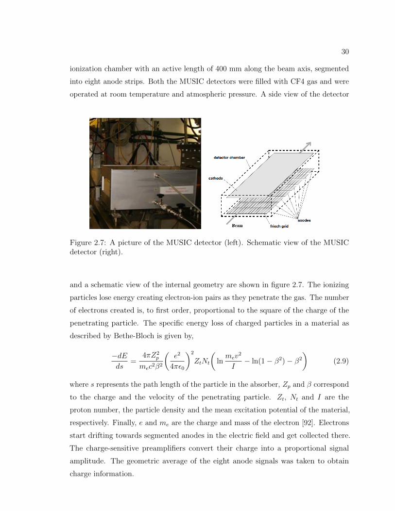
30

ionization chamber with an active length of 400 mm along the beam axis, segmented

into eight anode strips. Both the MUSIC detectors were filled with CF4 gas and were

operated at room temperature and atmospheric pressure. A side view of the detector

Figure 2.7: A picture of the MUSIC detector (left). Schematic view of the MUSICdetector (right).

and a schematic view of the internal geometry are shown in figure 2.7. The ionizing

particles lose energy creating electron-ion pairs as they penetrate the gas. The number

of electrons created is, to first order, proportional to the square of the charge of the

penetrating particle. The specific energy loss of charged particles in a material as

described by Bethe-Bloch is given by,

�dE

ds=

4⇡Z2p

me

c2�2

✓e2

4⇡✏0

◆2

Zt

Nt

✓ln

me

v2

I� ln(1� �2)� �2

◆(2.9)

where s represents the path length of the particle in the absorber, Zp

and � correspond

to the charge and the velocity of the penetrating particle. Zt

, Nt

and I are the

proton number, the particle density and the mean excitation potential of the material,

respectively. Finally, e and me

are the charge and mass of the electron [92]. Electrons

start drifting towards segmented anodes in the electric field and get collected there.

The charge-sensitive preamplifiers convert their charge into a proportional signal

amplitude. The geometric average of the eight anode signals was taken to obtain

charge information.

31

2.3.2 Time projection chambers

The particle positions in the horizontal (x) and vertical (y) directions were measured

using TPC [93]. Six TPCs were placed along the FRS: three were placed at the

dispersive focus (F2) and three at the achromatic focus (F4). These detectors have a

good spatial resolution with best achieved internal resolution of �x

⇡ 88 µm and �y

⇡38 µm for 40Ar beam. The TPC detector has a smaller volume of matter in the path

of the beam. This is useful because they are placed at F2 and every layer of matter at

F2 degrades the resolution of the spectrometer. The schematic layout and a picture

of the detector are shown in figure 2.8. The red grid shown in front of the detector

in figure 2.8 (right) is made of scintillator strips used for the position calibration of

the detector. Each TPC is a gas detector that is comprised of two di↵erent parts -

Figure 2.8: A picture of the detector on the left. A schematic view of a Time-ProjectionChamber (TPC) (right). Figure adapted from [94].

a drift space and a proportional area. The drift space is formed by a high-voltage

cathode and field-forming mylar strips. The mylar strips are connected to a high

resistance divider. A voltage of up to 400 V/cm is applied to the divider to form a

uniform electric field inside the drift volume. The drift volume is filled with Ar +

10% CH4 (P10) gas mixtures at atmospheric pressure and room temperature. The

proportional part is placed under the drift space and is separated by a shielding grid.

It consists of four anode wires (20 mm in diameter) placed inside C-pad cathodes as

shown in figure 2.8 (right). Each C-pad is connected to an integrated passive delay

line chip. As an ionizing particle passes through the detector, it creates a shower

of electrons along its track that drift towards the anode wires. A common start is

provided by the FRS trigger, which was the time signal from SC41 for this experiment.

32

The electrons drift towards the anode, creating the stop signals in the anodes. Each

Figure 2.9: The control sum distribution using the delay line 1 and anode 1 for TPC6.

TPC measures four anode times ta1, ta2, ta3, ta4. The electron drift times are used to

measure the y-coordinate of the ionizing particle. The induced signals in the delay

line travel to the left and the right and give the stop signals of the delay lines. The

x-coordinate of the ionizing particle is determined by using the time di↵erence between

the induced signal from the left and the right side of each delay line. Two independent

x measurements are produced by two independent delay lines times tdl

(left) and

tdr

(right). The detailed description of how position information is obtained from time

signals in TPC is discussed in section 3.1.3 in the next chapter. The time signals are

also used to discard noisy signals as the total delay line length is a constant (C). The

control sum which is given by equation 3.7

tcsi

= tdl

+ tdr

� 2tai

= C (2.10)

should therefore be equal to the total delay line length. tcsi

can be computed for each

of the four anode times tai

(i = 1, 4) separately. The control sum distribution using

the delay line 1 and anode 1 for TPC6 is shown in figure 2.9. The RMS of the control

sum distribution is �cs

⇡ 7 ns. This width is mainly due to the two-dimensional (total)

33

resolution of the TPC. The events which fulfil the control sum within 3�cs

were used.

The particle position was accepted if at least one of the four control sums was within

3�cs

.

2.3.3 Plastic scintillators

The time-of-flight measurement (TOF) was performed using the plastic scintillator

detectors [95]. A scintillator detector absorbs the energy of an incoming particle and

re-emits the absorbed energy in the form of light. A light sensor collects the light and

converts it into electric pulses that can give us information about the time and energy

deposited of ionizing particles. Three plastic scintillators were used for the experiment:

one was placed at F2 (SC21) and other two were placed at F4, one before (SC41) and

another after (SC42) the reaction target. The organic scintillator BC420 was used,

which provides a high light output (67% Anthracene) and a fast rise time (0.5 ns).

The readout was obtained with two Photo-Multiplier Tubes (PMTs) each attached

on the left and the right side of each plastic scintillator. The anode signals of the

PMTs were fed into the constant-fraction discriminators (CFD). The digital outputs

of these units served to start and stop the time-to-analog converters (TAC). An analog

signal corresponding to the time di↵erence between the two signals is generated which

is digitized by the amplitude-to-digital converter (ADC) and processed by the data

acquisition. In order to limit the data just to events where the scintillator signal from

both the detectors at F2 and F4 are present, the SC41 signal was used as the start

signal while SC21 was delayed and used as the stop signal in the TAC. The details

of TOF measurement and TAC calibration are given in chapter 3. The attenuated

analog signals of the photomultipliers, available as outputs from the CFD, were used

to measure the energy loss of the particles in the plastic scintillator.

2.3.4 Veto scintillator

A scintillator was placed right in front of the carbon reaction target, which acted as

an active veto detector to remove the unwanted events from the o↵-line analysis. The

veto scintillator has a central aperture slightly smaller than the reaction target area.

An image of veto scintillator is shown in figure 2.10 where the area marked on white

paper shows the location and area of the aperture. The readout was obtained from

34

Figure 2.10: A photograph of the veto plastic scintillator.

PMTs attached to the left and right side. The beam passed through the aperture and

Figure 2.11: The energy loss in left PMT of the veto detector.

reacted with the target. The signals detected in either PMT correspond to the events

incident near the edge of the reaction target and should be rejected. The signals

might also come from particles scattered by nuclear reactions in matter upstream.

The energy loss signal from left PMT of the veto detector for the 16O is shown in

figure 2.11. The events on the right-hand side of the red line represent events above

the pedestal. The signals detected above the pedestal in either PMT were rejected

from the selection of incident beam events for each isotope.

Chapter 3

Data Analysis

The raw data collected from the detectors is stored in the form of digital signals in

ADC (Analog to Digital converters), TAC (Time to Analog converters) or TDC (Time

to Digital converters) etc. In order to get physical observables of interest, one needs

to find the conversion constants between the ADC channel numbers and the energy

deposited in a particular detector, i.e. to perform detector calibrations. In the first few

sections of this chapter, the calibration procedures of all of the detectors are discussed.

The determination of �cc

requires the identification of particles before and after the

reaction target. All of the physical observables required for particle identification are

discussed in detail in this chapter. In the last section of the chapter, the phase space

restriction of the incident beam on the target is discussed.

3.1 Detector calibration

At first, the calibration of the MUSIC detectors is discussed, followed by the time of

flight and TPC calibration.

3.1.1 Calibration of the MUSIC detectors

The MUSIC detectors were used for Z-identification of the particles passing through

them. The calibration of the MUSIC detectors was done to associate the energy loss in

channels with Z of the particles using a 12C secondary beam (A/Z = 2). As discussed

earlier, the energy lost by the incident particle in the MUSIC is proportional to the

square of its charge. Therefore, the channel number (ch.no.) is related to Z2 according

to the following equation

Z2 = g(ch.no.) + o (3.1)

where g is the factor that converts channel into energy and o is the o↵set. The 8Be

nucleus is unbound, therefore the missing peak in energy loss spectrum when the FRS

35

36

Figure 3.1: (a) The uncalibrated MUSIC41 spectrum for the 12C secondary beam.Each peak is fitted with a Gaussian function (red curve). (b) A linear fit of Z2 versusthe mean channel number of the peaks. (c) The calibrated Z spectrum of the MUSIC41detector.

is set for A/Z = 2, should correspond to Z = 4. This was used as a reference to

identify the Z number associated with the energy loss peaks of the di↵erent particles.

As we see in figure 3.1 (a) the four peaks after the missing peak should correspond

to B, C, N and O. In order to get the mean, each peak was fitted with a Gaussian

function shown by the red curve in figure 3.1 (a). The linear fit of Z2 vs the mean

channel number is shown in figure 3.1 (b). The calibrated Z spectrum of MUSIC41

using the slope and intercept from the linear fit is shown in figure 3.1 (c). The Z

resolution of this detector was �Z = 0.11 (in �) for oxygen. Similarly, MUSIC42

detector was calibrated and the calibration is shown in figure 3.2. The Z resolution of

MUSIC 42 was also found to be �Z = 0.11 (in �) for oxygen.

3.1.2 Time of flight calibration

As mentioned in the previous chapter, the time of flight (TOF) of the fragments

was determined with PMTs attached on the left and the right side of the scintillator

37

Figure 3.2: (a) The uncalibrated MUSIC42 spectrum for the 12C setting. Each peakis fitted with a Gaussian function (red curve). (b) A linear fit of Z2 versus the meanchannel number of the peaks. (c) The calibrated Z spectrum of the MUSIC42 detector.

detectors. The TOFRR

i.e. the TOF from the right PMT of SC41 to the right PMT

of SC21 was obtained considering the quantity

TOFRR

= |T41R � T21R| (3.2)

where T41R is the signal detected in the right PMT of SC41 and T21R is the signal

detected in the right PMT of SC21. Similarly, TOFLL

was obtained using

TOFLL

= |T41L � T21L| (3.3)

where T41L is the signal detected in the left PMT of SC41 and T21L is the signal

detected in the left PMT of SC21. The digitized PMT signal T41R gave the start

signal, while T21R gave the stop signal in the TAC. The TOF information from the

TAC is in the form of channels. The TOFRR

in channels is denoted by RC

and TOFLL

in channels is denoted by LC

in what follows. An independent measurement with a

ORTEC Model 462 time calibrator unit was performed to calibrate the channels of

38

Figure 3.3: The TAC spectrum for 10 ns pulses from the TAC calibrator (a) TOFRR

in channels (RC

) (b) TOFLL

in channels (LC

).

TAC into nanoseconds. The time calibrator unit has switches to select the interval

steps between start and stop signals and also switches to set the calibration time scale.

Figure 3.3 (a) and (b) show the TAC spectrum for pulses of 10 ns duration from TAC

calibrator unit for RC

and LC

, respectively. The correlation plot of RC

versus TOFRR

in nanoseconds (Rns

) is shown in figure 3.4 (a). The calibration factors are obtained

by a linear fit and are listed in table 3.1. The calibrated TOF is determined using

the following equation:

Rns

= GR

RC

+OR

(3.4)

39

Figure 3.4: (a) The linear fit of Rns

(TOFRR

in ns) versus mean RC

(TOFRR

inchannels). (b) The linear fit of L

ns

(TOFLL

in ns) versus mean LC

(TOFLL

inchannel).

where GR

represents the gain and OR

represents the o↵set of RC

. A similar, plot for

LC

calibration into Lns

(TOFLL

in ns) is shown in figure 3.4 (b). The time di↵erence

in the left and right PMTs of the same scintillator was also calibrated using the

procedure mentioned above and the calibration parameters for this time di↵erence of

all three scintillator detectors are given in table 3.1. The average of Rns

and Lns

was

used as the final TOF in order to correct for the position of particle interaction in

the scintillator.

TOF =R

ns

+ Lns

2(3.5)

40

SC Dt Gain (ns/ch.no.) o↵set (ns)

TOFLL

0.0084 -10.662TOF

RR

0.0089 -10.810SC21

L�R

0.0054 -10.440SC41

L�R

0.0056 -5.565SC42

L�R

0.0055 -10.360

Table 3.1: The parameters for TAC calibration for the Scintillator detectors.

To deduce an absolute value of the TOF, an absolute TOF o↵set (O) must be sub-

tracted from the measured TOF . The TOF o↵set is determined by the measurement

of the TOF of the primary beam with exactly known energy. The TOF of three

Figure 3.5: Linear fit of TOF ⇥ � versus �. The slope of the linear fit is the TOFo↵set (O) and intercept (S) is the flight path.

di↵erent velocities (�) of the 22Ne primary beam was measured and the value of O

was determined according to this equation:

S

�= TOF �O (3.6)

where S is the flight path of the particles. If the above equation is rearranged as

� ⇥ TOF = O� � S (3.7)

41

then the linear fit of the product � ⇥ TOF versus � can be used to determine O and

S as shown in figure 3.5. The slope of the linear fit is the O and intercept is S.

3.1.3 TPC calibration

In our experiment, we used an active scintillator grid to calibrate the TPC detectors.

Figure 3.6: The scheme of scintillator plas-

tic fibers used for the calibration of TPCs.

The active scintillator grid consisted of

thin scintillator fibers of 1 mm thickness,

three vertical scintillator fibers placed at

intervals of 12 mm between them, and

three horizontal scintillator fibers placed

with interfiber spacings of 6 mm. The

scintillator grid was inserted in the path

of the beam in front of the TPC only for

the calibration that was done before the

experiment and was retracted from the

beam axis during the experiment. The

schematics of the scintillator grid is shown

in figure 3.6. The scintillator grid was placed in front of each TPC. As discussed in

chapter 2, the y- coordinate is determined by the electron’s drift time measured by

the anodes, while the x-coordinate is determined by using the di↵erence between the

induced signal in the left and the right side of delay lines. Figure 3.7 (a) shows the

di↵erence between left and right signals of delay line 1 (dl1) of TPC6 with no condition

from the grid. The same spectrum with scintillator grid coincidence is shown in figure

3.7 (b). The peaks were fitted with a three-Gaussian function which is represented

by the red curve. The scintillator grid has x-positions at -12 mm, 0 mm and 12 mm

and y-positions at -6 mm, 0 mm and 6 mm. The mean of each peak in figure 3.7

(b) is correlated to the corresponding x-positions of the grid. The linear fit of the

correlation plot for the delay line 1 is shown in figure 3.7(c). A similar procedure was

followed for each delay line and each anode for all of the six TPCs. Once we have the

linear fit parameters, the x and y coordinates in mm are obtained using the following

equations:

x =

�dl1m1 + c1

�+�dl2m2 + c2

�

2(3.8)

42

Figure 3.7: (a) The TPC delay line 1 spectrum with no condition. (b) The delay linespectrum with the scintillator grid coincidence with peaks fitted with a three-Gaussianfunction (red curve). (c) The linear fit of the mean of the peaks in channels vs.corresponding position in mm.

y =

�dt1a1 + o1

�+�dt2a2 + o2

�+�dt3a3 + o3

�+�dt4a4 + o4

�

4(3.9)

where dl1 and dl2 are the di↵erence between left and right signal of two delay lines of

a TPC and dt1�4 are the time signals of the four anodes of a TPC. The m1,2 and c1,2

represent the linear fit parameters corresponding to the gain and o↵set of each delay

line whereas a1�4 and o1�4 represent linear fit parameters corresponding to gain and

o↵set of each anode. In figure 3.8 the calibrated x (mm) vs. y (mm) plot for TPC6 is

demonstrated where the structure of the grid is visible. It can be observed that after

the calibration all of the particles are nicely aligned to their expected positions. The

calibration parameters for delay lines and anodes of all of the TPC detectors are given

in table 3.2.

43

gain (mm/ch.no.) o↵set (mm)TPC m1 m2 a1 a2 a3 a4 c1 c2 o1 o2 o3 o41 0.070 0.069 -0.036 -0.037 -0.036 -0.036 -0.776 2.735 33.590 33.220 32.720 32.5102 0.067 0.069 -0.042 -0.042 0.041 0.042 0.640 2.419 34.780 34.870 -42.140 -42.3803 0.069 0.068 -0.036 -0.035 -0.035 -0.036 1.054 5.106 43.580 43.140 42.900 42.9704 0.071 0.073 -0.040 -0.040 -0.040 -0.040 1.981 -1.316 32.470 32.370 30.850 30.8405 0.068 0.068 -0.034 -0.034 -0.033 -0.034 -0.063 0.245 27.020 26.810 26.010 26.0706 0.078 0.077 -0.039 -0.039 -0.039 -0.039 -1.562 -1.040 30.530 30.590 31.170 31.470

Table 3.2: The position calibration parameters for anodes and delay lines of TPC1�6.

Figure 3.8: The calibrated correlation plot of x (mm) vs. y (mm) of TPC 6 showingthe structure of scintillator grid.

3.2 Particle identification

The identification of the incident particles is one of the critical parts of the data

analysis. To identify a particular nucleus, its charge and mass number must be known.

The Z of the nuclei was determined from energy loss measured with the MUSICs. The

mass number information is contained in the mass-to-charge ratio which is related to

the motion of the ions in the magnetic dipole fields of the FRS according to equation

2.2. The value of � was determined event-by-event to identify the nuclei. The magnetic

rigidity associated with the trajectories of each of the nuclei for the second stage of

FRS, �F2, is given by

�F2 = �

central

✓1� M

B

xf2 � x

f4

DB

◆. (3.10)

44

where �central

is the magnetic rigidity of the central trajectory, MB

and DB

represent

the magnification and the dispersion of the second stage of FRS. The variables xf2 and

xf4 are the horizontal position coordinates of the nuclei at F2 and F4 focal planes. We

required only the magnetic rigidity of the second stage of the FRS because the reaction

target was placed at F4 and therefore the particle identification was required at F4

only. The location of focal planes was determined by beam tracking using the TPC

detectors and is discussed in the following section. The magnetic rigidity of the central

trajectory �centeral

was determined from the magnetic fields of the dipoles measured

by the Hall probes. The e↵ective radius of the central trajectory was calculated using

the centered primary beam with a well-known energy. The dispersion (D) corresponds

to the change of the horizontal position of the fragment if the magnetic rigidity of the

fragment di↵ers by 1%. It is written as the following.

D =dx

d(B⇢)/(B⇢)(3.11)

The value of dispersion DA

(DB

) in the first (second) stage was determined experi-

mentally with the primary beam. The magnetic field in the first (second) stage of the

FRS was changed in small steps, and the corresponding change in x2 (x4) positions of

the beam was measured. DA

and DB

were found to be -6.47 cm/% and 7.71 cm/%

resp. The magnification (MB

) is the ratio of DB

to DA

, which equals 1.19 in our case.

3.2.1 Location of focal planes

The position information from the TPC detectors was used to obtain the horizontal x

position of each particle at the F2 and F4 focal planes. The angles were evaluated

using the x position from the TPCs and the detector location (z). The angles and

coordinates of foci were found in the following way. The position coordinates of six

TPC detectors can be considered as (xi

, zi

) where index i represents the TPC number,

which runs from 1 to 6. The detector distances are shown in figure 2.6. The equation

of a straight line in xz plane at TPC4 (x4, z4) can be written as

x4 = m4z4 + c (3.12)

45

The slope of the beam at F4, using the measured positions, x4 and x5 of TPC4 and

TPC5, respectively, is given by

m4 =x5 � x4

z5 � z4(3.13)

and the intercept can be solved as

c = x4 �m4z4 (3.14)

If we consider the coordinates of focal plane at F4 as xf4 and z

f4 then the straight

Figure 3.9: The correlation between the angle x (mrad) and the x position (mm) at(a) One meter before the focal plane (b) One meter after the focal plane (c) At thefocal plane at F4 region.

line equation at these coordinates can be written as

xf4 = m4zf4 + c (3.15)

46

Using m4 and c from eq. 3.13 and eq. 3.14, in eq. 3.15, we get xf4 as

xf4 = m4(zf4 � z4) + x4 (3.16)

In a system with point-to-point imaging, the horizontal position should not depend

on the angle. To investigate this, the correlation spectrum of the angle at F4 (a4)

versus xf4 of the particle of interest at di↵erent z

f4 locations was observed. If the

condition (x|a) = 0 is fulfilled, the correlation plot should reflect the position xf4

being independent of angle a4. Consequently, the x-distribution should be narrowest

at this z position. Figure 3.9 shows this correlation spectrum for three di↵erent zf4,

(a) one meter before the focal plane (b) one meter after the focal plane and (c) at

the focal plane for 16O. It can be observed in figure 3.9 (c) that the x distribution is

independent of angle.

Figure 3.10: (a) The identification plot for the 23O setting. The black circle shows anexample of background events.

Therefore, with all of the necessary physical quantities, the A/Z ratio could be

determined using Eq. 2.2. The identification of the particles was achieved by using

the correlation plot of Z versus A/Z. Figure 3.10 shows the PID plot for the 23O

secondary beam. Some background events are clearly visible. One example is shown by

the black circle; these events with Z = 5 and A/Z = 2.68 would result in a non-integer

mass number. Therefore, we need to identify and reject such background events from

47

the PID. There are several reasons which can be accounted for the appearance of

these events for example the reactions happening in the scintillator material placed

before the target, or multiple scattering events. The first rejection was done using the

veto detector. The correlation of the energy loss signal of the left PMT of the veto

detector (V etoL

) vs the energy loss signal of the right PMT (V etoR

) for 23O is shown

in figure 3.11. The signals detected above the pedestal in energy loss signal of either

PMTs were rejected. The PID spectrum after the veto rejection is shown in figure 3.12.

Figure 3.11: The correlation of V etoL

vs. V etoR

for the 23O secondary beam.

After the rejection using the veto detector, the remaining background events were

rejected by investigating di↵erent correlations of energy and the time signals among

di↵erent detectors. The energy loss signal of one detector should be linearly correlated

to energy loss signal of the other detector for the real events. Figure 3.13 shows the

energy loss signal in the MUSIC41 detector vs energy loss signal in the TPC4 detector.

The black contour represents the selection region of good events. Similar rejections

were done using the energy loss signals from the TPC5 and MUSIC41 detectors as well

as the SC41 and MUSIC41 detectors as shown in figure 3.14 (a) and (b), respectively.

In addition to the energy loss signal, TOFLL

and TOFRR

should also be linearly

correlated as both represent TOF from SC21 to SC41. The figure 3.14 (c) shows

TOFLL

vs TOFRR

with all of the previous selection conditions applied. The particles

seen outside our selection cut (black contour) might originate from artifacts of signal

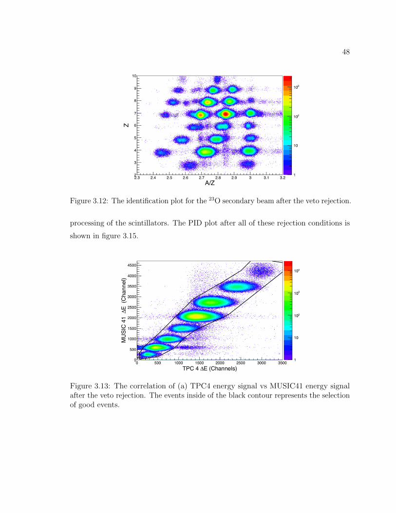
48

Figure 3.12: The identification plot for the 23O secondary beam after the veto rejection.

processing of the scintillators. The PID plot after all of these rejection conditions is

shown in figure 3.15.

Figure 3.13: The correlation of (a) TPC4 energy signal vs MUSIC41 energy signalafter the veto rejection. The events inside of the black contour represents the selectionof good events.

49

Figure 3.14: The correlation of (a) MUSIC41 energy signal vs. TPC5 energy signal (b)MUSIC 41 energy signal vs. SC41 energy signal (c) TOF

LL

vs. TOFRR

. The eventsinside black contour represents the selection of good events. The spectra show eventsafter veto rejection.

3.3 Incident beam selection

As discussed in the previous chapter, the �cc

is given by

�cc

=1

tlnR

out

Rin

(3.17)

where Rin

= Nsamez

/N0 is the transmission ratio with the target and Rout denotes the

transmission ratio without the target. The black contour region in figure 3.15 shows

the 23O selection before the target for determining the incident beam counts N0.

This selection should be such that the contamination from neighbouring Z isotopes

should be less than 10�4. Figure 3.16 shows the projection of the y-axis of the PID

plot, i.e. the Z spectrum of the incident beam. The blue histogram is obtained with

the 23O selection condition and the red histogram is the total Z spectrum normalized

to the 23O counts. The estimated contamination from Z = 7 is 6⇥ 10�5 and that from

50

Figure 3.15: The identification plot for the 23O before the reaction target. The blackcontour represents the 23O incident beam selection.

Figure 3.16: The MUSIC41 Z spectrum where the blue histogram represents the 23Oselection and the red histogram is the total Z spectrum normalized for 23O.

Z = 9 is 2⇥ 10�5 for this secondary beam. The procedure of background reduction

and the selection of the incident beam events as described above was followed for each

FRS setting for the di↵erent oxygen isotopes.

3.4 Z identification after the target

To determine �cc

we need to count the number of particles that have unchanged charge

after the reaction (NsameZ

). The energy loss spectrum of MUSIC42 (MUSIC after the

target) with the incident beam selected is shown in figure 3.17 using the example of

the 23O beam. The red histogram represents the Z spectrum with the reaction target

51

whereas the blue histogram represents the Z spectrum without the reaction target.

In these spectra the production of Z = 9 events after the target originate from the

charge exchange or proton transfer reactions where one proton is added to the incident

nucleus, 23O in this case. These reaction processes do not involve the reactions with

Figure 3.17: The MUISC42 Z spectrum with the target (red) and without the target(blue) to identify the particles with unchanged Z after the reaction.

the protons in the incident oxygen isotope. Therefore, such reaction events should be

subtracted in order to measure the charge-changing cross sections for determining the

proton radii and hence we took the total number of counts under Z = 8 and Z = 9

peaks in our NsameZ

selection. As 16-18O isotopes are not in the vicinity of any proton

unbound isotopes (the one-proton separation energy of 15O is 7.3 MeV and for 17O

is 13.8 MeV) therefore, the e↵ect of proton evaporation from neutron removal cross

sections to states above the proton threshold is negligibly small. This e↵ect is neglibly

small in 19-24OO isotopes because the proton separation energies rapidly increase as

move to the neutron-rich nuclei. At beam energies of ⇠ 900A MeV, nuclear inelastic

excitation cross section to states above the proton emission threshold is also negligibly

small for the isotopes of interest. The NsameZ

selection is marked by black vertical

lines in figure 3.17 which covers ± 3.5� regions of both the Z = 8 and Z = 9 peaks.

52

3.5 The target position dependence of transmission ratios

To eliminate losses of NsameZ

events after the target due to the large angle scattering

of particles out of the detector acceptance, we need to restrict the phase space of the

incident beam events at the target. The TPC detectors at F4 were used for beam

tracking to determine the beam angle and horizontal (x) and vertical (y) coordinates

of the beam event-by-event at the target location. The x position at the target for the

Figure 3.18: (a) The beam x position at the target (Xtarget) (b) Transmission ratiofor di↵erent Xtarget positions where green vertical lines represent the selection regionof constant R.

23O beam is shown in figure 3.18 (a) where the red histogram represents the data taken

during the measurement with the reaction target and the blue histogram represents

the data taken during the measurement without the reaction target. Figure 3.18 (b)

Figure 3.19: (a) The beam y position at the target (Y target) (b) Transmission ratiofor di↵erent Y target positions where green vertical lines represent the selection regionof constant R.

shows the transmission ratio (R) determined for di↵erent selection regions of the beam

53

position Xtarget at 10 mm intervals. The horizontal bars represent the size of the

bin and the vertical bars represent the statistical uncertainty in R. As we can see that

Rout

(blue points) is constant from Xtarget = -20 mm to Xtarget = 30 mm and the

Rin

(red points) is nearly constant from Xtarget = -30 to Xtarget = 40 mm. We

select the region in which both Rin

and Rout

are nearly constant (i.e. from Xtarget

= -20 to 30 mm in this case), to determine the �cc

. Similarly, the y position, the

Figure 3.20: (a) The x angle of the beam at the target in mrad (b) Transmissionratio for di↵erent x angles where green vertical lines represent the selection region ofconstant R.

Figure 3.21: (a) The y angle of the beam at the target in mrad (b) Transmissionratio for di↵erent y angles where green vertical lines represent the selection region ofconstant R.

x angle and the y angle of the beam at the target location were determined and the

transmission variation for them are shown in figure 3.19, 3.20 and 3.21 with respective

selection regions shown by green vertical lines. The phase space restriction conditions

were independently determined for each oxygen isotope. After the rejection of events

from all of these conditions, the Rin

and Rout

were calculated by integrating over

54

constant transmission region and are discussed in the following chapter along with

the �cc

determined from them.

Chapter 4

Discussion

In this chapter, the results and an interpretation is discussed. The chapter begins

with a description of the process used for determining the �cc

and their uncertainties.

After which is a review of the extraction of the proton radii from the measured �cc

using the Glauber Model analysis. Finally, the trend of the proton radii as a function

of the neutron number is analyzed.

4.1 The transmission ratios and �cc

As stated before, the �cc

is given by

�cc

=1

tlnR

out

Rin

(4.1)

where Rin(out) = N

samez

/N0 is the transmission ratio with (without) the reaction target

and t is the number of target atoms per cm2 given by

t = d⇥✓

Na

MC

◆(4.2)

where Na

= 6.022 ⇥ 1023 is Avogadro’s number, MC

= 12.0107u is molar mass of

carbon, and d = 4.010 g/cm2 is the thickness of the carbon reaction target used

during the experiment. The Rin

and Rout

for 16,18-24O determined from the selection

criteria of Nin

and NsameZ

discussed in the previous chapter are shown in the figure

4.1 (a) and (b). There was no data taken for 17O. In figure 4.1 (a) and (b) there are

two Rin

and Rout

values shown for 22O. The first point represents Rin

and Rout

of22O determined from the data where FRS was centered for 22O (22O set 1) and the

second point represents Rin

and Rout

of 22O determined from the data where FRS was

centered for 23O (22O set 2). Rin

and Rout

for both sets of 22O are consistent with

each other.

55

56

Figure 4.1: The transmission ratios for 16,18-24O (a) with the reaction target (Rin

) (b)without the reaction target (R

out

).

57

Figure 4.2: The �cc

found by varying the x position, y position, x angle and y angleof the beam at the target location for two sets of data for 24O.

Rin

and Rout

of 24O are not shown in the figure 4.1 (a) and (b) and are discussed

here. There were two sets of data taken for 24O, one before empty target run for 24O

and one after it. The analysis of each set of data was done separately. The central

value of �cc

for both sets showed some fluctuation with the changes in the horizontal

(x) position, vertical (y) position, the x angle and y angle of the beam at the target

location as shown in figure 4.2. The events at the edge of the target have been rejected.

Isotope �cc

(mb) ��stat

cc

(mb)16O 850 3.818O 879 4.419O 852 7.120O 846 4.521O 848 5.8

22O set 1 839 4.322O set 2 837 4.422O wt.av 838 3.3

23O 857 7.824O set 1 843 13.824O set 2 835 18.924O wt.av 840 11.1

Table 4.1: The measured �cc

of 16,18-24O with statistical uncertainties.

The error bars represent the statistical uncertainties and are discussed in detail

in section 4.2. Each red box in figure 4.2 represents the �cc

found by changing each

variable (x position, y position, x angle and y angle) of the beam one at a time. The

integrated cross sections for all points in each red box were found. The average of all

58

four integrated �cc

and the standard deviation for both sets are given in the table 4.3

along with the measured �cc

for 16,18-24O. The measured �cc

for 16,18-24O as a function

of mass number of the oxygen isotopes are shown in figure 4.3. The blue circles

represent the weighted average �cc

for 22O and 24O from two independent data sets

that are shown by black circles.

Figure 4.3: The measured �cc

of 16-18,24O with statistical uncertainties.

4.2 Uncertainty of the measured cross section

The uncertainty in the measured �cc

arises from the statistics (number of same Z

events after the target), the target thickness measurement and the selection of the

same-Z events after the target.The statistical and systematic uncertainties in the

measured �cc

are discussed in following sections. There is no statistical uncertainty

in the number of incident particles in this measurement as the incident beam counts

are from the desired event by event selection of the secondary beam. There is no

uncertainty related to dead time losses because the same Data Acquisition system

(DAQ) was used to count the incident and the same Z events. The rate per second

for stable isotopes is 500 counts/sec and much lower for the neutron-rich isotopes of

oxygen. The isotope intensities are given in Table. 2.1. Therefore, the probability

of having a multi-hit events is negligible. If there is a multi-hit event for the same Z

or nearby Z in MUSIC41, then it should have a much higher pulse height than the

59

real events and is not taken in our incident beam selection. In order to assess and

reject multi-hit events where Z = 8 only hit MUSIC41 but both the events hit the

MUSIC42 after the target, a veto scintillator was used. The veto scintillator rejection

was discussed in section 3.3.

4.2.1 Statistical uncertainty

In this experiment, statistics were the main source of error. The statistical uncertainty

of the �cc

was found in the following way. The standard deviation of charge-changing

cross sections (��cc

) is given by

��cc

=

s✓@�

cc

@Rin

◆2

�R2in

+

✓@�

cc

@Rout

◆2

�R2out

+

✓@�

cc

@t

◆2

�t2 (4.3)

where �Rin

, �Rout

and �t are standard deviations of Rin

, Rout

and target thickness

respectively, and

@�cc

@Rin

=1

t

1

Rin

,@�

cc

@Rout

=1

t

1

Rout

,@�

cc

@t=

1

t2ln

Rout

Rin

(4.4)

Substituting the derivatives given above (eq. 4.4), in eq. 4.3, the ��cc

can be expressed

as

��cc

�cc

=

s✓�R

in

Rin

◆2

+

✓�R

out

Rout

◆2�✓ln

Rout

Rin

◆�2

+

✓�t

t

◆2

(4.5)

There is no uncertainty in the number of incident particles, �Rin

(�Rout

) were

obtained using the variance of a binomial distribution and are given below:

✓�R

in

Rin

◆2

=N in

0 Rin

(1�Rin

)�N in

0 Rin

�2 =1�R

in

N in

0 Rin

(4.6)

✓�R

out

Rout

◆2

=1�R

out

N out

0 Rout

(4.7)

where N in(out)0 denotes incident beam counts with(without) the target. The uncertainty

of the cross section, ��cc

, can therefore be written as

✓��

cc

�cc

◆2

=

1�R

in

N in

0 Rin

+1�R

out

N out

0 Rout

�✓1

�cc

t

◆2

+

✓�t

t

◆2

(4.8)

60

The thickness (t) of the secondary C target was measured to be 21.771 mm with a

standard deviation �t = 0.0158 mm. It was measured sampling ⇡ 3000 points in

the central region of the target (1mm x 1mm raster). �t was substituted in the last

term in equation 4.8. The estimated uncertainties in �cc

due to the target thickness

measurement for all oxygen isotopes are given in table 4.4.

4.2.2 Uncertainty from contaminants in the same Z events after the

target

As discussed in the previous chapter, the events with NsameZ

(i.e. the events that

did not interact with the protons of the projectile) were measured by taking ± 3.5

� of the Z = 8 and Z = 9 peaks detected by MUSIC42 (MUSIC after the target at

F4). However, this selection may also contain some contamination from the Z = 7

events which could contribute to the uncertainty in the cross section. We denote this

uncertainty by ��cont

cc

. The Z = 7 contamination within the Z = 8 selection region

was estimated by fitting the tail of the Z = 7 peak with an exponential function. The

energy loss signal of MUSIC42 detector for 23O secondary beam after reaction with

the carbon target, is shown as an example in figure 4.4. The exponential function fit

Figure 4.4: The MUSIC42 detector spectrum for the 23O secondary beam. The redcurve shows an exponential function fit of the tail of the Z = 7 peak.

is shown by the red curve in figure 4.4. The estimated contamination from Z = 7

61

within the NsameZ

selection is 5⇥ 10�5. The Z = 7 contamination within the Z = 8

peak of MUSIC42 spectrum without the reaction target was estimated to be 8⇥ 10�5.

The ��cont

cc

was estimated to be ± 0.07 mb in the measured �cc

of 23O. The estimated

��cont

cc

of each isotope is listed in table 4.4.

4.3 Secondary beam energies

The velocity (�) of the particles at F4 was measured by SC41 (the first scintillator

detector at F4). � of the 23O incident beam at SC41 is shown as an example in

figure 4.5, in which the mean of the peak = 0.857 which corresponds to E = 874.3A

MeV. The energy loss of the particles in the matter between SC41 and the target was

Figure 4.5: The measured velocity ( � ) of the particles at SC41 for the 23O secondarybeam.

calculated using the LISE code [89]. The total energy loss was subtracted from the

beam energy measured at SC41 to obtain the beam energy at the entrance of the

target and the values are given in table 4.2.

62

E/A in MeVAO At SC41 EMUSIC

loss

ETPCs

loss

Eair

loss

In front of target16O 863 2.18 3.13 0.36 85718O 877 1.93 2.77 0.32 87219O 961 1.79 2.57 0.30 95620O 884 1.73 2.49 0.29 88021O 938 1.63 2.34 0.27 934

22O set 1 869 1.58 2.27 0.26 86522O set 2 941 1.55 2.23 0.26 937

23O 875 1.51 2.17 0.25 87124O set 1 870 1.45 2.08 0.24 86624O set 2 870 1.45 2.08 0.24 866

Table 4.2: The energy losses in materials placed between SC41 and the carbon reactiontarget at F4.

4.4 MUSIC42 detection e�ciency correction

The e�ciency of the MUSIC detector after the reaction target was determined using

the TPC detector and the scintillator detector placed after it. The e�ciency (✏) of a

detector is given

✏ =N

i

NT

(4.9)

where is Ni

is number of particles detected by a detector and NT

is the total number

of particles incident on a detector. If we denote the e�ciencies of TPC6, SC42 and

MUSIC42 for oxygen isotope detection by ✏1, ✏2 and ✏3, respectively, then eq. 4.9 for

each of these detector becomes

✏1 =N1

NT

, ea✏2 =N2

NT

, ea✏3 =N3

NT

(4.10)

where N1, N2 and N3 are number of oxygen nuclei detected in the corresponding

detector. The e�ciency of MUSIC42 detector can be found using the correlation of

number of oxygen nuclei detected in the three detectors. Figure 4.6 (a) shows the

SC42 energy loss signal vs TPC energy loss signal for the 23O incident beam. The

red geometric contour region shows the selection of oxygen nuclei where both TPC6

and SC42 are hit. The energy loss signal of the MUSIC detector with the selection

condition from the left figure applied to it is shown in figure 4.6 (b). The number

63

Figure 4.6: (a) The TPC detector energy loss vs. SC42 energy loss. The blackgeometric cut represents the selection of oxygen nuclei. (b) The energy loss spectrumof MUSIC after the detector with a selection cut from the left figure.

of counts in the MUSIC detector under oxygen peak represent the number of nuclei

which hit all three detectors. By dividing the number of counts under the oxygen

peak in figure 4.6 (b) by the number of nuclei in the enclosed selection in figure 4.6

(a) ✏3 was determined for both with and without the reaction target. The e�ciency of

the MUSIC detector was found to be 99.99% for 23O for “with target” case. The �cc

of 16-18,24O were corrected for the detection e�ciency of MUSIC42 and the e�ciency

correction values are listed in table 4.3. The e�ciency corrected �cc

are given in table

4.4.

Isotope ✏corr

(mb)16O 2.1418O -0.0519O -0.0520O -0.2321O 0.24

22O set 1 0.3922O set 2 0.86

23O -0.0624O set1 0.6324O set2 1.20

Table 4.3: The MUSIC42 detection e�ciency corrections to �cc

for 16-18,24O.

64

4.5 Table of charge-changing cross sections

The e�ciency corrected �cc

values with the uncertainties and the secondary beam

energies in front of the target for 16,18-24O are listed in table 4.4. The �cc

of 22O and24O were found by taking a weighted average of �

cc

from the two sets of data.

Isotope E/A �cc

statistical Systematic TotalMeV mb ��stat

cc

��cont

cc

�t ��total

cc

mb16O 857 848 3.8 0.082 0.62 3.918O 872 879 4.4 0.46 0.64 4.519O 956 852 7.1 0.59 0.62 7.220O 880 846 4.5 0.06 0.61 4.521O 934 847 5.8 0.64 0.62 5.9

22O set1 865 838 5.0 0.14 0.61 5.022O set2 937 837 4.4 0.05 0.61 4.422O wt.av 837 3.3

23O 871 857 7.8 0.07 0.62 7.824O set1 866 842 13.8 1.14 0.61 13.924O set 2 866 834 18.9 1.11 0.61 18.924O wt.av 839 11.2

Table 4.4: The measured �cc

with the uncertainties and secondary beam energies infront of the target.

The �cc

values listed in table 4.4 show a significant variation with increasing

neutron number. The �cc

of 16-24O were also measured by Chulkov et al. [77]. The �cc

reported in Ref. [77] have higher uncertainties and are inconsistent with the �cc

derived

using Rp

from e� scattering experiments. Therefore the measured �cc

in Ref. [77]

are unsuitable for studying nuclear structure evolution. The proton radii were not

determined from the measured charge-changing cross section in Ref. [77]. The finite

range Glauber Model was used to determine proton radii from charge-changing cross

sections. In the following section, the determination of the proton radii from �cc

is

discussed.

4.6 Proton radii determination

The evolution of the experimentally determined proton radii with increasing neutron

number allows us to test the predictions from newly developed models of nuclear

65

structure based on the ab initio theory. The proton radii are also necessary to

determine the nuclear skin thickness. The proton radii were determined using the

Glauber model framework, described in section 1.5. The density distribution of

target nucleus, 12C, is well known from e� scattering. Therefore, the only unknown

quantity in Pcc

(b) according to equation 1.12, is the projectile’s proton density. When

calculating the �cc

, we used the harmonic oscillator density [96] for both the projectile

and the target. Figure 4.7 shows �cc

calculated for three di↵erent oscillator widths for

Figure 4.7: The �cc

for 16O calculated using three di↵erent harmonic oscillator widthsfor the density distributions with di↵erent R

p

. The blue horizontal line represents thecentral value of the measured �

cc

. The black lines represent the uncertainties. Thevertical lines show the rms proton radii corresponding to the measured �

cc

proton density of 16O. These three oscillator widths correspond to three di↵erent rms

proton radii that are shown in figure 4.7. The bright red line is a linear fit of these

three points. The measured �cc

for 16O = 848 ± 3.9 mb is shown by the horizontal

band in figure 4.7. The vertical band shows proton radii corresponding to the measured

�cc

i.e. the measured point proton radii from the measured �cc

(Rcc

p

). The value

of the extracted proton radius for 16O is given in table 4.5. Similarly, the proton

radii of 18-24O isotopes were extracted by comparing the measured �cc

to the Glauber

Model calculations and are listed in table 4.5. This is the first determination of the

proton radii of the neutron-rich oxygen isotopes. The point proton radii of 16,18O are

66

consistent with the those determined from electron scattering [37]. The Rcc

p

for 10B,12-14C [82,84] and 14N [85] determined using the finite-range Glauber Model framework

are also consistent with point proton radii determined from the electron scattering

experiments. These demonstrate the successful use of the Glauber model to extract

radii at 800-900A MeV. The study of �cc

for 12C + 12C at energies around 900A MeV

in Ref. [80] shows that the uncertainty from profile function parameters is less than

1%. In Ref. [56], for a 2% uncertainty in �R

, the uncertainty in the matter radius

due to di↵erent densities was estimated to be 5%. The uncertainty due to di↵erent

densities largely comes from the extended neutron density tail. As the protons are

deeply bound, the density distribution of protons do not have extended tail. Hence,

the uncertainty in the proton radius due to the di↵erent projectile densities with the

same radius may be expected to be small in comparison to matter radii. Yamaguchi

et al. [83] measured the charge-changing cross sections of 16-18O at 300A MeV and

employed the zero range Glauber Model to determine the proton radii. However, they

had to introduce a scaling factor to reproduce the proton radii consistent with the e�

scattering experiments.

Isotope Rcc

p

(fm) R(e�)p

(fm)16O 2.54(2) 2.55(1)18O 2.67(2) 2.66(1)19O 2.55(3)20O 2.53(2)21O 2.53(2)22O 2.50(1)23O 2.58(3)24O 2.51(4)

Table 4.5: The measured Rcc

p

of 16-18,24O extracted from the measured �cc

. The R(e�)p

for 16-18O are from Ref. [37].

4.7 Discussion of results

The point proton radii determined from the measured �cc

(Rcc

p

) are shown in figure

4.8 and are represented by the black filled circles. The point proton radii from e�

scattering [37] are also shown in figure 4.8 (red filled squares). The Rcc

p

increases from

67

16O to 18O in agreement with the e� scattering results. The Rcc

p

shows a decrease for19O and following that the Rcc

p

of 19-21O do not show any variation with increasing

neutron number within the uncertainties.

However, the Rcc

p

of 22O decreases followed by an increase in Rcc

p

of 23O. The

decrease in Rcc

p

at N = 14 is an indication of the presence of a shell gap at this neutron

number. The shell gaps can be visible as local minima in the radii along an isotopic

chain [11]. The high-lying first excited state in 22O at 3.17 MeV [43,44] also supports

the shell closure at N = 14. This finding is also supported by a small deformation

factor (�) = 0.26(4) for 22O which was derived from the phenomenological analysis

of proton inelastic scattering [46]. The new magic numbers in neutron-rich nuclei

can be considered to originate due to the strong monopole interaction of the nuclear

force [41]. The monopole interaction between the protons and neutrons (T = 0) orbit

pairs with j = l+1/2 and j = l� 1/2 is stronger than the j = l+1/2 and j = l+1/2

(or j = l � 1/2 and j = l � 1/2) pairs. Therefore, the strong attractive monopole

proton-neutron interaction between the p(1p1/2) and n(1d5/2) causes the lowering of

the n(1d5/2) orbital, creating the energy gap. This shell gap between 1d5/2 and 2s1/2

in 22O was found to be 2.8 (1) MeV [45]. This attraction also causes the lowering of

p(1p1/2) and thus the observed decrease in Rcc

p

of 22O. In 23O, the neutron is expected

to be in the 2s1/2 level in its ground state. The 2s1/2 spectroscopic factor was found to

be 0.97(19) in Ref. [48] from the one-neutron knockout of 23O and 0.78(13) from the

Coulomb dissociation [49]. Both of the values agree within uncertainties and support

the 2s1/2 single particle structure of 23O. Therefore, the observed increase in Rcc

p

of23O is a result of its extended neutron density for the valence neutron in the 2s1/2

orbital with a closed-shell core of 22O. The center-of-mass (c.m) of 23O is therefore

di↵erent from that of the core (22O) causing the c.m motion smearing of the core

density and hence an increased proton radius.

The measured Rcc

p

of 24O show a decrease, a�rming the shell closure at N = 16.

The study of the of neutron separation energies with increasing neutron number [9],

systematic study of the beta decay Q values, and the energies of the first excited state

for even-even neutron-rich nuclei, showed sharp discontinuities and confirmed the shell

closure at N = 16 [10]. The spectroscopic factor (S) has been measured through the

neutron removal reaction of 24O [12]. A nearly pure 2s1/2 neutron spectroscopic factor

68

Figure 4.8: The measured point proton radii (Rp

) where the black circles represent

Rcc

p

and the red squares represent R(e�)p

.

of 1.74 ± 0.19 was determined which established the spherical shell closure at N = 16

in 24O. A quadrupole deformation parameter �2 of the first 2+ excited state of 24O

was determined by proton inelastic scattering to be 0.15 ± 0.04 [13]. The small �2 is

in agreement with the spherical nature of the shell closure at N = 16. The decrease in

Rcc

p

of 24O within the uncertainties is a signature of the reduction in deformation due

to the large shell gap (⇠ 4.8 MeV from Ref. [40]) between the 1d5/2 and 2s1/2 neutron

orbitals. The emergence of this new magic numbers is thought to be related to the

missing T = 0 monopole interaction between n(1d3/2) neutrons and p(1d5/2) [42]. The

p(1d5/2) orbit is vacant in oxygen isotopes, which causes the 1d3/2 orbital to move up,

thus creating a shell gap at N = 16. The shell gap at N = 16 disappears for stable

nuclei because the p(1d5/2) shell is almost filled.

4.7.1 Comparison with theory

The three-nucleon interaction is required to reproduce the magic number at 22O (N

= 14) and the position of the oxygen drip-line at 24O (N = 16) [24, 27, 29]. The ab

initio models have been successful in reproducing the binding energies of neutron-rich

oxygen isotopes [27–31, 34]. However, these theories have not been tested for the

proton radii as there were no data. A simultaneous reproduction of binding energies

69

and radii in stable and neutron-rich nuclei is important for the complete understanding

of nuclear forces and therefore also for nuclear structure. In figure 4.9 and 4.10 the

proton radii extracted from �cc

are compared to proton radii using di↵erent ab initio

approaches. Figure 4.9 shows the comparison of Rp

calculated using the NNLOsat

Figure 4.9: Rp

from Ref. [34] calculated using NNLOsat

interaction with three di↵erentmany-body approaches compared to the measured Rcc

p

(blue circles).

interaction with three di↵erent many-body approaches from Ref. [34] to the measured

Rcc

p

. The blue filled circles are experimental Rcc

p

whereas the blue open circles represent

the experimental Rp

derived from e� scattering [37]. The measured charge radius

of 16O is included in the set of LECs for the NNLOsat

interaction. The calculated

Rp

with all three many-body approaches: Dyson SCGF (DGF, represented by stars),

in-medium similarity renormalization group (IMSRG, represented by plusses) and

Gorkov SCGF (GGF, represented by triangles) show some di↵erence in the calculated

radii but the common feature is that these do not show any significant variation

of Rp

between 16O and 18O which is contrary to the experimental observations. In

1979 Brown et al. [97] calculated nuclear charge and matter distributions using the

Hartree-Fock method by taking into account shell model configuration mixing. The

6p � 4h excitations were included in the psd wave functions for 18O to reproduce

70

the di↵erence in rms radii between 16O and 18O, in agreement with the experiments.

Therefore, we believe in order to explain the increase in charge radii of 18O from first

principles, it is necessary to take into account the configuration mixing in the ab initio

calculations. Our collaboration is undertaking new coupled-cluster calculations with

the NNLOsat

interaction to have a better understanding of the measured Rcc

p

.

The observed decrease in Rcc

p

for 22O is also predicted by the IMSRG where GGF

on the other hand shows a very small increase. The Rp

of odd mass nuclei were not

calculated which makes it di�cult to observe the e↵ect of an increase in the radius of23O due to transition from the closed 1d5/2 shell to the odd neutron in 2s1/2 as seen

in the measured Rcc

p

. Overall, the predicted Rp

of 19-24O are higher than measured

Rcc

p

whereas the predicted Rp

for 18O is lower than the measured Rcc

p

and R(e�)p

.

Figure 4.10: The comparison of the measured Rcc

p

(blue circles) to Rp

from Ref. [34]calculated using the EM interaction with three di↵erent many-body approaches andR

p

from Ref. [27] computed using the coupled-cluster calculation.

Figure 4.10 shows Rcc

p

compared to the Rp

calculated using the same three many-

body approaches with EM interaction from Ref. [34] and coupled-cluster computations

from Ref. [27]. The stars represent Dyson SCGF (DGF), the plusses represent the

in-medium similarity renormalization group (IMSRG), triangles represent the Gorkov

71

SCGF (GGF) calculations from Ref. [34] whereas the squares represent the coupled-

cluster calculation (CC) from Ref. [27]. All four many-body approaches underestimate

the measured Rcc

p

(blue points). However, the trend of the proton radii calculated

using the coupled-cluster computations clearly show the dips at N =14 and N =

16 consistent with the evolutionary trend of the experimental proton radii, hence

supporting the signature of the shell closures at these neutron numbers. The new

data presented in this thesis therefore provide grounds for the further development

of the ab initio theories and the interactions employed in the di↵erent calculations.

Our collaboration is undertaking new coupled-cluster calculations with the NNLOsat

interaction to have a better understanding of the measured Rcc

p

.

4.8 Neutron skin thickness determination

The matter radii of oxygen isotopes are known from the interaction cross section

measurement [55,56]. The neutron radii were determined by substituting the measured

matter radii and the measured proton radii reported in this work in equation 1.6. The

Figure 4.11: The experimental neutron skin (blue circles) determined from measuredRcc

p

and the measured Rm

from Ref. [55,56]. �R calculated using IMSRG approachwith EM interaction (black symbols) and NNLO

sat

interaction (red symbols) fromRef. [34] is shown by plusses and �R calculated using radii from coupled-clustercalculation is shown by blue stars.

72

derived neutron skin thickness for 16,18-24O is shown in figure 4.11. It was found that

�R rapidly increases from 22-24O, approaching the neutron drip-line, and establishing

a thick neutron surface for the neutron-rich oxygen isotopes. The comparison of

the measured �R values to the calculated values is also shown in figure 1.9. The

plusses represent �R found from calculated radii using the IMSRG approach with EM

interaction (black symbols) and NNLOsat

interaction (red symbols) from Ref. [34].

The blue stars represent the coupled-cluster calculations from Ref. [27]. These ab

initio theories underestimate �R for 24O. The IMSRG approach overestimates �R

for 18O and coupled-cluster approach overestimates �R for 21O. Further theoretical

calculations are ongoing in our collaboration to determine the matter radii from

the measured interaction cross-sections [55, 56] using the Rcc

p

and the Glauber Model

framework discussed in Ref [80]. These new matter radii will more accurately determine

the neutron skin thickness in the oxygen isotopes.

4.9 Summary

The intent of the work described in this dissertation was to determine the proton

radii of neutron-rich oxygen isotopes. These are particularly interesting nuclei, with a

new magic number (N = 16) [9, 10,12,13] at the neutron drip-line [15–19]. We have

determined the proton radii using the measured charge-changing cross sections (�cc

),

which is the cross-section for the reactions in which the atomic number of the projectile

nucleus is decreased. The �cc

measurement can therefore be used to determine Rp

of

neutron-rich isotopes with short half-lives.

The experiment was performed at GSI, Darmstadt, Germany with exotic neutron-

rich projectiles of 16,18-24O. These projectiles were produced by fragmentation of a40Ar primary beam accelerated to 1A GeV. The charge-changing cross sections were

measured using a 4.010 g/cm2 thick carbon target placed at the final focus of FRS.

The measured �cc

show a significant variation with increasing neutron number and

have much smaller uncertainties compared to the �cc

values reported in Ref. [77].

The Rp

for 16,18-24O were extracted from the measured �cc

using the Glauber Model

framework [80]. The Rp

determined from �cc

for 16O and 18O are consistent with radii

determined from the electron scattering. The systematic trend of Rp

with increasing

neutron number indicates minima at N =14 and N = 16, that could be possible

73

signatures of shell closures at these neutron numbers. The appearance of the N = 14

gap between the n(1d5/2) and n(2s1/2) orbits in 22O could be understood to arise from

attractive monopole proton-neutron interaction between the spin-flip orbits p(1p1/2)

and n(1d5/2). This causes lowering of these levels and therefore a decrease in Rp

.

The observed increase in Rp

of 23O is a result of its extended neutron density for the

valence neutron in the 2s1/2 orbital with a closed-shell core of 22O. The shell closure

at N = 16 can be understood with the missing T = 0 monopole interaction between

the n(1d3/2) neutrons and p(1d5/2) as the p(1d5/2) orbit is vacant in oxygen isotopes.

A simultaneous reproduction of binding energies and radii in stable and neutron-

rich nuclei is crucial for understanding the nuclear structure. We compared the

measured data of Rp

to the predictions of two di↵erent interactions from the �

EFT, EM [35] and NNLOsat

interaction [36], calculated in di↵erent many-body ab

initio approaches; Dyson SCGF (DGF), in-medium similarity renormalization group

(IMSRG), Gorkov SCGF (GGF) calculations from Ref. [34] and the coupled-cluster

calculation (CC) from Ref. [27]. The di↵erence between the two interactions is that

in NNLOsat

interaction, the NN and 3N forces are optimized simultaneously in

contrast to the EM interaction [35] in which the 3NFs are optimized subsequently.

Another di↵erence is that the determination of the low-energy coupling constants in

the NNLOsat

interaction includes data on the binding energies and radii of 3H, 3,4He,14C and 16O isotopes whereas the EM interaction includes data on light elements

(A � 4) only. The values of Rp

predicted with a given interaction but calculated

using di↵erent many-body approaches are somewhat similar. Rp

of 19-24O predicted

by NNLOsat

interaction are higher than the measured Rp

whereas Rp

predicted using

EM interaction underestimate the measured Rp

for all O isotopes. The relative isotopic

trend of the proton radii calculated using the coupled-cluster computations clearly

show the dips at N = 14 and N = 16, which are consistent with the evolutionary

trend of the experimental proton radii.

We determined the neutron skin in neutron-rich oxygen isotopes using the mea-

sured Rp

reported in this work and the measured Rm

from Refs. [55, 56]. This first

determination of the neutron skin of neutron-rich oxygen isotopes shows that neutron

skin thickness rapidly increases from 22-24O, as N approaches the neutron drip-line.

The experimental neutron skin of 24O is significantly thicker than predicted by the

74

various ab initio models. The new data presented therefore provide valuable evidence

on the cause of apparent new shell gaps in neutron-rich oxygen isotopes as well as the

evolution of the neutron skin.

The Rcc

p

data presented in this dissertation, therefore provided grounds for the

further development of the ab initio theories and the interactions employed in the

di↵erent calculations. In order to have a better understanding of the measured Rcc

p

,

our collaboration is undertaking new coupled-cluster calculations with the NNLOsat

interaction. Further theoretical calculations are ongoing in our collaboration to

determine the matter radii from the measured interaction cross-sections [55, 56] using

the Rcc

p

and the Glauber Model framework discussed in Ref [80]. These new matter

radii will more accurately determine the neutron skin thickness in the oxygen isotopes.

Bibliography

[1] G.Hans, “On the Scattering of ↵-Particles by Matter”. Proc. Roy. Soc. A. 81 546(1908).

[2] J. Chadwick, “The existence of a neutron” Proc. Roy. Soc. A 136 692 (1932).

[3] H. Yukawa, “On the Interaction of Elementary Particles. I” Proc. Phys.Math. Soc.Jpn. 17, 48 (1935).

[4] C. M. G. LATTES, “Processes involving Charged Mesons” Nature 159: 694-7,(1947).

[5] CF Von Weizscker, “Zur theorie der kernmassen” Z. Phys. 96, 431 (1935).

[6] Maria Goeppert Mayer, “On Closed Shells in Nuclei. II” Phys. Rev. 75, 1969(1949).

[7] O. Haxel, J. H. D. Jensen, and H. E. Suess, “On the ”magic numbers” in nuclearstructure”, Phys. Rev., vol. 75, pp. 1766, (1949).

[8] T.Otsuka “Shell Structure of Exotic Nuclei.” Lect. Notes Phys. 764, 1?25 (2009).

[9] A. Ozawa et al., “New Magic Number, N = 16, near the Neutron Drip Line” Phys.Rev. Lett. 84, 5493 (2000).

[10] R. Kanungo et al., “Observation of new neutron and proton magic numbers” Phys.Lett. B 528, 58 (2002).

[11] I. Angeli et al., “N and Z dependence of nuclear charge radii” Nucl. Part. Phys.36 085102 (2009).

[12] R. Kanungo et al., “One-Neutron Removal Measurement Reveals 24O as a NewDoubly Magic Nucleus” Phys. Rev. Lett. 102, 152501 (2009).

[13] K. Tshoo et al., “N = 16 Spherical Shell Closure in 24O” Phys. Rev. Lett. 109,022501 (2012).

[14] M.Langevin et al., “Production of neutron-rich nuclei at the limits of particlesstability by fragmentation of 44 MeV/u 40Ar projectiles” Phys. Lett. B 150, 71(1985).

[15] D. Guillemaud-Mueller et al., “Particle stability of the isotopes 26O and 32Ne inthe reaction 44 MeV/nucleon 48Ca+Ta” Phys. Rev. C 41, 937 (1990).

[16] O. Tarasov et al., “Search for 28O and study of neutron-rich nuclei near the N =20 shell closure” Phys. Lett. B 409 64 (1997).

75

76

[17] C. R. Ho↵man et al., “Determination of the N=16 Shell Closure at the OxygenDrip Line” Phys. Rev. Lett. 100, 152502 (2008).

[18] E. Lunderberg et al., “Evidence for the Ground-State Resonance of 26O ” Phys.Rev. Lett. 108, 142503 (2012).

[19] Y. Kondo et al., “Nucleus 26O: A Barely Unbound System beyond the Drip Line”Phys. Rev. Lett. 116, 102503 (2016).

[20] I. Tanihata et al., “Neutron halo nuclei” J. Phys. G: Nucl. Part.Phys. 22, 157(1996).

[21] C. M. Tarbert et al., “Neutron Skin of 208Pb from Coherent Pion Photoproduction”Phys. Rev. Lett. 112, 242502 (2014).

[22] I. Tanihata et al., “Revelation of thick neutron skins in nuclei” Phys. Lett. B289, 261 (1992).

[23] J. Fujita and H. Miyazawa, “Pion Theory of Three-Body Forces” Prog. Theor.Phys. 17, 360 (1957).

[24] T.Otsuka et al., “Three-Body Forces and the Limit of Oxygen Isotopes” Phys.Rev. Lett. 105, 032501 (2010).

[25] E. Epelbaum et al., “Modern theory of nuclear forces” Phys. 81, 1773 (2009).

[26] St Kistryn and E Stephan “Deuteron?proton breakup at medium energies” J.Phys. G: Nucl. Part. Phys. 40 063101 (2013).

[27] G. Hagen et al., “Continuum E↵ects and Three-Nucleon Forces in Neutron-RichOxygen Isotopes” Phys. Rev. Lett. 108, 242501 (2012).

[28] H. Hergert et al., “Ab Initio Calculations of Even Oxygen Isotopes with ChiralTwo-Plus-Three-Nucleon Interactions” Phys. Rev. Lett. 110, 242501 (2013).

[29] A. Cipollone et al., “Isotopic Chains Around Oxygen from Evolved Chiral Two-and Three-Nucleon Interactions” Phys. Rev. Lett. 111, 062501 (2013).

[30] J. D. Holt et al., “Chiral three-nucleon forces and bound excited states in neutron-rich oxygen isotopes” Eur. Phys. J. A 49, 39 (2013).

[31] A. Cipollone et al., “Chiral three-nucleon forces and the evolution of correlationsalong the oxygen isotopic chain” Phys. Rev. C 92, 014306 (2015).

[32] G. R. Jansen et al., “Ab Initio Coupled-Cluster E↵ective Interactions for the ShellModel: Application to ?Neutron-Rich Oxygen and Carbon Isotopes” Phys. Rev.Lett. 113, 142502 (2014).

[33] S. K. Bogner et al., “Nonperturbative Shell-Model Interactions from the In-MediumSimilarity Renormalization Group” Phys. Rev. Lett. 113 142501 (2014).

77

[34] V. Lapoux et al., “Radii and Binding Energies in Oxygen Isotopes: A Challengefor Nuclear Forces” Phys. Rev. Lett. 117, 052501 (2016).

[35] D. R. Entem and R. Machleidt “Accurate charge-dependent nucleon-nucleonpotential at fourth order of chiral perturbation theory” Phys. Rev. C 68, 041001(R)(2003).

[36] A. Ekstrm et al., “Accurate nuclear radii and binding energies from a chiralinteraction” Phys. Rev. C 91, 051301 (2015).

[37] I. Angeli and K. Marinova, “Table of experimental nuclear ground state chargeradii: An update” At. Data Nucl. Data Tables 99, 69 (2013).

[38] J. L. Friar et al., “Nuclear sizes and the isotope shift” Phys. Rev. A 56, 4579(1997).

[39] R.Kanungo et al., “A new view of nuclear shells” Phys. Scr. T152 014002 (2013).

[40] C.R. Ho↵man et al., “Evidence for a doubly magic 24O” Phys. Lett. B 672 17(2009).

[41] T. Otsuka et al., “Magic Numbers in Exotic Nuclei and Spin-Isospin Propertiesof the NN Interaction” Phys. Rev. Lett. 87, 082502 (2001).

[42] T.Otsuka et al., “Evolution of Nuclear Shells due to the Tensor Force” Phys. Rev.Lett. 95, 232502 (2005).

[43] M. Stanoiu et al., “N = 14 and 16 shell gaps in neutron-rich oxygen isotopes”Phys. Rev. C 69, 034312 (2004).

[44] P.G. Thirolf et al., “Spectroscopy of the 2+1 state in 22O and shell structure nearthe neutron drip line” Phys. Lett. B 485, 16 (2000).

[45] A. Schiller et al., “Selective population and neutron decay of the first excited stateof semi-magic 23O” Phys. Rev. Lett. 99 112501 (2007).

[46] E. Becheva et al., “The N=14 shell closure in 22O viewed through a neutronsensitive probe” Phys. Rev. Lett. 96 012501 (2006).

[47] C. Rodriguez-Tajes “One-neutron knockout from light neutron-rich nuclei atrelativistic energies” Phys. Rev. C 82, 024305 (2010).

[48] D. Cortina-Gil et al., “Shell Structure of the Near-Dripline Nucleus 23O” Phys.Rev. Lett. 93, 062501 (2004).

[49] Nociforo C et al., “Coulomb breakup of 23O” Phys. Lett. B 605 79 (2005).

[50] Z. Elekes et al., “Nuclear structure study of 19,20,21N nuclei by spectroscopy” Phys.Rev. C 82 027305 (2010).

78

[51] P. Diaz Fernandez et al., . “Quasifree (p,pN) scattering of light neutron-richnuclei near N = 14.” Phys. Rev. C 97 024311 (2018).

[52] D. Sohler et al., “In-beam ? -ray spectroscopy of the neutron-rich nitrogen isotopes19-22N” Phys. Rev. C 77, 044303 (2008).

[53] M.J. Strongman et al., “’Disappearance of the N = 14 shell’ Phys. Rev. C 80,021302(R) (2009).

[54] C. X. Yuan et al., “Shell evolution in neutron-rich carbon isotopes: Unexpectedenhanced role of neutron?neutron correlation” Nuc. Phys. A 883, 25 (2012).

[55] A. Ozawa et al., “Measurements of interaction cross sections for light neutron-richnuclei at relativistic energies and determination of e↵ective matter radii” Nucl.Phys. A691, 599 (2001).

[56] R. Kanungo et al., “Exploring the anomaly in the interaction cross section andmatter radius of 23O” Phys. Rev. C 84, 061304 (2011).

[57] R Hofstadter et al., “Electron Scattering and Nuclear Structure” Rev. Mod. Phys.28, 214 (1956).

[58] H. de Vries et al., “Nuclear charge-density-distribution parameters from elasticelectron scattering” At. Data Nucl. Data Table 36 495 (1987).

[59] F.-P. Juster, et al., “Tritium Electromagnetic Form Factors” Phys. Rev. Lett. 552261 (1985).

[60] F.J. Kline, et al., “Elastic electron scatterring from 14C” Nuclear Phys. A 209381 (1973).

[61] T. Ohnishi et al., “The SCRIT electron scattering facility project at RIKEN RIbeam factory” Phys. Scripta T166, 014071 (2015).

[62] K. Tsukada et al., “First Elastic Electron Scattering from 132Xe at the SCRITFacility” Phys. Rev. Lett. 118, 262501 (2017).

[63] T. Suzuki et al., “Neutron Skin of Na Isotopes Studied via Their InteractionCross Sections” Phys. Rev. Letters 75, 3241 (1995).

[64] L.B Wang et al., “Laser Spectroscopic Determination of the 6He Nuclear ChargeRadius” Phys. Rev. Letters 93, 142501 (2004).

[65] P. Mueller et al., “Nuclear Charge Radius of 8He” Phys. Rev. Let. 99, 252501(2007).

[66] R. Sanchez et al., “Nuclear Charge Radii of 9,11Li: The Influence of Halo Neutrons”Phys. Rev. Let. 96, 033002 (2006).

79

[67] W. D. Nrtershuser et al., “Nuclear Charge Radii of 7,9,10Be and the One-NeutronHalo Nucleus 11Be” Phys. Rev. Letters 102, 062503 (2009).

[68] I. Tanihata et al., “Recent experimental progress in nuclear halo structure studies”Prog. Part. Nucl. Phys. 68, 215 (2013).

[69] R. F. Garcia Ruiz et al., “Unexpectedly large charge radii of neutron-rich calciumisotopes” Nat. Phys. 12, 594 (2016).

[70] R. Engfer, et al., “Charge-distribution parameters, isotope shifts, isomer shifts,and magnetic hyperfine constants from muonic atoms” At. Data Nucl. Data Table14 509 (1974).

[71] C. S. Wu and L. Wilets Muonic atoms and nuclear structure Annu. Rev. Nucl.Sci. 19, 527 (1969).

[72] G. Fricke, et al., “Nuclear ground state charge radii from electromagnetic interac-tions” At. Data Nucl. Data Table 60 177 (1995).

[73] P. Strasser, et al., “Muon spectroscopy with trace alkaline-earth and rare-earthisotopes implanted in solid D2” Hyperfine Int. 193 121 (2009).

[74] W.R.Webber et al., “Individual charge-changing fragmentation cross sections ofrelativistic nuclei in hydrogen, helium, and carbon targets” Phys. Rev. C 41 520(1990) .

[75] J.R.Cummings et al., “Determination of the cross sections for the production offragments from relativistic nucleus-nucleus interactions. I. Measurements” PhysRev. C 42, 2508 (1990).

[76] B. Blank et al., “Charge-changing cross sections of the neutron-rich isotopes8,9,11Li” Z. Phys. A - Hadrons and Nuclei 343, 375 (1992).

[77] L. V. Chulkov et al., “Total charge-changing cross sections for neutron-rich lightnuclei” Nucl. Phys. A 674, 330 (2000).

[78] R. J. Glauber “Lectures in Theoretical Physics” vol.1, ed.W. E. Brittin et al.(New York,1959).

[79] P. J. Karol, “Nucleus-nucleus reaction cross sections at high energies: Soft-spheresmodel” Phys. Rev. C 11, 1203 (1975).

[80] Y. Suzuki et al., “Parameter-free calculation of charge-changing cross sections athigh energy” Phys. Rev. C 94 011602 (2016).

[81] B. Abu-Ibrahim et al., “Reaction cross sections of carbon isotopes incident on aproton” Phys. Rev. C 77, 034607 (2008).

80

[82] A. Estrade et al., Proton Radii of 12-17B Define a Thick Neutron Surface in 17BPhys. Rev. Let. 113, 132501 (2014).

[83] T. Yamaguchi et al. “Scaling of Charge-Changing Interaction Cross Sections andPoint-Proton Radii of Neutron-Rich Carbon Isotopes” Phys. Rev. Lett.107, 032502(2011).

[84] R. Kanungo et al. “Proton Distribution Radii of 12-19C Illuminate Features ofNeutron Halos” Phys. Rev. Lett. 117, 102501 (2016).

[85] S.Bagchi et al., “Evidence of the N = 14 shell gap and neutron skin found frommeasured proton radii of neutron-rich nitrogen isotopes” Preprint submitted toPhysics Letters B

[86] H. Geissel et al., “The GSI projectile fragment separator (FRS): a versatilemagnetic system for relativistic heavy ions” Nucl. Instr. and Meth., B 70, 286(1992).

[87] R. Kanungo et al., “Determination of proton radii and neutron skin thickness ofp-sd shell nuclei by charge-changing Cross Section measurement” GSI experimentS395 proposal, (2011).

[88] https://www-win.gsi.de/frs-setup/images/SISTAQ2.gif

[89] D. Bazin et al., “The program LISE: a simulation of fragment separators” Nucl.Instr. Meth. Phys. Res. A 482 307327 (2002).

[90] G.R. Satchler “Introduction to Nuclear Reactions Macmillan” London (1980).

[91] A. Stolz et al., “Projectile fragmentation of 112Sn at E =1 A GeV” Phys. Rev.C 65, 064603 (2002).

[92] S. P. Ahlen, “Theoretical and experimental aspects of the energy loss of relativisticheavily ionizing particles” Rev. Mod. Phys. 52 121 (1980).

[93] V. Hlinka et al., “Time Projection Chambers for tracking and identification ofradioactive beams” Nucl. Instrum. Meth. Phys. Res., Sect. A 419, 503 (1998).

[94] R. Janik et al., “Time Projection Chambers with C-pads for heavy ion tracking”Nucl. Instr. Meth. Phys. Res. A 640 54, (2011).

[95] B. Voss et al. “The scintillation-detector equipment of the GSI projectile-fragmentseparator” Nucl. Instr. Methods Phys. Res. A 364 150 (1995).

[96] A. Ozawa et al., “Nuclear size and related topics” Nucl. Phys. A 693, 32 (2001)

[97] B.A. Brown et al., “The charge distributions of the oxygen and calcium isotopes.”Phys. Lett. 85B 167 (1979).