Biospecific fractionation matrices for sequence specific endonucleases
Upload
khangminh22Category
view
0download
0
Chemical Geology 396 (2015) 239–254
Contents lists available at ScienceDirect
Chemical Geology
j ourna l homepage: www.e lsev ie r .com/ locate /chemgeo
Fractionation of silicon isotopes in liquids: The importance ofconfigurational disorder
Romain Dupuis a,b,⁎, Magali Benoit b, Elise Nardin a, Merlin Méheut a
a GET, CNRS UMR 5563, IRD UR 154, Université Paul-Sabatier, Observatoire Midi-Pyrénées, 14 avenue Edouard Belin, 31400 Toulouse, Franceb CEMES CNRS UPR8011, 29 rue Jeanne Marvig, 31055 Toulouse Cedex, France
⁎ Corresponding author.E-mail address: [email protected] (R. Dupuis).
http://dx.doi.org/10.1016/j.chemgeo.2014.12.0270009-2541/© 2015 Elsevier B.V. All rights reserved.
a b s t r a c t
a r t i c l e i n f oArticle history:Received 5 July 2014Received in revised form 29 December 2014Accepted 30 December 2014Available online 9 January 2015
Editor: Carla M Koretsky
Keywords:Silica precipitationSilicon isotopesStable isotope fractionationMolecular dynamicsFirst-principles calculationsDissolved silicon
Silicon isotopes are a promising tool to assess low-temperature geochemical processes such as weathering orchert precipitation. However, their use is hampered by an insufficient understanding of the fractionationassociatedwith elementary processes such as precipitation or dissolution. In particular, the respective contributionsof kinetic and equilibrium processes remain to be determined. In this work, equilibrium fractionation factors forsilicon isotopes have been calculated using first-principles methods for quartz, kaolinite, and dissolved silicic acid(H4SiO4 and H3SiO4
−) at 300 K.The two liquid systems are treated both as realistically as possible, and as consistently with the solids as possible.They are first simulated by ab initiomolecular dynamics, then individual snapshots are extracted from the trajec-tories and relaxed, giving inherent structures (IS). The fractionation properties of these IS are then calculated. Asignificant variability of the fractionation properties (σ=0.4‰) is observedbetween the independent snapshots,emphasizing the importance of configurational disorder on the fractionation properties of solutions. Further-more, a correlation is observed between the fractionation properties of these snapshots and the mean Si–O dis-tances, consistent with calculations onminerals. This correlation is used to identify other parameters influencingthe fractionation, such as the solvation layer. It is also used to reduce the number of configurations to be comput-ed, and therefore the computational cost.At 300 K, we find a fractionation factor of +2.1 ± 0.2‰ between quartz and H4SiO4, +0.4 ± 0.2‰ between ka-olinite and H4SiO4, and−1.6± 0.3‰ betweenH3SiO4
− andH4SiO4. These calculated solid–solution fractionationsshow important disagreement with natural observations in low-temperature systems, arguing against isotopicequilibration during silicon precipitation in these environments. On the other hand, the large fractionationassociated with the de-protonation of silicic acid suggests the importance of speciation, and in particular pH,for the fractionation of silicon isotopes at low temperature.
© 2015 Elsevier B.V. All rights reserved.
1. Introduction
Due to analytical progress, silicon isotopes have recently emerged asa promising tool for estimating the impact of alteration on thelong-term CO2 budget (Opfergelt and Delmelle, 2012, and referencestherein), understanding soil formation (Ziegler et al., 2005), orconstraining oceanic productivity (De La Rocha et al., 1998). Althoughnumerous studies have measured silicon isotope compositions innatural samples, very few document quantitatively the fractionation re-lated to elementary processes. A quantitative understanding ofthe basic mechanisms causing isotopic fractionation is nevertheless es-sential to realize the full potential of this isotopic system, and can beattained through careful theoretical studies and laboratory experiments.Such experiments are difficult to realize, due in particular to the slowspeed of Si precipitation, and to the complexity of alteration processes.So far, the identified causes for isotopic variability in these surface
environments are inorganic precipitation of clays or silica (Li et al.,1995; Basile-Doelsch, et al., 2005; Georg et al., 2007; Geilert et al.,2014), organic precipitation of silica (de la Rocha et al., 1997; Hendryand Robinson, 2012), dissolution of silica (Demarest et al., 2009), or ad-sorption of silica onto oxides (Delstanche, et al., 2009). In all these sit-uations, the fractionation occurs between a solid and a liquid phase.
In order to interpret these observations, and in particular to under-stand the relative contribution of kinetic and equilibrium processes, itis of primary importance to document fractionations related to theequilibria between minerals and liquids, and between different dis-solved species. The most common species of Si in solution at ambientconditions are silicic acid H4SiO4(aq) (denoted hereafter H4), and itsassociated base H3SiO4
−(aq) (denoted hereafter H3). In this work, wewill focus on the isotopic fractionation between these two species andbetween H4SiO4 and two minerals, quartz and kaolinite. The calculatedquartz/solution fractionation can be compared with the existing esti-mates of fractionation duringprecipitation of amorphous silica,whereasthe kaolinite/solution fractionation ismore relevant to the behavior of Siisotopes during clay precipitation.

240 R. Dupuis et al. / Chemical Geology 396 (2015) 239–254
Theoretical methods based on first-principles approaches haveproved their ability to predict the fractionation at equilibrium amongsolids or gaseous phases for many isotopic systems including silicon(e.g. Schauble, et al., 2006; Méheut et al., 2009; Huang et al., 2013).For these phases, fractionation factors are satisfactorily computedusing the harmonic approximation. The success of this approximationrelies on the fact that, in gases or solids, atomsmove around their equi-librium positions with small amplitudes.
For liquids, in particular aqueous solutions, however, the correcttreatment to compute fractionation properties under thermodynamicalequilibrium remains an open question. Most studies are based on thecluster approach (Yamaji et al., 2001; Domagal-Goldman and Kubicki,2008; Hill and Schauble, 2008; Zeebe, 2009, 2010; Hill et al., 2010;Rustad et al., 2010a,b), in which the dissolved species of interest(Fe2+, Fe3+, H3BO3) is surrounded by water molecules (the hydrationshell). This water cluster is then treated as an isolated molecule, andits fractionation properties are computed within the harmonic approx-imation. These approaches are hindered by several difficulties, such asthe number of water molecules to be included, the symmetry of thecluster, how to be consistent between several species, or whether wehave to consider implicit solvation models or other empirical schemes(see e.g. Zeebe, 2009; Rustad and Dixon, 2009).
A difficulty with the computation of the fractionation properties ofliquids is the dynamical aspects of solutions. In particular, the arrange-ment of water molecules around the species of interest is constantlyevolving in a solution. Rustad et al. (2008, 2010a, 2010b) used molecu-lar dynamics to generate several water clusters in order to study theconformational variability of fractionation properties. For dissolvedMg2+, for example, they found a variability of 1‰ for the β-factor. Inthe case of dissolved Si, such a variability would be very significant,compared to the limited fractionations of this element.
More recently, Schauble (2011) proposed to take hydrate mineralsas analogs for dissolved species. A major advantage of this approach isthat solids and solutions are treated in a fully consistent manner,using lattice dynamics to compute the vibrational properties of bothphases. To our knowledge, this approach is not applicable to the caseof silicic acid due to the non-existence of hydrate compounds contain-ing H4SiO4 or H3SiO4
− species.A way to take into account the dynamical aspects of solution, and
treat solution and solid in a consistent manner at the same time, reliesonmolecular dynamics (MD) simulations. Amolecular dynamics trajec-tory is realized with the species of interest. Then, individual configura-tions are quenched, giving the so-called “inherent structures” (IS), andthe IS harmonic vibrational properties are computed within latticedynamics, consistent with an “ice-like” model (by opposition to a“molecular-like” water cluster). The idea of using the inherent struc-tures for computing thermodynamic properties was introduced byStillinger and Weber (1983), and was first applied to the computationof fractionation properties by Rustad and Bylaska (2007) who consid-ered boron isotope fractionation between B(OH)3(aq) and B(OH)4−(aq).
In thiswork,we applied the approach of Rustad and Bylaska (2007) tothe H4SiO4 and H3SiO4
− species. We computed several configurations forboth systems, aiming at a clear understanding of the effects of configura-tional disorder in these systems. We consider solutions as statisticalensembles. Therefore, their fractionation properties are computed by av-eraging over several configurations extracted from the trajectory. Themajor drawback of this approach is its numerical cost. To be realistic,the present molecular dynamics simulation contains hundreds ofindependent atoms. The cost for computing complete vibrationalproperties on several configurations along the trajectory is far greaterthan computations on most solids. To remedy to this, Kowalski and Jahn(2011) proposed computing partial vibrational properties, byconsidering the displacement of a limited number of atoms (in theircase, only the Li atom). More precisely, they used a high-temperatureapproximation allowing the use of local force constants instead of thevibrational frequencies. Not only does this reduce computational costs
significantly, but it also permits the dynamical aspects of solutions to beconsidered as realistically as possible, since it requires only local relaxa-tion. We attempted similar approaches in our study (see Section 3.3)but this proved disappointing in our case. Instead, we carefully analyzethe relationships between fractionation properties and liquid structure,so as to rationalize the configurational disorder. This permits anapproach to be proposed that reduces the number of configurations tobe computed, and therefore the computational cost.
The paper is organized as follows. In the first section, the methodol-ogy used to compute the isotopic fractionation factor from first-principles calculations in the harmonic approximation is briefly detailedand the calculation of the fractionation factor in α-quartz, which will beused as a reference, is presented. The approximations used to computethe fractionation factor in liquids are then described. In the secondsection, the main results are given for the two species in solution, H4and H3. First, the structural properties of the simulated liquids arepresented, and then the correlations between these properties and thecalculated fractionation values are analyzed. The importance of theconfigurational disorder on the calculation of fractionation propertiesin liquids is subsequently investigated. Finally, the implications forgeochemical processes are discussed.
2. Methods
2.1. Calculation of the isotopic fractionation factor
A theoretical isotopic fractionation factor β30SiA for a rare isotope30Si and themost abundant form 28Si of an element Si, can be calculatedbetween a phase A and a perfect gas of Si atoms, having the naturalmean isotopic concentration:
β30SiA ¼ n30=n28ð ÞAn30=n28ð Þgas
ð1Þ
where n30 refers to the quantity of the heavy isotope 30Si and n28 corre-sponds to the quantity of the light element 28Si. The isotopic fraction-ation factor at equilibrium α30SiA ‐ B associated with the element Si,which can be measured experimentally, corresponds to the ratio oftwo β30SiA and β30SiB factors calculated in two phases A and B:
α30SiA−B ¼ β30SiAβ30SiB
ð2Þ
thus, the β30SiA and β30SiB factors correspond to the respective contri-butions of phases A and B to the isotopic fractionation α30SiA ‐ B andthe two systems A and B can be treated separately (Richet et al.,1977). The common formula (Richet et al., 1977) used for the calcula-tion of β30SiA is:
β30SiA ¼Q 30SiN� �
A
Q 28SiN� �
A
24
351=N
m28
m30
� �3=2ð3Þ
where Q(30SiN)A denotes the partition function of the system of N Siatoms, with all Si isotopes substituted with 30Si and Q(28SiN)A the onewith 28Si.
In order to estimate β30SiA, one then needs to calculate the partitionfunction ratio for the system having all heavy atoms and for the samesystem having all light atoms. For crystalline solids, this can bedone in the harmonic approximation using the phonon modesfrequencies:
Q ¼ ∏3�Nat
i¼1∏Nq
q¼1
e−hvq;i2kB T
1−e−hvq;i2kB T
8>><>>:
9>>=>>;
1Nq
ð4Þ

241R. Dupuis et al. / Chemical Geology 396 (2015) 239–254
where Nq is the number of q points used for the sampling of the Brillouinzone, Nat is the total number of atoms in the system, and vq,i are thephonon frequencies.
2.2. Calculation of the isotopic fractionation factors in solutions
Eq. (4), which requires the phonon dispersion to be taken intoaccount, is adapted to the computation of solid–solid fractionation. Inthis work, we attempt to compute fractionation factors of liquidsystems, with an approach as consistent with solids as possible. First,an ab initio molecular dynamics simulation is realized on a liquid sys-tem. The system should be sufficiently large (here, 60 water moleculesin addition to the species of interest) to avoid size effects in the dynam-ics of the liquid. Representative sets of configurations are extracted fromthese trajectories and the atomic positions are relaxed to 0 K, giving theso-called inherent structures (IS). On these IS, we proceed to phononcalculations to compute their β-factors, using the same approach asfor minerals (see above). The β-factor of the whole liquid is taken asthe statistical average of the IS β-factors. In this approach, we thereforeconsider solutions as a statistical average of IS, which are ice-like, orwater glass-like solids obtained by relaxing individual configurations(see Sections 3.4.1 and 4.1.1).
Phonon calculations on such large systems being computationallyvery expensive, it is desirable to find ways to reduce the computationaltime. First, since the system is sufficiently large, we chose to sample theBrillouin zone by taking only the eigenvalues of the dynamical matrixcomputed at the Γ point (q=0), effectively replacing Eqs. (3) and (4) by:
β30Siliquid ¼∏3�Nat
i¼3
v30;iv28;i
e−hv30;i2kBT
e−hv28;i2kBT
1−e−hv28;ikBT
1−e−hv30;ikBT
ð5Þ
where v(30, 28), i refers to the frequency associated with the system withall sites occupied by 30Si or 28Si isotopes. The product runs over all TOmodes. The validity of these approximations is discussed in Section 3.4.2.
Within DFPT (Baroni et al., 2001), the dynamical matrix is defined asthe Fourier transform of the derivative of the energy with respect tosmall displacements. The vibrational frequencies are obtained fromthe diagonalization of the dynamical matrix. The computation of thedynamical matrix is very expensive in the case of a liquid unit cell,and it is desirable to find ways to reduce this computational cost. Tothis end, Kowalski and Jahn (2011) proposed a formula using the localforce constants acting on the fractionating atom (Eq. (3) of Kowalskiand Jahn, 2011):
β≈ 1þm�−mm �m
ℏ2
24k2BT
2
X3i¼1
Ai; ð6Þ
wheremandm⁎ are themasses of the isotopes of interest, and Ai are theforce constants acting on the isotopic atom in the three perpendicularspacial directions (x, y and z). An essential aspect of this formulationis that it requires only local relaxations (i.e., only the Si atomic positionhas to be relaxed). By not requiring that all the atomic positions berelaxed, it permits a more realistic treatment of liquids.
The direct use of Kowalski and Jahn (2011)'s formulation requirestemperatures to bemuchhigher than in our case. In thiswork,we testeda similar approach by considering a partial dynamical matrix. Startingfrom the full dynamical matrix of a given IS, we considered only theterms relative to the motion of a limited number of atoms of interest.The other terms were set to zero. This partial dynamical matrix wasthen diagonalized, and the frequencies were used to compute thefractionation properties of the IS. This approximation is discussed inAppendix C. In the same vein, and in order to compare with molecularcluster approaches, we removed water molecules so as to obtain“isolated water clusters” (see Appendix C).
Eq. (5) gives the β-factor at any temperature, given vibrationalproperties. In this work, the liquid trajectories are computed at 300 K.Therefore, in order to be consistent, Eq. (5) should be used only at300 K. For computing fractionation properties at other conditions oftemperature or pressure, additional trajectories should be realized.However, since the computational cost is important, and since thestructure of a liquid is unlikely to change significantly for modesttemperature changes, we also used Eq. (5) at 273 K and 333 K. Theseextrapolated values were used for qualitative discussion only. Thislimitation of liquids is an important drawback compared to solids thatrequire a single structure for computing their fractionation propertiesat any temperature.
2.3. Liquid simulation details
Two liquids, one made of 60 water molecules and 1 H4 species andthe other one made of 60 water molecules and 1 H3 species weresimulated by ab initiomolecular dynamics in the Car–Parrinello scheme(CPMD, Car and Parrinello, 1985). The detailed setup of the DFT calcula-tions used in the CPMD simulations (cutoff energy, exchange and corre-lation functional, pseudopotentials and k-point sampling) is given inSection 2.4. We started from a configuration of 64 water molecules,equilibrated using classical molecular-dynamics at 300 K in a cubicbox of 12.41 Å length (Lee and Tuckerman, 2006), corresponding to adensity of 1.0 kg/m3. 4 water molecules were removed and replaced bythe H4 (resp. H3) species, the resulting density being of 1.020 kg/m3
(resp. 1.019 kg/m3). Before starting the ab initio MD simulations, ageometrical optimizationwas performed in order tominimize the forceson the atoms due to the substitution of the 4 water molecules by amedium-sized molecule. The geometry optimizations and the CPMDsimulations have been performed using the CPMD package (CPMD,1997). An optimized time step of 0.12 fs was chosen for all ab initiomo-lecular dynamics simulations. For the charged system containing H3, auniform background charge was added in order to ensure the neutralityof the system. A uniform background charge is a common technique inDFT calculations of charged systems using periodic boundary conditionsand it is usually preferred to the use of counterions since it is a betterapproximation to the high dilution limit (Makov and Payne, 1995;Blumberger et al., 2004).
For both systems, the same procedure was used. First, a brief molecu-lar dynamics trajectory in the NVE ensemblewas performed for 1 ps untila stable temperature was reached. Then, an annealing of the system wascarried out for 2 ps in order to increase smoothly the temperature up to300 K. Molecular dynamics simulations in the NVT ensemble were thenstarted in which the temperature was controlled using massive Nosé–Hoover thermostats in order to ensure a correct sampling of the phasespace (Martyna et al., 1992). The thermostat frequency was chosen tobe 3000 cm−1 and the fictitious electronic mass was taken equal to800 a.u. The two liquids were equilibrated for 15 ps in the NVT ensemblethen data were collected during the following 40 ps of trajectory. Every10 ps, the electrons were quenched down to the Born–Oppenheimerenergy surface to ensure that the Kohn–Sham orbitals remain very closeto the ground state ones. In order to assess the pressure of the liquids,independent trajectories have been realized at different cutoffs (80, 140and 160 Ry), along which stress tensors were computed. The liquidpressure is calculated as the mean value of the trace of the stress tensor.In particular, this will be used to assess the error related to a pressuredifference between the liquid and the solid (see Section 3.4.2).
2.4. DFT
The β-factors are obtained from Eqs. (3) and (4) or (5) using thephonon frequencies computed from first-principles within density-functional theory (DFT) (Hohenberg and Kohn, 1964; Kohn and Sham,1965). For solids, these phonon frequencies are computed on crystallinestructures relaxed at zero pressure. For liquids, ab initio molecular
242 R. Dupuis et al. / Chemical Geology 396 (2015) 239–254
dynamics simulations are realized, based on the same theoretical frame-work as phonon frequencies. Snapshot configurations are extracted andtheir atomic positions are relaxed for phonon calculations.
We use the generalized-gradient approximation to the exchangecorrelation functional of Becke, Lee and Par (BLYP) (Becke, 1988; Leeet al., 1988). The BLYP functional is known to provide a good descriptionof liquid water structure and dynamics (Sprik et al., 1996; Lin et al.,2012). As shown by these authors, the PBE functional gives pooreragreement with experiment for water structure. For vibrational proper-ties, Silvestrelli et al. (1997) and Lee and Tuckerman (2007) have shownthe capacity of BLYP to successfully reproduce the infrared spectrumofwater. On the other hand, for computational studies of silicates, eitherhydrous silicate crystals (Méheut et al., 2007), silicate melts (Pöhlmannet al., 2004), or even dissolved silicon species (Spiekermann et al.,2012a,b), the PBE functional has often been preferred. As discussed inSection 3.2 (Table 1) and Section 3.4.1, BLYP overestimates Si–O dis-tances slightly more than PBE with respect to experimental values.However, the harmonic vibrational properties (Fig. 4) and fractionationproperties (Fig. 6) computed for solids with the two functionals showexcellent agreement. In order to explore the links between liquidstructure and fractionation properties, the BLYP functional has beentherefore preferred over PBE for this study.
The ionic cores are described by norm-conserving pseudopotentials(Troullier and Martins, 1991) in the Kleinman-Bylander form(Kleinman and Bylander, 1982). The parameters used for these BLYPpseudopotentials are those described in the electronic annexes ofMéheut et al. (2007), who used the PBE functional. Further, thesepseudopotentials were generated using the atomic software in theUnified Pseudopotential Format (UPF). This procedure permits the useof the same pseudopotential files for the molecular dynamics(using the CPMD code) and for the phonon calculation (using theQuantum-Espresso code), giving a calculation as consistent as possible.Computational details for quartz and kaolinite are the same as inMéheut et al. (2007). For the liquids, the electronic wave-functions areexpanded in plane-waves up to an energy cut-off Ecut = 80 Ry, andthe charge density cut-off is 4Ecut. Electronic sampling is restricted tothe Γ point.
Phonon frequencies are computed using linear response (Baroniet al., 2001) with the Quantum-Espresso package (Giannozzi et al.,2009). For solids, we use a method based on Fourier-interpolation tocompute phonon properties in the whole Brillouin zone, from the com-putation of a limited number of dynamical matrices (see Méheut et al.,2007 for a detailed description). Phonon dispersion is therefore ade-quately treated and the convergence of the calculated fractionationproperties can be checked with respect to the Brillouin zone sampling.
For the inherent structures, the phonon sampling was limited to theeigenvalues of the dynamical matrix computed at the Γ-point (q = 0)(see also Section 2.2). The validity of this approximation is discussedin Section 3.4.2. To comparewith experimental frequencies of dissolved
Table 1Structural properties of quartz and kaolinite calculated with the BLYP functional andcompared to calculations with the PBE and LDA functionals and to experimental data.
dSiO denotes the average Si–O distance in the tetrahedron.
BLYP PBEa LDAa EXPb Error BLYP/EXP
Quartza [Å] 5.092 5.031 4.866 4.912 3.5%c [Å] 5.590 5.518 5.352 5.404 4.5%
dSiO 1.632 1.629 1.614 1.608 1.5%
Kaolinitea [Å] 5.269 5.226 – 5.154 2.2%b [Å] 9.144 9.077 – 8.942 2.3%c [Å] 7.660 7.509 – 7.391 3.5%
dSiO 1.646 1.633 – 1.615 2.0%
a Méheut et al. (2007).b Will et al. (1988) for quartz, Bish (1993) for kaolinite.
species, we have adapted the procedure proposed by Spiekermann et al.(2012a). Starting from the eigenvectors of our IS dynamical matrices,we projected them into the symmetric and antisymmetric stretchquasi-normal modes (QNM). For a given eigenvector, the projectiononto the v1 symmetric stretch QNMwill be:
Dv1¼
X4i¼1
d∥Si−Oi; ð7Þ
where d∥Si−Oiis the magnitude of the displacement of the Oi atom
relative to Si and projected on the Si − Oi bond direction, and
Dv3¼ d ∥
Si−Oiþ d ∥
Si−O2−d ∥
Si−O3−d∥
Si−O4; ð8Þ
for the projection onto the v3 antisymmetric stretch QNM. The differ-ence with Spiekermann et al. (2012a) is that they projected atomicvelocities instead of dynamical matrices eigenvectors. Their approachis more adapted to a direct comparison with anharmonic experimentalfrequencies. However, since our goal is to compute fractionationproperties, and since Eq. (5) requires harmonic frequencies (see alsoRustad and Bylaska, 2007), we chose to compare our harmonic frequen-cies directly to experiment (see Section 3.3).
3. Results
In this paper, the β-factor of α-quartz, β30SiQ is computed. It will thenbe used as a reference in the sense that fractionation properties will bediscussed in terms of the logarithmic fractionation factors of species(inherent structures or solids) versus quartz. The fractionation proper-ties of kaolinite are also computed to permit a direct comparisonwith fractionation factors computed with a different functional (seeSection 3.4.2), and validated against natural data (Méheut et al., 2009;Méheut and Schauble, 2014). We then test the extension of Eq. (4) toliquids, and apply it to the case of H3 and H4 in solution.
3.1. Liquids structural properties
In both liquids, the H4 and the H3 species do not break apartduring the whole time of the ab initio MD simulations. Felipe et al.(2003) estimated the proton exchange frequency between H4 andwater molecules to be 104 s−1 at 298 K, therefore the time for a protonexchange should be ≈ 100 μs. This is far longer than our runs (40 ps),consistent with the absence of proton exchange in our simulations.
The diffusion process takes place through the formation and breakingof hydrogenbonds between the hydrogen atomsof theH4 andH3 speciesand the water molecules of the liquid. In the case of the H3 species, oneoxygen atom is not bonded to a hydrogen atom by a covalent bond, itrather forms hydrogen-bonds to three water molecules of the liquid, onaverage. In Fig. 1, examples of the structure of the first solvation shellaround the Si atoms are presented. Hereafter, we will denote the one ox-ygen atom in theH3 species that does not forma covalent bondwith ahy-drogen atom as O*. The oxygen atoms belonging to theH4 andH3 specieswhich form a covalent bond with a hydrogen atom will be denoted OH.The notation Ow corresponds to oxygen atoms in a water molecule.
3.1.1. Radial distribution functionsThe radial distribution functions (RDF) have been calculated on the
last 40 ps of the trajectory. The distributions can be averaged over allatoms of the same type:
gi j rð Þ ¼ dni j rð Þ4πr2dr ρi
ð9Þ
where dnij is the number of j atoms at a distance between r and r+ dr ofatom i, ρi = Ni/V, V, V is the volume and Ni are the number of atoms of

Fig. 1. Snapshots of the first solvation shell of the H4 species (a) and of the H3 species (b) during the ab initioMD trajectory at 300 K.
243R. Dupuis et al. / Chemical Geology 396 (2015) 239–254
type i. The radial distribution functions give a measure of the spatialcorrelations between atoms in the liquid.
In Fig. 2, the RDFs between the different pairs of atoms present in theliquids are presented. In order to analyze in detail the structure and thecorrelations in the two liquids, we distinguished the pair correlationbetween the oxygen atoms in thewatermolecules (Ow) and the oxygenatoms in the H4 and the H3 species, denoted as OHwhen they are cova-lently bonded to a hydrogen atomandO*whennot. Note that due to thenormalization used in Eq. (9), the magnitude of the peaks can be verydifferent for correlations implying a single atom (Si andO*, for instance)or a large number of atoms (Ow and H in the water molecules).
The gOH curves (Fig. 2(a)) present the correlations between theoxygen and the hydrogen atoms in the liquids. As observed in pureliquid water at 300 K (Soper, 2000), the Ow-H RDF for oxygen atomsin the water molecules (bold lines) exhibit a first peak around 1.0 Å
Fig. 2. Radial distribution functions for (a)O–H, (b)O–O, (c)O–Si
corresponding to the length of the covalent bond in the water mole-cules. The second peak around 1.75 Å corresponds to the hydrogenbonds between neighboring water molecules (Hura et al., 2003). Onecan note that concerning the water molecules for the two systems(black and red bold lines), the Ow-H RDFs are superimposed. For the ox-ygen atoms bonded to the silicon atom (OH, black and red dashed lines),we observe nearly the same general aspect: a first peak around 1.0 Åand a second peak around 1.8 Å. The first peak corresponds to the cova-lent O–H bonds in the H4 and H3 species and the second peak indicatesthat the OH oxygen atoms are bonded through hydrogen-bonds to hy-drogen atoms of the water molecules. This second peak is howeverslightly shifted to larger distances than for the hydrogen-bonds be-tween the water molecules, which indicates that the hydrogen-bondsare slightly longer in that case (see inset). It is interesting to note thatthe black and red curves differ in a significant way after the second
and (d)Si–H in H4 (black lines) and H3 (red lines) systems.
244 R. Dupuis et al. / Chemical Geology 396 (2015) 239–254
minimum (around 2.5 Å): the RDFs involving the OH atoms exhibit adouble peak located at ∼3.1 Å and ∼3.5 Å whereas it is absent in theRDFs for the Ow. The splitting of this peak can be attributed to the corre-lations between the OH atoms and the H atoms of water molecules ofthe second and third solvation shells. Finally, the RDF between the O*atom and the hydrogen atoms in the H3 system (dotted-dashed blueline) exhibits a first peak at a distance slightly lower than the typicalhydrogen-bond length in liquid water and a second double peak atthe same position as the double peak observed in the OH-H RDFs. Thefirst peak corresponds to neighboring water molecules forming shorthydrogen-bonds with the negatively charged O* in H3. The doublepeak can be attributed to correlations between the O* atom and Hatoms of neighboring water molecules or of H3.
The gOO curves (Fig. 2(b)) present the correlations between the dif-ferent oxygen atoms and all the other oxygen atoms for the two liquids.In bold lines, the correlations between the oxygen atoms of the watermolecules are presented for both systems. One can observe a firstpeak at 2.73 Å and a second peak at ∼4.30 Å which is very similar towhat is observed in pure liquid water simulated using ab initio MD inthe PBE approximation and in analysis of X-ray and Neutron scattering(Hura et al., 2003; Soper, 2000). The positions and intensities ofthe peaks are the same for both liquids. The dashed curves show theOH–O correlations for both systems: they look very much like the O–ORDFs of the water molecules except for the intensity of the peaks,which can simply be explained by the normalization factor used inEq. (9). Nevertheless, one can observe a slight shift of the first peaks to-wards the small distances in the OH–O RDFs with respect to the Ow–Ow
ones. Since the OH–H distances are found to be slightly larger thanthe Ow–H ones in liquid water, this shift can simply be explained by aOH–H–Ow angle smaller than the Ow–H–Ow one. At long distances, wealso observe a third solvation shell around the OH atoms at ~5.25 Å,which is not visible in liquid water. This indicates that the presence ofthe Si atom induces a patterning of the liquid. The RDF between theO* and the other oxygen atoms (dotted-dashed blue line) is very similarto the OH–O RDFs and exhibits a third peak around 5.25 Å as well.
The gOSi curves (Fig. 2(c)) between the Si and OH atoms (red lines)present a first peak around 1.65 Å corresponding to the Si–O covalentbond in the H4 and H3 species. In H3, the maximum Si–OH bond dis-tance (1.665 Å) is shifted by 0.025 Å to larger distances with respectto the one in H4 (1.652 Å). But the Si–OH bond distance variability issmaller in H3 (σ = 0.065 Å) than in H4 (σ = 0.081 Å) (see inset).This suggests that the SiO4 tetrahedron is more constrained in H3 dueto the presence of the negatively charged O*. The RDF between Si andthis later oxygen atom (dotted-dashed blue line) exhibits a first peakat 1.60 Å which is much smaller than the Si–OH distance in this system,confirming the tetrahedron distortion.
Finally, in Fig. 2(d), the RDFs between Si and H are presented forboth systems. These RDFs give information on the structure of the solva-tion shell around the H4 (red lines) or the H3 (black lines) species. Thefirst peak corresponds to the H atoms of the H4 or H3 groups whereasthe second peak corresponds to the H atoms of the first neighborwater molecules. One can observe a slight shift of this second peak inthe H3 system, indicating a denser solvation shell in this case. By inte-grating these RDFs, one can obtain the average coordination number,i.e. the average number of water molecules in the first solvation shell.For H4, we found an average of ~4.6 watermolecules and, for H3, an av-erage of ~6.6 water molecules, among which the 3 water moleculesbonded to the O* atom. Using empirical potentials, Rustad and Hay(1995) found similar RDFs for the H3 and H4 systems. However, intheir simulations, the H4 species was surrounded by a smaller numberof water molecules (3.5 instead of 4.6).
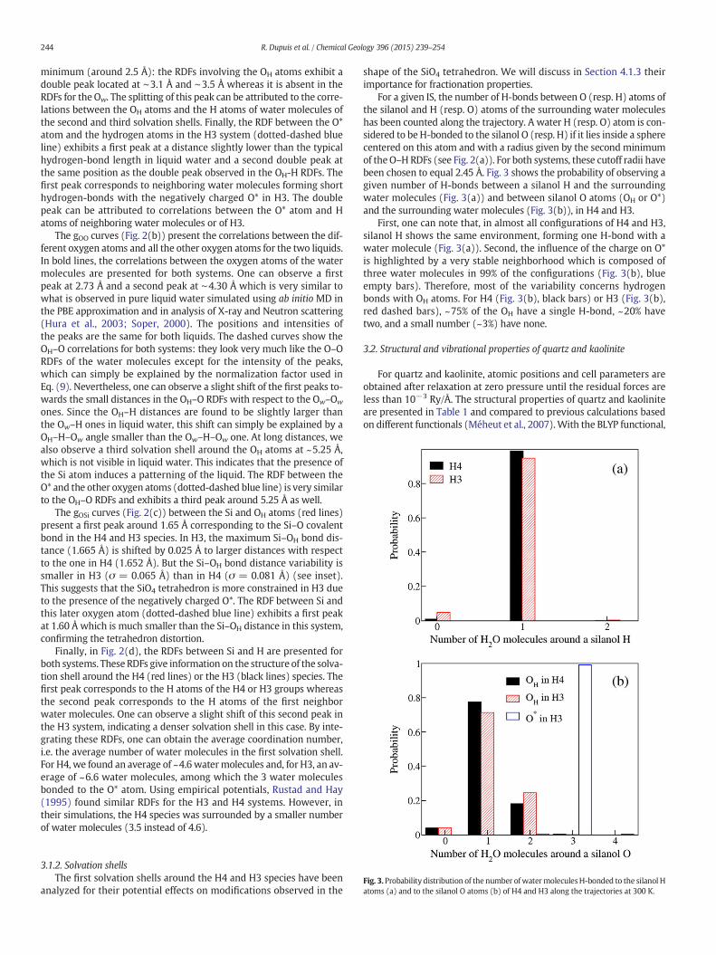
Fig. 3. Probability distribution of the number ofwatermoleculesH-bonded to the silanol Hatoms (a) and to the silanol O atoms (b) of H4 and H3 along the trajectories at 300 K.
3.1.2. Solvation shellsThe first solvation shells around the H4 and H3 species have been
analyzed for their potential effects on modifications observed in the
shape of the SiO4 tetrahedron. We will discuss in Section 4.1.3 theirimportance for fractionation properties.
For a given IS, the number of H-bonds between O (resp. H) atoms ofthe silanol and H (resp. O) atoms of the surrounding water moleculeshas been counted along the trajectory. A water H (resp. O) atom is con-sidered to be H-bonded to the silanol O (resp. H) if it lies inside a spherecentered on this atom and with a radius given by the second minimumof the O–HRDFs (see Fig. 2(a)). For both systems, these cutoff radii havebeen chosen to equal 2.45 Å. Fig. 3 shows the probability of observing agiven number of H-bonds between a silanol H and the surroundingwater molecules (Fig. 3(a)) and between silanol O atoms (OH or O*)and the surrounding water molecules (Fig. 3(b)), in H4 and H3.
First, one can note that, in almost all configurations of H4 and H3,silanol H shows the same environment, forming one H-bond with awater molecule (Fig. 3(a)). Second, the influence of the charge on O*is highlighted by a very stable neighborhood which is composed ofthree water molecules in 99% of the configurations (Fig. 3(b), blueempty bars). Therefore, most of the variability concerns hydrogenbonds with OH atoms. For H4 (Fig. 3(b), black bars) or H3 (Fig. 3(b),red dashed bars), ~75% of the OH have a single H-bond, ~20% havetwo, and a small number (~3%) have none.
3.2. Structural and vibrational properties of quartz and kaolinite
For quartz and kaolinite, atomic positions and cell parameters areobtained after relaxation at zero pressure until the residual forces areless than 10−3 Ry/Å. The structural properties of quartz and kaoliniteare presented in Table 1 and compared to previous calculations basedon different functionals (Méheut et al., 2007).With the BLYP functional,
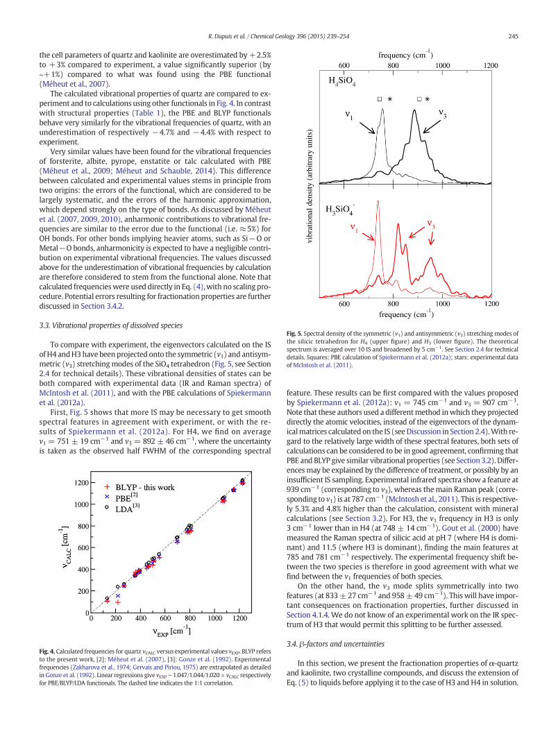
Fig. 5. Spectral density of the symmetric (v1) and antisymmetric (v3) stretching modes ofthe silicic tetrahedron for H4 (upper figure) and H3 (lower figure). The theoreticalspectrum is averaged over 10 IS and broadened by 5 cm−1. See Section 2.4 for technicaldetails. Squares: PBE calculation of Spiekermann et al. (2012a); stars: experimental dataof McIntosh et al. (2011).
245R. Dupuis et al. / Chemical Geology 396 (2015) 239–254
the cell parameters of quartz and kaolinite are overestimated by+2.5%to +3% compared to experiment, a value significantly superior (by~+1%) compared to what was found using the PBE functional(Méheut et al., 2007).
The calculated vibrational properties of quartz are compared to ex-periment and to calculations using other functionals in Fig. 4. In contrastwith structural properties (Table 1), the PBE and BLYP functionalsbehave very similarly for the vibrational frequencies of quartz, with anunderestimation of respectively −4.7% and −4.4% with respect toexperiment.
Very similar values have been found for the vibrational frequenciesof forsterite, albite, pyrope, enstatite or talc calculated with PBE(Méheut et al., 2009; Méheut and Schauble, 2014). This differencebetween calculated and experimental values stems in principle fromtwo origins: the errors of the functional, which are considered to belargely systematic, and the errors of the harmonic approximation,which depend strongly on the type of bonds. As discussed by Méheutet al. (2007, 2009, 2010), anharmonic contributions to vibrational fre-quencies are similar to the error due to the functional (i.e. ≈5%) forOH bonds. For other bonds implying heavier atoms, such as Si−O orMetal−O bonds, anharmonicity is expected to have a negligible contri-bution on experimental vibrational frequencies. The values discussedabove for the underestimation of vibrational frequencies by calculationare therefore considered to stem from the functional alone. Note thatcalculated frequencieswere used directly in Eq. (4), with no scaling pro-cedure. Potential errors resulting for fractionation properties are furtherdiscussed in Section 3.4.2.
3.3. Vibrational properties of dissolved species
To compare with experiment, the eigenvectors calculated on the ISof H4 andH3have beenprojected onto the symmetric (v1) and antisym-metric (v3) stretchingmodes of the SiO4 tetrahedron (Fig. 5, see Section2.4 for technical details). These vibrational densities of states can beboth compared with experimental data (IR and Raman spectra) ofMcIntosh et al. (2011), and with the PBE calculations of Spiekermannet al. (2012a).
First, Fig. 5 shows that more IS may be necessary to get smoothspectral features in agreement with experiment, or with the re-sults of Spiekermann et al. (2012a). For H4, we find on averagev1 = 751 ± 19 cm−1 and v3 = 892 ± 46 cm−1, where the uncertaintyis taken as the observed half FWHM of the corresponding spectral
Fig. 4. Calculated frequencies for quartz vCALC versus experimental values vEXP. BLYP refersto the present work, [2]: Méheut et al. (2007), [3]: Gonze et al. (1992). Experimentalfrequencies (Zakharova et al., 1974; Gervais and Piriou, 1975) are extrapolated as detailedin Gonze et al. (1992). Linear regressions give vEXP ∼ 1.047/1.044/1.020 × vCALC respectivelyfor PBE/BLYP/LDA functionals. The dashed line indicates the 1:1 correlation.
feature. These results can be first compared with the values proposedby Spiekermann et al. (2012a): v1 = 745 cm−1 and v3 = 907 cm−1.Note that these authors used a differentmethod inwhich they projecteddirectly the atomic velocities, instead of the eigenvectors of the dynam-icalmatrices calculated on the IS (seeDiscussion in Section 2.4).With re-gard to the relatively large width of these spectral features, both sets ofcalculations can be considered to be in good agreement, confirming thatPBE andBLYP give similar vibrational properties (see Section 3.2). Differ-encesmay be explained by the difference of treatment, or possibly by aninsufficient IS sampling. Experimental infrared spectra show a feature at939 cm−1 (corresponding to v3), whereas themain Raman peak (corre-sponding to v1) is at 787 cm−1 (McIntosh et al., 2011). This is respective-ly 5.3% and 4.8% higher than the calculation, consistent with mineralcalculations (see Section 3.2). For H3, the v1 frequency in H3 is only3 cm−1 lower than in H4 (at 748 ± 14 cm−1). Gout et al. (2000) havemeasured the Raman spectra of silicic acid at pH 7 (where H4 is domi-nant) and 11.5 (where H3 is dominant), finding the main features at785 and 781 cm−1 respectively. The experimental frequency shift be-tween the two species is therefore in good agreement with what wefind between the v1 frequencies of both species.
On the other hand, the v3 mode splits symmetrically into twofeatures (at 833± 27 cm−1 and 958± 49 cm−1). This will have impor-tant consequences on fractionation properties, further discussed inSection 4.1.4. We do not know of an experimental work on the IR spec-trum of H3 that would permit this splitting to be further assessed.
3.4. β-factors and uncertainties
In this section, we present the fractionation properties of α-quartzand kaolinite, two crystalline compounds, and discuss the extension ofEq. (5) to liquids before applying it to the case of H3 and H4 in solution.

246 R. Dupuis et al. / Chemical Geology 396 (2015) 239–254
Then, the potential sources of uncertainties in these calculations arethoroughly analyzed.
3.4.1. β-factorsThe results are discussed in terms of the logarithmic β-factors (ln β)
and logarithmicα fractionation factors (lnα) in parts per thousand (‰).For quartz and kaolinite, logarithmic β-factors have been computedevery 0.5 × 10⁶/T2 (in K−2), and at 300 K. For the liquid inherent struc-tures (32 in total), logarithmic β-factors have been computed at 373,300 and 273 K. At 300 K, silicon β-factors range from 67.2‰ for quartzto 62.9‰ for a H3 inherent structure. Due to their small variation withrespect to the mean value, we chose to discuss these β-factors withrespect to quartz for comparison. For H4, as a first approach,we have ar-bitrarily chosen 12 IS along the trajectory thenwe selected 10 additionalIS from a periodical sampling, chosen to insure random sampling. These10 IS will be used for computing fractionation properties, and when anidentical treatment of H4 and H3 is needed. The 12 additional IS areused for having better statistics on the regression law of H4 (see 6),and when we will have to choose IS based on their proximity to themean SiO distance (see Section 4.1.2).
Indeed, Méheut and Schauble (2014) have shown a correlationbetween the fractionation properties of silicates and their mean Si–O
distances, dSiO. For this reason, all the 300 K fractionation properties ofminerals, and IS alike, have been conveniently represented in Fig. 6 asa function of themeanSi–Odistances (see also Fig. 8 for the IS). The frac-tionation properties calculated on minerals with the PBE functional byMéheut and Schauble (2014) are also represented in Fig. 6, for purposeof comparison.
Fig. 6. Fractionation factors calculated between the IS extracted from the two liquids and
quartz, and between minerals and quartz, represented as a function of the mean dSiO dis-tance. Full symbols correspond to this work (BLYP functional), red triangles represent ISextracted from the H3 liquid, black squares represent IS extracted from the H4 liquid, cir-cles representminerals (quartz and kaolinite). Empty circles correspond to calculations onminerals byMéheut and Schauble (2014) using PBE functional. The dashed lines representlinear regressions. For the PBE functional, allminerals except forsterite areused in the regres-
sion, giving lnα30SiPBEmineral‐quartz ¼ −183 � dSiO−1:6296� �
R2 ¼ 0:98;p ¼ 3 � 10‐5;n ¼ 7� �
.
For the BLYP functional, all IS and minerals are considered, giving: lnα30SiBLYPIS;mineral‐quartz ¼−169 � dSiO−1:6363
� �R2 ¼ 0:94;pb2:2 � 10−16;n ¼ 34
� �.
As for the minerals calculated in Méheut and Schauble (2014), the ISof H4 and H3 liquids present a correlation between their fractionation
properties and their mean dSiO distance. A detailed statistical analysisof these correlations is presented in Appendix A and summarized below.
The two liquids can be first considered separately. The linear rela-tionships found for H4 and H3 liquids are statistically indistinguishable(Appendix A, Eqs. (A.1) and (A.2)). Therefore, we can consider a com-mon linear relationship for all IS (Eq. (A.3)). We will discuss how touse these different linear relationships to reduce the computationalcost required for liquid fractionation properties in Section 4.1.
Including our calculation of kaolinite and quartz, we can consider aregression including all our BLYP calculations, mineral and IS alike, inorder to compare with the regression obtained by Méheut andSchauble (2014) with the PBE functional (see legend of Fig. 6). Theslopes of both regressions are statistically equivalent (Appendix A).Furthermore, kaolinite–quartz fractionations calculated with BLYP(−1.61‰) and PBE (−1.69‰) give similar values at 300 K (see alsoFig. 7). Therefore, the BLYP regression appears as a horizontal transla-tion of the PBE regression towards higher Si–O distances, in agreementwith discussion in Section 3.2 and the results of Table 1.
The variability of the ln α30 Siliquid ‐ quartz values is found to be quitelarge for both H4 and H3 liquid systems. The values spread from−1.88to −2.61‰ for H4 with a root mean squared error of σα = 0.42‰ andfrom −2.65 to −4.16‰ for H3 with a root mean squared error ofσα = 0.36‰. This can be compared with the variability found byRustad et al. (2008) for CO2(aq), CO3
2− (aq) and HCO3− (aq)
(σ ≈ 0.5 %), by Rustad et al. (2010a) for B(OH)3(aq) and B(OH)4−(aq)(σ ≈ 0.4 %), and by Rustad et al. (2010b) for Mg2+(aq) (σ ≈ 1 %).Compared to the amplitude of the solid–solution fractionation, thisconfigurational variability is particularly significant for dissolved silicon.
Averaging over the 10 values obtained for ln α30SiIS ‐ quartz, themeanfractionation factors are −2.09 ± 0.13‰ and −3.69 ± 0.10‰ for H4and H3, respectively. Combining these two mean values, a mean isoto-pic fractionation factor ln α30SiH3 ‐ H4 of −1.60 ± 0.17‰ is estimatedfor the fractionation between the two species in solution.
The temperature dependence of these fractionation properties isfurther represented in Fig. 7 and fitted with polynomial functions of
Fig. 7. Fractionation properties between H4 (black), H3 (red) and quartz at 273 K, 300 Kand 333 K averaged over 10 IS for each liquid. Dashed lines: fit from Table 2, extrapolatedat high temperatures. Blue lines represent the fractionation properties between kaoliniteand quartz with the BLYP and PBE functionals. Fitting parameters are given in Table 2.

Table 3
List of β30SiH4 factors obtained for different q points grids (2*2*2, 1*1*1 and at Γ point)or for different cutoff energies for the relaxation of atomic positions (Relax) and the calcu-lation of the phonon spectra (Phonons): 80 Ry and 120 Ry.
q points Ecut (relax) [Ry] Ecut (phonons) [Ry] ln β30SiIS [‰]
2*2*2 120 120 64.9951*1*1 120 120 64.985Γ 120 120 65.092Γ 80 120 65.095Γ 80 80 65.088
247R. Dupuis et al. / Chemical Geology 396 (2015) 239–254
1/T (Table 2). Here, the liquid properties are averaged over 10 IS, andthe error bar is given by the standard error (see also Section 4.1.1).
One should note that, for the IS fractionation properties, only the300 K value is consistent with the molecular dynamics simulation. Inprinciple, a trajectory should have been realized at 373 K and 273 K aswell. The fractionations involving the liquid calculated at thesetemperatures have therefore limited confidence, and we will use themto discuss potential temperature effects only qualitatively.
3.4.2. UncertaintiesThe uncertainty on the calculation of the β-factors can have three
different origins: numerical errors on the calculated harmonic frequen-cies, the pressure inconsistency between our solid and liquid calcula-tions, and the neglect of anharmonicity. Numerical errors can arisefrom the choice of the plane-wave cut-off energy, or of the k-pointand q-point samplings of the Brillouin zone (Monkhorst and Pack,1976). For quartz and kaolinite, these parameters have already beenoptimized with the PBE functional (Section 3.2, Méheut et al., 2007).For the IS, the effect of these parameters is tested in Table 3. In particu-lar, it is shown that the Γ-point approximation leads to a slight overesti-mation (by ≈ 0.1‰) of the IS β-factor.
Further, as for the PBE functional, the use of the BLYP approximationis associated with systematic errors on harmonic frequencies. In thecase of quartz, BLYP underestimates harmonic frequencies by typically−5%, very close to the PBE case (see Section 3.2). The IS vibrationalfrequencies appear underestimated by the same amount compared toexperiment (see Section 3.3), which, as already discussed elsewhere(Méheut et al., 2009, Appendix B), leads to an underestimation of ln βby ~−5% at low temperature. For fractionation factors, Méheut et al.(2009) assumed that the uniformity of the error made on vibrationalproperties, and therefore on β-factors, between the two phases shouldlead to a partial error cancelation and to a similar relative error(a −5% underestimation at low temperature) on fractionation factors.In the framework of this study, the comparison of our calculatedquartz-kaolinite fractionation with the PBE value of Méheut et al.(2009) allows this assumption to be discussed. Both calculations giveindeed very close results (PBE:−1.61‰; BLYP:−1.69‰), in agreementwith the similarity of the error made on frequencies (see Section 3.2).The difference between the two fractionations is comparable to analyt-ical limits, and probably originates from imperfect error cancelations.Wewill further consider that PBE aswell as BLYP functionals identicallyunderestimate fractionation factors by ~−5%.
In this study, we did not choose to rescale the calculated frequenciesto experimental ones for several reasons. This represents an inconsis-tent procedure, since our calculated frequencies are harmonic, as thefrequencies that should be used in Eq. (4), but experimental frequenciesare in principle anharmonic. Further, as discussed by Méheut et al.(2009), the value of the scaling parameters is associated with a largeuncertainty, and cannot be obtained for all structures.
Another important source of error is the pressure inconsistencybetween our liquids and our solids. On one hand, our liquids havebeen computed by taking the experimental volume of the solution atambient conditions. On the other hand, our solids have been relaxedto zero pressure before computing their fractionation properties. By es-timating the pressure in the liquid calculated at experimental volume,and the effect of the liquid volume on pressure and fractionation prop-erties, we were able to estimate this effect (see Appendix B for details).The β30SiIS calculated at 300 K with the experimental volume appears
Table 2Fits of 1000 ln α30Siphase ‐ quartz based on ax2 + bx3, with x = 102/T.
Phase T(°C) a b
Kaolinite 0–1141 −21.90 20.0H4 0–50 −4.70 −42.3H3 0–50 −32.07 −2.6
overestimated by ≈+0.3‰ compared to what would be found for theequilibrium volume. Therefore, the inconsistency between the liquidand the solid will translate into α ≈+0.3‰ error on liquid-mineralfractionation.
Note that this inconsistency is a problem encountered by everystudy of mineral–solution fractionations. A perfectly consistent proce-dure would consist of a molecular dynamics simulation at constant(0 bar) pressure for the liquid, together with a relaxation at 0 bar forthe solid. Ab initiomolecular dynamics at constant pressure is computa-tionally very expensive, and therefore usually not considered. Tofree themselves from such a constraint, Kowalski and Jahn (2011)chose to consider both liquids and solids at their experimental volumes(therefore, at experimental unit cell parameters for the solids). This ap-proach is not fully satisfying for mineral calculations, as discussed byMéheut et al. (2007). On the other hand, Rustad and Dixon (2009)and Rustad et al. (2010b) considered cluster models both for dissolvedspecies and for solids. In this way, they were able to relax both systemsin a consistent manner.
The last source of error, yet themost difficult to assess, is the effect ofanharmonicity on fractionation properties. For crystalline solids, recentstudies (Blanchard et al., 2009; Méheut et al., 2009; Schauble, 2011)showed that fractionation properties computed within the harmonicapproximationwere in good agreementwithmeasurements for variousisotopic systems. In liquids, anharmonic effects are expected to havestronger impacts on fractionation properties. Generally, we expect“true” β-factors, including anharmonic effects, to be smaller than theirharmonic counterpart. Indeed, for molecules or solids, vibrationalanharmonicity leads to a decrease of the vibrational frequencies,and consequently to a decrease of the β-factor (cf Richet et al., 1977;Méheut et al., 2007; Balan et al., 2009). Another argument, relevantfor liquids, is that Si–O distances are slightly longer before relaxation(see Section 4.1.1). This can be seen as the effect of anharmonicity in liq-uids and should translate into decreasing solvated species β-factors.More quantitatively, we observe an elongation of roughly 0.002 Å forH4 and H3 (with a very large uncertainty on this value, see Table 4).Using Eq. (A.3) with no further precaution, this would translate into a0.4‰ decrease of the liquid β-factor. Assuming anharmonicity to benegligible for solids, this value can be seen as a rough estimate of theerror related to anharmonicity for our solid–liquid calculations. Forthe fractionation between H4 and H3, we expect anharmonic errors tocancel out, due to the similarity between the two systems.
It should benoted that sophisticated calculationmethodologies havebeen recently proposed to take into account anharmonic effects(Marsalek et al., 2014; Markland and Berne, 2012; Pinilla et al., 2014).However, their application to systems containing heavy nuclei such assilicon atoms are for now limited, and beyond the scope of the presentwork.
To conclude, we will consider: (1) that the BLYP functional causes arelative underestimate of the absolute value of lnα30Si by≈5%, (2) thatpressure inconsistency should correspond to a ≈+0.3‰ overestima-tion of the liquid β-factor, and therefore of the liquid-quartz fraction-ations calculated at 300 K, and (3) that anharmonic effects will cancelout for solution–solution fractionations, but will also lead calculatedliquid–solid fractionations to be overestimated. Since the liquid is al-ways lighter than the solid, for what concerns the present calculations,

Table 4
List of structural and fractionation properties of H4 and H3 systems for different sets of configurations. dSiO trajð ÞD E
refers to themean Si–O distances measured in the extracted snapshots
before relaxation. dSiO ISð ÞD E
refers to the mean Si–O distances measured in the extracted snapshots after relaxation.
SiO4 tetrahedron Number of H bondson silanol OH
Fractionationproperties
Sampling dSiO trajð ÞD E
σ dSiO ISð ÞD E
σ 1 H2O 2 H2O ⟨In α⟩
Type Number of configurations [Å] [%] [‰]
H4 Trajectory 8000 1.6522 0.0178 – – 79 18 – –
Arbitrarya 50 1.6523 0.0167 1.6492 0.0020 75 19 – –
Periodicb 20 1.6537 0.0177 1.6494 0.0022 76 19 – –
Periodicb 10 1.6545 0.0152 1.6493 0.0020 75 20 −2.09 0.42Selectedc 4 1.6573 0.0081 1.6492 0.0004 – – −2.06 0.24Selectedc 1 1.6516 – 1.6491 – – – −2.01 –
H3 Trajectory 8000 1.6522 0.0178 – – 79 18 – –
Periodicb 20 1.6590 0.0160 1.6569 0.0021 72 23 – –
Periodicb 10 1.6581 0.0157 1.6571 0.0020 73 20 −3.69 0.33Selectedc 4 1.6532 0.0196 1.6572 0.0004 66 33 −3.69 0.17Selectedc 1 1.6378 – 1.6577 – 66 33 −3.62 –
a All sampled configurations, periodically sampled or arbitrarily chosen along the trajectory.b Configurations have been sampled at constant time intervals along the trajectory.c Configurations that have been chosen among all calculated ones for their dSiO close to the liquid mean value.
248 R. Dupuis et al. / Chemical Geology 396 (2015) 239–254
these effects all go into the same direction, leading the calculated liquidto be isotopically heavier than the real one.
4. Discussion
4.1. Statistical variability and correlation between structure and fractionation
Fig. 6 shows (i) that IS fractionation properties are dispersed for a
given liquid, and (ii) that they correlatewithdSiO. This correlation is rea-sonable since longer bonds are expected to be weaker, and thereforeisotopically lighter (see e.g., Schauble, 2004, and discussion in Méheutand Schauble, 2014).
In the first part of this section, we analyze the statistical distributionof the mean Si–O distances in IS and the corresponding fractionationproperties, and discuss how to obtain a value for the fractionationproperties of a liquid from several IS. In particular, it is possible to usethe correlation between the Si–O distances and ln α30SiIS ‐ quartz
(Fig. 6) to choose the configurations to be computed for their fraction-ation properties “wisely”, and reduce the numerical burden.
Since the mean Si–O distances are closely related to fractionationproperties, we can look for other parameters influencing fractionationby correlating them to Si–O distances. The second part of this sectionpresents an example of this approach showing the influence of hydra-tion shell on fractionation properties.
In the third part, we analyze the vibrational contributions to thefractionation properties of the different IS, in an attempt to understandthe fractionation effects in terms of vibrations.
4.1.1. The issue of configurational disorderAs shown in Section 3, the values of ln α30SiIS ‐ quartz vary significant-
ly from one configuration to the other. To obtain a value for the liquid,we need to make a statistical average of ln α30SiIS ‐ quartz over the liquidtrajectory. Since fractionation properties and mean Si–O distances arestrongly correlated, and since obtaining Si–O distances is much cheaperin terms of computational time, we will use this correlation to discussthe statistical distribution of fractionation properties. In other words,we will consider that observations made on Si–O distances can beextrapolated to fractionation properties.
The results of our analysis are presented in Table 4. The values for
dSiO trajð ÞD E
and for dSiO ISð ÞD E
are obtained from averaging over the
different samplings used to select the liquid configurations from theMD trajectories:
dSiO trajð ÞD E
¼ 1n
Xni¼1
dSiO trajð Þ ð10Þ
dSiO ISð ÞD E
¼ 1n
Xni¼1
dSiO ISð Þ ð11Þ
where n refers to the number of selected configurations. As previ-ously mentioned in Section 3.4.1, we used different types of sam-pling to select the liquid configurations. Configurations wereextracted regularly at constant time intervals (“periodic” sam-pling), configurations were extracted randomly (“arbitrary” sam-pling) or configurations were selected with respect to the value of
their mean dSiO, close to the average one over the whole trajectory(“selected” sampling). If we look at the mean Si–O distances in the
tetrahedron before relaxation dSiO trajð Þ� �
, we can observe that the
different samplings (n = 50, 20, and 10 for H4; n = 20 and 10 forH3) are indistinguishable from each other and from the whole tra-jectory, for what concerns the means and σ of their Si–O distances.
The same can be said after relaxation dSiO ISð Þ� �
. This strongly sug-
gests that our n = 10 sampling is statistically representative ofthe whole solution. The Si–O distances vary upon relaxation from
dSiO trajð ÞD E
¼ 1:652� 0:018 Å to dSiO ISð ÞD E
¼ 1:649� 0:002 Å for H4,
and from dSiO trajð ÞD E
¼ 1:658� 0:017 Å to dSiO ISð ÞD E
¼ 1:657� 0:002 Å
for H3. The width of their statistical distribution therefore decreases bya factor of 10,while theirmean value stays essentially the same or slightlydecreases.
We can therefore assume that the n=10 samplings are represen-tative of the whole distributions and use them to compute the frac-tionation properties of the IS from their vibrational propertiesfollowing the protocol presented in Section 2.2. The fractionationproperties of the liquids are then given by averaging over the IS, andtheir uncertainty is given by the standard error of the meanSE ¼ σ=
ffiffiffin
p� �, giving: ln α30SiH4 ‐ quartz =−2.09 ± 0.13‰ (SE, n = 10),
and ln α30SiH3 ‐ quartz =−3.69 ± 0.10‰ (SE, n = 10).
249R. Dupuis et al. / Chemical Geology 396 (2015) 239–254
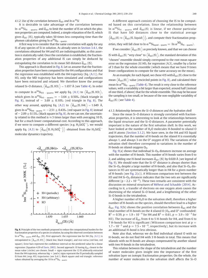
4.1.2. Use of the correlation between dSiO and ln α30SiIt is desirable to take advantage of the correlation between
ln α30SiIS ‐ quartz and dSiO to limit the number of IS on which the pho-non properties are computed. Indeed, a simple relaxation of the IS,which
gives dSiO (IS), typically takes 50 times less computing time than thephonon calculation giving ln α30SiIS ‐ quartz.
A first way is to consider that the same correlation will apply for anyIS of any species of Si in solution. As already seen in Section 3.4.1, thecorrelations obtained for H4 and H3 are indistinguishable, so this asser-tion is statistically valid. Once the correlation is established, the fraction-ation properties of any additional IS can simply be deduced by
extrapolating the correlation to its mean SiO distance dSiO (IS).This approach is illustrated in Fig. 8. Let us assume that the fraction-
ation properties have been computed for theH4 configurations and thatthe regression was established with the H4 trajectory (Eq. (A.1)). ForH3, only the MD trajectory has been simulated and configurationshave been extracted and relaxed. We therefore know the average
relaxed Si–O distance, dSiO IS;H3ð ÞD E
¼ 1:657 Å (see Table 4). In order
to compute ln α30SiH3 ‐ quartz, we apply Eq. (A.1) to dSiO IS;H3ð ÞD E
,
which gives ln α30SiH3 ‐ quartz = −3.64 ± 0.50‰ (black triangle inFig. 8), instead of − 3.69 ± 0.10‰ (red triangle in Fig. 8). The
other way around, applying Eq. (A.2) to dSiO IS;H4ð ÞD E
¼ 1:649 Å,
gives ln α30SiH4 ‐ quartz =−2.51 ± 0.43‰ (red square in Fig. 8) insteadof− 2.09±0.13‰ (black square in Fig. 8). Aswe can see, the uncertain-ty related to this method is ≈3 times larger than with averaging 10 IS,but for a much lower computational cost. According to this approach,if we were to compute a different species (e.g. H2SiO4
2−), we would
apply Eq. (A.3) to dSiO IS;H2SiO2−4
� �D Eobtained from the H2SiO4
2−
molecular dynamics trajectory.
Fig. 8. Principle of the two methods proposed to reduce the computational burden for thefractionation properties of a species in solution, by using the observed correlation between
ln α30SiIS ‐ quartz and dSiO (IS). First approach: the regression law for H4 (Eq. (A.1)) is
extrapolated to dSiO IS;H3ð ÞD E
(black line, black triangle), and vice-versa (red line, red
square). Error bars represent the confidence interval on the predicted value for a linear
regression (Equation 4.39 of Davis, 2002). Second approach: IS having dSiO closest to themean value (circles) are chosen. Small + signs represent the 12 IS arbitrarily extractedfrom the H4 trajectory, whereas big + (and x) signs represent the IS periodically sampledIS from H4 (resp. H3) trajectories (see 3.4.1). Black square and red triangle: referencevalues obtained by averaging the 10 ln α30SiIS ‐ quartz.
A different approach consists of choosing the IS to be comput-ed based on this correlation. Since the relationship between
ln α30SiIS ‐ quartz and dSiO ISð Þ is linear, if we choose particularIS that have SiO distances close to the statistical average
dSiO ISð Þ≈ dSiO IS; liquidð ÞD E� �
, and compute their fractionation prop-
erties, they will fall close to ln α30Siliquid ‐ quartz = ⟨ln α30SiIS ‐ quartz⟩.
If we consider dSiO ISð ÞD E
as precisely known, and that we can choose
IS with dSiO ISð Þ “very close” to dSiO ISð ÞD E
, the standard deviation of this
“chosen” ensemble should simply correspond to the root mean squareerror on the regression (0.14‰ for regression (A.3), smaller by a factorof 3 than for the whole ensemble (which means that we have 9 timesfewer configurations to compute for the same accuracy on the mean).
As an example, for each liquid,we chose 4 ISwithdSiO ISð Þclose to themean dSiO ISð Þ
D Evalue (encircled points in Fig. 8), and calculated their
mean ln α30SiIS ‐ quartz (Table 4). The result is very close to the referencevalues, with a variability a bit larger than expected, around half (insteadof one third, cf above) that for thewhole ensemble. Thismay be becausethe sampling is too small, or because of the non-negligible variability of
dSiO ISð Þ (see Table 4).
4.1.3. Relationship between the Si–O distances and the hydration shellSince the mean Si–O distance is strongly correlated with fraction-
ation properties, it is interesting to look at the relationships betweenthe liquid structure and the Si–O distances. A parameter potentiallyimportant is the nature of the first solvation shell. In this work, wehave looked at the number of H2O molecules H-bonded to silanol Oand H atoms (Section 3.1.2). We have seen, in the H4 and H3 liquidtrajectories, that the number of H-bonds on the silanol H is essentiallyalways 1, and always 3 on the O* oxygen of H3. The variations of thesolvation shell therefore correspond to variations in the number ofH-bonds on silanol oxygens OH.
Fig. 9(a) shows that individual Si–OH distances increase on averagewith the number of H-bonds. This number of H-bonds varies from 0 to
2, and adding one H-bond increases dSiO (IS) by 0.020 Å (see legend ofFig. 9). We should note that the Si–O* distance is always shorter thanthe Si–OH despite a large number of H-bonds, and also that Si–OH dis-tances in H3 are systematically longer than in H4 for a given numberof H-bonds (see Fig. 2(c)). A Wilcoxon comparison test between theH3 and H4 Si–OH distances indicates that the two sets are significantlydifferent (p b 2.2 ∗ 10−6). These two remarks are consistent with thediscussion on mineral structures of Méheut and Schauble (2014). Ac-cording to it, a transfer of electrons on one oxygen atom causes theshortening of the related Si–O bond, and a lengthening of the otherSi–O bonds in the tetrahedron.
A higher number of H2O in the solvation shell, therefore a highernumber of H-bonds on the species, should therefore lead to a higher
dSiO. Fig. 9(b) shows the positive correlation between dSiO and thetotal number of H-bonds on the 4 silanol O (OH and O* confounded:R2 = 0.59, p = 1.9 ∗ 10−6 for H4 and R2 = 0.61, p = 3.9 ∗ 10−3 for
H3). The increase of dSiO from 4 to 5 H-bonds for H4, and from 6 to7 H-bonds for H3 is significant (Wilcoxon comparison test at p =1.7 ∗ 10−5 and p = 7.5 ∗ 10−6, respectively), but its increase withan additional H-bond is less obvious.
Note also that, whereas we do find individual silanol O with noH-bonds, we do not find H4 with 3 H-bonds in total. This means thatsilanols with no H-bonds are always compensated by another silanolwith two H-bonds in the tetrahedron.
This relation between the shape of the tetrahedron and the numberof water molecules gives insight into the importance of the firstsolvation layer on isotopic fractionation properties. On the whole, thenumber of water molecules in the solvation shell affects the Si–O

Fig. 9. Influence of the environment of silanol oxygens on the length of the Si–O bond (dSi ‐ O). (a) Si–O distance as a function of the number of H-bonds on the O atom: OH are hydroxylgroups inH4 (black cross) orH3 (red plus), O* denotes the negatively charged oxygen inH3 (blue stars). Dashed lines correspond to linearfits. H4: dSi–O=1.626+0.0203 ∗NH-bonds (R2=
0.59, p=2.3 ∗ 10−16); H3: dSi–O=1.646+0.0224 ∗NH-bonds (R2=0.69, p=2.7 ∗ 10−16) (b)mean Si–Odistance in the tetrahedron dSiO ISð Þ� �
as a function of the total number of H-bonds
on silanol oxygens (OH or O*). Dash-dotted lines link statistical means dSiO ISð Þ� �
over IS having the same number of H-bonds.
250 R. Dupuis et al. / Chemical Geology 396 (2015) 239–254
distances and subsequently the fractionation factor. Fractionationproperties are therefore affected by the local structure.
4.1.4. Vibrational analysis
The data presented above link the mean tetrahedral distance dSiO,the number of water molecules in the first solvation layer and the frac-tionation factor, which suggests that most contributions to the fraction-ation come from the SiO4 tetrahedron. Méheut et al. (2009) calculatedthe spectral contribution of various minerals, in particular forsterite inwhich the polymerization degree (Q0) can be considered to be thesame as in H4 and H3. They observed an important contribution of thev3 modes (tetrahedral out-of-phase stretching) from 700 to 1000 cm−1.
The same method has been applied here to selected H4 and H3 in-herent structures. In Fig. 10, the spectral contribution to the totalβ30SiIS is plotted for two different configurations of each liquid. Theconfigurations with the shortest ((a) and (c)) and the longest ((b) and
(d)) mean distance dSiO. Additionally, the eigenvectors of the dynamicalmatrix have been looked at to determine the type of associated modes
Fig. 10. Contribution of phonon modes to the total ln β30SiIS factor for two configurations
of H4 (solid lines: (a) with the shortest dSiO and (b) with the longest dSiO) and H3 (dashed
lines: (c) with the shortest dSiO and (d) with the longest dSiO).
with important contributions (see Méheut et al., 2009). We can distin-guish afirst contribution around400 cm−1, corresponding to tetrahedralbending modes v4. This contribution is very similar for all systems andwill therefore not contribute much to fractionation. The domain thatcontributes the most, between 700 and 1100 cm−1, represents 75% ofall vibrational contributions. It essentially corresponds to v3 modes. ForH4 IS, there is essentially a single contribution in this domain, with IS
of longer dSiOHhaving vibrational frequencies shifted to lower values,
hence a lower final β-factor. On the other hand, H3 manifests asplit of the v3 contribution into two, one around 750 and one around950 cm−1, as already observed in Fig. 5. This splitting increases with
Δ ¼ dSiOH−dSiO� (in (c), Δ = 0.065 Å and in (d), Δ = 0.082 Å). Inter-
estingly, the modes at ~750 cm−1 are still associated with Si–OH
stretching modes (O* barely moves in the corresponding eigenvec-tors) whereas the higher frequency modes (~950 cm−1) mostly in-volve Si–O* stretching. These observations agree with the assesseddependence of fractionation properties on dSiO, but here for individ-ual bonds in the tetrahedron.
4.2. Geological implications
In surface environments, silicon in solution is almost exclusivelypresent under the H4 species. H3 is the second most abundant species,with the H3/H4 ratio varying typically between 10−1 and 10−5
(pKa(H4/H3) = 9.9 at 30 °C, Lide, 2004; typical pH of natural surfacewaters: 5.5 to 8.5). Therefore, we can consider the mineral-H4 equilib-rium as representative of the mineral-solution equilibrium. Withinthese considerations, our calculations predict fractionations of +2.1‰between quartz and solution, and of +0.4‰ between kaolinite and so-lution, at 25 °C (Fig. 11). These values show strong disagreement withnatural observations. In soils, clays are generally found enriched inlight silicon isotopes relative to the parent silicate material (Opfergeltand Delmelle, 2012, and references therein), and Georg et al. (2007a)estimated a fractionation of −1.5‰ associated with the precipitationof clays (square in Fig. 11), compared with our +0.4‰ value. For silica,natural samples, in particular silcretes, are also found enriched in lightisotopes (Opfergelt and Delmelle, 2012, and references therein). Basedon experiments of silica precipitation, Li et al. (1995) estimated a frac-tionation factor of −1‰ accompanying silica precipitation, while evenlarger negative values, further discussed below, are found by Geilertet al. (2014). If we make the assumption that amorphous silica and

Fig. 11.Calculated silicon fractionation factors betweenmineral phases andH4, andwithinsolution, between H3 and H4 species, and comparison with natural or experimentalestimates of silicon fractionation factors accompanying inorganic precipitation. Square:clay-dissolved silicon fractionation factor estimated from natural data by Georg et al.(2007) (temperature is taken as the average of Georg et al., 2007 data, i.e. 7 °C). Triangle: in-organic silica-dissolved silicon fractionation factor estimated from experiment by Li et al.(1995).
251R. Dupuis et al. / Chemical Geology 396 (2015) 239–254
quartz have similar equilibrium fractionation properties, we cancompare this value to our calculated +2.1‰ quartz-H4 fractionation.Compared to the case of clay, the disagreement with our calculation iseven more significant. The disagreement between our calculation andexperiment can be explained (1) by non-equilibrium fractionation oc-curring in natural processes, and (2) computational errors. The errorsinduced by our procedure are discussed in Section 3.4.2. In the case ofa solid–solution equilibrium, our calculation should underestimate,and not over-estimate the real fractionation. Furthermore, we notethat if equilibrium was the governing fractionation mechanism,clays and silica should behave quite differently, with a “quartz-clay frac-tionation” of +1.7‰. In other words, if equilibrium processes weredominating the fractionation of Si isotopes during low-temperatureprecipitation processes, fractionation values should be more system-dependent than what is observed. Natural observations (Opfergelt andDelmelle, 2012, and references therein), as well as the data shown inFig. 11, suggest on the contrary that silica and clays precipitation are as-sociated with very similar silicon fractionation. This further suggeststhat silicon fractionation does not follow equilibrium during lowtemperature processes.
This conclusion is in agreement with recent work by Geilert et al.(2014). In this experimental work, the Si fractionation duringprecipitation was measured at various temperatures from 10 to60 °C. Δ30SiSolid ‐ solution was shown to increase from −2.1‰ at 10 °Cto ~0‰ at 50−60 °C. As suggested by the authors, this steep increaseis unlikely to represent equilibrium effects, and more likely representa-tive of a transition from unidirectional kinetic processes to equilibrium,in the sense of a dynamic equilibrium between backward and forwardprocesses (Section 4.2 of Geilert et al., 2014). According to our study,however, this value of 0‰ is still far from equilibrium values, whichare close to +2‰ at 50 °C.
Interestingly, silicon isotopes behave differently from oxygen iso-topes for the same systems. For oxygen isotopes, calculated equilibriumquartz–water and kaolinite–water fractionations, based on the sameprocedure (Méheut et al., 2007), or based on experimental estimates
of quartz and water vibrational frequencies (Kawabe, 1978), showedgood agreement with natural values, at both high and low tempera-tures. Note that, for the fractionation of oxygen isotopes, quartz–wateras well as amorphous silica-water data seem to be aligned onthe same tendency, in relatively good agreement with equilibriumcalculations (Fig. 4 of Méheut et al., 2007). There does not seem to beany difference between the equilibrium fractionation properties(i.e. the β-factors) of crystalline quartz and those of amorphous silica,for what concerns oxygen isotopes. The same should be true for siliconisotopes.
If the equilibration of silicon isotopes is unlikely between a solidand a solution, it is on the contrary very likely for H4 and H3 to bein isotopic equilibrium within the solution, because the transforma-tion from one to the other corresponds to a proton exchange, a veryquick and easy chemical process. From the results of our calculation,H3 is significantly fractionated (by−1.6 ± 0.3‰) with respect to H4in the solution. Despite the small quantity of species other than H4 incommon solutions, this large fractionation effect suggests a poten-tially important impact of speciation on silicon fractionation. Varia-tions in the pH of the solution, or the presence of other speciesinteracting with H4may therefore lead to significant isotopic effects.For example, since H3 becomes the most abundant species at pH 11,any solid-solution equilibrium fractionation increases by +1.6‰when pH goes from 9 to 11.
5. Conclusion
This study develops methodological aspects for the computationof fractionation properties of dissolved species. It is based on a real-istic modeling of species in solution. These are first simulated by abinitio molecular dynamics, then individual snapshots of the dynamicare extracted and relaxed, giving inherent structures (IS). The frac-tionation properties of these IS are calculated. Primarily, this studyshows the important effect of configurational disorder on the frac-tionation properties. This effect needs to be taken into account foran accurate estimation of fractionation properties. On the otherhand, linear correlations between fractionation and other propertiesof the IS, such as bond lengths, can be used gainfully to reduce thecomputational time, by limiting the number of IS for which phononcalculations have to be performed.
We estimate the fractionation properties of quartz and kaoliniteminerals and of the dissolved species H4SiO4 and H3SiO4
−. We findquartz-H4SiO4, kaolinite–H4SiO4 and H3SiO4
−–H4SiO4 fractionations ofrespectively +2.1 ± 0.2‰; +0.4 ± 0.2‰ and −1.6 ± 0.3‰. The firsttwo values are irreconcilable with natural observations of fractionationsduring silica or clay precipitation. This suggests that these fractionationprocesses instead obey kinetic laws. On the other hand, the importantfractionation found between H4SiO4 and H3SiO4
− underlines the poten-tially important role of speciation for the fractionation of silicon isotopesin natural environments.
Acknowledgment
We would like to thank the three anonymous reviewers for help-ful and insightful comments, which have greatly improved thismanuscript. We thank M. E. Tuckerman for the initial water coordi-nates and fruitful discussions. Calculations were performed usingHPC resources from CALMIP (Grant 2013-P1037) and CINES (Grantc2014096831).
Appendix A. Statistical analysis
As shown on Fig. 6, the IS of H4 and H3 liquids present a correlation
between their fractionation properties and their mean dSiO distance. If
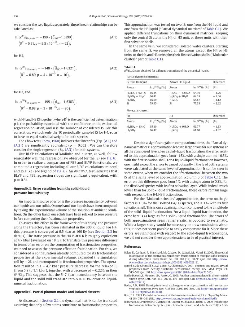
252 R. Dupuis et al. / Chemical Geology 396 (2015) 239–254
we consider the two liquids separately, these linear relationships can becalculated as:
ln α30SiIS‐quartz ¼ −199 � dSiO−1:6390� �
;
R2 ¼ 0:91;p ¼ 9:8 � 10−12;n ¼ 22
� �;
ðA:1Þ
for H4,
ln α30SiIS‐quartz ¼ −148 � dSiO−1:6321� �
;
R2 ¼ 0:89;p ¼ 4 � 10−5;n ¼ 10
� �;
ðA:2Þ
for H3, and
ln α30SiIS‐quartz ¼ −195 � dSiO−1:6383� �
;
R2 ¼ 0:98;p ¼ 3 � 10−16;n ¼ 20
� �;
ðA:3Þ
withH4 andH3 IS together, where R2 is the coefficient of determination,p is the probability associated with the confidence on the estimatedregression equation, and n is the number of considered IS. For thiscorrelation, we took only the 10 periodically sampled IS for H4, so asto have an equal statistical weight for both species.
The Chow test (Chow, 1960) indicates that linear fits (Eqs. (A.1) and(A.2)) are significantly equivalent (p = 0.052). We can thereforeconsider the single regression (Eq. (A.3)) for both systems.
Our BLYP calculations of kaolinite and quartz, as well, followreasonably well the regression law observed for the IS (see Fig. 6).In order to realize a comparison of PBE and BLYP functionals, wecomputed a regression including all our BLYP calculations, mineraland IS alike (see legend of Fig. 6). An ANCOVA test indicates thatBLYP and PBE regression slopes are significantly equivalent, withp = 0.34.
Appendix B. Error resulting from the solid–liquidpressure inconsistency
An important source of error is the pressure inconsistency betweenour liquids and our solids. On onehand, our liquids have been computedby taking the experimental volume of the solution at ambient condi-tions. On the other hand, our solids have been relaxed to zero pressurebefore computing their fractionation properties.
To assess this effect in the framework of this study, the pressurealong the trajectory has been estimated in the 300 K liquid. For H4,this pressure is converged at 6.5 kbar at 160 Ry (see Section 2.3 fordetails). The static pressure in the H4 IS at 0 K is roughly equivalentat 4.7 kbar (averaged on 18 IS). To translate this pressure differencein terms of an error on the computation of fractionation properties,we need to assess the pressure effect on fractionation. For this, weconsidered a configuration already computed for its fractionationproperties at the experimental volume, expanded the simulationcell by +2% and recomputed its fractionation properties. The opera-tion resulted in a −4.7 kbar pressure decrease for the relaxed IS(from 5.8 to 1.1 kbar), together with a decrease of −0.22‰ in theirβ30SiIS. This suggests that the 5–7 kbar inconsistency between theliquid and the solid will translate into α ≈ 0.3‰ error on liquid-mineral fractionation.
Appendix C. Partial phonon modes and isolated clusters
As discussed in Section 2.2 the dynamical matrix can be truncatedassuming that only a few atoms contribute to fractionation properties.
This approximation was tested on two IS: one from the H4 liquid andone from the H3 liquid (“Partial dynamical matrices” of Table C.1). Weapplied different truncations on their dynamical matrices: keepingonly the central Si atom, the H4 or H3 unit, or these units with theirfirst solvation shells.
In the same vein, we considered isolated water clusters. Startingfrom the same IS, we removed all the atoms except the H4 or H3units, or the H4 andH3 units plus their first solvation shells (“Molecularclusters” part of Table C.1).
Table C.1β30SiIS factors obtained for different truncations of the dynamical matrix.
Partial dynamical matrices
IS from H4 liquid
IS from H3 liquid DifferenceAtoms
ln β30SiIS [‰] Atoms ln β30SiIS [‰] [‰]H4SiO4 + 62H2O
66.15 H3SiO4− + 62H2O 64.39 +1.76H4SiO4 + 8H2O
66.41 H3SiO4 + 9H2O 64.35 +2.06 H4SiO4 66.99 H3SiO4−
65.87 +1.12 Si 79.95 Si 77.33 +2.62Molecular clusters
H4
H3 DifferenceAtoms
ln β30SiIS [‰] Atoms ln β30SiIS [‰] [‰]H4SiO4 + 8H2O
65.10 H3SiO4− + 9H2O 63.77 +1.33H4SiO4
66.47 H3SiO4− 61.60 +4.87Despite a significant gain in computational time, the “Partial dy-namicalmatrices” approximation leads to large errors for our systems atall the considered levels. For a solid–liquid fractionation, the error relat-ed to this approximation goes from ~15‰with a single atom to ~0.5‰with the first solvation shell. For a liquid–liquid fractionation however,onemight expect the errors to cancel out partly if the IS of both systemswere calculated at the same level of approximation. It can be seen insome extent, when we consider the “fractionation” between the twoIS at the same level of approximation (column 5 of Table C.1). Theerror on this difference goes from 1‰ with a single atom to 0.3‰ forthe dissolved species with its first solvation layer. While indeed muchlower than for solid–liquid fractionations, these errors remain largewith respect to the H4/H3 fractionation.
For the “Molecular clusters” approximation, the error on the β-factors is ≈3‰ for the isolated H4/H3 species, and ≈1‰ with its firstsolvation shell. This is once again significant compared to the amplitudeof the solid–liquid fractionation. For a liquid–liquid fractionation, theerror here is as large as for a solid–liquid fractionation. The errors ofboth approximations seem rather erratic, as opposed to systematic.While a larger study would be necessary to draw conclusions aboutthis, it does not seem possible to easily compensate for it. Since theseerrors are significant with respect to the solid–liquid fractionations,we did not consider these approximations to be of practical interest.
References
Balan, E., Cartigny, P., Blanchard, M., Cabaret, D., Lazzeri, M., Mauri, F., 2009. Theoreticalinvestigation of the anomalous equilibrium fractionation of multiple sulfur isotopesduring adsorption. Earth Planet. Sci. Lett. 284 (12), 88–93 (Jun, URL http://www.sciencedirect.com/science/article/pii/S0012821X09002313).
Baroni, S., de Gironcoli, S., Dal Corso, A., Giannozzi, P., 2001. Phonons and related crystalproperties from density-functional perturbation theory. Rev. Mod. Phys. 73,515–562 (Jul, URL http://link.aps.org/doi/10.1103/RevModPhys.73.515).
Basile-Doelsch, I., Meunier, J.D., Parron, C., 2005. Another continental pool in the terrestrialsilicon cycle. Lett. Nat. 433 (7024), 399–402 (Jan, URL http://dx.doi.org/10.1038/nature03217).
Becke, A.D., 1988. Density-functional exchange-energy approximation with correct as-ymptotic behavior. Phys. Rev. A 38 (6), 30983100 (Sep, URL http://link.aps.org/doi/10.1103/PhysRevA.38.3098).
Bish, D.L., 1993. Rietveldt refinement of the kaolinite structure at 1.5 K. Clays Clay Miner.41 (6), 738–744 (URL http://www.clays.org/journal/archive/volume38pdf).
Blanchard,M., Poitrasson, F., Méheut, M., Lazzeri, M., Mauri, F., Balan, E., 2009. Iron isotopefractionation between pyrite (fes2), hematite (fe2o3) and siderite (feco3): a first-

253R. Dupuis et al. / Chemical Geology 396 (2015) 239–254
principles density functional theory study. Geochim. Cosmochim. Acta 73 (21),6565–6578 URL http://www.sciencedirect.com/science/article/B6V66-4WXHBXP-2/2/5c6a5c3eef9fb015a1da09c312543bc.
Blumberger, Jochen, Bernasconi, Leonardo, Tavernelli, Ivano, Vuilleumier, Rodolphe,Sprik, Michiel, 2004. Electronic structure and solvation of copper and silver ions: atheoretical picture of a model aqueous redox reaction. J. Am. Chem. Soc. 126,3928–3938.
Car, R., Parrinello, M., 1985. Unified approach for molecular dynamics and density-functional theory. Phys. Rev. Lett. 55, 2471–2474 (URL http://link.aps.org/doi/10.1103/PhysRevLett.55.2471).
Chow, G.C., 1960. Tests of equality between sets of coefficients in two linear regressions.Econometrica 28, 591605.
CPMD, 1997. Copyright IMB corp 1990–2006 Copyright MPI fr FestkrperforschungStuttgart.
Davis, J.C., 2002. Statistics and Data analysis in Geology. John Wiley 0471172758.de la Rocha, C.L., Brzezinski, M.A., DeNiro, M.J., 1997. Fractionation of silicon isotopes
by marine diatoms during biogenic silica formation. Geochim. Cosmochim. Acta61 (23), 5051–5056 (URL http://www.sciencedirect.com/science/article/pii/S0016703797003001).
De La Rocha, C.L., Brzezinski, M.A., DeNiro, M.J., Shemesh, A., 1998. Silicon-isotope compo-sition of diatoms as an indicator of past oceanic change. Nature 395 (6703), 680–683Oct, URL http://dx.doi.org/10.1038/27174.
Delstanche, S., Opfergelt, S., Cardinal, D., Elsass, F., André, L., Delvaux, B., 2009. Silicon iso-topic fractionation during adsorption of aqueous monosilicic acid onto iron oxide.Geochim. Cosmochim. Acta 73 (4), 923–934 (URL http://www.sciencedirect.com/science/article/B6V66-4TYYT9K-1/2/78323746a60cd1d2369fd6b3a395aa18).
Demarest, M.S., Brzezinski, M.A., Beucher, C.P., 2009. Fractionation of silicon isotopesduring biogenic silica dissolution. Geochim. Cosmochim. Acta 73 (19), 5572–5583 URLhttp://www.sciencedirect.com/science/article/B6V66-4WMDHP4-2/2/4e1c5347e9c78f43f05fcc688ec702bf.
Domagal-Goldman, S.D., Kubicki, J.D., 2008. Density functional theory predictions of equi-librium isotope fractionation of iron due to redox changes and organic complexation.Geochim. Cosmochim. Acta 72 (21), 5201–5216 (URL http://www.sciencedirect.com/science/article/B6V66-4T4HP7H-1/2/8d39286912f4a0eb38fd21082982aebb).
Felipe, M.A., Kubicki, J.D., Rye, D.M., 2003. Hydrogen isotope exchange kinetics be-tween H2O and H4SiO4 from ab initio calculations. Geochim. Cosmochim. Acta67 (7), 1259–1276 (URL http://www.sciencedirect.com/science/article/pii/S0016703702012929).
Geilert, S., Vroon, P.Z., Roedink, D.L., Van Cappellen, P., van Bergen, M.J., 2014. Silicon iso-tope fractionation during abiotic silica precipitation at low temperatures: inferencesfrom flow-through experiments. Geochim. Cosmochim. Acta 142, 95–114 (URLhttp://dx.doi.org/10.1016/j.gca.2014.07.003).
Georg, R., Reynolds, B., West, A., Burton, K., Halliday, A., 2007. Silicon isotope varia-tions accompanying basalt weathering in iceland. Earth Planet. Sci. Lett. 261(3–4), 476–490 (URL http://www.sciencedirect.com/science/article/B6V61-4P6M65C-2/2/afb134fbb944f7f0d2a3c7e5d4210126).
Gervais, F., Piriou, B., 1975. Phys. Rev. B 11 (10), 3944–3950 (May, URL http://link.aps.org/doi/10.1103/PhysRevB.11.3944).
Giannozzi, P., Baroni, S., Bonini, N., Calandra, M., Car, R., Cavazzoni, C., Ceresoli, D.,Chiarotti, G.L., Cococcioni, M., Dabo, I., Corso, A.D., de Gironcoli, S., Fabris, S., Fratesi,G., Gebauer, R., Gerstmann, U., Gougoussis, C., Kokalj, A., Lazzeri, M., Martin-Samos,L., Marzari, N., Mauri, F., Mazzarello, R., Paolini, S., Pasquarello, A., Paulatto, L.,Sbraccia, C., Scandolo, S., Sclauzero, G., Seitsonen, A.P., Smogunov, A., Umari, P.,Wentzcovitch, R.M., 2009. Quantum espresso: a modular and open-source softwareproject for quantum simulations of materials. J. Phys. Condens. Matter 21 (39),395502 (URL http://stacks.iop.org/0953-8984/21/i=39/a=395502).
Gonze, X., Allan, D.C., Teter, M.P., 1992. Dielectric tensor, effective charges, and phonons inα-quartz by variational density-functional perturbation theory. Phys. Rev. Lett. 68,3603–3606 (Jun, URL http://link.aps.org/doi/10.1103/PhysRevLett.68.3603).
Gout, R., Pokrovski, G.S., Schott, J., Zwick, A., 2000. Raman spectroscopic study of alumi-num silicate complexes at 20 °C in basic solutions. J. Solut. Chem. 29, 1173–1186(URL http://dx.doi.org/10.1023/A%3A1026428027101).
Hendry, K.R., Robinson, L.F., 2012. The relationship between silicon isotope fractionationin sponges and silicic acid concentration: modern and core-top studies of biogenicopal. Geochim. Cosmochim. Acta 81 (0), 1–12 (URL http://www.sciencedirect.com/science/article/pii/S0016703711007319).
Hill, P.S., Schauble, E.A., 2008. Modeling the effects of bond environment on equilibriumiron isotope fractionation in ferric aquo-chloro complexes. Geochim. Cosmochim.Acta 72 (8), 1939–1958 (URL http://www.sciencedirect.com/science/article/B6V66-4RR1NWJ-3/2/a4951b793a8dcd3e91a49146fc874838).
Hill, P.S., Schauble, E.A., Young, E.D., 2010. Effects of changing solution chemistry on Fe3+/Fe2+ isotope fractionation in aqueous FeCl solutions. Geochim. Cosmochim. Acta 74(23), 6669–6689 (Dec, URL http://www.sciencedirect.com/science/article/pii/S0016703710004898).
Hohenberg, P., Kohn, W., 1964. Inhomogeneous electron gas. Phys. Rev. 136 (3B),B864–B871 (Nov, URL http://link.aps.org/doi/10.1103/PhysRev.136.B864).
Huang, F., Chen, L., Wu, Z., Wang,W., 2013. First-principles calculations of equilibriummgisotope fractionations between garnet, clinopyroxene, orthopyroxene, and olivine:implications for mg isotope thermometry. Earth Planet. Sci. Lett. 367 (0), 61–70(Apr, URL http://www.sciencedirect.com/science/article/pii/S0012821X13000927).
Hura, G., Russo, D., Glaeser, R.M., Head-Gordon, T., Krack, M., Parrinello, M., 2003. Waterstructure as a function of temperature from x-ray scattering experiments and abinitio molecular dynamics. Phys. Chem. Chem. Phys. 5 (10), 1981–1991 (URLhttp://dx.doi.org/10.1039/B301481A).
Kawabe, I., 1978. Calculation of oxygen isotope fractionation in quartz–water systemwith special reference to the low temperature fractionation. Geochim. Cosmochim.
Acta 42 (6, Part A), 613–621 (URL http://www.sciencedirect.com/science/article/pii/0016703778900066).
Kleinman, L., Bylander, D.M., 1982. Efficacious form formodel pseudopotentials. Phys. Rev.Lett. 48, 1425–1428 (May, URL http://link.aps.org/doi/10.1103/PhysRevLett.48.1425).
Kohn, W., Sham, L.J., 1965. Self-consistent equations including exchange and correlationeffects. Phys. Rev. 140, A1133–A1138 (Nov, URL http://link.aps.org/doi/10.1103/PhysRev.140.A1133).
Kowalski, P.M., Jahn, S., 2011. Prediction of equilibrium li isotope fractionation betweenminerals and aqueous solutions at high p and t: an efficient ab initio approach.Geochim. Cosmochim. Acta 75 (20), 6112–6123 (URL http://www.sciencedirect.com/science/article/pii/S0016703711004376).
Lee, H.-S., Tuckerman, M.E., 2006. Structure of liquid water at ambient temperature fromab initiomolecular dynamics performed in the complete basis set limit. J. Chem. Phys.125 (15), 154507 (URL http://scitation.aip.org/content/aip/journal/jcp/125/15/10.1063/1.2354158).
Lee, H.-S., Tuckerman, M.E., 2007. Dynamical properties of liquid water from ab initiomolecular dynamics performed in the complete basis set limit. J. Chem. Phys. 126(16) (URL http://scitation.aip.org/content/aip/journal/jcp/126/16/10.1063/1.2718521).
Lee, C., Yang, W., Parr, R.G., 1988. Development of the colle-salvetti correlation-energyformula into a functional of the electron density. Phys. Rev. B 37 (2), 785789 (Jan,URL http://link.aps.org/doi/10.1103/PhysRevB.37.785).
Li, Y., Ding, T., Wan, D., 1995. Experimental study of silicon isotope dynamic fractionationand its application in geology. Chin. J. Geochem. 14 (3), 212–219 (URL http://dx.doi.org/10.1007/BF02842044).
Lide, D.R. (Ed.), 2004. CRC Handbook of Chemistry and Physics. CRC Press, London.Lin, I.-C., Seitsonen, A.P., Tavernelli, I., Rothlisberger, U., 2012. Structure and dynamics of
liquid water from ab initio molecular dynamics — comparison of blyp, pbe,and revpbe density functionals with and without van der Waals corrections.J. Chem. Theory Comput. 8 (10), 3902–3910 (URL http://pubs.acs.org/doi/abs/10.1021/ct3001848).
Makov, G., Payne, M.C., 1995. Periodic boundary conditions in ab initio calculations. Phys.Rev. B 51, 4014–4022.
Markland, T.E., Berne, B.J., 2012. Unraveling quantum mechanical effects in water usingisotopic fractionation. Proc. Natl. Acad. Sci. U. S. A. 109 (21), 7988–7991 (URLhttp://www.pnas.org/content/109/21/7988.abstract).
Marsalek, O., Chen, P.-Y., Dupuis, R., Benoit, M., Méheut, M., Bačicć, Z., Tuckerman, M.E.,2014. Efficient calculation of free energy differences associatedwith isotopic substitu-tion using path-integral molecular dynamics. J. Chem. Theory Comput. 10 (4),1440–1453 (URL http://pubs.acs.org/doi/abs/10.1021/ct400911m).
Martyna, G.J., Klein,M.L., Tuckerman, M., 1992. Noshoover chains: the canonical ensemblevia continuous dynamics. J. Chem. Phys. 97 (4), 2635–2643 (URL http://scitation.aip.org/content/aip/journal/jcp/97/4/10.1063/1.463940).
McIntosh, G.J., Swedlund, P.J., Söhnel, S., 2011. Experimental and theoretical investiga-tions into the counter-intuitive shift in the antisymmetric v(Si–O) vibrational modesupon deuteration of solvated silicic acid (H4SiO4). Phys. Chem. Chem. Phys. 13,2314–2322 (URL http://dx.doi.org/10.1039/C0CP01664K).
Méheut, M., Schauble, E.A., 2014. Silicon isotope fractionation in silicate minerals: insightsfrom first-principles models of phyllosilicates, albite and pyrope. Geochim.Cosmochim. Acta 134, 137–154 (URL http://www.sciencedirect.com/science/article/pii/S0016703714001021).
Méheut, M., Lazzeri, M., Balan, E., Mauri, F., 2007. Equilibrium isotopic fractionation in thekaolinite, quartz, water system: prediction from first-principles density-functionaltheory. Geochim. Cosmochim. Acta 71 (13), 3170–3181 (URL http://www.sciencedirect.com/science/article/pii/S0016703707001858).
Méheut, M., Lazzeri, M., Balan, E., Mauri, F., 2009. Structural control over equilibriumsilicon and oxygen isotopic fractionation: a first-principles density-functional theorystudy. applications of non-traditional stable isotopes in high-temperature geochem-istry. Chem. Geol. 258 (1–2), 28–37 (URL http://www.sciencedirect.com/science/article/B6V5Y-4SXYG13-3/2/0349e1bd7321de88518b781446d82098).
Méheut, M., Lazzeri, M., Balan, E., Mauri, F., 2010. First-principles calculation of H/D isoto-pic fractionation between hydrous minerals and water. Geochim. Cosmochim. Acta74 (14), 3874–3882 (URL http://www.sciencedirect.com/science/article/B6V66-4YY8N2F-8/2/938a0c7ecef9ae8cb2c6326e981c3acf).
Monkhorst, H.J., Pack, J.D., 1976. Special points for brillouin-zone integrations. Phys.Rev. B 13, 5188–5192 (Jun, URL http://link.aps.org/doi/10.1103/PhysRevB.13.5188).
Opfergelt, S., Delmelle, P., 2012. Silicon isotopes and continental weathering processes:assessing controls on si transfer to the ocean. Erosion–Alteration: from fundamentalmechanisms to geodynamic consequences (Ebelmen's Symposium)Compt. RendusGeosci. 344 (11–12), 723–738 (URL http://www.sciencedirect.com/science/article/pii/S1631071312001605).
Pinilla, C., Blanchard, M., Balan, E., Ferlat, G., Vuilleumier, R., Mauri, F., 2014. Equilibriumfractionation of h and o isotopes in water from path integral molecular dynamics.Geochim. Cosmochim. Acta 135, 203–216 (URL http://www.sciencedirect.com/science/article/pii/S0016703714001926).
Pöhlmann, M., Benoit, M., Kob, W., 2004. First-principles molecular-dynamics simu-lations of a hydrous silica melt: structural properties and hydrogen diffusionmechanism. Phys. Rev. B 70, 184209 (Nov, URL http://link.aps.org/doi/10.1103/PhysRevB.70.184209).
Richet, P., Bottinga, Y., Javoy, M., 1977. A review of hydrogen, carbon, nitrogen, oxygen,sulphur and chlorine stable isotope fractionation among gaseous molecules. Ann.Rev. Earth Planet. Sci. 5, 65–110.
Rustad, J.R., Bylaska, E.J., 2007. Ab initio calculation of isotopic fractionation in B(OH)3(aq)and B(OH)4(aq)− . J. Am. Chem. Soc. 129 (8), 2222–2223 (Feb., URL http://dx.doi.org/10.1021/ja0683335).
254 R. Dupuis et al. / Chemical Geology 396 (2015) 239–254
Rustad, J.R., Dixon, D.A., 2009. Prediction of iron-isotope fractionation between hematite(α-Fe2O3) and ferric and ferrous iron in aqueous solution fromdensity functional the-ory. J. Phys. Chem. A 113 (44), 12249–12255 (Nov., URL http://dx.doi.org/10.1021/jp9065373).
Rustad, J.R., Hay, B.P., 1995. A molecular-dynamics study of solvated orthosilicic acid andorthosilicate anion using parameterized potentials. Geochim. Cosmochim. Acta 59(7), 1251.
Rustad, J.R., Nelmes, S.R., Jackson, V.E., Dixon, D.A., 2008. Quantum-chemical calculationsof carbon-isotope fractionation in CO2(g), aqueous carbonate species, and carbonateminerals. J. Phys. Chem. A 112, 542–555 (URL http://dx.doi.org/10.1021/jp076103m).
Rustad, J.R., Bylaska, E.J., Jackson, V.E., Dixon, D.A., 2010a. Calculation of boron-isotopefractionation between B(OH)3(aq.) and B(OH)4(aq)−. Geochim. Cosmochim. Acta74 (10), 2843–2850 (URL http://www.sciencedirect.com/science/article/pii/S001670371000102X).
Rustad, J.R., Casey, W.H., Yin, Q.-Z., Bylaska, E.J., Felmy, A.R., Bogatko, S.A., Jackson, V.E.,Dixon, D.A., 2010b. Isotopic fractionation of Mg(aq)2+, Ca(aq)2+, and Fe(aq)2+with carbonate minerals. Geochim. Cosmochim. Acta 74 (22), 6301–6323 (URLhttp://www.sciencedirect.com/science/article/pii/S0016703710004667).
Schauble, E.A., 2004. Applying stable isotope fractionation theory to new systems. Rev.Mineral. Geochem. 55, 65–111.
Schauble, E.A., 2011. First-principles estimates of equilibrium magnesium isotope frac-tionation in silicate, oxide, carbonate and hexaaquamagnesium(2+) crystals.Geochim. Cosmochim. Acta 75 (3), 844–869 (URL http://www.sciencedirect.com/science/article/B6V66-51H1DPP-1/2/af6c22ffbc8d68451ef9de2ce25d0105).
Schauble, E.A., Ghosh, P., Eiler, J.M., 2006. Preferential formation of 13C–18O bonds incarbonate minerals, estimated using first-principles lattice dynamics. Geochim.Cosmochim. Acta 70, 2510–2529.
Silvestrelli, P.L., Bernasconi, M., Parrinello, M., 1997. Ab initio infrared spectrum of liquidwater. Chem. Phys. Lett. 277 (56), 478–482 (URL http://www.sciencedirect.com/science/article/pii/S0009261497009305).
Soper, A.K., 2000. The radial distribution functions of water and ice from 220 to 673 K andat pressures up to 400 MPa. Chem. Phys. 258 (23), 121–137 (URL http://www.sciencedirect.com/science/article/pii/S0301010400001798).
Spiekermann, G., Steele-MacInnis, M., Kowalski, P.M., Schmidt, C., Jahn, S., 2012a. Vibra-tional mode frequencies of H4SiO4, D4SiO4, H6Si2O7, and H6Si3O9 in aqueous envi-ronment, obtained from ab initio molecular dynamics. J. Chem. Phys. 137 (16) (URLhttp://scitation.aip.org/content/aip/journal/jcp/137/16/10.1063/1.4761824).
Spiekermann, G., Steele-MacInnis, M., Schmidt, C., Jahn, S., 2012b. Vibrational mode fre-quencies of silica species in SiO2–H2O liquids and glasses from ab initio moleculardynamics. J. Chem. Phys. 136 (15) (URL http://scitation.aip.org/content/aip/journal/jcp/136/15/10.1063/1.3703667).
Sprik, M., Hutter, J., Parrinello, M., 1996. Abinitio molecular dynamics simulation of liquidwater: comparison of three gradient corrected density functionals. J. Chem. Phys. 105(3), 1142–1152 (URL http://scitation.aip.org/content/aip/journal/jcp/105/3/10.1063/1.471957).
Stillinger, F.H., Weber, T.A., 1983. Inherent structure in water. J. Phys. Chem. 87,2833–2840 (URL http://dx.doi.org/10.1021/j100238a027).
Troullier, N., Martins, J.L., 1991. Efficient pseudopotentials for plane-wave calculations.Phys. Rev. B 43, 1993–2006 (Jan, URL http://link.aps.org/doi/10.1103/PhysRevB.43.1993).
Will, G., Bellotto, M., Parrish, W., Hart, M., 1988. Crystal structures of quartz and magne-sium germanate by profile analysis of synchrotron-radiation high-resolution powderdata. J. Appl. Crystallogr. 21 (2), 182–191 (URL http://www.blackwell-synergy.com/doi/abs/10.1107/S0021889887011567).
Yamaji, K., Makita, Y., Watanabe, H., Sonoda, A., Kanoh, H., Hirotsu, T., Ooi, K., 2001. The-oretical estimation of lithium isotopic reduced partition function ratio for lithiumions in aqueous solution. J. Phys. Chem. A 105 (3), 602–613 (URL http://pubs.acs.org/doi/abs/10.1021/jp001303i).
Zakharova, E.K., Zubov, V.G., Osipova, L.P., 1974. sov. phys. crystallogr. 19, 489 (1975).Kristallographiya 19, 788.
Zeebe, R.E., 2009. Hydration in solution is critical for stable oxygen isotope fractionationbetween carbonate ion and water. Geochim. Cosmochim. Acta 73 (18), 5283–5291(URL http://www.sciencedirect.com/science/article/B6V66-4WKK1R0-1/2/315d17e1b3888a7a4ea5b7ee65bfbe4e).
Zeebe, R.E., 2010. A new value for the stable oxygen isotope fractionation between dis-solved sulfate ion and water. Geochim. Cosmochim. Acta 74 (3), 818–828 (URLhttp://www.sciencedirect.com/science/article/pii/S0016703709006735).
Ziegler, K., Chadwick, O.A., Brzezinski, M.A., Kelly, E.F., 2005. Natural variations of δ30Si ra-tios during progressive basalt weathering, Hawaiian Islands. Geochim. Cosmochim.Acta 69 (19), 4597–4610 (URL http://www.sciencedirect.com/science/article/B6V66-4H883G6-2/2/3e037a33d67fc8b12b010fbeb361fea2).
Copyright © 2022 FDOKUMEN