Mixing of Two Miscible Liquids with - DuEPublico 2
283
Mixing of Two Miscible Liquids with High Viscosity and Density Difference in Semi-Batch and Batch Reactors – CFD Simulations and Experiments (Mischen von zwei vollständig mischbaren Flüssigkeiten mit großen Viskositäts- und Dichte-Unterschieden in Semi-Batch- und Batch Reaktoren – CFD Simulationen und Experimente) by Fawzi A. Hamadi Al-Qaessi Thesis submitted to the Department of Chemistry of Universität Duisburg-Essen, in partial fulfilment of the requirements of the degree of Dr. rer. nat. Approved by the examination committee on December 17, 2007: Chair : Prof. Dr. Georg Jansen Advisor : Prof. Dr. Axel Schönbucher Reviewer : Prof. Dr. Mathias Ulbricht Essen, 2007
-
Upload
khangminh22 -
Category
Documents
-
view
1 -
download
0
Transcript of Mixing of Two Miscible Liquids with - DuEPublico 2

Mixing of Two Miscible Liquids with
High Viscosity and Density Difference in Semi-Batch and
Batch Reactors – CFD Simulations and Experiments
(Mischen von zwei vollständig mischbaren Flüssigkeiten mit
großen Viskositäts- und Dichte-Unterschieden in Semi-Batch- und
Batch Reaktoren – CFD Simulationen und Experimente)
by
Fawzi A. Hamadi Al-Qaessi
Thesis submitted to the Department of Chemistry of
Universität Duisburg-Essen, in partial fulfilment of
the requirements of the degree of
Dr. rer. nat.
Approved by the examination committee on December 17, 2007:
Chair : Prof. Dr. Georg Jansen
Advisor : Prof. Dr. Axel Schönbucher
Reviewer : Prof. Dr. Mathias Ulbricht
Essen, 2007

Declaration
I declare here that I have written this thesis on my own. The literature
and technical aids used have been completely indicated.
Essen, 14.11.2007 Signature:

III
Acknowledgements
First, I wish to express my deep gratitude and appreciation to my advisor
Prof. Dr. Axel Schönbucher for accepting me as a Ph.D. student in his
Institute of Chemical Engineering (Institut für Technische Chemie I,
Universität Duisburg-Essen), and for his guidance and support in the course
of this work. He has given me helpful advice on approaching and performing
challenging tasks. This research would not have been possible without his
prominent views and discussions.
I am very grateful to Prof. Dr. Mathias Ulbricht, Institut für Technische
Chemie II, Universität Duisburg-Essen, for his accepting the task of co-
examiner of this thesis and for his valuable remarks.
A special thank goes to Dr. Wolfgang Laarz for his engaged support and
the helpful discussions as well as for the use of his provided technical
devices, with which the light cut photographs and the video photographs
could be accomplished.
A warm thank goes to all Ph.D. students at the Institute for all the
professional and personal communications, and the very enjoyable time we
have spent together; with a special thank to my working group, Christian
Kuhr, Iris Vela, Peter Sudhoff and Markus Gawlowski. Another special
thank goes to Rafael Tarnawski at the Institut für Technische Chemie II,
Universität Duisburg-Essen, who has helped me in evaluating the
experimental data.

Acknowledgements IV
Especial thanks are extended to Mrs. Lieselotte Schröder for her
advisement, support and endless help in the communication with the DAAD
office and foreign office. I appreciate her kindness and cooperation.
All thanks are extended to Dieter Jacobi, Gerd Joppich, Anja Schröder,
and the staff of the Institute for their help during different stages of this work.
My most hearty thank and gratitude to my wife Laila Abu-Farah for her
endless support and patience. Also, our sons Sadid and Noor for providing
me so much love. I was always glad to know that they are with me.
I want to thank my parents, brothers and sisters for giving me support in
any way I needed it before and during the time this work has been done.
Their love and strong belief in me has always strengthened my self-
confidence.
Finally, I wish to gratefully acknowledge the financial support by the
DAAD (Deutscher Akademischer Austausch Dienst) in Bonn - Germany,
having made this work possible.

V
Abstract
The mixing behavior of two liquids with different viscosities and
different densities is investigated experimentally in a glass SBR and BR as
well as by CFD simulation.
With a torque method, the mixture viscosity m (t)η of ethanol and
glycerol is measured as a function of time. From m (t)η it is determined the
mixing time tm at which the mixture viscosity begins to remain constant.
In addition the mixing time tm is measured directly by a decolorisation
method using the iodine sodium thiosulfate reaction.
The dynamic mixing behavior of the ethanol and glycerol mixtures in a
SBR and a BR is analysed by video visualisation of the flow field with a
light cut procedure. In a BR a pan cake effect of an ethanol layer is observed.
The definition of mixing, the scales of mixing, some important mixing
characteristics and overview of types of stirrers as well as some essentials of
computational fluid dynamics (CFD) are discussed within the theoretical
background given in this work.
For a quantitative description of the measured dynamic mixing behaviour
of ethanol and glycerol, a CFD simulation is carried out by using the Ansys
CFX-10 tool. The used models are an isothermal, multiphase,
multicomponent, modified algebraic slip model and the following submodels:
A homogeneous standard free surface flow model for air/liquid interface,
a sliding mesh model and a laminar buoyant flow model for the liquid
mixture.
With Ansys ICEM CFD 5.1 an unstructured mesh with tetrahedron cells
is used. It is found that the computational time of simulation (CPU time) can
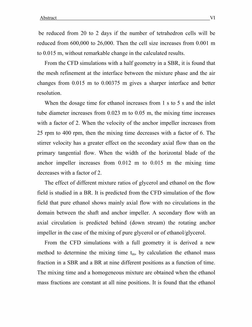
Abstract VI
be reduced from 20 to 2 days if the number of tetrahedron cells will be
reduced from 600,000 to 26,000. Then the cell size increases from 0.001 m
to 0.015 m, without remarkable change in the calculated results.
From the CFD simulations with a half geometry in a SBR, it is found that
the mesh refinement at the interface between the mixture phase and the air
changes from 0.015 m to 0.00375 m gives a sharper interface and better
resolution.
When the dosage time for ethanol increases from 1 s to 5 s and the inlet
tube diameter increases from 0.023 m to 0.05 m, the mixing time increases
with a factor of 2. When the velocity of the anchor impeller increases from
25 rpm to 400 rpm, then the mixing time decreases with a factor of 6. The
stirrer velocity has a greater effect on the secondary axial flow than on the
primary tangential flow. When the width of the horizontal blade of the
anchor impeller increases from 0.012 m to 0.015 m the mixing time
decreases with a factor of 2.
The effect of different mixture ratios of glycerol and ethanol on the flow
field is studied in a BR. It is predicted from the CFD simulation of the flow
field that pure ethanol shows mainly axial flow with no circulations in the
domain between the shaft and anchor impeller. A secondary flow with an
axial circulation is predicted behind (down stream) the rotating anchor
impeller in the case of the mixing of pure glycerol or of ethanol/glycerol.
From the CFD simulations with a full geometry it is derived a new
method to determine the mixing time tm, by calculation the ethanol mass
fraction in a SBR and a BR at nine different positions as a function of time.
The mixing time and a homogeneous mixture are obtained when the ethanol
mass fractions are constant at all nine positions. It is found that the ethanol

Abstract VII
mass fraction near the stirrer reaches a constant value earlier than that near
the shaft of the stirrer.
The new developed modified algebraic slip model (MASM) which
includes the ethanol droplets break up dp(t) as a function of time t by
modeling with a validated step function, gives the real mixing behaviour,
i.e. m (t)η and mixing times tm in a good agreement with the experimental
results in a SBR and a BR. Also the prolongation of the mixing time tm by
a factor of 1.5 caused by the pan cake effect is predicted by the MASM. The
often used algebraic slip model (ASM) and transport model (TRM) give an
unrealistic prediction of the experimental mixing behavior in the case of
ethanol and glycerol.

VIII
Table of Contents
Acknowledgements III
Abstract V
Table of Contents VIII
Nomenclature XV
Latin letters XV
Greek letters XVII
Indices XVIII
Abbreviations XIX
Dimensionless numbers XX
1. INTRODUCTION 1
2. THEORETICAL BACKGROUND 4
2.1 Mixing definition and perspective …....................................................... 4
2.2 Scales of mixing ………………….....………………………….……… 6
2.3 Mixing of liquid-liquid systems ……………….………….....……….... 7
2.4 Miscible and immiscible liquids …......................................................... 8
2.5 Details of the mixing process .........……………………..…..….…….. 10
2.6 Mixing characteristics ……………………………………………....... 11
2.6.1 Mixing time ……………………………....….………...…….. 11
2.6.1.1 Determination …………………….......................….. 11
2.6.1.2 Correlations ……………..…….....................……….. 13
2.6.2 Density differences and viscosity differences …...................... 16
2.6.2.1 Influence on the mixing time ….................................. 17
2.6.3 Flow patterns ………………………..……….….......……….. 23
2.6.3.1 Calculation methods …………..........………...…….. 30
2.6.3.1.1 Sliding mesh model …………...………….... 31
Table of Contents IX
2.6.3.1.1.1 Solution procedures ……………….. 32
2.6.3.1.1.2 Validation ......................................... 32
2.6.3.1.2 Rotating frame model …………..........…….. 33
2.6.3.1.3 Multiple reference frames model .....……….. 33
2.7 Types of stirrers …………………….………….………….....……….. 34
2.7.1 Anchor impeller ……………………......……….......……….. 37
2.8 Semibatch and batch mixing modes ………………………………….. 40
2.8.1 Semibatch operation ……………..…………………….…….. 41
2.8.2 Batch operation …..……………………...……….....……….. 42
2.9 Computational fluid dynamics (CFD) ……..………………...……….. 43
2.9.1 Developments ……………...................………..…...….…….. 43
2.9.2 Applications .....…..………..………....…………………..….. 44
2.9.3 Analysis steps ……..…....……………………….......……….. 45
2.9.4 Mathematical model …………………………………...…….. 46
2.9.5 Numerics .................................................................................. 46
2.9.5.1 Discretisation method …..………………...……….... 47
2.9.5.1.1 Finite difference method ……………..…….. 47
2.9.5.1.2 Finite element method ……………….…….. 48
2.9.5.1.3 Finite volume method …………......……….. 49
2.9.5.2 Iterative solution strategy …………....….....……….. 50
2.9.5.3 Uncertainty and error ……………….…....………..... 50
2.9.5.4 Verification of CFD codes ………………..…..…….. 51
2.9.5.5 Validation of CFD models …………….…...……….. 52
2.9.6 Simulation by CFX-10 software ..............…..............……….. 53
2.9.6.1 Introduction .................................………....………… 53
2.9.6.2 Structure ….........................…...…………………….. 53
2.9.6.2.1 Geometry and mesh generation …….......….. 54
Table of Contents X
2.9.6.2.1.1 Cell types ………..….......………..... 55
2.9.6.2.2 CFX-pre ......................................................... 56
2.9.6.2.3 CFX-solver ……………………………….... 56
2.9.6.2.3.1 Manager ..........……....................….. 57
2.9.6.2.3.2 Modeling .....…...................……….. 58
2.9.6.2.3.3 Numerical discretisation ................... 58
2.9.6.2.3.4 Coupled solver ................................. 59
2.9.6.2.4 CFX-post ……................…….…………….. 60
3. EXPERIMENTS 61
3.1 Mixture components ……...……...………………………………….... 61
3.2 Experimental setup for SBR and BR ...............................…………….. 62
3.3 Methods of measurement in SBR and BR ..............................……….. 63
3.3.1 Torque method …....................................................………..... 63
3.3.1.1 Voltage / Viscosity calibration curve ......................... 63
3.3.2 Decolorisation method …..............................................……... 64
3.4 The procedure of mixing process in SBR …..............................……... 65
3.4.1 td = 5 s (26 vol% ethanol) ......................................................... 66
3.4.2 td = 5 s and td = 10 s (33 vol% ethanol) .................................... 67
3.5 The procedure of mixing process in BR …............................................ 68
3.5.1 Hl = 0.14 m and Hl = 0.09 m (33 vol% ethanol) ….................. 69
3.6 Experimental setup for the visualization of the flow field with a light
cut procedure ......................................................................................... 70
4. CFD SIMULATION AND SUBMODELS 71
4.1 Simulation for half geometry in SBR and BR …......................………. 72
4.1.1 Geometry building …............................................................... 72
4.1.2 Mesh generation …................................................................... 73
4.1.3 CFX-pre …............................................................................... 74

Table of Contents XI
4.1.3.1 Kind of simulation ….................................................. 75
4.1.3.2 Multicomponent modeling ….......................................75
4.1.3.2.1 Mixture density .............................................. 76
4.1.3.2.2 Mixture viscosity .............…...............……... 76
4.1.3.2.2.1 Ideal case .......................................... 77
4.1.3.2.2.2 Nonideal case ................................... 77
4.1.3.2.3 Mixture molar mass …………................…... 77
4.1.3.2.4 Species mass fraction .................................... 78
4.1.3.3 Multiphase flow modeling ...…….....………...……... 78
4.1.3.3.1 Homogeneous model ………..............……... 79
4.1.3.3.1.1 Continuity equation …...............…... 79
4.1.3.3.1.2 Momentum equation ….............…... 80
4.1.3.3.1.3 Volume fraction equation ................. 81
4.1.3.3.2 Free surface flow model …….............……... 81
4.1.3.4 Submodels ……………...………….......................…. 82
4.1.3.4.1 Fluid buoyancy model …............................... 82
4.1.3.4.1.1 Density difference between two
liquids ............................................... 83
4.1.3.4.1.2 Pressure gradient between two
liquids ............................................... 84
4.1.3.4.1.3 Rotating domains ............................. 84
4.1.3.4.1.4 Multiphase flow ............................... 84
4.1.3.4.2 Laminar model …........................................... 84
4.1.3.4.3 Isothermal model …....................................... 85
4.1.3.4.4 Transport model …......................................... 85
4.1.3.4.5 Algebraic slip model ……...…………...…… 87
4.1.3.4.6 Modified algebraic slip model ……...……… 90

Table of Contents XII
4.1.3.4.7 Constraint equation ….................................... 90
4.1.3.4.8 Sliding mesh model …................................... 91
4.1.3.5 Domain conditions ….................................................. 94
4.1.3.5.1 General conditions ……........................……. 94
4.1.3.5.2 Anchor and shaft velocity ….......................... 94
4.1.3.5.3 Fluids …......................................................... 94
4.1.3.5.4 Semibatch reactor ….............................……. 95
4.1.3.5.4.1 Initial conditions …........................... 95
4.1.3.5.4.2 Boundary conditions ….................... 96
4.1.3.5.4.2.1 Wall top ..................................... 96
4.1.3.5.4.2.2 Bottom and cylindrical walls .... 98
4.1.3.5.4.2.3 Shaft and anchor impeller ......... 98
4.1.3.5.4.2.4 Inlet tube …................................ 99
4.1.3.5.4.2.5 Periodic boundary …............... 100
4.1.3.5.5 Batch reactor ...............................…........…. 101
4.1.3.5.5.1 Initial conditions …................……. 101
4.1.3.5.5.2 Boundary conditions ...................... 102
4.1.4 CFX-solver manager ….......................................................... 103
4.1.5 CFX-post ………………………...…..........……...………… 103
4.2 Simulation for full geometry in SBR and BR ….............................… 104
4.2.1 Geometry building …............................................................. 104
4.2.2 Mesh generation …................................................................. 105
4.2.3 CFX-Pre …............................................................................. 106
5. RESULTS AND DISCUSSION 108
5.1 Experimental results …........................................................................ 108
5.1.1 Mixture viscosities as a function of time and the
determination of mixing times ……………...…………...…. 108
Table of Contents XIII
5.1.1.1 Voltage / Viscosity calibration curves …………….. 108
5.1.1.2 Semibatch reactor ………………………….……… 111
5.1.1.2.1 td = 5 s (26 vol% ethanol) …………...……. 111
5.1.1.2.2 td = 5 s (33 vol% ethanol) ……………….... 116
5.1.1.2.3 td = 10 s (33 vol% ethanol) ……………….. 117
5.1.1.3 Batch reactor …………………………………...….. 120
5.1.1.3.1 Hl = 0.14 m (33 vol% ethanol) …………… 120
5.1.1.3.2 Hl = 0.09 m (33 vol% ethanol) …………… 125
5.1.2 Visualization of the dynamic behavior of pure glycerol in a
BR ………………………………………………………….. 129
5.2 Important quantities influencing the mixing behavior predicted by
CFD Simulation ………………………………………………….….. 131
5.2.1 Semibatch reactor ………………………………………...… 131
5.2.1.1 The effect of mesh refinement and cells number ….. 131
5.2.1.1.1 Flow field pattern for 26,000 cells .............. 137
5.2.1.2 The effect of dosage time …………………...…….. 148
5.2.1.2.1 Inlet tube diameter of 5 cm …………….…. 148
5.2.1.2.2 Inlet tube diameter of 2.3 cm …………...… 150
5.2.1.3 The effect of inlet tube diameter ………………..…. 152
5.2.1.3.1 Dosage time td = 1 s ………………………. 153
5.2.1.3.2 Dosage time td = 5 s ……………...……….. 155
5.2.1.4 The effect of anchor velocity ……………………… 157
5.2.1.4.1 Dosage time td = 1 s ……………...……….. 157
5.2.1.4.2 Dosage time td = 5 s ………………….…… 176
5.2.1.5 The effect of anchor dimensions ………...………… 182
5.2.2 Batch reactor ……………………………………………..… 190
5.2.2.1 The effect of different mixture ratios of glycerol to
s
s
Table of Contents XIV
ethanol …………………..………………………… 190
5.2.2.1.1 Glycerol (0.1 m) and ethanol (0.04 m) ….... 190
5.2.2.1.2 Glycerol (0.04 m) and ethanol (0.1 m) ….... 194
5.2.2.1.3 Pure glycerol ………………..…………….. 197
5.2.2.1.4 Pure ethanol ………………………………. 199
5.3 CFD simulations predicting the mixture viscosities as a function of
time and the mixing times in SBR and BR …....………………...….. 202
5.3.1 SBR at td = 5 s (26 vol% ethanol) ………………………..… 202
5.3.2 SBR at td = 5 s (33 vol% ethanol) ………...………………... 210
5.3.3 SBR at td = 10 s (33 vol% ethanol) ……...…………………. 214
5.3.4 BR at Hl = 0.14 m (33 vol% ethanol) ………………………. 217
5.3.5 Step functions of ethanol droplet diameter for CFD
simulations in SBR and BR ………..……...…………...…… 230
5.3.5.1 SBR at td = 5 s (26 vol% ethanol) ….................…… 232
5.3.5.2 SBR at td = 5 s (33 vol% ethanol) …………….…… 233
5.3.5.3 SBR at td = 10 s (33 vol% ethanol) …..................…. 234
5.3.5.4 BR at Hl = 0.14 m (33 vol% ethanol) ……................ 236
5.3.6 The modified CFD-Algebraic slip model (MASM) in
comparison with Algebraic slip model (ASM) and the
Transport model (TRM) in a SBR and a BR ……………… 237
5.3.7 Summary of the measured and calculated mη and tm ……… 239
6. CONCLUSIONS AND OUTLOOK 240
7. REFERENCES 241
List of Publications 256
Oral Presentations 257
Posters Presentations 259
Curriculum Vitae 260
XV
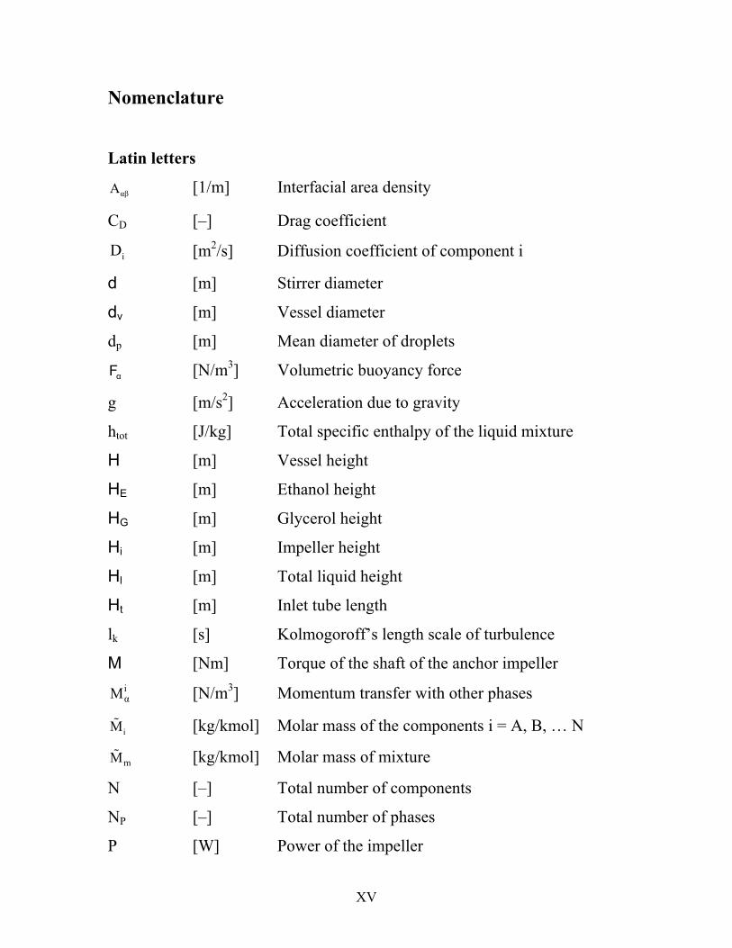
Nomenclature
Latin letters
αβA [1/m] Interfacial area density
CD [–] Drag coefficient
iD [m2/s] Diffusion coefficient of component i
d [m] Stirrer diameter
dv [m] Vessel diameter
dp [m] Mean diameter of droplets
αF [N/m3] Volumetric buoyancy force
g [m/s2] Acceleration due to gravity
htot [J/kg] Total specific enthalpy of the liquid mixture
H [m] Vessel height
HE [m] Ethanol height
HG [m] Glycerol height Hi [m] Impeller height
Hl [m] Total liquid height Ht [m] Inlet tube length
lk [s] Kolmogoroff’s length scale of turbulence
M [Nm] Torque of the shaft of the anchor impeller iαM [N/m3] Momentum transfer with other phases
iM% [kg/kmol] Molar mass of the components i = A, B, … N
mM% [kg/kmol] Molar mass of mixture
N [–] Total number of components
NP [–] Total number of phases
P [W] Power of the impeller

Nomenclature XVI
p [Pa] Pressure
αr [-] Volume fraction of phase α
AαS [kg/(m3s)] Source term in multicomponent multiphase flow
ES [W/m3] Source term in energy equation
MS [kg/(m2s2)] Source term in momentum equation
MSαS [kg/(m3s)] Source term in continuity equation in phase α
iS [kg/(m3s)] Reaction source of component i
T [K] Temperature
t [s] Time
td [s] Ethanol dosage time
tdf [s] Final ethanol dosing time
tdi [s] Initial ethanol dosage time
tk [s] Kolmogoroff time scale of turbulence
tm [s] Mixing time
tm,L [s] Mixing time for a level of uniformity L
U [m/s] Vector of velocity x
y
z
uuu
in bulk liquid
αU [m/s] Vector of velocity x
y
z
uuu
in phase α
WallU [m/s] Velocity at the wall
ijU% [m/s] Mass averaged velocity of component i through
coordinate j
jU% [m/s] Mass averaged velocity through coordinate j
Eu [m/s] Velocity of ethanol feed

Nomenclature XVII
mu [m/s] Flow velocity of the liquid mixture (mixture
velocity)
x
y
z
uuu
[m/s] Velocity in the coordinate directions x, y, z
iCu [m/s] Velocity of component i in continuous phase C iDαu [m/s] Drift velocity of component i in phase α imu [m/s] Velocity of component i in the mixture m iSαu [m/s] Slip velocity of component i in phase α iαu [m/s] Velocity of component i in phase α
V [m3] Volume of the liquid mixture in the vessel
EV& [m3/s] Ethanol volumetric flow rate
wh [m] Horizontal blade width of anchor impeller
x, y, z [m] Cartesian coordinates
iY [kg/kg] Mass fraction of component i
iΥ% [kg/kg] Averaged mass fraction of component i
vy [V] Voltage of the impeller momentum
v,0y [V] Blind voltage of the impeller momentum
v,nety [V] Net voltage of the impeller momentum
vy% [V] Averaged voltage of the impeller momentum
Greek letters ε [W/kg] Energy dissipation
ϕ [–] Volume ratio
η [Pa s] Mixture dynamic viscosity
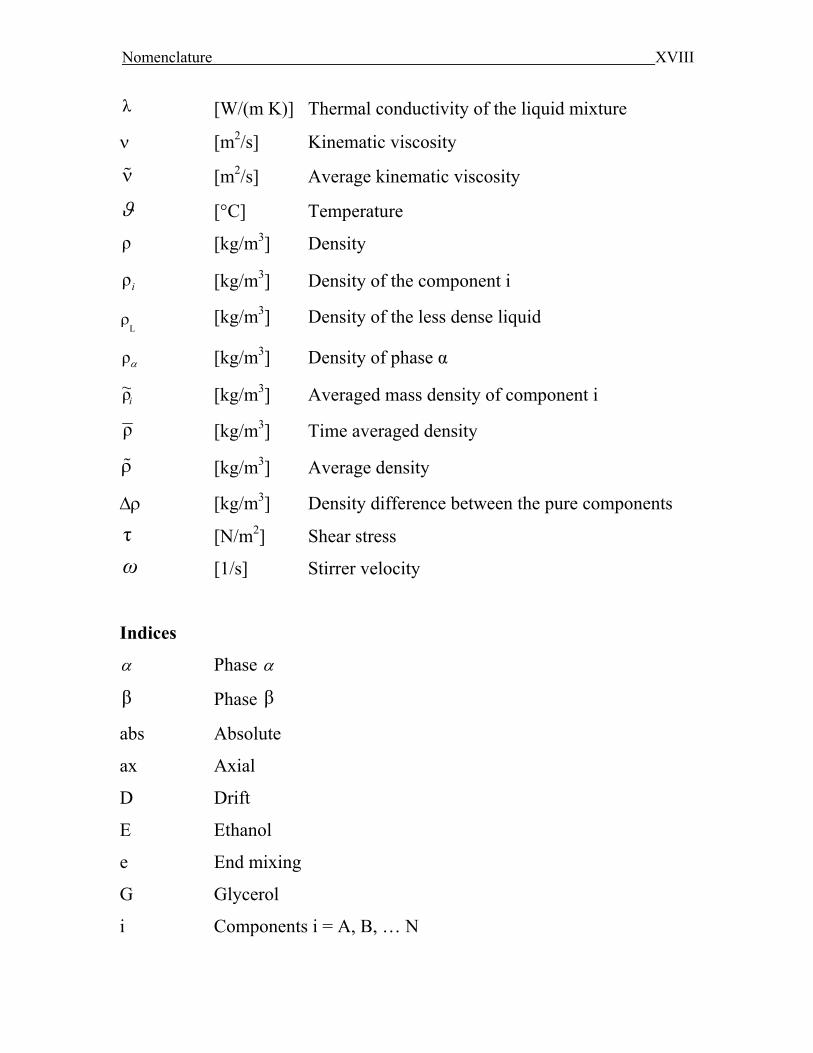
Nomenclature XVIII
λ [W/(m K)] Thermal conductivity of the liquid mixture
ν [m2/s] Kinematic viscosity
ν% [m2/s] Average kinematic viscosity
ϑ [°C] Temperature
ρ [kg/m3] Density
iρ [kg/m3] Density of the component i
Lρ [kg/m3] Density of the less dense liquid
αρ [kg/m3] Density of phase α
iρ~ [kg/m3] Averaged mass density of component i
ρ [kg/m3] Time averaged density
ρ% [kg/m3] Average density
∆ρ [kg/m3] Density difference between the pure components
τ [N/m2] Shear stress
ω [1/s] Stirrer velocity
Indices
α Phase α
β Phase β
abs Absolute
ax Axial
D Drift
E Ethanol
e End mixing
G Glycerol
i Components i = A, B, … N
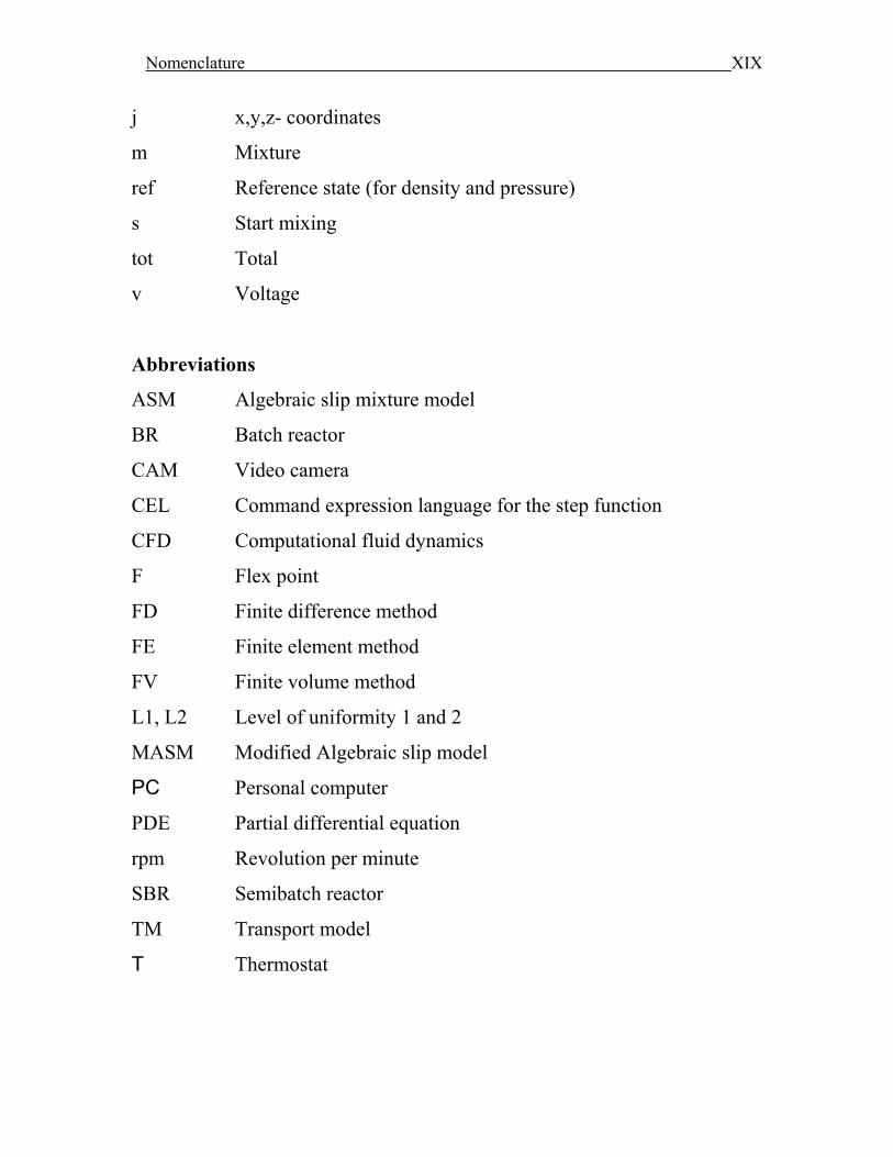
Nomenclature XIX
j x,y,z- coordinates
m Mixture
ref Reference state (for density and pressure)
s Start mixing
tot Total
v Voltage
Abbreviations
ASM Algebraic slip mixture model
BR Batch reactor
CAM Video camera
CEL Command expression language for the step function
CFD Computational fluid dynamics
F Flex point
FD Finite difference method
FE Finite element method
FV Finite volume method
L1, L2 Level of uniformity 1 and 2
MASM Modified Algebraic slip model
PC Personal computer
PDE Partial differential equation
rpm Revolution per minute
SBR Semibatch reactor
TM Transport model
T Thermostat

Nomenclature XX
Dimensionless numbers
Ar Archimedes number (s. Eq. 2-7)
Re Impeller Reynolds number (s. Eq. 2-6)
Re* Modified impeller Reynolds number (s. Eq. 2-9)
Ri Richardson number (s. Eq. 2-5)
1
1. INTRODUCTION
The mixing process is a common and important operation in a wide range
of industries such as polymer processing, petrochemicals, food,
biotechnology, cosmetics and paints. Insufficient understanding of these
processes causes the continuous loss of a large amount of money. The fluids
used in these processes are often highly viscous and have different
viscosities and densities. They are mixed in a semibatch or batch mode.
The literature dealing with the mixing effects of these fluids are mostly
limited to the case of mixing two large volume layers of liquids at the
beginning of the process (Batch mixing process). But, it is much interesting
in the process industry to mix small quantities of the inlet liquid with that in
the vessel while stirring is in progress for fast mixing and/or reactions
(Semibatch mixing process) rather than to begin mixing with large liquids
volumes. Present investigations study the mixing of liquids with density
differences and not consider the viscosity differences and the large volume
inlet liquid in case of semibatch mixing.
Mixing operation may involve difficulties in predicting the mixing time,
whereas high product quality control with a minimum mixing time is needed.
In many investigations of the mixing time in the past, the effects of
differences in viscosity or density have not been taken into account. It is
often not clear whether mixing problems like the scale of homogeneity and
the time available to accomplish mixing are caused by viscosity differences
or by density differences. These can yield unexpectedly long mixing times.
A series of experiments proved the dependence of mixing time on a
combination of viscosity and density differences.
Anchor impellers are often used for mixing high viscosity fluids in the
1. INTRODUCTION 2
range 1-10 Pa s. Very few investigations study these impellers and a little is
done by computational fluid dynamics (CFD) simulations. Anchor impellers
are especially preferred for mixing operations because they generate both
tangential and axial motion, which enhances the mixing efficiency and to
avoid the stagnation of the products at the vessel walls, since the anchor
blades work as a scraper.
The primary tangential flow using a two dimensional grid has been
studied; it is caused by the rotation of the horizontal blade of the anchor
impellers. Three dimensional flow patterns inside the vessel are important to
understand the state of flow of the fluids and the mechanisms responsible for
homogenization and transport processes. Secondary flow is the flow
generated by the action of the inertial forces due to the movement of the
anchor blades; it is generated by the rotation of the vertical blade of the
anchor impeller as well as the hydrodynamic conditions. It is necessary to
get more insight about the detailed picture of the secondary flow to
determine ways in which the mixing process can be improved. The great
majority of computational work for vessels with anchor stirrers presents
computational studies for the primary flow and very coarse grid was used,
but a little is known for the secondary flow and fine grid.
In this work the following topics will be investigated:
1. It should be described the theoretical back ground of the mixing process
of liquids with very high density and viscosity differences. A mixture of
high viscosity glycerol and low viscosity ethanol will be used as a test
mixing process in a semibatch reactor (SBR) and a batch reactor (BR)
with anchor impeller.
2. Viscosity of the liquid-liquid mixture should be measured as a function of
time. The mixing time in the case of a SBR and a BR will be measured.
1. INTRODUCTION 3
Different dosage times will be used in a SBR. The total height of the
liquid mixture will be varied in a BR. Flow field patterns of the dynamic
mixing behaviour will be visualised by a video camera.
3. The mixing phenomena should be described with transient 3D
computational fluid dynamics (CFD) simulations. The commercial
program Ansys CFX-10 will be used for solving the Navier-Stokes
equations. It should be found which kind of submodels must be included
to predict the mixing times. It should be proved to give prediction of the
mixing phenomena with the used liquids in a SBR and a BR.
4. It should be varied the size and the number of the cells by using ICEM
CFD program. The mixing process in a SBR will be calculated at
different dosage times, inlet tube diameters and anchor velocities. It
should be varied the dimensions of the anchor impeller. Different types
of liquids will be used such as pure ethanol, pure glycerol and mixture of
ethanol and glycerol at different compositions in a BR.
5. The time dependent dynamic viscosity of the liquid mixtures, the mixing
times and the flow field patterns should be determined based on CFD
simulations in a SBR and a BR. It will be proved the homogeneity of the
final liquid mixture in these reactors.

4
2. THEORETICAL BACKGROUND
2.1 Mixing definition and perspective
Mixing is understood to be any operation used to change a non-uniform
system into a uniform one. A quantity of matter may be called uniform or
homogeneous when the composition of a volume element of appropriate size
does not deviate by more than a fixed amount from the average composition
of the entire system. Mixing is very often part of a chemical or physical
process, such as blending, dissolving, emulsification, heat transfer and
chemical reactions. Chemical engineering recognizes it as one of the unit
operations.
Mixing can be classified according to the various combinations between
the phases gas, liquid, and solid. Liquid-liquid mixing, for instance, is
understood to be the mixing of two miscible or immiscible liquids.
Important methods of mixing are: flow mixing, e.g. circulation by pumping,
injection; vibrational mixing, e.g. by ultrasonic; mixing by rotating stirrers.
In mixing miscible liquids, the molecular diffusion also contributes to the
ultimate homogeneity of the system to be mixed [2] [57].
Mixing is the reduction of inhomogeneity in order to achieve a desired
process result. The inhomogeneity can be one of concentration, phase, or
temperature. Secondary effects, such as mass transfer, reaction, and product
properties are usually the critical objectives. Mixing process objectives are
critical to the successful manufacturing of a product. If the mixing scale-up
fails to produce the required product yield, quality, or physical attributes, the
costs of manufacturing may be increased significantly, and perhaps more
important, marketing of the product may be delayed or even canceled in
view of the cost and time required to correct the mixing problem. Failure to
2. THEORETICAL BACKGROUND 5
provide the necessary mixing may result in severe manufacturing problems
on scale-up, ranging from costly corrections in the plant to complete failure
of a process. The costs associated with these problems are far greater than
the cost of adequately evaluating and solving the mixing issues during
process development. Conversely, the economic potential of improved
mixing performance is large [75].
Mixing equipment design must go beyond mechanical and costing
considerations, with the primary consideration being how best to achieve the
key mixing process objectives [26]. Useful methods for mixing process
development effort have been evolving in academic and industrial
laboratories over the past several decades. They include improvements to
traditional correlations as well as increasingly effective methods both for
experiments and for simulation and modeling of complex operations. The
combination of these approaches is providing industry with greatly improved
tools for development of scalable operations [75].
Good experimental design based on an understanding of mixing
mechanisms is critical to obtaining useful data and right solutions. The two
principal tools used to investigate mixing phenomena and evaluate mixing
equipment: laboratory experiments and computational fluid dynamics (CFD)
[5]. A wide range of mixing equipment is now available like traditional
stirred tanks, baffling, the full range of impellers, and other tank internals
and configurations. Some study focuses on rotor-stators, which have been
used for many years [75].
Mixtures are different from single components because [77]:
(1) There is a new property, composition, associated with a mixture.
(2) Properties may not be a simple combination of those of the constituents.

2. THEORETICAL BACKGROUND 6
(3) If two or more phases are formed from a mixture, these have in general
different compositions.
(4) Reactions are associated with mixtures as there will be at least two
species present.
(5) Mixtures can be ideal when most properties combine in a readily
predictable manner or nonideal when they do not. In ideal mixture each
component is assumed to behave as it would in the absence of other
chemical species. If there is any form of chemical interaction between the
species, the mixture will be nonideal and properties cannot be simply
combined, this happens when the substances which are polar and
substances in a mixture have different functional groups.
2.2 Scales of mixing
- Macromixing is a mixing driven by the largest scales of motion in the fluid.
- Mesomixing is a mixing on a scale smaller than the bulk circulation (or the
vessel diameter) but larger than the micromixing scales, where molecular
and viscous diffusion become important. Mesomixing is most frequently
evident at the inlet tube of semibatch reactors.
- Micromixing is a mixing on the smallest scales of motion and at the final
scales of molecular diffusivity. It is the limiting step in the progress of fast
reactions, because micromixing dramatically accelerates the rate of
formation of interfacial area available for diffusion. This is the easiest way
to enlarge contact area at the molecular level, since the molecular
diffusivity remains more or less constant [75].
2. THEORETICAL BACKGROUND 7
2.3 Mixing of liquid-liquid system
Liquid-liquid mixing is one of the most difficult and least understood
mixing problems. Mixing in vessels is an important area when considering
the number of processes which are accomplished. Essentially, any physical
or transport process can occur during mixing [132]. Qualitative and
quantitative observations, experimental data, and flow regime identifications
are needed and should be emphasized in any experimental pilot studies in
mixing [141].
Fluid mechanics and geometry are key points to understand mixing. The
fluid mechanics transports the liquid in the vessel, whereas the geometry
determines the fluid mechanics [137]. Liquid-liquid dispersion is very much
dependent on the shape of the tank bottom, the geometry of the impeller, the
relative size of the vessel to the impeller and power draw on the impeller
geometry [142].
Mixing efficiency in a stirred vessel is affected by e.g. baffles, impeller
speed, impeller type, clearance, vessel geometry and position of the impeller
[147]. Mixing, mass and heat transfer between phases or external surfaces
can be accomplished by stirring. The operation of stirring, which includes
mixing as a special case, is now well established as an important and in a
wide variety of chemical processes [149]. Specifically, stirrers are applied to
three general classes of problems [56]:
(1) To produce static or dynamic uniformity in multicomponent multiphase
systems.
(2) To facilitate mass or energy transfer between the parts of a system not in
equilibrium.
(3) To promote phase changes in multicomponent systems with or without a
change in composition.
2. THEORETICAL BACKGROUND 8
Stirring plays a controlling role in the liquid-liquid systems. It controls
the breakup of drops (dispersion), the combining of drops (coalescence) and
the suspension of drops within the system [135]. The magnitude and
direction of convective flows produced by a stirrer affect distribution and
uniformity throughout the vessel as well as the kinetics of dispersion.
Stirring intensity is important, because the intense turbulence found near the
impeller leads to drop dispersion, not coalescence [25]. Lower turbulence or
laminar/transitional conditions found elsewhere in the vessel promote
coalescence by enabling drops to remain in contact long enough for them to
coalesce. Laminar shear also leads to drop dispersion [143]. If a drop is
stretched beyond the point of critical elongation, it breaks. If not, it returns
to its prestressed state [75]. Liquid mixing problems in laminar flow tend to
be very difficult in the pharmaceutical, food, polymer, and biotechnological
processes. They are carried out at low velocities or involve high viscosity
substances, such as detergents, ointments, creams, suspensions, antibiotic
fermentations, and food emulsions [72]. Both the mixing system and
duration of mixing have an important effect on drop size distribution, drop
breakup, and coalescence [75].
2.4 Miscible and immiscible liquids
Blending is the mixing of two or more miscible liquid components into a
more uniform mass [62]. Poor blending leads to concentration and
temperature gradients, which affect the product quality and yield. The
blending of miscible liquids is carried out for many purposes: to adjust the
pH in fermentation, viscosity in diluting or thickening and temperature in
sterilization to blend ingredients; to promote reactions in polymerization; to
avoid stratification in storage tanks [97]. Miscible liquid blending is the
2. THEORETICAL BACKGROUND 9
easiest mixing task. The miscible blending requires two things: The streams
must be completely soluble, and there must be no resistance to dissolution at
the fluid interface [75]. As soon as the two miscible liquids come into
contact, diffusion will produce a region of intermediate viscosity between
the bulk liquids. Although there may be considerable differences in the free
energy of the bulk materials, there is no phase discontinuity to give rise to
localized forces equivalent to an interfacial tension [69].
The term miscible refers to the property of various substances,
particularly liquids, that allows them to be mixed together and form a single
homogeneous phase [133]. For example, water and ethanol are miscible in
all proportions. By contrast, substances are said to be immiscible if they
cannot be mixed together, for example, oil and water. In organic compounds,
the length of the carbon chain often determines miscibility relative to
members of the homologous series. For example, in the alcohols, ethanol has
two carbon atoms and is miscible with water, whereas octanol has eight
carbon atoms and is not miscible with water. Miscibility can arise for a
number of reasons. In the alcohol examples above, the OH-group can form
hydrogen bonds with water molecules [81].
The term immiscible liquid-liquid system refers to two or more insoluble
liquids present as separate phases. These phases are referred to as the
dispersed or drop phase and the continuous phase. The dispersed phase is
usually smaller in volume than the continuous phase, but under certain
conditions, it can represent up to 99% of the total volume of the system
[136]. In dispersion, a two-phase system in which one phase is broken into
discrete particles which are completely surrounded by the second phase.
Particles may be solid, liquid or gas. For mixing purposes, the second phase
is generally a liquid [75] [62].
2. THEORETICAL BACKGROUND 10
2.5 Details of the mixing process
The history of added liquid to a liquid in a stirred tank is determined by a
combination of factors. Depending on the conditions in the vessel, the
properties of the liquids and the position of the addition point. The added
liquid may pass through several of four main zones: the stirrer region; the
free surface, the bottom of the vessel and the bulk. In each zone there is a
chance that the liquid drops will be divided into smaller drops or mixed into
the bulk liquid. In addition, in each zone the liquid drops have a chance to
move to another zone. If all these chances are known, a prediction of the
mixing time and of its expected standard deviation can be made. The
impeller's energy input is divided between large-scale flow and turbulence,
depending on the type of impeller. The distribution of these two flow types
over the regions in the vessel are also determined by the stirrer. Thus, each
region makes its own characteristic contribution to the process of mixing,
depending on the type of impeller and the flow conditions in the vessel [55]:
(1) In the stirrer region the turbulence intensities as well as the shear forces
are high, so that drops have a good chance of breaking up. Especially
when the viscosity of the added liquid is high compared to that of the
bulk, these shear forces are very important for the mixing process,
because in other parts of the vessel the shear forces may be too weak to
cause break-up. Drops may also be divided by physical contact with the
stirrer. The circulation time is the time between two passages of a liquid
volume through the impeller, is determined by the large scale flow. If a
drop is not broken up during a passage through the impeller, the mixing
time will be increased by circulation time before the drop will pass the
stirrer again.
(2) In the bulk, the shear stresses and the level of turbulence are lower, but

2. THEORETICAL BACKGROUND 11
deformed drops may be deformed further or be mixed completely.
(3) The large scale flow combined with the net force, resulting from density
differences, determines whether a drop reaches the free surface or the
bottom of the tank. If this happens, the added liquid will generally remain
there provided the net force is in the appropriate direction. The liquid can
then reenter the bulk by turbulent eddies or disappear by means of
diffusion. Both mechanisms yield relatively long mixing times.
2.6 Mixing characteristics
2.6.1 Mixing Time
The mixing time is defined as the required time to achieve certain degree
of homogeneity and to get a uniform mixture of two miscible liquids [46]
[62]. The prediction of mixing time is important and needed e.g. for the
purpose of quality control [32]. The mixing time for liquids of very different
physical properties can be long [123]. The added material has a tendency to
float at the surface or go to the vessel base due to the density difference.
Similarly, if the viscosity of the added material is much higher, due to
resistance to deformation, the mixing time will be much longer than for
liquids of similar properties [57] [55] [97].
2.6.1.1 Determination
The mixing time or homogenizing time designates the time which the
stirrer needs in order to obtain a desired homogeneity degree. There are
different measuring methods to determine the mixing time like [41] [85]:
(1) Probe methods.
(2) Schlieren method.
(3) Chemical methods.
2. THEORETICAL BACKGROUND 12
The determination of the mixing time by means of Probe methods
usually takes place with conductivity electrodes or photoelectric probes. The
advantage of this method is a relatively precise measurement of the
homogeneity degree within fluids of the medium. Since the homogeneity
degree is not reached at the same time at each place in the vessel, only a
partial mixing can be measured with several probes. The same problem
results also in the case of the measurement of pH values and temperature by
means of probes. Additionally the influence of diffusion is no longer
negligible.
The Schlieren method is an optical used technique to determine the
moment at which uniformity is reached. Optical inhomogenieties of the
liquid in the mixing vessel, in the form of gradients in refractive indices, will
produce Schlieren, whereas absence of the latter indicates homogeneity of
the liquid mixture. The mixing time is the time between the instant when the
stirrer starts mixing and the instant of disappearance of the Schlieren [57].
The chemical method is a measuring procedure developed by Käppel [87]
with which one of the liquids to be mixed is colored by an iodine solution;
the other transparent one contains a stoichiometric quantity of sodium
thiosulfat. The iodine liquid mixture is decolorised after the following
reaction with sodium thiosulfate [30] [31]:
→2 2 2 3 2 4 6I + 2Na S O 2NaI + Na S O
During most past investigations of the mixing time the liquids differed
only in the added chemical components (e.g. sulfuric acid/caustic solution
with phenolphthalein as indicator or sodium thiosulfate/iodine with starch as
indicator), the mixing time was determined when the reaction is completed
and determined by the indicator change with time (so called chemical
2. THEORETICAL BACKGROUND 13
decolorisation method) [58]. This technique can be followed by visual
observations using a video camera to see the color change during the
reaction. When the mixed liquids have negligible density and viscosity
differences, then the mixing time is determined from the number of
revolutions, the stirrer diameter and the kinematic viscosity of the medium.
The dimensionless mixing time is the product of the impeller speed and
mixing time, its value represents the number of revolutions an impeller must
make to blend the liquid [97].
2.6.1.2 Correlations
Hoogendoorn et al. [67] used several ways to represent their
experimental mixing time tm data in graphs. When comparing similar types
of impellers they plot the dimensionless mixing time against the impeller
Reynolds number. The value of dimensionless mixing time can be
interpreted as the number of stirrer revolutions needed for homogenization.
They introduced two dimensionless groups:
22m3
m
ρ P t = . t ηη v
vdd
f (2-1)
The left hand side of the equation (2-1) is a function of a modified
impeller Reynolds number which can be given in a form of diagram for
different types of stirrers as can be seen in Fig. 2.1. Also, the left hand side
of the equation (2-1) can be interpreted as [55]:
k
2 22 2m mm m3 3 2
1P t P t= t t . ρ t
ε∝ =
η ν νv vd d (2-2)
Where tk is Kolmogoroff’s time scale of turbulence = (ν/ ε )0.5. The left
hand side group ranges from 104 to 108, so tm / tk ranges from 102 to 104.
2. THEORETICAL BACKGROUND 14
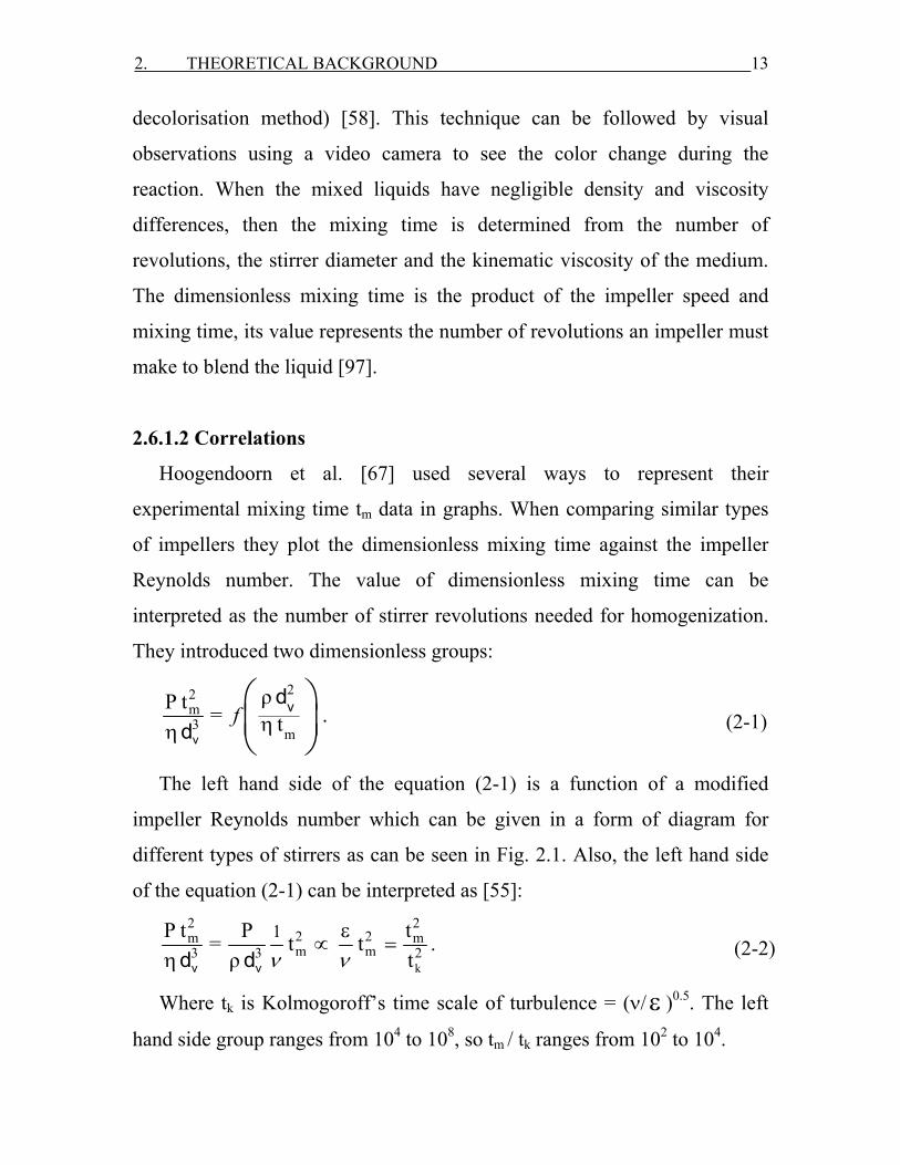
Figure 2.1: The dimensionless group 2 3mP t )(η vd as a function of modified impeller
Reynolds number 2mρ t )(ηvd for different types of stirrers [67]. 1: Turbine + baffles, 1a:
Turbine, 2: 3 inclined-blade paddles, 3: 3 inclined-blade paddles + draught tube, 3a: 1 inclined-blade paddles + draught tube, 4: Screw, 5: Screw + draught tube, 6: Ribbon, 7: Propeller A + draught tube, 8: Propeller B + draught tube, 8a: Propeller B, 9: Anchor.
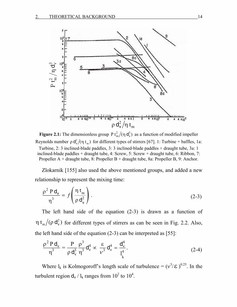
Zlokarnik [155] also used the above mentioned groups, and added a new
relationship to represent the mixing time:
( )2m23
t P .ρ
ηρ=
ηv
v
dd
f (2-3)
The left hand side of the equation (2-3) is drawn as a function of 2
m t (ρ )η vd for different types of stirrers as can be seen in Fig. 2.2. Also,
the left hand side of the equation (2-3) can be interpreted as [55]: 2 3 4
4 43 3 4
k
P P= .ρ lν3 3
ρ ρ ε∝ =
η ηv v
v vv
d dd dd
(2-4)
Where lk is Kolmogoroff’s length scale of turbulence = (ν3/ ε )0.25. In the
turbulent region dv / lk ranges from 102 to 104.
2mρ tηvd

2. THEORETICAL BACKGROUND 15
Figure 2.2: The dimensionless group 2 3P )ρ (ηvd as a function of 2m t (ρ )η vd for
different types of stirrers [155]. a: Anchor with 4 blades, b: Anchor with 2 blades, c: Spiral, d: Flat-blade with alternative current, e: Flat-blade without alternative current, f: Cross bar without alternative current, g: Cross bar with alternative current, h: Lattice
without alternative current, i: Lattice with alternative current, k: Propeller stirrer.
The above two literatures did not consider the effect of viscosity or
density differences. Rielly et al. [156] examined the mixing of two layers of
different viscosity, initially stratified as a result of a density difference in a
batch mixing situation. The mixing time correlation can be found from
drawing the dimensionless mixing time as a function of Richardson number
Ri which is defined as:
2 2L
gRi .
ρ=
ωlH
d∆ρ
(2-5)
Where d is the stirrer diameter, Hl is the liquid height and ∆ρ = ρ1 ρ2.
2m vη t ρ d
2. THEORETICAL BACKGROUND 16
2.6.2 Density differences and viscosity differences
Blending miscible liquids of different viscosities or densities is a
common operation in the process industries. This operation may involve
difficulties in predicting the mixing time [145]. Because is often not clear
whether mixing problems arising in these cases are caused by viscosity
differences or by density differences [73]. Moreover, in many investigations
in the past the effects of differences in viscosity or density have not been
taken into account [55]. The main problem with micromixing of liquids of
different viscosities is concerned with a proper modeling of deformation of
fluid elements, which generates the contact surface between the mixed
materials [134]. Any differences in viscosity of mixed liquids produce
discontinuity of the velocity gradients at an intermaterial surface, which may
lead to destabilization of laminar flow during mixing [54].
Rożeń et al. [53] investigated the mixing of two miscible liquids of
different viscosities in Couette flow (refers to the laminar flow of a viscous
liquid in the space between two surfaces, one of which is moving relative to
the other) by means of a single decolorization reaction to visualize mixing
and flow destabilization. They found that the simple laminar flow becomes
unstable when the contacted liquids have different viscosities. This
destabilization leads to formation of small streak and structures consisting
elements of one liquid, which remain segregated from the surrounding
liquid; for example an elongated filaments or a drop like inclusion are
transformed into a set of ellipsoidal or more complex structures, also the
flow becomes completely irregular.
Bouwmans et al. [55] studied the effect of density and viscosity
differences of different liquids on the mixing time when they are mixed
under different conditions like the type and speed of the stirrer, also the
2. THEORETICAL BACKGROUND 17
point of liquid addition to the second liquid in the vessel. They found that
the roll of the density and viscosity differences depends on the way the
energy input of the impeller is divided and distributed in the vessel
depending on the produced flow type. Also, when a liquid less dense than
the bulk liquid is added near the surface buoyancy effects, large mixing time
is obtained [146]. Low stirrer speeds yields long mixing time. When liquid is
added near the impeller, the mixing time is not affected by the density and
viscosity differences.
Smith et al. [69] carried out blending experiments of small quantities of
high viscosity additives into a turbulent low viscosity liquid. Mixing times
were measured by using conductivity method. They found that the higher
viscosity does not itself retard the later stages of blending and the addition
near the impeller shaft on the free surface is generally reliable and efficient,
also higher impeller speeds reduce the danger of settling out and adhesion of
the viscous material to arbitrary surfaces.
Bouwmans et al. [68] made measurements with very small quantities of
additions to viscous bulks; they found that density differences are more
likely to cause longer mixing times than viscosity differences.
2.6.2.1 Influence on the mixing time
Zlokarnik [58] [45] [83] determined the influence of density and
viscosity differences on the mixing time. The investigations were made with
cross bar stirrer in reinforced containers, so that with high viscosity
differences the two phases do not together-slide and/or with large density
variations no centrifugation effects arise. When homogenizing liquids
without density and viscosity differences in the vessel with a given type of
stirrer and installation, the mixing time tm is dependent on the stirrer
2. THEORETICAL BACKGROUND 18
velocity ω , the stirrer diameter d, the density ρ of the liquid, kinematic
viscosity ν and acceleration of gravity g.
When homogenizing liquids with different density and viscosity, the
mixing time is affected by the density ρ2 and kinematic viscosity ν2 of the
second mixing component which have the low density and viscosity value as
well as by the volume ratio ϕ = V2/V1 of the pure liquids which will be
homogenized (where V2 is the volume of the second mixing component
which have low density and viscosity value) , also the connection of g with
the density difference ∆ρ = ρ1 ρ2 between the pure components with the
term ∆ρ g has an influence on the mixing time. He used a similarity theory
to correlate the dimensionless mixing time as a function of impeller
Reynolds number Re and Archimedes number Ar which are defined as:
Re = ω d2 / %ν . (2-6)
Ar = d3 ∆ρց / ( %ν 2 %ρ ). (2-7)
Where %ν and %ρ are the average kinematic viscosity and density of the
mixed components, respectively. When homogenizing two soluble liquids
with a small density difference of ∆ρ ≤ 0.5 g/cm3, then ∆ρ has no influence
on ω tm. Zlokarnik found from the similarity theory and the experimental
measurements the following mixing time correlation:
mtω = 51.6 Re 1− (Ar1/3 + 3). (2-8)
Equation (2-8) is valid for 101 < Re < 105, 102 < Ar < 1011,
1 < ν1 /ν2 < 5300, 0.1 < ϕ < 1 and ∆ρ > 0.5 g/cm3.
The effect of density difference on the mixing time when the second
liquid component is added at different injection positions in SBR is studied
2. THEORETICAL BACKGROUND 19
by Bouwmans et al. [55]. They have considered two cases based on
∆ρ = ρ1 ρ2:
Case 1: ∆ρ ≥ 0
In this case the difference between the densities of the added liquid (ρ1)
and that of the bulk (ρ2) was always positive or zero. This causes the tracer
liquid to be drawn into the stirrer in all injection cases, so that injection of
the tracer near the surface results in the same mixing times as injection near
the stirrer, provided that the added liquid does not adhere to the vessel.
Case 2: ∆ρ ≤ 0
(a) Injection near the surface: When tracer liquid is injected about 1 cm
below the free surface the mixing time is strongly influenced by
density differences.
(b) Injection in the stirrer plane: When tracer liquid is added near the
stirrer, in a region where both shear stresses and turbulence intensities
are high, the mixing time is low and practically constant and the
relative standard deviation is small.
The effect of both density and viscosity differences of the miscible
liquids and the buoyant additions of small quantities of the liquids on the
mixing time measurements in turbulently stirred vessels are studied by
Bouwmans et al. [68]. They defined the Richardson number which includes
the density difference between the mixed liquids (see equation 2-5). Three
control regimes for buoyant additions based on a Richardson number were
determined:
(1) The stirrer regime when the liquid is added near the stirrer and when the
bulk flow succeeds in transporting all of the added liquid to the stirrer,
then the homogenization time depends on the rate of distribution of the
2. THEORETICAL BACKGROUND 20
added liquid over the vessel. The mixing time is independent on the
viscosity ratio, the location of the injection and the added liquid volume
for small volume ratio between the added and the bulk liquids, the
mixing times are equal to those for liquids of equal properties [148].
(2) The gravity regime when the liquid is added at the surface. The mixing
time is dependent on the viscosity and density differences, very long
mixing times can result.
(3) The intermediate regime when only part of the added liquid is
transported to the stirrer. The mixing time is unpredictable and can be
any where between the stirrer controlled mixing time and the gravity
controlled mixing time, and strongly depends on the amount of liquid that
is added at the surface.
The effect of viscosity differences when adding a small quantity of a
viscous liquid to water in a turbulently stirred vessel on the mixing time at
different impeller types and sizes and at different diameters of the stirred
vessels are studied by Pip et al. [98]. They considered a modified Reynolds
number ( Re* ), that incorporates the ratio of bulk to added viscosities
( 2 1/η η ), to identify the operating regime over which the addition of the
liquid has an effect on the mixing time:
2 2
2 1
2 .
η= η η
ω ρRe* d (2-9)
The stirrer regime when Re* >102 is considered, where the following
mixing time correlation for similar property liquids can be used to calculate
mixing time for a given level of uniformity L1 (0 < L1 < 1) from a measured
value of mixing time for another level of uniformity L2:

2. THEORETICAL BACKGROUND 21
( )( )
m,L1
m,L2
t ln 1.0 L1 .t ln 1.0 L2
−=
− (2-10)
The added liquid regime when Re* <102 is considered, in which the
blending process is considerably slower, mixing time depends on the
physical property differences as well as the impeller speed and the method
and location of addition. They found when the turbulent Reynolds or shear
stresses of the bulk liquid is higher than the viscous shear stress of the added
liquid, then the added liquid will be deformed and mixed rapidly. Also, large
viscosity differences require much longer mixing times which need to be
considered carefully in terms of product quality and energy requirements of
the process, the extent to which the mixing time is increased depends on the
operating conditions. The effect of the viscosity difference is more important
in small scale vessels. Increasing the ratio of the impeller diameter to the
vessel diameter or increasing the input power can reduce the mixing time in
the stirrer regime for similar property liquids. Using a small diameter and/or
low power number impeller gives shorter mixing times at a given power
input. They proposed the following correlation to calculate the mixing time
for turbulent mixing is:
m
1/31/32/3 ρVt 5.91 .
P =
vv
ddd (2-11)
The influence of the radial position of addition point of the tracer when
using sliding mesh model via CFX on the simulated flow field and mixing
times in the high transitional and turbulent flow regime for a vessel stirred
by a Rushton turbine are investigated by Bujaski et al. [44]. They found that
the radial distance from the wall of the vessel had a very big effect on both
mixing time and the development of the concentration field. When the
2. THEORETICAL BACKGROUND 22
addition point was close to the sliding mesh surface, the simulation was in a
good agreement with the empirical predictions whilst that for a point close to
the wall was much too longer. They proposed the following correlation to
calculate the mixing time for any level of uniformity L, where 0 < L < 1:
m,L 2.17 0.5
ln(1 L)t = .
1.06
− −
v
v
d dd H
(2-12)
The effects of turbulence model and different tracer adding and detecting
positions on the macro-mixing and mixing time in a baffled stirred vessel
with Rushton turbine are studied by Guozhong et al. [154]. 3D simulation
was done using the CFD package CFX-4.3. A sliding mesh model was used
to account for the relative movement impeller and baffles. The calculated
mixing times from CFD were compared with those obtained from tracer
experiments at different adding positions. They found that different tracer
adding position gives different mixing times. Mixing simulation highly rely
on the flow field prediction from different turbulence models.
The effects of various geometrical parameters of the mixing equipment
(e.g. wall-clearance and blade width) on the overall homogenization process
to optimize the mixing efficiency when mixing Newtonian viscous fluids
with a helical ribbon impeller are studied by Delaplace et al. [153]. The
degree of homogeneity is followed using a conductivity method after a tracer
injection. They showed that using the time-dependent stirrer velocity during
the mixing process allows energy saving. The mixing times have been
determined from tracer method.
2. THEORETICAL BACKGROUND 23
2.6.3 Flow patterns
Mixing by stirring of liquids involves the transfer of momentum from the
moved stirrers to the liquid. According to the way in which this occurs,
stirrers may be divided into two categories [57]:
(1) The momentum is transferred by shearing stress, i.e. the transfer is
perpendicular to the direction of flow. This category includes the cone
stirrer, the bulb stirrer and the rotating disc.
(2) The momentum is transferred by normal stress, i.e. the transfer is in the
direction of flow. This category includes the paddle stirrer, the
turbomixer and the propeller.
Flow patterns are influenced by the type of impellers. There exists four
categories axial, radial, tangential and secondary flow [13] [14]:
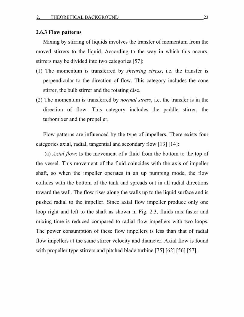
(a) Axial flow: Is the movement of a fluid from the bottom to the top of
the vessel. This movement of the fluid coincides with the axis of impeller
shaft, so when the impeller operates in an up pumping mode, the flow
collides with the bottom of the tank and spreads out in all radial directions
toward the wall. The flow rises along the walls up to the liquid surface and is
pushed radial to the impeller. Since axial flow impeller produce only one
loop right and left to the shaft as shown in Fig. 2.3, fluids mix faster and
mixing time is reduced compared to radial flow impellers with two loops.
The power consumption of these flow impellers is less than that of radial
flow impellers at the same stirrer velocity and diameter. Axial flow is found
with propeller type stirrers and pitched blade turbine [75] [62] [56] [57].
2. THEORETICAL BACKGROUND 24
Figure 2.3: Axial flow pattern of pitched blade turbine [75].
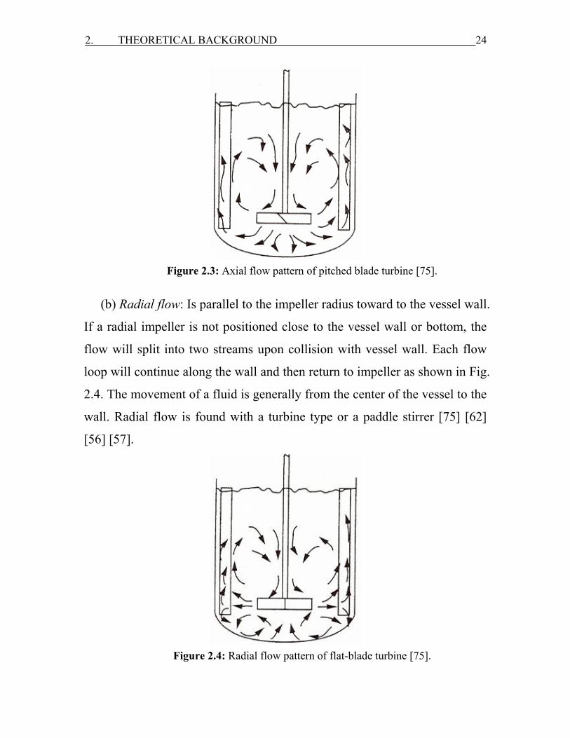
(b) Radial flow: Is parallel to the impeller radius toward to the vessel wall.
If a radial impeller is not positioned close to the vessel wall or bottom, the
flow will split into two streams upon collision with vessel wall. Each flow
loop will continue along the wall and then return to impeller as shown in Fig.
2.4. The movement of a fluid is generally from the center of the vessel to the
wall. Radial flow is found with a turbine type or a paddle stirrer [75] [62]
[56] [57].
Figure 2.4: Radial flow pattern of flat-blade turbine [75].
2. THEORETICAL BACKGROUND 25
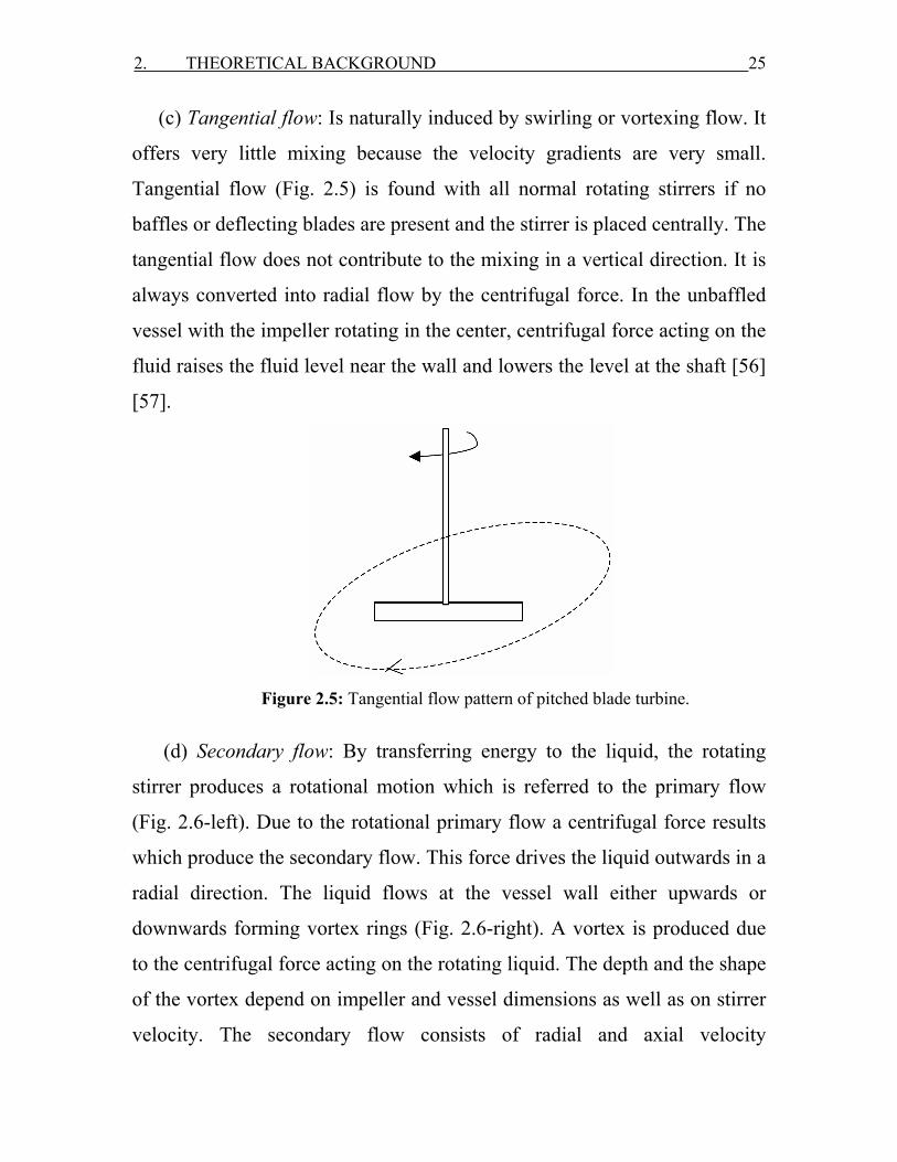
(c) Tangential flow: Is naturally induced by swirling or vortexing flow. It
offers very little mixing because the velocity gradients are very small.
Tangential flow (Fig. 2.5) is found with all normal rotating stirrers if no
baffles or deflecting blades are present and the stirrer is placed centrally. The
tangential flow does not contribute to the mixing in a vertical direction. It is
always converted into radial flow by the centrifugal force. In the unbaffled
vessel with the impeller rotating in the center, centrifugal force acting on the
fluid raises the fluid level near the wall and lowers the level at the shaft [56]
[57].
Figure 2.5: Tangential flow pattern of pitched blade turbine.
(d) Secondary flow: By transferring energy to the liquid, the rotating
stirrer produces a rotational motion which is referred to the primary flow
(Fig. 2.6-left). Due to the rotational primary flow a centrifugal force results
which produce the secondary flow. This force drives the liquid outwards in a
radial direction. The liquid flows at the vessel wall either upwards or
downwards forming vortex rings (Fig. 2.6-right). A vortex is produced due
to the centrifugal force acting on the rotating liquid. The depth and the shape
of the vortex depend on impeller and vessel dimensions as well as on stirrer
velocity. The secondary flow consists of radial and axial velocity
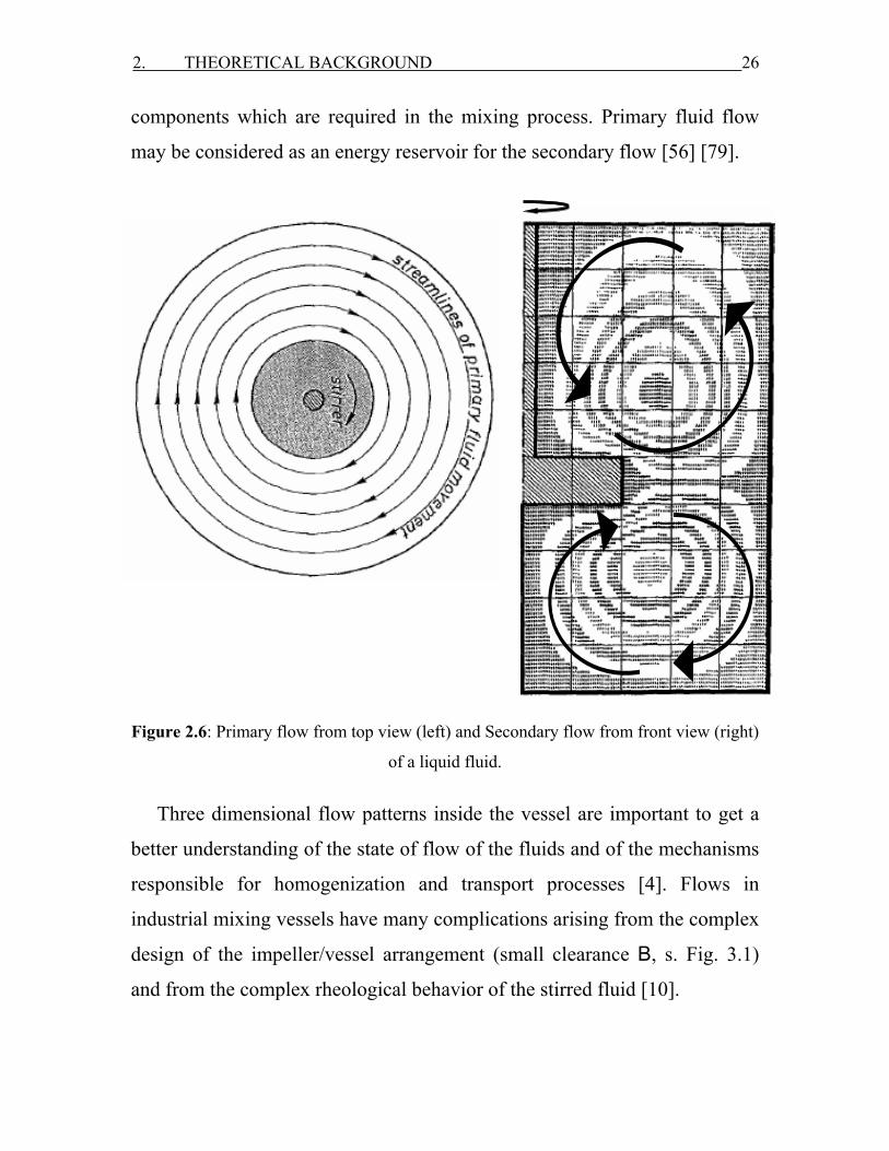
2. THEORETICAL BACKGROUND 26
components which are required in the mixing process. Primary fluid flow
may be considered as an energy reservoir for the secondary flow [56] [79].
Figure 2.6: Primary flow from top view (left) and Secondary flow from front view (right)
of a liquid fluid.
Three dimensional flow patterns inside the vessel are important to get a
better understanding of the state of flow of the fluids and of the mechanisms
responsible for homogenization and transport processes [4]. Flows in
industrial mixing vessels have many complications arising from the complex
design of the impeller/vessel arrangement (small clearance B, s. Fig. 3.1)
and from the complex rheological behavior of the stirred fluid [10].

2. THEORETICAL BACKGROUND 27
In the case of small clearance B when using a laser beam [1], no
experimental data can be measured and consequently it is impossible to
obtain the velocity profile at whole stage during a cycle (a cycle is the
required time for impeller to rotate one revolution), although a detailed
characterization of the three dimensional flow pattern inside the vessel is
important to get a better understanding of the flow state of the fluids and of
the mechanisms responsible for homogenization and transport processes.
Ohta et al. [54] proposed the numerical study for a Newtonian fluid
mixing in stirred vessels having different diameters. They studied a two
dimensional model for secondary flow to express the flow field in the
vertical plane of an anchor stirred vessel, the anchor has only long vertical
blade without horizontal blade. The effect of the clearance and the anchor
velocity on the flow field was studied. They found that two vortices are
formed in the upper and lower region of the vessel. The number and flow
rate of axial circulations become greater with an increase of the anchor
velocity. The stirrer velocity has a greater effect on the secondary axial flow
than on the primary tangential flow. The centre of the vortex seems to be
poorly mixed region.
Abid et al. [52] studied a three dimensional model applied to the flows
generated in a vessel by anchors stirrers in a laminar flow regime. Long
anchor stirrer without horizontal shaft and short anchor stirrer with
horizontal shaft are used for comparison of the mixing efficiency. The
secondary flows induced by anchor stirrer are investigated. The effects of
clearance B or the ratio of B/dv, the height Hi (s. Fig. 3.1) of the vertical
blades or the ratio Hi/Hl on the flow field and mixing were studied. They
found that the horizontal blades enhance the axial circulation and the vertical
blades are more efficient if their tips are slightly below the liquid level.
2. THEORETICAL BACKGROUND 28
Secondary flows are created between the blades and the central shaft when
short anchor stirrer with horizontal shaft is used, this enhance the mixing in
the vessel, by producing new axial circulations. Velocity of the stirrer or
Reynolds number influence the appearance of more or less recirculation
loops behind the blades, but does not change the flow structures. A large
upward axial flow is generated, and the radial movement increases,
compared with the long anchor for the same liquid level in the vessel. A big
recirculation is noted behind the crossing of the two blades below the stirrer,
near the bottom of the vessel. Primary tangential flow is created by the
rotation of the horizontal blade. They found that short anchor with the
horizontal blade is the best to use because it requires lower power
consumption and produces axial circulations; this achieves a best mixing at a
low price.
Peters et al. [49] [43] studied experimentally the flow patterns, velocity
profiles and mixing times in anchor stirred vessels. The effect of the anchor
velocity and blade-to-wall clearance on the velocity profiles and vortex
formation were determined. A dye coloration and decolorization technique is
used in the first experiment to measure the mixing time which is defined as
the time required to disperse the dye. The motion of the fluid was followed
by taking a cine record of the movement of small suspended polyethylene
and polystyrene beads in the second experiment. They found that as the
anchor velocity and Reynolds number increase, the flow reversal behind the
blade tip increases, also longer and larger vortices are formed. Decreasing
the clearance causes the vortices to be formed at lower Reynolds number
because of the greater amount of fluid flowing around the inside edge of the
blade at a higher velocity than at higher clearance. As the stirrer velocity
increases, the mixing rate increases up to a certain limit, then it decreases
2. THEORETICAL BACKGROUND 29
again. Vertical vortices are formed between the blades and the centre shaft.
The vortex core is the last region to be mixed. The vertical circulations are
resulting in a greater degree of homogenization. The primary flow of the
anchor impeller is attributed to horizontal blade and the secondary flow to
the vertical blades as well as the hydrodynamic conditions.
Peixoto et al. [8] studied the behavior of the stirred vessels with anchor
impellers using a computational fluid dynamics approach. CFX-4.2 software
tool was used to calculate the flow generated by the anchor impeller using
three dimensional and finite volume methods. A mesh independent study
was carried out, the radial and axial velocities for two mesh densities of
5492 and 13080 cells were calculated, and very similar results were found.
A single axial recirculation zone centered near the curve separating bottom
and vessel walls, a little bit above the curve of the anchor blade. As the
velocity of the impeller increases, the fluid circulation increases and the low
velocity region near the free surface is eliminated.
Delaplace et al. [10] [42] [1] studied the laminar and transient flow field
patterns of Newtonian and non- Newtonian fluids in a rounded bottom vessel
stirred by anchor and helical ribbon impellers experimentally and with CFD
simulations. Tracer experiments were done. For Newtonian fluid, they found
that the tangential flow is dominant and becomes smaller with radial
distances away from the impeller. For non-Newtonian fluid, the flow field of
yield stress fluids is quite similar to those obtained with high shear thinning
fluids. Also the tangential, axial and radial components of the velocity away
from the blades are smaller than the corresponding values obtained for
Newtonian fluids. They found that the used impellers generate an axial flow
and the maximum shear rates are along the vertical arms and helical ribbons.

2. THEORETICAL BACKGROUND 30
Espinosa et al. [151] studied the effect of wall and bottom clearance on
power consumption for anchors by considering the variations in the flow
patterns. They found that when the bottom clearance to the vessel diameter
ratio increases, then the necessary power input decreases. Changing the
bottom clearance produces axial flows which affect the primary flow
patterns and thus the power consumption.
Kampinoyama et al. [152] analyzed the three dimensional flow of a
Bingham fluid in an anchor impeller numerically using the equations of
continuity, motion and the Bingham model equation for the rheological
characteristics. They found that the apparent viscosity of the liquid strongly
increases in the region between the wall of the vessel and the impeller. The
downward fluid circulations are generated near the bottom of the vessel by
the lower part of the vertical blade. The rotation of the impeller generates a
strong upward flow with increasing the distance from the bottom of the
vessel. The circumferential velocity distribution varied in the region of high
shear rate next to impeller, and the velocity components have uniform
distribution in the region of low shear rate away from the impeller. The
circumferential velocity component increases from the axis of rotation to the
edge of the impeller, while the radial and axial velocity components are
almost constant.
2.6.3.1 Calculation methods
Computational fluid dynamics models are used to calculate the flow
patterns in stirred reactors. To model the impeller, it is common to describe
experimentally obtained velocity data in the outflow of the impeller. This
has the disadvantage that it is often necessary to extrapolate the data to
situations for which no experiments can be performed. Only recently new
2. THEORETICAL BACKGROUND 31
methods are available to calculate the flow pattern around the impeller
blades without describing any experimental data [157]. These methods are
following:
2.6.3.1.1 Sliding mesh model
It is a time dependent solution approach in which the grid surrounding
the rotating components physically moves during the solution. The velocity
of the impeller and shaft relative to the moving mesh region is zero, as the
velocity of the vessel and other internals in the stationary mesh region. The
motion of the impeller is realistically modeled because the grid surrounding
it moves as well as giving rise to a time accurate simulation of the impeller-
wall interaction as shown in Fig. 2.7. After each such motion, the set of
conservation equations is solved in an iterative process until convergence is
reached. The grid moves again, and convergence is once again obtained
from an iterative calculation. During each of these quasi-steady calculations,
information is passed through the interface from the rotating to the stationary
regions and back again [75].
In order to rotate one mesh relative to another, the boundary between the
meshes needs to be a surface of revolution. When it is initially in non rotated
position, the grid on this boundary must have two surfaces. During the
solution, one will remain with the rotating mesh region, and the other will
remain with the stationary mesh region. When information is passed
between the rotating and stationary grid regions, interpolation is required to
match each cell with its many neighbors across the interface [80].

2. THEORETICAL BACKGROUND 32
Figure 2.7: Sliding mesh in two orientations (shown in 2D).
2.6.3.1.1.1 Solution procedures
For transient model involving the motion of the impeller, starting the
simulation with the impeller at rest is required. After a period of time the
flow field reaches periodic steady state, but this period of time needs lot of
revolutions. If the goal of the simulation is to study the periodic steady state
conditions, minimizing the time spent to reach this state is desirable. One
way to pass through the startup conditions rapidly is to move the impeller by
large increments each time step in the early stage of the calculation. If the
model is a 90° sector, for example, the first few revolutions of the impeller
can be modeled using a large time step that corresponds to a 30°
displacement. The time step can be reduced to correspond to a 10°
displacement, and reduced again until the desired accuracy is achieved. The
solutions during these initial large time steps do not need to be converged
perfectly. Improved convergence can be obtained in the later stages of the
calculation [75].
2.6.3.1.1.2 Validation
Bakker et al. [80] presented the validation of the sliding mesh model in a
baffled stirred tank with a pitched blade turbine under laminar conditions.
The flow patterns were experimentally predicted by LDV (laser-Doppler
2. THEORETICAL BACKGROUND 33
velocimetry) [3]. They found that this method is suitable to predict the flow
patterns of the impellers without needing any experimental data and a good
agreement with the experimental data was found. The flow patterns were
shown by means of velocity vectors [9] [12]. Two circulation loops formed,
above and below the impeller. The length of the vectors is proportional to
the magnitude of the liquid velocity [11]. They found also as Reynolds
number increases, the flow changes from the radial to the axial.
2.6.3.1.2 Rotating frame model
The rotating frame model solves the momentum equations for the entire
domain in a rotating frame. Problems solved in a rotating frame typically use
the angular velocity of the primary rotating component as the angular
velocity of the frame. In stirred tanks, the impeller serves this purpose, so
the frame is assumed to rotate with the impeller. The tank, however, rotates
in the opposite direction, so must have a rotational boundary condition of
negative angular velocity value. The approach is therefore only useful for
unbaffled tanks with smooth tank walls that are geometrically equivalent to a
perfect surface of revolution. Thus an unbaffled cylindrical tank with an
axisymmetric bottom shape and no angular-dependent internals could be
simulated in this manner [75].
2.6.3.1.3 Multiple reference frames model
A modification of the rotating frame model is the multiple reference
frames (MRF) model. The modification is that more than one rotating or non
rotating reference frame can be used in a simulation. This steady state
approach allows for the modeling of baffled stirred tanks and tanks with
other complex rotating or stationary internals. A rotating frame is used for

2. THEORETICAL BACKGROUND 34
the region containing the rotating components while a stationary frame is
used for regions that are stationary. In the rotating frame containing an
impeller, the impeller is at rest. In the stationary frame containing the tank
walls and baffles, the walls and baffles are at rest [75].
2.7 Types of stirrers
Stirrer is a device consisting of at least a power package, a shaft and an
impeller to provide stirring of the contents of a vessel [62]. Basic types of
stirrers are shown in Figs. 2.8 and 2.9 [78] [65].
Propeller PR
Diagonal sheet agitator
Disk agitator
Trapezoid agitator
Sigma agitator
Alpha agitator
Anchor agitator
Toothed washer
Zeta agitator
Figure 2.8: Types of stirrers.

2. THEORETICAL BACKGROUND 35
Pitched Blade Turbine
The pitched blade turbine is suited for high speed liquid/solid applications where vessel baffles may be impractical. The pitch angle varies between 0 and 90 degrees from the vertical. It gives axial flow.
Straight Blade Turbine
It is known as Rushton Turbine, this impeller is suited for gas/liquid applications requiring high speeds. It gives radial flow.
Helical Impeller - Outer Flight
This impeller is used for very viscous materials. They operate with minimal clearance at the vessel wall and provide axial flow at low speed.
Anchor Impeller
Best suited for high viscosity fluid. This impeller provides tangential flow and improved heat transfer as relatively low speed.
Figure 2.9: Types of stirrers and flow fields.
There are other types of impellers and stirrers as follow [63] [140] [144]:
(1) High-Viscosity impellers: These impellers are described below and
shown in Fig. 2.10 [64] [111 – 113]:
(a) Double Helical Ribbon: It is proven as the best high viscosity over
30,000 mPa s, laminar flow impeller, highly effective in heat
transfer and efficiently incorporates surface liquids and solids [84].
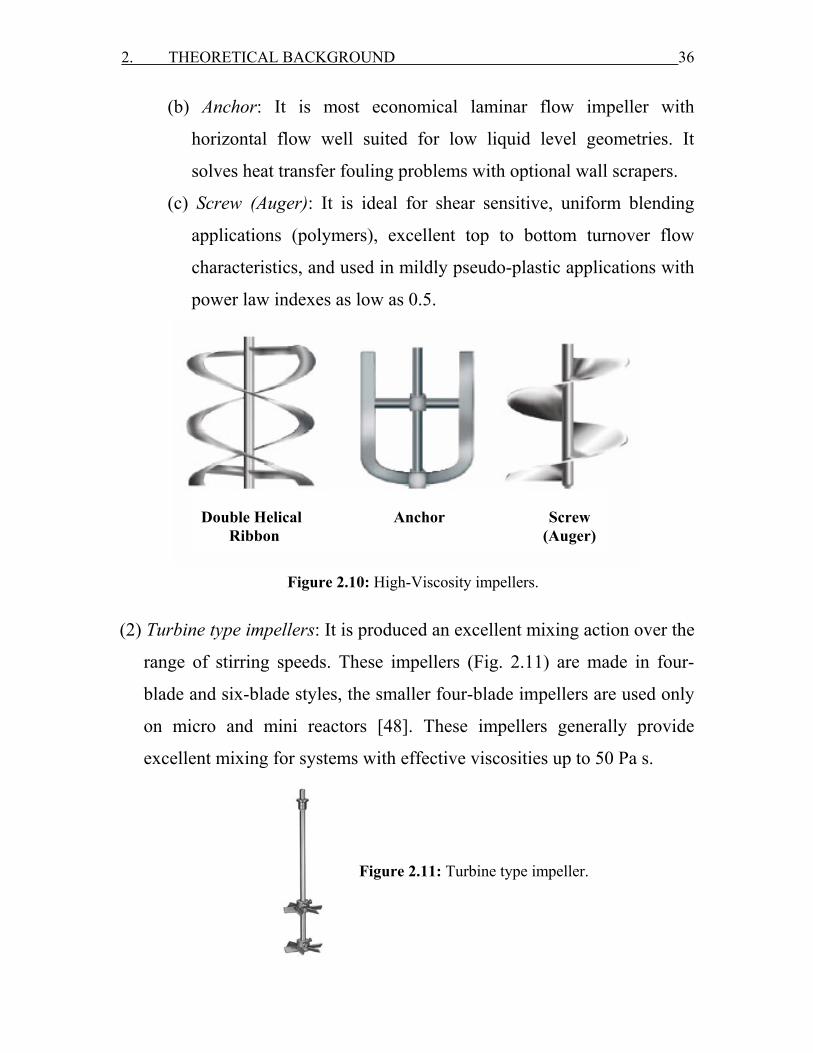
2. THEORETICAL BACKGROUND 36
(b) Anchor: It is most economical laminar flow impeller with
horizontal flow well suited for low liquid level geometries. It
solves heat transfer fouling problems with optional wall scrapers.
(c) Screw (Auger): It is ideal for shear sensitive, uniform blending
applications (polymers), excellent top to bottom turnover flow
characteristics, and used in mildly pseudo-plastic applications with
power law indexes as low as 0.5.
Figure 2.10: High-Viscosity impellers.
(2) Turbine type impellers: It is produced an excellent mixing action over the
range of stirring speeds. These impellers (Fig. 2.11) are made in four-
blade and six-blade styles, the smaller four-blade impellers are used only
on micro and mini reactors [48]. These impellers generally provide
excellent mixing for systems with effective viscosities up to 50 Pa s.
Figure 2.11: Turbine type impeller.
Double Helical Anchor Screw Ribbon (Auger)
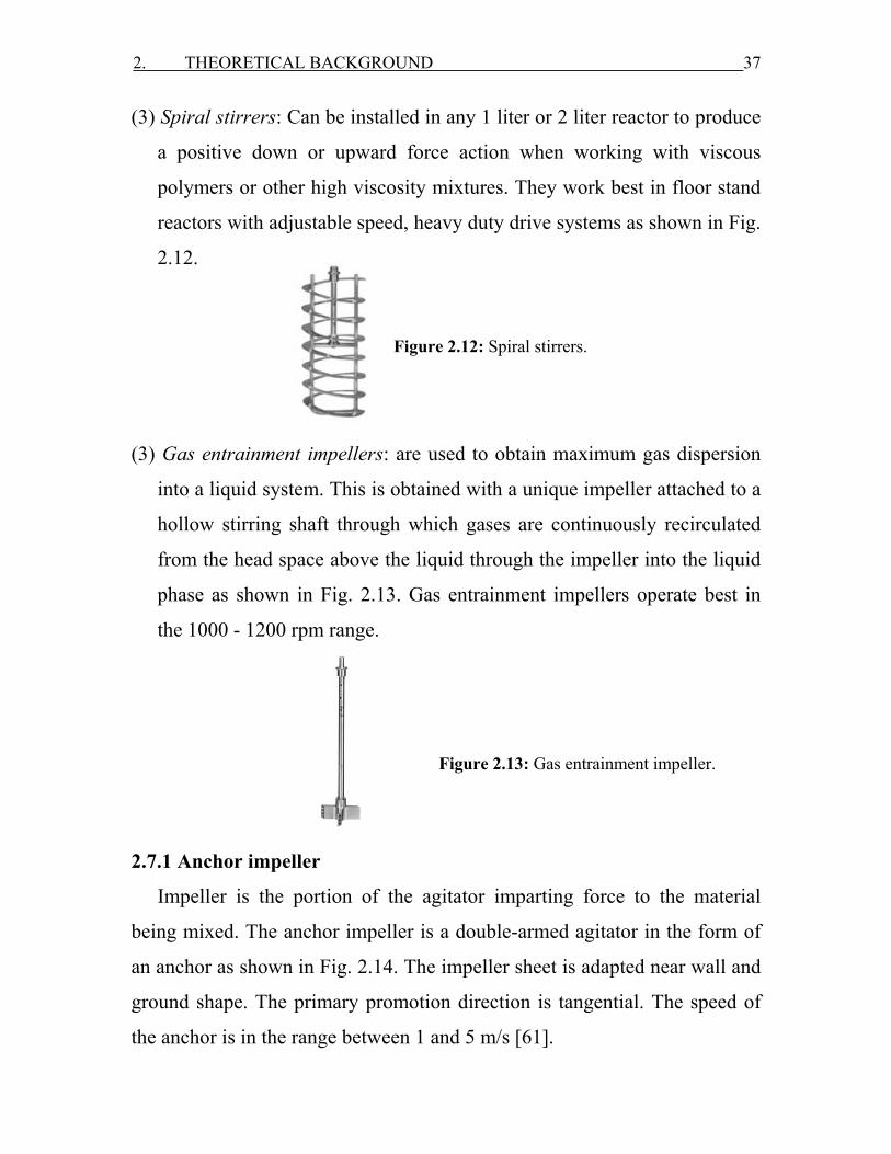
2. THEORETICAL BACKGROUND 37
(3) Spiral stirrers: Can be installed in any 1 liter or 2 liter reactor to produce
a positive down or upward force action when working with viscous
polymers or other high viscosity mixtures. They work best in floor stand
reactors with adjustable speed, heavy duty drive systems as shown in Fig.
2.12.
Figure 2.12: Spiral stirrers.
(3) Gas entrainment impellers: are used to obtain maximum gas dispersion
into a liquid system. This is obtained with a unique impeller attached to a
hollow stirring shaft through which gases are continuously recirculated
from the head space above the liquid through the impeller into the liquid
phase as shown in Fig. 2.13. Gas entrainment impellers operate best in
the 1000 - 1200 rpm range.
Figure 2.13: Gas entrainment impeller.
2.7.1 Anchor impeller
Impeller is the portion of the agitator imparting force to the material
being mixed. The anchor impeller is a double-armed agitator in the form of
an anchor as shown in Fig. 2.14. The impeller sheet is adapted near wall and
ground shape. The primary promotion direction is tangential. The speed of
the anchor is in the range between 1 and 5 m/s [61].
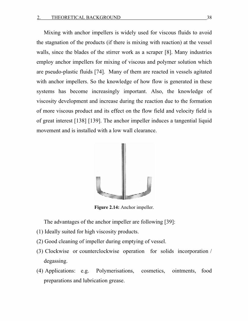
2. THEORETICAL BACKGROUND 38
Mixing with anchor impellers is widely used for viscous fluids to avoid
the stagnation of the products (if there is mixing with reaction) at the vessel
walls, since the blades of the stirrer work as a scraper [8]. Many industries
employ anchor impellers for mixing of viscous and polymer solution which
are pseudo-plastic fluids [74]. Many of them are reacted in vessels agitated
with anchor impellers. So the knowledge of how flow is generated in these
systems has become increasingly important. Also, the knowledge of
viscosity development and increase during the reaction due to the formation
of more viscous product and its effect on the flow field and velocity field is
of great interest [138] [139]. The anchor impeller induces a tangential liquid
movement and is installed with a low wall clearance.
Figure 2.14: Anchor impeller.
The advantages of the anchor impeller are following [39]:
(1) Ideally suited for high viscosity products.
(2) Good cleaning of impeller during emptying of vessel.
(3) Clockwise or counterclockwise operation for solids incorporation /
degassing.
(4) Applications: e.g. Polymerisations, cosmetics, ointments, food
preparations and lubrication grease.

2. THEORETICAL BACKGROUND 39
The velocity field around the stirrer, received from measurements, is
given as boundary condition at the stirrer sheets; the tangential speed is
given according to the number of revolutions. Tabs. 2.1 and 2.2 show the
standard design and working area of the anchor impeller respectively [82].
Table 2.1: Limitations of using standard anchor impeller.
Designation
Geometry arrangement
Installation
Primary flow
Anchor impeller
(s. Fig. 2.14)
Centrically
Tangential
Table 2.2: Work area and tasks of stirring.
d/dv Tip velocity
[m/s]
Re
Kind of flow Viscosity η
[Pa s]
0.9 - 0.98
1 - 5
Re > 102
Laminar, Transition
and turbulent
η < 20
Anchor impellers are available in several configurations for use with
moderate to high viscosity materials. This type of impellers usually works
best in vessels with an inside depth to diameter ratio of 1.5 to 1 or less. They
are intended to operate at relatively slow speeds and generally require a
heavy duty drive system capable of generating and delivering sufficient
torque to the stirrer. Three basic types are shown in Fig. 2.15 [63]:
H/dv = 1.000
d/dv = 0.960
B/dv = 0.025
Hi/d = 0.480
w/dv = 0.060
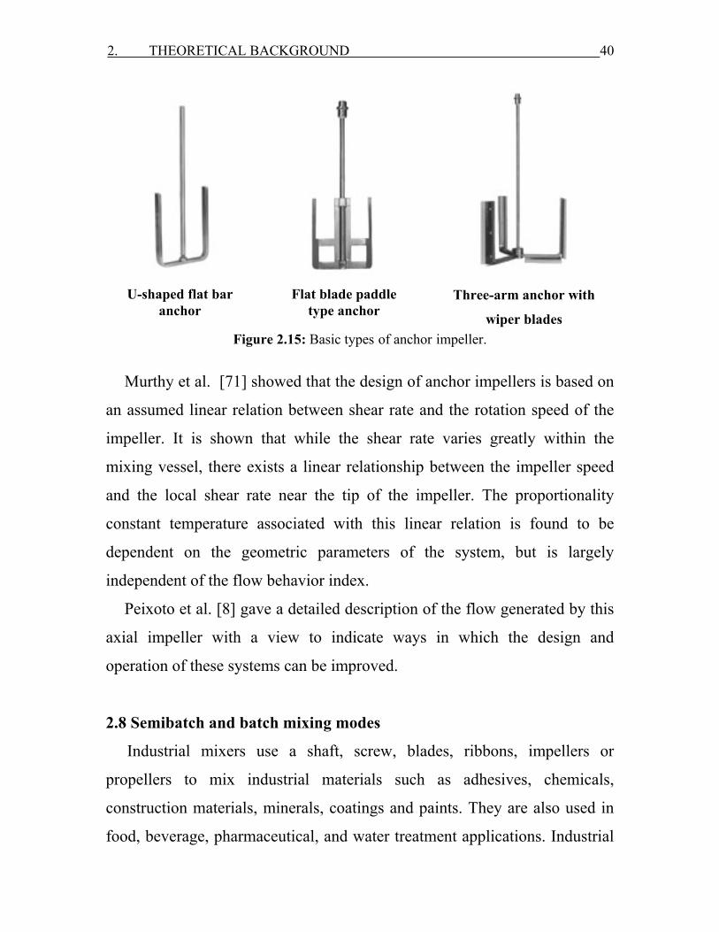
2. THEORETICAL BACKGROUND 40
Figure 2.15: Basic types of anchor impeller.
Murthy et al. [71] showed that the design of anchor impellers is based on
an assumed linear relation between shear rate and the rotation speed of the
impeller. It is shown that while the shear rate varies greatly within the
mixing vessel, there exists a linear relationship between the impeller speed
and the local shear rate near the tip of the impeller. The proportionality
constant temperature associated with this linear relation is found to be
dependent on the geometric parameters of the system, but is largely
independent of the flow behavior index.
Peixoto et al. [8] gave a detailed description of the flow generated by this
axial impeller with a view to indicate ways in which the design and
operation of these systems can be improved.
2.8 Semibatch and batch mixing modes
Industrial mixers use a shaft, screw, blades, ribbons, impellers or
propellers to mix industrial materials such as adhesives, chemicals,
construction materials, minerals, coatings and paints. They are also used in
food, beverage, pharmaceutical, and water treatment applications. Industrial
U-shaped flat bar anchor
Flat blade paddle
type anchor
Three-arm anchor with
wiper blades
2. THEORETICAL BACKGROUND 41
mixers force sediment to flow in one direction and can intensify physical
and chemical processes. Most industrial mixers have three modes: batch,
semibatch and continuous-feed. With continuous-feed industrial mixers, the
media to mix is added continuously as mixed fluid is removed. Continuous
mixers are suitable for production applications because they can run for long
periods of time without being shut down [61].
The reasons for the type of reactor choice include [75]:
(1) Complete conversion: Reactions are generally run to achieve complete
conversion of the limiting reagent-controlled by time and not subject to
differences in completeness of conversion because of residence time dis-
tribution in a continuous stirred tank reactor.
(2) Accuracy of charge: Reagent quantities can be carefully controlled and
procedures for over checks of quantities actually utilized.
(3) Productivity: Reactor volume is often consistent with the limited produc-
tivity requirements characteristic of this industry.
(4) Flexibility: Batch reactors can process a large variety of homogeneous
and heterogeneous reactions successfully with little modification of
internals and can be used in dedicated or multipurpose facilities. The uses
of variable speed drives along with versatile impellers are key factors.
2.8.1 Semibatch operation
Semibatch reactors are very common in the specialty chemical and
pharmaceutical manufacturing industries to accomplish mixing tasks [75].
Semibatch operations are typically carried out in standard type of stirred
mixing vessel in both homogeneous and heterogeneous applications,
although special provision is often required for fast and/or heterogeneous
reactions. Their use is very flexible in that they can be quickly reconfigured
2. THEORETICAL BACKGROUND 42
for various types of chemical reactions needed in a series of chemical
synthesis steps. The blending in semibatch operation is done by feeding a
particularly reactive reagent later or slower in a region of high energy
dissipation, the reactant that starts in the reactor is always the limiting
reactant [66]. The reactions can be forced along a more desirable path,
producing a better yield of desired products. If the chemical reaction is fast
enough to proceed during the addition of a chemical reactant or a catalyst,
the mode is actually semibatch, and mixing effects may be present [89].
2.8.1 Batch operation
Batch mixing is the simplest mode of operation. The industrial mixer is
filled with media and product mixing is allowed to proceed [153]. When
mixing is complete, the vessel’s contents are emptied for downstream
processing. The industrial mixer is then cleaned and refilled for mixing
another batch. Batch mixing of viscous fluids is widely used in the chemical
and food industry, the process requires a large amount of time and energy to
achieve good end product quality. If the chemical reaction is too slow, the
mode is actually batch [90]. The batch reactor is very useful to investigate a
wide variety of chemical reactions, particularly oscillatory reactions. The
advantages of the batch process like high flexibility towards different recipes
and operation procedures and the possibility to reach high conversions. It is
common operation in latex producing industry. The disadvantages of batch
reactors in processing should also be noted [75]:
(1) Reaction medium: There may exist nonuniformity of mixing intensity
throughout the vessel that can lead to undesirable side reactions caused
by variations in local concentrations.
(2) Optimum conditions: One of a reaction system may require different
2. THEORETICAL BACKGROUND 43
conditions than another which may overlap in time (i.e., a reaction that
results in precipitation of a product or by-product may require different
mixing intensities for the reaction and precipitation).
(3) Heat transfer: High rates of heat transfer are not achievable without
external pumping through a heat exchanger or by utilization of unwieldy
internal coils. In these systems, heat transfer is often achieved by
operating at reflux and using an external condenser to remove the heat.
(4) Thermal hazards: A large volume of a reacting system with highly
exothermic reactions can produce large thermal hazards.
2.9 Computational fluid dynamics (CFD)
It is a computer based tool for simulating the behavior of systems
involving fluid flow, heat transfer, and other related physical processes.
Fluid (gas and liquid) flows are governed by partial differential equations
(Navier-Stokes equations) which represent conservation laws for the mass,
momentum, and energy. CFD is the method of replacing such PDE (Partial
differential equations) systems by a set of algebraic equations which can be
solved using digital computers. These equations are solved over a region of
interest, with specified conditions on the boundary of that region [86] [102].
2.9.1 Developments
Computers have been used to solve fluid flow problems for many years.
Numerous programs have been written to solve either specific problems, or
specific classes of problem. From the mid-1970’s the complex mathematics
required to generalize the algorithms began to be understood, and general
purpose CFD solvers were developed. These began to appear in the early
1980’s and required powerful computers as well as knowledge of fluid

2. THEORETICAL BACKGROUND 44
dynamics, and large amounts of time to set up simulations. Consequently,
CFD was a tool used almost exclusively in research [122].
Recent advances in computing power, together with powerful graphics
and interactive three dimensions manipulation of models have made the
process of creating a CFD model and analyzing results much less labor
intensive, reducing time and hence cost. Advanced solvers contain
algorithms which enable right solution of the flow field in a reasonable time.
As a result of these factors, Computational Fluid Dynamics is now an
established industrial design tool, helping to reduce design timescales and
improve processes throughout the engineering world. CFD provides a cost
effective and accurate alternative to scale model testing, with variations on
the simulation being performed quickly, offering obvious advantages [102].
2.9.2 Applications
CFD provides a qualitative (and sometimes even quantitative) prediction
of fluid flows by means of [124]:
(1) Mathematical modeling (partial differential equations).
(2) Numerical methods (discretisation and solution techniques).
(3) Software tools (solvers, pre- and postprocessing utilities).
CFD enables scientists and engineers to perform numerical experiments
(computer simulations) in a real experiment CFD simulation. It is attractive
for two reasons. Firstly, the desire to be able to model physical fluid
phenomena that cannot be easily simulated or measured with a physical
experiment, for example weather systems or hypersonic aerospace vehicles.
Secondly, the desire to be able to investigate physical fluid systems more
cost effectively and more rapidly than with experimental methods [35] [36].

2. THEORETICAL BACKGROUND 45
CFD computer codes, both commercial and in-house are now considered to
be standard numerical tools, widely utilized within industry for design and
development. Numerical simulations of fluid flow will enable [24] [34] [40]
[131]:
(a) Architects to design comfortable and safe living environments.
(b) Designers of vehicles to improve the aerodynamic characteristics.
(c) Chemical engineers to maximize the yield from their equipment.
(d) Petroleum engineers to devise optimal oil recovery strategies.
(e) Surgeons to cure arterial diseases (computational hemodynamics).
(f) Meteorologists to forecast the weather and warn of natural disasters.
(g) Safety experts to reduce health risks from radiation and other hazards.
2.9.3 Analysis steps
The following steps are used by CFD for analysis and investigation
problems in a wide variety of applications [15] [16]:
(1) Problem statement information about the flow.
(2) Mathematical model.
(3) Mesh generation nodes/cells, time instants.
(4) Space discretisation coupled ordinary differential equations systems.
(5) Time discretisation algebraic system.
(6) Iterative solver discrete function values.
(7) CFD software implementation.
(8) Simulation runs parameters, stopping criteria.
(9) Post processing visualization, analysis of data.
(10) Verification model, validation / adjustment.
2. THEORETICAL BACKGROUND 46
2.9.4 Mathematical model
A mathematical model is used to describe the process as in the following:
(1) Choose a suitable flow model and reference frame.
(2) Identify the forces which cause and influence the fluid motion.
(3) Define the computational domain in which to solve the problem.
(4) Formulate conservation laws for the mass, momentum, and energy.
(5) Simplify the governing equations to reduce the computational effort:
(a) Use available information about the flow regime.
(b) Check for symmetries and predominant flow directions.
(c) Neglect the terms which have little or no influence on the results.
(d) Model the effect of small scale fluctuations that cannot be captured.
(e) Incorporate knowledge of the measurement data and CFD results.
(6) Add constitutive relations and specify initial/boundary conditions.
2.9.5 Numerics
The set of equations which describe the processes of momentum, heat
and mass transfer are known as the Navier Stokes equations. These partial
differential equations were derived in the early nineteenth century and have
no known general analytical solution but can be discretised and solved
numerically [92]. Equations describing other processes, such as combustion,
can also be solved in conjunction with the Navier Stokes equations [91].
Often, an approximating model is used to derive these additional equations,
turbulence models being a particularly important example. There are a
number of different solution methods which are used in CFD codes [93].
The most common and the one on which CFX is based, is known as the
finite volume technique. In this technique, the region of interest is divided
into small sub-regions, called control volumes. The equations are discretised

2. THEORETICAL BACKGROUND 47
and solved iteratively for each control volume. As a result, an approximation
of the value of each variable at specific points throughout the domain can be
obtained. In this way, a full picture of the behavior of the flow can be
derived [102].
2.9.5.1 Discretisation method
After selecting the mathematical model, a suitable discretisation method
should be chosen, i.e. a method of approximating the differential equations
by a system of algebraic equations for the variables at some set of discrete
locations in space and time. There are many approaches, but the most
important of which are: finite difference (FD), finite volume (FV) and finite
element (FE) methods. Other methods, like spectral schemes, boundary
element methods, and cellular automata are used in CFD but their use is
limited to special classes of problems. Each type of method yields the same
solution if the grid is very fine. However, some methods are more suitable to
some classes of problems than others. The preference is often determined by
the attitude of the developer [51].
2.9.5.1.1 Finite difference method
This is the oldest method for numerical solution of PDE’s has been
introduced by Euler in 18th century. It is also the easiest method to use for
simple geometries. The starting point is the conservation equation in
differential form. The solution domain is covered by a grid. At each grid
point, the differential equation is approximated by replacing the partial
derivatives by approximations in terms of the nodal values of the functions.
The result is one algebraic equation per grid node, in which the variable
value at this node and a certain number of neighbor nodes appear as
2. THEORETICAL BACKGROUND 48
unknowns. The FD method can be applied to any grid type; it has been
applied to structured grids. The grid lines serve as local coordinate lines.
Taylor series expansion or polynomial fitting is used to obtain approxima-
tions to the first and second derivatives of the variables with respect to the
coordinates. On structured grids, the FD method is very simple and effective.
It is especially easy to obtain higher order schemes on regular grids. The
disadvantage of FD methods is that the conservation is not enforced unless
special care is taken. Also, the restriction to simple geometries is a
significant disadvantage in complex flows [51].
2.9.5.1..2 Finite element method
The FE method is similar to the FV method in many ways. The domain is
broken into a set of discrete volumes or finite elements that are generally
unstructured; in two dimensions, they are usually triangles or quadrilaterals,
while in three dimensions, tetrahedral or hexahedra are most often used. The
distinguishing feature of FE methods is that the equations are multiplied by a
weight function before they are integrated over the entire domain. In the
simplest FE methods, the solution is approximated by a linear shape function
within each element in a way that guarantees continuity of the solution
across element boundaries. Such a function can be constructed from its
values at the corners of the elements. The weight function is usually of the
same form. This approximation is then substituted into the weighted integral
of the conservation law and the equations to be solved are derived by
requiring the derivative of the integral with respect to each nodal value to be
zero; this corresponds to selecting the best solution within the set of allowed
functions (the one with minimum residual). The result is a set of non-linear
2. THEORETICAL BACKGROUND 49
algebraic equations. An important advantage of finite element methods is the
ability to deal with arbitrary geometries [51].
2.9.5.1.3 Finite volume method
The FV method uses the integral form of the conservation equations as its
starting point. The solution domain is subdivided into a finite number of
continuous control volumes, and the conservation equations are applied to
each control volume. At the centroid of each control volume lies a
computational node at which the variable values are to be calculated.
Interpolation is used to express variable values at the control volume surface
in terms of the nodal (control volume-center) values. Surface and volume
integrals are approximated using suitable quadrate formula. As a result, an
algebraic equation is obtained for each control volume, in which number of
neighbor nodal values appear. The FV method can accommodate any type of
grid, so it is suitable for complex geometries. The grid defines only the
control volume boundaries and need not be related to a coordinate system.
The method is conservative by construction, so long as surface integrals
(which represent convective and diffusive fluxes) are the same for the
control volume sharing the boundary. The FV approach is the simplest to
understand and to program. All terms that need be approximated have
physical meaning which is why it is popular with engineers. The
disadvantage of FV methods compared to FD schemes is that methods of
order higher than second are more difficult to develop in three dimensions.
This is due to the fact that the FV approach requires two levels of
approximation: interpolation and integration [51].
2. THEORETICAL BACKGROUND 50
2.9.5.2 Iterative solution strategy
The coupled nonlinear algebraic equations must be solved iteratively
[130]:
(1) Outer iterations: the coefficients of the discrete problem are updated
using the solution values from the previous iteration so as to:
(a) Get rid of the nonlinearities by a Newton-like method.
(b) Solve the governing equations in a segregated fashion.
(2) Inner iterations: the resulting sequence of linear sub problems is typically
solved by an iterative method (conjugate gradients, multigrid) because
direct solvers (Gaussian elimination) are expensive.
(3) Convergence criteria: it is necessary to check the residuals, relative
solution changes and other indicators to make sure that the iterations
converge.
As a rule, the algebraic systems to be solved are very large (millions of
unknowns) but sparse, i.e., most of the matrix coefficients are equal to zero.
2.9.5.3 Uncertainty and error
Whether or not the results of a CFD simulation can be trusted depends on
the degree of uncertainty and on the cumulative effect of various errors
[130]:
(1) Uncertainty is defined as a potential deficiency due to the lack of
knowledge (turbulence modeling is a classical example).
(2) Error is defined as a recognizable deficiency due to other reasons:
(a) Acknowledged errors have certain mechanisms for identifying,
estimating and possibly eliminating or at least reducing them.
2. THEORETICAL BACKGROUND 51
(b) Unacknowledged errors have no standard procedures for detecting
them and may remain undiscovered causing a lot of harm.
(c) Local errors refer to solution errors at a single grid point or cell.
(d) Global errors refer to solution errors over the entire flow domain.
Local errors contribute to the global error and may move throughout the
grid. The acknowledged errors are classified as:
(1) Physical modeling error due to uncertainty and simplifications.
(2) Discretisation error approximation of PDEs by algebraic equations:
(a) Spatial discretisation error due to a finite grid resolution.
(b) Temporal discretisation error due to a finite time step size.
(3) Iterative convergence error which depends on the stopping criteria.
(4) Round-off errors due to the finite precision of computer arithmetic
Unacknowledged errors.
(5) Computer programming error due to coding and logical mistakes.
(6) Usage error: wrong parameter values, models or boundary conditions.
Knowledge of these error sources and an ability to control the error are
important prerequisites for developing and using CFD software.
2.9.5.4 Verification of CFD codes
Verifications (i.e. if the equations are solved right) to looking for errors
in the implementation of the models are done through [130]:
(1) Examine the computer programming by visually checking the source
code, documenting it and testing the underlying subprograms
individually.
2. THEORETICAL BACKGROUND 52
(2) Examine iterative convergence by monitoring the residuals, relative
changes of integral quantities and checking if the prescribed tolerance is
attained.
(3) Examine consistency (check if relevant conservation principles are
satisfied).
(4) Examine grid convergence: as the mesh and/or the time step are refined,
the spatial and temporal discretization errors, respectively, should
approach zero (in the absence of round-off errors).
(5) Compare the computational results with analytical and numerical
solutions for standard configurations (representative test cases).
2.9.5.5 Validation of CFD models
Validations (i.e. if the right equations are solved) to check if the model
itself is suitable for practical purposes are done by [94] [95] [130]:
(1) Verify the code to make sure that the numerical solutions are correct.
(2) Compare the results with available experimental data to check if the
reality is represented accurately enough.
(3) Perform sensitivity analysis and a parametric study to assess the inherent
uncertainty due to the insufficient understanding of physical processes.
(4) Try using different models, geometry, and initial/boundary conditions.
(5) Report the findings, document model limitations and parameter settings.
The goal of verification and validation is to ensure that the CFD code
produces reasonable results for a certain range of flow problems.
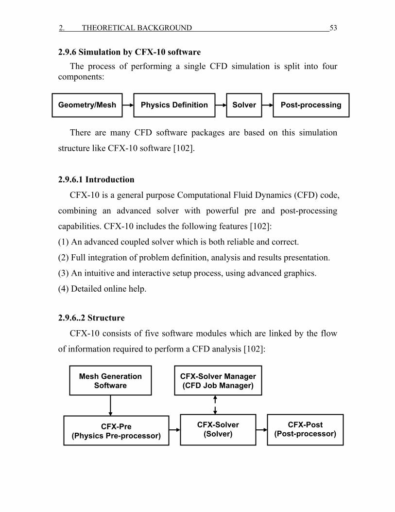
2. THEORETICAL BACKGROUND 53
2.9.6 Simulation by CFX-10 software The process of performing a single CFD simulation is split into four
components:
There are many CFD software packages are based on this simulation
structure like CFX-10 software [102].
2.9.6.1 Introduction
CFX-10 is a general purpose Computational Fluid Dynamics (CFD) code,
combining an advanced solver with powerful pre and post-processing
capabilities. CFX-10 includes the following features [102]:
(1) An advanced coupled solver which is both reliable and correct.
(2) Full integration of problem definition, analysis and results presentation.
(3) An intuitive and interactive setup process, using advanced graphics.
(4) Detailed online help.
2.9.6..2 Structure
CFX-10 consists of five software modules which are linked by the flow
of information required to perform a CFD analysis [102]:
Geometry/Mesh
Physics Definition Solver
Post-processing
Mesh Generation Software
CFX-Pre (Physics Pre-processor)
CFX-Solver Manager(CFD Job Manager)
CFX-Solver (Solver)
CFX-Post (Post-processor)
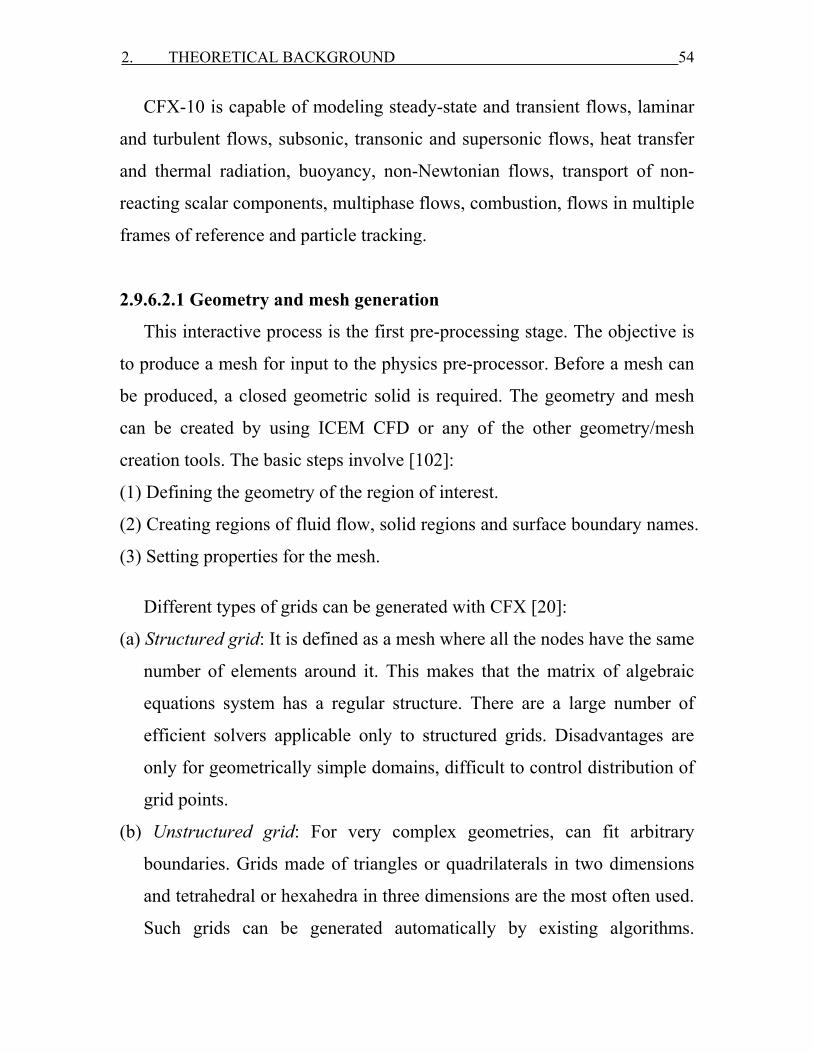
2. THEORETICAL BACKGROUND 54
CFX-10 is capable of modeling steady-state and transient flows, laminar
and turbulent flows, subsonic, transonic and supersonic flows, heat transfer
and thermal radiation, buoyancy, non-Newtonian flows, transport of non-
reacting scalar components, multiphase flows, combustion, flows in multiple
frames of reference and particle tracking.
2.9.6.2.1 Geometry and mesh generation
This interactive process is the first pre-processing stage. The objective is
to produce a mesh for input to the physics pre-processor. Before a mesh can
be produced, a closed geometric solid is required. The geometry and mesh
can be created by using ICEM CFD or any of the other geometry/mesh
creation tools. The basic steps involve [102]:
(1) Defining the geometry of the region of interest.
(2) Creating regions of fluid flow, solid regions and surface boundary names.
(3) Setting properties for the mesh.
Different types of grids can be generated with CFX [20]:
(a) Structured grid: It is defined as a mesh where all the nodes have the same
number of elements around it. This makes that the matrix of algebraic
equations system has a regular structure. There are a large number of
efficient solvers applicable only to structured grids. Disadvantages are
only for geometrically simple domains, difficult to control distribution of
grid points.
(b) Unstructured grid: For very complex geometries, can fit arbitrary
boundaries. Grids made of triangles or quadrilaterals in two dimensions
and tetrahedral or hexahedra in three dimensions are the most often used.
Such grids can be generated automatically by existing algorithms.
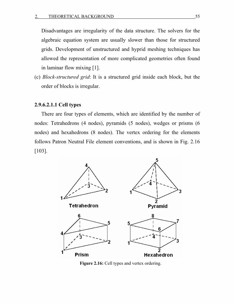
2. THEORETICAL BACKGROUND 55
Disadvantages are irregularity of the data structure. The solvers for the
algebraic equation system are usually slower than those for structured
grids. Development of unstructured and hyprid meshing techniques has
allowed the representation of more complicated geometries often found
in laminar flow mixing [1].
(c) Block-structured grid: It is a structured grid inside each block, but the
order of blocks is irregular.
2.9.6.2.1.1 Cell types
There are four types of elements, which are identified by the number of
nodes: Tetrahedrons (4 nodes), pyramids (5 nodes), wedges or prisms (6
nodes) and hexahedrons (8 nodes). The vertex ordering for the elements
follows Patron Neutral File element conventions, and is shown in Fig. 2.16
[103].
Figure 2.16: Cell types and vertex ordering.

2. THEORETICAL BACKGROUND 56
2.9.6.2.2 CFX-pre
This interactive process is the second pre-processing stage and is used to
create input required by the solver. It is the physics definition pre-processor
part of CFX-10. It is used to import meshes produced in mesh generation
software packages and to select physical models used in the CFD simulation
[88]. Flow physics, fluid properties, initial values and solver parameters are
specified in CFX-pre. A full range of boundary conditions, including inlets,
outlets and openings, together with boundary conditions for heat transfer
models and periodicity are all available in CFX-pre which has different
modes of operations [102]:
(1) General: this can be used for all cases.
(2) Turbo: It simplifies the set up of some turbomachinery simulations.
(3) Quick setup: this provides fewer model options and is suitable for more
simple cases. It allows setting up simple physics cases very quickly.
(4) Model library: It is used to import predefined library files for more
complex simulations. This will set up the physics required for a particular
case.
2.9.6.2.3 CFX-solver
The solver is the component which solves the CFD problem. It produces
the required results in a non-interactive/batch process. The CFD problem is
solved as follows:
(1) The partial differential equations are integrated over all the control
volumes in the region of interest. This is equivalent to applying a basic
conservation law (e.g. for mass or momentum) to each control volume.
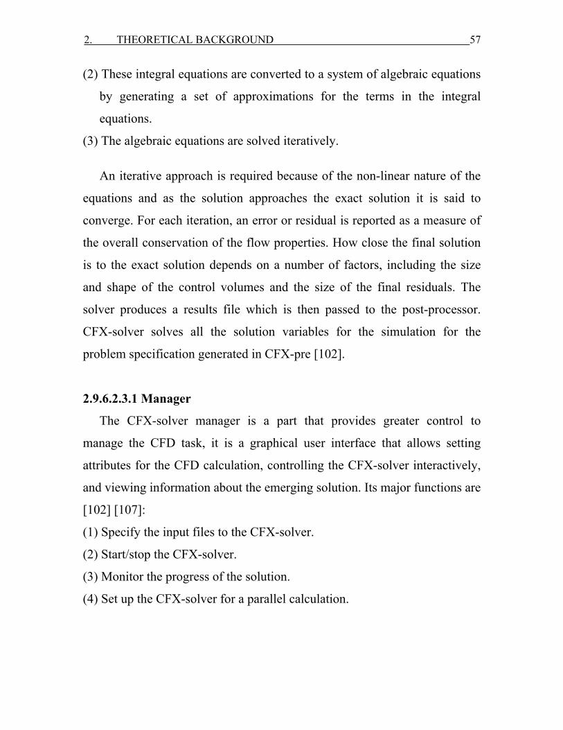
2. THEORETICAL BACKGROUND 57
(2) These integral equations are converted to a system of algebraic equations
by generating a set of approximations for the terms in the integral
equations.
(3) The algebraic equations are solved iteratively.
An iterative approach is required because of the non-linear nature of the
equations and as the solution approaches the exact solution it is said to
converge. For each iteration, an error or residual is reported as a measure of
the overall conservation of the flow properties. How close the final solution
is to the exact solution depends on a number of factors, including the size
and shape of the control volumes and the size of the final residuals. The
solver produces a results file which is then passed to the post-processor.
CFX-solver solves all the solution variables for the simulation for the
problem specification generated in CFX-pre [102].
2.9.6.2.3.1 Manager
The CFX-solver manager is a part that provides greater control to
manage the CFD task, it is a graphical user interface that allows setting
attributes for the CFD calculation, controlling the CFX-solver interactively,
and viewing information about the emerging solution. Its major functions are
[102] [107]:
(1) Specify the input files to the CFX-solver.
(2) Start/stop the CFX-solver.
(3) Monitor the progress of the solution.
(4) Set up the CFX-solver for a parallel calculation.
2. THEORETICAL BACKGROUND 58
2.9.6.2.3.2 Modeling
Descriptions of more advanced physical models and how the basic
models extend to more complex cases are provided in modeling multiphase
flow, turbulence, domain interface, particle transport, combustion, radiation
and real fluid properties [101].
2.9.6.2.3.3 Numerical discretisation
Analytical solutions to the Navier-Stokes equations exist for only the
simplest of flows under ideal conditions. To obtain solutions for real flows a
numerical approach must be adopted whereby the equations are replaced by
algebraic approximations which may be solved using a numerical method.
The domain is discretised into finite control volumes using a mesh. The
governing equations are integrated over each control volume and solved
with the initial and boundary conditions. Resolution of the algebraic
equations is carried out using high resolution advection and second order
backward Euler transient schemes. Fig. 2.17 shows a typical mesh in two-
dimension on which one surface of the finite volume is represented by the
shaded area; each node is surrounded by a set of surfaces which contain the
finite volume. All the solution variables and fluid properties are stored at the
element nodes [100].
Figure 2.17: Finite volume surface.
Element face centroid
Element
Node Finite volume surface

2. THEORETICAL BACKGROUND 59
2.9.6.2.3.4 Coupled solver
It is one of the most important features of CFX-10 in which all the
hydrodynamic equations are solved as a single system simultaneously. The
coupled solver is faster than the segregated solver and less iteration are
required to obtain a converged flow solution [102]. This solution approach
uses a fully implicit discretisation of the equations at any given time step.
The linear sets of equations that arise by applying the finite volume
method to all elements in the domain are discrete conservation equations.
The system of equations can be written in the form:
φ =∑i
nbi i i
nba b . (2-13)
Where φi is the variable vector, b here is the solution, a is the
coefficient matrix of the equation, i here is the identifying number of the
finite volume or node in question, and nb is the central coefficient
multiplying the solution at the ith location. This method is applicable to both
structured and unstructured meshes. The set of these, for all finite volumes
constitutes the whole linear equation system. For the coupled, three
dimensions mass-momentum equation set, they can be expressed as (4 x 4)
matrix and (4 x 1) vector as in the following:
=
uu uv uw up
vu vv vw vp
wu wv ww wp
pu pv pw pp
nb
nbi
i
a a a aa a a a
aa a a aa a a a
and ,
φ = =
u
v
w
p
bi i
i i
bubvbw
p b
2. THEORETICAL BACKGROUND 60
The advantages of such a coupled treatment over a non-coupled or
segregated approach are efficiency, generality and simplicity. These
advantages all combine to make the coupled solver an extremely powerful
feature of any CFD code.
2.9.6.2.4 CFX-post It is a flexible interactive post-processor graphics tools for CFX-10. It is
designed to allow easy visualization, analyzing, presenting and quantitative
post-processing the results of CFD simulation. Post-processing includes
anything from obtaining point values to complex animated sequences.
Examples of some important features of post-processors are [102] [108]:
(1) Visualization of the geometry and control volumes.
(2) Vector plots showing the direction and magnitude of the flow.
(3) Visualization of the variation of scalar variables which have only
magnitude not direction such as temperature and velocity in the domain.
(4) Visualization for representation of numbers of images:
(a) One dimension: function values connected by straight lines.
(b) Two dimensions: streamlines, contour levels, color diagrams.
(c) Three dimensions: cutlines, cutplanes, isosurfaces and isovolumes.
(d) Arrow plots, particle tracing and animations.
(5) Quantitative numerical calculations.
(6) Charts showing graphical plots of variables and hardcopy output.
(7) Calculation of derived quantities such as stream function and vorticity.
(8) Calculation of integral parameters like lift, drag and total mass.
(9) Systematic data analysis by means of statistical tools.
(10) Verification and validation of the CFD model.
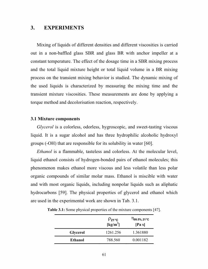
61
3. EXPERIMENTS
Mixing of liquids of different densities and different viscosities is carried
out in a non-baffled glass SBR and glass BR with anchor impeller at a
constant temperature. The effect of the dosage time in a SBR mixing process
and the total liquid mixture height or total liquid volume in a BR mixing
process on the transient mixing behavior is studied. The dynamic mixing of
the used liquids is characterized by measuring the mixing time and the
transient mixture viscosities. These measurements are done by applying a
torque method and decolorisation reaction, respectively.
3.1 Mixture components
Glycerol is a colorless, odorless, hygroscopic, and sweet-tasting viscous
liquid. It is a sugar alcohol and has three hydrophilic alcoholic hydroxyl
groups (-OH) that are responsible for its solubility in water [60].
Ethanol is a flammable, tasteless and colorless. At the molecular level,
liquid ethanol consists of hydrogen-bonded pairs of ethanol molecules; this
phenomenon makes ethanol more viscous and less volatile than less polar
organic compounds of similar molar mass. Ethanol is miscible with water
and with most organic liquids, including nonpolar liquids such as aliphatic
hydrocarbons [59]. The physical properties of glycerol and ethanol which
are used in the experimental work are shown in Tab. 3.1.
Table 3.1: Some physical properties of the mixture components [47].
ρ21 °C [kg/m3]
η99.5%, 21 °C [Pa s]
Glycerol
1261.256
1.361880
Ethanol
788.560
0.001182
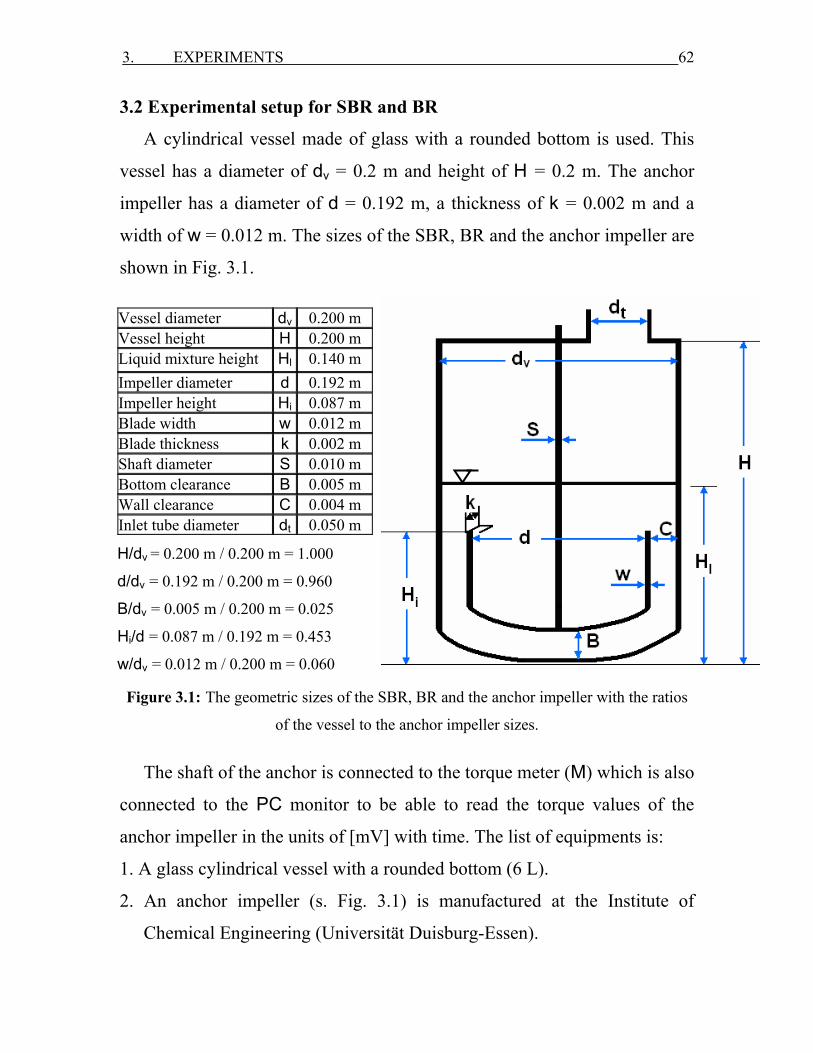
3. EXPERIMENTS 62
3.2 Experimental setup for SBR and BR
A cylindrical vessel made of glass with a rounded bottom is used. This
vessel has a diameter of dv = 0.2 m and height of H = 0.2 m. The anchor
impeller has a diameter of d = 0.192 m, a thickness of k = 0.002 m and a
width of w = 0.012 m. The sizes of the SBR, BR and the anchor impeller are
shown in Fig. 3.1.
Figure 3.1: The geometric sizes of the SBR, BR and the anchor impeller with the ratios
of the vessel to the anchor impeller sizes.
The shaft of the anchor is connected to the torque meter (M) which is also
connected to the PC monitor to be able to read the torque values of the
anchor impeller in the units of [mV] with time. The list of equipments is:
1. A glass cylindrical vessel with a rounded bottom (6 L).
2. An anchor impeller (s. Fig. 3.1) is manufactured at the Institute of
Chemical Engineering (Universität Duisburg-Essen).
Vessel diameter dv 0.200 m Vessel height H 0.200 m Liquid mixture height Hl 0.140 m Impeller diameter d 0.192 m Impeller height Hi 0.087 m Blade width w 0.012 m Blade thickness k 0.002 m Shaft diameter S 0.010 m Bottom clearance B 0.005 m Wall clearance C 0.004 m Inlet tube diameter dt 0.050 m
H/dv = 0.200 m / 0.200 m = 1.000
d/dv = 0.192 m / 0.200 m = 0.960
B/dv = 0.005 m / 0.200 m = 0.025
Hi/d = 0.087 m / 0.192 m = 0.453
w/dv = 0.012 m / 0.200 m = 0.060
3. EXPERIMENTS 63
3. An electrical motor (Janke & Kunkel IKA-Labortechnik RE 162,
10 – 1600 1/min, made in Germany).
4. A control box (Janke & Kunkel IKA-Labortechnik RE 162 Analog,
10 – 1600 1/min, made in Germany).
5. A pump (EHEIM, type: 1030, made in Germany) has a maximum height
of 4 m and volumetric flow rate of 22 L/min.
6. A Resistance Temperature Detector (RTD) (Jumo, Pt 100, made in
Germany).
7. A thermostat (Julabo, type: F25 (MH), made in Germany).
8. A water bath.
9. A personal computer (PC).
10. A digital video camera (Panasonic, NV-GS280, 800,000 pixel, made in
Japan).
11. A light source (500 W, home made).
12. A white screen.
13. Glass cylinders, beakers, glass rod, volumetric flasks and funnel.
3.3 Methods of measurement in SBR and BR
3.3.1 Torque method
For the torque method, a calibration curve of the pure glycerol is done.
This curve represents a connection between the measured voltage and
viscosity to determine the time dependent viscosity and mixing time.
3.3.1.1 Voltage / Viscosity calibration curve
A calibration curve of the pure glycerol is an important step for the
viscosity measurements using the torque method to make a connection
between the measured voltage and the viscosity. The viscosity values for
3. EXPERIMENTS 64
calibration are taken from the literature [47] in the temperature range
between 10 °C and 50 °C.
A batch glass vessel (6 L) is used to stir a mass of pure glycerol 2.45 L
(3089 g) with anchor impeller. This vessel as shown in Fig. 3.2 is inserted
into a water bath to keep the temperature of the pure glycerol constant. The
temperature is controlled by using thermostat (T), which is connected with
thermocouple inside the stirred vessel.
The torque of the impeller is measured by using a voltmeter which is
connected to the impeller shaft. The voltage (blank) value –which is
determined when the impeller is rotating in the empty vessel–, is 154.1 mV.
In each run, the temperature is adjusted to the desired value, for example
ϑ = 50 °C. The stirrer velocity is adjusted to 150 rpm, and then the mixing
process started until the voltage reading reached a constant value. This value
corresponds to the glycerol viscosity value which is taken from the literature
[47] at the same adjusted temperature. The same procedure is carried out for
other temperatures in the range between 10 °C and 50 °C. As a result, for
each temperature, there is a viscosity value in mPa s and a torque value in
mV. A calibration curve is established by measuring of a well known
viscosity solution.
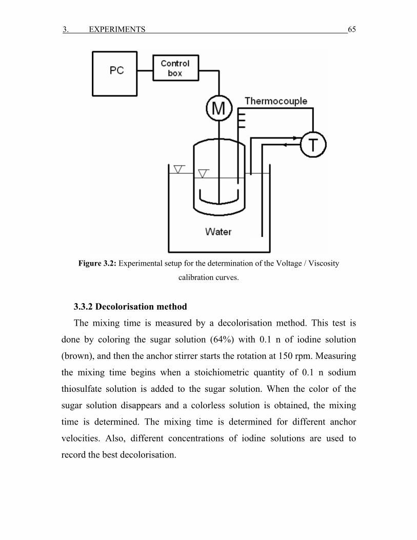
3. EXPERIMENTS 65
Figure 3.2: Experimental setup for the determination of the Voltage / Viscosity
calibration curves.
3.3.2 Decolorisation method
The mixing time is measured by a decolorisation method. This test is
done by coloring the sugar solution (64%) with 0.1 n of iodine solution
(brown), and then the anchor stirrer starts the rotation at 150 rpm. Measuring
the mixing time begins when a stoichiometric quantity of 0.1 n sodium
thiosulfate solution is added to the sugar solution. When the color of the
sugar solution disappears and a colorless solution is obtained, the mixing
time is determined. The mixing time is determined for different anchor
velocities. Also, different concentrations of iodine solutions are used to
record the best decolorisation.
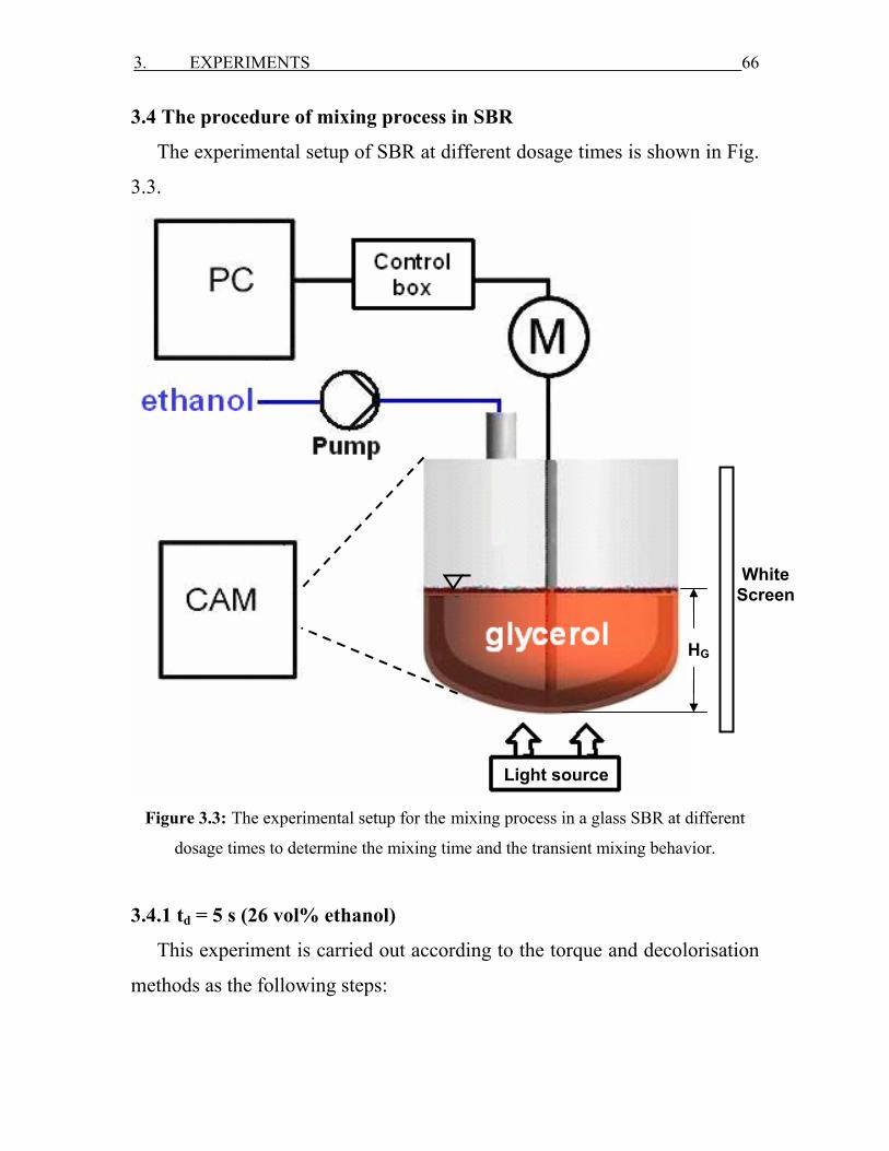
3. EXPERIMENTS 66
3.4 The procedure of mixing process in SBR
The experimental setup of SBR at different dosage times is shown in Fig.
3.3.
Figure 3.3: The experimental setup for the mixing process in a glass SBR at different
dosage times to determine the mixing time and the transient mixing behavior.
3.4.1 td = 5 s (26 vol% ethanol)
This experiment is carried out according to the torque and decolorisation
methods as the following steps:
Light source
HG
White Screen
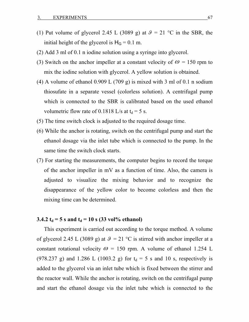
3. EXPERIMENTS 67
(1) Put volume of glycerol 2.45 L (3089 g) at ϑ = 21 °C in the SBR, the
initial height of the glycerol is HG = 0.1 m.
(2) Add 3 ml of 0.1 n iodine solution using a syringe into glycerol.
(3) Switch on the anchor impeller at a constant velocity of ω = 150 rpm to
mix the iodine solution with glycerol. A yellow solution is obtained.
(4) A volume of ethanol 0.909 L (709 g) is mixed with 3 ml of 0.1 n sodium
thiosufate in a separate vessel (colorless solution). A centrifugal pump
which is connected to the SBR is calibrated based on the used ethanol
volumetric flow rate of 0.1818 L/s at td = 5 s.
(5) The time switch clock is adjusted to the required dosage time.
(6) While the anchor is rotating, switch on the centrifugal pump and start the
ethanol dosage via the inlet tube which is connected to the pump. In the
same time the switch clock starts.
(7) For starting the measurements, the computer begins to record the torque
of the anchor impeller in mV as a function of time. Also, the camera is
adjusted to visualize the mixing behavior and to recognize the
disappearance of the yellow color to become colorless and then the
mixing time can be determined.
3.4.2 td = 5 s and td = 10 s (33 vol% ethanol)
This experiment is carried out according to the torque method. A volume
of glycerol 2.45 L (3089 g) at ϑ = 21 °C is stirred with anchor impeller at a
constant rotational velocity ω = 150 rpm. A volume of ethanol 1.254 L
(978.237 g) and 1.286 L (1003.2 g) for td = 5 s and 10 s, respectively is
added to the glycerol via an inlet tube which is fixed between the stirrer and
the reactor wall. While the anchor is rotating, switch on the centrifugal pump
and start the ethanol dosage via the inlet tube which is connected to the
3. EXPERIMENTS 68
pump. The pump is calibrated to the required ethanol volumetric flow rate
for td = 5 s is 0.251 L/s and td = 10 s is 0.129 L/s A stop watch is used to
determine the dosage time. In the same time the computer begins to record
the torque of the anchor impeller in mV as a function of time. The mixing
time is determined when a constant voltage is obtained.
3.5 The procedure of mixing process in BR
A schematic diagram of the experimental setup for the batch mixing
processes is shown in Fig. 3.4.
Figure 3.4: The experimental setup for the mixing process in a glass BR for the
Hl = 0.14 m to determine the mixing time and the transient mixing behavior.
White Screen
Light source
HE
HG

3. EXPERIMENTS 69
3.5.1 Hl = 0.14 m and Hl = 0.09 m (33 vol% ethanol)
These experiments are carried out in according to the torque and
decolorisation methods as the following steps:
(1) Put the volume of glycerol at ϑ = 21 °C in the BR, the initial height of
the glycerol HG = 0.1 m for the Hl = 0.14 m and HG = 0.07 m for
Hl = 0.09 m. The volumes of glycerol and ethanol which are used in the
two batch experiments are shown in Tab. 3.2.
(2) Add 3 ml of 0.1 n iodine solution using a syringe into glycerol.
(3) Stirring the solution in step 2 with the anchor impeller at a constant
velocity ω = 150 rpm, a yellow solution was obtained.
(4) A volume of ethanol is mixed with 3 ml of 0.1 n sodium thiosufate
solution in a separate vessel (colorless solution).
(5) Ethanol is added carefully with the help of a glass rod on the glycerin
surface. Two layers are formed; one for the lighter (ethanol) and the
second for the heavier (glycerol).
(6) Switch on the anchor impeller to start the mixing.
(7) For starting the measurements, the computer begins to record the torque
of the anchor impeller in mV as a function of time. Also, the camera is
adjusted to visualize the mixing behavior and to recognize the
disappearance of the yellow color to become colorless and then the
mixing time can be determined.
Table 3.2: The masses of ethanol and glycerol which are used in a BR at Hl = 0.14 m
and Hl = 0.09 m
Hl = 0.14 m (33 vol% ethanol)
Hl = 0.09 m (33 vol% ethanol)
Glycerol
2.45 L (3089 g)
1.25 L (1575 g)
Ethanol
1.25 L (975 g)
0.62 L (488 g )
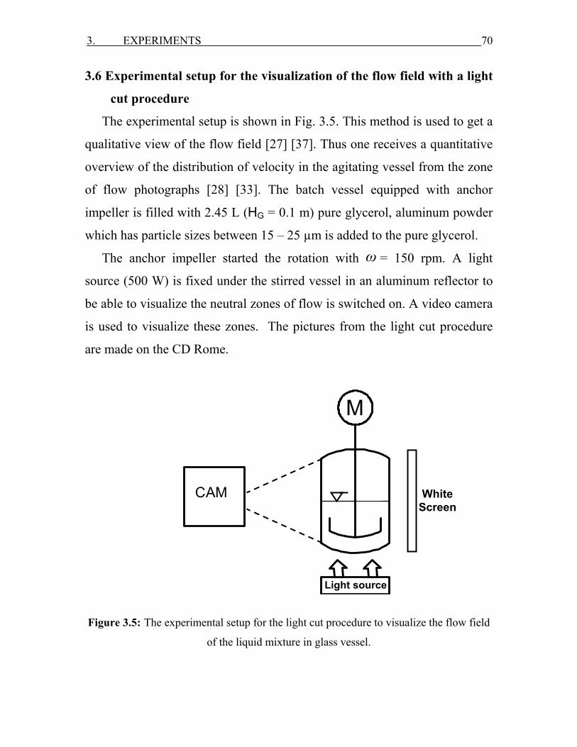
3. EXPERIMENTS 70
3.6 Experimental setup for the visualization of the flow field with a light
cut procedure
The experimental setup is shown in Fig. 3.5. This method is used to get a
qualitative view of the flow field [27] [37]. Thus one receives a quantitative
overview of the distribution of velocity in the agitating vessel from the zone
of flow photographs [28] [33]. The batch vessel equipped with anchor
impeller is filled with 2.45 L (HG = 0.1 m) pure glycerol, aluminum powder
which has particle sizes between 15 – 25 µm is added to the pure glycerol.
The anchor impeller started the rotation with ω = 150 rpm. A light
source (500 W) is fixed under the stirred vessel in an aluminum reflector to
be able to visualize the neutral zones of flow is switched on. A video camera
is used to visualize these zones. The pictures from the light cut procedure
are made on the CD Rome.
M
CAM
Lichtquelle
Figure 3.5: The experimental setup for the light cut procedure to visualize the flow field
of the liquid mixture in glass vessel.
White Screen
Light source
71
4. CFD SIMULATION AND SUBMODELS
This work presents a detailed CFD approach in connection with the CFX-
10 software. There are only few research work studied the CFD of
multicomponent mixing of the two miscible liquids ethanol and glycerol
with high different viscosities and densities without reaction in a non-baffled
stirred SBR and BR with anchor impeller. The effects of density and
viscosity differences between the dosage and bulk liquids in case of SBR
and between these liquids initially stratified in case of BR on the dynamic
mixing behavior are investigated. This behavior is described by determining
the mixing times, time dependent density-, viscosity- and velocity-fields as
well as the flow patterns and homogeneity of the liquid mixtures. The
concentration profile of the lighter liquid (ethanol) is determined at different
points near the shaft and walls of the vessel to determine the homogeneity
and mixing times. The mixing behavior is calculated at different dosage
times of the added liquid, inlet tube diameters, anchor velocities, anchor
dimensions (horizontal blade width) and the volumes of the mixed liquids.
Also, it was important to control the dosage of the lighter liquid (ethanol)
to the bulk liquid (glycerol) in the reactor with a suitable speed, flow rate
and dosage time by using appropriate time step functions and algebraic
equation in the simulations. Different mathematical and physical models are
used to describe the real mixing process like homogeneous multiphase
multicomponent model. The gas phase (air) is involved in the simulations;
the interaction between the gas-liquid mixture phases is modeled using the
free surface model, which is used to study the deformation of the liquid at
the interface and to get a sharp interface between air and liquid mixture
phases, this prevents both phases to be mixed. The pressure field is assumed
4. CFD SIMULATION AND SUBMODELS 72
to be hydrostatic in the liquid mixture phase and uniform in the air phase.
The mixing of liquids is calculated by the means of multicomponent model
under laminar flow [106] [109] [110].
4.1 Simulation for half geometry in SBR and BR
Half geometry is used in the simulation to reduce the required time for
numerical solution (tCPU) of the calculation. ANSYS ICEM CFD 5.1 is a
geometry and mesh generation pre-processor module of CFX. It is used for
creating and modifying the geometry of the mixing vessel and the anchor
impeller. It is an interactive program which enables to generate a mesh with
appropriate regions as an input to the CFX-pre.
4.1.1 Geometry building
Rounded bottom cylindrical vessel equipped with an anchor impeller is
generated in three dimensions. The bottom of the vessel should be modeled
curved, because the distance between the blades and vessel walls is very
small. This is due to the fact that the anchor blades act as scrappers to the
viscous solution.
ANSYS ICEM CFD 5.1 have different tools and options like points,
curves, surfaces and build topology to build and create this vessel with
dimensions according to the standard agitator dimensions which are shown
in Tab. 2.1. The dimensions of the used stirred vessel with the anchor
impeller and liquid mixture height in the simulation are shown in Fig. 4.1
which is the same as in the used experiments.
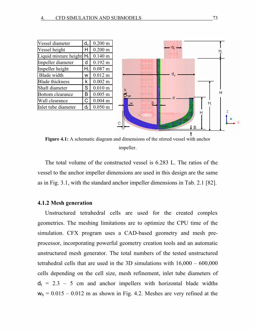
4. CFD SIMULATION AND SUBMODELS 73
Vessel diameter dv 0.200 m Vessel height H 0.200 m Liquid mixture height Hl 0.140 m Impeller diameter d 0.192 m Impeller height Hi 0.087 m Blade width w 0.012 m Blade thickness k 0.002 m Shaft diameter S 0.010 m Bottom clearance B 0.005 m Wall clearance C 0.004 m Inlet tube diameter dt 0.050 m
Figure 4.1: A schematic diagram and dimensions of the stirred vessel with anchor
impeller.
The total volume of the constructed vessel is 6.283 L. The ratios of the
vessel to the anchor impeller dimensions are used in this design are the same
as in Fig. 3.1, with the standard anchor impeller dimensions in Tab. 2.1 [82].
4.1.2 Mesh generation
Unstructured tetrahedral cells are used for the created complex
geometries. The meshing limitations are to optimize the CPU time of the
simulation. CFX program uses a CAD-based geometry and mesh pre-
processor, incorporating powerful geometry creation tools and an automatic
unstructured mesh generator. The total numbers of the tested unstructured
tetrahedral cells that are used in the 3D simulations with 16,000 – 600,000
cells depending on the cell size, mesh refinement, inlet tube diameters of
dt = 2.3 – 5 cm and anchor impellers with horizontal blade widths
wh = 0.015 – 0.012 m as shown in Fig. 4.2. Meshes are very refined at the
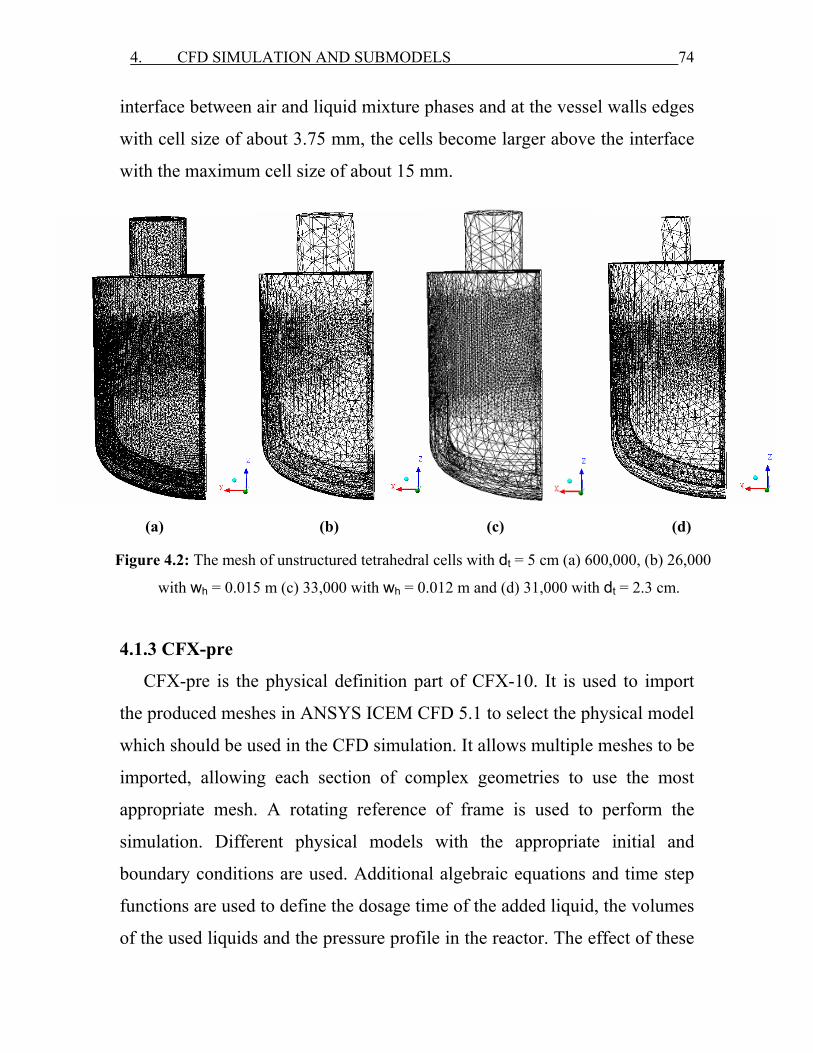
4. CFD SIMULATION AND SUBMODELS 74
interface between air and liquid mixture phases and at the vessel walls edges
with cell size of about 3.75 mm, the cells become larger above the interface
with the maximum cell size of about 15 mm.
Figure 4.2: The mesh of unstructured tetrahedral cells with dt = 5 cm (a) 600,000, (b) 26,000
with wh = 0.015 m (c) 33,000 with wh = 0.012 m and (d) 31,000 with dt = 2.3 cm.
4.1.3 CFX-pre
CFX-pre is the physical definition part of CFX-10. It is used to import
the produced meshes in ANSYS ICEM CFD 5.1 to select the physical model
which should be used in the CFD simulation. It allows multiple meshes to be
imported, allowing each section of complex geometries to use the most
appropriate mesh. A rotating reference of frame is used to perform the
simulation. Different physical models with the appropriate initial and
boundary conditions are used. Additional algebraic equations and time step
functions are used to define the dosage time of the added liquid, the volumes
of the used liquids and the pressure profile in the reactor. The effect of these
(a) (b) (c) (d)
4. CFD SIMULATION AND SUBMODELS 75
models on the flow and viscosity fields of the liquid mixture is performed by
transient 3D-Simulations by using finite volume method. This simulation is
carried out under laminar flow by using a homogeneous multiphase model to
calculate the velocity and pressure fields. Multicomponent model is used to
calculate the mass fractions of each component in the liquid mixture phase.
Free surface model is used to calculate the phase volume fractions.
Homogeneous multiphase flow is a limiting case of Eulerian-Eulerian
multiphase flow where all fluids share the same velocity field and pressure
profile.
The following is a detail description for the models which are used in the
simulation of multicomponent liquid mixture of ethanol and glycerol with
different viscosity and density in SBR and BR. The physical properties of
these components are the same as those used in the experiment as shown in
Tab. 3.1.
4.1.3.1 Kind of Simulation
Transient simulation is used to calculate the dynamic mixing behaviour
with time and space. The time step of 0.01 s is used to get sufficient accurate
and precise results.
4.1.3.2 Multicomponent modeling
A multicomponent fluid contains two or more components and its
properties are calculated from those of the components. The components are
assumed to be mixed at the molecular level and the properties of the fluid
depend on the mass fraction of the components. The components can exist
in a fixed or variable composition mixture. For fixed composition mixture,
the mass fraction of each material is specified and is not allowed to change
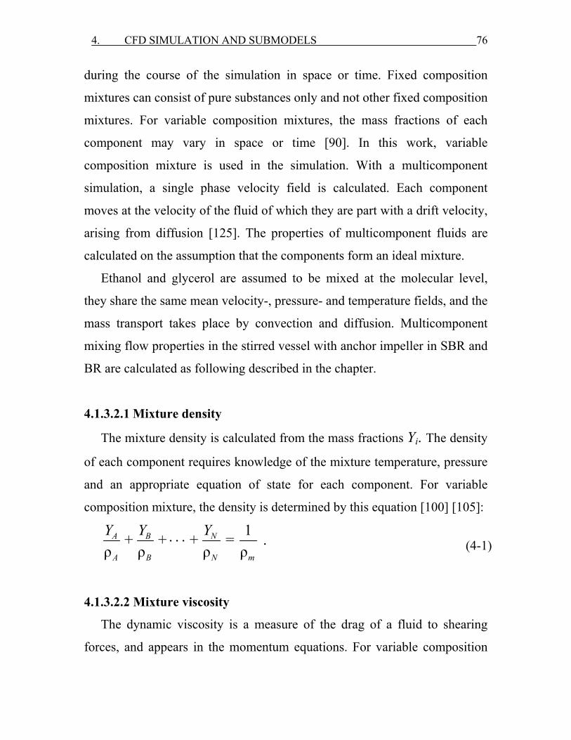
4. CFD SIMULATION AND SUBMODELS 76
during the course of the simulation in space or time. Fixed composition
mixtures can consist of pure substances only and not other fixed composition
mixtures. For variable composition mixtures, the mass fractions of each
component may vary in space or time [90]. In this work, variable
composition mixture is used in the simulation. With a multicomponent
simulation, a single phase velocity field is calculated. Each component
moves at the velocity of the fluid of which they are part with a drift velocity,
arising from diffusion [125]. The properties of multicomponent fluids are
calculated on the assumption that the components form an ideal mixture.
Ethanol and glycerol are assumed to be mixed at the molecular level,
they share the same mean velocity-, pressure- and temperature fields, and the
mass transport takes place by convection and diffusion. Multicomponent
mixing flow properties in the stirred vessel with anchor impeller in SBR and
BR are calculated as following described in the chapter.
4.1.3.2.1 Mixture density
The mixture density is calculated from the mass fractions Yi. The density
of each component requires knowledge of the mixture temperature, pressure
and an appropriate equation of state for each component. For variable
composition mixture, the density is determined by this equation [100] [105]:
1+ + + = .ρ ρ ρ ρ
⋅ ⋅ ⋅ NA B
A B N m
YY Y (4-1)
4.1.3.2.2 Mixture viscosity
The dynamic viscosity is a measure of the drag of a fluid to shearing
forces, and appears in the momentum equations. For variable composition

4. CFD SIMULATION AND SUBMODELS 77
mixture, the dynamic viscosity can be determined by the following equations
for ideal and non ideal liquid mixing.
4.1.3.2.2.1 Ideal case
In an ideal mixture the properties can be calculated directly from the
properties of the components and their mass fraction in the mixture. Then for
a liquid mixture of ethanol and glycerol the dynamic viscosity of this
mixture is calculated by using the following equation [76] [103]:
m = .N
i ii A,B,...
Y=
η η∑ (4-2)
4.1.3.2.2.2 Nonideal case
The viscosity of liquid mixtures in general has no linear dependence on
the composition and is difficult to calculate. Arrhenius viscosity equation is
proposed to predict the viscosity of the binary liquid mixtures of ethanol and
glycerol by using this equation [29] [70] [96] [99] [128] [129]:
mln = ln .N
i ii A,B,...
Y=
η η∑ (4-3)
4.1.3.2.3 Mixture molar mass
For variable composition mixture, the molar mass is determined by using
the equation [101]:
1... .+ + + =% % % %
NA B
A B N m
YY YM M M M (4-4)
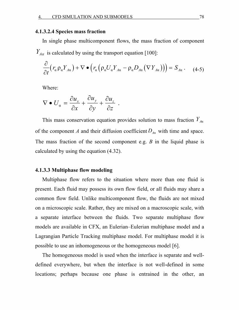
4. CFD SIMULATION AND SUBMODELS 78
4.1.3.2.4 Species mass fraction
In single phase multicomponent flows, the mass fraction of component
αAY is calculated by using the transport equation [100]:
( ) ( )( )( )α α α α α α α α α α αρ ρ ρ .∂+ ∇ • − ∇ =
∂ A A A A Ar Υ r U Υ D Υ St (4-5)
Where:
α .∂∂ ∂
∇ • = + +∂ ∂ ∂
yx zuu uUx y z
This mass conservation equation provides solution to mass fraction αAΥ
of the component A and their diffusion coefficient αAD with time and space.
The mass fraction of the second component e.g. B in the liquid phase is
calculated by using the equation (4.32).
4.1.3.3 Multiphase flow modeling
Multiphase flow refers to the situation where more than one fluid is
present. Each fluid may possess its own flow field, or all fluids may share a
common flow field. Unlike multicomponent flow, the fluids are not mixed
on a microscopic scale. Rather, they are mixed on a macroscopic scale, with
a separate interface between the fluids. Two separate multiphase flow
models are available in CFX, an Eulerian–Eulerian multiphase model and a
Lagrangian Particle Tracking multiphase model. For multiphase model it is
possible to use an inhomogeneous or the homogeneous model [6].
The homogeneous model is used when the interface is separate and well-
defined everywhere, but when the interface is not well-defined in some
locations; perhaps because one phase is entrained in the other, an
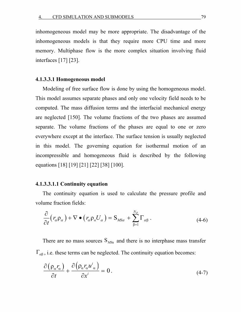
4. CFD SIMULATION AND SUBMODELS 79
inhomogeneous model may be more appropriate. The disadvantage of the
inhomogeneous models is that they require more CPU time and more
memory. Multiphase flow is the more complex situation involving fluid
interfaces [17] [23].
4.1.3.3.1 Homogeneous model
Modeling of free surface flow is done by using the homogeneous model.
This model assumes separate phases and only one velocity field needs to be
computed. The mass diffusion terms and the interfacial mechanical energy
are neglected [150]. The volume fractions of the two phases are assumed
separate. The volume fractions of the phases are equal to one or zero
everywhere except at the interface. The surface tension is usually neglected
in this model. The governing equation for isothermal motion of an
incompressible and homogeneous fluid is described by the following
equations [18] [19] [21] [22] [38] [100].
4.1.3.3.1.1 Continuity equation
The continuity equation is used to calculate the pressure profile and
volume fraction fields:
( ) ( ) ββ 1
ρ ρ S .α α α α α α=
∂+ ∇ • = + Γ
∂ ∑PN
α MSr r Ut (4-6)
There are no mass sources αSMS and there is no interphase mass transfer
βαΓ , i.e. these terms can be neglected. The continuity equation becomes:
( ) ( )ρ0 .α α αα α ∂ ρ∂
+ =∂ ∂
i
i
r urt x (4-7)
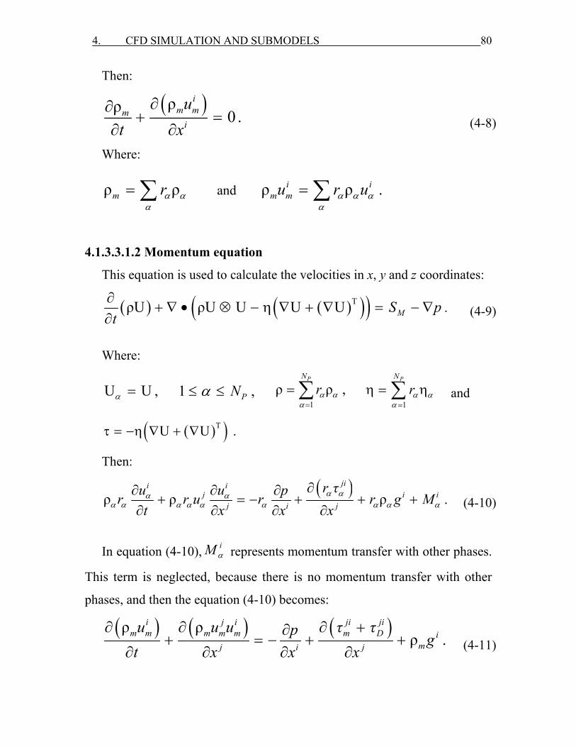
4. CFD SIMULATION AND SUBMODELS 80
Then:
( )ρρ 0 .∂∂
+ =∂ ∂
im mm
i
ut x (4-8)
Where:
andρ ρ ρ ρ .α α α α αα α
= =∑ ∑i im m mr u r u
4.1.3.3.1.2 Momentum equation
This equation is used to calculate the velocities in x, y and z coordinates:
( ) ( )( )( )TρU ρU U U U∂+ ∇ • ⊗ − η ∇ + ∇ = − ∇
∂ MS p .t (4-9)
Where:
U U ,α = 1 ,α≤ ≤ PN 1
ρ ρ ,α αα =
= ∑PN
r 1
α αα =
η = η∑PN
r and
( )( )TU U .τ = −η ∇ + ∇
Then:
( )ρ ρ ρ .α αα α
α α α α α α α α α
∂∂ ∂ ∂+ = − + + +
∂ ∂ ∂ ∂
jii ij i i
j i j
r τu u pr r u r r g Mt x x x (4-10)
In equation (4-10), iM α represents momentum transfer with other phases.
This term is neglected, because there is no momentum transfer with other
phases, and then the equation (4-10) becomes:
( ) ( ) ( )ρ ρρ .
∂ ∂ ∂ +∂+ = − + +
∂ ∂ ∂ ∂
i j i ji jim m m m m m D i
mj i j
u u u τ τp gt x x x (4-11)
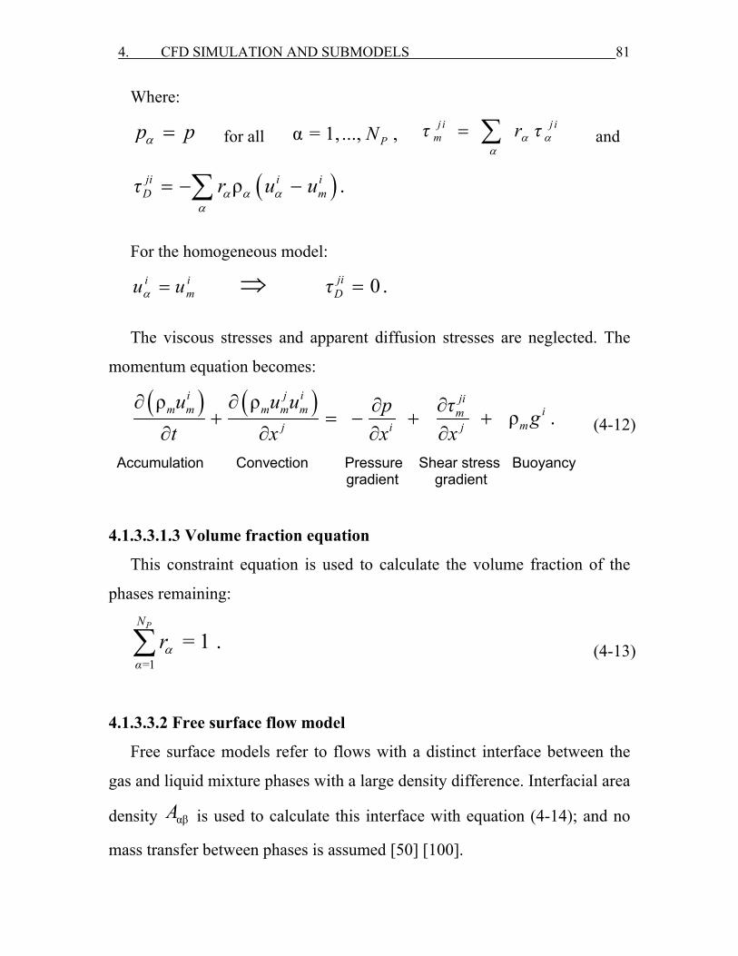
4. CFD SIMULATION AND SUBMODELS 81
Where:
α =p p for all α = 1, ..., ,ΡN α αα
= ∑j i j imτ r τ and
( )ρ .α α αα
= − −∑ji i iD mτ r u u
For the homogeneous model: im
i uu =α ⇒ 0 .=jiDτ
The viscous stresses and apparent diffusion stresses are neglected. The
momentum equation becomes:
( ) ( )ρ ρρ .
∂ ∂ ∂∂+ = − + +
∂ ∂ ∂ ∂
i j i jim m m m m im
mj i j
u u u τp gt x x x (4-12)
Accumulation Convection Pressure Shear stress Buoyancy gradient gradient
4.1.3.3.1.3 Volume fraction equation
This constraint equation is used to calculate the volume fraction of the
phases remaining:
=1= 1 .α∑
PN
αr (4-13)
4.1.3.3.2 Free surface flow model
Free surface models refer to flows with a distinct interface between the
gas and liquid mixture phases with a large density difference. Interfacial area
density αβA is used to calculate this interface with equation (4-14); and no
mass transfer between phases is assumed [50] [100].
4. CFD SIMULATION AND SUBMODELS 82
αβ α .= ∇A r (4-14)
The inertia of the gas is usually negligible due to its low density. The
only influence of the gas is its pressure acting on the interface. The liquid
can thus move freely, and the locations of the free surface can be determined
by solving the equation (4-14). Simulation of free surface flows usually
requires defining boundary and initial conditions to set up appropriate
pressure profile and volume fraction fields [7].
The implementation of free surface flow model in CFX-10 need some
special discretisation options to keep the interface sharp. These include:
(1) A compressive differencing scheme (High Resolution Scheme) for the
advection of volume fractions in the volume fraction equations.
(2) A compressive transient scheme (Second Order Backward Euler) for the
volume fraction equations.
(3) Special treatment of the pressure gradient and gravity terms to ensure
that the flow remain sharp at the interface.
4.1.3.4 Submodels
4.1.3.4.1 Fluid buoyancy model
Buoyancy is a natural and mixed convection flows in which gravity is
important. Natural convection happens when the fluid is driven only by local
density variations. Convection in the mixture occurs when the fluid is driven
by both a pressure gradient and buoyancy forces. Buoyancy is driven by
variations in density which can arise from a number of sources:
(1) Natural convection.
(2) In multicomponent flows, variations in the mass fraction cause density

4. CFD SIMULATION AND SUBMODELS 83
variations since each component usually has a different density.
(3) In multiphase flows, including particle transport modeling, the difference
in density between the phases results in a buoyancy force.
(4) If density is variable for a general fluid (i.e., defined by an expression), a
buoyancy force will arise.
(5) For ideal gases and real fluids, local pressure variations also cause
changes in density. These changes are often small and the buoyancy
effect is usually not important in the flow.
In the buoyancy calculations, the gravity vector components in x, y and z
are set in the Cartesian coordinate. Buoyancy is simulated in this work by
using the density difference buoyancy model.
4.1.3.4.1.1 Density difference between two liquids
For single phase flows, this model is used when the fluid density is a
function of temperature or pressure (which includes ideal gases and real
fluids) and when a multicomponent fluid is used. For Eulerian multiphase or
particle tracking, it is also set even if all phases have constant density.
Significant density variations with temperature occur for most gases. A
buoyancy reference density as an approximate average value of the expected
domain density is specified for the lower density phase. In multiphase
simulations, fluid buoyancy model with density difference is also used. The
volumetric buoyancy force αF is modeled by considering the difference in
density between phases with the equation:
( )ρ ρ g .−αα =F ref (4-15)

4. CFD SIMULATION AND SUBMODELS 84
4.1.3.4.1.2 Pressure gradient between two liquids
The hydrostatic pressure is responsible for driving the flow. It depends on
the density of the liquid mixture and buoyancy forces. Initial and boundary
conditions are defined in terms of this pressure gradient. The hydrostatic
pressure is included.
4.1.3.4.1.3 Rotating domains
In rotating domains transient simulations that include a buoyancy term, it
is necessary to set the components of the gravity vector to be a function of
the angle of rotation of the domain. The used set in this work is:
gx = 0 [m/s2] ,
gy = 0 [m/s2] ,
gz =− 9.81 [m/s2] .
4.1.3.4.1.4 Multiphase flow
The density difference between air and a liquid mixture produces a
buoyancy force in multiphase flows. The density of lighter fluid (air) is
chosen to be the buoyancy reference density in the free surface flow model
calculations; this gives constant pressure in the light phase and hydrostatic
pressure in the heavier liquid mixture phase. Also, it simplifies the
calculations of the pressure initial and pressure boundary conditions as well
as the force in post-processing.
4.1.3.4.2 Laminar model
Laminar flow is governed by the unsteady Navier-Stokes equations. The
laminar model is only appropriate if the flow is laminar. It can be applied at
low Reynolds number flows with Re < 1000.
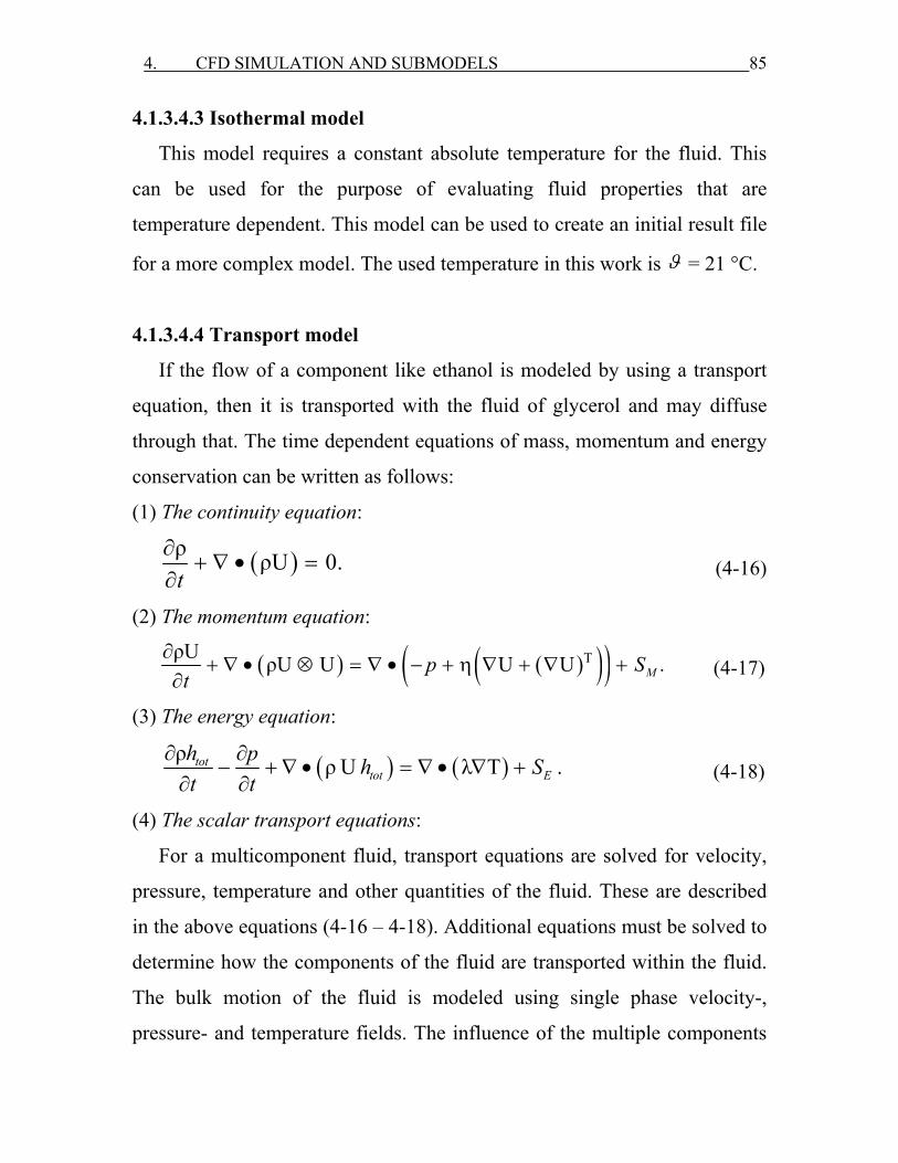
4. CFD SIMULATION AND SUBMODELS 85
4.1.3.4.3 Isothermal model
This model requires a constant absolute temperature for the fluid. This
can be used for the purpose of evaluating fluid properties that are
temperature dependent. This model can be used to create an initial result file
for a more complex model. The used temperature in this work is ϑ = 21 °C.
4.1.3.4.4 Transport model
If the flow of a component like ethanol is modeled by using a transport
equation, then it is transported with the fluid of glycerol and may diffuse
through that. The time dependent equations of mass, momentum and energy
conservation can be written as follows:
(1) The continuity equation:
( )ρ ρU 0.∂+ ∇ • =
∂t (4-16)
(2) The momentum equation:
( ) ( )( )( )TρU ρU U U U .∂+ ∇ • ⊗ = ∇ • − + η ∇ + ∇ +
∂ Mp St (4-17)
(3) The energy equation:
( ) ( )ρ ρ U λ T .∂ ∂− + ∇ • = ∇ • ∇ +
∂ ∂tot
tot Eh p h St t (4-18)
(4) The scalar transport equations:
For a multicomponent fluid, transport equations are solved for velocity,
pressure, temperature and other quantities of the fluid. These are described
in the above equations (4-16 – 4-18). Additional equations must be solved to
determine how the components of the fluid are transported within the fluid.
The bulk motion of the fluid is modeled using single phase velocity-,
pressure- and temperature fields. The influence of the multiple components
4. CFD SIMULATION AND SUBMODELS 86
is found from the variation of different properties for the various
components like variation in density which affects conservation of mass.
Each component has its own Reynolds-averaged equation for conservation
of mass, which can be expressed as:
( ) ( )( )ρρ ρ ρ " " . ∂∂ ∂
+ = − − − +∂ ∂ ∂
%%% % %i jii ij j i j i
j j
UU U U S
t x x (4-19)
Where: ( )ρ ρ ./= ∑% %%j i ijU U
The relative mass flux term ( )jiji UU ~~ρ − accounts for differential motion of
the individual components. This term is modeled to include effects of
concentration gradients through the diffusion effect as in this equation:
( ) ρ ρρ .ρ
∂− = −
∂%% % i i i
i ij jj
DU Ux (4-20)
The definition of the mass fraction of component i is:
ρ .ρ
=%% i
iΥ (4-21)
Substituting equation (4-20) and (4-21) into (4-19) gives:
( ) ( ) ( )ρ ρρ ρ .
∂ ∂ ∂∂ ∂+ = − + ∂ ∂ ∂ ∂ ∂
% % % %i j i " "ii i i j i
j j j j
Υ U Υ ΥD Υ U St x x x x (4-22)
No chemical reaction is considered, and then the source term iS can be
neglected. For laminar flow, the turbulent scalar fluxes "j
"i UΥρ are neglected.
The mass fraction equation becomes [104]:
( ) ( )ρ ρρ .
∂ ∂ ∂∂+ = ∂ ∂ ∂ ∂
% % % %i j i ii i
j j j
Υ U Υ ΥDt x x x (4-23)
This equation is used to calculate the composition of the fluid mixture.
4. CFD SIMULATION AND SUBMODELS 87
4.1.3.4.5 Algebraic slip model
Algebraic slip mixture model (ASM), as with the Eulerian multiphase
model is designed for use with two interpenetrating fluids and for liquid-
liquid or gas-liquid mixture. A full set of Navier-Stokes equations is solved
for the primary fluid (continuous phase). An algebraic equation for the slip
velocity between the fluids is solved. The slip velocity is derived from the
fluid properties and local flow conditions and is used to compute the
velocity of the secondary phase (dispersed phase). The ASM model is not set
up in the same way as other multiphase problems. It needs to define a
variable composition mixture containing the fluids when setting the
thermodynamic state of the mixture.
The continuous phase should be set to constraint. The remaining phases
can be set to either algebraic slip or transport equation. Transport equations
and algebraic slip components can be combined, meaning that a mixture of
components may be present in the continuous phase. At least one component
must be set to constraint. For the dispersed phases, the algebraic slip model
is chosen. The algebraic slip option can be set to drag force balance or slip
velocity. The drag force balance uses the closed relationship for the slip
velocity, as will be shown in derivation of the algebraic slip equation:
(1) Phase equations:
Each phase has its own velocity field which can be calculated. The
continuity equation for phase α is calculated from equation (4-7) and the
momentum equation is equation (4-10).
(2) Bulk equations:
A bulk continuity equation is derived by summing equation (4-7) over all
phases resulting in equation (4-8). And a bulk momentum equation by
summing equation (4-8) over all phases gives equation (4-11).
4. CFD SIMULATION AND SUBMODELS 88
(3) Drift and slip relations:
The slip velocity is the phase velocity relative to the continuous phase:
.α α= −i i iS Cu u u (4-24)
And the drift velocity is the phase velocity relative to the liquid mixture
velocity in the bulk as:
.α α= −i i iD mu u u (4-25)
The slip- and drift velocities are related by the following equation:
.α α α αα
= − ∑i i iD S Su u Y u (4-26)
With these relationships, the phase continuity equation may be written in
terms of mass fraction and drift velocity as:
( ) ( )( )ρρ 0 .α
α α
∂ ∂+ + =
∂ ∂m i i
m m Di
YY u u
t x (4-27)
(4) Derivation of the algebraic slip equation:
The phase and bulk momentum equations are first transformed to
nonconservative form by combining with the phase and bulk continuity
equations. The phase momentum equation is:
( )ρ ρ ρ .α αα α
α α α α α α α α α
∂∂ ∂ ∂+ = − + + +
∂ ∂ ∂ ∂
jii ij i i
j i j
r τu u pr r u r r g Mt x x x (4-10)
And the bulk momentum equation is:
( )ρ ρ ρ .
∂ +∂ ∂ ∂+ = − + +
∂ ∂ ∂ ∂
ji jii im Dj im m
m m m mj i j
τ τu u pu gt x x x (4-11)
Equation (4-10) and (4-11) are combined to eliminate the pressure
gradient term, yielding:

4. CFD SIMULATION AND SUBMODELS 89
( )
( ) ( )
( )
ρ ρ ρ
ρ ρ
ρ ρ .
αα α α α
αα α α
α αα
α α
τ τ τ
∂ ∂ = + − ∂ ∂
∂ ∂ + − ∂ ∂
∂ ∂ +− +
∂ ∂− −
i ii D m
m
i ij j m
m mj j
ji ji jim D
j j
im
u uM rt t
u ur u ux x
rr
x xr g
(4-28)
Several assumptions are now made:
(1) The dispersed phase is assumed to immediately reach its final
velocity, so the transient term on the drift velocity can be neglected.
(2) The approximation is made that:
.αα
∂ ∂≈
∂ ∂
i ij j m
mj j
u uu ux x
(3) The viscous stresses and apparent diffusion stresses are neglected.
With these approximations, the equation (4-28) simplifies to:
( )ρ .α α α ∂ ∂
= ρ − + − ∂ ∂
i ii j im m
m m j
u uM r u gt x (4-29)
Also, it is assumed that the interphase momentum transfer is due only to
drag and that the particles are spherical:
P
3 .4 dα
αα α
ρ= −i ii
D S SrM C u u (4-30)
This leads to the following closed relationship for the slip velocity:
( )P4 d ρ ρ .3 αα α
∂ ∂ = − − − ρ ∂ ∂
i ii j im m
S S m m ji D
u uu u + u g C t x (4-31)
4. CFD SIMULATION AND SUBMODELS 90
Where the subscript m refers to bulk quantities, α refers to dispersed
phase quantities and ρi refers to the density of component. The drag
coefficient CD is directly specified as a constant value of 0.47; the mean
diameter dp must be specified and is assumed to be a constant value of
0.0002 m [114 – 121]. Models for algebraic slip were introduced by Ishii
[126]. Manninen and Taivassalo [127], provide a more general formulation.
The effect of ji
Dτ in the bulk momentum equation is neglected in this work.
4.1.3.4.6 Modified algebraic slip model
The new developed modified algebraic slip model (MASM) is derived
from the ASM but the diameter of the droplet dp in Eq. 4-31 is a step
function of time dp(t) [s. Chap. 5.3.5].
4.1.3.4.7 Constraint equation
If the flow of a component is modeled using a constraint equation, its
mass fraction is calculated to ensure that all the component mass fractions
sum to unity, i.e. the mass fraction of the component is set equal to the total
mass fractions of the other components in the same fluid subtracted from
unity. The CFX-10 solver solves NC − 1 mass fraction equations (either
transport equations or algebraic equations) for all except one of the
components. The remaining component is known as the constraint
component because its mass fraction is determined by the constraint
equation: C
1=
=∑N
ii A,B,...
Y (4-32)
4. CFD SIMULATION AND SUBMODELS 91
4.1.3.4.8 Sliding mesh model
The sliding mesh method is a new way of dealing with the impeller
interaction. The main advantage of the sliding mesh method is that no
experimentally obtained boundary conditions are needed, as the flow around
the impeller blades is being calculated in detail. This allows modeling of
impeller systems and reactors for which experimental data is difficult or
impossible to obtain.
With the sliding mesh method the reactor is divided in two regions that
are treated separately: the impeller region and the reactor region that
includes the bulk of the liquid, the reactor wall and the reactor bottom, see
Fig. 4.3. The grid in the impeller region rotates with the impeller. The grid in
the reactor remains stationary. The two grids slide past each other at a
cylindrical interface. In the reactor region the conservation equations for
mass and momentum are solved. In the rotating impeller region a modified
set of balance equations is solved.
Sliding mesh methods can be used to accurately predict the time
dependent laminar flow pattern in stirred reactors, without the need for
experimental data. A disadvantage is the long calculation time which is
about an order of magnitude longer than with steady state calculations based
on experimental impeller data. An important application for the sliding mesh
method might be the development of new, optimized impeller designs for
specific industrial applications. Other applications are the prediction of flow
patterns with impellers for which no experimental data are available, the
prediction of flow patterns in multiple impeller systems where there is
significant interaction between the impellers and to predict time dependent
flow patterns in systems where steady state assumptions are not justified.

4. CFD SIMULATION AND SUBMODELS 92
Figure 4.3: The reactor (stationary) and anchor impeller (rotating) regions and grid for
the full geometry in the sliding mesh method at two different time steps. The grid in the
impeller region moves with the impeller and slides past the stationary grid for the
remaining part of the reactor.
The scheme in Fig. 4.4 shows the physical models and submodels are
used in the simulations of liquids mixing procedure with CFX.
t = 0 t = 0.25 s
Impeller region
Reactor region
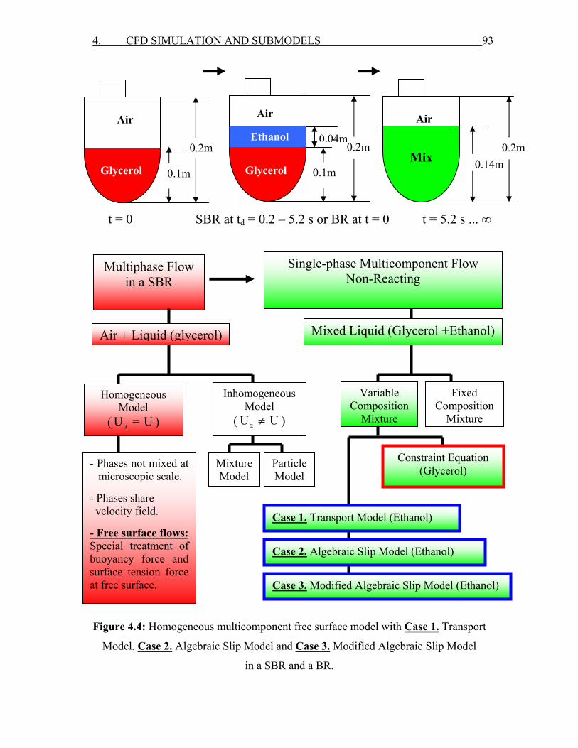
4. CFD SIMULATION AND SUBMODELS 93
t = 0 SBR at td = 0.2 – 5.2 s or BR at t = 0 t = 5.2 s ... ∞
Figure 4.4: Homogeneous multicomponent free surface model with Case 1. Transport
Model, Case 2. Algebraic Slip Model and Case 3. Modified Algebraic Slip Model
in a SBR and a BR.
Multiphase Flow in a SBR
Homogeneous Model
( αU = U )
Inhomogeneous Model
( αU U≠ )
Fixed Composition
Mixture
Air + Liquid (glycerol)
Particle Model
Mixture Model
Single-phase Multicomponent Flow Non-Reacting
Mixed Liquid (Glycerol +Ethanol)
Air
0.1m
0.2m
Glycerol
Air
0.1m
0.2m
Glycerol
Ethanol 0.04m
Air
Mix
0.14m
0.2m
Variable Composition
Mixture
- Phases not mixed at microscopic scale.
- Phases share velocity field. - Free surface flows: Special treatment of buoyancy force and surface tension force at free surface.
Constraint Equation (Glycerol)
Case 1. Transport Model (Ethanol)
Case 2. Algebraic Slip Model (Ethanol)
Case 3. Modified Algebraic Slip Model (Ethanol)
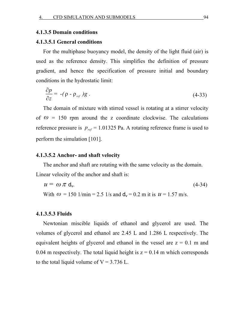
4. CFD SIMULATION AND SUBMODELS 94
4.1.3.5 Domain conditions
4.1.3.5.1 General conditions
For the multiphase buoyancy model, the density of the light fluid (air) is
used as the reference density. This simplifies the definition of pressure
gradient, and hence the specification of pressure initial and boundary
conditions in the hydrostatic limit:
ρ ρ∂∂ ref
p = -( - )g .z (4-33)
The domain of mixture with stirred vessel is rotating at a stirrer velocity
of ω = 150 rpm around the z coordinate clockwise. The calculations
reference pressure is refp = 1.01325 Pa. A rotating reference frame is used to
perform the simulation [101].
4.1.3.5.2 Anchor- and shaft velocity
The anchor and shaft are rotating with the same velocity as the domain.
Linear velocity of the anchor and shaft is:
u = ω π dv. (4-34)
With ω = 150 1/min = 2.5 1/s and dv = 0.2 m it is u = 1.57 m/s.
4.1.3.5.3 Fluids
Newtonian miscible liquids of ethanol and glycerol are used. The
volumes of glycerol and ethanol are 2.45 L and 1.286 L respectively. The
equivalent heights of glycerol and ethanol in the vessel are z = 0.1 m and
0.04 m respectively. The total liquid height is z = 0.14 m which corresponds
to the total liquid volume of V = 3.736 L.
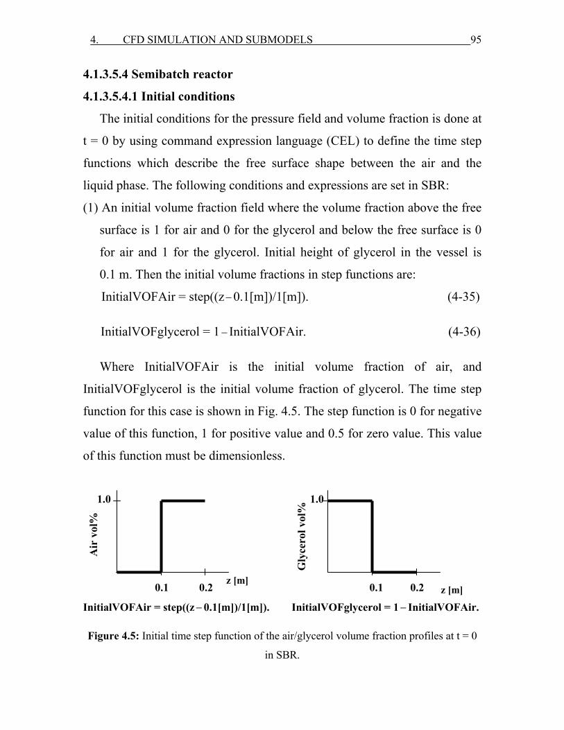
4. CFD SIMULATION AND SUBMODELS 95
4.1.3.5.4 Semibatch reactor
4.1.3.5.4.1 Initial conditions
The initial conditions for the pressure field and volume fraction is done at
t = 0 by using command expression language (CEL) to define the time step
functions which describe the free surface shape between the air and the
liquid phase. The following conditions and expressions are set in SBR:
(1) An initial volume fraction field where the volume fraction above the free
surface is 1 for air and 0 for the glycerol and below the free surface is 0
for air and 1 for the glycerol. Initial height of glycerol in the vessel is
0.1 m. Then the initial volume fractions in step functions are:
InitialVOFAir = step((z − 0.1[m])/1[m]). (4-35)
InitialVOFglycerol = 1 − InitialVOFAir. (4-36)
Where InitialVOFAir is the initial volume fraction of air, and
InitialVOFglycerol is the initial volume fraction of glycerol. The time step
function for this case is shown in Fig. 4.5. The step function is 0 for negative
value of this function, 1 for positive value and 0.5 for zero value. This value
of this function must be dimensionless.
InitialVOFAir = step((z − 0.1[m])/1[m]). InitialVOFglycerol = 1 − InitialVOFAir.
Figure 4.5: Initial time step function of the air/glycerol volume fraction profiles at t = 0
in SBR.
Gly
cero
l vol
%
z [m]0.2
1.0
z [m]0.1 0.2
1.0
0.1
Air
vol
%
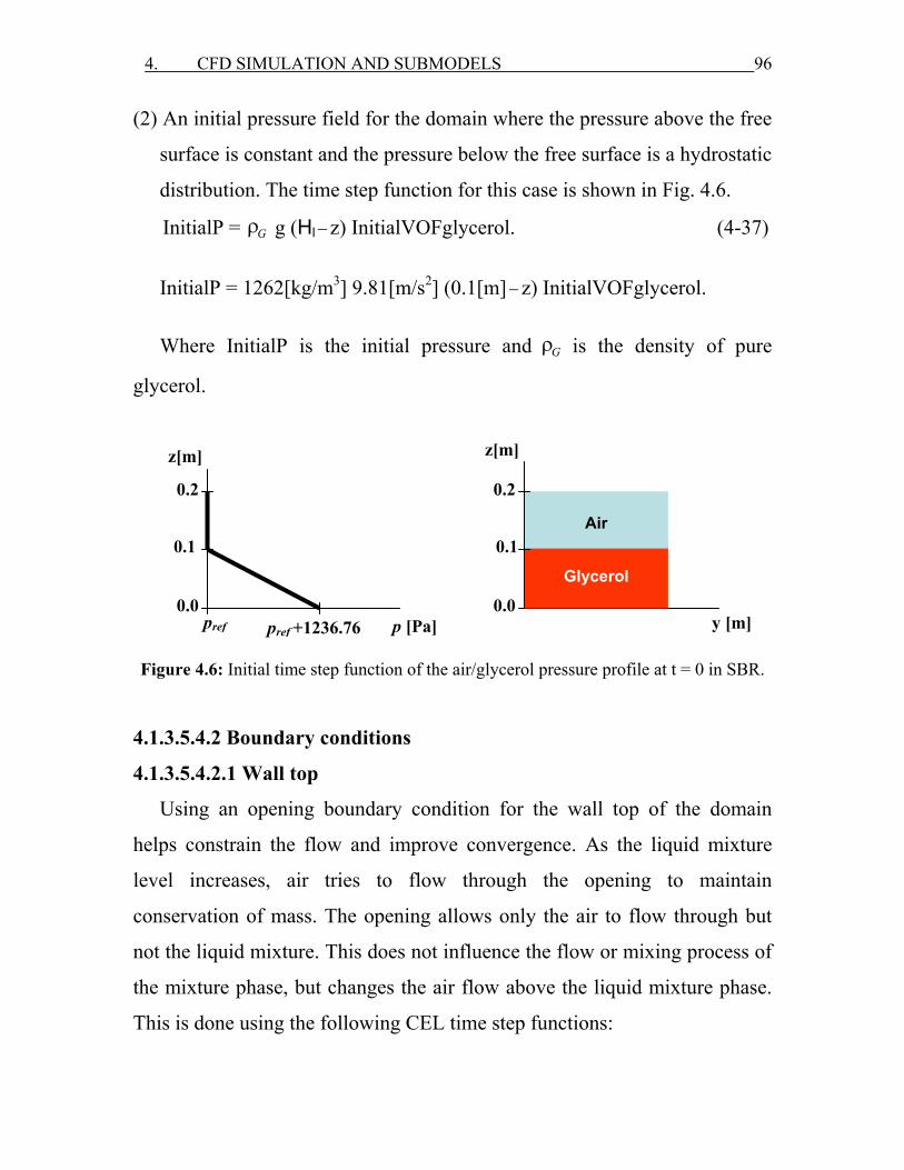
4. CFD SIMULATION AND SUBMODELS 96
(2) An initial pressure field for the domain where the pressure above the free
surface is constant and the pressure below the free surface is a hydrostatic
distribution. The time step function for this case is shown in Fig. 4.6.
InitialP = ρG g (Hl − z) InitialVOFglycerol. (4-37)
InitialP = 1262[kg/m3] 9.81[m/s2] (0.1[m] − z) InitialVOFglycerol.
Where InitialP is the initial pressure and ρG is the density of pure
glycerol.
Figure 4.6: Initial time step function of the air/glycerol pressure profile at t = 0 in SBR.
4.1.3.5.4.2 Boundary conditions
4.1.3.5.4.2.1 Wall top
Using an opening boundary condition for the wall top of the domain
helps constrain the flow and improve convergence. As the liquid mixture
level increases, air tries to flow through the opening to maintain
conservation of mass. The opening allows only the air to flow through but
not the liquid mixture. This does not influence the flow or mixing process of
the mixture phase, but changes the air flow above the liquid mixture phase.
This is done using the following CEL time step functions:
p [Pa]pref +1236.76
0.2
z[m]
0.1
0.2
z[m]
0.1
y [m]
Glycerol
Air
pref 0.0 0.0
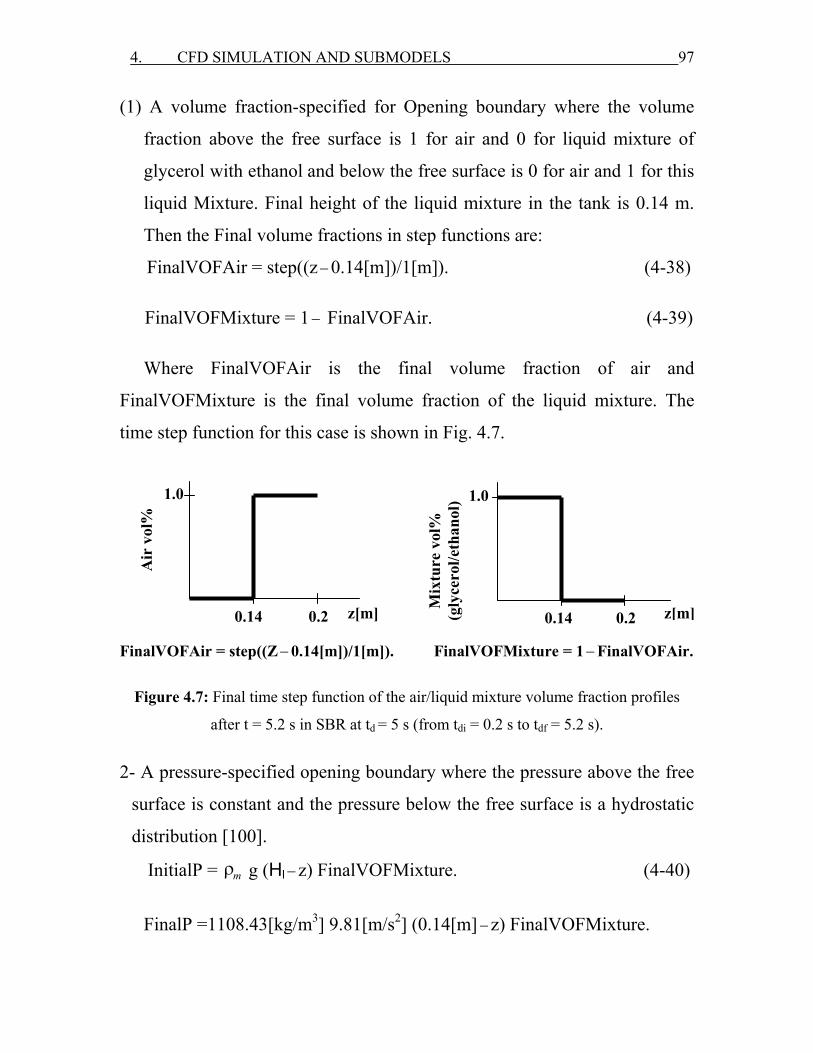
4. CFD SIMULATION AND SUBMODELS 97
(1) A volume fraction-specified for Opening boundary where the volume
fraction above the free surface is 1 for air and 0 for liquid mixture of
glycerol with ethanol and below the free surface is 0 for air and 1 for this
liquid Mixture. Final height of the liquid mixture in the tank is 0.14 m.
Then the Final volume fractions in step functions are:
FinalVOFAir = step((z − 0.14[m])/1[m]). (4-38)
FinalVOFMixture = 1 − FinalVOFAir. (4-39)
Where FinalVOFAir is the final volume fraction of air and
FinalVOFMixture is the final volume fraction of the liquid mixture. The
time step function for this case is shown in Fig. 4.7.
FinalVOFAir = step((Z − 0.14[m])/1[m]). FinalVOFMixture = 1 − FinalVOFAir.
Figure 4.7: Final time step function of the air/liquid mixture volume fraction profiles
after t = 5.2 s in SBR at td = 5 s (from tdi = 0.2 s to tdf = 5.2 s).
2- A pressure-specified opening boundary where the pressure above the free
surface is constant and the pressure below the free surface is a hydrostatic
distribution [100].
InitialP = ρm g (Hl − z) FinalVOFMixture. (4-40)
FinalP =1108.43[kg/m3] 9.81[m/s2] (0.14[m] − z) FinalVOFMixture.
Mix
ture
vol
%
(gly
cero
l/eth
anol
)
z[m]0.2
1.0
z[m] 0.14 0.2
1.0
0.14
Air
vol
%
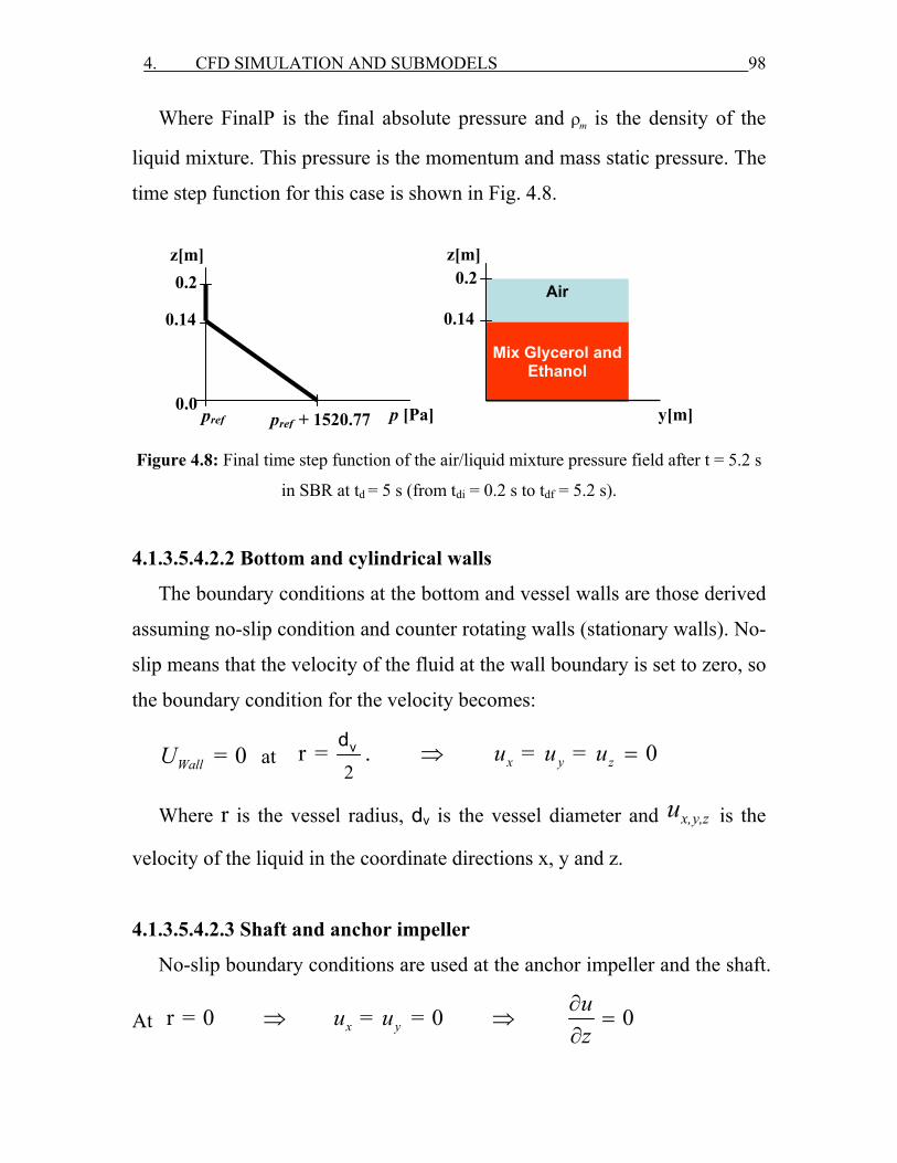
4. CFD SIMULATION AND SUBMODELS 98
Where FinalP is the final absolute pressure and ρm is the density of the
liquid mixture. This pressure is the momentum and mass static pressure. The
time step function for this case is shown in Fig. 4.8.
Figure 4.8: Final time step function of the air/liquid mixture pressure field after t = 5.2 s
in SBR at td = 5 s (from tdi = 0.2 s to tdf = 5.2 s).
4.1.3.5.4.2.2 Bottom and cylindrical walls
The boundary conditions at the bottom and vessel walls are those derived
assuming no-slip condition and counter rotating walls (stationary walls). No-
slip means that the velocity of the fluid at the wall boundary is set to zero, so
the boundary condition for the velocity becomes:
= 0WallU at 2
r = . 0x y zu = u = u⇒ = vd
Where r is the vessel radius, dv is the vessel diameter and x,y,zu is the
velocity of the liquid in the coordinate directions x, y and z.
4.1.3.5.4.2.3 Shaft and anchor impeller
No-slip boundary conditions are used at the anchor impeller and the shaft.
At r = 0 = 0 0x yuu = uz
∂⇒ ⇒ =
∂
p [Pa]
0.2 z[m]
0.14
0.2
0.14
y[m]
Mix Glycerol and
Ethanol
Air
0.0 pref
z[m]
pref + 1520.77
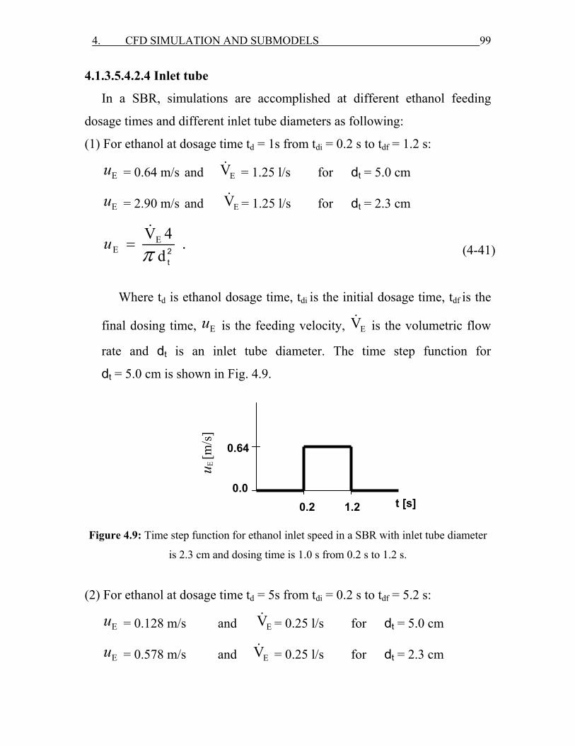
4. CFD SIMULATION AND SUBMODELS 99
4.1.3.5.4.2.4 Inlet tube
In a SBR, simulations are accomplished at different ethanol feeding
dosage times and different inlet tube diameters as following:
(1) For ethanol at dosage time td = 1s from tdi = 0.2 s to tdf = 1.2 s:
Eu = 0.64 m/s and EV& = 1.25 l/s for dt = 5.0 cm
Eu = 2.90 m/s and EV& = 1.25 l/s for dt = 2.3 cm
EE
V 4 .d
u =&
π 2t
(4-41)
Where td is ethanol dosage time, tdi is the initial dosage time, tdf is the
final dosing time, Eu is the feeding velocity, EV& is the volumetric flow
rate and dt is an inlet tube diameter. The time step function for
dt = 5.0 cm is shown in Fig. 4.9.
Figure 4.9: Time step function for ethanol inlet speed in a SBR with inlet tube diameter
is 2.3 cm and dosing time is 1.0 s from 0.2 s to 1.2 s.
(2) For ethanol at dosage time td = 5s from tdi = 0.2 s to tdf = 5.2 s:
Eu = 0.128 m/s and EV& = 0.25 l/s for dt = 5.0 cm
Eu = 0.578 m/s and EV& = 0.25 l/s for dt = 2.3 cm
u E [m
/s]
t [s] 0.2 1.2
0.64
0.0

4. CFD SIMULATION AND SUBMODELS 100
The inlet ethanol velocity and dosage time are defined and written
according to CEL as the following time step functions for dt = 2.3 cm:
f1 = step(t/1.0[sec] − tdi) 0.578 [m/sec]. (4-42)
f2= step(t/1.0[sec] − tdf) 0.578 [m/sec]. (4-43)
Inlet ethanol speed = f1 − f2. (4-44)
4.1.3.5.4.2.5 Periodic boundary
For periodic boundary condition: B1 = B2, where B is the transport
property. As a result the mesh and boundary conditions are used in the
simulations are shown in Figs. 4.10 and 4.11.
Figure 4.10: Meshing and boundaries for half geometry in SBR at td = 1 s, dt = 5 cm.
td = 1 s: 0.2 s t 1.2 s≤ ≤ Eu = 0.64 m/s
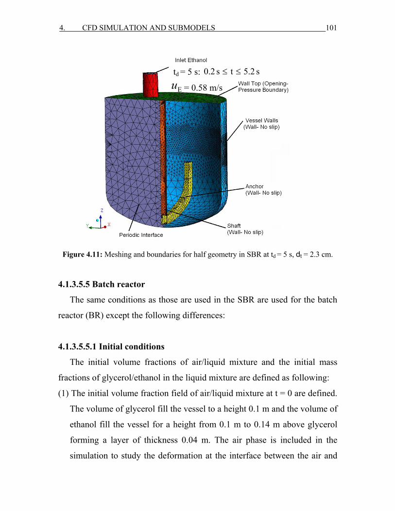
4. CFD SIMULATION AND SUBMODELS 101
Figure 4.11: Meshing and boundaries for half geometry in SBR at td = 5 s, dt = 2.3 cm.
4.1.3.5.5 Batch reactor
The same conditions as those are used in the SBR are used for the batch
reactor (BR) except the following differences:
4.1.3.5.5.1 Initial conditions
The initial volume fractions of air/liquid mixture and the initial mass
fractions of glycerol/ethanol in the liquid mixture are defined as following:
(1) The initial volume fraction field of air/liquid mixture at t = 0 are defined.
The volume of glycerol fill the vessel to a height 0.1 m and the volume of
ethanol fill the vessel for a height from 0.1 m to 0.14 m above glycerol
forming a layer of thickness 0.04 m. The air phase is included in the
simulation to study the deformation at the interface between the air and
td = 5 s: 0.2 s t 5.2 s≤ ≤
Eu = 0.58 m/s
4. CFD SIMULATION AND SUBMODELS 102
the multicomponent liquid mixture phase. Air is set to be above the total
liquid height of 0.14 m. CEL time step functions are set to define this
situation:
InitAir = step((z −0.14[m])/1[m]). (4-45)
InitMix = 1 − InletAir. (4-46)
Where InitAir is the initial volume fraction of the air phase and InitMix is
the initial volume fraction of the liquid mixture phase. This condition is used
for air/liquid mixture phases.
(2) The initial mass fractions of glycerol/ethanol in the liquid mixture are
defined relative to their heights in the vessel. Two distinct layers are
formed because of the density difference. These layers are defined in the
program by using the following time step functions:
InGlycerol = step((0.1[m] −z)/1.0[m]). (4-47)
InEthanol = 1 − InGlycerol. (4-48)
Where InGlycerol is the initial mass fraction of the glycerol and
InEthanol is the initial mass fraction of the ethanol in the liquid mixture
phase.
4.1.3.5.5.2 Boundary conditions
There is no inlet boundary condition. Opening boundary condition at a
static pressure of 1.0 atm is used for the mass and momentum equation at the
wall top.
4. CFD SIMULATION AND SUBMODELS 103
4.1.4 CFX-solver manager
The CFX solver manager provides a graphical user interface to the CFX-
solver in order to give information about the emerging solution, and to
provide with an easy way to control the CFX-solver. It allows setting some,
attributes for the CFD calculations and control the CFX-solver interactively
as the solution develops.
The coupled solver approach is used in this work to solve the four
linearised equations for momentum and mass conservation simultaneously.
Lower number of iterations is required to get the convergence with this
method. Resolution of the algebraic equations is carried out using high
resolution advection and transient 2nd order backward Euler schemes. The
maximum residuals for error calculation are 0.0001.
4.1.5 CFX-post
It is designed to allow easy visualisation and quantitative post-processing
for the results of CFD simulations. The flow patterns of the liquid mixture
with time can be predicted by drawing the vector plots of the mixture
velocity. The contour plots are used to describe the dynamic viscosity with
time. Different variables are calculated from CFD like ethanol concentration
at different points in the tank. Animation also is used to show the real
motion and flow of the liquid mixture stirred with the anchor impeller.

4. CFD SIMULATION AND SUBMODELS 104
4.2 Simulation for full geometry in SBR and BR
These simulations are based on the sliding mesh model (transient stator
rotor) which requires two domains with new interfaces between them for
transferring the calculated variables.
4.2.1 Geometry building
The 3-D full geometry is designed using ICEM CFD 5.1 as mentioned
before. Two separate assemblies are constructed, one is for the rotating part
(anchor) and the second is for the stationary part (the rest parts of the vessel
i.e. cylindrical walls, tank bottom, wall top and the inlet tube).
For the rotating part, the same anchor impeller as mentioned is used and
new anchor interfaces are created to cover the domain of the anchor, these
interfaces have the same shape as for the tank walls (bottom, cylindrical
walls and top) which are described before. The available ICEM CFD tools of
point, curve, surface, topology building, and e.g. transform are used to do
this.
For the stationary part which includes all the boundaries that mentioned
before except the anchor, also new interfaces were created same as those for
the anchor with a very small distance from the anchor interfaces. The tank
and anchor impeller assemblies are shown in Fig. 4.12.
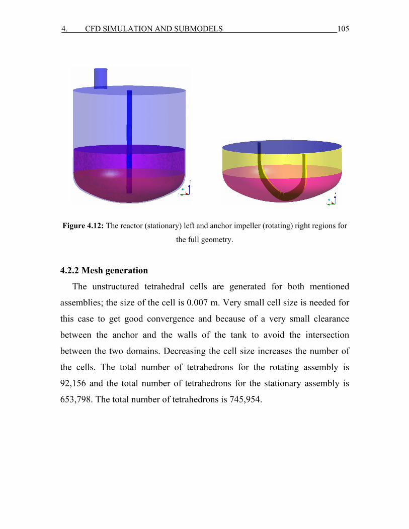
4. CFD SIMULATION AND SUBMODELS 105
Figure 4.12: The reactor (stationary) left and anchor impeller (rotating) right regions for
the full geometry.
4.2.2 Mesh generation
The unstructured tetrahedral cells are generated for both mentioned
assemblies; the size of the cell is 0.007 m. Very small cell size is needed for
this case to get good convergence and because of a very small clearance
between the anchor and the walls of the tank to avoid the intersection
between the two domains. Decreasing the cell size increases the number of
the cells. The total number of tetrahedrons for the rotating assembly is
92,156 and the total number of tetrahedrons for the stationary assembly is
653,798. The total number of tetrahedrons is 745,954.
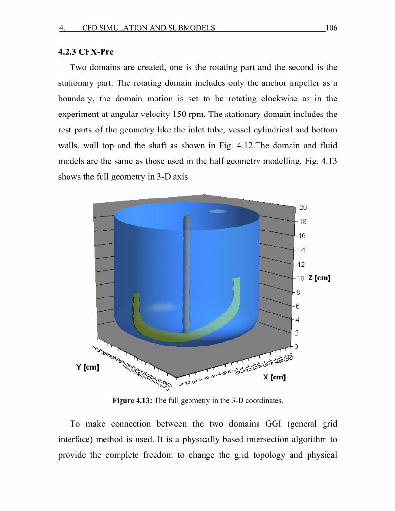
4. CFD SIMULATION AND SUBMODELS 106
4.2.3 CFX-Pre
Two domains are created, one is the rotating part and the second is the
stationary part. The rotating domain includes only the anchor impeller as a
boundary, the domain motion is set to be rotating clockwise as in the
experiment at angular velocity 150 rpm. The stationary domain includes the
rest parts of the geometry like the inlet tube, vessel cylindrical and bottom
walls, wall top and the shaft as shown in Fig. 4.12.The domain and fluid
models are the same as those used in the half geometry modelling. Fig. 4.13
shows the full geometry in 3-D axis.
Figure 4.13: The full geometry in the 3-D coordinates.
To make connection between the two domains GGI (general grid
interface) method is used. It is a physically based intersection algorithm to
provide the complete freedom to change the grid topology and physical
4. CFD SIMULATION AND SUBMODELS 107
distribution across the interfaces. This was done by creation three domain
interfaces:
1- Wall top interface
2- Wall bottom interface
3- Cylindrical wall interface
Through these fluid-fluid interfaces all the calculated variables are
transferred from the interface of the anchor to the corresponding interface of
the tank i.e. from the top interface of the anchor to the top interface of the
tank.
Transient rotor-stator model is a GGI frame change connection. It is used
to calculate the velocity transfer from the rotating domain to the stationary
domain. This model is important to account for transient interaction effects
at a sliding (frame change) interface. It predicts the true transient interaction
of the flow between the stator and rotor passage. The transient relative
motion between the components on each side of the GGI connection is
simulated. It accounts for all interaction effects between components that are
in relative motion to each other. The interface position is updated each
timestep, as the relative position of the grids on each side of the interface
changes.
The initial and boundary conditions are the same as those for the half
geometry. High resolution and second order Eulerian methods are used to
control the solution for the equations of the used models and to get a good
convergence with maximum residuals 0.001. The number of coefficient
loops to get more precise results is 15.
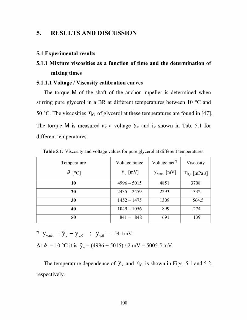
108
5. RESULTS AND DISCUSSION
5.1 Experimental results
5.1.1 Mixture viscosities as a function of time and the determination of
mixing times
5.1.1.1 Voltage / Viscosity calibration curves
The torque M of the shaft of the anchor impeller is determined when
stirring pure glycerol in a BR at different temperatures between 10 °C and
50 °C. The viscosities Gη of glycerol at these temperatures are found in [47].
The torque M is measured as a voltage vy and is shown in Tab. 5.1 for
different temperatures.
Table 5.1: Viscosity and voltage values for pure glycerol at different temperatures.
Temperature
ϑ [°C]
Voltage range
vy [mV]
Voltage net*)
v,nety [mV]
Viscosity
Gη [mPa s]
10 4996 – 5015 4851 3708
20 2435 – 2459 2293 1332
30 1452 – 1475 1309 564.5
40 1049 – 1056 899 274
50 841 − 848 691 139
*) v,net v v,0 v,0 154.1 mV.y y y ; y= − =%
At ϑ = 10 °C it is vy% = (4996 + 5015) / 2 mV = 5005.5 mV.
The temperature dependence of vy and Gη is shown in Figs. 5.1 and 5.2,
respectively.
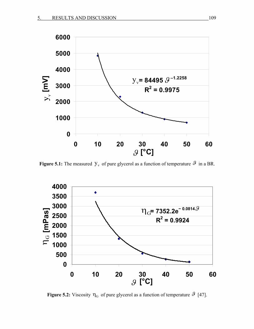
5. RESULTS AND DISCUSSION 109
Figure 5.1: The measured vy of pure glycerol as a function of temperature ϑ in a BR.
= 7352.2e− 0.0814
R2 = 0.9924
0500
1000150020002500300035004000
0 10 20 30 40 50 60[°C]
[mPa
s] Gη ϑ
ϑ
Gη
Figure 5.2: Viscosity Gη of pure glycerol as a function of temperature ϑ [47].
= 84495 –1.2258
R2 = 0.9975
0
1000
2000
3000
4000
5000
6000
0 10 20 30 40 50 60[°C]
[mV] ϑ
ϑ
vy
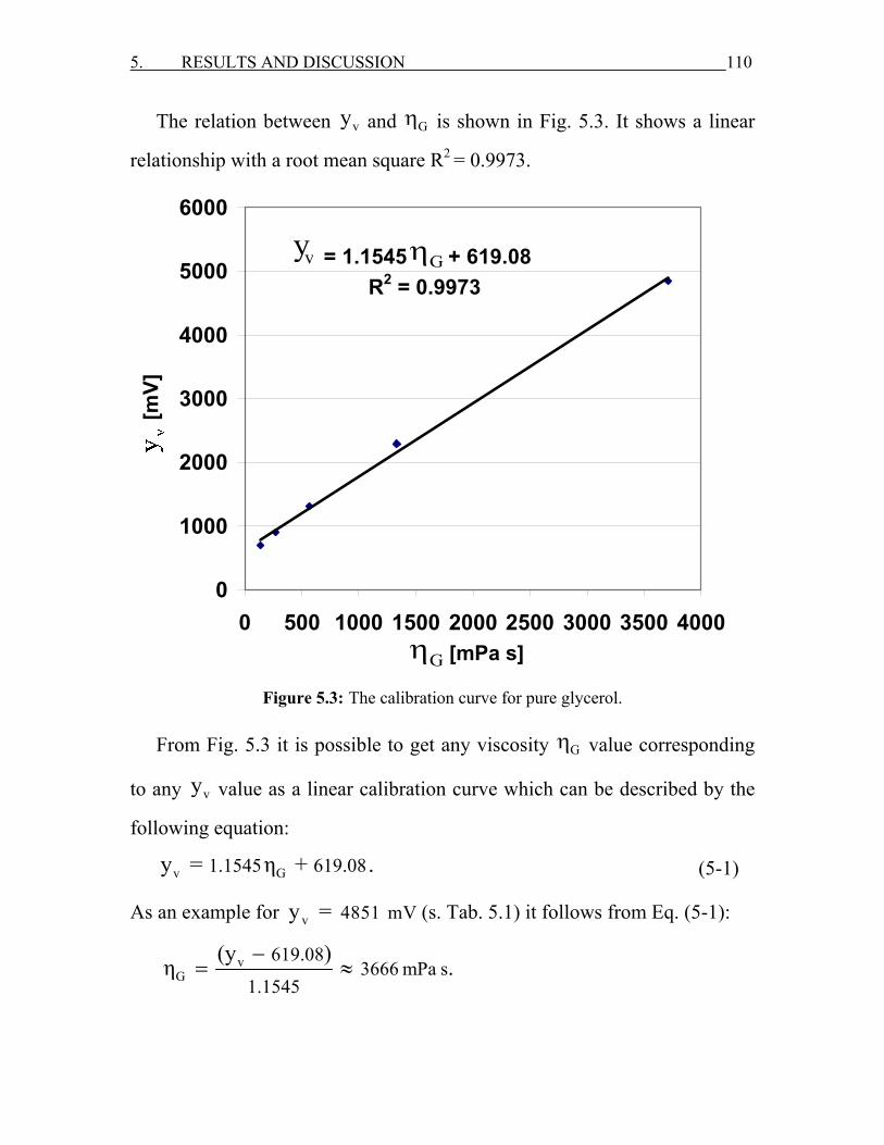
5. RESULTS AND DISCUSSION 110
The relation between vy and Gη is shown in Fig. 5.3. It shows a linear
relationship with a root mean square R2 = 0.9973.
= 1.1545 + 619.08R2 = 0.9973
0
1000
2000
3000
4000
5000
6000
0 500 1000 1500 2000 2500 3000 3500 4000[mPa s]
[mV]
vy
Gη
Gη
Figure 5.3: The calibration curve for pure glycerol.
From Fig. 5.3 it is possible to get any viscosity Gη value corresponding
to any vy value as a linear calibration curve which can be described by the
following equation:
v G1.1545 619.08 y = η + . (5-1)
As an example for v 4851 mVy = (s. Tab. 5.1) it follows from Eq. (5-1):
vG
619.083666 mPa s
1.1545
(y )η .−= ≈
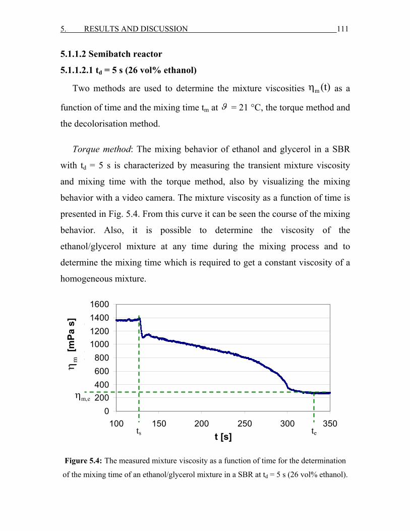
5. RESULTS AND DISCUSSION 111
5.1.1.2 Semibatch reactor
5.1.1.2.1 td = 5 s (26 vol% ethanol)
Two methods are used to determine the mixture viscosities m (t)η as a
function of time and the mixing time tm at ϑ = 21 °C, the torque method and
the decolorisation method.
Torque method: The mixing behavior of ethanol and glycerol in a SBR
with td = 5 s is characterized by measuring the transient mixture viscosity
and mixing time with the torque method, also by visualizing the mixing
behavior with a video camera. The mixture viscosity as a function of time is
presented in Fig. 5.4. From this curve it can be seen the course of the mixing
behavior. Also, it is possible to determine the viscosity of the
ethanol/glycerol mixture at any time during the mixing process and to
determine the mixing time which is required to get a constant viscosity of a
homogeneous mixture.
0200400600800
1000120014001600
100 150 200 250 300 350
Time [s]
Visc
osity
[mPa
s]
Figure 5.4: The measured mixture viscosity as a function of time for the determination
of the mixing time of an ethanol/glycerol mixture in a SBR at td = 5 s (26 vol% ethanol).
t [s]
[mPa
s]
mη
m,eη
te ts

5. RESULTS AND DISCUSSION 112
Fig. 5.4 shows that the viscosity of pure glycerol before the addition of
the second component ethanol has a constant value mη = 1366 mPa s
between 100 s t 124 s.≤ ≤ The dosage time is td = 5 s and the ethanol
started from ts = 124 s as a jet. The jet produce a local inlet pressure and
cause a fast mixing, so that a viscosity decreases takes place through the
period of the dosage time between 124 s t 129 s≤ ≤ from mη =
1366 mPa s up to mη = 1110 mPa s. This sharp decreasing in the viscosity is
due to the high pressure force and flow rate of the dosed ethanol. Between
129 s t 280 s,≤ ≤ the viscosity curve decreases slowly up to mη =
600 mPa s caused by the mixing process.
Because of the density and viscosity difference, ethanol and glycerol
form two layers. The upper layer of ethanol is the lighter one which has the
low density and viscosity. The lower layer of glycerol is the heavier one
which has the higher density and viscosity. After t = 280 s, the viscosity
decreases again fast to reach the complete mixing at the time te = 332 s. The
reason for this sharp decrease is the formation of a decreasing thickness
layer of ethanol. The homogenization of the mixture takes place at te = 332 s
with a final viscosity of mη = 279 mPa s. Then the mixing time tm is:
tm = te – ts = 332 s – 124 s = 208 s. (5-2)
Decolorisation method: Mixing time is determined when the yellow color
of the liquid mixture disappeared and becomes colorless, that means all the
iodine solution in glycerol has completely reacted with the stoichiometric
amount of the sodium thiosulfate solution in the ethanol, if a complete
homogeneous mixing is obtained. This mixing behavior as a function of time
is determined with a video camera. Figs. 5.5-a and 5.5-b show this
5. RESULTS AND DISCUSSION 113
behavior and it is possible to get the required mixing time if the liquid
mixture of ethanol and glycerol becomes colorless and homogeneous.
During the dosage of ethanol, part of the dosed ethanol is moved toward the
impeller and dispersed in glycerol from the circumference which has the
highest velocity towards to the shaft. After the dosage, the remaining part of
ethanol forms a thin layer of a lower viscosity and density liquid. This layer
is dispersed from the top end of the impeller toward to the shaft forming a
symmetrical vortex around the shaft. This vortex becomes larger with time
until a complete mixing is obtained. The mixing time from the
decolorisation method is found to be tm = 206 s which is very close to that
obtained from the torque method tm = 208 s.
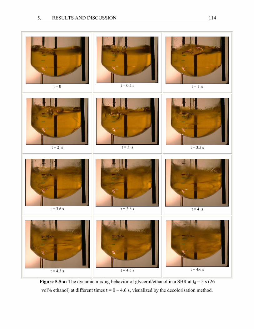
5. RESULTS AND DISCUSSION 114
t = 0
t = 0.2 s
t = 1 s
t = 2 s
t = 3 s
t = 3.5 s
t = 3.6 s
t = 3.8 s
t = 4 s
t = 4.3 s
t = 4.5 s
t = 4.6 s
Figure 5.5-a: The dynamic mixing behavior of glycerol/ethanol in a SBR at td = 5 s (26
vol% ethanol) at different times t = 0 – 4.6 s, visualized by the decolorisation method.
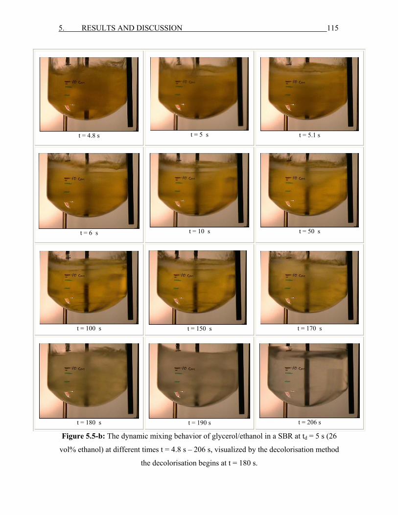
5. RESULTS AND DISCUSSION 115
t = 4.8 s
t = 5 s
t = 5.1 s
t = 6 s
t = 10 s
t = 50 s
t = 100 s
t = 150 s
t = 170 s
t = 180 s
t = 190 s
t = 206 s
Figure 5.5-b: The dynamic mixing behavior of glycerol/ethanol in a SBR at td = 5 s (26
vol% ethanol) at different times t = 4.8 s – 206 s, visualized by the decolorisation method
the decolorisation begins at t = 180 s.
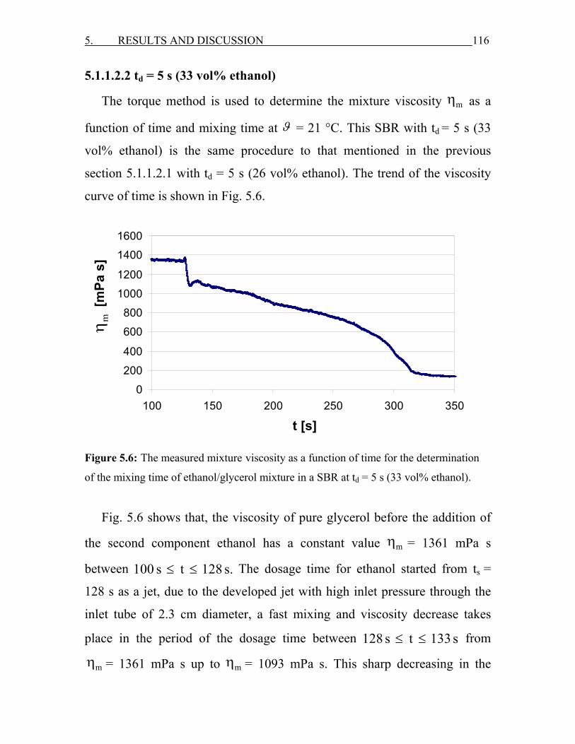
5. RESULTS AND DISCUSSION 116
5.1.1.2.2 td = 5 s (33 vol% ethanol)
The torque method is used to determine the mixture viscosity mη as a
function of time and mixing time at ϑ = 21 °C. This SBR with td = 5 s (33
vol% ethanol) is the same procedure to that mentioned in the previous
section 5.1.1.2.1 with td = 5 s (26 vol% ethanol). The trend of the viscosity
curve of time is shown in Fig. 5.6.
0
200
400
600
800
1000
1200
1400
1600
100 150 200 250 300 350
Time [s]
Vis
cosi
ty [m
Pa
s]
Figure 5.6: The measured mixture viscosity as a function of time for the determination
of the mixing time of ethanol/glycerol mixture in a SBR at td = 5 s (33 vol% ethanol).
Fig. 5.6 shows that, the viscosity of pure glycerol before the addition of
the second component ethanol has a constant value mη = 1361 mPa s
between 100 s t 128 s.≤ ≤ The dosage time for ethanol started from ts =
128 s as a jet, due to the developed jet with high inlet pressure through the
inlet tube of 2.3 cm diameter, a fast mixing and viscosity decrease takes
place in the period of the dosage time between 128 s t 133 s≤ ≤ from
mη = 1361 mPa s up to mη = 1093 mPa s. This sharp decreasing in the
t [s]
[mPa
s]
mη

5. RESULTS AND DISCUSSION 117
viscosity is due to the high pressure force and flow rate of the dosed ethanol.
Between 133 s t 310 s,≤ ≤ the viscosity curve decreases slowly and the
viscosity values decreases from mη = 1093 mPa s at t = 133 s up to mη =
716 mPa s at t = 260 s due to the disappearance of the inlet pressure force
and the appearance of the buoyancy force effect which depends on the
density difference between ethanol and glycerol.
Because of the density and viscosity difference, two layers of ethanol and
glycerol are formed. The upper layer of ethanol is the lighter one which has
the low density and viscosity. The lower layer of glycerol is the heavier one
which has the higher density and viscosity. After t = 260 s, again the
viscosity reduction increased strongly and fast to reach the final and the
complete mixing, this is may be due to the gradual formation of the liquid
mixture of ethanol/glycerol which has almost physical properties for the
density and viscosity are close to the small layer which is found at t = 260 s.
The homogenization of the mixture took place after te = 355 s and the final
viscosity of this mixture is mη = 134 mPa s. Then the mixing time tm is:
tm = te – ts = 355 s – 133 s = 222 s.
5.1.1.2.3 td = 10 s (33 vol% ethanol)
The torque method is used to determine the mixture viscosities mη as a
function of time and mixing time at ϑ = 21 °C. This SBR with td = 10 s is
the same procedure to that mentioned in the previous sections 5.1.1.2.1 with
td = 5 s (26 vol% ethanol) and 5.1.1.2.2 td = 5 s (33 vol% ethanol). The
profile for the viscosity of the liquid mixture as a function of time is shown
in Fig. 5.7.
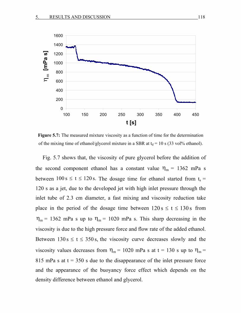
5. RESULTS AND DISCUSSION 118
0
200
400
600
800
1000
1200
1400
1600
100 150 200 250 300 350 400 450
Time [s]
Visc
osity
[mPa
s]
Figure 5.7: The measured mixture viscosity as a function of time for the determination
of the mixing time of ethanol/glycerol mixture in a SBR at td = 10 s (33 vol% ethanol).
Fig. 5.7 shows that, the viscosity of pure glycerol before the addition of
the second component ethanol has a constant value mη = 1362 mPa s
between 100 s t 120 s.≤ ≤ The dosage time for ethanol started from ts =
120 s as a jet, due to the developed jet with high inlet pressure through the
inlet tube of 2.3 cm diameter, a fast mixing and viscosity reduction take
place in the period of the dosage time between 120 s t 130 s≤ ≤ from
mη = 1362 mPa s up to mη = 1020 mPa s. This sharp decreasing in the
viscosity is due to the high pressure force and flow rate of the added ethanol.
Between 130 s t 350 s,≤ ≤ the viscosity curve decreases slowly and the
viscosity values decreases from mη = 1020 mPa s at t = 130 s up to mη =
815 mPa s at t = 350 s due to the disappearance of the inlet pressure force
and the appearance of the buoyancy force effect which depends on the
density difference between ethanol and glycerol.
t [s]
[mPa
s]
mη
5. RESULTS AND DISCUSSION 119
Because of the density and viscosity difference, two layers of ethanol and
glycerol are formed. The upper layer of ethanol is the lighter one which has
the low density and viscosity. The lower layer of glycerol is the heavier one
which has the higher density and viscosity. After t = 350 s, again the
viscosity reduction increased strongly and fast to reach the final and the
complete mixing at the time te = 402 s, this is due to a slow formation of the
liquid mixture of ethanol/glycerol which has almost physical properties for
the density and viscosity are close to the small layer which is found at t =
350 s. The homogenization of the mixture takes place at te = 402 s with a
final viscosity mixture mη = 130 mPa s. Then the mixing time tm is:
tm = te – ts = 402 s – 120 s = 282 s.
When comparing Fig. 5.6 with Fig. 5.7, it is clear that for td = 5 s (33
vol% ethanol) the flow rate of the added ethanol is higher from td = 10 s, the
reduction in the viscosity in the period of dosing is the same because
approximately the same quantity of ethanol is added for both dosage times.
In the slow viscosity reduction period, the viscosity reduction for td = 5 s (33
vol% ethanol) is higher from td = 10 s, this is due to the higher inlet flow rate
and pressure forces which force ethanol to distribute in glycerol and this
forces reduce the effect of buoyancy forces and density differences. This
also reduces the effect of drag forces and makes the mixing faster. As a
result, as the dosing time decreases from td = 10 s to td = 5 s, the flow rate of
the inlet flow increases from 0.129 L/s to 0.251 L/s, respectively. Also, the
mixing time to get a homogeneous mixture decreases from tm = 282 s to
tm = 222 s.
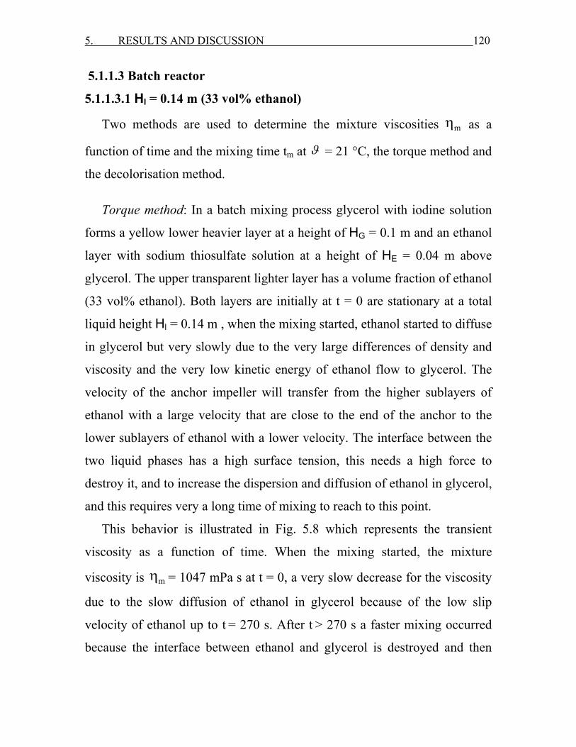
5. RESULTS AND DISCUSSION 120
5.1.1.3 Batch reactor
5.1.1.3.1 Hl = 0.14 m (33 vol% ethanol)
Two methods are used to determine the mixture viscosities mη as a
function of time and the mixing time tm at ϑ = 21 °C, the torque method and
the decolorisation method.
Torque method: In a batch mixing process glycerol with iodine solution
forms a yellow lower heavier layer at a height of HG = 0.1 m and an ethanol
layer with sodium thiosulfate solution at a height of HE = 0.04 m above
glycerol. The upper transparent lighter layer has a volume fraction of ethanol
(33 vol% ethanol). Both layers are initially at t = 0 are stationary at a total
liquid height Hl = 0.14 m , when the mixing started, ethanol started to diffuse
in glycerol but very slowly due to the very large differences of density and
viscosity and the very low kinetic energy of ethanol flow to glycerol. The
velocity of the anchor impeller will transfer from the higher sublayers of
ethanol with a large velocity that are close to the end of the anchor to the
lower sublayers of ethanol with a lower velocity. The interface between the
two liquid phases has a high surface tension, this needs a high force to
destroy it, and to increase the dispersion and diffusion of ethanol in glycerol,
and this requires very a long time of mixing to reach to this point.
This behavior is illustrated in Fig. 5.8 which represents the transient
viscosity as a function of time. When the mixing started, the mixture
viscosity is mη = 1047 mPa s at t = 0, a very slow decrease for the viscosity
due to the slow diffusion of ethanol in glycerol because of the low slip
velocity of ethanol up to t = 270 s. After t > 270 s a faster mixing occurred
because the interface between ethanol and glycerol is destroyed and then
s
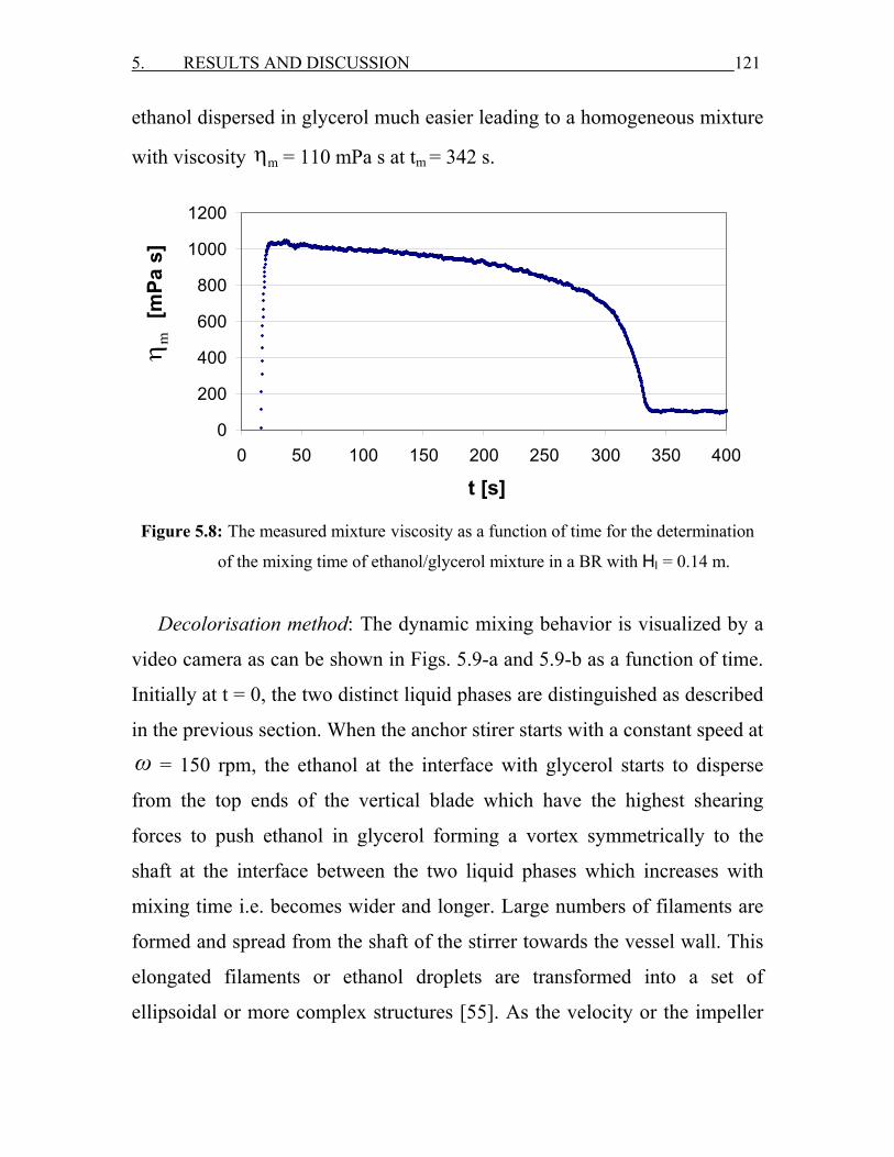
5. RESULTS AND DISCUSSION 121
ethanol dispersed in glycerol much easier leading to a homogeneous mixture
with viscosity mη = 110 mPa s at tm = 342 s.
0
200
400
600
800
1000
1200
0 50 100 150 200 250 300 350 400
Time [s]
Visc
osity
[mPa
s]
Figure 5.8: The measured mixture viscosity as a function of time for the determination
of the mixing time of ethanol/glycerol mixture in a BR with Hl = 0.14 m.
Decolorisation method: The dynamic mixing behavior is visualized by a
video camera as can be shown in Figs. 5.9-a and 5.9-b as a function of time.
Initially at t = 0, the two distinct liquid phases are distinguished as described
in the previous section. When the anchor stirer starts with a constant speed at
ω = 150 rpm, the ethanol at the interface with glycerol starts to disperse
from the top ends of the vertical blade which have the highest shearing
forces to push ethanol in glycerol forming a vortex symmetrically to the
shaft at the interface between the two liquid phases which increases with
mixing time i.e. becomes wider and longer. Large numbers of filaments are
formed and spread from the shaft of the stirrer towards the vessel wall. This
elongated filaments or ethanol droplets are transformed into a set of
ellipsoidal or more complex structures [55]. As the velocity or the impeller
t [s]
[mPa
s]
mη
5. RESULTS AND DISCUSSION 122
shear forces transfer to the top surface of ethanol layer, oscillations are
formed at the top surface of the light layer during the mixing process. After
4 minutes, the colourless lighter layer (ethanol) split and a faster mixing
occurs with the yellow heavier layer (glycerol) to get one colourless
homogeneous liquid phase (s. Fig. 5.9-b, t = 312 s). The mixing time from
the decolorisation method is found to be tm = 340 s which is very close to
that obtained from the torque method tm = 342 s.

5. RESULTS AND DISCUSSION 123
t = 0
t = 0.1 s
t = 0.5 s
t = 1 s
t = 2 s
t = 3 s
t = 5 s
t = 10 s
t = 20 s
t = 45 s
t = 55 s
t = 86 s
Figure 5.9-a: The dynamic mixing behavior (pan cake effect) of glycerol/ethanol in a BR
with Hl = 0.14 m (33 vol% ethanol) at different times t = 0 – 86 s, visualized by the
decolorisation method.

5. RESULTS AND DISCUSSION 124
t = 118 s
t = 157 s
t = 185 s
t = 213 s
t = 223 s
t = 233 s
t = 260 s
t = 299 s
t = 307 s
t = 312 s
t = 319 s
t = 340 s
Figure 5.9-b: The dynamic mixing behavior (pan cake effect) of glycerol/ethanol in a BR
with Hl = 0.14 m (33 vol% ethanol) at different times t = 118 s – 340 s, visualized by the
decolorisation method, the decolorisation begins at t = 312 s.
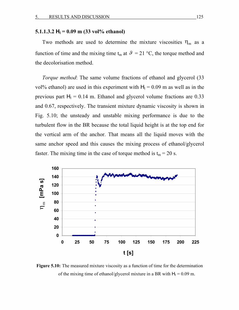
5. RESULTS AND DISCUSSION 125
5.1.1.3.2 Hl = 0.09 m (33 vol% ethanol)
Two methods are used to determine the mixture viscosities mη as a
function of time and the mixing time tm at ϑ = 21 °C, the torque method and
the decolorisation method.
Torque method: The same volume fractions of ethanol and glycerol (33
vol% ethanol) are used in this experiment with Hl = 0.09 m as well as in the
previous part Hl = 0.14 m. Ethanol and glycerol volume fractions are 0.33
and 0.67, respectively. The transient mixture dynamic viscosity is shown in
Fig. 5.10; the unsteady and unstable mixing performance is due to the
turbulent flow in the BR because the total liquid height is at the top end for
the vertical arm of the anchor. That means all the liquid moves with the
same anchor speed and this causes the mixing process of ethanol/glycerol
faster. The mixing time in the case of torque method is tm = 20 s.
0
20
40
60
80
100
120
140
160
0 25 50 75 100 125 150 175 200 225
Time [s]
Visc
osity
[mPa
s]
Figure 5.10: The measured mixture viscosity as a function of time for the determination
of the mixing time of ethanol/glycerol mixture in a BR with Hl = 0.09 m.
t [s]
[mPa
s]
mη
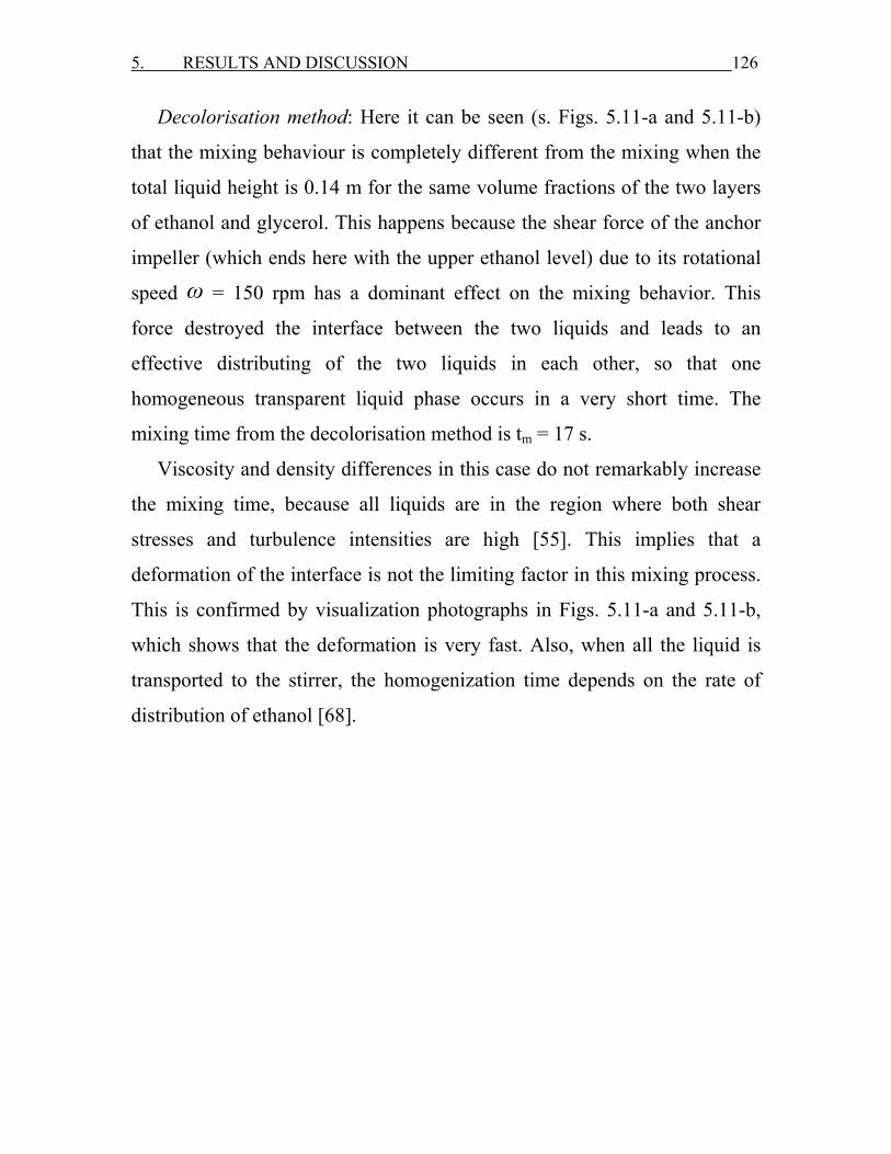
5. RESULTS AND DISCUSSION 126
Decolorisation method: Here it can be seen (s. Figs. 5.11-a and 5.11-b)
that the mixing behaviour is completely different from the mixing when the
total liquid height is 0.14 m for the same volume fractions of the two layers
of ethanol and glycerol. This happens because the shear force of the anchor
impeller (which ends here with the upper ethanol level) due to its rotational
speed ω = 150 rpm has a dominant effect on the mixing behavior. This
force destroyed the interface between the two liquids and leads to an
effective distributing of the two liquids in each other, so that one
homogeneous transparent liquid phase occurs in a very short time. The
mixing time from the decolorisation method is tm = 17 s.
Viscosity and density differences in this case do not remarkably increase
the mixing time, because all liquids are in the region where both shear
stresses and turbulence intensities are high [55]. This implies that a
deformation of the interface is not the limiting factor in this mixing process.
This is confirmed by visualization photographs in Figs. 5.11-a and 5.11-b,
which shows that the deformation is very fast. Also, when all the liquid is
transported to the stirrer, the homogenization time depends on the rate of
distribution of ethanol [68].
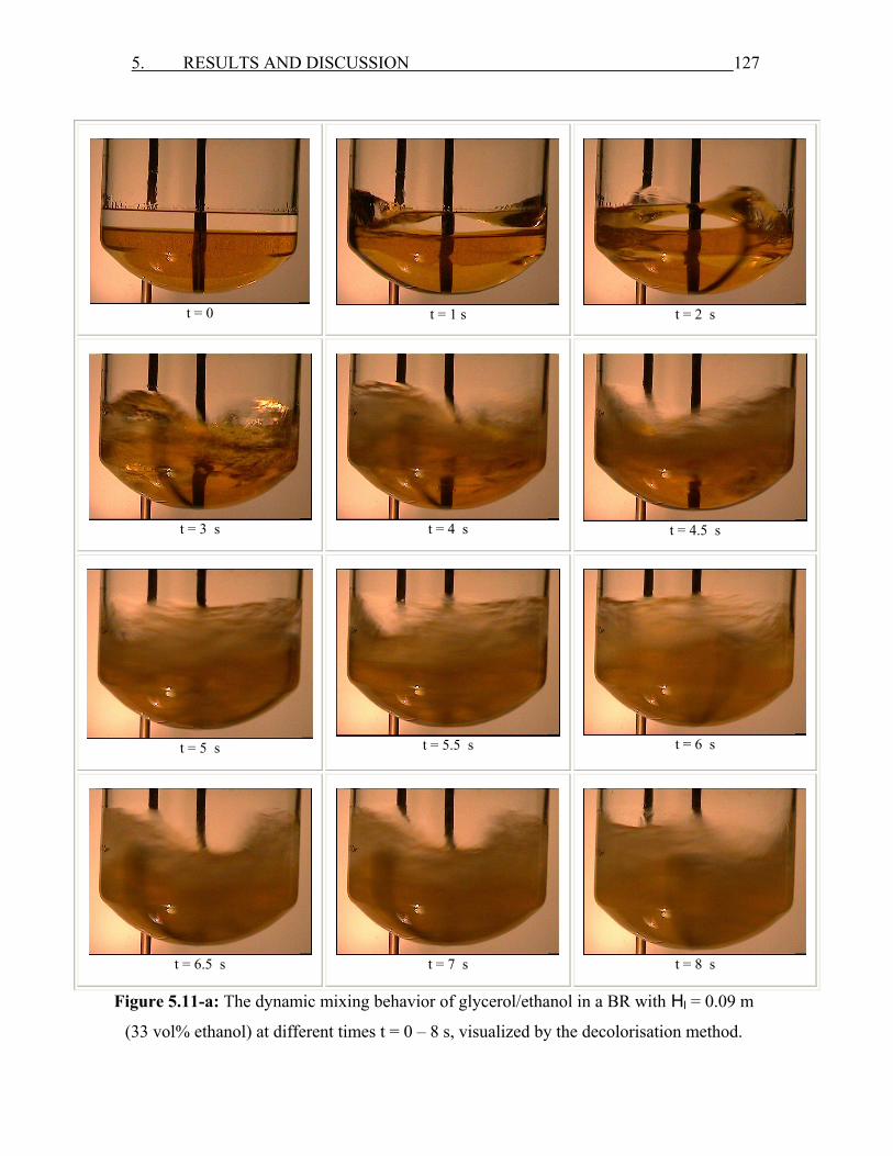
5. RESULTS AND DISCUSSION 127
t = 0
t = 1 s
t = 2 s
t = 3 s
t = 4 s
t = 4.5 s
t = 5 s
t = 5.5 s
t = 6 s
t = 6.5 s
t = 7 s
t = 8 s
Figure 5.11-a: The dynamic mixing behavior of glycerol/ethanol in a BR with Hl = 0.09 m
(33 vol% ethanol) at different times t = 0 – 8 s, visualized by the decolorisation method.
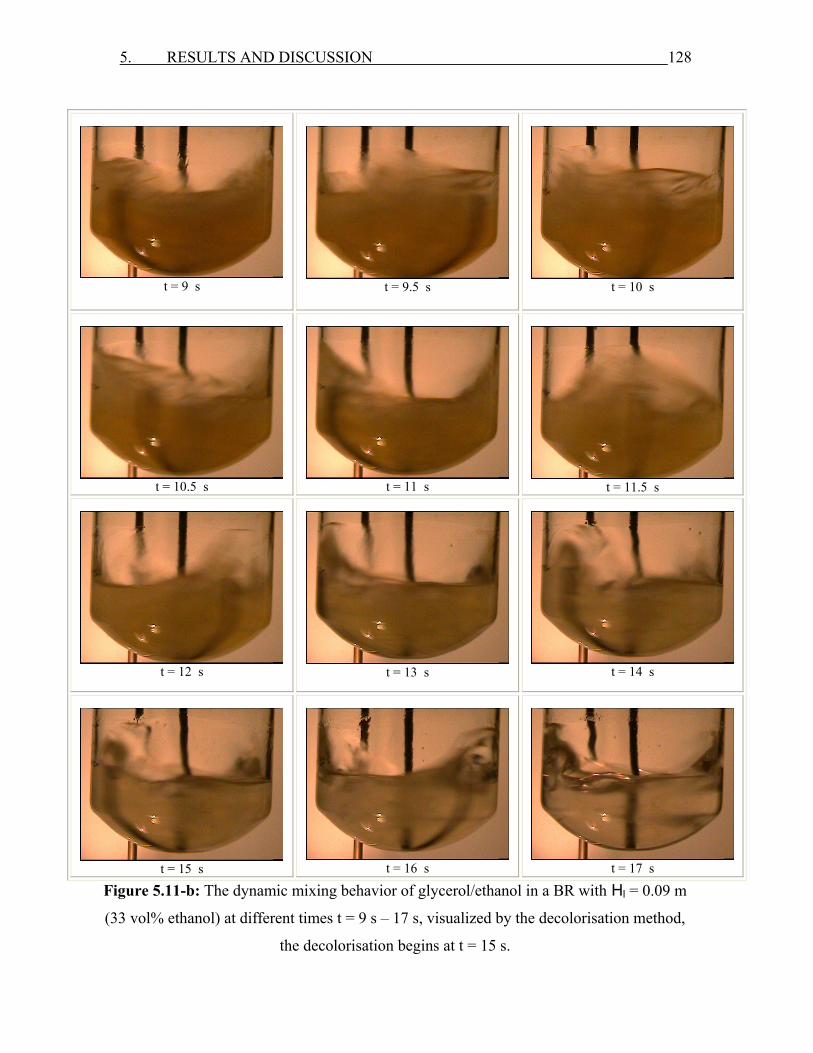
5. RESULTS AND DISCUSSION 128
t = 9 s
t = 9.5 s
t = 10 s
t = 10.5 s
t = 11 s
t = 11.5 s
t = 12 s
t = 13 s
t = 14 s
t = 15 s
t = 16 s
t = 17 s
Figure 5.11-b: The dynamic mixing behavior of glycerol/ethanol in a BR with Hl = 0.09 m
(33 vol% ethanol) at different times t = 9 s – 17 s, visualized by the decolorisation method,
the decolorisation begins at t = 15 s.
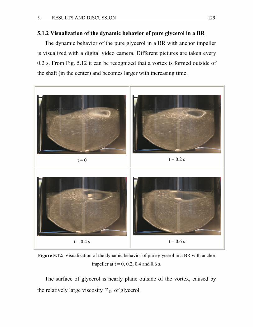
5. RESULTS AND DISCUSSION 129
5.1.2 Visualization of the dynamic behavior of pure glycerol in a BR
The dynamic behavior of the pure glycerol in a BR with anchor impeller
is visualized with a digital video camera. Different pictures are taken every
0.2 s. From Fig. 5.12 it can be recognized that a vortex is formed outside of
the shaft (in the center) and becomes larger with increasing time.
t = 0
t = 0.2 s
t = 0.4 s
t = 0.6 s
Figure 5.12: Visualization of the dynamic behavior of pure glycerol in a BR with anchor
impeller at t = 0, 0.2, 0.4 and 0.6 s.
The surface of glycerol is nearly plane outside of the vortex, caused by
the relatively large viscosity Gη of glycerol.

5. RESULTS AND DISCUSSION 130
The bottom of the vessel is curved, so that the distance between the
blades and the vessel is very small to allow the blades of the anchor impeller
to work as a scraper for the viscous glycerol. The direction of anchor
rotation is clock wise. The primary flow (Fig. 5.13) in the glycerol is
tangential which can be seen from the top view; it is created by the rotation
of the horizontal blade. From the front view, the secondary flow (axial and
radial) can be recognized (Fig. 5.13). The flow of the glycerol from the tip of
the anchor blade at point 1 is directed to the liquid in the vicinity to point 2,
then to the vessel wall at point 3 forming a vortex between the points 1, 2
and 3. A second vortex is formed between the points 4, 5 and 6 with an
opposite rotation direction.
Figure 5.13: The formation of a primary- and secondary flow in pure glycerol in a stirred
BR.
Point 1 +
+ Point 2 +
Point 3
Point 4 +
+ Point 5 +
Point 6
Primary flow
Secondary flow
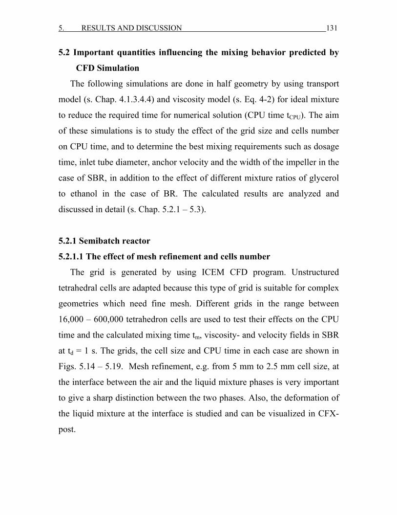
5. RESULTS AND DISCUSSION 131
5.2 Important quantities influencing the mixing behavior predicted by
CFD Simulation
The following simulations are done in half geometry by using transport
model (s. Chap. 4.1.3.4.4) and viscosity model (s. Eq. 4-2) for ideal mixture
to reduce the required time for numerical solution (CPU time tCPU). The aim
of these simulations is to study the effect of the grid size and cells number
on CPU time, and to determine the best mixing requirements such as dosage
time, inlet tube diameter, anchor velocity and the width of the impeller in the
case of SBR, in addition to the effect of different mixture ratios of glycerol
to ethanol in the case of BR. The calculated results are analyzed and
discussed in detail (s. Chap. 5.2.1 – 5.3).
5.2.1 Semibatch reactor
5.2.1.1 The effect of mesh refinement and cells number
The grid is generated by using ICEM CFD program. Unstructured
tetrahedral cells are adapted because this type of grid is suitable for complex
geometries which need fine mesh. Different grids in the range between
16,000 – 600,000 tetrahedron cells are used to test their effects on the CPU
time and the calculated mixing time tm, viscosity- and velocity fields in SBR
at td = 1 s. The grids, the cell size and CPU time in each case are shown in
Figs. 5.14 – 5.19. Mesh refinement, e.g. from 5 mm to 2.5 mm cell size, at
the interface between the air and the liquid mixture phases is very important
to give a sharp distinction between the two phases. Also, the deformation of
the liquid mixture at the interface is studied and can be visualized in CFX-
post.
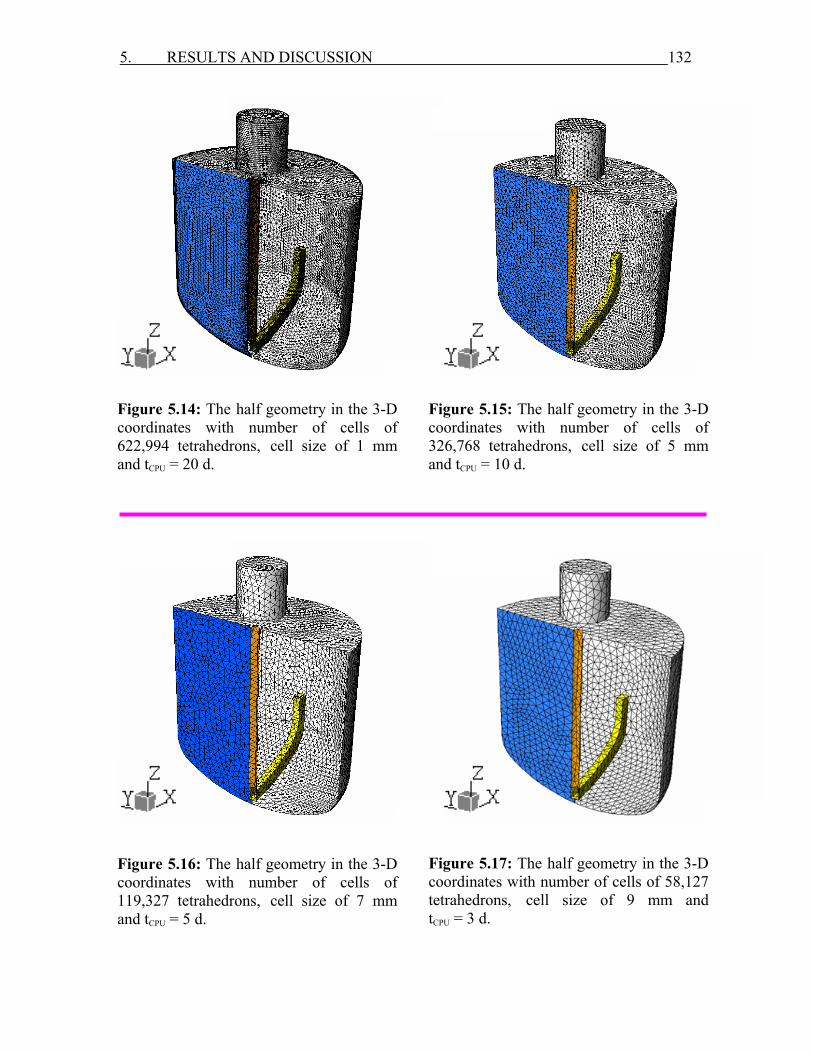
5. RESULTS AND DISCUSSION 132
Figure 5.14: The half geometry in the 3-D coordinates with number of cells of 622,994 tetrahedrons, cell size of 1 mm and tCPU = 20 d.
Figure 5.15: The half geometry in the 3-D coordinates with number of cells of 326,768 tetrahedrons, cell size of 5 mm and tCPU = 10 d.
Figure 5.16: The half geometry in the 3-D coordinates with number of cells of 119,327 tetrahedrons, cell size of 7 mm and tCPU = 5 d.
Figure 5.17: The half geometry in the 3-D coordinates with number of cells of 58,127tetrahedrons, cell size of 9 mm and tCPU = 3 d.
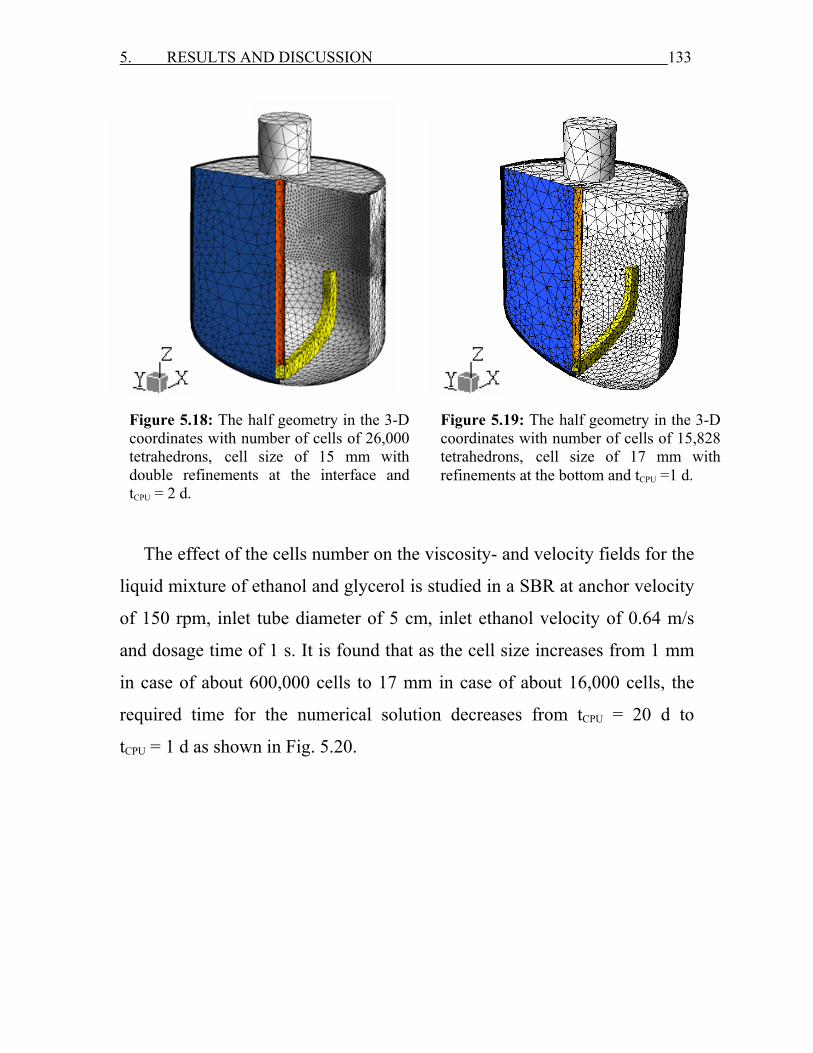
5. RESULTS AND DISCUSSION 133
The effect of the cells number on the viscosity- and velocity fields for the
liquid mixture of ethanol and glycerol is studied in a SBR at anchor velocity
of 150 rpm, inlet tube diameter of 5 cm, inlet ethanol velocity of 0.64 m/s
and dosage time of 1 s. It is found that as the cell size increases from 1 mm
in case of about 600,000 cells to 17 mm in case of about 16,000 cells, the
required time for the numerical solution decreases from tCPU = 20 d to
tCPU = 1 d as shown in Fig. 5.20.
Figure 5.18: The half geometry in the 3-D coordinates with number of cells of 26,000 tetrahedrons, cell size of 15 mm with double refinements at the interface and tCPU = 2 d.
Figure 5.19: The half geometry in the 3-D coordinates with number of cells of 15,828 tetrahedrons, cell size of 17 mm with refinements at the bottom and tCPU =1 d.

5. RESULTS AND DISCUSSION 134
Figure 5.20: The effect of cells number and mesh size on the time requirements of
numerical solution (CPU).
The flow- and viscosity fields for cells number of 26,000 and 600,000
tetrahedrons are shown in Fig. 5.21. For 600,000 tetrahedron cells, a sharper
and more distinct interface between the liquid mixture and air is obtained.
For both cells number the velocity fields are similar. In both cases the radial
and axial secondary flows are produced by the anchor impeller before and
during the dosage of ethanol, and new circulations near the maximum
curvature of the blade of the impeller are formed after the dosage. The dosed
ethanol flows towards to the impeller from the circumference forming eddies
or vortices in the vicinity between the impeller and the shaft. The liquid
mixture volume fraction field (contour surface plot), the dynamic viscosity
field (contour lines) and velocity field (vectors) are shown in Fig. 5.21
during the dosage period from t = 0.2 s to 1.2 s. After t = 1.2 s the liquid
mixture reaches a constant dynamic viscosity and a homogeneous mixture
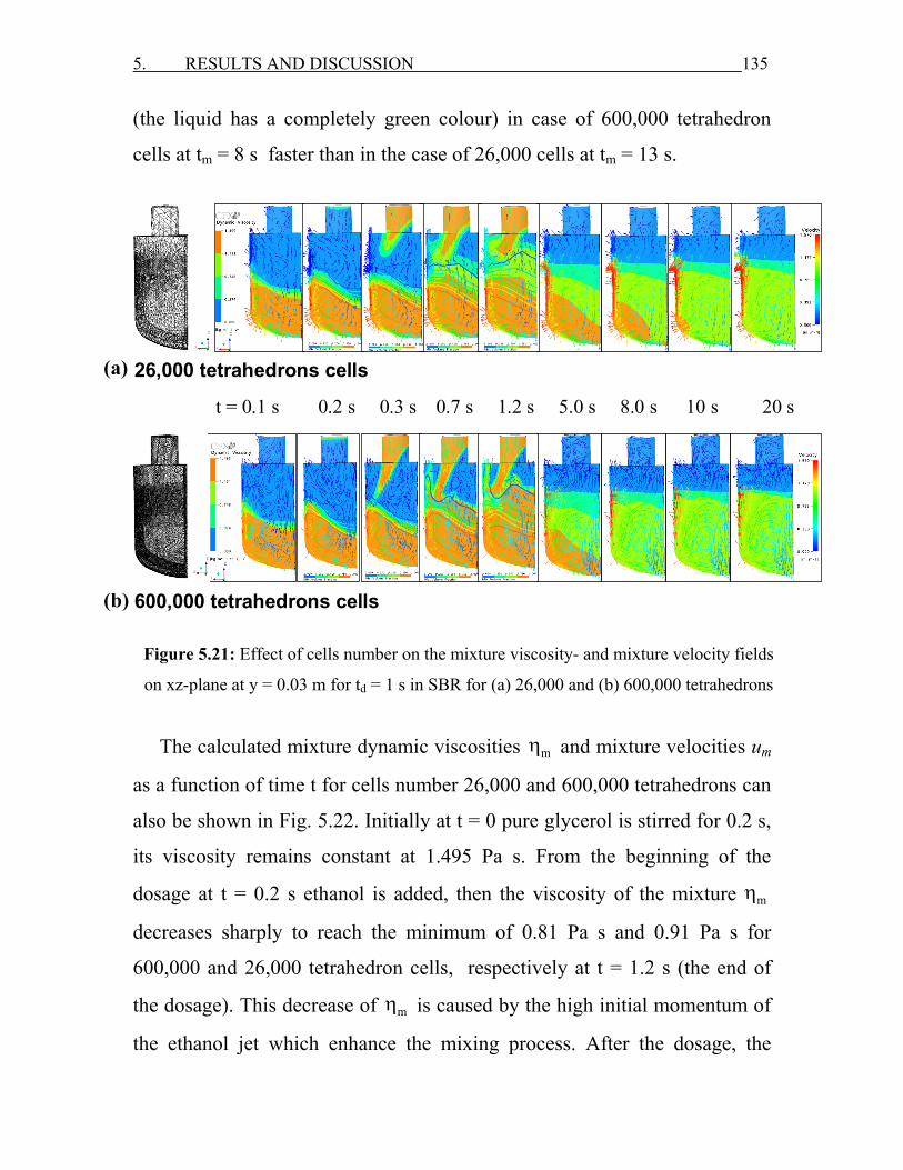
5. RESULTS AND DISCUSSION 135
(the liquid has a completely green colour) in case of 600,000 tetrahedron
cells at tm = 8 s faster than in the case of 26,000 cells at tm = 13 s.
The calculated mixture dynamic viscosities mη and mixture velocities um
as a function of time t for cells number 26,000 and 600,000 tetrahedrons can
also be shown in Fig. 5.22. Initially at t = 0 pure glycerol is stirred for 0.2 s,
its viscosity remains constant at 1.495 Pa s. From the beginning of the
dosage at t = 0.2 s ethanol is added, then the viscosity of the mixture mη
decreases sharply to reach the minimum of 0.81 Pa s and 0.91 Pa s for
600,000 and 26,000 tetrahedron cells, respectively at t = 1.2 s (the end of
the dosage). This decrease of mη is caused by the high initial momentum of
the ethanol jet which enhance the mixing process. After the dosage, the
t = 0.1 s 0.2 s 0.3 s 0.7 s 1.2 s 5.0 s 8.0 s 10 s 20 s
26,000 tetrahedrons cells
600,000 tetrahedrons cells
Figure 5.21: Effect of cells number on the mixture viscosity- and mixture velocity fields
on xz-plane at y = 0.03 m for td = 1 s in SBR for (a) 26,000 and (b) 600,000 tetrahedrons
(a)
(b)
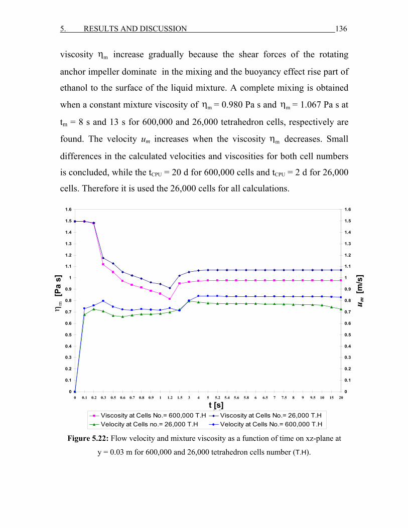
5. RESULTS AND DISCUSSION 136
viscosity mη increase gradually because the shear forces of the rotating
anchor impeller dominate in the mixing and the buoyancy effect rise part of
ethanol to the surface of the liquid mixture. A complete mixing is obtained
when a constant mixture viscosity of mη = 0.980 Pa s and mη = 1.067 Pa s at
tm = 8 s and 13 s for 600,000 and 26,000 tetrahedron cells, respectively are
found. The velocity um increases when the viscosity mη decreases. Small
differences in the calculated velocities and viscosities for both cell numbers
is concluded, while the tCPU = 20 d for 600,000 cells and tCPU = 2 d for 26,000
cells. Therefore it is used the 26,000 cells for all calculations.
Figure 5.22: Flow velocity and mixture viscosity as a function of time on xz-plane at
y = 0.03 m for 600,000 and 26,000 tetrahedron cells number (T.H).
0
0.1
0.2
0.3
0.4
0.5
0.6
0.7
0.8
0.9
1
1.1
1.2
1.3
1.4
1.5
1.6
0 0.1 0.2 0.3 0.5 0.6 0.7 0.8 0.9 1 1.2 1.5 3 4 5 5.2 5.4 5.6 5.8 6 6.5 7 7.5 8 9 9.5 10 15 20
Time [s]
0
0.1
0.2
0.3
0.4
0.5
0.6
0.7
0.8
0.9
1
1.1
1.2
1.3
1.4
1.5
1.6
Viscosity at Cells No.= 600,000 T.H Viscosity at Cells No.= 26,000 T.HVelocity at Cells no.= 26,000 T.H Velocity at Cells No.= 600,000 T.H
[Pa
s]
mη
u m [
m/s
]
t [s]
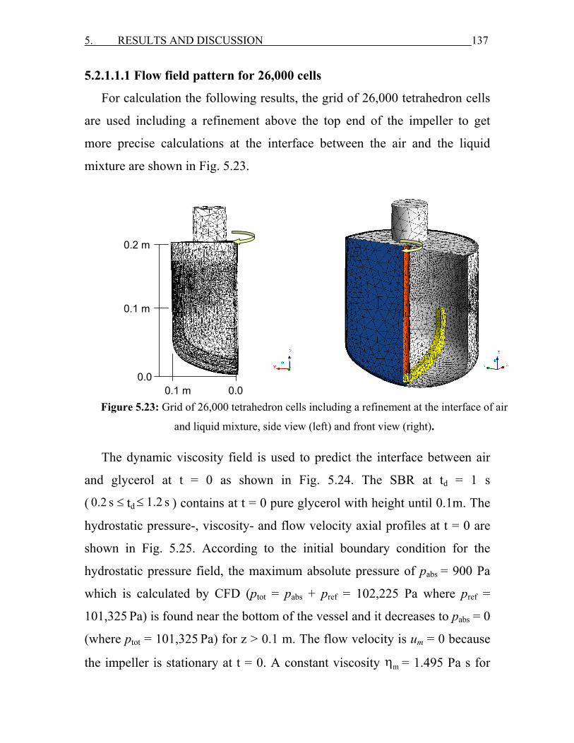
5. RESULTS AND DISCUSSION 137
5.2.1.1.1 Flow field pattern for 26,000 cells
For calculation the following results, the grid of 26,000 tetrahedron cells
are used including a refinement above the top end of the impeller to get
more precise calculations at the interface between the air and the liquid
mixture are shown in Fig. 5.23.
The dynamic viscosity field is used to predict the interface between air
and glycerol at t = 0 as shown in Fig. 5.24. The SBR at td = 1 s
( 0.2 s ≤ td 1.2 s≤ ) contains at t = 0 pure glycerol with height until 0.1m. The
hydrostatic pressure-, viscosity- and flow velocity axial profiles at t = 0 are
shown in Fig. 5.25. According to the initial boundary condition for the
hydrostatic pressure field, the maximum absolute pressure of pabs = 900 Pa
which is calculated by CFD (ptot = pabs + pref = 102,225 Pa where pref =
101,325 Pa) is found near the bottom of the vessel and it decreases to pabs = 0
(where ptot = 101,325 Pa) for z > 0.1 m. The flow velocity is um = 0 because
the impeller is stationary at t = 0. A constant viscosity mη = 1.495 Pa s for
0.00.0
0.1 m
0.1 m
0.2 m
Figure 5.23: Grid of 26,000 tetrahedron cells including a refinement at the interface of air
and liquid mixture, side view (left) and front view (right).
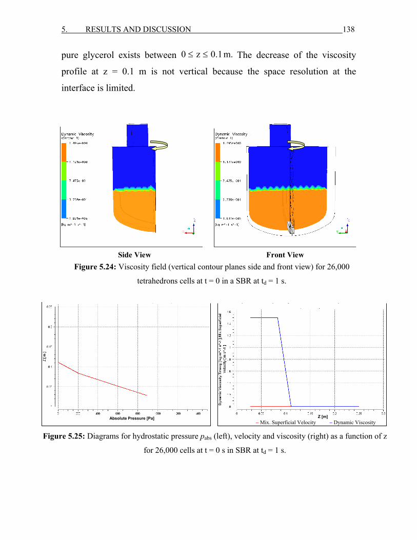
5. RESULTS AND DISCUSSION 138
pure glycerol exists between 0 z 0.1 m.≤ ≤ The decrease of the viscosity
profile at z = 0.1 m is not vertical because the space resolution at the
interface is limited.
Side View Front View Figure 5.24: Viscosity field (vertical contour planes side and front view) for 26,000
tetrahedrons cells at t = 0 in a SBR at td = 1 s.
Figure 5.25: Diagrams for hydrostatic pressure pabs (left), velocity and viscosity (right) as a function of z
for 26,000 cells at t = 0 s in SBR at td = 1 s.
Z [m] – Mix. Superficial Velocity – Dynamic Viscosity
Absolute Pressure [Pa]

5. RESULTS AND DISCUSSION 139
For t = 0.1 s the viscosity field is shown in Fig. 5.26-(A) indicates the
convex shape of the air/glycerol interface when the anchor rotates clock wise
at ω = 150 rpm. The velocity field in Fig. 5.26-(B) shows the mainly axial
flow of glycerol up towards the tip of the impeller which has the maximum
flow velocity (red colour). The axial pressure profile in Fig. 5.26-(C) is
similar to that in Fig. 5.25-(left) as described before but the ambient pressure
value is found for z > 0.08 m because of the existence of the convex shape at
the interface due to the movement of the impeller. The axial velocity profile
of the glycerol has a constant value of 0.2 m/s between 0 z 0.05 m≤ ≤ and
decreases for z > 0.05 m, caused by a decrease of the liquid velocity for
z > 0.05 m with increasing the height z above the impeller blade. A second
reason is that the vortex formation and the space resolution at the interface
are limited. The viscosity of glycerol remains constant up to z = 0.06 m. The
decrease of the viscosity profile at z = 0.08 m is not vertical because the
space resolution at the interface is limited as shown in Fig. 5.26-(D).
For t = 0.7 s, the dosed ethanol between 0.2 s ≤ td 1.2 s≤ , flows towards
to the impeller near the cylindrical wall of the vessel. A small mass of
ethanol is mixed with the bulk liquid, whereas a larger mass rise to the
surface of the liquid mixture. The viscosities mη are small in the upper part
and large in the lower part of the vessel (s. Fig. 5.27-(A)). The air above
glycerol is replaced by the dosed ethanol which forms a layer with a height
of HE = 0.04 m. A secondary flow velocity field is formed mainly axial
towards to the tip of the impeller. No circulations between shaft and impeller
at this time are formed (s. Fig. 5.27-(B)). The axial hydrostatic pressure
pabs = 1200 Pa which is calculated by CFD (ptot = pabs + pref = 102,525 Pa
where pref = 101,325 Pa) is a maximum near the bottom (z = 0.03 m) of the
vessel. It decreases gradually to reach the ambient pressure pref near the
5. RESULTS AND DISCUSSION 140
interface at z = 0.14 m between the air and liquid mixture as shown in
Fig.5.27-(C). The pressure near the bottom of the vessel increases from
pabs = 770 Pa at t = 0.1 s to pabs = 1200 Pa at t = 0.7 s.
The axial viscosity profile m (z)η is constant up to z = 0.06 m then it
decreases gradually until z = 0.15 m where a high mass fraction of ethanol
(low viscosity) is present. Higher axial velocities of the liquid mixture at t =
0.7 s are found compared with that at t = 0.1 s caused by the additional
momentum of the dosed ethanol. The axial velocity profile reaches a
minimum at a height of z = 0.15 m where the flow field of the anchor
impeller dominates and end the influence of the incoming ethanol flow still
very small. With increasing the height for z > 0.15 m the influence of inlet
flow increases until z = 0.25 m, there the flow field of incoming ethanol
dominates (s. Fig 5.27-(D)).
The mixing of ethanol with glycerol at t = 5 s from the tip of the impeller
towards to the shaft leading to concave shape of the interface between
ethanol and the liquid mixture, and then ethanol flows to the cylindrical wall
of the vessel. Above the tip of the impeller, the velocities of the liquid
decrease to reach the minimum at the interface between the liquid mixture
and air which has no concave shape (s. Fig. 5.28-(A)).
It is observed from the viscosity fields at t = 10 s in Fig 5.29-(A) that the
maximum viscosities of the liquid mixtures are found near the corner of the
vessel at the bottom. This is caused by only a weak mixing in this zone. A
homogeneous and a constant mixture viscosity are obtained at tm ≈ 15 s as
shown in Fig. 5.30-(A). A concave interface with the air is formed at t = 20 s
as shown in Fig. 5.31-(A). Secondary flow with a circulation in the direction
of the anchor movement (behind the impeller) is formed. The minimum
velocities are found near the shaft, whereas the maximum velocities are
5. RESULTS AND DISCUSSION 141
found near the cylindrical wall of the vessel see Fig 5.28-(B). Similar
velocity fields are obtained for t = 10 s, t = 15 s and t = 20 s as shown in Figs.
5.29-(B), 5.30-(B) and 5.31-B, respectively.
The axial hydrostatic pressure profiles at t = 5, 10, 15 and 20 s (after the
dosed ethanol) shows that the maximum pressure of pabs = 1300 Pa is found
near the bottom of the vessel, and then it decreases linearly to reach the
ambient pressure pref at the interface with air at z = 0.16 m (s. Figs. 5.28-(C),
5.29-(C), 5.30-(C) and 5.31-(C) for t = 5, 10, 15 and 20 s, respectively).
The axial velocities increase from the bottom of the vessel to reach the
maximum near the tip of the impeller and the interface between the liquid
mixture and air. For z > 0.15 m there is a decrease of the axial velocities
caused by the absence of the impeller effect. The axial mixture viscosity
profiles decrease to reach the minimum at the interface with air (s. Figs.
5.28-(D), 5.29-(D), 5.30-(D) and 5.31-(D) for t = 5, 10, 15 and 20 s,
respectively). The axial velocities of the liquid mixture decrease with time
until a complete mixing with constant mixture viscosity is obtained.
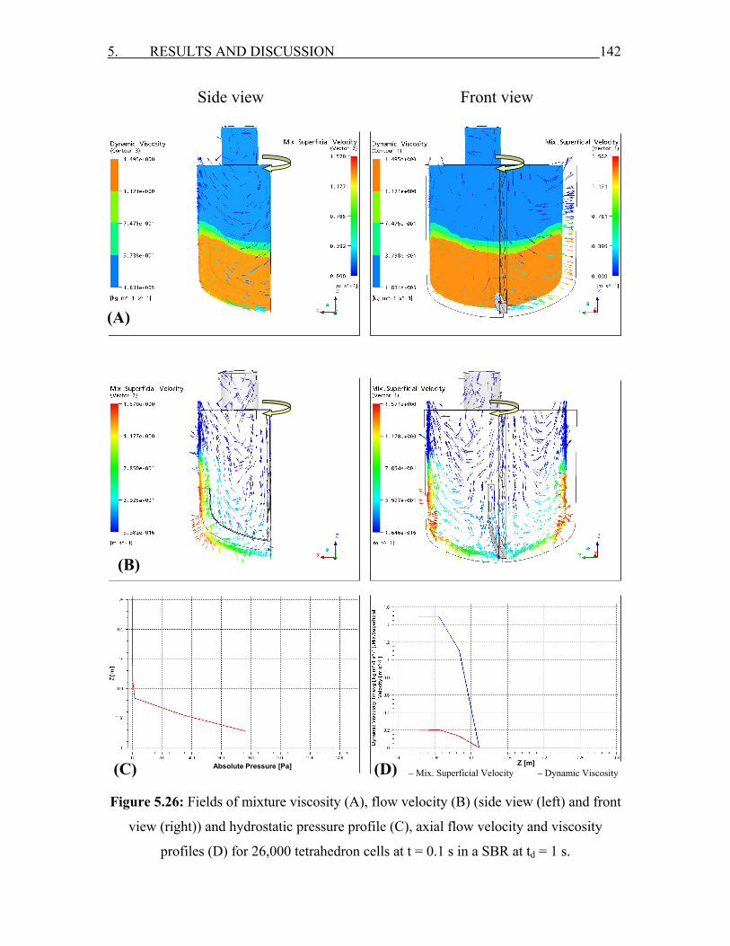
5. RESULTS AND DISCUSSION 142
Figure 5.26: Fields of mixture viscosity (A), flow velocity (B) (side view (left) and front
view (right)) and hydrostatic pressure profile (C), axial flow velocity and viscosity
profiles (D) for 26,000 tetrahedron cells at t = 0.1 s in a SBR at td = 1 s.
Side view Front view
(A)
(B)
Z [m] – Mix. Superficial Velocity – Dynamic Viscosity (D) (C)
Absolute Pressure [Pa]
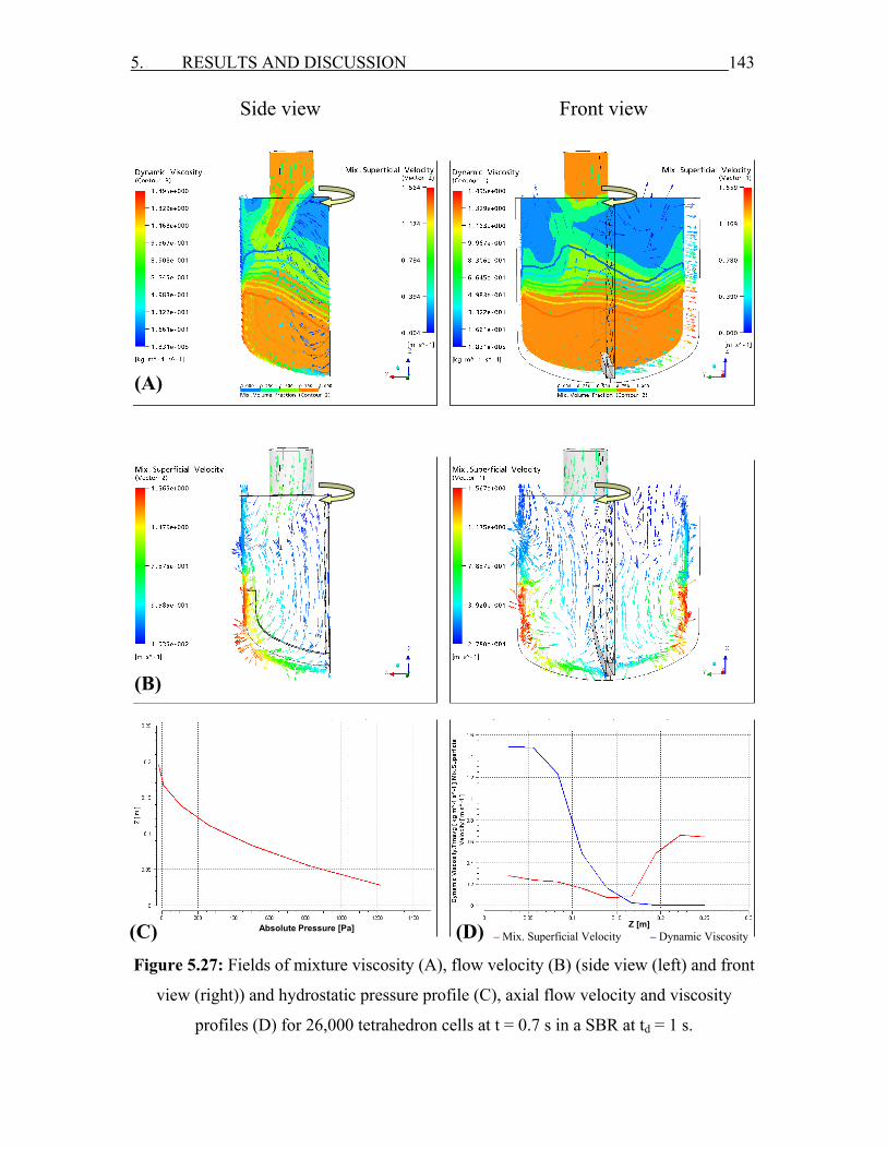
5. RESULTS AND DISCUSSION 143
Figure 5.27: Fields of mixture viscosity (A), flow velocity (B) (side view (left) and front
view (right)) and hydrostatic pressure profile (C), axial flow velocity and viscosity
profiles (D) for 26,000 tetrahedron cells at t = 0.7 s in a SBR at td = 1 s.
Side view Front view
(A)
(B)
(D) (C) Z [m] – Mix. Superficial Velocity – Dynamic Viscosity
Absolute Pressure [Pa]
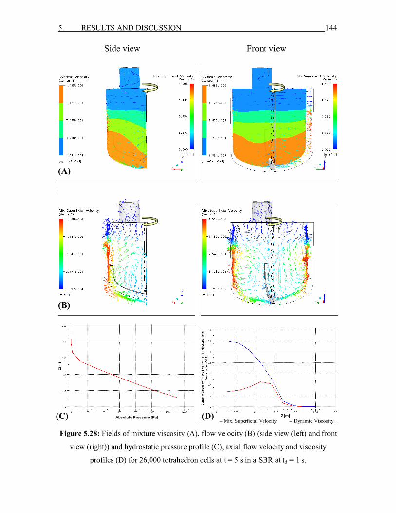
5. RESULTS AND DISCUSSION 144
Figure 5.28: Fields of mixture viscosity (A), flow velocity (B) (side view (left) and front
view (right)) and hydrostatic pressure profile (C), axial flow velocity and viscosity
profiles (D) for 26,000 tetrahedron cells at t = 5 s in a SBR at td = 1 s.
Side view Front view
(A)
(B)
(C) (D) Z [m] – Mix. Superficial Velocity – Dynamic Viscosity
Absolute Pressure [Pa]

5. RESULTS AND DISCUSSION 145
Figure 5.29: Fields of mixture viscosity (A), flow velocity (B) (side view (left) and front
view (right)) and hydrostatic pressure profile (C), axial flow velocity and viscosity
profiles (D) for 26,000 tetrahedron cells at t = 10 s in a SBR at td = 1 s.
Side view Front view
(A)
(B)
(C) (D) Z [m] – Mix. Superficial Velocity – Dynamic Viscosity
Absolute Pressure [Pa]
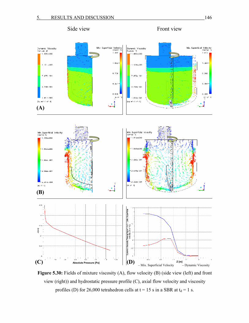
5. RESULTS AND DISCUSSION 146
Figure 5.30: Fields of mixture viscosity (A), flow velocity (B) (side view (left) and front
view (right)) and hydrostatic pressure profile (C), axial flow velocity and viscosity
profiles (D) for 26,000 tetrahedron cells at t = 15 s in a SBR at td = 1 s.
Side view Front view
(A)
(B)
(C) (D) Z [m] – Mix. Superficial Velocity – Dynamic Viscosity
Absolute Pressure [Pa]
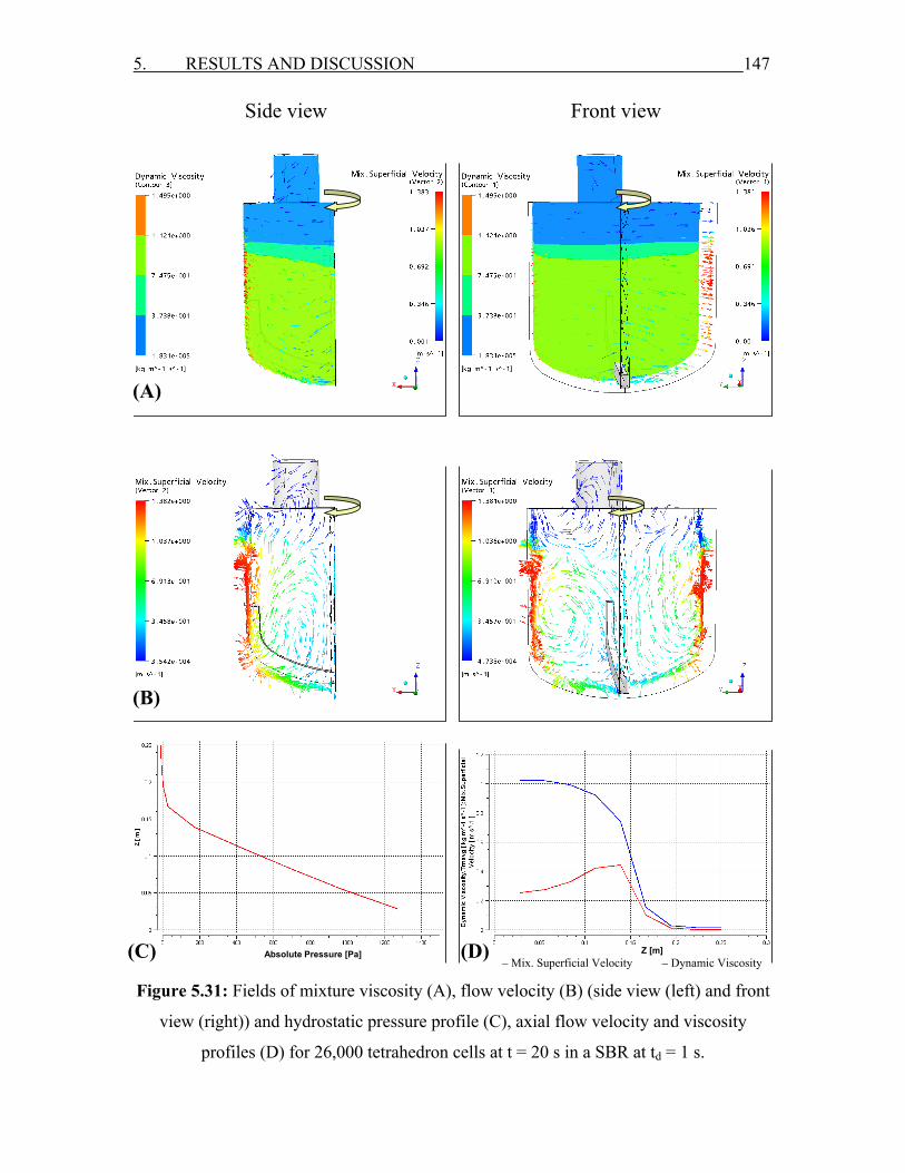
5. RESULTS AND DISCUSSION 147
Figure 5.31: Fields of mixture viscosity (A), flow velocity (B) (side view (left) and front
view (right)) and hydrostatic pressure profile (C), axial flow velocity and viscosity
profiles (D) for 26,000 tetrahedron cells at t = 20 s in a SBR at td = 1 s.
Side view Front view
(A)
(B)
(C) (D) Z [m] – Mix. Superficial Velocity – Dynamic Viscosity
Absolute Pressure [Pa]
5. RESULTS AND DISCUSSION 148
5.2.1.2 The effect of dosage time
Different dosage times of ethanol td = 1 s and td = 5 s are used in the CFD
simulations for inlet tube diameters of dt = 2.3 cm and dt = 5 cm. The fields
of flow velocity, viscosity and volume fraction of the liquid mixture are
studied at ω = 150 rpm. The time dependent velocity- and viscosity fields
are calculated.
5.2.1.2.1 Inlet tube diameter of 5 cm
The velocities of the dosed ethanol are uE = 0.64 m/s and uE = 0.128 m/s
for td = 1 s (from 0.2 s to 1.2 s) and td = 5 s (from 0.2 - 5.2 s), respectively.
The same mass of the dosed ethanol is used. For td = 1 s the fields of flow
velocity, viscosity and volume fraction of the liquid mixture as a function of
time in Fig. 5.32-a are presented as described in Fig. 5.21-a for 26,000
tetrahedron cells. When the dosage time increases to td = 5 s the inlet
volumetric flow rate of ethanol decreases from 1.25 L/s to 0.25 L/s. The
dosed ethanol will flow slowly near the wall of the inlet tube and the
cylindrical wall of the vessel to form a layer above glycerol. A very small
mass of ethanol is mixed with glycerol during the dosage which causes
longer mixing time as shown in Fig. 5.32-b.
For dosage time of td = 1 s the viscosity profile decreases sharply and
continuously up to the end of the dosage at t = 1.2 s. The reason of this
decrease is the high flow velocity, pressure force and volume of the dosed
ethanol which increase the flow velocity of the liquid mixture to 0.8 m/s and
accelerate the mixing process. For t > 1.2 s, ethanol is redistributed
completely in glycerol only under the effect of anchor rotation from the top
end of the impeller towards the shaft and towards the cylindrical wall as
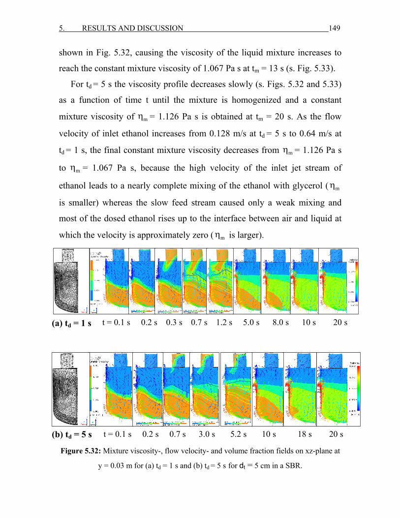
5. RESULTS AND DISCUSSION 149
shown in Fig. 5.32, causing the viscosity of the liquid mixture increases to
reach the constant mixture viscosity of 1.067 Pa s at tm = 13 s (s. Fig. 5.33).
For td = 5 s the viscosity profile decreases slowly (s. Figs. 5.32 and 5.33)
as a function of time t until the mixture is homogenized and a constant
mixture viscosity of mη = 1.126 Pa s is obtained at tm = 20 s. As the flow
velocity of inlet ethanol increases from 0.128 m/s at td = 5 s to 0.64 m/s at
td = 1 s, the final constant mixture viscosity decreases from mη = 1.126 Pa s
to mη = 1.067 Pa s, because the high velocity of the inlet jet stream of
ethanol leads to a nearly complete mixing of the ethanol with glycerol ( mη
is smaller) whereas the slow feed stream caused only a weak mixing and
most of the dosed ethanol rises up to the interface between air and liquid at
which the velocity is approximately zero ( mη is larger).
Figure 5.32: Mixture viscosity-, flow velocity- and volume fraction fields on xz-plane at
y = 0.03 m for (a) td = 1 s and (b) td = 5 s for dt = 5 cm in a SBR.
t = 0.1 s 0.2 s 0.3 s 0.7 s 1.2 s 5.0 s 8.0 s 10 s 20 sDosage time = 1 s
t = 0.1 s 0.2 s 0.7 s 3.0 s 5.2 s 10 s 18 s 20 sDosage
(a) td = 1 s
(b) td = 5 s
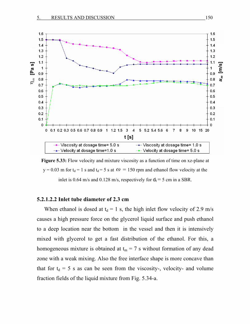
5. RESULTS AND DISCUSSION 150
Figure 5.33: Flow velocity and mixture viscosity as a function of time on xz-plane at
y = 0.03 m for td = 1 s and td = 5 s at ω = 150 rpm and ethanol flow velocity at the
inlet is 0.64 m/s and 0.128 m/s, respectively for dt = 5 cm in a SBR.
5.2.1.2.2 Inlet tube diameter of 2.3 cm
When ethanol is dosed at td = 1 s, the high inlet flow velocity of 2.9 m/s
causes a high pressure force on the glycerol liquid surface and push ethanol
to a deep location near the bottom in the vessel and then it is intensively
mixed with glycerol to get a fast distribution of the ethanol. For this, a
homogeneous mixture is obtained at tm = 7 s without formation of any dead
zone with a weak mixing. Also the free interface shape is more concave than
that for td = 5 s as can be seen from the viscosity-, velocity- and volume
fraction fields of the liquid mixture from Fig. 5.34-a.
u m [
m/s
]
t [s]
[Pa
s]
mη
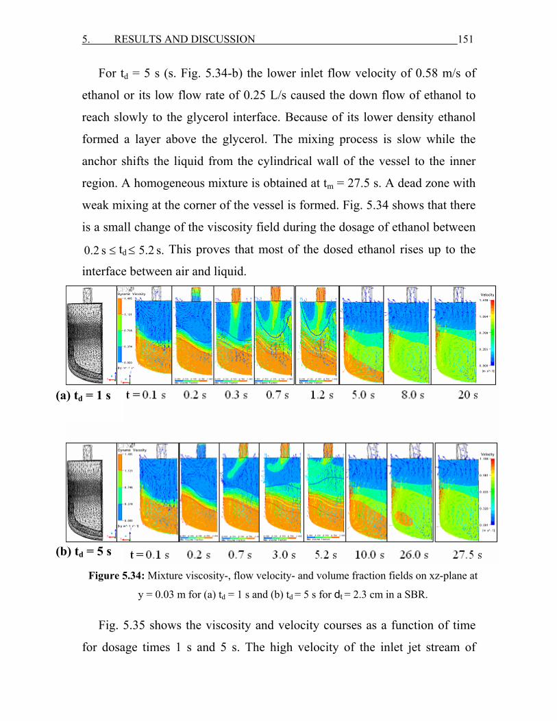
5. RESULTS AND DISCUSSION 151
For td = 5 s (s. Fig. 5.34-b) the lower inlet flow velocity of 0.58 m/s of
ethanol or its low flow rate of 0.25 L/s caused the down flow of ethanol to
reach slowly to the glycerol interface. Because of its lower density ethanol
formed a layer above the glycerol. The mixing process is slow while the
anchor shifts the liquid from the cylindrical wall of the vessel to the inner
region. A homogeneous mixture is obtained at tm = 27.5 s. A dead zone with
weak mixing at the corner of the vessel is formed. Fig. 5.34 shows that there
is a small change of the viscosity field during the dosage of ethanol between
0.2 s ≤ td 5.2 s.≤ This proves that most of the dosed ethanol rises up to the
interface between air and liquid.
Fig. 5.35 shows the viscosity and velocity courses as a function of time
for dosage times 1 s and 5 s. The high velocity of the inlet jet stream of
(a) td = 1 s
(b) td = 5 s
Figure 5.34: Mixture viscosity-, flow velocity- and volume fraction fields on xz-plane at
y = 0.03 m for (a) td = 1 s and (b) td = 5 s for dt = 2.3 cm in a SBR.
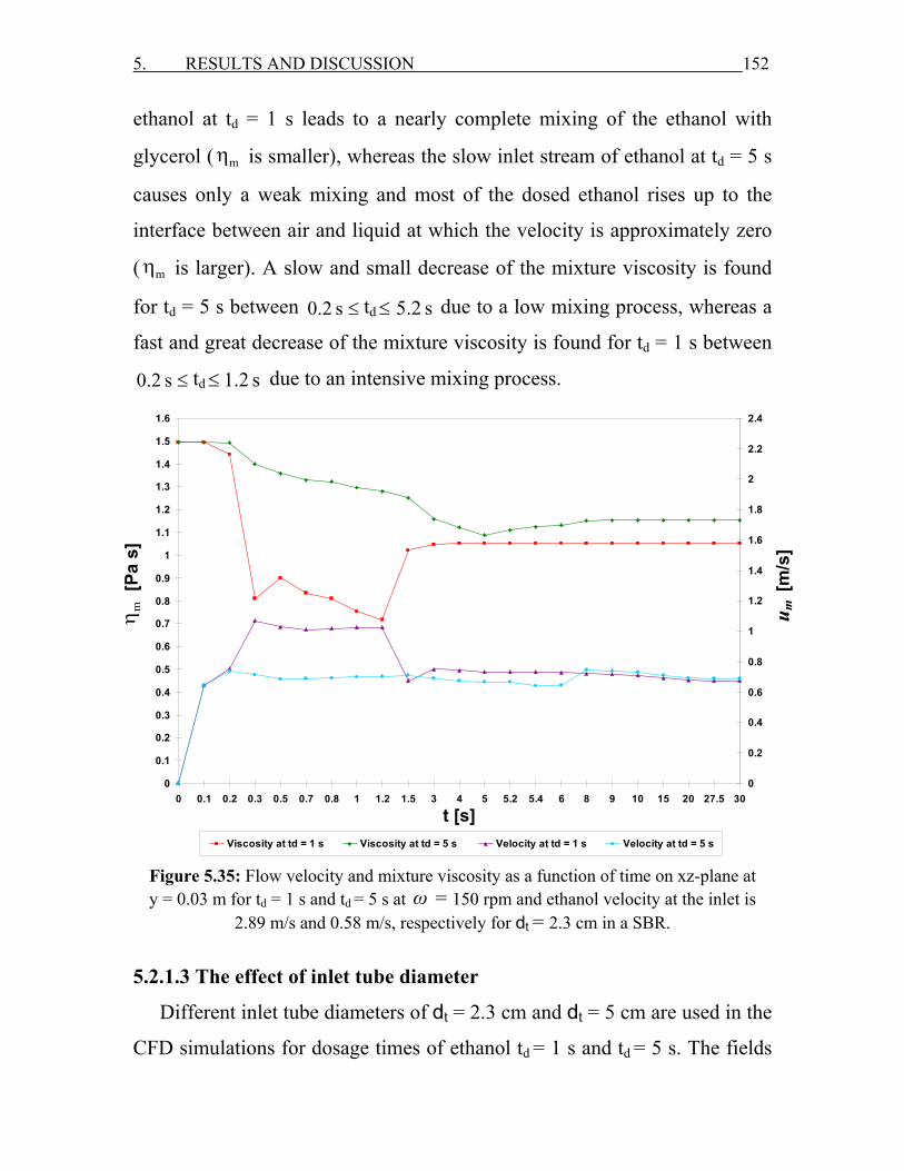
5. RESULTS AND DISCUSSION 152
ethanol at td = 1 s leads to a nearly complete mixing of the ethanol with
glycerol ( mη is smaller), whereas the slow inlet stream of ethanol at td = 5 s
causes only a weak mixing and most of the dosed ethanol rises up to the
interface between air and liquid at which the velocity is approximately zero
( mη is larger). A slow and small decrease of the mixture viscosity is found
for td = 5 s between 0.2 s ≤ td 5.2 s≤ due to a low mixing process, whereas a
fast and great decrease of the mixture viscosity is found for td = 1 s between
0.2 s ≤ td 1.2 s≤ due to an intensive mixing process.
0
0.1
0.2
0.3
0.4
0.5
0.6
0.7
0.8
0.9
1
1.1
1.2
1.3
1.4
1.5
1.6
0 0.1 0.2 0.3 0.5 0.7 0.8 1 1.2 1.5 3 4 5 5.2 5.4 6 8 9 10 15 20 27.5 300
0.2
0.4
0.6
0.8
1
1.2
1.4
1.6
1.8
2
2.2
2.4
Viscosity at td = 1 s Viscosity at td = 5 s Velocity at td = 1 s Velocity at td = 5 s
Figure 5.35: Flow velocity and mixture viscosity as a function of time on xz-plane at y = 0.03 m for td = 1 s and td = 5 s at ω = 150 rpm and ethanol velocity at the inlet is
2.89 m/s and 0.58 m/s, respectively for dt = 2.3 cm in a SBR.
5.2.1.3 The effect of inlet tube diameter
Different inlet tube diameters of dt = 2.3 cm and dt = 5 cm are used in the
CFD simulations for dosage times of ethanol td = 1 s and td = 5 s. The fields
u m [
m/s
]
[Pa
s]
mη
t [s]
5. RESULTS AND DISCUSSION 153
of flow velocity, viscosity and volume fraction of the liquid mixture as a
function of time are studied at ω = 150 rpm. The time dependent mixture
velocities um and mixture viscosities mη are calculated.
5.2.1.3.1 Dosage time td = 1 s
The velocities of the dosed ethanol are uE = 0.64 m/s and uE = 2.9 m/s for
dt = 5 cm and dt = 2.3 cm, respectively. In both cases the same mass of the
dosed ethanol is used. Initially glycerol is stirred until t = 0.2 s with
a constant viscosity of Gη = 1.495 Pa s (Figs. 5.36 and 5.37). For dt = 2.3 cm
when ethanol is dosed between 0.2 s ≤ td 1.2 s,≤ the viscosity mη decreases
much more than mη for dt = 5 cm (Fig. 5.37). This is due to the high velocity
of the dosed ethanol of uE = 2.9 m/s at dt = 2.3 cm which causes a high
pressure force on the bulk liquid and leads to a faster mixing with glycerol.
A second reason is the dosed ethanol may reaches the bottom of the vessel
because the inlet ethanol jet has higher velocity than the bulk and it is
normal to the glycerol interface in the middle of the vessel as can be shown
from mixture flow velocity-, viscosity- and volume fraction fields in
Fig. 5.36. The high inlet ethanol velocity leads to an increase in the bulk
velocity from um = 0.7 m/s to the maximum um = 1.03 m/s which causes the
sharp decrease in the viscosity mη during the dosage (Fig. 5.37). The higher
velocity of inlet ethanol stream gives the bulk liquid higher kinetic energy to
accelerate the mixing process with glycerol.
For dt = 5 cm the dosed ethanol stream between 0.2 s ≤ td 1.2 s≤ does not
fill the whole space of the inlet tube and flows therefore to the cylindrical
wall of the vessel because the velocity of the bulk liquid in this case is
higher than that for the dosed ethanol (Fig. 5.36-a). After the end of the
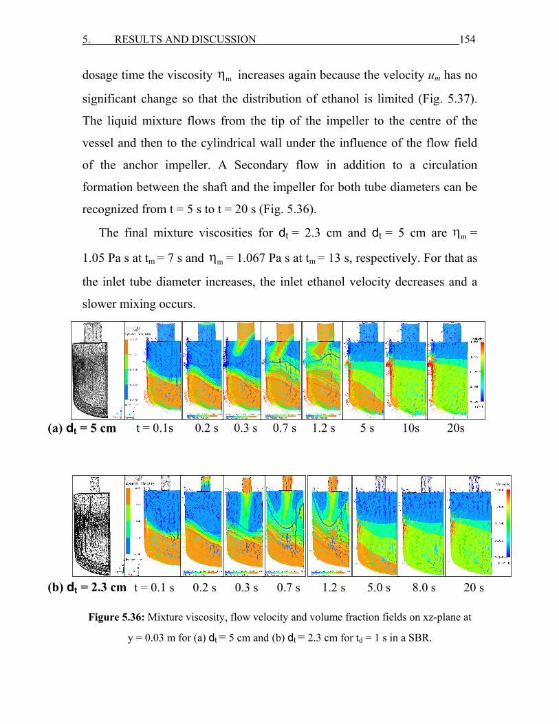
5. RESULTS AND DISCUSSION 154
dosage time the viscosity mη increases again because the velocity um has no
significant change so that the distribution of ethanol is limited (Fig. 5.37).
The liquid mixture flows from the tip of the impeller to the centre of the
vessel and then to the cylindrical wall under the influence of the flow field
of the anchor impeller. A Secondary flow in addition to a circulation
formation between the shaft and the impeller for both tube diameters can be
recognized from t = 5 s to t = 20 s (Fig. 5.36).
The final mixture viscosities for dt = 2.3 cm and dt = 5 cm are mη =
1.05 Pa s at tm = 7 s and mη = 1.067 Pa s at tm = 13 s, respectively. For that as
the inlet tube diameter increases, the inlet ethanol velocity decreases and a
slower mixing occurs.
Figure 5.36: Mixture viscosity, flow velocity and volume fraction fields on xz-plane at
y = 0.03 m for (a) dt = 5 cm and (b) dt = 2.3 cm for td = 1 s in a SBR.
t = 0.1 s 0.2 s 0.3 s 0.7 s 1.2 s 5.0 s 8.0 s 20 s
t = 0.1s 0.2 s 0.3 s 0.7 s 1.2 s 5 s 10s 20sTube diameter = 5 cm
Tube (b) dt = 2.3 cm
(a) dt = 5 cm

5. RESULTS AND DISCUSSION 155
Figure 5.37: Flow velocity and mixture viscosity as a function of time on xz-plane at
y = 0.03 m for dt = 5 cm and dt = 2.3 cm at ω = 150 rpm and ethanol velocity at the
inlet is 0.64 m/s and 2.89 m/s, respectively for td = 1 s in a SBR.
5.2.1.3.2 Dosage time td = 5 s
The velocities of the dosed ethanol are uE = 0.59 m/s and uE = 0.128 m/s
for dt = 2.3 cm and dt = 5 cm, respectively. As in the case of td = 1 s the inlet
velocity of ethanol is higher for the smaller tube but still lower than the bulk
velocity of the liquid mixture. The inlet flow stream will be shifted to the
cylindrical wall by the impeller and then mixed with glycerol from the
circumference to the shaft of the vessel as can be seen from the viscosity
fields mη in Figs. 5.32-b and 5.34-b leading to an circulation between the
shaft and impeller as can be seen from the flow velocity fields for t > 5.2 s.
A dead zone with a higher viscosity i.e. less mixing is found near the curved
0
0.1
0.2
0.3
0.4
0.5
0.6
0.7
0.8
0.9
1
1.1
1.2
1.3
1.4
1.5
1.6
0 0.1 0.2 0.3 0.5 0.6 0.7 0.8 0.9 1 1.2 1.5 3 4 5 5.2 5.4 5.6 5.8 6 7 7.5 8 9 10 15 200
0.2
0.4
0.6
0.8
1
1.2
1.4
1.6
1.8
2
2.2
2.4
Viscosity at tube diameter= 2.3 cm Viscosity at tube diameter= 5.0 cmVelocity at tube diameter= 5.0 cm Velocity at tube diameter= 2.3 cm
Dyn
amic
Vis
cosi
ty [k
g m
-̂1 s
-̂1]
Time [s]
Mix
.Sup
erfic
ial v
eloc
ity [m
/s]
u m [
m/s
]
t [s]
[Pa
s]
mη
5. RESULTS AND DISCUSSION 156
corner of the impeller at t = 26 s (s. Fig. 5.34-b). This behavior may be due
to the lower inlet velocity of ethanol than that of the bulk liquid. The
buoyant forces rise up ethanol (lower density) to the liquid interface. A
longer mixing time of tm = 27.5 s is required to get a complete mixing
compared with dt = 5 cm (s. Figs. 5.33 and 5.35).
For dt = 5 cm the inlet flow velocity of ethanol is three times lower from
that of dt = 2.3 cm. As in the cases before the inlet flow goes to the wall of
the vessel slowly and the mixing takes place between the shaft and the
impeller. The most of ethanol is mixed near the cylindrical wall with the
bulk glycerol, because the velocity at the cylindrical wall is higher than that
near the shaft, so that ethanol will be mixed faster with glycerol. A
homogeneous mixture is obtained in a shorter mixing time of tm = 20 s
compared with that for dt = 2.3 cm. When a small mass of ethanol flows
towards to the shaft and a large mass of ethanol is mixed near the cylindrical
wall, and then a small layer of ethanol will be formed above the bulk liquid
mixture. Therefore a homogeneous mixture will be obtained in shorter
mixing time tm (s. Fig. 5.32-b). It is noticed that the weak mixing zone in this
case is at t = 18 s near the corner of the vessel at the bottom. The axial
velocities are low above the tip of the anchor impeller and below the anchor
blades near the bottom of the vessel. This distribution of the axial velocity
leads to a circulation between the shaft and the impeller as can be seen from
the velocity field in Fig. 5.32-b for t > 5.2 s.
5. RESULTS AND DISCUSSION 157
5.2.1.4 The effect of anchor velocity
Radial and axial flow velocity fields as a function of time are calculated
by CFD simulations in a SBR with dt = 5 cm for different anchor velocities
from ω = 25 rpm to ω = 400 rpm and dosage times td = 1 s and td = 5 s.
The ethanol concentrations at four different positions in the vessel are
calculated as a function of time. The final mixture viscosity mη (tm) is
calculated as a function of the anchor velocity.
5.2.1.4.1 Dosage time td =1 s
When the anchor velocity increases from ω = 25 rpm to ω = 400 rpm
(s. Fig. 5.38), the shear forces and the mixture flow velocity um become
higher above the impeller and near the shaft. Then a larger mass of the dosed
ethanol flows towards to the impeller leading to a faster mixing as can also
be seen from the mixture viscosity field. A secondary flow not yet with
circulation between the shaft and impeller is obtained at ω = 25 rpm,
because the axial flow velocity is not large enough to push the ethanol layer
towards the bulk liquid, therefore a larger mass fraction of unmixed ethanol
exists and leads to a small viscosity decrease to the mixture viscosity at t =
20 s. Further increasing the anchor velocity gives higher axial velocity
which leads now to a circulation between the shaft and impeller. Indeed the
circulation accelerates the mixing of ethanol with glycerol and decreases
also the mass fraction of the unmixed ethanol. For that a final mixture
viscosity is obtained with smaller mixing time when increasing the anchor
velocity. The radial centrifugal forces rise up the liquid mixture near the
cylindrical wall leading to a concave interface with the air as shown in
Fig. 5.38.
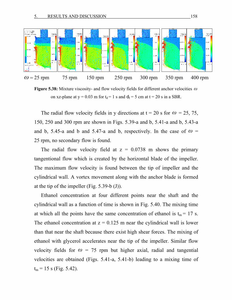
5. RESULTS AND DISCUSSION 158
Figure 5.38: Mixture viscosity- and flow velocity fields for different anchor velocities ω on xz-plane at y = 0.03 m for td = 1 s and dt = 5 cm at t = 20 s in a SBR.
The radial flow velocity fields in y directions at t = 20 s for ω = 25, 75,
150, 250 and 300 rpm are shown in Figs. 5.39-a and b, 5.41-a and b, 5.43-a
and b, 5.45-a and b and 5.47-a and b, respectively. In the case of ω =
25 rpm, no secondary flow is found.
The radial flow velocity field at z = 0.0738 m shows the primary
tangentional flow which is created by the horizontal blade of the impeller.
The maximum flow velocity is found between the tip of impeller and the
cylindrical wall. A vortex movement along with the anchor blade is formed
at the tip of the impeller (Fig. 5.39-b (J)).
Ethanol concentration at four different points near the shaft and the
cylindrical wall as a function of time is shown in Fig. 5.40. The mixing time
at which all the points have the same concentration of ethanol is tm = 17 s.
The ethanol concentration at z = 0.125 m near the cylindrical wall is lower
than that near the shaft because there exist high shear forces. The mixing of
ethanol with glycerol accelerates near the tip of the impeller. Similar flow
velocity fields for ω = 75 rpm but higher axial, radial and tangential
velocities are obtained (Figs. 5.41-a, 5.41-b) leading to a mixing time of
tm = 15 s (Fig. 5.42).
ω = 25 rpm 75 rpm 150 rpm 250 rpm 300 rpm 350 rpm 400 rpm ω =

5. RESULTS AND DISCUSSION 159
As the velocity of the anchor impeller increases to ω = 150, 250 and
300 rpm, then the axial and radial velocities increase. The circulation starts
to appear at ω = 150 rpm between the impeller and the shaft and it becomes
larger when the velocity increases. Similar flow velocity field can be seen in
Figs. 5.43-a and b, 5.45-a and b and 5.47-a and b for ω = 150, 250 and
300 rpm, respectively. As in the cases before secondary flow is caused by
the motion of the liquid mixture from the high velocity near the impeller to
the lower velocity near the shaft leading to a circulation between the
impeller and the shaft. The distribution of ethanol is controlled by the
secondary flow in the axial direction.
The upward radial and axial velocities are very high at y = 0.018 m
behind and close to the impeller, the downward axial velocity near the shaft
is low and can be seen in Figs. 5.43-a (A), 5.45-a (A) and 5.47-a (A). For
y = 0.027 m and y = 0.03 m the radial flow velocity decreases and the axial
flow velocity and circulation dominate (Figs. 5.43-a (B and C), 5.45-a (B
and C) and 5.47-a (B and C)). For y = 0.05 m a complete axial circulation
loop is found in the middle between the impeller and shaft (Figs. 5.43-a (D),
5.45-a (D) and 5.47-a (D)). In front of the impeller from y = - 0.018 m to
y = - 0.03 m the downward axial flow velocity dominates and a small
circulation can be seen above the impeller (Figs. 5.43-a and b (F, G and H),
5.45-a and b (F, G and H) and 5.47-a and b (F, G and H)).
When the anchor velocity increases the radial trailing vortex near the
anchor tip becomes larger at z = 0.074 m leading to a higher distribution of
ethanol in the bulk liquid (Figs. 5.43-b (J and K), 5.45-b (J and K) and 5.47-
b (J and K)). It can be concluded that the impeller velocity has a greater
effect on the secondary axial flow than on the primary tangentional flow.

5. RESULTS AND DISCUSSION 160
The mixing times for ω = 150 rpm, 250 rpm and 300 rpm are tm = 13 s,
7 s and 5 s, respectively as can be seen from ethanol concentration as a
function of time in Figs. 5.44, 5.46 and 5.48. As the anchor velocity
increases the mixing time decreases.
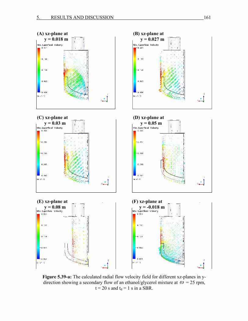
5. RESULTS AND DISCUSSION 161
Figure 5.39-a: The calculated radial flow velocity field for different xz-planes in y-direction showing a secondary flow of an ethanol/glycerol mixture at ω = 25 rpm,
t = 20 s and td = 1 s in a SBR.
(D) xz-plane at y = 0.05 m
(C) xz-plane at y = 0.03 m
(B) xz-plane at y = 0.027 m
(A) xz-plane at y = 0.018 m
(F) xz-plane at y = -0.018 m
(E) xz-plane at y = 0.08 m
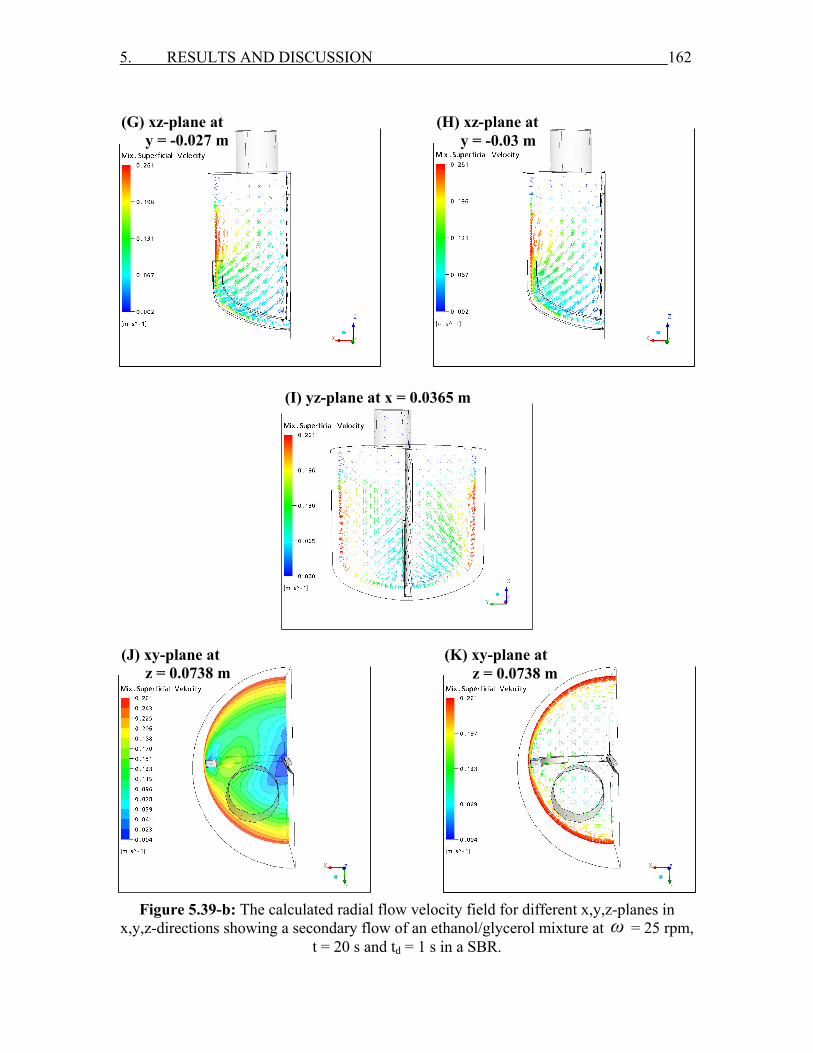
5. RESULTS AND DISCUSSION 162
Figure 5.39-b: The calculated radial flow velocity field for different x,y,z-planes in x,y,z-directions showing a secondary flow of an ethanol/glycerol mixture at ω = 25 rpm,
t = 20 s and td = 1 s in a SBR.
(H) xz-plane at y = -0.03 m
(G) xz-plane at y = -0.027 m
(I) yz-plane at x = 0.0365 m
(K) xy-plane at z = 0.0738 m
(J) xy-plane at z = 0.0738 m

5. RESULTS AND DISCUSSION 163
Figure 5.40: Ethanol concentration as a function of time at ω = 25 rpm at four different
positions in a SBR at td = 1 s.
t [s] – – – –

5. RESULTS AND DISCUSSION 164
Figure 5.41-a: The calculated radial flow velocity field for different xz-planes in y-direction showing a secondary flow of an ethanol/glycerol mixture at ω = 75 rpm,
t = 20 s and td = 1 s in a SBR.
(D) xz-plane at y = 0.05 m
(C) xz-plane at y = 0.03 m
(B) xz-plane at y = 0.027 m
(A) xz-plane at y = 0.018 m
(F) xz-plane at y = -0.018 m
(E) xz-plane at y = 0.08 m
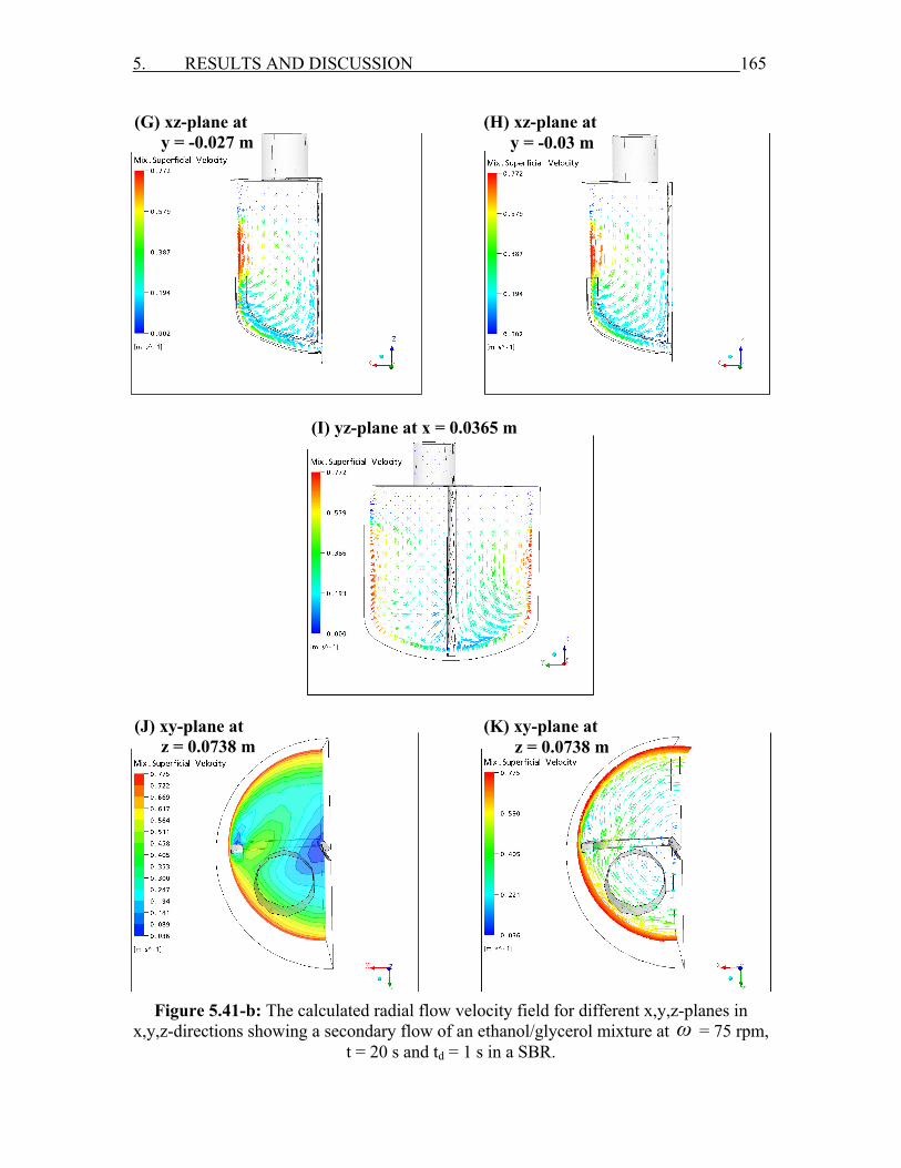
5. RESULTS AND DISCUSSION 165
Figure 5.41-b: The calculated radial flow velocity field for different x,y,z-planes in x,y,z-directions showing a secondary flow of an ethanol/glycerol mixture at ω = 75 rpm,
t = 20 s and td = 1 s in a SBR.
(H) xz-plane at y = -0.03 m
(G) xz-plane at y = -0.027 m
(I) yz-plane at x = 0.0365 m
(K) xy-plane at z = 0.0738 m
(J) xy-plane at z = 0.0738 m
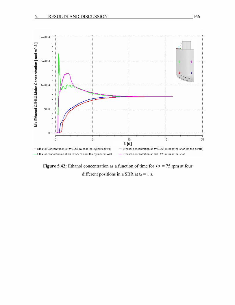
5. RESULTS AND DISCUSSION 166
Figure 5.42: Ethanol concentration as a function of time for ω = 75 rpm at four
different positions in a SBR at td = 1 s.
t [s] – – – –

5. RESULTS AND DISCUSSION 167
Figure 5.43-a: The calculated radial flow velocity field for different xz-planes in y-direction showing a secondary flow of an ethanol/glycerol mixture at ω = 150 rpm,
t = 20 s and td = 1 s in a SBR.
(D) xz-plane at y = 0.05 m
(C) xz-plane at y = 0.03 m
(B) xz-plane at y = 0.027 m
(A) xz-plane at y = 0.018 m
(F) xz-plane at y = -0.018 m
(E) xz-plane at y = 0.08 m

5. RESULTS AND DISCUSSION 168
Figure 5.43-b: The calculated radial flow velocity field for different x,y,z-planes in x,y,z-directions showing a secondary flow of an ethanol/glycerol mixture at
ω = 150 rpm, t = 20 s and td = 1 s in a SBR.
(H) xz-plane at y = -0.03 m
(G) xz-plane at y = -0.027 m
(I) yz-plane at x = 0.0365 m
(K) xy-plane at z = 0.0738 m
(J) xy-plane at z = 0.0738 m
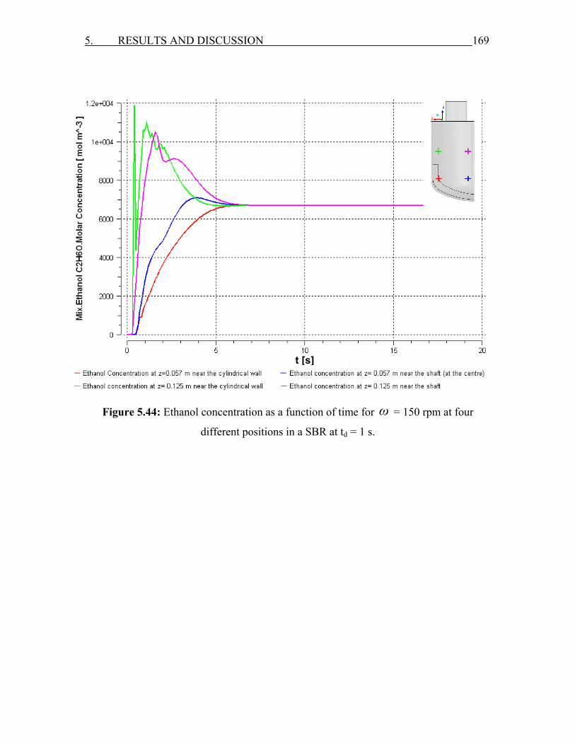
5. RESULTS AND DISCUSSION 169
Figure 5.44: Ethanol concentration as a function of time for ω = 150 rpm at four
different positions in a SBR at td = 1 s.
t [s]
– – – –
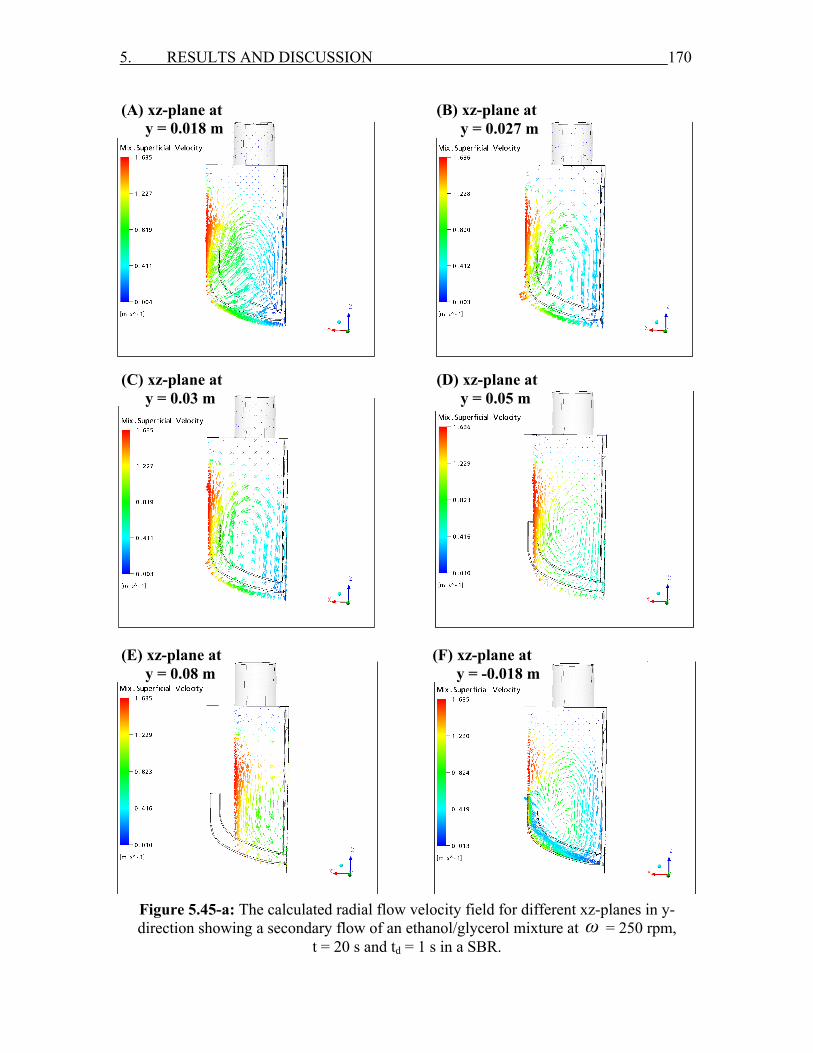
5. RESULTS AND DISCUSSION 170
Figure 5.45-a: The calculated radial flow velocity field for different xz-planes in y-direction showing a secondary flow of an ethanol/glycerol mixture at ω = 250 rpm,
t = 20 s and td = 1 s in a SBR.
(D) xz-plane at y = 0.05 m
(C) xz-plane at y = 0.03 m
(B) xz-plane at y = 0.027 m
(A) xz-plane at y = 0.018 m
(F) xz-plane at y = -0.018 m
(E) xz-plane at y = 0.08 m
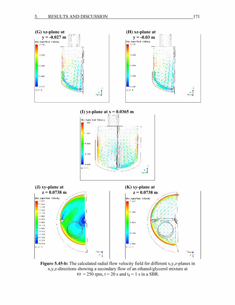
5. RESULTS AND DISCUSSION 171
Figure 5.45-b: The calculated radial flow velocity field for different x,y,z-planes in
x,y,z-directions showing a secondary flow of an ethanol/glycerol mixture at ω = 250 rpm, t = 20 s and td = 1 s in a SBR.
(H) xz-plane at y = -0.03 m
(G) xz-plane at y = -0.027 m
(I) yz-plane at x = 0.0365 m
(K) xy-plane at z = 0.0738 m
(J) xy-plane at z = 0.0738 m
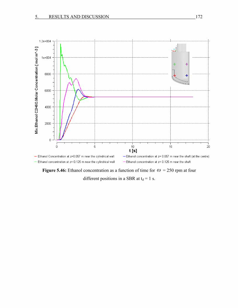
5. RESULTS AND DISCUSSION 172
Figure 5.46: Ethanol concentration as a function of time for ω = 250 rpm at four
different positions in a SBR at td = 1 s.
t [s]
– – – –

5. RESULTS AND DISCUSSION 173
Figure 5.47-a: The calculated radial flow velocity field for different xz-planes in y-direction showing a secondary flow of an ethanol/glycerol mixture at ω = 300 rpm,
t = 20 s and td = 1 s in a SBR.
(D) xz-plane at y = 0.05 m
(C) xz-plane at y = 0.03 m
(B) xz-plane at y = 0.027 m
(A) xz-plane at y = 0.018 m
(F) xz-plane at y = -0.018 m
(E) xz-plane at y = 0.08 m
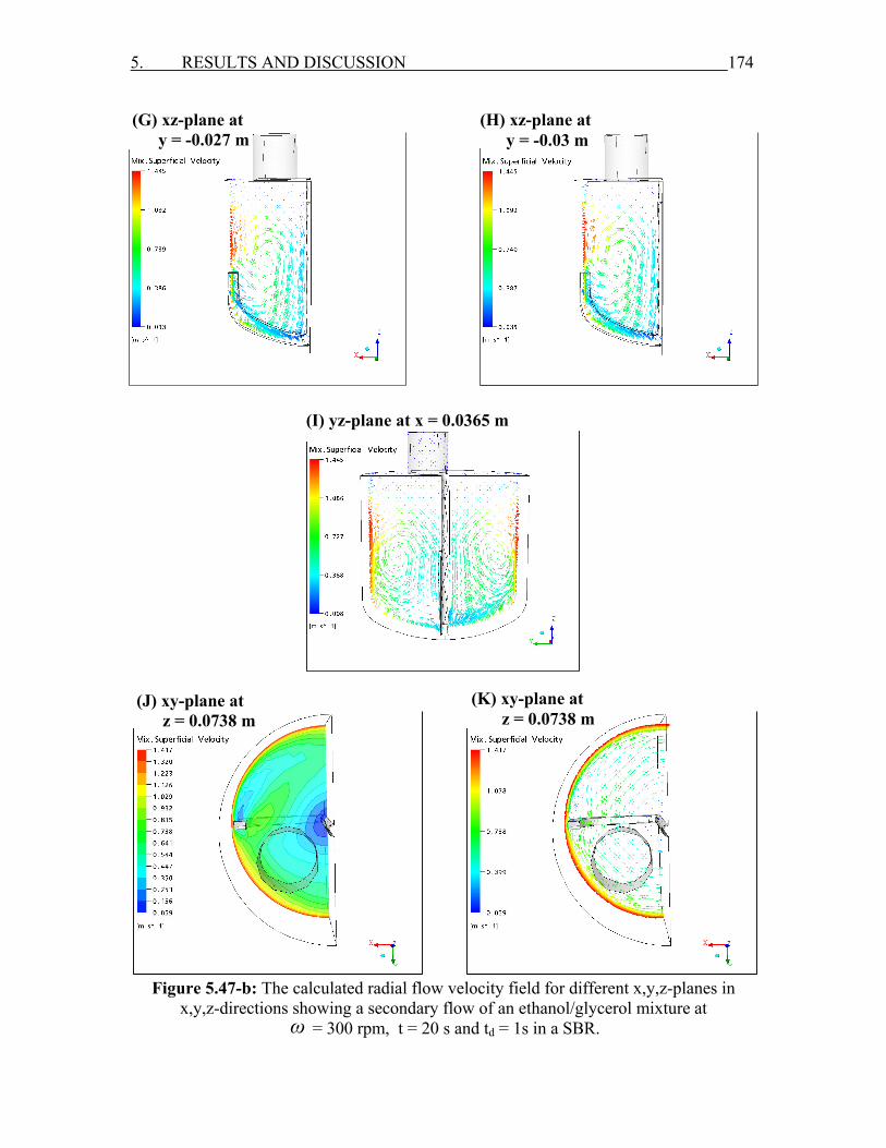
5. RESULTS AND DISCUSSION 174
Figure 5.47-b: The calculated radial flow velocity field for different x,y,z-planes in x,y,z-directions showing a secondary flow of an ethanol/glycerol mixture at
ω = 300 rpm, t = 20 s and td = 1s in a SBR.
(H) xz-plane at y = -0.03 m
(G) xz-plane at y = -0.027 m
(I) yz-plane at x = 0.0365 m
(K) xy-plane at z = 0.0738 m
(J) xy-plane at z = 0.0738 m

5. RESULTS AND DISCUSSION 175
Figure 5.48: Ethanol concentration as a function of time for ω = 300 rpm at four
different positions in a SBR at td = 1 s.
t [s]
– – – –
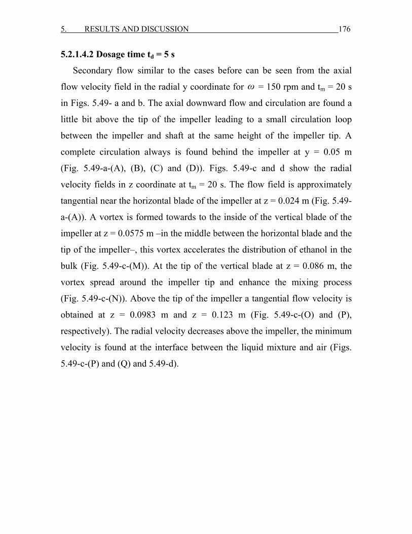
5. RESULTS AND DISCUSSION 176
5.2.1.4.2 Dosage time td = 5 s
Secondary flow similar to the cases before can be seen from the axial
flow velocity field in the radial y coordinate for ω = 150 rpm and tm = 20 s
in Figs. 5.49- a and b. The axial downward flow and circulation are found a
little bit above the tip of the impeller leading to a small circulation loop
between the impeller and shaft at the same height of the impeller tip. A
complete circulation always is found behind the impeller at y = 0.05 m
(Fig. 5.49-a-(A), (B), (C) and (D)). Figs. 5.49-c and d show the radial
velocity fields in z coordinate at tm = 20 s. The flow field is approximately
tangential near the horizontal blade of the impeller at z = 0.024 m (Fig. 5.49-
a-(A)). A vortex is formed towards to the inside of the vertical blade of the
impeller at z = 0.0575 m –in the middle between the horizontal blade and the
tip of the impeller–, this vortex accelerates the distribution of ethanol in the
bulk (Fig. 5.49-c-(M)). At the tip of the vertical blade at z = 0.086 m, the
vortex spread around the impeller tip and enhance the mixing process
(Fig. 5.49-c-(N)). Above the tip of the impeller a tangential flow velocity is
obtained at z = 0.0983 m and z = 0.123 m (Fig. 5.49-c-(O) and (P),
respectively). The radial velocity decreases above the impeller, the minimum
velocity is found at the interface between the liquid mixture and air (Figs.
5.49-c-(P) and (Q) and 5.49-d).
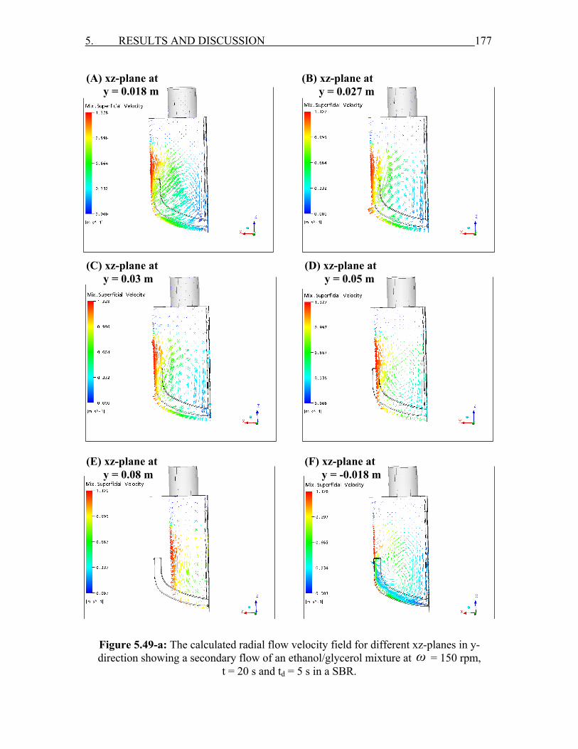
5. RESULTS AND DISCUSSION 177
Figure 5.49-a: The calculated radial flow velocity field for different xz-planes in y-direction showing a secondary flow of an ethanol/glycerol mixture at ω = 150 rpm,
t = 20 s and td = 5 s in a SBR.
(D) xz-plane at y = 0.05 m
(C) xz-plane at y = 0.03 m
(B) xz-plane at y = 0.027 m
(A) xz-plane at y = 0.018 m
(F) xz-plane at y = -0.018 m
(E) xz-plane at y = 0.08 m
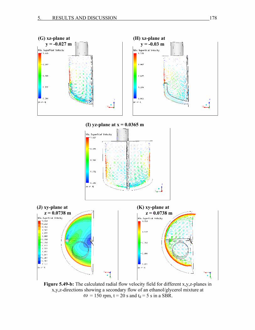
5. RESULTS AND DISCUSSION 178
Figure 5.49-b: The calculated radial flow velocity field for different x,y,z-planes in x,y,z-directions showing a secondary flow of an ethanol/glycerol mixture at
ω = 150 rpm, t = 20 s and td = 5 s in a SBR.
(H) xz-plane at y = -0.03 m
(G) xz-plane at y = -0.027 m
(I) yz-plane at x = 0.0365 m
(K) xy-plane at z = 0.0738 m
(J) xy-plane at z = 0.0738 m
5. RESULTS AND DISCUSSION 179
Figure 5.49-c: The calculated radial flow velocity field for different xy-planes in z-
direction of an ethanol/glycerol mixture at ω = 150 rpm, t = 20 s and td = 5 s in a SBR.
(L) xy-plane at z = 0.0235 m
(M) xy-plane at z = 0.0575 m
(N) xy-plane at z = 0.0861 m
(O) xy-plane at z = 0.0983 m
(P) xy-plane at z = 0.1231 m
(Q) xy-plane at z = 0.1599 m
5. RESULTS AND DISCUSSION 180
Figure 5.49-d: The calculated radial flow velocity fields of an ethanol/glycerol mixture
for different xy-planes in z-direction at ω = 150 rpm, t = 20 s and td = 5 s in a SBR.
For td = 5 s when the anchor velocity increases, the final mixture
viscosity increases up to ω = 250 rpm, because the mass fraction of the
unmixed ethanol decreases (Fig. 5.50). A small decreasing of the mixture
viscosity is found between ω = 250 rpm and ω = 350 rpm because it may
be exist a small mass of the low velocity dosed ethanol at the liquid interface
near the cylindrical wall. The high anchor velocity rise the level of the bulk
liquid near the cylindrical wall. A constant final mixture viscosity mη is
found after ω = 350 rpm.

5. RESULTS AND DISCUSSION 181
For td = 1 s the final mixture viscosity is directly proportional to the
anchor velocity up to ω = 350 rpm then it becomes constant, because all the
dosed mass of ethanol is completely mixed with glycerol (Fig. 5.50).
The final mixture viscosity at td = 1 s is lower than that for td = 5 s up to
ω = 250 rpm because the velocity of the dosed ethanol at td = 1 s is higher.
Similar final mixture viscosity for both dosages is found at ω = 300 rpm.
Above ω = 300 rpm it is surprising that the final mixture viscosity at
td = 1 s is higher than that at td = 5 s, because the high anchor velocity
produces high upward shear forces which collides with the high inlet ethanol
velocity stream in case of td = 1 s, and resists ethanol to be mixed completely
with glycerol leading to a higher final mixture viscosity.
Figure 5.50: Final mixture viscosity as a function of anchor velocity in a SBR with
dt = 5 cm and 26,000 tetrahedrons cells for td = 1 and td = 5 s at t = 20 s.
[mPa
s]
mη
ω [rpm]
5. RESULTS AND DISCUSSION 182
5.2.1.5 The effect of anchor dimensions
The mixing time and the flow velocity-, mixture viscosity- and volume
fraction fields as a function of time are studied in a SBR at td = 5 s between
0.2 s ≤ td 5.2 s,≤ dt = 5 cm and ω = 150 rpm for two types of anchors with
two different horizontal blade widths. The two anchor impellers with
horizontal blade widths of wh = 0.015 and 0.012 m for wide and thin
horizontal blades, respectively are shown in Fig. 5.51.
Figure 5.51: Anchor impellers with horizontal blade widths of wh = 0.015 m (left) and
wh = 0.012 m (right).
Old Anchor New AnchorWide horizontal blade anchor Thin horizontal blade anchor
5. RESULTS AND DISCUSSION 183
Before the dosage of ethanol similar fields of mixture viscosity and flow
velocity are obtained for both impellers but higher radial velocity is found
near the corner of the wide blade impeller (Fig. 5.52-a). A faster mixing of
ethanol with glycerol in the case of a wide blade impeller is obtained as it
can be seen from the velocity field of left column (e.g. in Fig. 5.52-b) in
comparison to the clear smaller velocities in the case of the thin horizontal
blade anchor (right column in Fig. 5.52-b). The faster mixing is caused by
the high axial velocities and circulation which lead to a decrease of the
mixture viscosity near the bottom of the vessel as can be seen from the
contour lines of constant mixture viscosity at t = 5.2 s in Fig. 5.52-b. A
larger mass of ethanol flows towards the shaft will be mixed with glycerol
leading to a clear lower mixture viscosity with a sharp convex shape for
wide horizontal blade anchor at t = 10 s (left column in Fig. 5.52-b) than in
the case of thin horizontal blade anchor at t = 10 (right column in Fig. 5.52-
b).
Ethanol is continuously transported by the impeller towards the shaft and
mixed with glycerol leading to a sharper convex shape in case of the blade
width of wh = 0.015 m (left column in Fig. 5.52-c) compared to that of
wh = 0.012 m (right column in Fig. 5.52-c) which can be seen from the
viscosity field between 11 s ≤ t 13 s.≤ Then ethanol is mixed with glycerol
from the shaft towards the cylindrical wall leading to a small zone with high
mixture viscosity near the corner of the vessel (left column in Fig. 5.52-d). A
faster mixing occurs in the case of the wide blade anchor compared with the
thin blade anchor (right column in Fig. 5.52-d) in which the mixing is still
from the impeller towards the shaft as can be seen from the viscosity field
between 15 s ≤ t 18 s.≤
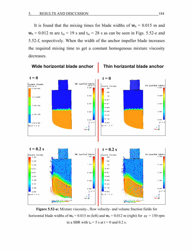
5. RESULTS AND DISCUSSION 184
It is found that the mixing times for blade widths of wh = 0.015 m and
wh = 0.012 m are tm = 19 s and tm = 28 s as can be seen in Figs. 5.52-e and
5.52-f, respectively. When the width of the anchor impeller blade increases
the required mixing time to get a constant homogenous mixture viscosity
decreases.
Figure 5.52-a: Mixture viscosity-, flow velocity- and volume fraction fields for
horizontal blade widths of wh = 0.015 m (left) and wh = 0.012 m (right) for ω = 150 rpm
in a SBR with td = 5 s at t = 0 and 0.2 s.
Old Anchor New AnchorWide horizontal blade anchor Thin horizontal blade anchor
t = 0 t = 0
t = 0.2 s t = 0.2 s
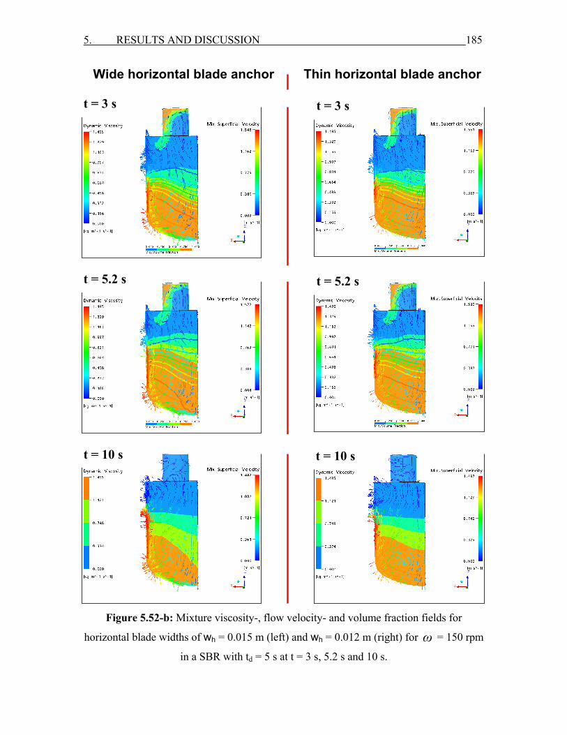
5. RESULTS AND DISCUSSION 185
Figure 5.52-b: Mixture viscosity-, flow velocity- and volume fraction fields for
horizontal blade widths of wh = 0.015 m (left) and wh = 0.012 m (right) for ω = 150 rpm
in a SBR with td = 5 s at t = 3 s, 5.2 s and 10 s.
Old Anchor New AnchorWide horizontal blade anchor Thin horizontal blade anchor
t = 3 s t = 3 s
t = 5.2 s t = 5.2 s
t = 10 s t = 10 s
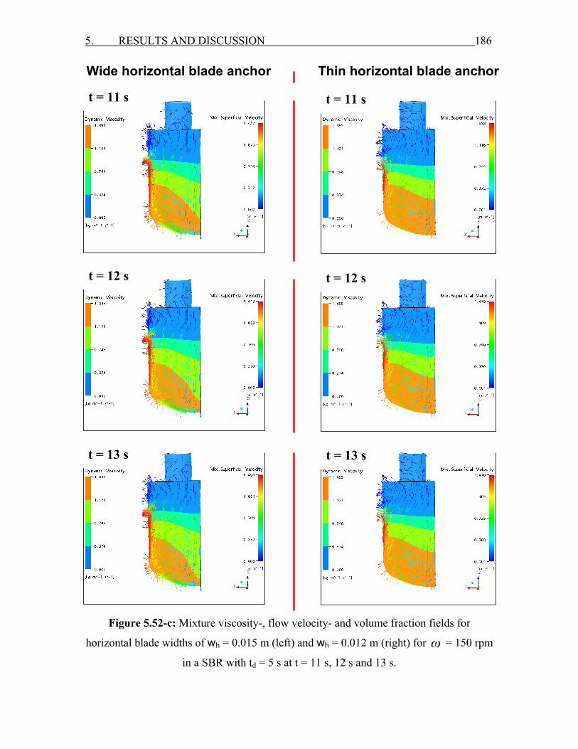
5. RESULTS AND DISCUSSION 186
Figure 5.52-c: Mixture viscosity-, flow velocity- and volume fraction fields for
horizontal blade widths of wh = 0.015 m (left) and wh = 0.012 m (right) for ω = 150 rpm
in a SBR with td = 5 s at t = 11 s, 12 s and 13 s.
Old Anchor New AnchorWide horizontal blade anchor Thin horizontal blade anchor
t = 11 s t = 11 s
t = 12 s t = 12 s
t = 13 s t = 13 s
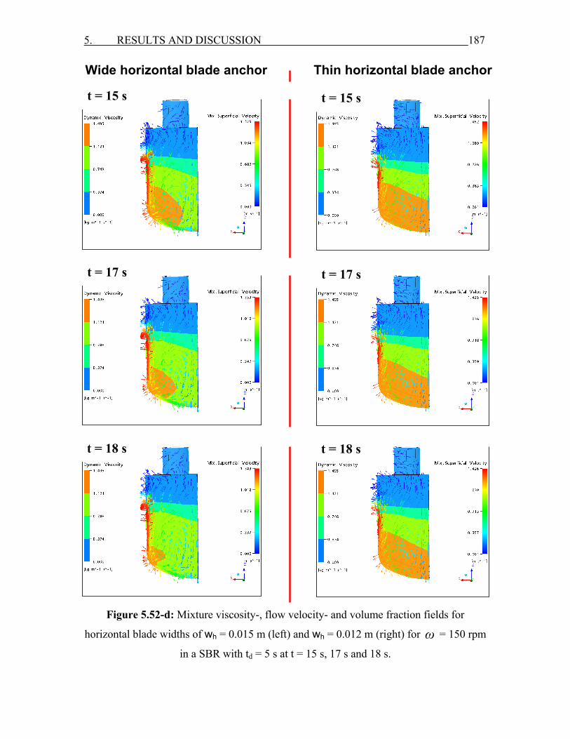
5. RESULTS AND DISCUSSION 187
Figure 5.52-d: Mixture viscosity-, flow velocity- and volume fraction fields for
horizontal blade widths of wh = 0.015 m (left) and wh = 0.012 m (right) for ω = 150 rpm
in a SBR with td = 5 s at t = 15 s, 17 s and 18 s.
Old Anchor New AnchorWide horizontal blade anchor Thin horizontal blade anchor
t = 15 s t = 15 s
t = 17 s t = 17 s
t = 18 s t = 18 s
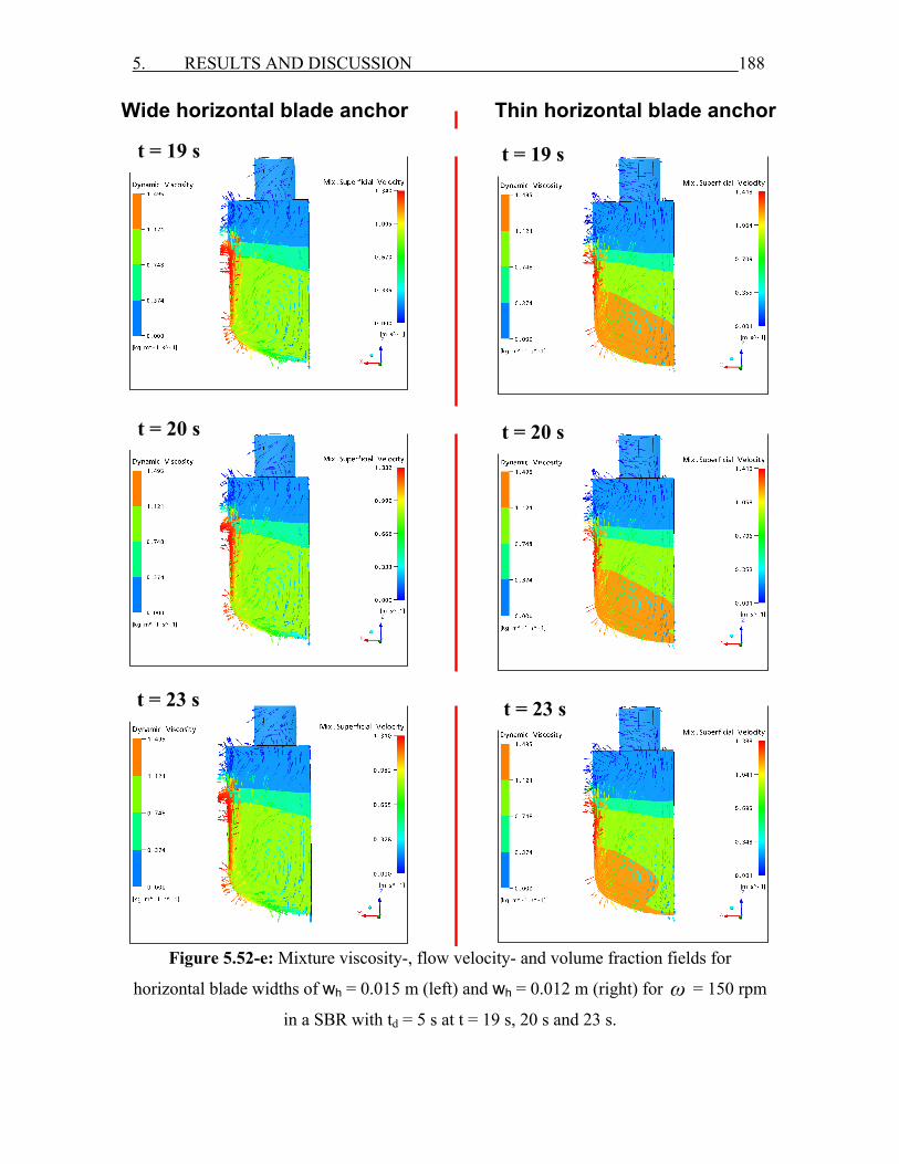
5. RESULTS AND DISCUSSION 188
Figure 5.52-e: Mixture viscosity-, flow velocity- and volume fraction fields for
horizontal blade widths of wh = 0.015 m (left) and wh = 0.012 m (right) for ω = 150 rpm
in a SBR with td = 5 s at t = 19 s, 20 s and 23 s.
Old Anchor New AnchorWide horizontal blade anchor Thin horizontal blade anchor
t = 19 s t = 19 s
t = 20 s t = 20 s
t = 23 s
t = 23 s

5. RESULTS AND DISCUSSION 189
Figure 5.52-f: Mixture viscosity-, flow velocity- and volume fraction fields for
horizontal blade widths of wh = 0.015 m (left) and wh = 0.012 m (right) for ω = 150 rpm
in a SBR with td = 5 s at t = 25 s, 27 s and 28 s.
Old Anchor New AnchorWide horizontal blade anchor Thin horizontal blade anchor
t = 25 s t = 25 s
t = 27 s t = 27 s
t = 28 s t = 28 s
5. RESULTS AND DISCUSSION 190
5.2.2 Batch reactor
5.2.2.1 The effect of different mixture ratios of glycerol to ethanol
Mixtures of different volume fraction of ethanol and glycerol are used i.e.
100 % glycerol (HG = 0.14 m), 100 % ethanol (HE = 0.14 m), a mixture of
67 % glycerol (HG = 0.1 m from the bottom) and 33 % ethanol (HE = 0.04 m
above the glycerol) and a mixture of 16 % glycerol (HG = 0.04 m from the
bottom) and 84 % ethanol (HE = 0.1 m above the glycerol).
From the calculated 3D-flow velocity field axial and radial (horizontal in
x-direction) velocity components as a function of x, y, z-directions in the BR
at ω = 150 rpm are determined.
5.2.2.1.1 Glycerol (HG = 0.1 m) and ethanol (HE = 0.04 m)
The final mixture viscosity mη = 1.07 Pa s of this liquid mixture is
determined as described in the case of SBR (s. Chap. 5.2.1.1). Similar to the
case of SBR a secondary flow can also be observed (Fig. 5.53). The highest
axial flow velocities are found at the tip of the impeller and near the
cylindrical wall of the vessel. The axial flow is caused by the vertical part of
the blade of the impeller, whereas the radial flow is caused by the horizontal
part of the blade of the impeller. An axial circulation is found behind the
anchor impeller at a distance of dv/2 from the shaft. The smallest flow
velocities are found near the shaft.
The axial velocities uax as a function of x at t = 10 s are shown in Fig.
5.54-(a). The negative flow velocities mean a downward flow and the
positive flow velocities are upward flow. It can be recognized that the
downward axial velocity reach the maximum at x ≈ 0.01 m. The sharp
decrease of the downward velocity uax and of the upward uax for x 0.03 m≥
s
5. RESULTS AND DISCUSSION 191
is caused by a circulation flow formed between 0.03 m ≤ x 0.06 m.≤ The
downward uax ≈ − 0.1 m/s at x = 0.03 m and the upward uax ≈ 0.1 m/s at x =
0.06 m have a similar absolute value. The centre of the circulation is found
at x = 0.045 m and corresponds to the flex point F of the velocity profile in
Fig. 5.54-(a). At the flex point F it is found the dead zone where is uax ≈ 0.
The maximum of uax is found at x = 0.078 m in the middle of the vertical
part of the impeller at which high shear forces exist.
The maximum of uax curve is shifted in the y-direction to y = 0.04 m due
to the position of the anchor impeller which has a relative large distance
from the y-axis (Fig. 5.54-(b)). This means that in the y-direction the upward
uax increase at a larger y-value then the x-value. A small circulation flow is
calculated between 0.07 m ≤ y 0.09 m≤ and it has the flex point F of the
velocity profile at the centre of the circulation at y = 0.076 m where is
uax ≈ 0. The upward uax reaches a maximum at y = 0.09 m and decreases to
uax ≈ 0 near the cylindrical wall at y = 0.1 m similar as in the x-direction.
The axial velocity uax increases in the z-direction from the bottom of the
vessel up to z = 0.07 m near the tip of the impeller to a maximum (Fig. 5.54-
(c)). Then uax decreases for z > 0.07 m above the impeller up to a minimum
uax is reached at z = 0.17 m. In this height the flow velocity is zero at the
interface between the liquid mixture and air. The sharp decrease of uax is
caused by an increasing vertical distance from the horizontal part of the
impeller, where the flow velocities decrease fastly to the neglecting velocity
at the interface between liquid and air.
The radial velocity profile in x coordinates in Fig. 5.54-(d) shows an
increase of the magnitude of the radial velocity between the shaft and
x = 0.06 m where the circulation exists. A small radial vortex exists between
x = 0.075 m and x = 0.085 m because of the symmetric velocities around
5. RESULTS AND DISCUSSION 192
x = 0.08 m. The maximum radial velocity is found near the cylindrical wall.
The radial velocity increases from the shaft up to y = 0.06 m and then it
decreases towards to the cylindrical wall (Fig. 5.54-(e)). The radial velocity
decreases from the bottom of the vessel up to z = 0.085 m near the impeller
tip and then increases up to z = 0.14 m (Fig. 5.54-(f)) near the interface of
the liquid mixture with air (the axial circulation zone). The velocities
decrease again above the interface.
Figure 5.53: Calculated flow velocity field at t = 10 s for a mixture of glycerol (HG = 0.1
m) and ethanol (HE = 0.04 m) in a BR.
000.1 m
0.1 m
0.2 m
0.05 m
0.05 m
0.15 m
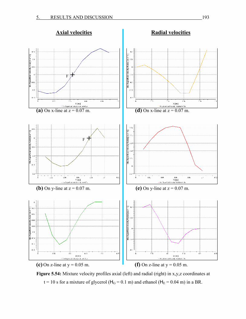
5. RESULTS AND DISCUSSION 193
Axial velocities Radial velocities
(a) On x-line at z = 0.07 m. (d) On x-line at z = 0.07 m.
(b) On y-line at z = 0.07 m. (e) On y-line at z = 0.07 m.
(c) On z-line at y = 0.05 m. (f) On z-line at y = 0.05 m. Figure 5.54: Mixture velocity profiles axial (left) and radial (right) in x,y,z coordinates at
t = 10 s for a mixture of glycerol (HG = 0.1 m) and ethanol (HE = 0.04 m) in a BR.
F +
F +

5. RESULTS AND DISCUSSION 194
5.2.2.1.2 Glycerol (HG = 0.04 m) and ethanol (HE = 0.1 m)
The final viscosity of this liquid mixture is 0.36 Pa s. Secondary flow
field mainly axial can be seen in Fig. 5.55 near the cylindrical wall of the
vessel and the vertical blade of the impeller. A wider and shorter circulation
compared to that obtained in the previous case in Fig. 5.53 is found near the
vertical blade of the anchor impeller.
The axial velocities as a function of x, y, z at t = 10 s are shown in
Fig. 5.56-(left). Similar axial velocity profiles to that for the case before in
Fig. 5.54-(a), (b) and (c) are found. The axial velocities as a function of x in
Fig. 5.56-(a) are lower than that in Fig. 5.54-(a), especially near the shaft
between 0 < x < 0.03 m. The axial velocities as a function of y in Fig. 5.56-
(b) are nearly similar to that in Fig. 5.54-(b), but the axial velocities near the
shaft between 0 < y < 0.06 m have lower values. The axial velocities as a
function of z in Fig. 5.56-(c) are higher than that in Fig. 5.54-(c) because the
liquid mixture here has a lower viscosity by a factor of 3.
The radial velocities as a function of x between 0.03 m < x < 0.07 m in
Fig. 5.56-(d) are lower than that in Fig. 5.54-(d) caused by the existed
circulation between the shaft and the impeller there. The radial velocities as
a function of y in Fig. 5.56-(e) are higher than that in Fig. 5.54-(e), whereas
the radial velocities as a function of z in Fig. 5.56-(f) are lower than that in
Fig. 5.54-(f).
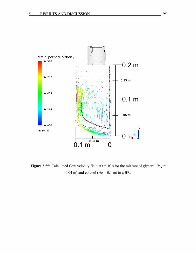
5. RESULTS AND DISCUSSION 195
Figure 5.55: Calculated flow velocity field at t = 10 s for the mixture of glycerol (HG =
0.04 m) and ethanol (HE = 0.1 m) in a BR.
0
0.2 m
00.1 m
0.1 m
0.05 m
0.05 m
0.15 m
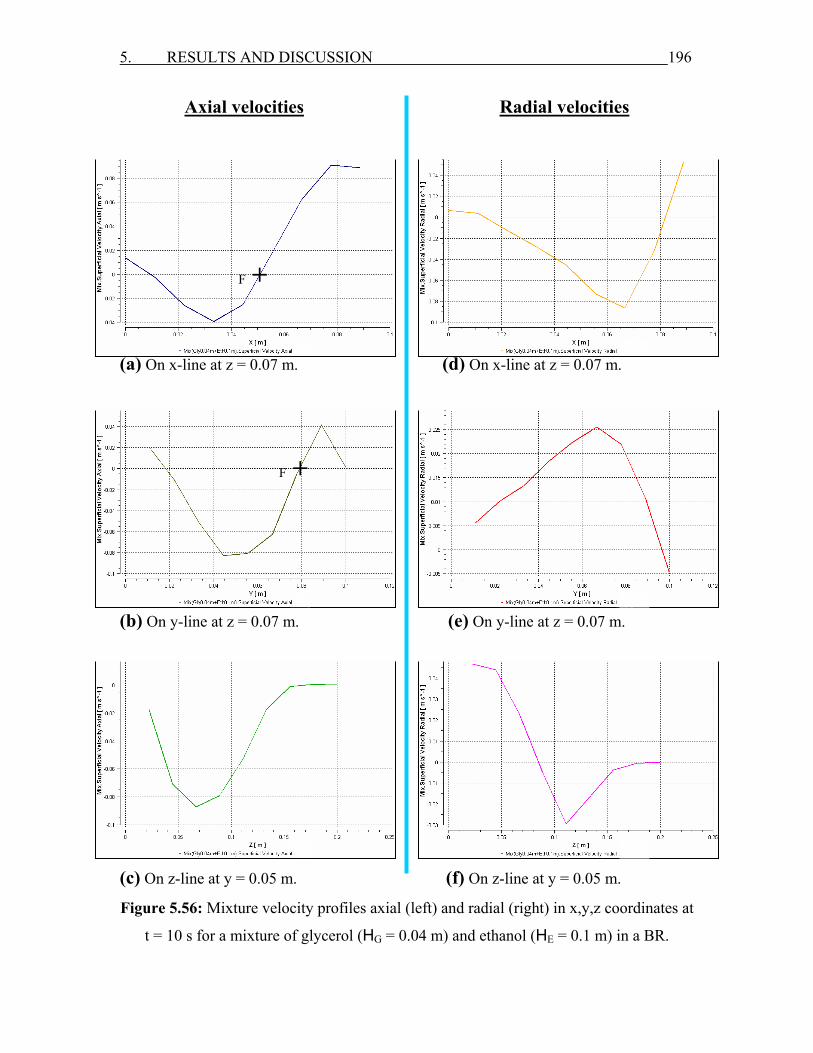
5. RESULTS AND DISCUSSION 196
Axial velocities Radial velocities
(a) On x-line at z = 0.07 m. (d) On x-line at z = 0.07 m.
(b) On y-line at z = 0.07 m. (e) On y-line at z = 0.07 m.
(c) On z-line at y = 0.05 m. (f) On z-line at y = 0.05 m.
Figure 5.56: Mixture velocity profiles axial (left) and radial (right) in x,y,z coordinates at
t = 10 s for a mixture of glycerol (HG = 0.04 m) and ethanol (HE = 0.1 m) in a BR.
F +
F +
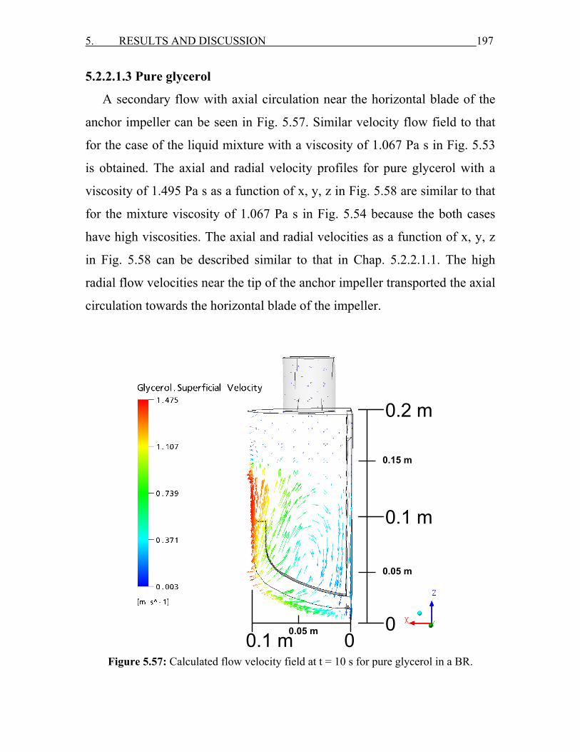
5. RESULTS AND DISCUSSION 197
5.2.2.1.3 Pure glycerol
A secondary flow with axial circulation near the horizontal blade of the
anchor impeller can be seen in Fig. 5.57. Similar velocity flow field to that
for the case of the liquid mixture with a viscosity of 1.067 Pa s in Fig. 5.53
is obtained. The axial and radial velocity profiles for pure glycerol with a
viscosity of 1.495 Pa s as a function of x, y, z in Fig. 5.58 are similar to that
for the mixture viscosity of 1.067 Pa s in Fig. 5.54 because the both cases
have high viscosities. The axial and radial velocities as a function of x, y, z
in Fig. 5.58 can be described similar to that in Chap. 5.2.2.1.1. The high
radial flow velocities near the tip of the anchor impeller transported the axial
circulation towards the horizontal blade of the impeller.
Figure 5.57: Calculated flow velocity field at t = 10 s for pure glycerol in a BR.
0
0.2 m
00.1 m
0.1 m
0.05 m
0.05 m
0.15 m
5. RESULTS AND DISCUSSION 198
Axial velocities Radial velocities
(a) On x-line at z = 0.07 m. (d) On x-line at z = 0.07 m.
(b) On y-line at z = 0.07 m. (e) On y-line at z = 0.07 m.
(c) On z-line at y = 0.05 m. (f) On z-line at y = 0.05 m.
Figure 5.58: Mixture velocity profiles axial (left) and radial (right) in x,y,z coordinates at
t = 10 s for pure glycerol (HG = 0.14 m) in a BR.
F +
F +
5. RESULTS AND DISCUSSION 199
5.2.2.1.4 Pure ethanol
Ethanol has a low viscosity of 0.00012 Pa s. The secondary flow velocity
field is mainly axial as can be seen in Fig. 5.59 at t = 10 s. No axial
circulation between the impeller and the shaft is obtained because ethanol
has a low viscosity and low axial and radial velocities compared to that in
the previous cases which have higher viscosities and velocities (Figs. 5.53,
5.55 and 5.57).
The axial and radial velocity profiles in as a function of x, y, z at t = 10 s
for pure ethanol are shown in Fig. 5.60. These velocity profiles are similar to
the axial and radial velocity profiles for the higher liquid mixture viscosities
in Figs. 5.54, 5.56 and 5.58 with small differences. Because the low
viscosity and density of ethanol causes a turbulent flow between the shaft
and impeller which leading to a higher variation of the axial and radial
velocities in this region compared with that in the cases before. The axial
velocities in x coordinate are high near the cylindrical wall of the vessel
upward and at x = 0.025 m downward as can be seen in Fig. 5.60-(a). The
axial velocities in y coordinate are high at x = 0.025 m upward and at x =
0.065 m downward (Fig. 5.60-(b)). The axial velocity profile in z coordinate
is similar to the cases before e.g. pure glycerol (Fig. 5.58-(c)) but lower
velocities are found near the shaft and the cylindrical wall as can be seen in
Fig. 5.60-(c).
The radial velocity profiles in x and y coordinates are similar to the cases
before e.g. pure glycerol (Fig. 5.58-(d) and (e)) near the shaft and the
cylindrical wall but a large variation of the radial velocities for pure ethanol
are found between 0.02 m ≤ x 0.08 m≤ and 0.02 m ≤ y 0.08 m≤ as can be
seen in Figs. 5.60-(d) and (e). The radial velocity is the highest near the
horizontal blade of the impeller at z = 0.025 m downward and near the

5. RESULTS AND DISCUSSION 200
impeller tip at z = 0.08 m as can be seen in Figs. 5.59 and 5.60-(f). A high
variation of the radial velocities are found between z = 0.08 m and z = 0.15
m due to the high fluctuations at the interface between the pure ethanol and
air.
Figure 5.59: Calculated flow velocity field at t = 10 s for pure ethanol in a BR.
0
0.2 m
00.1 m
0.1 m
00
0.05 m
0.05 m
0.15 m
5. RESULTS AND DISCUSSION 201
Axial velocities Radial velocities
(a) On x-line at z = 0.07 m. (d) On x-line at z = 0.07 m.
(b) On y-line at z = 0.07 m. (e) On y-line at z = 0.07 m.
(c) On z-line at y = 0.05 m. (f) On z-line at y = 0.05 m.
Figure 5.60: Mixture velocity profiles axial (left) and radial (right) in x,y,z coordinates at
t = 10 s for pure ethanol in a BR.
F +
F +
5. RESULTS AND DISCUSSION 202
5.3 CFD simulations predicting the mixture viscosities as a function of
time and the mixing times in SBR and BR
The simulations are carried out in a full 3D-geometry at ϑ = 21 °C and
ω = 150 rpm similar to that used in the experiment. These simulations are
done by using the sliding mesh method, homogeneous laminar buoyant flow
model for air/liquid, standard free surface flow model, algebraic slip mixture
model for ethanol/glycerol and non ideal binary mixture viscosity model.
The following experiments are used for validation of the CFD simulations.
5.3.1 SBR at td = 5 s (26 vol% ethanol)
A good agreement between the calculated and measured dynamic
viscosity m (t)η of the ethanol/glycerol liquid mixture as a function of time
is shown in Fig. 5.61. At t = 0 only glycerol exists in the vessel where the
maximum viscosity is Gη = 1361.88 mPa s. During the dosage time of
ethanol between 0.2 s ≤ td 5.2 s,≤ a sharp decrease of glycerol viscosity to
1142 mPa s occurs. This means an initial fast mixing of a part of the dosed
ethanol is observed because the dosed ethanol flow to the stirrer region near
the cylindrical wall where high shear forces exist leading to a break up into
ethanol droplets with a constant diameter dp = 0.2 mm (s. Fig. 5.62) [55].
The high flow rate of the dosed ethanol gives the bulk liquid additional
kinetic energy to exceed the buoyancy forces. After the dosage the
remaining part of the dosed ethanol rises up to the liquid interface forming a
thin layer of ethanol above the bulk liquid which has higher viscosity and
density. This small layer can re-enter the bulk glycerol by vortices or by
diffusion [55], then a slow deformation and dispersion of ethanol droplets
5. RESULTS AND DISCUSSION 203
[98] occurs leading to a slow decrease of the mixture viscosity to
mη = 669.5 mPa s at t = 150 s.
For t > 150 s a fast mixing again is observed due to the absence of the
buoyancy forces and destroying the rest layer of ethanol at the interface. The
remaining ethanol is rapidly transported into the bulk glycerol leading to a
fast deformation of the interface [55] and dispersion until a homogeneous
liquid mixture with viscosity of mη = 279 mPa s at tm = 208 s is obtained.
0
200
400
600
800
1000
1200
1400
0 20 40 60 80 100 120 140 160 180 200 220 240Time [s]
Dyn
amic
vis
cosi
ty η
m [m
Pa s
]
EXP. SBR td=5s (26 vol% ethanol)
CFD-SBR td=5s (26 vol% ethanol)
Figure 5.61: The dynamic viscosity of an ethanol/glycerol mixture as a function of time
in a SBR at td = 5 s (26 vol% ethanol), experimentally and by using CFD simulation.
The ethanol droplet diameters as a function of time for a SBR can be
seen in Fig. 5.62. It is shown that a large and slow break up of the droplet
diameter dp is found for t 50 s.≤ A small and fast decrease of the droplet
diameter is obtained for 50 s ≤ t 160 s≤ until a complete mixing occurs at
t = 180 s with a final mean droplet diameter dp ≈ 10–7 m (s. Chap. 5.3.5.1).
For dp < 10–7 m, there is no more influence of dp on mη . The droplets of the
t [s]
[mPa
s]
mη
5. RESULTS AND DISCUSSION 204
dosed ethanol may pass through several main zones: The stirrer region; the
free surface, the bottom of the vessel and the bulk. In each zone there is a
chance that the ethanol droplets will be divided into smaller droplets or
mixed into the bulk liquid. In addition, in each zone the droplets have a
chance to move to another zone [55].
0
0.02
0.04
0.06
0.08
0.1
0.12
0.14
0.16
0.18
0.2
0.22
0 20 40 60 80 100 120 140 160 180 200 220 240
t [s]
d p [m
m]
dp [mm] SBR td=5s (26 vol% ethanol)
Figure 5.62: Calculated ethanol droplet diameter as a function of time (s. Chap. 5.3.5.1)
in a SBR at td = 5 s (26 vol% ethanol) by using CFD simulation.
From Figs. 5.61 and 5.62 the dynamic viscosity of ethanol and glycerol
mixture as a function of ethanol droplet diameter can be shown in Fig. 5.63.
It is concluded that when the droplet diameter of ethanol decreases, the
mixture viscosity decreases and so the flow velocity of the liquid mixture
increases. This means when the droplet diameter of ethanol dp decreases
( mη decreases also), then the polynomial equation for a calculated Reynolds
number Rem(dp) (s. Eq. 2-6) increases (Fig. 5.64-a). The Reynolds number
Rem(t) of the liquid mixture as a function of time increases (Fig. 5.64-b)

5. RESULTS AND DISCUSSION 205
because the mixture viscosity m (t)η decreases and the velocity of the liquid
mixture um increases.
0
200
400
600
800
1000
1200
1400
1600
0 0.02 0.04 0.06 0.08 0.1 0.12 0.14 0.16 0.18 0.2 0.22dp [mm]
η m [m
Pa s
]
dp [mm] SBR td=5s (26 vol% ethanol)
Figure 5.63: The dynamic viscosity of an ethanol/glycerol mixture as a function of
ethanol droplet diameter in a SBR at td = 5 s (26 vol% ethanol) by using CFD simulation.
y = 4E+08x6 - 2E+08x5 + 6E+07x4 - 7E+06x3 + 443077x2 - 14839x + 550.13R2 = 0.9987
050
100150200250300350400450500550600
0 0.02 0.04 0.06 0.08 0.1 0.12 0.14 0.16 0.18 0.2Ethanol droplet diameter dp [mm]
Rey
nold
s nu
mbe
r Re
RePoly. (Re)
Figure 5.64-a: Reynolds number Rem as a function (polynomial) of ethanol droplet
diameter dp in a SBR at td = 5 s (26 vol% ethanol) with ω = 150 rpm by using
CFD simulation.
dp [mm]
Re m
Rem = 4x10⁸ 6pd – 2x10⁸ 5
pd + 6x10⁷ 4pd – 7x10⁶ 3
pd + 4.4x10⁵ 2pd – 1.5x10⁴
pd + 550.13
R2 = 0.9987

5. RESULTS AND DISCUSSION 206
Figure 5.64-b: Calculated Reynolds number Rem as a function of time in a SBR at
td = 5 s (26 vol% ethanol) with ω = 150 rpm by using CFD simulation.
To calculate the mixing time tm, ethanol mass fractions at different
positions in the vessel near the impeller, in the middle between the impeller
and the shaft (mixing is caused by the diffusion between ethanol and
glycerol) and near the shaft (mixing is caused essentially by the gravity) are
calculated as a function of time (Fig. 5.65). Initially at t = 0 there is no
ethanol in the vessel. During the dosage of ethanol high ethanol mass
fractions are found at the points P3, P4 and P5 above the anchor impeller
because a layer of ethanol is formed above the bulk mixture due to the
buoyancy forces. After the dosage for t > 0.2 s, ethanol mass fractions at the
points P3, P4, P5, P8 and P9 decrease as a function of time because the
dispersion and distribution of ethanol in glycerol increase. Low ethanol mass
fractions are found at the points P1, P2, P6 and P7 which are below the tip of
0
100
200
300
400
500
600
0 20 40 60 80 100 120 140 160 180 200 220
Time [s]
Rey
nold
s nu
mbe
r Re
Reynolds number
t [s]
R
e m
5. RESULTS AND DISCUSSION 207
the anchor impeller, and then for t > 0.2 s ethanol mass fractions increase
because ethanol is transported into the bulk mixture. The mixing time tm and
a homogeneous mixture are obtained when all the points have the same
constant mass fraction of ethanol at tm = 205 s. It is concluded from Fig. 5.65
that the mixing is faster at the tip of the anchor impeller where the maximum
shear forces and maximum flow velocity appear then at the intermediate
region between the shaft and impeller and last near the shaft where the
lowest velocity occurs. The calculated distribution of ethanol mass fractions
(Fig. 5.65) between all these points can explain the mixing behavior and
flow velocity field of ethanol in glycerol as a function of time.
Figure 5.65: Ethanol mass fraction as a function of time, calculated by using CFD
simulation at nine different positions in the SBR at td = 5 s (26 vol% ethanol).
The calculated dynamic mixing behaviors of ethanol with glycerol are
visualized as it is shown in Fig. 5.66. Initially at t = 0 only pure glycerol
exists in the vessel while the anchor stirrer do not rotate. During the dosage
of ethanol between 0.2 s ≤ td 5.2 s≤ a part of the dosed ethanol is transported
00.10.20.30.40.50.60.70.80.9
1
0 20 40 60 80 100 120 140 160 180 200 220
Time [s]
Etha
nol M
ass
Frac
tion P1 P2 P3
P4 P5 P6P7 P8 P9
t [s]
5. RESULTS AND DISCUSSION 208
to the stirrer region and transported into the bulk mixture from the
cylindrical wall of the vessel towards to the shaft as can be seen in Fig. 5.66
at t = 2 s. Then the ethanol input distributes over the bulk liquid as shown at
t = 5 s (fast mixing during the dosage time period). After the dosage, the
buoyant effect appears because the shear forces of the stirrer can not exceed
the buoyant forces which are caused by the density difference between
ethanol and glycerol. Then the remaining part of the dosed ethanol rises up
to the interface of the bulk mixture, and re-disperse from the tip of the
anchor impeller towards to the shaft and then towards to the cylindrical wall
of the vessel leading to a circulation behind the anchor as can be shown at
t = 100 s in agreement with the experiment.
The droplets of ethanol break up until all the dosed ethanol is completely
mixed with glycerol to get a homogeneous mixture with constant values of
viscosity, ethanol mass fraction and ethanol droplet diameter. The calculated
mixing time is tm = 205 s. The calculation and the visualisation of the mixing
behavior in a SBR at td = 5 s (26 vol% ethanol) are in a good agreement.
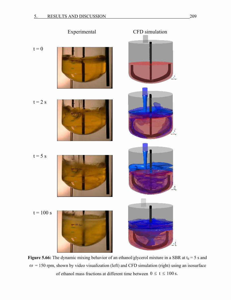
5. RESULTS AND DISCUSSION 209
Experimental CFD simulation
Figure 5.66: The dynamic mixing behavior of an ethanol/glycerol mixture in a SBR at td = 5 s and
ω = 150 rpm, shown by video visualization (left) and CFD simulation (right) using an isosurface
of ethanol mass fractions at different time between 0 t 100 s.≤ ≤
t = 0 t = 2 s t = 5 s t = 100 s
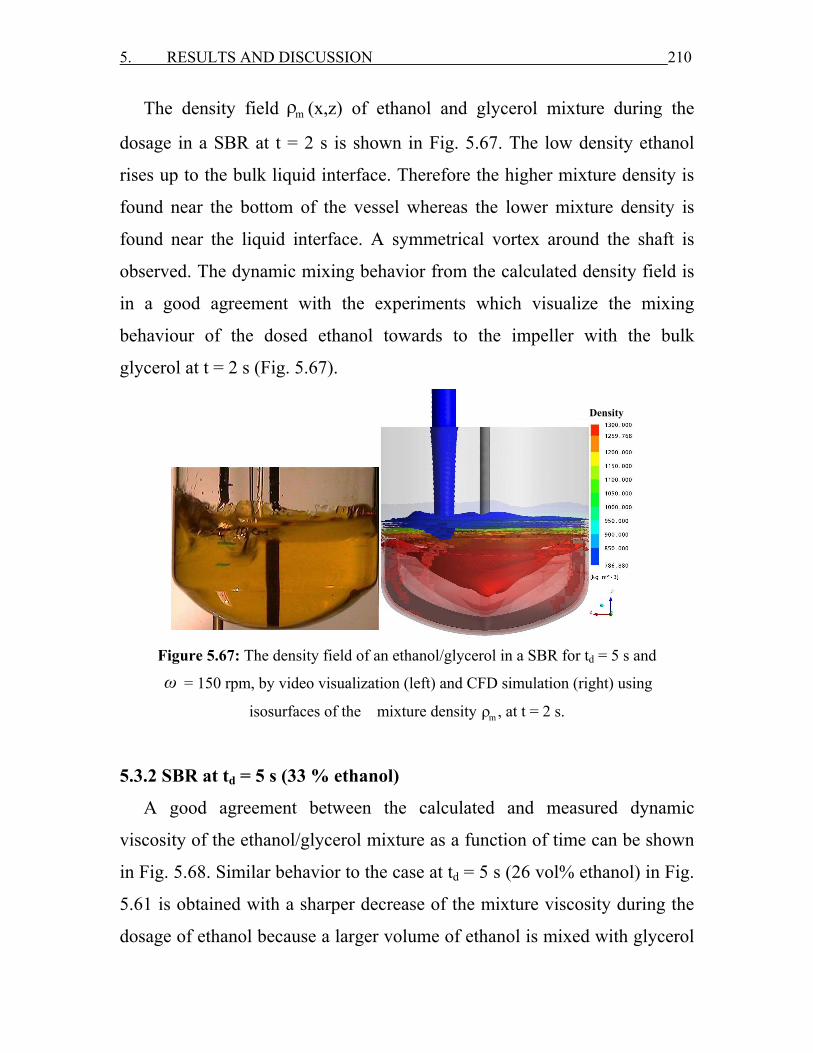
5. RESULTS AND DISCUSSION 210
The density field mρ (x,z) of ethanol and glycerol mixture during the
dosage in a SBR at t = 2 s is shown in Fig. 5.67. The low density ethanol
rises up to the bulk liquid interface. Therefore the higher mixture density is
found near the bottom of the vessel whereas the lower mixture density is
found near the liquid interface. A symmetrical vortex around the shaft is
observed. The dynamic mixing behavior from the calculated density field is
in a good agreement with the experiments which visualize the mixing
behaviour of the dosed ethanol towards to the impeller with the bulk
glycerol at t = 2 s (Fig. 5.67).
Figure 5.67: The density field of an ethanol/glycerol in a SBR for td = 5 s and
ω = 150 rpm, by video visualization (left) and CFD simulation (right) using
isosurfaces of the mixture density mρ , at t = 2 s.
5.3.2 SBR at td = 5 s (33 % ethanol)
A good agreement between the calculated and measured dynamic
viscosity of the ethanol/glycerol mixture as a function of time can be shown
in Fig. 5.68. Similar behavior to the case at td = 5 s (26 vol% ethanol) in Fig.
5.61 is obtained with a sharper decrease of the mixture viscosity during the
dosage of ethanol because a larger volume of ethanol is mixed with glycerol
Density
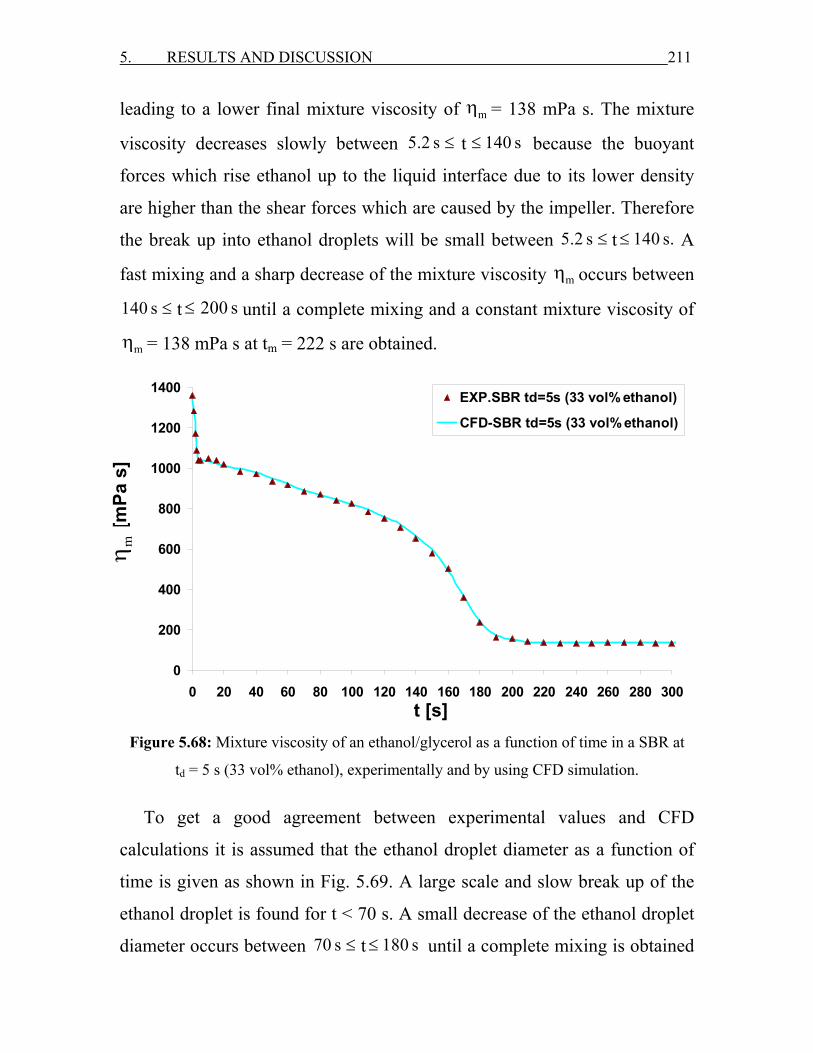
5. RESULTS AND DISCUSSION 211
leading to a lower final mixture viscosity of mη = 138 mPa s. The mixture
viscosity decreases slowly between 5.2 s ≤ t 140 s≤ because the buoyant
forces which rise ethanol up to the liquid interface due to its lower density
are higher than the shear forces which are caused by the impeller. Therefore
the break up into ethanol droplets will be small between 5.2 s ≤ t 140 s.≤ A
fast mixing and a sharp decrease of the mixture viscosity mη occurs between
140 s ≤ t 200 s≤ until a complete mixing and a constant mixture viscosity of
mη = 138 mPa s at tm = 222 s are obtained.
0
200
400
600
800
1000
1200
1400
0 20 40 60 80 100 120 140 160 180 200 220 240 260 280 300Time [s]
Dyn
amic
vis
cosi
ty η
m [m
Pa s
]
EXP.SBR td=5s (33 vol% ethanol)
CFD-SBR td=5s (33 vol% ethanol)
Figure 5.68: Mixture viscosity of an ethanol/glycerol as a function of time in a SBR at
td = 5 s (33 vol% ethanol), experimentally and by using CFD simulation.
To get a good agreement between experimental values and CFD
calculations it is assumed that the ethanol droplet diameter as a function of
time is given as shown in Fig. 5.69. A large scale and slow break up of the
ethanol droplet is found for t < 70 s. A small decrease of the ethanol droplet
diameter occurs between 70 s ≤ t 180 s≤ until a complete mixing is obtained
[mPa
s]
mη
t [s]
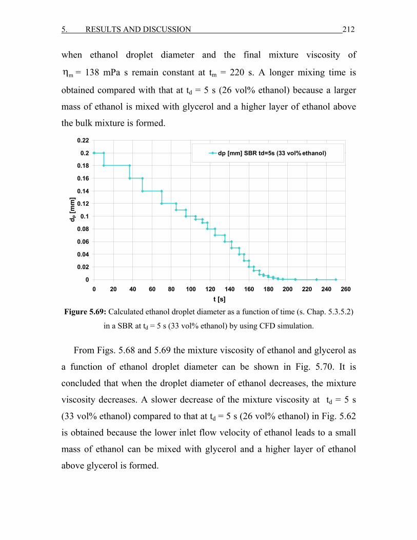
5. RESULTS AND DISCUSSION 212
when ethanol droplet diameter and the final mixture viscosity of
mη = 138 mPa s remain constant at tm = 220 s. A longer mixing time is
obtained compared with that at td = 5 s (26 vol% ethanol) because a larger
mass of ethanol is mixed with glycerol and a higher layer of ethanol above
the bulk mixture is formed.
0
0.02
0.04
0.06
0.08
0.1
0.12
0.14
0.16
0.18
0.2
0.22
0 20 40 60 80 100 120 140 160 180 200 220 240 260t [s]
d p [m
m]
dp [mm] SBR td=5s (33 vol% ethanol)
Figure 5.69: Calculated ethanol droplet diameter as a function of time (s. Chap. 5.3.5.2)
in a SBR at td = 5 s (33 vol% ethanol) by using CFD simulation.
From Figs. 5.68 and 5.69 the mixture viscosity of ethanol and glycerol as
a function of ethanol droplet diameter can be shown in Fig. 5.70. It is
concluded that when the droplet diameter of ethanol decreases, the mixture
viscosity decreases. A slower decrease of the mixture viscosity at td = 5 s
(33 vol% ethanol) compared to that at td = 5 s (26 vol% ethanol) in Fig. 5.62
is obtained because the lower inlet flow velocity of ethanol leads to a small
mass of ethanol can be mixed with glycerol and a higher layer of ethanol
above glycerol is formed.
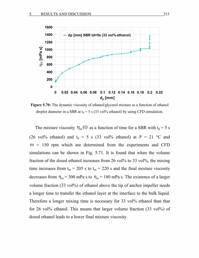
5. RESULTS AND DISCUSSION 213
0
200
400
600
800
1000
1200
1400
1600
0 0.02 0.04 0.06 0.08 0.1 0.12 0.14 0.16 0.18 0.2 0.22dp [mm]
η m [m
Pa s
]dp [mm] SBR td=5s (33 vol% ethanol)
Figure 5.70: The dynamic viscosity of ethanol/glycerol mixture as a function of ethanol
droplet diameter in a SBR at td = 5 s (33 vol% ethanol) by using CFD simulation.
The mixture viscosity m (t)η as a function of time for a SBR with td = 5 s
(26 vol% ethanol) and td = 5 s (33 vol% ethanol) at ϑ = 21 °C and
ω = 150 rpm which are determined from the experiments and CFD
simulations can be shown in Fig. 5.71. It is found that when the volume
fraction of the dosed ethanol increases from 26 vol% to 33 vol%, the mixing
time increases from tm = 205 s to tm = 220 s and the final mixture viscosity
decreases from mη = 300 mPa s to mη = 180 mPa s. The existence of a larger
volume fraction (33 vol%) of ethanol above the tip of anchor impeller needs
a longer time to transfer the ethanol layer at the interface to the bulk liquid.
Therefore a longer mixing time is necessary for 33 vol% ethanol than that
for 26 vol% ethanol. This means that larger volume fraction (33 vol%) of
dosed ethanol leads to a lower final mixture viscosity.

5. RESULTS AND DISCUSSION 214
0
200
400
600
800
1000
1200
1400
0 20 40 60 80 100 120 140 160 180 200 220 240 260 280 300Time [s]
Dyn
amic
vis
cosi
ty η
m [m
Pa s
]EXP. SBR td=5s (26 vol% ethanol) EXP.SBR td=5s (33 vol% ethanol) CFD-SBR td=5s (26 vol% ethanol) CFD-SBR td=5s (33 vol% ethanol)
Figure 5.71: The mixture viscosity as a function of time for ethanol/glycerol in a SBR
for td = 5 s (26 vol% ethanol) and td = 5 s (33 vol% ethanol) at ϑ = 21 °C and
ω = 150 rpm, determined experimentally and by using CFD simulation.
5.3.3 SBR at td = 10 s (33 % ethanol)
A good agreement between the calculated and measured dynamic
viscosity of the ethanol/glycerol mixture as a function of time at td = 10 s can
be seen in Fig. 5.72. A fast decrease of the mixture viscosity similar to the
case at td = 5 s (33 vol% ethanol) during the dosage of ethanol between
0.2 s ≤ td 10.2 s≤ is obtained. A slower decrease of the mixture viscosity
compared to that in the cases at td = 5 s is obtained during the dosage of
ethanol between 10.2 s ≤ t 210 s.≤ Because the velocity of the dosed ethanol
here is lower than that at td = 5 s (33 vol% ethanol), then a slower and a
smaller break up into ethanol droplets occurs. A small mass of ethanol
reaches to the bottom of the vessel and the larger mass of ethanol rise to the
t [s]
[mPa
s]
mη
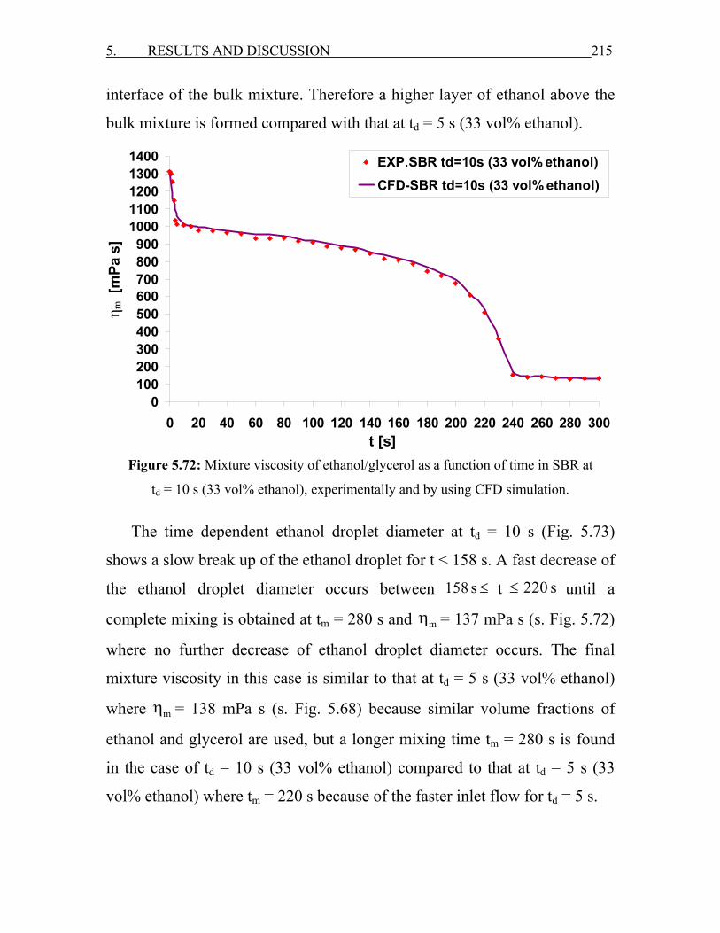
5. RESULTS AND DISCUSSION 215
interface of the bulk mixture. Therefore a higher layer of ethanol above the
bulk mixture is formed compared with that at td = 5 s (33 vol% ethanol).
0100200300400500600700800900
10001100120013001400
0 20 40 60 80 100 120 140 160 180 200 220 240 260 280 300t [s]
η m [
mPa
s]
EXP.SBR td=10s (33 vol% ethanol)CFD-SBR td=10s (33 vol% ethanol)
Figure 5.72: Mixture viscosity of ethanol/glycerol as a function of time in SBR at
td = 10 s (33 vol% ethanol), experimentally and by using CFD simulation.
The time dependent ethanol droplet diameter at td = 10 s (Fig. 5.73)
shows a slow break up of the ethanol droplet for t < 158 s. A fast decrease of
the ethanol droplet diameter occurs between 158 s ≤ t 220 s≤ until a
complete mixing is obtained at tm = 280 s and mη = 137 mPa s (s. Fig. 5.72)
where no further decrease of ethanol droplet diameter occurs. The final
mixture viscosity in this case is similar to that at td = 5 s (33 vol% ethanol)
where mη = 138 mPa s (s. Fig. 5.68) because similar volume fractions of
ethanol and glycerol are used, but a longer mixing time tm = 280 s is found
in the case of td = 10 s (33 vol% ethanol) compared to that at td = 5 s (33
vol% ethanol) where tm = 220 s because of the faster inlet flow for td = 5 s.
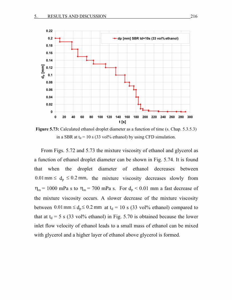
5. RESULTS AND DISCUSSION 216
0
0.02
0.04
0.06
0.08
0.1
0.12
0.14
0.16
0.18
0.2
0.22
0 20 40 60 80 100 120 140 160 180 200 220 240 260 280 300t [s]
d p [m
m]
dp [mm] SBR td=10s (33 vol% ethanol)
Figure 5.73: Calculated ethanol droplet diameter as a function of time (s. Chap. 5.3.5.3)
in a SBR at td = 10 s (33 vol% ethanol) by using CFD simulation.
From Figs. 5.72 and 5.73 the mixture viscosity of ethanol and glycerol as
a function of ethanol droplet diameter can be shown in Fig. 5.74. It is found
that when the droplet diameter of ethanol decreases between
0.01 mm ≤ dp 0.2 mm,≤ the mixture viscosity decreases slowly from
mη = 1000 mPa s to mη = 700 mPa s. For dp < 0.01 mm a fast decrease of
the mixture viscosity occurs. A slower decrease of the mixture viscosity
between 0.01 mm ≤ dp 0.2 mm≤ at td = 10 s (33 vol% ethanol) compared to
that at td = 5 s (33 vol% ethanol) in Fig. 5.70 is obtained because the lower
inlet flow velocity of ethanol leads to a small mass of ethanol can be mixed
with glycerol and a higher layer of ethanol above glycerol is formed.
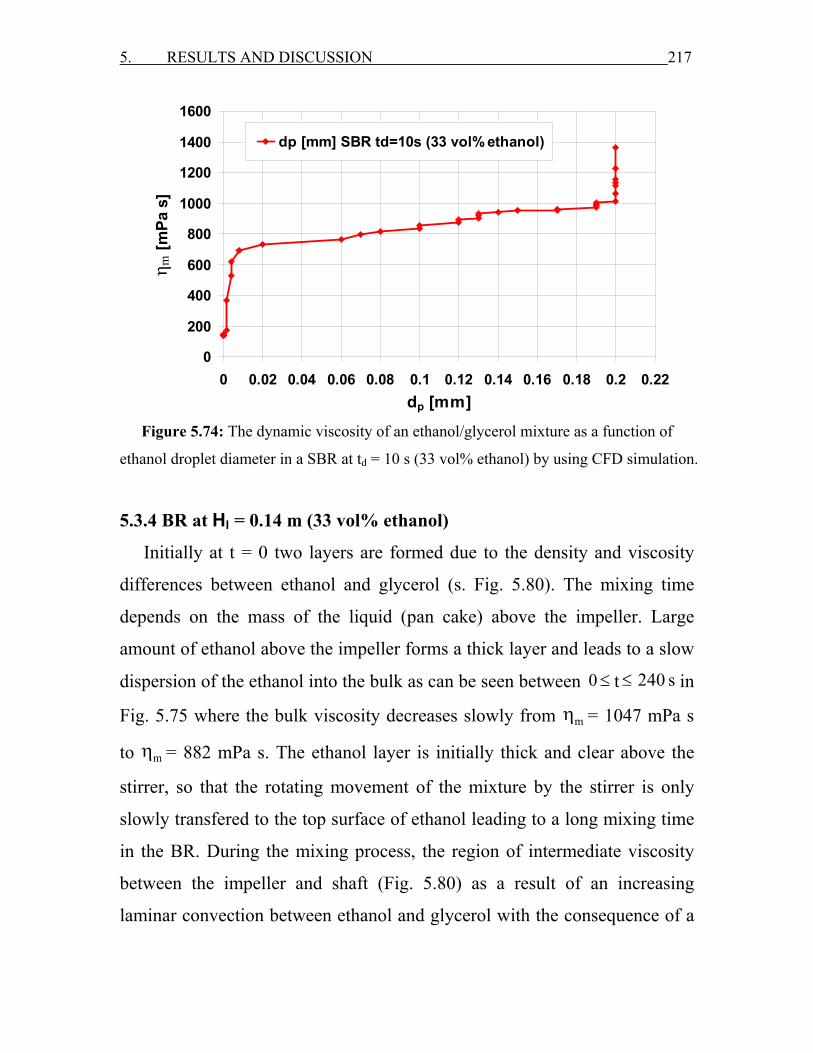
5. RESULTS AND DISCUSSION 217
0
200
400
600
800
1000
1200
1400
1600
0 0.02 0.04 0.06 0.08 0.1 0.12 0.14 0.16 0.18 0.2 0.22dp [mm]
η m [m
Pa s
]dp [mm] SBR td=10s (33 vol% ethanol)
Figure 5.74: The dynamic viscosity of an ethanol/glycerol mixture as a function of
ethanol droplet diameter in a SBR at td = 10 s (33 vol% ethanol) by using CFD simulation.
5.3.4 BR at Hl = 0.14 m (33 vol% ethanol)
Initially at t = 0 two layers are formed due to the density and viscosity
differences between ethanol and glycerol (s. Fig. 5.80). The mixing time
depends on the mass of the liquid (pan cake) above the impeller. Large
amount of ethanol above the impeller forms a thick layer and leads to a slow
dispersion of the ethanol into the bulk as can be seen between 0 ≤ t 240 s≤ in
Fig. 5.75 where the bulk viscosity decreases slowly from mη = 1047 mPa s
to mη = 882 mPa s. The ethanol layer is initially thick and clear above the
stirrer, so that the rotating movement of the mixture by the stirrer is only
slowly transfered to the top surface of ethanol leading to a long mixing time
in the BR. During the mixing process, the region of intermediate viscosity
between the impeller and shaft (Fig. 5.80) as a result of an increasing
laminar convection between ethanol and glycerol with the consequence of a
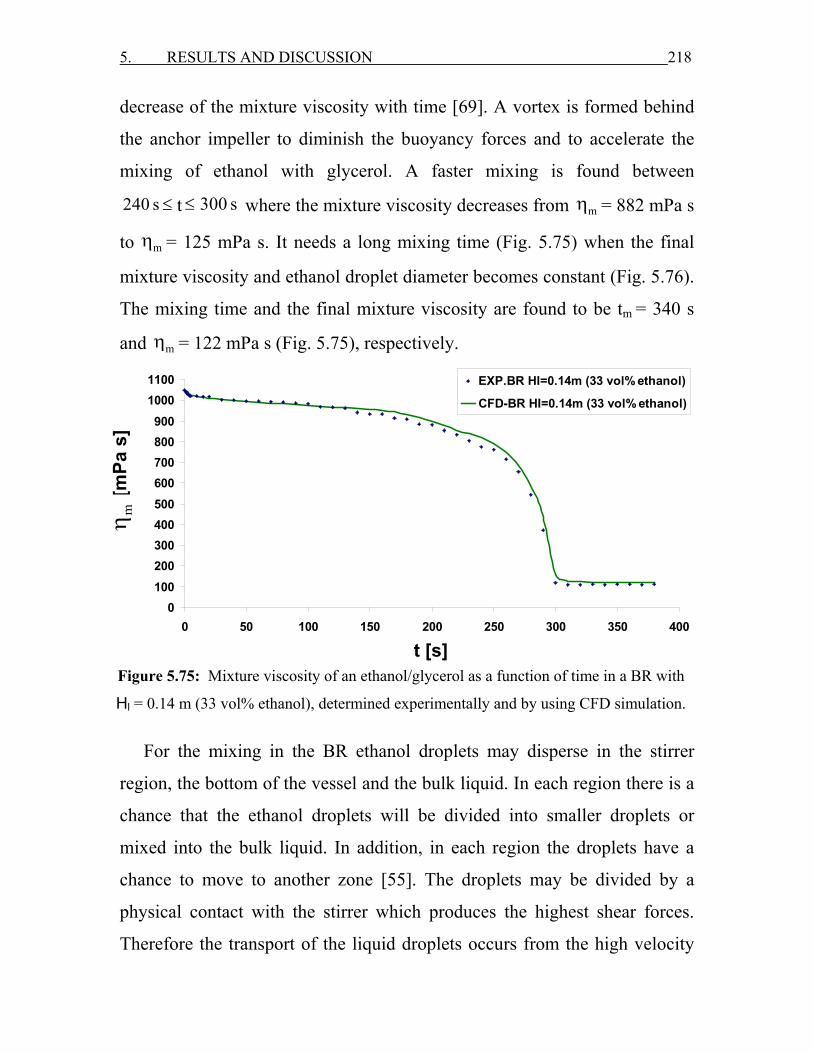
5. RESULTS AND DISCUSSION 218
decrease of the mixture viscosity with time [69]. A vortex is formed behind
the anchor impeller to diminish the buoyancy forces and to accelerate the
mixing of ethanol with glycerol. A faster mixing is found between
240 s ≤ t 300 s≤ where the mixture viscosity decreases from mη = 882 mPa s
to mη = 125 mPa s. It needs a long mixing time (Fig. 5.75) when the final
mixture viscosity and ethanol droplet diameter becomes constant (Fig. 5.76).
The mixing time and the final mixture viscosity are found to be tm = 340 s
and mη = 122 mPa s (Fig. 5.75), respectively.
0100200300400500600700800900
10001100
0 50 100 150 200 250 300 350 400Time [s]
Dyn
amic
Vis
cosi
ty η
m [
mPa
s]
EXP.BR HI=0.14m (33 vol% ethanol)
CFD-BR HI=0.14m (33 vol% ethanol)
Figure 5.75: Mixture viscosity of an ethanol/glycerol as a function of time in a BR with
Hl = 0.14 m (33 vol% ethanol), determined experimentally and by using CFD simulation.
For the mixing in the BR ethanol droplets may disperse in the stirrer
region, the bottom of the vessel and the bulk liquid. In each region there is a
chance that the ethanol droplets will be divided into smaller droplets or
mixed into the bulk liquid. In addition, in each region the droplets have a
chance to move to another zone [55]. The droplets may be divided by a
physical contact with the stirrer which produces the highest shear forces.
Therefore the transport of the liquid droplets occurs from the high velocity
[mPa
s]
mη
t [s]

5. RESULTS AND DISCUSSION 219
region (stirrer) to the lower velocity region (shaft). The shear stresses are
lower in the bulk liquid, but the droplets may be deformed further or be
mixed completely. Fig. 5.76 shows that ethanol droplet diameter as a
function of time in the BR also behaves as a time step function which predict
the pan cake effect. For 0 ≤ t 138 s≤ the diameter of ethanol droplets
remains constant (dp = 0.2 mm) and there is no break up of the droplets.
Therefore the mixing is caused by the gravitational forces and the shear
forces of the stirrer (below the ethanol layer) which transport ethanol into
the bulk glycerol (as explained above) from the tip of the impeller towards to
the shaft. This leads to a circulation between the impeller and the shaft
which enhance the mixing process. A small break up of the ethanol droplets
is found from dp = 0.2 mm at t = 138 s to dp = 0.16 mm at t = 160 s. A large
break up of the ethanol droplets is found between 160 s ≤ t 190 s.≤ Again a
small break up of the ethanol droplet is found between 190 s ≤ t 230 s≤ until
a complete mixing is obtained at tm = 340 s where no further decrease of the
droplet diameter occurs.
Figure 5.76: Calculated ethanol droplet diameter as a function of time (s. Chap. 5.3.5.4)
in a BR with Hl = 0.14 m (33 vol% ethanol) by using CFD simulation.
0
0.02
0.04
0.06
0.08
0.1
0.12
0.14
0.16
0.18
0.2
0.22
0 20 40 60 80 100 120 140 160 180 200 220 240 260 280 300 320 340 360 380t [s]
d p [m
m]
dp [mm] BR Hl=0.14m (33 vol% ethanol)
Figure 5.76: Calculated ethanol droplet diameters as a function of time (s. Chap. 5.3.5.4)
in a BR with Hl = 0.14 m (33 vol% ethanol) by using CFD simulation.
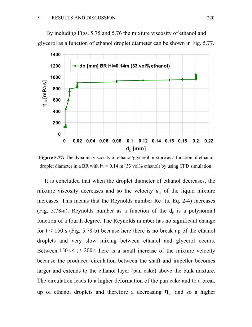
5. RESULTS AND DISCUSSION 220
By including Figs. 5.75 and 5.76 the mixture viscosity of ethanol and
glycerol as a function of ethanol droplet diameter can be shown in Fig. 5.77.
0
200
400
600
800
1000
1200
1400
0 0.02 0.04 0.06 0.08 0.1 0.12 0.14 0.16 0.18 0.2 0.22dp [mm]
η m [m
Pa s
]
dp [mm] BR Hl=0.14m (33 vol% ethanol)
Figure 5.77: The dynamic viscosity of ethanol/glycerol mixture as a function of ethanol
droplet diameter in a BR with Hl = 0.14 m (33 vol% ethanol) by using CFD simulation.
It is concluded that when the droplet diameter of ethanol decreases, the
mixture viscosity decreases and so the velocity um of the liquid mixture
increases. This means that the Reynolds number Rem (s. Eq. 2-4) increases
(Fig. 5.78-a). Reynolds number as a function of the dp is a polynomial
function of a fourth degree. The Reynolds number has no significant change
for t < 150 s (Fig. 5.78-b) because here there is no break up of the ethanol
droplets and very slow mixing between ethanol and glycerol occurs.
Between 150 s ≤ t 200 s≤ there is a small increase of the mixture velocity
because the produced circulation between the shaft and impeller becomes
larger and extends to the ethanol layer (pan cake) above the bulk mixture.
The circulation leads to a higher deformation of the pan cake and to a break
up of ethanol droplets and therefore a decreasing mη and so a higher
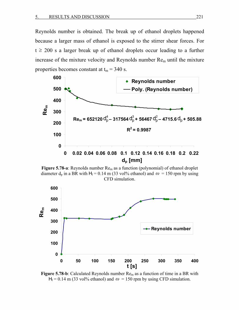
5. RESULTS AND DISCUSSION 221
Reynolds number is obtained. The break up of ethanol droplets happened
because a larger mass of ethanol is exposed to the stirrer shear forces. For
t ≥ 200 s a larger break up of ethanol droplets occur leading to a further
increase of the mixture velocity and Reynolds number Rem until the mixture
properties becomes constant at tm = 340 s.
Figure 5.78-a: Reynolds number Rem as a function (polynomial) of ethanol droplet diameter dp in a BR with Hl = 0.14 m (33 vol% ethanol) and ω = 150 rpm by using
CFD simulation.
Figure 5.78-b: Calculated Reynolds number Rem as a function of time in a BR with
Hl = 0.14 m (33 vol% ethanol) and ω = 150 rpm by using CFD simulation.
0
100
200
300
400
500
600
0 50 100 150 200 250 300 350 400Time [s]
Rey
nold
s nu
mbe
r Re
Reynolds number
y = 652120x4 - 317564x3 + 56467x2 - 4715.6x + 505.88R2 = 0.9914
0
100
200
300
400
500
600
0 0.02 0.04 0.06 0.08 0.1 0.12 0.14 0.16 0.18 0.2 0.22
Ethanol droplet diameter dp [mm]
Rey
nold
s nu
mbe
r Re Reynolds number
Poly. (Reynolds number)
R
e m
R
e m
t [s]
dp [mm]
Rem = 652120 4pd – 317564 3
pd + 56467 2pd – 4715.6 pd + 505.88
R2 = 0.9987

5. RESULTS AND DISCUSSION 222
The calculated ethanol mass fraction profile as a function of time at nine
different positions in the BR near the shaft, in the middle between the shaft
and the impeller and near the cylindrical wall can be shown in Fig. 5.79.
Initially at t = 0 high ethanol mass fractions exist at the points above
glycerol height of HG = 0.1 m (P3, P4 and P5). When the anchor starts to
rotate, ethanol mass fractions decrease slowly for 0 < t < 150 s and decrease
faster for t > 150 s until a complete mixing is obtained at relatively large
tm = 340 s. Ethanol mass fraction is zero at the points below glycerol level of
HG = 0.1 m (P1, P2 and P6) at t = 0 and increases slowly for 0 < t < 200 s and
increase faster for t > 200 s until the complete mixing is obtained at
tm = 340 s.
The points near the vertical blade of the impeller (P1 and P7) have the
lowest mass fractions of ethanol because the mixing near the cylindrical wall
of the vessel and in the impeller region is fast. Also the pushed ethanol by
the impeller to these positions (P1 and P7) is completely mixed with glycerol
due to the existence of the impeller high shear forces.
The points near the shaft P2 and P9 which are at the same height as that
for P1 and P7, respectively have higher ethanol mass fractions because the
mixing near the shaft is weak and the pushed ethanol by the impeller is
slowly mixed with glycerol. It is concluded that the points which exist near
the cylindrical wall and also near the impeller (P1, P3 and P7) reach the
mixing time faster than the points in the middle (P5, P6 and P8) and last are
the points near the shaft (P2, P4 and P9).
The calculated distribution of ethanol mass fractions in all the nine points
can explain the mixing behavior and flow velocity of ethanol in glycerol as a
function of time from the tip of the impeller towards the shaft and then
towards the cylindrical wall (Fig. 5.79).

5. RESULTS AND DISCUSSION 223
00.10.20.30.40.50.60.70.80.9
1
0 50 100 150 200 250 300 350Time [s]
Etha
nol M
ass
Frac
tion
P1 P2 P3P4 P5 P6P7 P8 P9
Figure 5.79: Calculated ethanol mass fraction as a function of time by CFD simulation at
different positions in the BR with Hl = 0.14 m (33 vol% ethanol) and ω = 150 rpm.
The calculated dynamic mixing behavior of ethanol with glycerol by
using the isosurface of ethanol mass fraction as a function of time shown in
Fig. 5.80 (right) and the video visualization, shown in Fig. 5.80 (left).
Initially at t = 0 two distinct layers appear, i.e. a pan cake is formed. When
the impeller starts the rotation for t > 0, ethanol is pushed into glycerol and
mixed from the cylindrical wall near the tip of the impeller to the shaft and
then towards to the cylindrical wall leading to a symmetrical vortex around
the shaft at the interface between ethanol and the bulk mixture for t = 50 s.
This vortex (trombe) becomes larger at t = 100 s, so that the length and
deformation of ethanol filaments increase leading to a fast convection of
ethanol in the glycerol for t = 200 s. The visualized mixing behaviour and its
CFD simulation in a BR with Hl = 0.14 m (33 vol% ethanol) are in a good
agreement.
t [s]
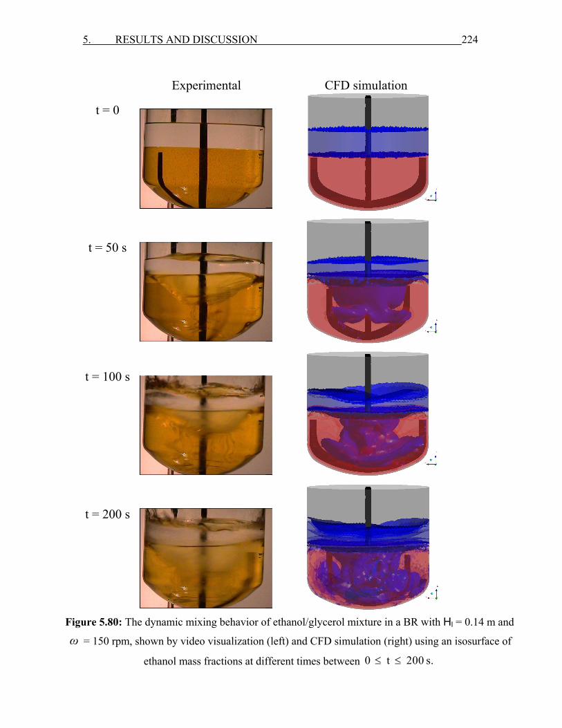
5. RESULTS AND DISCUSSION 224
Experimental CFD simulation
Figure 5.80: The dynamic mixing behavior of ethanol/glycerol mixture in a BR with Hl = 0.14 m and
ω = 150 rpm, shown by video visualization (left) and CFD simulation (right) using an isosurface of
ethanol mass fractions at different times between 0 t 200 s.≤ ≤
t = 0
t = 50 s
t = 100 s
t = 200 s

5. RESULTS AND DISCUSSION 225
The density field mρ (x,z) of ethanol and glycerol mixture in a BR at
t = 50 s is shown in Fig. 5.81 where a large mass of low density ethanol still
exists above the bulk glycerol and uptil now a small mass of ethanol is
mixed with glycerol. Therefore small mixture densities are found above the
tip of impeller and large mixture densities are found below the tip of
impeller. The calculated mixture density field (right) is very similar to the
visualized dynamic mixing (left).
Figure 5.81: The density field of ethanol/glycerol mixture in a BR (Hl = 0.14 m) and
ω = 150 rpm, by video visualization (left) and CFD simulation (right) using
isosurfaces of the mixture density mρ , at t = 50 s.
The calculated flow velocity- and mixture viscosity fields of
ethanol/glycerol as a function of time between 0 ≤ t 4.95 s≤ in a 3D BR by
using sliding mesh method (s. Chap. 4.1.3.4.7) are shown in Figs. 5.82-a and
5.82-b. These fields can explain the dynamic mixing behaviour shown in Fig.
5.80. It can be seen that the circulation flow behind the impeller rotation
(clock wise) exists at t = 0.45 s, 0.9 s and 2.25 s (Fig. 5.82-a) and at t = 2.7 s,
Density
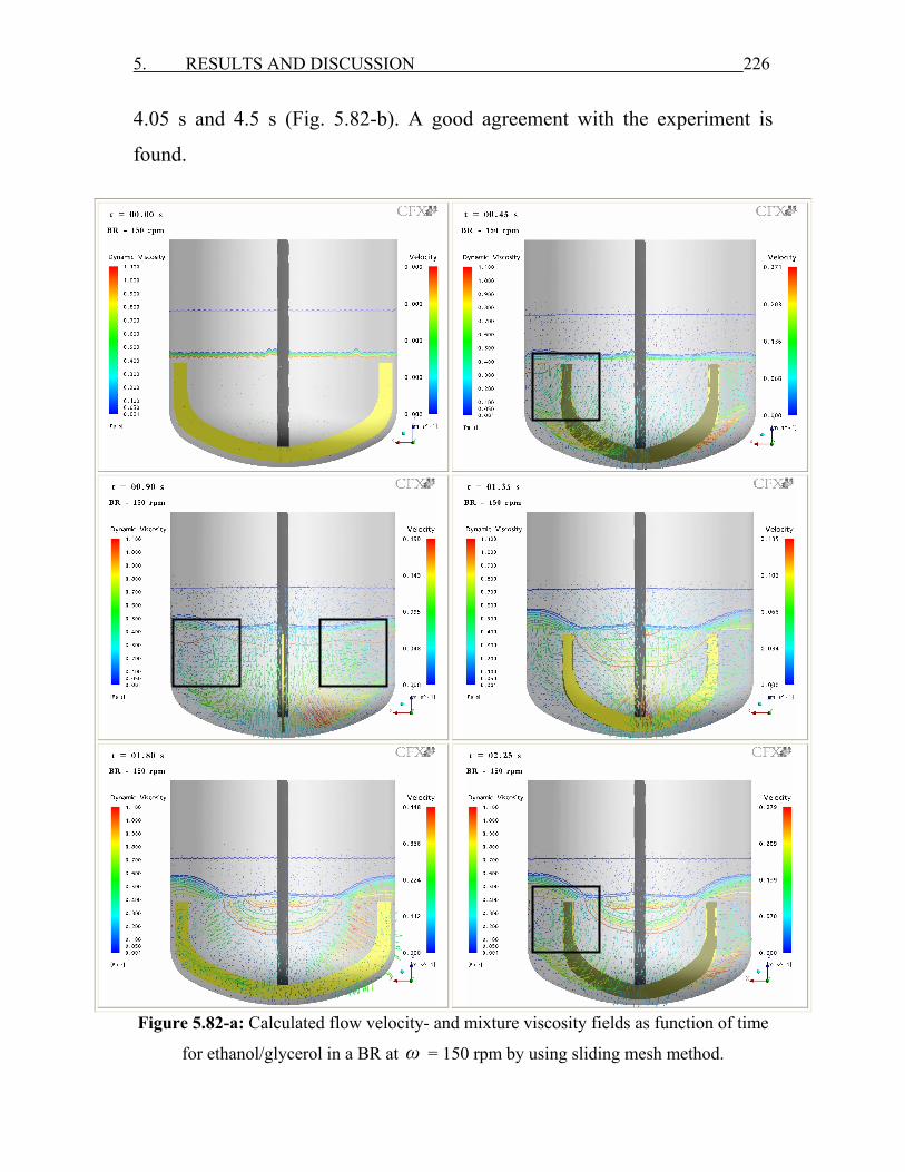
5. RESULTS AND DISCUSSION 226
4.05 s and 4.5 s (Fig. 5.82-b). A good agreement with the experiment is
found.
Figure 5.82-a: Calculated flow velocity- and mixture viscosity fields as function of time
for ethanol/glycerol in a BR at ω = 150 rpm by using sliding mesh method.
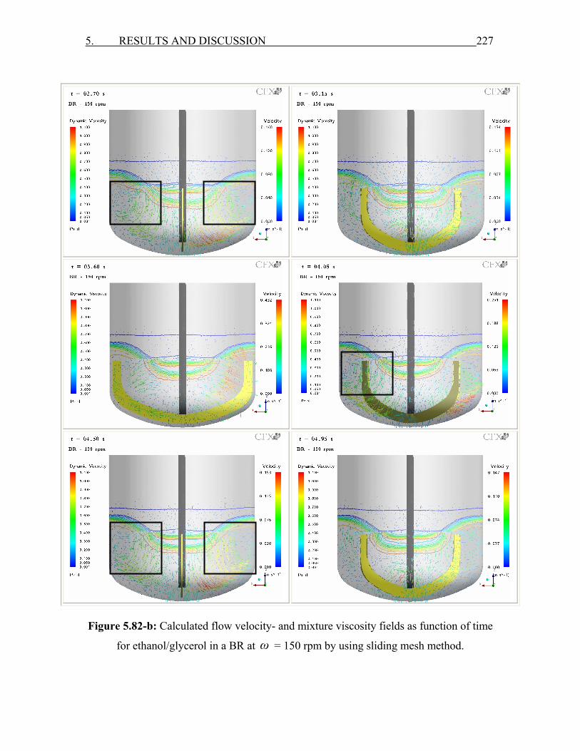
5. RESULTS AND DISCUSSION 227
Figure 5.82-b: Calculated flow velocity- and mixture viscosity fields as function of time
for ethanol/glycerol in a BR at ω = 150 rpm by using sliding mesh method.
5. RESULTS AND DISCUSSION 228
The radial viscosity profile mη (y) for ethanol and glycerol mixture in the
BR at t = 100 s is shown in Fig. 5.83. The maximum mixture viscosities are
found near the cylindrical wall at y = ± 0.078 m and decrease towards the
shaft. The mixture viscosity at y = − 0.078 m is lower than that at
y = 0.078 m because at this time the anchor is near y = − 0.078 m and
transport a larger mass of ethanol to this position leading there to a local
decrease of the mixture viscosity. Whereas a small mass of ethanol at the
same time t = 100 s reaches to the position at y = 0.078 m leading to a local
higher mixture viscosity because a weak effect by the impeller is present
here. As a consequence ethanol is transported by the impeller towards to the
shaft leading to a low mixture viscosity around the shaft. The viscosity at
y = − 0.025 m is higher than that at y = − 0.05 m because a very weak
mixing can be found in the centre of the formed circulation between the
shaft and the impeller at y = − 0.05 m.
Figure 5.83: Radial viscosity profile for ethanol/glycerol mixture in y-direction
for a BR, at t = 100 s.
0.86
0.87
0.88
0.89
0.9
0.91
0.92
0.93
0.94
-0.1 -0.08 -0.06 -0.04 -0.02 0 0.02 0.04 0.06 0.08 0.1r[m]
Dyn
amic
Vis
cosi
ty [P
a s]
y [m]
[mPa
s]
mη

5. RESULTS AND DISCUSSION 229
The calculated and simulated mixture viscosity mη of glycerol and
ethanol as a function of time t for a SBR at td = 5 s and td = 10 s and for a BR
with a total liquid height Hl = 0.14 m at ϑ = 21 °C and ω = 150 rpm are
shown in Fig. 5.84. It is found that the mixing times tm from the experiments
and CFD simulations for the SBR at td = 5 s and td = 10 s are lower than that
in the BR at Hl = 0.14 m because the dosage of ethanol gives additional
kinetic energy to the bulk liquid leading to a faster break up of ethanol
droplets and a larger contact area between ethanol and glycerol, then a faster
mixing occurs. In the case of the SBR a similar sharp decrease of the mη is
obtained for td = 5 s and td = 10 s during the dosage, but a slower decrease of
the mη after the dosage is found for td = 10 s because the velocity of the
bulk liquid in this case is lower than that for td = 5 s which leads to a slower
break up of ethanol droplets and longer mixing time. It is concluded that
when the dosage time in a SBR increases, then the mixing behavior becomes
similar to that in the BR and a longer mixing time is required to get a
complete mixing and a similar final mixture viscosity.
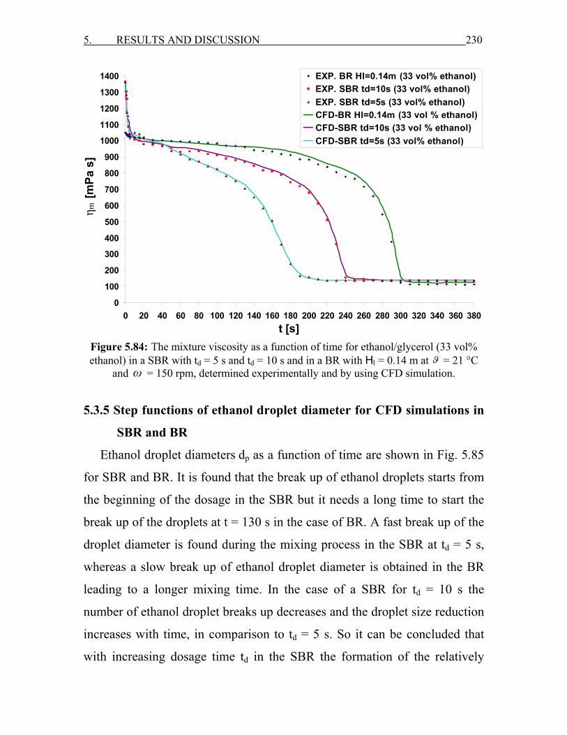
5. RESULTS AND DISCUSSION 230
0
100
200
300
400
500
600
700
800
900
1000
1100
1200
1300
1400
0 20 40 60 80 100 120 140 160 180 200 220 240 260 280 300 320 340 360 380t [s]
ηm
[m
Pa s
]EXP. BR Hl=0.14m (33 vol% ethanol) EXP. SBR td=10s (33 vol% ethanol) EXP. SBR td=5s (33 vol% ethanol)CFD-BR HI=0.14m (33 vol % ethanol) CFD-SBR td=10s (33 vol % ethanol)CFD-SBR td=5s (33 vol% ethanol)
Figure 5.84: The mixture viscosity as a function of time for ethanol/glycerol (33 vol% ethanol) in a SBR with td = 5 s and td = 10 s and in a BR with Hl = 0.14 m at ϑ = 21 °C
and ω = 150 rpm, determined experimentally and by using CFD simulation.
5.3.5 Step functions of ethanol droplet diameter for CFD simulations in
SBR and BR
Ethanol droplet diameters dp as a function of time are shown in Fig. 5.85
for SBR and BR. It is found that the break up of ethanol droplets starts from
the beginning of the dosage in the SBR but it needs a long time to start the
break up of the droplets at t = 130 s in the case of BR. A fast break up of the
droplet diameter is found during the mixing process in the SBR at td = 5 s,
whereas a slow break up of ethanol droplet diameter is obtained in the BR
leading to a longer mixing time. In the case of a SBR for td = 10 s the
number of ethanol droplet breaks up decreases and the droplet size reduction
increases with time, in comparison to td = 5 s. So it can be concluded that
with increasing dosage time td in the SBR the formation of the relatively
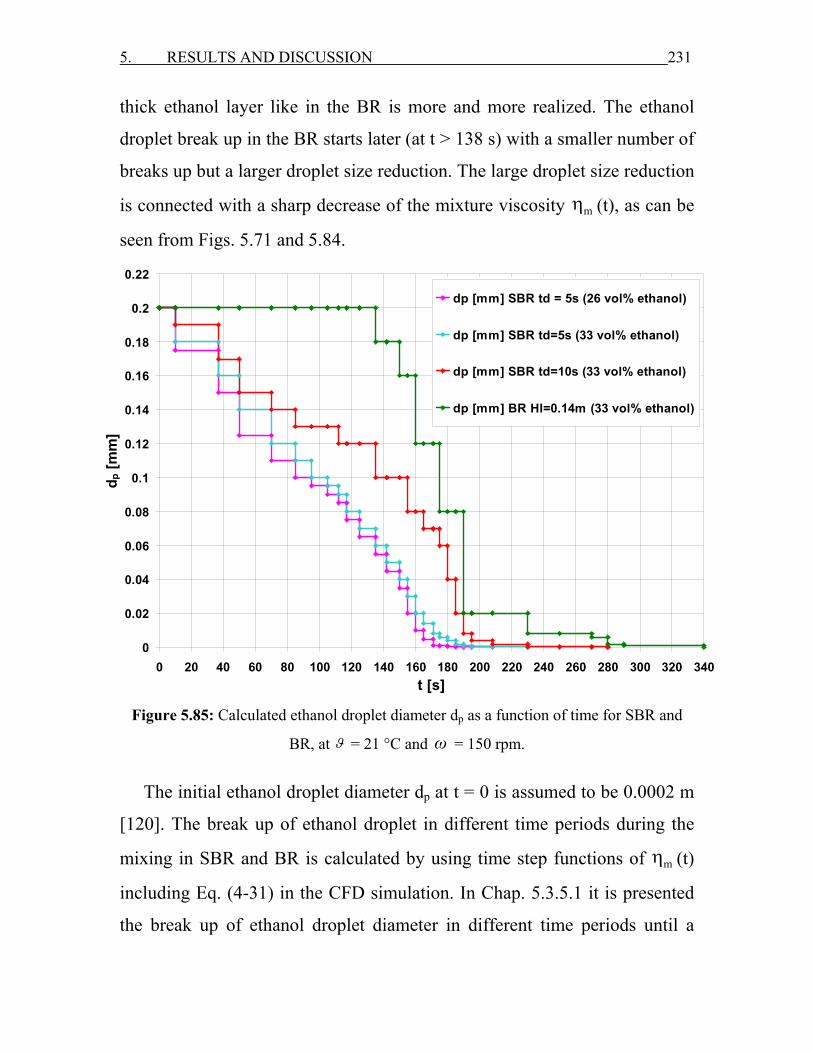
5. RESULTS AND DISCUSSION 231
thick ethanol layer like in the BR is more and more realized. The ethanol
droplet break up in the BR starts later (at t > 138 s) with a smaller number of
breaks up but a larger droplet size reduction. The large droplet size reduction
is connected with a sharp decrease of the mixture viscosity mη (t), as can be
seen from Figs. 5.71 and 5.84.
0
0.02
0.04
0.06
0.08
0.1
0.12
0.14
0.16
0.18
0.2
0.22
0 20 40 60 80 100 120 140 160 180 200 220 240 260 280 300 320 340t [s]
d p [m
m]
dp [mm] SBR td = 5s (26 vol% ethanol)
dp [mm] SBR td=5s (33 vol% ethanol)
dp [mm] SBR td=10s (33 vol% ethanol)
dp [mm] BR Hl=0.14m (33 vol% ethanol)
Figure 5.85: Calculated ethanol droplet diameter dp as a function of time for SBR and
BR, at ϑ = 21 °C and ω = 150 rpm.
The initial ethanol droplet diameter dp at t = 0 is assumed to be 0.0002 m
[120]. The break up of ethanol droplet in different time periods during the
mixing in SBR and BR is calculated by using time step functions of mη (t)
including Eq. (4-31) in the CFD simulation. In Chap. 5.3.5.1 it is presented
the break up of ethanol droplet diameter in different time periods until a
5. RESULTS AND DISCUSSION 232
complete mixing is obtained when the mixture viscosity mη remains
constant and no further break up of ethanol droplets happens.
5.3.5.1 SBR at td = 5 s (26 vol% ethanol)
By using the measured viscosities m (t)η of the liquid ethanol/glycerol
mixture as a function of time, the following validated step function is
formulated.
Between 0 t 10 s≤ ≤ ⇒ dp = 0.0002 m
S1 = step(t/1.0[s]-0) *0.0002[m]
S2 = step(t/1.0[s]-10) *0.0002[m]
dp ethanolSBR1 = S1-S2.
Where dp ethanolSBR1 is ethanol droplet diameter in a SBR in the first
time period of the mixing process.
Between 10.1 s t 37 s≤ ≤ ⇒ dp = 0.000175 m
S3 = step(t/1.0[s]-10.1) *0.000175[m]
S4 = step(t/1.0[s]-37) *0.000175[m]
dp ethanolSBR2 = S3-S4.
Similar step functions are used for the following time periods:
Between 37.1 s t 50 s≤ ≤ ⇒ dp = 0.00015 m
Between 50.1 s t 70 s≤ ≤ ⇒ dp = 0.000125 m
Between 70.1 s t 85 s≤ ≤ ⇒ dp = 0.00011 m
Between 85.1 s t 95 s≤ ≤ ⇒ dp = 0.0001 m
Between 95.1 s t 105 s≤ ≤ ⇒ dp = 0.000095 m
Between 105.1 s t 112 s≤ ≤ ⇒ dp = 0.00009 m
Between 112.1 s t 117 s≤ ≤ ⇒ dp = 0.000085 m
Between 117.1 s t 125 s≤ ≤ ⇒ dp = 0.000075 m

5. RESULTS AND DISCUSSION 233
Between 125.1 s t 135 s≤ ≤ ⇒ dp = 0.000065 m
Between 135.1 s t 142 s≤ ≤ ⇒ dp = 0.000055 m
Between 142.1 s t 150 s≤ ≤ ⇒ dp = 0.000045 m
Between 150.1 s t 155 s≤ ≤ ⇒ dp = 0.000035 m
Between 155.1 s t 160 s≤ ≤ ⇒ dp = 0.00002 m
Between 160.1 s t 165 s≤ ≤ ⇒ dp = 0.00001 m
Between 165.1 s t 171 s≤ ≤ ⇒ dp = 0.000005 m
Between 171.1 s t 175 s≤ ≤ ⇒ dp = 0.000001 m
Between 175.1 s t 180 s≤ ≤ ⇒ dp = 0.00000075 m
Between 180.1 s t 185 s≤ ≤ ⇒ dp = 0.0000005 m
Between 185.1 s t 190 s≤ ≤ ⇒ dp = 0.0000004 m
Between 190.1 s t 195 s≤ ≤ ⇒ dp = 0.0000003 m
Between 195.1 s t 208 s≤ ≤ ⇒ dp = 0.0000002 m
Between 208.1 s t 230 s≤ ≤ ⇒ dp = 0.0000001 m
5.3.5.2 SBR at td = 5 s (33 vol% ethanol)
In this case the validated step function dp(t) is formulated by the
following relationships.
Between 0 t 10 s≤ ≤ ⇒ dp = 0.0002 m
S1 = step(t/1.0[s]-0) *0.0002[m]
S2 = step(t/1.0[s]-10) *0.0002[m]
dp ethanolSBR1 = S1-S2.
Between 10.1 s t 37 s≤ ≤ ⇒ dp = 0.00018 m
S3 = step(t/1.0[s]-10.1) *0.00018[m]
S4 = step(t/1.0[s]-37) *0.00018[m]
dp ethanolSBR2 = S3-S4.
Between 37.1 s t 50 s≤ ≤ ⇒ dp = 0.00016 m
5. RESULTS AND DISCUSSION 234
Between 50.1 s t 70 s≤ ≤ ⇒ dp = 0.00014 m
Between 70.1 s t 85 s≤ ≤ ⇒ dp = 0.00012 m
Between 85.1 s t 95 s≤ ≤ ⇒ dp = 0.00011 m
Between 95.1 s t 105 s≤ ≤ ⇒ dp = 0.0001 m
Between 105.1 s t 112 s≤ ≤ ⇒ dp = 0.000095 m
Between 112.1 s t 117 s≤ ≤ ⇒ dp = 0.00009 m
Between 117.1 s t 125 s≤ ≤ ⇒ dp = 0.00008 m
Between 125.1 s t 135 s≤ ≤ ⇒ dp = 0.00007 m
Between 135.1 s t 142 s≤ ≤ ⇒ dp = 0.00006 m
Between 142.1 s t 150 s≤ ≤ ⇒ dp = 0.00005 m
Between 150.1 s t 155 s≤ ≤ ⇒ dp = 0.00004 m
Between 155.1 s t 160 s≤ ≤ ⇒ dp = 0.00003 m
Between 160.1 s t 165 s≤ ≤ ⇒ dp = 0.00002 m
Between 165.1 s t 171 s≤ ≤ ⇒ dp = 0.000014 m
Between 171.1 s t 175 s≤ ≤ ⇒ dp = 0.000008 m
Between 175.1 s t 180 s≤ ≤ ⇒ dp = 0.000006 m
Between 180.1 s t 185 s≤ ≤ ⇒ dp = 0.000004 m
Between 185.1 s t 190 s≤ ≤ ⇒ dp = 0.000002 m
Between 190.1 s t 195 s≤ ≤ ⇒ dp = 0.0000008 m
Between 195.1 s t 208 s≤ ≤ ⇒ dp = 0.0000004 m
Between 208.1 s t 220 s≤ ≤ ⇒ dp = 0.0000002 m
Between 220.1 s t 250 s≤ ≤ ⇒ dp = 0.0000001 m
5.3.5.3 SBR at td = 10 s (33 vol% ethanol)
In this case the validated step function dp(t) is formulated by the
following relationships.
5. RESULTS AND DISCUSSION 235
Between 0 t 10 s≤ ≤ ⇒ dp = 0.0002 m
S1 = step(t/1.0[s]-0) *0.0002[m]
S2 = step(t/1.0[s]-10) *0.0002[m]
dp ethanolSBR1 = S1-S2.
Between 10.1 s t 37 s≤ ≤ ⇒ dp = 0.00019 m
S3 = step(t/1.0[s]-10.1) *0.00019 [m]
S4 = step(t/1.0[s]-37) *0.00019[m]
dp ethanolSBR2 = S3-S4.
Between 37.1 s t 50 s≤ ≤ ⇒ dp = 0.00017 m
Between 50.1 s t 70 s≤ ≤ ⇒ dp = 0.00015 m
Between 70.1 s t 85 s≤ ≤ ⇒ dp = 0.00014 m
Between 85.1 s t 112 s≤ ≤ ⇒ dp = 0.00013 m
Between 112.1 s t 135 s≤ ≤ ⇒ dp = 0.00012 m
Between 135.1 s t 155 s≤ ≤ ⇒ dp = 0.0001 m
Between 155.1 s t 165 s≤ ≤ ⇒ dp = 0.00008 m
Between 165.1 s t 175 s≤ ≤ ⇒ dp = 0.00007 m
Between 175.1 s t 180 s≤ ≤ ⇒ dp = 0.00006 m
Between 180.1 s t 185 s≤ ≤ ⇒ dp = 0.00004 m
Between 185.1 s t 190 s≤ ≤ ⇒ dp = 0.00002 m
Between 190.1 s t 195 s≤ ≤ ⇒ dp = 0.000008 m
Between 195.1 s t 208 s≤ ≤ ⇒ dp = 0.000004 m
Between 208.1 s t 230 s≤ ≤ ⇒ dp = 0.000002 m
Between 230.1 s t 250 s≤ ≤ ⇒ dp = 0.0000004 m
Between 250.1 s t 270 s≤ ≤ ⇒ dp = 0.0000003 m
Between 270.1 s t 280 s≤ ≤ ⇒ dp = 0.0000002 m
Between 280.1 s t 290 s≤ ≤ ⇒ dp = 0.0000001 m
5. RESULTS AND DISCUSSION 236
5.3.5.4 BR at Hl = 0.14 m (33 vol% ethanol)
In this case the validated step function dp(t) is formulated by the
following relationships.
Between 0 t 135 s≤ ≤ ⇒ dp = 0.0002 m
B1 = step(t/1.0[s]-0) *0.0002[m]
B2 = step(t/1.0[s]-135) *0.0002[m]
dp ethanolBR1 = B1-B2.
Where dp ethanolBR1 is ethanol droplet diameter in a BR in the first time
period of the mixing process.
Between 135.1 s t 150 s≤ ≤ ⇒ dp = 0.00018 m
B3 = step(t/1.0[s]-135.1) *0.00018[m]
B4 = step(t/1.0[s]-150) *0.00018[m]
dp ethanolBR2 = B3-B4
Similar step functions to that above for the droplet diameter of ethanol as
a function of time are used for the following time periods:
Between 150.1 s t 160 s≤ ≤ ⇒ dp = 0.00016 m
Between 160.1 s t 175 s≤ ≤ ⇒ dp = 0.00012 m
Between 175.1 s t 190 s≤ ≤ ⇒ dp = 0.00008 m
Between 190.1 s t 230 s≤ ≤ ⇒ dp = 0.00002 m
Between 230.1 s t 270 s≤ ≤ ⇒ dp = 0.000008 m
Between 270.1 s t 280 s≤ ≤ ⇒ dp = 0.000006 m
Between 280.1 s t 290 s≤ ≤ ⇒ dp = 0.000002 m
Between 290.1 s t 340 s≤ ≤ ⇒ dp = 0.000001 m
Between 320.1 s t 360 s≤ ≤ ⇒ dp = 0.0000001 m
5. RESULTS AND DISCUSSION 237
5.3.6 The modified CFD-Algebraic slip model (MASM) in comparison
with Algebraic slip model (ASM) and the Transport model (TRM)
in a SBR and a BR
The calculated dynamic viscosity of ethanol and glycerol mixture mη as
a function of time t when it is used the modified algebraic slip model
(MASM), algebraic slip model (ASM) and the transport model (TRM) in the
CFD simulations at ϑ = 21°C and ω = 150 rpm can be shown in Figs. 5.86
and 5.87 for SBR and BR, respectively. It is shown that alone the MASM
developed in this work is able to describe realistic the measured mixture
viscosity m (t)η as a function of time.
The final mixture viscosities for the SBR by using the MASM and TRM
are mη = 300 mPa s at tm = 205 s and mη = 267 mPa s at tm = 60 s,
respectively. The final mixture viscosities for BR by using the MASM and
TRM are mη = 122 mPa s at tm = 340 s and mη = 178 mPa s at tm = 100 s,
respectively. The calculated final mixture viscosities mη have
approximately the same values, whereas the calculated mixing times tm are
completely different. Especially the m (t)η behavior is quite different. The
mixing time by using TRM is shorter than that by using MASM with a time
difference of t∆ = 145 s for the SBR and t∆ = 240 s for the BR. The reason
is that the transport model does not consider the density differences and the
relative velocity between ethanol (upper layer) and glycerol (lower layer).
For that the slow mixing process between 5.2 s ≤ t 150 s≤ is not realized
when the transport model is used to calculate the mixture viscosity mη in
the SBR and BR as can be seen in Figs. 5.87 and 5.88, respectively.
However the MASM considers the buoyancy forces, the interphase mass
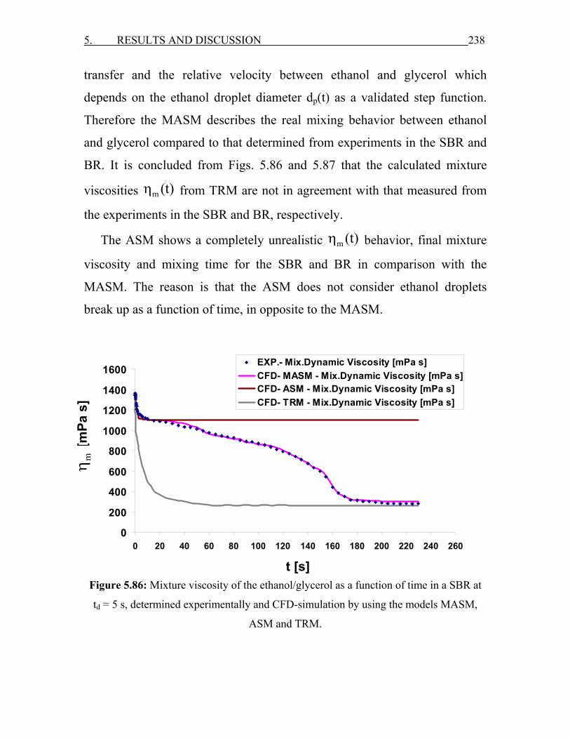
5. RESULTS AND DISCUSSION 238
transfer and the relative velocity between ethanol and glycerol which
depends on the ethanol droplet diameter dp(t) as a validated step function.
Therefore the MASM describes the real mixing behavior between ethanol
and glycerol compared to that determined from experiments in the SBR and
BR. It is concluded from Figs. 5.86 and 5.87 that the calculated mixture
viscosities m (t)η from TRM are not in agreement with that measured from
the experiments in the SBR and BR, respectively.
The ASM shows a completely unrealistic m (t)η behavior, final mixture
viscosity and mixing time for the SBR and BR in comparison with the
MASM. The reason is that the ASM does not consider ethanol droplets
break up as a function of time, in opposite to the MASM.
Figure 5.86: Mixture viscosity of the ethanol/glycerol as a function of time in a SBR at
td = 5 s, determined experimentally and CFD-simulation by using the models MASM,
ASM and TRM.
0
200
400
600
800
1000
1200
1400
1600
0 20 40 60 80 100 120 140 160 180 200 220 240 260
Time [s]
Dyn
amic
Vis
cosi
ty η
mix
[mPa
s] EXP.- Mix.Dynamic Viscosity [mPa s]
CFD- MASM - Mix.Dynamic Viscosity [mPa s]CFD- ASM - Mix.Dynamic Viscosity [mPa s]CFD- TRM - Mix.Dynamic Viscosity [mPa s]
t [s]
[mPa
s]
mη

5. RESULTS AND DISCUSSION 239
Figure 5.87: Mixture viscosity of ethanol/glycerol as a function of time in a BR with
Hl = 0.14 m determined experimentally and CFD-simulation by using the models MASM,
ASM and TRM.
5.3.7 Summary of the measured and calculated mη and tm
The measured and the calculated dynamic mixture viscosities mη of
ethanol and glycerol and mixing times tm in a SBR and a BR are summarized
in Tab. 5.2. Table 5.2: The measured and CFD calculated mixture viscosity mη and mixing time tm
for a SBR and a BR.
EXPERIMENT CFD-Simulation Mixing Time [s]
Mixture Viscosity [mPa s] Torque
method Decolorisation
Reaction
Mixture Viscosity [mPa s]
Mixing Time
[s] SBR at td = 5 s
(26 vol% ethanol)
279
208
206
300
205
SBR at td = 5 s (33 vol% ethanol)
134
222
-
138
220
SBR at td = 10 s (33 vol% ethanol)
130
282
-
137
280
BR with Hl = 0.14 m (33 vol% ethanol)
110
342
340
122
340
BR with Hl = 0.09 m (33 vol% ethanol)
135
20
17
-
-
0100200300400500600700800900
10001100
0 20 40 60 80 100 120 140 160 180 200 220 240 260 280 300 320 340 360 380Time [s]
Dyn
amic
Vis
cosi
ty η
mix
[mPa
s]
EXP.- Mix.Dynamic Viscosity [mPa s] CFD- MASM -Mix.Dynamic Viscosity [mPa s]CFD- ASM -Mix.Dynamic Viscosity [mPa s] CFD- TRM -Mix.Dynamic Viscosity [mPa s]
[mPa
s]
mη
t [s]
240
6. CONCLUSIONS AND OUTLOOK
• Conclusions
1. The mixing times and time dependent dynamic viscosities of the
liquid mixture with different viscosities and different densities can be
predicted by CFD simulation in a SBR and a BR and are in a good
agreement with experimental values.
2. The new developed MASM in connection with a step function of the
droplet diameter dp(t) predicts the mixing behaviour of these liquids.
3. Reducing the number of cells by a factor of 20 decreases the
computational time of simulation by factor of 10, without remarkable
change in the results.
4. The cell size should not exceed 0.015 m to get a good special
resolution.
5. It is found that a dosage time of 5 s, an inlet tube diameter 0.023 m,
anchor velocity of 150 rpm and the width of the horizontal blade of
the anchor impeller of 0.015 m are the best operating conditions.
6. With a decolourisation and a torque method for determination of the
time dependent mixture viscosities and the mixing times in a SBR and
a BR, it is possible to validate the used CFD models.
7. For the SBR, a jet phenomenon during the dosage of ethanol plays a
big role to get a fast mixing.
8. It is possible with CFD to predict the complex batch phenomenon
(pan cake effect) in a BR for liquids with high viscosity difference and
high density difference.
9. This thesis presents methods for recognition of more complex
problems and alternative mixing designs for critical applications.
6. CONCLUSIONS AND OUTLOOK 241
10. The high viscosity liquid mixture has also a great effect on an
observed secondary flow field with an axial circulation behind the
rotating impeller which can be predicted by CFD simulation.
Outlook
1. The mixing behavior of different liquid mixtures with different
geometries and stirrers should be carried out.
2. It is assumed the investigated mixing phenomena also are happened in
large scale vessel, the quantitative scale up relation ship could also be
developed and carried out with suitable volume of liquids.
3. It is intended to investigate the mixing behavior for non-miscible
liquids in a BR with different stirrer types and velocities.
4. The studied mixing processes are the first step to a CFD simulation of
polymerization reactions including high viscosity effects.
242
7. REFERENCES [1] Delaplace, G., Guerin, R., Leuliet, J., Torrez, C., Andre, C., Sliding
mesh method to simulate flow of highly viscous fluid in stirred tank
agitated with helical ribbon impeller, Proc.2th International
Conference on Simulation in food and Bio industries (2002) 151-157.
[2] Nakamura, S., Brodkey, R., Computational Flow Analysis for the
Chemical Mixing Vessel with Impeller and Baffles, ASME Fluid
Engineering Summer Conference Boston, Massachusetts, June 11-15
(2000) 1-8.
[3] Myers, K., Ward, R., Bakker, A., A Digital Particle Image
Velocimetry Investigation of Flow Field Instabilities of Axial- Flow
Impellers, J. Fluid Eng. 119 (1997) 623-631.
[4] Battello, G., Grisafi, F., Micale, G., Brucato, A., Flow Field In An
Unbaffled Stirred Tank via Particle Image Velocimetry, Dipartimento
di Ingegneria Chimica dei Processi e dei Materiali e Laboratoroi
INCA, Viale delle Scienze-90128 Palermo, Italy (1999) 1-6.
[5] Chemineer, Computational Fluid Mixing (CFM), (2003) online in the
Internet: http://www.Chemineer.com/technology.php
[6] Frank, T., Eulerian Multiphase Flow Modeling, Phase Interaction
Models, ANSYS Germany (2004).
[7] Sveen, J., New insights from Navier-Stockes modeling of free surface
flows, Dept. of Mathematics, University of Oslo., (2006) online in the
Internet: http://www.math.uio.no/~jks/work.html
[8] Peixoto, S.M.C., Nunhez, J.R., Duarte, C.G., Characterizing the Flow
of Stirred Vessels with Anchor type Impellers, Sao Paulo, BRASIL,
ISSN 0104-6632, Braz. J. Chem. Eng. 17 (2000) 1-15.

7. REFERENCES 243
[9] Ju, W., Huang, X., Wang, Y., Shi, L., Zhang, B.; Yuan, J., An
Investigation of the Flow Field of Viscoelastic Fluid in A Stirred
Vessel, 10th European Conference on Mixing, Elsevier Science B.V.
(2000) 312-320.
[10] Delaplace, G., Torrez, C., Gradeck, M., Leuliet, J., André, C., Flow of
Newtonian and non-Newtonian fluids in an agitated vessel equipped
with a non-standard anchor impeller, 10th European Conference on
Mixing, Elsevier Science B.V. (2000) 321-328.
[11] Dantecdynamic, Particle equipment, Seeding particles for PIV and
LDA measurements, (2005) online in the Internet:
http://www.dantecdynamic.com/PE/seeding/Index.html
[12] Dantecdynamic, Imaging Systems, (2005) online in the Internet:
http://www.dantecdynamic.com/PIV/System/Index.html
[13] Haam, S.J., Brodkey, R.S., Fort, I., Vanecek, V., Laser Doppler
Anemometry measurements in an Index of Refraction Matched in The
Presence of Dispersed Beads Part I, Int. J. of Multiphase Flow 15
(1998) 279-285.
[14] Haam, S.J., Brodkey, R.S., Motion of Dispersed Beads Obtained by
Particle Tracking Velocimetry Measurements Part II, Int. J. of
Multiphase Flow 220 (1998) 485-537.
[15] Nakamura, S., Brodkey, R.S., Computational and Experimental Study
of the Fluid Flow in A Cylindrical Cavity with An Impeller Rotor at
An Electric Location, 3rd ASME/ JSME Joint Fluids Engineering
Conference, San Francisco, California (1999) 1-6.
[16] Clifford, M.J., Cox, S.M., Finn, M.D., Reynolds number effects in a
simple planetary mixer, Chem. Eng. Sci. 59 (2004) 3371-3379.
7. REFERENCES 244
[17] Wörner, M., Computational Modeling of Multiphase Flows,
International Summer School on “Computational Modeling of
Combustion & Multiphase Flows in Energy Systems”, Neptun-Olimp,
Romania (2003) 1-35.
[18] Kvicinsky, S., Kueny, J., Avellan, F., Parkinson, E., Experimental and
Numerical Analysis of Free Surface Flows in a Rotating Bucket,
Proceeding of the XXlst IAHR Symposium on Hydraulic Machinery
and Systems, Lausanne (2002) 1-7.
[19] Kvicinsky, S., Kueny, J.-L., Avellan, F., Numerical and Experimental
Analysis of Free surface Flow in A 3D non Rotating Pelton Bucket,
The 9th International Symposium on Transport Phenomena and
Dynamics of Rotating Machinery, Honolulu, Hawaii, USA (2002) 1-8.
[20] Torrecilla, M., Introduction to numerical simulation of fluid flows,
Technical University of Munich, Winter school, Russia (2004) 24-34.
[21] Frank, T., Eulerian Multiphase Flow Modeling: Phase Interaction
Models, Ansys CFX, Otterfing, FZR-Dresden, Germany (2003).
[22] Frank, T., Free Surface Flow Theory, Chapter 1, Ansys CFX,
Otterfing, Germany (2004).
[23] Kat chalmers, The influence of complex rheology on mixing, reaction
and control of stirred vessels, (2005) online in the Internet:
http://www.kat.chalmers.se/cpdc/tvproj.htm
[24] Cremer, H.W., Chemical Engineering Practice, Vol. 8, Butterworths
Scientific Publications, London (1965).
[25] Zhao, Y., Brodkey, R.S., On Representation of Complex Turbulent
Flows, (2005) online in the Internet:
http://www.chbmeng.ohio-state.edu/~brodkey/RES_3D-Stereo
7. REFERENCES 245
[26] Nakamura, S., Brodkey, R.S., Direct and Large Eddy Simulation of
the Three-Dimensional Unsteady Flows in the Counter-Jet Mixing
Vessel, ASME Fluids Eng. Summer Conference, Boston (2000) 1-7.
[27] Frank, T., Flow Visualization Methods, Ansys CFX Germany (2004).
[28] Kirk-Othmer, Encyclopedia of Chemical Technology, 3rd edition, Vol.
24, John Wiley & Sons, USA (2006).
[29] Perry, R.H., Green, D., Perry’s Chemical Engineers’ Handbook, 7th
edition, McGraw-Hill (1997).
[30] Petersen, E.E., Chemical Reaction Analysis, Prentice Hall Inc., USA
(1965).
[31] Smith, J.M., Chemical Engineering Kinetics, 3rd edition, McGraw-
Hill (1987).
[32] Kalok C Lee, An experimental investigation of the trailing vortex
structure and mixing and mixing characteristics of stirred vessels,
(2005) online in the Internet:
http://www.eee.kcl.ac.uk/mecheng/kcl/kclphd.html
[33] Miettinen, T., Laakkonen M., Aittamaa J., The applicability of various
flow visualization techniques for the characterization of Gas-Liquid in
a mixed tank, Helsinki University of Technology, Espoo, Finland,
AIChE J. 48 (2002) 673-685.
[34] Kukura, J., Arratia, P.C., Szalai, E.S., Bittorf, K.J., Muzzio, F.J.,
Understanding Pharmaceutical Flows, Pharmaceutical Technology,
10 (2002) 48-72.
[35] Zalc, J.M., Szalai, E.S., Alvarez, M.M., Muzzio, F.J., Using CFD to
Understand Chaotic Mixing in Laminar Stirred Tanks, AIChE J. 48
(2002) 2124-2134.
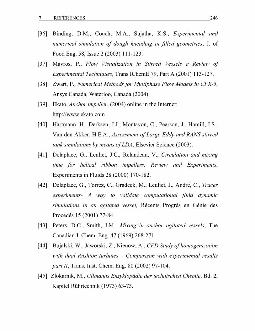
7. REFERENCES 246
[36] Binding, D.M., Couch, M.A., Sujatha, K.S., Experimental and
numerical simulation of dough kneading in filled geometries, J. of
Food Eng. 58, Issue 2 (2003) 111-123.
[37] Mavros, P., Flow Visualization in Stirred Vessels a Review of
Experimental Techniques, Trans IChemE 79, Part A (2001) 113-127.
[38] Zwart, P., Numerical Methods for Multiphase Flow Models in CFX-5,
Ansys Canada, Waterloo, Canada (2004).
[39] Ekato, Anchor impeller, (2004) online in the Internet:
http://www.ekato.com
[40] Hartmann, H., Derksen, J.J., Montavon, C., Pearson, J., Hamill, I.S.;
Van den Akker, H.E.A., Assessment of Large Eddy and RANS stirred
tank simulations by means of LDA, Elsevier Science (2003).
[41] Delaplace, G., Leuliet, J.C., Relandeau, V., Circulation and mixing
time for helical ribbon impellers. Review and Experiments,
Experiments in Fluids 28 (2000) 170-182.
[42] Delaplace, G., Torrez, C., Gradeck, M., Leuliet, J., André, C., Tracer
experiments- A way to validate computational fluid dynamic
simulations in an agitated vessel, Récents Progrés en Génie des
Procédés 15 (2001) 77-84.
[43] Peters, D.C., Smith, J.M., Mixing in anchor agitated vessels, The
Canadian J. Chem. Eng. 47 (1969) 268-271.
[44] Bujalski, W., Jaworski, Z., Nienow, A., CFD Study of homogenization
with dual Rushton turbines – Comparison with experimental results
part II, Trans. Inst. Chem. Eng. 80 (2002) 97-104.
[45] Zlokarnik, M., Ullmanns Enzyklopädie der technischen Chemie, Bd. 2,
Kapitel Rührtechnik (1973) 63-73.
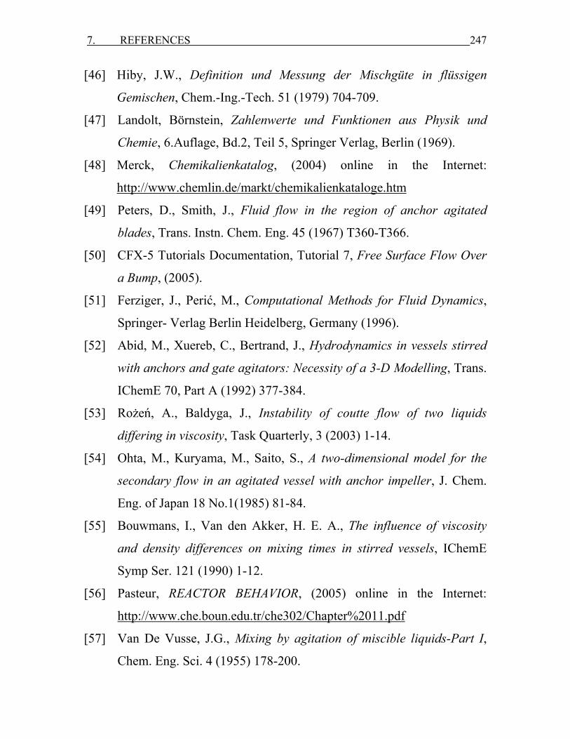
7. REFERENCES 247
[46] Hiby, J.W., Definition und Messung der Mischgüte in flüssigen
Gemischen, Chem.-Ing.-Tech. 51 (1979) 704-709.
[47] Landolt, Börnstein, Zahlenwerte und Funktionen aus Physik und
Chemie, 6.Auflage, Bd.2, Teil 5, Springer Verlag, Berlin (1969).
[48] Merck, Chemikalienkatalog, (2004) online in the Internet:
http://www.chemlin.de/markt/chemikalienkataloge.htm
[49] Peters, D., Smith, J., Fluid flow in the region of anchor agitated
blades, Trans. Instn. Chem. Eng. 45 (1967) T360-T366.
[50] CFX-5 Tutorials Documentation, Tutorial 7, Free Surface Flow Over
a Bump, (2005).
[51] Ferziger, J., Perić, M., Computational Methods for Fluid Dynamics,
Springer- Verlag Berlin Heidelberg, Germany (1996).
[52] Abid, M., Xuereb, C., Bertrand, J., Hydrodynamics in vessels stirred
with anchors and gate agitators: Necessity of a 3-D Modelling, Trans.
IChemE 70, Part A (1992) 377-384.
[53] Rożeń, A., Baldyga, J., Instability of coutte flow of two liquids
differing in viscosity, Task Quarterly, 3 (2003) 1-14.
[54] Ohta, M., Kuryama, M., Saito, S., A two-dimensional model for the
secondary flow in an agitated vessel with anchor impeller, J. Chem.
Eng. of Japan 18 No.1(1985) 81-84.
[55] Bouwmans, I., Van den Akker, H. E. A., The influence of viscosity
and density differences on mixing times in stirred vessels, IChemE
Symp Ser. 121 (1990) 1-12.
[56] Pasteur, REACTOR BEHAVIOR, (2005) online in the Internet:
http://www.che.boun.edu.tr/che302/Chapter%2011.pdf
[57] Van De Vusse, J.G., Mixing by agitation of miscible liquids-Part I,
Chem. Eng. Sci. 4 (1955) 178-200.

7. REFERENCES 248
[58] Zlokarnik, M., Einfluß der Dichte- und Zähigkeitsunterschiede auf die
Mischzeit beim Homogenisieren von Flüssigekeitsgemischen, Chem.-
Ing.-Tech. 42 Nr.15 (1970) 1009-1011.
[59] Lodgsdon, J.E., Ethanol, Encyclopedia of Chemical Technology, New
York, John Wiley & Sons, 4th Ed. 9 (1994) 812–860.
[60] Wikipedia, Glycerol, (2006) online in the Internet:
http://en.wikipedia.org/wiki/Glycerol
[61] Process equipment globalspec, Mixers, (2006) online in the Internet:
http://process-equipment.globalspec.com
[62] Clevelandmixer, Mixing glossary of terms, (2006) online in the
Internet: http://www.clevelandmixer.com/files/pdf
[63] Parrinst, Stirrer Options, (2006) online in the Internet:
http://www.parrinst.com/default.cfm
[64] Chemineer, Advanced Impeller Technology for Superior Performance,
(2006) online in the Internet: http://www.chemineer.com
[65] Autoclave, Impeller System, (2006) online in the Internet:
http://autoclave.en.ec21.com
[66] Engin.umich., Semibatch, (2006) online in the Internet:
http://www.engin.umich.edu
[67] Hoogendoorn, C .J., Den Hartog, A. P., Model studies on mixers in the
viscous flow region, Chem. Eng. Sci. 22 (1967) 1689-1695.
[68] Bouwmans, I., Bakker, A., Van Den Akker, H.E.A., Blending liquid
of differing viscosities and densities in stirred vessels, Trans. IChemE
75, Part A (1997) 777-783.
[69] Smith, J. M., Schoenmakers, A.W., Blending of liquids of differing
viscosity, Chem. Eng. Res. Des. 66 (1988) 16-21.
[70] Irving, J. R., Viscosities of Binary Liquid Mixtures, A Survey of
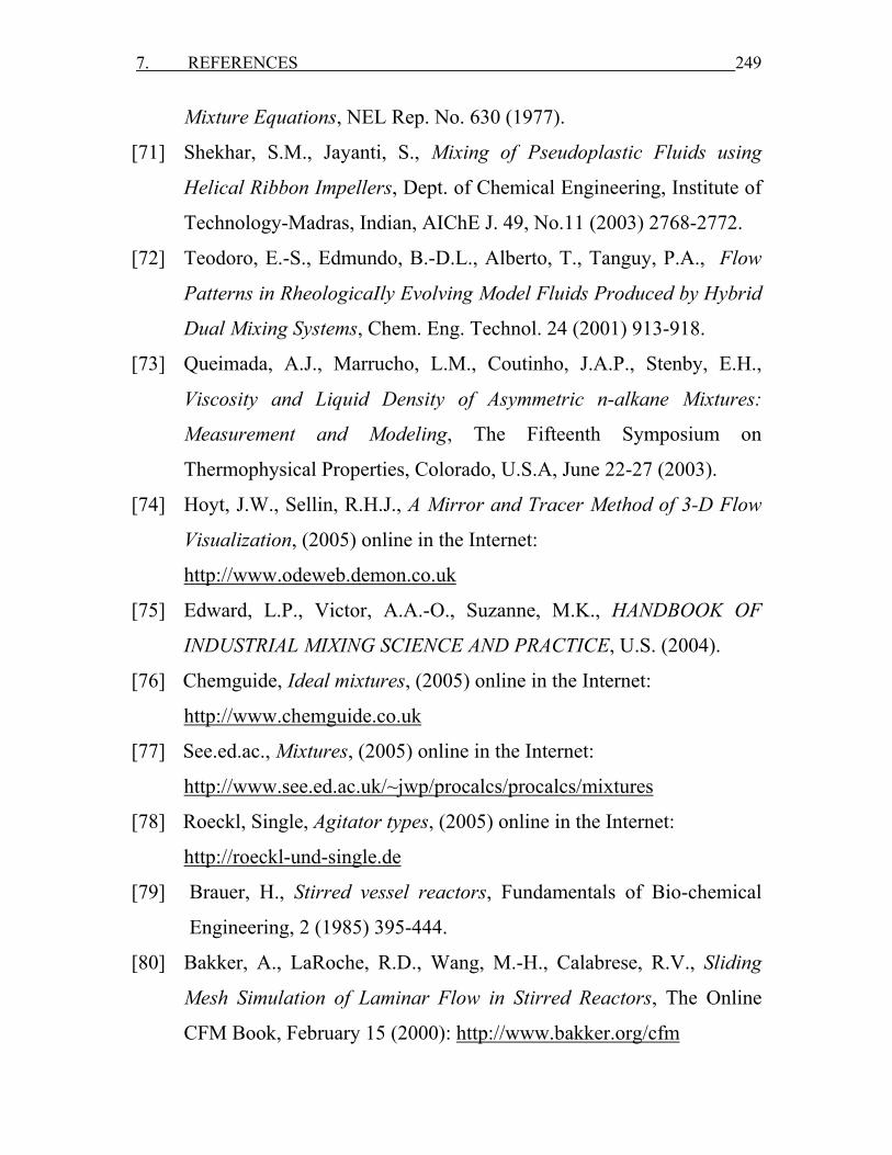
7. REFERENCES 249
Mixture Equations, NEL Rep. No. 630 (1977).
[71] Shekhar, S.M., Jayanti, S., Mixing of Pseudoplastic Fluids using
Helical Ribbon Impellers, Dept. of Chemical Engineering, Institute of
Technology-Madras, Indian, AIChE J. 49, No.11 (2003) 2768-2772.
[72] Teodoro, E.-S., Edmundo, B.-D.L., Alberto, T., Tanguy, P.A., Flow
Patterns in RheologicaIly Evolving Model Fluids Produced by Hybrid
Dual Mixing Systems, Chem. Eng. Technol. 24 (2001) 913-918.
[73] Queimada, A.J., Marrucho, L.M., Coutinho, J.A.P., Stenby, E.H.,
Viscosity and Liquid Density of Asymmetric n-alkane Mixtures:
Measurement and Modeling, The Fifteenth Symposium on
Thermophysical Properties, Colorado, U.S.A, June 22-27 (2003).
[74] Hoyt, J.W., Sellin, R.H.J., A Mirror and Tracer Method of 3-D Flow
Visualization, (2005) online in the Internet:
http://www.odeweb.demon.co.uk
[75] Edward, L.P., Victor, A.A.-O., Suzanne, M.K., HANDBOOK OF
INDUSTRIAL MIXING SCIENCE AND PRACTICE, U.S. (2004).
[76] Chemguide, Ideal mixtures, (2005) online in the Internet:
http://www.chemguide.co.uk
[77] See.ed.ac., Mixtures, (2005) online in the Internet:
http://www.see.ed.ac.uk/~jwp/procalcs/procalcs/mixtures
[78] Roeckl, Single, Agitator types, (2005) online in the Internet:
http://roeckl-und-single.de
[79] Brauer, H., Stirred vessel reactors, Fundamentals of Bio-chemical
Engineering, 2 (1985) 395-444.
[80] Bakker, A., LaRoche, R.D., Wang, M.-H., Calabrese, R.V., Sliding
Mesh Simulation of Laminar Flow in Stirred Reactors, The Online
CFM Book, February 15 (2000): http://www.bakker.org/cfm
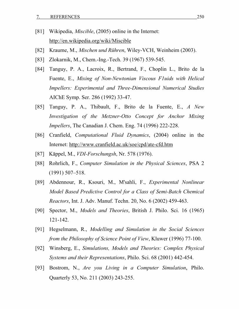
7. REFERENCES 250
[81] Wikipedia, Miscible, (2005) online in the Internet:
http://en.wikipedia.org/wiki/Miscible
[82] Kraume, M., Mischen und Rühren, Wiley-VCH, Weinheim (2003).
[83] Zlokarnik, M., Chem.-Ing.-Tech. 39 (1967) 539-545.
[84] Tanguy, P. A., Lacroix, R., Bertrand, F., Choplin L., Brito de la
Fuente, E., Mixing of Non-Newtonian Viscous F1uids with Helical
Impellers: Experimental and Three-Dimensional Numerical Studies
AIChE Symp. Ser. 286 (1992) 33-47.
[85] Tanguy, P. A., Thibault, F., Brito de la Fuente, E., A New
Investigation of the Metzner-Otto Concept for Anchor Mixing
Impellers, The Canadian J. Chem. Eng. 74 (1996) 222-228.
[86] Cranfield, Computational Fluid Dynamics, (2004) online in the
Internet: http://www.cranfield.ac.uk/soe/cpd/ate-cfd.htm
[87] Käppel, M., VDI-Forschungsh, Nr. 578 (1976).
[88] Rohrlich, F., Computer Simulation in the Physical Sciences, PSA 2
(1991) 507–518.
[89] Abdennour, R., Ksouri, M., M'sahli, F., Experimental Nonlinear
Model Based Predictive Control for a Class of Semi-Batch Chemical
Reactors, Int. J. Adv. Manuf. Techn. 20, No. 6 (2002) 459-463.
[90] Spector, M., Models and Theories, British J. Philo. Sci. 16 (1965)
121-142.
[91] Hegselmann, R., Modelling and Simulation in the Social Sciences
from the Philosophy of Science Point of View, Kluwer (1996) 77-100.
[92] Winsberg, E., Simulations, Models and Theories: Complex Physical
Systems and their Representations, Philo. Sci. 68 (2001) 442-454.
[93] Bostrom, N., Are you Living in a Computer Simulation, Philo.
Quarterly 53, No. 211 (2003) 243-255.
7. REFERENCES 251
[94] Bremermann, H. J., Minimum energy requirements of information
transfer and computing, Int. J. Theor. Phys. 21 (1982) 203-217.
[95] Raczynski, The Benefits of computer simulation, (2005) online in the
Internet: http://www.raczynski.com
[96] Bertrand, F., Tanguy, P. A., Brito de la Fuente, E., A New Perspective
for the Mixing of Yield Stress Fluids with Anchor Impellers, J. Chem.
Eng. Japan, 29, No. 1 (1996) 51-58.
[97] Action energy, Blending miscible liquids, (2006) online in the
Internet: http://www.actionenergy.org.uk
[98] Pip, N.J., Gül, N.Ö.-T., Effects of physical property differences on
blending, Chem. Eng. Technol. 28, No. 8 (2005) 908-914.
[99] Irving, J. R., Viscosities of Binary Liquid Mixtures: The Effectiveness
of Mixture Equations, NEL Rep. No. 631, 1977.
[100] CFX-5 Documentation, Solver Theory, (2005) 21-239.
[101] CFX-5 Documentation, Solver Modeling, (2005) 16-201.
[102] CFX-5 Documentation, Introduction to CFX-5, (2004) 94-104.
[103] CFX-5 Documentation, Reference Guide, (2004) 37-46.
[104] Ansys CFX-10 Documentation, Multiphase Flow Modeling, (2005).
[105] Ansys CFX-10 Documentation, Basic Capabilities Modeling, (2005).
[106] Ansys CFX-10 Documentation, Materials and Reactions, (2005).
[107] CFX-5 Documentation, Solver Manager, (2005) 2-10.
[108] CFX-5 Documentation, Post, (2005) 2-18.
[109] Ansys CFX-10 Documentation, Fluid-Fluid interfaces, (2005).
[110] Ansys CFX-10 Documentation, GGI and MFR Theory, (2005).
[111] Shamlou Ayazi, P., Edwards, M.F., Power Consumption of Helical
Ribbon Mixers in Viscous Newtonian and Non-Newtonian Fluids,
Chem. Eng. Sci. 40 (1985) 1773-1786.
7. REFERENCES 252
[112] Metzner, A.B., Otto, R.E., Agitation of Non-Newtonian Fluids, AIChE
J. 3 (1957) 3-12.
[113] Patterson, I.W.A., Carreau, P.J., Yap, C.Y., Mixing with Helical
Ribbon Agitators, Part II: Newtonian Fluids, AIChE J. 25 (1957) 508-
517.
[114] Frohn, A., Roth, N., Dynamics of Droplets, Springer (2000) 66-67.
[115] Patrick, P.M., Gary, M.H., Fluorimetric Analysis on Individual
Nanoliter sample Droplets, Applied Spectroscopy 48 (1994) 956-958.
[116] Science World, Drag Coefficient, (2006) online in the Internet:
http://scinenceworld.wolfarm.com/physics/DragCoefficient.html
[117] Tritton, D.J., Physical Fluid Dynamics, 2nd Ed. Oxford, England
(1988).
[118] Kaiser, T., Roll, G. Schweiger, G., Investigation of Coated Droplets
by Optical Levitation, J. Aerosol Sci. 27 (1996) 519-520.
[119] Hardalupas, Y., Taylor, A.M.K.P., Wilkins, J.H., Experimental
Investigation of Sub-millimeter Droplet Impingement on to Spherical
Surfaces, Int. J. Heat and Fluid Flow 20, No. 5, (1999) 477-485.
[120] Castanet, G., Lavieille, P., Lebouché, M., Lemoine, F., Measurement
of the Temperature Distribution within Monodisperse Combusting
Droplets in Linear Streams using Two-color Laser-induced, Exp.
Fluids 35, No. 6 (2003) 563-571.
[121] Mulholland, J.A., Srivastava R.K., Wendt, J.O.L., Influence of
Droplet Spacing on Drag Coefficient in Nonevaporating,
Monodisperese Stream, AIAA J. 26 (1988) 1231-1237.
[122] Mie.Utoronto, Computational Fluid Dynamics, (2004) online in the
Internet: http://www.mie.utoronto.ca/labs/MUSSL/cfd

7. REFERENCES 253
[123] Hiraoka, S., Tada, Y., Kato, Y., Model Analysis of Mixing Time
Correlation in an Agitated Vessel with Paddle Impeller, J. Chem. Eng.
Japan 34, No. 12 (2001) 1499-1505.
[124] Micale, G., CFD simulation of particle distribution in stirred vessels,
Trans. IChemE 78, A (2001) 435-444.
[125] Attila, R., Thomas, K., Stability limits in binary fluids mixtures, J.
Chem. Phys., 122 (2005) 64507-64508.
[126] Ishii, M., One-dimensional drift-flux model and constitutive equations
for relative motion between phases in various two-phase flow regimes,
ANL 77 (1977) 47-48.
[127] M., Tavassalo, V., On the Mixture Models for Multiphase Flow, VTT
Publications, (1996).
[128] John J. McKetta, Encyclopedia of Chemical Processing and Design,
Marcel Dekker, Inc., New York, 62 (1997) 451-455.
[129] Schönbucher, A., Thermische Verfahrenstechnik, Springer, Berlin; 1.
Auflage (2002).
[130] Mathematik, Introduction to Computational Fluid Dynamics, (2005)
online in the Internet: http://www.mathematik.uni-dortmund.de
[131] Cranfield, Computational Fluid Dynamics, (2006) online in the
Internet: http://www.cranfield.ac.uk/soe/cpd/ate-cfd.htm
[132] Bruce, W., Robert, E., Liquid- Liquid contacting in unbaffled, agitated
vessels, AIChE J. 19 (2004) 304-312
[133] Kostin, I., Martion, M., Texier, R., Modelling of Miscible Liquids with
the Korteweg Stress, EDP Sci. 37 (2002) 741-753.
[134] Jiao, C., Hötzl, H., An Experimental Study of Miscible Displacements
in Porous Media with Variation of Fluid Density and Viscosity, Tran.
Porous Media 54 (2004) 125-144.

7. REFERENCES 254
[135] Chen, C., Wang, L., Miscible droplets in a porous medium and the
effects of Korteweg stresses, Phys. Fluids 13 (2001) 2447-2456.
[136] Alargova, R.G., Bhatt, K.H., Paunov, V.N., Liquid-Liquid Dispersion
Technique, Advanced Materials 16 (2004) 1653-1657.
[137] Stieß, M., Mechanische Verfahrenstechnik 1, 2. Auflage, Springer
Verlag, Berlin (2002).
[138] Pahl, M.H., Wehry, T., Mischer für hochviskose Medien, Universität
Paderborn (2004) online in the Internet:
http://www-vt.upb.de/ahp/en/mitarbeiter/wehry/Mischer.pdf
[139] Takahashi, K., Arai, K., Saito, S., Power Correlation for Anchor and
Helical Ribbon Impellers in Highly Viscous Liquids, J. Chem. Eng.
Japan, 13 (1980) 147-156.
[140] Bakker, A., Gates, L.E., Properly Choose Mechanical Agitators for
Viscous Liquids, Chemical Engineering Progress, 12 (1995) 25-34.
[141] Shekhar, S.M., Jayanti, S., Mixing of Power Law F1uids Using
Anchor's Metzner-Otto Concept Revisited, AIChE J., 49 (2003) 30-52.
[142] Bakker, A., Fasano, J.B., Turbulent Mixing and Chemical Reaction in
Stirred Tanks, The Online CFM Book, February 15 (2000):
http://www.bakker.org/cfm
[143] Hardalupas, Y., Taylor, A.M.K.P., Wilkins, J.H., Experimental
investigation of Sub-millimeter droplet impingement on to spherical
surfaces, Int. J. Heat and Fluid Flow, 20, No.5 (1999) 477-485.
[144] Yoshida, M., Ito, A., Yamagiwa, K., Ohakawa, A., Abe, M., Tezura,
S., Shimazaki, M., Power characteristics of unsteadily forward-
reverse rotating impellers in an unbaffled aerated agitated vessel, J.
Chem. Technol. and Biotechnol. 76, No.4 (2001) 383-392.

7. REFERENCES 255
[145] Jones, P.N., Ozcan-Taskin, G.N., Effects of Physical Property
Differences on Blending, Chem. Eng. and Technol. 28, Issue 8 (2005)
905-914.
[146] Bujalski, J.M., Jaworski, Z., Bujalski, W., Nienow, A.W., The
Influence of the Addition Position of a Tracer on CFD simulated
Mixing Times in a Vessel Agitated by a Rushton Turbine, Chem. Eng.
Research and Design, 80 (2002) 824-831.
[147] Karcz, J., Szoplik, J., An effect of the eccentric position of the
propeller agitator on the mixing time, Proceeding of the 30th
International Conference of SSCHE, Poland, (2005) 135-144.
[148] Iguchi, M., Tsujino, R., Nakamura, K.-I., Sano, M., Effects of Surface
Flow Control on Fluid Flow Phenomena and Mixing Time in a
Bottom Blown Bath, Metallurgical and Materials Transactions, 30 B
(1999) 631-655.
[149] Verschuren, I.L.M., Wijers, J.G., Keurentjes, J.T.F., Mean
Concentration and Concentration Fluctuations in a Stirred-Tank
Reactor, AIChE J. 48, No.7 (2002) 1390-1400.
[150] Anderson, D.M., McFadden, G.B., Diffuse-Interface Methods in Fluid
Mechanics, Annual Review of Fluid Mechanics 30 (1998) 139-165.
[151] Espinosa, T., Brito, E., Thibault, F., Tanguy, P., Power consumption
with anchor mixers- effect of bottom clearance. Chem. Eng. Comm.
157 (1997) 65-71.
[152] Kampinoyama, Numerical analysis of flow of a Bingham fluid in an
anchor impeller, Int. Chem. Eng. 34, No. 2 (1994) 263-269.
[153] Dieulot, J., Delaplace, G., Guerin, R., Leuliet, J., Brienne, J., Laminar
mixing performances of a stirred tank equipped with helical ribbon

7. REFERENCES 256
agitator subjected to steady and unsteady rotational speed, Trans.
IChemE J. 80, Part A (2002) 335-343.
[154] Guozhong, Z., Litian, S., Peiqing, Y., CFD study of mixing process in
Rushton turbine stirred tanks, Third International Conference on CFD
in the Minerals and Process Industries, CSIRO, Melbourne, Australia
10-12 December (2003).
[155] Zlokarnik, M., Suitability of stirrers for the homogenization of liquid
mixtures, Chem.-Ing.-Tech. 39 Nr.9/10 (1967) 539-549.
[156] Rielly, C.D., Pandit, A.B., The mixing of Newtonian liquids with large
density and viscosity differences in mechanically agitated contactors,
6th Europ. Conf. on Mixing, Pavia, Italy (1988) 69-74.
[157] Paschedag, A.R., Kassera, V., Sperling, R., Aktuelle Entwicklung in
der CFD für gerührte systeme, Chem.-Ing.-Tech.79 Nr.7 (2007) 983-
999.
257
List of Conference Abstracts
1. Al-Qaessi, F., Abu-Farah, L., Sudhoff, P., Schönbucher, A., CFD
Simulation of Multicomponent Mixture of Ethanol and Glycerol in
Stirred SBR with Anchor Type Impeller, Chem.-Ing.-Tech. 77 (2005)
1058. www.cit-journal.de
2. Al-Qaessi, F., Abu-Farah, L., Schönbucher, A., CFD simulation for the
dynamic mixing of different density and different viscosity liquids in
stirred SBR and BR. – A preliminary study for the safety assessment of
polymerisation reactions, 8. Fachtagung: Anlagen-, Arbeits- und
Umweltsicherheit, P04 (2006), ISBN 3-936415-48-X.
3. Al-Qaessi, F., Abu-Farah, L., Schönbucher, A., Mixing times and
secondary flow phenomena of glycerol with ethanol in SBR and BR – an
experimental and CFD study, Chem.-Ing.-Tech. 79, 9 (2007).
Publications in Preparation
1. Al-Qaessi, F., Abu-Farah, L., Schönbucher, A., A new method to
determine the mixing time in miscible liquids of different viscosities and
densities, AIChE Journal.
2. Al-Qaessi, F., Abu-Farah, L., Schönbucher, A., The influence of a pan
cake effect on the mixing time in miscible liquids of different viscosities and
densities in a batch reactor, AIChE Journal.
3. Al-Qaessi, F., Abu-Farah, L., Schönbucher, A., Prediction of mixing times
and time dependent mixture viscosities in miscible liquids of different
viscosities and densities by CFD simulation, AIChE Journal.
258
Oral Presentations
2007 Al-Qaessi, F. (presented), Abu-Farah, L., Schönbucher, A.,
“CFD-simulation of the dynamic mixing of liquids with
different densities and viscosities in semi-batch and batch
reactors”
Neujahrskolloquium des Fachbereichs Chemie und dem
Ortsverband der Gesellschaft Deutscher Chemiker, University
Duisburg-Essen, Essen-Germany.
2006 Al-Qaessi, F., Abu-Farah, L. (presented), Schönbucher, A.,
“CFD simulation for the dynamic mixing of different density
and different viscosity liquids in stirred SBR and BR. – A
preliminary study for the safety assessment of polymerisation
reactions”
8. Fachtagung Anlagen-, Arbeits- und Umweltsicherheit,
Köthen - Germany.
2005 Al-Qaessi, F., Abu-Farah, L. (presented), Schönbucher, A.,
“CFD Simulation of Multicomponent Mixture of Ethanol and
Glycerol in Stirred SBR with Anchor Type Impeller”
DECHEMA/GVC - Jahrestagungen 2005, Wiesbaden, Rhein-
Main-Hallen - Germany.
2005 Al-Qaessi, F., Abu-Farah, L., Schönbucher, A. (presented),
“Experimental work and CFD-Simulation of mixing behavior in
chemical reactors”

Oral Presentations 259
Albaath University, Faculty of Chemical and Petroleum
Engineering, Homs-Syria.
2005 Al-Qaessi, F., Abu-Farah, L., Sudhoff, P. (presented),
Schönbucher, A.,
“Reaction calorimeter investigations and computations of
mixing processes in the SBR”
Neujahrskolloquium des Fachbereichs Chemie und dem
Ortsverband der Gesellschaft Deutscher Chemiker, University
Duisburg-Essen, Essen-Germany.

260
Posters
2007 Al-Qaessi, F., Abu-Farah, L., Schönbucher, A.,
“Mixing times and secondary flow phenomena of glycerol with
ethanol in SBR and BR – an experimental and CFD study”
DECHEMA and VDI-GVC - ProcessNet-Jahrestagung 2007,
from 16 – 18.10.2007, Aachen - Germany.
2006 Al-Qaessi, F., Abu-Farah, L., Schönbucher, A.,
“CFD simulation for the dynamic mixing of different density
and different viscosity liquids in stirred SBR and BR. – A
preliminary study for the safety assessment of polymerisation
reactions”
8. Fachtagung Anlagen-, Arbeits- und Umweltsicherheit, from
9 – 10/11/2006, Köthen - Germany.
2005 Al-Qaessi, F., Abu-Farah, L., Sudhoff, P., Schönbucher, A.,
“CFD Simulation of Multicomponent Mixture of Ethanol and
Glycerol in Stirred SBR with Anchor Type Impeller”
DECHEMA/GVC - Jahrestagungen 2005, from 6 – 8/9/2005,
Wiesbaden, Rhein-Main-Hallen - Germany.

261
Curriculum Vitae
Name : Fawzi A. Hamadi Al-Qaessi
Place / Date of birth : Baghdad – Iraq / 03.08.1970
Academic Qualification
10/1988 – 06/1990 Technical Diploma in Chemical Industries from
Department of Chemical Industries, Specialized in
Operation of Industrial Units at Technical
Institution of Baghdad, Ranked (1) from (198)
students with average 82.577% in Baghdad-Iraq.
10/1991 – 06/1995 B.Sc. Degree in Chemical Engineering from the
Chemical Engineering Dept. - College of
Engineering at University of Baghdad in Baghdad-
Iraq.
10/1998 – 06/2001 M.Sc. Degree in Chemical Engineering from the
Chemical Engineering Dept. at the University of
Jordan in Amman-Jordan.
10/2003 – 11/2007 Ph.D. Degree in Chemical Engineering from
Institute of Chemical Engineering at University
Duisburg-Essen – Campus Essen (Institut für
Technische Chemie I in Universität Duisburg-
Essen, Campus Essen) in Essen-Germany.
10/2003 – 10/2007 I have got a DAAD scholarship for the financial
support of my doctorate study in the Institute of
Chemical Engineering at University Duisburg-
Essen – Campus Essen in Essen-Germany.

Curriculum Vitae 262
Scientific Biography and Work Experiences
10/1995 – 10/1998 Quality control, Design, Processing and Operating
of Ethanol, Acetic Acid, Ethel Acetate, Citric Acid
products and Recycling process of Plastics for
private factory (AL-TAI BUREAU) in Baghdad -
Iraq.
10/1996 – 10/1998 Lecturer, in Computer Programming Labs in two
languages (FORTRAN 77 and QBASIC), six
programs (Windows, MSDOS, AutoCAD R14,
Internet, Microsoft PowerPoint, Word and Excel),
the subject of Engineering Drawing and The
Laboratory of Industrial Units for the subjects of
Unit Operation, Math, Chemistry, Mass, Fluids
and Heat Transfer, in the Chemical Engineering
Dept.-College of Engineering at University Of
Baghdad in Baghdad - Iraq.
10/1998 – 06/2001 Teaching Assistant, in Heat and Mass Transfer,
Unit Operation Lab. (Math and Chemistry),
Numerical Methods (FORTRAN77 and
MATHLAB), Mass transfer, Thermodynamics and
Computer Aided Design (simulation and modeling)
in the Chemical Engineering Dept. at the
University of Jordan in Amman-Jordan.
07/1999 – 08/2000 Chemical Engineer, Analysis and Design of Water
Treatment at the Orient Water Treatment and
Safety Est. in Amman - Jordan.
Curriculum Vitae 263
06/2000 – 06/2001 Chemical Engineer and Researcher, in Production
of Activated Carbon from Date Stones using a
Fluidized-Bed Reactor by using Zinc Chloride and
Phosphoric Acid, in Department of Chemical
Engineering-Faculty of Engineering Technology at
Al-Balqa’ Applied University in Amman - Jordan.
03/2002 – 10/2002 Chemical Engineer (Supervisor on installation and
Maintenance the equipments of physically and
chemically water treatment) in Water Treatment
Department for Juma Almajed Est., in Dubai -
United Arab Emirates.
10/2002 – 03/2003 Chemical Engineer and Researcher in Waste Water
Treatment in the laboratory of Institute for
Thermal Process Engineering at Technical
University of Clausthal with Prof. em. Dr.-Ing. A.
Vogelpohl, in Clausthal-Zellerfeld - Germany.