Microwave-Assisted Functionalization of Carbon Nanostructures in Ionic Liquids
Upload
khangminh22Category
view
1download
0
Investigations of Ionic Liquids Based on
Chloroiodates, Bromostannates, and
Chloromanganates: Towards Their
Application in Redox Flow Batteries
Economic Evaluation of Battery Design Concepts and
Development of a Battery Test Software
INAUGURALDISSERTATION
zur Erlangung des Doktorgrades
der Fakultät für Chemie und Pharmazie
der Albert-Ludwigs-Universität Freiburg im Breisgau
vorgelegt von
Dipl.-Chem. Simeon Benedikt Burgenmeister
aus Tübingen
2017

Die vorliegende Arbeit wurde von September 2013 bis Mai 2017 am Institut für Anorganische
und Analytische Chemie der Albert-Ludwigs-Universität Freiburg unter der Anleitung von
Prof. Dr. Ingo Krossing angefertigt.
Dekan der Fakultät für Chemie und Pharmazie Prof. Dr. Manfred Jung
Vorsitzender des Promotionsausschusses: Prof. Dr. Stefan Weber
Referent: Prof. Dr. Ingo Krossing
Korreferent: Prof. Dr. Sebastian Hasenstab-Riedel
Tag der mündlichen Prüfung: 7. Juli 2017
Der Hauptteil des Kapitels “Structure and Properties of Novel Chloroiodate(III) Ionic Liquids” dieser
Arbeit wurde bei der Zeitschrift Chemistry – a European Journal (Wiley-VCH Verlag GmbH & Co. KGaA,
Weinheim) unter folgendem Titel veröffentlicht:
„From Square-planar [ICl4]– to Novel Chloroiodates(III)? A Systematic Experimental and Theoretical
Investigation of their Ionic Liquids“ von Benedikt Burgenmeister, Karsten Sonnenberg, Sebastian Riedel
und Ingo Krossing.
Eine Genehmigung zur Reproduktion des Artikels im Rahmen dieser Dissertationsschrift wurde bei
WILEY-VCH Verlag GmbH & Co. KGaA, Weinheim eingeholt. Die Nummerierungen von Tabellen,
Abbildungen, Gleichungen und Referenzen wurden im Sinne eines konsistenten Aufbaus der Arbeit
angepasst. Die Publikation enthält Beiträge von M. Sc. Karsten Sonnenberg (AG Riedel, FU Berlin) und
Ergebnisse aus meiner Diplomarbeit an der Albert-Ludwigs-Universität Freiburg (2013), die im Rahmen
meiner Dissertation weitergeführt und vertieft wurden.
Auf weitere Ergebnisse und Beiträge Dritter, die in dieser Dissertation, enthalten sind wird zu Beginn
jedes Kapitels explizit hingewiesen. Dazu gehören insbesondere die Ergebnisse aus der Bachelorarbeit
von B. Sc. Niklas Gebel und der Masterarbeit von M. Sc. Maximilian Schmucker sowie Ergebnisse aus
den Forschungspraktika von M. Sc. Sarah Jenne und M. Sc. Tobias Fischer.
Das dieser Arbeit zugrundeliegende Vorhaben wurde mit Mitteln des Bundesministeriums für Bildung
und Forschung unter dem Förderkennzeichen 03SF0526A gefördert. Die Verantwortung für den Inhalt
dieser Veröffentlichung liegt beim Autor.


Danksagung
Ich danke Herrn Prof. Dr. Ingo Krossing für die Möglichkeit, diese Arbeit unter seiner Anleitung
anzufertigen. Insbesondere möchte ich mich für den kreativen Spielraum und das mir damit
entgegengebrachte Vertrauen bedanken, ohne die ich viele Teile dieser Arbeit nicht oder nicht mit
Begeisterung hätte durchführen können. Das Wissen und die Erfahrung, auch bei schwierigen Themen
ein offenes Ohr zu finden, hat mir die Ruhe gegeben, um auch anspruchsvolle Aufgaben zu meistern.
Herrn Prof. Dr. Sebastian Hasenstab-Riedel danke ich für die Übernahme des Korreferats und die
immer wieder anregenden wissenschaftlichen Diskussionen.
Herrn Prof. Dr. Koslowski danke ich für die Bereitschaft, die Arbeit des Drittprüfers zu übernehmen.
Heinrich Stülpnagel unterstützte mich mit Verstand, Herz und Zuversicht bei meinen Aufgaben im
Rahmen des Kommunikationsmanagements für das IL-RFB-Projekte und bei der Vorbereitung von
diversen Projektmeetings. Er öffnete mir die Augen für neue Möglichkeiten, gemeinschaftlich Wege
und Ziele zu finden und zu erreichen.
Mit Michael Hog durchlebte ich die Höhen und Tiefen des Projekts von Anfang an und bis zu diesem
Punkt. Gemeinsam haben wir immer einen Weg gefunden.
Carola Sturm führte mit beeindruckender Geduld und großer Zuverlässigkeit die Viskositäts- und die
unzähligen DSC-Messungen durch. Sie ermöglichte meinen Umzug in ihr Labor, was mich in meinem
Arbeitsalltag zunächst einmal räumlich sehr entlastete. Durch wertvolle Gespräche, Unterstützung in
vielerlei Hinsicht und „Celebrations“ hast du es bald zu „unserem“ Büro und zu einem Ort gemacht,
den ich vermissen werde.
Karsten Sonnenberg war ein verlässlicher Draht zur AG Riedel und die wöchentlichen Telefonate waren
nur selten Arbeit. Niklas Gebel leistete durch seine zuverlässige Arbeit und seine Freude im Laboralltag
einen großen Beitrag zu dieser Arbeit. Sarah Jenne und Tobias Fischer führten seine Arbeit in ihren
Forschungspraktika fort.
Maximilian Schmucker bearbeitete mit viel Elan das Thema seiner Masterarbeit und übernahm schnell
und bereitwillig große Verantwortung im BMBF-Projekt, was mich in der Phase des Schreibens sehr
entlastete. Alexei Schmidt führte mit Geduld und Witz einen schwierigen Teil meiner Arbeit fort. Beide
lasen Teile dieser Dissertation Korrektur.
Katharina Pütz und Andreas Ermantraut machten die Betreuung des LAFP zur Freude. Werner Deck
leitete den EFK und das LAFP und trug dazu bei, dass ich lernte, mit großen Ansätzen von
Carbonylverbindungen sicher umzugehen.
Markus Melder und die Mitarbeiter der Mechanikwerkstatt des Instituts waren eine große Hilfe beim
Finden von Lösungen für allerlei große und kleine technische Probleme und fertigten mit viel Geduld

auch den x-ten Tefloneinsatz. Daniel Himmel half bei allerlei quantenchemischen, Valentin Radke bei
elektrochemischen, Anke Hoffman bei informationstechnischen und Harald Scherer bei NMR-
spektroskopischen Fragestellungen. Boumahdi Benkmil und Thilo Ludwig halfen bei der Durchführung
von Einkristall- und Pulverdiffraktometrie und Daniel Kratzert löste nicht nur Strukturen, sondern auch
einige Probleme bei deren Verfeinerung. Fadime Bitgül führte NMR-spektroskopische Messungen
durch, Brigitte Breitling, Vera Brucksch und Stefanie Kuhl bahnten Wege durch den bürokratischen
Dschungel.
Dr. Martin Wiesenmayer vom Projektträger Jülich war ein verlässlicher und hilfreicher
Ansprechpartner im Rahmen des BMBF-Projekts IL-RFB. Kolja Bromberger akzeptierte mit Freude alle
chemischen Unwägbarkeiten des Projekts und half an etlichen Stellen durch Know-How und eine
komplementäre Sichtweise. Prithiv Mohan ließ sich auf das Experiment einer riesigen Schraubzelle ein
und schuf ein überzeugendes Ergebnis. Die Industriepartner Dr. Thomas Schubert, Dr. Boyan Iliev, Dr.
Michael Schuster und Dr. Holger Kühnlein trugen immer wieder wertvolle Blickwinkel auf
wissenschaftliche Fragestellungen des Projektes bei.
Von David Allen, Jon Kabat-Zinn, Jörg Blömeling, Pamela Alean-Kirkpatrick, Matthias Mayer und Hans
Aerts lernte ich im Laufe der Promotion viele bereichernde Fähigkeiten. Meine Chemielehrer Frau
Berthold, Herr Schumacher und Frau Krauch legten den Grundstein für den Weg bis zu diesem Punkt.
Microsoft stellte kommentarlose bzw. sicherheitsbedingt die Unterstützung von EPS-Grafiken im April
2017 ein und leiste damit, wie so oft, einen kleinen, aber entscheidenden Beitrag, um meine Fähigkeit
zur inneren Ruhe zu trainieren.
Die momentanen und früheren Mitgliedern des Arbeitskreises Krossing, Alexander Rupp, Heike Haller,
Franziska Scholz, Philipp Eiden, Mathias Hill, Mario Sander, Olaf Petersen, Tobias Engesser, Miriam
Schwab, Pengcheng Zhang, Meipin Liu, Jennifer Beck, Valentin Dybbert, Ulf Breddemann, Stefan Meier,
Samuel Fehr, Arthur Martens, Philippe Weis, Simon Weigel, Jan Bohnenberger, Lea Eisele, Kim Glootz,
Wiebke Unkrig, Marcel Schorpp und Ian Riddlestone, unterstützten bei großen und kleinen Problemen
des Laboralltags.
Das L&D-Team+, Caro, Andreas, Heike, Alexis, Birte, Timon, Jens, Ricardo, Jojo, Phil, Lisa, die gesamte
Good Company, alle Mitwirkenden der Stadtoper und meine Familie waren ein unverzichtbarer Teil
der letzten Jahre.
Ihnen allen möchte ich an dieser Stelle herzlich danken.
Und was könnte ich schreiben, was könnte ich sagen, um die Unterstützung und Liebe zu
beschreiben, die ich von meiner Sophia jeden Tag geschenkt bekomme?
If love is the answer,
I have found mine.
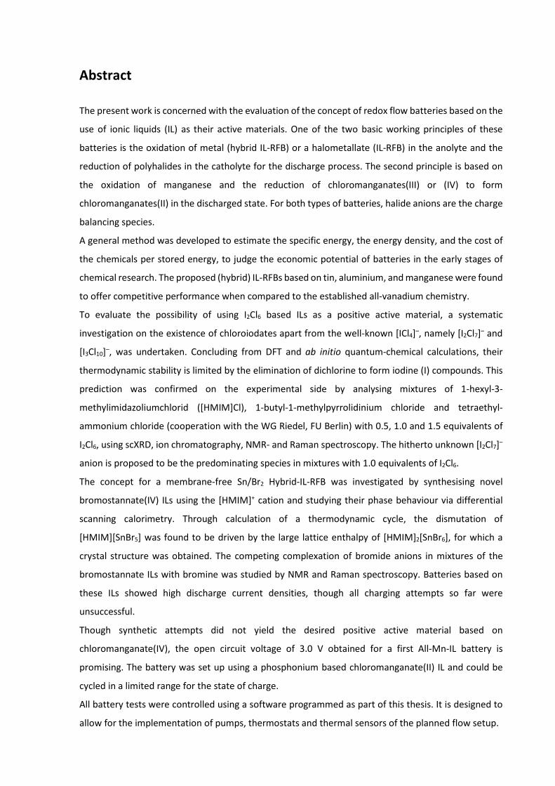
Abstract
The present work is concerned with the evaluation of the concept of redox flow batteries based on the
use of ionic liquids (IL) as their active materials. One of the two basic working principles of these
batteries is the oxidation of metal (hybrid IL-RFB) or a halometallate (IL-RFB) in the anolyte and the
reduction of polyhalides in the catholyte for the discharge process. The second principle is based on
the oxidation of manganese and the reduction of chloromanganates(III) or (IV) to form
chloromanganates(II) in the discharged state. For both types of batteries, halide anions are the charge
balancing species.
A general method was developed to estimate the specific energy, the energy density, and the cost of
the chemicals per stored energy, to judge the economic potential of batteries in the early stages of
chemical research. The proposed (hybrid) IL-RFBs based on tin, aluminium, and manganese were found
to offer competitive performance when compared to the established all-vanadium chemistry.
To evaluate the possibility of using I2Cl6 based ILs as a positive active material, a systematic
investigation on the existence of chloroiodates apart from the well-known [ICl4]–, namely [I2Cl7]– and
[I3Cl10]–, was undertaken. Concluding from DFT and ab initio quantum-chemical calculations, their
thermodynamic stability is limited by the elimination of dichlorine to form iodine (I) compounds. This
prediction was confirmed on the experimental side by analysing mixtures of 1-hexyl-3-
methylimidazoliumchlorid ([HMIM]Cl), 1-butyl-1-methylpyrrolidinium chloride and tetraethyl-
ammonium chloride (cooperation with the WG Riedel, FU Berlin) with 0.5, 1.0 and 1.5 equivalents of
I2Cl6, using scXRD, ion chromatography, NMR- and Raman spectroscopy. The hitherto unknown [I2Cl7]–
anion is proposed to be the predominating species in mixtures with 1.0 equivalents of I2Cl6.
The concept for a membrane-free Sn/Br2 Hybrid-IL-RFB was investigated by synthesising novel
bromostannate(IV) ILs using the [HMIM]+ cation and studying their phase behaviour via differential
scanning calorimetry. Through calculation of a thermodynamic cycle, the dismutation of
[HMIM][SnBr5] was found to be driven by the large lattice enthalpy of [HMIM]2[SnBr6], for which a
crystal structure was obtained. The competing complexation of bromide anions in mixtures of the
bromostannate ILs with bromine was studied by NMR and Raman spectroscopy. Batteries based on
these ILs showed high discharge current densities, though all charging attempts so far were
unsuccessful.
Though synthetic attempts did not yield the desired positive active material based on
chloromanganate(IV), the open circuit voltage of 3.0 V obtained for a first All-Mn-IL battery is
promising. The battery was set up using a phosphonium based chloromanganate(II) IL and could be
cycled in a limited range for the state of charge.
All battery tests were controlled using a software programmed as part of this thesis. It is designed to
allow for the implementation of pumps, thermostats and thermal sensors of the planned flow setup.
Kurzzusammenfassung
Die vorliegende Arbeit beschäftigt sich mit der Erforschung von Redox-Flow-Batterien auf Basis von
ionischen Flüssigkeiten (ionic liquids, ILs) als Aktivmassen. Eines der zwei grundsätzlichen
Funktionsprinzipien ist die Oxidation eines Metalls (Hybrid-IL-RFB) oder Metallhalogenids (IL-RFB) im
Anolyten und die Reduktion von Polyhalogenverbindungen im Katholyten während des
Entladevorgangs. Das zweite Prinzip beruht auf der Oxidation von elementarem Mangan und der
Reduktion von Chloromanganaten(III) oder (IV) unter Bildung von Chloromanganaten(II) im entladenen
Zustand. Für beide Funktionsprinzipien sind Halogenidionen die ladungsausgleichenden Spezies.
Eine allgemein anwendbare Methode zur Abschätzung von spezifischen Energien, Energiedichten und
Kosten der Chemikalien pro speicherbarer Energie wurde entwickelt. Damit kann das ökonomische
Potential von Batterien im frühen, chemischen Forschungsstadium ermittelt werden. Die
vorgeschlagenen (Hybrid-)IL-RFB auf Basis von Zinn, Aluminium und Mangan erwiesen sich innerhalb
dieser Abschätzung als ökonomisch konkurrenzfähig im Vergleich zur etablierten All-Vanadium-
Chemie.
Die Möglichkeit, ionische Flüssigkeiten auf Basis von I2Cl6 als Aktivmassen zu verwenden, wurde durch
eine systematische Erforschung von bisher unbekannten Chloroiodaten [I2Cl7]– und [I3Cl10]– untersucht.
Quantenchemischen Rechnungen (ab initio und DFT) zeigten, dass die Stabilität dieser Chloroiodate in
Bezug auf die reduktive Eliminierung von elementarem Chlor limitiert ist. Diese Vorhersage
bewahrheitete sich in den experimentellen Arbeiten, bei denen Mischungen von 1-Hexyl-3-
methylimidazoliumchlorid ([HMIM]Cl), 1-Butyl-1-methylpyrrolidiniumchlorid und Tetraethyl-
ammoniumchlorid (in Kooperation mit der AG Riedel, FU Berlin) mit 0.5, 1.0 and 1.5 Äquivalenten I2Cl6
mittels Einkristalldiffraktometrie, Ionenchromatographie, sowie Raman- und NMR-Spektroskopie
untersucht wurden. Das bis dato unbekannte [I2Cl7]– wurde als die vorherrschende anionische Spezies
in Mischungen mit einem Äquivalent I2Cl6 identifiziert.
Das Konzept einer membranfreien Sn/Br2 Hybrid-IL-RFB wurde ausgehend von der Synthese der neuen
Bromostannat(IV)-ILs untersucht. Dazu wurde zunächst deren Phasenverhalten mittels Differenz-
Thermoanalyse studiert. Über die Berechnung eines Kreisprozesses wurde die Dismutierung von
[HMIM][SnBr5] als Resultat der hohen Gitterenergie von [HMIM]2[SnBr6] erklärt, von welchem auch
eine Einkristallstruktur erhalten wurde. Die konkurrierende Komplexierung von Bromidionen in
Mischungen der Bromostannat(IV)-ILs mit Brom wurde mithilfe von Raman- und NMR-Spektroskopie
untersucht. Batterien auf Basis dieser ILs zeigten hohe Entladestromdichten, wobei alle Versuche,
derartige Batterien zu laden, bisher scheiterten.
Obgleich die Versuche zur Synthese von Chloromanganat(IV)-ILs nicht erfolgreich verliefen, zeigte eine
erste All-Mn-IL-Batterie eine hohe Leerlaufspannung von 3.0 V. Die Batterie wurde mit einer
phosphoniumbasierten Chloromanganat(II)-IL aufgebaut und konnte in einem begrenzten Umfang
ihrer Kapazität zykliert werden.
Alle Batteriemessungen wurden mit einer im Rahmen dieser Dissertation programmierten Software
gesteuert. Sie ist darauf ausgelegt, auch die Steuerung von Pumpen, Thermostaten und
Thermosensoren des geplanten Flow-Betriebs zu übernehmen.
Abbreviations and Constants
IL-RFB ionic liquid redox flow battery
(MF)-Hyb-IL-RFB (membrane-free) hybrid ionic liquid redox flow battery
OCV open circuit voltage
SOC state of charge of a battery (in %)
SHE standard hydrogen electrode
UME ultramicroelectrode
RBF round bottom flask
[cat]X salt composed of an organic cation [cat] and a halide X
[Nwxyz]+/[Pwxyz]+ ammonium/phosphonium cations with hydrocarbon substituents of a
chain length indicated by the indices w,x,y and z
[NEt4]+ tetraethyl ammonium
[NBu4]+ tetrabutyl ammonium
[bipyH2]2+ 2,2’-dihydro-2,2’-bipyridinium
[NTf2]– bis((trifluoromethyl)sulfonyl)imide
[OTf]– trifluoromethanesulfonate
[DCA]– dicyanamide
Fc / Fc+ ferrocene / ferrocenium
DCM dichloromethane
iPrOH isopropyl alcohol
o-DFB ortho-difluorbenzol
MeCN acetonitrile
pn 1,2-diaminopropane
scXRD single crystal X-ray diffraction
pXRD powder X-ray diffraction
EDX energy-dispersive X-ray spectroscopy
(F-)IR (far) infrared
NMR nuclear magnetic resonance
DSC differential scanning calorimetry
IC ion chromatography

� amount of substance � mass � molar mass � potential (battery measurement) � electrical resistance � electrical current � Charge � potential (cyclic voltammetry) density conductivity � viscosity
� = 96 485 C mol–1 Farraday constant[1]
[1] P. Atkins, J. de Paula, Atkins’ Physical Chemistry, OUP Oxford, 2006.


1
Table of Content
A Introduction .......................................................................................................................... 5
A.1 Motivation ............................................................................................................................... 5
Why Ionic Liquids?........................................................................................................... 6
Why Redox Flow Batteries? ............................................................................................ 6
A.2 Overview over the Areas of Research Concerned .................................................................. 9
Terms and Definitions used Throughout this Work ........................................................ 9
Redox Flow Batteries ..................................................................................................... 10
Ionic Liquids ................................................................................................................... 14
Redox Flow Batteries Based on Ionic Liquids ................................................................ 17
A.3 Analytical Methods ............................................................................................................... 19
Raman Spectroscopy ..................................................................................................... 19
Electrochemical Characterization of Batteries .............................................................. 21
A.4 Objectives of this Work ......................................................................................................... 27
References ......................................................................................................................................... 29
B IL-RFB: Membrane-Free Concepts and Economic Potential ................................................... 33
B.1 Concepts for a Membrane-Free Flow Battery ....................................................................... 33
General Considerations ................................................................................................. 33
Concepts for a Membrane-Free Hybrid IL Redox Flow Battery System ........................ 35
Discussion ...................................................................................................................... 38
B.2 Tool for the Evaluation of the Economic Potential of IL-RFB Concepts ................................ 41
Scope, General Approach and Systems Studied ........................................................... 42
Equations ....................................................................................................................... 46
Results and Discussion .................................................................................................. 49
Conclusion ..................................................................................................................... 52
References ......................................................................................................................................... 53

2
C Structure and Properties of Novel Chloroiodate(III) Ionic Liquids ........................................... 55
C.1 Introduction ........................................................................................................................... 57
C.2 Results and Discussion ........................................................................................................... 61
Quantum Chemical Calculations I: Structures in the Gas Phase and Thermodynamics 61
Syntheses, Melting Points and Crystal Structures ......................................................... 64
Quantum Chemical Calculations II: Computed Raman Spectra .................................... 71
Identification of the Anions in the Mixtures by Vibrational Spectroscopy ................... 73
C.3 Conclusion and Outlook ........................................................................................................ 77
C.4 Electronic Supporting Information ........................................................................................ 79
Synthesis ........................................................................................................................ 80
Quantum Chemical Calculations.................................................................................... 84
Single-Crystal X-Ray Diffraction ..................................................................................... 88
References ......................................................................................................................................... 92
D Membrane-Free Sn/Br2 Hybrid IL-RFB ................................................................................... 97
D.1 Introduction ........................................................................................................................... 97
Bromostannate Salts and Ionic Liquids.......................................................................... 98
Tin Deposition from Ionic Liquids .................................................................................. 98
Polybromide Ionic Liquids ............................................................................................. 99
Tin and Polybromide Based Batteries.......................................................................... 100
D.2 Results and Discussion ......................................................................................................... 101
Bromostannate(IV)-ILs ................................................................................................. 101
Mixed Bromostannate(IV) and Polybromide ILs.......................................................... 111
Electrochemical Measurements on the System Sn/[HMIM]Br/Br2/SnBr4 ................... 119
D.3 Conclusion and Outlook ...................................................................................................... 137
D.4 Experimental ........................................................................................................................ 139
Theoretical Methods ................................................................................................... 141
Bromostannate Ionic Liquids ....................................................................................... 142
3
Mixtures of [HMIM]Br, Br2, and SnBr4......................................................................... 148
Electrochemistry ......................................................................................................... 151
References ....................................................................................................................................... 155
D.5 Appendix ............................................................................................................................. 158
Crystallographic data for [HMIM]2[SnBr6] ................................................................... 158
E Investigation Towards an All-Mn Hybrid IL-RFB .................................................................. 161
E.1 Introduction ........................................................................................................................ 161
Chloromanganate Salts and Ionic Liquids ................................................................... 161
Manganese Deposition from Ionic Liquids .................................................................. 163
Manganese and Manganese Salts in Batteries ........................................................... 164
E.2 Results and Discussion ........................................................................................................ 165
Chloromanganate(II) Ionic Liquids .............................................................................. 165
Attempted Synthesis of Chloromanganate(IV) ILs ...................................................... 169
All-Mn Hybrid Ionic Liquid Battery Tests ..................................................................... 171
E.3 Conclusion and Outlook ...................................................................................................... 177
E.4 Experimental ....................................................................................................................... 179
Synthesis of Chloromanganat(II) Ionic Liquids ............................................................ 180
Attempted Synthesis of Chloromanganats(IV) ............................................................ 182
Electrochemical Measurements on Solutions of [P666 14]2[MnCl4] in MeCN ................ 187
References ....................................................................................................................................... 189
E.5 Appendix ............................................................................................................................. 191
Crystallographic data for [NEt4]4[MnCl4][MnCl5] ......................................................... 191
Cyclic Voltammetry ..................................................................................................... 192
Powder Diffractogram of K2[MnCl6] ............................................................................ 193
F Development of a Battery Test Setup ................................................................................. 195
F.1 Hardware I: Battery Test Setup for Static Liquid Active Materials ...................................... 195
Test Cell ........................................................................................................................... 195

4
Source Measure Unit, Temperature Control, Environmental Sealing ............................. 197
F.2 Software: bbat ..................................................................................................................... 199
Documentation ................................................................................................................ 201
User Interaction: pcontrol and extras ............................................................................. 203
Inner Workings: script Folder .......................................................................................... 203
F.3 Hardware II: Progress Towards a Flow-Battery Test Setup ................................................. 207
Flow Test Cell ................................................................................................................... 207
Process Engineering ......................................................................................................... 209
References ....................................................................................................................................... 213
F.4 Appendix: bbat Source Code and Documentation .............................................................. 215
documentation ................................................................................................................ 215
testlibrary ........................................................................................................................ 231
pcontrol & extras ............................................................................................................. 238
script ................................................................................................................................ 243
script/lib ........................................................................................................................... 252
script/gnuplot .................................................................................................................. 270
G Conclusion and Outlook ..................................................................................................... 273
Lebenslauf ................................................................................................................................ 277
A.1 Motivation
5
A Introduction
A.1 Motivation
The conviction that the climate change observed throughout the world is caused by human
greenhouse gas emissions has become, despite some exceptions, a politically and scientifically
accepted truth. This recognition was shown most prominently by 195 countries signing the Paris
Agreement, which entered into force on 4 November 2016, and thereby agreed to work towards the
goal of limiting the increase in the global average temperature compared to pre-industrial levels to
well below 2 °C and to pursue efforts to reach only a 1.5 °C increase.[1]
It was predicted that, in order to reach the 1.5 °C goal, carbon dioxide emissions, which are the
dominating cause for global warming, must reach a net zero between the years 2045 to 2060.[2] This
demands a tremendous effort starting as soon as possible, since the window for this change to happen
is closing rapidly.[2]
85 % of the CO2 emitted by Germany in 2013 was caused by the energy sector.[3] This is due to the large
share of 80 % of the total primary energy consumption being provided by fossile fuels, with nuclear
energy and renewable energies having a share of only 8 and 12 %, respectively.[3] The largest share of
the energy related CO2 emission, 45 %, is due to the production of electricity, 19 % are caused by street
traffic, 13 % by households (mostly heating) and the residual 23 % by the industry, the public sector
and a few minor consumers.[3] There are many ways in which the primary energy consumption can and
will have to be lowered, like for example more efficient devices, improved building insulation, or a
general decrease in consumption. It seems likely, at least at the moment that a large share of the street
traffic will be using electric energy in the future. This means that the emission of CO2 can be lowered
by a total of 64 % if the energy used for the production of electricity and the energy consumed by
street traffic will be produced from renewable sources.
One of the troublesome aspects of renewable energy is that the energy is not provided on demand,
but in a fluctuating way. This problem can be met by finding creative ways of shifting the energy
demand, for example by equipping millions of fridges with cold storage devices and charging them only
at times when there is excess energy available[4] or by running washing machines on a remotely
controlled schedule. Another way is to regulate the supply of electricity to the consumer by using
storage systems for the electrical energy. Besides the established pumped hydroelectric energy
storage, two major technologies are investigated at the moment. One is chemical storage, e.g. the
A Introduction
6
production of hydrogen from electricity, the other is electrochemical storage devices, in other words,
secondary batteries, which are the topic of this work.
Why Ionic Liquids?
Ionic liquids (ILs), which are commonly defined as salts with a melting point of 100 °C[5] and often
exhibit melting points below room temperature (RTILs), were first systematically studied and
developed as an electrolyte for battery applications.[6] Since these early times, they have also found
widespread use as a new type of solvent, in synthesis and catalysis, and numerous other applications.[5]
They have, however, not been investigated systematically as an active material for batteries, which
means that the IL itself is used to store the energy, and not merely as a solvent, transporting agent, or,
as in the case of Zn/Br2 batteries, as a complexing agent to reduce the vapour pressure of bromine in
an otherwise aqueous system.
The lifetime of conventional batteries is often limited by changes in the structure of the solid active
materials. In redox flow batteries, this limitation is overcome by dissolving the active materials in a
solvent, though at the cost of a significantly reduced energy density. For cost reasons, the employed
solvent is often water, and so the choice of active materials is limited by its electrochemical potential
window. Since ILs are liquid without the addition of a solvent and typically exhibit a very broad
electrochemical window, their use as active material could potentially combine high energy density
with a long lifetime and additionally allow for the use of active materials, which are not usable in
aqueous solution.
Why Redox Flow Batteries?
From the preliminary results obtained by myself and Dipl.-Chem. Michael Hog during the work on our
diploma theses, it became clear that the achievable energy density would most likely not be able to
compete with existing technologies, like li-ion batteries.[7,8] The alternative use case would be
stationary applications, like the large-scale storage of renewable energies.
For stationary applications, a more complicated redox flow setup is viable, which has the benefit of
allowing to independently scale storage capacity (volume of the tanks) and power output (number of
stacks/specific design). This allows for the batteries to be assembled specifically for each use case.
Compared with the established redox flow systems, the energy densities most likely to be achieved
using ILs were very competitive. Additionally, though there certainly are safety issues associated with

A.1 Motivation
7
storing large amounts of bromine, they are no fire hazard, which is also true for ionic liquids. Both are
certainly not as flammable as Li-ion batteries, which is especially important when thinking of large-
scale applications.
The sum of these considerations led to the decision to investigate the technology of redox flow
batteries based on ionic liquids.

A Introduction
8

A.2 Overview over the Areas of Research Concerned
9
A.2 Overview over the Areas of Research Concerned
The section of this overview which is concerned with ionic liquids is based on the respective chapter
of the introduction to my diploma thesis.[8]
Terms and Definitions used Throughout this Work
Electrochemical cells designed to be used as a convenient source of electrical energy are commonly
referred to as batteries. If the battery can only be discharged once, it is more precisely called a primary
battery, if it can be discharged and charged multiple times, it is called a secondary battery. Since this
work is only concerned with the development of secondary batteries, they will be referred to simply
as “batteries” and the distinction will only be made explicitly, when it is considered helpful for the
reader.
In electrochemical cells, the anode is the electrode at which the oxidation of a chemically active
substance takes place, and the electrode at which the corresponding reduction proceeds is called the
cathode. The respective half cells are called the anodic and the cathodic half-cell, containing the
anolyte and the catholyte. If this convention were followed for secondary batteries, the names of the
electrodes, half-cells, and electrolytes would be different when referring to the charging or the
discharging process. The convention, which will be followed throughout this work, is to define the
name of the electrode in respect to the processes which occur during discharge. This means that the
negative pole, which is in contact with the negative electrochemically active material, is always called
the anode, and the positive pole, which is in contact with the positive electrochemically active material,
is always called the cathode, independent of the actual local reactions occurring.
A redox flow battery (RFB) is typically defined as a battery in which the active material is dissolved in
a solvent throughout all states of charge. A flow battery, in which a phase change of the active material
is observed during operation, for example the deposition of metal, is commonly referred to as a hybrid
redox flow battery (Hyb-RFB).[9] Since this work is also concerned with membrane-free flow batteries,
these shall at some points be abbreviated as MF-Hyb-IL-RFB.
A Introduction
10
Redox Flow Batteries
Many organic and inorganic redox couples have been studied for use as positive/negative active
materials in redox flow batteries, selected examples being Br2/[S2]2–, Ce4+/Zn, Cr2+/Fe3+ couples.[9] The
most common drawback to these battery systems is cross contamination due to the leaching of the
two active materials through the membrane. However, the vanadium RFB and the Zn/Br2 Hyb-RFB
have reached commercialisation and will be covered in more detail in the following sections.
A.2.2.1 General Considerations in Respect to the Physical Design of Redox Flow Batteries
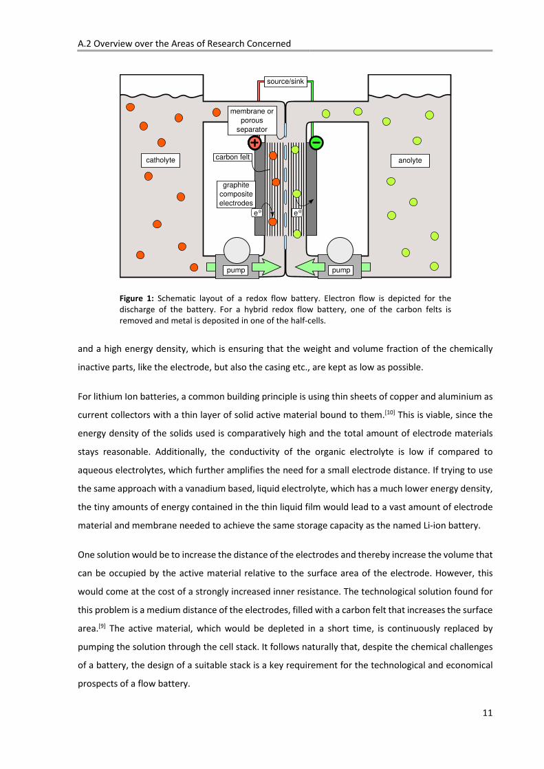
The typical layout of a redox flow battery is shown in Figure 1. The active materials are dissolved in a
solvent and the residual catholyte and anolyte stored in tanks. For charging and discharging, the liquids
are pumped through a cell stack, where the two half cells are separated by a membrane. The space
between the solid electrode plate and the membrane is often filled with a carbon felt to increase the
electrochemically active surface area.
This concept and design of RFBs can easily be seen as a given fact, since development of the technology
started as early as 1971[9] and nowadays commercial products are readily available. Many chemical
species have been investigated as active materials, of which a selection will be covered in the following
sections. However, the chemical systems investigated in this work are significantly different from these
established, mostly aqueous systems. Therefore, this section aims to look at the building principle of
RFBs in a broader perspective by comparing it with the building principle of typical solid state batteries.
In classical batteries, like the Li-ion or the lead-acid battery, the active material is solid and the two
active masses are typically separated by a macroporous insulator.[10] The ions needed to counteract
the charge imbalance produced by electrons being transferred from the anode to the cathode are
transported by the electrolyte, which fills the gap between the electrodes including the pores of the
separator. Since the active masses in redox flow batteries are dissolved in a liquid phase, their electrical
insulation becomes a more challenging part of the chemical design. No liquid electrolyte is needed,
but a solid and selective ion exchange membrane, which is designed to minimize crossover of the active
masses and to only transfer the charge balancing ions. A cheaper alternative to these costly
membranes are micro porous separators, though with the downside of a non-selective operation.
Key goals in the physical design of batteries are to achieve a high power density and a high energy
density at the lowest price possible. To ensure a small inner resistance and high power density, the
surface of the electrode should be as large as possible and the distance between the electrodes as
small as possible. However, this can be contradictive with the measures needed to achieve a low cost
A.2 Overview over the Areas of Research Concerned
11
pump
graphite
composite
electrodes
catholyte
membrane or
porous
separator
e e
anolyte
pump
source/sink
carbon felt
Figure 1: Schematic layout of a redox flow battery. Electron flow is depicted for the discharge of the battery. For a hybrid redox flow battery, one of the carbon felts is removed and metal is deposited in one of the half-cells.
and a high energy density, which is ensuring that the weight and volume fraction of the chemically
inactive parts, like the electrode, but also the casing etc., are kept as low as possible.
For lithium Ion batteries, a common building principle is using thin sheets of copper and aluminium as
current collectors with a thin layer of solid active material bound to them.[10] This is viable, since the
energy density of the solids used is comparatively high and the total amount of electrode materials
stays reasonable. Additionally, the conductivity of the organic electrolyte is low if compared to
aqueous electrolytes, which further amplifies the need for a small electrode distance. If trying to use
the same approach with a vanadium based, liquid electrolyte, which has a much lower energy density,
the tiny amounts of energy contained in the thin liquid film would lead to a vast amount of electrode
material and membrane needed to achieve the same storage capacity as the named Li-ion battery.
One solution would be to increase the distance of the electrodes and thereby increase the volume that
can be occupied by the active material relative to the surface area of the electrode. However, this
would come at the cost of a strongly increased inner resistance. The technological solution found for
this problem is a medium distance of the electrodes, filled with a carbon felt that increases the surface
area.[9] The active material, which would be depleted in a short time, is continuously replaced by
pumping the solution through the cell stack. It follows naturally that, despite the chemical challenges
of a battery, the design of a suitable stack is a key requirement for the technological and economical
prospects of a flow battery.
A Introduction
12
An approach on how to adapt these building principles to the specific characteristics of a RFB utilizing
ILs as its active material is the concept of a membrane-free Hyb-IL-RFB. This concept will be covered
briefly in the section regarding IL-RFBs within this chapter and discussed in detail in Section B.1.
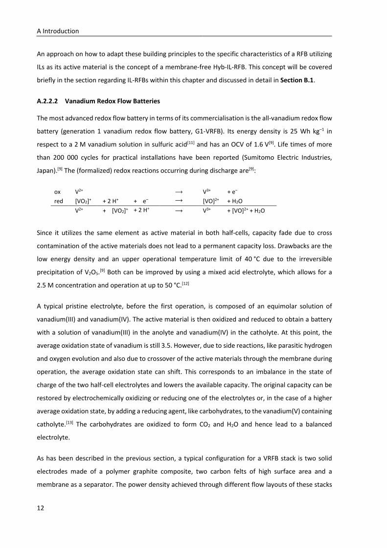
A.2.2.2 Vanadium Redox Flow Batteries
The most advanced redox flow battery in terms of its commercialisation is the all-vanadium redox flow
battery (generation 1 vanadium redox flow battery, G1-VRFB). Its energy density is 25 Wh kg–1 in
respect to a 2 M vanadium solution in sulfuric acid[11] and has an OCV of 1.6 V[9]. Life times of more
than 200 000 cycles for practical installations have been reported (Sumitomo Electric Industries,
Japan).[9] The (formalized) redox reactions occurring during discharge are[9]:
ox V2+ ⟶ V3+ + e–
red [VO2]+ + 2 H+ + e– ⟶ [VO]2+ + H2O
V2+ + [VO2]+ + 2 H+ ⟶ V3+ + [VO]2+ + H2O
Since it utilizes the same element as active material in both half-cells, capacity fade due to cross
contamination of the active materials does not lead to a permanent capacity loss. Drawbacks are the
low energy density and an upper operational temperature limit of 40 °C due to the irreversible
precipitation of V2O5.[9] Both can be improved by using a mixed acid electrolyte, which allows for a
2.5 M concentration and operation at up to 50 °C.[12]
A typical pristine electrolyte, before the first operation, is composed of an equimolar solution of
vanadium(III) and vanadium(IV). The active material is then oxidized and reduced to obtain a battery
with a solution of vanadium(III) in the anolyte and vanadium(IV) in the catholyte. At this point, the
average oxidation state of vanadium is still 3.5. However, due to side reactions, like parasitic hydrogen
and oxygen evolution and also due to crossover of the active materials through the membrane during
operation, the average oxidation state can shift. This corresponds to an imbalance in the state of
charge of the two half-cell electrolytes and lowers the available capacity. The original capacity can be
restored by electrochemically oxidizing or reducing one of the electrolytes or, in the case of a higher
average oxidation state, by adding a reducing agent, like carbohydrates, to the vanadium(V) containing
catholyte.[13] The carbohydrates are oxidized to form CO2 and H2O and hence lead to a balanced
electrolyte.
As has been described in the previous section, a typical configuration for a VRFB stack is two solid
electrodes made of a polymer graphite composite, two carbon felts of high surface area and a
membrane as a separator. The power density achieved through different flow layouts of these stacks
A.2 Overview over the Areas of Research Concerned
13
is a key cost factor for the price of the cell, since in case of a high power density, less of all of these
materials, and especially of the expensive membrane, need to be used.[14] The total cost of the system
also largely depends on whether a high or a low power to capacity ratio is desired.[14] For a
1 MW/4 MWh system, 48 % of the costs are due to the battery chemicals, whereas the next highest
cost fraction is 22 % for the membrane. For a 1 MW/0.25 MWh system, the membrane costs are even
higher, contributing 42 % of the total system costs.
Though many large scale commercial installations have been commissioned, and the number of papers
published on this type of battery did breach 300 in 2014, there is still little research attributed to this
type of battery, when compared to technologies like Li-Ion batteries or fuel cells.[15]
For the generation 2 vanadium redox flow battery (G2-VRFB), the bromide salts of vanadium are used
in a mixed HCl/HBr electrolyte.[16] Improvements include a higher energy density of 25–50 Wh kg–1 and
a wider operational temperature window.[16] Upon oxidation during charging, polyhalide anions
including [ClBr2]– form, which are complexed in an organic layer in similarity to the Zn/Br2 Hyb-RFB.
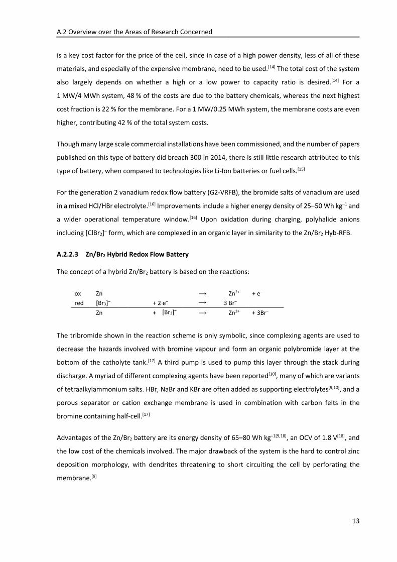
A.2.2.3 Zn/Br2 Hybrid Redox Flow Battery
The concept of a hybrid Zn/Br2 battery is based on the reactions:
ox Zn ⟶ Zn2+ + e–
red [Br3]– + 2 e– ⟶ 3 Br–
Zn + [Br3]– ⟶ Zn2+ + 3Br–
The tribromide shown in the reaction scheme is only symbolic, since complexing agents are used to
decrease the hazards involved with bromine vapour and form an organic polybromide layer at the
bottom of the catholyte tank.[17] A third pump is used to pump this layer through the stack during
discharge. A myriad of different complexing agents have been reported[10], many of which are variants
of tetraalkylammonium salts. HBr, NaBr and KBr are often added as supporting electrolytes[9,10], and a
porous separator or cation exchange membrane is used in combination with carbon felts in the
bromine containing half-cell.[17]
Advantages of the Zn/Br2 battery are its energy density of 65–80 Wh kg–1[9,18], an OCV of 1.8 V[18], and
the low cost of the chemicals involved. The major drawback of the system is the hard to control zinc
deposition morphology, with dendrites threatening to short circuiting the cell by perforating the
membrane.[9]
A Introduction
14
N
[BMP]+
butyl
NNalkyl
ethyl
butyl
hexyl
octyl
[EMIM]+
[BMIM]+
[HMIM]+
[OMIM]+
alkyl =
PF
F
FF
FF
[PF6]- [BF4]
-
B
F
F
FF
Al
Cl
Cl
ClCl
[AlCl4]-⁻
NSO2CF3
[NTf2]-
F3CO2S
Ionic Liquids
This section is intended to give a brief overview on the history of research on ILs and their general
properties. More information related to the specific ILs relevant to this work will be given in the
introductions to the respective chapters.
As has been stated previously, ILs are commonly defined as salts having a melting point below 100 °C.[5]
Most ILs consist of an organic cation and a polyatomic anion, and the first report[5] about such liquid
salts was published early in the 20th century.[19] In 1978, the U.S. Airforce Academy was looking for
electrolytes for a possible aluminum/chlorine battery and thereby rediscovered a family of ILs that had
first been mentioned in 1948.[5] These ILs were based on alkylpyridinium cations and aluminum halides,
but since the pyridinium cation was prone to chemical and electrochemical reduction, it was soon
replaced by dialkylimidazolium. IL-stability towards water was achieved by replacing haloaluminate
anions with water stable anions in 1992.[20][5] Some of the most commonly employed anions and
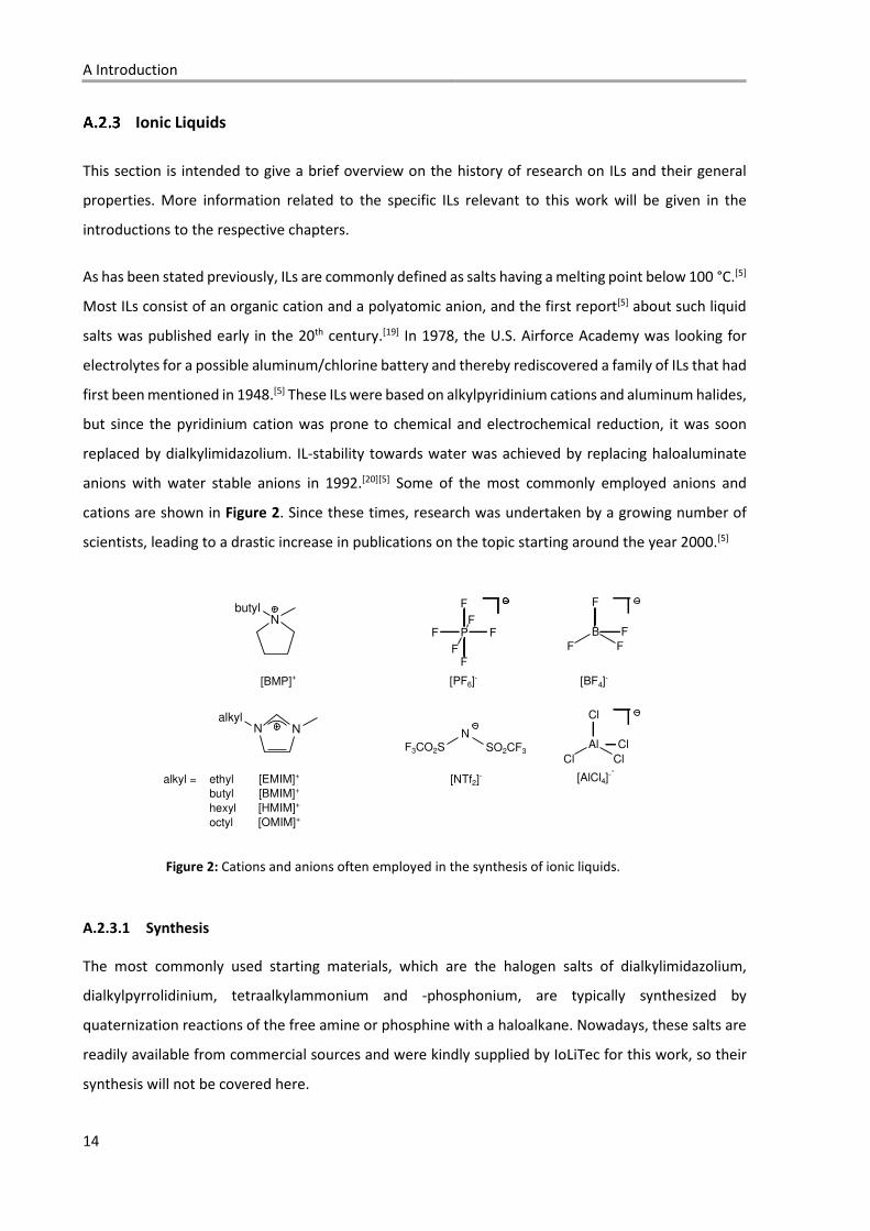
cations are shown in Figure 2. Since these times, research was undertaken by a growing number of
scientists, leading to a drastic increase in publications on the topic starting around the year 2000.[5]
Figure 2: Cations and anions often employed in the synthesis of ionic liquids.
A.2.3.1 Synthesis
The most commonly used starting materials, which are the halogen salts of dialkylimidazolium,
dialkylpyrrolidinium, tetraalkylammonium and -phosphonium, are typically synthesized by
quaternization reactions of the free amine or phosphine with a haloalkane. Nowadays, these salts are
readily available from commercial sources and were kindly supplied by IoLiTec for this work, so their
synthesis will not be covered here.
A.2 Overview over the Areas of Research Concerned
15
The synthetic route for ILs based on these cations follows mostly two routes starting from the
mentioned halide salts.[10] The first route, which is also employed for all ILs studied in this work, is the
addition of Lewis acids, like metal halides or halogens, to the [cat]X halide salt. The exact type of anion
obtained as an adduct of the Lewis acid and the Lewis basic halide depends strongly on the
stochiometric ratio of the two components. For example, the addition of one equivalent of AlCl3 to
1-ethyl-3-methyl-imidazolium chloride ([EMIM]Cl) yields the [AlCl4]– anion, however, for higher
stochiometric ratios of AlCl3, the formation of complicated mixtures of larger anions like [Al2Cl7]– and
even [Al3Cl10]– is observed.[21]
The second synthetic route is based on metathesis reactions for which the [cat]X salt is mixed with a
silver or lithium salt of the desired anion. The resulting silver/lithium halide salt has to be insoluble in
the formed IL and can then be removed by filtration.[5]
A.2.3.2 Physical Properties
The basic physical properties of some common imidazolium based ionic liquids are shown in Table 1.
Melting points are usually measured through differential scanning calorimetry (DSC), but are
sometimes hard to determine due to glass and other more complex phase transitions.[5] In general, the
melting points of ILs increase with the number of charges per ion. Lower melting points are found for
less symmetric ions and often with increasing ion size.[5] Influences by more specific interactions
between cation and anion for certain combinations thereof are also common.[5]
In regard to organic cations, which are usually designed to carry only one positive charge, the
symmetry and the length of alkyl substituents are the most influencing factors for the melting points.
For imidazolium cations, the substitution pattern is important, with the most common modification
being the variation of the length of one alkyl chain substituent, as is also seen in the data shown in
Table 1. For 1-alkyl-3-methyl-imidazolium cation ([RMIM]+), melting points decrease on lengthening
the alkyl chain, but start to increase as decyl substituents are reached. The first decline is due to a
decrease in packing efficiency and the later increase can be attributed to growing van der Waals
forces.[5] Melting points also increase with increased branching of the substituents, since rotational
freedom of the alkyl chain is hindered, which results in lower melting entropies.[5]
ILs often behave as Newtonian fluids[5] and can vary in their viscosity from 10 to 20.000 mPa s and
more. The viscosity is strongly dependent on temperature and on purity, for example, a concentration
of 2 wt% water can lower the viscosity of [BMIM][BF4] by 50 %.[5] For comparison, the viscosities of
pentane, water, and sulfuric acid are 0.224, 0.891, and 27 mPa s respectively.[30] Viscosity increases in
A Introduction
16
most cases with the length of the alkyl substituents and the symmetry of the organic cation. It is not
generally correlated to the size of the anion and rather influenced by anion specific interaction with
the cations.[5]
The properties of Lewis acid based ILs change on variation of the molar ratio of their components. This
is also shown in Table 1 for the ILs resulting from mixtures of [EMIM]Cl and AlCl3 with molar ratios of
1:1 and 1:2.
The upper limit of the liquid range is usually determined by the decomposition temperature, which is
determined through thermogravimetric analysis (TGA) and can be as high as 350 °C.[5]
A.2.3.3 Electrochemical Properties
One of the limiting factors for the use of a specific solvent for electrochemical applications is its
potential window. For ILs, this is usually defined by the potentials for the reduction of the cation and
the oxidation of the anion.[5] These can be measured through cyclic voltammetry and can be
significantly influenced by impurities like water or halides.
The cathodic limit for [RMIM]+ cations is usually set by the reduction of the hydrogen atom in the
2-position.[5] The anodic limit is reduced in basic aluminum chloride ILs that contain free chloride, since
it is more easily oxidized than chloride coordinated to aluminum.[5] In acidic mixtures, the anodic
(reduction) limit of these ILs is further lowered due to the reduction of aggregated anions.[5]
ILs exhibit good conductivity compared to other non-aqueous solvents, but are less conductive than
concentrated solutions of salts in water. Temperature dependence is often linear above room
temperature (Arrhenius behavior) though negative deviations are observed when approaching the
glass transition temperature of the respective IL and conductivities are best explained with the Vogel-
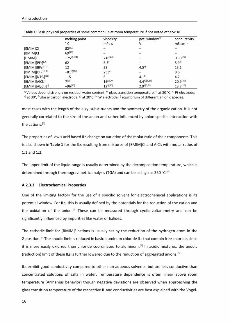
Table 1: Basic physical properties of some common ILs at room temperature if not noted otherwise.
melting point ° C
viscosity mPa s
pot. windowa) V
conductivity mS cm–1
[EMIM]Cl 82[22] – – – [BMIM]Cl 69[23] – – – [HMIM]Cl –75b),[24] 716[24] – 0.30[25] [EMIM][PF6][26] 62 6.3c) – 5.9c) [EMIM][BF4][27] 12 38 4.5c) 13.1 [BMIM][BF4][28] –81b)[24] 233e) – 8.6 [EMIM][NTf2][26] –15 6 4.1f) 4.7 [EMIM][AlCl4] 7[20] 16g)[20] 4.4h)[5,29] 20.9[20] [EMIM][Al2Cl7]h) –96[20] 12f)[20] 2.9i)[5,29] 13.7[20] a) Values depend strongly on residual water content; b) glass transition temperature; c) at 80 °C; d) Pt electrode; e) at 30°; f) glassy carbon electrode; g) at 20°C; h) W electrode; i) equilibrium of different anionic species.
A.2 Overview over the Areas of Research Concerned
17
Tammann-Fulcher equation in this region.[5] Again, impurities have a strong effect, potentially due to
the resulting decrease or increase in viscosity.[5] Accordingly, the addition of a co-solvent can
significantly increase conductivity and is associated with effects like solvation of the anion, decreased
ion pairing and thus resulting greater mobility of the charge carriers.[5] For high mole fractions of co-
solvent, conductivity decreases caused by the lowering of the concentration of charge carriers.
There is a strong interest in ILs as possible electrolytes for the deposition of metals such as aluminum,
titanium and tungsten.[31] These materials offer excellent corrosion stability but cannot be deposited
from aqueous solution. Even though a lot of metals have already been successfully deposited from ILs,
the mechanism of these reactions is still unclear and more research is needed to develop controlled
and reproducible processes. A literature overview for the deposition of tin and manganese from ILs
will be given in Chapters D and E, respectively.
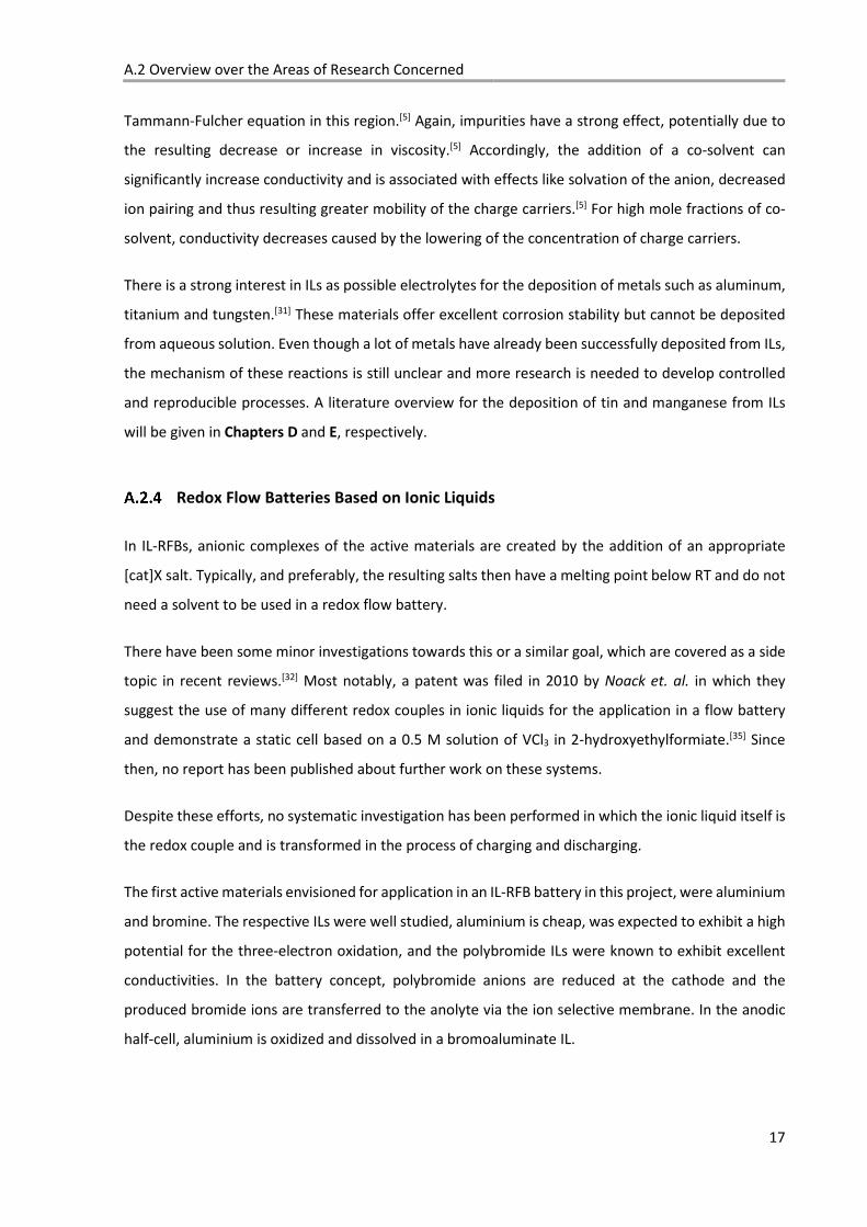
Redox Flow Batteries Based on Ionic Liquids
In IL-RFBs, anionic complexes of the active materials are created by the addition of an appropriate
[cat]X salt. Typically, and preferably, the resulting salts then have a melting point below RT and do not
need a solvent to be used in a redox flow battery.
There have been some minor investigations towards this or a similar goal, which are covered as a side
topic in recent reviews.[32] Most notably, a patent was filed in 2010 by Noack et. al. in which they
suggest the use of many different redox couples in ionic liquids for the application in a flow battery
and demonstrate a static cell based on a 0.5 M solution of VCl3 in 2-hydroxyethylformiate.[35] Since
then, no report has been published about further work on these systems.
Despite these efforts, no systematic investigation has been performed in which the ionic liquid itself is
the redox couple and is transformed in the process of charging and discharging.
The first active materials envisioned for application in an IL-RFB battery in this project, were aluminium
and bromine. The respective ILs were well studied, aluminium is cheap, was expected to exhibit a high
potential for the three-electron oxidation, and the polybromide ILs were known to exhibit excellent
conductivities. In the battery concept, polybromide anions are reduced at the cathode and the
produced bromide ions are transferred to the anolyte via the ion selective membrane. In the anodic
half-cell, aluminium is oxidized and dissolved in a bromoaluminate IL.
A Introduction
18
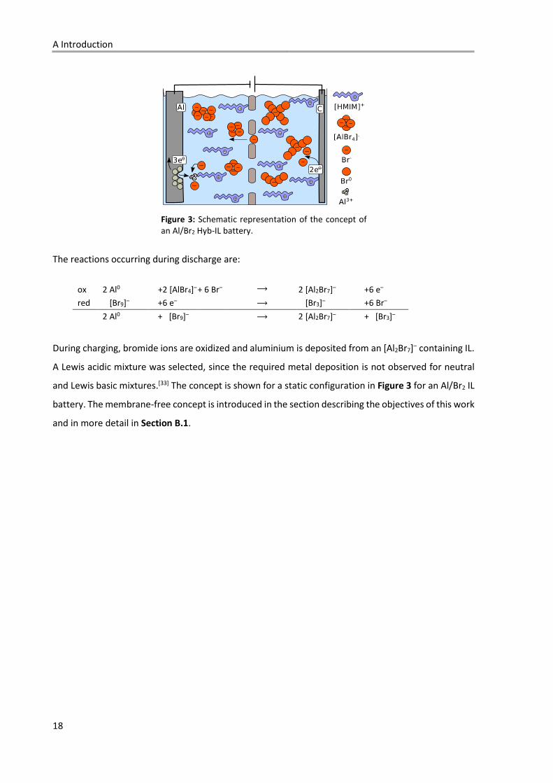
Figure 3: Schematic representation of the concept of an Al/Br2 Hyb-IL battery.
The reactions occurring during discharge are:
ox 2 Al0 +2 [AlBr4]– + 6 Br– ⟶ 2 [Al2Br7]– +6 e–
red [Br9]– +6 e– ⟶ [Br3]– +6 Br–
2 Al0 + [Br9]– ⟶ 2 [Al2Br7]– + [Br3]–
During charging, bromide ions are oxidized and aluminium is deposited from an [Al2Br7]– containing IL.
A Lewis acidic mixture was selected, since the required metal deposition is not observed for neutral
and Lewis basic mixtures.[33] The concept is shown for a static configuration in Figure 3 for an Al/Br2 IL
battery. The membrane-free concept is introduced in the section describing the objectives of this work
and in more detail in Section B.1.
A.3 Analytical Methods
19
A.3 Analytical Methods
The major concern of this work was the synthesis of anionic coordination complexes and their
transformation through electrochemical reactions. Many analytical methods including nuclear
magnetic resonance (NMR), (far-) infrared ((F-)IR), and Raman spectroscopy, powder and single crystal
X-ray diffraction (pXRD, scXRD), quantum-chemical calculations (QCC), elemental analysis (EA), ion
chromatography (IC), differential scanning calorimetry (DSC), measurement of viscosity and
conductivity, cyclic voltammetry (CV), and chronoamperometry (CA) were employed for the
investigation. Raman spectroscopy and electrochemical characterization of batteries were most
strongly relied upon and will be covered explicitly in this section.
Raman Spectroscopy
Physicist C.V. Raman first observed an effect, which was later named in honour of its discoverer, that
when matter is irradiated using monochromatic light, the scattered light includes a small amount with
a slightly shifted frequency.[34] This shift is caused by an interaction of the electromagnetic wave with
the irradiated compound and its vibrational states. The interaction relevant for the Raman scattering
is only observed when the compound has vibrational modes in which its polarizability changes.[34] For
such an interaction, the energy of the scattered wave or photon is increased or decreased by the
amount of energy stored in the vibrational mode. If the respective vibration was excited before the
interaction (Stokes scattering), the energy of the scattered photon is increased, and it is lowered if the
vibration was not excited but is excited after the interaction (anti-Stokes scattering).[34] The first
comprehensive publication about Raman spectroscopy, the analytical method based on this effect,
was published by Kohlrausch in 1943 and gained in popularity with the event of high energy lasers.[34]
In combination with IR spectroscopy, most of the vibrations of a molecule can be studied, though not
all frequencies are Raman and IR active. For molecules with an inversion centre, the exclusion rule
applies, which means that only those vibrations symmetrical to the inversion centre are Raman active,
and all others are only IR active.[34]
A.3.1.1 Normal Modes for Selected Coordination Polyhedra
Particles moving in three-dimensional space have three degrees of freedom. When particles, in this
case atoms, are combined to form molecules, the total number of degrees of freedom for the molecule
is three times the number of its atoms N. When reserving three degrees of freedom for the translation
of the complete molecule in space, and three for its rotation split into the components for three axes
A Introduction
20
(two for linear molecules), then the remaining 3N – 6 degrees of freedom for non-linear molecules are
related to its internal movements.[34] The combined internal movements of the atoms of the molecule
can be split into the 3N – 6 independent vibrations, its so called normal modes, which can be visualized
and be assigned to a specific frequency.[34] For symmetrical molecules or coordination complexes,
some of these normal modes can be degenerate, which means they are closely related and exhibit the
same frequency. The lower the symmetry, and the higher the number of atoms in the molecule or
coordination complex, the more non-degenerate normal modes are present, and the more complex
becomes their visualisation. In these cases, quantum-chemical calculations can be of great help to
visualise the vibrational modes and to calculate their expected frequencies.
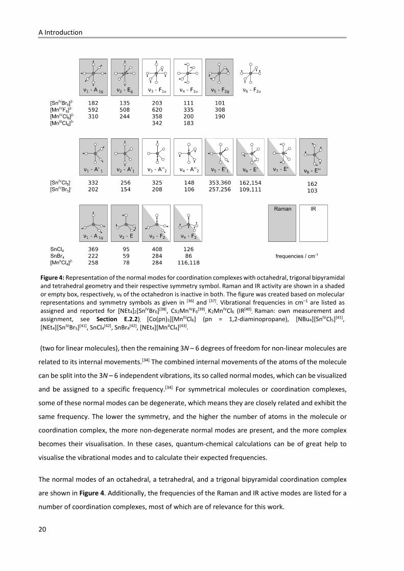
The normal modes of an octahedral, a tetrahedral, and a trigonal bipyramidal coordination complex
are shown in Figure 4. Additionally, the frequencies of the Raman and IR active modes are listed for a
number of coordination complexes, most of which are of relevance for this work.
Figure 4: Representation of the normal modes for coordination complexes with octahedral, trigonal bipyramidal and tetrahedral geometry and their respective symmetry symbol. Raman and IR activity are shown in a shaded or empty box, respectively, ν6 of the octahedron is inactive in both. The figure was created based on molecular representations and symmetry symbols as given in [36] and [37]. Vibrational frequencies in cm–1 are listed as assigned and reported for [NEt4]2[SnIVBr6][38], Cs2MnIVF6
[39], K2MnIVCl6 (IR[40]
, Raman: own measurement and assignment, see Section E.2.2), [Co(pn)3][MnIIICl6] (pn = 1,2-diaminopropane), [NBu4][SnIVCl5][41], [NEt4][SnIVBr5][41], SnCl4[42], SnBr4
[42], [NEt4][MnIICl4][43].
A.3 Analytical Methods
21
When comparing the frequencies of SnBr4, SnCl4 and [MnCl4]2–, or [MnCl6]3– and [MnCl6]2–, general
trends are observable, namely that the vibrational frequency depends not only on the geometry, but
also on the type of bonding, the mass of the ligand and the central atom, the oxidation states and in
general the electronic structure of the molecule or coordination complex in focus.[36] The vibrational
modes for more complicated cases, like for example [I2Cl7]– or [I3Cl10]– with a C2 and a C1 symmetry,
respectively, will be covered in detail in Section C.2.3.
Electrochemical Characterization of Batteries
A.3.2.1 Open Circuit Voltage, State of Charge and Self-Discharge
One of the key properties of a battery is its open circuit voltage (OCV, UOC), which is the voltage
measured when no external current is allowed to flow. For many battery types, the OCV reaches its
highest value at a state of charge (SOC) of 100 % and decreases for lower SOCs due to changes in the
concentration of the active masses, morphology changes and other effects.[18] It can therefore often
be used as an indicator for the current SOC of the battery, if the exact relationship has been
determined experimentally. This can be done by charging and discharging the battery, while
intermediately measuring the OCV at regular intervals. The self-discharge behaviour of a battery can
then be tested by charging a battery to a certain SOC, stopping the current flow and then observing
the change of the OCV over time.
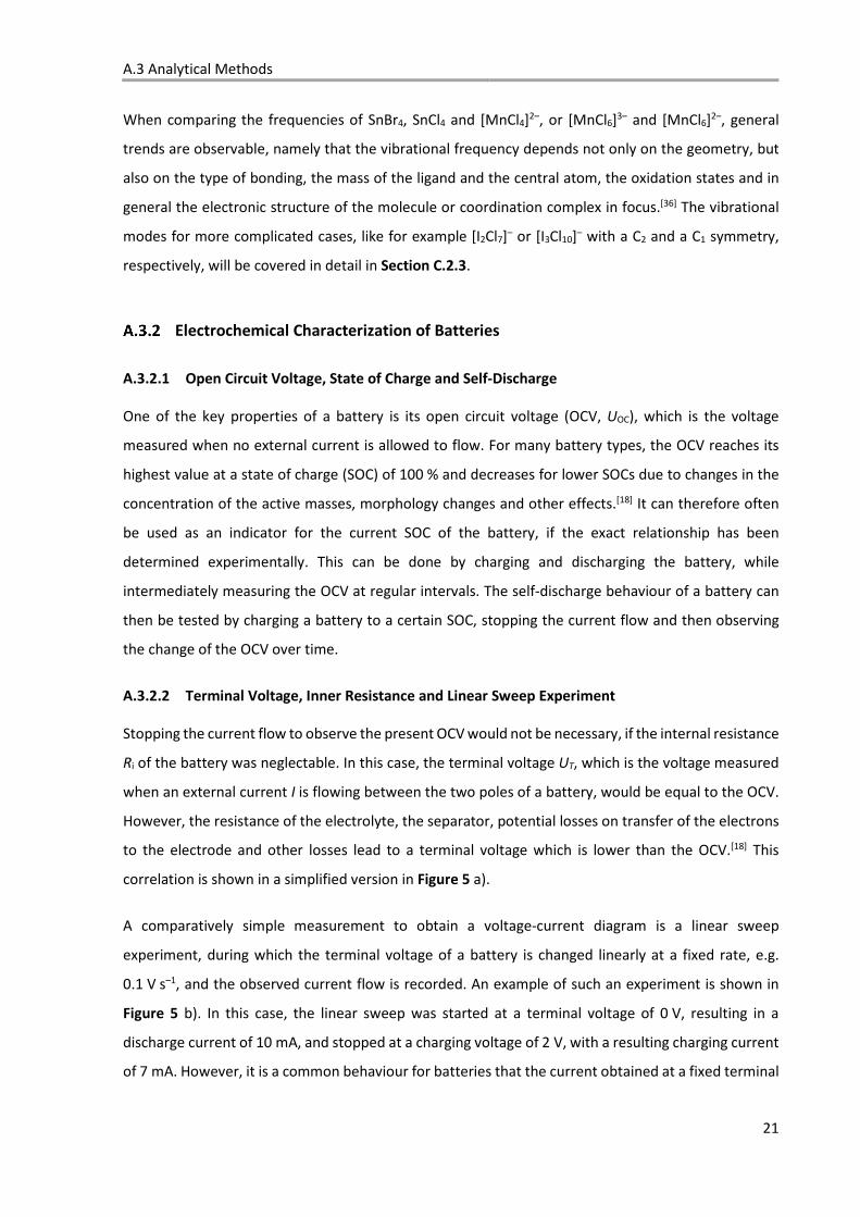
A.3.2.2 Terminal Voltage, Inner Resistance and Linear Sweep Experiment
Stopping the current flow to observe the present OCV would not be necessary, if the internal resistance
Ri of the battery was neglectable. In this case, the terminal voltage UT, which is the voltage measured
when an external current I is flowing between the two poles of a battery, would be equal to the OCV.
However, the resistance of the electrolyte, the separator, potential losses on transfer of the electrons
to the electrode and other losses lead to a terminal voltage which is lower than the OCV.[18] This
correlation is shown in a simplified version in Figure 5 a).
A comparatively simple measurement to obtain a voltage-current diagram is a linear sweep
experiment, during which the terminal voltage of a battery is changed linearly at a fixed rate, e.g.
0.1 V s–1, and the observed current flow is recorded. An example of such an experiment is shown in
Figure 5 b). In this case, the linear sweep was started at a terminal voltage of 0 V, resulting in a
discharge current of 10 mA, and stopped at a charging voltage of 2 V, with a resulting charging current
of 7 mA. However, it is a common behaviour for batteries that the current obtained at a fixed terminal
A Introduction
22
I
U
UOC
Re I
R i I
R i I
charge
discharge
power output
internal heat lossesUT
−5
0
5
0.0 0.5 1.0 1.5 2.0
cu
rre
nt
/ m
A
potential / V
a) b)
Figure 5: a) Simplified schematic of the relationship between the terminal voltage UT and the current I for an assumed constant inner resistance Ri while charging or discharging. The internal and external potential losses can be calculated by multiplying the internal or the external resistance (Ri, Re) with the current I. The figure was modified based on a scheme in [18]. b) Sweep measurement performed for a terminal voltage of 0 to 2 V at a sweep rate of 0.1 V s–1 on a membrane-free Sn/Br2 IL battery. The measurement is depicted with reversed x and y axes compared to the figures in the rest of the work in order to be visually compatible with figure a).
voltage decreases over time. This is due to a local depletion in the concentration of the charged active
masses,[18] a non-equilibrium state which is reversed through diffusion, or in the case of flow batteries
by forced convection, when the current flow is stopped. A result obtained by a sweep measurement is
therefore always a combination of this time dependent drop in the current and all other effects which
are only related to the current flow.
A.3.2.3 Polarisation Curves and Area Specific Resistance
A polarisation experiment is a more sophisticated measurement procedure compared to the linear
sweep. It allows to specifically obtain information about the effects caused by a changing current flow
and to isolate them from the time dependent changes on current and terminal voltage. The specific
form of this widely applied method was adopted from a procedure suggested by our collaboration
partner Kolja Bromberger from Fraunhofer ISE.
In this experiment, the battery is subjected to predefined and increasing charge and discharge
currents. The measurement is typically performed at an SOC 50 %, but charging polarisations or
discharging polarisations can also be measured at an SOC 0 % and 100 %, respectively. In all cases, the
currents are only applied for a short interval, after which the current flow is interrupted for a resting
phase. This phase has to be set to be long enough to allow the battery to recover into a state close to
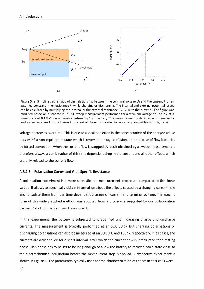
the electrochemical equilibrium before the next current step is applied. A respective experiment is
shown in Figure 6. The parameters typically used for the characterization of the static test cells were
A.3 Analytical Methods
23
a 15 second current pulse followed by a resting state of 45 seconds. The currents were set to
experimentally determined values based on an upper limit for the terminal voltage during charging as
defined individually for each tested battery, and a lower limit of 0 V for the terminal voltage during
discharge.
From the obtained values, the area specific resistance (ASR) can be calculated for each current pulse,
the results being characteristic for the battery under testing. If measured and calculated in a
standardised way for multiple batteries, the ASR values become a valuable tool to judge and compare
the performance of different cell designs and/or different chemical systems.
In our case, the ASR values were calculated, as suggested by Kolja Bromberger, based on the difference
of the voltage ΔU between the last measurement point of the OCV UOC and the first measurement
point for the terminal voltage U1 measured at the specified current I1 0.5 seconds later. With the
electrode surface A, the ASR is obtained according to Equation (1).
��� = �� − ����� ∙ � = ∆��� ∙ � (1)
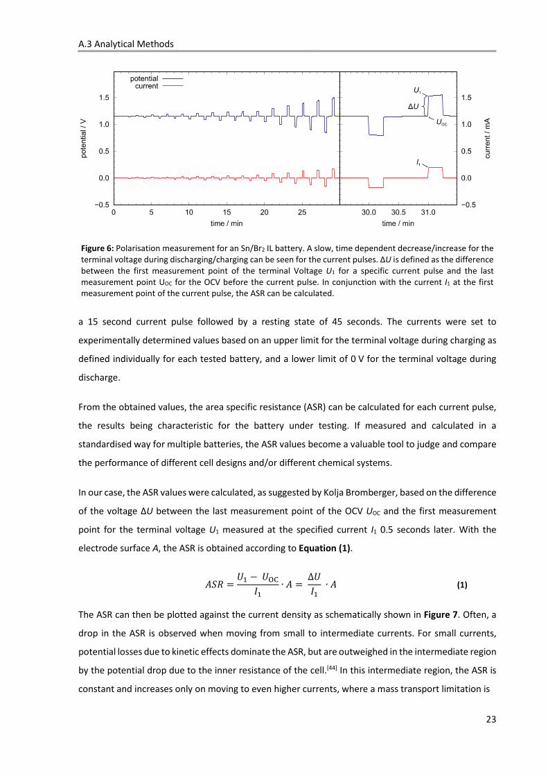
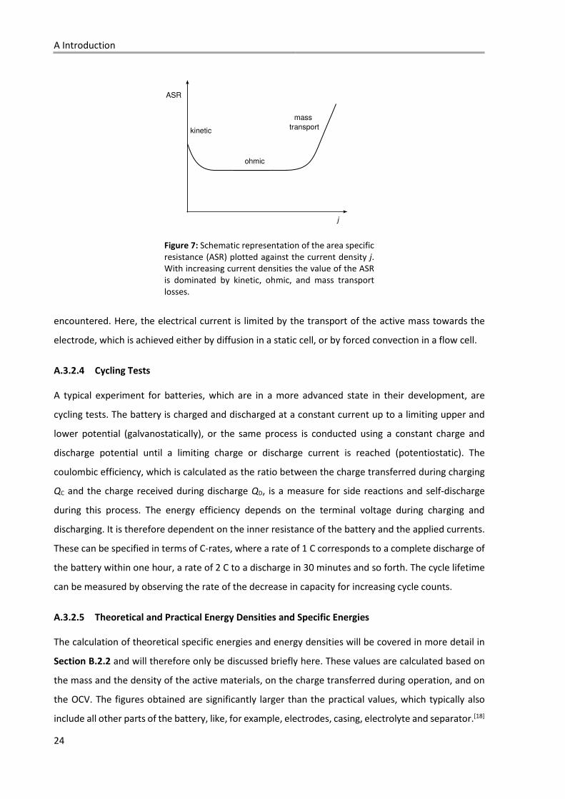
The ASR can then be plotted against the current density as schematically shown in Figure 7. Often, a
drop in the ASR is observed when moving from small to intermediate currents. For small currents,
potential losses due to kinetic effects dominate the ASR, but are outweighed in the intermediate region
by the potential drop due to the inner resistance of the cell.[44] In this intermediate region, the ASR is
constant and increases only on moving to even higher currents, where a mass transport limitation is
Figure 6: Polarisation measurement for an Sn/Br2 IL battery. A slow, time dependent decrease/increase for the terminal voltage during discharging/charging can be seen for the current pulses. ΔU is defined as the difference between the first measurement point of the terminal Voltage U1 for a specific current pulse and the last measurement point UOC for the OCV before the current pulse. In conjunction with the current I1 at the first measurement point of the current pulse, the ASR can be calculated.
A Introduction
24
j
ASR
ohmic
kinetic
mass
transport
Figure 7: Schematic representation of the area specific resistance (ASR) plotted against the current density j. With increasing current densities the value of the ASR is dominated by kinetic, ohmic, and mass transport losses.
encountered. Here, the electrical current is limited by the transport of the active mass towards the
electrode, which is achieved either by diffusion in a static cell, or by forced convection in a flow cell.
A.3.2.4 Cycling Tests
A typical experiment for batteries, which are in a more advanced state in their development, are
cycling tests. The battery is charged and discharged at a constant current up to a limiting upper and
lower potential (galvanostatically), or the same process is conducted using a constant charge and
discharge potential until a limiting charge or discharge current is reached (potentiostatic). The
coulombic efficiency, which is calculated as the ratio between the charge transferred during charging
QC and the charge received during discharge QD, is a measure for side reactions and self-discharge
during this process. The energy efficiency depends on the terminal voltage during charging and
discharging. It is therefore dependent on the inner resistance of the battery and the applied currents.
These can be specified in terms of C-rates, where a rate of 1 C corresponds to a complete discharge of
the battery within one hour, a rate of 2 C to a discharge in 30 minutes and so forth. The cycle lifetime
can be measured by observing the rate of the decrease in capacity for increasing cycle counts.
A.3.2.5 Theoretical and Practical Energy Densities and Specific Energies
The calculation of theoretical specific energies and energy densities will be covered in more detail in
Section B.2.2 and will therefore only be discussed briefly here. These values are calculated based on
the mass and the density of the active materials, on the charge transferred during operation, and on
the OCV. The figures obtained are significantly larger than the practical values, which typically also
include all other parts of the battery, like, for example, electrodes, casing, electrolyte and separator.[18]

A.3 Analytical Methods
25
The practical values can also be specified in respect to a defined discharge current using the respective
terminal voltage, in which case they are even lower, though closest to values obtained during real
application.[18] For RFBs, the theoretical values are commonly given based on the mass and density of
the electrolyte and the concentration of the active material in conjunction with the OCV.

A Introduction
26
A.4 Objectives of this Work
27
A.4 Objectives of this Work
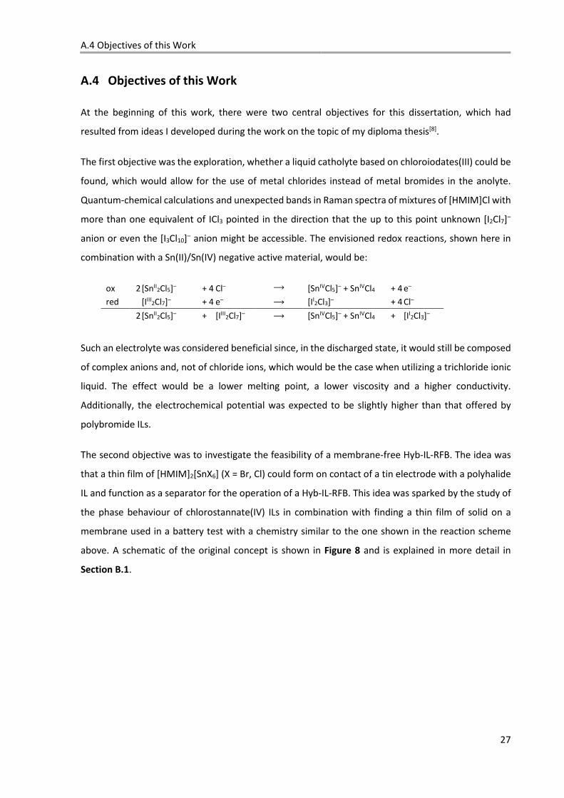
At the beginning of this work, there were two central objectives for this dissertation, which had
resulted from ideas I developed during the work on the topic of my diploma thesis[8].
The first objective was the exploration, whether a liquid catholyte based on chloroiodates(III) could be
found, which would allow for the use of metal chlorides instead of metal bromides in the anolyte.
Quantum-chemical calculations and unexpected bands in Raman spectra of mixtures of [HMIM]Cl with
more than one equivalent of ICl3 pointed in the direction that the up to this point unknown [I2Cl7]–
anion or even the [I3Cl10]– anion might be accessible. The envisioned redox reactions, shown here in
combination with a Sn(II)/Sn(IV) negative active material, would be:
ox 2 [SnII2Cl5]– + 4 Cl– ⟶ [SnIVCl5]– + SnIVCl4 + 4 e–
red [IIII2Cl7]– + 4 e– ⟶ [II
2Cl3]– + 4 Cl–
2 [SnII2Cl5]– + [IIII
2Cl7]– ⟶ [SnIVCl5]– + SnIVCl4 + [II2Cl3]–
Such an electrolyte was considered beneficial since, in the discharged state, it would still be composed
of complex anions and, not of chloride ions, which would be the case when utilizing a trichloride ionic
liquid. The effect would be a lower melting point, a lower viscosity and a higher conductivity.
Additionally, the electrochemical potential was expected to be slightly higher than that offered by
polybromide ILs.
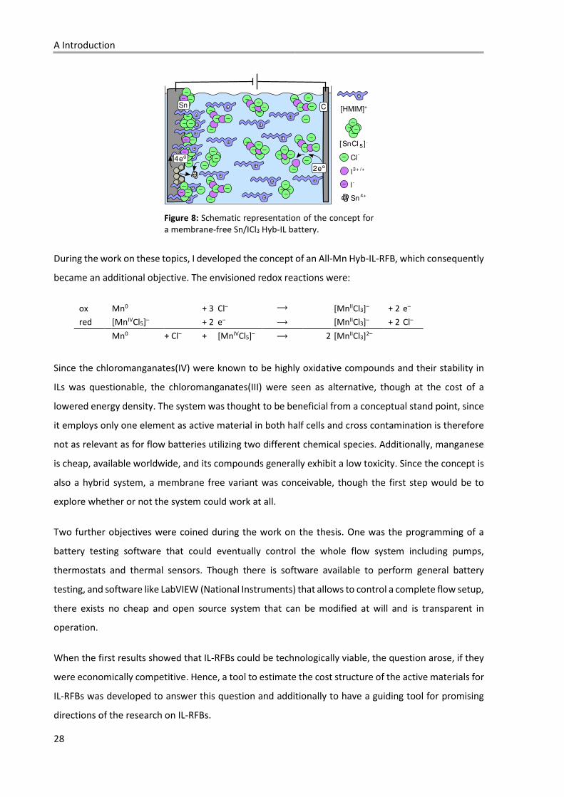
The second objective was to investigate the feasibility of a membrane-free Hyb-IL-RFB. The idea was
that a thin film of [HMIM]2[SnX6] (X = Br, Cl) could form on contact of a tin electrode with a polyhalide
IL and function as a separator for the operation of a Hyb-IL-RFB. This idea was sparked by the study of
the phase behaviour of chlorostannate(IV) ILs in combination with finding a thin film of solid on a
membrane used in a battery test with a chemistry similar to the one shown in the reaction scheme
above. A schematic of the original concept is shown in Figure 8 and is explained in more detail in
Section B.1.
A Introduction
28
C
2e
Sn
4e
[SnCl 5 ] -
Cl-
Sn4+
l3+ /+
l-
[HMIM]+
Figure 8: Schematic representation of the concept for a membrane-free Sn/ICl3 Hyb-IL battery.
During the work on these topics, I developed the concept of an All-Mn Hyb-IL-RFB, which consequently
became an additional objective. The envisioned redox reactions were:
ox Mn0 + 3 Cl– ⟶ [MnIICl3]– + 2 e–
red [MnIVCl5]– + 2 e– ⟶ [MnIICl3]– + 2 Cl–
Mn0 + Cl– + [MnIVCl5]– ⟶ 2 [MnIICl3]2–
Since the chloromanganates(IV) were known to be highly oxidative compounds and their stability in
ILs was questionable, the chloromanganates(III) were seen as alternative, though at the cost of a
lowered energy density. The system was thought to be beneficial from a conceptual stand point, since
it employs only one element as active material in both half cells and cross contamination is therefore
not as relevant as for flow batteries utilizing two different chemical species. Additionally, manganese
is cheap, available worldwide, and its compounds generally exhibit a low toxicity. Since the concept is
also a hybrid system, a membrane free variant was conceivable, though the first step would be to
explore whether or not the system could work at all.
Two further objectives were coined during the work on the thesis. One was the programming of a
battery testing software that could eventually control the whole flow system including pumps,
thermostats and thermal sensors. Though there is software available to perform general battery
testing, and software like LabVIEW (National Instruments) that allows to control a complete flow setup,
there exists no cheap and open source system that can be modified at will and is transparent in
operation.
When the first results showed that IL-RFBs could be technologically viable, the question arose, if they
were economically competitive. Hence, a tool to estimate the cost structure of the active materials for
IL-RFBs was developed to answer this question and additionally to have a guiding tool for promising
directions of the research on IL-RFBs.
A.4 Objectives of this Work
29
References
[1] United Nations, “Paris Agreement”, can be found under https://treaties.un.org, 2017.
[2] J. Rogelj, G. Luderer, R. C. Pietzcker, E. Kriegler, M. Schaeffer, V. Krey, K. Riahi, Nat. Clim. Change
2015, 5, 519.
[3] H.-M. Henning, A. Palzer, Was kostet die Energiewende? Wege zur Transformation des deutschen
Energiesystems bis 2050, Freiburg, 2017.
[4] A. Hauer, M. Braun, H. C. Gils, D. Laing, S. Gschwander in Forschung für ein nachhaltiges Strom-
Wärme-System (Themen 2013), Forschungsverbund Erneuerbare Energien, Berlin, 2014.
[5] P. Wasserscheid, T. Welton, Ionic Liquids in Synthesis, Wiley-VCH, Weinheim, 2007.
[6] A. A. Fannin Jr, D. A. Floreani, L. A. King, J. S. Landers, B. J. Piersma, D. J. Stech, R. L. Vaughn, J. S.
Wilkes, L. Williams John, J. Phys. Chem. 1984, 88, 2614.
[7] M. Hog, University of Freiburg, Freiburg im Breisgau, 2013.
[8] S. B. Burgenmeister, University of Freiburg, Freiburg im Breisgau, Germany, 2013.
[9] M. Skyllas-Kazacos, M. H. Chakrabarti, S. A. Hajimolana, F. S. Mjalli, M. Saleem, J. Electrochem.
Soc. 2011, 158, R55-R79.
[10] J. O. Besenhard (Ed.) Handbook of Battery Materials, Wiley-VCH, 2011.
[11] M. Skyllas-Kazacos, C. Peng, M. Cheng, Electrochem. Solid-State Lett. 1999, 2, 121.
[12] S. Kim, M. Vijayakumar, W. Wang, J. Zhang, B. Chen, Z. Nie, F. Chen, J. Hu, L. Li, Z. Yang, Phys.
Chem. Chem. Phys. 2011, 13, 18186.
[13] M. Keshavarz, G. Zu, WO2016069402 (A1), 2017.
[14] B. R. Chalamala, T. Soundappan, G. R. Fisher, M. R. Anstey, V. V. Viswanathan, M. L. Perry, Proc.
IEEE 2014, 102, 976.
[15] M. L. Perry, A. Z. Weber, J. Electrochem. Soc. 2016, 163, A5064-A5067.
[16] M. Skyllas-Kazacos, G. Kazacos, G. Poon, H. Verseema, Int. J. Energy Res. 2010, 34, 182.
[17] C. Ponce de León, A. Frías-Ferrer, J. González-García, D. A. Szánto, F. C. Walsh, J. Power Sources
2006, 160, 716.
[18] C. H. Hamann, W. Vielstich, Elektrochemie, Wiley-VCH, 2005.
[19] P. Walden, Bull. Acad. Imper. Sci. (St. Petersburg) 1914, 8, 405.
A Introduction
30
[20] J. S. Wilkes, M. J. Zaworotko, J. Chem. Soc., Chem. Commun. 1992, 0, 965.
[21] H. A. Øye, M. Jagtoyen, T. Oksefjell, J. S. Wilkes, Mater. Sci. Forum 1991, 73-75, 183.
[22] A. Bagno, F. D’Amico, G. Saielli, ChemPhysChem 2007, 8, 873.
[23] U. Domańska, E. Bogel-Łukasik, R. Bogel-Łukasik, Chem. Eur. J. 2003, 9, 3033.
[24] J. G. Huddleston, A. E. Visser, W. M. Reichert, H. D. Willauer, G. A. Broker, R. D. Rogers, Green
Chem. 2001, 3, 156.
[25] C. Guerrero-Sanchez, T. Lara-Ceniceros, E. Jimenez-Regalado, M. Raşa, U. S. Schubert, Adv.
Mater. 2007, 19, 1740.
[26] A. B. McEwen, H. L. Ngo, K. LeCompte, J. L. Goldman, J. Electrochem. Soc. 1999, 146, 1687.
[27] J. Fuller, R. T. Carlin, R. A. Osteryoung, J. Electrochem. Soc. 1997, 144, 3881.
[28] P. a. Z. Suarez, S. Einloft, J. E. L. Dullius, R. F. d. Souza, J. Dupont, J. Chim. Phys. 1998, 95, 1626.
[29] Z. J. Karpinski, R. A. Osteryoung, Inorg. Chem. 1984, 23, 1491.
[30] P. W. Atkins, J. de Paula, Atkins’ Physical chemistry, Oxford University Press, Oxford, New York,
2006.
[31] F. Endres, D. MacFarlane, A. Abbott (Eds.) Electrodeposition from Ionic Liquids, Wiley-VCH, 2008.
[32] a) S.-H. Shin, S.-H. Yun, S.-H. Moon, RSC Adv. 2013, 3, 9095; b) A. Parasuraman, T. M. Lim, C.
Menictas, M. Skyllas-Kazacos, Electrochim. Acta 2013, 101, 27; c) G. L. Soloveichik, Chem. Rev.
2015, 115, 11533; d) J. Noack, N. Roznyatovskaya, T. Herr, P. Fischer, Angew. Chem. Int. Ed.
2015, 54, 9776.
[33] J. S. Wilkes, J. A. Levisky, R. A. Wilson, C. L. Hussey, Inorg. Chem. 1982, 21, 1263.
[34] W. J. Moore, D. O. Hummel, G. Trafara, Physikalische Chemie, de Gruyter, Berlin, 1986.
[35] J. Noack, J. Tuebke, K. Pinkwart, DE102009009357 (A1), 2010.
[36] K. Nakamoto, Infrared and Raman spectra of inorganic and coordination compounds, Wiley-
Blackwell, Oxford, 2009.
[37] J. Weidlein, U. Müller, K. Dehnicke, Schwingungsspektroskopie: eine Einführung, Thieme,
Stuttgart, 1988.
[38] R. J. H. Clark, L. Maresca, R. J. Puddephatt, Inorg. Chem. 1968, 7, 1603.
[39] C. D. Flint, J. Mol. Spectrosc. 1971, 37, 414.

A.4 Objectives of this Work
31
[40] D. M. Adams, D. M. Morris, J. Chem. Soc. A 1968, 694.
[41] J. A. Creighton, J. H. S. Green, J. Chem. Soc. A 1968, 808.
[42] R. J. H. Clark, D. M. Rippon, J. Chem. Soc. D 1971, 0, 1295.
[43] J. S. Avery, C. D. Burbridge, D. M. L. Goodgame, Spectrochim. Acta, Part A 1968, 24, 1721.
[44] D. Aaron, Z. Tang, A. B. Papandrew, T. A. Zawodzinski, J. Appl. Electrochem. 2011, 41, 1175.

A Introduction
32

B.1 Concepts for a Membrane-Free Flow Battery
33
B IL-RFB: Membrane-Free Concepts and Economic Potential
B.1 Concepts for a Membrane-Free Flow Battery
Though this work in general and this section in particular mainly concentrates on tin and bromine as
active materials for a membrane-free IL-RFBs, the general principle does apply to similar Hyb-IL-RFBs
based on other elements.
General Considerations
In a classical Redox flow battery, in which both active masses are liquid, a membrane is indispensable
to prevent direct reaction of the oxidizing and the reductive species. As has been stated in the
introduction, the need to use an ion exchange membrane has several drawbacks like
� high price
� increase in inner cell resistance
� possible mechanical failure
� not preventing crossover completely.
These limitations apply in the same manner to IL-RFBs. The crossover of ions is especially problematic
in cells which, unlike the V-RFB, use different elements in both half cells and can lead to an irreversible
capacity fade.[1]
The need for a membrane is less pronounced in hybrid redox flow cells, in which the reaction of the
reducing and the oxidizing species is hindered by the limited surface of the phase boundary. However,
for Hyb-IL-RFBs, additional considerations have to be made.
As has been described in the introduction, the ILs used in IL-RFBs are formed by combining the active
material with a [cat]X salt. On charging a Hyb-IL-RFB, part of the active material is removed from the
anolyte and deposited as solid metal. The remaining [cat]X salt often has a higher melting point
compared to the original IL and also a dramatically decreased electrical conductivity.
This problem is mirrored in the catholyte, where, on discharging, the active material is reduced and
again, the [cat]X salt remains. The composition of the liquid and solid phases for both charged and
discharged state of an Sn/Br2 Hyb-IL-RFB are listed in the top section of Table 2.
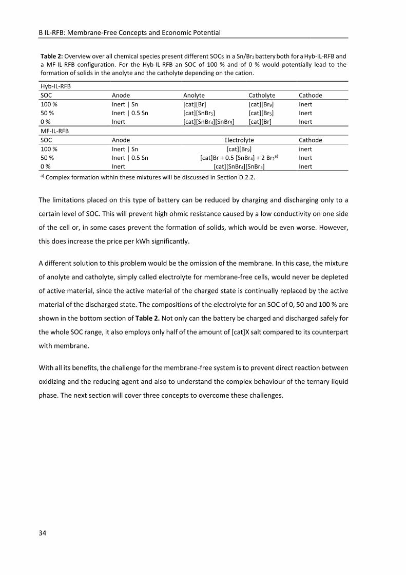
B IL-RFB: Membrane-Free Concepts and Economic Potential
34
Table 2: Overview over all chemical species present different SOCs in a Sn/Br2 battery both for a Hyb-IL-RFB and a MF-IL-RFB configuration. For the Hyb-IL-RFB an SOC of 100 % and of 0 % would potentially lead to the formation of solids in the anolyte and the catholyte depending on the cation.
Hyb-IL-RFB
SOC Anode Anolyte Catholyte Cathode
100 % Inert | Sn [cat][Br] [cat][Br9] Inert 50 % Inert | 0.5 Sn [cat][SnBr5] [cat][Br5] Inert 0 % Inert [cat][SnBr4][SnBr5] [cat][Br] Inert
MF-IL-RFB
SOC Anode Electrolyte Cathode
100 % Inert | Sn [cat][Br9] inert 50 % Inert | 0.5 Sn [cat]Br + 0.5 [SnBr4] + 2 Br2
a) Inert 0 % Inert [cat][SnBr4][SnBr5] Inert a) Complex formation within these mixtures will be discussed in Section D.2.2.
The limitations placed on this type of battery can be reduced by charging and discharging only to a
certain level of SOC. This will prevent high ohmic resistance caused by a low conductivity on one side
of the cell or, in some cases prevent the formation of solids, which would be even worse. However,
this does increase the price per kWh significantly.
A different solution to this problem would be the omission of the membrane. In this case, the mixture
of anolyte and catholyte, simply called electrolyte for membrane-free cells, would never be depleted
of active material, since the active material of the charged state is continually replaced by the active
material of the discharged state. The compositions of the electrolyte for an SOC of 0, 50 and 100 % are
shown in the bottom section of Table 2. Not only can the battery be charged and discharged safely for
the whole SOC range, it also employs only half of the amount of [cat]X salt compared to its counterpart
with membrane.
With all its benefits, the challenge for the membrane-free system is to prevent direct reaction between
oxidizing and the reducing agent and also to understand the complex behaviour of the ternary liquid
phase. The next section will cover three concepts to overcome these challenges.
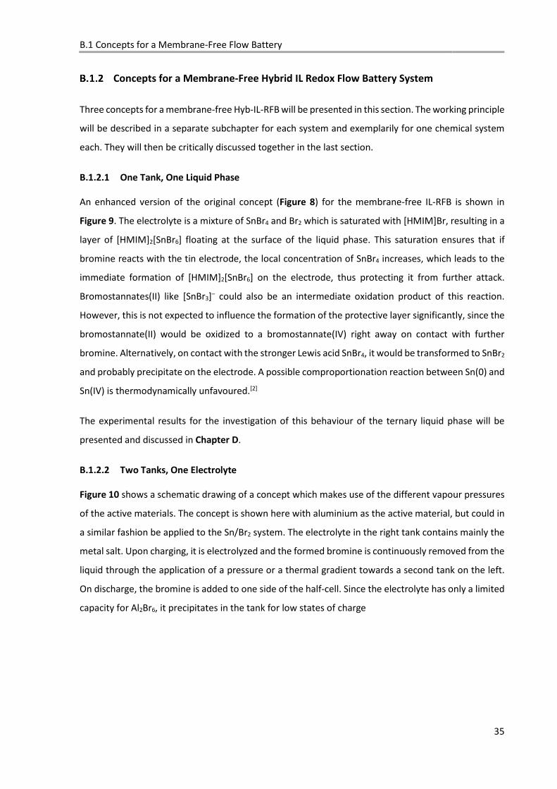
B.1 Concepts for a Membrane-Free Flow Battery
35
Concepts for a Membrane-Free Hybrid IL Redox Flow Battery System
Three concepts for a membrane-free Hyb-IL-RFB will be presented in this section. The working principle
will be described in a separate subchapter for each system and exemplarily for one chemical system
each. They will then be critically discussed together in the last section.
B.1.2.1 One Tank, One Liquid Phase
An enhanced version of the original concept (Figure 8) for the membrane-free IL-RFB is shown in
Figure 9. The electrolyte is a mixture of SnBr4 and Br2 which is saturated with [HMIM]Br, resulting in a
layer of [HMIM]2[SnBr6] floating at the surface of the liquid phase. This saturation ensures that if
bromine reacts with the tin electrode, the local concentration of SnBr4 increases, which leads to the
immediate formation of [HMIM]2[SnBr6] on the electrode, thus protecting it from further attack.
Bromostannates(II) like [SnBr3]– could also be an intermediate oxidation product of this reaction.
However, this is not expected to influence the formation of the protective layer significantly, since the
bromostannate(II) would be oxidized to a bromostannate(IV) right away on contact with further
bromine. Alternatively, on contact with the stronger Lewis acid SnBr4, it would be transformed to SnBr2
and probably precipitate on the electrode. A possible comproportionation reaction between Sn(0) and
Sn(IV) is thermodynamically unfavoured.[2]
The experimental results for the investigation of this behaviour of the ternary liquid phase will be
presented and discussed in Chapter D.
B.1.2.2 Two Tanks, One Electrolyte
Figure 10 shows a schematic drawing of a concept which makes use of the different vapour pressures
of the active materials. The concept is shown here with aluminium as the active material, but could in
a similar fashion be applied to the Sn/Br2 system. The electrolyte in the right tank contains mainly the
metal salt. Upon charging, it is electrolyzed and the formed bromine is continuously removed from the
liquid through the application of a pressure or a thermal gradient towards a second tank on the left.
On discharge, the bromine is added to one side of the half-cell. Since the electrolyte has only a limited
capacity for Al2Br6, it precipitates in the tank for low states of charge
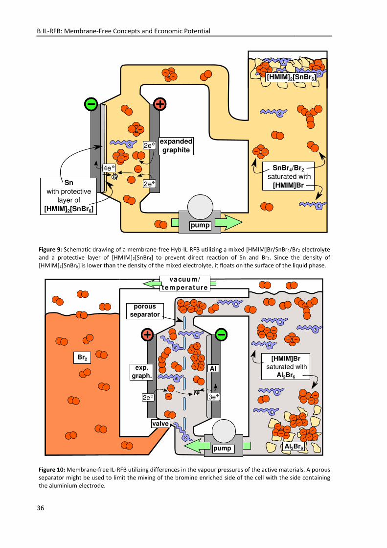
B IL-RFB: Membrane-Free Concepts and Economic Potential
36
SnBr4/Br2
saturated with
[HMIM]BrSn
with protective
layer of
[HMIM]2[SnBr6]
pump
expanded
graphite
2e
4e
[HMIM]2[SnBr6]
2e
[HMIM]Br
saturated with
Al2Br6
Al
pump Al2Br6
exp.
graph.
vacuum /
t em perat ure
Br2
valve
porous
separator
2e 3e
Figure 9: Schematic drawing of a membrane-free Hyb-IL-RFB utilizing a mixed [HMIM]Br/SnBr4/Br2 electrolyte and a protective layer of [HMIM]2[SnBr4] to prevent direct reaction of Sn and Br2. Since the density of [HMIM]2[SnBr6] is lower than the density of the mixed electrolyte, it floats on the surface of the liquid phase.
Figure 10: Membrane-free IL-RFB utilizing differences in the vapour pressures of the active materials. A porous separator might be used to limit the mixing of the bromine enriched side of the cell with the side containing the aluminium electrode.
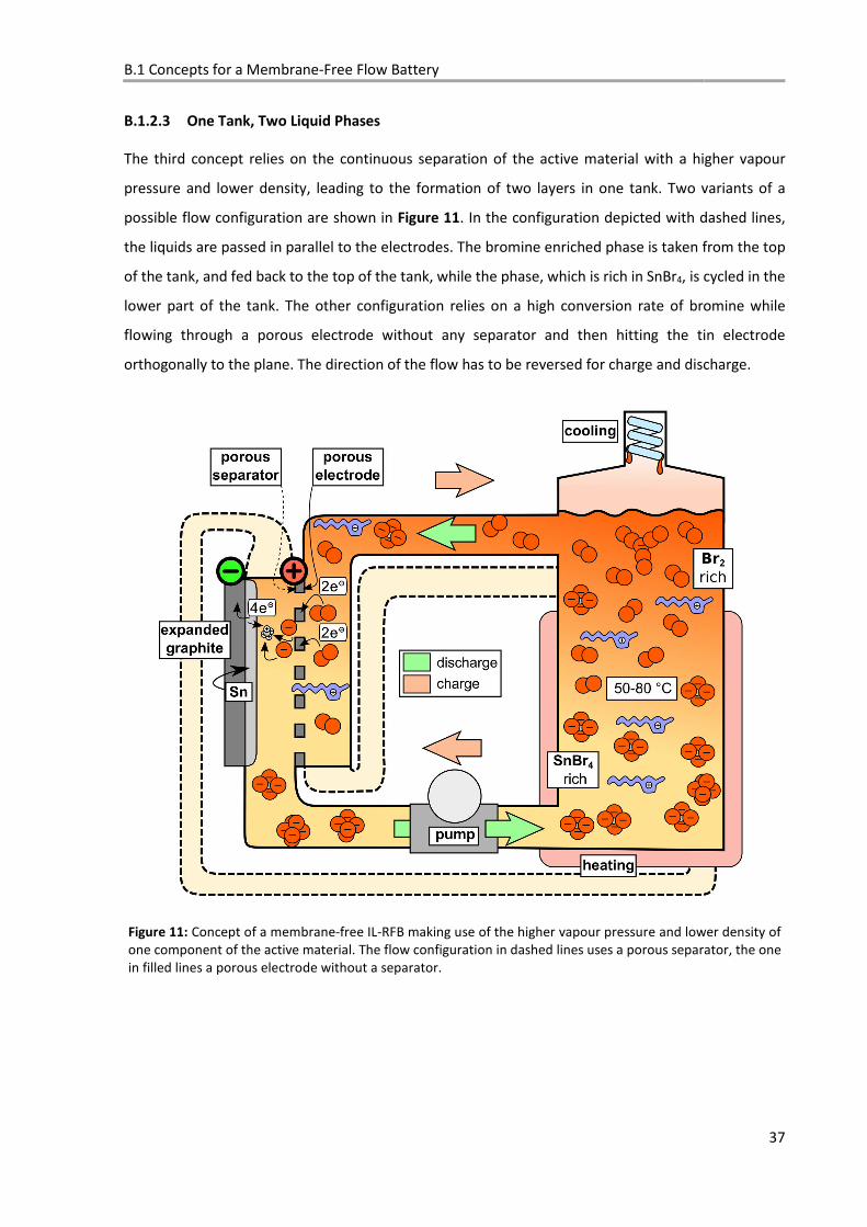
B.1 Concepts for a Membrane-Free Flow Battery
37
B.1.2.3 One Tank, Two Liquid Phases
The third concept relies on the continuous separation of the active material with a higher vapour
pressure and lower density, leading to the formation of two layers in one tank. Two variants of a
possible flow configuration are shown in Figure 11. In the configuration depicted with dashed lines,
the liquids are passed in parallel to the electrodes. The bromine enriched phase is taken from the top
of the tank, and fed back to the top of the tank, while the phase, which is rich in SnBr4, is cycled in the
lower part of the tank. The other configuration relies on a high conversion rate of bromine while
flowing through a porous electrode without any separator and then hitting the tin electrode
orthogonally to the plane. The direction of the flow has to be reversed for charge and discharge.
Figure 11: Concept of a membrane-free IL-RFB making use of the higher vapour pressure and lower density of one component of the active material. The flow configuration in dashed lines uses a porous separator, the one in filled lines a porous electrode without a separator.
B IL-RFB: Membrane-Free Concepts and Economic Potential
38
Discussion
The first concept presented in Section B.1.2.1 is advantageous compared to the other two concepts in
terms of the necessary process engineering. While it can be operated at elevated temperature, its basic
principle does not rely on it. The vapour pressure can be kept as low as possible and does not have to
be maximized for the system to work efficiently. However, the metal deposition could be more
challenging when performed through a layer of salt. Also, if the conditions in the battery might change
due to a malfunction, so that the protective layer gets damaged or dissolve completely at a high state
of charge, a direct reaction between the metal and the halogen would be unhindered and a significant
amount of energy would be released.
The second and third option do not rely on a protective layer on the tin electrode and are therefore
chemically less complex systems. A safety concern could be the inherent high vapour pressure of
bromine. This is especially the case for the second concept since the bromine is stored in an external
tank without any IL additive that could reduce the vapour pressure. It might be possible, though, to
keep this tank at a lower temperature to help the removal of bromine from the IL phase and to reduce
the vapour pressure. For example, a heat pump could be used to transfer thermal energy from the
bromine tank to the tank containing the electrolyte, but the cost of this thermal pumping has to be
weighed against the benefits of a membrane-free system.
For the third concept, keeping the whole apparatus under a pure bromine atmosphere would help in
increasing the rate of a phase separation and reduce the temperature needed for this process. As long
as the temperature of the electrolyte is kept below its atmospheric boiling point, the resulting reduced
pressure inside the apparatus compared to the environment would also be an effective measure to
prevent any leakage of bromine vapour. Since any battery will produce excess heat on charging and
discharging, the heat energy might in this setup be put to good use for the phase separation process.
In conclusion, from a conceptual point of view, systems one and three seem to be the most promising.
The main challenge for both systems is understanding the ternary phase system, which is in this work
consists of Br2, SnBr4 and [HMIM]Br. For the first system, the formation of a protective layer on a tin
electrode and for the third concept, the formation of two layers in a heated tank with condenser at
the top need to be studied.
So far, the feasibility of these concepts has only been judged from a chemical perspective. Another
part of the equation is the question: can the outlined challenges and the necessary investment in
research be outweighed by the economic prospects of a membrane free system? To get an insight into

B.1 Concepts for a Membrane-Free Flow Battery
39
this matter, a tool for the evaluation of the economic potential of specific battery chemistries at the
concept stage will be presented and applied to both IL-RFBs and membrane-free Hyb-IL-RFBs in the
next section.

B IL-RFB: Membrane-Free Concepts and Economic Potential
40

B.2 Tool for the Evaluation of the Economic Potential of IL-RFB Concepts
41
B.2 Tool for the Evaluation of the Economic Potential of IL-RFB Concepts
As soon as our preliminary studies had shown that and how an IL-RFB could work in principle, the
question arose: Do these types of battery have economic potential? Of course, this question is not an
easy one to answer for any technology until its potential does unfold. Especially considering the early
state of the research of the project at that time, any answer, let alone a precise answer, was difficult
to give.
The approach taken in an attempt to answer the question, was partly inspired by the German
translation of an essay titled “The Fermi solution”, which I read several years ago.[3] “Fermi problems”
are named after the famous physicist Enrico Fermi, who challenged his students with questions which
were deliberately chosen to seem very hard to answer at least without further help or information.
One of the questions mentioned in the essay is: How many piano tuners are there in Chicago? Fermi’s
approach on answering such questions was to split the problem into sub problems for which an
estimate can be given either by common sense or by using knowledge already available. In this case,
the number of inhabitants of Chicago was known to be three million, the number of persons in a
household estimated to four and every third household was assumed to own a piano. If a piano is
tuned once every ten years, and a piano tuner can tune four pianos a day, working 250 days per year,
this comes down to an estimate of 25 piano tuners in Chicago. It could be 15 or 60, but probably not
250 or two. Arriving at such a reasonable estimate is possible following many different paths, and
typically the errors in overestimating some parts of the calculation are counterbalanced by
underestimating other parts. Another famous example of this way of thinking is that, by dropping
pieces of paper from above his head as he witnessed the blast wave of the world’s first atomic
explosion, Fermi was able to estimate the released energy to be equivalent to 10 kt of TNT within
moments after the paper had touched the ground. Several weeks later, and after all data had been
meticulously analysed, his estimate was confirmed to be off only by a factor of less than two.
In this spirit, namely that a reasonable estimate is almost always possible and usually better than
simply stating that no precise answer can be given, a tool to evaluate the economic potential of the
different proposed IL-RFB concepts was developed. The goal was to get both a rough estimate whether
or not the concepts could compete with existing technologies and an idea on the direction that would
be most promising for further research. The approach taken is one that does trade a reduced precision
in terms of the resulting numbers for the flexibility to easily compare a large variety of batteries
including a great amount of different stochiometric ratios as well as several different types of battery
chemistries.
B IL-RFB: Membrane-Free Concepts and Economic Potential
42
Based on the results obtained by this tool, some alternative battery chemistries were not pursued
since the results clearly showed that they would not be economical. Only the most favourable systems,
which were also experimentally investigated in the project, will be discussed in the following chapters.
Though more precise numbers can be calculated at the present state of the research and will be
presented in the respective subchapters, the tool will be presented here not only to explain certain
aspects of the direction of the research taken, but also because it can in principal be applied to any
type of battery and could provide a guideline in early stages of research beyond the IL-RFB project.
Scope, General Approach and Systems Studied
B.2.1.1 Scope of the Model
The crucial part for an economic feasibility were considered the energy densities for the different IL-
RFB concepts and the price of the electrolyte per stored energy.
The energy density, or volumetric energy density, is economically relevant because the tanks of an RFB
usually consume the most space of the whole setup, and space in itself and the derived size of the
housing and barrier basin for the battery are a cost factor.
The economically most significant measurement entity for the electrolyte is the price per stored
amount of energy in € kWh–1. Splitting the price to specify contributions from each component was
considered helpful to give an idea on which part of the battery could benefit the most from further
development.
The specific energy, or gravimetric energy density, was considered less relevant for the envisioned
stationary application, but is the basis value for the calculation of prices per stored energy. The cost
for pumps and the cell stack was estimated to be roughly the same as for common V-RFBs.
B.2.1.2 General Approach
Many of the materials to be used in the IL-RFBs were at this stage of the project not commercially
available or had not even been synthesized at all. It was therefore decided to estimate the prices of
the electrolyte by using world market prices for the elements constituting the active materials. For the
[cat]X salts, Dr. Thomas Schubert, CEO and founder of IoLiTec GmbH, kindly provided us with price
estimates for both [HMIM]+ and [N2225]+/[P2225]+ at a 10 t scale. All values are listed in Table 3.
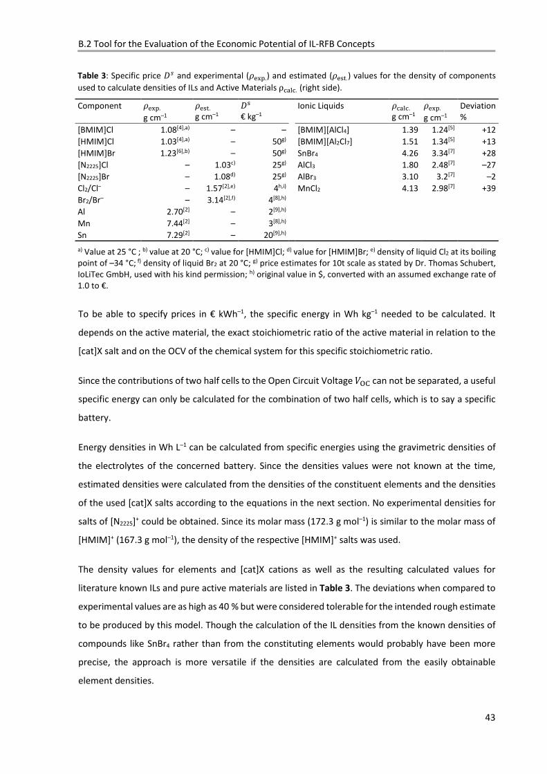
B.2 Tool for the Evaluation of the Economic Potential of IL-RFB Concepts
43
Table 3: Specific price �� and experimental (���.) and estimated (���.) values for the density of components
used to calculate densities of ILs and Active Materials ρ!"#!. (right side).
Component ���. g cm–1
���. g cm–1
��
€ kg–1 Ionic Liquids !"#!.
g cm–1 ���. g cm–1
Deviation %
[BMIM]Cl 1.08[4],a) – – [BMIM][AlCl4] 1.39 1.24[5] +12 [HMIM]Cl 1.03[4],a) – 50g) [BMIM][Al2Cl7] 1.51 1.34[5] +13 [HMIM]Br 1.23[6],b) – 50g) SnBr4 4.26 3.34[7] +28 [N2225]Cl – 1.03c) 25g) AlCl3 1.80 2.48[7] –27 [N2225]Br – 1.08d) 25g) AlBr3 3.10 3.2[7] –2 Cl2/Cl– – 1.57[2],e) 4h,i) MnCl2 4.13 2.98[7] +39 Br2/Br– – 3.14[2],f) 4[8],h) Al 2.70[2] – 2[9],h) Mn 7.44[2] – 3[8],h) Sn 7.29[2] – 20[9],h)
a) Value at 25 °C ; b) value at 20 °C; c) value for [HMIM]Cl; d) value for [HMIM]Br; e) density of liquid Cl2 at its boiling point of –34 °C; f) density of liquid Br2 at 20 °C; g) price estimates for 10t scale as stated by Dr. Thomas Schubert, IoLiTec GmbH, used with his kind permission; h) original value in $, converted with an assumed exchange rate of 1.0 to €.
To be able to specify prices in € kWh–1, the specific energy in Wh kg–1 needed to be calculated. It
depends on the active material, the exact stoichiometric ratio of the active material in relation to the
[cat]X salt and on the OCV of the chemical system for this specific stoichiometric ratio.
Since the contributions of two half cells to the Open Circuit Voltage $�� can not be separated, a useful
specific energy can only be calculated for the combination of two half cells, which is to say a specific
battery.
Energy densities in Wh L–1 can be calculated from specific energies using the gravimetric densities of
the electrolytes of the concerned battery. Since the densities values were not known at the time,
estimated densities were calculated from the densities of the constituent elements and the densities
of the used [cat]X salts according to the equations in the next section. No experimental densities for
salts of [N2225]+ could be obtained. Since its molar mass (172.3 g mol–1) is similar to the molar mass of
[HMIM]+ (167.3 g mol–1), the density of the respective [HMIM]+ salts was used.
The density values for elements and [cat]X cations as well as the resulting calculated values for
literature known ILs and pure active materials are listed in Table 3. The deviations when compared to
experimental values are as high as 40 % but were considered tolerable for the intended rough estimate
to be produced by this model. Though the calculation of the IL densities from the known densities of
compounds like SnBr4 rather than from the constituting elements would probably have been more
precise, the approach is more versatile if the densities are calculated from the easily obtainable
element densities.
B IL-RFB: Membrane-Free Concepts and Economic Potential
44
The tool to actually calculate the desired values for the energy density, specific energy and the price
per stored amount of energy, was implemented as an Excel sheet with multiple subpages. By specifying
molar masses, densities and prices in the first sheet for all employed materials and elements, then
using these to define the composition of positive and negative half cells in the second and third sheet
and finally combining these half cells to form the desired batteries in the last sheet, a reliable and very
flexible tool was obtained. The design eliminates the need to enter formulas and material properties
multiple times and instead references all cells back to properties defined in prior sheets, thereby saving
time and reducing errors.
B.2.1.3 Studied Systems and Concepts
The electrolytes for Al/Br2, Sn/Br2, All-Mn IL-RFBs and, to have a reference standard, V-RFBs were
analysed. For the IL based RFBs, hybrid concept with membrane (Hyb-IL-RFB), a hybrid concept with a
limited SOC range as explained in Section B.1.1 (Hyb-IL-RFB lim. SOC) and a membrane-free hybrid
system (MF-Hyb-RFB) were taken into account. For Sn, a system utilizing an Sn(II) IL without the
deposition of metal (IL-RFB) was studied as well.
RFBs based on ICl3 electrolytes have not been considered, since the first results showed that the
interhalide half-cell behaves more complicated than anticipated. A discussion on this matter will be
given in Chapter C.
For the membrane-free variant, only the concept in its original form presented in the introduction was
analysed. Concept 1 presented in Section B.1.2 is a modified version for which a calculation will be
discussed in Chapter D. For concept 2, the energy density, specific energy and specific price approach
the values of the active materials for large systems, since the IL is only used in a small circulating part
of the RFB. All values for concept 3 should be equal to the original concept, since the electrolyte is
identical in both concepts.
The OCVs and exact stoichiometries for the charged and discharged constitution of the electrolyte are
given in Table 4.
The stoichiometries are those deemed viable based on first experiments. On further research, all
systems showed individual characteristics and the need for custom modifications. For the systems
studied in this work, namely the Sn MF-Hyb-IL-RFB and the All-Mn Hyb-IL-RFB, the findings along with
updated calculations will be presented in the separate chapters (Chapter D and E, respectively). The
general trend and the conclusions made from the following calculated values are presented here to
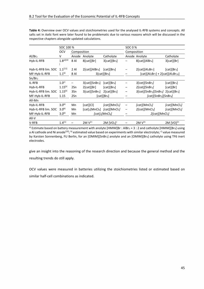
B.2 Tool for the Evaluation of the Economic Potential of IL-RFB Concepts
45
Table 4: Overview over OCV values and stoichiometries used for the analysed IL-RFB systems and concepts. All salts set in italic font were later found to be problematic due to various reasons which will be discussed in the respective chapters alongside updated calculations.
SOC 100 % SOC 0 % OCV Composition Composition
Al/Br2 V Anode Anolyte Catholyte Anode Anolyte Catholyte
Hyb-IL-RFB 1.8a)[10
] 8 Al 8[cat][Br] 3[cat][Br9] – 8[cat][AlBr4] 3[cat][Br]
Hyb-IL-RFB lim. SOC 1.1[11] 2 Al 2[cat][AlBr4] [cat][Br9] – 2[cat][Al2Br7] [cat][Br3] MF-Hyb-IL-RFB 1.1b) 8 Al 3[cat][Br9] – [cat][Al2Br7] + 2[cat][Al3Br10]
Sn/Br2
IL-RFB 1.0c) – 3[cat][SnBr3] [cat][Br9] – 3[cat][SnBr5] [cat][Br3] Hyb-IL-RFB 1.15b) 2Sn 2[cat][Br] [cat][Br9] – 2[cat][SnBr5] [cat][Br] Hyb-IL-RFB lim. SOC 1.15b) 3Sn 3[cat][SnBr5] 2[cat][Br9] – 3[cat][SnBr5][SnBr4] 2[cat][Br3] MF-Hyb-IL-RFB 1.15 2Sn [cat][Br9] – [cat][SnBr5][SnBr4]
All-Mn
Hyb-IL-RFB 3.0b) Mn [cat][Cl] [cat][MnCl5] – [cat][MnCl3] [cat][MnCl3]
Hyb-IL-RFB lim. SOC 3.0b) Mn [cat]2[MnCl4] [cat][MnCl5] – 2[cat][MnCl3] [cat][MnCl3]
MF-Hyb-IL-RFB 3.0b) Mn [cat]2[MnCl6] – 2[cat][MnCl3]
All-V
V-RFB 1.4[1] – 2M V2+ 2M [VO2]+ – 2M V3+ 2M [VO]2+ a) Estimate based on battery measurement with anolyte [HMIM]Br : AlBr3 = 3 : 2 and catholyte [HMIM][Br9] using a Al cathode and Ni anode[10]; b) estimated value based on experiments with similar electrolyte; c) value measured by Karsten Sonnenberg, FU Berlin, for an [OMIM][SnBr3] anolyte and an [OMIM][Br9] catholyte using TF6 inert electrodes.
give an insight into the reasoning of the research direction and because the general method and the
resulting trends do still apply.
OCV values were measured in batteries utilizing the stoichiometries listed or estimated based on
similar half-cell combinations as indicated.
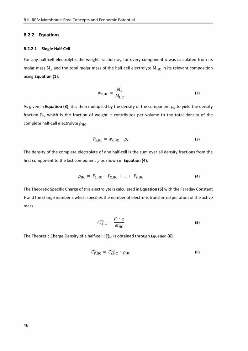
B IL-RFB: Membrane-Free Concepts and Economic Potential
46
Equations
B.2.2.1 Single Half-Cell
For any half-cell electrolyte, the weight fraction w� for every component x was calculated from its
molar mass M� and the total molar mass of the half-cell electrolyte M(� in its relevant composition
using Equation (1).
)�,(� = ���(� (2)
As given in Equation (3), it is then multiplied by the density of the component + to yield the density
fraction Ρ�, which is the fraction of weight it contributes per volume to the total density of the
complete half-cell electrolyte ρ(�.
-�,(� = )�,(� ∙ � (3)
The density of the complete electrolyte of one half-cell is the sum over all density fractions from the
first component to the last component . as shown in Equation (4).
(� = -�,(� / -0,(� / … / -2,(� (4)
The Theoretic Specific Charge of this electrolyte is calculated in Equation (5) with the Faraday Constant F and the charge number z which specifies the number of electrons transferred per atom of the active
mass.
5�,(��6 = � ∙ 7�(� (5)
The Theoretic Charge Density of a half-cell 58,(��6 is obtained through Equation (6).
58,(��6 = 5�,(��6 ∙ (� (6)
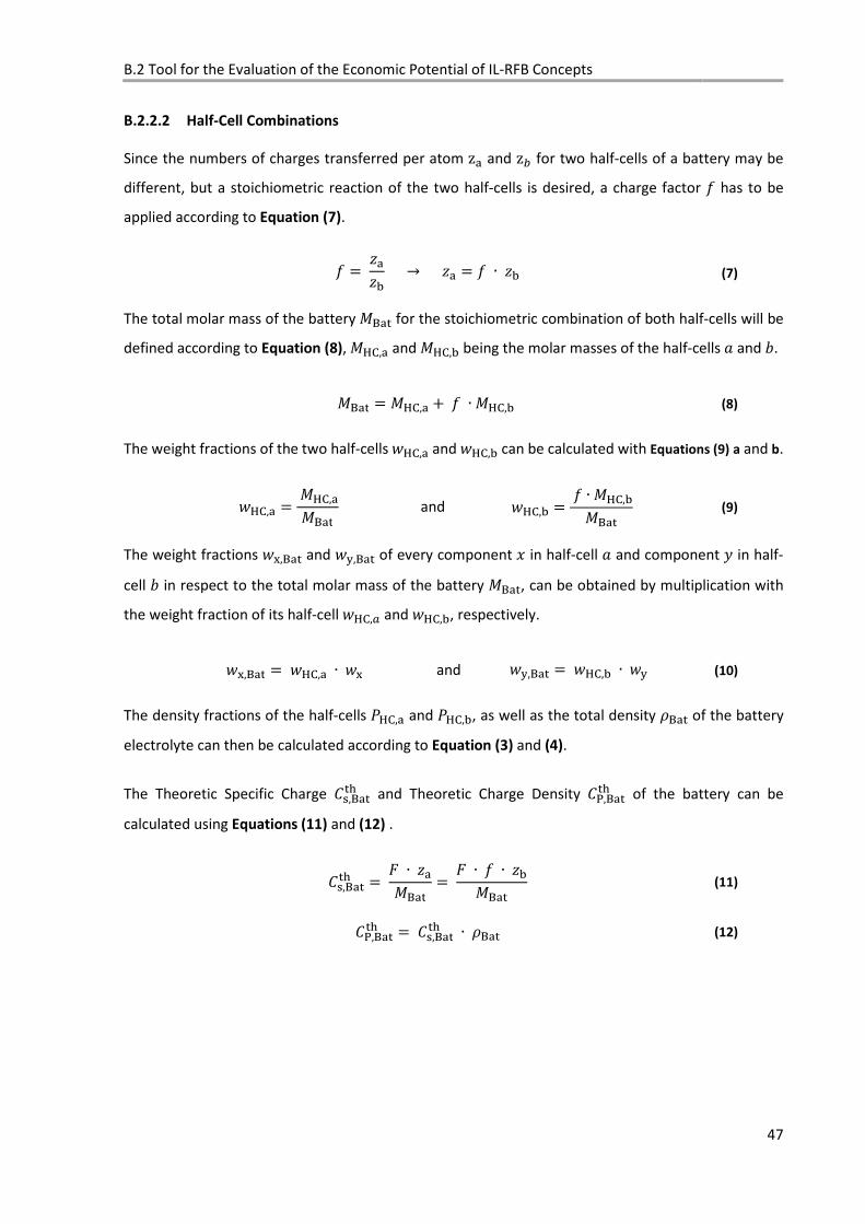
B.2 Tool for the Evaluation of the Economic Potential of IL-RFB Concepts
47
B.2.2.2 Half-Cell Combinations
Since the numbers of charges transferred per atom z" and z9 for two half-cells of a battery may be
different, but a stoichiometric reaction of the two half-cells is desired, a charge factor : has to be
applied according to Equation (7).
: = 7"7; → 7" = : ∙ 7; (7)
The total molar mass of the battery �="� for the stoichiometric combination of both half-cells will be
defined according to Equation (8), �(�," and �(�,; being the molar masses of the half-cells > and ?.
�="� = �(�," / : ∙ �(�,; (8)
The weight fractions of the two half-cells )(�," and )(�,; can be calculated with Equations (9) a and b.
)(�," = �(�,"�="� and )(�,; = : ∙ �(�,;�="� (9)
The weight fractions )�,="� and )2,="� of every component @ in half-cell > and component . in half-
cell ? in respect to the total molar mass of the battery �="�, can be obtained by multiplication with
the weight fraction of its half-cell )(�,A and )(�,;, respectively.
)�,="� = )(�," ∙ )� and )2,="� = )(�,; ∙ )2 (10)
The density fractions of the half-cells B(�," and B(�,;, as well as the total density ="� of the battery
electrolyte can then be calculated according to Equation (3) and (4).
The Theoretic Specific Charge 5�,="��6 and Theoretic Charge Density 58,="��6 of the battery can be
calculated using Equations (11) and (12) .
5�,="��6 = � ∙ 7"�="� = � ∙ : ∙ 7;�="� (11)
58,="��6 = 5�,="��6 ∙ ="� (12)
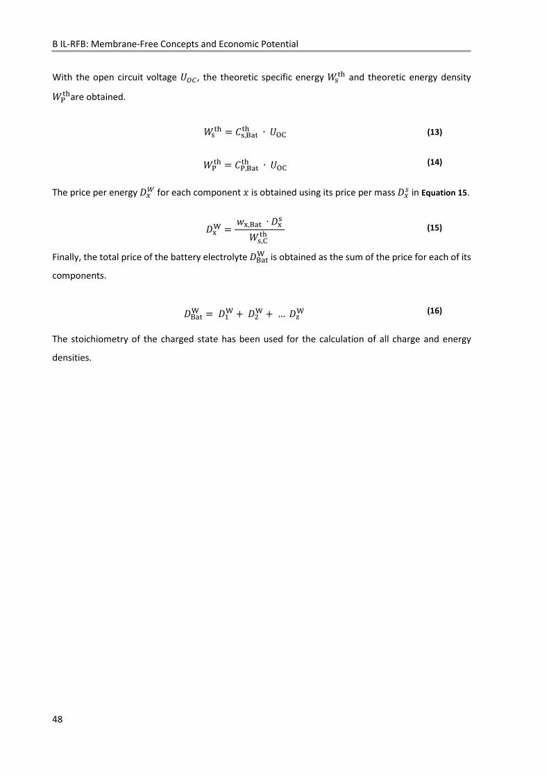
B IL-RFB: Membrane-Free Concepts and Economic Potential
48
With the open circuit voltage �CD, the theoretic specific energy E��6 and theoretic energy density E8�6are obtained.
E��6 = 5�,="��6 ∙ ��� (13)
E8�6 = 58,="��6 ∙ ��� (14)
The price per energy �+F for each component @ is obtained using its price per mass �+� in Equation 15.
��G = )�,="� ∙ ��� E�,��6 (15)
Finally, the total price of the battery electrolyte �="�G is obtained as the sum of the price for each of its
components.
�="�G = ��G / �0G / … �HG (16)
The stoichiometry of the charged state has been used for the calculation of all charge and energy
densities.
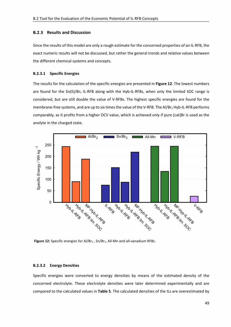
B.2 Tool for the Evaluation of the Economic Potential of IL-RFB Concepts
49
0
50
100
150
200
250
Hyb−IL−R
FB
Hyb−IL−R
FB lim
. SOC
MF−H
yb−IL−RFB
IL−RFB
Hyb−IL−R
FB
Hyb−IL−R
FB lim
. SOC
MF−H
yb−IL−RFB
Hyb−IL−R
FB
Hyb−IL−R
FB lim
. SOC
MF−H
yp−IL−RFB
V−R
FB
Specific
Energ
y / W
h k
g −1
Al/Br2 Sn/Br2 All−Mn V−RFB
Results and Discussion
Since the results of this model are only a rough estimate for the concerned properties of an IL-RFB, the
exact numeric results will not be discussed, but rather the general trends and relative values between
the different chemical systems and concepts.
B.2.3.1 Specific Energies
The results for the calculation of the specific energies are presented in Figure 12. The lowest numbers
are found for the Sn(II)/Br2 IL-RFB along with the Hyb-IL-RFBs, when only the limited SOC range is
considered, but are still double the value of V-RFBs. The highest specific energies are found for the
membrane-free systems, and are up to six times the value of the V-RFB. The Al/Br2 Hyb-IL-RFB performs
comparably, as it profits from a higher OCV value, which is achieved only if pure [cat]Br is used as the
anolyte in the charged state.
Figure 12: Specific energies for Al/Br2 , Sn/Br2, All-Mn and all-vanadium RFBs.
B.2.3.2 Energy Densities
Specific energies were converted to energy densities by means of the estimated density of the
concerned electrolyte. These electrolyte densities were later determined experimentally and are
compared to the calculated values in Table 5. The calculated densities of the ILs are overestimated by
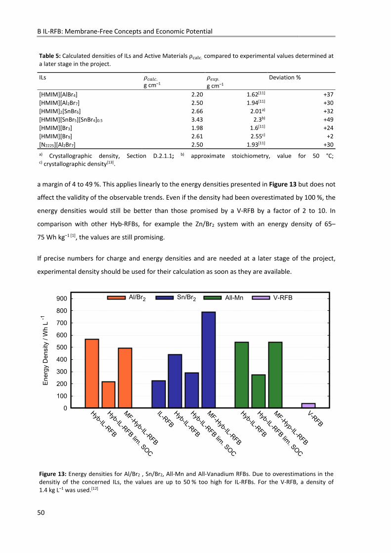
B IL-RFB: Membrane-Free Concepts and Economic Potential
50
0
100
200
300
400
500
600
700
800
900
Hyb−IL−R
FB
Hyb−IL−R
FB lim
. SOC
MF−H
yb−IL−RFB
IL−RFB
Hyb−IL−R
FB
Hyb−IL−R
FB lim
. SOC
MF−H
yb−IL−RFB
Hyb−IL−R
FB
Hyb−IL−R
FB lim
. SOC
MF−H
yp−IL−RFB
V−R
FB
En
erg
y D
en
sity /
Wh
L −1
Al/Br2 Sn/Br2 All−Mn V−RFB
a margin of 4 to 49 %. This applies linearly to the energy densities presented in Figure 13 but does not
affect the validity of the observable trends. Even if the density had been overestimated by 100 %, the
energy densities would still be better than those promised by a V-RFB by a factor of 2 to 10. In
comparison with other Hyb-RFBs, for example the Zn/Br2 system with an energy density of 65–
75 Wh kg–1 [1], the values are still promising.
If precise numbers for charge and energy densities and are needed at a later stage of the project,
experimental density should be used for their calculation as soon as they are available.
Figure 13: Energy densities for Al/Br2 , Sn/Br2, All-Mn and All-Vanadium RFBs. Due to overestimations in the densitiy of the concerned ILs, the values are up to 50 % too high for IL-RFBs. For the V-RFB, a density of 1.4 kg L–1 was used.[12]
Table 5: Calculated densities of ILs and Active Materials ρ!"#!. compared to experimental values determined at a later stage in the project.
ILs IAJI. g cm–1
K+L. g cm–1
Deviation %
[HMIM][AlBr4] 2.20 1.62[11] +37 [HMIM][Al2Br7] 2.50 1.94[11] +30 [HMIM]2[SnBr6] 2.66 2.01a) +32 [HMIM][SnBr5][SnBr4]0.5 3.43 2.3b) +49 [HMIM][Br3] 1.98 1.6[11] +24 [HMIM][Br9] 2.61 2.55c) +2 [N2225][Al2Br7] 2.50 1.93[11] +30
a) Crystallographic density, Section D.2.1.1; b) approximate stoichiometry, value for 50 °C; c) crystallographic density[13].
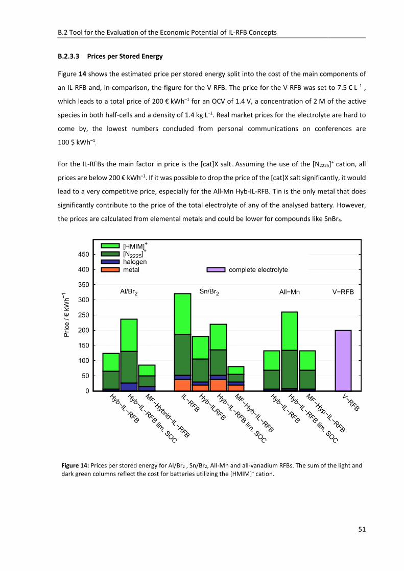
B.2 Tool for the Evaluation of the Economic Potential of IL-RFB Concepts
51
B.2.3.3 Prices per Stored Energy
Figure 14 shows the estimated price per stored energy split into the cost of the main components of
an IL-RFB and, in comparison, the figure for the V-RFB. The price for the V-RFB was set to 7.5 € L–1 ,
which leads to a total price of 200 € kWh–1 for an OCV of 1.4 V, a concentration of 2 M of the active
species in both half-cells and a density of 1.4 kg L–1. Real market prices for the electrolyte are hard to
come by, the lowest numbers concluded from personal communications on conferences are
100 $ kWh–1.
For the IL-RFBs the main factor in price is the [cat]X salt. Assuming the use of the [N2225]+ cation, all
prices are below 200 € kWh–1. If it was possible to drop the price of the [cat]X salt significantly, it would
lead to a very competitive price, especially for the All-Mn Hyb-IL-RFB. Tin is the only metal that does
significantly contribute to the price of the total electrolyte of any of the analysed battery. However,
the prices are calculated from elemental metals and could be lower for compounds like SnBr4.
Figure 14: Prices per stored energy for Al/Br2 , Sn/Br2, All-Mn and all-vanadium RFBs. The sum of the light and dark green columns reflect the cost for batteries utilizing the [HMIM]+ cation.
B IL-RFB: Membrane-Free Concepts and Economic Potential
52
Conclusion
The tool1 presented in this study, and which gives access to an estimate for the economic potential of
specific battery chemistries. Since it is designed to be used in the early stages of chemical research,
the scope of the model is limited to estimating the specific energy, the energy density, as well as the
first time investment concerning the battery chemicals but does not include costs of operation, safety
and maintenance. From this limited viewing angle, all presented battery systems seem viable when
considering the V-RFB as an established reference technology.
The membrane-free concept is a chemically challenging system that could yield a highly competitive
battery both for aluminium and tin. The All-Mn Hyb-IL-RFB could have less safety issues than the
batteries utilizing bromine, and, assuming the price of the [cat]X salt can be reduced, could offer a very
competitive price.
First results for the Sn/ICl3, membrane-free Sn/Br2 and the All-Mn Hyb-IL-RFB will be presented in the
next chapters.
1 The Excel file is provided on the DVD accompanying this dissertation and will be made available on the server of the work group.
B.2 Tool for the Evaluation of the Economic Potential of IL-RFB Concepts
53
References
[1] M. Skyllas-Kazacos, M. H. Chakrabarti, S. A. Hajimolana, F. S. Mjalli, M. Saleem, J. Electrochem.
Soc. 2011, 158, R55-R79.
[2] A. F. Holleman, E. Wiberg, G. Fischer, Lehrbuch der Anorganischen Chemie, Walter de Gruyter,
Berlin, New York, 2007.
[3] P. A. Tipler, Physik. Hans Christian von Baeyer “Essay: Fermis Lösung”, Spektrum Akademischer
Verlag, Heidelberg, 1994.
[4] J. G. Huddleston, A. E. Visser, W. M. Reichert, H. D. Willauer, G. A. Broker, R. D. Rogers, Green
Chem. 2001, 3, 156.
[5] A. A. Fannin Jr, D. A. Floreani, L. A. King, J. S. Landers, B. J. Piersma, D. J. Stech, R. L. Vaughn, J. S.
Wilkes, L. Williams John, J. Phys. Chem. 1984, 88, 2614.
[6] J.-G. Li, Y.-F. Hu, S.-F. Sun, Y.-S. Liu, Z.-C. Liu, J. Chem. Thermodyn. Thermochem. 2010, 42, 904.
[7] D. R. Lide, CRC Handbook of Chemistry and Physics, 84th Edition, Cleveland, Ohio, 2003.
[8] U. S. Geological Survey, Mineral commodity summaries 2013: Geological Survey, US Govt.
Printing Office, Reston, Virginia, 2013.
[9] Commodity Price Data, The World Bank, 2013.
[10] M. Hog, Diploma Thesis, University of Freiburg, Freiburg im Breisgau, 2013.
[11] M. Hog, Dissertation, University of Freiburg, Freiburg im Breisgau, 2017.
[12] GfE Metalle und Materialien GmbH, “Vanadium Electrolyte Solution 1.6 M, data sheet”, can be
found under http://www.gfe.com/en/product-range/vanadium-chemicals/applications/energy-
storage/.
[13] H. Haller, M. Hog, F. Scholz, H. Scherer, I. Krossing, S. Riedel, Z. Naturforsch., B: Chem. Sci. 2013,
68b, 1103.

B IL-RFB: Membrane-Free Concepts and Economic Potential
54
55
C Structure and Properties of Novel Chloroiodate(III) Ionic Liquids
The first clues that mixtures of [cat]Cl salts with more than 0.5 equivalents of I2Cl6 could yield liquid
positive active material for IL batteries were obtained during the work on my diploma thesis.[1] Thus,
at the beginning of the work on this dissertation, a mixture of [BMP]Cl with 1.0 equivalents of I2Cl6 was
prepared and found to be a homogeneous liquid at room temperature. The IL was then used as the
positive active material in a membrane-free Sn/ICl3 IL battery utilising a tin and a TF6 electrode. Though
the cell showed a starting OCV of 1.38 V and could be discharged with a maximum current of 1.4 mA,
the OCV dropped over the course of the following days and the battery could not be recharged. Upon
opening the cell, evidence for the formation of iodine was obtained by analysing the solid products via
Raman spectroscopy. It was therefore decided that for a first investigation of the inherently challenging
concept of a membrane-free battery, the simpler and better understood polybromide ILs would be
more suitable. Nevertheless, ILs based on I2Cl6 were further studied to understand their structure and
properties and to evaluate if these novel compounds could be useful for other IL-RFB concepts.
The following chapter is based on the manuscript “From Square-planar [ICl4]– to Novel
Chloroiodates(III)? A Systematic Experimental and Theoretical Investigation of their Ionic Liquids” by
Benedikt Burgenmeister, Karsten Sonnenberg, Sebastian Riedel and Ingo Krossing, which has been
published as a full paper in Chemistry – A European Journal (© 2017 WILEY-VCH Verlag GmbH & Co.
KGaA, Weinheim, http://dx.doi.org/10.1002/chem.201701555) and is reprinted here with permission
from John Wiley and Sons. The report includes the results for [HMIM][ICl4] which were obtained during
my diploma thesis, as were quantum-chemical calculations on the structure of chloroiodates [IxClx+y+1]–
(x = 1,2,3, y = 0 … 2x) and computed Raman spectra (PBE0/def2-TZVPP). The calculations were further
refined during the work on the dissertation (CCSD(T)/def2-TZVPP for x = 3 and all calculations using
A’QZ basis sets), and additional Raman spectra were computed (RI-MP2/def2-TZVPP). The figures
containing representations of the calculated structures were reworked based on the figures included
in my diploma thesis.
Karsten Sonnenberg (AG Riedel, FU Berlin) conducted all experiments for mixtures based on [NEt4]Cl.
Tobias Fischer synthesised [BMP][ICl4] during the research internship he conducted under my
supervision. Sabine Zylsdorf introduced me to ion chromatography and helped with the first
measurements.
Compared to the original manuscript, the abstract was removed, and the numbering and
nomenclature of subchapters, figures and tables have been modified for a uniform format.

C Structure and Properties of Novel Chloroiodate(III) Ionic Liquids
56
C.1 Introduction
57
C.1 Introduction
Polyhalide salts include a large range of mono- or multi-charged anions, their structures varying from
isolated moieties to large networks depending on the employed cation. This long known material class
has been subject of a renewed interest and reviews on recent developments were published.[2,3]
Such polyhalogen monoanions can be described – and often also synthesized – by the addition of one
or several equivalents of a neutral dihalogens X2 to a halide Y–. The formation of these complexes can
be explained by donor-acceptor interactions, for which the term halogen-bonding has been
established.[4] The simplest form are isopolyhalogen anions, in which both the anion and all other
atoms are the same (X = Y). Numerous compounds comprising anions composed of more than one and
even several di-halogen molecules exist.[5] Organic salts of these anions exhibit relatively low melting
points, for example 82 °C in the case of [N(C3H7)4][I5][5] and can be considered to be ionic liquids (ILs)
according to the common definition of an IL being a salt with a melting point below 100 °C. By
employing asymmetric cations typically used in IL-chemistry, melting points can be even further
lowered to yield room temperature ionic liquids (RTILs), like [HMIM][Br9][6] or [P1,10,10,10][Br3][7]
([HMIM]+ = 1-hexyl-3-methylimidazolium, [P1,10,10,10]+ = tridecylmethylphosphonium). In the solid state
structures of [NCH3(C4H9)3]2[Br20] (m.p. 10°C) and [BMP]2[Br20] (m.p. 9 °C, [BMP]+ = 1-butyl-1-
methylpyrrolidinium chloride), two and three dimensional polybromide networks were identified,
respectively.[8]
By combining more than one kind of halogen, for example dihalogens X2 or interhalogens XYn with
halides Z–, a great variety of polyinterhalogen monoanions is accessible. It has to be noted, though,
that if Z– is more electropositive than X or Y, redox reactions can occur upon mixing of the components.
After a rearrangement reaction, the formal oxidation state of –I will reside on the more electronegative
elements X or Y. If restricting the possible combinations by allowing only two elements, still two
general building principles exist. The first is the addition of homoatomic dihalogen molecules to a
different, more electronegative halogen anion, yielding polyinterhalogen monoanions like those in
[N(CH3)4][ClI4] (m.p. 110 °C) or [N(C2H5)4][ClBr6] (m.p. 53 °C). Those were already described by
Chattaway and Hoyle, and are also found in RTILs like [HMIM][ClBr2][9] or [P1,10,10,10][BrI2].[10] The second
possibility is to add neutral interhalogen molecules, in which one of the atoms has an oxidation state
of greater than zero, to a single halogen anion of the more electronegative element. One example of
a compound containing this anion type is [N(C4H9)4][ICl4] (m.p. 137-139 °C),[11] which can be considered
to be an adduct of ICl3 and Cl–. ILs of triatomic anions of the general type [XY2]– have already been
studied as reagents in organic synthesis[12] and as electrolytes for dye sensitized solar cells[10]. However,
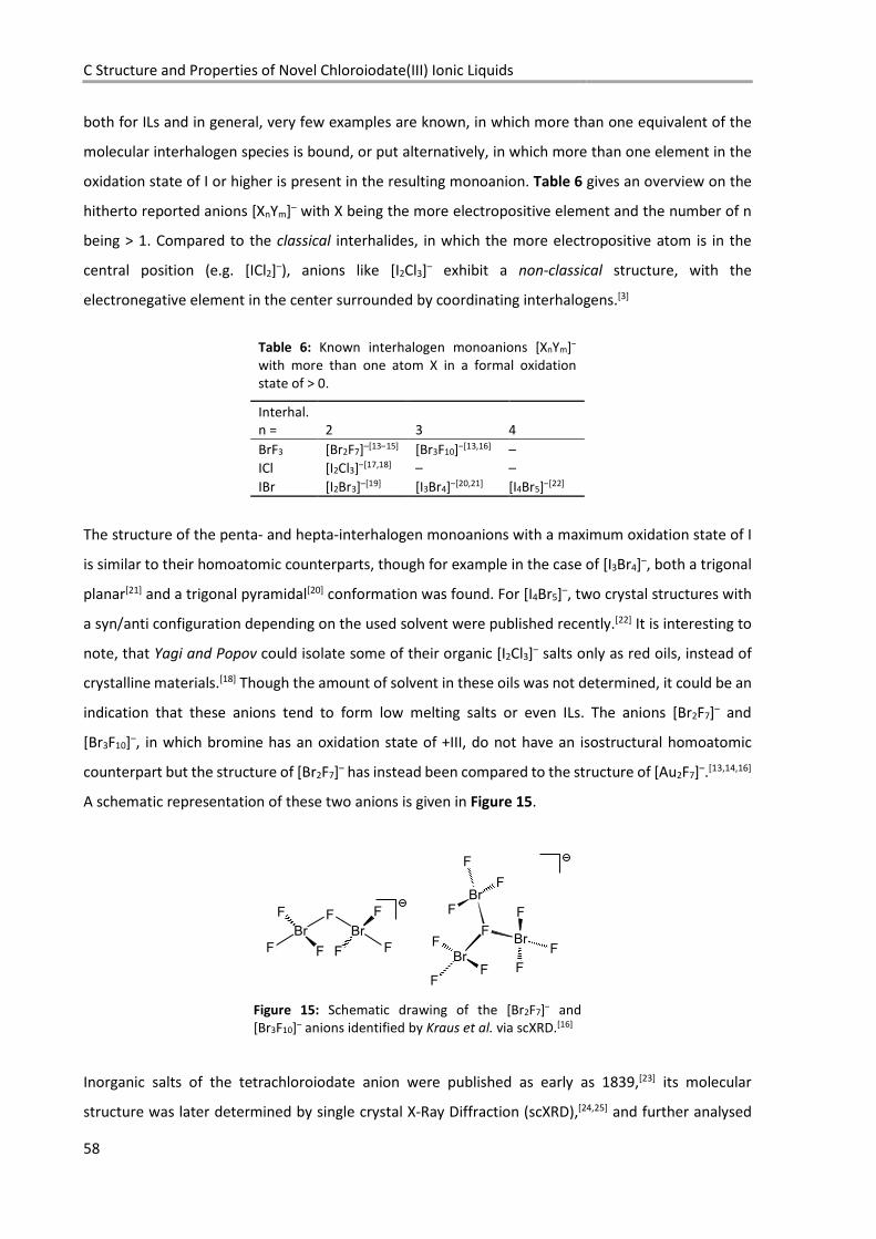
C Structure and Properties of Novel Chloroiodate(III) Ionic Liquids
58
both for ILs and in general, very few examples are known, in which more than one equivalent of the
molecular interhalogen species is bound, or put alternatively, in which more than one element in the
oxidation state of I or higher is present in the resulting monoanion. Table 6 gives an overview on the
hitherto reported anions [XnYm]– with X being the more electropositive element and the number of n
being > 1. Compared to the classical interhalides, in which the more electropositive atom is in the
central position (e.g. [ICl2]–), anions like [I2Cl3]– exhibit a non-classical structure, with the
electronegative element in the center surrounded by coordinating interhalogens.[3]
Table 6: Known interhalogen monoanions [XnYm]– with more than one atom X in a formal oxidation state of > 0.
Interhal. n = 2 3 4
BrF3 [Br2F7]–[13–15] [Br3F10]–[13,16] – ICl [I2Cl3]–[17,18] – – IBr [I2Br3]–[19] [I3Br4]–[20,21] [I4Br5]–[22]
The structure of the penta- and hepta-interhalogen monoanions with a maximum oxidation state of I
is similar to their homoatomic counterparts, though for example in the case of [I3Br4]–, both a trigonal
planar[21] and a trigonal pyramidal[20] conformation was found. For [I4Br5]–, two crystal structures with
a syn/anti configuration depending on the used solvent were published recently.[22] It is interesting to
note, that Yagi and Popov could isolate some of their organic [I2Cl3]– salts only as red oils, instead of
crystalline materials.[18] Though the amount of solvent in these oils was not determined, it could be an
indication that these anions tend to form low melting salts or even ILs. The anions [Br2F7]– and
[Br3F10]–, in which bromine has an oxidation state of +III, do not have an isostructural homoatomic
counterpart but the structure of [Br2F7]– has instead been compared to the structure of [Au2F7]–.[13,14,16]
A schematic representation of these two anions is given in Figure 15.
Figure 15: Schematic drawing of the [Br2F7]– and [Br3F10]– anions identified by Kraus et al. via scXRD.[16]
Inorganic salts of the tetrachloroiodate anion were published as early as 1839,[23] its molecular
structure was later determined by single crystal X-Ray Diffraction (scXRD),[24,25] and further analysed

C.1 Introduction
59
by UV/VIS,[11] vibrational[26,26,27] and NQR Spectroscopy.[28] The relative instability of tetrachloroiodate
salts in respect to the elimination of elemental dichlorine to yield the [ICl2]– anion, was investigated on
experimental grounds both for the decomposition in solution[11] and in the solid state[29]. Buckles and
Mills noted that the evolution of dichlorine from the tetramethylammonium salts was faster than for
the tetrabutylammonium salts, and that, upon irradiation, the chlorination of the butyl residue
combined with the evolution of HCl took place.[11] Like many others after them[30], they also studied
the reactivity of organic tetrachloroiodate salts towards double bond containing organic substances. If
compared to reactions with elemental dichlorine, they found a similar, but more controlled reaction
under the influence of these salts.
Here, we have investigated salts and ionic liquids obtained through the addition of 0.5 to 1.5
equivalents of I2Cl6 to [HMIM]Cl, [BMP]Cl and [NEt4]Cl (= tetraethylammonium chloride) and
characterized the products through vibrational and NMR-spectroscopy, scXRD and Ion
Chromatography (IC). The thermodynamics of their formation as well as spectroscopic characteristics
were in addition investigated by DFT and ab initio methods up to the CCSD(T)/A’QZ level. Although the
[ICl4]– anion has been known for over 170 years, in this report we present for the first time an
investigation of the existence of the anions [I2Cl7]– and [I3Cl10]–.

C Structure and Properties of Novel Chloroiodate(III) Ionic Liquids
60
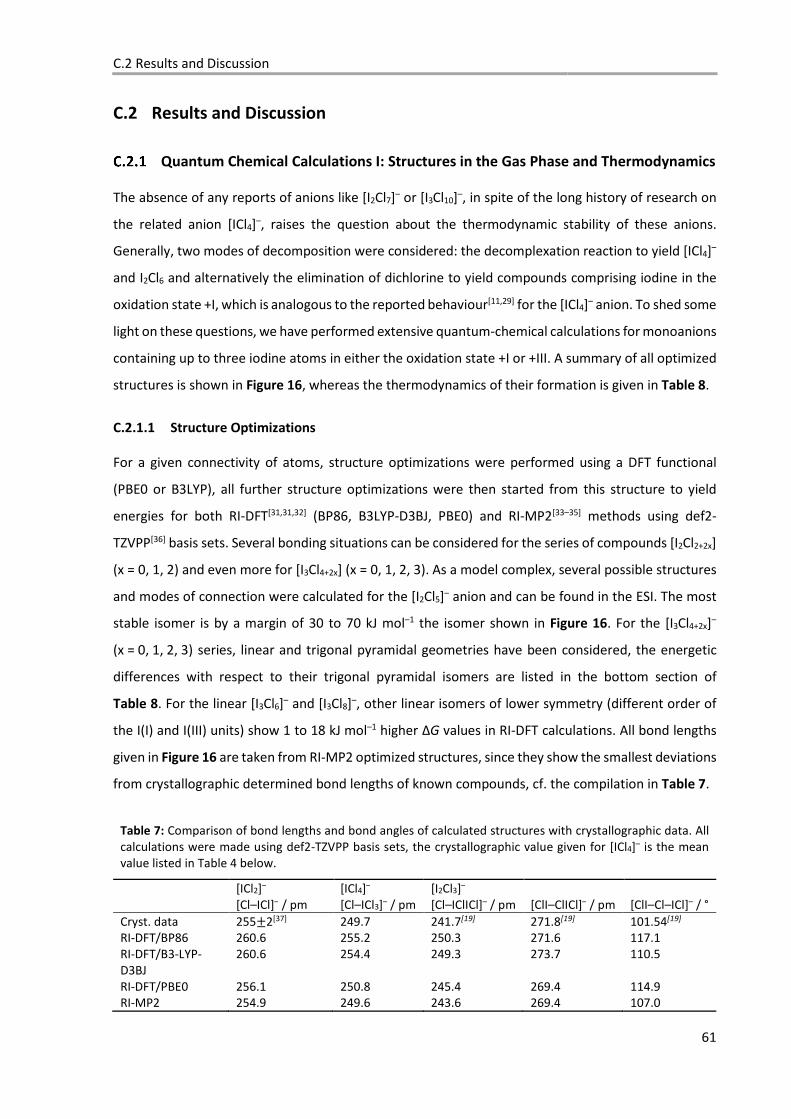
C.2 Results and Discussion
61
C.2 Results and Discussion
Quantum Chemical Calculations I: Structures in the Gas Phase and Thermodynamics
The absence of any reports of anions like [I2Cl7]– or [I3Cl10]–, in spite of the long history of research on
the related anion [ICl4]–, raises the question about the thermodynamic stability of these anions.
Generally, two modes of decomposition were considered: the decomplexation reaction to yield [ICl4]–
and I2Cl6 and alternatively the elimination of dichlorine to yield compounds comprising iodine in the
oxidation state +I, which is analogous to the reported behaviour[11,29] for the [ICl4]– anion. To shed some
light on these questions, we have performed extensive quantum-chemical calculations for monoanions
containing up to three iodine atoms in either the oxidation state +I or +III. A summary of all optimized
structures is shown in Figure 16, whereas the thermodynamics of their formation is given in Table 8.
C.2.1.1 Structure Optimizations
For a given connectivity of atoms, structure optimizations were performed using a DFT functional
(PBE0 or B3LYP), all further structure optimizations were then started from this structure to yield
energies for both RI-DFT[31,31,32] (BP86, B3LYP-D3BJ, PBE0) and RI-MP2[33–35] methods using def2-
TZVPP[36] basis sets. Several bonding situations can be considered for the series of compounds [I2Cl2+2x]
(x = 0, 1, 2) and even more for [I3Cl4+2x] (x = 0, 1, 2, 3). As a model complex, several possible structures
and modes of connection were calculated for the [I2Cl5]– anion and can be found in the ESI. The most
stable isomer is by a margin of 30 to 70 kJ mol–1 the isomer shown in Figure 16. For the [I3Cl4+2x]–
(x = 0, 1, 2, 3) series, linear and trigonal pyramidal geometries have been considered, the energetic
differences with respect to their trigonal pyramidal isomers are listed in the bottom section of
Table 8. For the linear [I3Cl6]– and [I3Cl8]–, other linear isomers of lower symmetry (different order of
the I(I) and I(III) units) show 1 to 18 kJ mol–1 higher ΔG values in RI-DFT calculations. All bond lengths
given in Figure 16 are taken from RI-MP2 optimized structures, since they show the smallest deviations
from crystallographic determined bond lengths of known compounds, cf. the compilation in Table 7.
Table 7: Comparison of bond lengths and bond angles of calculated structures with crystallographic data. All calculations were made using def2-TZVPP basis sets, the crystallographic value given for [ICl4]– is the mean value listed in Table 4 below.
[ICl2]– [ICl4]– [I2Cl3]– [Cl–ICl]– / pm [Cl–ICl3]– / pm [Cl–IClICl]– / pm [ClI–ClICl]– / pm [ClI–Cl–ICl]– / ° Cryst. data 255M2[37] 249.7 241.7[19] 271.8[19] 101.54[19] RI-DFT/BP86 260.6 255.2 250.3 271.6 117.1 RI-DFT/B3-LYP-D3BJ
260.6 254.4 249.3 273.7 110.5
RI-DFT/PBE0 256.1 250.8 245.4 269.4 114.9 RI-MP2 254.9 249.6 243.6 269.4 107.0
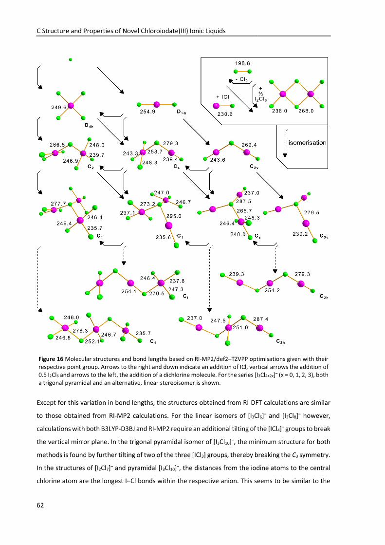
C Structure and Properties of Novel Chloroiodate(III) Ionic Liquids
62
Except for this variation in bond lengths, the structures obtained from RI-DFT calculations are similar
to those obtained from RI-MP2 calculations. For the linear isomers of [I3Cl6]– and [I3Cl8]– however,
calculations with both B3LYP-D3BJ and RI-MP2 require an additional tilting of the [ICl4]– groups to break
the vertical mirror plane. In the trigonal pyramidal isomer of [I3Cl10]–, the minimum structure for both
methods is found by further tilting of two of the three [ICl3] groups, thereby breaking the C3 symmetry.
In the structures of [I2Cl7]– and pyramidal [I3Cl10]–, the distances from the iodine atoms to the central
chlorine atom are the longest I–Cl bonds within the respective anion. This seems to be similar to the
Figure 16 Molecular structures and bond lengths based on RI-MP2/def2–TZVPP optimisations given with their respective point group. Arrows to the right and down indicate an addition of ICl, vertical arrows the addition of 0.5 I2Cl6 and arrows to the left, the addition of a dichlorine molecule. For the series [I3Cl4+2x]– (x = 0, 1, 2, 3), both a trigonal pyramidal and an alternative, linear stereoisomer is shown.
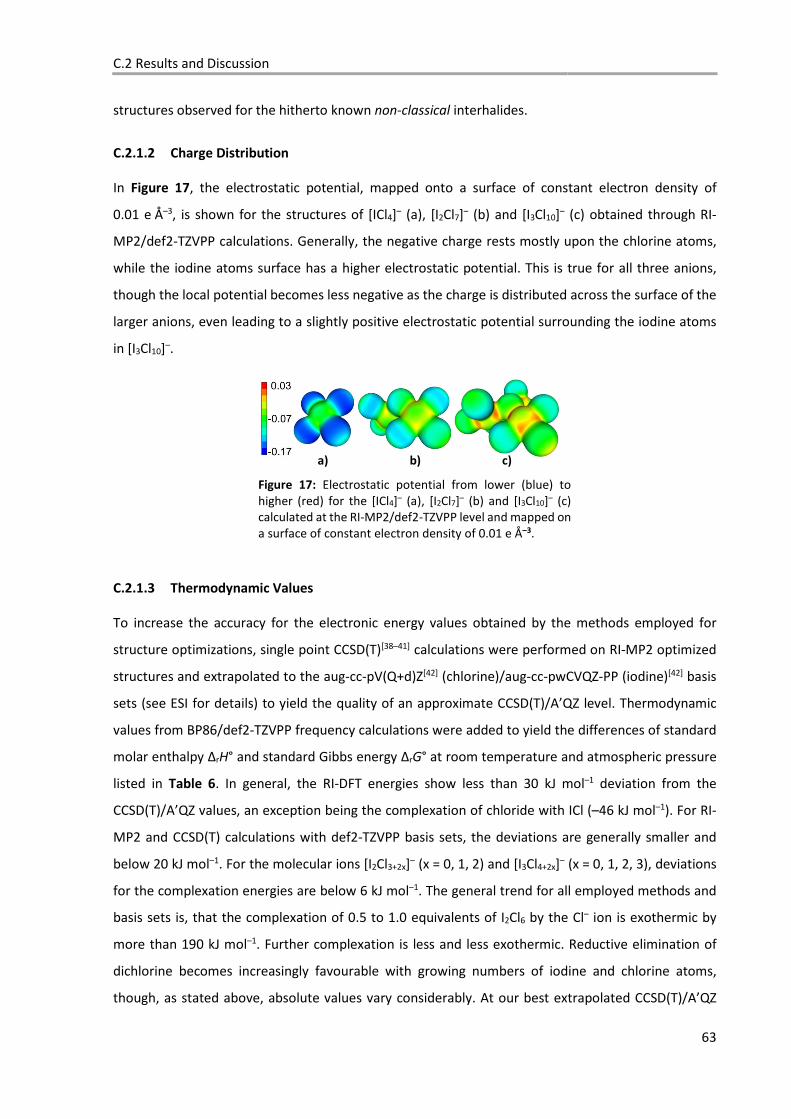
C.2 Results and Discussion
63
structures observed for the hitherto known non-classical interhalides.
C.2.1.2 Charge Distribution
In Figure 17, the electrostatic potential, mapped onto a surface of constant electron density of
0.01 e Å–3, is shown for the structures of [ICl4]– (a), [I2Cl7]– (b) and [I3Cl10]– (c) obtained through RI-
MP2/def2-TZVPP calculations. Generally, the negative charge rests mostly upon the chlorine atoms,
while the iodine atoms surface has a higher electrostatic potential. This is true for all three anions,
though the local potential becomes less negative as the charge is distributed across the surface of the
larger anions, even leading to a slightly positive electrostatic potential surrounding the iodine atoms
in [I3Cl10]–.
a) b) c)
Figure 17: Electrostatic potential from lower (blue) to higher (red) for the [ICl4]– (a), [I2Cl7]– (b) and [I3Cl10]– (c) calculated at the RI-MP2/def2-TZVPP level and mapped on a surface of constant electron density of 0.01 e Å–3.
C.2.1.3 Thermodynamic Values
To increase the accuracy for the electronic energy values obtained by the methods employed for
structure optimizations, single point CCSD(T)[38–41] calculations were performed on RI-MP2 optimized
structures and extrapolated to the aug-cc-pV(Q+d)Z[42] (chlorine)/aug-cc-pwCVQZ-PP (iodine)[42] basis
sets (see ESI for details) to yield the quality of an approximate CCSD(T)/A’QZ level. Thermodynamic
values from BP86/def2-TZVPP frequency calculations were added to yield the differences of standard
molar enthalpy ΔrH° and standard Gibbs energy ΔrG° at room temperature and atmospheric pressure
listed in Table 6. In general, the RI-DFT energies show less than 30 kJ mol–1 deviation from the
CCSD(T)/A’QZ values, an exception being the complexation of chloride with ICl (–46 kJ mol–1). For RI-
MP2 and CCSD(T) calculations with def2-TZVPP basis sets, the deviations are generally smaller and
below 20 kJ mol–1. For the molecular ions [I2Cl3+2x]– (x = 0, 1, 2) and [I3Cl4+2x]– (x = 0, 1, 2, 3), deviations
for the complexation energies are below 6 kJ mol–1. The general trend for all employed methods and
basis sets is, that the complexation of 0.5 to 1.0 equivalents of I2Cl6 by the Cl– ion is exothermic by
more than 190 kJ mol–1. Further complexation is less and less exothermic. Reductive elimination of
dichlorine becomes increasingly favourable with growing numbers of iodine and chlorine atoms,
though, as stated above, absolute values vary considerably. At our best extrapolated CCSD(T)/A’QZ
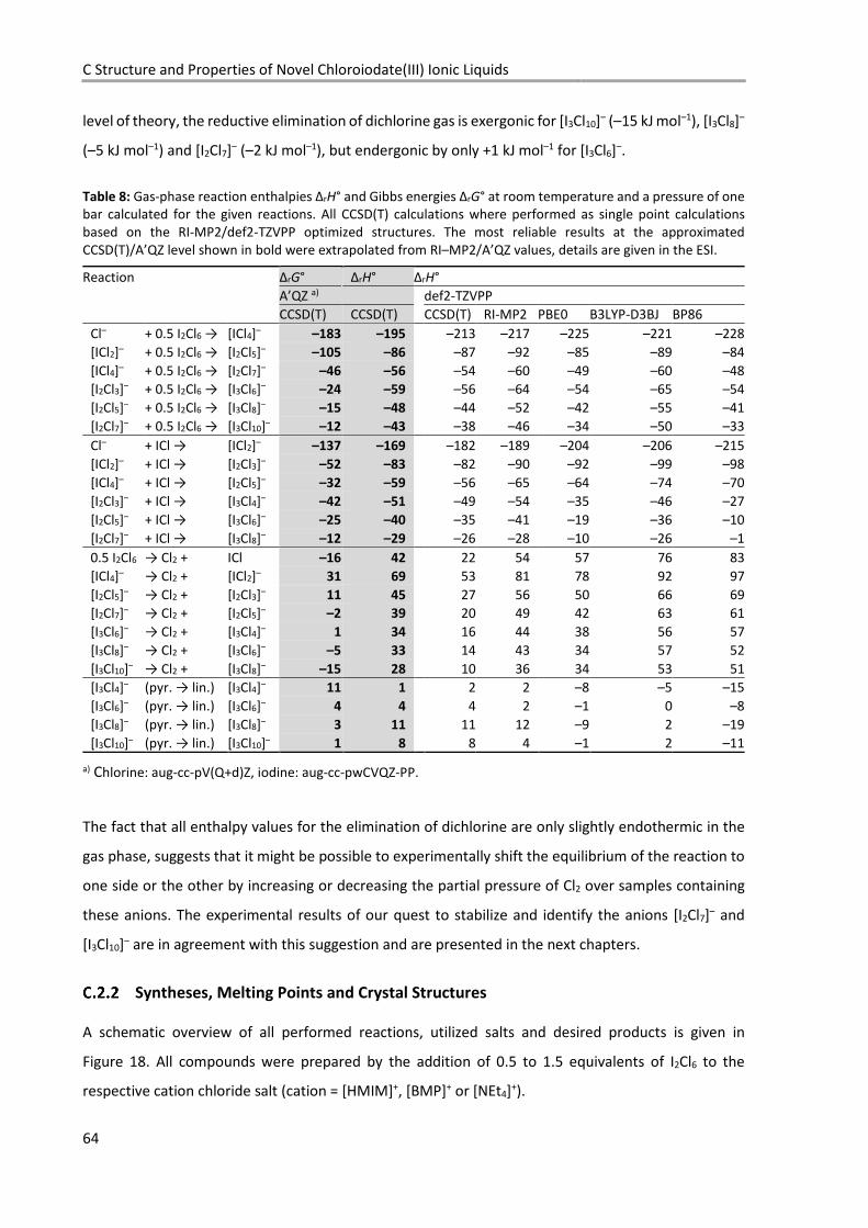
C Structure and Properties of Novel Chloroiodate(III) Ionic Liquids
64
level of theory, the reductive elimination of dichlorine gas is exergonic for [I3Cl10]– (–15 kJ mol–1), [I3Cl8]–
(–5 kJ mol–1) and [I2Cl7]– (–2 kJ mol–1), but endergonic by only +1 kJ mol–1 for [I3Cl6]–.
Table 8: Gas-phase reaction enthalpies ΔrH° and Gibbs energies ΔrG° at room temperature and a pressure of one bar calculated for the given reactions. All CCSD(T) calculations where performed as single point calculations based on the RI-MP2/def2-TZVPP optimized structures. The most reliable results at the approximated CCSD(T)/A’QZ level shown in bold were extrapolated from RI–MP2/A’QZ values, details are given in the ESI.
Reaction ΔrG° ΔrH° ΔrH° A’QZ a) def2-TZVPP CCSD(T) CCSD(T) CCSD(T) RI-MP2 PBE0 B3LYP-D3BJ BP86
Cl– + 0.5 I2Cl6 → [ICl4]– –183 –195 –213 –217 –225 –221 –228 [ICl2]– + 0.5 I2Cl6 → [I2Cl5]– –105 –86 –87 –92 –85 –89 –84 [ICl4]– + 0.5 I2Cl6 → [I2Cl7]– –46 –56 –54 –60 –49 –60 –48 [I2Cl3]– + 0.5 I2Cl6 → [I3Cl6]– –24 –59 –56 –64 –54 –65 –54 [I2Cl5]– + 0.5 I2Cl6 → [I3Cl8]– –15 –48 –44 –52 –42 –55 –41 [I2Cl7]– + 0.5 I2Cl6 → [I3Cl10]– –12 –43 –38 –46 –34 –50 –33
Cl– + ICl → [ICl2]– –137 –169 –182 –189 –204 –206 –215 [ICl2]– + ICl → [I2Cl3]– –52 –83 –82 –90 –92 –99 –98 [ICl4]– + ICl → [I2Cl5]– –32 –59 –56 –65 –64 –74 –70 [I2Cl3]– + ICl → [I3Cl4]– –42 –51 –49 –54 –35 –46 –27 [I2Cl5]– + ICl → [I3Cl6]– –25 –40 –35 –41 –19 –36 –10 [I2Cl7]– + ICl → [I3Cl8]– –12 –29 –26 –28 –10 –26 –1
0.5 I2Cl6 → Cl2 + ICl –16 42 22 54 57 76 83 [ICl4]– → Cl2 + [ICl2]– 31 69 53 81 78 92 97 [I2Cl5]– → Cl2 + [I2Cl3]– 11 45 27 56 50 66 69 [I2Cl7]– → Cl2 + [I2Cl5]– –2 39 20 49 42 63 61 [I3Cl6]– → Cl2 + [I3Cl4]– 1 34 16 44 38 56 57 [I3Cl8]– → Cl2 + [I3Cl6]– –5 33 14 43 34 57 52 [I3Cl10]– → Cl2 + [I3Cl8]– –15 28 10 36 34 53 51 [I3Cl4]– (pyr. → lin.) [I3Cl4]– 11 1 2 2 –8 –5 –15 [I3Cl6]– (pyr. → lin.) [I3Cl6]– 4 4 4 2 –1 0 –8 [I3Cl8]– (pyr. → lin.) [I3Cl8]– 3 11 11 12 –9 2 –19 [I3Cl10]– (pyr. → lin.) [I3Cl10]– 1 8 8 4 –1 2 –11
a) Chlorine: aug-cc-pV(Q+d)Z, iodine: aug-cc-pwCVQZ-PP.
The fact that all enthalpy values for the elimination of dichlorine are only slightly endothermic in the
gas phase, suggests that it might be possible to experimentally shift the equilibrium of the reaction to
one side or the other by increasing or decreasing the partial pressure of Cl2 over samples containing
these anions. The experimental results of our quest to stabilize and identify the anions [I2Cl7]– and
[I3Cl10]– are in agreement with this suggestion and are presented in the next chapters.
Syntheses, Melting Points and Crystal Structures
A schematic overview of all performed reactions, utilized salts and desired products is given in
Figure 18. All compounds were prepared by the addition of 0.5 to 1.5 equivalents of I2Cl6 to the
respective cation chloride salt (cation = [HMIM]+, [BMP]+ or [NEt4]+).
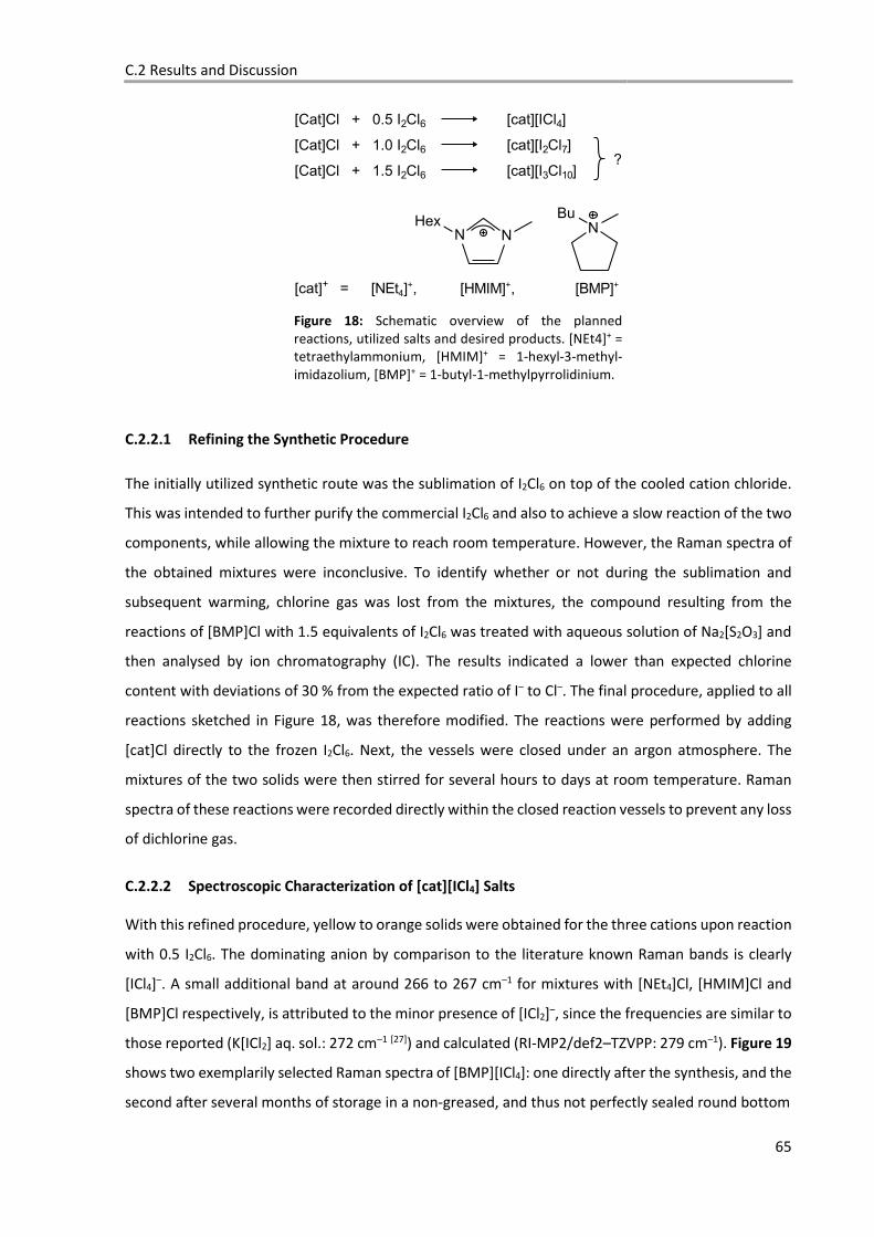
C.2 Results and Discussion
65
Figure 18: Schematic overview of the planned reactions, utilized salts and desired products. [NEt4]+ = tetraethylammonium, [HMIM]+ = 1-hexyl-3-methyl-imidazolium, [BMP]+ = 1-butyl-1-methylpyrrolidinium.
C.2.2.1 Refining the Synthetic Procedure
The initially utilized synthetic route was the sublimation of I2Cl6 on top of the cooled cation chloride.
This was intended to further purify the commercial I2Cl6 and also to achieve a slow reaction of the two
components, while allowing the mixture to reach room temperature. However, the Raman spectra of
the obtained mixtures were inconclusive. To identify whether or not during the sublimation and
subsequent warming, chlorine gas was lost from the mixtures, the compound resulting from the
reactions of [BMP]Cl with 1.5 equivalents of I2Cl6 was treated with aqueous solution of Na2[S2O3] and
then analysed by ion chromatography (IC). The results indicated a lower than expected chlorine
content with deviations of 30 % from the expected ratio of I– to Cl–. The final procedure, applied to all
reactions sketched in Figure 18, was therefore modified. The reactions were performed by adding
[cat]Cl directly to the frozen I2Cl6. Next, the vessels were closed under an argon atmosphere. The
mixtures of the two solids were then stirred for several hours to days at room temperature. Raman
spectra of these reactions were recorded directly within the closed reaction vessels to prevent any loss
of dichlorine gas.
C.2.2.2 Spectroscopic Characterization of [cat][ICl4] Salts
With this refined procedure, yellow to orange solids were obtained for the three cations upon reaction
with 0.5 I2Cl6. The dominating anion by comparison to the literature known Raman bands is clearly
[ICl4]–. A small additional band at around 266 to 267 cm–1 for mixtures with [NEt4]Cl, [HMIM]Cl and
[BMP]Cl respectively, is attributed to the minor presence of [ICl2]–, since the frequencies are similar to
those reported (K[ICl2] aq. sol.: 272 cm–1 [27]) and calculated (RI-MP2/def2–TZVPP: 279 cm–1). Figure 19
shows two exemplarily selected Raman spectra of [BMP][ICl4]: one directly after the synthesis, and the
second after several months of storage in a non-greased, and thus not perfectly sealed round bottom
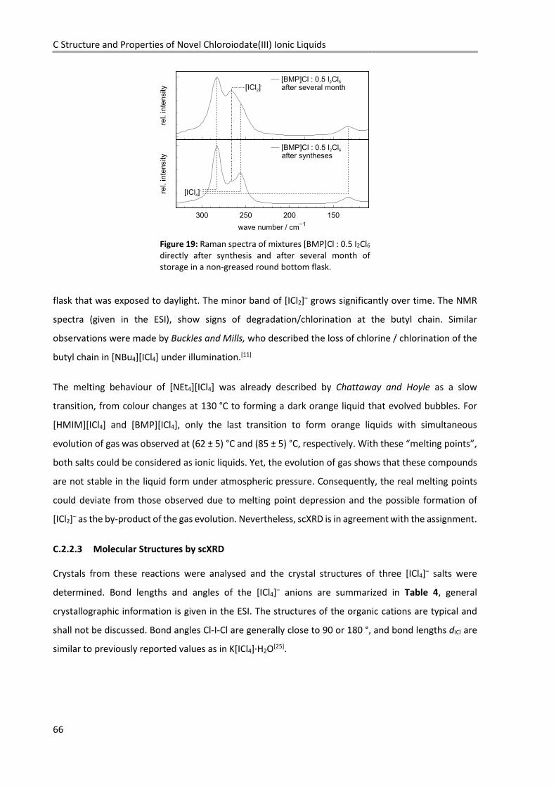
C Structure and Properties of Novel Chloroiodate(III) Ionic Liquids
66
Figure 19: Raman spectra of mixtures [BMP]Cl : 0.5 I2Cl6 directly after synthesis and after several month of storage in a non-greased round bottom flask.
flask that was exposed to daylight. The minor band of [ICl2]– grows significantly over time. The NMR
spectra (given in the ESI), show signs of degradation/chlorination at the butyl chain. Similar
observations were made by Buckles and Mills, who described the loss of chlorine / chlorination of the
butyl chain in [NBu4][ICl4] under illumination.[11]
The melting behaviour of [NEt4][ICl4] was already described by Chattaway and Hoyle as a slow
transition, from colour changes at 130 °C to forming a dark orange liquid that evolved bubbles. For
[HMIM][ICl4] and [BMP][ICl4], only the last transition to form orange liquids with simultaneous
evolution of gas was observed at (62 ± 5) °C and (85 ± 5) °C, respectively. With these “melting points”,
both salts could be considered as ionic liquids. Yet, the evolution of gas shows that these compounds
are not stable in the liquid form under atmospheric pressure. Consequently, the real melting points
could deviate from those observed due to melting point depression and the possible formation of
[ICl2]– as the by-product of the gas evolution. Nevertheless, scXRD is in agreement with the assignment.
C.2.2.3 Molecular Structures by scXRD
Crystals from these reactions were analysed and the crystal structures of three [ICl4]– salts were
determined. Bond lengths and angles of the [ICl4]– anions are summarized in Table 4, general
crystallographic information is given in the ESI. The structures of the organic cations are typical and
shall not be discussed. Bond angles Cl-I-Cl are generally close to 90 or 180 °, and bond lengths dICl are
similar to previously reported values as in K[ICl4]∙H2O[25].
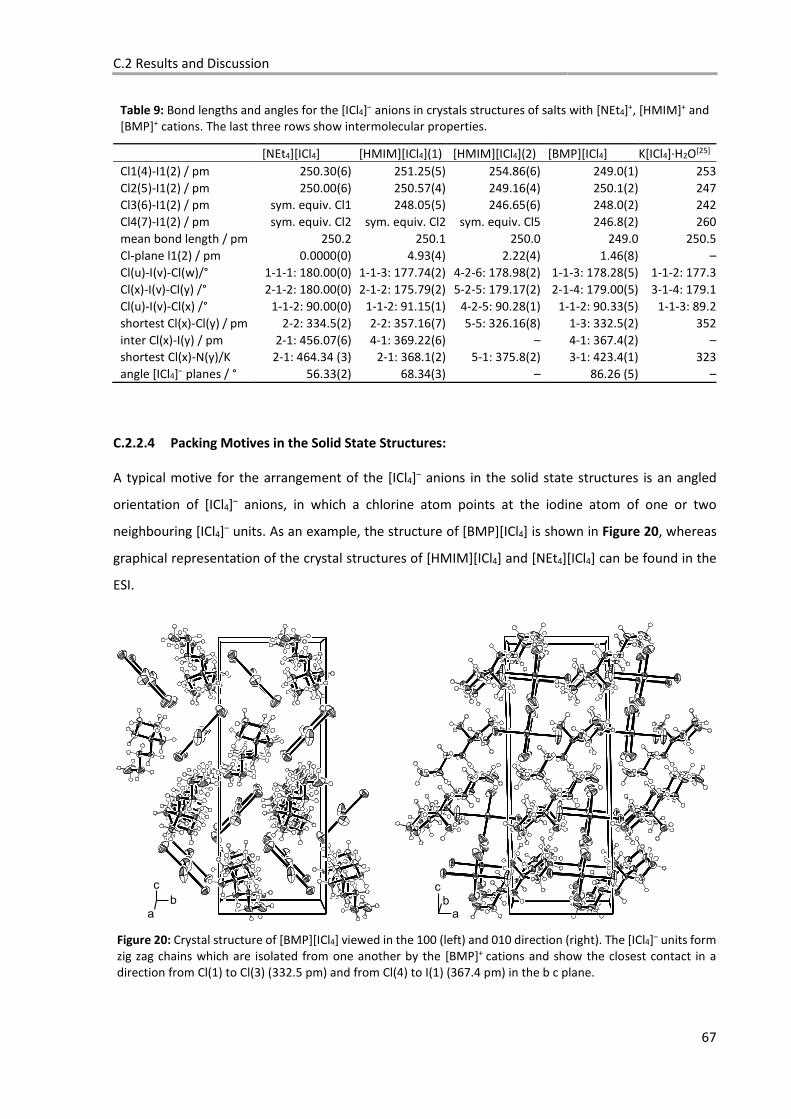
C.2 Results and Discussion
67
Table 9: Bond lengths and angles for the [ICl4]– anions in crystals structures of salts with [NEt4]+, [HMIM]+ and [BMP]+ cations. The last three rows show intermolecular properties.
[NEt4][ICl4] [HMIM][ICl4](1) [HMIM][ICl4](2) [BMP][ICl4] K[ICl4]∙H2O[25]
Cl1(4)-I1(2) / pm 250.30(6) 251.25(5) 254.86(6) 249.0(1) 253Cl2(5)-I1(2) / pm 250.00(6) 250.57(4) 249.16(4) 250.1(2) 247Cl3(6)-I1(2) / pm sym. equiv. Cl1 248.05(5) 246.65(6) 248.0(2) 242Cl4(7)-I1(2) / pm sym. equiv. Cl2 sym. equiv. Cl2 sym. equiv. Cl5 246.8(2) 260mean bond length / pm 250.2 250.1 250.0 249.0 250.5Cl-plane l1(2) / pm 0.0000(0) 4.93(4) 2.22(4) 1.46(8) –Cl(u)-I(v)-Cl(w)/° 1-1-1: 180.00(0) 1-1-3: 177.74(2) 4-2-6: 178.98(2) 1-1-3: 178.28(5) 1-1-2: 177.3Cl(x)-I(v)-Cl(y) /° 2-1-2: 180.00(0) 2-1-2: 175.79(2) 5-2-5: 179.17(2) 2-1-4: 179.00(5) 3-1-4: 179.1Cl(u)-I(v)-Cl(x) /° 1-1-2: 90.00(0) 1-1-2: 91.15(1) 4-2-5: 90.28(1) 1-1-2: 90.33(5) 1-1-3: 89.2shortest Cl(x)-Cl(y) / pm 2-2: 334.5(2) 2-2: 357.16(7) 5-5: 326.16(8) 1-3: 332.5(2) 352inter Cl(x)-I(y) / pm 2-1: 456.07(6) 4-1: 369.22(6) – 4-1: 367.4(2) –shortest Cl(x)-N(y)/K 2-1: 464.34 (3) 2-1: 368.1(2) 5-1: 375.8(2) 3-1: 423.4(1) 323angle [ICl4]– planes / ° 56.33(2) 68.34(3) – 86.26 (5) –
C.2.2.4 Packing Motives in the Solid State Structures:
A typical motive for the arrangement of the [ICl4]– anions in the solid state structures is an angled
orientation of [ICl4]– anions, in which a chlorine atom points at the iodine atom of one or two
neighbouring [ICl4]– units. As an example, the structure of [BMP][ICl4] is shown in Figure 20, whereas
graphical representation of the crystal structures of [HMIM][ICl4] and [NEt4][ICl4] can be found in the
ESI.
Figure 20: Crystal structure of [BMP][ICl4] viewed in the 100 (left) and 010 direction (right). The [ICl4]– units form zig zag chains which are isolated from one another by the [BMP]+ cations and show the closest contact in a direction from Cl(1) to Cl(3) (332.5 pm) and from Cl(4) to I(1) (367.4 pm) in the b c plane.
C Structure and Properties of Novel Chloroiodate(III) Ionic Liquids
68
In the structure of [HMIM][ICl4], the chlorine atom with the longest bond (Cl4-I2, 254.9 pm) is also the
one closest to the (non-bonding) iodine of a neighbouring [ICl4]– anion (Cl4-I1, 369.2 pm; cf. ΣrvdW(Cl,I)
= 373 pm[43]). This elongation of the iodine chlorine bond is not observed in the structure of [BMP][ICl4],
in which the shortest bond (Cl4-I1, 246.8 pm) is the one closest to the next iodine atom (Cl4-I1,
367.4 pm) and the longest bond is the one just opposite (Cl2-I1, 250.1 pm). The bond lengths are
almost the same for the two symmetry independent chlorine atoms of [NEt4][ICl4] (Cl1-I1, 250.3 pm ;
Cl2-I1, 250.0 pm ). The two symmetry equivalent chlorine atoms on opposite sides of the central iodine
are framed by the iodine atoms of neighbouring [ICl4]– anions at a distance of 456.07 pm, which is
significantly longer than the closest contacts in the [HMIM]+ and [BMP]+ salts. In the electrostatic
potential plot of [ICl4]– shown in Figure 18 a), the highest potential is found at a ring surrounding an
axis through the iodine and perpendicular to the plane defined by the iodine and chlorine atoms. The
lowest potentials are situated on rings perpendicular to the I–Cl bond at the chlorine atoms. This
charge distribution suggests that the angular configuration of the [ICl4]– molecules found in all
presented structures, could minimize coulombic repulsion of neighbouring anions.
C.2.2.5 Hirshfeld Analysis
An exemplarily selected Hirshfeld analysis is shown for [HMIM][ICl4] in Figure 21 a) and b). Contacts
shorter or close to the sum of the van der Waals radii are found from the hydrogen atoms in the
imidazolium rings (H2-Cl4: 274 pm, H3-Cl2: 273 pm H4-Cl6: 290 pm; ΣrvdW(H,Cl) = 284 pm[43]), the
hydrogen atoms on the first carbon atom of the alkyl chain to the chlorine atoms of the [ICl4]– units
(disordered, shortest distance H5AB-Cl3: 275 pm) and in Cl–Cl interactions between neighbouring
[ICl4]– anions (Cl5-Cl5: 326 pm, ΣrvdW(Cl,Cl) = 350 pm[43]). The strong positive influence of hydrogen
bonds from the imidazolium ring to the respective anion on the physical properties of imidazolium
based ionic liquids has been shown before.[44] It could contribute to the observed lowest melting point
of all [ICl4]– salts in this investigation. Compared to these bonds in N,N’-dimethylimidazolium
methylsulfate (average H-O: 209.1 pm, ΣrvdW(H,O): 261 pm[43]), with an average H-O distance 50 pm
shorter than the sum of their van der Waals radii,[45] the interaction seems to be much weaker. This is
in agreement with the more diffuse charge of the chlorine atom compared to the oxygen atom in the
sulfate. Except for the absence of the imidazolium ring and its hydrogen bonds, the Hirshfeld plots for
[BMP][ICl4] and [NEt4][ICl4] show similar results and are included in the ESI.
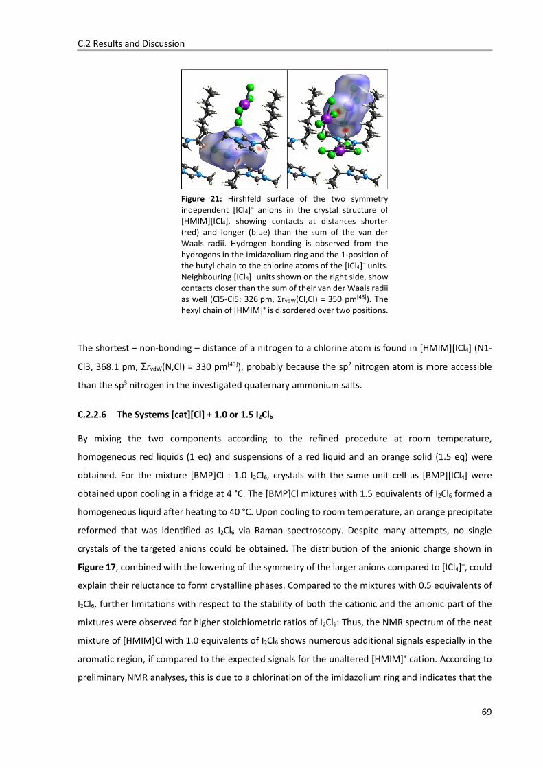
C.2 Results and Discussion
69
Figure 21: Hirshfeld surface of the two symmetry independent [ICl4]– anions in the crystal structure of [HMIM][ICl4], showing contacts at distances shorter (red) and longer (blue) than the sum of the van der Waals radii. Hydrogen bonding is observed from the hydrogens in the imidazolium ring and the 1-position of the butyl chain to the chlorine atoms of the [ICl4]– units. Neighbouring [ICl4]– units shown on the right side, show contacts closer than the sum of their van der Waals radii as well (Cl5-Cl5: 326 pm, ΣrvdW(Cl,Cl) = 350 pm[43]). The hexyl chain of [HMIM]+ is disordered over two positions.
The shortest – non-bonding – distance of a nitrogen to a chlorine atom is found in [HMIM][ICl4] (N1-
Cl3, 368.1 pm, ΣrvdW(N,Cl) = 330 pm[43]), probably because the sp2 nitrogen atom is more accessible
than the sp3 nitrogen in the investigated quaternary ammonium salts.
C.2.2.6 The Systems [cat][Cl] + 1.0 or 1.5 I2Cl6
By mixing the two components according to the refined procedure at room temperature,
homogeneous red liquids (1 eq) and suspensions of a red liquid and an orange solid (1.5 eq) were
obtained. For the mixture [BMP]Cl : 1.0 I2Cl6, crystals with the same unit cell as [BMP][ICl4] were
obtained upon cooling in a fridge at 4 °C. The [BMP]Cl mixtures with 1.5 equivalents of I2Cl6 formed a
homogeneous liquid after heating to 40 °C. Upon cooling to room temperature, an orange precipitate
reformed that was identified as I2Cl6 via Raman spectroscopy. Despite many attempts, no single
crystals of the targeted anions could be obtained. The distribution of the anionic charge shown in
Figure 17, combined with the lowering of the symmetry of the larger anions compared to [ICl4]–, could
explain their reluctance to form crystalline phases. Compared to the mixtures with 0.5 equivalents of
I2Cl6, further limitations with respect to the stability of both the cationic and the anionic part of the
mixtures were observed for higher stoichiometric ratios of I2Cl6: Thus, the NMR spectrum of the neat
mixture of [HMIM]Cl with 1.0 equivalents of I2Cl6 shows numerous additional signals especially in the
aromatic region, if compared to the expected signals for the unaltered [HMIM]+ cation. According to
preliminary NMR analyses, this is due to a chlorination of the imidazolium ring and indicates that the
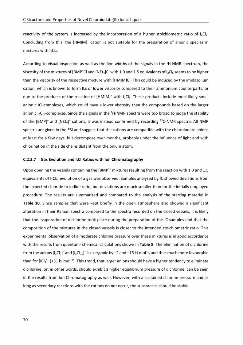
C Structure and Properties of Novel Chloroiodate(III) Ionic Liquids
70
reactivity of the system is increased by the incorporation of a higher stoichiometric ratio of I2Cl6.
Concluding from this, the [HMIM]+ cation is not suitable for the preparation of anionic species in
mixtures with I2Cl6.
According to visual inspection as well as the line widths of the signals in the 1H-NMR spectrum, the
viscosity of the mixtures of [BMP]Cl and [NEt4]Cl with 1.0 and 1.5 equivalents of I2Cl6 seems to be higher
than the viscosity of the respective mixture with [HMIM]Cl. This could be induced by the imidazolium
cation, which is known to form ILs of lower viscosity compared to their ammonium counterparts, or
due to the products of the reaction of [HMIM]+ with I2Cl6. These products include most likely small
anionic ICl-complexes, which could have a lower viscosity than the compounds based on the larger
anionic I2Cl6-complexes. Since the signals in the 1H-NMR spectra were too broad to judge the stability
of the [BMP]+ and [NEt4]+ cations, it was instead confirmed by recording 13C-NMR spectra. All NMR
spectra are given in the ESI and suggest that the cations are compatible with the chloroiodate anions
at least for a few days, but decompose over months, probably under the influence of light and with
chlorination in the side chains distant from the onium atom.
C.2.2.7 Gas Evolution and I:Cl Ratios with Ion Chromatography
Upon opening the vessels containing the [BMP]+ mixtures resulting from the reaction with 1.0 and 1.5
equivalents of I2Cl6, evolution of a gas was observed. Samples analysed by IC showed deviations from
the expected chloride to iodide ratio, but deviations are much smaller than for the initially employed
procedure. The results are summarized and compared to the analysis of the starting material in
Table 10. Since samples that were kept briefly in the open atmosphere also showed a significant
alteration in their Raman spectra compared to the spectra recorded on the closed vessels, it is likely
that the evaporation of dichlorine took place during the preparation of the IC samples and that the
composition of the mixtures in the closed vessels is closer to the intended stoichiometric ratio. This
experimental observation of a moderate chlorine pressure over these mixtures is in good accordance
with the results from quantum- chemical calculations shown in Table 8. The elimination of dichlorine
from the anions [I2Cl7]– and [I3Cl10]– is exergonic by –2 and –15 kJ mol–1, and thus much more favourable
than for [ICl4]– (+31 kJ mol–1). This trend, that larger anions should have a higher tendency to eliminate
dichlorine, or, in other words, should exhibit a higher equilibrium pressure of dichlorine, can be seen
in the results from Ion Chromatography as well. However, with a sustained chlorine pressure and as
long as secondary reactions with the cations do not occur, the substances should be stable.
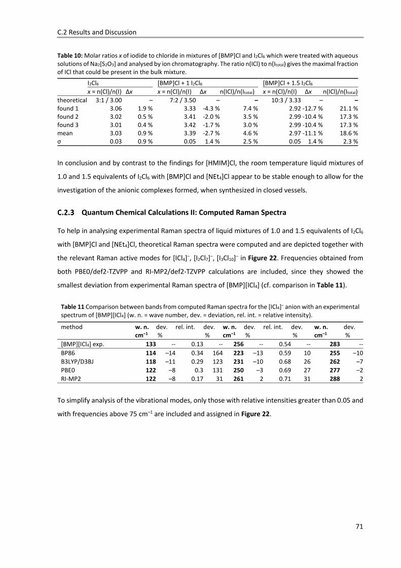
C.2 Results and Discussion
71
Table 10: Molar ratios x of iodide to chloride in mixtures of [BMP]Cl and I2Cl6 which were treated with aqueous solutions of Na2[S2O3] and analysed by ion chromatography. The ratio n(ICl) to n(Itotal) gives the maximal fraction of ICl that could be present in the bulk mixture.
I2Cl6 [BMP]Cl + 1 I2Cl6 [BMP]Cl + 1.5 I2Cl6 x = n(Cl)/n(I) Δx x = n(Cl)/n(I) Δx n(ICl)/n(Itotal) x = n(Cl)/n(I) Δx n(ICl)/n(Itotal) theoretical 3:1 / 3.00 – 7:2 / 3.50 – – 10:3 / 3.33 – –
found 1 3.06 1.9 % 3.33 -4.3 % 7.4 % 2.92 -12.7 % 21.1 %found 2 3.02 0.5 % 3.41 -2.0 % 3.5 % 2.99 -10.4 % 17.3 %found 3 3.01 0.4 % 3.42 -1.7 % 3.0 % 2.99 -10.4 % 17.3 %mean 3.03 0.9 % 3.39 -2.7 % 4.6 % 2.97 -11.1 % 18.6 %σ 0.03 0.9 % 0.05 1.4 % 2.5 % 0.05 1.4 % 2.3 %
In conclusion and by contrast to the findings for [HMIM]Cl, the room temperature liquid mixtures of
1.0 and 1.5 equivalents of I2Cl6 with [BMP]Cl and [NEt4]Cl appear to be stable enough to allow for the
investigation of the anionic complexes formed, when synthesized in closed vessels.
Quantum Chemical Calculations II: Computed Raman Spectra
To help in analysing experimental Raman spectra of liquid mixtures of 1.0 and 1.5 equivalents of I2Cl6
with [BMP]Cl and [NEt4]Cl, theoretical Raman spectra were computed and are depicted together with
the relevant Raman active modes for [ICl4]–, [I2Cl7]–, [I3Cl10]– in Figure 22. Frequencies obtained from
both PBE0/def2-TZVPP and RI-MP2/def2-TZVPP calculations are included, since they showed the
smallest deviation from experimental Raman spectra of [BMP][ICl4] (cf. comparison in Table 11).
Table 11 Comparison between bands from computed Raman spectra for the [ICl4]– anion with an experimental spectrum of [BMP][ICl4] (w. n. = wave number, dev. = deviation, rel. int. = relative intensity).
method w. n.
cm–1
dev. %
rel. int. dev. %
w. n.
cm–1
dev. %
rel. int. dev. %
w. n.
cm–1
dev. %
[BMP][ICl4] exp. 133 -- 0.13 -- 256 -- 0.54 -- 283 --
BP86 114 –14 0.34 164 223 –13 0.59 10 255 –10B3LYP/D3BJ 118 –11 0.29 123 231 –10 0.68 26 262 –7PBE0 122 –8 0.3 131 250 –3 0.69 27 277 –2RI-MP2 122 –8 0.17 31 261 2 0.71 31 288 2
To simplify analysis of the vibrational modes, only those with relative intensities greater than 0.05 and
with frequencies above 75 cm–1 are included and assigned in Figure 22.
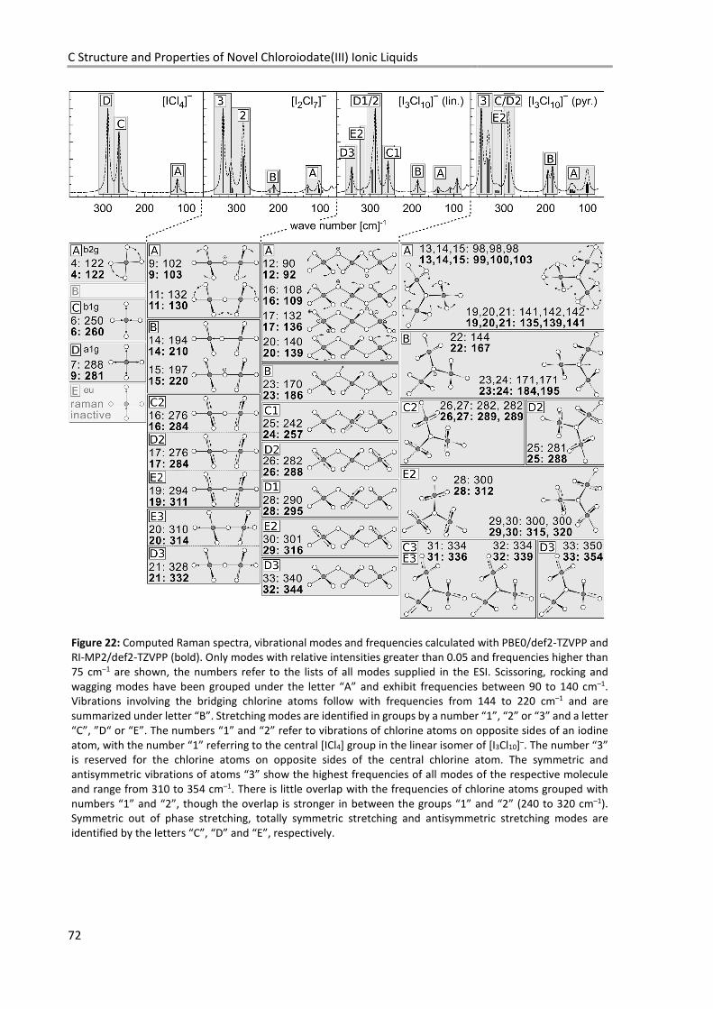
C Structure and Properties of Novel Chloroiodate(III) Ionic Liquids
72
Figure 22: Computed Raman spectra, vibrational modes and frequencies calculated with PBE0/def2-TZVPP and RI-MP2/def2-TZVPP (bold). Only modes with relative intensities greater than 0.05 and frequencies higher than 75 cm–1 are shown, the numbers refer to the lists of all modes supplied in the ESI. Scissoring, rocking and wagging modes have been grouped under the letter “A” and exhibit frequencies between 90 to 140 cm–1. Vibrations involving the bridging chlorine atoms follow with frequencies from 144 to 220 cm–1 and are summarized under letter “B”. Stretching modes are identified in groups by a number “1”, “2” or “3” and a letter “C”, ”D“ or “E”. The numbers “1” and “2” refer to vibrations of chlorine atoms on opposite sides of an iodine atom, with the number “1” referring to the central [ICl4] group in the linear isomer of [I3Cl10]–. The number “3” is reserved for the chlorine atoms on opposite sides of the central chlorine atom. The symmetric and antisymmetric vibrations of atoms “3” show the highest frequencies of all modes of the respective molecule and range from 310 to 354 cm–1. There is little overlap with the frequencies of chlorine atoms grouped with numbers “1” and “2”, though the overlap is stronger in between the groups “1” and “2” (240 to 320 cm–1). Symmetric out of phase stretching, totally symmetric stretching and antisymmetric stretching modes are identified by the letters “C”, “D” and “E”, respectively.
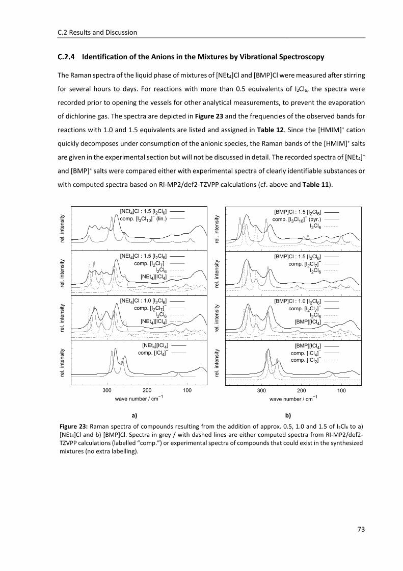
C.2 Results and Discussion
73
Identification of the Anions in the Mixtures by Vibrational Spectroscopy
The Raman spectra of the liquid phase of mixtures of [NEt4]Cl and [BMP]Cl were measured after stirring
for several hours to days. For reactions with more than 0.5 equivalents of I2Cl6, the spectra were
recorded prior to opening the vessels for other analytical measurements, to prevent the evaporation
of dichlorine gas. The spectra are depicted in Figure 23 and the frequencies of the observed bands for
reactions with 1.0 and 1.5 equivalents are listed and assigned in Table 12. Since the [HMIM]+ cation
quickly decomposes under consumption of the anionic species, the Raman bands of the [HMIM]+ salts
are given in the experimental section but will not be discussed in detail. The recorded spectra of [NEt4]+
and [BMP]+ salts were compared either with experimental spectra of clearly identifiable substances or
with computed spectra based on RI-MP2/def2-TZVPP calculations (cf. above and Table 11).
a)
b)
Figure 23: Raman spectra of compounds resulting from the addition of approx. 0.5, 1.0 and 1.5 of I2Cl6 to a) [NEt4]Cl and b) [BMP]Cl. Spectra in grey / with dashed lines are either computed spectra from RI-MP2/def2-TZVPP calculations (labelled “comp.”) or experimental spectra of compounds that could exist in the synthesized mixtures (no extra labelling).
rel. in
ten
sity
[BMP]Cl : 1.5 [I2Cl6]
comp. [I3Cl10]- (pyr.)
I2Cl6
rel. in
ten
sity
[BMP]Cl : 1.5 [I2Cl6]
comp. [I2Cl7]-
I2Cl6
rel. in
ten
sity
[BMP]Cl : 1.0 [I2Cl6]
comp. [I2Cl7]-
I2Cl6[BMP][ICl4]
100200300
rel. in
ten
sity
wave number / cm-1
[BMP][ICl4]
comp. [ICl4]-
comp. [ICl2]-
rel. in
ten
sity
[NEt4]Cl : 1.5 [I2Cl6]
comp. [I3Cl10]- (lin.)
rel. in
ten
sity
[NEt4]Cl : 1.5 [I2Cl6]
comp. [I2Cl7]-
I2Cl6[NEt4][ICl4]
rel. in
ten
sity
[NEt4]Cl : 1.0 [I2Cl6]
comp. [I2Cl7]-
I2Cl6[NEt4][ICl4]
100200300
rel. in
ten
sity
wave number / cm-1
[NEt4][ICl4]
comp. [ICl4]-
C Structure and Properties of Novel Chloroiodate(III) Ionic Liquids
74
C.2.4.1 Mixtures Aiming at [I2Cl7]–
The spectrum of [BMP]Cl : 1.0 I2Cl6 is in good agreement with the computed spectrum of [I2Cl7]–. A
clear indication is the presence of the band at 216 cm–1, which is in the expected region for vibrations
of a bridging chlorine atom. A further hint is the appearance of two (107 and 141 cm–1) instead of one
band (133 cm–1) in the region of the scissoring modes. This also follows from the calculated spectra
(122 vs. 103 and 130 cm–1). However, it has to be noted that the observed bands are very broad, which
could conceal the presence of small amounts of [ICl4]–, dissolved I2Cl6 or
[I3Cl10]–. The same holds true for [NEt4]Cl : 1.05 I2Cl6, where the unexpectedly intense band at
276 cm–1 could possibly be explained by the presence of [ICl4]– in this mixture.
C.2.4.2 Mixtures Aiming at [I3Cl10]–
The situation becomes less clear for the stoichiometry [cat]Cl : 1.5 I2Cl6. The bands of the [BMP]+
mixture do not show good agreement with the computed spectrum for
[I3Cl10]– - neither in the pyramidal nor planar form. Compared to the spectrum of [BMP]Cl : 1.0 I2Cl6,
the decrease in relative intensity of the band at 278 cm–1 and the small shift of the highest frequency
band from 333 to 337 cm–1 do not follow the trend of the computed spectra. A better fit is provided
by the combination of the computed bands of [I2Cl7]– and the experimental bands of I2Cl6. A clear
assignment is even more difficult for the mixture [NEt4]Cl : 1.5 I2Cl6. The best fit is provided by a
combination of I2Cl6, calculated [I2Cl7]– and [NEt4][ICl4], but definitive answers about the real
composition of the mixture are hard to give.
Since the clearest Raman spectra were obtained for the [BMP]+ compounds, far infrared spectra were
also recorded for these substances. However, the evaporation of chlorine could not be suppressed in
the ATR measurements, so the bands are given in the experimental section in the ESI, but no
conclusions about the anionic composition can be drawn from them.
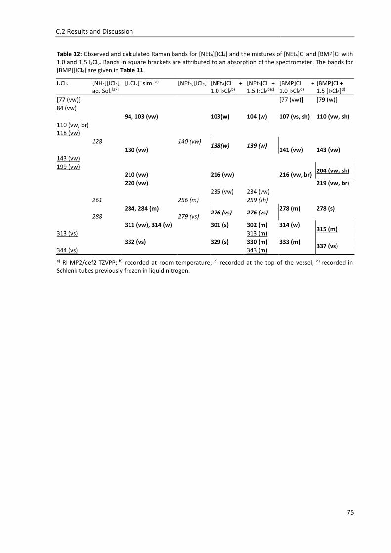
C.2 Results and Discussion
75
Table 12: Observed and calculated Raman bands for [NEt4][ICl4] and the mixtures of [NEt4]Cl and [BMP]Cl with 1.0 and 1.5 I2Cl6. Bands in square brackets are attributed to an absorption of the spectrometer. The bands for [BMP][ICl4] are given in Table 11.
I2Cl6 [NH4][ICl4] aq. Sol.[27]
[I2Cl7]– sim. a) [NEt4][ICl4] [NEt4]Cl + 1.0 I2Cl6
b) [NEt4]Cl + 1.5 I2Cl6
b)c) [BMP]Cl + 1.0 I2Cl6
d) [BMP]Cl + 1.5 [I2Cl6]d)
[77 (vw)] [77 (vw)] [79 (w)] 84 (vw)
94, 103 (vw) 103(w) 104 (w) 107 (vs, sh) 110 (vw, sh) 110 (vw, br)
118 (vw) 128 140 (vw)
138(w) 139 (w)
130 (vw) 141 (vw) 143 (vw) 143 (vw)
199 (vw) 204 (vw, sh)
210 (vw) 216 (vw) 216 (vw, br)
220 (vw) 219 (vw, br) 235 (vw) 234 (vw)
261 256 (m) 259 (sh) 284, 284 (m)
276 (vs) 276 (vs) 278 (m) 278 (s)
288 279 (vs) 311 (vw), 314 (w) 301 (s) 302 (m) 314 (w)
315 (m) 313 (vs) 313 (m)
332 (vs) 329 (s) 330 (m) 333 (m) 337 (vs)
344 (vs) 343 (m)
a) RI-MP2/def2-TZVPP; b) recorded at room temperature; c) recorded at the top of the vessel; d) recorded in Schlenk tubes previously frozen in liquid nitrogen.

C Structure and Properties of Novel Chloroiodate(III) Ionic Liquids
76
C.3 Conclusion and Outlook
77
C.3 Conclusion and Outlook
We have presented an extensive thermodynamic study on the gas-phase structures and stabilities of
chloroiodate anions incorporating up to three iodine atoms in the oxidation states of either +I or +III.
After careful analysis of experimental and calculated data, the constitution of the experimental
mixtures of [HMIM]Cl, [BMP]Cl and [NEt4]Cl with 0.5, 1.0 and 1.5 equivalents of I2Cl6 was evaluated.
The reaction with 0.5 equivalents I2Cl6 yielded, as expected, the salts [cat][ICl4] that are stable in closed
vessels over a period of days to weeks. The existence of novel and larger chloroiodate anions was
investigated by means of Raman spectroscopy and supported by computed Raman spectra and
thermodynamics. Thus, the formerly unknown [I2Cl7]– anion is the main anionic species in mixtures of
[BMP]Cl and [NEt4]Cl with 1.0 equivalents of I2Cl6. However, the tendency of these materials to lose
dichlorine is marked (both, based on experimental observation and calculated thermodynamics). This
tendency, or the increased chloroiodate-reactivity of these mixes, makes the [HMIM]+ cation
incompatible with this anion, due to facile and fast ring chlorination. Yet, all of these mixtures are
homogeneous liquids at RT even with a symmetrically substituted ammonium cation like [NEt4]+. This
is in contrast to the respective [ICl4]– salts and is possibly due to the reduced symmetry and greater
charge distribution in the anion as suggested by calculated electrostatic potential plots. Though three
new crystal structures for the [ICl4]– salts of [HMIM]+, [NEt4]+ and [BMP]+ were determined,
crystallographic proof for the existence of the [I2Cl7]– anion could not be obtained, despite many
attempts.
Although the combination of [BMP]Cl with 1.5 equivalents of I2Cl6 yields a homogeneous liquid phase
at 40°C, the existence of [I3Cl10]– cannot be clearly deduced from the experimental Raman spectra. This
is coherent with the decreasing gas phase complexation energy for the stepwise addition of ½ I2Cl6 to
a chloride anion as well as the further increased tendency to lose dichlorine, as shown in our quantum-
chemical calculations. Further research is needed to better understand the behaviour and to clarify, if
cations like [NEt]4+ are stable over largely extended periods of time in this harsh environment. After
several months, also the else rather stable [BMP]+ cation showed signs of side chain chlorination in the
investigated mixtures. An interesting objective for further research could be to determine, whether or
not the aggressive nature can be channelled into selective reactivity to yield a valuable tool in
synthesis.

C Structure and Properties of Novel Chloroiodate(III) Ionic Liquids
78
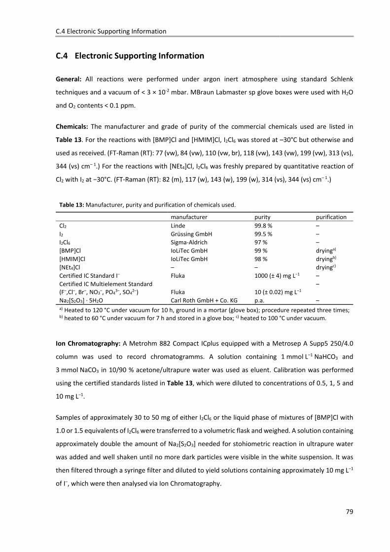
C.4 Electronic Supporting Information
79
C.4 Electronic Supporting Information
General: All reactions were performed under argon inert atmosphere using standard Schlenk
techniques and a vacuum of < 3 × 10⁻² mbar. MBraun Labmaster sp glove boxes were used with H2O
and O2 contents < 0.1 ppm.
Chemicals: The manufacturer and grade of purity of the commercial chemicals used are listed in
Table 13. For the reactions with [BMP]Cl and [HMIM]Cl, I2Cl6 was stored at –30°C but otherwise and
used as received. (FT-Raman (RT): 77 (vw), 84 (vw), 110 (vw, br), 118 (vw), 143 (vw), 199 (vw), 313 (vs),
344 (vs) cm– 1.) For the reactions with [NEt4]Cl, I2Cl6 was freshly prepared by quantitative reaction of
Cl2 with I2 at −30°C. (FT-Raman (RT): 82 (m), 117 (w), 143 (w), 199 (w), 314 (vs), 344 (vs) cm– 1.)
Table 13: Manufacturer, purity and purification of chemicals used.
manufacturer purity purification
Cl2 Linde 99.8 % – I2 Grüssing GmbH 99.5 % – I2Cl6 Sigma-Aldrich 97 % – [BMP]Cl IoLiTec GmbH 99 % dryinga) [HMIM]Cl IoLiTec GmbH 98 % dryingb) [NEt4]Cl – – dryingc) Certified IC Standard I– Fluka 1000 (± 4) mg L–1 – Certified IC Multielement Standard (F–,Cl–, Br–, NO3
–, PO43–, SO4
2–) Fluka 10 (± 0.02) mg L–1 –
Na2[S2O3] ∙ 5H2O Carl Roth GmbH + Co. KG p.a. – a) Heated to 120 °C under vacuum for 10 h, ground in a mortar (glove box); procedure repeated three times; b) heated to 60 °C under vacuum for 7 h and stored in a glove box; c) heated to 100 °C under vacuum.
Ion Chromatography: A Metrohm 882 Compact ICplus equipped with a Metrosep A Supp5 250/4.0
column was used to record chromatogramms. A solution containing 1 mmol L–1 NaHCO3 and
3 mmol NaCO3 in 10/90 % acetone/ultrapure water was used as eluent. Calibration was performed
using the certified standards listed in Table 13, which were diluted to concentrations of 0.5, 1, 5 and
10 mg L–1.
Samples of approximately 30 to 50 mg of either I2Cl6 or the liquid phase of mixtures of [BMP]Cl with
1.0 or 1.5 equivalents of I2Cl6 were transferred to a volumetric flask and weighed. A solution containing
approximately double the amount of Na2[S2O3] needed for stohiometric reaction in ultrapure water
was added and well shaken until no more dark particles were visible in the white suspension. It was
then filtered through a syringe filter and diluted to yield solutions containing approximately 10 mg L–1
of I–, which were then analysed via Ion Chromatography.
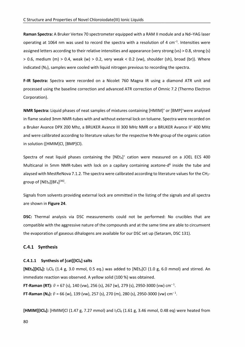
C Structure and Properties of Novel Chloroiodate(III) Ionic Liquids
80
Raman Spectra: A Bruker Vertex 70 spectrometer equipped with a RAM II module and a Nd–YAG laser
operating at 1064 nm was used to record the spectra with a resolution of 4 cm–1. Intensities were
assigned letters according to their relative intensities and appearance (very strong (vs) > 0.8, strong (s)
> 0.6, medium (m) > 0.4, weak (w) > 0.2, very weak < 0.2 (vw), shoulder (sh), broad (br)). Where
indicated (N2), samples were cooled with liquid nitrogen previous to recording the spectra.
F-IR Spectra: Spectra were recorded on a Nicolet 760 Magna IR using a diamond ATR unit and
processed using the baseline correction and advanced ATR correction of Omnic 7.2 (Thermo Electron
Corporation).
NMR Spectra: Liquid phases of neat samples of mixtures containing [HMIM]+ or [BMP]+were analysed
in flame sealed 3mm NMR-tubes with and without external lock on toluene. Spectra were recorded on
a Bruker Avance DPX 200 Mhz, a BRUKER Avance III 300 MHz NMR or a BRUKER Avance II+ 400 MHz
and were calibrated according to literature values for the respective N-Me group of the organic cation
in solution ([HMIM]Cl, [BMP]Cl).
Spectra of neat liquid phases containing the [NEt4]+ cation were measured on a JOEL ECS 400
Multicanal in 5mm NMR-tubes with lock on a capilary containing acetone-d6 inside the tube and
alaysed with MestReNova 7.1.2. The spectra were calibrated according to literature values for the CH2-
group of [NEt4][BF4][46].
Signals from solvents providing external lock are ommitted in the listing of the signals and all spectra
are shown in Figure 24.
DSC: Thermal analysis via DSC measurements could not be performed: No crucibles that are
compatible with the aggressive nature of the compounds and at the same time are able to circumvent
the evaporation of gaseous dihalogens are available for our DSC set up (Setaram, DSC 131).
Synthesis
C.4.1.1 Synthesis of [cat][ICl4] salts
[NEt4][ICl4]: I2Cl6 (1.4 g, 3.0 mmol, 0.5 eq.) was added to [NEt4]Cl (1.0 g, 6.0 mmol) and stirred. An
immediate reaction was observed. A yellow solid (100 %) was obtained.
FT-Raman (RT): NO = 67 (s), 140 (vw), 256 (s), 267 (w), 279 (s), 2950-3000 (vw) cm– 1.
FT-Raman (N2): NO = 66 (w), 139 (vw), 257 (s), 270 (m), 280 (s), 2950-3000 (vw) cm– 1.
[HMIM][ICl4]: [HMIM]Cl (1.47 g, 7.27 mmol) and I2Cl6 (1.61 g, 3.46 mmol, 0.48 eq) were heated from
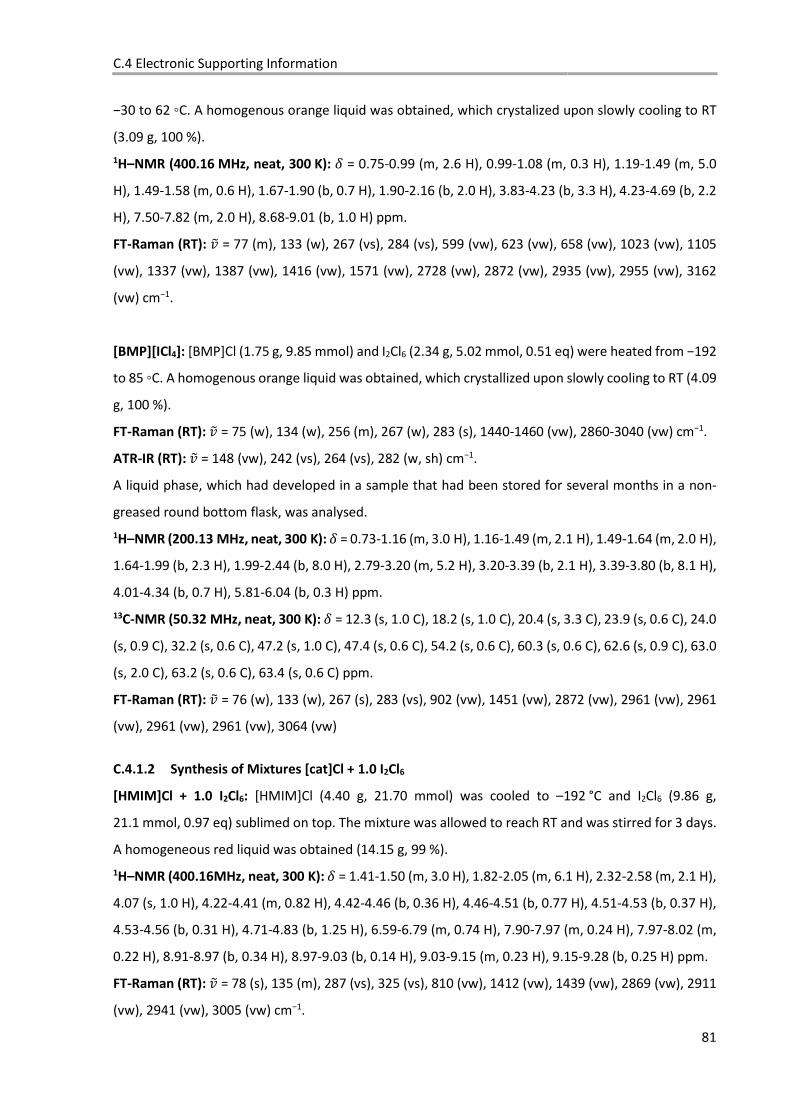
C.4 Electronic Supporting Information
81
−30 to 62 ◦C. A homogenous orange liquid was obtained, which crystalized upon slowly cooling to RT
(3.09 g, 100 %).
1H–NMR (400.16 MHz, neat, 300 K): P = 0.75-0.99 (m, 2.6 H), 0.99-1.08 (m, 0.3 H), 1.19-1.49 (m, 5.0
H), 1.49-1.58 (m, 0.6 H), 1.67-1.90 (b, 0.7 H), 1.90-2.16 (b, 2.0 H), 3.83-4.23 (b, 3.3 H), 4.23-4.69 (b, 2.2
H), 7.50-7.82 (m, 2.0 H), 8.68-9.01 (b, 1.0 H) ppm.
FT-Raman (RT): NO = 77 (m), 133 (w), 267 (vs), 284 (vs), 599 (vw), 623 (vw), 658 (vw), 1023 (vw), 1105
(vw), 1337 (vw), 1387 (vw), 1416 (vw), 1571 (vw), 2728 (vw), 2872 (vw), 2935 (vw), 2955 (vw), 3162
(vw) cm−1.
[BMP][ICl4]: [BMP]Cl (1.75 g, 9.85 mmol) and I2Cl6 (2.34 g, 5.02 mmol, 0.51 eq) were heated from −192
to 85 ◦C. A homogenous orange liquid was obtained, which crystallized upon slowly cooling to RT (4.09
g, 100 %).
FT-Raman (RT): NO = 75 (w), 134 (w), 256 (m), 267 (w), 283 (s), 1440-1460 (vw), 2860-3040 (vw) cm−1.
ATR-IR (RT): NO = 148 (vw), 242 (vs), 264 (vs), 282 (w, sh) cm−1.
A liquid phase, which had developed in a sample that had been stored for several months in a non-
greased round bottom flask, was analysed.
1H–NMR (200.13 MHz, neat, 300 K): P = 0.73-1.16 (m, 3.0 H), 1.16-1.49 (m, 2.1 H), 1.49-1.64 (m, 2.0 H),
1.64-1.99 (b, 2.3 H), 1.99-2.44 (b, 8.0 H), 2.79-3.20 (m, 5.2 H), 3.20-3.39 (b, 2.1 H), 3.39-3.80 (b, 8.1 H),
4.01-4.34 (b, 0.7 H), 5.81-6.04 (b, 0.3 H) ppm.
13C-NMR (50.32 MHz, neat, 300 K): P = 12.3 (s, 1.0 C), 18.2 (s, 1.0 C), 20.4 (s, 3.3 C), 23.9 (s, 0.6 C), 24.0
(s, 0.9 C), 32.2 (s, 0.6 C), 47.2 (s, 1.0 C), 47.4 (s, 0.6 C), 54.2 (s, 0.6 C), 60.3 (s, 0.6 C), 62.6 (s, 0.9 C), 63.0
(s, 2.0 C), 63.2 (s, 0.6 C), 63.4 (s, 0.6 C) ppm.
FT-Raman (RT): NO = 76 (w), 133 (w), 267 (s), 283 (vs), 902 (vw), 1451 (vw), 2872 (vw), 2961 (vw), 2961
(vw), 2961 (vw), 2961 (vw), 3064 (vw)
C.4.1.2 Synthesis of Mixtures [cat]Cl + 1.0 I2Cl6
[HMIM]Cl + 1.0 I2Cl6: [HMIM]Cl (4.40 g, 21.70 mmol) was cooled to –192 °C and I2Cl6 (9.86 g,
21.1 mmol, 0.97 eq) sublimed on top. The mixture was allowed to reach RT and was stirred for 3 days.
A homogeneous red liquid was obtained (14.15 g, 99 %).
1H–NMR (400.16MHz, neat, 300 K): P = 1.41-1.50 (m, 3.0 H), 1.82-2.05 (m, 6.1 H), 2.32-2.58 (m, 2.1 H),
4.07 (s, 1.0 H), 4.22-4.41 (m, 0.82 H), 4.42-4.46 (b, 0.36 H), 4.46-4.51 (b, 0.77 H), 4.51-4.53 (b, 0.37 H),
4.53-4.56 (b, 0.31 H), 4.71-4.83 (b, 1.25 H), 6.59-6.79 (m, 0.74 H), 7.90-7.97 (m, 0.24 H), 7.97-8.02 (m,
0.22 H), 8.91-8.97 (b, 0.34 H), 8.97-9.03 (b, 0.14 H), 9.03-9.15 (m, 0.23 H), 9.15-9.28 (b, 0.25 H) ppm.
FT-Raman (RT): NO = 78 (s), 135 (m), 287 (vs), 325 (vs), 810 (vw), 1412 (vw), 1439 (vw), 2869 (vw), 2911
(vw), 2941 (vw), 3005 (vw) cm−1.

C Structure and Properties of Novel Chloroiodate(III) Ionic Liquids
82
[BMP]Cl + 1.0 I2Cl6: [BMP]Cl (1.16 g, 6.50 mmol) and I2Cl6 (3.14 g, 6.73 mmol, 1.04 eq) were combined
at –192 °C and stirred over night at room temperature. A homogenous red liquid was obtained (4.29 g,
100 %).
1H–NMR (300.18 MHz, neat, 300 K): P = 0.48-1.19 (b, 3 H, CH2CH2CH2CH3), 1.20-1.58 (b, 2 H,
CH2CH2CH2CH3), 1.58-1.93 (b, 2 H, CH2CH2CH2CH3), 1.93-2.59 (b, 4 H, NCH2CH2CH2CH2), 2.60-3.11 (b,
3 H, NCH3), 3.12-4.80 (b, 6 H, CH2CH2CH2CH3, NCH2CH2CH2CH2) ppm.
13C-NMR (75.48 MHz, neat, 300 K): P = 11.8 (s, 1 C, CH2CH2CH2CH3), 17.5 (s, 1 C, CH2CH2CH2CH3), 19.7
(s, 2 C, NCH2CH2CH2CH2), 23.3 (s, 1 C, CH2CH2CH2CH3), 47.2 (s, 1 C, NCH3), 62.3 (s, 1 C, CH2CH2CH2CH3),
62.7 (s, 1 C, NCH2CH2CH2CH2) ppm.
FT-Raman (RT): NO = 77 (m), 106 (w, sh), 138 (w), 219 (vw, br), 277 (vs), 310 (m), 332 (vs), 525 (vw), 904
(vw), 1054 (vw), 1120 (vw), 1452 (vw), 1484 (vw), 2873 (vw), 2963 (vw), 2985 (vw), 3027 (vw).
FT-Raman (N2): NO = 77 (vw), 107 (vs, sh), 141 (vw), 216 (vw, br), 278 (m), 314 (w), 333 (m), 521 (vw),
1451 (vw), 2872 (vw), 2892 (vw), 2911 (vw), 2942 (vw), 2965 (vw), 2984 (vw), 3009 (vw),
3026 (vw cm–1.
ATR-IR (RT): NO = 264 (vs), 280 (vs), 306 (m, sh), 329 (w) cm–1.
C.4.1.3 Synthesis of Mixtures [cat][Cl] + 1.5 I2Cl6
[BMP]Cl + 1.5 I2Cl6: [BMP]Cl (0.97 g, 5.48 mmol) and I2Cl6 (3.75 g, 8.03 mmol, 1.47 eq) were combined
at –192 °C and stirred over night at room temperature. After heating to 40 °C, a homogenous red liquid
was obtained (4.71 g, 100 %). Upon leaving the mixture at room temperature and after the raman
spectra had been recorded, a small amount of an orange solid precipitated.
1H–NMR (300.18 MHz, neat, 300 K): P = 0.40-1.23 (b, 3 H, CH2CH2CH2CH3), 1.23-1.60 (b, 2 H,
CH2CH2CH2CH3), 1.61-1.97 (b, 2 H, CH2CH2CH2CH3), 1.97-2.62 (b, 4 H, NCH2CH2CH2CH2), 2.63-3.13 (b,
3 H, NCH3), 3.14-4.80 (b, 6 H, CH2CH2CH2CH3, NCH2CH2CH2CH2) ppm.
13C–NMR (75.48 MHz, neat, 300 K): P = 11.9 (s, 1 C, CH2CH2CH2CH3), 17.5 (s, 1 C, CH2CH2CH2CH3), 19.7
(s, 2 C, NCH2CH2CH2CH2), 23.3 (s, 1 C, CH2CH2CH2CH3), 47.2 (s, 1 C, NCH3), 62.4 (s, 1 C, CH2CH2CH2CH3),
62.7 (s, 2 C, NCH2CH2CH2CH2) ppm.
FT-Raman (RT): NO = 77 (m), 106 (w, sh), 142 (w), 239 (vw), 276 (m), 314 (m, sh), 336 (vs), 528 (vw), 903
(vw), 1452 (vw), 2873 (vw), 2897 (vw), 2941 (vw), 2964 (vw) cm–1.
FT-Raman (N2): NO = 79 (w), 110 (vw, sh), 143 (vw), 204 (vw, sh), 219 (vw, br), 278 (s), 315 (m), 337 (vs),
444 (vw), 508 (vw), 1450 (vw), 2867 (vw), 2890 (vw), 2939 (vw), 2962 (vw), 2982 (vw), 3000 (vw), 3037
(vw) cm–1.
ATR-IR (RT): NO = 228 (w), 266 (vs), 280 (vs), 303 (s), 329 (m), 334 (m) cm–1.

C.4 Electronic Supporting Information
83
[NEt4]Cl + 1.0 [I2Cl6]: I2Cl6 (1.00 g, 2.14 mmol, 1.0 eq.) was added to [NEt4]Cl (0.344 g, 2.08 mmol) and
stirred. An immediate reaction was observed. A red liquid (100 %) was obtained.
FT-Raman (RT) : NO = 103 (w), 138 (w), 216 (vw), 235 (vw), 276 (vs), 301 (s), 329 (s), 1458 (vw), 2941
(vw), 2992 (vw) cm¬1.
FT-Raman (N2): NO = 106 (w), 140 (w), 236 (vw), 278 (vs), 304 (s), 330 (s), 1458 (vw), 2940 (vw), 2992
(vw) cm¬1.
1H-NMR (401 MHz, neat, RT): P = 1.34.31 (b, 3H, CH3), 1.56 (b, 2H, CH2), 7.73 ppm.
13C-NMR (101 MHz, neat, RT): P =6.6 (CH3), 51.3 (CH2) ppm.
[NEt4]Cl + 1.5 [I2Cl6]: I2Cl6 (2.18 g, 4.67 mmol, 1.55 eq.) was added to [NEt4]Cl (0.501 g, 3.02 mmol) and
stirred. An immediate reaction was observed. A red liquid with orange solid (100 %) was obtained.
Raman spectra are given both for the top of the vessel and for the bottom of the vessel.
FT-Raman (bottom, RT): NO = 108 (w), 142 (w), 200 (w), 275 (m), 314 (s), 344 (vs), 1459 (vw), 2942 (vw),
2991 (vw) cm– 1.
FT-Raman (bottom, N2): NO = 114 (w), 143 (w), 201 (w), 235 (vw), 278 (m), 303 (sh), 315 (vs), 330 (m),
346 (vs), 1458 (vw), 2939 (vw), 2992 (vw) cm– 1.
FT-Raman (top, RT): NO = 104 (w), 139 (w), 234 (vw), 259 (sh), 276 (vs), 302 (m), 313 (m), 330 (m), 343
(m), 1459 (vw), 2941 (vw), 2992 (vw) cm– 1.
FT-Raman (top, N2): NO = 113 (w), 143 (w), 201 (w), 238 (vw), 258 (w), 278 (vs), 315 (vs), 329 (m), 346
(s), 1458 (vw), 2940 (vw), 2992 (vw) cm– 1.
1H-NMR (401 MHz, neat, RT): P = 0.20-2.45 (b, CH3), 2.45-4.2 (b, CH2) ppm.
13C-NMR (101 MHz, neat, RT): P = 6.8 (b, CH3), 51.3 (b, CH2) ppm
C.4.1.4 Additional Figures
The measured NMR spectra are shown in Figure 24.
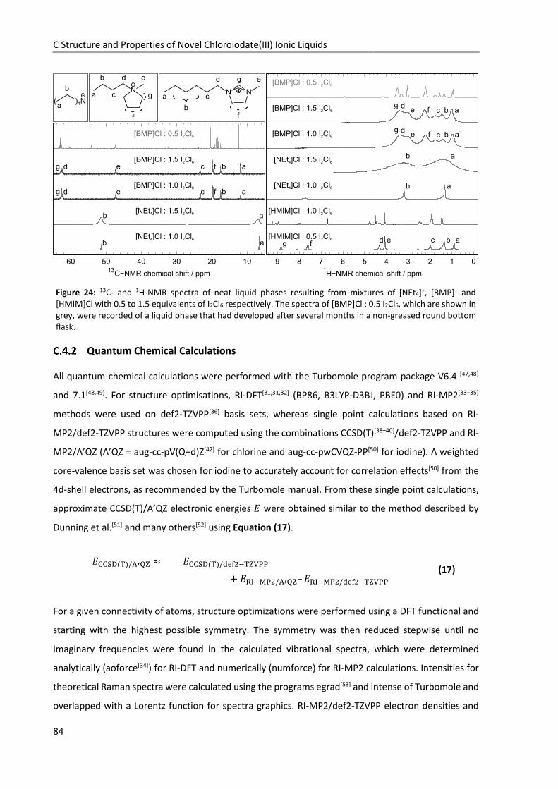
C Structure and Properties of Novel Chloroiodate(III) Ionic Liquids
84
Figure 24: 13C- and 1H-NMR spectra of neat liquid phases resulting from mixtures of [NEt4]+, [BMP]+ and [HMIM]Cl with 0.5 to 1.5 equivalents of I2Cl6 respectively. The spectra of [BMP]Cl : 0.5 I2Cl6, which are shown in grey, were recorded of a liquid phase that had developed after several months in a non-greased round bottom flask.
Quantum Chemical Calculations
All quantum-chemical calculations were performed with the Turbomole program package V6.4 [47,48]
and 7.1[48,49]. For structure optimisations, RI-DFT[31,31,32] (BP86, B3LYP-D3BJ, PBE0) and RI-MP2[33–35]
methods were used on def2-TZVPP[36] basis sets, whereas single point calculations based on RI-
MP2/def2-TZVPP structures were computed using the combinations CCSD(T)[38–40]/def2-TZVPP and RI-
MP2/A’QZ (A’QZ = aug-cc-pV(Q+d)Z[42] for chlorine and aug-cc-pwCVQZ-PP[50] for iodine). A weighted
core-valence basis set was chosen for iodine to accurately account for correlation effects[50] from the
4d-shell electrons, as recommended by the Turbomole manual. From these single point calculations,
approximate CCSD(T)/A’QZ electronic energies � were obtained similar to the method described by
Dunning et al.[51] and many others[52] using Equation (17).
���QRSTU/WXYZ [ ���QRSTU/\�]0^TZ_88 (17)
/ �`a^b80/WXYZ– �`a^b80/\�]0^TZ_88
For a given connectivity of atoms, structure optimizations were performed using a DFT functional and
starting with the highest possible symmetry. The symmetry was then reduced stepwise until no
imaginary frequencies were found in the calculated vibrational spectra, which were determined
analytically (aoforce[34]) for RI-DFT and numerically (numforce) for RI-MP2 calculations. Intensities for
theoretical Raman spectra were calculated using the programs egrad[53] and intense of Turbomole and
overlapped with a Lorentz function for spectra graphics. RI-MP2/def2-TZVPP electron densities and
C.4 Electronic Supporting Information
85
charge distribution were calculated using Turbomole and plotted with gOpenMol[54]. Molecular
structure representations were produced using Diamond 3.0a.[55] Thermodynamic functions at room
temperature and a pressure of 1 bar were calculated using the tool freeh (default symmetry, scaling
factor 1) provided with Turbomole based on frequencies obtained from BP86/def2-TZVPP calculations.
It provides thermodynamic values for the molar Internal Energy �, from which the molar Enthalpy d
can be calculated following Equation (18).
d = � / � ∙ e (18)
With the molar Entropy �, the molar Gibbs Enthalpy f is obtained with Equation (19).
f = d / e ∙ � (19)
C.4.2.1 Energies, Entropy and Vibrational Spectra
The electronic energies of all investigated anions as well as their internal energy and entropy at
298.15 K and a pressure of 1 bar are given in Table 13. Frequencies of vibrational modes and intensities
of [I2Cl7]– and [I3Cl10]– in a pyramidal and a linear isomer along with relative intensities for both IR and
Raman are given in Table 15.
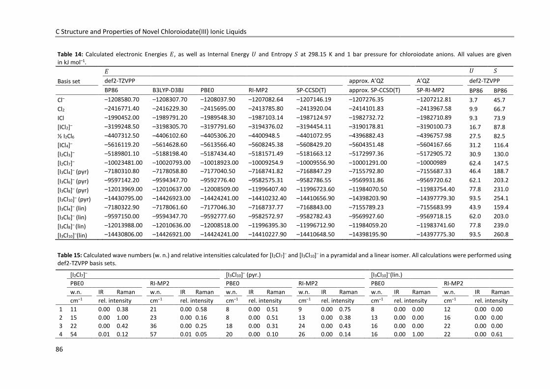
C Structure and Properties of Novel Chloroiodate(III) Ionic Liquids
86
Table 14: Calculated electronic Energies �, as well as Internal Energy � and Entropy � at 298.15 K and 1 bar pressure for chloroiodate anions. All values are given in kJ mol–1.
� � �
Basis set def2-TZVPP approx. A’QZ A’QZ def2-TZVPP
BP86 B3LYP-D3BJ PBE0 RI-MP2 SP-CCSD(T) approx. SP-CCSD(T) SP-RI-MP2 BP86 BP86
Cl– –1208580.70 –1208307.70 –1208037.90 –1207082.64 –1207146.19 –1207276.35 –1207212.81 3.7 45.7
Cl2 –2416771.40 –2416229.30 –2415695.00 –2413785.80 –2413920.04 –2414101.83 –2413967.58 9.9 66.7
ICl –1990452.00 –1989791.20 –1989548.30 –1987103.14 –1987124.97 –1982732.72 –1982710.89 9.3 73.9
[ICl2]– –3199248.50 –3198305.70 –3197791.60 –3194376.02 –3194454.11 –3190178.81 –3190100.73 16.7 87.8
½ I2Cl6 –4407312.50 –4406102.60 –4405306.20 –4400948.5 –4401072.95 –4396882.43 –4396757.98 27.5 82.5
[ICl4]– –5616119.20 –5614628.60 –5613566.40 –5608245.38 –5608429.20 –5604351.48 –5604167.66 31.2 116.4
[I2Cl3]– –5189801.10 –5188198.40 –5187434.40 –5181571.49 –5181663.12 –5172997.36 –5172905.72 30.9 130.0
[I2Cl7]– –10023481.00 –10020793.00 –10018923.00 –10009254.9 –10009556.90 –10001291.00 –10000989 62.4 147.5
[I3Cl4]– (pyr) –7180310.80 –7178058.80 –7177040.50 –7168741.82 –7168847.29 –7155792.80 –7155687.33 46.4 188.7
[I3Cl6]– (pyr) –9597142.20 –9594347.70 –9592776.40 –9582575.31 –9582786.55 –9569931.86 –9569720.62 62.1 203.2
[I3Cl8]– (pyr) –12013969.00 –12010637.00 –12008509.00 –11996407.40 –11996723.60 –11984070.50 –11983754.40 77.8 231.0
[I3Cl10]– (pyr) –14430795.00 –14426923.00 –14424241.00 –14410232.40 –14410656.90 –14398203.90 –14397779.30 93.5 254.1
[I3Cl4]– (lin) –7180322.90 –7178061.60 –7177046.30 –7168737.77 –7168843.00 –7155789.23 –7155683.99 43.9 159.4
[I3Cl6]– (lin) –9597150.00 –9594347.70 –9592777.60 –9582572.97 –9582782.43 –9569927.60 –9569718.15 62.0 203.0
[I3Cl8]– (lin) –12013988.00 –12010636.00 –12008518.00 –11996395.30 –11996712.90 –11984059.20 –11983741.60 77.8 239.0
[I3Cl10]–(lin) –14430806.00 –14426921.00 –14424241.00 –14410227.90 –14410648.50 –14398195.90 –14397775.30 93.5 260.8
Table 15: Calculated wave numbers (w. n.) and relative intensities calculated for [I2Cl7]– and [I3Cl10]– in a pyramidal and a linear isomer. All calculations were performed using def2-TZVPP basis sets.
[I2Cl7]– [I3Cl10]– (pyr.) [I3Cl10]–(lin.)
PBE0 RI-MP2 PBE0 RI-MP2 PBE0 RI-MP2
w.n. IR Raman w.n. IR Raman w.n. IR Raman w.n. IR Raman w.n. IR Raman w.n. IR Raman
cm–1 rel. intensity cm–1 rel. intensity cm–1 rel. intensity cm–1 rel. intensity cm–1 rel. intensity cm–1 rel. intensity
1 11 0.00 0.38 21 0.00 0.58 8 0.00 0.51 9 0.00 0.75 8 0.00 0.00 12 0.00 0.00 2 15 0.00 1.00 23 0.00 0.16 8 0.00 0.51 13 0.00 0.38 13 0.00 0.00 16 0.00 0.00 3 22 0.00 0.42 36 0.00 0.25 18 0.00 0.31 24 0.00 0.43 16 0.00 0.00 22 0.00 0.00 4 54 0.01 0.12 57 0.01 0.05 20 0.00 0.10 26 0.00 0.14 16 0.00 1.00 22 0.00 0.61
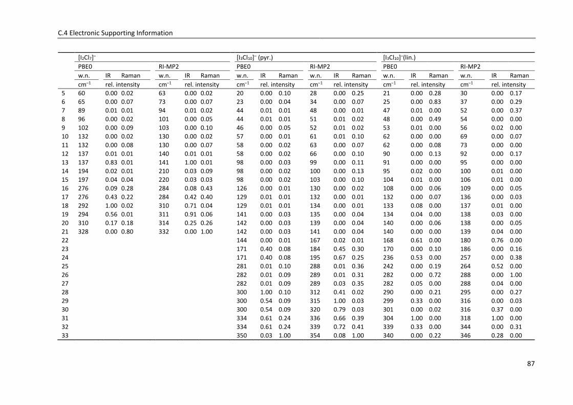
C.4 Electronic Supporting Information
87
[I2Cl7]– [I3Cl10]– (pyr.) [I3Cl10]–(lin.)
PBE0 RI-MP2 PBE0 RI-MP2 PBE0 RI-MP2
w.n. IR Raman w.n. IR Raman w.n. IR Raman w.n. IR Raman w.n. IR Raman w.n. IR Raman
cm–1 rel. intensity cm–1 rel. intensity cm–1 rel. intensity cm–1 rel. intensity cm–1 rel. intensity cm–1 rel. intensity 5 60 0.00 0.02 63 0.00 0.02 20 0.00 0.10 28 0.00 0.25 21 0.00 0.28 30 0.00 0.17 6 65 0.00 0.07 73 0.00 0.07 23 0.00 0.04 34 0.00 0.07 25 0.00 0.83 37 0.00 0.29 7 89 0.01 0.01 94 0.01 0.02 44 0.01 0.01 48 0.00 0.01 47 0.01 0.00 52 0.00 0.37 8 96 0.00 0.02 101 0.00 0.05 44 0.01 0.01 51 0.01 0.02 48 0.00 0.49 54 0.00 0.00 9 102 0.00 0.09 103 0.00 0.10 46 0.00 0.05 52 0.01 0.02 53 0.01 0.00 56 0.02 0.00 10 132 0.00 0.02 130 0.00 0.02 57 0.00 0.01 61 0.01 0.10 62 0.00 0.00 69 0.00 0.07 11 132 0.00 0.08 130 0.00 0.07 58 0.00 0.02 63 0.00 0.07 62 0.00 0.08 73 0.00 0.00 12 137 0.01 0.01 140 0.01 0.01 58 0.00 0.02 66 0.00 0.10 90 0.00 0.13 92 0.00 0.17 13 137 0.83 0.01 141 1.00 0.01 98 0.00 0.03 99 0.00 0.11 91 0.00 0.00 95 0.00 0.00 14 194 0.02 0.01 210 0.03 0.09 98 0.00 0.02 100 0.00 0.13 95 0.02 0.00 100 0.01 0.00 15 197 0.04 0.04 220 0.03 0.03 98 0.00 0.02 103 0.00 0.10 104 0.01 0.00 106 0.01 0.00 16 276 0.09 0.28 284 0.08 0.43 126 0.00 0.01 130 0.00 0.02 108 0.00 0.06 109 0.00 0.05 17 276 0.43 0.22 284 0.42 0.40 129 0.01 0.01 132 0.00 0.01 132 0.00 0.07 136 0.00 0.03 18 292 1.00 0.02 310 0.71 0.04 129 0.01 0.01 134 0.00 0.01 133 0.08 0.00 137 0.01 0.00 19 294 0.56 0.01 311 0.91 0.06 141 0.00 0.03 135 0.00 0.04 134 0.04 0.00 138 0.03 0.00 20 310 0.17 0.18 314 0.25 0.26 142 0.00 0.03 139 0.00 0.04 140 0.00 0.06 138 0.00 0.05 21 328 0.00 0.80 332 0.00 1.00 142 0.00 0.03 141 0.00 0.04 140 0.00 0.00 139 0.04 0.00 22 144 0.00 0.01 167 0.02 0.01 168 0.61 0.00 180 0.76 0.00 23 171 0.40 0.08 184 0.45 0.30 170 0.00 0.10 186 0.00 0.16 24 171 0.40 0.08 195 0.67 0.25 236 0.53 0.00 257 0.00 0.38 25 281 0.01 0.10 288 0.01 0.36 242 0.00 0.19 264 0.52 0.00 26 282 0.01 0.09 289 0.01 0.31 282 0.00 0.72 288 0.00 1.00 27 282 0.01 0.09 289 0.03 0.35 282 0.05 0.00 288 0.04 0.00 28 300 1.00 0.10 312 0.41 0.02 290 0.00 0.21 295 0.00 0.27 29 300 0.54 0.09 315 1.00 0.03 299 0.33 0.00 316 0.00 0.03 30 300 0.54 0.09 320 0.79 0.03 301 0.00 0.02 316 0.37 0.00 31 334 0.61 0.24 336 0.66 0.39 304 1.00 0.00 318 1.00 0.00 32 334 0.61 0.24 339 0.72 0.41 339 0.33 0.00 344 0.00 0.31 33 350 0.03 1.00 354 0.08 1.00 340 0.00 0.22 346 0.28 0.00
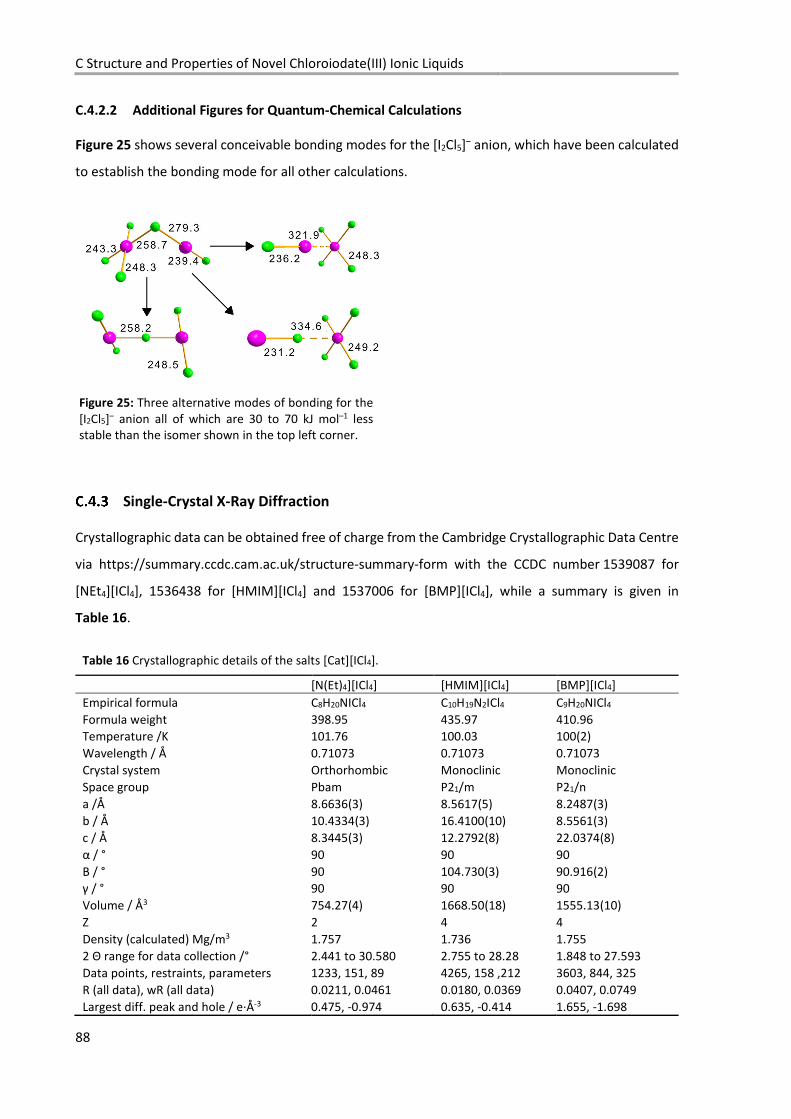
C Structure and Properties of Novel Chloroiodate(III) Ionic Liquids
88
C.4.2.2 Additional Figures for Quantum-Chemical Calculations
Figure 25 shows several conceivable bonding modes for the [I2Cl5]– anion, which have been calculated
to establish the bonding mode for all other calculations.
Figure 25: Three alternative modes of bonding for the [I2Cl5]– anion all of which are 30 to 70 kJ mol–1 less stable than the isomer shown in the top left corner.
Single-Crystal X-Ray Diffraction
Crystallographic data can be obtained free of charge from the Cambridge Crystallographic Data Centre
via https://summary.ccdc.cam.ac.uk/structure-summary-form with the CCDC number 1539087 for
[NEt4][ICl4], 1536438 for [HMIM][ICl4] and 1537006 for [BMP][ICl4], while a summary is given in
Table 16.
Table 16 Crystallographic details of the salts [Cat][ICl4].
[N(Et)4][ICl4] [HMIM][ICl4] [BMP][ICl4]
Empirical formula C8H20NICl4 C10H19N2ICl4 C9H20NICl4 Formula weight 398.95 435.97 410.96 Temperature /K 101.76 100.03 100(2) Wavelength / Å 0.71073 0.71073 0.71073 Crystal system Orthorhombic Monoclinic Monoclinic Space group Pbam P21/m P21/n a /Å 8.6636(3) 8.5617(5) 8.2487(3) b / Å 10.4334(3) 16.4100(10) 8.5561(3) c / Å 8.3445(3) 12.2792(8) 22.0374(8) α / ° 90 90 90 Β / ° 90 104.730(3) 90.916(2) γ / ° 90 90 90 Volume / Å3 754.27(4) 1668.50(18) 1555.13(10) Z 2 4 4 Density (calculated) Mg/m3 1.757 1.736 1.755 2 Θ range for data collection /° 2.441 to 30.580 2.755 to 28.28 1.848 to 27.593 Data points, restraints, parameters 1233, 151, 89 4265, 158 ,212 3603, 844, 325 R (all data), wR (all data) 0.0211, 0.0461 0.0180, 0.0369 0.0407, 0.0749 Largest diff. peak and hole / e∙Å-3 0.475, -0.974 0.635, -0.414 1.655, -1.698
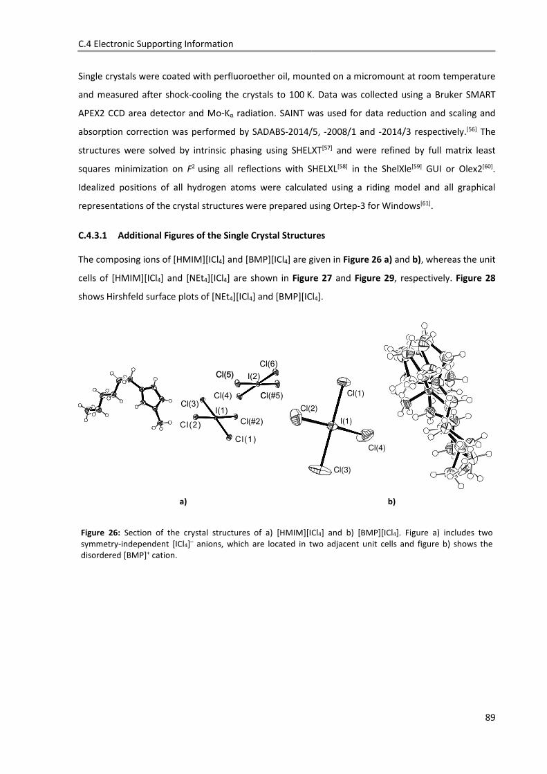
C.4 Electronic Supporting Information
89
Single crystals were coated with perfluoroether oil, mounted on a micromount at room temperature
and measured after shock-cooling the crystals to 100 K. Data was collected using a Bruker SMART
APEX2 CCD area detector and Mo-Kα radiation. SAINT was used for data reduction and scaling and
absorption correction was performed by SADABS-2014/5, -2008/1 and -2014/3 respectively.[56] The
structures were solved by intrinsic phasing using SHELXT[57] and were refined by full matrix least
squares minimization on F2 using all reflections with SHELXL[58] in the ShelXle[59] GUI or Olex2[60].
Idealized positions of all hydrogen atoms were calculated using a riding model and all graphical
representations of the crystal structures were prepared using Ortep-3 for Windows[61].
C.4.3.1 Additional Figures of the Single Crystal Structures
The composing ions of [HMIM][ICl4] and [BMP][ICl4] are given in Figure 26 a) and b), whereas the unit
cells of [HMIM][ICl4] and [NEt4][ICl4] are shown in Figure 27 and Figure 29, respectively. Figure 28
shows Hirshfeld surface plots of [NEt4][ICl4] and [BMP][ICl4].
a) b)
Figure 26: Section of the crystal structures of a) [HMIM][ICl4] and b) [BMP][ICl4]. Figure a) includes two symmetry-independent [ICl4]– anions, which are located in two adjacent unit cells and figure b) shows the disordered [BMP]+ cation.
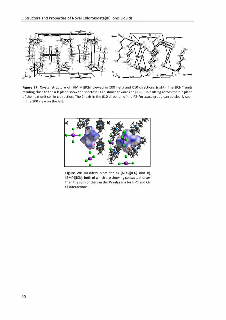
C Structure and Properties of Novel Chloroiodate(III) Ionic Liquids
90
Figure 27: Crystal structure of [HMIM][ICl4] viewed in 100 (left) and 010 directions (right). The [ICl4]– units residing close to the a-b plane show the shortest I-Cl distance towards an [ICl4]– unit sitting across the b-c plane of the next unit cell in c direction. The 21 axis in the 010 direction of the P21/m space group can be clearly seen in the 100 view on the left.
a) b)
Figure 28: Hirshfeld plots for a) [NEt4][ICl4] and b) [BMP][ICl4], both of which are showing contacts shorter than the sum of the van der Waals radii for H-Cl and Cl-Cl interactions..
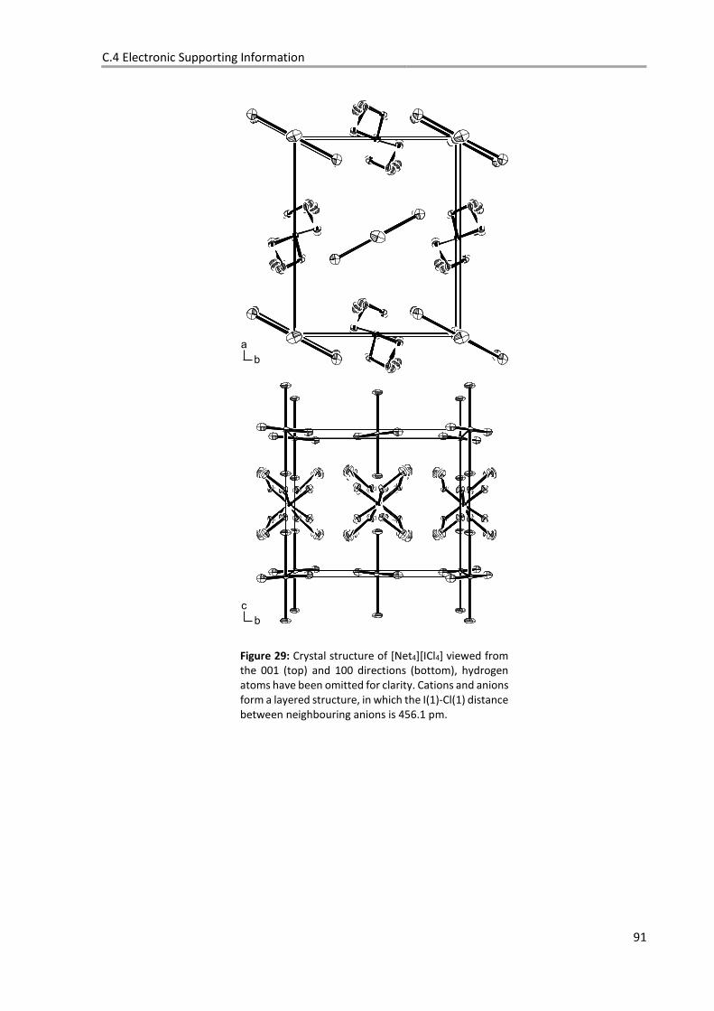
C.4 Electronic Supporting Information
91
Figure 29: Crystal structure of [Net4][ICl4] viewed from the 001 (top) and 100 directions (bottom), hydrogen atoms have been omitted for clarity. Cations and anions form a layered structure, in which the I(1)-Cl(1) distance between neighbouring anions is 456.1 pm.
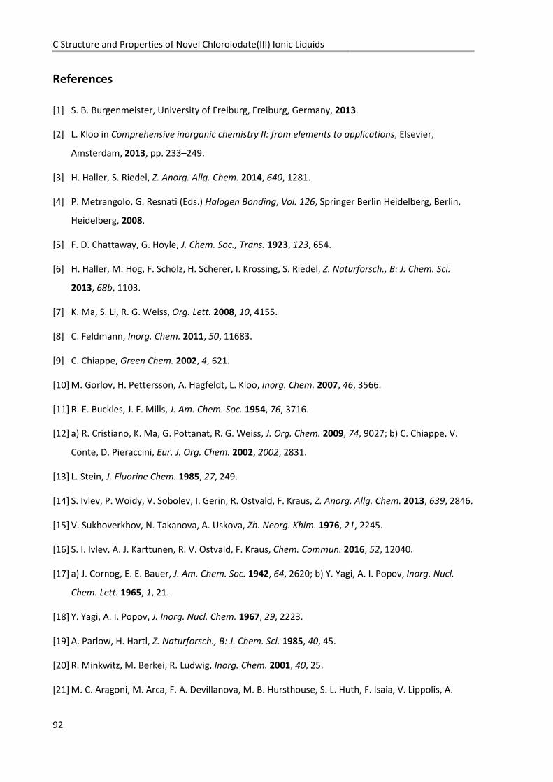
C Structure and Properties of Novel Chloroiodate(III) Ionic Liquids
92
References
[1] S. B. Burgenmeister, University of Freiburg, Freiburg, Germany, 2013.
[2] L. Kloo in Comprehensive inorganic chemistry II: from elements to applications, Elsevier,
Amsterdam, 2013, pp. 233–249.
[3] H. Haller, S. Riedel, Z. Anorg. Allg. Chem. 2014, 640, 1281.
[4] P. Metrangolo, G. Resnati (Eds.) Halogen Bonding, Vol. 126, Springer Berlin Heidelberg, Berlin,
Heidelberg, 2008.
[5] F. D. Chattaway, G. Hoyle, J. Chem. Soc., Trans. 1923, 123, 654.
[6] H. Haller, M. Hog, F. Scholz, H. Scherer, I. Krossing, S. Riedel, Z. Naturforsch., B: J. Chem. Sci.
2013, 68b, 1103.
[7] K. Ma, S. Li, R. G. Weiss, Org. Lett. 2008, 10, 4155.
[8] C. Feldmann, Inorg. Chem. 2011, 50, 11683.
[9] C. Chiappe, Green Chem. 2002, 4, 621.
[10] M. Gorlov, H. Pettersson, A. Hagfeldt, L. Kloo, Inorg. Chem. 2007, 46, 3566.
[11] R. E. Buckles, J. F. Mills, J. Am. Chem. Soc. 1954, 76, 3716.
[12] a) R. Cristiano, K. Ma, G. Pottanat, R. G. Weiss, J. Org. Chem. 2009, 74, 9027; b) C. Chiappe, V.
Conte, D. Pieraccini, Eur. J. Org. Chem. 2002, 2002, 2831.
[13] L. Stein, J. Fluorine Chem. 1985, 27, 249.
[14] S. Ivlev, P. Woidy, V. Sobolev, I. Gerin, R. Ostvald, F. Kraus, Z. Anorg. Allg. Chem. 2013, 639, 2846.
[15] V. Sukhoverkhov, N. Takanova, A. Uskova, Zh. Neorg. Khim. 1976, 21, 2245.
[16] S. I. Ivlev, A. J. Karttunen, R. V. Ostvald, F. Kraus, Chem. Commun. 2016, 52, 12040.
[17] a) J. Cornog, E. E. Bauer, J. Am. Chem. Soc. 1942, 64, 2620; b) Y. Yagi, A. I. Popov, Inorg. Nucl.
Chem. Lett. 1965, 1, 21.
[18] Y. Yagi, A. I. Popov, J. Inorg. Nucl. Chem. 1967, 29, 2223.
[19] A. Parlow, H. Hartl, Z. Naturforsch., B: J. Chem. Sci. 1985, 40, 45.
[20] R. Minkwitz, M. Berkei, R. Ludwig, Inorg. Chem. 2001, 40, 25.
[21] M. C. Aragoni, M. Arca, F. A. Devillanova, M. B. Hursthouse, S. L. Huth, F. Isaia, V. Lippolis, A.
C.4 Electronic Supporting Information
93
Mancini, G. Verani, Eur. J. Inorg. Chem. 2008, 2008, 3921.
[22] L. Mann, P. Voßnacker, C. Müller, S. Riedel, Chem. Eur. J. 2017, 23, 244.
[23] Filhol, Jour. Pharm. 1839, 18, 431.
[24] a) R. C. L. Mooney, Z. Kristallogr., Kristallgeom., Kristallphys., Kristallchem. 1938, 98, 377; b) R. C.
L. Mooney, Z. Kristallogr. - Cryst. Mater. 2015, 98, 377; c) R. C. L. Mooney, Z. Kristallogr.,
Kristallgeom., Kristallphys., Kristallchem. 1938, 98, 377.
[25] T. Ejima, J. L. de Boer, A. Vos, Acta Crystallogr. 1963, 16, 243.
[26] H. Stammreich, R. Forneris, Spectrochim. Acta, Part A 1960, 16, 363-E9.
[27] W. B. Person, G. R. Anderson, J. N. Fordemwalt, H. Stammreich, R. Forneris, J. Chem. Phys. 1961,
35, 908.
[28] a) R. S. Yamasaki, C. D. Cornwell, J. Chem. Phys. 1959, 30, 1265; b) C. D. Cornwell, R. S. Yamasaki,
J. Chem. Phys. 1957, 27, 1060.
[29] D. M. Smyth, M. E. Cutler, J. Am. Chem. Soc. 1958, 80, 4462.
[30] a) H.-H. Höurhold, G. Drefahl, P. Hindersin, Z. Chem. 1968, 8, 300; b) H. J. Brentnall, D. W.
Hutchinson, Tetrahedron Lett. 1972, 13, 2595; c) S. Kajigaeshi, T. Kakinami†, M. Moriwaki, T.
Tanaka, S. Fujisaki, Tetrahedron Lett. 1988, 29, 5783; d) S. Kajigaeshi, Chem. Express 1988, 3,
659; e) S. Kanemasa, H. Matsuda, A. Kamimura, T. Kakinami, Tetrahedron Lett. 2000, 56, 1057; f)
L. Wu, C. Yang, B. Niu, F. Yan, Monatsh. Chem. 2009, 140, 1195.
[31] K. Eichkorn, O. Treutler, H. Öhm, M. Häser, R. Ahlrichs, Chem. Phys. Lett. 1995, 240, 283.
[32] K. Eichkorn, F. Weigend, O. Treutler, R. Ahlrichs, Theor. Chem. Acc. 1997, 97, 119.
[33] F. Weigend, M. Häser, Theor. Chem. Acc. 1997, 97, 331.
[34] P. Deglmann, K. May, F. Furche, R. Ahlrichs, Chem. Phys. Lett. 2004, 384, 103.
[35] F. Weigend, M. Häser, H. Patzelt, R. Ahlrichs, Chem. Phys. Lett. 1998, 294, 143.
[36] F. Weigend, R. Ahlrichs, Phys. Chem. Chem. Phys. 2005, 7, 3297.
[37] G. J. Visser, A. Vos, Acta Crystallogr. 1964, 17, 1336.
[38] A. Hellweg, C. Hättig, S. Höfener, W. Klopper, Theor. Chem. Acc. 2007, 117, 587.
[39] A. Köhn, C. Hättig, J. Chem. Phys. 2003, 119, 5021.
[40] C. Hattig, K. Hald, Phys. Chem. Chem. Phys. 2002, 4, 2111.
C Structure and Properties of Novel Chloroiodate(III) Ionic Liquids
94
[41] A. Hellweg, C. Hättig, S. Höfener, W. Klopper, Theor. Chem. Acc. 2007, 117, 587.
[42] C. Hättig, G. Schmitz, J. Koßmann, Phys. Chem. Chem. Phys. 2012, 14, 6549.
[43] A. Bondi, J. Phys. Chem. 1964, 68, 441.
[44] K. Fumino, T. Peppel, M. Geppert-Rybczyńska, D. H. Zaitsau, J. K. Lehmann, S. P. Verevkin, M.
Köckerling, R. Ludwig, Phys. Chem. Chem. Phys. 2011, 13, 14064.
[45] W. Beichel, N. Trapp, C. Hauf, O. Kohler, G. Eickerling, W. Scherer, I. Krossing, Angew. Chem. Int.
Ed. 2014, 53, 3143.
[46] “SDBSWeb: http://sdbs.db.aist.go.jp (National Institute of Advanced Industrial Science and
Technology)”, 2017.
[47] TURBOMOLE V6.4, TURBOMOLE GmbH, 2012.
[48] R. Ahlrichs, M. Bär, M. Häser, H. Horn, C. Kölmel, Chem. Phys. Lett. 1989, 162, 165.
[49] TURBOMOLE V7.1, TURBOMOLE GmbH, 2016.
[50] C. Hättig, G. Schmitz, J. Koßmann, Phys. Chem. Chem. Phys. 2012, 14, 6549.
[51] T. H. Dunning, K. A. Peterson, 113, 7799.
[52] a) M. O. Sinnokrot, C. D. Sherrill, 108, 10200; b) Y. Zhao, D. G. Truhlar, 109, 6624; c) P. Jurečka, P.
Hobza, 365, 89; d) A. D. Boese, J. M. L. Martin, W. Klopper, 111, 11122.
[53] a) F. Furche, R. Ahlrichs, J. Chem. Phys. 2002, 117, 7433; b) D. Rappoport, F. Furche, J. Chem.
Phys. 2005, 122, 64105.
[54] Leif Laaksonen, gOpenMol, Center for Scientific Computing.
[55] Diamond - Crystal and Molecular Structure Visualization, Crystal Impact - Dr. H. Putz & Dr. K.
Brandenburg GbR, Bonn, Germany, 2004.
[56] a) SAINT, Bruker AXS Inc., Madinson, Wisconsin, USA; b) SADABS, Bruker AXS Inc., Madinson,
Wisconsin, USA.
[57] G. M. Sheldrick, Acta Crystallogr., Sect. A: Found. Crystallogr. 2015, 71, 3.
[58] G. M. Sheldrick, Acta Crystallogr., Sect. A: Found. Crystallogr. 2008, 64, 112.
[59] C. B. Hubschle, G. M. Sheldrick, B. Dittrich, Journal of Applied Crystallography 2011, 44, 1281.
[60] O. V. Dolomanov, L. J. Bourhis, R. J. Gildea, J. a. K. Howard, H. Puschmann, J. Appl. Crystallogr.
2009, 42, 339.

C.4 Electronic Supporting Information
95
[61] L. J. Farrugia, J. Appl. Crystallogr. 2012, 45, 849.

C Structure and Properties of Novel Chloroiodate(III) Ionic Liquids
96
D.1 Introduction
97
D Membrane-Free Sn/Br2 Hybrid IL-RFB
The Sn/polyhalide IL battery was originally envisioned by Prof. Krossing and kindly handed out as the
topic of my diploma thesis. The membrane-free setup was a further development devised by myself
and based on the results obtained in this period.
The experiments on the bulk mixtures of SnBr4 and [HMIM]Br, the mixtures thereof with Br2, and the
battery tests starting from an SOC of 100 % were carried out by Niklas Gebel during the work on his
bachelor thesis, which he conducted under my direct supervision. Carola Sturm performed the
viscosity measurements and prepared and measured all DSC samples based on the procedure and
directions provided. Thilo Ludwig calculated the powder diffractrogram from the crysrtal structure of
[HMIM]2[SnBr6]. The bulk mixtures of [HMIM]Br with SnBr4 and Br2 were prepared by Sarah Jenne and
Tobias Fischer during their research internships performed under my direction. Sarah Jenne
additionally measured the conductivity for the mixtures [HMIM]Br + 2 Br2 and [HMIM]Br + 2 Br2 + SnBr4
and conducted the charging experiments for the tempered membrane-free batteries.
D.1 Introduction
The general concept of a membrane-free Hyb-IL-RFB has already been outlined in Section B.1. From
the first experiments with the Sn/ICl3 system presented in Chapter C, it became clear that this system
is not ideal as a first step in the research towards a membrane-free battery. For once, the ICl3-based
electrolyte is not particularly stable in respect to the elimination of dichlorine, and additionally, it
comprises two sorts of halogen atoms, iodine and chlorine, and hence adds another complication to
an already challenging concept. For these reasons, it was decided to focus first on a chemically less
complex system, namely the combination of Sn, SnBr4, Br2 and [HMIM]Br. The strategy chosen for the
research towards the envisioned battery was to initially look at the batteries’ components separately,
to understand them in detail, and only then step by step combining them to finally form the
electrochemical system and to study its characteristics. The first step was to synthesize the hitherto
unknown ILs based on SnBr4. The [HMIM]Br cation was chosen, because it had shown to provide a
good balance between low melting points and moderate viscosities in its ILs. Additionally, a candidate
for the oxidative side based on [HMIM]Br, namely [HMIM][Br9], had already been studied in detail and
found to have an excellent electronic conductivity. The second step was to look at the ternary system
formed between [HMIM]Br, SnBr4 and Br2. If at this point no major and unscalable barrier had been
hit, the third step was adding electrodes and to see if the system could function as a battery. As always,
the unmentioned step zero is a study of the literature.
D Membrane-Free Sn/Br2 Hybrid IL-RFB
98
Bromostannate Salts and Ionic Liquids
Elemental tin reacts readily at room temperature with Br2 to form SnBr2 and SnBr4.[1] While SnBr2 is
composed of bent molecules with a lone pair in the gas phase, it polymerizes to form chains in the
solid state.[1] Each Sn(II) is then the centre of a pseudo tetrahedron lined out by two bridging and one
terminal bromine atom and a lone pair. Solid SnBr4 has a melting point of 29.1 °C and is, like its lighter
group 14 homologues, composed of molecules. The tendency for group 14 elements in the oxidation
state +II to undergo a disproportionation reaction towards the oxidation states 0 and +IV decreases
with increasing element mass. The process is endothermic for Pb(II), but exothermic for all lighter
homologues, thus, the Sn(II) halides are only kinetically but not thermodynamically stable at room
temperature.[1]
Multiple bromostannates(II) anions are known in the solid state and in solution. For example, [SnBr3]–
anions were studied via Raman spectroscopy in solution[2] and additionally as [Sn2Br5]– in inorganic
melts[3]. Both anions were identified in the solid state in multiple organic and inorganic salts by pXRD,
Mössbauer and Raman spectroscopy.[3,4] Even fourfold negatively charged octahedra are found in
Cs4SnIIBr6.[1]
For bromostannates(IV), both the [SnBr5]– [5]anion and the [SnBr6]2– [5,6] dianion were studied in solution
via Raman Spectroscopy. The [SnBr5]– anion was identified in solid [NEt4][SnBr5] via Raman
Spectroscopy as well.[5] However, only very few examples of such salts have been crystallographically
analysed, and a CCDC search yields only one donor free structure comprising a trigonal bipyramidal
[SnBr5]–.[7] The salt was obtained through heterolytic dissociation of SnBr4 in solution and the cationic
species is a [SnBr3]+ unit coordinated by the three nitrogen atoms of the neutral, three dentate
tris(pyrazol-1-yl)methane ligand. In comparison, more than 20 crystal structures with many different
organic and inorganic cations were found for the [SnBr6]2– anion in the CCDC. Though some
chlorostannate(II) ILs have been synthesized and investigated, [8,9] to the best of my knowledge, there
have been no reports on ILs based on either bromostannates in the oxidation state +II or +IV.
Tin Deposition from Ionic Liquids
In most cases, the study of tin deposition is motivated by its use as a corrosion inhibiting coating for
other metals. In aqueous solutions, it is typically deposited from Sn(II) salts in acidic and from Sn(IV)
salts in basic conditions.[10] However, the aqueous process is associated with problems like the
evolution of hydrogen or the precipitation of hydroxide salts.[10]
D.1 Introduction
99
A number of reports have been published on the successful deposition of tin from solution in ionic
liquids, e.g. [EMIM]Cl/AlCl3[11], [EMIM]Cl/ZnCl2[12] or [BMP][NTf2][13], and deep eutectic solvents based
on choline chloride[14]. In these studies, tin was either brought into the solvent through anodic
dissolution as Sn(II), or added to the liquid as SnCl2. Hussey et al. also attempted a deposition from
SnCl4 dissolved in basic or acidic chloroaluminate ILs, but were unsuccessful. [11]
Endres et al. studied deposition from [BMP][DCA], BMP[OTf] and [EMIM][DCA] and found that the
morphology of the tin deposit depends both on the anion and the cation. Dendrite free deposits were
only obtained for [BMP][OTf]. [10]
Despite the promising fact that tin deposition from ionic liquids has been demonstrated, there have
been no reports on successful deposition from Sn(IV) species or from any bromostannate salts
dissolved in ILs. Additionally, no attempts were made to electrodeposit tin from ILs, which contain tin
as the anion.
Polybromide Ionic Liquids
An overview over the great variety of polyhalogen salts and the long history of research on the derived
class of materials was already given in the introduction to the section concerning the results on novel
interhalogen complexes based on ICl3 Chapter C. This section will therefore only give a brief overview
on polybromides and the properties of their salts and ILs.
In 2010, Chen et al. reported the first systematic study on the Raman spectra of polybromides prepared
by reaction of [NEt4]Br with 1 to 5 equivalents of Br2 vapour.[15] With the help of calculated spectra,
they were able to assign the observed bands to the monoanions [Br3]–, [Br5]–, [Br7]– and [Br9]–.
Subsequently, crystal structures were reported for the larger of these anions [Br5]– to [Br9]–[16] and an
even larger [Br11]–[17] anion was characterized by Riedel et al.
The remarkable conductivity of solutions of [NEt4]Br in a mixed solvent composed of bromine and
nitrobenzene was already investigated by Gileadi et al. in 1980.[18] They ascribed their observations to
a Grotthus type hopping mechanism, which is also used to explain the high proton conductivity of
water.
D Membrane-Free Sn/Br2 Hybrid IL-RFB
100
By employing a cation typically used for the preparation of ILs, namely [HMIM]+, in combination with
4 equivalents of bromine, the RTIL [HMIM][Br9] with a very high conductivity of 52 mS cm–1 at room
temperature is obtained.[19] The high conductivities, combined with the high percentage of bromine
contained in these materials, make them ideal candidates for the application in IL-RFBs.
Tin and Polybromide Based Batteries
To the best of my knowledge, elemental tin has not been used in a battery as active material to this
point, though it has been investigated as a potential storage material in lithium ion batteries, since tin
and lithium form alloys of high Li content.[20] Recently, an investigation into the mechanism of the
electrochemical reactions for the Sn(II)/Sn(IV) system in aqueous solution has been published.[21] The
authors state their motive to be the evaluation of this system for an aqueous Sn/Br2 RFB, though no
further research in this direction is presented. Presser et al. report on their first experiments for a
tin/vanadium redox electrolyte, which is hoped to combine the storage capacity of batteries with the
energy density of capacitors.[22] From the presented data, the working principle of the device and the
potential of the envisioned technology are not clearly deducible. The most prominent use of
polybromide salts for batteries is the Zn/Br2 Hyb-RFB, which has already been discussed in the
introduction.
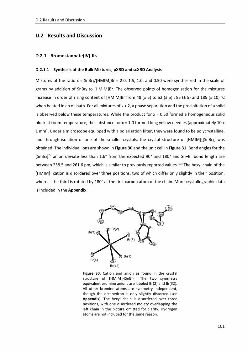
D.2 Results and Discussion
101
D.2 Results and Discussion
Bromostannate(IV)-ILs
D.2.1.1 Synthesis of the Bulk Mixtures, pXRD and scXRD Analysis
Mixtures of the ratio x = SnBr4/[HMIM]Br = 2.0, 1.5, 1.0, and 0.50 were synthesized in the scale of
grams by addition of SnBr4 to [HMIM]Br. The observed points of homogenisation for the mixtures
increase in order of rising content of [HMIM]Br from 48 (± 5) to 52 (± 5) , 85 (± 5) and 185 (± 10) °C
when heated in an oil bath. For all mixtures of x < 2, a phase separation and the precipitation of a solid
is observed below these temperatures. While the product for x = 0.50 formed a homogeneous solid
block at room temperature, the substance for x = 1.0 formed long yellow needles (approximately 10 x
1 mm). Under a microscope equipped with a polarisation filter, they were found to be polycrystalline,
and through isolation of one of the smaller crystals, the crystal structure of [HMIM]2[SnBr6] was
obtained. The individual ions are shown in Figure 30 and the unit cell in Figure 31. Bond angles for the
[SnBr6]2– anion deviate less than 1.6° from the expected 90° and 180° and Sn–Br bond length are
between 258.5 and 261.6 pm, which is similar to previously reported values.[23] The hexyl chain of the
[HMIM]+ cation is disordered over three positions, two of which differ only slightly in their position,
whereas the third is rotated by 180° at the first carbon atom of the chain. More crystallographic data
is included in the Appendix.
Figure 30: Cation and anion as found in the crystal structure of [HMIM]2[SnBr6]. The two symmetry equivalent bromine anions are labeled Br(2) and Br(#2). All other bromine atoms are symmetry independent, though the octahedron is only slightly distorted (see Appendix). The hexyl chain is disordered over three positions, with one disordered moiety overlapping the left chain in the picture omitted for clarity. Hydrogen atoms are not included for the same reason.
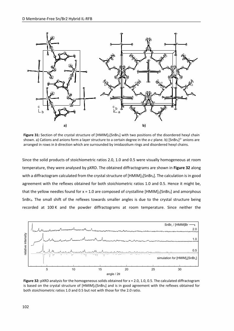
D Membrane-Free Sn/Br2 Hybrid IL-RFB
102
a) b) b
Figure 31: Section of the crystal structure of [HMIM]2[SnBr6] with two positions of the disordered hexyl chain shown. a) Cations and anions form a layer structure to a certain degree in the a-c plane. b) [SnBr6]2– anions are arranged in rows in b direction which are surrounded by imidazolium rings and disordered hexyl chains.
Since the solid products of stoichiometric ratios 2.0, 1.0 and 0.5 were visually homogeneous at room
temperature, they were analysed by pXRD. The obtained diffractograms are shown in Figure 32 along
with a diffractogram calculated from the crystal structure of [HMIM]2[SnBr6]. The calculation is in good
agreement with the reflexes obtained for both stoichiometric ratios 1.0 and 0.5. Hence it might be,
that the yellow needles found for x = 1.0 are composed of crystalline [HMIM]2[SnBr6] and amorphous
SnBr4. The small shift of the reflexes towards smaller angles is due to the crystal structure being
recorded at 100 K and the powder diffractograms at room temperature. Since neither the
Figure 32: pXRD analysis for the homogeneous solids obtained for x = 2.0, 1.0, 0.5. The calculated diffractogram is based on the crystal structure of [HMIM]2[SnBr6] and is in good agreement with the reflexes obtained for both stoichiometric ratios 1.0 and 0.5 but not with those for the 2.0 ratio.
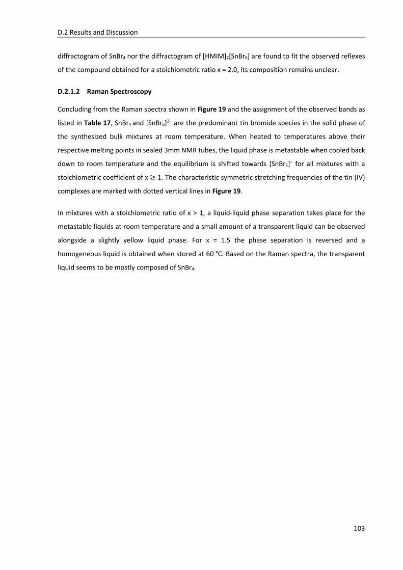
D.2 Results and Discussion
103
diffractogram of SnBr4 nor the diffractogram of [HMIM]2[SnBr6] are found to fit the observed reflexes
of the compound obtained for a stoichiometric ratio x = 2.0, its composition remains unclear.
D.2.1.2 Raman Spectroscopy
Concluding from the Raman spectra shown in Figure 19 and the assignment of the observed bands as
listed in Table 17, SnBr4 and [SnBr6]2– are the predominant tin bromide species in the solid phase of
the synthesized bulk mixtures at room temperature. When heated to temperatures above their
respective melting points in sealed 3mm NMR tubes, the liquid phase is metastable when cooled back
down to room temperature and the equilibrium is shifted towards [SnBr5]– for all mixtures with a
stoichiometric coefficient of x ≥ 1. The characteristic symmetric stretching frequencies of the tin (IV)
complexes are marked with dotted vertical lines in Figure 19.
In mixtures with a stoichiometric ratio of x > 1, a liquid-liquid phase separation takes place for the
metastable liquids at room temperature and a small amount of a transparent liquid can be observed
alongside a slightly yellow liquid phase. For x = 1.5 the phase separation is reversed and a
homogeneous liquid is obtained when stored at 60 °C. Based on the Raman spectra, the transparent
liquid seems to be mostly composed of SnBr4.
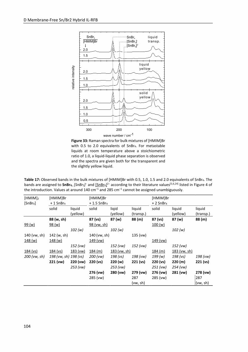
D Membrane-Free Sn/Br2 Hybrid IL-RFB
104
Figure 33: Raman spectra for bulk mixtures of [HMIM]Br with 0.5 to 2.0 equivalents of SnBr4. For metastable liquids at room temperature above a stoichiometric ratio of 1.0, a liquid-liquid phase separation is observed and the spectra are given both for the transparent and the slightly yellow liquid.
Table 17: Observed bands in the bulk mixtures of [HMIM]Br with 0.5, 1.0, 1.5 and 2.0 equivalents of SnBr4. The bands are assigned to SnBr4, [SnBr5]– and [SnBr6]2– according to their literature values[5,6,24] listed in Figure 4 of the introduction. Values at around 140 cm–1 and 285 cm–1 cannot be assigned unambiguously.
[HMIM]2
[SnBr6] [HMIM]Br + 1 SnBr4
[HMIM]Br + 1.5 SnBr4
[HMIM]Br
+ 2 SnBr4
solid liquid (yellow)
solid liqid (yellow)
liquid (transp.)
solid liquid (yellow)
liquid (transp.)
88 (w, sh) 87 (vs) 87 (w) 88 (m) 87 (vs) 87 (w) 88 (m)
99 (w) 98 (w) 98 (vw, sh) 100 (w) 102 (w) 102 (w) 102 (w) 140 (vw, sh) 142 (w, sh) 140 (vw, sh) 135 (vw) 148 (w) 148 (w) 149 (vw) 149 (vw) 152 (vw) 152 (vw) 152 (vw) 152 (vw) 184 (vs) 184 (vs) 183 (vw) 184 (m) 183 (vw, sh) 184 (m) 183 (vw, sh) 200 (vw, sh) 198 (vw, sh) 198 (vs) 200 (vw) 198 (vs) 198 (vw) 199 (w) 198 (vs) 198 (vw)
221 (vw) 220 (vw) 220 (vs) 220 (w) 221 (vs) 220 (vs) 220 (m) 221 (vs)
253 (vw) 253 (vw) 251 (vw) 254 (vw)
276 (vw) 280 (vw) 279 (vw) 276 (vw) 281 (vw) 278 (vw)
285 (vw) 287 (vw, sh)
285 (vw) 287 (vw, sh)
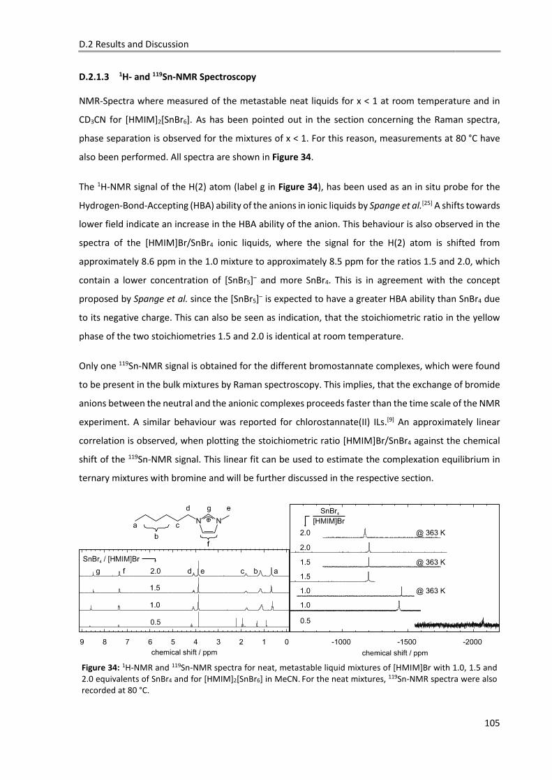
D.2 Results and Discussion
105
D.2.1.3 1H- and 119Sn-NMR Spectroscopy
NMR-Spectra where measured of the metastable neat liquids for x < 1 at room temperature and in
CD3CN for [HMIM]2[SnBr6]. As has been pointed out in the section concerning the Raman spectra,
phase separation is observed for the mixtures of x < 1. For this reason, measurements at 80 °C have
also been performed. All spectra are shown in Figure 34.
The 1H-NMR signal of the H(2) atom (label g in Figure 34), has been used as an in situ probe for the
Hydrogen-Bond-Accepting (HBA) ability of the anions in ionic liquids by Spange et al.[25] A shifts towards
lower field indicate an increase in the HBA ability of the anion. This behaviour is also observed in the
spectra of the [HMIM]Br/SnBr4 ionic liquids, where the signal for the H(2) atom is shifted from
approximately 8.6 ppm in the 1.0 mixture to approximately 8.5 ppm for the ratios 1.5 and 2.0, which
contain a lower concentration of [SnBr5]– and more SnBr4. This is in agreement with the concept
proposed by Spange et al. since the [SnBr5]– is expected to have a greater HBA ability than SnBr4 due
to its negative charge. This can also be seen as indication, that the stoichiometric ratio in the yellow
phase of the two stoichiometries 1.5 and 2.0 is identical at room temperature.
Only one 119Sn-NMR signal is obtained for the different bromostannate complexes, which were found
to be present in the bulk mixtures by Raman spectroscopy. This implies, that the exchange of bromide
anions between the neutral and the anionic complexes proceeds faster than the time scale of the NMR
experiment. A similar behaviour was reported for chlorostannate(II) ILs.[9] An approximately linear
correlation is observed, when plotting the stoichiometric ratio [HMIM]Br/SnBr4 against the chemical
shift of the 119Sn-NMR signal. This linear fit can be used to estimate the complexation equilibrium in
ternary mixtures with bromine and will be further discussed in the respective section.
Figure 34: 1H-NMR and 119Sn-NMR spectra for neat, metastable liquid mixtures of [HMIM]Br with 1.0, 1.5 and 2.0 equivalents of SnBr4 and for [HMIM]2[SnBr6] in MeCN. For the neat mixtures, 119Sn-NMR spectra were also recorded at 80 °C.
D Membrane-Free Sn/Br2 Hybrid IL-RFB
106
The signal of the mixture of [HMIM]Br with 2.0 equivalents of SnBr4 does not follow the linear
relationship observed for the other mixtures. Most likely since only the ionic, yellow phase is analysed
in the NMR experiment and the residual SnBr4 at the bottom of the tube masks the true composition
of the mixture.
When comparing the 119Sn NMR spectra at room temperature with the ones recorded at 80 °C, the
signals for the mixtures of x = 0.67 and 1.0 move towards lower chemical shifts, whereas the signal for
the mixture of x = 0.5 moves the opposite direction. A possible explanation for this behaviour would
be, that a general temperature dependent shift to lower ppm values is combined with the dissolution
of some of the SnBr4 phase in the ionic phase of the mixtures of x = 1.5 and 2.0 at elevated
temperatures. In this case, only the temperature shift would be seen for the mixture x = 1.0, both
phenomena would cancel each other’s effect for the mixture with a ratio of x =1.5, and the effect of
the dissolution of SnBr4 would outweigh the temperature effect for x = 2.0. However, the shift in the
signals could also be due to a shift in the equilibria between the different tin species and a clear answer
can only be given by performing additional experiments.
D.2.1.4 Viscosity of [HMIM]Br Saturated with SnBr4
A low viscosity is generally desired for the liquids used in RFBs to yield a high electrolyte conductivity
and to reduce pumping losses. The cell stack has to be designed to accommodate the viscosity by
employing an appropriate combination of channel diameters and channel lengths. For a membrane-
free Hyp-IL-RFB, the viscosity of the Sn-rich phase would be the limiting factor in the stack-design, since
all phases containing bromine showed a significantly lower viscosity as determined by visual
inspection.
The dynamic viscosity of a liquid phase composed of [HMIM]Br saturated with SnBr4 was found to be
between 42.9 and 24.9 Pa s for a temperature range of 45 to 60 °C. This is a drastic increase, if
compared to the dynamic viscosity of SnBr4 of 1.56 to 1.24 Pa s in the same temperature range.
Compared to the viscosity of typical electrolytes in the V-RFB of approximately 2 mPa s at room
temperature[26], these are high values. However, the charge density would also be significantly higher,
thus counterweighing the increased viscosity by a decreased pumping volume for a similar power
output when viewed only from a mass transport perspective.
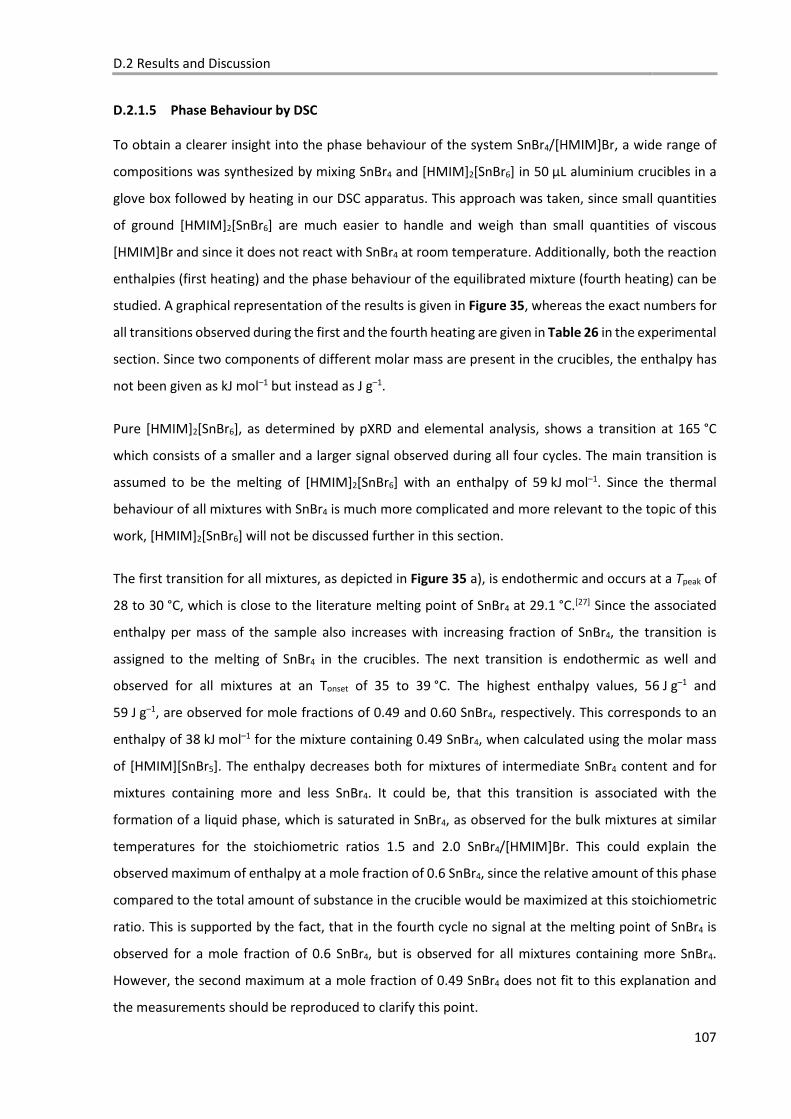
D.2 Results and Discussion
107
D.2.1.5 Phase Behaviour by DSC
To obtain a clearer insight into the phase behaviour of the system SnBr4/[HMIM]Br, a wide range of
compositions was synthesized by mixing SnBr4 and [HMIM]2[SnBr6] in 50 µL aluminium crucibles in a
glove box followed by heating in our DSC apparatus. This approach was taken, since small quantities
of ground [HMIM]2[SnBr6] are much easier to handle and weigh than small quantities of viscous
[HMIM]Br and since it does not react with SnBr4 at room temperature. Additionally, both the reaction
enthalpies (first heating) and the phase behaviour of the equilibrated mixture (fourth heating) can be
studied. A graphical representation of the results is given in Figure 35, whereas the exact numbers for
all transitions observed during the first and the fourth heating are given in Table 26 in the experimental
section. Since two components of different molar mass are present in the crucibles, the enthalpy has
not been given as kJ mol–1 but instead as J g–1.
Pure [HMIM]2[SnBr6], as determined by pXRD and elemental analysis, shows a transition at 165 °C
which consists of a smaller and a larger signal observed during all four cycles. The main transition is
assumed to be the melting of [HMIM]2[SnBr6] with an enthalpy of 59 kJ mol–1. Since the thermal
behaviour of all mixtures with SnBr4 is much more complicated and more relevant to the topic of this
work, [HMIM]2[SnBr6] will not be discussed further in this section.
The first transition for all mixtures, as depicted in Figure 35 a), is endothermic and occurs at a Tpeak of
28 to 30 °C, which is close to the literature melting point of SnBr4 at 29.1 °C.[27] Since the associated
enthalpy per mass of the sample also increases with increasing fraction of SnBr4, the transition is
assigned to the melting of SnBr4 in the crucibles. The next transition is endothermic as well and
observed for all mixtures at an Tonset of 35 to 39 °C. The highest enthalpy values, 56 J g–1 and
59 J g–1, are observed for mole fractions of 0.49 and 0.60 SnBr4, respectively. This corresponds to an
enthalpy of 38 kJ mol–1 for the mixture containing 0.49 SnBr4, when calculated using the molar mass
of [HMIM][SnBr5]. The enthalpy decreases both for mixtures of intermediate SnBr4 content and for
mixtures containing more and less SnBr4. It could be, that this transition is associated with the
formation of a liquid phase, which is saturated in SnBr4, as observed for the bulk mixtures at similar
temperatures for the stoichiometric ratios 1.5 and 2.0 SnBr4/[HMIM]Br. This could explain the
observed maximum of enthalpy at a mole fraction of 0.6 SnBr4, since the relative amount of this phase
compared to the total amount of substance in the crucible would be maximized at this stoichiometric
ratio. This is supported by the fact, that in the fourth cycle no signal at the melting point of SnBr4 is
observed for a mole fraction of 0.6 SnBr4, but is observed for all mixtures containing more SnBr4.
However, the second maximum at a mole fraction of 0.49 SnBr4 does not fit to this explanation and
the measurements should be reproduced to clarify this point.
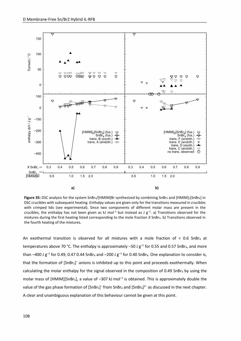
D Membrane-Free Sn/Br2 Hybrid IL-RFB
108
a) b)
Figure 35: DSC analysis for the system SnBr4/[HMIM]Br synthesized by combining SnBr4 and [HMIM]2[SnBr6] in DSC crucibles with subsequent heating. Enthalpy values are given only for the transitions measured in crucibles with crimped lids (see experimental). Since two components of different molar mass are present in the crucibles, the enthalpy has not been given as kJ mol–1 but instead as J g–1. a) Transitions observed for the mixtures during the first heating listed corresponding to the mole fraction X SnBr4. b) Transitions observed in the fourth heating of the mixtures.
An exothermal transition is observed for all mixtures with a mole fraction of < 0.6 SnBr4 at
temperatures above 70 °C. The enthalpy is approximately –50 J g–1 for 0.55 and 0.57 SnBr4, and more
than –400 J g–1 for 0.49, 0.47 0.44 SnBr4 and –200 J g–1 for 0.40 SnBr4. One explanation to consider is,
that the formation of [SnBr5]– anions is inhibited up to this point and proceeds exothermally. When
calculating the molar enthalpy for the signal observed in the composition of 0.49 SnBr4 by using the
molar mass of [HMIM][SnBr5], a value of –307 kJ mol–1 is obtained. This is approximately double the
value of the gas phase formation of [SnBr5]– from SnBr4 and [SnBr6]2– as discussed in the next chapter.
A clear and unambiguous explanation of this behaviour cannot be given at this point.
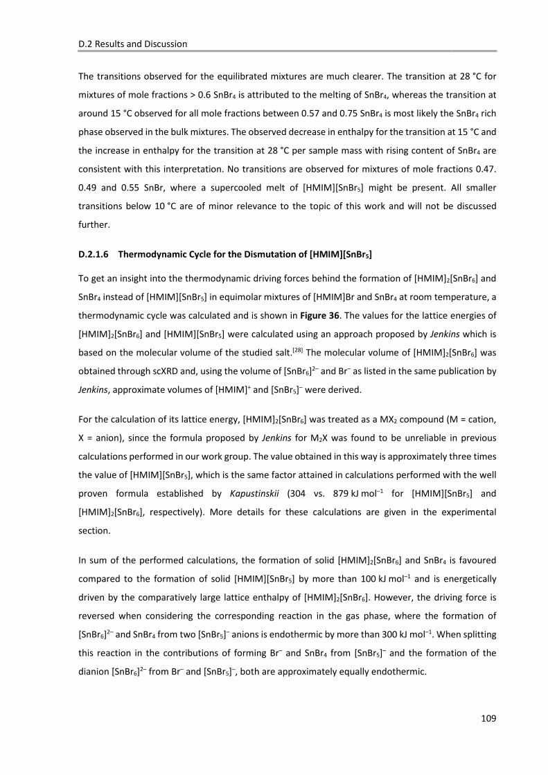
D.2 Results and Discussion
109
The transitions observed for the equilibrated mixtures are much clearer. The transition at 28 °C for
mixtures of mole fractions > 0.6 SnBr4 is attributed to the melting of SnBr4, whereas the transition at
around 15 °C observed for all mole fractions between 0.57 and 0.75 SnBr4 is most likely the SnBr4 rich
phase observed in the bulk mixtures. The observed decrease in enthalpy for the transition at 15 °C and
the increase in enthalpy for the transition at 28 °C per sample mass with rising content of SnBr4 are
consistent with this interpretation. No transitions are observed for mixtures of mole fractions 0.47.
0.49 and 0.55 SnBr, where a supercooled melt of [HMIM][SnBr5] might be present. All smaller
transitions below 10 °C are of minor relevance to the topic of this work and will not be discussed
further.
D.2.1.6 Thermodynamic Cycle for the Dismutation of [HMIM][SnBr5]
To get an insight into the thermodynamic driving forces behind the formation of [HMIM]2[SnBr6] and
SnBr4 instead of [HMIM][SnBr5] in equimolar mixtures of [HMIM]Br and SnBr4 at room temperature, a
thermodynamic cycle was calculated and is shown in Figure 36. The values for the lattice energies of
[HMIM]2[SnBr6] and [HMIM][SnBr5] were calculated using an approach proposed by Jenkins which is
based on the molecular volume of the studied salt.[28] The molecular volume of [HMIM]2[SnBr6] was
obtained through scXRD and, using the volume of [SnBr6]2– and Br– as listed in the same publication by
Jenkins, approximate volumes of [HMIM]+ and [SnBr5]– were derived.
For the calculation of its lattice energy, [HMIM]2[SnBr6] was treated as a MX2 compound (M = cation,
X = anion), since the formula proposed by Jenkins for M2X was found to be unreliable in previous
calculations performed in our work group. The value obtained in this way is approximately three times
the value of [HMIM][SnBr5], which is the same factor attained in calculations performed with the well
proven formula established by Kapustinskii (304 vs. 879 kJ mol–1 for [HMIM][SnBr5] and
[HMIM]2[SnBr6], respectively). More details for these calculations are given in the experimental
section.
In sum of the performed calculations, the formation of solid [HMIM]2[SnBr6] and SnBr4 is favoured
compared to the formation of solid [HMIM][SnBr5] by more than 100 kJ mol–1 and is energetically
driven by the comparatively large lattice enthalpy of [HMIM]2[SnBr6]. However, the driving force is
reversed when considering the corresponding reaction in the gas phase, where the formation of
[SnBr6]2– and SnBr4 from two [SnBr5]– anions is endothermic by more than 300 kJ mol–1. When splitting
this reaction in the contributions of forming Br– and SnBr4 from [SnBr5]– and the formation of the
dianion [SnBr6]2– from Br– and [SnBr5]–, both are approximately equally endothermic.
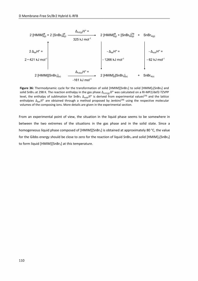
D Membrane-Free Sn/Br2 Hybrid IL-RFB
110
Figure 36: Thermodynamic cycle for the transformation of solid [HMIM][SnBr5] to solid [HMIM]2[SnBr6] and solid SnBr4 at 298 K. The reaction enthalpy in the gas phase ∆h!�SiUd° was calculated on a RI-MP2/def2-TZVPP
level, the enthalpy of sublimation for SnBr4 ∆�k;d° is derived from experimental values[29] and the lattice enthalpies ∆#"�d° are obtained through a method proposed by Jenkins[28] using the respective molecular volumes of the composing ions. More details are given in the experimental section.
From an experimental point of view, the situation in the liquid phase seems to be somewhere in
between the two extremes of the situations in the gas phase and in the solid state. Since a
homogeneous liquid phase composed of [HMIM][SnBr5] is obtained at approximately 80 °C, the value
for the Gibbs energy should be close to zero for the reaction of liquid SnBr4 and solid [HMIM]2[SnBr6]
to form liquid [HMIM][SnBr5] at this temperature.
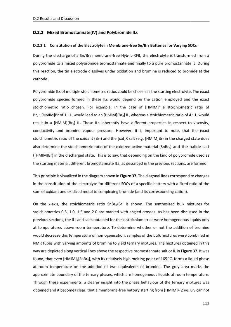
D.2 Results and Discussion
111
Mixed Bromostannate(IV) and Polybromide ILs
D.2.2.1 Constitution of the Electrolyte in Membrane-free Sn/Br2 Batteries for Varying SOCs
During the discharge of a Sn/Br2 membrane-free Hyb-IL-RFB, the electrolyte is transformed from a
polybromide to a mixed polybromide bromostannate and finally to a pure bromostannate IL. During
this reaction, the tin electrode dissolves under oxidation and bromine is reduced to bromide at the
cathode.
Polybromide ILs of multiple stoichiometric ratios could be chosen as the starting electrolyte. The exact
polybromide species formed in these ILs would depend on the cation employed and the exact
stoichiometric ratio chosen. For example, in the case of [HMIM]+ a stoichiometric ratio of
Br2 : [HMIM]Br of 1 : 1, would lead to an [HMIM][Br3] IL, whereas a stoichiometric ratio of 4 : 1, would
result in a [HMIM][Br9] IL. These ILs inherently have different properties in respect to viscosity,
conductivity and bromine vapour pressure. However, it is important to note, that the exact
stoichiometric ratio of the oxidant (Br2) and the [cat]X salt (e.g. [HMIM]Br) in the charged state does
also determine the stoichiometric ratio of the oxidized active material (SnBr4) and the halide salt
([HMIM]Br) in the discharged state. This is to say, that depending on the kind of polybromide used as
the starting material, different bromostannate ILs, as described in the previous sections, are formed.
This principle is visualized in the diagram shown in Figure 37. The diagonal lines correspond to changes
in the constitution of the electrolyte for different SOCs of a specific battery with a fixed ratio of the
sum of oxidant and oxidized metal to complexing bromide (and its corresponding cation).
On the x-axis, the stoichiometric ratio SnBr4/Br– is shown. The synthesized bulk mixtures for
stoichiometries 0.5, 1.0, 1.5 and 2.0 are marked with angled crosses. As has been discussed in the
previous sections, the ILs and salts obtained for these stoichiometries were homogeneous liquids only
at temperatures above room temperature. To determine whether or not the addition of bromine
would decrease this temperature of homogenisation, samples of the bulk mixtures were combined in
NMR tubes with varying amounts of bromine to yield ternary mixtures. The mixtures obtained in this
way are depicted along vertical lines above the respective bromostannate salt or IL in Figure 37. It was
found, that even [HMIM]2[SnBr6], with its relatively high melting point of 165 °C, forms a liquid phase
at room temperature on the addition of two equivalents of bromine. The grey area marks the
approximate boundary of the ternary phases, which are homogeneous liquids at room temperature.
Through these experiments, a clearer insight into the phase behaviour of the ternary mixtures was
obtained and it becomes clear, that a membrane-free battery starting from [HMIM]+ 2 eq. Br2 can not
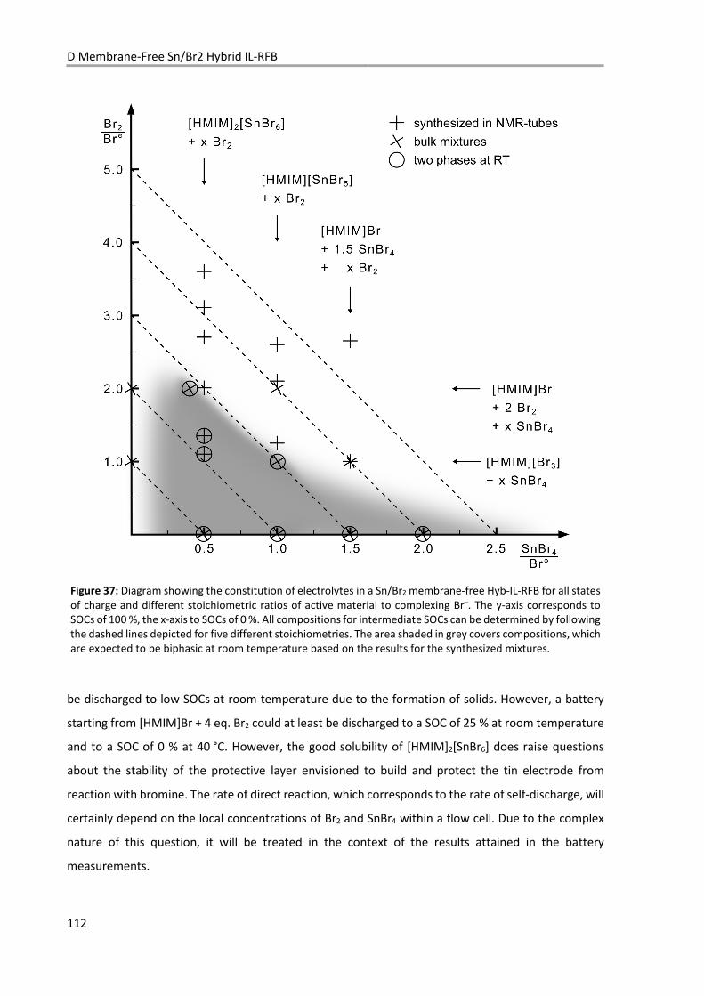
D Membrane-Free Sn/Br2 Hybrid IL-RFB
112
Figure 37: Diagram showing the constitution of electrolytes in a Sn/Br2 membrane-free Hyb-IL-RFB for all states of charge and different stoichiometric ratios of active material to complexing Br–. The y-axis corresponds to SOCs of 100 %, the x-axis to SOCs of 0 %. All compositions for intermediate SOCs can be determined by following the dashed lines depicted for five different stoichiometries. The area shaded in grey covers compositions, which are expected to be biphasic at room temperature based on the results for the synthesized mixtures.
be discharged to low SOCs at room temperature due to the formation of solids. However, a battery
starting from [HMIM]Br + 4 eq. Br2 could at least be discharged to a SOC of 25 % at room temperature
and to a SOC of 0 % at 40 °C. However, the good solubility of [HMIM]2[SnBr6] does raise questions
about the stability of the protective layer envisioned to build and protect the tin electrode from
reaction with bromine. The rate of direct reaction, which corresponds to the rate of self-discharge, will
certainly depend on the local concentrations of Br2 and SnBr4 within a flow cell. Due to the complex
nature of this question, it will be treated in the context of the results attained in the battery
measurements.
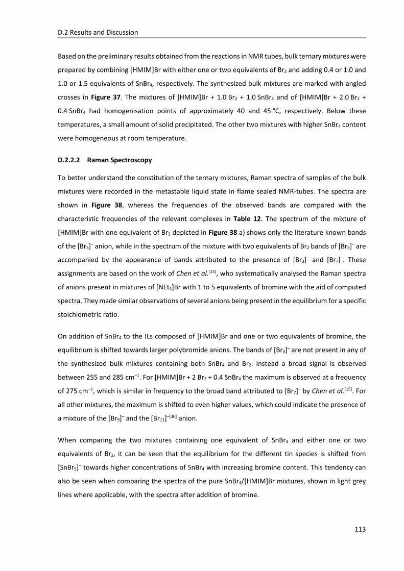
D.2 Results and Discussion
113
Based on the preliminary results obtained from the reactions in NMR tubes, bulk ternary mixtures were
prepared by combining [HMIM]Br with either one or two equivalents of Br2 and adding 0.4 or 1.0 and
1.0 or 1.5 equivalents of SnBr4, respectively. The synthesized bulk mixtures are marked with angled
crosses in Figure 37. The mixtures of [HMIM]Br + 1.0 Br2 + 1.0 SnBr4 and of [HMIM]Br + 2.0 Br2 +
0.4 SnBr4 had homogenisation points of approximately 40 and 45 °C, respectively. Below these
temperatures, a small amount of solid precipitated. The other two mixtures with higher SnBr4 content
were homogeneous at room temperature.
D.2.2.2 Raman Spectroscopy
To better understand the constitution of the ternary mixtures, Raman spectra of samples of the bulk
mixtures were recorded in the metastable liquid state in flame sealed NMR-tubes. The spectra are
shown in Figure 38, whereas the frequencies of the observed bands are compared with the
characteristic frequencies of the relevant complexes in Table 12. The spectrum of the mixture of
[HMIM]Br with one equivalent of Br2 depicted in Figure 38 a) shows only the literature known bands
of the [Br3]– anion, while in the spectrum of the mixture with two equivalents of Br2 bands of [Br5]– are
accompanied by the appearance of bands attributed to the presence of [Br3]– and [Br7]–. These
assignments are based on the work of Chen et al.[15], who systematically analysed the Raman spectra
of anions present in mixtures of [NEt4]Br with 1 to 5 equivalents of bromine with the aid of computed
spectra. They made similar observations of several anions being present in the equilibrium for a specific
stoichiometric ratio.
On addition of SnBr4 to the ILs composed of [HMIM]Br and one or two equivalents of bromine, the
equilibrium is shifted towards larger polybromide anions. The bands of [Br3]– are not present in any of
the synthesized bulk mixtures containing both SnBr4 and Br2. Instead a broad signal is observed
between 255 and 285 cm–1. For [HMIM]Br + 2 Br2 + 0.4 SnBr4 the maximum is observed at a frequency
of 275 cm–1, which is similar in frequency to the broad band attributed to [Br7]– by Chen et al.[15]. For
all other mixtures, the maximum is shifted to even higher values, which could indicate the presence of
a mixture of the [Br9]– and the [Br11]–[30] anion.
When comparing the two mixtures containing one equivalent of SnBr4 and either one or two
equivalents of Br2, it can be seen that the equilibrium for the different tin species is shifted from
[SnBr5]– towards higher concentrations of SnBr4 with increasing bromine content. This tendency can
also be seen when comparing the spectra of the pure SnBr4/[HMIM]Br mixtures, shown in light grey
lines where applicable, with the spectra after addition of bromine.
D Membrane-Free Sn/Br2 Hybrid IL-RFB
114
Summarizing, the equilibrium for the complexation of bromide anions in competition of SnBr4 and Br2
lies on the side of the formation of [SnBr5]– in mixtures with [HMIM]Br, but it can be shifted in favour
of the formation of polybromides by increasing the amount of bromine in the mixtures. Only very little
[SnBr6]2– appears to be present in the mixtures.
a) b)
Figure 38: Raman spectra for binary mixtures of [HMIM]Br and Br2 and ternary mixtures containing additionally SnBr4. a) Mixture of [HMIM]Br with one equivalent of Br2 and also with 1.0 or 1.5 equivalents of SnBr4 added to the mixture. b) Mixture of [HMIM]Br with two equivalents of Br2 and with additional 0.4 or 1.0 equivalents of SnBr4.
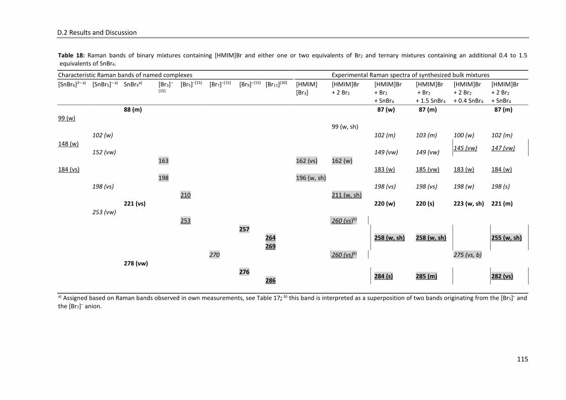
D.2 Results and Discussion
115
Table 18: Raman bands of binary mixtures containing [HMIM]Br and either one or two equivalents of Br2 and ternary mixtures containing an additional 0.4 to 1.5 equivalents of SnBr4.
Characteristic Raman bands of named complexes Experimental Raman spectra of synthesized bulk mixtures
[SnBr6]2– a) [SnBr5]– a) SnBr4a) [Br3]–
[15] [Br5]–[15] [Br7]–[15] [Br9]–[15] [Br11][30] [HMIM]
[Br3] [HMIM]Br + 2 Br2
[HMIM]Br + Br2 + SnBr4
[HMIM]Br + Br2 + 1.5 SnBr4
[HMIM]Br + 2 Br2 + 0.4 SnBr4
[HMIM]Br + 2 Br2 + SnBr4
88 (m) 87 (w) 87 (m) 87 (m)
99 (w) 99 (w, sh) 102 (w) 102 (m) 103 (m) 100 (w) 102 (m)
148 (w) 145 (vw) 147 (vw)
152 (vw) 149 (vw) 149 (vw)
163 162 (vs) 162 (w) 184 (vs) 183 (w) 185 (vw) 183 (w) 184 (w) 198 196 (w, sh)
198 (vs) 198 (vs) 198 (vs) 198 (w) 198 (s)
210 211 (w, sh) 221 (vs) 220 (w) 220 (s) 223 (w, sh) 221 (m)
253 (vw) 253 260 (vs)b) 257
258 (w, sh) 258 (w, sh)
255 (w, sh) 264 269 270 260 (vs)b) 275 (vs, b)
278 (vw) 276
284 (s) 285 (m)
282 (vs) 286 a) Assigned based on Raman bands observed in own measurements, see Table 17; b) this band is interpreted as a superposition of two bands originating from the [Br5]– and the [Br7]– anion.
D Membrane-Free Sn/Br2 Hybrid IL-RFB
116
D.2.2.3 NMR Spectroscopy
As for the binary mixtures, only one 119Sn-NMR signal is obtained in the spectra of the ternary mixtures,
despite the presence of a mixture of complexes as observed via Raman spectroscopy. To retrieve
information about the nature of the tin complexes in the mixtures from the coalescence signal, the
linear relationship between the average number y of complexed Br– anions in complexes [SnBr4+y]y–
and the 119Sn signal of the binary mixtures with known composition can be employed. To this end, a
linear regression was performed on the experimental 119Sn-NMR chemical shifts obtained from the
binary mixtures under the assumption that every available bromide anion is complexed by SnBr4 and
that, depending on the stoichiometric ratio, only SnBr4 and [SnBr5]– or [SnBr5]– and [SnBr6]2– are present
simultaneously in any of the mixtures. The used data points are listed in Table 19. As has been
discussed before, the signal of the mixture with two equivalents of SnBr4 is excluded from the fit, due
to the large amount of undissolved SnBr4. Since the residual amount of undissolved SnBr4 in the x = 1.5
mixture at room temperature is very small, its composition is assumed to be exactly as the
stoichiometric ratio of the starting materials.
Equations (20) and (21) were used to calculate the slope ? and the y-intercept > using the individual
measurement points @l, .l.and the total number of measurement points �.
? = ∑ @l.l − �@̅.o∑ @l0 − �@l@²q (20)
> = .o ∑ @l0 − @̅ ∑ @l.l∑ @l0 − �@l@²q (21)
The standard deviation for the data points is calculated using Equation (22).
r = s 1� – 2 vS.l– ?@l − >U²wlx� (22)
Fro these calculations, the linear Equation (23) is obtained.
y = –1.40 ∙ 10–3 – 0.948 (23)
The standard deviation for the data points is 0.08 regarding the average number y in complexes
[SnBr4+y]y–, which is considered sufficient for the purpose of this investigation.
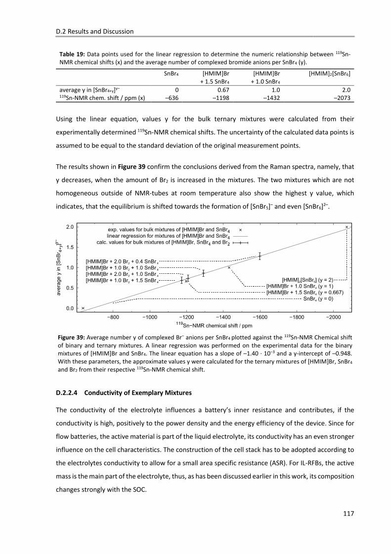
D.2 Results and Discussion
117
Table 19: Data points used for the linear regression to determine the numeric relationship between 119Sn-NMR chemical shifts (x) and the average number of complexed bromide anions per SnBr4 (y).
SnBr4 [HMIM]Br + 1.5 SnBr4
[HMIM]Br + 1.0 SnBr4
[HMIM]2[SnBr6]
average y in [SnBr4+y]y– 0 0.67 1.0 2.0 119Sn-NMR chem. shift / ppm (x) –636 –1198 –1432 –2073
Using the linear equation, values y for the bulk ternary mixtures were calculated from their
experimentally determined 119Sn-NMR chemical shifts. The uncertainty of the calculated data points is
assumed to be equal to the standard deviation of the original measurement points.
The results shown in Figure 39 confirm the conclusions derived from the Raman spectra, namely, that
y decreases, when the amount of Br2 is increased in the mixtures. The two mixtures which are not
homogeneous outside of NMR-tubes at room temperature also show the highest y value, which
indicates, that the equilibrium is shifted towards the formation of [SnBr5]– and even [SnBr6]2–.
Figure 39: Average number y of complexed Br– anions per SnBr4 plotted against the 119Sn-NMR Chemical shift of binary and ternary mixtures. A linear regression was performed on the experimental data for the binary mixtures of [HMIM]Br and SnBr4. The linear equation has a slope of –1.40 ∙ 10–3 and a y-intercept of –0.948. With these parameters, the approximate values y were calculated for the ternary mixtures of [HMIM]Br, SnBr4 and Br2 from their respective 119Sn-NMR chemical shift.
D.2.2.4 Conductivity of Exemplary Mixtures
The conductivity of the electrolyte influences a battery’s inner resistance and contributes, if the
conductivity is high, positively to the power density and the energy efficiency of the device. Since for
flow batteries, the active material is part of the liquid electrolyte, its conductivity has an even stronger
influence on the cell characteristics. The construction of the cell stack has to be adopted according to
the electrolytes conductivity to allow for a small area specific resistance (ASR). For IL-RFBs, the active
mass is the main part of the electrolyte, thus, as has been discussed earlier in this work, its composition
changes strongly with the SOC.
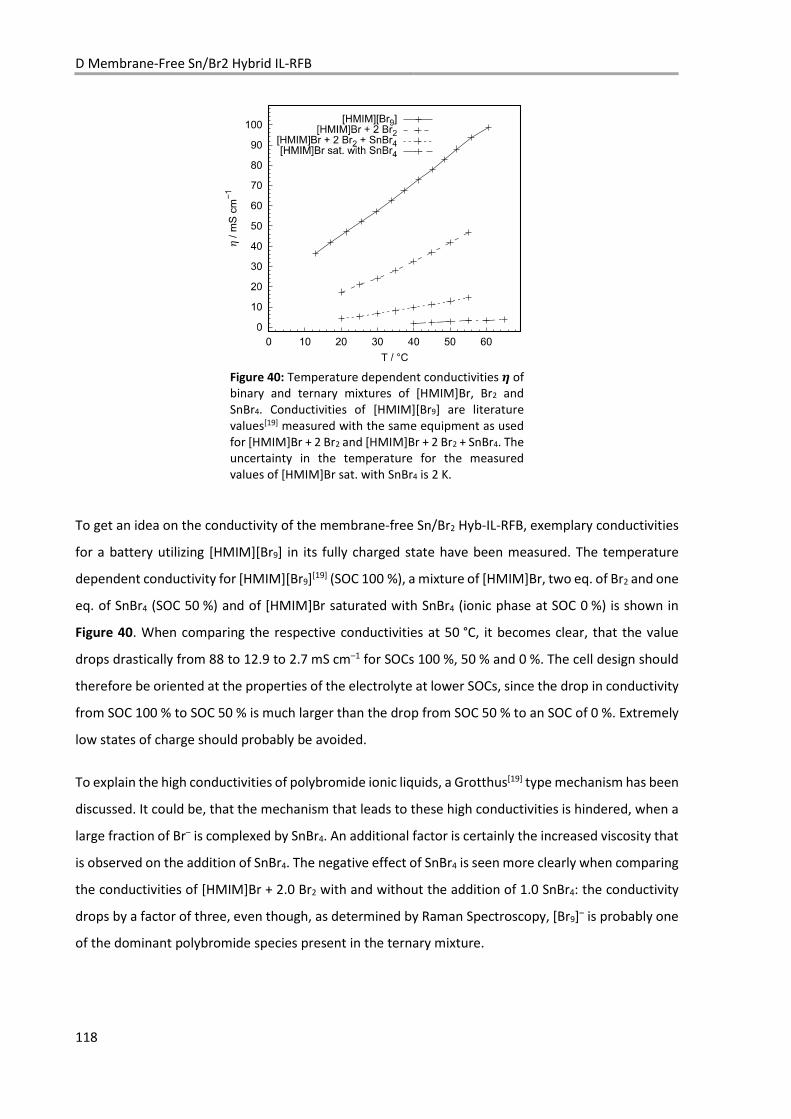
D Membrane-Free Sn/Br2 Hybrid IL-RFB
118
Figure 40: Temperature dependent conductivities y of binary and ternary mixtures of [HMIM]Br, Br2 and SnBr4. Conductivities of [HMIM][Br9] are literature values[19] measured with the same equipment as used for [HMIM]Br + 2 Br2 and [HMIM]Br + 2 Br2 + SnBr4. The uncertainty in the temperature for the measured values of [HMIM]Br sat. with SnBr4 is 2 K.
To get an idea on the conductivity of the membrane-free Sn/Br2 Hyb-IL-RFB, exemplary conductivities
for a battery utilizing [HMIM][Br9] in its fully charged state have been measured. The temperature
dependent conductivity for [HMIM][Br9][19] (SOC 100 %), a mixture of [HMIM]Br, two eq. of Br2 and one
eq. of SnBr4 (SOC 50 %) and of [HMIM]Br saturated with SnBr4 (ionic phase at SOC 0 %) is shown in
Figure 40. When comparing the respective conductivities at 50 °C, it becomes clear, that the value
drops drastically from 88 to 12.9 to 2.7 mS cm–1 for SOCs 100 %, 50 % and 0 %. The cell design should
therefore be oriented at the properties of the electrolyte at lower SOCs, since the drop in conductivity
from SOC 100 % to SOC 50 % is much larger than the drop from SOC 50 % to an SOC of 0 %. Extremely
low states of charge should probably be avoided.
To explain the high conductivities of polybromide ionic liquids, a Grotthus[19] type mechanism has been
discussed. It could be, that the mechanism that leads to these high conductivities is hindered, when a
large fraction of Br– is complexed by SnBr4. An additional factor is certainly the increased viscosity that
is observed on the addition of SnBr4. The negative effect of SnBr4 is seen more clearly when comparing
the conductivities of [HMIM]Br + 2.0 Br2 with and without the addition of 1.0 SnBr4: the conductivity
drops by a factor of three, even though, as determined by Raman Spectroscopy, [Br9]– is probably one
of the dominant polybromide species present in the ternary mixture.
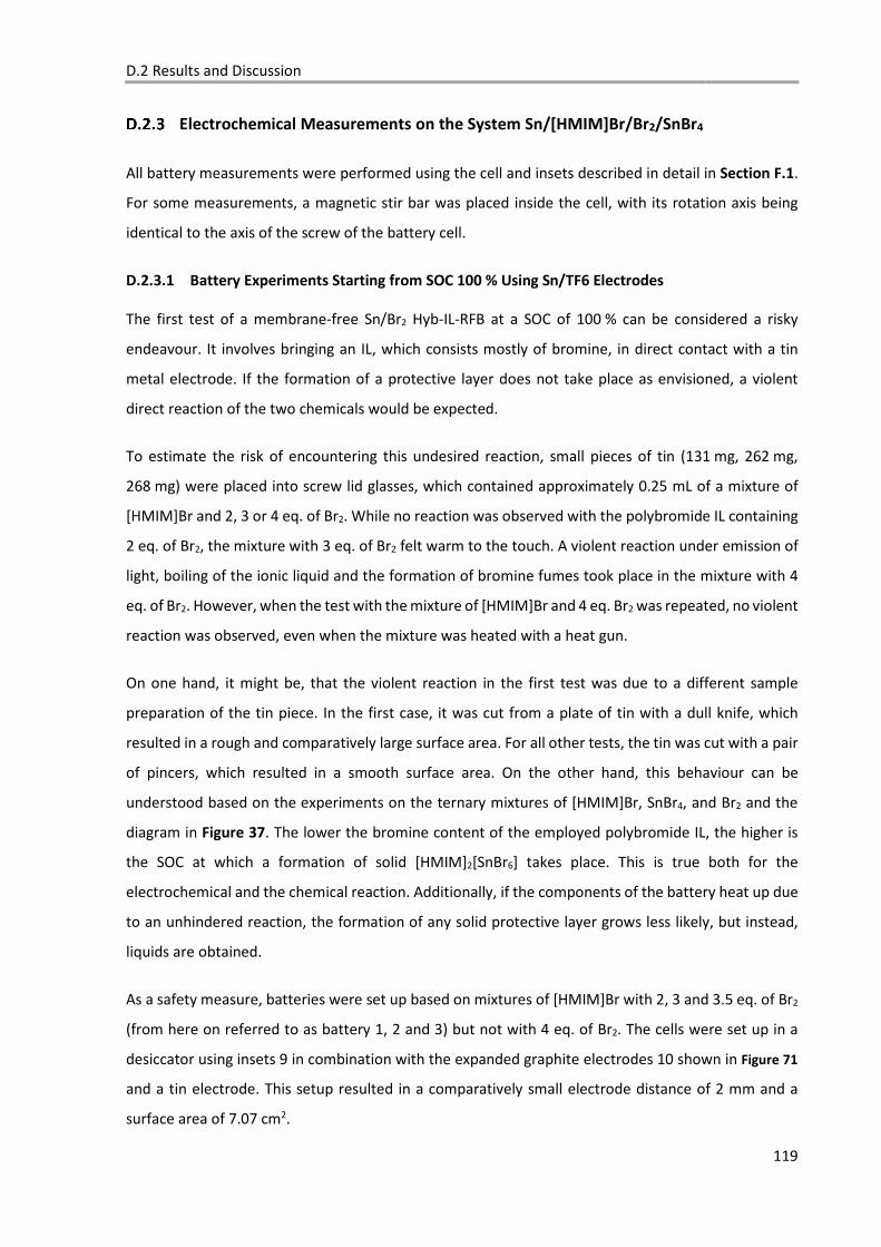
D.2 Results and Discussion
119
Electrochemical Measurements on the System Sn/[HMIM]Br/Br2/SnBr4
All battery measurements were performed using the cell and insets described in detail in Section F.1.
For some measurements, a magnetic stir bar was placed inside the cell, with its rotation axis being
identical to the axis of the screw of the battery cell.
D.2.3.1 Battery Experiments Starting from SOC 100 % Using Sn/TF6 Electrodes
The first test of a membrane-free Sn/Br2 Hyb-IL-RFB at a SOC of 100 % can be considered a risky
endeavour. It involves bringing an IL, which consists mostly of bromine, in direct contact with a tin
metal electrode. If the formation of a protective layer does not take place as envisioned, a violent
direct reaction of the two chemicals would be expected.
To estimate the risk of encountering this undesired reaction, small pieces of tin (131 mg, 262 mg,
268 mg) were placed into screw lid glasses, which contained approximately 0.25 mL of a mixture of
[HMIM]Br and 2, 3 or 4 eq. of Br2. While no reaction was observed with the polybromide IL containing
2 eq. of Br2, the mixture with 3 eq. of Br2 felt warm to the touch. A violent reaction under emission of
light, boiling of the ionic liquid and the formation of bromine fumes took place in the mixture with 4
eq. of Br2. However, when the test with the mixture of [HMIM]Br and 4 eq. Br2 was repeated, no violent
reaction was observed, even when the mixture was heated with a heat gun.
On one hand, it might be, that the violent reaction in the first test was due to a different sample
preparation of the tin piece. In the first case, it was cut from a plate of tin with a dull knife, which
resulted in a rough and comparatively large surface area. For all other tests, the tin was cut with a pair
of pincers, which resulted in a smooth surface area. On the other hand, this behaviour can be
understood based on the experiments on the ternary mixtures of [HMIM]Br, SnBr4, and Br2 and the
diagram in Figure 37. The lower the bromine content of the employed polybromide IL, the higher is
the SOC at which a formation of solid [HMIM]2[SnBr6] takes place. This is true both for the
electrochemical and the chemical reaction. Additionally, if the components of the battery heat up due
to an unhindered reaction, the formation of any solid protective layer grows less likely, but instead,
liquids are obtained.
As a safety measure, batteries were set up based on mixtures of [HMIM]Br with 2, 3 and 3.5 eq. of Br2
(from here on referred to as battery 1, 2 and 3) but not with 4 eq. of Br2. The cells were set up in a
desiccator using insets 9 in combination with the expanded graphite electrodes 10 shown in Figure 71
and a tin electrode. This setup resulted in a comparatively small electrode distance of 2 mm and a
surface area of 7.07 cm2.
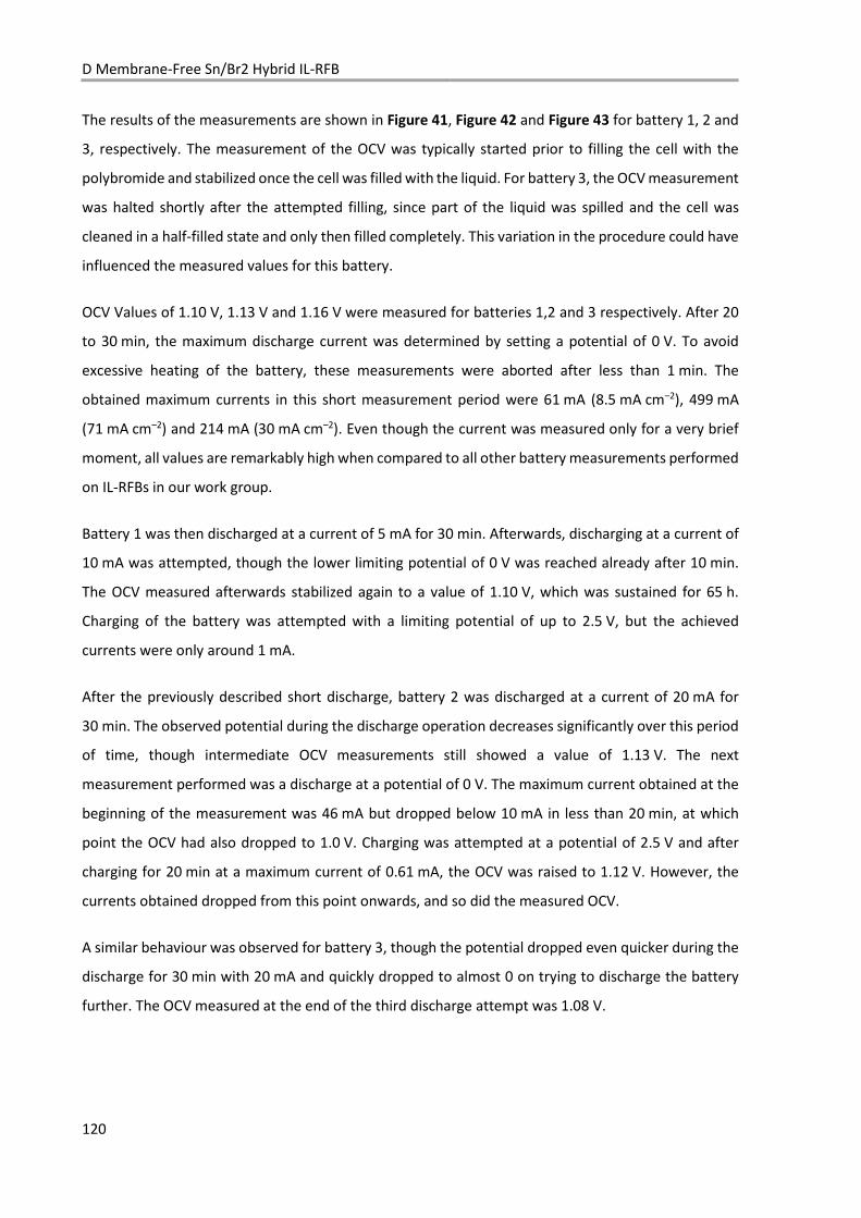
D Membrane-Free Sn/Br2 Hybrid IL-RFB
120
The results of the measurements are shown in Figure 41, Figure 42 and Figure 43 for battery 1, 2 and
3, respectively. The measurement of the OCV was typically started prior to filling the cell with the
polybromide and stabilized once the cell was filled with the liquid. For battery 3, the OCV measurement
was halted shortly after the attempted filling, since part of the liquid was spilled and the cell was
cleaned in a half-filled state and only then filled completely. This variation in the procedure could have
influenced the measured values for this battery.
OCV Values of 1.10 V, 1.13 V and 1.16 V were measured for batteries 1,2 and 3 respectively. After 20
to 30 min, the maximum discharge current was determined by setting a potential of 0 V. To avoid
excessive heating of the battery, these measurements were aborted after less than 1 min. The
obtained maximum currents in this short measurement period were 61 mA (8.5 mA cm–2), 499 mA
(71 mA cm–2) and 214 mA (30 mA cm–2). Even though the current was measured only for a very brief
moment, all values are remarkably high when compared to all other battery measurements performed
on IL-RFBs in our work group.
Battery 1 was then discharged at a current of 5 mA for 30 min. Afterwards, discharging at a current of
10 mA was attempted, though the lower limiting potential of 0 V was reached already after 10 min.
The OCV measured afterwards stabilized again to a value of 1.10 V, which was sustained for 65 h.
Charging of the battery was attempted with a limiting potential of up to 2.5 V, but the achieved
currents were only around 1 mA.
After the previously described short discharge, battery 2 was discharged at a current of 20 mA for
30 min. The observed potential during the discharge operation decreases significantly over this period
of time, though intermediate OCV measurements still showed a value of 1.13 V. The next
measurement performed was a discharge at a potential of 0 V. The maximum current obtained at the
beginning of the measurement was 46 mA but dropped below 10 mA in less than 20 min, at which
point the OCV had also dropped to 1.0 V. Charging was attempted at a potential of 2.5 V and after
charging for 20 min at a maximum current of 0.61 mA, the OCV was raised to 1.12 V. However, the
currents obtained dropped from this point onwards, and so did the measured OCV.
A similar behaviour was observed for battery 3, though the potential dropped even quicker during the
discharge for 30 min with 20 mA and quickly dropped to almost 0 on trying to discharge the battery
further. The OCV measured at the end of the third discharge attempt was 1.08 V.
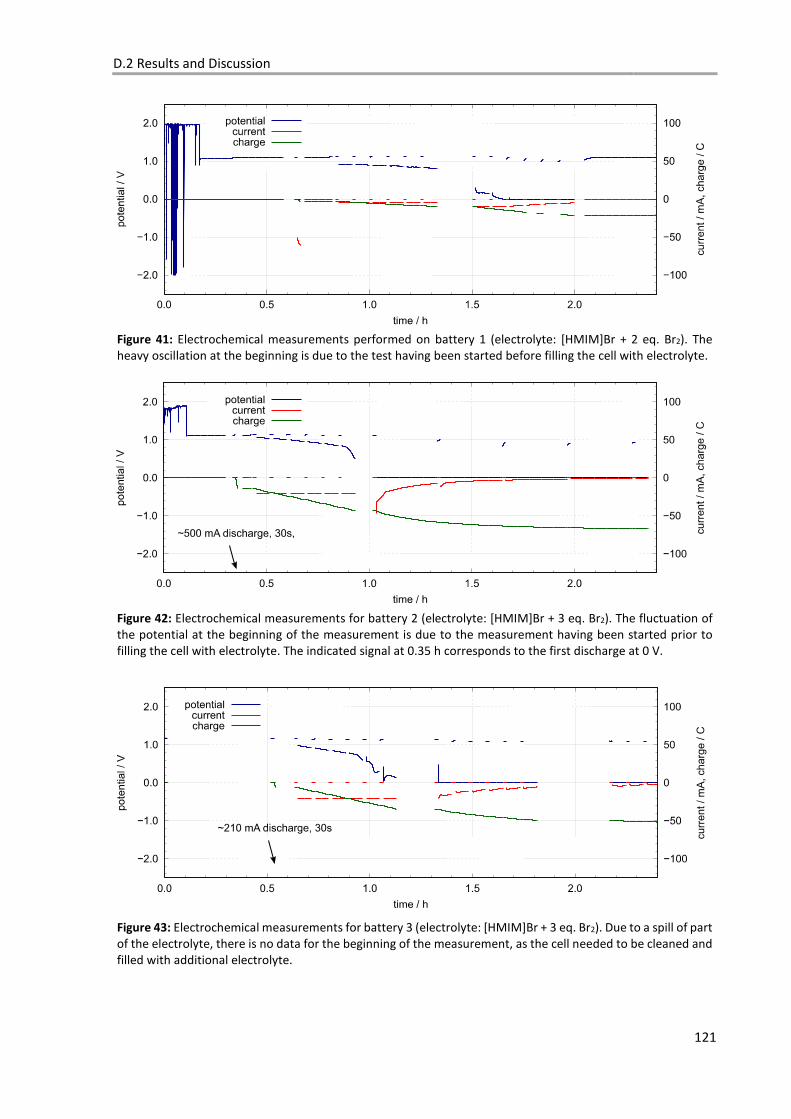
D.2 Results and Discussion
121
Figure 41: Electrochemical measurements performed on battery 1 (electrolyte: [HMIM]Br + 2 eq. Br2). The heavy oscillation at the beginning is due to the test having been started before filling the cell with electrolyte.
Figure 42: Electrochemical measurements for battery 2 (electrolyte: [HMIM]Br + 3 eq. Br2). The fluctuation of the potential at the beginning of the measurement is due to the measurement having been started prior to filling the cell with electrolyte. The indicated signal at 0.35 h corresponds to the first discharge at 0 V.
Figure 43: Electrochemical measurements for battery 3 (electrolyte: [HMIM]Br + 3 eq. Br2). Due to a spill of part of the electrolyte, there is no data for the beginning of the measurement, as the cell needed to be cleaned and filled with additional electrolyte.
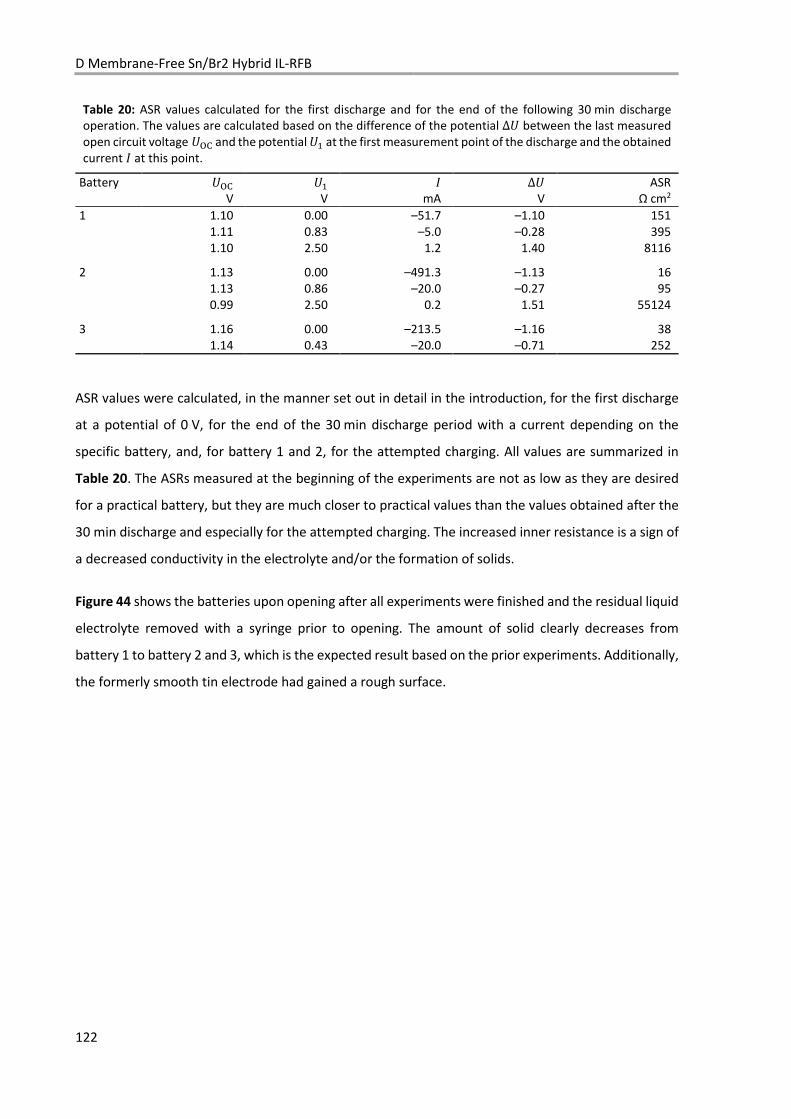
D Membrane-Free Sn/Br2 Hybrid IL-RFB
122
Table 20: ASR values calculated for the first discharge and for the end of the following 30 min discharge operation. The values are calculated based on the difference of the potential ∆� between the last measured open circuit voltage ��� and the potential �� at the first measurement point of the discharge and the obtained current � at this point.
Battery ��� �� � ∆� ASR
V V mA V Ω cm2 1 1.10 0.00 –51.7 –1.10 151
1.11 0.83 –5.0 –0.28 395 1.10 2.50 1.2 1.40 8116
2 1.13 0.00 –491.3 –1.13 16
1.13 0.86 –20.0 –0.27 95 0.99 2.50 0.2 1.51 55124
3 1.16 0.00 –213.5 –1.16 38
1.14 0.43 –20.0 –0.71 252
ASR values were calculated, in the manner set out in detail in the introduction, for the first discharge
at a potential of 0 V, for the end of the 30 min discharge period with a current depending on the
specific battery, and, for battery 1 and 2, for the attempted charging. All values are summarized in
Table 20. The ASRs measured at the beginning of the experiments are not as low as they are desired
for a practical battery, but they are much closer to practical values than the values obtained after the
30 min discharge and especially for the attempted charging. The increased inner resistance is a sign of
a decreased conductivity in the electrolyte and/or the formation of solids.
Figure 44 shows the batteries upon opening after all experiments were finished and the residual liquid
electrolyte removed with a syringe prior to opening. The amount of solid clearly decreases from
battery 1 to battery 2 and 3, which is the expected result based on the prior experiments. Additionally,
the formerly smooth tin electrode had gained a rough surface.
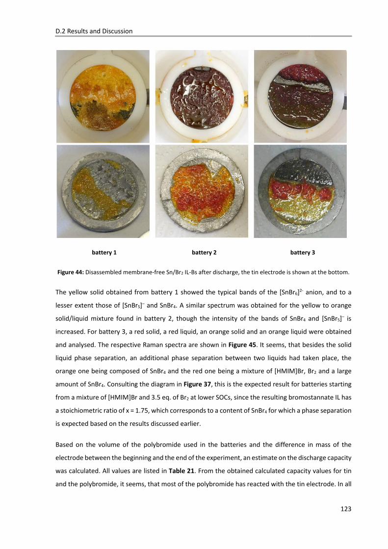
D.2 Results and Discussion
123
battery 1 battery 2 battery 3
Figure 44: Disassembled membrane-free Sn/Br2 IL-Bs after discharge, the tin electrode is shown at the bottom.
The yellow solid obtained from battery 1 showed the typical bands of the [SnBr6]2- anion, and to a
lesser extent those of [SnBr5]– and SnBr4. A similar spectrum was obtained for the yellow to orange
solid/liquid mixture found in battery 2, though the intensity of the bands of SnBr4 and [SnBr5]– is
increased. For battery 3, a red solid, a red liquid, an orange solid and an orange liquid were obtained
and analysed. The respective Raman spectra are shown in Figure 45. It seems, that besides the solid
liquid phase separation, an additional phase separation between two liquids had taken place, the
orange one being composed of SnBr4 and the red one being a mixture of [HMIM]Br, Br2 and a large
amount of SnBr4. Consulting the diagram in Figure 37, this is the expected result for batteries starting
from a mixture of [HMIM]Br and 3.5 eq. of Br2 at lower SOCs, since the resulting bromostannate IL has
a stoichiometric ratio of x = 1.75, which corresponds to a content of SnBr4 for which a phase separation
is expected based on the results discussed earlier.
Based on the volume of the polybromide used in the batteries and the difference in mass of the
electrode between the beginning and the end of the experiment, an estimate on the discharge capacity
was calculated. All values are listed in Table 21. From the obtained calculated capacity values for tin
and the polybromide, it seems, that most of the polybromide has reacted with the tin electrode. In all
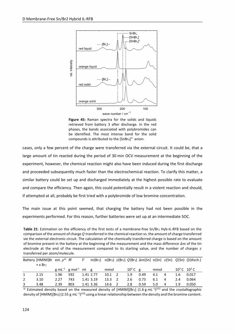
D Membrane-Free Sn/Br2 Hybrid IL-RFB
124
Figure 45: Raman spectra for the solids and liquids retrieved from battery 3 after discharge. In the red phases, the bands associated with polybromides can be identified. The most intense band for the solid compounds is attributed to the [SnBr6]2– anion.
cases, only a few percent of the charge were transferred via the external circuit. It could be, that a
large amount of tin reacted during the period of 30 min OCV measurement at the beginning of the
experiment, however, the chemical reaction might also have been induced during the first discharge
and proceeded subsequently much faster than the electrochemical reaction. To clarify this matter, a
similar battery could be set up and discharged immediately at the highest possible rate to evaluate
and compare the efficiency. Then again, this could potentially result in a violent reaction and should,
if attempted at all, probably be first tried with a polybromide of low bromine concentration.
The main issue at this point seemed, that charging the battery had not been possible in the
experiments performed. For this reason, further batteries were set up at an intermediate SOC.
Table 21: Estimation on the efficiency of the first tests of a membrane-free Sn/Br2 Hyb-IL-RFB based on the comparison of the amount of charge � transferred in the chemical reaction vs. the amount of charge transferred vie the external electronic circuit. The calculation of the chemically transferred charge is based on the amount of bromine present in the battery at the beginning of the measurement and the mass difference ∆� of the tin electrode at the end of the measurement compared to its starting value, and the number of charges 7 transferred per atom/molecule.
Battery [HMIM]Br + x Br2
est. a) � $ �(Br2) �(Br2) 7(Br2) �(Br2) ∆�(Sn) �(Sn) 7(Sn) �(Sn) �(disch.)
g mL–1 g mol-1 ml g mmol 103 C g mmol 103 C 103 C
1 2.15 1.96 592 1.41 2.77 10.1 2 1.9 0.49 4.1 4 1.6 0.017
2 3.10 2.27 743 1.41 3.19 13.3 2 2.6 0.73 6.1 4 2.4 0.064
3 3.48 2.39 803 1.41 3.36 14.6 2 2.8 0.59 5.0 4 1.9 0.050 a) Estimated density based on the measured density of [HMIM][Br3] (1.6 g mL–1)[31] and the crystallographic density of [HMIM][Br9] (2.55 g mL–1)[19] using a linear relationship between the density and the bromine content.
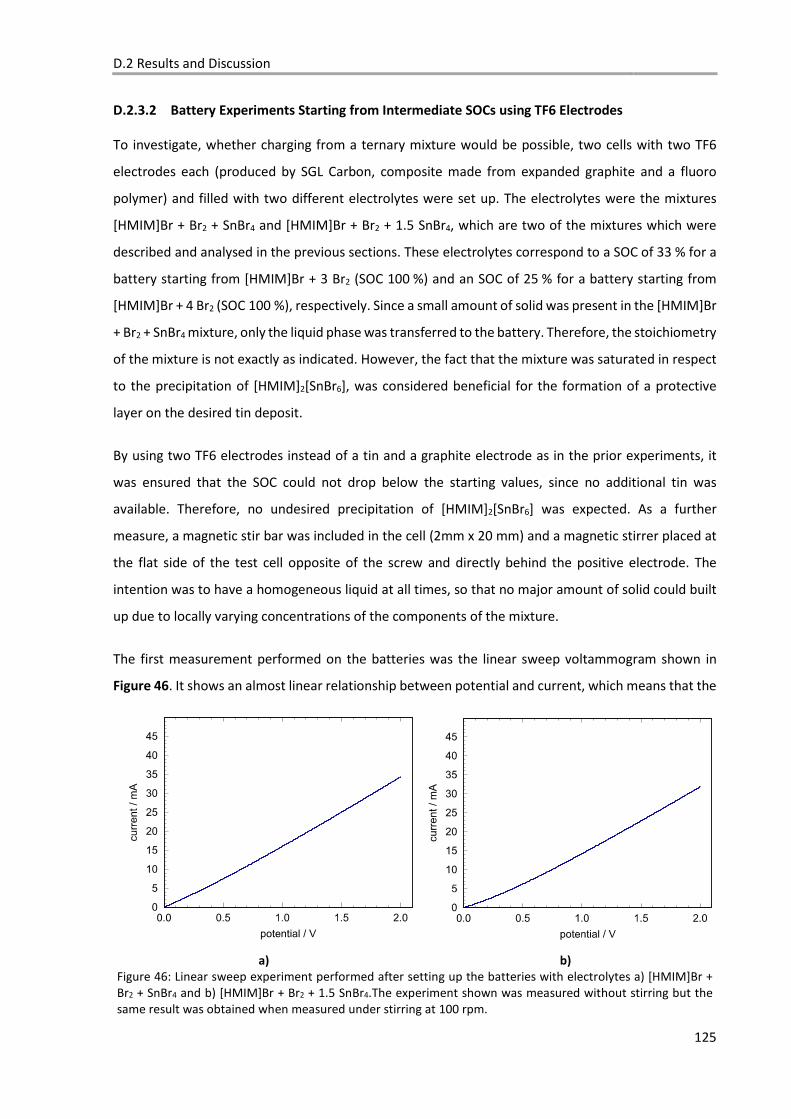
D.2 Results and Discussion
125
D.2.3.2 Battery Experiments Starting from Intermediate SOCs using TF6 Electrodes
To investigate, whether charging from a ternary mixture would be possible, two cells with two TF6
electrodes each (produced by SGL Carbon, composite made from expanded graphite and a fluoro
polymer) and filled with two different electrolytes were set up. The electrolytes were the mixtures
[HMIM]Br + Br2 + SnBr4 and [HMIM]Br + Br2 + 1.5 SnBr4, which are two of the mixtures which were
described and analysed in the previous sections. These electrolytes correspond to a SOC of 33 % for a
battery starting from [HMIM]Br + 3 Br2 (SOC 100 %) and an SOC of 25 % for a battery starting from
[HMIM]Br + 4 Br2 (SOC 100 %), respectively. Since a small amount of solid was present in the [HMIM]Br
+ Br2 + SnBr4 mixture, only the liquid phase was transferred to the battery. Therefore, the stoichiometry
of the mixture is not exactly as indicated. However, the fact that the mixture was saturated in respect
to the precipitation of [HMIM]2[SnBr6], was considered beneficial for the formation of a protective
layer on the desired tin deposit.
By using two TF6 electrodes instead of a tin and a graphite electrode as in the prior experiments, it
was ensured that the SOC could not drop below the starting values, since no additional tin was
available. Therefore, no undesired precipitation of [HMIM]2[SnBr6] was expected. As a further
measure, a magnetic stir bar was included in the cell (2mm x 20 mm) and a magnetic stirrer placed at
the flat side of the test cell opposite of the screw and directly behind the positive electrode. The
intention was to have a homogeneous liquid at all times, so that no major amount of solid could built
up due to locally varying concentrations of the components of the mixture.
The first measurement performed on the batteries was the linear sweep voltammogram shown in
Figure 46. It shows an almost linear relationship between potential and current, which means that the
a) b)
Figure 46: Linear sweep experiment performed after setting up the batteries with electrolytes a) [HMIM]Br + Br2 + SnBr4 and b) [HMIM]Br + Br2 + 1.5 SnBr4.The experiment shown was measured without stirring but the same result was obtained when measured under stirring at 100 rpm.
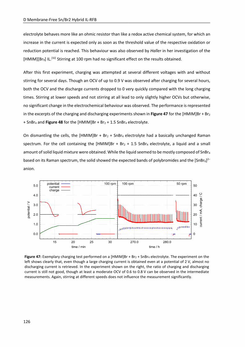
D Membrane-Free Sn/Br2 Hybrid IL-RFB
126
electrolyte behaves more like an ohmic resistor than like a redox active chemical system, for which an
increase in the current is expected only as soon as the threshold value of the respective oxidation or
reduction potential is reached. This behaviour was also observed by Haller in her investigation of the
[HMIM][Br9] IL.[32] Stirring at 100 rpm had no significant effect on the results obtained.
After this first experiment, charging was attempted at several different voltages with and without
stirring for several days. Though an OCV of up to 0.9 V was observed after charging for several hours,
both the OCV and the discharge currents dropped to 0 very quickly compared with the long charging
times. Stirring at lower speeds and not stirring at all lead to only slightly higher OCVs but otherwise,
no significant change in the electrochemical behaviour was observed. The performance is represented
in the excerpts of the charging and discharging experiments shown in Figure 47 for the [HMIM]Br + Br2
+ SnBr4 and Figure 48 for the [HMIM]Br + Br2 + 1.5 SnBr4 electrolyte.
On dismantling the cells, the [HMIM]Br + Br2 + SnBr4 electrolyte had a basically unchanged Raman
spectrum. For the cell containing the [HMIM]Br + Br2 + 1.5 SnBr4 electrolyte, a liquid and a small
amount of solid liquid mixture were obtained. While the liquid seemed to be mostly composed of SnBr4
based on its Raman spectrum, the solid showed the expected bands of polybromides and the [SnBr6]2–
anion.
Figure 47: Exemplary charging test performed on a [HMIM]Br + Br2 + SnBr4 electrolyte. The experiment on the left shows clearly that, even though a large charging current is obtained even at a potential of 2 V, almost no discharging current is retrieved. In the experiment shown on the right, the ratio of charging and discharging current is still not good, though at least a moderate OCV of 0.6 to 0.8 V can be observed in the intermediate measurements. Again, stirring at different speeds does not influence the measurement significantly.
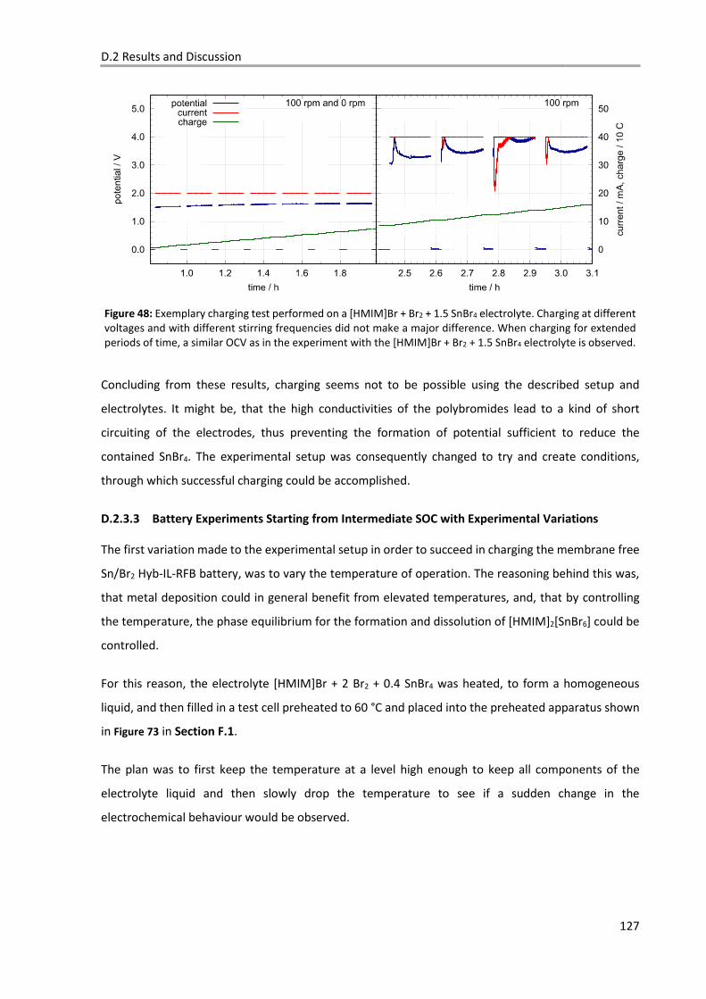
D.2 Results and Discussion
127
Figure 48: Exemplary charging test performed on a [HMIM]Br + Br2 + 1.5 SnBr4 electrolyte. Charging at different voltages and with different stirring frequencies did not make a major difference. When charging for extended periods of time, a similar OCV as in the experiment with the [HMIM]Br + Br2 + 1.5 SnBr4 electrolyte is observed.
Concluding from these results, charging seems not to be possible using the described setup and
electrolytes. It might be, that the high conductivities of the polybromides lead to a kind of short
circuiting of the electrodes, thus preventing the formation of potential sufficient to reduce the
contained SnBr4. The experimental setup was consequently changed to try and create conditions,
through which successful charging could be accomplished.
D.2.3.3 Battery Experiments Starting from Intermediate SOC with Experimental Variations
The first variation made to the experimental setup in order to succeed in charging the membrane free
Sn/Br2 Hyb-IL-RFB battery, was to vary the temperature of operation. The reasoning behind this was,
that metal deposition could in general benefit from elevated temperatures, and, that by controlling
the temperature, the phase equilibrium for the formation and dissolution of [HMIM]2[SnBr6] could be
controlled.
For this reason, the electrolyte [HMIM]Br + 2 Br2 + 0.4 SnBr4 was heated, to form a homogeneous
liquid, and then filled in a test cell preheated to 60 °C and placed into the preheated apparatus shown
in Figure 73 in Section F.1.
The plan was to first keep the temperature at a level high enough to keep all components of the
electrolyte liquid and then slowly drop the temperature to see if a sudden change in the
electrochemical behaviour would be observed.
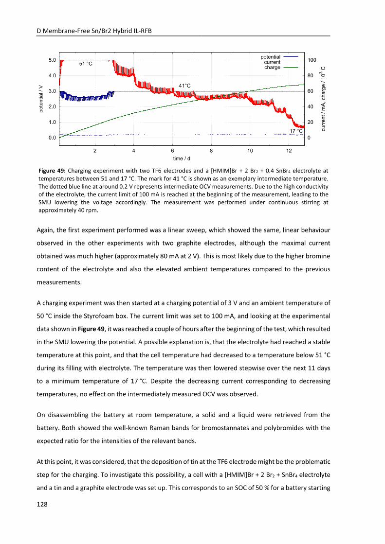
D Membrane-Free Sn/Br2 Hybrid IL-RFB
128
Figure 49: Charging experiment with two TF6 electrodes and a [HMIM]Br + 2 Br2 + 0.4 SnBr4 electrolyte at temperatures between 51 and 17 °C. The mark for 41 °C is shown as an exemplary intermediate temperature. The dotted blue line at around 0.2 V represents intermediate OCV measurements. Due to the high conductivity of the electrolyte, the current limit of 100 mA is reached at the beginning of the measurement, leading to the SMU lowering the voltage accordingly. The measurement was performed under continuous stirring at approximately 40 rpm.
Again, the first experiment performed was a linear sweep, which showed the same, linear behaviour
observed in the other experiments with two graphite electrodes, although the maximal current
obtained was much higher (approximately 80 mA at 2 V). This is most likely due to the higher bromine
content of the electrolyte and also the elevated ambient temperatures compared to the previous
measurements.
A charging experiment was then started at a charging potential of 3 V and an ambient temperature of
50 °C inside the Styrofoam box. The current limit was set to 100 mA, and looking at the experimental
data shown in Figure 49, it was reached a couple of hours after the beginning of the test, which resulted
in the SMU lowering the potential. A possible explanation is, that the electrolyte had reached a stable
temperature at this point, and that the cell temperature had decreased to a temperature below 51 °C
during its filling with electrolyte. The temperature was then lowered stepwise over the next 11 days
to a minimum temperature of 17 °C. Despite the decreasing current corresponding to decreasing
temperatures, no effect on the intermediately measured OCV was observed.
On disassembling the battery at room temperature, a solid and a liquid were retrieved from the
battery. Both showed the well-known Raman bands for bromostannates and polybromides with the
expected ratio for the intensities of the relevant bands.
At this point, it was considered, that the deposition of tin at the TF6 electrode might be the problematic
step for the charging. To investigate this possibility, a cell with a [HMIM]Br + 2 Br2 + SnBr4 electrolyte
and a tin and a graphite electrode was set up. This corresponds to an SOC of 50 % for a battery starting
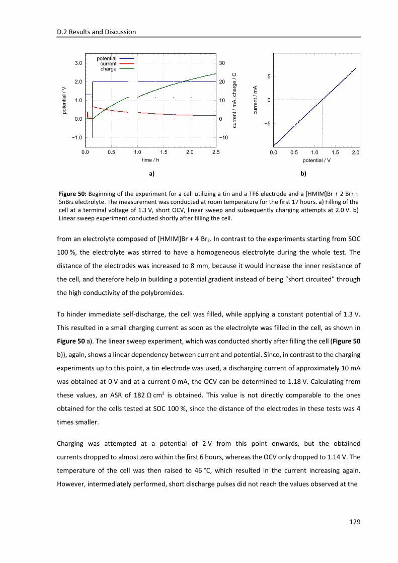
D.2 Results and Discussion
129
a) b)
Figure 50: Beginning of the experiment for a cell utilizing a tin and a TF6 electrode and a [HMIM]Br + 2 Br2 + SnBr4 electrolyte. The measurement was conducted at room temperature for the first 17 hours. a) Filling of the cell at a terminal voltage of 1.3 V, short OCV, linear sweep and subsequently charging attempts at 2.0 V. b) Linear sweep experiment conducted shortly after filling the cell.
from an electrolyte composed of [HMIM]Br + 4 Br2. In contrast to the experiments starting from SOC
100 %, the electrolyte was stirred to have a homogeneous electrolyte during the whole test. The
distance of the electrodes was increased to 8 mm, because it would increase the inner resistance of
the cell, and therefore help in building a potential gradient instead of being “short circuited” through
the high conductivity of the polybromides.
To hinder immediate self-discharge, the cell was filled, while applying a constant potential of 1.3 V.
This resulted in a small charging current as soon as the electrolyte was filled in the cell, as shown in
Figure 50 a). The linear sweep experiment, which was conducted shortly after filling the cell (Figure 50
b)), again, shows a linear dependency between current and potential. Since, in contrast to the charging
experiments up to this point, a tin electrode was used, a discharging current of approximately 10 mA
was obtained at 0 V and at a current 0 mA, the OCV can be determined to 1.18 V. Calculating from
these values, an ASR of 182 Ω cm2 is obtained. This value is not directly comparable to the ones
obtained for the cells tested at SOC 100 %, since the distance of the electrodes in these tests was 4
times smaller.
Charging was attempted at a potential of 2 V from this point onwards, but the obtained
currents dropped to almost zero within the first 6 hours, whereas the OCV only dropped to 1.14 V. The
temperature of the cell was then raised to 46 °C, which resulted in the current increasing again.
However, intermediately performed, short discharge pulses did not reach the values observed at the
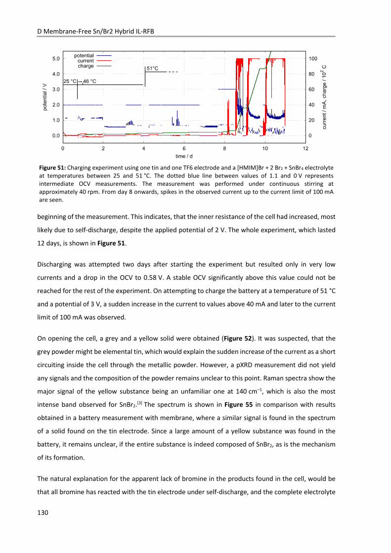
D Membrane-Free Sn/Br2 Hybrid IL-RFB
130
Figure 51: Charging experiment using one tin and one TF6 electrode and a [HMIM]Br + 2 Br2 + SnBr4 electrolyte at temperatures between 25 and 51 °C. The dotted blue line between values of 1.1 and 0 V represents intermediate OCV measurements. The measurement was performed under continuous stirring at approximately 40 rpm. From day 8 onwards, spikes in the observed current up to the current limit of 100 mA are seen.
beginning of the measurement. This indicates, that the inner resistance of the cell had increased, most
likely due to self-discharge, despite the applied potential of 2 V. The whole experiment, which lasted
12 days, is shown in Figure 51.
Discharging was attempted two days after starting the experiment but resulted only in very low
currents and a drop in the OCV to 0.58 V. A stable OCV significantly above this value could not be
reached for the rest of the experiment. On attempting to charge the battery at a temperature of 51 °C
and a potential of 3 V, a sudden increase in the current to values above 40 mA and later to the current
limit of 100 mA was observed.
On opening the cell, a grey and a yellow solid were obtained (Figure 52). It was suspected, that the
grey powder might be elemental tin, which would explain the sudden increase of the current as a short
circuiting inside the cell through the metallic powder. However, a pXRD measurement did not yield
any signals and the composition of the powder remains unclear to this point. Raman spectra show the
major signal of the yellow substance being an unfamiliar one at 140 cm–1, which is also the most
intense band observed for SnBr2.[3] The spectrum is shown in Figure 55 in comparison with results
obtained in a battery measurement with membrane, where a similar signal is found in the spectrum
of a solid found on the tin electrode. Since a large amount of a yellow substance was found in the
battery, it remains unclear, if the entire substance is indeed composed of SnBr2, as is the mechanism
of its formation.
The natural explanation for the apparent lack of bromine in the products found in the cell, would be
that all bromine has reacted with the tin electrode under self-discharge, and the complete electrolyte
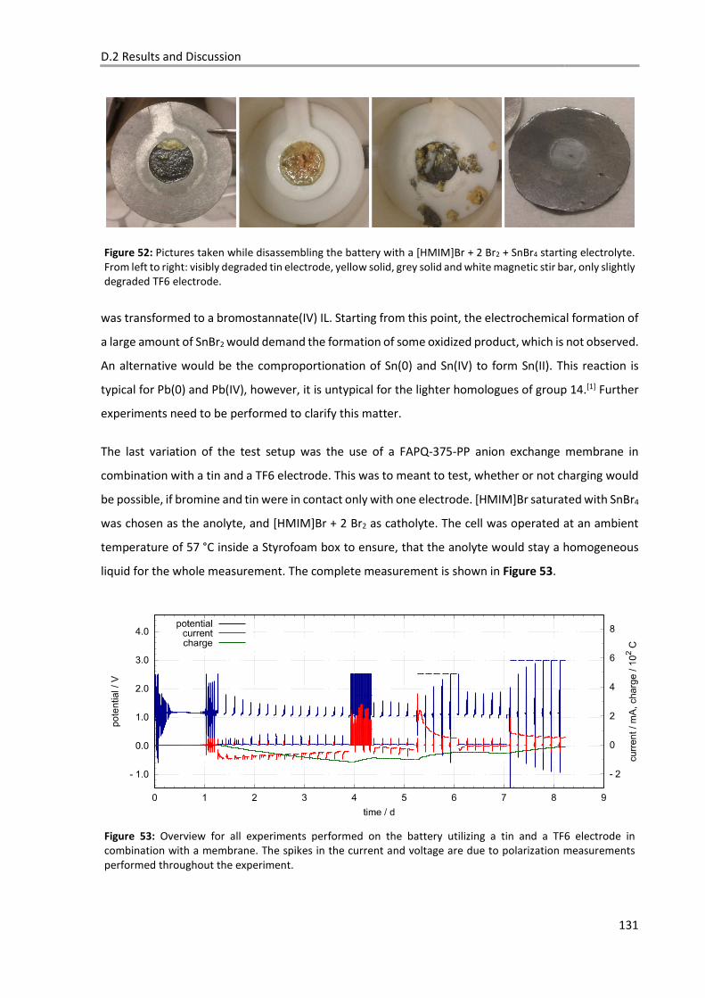
D.2 Results and Discussion
131
was transformed to a bromostannate(IV) IL. Starting from this point, the electrochemical formation of
a large amount of SnBr2 would demand the formation of some oxidized product, which is not observed.
An alternative would be the comproportionation of Sn(0) and Sn(IV) to form Sn(II). This reaction is
typical for Pb(0) and Pb(IV), however, it is untypical for the lighter homologues of group 14.[1] Further
experiments need to be performed to clarify this matter.
The last variation of the test setup was the use of a FAPQ-375-PP anion exchange membrane in
combination with a tin and a TF6 electrode. This was to meant to test, whether or not charging would
be possible, if bromine and tin were in contact only with one electrode. [HMIM]Br saturated with SnBr4
was chosen as the anolyte, and [HMIM]Br + 2 Br2 as catholyte. The cell was operated at an ambient
temperature of 57 °C inside a Styrofoam box to ensure, that the anolyte would stay a homogeneous
liquid for the whole measurement. The complete measurement is shown in Figure 53.
Figure 52: Pictures taken while disassembling the battery with a [HMIM]Br + 2 Br2 + SnBr4 starting electrolyte. From left to right: visibly degraded tin electrode, yellow solid, grey solid and white magnetic stir bar, only slightly degraded TF6 electrode.
Figure 53: Overview for all experiments performed on the battery utilizing a tin and a TF6 electrode in combination with a membrane. The spikes in the current and voltage are due to polarization measurements performed throughout the experiment.
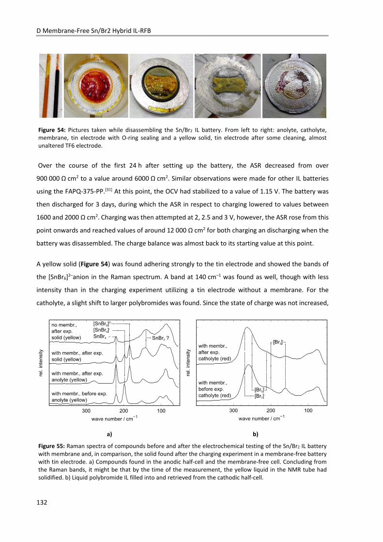
D Membrane-Free Sn/Br2 Hybrid IL-RFB
132
Figure 54: Pictures taken while disassembling the Sn/Br2 IL battery. From left to right: anolyte, catholyte, membrane, tin electrode with O-ring sealing and a yellow solid, tin electrode after some cleaning, almost unaltered TF6 electrode.
Over the course of the first 24 h after setting up the battery, the ASR decreased from over
900 000 Ω cm2 to a value around 6000 Ω cm2. Similar observations were made for other IL batteries
using the FAPQ-375-PP.[31] At this point, the OCV had stabilized to a value of 1.15 V. The battery was
then discharged for 3 days, during which the ASR in respect to charging lowered to values between
1600 and 2000 Ω cm2. Charging was then attempted at 2, 2.5 and 3 V, however, the ASR rose from this
point onwards and reached values of around 12 000 Ω cm2 for both charging an discharging when the
battery was disassembled. The charge balance was almost back to its starting value at this point.
A yellow solid (Figure 54) was found adhering strongly to the tin electrode and showed the bands of
the [SnBr6]2–anion in the Raman spectrum. A band at 140 cm–1 was found as well, though with less
intensity than in the charging experiment utilizing a tin electrode without a membrane. For the
catholyte, a slight shift to larger polybromides was found. Since the state of charge was not increased,
a) b)
Figure 55: Raman spectra of compounds before and after the electrochemical testing of the Sn/Br2 IL battery with membrane and, in comparison, the solid found after the charging experiment in a membrane-free battery with tin electrode. a) Compounds found in the anodic half-cell and the membrane-free cell. Concluding from the Raman bands, it might be that by the time of the measurement, the yellow liquid in the NMR tube had solidified. b) Liquid polybromide IL filled into and retrieved from the cathodic half-cell.
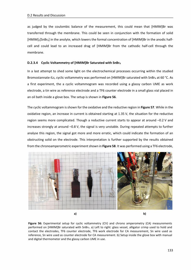
D.2 Results and Discussion
133
as judged by the coulombic balance of the measurement, this could mean that [HMIM]Br was
transferred through the membrane. This could be seen in conjunction with the formation of solid
[HMIM]2[SnBr6] in the anolyte, which lowers the formal concentration of [HMIM]Br in the anodic half-
cell and could lead to an increased drag of [HMIM]Br from the cathodic half-cell through the
membrane.
D.2.3.4 Cyclic Voltammetry of [HMIM]Br Saturated with SnBr4
In a last attempt to shed some light on the electrochemical processes occurring within the studied
Bromostannate-ILs, cyclic voltammetry was performed on [HMIM]Br saturated with SnBr4 at 60 °C. As
a first experiment, the a cyclic voltammogram was recorded using a glassy carbon UME as work
electrode, a tin wire as reference electrode and a TF6 counter electrode in a small glass vial placed in
an oil bath inside a glove box. The setup is shown in Figure 56.
The cyclic voltammogram is shown for the oxidative and the reductive region in Figure 57. While in the
oxidative region, an increase in current is obtained starting at 1.35 V, the situation for the reductive
region seems more complicated. Though a reductive current starts to appear at around –0.2 V and
increases strongly at around –0.8 V, the signal is very unstable. During repeated attempts to further
analyse this region, the signal got more and more erratic, which could indicate the formation of an
obstructing solid on the electrode. This interpretation is further supported by the results obtained
from the chronoamperometric experiment shown in Figure 58. It was performed using a TF6 electrode,
a) b)
Figure 56: Experimental setup for cyclic voltammetry (CV) and chrono amperometry (CA) measurements performed on [HMIM]Br saturated with SnBr4. a) Left to right: glass vessel, alligator crimp used to hold and contact the electrodes, TF6 counter electrode, TF6 work electrode for CA measurement, Sn wire used as reference, Sn wire used as counter electrode for CA measurement. b) Setup inside the glove box with manual and digital thermometer and the glassy carbon UME in use.
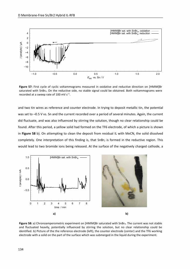
D Membrane-Free Sn/Br2 Hybrid IL-RFB
134
and two tin wires as reference and counter electrode. In trying to deposit metallic tin, the potential
was set to –0.5 V vs. Sn and the current recorded over a period of several minutes. Again, the current
did fluctuate, and was also influenced by stirring the solution, though no clear relationship could be
found. After this period, a yellow solid had formed on the TF6 electrode, of which a picture is shown
in Figure 58 b). On attempting to clean the deposit from residual IL with MeCN, the solid dissolved
completely. One interpretation of this finding is, that SnBr2 is formed in the reductive region. This
would lead to two bromide ions being released. At the surface of the negatively charged cathode, a
a) b)
Figure 58: a) Chronoamperometric experiment on [HMIM]Br saturated with SnBr4. The current was not stable and fluctuated heavily, potentially influenced by stirring the solution, but no clear relationship could be identified. b) Picture of the the reference electrode (left), the counter electrode (center) and the TF6 working electrode with a solid on the part of the surface which was submerged in the liquid during the experiment.
Figure 57: First cycle of cyclic voltammograms measured in oxidative and reductive direction on [HMIM]Br saturated with SnBr4. On the reductive side, no stable signal could be obtained. Both voltammograms were recorded at a sweep rate of 100 mV s–1.

D.2 Results and Discussion
135
layer of [HMIM]+ cations is most likely adsorbed as a Helmholtz or a diffuse double layer.[33] If SnBr4 is
now transported towards the cathode via diffusion, the conditions are ideal for the formation of solid
[SnBr6]– due to the high local concentration of [HMIM]Br. In sum, the formation of a “protective layer”
is observed, but most likely directly on the carbon electrode and not on top of deposited tin, as it would
be needed for a functional battery.

D Membrane-Free Sn/Br2 Hybrid IL-RFB
136
D.3 Conclusion and Outlook
137
D.3 Conclusion and Outlook
The phase behaviour of mixtures of SnBr4 and [HMIM]Br were systematically analysed both in the bulk
and via synthesis in DSC crucibles. The different bromostannate species present in these mixtures were
analysed by Raman and NMR spectroscopy both for the solid and the liquid state. The extremes of the
melting points are observed for [HMIM]2[SnBr6] (165 °C) and a phase containing a mixture of [HMIM]Br
saturated with SnBr4, for which a homogenisation in the bulk was observed around 40 °C. In the solid
state at room temperature, [HMIM]2[SnBr6] and SnBr4 are the dominating compounds. The
dismutation of [HMIM][SnBr5] on cooling the liquid to room temperature, was explored in more depth
by calculating a thermodynamic cycle and concluding, that the lattice enthalpy for the formation of
solid [HMIM]2[SnBr6] is the energetic driving force.
An overview over possible compositions for a ternary electrolyte based on [HMIM]Br, SnBr4 and Br2
and the anionic complexes present in these mixtures, was obtained by analysing experimental mixtures
via Raman and NMR spectroscopy. The conductivity of these samples decreased significantly on an
increase of the SnBr4 content.
Discharging experiments for the first membrane-free Sn/Br2 IL battery showed promising ASR values,
though the observed efficiencies were poor for all studied electrolytes. Charging experiments were
performed under variation of the electrolyte, electrode materials and operating temperature. None of
these variations led to successful charging of the membrane free Sn/Br2 IL battery. Charging was even
impossible when using a membrane to separate the anodic and the cathodic half-cell in a further
experiment. The observation of a band at 140 cm–1 in the Raman spectra obtained on solids found in
the cells after charging experiments which utilized a tin electrode, suggests the presence of SnBr2.
The problem of a poor discharge efficiency might be overcome when moving from static cells to a flow
setup. In these flow-cells, the electrolyte should be kept saturated with an [cat]2[SnBr6] salt, thus
ensuring that a protective layer would be stable over the whole SOC range. Such a setup was already
depicted in Figure 9 in Chapter B.1.2.1. The cost of the electrolyte could be reduced by utilizing a salt
which is less soluble in the electrolyte than [HMIM]Br.
The major problem of the envisioned battery is the fact that successful charging was not achieved
during the course of this work. It might be, that the formation of Sn(II) species play a role in preventing
a tin deposition. However, no firm conclusions can be drawn from the exploratory charging

D Membrane-Free Sn/Br2 Hybrid IL-RFB
138
experiments and neither from the cyclic voltammetry experiment. A systematic study of the charging
behaviour of the membrane-free Sn/Br2 IL battery should therefore be the next step in the course of
this research.
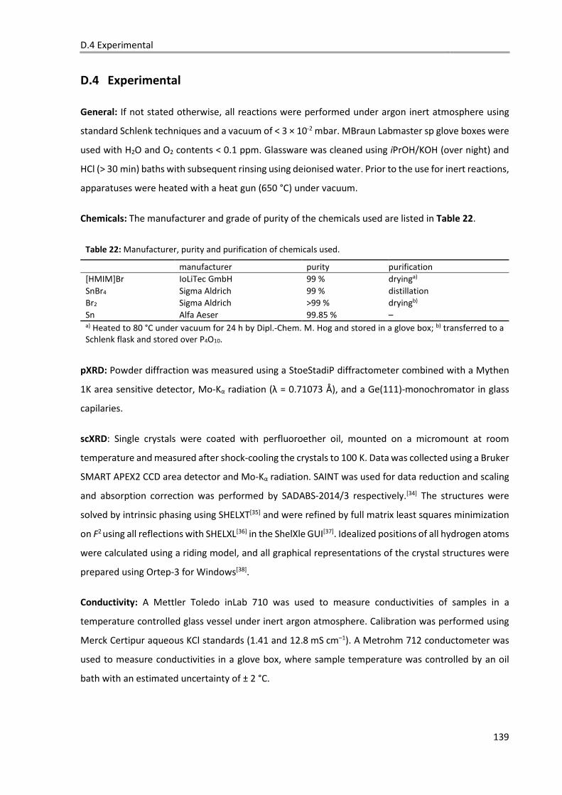
D.4 Experimental
139
D.4 Experimental
General: If not stated otherwise, all reactions were performed under argon inert atmosphere using
standard Schlenk techniques and a vacuum of < 3 × 10⁻² mbar. MBraun Labmaster sp glove boxes were
used with H2O and O2 contents < 0.1 ppm. Glassware was cleaned using iPrOH/KOH (over night) and
HCl (> 30 min) baths with subsequent rinsing using deionised water. Prior to the use for inert reactions,
apparatuses were heated with a heat gun (650 °C) under vacuum.
Chemicals: The manufacturer and grade of purity of the chemicals used are listed in Table 22.
Table 22: Manufacturer, purity and purification of chemicals used.
manufacturer purity purification [HMIM]Br IoLiTec GmbH 99 % dryinga) SnBr4 Sigma Aldrich 99 % distillation Br2 Sigma Aldrich >99 % dryingb) Sn Alfa Aeser 99.85 % – a) Heated to 80 °C under vacuum for 24 h by Dipl.-Chem. M. Hog and stored in a glove box; b) transferred to a Schlenk flask and stored over P4O10.
pXRD: Powder diffraction was measured using a StoeStadiP diffractometer combined with a Mythen
1K area sensitive detector, Mo-Kα radiation (λ = 0.71073 Å), and a Ge(111)-monochromator in glass
capilaries.
scXRD: Single crystals were coated with perfluoroether oil, mounted on a micromount at room
temperature and measured after shock-cooling the crystals to 100 K. Data was collected using a Bruker
SMART APEX2 CCD area detector and Mo-Kα radiation. SAINT was used for data reduction and scaling
and absorption correction was performed by SADABS-2014/3 respectively.[34] The structures were
solved by intrinsic phasing using SHELXT[35] and were refined by full matrix least squares minimization
on F2 using all reflections with SHELXL[36] in the ShelXle GUI[37]. Idealized positions of all hydrogen atoms
were calculated using a riding model, and all graphical representations of the crystal structures were
prepared using Ortep-3 for Windows[38].
Conductivity: A Mettler Toledo inLab 710 was used to measure conductivities of samples in a
temperature controlled glass vessel under inert argon atmosphere. Calibration was performed using
Merck Certipur aqueous KCl standards (1.41 and 12.8 mS cm–1). A Metrohm 712 conductometer was
used to measure conductivities in a glove box, where sample temperature was controlled by an oil
bath with an estimated uncertainty of ± 2 °C.
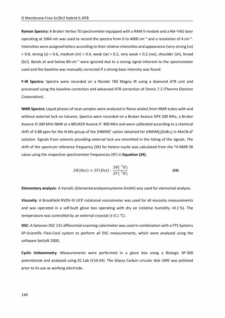
D Membrane-Free Sn/Br2 Hybrid IL-RFB
140
Raman Spectra: A Bruker Vertex 70 spectrometer equipped with a RAM II module and a Nd–YAG laser
operating at 1064 nm was used to record the spectra from 0 to 4000 cm–1 and a resolution of 4 cm–1.
Intensities were assigned letters according to their relative intensities and appearance (very strong (vs)
> 0.8, strong (s) > 0.6, medium (m) > 0.4, weak (w) > 0.2, very weak < 0.2 (vw), shoulder (sh), broad
(br)). Bands at and below 80 cm–1 were ignored due to a strong signal inherent to the spectrometer
used and the baseline was manually corrected if a strong base intensity was found.
F-IR Spectra: Spectra were recorded on a Nicolet 760 Magna IR using a diamond ATR unit and
processed using the baseline correction and advanced ATR correction of Omnic 7.2 (Thermo Electron
Corporation).
NMR Spectra: Liquid phases of neat samples were analysed in flame sealed 3mm NMR-tubes with and
without external lock on toluene. Spectra were recorded on a Bruker Avance DPX 200 Mhz, a Bruker
Avance III 300 MHz NMR or a BRUKER Avance II+ 400 MHz and were calibrated according to a chemical
shift of 3.88 ppm for the N-Me group of the [HMIM]+ cation obtained for [HMIM]2[SnBr6] in MeCN-d3
solution. Signals from solvents providing external lock are ommitted in the listing of the signals. The
shift of the spectrum reference frequency (SR) for hetero nuclei was calculated from the 1H-NMR SR
value using the respective spectrometer frequencies (SF) in Equation (24).
��Sdz{U = ��Sdz{U ∙ ��S d� U��S d� U (24)
Elementary analysis: A VarioEL (Elementaranalysensysteme GmbH) was used for elemental analysis.
Viscosity: A Brookfield RVDV-III UCP rotational viscosimeter was used for all viscosity measurements
and was operated in a self-built glove box operating with dry air (relative humidity <0.1 %). The
temperature was controlled by an external cryostat (± 0.1 °C).
DSC: A Setaram DSC 131 differential scanning calorimeter was used in combination with a FTS Systems
SP-Scientific Flexi-Cool system to perform all DSC measurements, which were analysed using the
software SetSoft 2000.
Cyclic Voltammetry: Measurements were performed in a glove box using a Biologic SP-300
potentiostat and analysed using EC-Lab (V10.44). The Glassy Carbon circular disk UME was polished
prior to its use as working electrode.
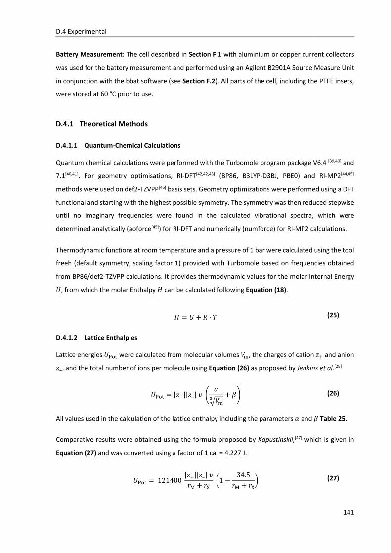
D.4 Experimental
141
Battery Measurement: The cell described in Section F.1 with aluminium or copper current collectors
was used for the battery measurement and performed using an Agilent B2901A Source Measure Unit
in conjunction with the bbat software (see Section F.2). All parts of the cell, including the PTFE insets,
were stored at 60 °C prior to use.
Theoretical Methods
D.4.1.1 Quantum-Chemical Calculations
Quantum chemical calculations were performed with the Turbomole program package V6.4 [39,40] and
7.1[40,41]. For geometry optimisations, RI-DFT[42,42,43] (BP86, B3LYP-D3BJ, PBE0) and RI-MP2[44,45]
methods were used on def2-TZVPP[46] basis sets. Geometry optimizations were performed using a DFT
functional and starting with the highest possible symmetry. The symmetry was then reduced stepwise
until no imaginary frequencies were found in the calculated vibrational spectra, which were
determined analytically (aoforce[45]) for RI-DFT and numerically (numforce) for RI-MP2 calculations.
Thermodynamic functions at room temperature and a pressure of 1 bar were calculated using the tool
freeh (default symmetry, scaling factor 1) provided with Turbomole based on frequencies obtained
from BP86/def2-TZVPP calculations. It provides thermodynamic values for the molar Internal Energy �, from which the molar Enthalpy d can be calculated following Equation (18).
d = � / � ∙ e (25)
D.4.1.2 Lattice Enthalpies
Lattice energies �8|� were calculated from molecular volumes $}, the charges of cation 7~ and anion 7–, and the total number of ions per molecule using Equation (26) as proposed by Jenkins et al.[28]
�8|� = |7~||7–| N � ��$}� / �� (26)
All values used in the calculation of the lattice enthalpy including the parameters � and � Table 25.
Comparative results were obtained using the formula proposed by Kapustinskii,[47] which is given in
Equation (27) and was converted using a factor of 1 cal = 4.227 J.
�8|� = 121400 |7~||7–| N�b / �� �1 − 34.5�b / ��� (27)
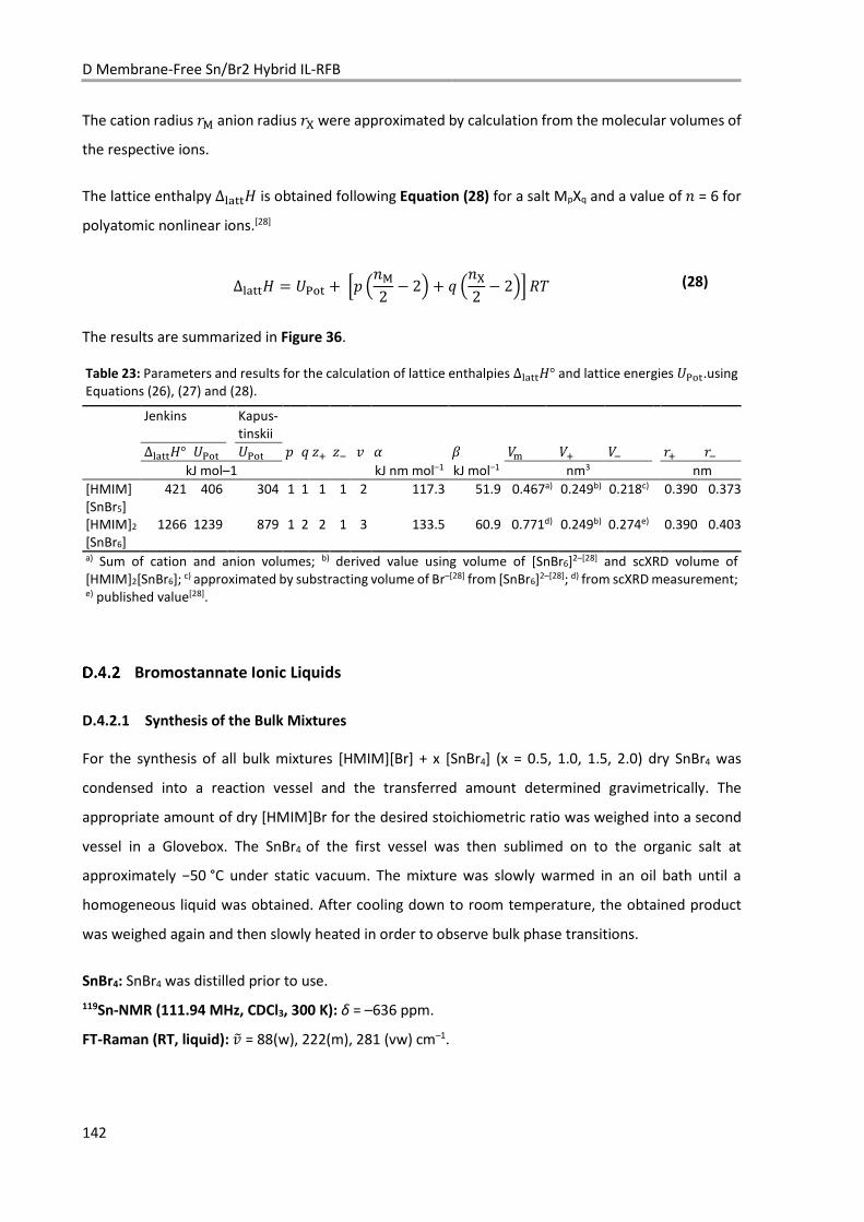
D Membrane-Free Sn/Br2 Hybrid IL-RFB
142
The cation radius �b anion radius �� were approximated by calculation from the molecular volumes of
the respective ions.
The lattice enthalpy ∆#"��d is obtained following Equation (28) for a salt MpXq and a value of � = 6 for
polyatomic nonlinear ions.[28]
∆#"��d = �8|� / �� ��b2 − 2� / � ���2 − 2�� �e (28)
The results are summarized in Figure 36.
Bromostannate Ionic Liquids
D.4.2.1 Synthesis of the Bulk Mixtures
For the synthesis of all bulk mixtures [HMIM][Br] + x [SnBr4] (x = 0.5, 1.0, 1.5, 2.0) dry SnBr4 was
condensed into a reaction vessel and the transferred amount determined gravimetrically. The
appropriate amount of dry [HMIM]Br for the desired stoichiometric ratio was weighed into a second
vessel in a Glovebox. The SnBr4 of the first vessel was then sublimed on to the organic salt at
approximately −50 °C under static vacuum. The mixture was slowly warmed in an oil bath until a
homogeneous liquid was obtained. After cooling down to room temperature, the obtained product
was weighed again and then slowly heated in order to observe bulk phase transitions.
SnBr4: SnBr4 was distilled prior to use.
119Sn-NMR (111.94 MHz, CDCl3, 300 K): δ = –636 ppm.
FT-Raman (RT, liquid): NO = 88(w), 222(m), 281 (vw) cm–1.
Table 23: Parameters and results for the calculation of lattice enthalpies ∆#"��d° and lattice energies �8|�.using Equations (26), (27) and (28).
Jenkins Kapus-tinskii
∆#"��d° �8|� �8|� � � 7~ 7^ N � � $} $~ $̂ �~ �̂
kJ mol–1 kJ nm mol–1 kJ mol–1 nm3 nm [HMIM] [SnBr5]
421 406 304 1 1 1 1 2 117.3 51.9 0.467a) 0.249b) 0.218c) 0.390 0.373
[HMIM]2
[SnBr6] 1266 1239 879 1 2 2 1 3 133.5 60.9 0.771d) 0.249b) 0.274e) 0.390 0.403
a) Sum of cation and anion volumes; b) derived value using volume of [SnBr6]2–[28] and scXRD volume of [HMIM]2[SnBr6]; c) approximated by substracting volume of Br–[28] from [SnBr6]2–[28]; d) from scXRD measurement; e) published value[28].
D.4 Experimental
143
[HMIM]2[SnBr6]: The mixture of [HMIM]Br (5.472 g, 22.14 mmol) and SnBr4 (4.810 g, 10.97 mmol,
0.495 eq) partly melted on heating to 160 °C and formed a brown homogeneous liquid at (185 ± 10)◦C
oil bath temperature.
1H-NMR (300.18 MHz, CD3CN, 300 K): δ = 0.84 – 0.93 (m, 3H), 1.23 – 1.39 (m, 6H), 1.77 – 1.91 (m, 2H),
2.21 (s, 1.38H, H2O), 3.88 (s, 3H), 4.18 (t, 3J H,H = 7.32Hz, 2H), 7.32 – 7.43 (m, 2H), 8.64 (b, 1H) ppm.
119Sn-NMR (111.94 MHz, CD3CN, 300 K): δ = 2073 ppm.
FT-Raman (RT, solid): NO = 99 (w), 140 (vw, sh), 148 (w), 184 (vs), 200 (vw, sh), 600 (vw), 1021 (vw),
1106 (vw), 1332 (vw), 1381 (vw), 1411 (vw), 1431 (vw), 1882 (vw), 2869 (vw), 2898 (vw), 2932 (vw),
2954 (vw), 3080 (vw), 3131 (vw), 3154 (vw) cm−1.
ATR-IR (RT, solid): NO = 108, 185, 197 cm−1.
EA: Anal. calculated for C20H38Br6N4Sn: C, 25.75; H, 4.11; N, 6.01. Found: C, 25.93; H, 4.13; N, 6.10.
[HMIM]Br + 1.0 SnBr4: The mixture of [HMIM]Br (5.162 g, 20.9 mmol) and SnBr4 (9.131 g, 20.8 mmol,
1.00 eq) partly melted on heating from RT and formed a hazy yellow liquid at (70 ± 5)◦C that clarified
to be homogeneous at (85 ± 5)◦C.
1H-NMR (300.18 MHz, 300 K): δ = 0.49 - 0.73 (m, 3H), 0.94 - 1.28 (m, 6H), 1.62 - 1.89 (m, 2H), 3.88 (s,
3H), 4.01 - 4.20 (m, 2H), 7.27 - 7.45 (m, 2H), 8.51 - 8.68 (b, 1H), ppm.
119Sn-NMR (111.94 MHz, 300 K): δ = –1432 ppm.
119Sn-NMR (149.23 MHz, 353 K): δ = –1451 ppm.
FT-Raman (RT, liquid): NO = 102 (w), 152 (vw), 183 (vw), 198 (vs), 220 (vw), 253 (vw), 414 (vw), 561 (vw),
623 (vw), 716 (vw), 891 (vw), 1023 (vw), 1339 (vw), 1415 (vw), 1670 (vw), 2868 (vw), 2933 (vw), 2954
(vw) cm−1.
FT-Raman (RT, solid): NO = 88 (w, sh), 98 (w), 142 (w, sh), 148 (w), 184 (vs), 198 (vw, sh), 221 (vw), 409
(vw), 442 (vw), 528 (vw), 598 (vw), 1021 (vw), 1104 (vw), 1332 (vw), 1408 (vw), 1448 (vw), 2906 (vw),
2954 (vw), 2989 (vw), 3079 (vw), 3133 (vw), 3154 (vw) cm−1.
ATR-IR (RT, solid): ν˜ = 108, 182, 196 cm−1.
[HMIM]Br + 1.5 SnBr4: The mixture of [HMIM]Br (2.63 g, 10.6 mmol) and SnBr4 (6.98 g, 15.9 mmol,
1.50eq) partly melted on heating from RT and formed a pale yellow homogeneous liquid at (52 ± 5)◦C.
A sample of the heated liquid was transferred into a 3 mm NMR-tube and flame-sealed. At room
temperature, a small amount of a transparent liquid formed next to the main liquid, yellow phase. The
phase separation could be reversed by storing the tube at 60 °C for several hours.

D Membrane-Free Sn/Br2 Hybrid IL-RFB
144
1H-NMR (300.18 MHz, 300 K): δ = 0.56 - 0.78 (m, 3H), 1.03 - 1.35 (m, 6H), 1.63 - 1.90 (m, 2H), 3.88 (s,
3H), 4.09 (t, 3JH,H = 7.31 Hz, 2H), 7.25 - 7.42 (m, 2H), 8.40 - 8.58 (b, 1H) ppm.
119Sn-NMR (111.94 MHz, 300 K): δ = –1198 ppm.
119Sn-NMR (149.23 MHz, 353 K): δ = –1201 ppm.
FT-Raman (RT, liquid yellow): NO = 87 (w), 102 (w), 152 (vw), 183 (vw, sh), 198 (vs), 220 (w), 253 (vw),
280 (vw), 622 (vw), 1023 (vw), 1414 (vw), 1438 (vw), 2862 (vw), 2931 (vw), 2954 (vw) cm−1.
FT-Raman (RT, solid): NO = 87 (vs), 98 (vw, sh), 140 (vw, sh), 149 (vw), 184 (m), 200 (vw), 220 (vs), 276
(vw), 285 (vw), 1334 (vw), 1360 (vw), 1410 (vw), 1439 (vw), 1474 (vw), 2857 (vw), 2883 (vw), 2903
(vw), 2925 (vw), 2956 (vw), 3971 (vw) cm−1.
FT-Raman (RT, liquid transp.): NO = 88 (m), 135 (vw), 152 (vw), 198 (vw), 221 (vs), 279 (vw), 287 (vw,
sh), 1023 (vw), 1415 (vw), 2859 (vw), 2954 (vw) cm−1.
ATR-IR (RT, solid): NO = 85, 112, 182, 200, 274 cm−1.
[HMIM]Br + 2.0 [SnBr4]: The mixture of [HMIM]Br (0.508 g, 2.06 mmol) and SnBr4 (1.82 g, 4.14 mmol,
2.01eq) partly melted on heating from RT and formed a liquid brown phase at (48 ± 5)◦C. A sample of
the heated liquid was transferred into a 3 mm NMR-tube and flame-sealed. At room temperature, a
small amount of a transparent liquid formed next to the main liquid, yellow phase. The transparent
phase was reduced in amount by storing the tube at 60 °C for several hours, but did not dissolve
completely.
1H-NMR (300.18 MHz, 300 K): δ = 0.61 - 0.73 (m, 3H) 1.01 - 1.29 (m, 6H) 1.65 - 1.89 (m, 2H) 3.88 (s, 3H)
4.09 (t, 3JH,H = 7.31 Hz, 2H) 7.27 - 7.41 (m, 2H) 8.44 - 8.55 (b, 1H) ppm.
119Sn-NMR (111.94 MHz, 300 K): δ = –1202 ppm.
119Sn-NMR (149.23 MHz, 353 K): δ = –1172 ppm.
FT-Raman (RT, liquid yellow): NO = 87 (w), 102 (w), 152 (vw), 183 (vw, sh), 198 (vs), 220 (m), 254 (vw),
281 (vw), 887 (vw), 1415 (vw), 1916 (vw), 2859 (vw), 2897 (vw), 2924 (vw), 2954 (vw) cm−1.
FT-Raman (RT, liquid trasp.): NO = 70 (w), 88 (m), 198 (vw), 221 (vs), 278 (vw), 287 (vw, sh) cm−1.
FT-Raman (RT, solid): NO = 87 (vs), 100 (w), 149 (vw), 184 (m), 199 (w), 220 (vs), 251 (vw), 276 (vw), 285
(vw), 599 (vw), 1021 (vw), 1105 (vw), 1333 (vw), 1357 (vw), 1383 (vw), 1412 (vw), 1432 (vw), 1569
(vw), 2726 (vw), 2868 (vw), 2893 (vw), 2932 (vw), 2955 (vw), 2989 (vw), 3037 (vw), 3083 (vw), 3133
(vw), 3157 (vw) cm−1.
ATR-IR (RT): NO = 83, 108, 200, 250, 274 cm−1.
[HMIM]Br saturated with SnBr4: SnBr4 (6.67 g, 15.2 mmol) was mixed with solid [HMIM]2[SnBr6]
(4.73 g, 5.07 mmol, 0.33 eq) in a glove box and stirred for 2 h at 60 °C. Two liquid phases were obtained
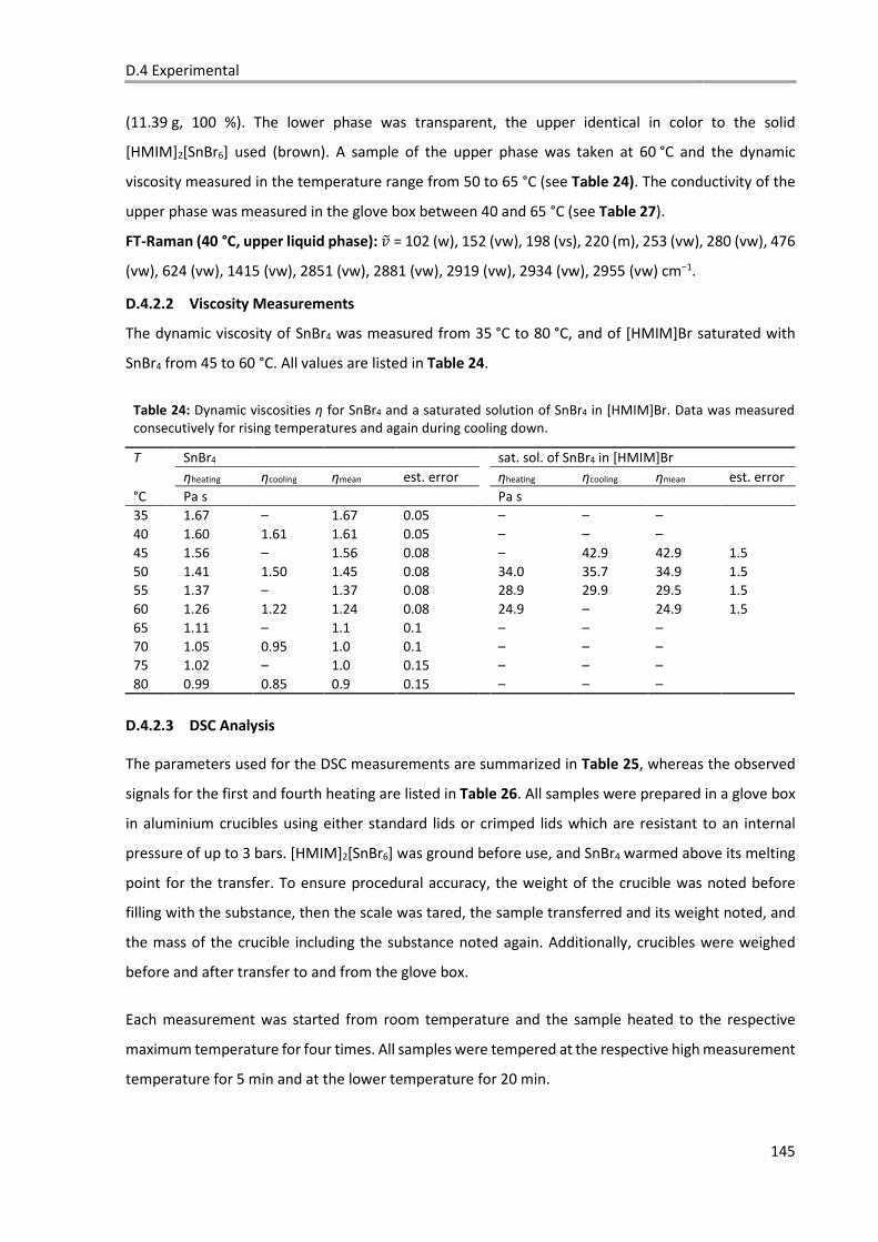
D.4 Experimental
145
(11.39 g, 100 %). The lower phase was transparent, the upper identical in color to the solid
[HMIM]2[SnBr6] used (brown). A sample of the upper phase was taken at 60 °C and the dynamic
viscosity measured in the temperature range from 50 to 65 °C (see Table 24). The conductivity of the
upper phase was measured in the glove box between 40 and 65 °C (see Table 27).
FT-Raman (40 °C, upper liquid phase): NO = 102 (w), 152 (vw), 198 (vs), 220 (m), 253 (vw), 280 (vw), 476
(vw), 624 (vw), 1415 (vw), 2851 (vw), 2881 (vw), 2919 (vw), 2934 (vw), 2955 (vw) cm−1.
D.4.2.2 Viscosity Measurements
The dynamic viscosity of SnBr4 was measured from 35 °C to 80 °C, and of [HMIM]Br saturated with
SnBr4 from 45 to 60 °C. All values are listed in Table 24.
Table 24: Dynamic viscosities ƞ for SnBr4 and a saturated solution of SnBr4 in [HMIM]Br. Data was measured consecutively for rising temperatures and again during cooling down.
T SnBr4 sat. sol. of SnBr4 in [HMIM]Br
ƞheating ƞcooling ƞmean est. error ƞheating ƞcooling ƞmean est. error
°C Pa s Pa s 35 1.67 – 1.67 0.05 – – – 40 1.60 1.61 1.61 0.05 – – – 45 1.56 – 1.56 0.08 – 42.9 42.9 1.5 50 1.41 1.50 1.45 0.08 34.0 35.7 34.9 1.5 55 1.37 – 1.37 0.08 28.9 29.9 29.5 1.5 60 1.26 1.22 1.24 0.08 24.9 – 24.9 1.5 65 1.11 – 1.1 0.1 – – – 70 1.05 0.95 1.0 0.1 – – – 75 1.02 – 1.0 0.15 – – – 80 0.99 0.85 0.9 0.15 – – –
D.4.2.3 DSC Analysis
The parameters used for the DSC measurements are summarized in Table 25, whereas the observed
signals for the first and fourth heating are listed in Table 26. All samples were prepared in a glove box
in aluminium crucibles using either standard lids or crimped lids which are resistant to an internal
pressure of up to 3 bars. [HMIM]2[SnBr6] was ground before use, and SnBr4 warmed above its melting
point for the transfer. To ensure procedural accuracy, the weight of the crucible was noted before
filling with the substance, then the scale was tared, the sample transferred and its weight noted, and
the mass of the crucible including the substance noted again. Additionally, crucibles were weighed
before and after transfer to and from the glove box.
Each measurement was started from room temperature and the sample heated to the respective
maximum temperature for four times. All samples were tempered at the respective high measurement
temperature for 5 min and at the lower temperature for 20 min.
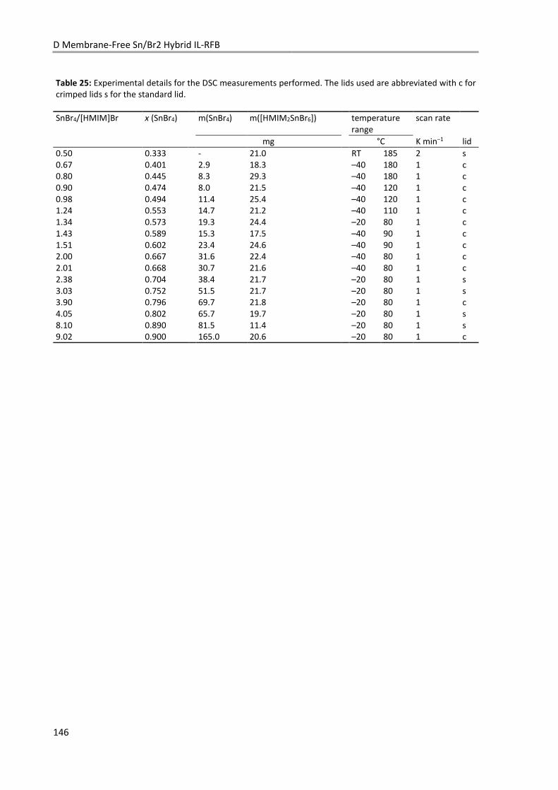
D Membrane-Free Sn/Br2 Hybrid IL-RFB
146
Table 25: Experimental details for the DSC measurements performed. The lids used are abbreviated with c for crimped lids s for the standard lid.
SnBr4/[HMIM]Br x (SnBr4) m(SnBr4) m([HMIM2SnBr6]) temperature range
scan rate
mg °C K min–1 lid 0.50 0.333 - 21.0 RT 185 2 s 0.67 0.401 2.9 18.3 –40 180 1 c 0.80 0.445 8.3 29.3 –40 180 1 c 0.90 0.474 8.0 21.5 –40 120 1 c 0.98 0.494 11.4 25.4 –40 120 1 c 1.24 0.553 14.7 21.2 –40 110 1 c 1.34 0.573 19.3 24.4 –20 80 1 c 1.43 0.589 15.3 17.5 –40 90 1 c 1.51 0.602 23.4 24.6 –40 90 1 c 2.00 0.667 31.6 22.4 –40 80 1 c 2.01 0.668 30.7 21.6 –40 80 1 c 2.38 0.704 38.4 21.7 –20 80 1 s 3.03 0.752 51.5 21.7 –20 80 1 s 3.90 0.796 69.7 21.8 –20 80 1 c 4.05 0.802 65.7 19.7 –20 80 1 s 8.10 0.890 81.5 11.4 –20 80 1 s 9.02 0.900 165.0 20.6 –20 80 1 c
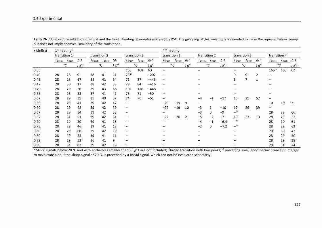
D.4 Experimental
147
Table 26: Observed transitions on the first and the fourth heating of samples analysed by DSC. The grouping of the transitions is intended to make the representation clearer, but does not imply chemical similarity of the transitions.
x (SnBr4) 1st heatinga) 4th heating transition 1 transition 2 transition 3 transition 1 transition 2 transition 3 transition 4 Tonset Tpeak ΔH Tonset Tpeak ΔH Tonset Tpeak ΔH Tonset Tpeak ΔH Tonset Tpeak ΔH Tonset Tpeak ΔH Tonset Tpeak ΔH
°C J g–1 °C J g–1 °C J g–1 °C J g–1 °C J g–1 °C J g–1 °C J g–1 0.33 165 168 63 – – – 165c) 168 62 0.40 28 28 9 38 41 11 75b) –202 – – 9 9 2 – 0.45 28 28 17 38 41 34 71 87 –443 – – 6 7 1 – 0.47 28 30 17 38 42 33 79 84 –416 – – – – 0.49 28 29 26 39 43 56 103 116 –448 – – – – 0.55 28 28 33 37 41 41 73 71 –50 – – – – 0.57 28 29 35 35 40 37 74 76 –51 – –4 –1 –17 15 25 57 – 0.59 28 29 41 39 42 47 – –20 –19 9 – – 10 10 2 0.60 28 29 42 39 42 59 – –22 –19 10 –3 1 –10 17 26 39 – 0.67 28 29 54 39 42 38 – – –3 0 –9 –d) 28 29 66 0.67 28 31 51 39 42 31 – –22 –20 2 –5 –2 –7 19 23 13 28 29 22 0.70 28 29 30 39 41 15 – – –4 –1 –6.4 –d) 28 29 61 0.75 28 29 46 39 41 13 – – –2 0 –7.2 –d) 28 29 62 0.80 28 29 68 39 42 19 – – – – 29 30 47 0.80 28 29 51 39 41 11 – – – – 28 29 50 0.89 28 29 53 36 41 9 – – – – 28 29 38 0.90 28 31 82 39 42 10 – – – – 29 31 74 a)Minor signals below 28 °C and with enthalpies smaller than 3 J g–1 are not included; b)broad transition with two peaks; c) preceding small endothermic transition merged to main transition; d)the sharp signal at 29 °C is preceded by a broad signal, which can not be evaluated separately.
D Membrane-Free Sn/Br2 Hybrid IL-RFB
148
Mixtures of [HMIM]Br, Br2, and SnBr4
D.4.3.1 Synthesis of Polybromide ILs used for Battery Measurements at SOC 100 %
For the following syntheses, bromine was used as received and not dried over P4O10.
[HMIM]Br + 4.07 Br2: [HMIM][Br] (5.53 g, 22.4 mmol) was transferred to a Schlenk RBF in a glove box.
Br2 (14.57 g, 91.2 mmol, 4.07 eq) was added via a syringe over a period of 25 min and under cooling
with a water bath. After stirring over night, a brown vapour was visible over the brown liquid (20.11 g,
100 %).
[HMIM]Br + 2.15 Br2: [HMIM][Br] (6.02 g, 24.4 mmol) was transferred to a Schlenk RBF in a glove box.
Br2 (8.39 g, 52.5 mmol, 2.15 eq) was added via a syringe over a period of 15 min and under cooling with
a water bath. After stirring overnight, a dark red liquid was obtained (14.42 g, 100 %).
[HMIM]Br + 3.10 Br2: [HMIM]Br + 4.07 Br2 (2.65 g, 2.95 mmol) was added to a mixture of [HMIM]Br +
2.15 Br2 (1.80 g, 3.04 mmol) in an RFB. After stirring overnight, a pale brown vapour was visible over a
dark red liquid (4.45 g, 100 %).
[HMIM]Br + 3.48 Br2: [HMIM]Br + 4.07 Br2 (3.89 g, 4.33 mmol) was added to a mixture of [HMIM]Br +
2.15 Br2 (1.15 g, 1.95 mmol) in an RFB. After stirring overnight, a pale brown vapour was visible over a
dark red liquid (4.45 g, 100 %).
D.4.3.2 Synthesis of Polybromides ILs Used for the Preparation of Bulk Mixtures with SnBr4
Bromine was dried over P4O10 prior to its use in the following syntheses. In a typical procedure, bromine
was condensed into Schlenk tube at –70 °C and weighed. The appropriate amount of [HMIM]Br was
then weighed into a second Schlenk tube in a glove box. The vessel was subsequently cooled to –70 °C
and the bromine condensed on top of the frozen [HMIM]Br. A reaction occurred upon slowly allowing
the mixture to reach room temperature.
[HMIM][Br3]: Br2 (9.39 g, 58.8 mmol, 1.00 eq) was condensed on [HMIM]Br (14.46 g, 58.50 mmol) at
–70 . The mixture was allowed to reach room temperature over a period of 50 min. A red liquid
(23.85 g, 100 %) was obtained after stirring overnight.
FT-Raman (RT): NO = 162 (vs), 196 (w, sh), 347 (vw), 603 (vw), 621 (vw), 696 (vw), 1023 (vw), 1106 (vw),
1336 (vw), 1387 (vw), 1416 (vw), 1497 (vw), 1565 (vw), 2733 (vw), 2871 (vw), 2932 (vw), 2952 (vw),
D.4 Experimental
149
3108 (vw), 3161 (vw) cm–1.
1H–NMR (300.18 MHz, neat, 300 K): P = 0.55-0.71 (m, 3 H, (CH2)5CH3), 0.98-1.27 (m, 6 H,
(CH2)2(CH2)3CH3), 1.67-1.84 (m, 2 H, CH2CH2(CH2)3CH3), 3.88 (s, 3 H, NCH3), 4.05-4.22 (m, 2 H,
CH2(CH2)4CH3), 7.37-7.50 (m, 2 H, NCHCHN), 8.67-8.76 (b, 1 H, NCHN) ppm.
[HMIM] + 2 Br2: Br2 (22.13 g, 179.2 mmol, 2.00 eq) was condensed on [HMIM]Br (22.13 g, 89.5 mmol)
at –79 °C. The mixture was allowed to reach room temperature over a period of 40 min. A dark red
liquid (50.76 g, 100 %) was obtained after stirring overnight.
The temperature dependent conductivity was measured and is listed in Table 27.
1H–NMR (300.18 MHz, neat, 300 K): P = 0.65-0.72 (m, 3 H, (CH2)5CH3), 1.06-1.27 (m, 6 H,
(CH2)2(CH2)3CH3), 1.75-1.84 (m, 2 H, CH2CH2(CH2)3CH3), 3.88 (s, 3 H, NCH3), 4.12 (t, 3JH,H = 7.49 Hz, 2 H,
CH2(CH2)4CH3), 7.29-7.37 (m, 2 H, NCHCHN), 8.49-8.53 (b, 1 H, NCHN) ppm.
FT-Raman (RT): NO = 99 (w, sh), 162 (w), 211 (w, sh), 260 (vs), 620 (vw), 736 (vw), 845 (vw), 1023 (vw),
1107 (vw), 1337 (vw), 1383 (vw), 1415 (vw), 1439 (vw), 1568 (vw), 1761 (vw), 1942 (vw), 2729 (vw),
2868 (vw), 2932 (vw), 2953 (vw), 3116 (vw), 3164 (vw) cm–1.
D.4.3.3 Synthesis of Mixtures of [HMIM]Br, SnBr4, and Br2
In a typical procedure, a polybromide IL was transferred to a Schlenk RBF and weighed. The appropriate
amount of SnBr4 was then weighed into a Schlenk tube in a glove box and subsequently condensed on
top of the cooled polybromide IL at –70 °C. A reaction occurred upon slowly allowing the mixture to
reach room temperature.
[HMIM]Br + Br2 + SnBr4: SnBr4 (3.67 g, 8.37 mmol, 1.01 eq) was condensed on [HMIM][Br3 (3.43 g,
8.42 mmol) at –79 °C. The mixture was allowed to reach room temperature. Since the dark red mixture
(7.10 g, 100 % ) was not completely clear after reaching room temperature, the mixture was heated to
40 °C, and turned into a homogeneous liquid. Upon cooling to room temperature, a precipitation was
observed again.
1H–NMR (300.18 MHz, neat, 300 K): P = 0.60-0.73 (m, 3 H, (CH2)5CH3), 1.03-1.27 (m, 6 H,
(CH2)2(CH2)3CH3), 1.70-1.85 (m, 2 H, CH2CH2(CH2)3CH3), 3.88 (s, 3 H, NCH3), 4.10 (t, 3JH,H = 7.37 Hz, 2 H,
CH2(CH2)4CH3), 7.28-7.35 (b, 2 H, NCHCHN), 8.45-8.53 (b, 1 H, NCHN) ppm.
119Sn-NMR (111.94 MHz, neat, 300 K): δ = –1291 ppm.
FT-Raman (RT): NO = 87 (w), 102 (m), 149 (vw), 183 (w), 198 (vs), 220 (w), 258 (w, sh), 284 (s), 599 (vw),
621 (vw), 849 (vw), 1023 (vw), 1107 (vw), 1307 (vw), 1339 (vw), 1386 (vw), 1414 (vw), 1570 (vw), 2728
(vw), 2869 (vw), 2934 (vw), 2954 (vw), 3165 (vw) cm–1.

D Membrane-Free Sn/Br2 Hybrid IL-RFB
150
[HMIM]Br + Br2 + 1.5 SnBr4: SnBr4 (4.22 g, 9.62 mmol, 1.52 eq) was condensed on [HMIM][Br3 (2.58 g,
6.34 mmol) at –79 °C. The mixture was allowed to reach room temperature over 1 h. A dark red liquid
(7.10 g, 100 %) was obtained after stirring over night at room temperature.
1H–NMR (300.18 MHz, neat, 300 K): P = 0.61-0.72 (m, 3 H, (CH2)5CH3), 1.04-1.27 (m, 6 H,
(CH2)2(CH2)3CH3), 1.70-1.85 (m, 2 H, CH2CH2(CH2)3CH3), 3.88 (s, 3 H, NCH3), 4.08 (t, 3JH,H = 7.35 Hz, 2 H,
CH2(CH2)4CH3), 7.27-7.35 (b, 2 H, NCHCHN), 8.43-8.50 (b, 1 H, NCHN) ppm.
119Sn-NMR (111.94 MHz, neat, 300 K): δ = –1173 ppm.
FT-Raman (RT): NO = 87 (m), 103 (m), 149 (vw), 185 (vw), 198 (vs), 220 (s), 258 (w, sh), 285 (m), 597
(vw), 620 (vw), 657 (vw), 744 (vw), 890 (vw), 1023 (vw), 1083 (vw), 1106 (vw), 1336 (vw), 1387 (vw),
1414 (vw), 1439 (vw), 1570 (vw), 2735 (vw), 2826 (vw), 2864 (vw), 2934 (vw), 2955 (vw), 3097 (vw),
3166 (vw) cm–1.
[HMIM]Br + 2 Br2 + SnBr4: SnBr4 (8.491 g, 19.37 mmol, 1.00 eq) was condensed on [HMIM]Br + 2 Br2
(2.58 g, 6.34 mmol) at –79 °C. The mixture was allowed to reach room temperature over 3 h. A dark
red liquid (19.29 g, 19.32 mmol, 100 %) was obtained.
1H–NMR (300.18 MHz, neat, 300 K): P = 0.63-0.71 (m, 3 H, (CH2)5CH3), 1.05-1.26 (m, 6 H,
(CH2)2(CH2)3CH3), 1.70-1.84 (m, 2 H, CH2CH2(CH2)3CH3), 3.88 (s, 3 H, NCH3), 4.08 (t, 3JH,H = 7.42 Hz, 2 H,
CH2(CH2)4CH3), 7.26-7.31 (m, 2 H, NCHCHN), 8.41-8.45 (b, 1 H, NCHN) ppm.
119Sn-NMR (111.94 MHz, neat, 300 K): δ = –1207 ppm.
FT-Raman (RT): NO = 87 (m), 102 (m), 147 (vw), 184 (w), 198 (s), 221 (m), 255 (w, sh), 282 (vs), 621 (vw),
737 (vw), 891 (vw), 1024 (vw), 1106 (vw), 1338 (vw), 1388 (vw), 1414 (vw), 1438 (vw), 1569 (vw), 2733
(vw), 2869 (vw), 2933 (vw), 2955 (vw), 3167 (vw) cm–1.
[HMIM]Br + 2 Br2 + 0.4 SnBr4: SnBr4 (1.015 g, 2.316 mmol, 0.387 eq) was condensed on [HMIM]Br + 2
Br2 (3.390 g, 5.981 mmol) at –79 °C. The mixture was allowed to reach room temperature. A dark red
suspension (4.405 g, 5.981 mmol, 100 %) was obtained, which could be liquefied at 44 °C, but turned
inhomogeneous upon cooling to room temperature again.
1H–NMR (300.18 MHz, neat, metastable liquid, 300 K): P =0.59-0.69 (m, 3 H, (CH2)5CH3), 1.00-1.26 (m,
6 H, (CH2)2(CH2)3CH3), 1.69-1.82 (m, 2 H, CH2CH2(CH2)3CH3), 3.88 (s, 3 H, NCH3), 4.09 (t, 3JH,H = 7.40 Hz,
2 H, CH2(CH2)4CH3), 7.27-7.33 (m, 2 H, NCHCHN), 8.51-8.55 (b, 1 H, NCHN) ppm.
119Sn-NMR (111.94 MHz, neat, 300 K): δ = –1598 ppm.
FT-Raman (RT): NO = 100 (w), 145 (vw), 183 (w), 198 (w), 223 (w, sh), 275 (vs, b), 613 (vw), 857 (vw),
1023 (vw), 1105 (vw), 1339 (vw), 1414 (vw), 1437 (vw), 1565 (vw), 2739 (vw), 2864 (vw), 2932 (vw),
2954 (vw), 3171 (vw) cm–1.
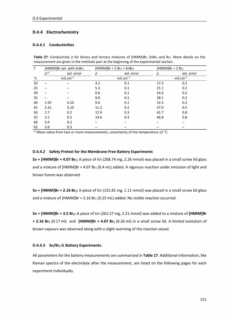
D.4 Experimental
151
Electrochemistry
D.4.4.1 Conductivities
Table 27: Conductivity σ for binary and ternary mixtures of [HMIM]Br, SnBr4 and Br2. More details on the measurement are given in the methods part at the beginning of the experimental section.
T [HMIM]Br sat. with SnBr4 [HMIM]Br + 2 Br2 + SnBr4 [HMIM]Br + 2 Br2
σ a) est. error σ est. error σ est. error °C mS cm–1 mS cm–1 mS cm–1 20 – – 4.2 0.1 17.3 0.2 25 – – 5.3 0.1 21.1 0.2 30 – – 6.6 0.1 24.0 0.2 35 – – 8.0 0.1 28.1 0.2 40 1.92 0.10 9.6 0.1 32.5 0.2 45 2.31 0.10 11.2 0.2 37.0 0.5 50 2.7 0.2 12.9 0.3 41.7 0.8 55 3.1 0.2 14.6 0.3 46.8 0.8 60 3.4 0.2 – – – – 65 3.6 0.3 – – – – a) Mean value from two or more measurements, uncertainty of the temperature ±2 °C.
D.4.4.2 Safety Pretest for the Membrane-Free Battery Experiments
Sn + [HMIM]Br + 4.07 Br2: A piece of tin (268.74 mg, 2.26 mmol) was placed in a small screw lid glass
and a mixture of [HMIM]Br + 4.07 Br2 (0.4 mL) added. A vigorous reaction under emission of light and
brown fumes was observed.
Sn + [HMIM]Br + 2.16 Br2: A piece of tin (131.81 mg, 1.11 mmol) was placed in a small screw lid glass
and a mixture of [HMIM]Br + 2.16 Br2 (0.25 mL) added. No visible reaction occurred.
Sn + [HMIM]Br + 3.5 Br2: A piece of tin (262.27 mg, 2.21 mmol) was added to a mixture of [HMIM]Br
+ 2.16 Br2 (0.17 ml) and [HMIM]Br + 4.07 Br2 (0.26 ml) in a small screw lid. A limited evolution of
brown vapours was observed along with a slight warming of the reaction vessel.
D.4.4.3 Sn/Br2 IL Battery Experiments.
All parameters for the battery measurements are summarized in Table 17. Additional information, like
Raman spectra of the electrolyte after the measurement, are listed on the following pages for each
experiment individually.
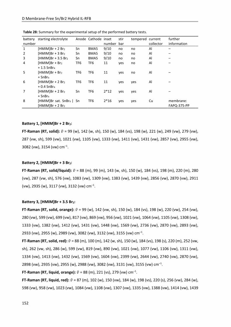
D Membrane-Free Sn/Br2 Hybrid IL-RFB
152
Table 28: Summary for the experimental setup of the performed battery tests.
battery number
starting electrolyte Anode Cathode inset number
stir bar
tempered current collector
further information
1 [HMIM]Br + 2 Br2 Sn BMA5 9/10 no no Al – 2 [HMIM]Br + 3 Br2 Sn BMA5 9/10 no no Al – 3 [HMIM]Br + 3.5 Br2 Sn BMA5 9/10 no no Al – 4 [HMIM]Br + Br2
+ 1.5 SnBr4 TF6 TF6 11 yes no Al –
5 [HMIM]Br + Br2
+ SnBr4 TF6 TF6 11 yes no Al –
6 [HMIM]Br + 2 Br2 + 0.4 SnBr4
TF6 TF6 11 yes yes Al –
7 [HMIM]Br + 2 Br2 + SnBr4
Sn TF6 2*12 yes yes Al –
8 [HMIM]Br sat. SnBr4 | [HMIM]Br + 2 Br2
Sn TF6 2*16 yes yes Cu membrane: FAPQ-375-PP
Battery 1, [HMIM]Br + 2 Br2:
FT-Raman (RT, solid): NO = 99 (w), 142 (w, sh), 150 (w), 184 (vs), 198 (w), 221 (w), 249 (vw), 279 (vw),
287 (vw, sh), 599 (vw), 1021 (vw), 1105 (vw), 1333 (vw), 1411 (vw), 1431 (vw), 2857 (vw), 2955 (vw),
3082 (vw), 3154 (vw) cm–1.
Battery 2, [HMIM]Br + 3 Br2:
FT-Raman (RT, solid/liquid): NO = 88 (m), 99 (m), 143 (w, sh), 150 (w), 184 (vs), 198 (m), 220 (m), 280
(vw), 287 (vw, sh), 576 (vw), 1083 (vw), 1309 (vw), 1383 (vw), 1439 (vw), 2856 (vw), 2870 (vw), 2911
(vw), 2935 (w), 3117 (vw), 3132 (vw) cm–1.
Battery 3, [HMIM]Br + 3.5 Br2:
FT-Raman (RT, solid, orange): NO = 99 (w), 142 (vw, sh), 150 (w), 184 (vs), 198 (w), 220 (vw), 254 (vw),
280 (vw), 599 (vw), 699 (vw), 817 (vw), 869 (vw), 956 (vw), 1021 (vw), 1064 (vw), 1105 (vw), 1308 (vw),
1333 (vw), 1382 (vw), 1412 (vw), 1431 (vw), 1448 (vw), 1569 (vw), 2736 (vw), 2870 (vw), 2893 (vw),
2933 (vw), 2955 (w), 2989 (vw), 3082 (vw), 3132 (vw), 3155 (vw) cm–1.
FT-Raman (RT, solid, red): NO = 88 (m), 100 (m), 142 (w, sh), 150 (w), 184 (vs), 198 (s), 220 (m), 252 (vw,
sh), 262 (vw, sh), 286 (w), 599 (vw), 819 (vw), 890 (vw), 1021 (vw), 1077 (vw), 1106 (vw), 1311 (vw),
1334 (vw), 1413 (vw), 1432 (vw), 1569 (vw), 1604 (vw), 2399 (vw), 2644 (vw), 2740 (vw), 2870 (vw),
2898 (vw), 2935 (vw), 2955 (w), 2988 (vw), 3082 (vw), 3131 (vw), 3155 (vw) cm–1.
FT-Raman (RT, liquid, orange): NO = 88 (m), 221 (vs), 279 (vw) cm–1.
FT-Raman (RT, liquid, red): NO = 87 (m), 102 (w), 150 (vw), 184 (w), 198 (vs), 220 (s), 256 (vw), 284 (w),
598 (vw), 958 (vw), 1023 (vw), 1084 (vw), 1108 (vw), 1307 (vw), 1335 (vw), 1388 (vw), 1414 (vw), 1439
D.4 Experimental
153
(vw), 1569 (vw), 2859 (vw), 2870 (vw), 2897 (vw), 2932 (vw), 2955 (vw), 3092 (vw), 3116 (vw), 3157
(vw) cm–1.
Battery 4, [HMIM]Br + Br2 + 1.5 SnBr4:
Disassembling: graphite corroded on one side, slimy substance at bottom of cell, liquid on top.
FT-Raman (RT, liquid) NO = 71 (vw), 88 (m), 221 (vs), 279 (vw), 313 (vw) cm–1.
FT-Raman (RT, solid/liquid mixture, red-brown,) NO = 99 (s), 142 (w, sh), 150 (w), 150 (w), 184 (vs), 198
(m), 278 (vs), 599 (vw), 816 (vw), 1021 (vw), 1106 (vw), 1334 (vw), 1382 (vw), 1413 (vw), 1413 (vw),
1448 (vw), 1567 (vw), 2829 (vw), 2857 (vw), 2898 (vw), 2933 (vw), 2954 (vw), 3081 (vw), 3131 (vw),
3156 (vw) cm–1.
Battery 5, [HMIM]Br + Br2 + SnBr4:
Disassembling: Small amount of solid at screw, otherwise completely liquid. No major change at
graphite electrodes.
FT-Raman (RT, liquid) NO = 86 (vs, sh), 102 (vw), 150 (vw), 183 (s), 198 (vw), 220 (vw), 248 (s, sh), 258
(vw), 285 (vw) cm–1.
Battery 6, [HMIM]Br + 2 Br2 + 0.4 SnBr4:
FT-Raman (RT, solid) NO = 98 (m), 141 (w, sh), 150 (m, sh), 161 (m), 183 (vs), 183 (vs), 197 (m), 261 (s),
599 (vw), 1020 (vw), 1105 (vw), 1313 (vw), 1335 (vw), 1374 (vw), 1388 (vw), 1413 (vw), 2821 (vw),
2870 (w), 2897 (w), 2910 (w), 2918 (w), 2935 (w), 2955 (w), 2989 (vw), 3117 (w), 3152 (w) cm–1.
FT-Raman (RT, liquid) NO = 99 (m), 144 (w), 183 (w), 198 (m), 221 (m), 276 (vs), 1023 (vw), 1374 (vw),
1415 (vw), 2869 (vw), 2897 (vw), 2915 (vw), 2932 (vw), 2955 (vw) cm–1.
Battery 7, [HMIM]Br + 2 Br2 + SnBr4:
FT-Raman (RT, solid, yellow): NO = 90 (vs, sh), 99 (vs), 142 (vs), 146 (vs, sh), 165 (w), 184 (s), 198 (w),
220 (vw), 251 (vw), 279 (vw), 599 (vw), 1021 (vw), 1107 (vw), 1278 (vw), 1301 (vw), 1332 (vw), 1383
(vw), 1413 (vw), 1441 (vw), 2856 (vw), 2870 (vw), 2894 (vw), 2930 (vw), 2954 (vw), 2990 (vw) cm–1.
FT-Raman (RT, solid, grey): NO = 87 (vs), 140 (s), 221 (w) cm–1.
Battery 8, Catholyte [HMIM]Br + 2 Br2, Anolyte [HMIM]Br saturated with SnBr4:
FT-Raman (RT, liquid, red, catholyte): NO = 100 (w, sh), 161 (w), 214 (w, sh), 264 (vs), 1024 (vw), 1340
(vw), 1414 (vw), 2868 (vw), 2932 (vw), 2954 (vw) cm–1.

D Membrane-Free Sn/Br2 Hybrid IL-RFB
154
FT-Raman (RT, liquid, yellow, anolyte): NO = 88 (s), 149 (w), 184 (vs), 200 (vw, sh), 221 (vs), 279 (vw),
599 (vw), 1021 (vw), 1106 (vw), 1333 (vw), 1382 (vw), 1412 (vw), 1433 (vw), 2870 (vw), 2891 (vw),
2933 (vw), 2954 (vw), 3081 (vw), 3133 (vw), 3155 (vw) cm–1.
FT-Raman (RT, solid, yellow, anode): NO = 92 (vs, sh), 99 (vs), 142 (vs), 149 (s, sh), 167 (w, sh), 185 (vs),
198 (m), 221 (w), 251 (vw), 279 (vw), 463 (vw), 494 (vw), 1022 (vw), 1038 (vw), 1059 (vw), 1107 (vw),
1311 (vw), 1335 (vw), 1382 (vw), 1412 (vw), 1429 (vw), 2738 (vw), 2826 (vw), 2869 (vw), 2891 (vw),
2931 (vw), 2955 (vw), 3086 (vw), 3121 (vw), 3155 (vw) cm–1.
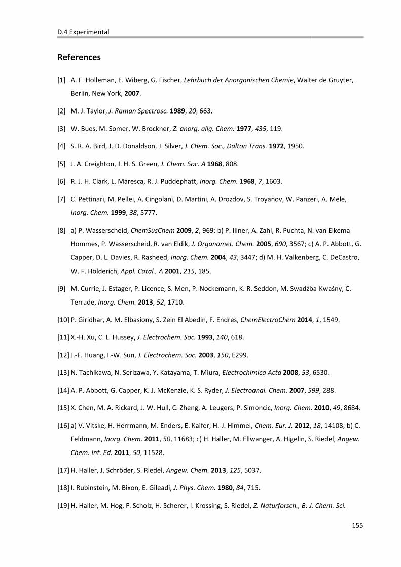
D.4 Experimental
155
References
[1] A. F. Holleman, E. Wiberg, G. Fischer, Lehrbuch der Anorganischen Chemie, Walter de Gruyter,
Berlin, New York, 2007.
[2] M. J. Taylor, J. Raman Spectrosc. 1989, 20, 663.
[3] W. Bues, M. Somer, W. Brockner, Z. anorg. allg. Chem. 1977, 435, 119.
[4] S. R. A. Bird, J. D. Donaldson, J. Silver, J. Chem. Soc., Dalton Trans. 1972, 1950.
[5] J. A. Creighton, J. H. S. Green, J. Chem. Soc. A 1968, 808.
[6] R. J. H. Clark, L. Maresca, R. J. Puddephatt, Inorg. Chem. 1968, 7, 1603.
[7] C. Pettinari, M. Pellei, A. Cingolani, D. Martini, A. Drozdov, S. Troyanov, W. Panzeri, A. Mele,
Inorg. Chem. 1999, 38, 5777.
[8] a) P. Wasserscheid, ChemSusChem 2009, 2, 969; b) P. Illner, A. Zahl, R. Puchta, N. van Eikema
Hommes, P. Wasserscheid, R. van Eldik, J. Organomet. Chem. 2005, 690, 3567; c) A. P. Abbott, G.
Capper, D. L. Davies, R. Rasheed, Inorg. Chem. 2004, 43, 3447; d) M. H. Valkenberg, C. DeCastro,
W. F. Hölderich, Appl. Catal., A 2001, 215, 185.
[9] M. Currie, J. Estager, P. Licence, S. Men, P. Nockemann, K. R. Seddon, M. Swadźba-Kwaśny, C.
Terrade, Inorg. Chem. 2013, 52, 1710.
[10] P. Giridhar, A. M. Elbasiony, S. Zein El Abedin, F. Endres, ChemElectroChem 2014, 1, 1549.
[11] X.-H. Xu, C. L. Hussey, J. Electrochem. Soc. 1993, 140, 618.
[12] J.-F. Huang, I.-W. Sun, J. Electrochem. Soc. 2003, 150, E299.
[13] N. Tachikawa, N. Serizawa, Y. Katayama, T. Miura, Electrochimica Acta 2008, 53, 6530.
[14] A. P. Abbott, G. Capper, K. J. McKenzie, K. S. Ryder, J. Electroanal. Chem. 2007, 599, 288.
[15] X. Chen, M. A. Rickard, J. W. Hull, C. Zheng, A. Leugers, P. Simoncic, Inorg. Chem. 2010, 49, 8684.
[16] a) V. Vitske, H. Herrmann, M. Enders, E. Kaifer, H.-J. Himmel, Chem. Eur. J. 2012, 18, 14108; b) C.
Feldmann, Inorg. Chem. 2011, 50, 11683; c) H. Haller, M. Ellwanger, A. Higelin, S. Riedel, Angew.
Chem. Int. Ed. 2011, 50, 11528.
[17] H. Haller, J. Schröder, S. Riedel, Angew. Chem. 2013, 125, 5037.
[18] I. Rubinstein, M. Bixon, E. Gileadi, J. Phys. Chem. 1980, 84, 715.
[19] H. Haller, M. Hog, F. Scholz, H. Scherer, I. Krossing, S. Riedel, Z. Naturforsch., B: J. Chem. Sci.

D Membrane-Free Sn/Br2 Hybrid IL-RFB
156
2013, 68b, 1103.
[20] J. O. Besenhard (Ed.) Handbook of Battery Materials, Wiley-VCH, 2011.
[21] D. Park, J. Chang, Electroanalysis 2016, 28, 1356.
[22] J. Lee, B. Krüner, A. Tolosa, S. Sathyamoorthi, D. Kim, S. Choudhury, K.-H. Seo, V. Presser, Energy
Environ. Sci. 2016, 9, 3392.
[23] a) T. Okuda, M. Nakao, M. Kawase, H. Terao, K. Yamada, J. Mol. Struct. 1995, 345, 181; b) K. B.
Dillon, J. Halfpenny, A. Marshall, J. Chem. Soc., Dalton Trans. 1983, 1091.
[24] T. Shimanouchi in NIST Standard Reference Database (Ed.: P. J. Linstrom), National Institute of
Standards and Technology, Gaithersburg MD, 20899.
[25] R. Lungwitz, S. Spange, ChemPhysChem 2012, 13, 1910.
[26] Q. Xu, T. S. Zhao, C. Zhang, Appl. Energy 2014, 130, 139.
[27] D. R. Lide, CRC Handbook of Chemistry and Physics, 84th Edition, Cleveland, Ohio, 2003.
[28] H. D. B. Jenkins, H. K. Roobottom, J. Passmore, L. Glasser, Inorg. Chem. 1999, 38, 3609.
[29] W. E. Acree, JR., J. S. Chickos in NIST Standard Reference Database (Ed.: P. J. Linstrom), National
Institute of Standards and Technology, Gaithersburg MD, 20899.
[30] H. Haller, J. Schröder, S. Riedel, Angew. Chem. Int. Ed. 2013, 52, 4937.
[31] M. Hog, Dissertation, University of Freiburg, Freiburg im Breisgau, 2017.
[32] H. Haller, Albert-Ludwigs-Universität Freiburg, Freiburg, 2014.
[33] F. Endres, D. MacFarlane, A. Abbott, Electrodeposition from Ionic Liquids, Wiley-VCH, 2008.
[34] a) SADABS, Bruker AXS Inc., Madinson, Wisconsin, USA; b) SAINT, Bruker AXS Inc., Madinson,
Wisconsin, USA.
[35] G. M. Sheldrick, Acta Crystallogr., Sect. A: Found. Crystallogr. 2015, 71, 3.
[36] G. M. Sheldrick, Acta Crystallogr., Sect. A: Found. Crystallogr. 2008, 64, 112.
[37] C. B. Hübschle, G. M. Sheldrick, B. Dittrich, J. Appl. Crystallogr. 2011, 44, 1281.
[38] L. J. Farrugia, J. Appl. Crystallogr. 2012, 45, 849.
[39] TURBOMOLE V6.4, TURBOMOLE GmbH, 2012.
[40] R. Ahlrichs, M. Bär, M. Häser, H. Horn, C. Kölmel, Chem. Phys. Lett. 1989, 162, 165.
[41] TURBOMOLE V7.1, TURBOMOLE GmbH, 2016.

D.4 Experimental
157
[42] K. Eichkorn, O. Treutler, H. Öhm, M. Häser, R. Ahlrichs, Chem. Phys. Lett. 1995, 240, 283.
[43] K. Eichkorn, F. Weigend, O. Treutler, R. Ahlrichs, Theor. Chem. Acc. 1997, 97, 119.
[44] a) F. Weigend, M. Häser, Theor. Chem. Acc. 1997, 97, 331; b) F. Weigend, M. Häser, H. Patzelt, R.
Ahlrichs, Chem. Phys. Lett. 1998, 294, 143.
[45] P. Deglmann, K. May, F. Furche, R. Ahlrichs, Chem. Phys. Lett. 2004, 384, 103.
[46] F. Weigend, R. Ahlrichs, Phys. Chem. Chem. Phys. 2005, 7, 3297.
[47] A. F. Kapustinskii, Q. Rev. Chem. Soc. 1956, 10, 283.
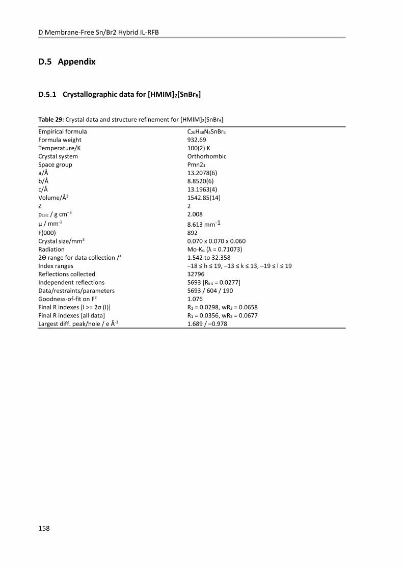
D Membrane-Free Sn/Br2 Hybrid IL-RFB
158
D.5 Appendix
Crystallographic data for [HMIM]2[SnBr6]
Table 29: Crystal data and structure refinement for [HMIM]2[SnBr6]
Empirical formula C20H38N4SnBr6 Formula weight 932.69 Temperature/K 100(2) K Crystal system Orthorhombic Space group Pmn21 a/Å 13.2078(6) b/Å 8.8520(6) c/Å 13.1963(4) Volume/Å3 1542.85(14) Z 2 ρcalc / g cm–3 2.008
μ / mm-1 8.613 mm-1 F(000) 892 Crystal size/mm3 0.070 x 0.070 x 0.060 Radiation Mo-Kα (λ = 0.71073) 2Θ range for data collection /° 1.542 to 32.358 Index ranges –18 ≤ h ≤ 19, –13 ≤ k ≤ 13, –19 ≤ l ≤ 19 Reflections collected 32796 Independent reflections 5693 [Rint = 0.0277] Data/restraints/parameters 5693 / 604 / 190 Goodness-of-fit on F2 1.076 Final R indexes [I >= 2σ (I)] R1 = 0.0298, wR2 = 0.0658 Final R indexes [all data] R1 = 0.0356, wR2 = 0.0677 Largest diff. peak/hole / e Å-3 1.689 / –0.978
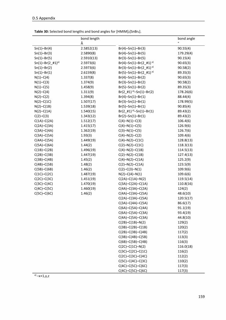
D.5 Appendix
159
Table 30: Selected bond lengths and bond angles for [HMIM]2[SnBr6].
bond length bond angle Å °
Sn(1)–Br(4) 2.5852(13) Br(4)–Sn(1)–Br(3) 90.55(4) Sn(1)–Br(3) 2.5890(8) Br(4)–Sn(1)–Br(5) 179.29(4) Sn(1)–Br(5) 2.5910(13) Br(3)–Sn(1)–Br(5) 90.15(4) Sn(1)–Br(2_#1)a) 2.5973(6) Br(4)–Sn(1)–Br(2_#1) a) 90.65(3) Sn(1)–Br(2) 2.5973(6) Br(3)–Sn(1)–Br(2_#1) a) 90.58(2) Sn(1)–Br(1) 2.6159(8) Br(5)–Sn(1)–Br(2_#1) a) 89.35(3) N(1)–C(4) 1.337(8) Br(4)–Sn(1)–Br(2) 90.65(3) N(1)–C(3) 1.374(9) Br(3)–Sn(1)–Br(2) 90.58(2) N(1)–C(5) 1.458(9) Br(5)–Sn(1)–Br(2) 89.35(3) N(2)–C(4) 1.311(9) Br(2_#1) a)–Sn(1)–Br(2) 178.26(6) N(2)–C(2) 1.394(8) Br(4)–Sn(1)–Br(1) 88.44(4) N(2)–C(1C) 1.507(17) Br(3)–Sn(1)–Br(1) 178.99(5) N(2)–C(1B) 1.539(18) Br(5)–Sn(1)–Br(1) 90.85(4) N(2)–C(1A) 1.540(15) Br(2_#1) a)–Sn(1)–Br(1) 89.43(2) C(2)–C(3) 1.343(12) Br(2)–Sn(1)–Br(1) 89.43(2) C(1A)–C(2A) 1.512(17) C(4)–N(1)–C(3) 106.4(6) C(2A)–C(3A) 1.415(17) C(4)–N(1)–C(5) 126.9(6) C(3A)–C(4A) 1.362(19) C(3)–N(1)–C(5) 126.7(6) C(3A)–C(5A) 1.93(3) C(4)–N(2)–C(2) 109.4(6) C(4A)–C(5A) 1.449(19) C(4)–N(2)–C(1C) 128.8(13) C(5A)–C(6A) 1.44(2) C(2)–N(2)–C(1C) 118.3(13) C(1B)–C(2B) 1.496(19) C(4)–N(2)–C(1B) 114.5(13) C(2B)–C(3B) 1.447(19) C(2)–N(2)–C(1B) 127.4(13) C(3B)–C(4B) 1.45(2) C(4)–N(2)–C(1A) 125.2(9) C(4B)–C(5B) 1.48(2) C(2)–N(2)–C(1A) 123.5(9) C(5B)–C(6B) 1.46(2) C(2)–C(3)–N(1) 109.9(6) C(1C)–C(2C) 1.487(19) N(2)–C(4)–N(1) 109.6(6) C(2C)–C(3C) 1.451(19) C(2A)–C(1A)–N(2) 119.5(14) C(3C)–C(4C) 1.470(19) C(3A)–C(2A)–C(1A) 110.8(16) C(4C)–C(5C) 1.460(19) C(4A)–C(3A)–C(2A) 124(2) C(5C)–C(6C) 1.46(2) C(4A)–C(3A)–C(5A) 48.6(10) C(2A)–C(3A)–C(5A) 120.5(17) C(3A)–C(4A)–C(5A) 86.6(17) C(6A)–C(5A)–C(4A) 91.1(19) C(6A)–C(5A)–C(3A) 93.4(19) C(4A)–C(5A)–C(3A) 44.8(10) C(2B)–C(1B)–N(2) 129(2) C(3B)–C(2B)–C(1B) 120(2) C(2B)–C(3B)–C(4B) 117(2) C(3B)–C(4B)–C(5B) 113(3) C(6B)–C(5B)–C(4B) 116(3) C(2C)–C(1C)–N(2) 116.0(18) C(3C)–C(2C)–C(1C) 116(2) C(2C)–C(3C)–C(4C) 112(2) C(5C)–C(4C)–C(3C) 110(2) C(4C)–C(5C)–C(6C) 117(3) C(4C)–C(5C)–C(6C) 117(3) a) –x+1,y,z
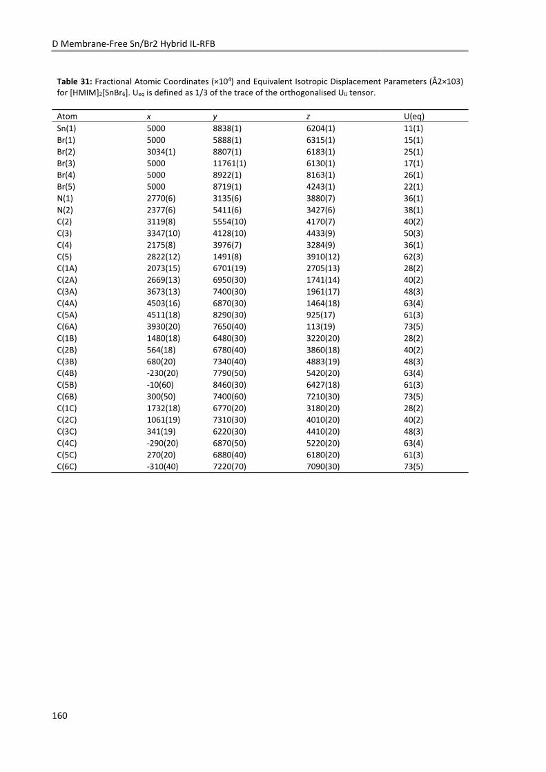
D Membrane-Free Sn/Br2 Hybrid IL-RFB
160
Table 31: Fractional Atomic Coordinates (×104) and Equivalent Isotropic Displacement Parameters (Å2×10³) for [HMIM]2[SnBr6]. Ueq is defined as 1/3 of the trace of the orthogonalised UIJ tensor.
Atom x y z U(eq)
Sn(1) 5000 8838(1) 6204(1) 11(1) Br(1) 5000 5888(1) 6315(1) 15(1) Br(2) 3034(1) 8807(1) 6183(1) 25(1) Br(3) 5000 11761(1) 6130(1) 17(1) Br(4) 5000 8922(1) 8163(1) 26(1) Br(5) 5000 8719(1) 4243(1) 22(1) N(1) 2770(6) 3135(6) 3880(7) 36(1) N(2) 2377(6) 5411(6) 3427(6) 38(1) C(2) 3119(8) 5554(10) 4170(7) 40(2) C(3) 3347(10) 4128(10) 4433(9) 50(3) C(4) 2175(8) 3976(7) 3284(9) 36(1) C(5) 2822(12) 1491(8) 3910(12) 62(3) C(1A) 2073(15) 6701(19) 2705(13) 28(2) C(2A) 2669(13) 6950(30) 1741(14) 40(2) C(3A) 3673(13) 7400(30) 1961(17) 48(3) C(4A) 4503(16) 6870(30) 1464(18) 63(4) C(5A) 4511(18) 8290(30) 925(17) 61(3) C(6A) 3930(20) 7650(40) 113(19) 73(5) C(1B) 1480(18) 6480(30) 3220(20) 28(2) C(2B) 564(18) 6780(40) 3860(18) 40(2) C(3B) 680(20) 7340(40) 4883(19) 48(3) C(4B) -230(20) 7790(50) 5420(20) 63(4) C(5B) -10(60) 8460(30) 6427(18) 61(3) C(6B) 300(50) 7400(60) 7210(30) 73(5) C(1C) 1732(18) 6770(20) 3180(20) 28(2) C(2C) 1061(19) 7310(30) 4010(20) 40(2) C(3C) 341(19) 6220(30) 4410(20) 48(3) C(4C) -290(20) 6870(50) 5220(20) 63(4) C(5C) 270(20) 6880(40) 6180(20) 61(3) C(6C) -310(40) 7220(70) 7090(30) 73(5)

E.1 Introduction
161
E Investigation Towards an All-Mn Hybrid IL-RFB
The concept for an All-Mn Hyb-IL-RFB, as described in the introduction, was developed by myself in
spring 2014 and it was subsequently included in the application for funds for the IL-RFB project. The
experiments described in the following chapter were performed by Maximilian Schmucker and are part
of his master thesis, which he conducted under my direct supervision.
The crystal structure of [NEt4]4[MnCl5][MnCl4] was solved and refined by M.Sc. Phillipe Weiss and the
simulated CVs created by Dr. Valentin Radke. pXRD measurements and analysis were carried out by
Dr. Thilo Ludwig.
E.1 Introduction
Three challenges present themselves, when trying to establish a working chemistry for an All-Mn Hyb-
IL-RFB. The first is to create liquid compounds, the second to stabilize manganese in the oxidation state
+III or +IV to be used in the catholyte, and the third, to electrodeposit elemental manganese from the
anolyte.
Chloromanganate Salts and Ionic Liquids
As has been described in the introduction to this thesis, a common type of IL is synthesized by using
[cat]X salts in conjunction with metal halides to form halometallate anions. When considering the
quest to stabilize higher oxidation states of manganese, it becomes clear that for this approach, salts
of heavier homologues to chlorine are not suitable, since even chloride is oxidized by Managnese(III)
at –40 °C.[1] Manganese(IV)fluoride is the only known binary manganese(IV) halide, however, it
decomposes at room temperature under evolution of fluorine gas.[1] Since the metal fluorides also
bear the immanent risk of releasing hydrofluoric acid by contact with humidity and organochloride
salts are much easier to obtain than the respective fluoride salts, fluoride was not considered as a
ligand for this preliminary study.
The limited stability of the binary manganese chloride salts in respect to the chlorine elimination for
oxidation states higher than +II, can be expanded when utilizing negatively charged chloromanganates.
So in a sense, the quest to obtain liquid compounds and the quest to stabilize manganese(III)/(IV)
species, can be combined and comes down to identifying suitable chloromanganate complexes – and
cations which allow their formation.
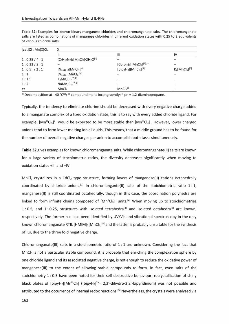
E Investigation Towards an All-Mn Hybrid IL-RFB
162
Table 32: Examples for known binary manganese chlorides and chloromanganate salts. The chloromanganate salts are listed as combinations of manganese chlorides in different oxidation states with 0.25 to 2 equivalents of various chloride salts.
[cat]Cl : Mn(X)Clx X
II III IV 1 : 0.25 / 4 : 1 (C6H10N2)2[MnCl6]∙2H2O[2] – – 1 : 0.33 / 3 : 1 – [Co(pn)3][MnCl6][3],c) – 1 : 0.5 / 2 : 1 [N1111]2[MnCl4][4] [bipyH2][MnCl5][5] K2[MnCl6][6] 1 : 1 [N1111][MnCl3][4] – – 1 : 1.5 K3Mn2Cl7[7],b) – – 1 : 2 NaMn2Cl5[7],b) – – ∞ MnCl2 MnCl3a) – a) Decomposition at –40 °C[1]; b) compound melts incongruently; c) pn = 1,2-diaminopropane.
Typically, the tendency to eliminate chlorine should be decreased with every negative charge added
to a manganate complex of a fixed oxidation state, this is to say with every added chloride ligand. For
example, [MnIIICl5]2– would be expected to be more stable than [MnIIICl4]–. However, lower charged
anions tend to form lower melting ionic liquids. This means, that a middle ground has to be found for
the number of overall negative charges per anion to accomplish both tasks simultaneously.
Table 32 gives examples for known chloromanganate salts. While chloromanganate(II) salts are known
for a large variety of stochiometric ratios, the diversity decreases significantly when moving to
oxidation states +III and +IV.
MnCl2 crystalizes in a CdCl2 type structure, forming layers of manganese(II) cations octahedrally
coordinated by chloride anions.[1] In chloromangante(II) salts of the stoichiometric ratio 1 : 1,
manganese(II) is still coordinated octahedrally, though in this case, the coordination polyhedra are
linked to form infinite chains composed of [MnIICl3]– units.[4] When moving up to stoichiometries
1 : 0.5, and 1 : 0.25, structures with isolated tetrahedra[4] and isolated octahedra[2] are known,
respectively. The former has also been identified by UV/Vis and vibrational spectroscopy in the only
known chloromanganate RTIL [HMIM]2[MnCl4][8] and the latter is probably unsuitable for the synthesis
of ILs, due to the three fold negative charge.
Chloromanganate(III) salts in a stoichiometric ratio of 1 : 1 are unknown. Considering the fact that
MnCl3 is not a particular stable compound, it is probable that enriching the complexation sphere by
one chloride ligand and its associated negative charge, is not enough to reduce the oxidative power of
manganese(III) to the extent of allowing stable compounds to form. In fact, even salts of the
stoichiometry 1 : 0.5 have been noted for their self-destructive behaviour: recrystallization of shiny
black plates of [bipyH2][MnIIICl5] ([bipyH2]2+= 2,2’-dihydro-2,2’-bipyridinium) was not possible and
attributed to the occurrence of internal redox reactions.[5] Nevertheless, the crystals were analysed via
E.1 Introduction
163
scXRD and isolated anions of quadratic pyramidal structure were identified.
Only very scarce reports exist for chloromanganate(IV) salts, even though the most investigated
compound, K2[MnCl6], has been described as early as 1899.[9] It has been characterized by vibrational
spectroscopy and pXRD.[6] Analogue compounds, like Cs2[MnCl6], Rb2[MnCl6], [NH4]2[MnCl6] and even
[NMe4]2[MnCl6] were prepared as well, but were less well characterized.[6]
A typical procedure to obtain chloromanganates both in oxidation states +III and +IV is the combination
of either Ca[MnO4]2 or K[MnO4] with a chloride salt in concentrated hydrochloric acid.[10] The following
equation was proposed for the synthesis of K2[MnIVCl6] through this route.[6]
2 K[MnVIIO4](s) + 16 HCl → K2[MnIVCl6](s) + 4 Cl2(g) + 8 H2O + Mn2+ + 2 Cl– (29)
The stabilization of chloromanganates in oxidation states higher than +II using cations typically utilized
for the synthesis of ILs has, to the best of my knowledge, not yet been attempted.
Manganese Deposition from Ionic Liquids
Despite a negative potential of –1.18 V vs. SHE, manganese can be deposited from aqueous
electrolytes.[11] In fact, it is the least noble metal to be obtained in this way on a technical scale, with
9 % of the world wide annually available manganese ore being used for the production of electrolytic
manganese.[11] However, coulombic efficiency is limited by simultaneous hydrogen evolution and
reaches values between 65 and 90 % depending on electrolyte impurities and the use of suitable
additives.[11]
Only few reports on the deposition of manganese[12,13] or manganese alloys (Al-Mn[14], Al-Mo-Mn[15],
Al-W-Mn[16], Zn-Mn[17], Cu-Mn[18]) from non-aqueous electrolytes exist. Manganese coatings were
obtained from the ILs [N1444][NTf2][17] and [BMP][NTf2][12] at a potential of approximately –2 V vs. Fc/Fc+
and coulombic efficiencies of >99 % were reported. Morphology was found to depend on the
temperature and the potential applied for the deposition, with compact spherical particles obtained
at 50 °C and a potential of –2.2 V vs. Fc/Fc+.[13] In these studies, manganese(II) ions were introduced in
the solution by anodic dissolution of elemental manganese prior to the experiment. There are no
reports on electrodeposition of manganese from chloromanganates in non-aqueous electrolytes.

E Investigation Towards an All-Mn Hybrid IL-RFB
164
Manganese and Manganese Salts in Batteries
Manganese(IV)oxide has found widespread application in primary (Zinc–carbon Battery, Alkaline
Battery, Lithium Manganese Dioxide Battery) as well as secondary batteries (Rechargeable Alkaline
Battery).[19] A lithiated derivate is found in Lithium Manganese Oxide Batteries (LiMn2O4).[19] In all of
these cases, the industrial use of manganese is helped by its low price, it’s the availability across the
globe and its low toxicity. Since the working principle of the named batteries is very different from the
envisioned All-Mn Hyb-IL-RFB, they will not be discussed in detail.
Recently, the concept of fluoride ion batteries (FIBs) has been studied by Hörmann et al.[20] In these
batteries, a metallic anode is oxidized, resulting in the formation of the respective fluoride salt. On the
cathode, a fluoride salt is reduced to elemental metal. A wide range of metals has been studied,
including a manganese anode in combination with AlF3 or TiF4 as positive active material. The batteries
were assembled in the charged state and only discharged once; charging was not possible and this
observation attributed to the formation of a fluoridic passivation layer on the anode. As one would
expect when trying to utilize aluminium or titanium salts as oxidizing agents, the OCV was only
between 0.2 and 0.4 V. Except for this report, to the best of my knowledge, there is no battery known
to date that utilizes elemental manganese or chloromanganates as their active material.
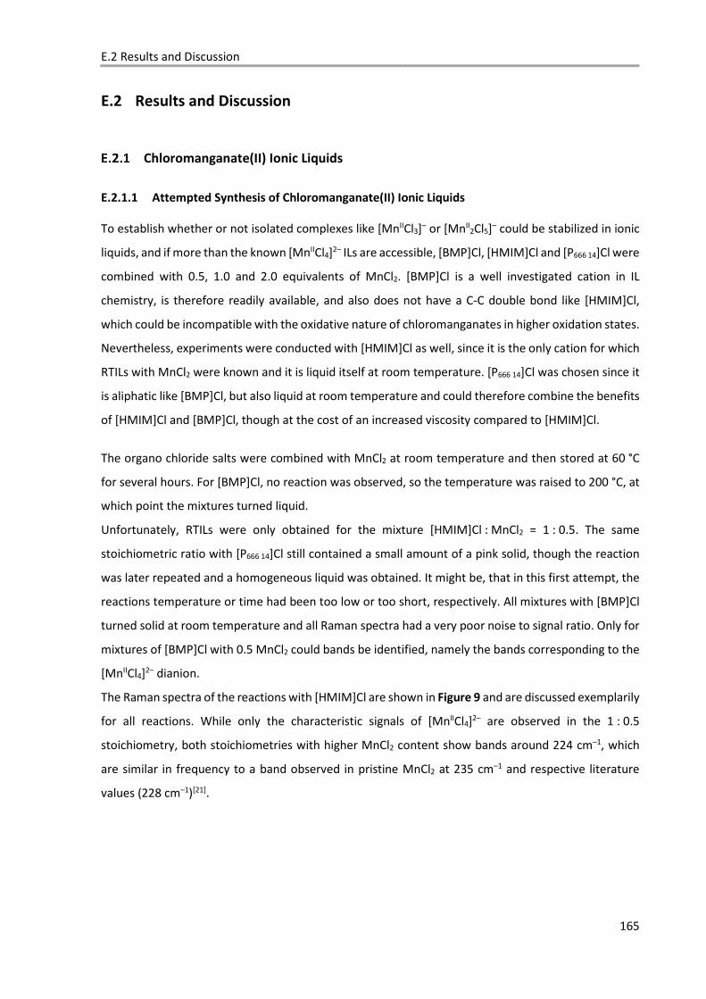
E.2 Results and Discussion
165
E.2 Results and Discussion
Chloromanganate(II) Ionic Liquids
E.2.1.1 Attempted Synthesis of Chloromanganate(II) Ionic Liquids
To establish whether or not isolated complexes like [MnIICl3]– or [MnII2Cl5]– could be stabilized in ionic
liquids, and if more than the known [MnIICl4]2– ILs are accessible, [BMP]Cl, [HMIM]Cl and [P666 14]Cl were
combined with 0.5, 1.0 and 2.0 equivalents of MnCl2. [BMP]Cl is a well investigated cation in IL
chemistry, is therefore readily available, and also does not have a C-C double bond like [HMIM]Cl,
which could be incompatible with the oxidative nature of chloromanganates in higher oxidation states.
Nevertheless, experiments were conducted with [HMIM]Cl as well, since it is the only cation for which
RTILs with MnCl2 were known and it is liquid itself at room temperature. [P666 14]Cl was chosen since it
is aliphatic like [BMP]Cl, but also liquid at room temperature and could therefore combine the benefits
of [HMIM]Cl and [BMP]Cl, though at the cost of an increased viscosity compared to [HMIM]Cl.
The organo chloride salts were combined with MnCl2 at room temperature and then stored at 60 °C
for several hours. For [BMP]Cl, no reaction was observed, so the temperature was raised to 200 °C, at
which point the mixtures turned liquid.
Unfortunately, RTILs were only obtained for the mixture [HMIM]Cl : MnCl2 = 1 : 0.5. The same
stoichiometric ratio with [P666 14]Cl still contained a small amount of a pink solid, though the reaction
was later repeated and a homogeneous liquid was obtained. It might be, that in this first attempt, the
reactions temperature or time had been too low or too short, respectively. All mixtures with [BMP]Cl
turned solid at room temperature and all Raman spectra had a very poor noise to signal ratio. Only for
mixtures of [BMP]Cl with 0.5 MnCl2 could bands be identified, namely the bands corresponding to the
[MnIICl4]2– dianion.
The Raman spectra of the reactions with [HMIM]Cl are shown in Figure 9 and are discussed exemplarily
for all reactions. While only the characteristic signals of [MnIICl4]2– are observed in the 1 : 0.5
stoichiometry, both stoichiometries with higher MnCl2 content show bands around 224 cm–1, which
are similar in frequency to a band observed in pristine MnCl2 at 235 cm–1 and respective literature
values (228 cm–1)[21].
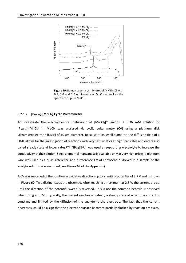
E Investigation Towards an All-Mn Hybrid IL-RFB
166
Figure 59: Raman spectra of mixtures of [HMIM]Cl with 0.5, 1.0 and 2.0 equivalents of MnCl2 as well as the spectrum of pure MnCl2.
E.2.1.2 [P666 14]2[MnCl4] Cyclic Voltammetry
To investigate the electrochemical behaviour of [MnIICl4]2– anions, a 3.36 mM solution of
[P666 14]2[MnCl4] in MeCN was analysed via cyclic voltammetry (CV) using a platinum disk
Ultramicroelectrode (UME) of 10 µm diameter. Because of its small diameter, the diffusion field of a
UME allows for the investigation of reactions with very fast kinetics at high scan rates and enters a so
called steady state at lower rates.[22] [NBu4][BF4] was used as supporting electrolyte to increase the
conductivity of the solution. Since elemental manganese is available only at very high prices, a platinum
wire was used as a quasi-reference and a reference CV of Ferrocene dissolved in a sample of the
analyte solution was recorded (see Figure 69 of the Appendix).
A CV was recorded of the solution in oxidative direction up to a limiting potential of 2.7 V and is shown
in Figure 60. Two distinct steps are observed. After reaching a maximum at 2.3 V, the current drops,
until the direction of the potential sweep is reversed. This is not the common behaviour observed
when using an UME. Typically, the current reaches a plateau, a steady state at which the current is
constant and limited by the diffusion of the analyte to the electrode. The fact that the current
decreases, could be a sign that the electrode surface becomes partially blocked by reaction products.
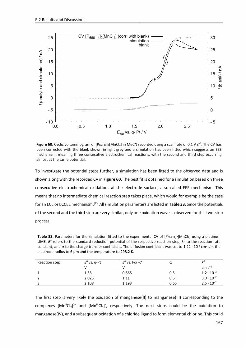
E.2 Results and Discussion
167
Figure 60: Cyclic voltammogram of [P666 14]2[MnCl4] in MeCN recorded using a scan rate of 0.1 V s–1. The CV has been corrected with the blank shown in light grey and a simulation has been fitted which suggests an EEE mechanism, meaning three consecutive electrochemical reactions, with the second and third step occurring almost at the same potential.
To investigate the potential steps further, a simulation has been fitted to the observed data and is
shown along with the recorded CV in Figure 60. The best fit is obtained for a simulation based on three
consecutive electrochemical oxidations at the electrode surface, a so called EEE mechanism. This
means that no intermediate chemical reaction step takes place, which would for example be the case
for an ECE or ECCEE mechanism.[23] All simulation parameters are listed in Table 33. Since the potentials
of the second and the third step are very similar, only one oxidation wave is observed for this two-step
process.
Table 33: Parameters for the simulation fitted to the experimental CV of [P666 14]2[MnCl4] using a platinum UME. E0 refers to the standard reduction potential of the respective reaction step, k0 to the reaction rate constant, and α to the charge transfer coefficient. The diffusion coefficient was set to 1.22 ∙ 10-5 cm2 s–1, the electrode radius to 6 µm and the temperature to 298.2 K.
Reaction step E0 vs. q-Pt E0 vs. Fc/Fc+ α k0 V V cm s–1
1 1.58 0.665 0.5 1.2 ∙ 10–3 2 2.025 1.11 0.6 3.0 ∙ 10–2 3 2.108 1.193 0.65 2.5 ∙ 10–2
The first step is very likely the oxidation of manganese(II) to manganese(III) corresponding to the
complexes [MnIICl4]2– and [MnIIICl4]–, respectively. The next steps could be the oxidation to
manganese(IV), and a subsequent oxidation of a chloride ligand to form elemental chlorine. This could
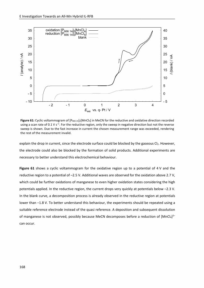
E Investigation Towards an All-Mn Hybrid IL-RFB
168
Figure 61: Cyclic voltammogram of [P666 14]2[MnCl4] in MeCN for the reductive and oxidative direction recorded using a scan rate of 0.1 V s–1. For the reductive region, only the sweep in negative direction but not the reverse sweep is shown. Due to the fast increase in current the chosen measurement range was exceeded, rendering the rest of the measurement invalid.
explain the drop in current, since the electrode surface could be blocked by the gaseous Cl2. However,
the electrode could also be blocked by the formation of solid products. Additional experiments are
necessary to better understand this electrochemical behaviour.
Figure 61 shows a cyclic voltammogram for the oxidative region up to a potential of 4 V and the
reductive region to a potential of –2.5 V. Additional waves are observed for the oxidation above 2.7 V,
which could be further oxidations of manganese to even higher oxidation states considering the high
potentials applied. In the reductive region, the current drops very quickly at potentials below –2.3 V.
In the blank curve, a decomposition process is already observed in the reductive region at potentials
lower than –1.8 V. To better understand this behaviour, the experiments should be repeated using a
suitable reference electrode instead of the quasi reference. A deposition and subsequent dissolution
of manganese is not observed, possibly because MeCN decomposes before a reduction of [MnCl4]2–
can occur.
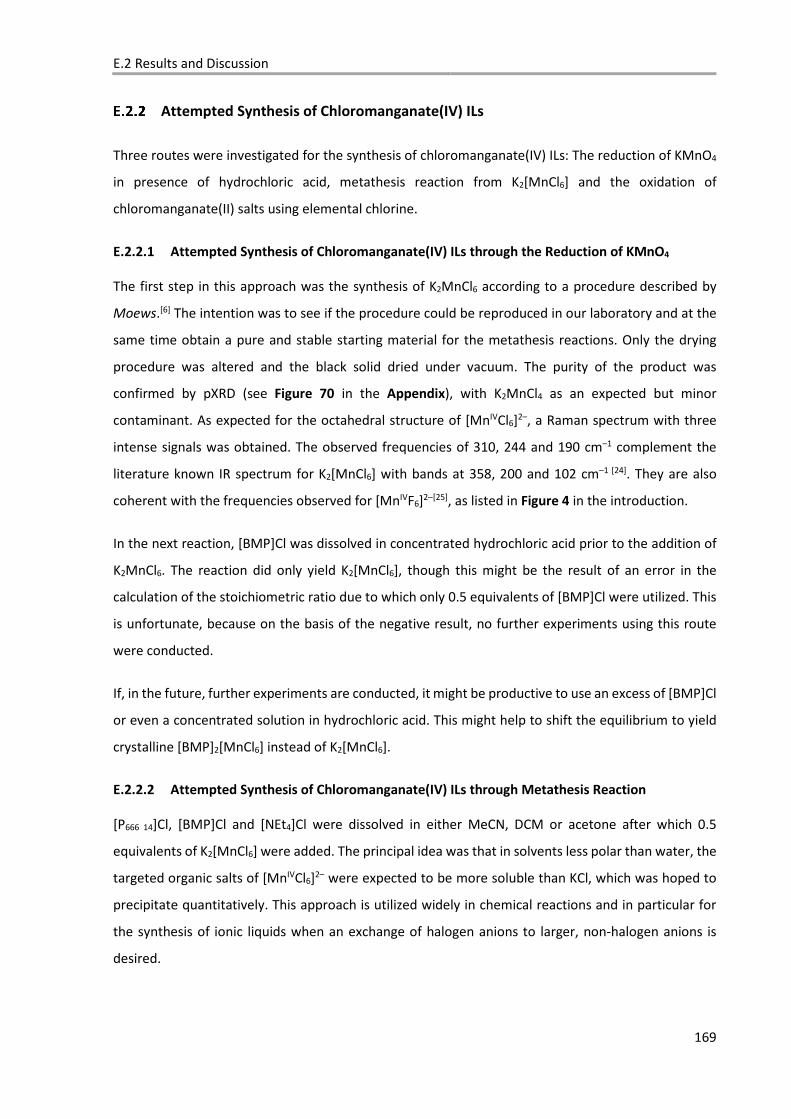
E.2 Results and Discussion
169
Attempted Synthesis of Chloromanganate(IV) ILs
Three routes were investigated for the synthesis of chloromanganate(IV) ILs: The reduction of KMnO4
in presence of hydrochloric acid, metathesis reaction from K2[MnCl6] and the oxidation of
chloromanganate(II) salts using elemental chlorine.
E.2.2.1 Attempted Synthesis of Chloromanganate(IV) ILs through the Reduction of KMnO4
The first step in this approach was the synthesis of K2MnCl6 according to a procedure described by
Moews.[6] The intention was to see if the procedure could be reproduced in our laboratory and at the
same time obtain a pure and stable starting material for the metathesis reactions. Only the drying
procedure was altered and the black solid dried under vacuum. The purity of the product was
confirmed by pXRD (see Figure 70 in the Appendix), with K2MnCl4 as an expected but minor
contaminant. As expected for the octahedral structure of [MnIVCl6]2–, a Raman spectrum with three
intense signals was obtained. The observed frequencies of 310, 244 and 190 cm–1 complement the
literature known IR spectrum for K2[MnCl6] with bands at 358, 200 and 102 cm–1 [24]. They are also
coherent with the frequencies observed for [MnIVF6]2–[25], as listed in Figure 4 in the introduction.
In the next reaction, [BMP]Cl was dissolved in concentrated hydrochloric acid prior to the addition of
K2MnCl6. The reaction did only yield K2[MnCl6], though this might be the result of an error in the
calculation of the stoichiometric ratio due to which only 0.5 equivalents of [BMP]Cl were utilized. This
is unfortunate, because on the basis of the negative result, no further experiments using this route
were conducted.
If, in the future, further experiments are conducted, it might be productive to use an excess of [BMP]Cl
or even a concentrated solution in hydrochloric acid. This might help to shift the equilibrium to yield
crystalline [BMP]2[MnCl6] instead of K2[MnCl6].
E.2.2.2 Attempted Synthesis of Chloromanganate(IV) ILs through Metathesis Reaction
[P666 14]Cl, [BMP]Cl and [NEt4]Cl were dissolved in either MeCN, DCM or acetone after which 0.5
equivalents of K2[MnCl6] were added. The principal idea was that in solvents less polar than water, the
targeted organic salts of [MnIVCl6]2– were expected to be more soluble than KCl, which was hoped to
precipitate quantitatively. This approach is utilized widely in chemical reactions and in particular for
the synthesis of ionic liquids when an exchange of halogen anions to larger, non-halogen anions is
desired.
E Investigation Towards an All-Mn Hybrid IL-RFB
170
a) b)
Figure 62: Crystal structure of [NEt4]4[MnCl4][MnCl5] with hydrogen atoms omitted for clarity and thermal ellipsoids at 50 % probability. a) Constituent ions, [NEt4]+ disordered over two positions, symmetry equivalent chlorine atoms are not labelled separately. b) Unit cell viewed in a direction showing the layered structure of the two different anions and cations.
Though the general principle does seem to work, the products obtained were either chloromanganates
in the oxidation state +III or +II or mixtures thereof. [MnIIICl5]2– ions could be identified in green solids
and solutions through their literature known[3] and intense Raman band at around 290 cm–1, though
the targeted [MnIVCl6]2– salts stayed elusive. Details on the results of the reactions are included in the
experimental part, but since no pure product was obtained through any of the routes, the results will
not be discussed in detail here.
Concluding from these results, it seems that the [MnIVCl6]2– anion is not stable in solution. One step in
the decomposition process was captured in the obtained crystal structure of [NEt4]4[MnCl4][MnCl5]. A
section of the crystal structure and the unit cell are shown in Figure 62, while more crystallographic
details are given in the Appendix. The structure includes tetrahedral and square pyramidal
chloromanganates in the oxidation states +II and +III respectively. The Mn–Cl bond lengths are
234.58(8) pm for manganese(II) whereas the chlorine atom at the tip and the atoms at the base of the
square pyramid are located at a distance of 240.3(2) pm and 229.77(9) pm from the central
manganese(III). These values are in the expected range compared to other salts of these anions.[26][5]
The [MnIICl4]2– tetrahedron is slightly distorted along the twofold axes in c direction with Cl–Mn–Cl
opening angles in this direction of 112.08(4)°. [MnIIICl5]2– shows Cl–Mn–Cl angles of 88.17(1)° between
the four symmetry equivalent chlorine atoms and of 100.28(4) to the chlorine atom located on the 4-
fold axis. The different types of anions form separate layers interspersed with a cationic layers in c
direction.
E.2 Results and Discussion
171
Since no stable products were obtained utilizing 0.5 equivalents of K2[MnCl6] and salts containing the
anion [MnIVCl5]– are expected to be even less stable, no reactions using one equivalent of K2[MnCl6]
were carried out.
E.2.2.3 Attempted Synthesis of [NEt4]2[MnCl6] Through the Oxidation of [NEt4]2[MnCl4]
The final attempt to stabilize an organic salt of [MnIVCl6]2– was the oxidation of [Net4]2[MnCl4] with
elemental chlorine. The [NEt4]+ cation was chosen, since the conclusion from the results obtained up
to this point suggested, that the [MnIVCl6]2– anion would most likely only be stable in the solid state,
and crystallisation is facilitated by using a symmetrically substituted ammonium salt. The apparatus
used is shown in Figure 18. Chlorine was not only passed through the solution, but liquefied using a
gas condenser cooled to temperatures below –40 °C and refluxed back into the solution. The
decreased temperatures and excess of chlorine were supposed to reduce the tendency of possible
products to eliminate chlorine and to shift the equilibrium towards their formation.
Unfortunately, neither chlorination in MeCN, concentrated hydrochloric acid or in pure liquid chlorine
yielded chloromanganates(IV), though, again, a green solution was obtained for the reaction in MeCN.
In a last attempt, o-DFB was added to the unchanged solid from the attempted oxidation with pure
liquid chlorine. When no visible change occurred during chlorine reflux, a small amount of MeCN was
added in the hope, that part of the salt would dissolve, and that the targeted product, [NEt4]2[MnCl6]
would precipitate. Only on heating to 50 °C under continuous chlorine reflux, a change in the solution’s
colour to dark green was observed, and on cooling to room temperature, a green solid precipitated.
The Raman spectrum shows the characteristic band of [MnIIICl5]2– at 288 cm–1, though, when measured
with a laser power of 100 mW instead of 3 mW, the additional band of [MnIICl4]2– at 258 cm–1 is
observed, and the green powder turns white at the spot of the measurement.
In conclusion, it seems possible to oxidize the [MnIICl4]2– anion to form [MnIIICl5]2– with elemental
chlorine, though the procedure still needs to be refined and the product should be analysed by pXRD
to confirm its purity. However, the oxidation to chloromanganates(IV) does not seem possible through
this route, at least not in combination with the [NEt4]+ cation.
All-Mn Hybrid Ionic Liquid Battery Tests
[P666 14]2[MnCl4] was chosen as electrolyte for a first All-Mn Hyb-IL battery test, since it seemed to be
able to stabilize chloromanganate(III) anions at least for a short period of time. A membrane-free cell
setup was chosen, since the viscosity of this specific ionic liquid was expected to limit self discharge to
a tolerable rate and in this way, any influence of the membrane chemistry could be avoided. Two inert
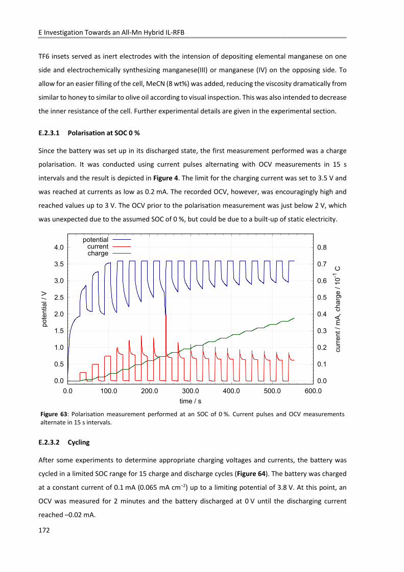
E Investigation Towards an All-Mn Hybrid IL-RFB
172
po
ten
tia
l /
V
cu
rre
nt
/ m
A,
ch
arg
e /
10
−1 C
time / s
potentialcurrentcharge
0.0
0.5
1.0
1.5
2.0
2.5
3.0
3.5
4.0
0.0 100.0 200.0 300.0 400.0 500.0 600.0
0.0
0.1
0.2
0.3
0.4
0.5
0.6
0.7
0.8
TF6 insets served as inert electrodes with the intension of depositing elemental manganese on one
side and electrochemically synthesizing manganese(III) or manganese (IV) on the opposing side. To
allow for an easier filling of the cell, MeCN (8 wt%) was added, reducing the viscosity dramatically from
similar to honey to similar to olive oil according to visual inspection. This was also intended to decrease
the inner resistance of the cell. Further experimental details are given in the experimental section.
E.2.3.1 Polarisation at SOC 0 %
Since the battery was set up in its discharged state, the first measurement performed was a charge
polarisation. It was conducted using current pulses alternating with OCV measurements in 15 s
intervals and the result is depicted in Figure 4. The limit for the charging current was set to 3.5 V and
was reached at currents as low as 0.2 mA. The recorded OCV, however, was encouragingly high and
reached values up to 3 V. The OCV prior to the polarisation measurement was just below 2 V, which
was unexpected due to the assumed SOC of 0 %, but could be due to a built-up of static electricity.
Figure 63: Polarisation measurement performed at an SOC of 0 %. Current pulses and OCV measurements alternate in 15 s intervals.
E.2.3.2 Cycling
After some experiments to determine appropriate charging voltages and currents, the battery was
cycled in a limited SOC range for 15 charge and discharge cycles (Figure 64). The battery was charged
at a constant current of 0.1 mA (0.065 mA cm–2) up to a limiting potential of 3.8 V. At this point, an
OCV was measured for 2 minutes and the battery discharged at 0 V until the discharging current
reached –0.02 mA.
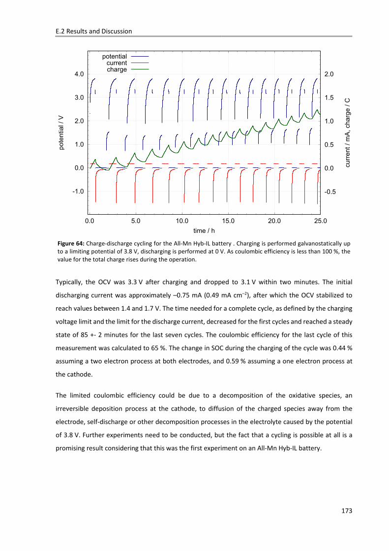
E.2 Results and Discussion
173
pote
ntial / V
curr
ent / m
A, charg
e / C
time / h
potentialcurrentcharge
−1.0
0.0
1.0
2.0
3.0
4.0
0.0 5.0 10.0 15.0 20.0 25.0
−0.5
0.0
0.5
1.0
1.5
2.0
Figure 64: Charge-discharge cycling for the All-Mn Hyb-IL battery . Charging is performed galvanostatically up to a limiting potential of 3.8 V, discharging is performed at 0 V. As coulombic efficiency is less than 100 %, the value for the total charge rises during the operation.
Typically, the OCV was 3.3 V after charging and dropped to 3.1 V within two minutes. The initial
discharging current was approximately –0.75 mA (0.49 mA cm–2), after which the OCV stabilized to
reach values between 1.4 and 1.7 V. The time needed for a complete cycle, as defined by the charging
voltage limit and the limit for the discharge current, decreased for the first cycles and reached a steady
state of 85 +- 2 minutes for the last seven cycles. The coulombic efficiency for the last cycle of this
measurement was calculated to 65 %. The change in SOC during the charging of the cycle was 0.44 %
assuming a two electron process at both electrodes, and 0.59 % assuming a one electron process at
the cathode.
The limited coulombic efficiency could be due to a decomposition of the oxidative species, an
irreversible deposition process at the cathode, to diffusion of the charged species away from the
electrode, self-discharge or other decomposition processes in the electrolyte caused by the potential
of 3.8 V. Further experiments need to be conducted, but the fact that a cycling is possible at all is a
promising result considering that this was the first experiment on an All-Mn Hyb-IL battery.
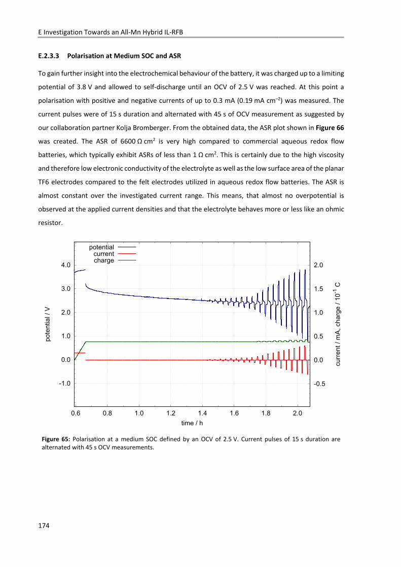
E Investigation Towards an All-Mn Hybrid IL-RFB
174
po
ten
tia
l /
V
cu
rre
nt
/ m
A,
ch
arg
e /
10
−1 C
time / h
potentialcurrentcharge
−1.0
0.0
1.0
2.0
3.0
4.0
0.6 0.8 1.0 1.2 1.4 1.6 1.8 2.0
−0.5
0.0
0.5
1.0
1.5
2.0
E.2.3.3 Polarisation at Medium SOC and ASR
To gain further insight into the electrochemical behaviour of the battery, it was charged up to a limiting
potential of 3.8 V and allowed to self-discharge until an OCV of 2.5 V was reached. At this point a
polarisation with positive and negative currents of up to 0.3 mA (0.19 mA cm–2) was measured. The
current pulses were of 15 s duration and alternated with 45 s of OCV measurement as suggested by
our collaboration partner Kolja Bromberger. From the obtained data, the ASR plot shown in Figure 66
was created. The ASR of 6600 Ω cm2 is very high compared to commercial aqueous redox flow
batteries, which typically exhibit ASRs of less than 1 Ω cm2. This is certainly due to the high viscosity
and therefore low electronic conductivity of the electrolyte as well as the low surface area of the planar
TF6 electrodes compared to the felt electrodes utilized in aqueous redox flow batteries. The ASR is
almost constant over the investigated current range. This means, that almost no overpotential is
observed at the applied current densities and that the electrolyte behaves more or less like an ohmic
resistor.
Figure 65: Polarisation at a medium SOC defined by an OCV of 2.5 V. Current pulses of 15 s duration are alternated with 45 s OCV measurements.
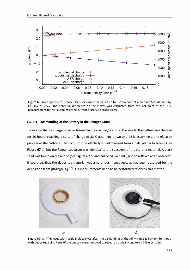
E.2 Results and Discussion
175
Figure 66: Area specific resistance (ASR) for current densities up to 0.2 mA cm–2 at a medium SOC defined by an OCV of 2.5 V. The potential difference on the y-axes was calculated from the last point of the OCV measurement to the first point of the current pulse 0.5 seconds later.
E.2.3.4 Dismantling of the Battery in the Charged State
To investigate the charged species formed in the electrolyte and on the anode, the battery was charged
for 50 hours, reaching a state of charge of 32 % assuming a two and 42 % assuming a one electron
process at the cathode. The colour of the electrolyte had changed from a pale yellow to brown (see
Figure 67 a), but the Raman spectrum was identical to the spectrum of the starting material. A black
solid was found on the anode (see Figure 67 b) and analysed via pXRD, but no reflexes were observed.
It could be, that the deposited material was amorphous manganese, as has been observed for the
deposition from [BMP][NTf2].[12] EDX measurements need to be performed to clarify this matter.
a) b)
Figure 67: a) PTFE inset with residual electrolyte after the dismantling of the All-Mn Hyb-IL battery. b) Anode with deposited solid. Parts of the deposit were removed to reveal an optically unaltered TF6 electrode.

E Investigation Towards an All-Mn Hybrid IL-RFB
176
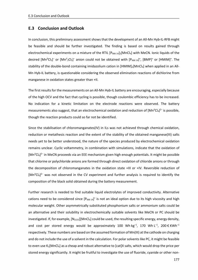
E.3 Conclusion and Outlook
177
E.3 Conclusion and Outlook
In conclusion, this preliminary assessment shows that the development of an All-Mn Hyb-IL-RFB might
be feasible and should be further investigated. The finding is based on results gained through
electrochemical experiments on a mixture of the RTIL [P666 14]2[MnCl4] with MeCN. Ionic liquids of the
desired [MnIICl3]– or [MnII2Cl5]– anion could not be obtained with [P666 14]+, [BMP]+ or [HMIM]+. The
stability of the double-bond containing imidazolium cation in [HMIM]2[MnCl4] when applied in an All-
Mn Hyb-IL battery, is questionable considering the observed elimination reactions of dichlorine from
manganese in oxidation states greater than +II.
The first results for the measurements on an All-Mn Hyb-IL battery are encouraging, especially because
of the high OCV and the fact that cycling is possible, though coulombic efficiency has to be increased.
No indication for a kinetic limitation on the electrode reactions were observed. The battery
measurements also suggest, that an electrochemical oxidation and reduction of [MnIICl4]2– is possible,
though the reaction products could so far not be identified.
Since the stabilisation of chloromanganates(IV) in ILs was not achieved through chemical oxidation,
reduction or metathesis reaction and the extent of the stability of the obtained manganese(III) salts
needs yet to be better understood, the nature of the species produced by electrochemical oxidation
remains unclear. Cyclic voltammetry, in combination with simulations, indicate that the oxidation of
[MnIICl4]2– in MeCN proceeds via an EEE mechanism given high enough potentials. It might be possible
that chlorine or polychloride anions are formed through direct oxidation of chloride anions or through
the decomposition of chloromanganates in the oxidation state +III or +IV. Reversible reduction of
[MnIICl4]2– was not observed in the CV experiment and further analysis is required to identify the
composition of the black solid obtained during the battery measurement.
Further research is needed to find suitable liquid electrolytes of improved conductivity. Alternative
cations need to be considered since [P666 14]+ is not an ideal option due to its high viscosity and high
molecular weight. Other asymmetrically substituted phosphonium salts or ammonium salts could be
an alternative and their solubility in electrochemically suitable solvents like MeCN or PC should be
investigated. If, for example, [N2225][MnCl4] could be used, the resulting specific energy, energy density,
and cost per stored energy would be approximately 100 Wh kg–1, 170 Wh L–1, 200 € KWh–1
respectively. These numbers are based on the assumed formation of Mn(III) at the cathode on charging
and do not include the use of a solvent in the calculation. For polar solvents like PC, it might be feasible
to even use K2[MnCl4] as a cheap and robust alternative to [cat]X salts, which would drop the price per
stored energy significantly. It might be fruitful to investigate the use of fluoride, cyanide or other non-

E Investigation Towards an All-Mn Hybrid IL-RFB
178
halogen ligands for the use in the All-Mn Hyb-IL-RFB since this could allow for the stabilization of
manganese(IV) complexes.
The metal deposition process needs to be studied in detail to yield reversible plating of elemental
manganese without the formation of dendrites. In this respect, the combination of [BMP]2[MnCl4] and
[BMP][NTf2] might be promising, since the electroplating of manganese from ILs containing the [NTf2]–
anion has been demonstrated with high coulombic efficiency and good morphology. An increase in
electrode surface, for example by employing graphite felts, should be considered as soon as the plating
process is optimized and better understood.
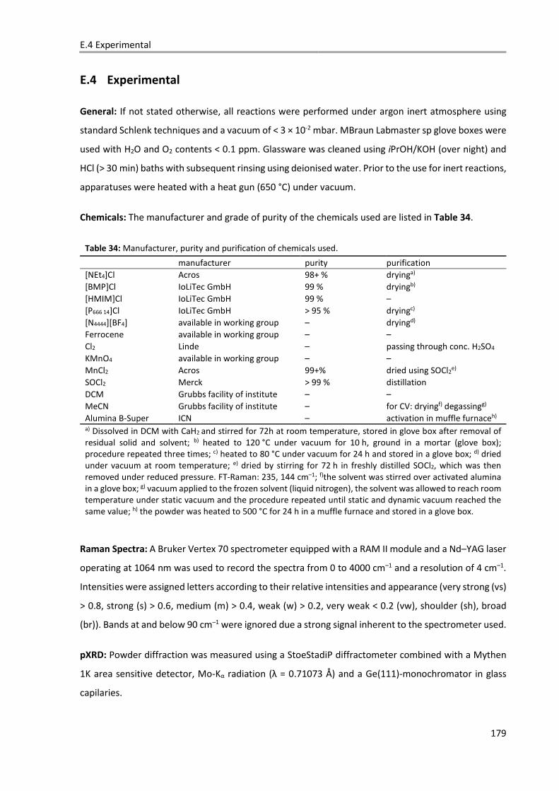
E.4 Experimental
179
E.4 Experimental
General: If not stated otherwise, all reactions were performed under argon inert atmosphere using
standard Schlenk techniques and a vacuum of < 3 × 10⁻² mbar. MBraun Labmaster sp glove boxes were
used with H2O and O2 contents < 0.1 ppm. Glassware was cleaned using iPrOH/KOH (over night) and
HCl (> 30 min) baths with subsequent rinsing using deionised water. Prior to the use for inert reactions,
apparatuses were heated with a heat gun (650 °C) under vacuum.
Chemicals: The manufacturer and grade of purity of the chemicals used are listed in Table 34.
Table 34: Manufacturer, purity and purification of chemicals used.
manufacturer purity purification [NEt4]Cl Acros 98+ % dryinga) [BMP]Cl IoLiTec GmbH 99 % dryingb) [HMIM]Cl IoLiTec GmbH 99 % – [P666 14]Cl IoLiTec GmbH > 95 % dryingc) [N4444][BF4] available in working group – dryingd) Ferrocene available in working group – – Cl2 Linde – passing through conc. H2SO4 KMnO4 available in working group – – MnCl2 Acros 99+% dried using SOCl2
e) SOCl2 Merck > 99 % distillation DCM Grubbs facility of institute – – MeCN Grubbs facility of institute – for CV: dryingf) degassingg) Alumina B-Super ICN – activation in muffle furnaceh) a) Dissolved in DCM with CaH2 and stirred for 72h at room temperature, stored in glove box after removal of residual solid and solvent; b) heated to 120 °C under vacuum for 10 h, ground in a mortar (glove box); procedure repeated three times; c) heated to 80 °C under vacuum for 24 h and stored in a glove box; d) dried under vacuum at room temperature; e) dried by stirring for 72 h in freshly distilled SOCl2, which was then removed under reduced pressure. FT-Raman: 235, 144 cm–1; f)the solvent was stirred over activated alumina in a glove box; g) vacuum applied to the frozen solvent (liquid nitrogen), the solvent was allowed to reach room temperature under static vacuum and the procedure repeated until static and dynamic vacuum reached the same value; h) the powder was heated to 500 °C for 24 h in a muffle furnace and stored in a glove box.
Raman Spectra: A Bruker Vertex 70 spectrometer equipped with a RAM II module and a Nd–YAG laser
operating at 1064 nm was used to record the spectra from 0 to 4000 cm–1 and a resolution of 4 cm–1.
Intensities were assigned letters according to their relative intensities and appearance (very strong (vs)
> 0.8, strong (s) > 0.6, medium (m) > 0.4, weak (w) > 0.2, very weak < 0.2 (vw), shoulder (sh), broad
(br)). Bands at and below 90 cm–1 were ignored due a strong signal inherent to the spectrometer used.
pXRD: Powder diffraction was measured using a StoeStadiP diffractometer combined with a Mythen
1K area sensitive detector, Mo-Kα radiation (λ = 0.71073 Å) and a Ge(111)-monochromator in glass
capilaries.
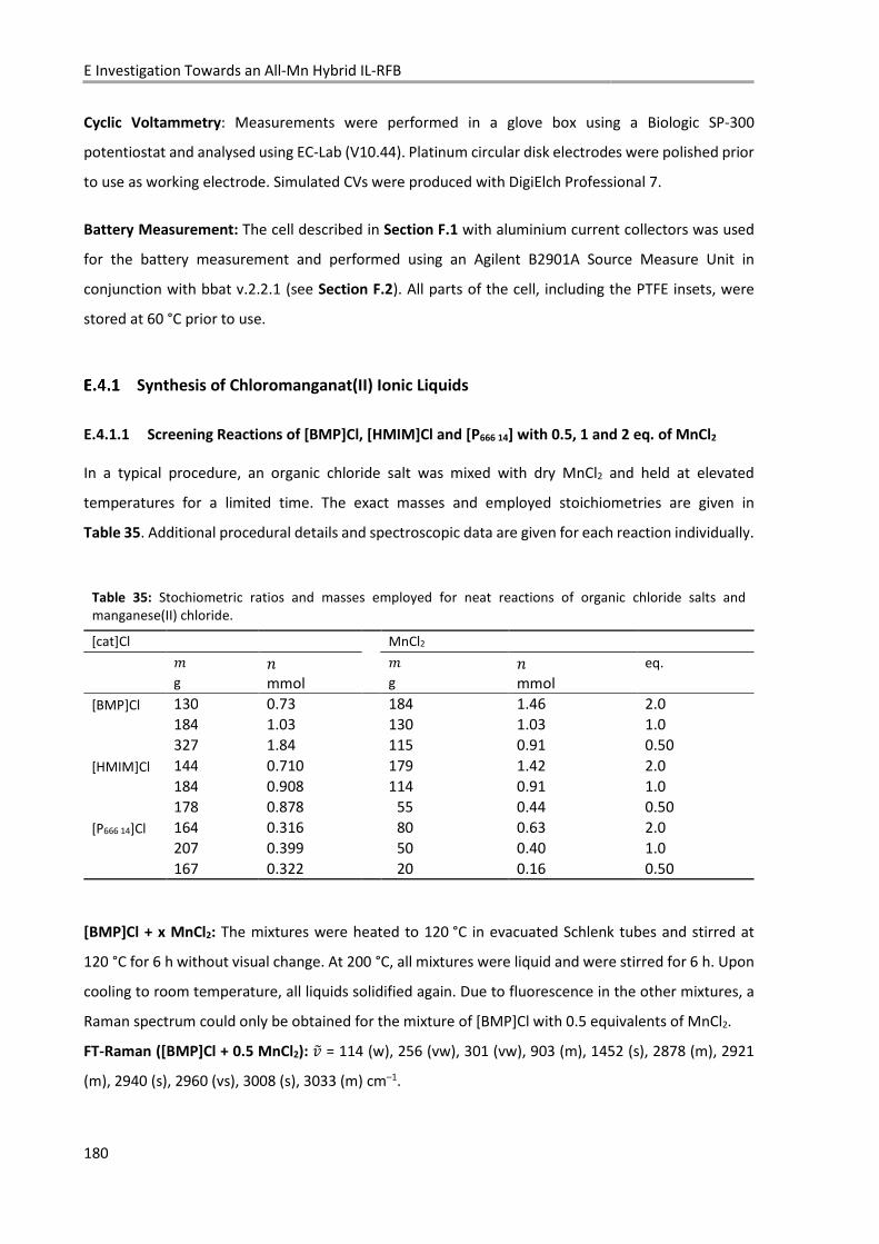
E Investigation Towards an All-Mn Hybrid IL-RFB
180
Cyclic Voltammetry: Measurements were performed in a glove box using a Biologic SP-300
potentiostat and analysed using EC-Lab (V10.44). Platinum circular disk electrodes were polished prior
to use as working electrode. Simulated CVs were produced with DigiElch Professional 7.
Battery Measurement: The cell described in Section F.1 with aluminium current collectors was used
for the battery measurement and performed using an Agilent B2901A Source Measure Unit in
conjunction with bbat v.2.2.1 (see Section F.2). All parts of the cell, including the PTFE insets, were
stored at 60 °C prior to use.
Synthesis of Chloromanganat(II) Ionic Liquids
E.4.1.1 Screening Reactions of [BMP]Cl, [HMIM]Cl and [P666 14] with 0.5, 1 and 2 eq. of MnCl2
In a typical procedure, an organic chloride salt was mixed with dry MnCl2 and held at elevated
temperatures for a limited time. The exact masses and employed stoichiometries are given in
Table 35. Additional procedural details and spectroscopic data are given for each reaction individually.
Table 35: Stochiometric ratios and masses employed for neat reactions of organic chloride salts and manganese(II) chloride.
[cat]Cl MnCl2
� � � � eq. g mmol g mmol
[BMP]Cl 130 0.73 184 1.46 2.0
184 1.03 130 1.03 1.0
327 1.84 115 0.91 0.50
[HMIM]Cl 144 0.710 179 1.42 2.0
184 0.908 114 0.91 1.0
178 0.878 055 0.44 0.50
[P666 14]Cl 164 0.316 080 0.63 2.0
207 0.399 050 0.40 1.0
167 0.322 020 0.16 0.50
[BMP]Cl + x MnCl2: The mixtures were heated to 120 °C in evacuated Schlenk tubes and stirred at
120 °C for 6 h without visual change. At 200 °C, all mixtures were liquid and were stirred for 6 h. Upon
cooling to room temperature, all liquids solidified again. Due to fluorescence in the other mixtures, a
Raman spectrum could only be obtained for the mixture of [BMP]Cl with 0.5 equivalents of MnCl2.
FT-Raman ([BMP]Cl + 0.5 MnCl2): NO = 114 (w), 256 (vw), 301 (vw), 903 (m), 1452 (s), 2878 (m), 2921
(m), 2940 (s), 2960 (vs), 3008 (s), 3033 (m) cm–1.
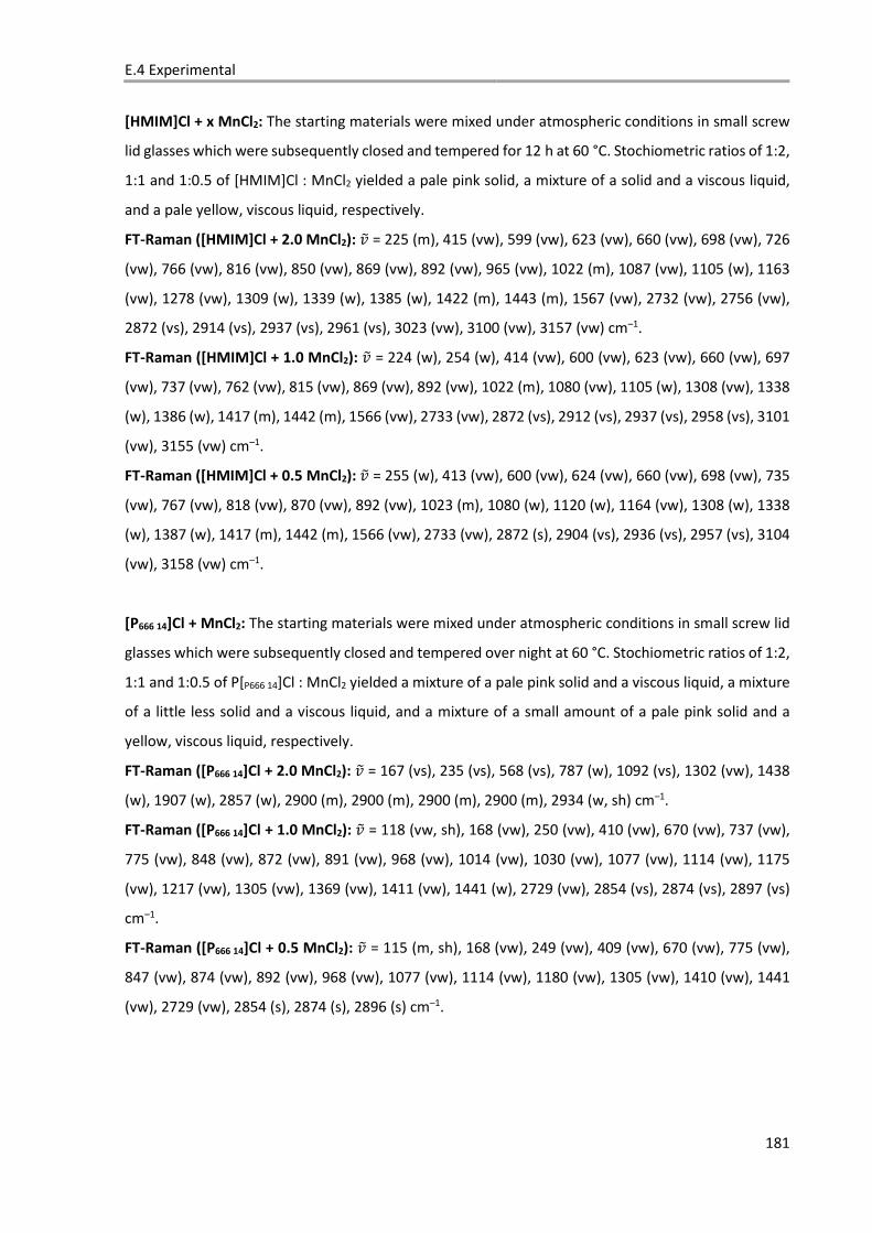
E.4 Experimental
181
[HMIM]Cl + x MnCl2: The starting materials were mixed under atmospheric conditions in small screw
lid glasses which were subsequently closed and tempered for 12 h at 60 °C. Stochiometric ratios of 1:2,
1:1 and 1:0.5 of [HMIM]Cl : MnCl2 yielded a pale pink solid, a mixture of a solid and a viscous liquid,
and a pale yellow, viscous liquid, respectively.
FT-Raman ([HMIM]Cl + 2.0 MnCl2): NO = 225 (m), 415 (vw), 599 (vw), 623 (vw), 660 (vw), 698 (vw), 726
(vw), 766 (vw), 816 (vw), 850 (vw), 869 (vw), 892 (vw), 965 (vw), 1022 (m), 1087 (vw), 1105 (w), 1163
(vw), 1278 (vw), 1309 (w), 1339 (w), 1385 (w), 1422 (m), 1443 (m), 1567 (vw), 2732 (vw), 2756 (vw),
2872 (vs), 2914 (vs), 2937 (vs), 2961 (vs), 3023 (vw), 3100 (vw), 3157 (vw) cm–1.
FT-Raman ([HMIM]Cl + 1.0 MnCl2): NO = 224 (w), 254 (w), 414 (vw), 600 (vw), 623 (vw), 660 (vw), 697
(vw), 737 (vw), 762 (vw), 815 (vw), 869 (vw), 892 (vw), 1022 (m), 1080 (vw), 1105 (w), 1308 (vw), 1338
(w), 1386 (w), 1417 (m), 1442 (m), 1566 (vw), 2733 (vw), 2872 (vs), 2912 (vs), 2937 (vs), 2958 (vs), 3101
(vw), 3155 (vw) cm–1.
FT-Raman ([HMIM]Cl + 0.5 MnCl2): NO = 255 (w), 413 (vw), 600 (vw), 624 (vw), 660 (vw), 698 (vw), 735
(vw), 767 (vw), 818 (vw), 870 (vw), 892 (vw), 1023 (m), 1080 (w), 1120 (w), 1164 (vw), 1308 (w), 1338
(w), 1387 (w), 1417 (m), 1442 (m), 1566 (vw), 2733 (vw), 2872 (s), 2904 (vs), 2936 (vs), 2957 (vs), 3104
(vw), 3158 (vw) cm–1.
[P666 14]Cl + MnCl2: The starting materials were mixed under atmospheric conditions in small screw lid
glasses which were subsequently closed and tempered over night at 60 °C. Stochiometric ratios of 1:2,
1:1 and 1:0.5 of P[P666 14]Cl : MnCl2 yielded a mixture of a pale pink solid and a viscous liquid, a mixture
of a little less solid and a viscous liquid, and a mixture of a small amount of a pale pink solid and a
yellow, viscous liquid, respectively.
FT-Raman ([P666 14]Cl + 2.0 MnCl2): NO = 167 (vs), 235 (vs), 568 (vs), 787 (w), 1092 (vs), 1302 (vw), 1438
(w), 1907 (w), 2857 (w), 2900 (m), 2900 (m), 2900 (m), 2900 (m), 2934 (w, sh) cm–1.
FT-Raman ([P666 14]Cl + 1.0 MnCl2): NO = 118 (vw, sh), 168 (vw), 250 (vw), 410 (vw), 670 (vw), 737 (vw),
775 (vw), 848 (vw), 872 (vw), 891 (vw), 968 (vw), 1014 (vw), 1030 (vw), 1077 (vw), 1114 (vw), 1175
(vw), 1217 (vw), 1305 (vw), 1369 (vw), 1411 (vw), 1441 (w), 2729 (vw), 2854 (vs), 2874 (vs), 2897 (vs)
cm–1.
FT-Raman ([P666 14]Cl + 0.5 MnCl2): NO = 115 (m, sh), 168 (vw), 249 (vw), 409 (vw), 670 (vw), 775 (vw),
847 (vw), 874 (vw), 892 (vw), 968 (vw), 1077 (vw), 1114 (vw), 1180 (vw), 1305 (vw), 1410 (vw), 1441
(vw), 2729 (vw), 2854 (s), 2874 (s), 2896 (s) cm–1.
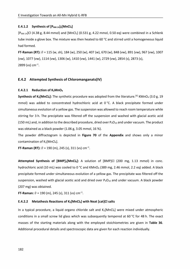
E Investigation Towards an All-Mn Hybrid IL-RFB
182
E.4.1.2 Synthesis of [P666 14]2[MnCl4]
[P666 14]Cl (4.38 g, 8.44 mmol) and [MnCl2] (0.531 g, 4.22 mmol, 0.50 eq) were combined in a Schlenk
tube inside a glove box. The mixture was then heated to 60 °C and stirred until a homogeneous liquid
had formed.
FT-Raman (RT): NO = 115 (w, sh), 184 (w), 250 (w), 407 (w), 670 (w), 848 (vw), 891 (vw), 967 (vw), 1007
(vw), 1077 (vw), 1114 (vw), 1306 (w), 1410 (vw), 1441 (w), 2729 (vw), 2854 (s), 2873 (s),
2899 (vs) cm–1.
Attempted Synthesis of Chloromanganats(IV)
E.4.2.1 Reduction of K2MnO4
Synthesis of K2[MnCl6]: The synthetic procedure was adopted from the literature.[6] KMnO4 (3.0 g, 19
mmol) was added to concentrated hydrochloric acid at 0 °C. A black precipitate formed under
simultaneous evolution of a yellow gas. The suspension was allowed to reach room temperature while
stirring for 3 h. The precipitate was filtered off the suspension and washed with glacial acetic acid
(150 mL) and, in addition to the described procedure, dried over P4O10 and under vacuum. The product
was obtained as a black powder (1.06 g, 3.05 mmol, 16 %).
The powder diffractogram is depicted in Figure 70 of the Appendix and shows only a minor
contamination of K2[MnCl4].
FT-Raman (RT): NO = 190 (m), 245 (s), 311 (vs) cm–1.
Attempted Synthesis of [BMP]2[MnCl6]: A solution of [BMP]Cl (200 mg, 1.13 mmol) in conc.
hydrochloric acid (10 mL) was cooled to 0 °C and KMnO4 (389 mg, 2.46 mmol, 2.2 eq) added. A black
precipitate formed under simultaneous evolution of a yellow gas. The precipitate was filtered off the
suspension, washed with glacial acetic acid and dried over P4O10 and under vacuum. A black powder
(207 mg) was obtained.
FT-Raman: NO = 190 (m), 245 (s), 311 (vs) cm–1.
E.4.2.2 Metathesis Reactions of K2[MnCl6] with Neat [cat]Cl salts
In a typical procedure, a liquid organo chloride salt and K2[MnCl6] were mixed under atmospheric
conditions in a small screw lid glass which was subsequently tempered at 60 °C for 48 h. The exact
masses of the starting materials along with the employed stoichiometries are given in Table 36.
Additional procedural details and spectroscopic data are given for each reaction individually.
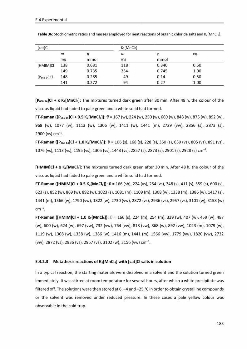
E.4 Experimental
183
Table 36: Stochiometric ratios and masses employed for neat reactions of organic chloride salts and K2[MnCl6].
[cat]Cl K2[MnCl6]
� � � � eq. mg mmol mg mmol
[HMIM]Cl 138 0.681 118 0.340 0.50
149 0.735 254 0.745 1.00
[P666 14]Cl 148 0.285 049 0.14 0.50
141 0.272 094 0.27 1.00
[P666 14]Cl + x K2[MnCl6]: The mixtures turned dark green after 30 min. After 48 h, the colour of the
viscous liquid had faded to pale green and a white solid had formed.
FT-Raman ([P666 14]Cl + 0.5 K2[MnCl6]): NO = 167 (w), 224 (w), 250 (w), 669 (w), 848 (w), 875 (w), 892 (w),
968 (w), 1077 (w), 1113 (w), 1306 (w), 1411 (w), 1441 (m), 2729 (vw), 2856 (s), 2873 (s),
2900 (vs) cm–1.
FT-Raman ([P666 14]Cl + 1.0 K2[MnCl6]): NO = 106 (s), 168 (s), 228 (s), 350 (s), 639 (vs), 805 (vs), 891 (vs),
1076 (vs), 1113 (vs), 1195 (vs), 1305 (vs), 1443 (vs), 2857 (s), 2873 (s), 2901 (s), 2928 (s) cm–1.
[HMIM]Cl + x K2[MnCl6]: The mixtures turned dark green after 30 min. After 48 h, the colour of the
viscous liquid had faded to pale green and a white solid had formed.
FT-Raman ([HMIM]Cl + 0.5 K2[MnCl6]): NO = 166 (sh), 224 (vs), 254 (vs), 348 (s), 411 (s), 559 (s), 600 (s),
623 (s), 852 (w), 869 (w), 892 (w), 1023 (s), 1081 (m), 1109 (m), 1308 (w), 1338 (m), 1386 (w), 1417 (s),
1441 (m), 1566 (w), 1790 (vw), 1822 (w), 2730 (vw), 2872 (vs), 2936 (vs), 2957 (vs), 3101 (w), 3158 (w)
cm–1.
FT-Raman ([HMIM]Cl + 1.0 K2[MnCl6]): NO = 166 (s), 224 (m), 254 (m), 339 (w), 407 (w), 459 (w), 487
(w), 600 (w), 624 (w), 697 (vw), 732 (vw), 764 (vw), 818 (vw), 868 (w), 892 (vw), 1023 (m), 1079 (w),
1119 (w), 1308 (w), 1338 (w), 1386 (w), 1416 (m), 1441 (m), 1566 (vw), 1779 (vw), 1820 (vw), 2732
(vw), 2872 (vs), 2936 (vs), 2957 (vs), 3102 (w), 3156 (vw) cm–1.
E.4.2.3 Metathesis reactions of K2[MnCl6] with [cat]Cl salts in solution
In a typical reaction, the starting materials were dissolved in a solvent and the solution turned green
immediately. It was stirred at room temperature for several hours, after which a white precipitate was
filtered off. The solutions were then stored at 6, –4 and –25 °C in order to obtain crystalline compounds
or the solvent was removed under reduced pressure. In these cases a pale yellow colour was
observable in the cold trap.
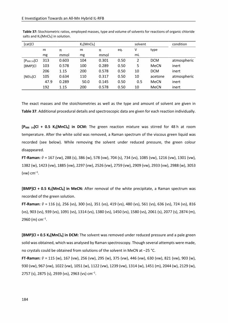
E Investigation Towards an All-Mn Hybrid IL-RFB
184
Table 37: Stochiometric ratios, employed masses, type and volume of solvents for reactions of organic chloride salts and K2[MnCl6] in solution.
[cat]Cl K2[MnCl6] solvent condition
� � � � eq. V type mg mmol mg mmol mL
[P666 14]Cl 313 0.603 104 0.301 0.50 02 DCM atmospheric
[BMP]Cl 103 0.578 100 0.289 0.50 05 MeCN inert
206 1.15 200 0.578 0.50 10 DCM inert
[NEt4]Cl 105 0.634 110 0.317 0.50 10 acetone atmospheric
047.9 0.289 050.0 0.145 0.50 00.5 MeCN inert
192 1.15 200 0.578 0.50 10 MeCN inert
The exact masses and the stoichiometries as well as the type and amount of solvent are given in
Table 37. Additional procedural details and spectroscopic data are given for each reaction individually.
[P666 14]Cl + 0.5 K2[MnCl6] in DCM: The green reaction mixture was stirred for 48 h at room
temperature. After the white solid was removed, a Raman spectrum of the viscous green liquid was
recorded (see below). While removing the solvent under reduced pressure, the green colour
disappeared.
FT-Raman: NO = 167 (vw), 288 (s), 386 (w), 578 (vw), 704 (s), 734 (vs), 1085 (vw), 1216 (vw), 1301 (vw),
1382 (w), 1423 (vw), 1885 (vw), 2297 (vw), 2526 (vw), 2759 (vw), 2909 (vw), 2933 (vw), 2988 (w), 3053
(vw) cm–1.
[BMP]Cl + 0.5 K2[MnCl6] in MeCN: After removal of the white precipitate, a Raman spectrum was
recorded of the green solution.
FT-Raman: NO = 116 (s), 256 (vs), 300 (vs), 351 (vs), 419 (vs), 480 (vs), 561 (vs), 636 (vs), 724 (vs), 816
(vs), 903 (vs), 939 (vs), 1091 (vs), 1314 (vs), 1380 (vs), 1450 (vs), 1580 (vs), 2061 (s), 2077 (s), 2874 (m),
2960 (m) cm–1.
[BMP]Cl + 0.5 K2[MnCl6] in DCM: The solvent was removed under reduced pressure and a pale green
solid was obtained, which was analysed by Raman spectroscopy. Though several attempts were made,
no crystals could be obtained from solutions of the solvent in MeCN at –25 °C.
FT-Raman: NO = 115 (w), 167 (vw), 256 (vw), 295 (w), 375 (vw), 446 (vw), 630 (vw), 821 (vw), 903 (w),
930 (vw), 967 (vw), 1022 (vw), 1051 (w), 1122 (vw), 1239 (vw), 1314 (w), 1451 (m), 2044 (w), 2129 (w),
2757 (s), 2875 (s), 2939 (vs), 2963 (vs) cm–1.
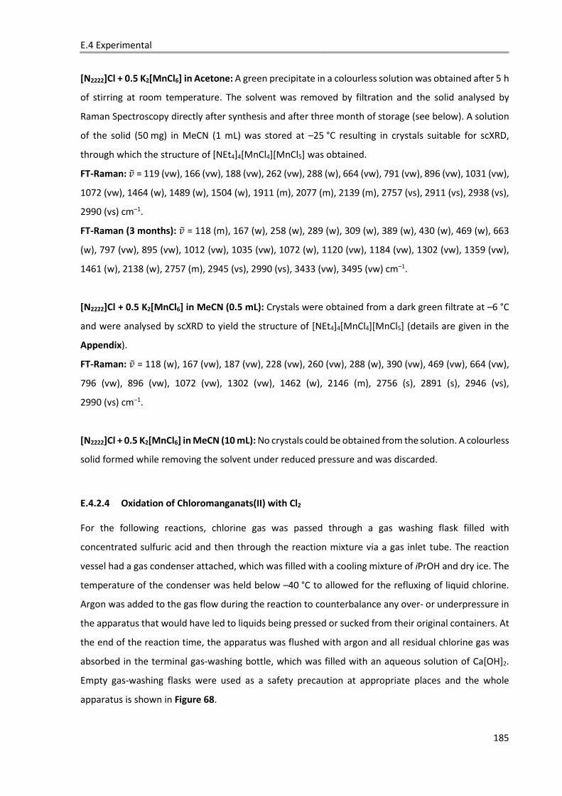
E.4 Experimental
185
[N2222]Cl + 0.5 K2[MnCl6] in Acetone: A green precipitate in a colourless solution was obtained after 5 h
of stirring at room temperature. The solvent was removed by filtration and the solid analysed by
Raman Spectroscopy directly after synthesis and after three month of storage (see below). A solution
of the solid (50 mg) in MeCN (1 mL) was stored at –25 °C resulting in crystals suitable for scXRD,
through which the structure of [NEt4]4[MnCl4][MnCl5] was obtained.
FT-Raman: NO = 119 (vw), 166 (vw), 188 (vw), 262 (vw), 288 (w), 664 (vw), 791 (vw), 896 (vw), 1031 (vw),
1072 (vw), 1464 (w), 1489 (w), 1504 (w), 1911 (m), 2077 (m), 2139 (m), 2757 (vs), 2911 (vs), 2938 (vs),
2990 (vs) cm–1.
FT-Raman (3 months): NO = 118 (m), 167 (w), 258 (w), 289 (w), 309 (w), 389 (w), 430 (w), 469 (w), 663
(w), 797 (vw), 895 (vw), 1012 (vw), 1035 (vw), 1072 (w), 1120 (vw), 1184 (vw), 1302 (vw), 1359 (vw),
1461 (w), 2138 (w), 2757 (m), 2945 (vs), 2990 (vs), 3433 (vw), 3495 (vw) cm–1.
[N2222]Cl + 0.5 K2[MnCl6] in MeCN (0.5 mL): Crystals were obtained from a dark green filtrate at –6 °C
and were analysed by scXRD to yield the structure of [NEt4]4[MnCl4][MnCl5] (details are given in the
Appendix).
FT-Raman: NO = 118 (w), 167 (vw), 187 (vw), 228 (vw), 260 (vw), 288 (w), 390 (vw), 469 (vw), 664 (vw),
796 (vw), 896 (vw), 1072 (vw), 1302 (vw), 1462 (w), 2146 (m), 2756 (s), 2891 (s), 2946 (vs),
2990 (vs) cm–1.
[N2222]Cl + 0.5 K2[MnCl6] in MeCN (10 mL): No crystals could be obtained from the solution. A colourless
solid formed while removing the solvent under reduced pressure and was discarded.
E.4.2.4 Oxidation of Chloromanganats(II) with Cl2
For the following reactions, chlorine gas was passed through a gas washing flask filled with
concentrated sulfuric acid and then through the reaction mixture via a gas inlet tube. The reaction
vessel had a gas condenser attached, which was filled with a cooling mixture of iPrOH and dry ice. The
temperature of the condenser was held below –40 °C to allowed for the refluxing of liquid chlorine.
Argon was added to the gas flow during the reaction to counterbalance any over- or underpressure in
the apparatus that would have led to liquids being pressed or sucked from their original containers. At
the end of the reaction time, the apparatus was flushed with argon and all residual chlorine gas was
absorbed in the terminal gas-washing bottle, which was filled with an aqueous solution of Ca[OH]2.
Empty gas-washing flasks were used as a safety precaution at appropriate places and the whole
apparatus is shown in Figure 68.
E Investigation Towards an All-Mn Hybrid IL-RFB
186
Figure 68: Apparatus used for the oxidation of organic chloromanganates(II) under reflux of elemental chlorine.
Attempted Oxidation in MeCN: In a glove box, [NEt4]Cl (658 mg, 3.97 mmol) and MnCl2 (250 mg, 1.99
mmol, 0.50 eq) were dissolved in MeCN (50 mL) and the reaction vessel then connected to the
chlorination apparatus. After 15 min of chlorine reflux, the colour of the solution had changed to a
dark green. The reaction was terminated after 1 h. Raman measurements on the reaction mixture did
not yield usable results and no crystals were obtained through storage of the solution at –25 °C.
Attempted Oxidation in HCl: [NEt4]Cl (553 mg, 3.34 mmol) and MnCl2 (210 mg, 1.67 mmol, 0.50 eq)
were dissolved in conc. hydrochloric acid (10 mL). After 30 min of chlorine reflux, the colour of the
solution had only changed from transparent to pale yellow and the reaction was therefore aborted.
Attempted Oxidation in liquid Cl2: In a glove box, [NEt4]Cl (329 mg, 1.99 mmol) and MnCl2 (125 mg,
0.99 mmol, 0.50 eq) were dissolved in MeCN (10 mL) and the mixture stirred for 2 h. The MeCN was
removed under reduced pressure and the reaction vessel then connected to the chlorination
apparatus. Cl2 was condensed on the solid and stirred under reflux for 30 min. After removal of the
residual chlorine, only a small portion of the white solid had turned green.
E.4 Experimental
187
Oxidation in o-DFB/MeCN: In this reaction the residue left in the apparatus from the attempted
oxidation in elemental chlorine was reused. o-DFB (20 mL) was added to the white solid and chlorine
passed through the suspension and refluxed. The solution turned yellow and was stirred for 3 h, after
which MeCN (2 mL) was added. After 1.5 h, additional MeCN (2.5 mL) was added and the colour of the
liquid phase turned pale green. The reaction mixture was heated to 50 °C, while passing chlorine
through the suspension and stirred under chlorine reflux for 4 h. During this time, the white solid
disappeared and the solution turned dark green. After cooling to RT and evaporation of the residual
chlorine, a green precipitate had formed in a transparent liquid phase. The solvent was decanted and
the product washed with pentane and dried under a weak argon flow.
FT-Raman (100mW): NO = 118 (w), 258 (vw), 288 (vw), 469 (vw), 555 (vw), 663 (w), 794 (vw), 895 (vw),
1034 (vw), 1072 (w), 1120 (vw), 1184 (vw), 1302 (vw), 1358 (vw), 1395 (vw), 1462 (w), 2147 (w), 2756
(m), 2891 (s), 2946 (vs), 2990 (vs) cm–1.
FT-Raman (3mW): NO = 123 (vw), 168 (vw), 189 (vw), 221 (vw), 259 (vw), 288 (vw), 664 (vw), 722 (vw),
2138 (m), 2758 (vs), 2792 (s), 2817 (s), 2847 (s), 2912 (vs), 2938 (vs), 2990 (s), 3124 (m),
3143 (m) cm–1.
Electrochemical Measurements on Solutions of [P666 14]2[MnCl4] in MeCN
E.4.3.1 Cyclic voltammetry
An electrolyte was prepared by dissolving [NBu4][BF4] (659 mg, 2.00 mmol, 100 mM) in dried and
degassed MeCN (20 mL). In a part of the electrolyte (13 mL), [P666 14]2[MnCl4] (51 mg, 0.044 mmol,
3.36 mM) was dissolved and analysed using a platinum circular disc electrode (diameter 10µm) as
working electrodes and platinum wires as quasi reference and as counter electrode. After addition of
ferrocene (10 mg, 0.054 mmol, 27 mM) to part of the solution (2 mL), the measurement was repeated
and is shown in Figure 69 in the Appendix.
E.4.3.2 Battery Measurements
[P666 14]2[MnCl4] (4.9 g, 4.2 mmol) and MeCN (0.42 g, 0.54 mL, 2.4 eq, 8 wt%) were combined in a glove
and the mixture stirred for 30 min. A cylindrical cell with circular SGL Carbon TF6 Electrodes (electrode
distance: 0.4 cm, surface area per electrode: 1.53 cm2, volume: 0.612 mL, inset 12 in Figure 71) was
filled with the mixture (590 mg, 0.467 mmol [P666 14]2[MnCl4]) inside the glove box and hermetically
sealed using appropriate screws. The cell was transferred to a desiccator and all electronic
measurements were performed under a slight argon flux. The electrolyte was removed and analysed
via Raman spectroscopy prior to dismantling the cell. A black solid was discovered on dismantling the

E Investigation Towards an All-Mn Hybrid IL-RFB
188
cell at an SOC of approximately 32 % for a one and 42 % assuming a two electron process at the
cathode. A pXRD measurement of the black solid did not yield any reflexes.
FT-Raman (prior to battery measurement): NO = 251 (vw), 381 (vw), 669 (vw), 749 (vw), 920 (vw), 1078
(vw), 1115 (vw), 1308 (vw), 1375 (vw), 1444 (vw), 2204 (vw), 2253 (s), 2293 (vw), 2733 (vw), 2877 (vw),
2943 (vs), 3001 (vw) cm–1.
FT-Raman (after battery measurement): NO = 184 (m), 250 (m), 379 (m), 407 (m), 669 (m), 848 (m), 873
(m), 891 (m), 919 (m), 967 (m), 1008 (m), 1077 (m), 1114 (m), 1306 (m), 1372 (m), 1410 (m), 1441 (s),
2061 (w), 2077 (w), 2158 (w), 2185 (w), 2221 (w), 2250 (w), 2284 (w), 2729 (w), 2856 (vs), 2873 (vs),
2900 (vs), 2932 (vs) cm–1.
E.4 Experimental
189
References
[1] A. F. Holleman, E. Wiberg, G. Fischer, Lehrbuch der Anorganischen Chemie, Walter de Gruyter,
Berlin, New York, 2007.
[2] A.-R. Song, I.-C. Hwang, K. Ha, Z. Kristallogr. - New Cryst. Struct. 2014, 222, 43.
[3] C. F. Bell, D. N. Waters, J. Inorg. Nucl. Chem. 1977, 39, 773.
[4] B. Morosin, E. J. Graber, Acta Crystallogr. 1967, 23, 766.
[5] I. Bernal, N. Elliott, R. Lalancette, J. Chem. Soc. D 1971, 803.
[6] P. C. Moews Jr, Inorg. Chem. 1966, 5, 5.
[7] H. J. Seifert, F. W. Koknat, Z. anorg. allg. Chem. 1965, 341, 269.
[8] S. Pitula, A.-V. Mudring, Chem. Eur. J. 2010, 16, 3355.
[9] R. J. Meyer, H. Best, Z. Anorg. Chem. 1899, 22, 169.
[10] a) H. A. Goodwin, R. N. Sylva, Aust. J. Chem. 1965, 18, 1743; b) R. F. Weinland, P. Dinkelacker, Z.
Anorg. Chem. 1908, 60, 173.
[11] J. Lu, D. Dreisinger, T. Glück, Hydrometallurgy 2014, 141, 105.
[12] P.-Y. Chen, C. L. Hussey, Electrochim. Acta 2007, 52, 1857.
[13] J.-K. Chang, C.-H. Huang, W.-T. Tsai, M.-J. Deng, I.-W. Sun, P.-Y. Chen, Electrochim. Acta 2008, 53,
4447.
[14] H. C. de Long, J. A. Mitchell, P. C. Trulove, High Temp. Mater. Processes 1998, 2, 507.
[15] T. Tsuda, C. L. Hussey, G. R. Stafford, J. Electrochem. Soc. 2005, 152, C620.
[16] T. Tsuda, Y. Ikeda, A. Imanishi, S. Kusumoto, S. Kuwabata, G. R. Stafford, C. L. Hussey, J.
Electrochem. Soc. 2015, 162, D405-D411.
[17] M.-J. Deng, P.-Y. Chen, I.-W. Sun, Electrochim. Acta 2007, 53, 1931.
[18] P.-Y. Chen, M.-J. Deng, D.-X. Zhuang, Electrochim. Acta 2009, 54, 6935.
[19] C. Daniel, J. O. Besenhard (Eds.) Handbook of Battery Materials, Wiley-VCH, 2011.
[20] F. Gschwind, G. Rodriguez-Garcia, D. J. S. Sandbeck, A. Gross, M. Weil, M. Fichtner, N. Hörmann,
J. Fluorine Chem. 2016, 182, 76.
[21] K. Tanemoto, T. Nakamura, Chem. Lett. 1975, 4, 351.

E Investigation Towards an All-Mn Hybrid IL-RFB
190
[22] J. Heinze, Angew. Chem. 1993, 105, 1327.
[23] J. Heinze, Angew. Chem. 1984, 96, 823.
[24] D. M. Adams, D. M. Morris, J. Chem. Soc. A 1968, 694.
[25] C. D. Flint, Journal of Molecular Spectroscopy 1971, 37, 414.
[26] a) J.-C. Chang, W.-Y. Ho, I.-W. Sun, Y.-K. Chou, H.-H. Hsieh, T.-Y. Wu, Polyhedron 2011, 30, 497; b)
M. Matsui, S. Koda, S. Ooi, H. Kuroya, I. Bernal, Chem. Lett. 1972, 1, 51; c) A. R. Parent, C. P.
Landee, M. M. Turnbull, Inorg. Chim. Acta 2007, 360, 1943.
E.5 Appendix
191
E.5 Appendix
Crystallographic data for [NEt4]4[MnCl4][MnCl5]
Table 38: Crystal data and structure refinement for [NEt4]4[MnCl4][MnCl5]
Empirical formula C32H80N4Cl9Mn2 Formula weight 949.93 Temperature/K 100.0 Crystal system tetragonal Space group P4/n a/Å 14.0370(4) b/Å 14.0370(4) c/Å 12.1648(4) α/° 90 β/° 90 γ/° 90 Volume/Å3 2396.92(16) Z 2 ρcalc / g cm–3 1.316 μ / mm-1 1.055 F(000) 1006.0 Crystal size/mm3 0.16 × 0.16 × 0.13 Radiation Mo-Kα (λ = 0.71073) 2Θ range for data collection /° 3.348 to 56.568 Index ranges -18 ≤ h ≤ 18, -18 ≤ k ≤ 18, -16 ≤ l ≤ 16 Reflections collected 59198 Independent reflections 2993 [Rint = 0.0297, Rsigma = 0.0120] Data/restraints/parameters 2993/84/165 Goodness-of-fit on F2 1.076 Final R indexes [I >= 2σ (I)] R1 = 0.0577, wR2 = 0.1415 Final R indexes [all data] R1 = 0.0637, wR2 = 0.1455 Largest diff. peak/hole / e Å-3 1.21/-0.98
Table 39: Selected bond lengths and bond angles for [NEt4]4[MnCl4][MnCl5].
bond length bond angle Å °
Mn01 Cl04 2.3458(8) Cl04c) Mn01 Cl042 108.181(19) Mn01 Cl04a) 2.3459(8) Cl05d) Mn02 Cl03 100.28(4) Mn01 Cl04b) 2.3459(8) Cl05e) Mn02 Cl03 100.28(4) Mn01 Cl04c) 2.3459(8) Cl05f) Mn02 Cl03 100.28(4) Mn02 Cl03 2.4025(17) Cl05 Mn02 Cl03 100.28(4) Mn02 Cl05 2.2977(9) Cl054 Mn02 Cl056 88.174(13) Mn02 Cl05d) 2.2977(9) Cl055 Mn02 Cl05 88.174(13) Mn02 Cl05e) 2.2977(9) Cl055 Mn02 Cl056 88.174(13) Mn02 Cl05f) 2.2977(9) a)1/2-X, 3/2-Y, +Z; b)1-Y, 1/2+X, 2-Z; c)-1/2+Y, 1-X, 2-Z; d)1/2-Y, +X, +Z; e)1/2-X, 1/2-Y, +Z; f)+Y, 1/2-X, +Z.
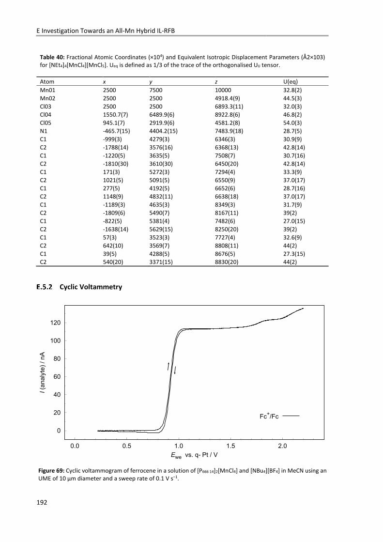
E Investigation Towards an All-Mn Hybrid IL-RFB
192
Table 40: Fractional Atomic Coordinates (×104) and Equivalent Isotropic Displacement Parameters (Å2×10³) for [NEt4]4[MnCl4][MnCl5]. Ueq is defined as 1/3 of the trace of the orthogonalised UIJ tensor.
Atom x y z U(eq)
Mn01 2500 7500 10000 32.8(2) Mn02 2500 2500 4918.4(9) 44.5(3) Cl03 2500 2500 6893.3(11) 32.0(3) Cl04 1550.7(7) 6489.9(6) 8922.8(6) 46.8(2) Cl05 945.1(7) 2919.9(6) 4581.2(8) 54.0(3) N1 -465.7(15) 4404.2(15) 7483.9(18) 28.7(5) C1 -999(3) 4279(3) 6346(3) 30.9(9) C2 -1788(14) 3576(16) 6368(13) 42.8(14) C1 -1220(5) 3635(5) 7508(7) 30.7(16) C2 -1810(30) 3610(30) 6450(20) 42.8(14) C1 171(3) 5272(3) 7294(4) 33.3(9) C2 1021(5) 5091(5) 6550(9) 37.0(17) C1 277(5) 4192(5) 6652(6) 28.7(16) C2 1148(9) 4832(11) 6638(18) 37.0(17) C1 -1189(3) 4635(3) 8349(3) 31.7(9) C2 -1809(6) 5490(7) 8167(11) 39(2) C1 -822(5) 5381(4) 7482(6) 27.0(15) C2 -1638(14) 5629(15) 8250(20) 39(2) C1 57(3) 3523(3) 7727(4) 32.6(9) C2 642(10) 3569(7) 8808(11) 44(2) C1 39(5) 4288(5) 8676(5) 27.3(15) C2 540(20) 3371(15) 8830(20) 44(2)
Cyclic Voltammetry
Figure 69: Cyclic voltammogram of ferrocene in a solution of [P666 14]2[MnCl4] and [NBu4][BF4] in MeCN using an UME of 10 µm diameter and a sweep rate of 0.1 V s–1.
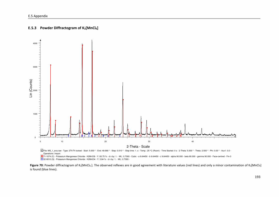
E.5 Appendix
193
32-0810 (Q) - Potassium Manganese Chloride - K2MnCl4 - Y: 3.84 % - d x by: 1. - WL: 0.7093 -
71-1074 (C) - Potassium Manganese Chloride - K2MnCl6 - Y: 93.75 % - d x by: 1. - WL: 0.7093 - Cubic - a 9.64450 - b 9.64450 - c 9.64450 - alpha 90.000 - beta 90.000 - gamma 90.000 - Face-centred - Fm-3
Operations: Import
File: MS_1_eva.raw - Type: 2Th/Th locked - Start: 5.000 ° - End: 49.990 ° - Step: 0.010 ° - Step time: 1. s - Temp.: 25 °C (Room) - Time Started: 0 s - 2-Theta: 5.000 ° - Theta: 2.500 ° - Phi: 0.00 ° - Aux1: 0.0 -
Lin
(C
oun
ts)
0
1000
2000
3000
4000
2-Theta - Scale
5 10 20 30 40
Powder Diffractogram of K2[MnCl6]
Figure 70: Powder diffractogram of K2[MnCl6.]. The observed reflexes are in good agreement with literature values (red lines) and only a minor contamination of K2[MnCl4] is found (blue lines).

E Investigation Towards an All-Mn Hybrid IL-RFB
194
F.1 Hardware I: Battery Test Setup for Static Liquid Active Materials
195
F Development of a Battery Test Setup
F.1 Hardware I: Battery Test Setup for Static Liquid Active Materials
Test Cell
The test cell shown in Figure 71 was used for battery tests on static liquid active materials. I developed
the design based on a central screw with self-sealing insets (Figure 71, number 5) during my diploma
thesis.[1] The advantage compared to other designs is the possibility to use easily producible and flat
electrodes with a clearly defined surface area and a constant distance between anode and cathode to
allow for the accurate determination of current densities. Additionally, it offers superior sealing
compared to typical designs utilizing several screws surrounding the electrodes, since the central screw
applies pressure more evenly, and is much easier to assemble reproducibly. The insets are machined
from PTFE and offer excellent chemical stability. No other materials needs to be in contact with the
liquid active materials, except, of course, for the electrodes and, as described below, O-rings when the
cell is used with a membrane.
During this doctorate the insets were further refined to allow the use of smaller volumes of active
material and a smaller distance of the electrodes. Details on dimensions, resulting electrode surfaces,
and cell volumes are given in Table 41. Screws were used to allow for hermetic sealing of the test cells
and O-rings were added as suggested by Kolja Bromberger to improve sealing when testing cells with
a membrane. One O-ring is used on each side of the membrane and the diameter differs by a few
millimetres so that the membrane is pressed against the opposing inset from both sides. This improved
the sealing significantly, as tested by Michael Hog. A typical configuration and an assembled test cell
is shown in Figure 72.
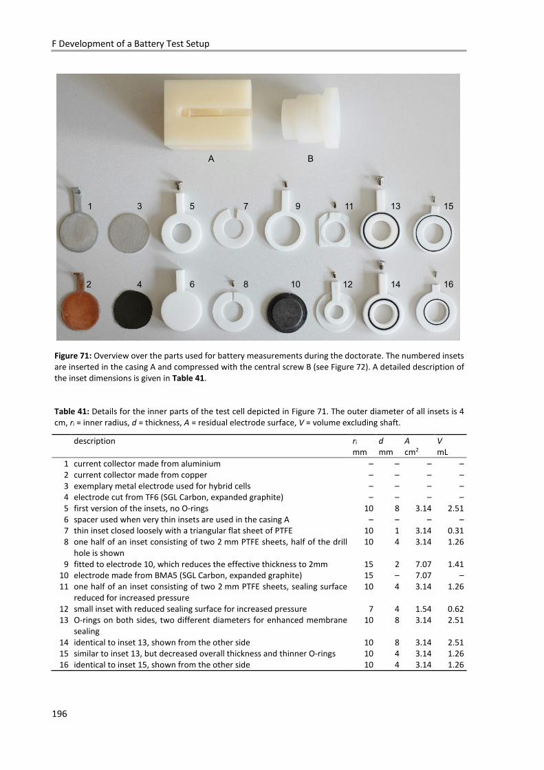
F Development of a Battery Test Setup
196
Figure 71: Overview over the parts used for battery measurements during the doctorate. The numbered insets are inserted in the casing A and compressed with the central screw B (see Figure 72). A detailed description of the inset dimensions is given in Table 41.
Table 41: Details for the inner parts of the test cell depicted in Figure 71. The outer diameter of all insets is 4 cm, ri = inner radius, d = thickness, A = residual electrode surface, V = volume excluding shaft.
description ri d A V mm mm cm2 mL
1 current collector made from aluminium – – – – 2 current collector made from copper – – – – 3 exemplary metal electrode used for hybrid cells – – – – 4 electrode cut from TF6 (SGL Carbon, expanded graphite) – – – – 5 first version of the insets, no O-rings 10 8 3.14 2.51 6 spacer used when very thin insets are used in the casing A – – – – 7 thin inset closed loosely with a triangular flat sheet of PTFE 10 1 3.14 0.31 8 one half of an inset consisting of two 2 mm PTFE sheets, half of the drill
hole is shown 10 4 3.14 1.26
9 fitted to electrode 10, which reduces the effective thickness to 2mm 15 2 7.07 1.41 10 electrode made from BMA5 (SGL Carbon, expanded graphite) 15 – 7.07 – 11 one half of an inset consisting of two 2 mm PTFE sheets, sealing surface
reduced for increased pressure 10 4 3.14 1.26
12 small inset with reduced sealing surface for increased pressure 7 4 1.54 0.62 13 O-rings on both sides, two different diameters for enhanced membrane
sealing 10 8 3.14 2.51
14 identical to inset 13, shown from the other side 10 8 3.14 2.51 15 similar to inset 13, but decreased overall thickness and thinner O-rings 10 4 3.14 1.26 16 identical to inset 15, shown from the other side 10 4 3.14 1.26
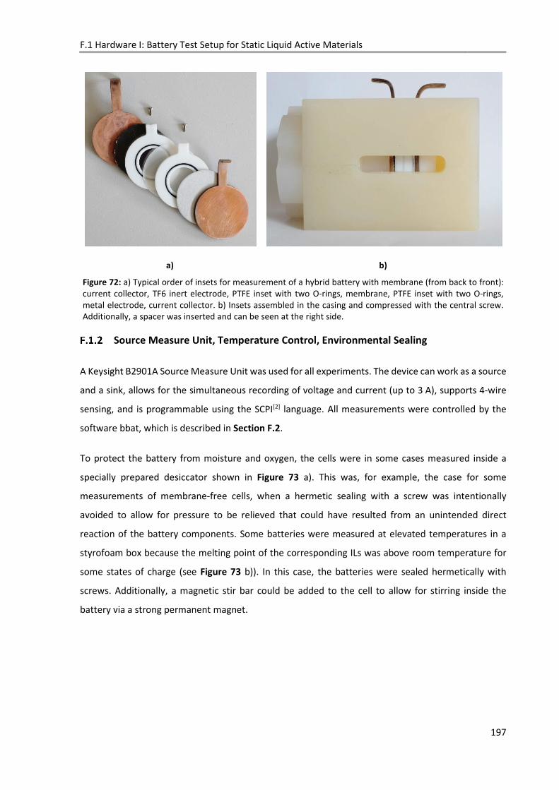
F.1 Hardware I: Battery Test Setup for Static Liquid Active Materials
197
a) b)
Figure 72: a) Typical order of insets for measurement of a hybrid battery with membrane (from back to front): current collector, TF6 inert electrode, PTFE inset with two O-rings, membrane, PTFE inset with two O-rings, metal electrode, current collector. b) Insets assembled in the casing and compressed with the central screw. Additionally, a spacer was inserted and can be seen at the right side.
Source Measure Unit, Temperature Control, Environmental Sealing
A Keysight B2901A Source Measure Unit was used for all experiments. The device can work as a source
and a sink, allows for the simultaneous recording of voltage and current (up to 3 A), supports 4-wire
sensing, and is programmable using the SCPI[2] language. All measurements were controlled by the
software bbat, which is described in Section F.2.
To protect the battery from moisture and oxygen, the cells were in some cases measured inside a
specially prepared desiccator shown in Figure 73 a). This was, for example, the case for some
measurements of membrane-free cells, when a hermetic sealing with a screw was intentionally
avoided to allow for pressure to be relieved that could have resulted from an unintended direct
reaction of the battery components. Some batteries were measured at elevated temperatures in a
styrofoam box because the melting point of the corresponding ILs was above room temperature for
some states of charge (see Figure 73 b)). In this case, the batteries were sealed hermetically with
screws. Additionally, a magnetic stir bar could be added to the cell to allow for stirring inside the
battery via a strong permanent magnet.
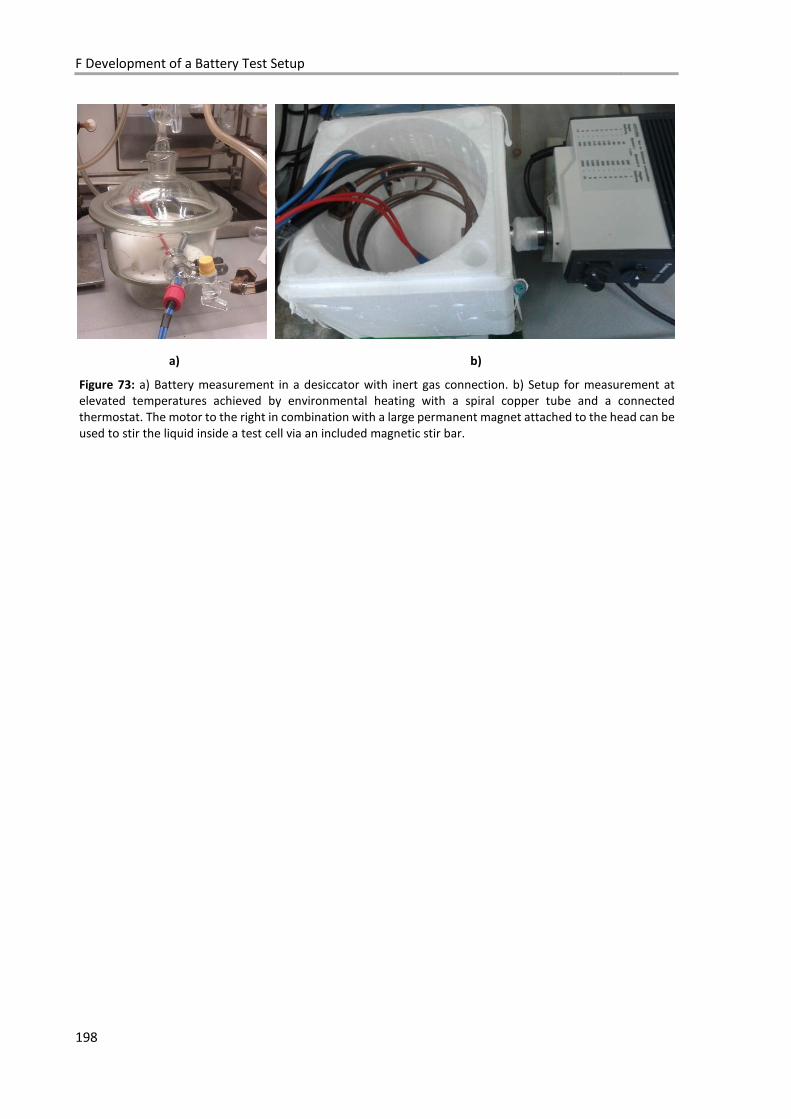
F Development of a Battery Test Setup
198
a) b)
Figure 73: a) Battery measurement in a desiccator with inert gas connection. b) Setup for measurement at elevated temperatures achieved by environmental heating with a spiral copper tube and a connected thermostat. The motor to the right in combination with a large permanent magnet attached to the head can be used to stir the liquid inside a test cell via an included magnetic stir bar.

F.2 Software: bbat
199
F.2 Software: bbat
The bbat program has been created to provide a software interface to perform standard battery testing
with the Source Measure Unit Keysight B2901A. The key goal in the design was to build a highly
customizable tool which would allow the user to create a reproducible test environment by providing
a reliable and comfortable interface and documenting both test results and conditions transparently.
bbat uses text files to store its source code, to define the tests performed, to save the measured data
and to save the files logging the test records. These text files are UTF-8 encoded, which has become
the accepted standard for the source code of websites, and are therefore readable by any graphical or
command line editor. This ensure transparency and accessibility throughout the program and also
means that the data produced during a test will be accessible even if bbat is not available or executable
at some point in the future.
The software runs under Linux and can therefore be easily transferred to a single-board computer like
the Raspberry Pi.[3] The Raspberry Pi in particular is supported by a large community which provides
valuable support. The program can be accessed via network through default SSH clients, which are
available for all common operating systems. Since the Keysight B2901A uses the standardised SCPI
(Standard Commands for Programmable Instrumentation)[2] commands, bbat should in principle be
adaptable to other devices which implement SCPI.
To help and encourage the user to understand and possibly modify the software, an extensive
documentation has been created. One part of this documentation is the source code itself, which
includes many comments to explain its inner workings.
Figure 74 gives an overview of the folders and files contained within the program folder. Since the
source code of bbat and the included documentation are designed to “speak” for themselves, the
following sections are structured according to the inner file structure of bbat. These sections are only
intended to help in getting an overview over the project and will mainly reference the documentation
and source code included in the Appendix of this chapter.
If one were to explain to an interested person the clockwork of a mechanical watch, it would be a good idea to first tell the person how to correctly tell the time from such a device. He or she would then be familiar with the purpose and the names of the different hands and the crown, which would be helpful to grasp the point behind the parts which constitute the clockwork of the watch. In the same manner,
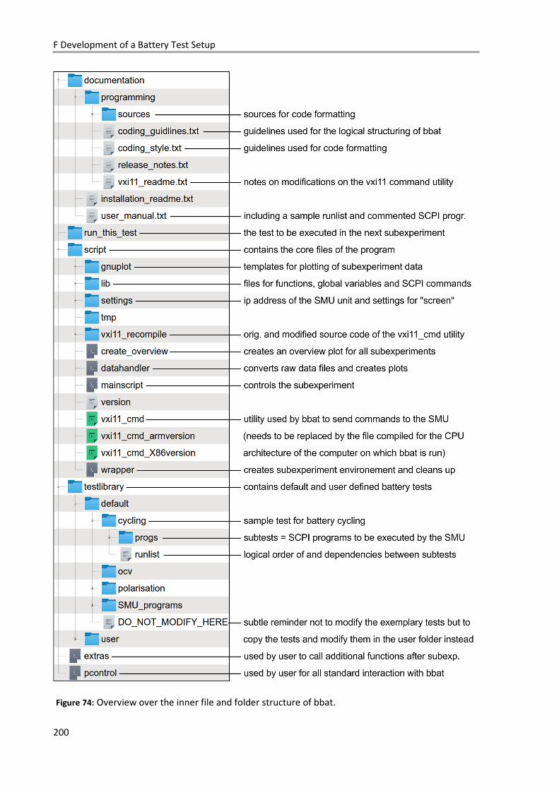
F Development of a Battery Test Setup
200
Figure 74: Overview over the inner file and folder structure of bbat.

F.2 Software: bbat
201
the next section will deal with the way a user can define and execute a battery test, before diving into
the inner workings of bbat in Section F.2.3.
Throughout the following chapter, names of folders and scripts as well as specific terms will be set in
quotes whenever it is considered helpful for the reader’s understanding of the matter.
Documentation
F.2.1.1 user_manual.txt and installation_readme.txt
The user manual (Section F.4.1.1) gives detailed instructions on how to operate bbat, starting with the
creation of a folder for the experiment via a command line terminal and setting up bbat inside. All
steps necessary to set up software requirements are explained in detail in the installation readme
(Section F.4.1.2).
The terms “experiment”, “subexperiment”, “test”, “subtest” and “SCPI Program” have a specific
meaning within bbat. An “experiment” refers to all actions performed on one battery, a
“subexperiment” to a specific run of a “test” performed on the battery. A “test” is a collection of
“subtests”, each defined by one line of an instructions file called "runlist". Each subtest is connected
to a “SCPI Program”, which is a set of commands stored in a file.
The commands of a “SCPI Program” are instructions defining settings and limits for the SMU. For
example, the SMU could be set to discharge the battery at a constant current for one hour. A limit
could be defined to report a “fail” as soon as the voltage drops below a certain value during this
discharge operation. An example for this “SCPI Program” is given in Section F.4.2.2 of the Appendix.
A “SCPI Program” combined with instructions on how many times to run it, what to do after it is
completed and what to do if a “fail” of a limit is detected is called a “subtest”. It is defined by one line
in the “runlist”.
Section F.4.2.1 contains an example “runlist” for a cycling test. The lines, or “subtests”, in the runlist
define in their sum the logic behind the “test” and are discussed in detail in the user manual starting
in line 104. Samples for a cycling test (Section F.4.2.1), an OCV measurement, and a polarisation
(Section F.4.2.4) are included in the bbat default test library.
The results of each run of a test, called a “subexperiment”, are stored in a “subexperiment folder”. An
overview of its contents after the conclusion of the “subexperiment” is given in Figure 75. To complete
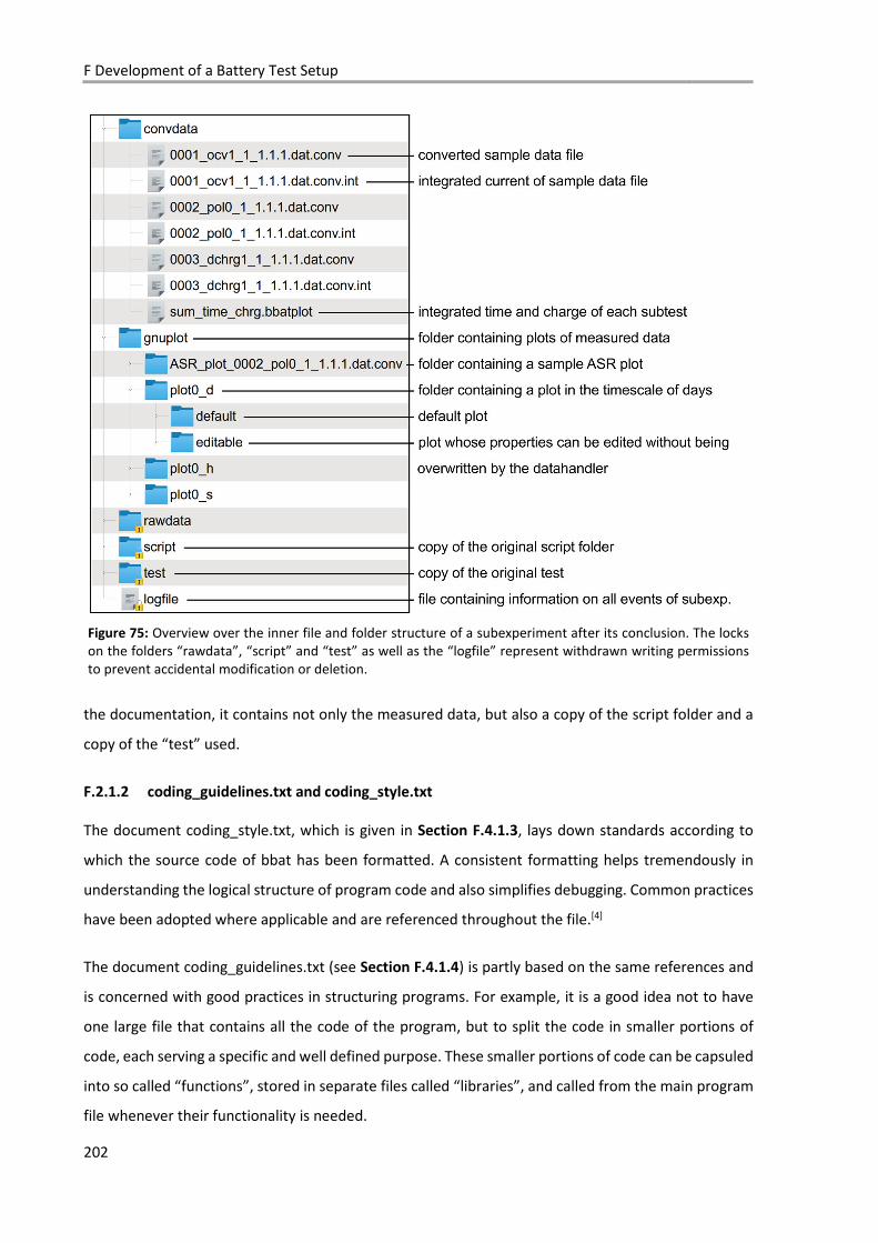
F Development of a Battery Test Setup
202
Figure 75: Overview over the inner file and folder structure of a subexperiment after its conclusion. The locks on the folders “rawdata”, “script” and “test” as well as the “logfile” represent withdrawn writing permissions to prevent accidental modification or deletion.
the documentation, it contains not only the measured data, but also a copy of the script folder and a
copy of the “test” used.
F.2.1.2 coding_guidelines.txt and coding_style.txt
The document coding_style.txt, which is given in Section F.4.1.3, lays down standards according to
which the source code of bbat has been formatted. A consistent formatting helps tremendously in
understanding the logical structure of program code and also simplifies debugging. Common practices
have been adopted where applicable and are referenced throughout the file.[4]
The document coding_guidelines.txt (see Section F.4.1.4) is partly based on the same references and
is concerned with good practices in structuring programs. For example, it is a good idea not to have
one large file that contains all the code of the program, but to split the code in smaller portions of
code, each serving a specific and well defined purpose. These smaller portions of code can be capsuled
into so called “functions”, stored in separate files called “libraries”, and called from the main program
file whenever their functionality is needed.

F.2 Software: bbat
203
User Interaction: pcontrol and extras
The script “pcontrol” (see Section F.4.3.1) is the script a user executes whenever he or she wishes to
start, change, or look at the current status of a subexperiment. When executed, “pcontrol” will first
check whether or not a subexperiment is already in progress. If this is the case, then the user can
choose to either abort the subexperiment, change to a different subtest, or execute the “datahandler”
(see Section F.4.4.3), which will convert and plot all data that has already been transferred to the
controlling computer. If no subexperiment is running, it will instead start the script “script/wrapper”,
which will set the whole program in motion (see next section).
The “extras” script is not a control tool for subexperiments but provides two features to evaluate them
(see Section F.4.3.2). The first is an option to call the script “script/create_overview” (see Section
F.4.4.4), which will create an overview plot displaying all subexperiments on a single time axis, with
the starting time of each subexperiment shown relative to the first subexperiment. The second feature
is an option to produce ASR plots from polarisation measurements. The script will accept user input
on experiment specific data like the surface area of the electrodes or the number of data points for
each polarisation step.
Inner Workings: script Folder
The “script” folder contains the core of the bbat program. If a user executes the “pcontrol” script while
no other subexperiment is running, the first script to be called is the “wrapper” script. It will create
directories for the subexperiment and check if a test and all corresponding programs can be found in
the “run_this_test” folder. During this process, the folder “script” is copied to the subexperiment
folder, and within this copy, the “mainscript” is then called. The “mainscript” contains the part of the
program that communicates with the SMU and switches between subtests according to the rules
dictated by the runlist. This includes considering whether or not predefined limits are failed during a
subtest. Only when the subexperiment is finished will the “mainscript” be left, and the “wrapper” script
takes over again. It will then call the “datahandler” (see Section F.4.4.3) which will convert the received
data files and create default plots. The last action of the wrapper script is to withdraw writing
permissions on the “rawdata”, “script”, and “test” folder as well as the “logfile”.
F.2.3.1 Script/lib
To do its work, bbat uses multiple “global” variables and constants. Unlike their “local” counterparts,
they are accessible throughout a script and not only in the block of code confined by a “function”. This

F Development of a Battery Test Setup
204
property has several advantages but has the disadvantage that the values of these “global” variables
can be changed from everywhere in the script, thus making debugging more difficult.
To restrict the use of global variables to the minimal amount necessary and also to have a clear
overview on what they are and what they are supposed to do, there is a file in the bbat library called
“globvars.sh” (see Section F.4.5.1). It is called at the beginning of every script and contains a list of all
global variables and constants even if they are not assigned at the very beginning but during the
runtime of the script. These “runtime” variables, like, for example, the name of the subexperiment
which is defined by the user, will be written to a file called “runtimeglobvars.sh” in the “script/tmp”
folder as soon as they are assigned. There are a number of variables which depend on the values of
these global runtime variables. These “dependent runtime global variables” are stored in the file
“script/lib/dep_runtimeglobvars.sh” and are loaded after the “global runtime variables” variables are
set (see Section F.4.5.2).
The last file containing constants is “SCPImessages.sh” (Section F.4.5.4). The constants defined in this
file contain command strings in the SCPI language and are sent to the SMU to control a subtest or to
pull data from it.
As mentioned before, it is a good idea to split the code of a program to form smaller blocks of code
called functions, which have a specific purpose and can be called whenever needed. For this reason,
the largest file of bbat is “script/lib/functions.sh” (see Section F.4.5.3) in the “lib” folder. It contains all
functions defined and used in bbat.
F.2.3.2 Script/gnuplot
bbat employs gnuplot[5] for the plotting of measured data. In the “gnuplot” folder a script
“GnuPlottingScript” is contained (Section F.4.6.1). It will merge the templates
“SP_template_bbat.head” (see Section F.4.6.2), containing all settings for the appearance of the plot,
“SP_template_bbat.body”, which contains links to the location of the data files, and
“SP_template_bbat.tail”, which contains instructions to produce cropped *.pdf and *.eps files, to form
a *.plt file, which it will then plot using gnuplot.
F.2.3.3 Script/Vxi11 Recompile
The creation of bbat would not have been possible without Steve D. Sharples'
([email protected]) program “VXI11 Ethernet Protocol for Linux”, which he published
under the GNU General Public License Version 2.[6] His “vxi11_cmd” utility is used in bbat to
communicate with the SMU. It has been modified only slightly to allow for longer data messages to be

F.2 Software: bbat
205
transmitted. See the “vxi11_readme.txt” for details (Section F.4.1.5). The utility has been compiled
both for x86 and ARM CPU architectures and is provided in both versions with bbat.

F Development of a Battery Test Setup
206
F.3 Hardware II: Progress Towards a Flow-Battery Test Setup
207
F.3 Hardware II: Progress Towards a Flow-Battery Test Setup
An extension of the static battery test setup to allow for thermally controlled flow battery testing has
been planned during and will be realised subsequent to the completion of this dissertation. A short
description of the selected compounds and the reasoning behind their selection will be given in the
following chapter.
All prices for components stated in this section are given as approximate values at the time of writing
and may not reflect the current prices.
Flow Test Cell
Following the results of the static battery tests, and due to the high price of the ionic liquids at least at
the research state, it was decided during the project meeting in November 2016 that the flow test cell
should be smaller in dimension than originally envisioned. I suggested to use a similar concept to the
one of the static test cell, possibly with fluid connections opposite of the central screw. Further
development of the flow cell based on this idea was then carried out in collaboration with our
cooperation partner Fraunhofer ISE. Prithiv Mohan, as part of his master thesis supervised by Kolja
Bromberger, designed the test cell shown in Figure 76.[7] A crossectional view is given in Figure 77. The
cell has been found to provide adequate and evenly distributed sealing pressure and has been tested
with pressurized air up to a pressure of 2 bar.[7]
For the first experiments an inset with a flow channel reduced to 1 cm in width was designed, so that
the inner volume of the cell is only 3.1 mL compared to 8.9 mL for the full-sized flow field. The two
different insets and the dimensions of the smaller inset are given in Figure 78.
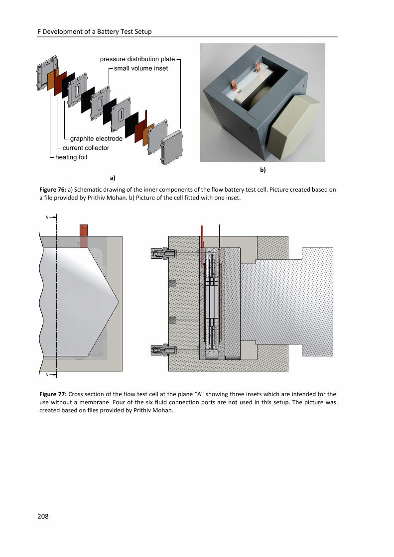
F Development of a Battery Test Setup
208
a)
b)
Figure 76: a) Schematic drawing of the inner components of the flow battery test cell. Picture created based on a file provided by Prithiv Mohan. b) Picture of the cell fitted with one inset.
Figure 77: Cross section of the flow test cell at the plane “A” showing three insets which are intended for the use without a membrane. Four of the six fluid connection ports are not used in this setup. The picture was created based on files provided by Prithiv Mohan.
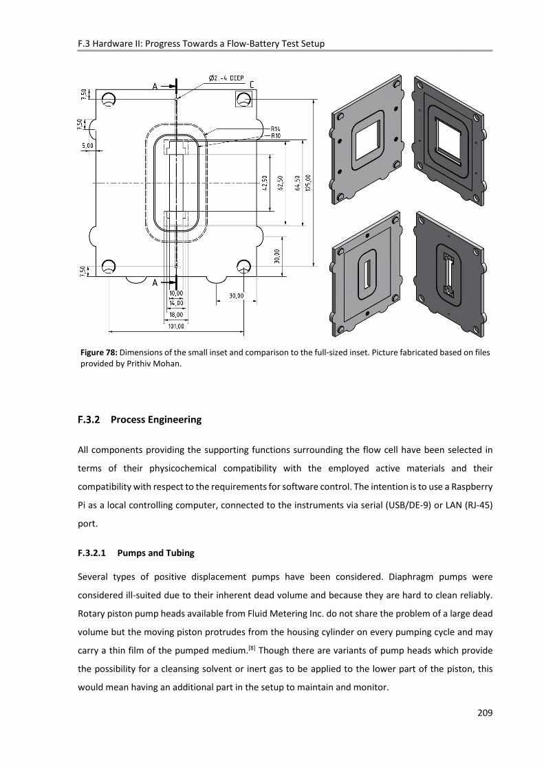
F.3 Hardware II: Progress Towards a Flow-Battery Test Setup
209
Figure 78: Dimensions of the small inset and comparison to the full-sized inset. Picture fabricated based on files provided by Prithiv Mohan.
Process Engineering
All components providing the supporting functions surrounding the flow cell have been selected in
terms of their physicochemical compatibility with the employed active materials and their
compatibility with respect to the requirements for software control. The intention is to use a Raspberry
Pi as a local controlling computer, connected to the instruments via serial (USB/DE-9) or LAN (RJ-45)
port.
F.3.2.1 Pumps and Tubing
Several types of positive displacement pumps have been considered. Diaphragm pumps were
considered ill-suited due to their inherent dead volume and because they are hard to clean reliably.
Rotary piston pump heads available from Fluid Metering Inc. do not share the problem of a large dead
volume but the moving piston protrudes from the housing cylinder on every pumping cycle and may
carry a thin film of the pumped medium.[8] Though there are variants of pump heads which provide
the possibility for a cleansing solvent or inert gas to be applied to the lower part of the piston, this
would mean having an additional part in the setup to maintain and monitor.
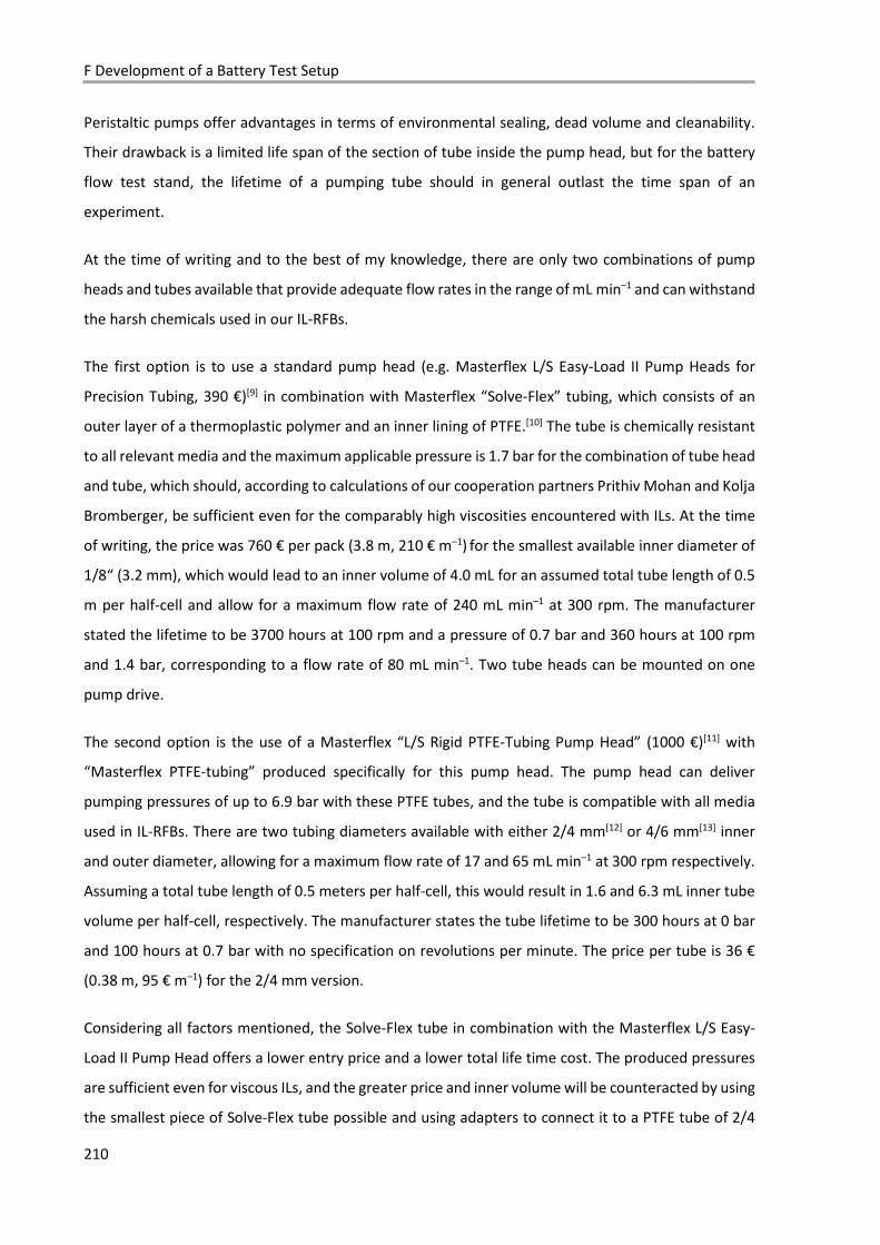
F Development of a Battery Test Setup
210
Peristaltic pumps offer advantages in terms of environmental sealing, dead volume and cleanability.
Their drawback is a limited life span of the section of tube inside the pump head, but for the battery
flow test stand, the lifetime of a pumping tube should in general outlast the time span of an
experiment.
At the time of writing and to the best of my knowledge, there are only two combinations of pump
heads and tubes available that provide adequate flow rates in the range of mL min–1 and can withstand
the harsh chemicals used in our IL-RFBs.
The first option is to use a standard pump head (e.g. Masterflex L/S Easy-Load II Pump Heads for
Precision Tubing, 390 €)[9] in combination with Masterflex “Solve-Flex” tubing, which consists of an
outer layer of a thermoplastic polymer and an inner lining of PTFE.[10] The tube is chemically resistant
to all relevant media and the maximum applicable pressure is 1.7 bar for the combination of tube head
and tube, which should, according to calculations of our cooperation partners Prithiv Mohan and Kolja
Bromberger, be sufficient even for the comparably high viscosities encountered with ILs. At the time
of writing, the price was 760 € per pack (3.8 m, 210 € m–1) for the smallest available inner diameter of
1/8“ (3.2 mm), which would lead to an inner volume of 4.0 mL for an assumed total tube length of 0.5
m per half-cell and allow for a maximum flow rate of 240 mL min–1 at 300 rpm. The manufacturer
stated the lifetime to be 3700 hours at 100 rpm and a pressure of 0.7 bar and 360 hours at 100 rpm
and 1.4 bar, corresponding to a flow rate of 80 mL min–1. Two tube heads can be mounted on one
pump drive.
The second option is the use of a Masterflex “L/S Rigid PTFE-Tubing Pump Head” (1000 €)[11] with
“Masterflex PTFE-tubing” produced specifically for this pump head. The pump head can deliver
pumping pressures of up to 6.9 bar with these PTFE tubes, and the tube is compatible with all media
used in IL-RFBs. There are two tubing diameters available with either 2/4 mm[12] or 4/6 mm[13] inner
and outer diameter, allowing for a maximum flow rate of 17 and 65 mL min–1 at 300 rpm respectively.
Assuming a total tube length of 0.5 meters per half-cell, this would result in 1.6 and 6.3 mL inner tube
volume per half-cell, respectively. The manufacturer states the tube lifetime to be 300 hours at 0 bar
and 100 hours at 0.7 bar with no specification on revolutions per minute. The price per tube is 36 €
(0.38 m, 95 € m–1) for the 2/4 mm version.
Considering all factors mentioned, the Solve-Flex tube in combination with the Masterflex L/S Easy-
Load II Pump Head offers a lower entry price and a lower total life time cost. The produced pressures
are sufficient even for viscous ILs, and the greater price and inner volume will be counteracted by using
the smallest piece of Solve-Flex tube possible and using adapters to connect it to a PTFE tube of 2/4
F.3 Hardware II: Progress Towards a Flow-Battery Test Setup
211
mm inner/outer diameter. Assuming a minimum 0.2 m of Solve-Flex tube and an additional 0.3 m of
2/4 mm PTFE tube per half-cell, the total inner volume of the tubing setup would be 2.55 mL for one
half-cell.
There are computer controllable pump drives available from Masterflex (L/S Computer-Compatible
Digital Drive, 0.1 – 600 rpm)[14] and ISMATEC (MCP Standard, 1 – 240 rpm)[15], which are both
compatible with the Masterflex pump heads specified above. Both utilise the RS-323 interface via a
DE-9 connector. The MCP Standard’s signalling language was considered more flexible and better
documented than the one used for the Masterflex pump drives, but in the end the Masterflex Drive
was chosen because it offered a wider range of revolutions especially at the low end.
F.3.2.2 Cryostats
To control the temperature of the flow setup and allow for a setup like the concept depicted in
Figure 73 b), cryostats of the manufacturers Huber, Lauda, and Julapo were compared. The Huber
Ministat 240[16] was chosen, since it offers a competitive price and is equipped with the Huber Pilot
One controller, which is accessible via LAN, USB and RS-232 interface. Additionally, there are very well
documented Python sample programs to communicate with this controller.[17]
F.3.2.3 Thermal Sensors
To monitor the temperature at different points of the test cell as well as the tanks of the electrolyte, a
Pico TC-08 thermocouple data logger was chosen.[18] It supports monitoring 8 thermocouples, which
are available in PTFE mantled versions and is supplied with a Linux driver. Sample programs exist for
the Raspberry Pi.

F Development of a Battery Test Setup
212

F.3 Hardware II: Progress Towards a Flow-Battery Test Setup
213
References
[1] S. B. Burgenmeister, University of Freiburg, Freiburg, Germany, 2013.
[2] “SCPI. Standard Commands for Programmable Instrumentation”, can be found under
http://www.ivifoundation.org/scpi/, 2017.
[3] “Raspberry Pi - Teach, Learn, and Make with Raspberry Pi”, can be found under
https://www.raspberrypi.org/, 2017.
[4] a) The kernel development community, “Linux kernel coding style”, can be found under
https://kernel.org/doc/html/latest/_sources/process/coding-style.txt, 2016; b) G. van Rossum,
B. Warsaw, N. Coghlan, “PEP 8 -- Style Guide for Python Code. Python.org”, can be found under
https://www.python.org/dev/peps/pep-0008/, 2016; c) P. Armstrong, “Google Shell Style
Guide”, can be found under https://google.github.io/styleguide/shell.xml, 2016.
[5] T. Williams, C. Kelley, gnuplot 4.6, An Interactive Plotting Program, 2014.
[6] S. D. Sharples, “VXI11 Ethernet Protocol for Linux”, can be found under
http://optics.eee.nottingham.ac.uk/vxi11/, 2016.
[7] P. Mohan, Master’s thesis, Fraunhofer ISE, Freiburg, Germany, 2017.
[8] Fluid Metering, Inc., Pump Heads, can be found under
http://fluidmetering.com/pumpheads.html.
[9] “Masterflex L/S Easy-Load II Head with Adjustable Occlusion for Precision Tubing, GZ-77201-60”,
can be found under https://www.coleparmer.com/i/masterflex-l-s-easy-load-ii-head-w-adj-
occlusion-for-precision-tubing/7720160.
[10] “Masterflex Solve-Flex Pump Tubing, L/S 16, 12 ft, GZ-96446-16”, can be found under
https://www.coleparmer.com/i/masterflex-solve-flex-pump-tubing-l-s-16-12-ft/9644616#eb-
item-specification.
[11] “Masterflex L/S Rigid PTFE-Tubing Pump Head, GZ-77390-00”, can be found under
https://www.coleparmer.com/i/masterflex-l-s-rigid-ptfe-tubing-pump-
head/7739000?searchterm=Masterflex+L%2fS+Rigid+PTFE-Tubing+Pump+Head.
[12] “Masterflex PTFE-tubing sets, 2mm ID, 4mm OD, GZ-77390-50”, can be found under
https://www.coleparmer.com/i/masterflex-ptfe-tubing-sets-2mm-id-4mm-od-set-of-
two/7739050.
[13] “Masterflex PTFE-tubing sets, 4mm ID, 6mm OD, GZ-77390-60”, can be found under

F Development of a Battery Test Setup
214
https://www.coleparmer.com/i/masterflex-ptfe-tubing-sets-4mm-id-6mm-od-set-of-
two/7739060.
[14] “Masterflex L/S Computer-Compatible Digital Drive, HV-07551-20”, can be found under
https://www.masterflex.com/i/masterflex-l-s-computer-compatible-digital-drive-0-1-to-600-
rpm-115-230-vac/0755120, 2017.
[15] “Ismatec MCP Standard, ISM 404”, can be found under
http://www.ismatec.com/int_e/pumps/t_mcp_bvp/mcp_stan.htm.
[16] “Huber Ministat 240 Compact cooling bath circulation thermostat, 2016.0005.01”, can be found
under http://www.huber-online.com/en/product_datasheet.aspx?no=2016.0005.01.
[17] Huber AG, pySoftcheck Operation Manual, 2013.
[18] “TC-08 Thermocouple data logger, Pico Technology”, can be found under
https://www.picotech.com/data-logger/tc-08/thermocouple-data-logger
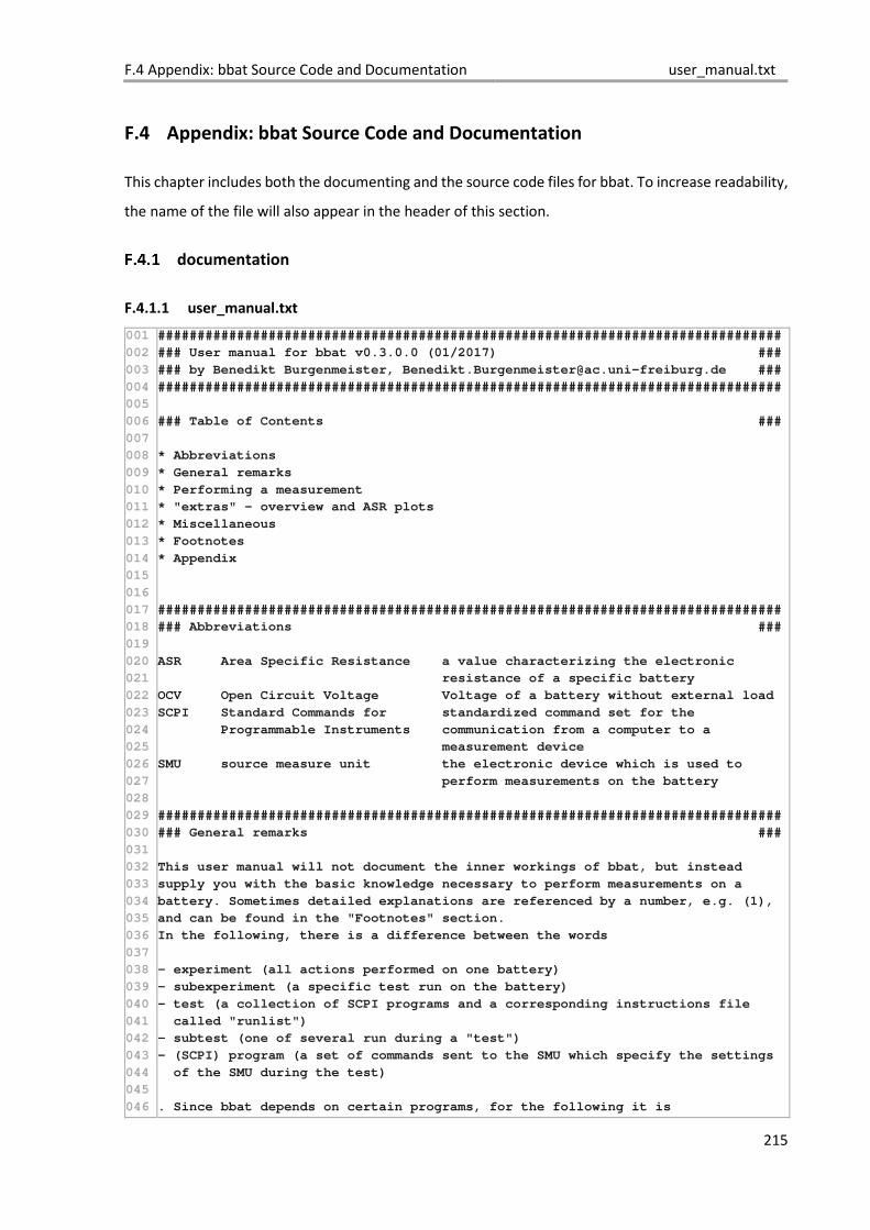
F.4 Appendix: bbat Source Code and Documentation user_manual.txt
215
F.4 Appendix: bbat Source Code and Documentation
This chapter includes both the documenting and the source code files for bbat. To increase readability,
the name of the file will also appear in the header of this section.
documentation
F.4.1.1 user_manual.txt
001
002
003
004
005
006
007
008
009
010
011
012
013
014
015
016
017
018
019
020
021
022
023
024
025
026
027
028
029
030
031
032
033
034
035
036
037
038
039
040
041
042
043
044
045
046
###############################################################################
### User manual for bbat v0.3.0.0 (01/2017) ###
### by Benedikt Burgenmeister, [email protected] ###
###############################################################################
### Table of Contents ###
* Abbreviations
* General remarks
* Performing a measurement
* "extras" - overview and ASR plots
* Miscellaneous
* Footnotes
* Appendix
###############################################################################
### Abbreviations ###
ASR Area Specific Resistance a value characterizing the electronic
resistance of a specific battery
OCV Open Circuit Voltage Voltage of a battery without external load
SCPI Standard Commands for standardized command set for the
Programmable Instruments communication from a computer to a
measurement device
SMU source measure unit the electronic device which is used to
perform measurements on the battery
###############################################################################
### General remarks ###
This user manual will not document the inner workings of bbat, but instead
supply you with the basic knowledge necessary to perform measurements on a
battery. Sometimes detailed explanations are referenced by a number, e.g. (1),
and can be found in the "Footnotes" section.
In the following, there is a difference between the words
- experiment (all actions performed on one battery)
- subexperiment (a specific test run on the battery)
- test (a collection of SCPI programs and a corresponding instructions file
called "runlist")
- subtest (one of several run during a "test")
- (SCPI) program (a set of commands sent to the SMU which specify the settings
of the SMU during the test)
. Since bbat depends on certain programs, for the following it is
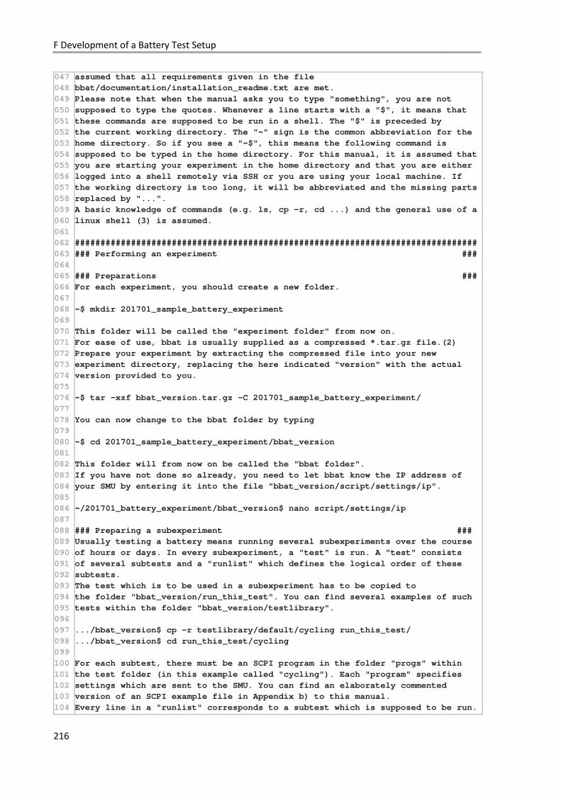
F Development of a Battery Test Setup
216
047
048
049
050
051
052
053
054
055
056
057
058
059
060
061
062
063
064
065
066
067
068
069
070
071
072
073
074
075
076
077
078
079
080
081
082
083
084
085
086
087
088
089
090
091
092
093
094
095
096
097
098
099
100
101
102
103
104
assumed that all requirements given in the file
bbat/documentation/installation_readme.txt are met.
Please note that when the manual asks you to type "something", you are not
supposed to type the quotes. Whenever a line starts with a "$", it means that
these commands are supposed to be run in a shell. The "$" is preceded by
the current working directory. The "~" sign is the common abbreviation for the
home directory. So if you see a "~$", this means the following command is
supposed to be typed in the home directory. For this manual, it is assumed that
you are starting your experiment in the home directory and that you are either
logged into a shell remotely via SSH or you are using your local machine. If
the working directory is too long, it will be abbreviated and the missing parts
replaced by "...".
A basic knowledge of commands (e.g. ls, cp -r, cd ...) and the general use of a
linux shell (3) is assumed.
###############################################################################
### Performing an experiment ###
### Preparations ###
For each experiment, you should create a new folder.
~$ mkdir 201701_sample_battery_experiment
This folder will be called the "experiment folder" from now on.
For ease of use, bbat is usually supplied as a compressed *.tar.gz file.(2)
Prepare your experiment by extracting the compressed file into your new
experiment directory, replacing the here indicated "version" with the actual
version provided to you.
~$ tar -xzf bbat_version.tar.gz -C 201701_sample_battery_experiment/
You can now change to the bbat folder by typing
~$ cd 201701_sample_battery_experiment/bbat_version
This folder will from now on be called the "bbat folder".
If you have not done so already, you need to let bbat know the IP address of
your SMU by entering it into the file "bbat_version/script/settings/ip".
~/201701_battery_experiment/bbat_version$ nano script/settings/ip
### Preparing a subexperiment ###
Usually testing a battery means running several subexperiments over the course
of hours or days. In every subexperiment, a "test" is run. A "test" consists
of several subtests and a "runlist" which defines the logical order of these
subtests.
The test which is to be used in a subexperiment has to be copied to
the folder "bbat_version/run_this_test". You can find several examples of such
tests within the folder "bbat_version/testlibrary".
.../bbat_version$ cp -r testlibrary/default/cycling run_this_test/
.../bbat_version$ cd run_this_test/cycling
For each subtest, there must be an SCPI program in the folder "progs" within
the test folder (in this example called "cycling"). Each "program" specifies
settings which are sent to the SMU. You can find an elaborately commented
version of an SCPI example file in Appendix b) to this manual.
Every line in a "runlist" corresponds to a subtest which is supposed to be run.
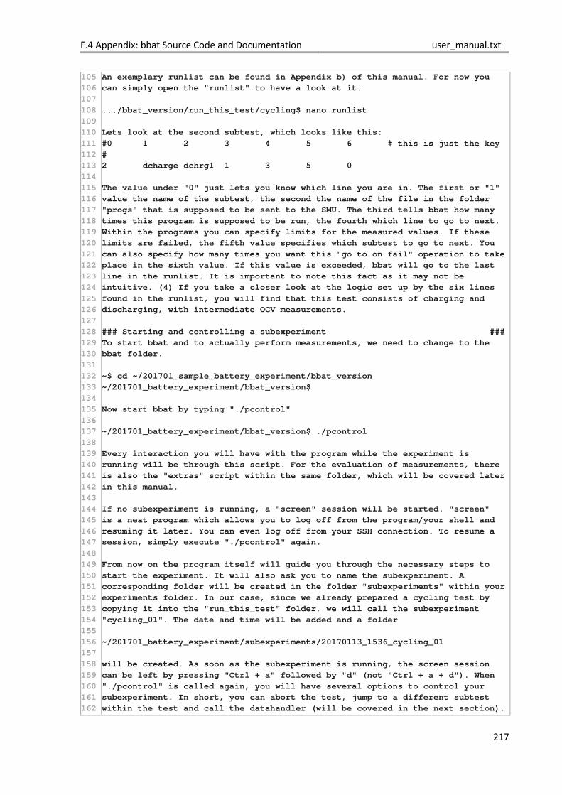
F.4 Appendix: bbat Source Code and Documentation user_manual.txt
217
105
106
107
108
109
110
111
112
113
114
115
116
117
118
119
120
121
122
123
124
125
126
127
128
129
130
131
132
133
134
135
136
137
138
139
140
141
142
143
144
145
146
147
148
149
150
151
152
153
154
155
156
157
158
159
160
161
162
An exemplary runlist can be found in Appendix b) of this manual. For now you
can simply open the "runlist" to have a look at it.
.../bbat_version/run_this_test/cycling$ nano runlist
Lets look at the second subtest, which looks like this:
#0 1 2 3 4 5 6 # this is just the key
#
2 dcharge dchrg1 1 3 5 0
The value under "0" just lets you know which line you are in. The first or "1"
value the name of the subtest, the second the name of the file in the folder
"progs" that is supposed to be sent to the SMU. The third tells bbat how many
times this program is supposed to be run, the fourth which line to go to next.
Within the programs you can specify limits for the measured values. If these
limits are failed, the fifth value specifies which subtest to go to next. You
can also specify how many times you want this "go to on fail" operation to take
place in the sixth value. If this value is exceeded, bbat will go to the last
line in the runlist. It is important to note this fact as it may not be
intuitive. (4) If you take a closer look at the logic set up by the six lines
found in the runlist, you will find that this test consists of charging and
discharging, with intermediate OCV measurements.
### Starting and controlling a subexperiment ###
To start bbat and to actually perform measurements, we need to change to the
bbat folder.
~$ cd ~/201701_sample_battery_experiment/bbat_version
~/201701_battery_experiment/bbat_version$
Now start bbat by typing "./pcontrol"
~/201701_battery_experiment/bbat_version$ ./pcontrol
Every interaction you will have with the program while the experiment is
running will be through this script. For the evaluation of measurements, there
is also the "extras" script within the same folder, which will be covered later
in this manual.
If no subexperiment is running, a "screen" session will be started. "screen"
is a neat program which allows you to log off from the program/your shell and
resuming it later. You can even log off from your SSH connection. To resume a
session, simply execute "./pcontrol" again.
From now on the program itself will guide you through the necessary steps to
start the experiment. It will also ask you to name the subexperiment. A
corresponding folder will be created in the folder "subexperiments" within your
experiments folder. In our case, since we already prepared a cycling test by
copying it into the "run_this_test" folder, we will call the subexperiment
"cycling_01". The date and time will be added and a folder
~/201701_battery_experiment/subexperiments/20170113_1536_cycling_01
will be created. As soon as the subexperiment is running, the screen session
can be left by pressing "Ctrl + a" followed by "d" (not "Ctrl + a + d"). When
"./pcontrol" is called again, you will have several options to control your
subexperiment. In short, you can abort the test, jump to a different subtest
within the test and call the datahandler (will be covered in the next section).
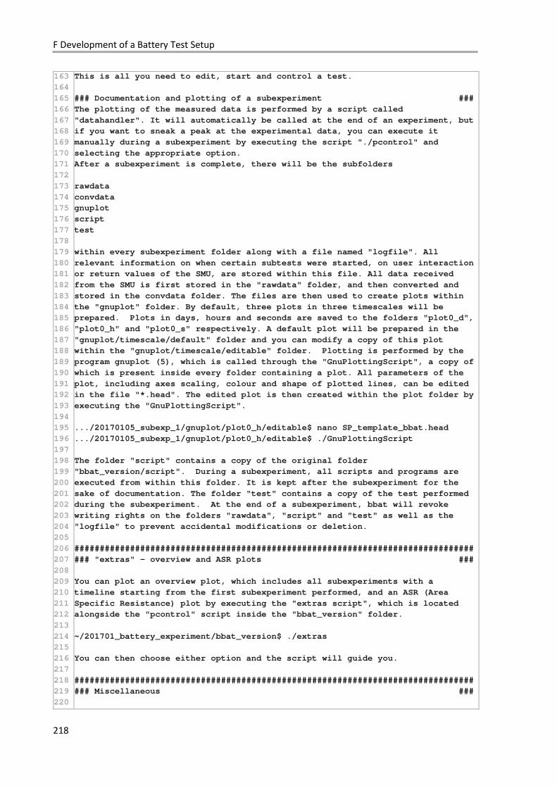
F Development of a Battery Test Setup
218
163
164
165
166
167
168
169
170
171
172
173
174
175
176
177
178
179
180
181
182
183
184
185
186
187
188
189
190
191
192
193
194
195
196
197
198
199
200
201
202
203
204
205
206
207
208
209
210
211
212
213
214
215
216
217
218
219
220
This is all you need to edit, start and control a test.
### Documentation and plotting of a subexperiment ###
The plotting of the measured data is performed by a script called
"datahandler". It will automatically be called at the end of an experiment, but
if you want to sneak a peak at the experimental data, you can execute it
manually during a subexperiment by executing the script "./pcontrol" and
selecting the appropriate option.
After a subexperiment is complete, there will be the subfolders
rawdata
convdata
gnuplot
script
test
within every subexperiment folder along with a file named "logfile". All
relevant information on when certain subtests were started, on user interaction
or return values of the SMU, are stored within this file. All data received
from the SMU is first stored in the "rawdata" folder, and then converted and
stored in the convdata folder. The files are then used to create plots within
the "gnuplot" folder. By default, three plots in three timescales will be
prepared. Plots in days, hours and seconds are saved to the folders "plot0_d",
"plot0_h" and "plot0_s" respectively. A default plot will be prepared in the
"gnuplot/timescale/default" folder and you can modify a copy of this plot
within the "gnuplot/timescale/editable" folder. Plotting is performed by the
program gnuplot (5), which is called through the "GnuPlottingScript", a copy of
which is present inside every folder containing a plot. All parameters of the
plot, including axes scaling, colour and shape of plotted lines, can be edited
in the file "*.head". The edited plot is then created within the plot folder by
executing the "GnuPlottingScript".
.../20170105_subexp_1/gnuplot/plot0_h/editable$ nano SP_template_bbat.head
.../20170105_subexp_1/gnuplot/plot0_h/editable$ ./GnuPlottingScript
The folder "script" contains a copy of the original folder
"bbat_version/script". During a subexperiment, all scripts and programs are
executed from within this folder. It is kept after the subexperiment for the
sake of documentation. The folder "test" contains a copy of the test performed
during the subexperiment. At the end of a subexperiment, bbat will revoke
writing rights on the folders "rawdata", "script" and "test" as well as the
"logfile" to prevent accidental modifications or deletion.
###############################################################################
### "extras" - overview and ASR plots ###
You can plot an overview plot, which includes all subexperiments with a
timeline starting from the first subexperiment performed, and an ASR (Area
Specific Resistance) plot by executing the "extras script", which is located
alongside the "pcontrol" script inside the "bbat_version" folder.
~/201701_battery_experiment/bbat_version$ ./extras
You can then choose either option and the script will guide you.
###############################################################################
### Miscellaneous ###
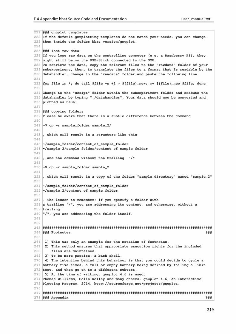
F.4 Appendix: bbat Source Code and Documentation user_manual.txt
219
221
222
223
224
225
226
227
228
229
230
231
232
233
234
235
236
237
238
239
240
241
242
243
244
245
246
247
248
249
250
251
252
253
254
255
256
257
258
259
260
261
262
263
264
265
266
267
268
269
270
271
272
273
274
275
276
277
278
### gnuplot templates
If the default gnuplotting templates do not match your needs, you can change
them inside the folder bbat_version/gnuplot.
### lost raw data
If you lose raw data on the controlling computer (e.g. a Raspberry Pi), they
might still be on the USB-Stick connected to the SMU.
To retrieve the data, copy the relevant files to the "rawdata" folder of your
subexperiment, then, to translate the files to a format that is readable by the
datahandler, change to the "rawdata" folder and paste the following line.
for file in *; do tail $file -n +2 > ${file}_new; mv ${file}_new $file; done
Change to the "script" folder within the subexperiment folder and execute the
datahandler by typing "./datahandler". Your data should now be converted and
plotted as usual.
### copying folders
Please be aware that there is a subtle difference between the command
~$ cp -r sample_folder sample_2/
, which will result in a structure like this
~/sample_folder/content_of_sample_folder
~/sample_2/sample_folder/content_of_sample_folder
, and the command without the trailing "/"
~$ cp -r sample_folder sample_2
, which will result in a copy of the folder "sample_directory" named "sample_2"
~/sample_folder/content_of_sample_folder
~/sample_2/content_of_sample_folder
. The lesson to remember: if you specify a folder with
a trailing "/", you are addressing its content, and otherwise, without a
trailing
"/", you are addressing the folder itself.
###############################################################################
### Footnotes ###
1) This was only an example for the notation of footnotes.
2) This method ensures that appropriate execution rights for the included
files are maintained.
3) To be more precise: a bash shell.
4) The intention behind this behaviour is that you could decide to cycle a
battery five times, a full or empty battery being defined by failing a limit
test, and then go on to a different subtest.
5) At the time of writing, gunplot 4.6 is used:
Thomas Williams, Colin Kelley and many others, gnuplot 4.6, An Interactive
Plotting Program, 2014, http://sourceforge.net/projects/gnuplot.
###############################################################################
### Appendix ###
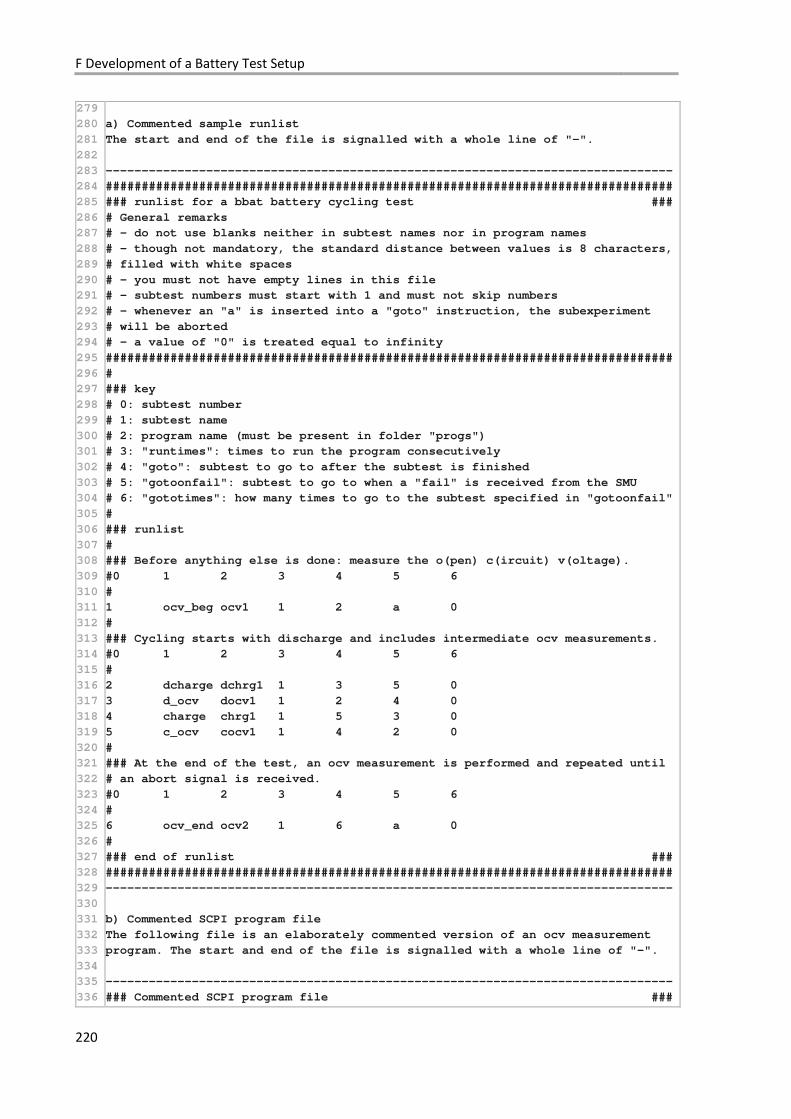
F Development of a Battery Test Setup
220
279
280
281
282
283
284
285
286
287
288
289
290
291
292
293
294
295
296
297
298
299
300
301
302
303
304
305
306
307
308
309
310
311
312
313
314
315
316
317
318
319
320
321
322
323
324
325
326
327
328
329
330
331
332
333
334
335
336
a) Commented sample runlist
The start and end of the file is signalled with a whole line of "-".
-------------------------------------------------------------------------------
###############################################################################
### runlist for a bbat battery cycling test ###
# General remarks
# - do not use blanks neither in subtest names nor in program names
# - though not mandatory, the standard distance between values is 8 characters,
# filled with white spaces
# - you must not have empty lines in this file
# - subtest numbers must start with 1 and must not skip numbers
# - whenever an "a" is inserted into a "goto" instruction, the subexperiment
# will be aborted
# - a value of "0" is treated equal to infinity
###############################################################################
#
### key
# 0: subtest number
# 1: subtest name
# 2: program name (must be present in folder "progs")
# 3: "runtimes": times to run the program consecutively
# 4: "goto": subtest to go to after the subtest is finished
# 5: "gotoonfail": subtest to go to when a "fail" is received from the SMU
# 6: "gototimes": how many times to go to the subtest specified in "gotoonfail"
#
### runlist
#
### Before anything else is done: measure the o(pen) c(ircuit) v(oltage).
#0 1 2 3 4 5 6
#
1 ocv_beg ocv1 1 2 a 0
#
### Cycling starts with discharge and includes intermediate ocv measurements.
#0 1 2 3 4 5 6
#
2 dcharge dchrg1 1 3 5 0
3 d_ocv docv1 1 2 4 0
4 charge chrg1 1 5 3 0
5 c_ocv cocv1 1 4 2 0
#
### At the end of the test, an ocv measurement is performed and repeated until
# an abort signal is received.
#0 1 2 3 4 5 6
#
6 ocv_end ocv2 1 6 a 0
#
### end of runlist ###
###############################################################################
-------------------------------------------------------------------------------
b) Commented SCPI program file
The following file is an elaborately commented version of an ocv measurement
program. The start and end of the file is signalled with a whole line of "-".
-------------------------------------------------------------------------------
### Commented SCPI program file ###
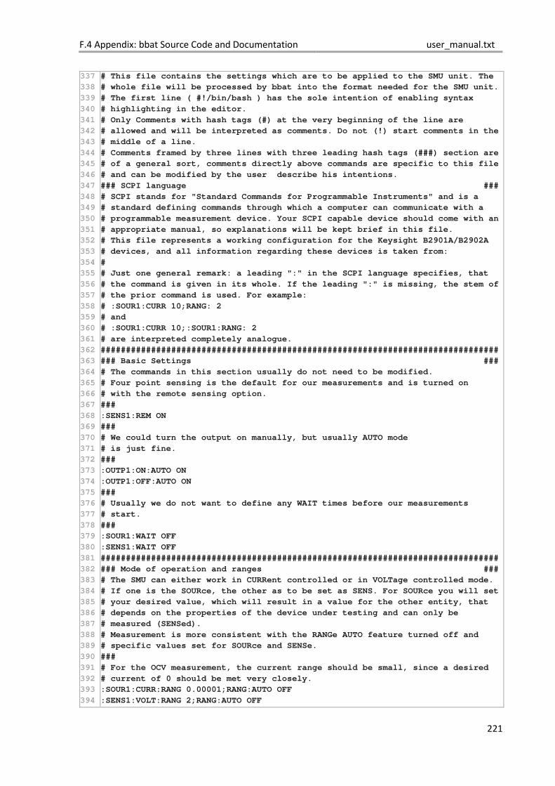
F.4 Appendix: bbat Source Code and Documentation user_manual.txt
221
337
338
339
340
341
342
343
344
345
346
347
348
349
350
351
352
353
354
355
356
357
358
359
360
361
362
363
364
365
366
367
368
369
370
371
372
373
374
375
376
377
378
379
380
381
382
383
384
385
386
387
388
389
390
391
392
393
394
# This file contains the settings which are to be applied to the SMU unit. The
# whole file will be processed by bbat into the format needed for the SMU unit.
# The first line ( #!/bin/bash ) has the sole intention of enabling syntax
# highlighting in the editor.
# Only Comments with hash tags (#) at the very beginning of the line are
# allowed and will be interpreted as comments. Do not (!) start comments in the
# middle of a line.
# Comments framed by three lines with three leading hash tags (###) section are
# of a general sort, comments directly above commands are specific to this file
# and can be modified by the user describe his intentions.
### SCPI language ###
# SCPI stands for "Standard Commands for Programmable Instruments" and is a
# standard defining commands through which a computer can communicate with a
# programmable measurement device. Your SCPI capable device should come with an
# appropriate manual, so explanations will be kept brief in this file.
# This file represents a working configuration for the Keysight B2901A/B2902A
# devices, and all information regarding these devices is taken from:
#
# Just one general remark: a leading ":" in the SCPI language specifies, that
# the command is given in its whole. If the leading ":" is missing, the stem of
# the prior command is used. For example:
# :SOUR1:CURR 10;RANG: 2
# and
# :SOUR1:CURR 10;:SOUR1:RANG: 2
# are interpreted completely analogue.
###############################################################################
### Basic Settings ###
# The commands in this section usually do not need to be modified.
# Four point sensing is the default for our measurements and is turned on
# with the remote sensing option.
###
:SENS1:REM ON
###
# We could turn the output on manually, but usually AUTO mode
# is just fine.
###
:OUTP1:ON:AUTO ON
:OUTP1:OFF:AUTO ON
###
# Usually we do not want to define any WAIT times before our measurements
# start.
###
:SOUR1:WAIT OFF
:SENS1:WAIT OFF
###############################################################################
### Mode of operation and ranges ###
# The SMU can either work in CURRent controlled or in VOLTage controlled mode.
# If one is the SOURce, the other as to be set as SENS. For SOURce you will set
# your desired value, which will result in a value for the other entity, that
# depends on the properties of the device under testing and can only be
# measured (SENSed).
# Measurement is more consistent with the RANGe AUTO feature turned off and
# specific values set for SOURce and SENSe.
###
# For the OCV measurement, the current range should be small, since a desired
# current of 0 should be met very closely.
:SOUR1:CURR:RANG 0.00001;RANG:AUTO OFF
:SENS1:VOLT:RANG 2;RANG:AUTO OFF
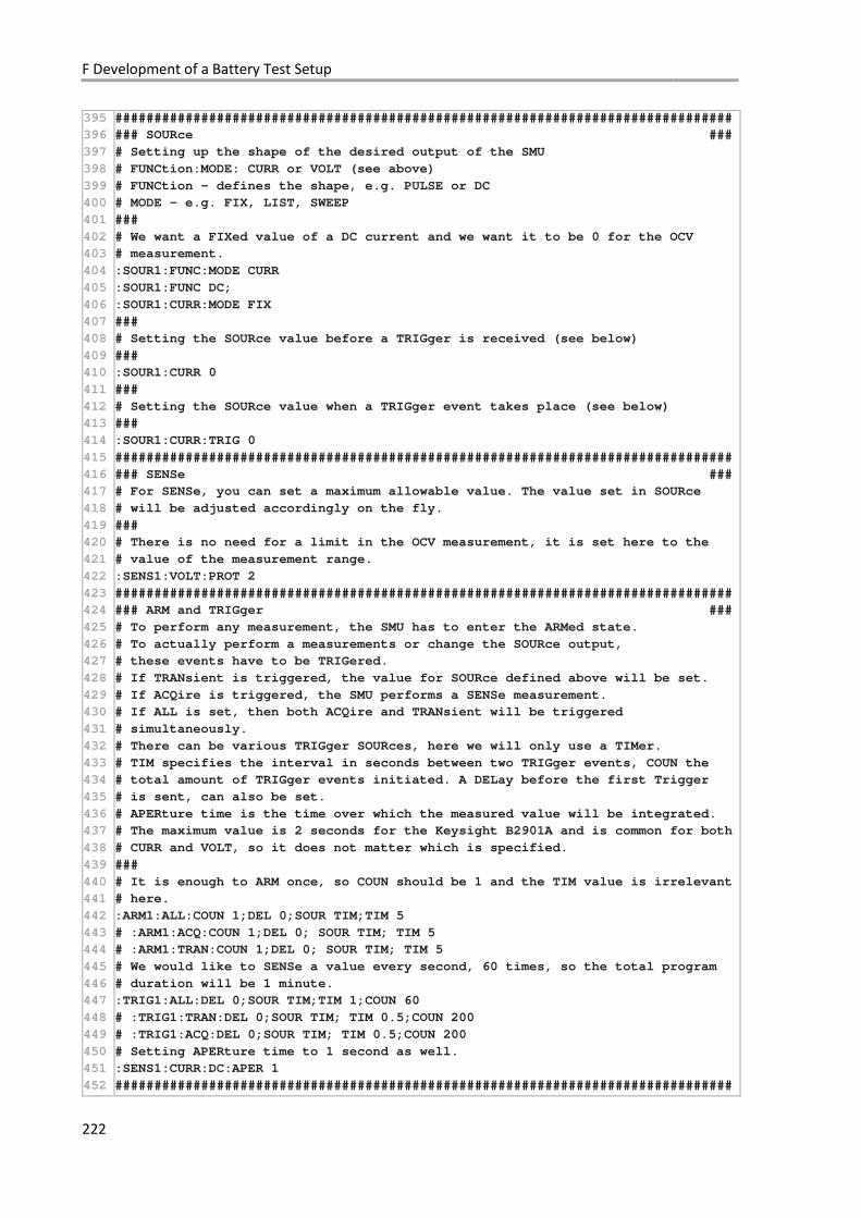
F Development of a Battery Test Setup
222
395
396
397
398
399
400
401
402
403
404
405
406
407
408
409
410
411
412
413
414
415
416
417
418
419
420
421
422
423
424
425
426
427
428
429
430
431
432
433
434
435
436
437
438
439
440
441
442
443
444
445
446
447
448
449
450
451
452
###############################################################################
### SOURce ###
# Setting up the shape of the desired output of the SMU
# FUNCtion:MODE: CURR or VOLT (see above)
# FUNCtion - defines the shape, e.g. PULSE or DC
# MODE - e.g. FIX, LIST, SWEEP
###
# We want a FIXed value of a DC current and we want it to be 0 for the OCV
# measurement.
:SOUR1:FUNC:MODE CURR
:SOUR1:FUNC DC;
:SOUR1:CURR:MODE FIX
###
# Setting the SOURce value before a TRIGger is received (see below)
###
:SOUR1:CURR 0
###
# Setting the SOURce value when a TRIGger event takes place (see below)
###
:SOUR1:CURR:TRIG 0
###############################################################################
### SENSe ###
# For SENSe, you can set a maximum allowable value. The value set in SOURce
# will be adjusted accordingly on the fly.
###
# There is no need for a limit in the OCV measurement, it is set here to the
# value of the measurement range.
:SENS1:VOLT:PROT 2
###############################################################################
### ARM and TRIGger ###
# To perform any measurement, the SMU has to enter the ARMed state.
# To actually perform a measurements or change the SOURce output,
# these events have to be TRIGered.
# If TRANsient is triggered, the value for SOURce defined above will be set.
# If ACQire is triggered, the SMU performs a SENSe measurement.
# If ALL is set, then both ACQire and TRANsient will be triggered
# simultaneously.
# There can be various TRIGger SOURces, here we will only use a TIMer.
# TIM specifies the interval in seconds between two TRIGger events, COUN the
# total amount of TRIGger events initiated. A DELay before the first Trigger
# is sent, can also be set.
# APERture time is the time over which the measured value will be integrated.
# The maximum value is 2 seconds for the Keysight B2901A and is common for both
# CURR and VOLT, so it does not matter which is specified.
###
# It is enough to ARM once, so COUN should be 1 and the TIM value is irrelevant
# here.
:ARM1:ALL:COUN 1;DEL 0;SOUR TIM;TIM 5
# :ARM1:ACQ:COUN 1;DEL 0; SOUR TIM; TIM 5
# :ARM1:TRAN:COUN 1;DEL 0; SOUR TIM; TIM 5
# We would like to SENSe a value every second, 60 times, so the total program
# duration will be 1 minute.
:TRIG1:ALL:DEL 0;SOUR TIM;TIM 1;COUN 60
# :TRIG1:TRAN:DEL 0;SOUR TIM; TIM 0.5;COUN 200
# :TRIG1:ACQ:DEL 0;SOUR TIM; TIM 0.5;COUN 200
# Setting APERture time to 1 second as well.
:SENS1:CURR:DC:APER 1
###############################################################################
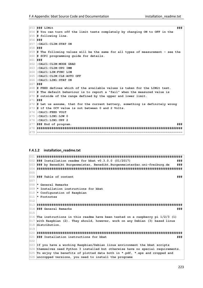
F.4 Appendix: bbat Source Code and Documentation installation_readme.txt
223
453
454
455
456
457
458
459
460
461
462
463
464
465
466
467
468
469
470
471
472
473
474
475
476
477
478
479
### LIMit ###
# You can turn off the limit tests completely by changing ON to OFF in the
# following line.
###
:CALC1:CLIM:STAT ON
###
# The following values will be the same for all types of measurement - see the
# SCPI programming guide for details.
###
:CALC1:CLIM:MODE GRAD
:CALC1:CLIM:UPD IMM
:CALC1:LIM:FUNC LIM
:CALC1:CLIM:CLE:AUTO OFF
:CALC1:LIM1:STAT ON
###
# FEED defines which of the available values is taken for the LIMit test.
# The default behaviour is to report a "fail" when the measured value is
# outside of the range defined by the upper and lower limit.
###
# Let us assume, that for the current battery, something is definitely wrong
# if the OCV value is not between 0 and 2 Volts.
:CALC1:FEED VOLT
:CALC1:LIM1:LOW 0
:CALC1:LIM1:UPP 2
### End of program. ###
###############################################################################
-------------------------------------------------------------------------------
F.4.1.2 installation_readme.txt
001
002
003
004
005
006
007
008
009
010
011
012
013
014
015
016
017
018
019
020
021
022
023
024
025
026
###############################################################################
### Installation readme for bbat v0.3.0.0 (01/2017) ###
### by Benedikt Burgenmeister, [email protected] ###
###############################################################################
### Table of content ###
* General Remarks
* Installation instructions for bbat
* Configuration of Raspbian
* Footnotes
###############################################################################
### General Remarks ###
The instructions in this readme have been tested on a raspberry pi 1/2/3 (1)
with Raspbian (2). They should, however, work on any Debian (3) based linux
distribution.
###############################################################################
### Installation instructions for bbat ###
If you have a working Raspbian/Debian linux environment the bbat scripts
themselves need Python 3 installed but otherwise have no special requirements.
To enjoy the benefits of plotted data both in *.pdf, *.eps and cropped and
uncropped versions, you need to install the programs
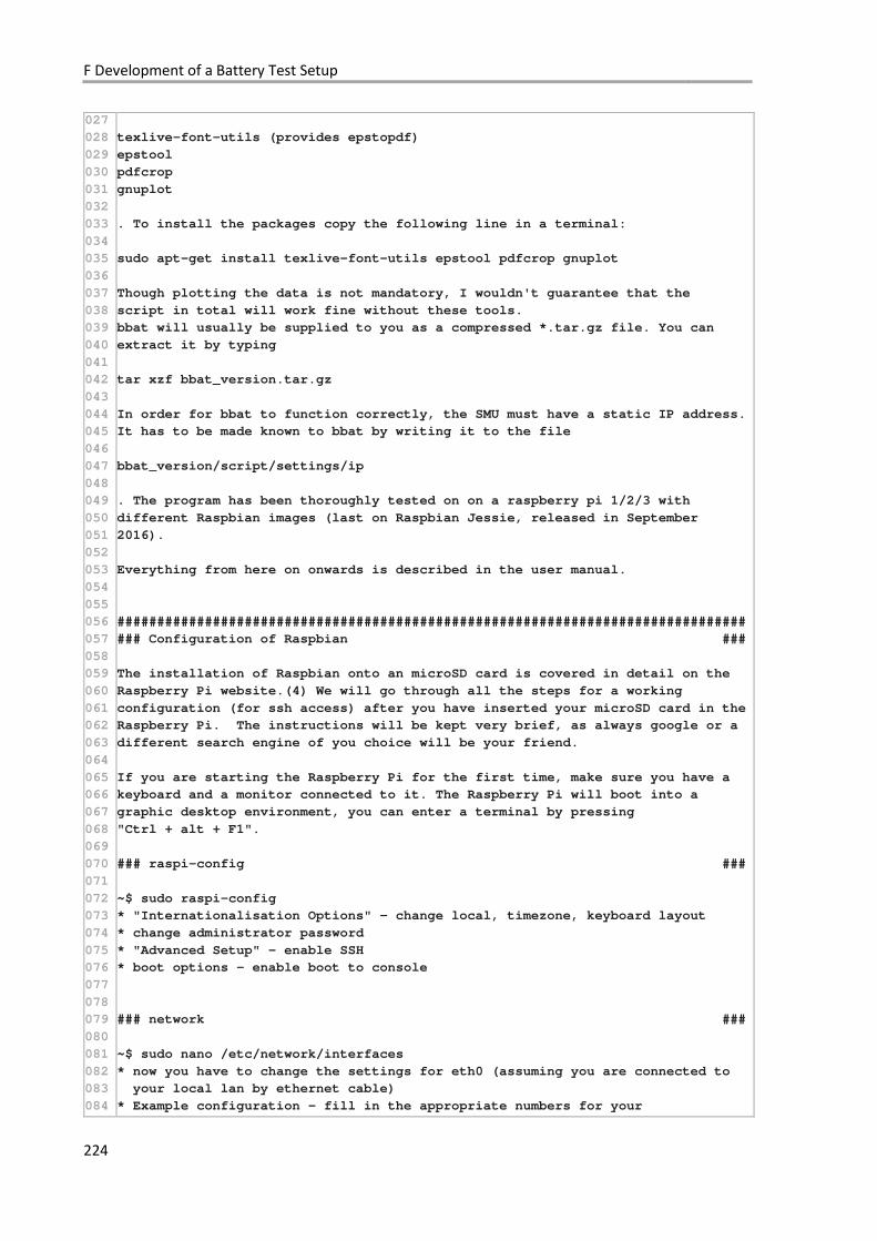
F Development of a Battery Test Setup
224
027
028
029
030
031
032
033
034
035
036
037
038
039
040
041
042
043
044
045
046
047
048
049
050
051
052
053
054
055
056
057
058
059
060
061
062
063
064
065
066
067
068
069
070
071
072
073
074
075
076
077
078
079
080
081
082
083
084
texlive-font-utils (provides epstopdf)
epstool
pdfcrop
gnuplot
. To install the packages copy the following line in a terminal:
sudo apt-get install texlive-font-utils epstool pdfcrop gnuplot
Though plotting the data is not mandatory, I wouldn't guarantee that the
script in total will work fine without these tools.
bbat will usually be supplied to you as a compressed *.tar.gz file. You can
extract it by typing
tar xzf bbat_version.tar.gz
In order for bbat to function correctly, the SMU must have a static IP address.
It has to be made known to bbat by writing it to the file
bbat_version/script/settings/ip
. The program has been thoroughly tested on on a raspberry pi 1/2/3 with
different Raspbian images (last on Raspbian Jessie, released in September
2016).
Everything from here on onwards is described in the user manual.
###############################################################################
### Configuration of Raspbian ###
The installation of Raspbian onto an microSD card is covered in detail on the
Raspberry Pi website.(4) We will go through all the steps for a working
configuration (for ssh access) after you have inserted your microSD card in the
Raspberry Pi. The instructions will be kept very brief, as always google or a
different search engine of you choice will be your friend.
If you are starting the Raspberry Pi for the first time, make sure you have a
keyboard and a monitor connected to it. The Raspberry Pi will boot into a
graphic desktop environment, you can enter a terminal by pressing
"Ctrl + alt + F1".
### raspi-config ###
~$ sudo raspi-config
* "Internationalisation Options" - change local, timezone, keyboard layout
* change administrator password
* "Advanced Setup" - enable SSH
* boot options - enable boot to console
### network ###
~$ sudo nano /etc/network/interfaces
* now you have to change the settings for eth0 (assuming you are connected to
your local lan by ethernet cable)
* Example configuration - fill in the appropriate numbers for your
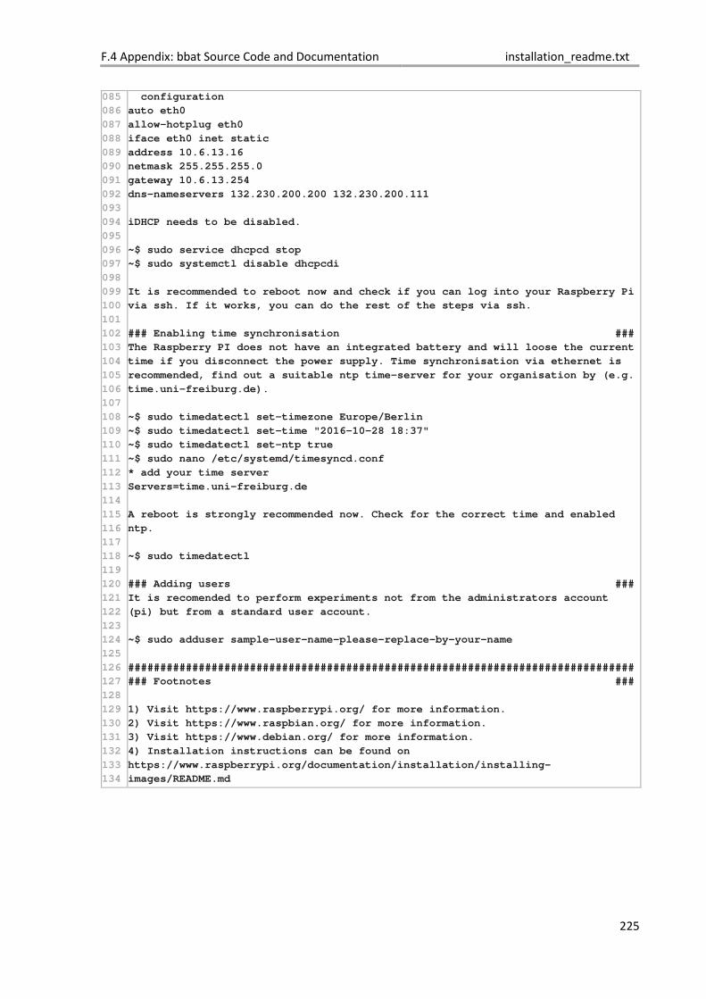
F.4 Appendix: bbat Source Code and Documentation installation_readme.txt
225
085
086
087
088
089
090
091
092
093
094
095
096
097
098
099
100
101
102
103
104
105
106
107
108
109
110
111
112
113
114
115
116
117
118
119
120
121
122
123
124
125
126
127
128
129
130
131
132
133
134
configuration
auto eth0
allow-hotplug eth0
iface eth0 inet static
address 10.6.13.16
netmask 255.255.255.0
gateway 10.6.13.254
dns-nameservers 132.230.200.200 132.230.200.111
iDHCP needs to be disabled.
~$ sudo service dhcpcd stop
~$ sudo systemctl disable dhcpcdi
It is recommended to reboot now and check if you can log into your Raspberry Pi
via ssh. If it works, you can do the rest of the steps via ssh.
### Enabling time synchronisation ###
The Raspberry PI does not have an integrated battery and will loose the current
time if you disconnect the power supply. Time synchronisation via ethernet is
recommended, find out a suitable ntp time-server for your organisation by (e.g.
time.uni-freiburg.de).
~$ sudo timedatectl set-timezone Europe/Berlin
~$ sudo timedatectl set-time "2016-10-28 18:37"
~$ sudo timedatectl set-ntp true
~$ sudo nano /etc/systemd/timesyncd.conf
* add your time server
Servers=time.uni-freiburg.de
A reboot is strongly recommended now. Check for the correct time and enabled
ntp.
~$ sudo timedatectl
### Adding users ###
It is recomended to perform experiments not from the administrators account
(pi) but from a standard user account.
~$ sudo adduser sample-user-name-please-replace-by-your-name
###############################################################################
### Footnotes ###
1) Visit https://www.raspberrypi.org/ for more information.
2) Visit https://www.raspbian.org/ for more information.
3) Visit https://www.debian.org/ for more information.
4) Installation instructions can be found on
https://www.raspberrypi.org/documentation/installation/installing-
images/README.md
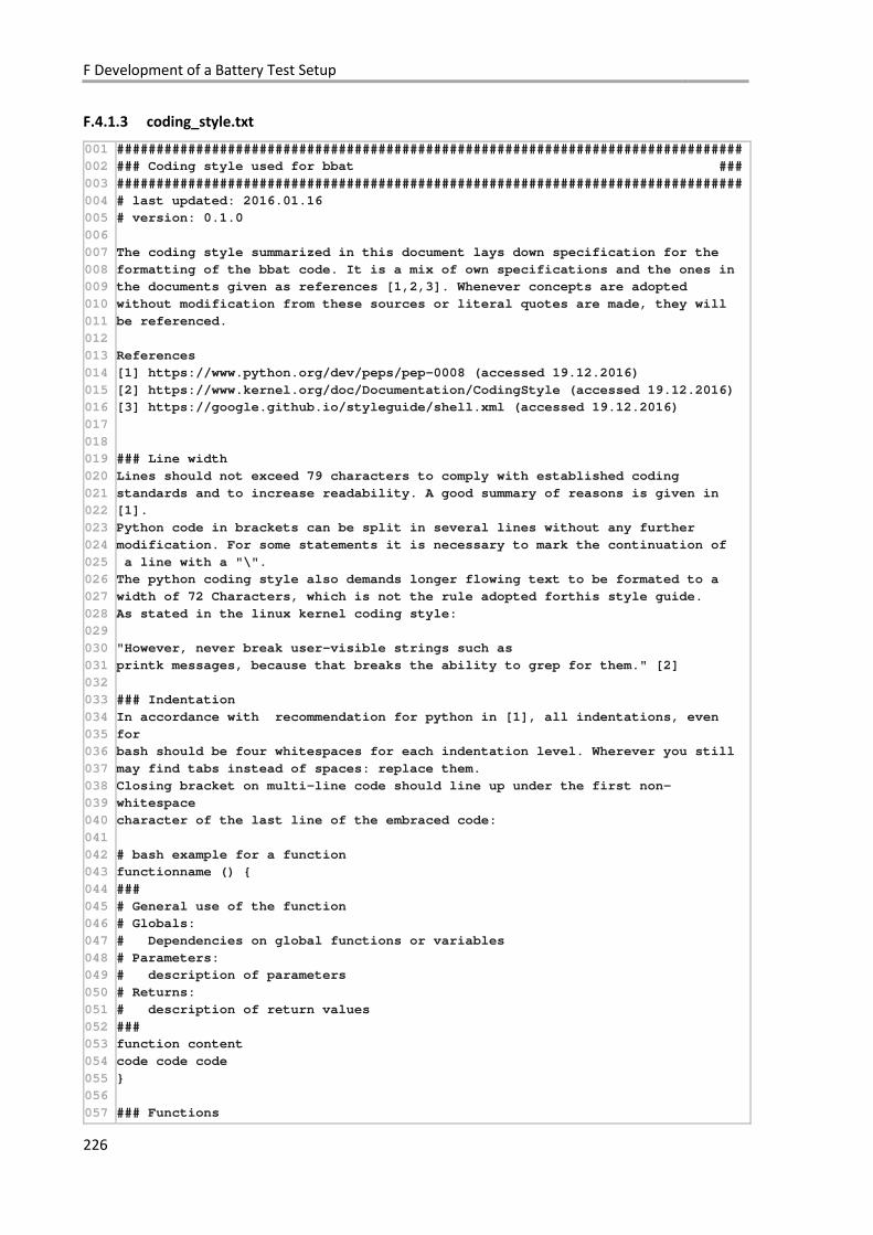
F Development of a Battery Test Setup
226
F.4.1.3 coding_style.txt
001
002
003
004
005
006
007
008
009
010
011
012
013
014
015
016
017
018
019
020
021
022
023
024
025
026
027
028
029
030
031
032
033
034
035
036
037
038
039
040
041
042
043
044
045
046
047
048
049
050
051
052
053
054
055
056
057
###############################################################################
### Coding style used for bbat ###
###############################################################################
# last updated: 2016.01.16
# version: 0.1.0
The coding style summarized in this document lays down specification for the
formatting of the bbat code. It is a mix of own specifications and the ones in
the documents given as references [1,2,3]. Whenever concepts are adopted
without modification from these sources or literal quotes are made, they will
be referenced.
References
[1] https://www.python.org/dev/peps/pep-0008 (accessed 19.12.2016)
[2] https://www.kernel.org/doc/Documentation/CodingStyle (accessed 19.12.2016)
[3] https://google.github.io/styleguide/shell.xml (accessed 19.12.2016)
### Line width
Lines should not exceed 79 characters to comply with established coding
standards and to increase readability. A good summary of reasons is given in
[1].
Python code in brackets can be split in several lines without any further
modification. For some statements it is necessary to mark the continuation of
a line with a "\".
The python coding style also demands longer flowing text to be formated to a
width of 72 Characters, which is not the rule adopted forthis style guide.
As stated in the linux kernel coding style:
"However, never break user-visible strings such as
printk messages, because that breaks the ability to grep for them." [2]
### Indentation
In accordance with recommendation for python in [1], all indentations, even
for
bash should be four whitespaces for each indentation level. Wherever you still
may find tabs instead of spaces: replace them.
Closing bracket on multi-line code should line up under the first non-
whitespace
character of the last line of the embraced code:
# bash example for a function
functionname () {
###
# General use of the function
# Globals:
# Dependencies on global functions or variables
# Parameters:
# description of parameters
# Returns:
# description of return values
###
function content
code code code
}
### Functions
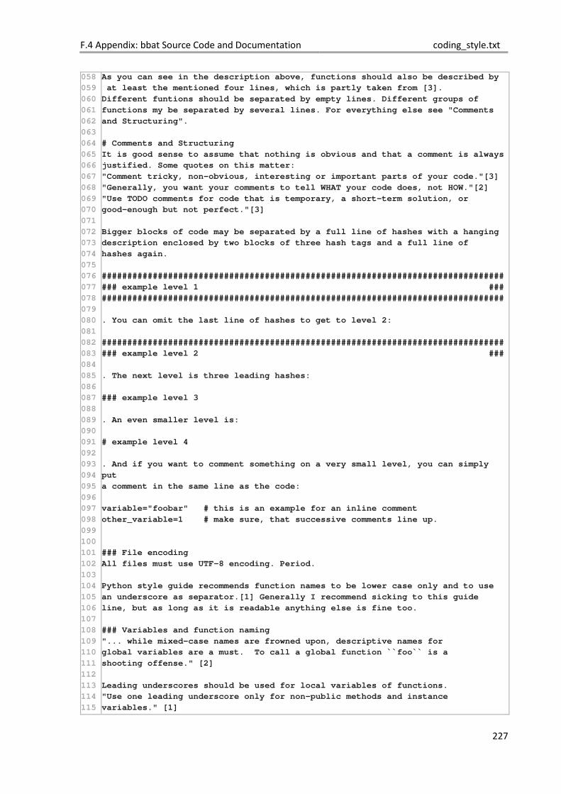
F.4 Appendix: bbat Source Code and Documentation coding_style.txt
227
058
059
060
061
062
063
064
065
066
067
068
069
070
071
072
073
074
075
076
077
078
079
080
081
082
083
084
085
086
087
088
089
090
091
092
093
094
095
096
097
098
099
100
101
102
103
104
105
106
107
108
109
110
111
112
113
114
115
As you can see in the description above, functions should also be described by
at least the mentioned four lines, which is partly taken from [3].
Different funtions should be separated by empty lines. Different groups of
functions my be separated by several lines. For everything else see "Comments
and Structuring".
# Comments and Structuring
It is good sense to assume that nothing is obvious and that a comment is always
justified. Some quotes on this matter:
"Comment tricky, non-obvious, interesting or important parts of your code."[3]
"Generally, you want your comments to tell WHAT your code does, not HOW."[2]
"Use TODO comments for code that is temporary, a short-term solution, or
good-enough but not perfect."[3]
Bigger blocks of code may be separated by a full line of hashes with a hanging
description enclosed by two blocks of three hash tags and a full line of
hashes again.
###############################################################################
### example level 1 ###
###############################################################################
. You can omit the last line of hashes to get to level 2:
###############################################################################
### example level 2 ###
. The next level is three leading hashes:
### example level 3
. An even smaller level is:
# example level 4
. And if you want to comment something on a very small level, you can simply
put
a comment in the same line as the code:
variable="foobar" # this is an example for an inline comment
other_variable=1 # make sure, that successive comments line up.
### File encoding
All files must use UTF-8 encoding. Period.
Python style guide recommends function names to be lower case only and to use
an underscore as separator.[1] Generally I recommend sicking to this guide
line, but as long as it is readable anything else is fine too.
### Variables and function naming
"... while mixed-case names are frowned upon, descriptive names for
global variables are a must. To call a global function ``foo`` is a
shooting offense." [2]
Leading underscores should be used for local variables of functions.
"Use one leading underscore only for non-public methods and instance
variables." [1]
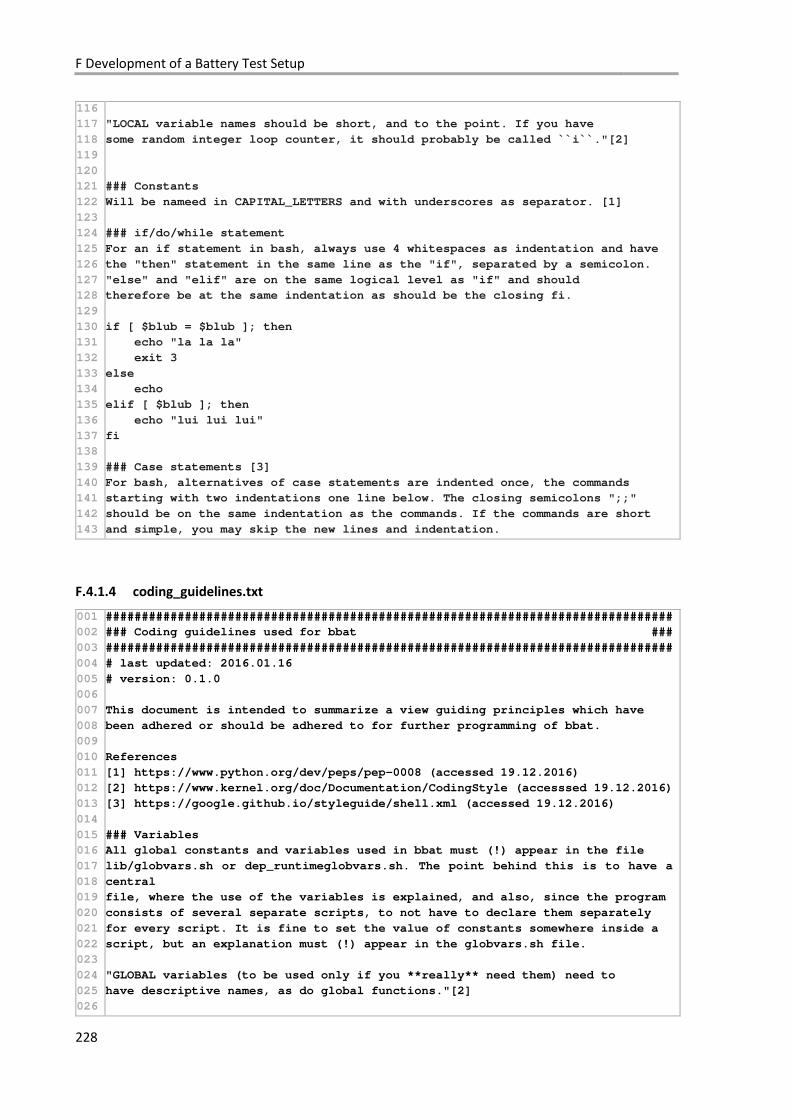
F Development of a Battery Test Setup
228
116
117
118
119
120
121
122
123
124
125
126
127
128
129
130
131
132
133
134
135
136
137
138
139
140
141
142
143
"LOCAL variable names should be short, and to the point. If you have
some random integer loop counter, it should probably be called ``i``."[2]
### Constants
Will be nameed in CAPITAL_LETTERS and with underscores as separator. [1]
### if/do/while statement
For an if statement in bash, always use 4 whitespaces as indentation and have
the "then" statement in the same line as the "if", separated by a semicolon.
"else" and "elif" are on the same logical level as "if" and should
therefore be at the same indentation as should be the closing fi.
if [ $blub = $blub ]; then
echo "la la la"
exit 3
else
echo
elif [ $blub ]; then
echo "lui lui lui"
fi
### Case statements [3]
For bash, alternatives of case statements are indented once, the commands
starting with two indentations one line below. The closing semicolons ";;"
should be on the same indentation as the commands. If the commands are short
and simple, you may skip the new lines and indentation.
F.4.1.4 coding_guidelines.txt
001
002
003
004
005
006
007
008
009
010
011
012
013
014
015
016
017
018
019
020
021
022
023
024
025
026
###############################################################################
### Coding guidelines used for bbat ###
###############################################################################
# last updated: 2016.01.16
# version: 0.1.0
This document is intended to summarize a view guiding principles which have
been adhered or should be adhered to for further programming of bbat.
References
[1] https://www.python.org/dev/peps/pep-0008 (accessed 19.12.2016)
[2] https://www.kernel.org/doc/Documentation/CodingStyle (accesssed 19.12.2016)
[3] https://google.github.io/styleguide/shell.xml (accessed 19.12.2016)
### Variables
All global constants and variables used in bbat must (!) appear in the file
lib/globvars.sh or dep_runtimeglobvars.sh. The point behind this is to have a
central
file, where the use of the variables is explained, and also, since the program
consists of several separate scripts, to not have to declare them separately
for every script. It is fine to set the value of constants somewhere inside a
script, but an explanation must (!) appear in the globvars.sh file.
"GLOBAL variables (to be used only if you **really** need them) need to
have descriptive names, as do global functions."[2]
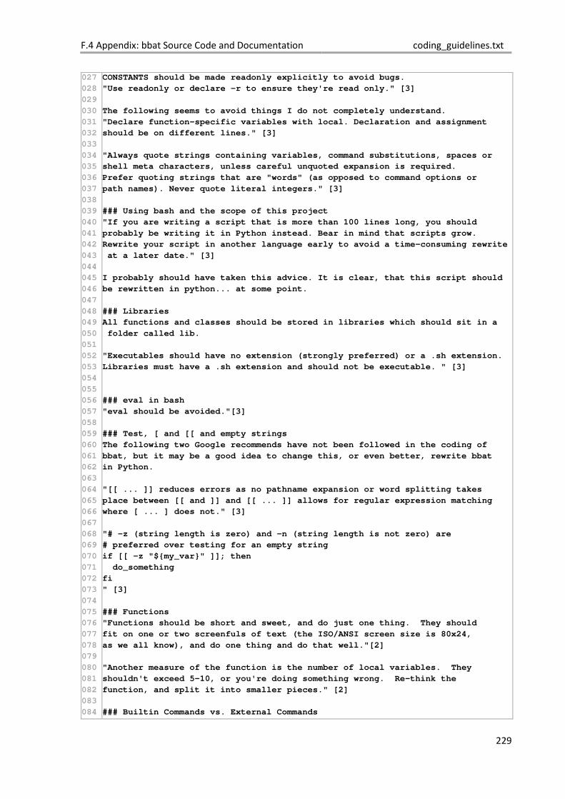
F.4 Appendix: bbat Source Code and Documentation coding_guidelines.txt
229
027
028
029
030
031
032
033
034
035
036
037
038
039
040
041
042
043
044
045
046
047
048
049
050
051
052
053
054
055
056
057
058
059
060
061
062
063
064
065
066
067
068
069
070
071
072
073
074
075
076
077
078
079
080
081
082
083
084
CONSTANTS should be made readonly explicitly to avoid bugs.
"Use readonly or declare -r to ensure they're read only." [3]
The following seems to avoid things I do not completely understand.
"Declare function-specific variables with local. Declaration and assignment
should be on different lines." [3]
"Always quote strings containing variables, command substitutions, spaces or
shell meta characters, unless careful unquoted expansion is required.
Prefer quoting strings that are "words" (as opposed to command options or
path names). Never quote literal integers." [3]
### Using bash and the scope of this project
"If you are writing a script that is more than 100 lines long, you should
probably be writing it in Python instead. Bear in mind that scripts grow.
Rewrite your script in another language early to avoid a time-consuming rewrite
at a later date." [3]
I probably should have taken this advice. It is clear, that this script should
be rewritten in python... at some point.
### Libraries
All functions and classes should be stored in libraries which should sit in a
folder called lib.
"Executables should have no extension (strongly preferred) or a .sh extension.
Libraries must have a .sh extension and should not be executable. " [3]
### eval in bash
"eval should be avoided."[3]
### Test, [ and [[ and empty strings
The following two Google recommends have not been followed in the coding of
bbat, but it may be a good idea to change this, or even better, rewrite bbat
in Python.
"[[ ... ]] reduces errors as no pathname expansion or word splitting takes
place between [[ and ]] and [[ ... ]] allows for regular expression matching
where [ ... ] does not." [3]
"# -z (string length is zero) and -n (string length is not zero) are
# preferred over testing for an empty string
if [[ -z "${my_var}" ]]; then
do_something
fi
" [3]
### Functions
"Functions should be short and sweet, and do just one thing. They should
fit on one or two screenfuls of text (the ISO/ANSI screen size is 80x24,
as we all know), and do one thing and do that well."[2]
"Another measure of the function is the number of local variables. They
shouldn't exceed 5-10, or you're doing something wrong. Re-think the
function, and split it into smaller pieces." [2]
### Builtin Commands vs. External Commands
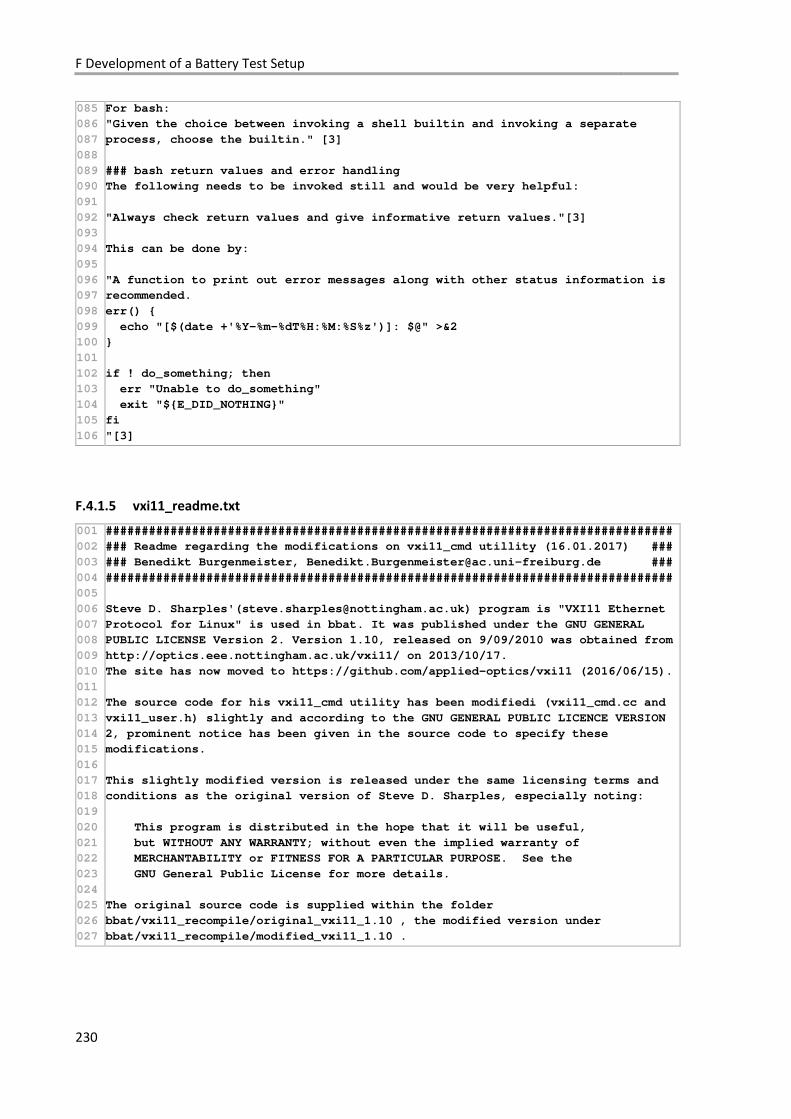
F Development of a Battery Test Setup
230
085
086
087
088
089
090
091
092
093
094
095
096
097
098
099
100
101
102
103
104
105
106
For bash:
"Given the choice between invoking a shell builtin and invoking a separate
process, choose the builtin." [3]
### bash return values and error handling
The following needs to be invoked still and would be very helpful:
"Always check return values and give informative return values."[3]
This can be done by:
"A function to print out error messages along with other status information is
recommended.
err() {
echo "[$(date +'%Y-%m-%dT%H:%M:%S%z')]: $@" >&2
}
if ! do_something; then
err "Unable to do_something"
exit "${E_DID_NOTHING}"
fi
"[3]
F.4.1.5 vxi11_readme.txt
001
002
003
004
005
006
007
008
009
010
011
012
013
014
015
016
017
018
019
020
021
022
023
024
025
026
027
###############################################################################
### Readme regarding the modifications on vxi11_cmd utillity (16.01.2017) ###
### Benedikt Burgenmeister, [email protected] ###
###############################################################################
Steve D. Sharples'([email protected]) program is "VXI11 Ethernet
Protocol for Linux" is used in bbat. It was published under the GNU GENERAL
PUBLIC LICENSE Version 2. Version 1.10, released on 9/09/2010 was obtained from
http://optics.eee.nottingham.ac.uk/vxi11/ on 2013/10/17.
The site has now moved to https://github.com/applied-optics/vxi11 (2016/06/15).
The source code for his vxi11_cmd utility has been modifiedi (vxi11_cmd.cc and
vxi11_user.h) slightly and according to the GNU GENERAL PUBLIC LICENCE VERSION
2, prominent notice has been given in the source code to specify these
modifications.
This slightly modified version is released under the same licensing terms and
conditions as the original version of Steve D. Sharples, especially noting:
This program is distributed in the hope that it will be useful,
but WITHOUT ANY WARRANTY; without even the implied warranty of
MERCHANTABILITY or FITNESS FOR A PARTICULAR PURPOSE. See the
GNU General Public License for more details.
The original source code is supplied within the folder
bbat/vxi11_recompile/original_vxi11_1.10 , the modified version under
bbat/vxi11_recompile/modified_vxi11_1.10 .
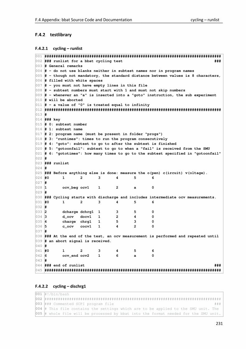
F.4 Appendix: bbat Source Code and Documentation cycling – runlist
231
testlibrary
F.4.2.1 cycling – runlist
001
002
003
004
005
006
007
008
009
010
011
012
013
014
015
016
017
018
019
020
021
022
023
024
025
026
027
028
029
030
031
032
033
034
035
036
037
038
039
040
041
042
043
044
045
###############################################################################
### runlist for a bbat cycling test ###
# General remarks
# - do not use blanks neither in subtest names nor in program names
# - though not mandatory, the standard distance between values is 8 characters,
# filled with white spaces
# - you must not have empty lines in this file
# - subtest numbers must start with 1 and must not skip numbers
# - whenever an "a" is inserted into a "goto" instruction, the sub experiment
# will be aborted
# - a value of "0" is treated equal to infinity
###############################################################################
#
### key
# 0: subtest number
# 1: subtest name
# 2: program name (must be present in folder "progs")
# 3: "runtimes": times to run the program consecutively
# 4: "goto": subtest to go to after the subtest is finished
# 5: "gotoonfail": subtest to go to when a "fail" is received from the SMU
# 6: "gototimes": how many times to go to the subtest specified in "gotoonfail"
#
### runlist
#
### Before anything else is done: measure the o(pen) c(ircuit) v(oltage).
#0 1 2 3 4 5 6
#
1 ocv_beg ocv1 1 2 a 0
#
### Cycling starts with discharge and includes intermediate ocv measurements.
#0 1 2 3 4 5 6
#
2 dcharge dchrg1 1 3 5 0
3 d_ocv docv1 1 2 4 0
4 charge chrg1 1 5 3 0
5 c_ocv cocv1 1 4 2 0
#
### At the end of the test, an ocv measurement is performed and repeated until
# an abort signal is received.
#
#0 1 2 3 4 5 6
6 ocv_end ocv2 1 6 a 0
#
### end of runlist ###
###############################################################################
F.4.2.2 cycling – dischrg1
001
002
003
004
005
#!/bin/bash
###############################################################################
### Commented SCPI program file ###
# This file contains the settings which are to be applied to the SMU unit. The
# whole file will be processed by bbat into the format needed for the SMU unit.
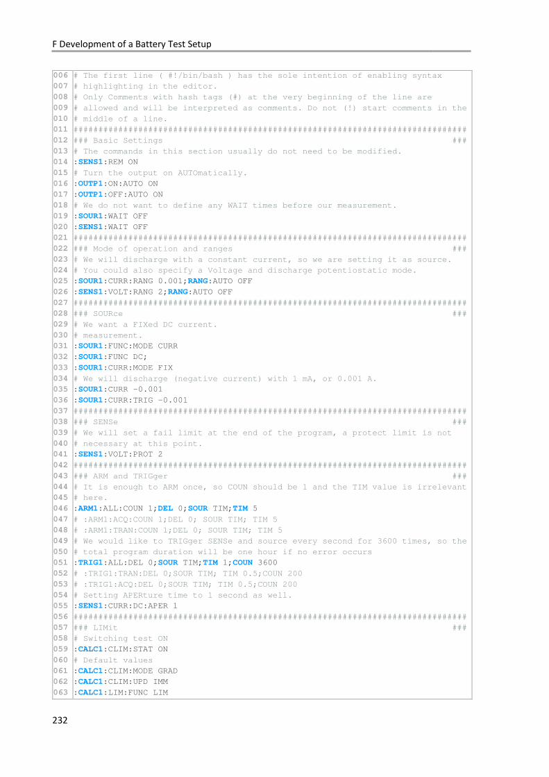
F Development of a Battery Test Setup
232
006
007
008
009
010
011
012
013
014
015
016
017
018
019
020
021
022
023
024
025
026
027
028
029
030
031
032
033
034
035
036
037
038
039
040
041
042
043
044
045
046
047
048
049
050
051
052
053
054
055
056
057
058
059
060
061
062
063
# The first line ( #!/bin/bash ) has the sole intention of enabling syntax
# highlighting in the editor.
# Only Comments with hash tags (#) at the very beginning of the line are
# allowed and will be interpreted as comments. Do not (!) start comments in the
# middle of a line.
###############################################################################
### Basic Settings ###
# The commands in this section usually do not need to be modified.
:SENS1:REM ON
# Turn the output on AUTOmatically.
:OUTP1:ON:AUTO ON
:OUTP1:OFF:AUTO ON
# We do not want to define any WAIT times before our measurement.
:SOUR1:WAIT OFF
:SENS1:WAIT OFF
###############################################################################
### Mode of operation and ranges ###
# We will discharge with a constant current, so we are setting it as source.
# You could also specify a Voltage and discharge potentiostatic mode.
:SOUR1:CURR:RANG 0.001;RANG:AUTO OFF
:SENS1:VOLT:RANG 2;RANG:AUTO OFF
###############################################################################
### SOURce ###
# We want a FIXed DC current.
# measurement.
:SOUR1:FUNC:MODE CURR
:SOUR1:FUNC DC;
:SOUR1:CURR:MODE FIX
# We will discharge (negative current) with 1 mA, or 0.001 A.
:SOUR1:CURR -0.001
:SOUR1:CURR:TRIG -0.001
###############################################################################
### SENSe ###
# We will set a fail limit at the end of the program, a protect limit is not
# necessary at this point.
:SENS1:VOLT:PROT 2
###############################################################################
### ARM and TRIGger ###
# It is enough to ARM once, so COUN should be 1 and the TIM value is irrelevant
# here.
:ARM1:ALL:COUN 1;DEL 0;SOUR TIM;TIM 5
# :ARM1:ACQ:COUN 1;DEL 0; SOUR TIM; TIM 5
# :ARM1:TRAN:COUN 1;DEL 0; SOUR TIM; TIM 5
# We would like to TRIGger SENSe and source every second for 3600 times, so the
# total program duration will be one hour if no error occurs
:TRIG1:ALL:DEL 0;SOUR TIM;TIM 1;COUN 3600
# :TRIG1:TRAN:DEL 0;SOUR TIM; TIM 0.5;COUN 200
# :TRIG1:ACQ:DEL 0;SOUR TIM; TIM 0.5;COUN 200
# Setting APERture time to 1 second as well.
:SENS1:CURR:DC:APER 1
###############################################################################
### LIMit ###
# Switching test ON
:CALC1:CLIM:STAT ON
# Default values
:CALC1:CLIM:MODE GRAD
:CALC1:CLIM:UPD IMM
:CALC1:LIM:FUNC LIM
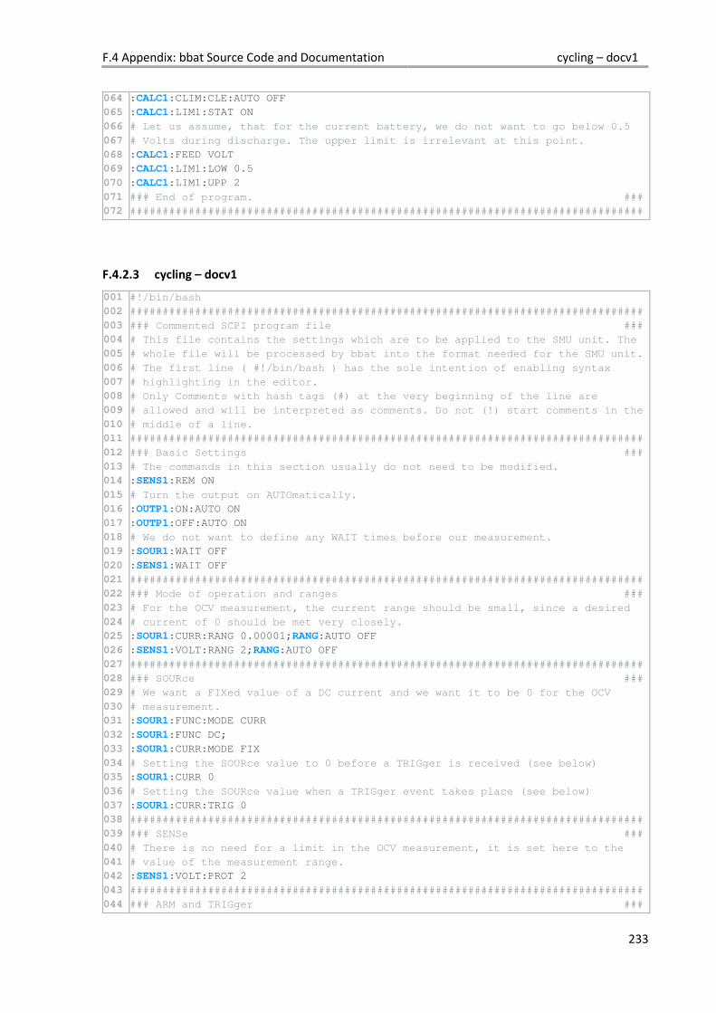
F.4 Appendix: bbat Source Code and Documentation cycling – docv1
233
064
065
066
067
068
069
070
071
072
:CALC1:CLIM:CLE:AUTO OFF
:CALC1:LIM1:STAT ON
# Let us assume, that for the current battery, we do not want to go below 0.5
# Volts during discharge. The upper limit is irrelevant at this point.
:CALC1:FEED VOLT
:CALC1:LIM1:LOW 0.5
:CALC1:LIM1:UPP 2
### End of program. ###
###############################################################################
F.4.2.3 cycling – docv1
001
002
003
004
005
006
007
008
009
010
011
012
013
014
015
016
017
018
019
020
021
022
023
024
025
026
027
028
029
030
031
032
033
034
035
036
037
038
039
040
041
042
043
044
#!/bin/bash
###############################################################################
### Commented SCPI program file ###
# This file contains the settings which are to be applied to the SMU unit. The
# whole file will be processed by bbat into the format needed for the SMU unit.
# The first line ( #!/bin/bash ) has the sole intention of enabling syntax
# highlighting in the editor.
# Only Comments with hash tags (#) at the very beginning of the line are
# allowed and will be interpreted as comments. Do not (!) start comments in the
# middle of a line.
###############################################################################
### Basic Settings ###
# The commands in this section usually do not need to be modified.
:SENS1:REM ON
# Turn the output on AUTOmatically.
:OUTP1:ON:AUTO ON
:OUTP1:OFF:AUTO ON
# We do not want to define any WAIT times before our measurement.
:SOUR1:WAIT OFF
:SENS1:WAIT OFF
###############################################################################
### Mode of operation and ranges ###
# For the OCV measurement, the current range should be small, since a desired
# current of 0 should be met very closely.
:SOUR1:CURR:RANG 0.00001;RANG:AUTO OFF
:SENS1:VOLT:RANG 2;RANG:AUTO OFF
###############################################################################
### SOURce ###
# We want a FIXed value of a DC current and we want it to be 0 for the OCV
# measurement.
:SOUR1:FUNC:MODE CURR
:SOUR1:FUNC DC;
:SOUR1:CURR:MODE FIX
# Setting the SOURce value to 0 before a TRIGger is received (see below)
:SOUR1:CURR 0
# Setting the SOURce value when a TRIGger event takes place (see below)
:SOUR1:CURR:TRIG 0
###############################################################################
### SENSe ###
# There is no need for a limit in the OCV measurement, it is set here to the
# value of the measurement range.
:SENS1:VOLT:PROT 2
###############################################################################
### ARM and TRIGger ###
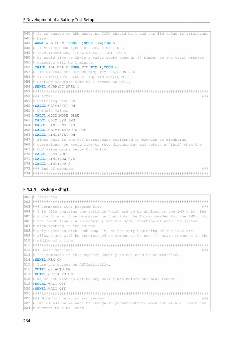
F Development of a Battery Test Setup
234
045
046
047
048
049
050
051
052
053
054
055
056
057
058
059
060
061
062
063
064
065
066
067
068
069
070
071
072
073
074
# It is enough to ARM once, so COUN should be 1 and the TIM value is irrelevant
# here.
:ARM1:ALL:COUN 1;DEL 0;SOUR TIM;TIM 5
# :ARM1:ACQ:COUN 1;DEL 0; SOUR TIM; TIM 5
# :ARM1:TRAN:COUN 1;DEL 0; SOUR TIM; TIM 5
# We would like to SENSe a value every second, 60 times, so the total program
# duration will be 1 minute.
:TRIG1:ALL:DEL 0;SOUR TIM;TIM 1;COUN 60
# :TRIG1:TRAN:DEL 0;SOUR TIM; TIM 0.5;COUN 200
# :TRIG1:ACQ:DEL 0;SOUR TIM; TIM 0.5;COUN 200
# Setting APERture time to 1 second as well.
:SENS1:CURR:DC:APER 1
###############################################################################
### LIMit ###
# Switching test ON
:CALC1:CLIM:STAT ON
# Default values
:CALC1:CLIM:MODE GRAD
:CALC1:CLIM:UPD IMM
:CALC1:LIM:FUNC LIM
:CALC1:CLIM:CLE:AUTO OFF
:CALC1:LIM1:STAT ON
# Since this is the OCV measurement performed in between to discharge
# operations, we would like to stop discharging and return a "fail" when the
# OCV value drops below 0.8 Volts.
:CALC1:FEED VOLT
:CALC1:LIM1:LOW 0.8
:CALC1:LIM1:UPP 2
### End of program. ###
###############################################################################
F.4.2.4 cycling – chrg1
001
002
003
004
005
006
007
008
009
010
011
012
013
014
015
016
017
018
019
020
021
022
023
024
#!/bin/bash
###############################################################################
### Commented SCPI program file ###
# This file contains the settings which are to be applied to the SMU unit. The
# whole file will be processed by bbat into the format needed for the SMU unit.
# The first line ( #!/bin/bash ) has the sole intention of enabling syntax
# highlighting in the editor.
# Only Comments with hash tags (#) at the very beginning of the line are
# allowed and will be interpreted as comments. Do not (!) start comments in the
# middle of a line.
###############################################################################
### Basic Settings ###
# The commands in this section usually do not need to be modified.
:SENS1:REM ON
# Turn the output on AUTOmatically.
:OUTP1:ON:AUTO ON
:OUTP1:OFF:AUTO ON
# We do not want to define any WAIT times before our measurement.
:SOUR1:WAIT OFF
:SENS1:WAIT OFF
###############################################################################
### Mode of operation and ranges ###
# Let us assume we want to charge in potentiostatic mode but we will limit the
# current to 5 mA later.
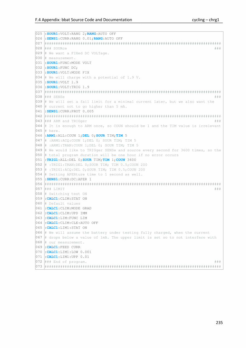
F.4 Appendix: bbat Source Code and Documentation cycling – chrg1
235
025
026
027
028
029
030
031
032
033
034
035
036
037
038
039
040
041
042
043
044
045
046
047
048
049
050
051
052
053
054
055
056
057
058
059
060
061
062
063
064
065
066
067
068
069
070
071
072
073
:SOUR1:VOLT:RANG 2;RANG:AUTO OFF
:SENS1:CURR:RANG 0.01;RANG:AUTO OFF
###############################################################################
### SOURce ###
# We want a FIXed DC VOLTage.
# measurement.
:SOUR1:FUNC:MODE VOLT
:SOUR1:FUNC DC;
:SOUR1:VOLT:MODE FIX
# We will charge with a potential of 1.9 V.
:SOUR1:VOLT 1.9
:SOUR1:VOLT:TRIG 1.9
###############################################################################
### SENSe ###
# We will set a fail limit for a minimal current later, but we also want the
# current not to go higher than 5 mA.
:SENS1:CURR:PROT 0.005
###############################################################################
### ARM and TRIGger ###
# It is enough to ARM once, so COUN should be 1 and the TIM value is irrelevant
# here.
:ARM1:ALL:COUN 1;DEL 0;SOUR TIM;TIM 5
# :ARM1:ACQ:COUN 1;DEL 0; SOUR TIM; TIM 5
# :ARM1:TRAN:COUN 1;DEL 0; SOUR TIM; TIM 5
# We would like to TRIGger SENSe and source every second for 3600 times, so the
# total program duration will be one hour if no error occurs
:TRIG1:ALL:DEL 0;SOUR TIM;TIM 1;COUN 3600
# :TRIG1:TRAN:DEL 0;SOUR TIM; TIM 0.5;COUN 200
# :TRIG1:ACQ:DEL 0;SOUR TIM; TIM 0.5;COUN 200
# Setting APERture time to 1 second as well.
:SENS1:CURR:DC:APER 1
###############################################################################
### LIMIT ###
# Switching test ON
:CALC1:CLIM:STAT ON
# Default values
:CALC1:CLIM:MODE GRAD
:CALC1:CLIM:UPD IMM
:CALC1:LIM:FUNC LIM
:CALC1:CLIM:CLE:AUTO OFF
:CALC1:LIM1:STAT ON
# We will assume the battery under testing fully charged, when the current
# drops below a value of 1mA. The upper limit is set so to not interfere with
# our measurement.
:CALC1:FEED CURR
:CALC1:LIM1:LOW 0.001
:CALC1:LIM1:UPP 0.01
### End of program. ###
###############################################################################
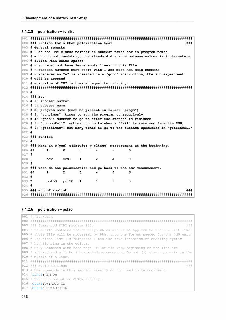
F Development of a Battery Test Setup
236
F.4.2.5 polarisation – runlist
001
002
003
004
005
006
007
008
009
010
011
012
013
014
015
016
017
018
019
020
021
022
023
024
025
026
027
028
029
030
031
032
033
034
035
036
###############################################################################
### runlist for a bbat polarisation test ###
# General remarks
# - do not use blanks neither in subtest names nor in program names.
# - though not mandatory, the standard distance between values is 8 characters,
# filled with white spaces
# - you must not have leave empty lines in this file
# - subtest numbers must start with 1 and must not skip numbers
# - whenever an "a" is inserted in a "goto" instruction, the sub experiment
# will be aborted
# - a value of "0" is treated equal to infinity
###############################################################################
#
### key
# 0: subtest number
# 1: subtest name
# 2: program name (must be present in folder "progs")
# 3: "runtimes": times to run the program consecutively
# 4: "goto": subtest to go to after the subtest is finished
# 5: "gotoonfail": subtest to go to when a "fail" is received from the SMU
# 6: "gototimes": how many times to go to the subtest specified in "gotoonfail"
#
### runlist
#
### Make an o(pen) c(ircuit) v(oltage) measurement at the beginning.
#0 1 2 3 4 5 6
#
1 ocv ocv1 1 2 a 0
#
### Then do the polarisation and go back to the ocv measurement.
#0 1 2 3 4 5 6
#
2 pol50 pol50 1 1 5 0
#
### end of runlist ###
###############################################################################
F.4.2.6 polarisation – pol50
001
002
003
004
005
006
007
008
009
010
011
012
013
014
015
016
017
#!/bin/bash
###############################################################################
### Commented SCPI program file ###
# This file contains the settings which are to be applied to the SMU unit. The
# whole file will be processed by bbat into the format needed for the SMU unit.
# The first line ( #!/bin/bash ) has the sole intention of enabling syntax
# highlighting in the editor.
# Only Comments with hash tags (#) at the very beginning of the line are
# allowed and will be interpreted as comments. Do not (!) start comments in the
# middle of a line.
###############################################################################
### Basic Settings ###
# The commands in this section usually do not need to be modified.
:SENS1:REM ON
# Turn the output on AUTOmatically.
:OUTP1:ON:AUTO ON
:OUTP1:OFF:AUTO ON
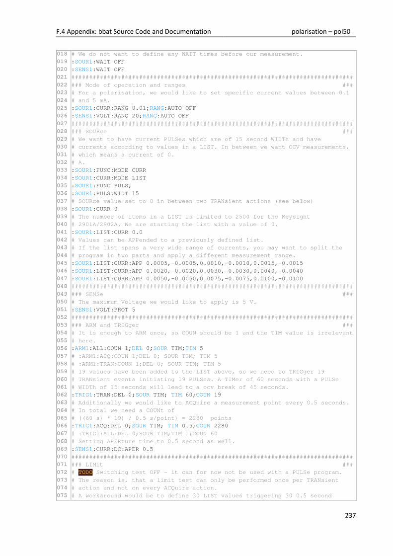
F.4 Appendix: bbat Source Code and Documentation polarisation – pol50
237
018
019
020
021
022
023
024
025
026
027
028
029
030
031
032
033
034
035
036
037
038
039
040
041
042
043
044
045
046
047
048
049
050
051
052
053
054
055
056
057
058
059
060
061
062
063
064
065
066
067
068
069
070
071
072
073
074
075
# We do not want to define any WAIT times before our measurement.
:SOUR1:WAIT OFF
:SENS1:WAIT OFF
###############################################################################
### Mode of operation and ranges ###
# For a polarisation, we would like to set specific current values between 0.1
# and 5 mA.
:SOUR1:CURR:RANG 0.01;RANG:AUTO OFF
:SENS1:VOLT:RANG 20;RANG:AUTO OFF
###############################################################################
### SOURce ###
# We want to have current PULSes which are of 15 second WIDTh and have
# currents according to values in a LIST. In between we want OCV measurements,
# which means a current of 0.
# A.
:SOUR1:FUNC:MODE CURR
:SOUR1:CURR:MODE LIST
:SOUR1:FUNC PULS;
:SOUR1:PULS:WIDT 15
# SOURce value set to 0 in between two TRANsient actions (see below)
:SOUR1:CURR 0
# The number of items in a LIST is limited to 2500 for the Keysight
# 2901A/2902A. We are starting the list with a value of 0.
:SOUR1:LIST:CURR 0.0
# Values can be APPended to a previously defined list.
# If the list spans a very wide range of currents, you may want to split the
# program in two parts and apply a different measurement range.
:SOUR1:LIST:CURR:APP 0.0005,-0.0005,0.0010,-0.0010,0.0015,-0.0015
:SOUR1:LIST:CURR:APP 0.0020,-0.0020,0.0030,-0.0030,0.0040,-0.0040
:SOUR1:LIST:CURR:APP 0.0050,-0.0050,0.0075,-0.0075,0.0100,-0.0100
###############################################################################
### SENSe ###
# The maximum Voltage we would like to apply is 5 V.
:SENS1:VOLT:PROT 5
###############################################################################
### ARM and TRIGger ###
# It is enough to ARM once, so COUN should be 1 and the TIM value is irrelevant
# here.
:ARM1:ALL:COUN 1;DEL 0;SOUR TIM;TIM 5
# :ARM1:ACQ:COUN 1;DEL 0; SOUR TIM; TIM 5
# :ARM1:TRAN:COUN 1;DEL 0; SOUR TIM; TIM 5
# 19 values have been added to the LIST above, so we need to TRIGger 19
# TRANsient events initiating 19 PULSes. A TIMer of 60 seconds with a PULSe
# WIDTh of 15 seconds will lead to a ocv break of 45 seconds.
:TRIG1:TRAN:DEL 0;SOUR TIM; TIM 60;COUN 19
# Additionally we would like to ACQuire a measurement point every 0.5 seconds.
# In total we need a COUNt of
# ((60 s) * 19) / 0.5 s/point) = 2280 points
:TRIG1:ACQ:DEL 0;SOUR TIM; TIM 0.5;COUN 2280
# :TRIG1:ALL:DEL 0;SOUR TIM;TIM 1;COUN 60
# Setting APERture time to 0.5 second as well.
:SENS1:CURR:DC:APER 0.5
###############################################################################
### LIMit ###
# TODO Switching test OFF - it can for now not be used with a PULSe program.
# The reason is, that a limit test can only be performed once per TRANsient
# action and not on every ACQuire action.
# A workaround would be to define 30 LIST values triggering 30 0.5 second
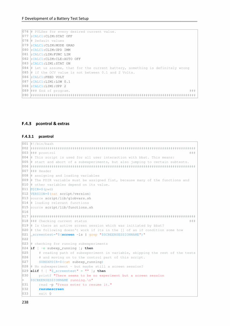
F Development of a Battery Test Setup
238
076
077
078
079
080
081
082
083
084
085
086
087
088
089
090
# PULSes for every desired current value.
:CALC1:CLIM:STAT OFF
# Default values
:CALC1:CLIM:MODE GRAD
:CALC1:CLIM:UPD IMM
:CALC1:LIM:FUNC LIM
:CALC1:CLIM:CLE:AUTO OFF
:CALC1:LIM1:STAT ON
# Let us assume, that for the current battery, something is definitely wrong
# if the OCV value is not between 0.1 and 2 Volts.
:CALC1:FEED VOLT
:CALC1:LIM1:LOW 0.1
:CALC1:LIM1:UPP 2
### End of program. ###
###############################################################################
pcontrol & extras
F.4.3.1 pcontrol
001
002
003
004
005
006
007
008
009
010
011
012
013
014
015
016
017
018
019
020
021
022
023
024
025
026
027
028
029
030
>
031
032
033
#!/bin/bash
###############################################################################
### pcontrol ###
# This script is used for all user interaction with bbat. This means:
# start and abort of a subexperiments, but also jumping to certain subtests.
###############################################################################
### Header
# assigning and loading variables
# The PDIR variable must be assigned fist, because many of the functions and
# other variables depend on its value.
PDIR=$(pwd)
VERSION=$(cat script/version)
source script/lib/globvars.sh
# loading relevant functions
source script/lib/functions.sh
###############################################################################
### Checking current status ###
# Is there an active screen session which was initiated by bbat?
# the following doesn't work if its in the [] of an if condition some how
_screentest="$(screen -ls | grep "$SCREENSESSIONNAME")"
# checking for running subexperiments
if [ -e subexp_running ]; then
# reading path of subexperiment in variable, skipping the rest of the tests
# and moving on to the control part of this script.
SUBEXPDIR=$(cat subexp_running)
# No subexperiment - but maybe still a screen session?
elif ! [ "$_screentest" = "" ]; then
printf "There seems to be no experiment but a screen session
$SCREENSESSIONNAME running.\n"
read -p "Press enter to resume it."
resumescreen
exit 0
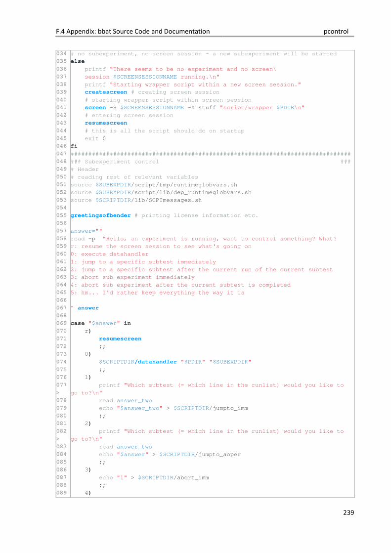
F.4 Appendix: bbat Source Code and Documentation pcontrol
239
034
035
036
037
038
039
040
041
042
043
044
045
046
047
048
049
050
051
052
053
054
055
056
057
058
059
060
061
062
063
064
065
066
067
068
069
070
071
072
073
074
075
076
077
>
078
079
080
081
082
>
083
084
085
086
087
088
089
# no subexperiment, no screen session - a new subexperiment will be started
else
printf "There seems to be no experiment and no screen\
session $SCREENSESSIONNAME running.\n"
printf "Starting wrapper script within a new screen session."
createscreen # creating screen session
# starting wrapper script within screen session
screen -S $SCREENSESSIONNAME -X stuff "script/wrapper $PDIR\n"
# entering screen session
resumescreen
# this is all the script should do on startup
exit 0
fi
###############################################################################
### Subexperiment control ###
# Header
# reading rest of relevant variables
source $SUBEXPDIR/script/tmp/runtimeglobvars.sh
source $SUBEXPDIR/script/lib/dep_runtimeglobvars.sh
source $SCRIPTDIR/lib/SCPImessages.sh
greetingsofbender # printing license information etc.
answer=""
read -p "Hello, an experiment is running, want to control something? What?
r: resume the screen session to see what's going on
0: execute datahandler
1: jump to a specific subtest immediately
2: jump to a specific subtest after the current run of the current subtest
3: abort sub experiment immediately
4: abort sub experiment after the current subtest is completed
5: hm... I'd rather keep everything the way it is
" answer
case "$answer" in
r)
resumescreen
;;
0)
$SCRIPTDIR/datahandler "$PDIR" "$SUBEXPDIR"
;;
1)
printf "Which subtest (= which line in the runlist) would you like to
go to?\n"
read answer_two
echo "$answer_two" > $SCRIPTDIR/jumpto_imm
;;
2)
printf "Which subtest (= which line in the runlist) would you like to
go to?\n"
read answer_two
echo "$answer" > $SCRIPTDIR/jumpto_aoper
;;
3)
echo "1" > $SCRIPTDIR/abort_imm
;;
4)
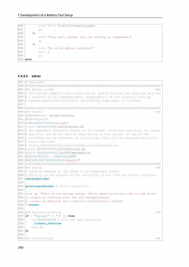
F Development of a Battery Test Setup
240
090
091
092
093
094
095
096
097
098
099
echo "1" > $SCRIPTDIR/abort_aoper
;;
5)
echo "Very well, bender will do nothing as requested."
;;
*)
echo "No valid option selected."
exit 0
;;
esac
F.4.3.2 extras
001
002
003
004
005
006
007
008
009
010
011
012
013
014
015
016
017
018
019
020
021
022
023
024
025
026
027
028
029
030
031
032
033
034
035
036
037
038
039
040
041
042
043
#!/bin/bash
###############################################################################
### Extras script ###
# This script supply's tools which can be used to process the acquired data for
# a specific or all subexperiments independently of the currently running
# subexperiments and even after the complete experiment is finished.
###############################################################################
### Header ###
VERSION=$(cat script/version)
PDIR="$(pwd)"
PSCRIPTDIR="$PDIR/script"
source $PSCRIPTDIR/lib/globvars.sh
# The dependent variables should not be loaded, since they are meant for normal
# operation and do not work as they should in this script. If any of the
# variables may be necessary in this script, they will be assigned explicitly
# below this text.
# source $PSCRIPTDIR/script/lib/dep_runtimeglobvars.sh
source $PSCRIPTDIR/lib/functions.sh
source $PSCRIPTDIR/lib/SCPImessages.sh
EXPDIR="$PDIR/../$EXPDIR_NAME"
GNUPLOTDIR="$PSCRIPTDIR/gnuplot"
###############################################################################
### Extras ###
# checking weather or not there is an experiment folder
# which is to say weather or not the script is run from the correct location
checkexpfolder
greetingsofbender # That's always fun.
read -p "This is the extras script. Which extra would you like to see done?
1: create an overview plot for all subexperiments
2: create an ASR plot for a specific polarisation subtest
" answer
### Overview plotting ###
if [ "$answer" == "1" ]; then
cd $PSCRIPTDIR # will not work otherwise
./create_overview
exit 0
fi
### ASR plotting ###
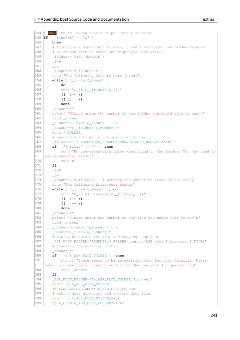
F.4 Appendix: bbat Source Code and Documentation extras
241
044
045
046
047
048
049
050
051
052
053
054
055
056
057
058
059
060
061
062
063
064
065
066
067
068
069
>
070
071
072
073
074
075
076
077
078
079
080
081
082
083
084
085
086
087
088
089
090
091
>
092
093
094
095
096
097
098
099
# TODO The following should be put into a function
if [ "$answer" == "2" ]
then
# listing all experiment folders, j and i variables are needed because
# we do not want to start our displayed list with 0
_folders=($(ls $EXPDIR))
_i=0
_j=1
_length=${#_folders[@]}
echo "The following folders were found:"
while [ $_j -le $_length ]
do
echo "$_j: ${_folders[$_i]}"
(( _i++ ))
(( _j++ ))
done
_answer=""
printf "Please enter the number of the folder you would like to use\n"
read _answer
_number=$( expr $_answer - 1 )
_FOLDER="${_folders[$_number]}"
echo $_FOLDER
# reading all files in the specified folder
_files=($(ls $EXPDIR/$_FOLDER/$CONVDATADIR_NAME/*.conv))
if [ "$_files" == "" ]; then
echo "No converted data files were found in the folder. You may need to
run datahandler first."
exit 0
fi
_i=0
_j=1
_length=${#_files[@]} # getting the number of items in the array
echo "The following files were found:"
while [ $_j -le $_length ]; do
echo "$_j: $( basename ${_files[$_i]})"
(( _i++ ))
(( _j++ ))
done
_answer=""
printf "Please enter the number of the file you would like to use\n"
read _answer
_number=$( expr $_answer - 1 )
_FILE="${_files[$_number]}"
# making directory for plot and copying templates
_ASR_PLOT_FOLDER="$EXPDIR/$_FOLDER/gnuplot/ASR_plot_$(basename $_FILE)"
# checking for existing plots
_answer=""
if [ -d $_ASR_PLOT_FOLDER ]; then
printf "There seems to be an existing plot for this datafile. Press
Enter to overwrite or input a suffix for the new plot (no spaces!).\n"
read _answer
fi
_ASR_PLOT_FOLDER="${_ASR_PLOT_FOLDER}$_answer"
mkdir -p $_ASR_PLOT_FOLDER
cp $GNUPLOTDIR/ASR/* $_ASR_PLOT_FOLDER
# making data directory and copying data file
mkdir -p $_ASR_PLOT_FOLDER/data
cp $_FILE $_ASR_PLOT_FOLDER/data/
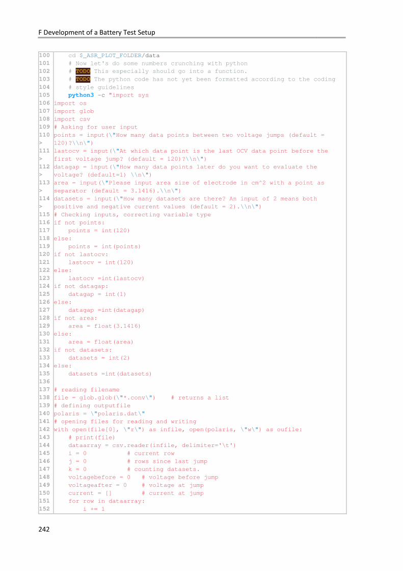
F Development of a Battery Test Setup
242
100
101
102
103
104
105
106
107
108
109
110
>
111
>
112
>
113
>
114
>
115
116
117
118
119
120
121
122
123
124
125
126
127
128
129
130
131
132
133
134
135
136
137
138
139
140
141
142
143
144
145
146
147
148
149
150
151
152
cd $_ASR_PLOT_FOLDER/data
# Now let's do some numbers crunching with python
# TODO This especially should go into a function.
# TODO The python code has not yet been formatted according to the coding
# style guidelines
python3 -c "import sys
import os
import glob
import csv
# Asking for user input
points = input(\"How many data points between two voltage jumps (default =
120)?\\n\")
lastocv = input(\"At which data point is the last OCV data point before the
first voltage jump? (default = 120)?\\n\")
datagap = input(\"How many data points later do you want to evaluate the
voltage? (default=1) \\n\")
area = input(\"Please input area size of electrode in cm^2 with a point as
separator (default = 3.1416).\\n\")
datasets = input(\"How many datasets are there? An input of 2 means both
positive and negative current values (default = 2).\\n\")
# Checking inputs, correcting variable type
if not points:
points = int(120)
else:
points = int(points)
if not lastocv:
lastocv = int(120)
else:
lastocv =int(lastocv)
if not datagap:
datagap = int(1)
else:
datagap =int(datagap)
if not area:
area = float(3.1416)
else:
area = float(area)
if not datasets:
datasets = int(2)
else:
datasets =int(datasets)
# reading filename
file = glob.glob(\"*.conv\") # returns a list
# defining outputfile
polaris = \"polaris.dat\"
# opening files for reading and writing
with open(file[0], \"r\") as infile, open(polaris, \"w\") as oufile:
# print(file)
dataarray = csv.reader(infile, delimiter='\t')
i = 0 # current row
j = 0 # rows since last jump
k = 0 # counting datasets.
voltagebefore = 0 # voltage before jump
voltageafter = 0 # voltage at jump
current = [] # current at jump
for row in dataarray:
i += 1
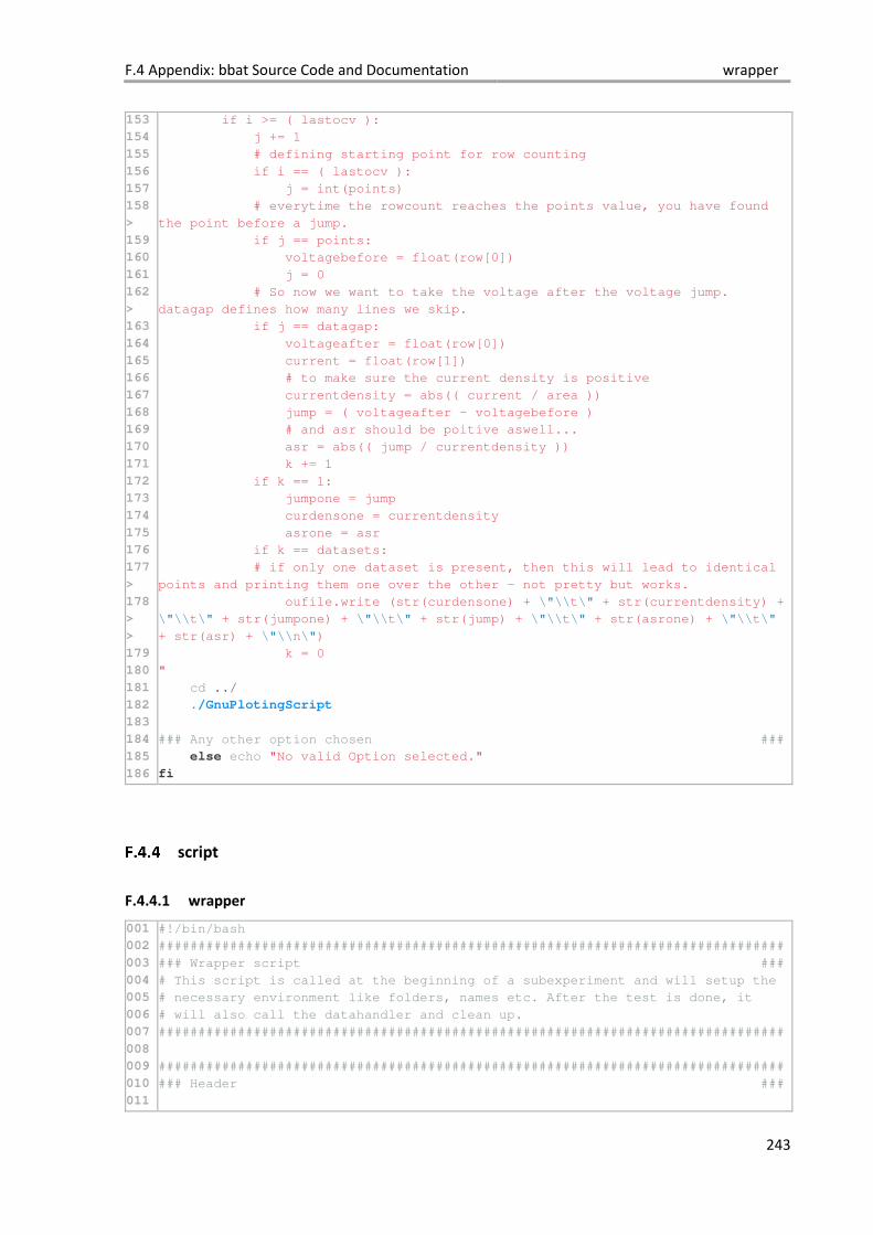
F.4 Appendix: bbat Source Code and Documentation wrapper
243
153
154
155
156
157
158
>
159
160
161
162
>
163
164
165
166
167
168
169
170
171
172
173
174
175
176
177
>
178
>
>
179
180
181
182
183
184
185
186
if i >= ( lastocv ):
j += 1
# defining starting point for row counting
if i == ( lastocv ):
j = int(points)
# everytime the rowcount reaches the points value, you have found
the point before a jump.
if j == points:
voltagebefore = float(row[0])
j = 0
# So now we want to take the voltage after the voltage jump.
datagap defines how many lines we skip.
if j == datagap:
voltageafter = float(row[0])
current = float(row[1])
# to make sure the current density is positive
currentdensity = abs(( current / area ))
jump = ( voltageafter - voltagebefore )
# and asr should be poitive aswell...
asr = abs(( jump / currentdensity ))
k += 1
if k == 1:
jumpone = jump
curdensone = currentdensity
asrone = asr
if k == datasets:
# if only one dataset is present, then this will lead to identical
points and printing them one over the other - not pretty but works.
oufile.write (str(curdensone) + \"\\t\" + str(currentdensity) +
\"\\t\" + str(jumpone) + \"\\t\" + str(jump) + \"\\t\" + str(asrone) + \"\\t\"
+ str(asr) + \"\\n\")
k = 0
"
cd ../
./GnuPlotingScript
### Any other option chosen ###
else echo "No valid Option selected."
fi
script
F.4.4.1 wrapper
001
002
003
004
005
006
007
008
009
010
011
#!/bin/bash
###############################################################################
### Wrapper script ###
# This script is called at the beginning of a subexperiment and will setup the
# necessary environment like folders, names etc. After the test is done, it
# will also call the datahandler and clean up.
###############################################################################
###############################################################################
### Header ###
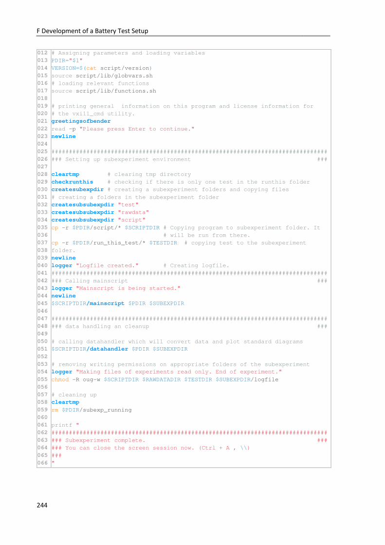
F Development of a Battery Test Setup
244
012
013
014
015
016
017
018
019
020
021
022
023
024
025
026
027
028
029
030
031
032
033
034
035
036
037
038
039
040
041
042
043
044
045
046
047
048
049
050
051
052
053
054
055
056
057
058
059
060
061
062
063
064
065
066
# Assigning parameters and loading variables
PDIR="$1"
VERSION=$(cat script/version)
source script/lib/globvars.sh
# loading relevant functions
source script/lib/functions.sh
# printing general information on this program and license information for
# the vxi11_cmd utility.
greetingsofbender
read -p "Please press Enter to continue."
newline
###############################################################################
### Setting up subexperiment environment ###
cleartmp # clearing tmp directory
checkrunthis # checking if there is only one test in the runthis folder
createsubexpdir # creating a subexperiment folders and copying files
# creating a folders in the subexperiment folder
createsubsubexpdir "test"
createsubsubexpdir "rawdata"
createsubsubexpdir "script"
cp -r $PDIR/script/* $SCRIPTDIR # Copying program to subexperiment folder. It
# will be run from there.
cp -r $PDIR/run_this_test/* $TESTDIR # copying test to the subexperiment
folder.
newline
logger "Logfile created." # Creating logfile.
###############################################################################
### Calling mainscript ###
logger "Mainscript is being started."
newline
$SCRIPTDIR/mainscript $PDIR $SUBEXPDIR
###############################################################################
### data handling an cleanup ###
# calling datahandler which will convert data and plot standard diagrams
$SCRIPTDIR/datahandler $PDIR $SUBEXPDIR
# removing writing permissions on appropriate folders of the subexperiment
logger "Making files of experiments read only. End of experiment."
chmod -R oug-w $SCRIPTDIR $RAWDATADIR $TESTDIR $SUBEXPDIR/logfile
# cleaning up
cleartmp
rm $PDIR/subexp_running
printf "
###############################################################################
### Subexperiment complete. ###
### You can close the screen session now. (Ctrl + A , \\)
###
"
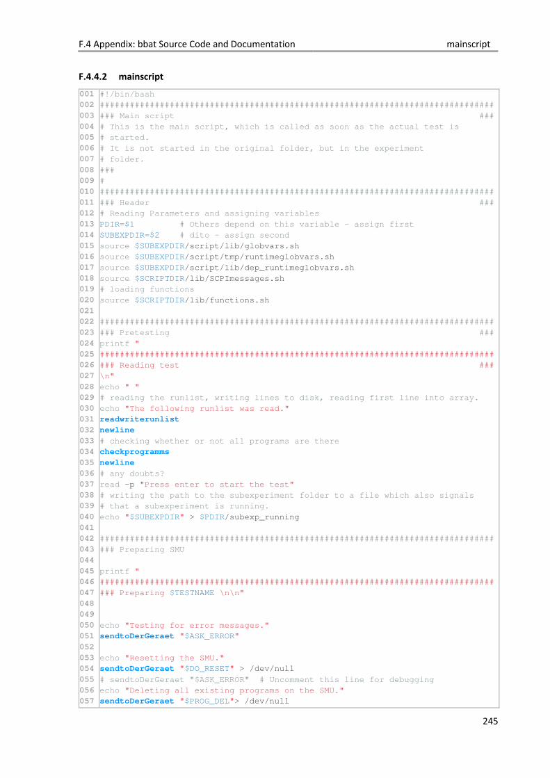
F.4 Appendix: bbat Source Code and Documentation mainscript
245
F.4.4.2 mainscript
001
002
003
004
005
006
007
008
009
010
011
012
013
014
015
016
017
018
019
020
021
022
023
024
025
026
027
028
029
030
031
032
033
034
035
036
037
038
039
040
041
042
043
044
045
046
047
048
049
050
051
052
053
054
055
056
057
#!/bin/bash
###############################################################################
### Main script ###
# This is the main script, which is called as soon as the actual test is
# started.
# It is not started in the original folder, but in the experiment
# folder.
###
#
###############################################################################
### Header ###
# Reading Parameters and assigning variables
PDIR=$1 # Others depend on this variable - assign first
SUBEXPDIR=$2 # dito - assign second
source $SUBEXPDIR/script/lib/globvars.sh
source $SUBEXPDIR/script/tmp/runtimeglobvars.sh
source $SUBEXPDIR/script/lib/dep_runtimeglobvars.sh
source $SCRIPTDIR/lib/SCPImessages.sh
# loading functions
source $SCRIPTDIR/lib/functions.sh
###############################################################################
### Pretesting ###
printf "
###############################################################################
### Reading test ###
\n"
echo " "
# reading the runlist, writing lines to disk, reading first line into array.
echo "The following runlist was read."
readwriterunlist
newline
# checking whether or not all programs are there
checkprogramms
newline
# any doubts?
read -p "Press enter to start the test"
# writing the path to the subexperiment folder to a file which also signals
# that a subexperiment is running.
echo "$SUBEXPDIR" > $PDIR/subexp_running
###############################################################################
### Preparing SMU
printf "
###############################################################################
### Preparing $TESTNAME \n\n"
echo "Testing for error messages."
sendtoDerGeraet "$ASK_ERROR"
echo "Resetting the SMU."
sendtoDerGeraet "$DO_RESET" > /dev/null
# sendtoDerGeraet "$ASK_ERROR" # Uncomment this line for debugging
echo "Deleting all existing programs on the SMU."
sendtoDerGeraet "$PROG_DEL"> /dev/null

F Development of a Battery Test Setup
246
058
059
060
061
062
063
064
065
066
067
068
069
070
071
072
073
074
075
076
077
078
079
080
081
082
083
084
085
086
087
088
089
090
091
092
093
094
095
096
097
098
099
100
101
102
103
104
105
106
107
108
109
110
111
112
113
114
115
# sendtoDerGeraet "$ASK_ERROR" # Uncomment this line for debugging
echo "Create folder for experiment"
sendtoDerGeraet "$SCPI_MAKE_DIR" > /dev/null
echo "Translating and sending programs."
progtranssend
newline
sendtoDerGeraet "$ASK_ERROR"
###############################################################################
### Starting test ###
printf "
###############################################################################
### $(echotime) Starting $TESTNAME !\n\n"
###############################################################################
### Starting the subtest loop ###
# This loop will control the order of the subtests according to the logic of
# the runlist and the limits set within each subtest (if applicable). It will
# also contain checks for user input (aborts or jumps). This is the logical
# core of the program.
# TODO When this program is rewritten in Python, there should be a subtest
# class with subtest objects for each subtest.
### ###
while true; do
### defining the runlinearray
# This is the array which contains one line of the runlist corresponding to and
# defining a particular subtest. Additionally it holds the history of this
# subtest during this experiment.
# reading file on the disk which contains the data for the subtest to be run
readrunlinearray "$crunnumber"
# st stands for subtest. The following values are defined by one line of the
# runlist
_st_runnumber="${runlinearray[0]}" # identical to line number
_st_runname="${runlinearray[1]}" # name of the subtest
_st_progname="${runlinearray[2]}" # program to be called for subtest
_st_runtimes="${runlinearray[3]}" # times the subtest is run consecutively
_st_gotonumber="${runlinearray[4]}" # which subtest is next?
_st_gotoonfail="${runlinearray[5]}" # which subtest to got to on fail?
_st_gototimes="${runlinearray[6]}" # number of times to go to a diff.
# subtest after a fail
# c stands for the current values of these variables which describe the history
# of the subtest during this subexperiment. For description see the file
# script/lib/globvars.sh
cfailtimes="${runlinearray[7]}"
ctotalruntimes="${runlinearray[8]}"
crtsincefail="${runlinearray[9]}"
cruntimes="${runlinearray[10]}"
cgototimes="${runlinearray[11]}"
inccruntimes # increases the cruntimes
# creating the filename to store the data of this run of the subtest
nameandincdata "$_st_runname"
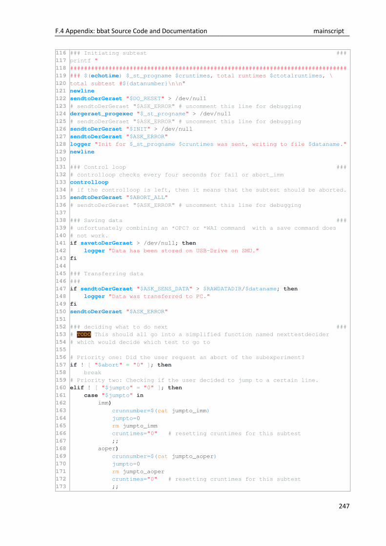
F.4 Appendix: bbat Source Code and Documentation mainscript
247
116
117
118
119
120
121
122
123
124
125
126
127
128
129
130
131
132
133
134
135
136
137
138
139
140
141
142
143
144
145
146
147
148
149
150
151
152
153
154
155
156
157
158
159
160
161
162
163
164
165
166
167
168
169
170
171
172
173
### Initiating subtest ###
printf "
###############################################################################
### $(echotime) $_st_progname $cruntimes, total runtimes $ctotalruntimes, \
total subtest #${datanumber}\n\n"
newline
sendtoDerGeraet "$DO_RESET" > /dev/null
# sendtoDerGeraet "$ASK_ERROR" # uncomment this line for debugging
dergeraet_progexec "$_st_progname" > /dev/null
# sendtoDerGeraet "$ASK_ERROR" # uncomment this line for debugging
sendtoDerGeraet "$INIT" > /dev/null
sendtoDerGeraet "$ASK_ERROR"
logger "Init for $_st_progname $cruntimes was sent, writing to file $dataname."
newline
### Control loop ###
# controlloop checks every four seconds for fail or abort_imm
controlloop
# if the controlloop is left, then it means that the subtest should be aborted.
sendtoDerGeraet "$ABORT_ALL"
# sendtoDerGeraet "$ASK_ERROR" # uncomment this line for debugging
### Saving data ###
# unfortunately combining an *OPC? or *WAI command with a save command does
# not work.
if savetoDerGeraet > /dev/null; then
logger "Data has been stored on USB-Drive on SMU."
fi
### Transferring data
###
if sendtoDerGeraet "$ASK_SENS_DATA" > $RAWDATADIR/$dataname; then
logger "Data was transferred to PC."
fi
sendtoDerGeraet "$ASK_ERROR"
### deciding what to do next ###
# TODO This should all go into a simplified function named nexttestdecider
# which would decide which test to go to
# Priority one: Did the user request an abort of the subexperiment?
if ! [ "$abort" = "0" ]; then
break
# Priority two: Checking if the user decided to jump to a certain line.
elif ! [ "$jumpto" = "0" ]; then
case "$jumpto" in
imm)
crunnumber=$(cat jumpto_imm)
jumpto=0
rm jumpto_imm
cruntimes="0" # resetting cruntimes for this subtest
;;
aoper)
crunnumber=$(cat jumpto_aoper)
jumpto=0
rm jumpto_aoper
cruntimes="0" # resetting cruntimes for this subtest
;;
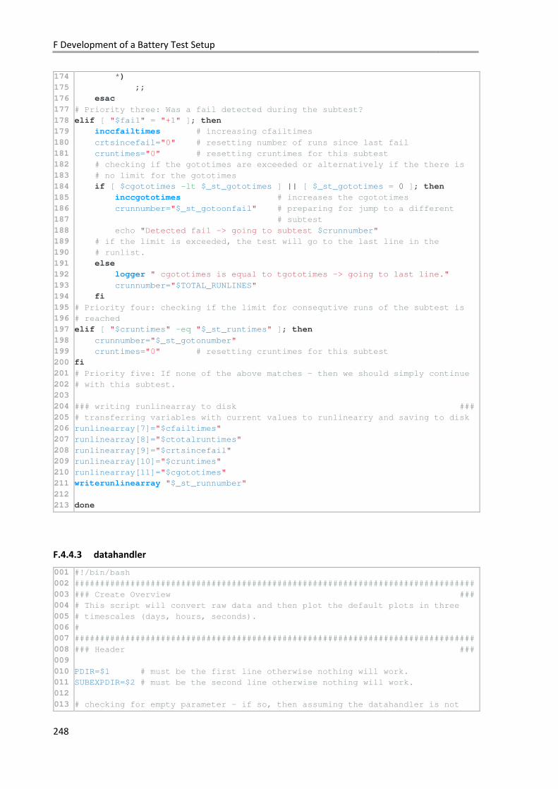
F Development of a Battery Test Setup
248
174
175
176
177
178
179
180
181
182
183
184
185
186
187
188
189
190
191
192
193
194
195
196
197
198
199
200
201
202
203
204
205
206
207
208
209
210
211
212
213
*)
;;
esac
# Priority three: Was a fail detected during the subtest?
elif [ "$fail" = "+1" ]; then
inccfailtimes # increasing cfailtimes
crtsincefail="0" # resetting number of runs since last fail
cruntimes="0" # resetting cruntimes for this subtest
# checking if the gototimes are exceeded or alternatively if the there is
# no limit for the gototimes
if [ $cgototimes -lt $_st_gototimes ] || [ $_st_gototimes = 0 ]; then
inccgototimes # increases the cgototimes
crunnumber="$_st_gotoonfail" # preparing for jump to a different
# subtest
echo "Detected fail -> going to subtest $crunnumber"
# if the limit is exceeded, the test will go to the last line in the
# runlist.
else
logger " cgototimes is equal to tgototimes -> going to last line."
crunnumber="$TOTAL_RUNLINES"
fi
# Priority four: checking if the limit for consequtive runs of the subtest is
# reached
elif [ "$cruntimes" -eq "$_st_runtimes" ]; then
crunnumber="$_st_gotonumber"
cruntimes="0" # resetting cruntimes for this subtest
fi
# Priority five: If none of the above matches - then we should simply continue
# with this subtest.
### writing runlinearray to disk ###
# transferring variables with current values to runlinearry and saving to disk
runlinearray[7]="$cfailtimes"
runlinearray[8]="$ctotalruntimes"
runlinearray[9]="$crtsincefail"
runlinearray[10]="$cruntimes"
runlinearray[11]="$cgototimes"
writerunlinearray "$_st_runnumber"
done
F.4.4.3 datahandler
001
002
003
004
005
006
007
008
009
010
011
012
013
#!/bin/bash
###############################################################################
### Create Overview ###
# This script will convert raw data and then plot the default plots in three
# timescales (days, hours, seconds).
#
###############################################################################
### Header ###
PDIR=$1 # must be the first line otherwise nothing will work.
SUBEXPDIR=$2 # must be the second line otherwise nothing will work.
# checking for empty parameter - if so, then assuming the datahandler is not
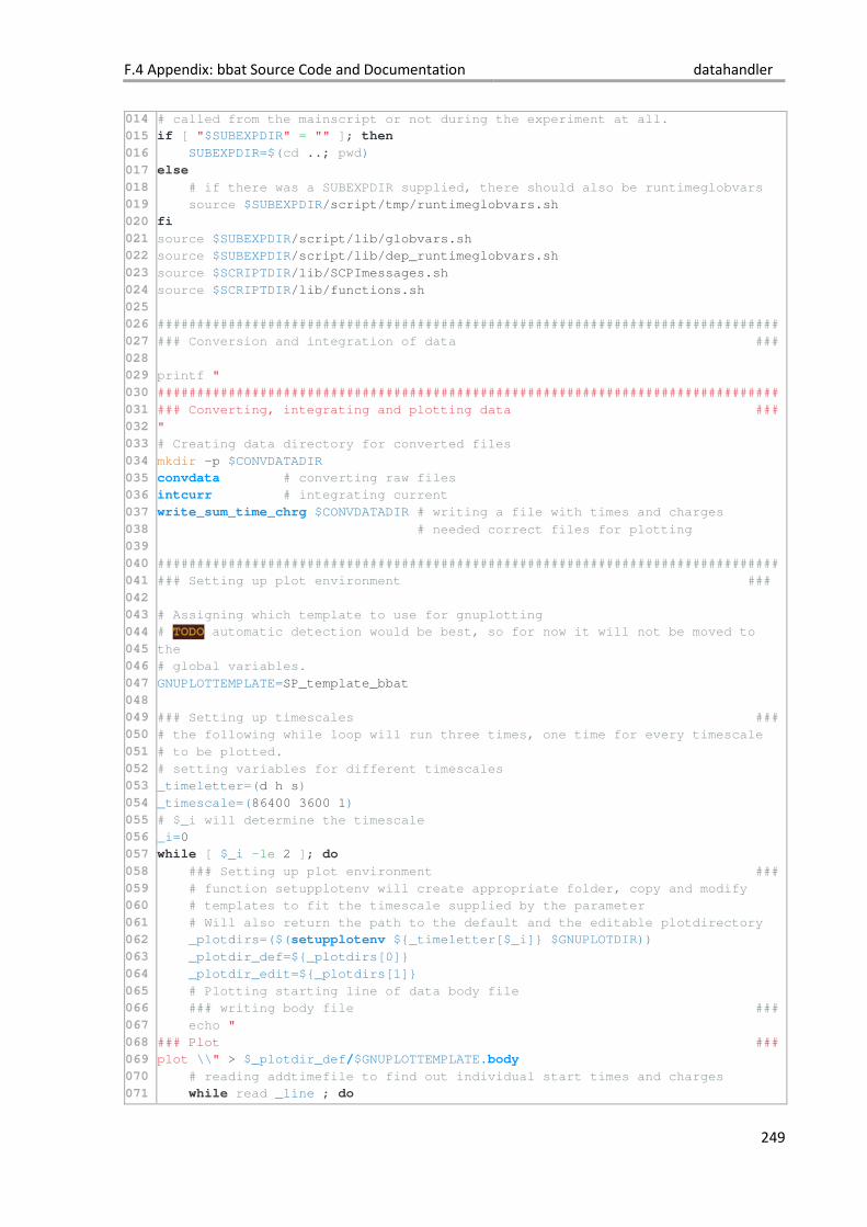
F.4 Appendix: bbat Source Code and Documentation datahandler
249
014
015
016
017
018
019
020
021
022
023
024
025
026
027
028
029
030
031
032
033
034
035
036
037
038
039
040
041
042
043
044
045
046
047
048
049
050
051
052
053
054
055
056
057
058
059
060
061
062
063
064
065
066
067
068
069
070
071
# called from the mainscript or not during the experiment at all.
if [ "$SUBEXPDIR" = "" ]; then
SUBEXPDIR=$(cd ..; pwd)
else
# if there was a SUBEXPDIR supplied, there should also be runtimeglobvars
source $SUBEXPDIR/script/tmp/runtimeglobvars.sh
fi
source $SUBEXPDIR/script/lib/globvars.sh
source $SUBEXPDIR/script/lib/dep_runtimeglobvars.sh
source $SCRIPTDIR/lib/SCPImessages.sh
source $SCRIPTDIR/lib/functions.sh
###############################################################################
### Conversion and integration of data ###
printf "
###############################################################################
### Converting, integrating and plotting data ###
"
# Creating data directory for converted files
mkdir -p $CONVDATADIR
convdata # converting raw files
intcurr # integrating current
write_sum_time_chrg $CONVDATADIR # writing a file with times and charges
# needed correct files for plotting
###############################################################################
### Setting up plot environment ###
# Assigning which template to use for gnuplotting
# TODO automatic detection would be best, so for now it will not be moved to
the
# global variables.
GNUPLOTTEMPLATE=SP_template_bbat
### Setting up timescales ###
# the following while loop will run three times, one time for every timescale
# to be plotted.
# setting variables for different timescales
_timeletter=(d h s)
_timescale=(86400 3600 1)
# $_i will determine the timescale
_i=0
while [ $_i -le 2 ]; do
### Setting up plot environment ###
# function setupplotenv will create appropriate folder, copy and modify
# templates to fit the timescale supplied by the parameter
# Will also return the path to the default and the editable plotdirectory
_plotdirs=($(setupplotenv ${_timeletter[$_i]} $GNUPLOTDIR))
_plotdir_def=${_plotdirs[0]}
_plotdir_edit=${_plotdirs[1]}
# Plotting starting line of data body file
### writing body file ###
echo "
### Plot ###
plot \\" > $_plotdir_def/$GNUPLOTTEMPLATE.body
# reading addtimefile to find out individual start times and charges
while read _line ; do
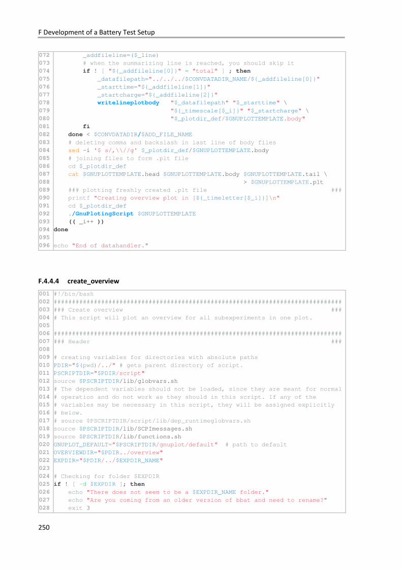
F Development of a Battery Test Setup
250
072
073
074
075
076
077
078
079
080
081
082
083
084
085
086
087
088
089
090
091
092
093
094
095
096
_addfileline=($_line)
# when the summarizing line is reached, you should skip it
if ! [ "${_addfileline[0]}" = "total" ] ; then
_datafilepath="../../../$CONVDATADIR_NAME/${_addfileline[0]}"
_starttime="${_addfileline[1]}"
_startcharge="${_addfileline[2]}"
writelineplotbody "$_datafilepath" "$_starttime" \
"${_timescale[$_i]}" "$_startcharge" \
"$_plotdir_def/$GNUPLOTTEMPLATE.body"
fi
done < $CONVDATADIR/$ADD_FILE_NAME
# deleting comma and backslash in last line of body files
sed -i '$ s/,\\//g' $_plotdir_def/$GNUPLOTTEMPLATE.body
# joining files to form .plt file
cd $_plotdir_def
cat $GNUPLOTTEMPLATE.head $GNUPLOTTEMPLATE.body $GNUPLOTTEMPLATE.tail \
> $GNUPLOTTEMPLATE.plt
### plotting freshly created .plt file ###
printf "Creating overview plot in [${_timeletter[$_i]}]\n"
cd $_plotdir_def
./GnuPlotingScript $GNUPLOTTEMPLATE
(( _i++ ))
done
echo "End of datahandler."
F.4.4.4 create_overview
001
002
003
004
005
006
007
008
009
010
011
012
013
014
015
016
017
018
019
020
021
022
023
024
025
026
027
028
#!/bin/bash
###############################################################################
### Create overview ###
# This script will plot an overview for all subexperiments in one plot.
###############################################################################
### Header ###
# creating variables for directories with absolute paths
PDIR="$(pwd)/../" # gets parent directory of script.
PSCRIPTDIR="$PDIR/script"
source $PSCRIPTDIR/lib/globvars.sh
# The dependent variables should not be loaded, since they are meant for normal
# operation and do not work as they should in this script. If any of the
# variables may be necessary in this script, they will be assigned explicitly
# below.
# source $PSCRIPTDIR/script/lib/dep_runtimeglobvars.sh
source $PSCRIPTDIR/lib/SCPImessages.sh
source $PSCRIPTDIR/lib/functions.sh
GNUPLOT_DEFAULT="$PSCRIPTDIR/gnuplot/default" # path to default
OVERVIEWDIR="$PDIR../overview"
EXPDIR="$PDIR/../$EXPDIR_NAME"
# Checking for folder $EXPDIR
if ! [ -d $EXPDIR ]; then
echo "There does not seem to be a $EXPDIR_NAME folder."
echo "Are you coming from an older version of bbat and need to rename?"
exit 3

F.4 Appendix: bbat Source Code and Documentation create_overview
251
029
030
031
032
033
034
035
036
037
038
039
040
041
042
043
044
045
046
047
048
049
050
051
052
053
054
055
056
057
058
059
060
061
062
063
064
065
066
067
068
069
070
071
072
073
074
075
076
077
078
079
080
081
082
083
084
085
086
fi
###############################################################################
### Creating data body ###
# Assigning wich template to use for gnuplotting
# TODO automatic detection would be best, so for now it will not be moved to
# the global variables.
GNUPLOTTEMPLATE=SP_template_bbat
### defining variables for overview plotting ###
_zerodate=0 # starting time relative to the first subexperiment
_lastcharge=0 # starting value of the charge for a subexperiment
### Setting up timescales ###
# The following while loop will run three times, one time for every
# timescale to be plotted.
# setting variables for different timescales
_timeletter=(d h s)
_timescale=(86400 3600 1)
# $_i will determine the timescale
_i=0
while [ $_i -le 2 ]; do
### Setting up plot environment ###
# function setupplotenv will create appropriate folder, copy and modfy
# templates to fit the timescale supplied by the parameter
# Will also return the path to the default and the editable plotdirectory
_plotdirs=($(setupplotenv ${_timeletter[$_i]} $OVERVIEWDIR))
_plotdir_def=${_plotdirs[0]}
_plotdir_edit=${_plotdirs[1]}
### writing body file ###
# Plotting starting line of data body file
printf "
### Plot ###
plot \\
" > $_plotdir_def/$GNUPLOTTEMPLATE.body
cd $EXPDIR
### Starting loop 1 - looping over subexperiment folders ###
echo "Determining experiment starting times and writing .body files"
for _folder in 20* ; do
### Subexperiment starting times ###
# determining differences between start of first subexperiment and all
# other sub experiments
# TODO this could be done once and written to a file instead of doing
# it for every time scale separately.
# substring extraction in bash: ${variable:offset:length}
_epocht="$(date -d "$(echo "${_folder:0:13}" | tr '_' ' ')" +%s)"
_newdate="$_epocht"
if [ "$_zerodate" = "0" ]; then
_zerodate="$_newdate" # on the first run timediff is 0
fi
_timediff=$(expr $_newdate - $_zerodate)
### Starting loop 2 - looping over .conv files ###
# Checking for folder with converted data files
if [ -d $_folder/$CONVDATADIR_NAME ] ; then
cd $_folder/$CONVDATADIR_NAME
else
newline
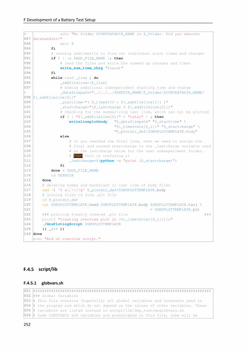
F Development of a Battery Test Setup
252
>
087
088
089
090
091
092
093
094
095
096
097
>
098
099
100
101
102
103
104
105
106
107
108
109
110
111
112
113
114
115
116
117
118
119
120
121
122
123
124
125
126
echo "No folder $CONVDATADIR_NAME in $_folder. Did you execute
datahandler?"
exit 3
fi
# reading addtimefile to find out individual start times and charges
if ! [ -e $ADD_FILE_NAME ]; then
# read the files and write the summed up charges and times
write_sum_time_chrg "$(pwd)"
fi
while read _line ; do
_addfileline=($_line)
# Adding additional subexperiment starting time and charge
_datafilepath="../../../$EXPDIR_NAME/$_folder/$CONVDATADIR_NAME/
${_addfileline[0]}"
_starttime="( $_timediff + ${_addfileline[1]} )"
_startcharge="($_lastcharge + ${_addfileline[2]})"
# checking for the summarizing last line, which can not be plotted
if ! [ "${_addfileline[0]}" = "total" ] ; then
writelineplotbody "$_datafilepath" "$_starttime" \
"${_timescale[$_i]}" "$_startcharge" \
"$_plotdir_def/$GNUPLOTTEMPLATE.body"
else
# if you reached the final line, then we need to assign the
# final and unused startcharge to the _lastcharge variable used
# as the lastcharge value for the next subesperiment folder.
# TODO this is confusing ;)
_lastcharge=$(python -c "print ($_startcharge)")
fi
done < $ADD_FILE_NAME
cd $EXPDIR
done
# deleting komma and backslash in last line of body files
sed -i '$ s/,\\//g' $_plotdir_def/$GNUPLOTTEMPLATE.body
# joining files to form .plt file
cd $_plotdir_def
cat $GNUPLOTTEMPLATE.head $GNUPLOTTEMPLATE.body $GNUPLOTTEMPLATE.tail \
> $GNUPLOTTEMPLATE.plt
### plotting freshly created .plt file ###
printf "Creating overview plot in [${_timeletter[$_i]}]\n"
./GnuPlotingScript $GNUPLOTTEMPLATE
(( _i++ ))
done
echo "End of overview script."
script/lib
F.4.5.1 globvars.sh
001
002
003
004
005
006
###############################################################################
### Global Variables
# This file contains (hopefully) all global variables and constants used in
# the program and which do not depend on the values of other variables. These
# variables are listed instead in script/lib/dep_runtimeglobvars.sh
# Some CONSTANTS and variables are preassigned in this file, some will be
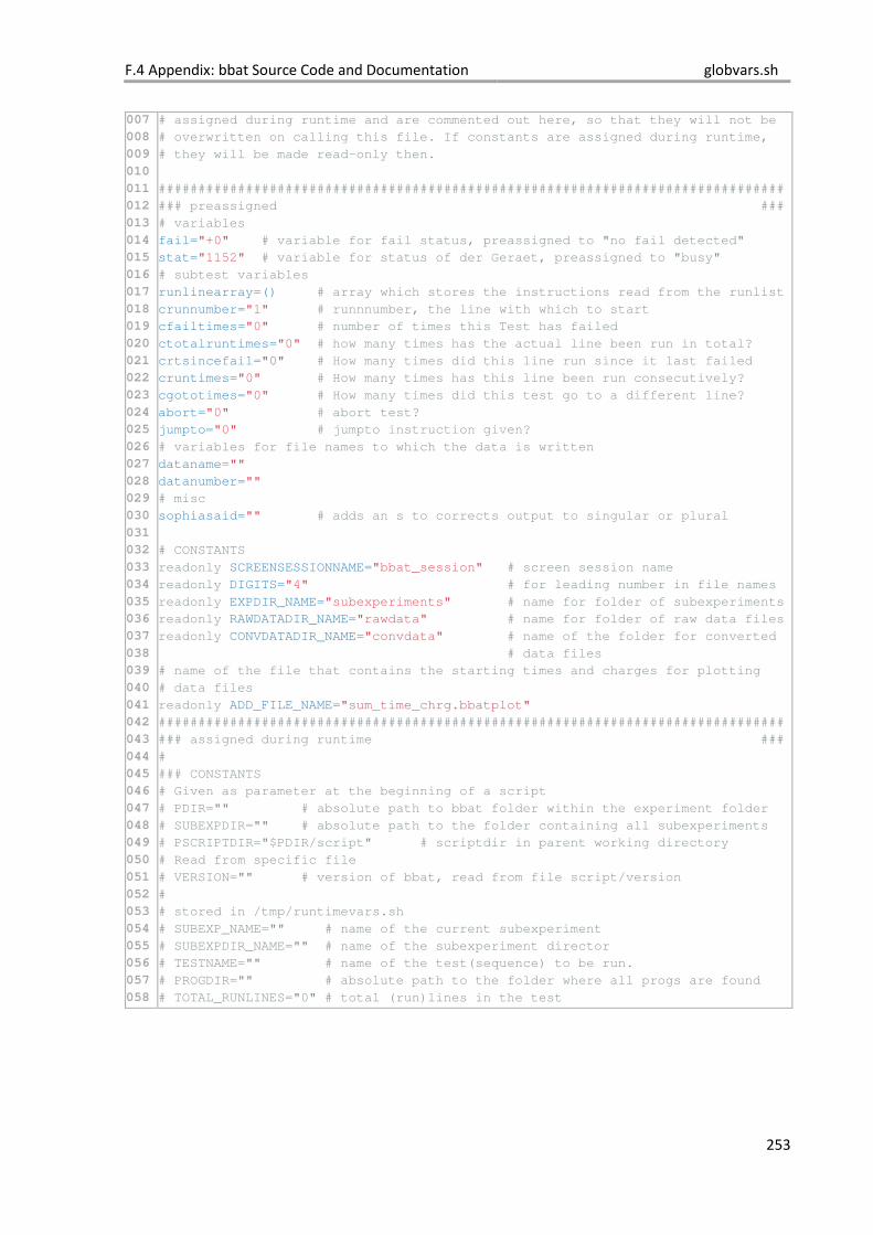
F.4 Appendix: bbat Source Code and Documentation globvars.sh
253
007
008
009
010
011
012
013
014
015
016
017
018
019
020
021
022
023
024
025
026
027
028
029
030
031
032
033
034
035
036
037
038
039
040
041
042
043
044
045
046
047
048
049
050
051
052
053
054
055
056
057
058
# assigned during runtime and are commented out here, so that they will not be
# overwritten on calling this file. If constants are assigned during runtime,
# they will be made read-only then.
###############################################################################
### preassigned ###
# variables
fail="+0" # variable for fail status, preassigned to "no fail detected"
stat="1152" # variable for status of der Geraet, preassigned to "busy"
# subtest variables
runlinearray=() # array which stores the instructions read from the runlist
crunnumber="1" # runnnumber, the line with which to start
cfailtimes="0" # number of times this Test has failed
ctotalruntimes="0" # how many times has the actual line been run in total?
crtsincefail="0" # How many times did this line run since it last failed
cruntimes="0" # How many times has this line been run consecutively?
cgototimes="0" # How many times did this test go to a different line?
abort="0" # abort test?
jumpto="0" # jumpto instruction given?
# variables for file names to which the data is written
dataname=""
datanumber=""
# misc
sophiasaid="" # adds an s to corrects output to singular or plural
# CONSTANTS
readonly SCREENSESSIONNAME="bbat_session" # screen session name
readonly DIGITS="4" # for leading number in file names
readonly EXPDIR_NAME="subexperiments" # name for folder of subexperiments
readonly RAWDATADIR_NAME="rawdata" # name for folder of raw data files
readonly CONVDATADIR_NAME="convdata" # name of the folder for converted
# data files
# name of the file that contains the starting times and charges for plotting
# data files
readonly ADD_FILE_NAME="sum_time_chrg.bbatplot"
###############################################################################
### assigned during runtime ###
#
### CONSTANTS
# Given as parameter at the beginning of a script
# PDIR="" # absolute path to bbat folder within the experiment folder
# SUBEXPDIR="" # absolute path to the folder containing all subexperiments
# PSCRIPTDIR="$PDIR/script" # scriptdir in parent working directory
# Read from specific file
# VERSION="" # version of bbat, read from file script/version
#
# stored in /tmp/runtimevars.sh
# SUBEXP_NAME="" # name of the current subexperiment
# SUBEXPDIR_NAME="" # name of the subexperiment director
# TESTNAME="" # name of the test(sequence) to be run.
# PROGDIR="" # absolute path to the folder where all progs are found
# TOTAL_RUNLINES="0" # total (run)lines in the test
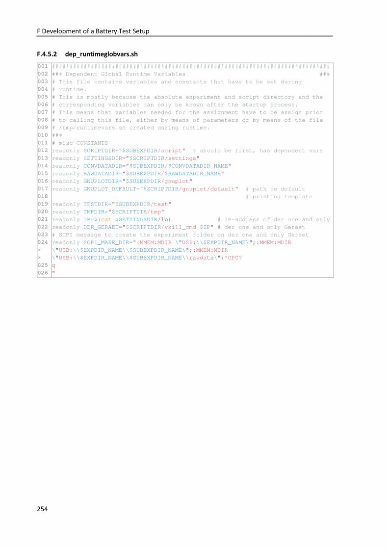
F Development of a Battery Test Setup
254
F.4.5.2 dep_runtimeglobvars.sh
001
002
003
004
005
006
007
008
009
010
011
012
013
014
015
016
017
018
019
020
021
022
023
024
>
>
025
026
###############################################################################
### Dependent Global Runtime Variables ###
# This file contains variables and constants that have to be set during
# runtime.
# This is mostly because the absolute experiment and script directory and the
# corresponding variables can only be known after the startup process.
# This means that variables needed for the assignment have to be assign prior
# to calling this file, either by means of parameters or by means of the file
# /tmp/runtimevars.sh created during runtime.
###
# misc CONSTANTS
readonly SCRIPTDIR="$SUBEXPDIR/script" # should be first, has dependent vars
readonly SETTINGSDIR="$SCRIPTDIR/settings"
readonly CONVDATADIR="$SUBEXPDIR/$CONVDATADIR_NAME"
readonly RAWDATADIR="$SUBEXPDIR/$RAWDATADIR_NAME"
readonly GNUPLOTDIR="$SUBEXPDIR/gnuplot"
readonly GNUPLOT_DEFAULT="$SCRIPTDIR/gnuplot/default" # path to default
# printing template
readonly TESTDIR="$SUBEXPDIR/test"
readonly TMPDIR="$SCRIPTDIR/tmp"
readonly IP=$(cat $SETTINGSDIR/ip) # IP-address of der one and only
readonly DER_GERAET="$SCRIPTDIR/vxi11_cmd $IP" # der one and only Geraet
# SCPI message to create the experiment folder on der one and only Geraet
readonly SCPI_MAKE_DIR=":MMEM:MDIR \"USB:\\$EXPDIR_NAME\";:MMEM:MDIR
\"USB:\\$EXPDIR_NAME\\$SUBEXPDIR_NAME\";:MMEM:MDIR
\"USB:\\$EXPDIR_NAME\\$SUBEXPDIR_NAME\\rawdata\";*OPC?
q
"
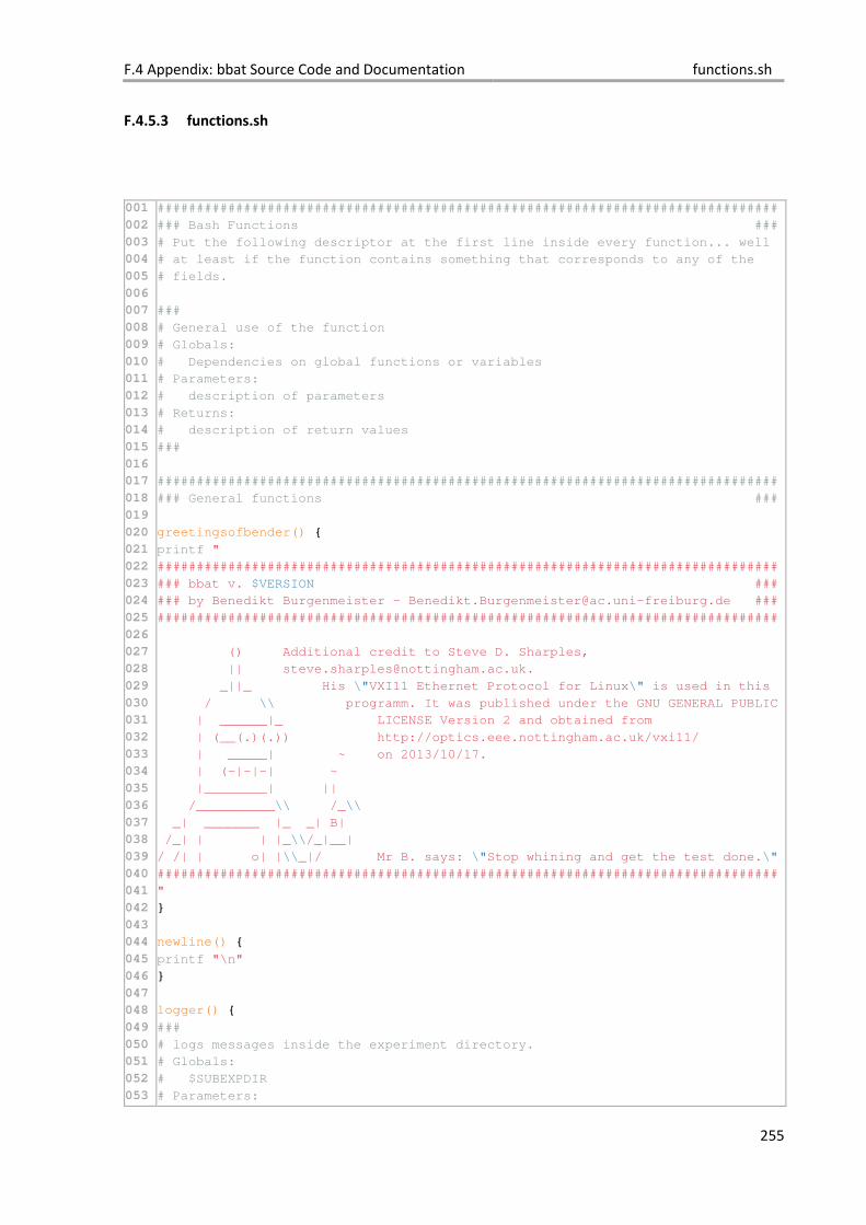
F.4 Appendix: bbat Source Code and Documentation functions.sh
255
F.4.5.3 functions.sh
001
002
003
004
005
006
007
008
009
010
011
012
013
014
015
016
017
018
019
020
021
022
023
024
025
026
027
028
029
030
031
032
033
034
035
036
037
038
039
040
041
042
043
044
045
046
047
048
049
050
051
052
053
###############################################################################
### Bash Functions ###
# Put the following descriptor at the first line inside every function... well
# at least if the function contains something that corresponds to any of the
# fields.
###
# General use of the function
# Globals:
# Dependencies on global functions or variables
# Parameters:
# description of parameters
# Returns:
# description of return values
###
###############################################################################
### General functions ###
greetingsofbender() {
printf "
###############################################################################
### bbat v. $VERSION ###
### by Benedikt Burgenmeister - [email protected] ###
###############################################################################
() Additional credit to Steve D. Sharples,
_||_ His \"VXI11 Ethernet Protocol for Linux\" is used in this
/ \\ programm. It was published under the GNU GENERAL PUBLIC
| ______|_ LICENSE Version 2 and obtained from
| (__(.)(.)) http://optics.eee.nottingham.ac.uk/vxi11/
| _____| ~ on 2013/10/17.
| (-|-|-| ~
|________| ||
/__________\\ /_\\
_| _______ |_ _| B|
/_| | | |_\\/_|__|
/ /| | o| |\\_|/ Mr B. says: \"Stop whining and get the test done.\"
###############################################################################
"
}
newline() {
printf "\n"
}
logger() {
###
# logs messages inside the experiment directory.
# Globals:
# $SUBEXPDIR
# Parameters:
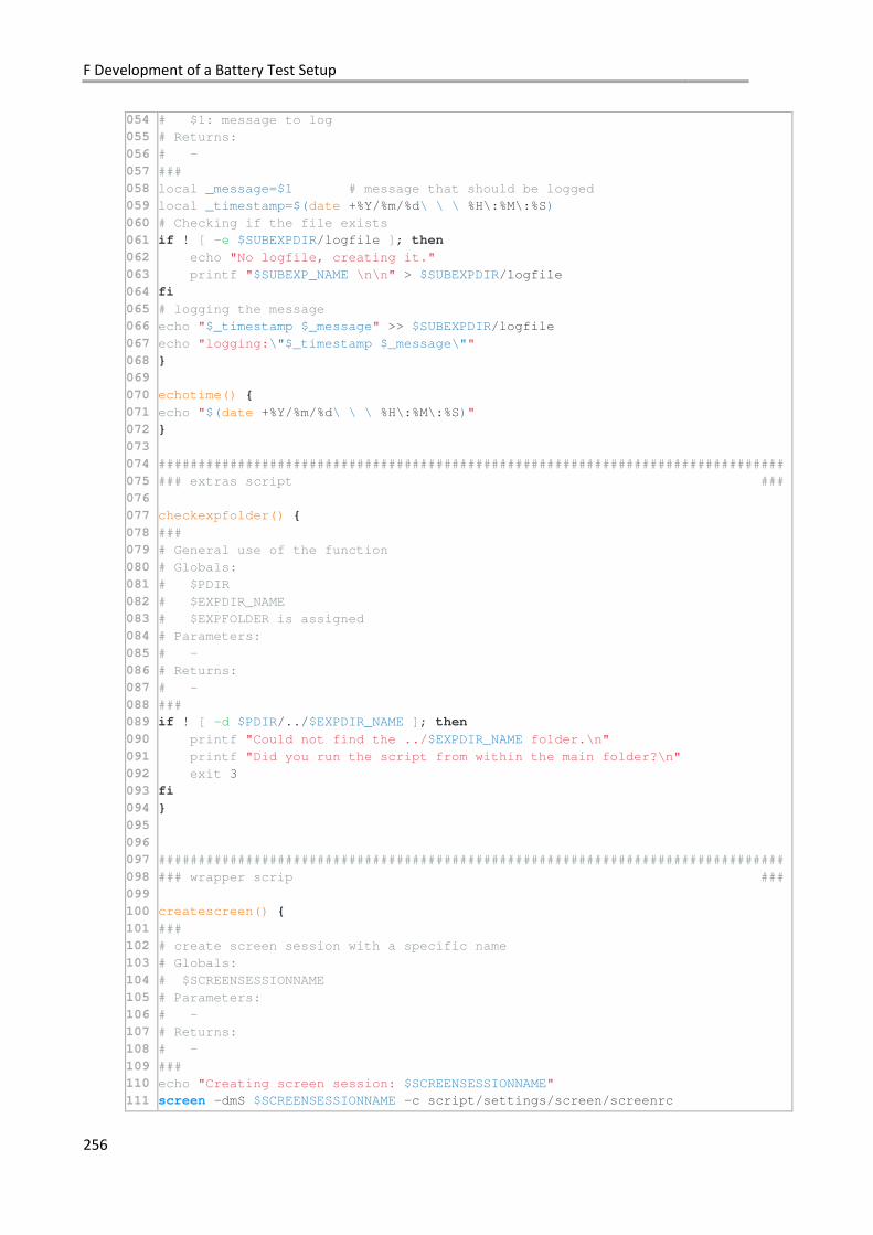
F Development of a Battery Test Setup
256
054
055
056
057
058
059
060
061
062
063
064
065
066
067
068
069
070
071
072
073
074
075
076
077
078
079
080
081
082
083
084
085
086
087
088
089
090
091
092
093
094
095
096
097
098
099
100
101
102
103
104
105
106
107
108
109
110
111
# $1: message to log
# Returns:
# -
###
local _message=$1 # message that should be logged
local _timestamp=$(date +%Y/%m/%d\ \ \ %H\:%M\:%S)
# Checking if the file exists
if ! [ -e $SUBEXPDIR/logfile ]; then
echo "No logfile, creating it."
printf "$SUBEXP_NAME \n\n" > $SUBEXPDIR/logfile
fi
# logging the message
echo "$_timestamp $_message" >> $SUBEXPDIR/logfile
echo "logging:\"$_timestamp $_message\""
}
echotime() {
echo "$(date +%Y/%m/%d\ \ \ %H\:%M\:%S)"
}
###############################################################################
### extras script ###
checkexpfolder() {
###
# General use of the function
# Globals:
# $PDIR
# $EXPDIR_NAME
# $EXPFOLDER is assigned
# Parameters:
# -
# Returns:
# -
###
if ! [ -d $PDIR/../$EXPDIR_NAME ]; then
printf "Could not find the ../$EXPDIR_NAME folder.\n"
printf "Did you run the script from within the main folder?\n"
exit 3
fi
}
###############################################################################
### wrapper scrip ###
createscreen() {
###
# create screen session with a specific name
# Globals:
# $SCREENSESSIONNAME
# Parameters:
# -
# Returns:
# -
###
echo "Creating screen session: $SCREENSESSIONNAME"
screen -dmS $SCREENSESSIONNAME -c script/settings/screen/screenrc
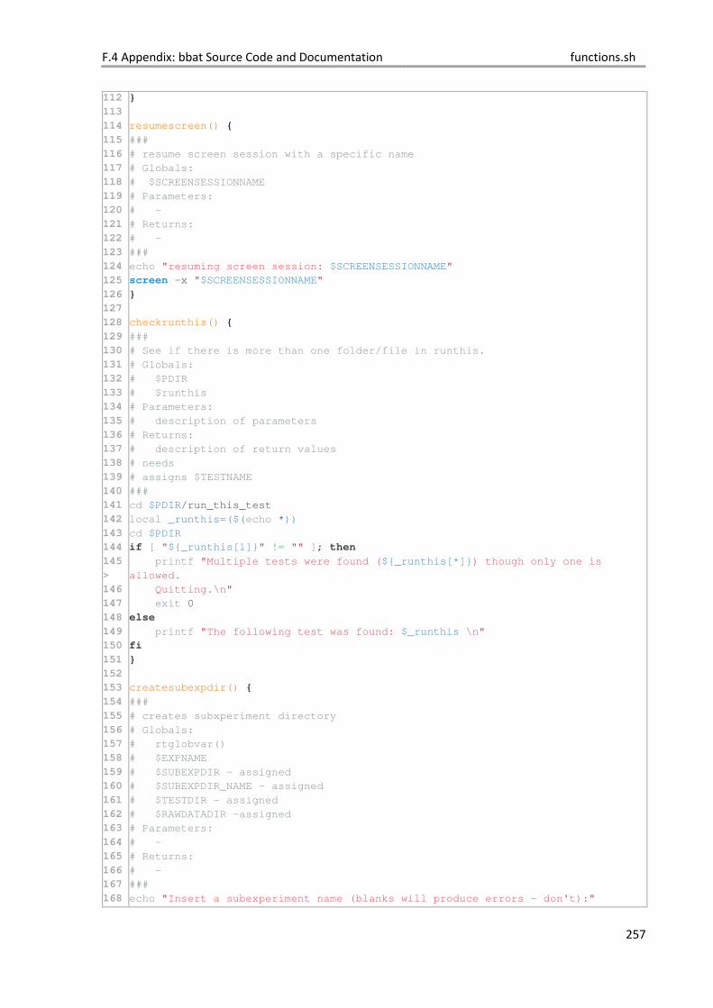
F.4 Appendix: bbat Source Code and Documentation functions.sh
257
112
113
114
115
116
117
118
119
120
121
122
123
124
125
126
127
128
129
130
131
132
133
134
135
136
137
138
139
140
141
142
143
144
145
>
146
147
148
149
150
151
152
153
154
155
156
157
158
159
160
161
162
163
164
165
166
167
168
}
resumescreen() {
###
# resume screen session with a specific name
# Globals:
# $SCREENSESSIONNAME
# Parameters:
# -
# Returns:
# -
###
echo "resuming screen session: $SCREENSESSIONNAME"
screen -x "$SCREENSESSIONNAME"
}
checkrunthis() {
###
# See if there is more than one folder/file in runthis.
# Globals:
# $PDIR
# $runthis
# Parameters:
# description of parameters
# Returns:
# description of return values
# needs
# assigns $TESTNAME
###
cd $PDIR/run_this_test
local _runthis=($(echo *))
cd $PDIR
if [ "${_runthis[1]}" != "" ]; then
printf "Multiple tests were found (${_runthis[*]}) though only one is
allowed.
Quitting.\n"
exit 0
else
printf "The following test was found: $_runthis \n"
fi
}
createsubexpdir() {
###
# creates subxperiment directory
# Globals:
# rtglobvar()
# $EXPNAME
# $SUBEXPDIR - assigned
# $SUBEXPDIR_NAME - assigned
# $TESTDIR - assigned
# $RAWDATADIR -assigned
# Parameters:
# -
# Returns:
# -
###
echo "Insert a subexperiment name (blanks will produce errors - don't):"
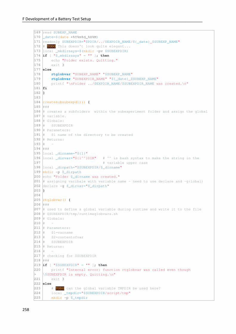
F Development of a Battery Test Setup
258
169
170
171
172
173
174
175
176
177
178
179
180
181
182
183
184
185
186
187
188
189
190
191
192
193
194
195
196
197
198
199
200
201
202
203
204
205
206
207
208
209
210
211
212
213
214
215
216
217
218
219
220
>
221
222
223
224
225
read SUBEXP_NAME
_date=$(date +%Y%m%d_%H%M)
readonly SUBEXPDIR="$PDIR/../$EXPDIR_NAME/${_date}_$SUBEXP_NAME"
# TODO This doesn't look quite elegant...
local _mkdirsays=$(mkdir -pv $SUBEXPDIR)
if [ "$_mkdirsays" = "" ]; then
echo "Folder exists. Quitting."
exit 3
else
rtglobvar "SUBEXP_NAME" "$SUBEXP_NAME"
rtglobvar "SUBEXPDIR_NAME" "${_date}_$SUBEXP_NAME"
printf "\nFolder ../$EXPDIR_NAME/$SUBEXPDIR_NAME was created.\n"
fi
}
createsubsubexpdir() {
###
# creates a subfolders within the subexperiment folder and assign the global
# variable.
# Globals:
# $SUBEXPDIR
# Parameters:
# $1 name of the directory to be created
# Returns:
# -
###
local _dirname="${1}"
local _dirvar="${1^^}DIR" # ^^ is bash syntax to make the string in the
# variable upper case
local _dirpath="$SUBEXPDIR/$_dirname"
mkdir -p $_dirpath
echo "Folder $_dirname was created."
# assigning varibale with variable name - need to use declare and -g(lobal)
declare -g $_dirvar="$_dirpath"
}
rtglobvar() {
###
# used to define a global variable during runtime and write it to the file
# $SUBEXPDIR/tmp/runtimeglobvars.sh
# Globals:
# -
# Parameters:
# $1=varname
# $2=contentofvar
# $SUBEXPDIR
# Returns:
# -
# checking for $SUBEXPDIR
###
if [ "$SUBEXPDIR" = "" ]; then
printf "Internal error: function rtglobvar was called even though
\$SUBEXPDIR is empty. Quitting.\n"
exit 3
else
# TODO can the global variable TMPDIR be used here?
local _tmpdir="$SUBEXPDIR/script/tmp"
mkdir -p $_tmpdir
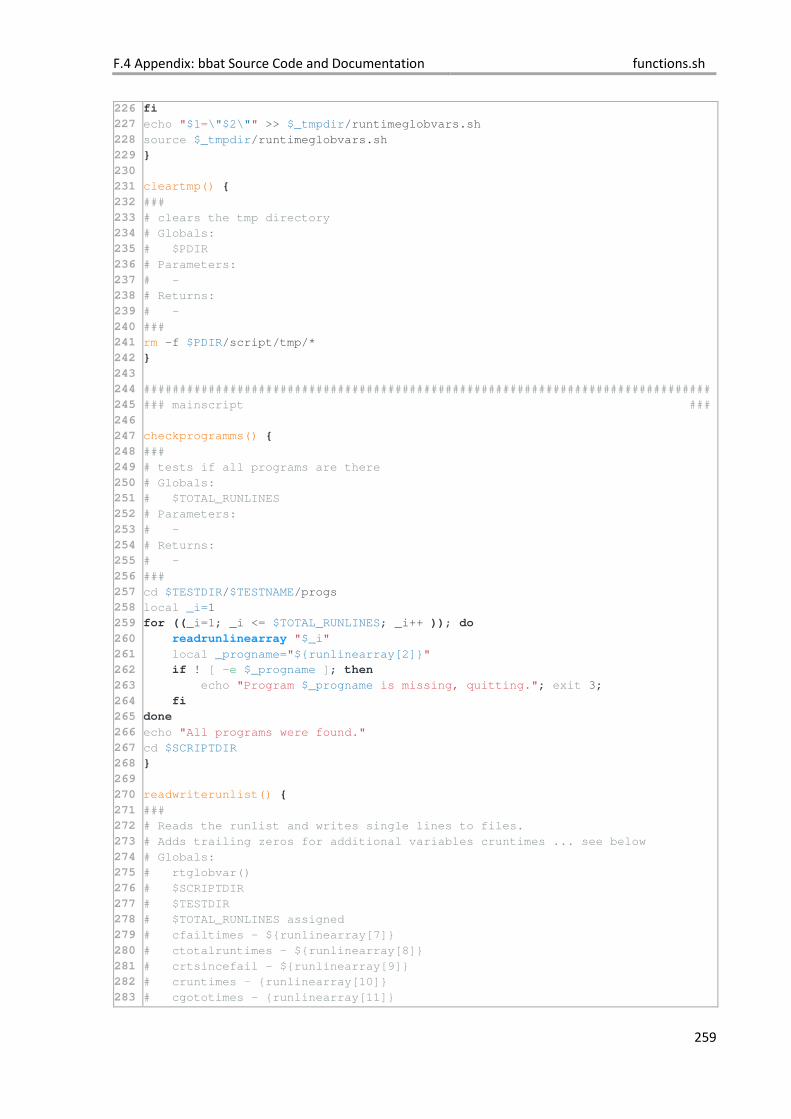
F.4 Appendix: bbat Source Code and Documentation functions.sh
259
226
227
228
229
230
231
232
233
234
235
236
237
238
239
240
241
242
243
244
245
246
247
248
249
250
251
252
253
254
255
256
257
258
259
260
261
262
263
264
265
266
267
268
269
270
271
272
273
274
275
276
277
278
279
280
281
282
283
fi
echo "$1=\"$2\"" >> $_tmpdir/runtimeglobvars.sh
source $_tmpdir/runtimeglobvars.sh
}
cleartmp() {
###
# clears the tmp directory
# Globals:
# $PDIR
# Parameters:
# -
# Returns:
# -
###
rm -f $PDIR/script/tmp/*
}
###############################################################################
### mainscript ###
checkprogramms() {
###
# tests if all programs are there
# Globals:
# $TOTAL_RUNLINES
# Parameters:
# -
# Returns:
# -
###
cd $TESTDIR/$TESTNAME/progs
local _i=1
for ((_i=1; _i <= $TOTAL_RUNLINES; _i++ )); do
readrunlinearray "$_i"
local _progname="${runlinearray[2]}"
if ! [ -e $_progname ]; then
echo "Program $_progname is missing, quitting."; exit 3;
fi
done
echo "All programs were found."
cd $SCRIPTDIR
}
readwriterunlist() {
###
# Reads the runlist and writes single lines to files.
# Adds trailing zeros for additional variables cruntimes ... see below
# Globals:
# rtglobvar()
# $SCRIPTDIR
# $TESTDIR
# $TOTAL_RUNLINES assigned
# cfailtimes - ${runlinearray[7]}
# ctotalruntimes - ${runlinearray[8]}
# crtsincefail - ${runlinearray[9]}
# cruntimes - {runlinearray[10]}
# cgototimes - {runlinearray[11]}
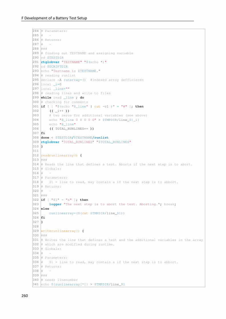
F Development of a Battery Test Setup
260
284
285
286
287
288
289
290
291
292
293
294
295
296
297
298
299
300
301
302
303
304
305
306
307
308
309
310
311
312
313
314
315
316
317
318
319
320
321
322
323
324
325
326
327
328
329
330
331
332
333
334
335
336
337
338
339
340
341
# Parameters:
# -
# Returns:
# -
###
# finding out TESTNAME and assigning variable
cd $TESTDIR
rtglobvar "TESTNAME" "$(echo *)"
cd $SCRIPTDIR
echo "Testname is $TESTNAME."
# reading runlist
declare -A runarray=() #indexed array deffinieren
local _i=0
local _line=""
# reading lines and write to files
while read _line ; do
# checking for comments
if ! [ "$(echo "$_line" | cut -c1 )" = "#" ]; then
(( _i++ ))
# two zeros for additional variables (see above)
echo "$_line 0 0 0 0 0" > $TMPDIR/line_${_i}
echo "$_line"
(( TOTAL_RUNLINES++ ))
fi
done < $TESTDIR/$TESTNAME/runlist
rtglobvar "TOTAL_RUNLINES" "$TOTAL_RUNLINES"
}
readrunlinearray() {
###
# Reads the line that defines a test. Aborts if the next step is to abort.
# Globals:
# -
# Parameters:
# $1 = line to read, may contain a if the next step is to abbort.
# Returns:
# -
###
if [ "$1" = "a" ]; then
logger "The next step is to abort the test. Aborting."; break;
else
runlinearray=($(cat $TMPDIR/line_$1))
fi
}
writerunlinearray() {
###
# Writes the line that defines a test and the additional variables in the array
# which are modified during runtime.
# Globals:
# -
# Parameters:
# $1 = line to read, may contain a if the next step is to abbort.
# Returns:
# -
###
# needs linenumber
echo ${runlinearray[*]} > $TMPDIR/line_$1
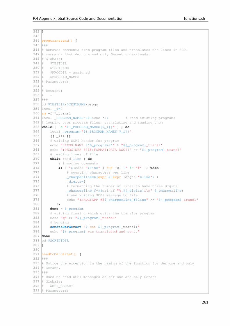
F.4 Appendix: bbat Source Code and Documentation functions.sh
261
342
343
344
345
346
347
348
349
350
351
352
353
354
355
356
357
358
359
360
361
362
363
364
365
366
367
368
369
370
371
372
373
374
375
376
377
378
379
380
381
382
383
384
385
386
387
388
389
390
391
392
393
394
395
396
397
398
399
}
progtranssend() {
###
# Removes comments from program files and translates the lines in SCPI
# commands that der one and only Geraet understands.
# Globals:
# $TESTDIR
# $TESTNAME
# $PROGDIR - assigned
# $PROGRAM_NAMES
# Parameters:
# -
# Returns:
# -
###
cd $TESTDIR/$TESTNAME/progs
local _i=0
rm -f *_transl
local _PROGRAM_NAMES=($(echo *)) # read existing programs
# looping over program files, translating and sending them
while [ -e "${_PROGRAM_NAMES[$_i]}" ] ; do
local _program="${_PROGRAM_NAMES[$_i]}"
(( _i++ ))
# writing SCPI header for program
echo ":PROG:NAME \"$_program\"" > "${_program}_transl"
echo ":PROG:DEF #218:FORMAT:DATA ASCII" >> "${_program}_transl"
# reading lines of file
while read line ; do
# ignoring comments
if [ "$(echo "$line" | cut -c1 )" != "#" ]; then
# counting characters per line
_charperline=$(expr $(expr length "$line") )
_digits=3
# formatting the number of lines to have three digits
_charperline_f=$(printf "%.${_digits}i\n" $_charperline)
# and writing SCPI message to file
echo ":PROG:APP #3$_charperline_f$line" >> "${_program}_transl"
fi
done < $_program
# writing final q which quits the transfer program
echo "q" >> "${_program}_transl"
# sending
sendtoDerGeraet "$(cat ${_program}_transl)"
echo "${_program} was translated and sent."
done
cd $SCRIPTDIR
}
sendtoDerGeraet() {
###
# Notice the exception in the naming of the function for der one and only
# Geraet.
###
# Used to send SCPI messages do der one and only Geraet
# Globals:
# $DER_GERAET
# Parameters:
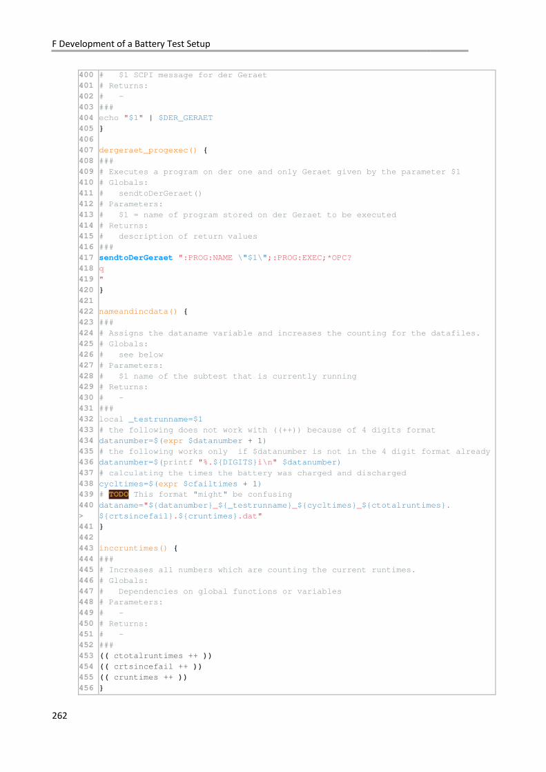
F Development of a Battery Test Setup
262
400
401
402
403
404
405
406
407
408
409
410
411
412
413
414
415
416
417
418
419
420
421
422
423
424
425
426
427
428
429
430
431
432
433
434
435
436
437
438
439
440
>
441
442
443
444
445
446
447
448
449
450
451
452
453
454
455
456
# $1 SCPI message for der Geraet
# Returns:
# -
###
echo "$1" | $DER_GERAET
}
dergeraet_progexec() {
###
# Executes a program on der one and only Geraet given by the parameter $1
# Globals:
# sendtoDerGeraet()
# Parameters:
# $1 = name of program stored on der Geraet to be executed
# Returns:
# description of return values
###
sendtoDerGeraet ":PROG:NAME \"$1\";:PROG:EXEC;*OPC?
q
"
}
nameandincdata() {
###
# Assigns the dataname variable and increases the counting for the datafiles.
# Globals:
# see below
# Parameters:
# $1 name of the subtest that is currently running
# Returns:
# -
###
local _testrunname=$1
# the following does not work with ((++)) because of 4 digits format
datanumber=$(expr $datanumber + 1)
# the following works only if $datanumber is not in the 4 digit format already
datanumber=$(printf "%.${DIGITS}i\n" $datanumber)
# calculating the times the battery was charged and discharged
cycltimes=$(expr $cfailtimes + 1)
# TODO This format "might" be confusing
dataname="${datanumber}_${_testrunname}_${cycltimes}_${ctotalruntimes}.
${crtsincefail}.${cruntimes}.dat"
}
inccruntimes() {
###
# Increases all numbers which are counting the current runtimes.
# Globals:
# Dependencies on global functions or variables
# Parameters:
# -
# Returns:
# -
###
(( ctotalruntimes ++ ))
(( crtsincefail ++ ))
(( cruntimes ++ ))
}
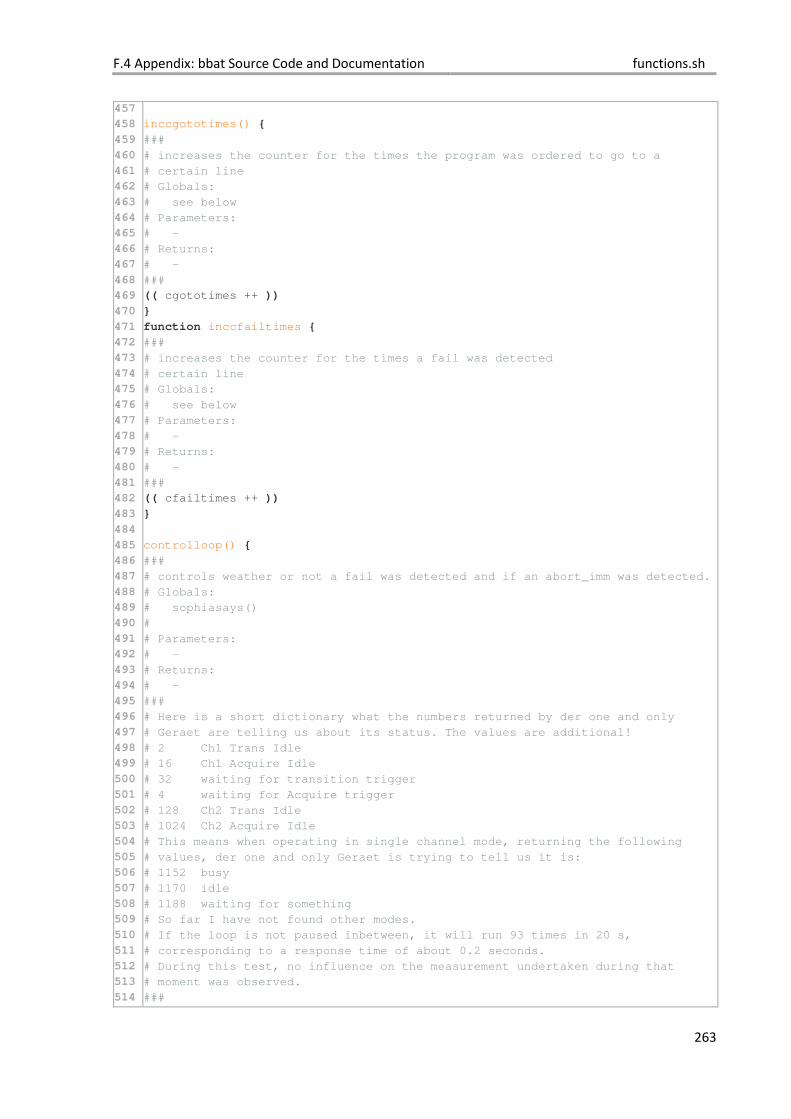
F.4 Appendix: bbat Source Code and Documentation functions.sh
263
457
458
459
460
461
462
463
464
465
466
467
468
469
470
471
472
473
474
475
476
477
478
479
480
481
482
483
484
485
486
487
488
489
490
491
492
493
494
495
496
497
498
499
500
501
502
503
504
505
506
507
508
509
510
511
512
513
514
inccgototimes() {
###
# increases the counter for the times the program was ordered to go to a
# certain line
# Globals:
# see below
# Parameters:
# -
# Returns:
# -
###
(( cgototimes ++ ))
}
function inccfailtimes {
###
# increases the counter for the times a fail was detected
# certain line
# Globals:
# see below
# Parameters:
# -
# Returns:
# -
###
(( cfailtimes ++ ))
}
controlloop() {
###
# controls weather or not a fail was detected and if an abort_imm was detected.
# Globals:
# sophiasays()
#
# Parameters:
# -
# Returns:
# -
###
# Here is a short dictionary what the numbers returned by der one and only
# Geraet are telling us about its status. The values are additional!
# 2 Ch1 Trans Idle
# 16 Ch1 Acquire Idle
# 32 waiting for transition trigger
# 4 waiting for Acquire trigger
# 128 Ch2 Trans Idle
# 1024 Ch2 Acquire Idle
# This means when operating in single channel mode, returning the following
# values, der one and only Geraet is trying to tell us it is:
# 1152 busy
# 1170 idle
# 1188 waiting for something
# So far I have not found other modes.
# If the loop is not paused inbetween, it will run 93 times in 20 s,
# corresponding to a response time of about 0.2 seconds.
# During this test, no influence on the measurement undertaken during that
# moment was observed.
###
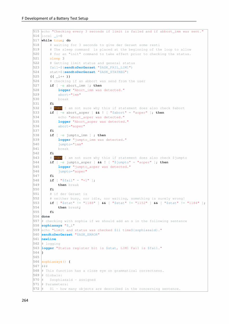
F Development of a Battery Test Setup
264
515
516
517
518
519
520
521
522
523
524
525
526
527
528
529
530
531
532
533
534
535
536
537
538
539
540
541
542
543
544
545
546
547
548
549
550
551
552
553
554
555
556
557
558
559
560
561
562
563
564
565
566
567
568
569
570
571
572
echo "Checking every 3 seconds if limit is failed and if abbort_imm was sent."
local _i=0
while true; do
# waiting for 3 seconds to give der Geraet some resti
# The sleep command is placed at the beginning of the loop to allow
# for an "init" command to take effect prior to checking the status.
sleep 3
# Getting limit status and general status
fail=$(sendtoDerGeraet "$ASK_FAIL_LIM1")
stat=$(sendtoDerGeraet "$ASK_STATREG")
(( _i++ ))
# checking if an abbort was send from the user
if [ -e abort_imm ]; then
logger "Abort_imm was detected."
abort="imm"
break
fi
# TODO I am not sure why this if statement does also check $abort
if [ -e abort_aoper ] && ! [ "$abort" = "aoper" ]; then
echo "abort_aoper was detected."
logger "Abort_aoper was detected."
abort="aoper"
fi
if [ -e jumpto_imm ] ; then
logger "jumpto_imm was detected."
jumpto="imm"
break
fi
# TODO I am not sure why this if statement does also check $jumpto
if [ -e jumpto_aoper ] && ! [ "$jumpto" = "aoper" ]; then
logger "jumpto_aoper was detected."
jumpto="aoper"
fi
if [ "$fail" = "+1" ];
then break
fi
# if der Geraet is
# neither busy, nor idle, nor waiting, something is surely wrong!
if [ "$stat" != "1188" ] && [ "$stat" != "1152" ] && [ "$stat" != "1184" ];
then break;
fi
done
# checking with sophia if we should add an s in the following sentence
sophiasays "$_i"
echo "Limit and status was checked $li time${sophiasaid}."
sendtoDerGeraet "$ASK_ERROR"
newline
# logging
logger "Status register bit is $stat, LIM1 Fail is $fail."
}
sophiasays() {
###
# This function has a close eye on grammatical correctness.
# Globals:
# $sophiasaid - assigned
# Parameters:
# $1 - how many objects are described in the concerning sentence.
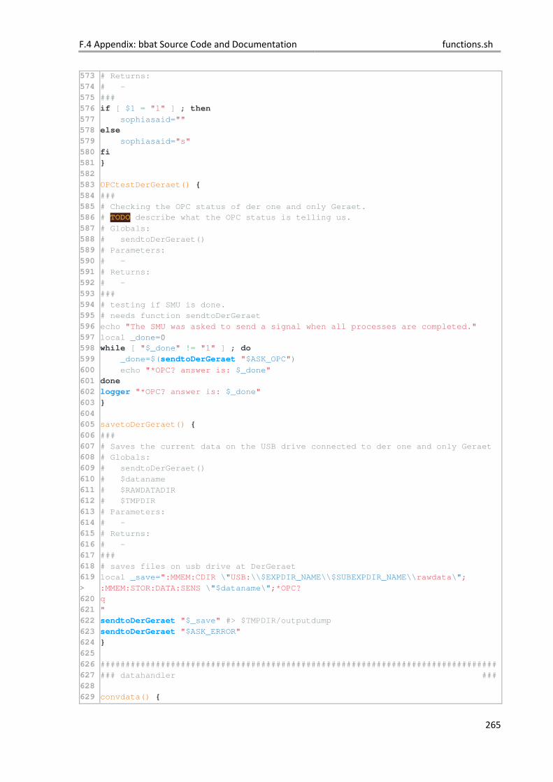
F.4 Appendix: bbat Source Code and Documentation functions.sh
265
573
574
575
576
577
578
579
580
581
582
583
584
585
586
587
588
589
590
591
592
593
594
595
596
597
598
599
600
601
602
603
604
605
606
607
608
609
610
611
612
613
614
615
616
617
618
619
>
620
621
622
623
624
625
626
627
628
629
# Returns:
# -
###
if [ $1 = "1" ] ; then
sophiasaid=""
else
sophiasaid="s"
fi
}
OPCtestDerGeraet() {
###
# Checking the OPC status of der one and only Geraet.
# TODO describe what the OPC status is telling us.
# Globals:
# sendtoDerGeraet()
# Parameters:
# -
# Returns:
# -
###
# testing if SMU is done.
# needs function sendtoDerGeraet
echo "The SMU was asked to send a signal when all processes are completed."
local _done=0
while [ "$_done" != "1" ] ; do
_done=$(sendtoDerGeraet "$ASK_OPC")
echo "*OPC? answer is: $_done"
done
logger "*OPC? answer is: $_done"
}
savetoDerGeraet() {
###
# Saves the current data on the USB drive connected to der one and only Geraet
# Globals:
# sendtoDerGeraet()
# $dataname
# $RAWDATADIR
# $TMPDIR
# Parameters:
# -
# Returns:
# -
###
# saves files on usb drive at DerGeraet
local _save=":MMEM:CDIR \"USB:\\$EXPDIR_NAME\\$SUBEXPDIR_NAME\\rawdata\";
:MMEM:STOR:DATA:SENS \"$dataname\";*OPC?
q
"
sendtoDerGeraet "$_save" #> $TMPDIR/outputdump
sendtoDerGeraet "$ASK_ERROR"
}
###############################################################################
### datahandler ###
convdata() {
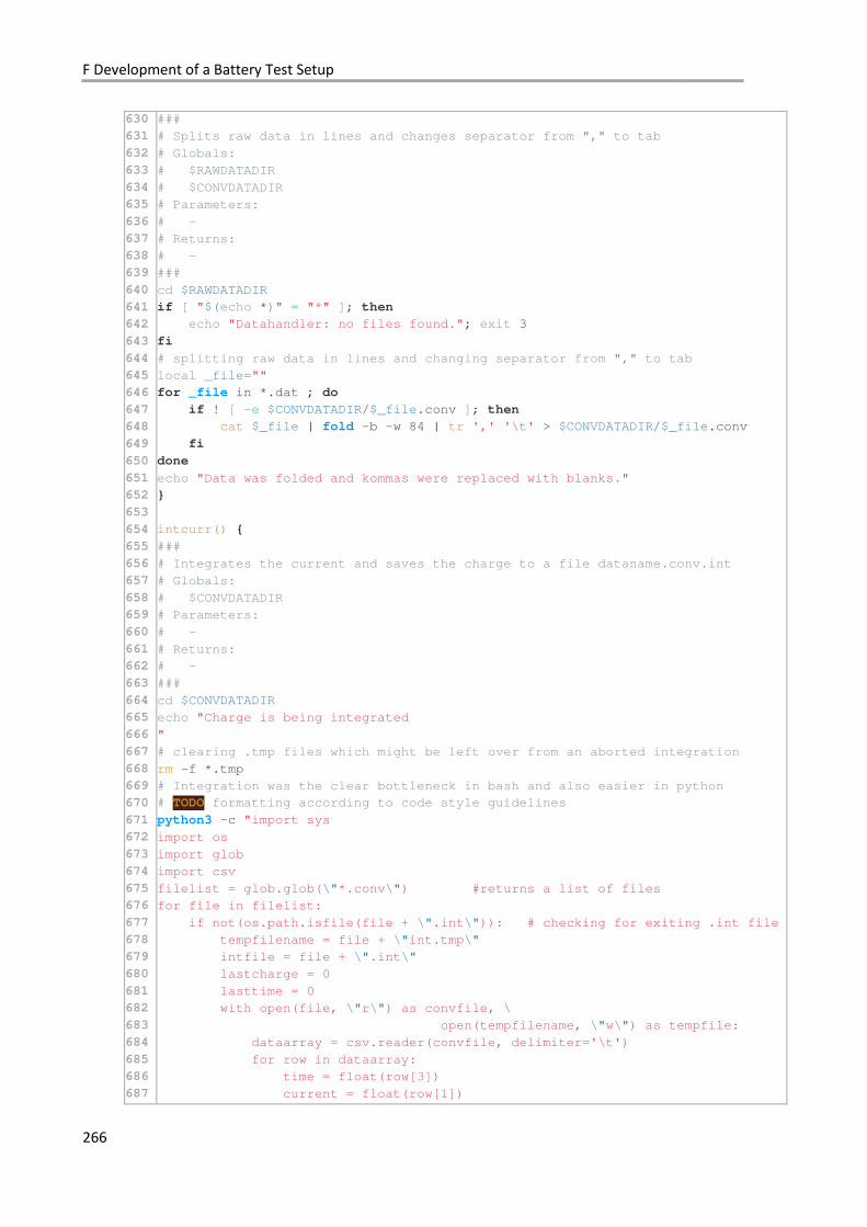
F Development of a Battery Test Setup
266
630
631
632
633
634
635
636
637
638
639
640
641
642
643
644
645
646
647
648
649
650
651
652
653
654
655
656
657
658
659
660
661
662
663
664
665
666
667
668
669
670
671
672
673
674
675
676
677
678
679
680
681
682
683
684
685
686
687
###
# Splits raw data in lines and changes separator from "," to tab
# Globals:
# $RAWDATADIR
# $CONVDATADIR
# Parameters:
# -
# Returns:
# -
###
cd $RAWDATADIR
if [ "$(echo *)" = "*" ]; then
echo "Datahandler: no files found."; exit 3
fi
# splitting raw data in lines and changing separator from "," to tab
local _file=""
for _file in *.dat ; do
if ! [ -e $CONVDATADIR/$_file.conv ]; then
cat $_file | fold -b -w 84 | tr ',' '\t' > $CONVDATADIR/$_file.conv
fi
done
echo "Data was folded and kommas were replaced with blanks."
}
intcurr() {
###
# Integrates the current and saves the charge to a file dataname.conv.int
# Globals:
# $CONVDATADIR
# Parameters:
# -
# Returns:
# -
###
cd $CONVDATADIR
echo "Charge is being integrated
"
# clearing .tmp files which might be left over from an aborted integration
rm -f *.tmp
# Integration was the clear bottleneck in bash and also easier in python
# TODO formatting according to code style guidelines
python3 -c "import sys
import os
import glob
import csv
filelist = glob.glob(\"*.conv\") #returns a list of files
for file in filelist:
if not(os.path.isfile(file + \".int\")): # checking for exiting .int file
tempfilename = file + \"int.tmp\"
intfile = file + \".int\"
lastcharge = 0
lasttime = 0
with open(file, \"r\") as convfile, \
open(tempfilename, \"w\") as tempfile:
dataarray = csv.reader(convfile, delimiter='\t')
for row in dataarray:
time = float(row[3])
current = float(row[1])
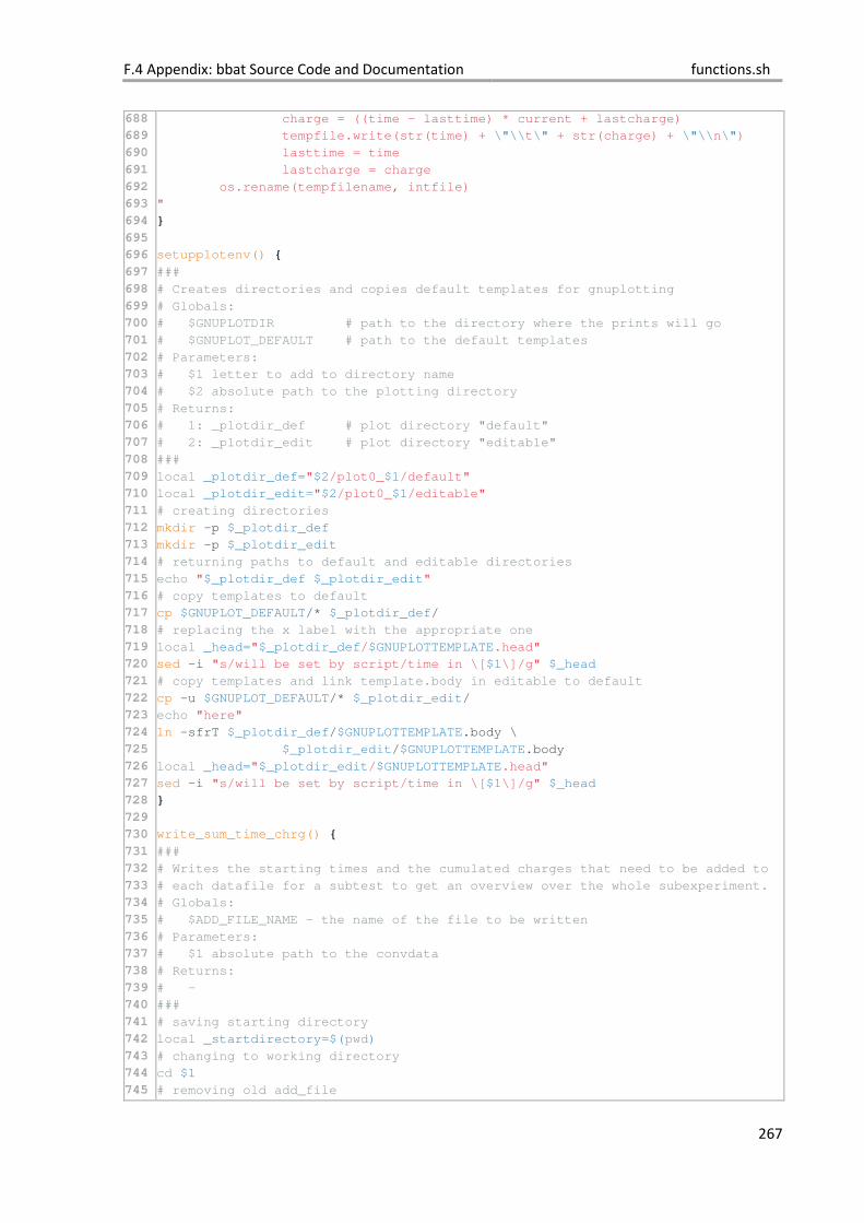
F.4 Appendix: bbat Source Code and Documentation functions.sh
267
688
689
690
691
692
693
694
695
696
697
698
699
700
701
702
703
704
705
706
707
708
709
710
711
712
713
714
715
716
717
718
719
720
721
722
723
724
725
726
727
728
729
730
731
732
733
734
735
736
737
738
739
740
741
742
743
744
745
charge = ((time - lasttime) * current + lastcharge)
tempfile.write(str(time) + \"\\t\" + str(charge) + \"\\n\")
lasttime = time
lastcharge = charge
os.rename(tempfilename, intfile)
"
}
setupplotenv() {
###
# Creates directories and copies default templates for gnuplotting
# Globals:
# $GNUPLOTDIR # path to the directory where the prints will go
# $GNUPLOT_DEFAULT # path to the default templates
# Parameters:
# $1 letter to add to directory name
# $2 absolute path to the plotting directory
# Returns:
# 1: _plotdir_def # plot directory "default"
# 2: _plotdir_edit # plot directory "editable"
###
local _plotdir_def="$2/plot0_$1/default"
local _plotdir_edit="$2/plot0_$1/editable"
# creating directories
mkdir -p $_plotdir_def
mkdir -p $_plotdir_edit
# returning paths to default and editable directories
echo "$_plotdir_def $_plotdir_edit"
# copy templates to default
cp $GNUPLOT_DEFAULT/* $_plotdir_def/
# replacing the x label with the appropriate one
local _head="$_plotdir_def/$GNUPLOTTEMPLATE.head"
sed -i "s/will be set by script/time in \[$1\]/g" $_head
# copy templates and link template.body in editable to default
cp -u $GNUPLOT_DEFAULT/* $_plotdir_edit/
echo "here"
ln -sfrT $_plotdir_def/$GNUPLOTTEMPLATE.body \
$_plotdir_edit/$GNUPLOTTEMPLATE.body
local _head="$_plotdir_edit/$GNUPLOTTEMPLATE.head"
sed -i "s/will be set by script/time in \[$1\]/g" $_head
}
write_sum_time_chrg() {
###
# Writes the starting times and the cumulated charges that need to be added to
# each datafile for a subtest to get an overview over the whole subexperiment.
# Globals:
# $ADD_FILE_NAME - the name of the file to be written
# Parameters:
# $1 absolute path to the convdata
# Returns:
# -
###
# saving starting directory
local _startdirectory=$(pwd)
# changing to working directory
cd $1
# removing old add_file
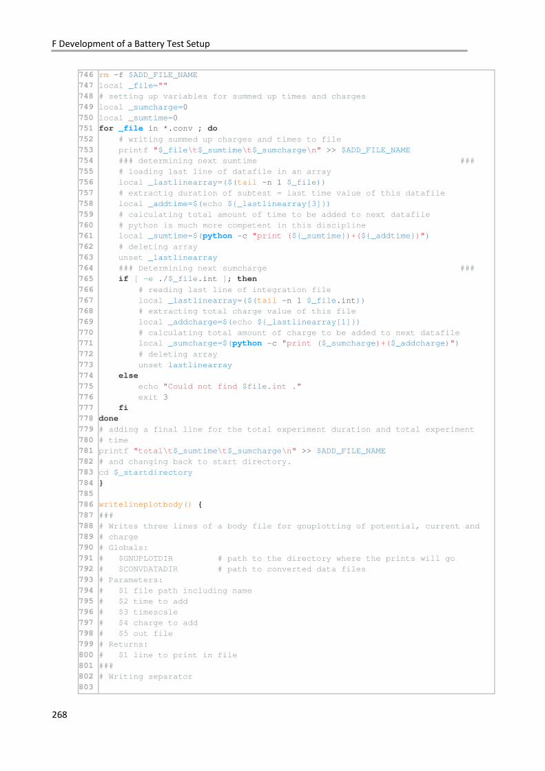
F Development of a Battery Test Setup
268
746
747
748
749
750
751
752
753
754
755
756
757
758
759
760
761
762
763
764
765
766
767
768
769
770
771
772
773
774
775
776
777
778
779
780
781
782
783
784
785
786
787
788
789
790
791
792
793
794
795
796
797
798
799
800
801
802
803
rm -f $ADD_FILE_NAME
local _file=""
# setting up variables for summed up times and charges
local _sumcharge=0
local _sumtime=0
for _file in *.conv ; do
# writing summed up charges and times to file
printf "$_file\t$_sumtime\t$_sumcharge\n" >> $ADD_FILE_NAME
### determining next sumtime ###
# loading last line of datafile in an array
local _lastlinearray=($(tail -n 1 $_file))
# extractig duration of subtest = last time value of this datafile
local _addtime=$(echo ${_lastlinearray[3]})
# calculating total amount of time to be added to next datafile
# python is much more competent in this discipline
local _sumtime=$(python -c "print (${_sumtime})+(${_addtime})")
# deleting array
unset _lastlinearray
### Determining next sumcharge ###
if [ -e ./$_file.int ]; then
# reading last line of integration file
local _lastlinearray=($(tail -n 1 $_file.int))
# extracting total charge value of this file
local _addcharge=$(echo ${_lastlinearray[1]})
# calculating total amount of charge to be added to next datafile
local _sumcharge=$(python -c "print ($_sumcharge)+($_addcharge)")
# deleting array
unset lastlinearray
else
echo "Could not find $file.int ."
exit 3
fi
done
# adding a final line for the total experiment duration and total experiment
# time
printf "total\t$_sumtime\t$_sumcharge\n" >> $ADD_FILE_NAME
# and changing back to start directory.
cd $_startdirectory
}
writelineplotbody() {
###
# Writes three lines of a body file for gnuplotting of potential, current and
# charge
# Globals:
# $GNUPLOTDIR # path to the directory where the prints will go
# $CONVDATADIR # path to converted data files
# Parameters:
# $1 file path including name
# $2 time to add
# $3 timescale
# $4 charge to add
# $5 out file
# Returns:
# $1 line to print in file
###
# Writing separator
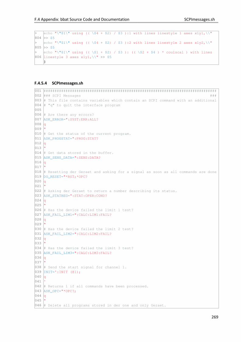
F.4 Appendix: bbat Source Code and Documentation SCPImessages.sh
269
F.4.5.4 SCPImessages.sh
001
002
003
004
005
006
007
008
009
010
011
012
013
014
015
016
017
018
019
020
021
022
023
024
025
026
027
028
029
030
031
032
033
034
035
036
037
038
039
040
041
042
043
044
045
046
###############################################################################
### SCPI Messages ###
# This file contains variables which contain an SCPI command with an additional
# "q" to quit the interface program
# Are there any errors?
ASK_ERROR=":SYST:ERR:ALL?
q
"
# Get the status of the current program.
ASK_PROGSTAT=":PROG:STAT?
q
"
# Get data stored in the buffer.
ASK_SENS_DATA=":SENS:DATA?
q
"
# Resetting der Geraet and asking for a signal as soon as all commands are done
DO_RESET="*RST;*OPC?
q
"
# Asking der Geraet to return a number describing its status.
ASK_STATREG=":STAT:OPER:COND?
q
"
# Has the device failed the limit 1 test?
ASK_FAIL_LIM1=":CALC:LIM1:FAIL?
q
"
# Has the device failed the limit 2 test?
ASK_FAIL_LIM2=":CALC:LIM2:FAIL?
q
"
# Has the device failed the limit 3 test?
ASK_FAIL_LIM3=":CALC:LIM3:FAIL?
q
"
# Send the start signal for channel 1.
INIT=':INIT (@1);
q
'
# Returns 1 if all commands have been processed.
ASK_OPC="*OPC?;
q
"
# Delete all programs stored in der one and only Geraet.
>
804
>
805
>
806
echo "\"$1\" using (( \$4 + $2) / $3 ):1 with lines linestyle 1 axes x1y1,\\"
>> $5
echo "\"$1\" using (( \$4 + $2) / $3 ):2 with lines linestyle 2 axes x1y2,\\"
>> $5
echo "\"$1\" using (( \$1 + $2) / $3 ): (( \$2 + $4 ) * coulscal ) with lines
linestyle 3 axes x1y1,\\" >> $5
}
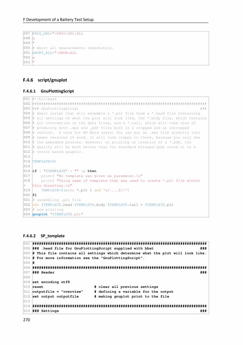
F Development of a Battery Test Setup
270
047
048
049
050
051
052
053
PROG_DEL=":PROG:DEL:ALL
q
"
# Abort all measurements immediately.
ABORT_ALL=":ABOR:ALL
q
"
script/gnuplot
F.4.6.1 GnuPlottingScript
001
002
003
004
005
006
007
008
009
010
011
012
013
014
015
016
017
018
>
019
020
021
022
023
024
#!/bin/bash
###############################################################################
### GnuPlottingScript ###
# Small script that will assemble a *.plt file from a *.head file containing
# all settings on what the plot will look like, the *.body file, which contains
# all information on the data files, and a *.tail, which will take care of
# producing both .eps and .pdf files both in a cropped and an uncropped
# version. A note for MS Word users: You can put an .eps file directly into
# newer versions of word. It will look crappy in there, because you only see
# the embedded preview. However, on printing or creation of a *.pdf, the
# quality will be much better than for standard bitmaps/jpgs since it is a
# vector based graphic.
TEMPLATE=$1
if [ "$TEMPLATE" = "" ]; then
printf "No template was given as parameter.\n"
printf "Using name of template that was used to create *.plt file within
this directory.\n"
TEMPLATE=$(echo *.plt | sed 's/....$//')
fi
# assembling .plt file
cat $TEMPLATE.head $TEMPLATE.body $TEMPLATE.tail > $TEMPLATE.plt
# and plotting
gnuplot "$TEMPLATE.plt"
F.4.6.2 SP_template
001
002
003
004
005
006
007
008
009
010
011
012
013
014
015
###############################################################################
### .head file for GnuPlottingScript supplied with bbat ###
# This file contains all settings which determine what the plot will look like.
# For more information see the "GnuPlottingScript".
#
###############################################################################
### Header ###
set encoding utf8
reset # clear all previous settings
outputfile = "overview" # defining a variable for the output
set output outputfile # making gnuplot print to the file
###############################################################################
### Settings ###
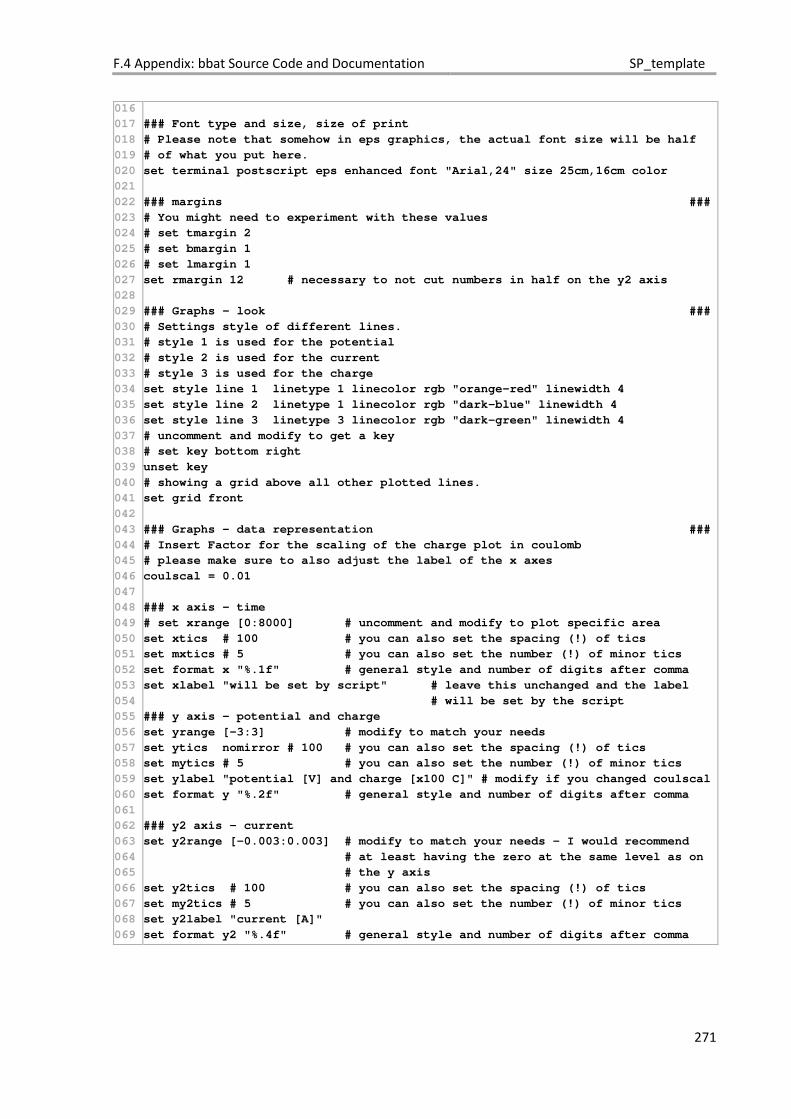
F.4 Appendix: bbat Source Code and Documentation SP_template
271
016
017
018
019
020
021
022
023
024
025
026
027
028
029
030
031
032
033
034
035
036
037
038
039
040
041
042
043
044
045
046
047
048
049
050
051
052
053
054
055
056
057
058
059
060
061
062
063
064
065
066
067
068
069
### Font type and size, size of print
# Please note that somehow in eps graphics, the actual font size will be half
# of what you put here.
set terminal postscript eps enhanced font "Arial,24" size 25cm,16cm color
### margins ###
# You might need to experiment with these values
# set tmargin 2
# set bmargin 1
# set lmargin 1
set rmargin 12 # necessary to not cut numbers in half on the y2 axis
### Graphs - look ###
# Settings style of different lines.
# style 1 is used for the potential
# style 2 is used for the current
# style 3 is used for the charge
set style line 1 linetype 1 linecolor rgb "orange-red" linewidth 4
set style line 2 linetype 1 linecolor rgb "dark-blue" linewidth 4
set style line 3 linetype 3 linecolor rgb "dark-green" linewidth 4
# uncomment and modify to get a key
# set key bottom right
unset key
# showing a grid above all other plotted lines.
set grid front
### Graphs - data representation ###
# Insert Factor for the scaling of the charge plot in coulomb
# please make sure to also adjust the label of the x axes
coulscal = 0.01
### x axis - time
# set xrange [0:8000] # uncomment and modify to plot specific area
set xtics # 100 # you can also set the spacing (!) of tics
set mxtics # 5 # you can also set the number (!) of minor tics
set format x "%.1f" # general style and number of digits after comma
set xlabel "will be set by script" # leave this unchanged and the label
# will be set by the script
### y axis - potential and charge
set yrange [-3:3] # modify to match your needs
set ytics nomirror # 100 # you can also set the spacing (!) of tics
set mytics # 5 # you can also set the number (!) of minor tics
set ylabel "potential [V] and charge [x100 C]" # modify if you changed coulscal
set format y "%.2f" # general style and number of digits after comma
### y2 axis - current
set y2range [-0.003:0.003] # modify to match your needs - I would recommend
# at least having the zero at the same level as on
# the y axis
set y2tics # 100 # you can also set the spacing (!) of tics
set my2tics # 5 # you can also set the number (!) of minor tics
set y2label "current [A]"
set format y2 "%.4f" # general style and number of digits after comma

F Development of a Battery Test Setup
272
273
G Conclusion and Outlook
In this work, a tool was presented, which gives access to an estimate for the economic potential of
specific battery chemistries. Applied to our IL based batteries and considering only the energy densities
and the cost for the active materials per stored energy, all proposed systems seemed viable, when
considering the all vanadium RFB as an established reference technology.
The results obtained through this tool also revealed the scope of the economic potential of the
membrane-free IL-RFB concept, which is due to a competitive price and a very high theoretical energy
density for both aluminium and tin based systems. The All-Mn Hyb-IL-RFB was also identified to offer
competitive characteristics, however, for all battery systems the price of the [cat]X salt was identified
as the main cost determining factor and should ideally be decreased.
Ionic liquids based on the combination of organic halide salts and I2Cl6 were first investigated in this
work as a possible electrolyte for a membrane-free IL-RFB. However, a battery test revealed iodine as
a reduction product in the discharged state. Based on this finding, it was decided that the well
characterized polybromides would be a better choice for the investigation of an inherently challenging
battery concept.
The chloroiodate compounds were investigated nevertheless, since they still seemed attractive for the
use in other batteries, which led to the finding of experimental evidence for the hitherto unknown
[I2Cl7]– anion. The experimental study included mixtures of [HMIM]Cl, [BMP]Cl and [NEt4]Cl (in
cooperation with Karsten Sonnenberg, AG Riedel, FU Berlin) with 0.5, 1.0 and 1.5 equivalents of I2Cl6
and was supplemented with quantum-chemical calculations both to obtain theoretical Raman spectra
and a deeper insight in the observed instability of the compounds. By calculating minimum structures
for anions containing iodine(I) and iodine(III) in the series [IxClx+y+1]– (x = 1,2,3, y = 0 … 2x), it was found
that the tendency for the elimination of dichlorine increases with the number of iodine and the number
of chlorine atoms contained in the anion. This is in accordance with the observation that [BMP][I2Cl7],
which is a homogeneous liquid at room temperature, is only stable if contained in a gas tight vessel.
Mixtures of [NEt4]Cl with one equivalent of I2Cl6 are liquid as well, despite their symmetrical cation,
which on one hand is a good sign for the intended use in redox flow batteries. On the other hand, the
instability of these compounds might be contradictory with their wide spread use for this application.
The concept for a membrane-free Sn/Br2 Hyb-IL-RFB was investigated starting with the synthesis of
novel bromostannate(IV) ILs, studying their phase behaviour and their mixtures with bromine, and
finally building batteries based on the synthesized ILs. The initially observed discharge currents
G Conclusion and Outlook
274
obtained in cells consisting of polybromide ILs, a tin, and a graphite electrode, were encouraging
despite the low electrochemical efficiency determined for these first experiments. However, all
attempts to charge this type of membrane-free battery, or even a battery set up with the same
chemicals and using a membrane, were unsuccessful. In some of these charging experiments evidence
for the formation of SnBr2 was found via Raman spectroscopy, which could indicate that the reduction
process of bromostannates(IV) to yield a deposit of elemental tin is problematic. Further research is
needed to better understand this behaviour.
The results obtained during in the preliminary assessment of the feasibility of an All-Mn Hyb-IL-RFB
were more promising. Though chemical attempts in synthesizing chloromanganate(IV) ILs were
unsuccessful and yielded at best manganese(III) compounds, the OCV obtained for a first All-Mn
battery was 3.0 V, which encourages further research. Even cycling in a very limited SOC range was
possible.
All battery tests were controlled using a software programmed as part of this thesis. The program was
proven to be reliable in operation and is intended to be the base for the planned integration of pumps
and thermostats in combination with the newly developed flow test-cell.
At the beginning of the work on this thesis, only very basic knowledge on the performance and
chemical characteristics of IL batteries existed, most of which had resulted from the two diploma
theses written on the topic. Through the combined efforts of all members of the IL-RFB project, a far
greater understanding of the potential and the limitations of the technology was achieved. Based on
the knowledge gathered to this point, it seems to me that a shift in the focus of this technology might
be necessary in future research.
In the introduction to this thesis, general considerations in respect to the physical design of flow
batteries in comparison with classical batteries based on solid active materials were laid out. It might
be that flow reactors designed for vanadium chemistry and a flow setup in general are not suited for
the use with ILs. The encountered conductivities of the halometallate ILs are too low to reach
competitive ASR values, even when considering the higher surface area of graphite felts, which might
be used in the future, and assuming that the reversible deposition and dissolution of metal in them
can be achieved. The resistance of the membrane is a problem at this point as well.
The membrane free variant of the setup might be a feasible alternative. However, the challenges
associated with the depositions of tin starting from the oxidation state IV are not likely to be overcome
without a sizeable amount of research or at all. The deposition from tin species in the oxidation state

275
II might be an alternative, though not for a membrane free system, where the respective
halostannate(II) would be oxidized by the halogen right away. Nevertheless, the investigation on the
membrane-free Sn/Br2 IL battery has led to a strongly increased understanding of the general principle
of a membrane free IL battery and on the effects of mixing halometallate ILs with halogens.
A variant of the membrane-free setup could be feasible for other IL chemistries, though. On reaction
of halogens with a metal, the metal halide is formed. If a saturated solution of the respective metal
halide in a polyhalide IL were prepared and kept saturated by keeping it in contact with a certain
amount of the salt in the tank of the RFB, it could be that an initially formed metal halide film on a
metal electrode might work as a separator, or at least limit the self-discharge to a tolerable rate. Since
metal deposition has been demonstrated for zinc from Lewis basic mixtures and it is a cheap, non-toxic
element with a good OCV when combined with bromine, it might be a good starting point for further
investigation in this direction.
For the All-Mn IL battery, the addition of a co-solvent might be feasible to decrease the inner resistance
of a future redox flow battery. A membrane free variant should be studied as well, since the high
observed OCVs combined with the comparatively simple and potentially robust chemical system could
yield flow batteries with both high energy efficiencies and a long cycle life.
However, especially for the All-Mn battery, I suggest the investigation of an additional, alternative
direction. When looking at the lead acid accumulator, which has been invented in the 19th century and
is, despite its shortcomings, still in use today, a similar battery based on manganese and an organic
electrolyte seems viable. The battery could use K2MnCl4 or salts of alternative cations in its discharged
state, and would yield K2MnCl6 and manganese metal on charging. An important design element would
be that the charged species precipitate on the electrodes and are thereby immobilized, which would
hinder any self-discharge. Since the discharged active material, K2MnCl4, is identical for both anode
and cathode reactions and unreactive towards the respective charged states, it could either be
completely dissolved in the electrolyte or be precipitated as well. In the latter case, the working
principle of the battery would be closest to the lead acid battery. In any case, the physical layout of
the battery should be developed with an open mind and creativity to fit this unique and promising
chemical system that might one day be used for the storage of climate neutral energy.

276

277
Lebenslauf
Simeon Benedikt Burgenmeister Geburtsdatum: 14.04.1986 Geburtsort: Tübingen
Universitäre Ausbildung
09/2013 Promotionsstudium – 05/2017 INSTITUT FÜR ANORGANISCHE UND ANALYTISCHE CHEMIE, ALBERT-LUDWIGS-UNIVERSITÄT FREIBURG
� Entwicklung von Redox-Flow-Batterien auf Basis von ionischen Flüssigkeiten � Kommunikations- und Informationsmanagement für das BMBF-Projekt IL-RFB
10/2006 Studium der Chemie (Diplom) – 05/2013 ALBERT-LUDWIGS-UNIVERSITÄT FREIBURG UND UBC VANCOUVER, KANADA
� Schwerpunkt Anorganische Chemie
10/2008 Studium der Philosophie (Bachelor of Arts, Doppelstudium) – 10/2010 ALBERT-LUDWIGS-UNIVERSITÄT FREIBURG UND UBC VANCOUVER, KANADA
� Wissenstheorie, Logik, Rechts- und Moralphilosophie
10/2008 Studentischer Vertreter Fakultätsrat und Studienkommission Chemie – 08/2009 ALBERT-LUDWIGS-UNIVERSITÄT FREIBURG
Schulische Bildung
09/1996 Allgemeine Hochschulreife – 07/2005 GEORG-BÜCHNER-GYMNASIUM WINNENDEN
� Profilfach: Physik, Neigungsfach: Chemie � Sprachen: Französisch, Englisch
Konferenzbeiträge
07/2016 Posterbeitrag zur Konferenz EuChem Molten Salts and Ionic Liquids 2016 � “Ionic Liquids Derived from Mixtures of Tin(IV) Bromide and
1-Hexyl-3-Methyl-Imidazolium Bromide”
09/2014 Posterbeitrag zur Wöhler Tagung 2014 (GDCh) � “Novel Iodine-Chloride-Anions in ILs?”
07/2014 Posterbeitrag zur Konferenz EuChem Molten Salts and Ionic Liquids 2014 � “Novel Iodine-Chloride-Anions in ILs?”
Publikationen
2017 „From Square-planar [ICl4]– to Novel Chloroiodates(III)? A Systematic Experimental and Theoretical Investigation of their Ionic Liquids“ Benedikt Burgenmeister, Karsten Sonnenberg, Sebastian Riedel und Ingo Krossing Chemistry – A European Journal (Wiley-VCH, 2017)
Copyright © 2022 FDOKUMEN