Isotopes in bones and teeth
29
117 M.J. Leng (ed.), 2005. Isotopes in Palaeoenvironmental Research. Springer. Printed in The Netherlands. 3. ISOTOPES IN BONES AND TEETH ROBERT E.M. HEDGES ([email protected]) Research Laboratory for Archaeology and the History of Art University of Oxford Oxford OX1 3QJ, UK RHIANNON E. STEVENS ([email protected]) School of Geography University of Nottingham Nottingham NG7 2RD, UK and NERC Isotope Geosciences Laboratory British Geological Survey Nottingham NG12 5GG, UK PAUL L. KOCH ([email protected]) Department of Earth Sciences University of California Santa Cruz California 95064, USA Key words: Carbon isotopes, nitrogen isotopes, oxygen isotopes, sulphur isotopes, strontium isotopes, bones, teeth, palaeodiets. Introduction The hardness and chemical stability of bone, especially in fossil form, explains its early importance for revealing the biological history of our planet. Potentially, bone supplies a very rich array of evidence, as it is organized into a structural hierarchy, in which each level corresponds to functions that are determined by the local environment. Thus, evidence at an isotope level can be directly connected with the existence of that particular animal species at that time and place, so increasing the scope and precision of palaeoenvironmental interpretation. Most interpretations based on bone have been (palaeo)biological; that is, to do with species and their ecological preferences and behaviour, to do with demographics, and to do with health and pathological issues such as nutritional, growth and disease status. These issues can have a strong or a weak dependence on the physical environment; the relationship may be quite straightforward in some cases, or very complex in others. A very extensive literature on this has grown up over the years. In contrast, the isotope composition of bone has been studied only for the last three decades, and provides a relatively restricted range of results (at best, two or three analyses per bone). Bone is composed from what the animal eats (and drinks). While its chemical composition, which is highly complex at all chemical levels, is pretty much controlled by the homeostatic environment in which it is formed, this is not true of its isotope composition, which directly reflects what is taken up as food, subject
Transcript of Isotopes in bones and teeth

117M.J. Leng (ed.), 2005. Isotopes in Palaeoenvironmental Research. Springer. Printed in The Netherlands.
3. ISOTOPES IN BONES AND TEETH
ROBERT E.M. HEDGES ([email protected]) Research Laboratory for Archaeology and the History of Art
University of Oxford
Oxford OX1 3QJ, UK
RHIANNON E. STEVENS ([email protected]) School of Geography
University of Nottingham
Nottingham NG7 2RD, UK
and
NERC Isotope Geosciences Laboratory British Geological Survey
Nottingham NG12 5GG, UK
PAUL L. KOCH ([email protected])Department of Earth Sciences
University of California Santa Cruz California 95064, USA
Key words: Carbon isotopes, nitrogen isotopes, oxygen isotopes, sulphur isotopes, strontium isotopes, bones, teeth, palaeodiets.
Introduction
The hardness and chemical stability of bone, especially in fossil form, explains its early importance for revealing the biological history of our planet. Potentially, bone supplies a very rich array of evidence, as it is organized into a structural hierarchy, in which each level corresponds to functions that are determined by the local environment. Thus, evidence at an isotope level can be directly connected with the existence of that particular animal species at that time and place, so increasing the scope and precision of palaeoenvironmental interpretation. Most interpretations based on bone have been (palaeo)biological; that is, to do with species and their ecological preferences and behaviour, to do with demographics, and to do with health and pathological issues such as nutritional, growth and disease status. These issues can have a strong or a weak dependence on the physical environment; the relationship may be quite straightforward in some cases, or very complex in others. A very extensive literature on this has grown up over the years. In contrast, the isotope composition of bone has been studied only for the last three decades, and provides a relatively restricted range of results (at best, two or three analyses per bone). Bone is composed from what the animal eats (and drinks). While its chemical composition, which is highly complex at all chemical levels, is pretty much controlled by the homeostatic environment in which it is formed, this is not true of its isotope composition, which directly reflects what is taken up as food, subject
118 HEDGES, STEVENS, AND KOCH
to alterations brought about by the processes of digestion, excretion and tissue synthesis and turnover. Therefore, to a first approximation, an animal’s bone isotope composition tells us (quantitatively) about the isotope composition of its diet, and to interpret the result in palaeoenvironmental terms requires insight into the isotope composition of the plants and other animals as potential food items, the availability and choice that was made from these, and fractionations associated with incorporation.
As with any archive, bone has advantages and disadvantages when compared with other archives, although the isotope information from different archives will often be complementary. Bone is ubiquitous (on land), and survives well in most, especially temperate, environments. Bone (and tooth) has a rich chemistry including several isotopes for study, in particular 13C, 15N, 2H, 18O, also 34S and 44Ca, and potentially for B and Mg and possibly others. Some of these isotopes occur in both organic and inorganic phases, and some of the complex organic material (mainly the protein collagen) can be subdivided into separate amino acids, adding to the possible richness of information. Bone is, at least originally, a very well defined biological entity, and the relevant isotope processes can in principle be studied today. To the extent that the environment is influenced by animals, information concerning their state and behaviour is directly relevant; on the other hand, animals respond to the environment in a variety of ways, and reconstructing palaeoenvironments from bone isotope data by itself is liable to be ambivalent. Also, animals vary individually, and the degree of isotope variability within an apparently homogeneous environment can be considerable, and may not be revealed if sampling is very limited. A major disadvantage of bones is that they rarely occur in a context enabling close association (e.g., stratigraphic) with the kind of stratified archival information so useful in palaeoenvironmental studies. Frequently their age is not known with useful precision, unless they can be separately dated by radiocarbon. Another problem with bone is the extent to which it may be altered during burial. Unfortunately, the food eaten by animals, such as plants and insects, hardly ever remains for isotope measurement, so there is a huge gap in our knowledge just where it is most needed. Finally, we are quite far from an adequate understanding of the processes responsible for isotope variation found in animal bone; so the application of bone isotopes to environmental questions is still very much a research area in which each part is learning from the other.
Isotope incorporation into bone
The mineral phase, bioapatite, of bone and teeth has the function of resisting compression and providing rigidity, and this constitutes some 75% of bone by weight, some 97% of enamel, and < 75% of tooth dentine. In enamel, bioapatite has a fairly well developed crystalline lattice, although it contains other ions such as carbonate, and can incorporate ions such as fluoride by exchange with OH, or Sr by exchange for Ca. In bone and dentine, about half the volume is taken up by the protein collagen, which is organised into structured microfibres, and which serves as a matrix for the deposition of bioapatite. The bioapatite is restricted to crystallites, intimately embedded between the collagen fibrils; on their own, the bioapatite crystallites are relatively unstable. Tooth enamel and dentine grow by accretion and preserve incremental laminae that form at a variety of timescales (daily to annual). Teeth may complete accretion well before bone

growth has finished; this depends on both the species (e.g. rodent teeth grow throughout life), and on the tooth type (except for wisdom teeth (third molar, M3), the human permanent dentition is fully formed at about age 12). So a tooth can often contain a complete record of the phase of rapid growth early in an animal's life. For bone, a growth pattern of re-absorption of old bone (both collagen and bioapatite) and deposition of new bone, carried out by specialised cells, is set up, so that earlier growth is erased. At maturity a dynamic pattern of re-absorption and new deposition, within the same space is maintained (the bone is said to “turnover”). A sample of bone will therefore have a complex representation of the time when it was formed in the animal’s lifetime, depending on the animal’s age, type of bone, etc. This can be relevant, for example, in considering seasonality of feeding. Yet most attempts to resolve temporal variations in the isotope chemistry of mammals have exploited measurements on tooth dentine or enamel (Koch et al. (1989); Balasse et al. (2003), see figure 1).
The deposition of bioapatite involves the binding of extracellular ions of calcium, phosphate and a small amount of carbonate to a pre-existing organic matrix which is mainly collagen, although other proteins in minor amount, especially osteocalcin, play an essential part. Interest in the isotope composition of the mineral phase has concentrated on the phosphate oxygen (phosphorus has only one stable isotope unfortunately), carbonate carbon and oxygen, and strontium. In the body, phosphate-oxygen bonds are exchangeable through phosphate cycling involving phosphate-phosphate linkages (as in ADP-ATP), but this does not happen in inorganic systems. Exchange between carbonate (or bicarbonate) oxygen and water oxygen is also prevalent, while the carbonate carbon is directly related to circulating (and respired) CO2.
As for the organic phase, collagen is assembled from circulating amino acids in specialised cells. Circulating extracellular amino acids are homeostatically controlled, and the total flux is several times that of the diet, showing that the body is highly active metabolically. Studies of protein deposits that grow without remodelling, such as hair or nails (O’Connell and Hedges 1999; Ayliffe et al. 2004; West et al. 2004) show a response to dietary change within a few days, with a new equilibrium established over several weeks to months (for humans or horses).
Relationship of bone isotope composition to an animal’s diet
The pioneering work of DeNiro and Epstein (1978; 1981), based on feeding experiments of small animals, established quite early on that the isotope composition of whole bodies and most tissues directly reflected that of the diet for C and N. Since the diet can contain a mixture of components (e.g., defined as protein, carbohydrate and fat) all with possibly different isotope values, and since different tissues are known to have different isotope compositions, (e.g., the 13C value of bone carbonate is quite different from that of collagen 13C), much effort has been put in to trying to define and characterise more precise relationships, and then to understand their metabolic basis. In the same way, bioapatite 18O (phosphate or carbonate) has been studied in relation to drinking water, although physiological models that can account for oxygen isotope systematics are more successful in providing an underlying theory (Kohn et al. 1996). The connection between an animal’s isotope composition and the food or water it
ISOTOPES IN BONES AND TEETH 119

120 HEDGES, STEVENS, AND KOCH
ingests is shown to be closely determined. The complexity of these connections becomes more apparent as more work is done. Furthermore, our understanding of controls on isotope patterns in modern animals has been hampered by the difficulty in establishing exactly the diets of wild animals. The size of environmental signal being considered is paramount, and it is only when small differences are being considered that the finer effects of animal physiology and nutritional status come into question.
Carbonate carbon
This represents the total dietary carbon isotope value, with an isotope offset (enrichment in the tissue) of between +9‰ and +14‰. This makes some sense in that in a steady state, the carbon isotope composition of the diet should equal that which is lost, of which most is expired CO2, which should equilibrate with plasma and general extracellular bicarbonate. An offset of 9‰ is close to equilibrium isotope discrimination between gaseous CO2 and calcite. The causes for values as high as 14‰ are not completely understood, though recent feeding experiments, as well as isotope mass balance models, suggest that in herbivores, where fermentation is common, loss of 13C-depleted methane may contribute to 13C-enrichment of the body carbonate pool (Hedges 2003; Passey et al. in press). (Reviewed by Kohn and Cerling (2002)).
Phosphate and carbonate oxygen
Phosphate oxygen is in isotope equilibrium with oxygen in body water. The most important source of oxygen to mammals is ingested water (both drinking water and water in plants), which may exhibit wide isotope variations correlated with climate. Oxygen in food is also highly variable with climate, whereas the oxygen flux into body water from the oxidation of food by atmospheric O2 should be relatively invariant isotopically. Carbonate oxygen is equivalent to phosphate oxygen (though easier to measure, at least when enamel is available and relevant). Good empirical correlation between drinking water and bone or enamel carbonate has been demonstrated. (Reviewed by Kohn and Cerling (2002)).
Bioapatite strontium
Sr isotopes are not measurably fractionated during uptake by animals or biomineralization, so the isotope composition of bone or tooth is identical that of the source of Sr that is passed up the food web. (Reviewed by Schwarcz and Schoeninger (1991))
Collagen carbon
Typically collagen is measured as a whole, that is, all the constituent amino acids are included. In fact, the isotope values of individual amino acids vary greatly and systematically. Clearly they could supply additional information, but progress on this front will require additional development, as current techniques are not adequate as yet for routine robust measurements. Differences in amino acid content and isotope

composition can account for much of the variation between different proteins. Thus collagen is generally 13C-enriched (2‰ to 4‰) compared to dietary protein (Drucker and Bocherens, 2003) mainly because of its high glycine content. It is generally assumed that collagen is enriched by about 5‰ with respect to (total carbon in) diet but this is only a guide. A key issue here is whether collagen carbon comes from dietary protein only (which must be the case for indispensable amino acids) or if it contains carbon from dietary carbohydrate and lipid. This probably depends on the animal species (especially whether herbivore or omnivore), its digestive system (rumination, hind gut fermentation, etc.), and perhaps the quality of diet (e.g., protein content). Different problems require different approaches, but in the context of palaeoenvironment reconstruction, it is most useful to compare collagen differences within the same species.
Cholesterol carbon
Compound-specific methods can evaluate the very small levels of cholesterol (about 1 to 10 ppm) found in subfossil bone. Metabolically, cholesterol (which may be associated with cell membranes generally trapped in the matrix of bone) is close to the general oxidation pathway for carbon, and in practice the similarity of cholesterol to carbonate, in terms of isotope response to diet, bears this out (Howland et al. 2003; Jim et al. 2004). Cholesterol has a much faster turnover time than bone, giving it the potential for additional information (such as season of death).
Collagen nitrogen
In one sense this is simpler than collagen carbon, because almost all nitrogen comes from dietary protein. Whereas the metabolically driven isotope discrimination of carbon seems to be small compared to other discriminations, nitrogen in collagen is found to be significantly 15N-enriched (about 3 to 5‰) with respect to the diet. In principle, faunal nitrogen isotope values enable the plant protein isotope values to be inferred; in practice, the magnitude and variability of isotope discrimination are not well enough documented, although work on this is proceeding. The main issues are the following. The quality of food and digestive physiology influences the balance of nitrogen excretion between urea and faeces, so that protein-poor diets tend to result in smaller enrichments (e.g., Pearson et al. (2003); Sponheimer et al. (2003a)). Water stress, while also acting on plants, seems to have an additional effect on 15N-enrichment, which has been attributed to changes in urea excretion (Heaton et al. 1986; Sealy et al. 1987; Ambrose 1991; Schwarcz et al. 1999). Starvation can increase 15N-enrichment. This is connected with nitrogen balance – where protein tissue is consumed it provides a source of amino acids enriched with respect to diet (Hobson et al. 1993). Where nitrogen balance is positive, as in pregnancy and lactation, a noticeable decrease in enrichment (of about 0.5‰) has been detected (Koch 1997; Fuller et al. 2004; Stevens 2004; T. O’Connell unpublished data).
ISOTOPES IN BONES AND TEETH 121
122 HEDGES, STEVENS, AND KOCH
Collagen hydrogen
About 75% of collagen hydrogen is bound to carbon, and therefore not directly exchangeable with body water or during burial. There are at least two steps in the Krebs cycle where H from body water bonds to a C atom. As Kreb cycle intermediates provide C-skeletons for amino acids synthesis, water H can label dispensable amino acids. The remaining (and likely more abundant) source of H in body proteins is diet (Hobson et al. 1999; Sharp et al. 2003). A broad correlation with drinking water has been shown for white-tailed deer (Cormie and Schwarcz 1994), while in regions where environmental variation in surface water isotope composition is small, such as the UK, collagen hydrogen shows a substantial trophic level enrichment recalling that of nitrogen (Birchall et al. in press). It might therefore, provide additional insight into animal diet, although this possibility has not been explored yet.
Collagen sulphur
Sulphur is present in collagen only in methionine, and so its value directly relates to sources of this essential amino acid. There is little isotope fractionation of S isotopes between diet and protein (Richards et al. 2003). Further discussion of sulphur isotope variation in foodwebs is given later on in this chapter.
Preservation of the isotope signal in bone and tooth
There is a large literature on the changes to bones and teeth during burial. These may alter the isotope composition of both the organic and the inorganic components. Collagen is broken down and leached away, and what remains can be chemically degraded state. Bone is frequently micro-excavated, probably early in its burial history, by fungi and bacteria, which locally consume all original organic material, leaving their own remnants. Also, exogenous organics, such as humic acids, can bind to and contaminate the original protein. Several protocols have been developed to optimise the extraction of the purest available collagen. Providing that more than a few percent of the original collagen remains it is generally possible to be reasonably confident that the results are valid. The main supporting evidence is the measurement of the materials’ C/N ratio (a range of 2.9 and 3.6 is considered to be indicative of good collagen preservation (DeNiro 1985; Ambrose 1990), and demonstration that the amino acid composition is close to that of pristine collagen). The few percent of collagen necessary for measurement have usually been lost from bone in hot burial environments (although the conditions within caves can protect the collagen), and even in temperate regions collagen rarely survives beyond a hundred thousand years.
It is likely that the collagen matrix helps to stabilise the inorganic (bioapatite) crystalline phase. However, measurements of crystallinity, and direct electron microscopy, show that most bone reorganises its bioapatite crystallites into a lower surface area and more stable phase. This 'recrystallisation' has serious implications for the preservation of the inorganic signals – for example, it allows for carbonate exchange with ground waters. Phosphate is relatively immune to inorganic exchange of oxygen with pore fluids, but experiments have shown that when reactions are catalyzed by soil

123
bacteria, isotope exchange of phosphate oxygen proceeds rapidly (Zazzo et al. 2004). In any case, uptake of entire phosphate or carbonate ions from pore fluid during recrystallization can reset bone isotope values. The low phosphate content in groundwater may permit isotope preservation in some settings, but this cannot be assumed for material older than several hundred thousand years. Tooth behaves more or less similarly to bone, but enamel, as already mentioned, is a much more stable and less porous form of bioapatite, and is the material of choice for phosphate and carbonate studies (as well as for trace elements, including, for example, Sr isotopes). Nevertheless, even enamel cannot be entirely relied upon (Lee Thorpe and Sponheimer 2003). Various protocols have been developed to partially dissolve powdered bone or enamel, in the hope that surfaces and newly formed crystals that have formed diagenetically can be preferentially dissolved (Koch et al. 1997). In the end any particular sample set has to be considered and tested on its own merits, and it is necessary to justify that diagenetic alteration has not corrupted the isotope ratios.
Environmental influences on isotope transport through food chains
Ultimately the ocean, atmosphere, and solid earth are the sources for O, H, C, N, S, and Sr in bones and teeth. Many subsequent transport processes can induce substantial isotope fractionation (except for Sr isotopes), although there must be branching (or reversible) points in the flow of material for this to be observable. Given the complexity of route from atmosphere to plant food, theory can guide observation, but it is mainly the results of actual field measurements that provide most of our understanding. Changes in the environment, as in climate, or in hydrology, or in soil composition, can lead to changes in the stable isotope composition of the diet of animals within the biome. While some changes can produce unmistakeable isotope signals (the shift between C3 and C4 plants being the outstanding example), most, especially within a C3 terrestrial environment such as Europe, lead to rather small effects. Faced with the fact that there is much variability within a single population, and that the faunal response incorporates the floral response at several levels, clarifying what are useful environmental signals is a challenging problem. However, it should be remembered that animals deliver a level of biological averaging over plants, and that the 3 isotope ratios from an averaged assemblage of bone provide a rich point-source of definite information even if, at present, its interpretation is tentative. The way forward in a given situation is to aim for as much corroboration as possible from other archives.
Oxygen and hydrogen
Little work has been done on bone hydrogen (already noted), so only oxygen is considered here. As mentioned above, to a good approximation bone oxygen (carbonate or phosphate) represents that of an animal’s drinking water, rather than food oxygen. This cuts out much of the complicated response of oxygen in plants relative to soil water, which varies sensitively with environmental conditions (particularly humidity) and rooting depth. The variation of meteoric water 18O values with climate and geography is very well documented (e.g., Bowen and Wilkinson (2002); Longinelli and Selmo (2003); Darling and Talbot (2003); Darling et al. (this volume)) and provides
ISOTOPES IN BONES AND TEETH
124 HEDGES, STEVENS, AND KOCH
good potential signals for tracking both geographical origins and climatic state. However, this may only be possible for unusually well chosen projects for several reasons. Firstly, the seasonal fluctuations in meteoritic water can be very large. Secondly, drinking water is affected by many locally specific processes, including evaporative and reservoir effects. Thirdly, when modern animals are studied in the wild (e.g., Hoppe et al. (2004)), local physiological effects contribute serious confounding factors. In any case, away from polar regions, the expected effects on meteoric water
18O values from shifts in climate will be relatively small (< 5‰), whereas the variability in bone and tooth 18O values for populations of terrestrial herbivores can be substantial (~ 2‰) (Clementz and Koch 2001). Although a few diachronic studies of bone 18O values from various sites have been made (Reinhard et al. 1996; Huertas et al. 1997), none has demonstrated a clear climatic signal. Rather, the results have been used to support a relatively general palaeoclimatic interpretation of the region. Studies of geographical movement have been more informative, although they can easily lack corroboration. Mostly these have looked at human movement (e.g., Dupras and Schwarcz (2001); Hoogewerff et al. (2001); Budd et al. (2004)) but also include animals (Bocherens et al. 2001; Balasse et al. 2002; Hoppe 2004). An area of application would be tracking migration routes, e.g. of reindeer – although there is a natural tendency for an animal to reduce the temperature extremes of its environment, and therefore to reduce the range of 18O values that it encounters. In any case, such kinds of movement are best investigated through analysis of structures of fine time resolution, such as tooth enamel (e.g., Bocherens et al. 2001). These possibilities, while already clearly demonstrated, have yet to be fully exploited.
Carbon and nitrogen
Plants are necessarily involved in the transport of C and N isotopes into bone. For carbon, the dominant isotope discrimination comes at photosynthesis. This is well explained by quantitative models (O’Leary 1988; Farquhar et al. 1989). The most critical parameters are how CO2 is physically delivered to the site of carbon fixation, and its partial pressure within the cell. The important biochemical differences in CO2
delivery within the plant between C3 and C4 or CAM (Crassulacean Acid Metabolism) plants are responsible for the very large difference (~ 10‰) in 13C between these different classes; and the differences in CO2 diffusion and delivery (often involving HCO3
–) in aquatic plants can lead to such plants having a very wide range of 13C (see Leng et al. (this volume)). Therefore species difference, in certain environments, can account for very large changes in the dietary carbon isotope values of animals. Of course, on top of this, the ecological preference of the animal must be considered. C4 plants do not form shrubs or trees, and therefore can not be 'browsed'.
Within a terrestrial C3 world there are many potential sources of subtle variation in plant 13C values offered to herbivores. First, shifts in environmental factors such as light intensity, availability of nutrients and water, temperature, salinity, and pCO2 affect stomatal conductance of CO2 into plants (primarily as a by-product of controlling the flux of water out of the plant) and/or the rate of enzymatic carboxylation. When stomatal conductance becomes a stronger limit on the rate of carbon fixation, plant 13Cvalues rise; when rate of carboxylation increases as a limit on carbon fixation, plant
125
13C values fall. Thus C3 plants along environmental and climatic gradients, with higher values in settings that are dry, saline, strongly illuminated, and/or nutrient deprived, and lower values where the opposite conditions apply (Heaton 1999). Second, within an ecosystem, differences in plant growth form that affect stomatal conductance (leaf shape or thickness, cuticle density) also affect 13C values. For example in boreal ecosystems, C3 plant 13C values consistently differ by more than 6‰, with highest values for conifers and lowest values for deciduous forbs (Brooks et al. 1997). Third, the local variation in the 13C value of atmospheric CO2 under conditions of poor mixing, where there is either strong draw-down of CO2 through very active photosynthesis, or the production of 12C-enriched CO2 through the oxidation of soil organic matter, and/or root respiration (Vogel 1978; Medina and Michin 1980; Buchmann et al. 1997). As a result of these processes and shifts in isotope discrimination at low light intensity, the 13Cvalue of plants at ground level within a forest can be 13C-depleted by 2-5‰ relative to ground plants in open environments, with values as low as –37‰ (Medina and Michin 1980). Finally, a plant is not chemically homogeneous; carbohydrates, lipids, and proteins differ in 13C value, and they will be differently distributed among the different plant tissues and maybe be selectively cropped by herbivores.
Although there is certainly the potential for recovery of environmental information from bone collagen 13C in a terrestrial C3 environment, the natural variability that registers this must first be very well documented. Measurements on collagen or apatite from contemporary populations of herbivores (red deer, black-tailed deer) show inter-individual variability from the same herd of up to 1.7‰ (standard deviation) (Clementz and Koch 2001; R. Stevens, unpublished data), whereas for herds of elephants in areas experiencing rapid flora change, within population variability was much higher (Tieszen et al. 1989; Koch et al. 1995). A few studies have demonstrated variations in faunal
13C values due to environmental parameters. Cerling et al. (2004) studied isotope variation in plants and animals in the Ituri forest (Democrat Republic of Congo) and found clear difference based on foraging position in and below the canopy. Altitudinal gradients of about 1.3‰ and 1.5‰ enrichment per 1000 metres are reported for the feather keratin of songbirds and humming birds respectively (Graves et al. 2002; Hobson et al. 2003) and correspond to gradients in plant 13C values that have been attributed to physiological adaptation of plants to changes in growing conditions, and to partial pressure of atmospheric CO2 (Marshall and Zhang 1994; Sparks and Ehleringer 1997; Hultine and Marshall 2000; Hobson et al. 2003). Holocene mean bone 13Cvalues were observed to be 1‰ to 2‰ more positive in warm C3-dominated regions (mainly southern European and the Middle East) compared to colder regions (mainly northern Europe) (van Klinken et al. 1994).
Potential sources of nitrogen to a plant (nitrate, ammonia, organic molecules) vary in abundance and isotope value, making it much more difficult to predict or model plant
15N values (Högberg 1997). Local differences in the soil nitrogen cycle play a fundamental role in determining the sources available to plants, and symbioses with soil microbes and fungi that are essential to plant nitrogen uptake also affect 15N values (Hobbie et al. 1999; Taylor et al. 2003). Soil nitrogen status varies on all spatial scales, and is influenced by water content and pH (which can affect the chemistry of nitrogen loss from soils), history and age of the soil, and herbivore activity. There is evidence for the broad generalisation that conditions encouraging a high N turnover rate lead to more
ISOTOPES IN BONES AND TEETH

126 HEDGES, STEVENS, AND KOCH
enrichment of 15N in the ecosystem (Handley et al. 1999a). This is thought to arise from the increased export of isotopically light N as volatile forms such as ammonia or nitrous oxide. Turnover is greater in hotter and drier conditions, and there is a general trend for enriched N in such ecosystems (Amundson 2003). Work in southern Africa has shown that 15N-enrichment in plants correlates closely with rainfall abundance, but only for C3 plants (Swap et al. 2004). Overall, low values of 15N are often interpreted as indicating cold and/or wet conditions. Under such conditions mycorrhiza are often involved in the transport of nitrogen to plants, and these mycorrizal associations have been shown to substantially influence plant 15N (Handley et al. 1999b)
Viewed optimistically, this complexity leads to a wide range of 15N values that may be found in animal bones. Pessimistically, it may be difficult to predict or interpret faunal 15N values in terms as palaeoenvironmental indicators without substantial additional information.
Sulphur and strontium
Plants are the dominant source of sulphur and strontium to vertebrate food webs. Plantstake up sulphur derived from 1) weathering of bedrock, which can be vary widely in
34S value, 2) wet atmospheric deposition (sea spray, acid rain), 3) dry atmospheric deposition (SO2 gas), and 4) microbial processes in soils (Krouse 1989). As a consequence, the 34S value of terrestrial plants varies with location, with values ranging from –22 to +22‰ (Peterson and Fry 1987). In a study of grizzly bears, Felicetti et al. (2003) detected a large within-ecosystem difference in 34S value between pine-nuts and all other plant and animal foods. They offered no explanation for the strong 34S-enrichment in pine nuts, but it may relate to differences in rooting depth or soil properties. In rivers and lakes, differences in the extent of anaerobic sulphate reduction (which produces sulphate extremely depleted in 34S) lead to a similarly wide range of 34S values (Peterson and Fry 1987). Sulphur in marine systems is relatively uniform, with a mean value of ~ +20‰ (Peterson and Fry 1987).
Soil 87Sr/86Sr ratios are controlled by bedrock age and chemical composition and by atmospheric deposition of Sr as dust and precipitation. Continental rocks exhibit a large range in 87Sr/86Sr ratios that varies with rock type and age (average for rock type 0.702 to 0.716) (see review of controls on Sr isotopes in ecosystems by Capo et al. (1998)). Plants have 87Sr/86Sr ratios that match those of the soluble or available Sr in soils. The 87Sr/86Sr ratio of modern seawater (0.7092) is globally uniform because the long residence time of marine Sr, and the seawater 87Sr/86Sr ratio has fluctuated between over the last 0.7095 and 0.7070 for the last 100 million years. The 87Sr/86Sr ratios of estuarine waters are controlled by mixing. As Sr concentrations are much lower in freshwater than in seawater, the 87Sr/86Sr ratios of estuaries is quickly dominated by marine inputs (Bryant et al. 1995).
Studies of sulphur and strontium in modern animals are much more limited than studies of C, N, and O. Strontium isotope variation has largely been used to identify foraging zone and migration (e.g., Koch et al (1995); Chamberlain et al. (1997)). Sulphur isotope analysis is also used in migratory studies (e.g., Lott et al. (2003)). It is becoming an important tool in dietary studies, with great potential to detect consumption of marine foods by terrestrial animals (Knoff et al. 2001).

Application of isotope techniques to bone and teeth
Determining sheep birth seasonality by analysis of tooth enamel oxygen isotope ratios:
The late Stone Age site of Kasteelberg (South Africa)
Environmental and genetic variables control the season of animal birth, but in domestic animals, humans can manipulate the timing of birth. In pastoralist subsistence economies, sustaining the availability of resources (e.g., milk and meat) throughout the year is determined by when and how many animals are born. Therefore the season of birth is crucial when attempting to understand the subsistence practices of past societies. Through intra-tooth analysis of enamel oxygen isotope ratios the distribution of birth season can be determined for herds of archaeological animals. As previously mentioned, the variation of meteoric 18O values with climate and geography is well documented. In high and middle latitudes, meteoric water 18O values are lower in the coldest months and higher in the warmest months (Gat 1980). The carbonate and phosphate oxygen in tooth enamel bioapatite precipitates in isotope equilibrium with body water, which tracks meteoric water 18O value. Thus seasonal changes in meteoric 18O are recorded within tooth enamel, and can be measured by isotope analysis of sequential enamel sub samples (e.g., Fricke and O’Neil (1996); Sharp and Cerling (1998); Kohn et al. (1998); Gadbury et al. (2000)). This relationship has been used in a study of sheep birth seasonality at the late Stone Age site of Kasteelberg (Balasse et al. 2003).
During the last 2000 years pastoralist societies have occupied the area of Kasteelberg on the Southern Cape, South Africa. Several middens have been excavated in the area, in which seal and sheep were the dominant fauna, suggesting that the site functioned as a sealing station and stock post (Klein and Cruz-Uribe 1989). Archaeological reports of the faunal evidence assumed that there was only one birthing season for the Kasteelberg sheep (Klein and Cruz-Uribe 1989; Cruz-Uribe and Schrire 1991), but reports from 18th
century European travellers visiting the area suggest that European breeds had a single birthing season, whereas the indigenous breeds lambed twice a year (Mentzel 1994; Kolb 1968). Oxygen isotope analyses were performed on up to 40 sequential enamel samples (Figure 1a) from 11 prehistoric sheep teeth from Kasteelberg in order to establish whether there was one of two birthing seasons per year. Results of sequential
18O analysis on the sheep teeth show a cyclical patterns corresponding to seasonal changes in meteoric water 18O (Figure 1b). One annual cycle is observed in second molar teeth (M2) and almost two are observed in third molar teeth (M3). Two distinct cyclic patterns are seen in both M2 and M3 teeth (Figure 1b). One group of sheep have their highest (winter) 18O values in the same section of the teeth that the other group have their lowest (summer) 18O values. The significance of the bimodal isotope pattern was statistically confirmed using non-parametric (loess) regression with bootstrapped confidence intervals (Figure 1c). The most likely explanation for the bimodal distribution of 18O values is that the two groups of sheep were born at different points in the year and that their ontogenetic development started in different seasons. This interpretation presumes that the sheep analysed are contemporaneous, which is unlikely as the bone assemblages cover many centuries. However, the bimodal pattern is seen in sheep teeth from a single archaeological horizon suggesting that the pattern is not a result of analysing non-contemporaneous fauna. The dual birthing season interpretation
ISOTOPES IN BONES AND TEETH 127
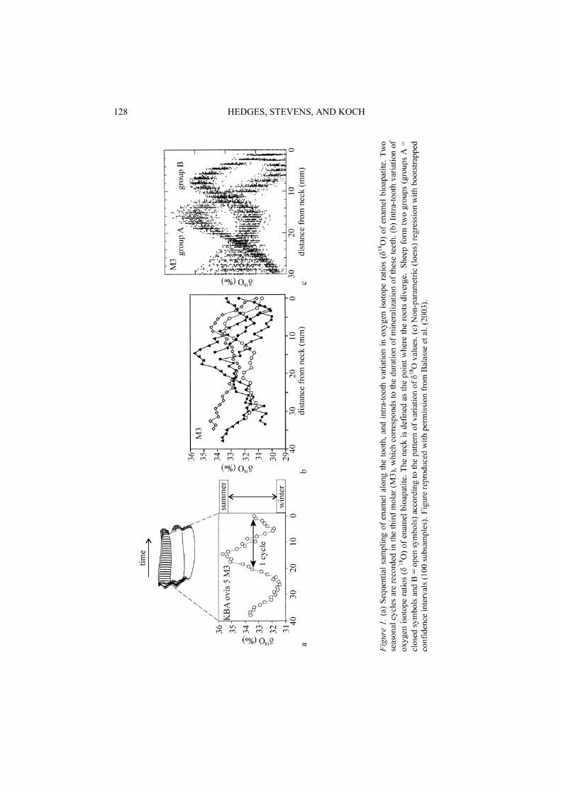
128 HEDGES, STEVENS, AND KOCH

also assumes that sheep from environments with different seasonality patterns were not included in this study. Again this is unlikely, as in pastoral societies animals are often traded or exchanges over long distances. Strontium isotope signatures from some of the Kasteelberg sheep teeth suggest that a few animals previously lived in a different area (Balasse et al. 2002). However, these animals are evenly distributed between the groups with different 18O patterns, suggesting that animal movement is not the cause of the bimodal pattern.
Although the birthing periods for the two groups are offset by approximately half an annual cycle, the seasons of birth cannot be accurately established from the 18O values, as the timing of tooth development has not been fully investigated for sheep. Nevertheless, the vegetation dynamics of the area suggest that conditions in autumn and spring would be the most appropriate for birthing and nursing lambs. Two births a year can put strain on the health of the females, potentially reducing their fertility. Additionally two lambing seasons would have restricted the mobility of the human population, although would not necessarily prevent a nomadic lifestyle. The observed bimodal 18O pattern could also have been produced by three births in two years (with the herder preventing a fourth birthing season) in order to preserve the health of the sheep. Alternatively, the bimodal 18O pattern could have been produced by two groups of females giving birth at different times of the year. Regardless of which of these interpretations is correct, as a result of having two birthing season per year the period of milk availability would have been extended, suggesting sheep played a dominant role in the subsistence economy of the pastoral society at Kasteelberg.
Variation in mammal carbon and nitrogen isotope values over the last 45,000 years
Temporal variations in European faunal 13C and 15N values have only been recognised in the last ten years. G.J. Van Klinken (unpublished data) first detected variation in both carbon and nitrogen bone isotope values over the last glacial/interglacial cycle. Pleistocene faunal 13C values were noted to be slightly 13C-enriched in comparison with Holocene 13C values (Figure 2) and faunal 15N values seemed relatively 15N-depleted around the time of the Last Glacial Maximum (LGM). Further work in this area has confirmed and refined these trends but interpretations of the isotope values (especially carbon) have been divergent.
The drop in faunal collagen 13C values with the onset of the Holocene could relate to the expansion of forests across Northwest Europe as climate warmed, and fauna obtained more of their food from forested environments. A gradual drop in bos, red deer, and horse 13C values between 32,600 and 13,300 years BP at Paglicci Cave, southern Italy, was interpreted by Iacumin et al. (1997) to relate to the progressive development of a forest habitat. Drucker et al. (2003a) also postulated that red deer 13Cvalues at the site of Rochedane in the Jura region of France during the Bölling / Alleröd and Younger Dryas periods were typical of an open environment, whereas the more lower red deer 13C values during the Boreal period were due to the deer consuming plants from under a forest canopy. If the observed 13C shifts were a result of consuming different types of vegetation, we would expect different isotope trends for different species depending on the ecological niche they occupy. But the change in
ISOTOPES IN BONES AND TEETH 129

130 HEDGES, STEVENS, AND KOCH
Figure 2. Carbon isotope values are plotted for equids, bovids and cervids over time (radiocarbonage). Each point represents the average of 1000 or 5000 years, with the number of samplesinvolved varying between about 20 and 2, but usually at least 4. Samples are predominantly fromthe UK, but include Europe generally, north of 45° Latitude. Reproduced with permission fromHedges et al. (2004).
faunal collagen 13C values is consistent and similar among species (horse, bovids, deer), over time and between geographical regions (UK, Belgium, Germany, France, Italy) (Stevens and Hedges 2004). This suggests that a large-scale regional mechanism is the trigger for the change in faunal 13C values.
An alternative explanation for the change in faunal bone collagen 13C values observed at the Late-glacial / Holocene transition is that collectively all plant 13Cvalues drop and the faunal 13C tracks changes in the plant 13C values. Several compilations of data from plant material (wood cellulose, bulk organic matter from lake sediment, and leaves) show similar variations in 13C over time (Krishnamurthy and Epstein 1990; Leavitt and Danzer 1991; Hammarlund 1993; van de Water et al. 1994; Beerling 1996; Prokopenko et al. 1999; Hatte et al. 2001). Firstly, changes in atmospheric CO2 concentration have been suggested as a possible cause of variation in plant (and thus fauna) 13C values (Richards and Hedges 2003; Stevens and Hedges 2004). Analysis of CO2 extracted from air bubbles trapped in ice cores have shown that interglacial periods had a higher CO2 concentration of around 270 ppm in comparison to glacial periods which had a lower CO2 concentration of around 190 ppm (Barnola et al. 1987; Jouzel et al. 1993; Smith et al. 1997). Increased atmospheric CO2 concentration potentially could have influenced the ratio of intercellular to atmospheric CO2
concentration (Ci/Ca), and indirectly the isotope composition of C3 plants (Arens et al. 2000). However, several studies have reported near zero-slope relationships between Ci/Ca and atmospheric CO2 concentration (Farquhar et al. 1982; Polley et al. 1993; Ehleringer and Cerling 1995; Beerling 1996; Arens et al. 2000). Although atmospheric CO2 concentration does not systematically influence C3 plant 13C, plants may respond
through physical changes their stomatal aperture and by changing the number of stomata.
Secondly, a small proportion of the change in plant 13C values could potentially be due to changes in the 13C values of atmospheric CO2 due to input of geological carbon with a different 13C value. Geological methane sources typically have very low 13Cvalues of around –53‰ (Quay et al. 1991; Lassey et al. 1999). At the end of the last glacial period, methane (CH4) was released into the atmosphere from clathrates contained in sediments on continental shelves exposed due to lowered sea level and from wetlands in response to climate change (Wuebbles and Hayhoe 2002). The large-scale release of methane into the atmosphere is recorded in the ice cores as an increase in CH4 concentration (Raynaud et al. 1988; Chappellaz et al. 1990, 1993; Blunier et al. 1993). Oxidation of CH4 to CO2 could potentially result in a lowering of 13C value of atmospheric CO2. However the 13C of CO2 from air trapped in ice cores has shown that atmospheric 13C only changed by 0.3 ± 0.2‰ over the glacial/interglacial transition (Leuenberger et al. 1992), thus it alone can not account for the observed change of around 2 to 5‰ in plant 13C values and about 2‰ in faunal 13C values. However the change in the 13C value of atmospheric CO2 could potentially be amplified by the biosphere resulting in part or all of the observed variation in plant 13Cvalues.
Thirdly, the change in plant 13C values over the last glacial transition may relate to availability of water. Increased relative humidity had been reported to result in a drop in plant 13C values (Ramesh et al. 1986; Stuvier and Braziunas 1987; van Klinken et al. 1994; Lipp et al. 1991; Hemming et al. 1998). Conditions in Europe became more humid from the LGM to the Holocene. This would allow C3 plants to keep their stomata open more, increasing stomatal conductance, resulting in a drop plant 13C values. The observed drop in plant and fauna 13C over the last glacial/interglacial transition most likely relates to a combination of factors including atmospheric 13C, humidity, forest development, and temperature each creating minor isotope variation, and collectively (perhaps synergistically) producing the overall trend. It would, however, be very difficult to quantify the influence of these different parameters in the archaeological context from that of other environmental and climatic parameters.
Temporal and geographical variation in faunal 15N values are also observed over the last 45,000 years, but due to limited data from certain time periods and geographical regions it is currently hard to establish if variations in different regions lead or lag behind the overall trend. The overall trend over the last 45,000 years is a gradual drop in faunal 15N values, with the lowest 15N values observed at the LGM or during the late glacial period. The onset of the drop in values may be later, depending on species and geographical location (as late as 25,000 years BP), but this disparity in timing could be purely due to limited data. Major gaps in the data occur in the UK and Belgium at the LGM as fauna were not present at this time due to the harsh environmental conditions. Data are available through the LGM in Germany, and the lowest faunal 15N values occur during the Late Glacial period (Stevens 2004). Different species give conflicting trends in the South of France, with the lowest bovid and horse 15N values occurring at the LGM, and the lowest reindeer 15N values being observed during the Late Glacial period (Drucker et al. 2003b; Stevens 2004). Faunal 15N values then rapidly rise, with
ISOTOPES IN BONES AND TEETH 131

132 HEDGES, STEVENS, AND KOCH
Figure 3. 15N of horse bone and tooth collagen from the British Isles, Germany, Belgium,Southern France, and Italy, over time (includes 10 horses from Drucker et al. (2000) and 11horses from Iacumin et al. (1997)). Reproduced with permission from Stevens and Hedges(2004).
early Holocene values being similar to pre-LGM values. The duration of the rise in 15Nmay vary between species and geographically but without extensive radiocarbon dating of samples it is hard to establish whether or not this is the case. However, 15N values of radiocarbon dated horses from the UK rise very rapidly in under 3000 years, with values around –0.7‰ to +0.5‰ at c.13,500 years BP, rising to 4‰ to 8‰ at c. 10,000 years BP (Figure 3) (Stevens and Hedges 2004).
No single climatic or environmental parameter has been identified as the primary factor controlling faunal 15N values over the last glacial/interglacial cycle, but a number of different, inter-related factors have been identified as possible factors contributing to the drop in herbivore 15N values during cold intervals. Firstly lower herbivore 15N values could be animal based. That is, they could be physiological adaptations to the harsh environmental conditions (Richards and Hedges 2003), or they could reflect preferential consumption of plants with lower 15N values (Nadelhoffer et al. 1996). Differences in digestive physiology among species clearly lead to different plant-to-animal isotope fractionations (Sponheimer et al. 2003a), and differences in diet quality, particularly protein content, also affect this fractionation (Sponheimer et al. 2003b; Pearson et al. 2003). Still, we consider it unlikely that diet quality and/or animal physiology would change so consistently across such a broad geographic region. Secondly (and more likely), the drop in herbivore 15N values could be due to a change in plant 15N values. Plant 15N values are dependant on multiple factors including soil
15N, soil development, nutrient availability (nitrogen and phosphorus), mycorrhizal
associations, nitrogen cycling (open system with preferential loss of 14N versus closed systems with very limited loss of 14N) (Handley et al. 1999a; 1999b; Amundson et al. 2003). Each of these factor are highly dependent on temperature and water availability, thus plant 15N values (and therefore herbivore 15N values) track climatic changes. In particular permafrost development, melting and standing water seem to play a significant role in faunal 15N values over the last glacial/interglacial cycle (Stevens and Hedges 2004). Thus the extreme climatic conditions and continuous permafrost at the LGM followed by extensive melting in northern regions could lead to dramatic depletion in faunal 15N values (Stevens 2004). In the south of France where conditions at the LGM were less harsh and permafrost was discontinuous the depletion in faunal
15N values was more limited (Figure 3)(Stevens 2004; Drucker et al. 2003b). In Italy, where the climate was much milder during the LGM and no permafrost was present, no obvious depletion in faunal 15N values occurred (Figure 3) (Iacumin et al. 1997; Stevens and Hedges 2004).
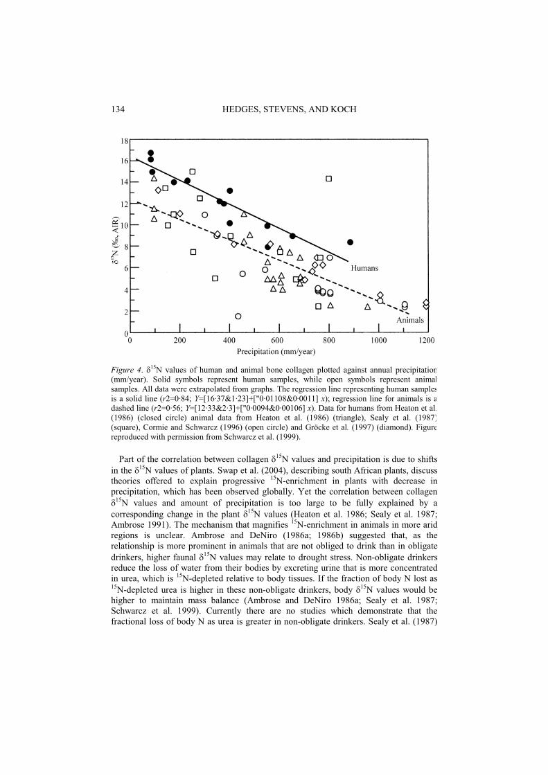
Aridity and bone collagen 15N enrichment
The quantity of rainfall can have a major influence on the 15N values of animal tissues (Heaton et al 1986). They found that modern faunal (elephants, wildebeests, giraffes and zebras) and archaeological human 15N values in South Africa and Namibia were negatively correlated with the amount of precipitation (Figure 4). For example, elephants in areas with around 800 mm rainfall per year typically had bone collagen
15N values of around +2.5‰, whereas elephants in areas with less than 200 mm of rainfall per year had values between +10‰ and +15‰. Ambrose and DeNiro (1986a; 1986b) observed a similar correlation in Kenya but the influence of rainfall was not independent from elevation in this case. Sealy et al. (1987) also reported a similar negative correlation, with herbivore collagen 15N values at Cape Point, an area with around 800 mm of precipitation per year, ranging between +3‰ and +5.5‰, whereas at Churchhaven, an area with around 250 mm of rainfall per year, herbivore collagen 15Nranging from +12‰ to +16‰ (Figure 4). Sealy et al. (1987) suggested that the correlation between amount of rainfall and faunal collagen 15N only occurs in areas with less that 400 mm rainfall per year. Cormie and Schwarcz (1996) did not observe a correlation between quantity of rainfall and white tailed deer bone collagen 15N values in North America when considering the whole population (Figure 4). However, the correlation was observed for a subset of the population that included only individuals that ate more than 10% C4 plants. Gröcke et al. (1997) also found a negative correlation between rainfall and Australian kangaroo 15N values, but did not observe a similar correlation for other marsupials (Figure 4). Ambrose (2000) observed no significant difference between bone collagen 15N of rats raised in the laboratory at 20oC and those raised at 36oC (on a controlled diet, with restricted water). The results from Gröcke et al. (1997) and Ambrose (2000) suggest that aridity may only affect the nitrogen isotope values of certain species. Gröcke et al. (1997) believe that, as the observed correlations between rainfall and herbivore bone 15N in South Africa and Australia are extremely similar, a global relationship may exist.
ISOTOPES IN BONES AND TEETH 133
134 HEDGES, STEVENS, AND KOCH
Figure 4. 15N values of human and animal bone collagen plotted against annual precipitation(mm/year). Solid symbols represent human samples, while open symbols represent animalsamples. All data were extrapolated from graphs. The regression line representing human samplesis a solid line (r2=0·84; Y=[16·37&1·23]+["0·01108&0·0011] x); regression line for animals is adashed line (r2=0·56; Y=[12·33&2·3]+["0·0094&0·00106] x). Data for humans from Heaton et al.(1986) (closed circle) animal data from Heaton et al. (1986) (triangle), Sealy et al. (1987)(square), Cormie and Schwarcz (1996) (open circle) and Gröcke et al. (1997) (diamond). Figurereproduced with permission from Schwarcz et al. (1999).
Part of the correlation between collagen 15N values and precipitation is due to shifts in the 15N values of plants. Swap et al. (2004), describing south African plants, discuss theories offered to explain progressive 15N-enrichment in plants with decrease in precipitation, which has been observed globally. Yet the correlation between collagen
15N values and amount of precipitation is too large to be fully explained by a corresponding change in the plant 15N values (Heaton et al. 1986; Sealy et al. 1987; Ambrose 1991). The mechanism that magnifies 15N-enrichment in animals in more arid regions is unclear. Ambrose and DeNiro (1986a; 1986b) suggested that, as the relationship is more prominent in animals that are not obliged to drink than in obligate drinkers, higher faunal 15N values may relate to drought stress. Non-obligate drinkers reduce the loss of water from their bodies by excreting urine that is more concentrated in urea, which is 15N-depleted relative to body tissues. If the fraction of body N lost as 15N-depleted urea is higher in these non-obligate drinkers, body 15N values would be higher to maintain mass balance (Ambrose and DeNiro 1986a; Sealy et al. 1987; Schwarcz et al. 1999). Currently there are no studies which demonstrate that the fractional loss of body N as urea is greater in non-obligate drinkers. Sealy et al. (1987)

also suggested that reduced amount of dietary protein during period of drought could result in increased recycling of nitrogen by the animal, through conversion of urea to bacterial protein in the gut, which would then raise the trophic level as the protein is eventually consumed by the organism (Sealy et al. 1987; Schwarcz et al. 1999). This model has been criticized by Ambrose (1991) and Schwarcz et al. (1999), who argued that recycling of nitrogen should result in 15N-depletion rather than enrichment as the urea consumed is 15N-depleted, and that if there is not net loss of nitrogen as a result of recycling, there should be no change in overall body 15N value. Although these studies have attempted to establish the mechanism by which the relationship between 15Nvalues and aridity occurs, a full understanding has not yet been achieved.
Isotope evidence for diet, migration, and herd structure in North American
proboscideans
Proboscideans (mastodons, mammoths, gomphotheres) are among the most common fossils in Pleistocene deposits in North America, South America, Eurasia, and Africa. Today, elephants can be keystone species, maintaining and structuring the diversity of plants and smaller animals through their roles as agents of floral disturbance, their propensity to dig wells during droughts, and other landscape transforming activities (Owen-Smith 1988). In addition, while late Pleistocene kill and butcher sites containing extinct large mammals are not common in North or South America, those that do exist frequently have proboscideans (Grayson and Meltzer 2002). As a consequence, proboscideans are central players in the debate over the cause of late Pleistocene extinctions in the New World (Fisher 1996). If the palaeoecology of proboscideans can be constrained through isotope, faunal, growth increment, or other types of analysis, the plausibility of different scenarios for extinction and the role of proboscideans as agents of ecosystem change can be assessed (Fisher 1987; Zimov et al. 1995).
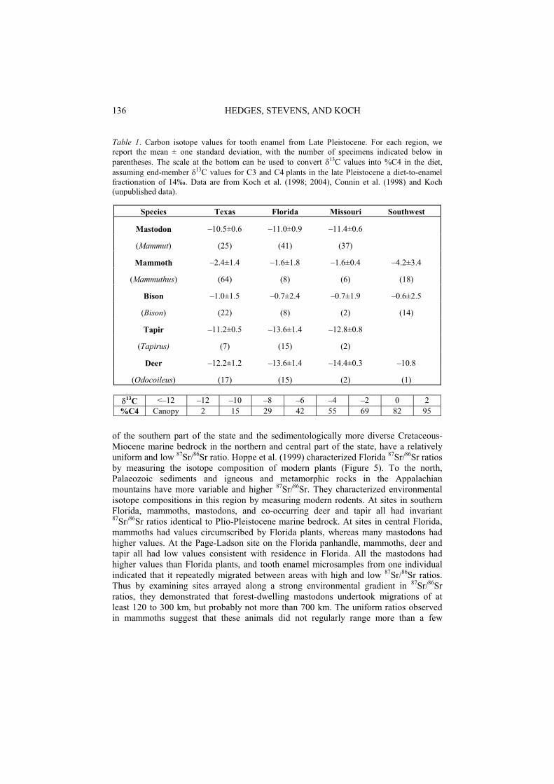
Carbon isotope analysis of sympatric and allopatric populations of mastodons and mammoths has shown that they had different habitat and dietary preferences. Mastodons were browsers, consuming exclusively C3 vegetation. Where mastodons co-occur with deer and tapir, mastodons consistently have higher 13C values, suggesting that they browsed in more open habitats, whereas deer and tapir were foraging in 13C-depleted, deep-forest habitats (Koch et al. (1998), Table 1). Mammoths, in contrast, were grazers, though when they co-occurred with bison (committed hyper-grazers), they frequently had lower 13C values, suggesting a small component of C3 browse in mammoth diets (Connin et al. (1998); Koch et al. (1998); (2004), Table 1).
Some models for late Pleistocene extinction suggest that preferred habitat patches became increasingly more isolated, or that prolonged drought forced animals to congregate in remaining well-watered regions (Owen-Smith 1988; Haynes 1991). In addition, proboscideans may have altered their migratory patterns or ranging behavior to avoid human predators. By analogy with modern mammals, we might predict that grassland adapted mammoths might have had greater home ranges or might have undertaken greater migratory loops than forest-dwelling mastodons. To understand the ranging behavior of mammoths and mastodons, Hoppe et al. (1999) studied the Sr isotope chemistry of animals in Florida. The Plio-Pleistocene marine carbonate bedrock
ISOTOPES IN BONES AND TEETH 135
136 HEDGES, STEVENS, AND KOCH
of the southern part of the state and the sedimentologically more diverse Cretaceous-Miocene marine bedrock in the northern and central part of the state, have a relatively uniform and low 87Sr/86Sr ratio. Hoppe et al. (1999) characterized Florida 87Sr/86Sr ratios by measuring the isotope composition of modern plants (Figure 5). To the north, Palaeozoic sediments and igneous and metamorphic rocks in the Appalachian mountains have more variable and higher 87Sr/86Sr. They characterized environmental isotope compositions in this region by measuring modern rodents. At sites in southern Florida, mammoths, mastodons, and co-occurring deer and tapir all had invariant 87Sr/86Sr ratios identical to Plio-Pleistocene marine bedrock. At sites in central Florida, mammoths had values circumscribed by Florida plants, whereas many mastodons had higher values. At the Page-Ladson site on the Florida panhandle, mammoths, deer and tapir all had low values consistent with residence in Florida. All the mastodons had higher values than Florida plants, and tooth enamel microsamples from one individual indicated that it repeatedly migrated between areas with high and low 87Sr/86Sr ratios. Thus by examining sites arrayed along a strong environmental gradient in 87Sr/86Sr ratios, they demonstrated that forest-dwelling mastodons undertook migrations of at least 120 to 300 km, but probably not more than 700 km. The uniform ratios observed in mammoths suggest that these animals did not regularly range more than a few
Table 1. Carbon isotope values for tooth enamel from Late Pleistocene. For each region, we report the mean ± one standard deviation, with the number of specimens indicated below inparentheses. The scale at the bottom can be used to convert 13C values into %C4 in the diet, assuming end-member 13C values for C3 and C4 plants in the late Pleistocene a diet-to-enamel fractionation of 14‰. Data are from Koch et al. (1998; 2004), Connin et al. (1998) and Koch(unpublished data).
Species Texas Florida Missouri Southwest
Mastodon –10.5±0.6 –11.0±0.9 –11.4±0.6
(Mammut) (25) (41) (37)
Mammoth –2.4±1.4 –1.6±1.8 –1.6±0.4 –4.2±3.4
(Mammuthus) (64) (8) (6) (18)
Bison –1.0±1.5 –0.7±2.4 –0.7±1.9 –0.6±2.5
(Bison) (22) (8) (2) (14)
Tapir –11.2±0.5 –13.6±1.4 –12.8±0.8
(Tapirus) (7) (15) (2)
Deer –12.2±1.2 –13.6±1.4 –14.4±0.3 –10.8
(Odocoileus) (17) (15) (2) (1)
13C <–12 –12 –10 –8 –6 –4 –2 0 2 %C4 Canopy 2 15 29 42 55 69 82 95

NW SELocality
Floridaplants
0.711
0.710
P.L. H.S. R.S. W.P.B. C.H.
87
86
SrSr
0.709
Figure 5. Average Sr isotope ratios of bulk samples of mastodons (circles), mammoths (squares),and deer and /or tapirs (triangles). Lines represent calculated 1 standard deviation from averagevalues for each population of more than three individuals, or range of samples values when onlytwo individuals were measured. P.L is Page-Ladson-Aucilla River, H.S. is Hornsby springs, R.S.us rock springs, W.P.B is West Palm Beach, and C.H. is Cutler Hammock. Reproduced withpermission from Hoppe et al. (1999).
hundred kilometers; they did not undertake transcontinental migration, as suggested by some authors (Churcher 1980).
Some fossil localities containing the remains of multiple mammoths have been interpreted as representing the mass death of an entire herd, or family group (Haynes 1991). Assuming that mammoths had a matriarchal social structure similar to modern African and Asian elephants, the age-sex structure of these associations has been interpreted as representing a catastrophic death assemblage. In the southwestern U.S., a number of these sites are associated with human artifacts, raising the possibility that Paleoindians were capable of harvesting entire family groups (Saunders 1992). Hunting elephants is a dangerous activity, and confronting an entire family group would require a remarkable level of skill and cooperative behavior. The interpretation of these sites remains controversial, however, because it is difficult to demonstrate that all the dead individuals died simultaneously. Hoppe (2004) argued if Pleistocene mammoths traveled together in small family groups, then mammoths from sites that represent family groups should have lower variability in carbon, oxygen, and strontium isotope values than mammoths from sites containing unrelated individuals. She tested this idea by comparing the isotope variability among mammoths from one mass death of a single
ISOTOPES IN BONES AND TEETH 137

138 HEDGES, STEVENS, AND KOCH
herd (Waco, Texas) and one site containing a time-averaged accumulation (Friesenhahn Cave, Texas). She found that low levels of carbon isotope variability were the most diagnostic signal of herd/family group association. She used the approach to study mammoths from three Clovis sites: Blackwater Draw, New Mexico; Dent, Colorado; and Miami, Texas. Blackwater Draw had been interpreted as an attritional assemblage based on age-sex structure, whereas Dent and Miami had been interpreted as catastrophic, mass-kill sites. Hoppe (2004) argued that high levels of variability in all three isotope systems indicated that all were time-averaged accumulations of unrelated individuals, rather than the mass deaths of single family groups. At Blackwater Draw, the strong co-variation among C, O, and Sr isotopes indicated that the site contained resident mammoths as well as migratory individuals, probably derived from cooler, higher-altitude regions to the west. Finally, the mean isotope values for residents at Blackwater Draw and Miami were similar values, whereas the values of Dent mammoths were significantly different. She argued that the Dent mammoths belonged to a separate population, supporting her results on mammoths from Florida indicating that late Pleistocene mammoths did not routinely undertake long distance migrations (600 km in this case).
Summary
The isotope composition of bone (and tooth) is dominated by biology. This is even true for such isotopes as strontium that are adventitiously taken up according to local geology, and so record animal movements within their ecological setting. Therefore, a measure of understanding of the main biological features in the subject of study (such as food web structure) is needed before environmental inferences can be successful. Such inferences may be coarse-grained, or rather subtle and highly resolved in time. The need to take account of biology makes the study of bone isotopes somewhat specialised. A further difference is the sporadic and somewhat acontextual deposition of bone, rarely enabling its data to be directly integrated with complementary data from the same site. Integration must be obtained by working on a larger, more general scale. On the other hand, as the chapter shows, as archives, bone and teeth are rich in the different kinds of isotope signal they can incorporate. Furthermore, some of these signals may be very sensitive – the non-linear change in C3/C4 plant abundance (and therefore with 13C in the bone collagen of herbivorous grazers) with local climate is a very clear case. The chapter has given the background to understanding how isotope changes in bone are caused, and shown how these changes may be understood, though not always, in terms of environmental effects. We hope it also shows that there is a wealth of data “out there” still to be systematically explored, in order to provide more penetrating insight into the interaction between environment, vertebrate biology, and the isotope chemistry of an archive.
References
Ambrose S.H. 2000. Controlled diet and climate experiments on nitrogen isotope ratios of rats. In: Ambrose S.H. and Katzenberg M.A. (eds), Biogeochemical approaches to paleodietary analysis. Advances in Archaeological and Museum Science. Kluwer Academic / Plenum, New York. pp 243–259.

Ambrose S.H. 1990. Preparation and characterization of bone and tooth collagen for isotopic analysis. J. Archaeol. Sci. 17: 431–451.
Ambrose S.H. 1991. Effects of diet, climate and physiology on nitrogen isotope abundances in terrestrial foodwebs. J. Archaeol. Sci. 18: 293–317.
Ambrose S.H. and DeNiro M.J. 1986a. The isotopic ecology of East African mammals. Oecologia 69: 395–406.
Ambrose S.H. and DeNiro M.J. 1986b. Reconstruction of African human diet using bone collagen carbon and nitrogen isotope ratios. Nature 319: 321–324.
Amundson R., Austin A.T., Schuur E.A.G., Yoo K., Matzek V., Kendall C., Uebersax, A., Brenner D. and Baisden W.T. 2003. Global patterns of the isotopic composition of soil and plant nitrogen. Global Biogeochem. Cy. 17: 1031.
Arens N.C., Jahren A.H. and Amundson R. 2000. Can C3 plants faithfully record the carbon isotopic composition of atmospheric carbon dioxide? Paleobiology 26: 137–164.
Ayliffe L.K., Cerling T.E., Robinson T., West A.G., Sponheimer M., Passey B.H., Hammer J., Roeder B., Dearing M.D. and Ehleringer J.R. 2004. Turnover of carbon isotopes in tail hair and breath CO2 of horses fed an isotopically varied diet. Oecologia 139: 11–22.
Balasse M., Smith A.B., Ambrose S.H. and Leigh S.R. 2003. Determining sheep birth seasonality by analysis of tooth enamel oxygen isotope ratios: The late stone age site of Kasteelberg (South Africa). J. Archaeol. Sci. 30: 205–215.
Balasse M., Ambrose S. H., Smith A. B. and Price T. D. 2002. The seasonal mobility model for prehistoric herders in the south-western Cape of South Africa assessed by isotopic analysis of sheep tooth enamel. J. Archaeol. Sci. 29: 917–932.
Barnola J.M., Raynaud D., Kortkevich Y.S. and Lorius C. 1987. Vostok ice core provides 160,000-year record of atmospheric CO2. Nature 329: 408–414.
Beerling D.J. 1996. C-13 discrimination by fossil leaves during the late-glacial climate oscillation 12-10 ka BP: Measurements and physiological controls. Oecologia 108: 29–37.
Birchall J., O'Connell T.C., Heaton T.H.E. and Hedges R.E.M. In press. Hydrogen isotope ratios in animal body protein reflect trophic level. J. Anim. Ecol.
Blunier T., Chappellaz J.A., Schwander J. Barnola J.M., Desperts T., Stauffer B., and Raynaud D. 1993. Atmospheric methane record from a Greenland ice core over the last 1000 years. Geophys. Res. Lett. 20: 2219–2222.
Bocherens H., Mashkour M., Billiou D., Pelle E. and Mariotti A. 2001 A new approach for studying prehistoric herd management in arid areas: intra-tooth isotopic analyses of archaeological caprine from Iran. Cr. Acad. Sci. IIA. 332: 67–74.
Bowen G.J. and Wilkinson B. 2002. Spatial distribution of delta O-18 in meteoric precipitation. Geology 30: 315–318.
Brooks J.R., Flanagan L.B., Buchmann N. and Ehleringer J.R. 1997. Carbon isotope composition of boreal plants: Functional grouping of life forms. Oecologia 110: 301–311.
Bryant J.D., Jones D.S. and Mueller P.A. 1995. Influence of fresh water flux on 87Sr/86Srchronostratigraphy in marginal marine environments and dating of vertebrate and invertebrate faunas. J. Paleontol. 69: 1–6.
Buchmann N., Guehl J.M., Barigah T.S. and Ehleringer J.R. 1997. Interseasonal comparison of CO2 concentrations, isotopic composition, and carbon dynamics in an Amazonian rainforest (French Guiana). Oecologia 110: 120–13.
Budd P., Millard A., Chenery C., Lucy S. and Roberts C. 2004. Investigating population movement by stable isotope analysis: a report from Britain. Antiquity 78:127–141.
Capo R.C., Stewart B.W. and Chadwick O.A. 1998. Strontium isotopes as tracers of ecosystem processes: Theory and methods. Geoderma 82: 197–225.
Cerling T.E., Hart J.A. and Hart T.B. 2004. Stable isotope ecology of the Ituri Forest. Oecologia 138: 5–12.
ISOTOPES IN BONES AND TEETH 139
140 HEDGES, STEVENS, AND KOCH
Chamberlain C.P., Blum J.D., Holmes R.T., Feng X.H., Sherry T.W. and Graves G.R. 1997. The use of isotope tracers for identifying populations of migratory birds. Oecologia 109: 132–141.
Chappellaz J.A., Blunier T., Raynaud D., Barnola J.M., Schwander J. and Stauffer B. 1993. Synchronous changes in atmospheric CH4 and Greenland climate between 40 and 8 kyr B.P. Nature 366: 443–445.
Chappellaz J.A. 1990. Etude du methane atmospherique au cours du dernier cycle climatique a partir d l'analyse de l'air piege dans la glace antarctique, PhD thesis, University of Grenoble.
Churcher C.S. 1980. Did North American mammoths migrate? Canadian Journal of Anthropology 1: 103–105.
Clementz M.T. and Koch P.L. 2001. Differentiating aquatic mammal habitat and foraging ecology with stable isotopes in tooth enamel. Oecologia 129: 461–472.
Connin S.L., Betancourt J. and Quade J. 1998. Late Pleistocene C4 plant dominance and summer rainfall in the southwestern United States from isotopic study of herbivore teeth. Quaternary Res. 50: 179–193.
Cormie A.B. and Schwarcz H.P. 1994. Stable isotopes of nitrogen and carbon of North American white-tailed deer and implications for paleodietary and other food web studies. Palaeogeogr. Palaeocl. 107: 227–241.
Cruz-Uribe K. and Schrire C. 1991. Analysis of faunal remains from Oudepost 1, an early outpost of the Dutch East India Company, Cape Province. S. Afr. Archaeol. Bull. 46, 92–106.
Darling W.G., Bath A.H., Gibson J.J. and Rozanski K. This volume. Isotopes in Water. In: M.J.Leng (ed.). Isotopes in Palaeoenvironmental Research. Springer, Dordrecht, The Netherlands.
Darling W.G. and Talbot J.C. 2003. The O & H stable isotopic composition of fresh waters in the British Isles. Hydrol. Earth Syst. Sc. 7: 163–181.
DeNiro M.J. 1985. Postmortem preservation and alteration of in vivo bone collagen isotope ratios in relation to palaeodietary reconstruction. Nature 317: 806–809.
DeNiro M.J. and Epstein S. 1978. Influence of diet on distribution of carbon isotopes in animals. Geochim. Cosmochim. Ac. 42: 495–506.
DeNiro M.J. and Epstein S. 1981. Influence of diet on distribution of nitrogen isotopes in animals. Geochim. Cosmochim. Ac. 45: 341–351.
Drucker D., Bocherens H., Bridault A. and Billiou D. 2003a. Carbon and nitrogen isotopic composition of red deer (Cervus elaphus) collagen as a tool for tracking palaeoenvironmental change during the Late-Glacial and Early Holocene in the northern Jura (France). Palaeogeogr. Palaeocl. 195: 375–388.
Drucker D.G., Bocherens H. and Billiou D. 2003b. Evidence for shifting environmental conditions in Southwestern France from 33 000 to 15 000 years ago derived from carbon-13 and nitrogen-15 natural abundances in collagen of large herbivores. Earth Planet. Sc. Lett. 216: 163–173.
Bocherens H. and Drucker D. 2003. Trophic level isotopic enrichment of carbon and nitrogen in bone collagen: Case studies from recent and ancient terrestrial ecosystems. Int J Osteoarchaeol 13, 46–53.
Dupras T.L. and Schwarcz H.P. 2001. Strangers in a strange land: Stable isotope evidence for human migration in the Dakhleh Oasis, Egypt. J. Archaeol. Sci. 28: 1199–1208.
Ehleringer J.R. and Cerling T.E. 1995. Atmospheric CO2 and the ratio of intercellular to ambient CO2 concentrations in plants. Tree Physiol. 15: 105–111.
Farquhar G.D., Ehleringer J.R. and Hubick K.T. 1989. Carbon isotope discrimination and photosynthesis. Annu. Rev. Plant Phy. 40: 503–537.
Farquhar G.D., O’Leary M.H. and Berry J.A. 1982. On the relationship between carbon isotope discrimination and the intercellular carbon dioxide concentration in leaves. Aust. J. Plant Physiol. 9:121–137.
Felicetti L.A., Schwartz C.C., Rye R.O., Haroldson M.A., Gunther K.A., Phillips D.L. and Robbins C.T. 2003. Use of sulfur and nitrogen stable isotopes to determine the importance of whitebark pine nuts to Yellowstone grizzly bears. Can. J. Zool. 81: 763–770.

Fisher D.C. 1987. Mastodont procurement by Paleoindians of the Great Lakes Region: hunting or scavenging? In: Nitecki M.H. and Nitecki D.V. (eds), The Evolution Of Juman Hunting. Plenum Publishing Corporation, Chicago, pp. 309–421.
Fisher D.C. 1996. Extinction of proboscideans in North America. In: Shoshani J. and Tassy P. (eds), The Proboscidea: Evolution and palaeoecology of elephants and their Relatives. Oxford University Press, New York, pp. 141–160.
Fricke H.C. and O’Neil J.R. 1996. Inter- and intra-tooth variation in the oxygen isotope composition of mammalian tooth enamel phosphate: Implications for palaeoclimatological and palaeobiological research. Palaeogeogr. Palaeocl. 126: 91–99.
Fuller B.T., Fuller J.L., Sage N.E., Harris D.A., O'Connell T.C. and Hedges R.E.M. 2004. Nitrogen balance and delta N-15: why you're not what you eat during pregnancy. Rapid Commun. Mass Sp. 18: 2889–2896.
Gadbury C., Todd L., Jahren A.H. and Amundson R. 2000. Spatial and temporal variations in the isotopic composition of bison tooth enamel from the Early Holocene Hudson-Meng Bone Bed, Nebraska. Palaeogeogr. Palaeocl 157: 79–93.
Gat J.R. 1980. The isotopes of hydrogen and oxygen in precipitation. In: Fritz P. and Fontes J.C (eds), Handbook of environmental isotope geochemistry volume 1: The terrestrial environment. Elsevier, Amsterdam, pp 21–42.
Graves G.R., Romanek C.S. and Navarro A.R. 2002. Stable isotope signature of philopatry and dispersal in a migratory songbird. P. Natl. Acad. Sci. USA 99: 8096–8100.
Grayson D.K. and Metlzer D.J. 2002. Clovis hunting and large mammal extinction: A critical review of the evidence. J. World Prehist. 16: 313–359.
Gröcke D.R., Bocherens H. and Mariotti A. 1997. Annual rainfall and nitrogen-isotope correlation in macropod collagen: application as a palaeoprecipitation indicator. Earth Planet.Sc. Lett. 153:279–285.
Hammarlund D. 1993. A distinct 13C decline in organic lake sediments at the Pleistocene-Holocene transition in Southern Sweden. Boreas 22: 236–243.
Handley L.L., Austin A.T., Robinson D., Scrimgeour C.M., Raven J.A., Heaton T.H.E., Schmidt S. and Stewart G.R. 1999a The N-15 natural abundance (delta N-15) of ecosystem samples reflects measures of water availability. Aust. J. Plant Physiol. 26: 185–199.
Handley L.L., Azcon R., Lozano, J.M.R. and Scrimgeour C.M. 1999b. Plant delta N-15 associated with arbuscular mycorrhization, drought and nitrogen deficiency. Rapid Commun. Mass Sp. 13: 1320–1324.
Hatte C., Antoine P., Fontugne M., Lang A., Rousseau D.D. and Zoller L. 2001. delta C-13 of loess organic matter as a potential proxy for paleoprecipitation. Quaternary Res. 55: 33–38.
Haynes G. 1991. Mammoths, mastodonts, and elephants: Biology, behaviour, and the fossil record. Cambridge University Press, Cambridge, 413 pp.
Heaton T.H.E., Vogel J.C., von la Chevallerie G. and Collett G. 1986. Climatic influence on the isotopic composition of bone collagen. Nature 322: 822–823.
Heaton T.H.E. 1999. Spatial, species, and temporal variations in the 13C/12C ratios of C3 plants: Implications for palaeodiet studies. J. Archaeol. Sci. 26: 637–649.
Hedges R.E.M. 2003. On bone collagen - apatite-carbonate isotopic relationships. Int. J. Osteoarchaeol. 13: 66–79.
Hemming D.L., Switsur V.R., Waterhouse J.S., Heaton T.H.E. and Carter A.H.C. 1998. Climate variation and the stable carbon isotope composition of tree ring cellulose: an intercomparison of Quercus robur, Fagus silvatica and Pinus silvestris. Tellus B. 50: 25–33.
Hobbie E.A., Macko S.A. and Shugart, H.H. 1999. Insights into nitrogen and carbon dynamics of ectomycorrhizal and saprotrophic fungi from isotopic evidence. Oecologia 118: 353–360.
Hobson K.A., Atwell L. and Wassenaar L.I. 1999. Influence of drinking water and diet on the stable hydrogen isotope ratios of animal tissues. P. Natl. Acad. Sci. USA 96: 8003–8006.
Hobson K.A., Alisauskas R.T. and Clark R.G. 1993. Stable-nitrogen isotope enrichment in avian issues due to fasting and nutritional stress: implications for isotopic analyses of diet. Condor 95: 388–394.
ISOTOPES IN BONES AND TEETH 141

142 HEDGES, STEVENS, AND KOCH
Hobson K.A., Wassenaar L.I., Mila B., Lovette I., Dingle C. and Smith, T.B. 2003. Stable isotopes as indicators of altitudinal distributions and movements in an Ecuadorean hummingbird community. Oecologia 136: 302–308.
Högberg P. 1997. 15N natural abundance in soil-plant systems. New Phytol. 137: 179–203. Hoogewerff J., Papesch W., Kralik M., Berner M., Vroon P., Miesbauer H., Gaber O., Kunzel
K.H. and Kleinjans J. 2001. The last domicile of the Iceman from Hauslabjoch: A geochemical approach using Sr, C and O isotopes and trace element signatures. J. Archaeol. Sci. 28: 983–989.
Hoppe K.A. 2004. Late Pleistocene mammoth herd structure, migration patterns, and Clovis hunting strategies inferred from isotopic analyses of multiple death assemblages. Paleobiology 30: 129–145.
Hoppe K.A., Stover S.M., Pascoe J.R. and Amundson R. 2004. Tooth enamel biomineralization in extant horses: implications for isotopic microsampling. Palaeogeogr. Palaeocl. 206: 355–365.
Hoppe K.A., Koch P.L., Carlson R.W. and Webb S.D. 1999. Tracking mammoths and mastodons: reconstruction of migratory behaviour using strontium isotope ratios. Geology 27: 439–442.
Howland M.R., Corr L.T., Young S.M.M., Jones V., Jim S., van der Merwe N.J., Mitchell A.D. and Evershed R.P. 2003. Expression of the dietary isotope signal in the compound-specific
13C values of pig bone lipids and amino acids. Int. J. Osteoarchaeol. 13: 54–65. Huertas A.D., Iacumin P. and Longinelli A. 1997. A stable isotope study of fossil mammal
remains from the Paglicci cave, southern Italy, 13 to 33 ka BP: Palaeoclimatological considerations. Chem. Geol. 141: 211–223.
Hultine K.R. and Marshall J.D. 2000. Altitude trends in conifer leaf morphology and stable carbon isotope composition. Oecologia 123: 32–40.
Iacumin P., Bocherens H. and Huertas A.D. 1997. A stable isotope study of fossil mammal remains from the Paglicci cave, Southern Italy. N and C as palaeoenvironmental indicators. Earth Planet. Sc. Lett. 148: 349–357.
Jim S., Ambrose S.H. and Evershed R.P. 2004. Stable carbon isotopic evidence for differences in the dietary origin of bone cholesterol, collagen and apatite: Implications for their use in palaeodietary reconstruction. Geochim. Cosmochim. Ac. 68: 61–72.
Jouzel J., Barkov N.I., Barnola J.M., Bender M., Chappellaz J., Genthon C., Kotlyakov V.M., Lipenkov V., Lorius C., Petit J.R., Raynaud D., Raisbeck G., Ritz C., Sowers T., Stievenard M., Yiou F. and Yiou P. 1993. Extending the Vostok ice-core record of paleoclimate to the penultimate glacial period. Nature 364: 407–412.
Klein R.G. and Cruz-Uribe K. 1989. Faunal evidence for pre-historic herder-forager activities at Kasteelberg, western Cape Province, South Africa. S. Afr. Archaeol. Bull. 44: 82–97.
Knoff A.J., Macko S.A. and Erwin R.M. 2001. Diets of nesting Laughing Gulls (Larus atricilla)at the Virginia Coast Reserve: Observations from stable isotope analysis. Isot. Environ. Healt. S. 37: 67–88.
Koch P.L., Fisher D.C. and Dettman D. 1989. Oxygen isotope variation in the tusks of extinct proboscideans - a measure of season of death and seasonality. Geology 17: 515–519.
Koch P.L., Heisinger J., Moss C., Carlson R.W., Fogel M.L. and Behrensmeyer A.K. 1995. Isotopic tracking of change in diet and habitat use in African elephants. Science 267: 1340–1343.
Koch P.L., Hoppe K.A. and Webb S.D. 1998. The isotopic ecology of late Pleistocene mammals in North America - Part 1. Florida. Chem. Geol. 152: 119–138.
Koch P. 1997. Reproductive status, nitrogen balance, and the isotopic ecology of horses. 5th Advanced Seminar on Palaeodiet, France.
Koch P.L., Tuross N. and Fogel M.L. 1997. The effects of sample treatment and diagenesis on the isotopic integrity of carbonate in biogenic hydroxylapatite. J. Archaeol. Sci. 24: 417–429

Kohn M.J., Schoeninger M.J. and Valley J.W. 1996. Herbivore tooth oxygen isotope compositions: Effects of diet and physiology. Geochim. Cosmochim. Ac. 60: 3889–3896
Kohn M.J., Schoeninger M.J. and Valley J.W. 1998. Variability in oxygen isotope compositions of herbivore teeth: reflections of seasonality or developmental physiology? Chem. Geol.152: 97–112.
Kohn M.J. and Cerling T.E. 2002. Stable isotope compositions of biological apatite, phosphates. In: Kohn M.L., Rakovan J. and Hughes J.M. (eds), Geochemical, geobiological, and materials importance. Reviews in Mineralogy and Geochemistry, 48: 455–488.
Kolb P. 1968. The present state of Cape of Good-Hope. Weston La Barre, New York. Krishnamurthy R.V. and Epstein S. 1990. Glacial-Interglacial excursion in the concentration of
atmospheric CO2 - Effect in the C-13/C-12 ratio in wood cellulose. Tellus B 42: 423–434. Krouse H.R. 1989. Sulfur isotope studies of the pedosphere and biosphere. In: Nagy K.A. (ed.),
Stable isotopes in ecological research. Springer-Verlag, New York, pp. 424–444. Lassey K.R, Lowe D.C. and Manning M.R. 1999. The trend in atmospheric methane 13C and
implications for isotopic restraints on the global methane budget. Global Biogeochem. Cy. 14: 41–49.
Leavitt S.W. and Danzer S.R. 1991. Chronology from plant matter. Nature 352: 671. Lee-Thorp J. and Sponheimer M. 2003. Three case studies used to reassess the reliability of fossil
bone and enamel isotope signals for paleodietary studies. J. Anthropol. Archaeol. 22: 208–216. Leng M.J., Lamb A.L., Heaton T.H.E., Marshall J.D., Wolfe B.B., Jones M.D, Holmes J.A. and
Arrowsmith C. This volume. Isotopes in lake sediments. In: M.J.Leng (ed.). Isotopes in Palaeoenvironmental Research. Springer, Dordrecht, The Netherlands.
Leuenberger M., Siegenthaler U. and Langway C.C. 1992. Carbon isotope composition of atmospheric CO2 from an Antarctic ice core. Nature 357: 488–490.
Lipp J., Trimborn P., Fritz P., Moser H., Becker B. and Frenzel B. 1991. Stable isotopes in tree ring cellulose and climate change. Tellus B. 43: 322–330.
Longinelli A. and Selmo E. 2003. Isotopic composition of precipitation in Italy: a first overall map J. Hydrol. 270: 75–88.
Lott C.A., Meehan T.D. and Heath J.A. 2003. Estimating the latitudinal origins of migratory birds using hydrogen and sulfur stable isotopes in feathers: influence of marine prey base. Oecologia 134: 505–510.
Marshall J.D. and Zhang J.W. 1994. Carbon isotope discrimination and water-use efficiency in native plants of the North-Central Rockies. Ecology 75: 1887–1895.
Medina E. and Michin P. 1980. Stratification of 13C in Amazonian rainforests. Oecologia 45 337–378.
Mentzel O.F. 1944. A geographical and topographical description of the Cape of Good Hope. Part Three. Cape Town: The Van Riebeeck Society no. 25.
Nadelhoffer K., Shaver G., Fry B., Giblin A., Johnson L. and Mackane R. 1996. 15N natural abundances and N use by tundra plants. Oecologia 107: 386–394.
O'Connell T.C. and Hedges R.E.M. 1999. Investigations into the effect of diet on modern human hair isotopic values. Am. J. Phys. Anthropol. 108: 409–425.
O'Leary M. H. 1988. Carbon isotopes in photosynthesis. Bioscience 38: 328–336. Owen-Smith R.N. 1988. Megaherbivores. Cambridge University Press, Cambridge, 369 pp.
Passey B.H., Robinson T.F., Ayliffe L.K., Cerling T.E., Sponheimer M., Dearing M.D., Roeder B.L. and Ehleringer J.R. In press. Carbon isotopic fractionation between diet, breath, and bioapatite in different mammals. J. Archaeol. Sci.
Pearson S.F., Levey D.J., Greenberg C.H. and del Rio C.M. 2003. Effects of elemental composition on the incorporation of dietary nitrogen and carbon isotopic signatures in an omnivorous songbird. Oecologia 135: 516–523.
Peterson B.J. and Fry B. 1987. Stable isotopes in ecosystem studies. Annu. Rev. Ecol. Syst. 18: 293–320.
ISOTOPES IN BONES AND TEETH 143
144 HEDGES, STEVENS, AND KOCH
Polley H.W., Johnson H.B., Marino B.D. and Mayeux H.S. 1993. Increase in C3 plant water-use efficiency and biomass over glacial to present CO2 concentrations. Nature 361: 61–64.
Prokopenko A.A., Williams D.F., Karabanov E.B. and Khursevich G.K. 1999. Response of Lake Baikal ecosystem to climate forcing and pCO(2) change over the last glacial/interglacial transition. Earth Planet. Sci. Lett. 172: 239–253.
Quay P.D., King S.L., Stutsman J., Wilbur D.O., Steele L.P., Fung I., Gammon R.H., Brown T.A., Farwell G.W., Grootes P.M. and Schmidt F.H. 1991. Carbon isotopic composition of atmospheric CH4: Fossil and biomass burning source and strengths. Global Biogeochem. Cy. 5, 25–47.
Ramesh R., Bhattacharya S.K. and Gopalan K. 1986. Stable isotope systematics in tree cellulose as palaeoenvironmental indicators - a review. J. Geol. Soc. India 27: 154–167.
Reinhard E., de Torres T. and O’Neil J. 1996. O-18/O-16 ratios of cave bear tooth enamel: A record of climate variability during the Pleistocene. Palaeogeogr. Palaeocl. 126: 45–59.
Raynaud D., Chappellaz J.A., Barnola J.M., Korotkevich Y.S., and Lorius C. 1988. Climatic and CH4 cycle implications of glacial-interglacial CH4 change in the Vostok ice core. Nature 333: 655–657.
Richards M.P., Fuller B.T., Sponheimer M., Robinson T. and Ayliffe L. 2003. Sulphur isotopes in palaeodietary studies: A review and results from a controlled feeding experiment. Int. J. Osteoarchaeol. 13: 37–45.
Richards M.P. and Hedges R.E.M. 2003. Variations in bone collagen 13C and 15N values of fauna from Northwest Europe over the last 40,000 years. Palaeogeogr. Palaeocl. 193: 261–267.
Saunders J. J. 1992. Blackwater Draw: mammoths and mammoth hunters in the terminal Pleistocene. In: Fox J.W., Smith C.B. and Wilkins K.T. (eds), Proboscidean and paleoindian Interactions. Baylor University Press, Waco, Texas, pp. 123–147.
Schwarcz H.P. and Schoeninger M.J. 1991. Stable isotope analyses in human nutritional ecology. Yearb. Phys. Anthropol. 34: 283–321.
Schwarcz H.P., Dupras T.L. and Fairgrieve S.I. 1999. 15N enrichment in the Sahara: in search of a global relationship. J. Archaeol. Sci. 26: 629–636.
Sealy J.C., van der Merwe N.J., Lee-Thorp J.A. and Lanham J.L. 1987. Nitrogen isotopic ecology in Southern Africa: implications for environmental and dietary tracing. Geochim. Cosmochim. Ac. 51: 2707–2717.
Sharp Z.D., Atudorei V., Panarello H.O., Fernandez J. and Douthitt, C. 2003. Hydrogen isotope systematics of hair: archeological and forensic applications. J. Archaeol. Sci. 30: 1709–1716.
Sharp Z.D. and Cerling T.E. 1998. Fossil isotope records of seasonal climate and ecology: straight from the horse's mouth. Geology 26: 219–222.
Smith H.J., Wahlen M., Mastroianni D. and Taylor K.C. 1997. The CO2 concentration of air trapped in GISP2 ice from the last glacial maximum-Holocene transition. Geophys. Res. Lett. 24: 1–4.
Sparks J.P. and Ehleringer J.R. 1997. Leaf carbon isotope discrimination and nitrogen content for riparian trees along elevational transects. Oecologia 109: 362–367.
Sponheimer M., Robinson T., Ayliffe L., Roeder B., Hammer J., Passey B., West A., Cerling T., Dearing D. and Ehleringer J. 2003a. Nitrogen isotopes in mammalian herbivores: Hair 15Nvalues from a controlled feeding study. Int. J. Osteoarchaeol. 13: 80–87.
Sponheimer M., Robinson T.F., Roeder B.L., Passey B.H., Ayliffe L.K., Cerling T.E., Dearing M.D. and Ehleringer J.R. 2003b. An experimental study of nitrogen flux in llamas: is 14Npreferentially excreted? J. Archaeol. Sci. 30: 1649–1655.
Stevens R.E. 2004. Establishing links between climate/environment and both modern and archaeological hair and bone isotope values: Determining the potential of archaeological bone collagen 13C and 15N as palaeoclimatic and palaeoenvironmental proxies. D.Phil thesis, University of Oxford.
Stevens R.E. and Hedges R.E.M. 2004. Carbon and nitrogen stable isotope analysis of Northwest European horse bone and tooth collagen, 40,000 BP - present: Palaeoclimatic interpretations. Quaternary Sci. Rev. 23: 977–991.

Stuiver M. and Braziunas T.F. 1987. Tree cellulose 13C/12C isotope ratios and climatic change. Nature 328: 58–60.
Swap R.J., Aranibar J.N., Dowty P.R., Gilhooly W.P. and Macko S.A. 2004. Natural abundance of 13C and 15N in C3 and C4 vegetation of southern Africa: patterns and implications. Glob. Change Biol. 10: 350–358.
Taylor A.F.S., Fransson P.M., Högberg P., Högberg M.N. and Plamboeck A.H. 2003. Species level patterns in 13C and 15N abundance of ectomycorrhizal and saprotrophic fungal sporocarps. New Phytol. 159: 757–774.
Tieszen L.L, Boutton T.W, Ottichilo W.K., Nelson D.E. and Brandt D.H. 1989. An assessment of long-term food habits of Tsavo elephants based on stable carbon and nitrogen isotope ratios of bone collagen. Afr. J. Ecol. 27: 219–226.
van de Water P.K., Leavitt S.W. and Betancourt J.L. 1994. Trends in stomatal density and 13C/12C ratios of Pinus flexilis needles during last glacial-interglacial cycle. Science 264: 239–243.
van Klinken G.J., van der Plicht J. and Hedges R.E.M. 1994. Bone 13C/12C ratios reflect (palaeo) climatic variations. Geophys. Res. Lett. 21: 445–448.
Wuebbles D.J. and Hayhoe K. 2002. Atmospheric methane and global change. Earth Sci. Rev. 57: 177–210.
Vogel J.C. 1978. Isotopic assessment of the dietary habits of ungulates. S. Afr. J. Sci. 74: 298–301.
West A.G., Ayliffe L.K., Cerling T.E., Robinson T.F., Karren B., Dearing M.D. and Ehleringer J.R. 2004. Short-term diet changes revealed using stable carbon isotopes in horse tail-hair. Func. Ecol. 18: 616–624.
Zazzo A., Lecuyer C. and Mariotti A. 2004. Experimentally-controlled carbon and oxygen isotope exchange between bioapatites and water under inorganic and microbially-mediated conditions. Geochim. Cosmochim. Ac. 68: 1–12.
Zimov S.A., Chuprynin V.I., Oreshko A.P., Chapin F.S. III., Reynolds J. F. and Chapin M.C. 1995. Steppe tundra transition: a herbivore-driven biome shift at the end of the Pleistocene. Am. Nat. 146: 765–794.
ISOTOPES IN BONES AND TEETH 145