arX

iv:1

101.

4832

v7 [

phys

ics.

com

p-ph

] 1

6 Fe

b 20

11

Multiconfiguration Time-Dependent Hartree-Fock Treatment of Electronic and

Nuclear Dynamics in Diatomic Molecules

D. J. Haxton,1 K. V. Lawler,1 and C. W. McCurdy1, 2

1Chemical Sciences and Ultrafast X-ray Science Laboratory,

Lawrence Berkeley National Laboratory, Berkeley CA 947202Departments of Applied Science and Chemistry, Davis CA 95616

The multiconfiguration time-dependent Hartree-Fock (MCTDHF) method is formulated fortreating the coupled electronic and nuclear dynamics of diatomic molecules without the Born-Oppenheimer approximation. The method treats the full dimensionality of the electronic motion,uses no model interactions, and is in principle capable of an exact nonrelativistic description ofdiatomics in electromagnetic fields. An expansion of the wave function in terms of configurationsof orbitals whose dependence on internuclear distance is only that provided by the underlying pro-late spheroidal coordinate system is demonstrated to provide the key simplifications of the workingequations that allow their practical solution. Photoionization cross sections are also computed fromthe MCTDHF wave function in calculations using short pulses.

PACS numbers: 31.15.-p, 33.80.Eh, 31.15.xv

I. INTRODUCTION

New sources of short radiation pulses, in particu-lar high-harmonic generation [1, 2] and free-electronlasers [3], promise to enable a new generation ofpump/probe experiments on molecules in which the cen-tral frequencies of both pulses are in the ultraviolet orX-ray. The short time scales that have recently becomepractical for these measurements extend to subfemtosec-ond pulses with delays between them on the order offemtoseconds or tens of femtoseconds. This generationof experiments can also involve probe pulses which ion-ize or dissociate the target molecule and thus add thedimension of the time-resolved measurement of the elec-tron and molecular fragment energy distributions. Toaccurately interpret and describe the results of these ex-periments, ab initio methods must be developed to treathighly electronically excited and strongly nonadiabaticmolecular dynamics. Coincidence experiments [4], for in-stance, demand the capability to describe multiple ion-ization and dissociation, and nonlinear effects [5, 6] mayentail the excitation of multiple electrons. In general,most of these phenomena currently remain beyond thereach of accurate ab initio theoretical descriptions.

However, significant headway has been made. Ap-proaches employing classical trajectories on coupledBorn-Oppenheimer surfaces [7, 8] are well suited for dy-namics on low lying excited bound electronic states, andhave been applied to molecules as large as DNA bases [9].With an approximate treatment of the coupling to theionization continuum, such trajectory methods may de-scribe time-resolved photoelectron signals in pump-probeexperiments [8, 9]; such a treatment also permitted thestudy of the quantum nuclear dynamics of Auger de-cay [10].

While these methods have already shown greatprogress in describing a range of non-Born-Oppenheimerand excited-state effects, their utility is greatest for situ-

ations in which ionization may be treated approximatelyand in which the interacting electronic states may be ex-plicitly identified. Several other approaches avoid the useof Born-Oppenheimer states altogether and show promisefor treating highly electronically excited or nonadiabaticelectronic and nuclear dynamics [11, 12]. In a similarcontext, ionization has been included in a variationaltreatment that explicitly includes electron-nuclear cor-relation [13] and has also been treated with coupled elec-tronic and semiclassical nuclear wave packets [14].The time-dependent multi-configuration Hartree Fock

(MCTDHF) approach would seem to be a natural andwidely applicable starting point to the electronic part ofthis problem, because it is capable in principle of ex-actly describing the dynamics of many-electron motion.There is a considerable literature on this subject alreadyincluding analysis of the formulation of MCTDHF andits application to small or model systems [15–23], andalso attacks on the combination of electronic and nu-clear motion [24]. On the basis of this literature, thefundamental idea can be said to be well established thata time-dependent linear combination of determinants oftime dependent orbitals should be flexible enough to de-scribe the electronic response a molecule to short intensepulses in any part of the spectrum.Similar ideas in a different context have under-

pinned the development of the multiconfiguration time-dependent Hartree (MCTDH) method [25–30], which hashad considerable success in treating problems of nucleardynamics, including vibronic coupling and reactive scat-tering. However, by comparison, the MCTDHF methodfor electrons has still not delivered its full potential, par-ticularly in the presence of ionizing fields or includingnuclear motion. The reason appears to lie in several seri-ous technical barriers to its implementation and generalapplication:

• Electronic and nuclear motion are strongly correlated;the cusps in the electronic wave function at the posi-

2

tions of the nuclei must be accurately represented forall geometries, and the basis set error in the electronicpart of the calculation must not depend strongly onnuclear coordinates.

• The evaluation of the two-electron integrals over thetime-dependent orbitals must be numerically efficient,otherwise it will dominate the computational time re-quired.

• The ionization continuum must be properly treatedwithin the MCTDHF description, if it is relevant tothe problem at hand.

• The nonlinear, unitary, stiff differential equation in-volving orbitals and configuration coefficients must ef-ficiently numerically integrated.

Here we address all these difficulties for the case of di-atomic molecules. The key to overcoming the first three isthe use of the Finite Element Method and Discrete Vari-able Representation (FEM-DVR) in prolate spheroidalcoordinates. The electronic basis is a set of piecewiseinterpolating polynomials with cusps at the nuclei, para-metrically dependent upon the bond distance. Such anatom-centered, parametrized basis has been used be-fore [13], but the choice of prolate spheroidal DVR hasseveral important advantages.

• Orbitals defined in these coordinates are orthogonalfor all values of the internuclear distance R, and there-fore a single set of orbitals may be used for all nucleargeometries, radically reducing numerical effort. Theprolate spheroidal DVR basis allows for a sparse rep-resentation of the primitive two-electron integrals andtheir rapid contraction into orbital matrix elements,and it leads to rapid convergence of both bound andcontinuum wave functions, as we have found in previ-ous fixed-nucei calculations on single and double pho-toionization of H2 [31–33].

• The basis enables rigorous inclusion of the ionizationcontinuum via Exterior Complex Scaling (ECS) [34].The implementation of the ECS formalism with theFEM-DVR approach is well established as a formallysound and computationally efficient treatment of bothphotoionization and electron-impact ionization [35],because it imposes correct outgoing scattering bound-ary conditions for both single and double ionization[31–33, 36–40].

• Finally, inclusion of nuclear motion in the caseof diatomics, without the necessity of the Born-Oppenheimer approximation, is also greatly simplifiedby the prolate spheroidal FEM-DVR. We employ agood approximation to the exact nonrelativistic molec-ular Hamiltonian including the interaction with the ra-diation field, omitting only the Coriolis coupling andmass polarization terms.

Thus, the prolate spheroidal DVR basis is ideallysuited for the study time dependent excited state dynam-ics of diatomic molecules. Its matrix elements appear ina nonlinear differential equation of potentially large di-mension, however, and the integration of this equationis a formidable challenge in its own right. Several differ-ent methods of integrating the MCTDHF equations havebeen described, and we have found an efficient and stablegeneralization of the method of Ref. [27].The choice of a single set of electronic orbitals with

parametric dependence on R that is used in this ap-proach might appear to be, from the traditional perspec-tive of the Born Oppenheimer approximation, an unnat-ural starting point, and raises questions regarding theconvergence of the wave function for coupled electronicand nuclear motion with respect to the numbers of con-figurations included, which we must address. However,this choice also offers important advantages, simplifyingthe working equations in a critical way and allowing theslow, nuclear degree of freedom to be distributed acrosssupercomputer processors.The outline of this paper is as follows. In Sec. II, we

first review the working formalism for MCTDHF with-out nuclear motion. In Sec. III we describe the formula-tion of the diatomic problem in prolate spheroidal coor-dinates, and the form of the Hamiltonian appropriate tothose coordinates when the underlying electronic basishas a parametric dependence on internuclear distance.Secs. IV and V describe the inclusion of nuclear mo-tion using a DVR basis in the nuclear coordinate R incombination with the MCTDHF treatment of electronicmotion. We then discuss the application of the ECStransformation to treat ionization within the MCTDHFframework in Sec. VI. The remaining sections discusscomputational details and some preliminary results forboth bound and continuum electronic motion. We useatomic units throughout.

II. MCTDHF FORMALISM FOR FIXED

NUCLEI

The MCTDHF working equations have been formu-lated previously [15–17, 19, 22, 23], and we will give hereonly a brief description of the working equations in or-der to establish the starting point for the inclusion ofnuclear motion using this approach, and to indicate howexterior complex scaling of the electronic coordinates isimplemented in this context to treat ionization. TheMCTDHF approach begins with an expansion of the elec-tronic wave function in antisymmetrized products (deter-minants) of time-dependent spin orbitals

|Ψ(t)〉 =∑

a

Aa(t)|~na(t)〉 (1)

in which each antisymmetrized product ofN spin orbitalsis specified by the vector ~na and is defined by

|~na(t)〉 = A (|φna1(t)〉 × ...|φnaN

(t)〉) . (2)

3

We use spin restricted orbitals which are product func-tions of the space and spin coordinates ~qi = ~ri,Ξi of asingle electron,

〈~q|φn(t)〉 = φαn(~r)Ωmsn(Ξ) (3)

where Ω is a spinor, Ω = α or Ω = β. Alternatively, insecond quantization we can write

|φn(t)〉 = a†αnmsn(t)|0〉 (4)

in terms the creation operator, a†, for spin orbitals. Thespace part of each spin orbital is expanded in a set oftime-independent DVR basis functions, fj, which we willspecify in Sec. III below,

φα(~r, t) =∑

j

cαj (t)fj(~r) , (5)

so each spatial orbital is associated with a time-dependent coefficient vector ~cα(t); the vector of all ~cαis denoted ~c.The MCTDHF equations are based on the application

of the Dirac-Frenkel variational principle for the time-dependent Schrodinger equation to the trial function inEq. (1),

⟨δΨ(t)

∣∣∣H − i∂

∂t

∣∣∣Ψ(t)⟩−∑

α≤β

λαβ

(〈δφα|φβ〉 − δαβ

)= 0 ,

(6)

where we include the constraint that the orbitals remainorthonormal, 〈φα|φβ〉 − δαβ = 0, along with the corre-sponding Lagrange multipliers λαβ . The variations inEq. (6) are variations in the coefficients A~n and ~cα.In this work we employ a full configuration interac-

tion (CI) representation of the wave function in Eq. (1),although further application of the method could entailrestricted CI wave functions such as the “complete activespace” approach that are standard in modern quantumchemistry. An important point is that in the full CI caseaddressed here the solution of Eq.(6) yields λαβ = 0.The wave function is invariant with respect to rotationsamong the orbitals, which may be compensated for by ro-tations among the A-coefficients. The solution of Eq.(6)is therefor not uniquely defined and unique time propa-gation requires an additional constraint besides orthog-onality of the orbitals. The simplest constraint is to setthe time-derivative matrix g in the orbital basis to zero,

gαβ =

⟨φα

∣∣∣∣i∂

∂t

∣∣∣∣φβ⟩

= 0 . (7)

For the orbitals one obtains the equation of motion

i∂

∂t~cα = (1−P)

∑

β

[h(1)δαβ +

∑

γ

ρ−1αγW

γβ

]~cβ , (8)

where the projector P is the matrix representation ofthe projection operator, P =

∑α |φα(t)〉〈φα(t)|, onto the

space spanned by the orbitals at time t,

Pj,j′ =∑

α

cαj (t) cα∗j′ (t) , (9)

so that 1−P projects this equation on to the space or-thogonal to that spanned by the orbitals. Our conven-tion is that boldface symbols are matrices in either the

orbital (~c) or configuration ( ~A) basis, and O~v stands formatrix multiplication. In Eq. (8), ραγ is the reducedone-electron density matrix for the wave function in Eq.(1),

ραβ =∑

a b ms

A∗aAb〈~na|a†αms aβms|~nb〉 , (10)

and h(1) is the matrix of one-body operators inthe Hamiltonian with respect to the underlying time-independent basis in Eq. (5). All quantities in Eq.(8) are time-dependent except for the identity and h(1)

matrices (in the absence of an external time-dependent

field). The reduced two-electron operator W is de-fined [15, 16] in terms of the reduced two-particle densitymatrix, Γγsαl and the electron repulsion, Wsl, expressedas its matrix representation in r1 in the underlying time-independent basis,

Wγβ =1

R

∑

sl

ΓγsαlWsl(t) , (11)

Wsl(t) =

∫φ∗s(~r2, t)

R

|~r1 − ~r2|φl(~r2, t)d~r2 . (12)

In Eq.(12) the electron repulsion operator appears asR/|~r1 − ~r2| because its matrix elements then have no Rdependence in the underlying prolate spheroidal DVR,and therefore also in the orbital basis. That fact signif-icantly simplifies the implementation of the MCTDHFequations in these coordinates.

The time derivative of the orbital coefficients beingspecified, one then obtains the equations of motion forthe A-coefficients

i∂

∂t~A = H ~A Ha,a′ = 〈~na|H |~na′〉 , (13)

where H is the matrix of the Hamiltonian in the config-uration basis, consistent with Eq.(7).

For Hermitian Hamiltonians, the MCTDHF equationsconserve the norm and the expectation value of the en-ergy [26]. We next turn to the specification of the under-lying basis in Eq.(5) in prolate spheroidal coordinates andthe implementation of ECS in that basis for the treat-ment of ionization during the propagation of Eqs. (13)and (8).

4

III. FIXED-NUCLEI HAMILTONIAN AND

WAVE FUNCTION

A. Hamiltonian

Prolate spheroidal coordinates were used in early quan-tum chemical calculations on diatomic molecules, be-cause analytic basis sets, such as Slater-type orbitals, inthose coordinates could exactly satisfy the cusp condi-tions on the two nuclei, and because their scaling proper-ties with internuclear distance offered additional compu-tational advantages [41, 42]. We use them here for someof the same reasons, but also because the implementationof the FEM-DVR approach in these coordinates dramat-ically simplifies the calculation of the two-electron inte-grals.

If the nuclei of our diatomic molecule are at ~RA and~RB, we can define prolate spheroidal coordinates (ξ, η, ϕ)for each electron in the usual way by rotating a two-dimensional elliptical coordinate system (ξ, η) about thefocal axis of the ellipse,

ξ =|~r − ~RA|+ |~r − ~RB |

R(1 ≤ ξ ≤ ∞)

η =|~r − ~RA| − |~r − ~RB |

R(−1 ≤ η ≤ 1) ,

(14)

and the remaining coordinate, ϕ, (0 ≤ ϕ ≤ 2π) is theazimuthal angle. The one-body operators in our Hamil-tonian in these coordinates are specified by the Laplacian,

∇2 =4

R2(ξ2 − η2)

[∂

∂ξi(ξ2 − 1)

∂

∂ξ+

∂

∂η(1 − η2)

∂

∂η

+

(1

(ξ2 − 1)+

1

(1− η2)

)∂2

∂ϕ2

],

(15)

and the electron-nuclear attraction

− ZA

|~r − ~RA|− ZB

|~r − ~RB|= −ZAZB

4ξ

R(ξ2 − η2), (16)

while the one-electron volume element is

dV = (R/2)3(ξ2 − η2) dξ dη dϕ . (17)

For an N-electron problem then, a factor of R3 appearsin the volume element in Eq.(17) for integration over thecoordinates of each electron. We eliminate that factorin a fixed-nuclei calculation by solving for R3N/2 timesthe electronic wave function. In Sec.V when we considernuclear motion we will solve for R3N/2+1 times the totalwave function to further simplify the form of the nuclearkinetic energy operator.

B. Wavefunction

We make use of an FEM-DVR in both ξ and η foreach electron, and our primitive basis functions are prod-ucts of those DVR functions with a factor describing the

φ motion with a particular angular momentum projec-tion, M, along the molecular axis. As we have noted inprevious studies [32, 33] on H2, the specification of theFEM-DVR depends on whether M is even or odd, in or-der to properly represent the analytic dependence of thewave function as ξ or η approach the singularity at ±1.Since we are constructing a DVR in each finite element,we use Gauss-Radau quadrature on in the element in ξbeginning at ξ = 1, and Gauss-Lobatto quadrature forthe others. We use Gauss-Legendre quadrature to definethe DVR in η. So defining the basic DVR interpolatingfunctions in terms of the quadrature points and weightsby (with x = η or ξ)

χi(x) =1√wi

N∏

j 6=i

x− xjxi − xj

×

1 even M√x2 − 1

x2i − 1odd M

.

(18)We define the one-electron primitive FEM-DVR func-tions according to

fMia =

√8

ξ2a − η2iχi(η)χa(ξ)

eiMϕ

√2π

(19)

Note that if we use the underlying quadrature to cal-culate the overlaps, because for fixed nuclei we solve forR3N/2 times the wave function, these functions are or-thonormal with respect to the volume element 1

8 (ξ2 −

η2) dξ dη dϕ.

We have discussed the simplifications of the integralsof 1/r12 in a similar basis before [33], in which we usedspherical harmonics in the variables η and ϕ instead ofthe DVR in η we are using here. In this basis the sim-plifications are even more powerful. By making use ofthe Neumann expansion of 1/r12 in prolate spheroidalcoordinates, and solving Poisson’s equation in ξ in theFEM-DVR basis followed by using the Gauss quadraturein η we arrive ultimately at expressions for the two elec-tron integrals of the general form

⟨fM1

ia (~r1)fM2

jb (~r2)

∣∣∣∣1

r12

∣∣∣∣ fM3

i′a′ (~r1)fM4

j′b′ (~r2)

⟩=

δi,i′δj,j′δa,a′δb,b′Fmi,j,a,b

(20)

Where in addition we have the requirement thatm = M3 −M1 = M2 −M4. We give the explicit for-mula in Appendix B. We can see therefore that the two-electron integrals in the FEM-DVR basis are diagonalin the indices corresponding to both ξ and η. This isan immense simplification over the use of analytic basisfunctions, like Gaussians, and dramatically reduces theeffort in transforming the two electron integrals from theFEM-DVR basis to the time-dependent orbital basis, andthereby simplifies and speeds up the both the construc-tion of the two-electron portion of reduced Hamiltonianin Eq.(12) and its operation in Eq.(8).

5

IV. HAMILTONIAN AND WAVE FUNCTION

FOR NUCLEAR MOTION

A. Hamiltonian

When we include nuclear motion, we must accountfor the fact that this FEM-DVR basis is R-dependentthrough the dependence of the electronic coordinates oninternuclear distance. The DVR quadrature points thatdefine the basis in Eq.(19) move with R. As has been dis-cussed before – for example by Esry and Sadgepour [43] –in a basis of functions of prolate spheroidal coordinates,the derivatives with respect to R in the Hamiltonian mustbe calculated holding the cartesian coordinates, x, y andz of the electrons fixed instead of holding ξ, η and φ fixed.The relation between those derivates is

(∂

∂R

)

xyz

=

(∂

∂R

)

ξηφ

−N∑

i=1

1

RYi (21)

where the sum is over electrons, and the operator Y is

Y =1

ξ2 − η2

((ξ + αη)(ξ2 − 1)

∂

∂ξ

+(η + αξ)(1 − η2)∂

∂η

) (22)

with α = (MA−MB)/(MA+MB) being the mass asym-metry parameter. We must use these relations when con-structing the second derivative term,

(∂2/∂R2

)x,y,z

, in

the nuclear kinetic energy. When including nuclear mo-tion, we calculate R3N/2+1 times the wave function, andso the radial part of the nuclear kinetic energy operatorthen becomes

KR =− 1

2µR

[(∂2

∂R2

)

ξηφ

+1

R2

(∑

i

Yi +3N

2

)2

−(∑

i

Yi +3N

2

)(2

R

(∂

∂R

)

ξηφ

− 1

R2

)] (23)

For more than one electron, we do not employ an exacttreatment, which might be accomplished in polyspheri-cal coordinates [44, 45] for example, but instead employa straightforward adaptation of the one-electron Hamil-tonian [43] that omits several minor terms unimportantfor a host of nonadiabatic dynamics relevant to attosec-ond physics. In particular, our electron position vectorsare represented in prolate spheroidal coordinates relativeto the center of mass of the nuclei. We therefore omitterms relating of mass polarization of the electrons, i.e.,for N electrons, the deviation of the center of mass ofthe nuclei from the center of mass of the nuclei and anyN-1 subset of the N electrons. In the chosen coordinatesystem, such terms would be represented as two-electronderivative operators. In contrast, an exact polyspheri-cal treatment such as that using heliocentric Radau co-ordinates [46], in prolate spheroidal form, would entail

nonseparable corrections to the electron-nuclear poten-tial which, without further approximation, would be in-tractable in the present framework.We additionally omit Coriolis coupling and write the

Hamiltonian for rotational quantum number J as

H = KR+1

2µRR2

[J(J + 1)− 2J2

z + l2]− 1

2µe

∑

i

2i+V

(24)The reduced masses are defined as µR = mAmB/(mA +mB) where A and B are the two nuclei, and (in atomicunits) µe for an N-electron system is µe = (mA +mB +N − 1)/(mA + mB + N). Jz is the projection of theelectronic angular momentum on the internuclear axisand equals the sum over the lz eigenvalues of the in-

dividual electrons,∑N

i=1 Mi. The operator l2 is thesquare of the electronic angular momentum operator.The potential, V , includes the electron-electron repul-sion, electron-nuclear attraction, internuclear repulsion,and time-dependent dipole interaction term, if an ex-ternal field is being applied. At present, we also omit

the two-electron terms in l2 (proportional to lilj and in

(∑

i Yi)2 (proportional to YiYj). These terms are in gen-

eral similar in magnitude to the mass polarization termsthat we have already omitted, and also not relevant tothe processes of immediate interest. Usual nonadiabaticeffects such as curve crossing transitions are driven bythe cross term in Eq.(23) involving products of electronicand vibrational momenta, as opposed to the terms thatwe have omitted containing terms quadratic in the elec-tronic momenta. They and the Coriolis coupling may beincluded in future applications, and their omission hereaccelerates the numerical implementation.

B. Wave function

To include nuclear motion and electronic motion si-multaneously, and also avoid the Born-Oppenheimer Ap-proximation, we begin with a trial function in which weuse the same configurations specified in Eq.(1), express-ing the time-dependent orbitals in the prolate spheroidalFEM-DVR, and taking advantage of the implicit depen-dence on the internuclear distance R of those orbitals,

〈R|Ψ(t)〉 =∑

a,κ

Aa,κ(t)|~na(t;R)〉χκ(R) . (25)

In Eq.(25) the function χκ(R) is an ordinary FEM-DVRbasis function based on Gauss-Lobatto quadrature withinfinite elements in R, and is labeled by the grid pointRκ at which it is nonzero. The coefficients, Aa,κ(t), ofthe configurations depend explicitly on the index κ aswell as the configuration index a. So this representationof the wave function uses MCTDHF for the electronswhile using a full primitive basis DVR representation ofnuclear motion. The configurations have a parametricdependence on R, which we emphasize with the notation

6

|~na(t;R)〉, and that dependence comes entirely throughthe R dependence of the prolate coordinates, and thus ofthe FEM-DVR grid for the electrons,

〈~q|φn(t;R)〉 = φαn(~r(R), t)Ωmsn(Ξ) (26)

where ~r(R) = (ξ(R), η(R), ϕ) are the prolate spheroidalcoordinates.Using this trial function in the variational principle

in Eq.(6) means that a single set of orbitals is used todescribe the electronic motion for all R, and thus thatthe coefficients cαi (t)

φα(~r, t) =∑

i

cαi (t)fi(~r(R)) , (27)

do not depend on R. This fact simplifies the resultingMCTDHF equations in a fundamental way, and is key tothe practically of this approach. The ansatz in Eq.(25)is largely motivated by this fact, but it is clear nonethe-less that it is capable in principle of representing the ex-act wave function if a sufficient number of orbitals is in-cluded. Our numerical tests below will test the efficiencyof this expansion. The coefficients of the configurationsdepend explicitly on the R index, and thus are capable ofweighting the configurations constructed from those or-bitals differently at different internuclear distances, andthus different orbitals can contribute differently at differ-ent values of R. The nuclear cusps of the wave functionare represented accurately at all values of R in this ap-proach, and the orbitals are automatically orthogonal forall internuclear distances.

V. MCTDHF WORKING EQUATIONS

INCLUDING NUCLEAR MOTION

Using the following notation for combining parts of theHamiltonian in Eq(24):

T el =∑

i

[− R2

2µe∇2

i −1

2µR

(Yi +

3

2

)2

+1

2µRli2

],

TR = −1

2

∂2

∂R2Del =

∑

i

[Yi +

3

2

],

DR =

(2

R

(∂

∂R

)

ξηφ

− 1

R2

),

(28)

the Hamiltonian including a radiation field employed herefor R3N/2+1 times the wave function, omitting Coriolis

and two-electron terms in l2 and (∑

i Yi)2, may be com-

pactly expressed as

H0 =1

R2T el +

1

RV +

1

µR

(TR + DRDel

)(29)

H(t) = H0 +R E(t) µ (length)

= H0 +1

R

A(t)

cµ (velocity)

(30)

where E(t) and A(t) are the electric field and vector po-tential, and µ is a coordinate or derivative operator inthe electronic prolate spheroidal coordinates. The oper-ators DR and Del are antihermitian, first order differen-tial operators, and the potential is a separable product of1/R times a potential for the nuclear repulsion plus twoelectron repulsion that is a function of only the prolatespheroidal coordinates:

V = (Z1Z2 + v12(ξ1, η1, ϕ1, ξ2, η2, ϕ2)) (31)

with v12 = R/r12.The working equations for MCTDHF with nuclear mo-

tion are similar to the Born-Oppenheimer version. Theinverse of the reduced single-particle (electronic) reduceddensity matrix still appears, and that matrix is a sumover nuclear grid points,

ραβ =∑

κ

ρκακβ , (32)

where

ρκατβ =∑

a b ms

A∗a,κAb,τ 〈~na|a†αms aβms|~nb〉 , (33)

and the reduced two-electron matrix Wγβ is defined sim-ilarly. We also have the reduced two-electron density ma-trix defined as

Γκ α α′ κ β β′ =∑

a b ms ms′

A∗a,κAb,κ〈~na| a†αms a

†α′ ms′ aβms aβ′ ms′ |~nb〉 .

(34)

By defining reduced matrices for 1/R, 1/R2, and R(which appears the length gauge dipole operator), anda reduced derivative operator,

R(Q)αβ =

∑

κ

ρκ α κ βRQκ Q = 1,-1,-2 ,

R(−1)αβα′β′ =

∑

κ

Γκ α α′ κ β β′

1

Rκ,

DR

αβ =∑

κ τ

ρκ α τ βDR

κτ , (35)

along with matrix elements of the differential operatorsin Eq.(28), we arrive at the MCTDHF equations for theorbital coefficients,

i∂

∂t~cα =

∑

β

(1−P)ρ−1αβ

∑

γ

[R

(−2)βγ Tel

+ DR

βγ Del +∑

β′γ′

R(−1)βγβ′γ′ Wβ′γ′

].cγ

(36)

The equation for the coefficients of the configurations still

has the form i ∂∂t~A = H ~A. We provide expressions for

the various matrix elements of the one-electron operatorsappearing in this section in Appendix A.

7

VI. EXTERIOR COMPLEX SCALING AND

THE TREATMENT OF IONZATION

In the application of the MCTDHF approach tomolecules subject to short UV pulses, there is in gen-eral some component of the wave function that is ion-ized. As the wave function is propagated the outgoingelectron flux will inevitably reach the end of the FEM-DVR grid in ξ and reflect back from it. In a numberof other time-dependent applications of grid methods ithas been shown that the ECS transformation is capableof perfectly extinguishing those reflections, both in theabsence of an external field [47] and in the presence of antime-varying field [48, 49].In a time-dependent calculation the ECS transforma-

tion enforces outgoing wave boundary conditions for theionized part of the wave function, even at very longtimes. In the application of the ECS method in pro-late spheroidal coordinates the electronic coordinates arescaled only beyond a radius ξ0 by a complex phase factoraccording to ξ → ξ0 + (ξ − ξ0)e

iΘ, where 0 < Θ < π/2is an angle on which the results do not depend formally.The value of ξ0 is chosen large enough that the physi-cal quantities of interest can be calculated from the wavefunction for all electronic coordinates satisfying ξ < ξ0.This is a formally exact procedure, and in a convergedcalculation does not alter the wave function in the innerregion from its exact value. In fact, we may calculate ac-curate bound state energies even with ξ0 = 1, as shownin Table I. However, to extract ionization information,we choose a larger ξ0 and perform analysis inward of thatvalue, on the real ξ axis.

The analytic continuation of the Hamiltonian underthe ECS transformation leads to a complex symmetricmatrix representation when the basis functions are realat real values of the coordinates, and the DVR implemen-tation of ECS, detailed previously [35, 50] also leads tocomplex symmetric matrices. So for example, the matrixrepresentation of the one-body operators in the Hamilto-nian, h(1) in the present FEM-DVR is complex symmet-ric, and the DVR basis functions, as defined in Eq.(18)are orthonormal when their overlap is quadratured alongthe ECS contour [50].

Once the MCTDHF orbitals are expanded in terms ofthe orthonormal FEM-DVR basis in Eq.(19), they arerepresented by the coefficient vectors ~cα in Eq.(27). Wemay define the inner product of a pair of those orbitalsin terms of the expansion coefficients in the usual, Her-mitian way,

〈φa|φb〉 = ~c †a · ~cb (37)

making use of the orthonormality of the DVR functionson the ECS contour. We can then arrange the coefficientsdefining the MCTDHF orbitals as the matrix Ci,α, anduse this inner product when transforming the operatorsfrom the FEM-DVR basis to the orbital basis. So forexample we would transform the ECS-scaled one-body

Hamiltonian according to

h(1) = C†h(1)ECSC (38)

where † denotes the Hermitian conjugate of the matrix.Because it is unitary (in the limit that there are thesame number of orbitals as FEM-DVR basis functions),this transformation does not change the spectrum of theECS-scaled matrix representation of h(1). Doing everytransformation to the orbital basis that is involved inconstructing the matrices in the working equations, Eqs.(13) and (8), in this way preserves the analytic propertiesof the ECS solutions.The implementation of ECS in this manner in the

MCTDHF equations has another, very important advan-tage. As the solutions are propagated forward in time,the constraint that the orbitals remain orthogonal, andthe constraint on their variations in time imposed byEq.(7), are then imposed with the usual sense of theHermitian inner product in Eq.(37). This procedure isessential to the numerical robustness of the MCTDHFmethod, because if an inner product without complexconjugation were used instead, as it is frequently in thecomplex scaling literature, an orbital could in principlehave zero overlap with itself. While there may be no for-mal reason to choose one implementation over the other,there is therefore a compelling numerical reason to chosethe Hermitian inner product. This choice does result inmatrices H and W that appear in the working equa-tions, Eqs. (13) and (8) for example, with no symmetry,but nonetheless the overall properties of the solutions, inparticular their outgoing wave character, under ECS arecorrectly reproduced.

VII. NUMERICAL INTEGRATION

The integration of the coupled nonlinear differentialequations of Eqs.(13) and (8) has been the source of sev-eral theoretical and numerical studies over the past years.Splitting of the orbital equation by separating the one-body, stiff kinetic energy terms from the two-body, local,nonstiff potential terms has received considerable atten-tion [51–53], but we do not pursue this avenue here.In the context of nuclear motion only within the

MCTDH method, it has been shown [27] that it is usefulto decouple the orbital and A-vector equations for shorttimes, which is enabled by the fact that the product of the

inverse density matrix and the reduced operator ρ−1W inEq.(8) is in general slowly changing with time. Within

the MCTDH implementation, ρ−1W and the A-vectorHamiltonian H are taken as constant over a short timestep, which approximation is denoted as “constant meanfield” (CMF). The orbital and A-vector equations areintegrated separately over the constant mean field timestep, which is typically much bigger than, for instance,the time step used in the integration of the nonlinearequation for the orbitals. The error is determined by

8

backwards propagation and the CMF time step is ad-justed to keep it within a specified tolerance.We employ a similar method, but without intelligent

error control and with constant stepsize, and with a pre-dictor/corrector scheme that appears numerically robust.The predictor step is identical to the CMF step in theMCTDH implementation, and the corrector step incor-porates a linear approximation to the matrices H(t) andρ−1W(t). In the MCTDH terminology, this would be“linear mean field” (LMF). Thus, in the CMF predictorstep starting at t0, with the matrices ρ0, W0, and H0 forthat time in hand, the wave function for the next timet1 = t0 + δt is obtained as

~A1 = e−iH0δt ~A0

i∂

∂t~c = (1−P(t))

[h(1) + ρ−1

0 W0

]~c, t = t0...t1

(39)

This first, predictor step in the propagation yields a first

guess for ~A(t1) and ~c(t1), which yields first guesses for thematrices ρ1, W1, and H1 at t1. These first guesses areused to propagate the wave function in a LMF correctorstep, in which the first order Magnus approximation isused for the A-vector and a linear approximation for theproduct ρ−1W is used.

~A1 = e−i(H0+H1)δt/2 ~A0

i∂

∂t~c = (1−P(t))

[h(1) +

( t1 − t

δtρ−10 W0

+t− t0δt

ρ−11 W1

)]~c, t = t0...t1

(40)

The splitting of the orbital and A-vector equations overthe mean field step is beneficial for, among other things,ensuring unitarity and parallelizing the algorithm. Al-though we have implemented versions of this method ofhigher order than linear (LMF), none exhibited its nearlyunconditional stability. We use the expokit package [54]to calculate both the matrix exponential for the A-vectorequation and the solution of the orbital equation. Theexponential propagation of the orbital equation was thefastest method tried in this study, although we note thatthe explicit, basic Verlet method also gave good results.Our wave functions are Slater determinants and are not

spin adapted; it is most efficient to calculate the high-spincase, so for a triplet we include projections of total spinMs = 1, but therefore higher multiplets are present in theconfiguration basis. However, we intermittently projectthe wave function on the proper spin subspace to ensurethat it is not contaminated by numerical error. A fulldescription of the integration method will be presentedin a forthcoming publication.

VIII. GROUND ELECTRONIC STATES FROM

IMAGINARY TIME PROPAGATION

Of course, one requires initial state eigenfunctions tobe used as a starting point for a time dependent cal-culation. While some aspects of the present method

R0 Nη nξ ξ elements Energy

H2 1.4 9 14 3.0, 10.0, 10.0 -1.13362957146

same with θ = 15 1.1×10−9 i -1.133629573

same with θ = 30 1.2×10−9 i -1.133629572

HF limit -1.1336295715 [55]

Li2 5.051 25 20 0.75, 3× 4.0 -14.8715620178

eliptic basis HF -14.8715619 [56]

LiH 3.015 21 19 1.0, 3× 5.0 -7.987352237

numerical HF -7.987352237 [57]

CO 2.132 21 19 1.5, 7.5, 7.5 -112.79090718

same with θ = 15 1.1×10−8 i -112.79090714

same with θ = 30 8×10−8 i -112.79090714

numerical HF -112.790907 [57]

N2 2.068 21 19 1.5, 7.5, 7.5 -108.99382563

numerical HF -108.9938257 [57]

N2 same basis, (14/10) CAS-SCF -109.14184793(5)

(14/10) Columbus ccpvtz -109.132509251

(14/10) Columbus ccpvqz -109.140039408

TABLE I: Converged Hartree-Fock energies from MCTDHFrelaxation calculations and the FEM-DVR basis sets requiredto converge them, compared with literature values. For H2

and CO, the calculation is repeated with complex scaling withξ0 = 1, for two scaling angles. In these ECS results the lastreal digit and the imaginary components are not convergedwith respect to primitive basis. Also in the last entry, anMCTDHF relaxation calculation equivalent to a 10 orbitalfull CI MCSCF result forN2, compared with results computedwith cartesian Gaussian functions and a triple or quadruplezeta basis set.

have been well established in the literature, others – inparticular, the use of prolate spheroidal orbitals sharedamong all points in R – have not, and for this rea-son here we provide various ground, metastable, andexcited vibrational state properties calculated with thepresent method. These are obtained by “improved re-laxation” [58, 59], in which the orbitals are propagatedforward in imaginary time and the CI Hamiltonian (ex-cept when there is only one configuration) is diagonal-ized at every time step. We have also implemented astate-averaged version analagous to a state-averagedmul-ticonfiguration self-consistent field (MCSCF) calculationin which the orbitals are optimized to minimize the aver-age energy of the first N eigenfunctions of the A-vectorHamiltonian. This procedure requires averaging the den-sity matrices and reduced operators for the first N eigen-functions of the A-vector Hamiltonian and propagatingtheir shared orbitals in imaginary time.

A. Fixed nuclei ground electronic states

First, as a measure of the performance of the prim-itive basis in representing electronic wave functions, welist calculated fixed-nuclei Hartree-Fock energies for a va-

9

Energy Natural occ.

no. orbitals E (hartree) orb. B.O. N.B.O.

1 -0.5946128688 1 .99634 0.99629

2 -0.5978526051 2 3.64 ×10−3 3.68 ×10−3

3 -0.5978974489 3 2.44 ×10−5 2.48 ×10−5

4 -0.5978979622 4 2.36 ×10−7 2.42 ×10−7

5 -0.5978979683 5 2.50 ×10−9 2.6 ×10−9

6 -0.5978979683 6 2.94 ×10−11 3.1 ×10−11

exact -0.5978979686 7 4.4 ×10−13 5 ×10−13

Ref. [62] -0.5978979686 8 7 ×10−15 1 ×10−14

TABLE II: Left: Energies of MCTDHF wave functions forground state HD+ as a function of orbitals, along with theexact result using our prolate spheroidal basis and the ex-act J = 0 nonadiabatic result of Balint-Kurti et al [62].Right: natural prolate spheroidal occupation numbers forBorn-Oppenheimer and non-Born-Oppenheimer HD+ calcu-lations.

riety of molecules in Table I. An MCTDHF calculationusing full CI in the space of 10 orbitals space for N2 is alsoreported and compared with the corresponding calcula-tion using the Columbus quantum chemistry suite [60]and the correlation-consistent triple and quadruple-zetabases of Dunning [61]. We also include results for a fewmolecules including complex scaling with ξ0 = 0, in whichthe coordinates of all electrons are continued into thecomplex plane. These latter complex scaling results wereobtained by using the c-norm, not the hermitian norm,as explained in Section VI, and demonstrate that theelectronic Hamiltonian has been accurately analyticallycontinued to complex ξ. To achieve a given accuracy,these in general require slightly more DVR basis func-tions because of the oscillatory nature of the solutionsunder complex scaling.

B. Nuclear motion: HD+ and natural orbitals for

electrons and nuclei

In our treatment the orbitals are used to span theentire range of internuclear distances R. Because theprolate spheroidal coordinates do not mimic the behav-ior of molecular orbitals – which asymptotically limit toatomic orbitals with constant size, whereas the prolatespheroidal coordinates continue to expand with increas-ing R – a greater number of orbitals is required to repre-sent a wave function with nuclear motion than one with-out. To precisely quantify this behavior, in Table II wegive ground state HD+ energies calculated both with anumerically exact, converged calculation we performedusing a large primitive FEM-DVR basis, and with theMCTDHF method for an increasing number of orbitals.One can see that sub-microhartree accuracy is achievedwith three orbitals, and essentially the exact result isachieved with 5 orbitals. For HD+, our Hamiltonian isexact for J = 0 and our exact result agrees with that of

1

1 2 3R (a0)

1

2

1 2 3

R (a0)

2

3

1 2 3

R (a0)

3

4

1 2 3

R (a0)

4

FIG. 1: (Color online) Schmidt decompositon of the HD+

ground state wave function: Natural prolate spheroidal (el-liptic) orbitals and conjugate natural orbitals in R for J=0ground state HD+, diagonalizing the reduced density ma-tricers in Eqs. (41) and (42), corresponding to the occupa-tion numbers listed in Table II. The origins of the prolatespheroidal coordinate system are denoted by black dots.

Balint-Kurti [62] to all significant figures given.

Also shown in Table II are the occupation numberscorresponding to the eigenfunctions of reduced densitymatrices for the ground J = 0 state of HD+. Theseare the natural orbitals for electronic and nuclear motionin this coupled system. These natural orbitals and theireigenvalues provide a compact representation of the wavefunction known in the quantum information literature asa Schmidt decomposition [68–70].

According to the theorems on which the Schmidt de-composition is based we may divide the HD+ moleculewith J = 0 into two subsystems, namely that representedby (1) the coordinates of the electron and (2) by the nu-clear separation, R. Then the two reduced density ma-trices, that for electronic motion,

ρel(ξ′, η′, φ′, ξ, η, φ) =

∫dRR2ψ(ξ, η, φ,R)ψ∗(ξ′, η′, φ′, R)

(41)

10

ν < E > 〈T 〉 〈V 〉 〈r1〉 〈r21〉 〈r2〉 〈r22〉 〈R〉 〈R2〉 D

5σ 1π H2 0 -1.16008 1.16006 -2.32014 1.5834 3.1894 1.5834 3.1893 1.4553 2.1451 0.0000

8σ 1π H2 0 -1.16088 1.16085 -2.32174 1.5784 3.1620 1.5784 3.1620 1.4527 2.1383 0.0000

Ref. [63]a, [64]b 0 -1.16403a,b 1.16403b 2.32805b 1.4487a 2.1270a

5σ 1π B.O. 0 -2.32242 1.5773 3.1557 1.5773 3.1557 1.4520 2.1367 0.0000

5σ 1π H2 1 -1.14047 1.14040 -2.28087 1.6270 3.3691 1.6270 3.3691 1.5482 2.4787 0.0000

8σ 1π H2 1 -1.14156 1.14167 -2.28324 1.6295 3.38286 1.6295 3.3826 1.5482 2.4817 0.0000

Ref. [63] 1 -1.14506 1.5453 2.4740

5σ 1π HD 0 -1.16164 1.16158 -2.32322 1.57520 3.14928 1.57547 3.15029 1.44634 2.11511 -.0005391

Ref. [65] 0 -1.16547 1.57119 3.13009 1.57148 3.13120 1.44223 2.10432

5σ 1π B.O. 0 -2.32506 1.5738 3.1409 1.5738 3.1409 1.4456 2.1142 0.0

6-σ 1π LiH 0 -8.03762 8.03765 -16.0753 2.5808 7.8354 1.9864 6.6936 3.0834 9.5398 2.3458

Ref.[66] 0 -8.06644 2.5651 7.74517 1.9719 6.5857 3.0610 9.4197

6-σ 1π BO 0 -16.08629 2.6219 8.1238 2.0066 6.8593 3.1285 9.8404 2.3306

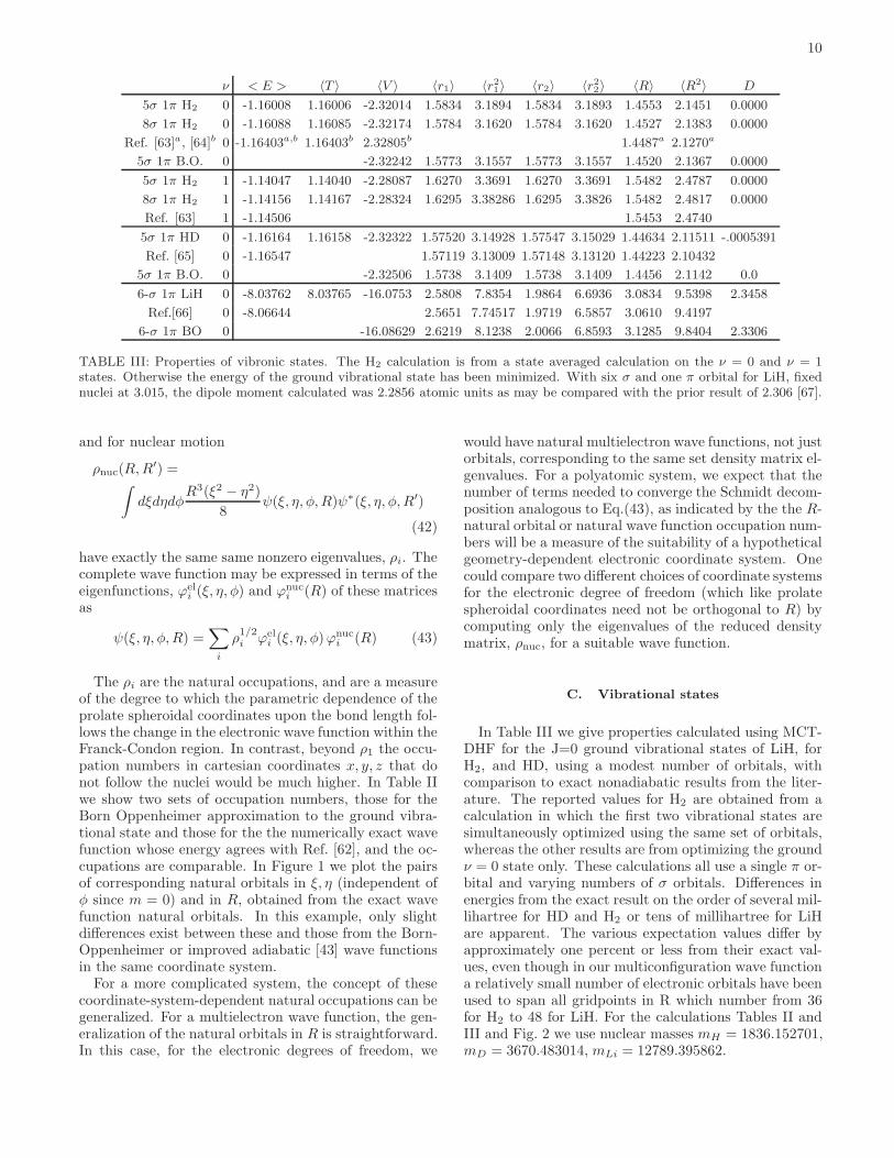
TABLE III: Properties of vibronic states. The H2 calculation is from a state averaged calculation on the ν = 0 and ν = 1states. Otherwise the energy of the ground vibrational state has been minimized. With six σ and one π orbital for LiH, fixednuclei at 3.015, the dipole moment calculated was 2.2856 atomic units as may be compared with the prior result of 2.306 [67].

and for nuclear motion

ρnuc(R,R′) =

∫dξdηdφ

R3(ξ2 − η2)

8ψ(ξ, η, φ,R)ψ∗(ξ, η, φ,R′)

(42)

have exactly the same same nonzero eigenvalues, ρi. Thecomplete wave function may be expressed in terms of theeigenfunctions, ϕel

i (ξ, η, φ) and ϕnuci (R) of these matrices

as

ψ(ξ, η, φ,R) =∑

i

ρ1/2i ϕel

i (ξ, η, φ)ϕnuci (R) (43)

The ρi are the natural occupations, and are a measureof the degree to which the parametric dependence of theprolate spheroidal coordinates upon the bond length fol-lows the change in the electronic wave function within theFranck-Condon region. In contrast, beyond ρ1 the occu-pation numbers in cartesian coordinates x, y, z that donot follow the nuclei would be much higher. In Table IIwe show two sets of occupation numbers, those for theBorn Oppenheimer approximation to the ground vibra-tional state and those for the the numerically exact wavefunction whose energy agrees with Ref. [62], and the oc-cupations are comparable. In Figure 1 we plot the pairsof corresponding natural orbitals in ξ, η (independent ofφ since m = 0) and in R, obtained from the exact wavefunction natural orbitals. In this example, only slightdifferences exist between these and those from the Born-Oppenheimer or improved adiabatic [43] wave functionsin the same coordinate system.For a more complicated system, the concept of these

coordinate-system-dependent natural occupations can begeneralized. For a multielectron wave function, the gen-eralization of the natural orbitals in R is straightforward.In this case, for the electronic degrees of freedom, we

would have natural multielectron wave functions, not justorbitals, corresponding to the same set density matrix el-genvalues. For a polyatomic system, we expect that thenumber of terms needed to converge the Schmidt decom-position analogous to Eq.(43), as indicated by the the R-natural orbital or natural wave function occupation num-bers will be a measure of the suitability of a hypotheticalgeometry-dependent electronic coordinate system. Onecould compare two different choices of coordinate systemsfor the electronic degree of freedom (which like prolatespheroidal coordinates need not be orthogonal to R) bycomputing only the eigenvalues of the reduced densitymatrix, ρnuc, for a suitable wave function.

C. Vibrational states

In Table III we give properties calculated using MCT-DHF for the J=0 ground vibrational states of LiH, forH2, and HD, using a modest number of orbitals, withcomparison to exact nonadiabatic results from the liter-ature. The reported values for H2 are obtained from acalculation in which the first two vibrational states aresimultaneously optimized using the same set of orbitals,whereas the other results are from optimizing the groundν = 0 state only. These calculations all use a single π or-bital and varying numbers of σ orbitals. Differences inenergies from the exact result on the order of several mil-lihartree for HD and H2 or tens of millihartree for LiHare apparent. The various expectation values differ byapproximately one percent or less from their exact val-ues, even though in our multiconfiguration wave functiona relatively small number of electronic orbitals have beenused to span all gridpoints in R which number from 36for H2 to 48 for LiH. For the calculations Tables II andIII and Fig. 2 we use nuclear masses mH = 1836.152701,mD = 3670.483014, mLi = 12789.395862.

11

0

250

500

750

1000

1250

5 6 7 8 9 10

Del

ta E

(cm

-1)

Number of orbitals

LiHv=0 to 1v=1 to 2v=2 to 3

-200

0

200

400

600

800

1000

1200

4 5 6 7 8 9

Del

ta E

(cm

-1)

Number of orbitals

H2v=0 to 1v=1 to 2v=2 to 3v=3 to 4v=4 to 5v=5 to 6v=6 to 7v=7 to 8v=8 to 9

FIG. 2: (Color online) Convergence of vibrational transitionfrequencies for H2 and LiH from state averaged MCTDHF cal-culations using one π orbital while optimizing 4 vibrationalstates for LiH and 10 vibrational states for H2. The differ-ence between the calculated transition frequency and the ex-perimental one is plotted with respect to the total numberof orbitals, varying the number of σ orbitals. For LiH, theerrors using the Hartree-Fock Born-Oppenheimer curve arealso plotted, with atomic masses as the arrows on the rightside. For H2, the errors for the same transitions from a Born-Oppenheimer calculation with five σ, one π orbitals are alsoplotted as arrows to the right.

In Table III we also report properties calculated forthe Born-Oppenheimer wave function, i.e., the solu-tion χ0(R)ψ1(~r;R) obtained by diagonalizing the Born-Oppenheimer vibrational Hamiltonian using the groundBorn-Oppenheimer electronic state ψ1(~r;R) with orbitalsoptimized for each Ri separately, and using the atomicmasses. For H2, the error in these results is comparableto that of our nonadiabatic MCTDHF wave functions.For LiH, we achieve better agreement with the previ-ously computed accurate values using the full nonadia-batic treatment than we do with the Born-Oppenheimercalculation using fixed masses.There is a striking observation to be made about these

results concerning the convergence of our approach inwhich a single set of electronic orbitals is used for all R.By accounting for the nonadiabatic coupling terms in theHamiltonian and using one small set of orbitals for all R,we achieve a better representation of the wave function

Born-Op. ν = 0

1.96 1.95

0.02100.02100.0210 0.0235

0.006340.006340.00634 0.0146

0.00203 0.000618

0.00191 0.000347

0.0000836 0.000182

0.00446 0.00443

FIG. 3: (Color online) Electronic natural orbitals of groundstate H2, with occupation numbers, from calculations withone π and six σ orbitals. Left column: Born-Oppenheimernatural orbitals at R = 1.4 a0; right column: natural orbitalsfrom nonadiabatic calculation of the ν = 0 state.

12

than we do using the Born-Oppenheimer wave functionwith orbitals optimized separately at each R.

In Fig. 2 we show the performance of the method inrepresenting the vibrational spectrum of H2 and LiH. ForLiH, the first four vibrational states are simultaneouslyoptimized using the same orbitals in these calculations,and for H2 the first 10 are optimized. The errors in the vi-brational transition frequencies are plotted with respectto the total number of orbitals. The corresponding er-rors in the transition frequencies for the vibrational statesof the Born-Oppenheimer curves (again, computed withatomic masses) are plotted as arrows on the right. Theseerrors are comparable so the arrows overlap.

Because in these calculations we are simultaneouslyoptimizing a set of vibrational states spanning a largerrange of internuclear distances than ν = 0 and ν = 1,the errors in Fig. 2 are greater than those in Table III.However, despite this fact the errors in the vibrationaltransitions may be made to be quite small even in a stateaveraged calculation. We obtain 4173.4cm−1 versus thecorrect value of 4161.1 for the ν = 0 to 1 transition ofH2.

In Fig. 3 we plot the natural orbitals from a Born-Oppenheimer calculation and the MCTDHF calculationwith the same number of orbitals for the ν = 0 state,labeled by their occupations. Although some differencesmay be seen, particularly in the sixth σ orbital, the over-all impression is that the two sets of natural orbitals areremarkably similar. That similarity suggests that theelectron-nuclear correlation is substantially accounted forby the dependence of the orbitals on R via the prolatespheroidal coordinate system, since they have no other Rdependence. A similar conclusion can be drawn from anexamination of the natural orbitals for the state averagedcalculation (not shown).

IX. CALCULATION OF IONIZATION CROSS

SECTIONS

We calculation ionization probabilities and cross sec-tions using the flux formalism of Jackle and Meyer [71].Three MCTHDF steps are involved: (1) relaxation tothe ground initial state, (2) propagation from t = −Tto t = 0 in which a pulse of duration T is applied, and(3) propagation of Ψ(0) forward in time until the ionizedportion has been absorbed by complex the ECS grid inξ. The wave function propagated during the third step,from t = 0 onward, is saved and used in the followinganalysis.

As per Ref. [71], the total ionized flux at energy E isdefined as

f(E) =∫ ∞

0

dt

∫ ∞

0

dt′⟨Ψ(0)

∣∣∣ei(H−E)t′ F e−i(H−E)t∣∣∣Ψ(0)

⟩

(44)

The flux operator F is defined as the flux through a hy-persurface, the region exterior to which corresponds tothe breakup process of interest – in this case, ioniza-tion. Defining the heaviside operator Θ(~r1, ~r2, ...) to bethe unit operator in this exterior region and zero within,the flux operator may be expressed as the commutatorof the Hamiltonian with this heaviside function,

F = i[H,Θ] . (45)

Under appropriate assumptions and after somealgebra[71], one arrives at

f(E) =

∫ ∞

0

dt

∫ ∞

0

dt′ eiE(t−t′)⟨Ψ(t′)

∣∣∣i(H − H†)∣∣∣Ψ(t)

⟩

(46)In this expression, the flux is obtained through matrixelements of the antihermitian part of the Hamiltonianbetween wave functions at different times; in deriving it,we have exploited the fact that the antihermitian partof the Hamiltonian lies only on the complex part of theECS contour.In the present context, the antihermitian part of the

Hamiltonian comes from the exterior complex scaling inthe ξ coordinates, and is nonzero only when at least oneelectron has reached the FEM-DVR element that termi-nates at ξ0, the start of the ECS tail. As long as ξ0 hasbeen chosen sufficiently large, the antihermitian part isnonzero in the region corresponding to single or multipleionization. In the MCTDH implementation for heavyparticle motion, complex absorbing potentials (CAPs)are used instead of ECS in the exterior region to absorbthe outgoing part of the wave function, and the validityof the above equations for the flux depend on the CAPbeing weak enough not to perturb the wave function inthe inner region. In contrast, ECS is an analytic contin-uation of the Hamiltonian to complex coordinates, anddoes not perturb the solution in the inner region at all,unless a significant basis set error is present.In terms of the flux, the integral photoionization cross

section (summed over final channels) is

σ(E) =2παω

|F(E)|2 f(E) (47)

where α is the fine structure constant, ω is the photonenergy, ω = E−E0 where E0 is the ground state energy,and F(E) is the Fourier transform of the pulse from alength gauge calculation, for example,

F(E) =

∫ 0

−T

dt E(t)ei(E−E0)t . (48)

To evaluate Eq.(46) it is necessary to evaluate the ma-

trix element of H − H† between wave functions at twodifferent times, comprised of two different sets of orbitals,in an efficient manner. Although for the present appli-cations to H2 simpler methods would suffice, we use anapproach that will be applicable to larger systems. To

13

that end, we transform to a biorthogonal set of orbitals,in the spirit of the treatment of Malmqvist [72], afterwhich we may evaluate matrix elements of arbitrary op-erators, for instance the flux operator, via Slater’s rulesfor zero, single and double excitations just as in the usual,orthogonal case. Thus, given orbitals and A-vectors at tand t′, we first transform the orbitals φ(t′) into a new setϕ(t′) which obey a biorthonormality relationship to φ(t):〈ϕi(t

′)|φj(t)〉 = δij . Whereas the MCTDHF orbitals φare themselves orthonormal at all times, the ϕ functionsalone obey no such relationship,

sij = 〈φi(t)|φj(t′)〉 ϕi(t′) =

∑

j

(s−1)jiφj(t′) . (49)

The full wave function at time t′ has a new A-vector ofconfiguration coefficients – which we denote as the B-

vector, ~B – corresponding to its expansion in the newbiorthogonal orbitals ϕ(t′). In our notation the A-vectorcorresponds to the configuration basis |~n(t′)〉, and we de-note the configurations made from the ϕ(t′) orbitals as

|~m〉, where 〈~n(t)|~m(t′)〉 = δ~n~m. We solve for ~B via

Ψ(t′) =∑

~m~n

B~m(t′)|~n〉〈~n|~m〉 =∑

~n

A~n(t′)|~n〉

~A(t′) = S(t′) ~B(t′) S~n~m = 〈~n(t′)|~m(t′)〉(50)

To solve these equations we must first construct S~n~m,the overlap between configurations defined in terms ofnonorthogonal sets of orbitals, a task which becomes in-creasingly more demanding as the number of electronsincreases. We can take advantage of the remarkable factthat for full CI wave functions, although the matrix S

is dense, its logarithm, lnS, has sparse representations.In fact, the matrix lnS is not unique, for the same rea-son that the multibranched complex function ln(z) is notunique, and it has both sparse and nonsparse represen-tations.The nonzero matrix elements of a sparse branch of lnS

may be calculated by applying Slater’s rules for the ma-trix elements of a one-electron operator such as the ki-netic energy, which usually are applied to a determinantbasis constructed of (bi)orthonormal orbitals. The ma-trix element lnS~n~m with respect to configurations |~na(t)〉and |~m(t′)〉 is zero if these configurations differ by morethan one index, and otherwise is given by Slater’s otherrules for a one electron operator as applied to any branchof the matrix logarithm lns.For full CI wave functions, which are employed in the

present work, the solution of the linear equation ~A =

S ~B can be done in sparse arithmetic using the Krylov-space expokit [54] subroutine ZGEXPV, which performs amatrix exponential onto a vector. The solution is therebyexpressed as

~B = exp (− lnS) ~A . (51)

The transformation to the biorthogonal basis beingdone, we proceed to evaluate matrix elements of the anti-hermitian parts of the Hamiltonian operators appearing

0

0.5

1

1.5

2

2.5

3

3.5

4

4.5

0.6 0.7 0.8 0.9 1 1.1 1.2 1.3 1.4

Cro

ss s

ectio

n (M

b)

Photon energy (hartree)

9 σ, 1 π3 σ2 σ1 σ

Sanchez and MartinFT of pulse

0

0.1

0.2

0.3

0.4

0.5

0.6

0.7

0.8

1.1 1.15 1.2 1.25 1.3 1.35

Cro

ss s

ectio

n (M

b)

Photon energy (hartree)

9 σ, 1 π3 σ2 σ1 σ

Sanchez and Martin

FIG. 4: (Color online) Fixed-nuclei ionization cross sectionof H2, Σ symmetry, calculated using the full wave functionwith one π and nine σ orbitals, with a single pulse of inten-sity 1×10−13 W cm−2, frequency 1.1 hartree, and duration0.5 fs in the length gauge. Top: cross section from threshold(0.60449 hartree) to the H+

2 1 Σu threshold at 1.28 hartree.The thresholds are marked with arrows and the Fourier trans-form of the pulse is plotted with arbitrary units as dots. Alsoshown are the results of Sanchez and Martın [73]. Bottom:magnification of resonance region, including result using onlythree sigma orbitals. Several other results are plotted thatnearly coincide: lower intensity (1 ×10−15 W cm−2); velocitygauge; and more orbitals of sigma, pi, and delta symmetry.

due to our use of exterior complex scaling, calculatingorbital matrix elements and assembling them into theconfiguration matrix elements in the same manner as inconstructing the A-vector Hamiltonian matrix H .The results for ionization of H2 in Σ symmetry (polar-

ization parallel to the bond axis) are shown in Fig. 4. Wefind that calculation is converged at a total of one π andnine σ orbitals. The other parameters of the calculationare given in the caption to Fig. 4. In obtaining Eq. 46we assumed that 〈ψ(0)|ψ(t)〉 = 〈ψ(0)|ψ(−t)〉∗, and viabackwards time propagation, we have verified that thisidentity is obeyed in general for these MCTDHF wavefunctions, at least to one part in 10−4. To eliminatethe oscillations of the Gibbs phenomenon in the Fourier

14

0

0.2

0.4

0.6

0.8

1

1.2

1.05 1.1 1.15 1.2 1.25 1.3 1.35

Cro

ss s

ectio

n (M

b)

Photon energy (hartree)

4-8 σ3-6 σ2-4 σ1-2 σ

FIG. 5: Fixed-nuclei ionization cross section of H2, Σ sym-metry, using the treatment of Eq.(52) to solve for only theperturbation to the wave function: results for one throughfour initial state σ orbitals, with twice that number for thepulse and flux steps, using the same pulse parameters as inFig. 4. Circles: results of Sanchez and Martın [73].

transform over a finite interval we additionally multiplyEq.(46) by a sinusoids in t and t′, as cos tπ

2T , where T isthe time for which we propagate the wave function af-ter the pulse. The result is converged to visual accuracywithin approximately 1600 atomic time units.

In Fig. 4 we also plot the results for one, two, andthree σ orbitals only. All reproduce the overall magni-tude and shape of the cross section, but are incorrect inthe energy range where the autoionizing resonances ap-pear. The one-orbital treatment is featureless there, asthe parent H+

2 (Σu) state is not represented in the basis,but otherwise correct. The two and three-orbital treat-ments reproduce the Fano lineshapes of the resonances,but place them at incorrect energies, and additionallytheir locations do not appear to converge until the nineσ, one π result shown in black.

However, the result converges to a cross sectionslightly different than the accurate results of Sanchez andMartın [73]. We may be able to understand this numer-ical behavior by realizing that at these intensities, onlyabout 1/1000th of the wave function has been ionized,and that these calculations have not converged that por-tion. This slow convergence behavior would seem to be aproblem for the utility of the MCTDHF method for de-scribing photoionization or other perturbative processesin general. One would like to treat perturbative problemsjust as well as nonperturbative ones, but the variationalansatz of the MCTDHF wave function will use the varia-tional flexibility in the calculation to optimize the larger,unperturbed (initial state) portion of the wave functionat the expense of the smaller components in which weare more interested.

In the limit of a large number of orbitals, the MCT-DHF equation should converge to the exact result. Itis likely that this number is much larger than we have

used in the calculations shown in Fig. 4, as additionalorbitals are likely to mostly further optimize the corre-lation within the ground state until enough have beenadded so that the occupation numbers of the natural or-bitals describing ground state correlation have fallen atleast two orders of magnitude. There is, however, analternative approach.

X. MORE EFFICIENT CALCULATION OF

IONIZATION

The problem that additional orbitals mostly serve toimprove the description of the initial state is particular tothe present application to calculate a perturbative result,and more intense-field applications would not suffer fromit. This state of affairs in unsatisfactory, but fortunatelythere is a straightforward solution to this problem. Wecan calculate not Ψ(t), the full wave function, but thequantity we label Ψ′(t), the change in the wave functiondue to the pulse:

Ψ(t) = e−iE0tΨ(0) + Ψ′(t)

i∂

∂tΨ′(t) = H(t)Ψ′(t) + V (t)e−iE0tΨ(0)

(52)

where E0 is the initial state eigenvalue and V (t) is theperturbation. This formulation modifies the MCTDHFworking equations, Eqs.(8) and (13), introducing drivingterms to each, but we were not immediately able to im-plement the orbital driving term in a numerically stableway. We thus double the orbital dimension at the startof the pulse, generating additional orbitals by operatingwith the dipole operator upon the occupied orbitals ofthe initial state, and causing the orbital driving term toequal zero at the start of the pulse. We then calculateΨ(t) ≡ eiE0tΨ′(t) by modifying Eq.(13) as

i∂

∂t~A(t) = (H(t)− E0) ~A(t) +V(t) ~A(0) , (53)

where the matrix V is the matrix of the dipole opera-tor in the nonorthogonal basis of orbitals at times t and0, V~n~n′ = 〈~n(t)|µ|~n′(0)〉. This equation is solved withroutine ZGPHIV in the expokit package[54].The results are significantly better than in our first

treatment, calculating the entire wave function, althoughwe find that we cannot accurately calculate the entirerange between the H2 ionization thresholds with the sin-gle pulse we used for the calculation of the full wave func-tion Ψ(t). We focus on the resonance region, where our~ω = 1.1 hartree, 0.5 fs pulse is centered. The resultsare again insensitive to intensity across the whole energyrange.In Fig. 5 we show that the ionization cross section con-

verges to essentially its correct value using σ orbitals only.In our treatment we double the number of orbitals goingfrom the ground initial state to the propagation stepsof the calculation; thus the minimum is two. We can

15

see that the minimum one orbital (Hartree-Fock) groundstate, two propagation orbital treatment yields an ioniza-tion cross section without the correct resonance features;the two orbitals of the propagation of Ψ′(t) correspondto the ground H+

2 1σg cation state and the wavepacketionized in its field. The resonances, which are based onthe 1σu cation state, are thus not represented. initial,six propagation orbitals, the resonances appear in essen-tially their correct locations. Two additional propagation(one additional initial) orbitals are all that is needed togive good agreement with the calculations of Sanchez andMartın [73].

XI. CONCLUSION AND OUTLOOK

We have explored the formulation of the MCTDHFapproach both for fixed nuclei and including nuclear mo-tion for application to any diatomic molecule within thenonrelativistic approximation. Furthermore methods forovercoming several important technical barriers to suchcalculations have been demonstrated. The use of pro-late spheroidal coordinates, and an expansion of the wavefunction including nuclear motion in terms of configura-tions of orbitals which depend on R only through thedependence of the underlying coordinates on internu-clear distance are crucial parts of the strategy describedhere. We have demonstrated that the use of such or-bitals gives a rapidly convergent representation of thevibrational states of diatomics in calculations that avoidthe Born-Oppenheimer approximation. Furthermore, wehave shown that photoionization cross sections can beextracted from the MCTDHF wave functions in full di-mensionality, and demonstrated that accurate photoion-ization cross sections can be calculated using a methodfor solving for only the perturbation caused by a time-dependent potential. The methods we describe hereshould be immediately applicable to calculation of thesingle (or total) ionization of larger molecules, as well asstudies of Auger spectra with or without nuclear motion.

Acknowledgments

This work was performed under the auspices of theUS Department of Energy by the University of Califor-nia Lawrence Berkeley National Laboratory under Con-tract DE-AC02-05CH11231 and was supported by theU.S. DOE Office of Basic Energy Sciences, Division ofChemical Sciences.

Appendix A: One electron matrix elements

We follow Ref. [33] in the derivation of the matrixelements of the electronic Hamiltonian in our prolatespheroidal DVR basis, and provide additional formulasfor the nonadiabatic terms. For details on the use of

FEM-DVR, see Ref. [35]. We evaluate all the integralsby quadrature; the only non-polynomial terms approx-imated by quadrature are the repulsive inverse integerpowers that appear, for example, in the centrifugal po-tentials.

We refer to the matrix elements using the notation ofEq.(28) representing the Hamiltonian we use here, whichis exact for J = 0 except for the omission of the two-

electron terms in l2. The Hamiltonian is otherwise ac-curate except for Coriolis coupling for J 6= 0. In theequations below, fM

iα refers to an electronic FEM-DVRproduct basis function of Eq.(19), χ to a primitive DVRfunction of Eq.(18), and χ′ to its first derivative.

The matrix elements in R are straightforward,

TRij =

⟨χi(R)

∣∣∣∣−1

2

∂2

∂R2

∣∣∣∣χj(R)

⟩

≈ 1

2

∑

k

wkχ′(i)(Rk)χ

′j(Rk)

DRij =

⟨χi(R)

∣∣∣∣∣2

R

(∂

∂R

)

ξηφ

− 1

R2

∣∣∣∣∣χj(R)

⟩

≈ 1

Riχ′j(Ri)−

1

Rjχ′i(Rj)

(A1)

The electronic matrix elements

TeliajbM =

⟨fMia

∣∣∣∣∣−R2

2µe∇2 +

1

2µR

[−(Y +

3

2

)2

+ l2

]∣∣∣∣∣ fMjb

⟩

DeliajbM =

⟨fMia

∣∣∣∣Y +3

2

∣∣∣∣ fMjb

⟩

(A2)

involving the operators

R22 =

4

(ξ2 − η2)

[

∂

∂ξ(ξ2 − 1)

∂

∂ξ+

∂

∂η(1− η

2)∂

∂η

]

Y =(ξ + αη)(ξ2 − 1)

ξ2 − η2

∂

∂ξ+

(η + αξ)(1− η2)

ξ2 − η2

∂

∂η

l2 = M2 +

1

2

(

l+l− + l

−l+)

= M2 +1

2

(

l−†l− + l+

†l+)

l± = e

±iφ

(

±ρ(η + αξ)

ξ2 − η2

∂

∂ξ∓

ρ(ξ + αη)

ξ2 − η2

∂

∂η−

ξη + α

ρM

)

where we use the shorthand ρ ≡√(ξ2 − 1)(1− η2), may

be expressed using the identities

Y +3

2=

1

2

(

Y − Y†)

(

Y +3

2

)2

= −

(

Y +3

2

)† (

Y +3

2

)

(A3)

16

as

TeliajbM ≈ δij

∑

c

χ′a(ξc)χ

′b(ξc)wc×

[

ξ2c − 1

2µe

+(ξc + αηi)

2(ξ2 − 1)2 + ρ2(η + αξ)2

2µR

]

+ δab∑

k

χ′i(ηk)χj(ηk)wk×

[

1− η2k

2µe

+(ηk + αξa)

2(1− η2k)

2 + ρ2(ξ + αη)2

2µR

]

−3

2δij

(

(ξa + αηi)(ξ2a − 1)χ′

b(ξa) + (ξb + αηi)(ξ2b − 1)χ′

a(ξb))

−3

2δab

(

(ηi + αξa)(1− η2i )χ

′j(ηi) + (ηj + αξa)(1− η

2j )χ

′i(ηj)

)

+ δijδab

(

9

4+

(

Mξaηi + α

ρ

)2)

(A4)

DeliajbM ≈ δij

((ξa + αηi)(ξ

2a − 1)χ′

b(ξa)

− (ξb + αηi)(ξ2b − 1)χ′

a(ξb))

+ δab

((ηi + αξa)(1− η2i )χ

′j(ηi)

+ (ηj + αξa)(1− η2j )χ′i(ηj)

)

(A5)

In the present applications the pulse was parallel to thebond axis, and the dipole operator is given in length andvelocity gauge as

⟨fMia |µ| fM

jb

⟩=⟨fMia

∣∣∣ zR

∣∣∣ fMjb

⟩≈ δijδab

ξaηi + α

2(A6)

and

⟨fMia |µ| fM

jb

⟩=

⟨fMia

∣∣∣∣R∂

∂z

∣∣∣∣ fMjb

⟩≈

2δij [(ξ2a − 1)(ηi + αξa)χ

′b(ξa)− (ξ2b − 1)(ηi + αξb)χ

′a(ξb)]

+ 2δab[(1 − η2i )(ξa + αηi)χ′j(ηi)− (1− η2j )(ξb + αηj)χ

′j(ηi)]

(A7)

respectively.

Appendix B: Two-electron matrix elements

We can follow the method of Refs. [33, 35] to con-struct the matrix elements of 1/r12 in the DVR basis.We evaluate the matrix elements of a multipole expan-sion of this operator by solving Poisson’s equation in theradial (ξ) coordinate while evaluating the η integrals byquadrature. The resulting matrix elements retain thesparsity of the DVR representation, being diagonal in ξand η and off-diagonal only in the M quantum numbersof the electrons. This point is crucial for the presenttime-dependent application, as it means that the two-electron transformations do not dominate the computa-tional time, which is instead primarily determined by the

action of the Jacobian of Eq.(8) onto the orbitals withinthe mean field step.We begin by defining regular and irregular Legendre

functions [74] with an additional normalization factor,

Plm(ξ) ≡ NlmPlm(ξ) =

√(2l+ 1)(l −m)!

2(l +m)!Plm(ξ)

Qlm(ξ) ≡ NlmQlm(ξ) =

√(2l + 1)(l −m)!

2(l +m)!Qlm(ξ)

(B1)

so that the Neumann expansion of 1/r12 may be written

1

r12=

8π

R

∑

lm

(−1)m2

2l + 1

eimφ1

√2π

e−imφ2

√2π

×

Plm(ξ<)Qlm(ξ>)Plm(η1)Plm(η2)

(B2)

Thus to compute the two-electron integrals we require

the matrix elements of Plm(ξ<)Qlm(ξ>) in the DVR ba-sis in ξ. This function is the Green’s function for thefollowing equation:

[∂

∂ξ1(ξ2 − 1)

∂

∂ξ1− l(l + 1)− m2

ξ21 − 1

]Plm(ξ<)Qlm(ξ>)

= (ξ21 − 1)W(Plm(ξ1), Qlm(ξ1)

)δ(ξ1 − ξ2) ,

(B3)

whereW is the Wronskian of the two Legendre functions,which has the value

Wlm(ξ1) =(−1)m22m

(1− ξ21)

Γ(l+m+2

2

)Γ(l+m+1

2

)

Γ(l−m+2

2

)Γ(l−m+1

2

) (B4)

Expressing the operator in square brackets in Eq.(B3) inthe DVR basis and approximating the matrix elements ofboth sides of that equation using the DVR quadrature,we arrive at an expression for the matrix elements of

Plm(ξ<)Qlm(ξ>),

Rlmab ≡

⟨χaχb

∣∣∣ 2

2l+ 1Plm(ξ<)Qlm(ξ>)

∣∣∣χcχd

⟩

= δacδbd

[−2

2l+ 1

Plm(ξa)Plm(ξb)Qlm(ξN )

Plm(ξN )

+(−1)m(l −m)!

(l +m)!

Γ(l+m+2

2

)Γ(l+m+1

2

)

Γ(l−m+2

2

)Γ(l−m+1

2

)(T−1lm

)ab√

wawb.

]

(B5)

In Eq.(B5), N is the last Gauss-Radau gridpoint in ξ,corresponding to a DVR function discarded to enforcethe correct boundary condition at the end of the ξ gridon the solution of Eq.(B3), and Tlm is the the ma-trix of the operator in square brackets in that equationin terms of the DVR functions χi(ξ) (for even m) or

17

√(ξ2 − 1)/(ξ2i − 1)χi(ξ) (for odd m), which are normal-

ized to one with respect to integration over ξ. Thosematrix elements are

(Tlm)ij =− δij

(m2

ξ2i − 1+ l(l+ 1)

)

+∑

k

χ′i(ξk)χ

′j(ξk)wk(ξ

2k − 1)

(B6)

Using the expression for Rlmab in Eq. (B5) we obtain

the final result for the two electron matrix elements inour DVR basis,

⟨fM1

ia fM2

jb

∣∣∣∣1

r12

∣∣∣∣ fM1−mkc fM2+m

ld

⟩

= δacδbdδikδjl4

R

lmax∑

l=0

Rlmab Plm(ηi)Plm(ηj)

(B7)

which has exactly the form in Eq.(20). This expressiondepends also on having used a fixed DVR quadratureto approximate the η1 and η2 integrations, and a givenquadrature order cannot be used for arbitrarily large lvalues in the Neumann expansion in Eq.(B2). In ournumerical calculations we use lmax = Nη where Nη isthe number of DVR functions in η. We have foundthis choice to be optimal when using this algorithmimplemented for spherical polar coordinates, and at leastnear optimal for the present case of prolate spheroidalcoordinates.

[1] F. Krausz and M. Ivanov, Rev. Mod. Phys. 81, 163(2009).

[2] T. Sekikawa, A. Kosuge, T. Kanai, and S. Watanabe,Nature 432, 605 (2004).

[3] V. Ayvazyan, et al., Eur. Phys. J. D 37, 297 (2006).[4] J. Ullrich, R. Moshammer, A. Dorn, R. Doerner,

L. Schmidt, and H. Schmidt-Bocking, Rep. Prog. Phys.66, 143 (2003).

[5] M. Lesius, V. Blanchet, M. Ivanov, and A. Stolow, J.Chem. Phys. 117, 1575 (2002).

[6] S. Tanaka and S. Mukamel, Phys. Rev. Lett. 89, 043001(2002).

[7] A. M. Virshup, C. Punwong, T. V. Pogorelov, B. A.Lindquist, C. Ko, and T. J. Martinez, J. of Phys. Chem.B 113, 3280 (2009).

[8] Y. Arasaki, K. Takatsuka, K. Wang, and V. McKoy, J.Chem. Phys. 132, 124307 (2010).

[9] H. Hudock, B. Levine, A. Thompson, H. Satzger,D. Townsend, N. Gador, S. Ullrich, A. Stolow, andT. Martinez, J. Phys. Chem. A 111, 8500 (2007).

[10] M. Eroms, O. Vendrell, M. Jungen, H.-D. Meyer, andL. Cederbaum, J. Chem. Phys. 130, 154307 (2009).

[11] H. Nakai, Int. J. Quantum Chem. 107, 2849 (2007).[12] T. Ishimoto, M. Tachikawa, and U. Nagashima, Int. J.

Quantum Chem. 109, 2677 (2009).[13] T. Kreibich, R. van Leeuwen, and E. Gross, Chem. Phys.

304, 183 (2004).[14] H. Yonehara, S. Takahashi, and K. Takatsuka, J. Chem.

Phys. 130, 214113 (2009).[15] O. E. Alon, A. I. Streltsov, and L. S. Cederbaum, J.

Chem. Phys. 127, 154103 (2007).[16] O. E. Alon, A. I. Streltsov, and L. S. Cederbaum, Phys.

Rev. A 79, 022503 (2009).[17] M. Kitzler, J. Zanghellini, C. Jungreuthmayer, M. Smits,

A. Scrinzi, and T. Brabec, Phys. Rev. A 70, 041401(2004).

[18] J. Caillat, J. Zanghellini, M. Kitzler, O. Koch,W. Kreuzer, and A. Scrinzi, Phys. Rev. A 71, 012712(2005).

[19] T. Kato and H. Kono, J. Chem. Phys. 128, 184102(2008).

[20] T. Kato and K. Yamanouchi, J. Chem. Phys. 131, 164118

(2009).[21] M. Nest, Phys. Rev. A 73, 023613 (2006).[22] M. Nest, R. Padmanaban, and P. Saalfrank, J. Chem.

Phys. 126, 214106 (2007).[23] M. Nest, F. Remacle, and R. D. Levine, New J. Phys.

10, 025019 (2008).[24] M. Nest, Chem. Phys. Letts. 472, 171 (2009).[25] J. Kucar, H.-D. Meyer, and L. S. Cederbaum, Chem.

Phys. Lett. 140, 525 (1987).[26] H.-D. Meyer, U. Manthe, and L. S. Cederbaum, Chem.

Phys. Lett. 165, 73 (1990).[27] M. H. Beck and H.-D. Meyer, Z. Phys. D 42, 113 (1997).[28] M. Beck, A. Jackle, G. Worth, and H.-D. Meyer, Physics

Reports 324, 1 (2000).[29] H.-D. Meyer and G. A. Worth, Theor. Chem. Acc. 109,

251 (2003).[30] G. A. Worth, M. H. Beck, A. Jackle, and H.-D.

Meyer, The MCTDH Package, Version 8.3, (2002),http://www.pci.uni-heidelberg.de/tc/usr/mctdh/.

[31] L. Tao, C. W. McCurdy, and T. N. Rescigno, Phys. Rev.A 79, 012719 (2009).

[32] L. Tao, C. W. McCurdy, and T. N. Rescigno, Phys. Rev.A 80, 013402 (2009).

[33] L. Tao, C. W. McCurdy, and T. N. Rescigno, Phys. Rev.A 82, 023423 (2010).

[34] N. Moiseyev, Physics Reports 302, 211 (1998).[35] C. W. McCurdy, M. Baertschy, and T. N. Rescigno, J.

Phys. B 37, R137 (2004).[36] D. A. Horner, C. W. McCurdy, and T. N. Rescigno, Phys.

Rev. A 78, 043416 (2008).[37] A. Palacios, T. N. Rescigno, and C. W. McCurdy, Phys.

Rev. A 77, 032716 (2008).[38] A. Palacios, T. N. Rescigno, and C. W. McCurdy, Phys.

Rev. A 79, 033402 (2009).[39] W. Vanroose, D. A. Horner, F. Martın, T. N. Rescigno,

and C. W. McCurdy, Phys. Rev. A 74, 052702 (2006).[40] F. L. Yip, C. W. McCurdy, and T. N. Rescigno, Phys.

Rev. A 81, 063419 (2010).[41] A. C. Wahl, P. E. Cade, and C. C. J. Roothaan, J. Chem.

Phys. 41, 2578 (1964).[42] J. E. A. McCullough, J. Chem. Phys. 62, 3991 (1975).[43] B. D. Esry and H. R. Sadeghpour, Phys. Rev. A 60, 3604

18

(1999).[44] The term polyspherical coordinates denotes a set of (Ja-

cobi or Radau) spherical polar vectors defining an or-thogonal internal coordinate system for the nuclei of amolecule in the center of mass frame.

[45] F. Gatti, C. Munoz, and C. Iung, J. Chem. Phys. 114,8275 (2001).

[46] F. T. Smith, Phys. Rev. Lett. 45, 1157 (1980).[47] C. W. McCurdy, C. K. Stroud, and M. K. Wisinski, Phys.

Rev. A 43, 5980 (1991).[48] L. Tao, W. Vanroose, B. Reps, T. N. Rescigno, and C. W.

McCurdy, Phys. Rev. A 80, 063419 (2009).[49] A. Scrinzi, Phys. Rev. A 81, 053845 (2010).[50] T. N. Rescigno and C. W. McCurdy, Phys. Rev. A 62,

032706 (2000).[51] O. Koch and C. Lubich, IMA Jour-

nal of Numerical Analysis (2010), URLhttp://imajna.oxfordjournals.org/content/early/2010/01/31/imanum.drp040.abstract.

[52] O. Koch, W. Kreuzer, and A. Scrinzi, Appl. Math. Comp.173, 960 (2009).

[53] C. Lubich, Appl. Numerical Mathematics 48, 355 (2004).[54] R. B. Sidje, ACM Trans. Math. Softw. 24, 130 (1998).[55] F. Jensen, J. Chem. Phys 110, 6601 (1999).[56] J. Thompson and S. Williams, J. Phys. B: At. Mol. Opt.

23, 2205 (1990).[57] J. Kobus, Chem. Phys. Lett. 202, 7 (1993).[58] H.-D. Meyer, F. Le Quere, C. Leonard, and F. Gatti,

Chem. Phys. 329, 179 (2006).[59] L. J. Doriol, F. Gatti, C. Iung, and H.-D. Meyer, J.

Chem. Phys. 129, 224109 (2008).[60] H. Lishka, R. Shepard, I. Shavitt, R. M. Pitzer, M. Dal-

los, T. Muller, P. G. Szalay, F. B. Brown, R. Ahlrichs,H. J. Bohm, et al., Columbus, an ab initio electronic

structure program (2006), release 5.9.1.[61] J. T.H. Dunning, J. Chem. Phys. 90, 1007 (1989).[62] G. G. Balint-Kurti, R. E. Moss, I. A. Sadler, and

M. Shapiro, Phys. Rev. A 41, 4913 (1990).[63] S. Bubin and L. Adamowicz, J. Chem. Phys. 118, 3079

(2003).[64] D. Kinghorn and L. Adamowicz, J. Chem. Phys. 113,

4203 (2000).[65] M. Stanke, S. Bubin, M. Molski, and L. Adamowicz,

Phys. Rev. A 79, 032507 (2009).[66] S. Bubin, L. Adamowicz, and M. Molski, J. Chem. Phys.

123, 134310 (2005).[67] D. Cooper, J. Gerratt, and M. Raimondi, Chem. Phys.

Lett. 118, 580 (1985).[68] A. Ekert and P. L. Knight, Am. J. Physics 63, 415 (1995).[69] A. Peres, Quantum Theory: Concepts and Methods

(Kluwer Academic, Boston, 1993).[70] M. A. Nielsen and I. L. Chuang, Quantum Computation

and Quantum Information (Cambridge University Press,Cambridge, England, 2000).

[71] A. Jackle and H.-D. Meyer, J. Chem. Phys. 105, 6778(1996).

[72] P. Malmqvist, Int. J. Quant. Chem. 30, 479 (2004).[73] I. Sanchez and F. Martın, J. Phys. B 30, 679 (1997).[74] M. Abramowitz and I. A. Stegun, Handbook of Mathe-

matical Functions (National Bureau of Standards, U. S.Government Printing Office, Washington, D. C., 1964).