arX

iv:1

202.

5246

v1 [

cond

-mat

.qua

nt-g

as]

23

Feb

2012

Quantum diffraction grating with cold atoms in an optical lattice

Adhip Agarwala, Madhurima Nath, Jasleen Lugani, K. Thyagarajan and Sankalpa Ghosh

Department of Physics, Indian Institute of Technology Delhi, New Delhi-110016, India

(Dated: February 24, 2012)

Abstract

Light transmission or diffraction from different quantum phases of cold atoms in an optical

lattice have recently come up as a useful tool to probe such cold atomic systems. The periodic

nature of the optical lattice potential closely resembles the structure of a diffraction grating in

real space, but loaded with a strongly correlated quantum many body state which interacts with

the incident electromagnetic wave, a feature that controls the nature of the light transmission

or dispersion through such quantum medium. The paper contains a detailed analysis of such a

quantum diffraction grating. We have particularly studied how the dispersion shift induced by the

cavity changes as a function of the relative angle between the cavity mode and the optical lattice.

PACS numbers: 03.75.Lm,42.50.-p,37.10.Jk

1

I. INTRODUCTION

Ultra cold atomic condensates loaded in an optical lattice [1, 2] provide a unique op-

portunity to study the properties of an ideal quantum many body system. After the first

successful experiment in this field [3] where a quantum phase transition from a Mott Insula-

tor(MI) to Superfluid(SF) phase was observed, extensive theoretical as well as experimental

study in this direction took place. The field continues to be a frontier research area of atomic

and molecular physics, quantum condensed matter systems as well as quantum optics si-

multaneously, and holds promise for application in fields like quantum metrology, quantum

computation and quantum information processing [4, 5].

The relevance of the field of ultra cold atomic condensates to quantum optics was sug-

gested much earlier when it was pointed out that the refractive index of a degenerate Bose

gas gives a strong indication of quantum statistical effects [6] and the interaction between

quantized modes of light and such ultra-cold atomic quantum many body system is going

to lead to a new type of quantum optics [7]. Subsequently, it was pointed out that the

optical transmission spectrum of a Fabry-Perot cavity loaded with ultra cold atomic BEC

in an optical lattice can clearly distinguish between a SF and MI state [8] and may be used

as an alternative way of detecting such phase transition without directly perturbing the

cold atomic ensemble through absorption spectroscopy. A successful culmination of some

of these theoretical predictions happened with the recent experimental success of realiza-

tion of a strongly coupled atom-photon system where an ultra cold atomic system is placed

inside an ultra-high finesse optical cavity[9, 10], such that a photon in a given quantum

state can interact with a large collection of atoms in same quantum mechanical state and

thereby enhancing the atom-photon coupling strength. As an aftermath, a host of inter-

esting phenomena such as cavity optomechanics [11], observation of optical bistability and

Kerr nonlinearity [12] has been experimentally achieved with such systems. It may be also

mentioned in this context that Bragg diffraction pattern from a quasi-two dimensional Mott

Insulator, but without any cavity, was also recently been observed experimentally [13].

The theoretical progress in understanding such atom-photon systems involving ultra cold

atomic condensates is also impressive. A series of work by the Innsbruck group [8, 14–20]

clearly pointed out how the optical properties of the cavity reveals the quantum statistics

of these many body systems. In another set of work, cavity induced bistability in the MI

2

to SF transition either due to strong cavity-atom coupling [21] or due to the change in the

boundary condition of the cavity [22] has been studied and its relation to cavity quantum

optomechanics [23, 24] has also been explored. The self organization of atoms in a mul-

timode cavity due to atom-photon interaction leading to the formation of exotic quantum

phases and phase transition [25–27] is another major development in this direction. The

recent observation of Dicke quantum phase transition through which a transition to a super-

solid phase was achieved [28] through such self organization is an important experimental

landmark in this direction.

The physics of ultracold atoms loaded inside an ultrahigh-finesse Fabry-Perrot cavity can

be analyzed from two different, but highly correlated perspectives. For example, ultra cold

atomic ensemble loaded in such optical lattices with short range interaction can exist in two

different types of quantum phases, MI and SF. The former is a definite state in the Fock space

with well defined number of particles at each lattice site and lacks phase coherence between

the atomic wavefunctions at different sites. The latter is a superposition of various Fock space

states and has phase coherence. A phase transition between these phases takes place as the

lattice depth varies. The statistical distribution of atomic number that characterizes these

many body states consequently influences the transmitted or diffracted electromagnetic wave

through atom-light interaction and thereby changes the dielectric response of such cavity in

the same way as the change of material leads to the change in refractive index.

From another perspective, the periodic optical lattice potential forms a grating like struc-

ture in the real space, but now each slit of the grating contains ultra cold atoms in their

quantum many-body state, that interacts with the light quanta of the electromagnetic field

through the dipole interaction. Such a system has been dubbed as a quantum-diffraction

grating in the literature [8]. It is well known that any quantum mechanical scattering process

leads to the diffraction effect and thus such effect is ubiquitous in various quantum systems.

As early as in 1977 in a review article by Frahn [29] an overview of such wide range of

quantum mechanical diffraction process was presented in a common theoretical framework

by comparing them with classical optical diffraction. Though some element of such quantum

diffraction is also present in atom-photon system under consideration, it is unique in the

sense that here electromagnetic wave is getting diffracted by a quantum phase of matter

wave loaded inside a cavity. A classical description of such diffraction of electromagnetic

wave by a single atom or an atomic ensemble placed inside a cavity was also discussed in

3

detail in ref. [30].

It has been pointed out [31] that in ultra cold fermionic atoms, the diffraction properties

of such quantum-diffraction grating is strongly dependent on the mode of quantization of the

cavity. In the limit of very large cavity detuning also, the features of such quantum diffraction

for ultra cold bosonic atoms and its departure from the classical behavior has been studied

[14]. The result from these earlier studies indicate that a detailed analysis of the diffraction

properties of such quantum diffraction grating has the potential to characterize the many-

body quantum states of ultra cold atoms in more detail. Since the relevant experimental

system is already available, such a study is even more encouraging. In the current paper we

carry an analysis of the diffraction property of such quantum diffraction grating in detail.

The plan of the paper is as follows. In the next section we begin with a brief review of the

formalism that is used to calculate the transmission from such a cavity loaded with ultra cold

atoms in optical lattice. We shall particularly discuss the cases when a single mode and two

modes are excited in the Fabry-Perot cavity and show how the transmitted intensity through

the cavity will be calculated in these two cases. The particular emphasis in this work will be

on how the transmitted intensity changes as one varies the relative angle between the optical

lattice and pump laser(s) that excite the modes. Using this theoretical framework in the next

sections we shall present our result which will show how the transmitted intensity varies both

for the MI and SF phases under different conditions. An analysis of these results and their

comparison against various classical diffraction pattern provides us a sound understanding of

this quantum diffraction phenomena. Finally we extend the results to a ring shaped cavity

and will show how cavity quantization procedure changes the transmitted intensity.

II. MODEL

The physical system we describe is depicted in Fig. 1 and consists of N identical two-level

bosonic atoms placed in an optical lattice of M sites inside a Fabry-Perot cavity. K sites

among these are illuminated by cavity modes, pumped into the system by external lasers.

We shall consider both the cases, in which single cavity mode, and two cavity modes will be

excited.

4

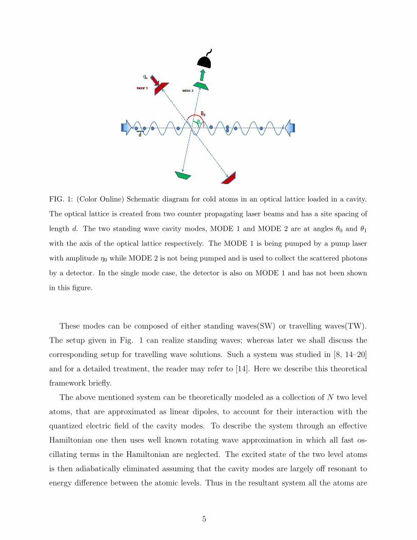
FIG. 1: (Color Online) Schematic diagram for cold atoms in an optical lattice loaded in a cavity.

The optical lattice is created from two counter propagating laser beams and has a site spacing of

length d. The two standing wave cavity modes, MODE 1 and MODE 2 are at angles θ0 and θ1

with the axis of the optical lattice respectively. The MODE 1 is being pumped by a pump laser

with amplitude η0 while MODE 2 is not being pumped and is used to collect the scattered photons

by a detector. In the single mode case, the detector is also on MODE 1 and has not been shown

in this figure.

These modes can be composed of either standing waves(SW) or travelling waves(TW).

The setup given in Fig. 1 can realize standing waves; whereas later we shall discuss the

corresponding setup for travelling wave solutions. Such a system was studied in [8, 14–20]

and for a detailed treatment, the reader may refer to [14]. Here we describe this theoretical

framework briefly.

The above mentioned system can be theoretically modeled as a collection of N two level

atoms, that are approximated as linear dipoles, to account for their interaction with the

quantized electric field of the cavity modes. To describe the system through an effective

Hamiltonian one then uses well known rotating wave approximation in which all fast os-

cillating terms in the Hamiltonian are neglected. The excited state of the two level atoms

is then adiabatically eliminated assuming that the cavity modes are largely off resonant to

energy difference between the atomic levels. Thus in the resultant system all the atoms are

5

in their ground states. The effective Hamiltonian arrived in this way is given by

H = Hf + Jcl0 N + JclB + ~g2

∑

l,m

a†l am∆ma

(

K∑

j=1

J lmj,j nj

)

+ ~g2∑

l,m

a†l am∆ma

(

K∑

<j,k>

J lmj,k b

†j bk

)

+U

2

M∑

j=1

nj(nj − 1)

(1)

Here

Hf =∑

l

~ωla†l al − i~

∑

l

(η∗l (t)al − ηl(t)a†l )

where first term denotes the free field Hamiltonian and the second depicts the interaction of

classical pump field with cavity mode, al is the annihilation operators of light modes with

the frequencies ωl, wave vectors kl, and mode functions ul(r). ηl(t) = η0e−iωpt is the time

dependent amplitude of the external pump laser of frequency ωp that populates the cavity

mode.

Here Jclj,k correspond to the matrix element of the atomic Hamiltonian in the site localized

Wannier basis, w(r− rj), namely

Jclj,k =

∫

drw(r− rj)Haw(r− rk) (2)

where Ha = −~2∇2

2ma+Vcl(r) is the Hamiltonian of a free atom of mass ma in an optical lattice

potential Vcl(r). Therefore, Jcl0 = Jcl

j,j, and Jcl =Jcl

j,j±1 are respectively the onsite energy and

the hopping amplitude of proto-type Bose Hubbard model given in [1]. At the atomic site

j, bj is the annihilation operator, and nj = b†j bj is the corresponding atom number operator,

N =∑M

j=1 nj denotes the total atom number and B =∑M

j=1 b†j bj+1.

The coefficients J lmj,k is similar to Jcl

j,k, but now generated from interaction between atoms

and quantized cavity modes and is given by ,

J lmj,k =

∫

drw(r− rj)u∗l (r)um(r)w(r− rk) (3)

∆la = ωl - ωa denotes the cavity atom detunings where ωa is the frequency corresponding to

the energy level separation of the two-level atom and g is the atom-light coupling constant.

Thus the fourth and fifth term in (1) respectively contribute to the onsite energy and hopping

amplitude due to the interaction between atoms and quantized cavity modes.

6

In the last term, U = 4πas~2

ma

∫

dr|w(r)|4 , where as denotes the s-wave scattering length

and gives the onsite interaction energy. For a sufficiently deep optical lattice potential Vcl(r),

the overlap between Wannier functions can be neglected. In this limit Jcl = 0 and J lmj,k = 0

for j 6= k. Such Wannier functions can be well approximated as delta functions centered at

lattice sites rj and consequently J lmj,j = u∗l (rj)um(rj).

The above Hamiltonian in (1) describes the zero temperature quantum phase diagram of

ultra cold bosonic atoms loaded in an optical lattice placed inside a optical cavity. This is

because their many body quantum mechanical ground state can exist in various quantum

phases [1, 3] as a function of parameters like U and J . In the subsequent analysis in this

work, the physical system that diffracts the photons is therefore a novel type of quantum

diffraction grating not only because the diffracting medium corresponds to a quantum phase

of ultra cold atoms, but also due to the fact that it is embedded in a optical lattice/grating

like structure in real space which in turn affects the nature of such quantum phase. As we

shall point out, one particular way of understanding the nature of such quantum diffraction

and differentiate from classical diffraction or any other quantum diffraction [29] is to study it

as a function of the relative angle between the cavity mode and direction of the optical lattice

in which the cold atoms are loaded. Quantum diffraction of electromagnetic wave by such

ultra cold atomic condensate inside an Fabry-Perot cavity, but without loading them in an

optical lattice (other than the one dynamically generated due to cavity-atom coupling), was

already experimentally studied in ref [11] in the context of cavity quantum optomechanics.

Thus the physical system under consideration is very much realizable experimentally. We

start our discussion by briefly outlining the relevant theoretical framework to understand

such quantum diffraction following ref [14].

III. METHODOLOGY

From the atom-photon Hamiltonian (1), the Heisenberg equation of motion of the photon

annihilation operator al is given by

˙al = −iωlal − iδlDllal − iδmDlmam − κal + ηl(t) (4)

with Dlm ≡∑K

j=1 ul∗(rj)um(rj)nj , where l 6= m and δl = g2/∆la. κ is the cavity relaxation

rate introduced phenomologically. The first, fourth and the fifth terms on the right hand side

7

correspond to property of light transmission through an empty cavity. The second and third

terms give the information about the atom-light interaction in the cold atomic condensates.

A. Single Mode

First we shall consider the case when a single cavity mode is excited. From the stationary

solution for one mode case, namely ˙al = 0 we obtain the expression for the corresponding

photon number operator as,

a†0a0 =|η0|

2

(∆p − δ0D00)2 + κ2(5)

Here ∆p = ω0p − ω0 is the probe-cavity detuning and al = a0. In this case am = 0 and

Dl,m = D00. The single mode transmission through the cavity is calculated by taking the

expectation value of the above expression in given many-body atomic ground state. As

expected such an expression is similar to the standard Breit Wigner form. However D00 is

in terms of the Fock space operators acting on the atomic ensemble, revealing the statistical

properties of the quantum matter of ultra cold atoms.

Now in the denominator of the above expression the shift in frequency is determined by

the eigenvalue of the operator D00, which is dependent on both the atomic configuration, i.e.,

the number of illuminated atoms and the mode functions. For plane standing waves the mode

function, u(rj)SW = cos(k.rj + φ) where φ is constant phase factor which has been set to

zero and rj denotes the position vector of the jth site on the optical lattice. Here we consider

a one dimensional optical lattice with site spacing d. For a cavity mode of wavelength λ

incident at an angle θ with the optical lattice, u(rj)SW = cos(2πλjdcosθ). We assume the

cavity mode wavelength to be 2d and thus, the mode function is u(rj)SW = cos(jπcosθ),

where j ∈ I. For such standing waves, the factor D00 becomes,

D00 =∑

j

u∗l ulnj =∑

j=1:K

cos2(jπcosθ)nj (6)

where K are the number of illuminated sites. This shows that shift in the cavity resonant

frequency is dependent on the relative angle of the cavity mode with the optical lattice.

To simplify the analysis, here it has been assumed that while changing this angle, the light

beam waist is modified in a way that we always illuminate only fixed K sites. However, as

8

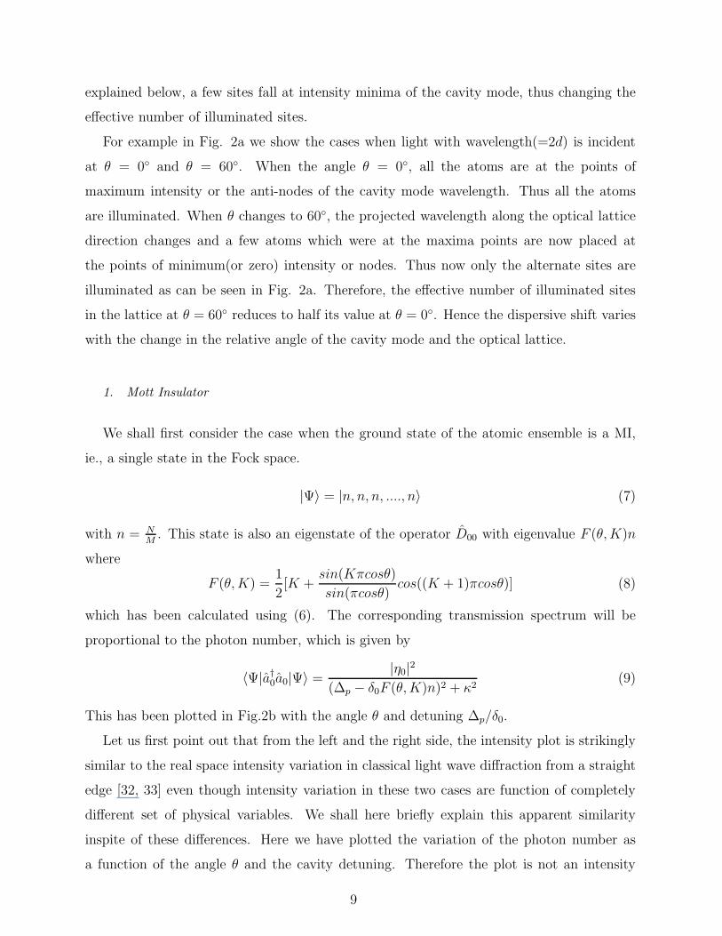
explained below, a few sites fall at intensity minima of the cavity mode, thus changing the

effective number of illuminated sites.

For example in Fig. 2a we show the cases when light with wavelength(=2d) is incident

at θ = 0 and θ = 60. When the angle θ = 0, all the atoms are at the points of

maximum intensity or the anti-nodes of the cavity mode wavelength. Thus all the atoms

are illuminated. When θ changes to 60, the projected wavelength along the optical lattice

direction changes and a few atoms which were at the maxima points are now placed at

the points of minimum(or zero) intensity or nodes. Thus now only the alternate sites are

illuminated as can be seen in Fig. 2a. Therefore, the effective number of illuminated sites

in the lattice at θ = 60 reduces to half its value at θ = 0. Hence the dispersive shift varies

with the change in the relative angle of the cavity mode and the optical lattice.

1. Mott Insulator

We shall first consider the case when the ground state of the atomic ensemble is a MI,

ie., a single state in the Fock space.

|Ψ〉 = |n, n, n, ...., n〉 (7)

with n = NM. This state is also an eigenstate of the operator D00 with eigenvalue F (θ,K)n

where

F (θ,K) =1

2[K +

sin(Kπcosθ)

sin(πcosθ)cos((K + 1)πcosθ)] (8)

which has been calculated using (6). The corresponding transmission spectrum will be

proportional to the photon number, which is given by

〈Ψ|a†0a0|Ψ〉 =|η0|

2

(∆p − δ0F (θ,K)n)2 + κ2(9)

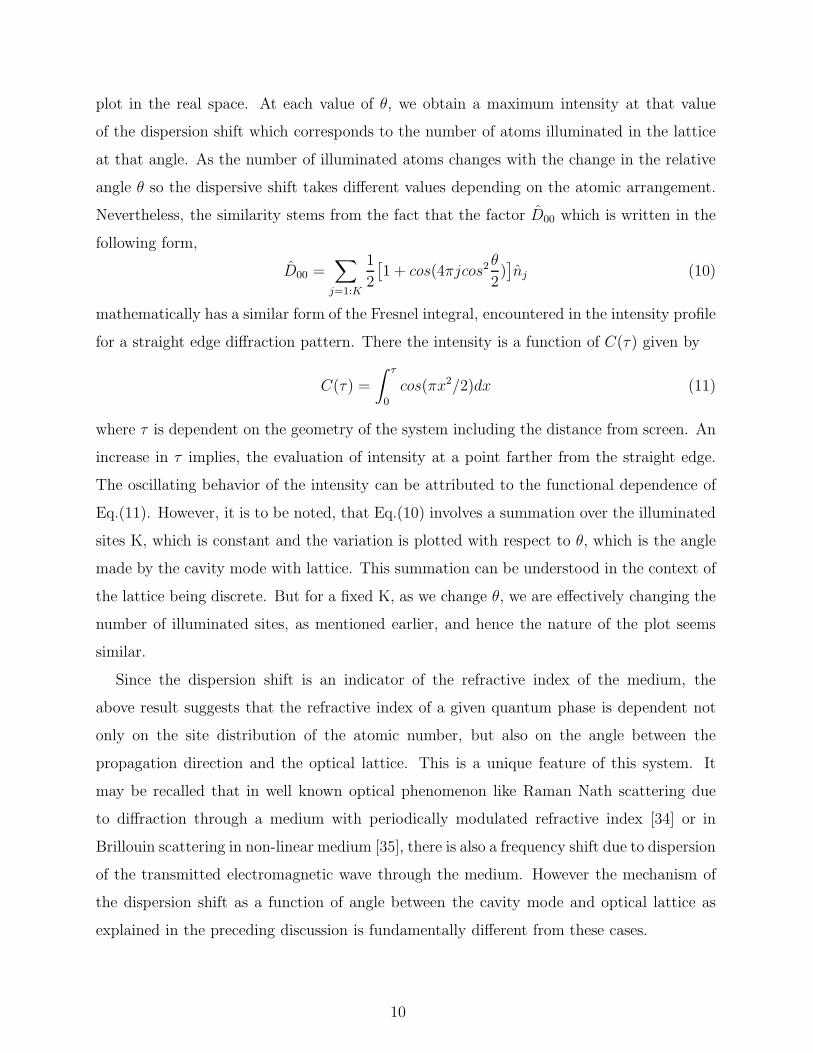
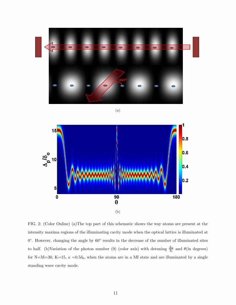
This has been plotted in Fig.2b with the angle θ and detuning ∆p/δ0.

Let us first point out that from the left and the right side, the intensity plot is strikingly

similar to the real space intensity variation in classical light wave diffraction from a straight

edge [32, 33] even though intensity variation in these two cases are function of completely

different set of physical variables. We shall here briefly explain this apparent similarity

inspite of these differences. Here we have plotted the variation of the photon number as

a function of the angle θ and the cavity detuning. Therefore the plot is not an intensity

9

plot in the real space. At each value of θ, we obtain a maximum intensity at that value

of the dispersion shift which corresponds to the number of atoms illuminated in the lattice

at that angle. As the number of illuminated atoms changes with the change in the relative

angle θ so the dispersive shift takes different values depending on the atomic arrangement.

Nevertheless, the similarity stems from the fact that the factor D00 which is written in the

following form,

D00 =∑

j=1:K

1

2

[

1 + cos(4πjcos2θ

2)]

nj (10)

mathematically has a similar form of the Fresnel integral, encountered in the intensity profile

for a straight edge diffraction pattern. There the intensity is a function of C(τ) given by

C(τ) =

∫ τ

0

cos(πx2/2)dx (11)

where τ is dependent on the geometry of the system including the distance from screen. An

increase in τ implies, the evaluation of intensity at a point farther from the straight edge.

The oscillating behavior of the intensity can be attributed to the functional dependence of

Eq.(11). However, it is to be noted, that Eq.(10) involves a summation over the illuminated

sites K, which is constant and the variation is plotted with respect to θ, which is the angle

made by the cavity mode with lattice. This summation can be understood in the context of

the lattice being discrete. But for a fixed K, as we change θ, we are effectively changing the

number of illuminated sites, as mentioned earlier, and hence the nature of the plot seems

similar.

Since the dispersion shift is an indicator of the refractive index of the medium, the

above result suggests that the refractive index of a given quantum phase is dependent not

only on the site distribution of the atomic number, but also on the angle between the

propagation direction and the optical lattice. This is a unique feature of this system. It

may be recalled that in well known optical phenomenon like Raman Nath scattering due

to diffraction through a medium with periodically modulated refractive index [34] or in

Brillouin scattering in non-linear medium [35], there is also a frequency shift due to dispersion

of the transmitted electromagnetic wave through the medium. However the mechanism of

the dispersion shift as a function of angle between the cavity mode and optical lattice as

explained in the preceding discussion is fundamentally different from these cases.

10

(a)

(b)

FIG. 2: (Color Online) (a)The top part of this schematic shows the way atoms are present at the

intensity maxima regions of the illuminating cavity mode when the optical lattice is illuminated at

0. However, changing the angle by 60 results in the decrease of the number of illuminated sites

to half. (b)Variation of the photon number (9) (color axis) with detuning∆p

δ0and θ(in degrees)

for N=M=30, K=15, κ =0.5δ0, when the atoms are in a MI state and are illuminated by a single

standing wave cavity mode.

11

2. Superfluid

Next we consider the case when the atoms are in SF phase. The SF wave function in the

Fock space basis can be written as superposition state, namely

|ψ〉 =1

MN/2

∑

〈nj〉

√

N !

n1!n2!...nM !|n1, n2, .., nM〉 (12)

where nj denotes the number of atoms at the jth site while 〈nj〉 denotes a set of nj for a

particular Fock state. Unlike the MI case, here D00 acts on a superposition of Fock states

each of which is an eigenstate of this operator. Each such Fock state carries a different set

of |n1, n2, .., nM〉. Hence,

〈Ψ|a†0a0|Ψ〉 =1

MN

∑

〈nj〉

N !

n1!n2!...nM !

|η0|2

(∆p − δ0Fs(θ,K, nj))2 + κ2

(13)

where, Fs(θ,K, nj) is the eigenvalue of the operator D00 acting on a particular Fock state.

Here the Fs functions are generalization of the F function described in (8), for the case of

SF phase in which the number of particles in each site is different as,

Fs(θ,K, nj) =∑

j=1:K

cos2(jπcosθ)nj (14)

where j is the site index and nj is the occupancy of site j. It can be easily checked for

nj = n for all j, Fs = nF .

The decomposition of the many body states in Fock space basis is now mapped in the fre-

quency shifts of the cavity mode. The probabilistic weight factor is mapped in the intensity

of the peak at that particular value of dispersion shift. At a particular angle of incidence, the

singular peak of MI now breaks into multiple peaks with varied peak strengths and disper-

sion shifts. Each particular peak corresponds to a particular group of Fock states which have

the same value of Fs(θ,K, nj) as defined in Eq.(14). Now as the angle θ is being changed,

the effective number of illuminated sites change. This changes the value of Fs(θ,K, nj) as

well as the set of Fock states which yield the same value of Fs(θ,K, nj).

This can be understood clearly by taking a case where the number of Fock states involved

is small. The corresponding states is few body correlated state which is a few body analogue

of a superfluid state, where the number of Fock states involved is thermodynamically large.

Consider the case when 2 atoms are placed in 3 sites among which the first 2 sites are

12

illuminated through a cavity mode. Here the average occupancy per site nj is 2/3. At

θ = 0, Fs(θ,K, nj) =∑K

j=1 nj . Hence states yielding the same amount of shift would be

|2, 0, 0〉 , |0, 2, 0〉 and |1, 1, 0〉 and the corresponding value of Fs(θ,K, nj) is 2nj. On the

other hand the states in which only a single atom is present in the illuminated sites, such as

|1, 0, 1〉 or |0, 1, 1〉 will show a shift of just nj in the cavity frequency. However, |0, 0, 2〉 does

not show any shift. Hence, the Fock states get distributed into groups having 3, 2, 1 states

respectively, each group having a different value of the dispersion shift.

Now as the angle between the cavity mode and lattice is varied, the effective number of

illuminated sites change and so changes the set of Fock states that has same Fs(θ,K, nj).

For example, at an angle 60, only the alternate sites are effectively illuminated. Therefore

in this case it is just the central site which is illuminated. Now under these circumstances,

state |0, 2, 0〉 show a distinctively separate shift from the states |2, 0, 0〉 and |1, 1, 0〉. It may

be recalled that at θ = 0 all these states had the same shift. Moreover, now the states

|0, 1, 1〉 and |1, 1, 0〉 will have same shift since only one atom gets illuminated in this case.

Thus this evolution of Fock states is imprinted in the shift of the cavity frequency. This is

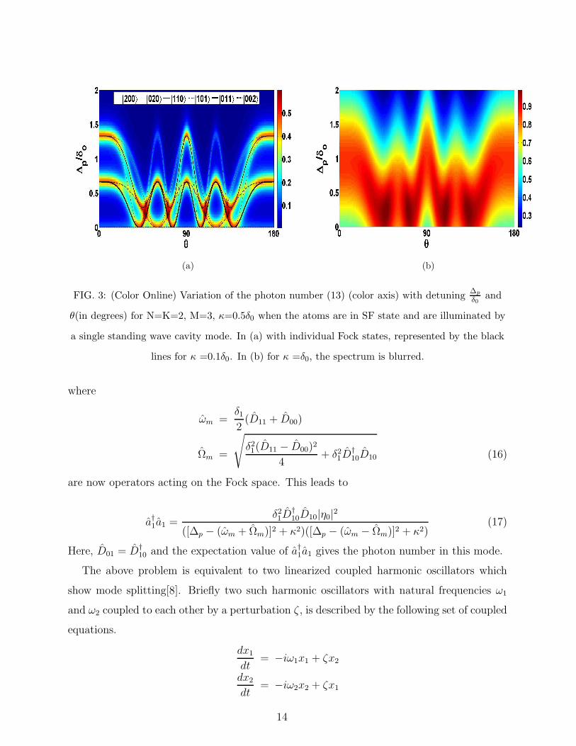
shown in Fig.3a. The transmitted intensity from the cavity mode will be proportional to

the photon number in that cavity mode. The color plot depicts this photon number whereas

the black lines (explained in the legend of Fig.3a) correspond to the Fs(θ,K, nj)δ0 for each

Fock state as a function of θ. As can be inferred wherever there is a maximum overlap

of Fs(θ,K, nj), the same location corresponds to the intensity peak. However an increase

in the cavity decay rate κ shows that the individual peaks cannot be resolved as shown in

Fig.3b.

B. Double mode

We shall now consider the case where two cavity modes are excited. The corresponding

photonic annihilation operators are given by a0 and a1. Following [8] we also assume that

the probe is injected only into a0, and hence, η1 = 0. Also both have the same frequencies,

i.e., ω0 = ω1 and are oriented at angles θ0 and θ1 with respect to the optical lattice. From

Eq.(4), ˙a1 = 0 yields

a1 =iη0δ1D10e

−i∆pt

([∆p − (ωm + Ωm)] + iκ)([∆p − (ωm − Ωm)] + iκ)(15)

13

(a) (b)

FIG. 3: (Color Online) Variation of the photon number (13) (color axis) with detuning∆p

δ0and

θ(in degrees) for N=K=2, M=3, κ=0.5δ0 when the atoms are in SF state and are illuminated by

a single standing wave cavity mode. In (a) with individual Fock states, represented by the black

lines for κ =0.1δ0. In (b) for κ =δ0, the spectrum is blurred.

where

ωm =δ12(D11 + D00)

Ωm =

√

δ21(D11 − D00)2

4+ δ21D

†10D10 (16)

are now operators acting on the Fock space. This leads to

a†1a1 =δ21D

†10D10|η0|

2

([∆p − (ωm + Ωm)]2 + κ2)([∆p − (ωm − Ωm)]2 + κ2)(17)

Here, D01 = D†10 and the expectation value of a†1a1 gives the photon number in this mode.

The above problem is equivalent to two linearized coupled harmonic oscillators which

show mode splitting[8]. Briefly two such harmonic oscillators with natural frequencies ω1

and ω2 coupled to each other by a perturbation ζ , is described by the following set of coupled

equations.

dx1dt

= −iω1x1 + ζx2

dx2dt

= −iω2x2 + ζx1

14

The normal modes of such a system are

ω =ω1 + ω2

2±

√

(ω1 − ω2

2)2 + ζ2 (18)

In the current problem, the shifted frequencies are given by the eigenvalues of

ωm ± Ωm (19)

acting on a particular state of the system. A particular case of interest will be when θ0 = θ1,

this implies D00 = D11 = D10 = D. Then the photon number a†1a1 is

a†1a1 =δ21D

†D|η0|2

[(∆p − 2Ωm)2 + κ2][∆2p + κ2]

(20)

Thus one of the normal mode is independent of the atomic dispersion, however the other

mode disperses by twice the value for a single mode. We shall now consider the case when

the cavity modes are Standing Waves. The many body ground state shall be considered as

either a MI or SF phase.

1. Mott Insulator

Again we shall first calculate the two mode transmission spectrum when the cavity con-

tains atomic ensemble in a MI state given in (7). The operators D00 and D11 are given by

(6) with eigenvalues F (θ0, K)n and F (θ1, K)n. Also for such a MI state the operator D10 is

given by∑

j=1:K

cos(jπcosθ0)cos(jπcosθ1)nj (21)

When this operator D10 acts on (7) its eigenvalue is given by F (θ0, θ1, K)n, where

F (θ0, θ1, K) =1

2

[

(

sin(Kπ cosθ0+cosθ12

)

sin(π cosθ0+cosθ12

)cos((K + 1)π

cosθ0 + cosθ12

)

)

+

(

sin(Kπ cosθ0−cosθ12

)

sin(π cosθ0−cosθ12

)cos((K + 1)π

cosθ0 − cosθ12

)

)

]

The photon number is hence given by

〈ΨMI |a†1a1|ΨMI〉 =

δ21|η0|2[F (θ0, θ1, K)n]2

([∆p − (f + F)]2 + κ2)([∆p − (f −F)]2 + κ2)(22)

15

where,

f = 〈ΨMI |ωm|ΨMI〉 =δ12(F (θ0, K) + F (θ1, K))n (23)

F = 〈ΨMI |Ωm|ΨMI〉 = n

√

δ21(F (θ1, K)− F (θ0, K))2

4+ δ21 [F (θ0, θ1, K)]2 (24)

are the eigenvalues of the operators ω and Ω acting on MI state respectively. The normal

modes are hence given by f ±F , and therefore the amount of mode splitting is given by 2F .

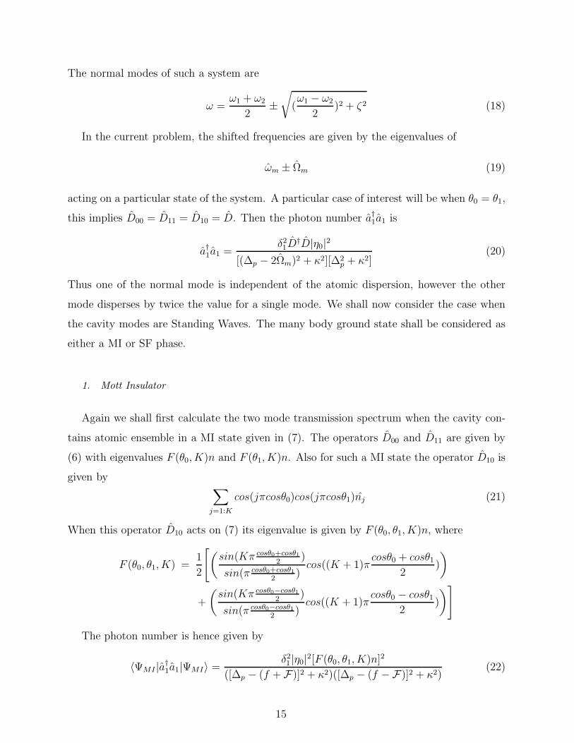
(a) (b)

FIG. 4: (Color Online)(a) shows the variation of |F (θ0, θ1,K)|2(color axis) with the angles θ0 and

θ1. (b) shows the mode splitting 2F Eq.(24) variation(color axis) in units of δ1 with angles θ0 and

θ1, N=5, K=5, M= 5. In both cases, θ0 and θ1 varies from 0 to 180.

The photon number and the mode splitting, are given by the expressions (22) and (24)

respectively. Both are dependent on the value |F (θ0, θ1, K)|2 and are thus related to each

other. Fig. 4 (a) shows the plot of the |F (θ0, θ1, K)|2 for n = 1 MI state and Fig. 4 (b)

shows the mode splitting at specific values of θ0 and θ1 and thus very clearly demonstrates

their inter-dependence.

This relation is also reflected in the plots of resulting transmission at certain demonstra-

tive values of θ0, θ1 as plotted in Fig. 5 and as explained below.

First we consider the case when both θ0 and θ1 are being varied from 0 to 180 always

maintaining the relation θ0 = θ1. The corresponding F (θ0, θ1, K) function shows a number

16

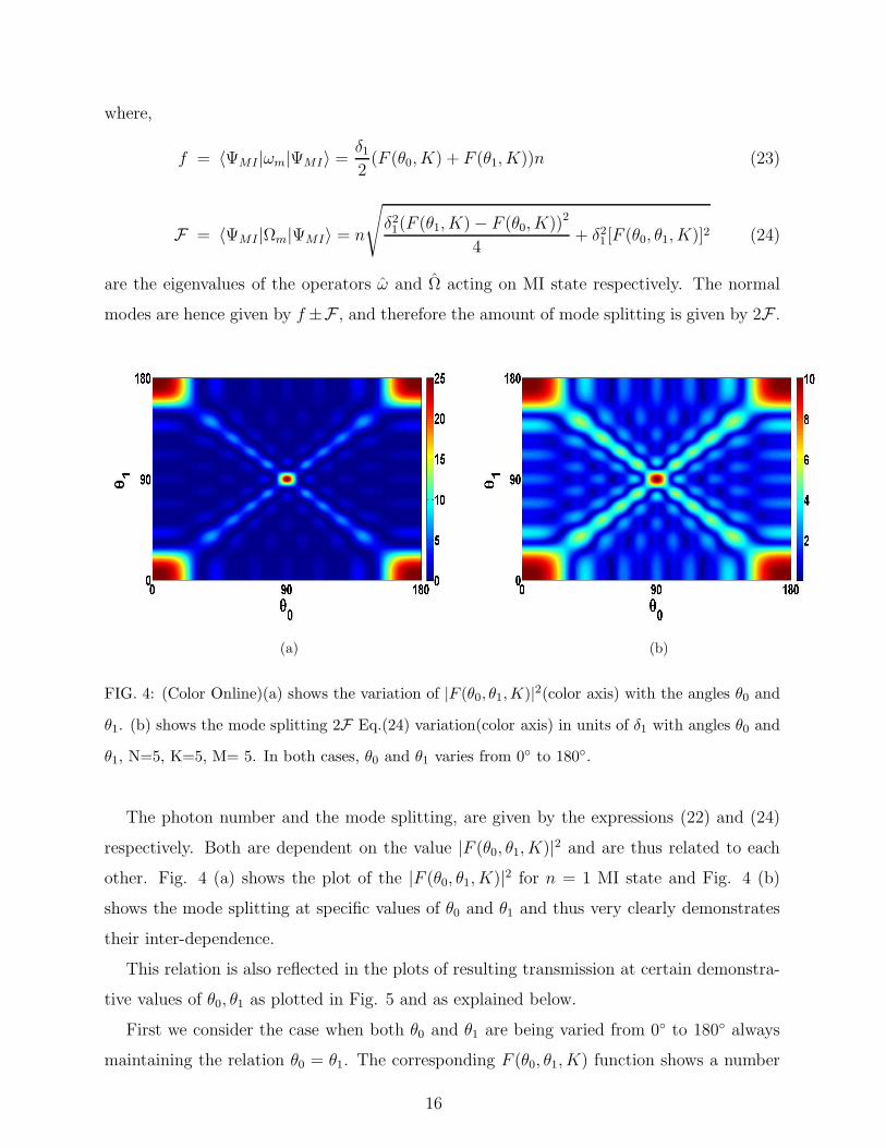
of maxima along the line θ0 = θ1 in Fig. 4(a). The photon number here is given by the

expressions (20, 22) where it was seen the normal modes will be zero and 2F . In Fig. 5(a)

we have plotted this variation in photon number along the color axis as a function of θ1 and

∆p/δ0.Therefore at each θ1 one gets a maxima at a value ∆p

δ0= 0 and at twice the value for

a single mode case(Fig. 2b).

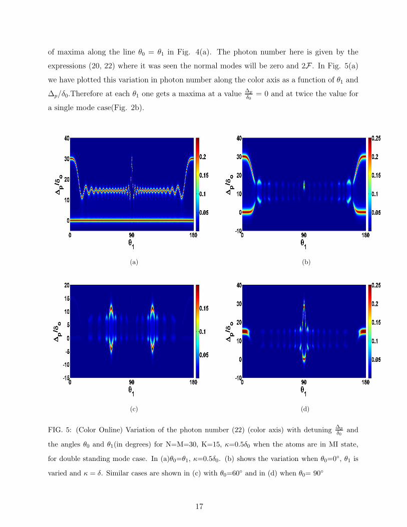
(a) (b)

(c) (d)

FIG. 5: (Color Online) Variation of the photon number (22) (color axis) with detuning∆p

δ0and

the angles θ0 and θ1(in degrees) for N=M=30, K=15, κ=0.5δ0 when the atoms are in MI state,

for double standing mode case. In (a)θ0=θ1, κ=0.5δ0. (b) shows the variation when θ0=0, θ1 is

varied and κ = δ. Similar cases are shown in (c) with θ0=60 and in (d) when θ0= 90

17

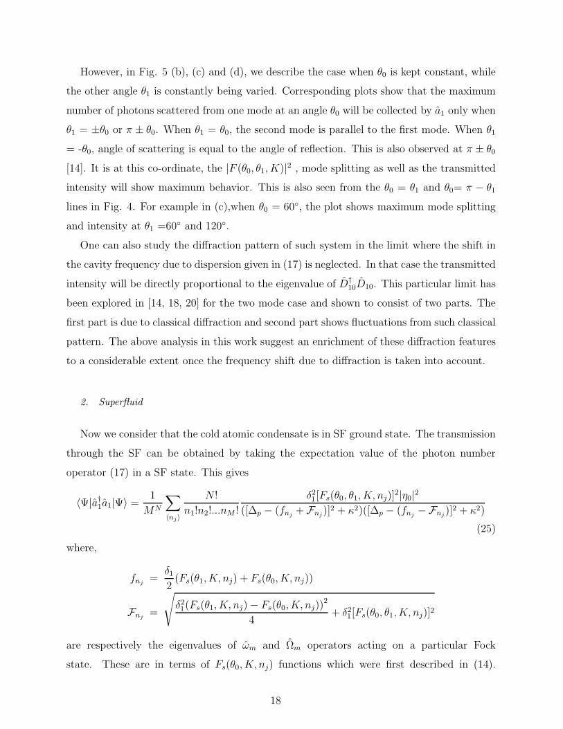
However, in Fig. 5 (b), (c) and (d), we describe the case when θ0 is kept constant, while

the other angle θ1 is constantly being varied. Corresponding plots show that the maximum

number of photons scattered from one mode at an angle θ0 will be collected by a1 only when

θ1 = ±θ0 or π ± θ0. When θ1 = θ0, the second mode is parallel to the first mode. When θ1

= -θ0, angle of scattering is equal to the angle of reflection. This is also observed at π ± θ0

[14]. It is at this co-ordinate, the |F (θ0, θ1, K)|2 , mode splitting as well as the transmitted

intensity will show maximum behavior. This is also seen from the θ0 = θ1 and θ0= π − θ1

lines in Fig. 4. For example in (c),when θ0 = 60, the plot shows maximum mode splitting

and intensity at θ1 =60 and 120.

One can also study the diffraction pattern of such system in the limit where the shift in

the cavity frequency due to dispersion given in (17) is neglected. In that case the transmitted

intensity will be directly proportional to the eigenvalue of D†10D10. This particular limit has

been explored in [14, 18, 20] for the two mode case and shown to consist of two parts. The

first part is due to classical diffraction and second part shows fluctuations from such classical

pattern. The above analysis in this work suggest an enrichment of these diffraction features

to a considerable extent once the frequency shift due to diffraction is taken into account.

2. Superfluid

Now we consider that the cold atomic condensate is in SF ground state. The transmission

through the SF can be obtained by taking the expectation value of the photon number

operator (17) in a SF state. This gives

〈Ψ|a†1a1|Ψ〉 =1

MN

∑

〈nj〉

N !

n1!n2!...nM !

δ21[Fs(θ0, θ1, K, nj)]2|η0|

2

([∆p − (fnj+ Fnj

)]2 + κ2)([∆p − (fnj− Fnj

)]2 + κ2)

(25)

where,

fnj=

δ12(Fs(θ1, K, nj) + Fs(θ0, K, nj))

Fnj=

√

δ21(Fs(θ1, K, nj)− Fs(θ0, K, nj))2

4+ δ21[Fs(θ0, θ1, K, nj)]2

are respectively the eigenvalues of ωm and Ωm operators acting on a particular Fock

state. These are in terms of Fs(θ0, K, nj) functions which were first described in (14).

18

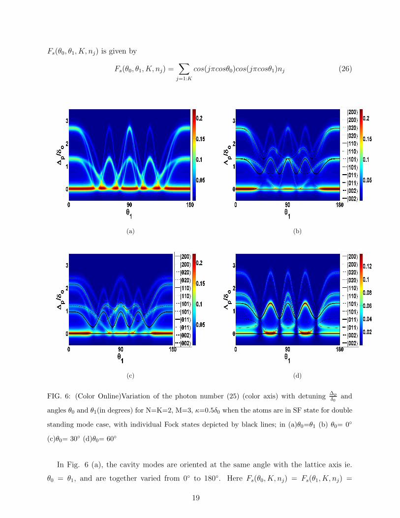
Fs(θ0, θ1, K, nj) is given by

Fs(θ0, θ1, K, nj) =∑

j=1:K

cos(jπcosθ0)cos(jπcosθ1)nj (26)

(a) (b)

(c) (d)

FIG. 6: (Color Online)Variation of the photon number (25) (color axis) with detuning∆p

δ0and

angles θ0 and θ1(in degrees) for N=K=2, M=3, κ=0.5δ0 when the atoms are in SF state for double

standing mode case, with individual Fock states depicted by black lines; in (a)θ0=θ1 (b) θ0= 0

(c)θ0= 30 (d)θ0= 60

In Fig. 6 (a), the cavity modes are oriented at the same angle with the lattice axis ie.

θ0 = θ1, and are together varied from 0 to 180. Here Fs(θ0, K, nj) = Fs(θ1, K, nj) =

19

Fs(θ0, θ1, K, nj) and thus corresponds to the case described in Eq.(20). In this figure, the

photon number has been plotted against the angle θ1 and ∆p/δ0. The plot exhibits that at

each angle there is maxima in the photon number when the value of the dispersive shift is

either zero or twice its corresponding value for the single mode case.

Fig.6 (b), (c) and (d) describes the variation of the photon number with the angle θ1

and ∆p/δ0, when one of the modes, θ0 is kept at a constant angle while the other, θ1 is

changed from 0 to 180. This makes Fs(θ0, K, nj), Fs(θ1, K, nj) and Fs(θ0, θ1, K, nj) change

separately for individual Fock states. To understand this, we again consider the case when

2 atoms are placed in 3 sites among which 2 are illuminated. We will have 6 Fock states and

the average occupancy will be 2/3. However each Fock state now gives maximum intensity

for two values of ∆p/δo corresponding to the two normal modes fnj± Fnj

.

Fig.6(b), shows the intensity distribution when θ0 = 0. Here, we observe that when

θ1=0, the 6 Fock states distribute themselves into groups having 3, 2, 1 states and each

group has a distinct value for the dispersion shift depending on the occupancy. However in

Fig.6(c) and 6(d),where the angle θ0 = 30 and 60 respectively, and the angle θ1 is varied,

we observe the Fock states separate out and each takes a distinct value for the dispersive

shift. This allows us to identify each Fock state separately. In Fig.6(d), it is to be noticed

that at specific values of θ1, the intensity drops to zero, although there is a superposition of

the Fock states. This happens as the intensity depending on Fs(θ0, θ1, K, nj) becomes zero

at these particular values as can be seen from eqs.(25,26).

IV. TRAVELLING WAVES

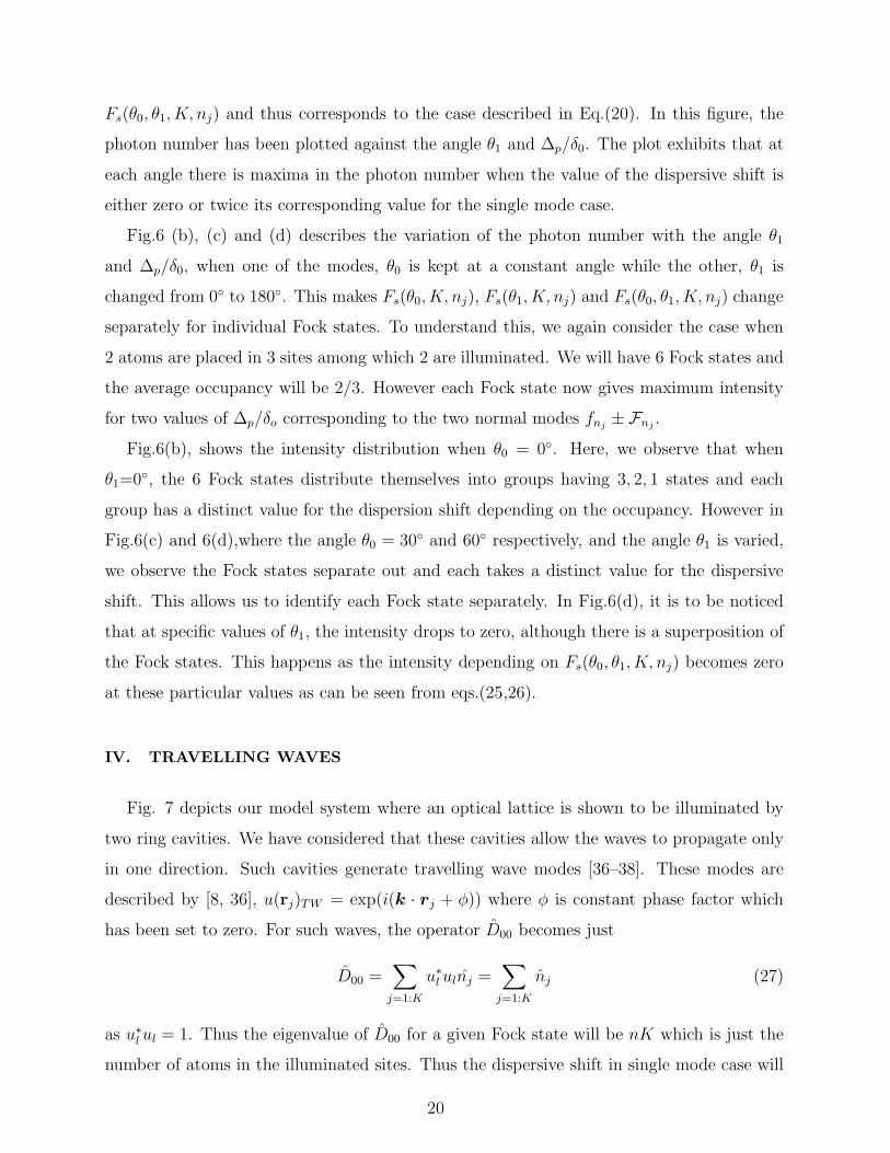
Fig. 7 depicts our model system where an optical lattice is shown to be illuminated by

two ring cavities. We have considered that these cavities allow the waves to propagate only

in one direction. Such cavities generate travelling wave modes [36–38]. These modes are

described by [8, 36], u(rj)TW = exp(i(k · rj + φ)) where φ is constant phase factor which

has been set to zero. For such waves, the operator D00 becomes just

D00 =∑

j=1:K

u∗l ulnj =∑

j=1:K

nj (27)

as u∗l ul = 1. Thus the eigenvalue of D00 for a given Fock state will be nK which is just the

number of atoms in the illuminated sites. Thus the dispersive shift in single mode case will

20

not depend on the angle θ.

FIG. 7: (Color Online) Schematic diagram of the atom cavity system for travelling wave. The

optical lattice is created from two counter propagating laser beams and has a site spacing d. The

two ring wave cavity modes, MODE 1 and MODE 2 are at angles θ0 and θ1 respectively with the

axis of the optical lattice. The MODE 1 is being pumped by a pump laser with amplitude η0 while

MODE 2 is not being pumped but is used to collect the scattered photons by a detector. In the

single mode case, the detector is also fixed in MODE 1, and has not been shown in this figure. The

ring cavities, are set in a way that the waves is allowed to propagate only in one direction.

However this is not the case when two cavity modes are excited. As we have seen for

the case of standing wave, the mode splitting which in turn influences the transmission

through such cavity is closely related to the relative angle between the two modes through

the function F (θ0, θ1, K) . In the current case the mode splitting is also dependent on the

relative angle between the cavity modes since only the eigenvalue of the operator D10 is

angle dependent which is given by,

D10 =∑

j=1:K

ei(jπ(cosθ1−cosθ0))nj (28)

21

A. Mott Insulator

Again, we first consider the cold atomic condensate in a MI state. The eigenvalue of ω

and Ω (16) when acting on the MI state (7) are

g = 〈Ψ|ω|Ψ〉 =nKδ1 + nKδ1

2= nKδ1

G = 〈Ψ|Ω|Ψ〉 =

√

(nKδ1 − nKδ1

2)2 + |G(θ0, θ1, K)nδ1|2 = |G(θ0, θ1, K)|nδ1 (29)

Here G(θ0, θ1, K) is

G(θ0, θ1, K) =sin(Kπ cosθ0−cosθ1

2)

sin(π cosθ0−cosθ12

)(30)

This system is equivalent to two coupled linearized harmonic oscillators (18), but with

same natural frequencies ie., ω1 = ω2 = ω and coupled by a perturbation ζ . The normal

modes for such a system is given by ω ± ζ . In the current problem, the normal modes are

hence given by g ± G and therefore the amount of mode splitting is 2G.

The photon number (17) is,

〈ΨMI |a†1a1|ΨMI〉 =

|η0G|2

([∆p − (g + G)]2 + κ2)([∆p − (g − G)]2 + κ2)(31)

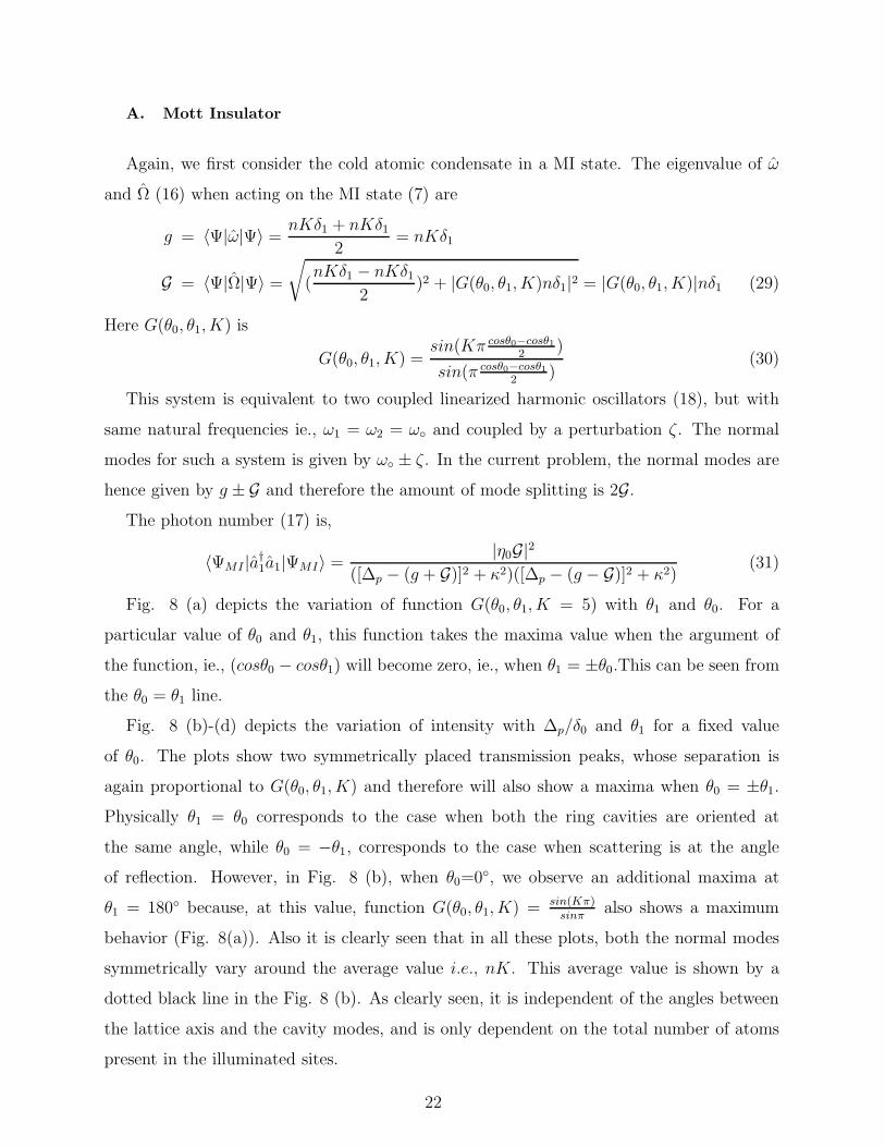
Fig. 8 (a) depicts the variation of function G(θ0, θ1, K = 5) with θ1 and θ0. For a

particular value of θ0 and θ1, this function takes the maxima value when the argument of

the function, ie., (cosθ0 − cosθ1) will become zero, ie., when θ1 = ±θ0.This can be seen from

the θ0 = θ1 line.

Fig. 8 (b)-(d) depicts the variation of intensity with ∆p/δ0 and θ1 for a fixed value

of θ0. The plots show two symmetrically placed transmission peaks, whose separation is

again proportional to G(θ0, θ1, K) and therefore will also show a maxima when θ0 = ±θ1.

Physically θ1 = θ0 corresponds to the case when both the ring cavities are oriented at

the same angle, while θ0 = −θ1, corresponds to the case when scattering is at the angle

of reflection. However, in Fig. 8 (b), when θ0=0, we observe an additional maxima at

θ1 = 180 because, at this value, function G(θ0, θ1, K) = sin(Kπ)sinπ

also shows a maximum

behavior (Fig. 8(a)). Also it is clearly seen that in all these plots, both the normal modes

symmetrically vary around the average value i.e., nK. This average value is shown by a

dotted black line in the Fig. 8 (b). As clearly seen, it is independent of the angles between

the lattice axis and the cavity modes, and is only dependent on the total number of atoms

present in the illuminated sites.

22

(a) (b)

(c) (d)

FIG. 8: (Color Online)(a)Variation in G(θ0, θ1,K = 5)(color axis) with θ0 and θ1(in degrees).

(b)Variation of the photon number(color axis) with detuning∆p

δ and θ1(in degrees), N=M=30,

K=15, κ =0.5δ0 when the atoms are in MI state, single travelling mode case. θ0=0 (c)θ0= 45

(d)θ0= 90

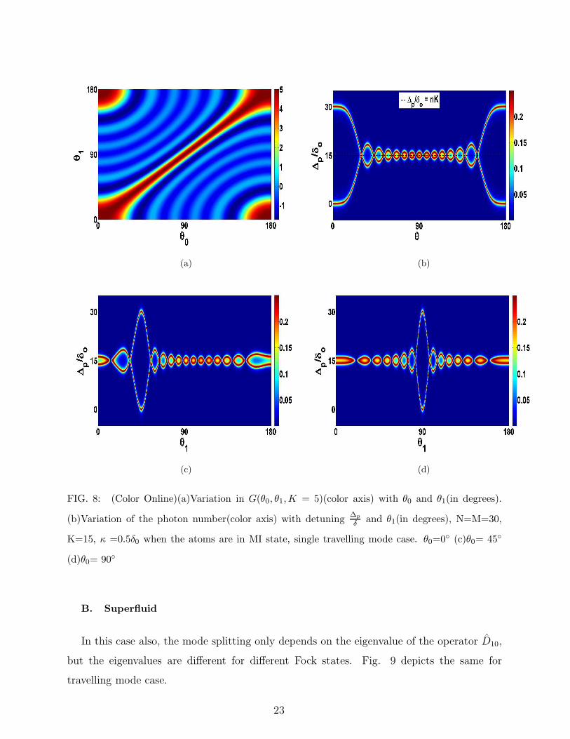
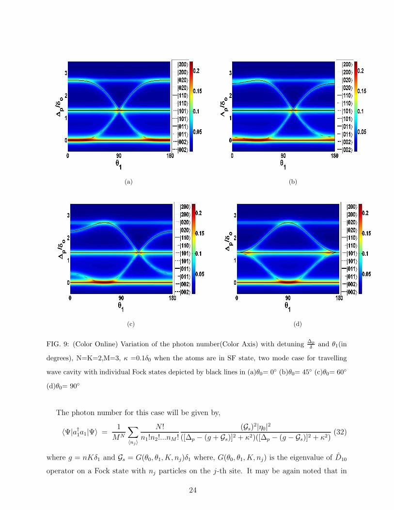
B. Superfluid

In this case also, the mode splitting only depends on the eigenvalue of the operator D10,

but the eigenvalues are different for different Fock states. Fig. 9 depicts the same for

travelling mode case.

23

(a) (b)

(c) (d)

FIG. 9: (Color Online) Variation of the photon number(Color Axis) with detuning∆p

δ and θ1(in

degrees), N=K=2,M=3, κ =0.1δ0 when the atoms are in SF state, two mode case for travelling

wave cavity with individual Fock states depicted by black lines in (a)θ0= 0 (b)θ0= 45 (c)θ0= 60

(d)θ0= 90

The photon number for this case will be given by,

〈Ψ|a†1a1|Ψ〉 =1

MN

∑

〈nj〉

N !

n1!n2!...nM !

(Gs)2|η0|

2

([∆p − (g + Gs)]2 + κ2)([∆p − (g − Gs)]2 + κ2)(32)

where g = nKδ1 and Gs = G(θ0, θ1, K, nj)δ1 where, G(θ0, θ1, K, nj) is the eigenvalue of D10

operator on a Fock state with nj particles on the j-th site. It may be again noted that in

24

a SF state nj varies with the site index j for a given Fock state. The transmission spectra

is shown in the Fig.(9) for certain demonstrative values of θ0, θ1. In each case we have also

plotted the Gs for different Fock states which are superposed to form the superfluid.

V. CONCLUSION

In our work, we have analyzed cold atomic condensates formed by bosonic atoms in an

optical lattice at ultra cold temperatures. It has been suggested that such system when

illuminated by cavity modes, can imprint their characteristics on the transmitted intensity.

We have studied the off resonant scattering from such correlated systems by varying the

angles that the cavity modes make with the optical lattice and thus obtained the transmission

spectrum as a function of the detunings and the dispersive shifts.

The main result of our work reveals the pattern in the shifts of the cavity mode fre-

quency as the relative angle between the cavity mode and the optical lattice is changed.

As we have pointed out in section IIIA 1 that a change in the dispersion shift implies the

effective change of the refractive index. Thus our finding implies even for a given quantum

phase, as the relative angle between the mode propagation vector and the optical lattice

changes, the cavity induced dispersion shift or the effective refractive index of the medium

also changes. This highlights the uniqueness of such quantum phase of matter as medium

of optical dispersion.

For the single mode case discussed in section IIIA, in MI phase, we have seen that the

transmitted intensity depends on the number of atoms in the illuminated sites, since the

presence of an atom shifts the cavity resonance and this shift is directly proportional to the

number of illuminated atoms. The SF phase is however a superposition of many Fock states

and set of Fock states group correspond to same shift. However changing the angle, these

group of Fock states change thus providing more information about the system.

As discussed in next section IIIB when two cavity modes are considered, the system

shows mode splitting between the cavity modes coupled by the atomic ensemble. This was

clearly visible in the MI case. In the SF state, at some specific angles of illumination, the

Fock states of SF distinctly map to different frequency shift. Thus giving the Fock state

structure of the system. However, it was noticed that such a system can only be achieved

through high finesse cavities, as such characteristic features in the plots for the SF phase

25

become blurred for an increase in κδ0

values. Such system when illuminated by ring cavities

show different features of intensity transmission as shown in the section IV that describes

the situation where the cavity modes are travelling waves. Thus the nature of diffraction

pattern is also dependent on the nature of the quantization of the electromagnetic wave

inside the cavity, which was also mentioned in the earlier work on such quantum diffraction

by fermionic cold atoms [31].

As our analysis shows that the variation of the relative angle between the cavity mode

and the optical lattice can resolve the Fock space structure of a quantum phase in detail,

by varying the effective number of illuminated sites. It has been pointed out in experiment

described in ref. [10] that it is possible to study the correlated many body states of few ultra

cold atoms in such cavity within the currently available technology. A few body correlated

system of ultra cold fermions was also experimentally achieved recently [39]. For example

in Fig. 3 and Fig. 6 it has been shown that in the limit of small cavity decay rate κ and

for few number of particles in the illuminated site, in a superfluid phase or more correctly a

few body analogue of a superfluid state it is possible to identify the extent of superposition

in different parameter regime. Such identification is potentially helpful in various type of

many body quantum state preparation.

VI. ACKNOWLEDGEMENT

One of us (JL) thanks Prof. H. Ritsch for helpful discussion.

[1] D. Jaksch et al., Phys. Rev. Lett. 81, 3108 (1998).

[2] I. Bloch, J. Dalibard and W. Zwerger, Rev. Mod. Phys. 80, 885 (2008).

[3] M. Greiner et al., Nature 415, 39 (2002).

[4] J. J. Garcza-Ripoll, J. I. Cirac, Phil. Trans. R. Soc. Lond. A 361, 1537 (2003) .

[5] J.M. Raimond, M. Brune, S. Haroche, Rev. Mod. Phys. 73,565 (2001).

[6] O. Morice, Y. Castin and J. Dalibard. Phys. Rev. A 51, 3896 (1995).

[7] M. G. Moore, O. Zobay and P. Meystre, Phys. Rev. A 60, 1491 (1999).

[8] I. B. Mekhov, C. Maschler and H. Ritsch, Nat. Phys 3, 319 (2007).

[9] F. Brennecke et al., Nature 450, 268 (2007).

26

[10] Y. Colombe, T. Steinmetz et al., Nature 450, 272 (2007).

[11] F. Brennecke, S. Ritter,T. Donner, T. Esslinger, Science 322, 235 (2008).

[12] S. Gupta, K. L. Moore, K. Murch, D. M. Stamper-Kurn, Phys. Rev. Lett 99, 213601 (2007).

[13] C. Weitenberg et al., Phys. Rev. Lett. 106, 215301 (2011).

[14] I. B. Mekhov, C. Maschler and H. Ritsch, Phys. Rev. A 76, 053618 (2007).

[15] I. B. Mekhov, H. Ritsch, Phys. Rev. Lett 102, 020403 (2009).

[16] C. Maschler, I.B. Mekhov, H. Ritsch Eur. Phys. J. D 46, 545 (2008).

[17] I. B. Mekhov, H. Ritsch, Phys. Rev. A 80, 013604 (2009).

[18] I. B. Mekhov, H. Ritsch, Laser Physics, 19, No. 4, 610 (2009).

[19] B.Wunsch et al., Phys. Rev. Lett. 107, 073201 (2011).

[20] I. B. Mekhov, H. Ritsch, Laser Physics, 20, No. 3, 694 (2010).

[21] J. Larson, B. Damski, G. Morigi and M. Lewenstein, Phys. Rev. Lett, 100, 050401 (2008).

[22] W. Chen et al., Phys. Rev. A 80, 011801 (2009).

[23] W. Chen, D. S. Goldbaum, M. Bhattacharya, P. Meystre, Phys. Rev. A 81, 053833 (2010)

[24] A. B. Bhattacherjee, Phys. Rev. A 80, 043607 (2009); T. Kumar, A. B. Bhattacharjee and

ManMohan, Phys. Rev. 81, 013835 (2010).

[25] S. Gopalakrishnan, B. L. Lev and P. M. Goldbart, Nat. Phys. 5, 845 (2009).

[26] S. Gopalakrishnan, B. L. Lev and P. M. Goldbart, Phys. Rev. A 82, 043612 (2010)

[27] S.F. Vidal, G. Chiara, J. Larson, G. Morigi, Phys. Rev. A 81, 043407 (2010).

[28] K. Baumann, C. Guerlin, F. Brennecke,T. Esslinger, Nature, 464 1301 (2010).

[29] W. E.. Frahn, Riv. Nuovo Cim, 7, 499 (1977).

[30] H. Tanji-Sujuki et al., Adv. At. Mol. Opt. Phys. 60, 201 (2011).

[31] D. Meiser, C. P. Search and P. Meystre, Phys. Rev. A 71, 013404 (2005).

[32] M. Born and E. Wolf, Principles of Optics, Cambridge University Press(1999).

[33] A. Ghatak and K. Thyagarajan, Optical Electronics, Cambridge University Press(1989).

[34] C. V. Raman and N. S. N. Nath, Proc. Indian Acad. Sci 4, 222 (1936)

[35] L. Brillouin, Annales des Physique 17, 88 (1922).

[36] M Gangl, H. Ritsch, Phys. Rev. A 61, 043405 (2000).

[37] S. Bux et al., Phys. Rev. Lett. 106, 203601 (2011).

[38] B. Nagorny, T. Elsasser, A. Hemmerich, Phys. Rev. Lett. 91, 153003 (2003).

[39] F. Serwane, G. Zurn, T. Lompe, T. B. Ottenstein, A. N. Wenz and S. Jochim, Science, 332,

27

336 (2011).

28