Fast and accurate modeling of waveguide grating

couplers

P. G. Dinesen

Dept. of Optics and Fluid Dynamics, Ris� National Laboratory

DK-4000 Roskilde, Denmark

J. S. Hesthaven

Division of Applied Mathematics, Brown University, Box F

Providence, Rhode Island 02912

March 15, 2000

Abstract

A boundary variation method for the analysis of both in�nite peri-

odic and �nite aperiodic waveguide grating couplers in 2-D will be

introduced. Based on a previously introduced boundary variation

method for the analysis of metallic and transmission gratings a nu-

merical algorithm suitable for waveguide grating couplers is derived.

Examples of the analysis of purely periodic grating couplers are given

illustrating the convergence of the scheme. An analysis of the use of the

proposed method for focusing waveguide grating couplers is given, and

a comparison with a highly accurate spectral collocation method yields

excellent agreement and illustrates the attractiveness of the proposed

boundary variation method in terms of speed and achievable accuracy.

1 Introduction

In recent years, an increasing interest in the design and use of di�raction

based integrated optics has lead to a need for fast and accurate numerical

methods for the analysis and design of di�raction dominated structures. The

formulation and development of such methods are severely complicated by

the rigorous treatment of the vector-�eld behavior in the resonant regime

where the wavelength of the optical �eld is comparable to the size of the

geometrical features.

For inherently periodic structures of in�nite extend, the rigorous coupled-

wave analysis has been widely used for more than a decade[1]. However, the

1

need to analyze structures with aperiodic features and of �nite extent has

lead to the need for methods capable of dealing with such structures, and the

use of the Finite-Element[2], Boundary element[3], Finite-Di�erence Time-

Domain[4, 5], and Spectral Collocation[6] methods has been proposed. The

latter two methods both compute a direct solution of the time-domain vec-

torial Maxwell equations and are very general in being adaptable to a wide

variety of geometries and physical settings. As the need to model problems

of realistic size and complexity becomes more pressing, however, the mem-

ory and computational time requirements of such direct volume methods

quickly becomes a limiting factor not only for the design process but also

for the analyses of particular structures.

In this work, we propose to take a di�erent road, guided by the work of

Bruno and Reitich[7]. They have established that solutions to electromag-

netic di�raction by a periodic structure depend analytically on the varia-

tions of the interface. In other words, di�raction from a periodic grating

can be determined from knowledge of re ection and refraction at a plane

interface. Using this result, Bruno and Reitich proposed a high-order per-

turbation scheme for �nite-size perturbations and successfully used it in

modeling di�raction by two and three-dimensional metallic and transmis-

sion gratings[8, 9].

In this paper, we propose a further development leading to a formulation

for the analysis of waveguide grating couplers, in which a guided wave in

a thin-�lm waveguide is coupled to free-space radiation through a surface

relief as sketched in Fig. 1. Moreover, we extend the analysis to structures

of �nite extent and demonstrate, by comparison with a highly accurate

spectral collocation method, that the method of boundary variation provides

surprisingly accurate results for the modeling of radiation from waveguide

grating couplers.

The remainder of this paper is organized as follows. In section 2 we

present the modi�ed boundary variation method as applied to the waveg-

uide grating coupler and discuss the details of the numerical implementa-

tion including post processing by free-space integration of the radiated �eld.

Section 3 demonstrates the use of the proposed code for the analysis of pe-

riodic waveguide grating couplers, and in section 4 we subsequently turn

to the analysis of �nite-length focusing grating couplers with an aperiodic

grating function. We present a comparison of the proposed method with a

spectral collocation code to demonstrate the accuracy the boundary varia-

tion method for the modeling of nontrivial waveguide grating couplers. We

conclude with a discussion of the superior computational eÆciency of the

proposed approach, and a few remarks of future directions of work.

2

u+

u-

z

x

Figure 1: Thin-�lm optical waveguide comprising surface relief grating for

coupling from guided wave to free-space radiation.

2 Boundary variation for grating couplers

In the following, we shall outline the elements of the proposed algorithm

without going into details with the algebra involved in the derivation of the

scheme but rather dwell on the properties of a �eld propagating in a thin

�lm waveguide. It is an understanding of these properties that allows us

to develop a method of boundary variation suitable for waveguide grating

couplers based on the method for periodic dielectric interfaces[8].

We restrict ourselves to the analysis of TE polarized, monochromatic

�elds in which case the E �eld remains parallel to the grating, E = Ey y and

therefore is determined by a single scalar quantity, u = u(z; x), satisfying

the homogeneous Helmholtz equation

�u+ k2u = 0; (1)

with k being the local wavenumber. We distinguish between the �eld that

is radiated into the free space above the grating coupler, u+, and the �eld

radiated downwards into the waveguide, u�, as illustrated in Fig. 1.

We furthermore assume that the incident �eld is given by the funda-

mental TE mode for the unperturbed thin �lm waveguide. For a multi-layer

waveguide the �eld in each individual layer is given on the form

Ei = Ai exp (ikix� i�z) +Bi exp (�ikix� i�z) ; (2)

where ki is given by

k2i + �2 = n2i k20 ; (3)

3

with k0 being the free-space wave number, while � is the propagation con-

stant, determined by the layer thicknesses and the refractive indices[10].

Ai and Bi in Eq. (2) are constants, which are given once the propagation

constant is calculated.

The TM case can be solved in a similar way using Hx rather than Ey.

Although the boundary conditions will be di�erent, the extension to the TM

case is straightforward.

2.1 Numerical algorithm

Let us now consider the case where the boundary between the top cladding

layer and free-space above the waveguide is perturbed in a way described

by the function f and a real number Æ, such that

x = fÆ(z) = Æf(z) (4)

describes the upper surface of the top cladding layer. Assuming that the

incoming �eld takes the form in Eq. (2), the radiation �elds u+ and u� must

satisfy the continuity conditions

u+ � u� = A0 exp (ik0Æf(z)� i�z) +B0 exp (�ik0Æf(z)� i�z)

�A1 exp (ik1Æf(z) � i�z)�B1 exp (�ik1Æf(z)� i�z) ; (5)

and

@u+

@n�

@u�

@n=

@

@n(A0 exp (ik0Æf(z)� i�z) +B0 exp (�ik0Æf(z)� i�z))

@

@n(�A1 exp (ik1Æf(z)� i�z)�B1 exp (�ik1Æf(z)� i�z)) ; (6)

at x = Æf(z). By requiring that the �eld vanishes for x ! 1, we have

A0 = 0.

The central idea underlying the boundary variation method is that the

radiated �elds u+ and u� can be expanded in powers of Æ

u�(z; x; Æ) =1Xn=0

u�n (z; x)Æn: (7)

Bruno and Reitich established the validity of this power series expansion,

which is a result of u� being analytic in its variables[11]. u, being a solution

to the Helmholtz equation, can be expanded in a Rayleigh series

u�(z; x; Æ) =1X

r=�1

B�r (Æ) exp(i� ��r x� i�rz): (8)

4

and likewise for the u�n

u�n (z; x) =1X

r=�1

d�n;r exp(�i�p

rmx� i�rz); (9)

Given

d�n;r =1

n!

dnB�rdÆn

(0); (10)

we recover the power series expansion

B�r (Æ) =1Xn=0

d�n;rÆn: (11)

for the Rayleigh coeÆcients B�r . To obtain the coeÆcients in this power

series expansion, we need the Fourier expansions

f l(z)

l!=

lFXr=�lF

Cl;r exp(iKrx); (12)

for f l=l! for l up to some N . In Eq. (12), K represents the smallest grating

vector, we wish to resolve. For a periodic cosine surface relief, K is simply

the grating wavenumber, K = 2�=�, where � is the period of the grating.

For that case, the Fourier expansions need only extend to F = 1. In the

case of an aperiodic grating of �nite length K = 2�=L where L is the total

length of the computational domain.

The wavevectors for the di�racted �elds are given by

�r = � + nK; (13)

and

(��r )2 + �2r = (ki)

2 (14)

where i = 0 for the �+r and i = 1 for the ��r . Only a �nite number of Rayleigh

modes B�r will be propagating, since �r's will have non-zero imaginary parts

for large r.

The derivation of the recursive expressions for dn;r is thoroughly de-

scribed in [8] for di�raction at an interface between two dielectrics. In this

work, we need to modify the original derivation by using the boundary con-

ditions for a grating coupler, Eqs. (5)-(6).

5

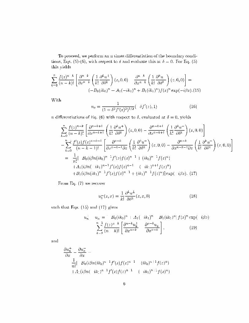
To proceed, we perform an n times di�erentiation of the boundary condi-

tions, Eqs. (5)-(6), with respect to Æ and evaluate this at Æ = 0. For Eq. (5)

this yields

nXk=0

f(z)n�k

(n� k)!

"@n�k

@xn�k

1

k!

@ku+

@Æk

!(z; 0; 0) �

@n�k

@xn�k

1

k!

@ku�

@Æk

!(z; 0; 0)

#=

(�B0(ik0)n +A1(�ik1)

n +B1(ik1)n)f(z)n exp(�i�z):(15)

With

nÆ =1

(1 + Æ2f 0(z)2)1=2(�Æf 0(z); 1) (16)

n di�erentiations of Eq. (6) with respect to Æ, evaluated at Æ = 0, yields

nXk=0

f(z)n�k

(n� k)!

"@n�k+1

@xn�k+1

1

k!

@ku+

@Æk

!(z; 0; 0) �

@n�k+1

@xn�k+1

1

k!

@ku�

@Æk

!(z; 0; 0)

#

�

n�1Xk=0

f 0(z)f(z)n�k�1

(n� k � 1)!

"@n�k

@xn�k�1@z

1

k!

@ku+

@Æk

!(z; 0; 0) �

@n�k

@xn�k�1@z

1

k!

@ku�

@Æk

!(z; 0; 0)

#

=1

n![�B0(i�n(ik0)

n�1f 0(z)f(z)n�1 + (ik0)n+1f(z)n)

+A1(i�n(�ik1)n�1f 0(z)f(z)n�1 � (�ik1)

n+1f(z)n)

+B1(i�n(ik1)n�1f 0(z)f(z)n�1 + (ik1)

n+1f(z)n)] exp(�i�z): (17)

From Eq. (7) we recover

u�k(z; x) =

1

k!

@ku�

@Æk(z; x; 0) (18)

such that Eqs. (15) and (17) gives

u+n � u�n = [�B0(ik0)n +A1(�ik1)

n +B1(ik1)n] f(z)n exp(�i�z)

�

n�1Xk=0

f(z)n�k

(n� k)!

"@n�ku+

k

@xn�k�

@n�ku�k

@xn�k

#; (19)

and

@u+n@x

�

@u�n@x

=

1

n![�B0(i�n(ik0)

n�1f 0(z)f(z)n�1 + (ik0)n+1f(z)n)

+A1(i�n(�ik1)n�1f 0(z)f(z)n�1 � (�ik1)

n+1f(z)n)

6

+B1(i�n(ik1)n�1f 0(z)f(z)n�1 + (ik1)

n+1f(z)n)] exp(�i�z)

+n�1Xk=0

f 0(z)f(z)n�k�1

(n� k � 1)!

"@n�ku+

k

@xn�k�1@z�

@n�ku�k

@xn�k�1@z

#

�

n�1Xk=0

f(z)n�k

(n� k)!

"@n�k+1u+

k

@xn�k+1�

@n�k+1u�k

@xn�k+1

#: (20)

By substituting the Rayleigh expansions for u�n , Eq. (9), into Eq. (19), we

recover the coeÆcients dn;r from a recurrence in dk;r, k < n and from the

Fourier coeÆcients Ck;r, on the form

1Xr=�1

(d+n;r � d�n;r) exp(�i�rz)

= (�B0(ik0)n +A1(�ik1)

n +B1(ik1)n)

nFXr=�nF

Cn;r exp(�i�rz)

�

n�1Xk=0

24 (n�k)FXr=�(n�k)F

Cn�k;r exp(iKrz)

35

�

(1X

r=�1

[(i�+r )

n�kd+k;r� (�i��r )

n�kd�k;r] exp(i�rz)

); (21)

In a similar fashion, substituting Eq. (9) into Eq. (20) yields

1Xr=�1

(i�+r d

+n;r + i��r d

�

n;r) exp(�i�rz)

=nFX

r=�nF

Cn;r[�B0(i�(ik0)n�1(iKr) + (ik0)

n+1)

+A1(i�(�ik1)n�1(iKr)� (�ik1)

n+1)

+B1(i�(ik1)n�1(iKr) + (+ik1)

n+1)] exp(�i�rz)

+n�1Xk=0

24 (n�k)FXr=�(n�k)F

Cn�k;riKr exp(iKrz)

35

�

(1X

r=�1

[(i�+r )

n�k�1(�i�r)d+k;r� (�i��r )

n�k�1(�i�r)d�

k;r] exp(�i�rz)

)

�

n�1Xk=0

24 (n�k)FXr=�(n�k)F

Cn�k;r exp(iKrx)

35

7

�

(1X

r=�1

[(i�+r )

n�k+1d+k;r� (�i��r )

n�k+1d�k;r] exp(�i�rz)

): (22)

After some manipulations, utilizing that d�k;q

= 0 for jqj > kF , we recover

following recursive formulas for the coeÆcients d�n;r

d+n;r � d�n;r

= (�B0(ik0)n +A1(�ik1)

n +B1(ik1)n)Cn;r

�

n�1Xk=0

min[kF;r+(n�k)F ]Xq=max[�kF;r�(n�k)F ]

Cn�k;r�q[(i�+q )

n�kd+k;q� (�i�q)

n�kd�k;q](23)

i�+r d

+n;r + i��r d

�

n;r

= (�B0(ik0)n�1[�Kr + (ik0)

2]

+A1(�ik1)n�1[�Kr + (�ik1)

2] +B1(ik1)n�1[�Kr + (ik1)

2])Cn;r

+n�1Xk=0

min[kF;r+(n�k)F ]Xq=max[�kF;r�(n�k)F ]

Cn�k;r�qf[iK(r � q)]

�(�i�q)[(i�+q )

n�k�1d+k;q� (�i��q )

n�k�1d�k;q]

�[(i�+q )

n�k+1d+k;q� (�i��q )

n�k+1d�k;q]g: (24)

Once the power series expansion coeÆcients, d�n;r, are determined, the Rayleigh

expansion coeÆcients, B�r may be computed from the power series, Eq. (11).

The radius of convergence, however, of this Taylor series is rather small. To

overcome this, we recast, as suggested in [8], the expansion as a Pad�e ap-

proximation which signi�cantly enhances the radius of convergence. We �nd

that in general using an [M/M] approximant, i.e., using the same order of

the polynomium in the numerator and denominator, yields the fastest con-

vergence for our problem. As for the computation of the Fourier spectrum

of the surface relief f(z), Eq. (12), we use the Fast Fourier Transform (FFT)

for enhanced computational speed.

It is important to observe that for the analysis of grating couplers, the

boundary variation method is approximate as it does not account for the

attenuation of the guided wave caused by the loss of energy by coupling to

free-space. Furthermore, the method does not account for any re ections at

lower lying boundaries of the downward radiation that is also subsequently

coupled to free space. As we shall demonstrate, however, the method pro-

vides highly accurate solutions to simple as well as non-trivial test problems.

8

2.2 Post-processing

In principle, the di�racted �eld can be recovered anywhere above the grat-

ing coupler from the Rayleigh series expansion, Eq. (8), directly. However,

due to the periodicity inherently assumed in the formulation of the scheme,

we �nd it more convenient to evaluate the di�ractive �eld along an aper-

ture covering the grating coupler and use this �eld to recover the near-

and far�eld radiation from the structure through the use of the surface-

equivalence theorem[12]. To maintain a high accuracy we compute the

di�racted �eld on a set of quadrature points on which high-order integration

can be performed.

3 Analysis of period grating couplers

In the following, we shall demonstrate the convergence of the proposed

scheme for purely periodic gratings of in�nite extent and give further exam-

ples of the analysis facilitated by the proposed method.

In the following all length parameters are normalized with the free-space

wavelength � of the incident �eld.

As the basic waveguide geometry for the numerical examples, we consider

a waveguide structure consisting of a core layer with refractive index n =

1:45 and thickness d1 = 0:8, sandwiched between two cladding layers of

refractive index n = 1:4. The top cladding layer has a �nite thickness of

d2 = 1 and above this layer is air with n = 1. For the fundamental TE mode

this geometry yields an e�ective index of 1.4213.

We consider a cosine surface relief

fÆ(z) = A cos

�2�

�z

�(25)

Let us �rst study the convergence of the scheme. As we do not have

an analytic solution to compare with, we are unable to compute the error.

Rather, we look at the power coupled to the -1st di�raction order as we

increase the number of terms in the Pad�e approximation to the Taylor series

expansion, Eq. (11). Table 1 con�rms the convergence in the case of A = 0:1

as the number of terms in the power series expansion increases.

To investigate the sensitivity of the convergence further, we consider the

convergence for increasing amplitudes of the surface relief. As we increase A,

the error of the scheme increases in the sense that the number of signi�cant

digits for �P decreases. To give an estimate of the error, we compute the

average and the standard deviation for M ranging from 15 to 49 for increasing

9

M �P (�10�2)

2 1.208589

3 1.218618

4 1.220834

5 1.220240

6 1.220247

7 1.220242

8 1.220243

9 1.220243

10 1.220243

Table 1: Power in the -1st di�raction order for di�erent number of terms

[M,M] in the Pad�e approximation to the power series expansion.

A �P �10�2 �

0.1 1.220243 8 � 10�7

0.2 2.410162 6 � 10�6

0.3 2.3120 0.004

0.4 2.14 0.11

Table 2: Convergence for periodic grating coupler analysis. �P is the average

power in the -1st di�raction order, and � is the standard deviation over the

length of the power series ranging from 15 to 49.

10

A. This is shown in Table 2 illustrating that as we increase the amplitude

of the surface relief, the standard deviation increases. However, even for

an amplitude of 0.4, yielding a height-to-period ratio of the surface relief of

more than one, the solution remains bounded with a reasonable error. We

�nd that increasing the amplitude beyond 0.4, the scheme fails to converge.

It is worthwhile making another observation from Table 2, which clearly

shows that there appears to be a maximum for the radiation into the -1st

di�raction order. To analyze this, the power in the -1st order as a function

of the grating height is shown in Fig. 2, con�rming that, as expected, more

Grating height

Pow

er(a

.u.)

0.1 0.2 0.3 0.4

0.005

0.01

0.015

0.02

Figure 2: Power in -1st di�raction order as a function of the grating depth

for a grating period of 0.7036 corresponding to perpendicular di�raction

outcoupling. �=2.

power is radiated when the height of the surface relief grating is increased.

However, the power has a maximum at a grating heigh of 0:23 above which

the grating coupler becomes less eÆcient. A possible explanation is that

when the surface relief becomes deep, the propagation of the guided wave

in the thin �lm waveguide becomes heavily disturbed by the surface relief

leading to a reduced coupling to the -1st di�raction order. Certainly, as we

shall see for the focusing grating coupler, the near�eld radiation from a deep

surface relief is severely distorted.

As another example we keep a �xed amplitude of A = 0:1� and consider

the output power in the di�raction orders as a function of the grating period,

�. Fig. 3 shows the power output in three di�raction orders, m=-1, -2

and -3 as a function of the grating period, and a number of things are

worth noticing. First of all, we see that the -1st di�raction order has a

global minimum for a grating period of � = 1=1:4213 corresponding to a

perpendicular output. This is not surprising from a physical point of view

because of the energy conservation. A second observation to be made is that

11

Grating Period

Pow

er(a

.u.)

0.6 0.8 1 1.2 1.4 1.6 1.8 2

0.012

0.013

0.014

0.015

0.016

Grating period

Pow

er(a

.u.)

0.6 0.8 1 1.2 1.4 1.6 1.8 20

5E-05

0.0001

0.00015

0.0002

0.00025

0.0003

0.00035

0.0004

0.00045

Grating period

Pow

er(a

.u.)

0.6 0.8 1 1.2 1.4 1.6 1.8 20.0x10+00

2.0x10-06

4.0x10-06

6.0x10-06

8.0x10-06

1.0x10-05

1.2x10-05

Figure 3: Power output in (a) -1st, (b) -2nd, and (c) -3rd di�raction order

as a function of the grating period, � of the surface relief.

12

the appearance of a second di�raction order leads to an abrupt change in

the slope of the curve of the �rst di�raction order. A similar change of slope

is seen for the -2nd di�raction order at the cuto� for the -3rd di�raction

order.

4 Focusing grating couplers

Let us now demonstrate the use of the proposed boundary variation method

to study aperiodic surface-relief gratings couplers of �nite length. Clearly,

as we use the periodic Rayleigh series expansion for the radiated �elds, the

grating is implicitly forced to be periodic. However, as we shall demon-

strate, choosing a suÆciently large total length of the computational do-

main as compared with the length of the �nite surface relief, the results

becomes consistent with those obtained using a method dealing with truly

�nite gratings.

For the FGC surface relief we use the generic pro�le

fÆ(z) = A exp

"�

�z � z0

w

�2#cos [2� (a0 + a1 (z � z0)) (z � z0)] (26)

where A is the amplitude, w is the width of the exponentially truncated

relief, z0 is the center of the relief, a0 = 1=� for the unchirped relief, and a1is the chirp parameter.

To establish the necessary length to simulate a FGC of �nite extent, we

investigate the far�eld radiation pattern when varying the total length, L,

of the computation domain. The number of modes in the Fourier transform

is scaled with L to maintain a constant resolution. Fig. 4 shows the far�eld

radiation pattern for di�erent values of L with the parameters for the surface

relief being: A = 0:25, a0 = 1:4213, a1 = 0:005, and w = 3. From the

�gure it is clear that once the length of the computation domain exceeds

16, or around 5w, the side-lobes caused by the periodicity are eÆciently

suppressed.

Another issue related to the Fourier transform is the resolution required

to accurately resolve the structure of the surface relief, i.e. the number

of terms in Eq. (12). To address this, we have performed a number of

simulations with a varying resolution for the same geometry as discussed in

the above. The results are illustrated in Fig. 5, where we �nd that once

the number of Fourier modes exceeds F = 26 corresponding to a little more

than 2 modes per wavelength for this case, the side lobes are eÆciently

suppressed and the center lobe well resolved. It should be noted that the

13

θ

Far

field

inte

nsity

(a.u

.)

-1 0 110-7

10-6

10-5

10-4

10-3

10-2

10-1

100

L=8L=12L=16L=20

Figure 4: Far�eld radiation pattern for di�erent length of the computational

domain, L.

θ

Far

field

inte

nsity

(a.u

)

-1 0 110-7

10-6

10-5

10-4

10-3

10-2

10-1

100

F=24F=25F=26F=27N=97

Figure 5: Far�eld radiation pattern for varying resolution used in the Fourier

series, Eq. (12), to represent the surface relief.

14

Fourier spectrum of the surface relief is a�ected by both the width of the

Gaussian truncation and the chirping of the grating period so that a higher

resolution may be necessary for other values of these parameters.

Having established resolution and computational domain requirements

for our problem, let us perform a direct comparison with a highly accurate

spectral collocation (SC) method[6]. This method computes a rigorous solu-

tion of the vectorial time-domain Maxwell equations, and we have previously

demonstrated its superior accuracy [13].

For the comparison, we study a longer FGC. The total length of the

computation domain is now 80�, w = 12�, a0 = 1:4213, a1 = 0:01, and

A = 0:3 yielding a height-to-period ratio close to one. As is seen in Fig. 6

θ

Far

field

inte

nsity

(a.u

.)

-1.5 -1 -0.5 0 0.5 1 1.510-7

10-6

10-5

10-4

10-3

10-2

10-1

100

Figure 6: Far�eld radiation patterns for FGC computed using the boundary

variation method (dashed) and the spectral collocation method (solid).

that there is an excellent agreement between the far�eld patterns of the two

methods even for this relatively deep surface relief grating.

To further validate the proposed approach, we compute a number of

solutions using both the BV and the SC methods and compared the near�eld

solutions. Fig. 7 shows a line scan of the intensity in the focal plane for both

methods for three di�erent values of the surface relief amplitude and Table 3

lists key �gures for the simulations. The computations were performed on

a single-processor Sun Ultra-1 workstation.

We �nd excellent correspondence in the far�eld maintained in the near�eld

even though the intensity is slightly lower for the BV method for all ampli-

tudes, which may be due to not accounting for multiple re ections. We also

con�rm that the use of deep surface reliefs leads to a deteriorated outcou-

pling from the waveguide grating coupler: While, it is clear that for A = 0:1

15

AM

ftim

e

BV

BV

SC

BV

SC

0.1

747.1

47.0

46s

30h

0.2

13

46.3

46.2

390s

64h

0.3

17

45.2

45.1

1081s

126h

Table3:Key

�gures

forspectra

lcollocatio

n(SC)andtheproposed

bound-

ary

varia

tion(BV)computatio

ns.

Aistheamplitu

deofthesurfa

cerelief.

An[M

,M]Pad�eapprox

imantisused

fortheBVmeth

od.fisthefocallen

gth

norm

alized

with

thefree-sp

ace

wavelen

gth,andtim

ere

ectsthetotalcom-

putatio

ntim

e.

x

Intensity (a.u.)3540

45x

Intensity (a.u.)3540

45x

Intensity (a.u.)3540

45

Figure

7:Near�eld

radiatio

npattern

sforsurfa

cerelief

amplitu

des

(a)0.1,

(b)0.2,and(c)

0.3

usin

gtheboundary

varia

tionmeth

od(dashed)andthe

spectra

lcollocatio

n(so

lid)meth

ods.1

6

the intensity is symmetric and Gaussian in the focal plane, we �nd that

as the amplitude increases to A = 0:2 and A = 0:3 side-lobes evolves and

an asymmetry becomes noticeable. We also see a shift in the focal plane,

Table 3, towards the surface relief for both methods which agree well on the

focal length. These conclusions are also consistent with computations using

the FDTD method[14].

Looking at the computation time in Table 3, it is evident that the use

of the approximate boundary variation method certainly pays o�: While

we �nd excellent agreement with the rigorous spectral collocation method,

we �nd a reduction in the computation time exceeding a factor of 2000 is

achievable, a fact which calls for the future use of the method as the forward

solver in an optimization scheme.

5 Conclusions

We have presented the development of a boundary variation method for the

analysis of both periodic and aperiodic waveguide grating couplers and given

examples of the analysis of continuous surface relief gratings. For a periodic

grating, we have found that the power radiated into the fundamental -1st

di�raction order does not increase monotonically with the grating height.

Rather an optimum exists and we attribute this to the distortion of the

guided wave propagation resulting from very deep surface reliefs.

For a focusing grating coupler, we have found excellent agreement with

the highly accurate spectral collocation method. A reduction in computation

time of up to more than 2000 times compared to a rigorous approach is

achieved.

These very encouraging results suggest that further development along

the lines discussed here are worthwhile and we are currently considering the

formulation of the boundary variation based methods for the 3-D forward

scattering problem.

6 Acknowledgments

Oscar Bruno and Fernando Reitich are gratefully acknowledged for fruitful

discussions on the boundary variation method. JSH wishes to acknowledge

the partial support for this work by DARPA/AFOSR Grant F49620-1-0426.

17

References

[1] T. K. Gaylord and M. G. Moharam, \Analysis and applications of op-

tical di�raction by gratings," Proc. IEEE, vol. 73, pp. 894{937, 1985.

[2] B. Lichtenberg and N. C. Gallagher, \Numerical modeling of di�ractive

devices using the �nite element method," Opt. Eng., vol. 33, pp. 1592{

1598, 1994.

[3] K. Hirayama, E. N. Glytsis, T. K. Gaylord, and D. W. Wilson, \Rig-

orous electromagnetic analysis of di�ractive cylindrical lenses," J. Opt.

Soc. Am. A, vol. 13, pp. 2219{2231, November 1996.

[4] D. W. Prather and S. Shi, \Formulation and application of the �nite-

di�erence time-domain method for the analysis of axially symmetric

di�ractive optical elements," J. Opt. Soc. Am. A, vol. 16, pp. 1131{

1141, May 1999.

[5] K. H. Dridi and A. Bjarklev, \Optical electromagneticvector-�eld mod-

eling for the accurate analysis of �nite di�ractive structures of high

complexity," Applied Optics, vol. 38, pp. 1668{1676, March 1999.

[6] J. S. Hesthaven, P. G. Dinesen, and J.-P. Lynov, \Spectral colloca-

tion time-domain modeling of di�ractive optical elements," Journal of

Computational Physics, vol. 155, pp. 287{306, 1999.

[7] O. P. Bruno and F. Reitich, \Numerical solution of di�raction problems:

a method of variation of boundaries," J. Opt. Soc. Am. A, vol. 10,

pp. 1168{1175, June 1993.

[8] O. P. Bruno and F. Reitich, \Numerical solution of di�raction problems:

a method of variation of boundaries. II. �nitely conducting gratings,

pad�e approximants, and singularities," J. Opt. Soc. Am. A, vol. 10,

pp. 2307{2316, November 1993.

[9] O. P. Bruno and F. Reitich, \Numerical solution of di�raction problems:

a method of variation of boundaries. III. doubly periodic gratings," J.

Opt. Soc. Am. A, vol. 10, pp. 2551{2562, December 1993.

[10] S. Ramo, J. R. Whinnery, and T. van Duzer, Fields and waves in com-

munications electronics. John Wiley & Sons, 3rd ed., 1993.

18

[11] O. Bruno and F. Reitich, \Solution of a boundary value problem for

helmholtz equation via variation of the boundary into the complex do-

main," Proc. Royal Soc. of Edin., vol. 122A, pp. 317{340, 1992.

[12] S. A. Schelknuo�, \Some equivalence theorems of electromagnetics and

their application to radiation problems," Bell Systems Technical Jour-

nal, vol. 15, pp. 92{112, 1936.

[13] P. G. Dinesen, J. S. Hesthaven, J. P. Lynov, and L. Lading, \Pseudo-

spectral method for the analysis of di�ractive optical elements," J. Opt.

Soc. Am. A, vol. 26, pp. 1124{1130, May 1999.

[14] P. G. Dinesen and K. H. Dridi, \Spectral collocation and fdtd ap-

proaches for the design of focusing grating couplers," submitted to J.

Opt. Soc. Am. A, 2000.

19