ABSTRACT SHAH, PARTH VIDYUT. Chemi-ionization and ...

ABSTRACT

SHAH, PARTH VIDYUT. Chemi-ionization and Nanoparticle Charging in Oxy-fuel

Flames. (Under the direction of Dr. Alexei Saveliev).

Charged species are formed in all combustion processes. Even though they are

present in small amounts they offer wider range of applications including flame

control and nanoparticle formation like soot. Hence, understanding the chemistry of

charged species and their interaction with particles is of critical importance.

In the present study, charged species formed in a laminar counterflow diffusion flame

of methane and oxygen enriched air are studied experimentally and numerically. An

experimental method of measuring electron and total positive ion concentration is

used. Electric current is measured as a function of the applied voltage, and volt-

ampere characteristics are obtained at different points between the two nozzles of the

counterflow burner at positive and negative potentials for different oxygen

concentrations and different strain rates. The Langmuir probe theory is used to

evaluate the spatial ion and electron concentrations from the volt-ampere curves.

Mole fractions and concentrations of major individual charged species are predicted

using a one-dimensional counterflow diffusion flame model. A 63 step chemi-

ionization mechanism in addition to a 208 step methane-air combustion mechanism

is used to model the chemical kinetics of the flame at different oxygen concentrations

and strain rates. The effect of thermoionization of the neutral species is also analyzed.

With no external electric field nanoparticle charging is mainly governed by diffusion

of charge carriers that are produced by chemi-ionization that electrostatically interact

with particles. Another mechanism involves thermal ionization at high temperatures.

A numerical model that describes the charging mechanism of a spherical nanoparticle

in a methane-air counterflow laminar diffusion flame in oxy-fuel conditions is

developed. The detailed kinetic model considers the production of ions and electrons

in a methane-air flame due to chemi-ionization, thermal ionization and charging due

to diffusion. The model is analyzed to study the effects of temperature, total

nanoparticle concentration and chemi-ionization on nanoparticle charging and on ion

and electron concentrations. The nanoparticle charging model is also extended to

agglomerates by making changes to the model for the primary particles. The effect of

charging for linear chain aggregates with fractal dimension of 1.0 is compared to that

for fractal agglomerates with fractal dimension of 1.6. The nanoparticle model is

validated by comparison with previous experimental results.

Chemi-ionization and Nanoparticle Charging in Oxy-fuel flames

by

Parth V. Shah

A dissertation submitted to the Graduate Faculty of

North Carolina State University

in partial fulfillment of the

requirements for the degree of

Doctor of Philosophy

Aerospace Engineering

Raleigh, North Carolina

2015

APPROVED BY:

_______________________________ _______________________________

Dr. Alexei Saveliev Dr. Mohamed Bourham

Committee Chair

_______________________________ _______________________________

Dr. Tarek Echekki Dr. Tiegang Fang

ii

DEDICATION

This work is dedicated to my parents and my sister for their unconditional and

undiminishing love and support. This work is also dedicated to my thesis advisor Prof.

Saveliev for his flawless and enlightening guidance and mentoring. Undoubtingly, this

short dedication is extremely insufficient to describe the immense contributions they have

made to this work.

iii

BIOGRAPHY

The author was born in Ahmedabad, India to a loving housewife and a charming

businessman, though soon he moved to the city of Mumbai where he grew up. He

also has a beautiful sister who is a French teacher at a prestigious high school in

Mumbai. He received a bachelor’s degree in Production Engineering from

Dwarkadas J. Sanghvi College of Engineering, Mumbai in 2007 which at that time was

affiliated with University of Mumbai. Since childhood he has always been fascinated

by NASA, space and planes. The closest thing he could do to learn about planes was

to go to the city airport and watch planes land and take off. Since he couldn’t fulfill

his dream of pursuing a career in aeronautics in India, in the fall of 2007 he moved to

sunny California where he received his Masters in Aerospace Engineering from

University of Southern California, Los Angeles in 2009 to pursue knowledge in

aeronautics. In the fall of 2009 he got accepted to North Carolina State University,

Raleigh for a doctoral degree in Aerospace Engineering to advance his interests in

combustion and propulsion. After a few semesters at the school, he found an amazing

opportunity to work with Prof. Alexei Saveliev to work pursue research in the

electrical aspects of flames. After graduation he will move to Minneapolis, MN to

begin his employment as a Postdoctoral Associate at the University of Minnesota with

Prof. Steven Girshick where he will have the exciting opportunity to work on

numerical modeling of nanodusty plasmas.

iv

ACKNOWLEDGEMENTS

Many people have my appreciation for my time at NC State. First and foremost, I

would like to express my deep gratitude towards Prof. Alexei Saveliev who has been

my thesis advisor and my mentor for the past four years. I haven’t met anyone with

as much knowledge coupled with humility and patience as Prof. Saveliev. He also

helped me during my tough financial times by providing me with assistantships and

research opportunities. I’m truly grateful. He not only provided me with valuable

scientific and technical inputs but has also taught me how to think as a researcher. I

feel truly privileged to have worked with him. I would also like to thank Prof.

Bourham, Prof. Echekki and Prof. Fang for their valuable inputs and valuable

academic classes. The above four gentlemen have helped me generate a profound

and an elevated sense of respect for professors and scientists and one day I hope to

become a great researcher like them.

My friends have made this journey incredible. I would have never thought that I’d

make so many friends who would become like family in Raleigh. They have always

encouraged me as well helped me through some tough financial times. The list of

these friends is too long for me to mention them all in one page. Kindly forgive me

for that.

Finally, I would like to thank my parents and my sister for supporting me and

sacrificing these many years so that I can fulfill my dream. I realize that this short

acknowledgement is far from enough to show my love and respect for my family.

v

TABLE OF CONTENTS

LIST OF TABLES ................................................................................................... viii

LIST OF FIGURES ................................................................................................... ix

1 Introduction ................................................................................................................1

1.1 Ions and electrons in flames ................................................................................1

1.1.1 Ionization in flames .....................................................................................1

1.1.2 Ions in methane- oxygen flames.................................................................5

1.1.3 Electric field effects......................................................................................6

1.1.4 Numerical models .......................................................................................6

1.2 Nanoparticle charging .........................................................................................7

1.2.1 Charging mechanisms ................................................................................8

1.2.2 Effect of particle morphology on charging ............................................. 14

1.3 Thesis Objectives ................................................................................................ 15

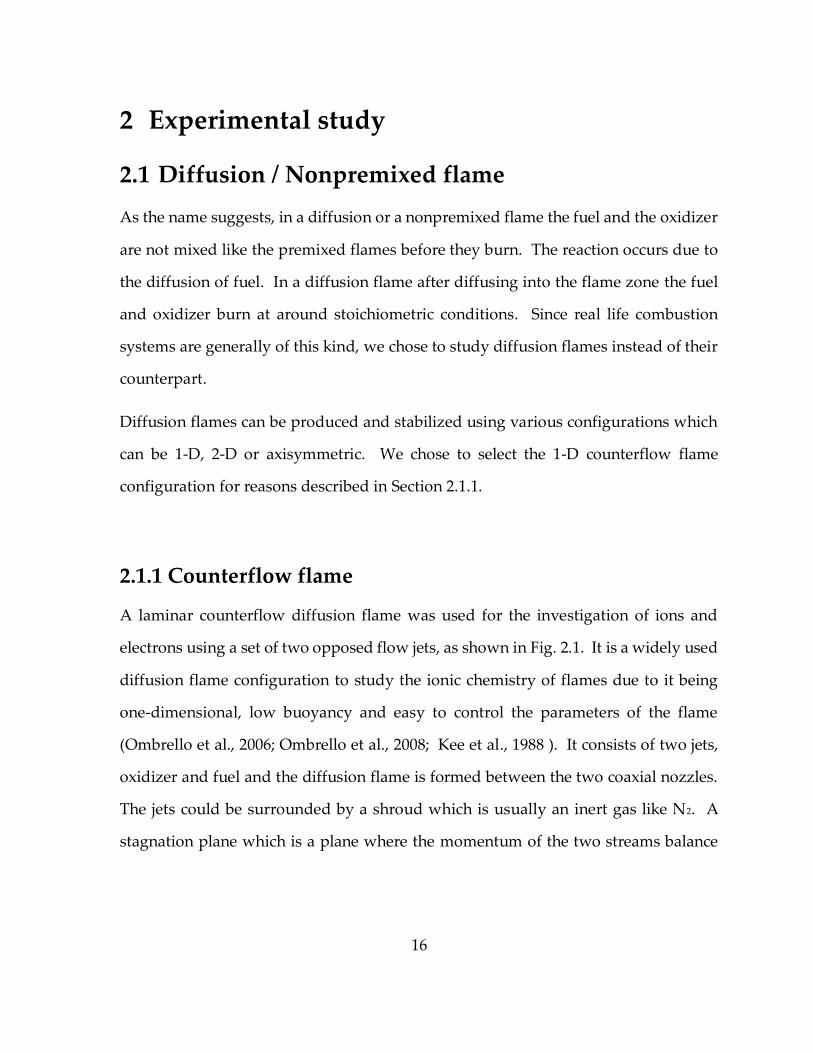
2 Experimental study .................................................................................................. 16

2.1 Diffusion / Nonpremixed flame ........................................................................ 16

2.1.1 Counterflow flame .................................................................................... 16

2.1.2 Burner configuration ................................................................................. 18

2.2 Electric probe ...................................................................................................... 20

2.2.1 Langmuir probe theory ............................................................................. 20

2.2.2 Modifications to the probe........................................................................ 28

3 Flame modeling ........................................................................................................ 30

3.1 Counterflow flame model .................................................................................. 30

3.2 Transport properties .......................................................................................... 33

3.3 Ambipolar diffusion ........................................................................................... 34

3.4 Numerical method ............................................................................................. 35

4 Model data ................................................................................................................. 36

4.1 Reaction mechanism .......................................................................................... 36

4.1.1 Charged species ......................................................................................... 37

vi

4.2 Thermodynamic data ......................................................................................... 38

4.3 Transport data .................................................................................................... 39

5 Results of the flame experiments and model ....................................................... 40

5.1 Flame structure ................................................................................................... 40

5.1.1 Effect of oxygen content............................................................................ 40

5.1.2 Effect of strain rate .................................................................................... 43

5.2 Volt-Ampere (VAC) Characteristics ................................................................. 45

5.3 Ion and electron profiles .................................................................................... 46

5.3.1 Effect of oxygen content and strain rate on peak charged species

concentrations ............................................................................................................ 50

5.4 Conservation of charge ...................................................................................... 52

5.5 Effect of gas-phase thermal-ionization ............................................................. 52

6 Primary nanoparticle charging model ................................................................... 56

6.1 Theory and Objective ......................................................................................... 56

6.2 Chemi-ionization model .................................................................................... 57

6.3 Bipolar diffusion charging model ..................................................................... 59

6.4 Thermal-ionization model ................................................................................. 62

6.5 Model formulation and validation ................................................................... 63

7 Results of the primary nanoparticle charging model .......................................... 69

7.1 Fixed ion and electron concentration................................................................ 69

7.2 Zero chemi-ionization ........................................................................................ 71

7.3 Negligible thermal-ionization ........................................................................... 72

7.4 Ions and electrons interacting with charged particles..................................... 75

7.4.1 Charged particle distribution ................................................................... 75

7.4.2 Average particle charge ............................................................................ 77

7.4.3 Electron concentration .............................................................................. 87

7.4.4 Ion concentration ....................................................................................... 92

8 Nanoparticle agglomerates charging model ......................................................... 95

8.1 Theory ................................................................................................................. 95

vii

8.2 Modifications to the primary nanoparticle charging model........................... 96

8.3 Model formulation and validation ................................................................... 99

8.4 Results of the nanoparticle agglomerates charging model ........................... 102

8.4.1 Zero chemi-ionization ............................................................................. 102

8.4.2 Zero thermal-ionization .......................................................................... 104

8.4.3 Relative charge and effects on ions and electrons ................................ 106

8.4.4 Ions and electrons in equilibrium with charged agglomerates ........... 109

9 Conclusions ............................................................................................................. 112

REFERENCES ................................................................................................................ 115

APPENDICES ................................................................................................................ 124

Appendix A: Numerical scheme for the charging model ....................................... 125

viii

LIST OF TABLES

Table 2-1. Parameters to calculate the ion and electron concentrations for probe

configuration P1. ............................................................................................ 25

Table 4-1. List of charged species included in the model. ............................................ 37

ix

LIST OF FIGURES

Fig. 1.1. Sources of ions and electrons in flames. ............................................................3

Fig. 1.2. Schematic of various nanoparticle charging mechanisms (Sahu et al, 2012). 8

Fig. 2.1 Schematic of a laminar counterflow diffusion flame....................................... 17

Fig. 2.2 Schematic of the counter flow diffusion flame burner (Desai, 2010). ........... 19

Fig. 2.3. Schematic of the Langmuir probe measurements for P1. .............................. 21

Fig. 2.4. Typical VAC of a single Langmuir probe........................................................ 22

Fig. 2.5. VAC curves with probe configuration P1 for 50% O2 at (a) 10 mm (b) 15 mm

from fuel nozzle. ............................................................................................... 26

Fig. 2.6. VAC curves with probe configuration P1 for 100% O2 at (a) 10 mm (b) 15

mm from fuel nozzle. ....................................................................................... 27

Fig. 2.7. Schematic of the probe with a cooling system (P2). ....................................... 29

Fig. 5.1. Effect of oxygen on flame structure at 20 s-1 (Desai, 2010). ............................ 41

Fig. 5.2. Effect of oxygen content at 20 s-1 on the (a) Flame temperature profile (b)

axial velocity profile. ........................................................................................ 42

Fig. 5.3. Effect of strain rate on flame structure at 100% O2 (Desai, 2010)................... 43

Fig. 5.4. Effect of strain rate at 100 s-1 on the (a) Flame temperature profile (b) axial

velocity profile. ................................................................................................. 44

Fig. 5.5. VAC for 21% O2 at 10 mm from the nozzle to measure electron saturation

current ion saturation current. ........................................................................ 45

Fig. 5.6. VAC for 75% O2 at 10 mm from the nozzle to measure (a) electron

saturation current (b) ion saturation current. ................................................. 46

Fig. 5.7 Distributions of major positive and negative ions in a methane –air diffusion

flame at 20 s-1. .................................................................................................... 47

Fig. 5.8. Ion and electron profiles at (a) 21% O2 (b) 75% O2. ........................................ 49

x

Fig. 5.9. Effect of (a) oxygen content (b) strain rate on peak charged species

concentration. .................................................................................................... 51

Fig. 5.10. Electron density as a function of temperature from major neutral species in

the flame. ........................................................................................................... 54

Fig. 5.11. Comparison of electrons produced from thermal-ionization and chemi-

ionization. .......................................................................................................... 55

Fig. 6.1. Schematic of the interaction between ions, electrons and nanoparticles in a

hydrocarbon flame. .......................................................................................... 64

Fig. 6.2. Comparison of relative soot volume fraction: experimental results by

Homann and Wolf (1983) (symbols), computed (solid lines) and model by

Balthasar et al. (2002) (dashed lines). .............................................................. 67

Fig. 6.3. Comparison of relative number density: our modeling results (solid lines)

and model by Balthasar et al. (2002) (dashed lines) (a) negatively charged

particles (b) positively charged particles. ....................................................... 68

Fig. 7.1. Comparison of fraction of charged particles for fixed total electron and ion

concentration at (a) 1000 K (b) 2000 K (c) 3000 K. .......................................... 70

Fig. 7.2. Comparison of fraction of charged particles for zero chemi-ionziation. ...... 72

Fig. 7.3. Comparison of distribution of charged particles for zero thermal -ionization

at (a) 1000 K (b) 2000 K (c) 3000 K for a fixed Np=1015 m-3.............................. 74

Fig. 7.4. Distribution of charged particles for different at (a) 1000 K, (b) 2000 K and

(c) 3000 K. .......................................................................................................... 76

Fig. 7.5. Charge distributions for the nanoparticles of TiO2, MoO3, and graphite

introduced in the flame environment with T = 3000 K and Ne(chemi) = 0. ........ 77

Fig. 7.6. Comparison of average charge carried by a 20 nm spherical particle at

different temperatures...................................................................................... 79

xi

Fig. 7.7. Comparison of average charge accumulated on a 20 nm particle as a

function of temperature with 15 3

( )10

e chemiN m at 3 different . ................. 81

Fig. 7.8 Comparison of average charge formed on a 20 nm particle versus electrons

and ions formed per unit volume by chemi-ionization at three different

temperatures with 15 310p

N m ........................................................................ 82

Fig. 7.9. Comparison of average charge formed on a 20 nm particle as a function of

total nanoparticle concentration for a fixed 15 3

( )10

e chemiN m . .................... 84

Fig. 7.10. Comparison of (a) average charge at 1000 K and 3000 K (b) average charge

at 1000 K and 2000 K (c) distribution of charges formed on a particle as a

function for 20 nm and 60 nm particle and 1 . ......................................... 86

Fig. 7.11. Electron concentration as a function of temperature for 15 3

( )10

e chemiN m

............................................................................................................................ 88

Fig. 7.12. Electron concentration as a function of electrons produced by chemi-

ionization at 15 310p

N m . ................................................................................ 89

Fig. 7.13. Electron concentration as a function of total particle concentration at

15 3

( )10

e chemiN m . ............................................................................................. 90

Fig. 7.14. Electron concentration as a function of particle diameter for

15 3

( )10

p e chemiN N m . ...................................................................................... 91

Fig. 7.15. Ion concentration as a function of (a) temperature for a fixed

15 3

( )10

e chemiN m (b) electrons from chemi-ionization for a fixed

15 310p

N m . ...................................................................................................... 92

Fig. 7.16. Ion concentration as a function of (a) total particle concentration fixed

15 3

( )10

e chemiN m and (b) particle diameter for 15 3

( )10

p e chemiN N m . ........ 94

xii

Fig. 8.1. Schematic of (a) straight chain (b) branched chain agglomerates. ................ 96

Fig. 8.2. Comparison of capacitance of straight and branched chain normalized by

capacitance of primary particles. ..................................................................... 98

Fig. 8.3. Comparison of previous experimental (Ball and Howard, 1971) and

numerical results. ........................................................................................... 101

Fig. 8.4. Comparison of net charge formed on an agglomerate as a function of the

number of primary particles for zero chemi-ionization. ............................. 103

Fig. 8.5. Comparison of net charge per particle of an agglomerate as a function of

the number of primary particles for zero chemi-ionization. ....................... 104


number of primary particles for zero thermal-ionization at (a) 1000 K (b)

3000K. .............................................................................................................. 105


number of primary particles for zero thermo-ionization (a) 1000 K (b)

3000K. .............................................................................................................. 106

Fig. 8.8. Comparison of relative charge for straight chain and branched chain

agglomerates with zero chemi-ionization. ................................................... 107

Fig. 8.9. Relative electron concentration as a function of number of primary

particles. .......................................................................................................... 108


agglomerates with zero thermal-ionization. ................................................ 109

Fig. 8.11. Comparison of charge on a primary particle as a function of particle

diameter for (a) NA= 50 (b) NA= 100 (c) NA= 200 (d) NA= 300. ..................... 111

1

1 Introduction

A hydrocarbon flame is characterized by complex chemical kinetics. It is beneficial to

study the formation of different species and their effect on the flame chemistry. In

addition to the neutral species a typical flame produces a small amount of charged

particles, i.e. ions and electrons. These particles not only play a role in the numerous

ion and ion-molecular reactions but also play an important role in reaction pathways

that generate soot and aerosols. It has been known for many decades that an electric

field can deflect the flame. This effect is attributed to the formation of charged

particles. In an external electric field, these particles can form ion wind which in turn

deflects the flame. Ions are also formed in many ignition processes like spark ignition

and laser ignition. Nowadays, there has been widespread interest in understanding

of ion and electron formation for engine diagnostics. Hence studying the electrical

composition of a flame has innumerable benefits.

1.1 Ions and electrons in flames

1.1.1 Ionization in flames

1.1.1.1 Hydrocarbon flames

Initially it was thought that the thermal ionization was the primary source of the high

concentration of ions and electrons in a combustion process. Calcote (1957) critically

reviewed the idea of production of ions by thermal ionization due to different species.

In the review, it was mentioned that impurities with low ionization potential can

produce ions from thermal ionization in a hydrocarbon flame (Fig. 1.1). Reaction

2

intermediates like OH, CH and NO have been suggested for the possible sources of

thermal ionization. But on careful study it was seen that the measured high ion

concentration in flames could not be explained by the low concentration of ions

produced due to thermal ionization at those flame temperatures. Carbon particles

with a work function between 4.35 eV and 11 eV in the form of solid and gaseous

particles respectively have been considered as a possible source for thermal ionization

by Perkins et al. (1962). But on further investigation it was found that the ions were

produced in the green-zone of the flame where the soot was not as prominent as in

other regions of the flame.

Charged species in flames have been studied extensively in the past and have been

reviewed by Fialkov (1997). Especially laminar premixed flames have been studied

extensively for charged species chemistry. It was found by Calcote (1957) that the

primary cause of ion production could be the chemi-ionization reaction. A chemi-

ionization reaction is a chemical reaction which produces charged species from

neutral reactants. The primary chemi-ionization reaction was determined by Calcote

(1961):

CH O CHO e

3

Fig. 1.1. Sources of ions and electrons in flames.

This reaction is negligibly dependent on temperature and it has been proved

comprehensively that this is the most dominant source of ionization. The second most

important chemi-ionizaton reaction was suggested by Knewstabb and Sugden (1960):

CH* + C2H2 → C3H3+ + e-

Unlike CHO+, it was shown experimentally C3H3+ is the most important species with

highest concentration in fuel rich flames. Other important chemi-ionization reaction

suggested by Burke et al. (1963 ) was:

CH + O2 → CHO+ + 𝑒−

4

1.1.1.2 Ionization in non-hydrocarbon flames

Low concentrations of charged species are found in pure hydrogen flames. The high

concentration of ions found in hydrogen flames are purely because of impurities

(Bascombe et al., 1962).

The following mechanism is proposed for pure hydrogen flames (Axford et al.,

1998):

*

2

*

2 3

*

2

*

2 3

H OH H O

H H O H O e

H H H

H OH H O e

Overall chemi-ionization reaction is given by

32H OH H O e

For a hydrogen flames with additives like metals and halogens, a large concentration

in ions and electrons is observed. This is because of the high temperatures and high

amount of radicals present in a hydrogen flame i.e. H, OH and O. The number of ion

and electrons due to thermal ionization can be estimated by using Saha equation given

in Chapter 5. The pathway of production of charged species due to alkali metals is

given as follows (Padley and Sugden, 1962; Kelly and Pradley, 1969)

*

*

A M A M

A M A e M

For nitrogen containing fuels (Bulewicz and Padley, 1963) ion concentration in

cyanogen-oxygen flames is very high and is at par with that observed in hydrocarbon

5

flames. The thermal ionization mechanism has very little to do with the ionization

even though the temperatures reached are of the ~4000 K.

The following ionization mechanisms was proposed:

22

2

NO C O NO e CO

NO N NO e N

CN O NO e CO

For very hot flames atomic nitrogen reacts with an oxygen atom to produce a positive

ion and an electron as given by

N O NO e

1.1.2 Ions in methane- oxygen flames

The types of ions produced in a flame vary according to mixture composition. But

still there are many common ions produced even for very dissimilar chemical

compositions. In all cases it has been found that ion concentration is usually of the

same order of magnitude as the electron concentration. The most common ions found

in methane-oxygen flames other than electrons are CHO+, H3O+, C2H3O+, OH-, O2- and

O- though the anions are present in very small quantities.

The ionic chemistry of methane-oxygen flames at atmospheric pressure were

successfully studied by Sugden et al. (1979) and Goodings et al. (1979). Methane –

oxygen flames were also studied at low pressures by Feugier and van Tiggelen (1965).

When the flame is highly fuel rich (Goodings et al., 1977) at 1 atm, the total ion and

6

electron concentration were found to be 4 x 1010 cm-3. At this condition, large amounts

of C2H5O+ and C3H3+ were also observed.

1.1.3 Electric field effects

It has been known for decades that electric fields affect the shape and behavior of

flames and also the soot particles (Brande, 1814). This means that there has been

strong evidence since many years for the presence of charged species as well as

particles in a flame. Harnessing this property could mean that the shape and hence

the heat and mass transfer properties of the flames could be controlled. There have

been studies on the modification of flame speed by using electric fields since many

years (Guenault and Wheeler, 1931). Scalov and Socolic (1934) concluded that the

speed of hydrocarbon flames decreased with increase in traverse DC electric field.

Electric fields can cause increase or decrease in the formation of soot and also can

change the nature of growth and morphology of soot (Place and Weinberg, 1966).

1.1.4 Numerical models

The number of numerical studies performed to study the electron and ion formation

have been limited. One study looks at the effect of external electric field on

stoichiometric and lean premixed methane-oxygen flame at atmospheric pressure but

the negative ions were neglected in the study (Pedersen and Brown, 1993). Also it

incorporates only a 13 step chemi-ionization reaction and a fewer number of ions. A

more recent study was made by Prager et al. (2007) on a lean to atmospheric methane-

7

oxygen laminar premixed flame which successfully demonstrates the more detailed

ionic chemistry and transport model. Unfortunately, not many studies have been

performed on diffusion flames which are more applicable to real combustion systems.

1.2 Nanoparticle charging

Recently, there has been a widespread interest to nanoparticle charging especially in

material synthesis, electrostatic filtration of particles and particle control (Schaeublin

et al., 2011 and Muzino, 2000). Hence, it has become very important to understand

the mechanism that governs the charging of nanoparticles under different conditions.

With no external electric field nanoparticle charging is mainly governed by diffusion

of charge carriers that are produced from chemi-ionization and electrostatically

interact with particles. Another mechanism involves thermal ionization at high

temperatures (Savel’ev & Starik, 2006; Sgro et al., 2010). A considerable number of

theories have been put forward to describe the diffusion charging mechanism. As

shown in Fig. 1.2, there are multiple ways for a particle to acquire a charge in a flame.

8

Fig. 1.2. Schematic of various nanoparticle charging mechanisms (Sahu et al, 2012).

A theory on stationary charge distribution on a spherical particle in a bipolar

environment has been widely accepted and verified (Fuchs, 1963). Wersborg et al.

(1973) reported that one third of soot particles greater than ~2 nm are charged while

Mayo & Weinberg (1970) reported that all soot particles formed in a counterflow

diffusion flame are charged.

1.2.1 Charging mechanisms

A good amount of experimental work has been performed recently on measuring

charge distribution of nanoparticles in flames. Maricq (2005 & 2006) experimentally

studied a charge distribution on soot particles in laboratory premixed flames by using

9

sampling methods coupled with DMA analyzer and compared the results with

theoretical equilibrium predictions. Sahu, Park & Biswas (2012) measured charge

distribution on TiO2 and Cu-TiO2 nanoparticles introduced in a diffusion flame. A

comprehensive model has been developed by Jiang, Lee & Biswas (2007) which

describes the nanoparticle charging for a soft X-ray enhanced electrostatic precipitator

(ESP) device. The model included simultaneous diffusion, thermal ionization and

photoionization. A model on charging and growth of soot particles has also been

studied by Savel’ev & Starik (2006) without considering high temperature thermal

ionization and chemi-ionization.

The charge deposited on a particle can affect the growth of the particle and its

structure including fractal shapes of aggregates formed under certain conditions

(Onischuk et al., 2008). Charging is extremely sensitive to the ion and electron

concentrations around a nanoparticle, temperature as well as the material of the

particle. There have been little or no studies on charging of particles in oxy-fuel flames

where thermal ionization becomes the dominant charging mechanism due to flame

temperatures reaching 3000 K.

Wen et al. (1984) reviewed a number of theoretical approaches to describe charging of

arbitrary shaped particles. They introduced the notion of a charging-equivalent

diameter into the Boltzmann expression and found it to provide a good

approximation to the general theory of Laframboise and Chang (1977) for the

charging of soot particles. Rogak and Flagan (1992) further examined the effect of

morphology by comparing the neutral fractions of spherical versus aggregate

particles leaving a diffusion charger. They concluded that aggregate and spherical

particle charging was very similar, observing only a 5% lower neutral fraction for

10

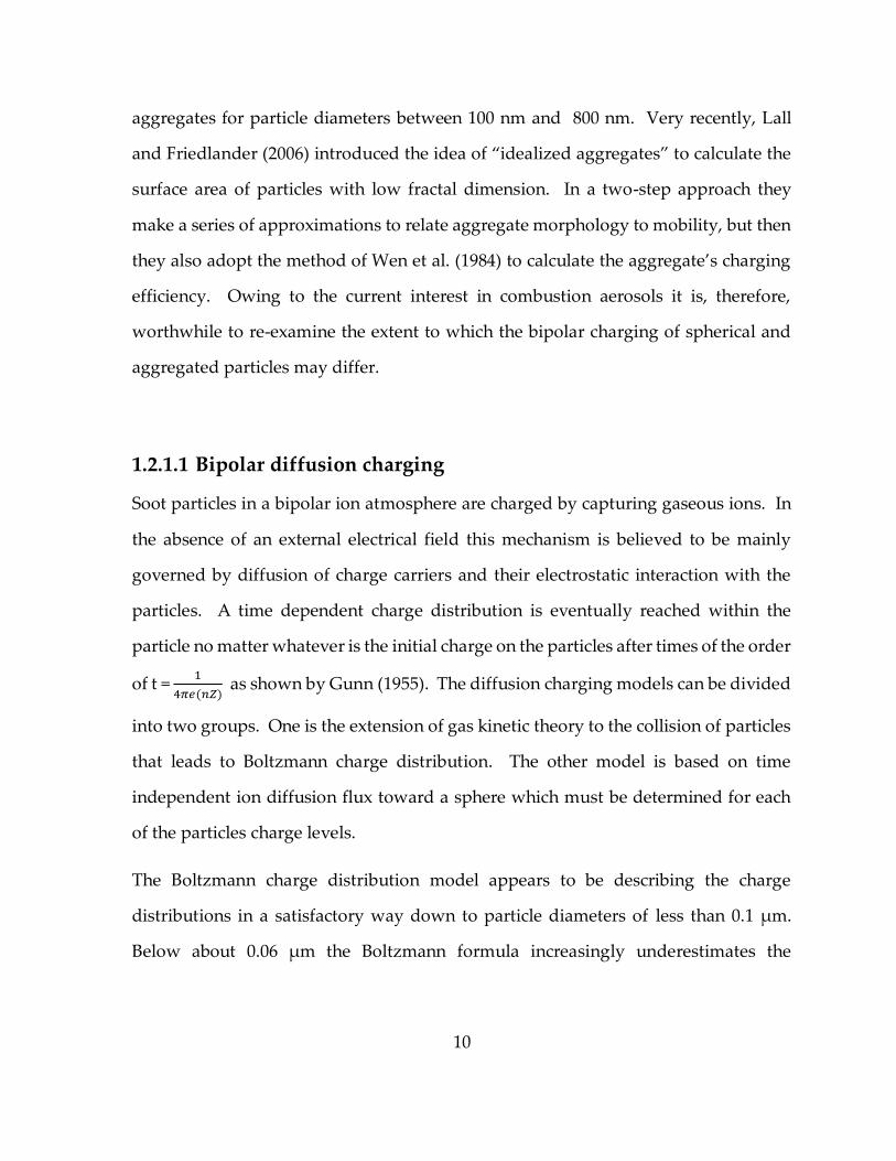
aggregates for particle diameters between 100 nm and 800 nm. Very recently, Lall

and Friedlander (2006) introduced the idea of “idealized aggregates” to calculate the

surface area of particles with low fractal dimension. In a two-step approach they

make a series of approximations to relate aggregate morphology to mobility, but then

they also adopt the method of Wen et al. (1984) to calculate the aggregate’s charging

efficiency. Owing to the current interest in combustion aerosols it is, therefore,

worthwhile to re-examine the extent to which the bipolar charging of spherical and

aggregated particles may differ.

1.2.1.1 Bipolar diffusion charging

Soot particles in a bipolar ion atmosphere are charged by capturing gaseous ions. In

the absence of an external electrical field this mechanism is believed to be mainly

governed by diffusion of charge carriers and their electrostatic interaction with the

particles. A time dependent charge distribution is eventually reached within the

particle no matter whatever is the initial charge on the particles after times of the order

of t = 1

4𝜋𝑒(𝑛𝑍) as shown by Gunn (1955). The diffusion charging models can be divided

into two groups. One is the extension of gas kinetic theory to the collision of particles

that leads to Boltzmann charge distribution. The other model is based on time

independent ion diffusion flux toward a sphere which must be determined for each

of the particles charge levels.

The Boltzmann charge distribution model appears to be describing the charge

distributions in a satisfactory way down to particle diameters of less than 0.1 μm.

Below about 0.06 μm the Boltzmann formula increasingly underestimates the

11

charging probabilities. Below that diameter Fuchs model is in better agreement with

the experimental results as shown by Reischl et al. (1983). Due to the simplicity of its

expression it is the most popular distribution function. The characteristic feature of

the steady state approximation is the assumption of a vacuum boundary layer of

thickness λ near the surface of the particle in which kinetic theory of gas applies. The

primary difference between the various models lies in the details of the motion and

capture of the ions in the vicinity of the particle.

Boltzmann distribution -

The electrostatic energy contained in the Coulomb field of a sphere in vacuum is

2 2

2

e

a

(1.1)

0

expN NkT

(1.2)

where v is the number of unit charges on the sphere, No is the concentration of the

neutrals.

Steady-state ion diffusion theory in the continuum limit -

For a sphere at rest with respect to its environment, the transport of ions outside the

transition layer is governed solely by the diffusion equation modified for the electric

force arising from the free charge carried by the sphere. The ion flux I transported

across a spherical shell of radius r in unit time is

24dn

I r D EZndr

(1.3)

12

where D is the ion diffusion coefficient, dn/dr is the radial concentration gradient of

ions at the shell, Z and n are electric mobility and ion concentration. When we solve

Eq. (1.3) we get a solution for n(r).

1.2.1.2 Charging from thermal ionization

Thermal ionization occurs inside the sooting region of the flame. The equilibrium

concentration of the thermoionized charged species with a single positive charge is

given by Saha's equation

2

1 1

30

2exp

( )e

e b

n g A

n n g k T

(1.4)

ne is the electron number density, n is the neutral particle number density, g1 is the

degeneracy of the states of the 1st ion, g0 is the degeneracy of the state of the neutral

species, A1 is the ionization potential and T is flame temperature. Thermal de Broglie

wavelength Λ can be found as

3b

h

mk T

The ionization potential for the small species is given by

2

1/ 2

wA A e C (1.5)

where Aw is the work function of the substance making up the particle, e is the electron

charge, C is the capacity of the particle equal to 2πεod for a sphere of a diameter d.

Mayo and Weinberg (1970) found that soot particles usually carry a single charge.

Others reported that the smallest soot particles in a low pressure flame carry a single

13

charge which could be positive or negative. Doubly positively charged particles were

only found in really hot C2H2- O2 flames as studied by Homann and Wolf (1983).

Calcote (1957) found that soot particles larger than 3 nm are formed as a result of

thermoionization but smaller particles are not. This is because the recombination

coefficient exceeds the rate of thermal ionization for larger particles to neutralize

them. Gerhardt et al. (1988) reported that the thermal ionization of particles with

diameter greater than 2 nm did not match with the experimental data. But a good

agreement was found for particles greater than 3 nm in diameter. Wesborg et al.

(1973) reported that one third of soot particles greater than about 2 nm are charged

while Mayo and Weinberg (1970) reported that all soot particles in a counterflow

diffusion flame are charged.

Balthasar et al. (2002) computationally modeled thermoionization in premixed and

diffusion flames by considering the oxidation of fuel, the formation and growth of

polycyclic aromatic hydrocarbons, and particle inception, coagulation, as well as mass

growth via surface reactions. They found that thermoionization is insignificant for

laboratory flames under 2100 K. Over that temperature it can play an important role.

The work function of the soot particle also decreases tremendously with the increase

in diameter which is primarily due to agglomeration. Hence the tendency to

thermally ionize increase with particle size.

Thus it can be said that although it may be intuitive to think that soot particle

thermoionization is the primary source of charge on soot, it is clear that there are other

processes that are mainly responsible for soot charging unless the temperature is very

high. Soot charging is a complex process which depends on a variety of factors like

14

sooting zone, type of fuel, temperature, pressure, height above the burner and particle

size.

1.2.2 Effect of particle morphology on charging

Recent work in this area is directed towards nanoparticles charging and the

comparison of experimental data to models of diffusion charging for example by

Hoppel et al. (1986). But the influence of morphology on particle charging has had

relatively little attention. It was supposed that Coulombic interactions may play a

considerable role in the aggregation process and affect essentially the aggregate

morphology as studied by Onischuk et al. (2008) and few others. It was shown that

soot aggregates formed in flame are charged. Onischuk et al. (2008) later studied the

morphology of soot in a propane/air diffusion flame to correlate the Coulombic

interactions and the soot structure. It was determined that Coulombic interactions

play an important role in soot deposition to the wall resulting in dendrite structure

formation at the surface. He found that Coulombic interactions may affect

considerably the aggregate–aggregate sticking process. This influence was

demonstrated by changing the orientation and by accelerated mutual approach when

sticking. An effect of soot aggregate restructuring resulting in transformation of

chain-like aggregates to compact structures was observed during the coagulation at

room temperature.

15

1.3 Thesis Objectives

The first part of this thesis is to study the ions and electrons experimentally and

numerically in a one-dimensional laminar counterflow oxy-fuel diffusion flame.

Experimentally the species are measured using a Langmuir probe by measuring volt-

ampere characteristics (VAC) at different positions in the flame. Appropriate theory

is used to interpret these curves so that we can calculate the charged species

concentrations to validate the numerical results. Then numerically the charged

species are computed using a counterflow flame model. Electron and ion profiles are

studied for different strain rates and oxygen contents.

The second part of this study is to analyze the interaction between ions, electrons and

nanoparticles in a hydrocarbon flame. To achieve this, a basic model was developed

that describes the physics governing the charge formation on a spherical nanoparticle

as well as its effect on the population of ions and electrons and vice versa in oxygen

enriched flames. The model includes diffusion charging and charging of a

nanoparticle from thermal ionization in the presence of ions and electrons produced

in a flame by chemi-ionziation. In order to validate the model the numerical results

under certain conditions were compared to the available experimental and numerical

results from the literature. This model was extended for fractal agglomerates.

16

2 Experimental study

2.1 Diffusion / Nonpremixed flame

As the name suggests, in a diffusion or a nonpremixed flame the fuel and the oxidizer

are not mixed like the premixed flames before they burn. The reaction occurs due to

the diffusion of fuel. In a diffusion flame after diffusing into the flame zone the fuel

and oxidizer burn at around stoichiometric conditions. Since real life combustion

systems are generally of this kind, we chose to study diffusion flames instead of their

counterpart.

Diffusion flames can be produced and stabilized using various configurations which

can be 1-D, 2-D or axisymmetric. We chose to select the 1-D counterflow flame

configuration for reasons described in Section 2.1.1.

2.1.1 Counterflow flame

A laminar counterflow diffusion flame was used for the investigation of ions and

electrons using a set of two opposed flow jets, as shown in Fig. 2.1. It is a widely used

diffusion flame configuration to study the ionic chemistry of flames due to it being

one-dimensional, low buoyancy and easy to control the parameters of the flame

(Ombrello et al., 2006; Ombrello et al., 2008; Kee et al., 1988 ). It consists of two jets,

oxidizer and fuel and the diffusion flame is formed between the two coaxial nozzles.

The jets could be surrounded by a shroud which is usually an inert gas like N2. A

stagnation plane which is a plane where the momentum of the two streams balance

17

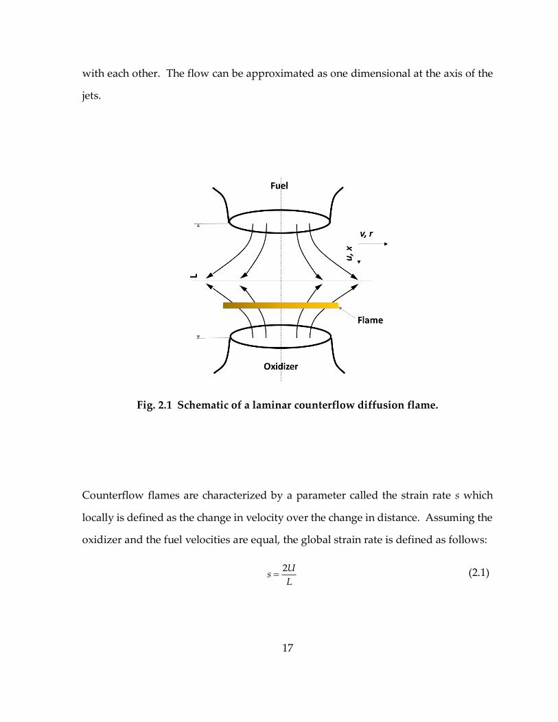
with each other. The flow can be approximated as one dimensional at the axis of the

jets.

Fig. 2.1 Schematic of a laminar counterflow diffusion flame.

Counterflow flames are characterized by a parameter called the strain rate s which

locally is defined as the change in velocity over the change in distance. Assuming the

oxidizer and the fuel velocities are equal, the global strain rate is defined as follows:

2Us

L (2.1)

18

where U is the velocity of the fuel and the oxidizer stream at the exit of the nozzle and

L is the distance between the two nozzles. The strain rate can be thought of as inverse

of the residence time take by the two streams. As mentioned earlier the global strain

rate is based on oxidizer and fuel exit velocity and not on local flow velocities which

makes it useful to characterize multiple experimental conditions, i.e., flow rate, nozzle

diameter and the axial distance by one parameter, i.e., strain rate. A comprehensive

information about the counterflow diffusion flames is available in Tsuji, (1982).

2.1.2 Burner configuration

To stabilize a counterflow diffusion flame we use a burner configuration with two

opposed nozzles. Fuel which is methane in this case runs from the top and oxidizer

which is oxygen enriched air runs from the bottom, as shown in Fig. 2.2. The two

streams collide and the flame is ignited manually using an acetylene torch at the

location where the two jets meet. The mixing chamber which carries the oxidizer is

filled with glass beads. Between the oxidizer and the fuel nozzle there is a concentric

annular space through which nitrogen is passed to act as a shroud in order to protect

the flame from external perturbations as well as to prevent oxidizer and the fuel to

spill outside which can be hazardous. The nitrogen is passed through a ceramic

honeycomb to have a stable and a laminar flow. The upper nozzles is surrounded by

a cooling system which is a cylindrical jacket also concentric to the two nozzles to cool

the exhaust gases. The distance between the two nozzles is fixed at 2 cm. The top

part of the burner is mounted on a sliding system and can be traversed in the vertical

direction using a motor relative to the bottom burner which is fixed. The supply lines

19

for all the gases except for air are connected to their individual cylinders and pressure

regulators, flow meter and flow controllers are used to monitor and control the flow.

Fig. 2.2 Schematic of the counter flow diffusion flame burner (Desai, 2010).

Compressed air comes in from the in-house compressor and it is mixed with oxygen

in the mixing chamber to control the oxygen to nitrogen ratio. Further information

regarding the burner set up and the burner operation procedures can be found

elsewhere (Salkar, 2011).

20

2.2 Electric probe

2.2.1 Langmuir probe theory

Langmuir probe is an intrusive technique to measure electrical properties of the flame.

The different properties that could be measured are electron temperature,

conductivity, mobility, and electron and ion concentration. In this study we focus our

attention at recording volt-ampere characteristics (VAC) by using an electric probe.

The formulation of the theory to measure concentrations from VAC can change

depending on the plasma conditions. The probes could be either of spherical or

cylindrical shape. For one dimensional flat flames like a counterflow diffusion flame,

a cylindrical probe is best suited.

The experimental setup to measure VAC is shown in Fig. 2.3. First we performed

experiments with a 0.25 mm tungsten probe. We call the first probe configuration as

P1 which is used here. Later a hollow steel probe (P2) for reasons described in section

2.2.2 is used by making some additional modifications to P1. The tungsten probe is

surrounded by a high temperature resistant ceramic tube. We get the VAC curves by

changing the potential of the probe with respect to the oxidizer nozzle, treating that

nozzle as a ground electrode. The probe is connected to an ammeter in series with a

24 V battery and a 10 KΩ potentiometer is used to change the potential. Also the

probe is mounted on a fixture and has the capability to traverse in the axial direction.

The electric current drawn from a flame depends on the probe length and the probe

diameter but the current density would be constant irrespective of the probe

geometry. When the probe is highly positive it attracts electrons and repels positively

charged ions. At such conditions, a thin layer around the probe becomes full of

21

electrons. Hence there is an electric field in the thin layer near the probe. There is no

electric field outside the layer since the plasma is quasineutral. Hence in this case the

current measured is the electron saturation current, as shown in Fig. 2.4.

Fig. 2.3. Schematic of the Langmuir probe measurements for P1.

22

Fig. 2.4. Typical VAC of a single Langmuir probe.

When the probe potential is reduced below the plasma potential, more positive ions

and less electron enter the probe. This process continues until the potential of the

probe equals the floating potential Vf at which the ion and electron currents to the

probe balance each other and the total current of the probe is equal to zero. At this

potential the ion current equals the electron current. When the probe potential is

strongly negative as compared to the plasma, the positive ions are attracted but the

electrons are repelled. In this case the probe is surrounded by a layer of positive ions

and the saturation ion current is reached. Even though saturation currents can be

23

reached for positive ions and electrons at high negative and positive potentials,

electrons and ions can ions can enter the probe from other parts of the flame causing

an increase in current. So from Fig. 2.4 it can be seen the saturation current is not truly

constant but it has a small slope. Hence we are interested in the value of the current

at which the slope of the VAC curve drops. Also it can be seen that the ion saturation

current is much lower than the electron saturation current due to the high difference

in masses.

From the saturation current ‘I’ we can determine the current density if we know the

probe area by the relation:

AI jS j dL (2.2)

where j is the current density and SA is the surface area of the probe exposed to the

plasma, d is the probe diameter and L is the length. The interpretation of the curve

varies depending on the application. For low pressure and temperature plasma

systems the following equation assuming Maxwell-Boltzmann distribution is often

used (Lochte-Holtegreven, 1968 and Clements, 1978):

1

221 1

4 4b e

e e e

e

k Tj en u en

m

(2.3)

where e is elementary charge, kb is the Boltzmann constant, Te is the electron

temperature, me is the electron mass, ne is the number density of the electrons and ue

is the thermal velocity of electrons. From Eqs. (2.2) and (2.3) the electron concentration

can be determined.

Similarly ion concentration ‘ni’ can be determined from the following relation:

24

1

221 1

4 4b

k Tj en u en

m

(2.4)

where the subscript ‘+’ stands for positive ions. The floating potential can also be

determined by equating the ion and electron currents, making the net current equal

to zero

1 1

2 22 21 1

4 4

fb e be

e b e

eVk T k Ten en

m k T m

Assuming quasineutrality, i.e., ne=n+, gives the solution for Vf as:

2b e e

f

e

k T T mV

e T m

(2.5)

For flames, Te = T+ = T, where T is the flame temperature.

Hence 2b

f

e

k T mV

e m

(2.6)

The above equations work well when the temperature of the plasma is low and the

pressure is way below atmospheric. But for high temperature and atmospheric

pressure conditions present in our flame we have to use a modified version of the

equation that relates current density and number density for cylindrical probes

(Calcote, 1963)

For electron number density,

1

22 0.751 ln

2 0.5e e

e

b e e e

j m d Ln

e k T d

(2.7)

25

For ion number density;

1

22 0.751 ln

2 0.5b

j m d Ln

e k T d

(2.8)

where, λe and λ+ represent the mean free paths of the electrons and ions,

respectively. We use the following values for parameters in Eqs. (2.7) and (2.8) to

calculate the concentrations for electrons and ions (Table 2-1). The mass for the ion

is assumed to be that of the hydronium ion, i.e. H3O+, since that is the most abundant

ion found in hydrocarbon flames (Fialkov, 1997).

Table 2-1. Parameters to calculate the ion and electron concentrations for probe

configuration P1.

Quantity Value

m+ 263.15 10 kg

me 319.1 10 kg

d 0.25 mm

L 101 mm

λ+ 55.26 10 cm

λe 41.9 10 cm

The values for the mean free paths for ions and electrons are taken from Calcote

(1963). These values are pressure and temperature dependent and the conditions

present in Calcote (1963) are also nearly similar to our conditions hence it is reasonable

to assume those values for our calculations. The temperatures used are the flame

temperatures and are not measured but computed as discussed in Chapter 5. VAC

26

curves for 50 % O2 and 100% O2 are shown in Figs. 2.5 and 2.6, respectively. The

saturation currents are measured at locations 10 mm and 15 mm from the fuel nozzle

for both the cases. We see that the electron saturation current for 50 % O2 at 10 mm

and 15 mm is approximately 1.5 μA and 0.5 μA which when plugged in Eq. (2.7) gives

the electron concentrations of 132 10 cm-3 and 128 10 cm-3 respectively. For 100 % O2

at 100 mm and 15 mm the saturation currents are ~7.5 μA and ~5 μA which when

used in the same equation gives 138 10 cm-3 and 136 10 cm-3, respectively. This agrees

reasonably well with classical experiments performed in flames (Fialkov, 1997).

(a) (b)

Fig. 2.5. VAC curves with probe configuration P1 for 50% O2 at (a) 10 mm (b) 15

mm from fuel nozzle.

27

(a) (b)

Fig. 2.6. VAC curves with probe configuration P1 for 100% O2 at (a) 10 mm

(b) 15 mm from fuel nozzle.

We only obtain the ion saturation current for 50 % O2 with an absolute value of ~1 μA

which corresponds to an ion concentration of ~1016 cm-3. This is much higher than

expected from Eqs. (2.7) and (2.8) assuming ion concentration is of the same order of

magnitude to that of electron concentration. It can be seen that the saturation current

does not occur when the oxygen content is increased even though the probe is highly

negative. The most probable causes for such anomalies are as follows:

Due to the high temperature of the flame thermionic emission takes place. So

when the probe is at high negative potential with respect to the oxidizer nozzle

the electrons released due to thermionic emission are further repelled by the

strong negative potential generating the additional current.

28

At high oxygen contents the soot generated and the flame temperatures are

relatively high as compared to low oxygen contents. Due to this the soot at

high oxygen contents gets thermally ionized. This can create a large error in

measuring the true ion current when the probe is at negative potential.

Another problem with the above system is that at high temperatures (>1700 K) and at

high oxygen content i.e. > 50% O2, the probe gets oxidized making it impossible to

measure the currents at certain locations. Hence there is a need to make certain

modifications to our probe setup as described in the next section.

2.2.2 Modifications to the probe

The problems associated with the above system can be minimized by cooling the

probe. The only feasible way to cool the probe would be through convection. The

rate of thermionic emission exponentially increases with the surface temperature of

the probe. By cooling the probe internally the thermionic emission can be significantly

reduced. Concurrently, the flame disturbances are minimized. Due to the strong

temperature effect on thermionic emission rate, even a small reduction in

temperature can have a significant effect on the thermionic current.

To minimize the any perturbation in the flame due to the probe, the size of the probe

has to be chosen carefully. Hence a tube is chosen which has an outer diameter of 0.9

mm and the inner diameter is 0.7 mm. Due to such small diameters the only feasible

manner to cool the probe is to use a gaseous cooling medium instead of liquid due to

significantly lower hydraulic resistance and negligible electric conductivity of the gas.

Compressed nitrogen at high pressure is passed through the hollow probe. Since the

29

ion currents are to be of the order of nano amperes, the previous method of measuring

current is replaced by Keithley – 6517 A electrometer which can measure currents

with very high precision and accuracy of 10-12 A, as shown in Fig. 2.7. The results

from this probe configuration (P2) are presented in Chapter 5.

Fig. 2.7. Schematic of the probe with a cooling system (P2).

30

3 Flame modeling

A one-dimensional counterflow flame model is used to study the ionic structure of

the flames. The flame is produced by burning 100% methane (CH4) with oxygen

enriched air and the oxygen content is varied from 21% to 100%. The strain rate of

the flame is increased from 20 s-1 to 90 s-1 in the steps of 10 s-1. The axial distance

between the two nozzles is kept at 2 cm.

3.1 Counterflow flame model

The model is solves for the steady state solution for opposed flow diffusion flames

axisymmetric and concentric in geometry, as shown in Fig. 2.1. The model is used to

predict the mole fractions, mass fractions, velocity and temperature profiles. The

model can be used for premixed flames as well, but unlike the diffusion flames, two

flames will be produced on the two sides of the stagnation flame.

If we exclude the edge effects, this type of flame geometry is very desirable because

the flames produced are flat unlike other types of axisymmetric flames reducing the

problem down from two dimensional to one dimensional and making it easier to

study the chemistry of the flames.

A brief summary of the model is given below. For more information about the model

and its derivation, one can refer to Kee et al., (1988) and Lutz et al. (1997).

The axisymmetric mass conservation equation in cylindrical system is

1

0u vrx r r

(3.1)

31

As shown in Fig. 2.1, ρ is the density, u and v are axial (x) and radial (r) components

of the velocity respectively.

Let, ( )v

G xr

and ( )

2

uF x

After formulating the momentum equation, one can realize that the v/r and other

variables like temperature, velocity, density, mole and mass fractions should be a

function of the axial distance only (Karman, 1946 and Kee et al. 1988). After plugging

in the above expressions into (3.1) one can find

( )( )

dF xG x

dx (3.2)

Hence,

(radial momentum) 1constant

pH

r r

(3.3)

(axial momentum) 23

2 0FG G G

Hx x x

(3.4)

Energy equation becomes

1 1

0pk k k k k

k kp p p

dT d dT dTu C Y V h

dx C dx dx C dx C

(3.5)

Species equation becomes

0kk k k k

dY du Y V W

dx dx k= 1,2,3…..N (3.6)

Where Vk is the diffusion velocity either given by the multicomponent formulation or

the mixture averaged formulation.

32

Mixture averaged diffusion velocity is

1 1T

k kk km

k k

dX D dTV D

X dx Y T dx (3.7)

Multicomponent diffusion velocity is

1

1 1TNj k

k j kjjk k

dX D dTV W D

X W dx Y T dx

(3.8)

(mixture averaged) 1

kkm N

j

j k jk

YD

X

D

(multi component)

N

j jj k

km Nj

j k jk

X M

DX

WD

(3.9)

where k

X is the mole faction, k

Y is mass fraction, Cp is the specific heat capacity, k

W is

the molecular weight of the species, k

w is the species production or consumption rate,

W is the mean molecular weight of the mixture, is the thermal conductivity of the

species, km

D is the mixture averaged diffusion coefficient, kjD is binary diffusion

coefficient and T

kD is the thermal diffusion coefficient.

The temperature, composition of the mixture and the velocities are specified at the

exit of the nozzles giving the following boundary conditions

0 : ,2F Fu

x F

0,G ,F

T T k k k k FuY Y V uY

33

: ,2

O Ou

x L F

0,G ,O

T T k k k k OuY Y V uY (3.10)

where the subscript ‘F’ and ‘O’ stand for fuel and oxidizer respectively.

3.2 Transport properties

The above equations need the values for kjD ,

kmD ,

T

kD , viscosities and thermal

conductivities so that we can solve them. In order to obtain values of those coefficients

we need to find those quantities we need we have an option to use either one of two

models, mixture-averaged or multicomponent method. Mixture-averaged quantities

easier to compute and take less computational time. But they are less accurate and

they may or may not conserve mass in the species equation.

The following gives a brief overview of the method to calculate mixture averaged

properties by conventional chemical kinetics package like CANTERA for combustion

applications.

Viscosity:

2

5

16k b

k

k

W k T

(3.11)

where k

is the Lennard-Jones collision diameter and is the collision integral which

depends on dipole moment and the temperature.

Binary diffusion coefficient:

34

3 3

2

/3

8

b jk

jk

jk

k T mD

(3.12)

where jkm is the reduced mass and jk

is reduced collision diameter and are given by

2

j k

jk

j k

m mm

m m

,

2j k

jk

j k

(3.13)

Mixture averaged viscosity:

2

0.5 0.5 0.251

11 1

8

Nk k

k

jk kj

j j k

X

MMX

M M

(3.14)

Mixture averaged thermal conductivity:

1

1

1 1

2

N

k k Nk k

k k

XX

(3.15)

For more details regarding the coefficients and also about the multicomponent

properties one can refer to Kuo, (1986).

3.3 Ambipolar diffusion

When charged species are included assumption of quasineutrality is used which

means at every point summation of all charges are zero. This is only possible if the

summation of all diffusion fluxes at that point is equal to zero (Franklin, 2003).

35

Ambipolar diffusion is the diffusion of positive and negative particles in a plasma at

the equal rate because of their interactions with the internal electric field inside a

plasma. Since electrons move faster than ions, there will always be a charge

separation between ions and electrons hence quasineutrality will not be achieved. The

internal electric field accelerates the ions and decelerates the electrons making them

diffuse together

Hence we have to make changes to the diffusion flux by introducing ambipolar

diffusion (Cancian et al., 2013)

(3.16)

where Eambi is the internal electric field created.

3.4 Numerical method

The method used is finite-difference approximation for the differential equations.

Central differencing scheme is used for the diffusive terms which gives a second order

error approximation. Upwind differencing is used for the convective terms and gives

first order error approximation with better convergence. To solve the system of

equations the TWOPNT (Gracar, 1992) solver is implemented. More information can

be found at Lutz et al. (1997) regarding the numerical scheme.

( ) , , ,

j j k ambi ek ambi k j m k k m j j j m

j e j ej b

Y dX Y E dXj Y D q eD q eY D

X dx k T dx

b e eambi

e e

k T dXE

q eX dx

36

4 Model data

This section contains the source of all the input data used for the simulations and

description of reaction mechanism, thermodynamic and transport data.

4.1 Reaction mechanism

The neutral reaction mechanism is based the combustion of lean to stoichiometric

methane-air flames which contains 208 reactions with 38 neutral species and describes

the chemistry reasonably well (Warnatz et al, 1997). This neutral mechanism was

selected because the charged species reaction mechanism used was developed based

on this neutral reaction mechanism.

Ions appear in the flame via chemi-ionization reaction. The following is the most

widely accepted chemi-ionization reaction especially in stoichiometric flames

(Fialkov, 1997; Prager et al., 2007; Speelman et al., 2014)

CH O CHO e (4.1)

Even though CHO+ is the first set of ions produced in a flame it is present in very low

quantities and is not the most abundant ion. Thus is because the CHO+ thus formed

from reaction (4.1) quickly undergoes a proton transfer reaction producing H3O+

(Prager et al., 2007 and Speelman et al., 2014).

2 3CHO H O CO H O (4.2)

37

4.1.1 Charged species

The charged species are the ones used by Prager et al. (2007). It consists of eleven

charged species, 4 positive ions and 7 negative ions including electrons which are the

most abundant ions found in experiments by Goodings et al. (1979) as shown in Table

4-1. In the previous experiments (Goodings et al., 1979) 70% of the net charge was

due to 3 of the charged species only in the cold region and about all the net charge in

the flame zone and the burnt region.

Table 4-1. List of charged species included in the model.

Positive ions Negative ions

3 2 3

5

, ,

,

H O C H O

CH O CHO

2

2 3 3

, , , ,

, ,

e O O OH

CHO CHO CO

In addition to the above two major reactions there are 61 more reactions that describe

the charged species reaction mechanism of flames which will can be found in Prager

et al., (2007). We chose this charged species mechanism because this is the only

mechanism that has included negative ions unlike other studies for flames where only

the cation chemistry was used (Pedersen et al., 1993). The cation chemistry used in

the flame is well established and observed in the experiments by Goodings et al. (1979)

and simulations by Eraslan et al. (1988). But the negative ion chemistry is not very

reliable and still needs work because the reaction rates used for the negative ion

38

chemistry are approximated. Hence the uncertainties involved in these reaction rates

are a little high.

The recombination reactions are also important due to the high reaction rates. One of

the most important recombination reactions is (Belhi et al., 2010 and Speelman et al.,

2014):

3 2H O e H O H (4.3)

4.2 Thermodynamic data

The thermodynamic data needed as input in the model are specific heat capacity,

entropy and enthalpy. These can be easily found in standard databases (Chase et al.,

1985; McBride et al., 2002 and Burcat et al., 2005) for most neutral species with full

confidence. Only for O, O2 and N2 the properties are taken from Warnatz et al., 2006.

Properties for O- and OH- are available in Burcat et al., 2001 and that for e-, CHO+,

H3O+ and O2- are taken from McBride et al., 2002. Properties for C2H3O+, CH5O+ , CHO2

-

, CHO3- and CO3

- are not readily available hence the properties for these molecules are

approximated by using values of those molecules that are similar in molecular

structure and molecular weight. For example the properties for C2H3O+ is considered

to be those used for neutral C2H3O. Since ions present in a flame have a mole fraction

of less than 10-8, their presence does not have a real effect on the flame temperature.

39

4.3 Transport data

The transport data for neutral species are taken from GRI Mech database. The

properties not available for the charged species and some of the neutral species i.e.

HCCO, CH2CHO, CH2CH2OH, CH3O2H had to be estimated with the properties of

similar molecules with available data. Since some of the ionic species didn’t have the

data for transport properties readily available, we used the properties for those

available and whose molecular weights and structures were close to that of the ionic

species. The detailed description of the transport properties and the equations in

which they are used is given in Section 3.2.

40

5 Results of the flame experiments and model

5.1 Flame structure

The flame has a unique appearance and structure depending on the conditions.

Oxygen content in the oxidizer stream and strain rate have a strong influence on the

flame structure.

5.1.1 Effect of oxygen content

Typically a counterflow diffusion flame has two distinct parts as shown in Fig. 5.1.

One is the yellow part which is near the fuel side and secondly a blue part which is

on the oxidizer side of the flame. The yellow part is rich in carbon content and

radiative soot due to fuel rich environment and the blue part is rich in oxygen

containing radicals (Glassman, 1989; Tree et al. 2007). It’s because the stagnation

plane is on the fuel side the soot is found on that side of the flame. Another reason of

formation of soot on the fuel side is the lack of oxygen containing radicals. In certain

flames, oxygen content and hence the temperature (Fig. 5.2(a)) can have complex

effects on soot formation and hence the structure of the flames. Initially the increase

in oxygen content will reduce the soot, then increase in oxygen content further

increases the soot content due to higher temperatures on the fuel side but incomplete

combustion. But with methane-oxygen flames increase in oxygen content causes an

increase in soot formation (Refs is required here). The higher the oxygen content the

larger is the shift of the more soot peak towards the fuel side because of the shifting

41

of the stagnation plane towards the fuel nozzle with increase in overall density of the

oxidizer, as shown in Fig. 5.2(b).

Fig. 5.1. Effect of oxygen on flame structure at 20 s-1 (Desai, 2010).

As the oxygen content increases the distance between the flame and the stagnation

plane decreases and fuel consumption increases making the flame much brighter over

a larger area, as shown in Fig. 5.2(a).

42

(a)

(b)

Fig. 5.2. Effect of oxygen content at 20 s-1 on the (a) Flame temperature profile (b)

axial velocity profile.

43

5.1.2 Effect of strain rate

Fig. 5.3. Effect of strain rate on flame structure at 100% O2 (Desai, 2010).

When the strain rate is low the flame is brighter and distinct. As the strain rate is

increased, the flame gets squeezed and hence the flame thickness decreases and

curves around the edge of the burner as seen in Figs. 5.3. With strain rate the

temperature gradients become larger, as shown in Fig. 5.4(a). With an increase in

strain rate, the soot formation is suppressed since the temperature is distributed over

a smaller area resulting in lower soot formation.

44

(a)

(b)

Fig. 5.4. Effect of strain rate at 100 s-1 on the (a) Flame temperature profile (b)

axial velocity profile.

45

5.2 Volt-Ampere (VAC) Characteristics

Volt-ampere characteristics were produced using the modified probe as discussed in

Section 2.2.2. VACs were measured at different points in the axial distance between

the two nozzles for different oxygen contents and different strain rates. Figure 5.5

shows the VAC recorded for 21 % O2 at 10mm from the fuel nozzle. The figure clearly

shows an electron saturation current at around 1.5 μA and a closer look at the ion

saturation current gives a small non-zero current of approximately 8 nA. The curves

are then interpreted using the equations describe in Section 2.2.1.

Fig. 5.5. VAC for 21% O2 at 10 mm from the nozzle to measure electron

saturation current ion saturation current.

46

Figure 5.6 shows the characteristic VAC recorded using the cooled probe

configuration (P2) for 75% O2 and we can clearly see the low ion saturation currents

and the electron currents with high precision using an electrometer.

(a) (b)

Fig. 5.6. VAC for 75% O2 at 10 mm from the nozzle to measure (a) electron

saturation current (b) ion saturation current.

It can be also noticed that the electron current measured at 75 % O2 is higher than

that with 21% O2 which is as expected.

5.3 Ion and electron profiles

Figure 5.7 shows the mole fractions of major positive ions and electrons for methane

air flame at 20 s-1. The major positive ion produced is H3O+ and the major negative

charge carried is electron. Hence the total ion concentration can be assumed to be that

47

of the hydronium ion. Even though the entire cation and anion chemistry is included

in the model it can be seen that the electron is the only dominant negative charge

carrier and negligible negative ions are formed in the flame. Even though CHO+ is

the first cation formed via chemi-ionziation it’s concentration is still lower than the

hydronium (H3O+) ion because once CHO+ is formed it quickly combines with a water

molecule to give the hydronium ion.

Fig. 5.7 Distributions of major positive and negative ions in a methane –air

diffusion flame at 20 s-1.

48

Using the modified Langmuir probe theory ion and electron concentrations were

calculated and compared with the numerical results as shown in Fig. 5.8. One can

clearly see the close agreement between the experimental and numerical results. It’s

also helpful to note that as the oxygen content is increased the peak electron and ion

concentration moves towards the fuel nozzle since the flame also moves in that

direction as shown in Fig. 5.2 (a).

49

Fig. 5.8. Ion and electron profiles at (a) 21% O2 (b) 75% O2.

50

5.3.1 Effect of oxygen content and strain rate on peak charged

species concentrations

In Fig. 5.9, we can see that strain rate has a very small impact on the peak charged

species concentration but oxygen content has a strong influence on charged species

concentration. The experimental and numerical results are in close agreement with

each other. The peak electron concentration increases as much as by three times and

the peak positive ion concentration increases as much as by four times.

51

(a)

(b)

Fig. 5.9. Effect of (a) oxygen content (b) strain rate on peak charged species

concentration.

52

5.4 Conservation of charge

The charged species in the flame are produced mainly from chemi-ionization reaction

which is a reaction where a positive ion and an electron is formed from two reacting

neutral molecules. Since we do not consider any particles present in the system, the

sum of all charges in the flame should be equal to zero. In other words

N N

Where N+ and N- stand for positive and negative charged species concentrations. Now

at the first glance in Fig. 5.8. its not clear whether the charges are conserved. But when

the respective areas under the positive and negative species are calculated they turn

out to be approximately equal.

5.5 Effect of gas-phase thermal-ionization

The Saha equation for ionization relates the ionization of a species to its pressure

and temperature

The equation is as follows:

2

1

30

2exp

( )e

e

n g

n n g kT

(5.1)

Where:

en = electron number density

n = neutral number density

= thermal de Broglie wavelength

1g = degeneracy of the states of the 1st ion

og = degeneracy of the state of the neutral species

= Ionization potential

http://en.wikipedia.org/wiki/Thermal_de_Broglie_wavelength

53

T= Temperature

2

2e

h

kTm (5.2)

Where:

h = Planck Constant = 6.626 ∙ 10−34 J∙s

em = electron mass = 9.1∙ 10-31 kg

k = Boltzmann’s constant = 1.38∙ 10-23 m2 kg s-2 = 8.62∙ 10−5𝑒𝑉/𝐾

From Fig. 5.10 it can be seen that O2 and H2O would be the most readily ionizable

species as compared to others due to its lowest ionization potential. Hence if we

estimate the number of electrons produced due to thermal-ionization for CH4 -100%

O2 flame we find that the electrons produced by thermal-ionization is much less as

compared to that produced from chemi-ionization even though the temperature is

close to 3000 K, as shown in Fig. 5.11. Hence we can neglect thermal-ionization when

we are trying to compute the charged species concentration in a flame.

54

Fig. 5.10. Electron density as a function of temperature from major neutral

species in the flame.

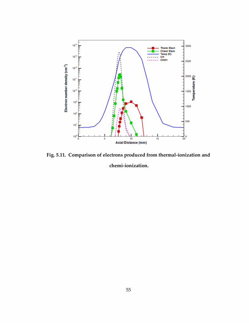
55

Fig. 5.11. Comparison of electrons produced from thermal-ionization and

chemi-ionization.

56

6 Primary nanoparticle charging model

6.1 Theory and Objective

Particles immersed in bipolar ion atmosphere are charged by capture of ions and

electrons due to diffusion even in the absence of external electric field. This is in

contrast to field charging wherein charging takes place when ions travel along the

electric field lines. For diffusion charging the actual number of charges on a particle

undergoing diffusion charging is approximately proportional to the particle diameter.

Diffusion charging is one of the primary mechanism to charge submicron particles in

any plasma system. A particle introduced in a hydrocarbon flame will also charge

due to bipolar diffusion as in the plasma containing both ions and electrons. Ions and

electrons collide with particles randomly and deposit a net charge on the particles.

Due to the random nature of charge transfer particles charged unequally but there is

a distribution of net charge on particles.

The purpose of this study is to analyze the interaction between ions, electrons and

nanoparticles in a hydrocarbon flame. To achieve this, a basic model was developed

that describes the physics governing the charge formation on a spherical nanoparticle

as well as its effect on the population of ions and electrons and vice versa in oxygen

enriched flames. The model includes diffusion charging and charging of a

nanoparticle from thermal ionization in the presence of ions and electrons produced

in a flame from chemi-ionziation. In order to validate the model the numerical results

under certain conditions were compared to the available experimental and numerical

results from the literature.

57

6.2 Chemi-ionization model

Electrons and numerous types of ions are observed in a flame (Prager et al., 2007;

Savel’ev, 2012) such as CHO+, C3H3+, H3O+, C2H3O+, CHO-, O-, O2

- and many more

depending on the type of the flame, equivalence ratio for premixed flame and the

mixture composition. Ions and electrons are generally produced first by the chemi-

ionization reaction which is the primary source of ions and electrons in a flame

(Calcote). To understand the formation of ions and electrons in hydrocarbon flames

many complex chemical mechanisms have been proposed (Prager et al., 2007; Starik

et al., 2002; Pedersen et al.; 1993). The composition of ions and electrons in the

diffusion flame strongly depends on the oxygen content of the flame.

The chemi-ionization reaction that produces the first set of charged species followed

by neutral-charged reactions and charged-charged reactions to generate more ions

and electrons is

CH O CHO e (6.1)

It is shown (Goodings et al., 1979; Prager et al., 2007) that the major ions produced in

a methane-oxygen flame are CHO , 3H O

, 2 3C H O

, 5CH OH

,OH , 2O

,O and 3CO

.

Amongst these ions, hydronium 3H O

represents 90% of the population of ions.

Hence, in order to simplify the chemistry for our model we can consider the average

ionic molecular mass to be that of the hydronium ion and neglect the negative ion

population other than the electrons. Also, since reaction (6.1) produces the initial set

of ions and electrons we can assume the net rate of ion and electron formation to be

equal to the rate of reaction (6.1).

58

The rate, k at which the ions and electrons are produced is given by the following

Arrhenius equation

expn a

u

Ek BT

R T

(6.2)

where B is the pre-exponential factor, T is the temperature, n is between 0 and 1, Ea is

the activation energy and Ru is the universal gas constant. These parameters for

chemi-ionization reaction (1) are taken from Prager et al. (2007). The ions and

electrons recombine to reach a steady state in a combustion system with a rater

k .

Hence the overall rates of formation e

and for electrons and ions respectively are

given by

e IR r ek N N

(6.3)

where IR

k CH O is the chemi-ionization rate, Ne is the concentration of

electrons, N+ is the concentration of ions, and kr is the effective recombination rate

describing electron and ion losses in flame. kr is obtained from Prager et al. (2007) and

Goodings et al. (1979) by using known quantities of Ne, N+ , concentrations of CH and

O and plugging them in Eq. (6.3) by substituting e

= 0. The calculated values of kr lie

between 16 3 14.5 10 cm mol s and 16 3 18 10 cm mol s for temperatures ranging from 1000

K and 3000 K respectively which is falls within range for the recombination rate for

the reaction 3 2H O e H O H (Prager et al., 2007).

Propensity of a nanoparticle-free flame to form ions and electrons through chemi-

ionization can be characterized by a steady state concentrations of ions and electrons,

( )e chemiN and ( )chemi

N

. In a nanoparticle free flame (Np = 0) Ne is equal to N+ and

59

Ne=Ne(chemi)=N+(chemi). Electron concentration ( )e chemiN can be used as a parameter in Eq.

(6.3) modifying it to the following form:

2

( )e r e chemi ek N N N

(6.4)

The effect of chemi-ionization on nanoparticle charging is further analyzed using the

chemi-electron concentration in a nanoparticle-free flame as the model parameter.

The ratio of total nanoparticle concentration to chemi-electron concentration at

nanoparticle-free flame serves as another parameter which is given by(chemi)

p

e

N

N .

Electrons are mainly produced from the chemi-ionization reaction (6.1) which is

basically a thermoneutral reaction (Calcote, 1957). Hence the production of electrons

is governed by the product of concentrations of CH and O only. The temperature in

the flame is strongly dependent on the oxygen content relative to the nitrogen content

and independent of the charged species concentration (Merchan-Merchan et al., 2003;

Prager et al., 2007). Therefore, the effect of chemi-electron concentration and

temperature on charging can be analyzed independently.

6.3 Bipolar diffusion charging model

The rate at which the particles capture the ions or the electrons depends strongly on

the mobility of the particles and the ion-particle or the electron particle Coulombic

forces which could be attractive or repulsive depending on the nature of the potential

difference between the ion or the electron and the particle. Van der Waals forces may

also be important for particles less than 10 nm in diameter. Irrespective of the initial

60

charge a time dependent charge distribution is eventually reached within the particle

after a characteristic time. When particles are more than 40 nm in diameter the

characteristic charge that they acquire is practically independent of the material

properties and is only a strong function of particle size and morphology. It is very

difficult to determine the rate at which ions or electrons attach to the particles

experimentally hence a number of models have been put forth to describe the same.

The traditional models describing charging can be split into three parts. The first one

is the Boltzmann charge distribution which is the extension of the equilibrium gas

kinetic theory, the second being a steady state model formulated for the continuum

region and the third one formulated for the free-molecular region. For nanoparticles

in atmospheric flames the characteristic length is very small as compared to the mean

free path, hence we consider the model for the free-molecular regime.

In a combustion system with no external applied electric field the thermal velocity

exceeds the drift velocity tremendously, hence it would be reasonable to assume the

drift velocity to be negligible as compared to the thermal velocity.

The flame has ions and electrons moving randomly and freely depending on their

individual temperatures and mass. We can assume that a nanoparticle introduced in

a chemically reacting ionized gas gets hit by ions and electrons from all directions and

gets captured or attached to the nanoparticle. Hence, we can put forth the following

equation for the rate at which rate at which electrons diffuse and attach to the

nanoparticles with charge z and radius a

( , )4

e ez A e e

vz a S N (6.5)

61

where e

v is the thermal velocity of the electrons,e

N is the number density of the

electrons, A

S is the surface area of the nanoparticle and e

is the electrostatic

interaction coefficient given by Orbital motion limited (OML) theory (Zobnin et al.,

2000) for submicron and nanoparticles:

2

0

exp 0 4

1 0

e b

zez

k Ta

z

(6.6)

And the thermal velocity of the electrons is given by the kinetic theory as

1

28b

e

e

k Tv

m

(6.7)

The rate at which ions diffuse and attach to the nanoparticles with charge z and

radius a is given by

( , )4z A

vz a S N

(6.8)

From the kinetic theory, the average thermal velocity of ions is given by

1

28b

k Tv

m

(6.9)

where me and m+ are the respective masses of electrons and ions.

62

6.4 Thermal-ionization model

Most of the ions and electrons in a flame appear due to chemi-ionization. But when

particles are introduced in a flame they can affect the charged species concentration

in the flame due to multiple processes. One of the ways it can be affected is thermal-

ionization. The rate at which electrons escape from the particles due to thermal-

ionization is strongly material dependent. The rate at which electrons are emitted

from a material surface is given by the modified Richard-Dushmann equation (Sodha

& Guha, 1971) for small particles:

2

2 2

2

0 0

-exp z < 0

( , )1 11

1 exp - z 04 4

A

b

z

A

b b

S ATk T

a zz e z e

S ATak T k T a

(6.10)

where SA is the surface area, A is the material dependent constant, φ is the work

function of that material, kb is the Boltzmann’s constant, ε0 is the vacuum permittivity

and e is the elementary charge.

In our model thermal ionization was not considered to be in equilibrium but treated

kinetically. The terms A and φ are taken from the literature for graphite (Jain et al.,

1952) except in Section 7.4.2.1 where φ is varied depending on the material. The work-

function φ corresponds to the minimum amount of energy needed by an electron to

overcome the barrier and escape the surface of the material. Also, the larger is the

particle, the easier is to thermally ionize it.

63

6.5 Model formulation and validation

Most of the modeling studies on charging of nanoparticles till now have been

performed in a low to mid temperature plasma and flame environment and do not

consider the effect of ions and electrons produced at oxygen enriched flame

conditions on charging of the particles. Due to the production of ions and electrons

in the flame in a high temperature environment we take into account charging due to

diffusion, thermal ionization and chemi-ionization in the model. Since ions, electrons

and nanoparticles occur simultaneously in a flame; their respective concentrations are

influenced by each other until they reach a steady state, as shown in Fig. 6.1. The time

required to reach a steady state depends on factors like temperature, total

nanoparticle concentration, nanoparticle size and chemi-ionization conditions.

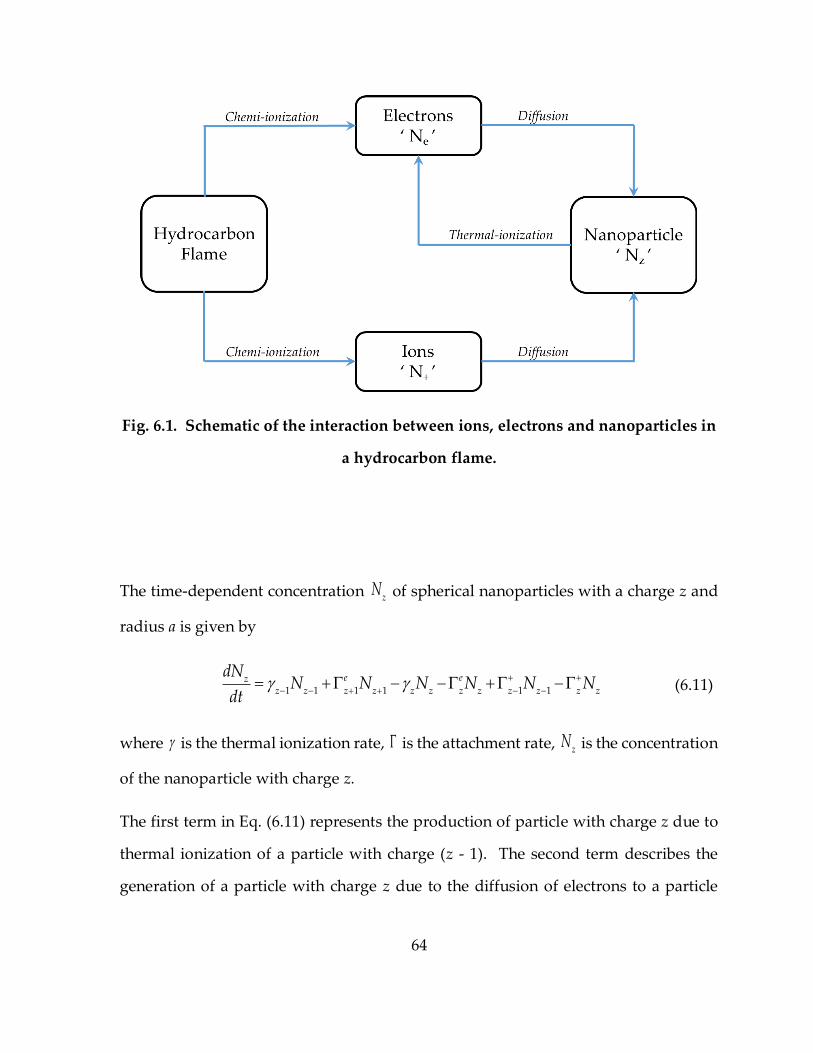
64

Fig. 6.1. Schematic of the interaction between ions, electrons and nanoparticles in

a hydrocarbon flame.

The time-dependent concentration zN of spherical nanoparticles with a charge z and

radius a is given by

1 1 1 1 1 1

e ezz z z z z z z z z z z z

dNN N N N N N

dt

(6.11)

where is the thermal ionization rate, is the attachment rate, zN is the concentration

of the nanoparticle with charge z.

The first term in Eq. (6.11) represents the production of particle with charge z due to

thermal ionization of a particle with charge (z - 1). The second term describes the

generation of a particle with charge z due to the diffusion of electrons to a particle

65

with charge (z + 1). The third term denotes the loss of a nanoparticle with charge z

due to thermal ionization of a particle with charge z. The fourth term indicates again

the loss of the particle with charge z due to diffusion of electrons to the same. The

fifth and the six terms are responsible for the increase and decrease of the charged

nanoparticle due to the diffusion of positive ions to a nanoparticle with charges (z - 1)

and z respectively.

The time evolution of electron and ion number density in a flame environment is

given by

ee

e z z z zz z

dNN N

dt

(6.12)

z zz

dNN

dt

(6.13)

Where eN and N

are the electron and ion concentrations respectively.

The first term in Eqs. (6.12, 6.13) describe the net generation or consumption of

electrons and ions due to chemi-ionization and volumetric recombination. The

second term in Eq. (6.12) denotes the emission of electrons from thermal-ionization.

The third term and the second term of Eqs. (6.12) and (6.13), respectively, represent

the loss of electrons and ions due to diffusion and recombination of charged species

to the nanoparticles with charge z.

Due to the interactions of ions, electrons and nanoparticles Eqs. (6.12-6.13) are

integrated over time. The numerical scheme implemented is forward difference Euler

method as shown in Appendix A. Since Eq. (6.11) describes particles with a charge z

66

which theoretically ranges from - ∞ to + ∞, practically to consider z varying between

– q to + q, the total number of equations that need to be solved are (2 q + 1) for the

nanoparticles and in addition one equation for ions and one equation for electrons.

The average charge carried by the particles is given by

zz

z f z

(6.14)

Here, zf is the fraction of the particle with charge z and ( / )

z z pf N N with p

N being

the total particle concentration. The initial conditions (t = 0) used to solve the system

of differential equations are

0 0, 0 , 0, 0.z z p e

N z N z N N N

(6.15)

There have been few experimental studies performed (Homann & Wolf, 1983) on

evaluating the characteristic charge on soot particles in laboratory flames. To validate

our model we use the limited experimental data available as well as a numerical study

of Balthasar et al. (2002). The experimental data of Homann & Wolf (1983) were

generated by measuring soot sizes and charges on primary soot particles in premixed

C2H2 and C6H6 flames. By using the experimental total nanoparticle concentration

and soot volume fraction we can calculate the particle diameter by the relationship

31

6v p pf N d , where fv is the soot volume fraction which in turn is used in our model

to predict the percentage charged particle distribution at different distances from the

burner, as shown in Fig. 6.2. It can be seen that the relative charged particle

distribution predicted by the model is in a reasonably good agreement with the

experimental results.

67

Fig. 6.2. Comparison of relative soot volume fraction: experimental results by

Homann and Wolf (1983) (symbols), computed (solid lines) and model by

Balthasar et al. (2002) (dashed lines).

The model of Balthasar et al. (2002) under predicts the charged particle distributions,

possibly because it does not include the ions and electrons produced due to chemi-

ionization and hence the additional effect of diffusion charging is not accounted for.

Results for the fraction of charged particles as a function of particle diameter were

also compared with the modeling results from Balthasar et al. (2002) (Fig. 6.3) and it

was found that the results compare well with the previous modeling results.

68

(a) (b)

Fig. 6.3. Comparison of relative number density: our modeling results (solid

lines) and model by Balthasar et al. (2002) (dashed lines) (a) negatively charged

particles (b) positively charged particles.

69

7 Results of the primary nanoparticle charging

model

Before considering the model comprehensively, the model was first simplified to

analyze the contributions of different processes to the particle charging.

7.1 Fixed ion and electron concentration

Let us first study the problem by keeping the net ion and electron concentration fixed

at 1015 m-3. In reality the electron and ion concentrations will be affected by particles

in the system but in this section we are assuming a fictitious possibility where the

electron and ion concentration can be held constant irrespective of the temperature,

nanoparticle concentration or particle diameter. From Fig. 7.1. we can see that 1000 K

the particles are equally charged irrespective of and the average charge is

approximately 4 electron charges. But as the temperature is increased to 2000 K and

even further to 3000 K, particles convey different behavior for different values of .

At 2000 K and = 0.1, each particle has ~100 electron charges.

70

(a)

(b) (c)

Fig. 7.1. Comparison of fraction of charged particles for fixed total electron and

ion concentration at (a) 1000 K (b) 2000 K (c) 3000 K.

The particles become negatively charged due to strong diffusion of electrons towards

the nanoparticles in comparison with the heavy ions. As is increased to 100 the

particles become electron deficient and hence the particles become more positively

71

charged due to the combined effect of thermal ionization and positive ions attaching

to the particles. At 3000 K and =100, the thermal ionization becomes the dominant

charging process and the thermal ionization rate increases rapidly to make the

particles strongly positively charged. Even for = 0.01 the particles are positively

charged because at such high flame temperatures the diffusion of electrons towards

the particles is practically switched off in relation to thermal ionization.

7.2 Zero chemi-ionization

By turning off the source of ions and electrons from chemi-ionization in the model we

can evaluate the individual effect of thermal-ionization on the charging of particles,

as shown in Fig. 7.2. For fixed Np=1015 m-3 ,when the temperature is 1000 K, the energy

acquired by the electrons is not enough to escape from the material surface and hence

the thermal ionization rate is zero. Because of this the electrons do not escape from

the surface to diffuse towards the particles thus leaving them uncharged. But as the

temperature rises to 2000 K some of the electrons acquire energy sufficient for escape

from the surface and attaching to small number of particles. Hence in this case about

an equal percentage of particles are positively and negatively charged, the remaining

30% of the particles are left uncharged.

But as the temperature is increased to 3000 K, the thermal ionization rate increases

exponentially making all the particles positively charged with a mean charge of +13.

The electrons are emitted from the particles at a high rate. As a result an equilibrium

is reached between highly positive charged particles and the free electrons.

72

Fig. 7.2. Comparison of fraction of charged particles for zero chemi-ionziation.

7.3 Negligible thermal-ionization

To analyze the influence of chemi-ionization we will neglect the thermal ionization

terms in the model and keep the nanoparticle concentration fixed at 1015 m-3. In Fig.

7.3, the distribution of charges on particles is compared at different temperatures as

well as different nanoparticle concentrations to electrons produced from chemi-

ionization (η) by assuming the thermal ionization rate equal to zero. In Figs. 7.3 (a-c)

we can see that at η = 100, the particles get charged negligibly. As η is decreased to 1,

particles get negatively charged, the effect becoming more pronounced with

temperature. The reason being, as the temperature is increased the thermal velocity

of the electrons is increased. As a result, more electrons are deposited on the particles

73

due to the additional kinetic energy available to overcome the electrostatic barrier.

We see the particles get more negatively charged when η is equal to 0.01 because of

the excess of electrons available in the flame environment.

Even though there is an equal number of ions and electrons considered in the model,

the particles become negatively charged. This is because the mass of the hydronium

molecule is 3.4 ∙104 times the mass of an electron, the thermal velocity of the electrons

is more than 180 times that of the ions. Hence, the probability of an electron attaching

to the particles is 180 times higher to that of an electron making them only negatively

charged.

74

Fig. 7.3. Comparison of distribution of charged particles for zero thermal -

ionization at (a) 1000 K (b) 2000 K (c) 3000 K for a fixed Np=1015 m-3.

75

7.4 Ions and electrons interacting with charged

particles

7.4.1 Charged particle distribution

Particles produced or introduced in a flame undergo bipolar charging due to quasi-

neutrality of the flame. Depending on the temperature, the bipolar environment and

the nanoparticle concentration the charge distribution would vary, as shown in Fig.

7.4. At 1000 K, for a fixed Ne(chemi)=1015 m-3, the particles assume strong negative

charges but the effect is opposite when the temperatures is increased to 3000 K. The

physics behind the charging mechanism can be better understood by using average

charge instead as given by Eq. (6.14). Hence, so forth instead of charge distribution,

average charge at different conditions will be presented.

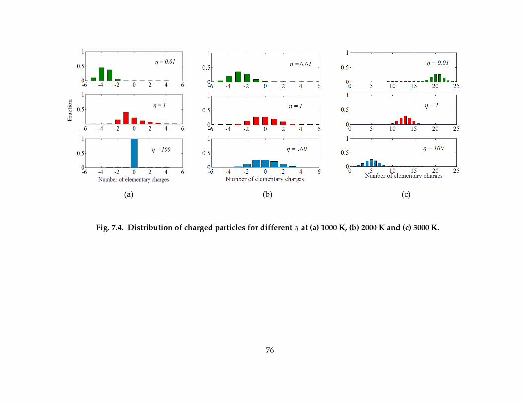
76

(a) (b) (c)

Fig. 7.4. Distribution of charged particles for different at (a) 1000 K, (b) 2000 K and (c) 3000 K.

77

7.4.2 Average particle charge

7.4.2.1 Effect of work function

The work function of the material has a strong influence on the charging of the

particles especially at high temperatures. The higher the work function, the more

difficult it becomes for electrons to escape the material and hence the particles become

less positively charged. Figure 7.5 shows the variation of fraction of charged particles

for graphite, molybdenum oxide (MoO3) and titanium oxide (TiO2) which are amongst

the common nanomaterials synthesized in flames.

Fig. 7.5. Charge distributions for the nanoparticles of TiO2, MoO3, and graphite

introduced in the flame environment with T = 3000 K and Ne(chemi) = 0.

78

The results are calculated by turning chemi-ionization off at 3000 K which is also a

temperature encountered in a flame environment when the oxygen content is very

high. The particle diameter used is 20 nm and the total nanoparticle concentration is

1015 m-3. Even a relatively small increase in work function from 4.85 eV to 5.2 eV

causes the nanoparticle to become less positively charged and the peak to move from

+5 to +3. Figure 7.6 represents the variation of average charge formed on the particle

versus the material work function. The work function of nanomaterials for flame

synthesis generally ranges from 4 eV to 7 eV. At 3000 K, as the work function increases

from 4 eV to 7 eV the average charge deposited on the particle decreases from +10 to

0 respectively. As an example, for φ =4 eV, the average nanoparticle charge varies

from +1 to +23 for 2000 K to 4000 K respectively. This shows as the temperature is

lowered thermal ionization becomes less influential and it will be shown later that

effect of charging due to diffusion becomes important.

79

Fig. 7.6. Comparison of average charge carried by a 20 nm spherical particle at

different temperatures.

7.4.2.2 Effect of temperature

Effect of temperature on nanoparticle charging has generally been ignored since most

of the work done in the past has usually been in low temperature environment and

also the work done for combustion studies have been limited to 2100 K (Savel’ev &

Starik, 2006). But in oxy-fuel flames the temperatures could reach more than 3000 K

where thermal ionization becomes very important, as shown in Fig. 7.7. When the

number of nanoparticles equals that of the electrons in a given volume the electrons

and ions attach to the nanoparticles creating a net zero charge until about 2100 K when

the thermal-ionization gets triggered creating a net positive charge on the particle.

80

When 0.01 , the diffusion charging and thermal ionization effect are more

pronounced. At very low temperature diffusion charging is weak hence the net

charge is close to 0, as shown in Figs. 7.4(a) and 7.7. The net charge formed on a

nanoparticle at 1000 K and 2000K are close to zero but in case at 1000 K most of the

particles stay neutral but at 2000 K almost equal number of particles acquire positive

and negative charge and some stay neutral, as shown in Fig. 7.4(a). But as the

temperature is increased the thermal velocity of electrons increases and they flow

towards the nanoparticles creating a net negative charge. Ions do not have a strong

effect on charging as compared to the electrons because of their much higher mass

and hence much lower thermal velocities. The negative charging increases as the

temperature increases until the temperatures become high enough to thermally ionize

the nanoparticles and make them strongly positively charged. At 100 the

environment around nanoparticles becomes electron deficient and hence the charging

due to diffusion from chemi-ions and electrons becomes negligible. But as the

temperature is increased the nano-particles themselves become highly positively

charged and increase the net free electron concentration as will be discussed later.

81

Fig. 7.7. Comparison of average charge accumulated on a 20 nm particle as a

function of temperature with 15 3

( )10

e chemiN m at 3 different .

7.4.2.3 Chemi-ionization

The electrons and ions formed in a flame by chemi-ionization create a bipolar

environment for nanoparticles because the total ion and electron population are

generally equal. The local peak concentration of ions and electrons produced in the

flame generally is of the order of 1016 m-3 depending on the type of the flame, the fuel

and oxidizer, the temperature, pressure and the local flame chemistry (Cancian et al.,

2013; Goodings et al., 1979). At temperatures up to 2000 K the average nanoparticle

82

charge is zero and at 3000 K the average charge is highly positive ~ +13, until Ne(chemi)

=1015 m-3, as shown in Fig. 7.8. The total nanoparticle concentration is fixed at

1015 m-3. As that ratio decreases with the increase in chemi-ions and electron

concentration the electron flux towards the nanoparticle increases because the

number of available electrons increase and due to that the net charge formed on the

particle becomes less positive and more negative.

Fig. 7.8 Comparison of average charge formed on a 20 nm particle versus

electrons and ions formed per unit volume by chemi-ionization at three different

temperatures with 15 310p

N m .

83

As the temperature is increased that effect is even more pronounced because of the

increase in electron thermal velocity and reduced effect of thermal ionization due to

decrease in nanoparticle population relative to chemi-ions and chemi-electrons. Also

it is evident, for temperatures 1000 K and 2000 K the average nanoparticle charge

increases between 0.01 1 . For 3000 K it starts to decrease when 1 .

7.4.2.4 Effect of nanoparticle concentration

The amount of soot produced in the flame changes rapidly from 21 % - 100 % O2. In

the study performed on methane-oxygen oxy-fuel flames by Beltrame et al., 2001 it is

evident from that increasing in oxygen content from 21 % to 100 % the soot volume

fraction increases approximately from 0.03 ppmv to 0.3 ppmv respectively which

corresponds to a particle density of ~1021 m-3 for a particle diameter of about 20 nm.

In premixed flames the soot concentration also has a wide range varying from 0 to

1017 m-3. Depending on the amount of nanoparticles per unit volume the charging

time and the distribution of charges would strongly vary.

As expected, at low to mid-range temperatures, i.e. 1000 K and 2000 K, the particles

become strongly negatively charged with an average charge of about -3.5 and at 3000

K the particles are highly positively charged (Fig. 7.9.). The average charge increases

between 0.01 1 for 1000 K and 2000 K but for 3000 K the charge decreases to zero

when the pN ~ 1019 m-3. Hence from Figs. 7.8 and 7.9 we can say that the charging of a

particle at a fixed diameter not only depends on the but also on the absolute value

of pN .

84

Fig. 7.9. Comparison of average charge formed on a 20 nm particle as a function of

total nanoparticle concentration for a fixed 15 3

( )10

e chemiN m .

7.4.2.5 Effect of particle diameter

Primary soot particles have a spherical structure and they generally vary between 10

and 20 nm depending on the nature of the flame (Merchan-Merchan et al., 2003). But

inorganic nanoparticles for flame synthesis can be as large 60 nm (Sahu et al., 2012).

At 1000 K and 2000 K with fixed nanoparticle (1015 m-3) and chemi-electron

concentrations (1015 m-3), the particles are weakly negative as shown in Fig. 7.10 and

85

the average charge formed is close to zero irrespective of the particle diameter. Figure

7.10 (b) indicates that at 1000 K and 2000 K, for low particle diameters, as the diameter

is increased the particles become more and more negatively charged. But after a

certain diameter the average charge slowly becomes close to zero with an increase in

diameter. At 3000 K, with increasing size and hence the surface area, more electrons

escape the potential barrier due to accelerated thermal ionization rates at those

temperatures making the particles strongly positive. At this temperature, the average

number of elementary charges formed on a 20 nm particle is ~ +13 and that on a 70

nm particle is ~ +38.

86

(a) (b)

(c)

Fig. 7.10. Comparison of (a) average charge at 1000 K and 3000 K (b) average

charge at 1000 K and 2000 K (c) distribution of charges formed on a particle as a

function for 20 nm and 60 nm particle and 1 .

dp

= 2

0 n

m

dp

= 6

0 n

m

87

7.4.3 Electron concentration

7.4.3.1 Temperature

Depending on the local temperature in a flame an electron will either attach to the

particle or be released due to thermal ionization. The effect of thermal ionization and

diffusion charging is more pronounced when the ratio of the total nanoparticle

concentration to that of chemi-electron concentration is higher, as shown in Fig. 7.11.

At >>1 most of the electrons available from chemi-ionization attach to the

nanoparticles via diffusion charging at low temperatures reducing the net electron

concentration but as the temperature is increased the particles start emitting electrons

and increase the number of electrons in a given volume.

As the above ratio decreases the effect of thermal ionization and diffusion charging

on net electron concentration reduces and therefore the change in net electron

concentration also decreases. Due to that when << 1 the net electron concentration

becomes equal to the chemi-electron concentration. At 1000 K, for low chemi-electron

concentration with the total nanoparticle concentration fixed at 1015 m-3, the net

electron concentration decreases because of much higher rate of attachment of

electrons making the particles negatively charged, as shown in Fig. 7.12. For the same

temperature at higher chemi-electron concentrations the net electron concentration

becomes equal to the chemi-electron concentration. For higher temperature such as

3000 K the net electron concentration exceeds the chemi-electron concentration due to

thermal ionization until ≈1.

88

Fig. 7.11. Electron concentration as a function of temperature for 15 3

( )10

e chemiN m

89

Fig. 7.12. Electron concentration as a function of electrons produced by chemi-

ionization at 15 310p

N m .

When < 0.1 nanoparticle concentration has a negligible influence on the net electron

concentration for all temperatures because the nanoparticle density isn’t high enough

for thermal ionization to have a strong effect to produce free electrons and electron

consumption from diffusion to reduce the electron concentration. As > 0.1, degree

of chemi-ionization has a great impact on net electron concentration depending on the

temperature, as shown in Fig. 7.13. At 1000 K, relatively negligible amount of free

electrons remain because most of them attach to the nanoparticles. As the

90

temperature is increased to 2000 K the ratio between thermal ionization rate and

diffusion rate approach to 1 and hence there is a small change in free electron

concentration as compared to that at 1000 K. With further rise in temperature to 3000

K the nanoparticles become thermally ionized for a large quantity of electrons to

escape as the particle concentration increases. But when ≈ 1000, the system reaches

an equilibrium for net electron concentration to reach a constant value of ~ 183 10 m-3.

Fig. 7.13. Electron concentration as a function of total particle concentration at

15 3

( )10

e chemiN m .

91

For fixed nanoparticle and chemi-electron concentration (1015 m-3), from Figs. 7.10 and

7.14 it can be seen that as the particle diameter increases electrons diffuse towards the

particles at low temperatures making them weakly negatively charged. However as

the temperature is increased to 3000 K, due to strong thermal-ionization effect

particles emits large quantities of electrons ~ 162 10 m-3 making them strongly

positive.

Fig. 7.14. Electron concentration as a function of particle diameter for

15 3

( )10

p e chemiN N m .

92

7.4.4 Ion concentration

From Eq. (6.13), we can see that unlike electrons which are generated from chemi-

ionization as well from the nanoparticles, ions are only formed in the flame. So

diffusion charging and chemi-ionization are the processes which determine ion

production and recombination with the nanoparticles. As expected, when the

nanoparticle concentration is very less as compared to the chemi-electron or chemi-

ion concentration there little or no change in the net ion concentration when the

temperature is varied, as shown in Fig. 7.15(a). But as the nanoparticle concentration

is increased relative to the fixed chemi-electron concentration, the nanoparticles act

like a sink and ions attach to them decreasing the net ion concentration.

(a) (b)

Fig. 7.15. Ion concentration as a function of (a) temperature for a fixed

15 3

( )10

e chemiN m (b) electrons from chemi-ionization for a fixed 15 310

pN m .

93

As the temperature is increased from around 600 K to about 2000 K the electrons

accelerate due to increase in thermal velocity and hence they create a potential barrier

in order for more ions or electron to deposit on the surface. As the temperature is

increased further the ion concentration reduces further because of increase in thermal

ion velocity and hence depositing more on the particle surface. According to Eq. (6.9),

the thermal velocity of ions has an influence at much higher temperatures as

compared to electrons because of the heavier mass of electrons. This effect is also seen

in Figs. 7.15(b) and 7.16(a) for low chemi-electron concentration as compared to

nanoparticle concentration. At 3000 K, more ions are consumed as compared at 1000

K and 2000 K. When < 1, the ion concentration stays unaffected and it is equal to

the chemi-ion concentration due to negligible attachment of ions towards the

nanoparticles. Without changing other conditions, increase in the particle diameter

causes decrease in ion concentration, as shown in Fig. 7.16(b). This is because with

increase in surface area, the number of ions that can attach to a particle significantly

increase causing the particles positively charged.

94

(a) (b)

Fig. 7.16. Ion concentration as a function of (a) total particle concentration fixed

15 3

( )10

e chemiN m and (b) particle diameter for 15 3

( )10

p e chemiN N m .

95

8 Nanoparticle agglomerates charging model

8.1 Theory

In combustion or plasma systems, nanoparticles generally appear not only as

separated primary particles but also as agglomerates which in the simplest form are

primary particles attached together. In hydrocarbon flames, soot particles are first

formed in the form of 5-10 nm primary particles from the reactive coagulation of PAH

molecules (Megaridis and Dobbins, 1989). After that, due to coalescence, coagulation

and surface growth the particles grow and become bigger. The spherical particles

thus formed can attach together to form agglomerates that are open structures like

linear chain or more closed structures like fractal morphology. The number of

primary particles per agglomerate can range anywhere from 2 to 10,000. When an

agglomerate is introduced in a bipolar ionic environment, the nature of the charge

acquired by the agglomerate as a whole is quite different from that of the primary

particles. Shin et al. (2010) showed that compact particles with high fractal dimension

had a lower charge as compared with particles with low fractal dimension and same

mobility diameter. This is because the electrical capacitance of agglomerates

decreases as its structure goes from open and straight chain like structure to a more

closed and branched chain like structure. Hence usually the characteristic charge of

a chain like structure is usually more than charges acquired by branched chain

agglomerates. In special cases, it has been shown that agglomerates with low fractal

values acquire more charges than spheres when charged using a photoelectric source

(Shin et al., 2010).

96

The objective of this study is to formulate a model and analyze the model to predict

the effect of number of particles per agglomerate on charging behavior for straight

chain and fractal (branched chain) particles with an aspect ratio of 1.6. The structure

of the two types of agglomerates is shown in Fig. 8.1.

(a) (b)

Fig. 8.1. Schematic of (a) straight chain (b) branched chain agglomerates.

8.2 Modifications to the primary nanoparticle charging

model

There have been a number of theories put forward to describe the charging of

agglomerates made of arbitrary and spherical shaped particles. Lafromboise and

Chang (1977) created a model to evaluate the charging efficiency of arbitrary shaped

particles. One of the most classical theories was put forth by Chang (1981) who

97

proposed a model for the mean charge for agglomerates. Chang and Yeh (1981)

proposed a model for the equilibrium bipolar charge distribution on straight chain

like agglomerates. Charging equivalent diameter was first put forth by Wen et al.

(1984 a). Filippov (1993) showed using charge balance equations that the correct way

to treat the charging of agglomerates is to use the modified Boltzmann solution

instead of the standard Boltzmann law. There have been no comprehensive theories

or models on agglomerate charging in a high temperature oxy-fuel environment.

The primary difference between the primary particles and the agglomerate particles

is the difference in the electrical capacitance between the two. As the number of

particles per agglomerate increases the capacity of the primary particles to store

charge decreases because of the increase in electrostatic interaction between the two

particles in the agglomerate. More open-like the structure, higher is the electrical

capacitance of the agglomerate as compared to the closed-like structures. Hence we

replace the conventional capacitance term by the one modified for agglomerates

depending whether the agglomerate is straight chain or branched chain. We use the

following capacitance ‘C’ terms as experimentally measured by Shin et al. (2010).

0.7692

00.5789 4

AC N a (straight chain with β=1.0) (8.1)

0.7874

00.4703 4

AC N a (branched chain with β=1.6) (8.2)

Also, 12 300A

N

Where NA is the number of primary particles in one agglomerate and β is fractal

dimension of the fractal agglomerate. The remaining parameters can be referred from

Chapter 6.

98

Figure 8.2 shows the difference in normalized capacitance of the two type of

agglomerates. It is clear that the capacitance of particles in an agglomerate is much

lower than that of a particle suspended freely and the capacitance of straight chain

particle is 10% - 15% higher than that of a branched chain agglomerate depending on

N.

Fig. 8.2. Comparison of capacitance of straight and branched chain normalized by

capacitance of primary particles.

Also if we neglect necking in the agglomerates then we can assume the surface area

of the aggregate Agg A AS N S . Applying these changes to Eqs. (6.5 – 6.11) we can

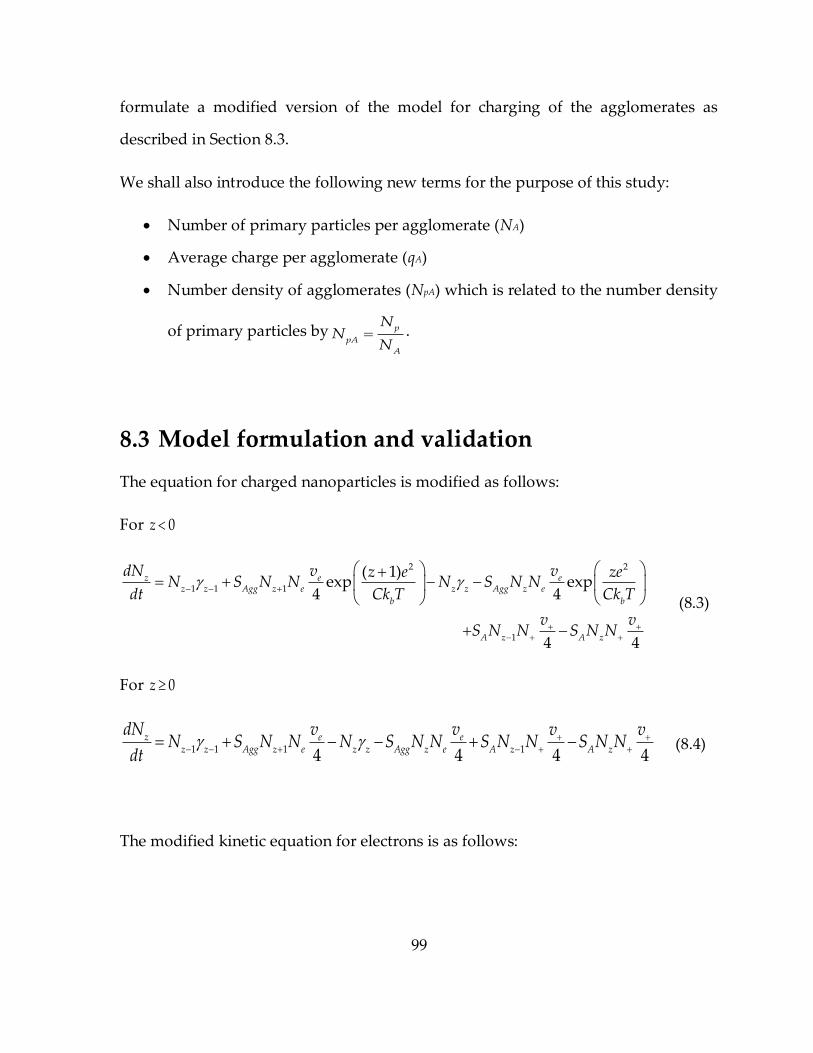
99

formulate a modified version of the model for charging of the agglomerates as

described in Section 8.3.

We shall also introduce the following new terms for the purpose of this study:

Number of primary particles per agglomerate (NA)

Average charge per agglomerate (qA)

Number density of agglomerates (NpA) which is related to the number density

of primary particles by p

pA

A

NN

N .

8.3 Model formulation and validation

The equation for charged nanoparticles is modified as follows:

For 0z

2 2

1 1 1

1

( 1)exp exp

4 4

4 4

z e ez z Agg z e z z Agg z e

b b

A z A z

dN v vz e zeN S N N N S N N

dt Ck T Ck T

v vS N N S N N

(8.3)

For 0z

1 1 1 14 4 4 4z e e

z z Agg z e z z Agg z e A z A z

dN v v v vN S N N N S N N S N N S N N

dt

(8.4)

The modified kinetic equation for electrons is as follows:

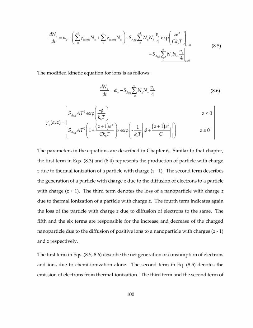
100

21 1

( 0) ( 0)0

0

0 0

exp4

4

e ee z z z z Agg z e

bz

eAgg z e

z

dN v zeN N S N N

dt Ck T

vS N N

(8.5)

The modified kinetic equation for ions is as follows:

4Agg z

dN vS N N

dt

(8.6)

2

2 2

2

-exp z < 0

( , )1 11

1 exp - z 0

Agg

b

z

Agg

b b

S ATk T

a zz e z e

S ATCk T k T C

The parameters in the equations are described in Chapter 6. Similar to that chapter,

the first term in Eqs. (8.3) and (8.4) represents the production of particle with charge

z due to thermal ionization of a particle with charge (z - 1). The second term describes

the generation of a particle with charge z due to the diffusion of electrons to a particle

with charge (z + 1). The third term denotes the loss of a nanoparticle with charge z

due to thermal ionization of a particle with charge z. The fourth term indicates again

the loss of the particle with charge z due to diffusion of electrons to the same. The

fifth and the six terms are responsible for the increase and decrease of the charged

nanoparticle due to the diffusion of positive ions to a nanoparticle with charges (z - 1)

and z respectively.

The first term in Eqs. (8.5, 8.6) describe the net generation or consumption of electrons

and ions due to chemi-ionization alone. The second term in Eq. (8.5) denotes the

emission of electrons from thermal-ionization. The third term and the second term of

101

Eqs. (8.5) and (8.6), respectively, represent the loss of electrons and ions due to

diffusion and recombination of charged species to the nanoparticles with charge z.

Eqs. (6.1 – 6.4), (6.14) and (6.15) apply here as well.

The model thus formulated is validated by comparing the results for average charge

per particle with previous experimental results (Ball and Howard, 1971), as shown in

Fig. 8.3. The conditions used here were Ne(chemi)=1014 m-3, Np=1010 m-3, T= 2100 K and φ =

4.35 eV for soot. The average charge thus calculated shows a similar trend and is

matches to a great degree for larger particles.

Fig. 8.3. Comparison of previous experimental (Ball and Howard, 1971) and

numerical results.

102

8.4 Results of the nanoparticle agglomerates charging

model

8.4.1 Zero chemi-ionization

The model is simplified to analyze the effect of thermal ionization only. Hence, the

chemi-ionization term is neglected. As discussed at Section 7.2, the thermal ionization

is dominant at 3000 K. Hence, the conditions used here are as follows: Np= 1015 m-3, T=

3000 K, dp = 20 nm.

Figure 8.4 shows that the net charge acquired by the agglomerates is higher for the

straight chain structures than the branched chain structures. The difference in charges

acquired become higher as the number of primary particles increases. But the average

charge acquired by per particle decreases with an increase in NA. This is because when

NA increases the electrostatic interaction between the particles increase making them

less and less positively charged. The reason they get positively charged is because at

3000 K, the electrons on the material surface acquire enough energy to escape and

hence the thermal ionization rate is very high. This makes the particles to become

strongly positively charged.

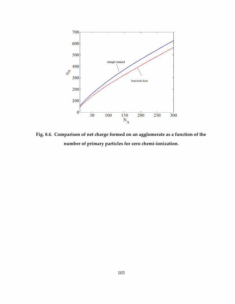
103


number of primary particles for zero chemi-ionization.

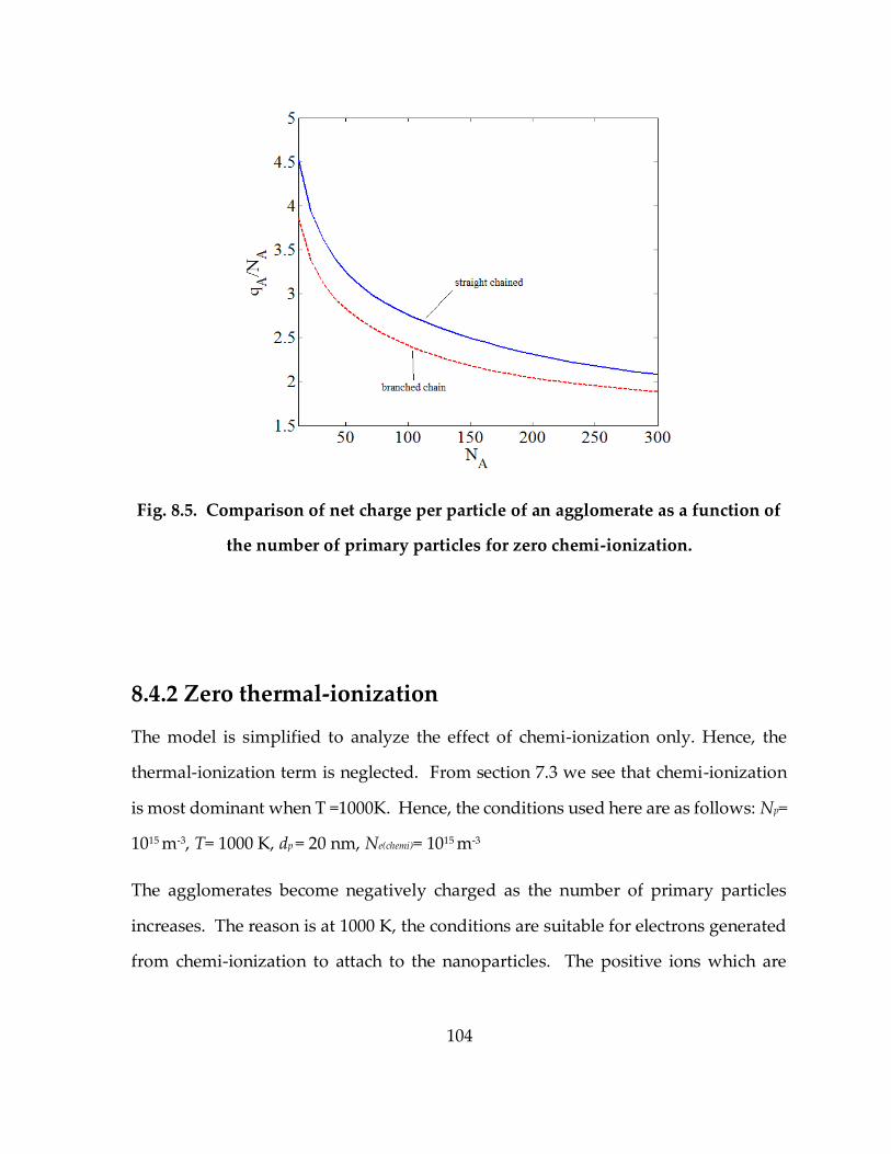
104

Fig. 8.5. Comparison of net charge per particle of an agglomerate as a function of

the number of primary particles for zero chemi-ionization.

8.4.2 Zero thermal-ionization

The model is simplified to analyze the effect of chemi-ionization only. Hence, the

thermal-ionization term is neglected. From section 7.3 we see that chemi-ionization

is most dominant when T =1000K. Hence, the conditions used here are as follows: Np=

1015 m-3, T= 1000 K, dp = 20 nm, Ne(chemi)= 1015 m-3

The agglomerates become negatively charged as the number of primary particles

increases. The reason is at 1000 K, the conditions are suitable for electrons generated

from chemi-ionization to attach to the nanoparticles. The positive ions which are

105

although available in equal number do not attach equally to the particles as their

thermal velocity is much lower than that of the electrons. As a result the agglomerates

are strongly negatively charged.

(a) (b)


number of primary particles for zero thermal-ionization at (a) 1000 K (b) 3000K.

In the case of chemi-ionization the average charge on particle is not highly negative

unlike thermal ionization where the agglomerates and the particles become highly

positive, as shown in Fig. 8.7. The reason being the strong electrostatic repulsion felt

by the particles as the number of particles increases, making the particles weakly

106

negatively charged. As the temperature is increased to 3000 K the agglomerates

become more negatively charged, as shown in Figs. 8.6(b) and 8.7(b).

(a) (b)


number of primary particles for zero thermo-ionization (a) 1000 K (b) 3000K.

8.4.3 Relative charge and effects on ions and electrons

It might be beneficial and more intuitive to express the charging behavior in terms of

charge deposited on a primary particle in an agglomerate relative to that on a single

particle under same conditions i.e. (1)

A

A

q

N q.

107

where, q(1) is the charge deposited on a single particle.

Let see the effect of thermal-ionization only under conditions same as in Section 8.4.1.

Figure 8.8 shows that the relative charge on an agglomerate decreases strongly with

an increase in number of primary particles. It is as low as 15% when the number of

primary particles is 300.


agglomerates with zero chemi-ionization.

108

We also calculate the relative charge when there is no thermal-ionization but only

chemi-ionization as in Fig. 8.9 for conditions same as in Section 8.4.2. We see the

relative charge does not decrease as much as it decreases when there is only thermal-

ionization. Also, there is not a big difference in the charging of straight chain and the

branched chain agglomerates. The electron concentration at 3000 K when there are

no agglomerates but only equal number of singular particles is 3.1018 m-3. When

agglomerates are introduced the particles become highly positively charged but not

as much as the singular particles. Hence less number of electrons are released, as

shown in Fig. 8.9.

Fig. 8.9. Relative electron concentration as a function of number of primary

particles.

109


agglomerates with zero thermal-ionization.

8.4.4 Ions and electrons in equilibrium with charged

agglomerates

8.4.4.1 Effect of primary particle diameter

Size of the primary particle in an agglomerate also has a strong influence on the

charging of the particles since the surface area increases with the size. We study the

effect of diameter on charging under following conditions: Ne(chemi) = 1013 m-3,

Np = 1015 m-3, T = 3000 K.

110

Figure 8.11 shows that as the diameter increases the charge deposited increases

linearly as anticipated. Also, the charge acquired by particles in an agglomerate is

small as compared to that by single particles due to the reduced relative capacitance.

As the number of primary particles in an agglomerate increases the charge acquired

by primary particle decreases.

111

Fig. 8.11. Comparison of charge on a primary particle as a function of particle

diameter for (a) NA= 50 (b) NA= 100 (c) NA= 200 (d) NA= 300.

112

9 Conclusions

The thesis had two major objectives. The first one was to experimentally measure and

numerically model the charged species concentration in a methane-oxygen

counterflow diffusion flame. This part of the effort was primarily to gain a better

understanding of the charged species distribution in a diffusion flame at different

oxygen contents and at different strain rates. This would help in better understanding

of the chemi-ionization processes and the ionic chemistry in diffusion flames and to

predict the charge species concentrations as a function of oxygen contents by using a

simple experimental and a numerical technique.

A model that used a detailed methane-oxygen neutral and ionic chemistry was

analyzed and compared with the experimental results. A traditional Langmuir probe

was modified specifically for high temperature and atmospheric conditions to

generate reasonable volt-ampere characteristics for different conditions to validate the

numerical results. The results proved to be in an appreciable agreement with the

experiments. The numerical results were successfully able to predict the effect of

oxygen and strain rate on electron and ion concentrations. The results showed that

increase in oxygen content has a big impact on peak electron and positive ion

concentration. The peak electron concentration increases as much as by three times

and the peak positive ion concentration increases as much as by four times. The

experiments also validated the fact that strain rate has a small effect on the charged

species concentrations. When the effect of thermal-ionization from major neutral

molecules in the flame at 3000 K was analyzed it was concluded that the number of

electrons emitted from those molecules was negligible as compared to those emitted

113

due to chemi-ionization and hence this effect was not included in the experiments and

the numerical model. It was shown with good agreement between experimental and

numerical results that electrons are the primary negative charge carriers and the

hydronium (H3O+) ions are the major positive charge carriers in the flame. Hence, the

total ion concentration was assumed to be equal to the hydronium ion concentration.

The second part of the thesis proposed and analyzed a numerical model to predict the

charging behavior of spherical and fractal agglomerates and the interaction of the

same with ions and electrons in oxy-fuel flame environment. A set of population

balance equations for nanoparticle charging, ion formation and electron formation are

solved temporally and the steady state solution is used to perform parametric studies

on the charging behavior of the nanoparticles. The model’s significant success was

proved when it was validated not only with previous numerical models but also with

previous experimental results and found to be in good agreement with both. The

model is one of a kind because it includes the three effects i.e. chemi-ionization,

diffusion charging and thermal-ionization in a simplified format. It shows that the

nanoparticle charging is extremely sensitive to material, temperature, nanoparticle

size, degree of chemi-ionization and also the total nanoparticle concentration. It

proved that the particles become highly positively charged at high temperatures in an

oxy-fuel flame environment because of high rate of thermal-ionization. At low

temperatures and the regions where chemi-ionization is dominant the particles

become strongly negatively charged due to the higher mobility of electrons and hence

the high rate of attachment. Also, the total nanoparticle concentration has a big

influence on electrons. Electron concentration increases as much as 105 times at 3000

K with increase in nanoparticle concentration from 108 to 1019 m-3 while at 1000 K

114

electrons almost get consumed with nanoparticle addition. Ion concentration

decreases strongly with nanoparticle concentration irrespective of the temperature

unlike the electrons. Another big accomplishment made by the model was to achieve

reasonable results when simple and empirical modifications were made to the

capacitance term in the case for the agglomerate particles. Increase in the chemi-

ionization effect makes the particles more charged whereas increase in the

nanoparticle concentration makes particles less charged. The model showed that the

linear chain agglomerates are charged more than the branched chain agglomerates

due to their relatively more open structure and hence less interaction with the other

nanoparticles in the agglomerates for the same number of particles per agglomerate.

With more number of primary particles per agglomerate the average negative or

positive charged formed on the particle decreases. This is because the capacitance per

primary particle would decrease with number of primary particles in an agglomerate.

Future studies can be performed by solving the flame model together with the

nanoparticle model and develop a comprehensive 1-D model to evaluate the charging

behavior of soot particles and their interaction with the individual charged species in

the flame.

115

REFERENCES

Axford, S. D. T., Goodings, J. M., & Hayhurst, A. N. (1998). Mass-spectrometric

sampling of ions from flames at atmospheric pressure: The effects of applied

electric fields and the variation of electric potential in a flame. Combustion and

flame, 114(3), 294-302.

Ball, R. T., & Howard, J. B. (1971, December). Electric charge of carbon particles in

flames. In Symposium (International) on Combustion (Vol. 13, No. 1, pp. 353-362).

Elsevier.

Balthasar, M., Mauss, F., & Wang, H. (2002). A computational study of the thermal

ionization of soot particles and its effect on their growth in laminar premixed

flames. Combustion and Flame, 129, 204-216.

Bascombe, K. N., Green, J. A., & Sugden, T. M. (1963). Advances in mass spectrometry,

vol. 2.

Beltrame, A., Porshnev, P., Merchan-Merchan, W., Saveliev, A., Fridman, A., Kennedy,

L. A., & Charon, O. (2001). Soot and NO formation in methane–oxygen enriched

diffusion flames. Combustion and Flame, 124, 295-310.

Belhi, M., Domingo, P., & Vervisch, P. (2010). Direct numerical simulation of the effect

of an electric field on flame stability. Combustion and flame, 157(12), 2286-2297.

Brande, W. T. (1814). The Bakerian Lecture: On some new electro-chemical

phenomena. Philosophical Transactions of the Royal Society of London, 51-61.

Bulewicz, E. M., & Padley, P. J. (1963). Ninth Symposium (International) on

Combustion. Academic Press, New York, 324, 638.

Burcat, A., & Ruscic, B. (2005). Third millenium ideal gas and condensed phase

thermochemical database for combustion with updates from active thermochemical tables.

Argonne, IL: Argonne National Laboratory.

116

Burke, R., Dewael, F., & Van Tiggelen, A. (1963). Kinetics of the propylene—Oxygen

flame reaction. Combustion and flame, 7, 83-87.

Calcote, H. F. (1957). Mechanisms for the formation of ions in flames. Combustion and

Flame, 1(4), 385-403.

Calcote, H. F. (1961). Ion production and recombination in flames. In Symposium

(International) on Combustion, 8(1), 184-199.

Calcote, H. F. (1963). Ion and electron profiles in flames. Symposium (International) on

Combustion 9: 1, 622-637.

Calcote, H. F. (1981). Mechanisms of soot nucleation in flames—a critical

review. Combustion and Flame, 42, 215-242.

Cancian, J., Bennett, B. A. V., Colket, M. B., & Smooke, M. D. (2013). Prediction of

electron and ion concentrations in low-pressure premixed acetylene and ethylene

flames. Combustion Theory and Modelling, 17, 294-315.

Chang, J. S. (1981). Theory of diffusion charging of arbitrarily shaped conductive

aerosol particles by unipolar ions. Journal of Aerosol Science,12(1), 19-26.

Chase, W., C.A. Davies, J.R. Downey, Jr., D.J. Frurip, R.A. McDonald, and A.N.

Syverud. J. Phys. Chem. Ref. Data, 14.

Cheng, Y. S., & Yeh, H. C. (1981). Equilibrium bipolar charge distribution of aerosols

consisting of chains of uniform spheres. Journal of Colloid and Interface Science, 84(2),

444-450.

Clements, R. M. (1978). Plasma diagnostics with electric probes. Journal of Vacuum

Science and Technology, 15(2), 193-198.

Desai, M. (2011). Gas-phase and Solid Support Flame Synthesis of Transition Metal Oxide

Structures in a Counter-flow Diffusion Flame (Doctoral dissertation, University of

Oklahoma).

Eraslan, A. N., & Brown, R. C. (1988). Chemiionization and ion-molecule reactions in

fuel-rich acetylene flames. Combustion and flame, 74(1), 19-37.

117

Fialkov, A. B. (1997). Investigations on ions in flames. Progress in Energy and Combustion

Science, 23, 399-528.

Filippov, A. V. (1994). Charge distribution among non-spherical particles in a bipolar

ion environment. Journal of aerosol science, 25(4), 611-615.

Fuchs, N. A. (1963). On the stationary charge distribution on aerosol particles in a

bipolar ionic atmosphere. Geofisica Pura e Applicata, 56, 185-193.

Feugier, A., & Van Tiggelen, A. (1965). Tenth Symposium (International) on

Combustion. The Combustion Institute, Pittsburgh, 621.

Franklin, R. N. (2003). Ambipolar diffusion is a misnomer. Journal of Physics D: Applied

Physics, 36(7), 828.

Gerhardt, P., Homann, K. H., Lffler, S., & Wolf, H. (1988). Large ionic species in sooting

acetylene and benzene flames. Combustion and Fuels in Gas Turbine Engines, 22, 2.

Glassman, I. (1989, December). Soot formation in combustion processes. In Symposium

(international) on combustion (Vol. 22, No. 1, pp. 295-311). Elsevier.

Goodings, J. M., Bohme, D. K., & Sugden, T. M. (1977, December). Positive ion probe

of methane-oxygen combustion. In Symposium (International) on Combustion (Vol.

16, No. 1, pp. 891-902). Elsevier.

Goodings, J. M., Bohme, D. K., & Ng, C. W. (1979). Detailed ion chemistry in methane-

oxygen flames. I. Positive ions. Combustion and Flame, 36, 27-43.

Goodings, J. M., Bohme, D. K., & Ng, C. W. (1979). Detailed ion chemistry in methane-

oxygen flames. II. Negative ions. Combustion and Flame, 36, 45-62.

Goodwin, D. (2009). Cantera: An object-oriented software toolkit for chemical kinetics,

thermodynamics, and transport processes", Caltech, Pasadena. [Online].

Available:http://code.google.com/p/cantera.

Grcar, J. F. (1992). The Twopnt program for boundary value problems. Sandia National

Laboratories Report SAND91-8230.

http://code.google.com/p/cantera

118

Guénault, E. M., & Wheeler, R. V. (1931). XXVII.—The propagation of flame in electric

fields. Part I. Distortion of the flame surface. Journal of the Chemical Society

(Resumed), 195-199.

Gunn, R. (1955). The statistical electrification of aerosols by ionic diffusion. Journal of

Colloid Science, 10(1), 107-119.

Homann, K. H., & Wolf, H. (1983). Charged Particles in Sooting Flames II.

Determination of the Fraction of Charged Soot. Berichte der Bunsengesellschaft für

Physikalische Chemie, 87, 1073-1077.

Hoppel, W. A., & Frick, G. M. (1986). Ion—Aerosol Attachment Coefficients and the

Steady-State Charge Distribution on Aerosols in a Bipolar Ion

Environment. Aerosol Science and Technology, 5(1), 1-21.

Jain, S. C., & Krishnan, K. S. (1952). The thermionic constants of metals and semi-

conductors. I. Graphite. Proceedings of the Royal Society of London. Series A.

Mathematical and Physical Sciences, 213(1113), 143-157.

Jiang, J., Lee, M. H., & Biswas, P. (2007). Model for nanoparticle charging by diffusion,

direct photoionization, and thermionization mechanisms. Journal of Electrostatics,

65, 209-220.

Karman, T. (1946). Ztsch. angew. Mathematik Mechanik (1921) 1. NACA Technical

Memorandum, (1092), 233.

Kee, R. J., Miller, J. A., Evans, G. H., & Dixon-Lewis, G. (1988). Twenty-Second

Symposium (International) on Combustion. The Combustion Institute, Pittsburgh,

1479-1494.

Kelly, R., & Padley, P. J. (1969). Use of a rotating single probe in studies of ionization

of metal additives to premixed flames. Part 1.—Measurement of total positive ion

concentrations, and ionization of gallium, indium and thallium.Transactions of the

Faraday Society, 65, 355-366.

Knewstubb, P. F., & Sugden, T. M. (1960). Mass-spectrometric studies of ionization in

flames. I. The spectrometer and its application to ionization in hydrogen

119

flames. Proceedings of the Royal Society of London. Series A. Mathematical and Physical

Sciences, 255(1283), 520-537.

Kuo, K. K. (1986). Principles of combustion.

Lawton, J., & Weinberg, F. J. (1969). Electrical aspects of combustion (Vol. 1). Oxford:

Clarendon Press.

Laframboise, J. G., & Chang, J. S. (1977). Theory of charge deposition on charged

aerosol particles of arbitrary shape. Journal of Aerosol Science, 8(5), 331-338.

Lall, A. A., & Friedlander, S. K. (2006). On-line measurement of ultrafine aggregate

surface area and volume distributions by electrical mobility analysis: I. Theoretical

analysis. Journal of Aerosol Science, 37(3), 260-271.

Lochte-Holtegreven, W. (1968). Plasma-diagnostics. Amsterdam: North-Holland

Publication Co., 1968, edited by Lochte-Holtegreven, W., 1.

Lutz, A. E., Kee, R. J., Grcar, J. F., & Rupley, F. M. (1997). OPPDIF: A Fortran program

for computing opposed-flow diffusion flames. Sandia National Laboratories Report

SAND96-8243.

Maricq, M. M. (2005). The dynamics of electrically charged soot particles in a premixed

ethylene flame. Combustion and Flame, 141, 406-416.

Maricq, M. M. (2006). A comparison of soot size and charge distributions from ethane,

ethylene, acetylene, and benzene/ethylene premixed flames. Combustion and Flame,

144, 730-743.

Mayo, P. J., and Weinberg, F. J. (1970). On the size, charge and number-rate of

formation of carbon particles in flames subjected to electric fields. Proceedings of the

Royal Society of London. A. Mathematical and Physical Sciences, 319, 351-371.

McBride, B. J., Zehe, M. J., & Gordon, S. (2002). NASA Glenn coefficients for calculating

thermodynamic properties of individual species. National Aeronautics and Space

Administration, John H. Glenn Research Center at Lewis Field.

120

Megaridis, C. M., & Dobbins, R. A. (1989, December). Soot aerosol dynamics in a

laminar ethylene diffusion flame. In Symposium (International) on Combustion (Vol.

22, No. 1, pp. 353-362). Elsevier.

Merchan-Merchan, W., Saveliev, A. V., & Kennedy, L. A. (2003). Carbon

nanostructures in opposed-flow methane oxy-flames. Combustion Science and

Technology, 175(12), 2217-2236.

Merchan-Merchan, W., Saveliev, A. V., & Kennedy, L. A. (2003). Carbon

nanostructures in opposed-flow methane oxy-flames. Combustion Science and

Technology, 175, 2217-2236.

Mizuno, A. (2000). Electrostatic precipitation. IEEE Transactions on Dielectrics and

Electrical Insulation, 7, 615-624.

Mott-Smith, H. M., & Langmuir, I. (1926). The theory of collectors in gaseous

discharges. Physical review, 28(4), 727.

Ombrello, T., Qin, X., Ju, Y., Gutsol, A., Fridman, A., & Carter, C. (2006). Combustion

enhancement via stabilized piecewise nonequilibrium gliding arc plasma

discharge. AIAA journal, 44(1), 142-150.

Ombrello, T., Ju, Y., & Fridman, A. (2008). Kinetic ignition enhancement of diffusion

flames by nonequilibrium magnetic gliding arc plasma. AIAA journal,46(10), 2424-

2433.

Onischuk, A. A., Di Stasio, S., Karasev, V. V., Baklanov, A. M., Makhov, G. A.,

Vlasenko, A. L., & Panfilov, V. N. (2003). Evolution of structure and charge of soot

aggregates during and after formation in a propane/air diffusion flame. Journal of

Aaerosol Science, 34, 383-403.

Padley, P. J., & Sugden, T. M. (1962). Eighth Symposium (International) on

Combustion. Williams and Wilkins, 164.

Perkins Jr, G., Laramy, R. E., & Lively, L. D. (1963). Flame Response in the Quantitative

Determination of High Molecular Weight Paraffins and Alcohols by Gas

Chromatography. Analytical Chemistry, 35(3), 360-362.

121

Pedersen, T., & Brown, R. C. (1993). Simulation of electric field effects in premixed

methane flames. Combustion and Flame, 94(4), 433-448.

Place, E. R., & Weinberg, F. J. (1966). Electrical control of flame carbon.Proceedings of

the Royal Society of London. Series A. Mathematical and Physical Sciences, 289(1417),

192-205.

Prager, J., Riedel, U., & Warnatz, J. (2007). Modeling ion chemistry and charged species

diffusion in lean methane–oxygen flames. Proceedings of the Combustion Institute,

31, 1129-1137.

Reischl, G. P., Scheibel, H. G., & Porstendörfer, J. (1983). The bipolar charging of

aerosols: Experimental results in the size range below 20-nm particle

diameter. Journal of Colloid and Interface Science, 91(1), 272-275.

Rogak, S. N., & Flagan, R. C. (1992). Bipolar diffusion charging of spheres and

agglomerate aerosol particles. Journal of aerosol science, 23(7), 693-710.

Sahu, M., Park, J., & Biswas, P. (2012). In Situ Charge Characterization of TiO2 and Cu–

TiO2 Nanoparticles in a Flame Aerosol Reactor. Journal of Nanoparticle Research, 14,

1-11.

Salkar, G. U. (2011). Opposed Flow Oxy-Fuel Diffusion Flame Synthesis of One-Dimensional

Vanadium Oxide Nanostructures on Solid Support (Master’s thesis, North Carolina

State University).

Savel’ev, A. M., & Starik, A. M. (2006). Interaction of ions and electrons with

nanoparticles in hydrocarbon combustion plasmas. Technical Physics, 51, 444-452.

Schaeublin, N. M., Braydich-Stolle, L. K., Schrand, A. M., Miller, J. M., Hutchison, J.,

Schlager, J. J., & Hussain, S. M. (2011). Surface charge of gold nanoparticles

mediates mechanism of toxicity. Nanoscale, 3, 410-420.

Sgro, L. A., D'Anna, A., & Minutolo, P. (2010). Charge distribution of incipient flame-

generated particles. Aerosol Science and Technology, 44, 651-662.

122

Shin, W. G., Wang, J., Mertler, M., Sachweh, B., Fissan, H., & Pui, D. Y. (2010). The

effect of particle morphology on unipolar diffusion charging of nanoparticle

agglomerates in the transition regime. Journal of Aerosol Science, 41(11), 975-986.

Skalov, B. and Sokolic, A., J. Phys. Chem. (Rus), 1934.5, 617.

Sodha, M. S., & Guha, S. (1971). Physics of colloidal plasmas. Advances in Plasma

Physics, 4, 219.

Speelman, N., Kiefer, M., Markus, D., Maas, U., de Goey, L. P. H., & van Oijen, J. A.

(2014). Validation of a novel numerical model for the electric currents in burner-

stabilized methane–air flames. Proceedings of the Combustion Institute.

Starik, A. M., Savel'ev, A. M., Titova, N. S., & Schumann, U. (2002). Modeling of sulfur

gases and chemiions in aircraft engines. Aerospace Science and Technology, 6(1), 63-

81.

Starik, A. M., Savel'ev, A. M., & Titova, N. S. (2008). Formation of charged

nanoparticles in hydrocarbon flames: principal mechanisms. Plasma Sources

Science and Technology, 17(4), 045012.

Sugden, T. M., Goodings, J. M., Jones, J. M., & Parkes, D. A. (1973). Combustion

Institute (European) Symposium.

Tree, D. R., & Svensson, K. I. (2007). Soot processes in compression ignition

engines. Progress in Energy and Combustion Science, 33(3), 272-309.

Tsuji, H. (1982). Counterflow diffusion flames. Progress in energy and combustion

science, 8(2), 93-119.

Warnatz, J., Maas, U., & Dibble, R. W. (2006). Combustion: physical and chemical

fundamentals, modeling and simulation, experiments, pollutant formation. Springer.

Wen, H. Y., Reischl, G. P., & Kasper, G. (1984). Bipolar diffusion charging of fibrous

aerosol particles—I. Charging theory. Journal of aerosol science, 15(2), 89-101.

Wersborg, B.L., Howard, J.B., & Williams, G.C. (1973) Physical mechanisms in carbon

formation in flames. Proceedings of the Combustion Institute , 14, 929-940.

123

Zhang, H., & Wang, D. (2008). Controlling the growth of charged‐nanoparticle chains

through interparticle electrostatic repulsion. Angewandte Chemie, 120, 4048-4051.

Zobnin, A. V., Nefedov, A. P., Sinel’Shchikov, V. A., & Fortov, V. E. (2000). On the

charge of dust particles in a low-pressure gas discharge plasma. Journal of

Experimental and Theoretical Physics, 91, 483-487.

124

APPENDICES

125

Appendix A: Numerical scheme for the charging

model

Fixed Ion and Electron concentration (Constant Bi-polar environment)

Let

For z < 0

( ) 0z A th z zA S n

;

1 ( 1) 0z A th z zA S n

;

2 2

1

( 1)exp ; exp

4 4 4 4e e

z A e z A e

o b o b

v vze z eB S N B S N

k Ta k Ta

;

1= ; = ;

4 4z A z A

v vC S N C S N

For z ≥ 0

( ) 0z A th z zA S n

;

1 ( 1) 0z A th z zA S n

; 1

;4 4

e ez A e z A e

v vB S N B S N

;

1= ; = ;

4 4z A z A

v vC S N C S N

∴ Hence,

For 0z & 0z

1 1 1 1 1 1z

z z z z z z z z z z z z

dNA N B N A N B N C N C N

dt

126

Using Forward Finite Difference method in time t, time step being k

1

1 1 1 1 1 1

k kk k k k k kz z

z z z z z z z z z z z z

N NA N B N A N B N C N C N

t

Electrons in equilibrium with the charged particles

For z < 0

2 2

1

( 1)exp ; exp

4 4 4 4e e

z A z A

o b o b

v vze z eB S B S

k Ta k Ta

1= ; = ;

4 4z A z A

v vC S C S

For z ≥ 0

1;

4 4e e

z A z A

v vB S B S

1= ; = ;

4 4z A z A

v vC S C S

∴ Hence,

For 0z & 0z

Nanoparticle charging equation, for z = − ∞ 𝑡𝑜 + ∞

127

1 1 1 1 1 1z

z z z e z z z z e z z z z z

dNA N B N N A N B N N C N N C N N

dt

Using Forward Finite Difference method in time t, time step being k

1

1 1 1 1 1 1

k kk k k k k k k k k kz z


N NA N B N N A N B N N C N N C N N

t

1

1 1 1 1 1 1

1

1 1 1 1 1 1

1

1 1 11

k kk k k k k k k k k kz z


k k k k k k k k k k k k

z z z z z e z z z z e z z z z z

k k k k k k

z z z z e z z z z

N NA N B N N A N B N N C N N C N N

t

N N t A N B N N A N B N N C N N C N N

N N t A B N C N N t A C N N

1 1

1 1 1

1

1 1

Let, = 1 ; = ; = ;

k k

z z e

k k k k k k k

z z e z z z z e

k k k k k k k

z z z z

tB N

P t A B N C N Q t A C N R tB N

N N P N Q N R

Electron production equation

1Let, e

recomb e

chemi

dNk CH O k N N

dt

1 1

1 ( 0) ( 0)0 00 0

erecomb e z z z z z z z e z z e z

z z

dNk CH O k N N A N A N N N B N N B

dt

Let 1

k CH O = D;

Using Forward-finite difference method in time t and step k;

128

1 1 1

( 0) ( 0)0 0 0

1 11

( 0) ( 0)0 0 0

1 1

k kk k k k k k k ke e

recomb e z z z z z z z e z z e z

z

k k k k k k k k k k

e e recomb e z z z z z z z e z z e z

z

k k

e e r

N ND k N N A N A N N N B N N B

t

N N t D k N N A N A N N N B N N B

N tD N t k

1 1

( 0) ( 0)0 0

k k k k k

ecomb z z z z z z z z z zN N B N B t A N A N

Let ; ;k k k k

z z z zA N U B N V

1 1k k k k k

e e recombN tD N t k N V t U

Ion production equation

1Let,

recomb e

chemi

dNk CH O k N N

dt

Using Forward-finite difference method in time t and step k;

1k kk k k k

recomb e z z

N ND k N N N N C

t

Let ;k k

z zC N W

1k kk k k k

recomb e

N ND k N N W N

t

1k k k k k k

recomb eN N t D k N N W N

129

1 1k k k k

recomb eN tD N t k N W

We have to solve the following (2m+ 3) equations for to +mz m at each

time step k; {1 equation for neutral particle, 2m equations to include positive

and negative charges and 1 equation for electron and ion each}

1

1 1

1

1

1

1

k k k k k k k

z z z z

k k k k k

e e recomb

k k k k

recomb e

N N P N Q N R

N tD N t k N V t U

N tD N t k N W

ABSTRACT SHAH, PARTH VIDYUT. Chemi-ionization and ...

Documents

Transcript of ABSTRACT SHAH, PARTH VIDYUT. Chemi-ionization and ...