jXcelEnergy

PRAIRIE ISLAND NUCLEAR GENERATING PLANT

LICENSE RENEWAL ENVIRONMENTAL REPORTADDITIONAL INFORMATION

U.

I I

Documents Requested During NRCEnvironmental Review

Surface Water

Binder 2 of 3

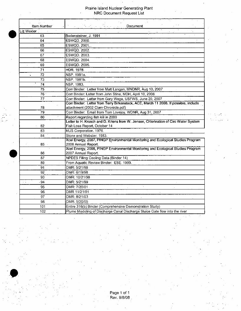
Prairie Island Nuclear Generating PlantNRC Document Request List

Item Number . • '• -Document

Liz Wexler63 Bodensteiner, J. 199164 ESWQD. 2000.65 ESWQD. 2001....66 ESWQD. 2002.67 ESWQD. 2003.68 ESWQD. 2004.69 ESWQD. 2005.71 HDR. 1978.72 NSP. 1981a.73 NSP. 1981b.74 NSP. 1983.75 Corr Binder: Letter from Matt Langan, MNDNR, Aug 10, 200776 Corr Binder: Letter from John Stine, MDH, April 10, 200877 Corr Binder: Letter from Gary Wege, USFWS, June 20, 2007

Corr Binder: Letter from Terry Birkenstock, ACE, March 11 2008. If possible, include78 attachment (2002 Clam Chronicle.pdf)79 Corr Binder: Email from Tom Lovejoy, WDNR, Aug 31, 200780 Report regarding fish kill in 2000

Letter to H. Krosch and D. Knens from W. Jensen, Chlorination of Circ Water System82 Fish Loss Report, October 1483 NUS Corporation. 1976.84 Stone and Webster. 1983.

Xcel Energy, 2007, PINGP Environmental Monitoring and Ecological Studies Program85 2006 Annual Report.

Xcel Energy, 2008, PINGP Environmental Monitoring and Ecological Studies Program86 2007 Annual Report.87 NPDES Filing Cooling Data (Binder 14)89 From Aquatic Review Binder: ESE. 1999.91 DMR: 5/21/9892 DMR 6/19/9893 DMR: 10/21/98

-94 DMR: 5/21/99- 95 DMR: 7/20/01

96 DMR 11/21/0197 DMR: 8/21/0398 DMR: 5/20/05101 Entire 316(b) Binder (Comprehensive Demonstration Study)102 Plume Modeling of Discharge Canal Discharge Sluice Gate flow into the river

Page 1 of 1Rev. 9/8/08

SECTION 316(a) DEMONSTRATION

FOR THE PRAIRIE ISLAND NUCLEAR GENERATING PLANT

ON THE MISSISSIPPI RIVER NEAR

RED WING, MINNESOTA

NPDES PERMIT NO. MN0004006

L. M. GROTBECK AND L. W. EBERLEY

PROJECT SUPERVISORS

ENVIRONMENTAL REGULATORY

ACTIVITIES DEPARTMENT

NORTHERN STATES POWER COMPANY

MINNEAPOLIS, MINNESOTA

AUGUST 1978

PREPARED BY

HENNINGSON, DURHAM AND RICHARDSON, INC.

ECOSCIENCES DIVISION

804 ANACAPA STREET

SANTA BARBARA. CALIFORNIA 93101

.. - r

TABLE OF CONTENTS

I. EXECUTIVE SUMMARY

A. INTRODUCTION I-1

B. ENVIRONMENTAL CHARACTERISTICS I-i

C. PLANT DESCRIPTION AND OPERATING PROCEDURE 1-5

D. THERMAL PLUME 1-6

E. BIOLOGICAL IMPACTS OF THERMAL DISCHARGE 1-6

F. CONCLUSIONS I-l

II. INTRODUCTION

A. LEGAL REQUIREMENTS AND RATIONALE II-i

B. SCOPE AND ORGANIZATION 11-2

C. ACKNOWLEDGEMENTS 11-3

III. ENVIRONMENTAL CHARACTERISTICS

A. HYDROLOGY III-1

1. River Basin Characteristics III-12. Characteristics of the PINGP Vicinity 111-63. River Morphometry near PINGP 111-124. Discharge Rates 111-17

B. WATER QUALITY OF THE MISSISSIPPI RIVER 111-19

1. Temperature 111-192. Water Quality in the Vicinity of PINGP 111-27

a. General Background Information 111-27b. Effects of PINGP Effluent 111-27c. Potential for Toxicity to Aquatic Biota 111-35

C. GENERAL AQUATIC BIOLOGY OF THE MISSISSIPP RIVERNEAR PINGP 111-36

1. Introduction 111-362. Fisheries 111-37

a. Distribution and Abundances 111-37b. Life Histories III-51

i

CONTENTS (continued)

c. Thermal Data for the RIS 111-58d. Spawning Areas and Migrations 111-58e. Predator-Prey Interactions for RIS 111-58f. Diseases and Parasites 111-59g. Influences of Man 111-59

3. Macroinvertebrates 111-644. Zooplankton 111-695. Primary Producers 111-72

a. Phytoplankton 111-72b. Periphyton 11I-74c. Aquatic Macrophytes 111-75

6. Birds 111-78

IV. PLANT DESCRIPTION AND OPERATING PROCEDURE

A. CIRCULATING WATER SYSTEM IV-I

1. Description IV-l2. Modes of Operation IV-53. Chlorination of Plant Cooling Water iV-74. Other Chemicals Used IV-9

.B. PLANT PERFORMANCE AND COINCIDENTAL ENVIRONMENTAL IV-12CONDITIONS

1. Plant Availability and Plant Outages IV-122. Past and Proposed Modes of Operation IV-14

V. THERMAL PLUME

A. DESCRIPTION OF THE HYDROTHERMAL MODEL V-I

1. Hydrodynamic Model V-i2. 2-D Thermal Plume Model V-13. 3-D Thermal Plume Model v-3

B. CASES STUDIED v-4

C. MODEL CALIBRATION V-5

D. COMPARISON OF MODEL RESULTS WITH TEMPERATURE STANDARDS V-6

VI. BIOLOGICAL IMPACTS OF THERMAL DISCHARGE

A. Fish VI-3

1. Field Studies Description and Critique VI-32. Temperature Criteria Vi-7

ii

*" CONTENTS (continued)

3. Attraction to and Avoidance of the ThermalDischarge VI-10

4. Effects on Spawning and Reproductive Success VI-335. Cold Shock Potential VI-376. Effects on Fish (RIS) Populations VI-387. Effects on Parasites and Diseases VI-41

B. MACROINVERTEBRATES VI-42

1. Discussion and Critique of Sampling Methods Vi-422. Effects of Past Operation VI-44

a. Results of Data Reanalysis VI-44

1) Analysis of Variance (ANOVA) andDuncan's Multiple Range Test VI-44

2) Student's One-Tailed t-Test VI-44

3) Multiple Regressions VI-47

b. Discussion VI-47

3. Predicted Impacts VI-51

C. ZOOPLANKTON

1. Discussion and Critique of Sampling Methods VI-59

2. Effects of Past Operation VI-60

a. Results of Data Reanalysis VI-60

1) Analysis of Variance (ANOVA) andDuncan's Multiple Range Test . VI-60

2) Student's One-Tailed t-Test VI-60

3) Multiple.Regressions VI-61

b. Discussion VI-62

3. Predicted Impacts VI-63

D. PHYTOPLANKTON VI-64

1. Discussion and Critique of Sampling Methods VI-642. Effects of Past Operation. VI-64

a. Results of Data Reanalysis VI-64

1) Analysis of Variance (ANOVA) andDuncan's Multiple Range Test VI-64

2) Multiple Regressions VI-65

b. Discussion VI- 65

3. Predicted Impacts VI- 66

E. PERIPHYTON VI- 67

9 1. Discussion and Critique of Sampling Methods VI- 67

2. Impacts of Past Operation VI- 68

iii

CONTENTS (continued)

a. Results of Data Reanalysisb. Discussion .

3. Predicted Impacts

F. AQUATIC MACROPHYTES

1. Discussion and Critique of Sampling Methods2. Effects of Past Operation3. Predicted Impacts

G. BIRDS

VII. CONCLUSIONS

VIII. REFERENCES

APPENDICES

VI- 68VI- 68

Vi--69

VI-69

VI-69VI-7 0VI-70

VI-70

VII-1

VIII-I

APPENDIX

APPENDIX

A:

B:

APPENDIX C:

APPENDIX D:

APPENDIX

APPENDIX

APPENDIX

APPENDIX

APPENDIX

APPENDIX

APPENDIX

APPENDIX

E.

F.

G.

H.

I.

J.

,K.

L.

DATA CATALOG

DETAILS OF NON-FISHERIES STATISTICALANALYSES

CROSS-REFERENCE TO STATE AND FEDERALREGULATIONS

CROSS-REFERENCE TO REGULATORY AGENCYREQUESTS

GLOSSARY

CONVERSION TABLES

AGENCY COMMUNICATION

UNPUBLISHED OR OBSCURE REFERENCE MATERIAL

THERMAL DISCHARGE ANALYSIS

REGULATORY AGENCIES QUESTIONS AND ANSWERS

SPECIES LISTS

STATISTICAL ANALYSIS: DISCHARGE ELECTROFISHING STUDY

JOINT FREQUENCY TABLES: RIVER FLOW-BLOWDOWN RATE

THERMAL SURVEYS AT PINGP

A-1

B-i

C-1

D-i

E-i

F-i

G-I

H-i

I-i

J-i

K-i

L-1

M-i

N-i

APPENDIX M.

APPENDIX N.

iv

LIST OF FIGURES

Figure No. Page No.

Figure I-1

Figure III-i

Figure 111-2

Figure 111-3

Figure 111-4

Figure 111-5

Figure 111-6

Figure 111-7

Figure III-8

Figure 111-9

Figure III-10

Figure III-11

Figure 111-12

Location of the Prairie Island Nuclear 1-2Generating Plant

Location of major streams and gaugingstations 111-2

Longitudinal section of the MississippiRiver from Dam No. 1 to DamrNo. 4 showingthe relative locations of Pool No. 3 andPINGP 111-3

Stage-discharge diagram for Pool No. 3 111-4

Schematic diagram of how water level inPool No. 3 is controlled 111-5

Typical Mississippi Valley cross sectionnear PINGP 111-7

Major water bodies in the vicinity of thePINGP 111-9

Sturgeon Lake channel system for the hydraulicnetwork calculations III-10

Downstream channel system for the hydraulicnetwork calculations III-ll

Sturgeon Lake discharge at Channel 42 versustotal river discharge 111-14

Bathymetry of Sturgeon Lake and the MississippiRiver near PINGP 111-15

Average monthly and weekly Mississippi Riverflows at Prescott, Wisconsin based on USGSdata from June 1928 through September 1976 III-18

Monthly 7-day, 10-year low flows for theMississippi River at Prescott, Wisconsin,and the percentage of time the daily flow-rate is less than or equal to the 7-day, 10-year flows 111-20

v

LIST OF FIGURES (Con't)

Figure No. Page No.

Figure 111-13

Figure 111-14

Figure 111-15

Figure 111-16

Figure 111-17

Figure 111-18

Figure 111-19

Figure 111-20

Figure 111-21

Figure 111-22

Figure 111-23

Figure 111-24

Location of the Minnesota Departmentof Natural Resources (MDNR) temperaturerecording station and the locations ofwater quality stations where temperatureis routinely monitored

Weekly average river temperature at RedWing

Cumulative frequency of occurrence. ofdaily maximum river temperatures at RWGP

Maximum, minimum, and average dissolvedoxygen levels for selected stations in thevicinity of PINGP, 1973-1977

Sampling locations for water quality,phytoplankton, periphyton, zooplankton,and macroinvertebrates

Sampling stations for fish in 1970 (stations1-6 only), 1971 and.,1972

Sampling locations for fish in 1973 through1977

Sampling stations for Sectors I through IIIfor 1977 DNR fisheries studies

Larval fish tow locations for 1974 and 1975

Mean electrofishing catch per unit effortby season for each RIS in Sturgeon Lake andthe Mississippi River from Brewer Lake.cutto Lock and Dam No. 3 combined over the period1974 through 1977

Spatial distribution of RIS near PINGP basedonelectrofishing data for the period 1974through 1977

Mean number of larval fish per 50 m tow atlocations 1, 2, and 4 near PINGP in 1974

111-21

111-25

111-26

111-30

111-31

111-38

111-39

111-40

111-41

111-44

111-45

111-47

0-)

vi

LIST OF FIGURES (Con't)

Figure No. Page No.

Figure 111-25

Figure 111-26

Figure 111-27

Figure 111-28

Figure 111-29

Figure IV-l

Figure IV-2

Figure IV-3

Figure IV-4

Figure IV-5

Figure IV-6

Figure IV-7

Figure V-i

Figure VI-I

Figure VI-.2

Mean larval fish densities at PINGP in1975 based on weekly sampling at thelocations shown in Figure 111-21

Estimated density of RIS larval fish drift-ing past PINGP in 1975

Spawning temperatures and times for theRIS

HDR station locations for biological studiesconducted near PINGP during 1969-1976

Locations of macrophyte beds observed nearPINGP during 1973 through 1976

Schematic diagram of the circulating watersystem

Representative flow diagram of the circulat-ing water system

Flow diagram for 50 percent recycle mode

Flow diagram for a 100 percent helpercycle mode

Flow diagram for a once-through mode witha maximum withdrawal rate of 1,410 cfs

Frequency of occurrence and cumulativefrequency of various blowdown rates from1975 through 1976

Frequency distributions of proposed blowdownrates and the calculated blowdown based onan intake temperature of 29.40 F

Boundary conditions and the grid network usedin the near-field 2-D thermal plume analysis

Empirical approaches to discharge impactanalysis for invertebrates and primaryproducers at PINGP, using site-specificbackground data

111-48

111-49

111-52

111-66

111-76

IV- 3

IV-4

IV-6

IV-6

IV-7

IV-15

IV-16

V-2

VI-2

HDR designated station locations for inver-tebrate, primary producer, and water qualitysampling conducted near PINGP during 1973-1976 VI-4

vii

LIST OF FIGURES (Con't)

Figure No.

Figure VI-3

Figure VI-4

Figure VI-5

Figure VI-6

Figure VI-7

Figure VI-8

Figure VI-9

Figure VI-10

Figure VI-1l

Figure VI-12

Figure VI-13

Page No.

The predictive approach for analyzing dis-charge impacts on invertebrates and primaryproducers at PINGP using thermal plume pre-dictions and non-site specific thermaltolerance data

Sampling locations for the DNR dischargeelectrofishing study

Nomograph to determine the permissible maximumweekly average temperature (MWAT) in the plumeduring winter for various ambient temperatures

Preferred temperatures for juvenile RIS

Preferred temperatures of juvenile and adultRIS during various seasons

Upper and lower lethal thresholds for variouslife stages of the RIS

Mean number of. RIS collected per month in thePINGP discharge (Runs 1 and 5) and at controlstations (Runs 4 and 7) near the intake duringthe period April 1976 through November 1977

Regression of number of total RIS collectedin the immediate discharge (Runs 1+5) andcontrol (Runs 4+7) areas against ambientriver temperature for the period April 1976through November 1977

Seasonal catch per unit effort at PINGP dis-charge and control stations for dominant RIS

Regression of number of carp collected in theimmediate discharge (Runs 1+5) and control(Runs 4+7) areas against ambient river tempera-ture for the period April 1976 through November1977

Regression of number of gizzard shad collectedin the immediate discharge (Runs 1+5) and control(Runs 4+7) areas against ambient river tempera-ture for the period April 1976 through November1977

VI-5

VI-6

VI-3

VI-lI

VI-12

VI-14

VI-26

VI-27

VI-28

VI-30

VI-31

viii

LIST OF FIGURES (Con't)

Figure No.

Figure VI-14

Page No.

Pathways by which planktonic organisms maydrift through the PINGP discharge area VI-35

ix

LIST OF TABLES

Table No.

Table III-1

Table 111-2

Table 111-3

Table 111-4

Table 111-5

Table 111-6

Table 111-7

Table 111-8

Table 111-9

Page No.

Comparison of the computed dischargesin Sturgeon Lake and Channel 42 withthe field measurements

Summary of the mean temperature dif-ferences between ecological monitoringstations and the Red Wing GeneratingPlant intake

Average diurnal river temperaturefluctuation measured at Lock and DamNo. 3

Minimum, maximum, and mean concentrationsof water quality parameters in subsurfacesamples collected from 21 June 1970 through13 September 1977

Selected Water quality for the MississippiRiver at Lock and Dam No. 3, 1969 to 1976

Summary of ANOVA for water quality datacomparisons for two stations (HDR Stations10 and 11) upriver and two stations (HDRStations 25 and 27) downriver from PINGPmeasured at the top and bottom of the watercolumn for 1975 and 1976

Mean values for chemical parameters measuredat the Prairie Island Nuclear Generating Plantduring 1975 and 1976

Species composition (percent) of the major taxaof fish collected in the vicinity of PINGPduring the period 1973 through 1976.

Taxa of fish parasites and types of infes-tation

111-13

111-23

111-24

111-29

111-33

III-34

111-43

II -60

X

LIST OF TABLES (Con't)

Table No. Page No.

Table III-10

Table III-1l

Table 111-12

Table 111-13

Table 111-14

Table IV-l

Table IV-2

Table IV-3

Table IV-4

Table IV-5

Table IV-6

Table V-1

Table V-2

Commercial catch (pounds) of carp, buffalo,catfish, and drum in Pool Nos. 3, 4, and 4aduring 1970 through 1974

Creel census data for the vicinity of PINGPin 1973 through 1976

Percent-composition of RIS in the estimatedsport harvest near PINGP for 1975 and 1976

HDR key to sampling stations comparisonsbetween studies conducted at PINGP

Pollution tolerance of selected benthicmacroinvertebrates collected in the vicinityof PINGP

Percentage of mean monthly Mississippi Riverflow entering the intake canal, January throughSeptember 1975

Modes-of operation for PINGP

Typical residual chlorine concentrations inthe discharge water and in the cooling water

Summary of liquid discharges into the circula--ting water system including effluent limitations

Chemical concentrations from neutralizing tankeffluents

Summary of availability factors, capacityfactors, and plant outages for November 1976through October 1977

Cases where the PINGP proposed NPDES thermalcriteria were exceeded

Computed monthly cumulative frequency (aspercent) of temperature rise at Barney'sPoint assuming no wind and full dilutionin Channel 42

111-62

111-63

111-64

111-67

111-70

IV-2

IV-8

IV-9

IV-10

IV-ll

IV-13

V-8

V-9

xi

LIST OF TABLES (Con't)

Table No. Page No.

Table V-3

Table VI-l

Table VI-2

Table VI-3

Table VI-4

Table VI-5

Table VI-6

Table VI-7

Table VI-8

Table VI-9

Table VI-10

Computed monthly cumulative frequency ofoccurrence (percent) for river temperaturesat Barney's Point assuming no wind and fulldilution in Channel 42

Temperature criteria for the RIS in Centigrade

Estimated potential effects of increased*temperature on the RIS in the vicinity ofPINGP

Predicted area in thedischarge from whichvarious life functions would be excluded undertypical and extreme conditions for walleye

Predicted area in the discharge from which variouslife functions would be excluded under typicaland extreme conditions for white bass,,

Predicted area in the discharge from whichvarious life functions would be excluded undertypical and extreme conditions for channel catfish

Predicted area in the discharge from which variouslife functions would be excluded under typicaland extreme conditions for northern pike

Predicted area in. the discharge from which variouslife functions would be excluded under typicaland extreme conditions for gizzard shad

Predicted area in the discharge from which variouslife functions would be excluded under typicaland extreme conditions for carp

Predicted area in the discharge from which variouslife functions would be excluded under typicaland extreme conditions for black crappie

Predicted area in the discharge from which variouslife functions would be excluded under typicaland extreme conditions for-:emerald shiner

V-10

VI-9

VI-13

VI-15

VI-16

VI-17

VI-18

VI-19

VI-20

VI-21

VI-22

xii

LIST OF TABLES (Con't)

Table No. Page No.

Table VI-11

Table VI-12

Table VI-13

Table VI-14

Table VI-15

Table VI-16

Table VI-17

Table VI-18

Table VI-19

Predicted area in the discharge from whichvarious life functions would be excludedunder typical and extreme conditions forwhite sucker

Predicted area in the discharge from whichvarious life functions would be excludedunder typical and extreme conditions forshorthead redhorse

Results of the chi-square analysis of thedischarge electrofishing data for the mostabundant RIS by season

Short-term thermal tolerances of larval fish

Power calculations for non-fisheries biolo-gical data collected near PINGP

Results of two-way ANOVA for biotic categoriessampled near PINGP in 1973-1977

Results of Duncan's Multiple Range Tests forbiotic categories sampled near PINGP, 1973-1977

Results of one-tailed t-Tests for invertebratescollected near PINGP from 1975-1977

Results of stepwise multiple linear regressionsfor biotic categories sampled near PINGP in1975 and 1976

VI-23

VI-24

VI-32

VI-36

VI-43

VI-45

vi-46

VI-48

VI-49

VI-53

VI-54

VI- 5.5

vi-56

Table VI-20 Estimated drift tines for plankton through thethermal plume at PINGP for typical and proposedextreme conditions

Table VI-21

Table VI-22

Table VI-23

Thermal matrix for response of the macroinverte-brate RIS, Stenonema, to conditions near PINGP

Thermal matrix for the response of the macroinver-tebrate RIS, Pseudocloeon, to conditions nearPINGP

Thermal matrix for response of the macroinverte-brate RIS, Hydropsyche, to conditions nearPINGP

xiii

LIST OF TABLES (Con't)

Table No. Page No.

Table VI-24 Thermal matrix for response of the macroinver-tebrate RIS, Macronemum, to conditions nearPINGP VI-57

xiv

I EXECUTIVE SUMMARY

A. INTRODUCTION'

Thermal discharges, including power plants such as PINGP, are regu-lated by state and federal laws. All dischargers to surface waters arerequired by the FWPCA Amendments of 1972 ("the Act,"P..L. 92-500)' toobtain a National Pollution Discharge Elimination System (NPDES) permitfrom an authorized agency. In Minnesota, the Minnesota Pollution ControlAgency (MPCA) has been designated as lead agency to the EnvironmentalProtection Agency (EPA) and administers the law using the Act and MPCARegulation WPC 36(u) (3).

For this 316(a) demonstration, a predictive Type 2 approach wasselected for assessing future impacts of the PINGP thermal dischargeupon indigenous biota. This involves selection of representative impor-tant species (RIS), including fish and invertebrates, and relies primarilyon literature data for thermal tolerances and on thermal plume models toestimate potential impacts. Appropriate site-specific data wereutilized to supplement the predictive approach.

B. ENVIRONMENTAL CHARACTERISTICS

PINGP is located on the west. bank of the Mississippi River approxi-mately 2.4 km (1.5 mi) upriver from Lock and Dam No. 3 (Figure I-1). Theplant intake and discharge areas are separated from the main river channelby a series of small islands that delineate the outlet channels of SturgeonLake, a backwater lake connected to the river by numerous small channels.The river is 300 t6 370 m (1,000 to 1,200 ft) wide near PINGP, and the banksof the main channel slope fairly steeply to the bottom. The Sturgeon Lakeoutlet area is quite shallow, and consequently, the intake and dischargeareas have been dredged to a depth of about 3.1 m (10 ft). The thermaleffluent flows approximately 610 m (2,000 ft) before entering the mainchannel of the river at Barney's Point.

River flows are regulated to maintain a minimum pool level for navi-gation during ice-free months (usually mid-March to early December). Theannual average discharge rate at Prescott, Wisconsin, was 16,200 cfs forthe period 1928 to 1976. River flows have seasonal fluctuations with apeak in April (weekly average of 44,000 cfs) and a low in December (weeklyaverage of 7,000 cfs). The maximum rate recorded was 228,000 cfs on18 April 1965, and the minimum was 2,100 cfs on 14 August 1936. River

I-1

~9Ofl3-'

0 5 10 15 20

SCALE (MILES .

Figure I-1. Location of the Prairie Island.Nuclear.Generating Plant.

I- 2

U

wY~ ~

The Prairie Island Nuclear Generating Plant is located on the west bankof the Mississippi River approximately 2.4 km (1.5 mi) upriver fromLock and Dam No. 3. Heated effluent is discharged into the southernend of Sturgeon Lake, which is separated from the main river channel bya series of small islands, and enters the river at Barney's Point.

temperatures also have seasonal, variations with a low of OO C (320 F)- inwinter when the river freezes over and a high of 290 C (850 F) in sum'mer.ýIntake temperature data from Northern States Power Company's Red Wing Gen-.ýerating Plant (RWGP) located 15 km (9.4 mi) downriver from PINGP were usedto represent PINGP "ambient river temperatures since long-term data werenot available near the plant. Daily temperature fluctuations are low inthe river [1.10* C (20 F)] but may be fairly high in backwater areas. , InSturgeon Lake, the average fluctuation was 20 to 3' C (3.50 to 5.41 F) witha maximum of 9.70 C (17.50 F) during ice-free months of 1974 through 1977.

Extensive water quality analyses have been conducted by NSP .in thevicinity of PINGP since 1969 in addition to the U.S.G.S. measurementsconducted at Lock and Dam No. 3 since 1969. Although dissolved oxygen

'(DO) levels never reach critically low levels, the high nutrient concen-trations reflect the upriver discharge of domestic wastewater into theMississippi River from the Minneapolis-St. Paul Metropolitan Sewage Treat-ment Plant. The Minnesota River also influences water quality in the

1-3

vicinity of PINGP through addition of suspended sediments, dissolved Wsolids, and other agriculturally related runoff. Elevated levels of po-tential toxicants such as ammonia, lead, mercury, and especially cyanidehave been observed periodically at Lock and Dam No. 3, indicating that somebiota may be pre-stressed before encountering the PINGP thermal plume.No significant non-thermal changes in water quality have been attributedto the operation of PINGP.

The Mississippi River near PINGP comprises numerous habitat typeS,

thus creating a complex ecosystem .. Th•e river is fairly eutrophic :,nearPINGP as a result of runoff from agriculture and wastewater dischargesfrom the Metropolitan Sewage Treatment Plant. Biota in all trophic levelshave been sampled in the vicinity .of 6 PINGP since 1969, and fr6m 'thisinformation a list of represen.tative important species (RIS) was ,selectedfor assessing impacts in 'this demonstration. "The fish s•s•cted wer•>'.walleye, white bass, channel daatfish, northern pikeb ,'black,,-crappie,:gizzardd shad;' -carp,. emerald 'sh-ner 'whifte-,sucker, aind• h~rhead iOt"e.The mAcroinvertebrate§ chosen were -yrpsc , oea se -odi nSacronemi~m. •Sampling,'frbi. 1973 t.through 01.976 has ,indicated hat'gizzard:shad, white bass, freshwater drum, 'and carp dominated the::adult. ancJi vnilfish-populations near ,PINGP from[late may. through October. -Abundancis~'varied.both seasonally and annually Ifor the dominant speci~es,.'L''Lara!' fishwere present in the water: column during spring and summer with peak iidensi-ties occ urring in July of 1974 and June of 1975. The most abundant 'specieswere white bass, emerald shiners, carp, and gizzard 'shad. Life histories,,,thermal tolerances!, migrations and spawning areas, predator-prey inter-actions, and diseases and parasites were included in the discussion:forthe RIS.

Both commercial and recreationalo.fishing occur in. ... f.: .atishj•carp dre. -~ ~i~p~ the, Mqok yluable omel sc

A, -~b5j a1 c p. ufQ: t. to - Pr J. -3 increased from 1970 throi'ghw.1 1'i iie declining in Pool Nos. 4 and 4af4 Based. on creel census informa-ition from 1973 through 1976, recreational: fishing pressure has remainedlower in theoývicinity of PINGP than in the tailwaters of .Dam No. 3;however, fishing success was higher above the Dam.'-.' Walleye and whit•ebass were the RIS~most frequently caught near PINGP, while white bassdominated the catch in the PINGP discharge area during spring.

A high diversity of benthic macroinvertebrate, zooplankton, and primaryproducer populations exists near PINGP. Marked seasonal variations inorganism abundance were common in all groups. Many of the macroinverte-brates are larval stages of terrestrial and aquatic insects that emergefrom the water during summer, while various taxa of phytoplankton and zoo-plankton bloom at intervals in response to changing levels of nutrients orfood organisms and temperature. Aquatic macrophytes are present in manyshallow backwater areas, but few occur in the PINGP discharge canal or themain channel of the river. Life histories and thermal tolerance informa-tion for all biotic categories except macrophytes are also discussed.

I-4

Northern bald eagles and various waterfowl migrate through theMississippi River Valley in spring and fall with some overwintering inareas of open water. The PINGP area does not appear to0be an importanteagle overwintering area although the discharge may enhance the numberof mallards overwintering. Peregrine falcons, an endangered species,are being reintroduced in former nesting areas along Lake.Pepin approxi-mately 48 to 80 km (30 to 50 mi) downriver from PINGP.

C. PLANT DESCRIPTION AND OPERATING PROCEDURE

The PINGP circulating water system may be operated in four basicmodes: closed, partial recycle, helper, or open cycle. Closed cycle isnormally used during the cooler parts of the year, and blowdown is heldat approximately 150 cfs. When the temperature of the mixed, makeup andrecycled water reaches 29..40 C (850 F) at the condenser, partial recycleis begun and increased as hecessary to maintain the condenser inlet tem-perature at or below 29.40 C. In this mode, cooling towers are still used,but the blowdown and makeup water flows are increased. Helper cycle(no recycle) and open cycle operation are optional modes that have notbeen used in the past but could be used if needed.

The circulating water syste% is not chlorinated since the condensertubes are cleaned mechanically (Amertap method). The cooling watwrsystem, however, is chlorinated to prevent biofouling of heat exchangersurfaces, and this water is discharged to the circulating water system.The volume of the cooling water is only 4 percent of the circulatiMwater volume, and chlorine may be lost to the atmosphere in the recyclecanal. Measurements of total residual chlorine at the discharge gateshave shown the concentration to be less than 0.03 pp#i.

PINGP is a base load facility and each of the two units is ratedat 507 MWe in summer and 523 MWe in winter. Refueling of one unit occursduring winter while refueling of the other is usually in early spring.These refueling periods are generally 4 to 6 weeks long. Based on pastoperation, the probability of a forced trip (outage) occurring while theother unit is being refueled is 0.55, and the probability of simultaneousforced trips is 0.00035.

Operating modes should remain similar to those utilized in the past.During summer, however, full helper cycle is proposed from 16 Junethrough 31 August to increase the efficiency of the plant. This wouldcause the temperature differential between ambient river water and blow-down to decrease, thus decreasing the maximum temperatures in the plume.during summer.

I-5

D. THERMAL PLUME

The thermal plume was modeled for various typical and extremeenvironmental conditions for each month of the year (61 cases total).A two-dimensional (2-%•) model was utilized for the near-field-area aboundedby the intake approach channel on the north, the river bank on the west,the islands on the east, and the entrance to the main river channt atBarney's Point on the south-. For the main channel of the river fromBarney's Point to Lock and Dam No. 3, a three-dimensional model (3-D)was utilized. The model descriptions and results are presented inAppendix 1, including plots of surface isotherms for representativeconditions. Historic typical and extreme cases were based on 1975 and1976 operational and environmental information, while proposed extremecases were a combination of 7-day, 10-year low river flow, high riverambient temperature, a maximum blowdown rate, a southerly wind, and ahigh wet bulb temperature which would result in poor cooling tower per-formance. The models were calibrated with data from the September 1974and August-1975 field thermal surveys.

The thermal plume model results were compared with the proposed NPDESpermit for PINGP, and 13 of 61 cases exceeded the proposed thermal limits.All but two of the cases that exceeded were for typical environment con-ditions in late fall and winter (October through March). These two cases,which were for proposed extreme conditions; exceeded the 300 C (860ý F)maximum temperature criterion at Barney's Point by less than 10 C(1.80 F). One case was in July and the other in August. The proposed,extreme cases, however, are one day events that occur with a proba1ilityof 0.000005 (l hour every 278 years) per month. The criterion exceededin the other 11 cases was the 2.80 C (50 F) AT limit at Barney's Point(edge of the mixing zone).

For future operation during typical environmental conditions of riverflow, ambient river temperature, and blowdown rate, a variance to theproposed NPDES'permit will be necessary to meet the thermal criteri4without derating the plant.. An extension of the mixing zone boundary488 m (1,600 ft) downriver for October through March would be sufficientto maintain compliance with the proposed NPDES permit.

E. BIOLOGICAL IMPACTS OF THERMAL DISCHARGE q

To predict the potential biological impacts of operating PINGP., bothliterature and field data were used along with the thermal plume modelresults. For fish, the predicti've approach based on literature infor-mation and model results was emphasized with some supportive use offield data. For invertebrates and primary producers, however, an exten-sive reanalysis of the existing field data was performed since literatureinformation was limited.

1-6

Based on preferred temperatures reported in the literature, all ofthe fish RIS would prefer to reside in some portion of the PINGP thermalplume when ambient water temperatures are low, and some species shouldavoid at least the warmer areas within the plume during summer. Thesepredictions have been confirmed by field studies which indicated thatwhite bass, carp, emerald shiner, walleye, and gizzard shad were definitelyattracted to the discharge during winter and/or spring. Shorthead red-horse, white bass, carp, and gizzard shad showed a distinct avoidanceof the warmest discharge areas during summer. Upper lethal temperatureswere used to estimate the potential areas of exclusion for long-termuse by adults during typical summer conditions. These areas were calcu-lated to be less than 4.4 ha (10.9 A) for all of the RIS fish and wouldoccur only in July and August.

. .. ! • i• ,• •.: % 9!-!• •• •''

'II

The PINGP thermal discharge attracts fish during most of theyear, although some species avoid the warmest portion of the-plume in summer. Impacts to the representative importantspecies (RIS) of fish and.macroinvertebrates, however, arepredicted to be minimal.

1-7

The thermal discharge could induce premature spawning in fish which W7reside in the plume during,spring. Field studies have shown that carp,walleye, gizzard shad, and emerald shiner are the dominant species inthe discharge area during spring; however, no premature spawning has,been observed during the field surveys. The warmest areas of the plumemay preclude successful spawning in a small area, either by exclusion ofadults or through thermal stress to embryos. The maximum area of poten-tial exclusion for typical environmental conditions is small [17 ha (42 A)for northern pike and less than 9 ha (22 A) for the other RIS], particu-larly when compared to the area of Sturgeon Lake [324 ha (800 A)] whichhas an abundance of suitable spawning habitat for most of the RIS. Further-more, the estimated exclusion areas may include little or no suitablespawning habitat for some species, and the maximum area of exclusion foreach species occurs during only a portion of the spawning period. Thus,the potential for impact would be considerably less than that estimatedfrom exclusion area alone. Larval fish drifting f-om Sturgeon Lakethrough the discharge area will be subjected to elevated temperatures,but literature data for larval thermal tolerances do not indicate thatstress would occur at PINGP.

Although the PINGP thermal discharge can affect various RIS lifefunctions in the discharge area, no measurable effects are expected tooccur in the fish populations of Pool No. 3. Potential premature spawningof carp and gizzard shad should have negligible effects since only asmall poportion of their populations are calculated to be present inthe discharge during spring. For walleye and emerald shiner, earlyspawning is also predicted to have minimal effects on river populationssince it is unlikely that all of those in the discharge would spawn early,and even if they did, it is unlikely that all such spawning would beunsuccessful. Exclusion of adults.from potentialspawning, areas in the

shoud hve negligible effects on 'riv~ oimmediate d ischarge ge area shouild .have nevgb e e fee ? i r 'popu ýý11-1lations.since many ,other suitable. spawning areas iae' present,-nearby-;.'.(e.g., Sturgeon and North lakes)..

The potential for cold shock exists at PINGP during winter, from *..eithersimulta•e0us..-shutdown of. bo"h' units or an unscheduled.trip while the otherunit is down.:-FiShare 'attracte to the themalplume -in winter,. tempera-tures ý'e>cceedih4,' the-ia'Zrec6m~mendý!d. ma~ximum- weekly~averiage temperature.- for-coldshock protectiorf'! exist !n-ahen p and th probability of aiforced tripoccurringý during refueling..of the other unit --is 0. 55 The thermal plumi issmaller, however, during one unit operation. The species most likely to beaffected is gizzard shad since it is the dominant species present in win-ter and one of the most sensitive to cold shock. Potential mortality togizzard shad is not expected to decrease river populations, however. Thisprolific species normally has large-winter die-offs as~ambient water tem-peratures approach 0' C (320 F), and the discharge and recycle canals mayprovide a temporary thermal refuge which would only delay. such naturaldie-offs.

The PINGP discharge is not expected to affect any endangered speciesof fish nor inhibit any fish migrations. Predator-prey interactions

I-8

as well as parasitism and diseases are likewise predicted to be negligiblyaffected.ý Fish population structure should not be changed althoughsuch Changes are very difficult to measure and are generally indistinguish-able from other influences, both natural and man-induced.

Sport fishing has not been in the past and should not be degraded asa result of the PINGP thermal discharge. Fishing success in recent yearshas been higher above Lock and Dam No. 3 than in the tailwaters of the Dam,although the fishing pressure and harvest have been lower. In the immediatedischarge area, fishing success should be enhanced during all but thewarmest periods in sUiMier. 'Fishing pressure has been observed to be higherin the discharge during spring which indicates that some fishermen weretaking advantage of the higher fish densities in the plume, and the catchat that time was primarily white bass.

Site-specific invertebrate and primary producer field data werereanalyzed primarily for the operational years of 1975 and 1976. Data forphytoplankton from 1973 and from the first 6 months of 1977 for macro-invertebrates were also utilized. Between station and between date samplevariability were computed by ANOVA, Duncan's Multiple Range Test, and theStudent t-Test. Power calculations were also used to establish the likeli-hood that actual differences between samples would be detected as signifi-cant by the above tests. In addition to the sample variance testing,multiple regressions were conducted in order to determine whether or nottemperature was highly related to abundances of biota on a spatial basis(i.e., between intake and discharge stations).

From these reanalyses, impacts appear to be minimal or non-existentin most biotic categories 'The following characteristics of biotic cats-gories were found nqo to differ significantly between intake 'nd dischargeistations: phytoplankton species diversity or biovolume; periphyton density,species diversity, and phaeophytin a content; zooplankton species diversityand density; and-macroinvertebrate (dredge and artificial substrate)density. The power 6f these statistical tests, however, is limited bythe inability to discern differences between station values as a resultof the low number of replicate samples taken at each station

The following characteristics' of biotic categories were found todiffer significantly between intake and discharge stations: phytoplanktonprimary productivity, periphyton chlorophyll a, and macroinvertebratespecies diversity for dredge samples. The significant differences inphytoplankton chlorophyll a between intake and discharge samples probablyresulted from plant entrainment damage, while the significant differencesbetween intake and discharge for dredge macroinvertebrate species diversitycould have resulted from differences in substrate and current rather than,or in addition to, thermal effects. A study of aquatic insect emergencerates showed that only the mayfly, Caenis, may have emerged slightlyearlier from heated water stations than from ambient temperature stations.All other aquatic macroinvertebrates including one RIS (Hydropsyche)

1-9

emerged at approximately equal rates and times from both heated and control Wstations. Variations in the distribution of aquatic macrophytes betweenyears in the discharge canal have not been definitely related to thethermal plume, but appear to be more dependent upon fluctuations inwater level, siltation, and currents.

Multiple regressions showed that although temperature was selectedas the parameter most highly related (R2 = 0.35) to zooplankton density(and its subgroups, rotifers and crustaceans),on an annual. basis, seasonalrelationships were low (R2 = 0.06). This indicates that annual variation(between intake and discharge) was negligible. Temperature was notsignificantly related to phytoplankton or macroinvertebrate ..(bothdredge and artificial substrate samples) densities. Periphyton wasnot tested for significant correlations with~water temperature becauseof insufficient coincidental water quality data.

Predictive impacts for non-fisheries biota were determined by comparingthe most relevant thermal bioassay information with the thermal plume modelresults for typical and proposed extreme environmental conditions. FourRIS macroinvertebrates. were selected (Hydropsyche, Macronemum, Pseudocloeon,and Stenonema), all of which are aquatic insect larvae. Thermal tolerancesfor selected zooplankton, phytoplankton, and periphyton were also compared.with thermal plume configurations for indications of potential driftmortality or exclusionary areas.

From this predictive analysis of comparing organism thermal tolerances,

with plume configurations, the following results were found: no driftmortalities are expected for phytoplankton, .,zooplankton, or. macroinver-tebrates.. Most habitats. in the discharge canal that ,are otherwise,.suitable for aquatic macroinvertebrates will not be rendered unsuitableas a result of high temperatures, except for small portions duringproposed extreme environmental conditions. For instance, the area in thedischarge canal equivalent to. approximately one to six percent of S•turgeonLake may be avoided by two macroinvertebrate RIS (Hydropsyche and Macro-nemum) . This does not mean, however, that these two taxa will be killedor even excluded from the discharge areas during extreme conditions,but that they will be less common at higher temperaturesr in the dischargearea than in control areas. Site-specific information for these twospecies during the unusually warm, low flow year of 1976 indicated,. however,that they did not avoid the discharge canal.

Based on literature data, a two-week acceleration of the, emergenceschedules for most aquatic macroinvertebrates is predicted for, the entirearea of.the discharge canal (equivalent to about 5.7 percent of SturgeonLake). These predictions, however, are not supported by site-specificstudy results conducted in 1974 (except possibly for Caenis) . In an.area comparable to. less than 0.5 percent of Sturgeon Lake, a five-monthacceleration of emergence schedules is predicted, although this has notbeen observed in the past to occur in.the PINGP discharge canal. Other

I-10

predictions indicate that warmer water areas of the discharge canal mayfavor more thermally tolerant taxa,.but this area would be insignificantcompared to the area of Sturgeon Lake. The thermal plume should notfavor the encroachment or proliferation of nuisance organisms, such asblue-green algae; blooms of these phytoplankton have occurred seasonallylong before PINGP became operational. Moreover, no federally protectedflora or fauna will be impacted by the thermal discharge.

The operation of past and proposed discharge modes at PINGP, there-fore, have not and should not inhibit the protection and propagation ofa balanced, indigenous invertebrate and primary producer biota. Thedischarge plume will cause neither appreciable harm nor adverse levelsof impact to non-fisheries biota. No drifting forms are expected to orhave been observed to be damaged by passage through the plume. Evenduring extreme environmental conditions, the maximum area of avoidanceas a result of heated water for certain RIS macroinvertebrates is smallin relation to the total area available in the adjacent backwater habitatof Sturgeon Lake. Moreover, emergence schedules of aquatic macroinver-tebrates are expected to be altered only slightly by the heated plume andonly negligible losses are expected as a result of premature emergence.Finally, the occurrence and distribution of aquatic macrophytes nearPINGP appears to be more influenced by fluctuations in water level,sedimentation, and current conditions than by temperature. Any lossesof aquatic macrophytes that may result from the thermal discharge issmall in comparison to the total distribution of macrophytes in SturgeonLake, as suitable habitat for these plants in the discharge canal isextremely limited.

F. CONCLUSIONS

It is concluded that the thermal discharge resulting from pastoperation of PINGP has not caused appreciable harm to any aquatic biota,and the protection and propagation of a balanced, indigenous biota hasbeen maintained. During future operation in pastor proposed modes,impacts are expected to remain similar to those in the past.

1-11

II INTRODUCTION

A. LEGAL REQUIREMENTS AND RATIONALE

The operation of all power plants in Minnesota is regulated bystate and federal laws. The Federal Water Pollution Control Act Amend-ments of 1972 ("The Act" P.L. 92-500) require that municipalities andindustries discharging into surface waters obtain a National PollutionDischarge Elimination System (NPDES) permit from an authorized agency.If the discharger can demonstrate that the required limitations are morestringent than necessary to assure the propagation of a balanced indi-genous population within the water body receiving the discharge, thenalternative effluent limitations may be in order.

Discharges from power plants in Minnesota fall primarily under thejurisdiction of the Minnesota Pollution Contkol Agency (MPCA) which hasbeen designated as lead environmental regulatory agency for this state bythe Environmental Protection Agency (EPA). The MPCA administers the' lawusing both the Act and MPCA Regulation WPC 36(u)(3). The Minnesota guidefor 316(a) demonstrations (MPCA, 1975) will be used as the primary sourceof information for developing this demonstration. The Interagency 316(a)Technical Guidance Manual (EPA, 1977) provides valuable ancillary infor-mation to the Minnesota Guide but will be considered tentative in viewof its draft status and Edison Electric Institute and Utilities Water ActGroup (1977) comments.

After conferring with MPCA and EPA personnel, a Type 2 demonstrationwas selected for assessing the impact of the PINGP discharge upon indigenousbiota. This type of demonstration involves selection of RepresentativeImportant Species (RIS) for discussion of potential thermal impacts tothe aquatic ecosystem. At PINGP, these include several fish and macro-invertebrate taxa. Other trophic levels including primary producersand zooplankton are considered also because of their potentially highbiological value to the aquatic ecosystem near.PINGP, but no RIS wereselected. The predictive Type 2 demonstration relies primarily uponliterature data for thermal tolerances of the RIS and other biota andmodeling of the thermal plume in the receiving waters. In addition, somesite-specific information will be utilized in this demonstration tosupplement the predictions of whether or not the RIS and other biota areprotected.

II-I

B. SCOPE AND ORGANIZATION

The requirements for this demonstration have been outlined by theMPCA and the EPA as discussed above. The demonstration begins with adescription of the environmental characteristics of the aquatic habitatnear PINGP. These characteristics include hydrology, water quality,and general aquatic biology of the Mississippi River and its associatedbackwater habitats. Life history descriptions and habitat preferencesof 10 fish RIS (black crappie, walleye, channel catfish, carp, emeraldshiner, gizzard shad, white sucker, shorthead redhorse, white bass,ý andnorthern pike) are provided as well as four macroinvertebrate RIS (twocaddisflies., Hydropsyche and Macronemum; and two mayflies, Stenonemaand Pseudocloeon) . In addition, thermal tolerance data are summarizedfor RIS and other selected taxa from all trophic levels.

A description of the plant and its operating procedures follows thediscussion of existing environmental characteristics. The circulatingwater system and its modes of operation are described along with asummary of chlorination procedures and other chemicals used.. Next,"plantperformance is discussed in relation to coincidental environmentalconditions such as river temperature and flow. The occurrence of plantoutages and potential recirculation of discharge water are then presented.

Following the plant description is a section on the,-past and predictedcharacteristics of the thermal plume. Results of thermal surveys-from,1974 through 1976 will be presented and discussed as~well as results of Ithe near-,and far-field plume models for various typical and .extreme.conditions. Finally, the observed and the predicted-plume will be comparedwith state temperature standards and the NPDES permit limitations.-

Biological impacts of the thermal~discharge arediscussed in the nextsection. Predicted impacts to the RIS are analyzed in order to assesswhether or not the propagation of these species is protected in spite ofthe PINGP discharge. In addition, biota for which no RIS were selectedare also considered with respect to impacts of the thermal discharge.These biota include zooplankton, primary producers .(phytdplankton,periphyton, and. aquatic macrophytes), and:other biota (waterfowl andeagles).

Finally, the conclusions of-the impact analyses including a discussionof whether appreciable harm or an adverse level of impact has or will occurare addressed. A complete list of all literature cited is provided.aswell as a number of appendices. These include:. Appendix A.--Data:Catalog;Appendix B. -Details of Non-fisheries Statistical Analyses; Appendix C.-Cross-Reference to State and Federal Regulations; Appendix D.--Cross-Referenceto Regulatory Agency Requests; Appendix E.-Glossary; Appendix F.--ConversionTables (Metric to English); Appendix G.--Agency Communication (Federal, State,and Local); Appendix H.--Unpublished or Obscure Reference Material; Appendix I.-

11-2

Thermal Discharge Analysis; Appendix J.-Regulatory Agencies Questionsand Answers; Appendix K.--Species Lists; Appendix L.--Statistical Analysis:Discharge Electrofishing Study; Appendix M.--Joint Frequency Tables: RiverFlow-Blowdown Rate; Appendix N.--Thermal Surveys at PINGP.

C. ACKNOWLEDGMENTS

A number of NSP personnel have been instrumental in providing thevoluminous information required to compile this 316(a) demonstration.The efforts and guidance of Mr. Larry Grotbeck, Mr. Richard McGinnis,and Mr. Lee Eberley are greatly appreciated. Also providing helpfulinformation regarding plant operation, history, and design were Mr. AlexSimich, Mr. Don Brown, and numerous others at NSP. Drs. George Yeh andY. Y. Shen of Stone and Webster Engineering Corporation compiled thepredictive modeling for the thermal plume and assisted in the develop-ment of the demonstration since its inception. Dr. J. S. Rao of theMathematics Department at the University of California at Santa Barbaraassisted in statistical analysis, and Dr. Charles Hanson of the Universityof California at Davis provided valuable comments in reviewing themanuscript.

Mr. Larry Olson of the MPCA in addition to Mr. Gary Milburn andMr. Vacys Saulys of EPA Region V in Chicago provided guidance andassistance in developing the demonstration outline and selecting the RIS.At the Minnesota Department of Natural Resources, Mr. Howard Krosch,Mr. Joe Geis, and Mr. Scott Gustafson generously provided data at ourrequest and continually responded to our information queries. Variouspersonnel from the Corps of Engineers Office in St Paul provided valuableinput into the data collection process regarding river flows, operationof the lock and dam system, and barge traffic. Dr. McConville ofSt. Mary's College expressed interest in the demonstration, and recommendeda number of unpublished theses and published articles that were useful ininterpreting many of the field survey data results. Drs. Kathleen andAlan Baker of the University of New Hampshire supplemented informationprovided in the annual reports regarding primary producers, such as phyto-plankton and periphyton. Personnel at the U.S. Fish and Wildlife Serviceoffice in Minneapolis and Dr. Harrison Tordoff at the Bell Museum ofNatural History relayed information concerning waterfowl and eaglesnear PINGP, and personnel from the Metropolitan Sewage Treatment Plant inSt Paul provided effluent water quality summaries defining nutrient andtoxicant loads that may impact biota in the vicinity of PINGP.

11-3

III ENVIRONMENTAL CHARACTERISTICS

A. HYDROLOGY

1. River Basin Characteristics. The principal surface waters in thevicinity of the site are the Mississippi, Cannon, St. Croix, and Vermillionrivers, as well as several connected river lakes such as Sturgeon and Northlakes. Water levels in the Mississippi River.and Sturgeon Lake are con-trolled by Lock and Dam No. 3 which is located approximately 2.4 km (i.5 mi)downstream from the site. The Vermillion and Cannon rivers enter the mainstream of the Mississippi below the dam, while the St. Croix River joinsthe Mississippi River channel about 20.8 km (13 mi) above the plant site.The location of these streams are shown in Figure III-1. The USGS gaugingstation closest to PINGP is at Prescott (14 river miles upstream), andwater quality is measured at Lock and Dam Nos. 2 and 3.

The stretch from Lock and Dam No. 3 (796.7 river miles above theconfluence of the Ohio and the Mississippi Rivers) to Lock and Dam No. 2near Prescott is called Pool No. 3 of the Upper Mississippi River navi-gation system. This includes the portion of the St. Croix River extendingupriver to Stillwater. Normal pool elevation is 674.5 ft above mean sealevel (1929 Datum). At normal level, Pool No. 3 (excluding the St. Croix)covers approximatel' 7,264 ha (17,950 acres), and the total drainage areaof the river at Lock and Dam No. 3 is 120,700 km2 (46,600 mi 2 ) including19,814 km2 (7,650 mi 2 ) contributed by the St. Croix River. A schematiclongitudinal section diagram from Lock and Dam No. 1 to No. 4 is shown inFigure 111-2.

The primary control point (Corps of Engineers, .1974) for Pool No. 3water level is situated at Prescott and is called Control Point No. 3.At low river flows (• 14,000 cfs), a constant pool elevation of 674.5 ft msl(Corps of Engineers uses 1912 Datum adjustment of 675 ft msl) is maintainedat Prescott by controlling headwater and discharge from Dam No. 3. At14,000 cfs, the headwater elevation would be 673.5 ft msl which is themaximum allowable drawdown for the pool (see Figures 111-3 and 111-4).The operating curve for discharges of less than 14,000 cfs (Stefan andAnderson, 1977) is described as:

h = 674.5 - 5.1 x 10-9 Q2 . 0 for 0 < < 14,000 cfs,

where h is the headwater elevation (ft msl) measured at Dam No. 3 andQ is the discharge at Dam No. 3.

III-I

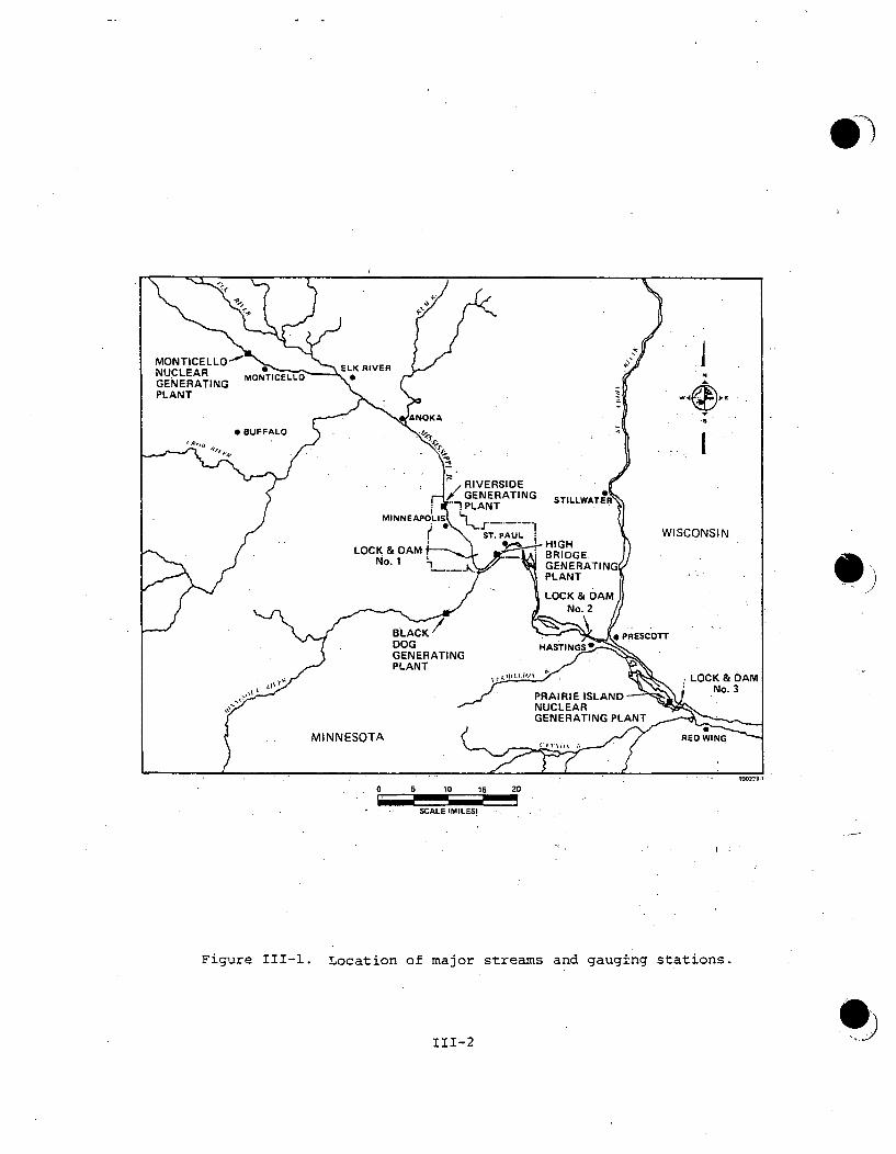
0 5 10 15 20

SCALE (MILES)

Figure III-1. Location of major streams and gauging stations.

111-2

a)N

U-

z0

w-J

UJw

oI

HHH

IA

547P-35RIVER MILES ABOVE OHIO RIVER

Figure 111-2. Longitudinal section of the Mississippi River from Dam No. 1 to Dam No'. 4 showingthe relative locations of Pool No. 3 and PINGP (adapted from AEC, 1973).

W

I

685

DI--

wCN

I-

LULUI.-

LM

0

ca

.4z04

LL-JLU

683

681

679

677

H--HH*p.*

675

6730 20 40 60 80 100 120 140 160 180

RIVER DISCHARGE (1,000 cfs) 547P-30

Figure 111-3. Stage-discharge diagram for Pool No. 3 (adapted from Corpsof Engineers, 1974).

(A) POOL IN PRIMARY CONTROL (constant elevation at Prescott): Flow 0 to 14,000 cfs

TAILWATER L/D No. 2

.. "- CONTROL T. No.3673.5' (max. allowable drawdown)S PRESCOTT PINGP -.. TAILWATER L/D No. 3

DAM No. 2 DAM No. 3

(B) POOL IN SECONDARY CONTROL (constant elevation at headwater L/D No. 3): Flow14,000 to 36,000 cfs

• / 680.3'

/.678.5'

67 .' 674.5'

67473.5'

CONTROL PT. No. 3PINGP

(C) DAM No. 3 ROLLER GATES OUT OF WATER (open river, water surface rising at allpoints): Flow > 36,000 cfs

NOTE: 7 INDICATES WATER LEVEL.

'547P.29-2

Figure 111-4. Schematic diagram of how water level in Pool No. 3is controlled.

111-5

After the headwater elevation reaches 673.5 ft msl, the discharge con-trol is shifted to the secondary control which requires that the headwaterat Dam No. 3 be kept the same until the discharge reaches 36,000 cfs or

h = 673.5 for 14,000 < Q < 36,000 cfs.

During secondary control, the discharge is calibrated against the watersurface elevation measured at Control Point No. 3 (Figure 111-3). At thiscontrol stage, the headwater at Dam No. 3 would be kept constant while theControl Point No. 3 elevation is allowed to rise due to the inflow fromDam No. 2 and the St. Croix River (Figure 111-4).

After the river discharge reaches 36,000 cfs, all the roller gates atDam No. 3 are raised to the maximum height (above the water surface), andthe dam no longer regulates the flow of the river (i.e., the open rivercondition prevails). The empirical head discharge equation for this con-dition is described as (Stefan and Anderson, 1977):

h = 673.5 + 2.5 x 10-9 (Q- 36,000)0-77 for Q > 36,000 cfs.

When the river flow decreases, the gates at Dam No. 3 are returned tothe water and secondary control is in effect until the stage at ControlPoint No. 3 is reduced to 674.5 ft msl, at a discharge of 14,000 cfs. Ifdischarge continues to drop, primary control would then take place to holdthe pool level constant (674.5 ft msl) at Control Point No. 3 and to allowthe headwater at Dam No. 2 to rise while that at Dam No. 3 decreases to673.5 ft. According to the discharge records at Prescott over the past49 years, the river is in primary control about 70 percent of the time.The river is in secondary control approximately 20 percent of the timeand the open river condition prevails for 10 percent of the time.

A 2.7 m (9 ft) deep navigation channel is maintained by the Corps ofEngineers between Minneapolis and the mouth of the Missouri River tofacilitate transport Of commodities by barge. In 1976, 6,050 lockageswere recorded for Lock No. 3 of which 2,377 were commercial (Corps ofEngineers, 1977). On the St. Croix River, a 2.7 m (9 ft) channel extendsfrom the confluence with the Mississippi River to Stillwater, Minnesota.

2. Characteristics of the PINGP Vicinity. The PINGP site is a lowlandterrace associated with the Mississippi River floodplain. The site isseparated from the other lowlands by the Vermillion River and various smalllakes on the west and the south, and by the Mississippi River and North andSturgeon Lakes on the east and north. The topography is almost flat exceptfor the low bluffs to the north. The hummocky nature of the terrain andthe sandy soils on the site results in little significant surface drainage.

In the immediate vicinity of the plant site, the surface elevation rangesfrom 206 to 215 m (675 to 706 ft) above mean sea level. A typical.crosssection of the floodplain is shown in Figure 111-5. The normal elevation of

111-6

CROSS SECTION DISTANCE (METERS)

0 1.000 2,000 3,000 4,000 .5,000

720 219.5

S,-

o 710 216.5M

(N oN

700 213.4 ILu I-"

wLUjRAILROAD IOA

-. 690 212.4 UH

EH LI. •

I > CATFISH SLOUGH MARSH >• .. O O o 600 V E R M IL L IO N ] •20 7 .3 Q

j SLOUGH zZ r. _0

670 204.3

...I ILlU.J

LU

660 201.2

6501-- I I II I I I , I I I 1 I I I I I 198.20 1,000 2,000 3,000 4,000 5,000 6,000 7.000 8,000 9,000 10,000 11,000 12,000 13,000 14,000 15,000 16,000 17,000

CROSS SECTION DISTANCE (FEET) 547P-32

Figure 111-5. Typical Mississippi Valley cross section near PINGP (AEC, 1973).

Pool No. 3 (at Prescott) is 674.5 ft msl, and the maximum recorded' floodlevel at Prescott was 692.61 ft msl on 18 April 1965. Due to the highpermeability of the sandy alluvial soils underlying Prairie Island, thegroundwater table is shallow and responds quickly to changes in riverstage. The groundwater level almost coincides with the river surface,ranging from 673 to 674 ft. The general regional groundwater flow isfrom the higher, partially glaciated bedrock-areas toward the MississippiRiver and its tributaries. Since Pool No. 3 is elevated by Lock andDam No. 3, the pool surface is usually higher than the Vermillion Riverand its backwater lakes, which enter downstream of Lock and Dam No. 3.Consequently, the groundwater table at Prairie Island slopes south-westward to charge the Vermillion River.

In Pool No. 3, there are two major backwater lakes connected to theriver by numerous small channels and river runs. These two lakes areNorth Lake and Sturgeon Lake (Figure 111-6).

Sturgeon Lake, from which almost all the plant intake water is withdrawn,is one of the largest backwater lakes in the area. Water in the lake comesprimarily from the Mississippi River through numerous coulees and reachesand through channels from North Lake. A small amount of the inflow is throughgroundwater seepage; however, .this is believed to be insignificant, comparedto surface inflows (Stefan and Anderson, 1977). The depth of Sturgeon Lakevaries from 1.2 to 4.6 m (4 to 15 ft). Like many other backwater lakes inthe area, it is probably the result of Pleistocene glaciation.

The hydraulics of North Lake, Sturgeon Lake, and the Mississippi Rivernear PINGP has been studied by Stefan and Anderson (1977).., They divided theriver/lake region into two network systems: Sturgeon Lake. and the downstreamarea (see Figures 111-7 and 111-8). The Sturgeon Lake system consistsof Sturgeon, North, and Brewer lakes; six river sections in the MississippiRiver; and 13 river runs between the three lakes and the river. The down-stream system consists of a section of the Mississippi River near PINGP;plant intake and discharge channels, and channels among the small islandsin lower Sturgeon Lake.

The hydraulic networks were analyzed b'y applying the laws of conser-vations of mass and energy. Conservation of mass requires that the sumof all flows into and out of a channel junction be zero; however, thisdoes not include water loss or exchange through seepage, evaporation, orevapotranspiration. Sturgeon Lake and North Lake were not treated aschannels since the velocity in them is too low as a result of their largecross-sectional areas. Conservation of energy requires that the totalhead losses in parallel channels be the same and head losses in channelsin series be additive. Head losses are from channel bed shear stressesand from wind shear stresses on the water surface. Twelve continuityequations (conservation of mass) and nine energy equations (conservationof energy) are necessary to compute the flow rates for the 21 channelsspecified in Figure 111-7. The details of the mathematical model can befound in Stefan and Anderson's report. The solution of this set of

111-8

,.•.: .. LOC K &...-,DAM NO.

54

Figure 111-6. Major water bodies in the vicinity of the PINGP.

9

7P-1-1

111-9

547P-31

Figure 111-7. Sturgeon Lake channel system for the hydraulic networkcalculations (from Stefan and Anderson, 1977).

III-10

547P-i8

Figure III-8. Downstream channel system for the hydraulic networkcalculations (from Stefan and Anderson, 1977).

III-Il

equations serves as the input to the downstream channel system analysis.For every river discharge and wind velocity, the outflows from Channel 1and Sturgeon Lake are used as inflows for the downstream channel system,i.e., in Channels 34, 36, and 1.

Similar sets of continuity equations and energy equations are con-structed for the 22 channels in the downstream channel system. The com-puted flow rates for Channels 36, 26, 27,28, 30, and 42 are in turn usedfor the thermal plume analysis described in Section V.

The results of the computation of the downstream channel system werecalibrated against limited field measurements conducted by the U.S. Geo-logical Survey and J. Gorman, Inc., of Minneapolis, and the results arepresented in Table III-1 for Sturgeon Lake and Channel 42. As shown by,the data, the predicted flow rate in Sturgeon Lake fell within 5 percentof the measured values when the river flow was less than 40,000 cfs.During flood conditions (> 60,000 cfs'), however,.the calculated tvaluewas 19 percent below the measured one. Thus,;-the trend is toward a flowdeficit for the computed flow rate inSturgeophLake as the total riverflow goes up. Since the primary emphasis in this study was on low riverflows, the error at higher flows is of little significance. Predicted flowsthrough Channel 42 for the three measurementsj.were 7 percent below, 17percent above, and 94 percent below the measured values. The large errorin the latter case could be caused by a variety of reasons, including thesensitivity of Channel 42 to winds from the west. to northwest and possiblestrong stratification during low river flows (2,890 cfs). Field instru-mentational errors could also be a cause, particularly during the lowflow conditions, since most of the velocities in Channel 42 were less thanthe threshold value of the flow meter. Counter flows (or recirculatingflows) could easily be overlooked. In general, the hydraulic networkmodel developed by Stefan and Anderson is considered to reasonably predict"the flow rates,.'in Sturgeon Lake and Channel 42 as a function of total riverdischarge. The Sturgeon Lake discharge versus the Mississippi River dis-charge with no wind is shown in. Figtire 111-9. From this figure, it iscalculated that between 19 and 32 percent of the total river flow at Lockand Dam No. 3 passes through Sturge6n Lake (Channels 34 and 36)_. The Channel42 flow, with no wind, can also be approximated by the equation Q42 = 0.14 QJ.96

from the results of Stefan and Anderson's model.

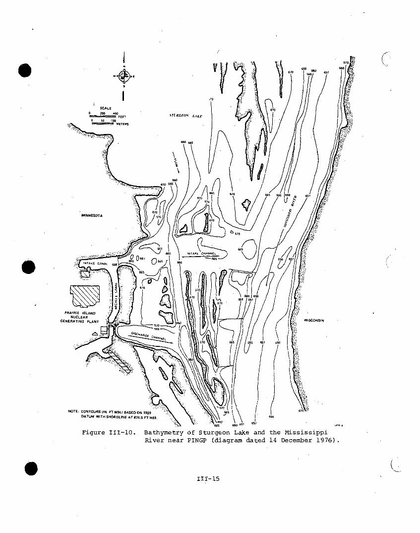
3. River Morphometry Near PINGP. The Mississippi River in thevicinity of PINGP is 300 to 370 m (1,000 to 1,200 ft) wide, and thebathymetry is shown in Figure III-10. The river banks slope fairlysteeply to the river bottom,. and the navigation channel has requiredminimal dredging since 1935 (Cin, 20 October 1977).

Sturgeon Lake is a very shallow lake and its important morphometricparameters'are summarized as follows:

* Maximum length: 5.0 km (3.1 mi)

o Maximum effective length: 3.5 km (2.2 mi)

111-12

.

Table III-1. Comparison of the computedfield measurements.

discharges in Sturgeon Lake and Channel 42 with the

QRiver Qsturg. L. Q42 Wind Wind QP p

Date (cfs) (c fs) Speed Dire Intake Discharge Source Qstur. L. 42

(mph) (cfs) (cefs)

3/26/73 62,000 18,820 - 8.6 700 0 0 JGG 15,270 6,150

5/02/74 40,400 10,900 - 18.9 180I 185 150 U.S. .S.2 10,020 3,930

5/09/74 32,360 7,430 - 8.0 1250 185 150 U.S.G.S. 7,140 3,110

7/01/74 21,880 4,590 - - 14.7 2250 185 150 U.S.G.S. r 4,740 2,060

11/26/74 10,400 - 960 17.7 1450 185 150 JG 1,640 890

8/01/75 13,500 2,700 1,150 12.9 2000 1,095 1,060 JG 2,580 1,340

10/13/76 2,890 - 1,070 18.0 2950 245 210 JG 1,150 70

MEASURED L-COMPUTED ]

HHH

IJ. Gorman, Inc., Minneapolis, Minnesota, 1973.

20.S. Geological Survey, Water Resources Data for Minnesota, 1974.

(..

TOTAL RIVER DISCHARGE (m3 /sec)

1,0000 500 1,500 2,00024,000

21,000

LU

LUCC

0

z0LU0,

x-

18.000

15.000

12.000

9,000

6.000

700

600

U

500E

LU

400U

300

4

0

200 CrI-CA)

100

1"-IHH

I4'-'

3.000

0 P' - I I i i I ii i i i I , • o0 5,000 10.000 15.000 20.000 25,000 30.000 35.000 40,000 45,000 50,000 55.000 60.000 65,000 70,000

TOTAL RIVER DISCHARGE (cfs) 547P-34

Figure 111-9. Sturgeon Lake discharge versus total river discharge (Stefan, 1973).

S

GO 6700

1 ;70SCALE

6.00 2 00.FEV L4:Jr

0 so too

~'METERS

660 /670 650\

70670 665 660 go0 6507

MINNESOTA /67 ~ 7

670

640

fl~. 660 INTAKE C.ANNEI.•FG

o 656 6 657INTAKE CANA, 0 60 0 6 660S 665

z 670

070 6416550

PRAIRIE ISLAND /

O S

GNNUCLEAR L

GENERATING PLANT ,7"

WISCONSIN

670 " 657Figure III-10. Bathymetry of Sturgeon Lake and the MississippiRiver near PINGP (diagram dated 14 December 1976).

06 5

'67-I

..W

NOTE: CONTOURS (IN FT MSLI BASED ON 1929DATUM WITH SHORELINE AT 674.5 FT MSL.

I

SCALE

II ml 4w.-. . FtEE"

WISCONSIN U0 S f•\ .ME It FtS

H-H

MINNESOTA

Figure III-10. (Continued)

. Maximum width: 2.8 km (1.75 mi)

* Direction of major axes: SE-NW

* Surface area: 323.8 hectares (800 acres)

e Mean width: 0.8 km (0.5 mi)

e Volume: 6.7 x 10 6 m3 (2.37 x 108 ft 3 )

* Maximum depth (based on water surface elevation of 674.5 ft msl):6 m (20 ft).

o Average depth (based on water surface elevation of 674.5 ft msl):2.07 m (6.79 ft)

* Shoreline: 17.3 km (10.7 mi)

* Range of retention time of water: 3.8 hr to 42.6 hr (corresponding toriver flows of 1,868 m3 /sec and 226.4 m3/sec)

Near its southern end, numerous small islands occur, and this is where thePINGP intake and discharge are located. In 1970, the approach channel(Class I structure).for the plant intake water supply was dredged to abottom elevation of 664.5 ft msl (3.1 m deep at normal pool level) anda width of 183 m (600 ft),,.. The discharge canal (Class III structure)was dredged to a bottom elevation of 664.5 ft msl also, and the widthincreases from 30.5 m (100 ft) at the discharge gates to 122 m (400 ft )at a distance of 213 m (700 ft). The canal dikes were compacted fill andare constructed to appear as a natural channel. A survey of the channelsin 1976 by J. Gorman, Inc., indicated no substantial sediment deposit.

4. Discharge Rates. There are two major gauging stations on theMississippi River near the plant site: at Prescott, Wisconsin, and atWinona, Minnesota. Prescott is about 24 km (15 mi) above the plant(811.4 river miles above the Ohio River), and the drainage areas is esti-

mated to be 116,032 km2 (44,800 mi 2 ). The St. Croix River enters theMississippi River at Prescott, and there are no other major tributariesbetween Prescott and the plant site. Winona is about 135.5 km (84.2 mi)downstream from the plant site (725.7 river miles above the Ohio River),and the total drainage area there is about 153,328 km2 (59,200 mi2).Because of the proximity of the Prescott station, flowrates from there areused throughout this demonstration.

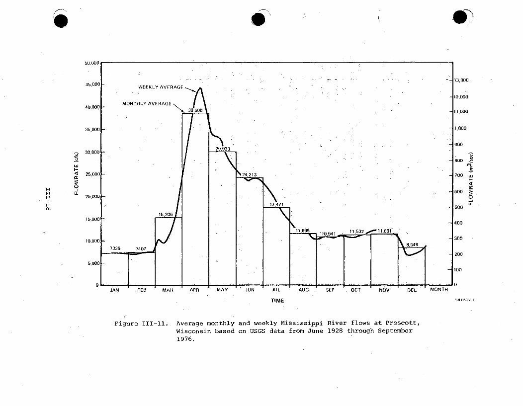
Prescott has a continuous discharge record since June 1928 (49 years).The average discharge for the first 48 years (up to 1976) was 16,200 cfs.The instantaneous maximum flowrate ever recorded was 228,000 cfs on18 April 1965, while the minimum daily flow was 2,100 cfs, observed on14 August 1936*. The average monthly and weekly-river flows are shown inFigure III-11.

*On 13 July 1940, a record minimum flow of 1,380 cfs was observed. This

was probably the result of an operator error at Dam No. 2 (see PreliminarySafety Report for PINGP).

111-17

14-1

ci

0-jLL

50.000

4b.000

40.000

35.000

30,000

25,000

20,000

15,000

10,000

5.000

0

rMONT

WEEKLY AVERAGE

HLYAVERAGE3B,6 08

29,933

W",

13,000

12.000

11.000

- 1,000

900

800 -

E100 w%24.213

HHH

I--,

73363 7407

15,206

17,471

•11.6951Ipý 115T 0-1,61

600

500

400

300

200

100

F-

0-Ju.

1 1-1-4. 1 11 4. 1 I 4.-P UJAN FEB MAR APR MAY JUN JUL

TIME

,AUG SEP OCT NOV DEC MONTH

S,411'21I 1

rFigure III-il. Average monthly

Wisconsin based1976.

and weekly Mississippi River flows at Prescott,on USGS data from June 1928 through September

It can be seen that the discharge usually peaks in April due to snow-melt runoff and levels off from September to February when the river ischarged mostly by groundwater. Figure 111-12 shows the calculated 7-day,10-year recurrence flows for each month. A standard log-Pearson Type IIIdistribution was used in computing these numbers. Also shown on the figureis the percentage of time in each month when the 7-day, 10-year low flowwas not exceeded. These values ranged from 2.2 to 8.4 percent and will beused in Section IV to estimate the probabilities of the joint-eventoccurrences.

B. WATER QUALITY OF THE MISSISSIPPI RIVER

I. Temperature. Ambient river temperature data in the vinicity ofPINGP provide necessary input for the thermal plume model (see Section V)as well as a reference for spawning and thermal tolerance informationdiscussed in Section III C. The following discussion assesses the avail-able data to determine the most adequate record.

The stations at which water temperature has been recorded regularlyinclude the resistance temperature detector (RTD) station at the intakecanal of PINGP, a temperature recording station in Sturgeon Lake maintainedby the Minnesota Department of Natural Resources (MDNR station), a stationat Lock and Dam No. 3, several stations utilized for water quality samplingin the ecological monitoringprogram, and the intake temperature stationat NSP's Red Wing Generating Plant (RWGP).

The RTD intake station at PINGP is located on the river side of theintake canal barrier wall. Temperature sensors are vertically spaced at0.6 m (2 ft) intervals on two pilings for a total of 10 sensors. AllRTD readings are averaged by the plant computer and recorded hourly onthe plant log. These recorded values enter the plant environmental eventlog only when discharge flow is adjusted. Even though the RTD datarepresent a continuous record, they cannot be considered representativeof river temperature for several reasons. First, the period of record istoo short since data are only available from February 1975 to present.Second, possible instrumentation problems exist which would make the dataunreliable. And third, during high blowdown rates and southerly winds,intake temperature readings may be above ambient river temperature due toupriver movement of heated effluent.

The MDNR station is on the river (northwest) side of Sturgeon Lake(Figure 111-13) at a depth of 0.8 to 0.9 m (2.5 to 3 ft). The station islocated in shallow water since the rest of the lake averages 2.1 m (6.8 ft)in depth. Temperatures were recorded on strip charts 'during the ice-freemonths of 1975 through 1977. Due to lack of calibration and maintenancerecords, these data will be used only to indicate diurnal fluctuationsin temperature. The observed diurnal fluctuations were fairly large,

111-19

/ N

1 0000

9, W)(3

8,001)

7.000

4,000

0-jLL 4,000

250

200

150 Ir.

0-1

1600

H

0

3.000

2.0011

1.000

JAN FEBt MAR APR MAY JUN JUL AUG SEP . OCT NOV DEC

MONTH b4IP'28.1

Figure 111-12. Monthly 7-day, 10-year low flows for the Mississippi River at Prescott,Wisconsin, and the percentage of time the daily flowrate is less thanor equal to the 7-day, 10-year flows. Based on USGS data for June 1928through September 1976.

Figure III-13.

547P-122

Location of the Minnesota Department of Natural Resources(MDNR) temperature recording station and the locations ofwater quality stations where temperature is routinelymonitored.

111-21

averaging 20 to 30 C (3.50 to 5.4* F) with a maximum of 9.7* C (17.50 F).Vertical temperature stratification is not expected to be significant atthis station because of its shallow depth; however, no records are avail-able to substantiate this assumption.

Daily maximum and minimum river temperatures -have been recorded atLock and Dam No. 3 since 6 August 1969. Two temperature probes areused at this station: a primary probe located approximately 1.2 m (4 ft)below normal pool elevation on the upstream face of the dam, and a secon-dary sensor located on the downstream face of the dam which is used onlywhen the primary probe malfunctions. Measurements were taken first by theMinneapolis-St. Paul Sanitary District, then by the Federal Water PollutionControl Administration, and presently by -the U.S. Geological Survey.Since Lock and Dam No. 3 is located only 1.6 km (1 mi) downriver from thePINGP discharge, temperatures may have been periodically influenced bythermal discharges from the plant. Thus, only the four years of pre-operational data may be used (the first unit of PINGP came on-line inDecember 1973), and this period of record is probably 'insufficient todefine long-term temperature trends.

In addition to the PINGP intake, Lock and Dam No. 3, and MDNR records,temperatures were measured at several NSP water quality stations shown inFigure 111-13 from 1972 through 1976. Surface, mid-depth, and bottomtemperatures were taken once or twice a month with a thermister. Tempera-tures measured near the intake are probably most representative of PINGPintake water temperatures;ihowever, because of infrequent measurements(twice a month maximum) these data are of limited value.

Temperature measurements at RWGP intake located 15 km (9.4 mi) down-river from PINGP have been taken manually since 1950. RWGP is a 28 MWe(summer rating) natural gas/coal-fired plant that utilizes once-throughcooling. The plant initially operated as a base load facility, butbecame a peaking plant in 1974. Itloperates approximately 16 hours aday during weekdays, and intake temperatures are recorded hourly duringoperation from thermocouples located on the discharge side of the cir-culating water pumps. These thermoc0uples were calibrated on 29 March1978 and the temperature readouts were found to be within 0.3' C (0.5" F)of a mercury thermometer (MbcGinnis, Zimmel, and Martin, 1978). Despitethe lack of previous calibration, the RWGP data are expected to be within0.60 C (1.00 F) of the true temperatures given the general accuracy ofbimetal (thermocouple) measurements.

Owing to the small heat rejection and circulating water flows fromRWGP and the do0nriver location of the discharge, the intake temperaturesare assumed to be free of thermal recirculation-. slightly higher thanambient readings of less than 1.10 C (20 F), however, might be expectedduring winter deicing operations. RWGP intake temperature is also consideredto be unaffected by the PINGP thermal discharge since thorough mixing anddilution of the PINGP plume with ambient river water is accomplished bypassage through Lock and Dam No. 3. Immediately downriver from Lock and

111-22

Dam No. 3, river temperature rise should be less than 1.10 C (20 F) 90 percentof the time (see Section IV B.1). Residual heat passing through Lock andDam No. 3 should readily dissipate befolre reaching RWGP, 11.6 km (7 mi)downriver. /

To test the validity of RWGP data, temperatures taken during the

PINGP water quality monitoring studies were compared with RWGP temperaturesfor the same date. Surface, mid-depth, and bottom temperatures atStation X-1 (Figure 111-13) were averaged*, and the daily maximum at RWGPon the same day was subtracted to obtain a ATa. The positive arid thenegative ATa's were then averaged separately for each year. Data presentedin Table 111-2 indicate,,that temperatures were similar at both locationsfor the sample dates compared. The small differences observed may be theresult of differences in the time of day when measurements were taken,flows, flow ratios, and wind. The RWGP data represent daily maxima whichgenerally occur in mid-morning to late afternoon. Table 111-3 shows thediurnaltemperature fluctuations calculated from daily maxima and minimarecorded at Lock and Dam No. 3. During the warm months (April throughAugust) the average ATa is less than the diurnal temperature fluctuation.Thus, it can be concluded that RWGP temperatures are generally an acceptablerepresentation of average river temperatures..

Table 111-2. Summary of the mean temperature differences (AT)between ecological monitoring stations and theRed Wing Generating Plant intake,

ANNUAL AVERAGEYEAR TEMPERATURE DIFFERENCE (C)

+1 _2

1972 1.0 0.95

1973 0.9 0.47

1974 0.49 0.65

1975 0.60 0.86

1976 0.56 0.85

Mean 0.71 0.76

(•1. 30 F) (0,1. 4 F)

1 PINGP field temperatures above RWGP intaketemperatures.

2 RWGP intake temperatures above PINGP field

temperatures.

*This takes into account heat recirculation and stratification.

111-23

Table 111-3. Average diurnal river temperature fluctuation measuredat Lock and Dam No. 3 (U.S.G.S., 1969-1976)1.

MONTH JAN FEB MAR APR MAY JUNE

DiurnalTemperature 0.17 0.30 0.64 1.17 1.37 1.04Difference (0.3) (0.54) (1.2) (2.1) (2.5) (1.9)in 0 C (OF)

MONTH JULY AUG SEPT OCT NOV DEC

Diurnal.Temperature 1.16 0.4 0.68. 0.58 0.5 0.18Difference (2.1) (0.7) (1:.2) (1.0) (0.9) (0.3)in 'C (OF)

iThe record is based on the maximum and minimum dailytemperatures taken at Lock and Dam No. 3.

A graphical presentation of weekly mean river temperature for theperiod 1959 through 1974 is shown in Figure III-14. The river surfaceremains frozen in winter months until late February, and temperatures 0gradually increase in spring.. After reaching a peak of about 240 C(760 F) in late July, -temperatures: decline until late December when theriver surface again freezes. A maximum temperature at RWGP of 290 C(850 F) occurred on 2 August 1977.,

Weekly averages of daily minima, means, and maxima for the period1959 through 1974 are given in Appendix Table A-i, and monthly averagesare shown in Appendix Table A-2. Weekly and monthly average river flowsare also included in these two tables for reference. Combining flow andtemperature shows that, in general, both river flow and temperature! riseuntil late May when spring runoff reaches its peak. Then, river flowstarts to decrease gradually while water temperature keeps rising as aresult of increases in air temperature and warmer inflows from tributaries.After late August, both river flow and temperature decrease because of lowrainfall and declining solar angle. In winter months, river flow ismainly supplied by groundwater, and temperatures remain near freezing.The tables also show that the difference between daily maximum and minimumtemperatures for any given period is less than 1.10 C (20 F).

Appendix Table A-3 shows the monthly and annual cumulative distributionof daily maximum temperatures. The range of temperature variationsindicates that large fluctuations exist during spring and fall, and minimumfluctuations are observed in winter. The annual cumulative distribution(last column of Appendix Table A-3) is plotted on Figure 111-15, an d it can

be seen that the river remains frozen almost 25 percent of the time!,.

111-24

j

- 90w wja: 3o

I- I-< BO0

H w 25 w

Ln w w

I- 70 2020

60 15

50 to

40 O

32

JAN FEB MAR APRIL MAY JUNE JULY AUG SEPT OCT NOV DEC

MONTH372P-659-1

Figure m11-14. Weekly average river temperature at Red Wing (from the RWGP log, 1959-1974).

4.0

0 0~>

0

X

0aU,

-1

0

I.-

zIl'-II

- 10

- _ _ __ _ _ _ 90

80 - ___ - ___-so

710 - -____ - ___ 70

30 3 -- ___ 0

2o -- - ___ ___- 20

10 - -___ 0

0 -0 _ _ _ _ _ __ _

0O

HH

0I

30 32 35 40 46 50 55 60 65 70

DAILY MAXIMUM RIVER TEMPERATURE (F)

80 85 90 95

547P.123

Figure 111-15. Cumulative frequency of occurrence of daily maximum rivertemperatures at RWGP (from RWGP log).

2. Water Quality in the Vicinity of PINGP.

a. GENERAL BACKGROUND INFORMATION. The.segmentof theMississippiRiver immediately upriver from Lock and Dam No. 3 near PINGP is more ofa lacustrine than a riverine habitat, characterized by low turbidity through-out most of the year.: The water is moderately hard and slightly eutrophic(Tables 111-4 and 111-5). Measurements of trace metals (Table 111-5)indicate that levels may be elevated above normal background conditionsat tim•s•. In addition, toxicants such as phenols and cyanidehave beenmeasured at relatively high levels in this section of the river.

The Metropolitan Wastewater Treatment Plant (MWTP), located approxi-.mately 61 km (38 mi) upstream from PINGP, contributes a substantial amountof the nutrient and toxicant load in the Mississippi River as far down-stream as PINGP. The MWTP was constructed in 1938, and provided primarytreatment.Only. In 1966, secondary treatment was added to a'designedcapacity of 218 million gallons a day (mgd), and additional facilities foractivated sludge treatment were constructed in 1972. At present, con-struction is also underway to further expand the plant which will resultin enhanced effluent quality in future years. Appendix Table A-4summarizes the effluent quality in 1975 and 1976. Besides the gradualdecrease in volume, it is also apparent that effluent quality has beenimproving (and is expected to improve in future years), thus furtherminimizing the influence of this domestic sewage upon water qualityconditions in the Mississippi River. The enhanced levels of metalsand other toxicants at Lock and Dam No. 3 may be a result of.-the MWTPdischarge, although agricultural sources may also be a source of someconstituents (Omernick, 1977). BOD levels measured at Lock and DamNo. 3 since 1969 usually appear to be well below the average dissolvedoxygen levels, which may explain the consistently high dissolved oxygenlevels-measured at Lock and Dam No. 3 (Table 111-5) and near PINGP.

b. EFFECTS OF PINGP EFFLUENT.- Average, maximum, and minimum dissolvedoxygen levels have been measured at seven water quality stations in thevicinity of PINGP from 1973 to present, and the concentrations usuallyaveraged well above the minimum levels necessary for most aquatic life(i.e., minimum levels rarely dropping below 5 mg/l). In most instances,

mean, maximum, and minimum oxygen concentrations were higher in surface>samples.than in those near the bottom, although in some instances (seeFigure 111-16), dissolved oxygen inversion occurred. At Station 12 (seeFigure 111-17 for location), a more measureable oxygen inversion was notedat Stations 21 and 25, located in the PINGP discharge. This mayhave been the result of less oxygen saturated thermal effluent floatingabove the colder, more oxygen laden ambient river waters. It should.benoted, however, that an oxygen inversion was, observed at Station 25 in1973, also, when the plant was not operational. This indicates thatdissolved oxygen inversions may periodically occur naturally in this area.During operational years (1974 to 1977), it appears that the dissolvedoxygen content of water passing through the plant decreased slightly(compare Stations 12 and 18 in Figure 111-16), probably as a result of

111-27

Table III-4. Minimum, maximum, and mean concentrations of water quality

parameters in subsurface samples collected from 21 June 1970through 13 September 1977 (from NUS, 1976; Eberley, i977;NSP, unpublished)'.

CONCENTRATION(mg/l UNLESS OTHERWISE NOTED)>PARAMETER

MINIMUM MAXIMUM MEAN.

Solids, Total 168 443 269

Solids, Dissolved 134 367 243

Solids, Suspended 1.4 85 27

Hardness, Total (as CaCO3) 110 268 1823

Hardness, Calcium (as CaCO ) 76 180 117

Hardness, Magnesium (as CaCO 3) 34 100 65

Alkalinity, Total (as CaCO3 ) 86 232 154

33Alkalinity, Phenolphthalein (as CaCO 3 01 2.4. 3.3

Ammonia Nitrogen (N) 0 2.4 0.45

Carhonate 2 (CO 3 ) 0 29 3.1lBicarbonate 2 (HC0 3 ) 103 235 176

Chloride -(Cl) 2 32.9 14.8

Nitrate'Nitrogen 3 (N) <0.01 4.2 0.87

Sulfate (SO 4 ) 10 110 38

Phosphorus, Soluble 3 (P) 0.005. 0.550 0.14

Silica (SiO2 ) 0.1 16.2 81

Calcium2 (Ca) 30.4 72 47

Magnesium2 (Mg) 8..3 . 24 16

Sodium, (Na) 3.9 28.5 13,

Iron, Total3 (Fe) 0.0 2.36 0.57

Color 3 (APHA units) 15 100 50

Turbidity (JTU) 1 52 12

Conductivity (imhos/cm) 230 572; 393:

pH / 7.4 9.4 8.2

Biochemical Oxygen Demand 1.1 9.45 3.5

iPrior' to plant operation (1970-1973) samples were collected at the location ofthe intake and after 1973 the samples were collected in the main channel of theriver just upstream from the intake.

2Minimum, maximum, and mean calculated for the period of June 1970 to September 1977.3Minimum, maximum, and mean calculated for. the period of January 1970 toSeptember 1977.

.9111-28

Table 111-5. Selected water quality for the Mississippi River at Lock andDam No. 3, 1969 to 1976 (U.S.G.S., 1967-1976)..

WATER VJIALITY PAIOLMEI126

m-oo. Nil I).q/

8110,.1 C., 1/ /

1'i,. ,.qI zw/

N. #q/1

VishI - Hui0 Ni, .011 Nýl IN). ",)/I

NAX

12.0

5.4

0.6

M969

6.6

0.4

MEAN

0.4912

0. J4

MAX

14.2

4.8

1.0

1970

2M.

2.0

MEAN

9.072

3.142

1971

2.M2 N MEAN

12.2,-6.2 94.53•

4.6 6.1 2.753

NAX

2.8

4.5

0.11 1- 0.-I..1 -.3 1 .

1972

SIN

"6.1

7.6

1.4

0.9SI 0.11

9. 81.

U.057

2.64W

0.4112

231)

511d'

3d

.01 14

L1.1111

7.d12.2

8.0

KA7.4i

0.86

I023

to0

140

.01

3.05

0.400.260

H1I

1.2

1.4

70

30500

0.37

0.05

IS. b8l

3.255

0.568

0~

257

0.057

0.005,

1.545

0.1s,

MAX

13.0

11.0

II

1.85

1973 1974

mIN KMAN

0O.6

2.4

0

I .02

912

4.331'

J.55k

4)11

sd3

1.105

1975

MAX Kim MEAN

12.7 6.5 9*41'

3 4 2.0 7.746

3.5 1.2 2.43

to 0 5,1"7

1.1 0 U.401

213

00111

2. 1330| }

0

4.67 0.24 1.145

0.25 0.01 0..14

1976

MAX N0 K MEAN

12 7.6

7.2 2.4 4.866

10 0 4.67

213

ioo''

013

1113.

1.7 0.04 0. !

0.27 1 0.06 0.106.I • . ":,ý v1.531o.201,

-44I 0.28 ,:,I6 u::: 0..210 :.04 0.350.5 I0.05

0.431 0.06

H-,H-H.-

I0EIvv,- M11tL~ly 0~U,1-,10.. ilyjl,

-9i, OuulVl -1-u,, tw, hloo,,thly v41we.

".1 1- lO.IIL -~1-.o oboa0~y01.. ,.

'lS-111~ -010.1,1 VdIoO. I

-ltha uothl:.,

'$U,,.00 -Ahl.y 021.0I 004bU-olyo,~

"''101 oothlyvIN..

W,

E

ZLU

X0

LU

0

o.

20

10

0

20

10

0

20

10

0

20

10

0

20

10

0

1973

1974

1975

1976

1977

1 +410 6 12 18

HDR STATION

21 25 27

547P.10

Figure 111-16. Maximum, minimum, and average dissolved oxygen levels forselected stations in the vicinity of PINGP, 1973-1977.Open bars indicate range of surface DO, vertical linesindicate range of bottom DO, and horizontal lines indi-cate mean levels of DO (Dieterman, 1974-75; Schmidt,1977; NSP, unpublished).

111-30

547P-6

Figure 111-17. Sampling locations for water quality, phyto-plankton, periphyton, zooplankton, and macro-invertebrates.

111-31

increased water temperature, and therefore, lower oxygen saturation. Upondischarge from the plant, however, the dissolved oxygen levels quicklyreached those of the receiving waters; thus, the. effect of plant operationupon receiving water dissolved oxygen appeared to be temporary and minimal.

In order to determine quantitatively what effect PINGP exerts uponvarious water quality parameters, an analysis of variance was performed bySchmidt (1977) on data from two pairs of stations upriver and two pairsof stations downriver for 1975 and 1976. A comparison was also madebetween top and bottom samples collected at the same stations (Table 111-6).Significant differences between up- and downriver stations might indicatea plant effect; between surface and bottom samples, a vertical stratifi-cation effect; between months, a temporal effect. The basic expectedplant effect would be temperature controlled parameters such as dissolvedoxygen. Enhanced temperature might also indirectly alter nutrient levelsby enhancing primary production. Plant effluents may also increasedissolved solids and conductivity in the immediate vicinity of the dischargeas a result of evaporation of cooling water during the closed and helpercycle modes of operation. Plant operation might also disrupt sedimentrelated density stratification as a result of turbulence in the dischargewater. In general, depth stratification exclusive of plant effect maybe expected for sediment related parameters (due to density) and dissolvedoxygen (due to depletion, production, and re-aeration), which in turn mayindirectly cause variations between top and bottom pH, alkalinity, andnutrient levels. No measureable'effect, however, is expected as a resultof plant operation upon river water alkalinity and pH. Temporal variationin water quality parameters, in addition, is expected to occur mainlybecause of variations in river flow, temperature, allocthonous (originatingoutside the river) and autocthonous (originating in the river) inputs overtime. Interaction between temporal and spatial (vertical and horizontal)values for all parameters may also result in significant variation, whetheror not such significant variation was shown to occur without interaction.

In both 1975 and>1976, water quality parameters varied significantlyat the a < 0.05 level over time, that is, from month to month. Sedimentrelated parameters, such as no'nfilterable residue and turbidity, variedsignificantly between top and bottom samples at all stations compared.Plant impact on dissolved-oxygen, conductivity, and ammonia nitrogen wasalso noted in-both 1975 and 1976. According to Schmidt (1977), the causefor the difference inupriver and downriver ammonia nitrogen levels isunknown, while that for dissolved oxygen was. probably a result of erroneousmeasurement. He also stated that increased conductivityr;i'eadings downriverfrom the plant may be the result of the PINGP discharge since evaporationin the cooling towers' increases the dissolved solids of ithe blowdown.Conductivity readings, however, were not corrected for temperature variations,which also may account forconsistently'higher levels measured in thedischarge (Eberley, personal communication). Data for one station upstreamand one downstream from PINGP are presented in Table 111-7 (see Figure 111-17for locations). Eberley (1977), using a Student's t-Test on both years(1975 and 1976) combined, found no significant (a = 0.05 level) differences

111-32

Table 111-6. Summary of ANOVA for water quality data comparisons for two stations (HDR Stations

10 and 11) upriver and two stations (HDR Stations 25 and 27) downriver from PINGP

measured at the top and bottom of the water column for 1975 and 1976 (from Schmidt, 1977).

VARIATIONS SIGNIFICANT AT o < 0.05

BETWEEN ABOVE VS BELOW ABOVE AND BELOW BETWEEN BETWEEN DEPTHS ABOVE AND BELOW

WATER QUALITY PARAMETER MONTHS PLANT PLANT BY MONTH DEPTHS BY MONTH PLANT BY DEPTH

1975 1976 1975 1976 1975 1976 1975 1976 1975 1976 1Q75 1976

Phenolphthalein alkalinity x x x1

Methyl-orange alkalinity x x

.Dissolved orthophosphate (P) x x

Total dissolved phosphorus (P) x x

Filterable Residue (TDS) x x

Non-filterable residue (TSS) x x x 2 x 2

Ammonia nitrogen (N) x x x!

Nitrite nitrogen (N) x x

Nitrate nitrogen (N) x x

pH x x

Conductivity x x X3

Dissolved Oxygen x x x4

Turbidity x x x 2 x2

I~

lUnknown explanation for significant variation.2Variation due to natural density stratification.3Variatio-npossibly resulting from PINGP effluents; conductivity measurements were not

account'for a significant difference between upriver and downriver stations in 1976.

4Variation possibly resulting from erroneous chemical measurement.

corrected for temperature, which may

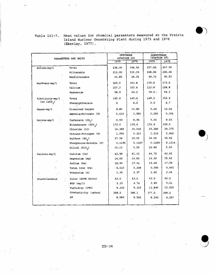
Table III-7. Mean values for chemical parameters measured at the PrairieIsland Nuclear Generating Plant during 1975 and 1976(Eberley, 1977).

UPSTREAM(STATION 10)

DOWNSTREAM(STATION 25)PARAMETERS AND UNITS

1975 1976 1975 1976

Solids-mg/l

Hardness-mg/l

Alkalinity-mg/l(as CaCO3

Gases-mg/i

Anions-mg/l

Cations-mg/l

Miscellaneous

Total

Filterable

Nonfilterable

Total

Calcium

Magnesium

Total

Phenolphthalein

'Dissolved Oxygen

Ammonia-Nitrogen (NM

Carbonate (CO 3 )

Bicarbonate (HCO 3)

Chloride (Cl)

Nitrate-Nitrogen (N)

Sulfate (SO 4 )

Phosphorus-Soluble (P)

Silica (SiO2 )

Calcium (Ca)

Magnesium (Mg)

Sodium (Na)

Total Iron (Fe)

Potassium (K)

Color (APHA Units)

,BOO (mg/1)

Turbidity (JTU)

Conductivity (umhos)

pH

236.00

213.00

22.80

165.0

107.0

58.0

142.0

0

9.80

0.410

0.50

172.0

14.360

1.090

27.50

0.1190

10.10

42.90

14.00

10.90

0.410

2.30

42.0

2.30

9.220

368.0

8.060

246.50

222.20

24.36

257.00

228.00

30.70

163.8

103.6

60.2

145.8

6.5

10.85

0.380

8.96

159.4

20.500

0.352

29.55

0.1007

5.09

41.53

14.63

17.51

0.208

2.37

43.6

4.74

9.355

386.1

8.582

170.0i12 -.0

59.0.

148.0

2.0

9.20

0.350

3.30

174.0

15.380

1.210

30.00

0.1240

10.40

44.70

14.30

12.00

0.590

2.40

43.0

2.90

12.840

377.0

8.240

257.00

226.40

30.53

173.0

108.8

64.2

152.4

6.7

10.02

0.301

8.03

169.6

20.375

0.400

30.92

0.1214

5.40

43.62

15.62

17.59

0.442

2.44

45.8

5.01

12.825

399.6

8.567

________________________________________ ________ ________ J ________

09111-34

\

between-the upstream and downstream stations for any of the water qualityconstituents. When comparing 1976 to 1975, however, some significantdifferences occurred for certain parameters. These'differences occurred inboth the upstream and downstream stati6ns''(phenolphthaleihi alkalinity,BOD, nitrate nitrogen, and silica) or in only the upriver stations (chlorideandbcarbonates), suggesting that the differences were naturally occurringand not caused by plant operation.

c. POTENTIAL FOR TOXICITY TO AQUATIC BIOTA. Certain water qualityparameters such as toxicants may interact with temperature to enhancetheir toxic qualities to certain affected biota (Jensen et al.,' 1969).However, most bioassays are conducted in the absence of thermal variation;the few tests conducted with variable temperature and toxicant levelstend to indicate that elevated temperatures enhance toxic responses bysusceptible biota (Jensen et al., 1969). Alkalinity, hardness, and pHhave also *been shown to potentiate or alleviate toxicity (Becker and'Thatcher, 1973,.p. M.2). Some water quality constituents measured in thevicinity of PINGP may be potentially toxic to aquatic organisms and mayalso contribute to or enhance any potential thermal impacts. Toxicantssuch as metals, phenols, and cyanides (for which data exist) are examinedin relation to bioassay information in Appendix Table A-6.- The data indi-cate that several constituents may be toxic to some organisms•'at the concen-trations measured in the river near PINGP,'in the absence of'thermal synergisms.It must be noted, however, that most'of these measurements were taken onlyonce or twice a year, and, thereforer should be c6nsidered as conservative(i.e., they probably underestimate high or critical levels actuallyoccurring in the river). The available bioassay literature""indicatesthat phenol and arsenic concentrations measured near the plant should notcause problems when' onsidered separately. Copper;' however,' may be detri-mental to certain phytoplankton,' zooplankton, benthos, and fish at thehigher concentrations measured near PINGP and, thus, could be considered acritical toxicant at certain times of the year, either by itself or' in'combination with other toxicants and temperature.< Zinc, also, could damagesome of the zooplankton at the higher concentrations measured near PINGP.Ammonia, at lOw levels, is considered a nutrient, whereas in high concen-trations, it can act as a toxicant. The latter condition appears tooccur periodically near Prairie Island, as evidenced by a measurement of2.4 mg/l of ammonia nitrogen. This concentration coulde cause damage tozooplankton, phytoplankton, and fish, as well as certain benthic organisms.However, the most toxic water quality constituent measured. near PINGP wascyanide ion, which in 1976 was recorded at 11 mg/l. This greatly exceeds thestate standard of 0.02 mg/l, and although only one measurement was taken,the potential for damage at this high concentration is.exceedingly great.For instance, bioassay information indicates that most kinds of fish andother biota would be killed'or repelled by'this concentration if it weremaintained over a relatively long period of time. It is likely, however,that the level measured was either an artifact in the measurement or anextremely temporary pulse of highly toxic water originating upriver ofPINGP. Elevated lead and mercury concentrations have also been measuredin the vicinity of the plant, and although the ecological significance ofthese levels is not well documented, there is a potential that they couldalso cause temporary damage to the aquatic ecosystem. It is important to

111-35

point out that the potential impacts of toxicants shown in Appendix.Table A-5are presented for constituents tested separately. It should be emphasizedthat sublethal concentrations of toxicants occurring simultaneously couldinteract synergistically to create an environment incompatible with manyforms of aquatic life. Such conditions may exist in the. vicinity ofPINGP at certain.,times of the year as evidenced by the water quality data,causing mortality or decreases in diversity exclusive of any effects ofPINGP. Moreover, unmeasured toxicants specified in the Clean Water'Act of1977 may periodically contribute to and potentiate unfavorable water qualityconditions near PINGP.

C. GEI4ERAL AQUATIC BIOLOGY OF THE MISSISSIPPI RIVER NEAR PINGP

1:. Introduclton. In this section, baseline ecological conditionsin the Mississippi River and associated backwaters near PINGP are des--cribed. These data along with hydrological, engineering,.and thermalplume information will be utilized in Section VI, to describe .impacts ofpast PINGP discharges as well:as to predict~future impacts..,

The Mississippi River near PINGP comprises numerous habitat types,thus creating. a complex ecosystem. In addition .to fluctuating flowcharacteristics and.water levels, water quality in the river influencesthe general dynamics and tropic structure, of. biota near. the site. Waterquality near PINGP is altered considerably from that upriver of theTwin Cities,,- primarily as a result of the Minneapolis-St Paul urbancomplex. Large< quantities of. treated sewage enter the river from theMetropolitan Treatment Plant near St Paul (see Section. III B), and-theMinnesota River contributes. a considerable amount of sediments and otheragricultural-related constituents from runoff. Flows from -the St. CroixRiver, which is relatively clean, tend to. dilute the influxes from theMetro Treatment Plant and the Minnesota River; nevertheless-, the zonenear PINGP can. be considered a ",recovery," area, where the biota begin tobenefit from added nutrients without the handicap of low dissolved oxygen.In addition, concentrations of toxicants from sources upriver usuallyattenuate by the time they reach. the recovery zone.

Near PINGP, energy sources for the aquatic food webhave allochthonous(outside the river) and autochthonous (within the river)- origins.Detritus from runoff and sewage discharge provide a continual food supplyfor heterotropic metabolism, and autotropic organisms utilize the dissolvednutrients. The backwater lakes connected to the river providezexcellent.habitats for the proliferation of autotropic primary producers such asphytoplankton, periphyton,.-and-macrophytes, especially considering theabundance of nutrients. Activities of man, however, have reduced naturaldetrital'inputs to the river ecosystem. For instance, as water levelsin the pools of the Mississippi River-,rose; the ratio of shorelinelength to surface area decreased.: As this-ratio became smaller, therelative amount of organic matter (primarily leaf- fall) provided decreased.

ii-i36

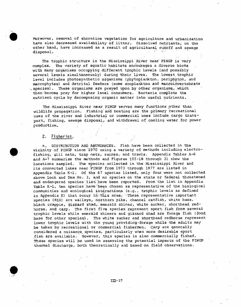
Moreover, removal of shoreline vegetation for agriculture and urbanizationhave also decreased availability of litter. Dissolved nutrients, on theother hand, have increased as a result of agricultural ruhoff and sewagedisposal.

The trophic structure in the Mississippi River near PINGP is verycomplex. The variety of aquatic habitats encourages a diverse biotawith many organisms occupying different trophic levels (and possiblyseveral levels simultaneously) during their lives. The lowest trophiclevel includes photosynthetic organisms (phytoplankton, periphyton, andmacrophytes) and detrital feeders (some zooplankton and macroinvertebratespecies). These organisms are preyed upon by other organisms, whichthen/become prey for higher level consumers. Bacteria complete thenutrient cycle by decomposing organic matter into useful nutrients.

The Mississippi River near PINGP serves many functions other than.wildlife propagation. Fishing and boating are the primary recreationaluses of the river and industrial or commercial uses include cargo trans-port, fishing, sewage disposal, and withdrawal of cooling water for powerproduction.

2. Fisheries.

a. DISTRIBUTION AND ABUNDANCES. Fish have been collected in thevicinity of PINGP since:1970 using a variety of methods including electro-fishing, gill nets, trap nets, seines, and trawls. Appendix Tables A-6and A-7 summarize the methods and Figures 111-18 through 21 show thelocations sampled. The species collected in the Mississippi River andits connected lakes near .PINGP from 1973 through 1977 are listed inAppendix Table K-1. Of the 67 species listed, only four were not collectedabove Lock and Dam No. 3, and no species on the state or federal threatenedand endangered species list have been reported. From the list in AppendixTable K-l, ten species have'been chosen as representative of the biologicalcommunities and ecological interactions (e;g., trophic levels as definedin Appendix E) that occur iný this area. 'These representative importantspecies (RIS) are walleye, northern pike, channel catfish, white bass,black crappie, gizzard shad,:emerald shiner, white sucker, shorthead red-horse, and carp. The first five species represent sport fish from severaltrophic levels while emerald shiners and gizzard shad are forage fish (foodbase for other species). The white sucker and shorthead redhorse representlower trophic levels with the young providing-forage while the adults maybe taken by recreational or commercial fishermen. Carp are generallyconsidered a nuisance species, particularly when more desirable sportfish are available. However, this species is also commercially fished.These species will be used in assessing the potential impacts of the PINGPthermal discharge, both theoretically and based on field observations.

IMl-37

WISCONSIN

IW £

1'

MINNESOTA

SCALE

500 0 500 1000

meters1000 0 1000 2000 3000 4000

STA I

STA 7

LOCK &

STA 3

feet

547 P-84

Figure 111-18. Sampling stations for fish in 1970 (Stations 1-6 only), 1971and 1972. Station 6 (not shown) was at the confluence of theVermillion River below Lock and Dam No. 3, and Station 8 (notshown) was from Lock No. 3 downriver 4.4 km (2.75 mi). 0

111-38

SCALE

1 'A 0 1MILES3000 0 3000 6000

1 5 0 1 FEKILOMETERS

4 47

-N.E

0.

.... ... ... .

.......... SECTI O CN.

i~~~.. ..."-I"DMno.k

547P-85

Figure 111-19. Sampling locations for fish in 1973 through 1977. Eachsection was subdivided into 10 stations, and SectionsIV-VI were below Lock and Dam No. 3.

-1

13-39

WISCONSIN

N

w C

'VS

I

MINNESOTA

PINGP

LOCK &

SCALE

500 0 500 1000

meters1000 0 1000 2000 3000 4000

feet

547PA- IFigure 111-20. Sampling stations for Sectors I through III

for 1977 DNR fisheries studies.

111-40

WI SCONSI N Iw4@)~E

S

I

'I.

-.-%

MINNESOTA

0

LOCK &

SCALE

o500 0 500 " 1000

meters1000 0 1000 2000 3000. 4000

feet

Figure 111-21. Larval fish tow locations for 1974 and 1975. Only locations1 through 4 were sampled in 1974 (Gustafson et al., 1976).

111-41

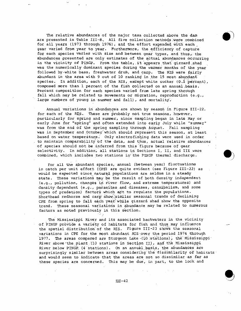
The relative abundances of the major taxa collected above the damare presented in Table 111-8.. All five collection methods were combinedfor all years (1973 through 1976), and the effort expended with eachgear varied from year to year. Furthermore, the efficiency of capturefor each species varies with size and between gear types, and thus, theabundances presented are only estimates of the actual abundances occurringin the vicinity of PINGP. From the table, it appears that gizzard shadwas the numerically dominant species during the warmer months of the yearfollowed by-white bass, freshwater drum, and carp. The RIS were fairlyabundant in the area with 9 out of 10 ranking in the 15 most abundantspecies. In addition, each of the RIS, except white sucker (0,.1 percent),composed more than 1 percent of the fish collected on an annual basis.Percent composition for each species varied from late spring throughfall which may be related to movements or migration, reproduction (e.g.,large numbers of young in summer and fall), and mortality.

Annual variations in abundances are shown by season in Figure 111-22.for each of the RIS. These are probably not true seasons, however,particularly for spring and summer, since sampling began in late May orearly June for "spring" and often extended into early July while "summer"was from the end of the spring sampling through August. Fall sampling.was in September and October'which should represent this season, at leastbased on water temperature. Only electrofishing data were used in orderto maintain comparability of the data, and thus, actual relative abundancesof species should not be inferred from this figure because of gearselectivity. In addition, all stations in Sections I, II, and III werecombined, which includes two stations in'the PINGP thermal discharge.

For all the abundant species, annual (between year) fluctuationsin catch per unit effort (CPE) are quite evident (see Figure 111-22) aswould be expected since- natural populations are seldom in a steadystate. These variations may be the result of both density independent(e.g., pollution, changes in river flow, and extreme temperatures) anddensity dependent (e.g., parasites and diseases, cannibalism, and sometypes of predation) factors which act to regulate the populations.Shorthead redhorse and carp: show lsimilar seasonal trends of decliningCPE from spring to fall each year.-while gizzard shad show the oppositetrend. These seasonal variations in abundance may be related to numerousfactors as noted previously in this section.

The Mississippi River and its associated backwaters in the vicinityof PINGP provide a variety of habitats' for fish and thus may influencethe spatial distribution of the RIS. Figure 111-23 shods the seasonalvariations in CPE for the most abundant RIS over the period 1974 through1977. The areas compared are Sturgeon Lake 4(10 'sta'tions), the MigsissippiRiver above,-the plant (10 stations in Section II), and the MississippiRiver below PINGP (4 stations). On an annual basis, the abundances aresurprisingly similar between areas considering the dissimilarity of habitatsand would seem to indicate -that the areas are not so dissimilar-as far asthese species are concerned. This may be due, in part, to the lock and

11T-42 '9

Table 111-8. Species composition (percent) of the major taxaof fish collected in the vicinity of PINGP duringthe period 1973 through 1976.1

TAXA2 SPRING3 SUMMER 3 FALL 3 ANNUAL

Gizzard Shad*I 9.9. 10.7 36.5 20.8

White Bass* 22.3 12.1 13.5 15.6

Freshwater. Drum 10.1 24.6 5.6 12.8

Carp* 16.4 11.8 6.8 11.1

Emerald Shiner* 7.0. 4.8 4.5 5.3

Sauger 3.6 1.9 5.6 3.9

Shorthead Redhorse* 4.5 4.5 2.6 3.8

Bluegill 1.3 3.8 5.0 3.6

Black Crappie* 1.6 3.6 3.1 2.8

Channel Catfish* 3.1 3.6 0.5 2.2

White Crappie 1.6 1.4 3.1 2.1

Spottail Shiner 0.9 2.0 2.4 1.8

Shortnose Gar 2.0 2.0 0.9 1.6

Walleye* 1.4 0.5 1.7 1.3

Northern Pike* 2.0 0.7 1.1 1.3

Carpsucker sp. 2.1 1.6 0.4 1.3

N 12,962 13,976 18,067 45,005

1The areas sampled are North and Sturgeon Lakes, the main channelfrom Brewer Lake cut to the PINGP intake, and from PINGP toLock and Dam No. 3. The effort expended with each gear typevaried from year to year so that the composition may notreflect the actua.. composition as a result of gear selectivityfor some species.

2Asterisk indicates RIS.3 Seasons are not defined by water temperature but are thosepresented in the annual reports for the fisheries data.They are generally: spring = late May to early July; sum-mer = early or mid-July through August; and fall =-Septemberand October.

111-43

0

S- SPRING SUMMER [ -FALL

2

z

2

wi

U.

(2

3.0 - SHORTHEAD " = 1.12

2.0 II

05 WHITE SUCKER =0.03

0.00.5 BLACK CRAPPIE 0.31

00.- =20.5 NORTHERN PIKE = 0.040.0 - _ -- 47"2"',''',, -

CHANNEL CATFISH 0.31

00 A mmm,a,-~10.0 - WHITE BASS T 2.94 F-1

4.0 -

3.03 (j

2.0

1.0

0.0WALLEYE T = 0.5

1.0.

1974 1975 1976 1977YEAR

GIZZARD SHAD T = 12.17

26.0 1-

I25.0

24.0

23.0

19.0

16.0

15.0

9:0

n:::;Ii;

27.0

8.0 [-

7.0

4.0

17" 11F]rii ii

3.01-

2.0 -

1.0 VnF, i- I

1974 1975 1976 - 1977 1974 1975 1976 1977YEAR 547P-83

YEAR

Figure 111-22. Mean electrofishing catch per unit effort (CPE) by season for each RIS in Sturgeon

Lake and the Mississippi River from Brewer Lake cut to Lock and Dam No. 3 combined

over the period 1.974 through 1977. This includes data for the PINGP discharge.

Seasons are defined in the text (from DNR data).

1-SPRING [a SUMMERI f0-FAiL E] ANNUAL

BLACK CRAPPIE

1.04

HH-H-

U,

2ý

La12

02

2.11

'U

SHORTHEAD REDHORSE

0 "- EMERALD SHINER

I - " I l-

IAKE RIVER II RIVER III

LOCATION

STURGEGN MISSISSIPPI MISSISSIPPILAKE RIVER II RIVER III

LOCATION I~UJILOCATION

NO IE. S p biW. M,, l. s..IV JlIv. flhhhI -1 .~l ..... I July , W~j A~njI., -.d 6t.1 S.IUIW stdCcu.All s~l~ i - -,ud lo Subwud , I I L.,i o~iLkt lI I' Io1 Willv d ,5UI I islo R-ino 44.6. 7 "1, i 91 I

-- 1ill5- .lio I llns I -Ito Fs.pso U3 Al I.,, sVitunil

Figure 111-23. Spatial distribution of RIS near PINGP based on electrofishing data for theperiod 1974 through 1977 (from DNR data).

(.0

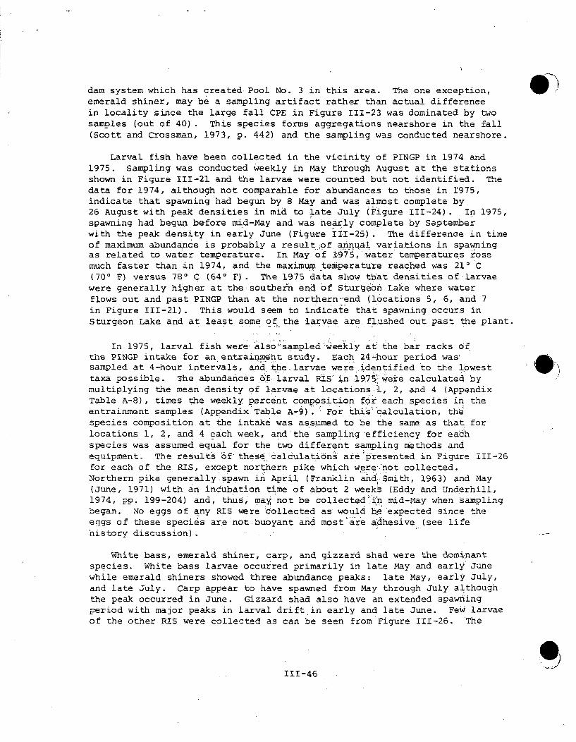
dam system which has created Pool No. 3 in this area. The one exception,emerald shiner, may be a sampling artifact rather than actual differeneein locality since the large fall CPE in Figure 111-23 was dominated by twosamples (out of 40) . This species forms aggregations nearshore in the fall(Scott and Crossman, 1973, p. 442) and the sampling was conducted nearshore.

Larval fish have been collected in the vicinity of PINGP in 1974 and1975. Sampling was conducted weekly in May through August at the stationsshown in Figure 111-21 and the larvae were counted but not identified. Thedata for 1974, although not comparable for abundances to those in 1975,indicate that spawning had begun by 8 May and was almost complete by26 August with peak densities in mid to late July (Figure 111-24) . In 1975,spawning had begun before mid-May and was nearly complete by Septemberwith the peak density in early June (Figure 111-25). The difference in timeof maximum abundance is probably a result of annual variations in spawningas related to water temperature. In May of 1975, water temperatures rosemuch faster than in 1974, and the maximum temiperature reached was 210 C(700 F) versus 780 C (640 F). The 1975 data show that densities of larvaewere generally higher at the southeri-n end of Sturgeon Lake where waterflows out and past PINGP than at the northern--end (locations 5, 6, and 7in Figure 111-21). This would seem to indicate that spawning occurs inSturgeon Lake and at least some of the larvae are flushed out past the plant.

In 1975, larval fish were- alsol.sampled weekly at the bar racks ofthe PINGP intake for an entrainme~nt study. Each 24-hour period was,sampled at 4-hour intervals, and the-larvae were identified to the lowesttaxa possible. The abundances of larval R±S'inl1975 were calculated bymultiplying the mean density of larvae at locations -1, 2, and 4 (AppendixTable A-8), times the weekly percent composition for each species in theentrainment samples (Appendix Table A-9). For this 'calculation, thespecies composition at the intake was assumed to be the same as that forlocations 1, 2, and 4 each week, and the sampling efficiency for eachspecies was assumed equal for the two different sampling methods andequipment. The results bf these calculati6n are presented in Figure 111-26for each of the RIS, except northern pike which were not collected.Northern pike generally spawn in April (Franklin and Smith, 1963) and May(June, 1971) with an incubation time of about 2 weeks (Eddy and Underhill,1974, pp. 199-204) and, thus, may not be collectedýln mid-May when samplingbegan. No eggs of any RIS were collected as would be expected since theeggs of these species are not buoyant and most'are adhesive (see lifehistory discussion).

White bass, emerald shiner, carp, and gizzard shad were the dominantspecies. White bass larvae occurred primarily in late May and early' Junewhile emerald shiners showed three abundance peaks: late May, early July,and late July. Carp appear to have spawned from May through July althoughthe peak occurred in June. Gizzard shad also have an extended spawningperiod with major peaks in larval drift in early and late June. Few larvaeof the other RIS were collected as can be seen from Figure 111-26. *The

111-46

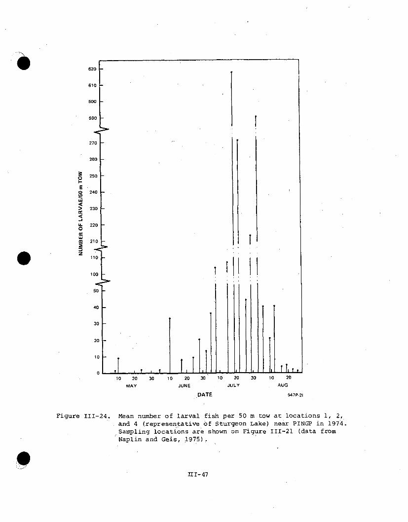
620

610 I-

600 F

590 1-

270 -

260, --

I

0I-E0

U.0

wUin

z

250 I-

240 I-

230 F-

220 F-

210

110

1 00

so

I

40 I-

30 F

20 I-

10 1-

.1 $I .1 I ?P I T010 20 30 10 20

MAY JUNE

30 10 20

JULY

DATE

30 10 20

AUG

547P-21

Figure 111-24. Mean number of larval fish per 50 m tow at locations 1, 2,and 4 (representative of Sturgeon Lake) near PINGP in 1974.Sampling locations are shown on Figure 111-21 (data fromNaplin and Geis, 1975).

II-47

E

LL

0

LU

z

L _ I .. . ___ _ ,_ - 'II ' I 'S , S -419-23 26-30 2-6 9-13 16-20 23-27 30-4 7-11 14.18 21-25 28-1 4-8 11-15 18-22 25-29 1.5

MAY MAY JUNE JUNE JUNE JUNE JULY JULY JULY JULY JULY AUG AUG AUG AUG SEPT

Figure 111-25. Mean'larvalsampling at5, 6, and 7

WEEK547P-22

fish densities at PINGP in 1975 based on weeklythe locations shbwn in Figure 111-21. Stationsrepresent upper Sturgeon Lake and Stations 1, 2,

and 4 represent lower Sturgeon Lake. The vertical barsrepresent the standard error of the mean and NS is nosample (data from Gustafson et al., 1976).

111-48

0

w

U.0

z0w

l-

I-

19-23 26-30 2-6 9o13 16-20 23-27 30-4 7-11 14.18 21-25 28-1 4-8 11.15 18-22 25-29 1-5MAY MAY JUNE JUNE JUNE JUNE JULY JULY JULY JULY JULY AUG AUG AUG AUG SEPT

WEEK547P.23

Figure 111-26. Estimated density of RIS larval fish drifting past PINGPin 1975. No northern pike larvae were collected.Estimates were calculated from densities at Stations 1,2, and 4, which represent drift from Sturgeon Lake(Gustafson et al., 1976), and the species composition inthe weekly entrainment samples (NUS, 1976).

111-49

0 o -I II BLACK CRAPPIE

0 p IN S NS

REDHORSE SR,0.02, NS NS

1 WHITE SUCKER0 .0031 1 1 NS NS0

0.14 WALLEYEM'• 0 04I I 9 9 9 NS NSE 2 CHANNEL CATFISH

W 0 9 i ri i*NS NS

< 168

U,,.o GIZZARD SHAD

ILl

22!

zo 20U3

I--

186

W 16

14

12 "

10 -

8

6

4

2

9 9NS NS

19-23 26-30 2-6 9-13 i6.20 23-27 30.4 7.11 14-18 21.25 28-1 4-8 11-15 18.22 25-29 1.5

MAY MAY JUN JUN JUN JUN JULY JULY JULY JULY JULY AUG AUG AUG AUG SEPT

WEEK 547P-24

Figure IIi-26, (Continued).

1J-j.L - -ý U

r~edhorse, white sucker, and walleye are early spring spawners that usuallymigrate upstream to spawn, and thus, most spawning in Pool No. 3 would beexpected in the tailwaters of Dam No. 2. Channel catfish and blackcrappie are nesters, and few larvae would be expected in the drift ascompared to the other prolific broadcast spawners.

b. LIFE HISTORIES. The following life history information for therepresentative important species (RIS) is presented as a background uponwhich to base impact analyses. The reproductive characteristics forthese species are summarized in Appendix Table A-10, and the spawningtemperatures and times are shown in Figure 111-27. Metric units wereused throughout this section, and English conversions are given inAppendix F.

Walleye. Walleye live in large lakes and streams from Great SlaveLake to Labrador on the north to northern Alabama and Arkansas on thesouth and west to Nebraska (Niemuth et al., 1972). They prefer water oflow turbidity over a firm substrate and can survive temperature rangesof 00 to 320 C (Goodson, 1966a). Pollution in the Mississippi Riverbelow t-Minneapolis-St Paul and in parts of the Minnesota River has dras-tically reduced the walleye population in these areas (Eddy ,and underhill,1974, pp. 369-373). This pollution has come from numerous sources,including agriculture, industries, and municipal sewage treatment plants.

In the spring, usually just after the spring thaw, walleye make massspawning migrations up rivers and streams to tributaries and lakes (Eddyand Underhill, 1974, pp. 369-373). Tagging studies in Oneida Lake, NewYork, showed that most walleye returned to the same spawning area eachyear (Forney, 1963). Spawning occurs at 60 to 170 C with the peak at90 to 100 C. The eggs are randomly broadcast at a depth of less than1.2 m with most laid in less than 61 cm of water on a clean substrate.with flowing water (Niemuth et al., 1972). The eggs are 1.5 :to 2.0 mm`in diameter and lose their adhesiveness after water hardening (Scott andCrossman, 1973, pp. 690-691). Hatching is in 7 to 26 days, depending ontemperature, and DO concentrations below 35 percent saturation increasesegg mortality. Females longer than 38 cm lay 35,000 to 600,000 eggs withan average of 28.6 to 99.2 per gram of body weight (Niemuth et al., 1972;Siefert and Spoor, 1974). Males mature at 4 years and females at 5 yearsof age in Lake Erie (Goodson, 1966a).

/

walleye are predators. Young less than 75 mm in length feed uponplankton and then progress to insect larvae and fish with increasingsize (Priegel, 1969)-. Their life span is approximately 7 years althoughsome rhay exceed this. The maximum recorded length is 92 cm.and the weight10 kg (Niemuth et al., 1972). The largest walleye caught by angling inMinnesota weighed 7.6 kg (DNR, 1977).

111-51

HHH

If

cc.

C-)

I-

E-

JUN JUL

MONTH

Figure 111-27. Spawning temperatures and times for the RIS. The optimum or mean temperature wasplotted on the river ambient and the verticaY bars indicate the range while thehorizontal bars represent the time period. The dashed curves show temperaturesof the 50 and 90 F ATs in the discharge while the upper curve indicates the monthlyaverage temperature discharged by PINGP.

White Bass. White bass are found from the St. Lawrence River westthrough the Great Lakes to South Dakota and south in the Ohio andMississippi drainages to the Gulf of Mexico. Stocking has increasedtheir range. They prefer clear waters since feeding and schooling aresight dependent (Scott and Crossman, 1973, pp. 689-692).

In the spring, adults move upstream into large lakes to spawn, some-times traveling long, distances (Eddy and Underhill, 1974, pp. 335-336).The fish form schools which may be unisexual and move into shallow areaswhen the water temperature reaches 12.80 to 15.60 C in late. May and June.The 0.8 mm adhesive eggs are broadcast near the surface or in midwaterduring the day and adhere to boulders, gravel, or vegetation as they sink(Scott and Crossman, 1973, pp. 689-692). In Lewis and Clark Lake,spawning occurs when the water temperature is i4.4* to 200 C (Ruelle,1971), and may continue for 5 to 10 days per population with the adultsforming schools again after spawning. Incubation time is 46 hours at15.60 C (Scott and Crossman, 1973, pp. 689-692), and the newly hatchedlarvae are 3 mm in length (Ruelle, 1971) . Growth.is fairly rapid andthe YOY may reach 126 to 162 mm by fall. Fecundity is 242,000 to 933,000eggs per female with an average of 565,000 and varies with the size ofthe fish. Age at maturity is 3 years in Lake Erie (Scott and Crossman,1973, pp. 689-692), and 2 years in Minnesota (Eddy and Underhill, 1974,pp. 335-336).

White bass are carnivorous. Young fish feed upon zooplankton suchas Diaptomus, Cyclops, Daphnia, and copepod nauplii. and progress toaquatic insects and fish as they increase in size (Ruelle, 1971). InIowa lakes, the adults feed primarily upon yellow perch, bluegill, carp,and black crappie, although some also eat crustaceans and aquatic insectssuch as mayflies. In other areas, small gizzard shad and minnows may forma significant portion of their diet (Scott and .Crossman, 1973, pp. 689-692).

Channel Catfish. The distribution of channel catfish ranges fromMontana to the Ohio Valley and south through the Mississippi.Valley tothe Gulf of Mexico and into Florida (Eddy and Underhill, 1974). Theyoccur in swift streams as well as lakes and large reservoirs, preferringsand, gravel, or rubble bottoms without vegetation (Miller, 1966). inMinnesota, they are found in the swift water tributaries of the Missis-sippi River (Eddy and Underhill, 1974, pp. 299-300).

spawning takes place in nests in protected areas such as holes orunder logs and occurs at 210 to 290 C with an optimum of 26.70 C(Clemens and Sneed, 1957). The eggs are 3.5 to 4.0 mm in diameter, areguarded by the males, and hatch in 5 to 10 days (Scott and Crossman,1973, pp. 604-610). The young remain in the nest for approximately1 week before dispersing (Lopinot, 1960). Females produce 6.6 to 8.8eggs per gram of body weight (Clemens and Sneed, 1952), and the eggswill not develop if the water is less than 15.6 0 C (Miller, 1966).

_jIII-53

Channel catfish are omnivorous, feeding upon fish, invertebrates,and plant material. They feed by sight, taste, or touch (Lopinot, 1960).The maximum size for this species is 90 cm in length and more than 11 kgin weight, although most are only 1.4 to 1.8 kg in Minnesota (Eddy andUnderhill, 1974, pp. 299-300). The angling record in Minnesota is17.5 kg (DNR, 1977).

Northern Pike. Northern pike inhabit lakes and streams east of theRocky Mountains and north of the Ohio River northwest into Alaska aswell as in northern Europe and Asia (Eddy and Underhili, 1974, pp.199-204).

Just after the ice melts in April, adults ascend smal~l streams orseek flooded grassy areas of lakes (Eddy and Underhill, 1974, pp. 199-204).Spawning occurs at 110 to 170 C in Lake George, Minnesota, and the eggsare broadcast on all types of vegetation except cattails (Franklin andSmith, 1963). The adhesive eggs are 2.5 to 3.0 mm in diameter and usuallyhatch in about 2 weeks depending on temperature. The yolk sac larvaeattach to vegetation with adhesive glands on their heads and feed fromthe yolk for 6 to 10 days (Scott and Crossman, 1973, pp. 357-359). Thefemales produce 19,200 to 193,000 eggs. Males mature at 2 to 3 years ofage and females at 3 to 4 years (June, 1971).

The young feed on zooplankton for the first 2 weeks progressing tolarger prey, such as fish fry, after that. They are cannibalistic iffood is scarce. The adults feed by sight on fish such as crappie, sun-fish, suckers, and minnows (Eddy and Underhill, 1974, pp. 199-204).

Pike grow to a length of more than 1 m and may weigh over 23 kg(Eddy, 1969, p. 64). The angling record for Minnesota is 20.7 kg (DNR,1977).

Gizzard Shad. Gizzard shad inhabit large rivers and muddy lakesfrom central Minnesota east to the St. Lawrence drainage and south toNew Jersey and brackish waters along the Gulf of Mexico as well as intoMexico (Eddy and Underhill, 1974, pp. 147). Taylor Falls on the St.Croix River is apparently the northern limit of their range in Minnesota.

Spawning occurs in spring and summer, generally in April throughJune when the water temperature is 100 to 210 C; however, it may takeplace when the water is as warm as 290 C. The eggs are randomly broad-cast at the water surface in shallow water and slowly sink tor the bottom.The eggs are 0.75 mm in diameter, adhesive, and hatch in 1.5 to 4 days,at temperatures of 26.70 C and 16.70 C (Miller, 1960). Fecundity forgizzard shad in Lake Erie ranged from 211,380 to 543,910 eggs and averaged379,000 eggs for 2-year-old fish, and it declined with age. In ElephantButte Lake (New Mexico), the mean fecundity of 3-year-old fish was 40,500eggs (Jester, 1972, p. 40). Both males and females mature at 1 to 2 yearsof age (Carlander, 1969, p. 88).

111-54

Young gizzard shad feed upon protozoa, rotifers, and entomostracaWhile the adults eat phytoplankton and zooplankton (Carlander, 1969,p. 89). Young-of-the-year fish generally school, but older fish do not.The young are important forage fish, and they tend to overpopulate inareas where predation is not sufficient to keep their numbers down (Eddyand Underhill, 1974i p. 148). Gizzard shad grow to 52 mm in lengthalthough most do not exceed 25 to 36 mm (Miller, 1960). -

Carp. Carp are not native to the United States but were widelyintroduced from Europe in the 1800s. This species prefers warm watersand is generally not found in trout streams. In the Mississippi River,carp were found above St. Anthony Falls after 1920 and as far upriveras Little Falls by 1935 (Eddy and Underhill, 1974, p. 220). They thrivein eutrophic waters and can tolerate low dissolved oxygen, extremetemperature variations, and pollution as well as high turbidity. They areinactive at temperatures below 300 C (Burns, 1966)

Spawning begins in late April or May when the water reaches 15.60 C(Jester, 1974, p. 38) with maximum activity at 190 to 230 C. Spawningcontinues through July but does not occur when temperatures exceed 28. C(Swee and McCrinmmon, 1966). Adhesive 'eggs 1 mm in diameter are randomlybroadcast in very shallow water, usually over vegetation (Scott andCrossman, 1973, pp. 407-411), and hatching occurs from 3 to 6 days up.to 10 to 20 days depending on temperature, (Eddy and Underhill, 1974,p. 220; Swee and McCrimmon, 1966). The eggs do not develop at temperaturesabove 42.50 C, and the rate of egg development is controlled by tempera-ture although sensitivity to temperature extremes varies with develop-mental stage'. For example, a 10 minute exposure to 410 C is lethal toall eggs during the first 6 hours of development, kills some eggs between6 and 9 hours of development, kills all eggs between 12 and 20 hours ofdevelopment, and has a diminishing effect therafter (Frank, 1974).Fecundity ranges from 36,000 to 2,208,000 (Swee and McCrimmon, 1966)and is about 220.8 eggs per gram of body weight, with males maturing at2 years of age while females mature at 3 years (Burns, 1966).

Carp are omnivorous, feeding on plant material, aquatic insects,crustaceans, molluscsi and annelids. They suck up bottom substrate,expel it into the water, and then select the food items. In addition,they sometimes feed on floating animal!S or algae at the water surface"(Scott and Crossman, 1973, pp. 407-411). Their habit of stirring upthe bottom and uprooting vegetation makes them a nuisance since this causesturbidity and may also ruin the feeding and spawning beds of other moredesirable species; Carp may exceed 61 cm in length and 9 kg in weightwith records of fish weighing more than 23 kg (Eddy and Underhill, 1974,p. 220).

Black Crappie. Black crappie are found in medium-sized lakes andlarge streams from southern Manitoba to Quebec south to Florida andTexas. This species is absent from the deep lakes of northeast Minnesota,particularly in the Lake Superior drainage (Eddy and Underhill, 1974,pp. 360-362). It has been introduced elsewhere (Eddy, 1969, p. 212).

111-55

Spawning occurs in May and June. The males make nests in water 1 WI'to 2 m deep and on bottoms that are often softer or muddier than preferredby most centrarchids (Eddy and Underhill, 1974, pp. 360-362),. Thesenests are 20.3 to 38.1,cm in diameter, 1.5 to 1.8 m apart, and may be incolonies. The eggs are 0.93 mm in diameter (Merriner, 1971a), are laidwhen the water is about 141 to 20-0 C, and hatch in 3 to 5 days. Blackcrappie have a very high reproductive potential with females laying11,000 to 188,000 eggs, and both sexes mature at 2 to 3 years of age(Goodson, 1966b; Scott and Crossman, 1973, pp. 745-750).

Their diet consists of aquatic insects, small crustaceans, minnows,and small fish. In winter they feed more actively than other species ofcentrarchids (Eddy and Underhill, 1974, pp. 360-362).

Black crappie may reach an age of 8 to 10 years (Scott and Crossman,1973, pp. 745-750) but seldom exceed 30.5 cm in length. The recordweight for Minnesota is 2.3 kg for a fish caught near the mouth of theVermillion River in 1970 (Eddy and Underhill, 1974, pp. 360-362).

Emerald.Shiner. Emerald shiners are most common in lakes and largerivers (Eddy and Underhill, 1974, pp. 253-254) from Lake Athabaska andthe western Hudson Bay drainage in Saskatchewan to the St. LawrenceRiver system and Lake Champlain south to the Trinity River system in Texasand the Potomac River system (Hubbs and Lagler, 1964, p. 81). 1his speciesforms large schools near the surface offshore during summer and movesinshore' in the fall forming aggregations near piers and docks and in themouths of rivers (mainly YOY). They move to deeper water for over-wintering and come to the surface at night during spring (Scott andCrossman, 1973, pp. 440-443). This fish is an important forage speciesfor fish as well as birds, and the population size fluctuates widelyfrom year to year.

Spawning generally occurs from Mlay through August (McCormick andKleiner, 1976), while maximal activity is in late July and August inLewis and Clark Lake (Fuchs, 1967). Spawning may occur more than onceper season. The 0.01 to 0.67 mm diameter eggs are broadcast near thesurface in open water when the water is 200 to 270 C, and hatching maybe in 24 to 32 hours. The newly hatched larvae are 4 mm in length,and young fry are weak swimmers. The average fecundity is 3,410 eggsper female with maturity atl to 2 years of age, and the adults incurpost spawning mortalities (Campbell and MacCrimmon, 1970; Fuchs, 19.67;McCormick and Kleiner, 1976).

Young emerald shiners feed upon blue-green algae, rotifers, ciliatedprotozoa, and green algae while the adults primarily eat zooplanktonwith insects of secondary importance. The adults feed selectively onlarge organisms with Daphnia spp. often composing 90 percent of thestomach contents while forming only 20 percent of the plankton. Diap~tomussp. is of secondary importance while Leptodora sp. is also preferred(Fuchs, i967).

111-56

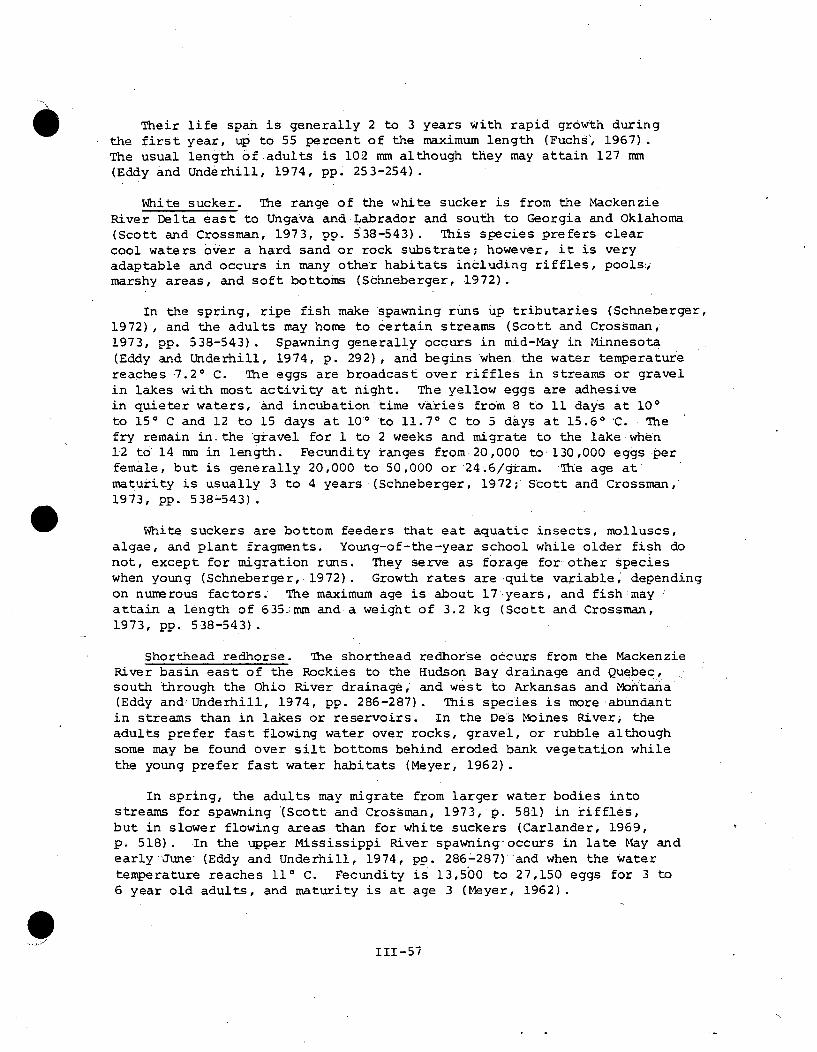
Their life span is generally 2 to 3 years with rapid growth duringthe first year, up to 55 percent of the maximum length (Fuchs, 1967).The usual length of adults is 102 mm although they may attain 127 mm(Eddy and Underhill, 1974, pp. 253-254).

White sucker. The range of the white sucker is from the MackenzieRiver Delta east to Ungava and Labrador and south to Georgia and Oklahoma(Scott and Crossman, 1973, pp. 538-543). This species prefers clearcool waters over a hard sand or rock substrate; however, it is veryadaptable and occurs in many other habitats including riffles, pools:,marshy areas, and soft bottoms (Schneberger, 1972).

In the spring, ripe fish make spawning runs up tributaries (Schneberger,1972), and the adults may home to certain streams (Scott and Crossman,1973, pp. 538-543). Spawning generally occurs in mid-May in Minnesota(Eddy and Underhill, 1974, p. 292), and begins when the water temperaturereaches 7 . 2 * C. The eggs are broadcast over riffles in streams or gravelin lakes with most activity at night. The yellow eggs are adhesivein quieter waters, and incubation time varies from 8 to 11 days at 100to 150 C and 12 to 15 days at 100 to 11.70 C to 5 days at 15.60 'C. Thefry remain in. the gravel for 1 to 2 weeks and migrate to the lake when12 to 14 mm in length. Fecundity ranges from 20,000 to 130,000 eggs perfemale, but is generally 20,000 to 50,000 or '24.6/gram. The age at'

maturity is usually 3 to 4 years (Schneberger, 1972;' Scott and Crossman,1973, pp. 538-543)

White suckers are bottom feeders that eat aquatic insects, molluscs,algae, and plant fragments. Young-of-the-year school while older fish donot, except for migration runs. They serve as forage for other specieswhen young (Schneberger, 1972). Growth rates are quite variable, dependingon numerous factors. The maximum age is about 17 years, and fish mayattain a length of 635ýmm and a weight of 3.2 kg (Scott and Crossman,1973, pp. 538-543)

Shorthead redhorse. The shorthead redhorse occurs from the MackenzieRiver basin east of the Rockies to the Hudson Bay drainage and Quebec,south through the Ohio River drainage, and west to Arkansas and Montana(Eddy and Underhill, 1974, pp. 286-287). This species is more abundantin streams than in lakes or reservoirs. In the Des Moines River, theadults prefer fast flowing water over rocks, gravel, or rubble althoughsome may be found over silt bottoms behind eroded bank vegetation whilethe young prefer fast water habitats (Meyer, 1962).

In spring, the adults may migrate from larger water bodies intostreams for spawning '(Scott and Crossman, 1973, p. 581) in riffles,but in slower flowing areas than for white suckers (Carlander, 1969,p. 518). -In the upper Mississippi River spawning occurs in late May andearly June (Eddy and Underhill, 1974, pp. 286-287)'and when the watertemperature reaches 110 C. Fecundity is 13,500 to 27,150 eggs for 3 to6 year old adults, and maturity is at age 3 (Meyer, 1962).

111-57

Fish longer than 10 cm feed primarily on benthic invertebrates suchas chironomids, Ephemeroptera, and Trichoptera (Meyer, 1962). Theirlife span in Canada is 12 to 14 years. The maximum length recorded was620 mm for a fish caught in Ohio, and the maximum weight recorded was2.7 kg for a fish from Lake Erie (Scott and Crossman, 1973, pp. 579-583).

c. THERMAL DATA FOR THE RIS. The temperature requirements andtolerance of fish are the basis for the predictive Type 2 impactanalysis discussed later in this demonstration. Of prize concern arethe upper thermal tolerances for survival. durinag the, spawning season andduring summer, maximum temperatures for continued growth, and lowerthermal tolerances (cold shock potential). The most pertinent literaturethermal data for each of the RIS. are presented in Appendix Tables A-Ilthrough A-20,and Appendix Figures.A-l through A-5.

d. SPAWNING AREAS AND MIGRATIONS. No spawning areas have been.identified in the vicinity of PINGP during the field surveys. From theinformation in Appendix Table A-10, however, northern. pike, carp, blackcrappie, and emerald shiner probably spawn in all the backwater areasnear PINGP such as North and Sturgeon Lakes. Walleye, white sucker, andshorthead redhorse prefer flowing waters and probably move upstream tothe tailwaters of Dam No. 2 or up tributary streams. -White bass prefershallow water over gravel and thus may spawn in areas. of riprap near theplant or in the main channel, as well as in natural areas of gravel...Channel catfish probably spawn in the main channel since they preferprotected sites, such as under logs or in holes, in areas with flowingwater.

None of the RIS undergo such spectacular mass migrations as salmonor eels, but walleye, suckers, and northern pike will migrate to appro-priate spawning areas. Walleye and suckers generally migrate upstream,and the distance is limited by the lock and~dam system in the MississippiRiver. That walleye migrate to the tailwaters of the dams is evidencedýby the excellent fishing for this species and the closely related saugerjust below Lock and Dam No. 3 in the spring.

Tagging studies in 1974 (Naplin and Geis, 1975) and 1975 (Gustafsonet al., -1976) showed that white bass and walleye were very:-mobile,while northern pike tended to remain in the area where tagged. In 1974,24 white bass moved an average of 51.1 km (31.7 mi) and 7 walleye traveleda mean of 43.7 km (27.1 mi) while 6 northern pike averaged only 15.9 km(9.9 mi). In 1975, the mean distance traveled by .35 walleye was 27.5 km(17.1 mi) and by 77 white bass was 29.6 km (18.4 mi).

e. PREDATOR-PREY INTERACTIONS FOR RIS. The trophic relationshipsof the RIS in aquatic ecosystem near PINGP~are quite complex sincefeeding habits change with age as well as season and food availability.Appendix Table A,21 summarizes the food habits for each of the RIS duringthe larval stages as well as for juveniles and adults. Larvae of all the

111-58

species feed on algae, zooplankton, and aquatic insectllarvae. As thelarvae develop into juveniles and adults their feeding habits change.Gizzard shad become herbivorous, feeding predominantly on phytoplankton.Emerald shiner-, carp, white sucker, and shorthead redhorse generallyoccupy low to intermediate trophic levels, and may provide forage forhigher trophic level fish. Their diet includes algae, plant material,and a variety of micro- and macroinvertebrates. Channel catfish, blackcrappie, and white bass feed upon fish as well. as invertebrates, andthus, may occupy more than one trophic level. Walleye and northern pikefeed primarily upon fish and other vertebrates as adults althoughjuveniles (and occasionally adults) may sometimes feed upon macroinver-tebrates.

In conclusion, the RIS feed upon a variety of prey (ranging fromalgae to vertebrates) throughout their life, and the piscivorous speciesprey upon some of the other RIS, particularly emerald shiners and younggizzard shad. These predators may also utilize young of other RIS asforage (e.g., white sucker, carp, shorthead redhorse, white bass, andnorthern pike).

f. DISEASES AND PARASITES. Fish are host to numerous internal andexternal parasites ranging from fungi to vertebrates. Table 111-9 liststhe general taxa of parasites and the types of infestation. Severalbacterial or viral diseases, such as bacterial furunculosis and lympho-cystis, may infect fish, also. Most parasites and diseases of fish arespecies-specific and thus cannot be passed to humans. The broad tape-worm (Diphyllobothriuzr latum), however, can infect humans via ingestionof raw or partially cooked fish. Freezing or thorough cooking destroysmost parasites although some may be aesthetically displeasing (e.g., largecysts in muscle tissue)

The RIS chosen for this demonstration may be host to a variety ofparasites. Gizzard shad are generally free of parasites which may bea result of their herbivorous diet (Miller, 1960). Carp apparently havefew parasites, which are predomonantly external or gill flukes, whileemerald shiners and shorthead redhorse also are slightly infested (Scottand Crossman, 1973, p. 443; Hoffman, 1967, pp. 321-406) . The other RISmay be infected with most of the parasites listed in Table 111-9. Twoof the more noticeable parasites are externally encysted stage of trema-todes which are known as black spot (Uvulifer ambloplitis) and yellowgrub (Clinostomum marginatum).

g. INFLUENCES OF MAN. The Mississippi River in the vicinity ofPINGP has been altered by various activities of man for many years.The lock and dam system from Minneapolis to the confluence of theMissouri River was constructed to improve navigation on the upper Missis-sippi and has changed the free flowing river into, a series of lakes orpools. Depths and flows are controlled during moderate to low flows(see Hydrology section) while the areal extent of backwaters is increased.

111-59

Table 111-9. Taxa of fish parasites and types of infestation(from Hoffman, 1967).

TAXA INFESTATION

Fungi External, generally infect damaged or stressedfish

Protozoa Wide variety of external and internalparasitism

Trematoda (flukes)

•Monogenetic Generally external, requiring only one host

Digenetic Generally internal with multi-host life cycle

Cestoda (tapeworms) Internal with multi-host life cycle

Nematoda Mainly internal with two host life cycle, oneof which is an invertebrate

Acanthocephala Internal, usually require at least two hostsduring life cycle

Hirudinea' (leaches) External

Crustacea (copepods) External, most common are Lernaea, Ergasilus,and Argul us

Mollusca External, glochidia of freshwater clamsencyst in fins or gills

Vertebrata External, lampreys

Physical conditions such as temperature and turbidity may also be alteredduring controlled flows. The biological changes that may have resultedfrom these alterations have not been monitored, but some estimates canbe made. Species preferring fast flowing waters would tend to be foundonly in the tailwaters of the dams while species preferring lake-likehabitats or backwater areas would increase in numbers. . Thus, thegeneral aquatic community has probably shifted towards- a lacustrinecommunity as a result of the lock and dam system.

The navigation channel is maintainedby dredging,, although littledredging has been necessary in the vicinity of P.INGP (Cin, 20 October 1977).The river is heavily used by commercial and recreational interests during

111-60

W ice-free months, approximately 15 March to 10 December (Erickson, 15 June1977). In 1976, a total of 6,050 lockages were recorded at Lock No. 3just downriver from PINGP. Of these, 2,377 were commercial (barges),and 3,671 were for 11,390 pleasure boats (Corps of Engineers, 1977).If barge traffic were-assumed to be even throughout the navigation season,an average of 8.8 barges per day would pass PINGP (2,377 barges in 270days).

In constructing the PINGP intake and discharge, two channels weredredged in the southern end of Sturgeon Lake as described in the Hydrologysection, and several areas were ripraped. The areas dredged, however,compose only 3.6 percent of the total surface area of Sturgeon Lake.Riprap was placed at the intake just prior to 'the skimmer wall, along thedike separating the refuge from the discharge, and along the west side ofthe discharge canal at Barney's Point. Dredging altered a small area ofbenthic habitat while the riprap provided a substrate for benthic organismsand fish.

Both commercial and recreational fishing occur in Pool No. 3. Themost valuable commercial species are catfish, carp, buffalo, and drumalthough some suckers, quillback, mooneye, goldeye, bowfin, gar, andturtles are takdn, also. The methods used are gill nets, seines, andset lines, and catch data for 1970 through-1974 are presented in Table III-10for Pool Nos. 3, 4, and 4a (Lake Pepin). From these data it appears thatthe commercial harvest has been much greater in Lake Pepin than in eitherPool Nos. 3 or 4, which is probably the result of greater fishing pressure(MDNR and WDNR records). The catch in Pool No. 3 has increased, and thecatch in Pool No. 4 has decreased substantially while that in Lake Pepinhas declined slightly. The increased harvest in Pool No. 3 has resultedfrom a dramatic increase in the catch of carp; the catch of catfish andbuffalo has been declining over the same time period, while the catch perunit of effort (amount of gear or number of permits) has increased. Forthe other two pools, however, the catch per effort has declined. In allthree pools, carp have dominated the commercial catch followed by buffalo,drum, and catfish in Pool No. 3; catfish, buffalo, and drum in Pool No. 4;and drum, buffalo, and catfish in Pool No. 4a.

Recreational fishing is .open all year in the Mississippi River forall species, except sturgeon for which the season is 30 April through31 October above Lock and Dam No. 3 (DNR, 1977). Little ice fishingoccurs, however, because of limited accessibility and hazardous iceconditions (Naplin and Gustafson, 1975). The sport fishery in thevicinity of PINGP has been estimated by creel census since 1973 in thesame sections used for the fisheries studies described previously.Table III-11 summarizes the fishing pressure and harvest in each sectionfor 1973 through 1976. Although the fishing pressure h'as varied fromyear to year, it has remained substantially higher below Lock and Dam

1I1-61

No. 3 (Section 4) than in the immediate vicinity of PINGP (Sections 1,2, and 3). The average number of man-hours (M-H) expended in Section 3was lower than in either Section 1 or 2, but in terms of effort per unitof water area the fishing pressure has been higher in Section 3. Fishingsuccess, as fish/M-H, has been higher above than below Lock and Dam No. 3except in 1973; however, the harvest in terms of fish/ha has been sub-stantially higher below the dam. Thus, even though fishing pressure(M-H expended) and total harvest have been higher below Lock and DamNo. 3, the fishing success (fish/M-H) has been higher above Lock and DamNo. 3.

Walleye and white bass were the dominant RIS in the sport catch(Table 111-12), particularly in Sections I through 3. The only otherRIS reported in the sport harvest were channel catfish, northern pike,carp, and black crappie.

Table IIl-10. Commercial catch (pounds) of carp, buffalo,catfish, and drum in Pool Nos. 3, 4, and 4aduring 1970 through 1974 (data from NUS, 1976).

POOLYEAR "3 4 4a

1970 115,716 139,651 1,770,358

1971 37,963 221,690 2,289,455

1972 237,062 76,687 1,149,235

1973 357,581 53,363 1,468,224

1974 245,355 85,383 1,141,130

/0

111-62

Table III-11. Creel census data for the vicinity of PINGP in1973 through 1976.

SECTION 1 2 3 4- - YEAR

AREA (ha) .324 180 83 257

Days surveyed 198 205 261 261

Estimated M-H (Total) 1,208 1,983 1,126 109,541

M-H/ha-da 0.019 0.054 0.052 1.633 19762

Harvest (Fish/M-H) 0.736 0.960 1.171 0.633

(Fish/ha-da) 0.014 0.052 0.061 1.034

(Fish/ ha) 2.77 .10.63 15.89 269.79

Days Surveyed 207 207 207 268

Estimated M-H (Total) 394 187 212 88,855

M-H/ha-da 0.006 0.005 0.012 1.290 19753

Harvest (Fish/M-H) 1.273 0.503 0.500 0.385

(Fish/ ha-da) 0.008 0.0025 I 0.006 0.497

(Fish/ ha) 1.58 0.52 1.24 133.10

Days Surveyed 218 218 218 218

Estimated M-H (Total) 812 696 153 46,311

M-H/ha-da 0.012 0.018 0.009 0.827

Harvest (Fish/M-H) 2.21 2.14 NO 0.63

(Fish/ ha-da) 0.027 0.039 NO 0.521

(Fish,, ha) 5.78 8.40 NO 113.58

Days Surveyed 180 180 180 180

Estimated M-H (Total) 200 670 500 41,210

M-H/ha-da 0.003 0.027 0.034 0.8911973-

Harvest (Fish/M-H) 0.36 0.75 0.33 0.69

(Fish/ha-da) 0.001 0.020 0.011 0.615.(Fish/ha) 0.19. 3.65 2.02 110.66

!Section 1=Sturgeon Lake, Section 2=Mississippi River from Brewer Lakecit to PINGP intake, Section 3=PINGP intake to Lock and Dam No. 3,and Section 4-Lock and Dam No. 3 to Highway 63 bridge.

2Geis and Gustafson, 1977.

3Gustafson and Diedrich, 1976.

4Naplin and Gustafson, 1975.5Hawkinson, 1974.

II1-63

Table 111-12. Percent composition of RIS in the estimated sportharvest near PINGP for 1975 and 1976.

ECTION 19751 19762

SPECIES 1 2 3 4 1 2 3 4

Walleye 33 100 50 14 56 14 3 9

White bass 5 0 50 17 24 43 74 32

Channel catfish 0 0 0 1 2 0 6 1

Northern pike 0 0 0 1 3 0 4 <1

Carp 0 0 0 <1 0 7 1 1

Total harvest 501 .94 106 34,119 853 1,973 1,333 69,981(No. fish)

IGustafson and Diedrich, 1976.2 Geis and Gustafson, 1977.

3. Macroinvertebrates. The many uses of the river are both detri-mental and beneficial to the macroinvertebrates that occur in itsnumerous habitats. Some of the natural controlling factors which influencethe distribution and abundance of macroinvertebrates include sedimenttype and currents. Sediment types vary with location mainly as a resultof external inputs (e.g., leaves and sediments).and currents. The lattercontrols the sediment grain size with finer sediments occurring in slowflow or still areas and coarser sediments in faster flow areas. Currentsin the vicinity of PINGP are generally slow, particularly in the backwaterareas, because of the lock and dam system. In addition to currents,turbulence caused by the frequent passage of barge tugboats tends toscour the main channel more so than natural currents. Thus, the mainchannel of the river presents a formidable habitat for most macroinverte-brates. Along the main channel banks, however, manmade structures suchas wing dams and bank stabilization mats provide a limited amount ofrelatively shallow stillwater habitat. PINGP is situated in a backwaterarea at the southern end of Sturgeon Lake. The plant creates its ownintake and discharge currents which are superimposed upon those of theriver, and these conditions also limit the distribution of certain macro-invertebrates.

Iii-64

Because the Mississippi River near PINGP is a combination of lake:and riverine habitats, both fast-water and still-water macroinvertebrates

:would be. expected therein. The damming of a river usually eliminatesmany of 2 the stream and current-loving fauna such as Trichoptera (caddis-flies) , Ephemeroptera (mayflies) and Plecoptera (stoneflies) which arereplaced by chironomids (midges). Chironomids are predominantly filterfeeders that can endure low DO and are exceedingly fecund. Second inabundance to chironomids and usually displacing, them at a later date arethe oligochaetes (iquatic earthworms). Acari (aquatic mites) are usuallythe third largest group. In lakelike habitats where a gentle flow ofrelatively clean water occurs, certain sessile organisms such aslbryazoans(moss animals) may occur also (Baxter, 1977).

Sampling of the macroinvertebrate communities near PINGP began in1970 (see Figure 111-28 and Table 111-13 for locations), and since thattime a variety of methods have been used to sample the multiple habitatsin the area (see Appendix Table. A-22). To date, ;four different methodshave been utilized: dredging, artificial substrates, dip netting/handpicking natural substrates, and collecting aerial stages of aquaticmacroinvertebrates as they emerge from the water column. From thesesampling efforts, at least 371 taxa of macroinvertebrates have beenidentified (Appendix Table K-2). From 1974 through 1976, 91 taxa werecollected by various dredging methods, 103 on artificial substrates, 231from natural substrates, and 53 in emergence studies. Fifty-three taxa werecommon to both the dredge and the artificial substrate sampling, whereas45 were common to the dredge, artificial substrate, and natural substratesamplinq methods. Only 10 taxa were common to all four sampling methods.In addition, 176 taxa were collected prior to 1974 by a combination ofthe dredge, artificial substrate, and natural substrate methods butthe specific collection method. for each taxa was not delineated.

Dominant macroinvertebrates collected by dredging in 1974 through1976 are ranked according to their abundance in Appendix Table A-23 atthree locations in the vicinity of.PINGP. Tubificids (sludge worms)appeared to be numerically dominant near the plant, although dipterans alsorated high in abundance. on artificial substrates (Appendix Table A-24),the naidids (worms) were by far the most abundant with a dipteran (Glypto-tendipes) second in abundance. Trichopterans and ephemeropterans werecollected commonly on artificial substrates but rarely in dredge samples.Diversity in both the dredge and artificial substrate samples was relativelylow indicating, thatý,,A few taxa usually dominated the samples. A widevariety of insects were collected in the emergence studies although onlythose of aquatic origin are relevant to the present study. Dipteransdominated the catch with trichopterans second (Appendix Table A-25). Mostof the dipterans in the emergence studies were not identified to genus butthe dominant trichoperan was Hydropsyche.

111-65

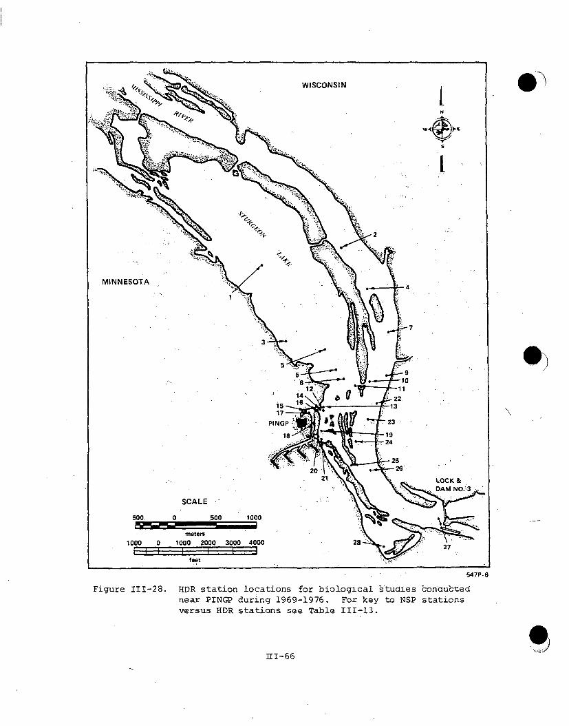
547P-6

Figure 111-28. HDR station locations for biological •tudies bonauctednear PINGP during 1969-1976. For key to NSP stationsversus HDR stations see Table 111-13.

I1-66

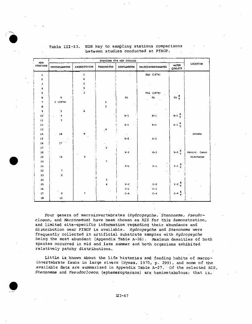
Table 111-13. HDR key to sampling stations comparisonsbetween studies conducted at PINGP.

NO R STATIONS FOR NSP STUDIES.STATION WATER !lOCATIO

STAONS PHYTOPLANKTON PRODUCTIVITY PERIPHYTON ZOOPLAXTON MACROINVERTEBRATES QU T __

I , SLU (1974)

2 I 4I2 4

32

4 5

5 3 SLL (1974).

6 SL SL (197

7 2 (1974) L

a 5

9S6

10 4 B-1 B-1 TB

11 3B

12 X-1 X-1 X-1

13 16

14 18 9 Intake

15 X-2 X-2

16 17

17 3

18 X-3 X-3 X-3

RecirT. CanalT

19 16 8 Discharge

20 7B

21 -1 Y-. Y-1 T

22 7

23 , 8

24 2

25 4 Y-2 Y-2 Y T

.26 CC-1 -i

27 9 7 C-4 C-4 C-4 T28 15

Four genera of macroinvertebrates (Hydropsyche, Stenonema, Pseudo-cloeon, and Macronemum) have been chosen as RIS for this demonstration,and limited site-specific information regarding their abundance anddistribution near PINGP is available. Hydropsyche and Stenonema werefrequently collected in artificial substrate samples with Hydropsychebeing the most abundant (Appendix Table A-26). Maximum densities of bothspecies occurred in mid and late summer and both organisms exhibitedrelatively patchy distributions.

Little is known about the life histories and feeding habits of macro-invertebrate fauna in large rivers (Hynes, 1970, p. 299), and some of theavailable data are summarized in Appendix Table A-27. Of the selected RIS,Stenonema and Pseudocloeon (ephemeropterans) are hemimetabolous; that is,

11-67

a naiad (nymph) develops from an egg and then molts into a winged sub- * )imago which emerges from the water. The sub-imago rests and molts intoa mature imago. The adult males swarm and the females fly through forcopulation. After a few days, the female deposits fertilized eggs eitherby dropping them from the air or attaching them to trees, the water surface(in foam), or various other substrates. The other two RIS, Hydropsycheand Macronemum (trichoperans) , are homometabolous. In this type ofreproduction, larvae hatch from eggs and develop into pupae. After severalmolts the adult insect emerges from the water usually just before sunsetor during twilight. Adult trichoperans live from 1 to 2 months duringwhich time mating occurs.

In the north temperate U.S., the most common type of emergence isseasonal, usually occurring during mid-summer, and appears to be initiatedby a combination of temperature thresholds and photoperiod. In additionto mating, emergence may aid in redistribution to compensate for down-stream behavioral drift of the aquatic forms or for catastrophic losses.This is substantiated by the observation that the flight of emergentinsects is almost exclusively upstream (Shyne, 1977).

Thermal tolerances of macroinvertebrates are summarized in AppendixFigure A-6 and Appendix Tables A-28 and A-29. Information presented inAppendix Table A-28 and Figure A-6 pertain to the types of macroinver-tebrates that are likely to drift and encounter the thermal plume fromPINGP. It is these drifting macroinvertebrates that are primarily sampledby the artificial substrates. Appendix Table A-29 summarizes thermaldata for those organisms that are primarily fixed or sessi~le and, there-fore, subject to elevated temperatures for a period of time considerablylonger than for those drifting through the plume. It is difficult toclassify major groups of macroinvertebrates with regard to their thermaltolerance because thermal tolerance is generally species-specific. Thus,two species in the same genus may have very different thermal tolerances.Thermal tolerances will be discussed in great detail later in this demon-stration (see Section VI).

The only species. of macroinvertebrate that is designated as endangeredby the U.S. Fish and Wildlife Service is the Higgin's eye pearly mussel(Lampsilis higginsii). Since 1970, when sampling for benthic macroin-vertebrates began at PINGP, not a single individual of this endangeredmacroinvertebrate has been collected although another species of thesame genus has been collected in the area (Appendix Table K-2).

Nuisance macroinvertebrates occurring in the area include sludgeworms (tubificids), leeches (Hirundinea), mosquitos (dipterans), blackflies (dipterans), and midges (dipterans) (APHA et al., 1975). An abun-dance of sludge worms is generally considered objectionable since theseorganisms usually indicate the presence of "sludge" while leeches areundesirable because they are parasitic. Mosquitos are considered anuisance as well as a potential public health threat. Mosquitos, however,do not dominate the dipteran macroinvertebrate fauna near PINGP and havenot been implicated in any public health problems. Black flies create

III-68:

a rather ubiquitous nuisance in most northern latitudes during latespring and early summer, but outside of being rather annoying, they aregenerally innocuous. Midges, when emerging from the water in greatnumbers, can cause a navigation hazard to tugboat captains.

Benthic macroinvertebrates may be classified as pollution sensitive,facultative, or pollution tolerant. The organisms in each of thesecategories collected near PINGP are listed in Table 111-14. The rivernear the-plant site is characterized by few pollution tolerant taxawhile many facultative and pollution sensitive macroinvertebrates arepresent, thus justifying the classification of this section of the riveras a recovery zone rather than a polluted or clean water zone.

4. Zooplankton. It is generally understood that rapidly flowinglarge rivers support relatively sparse populations of zooplankton (Hynes,1970, p. 110); however, lacustrine plankton populations may develop ifthe flow rate is less than about 0.2 rm/sec, although no simple flowcriterion is universally applicable (Baxter, 1977). In general, reser-voirs contain regions of fairly rapid flow where plankton populationsmay be small and other areas of relatively still water where considerable.populations may develop. In the upper: reaches of a reservoir, zooplanktonpopulations may. be small before they drift into quieter waters where theycan accumulate as a result of the gradually slowing current and increasetheir numbers.

Near PINGP, the slow flowing currents (0.2 to 0.5 m3/sec average)and extensive backwater areas created by Dam No. 3 have allowed the sparsenatural zooplankton populations in the Mississippi River to proliferatebefore passing, downstream. Turbulence in the main channel of the rivertends to reduce zooplankton populations simply by limiting food sources andby mechanical scouring. A characteristic of the recovery zone of the rivernear PINGP is that rotifers seem to dominate the zooplankton population.According to Dieterman (1975), as the river progresses from a pollutedstate immediately downriver from the Twin Cities area, the d6minant zooplank-ton grade from ciliates and bacteria to rotifers near PINGP to crustaceansdownriver from Lock and Dam No. 3. Moreover, while progressing downriver

.from the metropolitan sewage treatment plant, the zooplankton populationbecomes dominated by individuals with greater longevity.

Zooplankton have been collected near PINGP since 1970 either bypumpiag or pouring whole water samples through a plankton net to concen-trate the catch (Appendix Table A-22). The mesh of the net (probably64 pm) concentrated most rotifers and crustaceans as well as a few proto-zoans. Stations were generally sampled both up and downriver (far-field)and in the near-field region of the plant (see Table 111-13, and Figure111-28). Approximately 188 taxa of zooplankton were collected over thefirst seven years of pre-operational and operational sampling (AppendixTable K-3). If euglenoids and other flagellated protists areconsidered,then almost 200 zooplankton taxa were collected. Numerically, rotifers

111-69

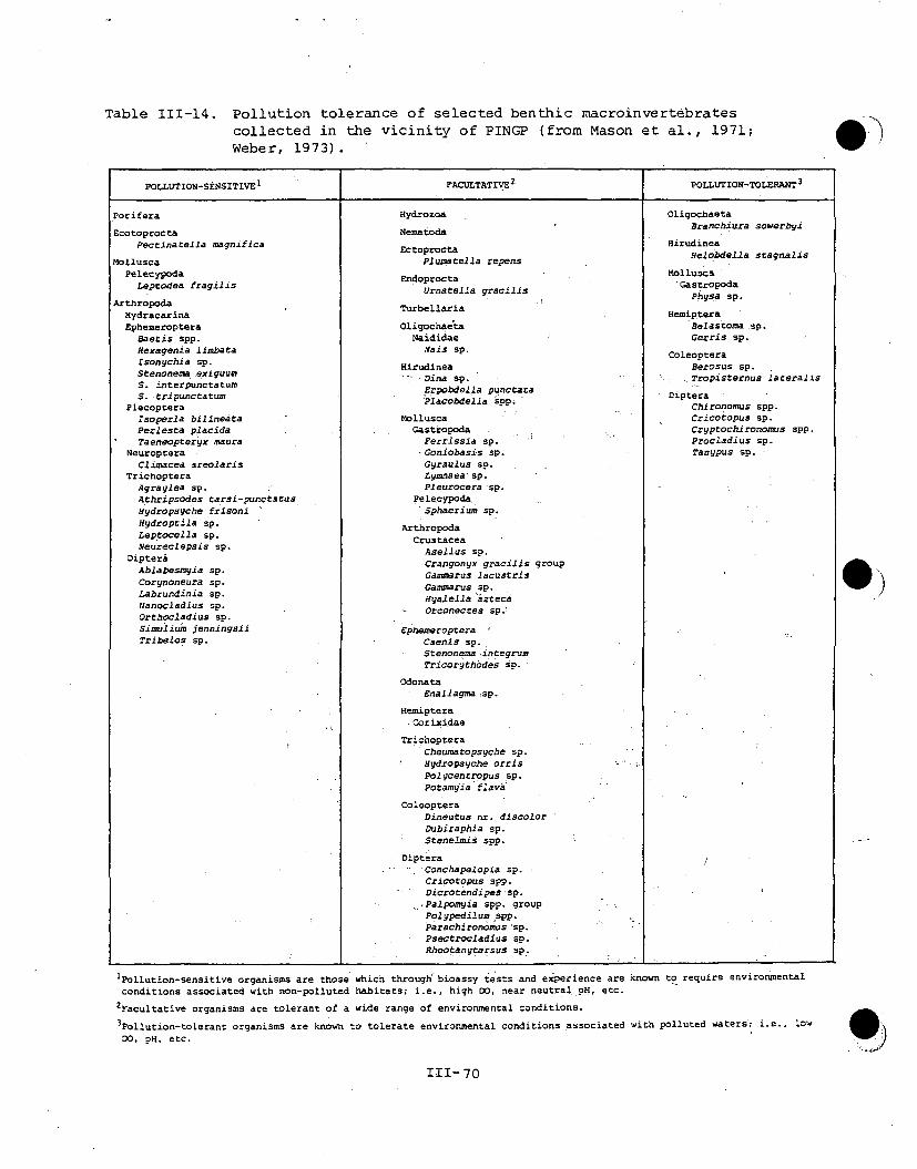
Table 111-14. Pollution tolerance of selected benthic macroinvertebratescollected in the vicinity of PINGP (from Mason et al., 1971;Weber, 1973).

POLLUTION-SENSITIVE' FACULTATIVE 2POLLUTION-TOLERANT 3

Porifera

EcotoproctaPectinatella magniflca

MolluscaPelecypoda

Leptodea fragills

ArthropodaHydracarinaEphemeroptera

Baetis spp.Hexagenia limbataIsonychia sp.Stenonema exiguumS. interpunctatumS. tripunctatum

PlecopteraIsoperla bilineataPerlesta placidaTaeneopteryx maura

NeuropteraClimacea areolaris

TrichopteraAgraylea sp.Athripsodes carsi-punctatusHydropsyche frisoniHydroptila sp.Leptocella sp.Neureclepsis sp.

DipteriAblabesmyia sp.Corynoneura sp.Labrundinia sp.Nanocladius sp.Orthocladius sp.Simulium jenningsiiTribelos sp.

HydrozoaNematoda

EctoproctaPlumatella repens

EndoproctaUrnatella gracilis

Turbellaria

OligochaetaNaididae

Nais sp.

HirudineaDina sp.Erpobdella punctaraPlacobdella spp.

molluscaGastropoda

Ferrissia sp.-Goniobasis sp.Gyraulus sp.Lymnaea sp.Pleurocera sp.

Pelecypoda"Sphaerium sp.

ArthropodaCrustacea

Asellus sp.Crangonyx gracilis groupGansarus lacustrisGammarus sp.Hyalella aztecaOrconectes sp.!

EphemeropteraCaenis sp.Stenonema integrumTricorythodes Sp.

OdonataEnallagma.sp.

Kemiptera.Corixidae

TrichopteraCheumatopsyche sp.Hydropsyche OrrisPolycentropus sp.Potamyia ffava

ColeopteraDineutus nr. discolorDubiraphia sp..Stenelmis spp.

DipteraConchapelopia sp.Cricotopus spp.Dicrotendipes sp.

.. Palpomyia spp. groupPolypedilum spp.Parachironomus sp.Psectrocladius sp.Rheotanytarsus sp.

OligochaetaBranchiura sowerbyi

HirudineaHelobdella stagnalis

Mollusca'Gastropoda

Physa sp.

HemipteraBelastoma .sp.Gerris sp.

ColeopteraBerosus sp.Tropisternus lateralis

DipteraChironomus spp.Cricotopus sp.Cryptochironomus spp.Procladius sp.Tanypus sp.

L & --

IPollution-sensitive organisms are those which through bioassy tests and experience are known to require environmentalconditions associated with non-polluted habitats; i.e., high DO, near neutral, pH, etc.

2Facultative organisms are tolerant of a wide range of environmental conditions.

3Pollution-tolerant organisms are known to tolerate environmental conditions associated with polluted waters; i.e., lowDO, oH, etc.

111-70

dominated the zooplankton at all stations during all seasons of theyear (Appendix Table A-30). Rotifers were dominated by Keratella cochlearisand Brachionus calyciflorus, with population densities greatest in summerand fall. Cyclops vernalis dominated the copepods while Bosmina longi-rostris and Chydorus. sphaericus were the most abundant cladocerans.Maximum copepod and cladoceran populations also occurred in summer andfall. Like macroinvertebrates, zooplankton showed patchy distributions,but their diversity was generally higher than that for most macroinverte-brate populations.

Rotifers have shorter. lifespans than both copepods and cladocerans.Their fast turnover rate may be one reason why they tend to dominatethe summer .zooplankton populations of the sluggish water habitats in thevicinity of PINGP. Appendix Table A-27 summarizes the life history andfeeding habits, for most of the zooplankton taxa. Many of the rotifersand cladocerans are filter feeders although some cladocerans are predatoryand the dominant copepod, Cyclops vernalis, is also carnivorous. Filterfeeding zooplankton are often opportunistic and will feed on bacteria,detritus, or phytoplankton. According to Miller (1971), zooplanktonappear to be entrapped among aquatic macrophytes but also reproduce there.Thus, submerged and emergent macrophyte beds in shallow backwater areasalong the river are important for the propagation of zooplankton.Larger zooplankton, especially cladocerans and copepods, are favoriteprey for almost all types of young fish as well as predatory macro-invertebrates.

The thermal tolerances of zooplankton are summarized in AppendixFigure A-7 and Appendix Table A-31. Cladocerans are generally moretolerant of high temperatures than copepods, although certain membersof each group may be more or less tolerant than members of the othergroup. Rotifers appear to be even more thermally tolerant than eithercopepods or cladocerans, although little information exists regardingthe tolerances of specific rotifers.

No zooplankton have been classified as endangered by the U.S. Fish andWildlife Service nor are any considered as nuisance or:objectionablespecies found near PINGP. Most protozoans and rotifers, besides beingcapable of withstanding high temperatures, are also noted for theirability to adapt to and dominate zooplankton populations in nutrientenriched waters.. Most cladocerans are in the same pollution tolerantcategory as rotifers and protozoans. Copepods, however, may be pollution-tolerant, intolerant, or facultative. Again, the composition of zooplanktonpopulations near PINGP re-emphasize that the Mississippi River near PIN GPis a zone of recovery from upriver nutrient inputs.

111-71

5. Primary Producers.

a. PHYTOPLANKTON. As mentioned previously, the unlimited source ofnutrients from upriver and the abundance of shallow water areas borderingthe main channel provide the section of the river near PINGP with bothallochthonous and autochthonous energy sources for the base of the foodweb. Phytoplankton utilize both nutrient sources to photosynthesizeorganic matter for consumption by herbivores. In the main channel of theriver, phytoplankton populations may be somewhat depressed because ofthe higher turbidity and turbulence caused by barge traffic as well asstronger currents while backwaters such as Sturgeon Lake that have -lowerflushing rates, longer residence times, and slightly higher daytimetemperatures tend to enhance phytoplankton growth rates and allow moreblooms to occur. Diatoms tend to dominate regions of faster current andblue-green algae areas of slow current, apparently since diatoms are moredense and do hot form-the same buoyant mats that often allow blue-greenalgae to float and accumulate in stagnant and slow-moving ,water. Further-more, southerly winds may pile up surface.,phytoplankton into massiveconcentrations and mats duringithe' summer to augment blooms.. Baker(1975) has stated that phytoplankton concentrations and productivity near

PINGP, especially in Sturgeon Lake, are probably as high as in any aquaticsystem considering the unlimited nutrient supply and limited light penetra-tion. It was found that in both Sturgeon Lake and the main channel,

primary production can occur only in the upper 50 cm of the water column(Baker, 1974).

Phytoplankton have been sampled more consistently and over a longertimer period than most of 1the other biological parameters measured at PINGP(Appendix Table A-22). Whole waterksamples collected.since 1969 have beenanalyzed for phytoplankton density, taxonomy, distribution, productivity,and pigments. A large number of stations (see Table iII-13 and Figure 1II-28)have been established since the beginning of the studies in order to

define the phytoplankton populations of the area. More than 300 taxa ofphytoplankton and periphyton have been collected near PINGP (AppendixTable K-4) with more than 171 of those being phytoplankton. Incidentally,a total of 60 diatom taxa were common t6 both phytoplankton and pern-phyton collections.

Temporal and spatial variations in the abundances of various phyto-plankton taxa normally occur in aquatic ecosystems with diatoms generallydominant during spring and fall, green algae in early summer, and blue-greens in mid-summer (especially in nutrieht-rich waters). 'Diatoms,however, dominated phytoplahkton year-round at PINGP, whereas greenswere second in abundance during most of the year and blue-greens reachedmaximum abundance during summer and fall, sometimes surpassing green algaein density (Appendix Table A-32). Near PINGP, the centric diatoms, Stephan-odiscus/Cyclotella spp., were most abundant followed by Nitzschia aci-cularis. Densities of these diatoms were lowest in winter and highestin spring, summer, and fall. Scenedesmus quadricauda, Ankistrodesmus spp.,

111-72

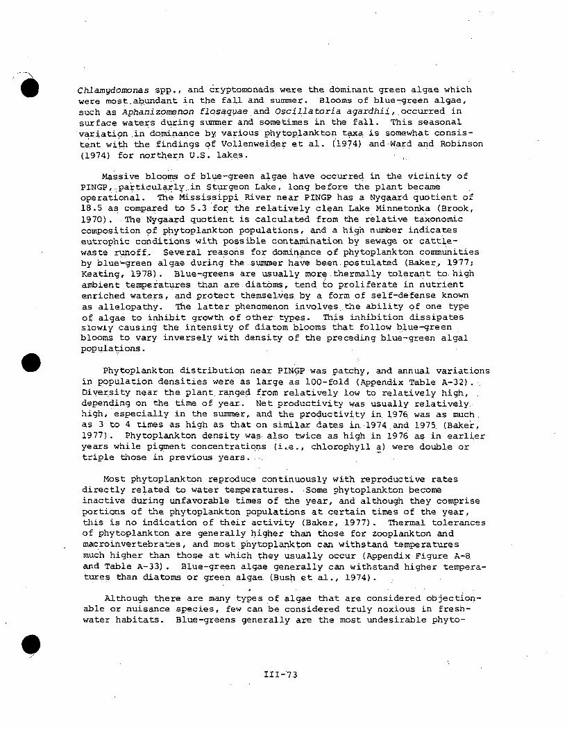
Chlamydomonas spp., and cryptomonads were the dominant green algae whichwere most abundant in the fall and summer. Blooms of blue-green algae,such as Aphanizomenon flosaquae and Oscillatoria agardhii,.occurred insurface waters during summer and sometimes in the fall. This seasonalvariation in dominance by various phytoplankton taxa is somewhat consis-tent with the findings of Vollenweider et al. (1974) and Ward and Robinson(1974) for northern U.S. lakes.

Massive blooms of blue-green algae have occurred in the vicinity ofPINGP,...particularlyin Sturgeon. Lake, long before the plant becameoperational. The Mississippi River near PINGP has a Nygaard quotient of18.5 as compared to 5.3 for the relatively clean Lake Minnetonka (Brook,1970). The Nygaard quotient is calculated from the relative taxonomiccomposition of phytoplankton populations, and a high number indicateseutrophic conditions with possible contamination by sewage or cattle-waste runoff.. Several reasons for dominance of phytoplankton communitiesby blue-green algae during the summer have been postulated (Baker:, 1977;Keating, 1978). Blue-greens are usually more thermally tolerant to highambient temperatures than are diatoms, tend to proliferate in nutrientenriched waters, and protect themselves by a form of self-defense knownas allelopathy. The latter phenomenon involves the ability of one typeof algae to inhibit growth of other types. This inhibition dissipatesslowly causing the intensity of diatom blooms that follow blue-greenblooms to vary inversely with density of the preceding blue-green algalpopulations.

Phytoplankton distribution near PINGP was patchy, and annual variationsin population densities were as large as 100-fold (Appendix Table A-32).Diversity near the plant ranged from relatively low to relatively high,depending on the time of year. Net productivity was usually relatively.high, especially in the summer, and the productivity in. 1976 was as much.as 3 to 4 times as high as that on similar dates in. 1974 and 1975 (Baker,1977). Phytoplankton density was also twice as high in 1976 as in earlieryears while pigment concentrations (i.e., chlorophyll a) were double ortriple those in previous years.

Most phytoplankton reproduce continuously with reproductive ratesdirectly related to water temperatures. Some phytoplankton becomeinactive during unfavorable times of the year, and although they compriseportions of the phytoplankton populations at certain times of the year,this is no indication of their activity (Baker, 1977). Thermal tolerancesof phytoplankton are generally higher than those for zooplankton andmacroinvertebrates, and most phytoplankton can withstand temperaturesmuch higher than those at which they usually occur (Appendix: Figure A-8and Table A-33). Blue-green algae generally can withstand higher tempera-tures than diatoms or green algae (Bush et al., 1974).

Although there are many types of algae that are considered objection-able or nuisance species, few can be considered truly noxious in fresh-water habitats. Blue-greens generally are the most undesirable phyto-

111-73

plankton, and the genera most commonly associated with taste and odorproblems are Anabaena, Anacystis, and Aphanizomenon. In addition,some diatoms (Asterionella, Synedra, and Tabellaria) and green algae(Volvox, Staurastrum, and Pandorina) are associated with objectionabletaste and odor in water. Staurastrum is also an indicator of cleanwater while some of these phytoplankton are indicators of polluted water,especially the blue-greens, some diatoms (Nitzschia aand Gomphonema), andsome euglenophytes (Euglena, Phacus, and Lepocynclis) (APHA et al., 1975).It should be emphasized, however, that many of these so-called pollutedwater or nuisance algae naturally inhabit unpolluted waters, and onlywhen they reach extremely high densities do they become objectionable.

b. PERIPHYTON. Periphyton comprises diatoms, blue-greens, andother types of algae that occur ubiquitously on substrates in freshwaterhabitats. They grow on whatever substrate is available-which at PINGPis primarily in the upper 50 cm of water where light can penetrate.Periphyton contain many of the same taxa that are found in the phyto-plankton and in fact contribute '*may of the planktonic diatoms that arecollected in whole water samples. Periphyton communities near PINGPhave been defined primarily as the diatoms that are capable of growingupon an artificial substrate (cleaned glass slides suspended just belowthe water surface over a period of two weeks) . The stations sampledare shown in Table III-13 and Figure 111-28 and the sampling methods aredescribed in Appendix Table A'22.

A total of 207 periphyton taxa (Appendix Table K-4) have been enumeratednear PINGP, and these follow many of the same general seasonal trendsas do the planktonic diatoms. Centric diatoms of the genus Cyclotell-aappear to be numerically dominant much of the year, except during winter.Navicula cincta and Nitzschia acuta occur abundantly throughout the year,including winter (Appendix Table A-34). It is of interest to note that inperiphyton; as in many bther:groups of-organisms, different species of thesaine genus may have remarkably different thermal optima with one species-abundant in winter while another is abundant in summer. Periphytondistribution at PINGP was characterized by sizeable temporal and spatialvariations. Diversity, however, was consistently high at all stationswhere it was measured, as was chlorophyll a, except during winter.Phaeophytin a (a degradation product of chlorophyll a) increased relativeto chlorophyll a during the summer, indicating increased mortality ofperiphyton at higher temperatures.

Periphyton, like phytoplankton, reproduce continuously with'theirreproductive rates related to parameters such as water temperature,nutrient levels, and light. In addition, they can become dormant duringperiods of sub-optimum environmental conditions. Thermal tolerances ofperiphyton are suanarized-in Appendix Tables A-35 and A-33 as well as inFigure A-8. In general,. those diatoms that can survive at higher tempera-tures are more abundant in summer or fall whereas those that prefer lowertemperatures are more abundant in winter.

111-74

Periphyton are among the first colonizers of solid substrates andmay attract invertebrates and be grazed upon by many types. of fish.However, they often cause objectionable growths onhm an-made structures.These growths may be undesirable from a functional standpoint (e.g.,reduction of water flow) or from an aesthetic viewpoint (e.g., unsightlygrowths on boats or piers). In fact, where surface friction is designedto be minimal, the use of biocides or mechanical methods are sometimesnecessary to inhibit growth of these organisms.

c. AQUATIC MACROPHYTES. The importance of macrophytes in any aquaticecosystem cannot be underestimated. Wetlands and marshes provide bothdirect and indirect benefits to the organisms living on, among, or nearthem. First and most importantly, they provide an energy source for manylarge and small primary consumers (herbivores). Secondly, they provideimportant spawning and feeding habitats for zooplankton, macroinvertebrates,fish, and birds. The importance of these beds to migratory and residentwaterfowl as well as predatory birds is well known. Thirdly, macrophytebeds provide shelter for many aquatic organisms and provide one of themost important fish nursery areas in any aquatic habitat. And fourthly,they provide a substrate for periphyton and many sessile invertebrates.

Aquatic macrophytes in the vicinity of PINGP have been recordedby observation from landK and aerial photography since 1970. A total of74 taxa were found near PINGP (Appendix Table K-5): 7 taxa of submergedmacrophytes, 18 taxa of emergent macrophytes, and 49 taxa. of shoreline andisland plants. The location of these macrophyte beds is shown in Fig re111-29, and the taxa for each area are listed in Appendix Table A-36 ' Thegreatest concentration of macrophyte beds was located in the northern reachesof Sturgeon Lake, and these consisted of pondweeds, wild celery, and bull-rush. Very little.habitat for macrophytes was found in the main channel ofthe river or near PINGP. Pondweed was found in the intake area south tothe discharge canal, while along the southwest shore of the dischargecanal a variety of macrophyt:es, including pondweed, spike-rush, bullrush,and Phragmites occurred from 1974 to 1976. Distribution of macrophytesdepends upon the availability of sui table substrate, water depth, andcurrents. Siltation, in addition to changing sand bars and mud banks,can bury macrophyte beds during floods and at other times of the year.Furthermore, large fluctuations in water level can obliterate macrophytebeds.

Most macrophytes are flowering plants, requiring alternation ofgenerations and pollen production for reproduction. Water level iscritical for the growth and development of new plants, as is type ofsubstrate. Little is known about the thermal t6lerances of variousmacrophytes, and it is often unknown which environmental factor(s)causes the disappearance or appearance of a particular macrophyte taxa.There are no known nuisance or objectionable macrophytes near PINGP,and for reasons stated previously, these plants are generally •consideredbeneficial to aquatic habitats. Marshy areas may be considered as breedinghabitats for undesirable insects, such as black flies and mosquitoes;

111-75

01)

547P-5

Figure 111-29. Locations of macrophyte beds observed near PINGP during1973 through 1976. For description of areas, seeAppendix Table A-36.

111-76

L L-Ifl

(panu1luoo) 6Z-TII aanbvTj

however, under normal environmental conditions, these populations ofnuisance organisms are held in check by fish, macroinvertebrates, andzooplankton residing therein.

6. Birds. Northern bald eagles, ducks, and other waterfowl migratethrough the Mississippi River Valley in the fall and spring with some over-wintering in areas' of open water. A thermal discharge such as that atPINGP may influence the numbers overwintering by providing open waterand by attracting fish and other organisms utilized as food by the birds.

Eagles migrate into the PINGP area from late September to mid-Decemberand are diffusely distributed until the water begins toý freeze (Faanes,1975). The 'main concentrations during the faill and winter of 1975-1976.were near Prescott-, Trentonj Bay Point Park, •ind Lock and Dam No. 3,with a few (about 4 percent) at PINGP. ConseqUently, the latter areadoes not appear rtoýbe an important eagle, overwinte ring area, and pIeakutilization of the plant area occurred in January (Faaries, 1975).: Duringthe fall and winter of 1976-1977, similar numbers were' observed nearPINGP, although few eagles were observed •from January through Marchwhich may be the result of the severe winter, and peak' utilization ofthe PINGP area was in mid-November (Hibbard, unpublished). Eagles in thearea from Prescott to Lake Pepin fed primarily on gizzard shad althoughsome suckers, redhorses, white bass, and goldeye were eaten (Faanes,1975)_

Ducks and other waterfowl utilize open water areas along the Missis-sippi River during their migrations, and some may overwinter in thevicinity of PINGP. Mallards are common, and the PINGP thermal dischargemay enhance the numbers overwintering in the area (Hibbard, 14 November1977). Other migratory ducks using the river in the fall of 1976 includegoldeneye, lesser scaup, canvasbacks, and redheads along with waterfowlsuch as swans and cormorants (Hibbard, unpublished).

Peregrine falcons., an endangered species, formerly nested in theMississippi River Valley as far north as Diamond Bluff (Tordoff,23 January 1978). Recently some have been transferred to previousnesting sites along Lake Pepin 48 to 80 km (30 to 50 mi) downriver fromPINGP (Hibbard, 14 November 1977). None of these' have returned andnested successfully thus far but some a re expected this year. Experiencefarther east has shown that approximatebly 15 years of releasing peregrinefalcons is necessary for reestablishment (Tordoff, 23 January 1978).This species feeds upon medium sized birds of many species, includingsmall ducks.

111-78

IV. PLANT DESCRIPTION AND

OPERATING PROCEDURE

A. CIRCULATING WATER SYSTEM

1. Description. The circulating water system serves as a heatsink for both the condenser and the plant cooling water systems. Con-denser cooling water removes latent heat from exhaust steam leavingthe low pressure turbine, while plant cooling water removes heat from thein-plant auxiliary machinery.

Most of the circulating water comes from Sturgeon Lake, with littleto none coming directly from the main river channel. The balculatedpercentage of total Mississippi River water in the circulating watermakeup for 1975 is shown in Table IV-l. The maximum intake makeup watervolume amounts, in general, to less than 5 percent of the mean monthlyriver flow. The amount of makeup water is small compared to the flow inthe main river channel.

The major components of the circulating water system are shown inFigure IV-l, and the flow diagram is presented in Figure IV-2. Note thatthe flow rates indicated in Figure IV-2 are for the closed cycle mode.The typical flow rates for various cooling modes are discussed inSection IV A.2.

The approach channel has been dredged to a width of 183 m (600 ft)and a depth of 3.1 m (10 ft) at normal pool elevation of 674.5 ft msl.A barrier wall separates the approach channel and the intake canal. Thefunction of this wall is to prevent warm water from the recycle canal fromescaping to the river. The barrier wall also effectively prevents recir-culation of the blowdown discharge which may be blown upstream by southerlywinds during periods of low river flow and prevents floating objectsfrom entering the system. Circulating water is drawn from the approachchannel into the intake canal and after mixing with recycled water entersthe screenhouse. Trash racksi and traveling screens collect organisms anddebris from the intake stream to prevent them from entering the circulatingwater pump basin.

Four vertical shaft, volute type water pumps inside the screenhouseprovide 1,350 cfs of water through 84-inch steel inlet pipes to thecondensers, and two horizontal centrifugal motor pumps withdraw up to60 cfs for the plant cooling water system. Each rectangular shaped,welded steel plate condenser is divided into an inner and outer waterpass. Crossover piping connects the inner passes in series and also theouter passes in series. There are two interconnected condensers and two

IV-1

Table IV-l. Percentage of mean monthly Mississippi River flowentering the intake canal, January through Septem-ber 1975.

AVERAGE PERCENT OF MEAN

NTH RIVER INTAKE FOW MONTHLY RIVERFLOW, (FLOW ENTERING

INTAKE CANAL

January 7,995 175 2.2

February 8,691 289 3.3

March 9,944 281 2.8

April 45,860 414 1.0

May 65,220 618 1.0

June 36,200 326 0.9

July 38,010, 761 2_6

August 111790 541 4.6

September l0,950 378 3.4

October 10,070 265 2.6

November 12,570 190 1.5

December 12,561 175 1.4

11975 USGS data (cfs) at Prescott, Wisconsin.

2 From PINGP Environmental Event Log.

circulating water pumps per unit. One pump circulates water through theinner pass and the other through the outer pass so that circulating watermakes one pass through the tubes of the interconnected condensers. Theoverall temperature rise through the plant is about 13.80 C (24.80 F). Thecirculating water carrying approximately 7.86 x 109 BTU/hr of rejectedheat (total for both units) is then directed to the cooling tower pump.suction .bay through two concrete.-pipes (102-inch ID).

From the cooling tower pump suction bay, four cooling tower pumpsconvey the heated circulating water through individual pipes to headerpipes at the top of the four 12-cell crossflow cooling towers. Flowcontrol valves along the header distribute water to the hot water basinwhich evenly dispenses the water through nozzles to the fill area below.Tower fill is PVC slats used to break the water into fine droplets.The water falls by gravity through the fill section and is collectedin a concrete basin at the bottom of each tower.- Fans draw air through,this fill area to aid in the evaporative heat loss, and the heat is carriedinto the atmosphere by the air 'flow. From the basin at the bottom of the

IV-2

OI* BARRIER

INTAKE WALL APPROACH CHANNEL

CANAL

-- -SC RE ENHOUSE

RECYCLE CANAL

S POWER HOUSE

RECYCLE CANAL GATES, 4 - 10" X 12"

aY-PASS GATES DISCHARGE GATES

COOLING TOWER PUMP SUCTION BAY

EQUIPMENT HOUSE, DISCHARGE CANAL

COOLING TOWER

PUMP HOUSE

DISTRIBUTION BASIN

COOLING TOWERRETURN CANAL " -

COOLING TOWERS

COOLING TOWER CONTROL HOUSES

547P-26.1

Figure IV-l. Schematic diagram of the circulating water system.

IV- 3

Figure IV-2. Representative flow diagram of the circulatingwater system (closed cycle).

towers, water flows through the cooling tower return canal to the dis-tribution basin. If desired, circulating water in the cooling towerpump forebay can can be routed.,directly to the distribution basin throughinterconnecting gates. Recycle canal gates in the north wall of thedistribution basin route the water to the recycle canal for return tothe intake canal.

In order to avoid evaporative accumulation of dissolved solids (designconcentration factor* = 1.25) in the circulating water system, continuousblowdown is needed. The thermal discharges from blowdowns in both-theclosed and partial recycle modes are considered in this demonstration.The discharge gates are 10 x 12 ft motor-operated steel gates which can beoperated remotely from the control room. After the warmed water leavesthe discharge gates, it enters the discharge canal and ultimately themain channel of the river.

*Concentration factor volume makeupvolume blowdown + drift

IV-4

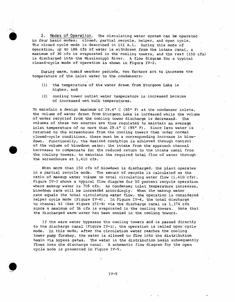
2. Modes of Operation. The circulating water system can be operatedin four basic modes: closed, partial recycle, helper, and open cycle.The closed cycle mode is described in III A.1. During, this mode ofoperation, up to 186 cfs of water is withdrawn from the intake canal, amaximum of 36 cfs is evaporated in the cooling towers, and the rest (150 cfs)is discharged into the Mississippi River. A flow diagram for a typicalclosed-cycle mode of operation is shown in Figure IV-2.

During warm, humid weather periods, two factors act to increase thetemperature of the inlet water to the condensers:

(1) the temperature of the water drawn from Sturgeon Lake ishigher, and

(2) cooling tower outlet water temperature is-increased becauseof increased wet bulb temperatures.

To maintain a design maximum of 29.40 C (851 F) at the condenser inlets,the volume of water drawn from Sturgeon Lake is increased while the volumeof water recycled from the cooling tower discharge is decreased. Thevolumes of these two sources are thus regulated to maintain an averageinlet temperature of no more than 29.40 C (85* F). Since less water isreturned to the screenhouse from the cooling towers than under normalclosed-cycle conditions, there must be a corresponding increase in blow-down. Functionally, the desired condition is achieved through controlof the volume of blowdown water; the intake from the approach channelincreases to compensate for the reduced return to the intake canal fromthe cooling towers, to maintain the required total flow of water throughthe screenhouse at 1,410 cfs.

When more than 150 cfs of blowdown is discharged, the plant operatesin a partial recycle mode. The amount of recycle is calculated as theratio of makeup water volume to total circulating water flow'(1,410 cfs).Figure IV-3 shows a typical flow diagram for 50 percent recycle operationwhere makeup water is 705 cfs. As condenser inlet temperature increases,blowdown rate will be increased accordingly. When the makeup waterrate equals the total circulating water flow,. the operation is consideredhelper cycle mode (Figure iV-4). In Figure IV-4, the total dischargeto channel 42 (See Figure 111-8) via-the discharge canal is 1,374 cfssince a maximum of 36 cfs is evaporated in the cooling towers. Note thatthe discharged warm water has been cooled in the cooling towers.

If the warm water bypasses the cooling towers and is passed directlyto the discharge canal (Figure IV-l), the operation is called open cyclemode. In this mode, after the circulation water reaches the coolingtower pump forebay, the water is allowed to flow in'to the distributionbasin via bypass gates. The water in the distribution basin subsequentlyflows into the discharge canal. A schematic flow diagram for the opencycle mode is presented in Figure IV-5.

IV-5

MAKEUP

1410 cfs

547P-1 91

Figure IV-3. Flow diagram for a 50 percent recycle mode.

TOWER LOSS36 cfs.(MAX)

0 CIS PLANT 60 cfsSERVICECOOLING

cfs SCREEN 130'301-40 COOLING DI SCHARGE

REEN •

1ASH 5fh

Figure IV-4. Flow diagram for a helper cycle mode.

Iv-6

60 cfs. 60 cft

MAKEUP

1410 cfs

5 cfs

Figure IV-5. Flow diagram for a once-through mode with a maximum with-drawal rate of 1,410 cfs.

The helper and open cycle modes have not been used. Servicing coolingtowers may result in bypassing part or all of the circulating water tothe distribution basin and then to the discharge canal. -The main differencebetween open cycle and helper cycle modes is that during open cycleoperation, circulating water is not cooled by the cooling towers beforeit is discharged to the river. The makeup flow requirements and the"blowdown rates for each mode of operation are summarized in Table IV-2.

3. Chlorination of Plant Cooling Water. Condenser water at PINGPis not chlorinated to prevent biofouling of the condenser surfaces sincethe Amertap method* is used to clean the condenser tubes. The plant

*(Amertap utilizes many sponge balls, whose diameter is slightly greater

than the diameter of condenser tubes, to scrape any surficial depositfrom the condenser tubes).

IV-7

Table IV-2. Modes of operation for PINGP.

COOLING WATER RECYCLE DISCHARGE MAXIMUMOPERATION INTAKE OR CANAL OR EVAPORATIVE

MODE MAKEUP FLOW FLOW BLOWDOWN LOSS

(cfs) (cfs) FLOW (cfs) (cfs)

Closed Cycle 186 1,312 150 36

50 PercentRecycle 705 705 669 36

Helper Cycle 1,410 - 1,374 36

Open Cycle(Once Through) 1,410 1,410

cooling water (service water), however, is chlorinated, on the suctionside of the two cooling water pumps. The purpose of the chlorinationis to prevent fouling of heat exchanger surfaces by growth of algae orother microorganisms. The current method of injecting chlorine is throughan electric valve controlled by a timer. The valve is opened every 6 hoursand remains-open for approximately .30 minutes. The amount of chlorinerelease is about 22.7 kg (50 lbs)/day or 5.7 kg (12.5 ibs) Per each30-minute release.

Chlorine is stored in liquid form at room temperature in standard1-ton containers. As many as four containers may be stored at a time.Chlorination is carried out in a well-established procedure by injectingwater with elemental chlorine gas. In aqueous solution, the activeforms of chlorine are mainly the hypochlorite ion and hypochlorous acid.

In open cycle or helper cycle mode of operatioy, chlorinated plantcooling water would mix with condenser circulating water and'dischargedirectly to the river. In a closed or recycle mode, part of the mixedwater is returned, through the recycle canal, to the intake basin andinto the plant curculating/cooling water systems. Elemental chlorine mayescape into the atmosphere through surface contact with air in thecooling towers, the recycle canal, and the intake canal. It would bedifficult, if not impossible, to compute the chlorine residual in thedischarge water; consequently, a monthly measurement of residual chlorineis conducted on the river side of the discharge gates (Table IV-3). Thelower threshold of the instrument used is about 0.01 ppm. From thesedata, it can be concluded that the residual chlorine concentration inthe circulating water is too low to be of any biological significance andis much less than the 0.2 ppm specified in the NPDES permit. In

IV-8

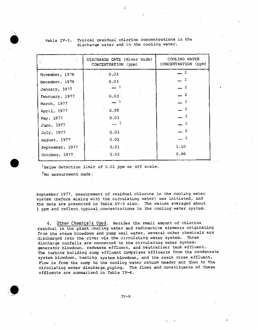
2

Table IV-3. T¶vpical residual chlorine concentrations in thedischarge water and in the cooling water.

DISCHARGE GATE (River Side) COOLING WATERCONCENTRATION (ppm) CONCENTRATION (ppm)

November, 1976 0.03 - 2

December, 1976 0.03 - 2

January, 1977 - 1 2

February, 1977 0.03 - 2

March, 1977 1 2

April, 1977 0.05 2

May, 1977 0.03 2

June, 1977 - 1 __ 2

July, 1977 0.03 - 2

August, 1977 0.02 2

September, 1977 0'.01 1.10

October, 1977. 0.02 0.86

iBelow detection limit of 0.01 ppm or off scale.2 No measurement made.

September 1977, measurement of residual chlorine in the cooling watersystem (before mixing with the circulating water) was initiated, andthe data are presented :in Table IV-3 also. The values averaged about1 ppm and reflect. typical. concentrations in the cooling water system.

4. Other Chemicals Used.- Besides the small amount of chlorineresidual in the plant cooling water and radioactive elements originatingfrom the steam blowdown and pump seal water, several other chemicals aredischarged into the river via the circulating water system. Threedischarge outfalls are connected to the circulating water system:generator blowdown, radwaste effluent, and neutralizer tank effluent.The turbine building sump effluent comprises effluents from the condensatesystem blowdown, heating system blowdown, and the resin rinse effluent.Flow is from the sump to the cooling water return header and then to thecirculating water discharge, piping. The flows and constituents of theseeffluents are surmmarized in Table IV-4.

IV-9.

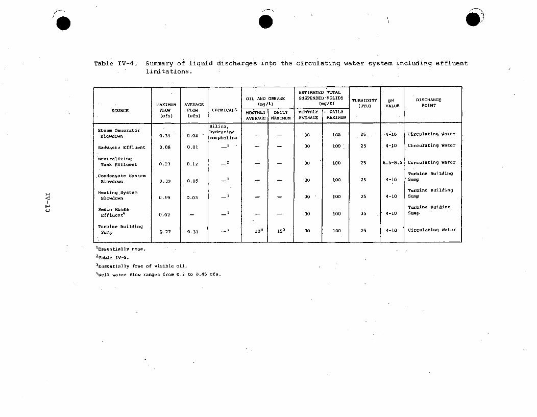
i I

Table IV-4. Summary o~f liquid discharges-into thelimitations.

circulating water system including effluent

ESTIMATED TOTAL

OIL AND GREASE SUSPENDED-SOLIDS DISCHARGE1AXIMUM AVERAGE' (mg/0) (mg/)) VALUE T IPOINT

SOURCE FLOW FLOW CHEMICALS MONTHLY DAILY MONTHLY DAILY

(cfs) (cfs) AVERAGE MAXIMUM AVERAGE MAXIMUM

Silica,Steam Generator hydrazine -10

Blowdown 0.39 0.04 morpholine

Radwaste Effluent 0.08 0.01 -1 - - 30 100 25 4-10 Circulating Water

Neutralizing

Tank Effluent 0.23 0.12 2 3U 100 '25 6.5-8.5 Circulating Water

.Condensate System Turbine Building

Blowdown 0.39 0.05 -1 30 100 25 4-10 'Sump

Heating System Turbine Building

Blowdown 0.39 0.03 - - 30 100 25 4-10 Sump

Resin Rinse Turbine Buiding

EffluentO 0.02 - -- 30 100 25 4-10 Sump

Turbine Building

Sump 0.77 0.31 1 0 153 30 100 25 4-10 Circulating Water

1Essentially none.

2Taable IV-5.

3Essentially free of visible oil.

1,Well water flow ranges from 0.2 to 0.45 cfs.

HH0

Neutralizing tank effluents account for most of the chemicals dis-charged. Liquid effluent from the neutralizing tank is from regenerationof demineralizers for purifying makeup water. During normal batch opera-tion, effluent is released to the circulating water system at a maximumrate'of 20,000 gallons per day and at a minimum of 6-hour intervals..Dissolved minerals include approximately 213 kg (470 ibs) of variouschemicals occurring naturally in the well water and up to 327 kg (720 lbs)of regeneration and neutralization chemicals. Chemicals in the naturalwell water are typically Ca+ , Mg++, Na+, HC03-, SOL,, SiO2 =, and C1-.Chemicals from the regeneration and neutralization consist primarily ofNa+ and SO4=. Table IV-5 lists:the estimated quantities of these chemicalsdischarged to the river. The equivalent discharge canal and river concen-trations were estimated by assuming complete mixing with the circulatingwater and the water in the discharge canal (1,410 cfs assumed) and with theriver (11,000 cfs assumed). The equivalent increases in concentrationare less than 0.8 percent and 0.1 percent in the discharge canal and inthe river water flow, respectively. The percentage increase is thusinconsequential.

Table IV-5. Chemical Concentrations from neutralizinq tankeffluents (based on data from AEC, 1973).

DAILY EQUIVALENT EQUIVALENT NORMALDISCHARGE CANAL RIVER RIVER

CHEMICAL DISCHARGE CONCENTRATION I CONCENTRATION 2 CONCENTRATION

(lbs) (kg) (mg/i) (mg/£) (mg/Z)

RegenerationChemicals

+Na 233 106 0.0300 0.0039 6 to 18

S04 487 217 0.0600 0.0080 10 to 75

Total 720 327 0.0900

Well WaterMinerals 3

Ca++ 74.4 33.8 0.0092 0.0012 34 to 72

Mg++ 23.2 10.5 0.0029 0.0004 11 to 22

Na4 12.5 5.7 0.0020 0.0002 6 to 18

HCCO3 285.0 129 0.0400 0.0048 66 to 235

S04= 31.3 14.2 0.0039 0.0005 10 to 75

,SiO2 = 24.4 11.1 0.0030 0.0004 0.4 to 13

•C1- 17.8 8.1 0.0022 0.0003 2 to 25

Total .. 470.0 213 0.0600

iAssuming a discharge dilution flow rate of 1,410 cfs which includes blowdown and

natural dilution in the discharge canal.2Assuming an average river flow rate of 11,000 cfs.3Based on well water analysis of 5/2/72 and on 150,000 gallons of water purifiedper regeneration cycle (once per day).

IV-ll

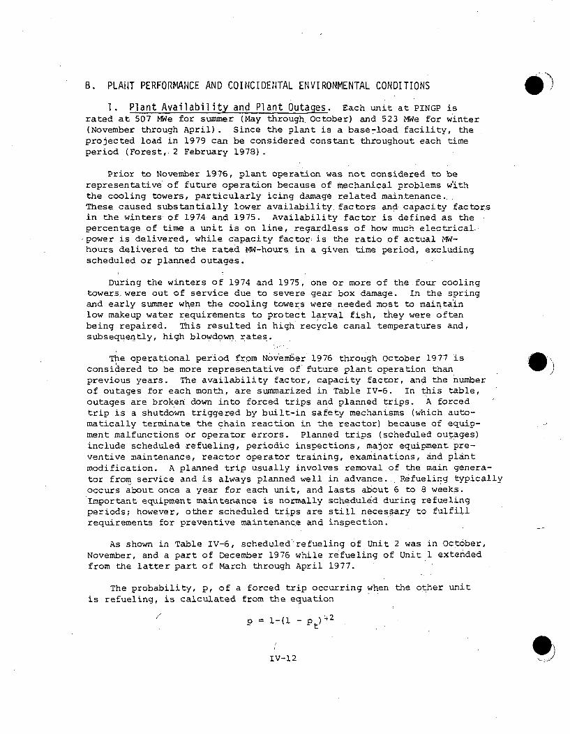
B. PLANT PERFORMANCE AND COINCIDENTAL ENVIRONMENTAL CONDITIONS

1. Plant Availability and Plant Outages. Each unit at PINGP israted at 507 MWe for summer (May through. October) and 523 MWe for winter(November through April). Since the plant is a base-load facility, theprojected load in 1979 can be considered constant throughout each timeperiod (Forest, 2 February 1978).

Prior to November 1976, plant operation was not considered to berepresentative of future operation because of mechanical problems withthe cooling towers, particularly icing damage related maintenance...These caused substantially lower availability factors and capacity factor.sin the winters- of 197.4 and 1975. Availability factor is defined as thepercentage of time a unit is on line, regardless of how much electrical.power is delivered, while capacity factor is the ratio of actual MW-hours delivered to the rated MW-hours in a given time period, excludingscheduled or planned outages.

During the winters of 1974 and 1975, one or more of the four coolingtowers, were out of service due to severe gear box damage. In the springand early summer when the cooling towers were needed most to maintainlow makeup water requirements to protect larval fish, they were oftenbeing repaired. This resulted in high recycle canal temperatures and,subsequently, high blowdown rates.

The operational period from November 1976 through October 1977 isconsidered to be more representative of future plant operation thanprevious years. The availability factor, capacity factor, and the numberof outages for each month, are summarized in Table IV-6. In this table,outages are broken down into forced trips and planned trips. A forcedtrip is a shutdown triggered by built-in safety mechanisms (which auto-matically terminate the chain reaction in the reactor) because of equip-ment malfunctions or operator errors. Planned trips (scheduled outages)include scheduled-refueling, periodic inspections, major equipment- pre-ventive maintenance, reactor operator training, examinations, and plantmodification. A planned trip usually involves removal of the main genera-tor from service and is always planned well in advance... Refueling typicallyoccurs about once a year for each unit, and lasts about 6 to 8 weeks.Important equipment maintenance is normally scheduled during refuelingperiods; however, other scheduled trips are still necessary to fulfillrequirements for preventive maintenance and inspection.

As shown in Table IV-6, scheduled'refueling of Unit 2 was in October,November, and a part of December 1976 while refueling of Unit 1 extendedfrom the latter part of March through April 1977.

The probability, p, of a forced trip occurring when the other unitis refueling, is calculated from the equation

p = i-(I - pt)%2

IV-12

HH

F,Li

Table IV-6. Summary of availability factors, capacity factors, and plant outagesfor November 1976 through October 1977 (Brown, 7 November 1977). See text.

1977 PLANT OPERA'ION

UNIT I UNIT 2

1NUMBER OF OUTrAGES fNUMBER OF OUTAGESDATE AVAILABILITY CAPACITY R AVAILABILITY CAPACITY

FACTOR' FI At l' PORCED PLANNED VA(-PO, F.ACTOR:' FORCED PLANNEDTRIP TRIP TRIP TRIP

I 1~

Nov 76 98.1 97.4 (Inverter Failure, Refuelin.g Outage14 lis)

1 2(Feed Water Ruau- (Testing and

Duc 76 100.0 98.0 39.1 31.V latur Valve Con- Other Mi4sel-troltln 5 hra) lancous from

Outage, JO hrs)

Jan 77 98.1 96.4 (Rod Dirop; BDd 100.0 98.0Fusj,, 14.2 hrs)

I I I( Condiii stir

-Feb 77 94.4 92.2 (Condenser 93.9 91.5 (0-unerator Cd111111(Cleaning) Executor Maifunc- 7.1 hlra)

_________________t~oll) 71b1' 1 1

(Inrvur tor Failure, (R tI i.q, 98.6 97.3 (1 C Error During C17.1 lira) 34() liC

ro)

lI,r)

Ap:t 77 Refueliit9 Uutage 100.0 98.4

2 2(T.tili9 anld (Condu..e.r Vdavin9

Other Miscel- 9 9 XcError, 5 hrs;.May 7C9.0 O2.O - laneou. Itums 7. .4 Flow 2M Trans-

from Outages, former, 10.6 hrs)

726 irts)

I 1

June 77 93.6 91.9 (Turbine Work. 97.8 95.0 (2M T'ransforumr,46.1 hrs) lb irs)

(ated Water Regu - 100.0 98.5July 77 98.8 97. aItor Value C:o£1-

troflur, 8.7 firs)

(Steamn-!a.d Water

Aug 77 10U.u 98.2 .99.1 93.1 Valuus Failure,6.7 fir.)

Sept 77 100.0 95.8 100.0 98.01 1

(-)C;ndc•elI•1er Pll- (Turbijie Work,Oct 77 95.9 94.9 ahinJ Value Error, S.uam Leaks 100.0 98.4

3.1 hr.r) 27.1 lira)

6 i 7 4Total 6f 7

Trips II- - ---- ________

lPercent of time unit is on line, excluding p1lanned outages.2Delivered energy/rated energy.

where Pt is the probability of a forced trip on any day of the year.Based on the typical plant performance record shown in Table IV-6,forced trips occur about 6 times a year for each unit. Assuming that theplanned refueling period is 6 weeks or 42 days (shown as the exponent inthe equation), the probability for a forced trip on any day, pt, is6/(365-42) = 0.0186. Thus the probability (p) of a trip during refuelingis 1 -(1-0.0186)42 = 0.55. The probability of simultaneous forced tripsis 0.0186 x 0.0186 = 0.00035 since they are independent events. Refuelingoutages are not scheduled to occur simultaneously. Table IV-6 showsthat all of the forced trips lasted for less than 24 hours, but in theabove calculation, each forced trip was assumed to last for a one-dayperiod., which gives a more conservative estimate of p.

2. Past and Proposed Modes of Operation. As described in SectionIV A.2, the basic mode of operation is a closed cycle with 150 cfs ofblowdown. As the condenser inlet temperature reaches 29.4' C (85' F),blowdown is increased to remove the excessive heat from the circulatingwater system. Based on 16,156 hours of operating data for 1975 and 1976,the frequency of various blowdown rates and the cumulative frequency ofthese blowdown rates were summarized in Figure IV-6.

From Figure IV-6, it can be shown that the closed cycle mode wasused more than 53 percent of the time during 1975-1976, and blowdown wasless than 400 cfs about 81 percent of the time. Plant discharge exceeded1,000 cfs for about 180 hours or one percent of the time. The higherblowdown rates resulted from the combination of warm intake water tempera-ture, high wet-bulb temperature, and malfunction of cooling towers.

Blowdown rates necessary to maintain a condenser inlet temperature of'29.40 C (85' F) were calculated using the average river temperaturesfrom RWGP, and wet/dry bulb temperatures taken from the Minneapolis-St.Paul Airport for the period 1965 through 1974. The calculated frequencyof blowdown rates is presented in Figure IV-7 (dashed lines) and showsblowdown rates of less than 200 cfs would occur 314 days per year. Thisamounts to 86 percent of the time versus the actual 53.8 percent for 1975through 1976 (shown in Figure IV-6) when cooling towers did not functionproperly. A blowdown of 800 cfs would be exceeded only a small percentageof the time.

.A proposed operating. mode consisting of helper cycle from 16 June through31 August is also presented in Figure IV-7 (solid lines). With the twoand one-half months of helper cycle and zero cooling tower outage, ablowdown rate of 150 to 200 cfs would be expected about 277 days (6r 76percent) per year. Except during helper cycle (about 79 days), thenecessity of having blowdown rates higher than 400 cfs during the remainderof the year is essentially eliminated.

IV-14

100 10.00060

9500

90- 90008684 Hrs.

r-->. -850053.8% 8

z50 80- D 8000a

w

L 7500I.U> top~,,

70- 1*- 7000 (n~~CUMULATIVE FREQUENCY70IR 0

zz40 D 3

wj 60- 6000

D :zU. 5500 ccU.o 0

a 50-. 5000

>. 30o0Z 4500 =

0"U 4000 d

LA. zU--

3500 I-

20 - 03012 -30O0

19

- 2500

- 2000

1394 -15008.6

826 - 1000

5.1 636 598 6823.9 I 3 0 3 0367 4, 04 4 500

45 9 "j 1 "30I I.| ~ ~I--•--•-1 .- 4 61.•-/ 10• 1, o 5 1,o100 200 -300 400 500' 600 '700 `800' 900' 1000 1100 1200 '1300 1400 1500

BLOWDOWN (cfs) 547P.33

Figure IV-6. Frequency of occurrence and cumulative frequency ofvarious blowdown rates from 1975 through 1976 (fromPINGP Environmental Event Log).

IV-15

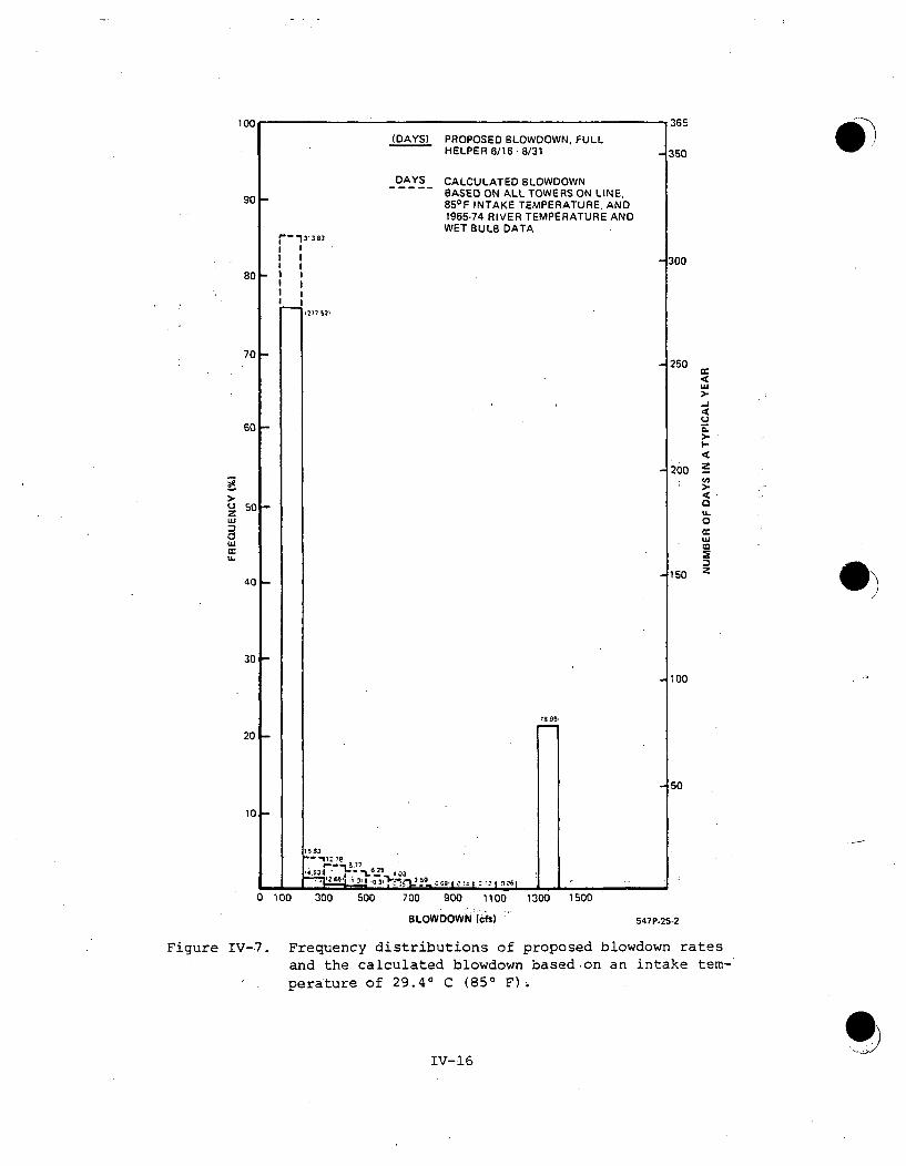
innA ;6i36E

(DAYS) PROPOSED BLOWDOWN. FULLHELPER 6/16 - 8/31

DAYS CALCULATED BLOWDOWNBASED ON ALL TOWERS ON LINE.850F INTAKE TEMPERATURE. AND1965-74 RIVER TEMPERATURE AND

WET BULB DATA

350

90

80

31- 8

1277 52'

701-

6a -

o 50

tL

300

250

w

-JLU._j

I-4

200 z

(n0

w

150 z

100

50

401-

30F

20 -

101-

~178ý____ o 3 7B 76

0 100 300 500 700 900 1100 13oo 1500

BLOWDOWN Wcfs) 547P.25-2

Figure IV-7. Frequency distributions of proposed blowdown ratesand the calculated blowdown based on an intake tem-perature of 29.40 C (850 F)-.

IV-16

This proposed mode of operation is designed to increase plant efficiencyduring summer when the demand is high. Plant efficiency is increased byutilizing the maximum makeup of 1,410 cfs from the river (Sturgeon Lake)without having to recycle partially cooled water from the cooling towers.The total heat rejection rate is not greatly increased with the higherblowdown rate; however, the temperature difference between blowdownand ambient water is proportionally decreased. The monthly breakdownsof computed. .joint occurrences of blowdown rate and river flow are summarizedin Appendix M. In the Appendix, Table M-1 lists the number of hours for agiven set of blowdown rate and river flow conditions to occur.for theprojected present mode of operation (29.40 C intake temperature and nocooling tower outage). Table M-2 lists the same information for theproposed mode of operation (29.40 C intake temperature, no cooling toweroutage, and helper cycle from 16 June through 31 August).

IV-17

V. THERMAL PLUME-

A.. DESCRIPTION OF THE, HYDROTHERMAL MODEL.

The numerical model for thermal plume predictions can be dividedinto three parts. A one-dimensional (1-bD) hydrodynamic model developedby Stefan and Anderson (1977) was first used. to calculate the, overallflow pattern in lower Pool No. 3. This overall flow pattern was thenused as an input for computing the velocity field in the near-fieldregion. Due to the irregular geometries of the: boundary in this region,a two-dimensional (2-D) model was used for computing both velocity andtemperature fields. A closed-form three-dimensional (3-D) solution wasused to simulate the thermal dispersion behavior downriver from Barney'sPoint because of the relatively well-defined river channel geometry.The computations for these three models (l-D, 2-D, and 3-D) are brieflyoutlined in the following sections.

1. Hydrodynamic Model. The I-D hydrodynamic model formulated byStefan and Anderson (1977) employed the simplifying assumption that flowin any channel section is uniformly distributed. The 1-D. hydrodynamicmodel is analogous to pipe flow analysis. The model computes the flowrates for all the :channels shown in Figures 111-7 and 111-8 for a givenset of river flows, wind speeds, and wind directions. Laws of mass andenergy conservation were applied in the computation. A brief discussionof the hydraulic network analysis is presented in Section III A.2, and'detailed descriptions can be found in Stefan and Anderson's report. Theresults of the channel flow rate estimates were used as inputs for the2-D model, particularly Channels 36, 26, and 42 (See Figure 111-8).

2. 2-D Thermal Plume Mlodel. The region in which two-dimensionalflow was assumed is shown in Figure V-1 and this defines the near-fieldarea. The input variables for the model were flows in Channels 36, 26,and 42 and intake and blowdown rates. Also shown in the figure areinflows into the region, indicated by a plus (+), and outflows from theregion, indicated by a minus (-). The intake flow .always has a minussign and the blowdown always has a plus sign while channel flows may haveeither sign. Typically, water from Sturgeon Lake flows into the 2-Dregion through Channel 36, and a part of it flows out to the riverthrough Channel 26 while the remainder flows out of Channel,42.Occasionally, when strong southerly winds occur in conjunction with lowriver flows, the channel flows may reverse direction.

V-1

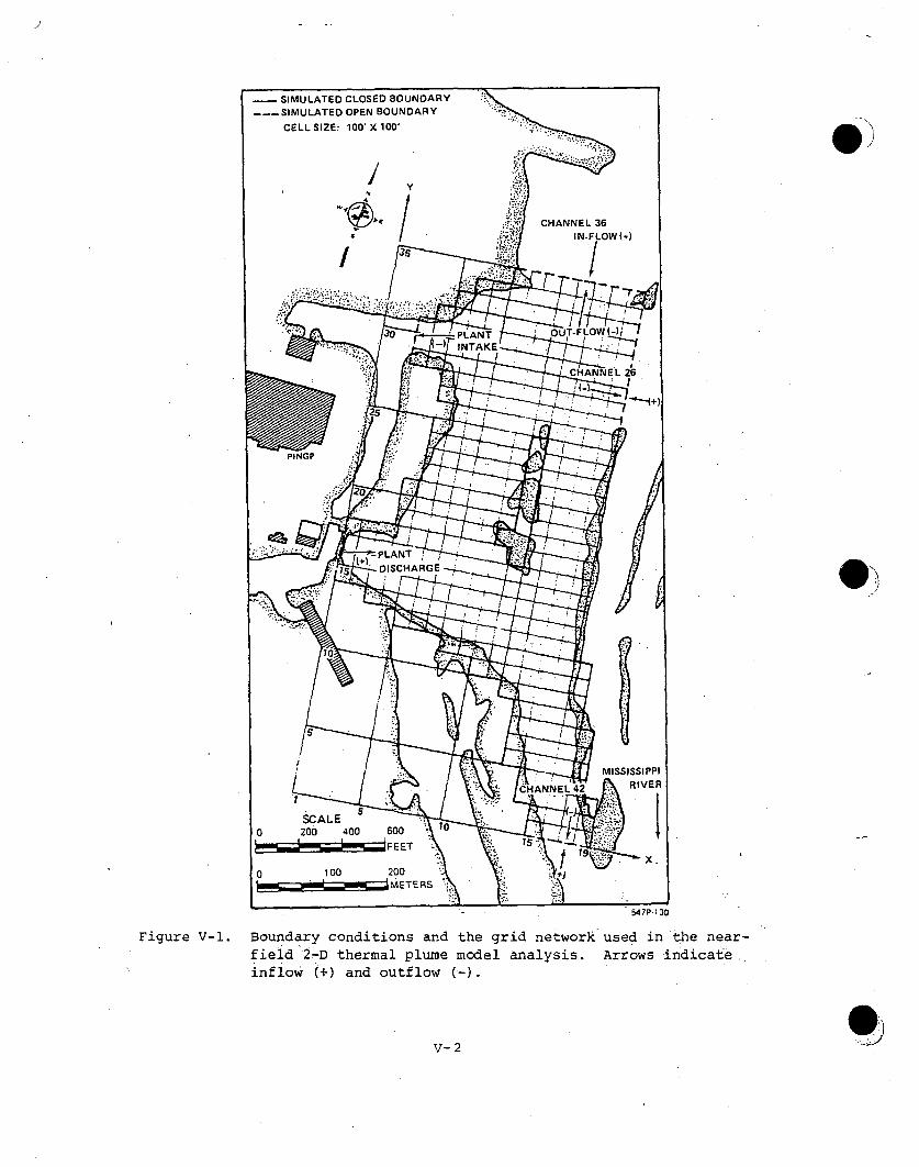
CELL SIZE: 100' X 100'

Y.

CHANNEL 36

r,"7i-.•,

;•.:• IN-FLOW (+)

, -!F

0 200 400 600 10-

547PN. 30

Figure V-l. Boundary conditions and the grid network used in the near-field 2-D thermal plume model analysis. Arrows indicateinflow (+) and outflow ()

V- 2

In order to compute the thermal plume dispersion, the velocity fieldmust be defined. For the latter, a grid network (Figure V-l) was selectedto approximate the shoreline configuration in the region. The four smallislands in the center of the region were assumed to be connected becauseof the relatively shallow depth occurring between them. The grid networkconsisted of a 19 x 35 matrix with the y-axis oriented toward north. Theheavy solid lines in Figure V-1 were assumed to be closed (impervious)boundaries while the dashed lines indicate open boundaries which in thiscase were input flow rates.

Since this is a 2-D model, flow was assumed to be constant with depth;therefore, only one velocity vector occurs at each grid point within thesite boundary. A continuity equation was combined with two momentumequations to solve for the velocity vector at each grid point. In themomentum equations, the only driving forces were surface wind shear andbottom frictional stress. These three equations (continuity and twoequations of momentum) were then normalized (with depth) and combinedinto a single equation by introducing the stream function. Subsequently,the stream function equation was solved numerically using a successiveover-relaxation (SOR) method (Chu, 1968) After the stream'function valueat each grid point was computed, the two velocity components at each pointwere calculated as inputs for the energy equation (heat flow equation).

The energy equation was 'solved with the alternating directionalimplicit (ADI) method (Yeh, Lig, and Verna, 1973). Boundary conditionsused for the energy equation were: uniform heat flux across the plantdischarge points' ((1,14) through (1,18)], zero heat flux across theclosed boundaries, and heat sinks on all the open boundaries. This modeldescription and development is presented in detail in Appendix I.

3. 3-D Thermal Plume Model. Downriver from Barney's Point in themain river channel a three-dimensional (3-D) thermal plume model was usedfor dispersion computation. A closed-form solution for an unsteadypoint source (Yeh, 1976) was employed for computing the temperature rise.(AT) in this region. As the river channel approaches uniformity inwidth, the 3-D model becomes more representative of the actual three-dimensional plume behavior. Assumptions for the 3-D model were: heatsource uniformly distributed on the plane perpendicular to Channel 42 atBarney'sPoint (i.e., no initial thermal stratification), zero heat fluxthrough the shoreline, and uniform velocity across the flow region. Theheat source was based on the temperature output of the 2-D model at Barney'sPoint. The detailed description of the governing equation and its boundaryconditions are presented in Appendix I.

V-3

B. CASES STUDIED

Sixty-one (61) cases have been modeled using the plume models describedin Section V A. These sixty-one cases are:

SMonthly typical operating conditions in 1975 (12 cases)

Monthly typical operating conditions in 1976 (12 cases)

* Monthly extreme conditions in 1975 (12 cases),

* Monthly extreme conditions in 1976 (12 cases) and,

* Proposed monthly extreme conditions (13 cases)

The parameters used to, describe the operating conditions consist ofblowdown rate (Qp), intake flow rate (Qi), river flow rate- measured atPrescott (Qr), wind speed (Wa) and direction (Wd), flow rates at ChannelNos. 36, 42, and 26 (Q36, Q42, Q26), blowdown temperature (Tp), andambient river temperature (Ta). The breakdown of these values for eachcondition modeled is summarized in Table 5-1 through.. Table. 5-5 ofAppendix I. Also given in these tables is the, predicted temperature rise(AT) at Barney's Point, for each condition..

For typical operating conditions, the blowdown rate, intake flow rate,river flow rate, and the river temperature (daily maximum) consisted ofaverage values for the month. Blowdown temperature was computed usingvalues for, intake temperature, wet bulb temperature, and the coolingtower performance curve. In general, typical conditions for 1975 areconsidered to be more representative of average conditions because ofthe low river flows that occurred in 1976.

The extreme conditions for 1975 and 1976 were chosen as the datewhen the maximum daily blowdown rate was recorded'during .each month,For instance, the maximum blowdown rate in July 1975 was 1,,200 cfs on8 July. Then, coincidental operating conditions on this day were-usedas inputs for the analysis..

The proposed extreme conditions for each month comprised the worstpossible environmental conditions of: 7-day, 10-year low river flow;expected maximum blowdown rate for future operation; maximum rivertemperature ever recorded at RWGP, except for winter months (from Novemberthrough March) when river temperature was assumed to be 00 C (320 F); andupper fifth percentile wet-bulb temperature for computing blowdown tempera-ture.

To assess the probability of occurrence for the proposed extremeconditions, it can be assumed that all the recorded environmental conditionsare stati-sticaliy independent of each other. In other words, blowdowntemperature, blowdown rate, river flow, and river temperature are notcorrelated within a given month. The 7-day, 10-year low flow frequency isless than 8.4 percent (see Figure 111-12) for a given month. The blowdown

V-4

4 temperature would not be exceeded 95 percent of the time, and the maximuintemperature occurs less than once in the 27-year record, or 0.12 percentof the time. Thus, even if t•he proposed maximum blowdown rate remainsconstant throughout the month, the probability that the proposed extremecondition will occur on any day in a given month is 0.084 x 0.05 x 0.0012 =

0'.000005 (or 0.000b5 percent)*.

The model results for these typical and extreme operating conditionstogether with the proposed extreme conditions are presented in Figures 5-1through 5-15 of Appendix I. These figures will be used as the basis forassessing biological impacts of the thermal discharge in this demonstration.

C. MODEL CALIBRATION

Seven field thermal surveys were conducted at PINGP from 1974 through1976 (see Appendix N). However, only the thermal survey conducted onI August 1975 was used to calibrate the 2-D numerical model since it wasthe only one with comprehensive water velocity measurements taken in thenear-field region. The 5 September 1974 field data were used to calibratethe 3-D model because of the relatively smooth isotherms found immediatelydownstream of Barney's Point on that date.

The numerical constants derived from the field measurements are thelongitudinal diffusivity (Kx) and the lateral diffusivity (K.) for the 2-Dmodel. The values for these two diffusivities were found to be aboutthe same, 75 f t 2 /sec. These values were determined by adjusting. thediffusivities so that the computed surface isotherms were similar to thosemeasured in the field on 1.August 1975. The comparison among isothermsbased on the selected diffusivities and the field measurements is illustra-ted in Figure 4-3 of Appendix I.

In the 3-D region, the longitudinal, lateral, and vertical diffusivi-ties are assumed to be proportional to the mean river velocity. The pro-portionality coefficients ax, ay .and az were calibrated against fieldmeasurements conducted on 5 September 1974. In this calibration, a 76 m(250 ft) wide by 1.8 m (5.2 ft) deep heat source was established as theinput for the numerical model. ,A 1.8 m (5.2 ft) deep source was usedsince, on the day of field survey, warm water seemed to float in the upper1.8 m (5.2 ft) of the water column. The proportionality coefficientswere determined to be: ax = 15 m (50 ft), ay = 1.5 m (5 ft), and az = 1.5 cm(0.05 ft). The vertical proportionality coefficient (az) was assumed to beorders of magnitude less than ax and ay because of the natural buoyancy ofwater.

In the cases studied, however, a full plane source 76 m (250 ft) wideand 3.1 m (10 ft) deep was used instead of a 1.8 m (5.2 ft) deep planesource. A negligible difference between these-two source configurationsis expected 152 m (500 ft) downstream from Barney's Point because of thereflecting surface condition assumed in the solution. This set ofproportionality coefficients was'also used to compare the model with the

V-5

field data collected on 1 August 1975 (Figure 4-6 of Appendix I). WPredicted isotherms compared favorably with the field measurement withinapproximately 396 m (1,300 ft) downriver of Barney's Point.

D. COMPARISON OF MODEL RESULTS WITH TEMPERATURE STANDARDS

The numerical models previously presented in this section were used todescribe the PINGP thermal plume since adequate field data were not availablefor all of the environmental conditions and months necessary f0i esti-mating biological impacts of the discharge. The models were calibrated withfield data and thus can be assumed to provide a reasonable representationof the actual plume behavior. The model results will therefore be used forcomparison with the state temperature criteria (NPDES permit).,

The proposed NPDES permit issued by the MPCA specifies the followinglimitations:

1. The discharge shall not raise the temperature of the receivingwater at the edge of the mixing zone specified below by more than2.80 C (50 F) above natural based On the monthly average of the •maxi-mum daily temperatures, above 300 C (860 F) at any time, or above thefollowing weekly average temperatures* whichever is more stringent:

January 4.4 0 C(40 0 F) July 28.9 0 C(840 F)February 4.4 0 C(400 F) August 28.9-C(840 F)March 12.2 0 C(54 0 F) September 27.8 0 C(820 F)-April 18.3 0 C(650 F) October 22.8 0 C(73PF)May 23.9 0 C(75 0 F) November 14.4 0 C(580 F)June 28.9 0 C(840 F) December 8.9 0 C(480 F)

2. Mixing Zone. The mixing zone shall be the confluence of thedischarge canal and the main channel of the Mississippi Riverat the place commonly known as Barney's Point. The.Permitteeshall determine compliance by the use of their temperaturesensors as they exist at the time of the issuance. of this permit.

3. Frequency of Monitoring andý Reporting. The Permittee shallmonitor the temperature at the edge of the mixing zone continu-ously and report it along with other monitoring data to theDirector.

4. Natural River Water Temperature. The natural river water tempera-ture is the temperature of the river water at a point unaffectedby the plant discharge or any other man made source.

*Where the background weekly average temperature of natural origin is

normally higher than that specified for a particular month, the naturalweekly average temperature may be used as the limiting value which shallnot be exceeded at the edge of mixing zone.

V-6

5. The final thermal limitations specified above may be subjectto modification after opportunity for a public hearing followingthe completion of the Permittee's 316(a) demonstration pursuantto WPC 36(s) (1) and WPC 36(u) (3).

The natural ambient water temperature, as discussed in Section III B.1,is taken as the condenser inlet temperature measured at RWGP.

These criteria apply to the 1975 and 1976 typical cases under studywhich are assumed to represent typical conditions for future operation,as well as the proposed extreme cases. Based on the model predictions,thirteen cases were found to exceed the thermal criteria listed above:six cases for 1975 typical conditions, five cases for 1976 typical condi-tions, and two cases for proposed extreme conditions (Table V-l). Fromthis table, it appears that meeting the 2.80 C (5° F) temperature risecriterion is most difficult during the winter months since the low flowin Channel 42 would not supply an adequate volume of water for dilutionbefore Barney's Point. Little problem would be encountered in meeting thedaily maximum thermal criterion of 300 C (860 F) and the weekly averagetemperature criterion for each month.

In Table V-l, the additional distances required to meet all thethermal criteria are also presented, based on the 3-D model numericalresults shown in Tables 5-7 and 5-8 of Appendix I. The distances wereinterpolated on a log-log plot. These distances ranged from 91 m (300 ft)to 488 m (1600 ft) downriver from Barney's Point. For the August proposedextreme.condition, the required compliance distance was not computedbecause the assumption of strong southerly wind reduces the Channel 42flow to only 1 cfs. In this case, most of the discharged heat would beblown upriver instead of being diluted in Channel 42.

In terms of thermal criteria exceeded, it is apparent that the proposedextreme conditions do not represent the worst case thermal conditions atBarney's Point. Instead, the conditions reflect the worst case heatrecirculation conditions because strong (10 mph) southerly winds were assumedin most cases. The estimated heat recirculation to the intake is summarizedin Table 5-6, Appendix I, and varies from 10 to 44 percent for the proposedextreme conditions. For the typical cases, the maximum heat recirculationis 10 percent for 1975 and 28 percent for 1976. The higher the recirculationrate, the less efficient is the cooling system because the rejected heatreturns to the intake and thus increases the condenser inlet temperature.The proposed extreme conditions, instead of representing the worst possiblethermal conditions at Barney's Point, reflect worst operational conditionsat PINGP. These conditions also reflect the worst possible thermal build-upin the near-field area. The warm water, in these instances, often flows outof the near-field region into lower Sturgeon Lake through Channel 36 andinto the Mississippi River by way of Channel 26.

V-7

Table V-1. Cases where the PINGP proposed NPDES thermal criteria wereexceeded. The additional distance required for the dischargedthermal plume to meet the criteria is also presented.

BARNEY'S POINT ADDITIONAL DISTANCEREQUIRED TO MEET

MONTH AT T CRITERIA 1

(C) (F) (C) (F) (m) (ft)

January 1975 4.7 8.42 4.9 40.92 335 1100

February 1975 5.,0 9.02 5.6 42.12 427 1400

March 1975 4.4 8.02 6.1 43.0 274 900

October 1975 3.0 5.42 16.2 61.2 61 200

November 1975 3.2 5.82 10.0 50.0 91 300

December 1975 4.7 8.52 5.2 41.4 366 1200

January 1976 4.5 8.12 4.6 40.32 305 i000

February 1976 5.2 9.32 6.5 43.72 488 1600

October 1976 3.5 6.32. 14.9 58.8 91 300

November 1976 3.9. 7.02 7.1 44.7 177 580

December 1976 4.7 8.42 5.2 41.4 335 1100

JulyProposed

Extreme 2.2 3.9 30.5 86.92ý 107 350

AugustProposed

Extreme 1.5 2.7 30.9 87.72 ,3

1Extrapolated from Tables 5-7 and 5-8 of Appendix I.2 Thermal criteria exceeded.

3No distance calculated sinceand wind was southerly.

flow atBarney's Point was only lcfs,

V-8

To estimate the frequency of occurrence for various temperature rises(ATs) at.Barney's Point, a simple complete-mixing model was used. The flowrates in Channel 42 for each river flow during calm conditions were calcu-lated using the results from Stefan and Anderson's report (1977). Theapproximate relationship between these two flow rates, as described inSection IV A.2, is:

Q42 = 0.14 Qr 0 . 9 6

The total heat discharged was based on the present operating mode and wasassumed to be fully diluted (no recirculation) in Channel 42. Thus, thetemperature rise at Barney's Point is only a function of total heat dis-charged and the flow rate in Channel 42. The frequency (percent of time)with which various temperatures and ATs are calculated to occur at Barney'sPoint for every month are summarized in Tables V-2 and V-3. A temperaturerise exceeding 2.80 C (50 F) could be expected approximately 71 percent of

the time during January and February (Table V-2), and the frequency would beless than 46 percent of the time during the remainder of the year. Thefrequency of occurrence for absolute temperatures expected at Barney's Pointduring each month is presented in Table V-3. As expected, the maximumdaily temperature limit of 300 C (86' F) would be exceeded only during thewarm water months of July, Augus't, and September. Based on the aboveanalysis, it is evident that meeting the 300 C (860 F) limit would notbe nearly as difficult as meeting the 2.80 C (50 F) temperature riselimit.

The above comparisons and calculations indicated that PINGP willnot be able to meet the proposed NPDES thermal criteria, particularlyduring winter. Therefore, a variance of an additional 488 m (1600 ft)distance downriver would be needed to provide sufficient dilution tomeet the mixing zone thermal criteria without derating the plant.

Table V-2. Computed monthly cumulative frequency (as percent) oftemperature rise (AT) at Barney'.s Point assuming nowind and full dilution in Channel 42.

CT F) JAN FEB MAR APR MAY JUN JUL AUG SEP OCT NOV DEC

19 0.2is 0.4 0.1 0.2 0.217 0 .9 0.4 0.2 1.016 1.6 0.4. 0.4 1.9is 2.3 0 8 0 . 0.1 2.314 3.2 2.0 0.2 0.7 0.4 2.913 4.1 4.0 0.2 0.0 0.4 0.7 1.- 4.2 .12 8.0 8.5 1.2 0.2 0.7y 1.0 1.7 9.811 12.3 12.6 1.9 0.4 1.5 1.3 0.0. 1.7 6.710 17.1 17.8 Z.8 1.2 2.7: 1.7 0.1 2.3 7.9

9 24-.4 23.9 S.9 2.1 4.8 2.3 05. 4.2 .10.98 31.9 33.9 9.2 3.9 7. 0 3. 0 1.3 :6.4 17.77 49.0 91.2 15.5 S.8 10.2 4.5 3.1 12.4 32.76 70.6 71.0 26.8 0.7 0.1 9.0 14.1 .9.3 7.6 19.S '9.8S 88.7 89.1 40.5 1.9 0.9 13.7 18.9 17.9 17.S 31.4 64.84. 98.7 93.6 S3.0 4.3 2.3 21.1 26.3 32.9 35.0 42.9 80.03 100.0 96.1 65.7 9.7 6.2 31.6 37.5 *91.3 52.1 49.0 90.02 100.0 98.6 80.9 15.3 6.6 16.9 47.9 61.6 78.0 69.6 73.5 99.71 100.0 100.0 93.7 55.2 53.1 S0.0 7S.2 90.0 96.9 91.S 98.0 100.00 100.0 100.0 100.0 100.0 100.0 100.0 100.0 100.0 100.0 10.0.0 100.0 100.0

V-9

Table V-3. Computed monthly cumulative frequency of occurrence (percent)for river temperatures at Barney's Point assuming no windand full dilution in Channel 42.

(F)92919089a8878685asa e.

33828180797877767574,73727170696867666s646362616059sa5756S3S453

SI

5o4948'7464544,

4,342414.03938373635

343332

JAW FKB MAX APR MAY JUN JUL AU, SgP OCT NOV 0EC

1.42.12

3.~7

4.24.4

5.87.18.3'

10.916. 0

32.9

39.047. 354.060.370.679.581 .S87.090.694-.8

95.898.1

98.799.7

100.0

0.20.5

1.01,71. 1

6.28.3

12.618.624 .4eC9.836.8a'5.354 .8

66.678.387.790.794.4.9 6

i. 7

98.7100.0

0.20.61.22. 4.4.15.98.8

12.9

18.323.029.637.6

4S.653.662.471.6'76.480.485. 090 .8

96. 097.398. S

100.0

0.a0.5

1 .42.23.35.27.19.5

12.9.17. 723. 128.5

35. 943.151 .259.6

67.376. 18z.491.295.,496.297.3

98a.799.4

100.0

0.10 .20 .30. 40 S0 .6

.0.60.9

2.73.7

4.4.5.37.08.S

11.112.51S.321.823.234.4

42. 6S2.662.5691.779.2

87.08.9. 691.693.795.0

95.796.797.097.79.7.798.999.400 .••.

0.81.52.33.24. 18.0

12.317.1

2' . z

72.189.598.7

100.0

0.10.4,0.82.0

3.98.5

13.218.324. 335.3S8.9

75.991 .S94..096.1

98.6100.0

0.00.51.01.2

1.72.55.08.7

13.122. 332.3.47.960.0-70.8"78.784.2

90.697. 0

t0o .0

0.31.72.S

5.37.0

10.2.

:15.717.52-2. . 827.233.2

38.1•-38

51 .860 .066. 8'71.078. 081 .986.590.291 .7(94.396.398.799. 3

100 .0

0.10.1o.S1.93.2.5.27.39.s

12.3.14-918.323. 130.236.042. 551 4'61.165 872- 278.3.82.286.590.295.097.1

98.299.0

100..o

0.73.2

5.410.1

14.719.8ZS.732. 4

42. 148 .7

53.962.769. 1,-77 . 083..791 .. 797.699.4

0.10.41.2

1.92.32.94.6,8.1

11 .0-12.015.923.037.652.274.792.099. 2

100.0 100.0 0)v-10

VI. BIOLOGICAL IMPACTS OF THERMAL DISCHARGE

Potential impacts of the PINGP thermal-discharge were predictedbased on literature data for thermal tolerances and the thermal plumemodel results for typical and extreme. environmental conditions. In allcases, plant operation was assumed to remain essentially the same as at.present, that is, closed cycle in winter with a gradual increase in theamount of partial recycle used in summer followed by a decrease to closedcycle again. Site-specific data were also used as much as possible tosupplement the literature data and the predictive, approach, particularlywhere literature information was limited.

For fish, the predictive Type 2 approach was the primary focus forimpact analysis with some use of relevant field data. Thermal criteriafor maintaining growth, reproduction, and winter survival as well as forproviding short-term survival'of juveniles and adults in summer and ofembryos during the spawning period were developed for each RIS fromliterature data. These were then compared to the thermal plume modelresults (for typical and extreme environmental conditions) to calculateareas affected and time of occurrence. From this information and thefield data, potential, impacts were predicted and related to fish popula-tions in the area.

For invertebrates and primary producers,'however, information availablefor the Type 2 approach is limited so emphasis was placed on a reanalysisof the existing field data. A flow chart showing a conceptual summary ofsite-specific data reanalysis is presented in Figure VI-l and is discussedin detail in Appendix B. The primary approaches involved are: (A) analysisof differences between stations and between dates and (B) correlationbetween biological variables and water quality variables (includingtemperature). Each approach examined plant impact from different pers-pectives. Approach. A determined if spatial and/or temporal variationsin biological parameters such as organism density and diversity existedin relation to the PINGP thermal discharge. Approach B, on the other hand,determined if organism density was related to water quality parameters,particularly temperature, regardless of time and space (location).

In Approach A, two-way differences between stations and betweendates were, first tested by ANOVA. If significant differences were foundby ANOVA, Duncan's Multiple Range Test (DMRT) was used to group thestations or dates according to their quantitative similarities. Finally,

VI-l

0 .

APPROACH DATA INPUT ANALYSIS TECHNIQUE EXPECTED RESULTS INTERPRETATION CONCLUSIONS

AAre biological cate-gories measurablyaffected by pastplant discharges?

H

B

For each biologicalcategory: density

VERSUS

Water quality

parameters,

Table showing sig-Mulil nificant correlationsMultiple regression -between biologicaland correlation -- categories and water

quality parameters.

If not, then past

plant discharge

effect small, or

some other unmeas-

ured parameter

more important.

If yes, then plant

discharge may need

mitigation.

547P.91

Figure VI-I. Empirical approaches to discharge impact analysis for invertebrates and primaryproducers at PINGP, using site-specific background data.

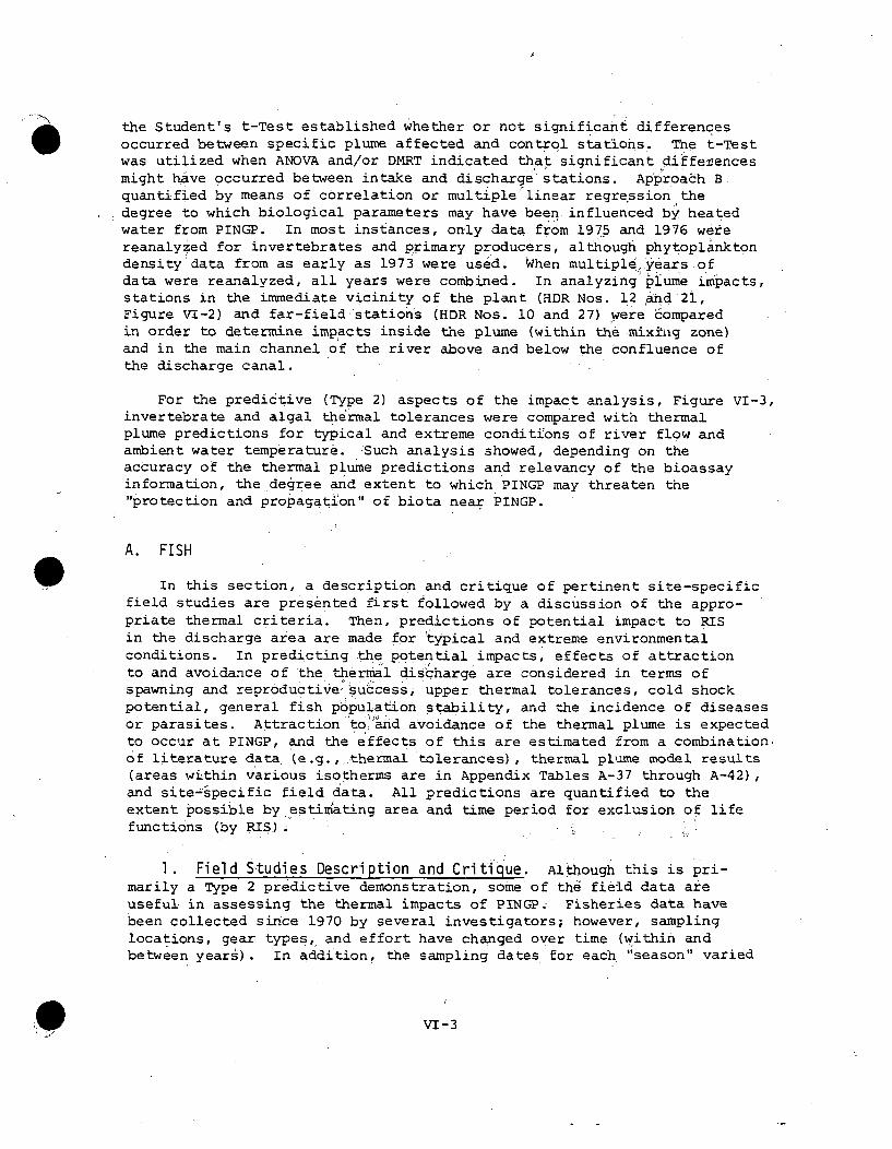
the Student's t-Test established whether or not significant differencesoccurred between specific plume affected and control stations. The t-Testwas utilized when ANOVA and/or DMRT indicated that significant differencesmight have occurred between intake and discharge stations. Approach Bquantified by means of correlation or multiple linear regression thedegree to which biological parameters may have been. influenced by heatedwater from PINGP. In most instances, only data from 1975 and 1976 werereanalyzed for invertebrates and primary producers, although phytoplanktondensity data from as early as 1973 were used. When multiple '.years ofdata were reanalyzed, all years were combined. In analyzing plume impacts,stations in the immediate vicinity of the plant (HDR Nos. 12 and 21,Figure VI-2) and far-field stations (HDR Nos. 10 and 27) were Comparedin order to determine impacts inside the plume (within the mixkig zone)and in the main channel of the river above and below the confluence ofthe discharge canal.

For the predictive (Type 2) aspects of the impact analysis, Figure VI-3,invertebrate and algal thermal tolerances were compared with thermalplume predictions for typical and extreme conditions of river flow andambient water temperature. 'Such analysis showed, depending on theaccuracy of the thermal plume predictions and relevancy of the bioassayinformation, the degree and extent to which PINGP may threaten the"protection and propagation" of biota near PINGP.

A. FISH

In this section, a description and critique of pertinent site-specificfield studies are presented first followed by a discussion of the appro-priate thermal criteria. Then, predictions of potential impact to RISin the discharge area are made for 'typical and extreme environmentalconditions. In predicting the potential impacts, effects of attractionto and avoidance of the thermal discharge are considered in terms ofspawning and reproductive, success, upper thermal tolerances, cold shockpotential, general fish population stability, and the incidence of diseasesor parasites. Attraction toind avoidance of the thermal plume is expectedto occur at PINGP, and the effects of this are estimated from a combinationof literature data (e.g.,, thermal tolerances), thermal plume model results(areas within various isotherms are in Appendix Tables A-37 through A-42),and site-specific field data. All predictions are quantified to theextent possible by estimating area and time period for exclusion of lifefunctions (by RIS).

1. Field Studies Description and Critique. Although this is pri-marily a Type 2 predictive demonstration, some of the field data areuseful in assessing the thermal impacts of PINGP; Fisheries data havebeen collected since 1970 by several investigators; however, samplinglocations, gear types, and effort have changed over time (within andbetween years). In addition, the sampling dates for each. "season" varied

VI-3

WISCONSIN

IN

w £

.5

I

2

MINNESOTA

3-

NEAR-FIELD_.

SCALE

500 0 500 10001- ;;;;a.

meters1000 0 1000 2000 3000 4000

4

7

,)-10-11

1517'

LOCK &

28. . . . I _ . - 27feet

547P-93

Figure VI-2. HDR designated station locations for invertebrate, primaryproducer, and water quality sampling conducted near PINGPduring 1973-1976. Enclosed area indicates near-field.

OkVI-4

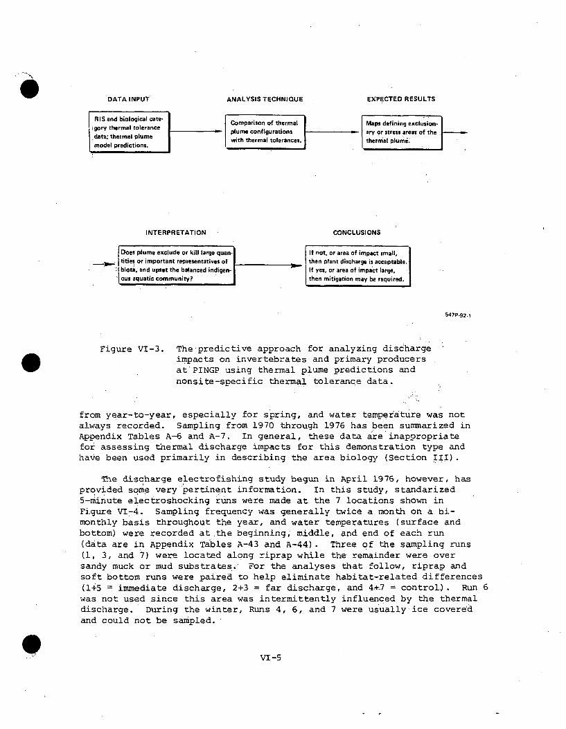
DATA INPUT

RIS and biological cate-gory thermal tolerancedata; thermal plumemodel predictions.

INTERPRETATION

ANALYSIS TECHNIQUE EXPECTED RESULTS

Comparison of thermal Maps defining exclusion-plume configurations ary or stress areas of the

with thermal tolerances. thermal plume.

CONCLUSIONS

Does plume exclude or kill large quan. If not, or area of impact small,tities or important representatives of then plant discharge is acceptable.biota, and upset the balanced indigen- If yes, or area of impact large,

ous aquatic community? then mitigation may be required.

547P-92.1

Figure VI-3. The;predictive approach for analyzing dischargeimpacts on invertebrates and primary producersat PINGP using thermal plume predictions andnonsite-specific thermal tolerance data.

from year-to-year, especially for spring, and water temperature was notalways recorded. Sampling from 1970 through 1976 has been summarized inAppendix Tables A-6 and A-7. In general, these data are inappropriatefor assessing thermal discharge impacts for this demonstration type andhave been used primarily in describing the area biology (Section III).

The discharge electrofishing study begun in April 1976, however, hasprovided some very pertinent information. In this study, standarized5-minute electroshocking runs were made at the 7 locations shown inFigure VI-4. Sampling frequency was generally twice a month on a bi-monthly basis throughout the year, and water temperatures (surface andbottom) were recorded at the beginning, middle, and end of each run(data are in Appendix Tables A-43 and A-44). Three of the sampling runs(1, 3, and 7) were located along riprap while the remainder were oversandy muck or mud substrates., For the analyses that follow, riprap andsoft bottom runs were paired to help eliminate habitat-related differences(1+5 = immediate discharge, 2+3 = far discharge, and 4+7 = control). Run 6was not used since this area was intermittently influenced by the thermaldischarge. During the winter, Runs 4, 6, and 7 were usually ice coveredand could not be Sampled.

VI -5

STURGEON LAKE

!2 63ý

SKIMMER WALL

0

6

'ýQ5 5

. SCALE

' 200 O 0

iirm@

0 0

I

Figure VI-4. Sampling locations for the DNR discharge electrofishingstudy. Runs 1, 3, and 7 are riprap while runs 2, 4, 5,and 6 are sandy muck or mud (Gustafson and Geis, 1977).

e)VI-6

Data from the discharge electroshocking study were used in the followingimpact analysis to strengthen the predictions based on literature informa-tion.

2. Temperature Criteria. EPA recommended temperature criteria(as defined in Brungs and Jones, 1977) for protecting fish during criticallife stages throughout the year are utilized in this report, and thefollowing discussion summarizes these criteria. To maintain growth,reproduction, and winter survival, water temperatures in the thermaldischarge should not exceed a maximum weekly average temperature (MWAT)that is calculated as follows: For growth, the :LAT is the optimumtemperature for growth plus one-third of the, upper incipient lethaltemperature minus the optimum for growth (M[AT = optimum growth T +(upper incipient lethal T - optimum growth T)/3]. This criterion shouldbe applied considering the normal spatial distribution of the speciesduring the season in which growth occurs (i.e., would the species normallyoccur in the area influenced by the thermal discharge during its growingseason). This criterion, however, does not apply within the mixing zone.For spawning, the MWAT is taken to be the optimum spawning temperature,and if this is not available, the middle of the spawning temperaturerange is used. The MWAT for winter survival is taken from the nomographin Figure VI-5.

Short-term exposure to moderately elevated temperatures can betolerated by fish without adverse effects, and the maximum temperaturesdepend upon past thermal history of the fish (acclimation), duration ofexposure, and AT. The relationship of exposure' time (minutes) totemperature (CC) is described by the equation:

log time = a + b (T)

where a is the Y-axis intercept, b is the slope of the line, and T istemperature in 0C.. Appendix Table A-45 summarizes a and b values deter-mined at different acclimation temperatures for some of the RIS. Themaximum temperature for short-term (24 hours) survival in summer can becalculated from this equation by choosing aanddb for the acclimationtemperature closest to the MWAT for growth. The safety factor of 21 C(3.60 F) must be subtracted from the resulting temperature to ensuresurvival of 100 percent of the population since a and b were determinedf:'om LT 5 0 data. The temperature for short-term survival of embryos duringthe spawning period is estimated as the maximum spawning temperature ormaximum for incubation and hatching, whichever is higher. For adults,short-term survival (24 hours) during the spawning period is calculatedusing the time-temperature equation for acclimation temperatures closestto the MWAT for spawning. Table VI-l summarizes the above criteria foreach of the RIS to be used for impact analysis in the following sections.

VI-7

AMBIENT TEMPERATURE (F)

32

30

59

86

2w

-j

ca

0.

LU

Lu25

U-

LU

< 15

LU

77 ?.

Uj;

68 D-j

59

LU

CL

U-

LU

C-

Ul

LU

LU

10

5

50

41i5

AMBIENT TEMPERATURE (C)547 P-122

Figure VI-5. Nomograph to determine the permissible maximum weeklyaverage temperature (MWAT) in the plume during winterfor various ambient temperatures (adapted from Brungsand Jones, 1977).

VI-8

Table VI-I. Temperature criteria for the RIS in Centigrade(Farenheit in parenthesis).

MAXIMUMWEKYMAXIMUM WEEKLY

MAXIMUM AXIMUM MAXIMUM WEEKLY TEMPERATURE AE•TEMPERATURE TEMPRAGER AVE RAGEAVERAGEAVERAGE

SPECIES AVERAGE FOR SHORT-TERM TEMPERATURE FOR SHORT-TERM TEMPERATURES P E C I E S T E M P E R A T U R ET E E R U ET M P A U E

SURVIVAL IN SURVIVAL DURINGFOR GROWTH SUMMER 3 FOR SPAWNING SW SPA GURVIVALDRWINE7

EMBRYO 5 ADULT 6

Walleye 24.5 (76) 29.5 (85)8 7.5 (46) 19 (66) 25. (77)9 10 (51)

White Bass N.D. N.D. 1.6.5. (62) 26 (79) N.D. 10 (51)

Channel Catfish 31.9 (89) 35.2 (95) 27 (81) 29 (84) 33.6 (93) 10 (51)

-Northern Pike 28.4 (83) 30.•1 (86) 8.4 (47) 18 (64) 24 (75)10' 10 (51)

Gizzard Shad N.D. 34 (93)11 19.5 (67) 29 (84) 31 (88)i 10 (51)

Carp 30.2 (86)12 38 (100)8 21 (70) 33 (91) 30.5 (87)9 10 (51)

Black Crappie 26.7 (80) 31 (88)8 17 (63) 20 (68) N.D. 10 (51)

Emerald Shiner 29.6 (85) 30 (86)13 23.5 (74) 27 (8i) 29.5 (85) 10 (51)

White Sucker 27.7 (82)12 28.4 (83) 7.2 (45) 21 (70) 23.3 (74) 10 (51)

Shorthead Redhorse N.D. N.D. 11 (52) N.D. N.D. 10 (51)

H

]Data used for the calculations are from Appendix Tables A-11through A-20 and A-45. References are listed with the data.

2 MWAT = Optimum for growth + Ultimate incipient lethal-Optimum3

324-hour survival calculated from log time = a + b(T) at anacclimation temperature of the MWAT for growth and with

the: 20 C safety factor subtracted.

40ptimum or mid-range for spawning.

5 Maximum of incubation and spawning temperatures.6 24-hour survival calculated from log time = a + b(T) at anacclimation temperature of the MWAT for spawning and withthe 2°C safety factor subtracted.

7 From Figure VI-5 when ambient is< 2.5'C (December to mid-March atPINGP).

8 Ultimate lethal -2WC since no regres-sion equation available.

9 Upper lethal of juvenile -20C sinceno regression equation available.

1 0 Upper lethal of larvae -2°C since no

regression equation constants for18WC acclimation.

1iAt an acclimation temperature of 300C.1 2 Based on data for larvae.1 3 At an acclimation temperature of 25 0 C.

3. Attraction to and Avoidance of the Thermal Discharge. Warmedwaters in the discharge canal may attract or repel fish depending ontemperatures in the discharge and preferred temperatures for each species.Thermal data for each of the RIS have been presented previously (AppendixA), and the preferred temperatures at various acclimation (ambient)temperatures and seasons are shown in Figures VI-6 and 7. Based on thesedata, all of the RIS should be attracted to some portion of the dischargewhen ambient river temperatures are low while some species should avoidat least the warmer portions during summer. Table VI-2 summarizes thesedata and shows that walleye, white sucker, emerald shiner, and northernpike would probably not frequent the mixing zone [> 2.80 C (50 F) aboveambient] when ambient temperatures are warmest (253 C) in summer. Areasin which the temperature is increased 8* C (140 F) or more during maximumsummer temperatures would not be preferred by the other species, exceptpossibly carp.

Even though preferred temperatures of many of the RIS are exceededin the thermalplume during summer, these species may not necessarilybe excluded from this area; it only means that they do not prefer thesetemperatures. Fish may avoid the areas above their preferred level butenter occasionally for feeding or predator escape. Based on the resultsof the thermal plume model, the maximum calculated area within whichtemperatures exceed 31.30 C (88.50 F.) is typically 0.7 ha (1.7 A), and,the area within which they exceed 27.20 C (81 F) is typically 14 ha(34.6 A) in July. Thus, the areas which exceed the preferred temperaturesof some of the RIS are small compared to the available area in SturgeonLake [624 ha (800 A)], for example. These calculated areas would be 0larger during the proposed extreme conditions, but these occur veryinfrequently (see Section IV B for calculation of occurrence).

Upper lethal temperatures of the RIS more accurately define the areasin the plume that may be excluded from long-term use by the RIS. Theupper lethal levels for each species acclimated to ambient temperaturesare shown in Figure VI-8. From this figure, it appears that exclusion ofsome species would begin at the 50 C (90 F) isotherm during, the highestambient temperatures, and estimated exclusion for each species is summarizedin Table VI-2. The latter estimates of exclusion, however, must be inter-preted carefully since they were derived from the highest reported lethaltemperature for each species, and many.other factors are involved (asdiscussed in Bush et al., 1974). For example, the data are based onlaboratory experiments that undoubtedly did not simulate all of the conditionsnear PINGP that influence thermal tolerance. In addition, the data arebased on a 50 percent survival rate at a specified time and acclimationtemperature. Small changes in temperature near the upper tolerance limitcan cause large increases in mortality (Bush et al., 1974), and exposuretime is important..

VI-10

N-H

H-H-

a

4.

Figure VI-6.

30

25

N\ 2o

N 20

lb

10

\ N•~N NN

0OCT NOV DEC

04)p.I 3t .1

data are plotted using riverFor these species, pre-

JUN JUL AUG SEP

MONTH

Preferred temperatures for juvenile RIS. Theseambient temperatures as acclimation temperature.ferred temperatures are always above ambient.

60

iZ

I-

50

45

40

35

30 Dr2-

20

15

in

030)

JAN FEB MAR APR MAY JUN JUL

MONTH

AUG SEP OCT NOV DEC

Figure VI-7. Preferred temperatures of juvenile (J) and adult (A) RIS during variousseasons. The values plotted apply to the entire season, although theyare located arbitrarily within each season. Seasons are defined aswinter = < 50. C; spring = 5 to 210 C; summer = < 211 C; and fall = 21 to 50 C.Most of these fish would prefer temperatures above ambient, except for afew species (e.g., white sucker) when waters are warmest.

O Table vI-2. Estimated potential effects of increased temperature on theRIS in. the vicinity of PINGP.

0

TEMPERATURE RIS NOT IN ESTIMATED

C (F) PREFERRED RISTEMPERATURE1 EXCLUDED 2

20 (68)21 (70)22 (72)23 (73) white sucker24 (75)25 (77)26 (79) walleye, emerald shiner27 (81) northern pike28 (82) shorthead redhorse29 (84)30 (86)31 (88) white bass, black crappie emerald shiner, white sucker32 (90) gizzard shad walleye, shorthead redhorse, 3

white bass 3

33 (91) channel catfish northern pike, black crappie

34 (93)35 (95)36 (97) carp37 (99) gizzard shad38 (100) channel catfish39 (102)40 (104)41 (106) carp

1 Based on maximum preferred temperature in Appendix A.2 Maximum upper lethal temperature (LT 5 0 ) at highest reportedacclimation temperature for juvenile fish. Adults generallyhave a slightly lower upper lethal temperature..

3 From Bush et al., 1974.

The maximum area excluded from use in summer for each RIS was calcu-lated based on short-term survival information presented in Tables VI-3through 12. The largest area excluded during typical conditions is 4.4 ha(10.9 A) for white sucker, and the area is less than 1 ha (2.5 A) for all the

other species except walleye and northern pike. No data were available forwhite bass or shorthead redhorse, but these species should be similar tothe other species. For extreme conditions of 7-day 10-year low river flows,maximum daily river temperatures, and maximum blowdown rates the exclusionareas in summer are predicted to be less than 0.5 ha (1.2 A) for channelcatfish, gizzard shad, and carp. The areas of exclusion ranged from 0 toapproximately 45 ha (0 to '\ 111 A) during May through September with the

VI-13

S

60

bb

45

401

ft

4Er

H 0~

G

30

2b

20

is

10

030

JAN FEB MAR APR MAY JUN JUL

MONTH

AUG SEP OCT NOV DJEC

A IP3811

Figure VI-8. Upper and lower lethal thresholds for various life stages (A = adult, Jand L = larvae) of -the RIS. Upper lethals were plotted for acclimationambient while lower lethals were plotted for acclimation to the maximumtemperature.

= juvenile,to riverdischarge

O/

Table VI-4. Predicted area in the discharge from which various life functions would beexcluded under typical and extreme conditions. Estimated time periods forexclusion are also given.

SPECIES: White Bass

TEMP. 1 AREA EXCLUDING TIME FUNCTION(C) FUNCTION (HA) 2 EXCLUDED REMARKS

PARAMETERTypical Extreme 3 Typical Extreme 3

Maximum for short-term survival in N.D.summer

Maximum for short-term survival of Spawn late May and June.

adult during N.D.

spawning

Maximum forincubation and 26 0.3 8 May May *Ambient river tempera-larval development 2.6 June June* ture exceeds tempera-

ture criteria.Maximum weeklyaverage for N.D.growthh

H

lFrom Table VI-l.

From Appendix Tables A-37 through A-42 and computer3Probability of occurrence is < 0.000005 or < 1 hour

printout for June. ,

every 278 years for each month.

Table VI- 3 . Predicted area in the discharge from which various life functions would be

excluded under typical and extreme conditions. Estimated time periods for

exclusion are also given.

H

SPECIES: Walleye

TEMP. 1 AREA EXCLUDING TIME FUNCTION

PARAMETER (C) FUNCTION (HA) 2 EXCLUDED REMARKS

Typical Extreme 3 Typical Extreme 3

Maximum for short- 2.6 0.5 to July Mayterm survival in 29.5 1.5 n, 45 August throughsumrmner Sept

Maximum for short-term survival oftdrm duriva 25 0.5 15 May May Spawn April to mid-May.adult during

spawning

Maximum for 0.Apl *bient river tempera-

incubation and 19 0.8 April May* ture exceeds temperaturelarval development 9.0 May criteria.

Maximum weekly 1 10 May Main river channel

average for 24.5 -* -* July* June* - (barge channel) may not

growth % 40 August Sept* be suitable habitat.

1 From Table VI-l.2 From Appendix Tables A-37 through A-42 and computer output for April, June, and July.,3probability of occurrence is < 0.000005 or < 1 hour every 278 years for each month.

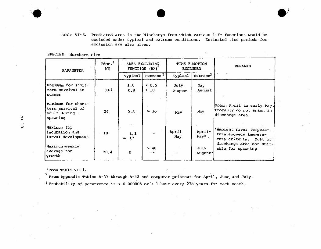
Table VI-6. Predicted area in the discharge from which various life functions would beexcluded under typical and extreme conditions. Estimated time periods forexclusion are also given.

oHI

SPECIES: Northern Pike

TEMP. 1 AREA EXCLUDING TIME FUNCTION

PARAMETER (C) FUNCTION (HA) 2 EXCLUDED REMARKS

Typical Extreme 3 Typical Extreme 3

Maximum for short- 1.8 < 0.5 July Mayterm survival in 30.1 0.9 > 18 August Augustsummer

Maximum for short- Spawn April to early May.term survival ofadult during 24 0.8 " 30 May May Probably do not spawn in

spawningdischarge area.spawning

Maximum for *Ambient river tempera-incubation and 18 1.1 -* April April* tube excee tempera-

larval development 17 May May* ture crera mostaoture criteria. Most ofdischarge area not suit-

Maximum weekly 40 July able for spawning.average for 28.4 0 -* - August*growth-

LJ

1 From Table VI- 1..2 From Appendix Tables A-37 through A-42 and computer printout for April, June, and July.

3 Probability of occurrence is < 0.000005 or < 1 hour every 278 years for each month.

Table VI-5. Predicted area in the discharge from which various life functions would beexcluded under typical and extreme conditions. Estimated time periods forexclusion are also given.

HH

-a

SPECIES: Channel Catfish

TEMP. AREA EXCLUDING TIME FUNCTION

PARAMETER (C) FUNCTION (HA) 2 EXCLUDED REMARKS

Typical Extreme3 Typical Extreme 3

Maximum for short- July Small area near discharg•term survival in 35.2 <0.2 <0.5 August August gates.summer

Maximum for short-term survival of 33.6 0 <0.5 July Spawn May through July.adult during

spawning

Maximum forincubation and 29 0.9 1 June Maylarval development 2.8 > 20 July July

Maximum -weeklyaverage for 31.9 0 - r 3 Augustgrowth

.lFrom Table VI-I.2 From Appendix Tables A-37 through A-42 and computer printout for June and July.3 probability of occurrence is < 0.000005 or < 1 hour every 278 years for each month.

Table VI- 7. Predicted area in the discharge from which various life functions would beexcluded under typical and extreme conditions.exclusion are also given.-

Estimated time periods for

HHw

SPECIES: Gizzard Shad

TEMP. 1 AREA EXCLUDING TIME FUNCTIONPARAMETER (C) FUNCTION (HA) 2 EXCLUDED REMARKS

Typical Extreme 3 Typical Extreme 3

Maximum for short- July Small area nearterm survival in 34 <0.2 <0.5 August August smlareaneardischarge gates.summer

Maximum for short- < 0.5 Mayterm survival of 31 <0.1 <64 June June Spawn April through June.adult duringspawning

Maximum forincubation and 29 "U 1 June Maylarval development

Maximum weeklyaverage for N.D.growth

lFrom Table VI-.2 From Appendix Tables A-37 through A-42 and computer printout for June.3Probability of occurrence is < 0.000005 or < 1 hour every 278 years for each month.

4Extrapolated from May and August values.

0 B[0

Table VI-8. Predicted area in the discharge from which various life functions would be

excluded under typical and extreme conditions. Estimated time periods for

exclusion are also given.

I

0

SPECIES: Carp

TEMP. 1 AREA EXCLUDING TIME FUNCTION REMARKS

PARAMETER (C) FUNCTION (HA) 2 EXCLUDED

Typical Extreme 3 Typical Extreme 3.

Maximum for short-term survival in 38 0 0summer

Maximum for short-term survival ofadult during30.5 0.5 " 84 June June Spawn May through July.spawning 1.4 -164 July July

Maximum' for -Small area near dischargeincubation and 33 0.1 <0.54 July July gates but probably not

larval development suitable for spawning.

Maximum weeklyaverage for 30.2 0 %40 Augustgrowth

lFrom Table VT-I.2 From Appendix Tables A-37 through A"42 and computer printout for June and July.3Probability of occurrence is < 0.000005 or < 1 hour every-278 years for each month.

4Extrapolated from May and August values.

Table VI-9 . Predicted area in the discharge from which various life functions would beexcluded under typical and extreme conditions. Estimated time periods forexclusion are also given.

H

SPECIES: Black Crappie

TEMP.1 AREA EXCLUDING TIME FUNCTIONPARAMETER (C) FUNCTION (HA) 2 EXCLUDED REMARKS

Typical. Extreme 3 Typical Extreme 3

Maximum for short-term survival in 31 1 < 0.5 July Maysummer 0.3 "18 August August

Maximum for short- Spawn May and June.term survival of Little suitable spawningadult during N.D. in discharge.spawning

Maximum for *Ambient river temperatureincubation and 20 5.4 May May* exceeds temperature criteria.

lv June*dJune* Most of discharge area notsuitable for spawning.

Maximum weeklyaverage for 26.7 A,40 -* July July*growth 3 August August*

1 From Table VI-I.2 From Appendix Tables A-37 ,through A-42 and computer printout for July.3Probability of occurrence is < 0.000005 or < 1 hour every 278 years for each month.

0

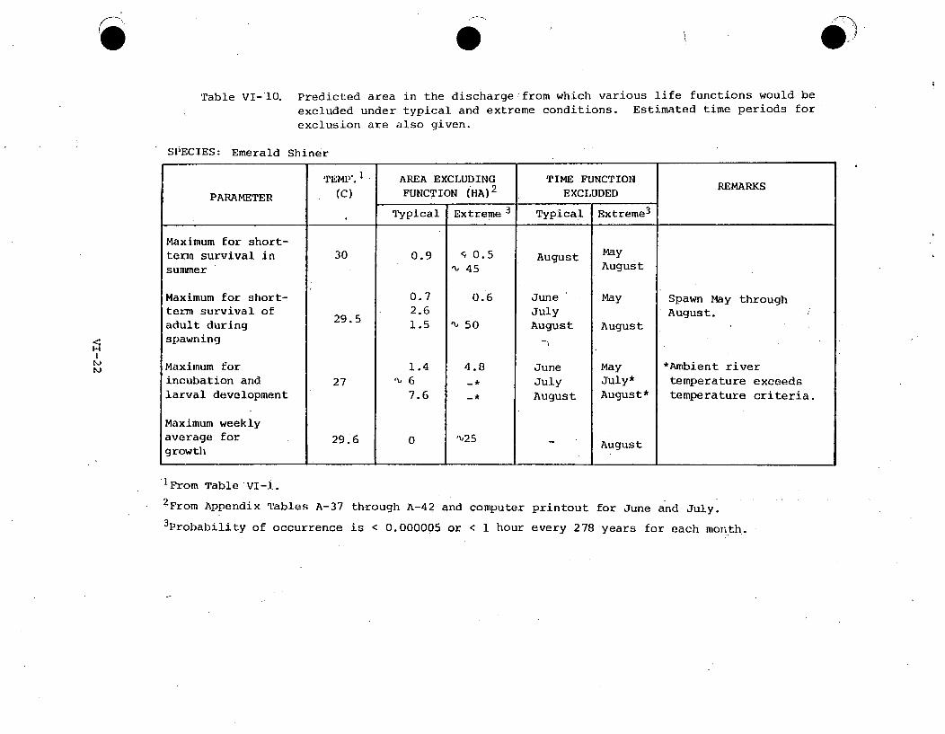
0 .Table VI-10. Predicted area in the discharge from which various life functions would be

excluded under typical and extreme conditions. Estimated time periods forexclusion are also given.

!'Mo

SPECIES: Emerald Shiner

TEMP'. AREA EXCLUDING TIME FUNCTION

PARAMETER (C) FUNCTION (HA) 2 EXCLUDED REMARKS

Typical Extreme 3 Typical Extreme 3

Maximum for short-term survival in 30 0.9 - 0.5 Augustsummer , 45 August

Maximum for short- 0.7 0.6 June May Spawn May throughterm survival of 2.6 July August.adult during 29.5 1.5 ' 50 August Augustspawning

Maximum for 1.4 4.8 June May *Ambient riverincubation and 27 b 6 _, July July* temperature exceedslarval development 7.6 _, August August* temperature criteria.

Maximum weeklyaverage for 29.6 0 "'25 Augustgrowth

'From Table VI-l.2 From Appendix Tables A-37 through A-42 and computer printout for June and July.3Probability of occurrence is < 0.000005 or < 1 hour every 278 years for each month.

Table VI-li. Predicted area in the discharge from which various life functions would beexcluded under typical and extreme conditions. Estimated time periods forexclusion are also given.

SPECIES: White Sucker

TEMP. AREA EXCLUDING TIME FUNCTION

PARAMETER (C) FUNCTION (HA)2 EXCLUDED REMARKS

Typical Extreme3 Typical Extreme 3

Maximum for short- 1.1 1.6 June May *Ambient riverterm survival in 28.4 4.4 July temperature exceedssummer 2.7 August August* temperature criteria.

Maximum for short- Spawn late Aprilterm survival of 23.3 1 50 to mid-may.adult during May Mayspawning

Maximum for No suitable spawningincubation and 21 0.5 April area in discharge.larval development 3.4 -* May May*

Maximum weeklyaverage for 28.4 0 u 45 Julygrowth -* August*

lFrom Table VI-l.2 From Appendix Tables A-37 through A-42 and computer printout for April, June, and July.3probability of occurrence is < 0.000005 or < I hour every 278.years for each month..

HM1.)

Table VI-12. Predicted area in the discharge'from which various life functions would beexcluded under typical and extreme conditions. Estimated time periods forexclusion are also given.

SPECIES: Shorthead Redhorse

TEMP. AREA EXCLUDING TIME FUNCTION

PARAMETER (C) FUNCTION (HA) EXCLUDED REMARKS

Typical Extreme. Typical Extreme

Maximum for short-term survival in N.D.

summer

Maximum for short- Spawn late April to earlýterm survival of June. Probably do notadult during N.D.Jue Prblydnospad ding Nspawn in discharge area.spawning

Maximum forincubation and N.D.larval development

Maximum weeklyaverage for N.D.growth

I'-

1From Table VI-I.

maximum occurring in August for walleye and emerald shiner. The maximumarea of exclusion for northern pike and black crappie was about 18 ha(44.5 A) and for white sucker was 1.6 ha (4 A). No data were availablefor white bass or shorthead redhorse, although these species probably aresimilar to walleye in their, tolerances.

During typical summer conditions the areas excluded would only occurin July and August. For extreme conditions, the areas excluded wouldprobably occur only in August for channel catfish and gizzard shad whilethe area would vary from May through September with a peak in August forthe other RIS. The probability that the proposed extreme conditionswould occur in any month is less than 0.000005 or a frequency of 1 hourevery 278 years. These calculated areas of exclusion represent themaximum in which thermal mortality could possibly occur since the 20 C(3.60 F) safety factor was subtracted from the median tolerance tempera-ture.

Field data collected in the discharge electrofishing study describedpreviously generally support these predictions. Figure VI-9 shows thatthe mean number of RIS collected in the immediate discharge area (Runs1+5 in Figure VI-4) is inversely related to the ambient river temperaturewhile the mean catch in the control area (Runs 4+7) shows little relation-ship to ambient temperature. Regression analyses of total RIS collectedin the immediate discharge and control areas versus ambient temperaturewere performed (see Appendix L). Both polynomial and exponential curveswere drawn, and an exponential curve of the form Y = ea+b(T) provided thebest fit (Figure VI-lO). In this equation, Y is the number of fish, a isthe intercept, b is the slope, and T is temperature in OC. The coefficientof determination (R2 ) for the discharge regression was 0.60, whichindicates that the number of fish collected in the discharge was moderatelyrelated to changes in ambient temperature. The regression line has anegative slope which indicates that attraction to the discharge occursas ambient temperatures decrease. The regression of total RIES ,in thecontrol. area versus ambient temperature (Figure VI-bO) shows that thenumber of fish was less related to temperature. (R2 = 0.35), as"'would beexpected. The regression line has a positive'slope_ Iwhich indiclates thatmore fish were found in the control area when the water was warm thanwhen cold.

Figure VI-11 shows the mean catch per unit effort in two areas ofthe disc6harge and 'in the control area by season for the dominant RIS.Gizzard shad followed the same seasonal trends in attraction to andavoidance of the plume as for total RIS as would be expected since thisspecies dominated the catch. Carp, the second most abundant species,showed a preference for the southern part of the discharge canal (Runs.2+3)during spring through fall and 'the immediate discharge area in winter.White bass apparently avoided the discharge in summer but were attractedto the immediate discharge in spring and fall. The number of shortheadredhorse and emerald shiners collected was very low in most seasonsprecluding most analyses. The redhorse, however, was more abundant inthe control area in summer than in the discharge, and emerald shiners weremore abundant in the discharge than in the control areas during spring.

VI-25

Regression of carp and gizzard shad abundances in the discharge(Runs 1+5) and control (Runs 4+7) areas versus ambient river temperatureare shown in Figures VI-12 and 13. The numbers of these species in thedischarge are only moderately related to ambient temperature since R2

values were 0.49 for both. The slopes of both discharge regression curvesare negative indicating attraction to the plume as ambient temperaturesdecrease. The numbers of carp and gizzard shad in the control areawere poorly related to ambient river temperature.

The R2 values were tested for significance by calculating an F value(Harnett, 1970, pp. 343 and 348) from the equation

F = (n-2) R2 - (1-R 2 )

whereTheseand 1

400

390

160

IS1 00

0 90

so--

Z70

0

n is the number of samples (21 for control and 24 for discharge).F values were then compared to critical F values for n-2 samplesdegree of freedom (Harnett, 1970, pp. 512-513). All of the R2

U

Z

Lu

J F M A M J A S 0 N D_

MONTH s47p.13.)

Figure VI-9. Mean number of RIS collected per month in. the PINGP dis-charge (Runs I and 5) and at control stations (Runs 4 and 7)near the intake during the period April 1976 throughNovember 1977. The mean temperatures for the samples arealso shown (open and closed circles) as well as the numberof samples per month (N). NS = no sample.

VI-26

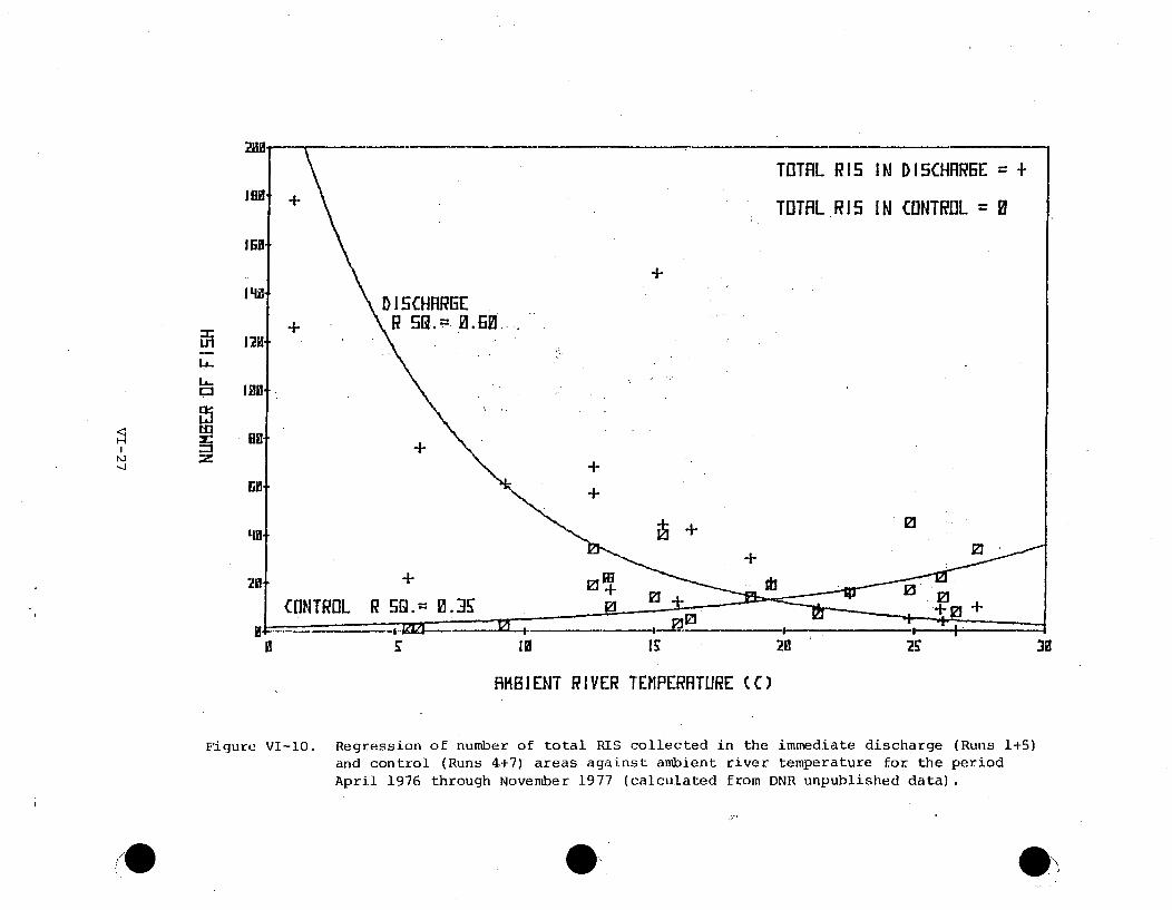
Lii

i..

LAIW1H

IJ

II 10

AMBIENT RIVER TEMPERATURE (C)

Figure VI-10. Regression of number of total RIS collected in the immediate discharge (Runs 1+5)and control (Runs 4+7) areas against ambient river temperature for the periodApril 1976 through November 1977 (calculated from DNR unpublished data).

I.O .

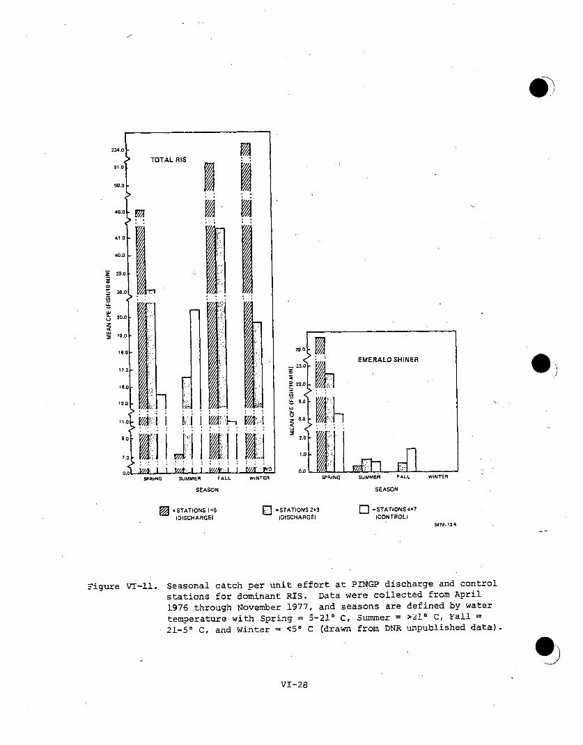
0

234.0

51.0

50.0

46 .0

41.0

TOTAL RIS

40.o L

z[0_

=z

wJ

39.0 F

20.0

20.0 7w

V/4k

I V/I,~~ I I

U

r1iaJ.~2

19.0 F

18.0-

1670

16.0

WnAI I t'/!A I

IJ U,

LUz

29.0EMERALD SHINER

22.0

22.0

2.0

O

0.0 I PIG SMER AL WNEum, _,,_ ,SPRING SUMMER FALL WINTER

SEASON

SPRING SUMMER F ALL WINTER

SEASON

'STATIONS 1+5IDISCHARGE)

=STATIONS 2+3(DISCHARGE)

-STATIONS 4+7(CONTROL)

547P. 12 4

Figure VI-lI. Seasonal catch per unit effort at PINGP discharge and controlstations for dominant RIS. Data were collected from April1976 through November 1977, and seasons are defined by watertemperature with Spring = 5-21 C, Summer = >21* C, Fall21-50 C, and Winter = <50 C (drawnifrom DNR unpublished data).

0)

VI-28

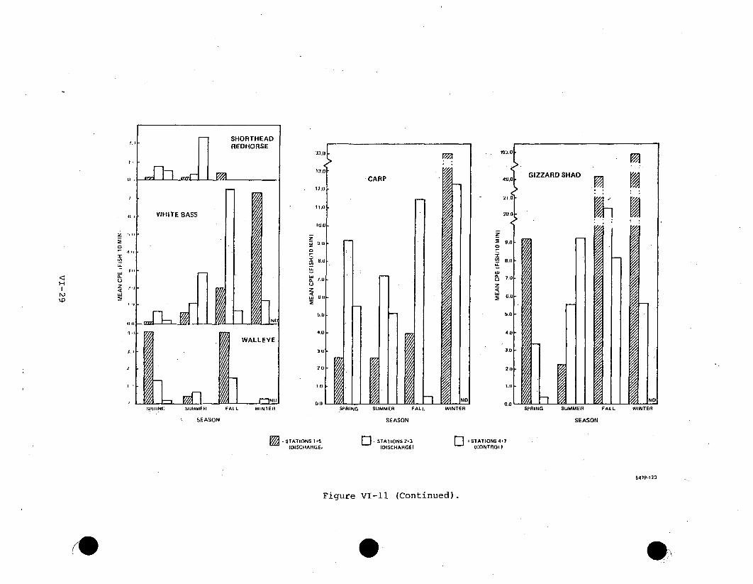
H

12.0

13.0-

12.0

11.0

111(1

l .Uz

,UO

4.U2 tNJ.110

1.0

4.11

CARP

z

fwu.01

NJ0z[

FzZVi ND1

S.EASON

SPRING SUIMMER FALL

SEASON

WINTER SPRING SUMMER FALL WINTER

SEASON

STATIONS 1-50DISCIRAGE, IDISCHARGEI

STATIONS 417U(CONTROL)

547P-123

Figure VI-l (Continued).

+ CRRP IN DI5CHRREE +

CRRP IN CONTROL :

tL..

< 'LaH

U ~ 20-0 " + DI5CHRRGE

4++

CEONTROL R SR.= 0.3+

IB1 523 0. ]

IM13 I ENT RIVER T'EMPERR'IURE (C)

Figure VI-12. Regression of number of carp collected in the immediate discharge (Runs 1+5)

and control (Runs 4+7) areas against ambient river temperature for the period

April 1976 through November 1977 (calculated from DNR unpublished data).

U1La..La..

cz3HLI

AMOIENT RIVER TEHPERRTURE (M)

Figure VI-13. Regression- of number of gizzard shad collected in the immediate discharge (Runs 1+5)and control (Runs 4+7) areas against ambient river temperature for the period April1976 through November 1977 (calculated from DNR unpublished data).

0.

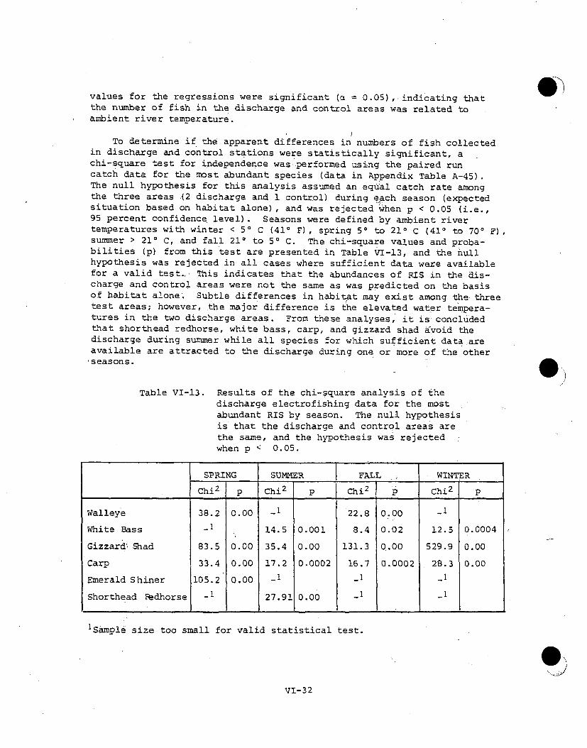
values for the regressions were significant (a =.0.05), indicating thatthe number of fish in the discharge and control areas was related toambient river temperature.

To determine if the apparent differences in numbers of fish collectedin discharge and control stations were statistically significant, achi-square test for independence was performed using the paired runcatch data for the most abundant species (data in Appendix Table A-45).The null hypothesis for this analysis assumed an equal catch rate amongthe three areas (2 discharge and 1 control) during each season (expectedsituation based on habitat alone), and was rejected when p < 0.05 (i.e.,95 percent confidence level). Seasons were defined by ambient rivertemperatures with winter < 50 C (410 F), spring 50 to 210 C (410 to 700 F),summer > 210 C, and fall 210 to 50 C. The chi-square values and proba-bilities (p) from this test are presented in Table VI-13, and the nullhypothesis was rejected in all cases where sufficient data were availablefor a valid test.. This indicates that the abundances of RIS in the dis-charge and control areas were not the same as was predicted on the basisof habitat alone. Subtle differences in habitat may exist among the threetest areas; however, the major difference is the elevated water tempera-tures in the two discharge areas. From these analyses, it is concludedthat shorthead redhorse, white bass, carp, and gizzard shad a'void thedischarge during summer while all species for which sufficient data .areavailable are attracted to the discharge during one or more of the other,seasons.

Table VI-13. Results of the chi-square analysis of thedischarge electrofishing data for the mostabundant RIS by season. The null hypothesisis that the discharge and control areas arethe same, and the hypothesis was rejectedwhen p < 0.05.

SPRING SUMMER FALL WINTER

Chi 2 p Chi 2 p Chi 2 P Chi 2 p

Walleye 38.2 0.00 -1 22.8 0.00 _1

White Bass -_ 14.5 0.001 8.4 0.02 12.5 0.0004

Gizzard Shad 83.5 0.00 35.4 0.00 131.3 0.00 529.9 0.00

Carp 33.4 0.00 17.2 0.0002 16.7 0.0002 28.3 0.00

Emerald Shiner 105.2 0.00 -1 _1 _1

Shorthead Fedhorse -1 27.91 0.00 _1 _1

iSample size too small for valid statistical test.

VI-32

4. Effects on Spawning and Reproductive Success.- Alterations ofnatural thermal regimes in aquatic ecosystems may adversely affect spawningand reproductive success of various organisms. Short-term temperaturefluctuations that result from irregular water uses for projects such aselectric power generation, irrigation, and navigation appear to havegreater ecological effects than uniform elevations of temperature by a fewdegrees (Coutant, 1972, p. 13). Shifts in spawning time of up to a monthoccur as a result of natural changes in temperature regimes, and thissuggests that constant thermal additions may not be harmful as long astemperatures for migration, spawning,. and development are not eliminatedfor important species.

PINGP is a base load facility and thus discharges a fairly constantamount of heat to the Mississippi River. Prolonged residence of fishin the thermal plume may 'induce premature spawning in those species forwhich temperature is the predominant controlling factor since suitabletemperatures would be available sooner than normal (see Figure 111-27).Such altered spawning has been observed at several power plants for whitesucker and several species of catfish (Coutant, 1970, p. 375). Prematurespawning has not been observed during any of the field studies at PINGPalthough it could occur in walleye, carp, gizzard shad, and emerald shiners.Field studies have shown that these are the dominant RIS in the dischargeduring spring, and suitable spawning areas for each of these species existin the discharge area, although walleye may migrate upriver. Suitablespawning areas also exist in Sturgeon and North Lakes as well as partsof the main river channel. All four species are prolific broadcastspawners, and carp and emerald shiners have an extended spawning period(3 to 4 months). The potential impacts of premature spawning in thesespecies to river populations will be discussed along with other effectson river populations in Section VI A.6.

Temperatures within the thermal plume are calculated to exceed themaximum for short-term (24-hour) survival of adults during the 'spawningperiod for most of the RIS (Tables VI-3 through 12) During typicalconditions, however, the areas within these potentially lethal tempera-tures are small [less than 2.6 ha (6.4 A)], particularly WHen comparedto areas in the vicinity of PINGP [e.g., Sturgeon Lake is 324 ha (800 A)]which contain abundant spawning habitat. In addition, not all of thedischarge area excluded would be suitable spawning habitat for each RIS.For the proposed extreme conditions, the calculated exclusion areas areless than 16 ha (40 A) (less than 5 percent of the area in Sturgeon Lake)for walleye, channel catfish, gizzard shad,'and carp while exclusionareas for northern pike, emerald shiner, and white sucker may be 30 to50 ha (74 to 124 A). The proposed extreme conditions,' however, areexpected to occur less than 1 hour in a given month every 278 years(see Section IV B) and thus probably will not occur during the life ofthe plant. These calculated areas of exclusion are the maximum whichadults would avoid as being lethal.

VI-33

The temperature limits for embryo development are lower than those Wfor adult survival which indicates, that adults could lay eggs in areasnot suitable for their development. The areas calculated to exceed thelimits for embryo development are listed in Tables VI-3 through 12 'foreach RIS. The maximum areas excluded during typical conditions are17 ha (42 A) for northern pike and 9 ha (22 A) for walleye in May,which is the end of the spawning period for these species. For the otherRIS, exclusion areas are less than 7.6 ha (19 A), and these occur duringonly a portion of the spawning period. The calculated exclusion areasfor ty'pical and extreme conditions are the maximum necessary for completeprotection of development; that is, the 20 C safety factor has beenincluded for adult survival, and the most conservative upper limits fordevelopment have been used. Furthermore, the areas may include littleor no suitable spawning habitat for some species, such as northern pikeand white sucker, thus reducing the potential for impact considerably.

* Larvae produced upriver may also be. affected by drifting through thePINGP thermal discharge. Based on a hydraulic study of the area (Stefanand Anderson, 1977), most larvae drifting through the PINGP dischargewould have originated in Sturgeon Lake. •The horizontal and verticaldistribution of these larvae in the water column is not known but probablyis not uniform since sampling at the bar racks of the screenhouse hasshown densities to be highest near the bottom (NUS, 1976, p. 185).Several possible drift pathways through thel discharge area are shown inFigure VI-14 for typical, conditions, although southerly winds and eddieswould lengthen these pathways considerably. To calculate the drifttimes, average flow rate through. ,the discharge area was assumed to be6 cm/sec (0.2 fps) based on velocity measurements taken in the August 1975

thermal survey (see Appendix N), and the longest pathway (A) in Figure VI-14was utilized. The period of time each species is most likely to occur inthe drift was estimated from Figure 111-26, and then, short-term lethaltemperatures (minus 20. C for 100 percent survival) for each RIS (Table VI-14)were compared to the thermal plume model results for typical conditionsin the appropriate months. These data indicate that drifting walleye,white bass, northern pike., carp, and white sucker larvae acclimated toambient river temperatures would not be thermally stressed. The potentialfor thermal stress to channel catfish larvae drifting through the dischargearea exists in July *and August since larvae could be exposed to 316 C(880 F) for 23 minutes and 290 to 310 C (840 to 881 F) for 73 minutes inJuly and 290 to 30 0 C (84 0 to 860 F) for 50 minutes in August. The uppertolerance limit of 310 C (50 percent mortality) in Table VI-14 is foran unspecified time of exposure (probably 24-hours or longer) so thatshorter exposure (approximately 1 hour) to this temperature would not beexpected to have adverse effects on drifting larvae. Furthermore, channelcatfish guard their eggs and larvae (see Section III C.2.b) so that fewwould be expected. to occur in the drift.

VI -34

Figure VI-14.

547P-3-1

Pathways by which planktonic organisms may drift throughthe PINGP discharge area (without considering recircu-lation).

VI-35

Table VI-14. Short-term thermal tolerances of larval fish.

S S LARVAL ACCLIMATION TERN

TEMPERATURE LT 5 0 REFERENCESTAGE CcE(C)

Northern Pike 1 day old 6.1 22.2 24 hrs. Hokanson et al.,1973

11.8 28.2 24 hrs.'17.6 .28.0 .24 hrs.

free 7.2 23.5 24 hrs.swimming 12.6 26.3 24 hrs.

17.7 28.4 24 hrs.

White Sucker new hatch 8.9. 29.0, 24 hrs. McCormick et al.,15.2 31.0 24 hrs. 197721.1 31.5 24 hrs.

swim-up 10.0 28.5 24 hrs.15.8 30.7 24 hrs.21.1 32.0 24 hrs.

Walleye 2"5 days 6 211 72 min. Smith and Koenst,old 11 212 72 min. 1975,'

Channel Catfish 29 31 - West, 1q966

White Bass pre- 21.5 32 17 min. Coutant, 1974feeding 21.5 34 7 min.

Carp 3 days old 25 37 24 hrs. 3 Coutant, 1974

9 days old 25 36 24 hrs.

19 days old 25 38 24 hrs.,

2 LT 2 23After a 10 minute exposure to test temperature

VI-36

5. Cold Shock Potential. Cold shock may occur during winter whenfish that have become acclimated to temperatures in the thermal dischargeand recycle canal are suddenly exposed to ambient temperatures either fromsudden removal of the heat source (both units shut down) or from swimmingout of the plume (predator escape, etc.). Effects may be sublethal(e.g., loss of equilibrium) or lethal depending on temperature differential,species of fish, ambient temperature, and physiological state 'of theorganism. Although not directly-lethal, loss of equilibrium may resultin death through increased susceptibility to predation.

To ensure protection of all warm water fish species a MWAT of 100 C(500 F) when the ambient temperature is 2.50 C (370 F) or 150 C (590 F)

when the ambient temperature is 50 C (41' F) should not be exceeded inthe plume (Figure VI-5). At PINGP, maximum weekly ambient temperaturesare less than 50 C (410 F) from mid November to early April and lessthan 2.50 C (370 F) from December to mid March. Temperatures in theplume routinely exceed the recommended MWAT. During typical winterconditions (December 1975) when ambient temperatures were near 00 C(320 F), plume temperatures exceeded 100 C (500 F) in an area of approxi-mately 4.4 ha (10.9 A). This area is sufficient for fish to congregateand acclimate to the elevated temperatures; thusi, the potential for coldshock at PINGP exists. For proposed worst case conditions of 7-day,10-year low flows and low ambient temperature, the area with temperaturesgreater than 100 C (500 F) is predicted to be 6.9 ha (17 A).

Both units may shut down simultaneously during, winter,, and theprobability of this has been calculated in Section VI B. During refuelingof one unit, the probability of a trip at the other unit is 0.55 (55 per-cent), and the probability of simultaneous unscheduled trips is 0.0004.Since refueling occurs during winter and early spring, the probability ofsimultaneous shutdowns and potential cold shock to fish residing in theplume is at least 0.55 per year.

Based on thermal data for the RIS presented in Appendix A (Tables A-11through A-20), cold shock (direct lethal effects) to fish acclimated toabout 200 C (680 F) is predicted to be minimal for channel catfish,northern pike, and white suckers. Cold shock may occur in walleye andemerald shiners acclimated to 200. C (680 F) or higher, while gizzardshad would be very likely to suffer cold shock. The area within the plume(2 unit operation) where temperatures are above 200 C is 0.6 ha (1.5 A)for typical conditions (December) and 0.9 ha (2.2 A) for proposed extremeconditions (January). The areas would be somewhat smaller during one unitoperation during refueling. No data are available for predicting coldshock potential in the other RIS; however, shorthead redhorse are probablysimilar to white suckers in their tolerances, and carp would probably notbe adversely affected by cold shock.

Data from the discharge electrofishing study performed at PINGP inthe winter of 1976-1977 indicate that gizzard shad and carp are the mostabundant RIS in the discharge along with some white bass and black

VI-37

crappie. Thus, cold shock mortality is predicted primarily for gizzardshad. During past operation of PINGP, forced trips have occurred whenone unit was refueling, although no surveys were conducted to assess coldshock. Based on past operating experience, procedures have been devisedto minimize potential cold shock when a forced trip occurs during refueling.The cooling towers will be bypassed and the discharge gates lowered toallow a more gradual temperature decrease.

To summarize, cold shock effects are predicted to occur at PINGP atleast once every two years during the winter refueling of one unit. Thespecies most likely to be affected is gizzard shad, although some whitebass, black crappie, and carp may be killed also.. Current operatingprocedures at PINGP are designed to reduce the effects of cold shock, andthe potential impacts' of cold shock mortality on river, populations arediscussed in, the next section.

6. Effects on Fish (RIS) Populations. In general, the "effects ofenvironmental perturbations on fish populations are difficult to assess,particularly in a large river such as the Mississippi. 'An inordinate

amount of sampling would be necessary to determine anything except largechanges,' and such long-term data are not available for most water bodies.Furthermore, the evaluation of a single perturbation such as a power plantdischarge are often complicated by other activities of man (e.g., sewagedisposal, dredgingi building dams, etc).'

The PINGP discharge could affect fish populations primarily throughaltered spawning, exclusion of spawning areas, thermal stress to driftinglarvae, cold,shock, blockage of migrations, species shifts, and alteredgrowth rates. Most of these have been discussed for the discharge areain previous sections with quantitative information where possible.

Spawning a few weeks early should not have adverse effects on' riverpopulations unless a large proportion of the population were involvedand this' spawning were unsuccessful.. Since population estimates for theRIS are not available for various habitats near PINGP in spring,' electro-fishing catch per unit effort will be compared to assess relativeabundances. Walleye, gizzard shad, and emerald shiner were more abundantin the warmest parts of the discharge than in the intake area (Figure VI-lI)while carp were more abundant in the cooler parts of the discharge. Acomparison of catch rates during spring in the intake and dischargeareas (Figure VI-I1) with those in Sturgeon Lake and the MississippiRiver (Figure 111-23) shows that the density near the intake was similarto the density in Sturgeon Lake for most of the RIS while the catch ratefor walleye, gizzard shad, emerald shiner, and carp was considerably higherin the discharge than in either'Sturgeon Lake or the Mississippi River.The difference, however, may not be as great as noted here since the twostudies were not conducted simultaneously. This may be particularly truefor walleye which spawn in April to mid-May. The discharge study data werecollected in April and early May while the river study data were collectedprimarily in late May and June.

VI-38

To estimate potential effects of premature spawning, relative abun-dances must be known for the discharge canal area and the area outsidethe plume for each of the RIS. To calculate abundance from catch rate,two assumptions were made: equal sampling efficiency at all locations,and the locations sampled are representative of the areas to be compared.The first assumption is probably true while the second may not be sincefish are usually not evenly distributed in a water body. Mean catch pereffort (15 minutes) for each location (from Figures VI-lI and 111-23) wasmultiplied by the surface area of the locality sampled: 324 ha (800 A)for Sturgeon Lake, 180 ha (445 A) for the Mississippi River from BrewerLake cut to the PINGP intake, 83 ha (205 A) for the Mississippi from thePINGP intake to Lock and Dam No. 3, 4 ha (10 A) forRuns 1+5 in thedischarge, and 3 ha (7.5 A) for Runs 2+3 in the discharge. From thesecalculations, an estimated 13 percent of the walleye collected near PINGPwere found in the discharge areas during spring while only 2 percent ofthe carp and 3 percent of the gizzard shad occurred there. Emerald shiner,on the other hand, appeared to concentrate in the discharge with anestimated 50 percent of the population present there in spring. Twofactors,, however, weaken the reliability of this estimate. Emerald shinersschool and remain offshore in spring and summer seeking deeper watersduring the daytime in spring (Scott and Crossman, 1973, p. 442). Electro-fishing in Sturgeon Lake and the main channel of the Mississippi River wasconducted along the shoreline during daytime and, thus, probably under-estimated abundances considerably in spring.

Based on the above calculations, potential premature spawning ofcarp or gizzard shad in t~he discharge canal is predicted to have negligibleeffects on river populations since relatively few fish of these speciesare present in the discharge during spring. For walleye and emeraldshiner, which are calculated to be relatively abundant in the dischargein spring, potential effects of premature spawning on river populationsare predicted to be minimal. The relative abundances of these species inthe discharge are probably overestimated as a result of differences inthe time periods sampled and their patchy distributions, and it is unlikelythat all of the fish in the discharge would spawn early. Furthermore,premature spawning in itself should not-affect general population levelsunless much of it were unsuccessful. Emerald shiners have an-extendedspawning period (May through August, with maximal activity in summer)and may spawn more than once per season (see Section III C). Thus,spawning a few weeks early by part of the, population would be expected tohave little affect on the whole population.

Another potential effect of the PINGP discharge on river populationsis the exclusion of fish from otherwise suitable spawning areas. Basedon data presented in Tables VI-3 through 12, however, the areas potentiallyexcluded from reproduction are less than 10.8 ha (26.7 A) for those speciesexpected to spawn in the discharge, and this is less than 2 percent of.the area in Sturgeon Lake and the Mississippi River from Brewer Lake cutto' Lock and Dam No. 3. Therefore, exclusion of spawning areas is predictedto have negligible effects on river populations since adequate alternateareas exist nearby.

VI-39

Thermal stress to larvae drifting through the discharge is notpredicted to adversely affect any of the RIS (see Section VI A.2); conse-quently, no impacts to river populations are expected. Cold shock inwinter is predicted to occur primarily to gizzard shad when one unittrips while the other is refueling (greater than ,55 percent chance peryear); however, no adverse impacts to river populations are expectedfrom such phenomena. Gizzard shad naturally have large winter die-offs(Jester, 1972, p. 46), and the PINGP discharge may provide a thermalrefuge for those individuals residing in the plume during the coldermonths, thus reducing their natural winter mortality rate. Cold shockmortality resulting from plant outages would then represent delayednatural mortality. A further consideration is that this prolific speciesneeds cropping to control population size (Eddy and Underhill, 1974,p. 148).

The PINGP thermal discharge should not inhibit any fish migrationsin the area. The discharge is located in a backwater area off the mainchannel of the river, and the plume entering the river remains along thewest (Minnesota) bank of the river which is also the navigation channel.In addition, the temperature increase in the main channel generallydoes not exceed 2.8' C (50 F). Thus, most of the river is not influencedby the plume and is available for migrations. Walleye and suckers arethe only species that may migrate to spawn, and these species can easilyavoid the plume.

Less than large scale changes in fish population structure are:difficult to predict and nearly impossible to measure as noted previously.Many factors are involved in population structure stability includingnatural density-dependent compensatory mechanisms and influences ofman including fishing, navigation, and pollution.' Any potential dhiftsin fish population structure as a result of the PINGP thermal dischargecould be masked by other man-induced or natural changes.'

No impacts to endangered species are predicted since no endangered

species 'have been reported in the area.

\Potential effects of the PINGP discharge on sport fishing are

expected to be beneficial. Fishing pressure in the immediate vicinityof PINGP (Section 3 of creel census) is light compared to that in thetailwaters of Lock and Dam No. 3 (Section 4 of creel census) and occursmainly during open water months (see Section III C.2.g) . Fishing. success,however, has remained higher in the vicinity of PINGP than in the tail-waters below Dam No. 3 during plant operation. Fishing success shouldbe enhanced in the immediate discharge area (approximately 6 ha) duringspring and fall when fish are attracted to the plume, an area that repre-sents 7 percent of Section 3. This is corroborated by the fact thatfishing pressure in the discharge has been observed to be somewhat higherduring March and April (Geis 'and Gustafson, 1977) . Thus, some fishermenwere apparently taking advantage of the situation, and the catch wasprimarily white bass.

VI-40

The PINGP thermal discharge is expected to have negligible effectson RIS predator-prey interactions in the aquatic ecosystem near theplant. The area of potential influence is small (less than 10 ha) inrelation to the area of lower Pool No. 3 (587 ha). Forage species (e.g.,emerald shiners and gizzard shad) may be subject to somewhat higherpredation rates when they are attracted to the discharge in large numbers,primarily during the cooler months of the year. Walleye and white bassare the only piscivorous (fish-eating) RIS which show an increasedabundance in the discharge that is concurrent with the congregation offorage species, and it is unlikely that increased predation by-thesefish would deplete the forage stocks in the general area. In fact, thepredators,. which are important sport species, could benefit from suchprey concentration. Lower. trophic level interactions among fish andinvertebrates should be relatively unaffected by the discharge.

Growth rates of fish may also be influenced by the PINGP thermaldischarge and subsequently affect populations through physiological changessuch as altered age at maturity. During typical conditions, temperaturesoutside the mixing zone are not expected to exceed the MWAT for growthfor channel catfish, northern pike, carp, emerald shiner, or white sucker(Tables VI-3 through 12). For walleye and black crappie, however, mostof the plume is expected to exceed the MWAT for growth during August andJuly, respectively. Ambient temperatures in July exceed the criterionfor walleye. The plume beyond the mixing zone is located along the west*bank of the river main channel which is also the navigation channel.Thus, this area is probably not very suitable for residence by mostspecies, particularly quietwater species such as black crappie. Con-dition factors (relation of length to weight) for fish collected insideand outside the plume were not found to differ significantly (Krosch,25 October 1977). Consequently, thermal plume. effects on growth andriver populations are expected to be negligible. During extreme environ-mental. conditions, the areas affected are larger, but the frequency ofoccurrence (0.000005) of these conditions is so low as to have no measur--vable effect on fish growth. -

7. Effects on Parasites and Diseases. No specific parasitologicalstudies have been performed near PINGP to determine if parasitism ordiseases in fish-are influenced by the thermal discharge. During routinefield sampling, however, the incidence of external parasites and diseaseshas not been observed to occur more frequently in the discharge than inother areas. These observations are supported by studies at a powerplant on the White River, Indiana which have shown no definite influenceof the thermal discharge on infestation rate by the ectoparasites,Lernaea cyprinacea and Argulus sp. The occurrence of Lernaea on centrachidsdid not appear to be related to the effluent (Proffitt and Benda, 1971,p. 60), and this parasite was not found on carp, gizzard shad, channelcatfish, or black crappie, while less than one percent of the emeraldshiners in both discharge and control areas were parasitized (Whitakeret al., 1973, pp. 81-91). Argulus was only found on one carp (Proffittand Benda, 1971, p. 61).

V1-41

The incidence of other parasites, particularly internal parasites,is not expected to increase as a result of the PINGP thermal discharge.Several of these require intermediate hosts which may-be terrestrialduring their life cycle and thus may not be influenced appreciably byPINGP.

B. MACROINVERTEBRATES

1. Discussion and Critique of Sampling Methods. The chronology and.methodology of sampling are summarized in: Appendix Table A-22. Althougha number of methods were utilized for collecting macroinvertebratesnear PINGP, the two primary sampling methods during the last two years(1975 and 1976) were dredge and artificial substrate. The basic criticismssummarized by Murarka (1976) covered most of the shortcomings of themacroinvertebrate data collection at PINGP. These included the changingor 'dropping of stations and methods unjustifiably or without intercalibra-tion'. These inconsistencies, possibly a result of changing consultantswhile monitoring was in progress, have rendered much of the preoperationaldata useless for statistical comparisons with operational periods. Anotherproblem with the macroinvertebrate data was that the number of replicatescollected at each'station after the monitoring methods had become relativelystandardized was inadequate to show anything but large temporal or spatialvariations between stations. Weibe (1971) has shown that Single samplescollected at two separate stations would have to vary by a factor of fourto be significantly different. Replicate samples were taken at somestations during later years, although only one value was reported for each 0)station as a result of replicate pooling. Table VI-15 shows that with -nosimultaneous replicates taken at each sampling station, only largedifferences between stations were likely to appear to be statisticallysignificant. Generally, as the number of replicates increases, the powerof a statistical test for showing differences between 'stations increases;that is, the percentage difference between stations required to demonstratea significant difference decreases with an increase in the number .Ofreplicates. The same argument holds for demonstrating the significanceof temporal variation at a single station. Further discussion regardingthe power of sampling procedures is provided in Appendix B.

The wide variety of sampling techniques used to assess macroinverte-brate populations near PINGP, however, enhances the utility of theinformation. McConville (1975) summarized both dredge and artificialsubstrate procedures tested for sampling, efficiency near PINGP. AppendixTable A-22 describes the various methodologies used. Even though samplingmethods were not standardized until operational years, information onmacroinvertebrate populations have been accruing since 1970. This isimportant in defining the variety of macroinvertebrates occurring nearPINGP, especially the occurrence of uncommon taxa which may includeunusual, nuisance, or endangered species. The number of macroinvertebratetaxa collected (see Appendix K) is large for midwestern rivers; however,

VI-42

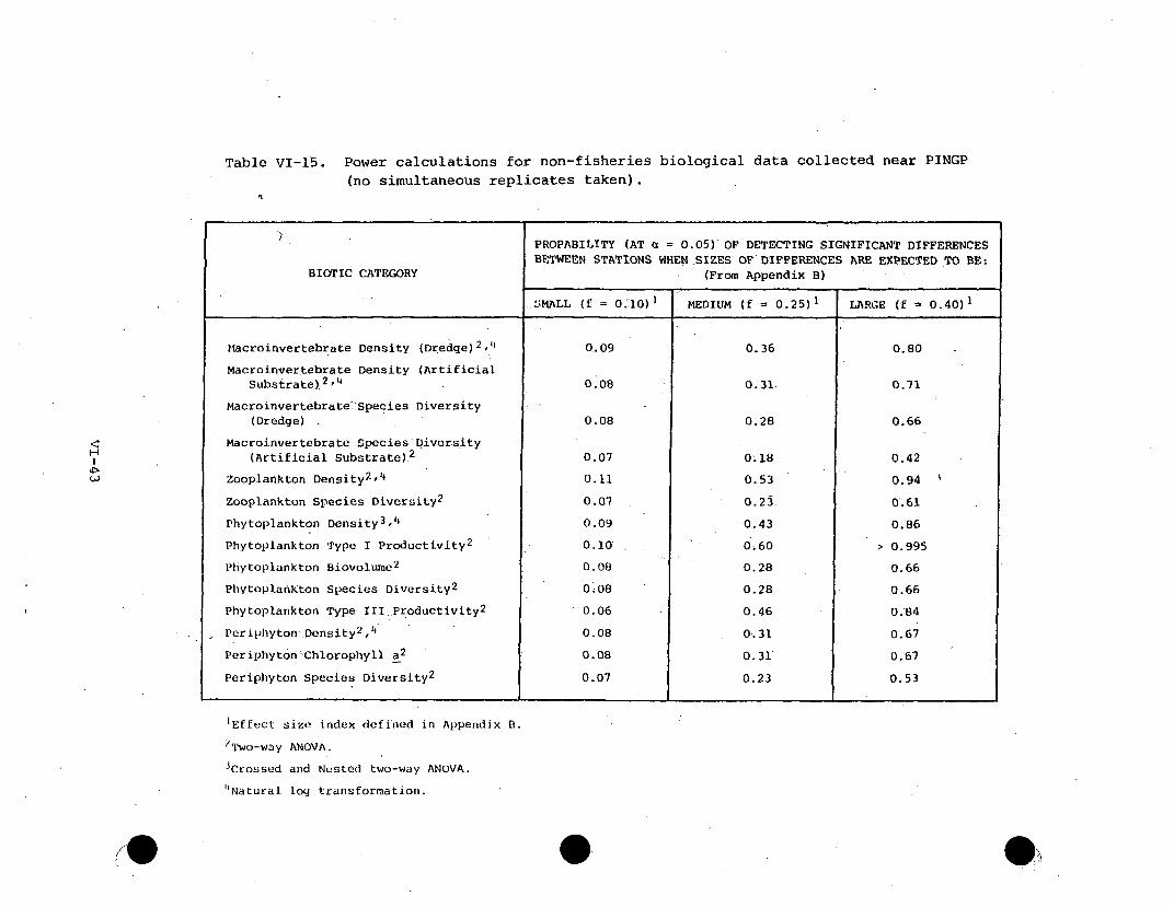
Table VI-15. Power calculations for non-fisheries biological data collected near PINGP

(no simultaneous replicates taken).

H4.rI(A

PROPABILITY (AT a = 0.05) OF DETECTING SIGNIFICANT DIFFERENCES

BETWEEN STATIONS WHEN.SIZES OF DIFFERENCES ARE EXPECTED TO BE:

BIOTIC CATEGORY (From Appendix B)

S-MALL (f = 0.10)1 MEDIUM (f = 0.25)1 LARGE (f 0.40)1

flacroinvertebrate Density (Dredge)2 ,4 0.09 0.36 0.80

Macroinvertebrate Density (ArtificialSubstrate)

2 ,4 0.08 0.31 0.71

Macroinvertebrate:Species Diversity(Dredge) 0.08 0.28 0.66

Macroinvertebrate Species'Diversity(Artificial Substrate)

2 0.07 0.18 0.42

Zooplankton Density2 , 4 0.11 0.53 0.94

Zooplankton Species Diversity2 0.07 0.23. 0.61

Phytoplankton Density3 ,#o 0.09 0.43 0.86

Phytoplankton Type I Productivity2 0.10 0.60 > 0.995

Phytoplankton Biovolume2 0.08 0.28 0.66

Phytoplankton Species Diversity2 0.08 0.28 0.66

Phytoplankton Type III Productivity2 0.06 0.46 0.84

Periphyton.Density2 ,4 0.08 0.31 0.67

PeriphytonChlorophyll a 2 0.08 0.31 0.67

Periphyton Species Diversity2 0.07 0.23 0.53

'Effect size index defined in Appendix B.

.|Two-way ANOVA.

3Crossed and Nested two-way ANOVA.

"1Natural log transformation.

O

the federally endangered Higgins Eye pearly mussel has not been collected 0during the seven years of sampling near the site. Such information iscritical in assessing impacts at PINGP because the same mussel has beenfound both up and downriver from the site at a distance of less than81 km (50 mi) (Krosch, 25 October 1977).

2. Effects of Past Operation.

a. RESULTS OF DATA REANALYSIS. The following section presents onlythe results of the data reanalysis. A discussion of the biological rele-vance of these findings is presented later in Section VI B.2.b.

i) Analysis of Variance (ANOVA) and Duncan's Multiple Range Test.Table VI-16 summarizes a reanalysis of the macroinvertebratedata. For operational years, ANOVA indicates that macroinverte-brate densities for both dredge and artificial substrate samnplesvaried significantly among sampling dates. Comparisons of macro-invertebrate densities among stations for dredge and artificialsubstrate samples indicate that the densities were also signifi-cantly different during the same period. Further analysis ofthe dredge data using Duncan's Multiple Range Test (DMRT)(Table VI-17; Figure VI-2) shows that only Station 18 (recyclecanal) was grouped separately from the other stations. Forartificial substrate densities, the group containing Stations18, 10 (upriver main channel), and 21 (near-field discharge) wasfound to be significantly different from the group includingStations 12 (near-field intake), 25 (discharge near Barney'sPoint), and 6 (south-central Sturgeon Lake). Some of the samestations are included in separate groupings because their affinity._to other stations is ambiguous. Further analysis with the t-Test(Section VI 2.a.2) was conducted to determine whether or notspecific station pairs differed significantly from each otherwhen the DMRT presented ambiguous results.

Analysis of variance showed species diversity to be significantlydifferent between stations for both artificial substrates anddredge samples over the period 1975 to midTl977 (Table VI.-16).The DMRT (Table VI-17) then grouped artificial substrate diversityStations 6 and 10 as significantly different from grouped Stations6, 12, 21, and 25. Station 18 differed significantly from the otherstation groups. For dredge species diversity Stations 6, 10, 12,and 25 were grouped as significantly different from Stations 18and •21 during the same period.

Power calculations are summarized in Table VI-15 and indicate thatonly large differences between station mean values would likelybe detected as significant.

2) Student's One-Tailed t-Test. When the ANOVA indicated thatdensities varied significantly among stations and the DMRT

VI-44

Table VI-16. Results of two-way ANOVA for biotic categories samplednear PINGP in 1973-1977 (summarized in Appendix B).

YEARS DEGREES IBlTC AEGR IA~Iyz O JF IE VALUEJ P > F~ SIGNIFICANTI

4JAlALYZED I__________ ____ FREEDOM,______ DFFRNE

Macro invertebrates

Density2

(Dredge)

Density2

(Dredge)

Species Diversity(Dredge)

Species Diversity(Dredge)

Density2 (ArtificialSubstrate)

Density2 (ArtificialSubstrate)

Species Diversity(Artificial Substrate)

Species 'Diversity(Artificial Substrate)

Zooplankton

Density2

2Density

Species Diversity

Species Diversity

Phytoplankton

Density-

Density2

Density2

DensDty2

Species Diversity

Species Diversity

Biovolume

Biovolume

Productivity3

Productivity3

Productivity'Productivity4

Periphyton

Density2

* Density2

* Species Diversity

* Species Diversity

Chlorophyll a

Chlorophyll a

* Phaeophytin a

Phaeophytin a

75-77

75-77

75-76

75-76

75-77

75-77

75-76

75-76

75-76

75-76.

75-76

75-76

73,75-76

75-76

75-76

75-76

75-76

75-76

75-76

75-76

76

76

76

76

75-76

75-76

75-76i

75-76

75-76

75-76

75-76

75-76

Between Stations

Between Months

Between Stations

Between Months

5 14.57

4.5013

Between Stations

Between Months

Between Stations

Between Months

Between Stations

Between Months

Between Stations

Between Months

Between years 73 and 75-76

Between years 75 and 76

Between Stations

Between Months

Between Stations

Between Months

Between Stations

Between Months

Between Stations

5 10.82

21 11.71

5 3.06

10 9.89

6 7.21

23 55.45

6 0.45

23 6.07

1 4.29

1 0.00

4 1.00

23 28.71

4 1.06

10 2.21

4 1.11

10 -8.48

1 178.16

8 6.75

4 14.26

34 24.41

2 15.63

22 6.79

2 1.50

14 5.09

2 3.98

21 6. 85

2 0.36

21 4.84

6 1 17.6616 11.760.0001

0.001

0.0001,

0.0001

0.001

0.001

0.0001

0.0001

0.0001

0.0001

0.8445

0.0001

0.0414

0.9653

0.4143

0.001

0.3864

0.0316

0.1789

0.0001

0.0001

0.0001

0.0001

0.0001

0.0001

*0.OOl

0.2381

U.0001

0.0256

0.0001

0.6975

0.0001

yes

yes

yes

yes

yes

yes

yes

yes

yes

yes

no

yes

yes

no

no

yes

no

yes

no

yes

yes

yes

yes

yes

yes

yes

no

yes

yes

yes

no

yes

Between

Between

Between

Days

Stations

Days

Between Stations

Between

Between

Between

Between

Between

Between

Between

Months

Stations

Months

Stations

Months

Stations

Months

IType I as defined in Appendix B.

2Natural log transformation.

3Only near-field intake and discharge stations (HDR Nos. 14 and 19)involved; known as a Type III experiment.

Both near- and far-field stations involved (HDR Nos. 5, 9, 14, 19, and 27): known as a Type I experiment.

'The null hypothesis that no difference exists between stations or dates is rejected (., 0.J5).

VI-45

I S

Table VI-17. Results of Duncan's Multiple Range Tests for biotic categories sampled nearPINGP, 1973-1977.

. /

!n

DUNCAN'S MULTIPLE RANGE TEST FOR STATIONS1

BIOTIC CATEGORY (HDR DESIGNATED STATIONS)

A GROUPING 3 B GROUPING C GROUPING D GROUPING

Macroinvertebrate Density2 (Dredge) 6, 10, 12, 1821, 25, 27

Macroinvertebrate Density2 (Artificial 18, 10, 21 12, 25, 6Substrate)

Macroinvertebrate Species Diversity 10, 6,-12, 21, 18(Dredge) 25

Macroinvertebrate Species Diversity 6, 10 6, 21, 12, 18(Artificial Substrate) 25

Zooplankton Density2 27, 10 10, 12, 6 12, 6, 25, 21 21, 18

Phytoplankton Productivity (Type III1 ) 14 19

Phytoplankton Productivity (Type is) 14 27, 9, 5 19

Periphyton Chlorophyll a 13 • 20, 25

Periphyton Density2 13, 20 25

1 Data base derived from Table VI-16.

2 1ndicates natural log transformations.

3 A grouping is a number of stations (or one station) whose mean value differs. significantly

(a = 0.05) from other station groupings (see Appendix B for details).

"Type III productivity refers to measurements taken only at near-field intake and discharge

stations.

5'lype I productivity refers to measurements taken at several stations, both near- and far-field.

produced ambiguous results regarding specific station groupings,-then selected ambiguous station pairs were subjected to theStudent's t-Test. The One-Tailed Student's t-Test was utilizedto specifically address the questions: 1) are macroinvertebratedensities in the discharge significantly lower than those inthe intake, and 2) are densities upriver from PINGP significantlylower than those downriver and influenced by the thermal plume?Table VI-18 shows that for dredge macroinvertebrate density,Station 12 (intake) did not differ significantly from, Station 21(discharge), nor did Stations. 10 (upriver) and 27 (downriver)differ significantly. For artificial substrates, only stationsin the immediate plant area could be compared since .insufficientdata. were available; for the. other. stations. No significantdifference was found between Stations 12 and 21 which clarifiesthe results of the analysis of variance and Duncan's MultipleRange Test. . Since no significant differences were observed inthe immediate vicinity of the plant, it is unlikely that signifi-cant differences would occur between the up and downriver artificialsubstrate samples as a result of the PINGP thermal discharge.

3) Multiple Regressions. Stepwise multiple linear regressionswere performed, comparing dredge and artificial substrate macro-invertebrate population densities with a limited number ofrelatively simultaneous (sampled within one week of biologicalsamples) water quality parameters (Table VI-19) collected athydrographically Similar stations (Table 111-31) . For a completelist of all water quality variables considered, see Appendix B.For dredge macroinvertebrates, neither temperature nor dissolvedoxygen was found to be significantly related to total populationdensities; 'only bottom suspended residue (sediments) was selectedby stepwise regressi6n 'at a low R2 value of 0.15. This indicatesthat macroinvertebr~tes collected in bottom substrates may havevaried in density as a result of parameters 'other than temperatureor dissolved oxygen, and coincided only weakly with concentrationsof suspended residue. Surface ammonia was the only water qualityparameter selected as' related to artificial substrate macroinverte-brate densities (R2 = 0.42). 'All R2 values were found to besignificant at a < 0.05 (see Appendix B). If more intensivewater quality' sampling had been conducted during the artificialsubstrate colonization period, better regressions might haveresulted.

b. DISCUSSION. Statistical reanalysis of more than two years ofoperational data tends to confirm the conclusions made by Haynes (1976)and Texas Instruments, Inc. (1977b). In 1975 and 1976, these authorsfound that the density of macroinvertebrates collected on artificialsubstrates and in dredge samples was either 'equal in the intake anddischarge or higher in discharge stations on an annual basis. In addition,intake and discharge stations had significantly greater densities thanmain channel (upriver and downriver) stations for artificial substrate

VI-47

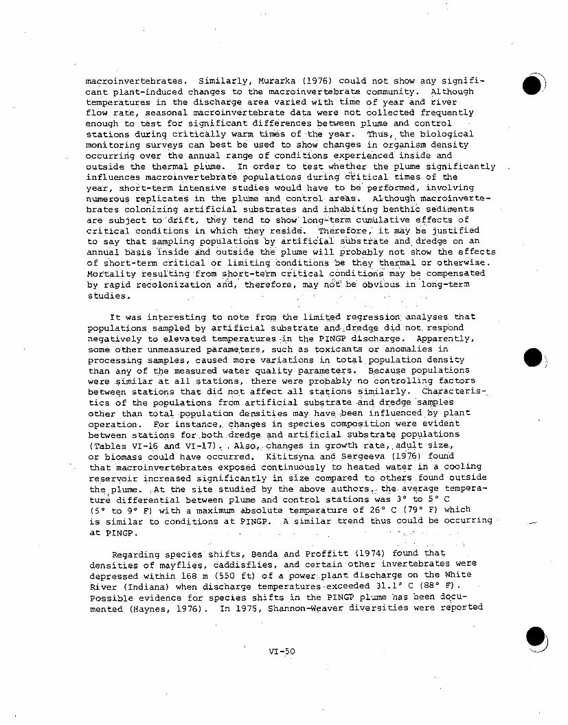
macroinvertebrates. Similarly, Murarka (1976) could not show any signifi-cant plant-induced changes to the macroinvertebrate community. Althoughtemperatures in the discharge area varied with time of year and riverflow rate, seasonal macroinvertebrate data were not collected frequentlyenough to test for significant differences between plume and controlstations during critically warm times of the year. Thus, the biologicalmonitoring surveys can best be used to show changes in organism densityoccurring over the annual range of conditions experienced inside andoutside the thermal plume. In order to test whether the plume significantlyinfluences macroinvertebrate populations during critical 'times of theyear, short-term intensive studies would have to be performed, involvingnumerous replicates in the plume-and con trol areas. Although macroinverte-brates colonizing artificial substrates and inhabiting benthic sedimentsare subject to'drift, they tend to show' long-term cumulative effects ofcritical conditions in which they reside. Therefore, it may be justifiedto say that sampling populations by artificial substrate and dredge on anannual basis Inside and outside the plume will probably not show the effectsof short-term critical or limiting conditions 'be they thermal or otherwise.Mortality resulting from short-term critical conditions may be compensatedby rapid recolonization and, therefore, may not be obvious in long-termstudies.

It was interesting to note from the limited regression analyses thatpopulations sampled by artificial substrate and..dredge did not. respondnegatively to elevated temperatures-.in the PINGP discharge. Apparently,some other unmeasured parameiters, such as toxicants or anomalies inprocessing samples, caused more variations in total population densitythan any of the measured water quality parameters. Because populationswere similar at all stations, there were probably no controlling factorsbetween stations that did not affect all stations similarly. Characteris-tics of the populations from artificial substrate and dredge samplesother than total population densities may have been influenced by plantoperation. For instance, changes in species composition were evidentbetween stations for both dredge. and artificial substrate populations(Tables VI-16 and VI-17). Also,:-changes in growth rate, adult size,or biomass could have occurred. Kititsyna and Sergeeva (1976) foundthat macroinvertebrates exposed continuously to heated water in a coolingreservoir increased significantly in size compared to others.found outsidetheplume.ý At the site studied by the above authors,•. the. average tempera-ture differential between plume and control stations was 30 to 50 C(50 to 90 F) with a maximum absolute temperature of 260 C (790 F) whichis similar to conditions at PINGP. A similar trend thus could be occurringat PINGP. • -. -

Regarding species shifts, Benda and Proffitt (1974) found thatdensities of mayflies, caddisflies, and certain other invertebrates weredepressed within 168 m (550 ft) of a poweriplant discharge on the WhiteRiver (Indiana) when discharge temperatures exceeded 31.1* C (88' F),.Possible evidence for species shifts in the PINGP plume has been docu-mented (Haynes, 1976). In 1975, Shannon-Weaver diversities were reported

VI-50

to be significantly greater in control (intake) stations for both dredgeand artificial substrate samples than at Station 21 (immediately outsidethe discharge gates). Reanalysis of dredge and artificial substratespecies diversity data-showed that for 'dredge data, the near-field plumestation (21) and the recycle canal (18) were found to differ significantlyfrom all other0 statons. For artificial substrate data, near-field plumestations (21 and 25) did not differ significantly from near-field controlstations (12 and 6) for species diversity, but Station 18 differed signi-ficantly from all other stations. Differences in substrates or currentsbetween stations may have partially caused these inconsistencies, andthese are discussed later in this section.

Examination of population densities for RIS shows that only Hydropsycheand Stenonema were •found in sufficient numbers to make comparisons betweencontrol and plume stations and then only on artificial substrates. AppendixTable A-26 summarizes the information regarding these two RIS. Althoughdata are insufficient to conduct detailed statistical analysis, densitiesin plume stations as opposed to non-plume stations appear enhanced. Largeseasonal variation is also quite evident.

To summarize, reanalysis of the limited site-specific informationindicates that the only measurable effects of PINGP, thermal dischargesto macroinvertebrates during more than two years of o0peration may! haveinvolved changes in species diversity between plume and control stations,indicating a shift in species composition. Total population densitieshave remained similar inside and outside the plume over the same period.It is apparent that neither temperature nor bottom substrate variationsbetween stations were significantly related to macroinvertebrate density,although one of these parameters may have influenced changes in speciesdiversity. According to Simonet (1975), bottom sediments and currentlconditions for various stations were as follows: Stations 25, 27, and 25were sand with current; Stations 6, 10, and 12 were mud with or withoutcurrent; and Stations 15, 18, and 21 were light, shifting sand withcurrent. These differences in current and substrate between both near-field and far-field stations may have accounted for some of the variationsin diversity between plume and control stations for dredge and artificialsubstrate macroinvertebrates. Thus, background information does notindicate that the plant has affected the density of macroinvertebrates,although a combination of elevated temperatures, current, and bottomconditions could have caused a difference in diversity for intake andupriver control stations as compared to discharge canal and downriverstations in the plume.

3. Predicted Impacts. Thermal effects on macroinvertebrates dependupon absolute temperature in addition to exposure time and thermal eleva-tion. Macroinvertebrates may be either sessile or drifting, resultingin differing exposures to the PINGP discharge. While drifting, organismswill generally be exposed for shorter periods and to lower elevated watertemperatures than those organisms attached to substrates near the head

VI-51

of the discharge canal at the discharge ,gates (Figure VI-14) . Drift timewithin the discharge area may) be increased substantially by wind-inducedrecirculation; however, drifting macroinvertebrates will generally besubjected to a lower level of thermal stress than aufwuchs and benthosoccurring in the near-field discharge. Table VI-20 lists drift times andmaximum exposure temperatures for the longer two pathways in Figure ,VI-14.

Although literature data (Appendix Tables A-28 and A-29 and Figure A-6)for thermal tolerances of macroinvertebrate RIS are limited, some driftsurvival predictions can be made regarding proposed plume conditions. Allfour RIS have been observed to survive maximum temperatures far. inexcess of any they could encounter in the plume, either drifting or sessilein the discharge, canal. The 96-hr LT 5 0 for Stenonema has been establishedat 25.50 C (800 F). at an acclimation temperature. of 100 C (50° F).

Stenonema could drift through temperatu.res up to about 290 C (840 F) for198 minutes during the propossed extreme conditions in May with an ambienttemperature of 22.80 C (73' F). Stenonema would be expected to survivesuch a worst case temperature, elevation, however, because its acclimationtemperature would be increased by almost 130 C (230 F) and exposure time;would be much shorter than the 96-hour LT 5 0 . Proposed extreme plumepredictions for an ambient temperature of 100 C (501 F) would approximate170 to 180 C (630 to..64' F) for a maximum drift encounter. temperature withno predicted lethal effects. These extreme conditions are predicted tooccur at a frequency of less than one hour in a given month over a 278-yearperiod. All other, RIS appear to be less, sensitive, than Stenonema to

.drift stress. '

From similar information for non-RIS macroinvertebrates, it appearsthat most other macroinvertebrates will not be harmed by drifting throughthe plume. only in locations closest to the discharge gates should someof the benthic macroinvertebrates (e.g., Taeniopteryx maura, Baetis tenax,and Ephemerella subvaria) be periodically eliminated. Since other speciesshould take the places of those benthic invertebrates lost from the headof the discharge canal, total densities should not be reduced althoughspecies diversity and composition may change.

For fixed benthic or .aufwuchs macroinvertebrates, preferred or mostcommon temperature at which a taxon is recorded appears to be the relevantcriterion for predicting impact (Tables VI-21 through VI-24). This tempera-ture range, has been established at 270 to 290 C (81' to 840 F) forHydropsyche and at 280 C (820 F) for Macronemum (Appendix Table A-29).Similar information for the other RIS is lacking. Information presented inthermal matrix Table VI-23 indicates that Hydropsyche will be excludedfrom 6.6 ha (16 A) or less during typical spring to summer conditionswhich is the equivalent of about 2.0 percent of Sturge.on:Lake, Habitatexclusion in the discharge canal is compared to that available in SturgeonLake because of the similarity of hydrological conditions (except forthe thermal plume) and because of the proximity of the two locations.For proposed extreme conditions, the exclusion area is predicted to varyfrom about 0.1 ha (0.3 A) in January to the entire discharge canal inAugust [18 ha (44.5 A)].

VI-52

H

tu-

Table VI-20. Estimated drift times for plankton through the thermal plume at PINGP for typicaland proposed extreme conditions.

ESTIMATED DRIFT TIME (MIN)' HIGHEST EXPECTED TEMPERATURE ENCOUNTEREDCONDITIONS MODELED

MAXIMUM MEAN DURING MAXIMUM DRIFT DURING MEAN DRIFT

Typical

Spring (May 1976) 138 120 22.80 C (73.00 F) 21.70 C (71.00 F)

Summer (August 1975) 120 100 29.40 C (84.90 F) 28.50 C 83.30 F)

Winter (December 1975) 405 388 16.50 C (61.70 F) 11.60 C 52.90 F)

Proposed Extreme

Spring (May) 198 180 28.80 C (83.80 F) 27.30 C 81.10 F)

Summer (August) 108 93 32.80 C (91.00 F) 32.50 C 90.5- F)

Winter (January) 483 445 16.70 C (62.10 F) 12.50 C 54.50 F)

1 Time required for a neutrally buoyant particle to drift from the upriver to the downriver extentof the 50 F isotherm in the near-field, assuming an average velocity of 0.2 fps. Drift pathsare shown in Figure VI-14.

0 O

1@

H

31

Table VI-21. Thermal matrix for response of the macroinvertebrate RIS, Stenonema, to conditions

near PINGP. Organism: Stenonema; trophic level: primary consumer; bioticcategory: macroinvertebrate.

TEMPERATURE1 AREA EXCLUDING TIME FUNCTIONBIOLOGICAL ACTIVITY (C) FUNCTION (HA) EXCLUDED REMARKS

TYPICAL 2 EXTREME 3 TYPICAL 2 EXTREME 3

Maximum temperature where live 32.0 0 0specimens have been observed.

Mean lethal temperature (48 or96 hr TLm or LT 5 0) of mature 25.5 0 0

larval or adult stage.

Most common temperature taxonrecorded at, based on frequency ND," - -__of occurrence of differenttemperature levels.

Temperature increases whichhave been shown to affect emer- ND4

- --

gence period.

lFrom Appendix Table A-29.2 From Appendix Tables A-37 through A-39.3From Appendix Tables A-40 through A-42.

Nb" = no data.

Table VI-22. Thermal matrix for the response of the macroinvertebrate RIS, Pseudocloeon, toconditions near PINGP. Organism: Pseudocloeon; trophic level: primaryconsumer; biotic category: macroinvertebrate.

H

U,Ln

TEMPERATURE1 AREA EXCLUDING TIME FUNCTION

BIOLOGICAL ACTIVITY FUNCTION (HA) EXCLUDED REMARKS

TYPICAL 2 EXTREME 3 TYPICAL2 EXTREME 3

Maximum temperature where live 40.7 0 0specimens have been observed.

Mean lethal temperature (48 or96 hr TLm or LT 5 0) of mature ND4

larval or adult stage.

Most common temperature taxonrecorded at, based on frequency NA -- --

of occurrence of differenttemperature levels.

Temperature increases whichhave been shown to affect emer- ND4 - -

gence period.

1From Appendix Table A-29.2 From Appendix Tables A-37 through A-39.3 From Appendix Tables A-40 through A-42.

ND4I = no data.

9

Table VI-23. Thermal matrix for response of the macroinvertebrate RIS, Hydropsyche, toconditions near PINGP. Organism: Hydropsyche; trophicconsumer; biotic category: macroinvertebrate.

level: primary

H

0,

TEMPERATURE1

AREA EXCLUDING TIME FUNCTIONBIOLOGICAL ACTfVITY FUNCTION (HA) EXCLUDED REMARKS

(C) TYPICAL2 EXTREME3

TYPICAL? EXTREME3

Maximum temperature where

live specimens have been 35-38 0 0 - -

observed.

Mean lethal temperature(48 or 96 hr TIn or LT, 0 ) 32-3n 0 0 -

of mature larval or (Spring, Fall)

adult stage. 38 (Summer) 0 0 -0adolt somntaem. rtr

Most cominon temperature Ambient river temperature exceededtaxon recorded at, based 29* C for August proposed extremeon frequency of occur- 27-29 6.6 0.08 to Auut May-Aug 29CfoAuutppseexrm

648 August January condition; therefore,*this RIS'srence of different - optimum temperature is exceededtemperature levels. naturally.

Temperature increases 1=2 wk advance 18.5 ]8.5 All year All year Coutant (1968)which have been shown 14 (±-2)=5 moto affect emergence per- advance 1.5 2.5 December January Nebeker (1971)lod. in winter

tFroa Appendix Table A-29.2From Appendix Tables A-37 through A-39.

rein Appendix Tables A-40 through A-42.

Table VI-24. Thermal matrix for response of the macroinvertebrage RIS, Macronemum, to conditionsnear PINGP. Organism: Macronemum; trophic level: primary consumer; bioticcategory: macroinvertebrate.

HI-j

TEMPERATUREI AREA EXCLUDING TIME FUNCTION

BIOLOGICAL ACTIVITY T E U FUNCTION (HA) EXCLUDED REMARKS

TYPICAL2

EXTREME3

TYPICAL2

EXTREME3

Maximum temperature wherelive specimens have been 35 - 0 0 - -

observed.

Mean lethal temperature(48 or 96 hr TL, or LT5 0 ) ND" ..-of mature larval.;oradult stage.

Most common temperaturetaxon recorded at, based River exceeds 28* C in August proposeden frequency of occur- 28 1-5 - June-: May- extreme conditions; therefore, thisrence of different August August RIS's optimum temperature is

renc of iffeentexceeded naturally.temperature levels.

Temperature increaseswhich have been shown -0 = 2 wk 18.5 18.5 All year All year Hopwood (1975)to affect emergence per- advanceiod.

From Appendix Table A-29.

2 From Appendix Tables A-37 through A-39.

3From Appundix TabJes A-40 through A-42.4

ND = no data.

0

Likewise, 1 to 5 'ha (2.5 to 12.4 A) in the discharge canal, comparable @1

to 0.3 to 1.5 percent of Sturgeon Lake, will not be suitable for Macro-nemum for typical conditions in June through August (Table VI-24) . Underproposed extreme conditions, the unsuitable area would increase from 1.7 ha(4 A) in May to the entire river in August; however, these conditions areexpected to occur at a frequency of less than 1 hour in a given monthover a 278-year period. No information on cold shock tolerance wasavailable for macroinvertebrate RIS.

Information regarding thermal effects on emergence schedules are alsosummarized in Tables VI-23 and VI-24 for both Hydropsyche and Macronemum.It has been found that a temperature increase of 10 C (20 F) or less mayadvance emergence by as much as 2 weeks. This would involve the entiredischarge canal [18 ha (44.5 A)]' which is equivalent to-about 5.7 percentof Sturgeon Lake. For Hydropsyche, it has been estimated (Nebeker, 1971)that a 14 ± 20 C (25 ± 4' F) temperature elevation occurring in the wintercould accelerate emergence by as much as 5 months. In January, the areain the discharge canal affected by at least a 140 C (250 F) AT would be1.5 ha (3..7 A or 0.46 percent of Sturgeon Lake). Nebeker (1971) foundthat if an insect emerges prematurely, successful reproduction may notbe possible because environmental conditions may be unfavorable, or matesmay not emerge during the short life span of the too-early insect. Inaddition, if a difference in time normally occurs between emergence ofseparate sexes (e.g., in stoneflies) and exposure to elevated temperaturesenhances this differential, then reproduction will not occur if no indivi-duals of the opposite sex emerge during the life span of the early emergedinsects. In the case of either Hydropsyche or Macronemum, however,accelerated emergence schedules should not degrade the overall "protectionand propagation" of these two taxa. In the first case, even if all thelarvae that emerged two weeks early were lost (which is unlikely), thiswould amount to less than 6 percent of all those produced in Sturgeon Lakealone, and many other backwaters exist in the vicinity of PINGP. On theother hand, should elevated temperature in the.discharge initiate emergence5 months early, this would amount to a loss of less than 0.5 percent ofall larvae that would be expected to emerge from Sturgeon Lake during thewarmer seasons. These predictions are based on the assumption thatmacroinvertebrate densities are somewhat similar between discharge andSturgeon Lake locations (Table VI-17).

In his study of aquatic insect emergence near PINGP, Shyne (1977)found that mayflies (especially Caenis) emerged earlier near heated waterstations than at control stations, but because heating was sporadic(May-December 1974), other factors may have caused this early emergence.The caddisflies, Hydropsyche/Cheumatopsyche, appeared to emerge at equalrates and times from both heated and control 'stations. Midges emergedearlier in Sturgeon Lake than the simultaneous peak observed at allother stations. Thus, with the possible exception of the mayfly, Caenis,emergence of aquatic insects seemed to be unaffected by the thermal plumein 1974.

VI -58

Comparing the predicted impact of the PINGP discharge with previouslyobserved impacts, it is obvious that field data are inadequate to verifypredicted species shifts or changes in abundance of individual speciesthat may have resided in the thermal plume. Practically no informationis available regarding the selective processes occurring inside the plumeas compared with control stations. If anything (see Appendix Table A-26),artificial substrate abundances. of two RIS, Hydropsyche and Stenonema,were higher during the summer months at discharge than at intake station•.In addition, Haynes (1976) and Texas Instruments, Inc. (1977b) reportedthat species diversity changed significantly between intake and dischargestations for both artificial substrate and dredge samples, even thoughcombined densities of all organisms remained approximately the samebetween these stations during both years. Reanalysis of these and newerdata (1975-1977) confirmed the differences for macroinvertebrates in thedredge samples, but not for those on artificial substrate samples. Thus,even though thermal tolerance data suggest that some macroinvertebrate RISmay be eliminated from certain benthic portions of the plume during partof the year, site-specific data, at least for Hydropsyche and Stenonema,show that the reverse may be true. It should be pointed out, however,that the site-specific data on RIS are insufficient and do not necessarilycontradict the impacts predicted .from the thermal tolerance information;i.e., that losses of some RIS macroinvertebrates may occur in the discharge

.canal. It also should be pointed out that site-specific data did indicatea general shift in total species composition between intake and dischargestations.

C. ZOOPLANKTON

1. Discussion and Critique of Sampling Methods. Methods for zooplank-ton sampling are summarized in Appendix Table A-22,-:and many of thecriticisms of data collection mentioned in the macroihvertebrates sectionapply also to zooplankton. Samples were taken with a Van Dorn (or Kemmerer)bottle or by pumping, and water was then filtered through a plankton net.The mesh of the plankton net was not specified in the earlier studies butpresumably was the same for all studies since sampling began in 1970.Plant entrainment mortality testing was begun in 1974, utilizing a pumpfiltration system, which sampled at a rate of approximately 130 liters/min.pumping is probably more efficient for sampling agile zooplankton (such ascopepods) than is sampling by means of a Van Dorn bottle because of thelarger volume sampled and less avoidance of the sampler. Thus, Withoutintercalibration, the two methods are probably not comparable, nor werethey designed to be. Patchy zooplankton distribution can also presentproblems in asesse ing impact of the plant, no matter what sampling methodis used, since an apparent increase or decrease in zooplankton numbers atthe discharge in relation to the intake may actually result from variationsdue to patchiness. Moreover, if no attempt is made to sample the intakeand discharge at approximately the same time, allowing for travel timethrough the plant (especially when discharging at maximum blowdownvolume), natural density variations occurring between intake and dischargemay be inseparable from those resulting from plant related losses. Thus,

VI-59

it is important either that enough replicates be taken at each station 0to define temporal and spatial variation, or that samples of adequatevolume be collected to compensate for patchiness. Table VI-15 indicatesthat with no simultaneous replicates taken, only moderate to largeývariations between mean station values would be detected as significant.In this, as with other types of sampling, it is obvious that with anincrease in number of replicates taken at each station, a smallerpercentage difference between stations is required to reveal a signifi-cant difference.

Since the viability of the sampled zooplankton at stations other than14 and 20 (Figure VI-2) was not recorded, it is doubtful that reductionsin zooplankton densities at other stations resulting from plant operationcould be readily determined. Zooplankton that may have been recentlykilled as a result: of plant operation would remain almost neutrally buoyantfor at least several hours and, therefore, inseparable from live organismsafter sample preservation. Little is known abou . zooplankton settlingrates after death, but there is some indication that reductions in densitiesfrom settling of dead zooplankton in the discharge canal as a result ofplant operation may be measurable (Carpenter et al., 1974). However, itis difficult to separate zooplankton losses resulting from plant entrain-ment and those resulting from plume entrainment. Thus, determinationof zooplankton mortality resulting from plume entrainment is, at best,difficult.

4. Effects of Past Operations. 0 1

a. RESULTS OF DATA REANALYSIS.

I) Analysis of Variance (ANOVA) and Duncan's Multiple Range Test.Zooplankton data collected near PINGP in 1975 and 1976 (opera-tional years) were reanalyzed, and the ANOVA results are summarized

in Table VI-16. Densities varied significantly between. stationsA(l < 0.001), and variation between months was also highly signifi-cant. Further reanalyses using Duncan's Multiple Range Test (DMRT)(see Table VI-17) indicated that certain station groups differedsignificantly relative to other station groups. For example,Stations 10 and 27 comprised a group which differed significantlyfrom the group containing Stations 6, 10, and 12. Moreover,grouped Stations 6, 12, 21, and 25 differed significantly fromother stations, and stations 18 and 21 combined differed fromother groups of stations., Zooplankton species diversities,however, did not differ significantly between stations based onthe ANOVA test but did vary seasonally (Table VI-16).

2) Student's One-Tailed t-Test. Since the DMRT showed that certain

groups of'stations differed significantly from other groups ofstations, a directional (one-tailed) Student's t-Test wasutilized to determine whether zooplankton were more dense atStation 12 (the intake) 'than at Station 21 (the immediate dis-charge area), and did zooplankton density at Station 10 (upriver

VI -60

of PINGP) exceed significantly that of Station 27 (near Lockand Dam No. 3). The results (Table Vf-18) did not demonstratethat significant differences existed between both near-field andfar-field stations. As mentioned previously, however, the factthat no differences were shown between stations does not neces-sarily mean that no differences actually existed. It simplyindicates that the power Of the data may not have been great enoughto show differences if they did occur. It is also likely thatif zooplankton were killed by plant operation, they would nothave settled out of the water column during the short transittime between stations. Subgroups of the zooplarkton (that is,rotifers and crustaceans) showed results similar to those forthe total zooplankton analysis.

3) Multiple Regressions. Although zooplankton and its subgroups,rotifers. and crustaceans., were not found to vary significantlyin density between some, stations, densities of these taxa werefound to be related to several water quality parameters. Fortotal.zooplankton density, five water quality parameters wereselected in a stepwise linear regression procedure. The mostimportant of these was temperature (Table VI-19) followed bynitrate, orthophosphate, dissolved oxygen, and ammonia,. Allselected parameters accounted for 64 percent of the variationrecorded in.zooplankton numbers.. Because temperature was selectedas the most important parameter relating, tO zooplankton densities,this does not necessarily mean that the plant caused this variation.Significant variation between stations and between months didoccur (Table VI-16), and thus, variation in zooplankton densitiesresulted from variations in temperature on both a seasonal basisand a station basis.

Regressions of rotifer density with water quality parametersproduced results almost identical to those for total zooplankton.The same five water quality parameters were selected with a totalR2 of 0.66, and temperature was the most important parameter.Crustacean densities were related only to temperature, nitrates,and orthophosphates with a total R2 of only 0.53. itis importantto note, however, that 41 percent of the variation in crustaceandensities resulted from temperature which is somewhat higher than37 percent for rotifers and 35 percent for total Zooplankton.All of the R2 values were high enough to indicate that densityof total zooplankton or either of its subgroups were significantly(a < 0.05) related to some of the water quality parameters (seeAppendix B).

Seasonal correlations (r) of total zooplankton and crustaceanswith temperature were always relatively low. During summer, thecorrelation of total zooplankton populations with temperatureappeared to be slightly negative (r = - 0.24), and crustaceandensities showed a similar relationship with temperature (r. - 0.29)in winter. Both total zooplankton (r = 0.21) and crustaceanabundances (r = 0.18) exhibited positive, but weak, correlations

VI -61

to temperature in spring. These results tend to indicate thatalthough annual temperature fluctuations may influence zooplanktonpopulations through seasonal variation, when considered only ona seasonal basis, temperature is not so important. Thus, theannual influence of temperature variation must be more importantthan that of spatial influences (such as the thermal plume), orelse the seasonal correlations would have been higher than thoseof the annual correlations. In summary, zooplankton densitiesare influenced by temperature variation to a moderate extent,with seasonal variations of water temperature a stronger determinantthan spatial variation.

b. DISCUSSION. Daggett (i976) found. no significant difference intotal zooplankton densities between PINGP stations for 1975, althoughcopepods did show a difference at the p < 0.08 level. Using;Tukey'sMultiple Comparison-Test, Daggett showed that Stations 6 and 12 (SturgeonLake and the intake) had significantly greater copepod densities thanStations 10, 21, and 26 (Sturgeon Lake, the discharge canal, and;down-river from Barney's Point). Diversityrwas high at all-•stations, but nostatistical tests were conducted to ascertain; if significant differencesoccurred between stations. Reanalysis of the data by ANOVA,' however,confirmed the expectation that species diversity did not differý significantlybetween stations. In 1976, data analyses using the Newman Kuels Test(Texas Instruments, Inc.,-1977a) showed that copepod densities weresignificantly higher at 'the intake (Station 12) than in the discharge(Stations 21 and 25), but Station 5 (Sturgeon Lake) was not significantlydifferent from Station 25. Similar results were found for both cladoceransand copepods; however, rotifers showed no significant differences betweenstations.

The primary differences between stations that affected abundances ofplanktonic organisms were temperature and current. Thermal surveystaken during representative periods of 1975 and 1976 (summarized inAppendix N) and water velocity measurements (conducted by Stefan andAnderson, 1977 and Szluha, 1975) have characterized several stationdifferences (Sections III A.3, and B.1). Analyses of field data, however,have shown no. large variations in spatial abundance of zooplankton asrelated to temperature, and insufficient data were available to analyzevelocity related effects. Differences in zooplankton densities betweenintake and discharge may exist, but the number of replicates was insuf-ficient to show anything but large percentage differences. Even if therehad been significantly more zooplankton observed at the intake rather thanthe discharge, the majority of the decrease in density would have probablybeen caused by plant entrainment rather than plume entrainment, as a resultof the greater stress involved in plant entrainment (Davies and Jensen,1975).

Statistical tests do not indicate that any reductions in speciesdiversity have occurred between intake and discharge stations at PINGP.King (1974) foundthat no zooplankton species were eliminated from the

V0V1-6 2

heated zones of a Missouri cooling reservoir where AT's averaged 40 to60 (7 to 110 F); however, cladocerans and copepods were more abundant inthe heated cove, whereas rotifers were more common in the control area.Nevertheless, no significant differences in species diversity were.found between the control and heated zones of this reservoir.

Thus, site-specific data for zooplankton indicate that the thermalplume did not significantly alter either density or species diversity atPINGP in 1976 and 1977. However, data were such that only very severechanges would have been detectable, and even then most reductions wouldprobably have resulted from plant rather than plume entrainment.

3. Predicted Impacts. No RIS were selected for zooplankton; however,thermal tolerance information'-for a number of species found near PINGPis summarized in Appendix Table A-31 and Figure A-7. Although exposureperiods differ greatly between thermal tolerance data and expected driftexperien~ce, it is expected that most cladocerans, because of theirrelatively high thermal tolerance, could withstand the maximum thermalincreases encountered while drifting in the discharge canal (Table VI-20),even during the hottest part of the summer. On the other hand, the copepod,Diaptomus, might be damaged by drifting through the hottest part of theplume during certain times (Table Appendix A-31 and Figure A-7), especiallyduring proposed extreme conditions from June to September when maximumencountered plume temperatures exceed 310 C (880 F). However, acclimationto these thermal maxima will be gradual and duration of exposure to highesttemperatures will not exceed 108 minutes. Thus, Diaptomus would probablynot be killed by drifting through the plume even during the proposedextreme conditions. If, however, there were other mitigating factors,such as abnormally low dissolved oxygen (DO), high levels of a toxicantfrom upstream, or abnormally long retention times in the discharge' canal,then the already-weakened Diaptomus may be unfavorably affected by the,thermal plume. Similar limitations may occur for Cyclops vernalis,although this taxon is slightly more thermally tolerant than Diaptomus.

Little information is available on thermal tolerances of rotifers,but they are considered to be generally more thermally tolerant thaneither cladocerans or copepods (Jensen et al., 1969). Protozoans areknown to withstand maximum temperatures of 350 to 400 C (950 to.1040 F)after acclimation to only 210 to 250 C (700 to 770 F) (see Appendix TableA-31), and are considered more tolerant than most other types of zooplankton.Brock (1975) suggested that the upper limits for some protozoans approach500 C (1220 F), although diversity may be severely restricted at tempera-tures below this upper limit.

Although no individual species at PINGP have been selected forstatistical analysis, the lack of major. variations in density and diver-sity of zooplankton indicate that the plant has little impact on driftingpopulations, even in the immediate vicinity of the discharge. Even if adecrease in density and diversity hadbeen observed, the relatively rapid

VI-63

reproductive rates and short life spans of most zooplankton, especiallyduring the summer, would be expected to compensate for any losses in-curred due to drifting through the plume at PINGP (EPA, 1976b).

Power plants on large midwestern rivers have rarely caused signifi-cant losses in zooplankton, either by plant or plume entrainment (OPPD,1976). When losses do occur as a result of power plant operation,* theloss is largely due to entrainment through the plant rather than by. otherplant-related causes (Davies and Jensen, 1975).

D. PHYTOPLANKTON

1. Discussion and Critique of Sarpling.Methods. Phytoplanktonhave been sampled since 1969 (Appendix Table A-22), and most samplingmethods and procedures were state-of-the-art. The. following considerations,however, limit their. utility. First, it is questionable that diatomscould have been identified to species without leaching or incineratingcell contents before examining frustule sculpturing. . Second, althoughsampling methods have remained somewhat similar since the inception ofphytoplankton sampling in 1969,r the stations and dates sampled fordensities varied considerably prior to 1973. Use of the oxygen productionmethod for determining phytoplankton productivity (Baker., 1975a) insteadof the more widely used 14C method limits comparison with.some literature.moreover, location of sampling stations and sampling frequency wereinconsistent from year -to year. Simultaneous replicates were not collectedfor density estimates, while only a limited number of productivitysamples had replicates. Thus, the power of the data for showing significantdifference between stations wasrather low except for the few cases wheremultiple productivity samples were taken (Table VI-15)-. Little or notabular data were available, and the results from several stations weregenerally pooled.

2. Effects of Past Operation.

a. RESULTS OF DATA REANALYSIS.

i) Analysis of Variance (ANOVA) and Duncan's Multiple Range Test.Phy'toplankton abundance data were reanalyzed by nested analysisof variance 'to determine, first, if there :was a difference betweenthe preoperational year of 1973 and the operational 'years of 1975and 1976, and then whether there was a difference between allstations or months during operational periods (1975 and 1976).Table VI-16 summarizes some of this information and shows that rphytoplankton densities appeared to differ significantly between1973 and 1975-1976. 'This may or may not have been associated 'withinitiation of plant operation. Differences bet-een stationdensities for both operational years combined were not 'significant,although differences between months were highly significant'. Thelatter reflects natural seasonal variations.

VI-64

WNeither phytoplankton biovolume (mg/i) nor Shannon-Weaverdiversity differed significantly. between stations for 1975and 1976 (Table VI-16).. Net phytoplankton productivity (Type Iof Baker, 1977) for the near-field intake station (14) variedsigni ficantly from the near-field discharge station (19), whereasboth of these near-field intake and discharge stations differedsignificantly from the far-field Sturgeon Lake (5) and riverstations (9 and 27) (Table VI-17). Intensive near-fieldType III (of Baker, 1977a) productivity studies confirmedthese results, showing significant variation between intake(14) and discharge (19) stations (Table VI-17).

Power calculations summarized in Table VI-15 indicate thatphytoplankton values estimated by means of simultaneous repli-cates, such as with some of the productivity studies (Type III),were more suited to detecting moderate differences betweenstation means than were samples collected without simultaneousreplicates. No t-Test was needed for confirming Type III prom-ductivity station differences, as the Duncan's Multiple RangeTest already showed that the two stations were significantlydifferent. Similarly, no t-Tests were conducted for densitydifferences since ANOVA indicated that all station densitieswere essentially alike.

2) Multiple Regressions. In order to determine if any of theselected water quality parameters were significantly related tophytoplankton abundances, stepwise multiple regression wasperformed. Table VI-19 indicates that only surface ammonia wassignificantly related (a < 0.05) to phytoplankton abundanceswith an R2 of 0.47. Such an affinity is not high and tends toindicate that some other factors may have acted separately orin combination to cause the majority of the phytoplankton variationin density, either temporal or spatial. Productivity data werenot regressed against water quality Values for lack of adequatecoincidental data.

b. DISCUSSION. The above analyses" tend to confirm the generalconclusions stated in the annual rePorts (Baker and Baker, 1974; Baker,1975a, 1976a, and 1977a) that no variations in density, biovolume, orspecies diversity were obvious between control and plume stations. Near-field control and plume stations, however, differed significantly inproductivity. Reduced productivity (both gross and net) in the dischargemost likely resulted from plant entrainment damage rather than frominhibition by the plume as samples were taken very near the dischargegates. In addition, Baker (1975a) was uhable to detect any difference inphytopiankton productivity between main channel stations upriver anddoWnriver from the plant., Because productivity in Sturgeon Lake wasgenerally higher than that in the main channel, any reductions of phyto-plankton productivity due to passage through the plant might be misleadingwhen compared with main channel stations upriver and downriver from theplant. Baker (1977a) estimated that phytoplankton productivity in the

0V1 -65

Mississippi River was reduced by as much as 30 percent in midsummer,1976, as a result of PINGP operation (as extrapolated from near-fieldType III studies). This conclusion, however, is misleading since nearlysimultaneous far-field productivity measurements (Type I) taken both up-and downriver from the plant were found to vary by as much as 325 percent.Thus, projected loss of primary productivity in the river as a result ofPINGP operation should be considered in conjunction with the variabilityinherent in the system. And to show upriver to downriver reduction inphytoplankton productivity, an adequate number of replicates need to be.collected to define the variation in sample estimates. Without propersampling design, testing, and verification, predicting impacts upon theriver phytoplankton productivity is very difficult.

The indication (Table VI-16) that phytoplankton densities variedsignificantly between the preoperational years (1973) and operationalyears (1975 and 1976) may have resulted from plant operation. However,comparison between more years of preoperational and operational datawould be necessary to reach a definitive, conclusion.., Climatic variationsor long-term changes in water quality would require years of assessmentin order to separate plant from non-plant induced effects.

3. Predicted Impacts. In general, phytoplankton are some of themost thermally tolerant of all planktonic organisms susceptible to plumeentrainment at PINGP. Appendix A-33,, A-35 and Figure A-8 summarizeinformation on thermal tolerances of phytoplankton either found orexpected to be found in the vicinity of the plant. Diatoms are dominantthroughout most of the year whereas green algae occur most commonly inearly summer and blue-green algae in mid-summer to early fall. Thissuccession of' groups occurs in response to annual cycles in ambienttemperature, among other things,, as a result of variable thermal tolerances.Thus, blue-green algae are the most thermally tolerant of the threedominant groups of phytoplankton, and most can probably survive thehottest temperatures expected to occur in the plume during midsummer.Some diatoms also can survive high temperatures as shown in AppendixFigure A-8. The short-term survival temperature for mesophilic diatomsis about 300 C (860 F) although total biomass for drifting forms may notdecrease until. 360 C (970 F) is reached. Green.algae can tolerate awide range of temperatures, also depending on the species. Thus, it isunlikely that any species will be detrimentally affected by driftingthirough the plume. Most phytoplankton are capable of withstandingtemperature elevations as great as any occurring in the plume (Table VI-20)during the time of the year when each phytoplankton taxon occurs.Moreover, no true thermal bioassays for phytoplankton which define limitsof short-term mortality have been found in the literature. Many phytp-plankton are capable of becoming physiologically inactive when encounteringunfavorable environmental conditions, such as abnormally high tempera-ture, but this does not indicate that they are permanently damaged.According to Baker (1977a), productivity near Prairie Island tends toincrease until ambient temperatures reach about 160 C (610 F) for

VI-66

spring diatom flora, whereas blue-green algae reach maximum productivitybetween 280 C (820 F) and 350 C (950 F) in summer. Thus, productivityreductions observed in the discharge (as compared to intake) during 1976probably resulted from thermal and physical stresses occurring duringplant entrainment rather than during plume entrainment. If anything,phytoplankton productivity is enhanced during all times of the year as aresult of entrainment into the PINGP plume. Thermal elevations, maximumtemperatures, and drift exposure times in the discharge canal were usuallynot limiting to most seasonally occurring phytoplankton.

As mentioned previously, analyses of phytoplankton densities andproductivity indicate that plume entrainment at PINGP does not affectphytoplankton, even during midsummer. This tends to confirm the impactspredicted from thermal tolerance data. Brock and Hoffman (1974) detectedsome shifts in species composition between intake and discharge stationsnear a power plant on Lake Monona, Wisconsin, when discharge temperaturesexceeded 400 C (104q F), although variations in water velocity may haveaccounted for some of the differences. These same authors also foundthat primary productivity was quite high in the discharge canal at42.50 C (108.50 F), -while none was observed in thermally unaffectedstatiOns when samples were heated to this same temperature. These findingssuggest that algae living in the vicinity of the discharge comprise speciesmore capable of functioning at higher temperatures than those occurring atthermally unaffected stations. Elevated plume temperatures at PINGP arenot expected to significantly alter either phytoplankton composition,abundance, or productivity because drift time through the plume is relativelyshort. The small potential losses that may be sustained as a result ofpassage through the plume should be easily compensated by river phyto-plankton since their life spans and turnover rates are generally veryshort. Thus, no long lasting or major-impact upon receiving water phyto-plankton populations is expected to occur.

E. PERIPHYTON

1. Discussion and Critique of Sampling Methods. Periphyton studies.suffered from many of the same deficiencies as did phytoplankton (AppendixTable A-22) studies. Although replicates were collected, they were notreported (Appendix Table A-22), and samples were collected rather incon-sistently by station and date with the predominance of samples collectedbetween midsummer and early fall. The frequency and number of samplinglocations were greatly diminished during other times of the year becauseof unsafe sampling conditions, damage to samples by ice, vandalism, andhigh river flow (Baker, 1974; 1975b, 1976b, 1977b). One of the mostcritical omissions during operational years was that of Station 27, theonly one located in the downriver plume area.

Periphyton studies included density estimates, taxonomic identifi-cation, chlorophyll a, and phaeophytin a-measurements. Baker (1976b),however, suggested that his procedures for periphyton analysis did not"do justice to" rare species which may have been most heat-sensitive,

VI -6 7

nor did they measure the actual or climax periphyton community occurring 0on natural substrates near PINGP. Thus, whatever periphyton colonizedartificial substrates during the 2-week incubation period was undoubtedlydissimilar to those colonizing the rip-rap and other natural substratesoccurring in the river and Sturgeon Lake near PINGP. However, no otherbetter quantitative method for measuring variations in periphytonpopulations has been suggested in the literature and thus, the glasssubstrate method can be considered as state-of-the-art.

2. Impacts of Past Operation.

a. RESULTS OF DATA REANALYSIS. Periphyton for 1975 and 1976 werereanalyzed from only three stations using analysis of variance (ANOVA)and Duncan's Multiple Range Test (DMRT) since data from other stationswere insufficient. ANOVA revealed significant differences-betweenstations for:density and chlorophyll a but-not for species diversity andphaeophytin a (Table-VI-16). Annual variations-in all parameters, how-ever, were significant, but these were probably related to naturalseasonal fluctuations. Further analysis using DMRT (Table VI-17) showedthat grouped Stations 13 (intake) and 20 (discharge) differedl significantlyfrom Station 25 (discharge) for density while Station 13 differed signifi-cantly from Stations 20 and 25 combined for chlorophyll a.

Power calculations (Table VI-15) for periphyton parameters indicatedthat the probability of detecting small variations between station meanswere minimal, and with no simultaneous replicates, even large variations 9)will be detected with a probability of 0.53 to 0.67 at an a = 0.05 level.

No t-Tests were conducted because the few stations involved in ANOVAand DMRT provided enough information to determine specific station.differences.

b. DISCUSSION. Baker (1977b), contrary to the above findings,stated that phaeophytin a (a degradation product of chlorophyll a)concentrations appeared to be higher at heated stations than in unheatedstations. This tends to indicate, according-to Baker, that deteriorationof periphyton was greater at stations affected by the plume than atthose not affected. In addition, Baker concluded that periphytonabundance between stations inside and outside- the thermal plume did notdiffer greatly, although he did not report details of statistical analysesused to test these differences. Results of the data reanalysis areambiguous for abundance, probably as a result of too-<few samples (low.power). Baker also qualitatively observed that periphyton residing onsubstrates continually influenced by ,the thermal plume exhibited a -

different flora than those found outside the plume as a result of variationsin thermal optima. However, only diatom populations were analyzed, andtherefore, quantitative dominance of blue-greens over diatoms during thesummer in discharge stations as opposed to nondischarge stations could notbe determined.-The taxonomic composition of attached diatoms did not :-

VI-68

vary greatly between the intake and discharge stations at any time ofthenyear. (Baker 1977b), but a marked seasonal succession of dominant diatomspecies inhabiting the artificial substrates in general was observed.Moreover, reanalysis of the data (ANOVA) showed no significant differencein diatom species diversity between intake and discharge stations, but -

did show a significant difference between months (Table VI-16).

3. Predicted Impacts. Diatoms were the only taxa of periphytonstudied on artificial substrates, and thus, thermal tolerance of onlythis group will be related to the predicted plume. Appendix Tables A-33and A-35 summarize available thermal tolerance information for diatoms,and it is obvious from this information that although thermal tolerancesand optima of diatoms vary widely between species, they generally arehigh (> 300 C). Thus, species composition may be altered in those areasof the plume where tolerances are exceeded for some species. Analysis ofbackground periphyton data for conditions similar to those expected forfuture operational conditions tend to support -the prediction of negligibleimpact for periphyton populations 'inhabiting substrates in the PINGPplume. It is important to note, however, that even though high tempera-tures will tend to eliminate certain diatom species (e.g., Nitzschiatryblionella) at least some species -will be capable of colonizinq thesubstrates, even during the warmest times of the year. Thus, no overallreduction in periphyton production is expected in. the discharge as com-pared to nonplume affected stations.

Hickman and Klarer (1974) studied the effects of a thermal effluenton epiphytic algae in Lake Walbamum, Canada, and found that the thermaldischarge rarely extended the seasonal maxima in abundance of variousgroups of diatoms beyond those occurring outside the thermal influence.However, the growth of two diatoms, Epithemia turgida and Mougeotia sp.,were found to b& detrimentally affected by the thermal discharge. Inthe above study these algae were observed colonizing the emergent macro-phyte, Scirpus validus, rather than on glass artificial substrates.Similarly, few detrimental effects on peripliyton can be expected nearthe PINGP site., General abundances of total periphyton are not expectedto be reduced because continual succession to more thermally tolerantspecies should occur as temperature increases to summer highs. Furthermore,cold shock as a result of plant outages during winter months should notcause damage to periphyton because of the wide range of temperaturesthat most primary producers can accommodate.

F. AQUATIC [IACROPHYTES

1.• Discussion and Critique of Sampling Methods. Macrophyte analysiscomprised mainly qualitative observations of changes in the extent andcomposition Of submerged, emergent, and shoreline macrophytes in thevicinity of P INGP (Appendix Table A-22) . Quantitative sampling, suchas measurements of standing crop, would be necessary for statistical

VI-69

comparisons within and between years as well as between. stations.Quantitative measurements also would be useful for determining relativespecies abundance at various stations. The macrophyte studies that were-conducted, however, provide a good data base, both before and after- PINGP'start-up, for estimating operational impacts.

2. Effects of Past Operation. No reanalyses were.conducted inaddition to those analyses by the original authors because none of theresults were quantified; however, the observations by the investigatorswere useful in assessing impact of plant operation (Figure 111-37 andAppendix Table A-36) . In 1975, Mueller (1,976) noted a.reduction insubmerged aquatic macrophytes in the discharge area as compared- toprevious years and suggested that -this may have resulted from highwater during the growing season, bottom changes due to scouring orsiltation, general climatic changes,-or the heated effluent. In 1976,however, he found that the distribution and general abundance of macro-phytes had increased over 1975 levels, especially at Barney's Point,which is near Station 25-. The amount of macrophyte habitat within thedischarge area was extremely limited (Figure 1-11-47), and the macro-phytes were subject to numerous limiting environmental stresses otherthan the thermal stress plume (Muelleri 1977). Thus, any decreases inthe limited macrophyte populations in the discharge canal, no matter whythey occurred, can be considered to have negligible effects on the aquaticecosystem since large macrophyte beds occur in the shallow water areasof the nearby backwater lakesi especially the northern section of SturgeonLake'.

3. Predicted Impacts. No species-specific information on thermaltolerances of macrophytes occurring in the vicinity of PINGP has beenfound. The upper limits for various biota, including vascular plants,is about 450 C (113' F) (Brock, 1975), and this temperature will not bereached under any circumstances'within the PINGP discharge. Thus, thethermal plume should not reduce the general abundances of macrophytesas a result of temperature only, although species composition may change.Site-specific and literature data indicate that no detrimental effectsof the PINGP thermal plume on macrophyte beds in the area are expected,and, as stated previously, if detrimental effects do occur, they wouldbe confined to an extremely small zone since limited habitat is availablefor macrophytes within the thermal plume.

G. BIRDS

The PINGP thermal discharge may affect eagles and waterfowl primarilyby providing an open water area during winter for feeding. (fiSh attractedto plume) and resting. The potential impacts of the PINGP thermaldischarge on eagles are predicted to be minimal since few eagles appear tofrequent the plant area compared to other locations between Prescott and

vI-70

Lake Pepin (see Section III C.b). Those that are present may remainin the area longer because of the open water in the discharge channelduring winter; however, the available data are insufficient to determineif eagles remain longer than if the discharge were not present. Fishattracted to the discharge in late fall and winter, particularly gizzardshad, could benefit the eagles by providing an abundance of forage. Inaddition, the PINGP thermal discharge would not be expected to adverselyimpact the migrations or survival of ducks and other waterfowl and may.even be beneficial by providing open water and food.

Peregrine falcons, an endangered species, are being reintroducedalong Lake Pepin (see Section III C.b) . The potential impacts to thisspecies are expected to be minimal and indirect since they do not.requireopen water and feed upon other birds (including small ducks). Thus, ifthe PINGP thermal discharge were to have any impacts on the falcons,assuming they became reestablished in the area, the effects would probablybe beneficial.

VI-71

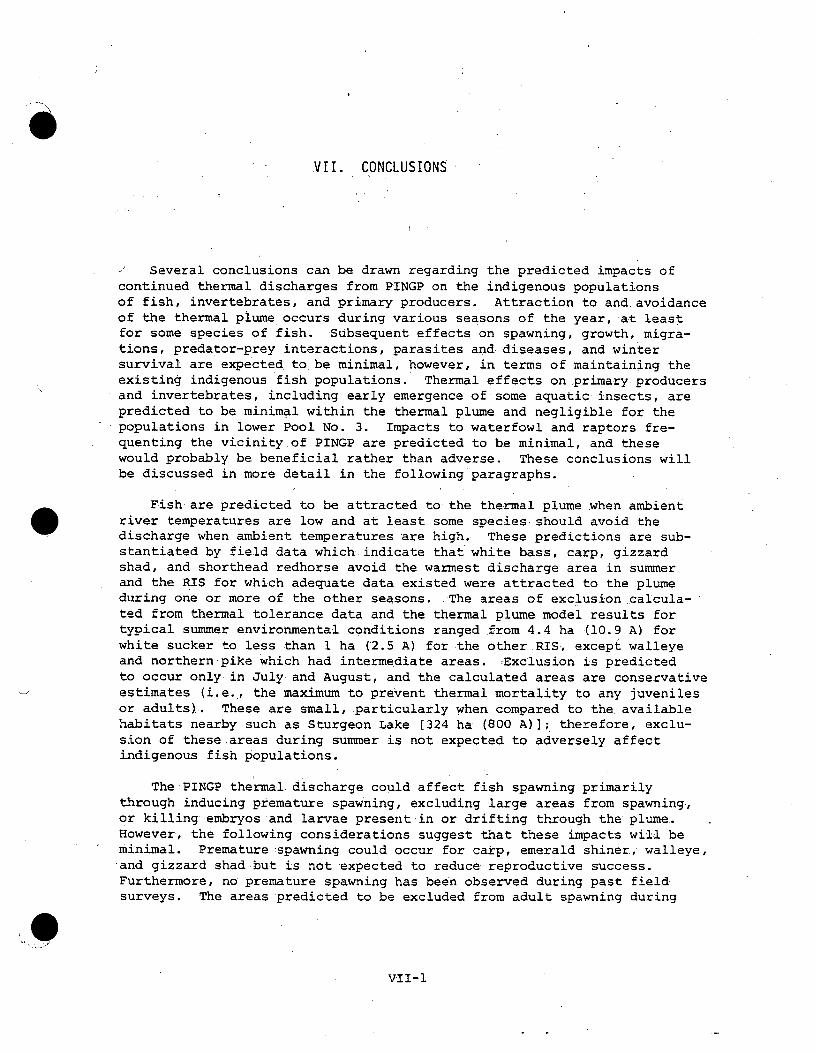
VII. CONCLUSIONS

Several conclusions can be drawn regarding the predicted impacts ofcontinued thermal discharges from PINGP on the indigenous populationsof fish, invertebrates, and primary producers. Attraction to andavoidanceof the thermal plume occurs during various seasons of the year, at leastfor some species of fish. Subsequent effects on spawning, growth, migra-tions, predator-prey interactions, parasites and diseases, and wintersurvival are expected to be minimal, however, in terms of maintaining theexisting indigenous fish populations. Thermal effects on primary producersand invertebrates, including early emergence of some aquatic insects, arepredicted to be minimal within the thermal plume and negligible for thepopulations in lower Pool No. 3. Impacts to waterfowl and raptors fre-quenting the vicinity of PINGP are predicted to be minimal, and thesewould probably be beneficial rather than adverse. These conclusions willbe discussed in more detail in the following paragraphs.

Fish are predicted to be attracted to the thermal plume when ambientriver temperatures are low and at least some species should avoid thedischarge when ambient temperatures are high. These predictions are sub-stantiated by field data which indicate that' white bass, carp, gizzardshad, and shorthead redhorse avoid the warmest discharge area in summerand the RIS for which adequate data existed were attracted to the plumeduring one or more of the other seasons. The areas of exclusion calcula-ted from thermal tolerance data and the thermal plume model results fortypical summer environmental conditions ranged from 4.4 ha (10.9 A) forwhite sucker to less than 1 ha (2.5 A) for the other RIS, except walleyeand northern pike which had intermediate areas. .Exclusion is predictedto occur only in July and August, and the calculated areas are conservativeestimates (i.e., the maximum to prevent thermal mortality to any juvenilesor adults). These are small, particularly when compared to the availablehabitats nearby such as Sturgeon Lake [324 ha (800 A)]; therefore, exclu-sion of these.areas during summer is not expected. to adversely affectindigenous fish populations.

The PINGP thermal discharge could affect fish spawning primarilythrough inducing premature spawning, excluding large areas from spawning.,or killing embryos and larvae present in or drifting through the plume.However, the following considerations suggest that these impacts will beminimal. Premature spawning could occur for carp, emerald shiner, walleye,

'and gizzard shad-but is not expected to reduce reproductive success.Furthermore, no premature spawning has been observed during past fieldsurveys. The areas predicted to be excluded from adult spawning during

VII-1

typical environmental conditions are less than 2.6 ha (6.4 A). The cal-culated areas precluding embryo development are 17 ha (42 A) for northernpike and 9 ha (22 A) for walleye.in May (end ofspawning period) whilethe areas are less than 7.6 ha (19 A) for the other RIS. Suitableý spawninghabitat for each RIS does not exist throughout these calculated exclusionareas, and adequate spawning areas exist nearby in both the backwater lakesand the main river channel. Larval fish drifting through the plume are notexpected to be thermally stressed. Thus, potential thermal impacts on spawn-ing and reproductive success are predicted to be negligible.

The potential for cold shock mortality exists at PINGP since fish areattracted to the plume in-winter and plume temperatures exceed the'maximumweekly average temperature (MWAT) recommended for protection of warm waterspecies from cold shock. The probability of an unscheduled trip occurringwhen the other unit is refueling is 0.55 so that cold shock would occur atleast once every 2 years. Based on field surveys at PINGP, gizzard shad wasthe most abundant species in the discharge although some white bass,- carp,and black crappie were present. Of the RIS, gizzard shad is. the most sensi-tive to cold shock, but any winter losses of this species are not expected toadversely affect river populations since it is a very prolific species andlarge winter die-offs normally occur when ambient-temperatures approach00 C (320 F).

Other effects on river populations are also expected to be minimal.Migrations, predator-prey interactions, growth rates, and the incidenceof parasites and diseases should be negligibly affected by- the thermaldischarge. Sport fishing may be benefitted through increased fishingsuccess in the discharge during spring.

Reanalysis of site-specific invertebrate and primary producer datashowed that impacts appear to be minimal or non-existent in most ofthese biotic categories. Only phytoplankton primary productivity, peri-phyton chlorophyll a, and macroinvertebrate species diversity for dredgesamples were found to differ significantly -between intake and dischargestations. These differences, however, most likely were not the result ofPINGP thermal discharges. Annual variations in water temperatures appearto regulate zoop-lankton abundances to some extent, but the -influence of-spatial variations (as between intake and discharge) was negligible. Tem-perature was not significantly related to phytoplankton, artificial sub-strate macroinvertebrate, or dredge macroinvertebrate densities.

Based on the predictive analysis of comparing invertebrate and pri&mary producer thermal tolerances with plume configurations, no mortalitiesare expected for phytoplankton, zooplankton, or macroinvertebrates' driftingthrough the plume. Most habitat in the discharge canal that is otherwisesuitable for aquatic macroinvertebrates, will not be rendered unsuitable asa result of high temperatures, except for small portions during proposedextreme environmental conditions. For instance, the area in the dischargecanal equivalent to approximately one to six percent of Sturgeon Lake maybe avoided by the macroinvertebrates, Hydropsyche and Macronemum (RIS).

VII-2

This does not mean, however, that these two taxa will be killed or evenexcluded from the discharge areas during extreme conditions, only that theywill be less common at higher temperatures than in other areas. Site-specific information for these two species during the unusually warm,low flow year of 1976 indicated that they did not avoid the dischargecanal.

A two-week acceleration of the emergence schedules for some aquaticmacroinvertebrates is predicted for the entire area of the dischargecanal (equivalent to about 5.7 percent of Sturgeon Lake). in an area of1.5 ha (3.7 A) which is 0.5 percent of Sturgeon Lake, a five-month accelera-tion of emergence schedules is predicted for Hydropsyche during typicalconditions. Early emergence, however, has not been observed to occur inthe past in the PINGP discharge canal; thus, little impact to most cate-gories of aquatic insects is expected from operation of PINGP.

Other predictive results indicate that warmer water areas of thedischarge canal may favor more thermally tolerant taxa, but these areaswould be insignificant compared to the area in Sturgeon Lake. Theheatedplume should not favor the encroachment or proliferation of nuisanceorganisms, such as blue-green algae; blooms of these phytoplankton haveoccurred seasonally long before PINGP became operational. Moreover, nofederally protected flora or invertebrate fauna will be impacted by thethermal discharge.

Finally, no impacts to aquatic macrophytes are predicted since theiroccurrence and distribution near PINGP appear to be more influenced byfluctuations in water level, sedimentation, and current conditions thanby temperature. Any losses of aquatic macrophytes that may result fromthermal discharge would be small. Suitable habitat for these plants inthe discharge canal is extremely limited in comparison to the total dis-tribution of macrophytes in Sturgeon Lake.

Eagles, waterfowl, and peregrine falcons are not expected to beadversely affected by the PINGP thermal discharge. Availability of openwater and a food source may even be beneficial.

Therefore, it is concluded that the thermal discharge resulting frompast operation of PINGP has not caused appreciable harm to any aquaticorganisms, and the protection and propagation of a balanced indigenousbiota has been maintained. In the future, the discharge plume is pre-dicted to cause neither appreciable harm nor adverse levels of impactto aquatic biota.

VII-3

REFERENCES

Allen, K.O., and K. Strawn. 1968. Heat tolerance of channel catfish,Ictalurus punctuatus. Proc. 21st Ann. Conf. S.E. Assoc. Game andFish Comm., 1967:399-411.

Altman, P., and D. Dittmer, eds. 1966. Tolerance to temperature extremes:animals. 'Part V. Aquatic invertebrates. Pages 81-87?in Environmentalbiology. Fed. Am. Soc. Exp. Biol. Bethesda, MD.

American Public Health Association (APHA), American Water Works Associa-tion (AWWA), and Water Pollution Control Federation (WPCF). 1975.Standard methods for the examination of water and wastewater, 13th ed.APHA, AWWA and WPCF. Washington, D.C.

Anderson, R.A. 1975. Thermal plume surveys. Pages 19-62 in Environmentalmonitoring andiecological studies program 1974 annual report for thePrairie Island Nuclear Generating Plant near Red Wing, Minnesota.Vol. 1. (Northern States Power Co., Minneapolis, MN)

Andrews, J.W., and R.R. Stickney. 1972. Interaction of feeding rates andenvironmental temperature of growth, food.conversion, and body compo-sition of channel catfish. -Trans. Amer.. Fish. Soc. 101:94-99.

Andrews, J.W., L.H. Knight, and T. Murai. 1972. Temperature requirementsfor high density rearing of channel catfish from fingerling to marketsize. Prog. Fish-Cult. 34:240-241.

Baker, A.L. 1977a. Primary productivity of the phytoplankton community inthe Mississippi River at Prairie Island. Pages 2.1.2-1 through 2.1.2-72in Environmental monitoring and ecological studies program 1976 annualreport for the Prairie Island Nuclear Generating Plant near Red Wing,Minnesota. Vol. 1. (Northern States Power Co., Minneapolis, MN)

Baker, A.L. 1977b. 1976 studies of the attached algae in the vicinity ofPINGP. Pages 2.2-1 through 2.2-62 in Environmental monitoring andecological studies program 1976 annual report for the Prairie IslandNuclear Generating Plant near Red Wing, Minnesota. Vol. 1. (NorthernStates Power Co., Minneapolis, MN)

VIII-1

Baker, A. L. 1976a. Studies of the productivity of the phytoplankton of Wthe Mississippi River at Prairie Island-1975. Pages 2.1.1-1 through2.1.1-35 in Environmental monitoring and ecological studies program1975 annual report for the Prairie Island Nuclear Generating Plantnear Red Wing, Minnesota. Vol. 1 (Northern States Power Co.,Minneapolis, MN)

Baker, A.L. 1976b. 1975 studies of the attached algae in the vicinity ofPINGP. Pages 2.2-1 through 2.2-59 in Environmental monitoring andecological studies program 197.5 annual report for the Prairie IslandNuclear Generating Plant near. Red Wing, Minnesota. Vol. 1. (NorthernStates Power Co., Minneapolis, MN)

Baker, A.L. 1975a. Primary productivity of the phytoplankton in the Missi-ssippi River at Prairie Island; the effects of heatedwater dischargeon the levels of production; and a turbidometric:analysis of massflow. Pages 299-362 in Environmental monitoring and ecological studiesprogram 1974 annual report for the Prairie Island Nuclear GeneratingPlant near Red Wing, Minnesota. Vol. 1. (Northern States Power Co.,Minneapolis, MN)

Baker, A.L. 1975b. Attached algae in the Mississippi River at PrairieIsland 1974. Pages 363-411 in Environmental monitoring and ecologicalstudies program 1974 annual report for the Prairie Island NuclearGenerating Plant near Red Wing, Minnesota. Vol. 1. (Northern StatesPower Co., Minneapolis., MN)-

Baker, A.L. 1974. Studies of the periphyton of the Mississippi River,:near PINGP-1973. Pages C-7.1 through C-7.40 in Environmental moni-toring and ecological studies program 1973 annual report for thePrairie Island Nuclear Generating Plant near Red Wing, Minnesota.Vol 2. (Northern States Power Co., Minneapolis, MN)

Baker, K.K. and A.L. Baker. 1974. Studies of the phytoplankton of theMississippi River, near the PINGP-1973. Pages C-6.1 through C-6.35in Environmental monitoring and ecological studies program 1973 annualreport for the Prairie Island Nuclear Generating Plant near Red Wing,Minnesota. Vol 2. (Northern States Power Co., Minneapolis,.MN)

Barans, C.A. and R.A. Tubb. 1973. Temperatures selected seasonally byfour fishes from western Lake Erie. J. Fish. Res.Bd. Canada30:1697-17.03.

Bardach, J.E., J.H. Ryther, and W.D. McLarney. 1975. Aquaculture: ithefarming and husbandry of freshwater and marine organisms. Wiley-Interscience, New York. 868 pp.

0VIII -2

Barker, N.A. 1935. Photosynthesis in diatoms. Arch. Microbiol. 6:141-

156.

Barnes, R.D. 1963. Invertebrate zoology. W.B. Saunders Co., Philadelphia.632 pp.

Baxter, R.M. 1977. Environmental effects of dams and impoundments. Ann.Rev. Ecol. Syst. 8:255-283.

Becker, C.D., and T.O. Thatcher. 1973. Toxicity of power plant chemicalsto aquatic life. Batelle Pacific NW Labs., Richland, WA.

Benda, R.S., and M.A. Proffitt. 1974. Effects of thermal effluents onfish and invertebrates. Pages 435-447 in J.W. Gibbons and R.R. Sharitz,eds. Thermal ecology. U.S.A.E.C. CONF. '730505.

Beyerle, G.B., and J.E. Williams. 1973. Contribution of northern pikefingerlings raised in a managed marsh to the pike population of anadjacent lake. Prog. Fish-Cult. 35(2):99-103.

Black, E.C. '1953. Upper lethal temperatures of some British Columbiafreshwater fishes. J. FisH. Res. Bd. Canada 10:196-210.

Brett, J.R. 1944. Some lethal temperature relations of Algonquin Parkfishes. Publ. Ont. Fish. Res. Lab. 63:1-49. Cited in Brungs, W.A.,and B.R. Jones. 1977. Temperature criteria for freshwater fish:protocol and procedures. EPA-600/3-77-061.

Brock, T.D.. 1975. Predicting the ecological consequences of thermalpollution from observations on geothermal habitats. Pages 599-622in Proceedings of a symposium on environmental effects of coolingsystems at nuclear power plants. CONF-740820; STI/PUB/378; IAEA-SM-187/9.

Brock, T.D., and J. Hoffmann. 1974. Temperature optima of algae living inan outfall of a power plant on Lake Monona. Trans. Wisc. Acad. Sci.,Arts and Letters 62:195-203.

Brook, A.J. 1971. Phytoplankton. Pages 1-9 in Environmental monitoringand ecological studies program 1970 annual report for the PrairieIsland Nuclear Generating Plant near Red Wing, Minnesota. (NorthernStates Power Co., Minneapolis, MN)

Brown, H.W. 1974. Handbook of the effects of temperature on someNorth American fishes. Am. Elect. Power Serv. Co., Canton, OH. 524 pp.

Brown L.A. 1929. The natural history of cladocerans in relation to tem-perature. I. Distribution and temperature limits of vital activities.Am. Nat. 63:248-264.

VIII-3

Brungs, W.A., and B.R. Jones. 1977. Temperature criteria for freshwaterfish: protocol and procedures. EPA Environ. Res. Lab, Duluth, MN,EPA-600/3-77-061. 130 pp.

Burns, J.W. 1966. Carp. Pages 510-515 in A. Calhoun, ed. Inlandfisheries management. Calif. Dept. Fish and Game.

Bush, R.M., E.B. Welch, and B.W. Mar. 1974. Potential effects of thermaldischarges on aquatic systems.ý Environ. Sci. Tech. 8(6):561-568.

Campbell, J.S., and H.R. MacCrimmon. 1970. Biology of the emerald shinerNotropis atherinoideF Rafinesque in Lake Simcol, Canada. J. Fish.Biol. 2:259-273.

Carlander, K.D. 1969. Handbook of freshwater fishery biology. Vol. 1.Iowa State Univ. Press, Ames. 752 pp.

Carlson, D.M. 1972. Responses of planktonic cladocerans (Crustacea) toheated waters. M.S. Thesis. Cornell Univ., Ithaca, NY.

Carpenter, E.J., B.B. Peck, and S.J. Anderson. 1974. Summary of entrain-ment research at the Millstone Point Nuclear Power Station, 1970 to1972. Pages 31-36 in L.D. Jensen, ed. 'Proc. second workshop on entrain-ment and intake screening. EPRI Publ. No 74-949-00-5. Electric PowerRes. Inst., Palo Alto, CA.

Cherry, D.S., K.L. Dickson, and J. Cairns, Jr. 1975. Temperature selectedand avoided by fish at various acclimation temperatures. J. Fish. Res.Bd. Canada 32:485-491.

Chu, C.K. 1968. Computational fluid dynamics. Vol. IV, American Insti-tute of Aeronautics and Astronautics, selected reprint series.

Clemens, H.P., and K.E. Sneed. 1957. The spawning behavior of the channelcatfish Ictalurus punctatus. U.S. Dept. Int., Fish and Wildlife Service,Special Scientific Report-Fisheries No. 219. 11 pp.!

Coker, R.E. 1934. The reaction of some freshwater copepods to high teL,.pera-ture with a note concerning the rate of development and relation to.temperature. J. Elisha Mitchell Sci. Soc. 50:143-159.

Corps of Engineers. 1977. Log of annual lockages. St. Paul. 2 pp.

Corps of Engineers. 1974. Reservoir regulation manual, Appendix 3,Lock and Dam No. 3. Mississippi River Nine Foot Channel NavigationProject, St. Paul District. 33 pp.

Coutant, C.C. 1975. Resistance of gizzard shad to instantaneous coldshock. Part III, Ch. 7. ORNL Environ. Sci. Div. Publ. No. 653,ORNL-5016:41-42. (Oak Ridge National Laboratory, Oak Ridge, TN)

VIii-4

Coutant, C.C. 1974. 4. Power plant effects. Pages 24-33 in Environmen-tal sciences division annual progress report for period endingSeptember 30, 1973. Part I, ORNL Publication No. 570. (Oak RidgeNational Laboratory, Oak Ridge, TN)

Coutant, C.C' 1972. Biological aspects of thermal pollution. II. Scien-tific basis for water temperature standards at power plants. CRCCritical Reviews in Environ. Control 3(1):1-24.

Coutant, C.C. 1970. Biological aspects of thermal pollution. I. Entrain-ment and discharge canal effects. CRC Critical Reviews in Environ.Control 1(3):341-381.

Coutant, C.C. 1968. The effect of temperature on the development ofbottom organisms. Pages 9.13-9.14 in ýBiological effects of thermaldischarges: annual progress report for-1967. USAEC Res. and Dev.Rep'. No. BNWL-714 Pacific NW Lab.

Coutant, C.C. 1962. The effect of a heated water effluent upon the macro-invertebrate riffle fauna of the Delaware River. Proc. Penn. Acad.Sci. 36:58-71.

Curry, L.L. 1965. A survey of environmental requirements for the midge(Diptera: Tendipedidae). Pages 127-140 in C.M.-Tarzwell, ed. Biolo-gical problems in water pollution. 3rd Seminar. PHS Bur. 999-WP-25.

Daggett, R.F. 1976. Zooplankton study. Pages 2.3.1-1 through 2.3.1-80in Environmental monitoring and ecological studies program 1975annual report for the Prairie Island Nuclear Generating Plant nearRed Wing, Minnesota. Vol. 1. (Northern States Power Co., Minneapo-lis, MN)

Davies, R.M., and L.D. Jensen. 1975. Zooplankton entrainment at threemid-Atlantic power plants. J. Water Poll. Control Fed. 47(8):2130-2142.

Dendy, J.S. 1948. Predicting depth distribution of fish in three TVAstorage-type reservoirs. Trans. Amer. Fish. Soc. 75(1945):65-71.

Dieterman, L. 1974. Water chemistry. Pages C-1.1 through C-1.78 inEnvironmental monitoring and ecological studies program 1973 annualreport for the Prairie Island Nuclear Generating Plant near Red Wing,Minnesota. Vol. 1 (Northern States Power Co., Minneapolis, MN)

Dieterman, S.M. 1975. A short-term impact study of the zooplanktonpopulation dynamics in Pool 3 of the Mississippi River near theNorthern States Power Red Wing Nuclear Power Plant (sic). M.S. Thesis.St. Mary's College. Winona, MN. 40 pp.

VIII-5

Duncan, T.O., and M.R. Myers. Artificial rearing of white bass, Roccuschrysops, Rafinesque. Unpublished data. South Central ReservoirInvestigations, Bureau Sport Fisheries and Wildlife, Fayetteville,Arkansas. Cited in Brungs, W.A.,. and B.R.* Jones.. 1977. Thermalcriteria for freshwater fish: protocol and procedures. EPA-600/3-77-061.

Eberley, L.W. 1977. Upstream-downstream water chemistry. Pages 1.2-1through 1.2-21 in Environmental monitoring and ecological studiesprogram 1976 annual report for the Prairie Island Nuclear GeneratingPlant near Red Wing, Minnesota. Vol. 1. (Northern States Power Co.,Minneapolis, MN)

Eberley, L.W., and S.F. Schmidt. 1976. Thermal plume surveys. Pages1.4-1 through 1.4-19 in Environmental monitoring and ecologicalstudies program 1975 annual report for the Prairie Island NuclearGenerating Plant near Red. Wing, Minnesota. Vol. 1. (Northern StatesPower Co., Minneapolis, MN)

Eddy, S. 1969. How to know the freshwater fishes, 2nd edition. Wm. C.Brown Co. Publishers, Dubuque, IA. 286 pp.

Eddy, S., and J.C. Underhill. 1974. Northern fishes. Univ,. of Minn.Press, Minneapolis. 414 pp.

Edison Electric Institute andUtility Water Act Group (EEI and UWAG),1977. Comments on "Draft interagency 316(a) technical guidancemanual and guide for the thermal effects sections on nuclear facili-ties environmental impact statement, May 1, 1977." EEI and UWAG,69 pp.

Faanes, C. 1975. . Ecology of wintering bald eagles near the Prairie IslandNuclear Generating Plant. Pages 2.7.3.1-1 through 2.7.3.1-24 inEnvironmental monitoring and ecological studies program 1975 annualreport for the'Prairie Island Nuclear Generating Plant near Red Wing,Minnesota. Vol 2. (Northern States Power Co., Minneapolis, MN)

Faber, D.J. 1967. Limnetic larval fish in northern Wisconsin lakes. J.Fish. Res. Bd. Canada 24:927-937.

Ferguson, R.G. 1958. The preferred temperature of fish and Itheir midsummerdistribution in temperate lakes and streams. J. Fish Res. Bd. Canada15(4) :607-624.

Fogg, G.E., and C.W. Reimer. 1962. Environmental requirements of planktonalgae and their effects on water quality. Pages 19-28 in Biologicalproblems in water pollution control. U.S. Dept. H.E.W.

Forney, J.L. 1963. Distribution and movement of marked walleye inOneida Lake, New York. Trans. Amer. Fish Soc. 92:47-52.

VIII-6

Frank, M.L. 1974. Relative sensitivity of different development stagesof carp eggs to thermal shock. Pages 171-176 in J.W. Gibbons andR.R. Sharitz, eds. Thermal ecol., AEC Sym. Ser. 32, CONF 730505.

Franklin, D.R., and L.L. Smith, Jr. 1963. Early life history of thenorthern pike, Esox lucius L., with special reference to the factorsinfluencing the numerical strength of year classes. Trans. Amer.Fish. Soc. 92(2):91-110.

Fuchs, E.H. 1967. Life history of the emerald shiner, Notropis atheri-noides, in Lewis and Clark Lake, South Dakota. Trans. Amer. Fish.Soc. 96(3):247-256.

Gammon, J.R. 1973. The effect of thermal inputs on the populations offish and macroinvertebrates in the Wabash River. Purdue Univ. WaterResources Res. Center, Lafayette, IN. Tech. Rept. 32. 106 pp.

Gammon, J.R. 1971. The response of fish populations in the Wabash Riverto heated effluents. Proc. 3rd-Nat. Symp. Radioecol. CONF-7105011:513-523.

Geis, J.L., and S.P. Gustafson. 1977. Progress report on the PrairieIsland creel survey, March 6 - November 21, 1976. Pages 2.5.3-1 through2.5.3-60 in Environmental monitoring and ecological studies program 1976annual report for the Prairie Island Nuclear Generating Plant nearRed Wing, Minnesota. Vol. 2 (Northern States Power Co., Minneapolis,MN)

Ginn, T.C., W.T. Waller, and G.J. Lauer. 1974. The effects of powerplant condenser cooling water entrainment on the amphipod Gammarus.Water Res. 8:973-975.

Goodson, L.F., Jr. 1966a. Walleye. Pages 423-426 in A. Calhoun, ed.Inland fisheries management. Calif. Dept. Fish and Game.

Goodson, L.F., Jr. 1966b. Crappie. Pages 312-3.32 in A. Calhoun,: ed.Inland fisheries management. Calif. Dept. Fish and Game.

Gustafson, S.P., and P.J. Diedrich. 1976. Progress report on the PrairieIsland creel survey March 1 - November 23, 1975. Pages 2.5.3-1 through2.5.3-35 in Environmental monitoring and ecological studies program1975 annual report for the Prairie Island Nuclear Generating Plantnear Red Wing, Minnesota. Vol. 2. (Northern States Power Co.,Minneapolis, MN)

Gustafson, S.P., and J.L. Geis. 1977. 1976 progress report on thePrairie Island fish population study. Pages 2.5.2-1 through 2.5.2-148in Environmental monitoring and ecological studies program 1976annual report for the Prairie Island Nuclear Generating Plant nearRed Wing, Minnesota. Vol. 2. (Northern States Power Co., Minneapolis,MN)

VIII-7

Gustafson, S.P., J.L. Geis, and P.J. Diedrich. 1976. 1975 progress reporton the Prairie Island fish population study. Pages 2.5.2-1 through2.5.2-13 in EnvironmenEal monitoring and ecological studies program1975 annual report for the Prairie Island Nuclear Generating Plantnear Red Wing, Minnesota. Vol. 2. (Northern States Power Co.,Minneapolis, MN)

Harnett, D.L. 1970. Introduction to statistical methods. Addison-Wesley Publ. Co., Massachusetts. 530 pp.

Hart, J.S. 1952. Geographical variations of some physiological andmorphological characters in certain freshwater fish. Univ. Toronto,Toronto, Ontario. Biological Series No. 60. Cited in Brungs, W.A.,and B.R. Jones. 1977. 'Temperature criteria for freshwater fish:protocol and procedures. EPA-600/3-77-061.

Hart, J.S. 1947. Lethal temperature relations of certain fish of theToronto region. Trans.; Roy. Soc. Canada. Ser. III 41(5):57-71.

Hawkinson, B.W. 1974. Progress report on the Prairie Island creel surveyMay 10 - November 5, 1973. Pages C-5.59 through 5.85 in Environ-mental monitoring and ecological studies program 1973 annual reportfor the Prairie Island Nuclear Generating Plant near Red Wing, Minne-sota. Vol. 1. (Northern States Power Co., Minneapolis, MN)

Haynes, C.M. 1976. Macroinvertebrate study. Pages 2.4-1 through 2.4-92in Environmental monitoring and ecological studies program 1975annual report for the Prairie Island Nuclear Generating Plant nearRed Wing, Minnesota. Vol. 1. (Northern States Power Co., Minneapolis,MN)

Hickman, M..' and D.M. Klarer. 1974. The growth of some epiphytic algaein a lake receiving thermal effluent. Arch. Hydrobiol. 74:403-436.

Hirayamo, K., and R. Hirano. 1970. Influences of high temperature andresidual chlorine on marine phytoplankton. Marine Biol. 7:205-213.

Hoffman, G.L. 1967. Parasites of North American freshwater fishes.Univ. of Calif. Press, Berkeley and Los Angeles. 486 pp.

Hokanson, K.E.F., and C.F. Kleiner. Effects of constant and diel fluc-tuations in temperature on growth and survival of black crappie.Unpublished data, U.S. Environmental Protection Agency, Duluth,Minnesota. Cited in Brungs, W.A., and B.R. Jones. 1977. Tempera-ture criteria for freshwater fish: protocol and procedures.EPA-600/3-77-061.

Hopwood, A.J. 1975. Monticello ecological studies program, macroinverte-brates. Pages 123-205 in 1974 annual report, Monticello NuclearGenerating Plant. (Northern States Power Co., Minneapolis, MN)

VIII-8

Horak, D.L., and H.A. Tanner. 1964. The use of vertical gill nets instudying fish depth distribution, Horsetooth Reservoir, Colorado.Trans. Amer. Fish. Soc. 93:137-145.

Horoszewicz, L. 1973. Lethal and "disturbing" temperatures in some fishspecies from lakes with normal and artificially elevated temperatures.J. Fish. Biol. 5:165-181.

Hubbs, C.L., and K.F. Lagler. 1964. Fishes of the Great Lakes region.Univ. of Mich. Press, Ann Arbor. 213 pp.

Huet, N. 1953. Cited in Meuwis, A.L. ,and M.J. Heuts. 1957 Temperaturedependence of breathing rate in carp. Biol. Bull. 112(1):97-107.

Hynes, H.B.N. 1970. The ecology of running waters. Univ. TorontoPress, Toronto.

Jensen, L.D., R.M. Davies, A.S. Brooks, and C.D. Meyers. 1969. The effectsoflelevated temperatures upon aquatic invertebrates. John HopkinsUniv., Baltimore, MD. Prep. for Edison Electric Inst. RP-49, EEIPubl. 69-900.

Jester, D.B. 1974. Life history, ecology, and management of the carp,Cyprinus carpio Linnaeus, in Elephant Butte Lake. Agri. Expt. Sta.Res. Rept. 273, New Mexico State Univ., Las Cruces. 80 pp.

Jester, D.B. 1972. Life history and ecology of the gizzard shad, Dorosomacepedianum (Le Sueur) with reference to Elephant Butte Lake. Agri.Expt. Sta. Res. Rept. 218, New Mexico State Univ., Las Cruces. 56 pp.

June, F.C. 1971. The reproductive biology of northern pike, Esox lucius,in Lake Oahe, an upper Missouri River storage reservoir. ReservoirFish. Limnol., Am. Fish. Soc. Spec. Publ. No. 8:53-71.

Keating, K.I. 1978. Blue-green algal inhibition of diatom growth: transi-tion from mesotrophic to eutrophic community structure. Science 199:971-973.

Kelso, J.R.M. 1972. Conversion, maintenance, and assimilation for walleye,Stizostedion vitreum vitreum, as affected by size, diet, and- tempera-ture. J. Fish. Res. Bd. Canada 29:1181-1192.

Kilambi, R.V., J. Noble, and C.E. Hoffman. 1970. Influence of temperatureand food conversion efficiency of the channel catfish. Proc. 24thAnn. Conf. S.E. Assoc. Game and Fish Comm. 1969:519-531.

King, R.G. 1974' The effects of heat water~discharge on zooplankton ina 4500 acre Missouri reservoir. M. S. Thesis. Univ. Missouri atColumbia. 78 pp.

VIII-9

Kititsyna, L.A., and O.A. Sergeeva. 1976. Influence of heating on size 0and weight in invertebrate populations in the cooling reservoir ofKurakhovska State Regional Electric Power Station. Soviet J. Ecol.7(5):475-477.

Kreuger, J.F. 1975. Thermal tolerance determinations for Lake Michiganzooplankton, July 1972-March 1973. Pages 39-120 in Evaluation ofthermal effects in southwestern Lake Michigan, Special studies1972-1973. Rept. to Commonwealth Edison Co. by Industrial Bio-TestLabs., Inc. Northbrook, IL.

Lopinot, A. 1960. Channel catfish facts in artificial lakes and ponds.Outdoors in Illinois 7(1).

Martin, W.J., and J.B. Gentry. 1974. Effects of. thermal stress ondragonfly nymphs. Pages 133-145 in J.W. Gibbons and R.R. Sharitz,eds. Thermal ecology. U.S.A.E.C. CONF-730505.

Mason, W.T.,.A.Q. Lewis, and J.B. Patterson. 1971. Macroinvertebratecollections and water quality-monitoring in the Ohio River Basin1963-1967. Off. Techn. Prog., Ohio Basin Reg. and Anal. Qual.Control Lab., Water Qual. Off., EPA. 52 pp.

McConville, D.R. 1975. Comparison of artificial substrates in bottomfauna studies on a large river. J. Minn. Acad. Sci. 41: 21-24.

McCormick, J.H. 1976a. Temperature effects on the growth of juvenile whitebass. U.S. Environmental Protection Agency, Duluth, Minnesota. Citedin Brungs, W.A., and B.R. Jones. 1977. Thermal criteria for freshwaterfish: protocol and procedures. EPA-600/3-77-061.

McCormick, J.H. 1976b. Temperature effects on white bass (Morone chrysops)embryo development, and survival of one-day-old larvae. U.S. EnvironmentalProtection Agency, Duluth, Minnesota. Cited in Brungs, W.A., and B.R.Jones. 1977.. Thermal criteria for freshwater fish: protocol andprocedures. EPA-600/3477-061.

McCormick, J.H., B.R. Jones, and K.E.F. Hokanson. 1977. White sucker(Catostomus commersoni) embryo development, and early growth andsurvival at different temperatures. J. Fish. Res. Bd. Canada 34:1019-1025.

McCormick, J.H., and D.F. Kleiner. 1976. Growth and survival of young-of-the-year emerald-shiners (Notropis atherinoides) at different tempera-tures. J. Fish. Res. Bd. Canada 33:839-842.

McGinnis, R., D. Zimmel, and E. Martin. 1978. Multiple linear regressionanalysis of Prairie Island temperatures versus Red Wing temperatufes.Unpublished report by Northern States Power Co.

VIII-10

Merriner, J.V. 1971a. Egg size as a factor in intergeneric hybrid. successof centrarchids. Trans. Amer. Fish Soc. 100(1) :29-32.

Merriner, J.V. 1971b. Development of intergeneric centrarchid hybridembryos. Trans. Amer. Fish Soc. 100(4):611-618.

Meyer, W.H. 1962. Life history of three species of redhorse. (Moxostoma) inthe Des Moines River, Iowa. Trans. Amer. Fish. Soc. 91:412-419.

Miller, E.E. 1966. Channel catfish. Pages 440-463 in A. Calhoun, ed.Inland fisheries management. Calif. Dept. Fish and Game.

Miller, E.F. 1972. Zooplankton study. Pages 50-97 in Environmentalmonitoring and ecological studies program 1971 annual report, PrairieIsland Nuclear Generating Plant near Red Wing, Minnesota. (NorthernStates Power Co., Minneapolis, MN)

Miller, R.R. 1960. Systematics and biology of the gizzard shad (Dorosomacepedianum) and related fishes. Fisheries Bulletin 173 60:371-392.

Minnesota Department of Natural Resources (DNR). 1977. MinnesotaFishing Regulations.

Minnesota Pollution Control Agency (MPCA). 1975. Minnesota's guide forbiological demonstrations for administration of 316(a) -nd .(b) of theFederal Water Pollution Control Act Amendments of 1972 and MinnesotaRegulation WPC 36(u)(3). 83 pp.

Mueller, K.N. 1977. Aquatic vegetation study. Pages 2.6-1 through 2.6-17in Environmental monitoring and ecological studies program 1976 annualreport for -the Prairie Island Nuclear Generating Plant near Red Wing,Minnesota. Vol. 2. (Northern States Power Co., Minneapolis, MN)

Mueller, K.N. 1976. Prairie Island aquatic vegetation study 1975. Pages2.6-1 through 2.6-13 in Environmental monitoring and ecological studiesprogram 1975 annual report for the Prairie Island Nuclear GeneratingPlant near Red Wing, Minnesota. Vol. 2. (Northern States Power Co.,Minneapolis, MN)

Muewis, A.L. and M.J. Huets. 1957. Temperature dependence of breathingrate in carp. Biol. Bull. 112(l):97-107.

Muraka, I.P., Project Leader. 1976. An evaluation of environmental datarelating to selected nuclear power plant sites. Div. Env. ImpactStudies, Argonne Nat. Lab, Argonne, IL. 54 pp. + Appendices.

Naplin, R.L., and J.L. Geis. 1975. 1974 progress report on the PrairieIsland fish population study. Pages 563-715 in Environmental monitor-ing and ecological studies program 1974 annual report for the PrairieIsland Nuclear Generating Plant near Red Wing, Minnesota. Vol. 2.(Northern States Power Co., Minneapolis, MN)

VIII-II

Nebeker, A.V. 1971. Effect of high winter water temperatures on adultemergence of aquatic insects. Water Res. 5:777-783.

Nebeker, A.V., and A.E. Lemke. 1968. Preliminary studies on thetolerance of aquatic insects to heated waters. J. Kan. Entomolog.Soc. 41:413-418.

Neill, W.H., and J.J. Magnuson. 1974. Distributional ecology andbehavioral thermoregulation of fishes in relation to heatedeffluent from a power plant at Lake Monona, Wisconsin. Trans. Amer.Fish. Soc. i03:663-710.

Neill, W.H., J.J. Magnuson, and G.G. Chipman. 1972. Behavioral thermo-regulation by fishes: a new experimental approach. Science176:1442-1443.

Niemuth, W., W. Churchill, and T. Wirth. 1972. Walleye: its lifehistory, ecology and management. Wisconsin Dept. Nat. Res.,Publ. No. 227-72. 20 pp.

NUS. 1976. Section 316(b) demonstration for the Prairie .Island NuclearGenerating Plant on the Mississippi River near Red Wing, Minnesota.Prep. for No. States Power Co. (NUS Corp., Pittsburg, PA)'

Omaha Public Power District (OPPD). 1976.. Zooplankton. Pages 5.1-5.41in Fort Calhoun Station Unit No. 2 environmental report. Con-struction permit stage. Vol. 3. Suppl. i. NRC Docket No. 50-548.

Omernick, J.M. 1977. Nonpoint source-stream nutrient level relation-ships: a national survey. EPA-600/3-77-105. Corvallis Env.Res. Lab., Off. Res. Dev., U.S.E.P.A., Corvallis, OR. 151 pp.

Patrick, R. 1969. Some effects of temperature on freshwater algae.Pages 161-185 in P.A. Krenkel and B.L. Parker, eds. Biological aspectsof thermal pollution. Vanderbilt Univ. Press,' Nashville, TN.

Peterson, S.E., R.M. Schutsky, and S.E. Allison. 1974. Temperature pre-ference, avoidance and shock experiments with freshwater fishes andcrayfishes. [Ichthyological Assoc., Inc.] Bull. 10. Drumore, PA.

Pitt, T.K., E.T. Garside, and R.L. Hepburn. 1956. Temperature selectionof the carp (Cyprinus carpio Linn.). Can. J. Zool. 34:555-557.

Priegel, G.R. 1969. Food and growth of young walleye in Lake Winnebago,Wisconsin. Trans. Amer. Fish. Soc. 98:121-124.

VIII-12

Proffitt, M.A., and R.S. Benda. 1971. Growth and movement of fishes, anddistribution of invertebrates, related to a heated discharge into theWhite River at Petersburg, Indiana. Water Resources Research Center,Rept. of Invert. No. 5, Indiana Univ., Bloomington. 94 pp.

Reutter, J.M., and C.E. Herdendorf. 1974. Laboratory estimates of theseasonal final temperature preferenda of some Lake Erie fish. Proc.17th Conf. Great Lakes. Res.:59-67.

Robach, S.S. 1965. Enviorn'mental requirements of Trichopter&. Pages118-126 in C.M. Tarzwell, ed. Biological problems in water pollution.U.S.H.E.W.

Ruelle, R. l i•71. Factors influencing growth of white bass in Lewis andClark Lake. Reservoir Fish. Limnol.,, Special Publ. No. 8 of Am. Fish,Soc. :411-423.

Schaeperclaus, W. 1949. Cited in Meuwis, A.L.,,and M.J. Heuts. 1957.Temperature dependence of breathing rate in carp. Biol. Bull.112(1) :97-107.

Schmidt, S.F. 1977. Water chemical analyses. Pages 1.1-1 through 1.1-73in Environmental monitoring and ecological studies program 1976annual report for the Prairie Island Nuclear Generating Plant nearRed Wing, Minnesota. Vol. 1. (Northern States> Power C&., Minnea-polis, MN)

Schneberger, E. 1972. The white sucker: its life history, ecology andmanagement. Wisconsin Dept. Nat. Resources Pub!. No. 245-72. 18 pp.

Schwabe, G.H. 1936. Beitrage zur Kenntris islhndischer thermalbiotope.[In German]. Arch. Hydrobiol., Suppl. Bd. 6(2):161-352.

Scott, D.P. 1964., Thermal. resistance of pike (Esox lucius L.),muskellunge,. (E. masquinongy Mitchell), and their F lhybrid. J. Fish.Res. Bd. Canada 21:1043-1049..

Scott; W.B., and E.J. Crossman. 1973. Freshwater fishes of Canada. Fish.Res. Bd. Canada. Bull. 184. 966 pp.

Seaburg, K.G., and J.B. Moyle. 1964. Feeding habits, digestive rates,and growth of some Minnesota warmwater fishes. Trans. Amer. Fish.Soc. 93:269-285.

Sherberger, F.F., E.F. Benfield, K.L. Dickson, and J. Cairns, Jr. 1977.Effects of thermal shocks on drifting aquatic insects: a laboratorysimulation. J. Fish. Res. Bd. Canada 34:529-536.

Shyne, J.T. 1977. Adult aquatic insect emergence from Pool No. 3 of theupper Mississippi River. M.S. Thesis. St. Mary's College. Winona,MN. 155 pp.

VIII-13

Wallace, N.M. 1935. The effect of temperature on the growth of somefreshwater diatoms. Not. Nat. Acad. Nat. Sci. Phil. No. 280:1-11.

Ward, F.J., and .G.G.C. Robinson. 1974. A review of research on thelimnology of West Blue Lake, Manitoba. J. Fish. Res. Bd. Canada31(5) :977-1005.

Weber, C.I. 1973. Biological field and laboratory methods for measuringthe quality of surface waters and effluents. Nat.:Env. Res. Center,EPA. Cincinnati, OH.

Weibe, P.H. 1971. A computer model study of zooplankton patchiness andits effects on sampling error. Limnology and Oceanography 16:29-38.

West, B.W. 1966. Growth, food conversion, food consumption, and survi-val at various temperatures of the channel catfish, Ictaluruspunctatus (Rafinesque). M.S. Thesis, Univ. AR, Tucson, ARCited in Brungs, W.A.,..and B.R. Jones. 1977. Temperature criteria forfreshwater fish: protocol and procedures. EPA-600/3-77-061..

Whitaker, J.O., Jr., and R.A. Schlueter. 1973. Effects of heated dis-charge on fish and invertebrates of White River at Petersburg,Indiana. Water Resources Research Center, Rept. of Invert. No.. 6,

Indiana Univ., Bloomingtoni 123 pp.

Yeh, G.T. 1976. Analytical three-dimensional transient modeling ofeffluent discharge. Water Resources Research .1. 12(3) :533-539.

Yeh, G.T., F.H. Lia, and A.P. Verna. 1973. Unsteady temperature pre-diction for cooling ponds.' Water Resources Research J. 9(6):555-1,563.

Yellayi, R.R. 1972. Ecological life history and population dynamics ofwhite bass, Morone chrysops (Rafinesque) in Beaver Reservoir. Part2. A contribution to the dynamics of white bass, vorone chrysops(Rafinesque), population in Beaver Reservoir, Arkansas. Report toArkansas Game and Fish Commission. Univ. of Arkansas., Fayetteville.Cited in Brungs, W.A., and B.R. Jones. 1977. Thermal criteria forfreshwater fish: protocol and procedures. EPA-600/3-77-061.

VllI-16

SECTION 316(a) DEMONSTRATION

FOR THE PRAIRIE ISLAND NUCLEAR GENERATING PLANT

ON THE MISSISSIPPI RIVER NEAR

RED WING, MINNESOTA

NPDES PERMIT NO. MN0004006

L. M. GROTBECK AND L. W. EBERLEY

PROJECT SUPERVISORS

ENVIRONMENTAL REGULATORY

ACTIVITIES DEPARTMENT

NORTHERN STATES POWER COMPANY

MINNEAPOLIS, MINNESOTA

AUGUST 1978

PREPARED BY

HENNINGSON, DURHAM AND RICHARDSON, INC.

ECOSCIENCES DIVISION

804 ANACAPA STREET

SANTA BARBARA, CALIFORNIA 93101

R"

APPENDICES CONTENTS

APPENDICES

APPENDIX

APPENDIX

A.

B.

APPENDIX C.

APPENDIX D.

APPENDIX

APPENDIX

APPENDIX

APPENDIX

APPENDIX

APPENDIX

APPENDIX

APPENDIX

E.

F.

G.

H.

I.

J;

K.

L.

DATA CATALOG

DETAILS OF NON-FISHERIES STATISTICALANALYSES

CROSS-REFERENCE TO STATE AND FEDERALREGULATIONS

CROSS-REFERENCE.TO REGULATORY AGENCYREQUESTS

GLOSSARY

CONVERSION TABLES

AGENCY COMMUNICATION

UNPUBLISHED OR OBSCURE REFERENCE MATERIAL

THERMAL DISCHARGE ANALYSIS

REGULATORY AGENCIES QUESTIONS AND ANSWERS

SPECIES LISTS

STATISTICAL ANALYSIS: DISCHARGE ELECTROFISHING STUDY

JOINT FREQUENCY TABLES: RIVER FLOW-BLOWDOWN RATE

THERMAL SURVEYS AT PINGP

A-i

B-i

C-I

D-I

E-1

G-I

H-I

I-i

J-i

K-i

L-I

M-I

N-i

APPENDIX M.

APPENDIX N.

APPENDIX A

DATA CATALOG

TABLES

Table Page

Water Quality

A-i. Weekly averages of river flows at Prescott and weeklyaverages of daily minimum, mean, and maximum rivertemperatures at RWGP. A-1

A-2. Monthly averages of river flows at Prescott and monthlyaverages of daily minimum, mean, and maximum rivertemperatures at RWGP. A-3

A-3. Monthly and annual cumulative distributions of dailymaximum river temperatures at RWGP. A-4

A-4. Flow and selected constituent concentrations for theMetropolitan Wastewater Treatment Plant effluents in1975 and 1976. A-6

A-5. Selected representative toxicity values for certainwater quality constituents found in the MississippiRiver at Lock and Dam No. 3, 1972-1976. A-7

General Aquatic Biology

A-6. Summary of adult and juvenile fish sampling near PINGPduring 1970 through 1976. A-10

A-7. Summary of larval fish sampling near PINGP. A-lI

A-8. Mean density of larval fish collected at PINGP.in 1975. A-12

A-9. Percent of total density for each RIS in the PINGP en-trainment samples collected in 1975. A-13

A-10. Reproductive characteristics of the fish RIS. A-14

A-li. Thermal data for walleye. A-15

A-12. Thermal data for white bass. A-16

A-13. Thermal data for channel catfish. A-17

A-14. Thermal data for northern pike. A-18

A-1i. Thermal data for gizzard shad. A-19

A-16. Thermal data for carm. A-20

i

Table Page

A-17. Thermal data for black crappie. A-21

A-18. Thermal data for emerald shiner. A-22

A-19. Thermal data for white sucker. A-23

A-20. Thermal data for shorthead redhorse. A-24

A-21. Food habits during various life stages for the fish RIS. A-25

A-22. Summary of sampling methods for non-fisheries biota col-lected near PINGP during 1969 through 1976. A-26

A-23. Ranking of benthic macroinvertebrate abundances at threelocations near PINGP during 1973 through 1976 for dredg-ing samples. A-33

A-24. Ranking of drift macroinvertebrate abundances (artificialsubstrate) at three locations near PINGP for 1975 and1976. A-34

A-25. Composition of orders of emergent aquatic insects col-lected from the Mississippi River near PINGP. A-35

A-26. Abundance and distribution of Hydropsyche spp. andStenonema spp. in 1975-1976. A-36

A-27. Life history and feeding habits of major invertebrategroups. A-37

A-28. Summary of macroinvertebrate thermal tolerances. A-38

A-29. Macroinvertebrate thermal data. A-41

A-30. Ranking of zooplankton abundances at three locations nearPINGP during 1975 and 1976. A-44

A-31. Summary of zooplankton thermal tolerances. A-45

A-32. Ranking of phytoplankton abundances at three locationsnear PINGP during 1970 and 1974-1976. A-46

A-33. Phytoplankton and periphyton thermal tolerances. A-47

A-34. Ranking of periphyton abundances at three locations nearPINGP from 1972 through 1976. A-48

A-35. Periphyton thermal criteria. A-49

A-36. Dominant species comprising major beds of submerged andemergent aquatic vegetation in the vicinity of PINGP. A-30

Biological Impacts of Thermal Discharge

A-37. Areas within various isotherms from the thermal plumemodel (Appendix I) for typical spring (May 1976) condi-tions. A-53

ii

Table Page

A-38. Areas within various isotherms from the thermal plume

model (Appendix I) for typical summer (August 1975)

conditions. A-53

A-39. Areas within various isotherms from the thermal plume

model (Appendix I) for typical winter (December 1975)

conditions. A-54

A-40. Areas within various isotherms from the thermal plume

model (Appendix I) for winter (January) proposed extreme

conditions. A-55

A-41. Areas within various isotherms from the thermal plume

model (Appendix I) for spring (May) prooosed extreme

conditions. A-56

A-42. Areas within various isotherms from the thermal plume

model (Appendix I) for summer (August) proposed extreme

conditions. A-56

A-43. Mean temperatures (C) at each discharge electrofishing

study station. A-57

A-44. Catch per unit effort (fish/5 min. run) at each station

for the discharge electrofishing study. A-58

A-45. Constants for the time-temperature equation. A-62

A-46. Data used in chi-square analysis. A-63

iii

FIGURES

Figure Page

A-1. Median resistance times for juvenile northern pike. A-64

A-2. Median resistance times for channel catfish. A-65

A-3. Median resistance times for gizzard shad. A-66

A-4. Median resistance times for emerald shiners. A-67

A-5. Median resistance times for white suckers. A-68

A-6. Thermal tolerances of macroinvertebrates collected nearPINGP. A-69

A-7. Thermal tolerances of zooplankton collected near PINGP. A-70

A-8. Thermal tolerances of phytoplankton collected near PINGPin 1969 through 1976. A-71

iv

Table A-1. Weekly averages of river flows at Prescott and weekly

averages of daily minimum, mean, and maximum riverriver temperatures at RWGP.

AVERAGE RIVER FLOW AVERAGE RIVER TEMPERATURE (FW 1959-1974AT PRESCOTT (CFS) , ' .

1928-1976 WATER YEARS DAILY MINLMUM DAILY MEAN DAILY MAXIMUM

7,708.98

7,339.34

7,225.15

7,174.02

7,099.16

7,237.80

7,520.71

7,414.34

10,572.80

9,303.06

12,145.74

19,058.00

25,535.21

31,902.23

41,044.88

44,447-32

38,903.51

33,368.15

30,584.25

29,034.46

26,800.12

25,585.12

24,410.03

23,599.21

24,275.94

22,745.10

zi1,531.30

31.83

32.00

32.00

32.00

32.00

32.00

33.00

33.00

33.57

35.71

36.00

38.71

36.81

38.71

41.84

46.24

49.77

53.22

55.3.

38.25

61.13

62.64

67.98

69.37

69.73

72.11

73.26

31.83

32.00

32.00

32.00

32.00

32.00

33.00

33.00

33.80

35.79

36.25

34.15

37.14

39.20

42.51

46.92

50.31

53.91

55.87

58.92

61.74

83.22

8.350

59.93

70.36

72.831

73.92

31.83

32.00

32.00

32.00

32.00

32.00

33.30

33.00

34.00

35.86

36.43

34.57

37 .57

39.61

43.10

47.57

51.18

54.64

56.43

59.80

62.37

53.88

69.04

70.46

70.97

73.42

74.43

A-I

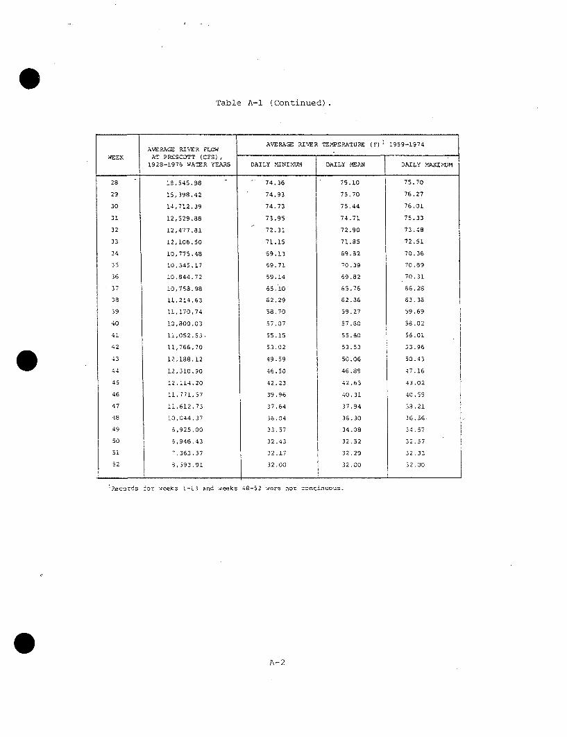
Table A-i (Continued).

AVE8ACZ RIVER TEMPERATURE (F) 1959-1974AVE.A(Z RIVER FLOW

WEEK AT PRESCOTT (CFS),1928-1976 WATER YEARS DAILY kIINIW.U4 DAILY MEAN DAILY MAXamJM

28 19,545.98 - - 74.36 75.10 75.70

29 15,398.42 74.93 75.70 76.27

30 14,712.39 74.73 75.44 76.01

31 12,529.a8 73.95 74.71 75.33

32 12,477.81 72.31 72.90 73.48

33 12,106.50 71.15 71.35 72.51

34 10,775.48 69.13 69.32 70.36

35 10,345.17 69.71 70.39 70.89

36 10,844.72 69.14 69.82 70.31

37 10,758.98 65.10 65.76 66.28

38 11,214.63 62.29 62.36 63.38

39 11,170,74 58.70 59.27 59.69

40 10,800.03 57.07 57.60 58.02

41 11,052.53. 55.15 55.60 56.0i

42 11,766.70 53.02 53.53 33.96

43 12,188.12 49.59 50.06 50.43

44 12,310.90 46.50 46.89 47.16

45 12,114.20 42.23 42.65 43.02

46 11,771.57 39.96 40.31 40.59

47 11,612.73 37.64 37.94 38.21

48 10,C44.37 36.04 36.30 36.56

49 6,925.00 33.37 34.08 34.57

50 6,946.43 32.43 32.52 32.57

3i 7,363.57 32.17 32.29 32.33

52 3,593.91 32.00 32.00 32.00

-. ecords for weeks 1-L3 and weeks 48-52 were not zontinuous.

A-2

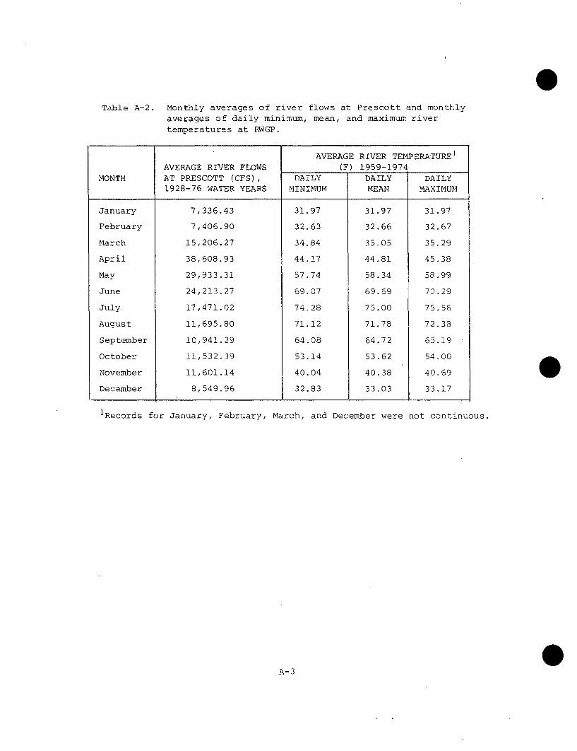
Table A-2. Monthly averages of river flows at Prescott and monthlyaverages of daily minimum, mean, and maximum rivertemperatures at RWGP.

AVERAGE RIVER TEMPERATURE]

AVERAGE RIVER FLOWS (F) 1959-1974MONTH AT PRESCOTT (CFS), DAILY DAILY DAILY

1928-76 WATER YEARS MINIMUM MEAN MAXIMUM

January 7,336.43 31.97 31.97 31.97

February 7,406.90 32.63 32.66 32.67

March 15,206.27 34.84 35.05 35.29

April 38,608.93 44.17 44.81 45.38

May 29,933.31 57.74 58.34 58.99

June 24,213.27 69.07 69.69 70.29

July 17,471.02 74.28 75.00 75.56

August 11,695.80 71.12 71.78 72.38

September 10,941.29 64.08 64.72 65.19

October 11,532.39 53.14 53.62 54.00

November 11,601.14 40.04 40.38 40.69

December 8,549.96 32.83 33.03 33.17

1Records for January, February, March, and December were not continuous.

A-3

Table A-3. Monthly and annual cumulative distributions of dailymaximum river temperatures at RWGP (1950-1976 plant logs).

TE1~AUE- PE'R<M, OF TINE~ TEERATURE EUALZ.0 OR E'X(--E:DEI

TEMPE PATUR, . . ..

JAN MAR : R MAY JUME JULY AUG SEPT OCT .;NOV DEC AMUAL

85 1OI I.O

84 i 0.0 0.1 .01

83 0.7 0 I 1 1632 2-1 13.3 1.2881 5.4 1 .9 61

so 0.0 15-i 5.3 1.72

39 3.4 23.9 9.9 0.0 283678 1,4 34.0 20.3 1.0 4.76

77 4.4 44-2 30.5 2.2 6.7676 7,6 56.0 39.3 3.0 3.30I i I I75 12.5 6 7.0 48.5 4. 11 .0

74 00 18 . 5 7 5 . 6 52.2 5.6 13.4

-3 0.1 27.1 34.0 72.1 7.1 15.372 0.2 36.6 89.6 30.6 10 18.0

.i- 46,3 93.8 86.7 '5-6 0,0 20.0

70 2I3 56.6 1 97.1. 915 22.5 0 22.2

I 3.5 1 63.3 1 98.2 94.4 27.1 .! 23.668 5.6 72.6 99.6 97.-3 34 .9 0.i 25.3

S 7.9 31.4 99.9 99.4 1 27.4

0.0 1..! 77 997 99 9 6 49.9 0,4 28.7

63 S0. 15.1 92.2 99-9 iO0. 58.3 -6 30.264 0. 04 939 1000 74 2.3 31.6

62 0 3 6. 9 .3 73. S i . 33.163 0. 3 -16.9 36 n i 73. A Ii

62 I 0.3 34.9 98-1 9 .9 8.o 34.7

I1 0.5 42.i 99.1 36,5 j '0.7 35.

610 0.6 301 99.5 92. L- 7.339 0.0 6.6 0 0.0 94.3 22.1 39.0

38 2.5 63.1 96.3 29.7 0739 . '8,0 3 6 4 9

A-4

Table A-3 (Continued).

PERCENT OF TIME TEMPERATURE EQUALED OR EX(--EED

TEIM!PERATURE I MAY J JtEY AUG SPT oct NoI DECJAN4 FEB N A PR __ MAY JM JUY AG SP C NV DC A'NA

56 5.6 77.4 I 98.7 41.5 0.0 43.1

.3 . 49.4 0.60 4.4

54 I 11. 84.5 99.0 55.5 0.9I 45.5

53 14.5 8.5 99.1 62.11 1.3 I 46.5

52 17.2 90.4 99.3 68.4 2.4 47.7

51 1 20.7 92.3 I I 99.9 73.0 4.2 43.7

50 I 5.8 93.6 100.0 81.3 6.7 30.2

49 29.3 95.4 85.6 7.7 51.0

48 34.2 96.0 88.7 8.7 51.9

47 37.3 97.0 j 91.1 11.1 52.6

46 0.0 42.9 97. i 93.21 5..5 53.5

45 0.1 48.1 98.6 98.3 1-9.3 0.0 54.9

44 0.4 54.8 ,99.3 99.4 24.5 0.1 36.1

43 0.939 9. ~,9. 6 29.6 0.2 57.0

42 1.2 63.3 99.6 99.9 36.8 0 5

41 2.1 69.3 99.8 I 1i00.0 42.5 0.6 59.0

40 I3.7, 73.9 99. '5111 0.6 6.

39 i 0.0 60. 78.41100' I S6. o.7 61..338aI 0 1 4 I o63. 6 1.3 62.7

0.4 1.0 34.0

37 0.7 16.4 36.2 70.0 2.2 64.1

36 . 5 39.9ii -15.2i 4.2, 65.7

35 0.0 2.4 37 .3 93•7, 79.9 9.3 68. 136.2 IB J

34 0.4 7.5 50.4 97.2 71: 18.

33 5. i 16.9 59i ~9 9.7 90.0 35.0 75.

32 99.6 9 1000 00.i 0 1 00.0 100

NO. 332 7 321 "4 802 774 S00 a 311 791 824

A-5

Table A-4. Flow and selected constituent concentrations for theMetropolitan Wastewater Treatment Plant effluents in1975 and 1976 (MWTP, unpublished).

MAIN EFFLUENT RAIN EFFLUENT ASH POND ASH POND1976 1975 1976 1975

PARAMETERAV

MAX MIN AVE MAX MIN AVE MAX MIN V MAX MIN AVE

Wastewater Flow, mgd 214 171 196 ,2 232 174 2021,2 3.0 2.56 2.852'3

Dissolved (Aygen, mg/l 3.5 0.8 2.6 4.3 1.3 2.8 8.1 3.3 4.3

Biochemical oxyyullirtand, mg/i 135 26 67 156 21 41 9.9 24 59 22.0 7.0 1 f7"

Aioflia, mg/o 14.9 9.2 12.3 14.9 7.1 10.6 17.9 '7.4 12.0 12.0 11.0 l- .0--

Nitrite and Nitrate, mg/I 1.24 .12 .38 1.11 < .08 .25 .366 .036 .186 1.41 1.18 1.3056

Total Phosphorus 5.5 3.2 4.2 5.1 2.4 3.5 2.7 1.5 2.1 2.0 1.8 1.95

pit 8.1 7.0 8.4 7.0 9.6 8.8 9.8' 8.84"

Copper, pg/l 250 60 130 120 30 70

Mercury, ag/I 1.3 0.3 0.7 6 < .2 1.5

Lead, g/il 140 <50 100 100 <50 '90

Zinc, pg/l 270 130 180 260 110 170

Cyanide, [ig/l 132 47 74 80 21 48

1L'esign flow, 218 mgd.

2I1hfluent.

3Three monthly values only.

Four monthly values only.

5T[o monthly values only.

6INO 3 on ly.

Table A-5. Selected representative toxicity values for certain water qualityconstituents found in the Mississippi River1972-1976 (from Becker and Thatcher, 1973).

at Lock and Dam No. 3,

TOX ICANT

Phenols

STATEPANDARD'

0.01

No Standard

0. 01

MEASUREDMAX CONC.NEAR PI NG PI

-0.01

0.U02

0.023

Ar cni Al

Coppo r

-.

U IOASSAYTEST

LEVELS'

0.56-0.75

0.06

0.05

0.5

0.43

0.1

0.06-0.5

0. 06-0. 125

0. 06

0.05

0.035

0.027

0.02?

0. 025

0.024

0. 013-0. 030

0.01

o. 0098

".005

0. 001

TEST CHEMICAL

SodiumA pentachloropAuenatg

PtjntachlorophInol Sodium salt

Sodium arsenite

Copter

COpp, A chloride

Copper Sul fate

Coppu r

tC'lpper ; uIfate

C'oJper (Cuo

Culppu r

Cop1peOr sulAfate

ORGANISM

Poncais anjnularis

'fish"

NotropiS athAAinoides

Lopxomis macrochirus

Pimephales proAlslaso

aOphAia AVLJna (ciadoceran)

Spiroq.)ra

Orconactes rusticus (crayfish)

Daphnuia mayna (cladoceran)

MiCrorega h•teroStoma(protozoan)

Dapinuia Aiacr)a (cladoceran)

PimAphajes pro-solas

CyplitnuS carpio

PimephSils pronelas

Phisia het.rosti opAha

(young snails)

Daphnia aýAyanF (cladoceran)

Nitzschia pulea (diaLom)

"hydra"

RESPONSE

Caused losses

Can be lethal under laboratoryconIditioins

Minimum lethal concentration,

100% survival in 120 m

48 hr-Tim

96 hr-TILn, chronic, hard water

Killed

Maximum non-inhibitory at 20 C

Acute toxicity threshold, young

48 hr-TIJll, acute; without food

Toxic threshold; 28 hr, 27 C

50% reproductive loss in 3 weeks,(tests at 18 C, pit 7.4-8.2)

Threshold concentration, ittmebi li-zation in 64 hAr; Lake Erie water,25 C

Threshold cuuceuLrtration sub-lethal;il•i~bilizatiou in 64 h., 25 C

Most died within 8 hr, soft water;w ith 1000 11J/L zinc

Growth decreased, minlimum

Sub-lethal concentrationsi affecting

growth and reproduction;hard water

96 Ar-Tas; hard water, 21.1 C

48 hAr-TIin, acute: without food

Prevents growth entirely

Damaged

Table A-5 (Continued).

'CCX ICOANT

Mercury

zh-

Anartoca .ý (N)

'11ASURECC IJIC(ASSAYANDAkC1

0. 02

'CAX CONC.NEAH ('1(303

0 .0 023

(C.) I W

TEST

0 .23 5

CO. 358

0.070

0J. *C2

2.5

1.1

Iu-2 .0

0.4-0.5

0.3

0.3-1. 0

0i. 29

0.2--0.4

0. 00

5.0

1.0

0.38

0. 53-,. .5

0. 432

0.26

0.24

0.2

TIST CIEMICAL

No dat -, -,

Zinc (ion)

Zinc sulfate

enkmonica (free)

Ammonia

(un-ionized)

Acnna•]n i a

Aactronia (free)

Anmmon ia

Ainon i a Cý (i -ion i zC!d)

A•nronia (f rte )

Sodium cyanide

Cyani de

(CN-)

Potassium cyanide

ORGAN I SM RESPONSE

Tubi2fex sp. Coligoclhaete worm)

Lepomtis a cSCrochlOrc

Gamb.sia affinis

"fist,

Ap C z.. enor~t p). Ca) yac)

St)Clatria sp.

PJjanazia app. CTurloellarianC

ACtinuspChaerium sp,. (protozoan)

cyneCu

I'Cngsa C.-eroc].li a (snail1)

L.OkxCCCs ,nCarochizuca

VapCCCia mugna cl adoceran)

Inhibited spawning and killed new fry

3 week-TI~ll, chronic, 18 C

16% reproduction loss in 3 weeks;18 C, pHi 7.4-8.2

Killed in hard water

Lethal level

Toxic level; toxicity dependent onpit and extent of ionization

1000 ain-Pum; 22 C, p1i 7.8(pit and temp. profoundly affecttoxicity)

lethal

Il

Complete disappearance

Lethal level

Lethal in hatchery ponds under warmtemperatures and low flows

7 day-Tin

Lethal level

Lethal level

Moderately effective as repellant(lake studies)

100% kill in 5-10 hr; 24-26 C,pit 7.0-8.2

100% mortality in 24 hr

Toxic; toxicity increased over1.2 to 25.4 C

96 hr-TAI, acute; with 3.9 mn/lzi.c C(Zn+)

Total kill in 96 hr

24 hr and 48 hr-TLm, acute

Toxicity threshold, 4 days at 24 CU. 16 Scenodesmus quadricauda (algae)l

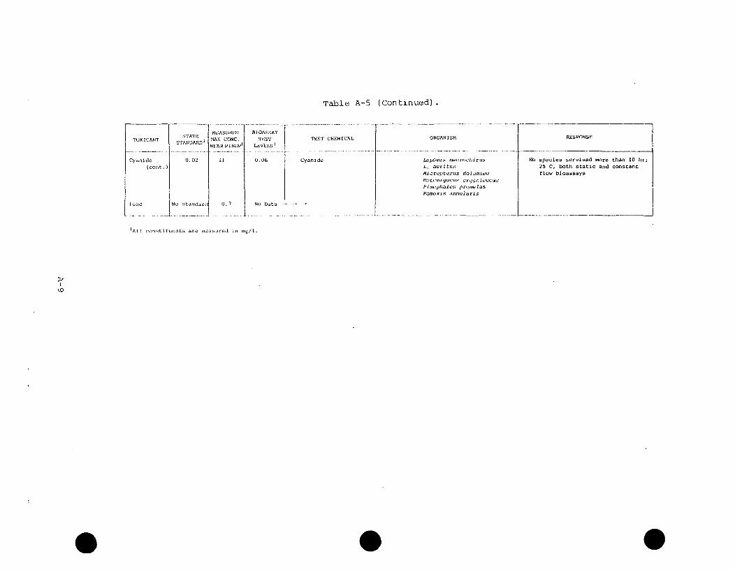
'rable A-5 (Continued).

STATE

STANDARDU7

0.02

- - -tandac-

MEASURLI)MAX CONC.lEAR PINGPI

i7

0,7

R]OASSAYTEST

LEVEISl

0.06

TEST CHEMICAL

Cyanide

ORGANISM

L, auritlsM~croptaxas dolomtoaiNotcmi gonus Crqsoh_•utjS

Pn,..phal1VŽ• promeniasPom)oxis .nnfularis

RESPONSE

No species survived more than 10 hr;25 C, both static and constantflow bioassays

NO Wt. - -.

'All conlstituents are iucasured in ingy/.

Table A-6. Summary of adult and juvenile fish sampling near PINGPduring 1970 through 1976 (from PINGP annual reports).

YEAR SAMPLING SAMPLING STATIONS INVESTIGASRS .EX.RKSOEThODS OFRQUEMICY SAMP LED

1970 Trap net. (fykel wit Ih Sa.- overight sets; Unspecified Miller of Mo data for

.0 ft wings fall (Sept to 2 O~t)-t St. Mary's su5aer trapsets College net

eln•trofishing: Summer (1-24 Aug) and Statton i230 o, I-phase AC fall (8-22 Sept)

Seine 1/4 in. Nesn) iot atecified Shores of Station I;beaches along mainchannel in pool No. 3

1971 rrap nets (Fyke) with Spring, summer, and fall Above Itk and Dam Miller of Trap nets nainly

10 ft wines No. 3 in Stations St. Mary's in Station i;1-4 Colle ;e some scales

take. for agingExperiment gill nets Sameer and tell- 24 Sr Above Lock and Dam

sets No.

Electrofisning: same Spring, suaner, and fall Unspetified.aS 1970

Seine Spring, ,are r, and fall Unspeoified

L972 Trap nets Summer and fail-52 sets Unsopeciied Miller ofin fall St. Mary's

Colle.gHOop nets Utnsecified tnspe-ilied

Sill sets Sosemer and fall--28 sets Uospeifiedin fall

Se~ine Unspecified inS pe ci id

1973 Trap nets 1 24-nr set/station in Settions - (10 nsa., aawkirnos of Sale samtriesSuoar (Aug) and fall (/ct) r 17 stan, Mn4 15: Min- .NR taken tsr

(7-8 stan aging; Suannrnlate July-Aua

Leoctrofitshig: 230 a. I l5-sin run/station n Seations 0 ;4 sta), and fal=Sept-

3-ahtse AC fall (6 sna), I ;4 sta), Octand iI b Sta)

Gill nets: 250' x 6' 4-Itaet/statton is fyi1 Snot-ats S ta.), Y

with 10' aetons of 1.3, Secpt 00d Sct) if stai and 1112. 2.5, 3, and 4 in. mesh 3 ata(

Seine: L/4 tn. -enh Suamoer and tall Selected stationsand 100 ft long .wah I8a to saitabli

It tag shnneline

Trawl Istter) Surer :Aug) antake and StashacqeSreas

Creel cnns-s Surceyed eatS 5ectlon Settlns I - IV Hawkissna oseveral imes fro- "l ay Mrinn. INR

otseaso o~is of for tovement-;1974 Trap nets 1 24-hr e/t nice n. ill Snepfarr-f 'JasL-tt - ogs St-d'

Irnt. SNt scals taKentor agin ;

tlectrosi'.ovkbg: sate i la-nit -na/sta rio eacS All StliAn Sring=ri-ji-e

is .971 staso so-e -iqht Summe-rJuls-AoS

suiokana also and F.allSepn -Dct'

3i11 tots; sa-e as 1373 1 24-h1 sot/station u- Sections 10 waa , engt-weizntv ,rrng Snd :1l1 3" na . :nd iII nd , on ition

3 Ota) factor

Seant. 503 a 4I' 'with Sy pri a, 3r-et, -nd fSlt 2-3 stanions/st-isn' a ag awith saitable

L/ in. tMtan ohartlit

T-ral a.tnsri Scring. na-1er, and fall 2 stations in section, a -d an ttakn _d

Sct)Srteyed eco section Soctuovs i - it ( taoiit -ndseteral ti-s 3C April to SUstafsos of

c 1e[ _ _ Sina. DNR

A-10

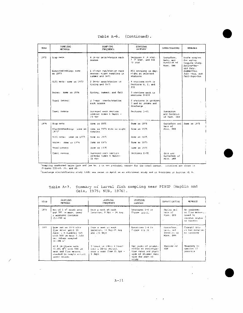
Table A-6. (Continued).

SAMPLING SAMPLING STATIONS.BAR METHODS FREQENC SAMPLED' INVESTIGATORS REMARKS

1975 Trap nets 4 24-hr sets/station each Sections 0 (4 sta), Gustafson, Scale samplesseason I (U sta) , and I1. Geis, and for aging;

(5 sta) Diedrich of tagging study;

Minn. DNR Sprieg=May-mid July,

Electroshockingt same 1 iS-min run/station each All sections in day; summer-midas 1973 season: night sampling in night at selected July -Aug. and

snmmer and fall stations Fall Sept-Oct

Gill nets: sane as 1973 2 24-hr sets/station in 4 stations each inspring and fall Sections 0, I, and

III

Seine: same as 1974 Spring, sumner, and fall 3 stations each inSections 0-511

Trawl (otter) 2 7-mnn trawls/station 2 stations in Sectioneach season 7 and at intake and

discharge

Creel census Surveyed each section Sections I-VI Gustafsonseveral times I March - and Diedrich23 Nov of Minn. DNR

1976 Trap nets Same as 1975 Same as 1975 Gustafson and Same as 197SGeis of

Electroshocking: same as Same as 1975 with no night Sane as 1975 Minn. ONR

19732 samples

Gill nets: same as 1973 Same as 1975 Same as 1975

Seine; same as L974 Same as 1975 Sane as 1975

Trawl (otter) Same as 1975 Same as 1975

Creel census Surveyed each seczbon Sections I-VI Gelis andseveral times 6 Mtarch- Gustafson of21 Nov Minn. DNR

!Sa.ling conducted below Lock and Dam No. 3 is not included, except for the creel census. Locations are shown in

Figures 111-i, 19, and 20.

2Discharge electrofishing study (DES) was begun in April as an additional study and is described in Section V1 A.

Table A-7. Summary of larval fish sampling near PINGP (Naplin andGeis, 1975; NUS, 1976).

SAIPLING SAMPLING r TATIONS

{EAR .TiTODS FREQUENCY SACTSEED

1974 Net of 1 T2 mouth area Once a week at each Locations L-4 in Naplin a Nod 30 saxonomy.;and 757 -m msh; towed location, 3 May - 26 AU f Figure 511-21 eLss of no -low meter.;

a measured distance finn. DNR towed at(50-250 m) various angles

to current

1975 Sae uet as 1974 with Once a week at each Locations 1-8 in Gustafs, Changed nets

flow meter *,ntil 30 location, 16 May-15 Aug figure 111-21 7-en, and in nid program;June; I n diameter net and 1-5 Sept Diedrich of no taxonomy

with 560 Ln mesh 3 July Minn. DNRon: volume sampled30-286 n3

42.5 cn square nets 2 .ours in every, 4 hours Bar racks of intake; Mueller of Taxonomy to(0.181 .

2) with 560 un over a 24-hr period, middle of recircula- NsP species if

mesh and flow meters; once a week from 25 Apt - tson canal and plant possiblestacked to sample entire 5 Sept Side of skimmer wallwater column also for part of

study

A-11

Table A-8. Mean density of larval fish collected at PINGP in 1975(data from Gustafson et al., 1976).

MEAN NUMBER LARVAE/m 3 + SE

STATIONS STATIONS STATIONS1 AND 2 5, 6, AND 7 1, 2, AND 4

(LOWER (UPPER (LOWERSTURGEON LAKE) STURGEON LAKE) STURGEON LAKE)

19-23 May 0.15 ± 0.02 0.11 0.06 0.10 0.03

26-30 May 0.64 0.20 0.01 0.01 0.42 0.22

2-6 June 7.80 3.11 0.32 0.21 5.32 2.90

9-13 June 0.50 0.17 0.12 0.02 0.34 0.17

16-20 June 0.54 0.01 0.06 0.02 0.36 0.15

23-27 June 0.25 0.07 0.04 0.02 0.17 0.08

30-04 July1 0.63 0.12 0.08 0.06 0.44 0.17

7-11 July 0.12 0.02 0.13 0.04 0.08 0.04

14-18 July 0.24 0.10 0.04 0.03 0.16 0.09

21-25 July 0.10 0.06 0.13 0.06 0.08 0.05

28-1 July 0.26 0.03 0.15 0.05 0.20 0.06

4-8 August 0.21 0.09 0.03 0.02 0.16 0.08

11-15 August 0.15 0.03 0.11 0.06 0.10 0.05

18-22 August NS2 NS NS

25-29 August NS NS NS

1-5 September 0.01 0.01 NS j0.01 0.01

1Changed nets.

-No sample.

A-12

Table A-9. Percent of total density for each RIS in the PINGP entrainment

samples collected in 1975 (NUS, 1976).

SPECIES

NORTHERN CHANNEL WHITE BLACK WHITE REDHORSE EMERALD GIZZARDDATE WALLEYE (:R

PIKE CATFISH BASS CRAPPIE SUCKER SPP. SHINER1 SHAD CARP

15 May 17.3 0.5 0.0 25.2 0.0 0.0 0.0 0.0 0.0 19.7

21 May 0.9 0.0 0.0 3.3 0.0 0.02 0.1 0.3 1.2 2.9

29 May 0.0 0.0 0.0 21.5 0.0 0.0 0.0 47.6 15.7 0.6

5 June 0.0 0.0 0.0 25.0 0.0 0.0 0.0 1.0 21.6 0.0

12 June 0.0 0.0 0.8 60.0 0.0 0.0 0.0 1.6 24.7 1.6

19 June 0.0 0.0 0.3 7.2 0.6 0.0 0.0 0.2 17.0 0.0

26 June 0.0 0.0 0.0 1.0 0.0 0.0 0.0 5.0 56.6 24.6

2 July 0.0 0.0 0.0 0.0 0.0 0.0 0.0 36.7 34.6 14.6

10 July 0.0 0.0 5.6 0.0 0.0 0.0 0.0 38.0 9.6 17.1

17 July 0.0 0.0 5.6 0.8 1.3 0.0 0.0 8.4 28.2 1.3

24 July 0.0 0.0 0.0 1.4 0.0 0.0 0.0 65.9 1.0 1.4

31. July 0.0 0.0 3.7 0.0 0.0 0.0 0.0 62.1 10.2 0.0

7 August 0.0 0.0 8.9 0.0 0.0 0.0 0.0 28.9 32.8 2.2

14 August 0.0 0.0 0.0 0.0 0.0 0.0 0.0 29.8 23.7 0.0

21 August 0.0 0.0 0.0 0.0 0.0 0.0 0.0 37.7 11.5 0.0

28 August NS NS NS NS NS NS NS NS NS NS

4 September 0.0 0.0 0.0 0.0 0.0 0.0 0.0 100.0 0.0 0.0

1Identification questionable.

Table A-10. Reproductive characteristics of the fish RIS

4.122..

S(lII N IN,

-j j-,..7

9,71211

I4I7N2211,3 ,,,1I.,'

(LII N 11921 71

O(lI.IINl17l111N

.1.112(1

N- -, I I ýp, , I ,(UN,: 33.1W

In-Na,, Al., L

012 • ls.;,I

LI..,",: N

(1.17•

N••,i• Ml 1.h179

(2,. N-I"

J4.0-2(1'

21. "

17- 27'

6-2(7'

112.1(,2?

.. 1'i

14. 8 /.9

I4I , 011 -I 3, ow7)

4110,1(7 -(79, (7.(

2,D.oov,

2 4 6/, 1

-0- 1 o. 11. ,

7(224*: h,7r42;-

1.0-4.u ,, 1(7,

111 11h(1 i w

I(NCU0J I'JN

47,4 c'

1ý6 ••Cb

.14I- I

177 (4-1, C '

1((-2 ,7

2,4 a.1( (0.1 I:

17-I 11 1,1-1 Ii'

l1'. 71,1. 194

0LNC2 .1 , 1(1.

I'Vdy -(d 7-d2rhll, 1974,

,,,. ]JS- 31C6

'Kill- , 196 1

'Eddy 1-d UW-1gl4

' 1. IWNMI

Itj-iN.. -d INNII

,,tI 19(77

44J1(t-.1, 1512,1,l 4 '

'EIddy -d U1d0-4 W, I I, ('74,

.22 0

"N24re2 71"14, CINNl,. 4974

E ,M},y t-ld WrO., hi I I, IW"4P.I,, 3-,1- Il

'. C1Nu--, ('4(7

"46,I12llzr, ((72(. 411',l.4L

IN 70y .41,4 I 1 1974,

1.I-I'4N4 ,llt (9h4.lu h I' I,7

N~It. 711 29 N44,l 91(7( 1~b: • uI 4117-4

Illiddy - ld U 1 41hilt, 1?7,1,

'324.IIIIN- 19'I

4241414l,2h1. (14(7.t.•t

1(7,,y2 ,,11 CI7NN1, 'il

1 -.9 ( I.u4' l=

Wh I L ,'•;ll•: kc,/

I.,.L. (7lfl i Jt,

174 1 33.1 .711,1

ill(7(7,.::

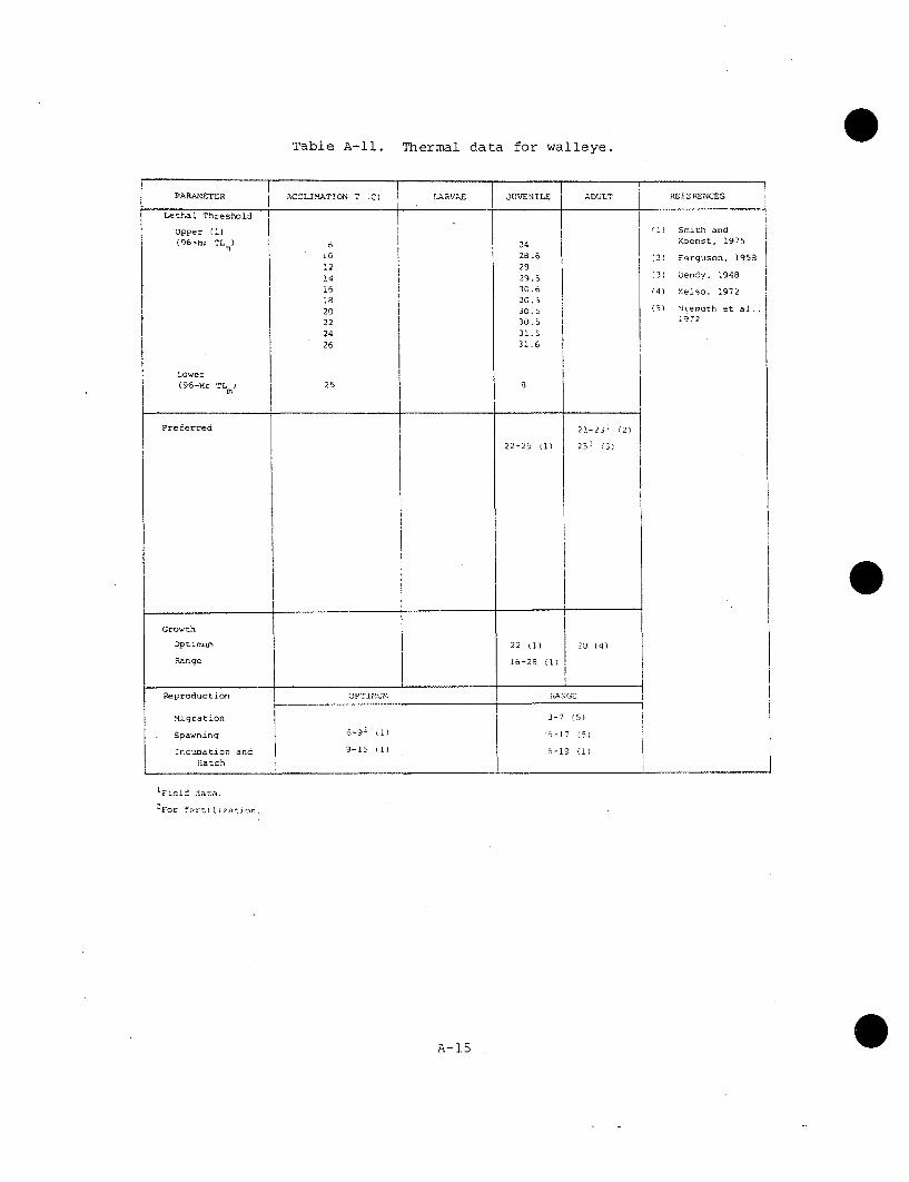
Table A-I1. Thermal data for walleye.

PARAMETER ACCLIMATION T (C) LARVAE JUVENILE ADULT REFERENCES

Lethal Threshold IUpper ý1) iI) Smith and(

96-Hr Lm 24 Koenst, 1975

I C, 2t.6 f2) Ferguson , 195 3

12 2914 ) 9 . (3) Dendv. 1948

16 ().6 (4) Kelso, 197220 30.5 (5) Iiemuth et al.,

22 30.5 197224 31.526 31.6

Lower(96-rTm 25

Preferred 21-231 (2)

22-25 (1) 251 (3)

Growth

Optimum 22 (1) 20 [4)

Range 16-28 (1)

Reproduction OPTIMIUM RANGE

Migration 3-7 (5)

Spawning 9-17 (5)

Incubation and 9-15 (1) 6-19 .1)Hatch

1Field data.

2For fertilization.

A- 15

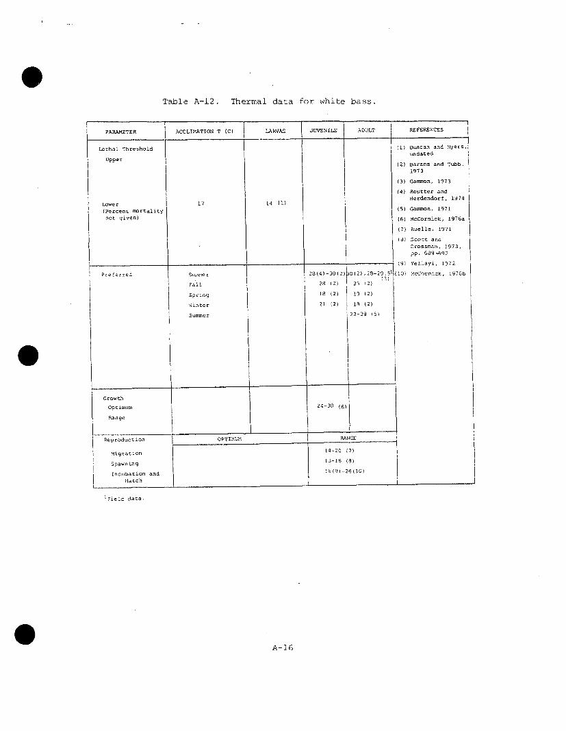
Table A-12. Thermal data for white bass.

'Field data.

A-16

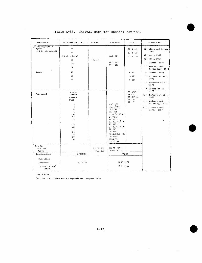
Table A-13. Thermal data for channel catfish.

IPARAMETER ACCLIMATION T (C) LARVAE JUVENILE ADULT REFERENCES

Lethal ThresholdUpper 15 30.4 (2) (1) Allen and Strawn(24-Hr threshold) 196820 32.8 (2) 196

25 (2), 26 (1) 36.6 (1) 33.5 (2) (2) Hart, 1952

29 31 (3) (3) West, 1966

037. fl) (4) Gammon, 197138.3 (1)

34 (5) Reutter andHerdendorf, 1974

Lower 15 0 (2) (6) Gamnon, 1973

20 3 (2) (7) Kilamrbi et al.,25 6 (2) 1970

(8) Peterson et al..

1974

(9) Cherry et alSummer 26-32(11) 1975

Preferred Sueme r 25 (5) (10) Andrews et al..Summer 30-321 (6) 1972Fall 25 (5)

32 (7) (1ll Andrews and2Stichrey, 197

5 17,152(8) (12) Clemens and6 18.9(9) Sneed, 19579 20.4(9)

10 20.6,18.3'(8)12 19-9(9)15 21.7(9ý

23.8,22.0 (B)

18 22.9(9)20 27.0,25.42 8)21 26.1(9)24 29.4(9)

25 30.2,28.91) ()27 29.5(9)30 30.5(9)

32.42(8)

GrowrhOptimum 29-30 (3) 2S-30 (10)

Rance 27-31 (3) 26-34 (11)

Reproduction CPTIMUM RAN7

migration

Spawning 27 (12) 21-29 (12)

Incubation and 24-28 (-2)Hatch

IField data.2Falling and rising field temperatures, respectively

A-17

Table A-14. Thermal data for northern pike.

PARAMETER ACCLIMATION T (C) LARVAE JUVENILE ADULT REFERENCES

LeUppe r 12, 12.6

is6,7

25

27.5

30

171.7

24, 26' (1)

25, 28' (1)

20.5, 231 (I)

(1) Hokansco et al.1973

(2) Scott, 1964

(3) Ferguson, 1958

(4) Franklin andSmith, 1963

(5) Swift, 1965

32.3 (2)

32.8 (2)

33.32 (2)

Lower < 3' (1)

Preferred 24, 263 (3)

GrOwth

Optimum 21 (1) 26 (1)

Range 18-26 (1)

Reproduction

Migration

Spawning

Incubation andHatch

OPTIMUMI.-

2.2-2.8 (4)

12 (1), 16 (5S

1.1-4.4 (4)

11-17 (4)

6-18 (i)

-At hatch and free swimmino1Ultimate incipient level

5Orass pickerel and musky, respectively

A-18

Table A-15. Thermal data for gizzard shad.

PARAMETER ACCLIMATION T (C) LARVAE JUVENILE ADULT REFERENCES

Lethal Threshold (I) Hart, 1952Upper 25 34.0-34.5(1(1 (2) Coutant, 197S

30 36.0 (a)(3) Reutter and

35 36.5 (1) Herdendorf,

1974Lower 25 10.8 (1) (4) Dendy, 1948

30 14.5 (1) (5) Gammon, 197335 20.0 (1) (6) Miller, 196020, 17.5 6.5 (2) (7) Carlander, 1969

Preferred Summer 19.0 (3)

Fall 20.5 (3)

Sumter 23-25] (4)

Sumner 28.5-31 (5)

Growth"

Optimutn

Range

Reproduction OPTIMUM RANGE

Migration

Spawning (0-21 (6) 10-29 (7)

Incubation andHarch

Field data

0A-19

Table A-16. Thermal data for carp.

PARAMETER ACCLIMATION T (C) LARVAE JUVENILE ADULT REFERENCES

Lethal ThresholdUpper 20 31-34 (1) (1) Black, 1953

(24-hr TLs 0) ( 1) 26 26 (1) (2) Horoszewicz, 1973i

25-27 40-41 (2) (3) Meuwis and Heute,

24 39 (3) 36 (3) 1957(4) Pitt et al., 19561

(5) Reutter and I

Herdendorf, 1974

(6) Gammon, 1973

(7) Neill andMagnuson, 1974

(8) Gammon, 1971

(9) Huet, 1953

(10) Schaeperclaus,

Preferred .0 17 (4) 1949

15 25 (4) (11) Tatarko, 1965

20 27 (4) (12) Swee and20 McCrimmon, 1966

25,30,35 31,31,32(4)(13) Jester, 1974,

Summer 29,7(5) 33-351 p. 38

20-22 30-33.5 (7) (6) (14) Burns, 1966,

Spring ( I 27.4 (5) Pp n10-513

Summer 27-341 (8) (15) Frank, 1974

Growth

Ootiaum. 20-25 (9), 27(10)

Range 16-30 (11)

Reproduction OPTIMUM RANGE

Migration

Spawning 19-23 (12) 16(13) -28 (12)

Incubation and 17-22 (14) 7-33 (15)Hatch Limit for 10 min. exocsure of earl-v r'o iS 35'.

-Field data

A-20

Table A-17. Thermal data for black crappie.

PARAMETER ACCLIMATION T (C) LARVAE J4VEENILE ACULTT REF-PRENCZS

t 4 4-Lethal Threshold

Upper(Ultimateincipient level)

29 33 (1)

Lower

(1) Hokanson andKleiner, undated

2} Fiaber, 1967

3: :;-1.. and:.!anuson; -974

-4) Reutner andHerdendorf, 1974

(5) N(eill et al.1972

(6) Zoodson, 1966b,pp. 312-332

(7) Scott andCrossman, 1973

pp. 745-75,)

Preferred2umer 1-20 (2) 2 (7-2933) 21.7 (4) ,29(5)

20-22 26.5-30 (3)

Fall 22.2 (4)

Winter 20.3 :4)

Spr~ng 21.0 (4)

Growth

Optimum 22-25 (1)

Range (i11,ts of 11-30 (1)

zero growth)

Reproduction

Migration

Spawning

Incubation andHatch

UPTIMUM

14 (6) - 20 (7)

150 percent catch/eflorr

A-21

Table A-18. Thermal data for emerald shiner.

PAPbMETER ACCLIMATION T (C) LARVAE JUVENILE ADULT REFERENCES

Lethal Threshold(1) Hart, 1947

Upper (1) 5 213.210 26.7 (2) Barans and15 28.9 Tubb, 1973

30.7 (3) Campbell and25 30.7 MacCrimeeon, 19701

.oer 1 '5 1.6 (4) MCCorcick and

20 5.2 KIeiner, 197625 8.0 (5) Reutter and

Herdendorf, .974

Preferred Summer 22 (2),25(3) 23 (2)

Fall 14 (2) 18 (21

Winter 11 (2) 9.3(5)6(21

Spring 15 ý2) 17 (2)

Growth~

Optcnu in29 (4)

Ran ge 24-31 4)

Reproduction OPTIMUM RANG

Migrati-onM~gratum,0-27Spawning -2 4

incubation andHatch

A-22

Table A-19. Thermal data for white sucker.

PARPAIETER I NC ~ - I LE1 ADLACCLIMATION T (C)

Lethal threshold

Uppe r 510

20 (2), 21 (1)25

25-26

2a' (1)31 (1)30 (1)

26.3 (2)

27.7 ' 2)

29.3 (2)

29. 3 (2)

29.3 :2)

2.5 (2)

31 (3)

2-3 (4)Lower 202125

(1) .McCormuzk er. 33[,

197'

2) Hart, :947

B3) 9rett, 1944

(4) Cariander, (969

(5) Schneberger,1972

(6) Brown, 1974

(7) Horak and Tanner,L964

(8) Reutter and

hendendori, 1974

(9) rerguson, 19,3

(10) Scott and Crossman1973, pp. 538-543

51, 4.82 (1)

6 (2)

Preferred Spring-fall 19-21 (7)

Fall 22.4 (8)

Sunieer 12-21 (9)

GrowhOptimun 26.9 (1)

Range 24-27 (1)

Reproduction

nigraton

Spawning

incubation andHatch

OPTIMUM RAN-

7.2 (5)

15 (1)

10-? (10)

6-23 '6)

3-21 (1)

!7-day 71L50 for swimup

27-day TL50 for nwely hatched

A-23

0Table A-20. Thermal data for shorthead redhorse.

Shorchead and golden redhorses

A-24

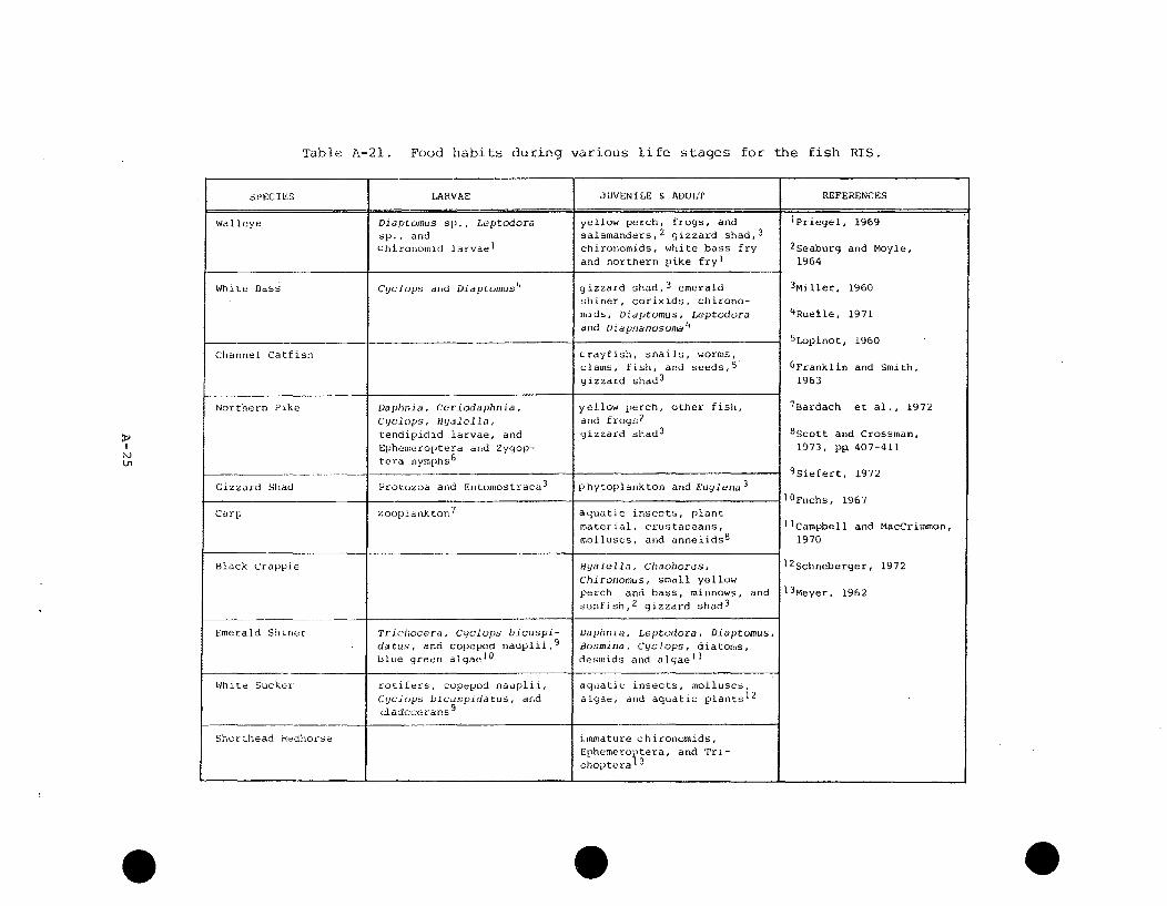
Table A-21. Food habits during various life stages for the fish RIS.

r'ii-n

SPECIES LARVAE JUVENILE & ADULT REFERENCES

Walleye Diaptomus sp., Leptodora yellow perch, frogs, and 1Priegel, 1969

sp., and salamanders,2 gizzard shad,

3

chironomid larvael chironomids, white bass fry 2Seaburg and Moyle,

and northern pike fry; 1964

White Bass Cyclops and Diaptonsus" gizzard shad,3

emerald 3Miller, 1960

shiner, corixids, chirono-mids, Diaptomus, Leptodora 4Ruelle, 1971and Di aphanososma

5Lopinot, 1960

Channel Catfish crayfish, snails, worms,clams, fish, arid seeds,

5 6Franklin and Smith,

gizzard shad3

1963

Northern Pike Daphnia, Ceriodaphnia, yellow perch, other fish, 7Bardach et al., 1972

Cyclops, 1lyalella, arid frogs2

tendipidid larvae, and gizzard shad3 8

Scott and Crossman,Ephemeroptera and Zygop- 1973, pp. 407-411tera nymphs

6

9Siefert, 1972

Gizzard Shad Protozoa and Entomostraca3 phytoplankton arid Euglena3

1 0Fuchs, 1967

Carp zooplankton7

aquatic insects, plantmaterial, crustaceans, lCampbell and MacCrimmon,molluscs, arid annelids

8 1970

Black crappie Hyalella, Chaoborus, 12

Schneberger, 1972Chironomus, small yellowperch and bass, minnows, and

1 3Meyer, 1962

sunfish,2 gizzard shad

3

Emerald Shiner Trichocera, Cyclops bicuspi- Daphnia, Leptodora, Diaptomus,datus, and copepod nauplii,

9 Bosmina, Cyclops, diatoms,

blue green algae1 0 desmids and algae

1 1

White Sucker rotifers, cupepod nauplii, aquatic insects, molluscs,Cyclops bicuspidatus, and algae, and aquatic plants

1 2

cladocerans9

Short head h<dhorse immature chironomids,Ephemeroptera, and Trm-choptera 13

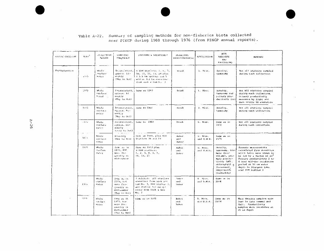
Table A-22. Summary of sampling methods for non-fisheries biota collected

near PINGP during 1969 through 1976 (from PINGP annual reports).

150I AIýR E CULLI9l TI U11 SAMI I.JW0 bTATIUN 05 5 CAl 1032 ph PIJOIJPAI 29(9

PROCESSING

L ookNPl y to l nk t ii selil iict

wr fttO

I,,, -,I Is L,:, lt,

ulpr-n h -wit Lily(May Ui, Olt)

i %-9

9 III 111k 010 "1i, 7.to, H1, 22, 23, 2H Ilit.I S.', i k. yiv -i -,

.iui 111 1.2 kol luoi.,v-I-

r-l~ll Lock & I)-n N-.. I

U. M- il,. Ltsttti ty,taXCOhiOny

Not all stations dampled

during each collection

1970 iholc rlolj Lutlnt, Sa.. ao 1969 Brook U. e.ill, lbunsi ty, Not all statioils sampled

u-rf.ce i|ppox. hi-- taxolnoy and duritln eactk Collecti•rnwatr weekly p(ila-y pro- Privury produtvivLty

(Msy to (N)t) ductivIty (DO) si-asurcd by light and

duck bottle DO evUlution(

l19l1 Wlniel Inioisis tetL, _ui_ as 1969 eBt'ok LI. Mi la. Density, Not 1ll stationl sample

lton t.5:- illo0

. I-, Lasnotnly durilg eac:lt voll-ction

outer utllY(May to Olt)

(912 Whole Inionsistent sutw a.s 1969 Brook U. Minn. Samii, as in Ikit all stations stamiled

nittfac:o - oi .bi- 1971 during each collectiotn

wator weekly(.lily to loL)

Whole blowely .1nO,- a. 1)t19, plu. ItluR Baker U. Mill-. Santn as ItI(991 ailt'ioc (Cle, to Ntin) S1iii onl 16 -0lik 19 a(ld andO Ud .N1. 1971

autoe, Sadks

1914 WItul. S-. lto, Is (197 plu( Baker U. Mimt. 92xandity, wIsonaa taiu-enteI.1ts

5u-f- j 19/3, but 13 11th Litit..il oil and U.N.il. LaonptOiy, Lie- calculated Cfro dc-isttiosware. -- fr,- i, 2. 3, 4, 5, 9, Biker -usa (buo- which later -ere shown to

epli-itly SIe 14, 19, 27 volaut), ltrI- bU low by a factor of 103m•id-,,ttnl~isc Ir'y prodiUt- Irilli4a•y productivity 2 to

tivity (WO), 4 hour iteid-day incubationcilucoritytl a petiod at 50 -m water(Loea~nani) , dep)thl in Sturgeonti Lake

nusnj-ntoids ti!ar IIDUI Staioit1 8

(turbidi ty)

Wh1le 1 atti al in Ba kh"!ote.); all titltis hukie U. MOint, Saln, as in,

curfaci 1971, lot .hwiur ft'oill kock ail- Iid ai-d U.NJ.I. 19741919 w tile rn')/ ifro- tit* No. 3, DilR s.tatlion 2, Baker

clu,. ly ill seh Stoti-oI 5.1, k)nllI-

Rliid-i•-ts[uni r i Vle" ftrolt Iohk 4 Duill

(May to Di-o) No. 3

9 it. SaIll, at, i

199), bie

qli~l [ 1y ill

nld-us sinc(Mal to Wkv)

auil- as ii, 197% Bake

Bakor

U. Mtnil.

and U.N.I.Salu as in1 914

Maty denisity 5anlles were

lost in late suilnatr andfall. ProductivitysdampLes were incubated at

25 um depth

________ -e 4

Table A-22. (Continued).

A

LI IUJ'JC CATLGORtY

[19/21

1974,

COLIZC'l'Ill

Il id-o

S."i, aI, for

1927,

SJAMI5'I.NGFREQUJENCY

Biotrskiy

Idol to Non'

W- ,kf lto3t o -7.I) -

1oktOd~

S'T-ATIONS LOC'1ATIONS'

4 1701 slati/ils 7, 17.

24, atd 25

Sa 1972, plU 1 -jiltl -na 8los 1(, 13. 1nd2'L); -titaund icv-frc, por-ods antdioat io01

Sat~ as in 1973, pt-s 1

otatioli ]oa.t , d Jos-than i.llý dowtli viifrot Lonk and DaM No. 3

c-Ott in 1974, le-s

tt -tot dtultttlvir from

Li.k aid Don, Nu. -

s-O as on 1975

SLio 4 tfarnsects I,,ostio-s A to G W titit1.04 1, , Ld diwsirin nor

fron Lock ,id Ua- tO. N

oSI- Ltt 197U

Upriver from Lock andDi No. 3 tIt o ead ot

Stutigeon LWke

PRINC17IPAL, A''LA'O

INVES'r1IAOIUi(*)

1:1(0, olOnllta 1So t.ttlSt/DaIsies Sectnott

NSI,

Oaker U.N.l.

DA'£AANALYS IS

AND1Pl4.CESSING

piq-nst anal-

ysis of:hloroldhyll a

and phato-phyttin a bylafr 0 ntzenn lthod

Sa•l a. 1972,xcefpt. with

addition ofIlottsity Std

tattinttfly

1973 Ltopttno phane-pbty titt a

Satin',-tti 1974,

,'byti, i -(-tnimoo It Iniao,

Sa17 a5 in1975

5l.MARIKs

Slide were staled for

ell coutttt and ta-oltomy,b 1t lnft utartalysod outil

nett year bocau,;o of

Catge itf cottsulltaitts.Slides h eld ill plesiglals

floats suiJiotdnd atappro1ip.tnly I - 2 ncdethlt, Witth -rtCial

orientation to mWirtktinsilts at io~t.

D-ittity Itd tasottotly fto

1972 sa.ltpl.s wore alsodetentntved. SlId, ontlyWith t -0,jtt.tt groott weno

.elected tor -nl1

comllti,,q.

-or7 1 dyotOlr (,--i it-lI:. itrq; l I t.Ji.ciq

liti-ti•,naJly ob-nrvod but liAt

r-o, dod.

will... -.tJeled o sýaC rphytos,

1).N,.

0191 7 t o' tttr4 0U)N.1 I.

U, N. II.I ~7i 1S t 74as t ~

c:'Ifo~ 1/tot, VlS Y

Mtllmr

Miller

Vest

St. Mary's T.''atOtty -J0

College Dad lizt

1.1)13photuyr•1hy

Ind obsoer-

boI.t-"byboat

11.171•:;1 : St. Mary'sC11t ItIq

St. Mary's

CI I 1nIc

hod 'i..

nIdoltl id

bod size

Table A-22. (Continued).

co,00

,YlL C L IOEA R idL L l. 'l N cA S LMC A I S T A T IO N S ' L 3 0A ' I M S N • S I l' A L A TABsIOTIC CAT•(ý) RY EIAP TAIN A.S5MRW

I AND

PROCESSING

AqUlLlC 1974 Otnoinaot IUI CU to lillir:di at plant sitL. Mite týr NtA, Inosn-itly anI PI-Lt w.r- elassifind a

K, otphy L-,, a lI Co. Ie0 Aumj -4 at I tCfmley, in.in iver bed size aub..rged and eergýrntL.(Citjinu•sJ l.ion by tot 2 ips hale. nI siovellines and

boat and 1- 2 - ok i ,aI-d' from Lo- k jaldwailing, p anD No. 3 to lanit iitakn

rakiay,_,,, nita, Sturtoor Lake

walking9

]13 Na1,. as JUly I; Appiroxinlatly Cth 5,15 Man!1-e NSP MTaxonomny and Only submelrged plasls

1174 Auj 6 an in 1974, ell olt bed si.e studied*ait 4, Omnsien~OI of upper

X 23 Sturgonli Lake

19/6 S-lO an Jaune 4, 7, San. is in 1975 M-ellt- NSV Tlaxonony and1974 3, II; bed size

July 30>;A Uly IllSAg 13]

D-l No.3

I1 ) " 1 19 , 2AI '- iw t ly , ,1 1 4 - iL tt ri ý, i , 4 , M i l l e - S t . NK l r y ' s I kin s i t y a n d J a n e tn o n y t o g e nu s

SInti ,lseil " dalnil€ •ire- 3 3(:t,d Iils r 2%, olar|,, Coii •• t xlle nta o omy a u t

t L- liki J-i .ye dlt-td -a , IV h tl 4O I linit -

Ila No. _3i

Ci A, iiI " eular to thit lakt: ais;

nnLllaisit'iil I ('tAnJlolil i tIk• l neetI

areol lakerio 111)kta 'hoe .t .,{tifi olat La i,,-,!; ili

lioai lane ittaketittt- 1511!ants. I:pi- Stliti Iii 1, enttciditig,:at , i aw,,rri tins• r'iv,.rtsltniisi:l

iii 1970)1

1772 19 n sxtin 55 Satins an in £930 Miller St. Mtary's tblnsity ard lonoyto o i~ei55 inlQ,)l, 1970 Col Iege taxo-lolny -mllly .as.sIithi-•tgh

"WI kCoilj-"

1L. sitk e-

sý.t tae

Table A-22. (Continued).

- -I 0 1

[aLOTIC CAW'lWt1Y YEAR )COLLECTION

METHOD

SAMPLING

FF1,2UENICY

STATIONS & LOCATIONS2 PXINU IPAI.

INVEITIOA'ltilllSlAFFI L)•TIDI)

DATAANALYSIS

ANDIIJIOESSING

REIMARKS

I- I 1 .i

opl tink torn(Continue~d)

1974

Can I rairdtl40t ll-!

pl11anlc 1,1

to, I'll

and,, lecttinci

I'ltll; atan

-ah ltat'icnlii tra9ilirrian

sorqiKrcmm,L

1, I't-tI

wit sti joi

[itota v)u

0-ilr gh 1141(1

Ell L1 It a i nnil

.,mp 1974lam.

s30i-2Liilll

1972

as tor

Apr to ftc;[litolirsi 5 te nit

"molnthly";and til Ka Oionml

tOll ntt'd

July 30,Any 14,

Scpt 4,

Nov 21, and

Appro xitrat ly

whl l rli lyd

f rtl,p ii

to ily 9 A,;

cllaia thadl-ll LI I

4 I112 St.tialsr .1 ,12,25, 27 plus I ini1•idi attlydowlirivor fruom lck aduoi

Da01, No. 3. 4 trarakn tLs-an, as it, 1971 i1,

Stury-n Llake vlci-lty

3, 3-statitio tialr-1-ts

il. iturauco LakeCa 'ri-spolldij riough ly

to RIOR Stltirln 1, 1,eind 0; 2 HIdR 1taLians

(1 anid Il); 3 atatiansat thi north ar-d ofStar 4rl0' Lake; I IHDR

t4UII. (i10) - HDR1)

statlai, (14 .rid 10)ft- critl 11i0nc; t saliqlhl-;cl:pthr jiltc'giattd Lit

intakc b t tir.1h airI[ III

B JID4 l tatwlll : G, Wi,

14, lh, 18, 21, 24,

f5 arid otlc Ut,LtilOlwn thin 1.6 ki driowni vtroi Lock arId 0am No. 3;,lirl a i'ilnoci stat 1011i

-ait: a, in 1974

Middlebirook

NiddLna~r~oo

St. Mary'sCoilegc

St. Mary's

NSP

Ecollogy

Consul tLa ts,

Inc .;NSIP

Density aridtamOrlorny

Density andtaxonomy;iitility

feirsity andtax roromy ;

Rolt I Ii ty

Taxonomy to sljrCwcs dInmany cases.

River and lake florpatterns studied by dyndispersion; variation in

density by depth casstudied in recycle canral.Night sanplalcs were alsocollected iii recyclena ll.

Excellent taxonomy

0

Tabl.e A-22. (Continued).

u7

to

2 1 - 2 DATA13 1U T l C C A T E U A ,) y i Y E A R < C O L L E C T I ON S A W ' L I N G !1 S T IA T I O N S 6 [IX X :A TP I ( N SP I ' C P LA F L A I ' O N L S •I t A K

SL'YHiC CATSIy IStEl ý1jlcl AFFILIAT1i0iN ANALYSIS REMARKSSi2'1TIOLC V".U9NCJY i lN VINVES'IGATCIC(9) AND

pROCESSING

(&.CC C. i IIedI) DOz-C NOt • t ie 197(5 C c traiCl- sL~iC t dCow ICCCrC r from ii975;aCSCC~t , t-t lonoy

sC Lnpi m.C9t to May I k• Oa' C aCC NC. I InC.

9olICCCCC at 1917 0IC- 1tCd (U -;Ct.CtCiCCe ach stat OCio iCI ail

CCCa• as CCC

M O- CC[ CC0C-CCCCC OCC0C. 1C CI, , 119CC, S tat SCCCC at 1970 Miller St. Mary's Ounsity Cwhere PrelimC iary studies

i-,cCCtebCwt9s CdCC (dCC I wiC ICl Aj, ...oCpIanktoC Col[eg, 3 quantitatise)

1 9199CiC 1.0); -c .C SIoJL, -Cd taxonoCty

CC•CCC tat t y -C C

Ib td t r LCCS tlkCow foC

11, fu-C.Ib]ae)Cnd1,71 CCCC Conete ;CtC U Cia) 5nea Sta'tl~ ICCCSCC 19 IC Mi ller 2t. Cry' C L Manlity (whCCCC Maw artificial saD-

CCCCIt bCCIC;C S•CtC.stCCe! CCCI lI59C foas~ible) "aCCl SteateC Ca~eritr~nt

blocks CCoCCiC to.u.aCny

( L)h bIock for 30 dayc

iO a 11) a S CtCCvai iCC

, CCCCCQLC- lc - tree

CJICeLaioCC ..CC~ t CCIC.-

CC S Ct C'CCa l

9-972 SatC a '0).! , y 12 teaiCLCCCt, CCCCC;OC Mii-c St. Maryy's S unsity

1971 'C -Cit l,> ", VCt -- r C.C--1a ] wi th 2 CoiteCJ IIantitatvc

l'CUCr ,OCl 1C ' ILC- s LCtio • Ca,, troll, sa. Iplls) Laid

,I e:cd , o- U fi t 'tI ) -,ib- hiICaw•tia .i of StUrC9 ,CC ta otomCO y

CC9,CCC CtC b l CkC to wCCithi 1.2 kICo

hCC9dr•iiv froCC I.-Ck and•;,Jll~i :;I':• )w m{ Nt). 3; 'Is" iIDJR

Am) •,hiy C OC7, 2I , 9, wit ,l .25 l,

ACIC CCCCCC I C~tCCCC .2 CC

dCCCCCvC r if LCCk ujC

Table A-22. (Continued).

DATA

BIOTIC CATEGORY YEAR COLLECTION SAMPLING STATIONS & LOCATIONS 2 PRINCIPAL A ANALYSIS W"KARKS

METHOD FREQUEoCY INVESTICATOR (s) AFFILIATION AND

PRO0CESSING

Macro-invertebrates(Continued)

173*I I Ar tifi cia ls ubsi I"' tins

I) con,:rete 5

balsa w.od(as ie 191.1)2) concreteblock (31.6x11.6b8 a",approx. 18 k )

(Blitt, 1955);drudge:1) P'tto•soti(15 ci:i •q ?

(22.9 cm s.?)

Qualitativeobse rvat ionon naturalsubstrateLs

Artificialsubs trate:uncertain

Drcdge :initiated in

Oc t, repli-cates (?),Once/mre when

and wherepossible.Randomlycollecteduntil Oct.then once a-sith

Sali as in 1972, {4lusHDR stations 12, 15, 18,and 21 for artificialsubstrates

Dredge at HDR stations1, 2, 10, 20, near 28,27, 12, 15, 18, 21, 25,

and 3 stations andwithin 1.6 km downriverof Lock and Dam No. 3

Qnal itative samplingalong shoreline wherepossible, or after Oct at

shoreline locations near

HDR stations 8, 15, 18,21,

2 7; L upriver approx.

6.4 kll from Lock & DaisNo. 3 and 2 within 3.2 km

downriver from Lock anidDam No. 3

Mil ler andMcConville

St. Mary'Col leuj

Desnsity

(quanti-tative) ardtaxltonoty

Mostly experieirmntal;mansy artificial sub-strate saulnles lostduo to weather orvandal isms

1 1 *t 1- f I +

1974 UV light

traps

Qua itaLt ivcobse ratliollof naturalri t5) t r a ton•

Quanti tative1) 22.9 cms6q. Poeunand 15 smsq. peteL -on

1 i"d gqes

TIraps emptiedevery 2-3days froutabout May 13to IDrc 1

Apr 19, Jneie

22, Aurj 31,Oct 12

Onice /1eebelil a.id

who Ce i CC -l•-errmi tting

Near 31D0 stations C(along shore) , 12, 21,and 25

Same as in 1973

3 1DR stationts; 15 and 18

(a & b) (Ponar); Ii HDRstationsr 1, 2, 5, 6, 10,12, 21, 25, 26, 27, aridtneat 26, and twostatlions within 1.6 kin

downrivur frot Lock anid

Dam No. 3 (Puterson)

Shyne

S istinee

St. Mary'sCollege

St. Mary'sCollege

St. Mary'scol lege

Taxonomy andrelativedensity ofemergent

insects;Taxonomy

Lensity andtaxonomy

Problems with collection,praservation,and storage

0

Table A-22. (Continued).

DA 'rAiiiiLI.CATECTYItliN SAMiPI.1NGj Ž'tATIiNS A91) [LiCAi'|'iiiS? ikllNCII'Ai ANAl.YSIS

bIOTIC CATE(;C~kY YE1.11 MWIIIOD kIETIQULNY INVE S ,TATIION A NDOiIAAAN

P I-JCF2:SSING

Mdccouiivertu-i.E ir Lii ii

1,141i2EiiiE.

iSiS

Eid

NJ

;il.k l1i1i.ii

ii 19713

LA- Lii I L iii

fil Iu hLo n,

L•i ti ii,

"I'd h-ad

i , i kiEL] f

(.tk), 1L t Lii:

] iLi C E I. VIib

iii. 3 ; o' dr,-3t2mm ]2. Eh•il

diji liiidii

piiskum q irt

di[. i~tih

iuin9 . fi

Lmii,iy, 1:71 Ž)

iii dm5 ii iii-

1e -- v t t in

'i.)iL~c. t i e-

I-y, ,li -y,

3Veil, ,ii ik:atv

ŽL Is,)dch

t-pl i"O.y

Li-45 idys

e mis ISIg~+t i

tiuii Ni'l ii~~u

uVy 45 dliy..

lii's, y 45i dmays

l~ui IiL ftiiuiiqh

tSoii

S l a t t i lu b dL. , i l i iL , liismbuLi-i, Y[1mi.

Si iitik] it 11DR s~it hiii,15, 18i i1, Ž5, 2 iid

1 ), i , il• l 5' ,I'.f',,, Lk,:t, it 14)R 4 tut--l , 10, 12, 15,3 ]

8 Il)H tatons b,10,12.

U Ui, 1, Ž5, 26, 27

ii SEL2 ,iis 25.

b l11yiii t

E-: I -3y

I

iCoiisul EtiiES,I

lire.x

ld it ftin:S

trimEe.uu~ii

, t.Em1 eicu

iktiusi ty amdta..lo-y

Tcmx.i o my

ikusu i Ly mnd

t a o"."my

lal Ly .. dtaxonomy

AiiLouyI~simL15 A,

_____________________ S __________________ ~ ~ I. - L

i -ulijE I iejui i l, m ioii io Eidiliits2" 127/3 Sal, itiiiL 2 iri iiiii + 19i 4

"ti,,, Liiji iIu lt-2L lir l- iti i,

Table A-23. Ranking of benthic macroinvertebrate abundances at three locations near PINGP during

1973 through 1976 for dredging samples. Diversities and evenness indices are also

included.

________________________________________ - t19731 9*14

1976 19i/ 19"•4

MACFINV1111BRA-1.

1)1 i qnnchaeta

(Onyrnnltunmd wclrlrL-)

'n .1n fi 79d- 1

N,ý,at,,d, (-"."Id wu,-•)

Uthid,''lti fwd •pi,,

.1.27~+O• joinI-

il"'. •li", I'{'.-

W-1- f03i1.1-1 - t717id. sli').

Lt.h:tno toI It.ot-

:2.,1,0, 45717 017r.1.1.

FALL'

74°SUM',-• T - T - <-Z - WI 'rrh774 FAIL SUMMER FALL A'JMRL I

[T- l~Mý 1. tIT197ý

FALL

FT.II) U U I UI1

U U I V U IjU

Y4

U)

tOJL

2.20

76

3

2

2 .1

63

1.43

AAb

l J_

1

2

2 .41

.7_i-t.

2 l

42I2 22

1.95

2

.3

L 212 2

2

28:

III .,,I

.'4

1 .62

3.7

1..6-F, 1101 1. 42

.37.21 .61

I L 6 .1 -~. I. ... I - 1 .1 - I. - 3 .. ~. 1 2 - .1 I I I J I + I I I I I I I .• • 1 l I L 1

KAy: Abundanc1, 1 1.0-. : 10-99; 3 100-991; 4 1,000-9.999 ror -oi.,7/ 2

j, i, 1974 -nd J973 o-9/dll; n .oampl.; blnk lndicatnA E- orga77i5mn fond

'JS01 1l y ",, I llid-.1u l

'A+,u-11 Y l lll~ l '7 l

I'IIa l lCJ 10-.,1: , y I) .1 1.1 1,5ryI 1

- 17 11. 1 II -, 12, y Wk :31 L 1,,. n2lj

/L1 - 15 J- 1 In fn llty f-r 27 l1 3-- 1039 1..

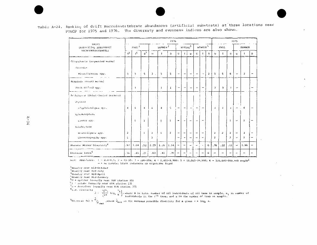
0Table A-24. Ranking of drift macroinvertebrate abundances (artificial substrate) at three

PINGP for 1975 and 1976. rmhe diversity and evenness indices are also shown.

locations near

1976 1975

DR IFT

(ARTIF'ICIAL SUIIS'1 ATnRAC ROIi NVE RTEB R1ATES

Nal i d.,

mjjCwflaunc'oos sn'.

N2 ma odia (round wo rms)

Oln Jo t 1ifi d sip.

ArtI, 1o.... ia (Joil t- to,.ted anliiml a)

Lph1 1,otIlil pt1(0ra

Ca4;211 IS PP

tici, sop t ra

No Sf00i 2pa a sill.

0:1,1110 t~15 gSCll Spil.

Shannon lnýaver Divursityl

I~rns lnd00X9 10I I.1 .2 .2 *

4

2

4

L

2 I. 2 3

S2-12

3

3

2.29

2

1.14

2 1

2

2 2

2

3

2

L A1. 6520 •76.-22 .111

1. 96

1:6 1 .45 1 .21 .62 1 - 42 1 - - I0

Koy: 1l1u)dalul00 1. 0.0-9.9i 2 = 10-99; 3 = 100-

9 99; 4 = 1,000-9,999; 5 = 10,000-99,999; 6 I00,0100-999,999 org/m

2

- Ito szim5lf ; blank indicatLs tic organisms found

IUsu.•lly bear llid-oct•lblr?Uaually near mid-.july

3Usuall.y (lar Imid-April

usually nleac Iid-January5U1 = privvt- (usually olar HDI station 10)61 = intakt (usuelly near 11Dk station 12)71- ,= dowIiilvel (usually near HDR stationf 27)

8S iq. W -Leth y - r' s.I" Ild1 L 1- 0 9 2 where N is total nuiinbe of all individuals of all taxa in sample, si is ntier of

I individuals inl thi ijtO taxa, alnd s is tde number of taxa in sample.

9E~v loes (L-) ý I /d- lax ,where d, is the maximum possible diversity for a given s = 1092 s.

Table A-25. Composition of orders of emergent aquaticinsects collected from the Mississippi Rivernear PINGP, 13 May through(from Shyne, 1977).

6 December 1974

ORER/FAILY HDR STATION 6 HDR STATION 12

NUMBER PERCENT NUMBER PERCENT

Trichoptera

Hydropsychidae 151,277 81.89 9,155 52.26

Psychomiidae 13,406 7.26 4,228 24.14

Leptoceridae 7,240 3.90 1,171 6.68

Hydroptilidae 12,801 6.93 2,960 16.89

Other 4 * 3 *

Total 184,728 100.00 17,517 100.00

Ephemeroptera

Caenidae 740 51.75 2,980 86.85

Ephemeridae 670 46.85 439 12.80

Other 20 1.40 12 0.35

Total 1,430 100.00 3,431 100.00

Diptera

Chironomidae 440,602 99.13 71,581 98.69

Other 3,888 0.87 947 1.31

Total 444,490 100.00 72,528 100.00

*less than 0.10 percent

A-35

Table A-26. Abundance and distribution of Hlydropsyche spp. (Trichoptera) andStenornema spp. (Ephemeroptera) in 1975 and 1976 (from Haynes,1976; Texas Ins., Inc., 1977).

ARTIFICIAL SUBSTRATE (No. /m 2 )

DATE Hydropsyche sp3p. Stenonema spp.

U 1 S152 13 Di If BS U SL I Di. B

October 1976 2.7

August 1976 8

July 1.976 3,542 129 48 105

,Tune 1976 65 59

March 1976 54 2.7

April 1976 8.1 2.7

December 1975 27 27

November 1.975 351 3.6 27 75.6 72 72

September 1.975 67.5 10.8 10.8 10.8

August 1975 4,657 4,320 124 1,608 3,996 162 173 67.5 43.2 119

July 1975 5,724 75.6 359 65 173 35

May 1975 10.8 5.4

1 1DR Station 10 (Upriver)2 1DR Station 6 (Sturgeon Lake)

3HDR Station 14 (Intake)

"11DR Station 21 (Discharge)5HDR Station 25 (Barney's Point)

Table A-27. Life history and feeding habits of major invertebrate groupscharacteristic of the Mississippi River, lakes, and creeksnear PINGP.

S GROUP

Ephemeropteral

PlecopteraI

Trirhoptera.

Coleoptera1

Dipterar

Oligochaeta2

Hirundinea2

:METAIIORPHOSISII LIF

Simple

Simple

Complete

Complete

Complete

Notapplicable

Notapplicable

Direct

Not

applicable

gradual

Direct

SI

L DURATION 0FSSTAGES i LIFE STAGE

Nymph I yearubimago 1-2 daysPOWl t -2 days

Nymph 1-3 years

Adult Unavailable

Nymph I year

Pupa UnavailableAdult I moeth

Nymph .Uavailable

Pupa UnavailableAdult uravailable

Nymph Unavailable

Pupa UnavailableAdult uravailable

Cocoon 9 days toI1 weeks

YounS UnavailableAdult Unavailable

Cocoon days toI0 weeks

Young UnavailableAdult Unavailable

Sauplius 1 aeek toopepodid rAdult r

Young UnavailableAdult Unavailable

HABITAT FEEDING HABITSI1

Aquatic HerbivorousTerrestrial Does not feedTerrestrial Does not feed

Aqua tic Carnivorous orI herbivorous

Terrestrial Either does not feedor is herbivorous

Aquatic Carnivorous orherbivorous

Aquatical Does not feedTerrestrial Liquid foods

Aquatic or Camvoosq:eri.,.ria. Carnivorous,

tarrsstria11 herbivorousor omnivorous

Terrestrial Goes nor Feed

Terrestrial Carnivorous orherbivorous

Aquatic or Unavailableterrestrial!

Terrestrial UnavailableTerrestrial Unavailable

Aquatic or Detritus feederterrestrial] or parasitic

Terrestrial

BREEDING HABITS

Swarms after finalmolt and lays eggson surface of water

Lays eggs on surfaceof water

Lays eggs on surfaceof water oa on ob-jeots near water

~1

opepoda~Co

Terrestrial.

Aquatic

AquaticAquatic

AquaticAquaticAqiatic

AquaticAquatic

A- a ticAquaticAquatic

lenthic,Pseudo-planktonic

BenthicPseudo-planktonic

AquaticAquacicAquatic

PlaIktonic

Cladocera2

Isopoda2

Amphipoda'

Acarina2

Gas tropoda'

Direct

Unavailable

Not

NeonateJuvenile

Adult

MancaYoungAdult

YoungAdult

LarvaNymphAdult

TroconhoredeliterMoult

unavailable

1-3 .o.ths

unavailableUnavailableUnavailable

Unava lableUnavailable

"navallableUnavailableUnavailable I

UnavailableUnavailable 1Unavailable

Carnivorous

Parasitic

Scavenger

I Herbivorous,-arnivorous,and parasitic

derbsvorous,ýarnivorous,

and parasitic

cerbivo~ous oocirclorous o

i Parasiti: orI scavenger

Carniv .orows,parasitic or

ý-~ivorous.ISacrni boroos.

carasitic, Or

lestaveners

carnivorous or

lays eggs in toewater on algae.roots or stones

Unava•lable

Asexual division,I sexual (hermaphroditic),Cocoon in mud or on

vegetation

Corcon buried in mud orattached to submerged

* objects, vegetationor brood eggs. Herma-phroditic

Sexes separateeggs brooded

:Sexual, out dioecicus;some parthenogenic.Eggs attached to sub-strate or female.Some -ovoisipatout.

Parthinoqenic or se..al.norvivipartus-

Sexes 3eparateeggs brooded.

;Sexes separateeggs brooded.

Sexual

Hermaphroditic. laysegg causes .. Sub-merged objects.,oviparous

applicable Denthic,:leustonic,terrestria I;

5cavencer

*USNRC, 1975.

22ares., 1963.

A-37

Table A-28. Summary of macroinvertebrate thermal tolerances.

ACCLIMATION EXPOSURETAXA TEMPERATURE (C) LT 5 0 (C) TIME REFERENCE

AND SEASON

Ephemoptera

Zsonychia spp.2 10, spring 26 5-40 min Sherbergerfall 30 et al., 1977

13, spring 32.5 Significant16, spring 35 mortality18, spring 34.5 (a=0.05)25, summer 31 after 1-718, fall 30, 34 days10, fall 30, 33

Baetis tenax 2 10 21 24 hour Altman andDittmer, 1966

Stenonema tripunctatum 1 10 25.5 96 hour Nebeker andLembke, 1965

Ephemerella subvaria 2 10 21.5 96 hour Nebeker andLembke, 1965

Trichoptera

Hydropsyche spp. 2 16, fall 31, 35, 36 10-30 min Sherberger21, fall 30, 38 et al., 197724, summer 38 Significant20, spring 38 mortality

(a=0.05)after 1-10days

Odonata

Libellula sp. 2 15 45 Lethal Tem- Martin and25 43 perature at Gentry, 197425.5 47 10'C/min

increase rate

Boyeria vinosa 10 32.5 96 hour Nebeker and

Lembke, 1968

Ophiogomphus 10 33 96 hour Nebeker andrupinsulensis Lembke, 1968

A-38

Table A-28. (Continued).

TAXA ACCLIMATION LT (C) EXPOSURE REFERENCETEMPERATURE (C) TIME

I AND SEASON

Plecoptera

Isogenus 10 22.5 96 hour Nebeker andfrontalis Lembke, 1968

Taeniopteryx 10 21 96 hour Nebeker andma ura1 Lembke, 1968

Hemiptera

Notonecta glauca 25.5 44-46 Altman andDittmer, 1966

Diptera

Aedes spp. and 35-47 Altman andAnopheles spp. Dittn'er, 1966Culex spp.

Atherix 10 32 96 hour Nebeker andvariegata2 Lembke, 1968

Tanytarsus 17 29 96 hour Nebeker andbrunnipes2 Immediate Lembke, 1968

temperaturerise-22 hour

exposure

Chironomus 17 34.5 96 hour Nebeker andriparius 2 Lembke, 1968

C. albimanus2 17 35 96 hour Nebeker andLembke, 1968

C. longistyl us 2 17 35.5 96 hour Nebeker andLembke, 1968

Amphipoda

Gammarus 2 27 30 min Ginr. t al.,fasciatus 10 30 30 min L974

20 35 30 min25 38 30 min

A-39

Table A-28. (Continued).

TAXA ACCLIMATION LT 5 0 (C) EXPOSURE REFERENCESTEMPERATURE (C) TIME

AND SEASON

PlatyhelminthesDugesia tigrinal 13 32-33 14 day Jensen et al.

1969

D. dorotocephala2 13 30-31 4 day Jensen et al.1969

iSpecies found near PINGP

2Genus found near PINGP.

A-40

Table A-29. Macroinvertebrate thermal data.

MAXIMUM OPTIMUM

TAXA TEMPE RATURE TEMPERATURE REFERENCETOLERATED (C) (C)

Trichoptera

Hydropsyche spp. 2 38 27-29 Sherbergeret al., 1977

41 Trembley,1961

Macronemum spp.2 35 28 Robach, 1965

Ephemeroptera

Stenonema spp. 2 32 - Trembley,1961

Pseudocloeon spp. 2 40.7 Trembley,1961

Diptera

Simulium spp. 2 41.5 Trembley,1961

Chironomidae

Chironomus attenuatus2 32.8 - Curry, 1965

Cricotopus spp. (6)2 32.8-34 - Curry, 1965

Cryptochironomus digiratus2 30.0 - Curry, 1965

Glyptotendipes lobiferus2 32.8 - Curry, 1965

Harnischia tenuicaudata2 30.0 - Curry, 1965

Micropsectra dives 26.7 -Curry, 1965

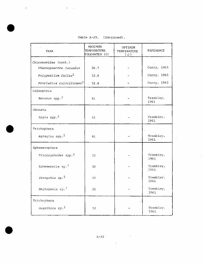
Table A-29. (Continued).

MAXIMUM OPTIMUM

TAXA TEMP ERATURE TEMPERATURE REFERENCETOLERATED (C) ( C)

Chironomidae (cont.)

Phaenopsectra jucundus 26.7 - Curry, 1965

Polypedilum fallax 2 32.8 - Curry, 1965

Procladius culiciformes2 32.8 - Curry, 1965

Coleoptera

Berosus spp. 2 41 - Trembley,1961

Odonata

Argia spp. 2 41 - Trembley,1961

Trichoptera

Agraylea spp.2 41 Trembley,1961

Ephemeroptera

Tricorythodes spp.2

Ephemerella sp. 2

Isonychia sp. 2

Heptagenia sp. 2

32

30

30

28

Trembley,1961

Trembley,1961

Trembley,1961

Trembley,1961

Trichoptera

Oxyethira so.

A-42

Table A-29. (Continued).

MAXIMUM OPTIMUMTAXA TEMPERATURE TEMPERATURE REFERENCE

TOLERATED (C) ( C)

Trichoptera (cont.)

Psychomyia sp. 2 30 Trembley,1961

Athripsodes sp. 2 27 Trembley,1961

Coleoptera

Elmidae unidentified 30 Trembley,app3 1961

Diptera

Empididae unidenti- 30 Trembley,

fied spp. 3 1961

iSpecies found near PINGP2Genus found near PINGP3 Family found near PINGP

A-43

Table A-30. Ranking of zooplankton abundances at three locations near PINGP during 1975 and

1976. Diversity and evenness indices are also presented.

1976 1975

ZOOPLANKTON FALL1

SUMMER2

SPRING3

WINTER4 FALL SUMMER SPRING WINTER

Ub 16 D7 U I D U I U I I D U I D U I D U I D U I D

Rotatoria (Rotifers)

Brachionus calycif1ozus 3 3 3 4 4 5 3 3 3 - 2 - 4 4 5 4 4 4- 3-

B. urceolalis 2 2 2 - 2 - 2 - 1 -

Keratolla cochlealis 5 5 5 5 5 5 3 3 3 - 4 - 4 4 2 32 2 2 - 3-

K. quadrata 3 3 3 - 2 - 22 - 2 -

Polyarthra sp. 3 3 4 4 4 4 2 2 2 - 3 - 3 2 2 2 3 3 2 - 2 -

Copepoda (Copepuds)

Cyclops vernalis 3 3 4 4 4 4 2 1 2 2 2 2 2 3 2 1 1 2 - 1 -

Cladocera (Cladocerans)

Bosmina longirustris 3 3 3 2 3 2 2 2 - 2 - 2 2 2 4 3 4 1 2 - 2 -

Chydorus ,ha 'us 4 4 4 2 2 2 - 2 - 3 3 3 2 2 1 - -

Shannon weaver Diversity8

2.04 1.44 2.08 2.18 2.13 2.65 2.00 2.01 1.88 - 2.33

Evenness Index9 .51 .37 .51 .56 .58 .68 .46 .44 .42 - .60 -

Key: Abundance: I = 0.0170.09; 2 = 0.1-0.9; 3 = 1.0-9.9; 4 = 10-99; 5 = 100-999 org/i; -= no sample; blank indicates no organisms found

IUsually near mid-October2Usually near mid-July

3Usu;ally near mid-April

'Usually near mid-January51j upriver (usudlly near iOjU station 10)61 intake (usually near IDR station 12)7U - downriver (usually near HDRl station 21)8S.W. Diversity n i 013

Y. -- I092 N--, where N is total number of all individuals of all taxa in sample, ni is number of individuals in

the ith taxa, and s is the number of taxa in sample.

Evenness (e) = d/ where d m~ is the maximum possible diversity for a given s = 10g2 s.

d ma x,

Table A-31. Summary of zooplankton thermal tolerances.

ACCLIMATION EXPOSURE REFERENCETAXA TEMPERATURE (C) LTs 0 (C) TIME

Copepoda

Diaptomus spp.1 1 28.4 30 min Kreuger, 1975

5 30.4 30 min

10 31.0 30 min

15 31.2 30 min

20 31 30 min

Cyclops vernalisI 21 32.3 30 min Coker, 1934

27.5 35 30 min

35.5 40 30 min

Cladocera

Daphnia pulexi 44 30 sec Altman andDittmer, 1966

Scapholeberis kingil Carlson, 1972;Simocephalus vetulusI 21 38-43 30 min Brown, 1929i

Latanopsis occidentalis - 46 - Altman and

Dittmer, 1966

Macrothrix rosea2 50 Altman andDittmer, 1966

Moina macrocopa2 - 48 30 min Altman and

Dittmer, 1966

Sida crystallina1

- 40 30 min Altman and

Dittmer, 1966

Ciliophora

Colpoda cucullus 21 40 2 min Altman andDittmer, 1966

Paramecium caudatum 20 39 Altman andDittmer, 1966

Rhizopoda

Amoeba proteus - 35.5-38.3 60 min Altman andDittmer, 1966

iSpecies found near PINGP2 Genus found near PINGP.

A-45

0

Table A-32. Fa19

P I1Y 10 LAN0l4

Aoi,ltridl in,

cyilphl.ria i.4-iOi144I

A19,5)

Apl I. 04 ',I.. ...

t4.ao-iq-s

(i.- 4Ia11 i aoi.4,

nking of phytoplankton abundances at three locations near PINGP during 1970 and 1974-

76. Diversities, chlorophyll a concentrations, and productivity are also presented.

19476 1975

FALL' I

3

42. 4404

43

'.58

'544M~l4

5

2.3

SPR IK

2

3

3

5

3

42

W14 N'4'43Ri

25

.65

42

4

,i

4FA4L

I

2 213

5 4 4

2

3 3

2 2 2

3-

222

34

0544434 S PIK ING

I1U421L5

32233 3

4 4 555

32

544420,4i.4,i Wr400r 040r1,i 4444'

"2".34

2.25 1.33 1.53

.4 2

2,. 95

N. t &izodiioivity 22

2 2 2

2 2

2

3 3 S

KY; L i.1-lPhill 2; 1 J-049. 9;3.3 2 - 1(4-99; 3 - 100-9997i 1111b

N401 Vt4di4 ýV-4I4tjy .4 11.015-03.09; 3 - 421-04.9 54.4 02

/tl; -- 44 4i1

4

AbinaiiiOiCi I 1 34.JS 2 1- l49'3 3 -100-999; 4 1 ,0i00-9,939;. li 10,000i-)99999 04qni - OO-t.4i -poo ..4

.Foto Ito 00' 00 f-Iioi

i'u-') ly l riii-iciii

L.ii4 d--0 i od-Jo

" S . W . it e i t 244d3 vO4i~ j , h-,i~ Ni~ ii,,,, I-42 f .11iii Iii)1- ý fA 1 lli ~ dvi - ýi h i -

4~~~~~~ Ii4~o IioUa44 ii.i 44r4 "xtL4J4 in4

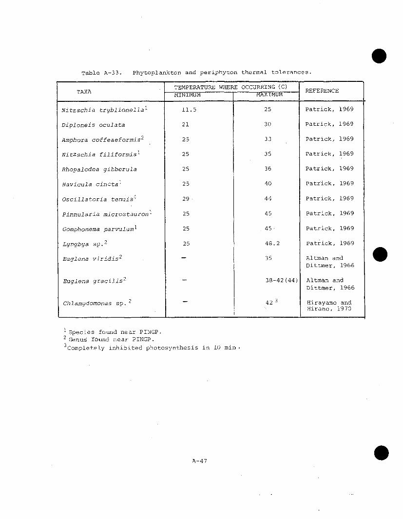
Table A-33. Phytoplankton and periphyton thermal tolerances.

TAXA TEMPERATURE WHERE OCCURRING (C) REFERENCEMINIMUM MAXIMUM

Nitzschia tryblionella 1 11.5 25 Patrick, 1969

Diploneis oculata 21 30 Patrick, 1969

Amphora coffeaeformis2 25 33 Patrick, 1969

Nitzschia filiformis 1 25 35 Patrick, 1969

Rhopalodea gibberula 25 36 Patrick, 1969

Navicula cinctal 25 40 Patrick, 1969

Oscillatoria tenuis' 29 44 Patrick, 1969

Pinnularia microstauroni 25 45 Patrick, 1969

Gomphonema parvulumI 25 45 Patrick, 1969

Lyngbya sp. 2 25 48.2 Patrick, 1969

Euglena viridis 2 - 35 Altman andDittmer, 1966

Euglena gracilis 2 38-42(44) Altman andDittmer, 1966

Chlamydomonas sp. 2 423 Hirayamo andHirano, 1970

I Species found near PINGP.2 Genus found near PINGP.3 Completely inhibited photosynthesis in 10 min.

A-47

Table A-34. Ranking of periphyton abundances at three locations near PINGP from 1972 through 1976.

Diversity and pigment concentrations are also presented.

" " 1974 6 194.74

-AA M4 ̀,1;44 5w I~ N, . 1 AL. SMMH -4 .C

-: ,1 ........... ...............-.-... .. . . . .4 hWIN 44 4 441 sn~ .5 4S 54- ,~~~,ill= I4 I~ U !

I U 5} I IN 4 ~ 4 . s, u i ~ s r s u

I2, I.,o.y. k-, 4 4 454 4 4 b - --.- *--..--------4---.--------- - 1 ]S4 - . : . - - ' 4 4 4 5 S 44 3

!1 - 4 44 4 -

444;4

*.fl1444. 4 .4 ' 4 3 ' 4 4 - - 3 3 4 .

4 b 6 5 5 6 5 4 4 4

4'--- 44 - 4 . 4 5 b, 11. - - 4 4 4 6 6 (i4 5 44 5

44j,.., ,s. 4 4 4. - . 4. 4 * 4 4 4 3, 4 5 5 - 4 43 5 4. 3-

- - 5 , - - 3 4 4 b 5 6 -

>4,4,,N4,< i4,---V! 4 3.81 .2 3 T 41 4.i 4; 3.W 4 3.3 2.54 53. 71 3.5!,0 1.1S 2.35 314 3t .20 1,653.19 4.ti4 3.4537.ý4.- -- -

.2. 444544 4 3 4 3 - j 1 3- 4 3 3 4 3 3 4 3 - 3 34 -

Ssy4444ha 44lh¥.;; • I - .44- .544; 33444-.,4; 4 I 4.91-0; 4 1045; 44 5,44p44

;4h1or4,hyl4 .:I•4 , 41 J- , .; 3 ; - 4. , I4 - 91-9 54j/444 -0 ,.4_9 4"

'44.;;,,14y 4n4 44i4

-3544u.ry

4.1 -n;,s.kv (.4.4445 l ,y n4 44444 4.5.S644 13)4;-4,;do,rgrv.~r (u.u.4•l•y, u.r4jt' tl5444,44!~l 274

'.A" ..4 4 4 . 4 4.4-]

'U 1- 1 MIR I• • N t5 Lla iI•I f a l Jt~i i u l +[ a l • • t•:;l,,u '1 I;lttl~~ • tll~i ul • iltlU i~ a a

Table A-35. Periphyton thermal criteria.

MAXIMUM OPTIMUM

TAXA TEMPERATURE TEMPERATURE REFERENCE

FOR SURVIVAL (C) (C)

Nitzchia tryblionella1

N. filiformis1

N. linearis1

N. amphibia1

N. acuta1

N. sp.2

Navicula cinctal

Pinnularia microstauron1

Gomphonema parvulumr

Asterionella formosa]

Cocconeis scutellum1

Cyclotella comtal

C. meneghiana1

Cymnbella sp.2

Melosira islandica1

M. varians1

M. italica1

M. granulata'

Stephanodiscus astraea1

Synedra acus'

Diatoma vulgare var. producta

Fragilaria intermedia

25

35

30

36

403

40

45

45

20

20

10

4

18

30

5

34-36

Schwabe, 1936

Schwabe, 1936

Wallace, 1955

Fogg andReimer, 1962

Baker, 1977

Barker, 1935

Altman andDittmer, 1966;Baker, 1977

Altman andDittmer, 1966

Altman andDittmer, 1966;Baker, 1977

Stoermer andLadewski, 1974

Stoermer andLadewski, 1974

Stoermer andLadewski, 1974

Baker, 1977

Fogg andReimer, 1962

Stoermer andLadewski, 1974

Fogg andReimer, 1962

Stoermer andLadewski, 1974

Stoermer andLadewski, 1974

Stoermer andLadewski, 1974

Baker, 1977

Baker, 1977

Baker, 1977

29

36

17

2.5

10

5

5

ISpecies found near PINGP.2 Genus found near PINGP.3Photosynthetic rate irreversibly lowered.

A-49

Table A-36. Dominant species comprising major beds of submerged andemergent aquatic vegetation in the vicinity of PINGP.

LOCATIONNUMBER LOCATION

Wisconsin Shore Immediately Upstream of Lock & Dam No. 3

Potamogeton crispusPotamogeton filiformisPotamogeton nodosusPotamogeton pectinatusSagittaria spp.

2 Refuge Outlet

Potamogeton crispusPotamogeton filiformisPotamogeton pectinatus

3 Barney's Point

Potamogeton crispusPotamogeton pectinatus

4 Discharge Canal-Southwest Shore

Potamogeton crispusEleocharis ovataEleocharis palustrisScirpus fluviatilisScirpus validusPhragmites cormnunis

5 Between PINGP Intake and Discharge Areas

Potamogeton crispusPotamogeton nodosus

5a Shoreline Between PINGP Intake and Discharge Areas

Potamogeton pectinatus

6 Sturgeon Lake at Mouth of Buffalo Slough

Potamogeton crispusPotamogeton filiformisPotamogeton natansPotamogeton nodosusPotamogeton pectinatus

A-50

Table A-36. (Continued).

LOCATIONNUMBER LOCATION

7 Bay at Mouth of Buffalo Slough

Potamogeton crispusPotamogeton filiformisPotamogeton nodosusPotamogeton pectinatusSagittaria cuneataSagittaria latifoliaScirpus fluviatilisPhragmites communisSparganium eurycarpumTypha angustifoliaCyperaceae (unidentified)Zizania aquatica

8 Sturgeon Lake "Cut" Delta-East Half

Potamogeton filiformisPotamogeton pectinatusPotamogeton crispus

9 Sturgeon Lake "Cut" Delta-West Half

Potamogeton crispusPotamogeton pectinatus

10 Side Channel of Sturgeon Lake "Cut"

Vallisneria americanaPotamogeton crispusPotamogeton pectinatusPotamogeton nodosus

11 North Shore of Sturgeon Lake

Sagittaria spp.Scirpus fiuviatilisPhragmites communis

12 East Shore of Brewer Lake

Sagittaria spp.

A-51

Table A-36. (Continued).

LOCATION LOCATIONNUMBER

13 West Shore of Brewer Lake

Sagittaria spp.Scirpus fluviatilisPhragmites communis

Al Intake Area, Outside of Skimmer Wall

Potamogeton pectinatus

A2 Bay Upstream of PINGP Intake

Potamogeton pectinatus

A3 Bay at End of the Long Island Separating SturgeonLake and the Main Channel

Potamogeton pectinatusPotamogeton crispus

A4 Point on West Side of "Lab Bay"

Potamogeton pectinatusPotamogeton crispus

A5 Buffalo Slough

Cyperaceae (unidentified)Polygonum sp.Eleocharis sp.Anacharis canadensisCeratophyllum demersum

A-52

Table A-37. Areas within various isotherms from the thermalplume model (Appendix I) for typical spring(May 1976) conditions (determined by computerplanimetry). River temperature = 16.50 C(61.70 F) and river flow = 11,028 cfs.

ABSOLUTEAT TEMPERATURE AREA(F) (C) (F) (ft 2 ) (m 2 ) (ha)

18 26.5 80 19,412 1,083 0.1

15 24.8 77 51,058 4,743 0.5

12 23.1 74 117,740 10,938 1.1

10 22.0 72 206,750 19,207 1.9

9 21.5 71 275,766 25,619 2.6

8 20.9 70 364,257 33,840 3.4

6 19.8 68 638,574 54,324 5.4

5 19.2 67 779,430 72,409 7.2

4 18.7 66 1,159,270 107,696 10.8

2 17.6 64 2,187,072 203,179 20.3

Table A-38 Areas within various isotherms from the thermalplume model (Appendix I) for typical summer(August 1975) conditions (determined by computerplanimetry). River temperature = 24.4 0 C (760 F)

and river flow = 11,790 cfs.

ABSOLUTEAT TEMPERATURE AREA(F)

(C) (F) (ft 2 ) (m 2 ) (ha)

12.5 31.3 88.5 16,194 1,504 0.2

10 30.0 86.0 97,854 9,091 0.9

9 29.4 85.0 156,313 14,522 1.5

7.5 28.5 83.5 292,051 27,132 2.7

5 27.2 81.0 714,288 66,357 6.6

4 26.6 80.0 1,030,128 95,699 9.6

3 26.1 79.0 1,529,365 142,078 14.2

A-53

Table A-39. Areas within various isotherms from the thermalplume model (Appendix I) for typical winter(December 1975) conditions (determined by com-puter planimetry). River temperature = 0.50 C(32.90 F) and river flow = 12,561 cfs.

ABSOLUTE AREAAT TEMPERATURE(F)

(C) (F) (ft2) (m 2 ) (ha)

45 25.5 77.9 6,060 563 0.06

40 22.7 72.9 23,076 2,144 0.2

35 19.9 67.9 59,555 5,533 0.6

30 17.2 62.9 95,116 8,836 0.9

25 14.4 57.9 159,795 14,845 1.5

20 11.6 52.9 301,347 27,995 2.8

17 9.9 49.9 475,726 44,195 4.4

15 8.8 47.9 553,997 51,466 5.2

10 6.1 42.9 901,820 83,779 8.4

9 5.5 41.9 1,140,719 105,973 10.6

5 3.3 37.9 1,804,367 167,626 16.8

A-54

Table A-40. Areas within various isotherms from the thermalplume model (Appendix I) for winter (January)proposed extreme conditions (determined by com-puter planimetry). River temperature = 00 C(320 F) and river flow = 3,699 cfs.

ABSOLUTE AREAAT TEMPERATURE(F) (C) (F) (ft 2 ) (m2 ) (ha)

50 27.8 82 8,902 827 0.08

45 25.0 77 31,835 2,958 0.3

40 22.2 72 59,567 5,534 0.6

35 19.4 67 95,658 8,887 0.9

30 16.7 62 165,667 15,391 1.5

25 13.9 57 305,022 28,337 2.8

20 11.1 52 561,199 52,135 5.2

15 8.3 47 921,918 85,646 8.6

10 5.6 42 1,648,929 153,186 15.3

9 5.0 41 1,720,787 159,861 16.0

A-55

Table A-41. Areas within various isotherms from the thermalplume model (Appendix I) for spring (May) pro-posed extreme conditions (determined by computerplanimetry). River temperature =and river flow = 8,475 cfs.

22.80 C (730 F)

ABSOLUTEAT TEMPERATURE AREA

(F)(C) (F) (ft 2 ) (m2 ) (ha)

12.5 29.7 85.5 50,151 4,659 0.5

10 28.3 83.0 174,145 16,178 1.6

9 27.8 81.0 281,460 26,148 2.6

7.5 26.9 80.5 516,518 47,985 4.8

5 25.6 78.0 1,180,507 109,669 11.0

3 24.4 76.0 2,230,161 207,182 20.7

Table A-42. Areas within various isotherms from the thermalplume model (Appendix I) for summer (August)proposed extreme conditions (determined bycomputer planimetry). River temperature =29.40 C (850 F) and river flow = 3,390 cfs.

ABSOLUTE

AT TEMPERATURE(F) (C) (F) (ft2) (m2 ) (ha)

6.5 33.0 91.5 54,454 5,059 0.5

6 32.8 91.0 188,154 17,480 1.8

5 32.2 90.0 670,391 62,279 6.2

4 31.7 89.0 1,280,753 118,982 11.9

3 31.1 88.0 1,919,618 178,333 17.8

A-56

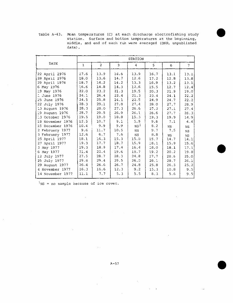
Table A-43. Mean temperatures (C) at each discharge electrofishing studystation. Surface and bottom temperatures at the beginning,middle, and end of each run were averaged (DNR, unpublisheddata).

STATIONDATE 1 2 3 4 5 6 7

22 April 1976 17.6 13.9 14.6 13.9 16.7 13.1 13.128 April 1976 18.0 13.6 14.7 1.2.6 17.2 12.8 13.829 April 1976 18.7 14.2 14.2 13.3 16.9 13.2 13.16 May 1976 16.6 14.8 14.3 12.6 15.5 12.7 12.419 May 1976 22.0 23.2 21.3 19.5 20.3 21.9 19.01 June 1976 24.1 26.4 22.4 21.3 23.4 24.1 22.225 June 1976 24.5 25.8 24.1 22.5 24.9 24.7 22.222 July 1976 28.3 29.1 27.8 27.4 28.0 27.7 28.913 August 1976 28.3 28.0 27.3 26.6 27.2 27.1 27.419 August 1976 28.7 29.5 26.9 26.1 26.6 27.7 26.313 October 1976 19.5 19.0 18.8 15.3 19.3 19.9 14.919 November 1976 12.5 10.7 9.1 5.9 9.6 7.1 4.415 December 1976 10.4 9.9 9.9 NS 1 8.2 NS NS2 February 1977 9.6 11.7 10.5 NS 9.7 7.5 NS3 February 1977 12.6 6.7 7.6 NS 8.8 NS NS25 April 1977 18.1 16.3 15.3 15.0 15.7 14.7 14.127 April 1977 19.3 17.7 18.7 15.9 18.1 15.9 15.63 May 1977 19.3 18.9 17.4 16.4 18.0 18.1 17.16 May 1977 21.4 22.4 19.6 18.7 19.2 20.2 19.812 July 1977 27.5 28.7 28.3 24.8 27.7 28.6 25.025 July 1977 29.8 29.4 29.5 26.0 28.1 28.7 26.129 August 1977 26.4 26.6 26.7 24.8 25.8 26.5 25.24 November 1977 16.3 16.6 12.3 9.2 15.3 10.8 9.514 November 1977 11.1 7.7 5.3 5.5 8.3 5.6 9.5

iNS = no sample because of ice cover.

A-57

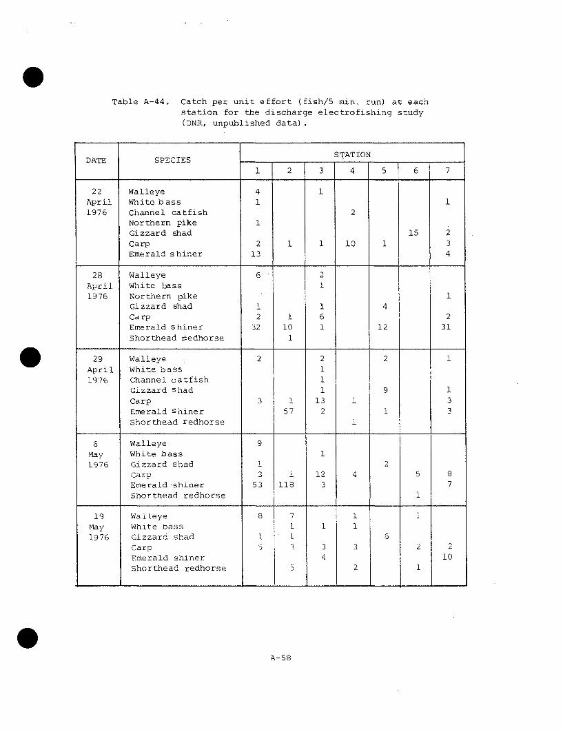
Table A-44. Catch per unit effort (fish/5 min. run) at eachstation for the discharge electrofishing study(DNR, unpublished data).

DATE SPECIES STATION

1 2 3 4 5 6 7

22 Walleye 4 1April White bass 11976 Channel catfish 2

Northern pike 1Gizzard shad 15 2Carp 2 1 1 10 1 .3Emerald shiner 13 4

28 Walleye 6 2April White bass 11976 Northern pike 1

Gizzard shad 1 1 4Carp 2 1 6 2Emerald shiner 32 10 1 12 31Shorthead r-edhorse 1

29 Walleye 2 2 2 1

April White bass 11976 Channel catfish 1

Gizzard shad 1 9 1Carp 3 1 13 1 3Emerald shiner 57 2 1 3Shorthead redhorse 1

6 Walleye 9May White bass 11976 Gizzard shad 1 2

Carp 3 1 12 4 5 8Emerald shiner 53 118 3 7Shorthead redhorse i

19 Walleye 8 7 1 1May White bass 1 1 11976 Gizzard shad 1 1 6

Carp 5 3 3 3 2 2Emerald shiner 4 10Shorthead redhorse 2 1

A-58

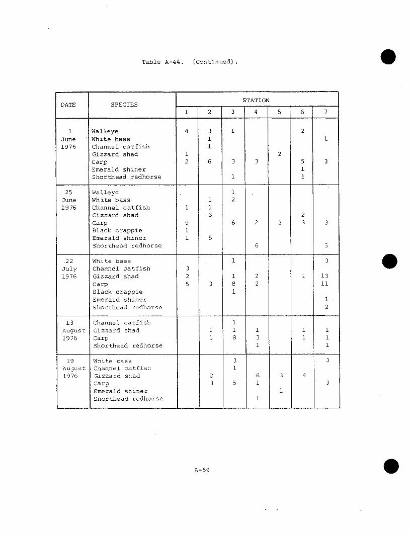
Table A-44. (Continued).

STATIONDATE SPECIES

1 3 4 5 6 7

I Walleye 4 3 1 2

June White bass 11976 Channel catfish 1

Gizzard shad 1 2

Carp 2 6 3 3 5 3Emerald shiner 1Shorthead redhorse 1 1

25 Walleye 1June White bass 1 21976 Channel catfish 1 1

Gizzard shad 3 2Carp 9 6 2 3 3 3Black crappie 1Emerald shiner 1 5

Shorthead redhorse 6 5

22 White bass 1 3July Channel catfish 3

1976 Gizzard shad 2 1 2 1 13

Carp 5 3 8 2 11Black crappie 1Emerald shiner 1Shorthead redhorse 2

13 Channel catfish 1August Gizzard shad 1 1 1 1 1

1976 Carp 1 8 3 1 1Shorthead redhorse 1 1

19 White bass 3 3

August Channel catfish 11976 Gizzard shad 2 6 3 4

Carp 3 5 1 3Emerald shiner I

Shorthead redhorse 1

A-59

Table A-44 (Continued).

STATION

DATE SPECIES 324

13 Walleye 5 2October White bass 1 2 1

1976 Gizzard shad 22 25 11 3 14 23 29Carp 1 8 5 1 1Emerald shiner 1 3Shorthead redhorse 1

19 Walleye 1 1November White bass 7 8 7

1976 Gizzard shad 45 5 14Carp 9 2 8Emerald shiner 1

15 Walleye 1December White bass 1 11976 Gizzard shad 1 17 NS1 377 NS NS

Carp 17 1 1 2

2 White bass 7 1 1 1February Gizzard shad NS 69 56

1977 Carp 46 27 8 2

Black crappie 2

3 WalleyeFebruary White bass 11 1 2

1977 Gizzard shad NS 132 NS NSCarp 31 1Black crappie 1

25 walleye 2April Gizzard shad 10 1 231977 Carp 1 14 1 1

Emerald shiner 11 1 1 13

27 Walleye 1 1April White bass 11977 Gizzard shad 2 14 2

Carp 1 4 4 2Emerald shiner 5 2 3 1

INS = no sample because of ice cover.

A-60

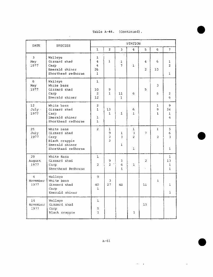
Table A-44. (Continued).

DATE SPECIES STATION

1 2 3 4 5 6 7

3 Walleye 1May Gizzard shad 4 1 1 4 6 11977 Carp 4 7 1 2

Emerald shiner 26 2 10Shorthead redhorse 1 1

6 Walleye 1May White bass 31977 Gizzard shad 10 9 5

Carp 2 1 11 6 6 2Emerald shiner 12 1 6

12 White bass 2 1 9July- Gizzard shad 1 13 6 9 241977 Carp 1 1 1 1 1

Emerald shiner 1 4Shorthead redhorse 1

25 White bass 2 1 1 1 5July Gizzard shad 9 1 3 7 61977 Carp 2 3 2 2 3

Black crappie 2Emerald shiner 1Shorthead redhorse 1 1

29 White Bass 1 1August Gizzard shad 9 5 2 13

1977 Carp 2 2 6 1 1

Shorthead Redhorse 1 1

4 Walleye 9November White bass 3

1977 Gizzard shad 40 27 NS 11 1Carp 1Emerald shiner 1

14 Walleye 1November Gizzard shad 15

1977 Carp 5Black crappie 1 1

A-61

Table A-45. Constants for the time-temperature equationlog time = a+ b(T) for the RIS (Brungs andJones, 1977).

ACCLIMATION DATA LIMITSSPECIES TM.C) ab UPRDATA SOURCETEMP. (C) UPPER LOWER

26 34.7119 -0.8816 39.0 36.630 32.1736 -0.7811 40.6 37.434 26.4204 -0.6149 42.0 38.0 Allen and

Strawn,25 34.5554 -0.8854 37.5 35.5 1968

Channel Catfish 30 17.7125 -0.4058 40.0 37.535 28.3031 -0.6554 41.0 38.0

15 34.7829 -1.0637 31.5 30.520 39.4967 -1.1234 34.0 33.0 Hart, 195225 46.2155 -1.2899 35.0 34.0

25 17.3066 -0.4523 34.5 32.5Northern Pike 27.5 17.4439 -0.4490 35.0 33.0 Scott, 1964

30.0 17.0961 -0.4319 35.5 33.5

25 47.1163 -1.3010 35.5 34.530 38.0658 -0.9694 38.0 36.535 31.5434 -0.7710 39.0 37.0

Gizzard Shad Hart, 195225 32.1348 -0.8698 35.5 35.030 41.1030 -1.0547 38.0 36.535 33.2846 -0.8176 39.0 36.5

5 20.9532 -0.7959 24.5 23.510 36.5023 -1.2736 27.5 27.0

Emerald Shiner 15 47.4849 -1.5441 30.5 29.5 Hart, 194720 33.4714 -0.9858 32.5 31.525 26.7096 -0.7337 34.0 31.5

5 33.6957 -1.1797 27.5 27.0

10 18.9890 -0.6410 29.0 28.0White Sucker 15 31.9007 -1.0034 30.0 29.5 Hart, 1947

20 27.0023 -0.8068 31.5 30.025 22.2209 -0.6277 32.5 29.5

A-62

Table A-46. Data used in chi-square analysis. Total number ofeach RIS collected in the immediate discharge (Runs1+5), far discharge (Runs 2+3), and intake or control(Runs 4+7), during the period April 1976 throughNovember 1977 (DNR, unpublished data).

SPECIES STATION SPRING 1 SUMMER 1 FALL1 WINTER 1

Walleye 1 & 5 37 4 16 02 & 3 12 5 3 14 & 7 2 0 0 ND2

White Bass 1 & 5 1 5 8 22

2 & 3 6 9 15 44 & 7 2 23 3 ND

Gizzard Shad 1 & 5 84 18 161 5792 & 3 31 45 41 174 & 7 4 75 33 ND

Carp 1 & 5 24 21 16 992 & 3 83 58 23 37

4 & 7 50 41 2 ND

Emerald Shiner 1 & 5 267 3 0 02 & 3 203 6 1 04 & 7 75 5 5 ND

Shorthead 1 & 5 1 1 1 0Redhorse 2 & 3 6 2 0 0

4 & 7 4 19 0 ND

iSeasons are defined byspring = 5 to 210 CSummer = > 210 C

Fall = 21 to 51 C

Winter = < 50 C2 No data.

ambient river temperature as:

A-63

36ACCLIMATION

T

30.0

27.5 4

25.0 G.

35 F

G

34DI-

LU

LU

33C,LU

32 I-

I I I I . I . I I i i I I i i

40 60 80 100 200 400 600 800 1000 2000

RESISTANCE TIME (MIN) 547P-13

Figure A-i. Median resistance times (time to 50 percent mortality) for juvenile northern pike

acclimated to 25' 27.5', and 30'C (adapted from Scott, 1964).

C-,

wL

!-U,

5 10 50 100 500 1000 5000

RESISTANCE TIME (MIN) 547P-14

Figure A-2. Median resistance times (time to 50 percent mortality) for juvenile channel catfishfrom state fish hatcheries in Lonoke (open symbols) and Centerton (closed symbols),Arkansas at acclimation temperatures of 250 to 350 C (adapted from Allen and Strawn,1968).

0

39 1-

0 *

0 *t 337

X

cc

wCL

30

0

35ACCLIMATION

T

25

33

I I I , I I I I , II I I I I I 1 1 1 I I I I I l I10 50 100 500

RESISTANCE TIME (MIN)

1000 5000547P-15

Figure A-3. Median resistance times (time to 50 percent mortality) of gizzard shad from Put-in-Bay,Ohio (closed symbols) and Knoxville, Tennessee (open symbols), for fish acclimated to 25',300, and 35 0 C (adapted from Hart, 1952).

203O

= 28

26

24

22

201

32

28

24

0 20 e

16

4

0

Figure A-4.

RESISTANCE TIME (MINI

16 20 24 28 32 36 40

ACCLIMATION TEMPERATURE (CI

A. Median resistance times (time to 50 percent mortality)for emerald shiners acclimated to temperatures from5 0 to 2502 (adapted from Hart, 1947).

B. Median thermal tolerance polygon for emerald shiners.The dashed lines represent 10 percent (outer) and 90 per-cent (inner) survival (adapted from Hart, 1947).

36

.132

< 30

~28

• 323o

2•

A

ACCLIMATION

T 25

20 .

10

. . I , . I , I . . . , , , , , , , , ,24

32

.1 .15 10 50 101121S500 1000 5400

5 1 U 5s 100RESISTANCE TIME WMIN)

500 IWO0 5000

321

0:

16 20 24

ACCLIMATION TEMPERATURE (C)

Figure A-5. A. Median resistance times (time to 50 percent mortality)for white suckers acclimated to temperatures from 5*to25'C (adapted from Hart, 1947).

B. Median thermal tolerance polygon for the white sucker(adapted from Hart, 1947).

60

LEGEND

130 - AHTHROPODA INSECTA

EPI4EMEROPTEHA

120 -50 0 ..ti•t - .l

N .l I tI:I . ,'I:k ,:I.~~~I'RI'1 ,V( IA1 1, 31"J

11}0 E) }lH 'Il

40 TRICHOPTERA

00 ......... . ) t s

+ PLEC0!'TERA

90 1 0

LDWNAOACrAVERACE Ut.OWOOUVVN ) ''W ./il( I - -

0' LU 80 -- , / -'• \'{IJIUAI (JA. (.'.>t 1 '30 "

1.1"l\

0- - 15/ • I It lll#llt IX I*l';.l,

50 --. • //F\\ \ N 0 AMPH'I P ',O.A/ PLAIDHE MI NTH'.

80 -

JAN FEB MAH APR MAY JUN JUL AUO SEP OCT NOV !)EC

MOE/Il M/. 9

Figure A-6. Thermal tolerances of macroinvertebrates collected near PINGP

(from Table A-28).

0 0

60

130 55

50

120 -

45

10 iLEGEND

V 40 COPEPODA300 0 -. a f 1 a"'N Spi -

t I I' I• • I IA AN . if. I.S,- - -

•- ACLADOCERA,u 90 ... ra• I I•• ' (1•1.1 I V.t

3AVERAGE BLOW OWN SIII(,/I./Ji/j/is AI/Al\/:I 1EMPERATLIRE " 30

f- tumNi/l P/d 1.1/1/s

80-<rj..

o 70 - H *sa Ni/ l sra I N .ifi~

20 CiLIOPHORA

A ( 0/ Pi00, I CI .1. U/S

60 1 - 5 V "-IRA Vl~f'IA~ aa*i

RHIZOPODA

50 • .1104/ I-foll, I sR/ 111"N

,9F

40

30 AMBIeNT

30 o•.. .. J 2 iL O H R

JAN FEB MAR APH MAY JUN JU L AUG SEP OCT NOV DEC

MONTH 547P .ill-

Figure A-7. iliermal tolerances for zooplankton collected near PINGP (information

derived from Table A-31).

140

30

120 -. 50

V+*rA 450 -- (

0 40 LEGEND100 0 I I I R II.W.\'1'I. 1..1

(D0 35 VI s111¢.1 ( 1 .41 I114. I ll"

90 Nu --- I. l. l4lwkAVERAGE BLOWDOWN

TEMPERATURE .) 3 c ) i 4 w,1...\ I I441 1is

-- (1) 110~(D 0 /0-41-01 11"Hut 1,"I IX 180 .-4 .\: ,I ( IN( V I

20 a- (I t, I4.1l '4M114 V. S 4 .1 .

/0 20 1 ( 4. I 1:. 4,A'

V 'I.N \' I4.4 4.I II 4II(41 ,41I4II Ro4.\

410 -X ;/.., . I.I Sp

50 /0

ao - ... ,s - 7""//• ,

3 -A MBIE NT0

JAN FES MAR APR MAY JUN JUL AUG SEP OCT NOV DEC

MONTH 547P-80-4

Figure A-8. Thermal tolerances of phytoplankton collected near PINGP, 1969 through 1976

(information derived from Table A-33).

APPENDIX B

DETAILS OF NON-FISHERIESSTATISTICAL ANALYSES

LIST OF TABLES

Table APPENDIX B Page

Details of Non-Fisheries Statistical Analyses

B-i. Table summarizing statistical analysis of the data B-2

B-2. Statistical power calculations for the analysis ofvariance. B-10

B-3a. Phytoplankton densities for 1973 B-15

B-3b. Phytoplankton densities for 1974 B-16

B-3c. Phytoplankton densities for 1975 B-17

B-3d. Phytoplankton densities for 1976 B-18

B-4. Phytoplankton density (Log transformed), 1975-76 B-19

B-5. Phytoplankton density (Log transformed), 1975-76 B-20

B-6. Phytoplankton Type I productivity B-21

B-7. Phytoplankton Biovolume (mg/liter) B-22

B-8. Phytoplankton production: Chlorophyll a (ppb) B-23

B-9. Phytoplankton-species diversity B-24

B-10. Phytoplankton: Type III productivity analysis (P=PSg-R)in ppm 0 2/hr for intake and discharge (1976) B-25

B-lla. Periphyton density, 1976 B-26

B-llb. Periphyton density (1975) B-27

B-12a. Periphyton chlorophyll a concentration (1976) B-28

B-12b. Periphyton chlorophyll a concentration (1975) B-29

B-13a. Periphytonc-phaeophytin a concentration (1976) B-30

B-13b. Periphyton-phaeophytin a concentration (1975) B-31

B-14. Periphyton-species diversity B-32

B-15a. Zooplankton-total densities for 1975 B-33

B-15b. Zooplankton-total densities for 1976 B-33

B-16. Zooplankton total density (Log transformed) 1975-76 B-34

B-17. Zooplankton total density (Log transformed) 1975-76 B-35

Table

B-18. Zooplankton: Rotifer density (Log transformed),1975-76

B-19. Zooplankton: Rotifer density (Log transformed),1975-76

B-20 Zooplankton: Crustacea density (Log transformed)1975-76

B-21 Zooplankton: Crustacea density (Log transformed)1975-76

B-22. Zooplankton-species diversity

B-23a. Total macroinvertebrate density collected byPetersen dredge methods (1975)

B-23b. Total macroinvertebrate density collected byPetersen dredge methods (1976)

B-23c. Total macroinvertebrate density collected byPetersen dredge methods (1977)

B-24. Macroinvertebrate density (Log transformed)collected by dredge methods, 1975-76

B-25. Macroinvertebrate density (Log transformed) collectedby dredge methods, 1975-76

B-26a. Total macroinvertebrate density collected by.artificial substrate method (1975)

B-26b. Total macroinvertebrate density collected byartificial substrate sampler (1976)

B-26c. Total macroinvertebrate density collected by Hester Dendymultiplate sampler (1977)

B-27. Macroinvertebrate density (Log transformed) collectedby artificial substrate methods, May-Oct, 1975-76

B-28. Macroinvertebrate diversity (dredge)

B-29. Macroinvertebrate diversity (artificial substrates).

B-30. Data used in stepwise regression I biological variablesHDR Station 46 for 1975

B-31. II Water quality variables

B-32. Data used in stepwise regression (biological variables),Sturgeon Lake, HDR Station No. 6 (1976)

B-33. II Environmental variables (water quality)

Page

B-36

B-37

B-38

B-39

B-40

B-41

B-42

B-43

B-44

B-45

B-46

B-47

B-48

B-49

B-50

3-5I

B-52

B-53

B-55

B-56

ii

Table Page

B-34. Data used in stepwise regression (biologicalvariables), HDR Station Nos. 9 and 10 (1976) B-58

B-35. II Environmental variables (water quality)HDR Stations 9 and 10, 1976 B-59

B-36. Data used in stepwise regression (biological variables),HDR Station Nos. 12, 13, and 14 (1975). B-61

B-37. II Environmental variables (water quality),HDR Stations 12, 13, and 14 for 1975 B-62

B-38. Data used in stepwise regression (biological variables),HDR Station Nos. 12, 13, and 14 (1976) B-64

B-39. II Environmental variables (water quality),HDR Stations 12, 13, and o4 (intake) for 1976 B-65

B-40. Data used in stepwise regression (biological variables),HDR Station Nos. 19, 20, and 21 (1975). B-67

B-41. II Environmental variables (water quality),HDR Stations 19, 20, and 21, for 1975 B-68

B-42. Data used in stepwise regression (biological variables),HDR Station Nos. 19, 20, and 21 (1976) B-70

B-43. II Environmental variables (water quality),HDR Stations 19, 20, and 21, for 1976 B-71

B-44. Data used in stepwise regression (biological variables),HDR Station*No. 27, 1976) B-73

B-45. II Environmental variables (water quality),HDR Station 27, for 1976 B-74

COMPUTER PRINTOUTS B-76

iii

Introduction

This appendix presents raw data and the statistical methods of the

reanalyses that were used in determining PINGP discharge impacts upon

non-fisheries biota. The raw data were taken from 1973-1976 Annual

Reports and unpublished reports for 1977 of the Environmental Monitoring

and Ecological Studies Program for the Prairie Island Nuclear Generating

Plant (PINGP). Station and month code numbers were substituted for HDR

station numbers and months (as shown in the appropriate raw data tables).

The statistical analyses were done using: (a) the Biomedical Computer

Programs (BMDP), edited by W. J. Dixon, (b) the Statistical Analysis

System (SAS-76), developed by Barr et al., and (c) the General Statistics

Pac, by Hewlett Packard. A complete listing of the various statistical

analyses used is given in Table 1, and a brief description is given below.

Treatment of Missing Values

Most of the variables had several missing values and this was a

major problem in the statistical analysis. A missing value in the data

was represented by a decimal point in the SAS-76 programs, whereas a

missing value code of -1.0 was used for the BMDP programs. The SAS-76

programs handle missing values by omitting them in calculating the result

(Barr et al., 1976). In the BMDP package, some programs such as Stepwise

Regression, t-Test, T2 Routine, and Frequency Count Routine, complete the

analysis using the remaining variables for that case; other programs omit

the entire case (Dixon, 1975). To the extent possible, programs utilizing

maximum available data were used.

B-1

Table B-I. fable summarizing statistical analysis of the data.

I3

DATA USED 13RIEF DESCRIPTION

PARAMEthS fOROF STATISTICAL REFERENCES PAUEYEARS PROCEDURES USED

NIIMI3ER RPE PL ICATES

1. All complete data sets 6, 10, 12, 1975- - Histogram plots and BMDP2D (Frequency Dixon, W. J., ed.,

for phytoplankton 18, 21, 25, 1976 general data des- Count Routine) of 1975. BNDP: Bio-

density, 2,:ooplankton 27 cription for real the BioMedical medical Computer Pro-

density, Macroinverte- nuitbers which showed Computer Programs grams, Los Angeles, 77

brate (drtedye) and that the data was CA, Univ. Calif.

Macroinvertebrare not norrmally distri- Press

(artificial slbStra t) butedd- i Lies,

2. saue as adove using The log transforma- BMDP2D (Frequency Dixon, 1975

log trnnuformod data tion of the data Count Routine) ofwhich showed a more the BioMedical 81

norlal distribution Computer Programs

3.PytcL'1aekto)t[ ity 6, 9, 14, (9"3-'6 2 obs/month Two-way Analysis of GLM Procedure Of Barr, A. J. et al.,

(Nu/mI). 19, 27 Variance or, log the SAS-76 Package 1976. A User's Guidetransformed data and to SAS-76 and SAS 85

Duncan's Multiple Supplemrcntail Library

Ralge Test User's t;uide, Raleigh,

NC, SAS Institute.

4. Phytuplunktoa Density 6, 9, 14, Preop= 2 obs/imonth Crossed and Nested GLM Procedure of Barr, A. J. et a8.,(N.,/11). 19, 27 1973 Factor Analysis using the SAS-76 Package 1976

0p, log- trans formed1975-76 preoperational data 95

(1973) and opera-tional data (1975-76)

5. l'hytoplankton t(nsity intake (14) May to Paired t-Test on Hewlett-Packard Hewlett-Packard,

(No./el) . and Oct log tralisfurmud General Statistics 1975discharge 1975-76 data Package 19

(19)

6. Phytopiunkton Density Io, 27 May to Paired t-Test on Hewlett-l'ackdrd llewlett-Packard,

(No./ml). Oct log transformed General Statistics 1975 201975-76 data Package

7. phytoplankton 1,, 9, 14, Mar-July 2 obs/month TwO-way Analysis of GLM Procedure of Barr, A. J. et al..

I/iovoluec (mg/I) 19, 27 1976 and Variance using real the SAS-76 Package 1976May-Oct numbers and Duncan's 105

1975 multiple Range Test

8. Phytoplanktun Intake (14) May-Oct 22 obs/ Paired t-Test Hewlett-Packard Hlewlett-Packard,

Productioln: Chlor- Discharge 1975 sample Gcneral Statistics 1975 23

ophyl . (1,pb) (19) Package

9. Phytoplankton Type I b, 10, 14, Apr-Nov 3 obs/month Two-way Analysis of GLM Procedure of Barr, A. J. ut al.,

Productivity (ppm 19, 27 - 1976 for Stuis 6, Variance using real SAS-76 197b

O.2/hr.) May-Oct 10 and 1 oh/ numbers and Duncan's ill1975 month for 14, Multiple Range Test

19, and 27

0Table B-I. (Continued).

w0)2

DATA USED BRIEF DESCRIPTION

PARAMETER HlU STATION NUMBER OF OF STATISTICAL COMPUTER PROGRAM REFERENCES PAGE

NUMBERS YEARS NMERLICAS O PROCEDURES USED USED

10. Phytoplankton 'ype fII1 Int.ake (14) 9 days 4/day IWO-way Analysis of GLM Procedure of Barr, A. J. et al.,

Productivity (ppm Discharge in Fall Variance using real SAS-76 1976

O,/hr.) (19) 1976 numbers and Duncan's 118

Multiple Rflange Test

Il. Phytoplankton Spocies 6, 9, 14, Mar-July 2 obs/,noth 'Ido-way Analysis of GLM Procedure of Barr, A. J. et al.,

Diversity (Shannon- 19, 27 1976 and Variance using real SAS-76 1976

Weaver Index) May-Oct numbers and Louican's 125

1975 Multiple Range Iest

12. Periphyton total 13, 2o, 25 1975--75 2 obs/nonth Two-way Analysis of GLM Procedure of Barr, A, J. et al.,abundanrs, (un./Am) Variance asd SAS-76 1976

Du•can' s Multiple 131

Range (Vst on 109transformed data

I 1. Periphyton ProdUctivity: 13, 20, 25 1975-76 2 obs/month Two-way Analysis of GLM Procedure of Barr, A. J. ot al.,

Chlorophyll a Variance and of SAS-76 1976

Duncan's Multiple 138

Range T•it

14. Periphyton Prodnctivity: 13, 20, 25 1975-76 2 obs/month Two-way Analysis of GLM Procedure of Barr, A. J. et al.,

PhIa•ophytin a Variance and SAS-76 1976Duncan's Multiple 145

Vainge Test

15. Periphyton: Spocies 13, 20, 25 1975-76 2 obs/nonth Tw1o-way Analysis of CLM Procedure of Barr, A. J. et al.,

0iversity (Ilanson- Variance and SAS-76 1976

Weaver Index) Duncan's Multiple 152

Range Twst

16. Zooplaihton total 6, 10, 12, ]975-76 1 obs/month 'i(o-way Analysis of GLM Procedure of Barr, A. J. et al.,

density (Io/nI.) 18, 21, 25 Variance on log SAS-76 197627 transformed data and 158

Duncan's MultipleRange ist

17. Zuollarnkton Total Intake May-Oct Paired t-Test on Hewlett-Packard Hewlett-Packard,Density (no./ml) (12) and 1975-76 log transformed data General Statistics 1975 34

Discharge Package(21)

l8. Zooplankton Total i0 and 27 May-Oct Paired t-Test on Hewlett-Packard Hewlett-Packard, 35

DocSity (no./ml) 1975-76 log transformed data General Statistics 1975Package

19. Zooplankton; Router lintake May-Oct Paired t-Test on Hewlett-Packard Hewlett-Packard,

Density (no./ml) (12) and 1975-76 log transformed data General Statistics 1975 36

Discharge Package(21)

Table B-I. (Continued).

DATA USED BRIEF DESCRIPTION COMPUTER PROGRAM

PARAME'tER NDR STATION RI NUMBER OF OF STATISTICAL USED REFERENCES PAGE

NUMBERS REPLICATES PROCEDURES USED

20. Zooplailktoi: Rotifer to and 27 May-Oct - Paired t-Test on Hewlett-Packard Hewlett-Packard,

Density (no/mI) 1975-76 log transformed General Statistics 1975 37data Package

21. zoplarkLon: Cresta-ea Intake (12 MRy-Oct - Paired t-Test on Hewlett-Packard Hewlett-Packard,

enSity (0e./ni]) and 1975-7b lug transformed Generdl Statistics 1975 38Discharge data Package(21)

22. Zooplankton: Crustacea 10 and 27 May-Oct - Paired t-Test on Hewlett-Packard Hewlett-Packard,

[ensity (no./isl) 1975-76 log transformed General Statistics 1.975 39data Package

23. Ze,,planikt-i Species 6, 10, 12 1975-76 1/month Two-way Analysis of GLM Procedure of Barr, A. J. et al.,

Diversity (Shano-n- 18, 21, 25 Variance using real SAS-76 1976 164

Weaver tluex) 27 numbers and Duncan'sMultiple Range Test

24. Macroinvertebrate total 6, 101, 12, Mar-Dec I/montih Two-way Analysis of GLM Procedure of Barr, A. J. et al.,

density; collected bl 18, 21, 25 1975 anC Variance on log SAS-76 1976

dredge methods (,io./s) 27 1976 transformed data 170

and Duncan'sMultiple Range Test

25. Ntacrcirivertebrate Intake 712 MRy-Oct - Paired t-Test on Hewlett-Packard Hewlett-Packard,

Dienasl y (dredge) a4d 1975-76 log transformed General statistics 1975discharge data Package 44

(21)

26. Mjacrouiivextbrateu Intake (12 May-4)ct - Paired t-Test on Hewlett-Packard flewlett-Packard,

Gensity (diedgu) and 1975-76 log transformed General statistics 1975di scharge data Package(21)

27. lbcroiivertibraete 6, I0, 12, Jan, Feb, 1 ob/month Two-way Analysis of GI.M Procedure of

(dredrge): ipecies 18, 21, 25 Apr, May, Variance and SAS-76 Barr, A. J. et al., 175

diversity (Shianrioi Jun, Aug, Duncan's Multiple 1976Weaver Inideu) Sept,Nuv, Range Test

Dec 1976and Mar,July,Sept,Oct,Dcc 1975

W

28. Macroinvertebratestotal densiry;collected by ArtificialSubstrate Methods(no.1/i

2)

6, 10, 12,1e, 21,25

Feb-Dec1975Feb-Nov1976

I ob/motnth Wo-way Analysis ofVariance andDuncan's MultipleRange Test

GLM Procedure of Barr, A. j. et al.,SAS-76 1976

179

_______________ 1~ -I I. ________

Table B-i. (Continued).

P ARAM ETJE B _________ DA'~TA USED BRIEF DESCRIPTION COMPTER PROGRAM1IDR STATION NUMBER OF OF STATISTICAL REFERENCES PAGE

NUMBERS EARS REPLICATES PROCEDURES USED USED

29. Macruinvertebrate Intake (12) May-Oct Paired t-Test on Hewlett-Packard Hewlett-Packard,DoeJity (artificial and 1975-76 log transformed General Statis- 1975 49

sub trantes) Discharge data tics Package(21)

30. Macroinvýrtebrate 6, 10, 12, June-Dec I ob/month Two-way Analysis GLM Procedure of Barr, A. J. et al.,(artificial sob- 18, 21, 25 1976 of Variance and SAS-76 1976strates): Specics July-Dec Duncan's Multiple 184diversilty (Shalnnon 1975 Range TestWeaver Index)

31. biological variables: 6, 9, 14, 1975-76 Stepwise multiple BMDP2R; Step- Barr, A. J. et al.,Phytoplankton 19, 27 regression wise Regression 1976D•nsity analysis for eachZooplankton 1),usity, b, 10, 12, log transformedRotifera D nsi ty 18, 21, biological

25, 27 variables withselected water

quality variables.

crustacea de•nsity, 6, 10, 12, Phytoplankton withMacroinvertebrate 18, 21, surface water(dredge) and Macro- 25 quality values, 189invertebrate (Art. zooplankLon,Sub.) densities Rotifera, andwith Orthcphospliate, Crustacea withfilterabl. residnes, averages of topammonia, nitrite, and bottom values.nitrate, diss. 02 Macroinvertebrate

(dredge) with

bottom values.Macroinvertebrate(art. Sub.) wit•h

top values.

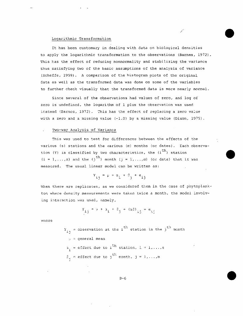
Logarithmic Transformation

It has been customary in dealing with data on biological densities

to apply the logarithmic transformation to the observations (Barnes, 1972).

This has the effect of reducing nonnormality and stabilizing the variance

thus satisfying two of the basic assumptions of the analysis of variance

(Scheffe, 1959). A comparison of the histogram plots of the original

data as well as the transformed data was done on some of the variables

to further check visually that the transformed data is more nearly normal.

Since several of the observations had values of zero, and log of

zero is undefined, the logarithm of 1 plus the observation was used

instead (Barnes, 1972). This has the effect of replacing a zero value

with a zero and a missing value (-1.0) by a missing value (Dixon, 1975).

Two-way Analysis of Variance

This was used to test for differences between the effects of the

various (s) stations and the various (m) months (or dates). Each observa-

tion (Y) is classified by two characteristics, the (i th) station

(i = 1,...,s) and the (j th) month (j = !_...,m) (or date) that it was

measured. The usual linear model can be written as:

Y,. u+ a. + 3. + e,.

When there are replicates, as we considered them in the case of phytoplank-

ton where density measurements were taken twice a month, the model involv-

ing interaction was used, namely,

Y.. = + a. + 3. + (cB) . + e..

wne re

Y. = observation at the i station in the j month

u = general mean

• thA = effect due to i station, i 1...s

1

5. = effect due to jth month, j =1...

B-6

(ae) . = interaction1J

e. = error

To compare the station effects, we formulate the null hypothesis

H0 : CL1 = a2 ....

which says that the stations are not different. To test the hypothesis

H0 against the alternative hypothesis which says at least two of these a

values are different, the two-way analysis of variance was used. Similar

null and alternate hypotheses are formulated for the month (or date)

effects ý or the interaction effects. The computer printout gives us

the value of the test statistic F and the probability (P-value) that the

computed F-value is exceeded under the null hypothesis. If this P-value

is < a (where a is a preassigned level of significance), then the null

hypothesis should be rejected. If it is > a then we do not have enough

evidence to reject the null hypothesis of equality of the effects.

For example, the two-way analysis of variance for phytoplankton

biovolume gives a station P-value of 0.3625 (see printout No. 7, pg. B-l18.

This implies that there is a 36 percent chance that the null hypothesis

is correct. Since the level of significance is commonly set at a = 0.05,

and the observed P-value is much larger than 0.05, we accept the null

hypothesis, which is that the mean biovolumes at the seven stations tested

are not significantly different. Duncan's Multiple Range Test was done

in each case to group stations that were alike (i.e., with means that were

not significantly distinguished) into subgroups.

Statistical Power Analysis for the Analysis of Variance

Analysis of variance, as explained above, is a procedure for detect-

ing significant differences in the time means of the populations being

considered. Just as there is a possibility of rejecting a correct null

hypothesis (the so-called Type I Error), there is a chance of accepting

a null hypothesis that is incorrect (the so-called Type II Error), i.e.,

concluding that the means are not different even when they are. We

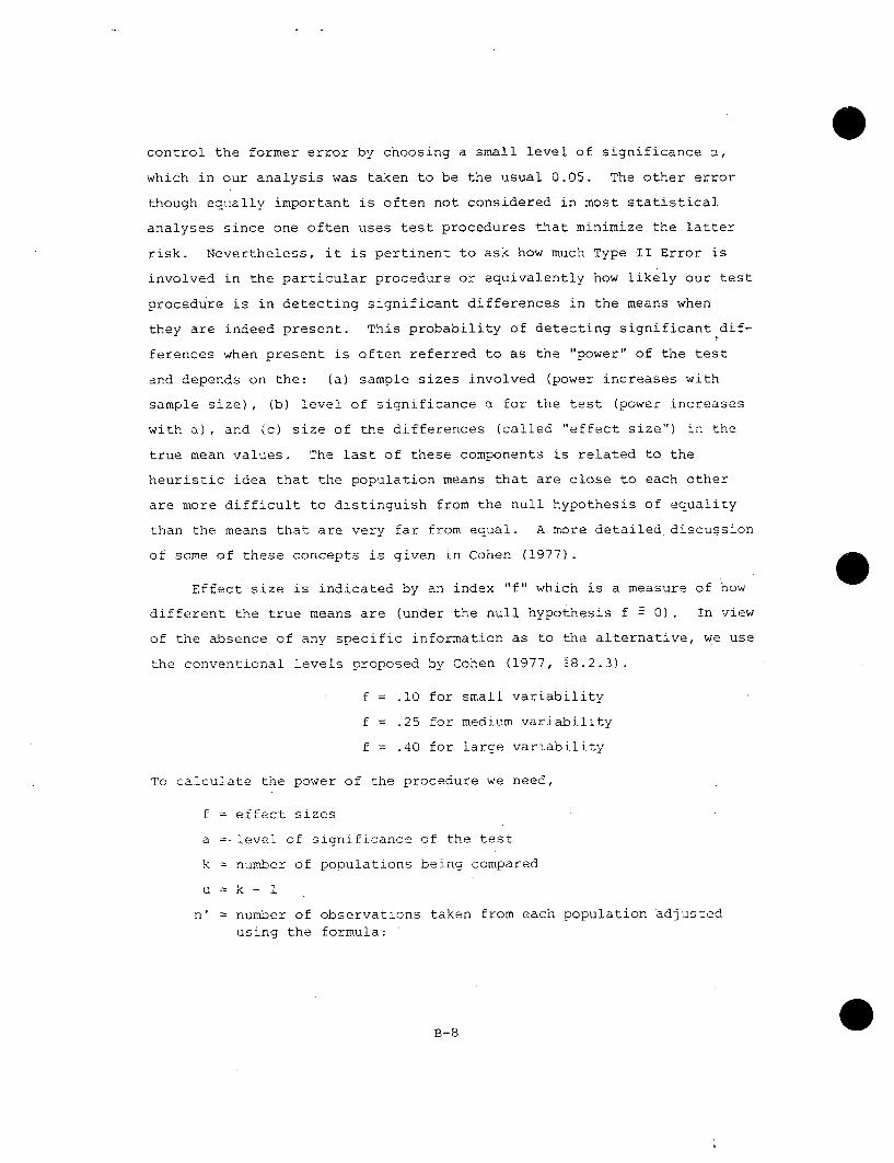
control the former error by choosing a small level of significance a,

which in our analysis was taken to be the usual 0.05. The other error

though equally important is often not considered in most statistical

analyses since one often uses test procedures that minimize the latter

risk. Nevertheless, it is pertinent to ask how much Type II Error is

involved in the particular procedure or equivalently how likely our test

procedure is in detecting significant differences in the means when

they are indeed present. This probability of detecting significant dif-

ferences when present is often referred to as the "power" of the test

and depends on the: (a) sample sizes involved (power increases with

sample size), (b) level of significance a for the test (power increases

with M), and (c) size of the differences (called "effect size") in the

true mean values. The last of these components is related to the

heuristic idea that the population means that are close to each other

are more difficult to distinguish from the null hypothesis of equality

than the means that are very far from equal. A more detailed discussion

of some of these concepts is given in Cohen (1977).

Effect size is indicated by an index "f" which is a measure of how

different the true means are (under the null hypothesis f E 0). In view

of the absence of any specific information as to the alternative, we use

the conventional levels proposed by Cohen (1977, j8.2.3).

f = .10 for small variability

f = .25 for medium variability

f = .40 for large variability

To calculate the power of the procedure we need,

f = effect sizes

a =,level of significance of the test

k = number of populations being compared

u=k- 1

n' = number of observations taken from each population adjusted

using the formula:

B-8

= (error degrees of freedom in F-statisticn = (k 1. 1/

The results of the power analysis are presented in Table 2. For

example, for the first variable, phytoplankton density, analysis of

variance was done using five stations. When comparing station means:

k = 5; u = (k- 1) = 4; and using the error degrees of freedom given in123

computer printout No. 3, page B-85, n' = -12 + 1 = 25; and a = 0.05.

Using the power tables in Cohen (1977) for the three effect sizes,

f = 0.10, 0.25, and 0.40, the probability of detecting a small, medium,

or large variability in the station means is 0.12, 0.60, and 0.96 res-

pectively. Thus, there is a poor chance of detecting small differences

in the station means, a fair chance of detecting medium differences, and

an excellent chance of finding large differences.

t-Tests

To confirm and clarify the results of the two-way analysis of vari-

ance procedures, single variable paired t-Tests were used. The idea of

a multivariate test, such as the Hotelling's T2 was abandoned because of

scanty data. A paired t-Test was considered appropriate as the measure-

ments from the stations were taken on the same day and the data sets may

be considered to be related. Two pairs of stations were chosen for com-

parison. The nearfield stations compared were the intake (HDR Station

No. 14) and the discharge (HDR Station No. 19). The farfield stations

were one upriver station (HDR Station No. 10) and one downriver station

(HDR Station No. 27). The biological variables used were densities of

phytoplankton, zooplankton, rotifera, crustacea, macroinvertebrates (col-

lected by dredge methods), macroinvertebrates (collected by artificial

substrate methods), and phytoplankton production, measured as chlorophyll a.

The last was included because data for this parameter were available for

intake and discharge stations only and a two-way analysis of variance was

irrelevant. A usable data set with no missing values (May to October,

1975 to 1976) was selected for all the t-Tests.

B-9

Table B-2. Statistical power calculations for the analysis ofvariance.

:IE-REE_ !T..iBE1z rnTAL CR~- JF ' L 7 5 IUNI

.7LL :ADIM 5

Error- L

2. nytoplanknon lAg P t3nnrt:r~nsse and 4ot4 Ina- ,~~ '

e~ar-o UMon d U

S. Pinvropior 4ron rye)9'i 'r

Ione. al 24lS . 3 (U Ii '2

. , nolakiorSraror

Error3

07'tool~nk'nXr nra a

Soncien 2trnrsvtvl MontOError

1.0 3. "• I .50

II-

(Log) Mon tha

Error

32

w

? ''ahvcon Station 2 1ý 31 D.TC7Irop'ynll .i 2j 32

Peri: y~on (Spocino S t.tion 1 *i-5Ov'r.x L,)a Mon jtLS 1

plnttat ionI

Lnn'. og MonO Il ýfr.,r 2jI

1I. !o:;IaLank a

a3 ttn~o Drninc I4 3St'ti

3.o 3A

Error -4

-l1t I 7 "1" ------

Stat I I

n I y Ero

IS . :-Oorot-.n---on --. A

a )C 1)3 It A. S

Station [Mon h *i 1 3

I

0B-10

Stepwise Regression

This was done to study the relationship between each biological

variable (dependent variable, y) with all the water quality variables

(independent variables, x.). The water quality measurements were taken

for both surface (top) as well as bottom so appropriate values were used

for each log transformed biotic variable. For phytoplankton density

(dependent variable), the surface water quality values were used as

independent variables, while for zooplankton, rotifera, and crustacea

densities, the average of top and bottom values were used. Macroinverte-

brate density (collected by dredge methods) was paired with the bottom

values while macroinvertebrate density (by artificial substrates) was

paired with top values. The regression model can be written as

Y 0 + IX(1)j + i.. + X (i)j +

with i = 1,...,p for each j = 1,...,n, where 8 is constant, £ is theth

error, Y is the j observed value of the dependent variable, and x

is the jth observed value of the ith independent variable. The objective,

then, of the selection procedures in the regression analysis is to deter-

mine the "best" subset of the p independent variables which yields a model

of the form:

Yj = 0 + y 1X(1)j + Y2X(2)j + --- + YiX(i)j + E

with i = 1,...,q for each j = 1,... ,n, where y and c are constants,

and the independent variables X. = 1 to q are a subset of the original1

set of X. where i = 1 to p.

The "best" q independent variables selected from the p original

variables may be determined in several ways, the most popular being the

stepwise regression procedure. This procedure starts with no independent

variables in the equation. The first variable added to the regression

is the one most highly correlated (linearly) with the dependent variable.

In addition, the correlation coefficient and its associated F statistic

must be statistically significant at a predetermined probability level,

such as a < 0.05. The second step in the analysis is to select a second

B-11

independent variable, is any of the remaining variables have an F larger

than the F value specified. This procedure chooses the independent

variable which is most correlated to the dependent variable, given that

the variable included in step one is in the model. Moreover, the step-

wise procedure "looks back" to see if any of the independent variables

interact; for instance, the addition of one X. might reduce the importance1

of another X. to the point where it should be deleted. Hence, the step-1

wise procedure may add or delete variables at any step rather than just

add variables. The stepwise procedure continues in this manner until

either no further X. values require entry or deletion from the equation,1

all variables are included in the equation, or the "tolerance values"

for the remaining significant independent variables are less than a pre-

determined level. The R2 values (coefficients of determination) obtained

in the analyses indicate the fraction of the variability in the dependent

parameter (Y) that is "explained" by the selected independent variables

(X). For instance, an R2 of 1.00 indicates that all Y variation is

explained, whereas an R2 of 0.00 indicates that none is explained.

B-12

RAW DATA TABLES*

(Tables 3-45)

*Except Tables 4, 5, 8, 16, 17, 18, 19, 20, 21, 24,

25, and 27 which also include computer printout.

B-13

Table B-3a. Phytoplankton densities for 1973.

HDR STATION NUMBER 6 9 19 27

STATION CODE1 1 2 4 5

MONTH CODE 1 DATE DENSITY PER ml

March 12 846 821 - 826

March 26 2,868 1,729 - 2,790

April 16 - 41,205 5- 5,725April 30 32,250 -- 40,650

May 14 21,375 24,450 - -

May 28 8,625 9,465 17,588 8,145

June 11 11,175 5,925 13,620 6,990June 25 7,755 6,945 11,040 5,790

July 9 8,880 4,800 9,180 5,250July 23 15,780 10,755 27,600 8,020

8 August 6 15,000 4,407 23,730 8,450August 27 7,770 9,690 12,690 5,100

September 10 10,560 5,640 22,590 6,300September 24 16,890 6,030 25,840 6,780

October 8 10,890 1,080 12,840 8,400October 22 4,050 4,770 5,760 3,480

November 5 2,625 4,710 3,870 3,480November 19 - 3,600 2,460 3,780

'As used on the computer printout.

B-14

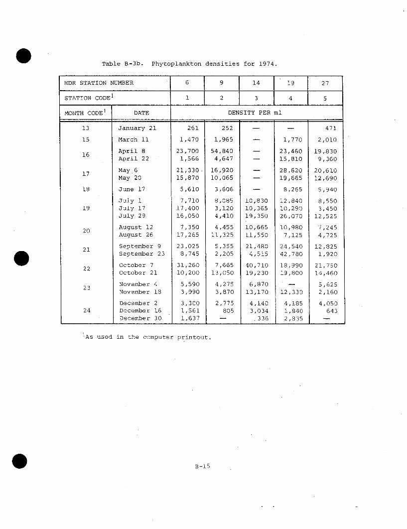
Table B-3b. Phytoplankton densities for 1974.

HDR STATION NUMBER 6 9 14 19 27

STATION CODE 1 1 2 3 4 5

MONTH CODE 1 DATE DENSITY PER ml

13 January 21 261 252 - - 471

15 March 11 1,470 1,965 - 1,770 2,010

16 April 8 23,700 54,840 - 23,460 19,830April 22 1,566 4,647 - 15,810 9,360

17 May 6 21,330 16,920 - 28,620 20,610May 20 15,870 10,065 - 19,665 12,690

18 June 17 5,610 3,606 - 8,265 5,940

July 1 7,710 8,085 10,830 12,840 8,55019 July 17 17,400 3,120 10,365 10,290 3,450

July 29 16,050 4,410 19,350 26,070 12,525

20 August 12 7,350 4,455 10,665 10,980 7,245August 26 17,265 11,325 11,550 7,125 4,725

21 September 9 23,025 5,355 21,480 24,540 12,825September 23 8,745 2,205 4,515 42,780 1,920

22 October 7 31,260 7,665 40,710 18,990 21,750October 21 10,200 13,050 19,230 19,800 14,460

23 November 4 5,590 4,275 6,870 - 5,625November 18 3,990 3,870 13,170 12,330 2,160

December 2 3,300 2,775 4,140 4,185 4,05024 December 16 1,561 805 3,034 1,840 643

December 30 1,637 - .336 2,835

'As used in the computer printout.

B-15

Table B-3C. Phytoplankton densities for 1975.

HDR STATION NUMBER 6 9 14 19 27

STATION CODE 1 1 2 3 4 5

MONTH CODE 1 DATE DENSITY PER ml

29 May 7 10,590 14,640 12,660 15,000 18,990May 21 14,190 22,590 14,490 17,610 11,670

30 June 4 14,460 12,300 19,860 24,540 11,880June 18 9,960 12,780 17,910 17,850 9,480

31 July 1 1,883 2,032 6,945 868 1,391July 16 4,839 4,513 4,299 846 5,912

32 August 12 11,265 2,905 5,625 8,985 5,655August 26 5,265 12,300 18,480 20,550 10,890

33 September 10 7,995 13,500 8,310 7,425 14,850September 24 11,910 12,960 10,650 10,065 10,530

34 October 8 25,440 13,830 22,260 18,120 11,670October 22 18,840 9,030 21,030 48,780 10,830

35 November 19 6,420 5,250 - 13,980 -

36 December 17 - - 2,475 2,670 -

December 31 -- I - 990 885 - 0lAs used in the computer printout.

0B -16

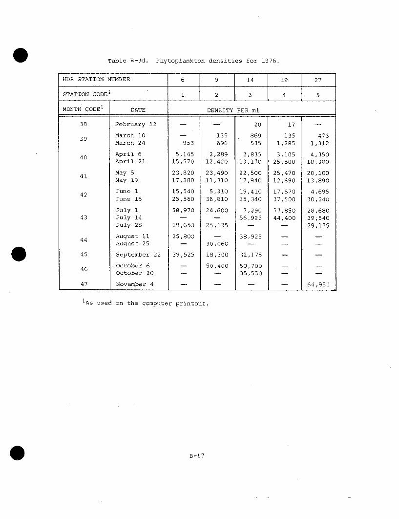
Table B-3d. Phytoplankton densities for 1976.

HDR STATION NUMBER 6 9 14 19 27

STATION CODE]. 1 2 3 4 5

MONTH CODE1 DATE DENSITY PER ml

38 February 12 - 20 17 -

39 March 10 - 135 869 135 473March 24 953 696 535 1,285 1,312

40 April 6 5,145 2,289 2,835 3,105 4,350April 21 15,570 12,420 13,170 25,800 18,300

41 May 5 23,820 23,490 22,500 25,470 20,100May 19 17,280 11,310 17,940 12,690 13,890

42 June 1 15,540 5,310 19,410 17,670 4,695June 16 25,560 36,810 35,340 37,500 30,240

July 1 58,970 24,600 7,290 77,850 28,68043 July 14 - - 56,925 44,400 39,540

July 28 19,650 25,125 - - 29,175

44 August 11 25,800 - 38,925 -

August 25 - 30,060 - - -

45 September 22 39,525 18,300 32,175 -

46 October 6 - 50,400 50,700 --

October 20 - - 35,550 -

47 November 4 -- 64,950

1As used on the computer printout.

B-17

Table B-4. Phytoplankton density (Log transformed), 1975-76. 0

PAIRED t-TEST

SAMPLE NUMBER INTAKE DISCHARGE

1 31.6330 2.9270

2 4.2660 4.3130

3 3.9190 3.8700

4 4.3470 4.2580

5 1.3010 1.2300

6 3.4520 3.4920

7 4.2540 4.1030

8 4.5480 4.5740

t-Test

1) H0: MU(X)-MU(Y) 0

H1: MU(X)-MU(Y) > 0

t Value = 0.482

DF = 7

t(0.950, 7) = 1.895

Do not reject HO at 0.05level of significance

t = 0.4820, DF = 7

Prob t > 0.4820 = 0.3223

B-18

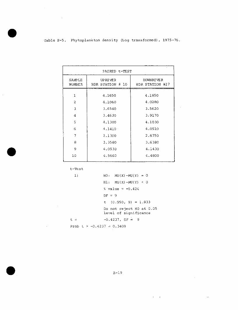
Table B-5. Phytoplankton density (Log transformed), 1975-76.

PAIRED t-TEST

SAMPLE UPRIVER DOWNRIVERNUMBER HDR STATION # 10 HDR STATION #27

1 4.1650 4.1850

2 4.1060 4.0280

3 3.6540 3.5620

4 3.4630 3.9170

5 4.1300 4.1030

6 4.1410 4.0510

7 2.1300 2.6750

8 3.3580 3.6380

9 4.0530 4.1430

10 4.5660 4.4800

t-Test

1) HO: MU(X)-MU(Y) = 0

Hi: MU(X)-MU(Y) < 0

t value = -0.424

DF = 9

t (0.950, 9) = 1.833

Do not reject HO at 0.05level of significance

t. -0.4237, DF = 9

Prob t > -0.4237 = 0.3409

B-19

Table B-6. Phytoplankton Type I productivity.

NDR STATION NUMBER 6 10 14 21 27

STATION CODEI 1 2 3 5

MONTH CODE1 DATE PRODUCTIVITY (ppm 02 /hr)

1 April 1 -0.14 0.02 -0.01 0.03 0.03 0.03 0.12 0.07 0.03

2 April 8 0.02 0.21 0.16 -0.02 0.06 0.05 0.30 -0.02 0.16

3 April 26 0.17 0.28 0.35 0.32 0.40 0.39 0.60 0.22 0.38

4 May 6 0.64 0.75 0.78 0.57 0.49 0.66 0.87 0.14 0.70

5 May 14 0.66 0.92 0.88 0.76 0.88 0.88 0.92 0.18 0.86

6 May 22 0.47 0.60 0.59 0.45 0.39 0.45 0.48 0.30 0.41

7 May 27 0.78 0.29 0.36 0.63 0.76 0.54 0.69 0.28 0.49

8 June 4 0.84 0.62 0.67 0.82 0.69 0.69 0.93 0.03 0.92

9 June 14 -0.06 0.53 0.85 0.32 0.23 0.56 1.08 0.54 0.37

10 June 25 1.23 1.15 1.42 0.23 0.40 0.57 1.87 0.88 -

Ii July 2 0.71 0.83 1.27 1.28 0.88 0.92 1.04 1.08 0.93

12 July 8 1.06 0.88 0.68 0.86 1.24 1.10 1.61 0.17 0.80

13 July 22 1.14 1.05 1.08 1.16 1.50 1.23 1.34 0.54 1.20

14 July 29 0.60 1.06 1.32 1.03 0.51 0.36 0.97 0.28 0.83

15 August 27 1.02 1.23 1.30 0.68 1.47 1.00 0.96 0.66 0.49

16 September 9 1.03 1.09 0.87 0.92 0.87 0.50 1.70 1.19 1.00

17 September 24 0.86 0.96 1.04 0.67 1.04 0.96 0.54 0.46 0.72

18 October 7 0.36 0.54 0.80 0.39 0.80 0.30 0.16 0.13 0.45

19 October 22 0.80 1.17 0.96 0.71 0.96 0.68 1.37 1.08 0.95

20 November 10 0.22 0.43 0.54 - 0.50 0.54 0.54 0.21 0.40

21 May 26 0.33 0.28 0.42 0.35 0.27 0.27 0.36 0.27 0.19

22 June 2 0.13 0.09 0.15 0.15 0.21 0.11 0.15 0.09 0.15

23 June 23 -0.06 -0.07 -0.05 0.16 0.26 0.26 1.00 0.23 0.26

24 June 30 0.06 0.05 0.18 0.07 0.13 0.13 0.33 0.27 0.12

25 July 21 -0.20 -0.01 0.08 0.02 0.12 0.17 0.46 0.05 0.15

26 August 8 -0.99 -0.99 -0.37 0.03 0.10 0.24 0.10 0.00 0.18

27 August 11 0.04 -0.10 0.06 0.06 0.12 0.13 0.42 0.15 0.11

28 August 18 0.21 0.27 0.17 0.19 0.18 0.12 0.17 0.08 0.16

29 August 25 0.05 0.41 0.21 0.04 0.08 0.07 0.28 0.19 0.20

30 September 4 0.24 0.20 -0.06 0.10 0.17 0.07 0.23 0.08 0.15

31 September 8 0.04 0.29 0.28 0.13 0.18 0.24 0.47 0.08 0.31

32 September 22 0.20 0.36 0.36 0.25 0.23 0.12 0.98 0.34 0.29

33 September 29 -0.02 0.23 0.05 0.11 0.09 0.08 0.34 0.08 0.15

34 October 7 -0.08 0.27 0.08 0.10 0.14 0.16 0.16 0.00 0.22

35 October 20 0.01 0.09 0.50 0.14 0.16 0.11 0.34 0.23 0.33

IA5 used on the computer printout.

B-20

Table B-7. Phytoplankton Biovolume (mg/liter).

HDR STATION NUMBER 6 10 14 21 27

STATION CODE1 1 2 3 5 7

MONTH CODE 1 DATE (mg/liter)

1976-- 0.16 0.42 0.06 0.22

2.16 3.76 0.53 0.81 3.64

1.99 2.15 1.67 1.50 1.81April 10.24 7.15 7.38 12.01 8.12

19.27 17.50 11.99 17.03 12.4214.08 8.42 20.48 13.03 12.84

6 June 19.24 9.75 49.94 47.11 16.2242.05 52.44 52.05 55.16 56.55

49.87 18.34 6.88 61.01 23.40July 29.71 31.08 48.60 33.76 33.62

1975

5.30 6.41 - 5.49 9.788.29 11.01 6.65 8.87 5.74

9.00 9.25 15.72 10.44 1.1.887.87 10.43 13.19 12.07 7.08

2.51 2.53 4.92 0.98 1.7219 July 4.01 4.56 3.49 0.88 4.18

20 August 11.52 3.76 6.06 9.08 5.063.08 12.92 17.25 23.18 10.29

9.06 16.07 8.26 6.51 12.8721 September 7.82 7.41 9.15 7.93 7.12

12.94 12.33 13.18 12.48 7.748.43 3.96 8.74 18.61 9.98

1As used in computer printout.

B-21

Table B-8. Phytoplankton production: Chlorophyll a (ppb).

PAIRED t-TEST

SAMPLENUMBER INTAKE DISCHARGE

1 40 402 49 383 54 484 43 285 50 306 30 307 38 388 23 10

9 50 2510 54 2611 75 4012 110 3013 55 3214 85 6115 60 4516 75 4517 60 3218 85 6019 60 5220 80 4721 45 2522 125 48

t -Test:

2) HO: ABS(MU(X)-MU(Y)) = 0Hi: ABS(MU(X)-MU(Y)) # 0

t Value = 1.133DF = 21

t(0.975, 21) = 2.080

Do not reject HO at 0.05 levelof significance.

t = 1.1327, DF 21

PROB t > 1.1327 = 0.1350

B-22

Table B-9. Phytoplankton-species diversity.

HDR STATION NUMBER 6 10 14 21 27

STATION CODE 1 1 2 3 5 7

MONTH CODE 1 MONTH SHANNON-WEAVER INDEX

1976

3 March - 2.95 2.79 2.18 2.673.75 4.12 3.61 3.65 3.27

4 April 1.31 2.28 1.36 1.43 1.711.96 2.20 1.63 1.09 1.58

5 May 2.35 2.34 2.10 2.59 2.572.83 3.49 3.01 2.95 3.14

6 June 4.42 4.18 3.75 3.82 3.473.87 3.40 2.98 2.89 3.66

7 July 2.99 3.05 2.84 2.45 2.933.78 3.69 3.17 3.00 2.31

1975

17 May 1.51 1.32 - 1.02 1.552.48 2.34 2.43 2.15 2.25

18 June 3.01 2.85 3.14 2.96 3.673.21 3.07 2.51 2.27 2.17

19 July 4.19 3.45 3.29 3.55 3.533.37 3.32 3.26 4.21 3.43

20 August 3.84 3.90 2.98 3.41 3.873.02 3.50 3.00 2.87 3.17

21 September 3.59 3.75 3.27 2.90 3.523.02 3.07 3.35 3.47 3.00

22 October 2.52 2.88 2.37 2.43 2.742.47 2.30 2.44 1.54 3.02

1As used on the computer printout.

B-23

0Phytoplankton: Type III productivity analysis (P=PSg-R)in ppm 0 2 /hr for intake and discharge (1976).

Table B-10.

DATE INTAKE DISCHARGE DATE INTAKE DISCHARGECODE CODE

1 1.00 0.9 6 1.33 0.51.35 0.7 1.0 0.351.57 0.55 1.05 0.30.85 0.65 0.8 0.6

2 0.85 0.1 7 0.9 0.150.4 0.2 0.5 0.50.9 0.1 1.1 0.10.7 0.15 0.9 0.15

3 0.7 0.6 8 0.8 0.40.4 0.4 0.8 0.40.7 0.4 1.0 0.30.6 0.4 0.5 0.4

4 0.85 0.4 9 0.6 0.41.10 0.3 0.7 0.450.6 0.2 0.75 0.41.1 0.25 1.1 0.3

5 0.8 0.11.0 0.21.0 0.151.0 0.1

0

B-24

Table B-lla. Periphyton density, 1976.

HDR STATION NUMBER 13 20 25

STATION CODE 1 3 5 6

MONTH CODE 1I DATE DENSITY/cm2

1 January 14 - 67,636 2,424January 28 - 688,152 485

2 February 12 - 97,970 3,584February 25 - 90,968 56,209

3 March 10 - 1,821,879 6,162March 24 - 2,929,954 -

4 April 6 - 405,809 -

April 21 - 1,031,068 -

5 May 5 - 170,279 -

May 19 1,119,725 380,232 1,124,381

6 June 1 573,854 284,587 690,488June 16 198,278 107,297 247,261

7 July 14 415,232 247,272 368,576July 28 578,524 95,641 179,620

8 August 11 272,928 447,886 284,593August 25 27,991 359,245 312,589

9 September 8 265,932 209,946 513,207September 22 494,544 797,805 205,281

10 October 6 220,443 415,230 387,237October 20 88,641 737,152 108,471

11 November 4 5,261 12,725 93,307November 17 - 312,588 56,566

12 December 15 - 72,892 19,957December 30 - 60,646 26,934

iAs used in computer printout.

B-25

Table B-lib. Periphyton density (1975).

HDR STATION NUMBER 13 20 25

STATION CODE1 3 5 6

MONTH CODE 1 DATE DENSITY/cm2

13 January13 NS 51,313 594January 27 NS 310,245 2,464

14 February 10 NS 100,885 1,182February 24 NS 265,924 41,318

15 March 26 NS 2,262,806 59,705

16 April NS NS NS

17 May 21 919,103 998,418 -

18 June 4 1,408,982 524,865 667,160June 18 1,313,337 807,128 1,255,017

19 July 16 557,518 228,595 737,151July 30 856,111 401,224 753,476

20 August 12 923,773 181,945 797,803August 26 352,232 69,975 657,825

21 September 10 727,814 825,793 895,779September 24 1,077,734 494,540 410,558

October 8 1,082,393 559,858 419,884October 22 629,839 919,099 1,185,044

23 November 19 1,194,370 632,166 592,512

December 17 - 942,428 124,094December 31 - 18,659 -

tAs used in computer printout.

0

0B-26

Table B-12a. Periphyton chlorophyll a concentration (1976).

HDR STATION NUMBER 13 20 25

STATION CODE 1 3 5 6

MONTH CODE 1 DATE CONCENTRATION (pg/cm2 )

1 January 14 - 0.64 0.05January 28 - 1.59 0.04

2 February 12 - 3.24 0.12February 25 - 5.70 0.19

3 March 10 - 11.97 0.12March 24 - 13.97 -

May 5 - 2.85 -May 19 6.63 3.37 3.62

6 June 1 4.47 4.34 8.37June 16 3.93 4.26 4.08

7 July 1 4.15 1.49 3.02July 14 5.88 3.27 1.78

8 August 11 2.50 2.00 4.42August 25 3.00 3.10 3.60

September 8 2.38 1.90 3.29September 22 2.69 2.93 5.13

10 October 6 4.92 2.42 2.83October 20 1.58 2.43 1.36

11 November 4 0.16 1.87 1.26November 17 - 2.29 0.51

12 December 15 - 1.00 0.27December 30 - 0.64 0.62

IAs used in the computer printout.

B-27

Table B-12b. Periphyton chlorophyll a concentration (1975).

HDR STATION NUMBER 13 20 25

STATION CODE 1 3 5 6

MONTH CODE 1 DATE CONCENTRATION (vg/cm2 )

13 January 13 - 0.36 0.04January 27 - 2.20 0.05

14 February 10 - 1.01 0.06

February 24 - 1.53 5.27

15 March 26 - 9.37 0.58

17 May 21 4.02 7.30 -

June 4 6.66 3.38 2.21June 18 7.15 3.29 6.16

19 July 1 7.43 4.52 9.75July 16 4.09 5.65 4.51

20 August 12 4.72 2.94 5.70August 26 7.07 7.03 9.84

21 September 10 6.06 5.52 11.57September 24 9.30 3.76 3.64

October 8 8.51 6.59 6.80October 22 6.65 11.84 12.52

23 November 192 3.48 2.08 4.76

24 December 172 - 3.15 0.58December 31 0.17 -

IAs used in the computer printout.2 4-week incubation periods.

B-28

Table B-13a. Periphyton-phaeophytin a concentration (1976).

HDR STATION NUMBER 25 13 21

STATION CODE 1 6 3 5

MONTH CODE 1 DATE CONCENTRATION (Cg/cm2 )

1 January 14 0.00 - 0.05January 28 0.01 - 0.05

2 February 12 0.02 - 0.45February 25 0.04 - 0.08

3 March 10 0.02 - 0.27March 24 - - 0.66

5 May 5 - - 0.56May 19 0.22 0.01 0.33

6 June 1 2.24 0.95 1.49June 16 6.04 2.33 4.23

7 July 1 2.79 1.44 1.31July 14 1.30 4.66 2.27

8 August 11 1.73 0.71 3.43August 25 2.41 1.08 2.08

9 September 8 1.97 1.76 3.90September 22 2.37 1.34 1.64

10 October 6 2.58 4.40 3.04October 20 1.07 0.42 1.90

11 November 4 0.88 0.06 0.84November 17 0.13 - 1.23

12 December 15 0.12 - 1.25December 30 0.05 - 0.62

1As used on the computer printout.

B-29

Table B-13b. Periphytonr-phaeophytin a concentration (1975).

HDR STATION NUMBER 25 13 21

STATION CODE 1 6 3 5

MONTH CODE 1 DATE CONCENTRATION ('bg/cm2 )

13 January 13 0.03 - 0.10

January 27 0.01 - 0.11

14 February 10 0.00 - 0.00February 24 0.21 - 0.00

15 March 10 - - -

March 26 0.00 - 0.24

16 April 9 - - -

April 23 - -

17 May 7 - - -

May 21 - 0.60 1.90

18 June 4 0.17 0.42 0.48June 18 0.16 0.37 0.35

19 July 1 0.22 0.32 0.70July 16 1.01 0.92 0.92

20 August 12 3.74 1.01 1.18August 26 0.98 0.86 0.96

21 September 10 0.36 0.86 0.61September 24 1.05 0.71 0.46

22 October 8 0.62 1.32 0.97October 22 0.86 0.12 1.73

23 November 192 0.12 0.08 0.42

24 December 172 0.02 - 0.28

IAs used on the computer printout.2 4-week incubation periods.

B-30

Table B-14. Periphyton-species diversity.

HDR STATION NUMBER 13 21 25

STATION CODE 1 3 5 6

MONTH CODE 1 MONTH SHANNON-WEAVER INDEX

1976

5 May 3.70 -2.54 3.50 3.70

3.02 3.19 3.653.16 3.27 3.45

2.96 2.59 2.61July 1.96 2.12 2.94

2.13 2.55 2.26August 2.08 2.39 2.43

2.38 2.25 2.032.41 2.78 2.25

2.67 2.83 2.742.95 2.70 2.21

2.74 2.80 2.97ii November1.4 .3-- 1.94 1.32

1975

17 May 3.62 2.61 -

4.04 3.00 2.903.53 3.10 3.12

3.78 3.49 3.1519 July 3.75 3.78 2.18

2.13 3.34 3.2720 August 3.82 3.26 3.38

3.88 3.50 2.1621 September 3.18 3.50 2.61

3.52 3.03 3.742.38 2.21 3.18

23 November 3.74 4.11 3.82

-- 4.13 2.7224 December - 3.11 -

-- 3.11 --

lAs used on the computer printout.

B-31

Table B-15a. Zooplankton -total densities for 1975.

HDR STATION NUMBER 6 10 12 18 21 25 27

STATION CODE 1 1 2 3 4 5 6 7

MONTH CODE 1 DATE DENSITY (Number/£)

1 January 15 16.2 - 14.1 11.2 23.4 104.2 -

2 February 18 5.7 - 7.9 7.5 4.0 11.7 -

3 March 11 28.0 8.4 11.4 .14.4 11.3 23.4 302.0

4 April 15 12.8 22.9 8.9 11.2 15.8 12.2 18.9

5 May 20 35.8 14.3 28.7 15.3 27.0 17.5 10.2

6 June 24 31.3 30.1 75.3 40.0 55.0 53.9 48.7

7 July 30 358.9 231.0 263.6 398.6 234.4 242.2 350.4

9 September 2 91.6 198.6 143.0 91.3 56.8 82.5 111.1September 16 91.1 328.3 127.9 75.1 125.7 137.0 262.8

10 October 14 213.9 106.5 124.8 72.5 133.1 123.0 144.8

11 November 25 75.8 51.7 81.1 64.8 91.7 97.3 74.6

12 December 19 - - - 28.2 36.4 46.5 -

1As used on the computer printout.

Table B-15b. Zooplankton -total densities for 1976.

HDR STATION NUMBER 6 10 12 18 21 25 27

STATION CODE 1 1 2 j 3 4 5 6 7

MONTH CODE 1 MONTH DENSITY (Number/0)

13 January 19.1 N.S. 30.7 9.1 T 15.2 16.2 N.S.

14 February 16.2 N.S. 13.5 9.2 10.2 11.8 N.S.

15 March 28.0 34.3 240.2 56.7 27.2 19.8 30.0

16 April 91.2 45.8 82.9 29.2 57.7 63.3 32.3

17 May 938.2 802.4 790.0 360.1 626.1 638.3 878.7

18 June b810.0 948.9 547.8 282.1 385.7 329.8 632.3

i9 July 576.4 739.9 818.2 576.2 536.8 744.1 703.0

20 August 851.0 870.0 560.3 521.7 529.0 542.3 638.9

21 September 463.7 609.5 444.9 340.0 765.4 446.8 650.8

22 October 500.5 312.0 363.5 336.8 445.8 284.1 398.2

23 November N.S. 57.7 115.9 108.8 137.2 96.4 33.0

24 December 135.3 N.S. 169.9 69.2 191.1 206.7 N.S.

IAs used on the computer printout.

B-32

Table B-16. Zooplankton total density (Log transformed) 1975-76.

SAMPLE NUMBER INTAKE DISCHARGE

1 2.4210 2.3700

2 2.1550 1.7540

3 2.1070 2.1070

4 2.0960 2.1240

5 1.9090 1.9620

6 1.4870 1.1810

7 1.1300 1.0080

8 1.9180 1.7610

9 2.8970 2.7960

10 2.7380 2.5860

11 2.7480 2.7230

12 2.6480 2.8840

13 2.5600 2.6590

14 2.0640 2.1370

t-Test

I) HO: MU(X)-MU(Y) = 0

Hi : MU(X)-MU(Y) > 0

t value = 0.356

DF = 13

t (0.950, 13) = 1.771

Do not reject HO at 0.05level of significance

t 0.3564, DF 13

Prob t > 0.3564 = 0.3636

B-33

Table B-17. Zooplankton total density (Log transformed) 1975-76.

PAIRED t-TEST

SAMPLE UPRIVER DOWNRIVERNUMBER HDR STATION #10 HDR STATION #27

1 1.1550 1.0080

2 1.4780 1.6870

3 2,3630 2.5440

4 2.5160 2.4190

5 2.0270 2.1600

6 1.7130 1.8720

7 1.5350 1.4770

8 1.6600 1.5090

9 2.9040 2.9430

10 2.9770 2.8000

11 2.8990 2.8460

12 2.9390 2.8050

13 2.7850 2.8134

14 2.4940 2.6000

15 1.7610 1.5180

t-Test

1) HO: MU(X)-MU(Y)

Hi: MU(X)-MU(Y)

t value = 0.093

DF = 14

t (0.950, 14)

= 0

> 0

1. 761

at 0.05 levelDo not reject HOof significance

t = 0.0934, DF 14

Prob t > 0.0934 = 0.4635

B-34

Table B-18. Zooplankton: Rotifer density (Log transformed),1975-76.

SAMPLE NUMBER INTAKE DISCHARGE

1 2.2480 2.2300

2 1.9780 1.4930

3 2.0280 1.6530

4 2.0040 2.0610

5 1.7430 1.7590

6 1.2090 0.6360

7 0.3980 0.5220

8 1.5750 1.4400

9 2.8490 2.7470

10 2.3400 2.2010

11 2.5760 2.6320

12 2.4700 2'.8370

13 2.4610 2.5350

14 2.0030 2.0820

t-Test

1) HO: MU(X)-MU(Y)

HI: MU(X)-MU(Y)

= 0

> 0

t value = 0.296

DF = 13

t (0.950, 13) = 1.771

Do not reject HO at 0.05 levelof significance

t = 0.2959, DF = 13

Prob t > 0.2959 = 0.3860

B-35

Table B-19. Zooplankton: Rotifer density (Log transformed),1975-76.

PAIRED t-TEST

SAMPLE UPRIVER DOWNRIVERNUMBER HDR STATION #10 HDR STATION #27

1 0.8260 0.7710

2 1.1730 1.4310

3 2.3030 2.4840

4 2.3380 2.3840

5 1.9570 2.1020

6 1.6020 1.7420

7 0.8550 0.7800

8 1.3420 1.1590

9 2.8650 2.9080

10 2.7290 2.5230

11 2.7720 2.6810

12 2.7900 2.6560

13 2.6480 2.6790

14 2.3340 2.3240

15 1.6650 1.2920

t-Test

1) HO: MU(X)-MU(Y) 0

HI: MU(X)-MU(Y) > 0

t value = 0.113

DF = 14

t (0.950, 14) = 1.761

Do not reject HO at 0.05level of significance

t = 0.1131, DF = 14

Prob t > 0.1131 = 0.4558

B-36

Table B-20. Zooplankton: Crustacea1975-76.

density (Log transformed)

PAIRED t-TEST

SAMPLE NUMBER INTAKE DISCHARGE

1 1.9100 1.9630

2 1.6530 1.3540

3 1.2940 1.6350

4 1.3580 1.1960

5 1.3760 1.2640

6 1.1370 0.3850

7 0.4190 0.2040

8 1.0190 0.9270

9 1.3730 1.4830

10 1.8320 1.6560

11 2.2640 2.0000

12 2.1740 1.8880

13 1.8690 2.0510

14 1.1770 1.2010

t-Test

1) HO:

HI:

MU(X) -MU (Y)

MU(X) -MU(Y)

0

0

t value = 0.447

DF = 13

T (0.950, 13) = 1.771

Do not reject HO at 0.05level of significance

t = 0.4469, DF = 13

Prob t > 0.4469 0.3311

B-37

Table B-21. Zooplankton: Crustacea density (Log transformed)1975-76.

PAIRED t-TEST

SAMPLE UPRIVER DOWNRIVE RNUMBER HDR STATION #10 HDR STATION #27

1. 0.8260 0.5680

2 0.8860 1.0080

3 1.4750 1.6430

4 1.6180 1.2690

5 1.1640 1.2120

6 0.8190 1.2090

7 0.6530 0.5900

8 0.6300 0.5050

9 1.1630 1.1430

10 1.8340 1.8220

11 2.3050 2.3470

12 2.4040 2.2670

13 2.2160 2.2370

14 1.9810 2.1000

15 1.0520 1.1250

t-Te st

i) HO: MU(X)-MU(Y) 0

HI: MU(X)-MU(Y) < 0

t value = -0.007

DF = 14

t (0.950, 14) = 1.761

Do not reject HO at 0.05level of significance

t = -0.0071, DF : 14

Prob t > -0.0071 = 0.4972

B-38

Table B-22. Zooplankton-species diversity.

L I IHDR STATION NUMBER 6 10 12 18 21 25 27

STATIONCODEI 1 2 3 4 5 6 7

MONTH CODE 1 MONTH SHANNON-WEAVER INDEX

1976

1 January 2.74 - 2.33 2.87 2.89 -

2 February 2.73 - 2.93 3.14 2.94 - -

3 March 2.97 3.00 1.98 2.25 3.09 2.83 2.84

4 April 3.13 3.26 3.19 3.04 3.41 3.20 3.23

5 May 1.93 2.00 2.01 2.05 2.34 1.95 1.88

6 June 2.07 2.28 2.11 2.42 2.17 2.41 2.47

7 July 2.43 2.18 2.13 2.48 2.43 2.26 2.65

8 August 2.25 2.34 2.45 2.32 2.23 2.43 2.68

9 September 2.17 1.71 2.33 1.94 1.65 1.84 1.77

10 October 2.08 2.04 1.44 1.86 1.74 2.08 2.08

11 November - 2.24 2.11 1.86 2.18 2.60 2.70

12 December 1.07 - 0.89 0.66 0.71 - -

1975

13 January 3.39 - 2.66 2.57 2.36 - -

14 February 1.96 - 1.93 2.04 2.14 - -

15 March 3.04 3.12 3.63 0.10 2.60 - 0.10

16 April 3.47 2.15 2.53 2.31 1.80 1.67 2.37

17 May 2.09 2.98 1.90 2.64 2.29 3.10 3.00

18 June 2.53 2.81 2.45 2.79 2.70 2.47 2.37

19 July 2.74 2.39 3.02 2.69 2.71 2.46 2.20

20 August 3.31 2.66 3.16 3.43 3.34 3.09 2.74

21 September 2.46 1.15 1.76 2.90 3.13 1.10 0.98

22 October 1.15 1.28 1.17 2.68 1.17 1.97 1.44

23 November 1.90 2.15 2.22 1.82 2.61 2.38 2.41

24 December -- -- 2.76 2.75 - -

'As used on the computer printout.

B-39

Table B-2 3a. Total macroinvertebrate density collected by Petersen dredge methods (1975).

IiDR STATION NUMBER 6 10 12 21 25 27

STATION CODE1 1 2 3 5 6 7

MONTH CODE9 MONTH DENSITY (Number/m 2 )

3 March 11,589.5 - 11,230.7 4,099.9 6,499.8 -

7 July 392.4 439.2 205.2 864.0 396.0 734.4

9 September 457.2 540.0 136.8 903.6 374.4 140.4

10 October 226.8 212.4 273.6 309.6 108.0 10.8

12 December - 504.0 212.4 25.2 518.4 64.8

0

0

1As used on the computer printout.

0

-4 N O CO COr- 0) CO m 0) O

NN M 0 I ( 1- ()

(3) CD 4 (N CN , m0 C q

ci) (l o-, N r-4 -4T N

r-4 mn CO m ,- r- i10C 0 0 0I N O

w 4 O CO 1 (N N) C-4 0 0 C-() r-i -

('1 CN rn "T ( n CO 0 fn

ci)H 'N 0 ( ý 0 C CO 0 (N CU)4 r- ( CN (n 0o r- N O O

w ci) CO r, a'. 00 0 1 O (N

0. .

-4 m 0 (- N 1--1 1 -1 '.

v4 co c_ _-4__ _M__ _ _ _ _ _ _

.0 4~ 0 ' 0 (. (.0 C

(\I (N4 Hn 00 -. 0 O 0 CODCC/)~Lr NN CN k O CO 04

00C.) '0 CO ~ ' CO 1001

4.)~~~ý 0a)C C O 10 C

ci) W CO - CO P4 >O

ci))

1-4 -4 0- - 0 (

C))C) U4

B-41

Table B-23c. Total macroinvertebrate density collected by Petersen dredge methods (1977).

HDR STATION NUMBER 6 10 12 21 25 27

STATION CODE 1 1 2 3 5 6 7

MONTH CODE 1 DATE DENSITY (Number/mr2 )

25 January 24 1,397.85 - 8,630.81 1,157.71 1,340.50 -

28 April 18 3,949.82 4,465.95 6,186.37 3,473.11 3,860.21 4,200.71

29 May 31. 3,240.14 - 7,218.62 4,939.06 4,810.03 15,505.37

lAs used on the computer printout.

to

Table B-24. Macroinvertebrate density (Log transformed) collectedby dredge methods, 1975-76.

PAIRED t-TEST

SAMPLE NUMBER INTAKE DISCHARGE

1 2.3120 2.9360

2 2.1360 2.9560

3 2.4370 2.4910

4 2.5770 2.9660

5 3.2360 2.6320

6 3.1000 2.5520

7 2.8730 3.3230

8 3.2850 4.0030

9 3.7730 3.3380

10 3.5420 3.5670

11 3.7680 3.7230

t-Test

1) HO: MU(X) -MU(Y)

HIl: MU(X)-MU(Y)

= 0

< 0

t value = -0.258

DF = 10

t (0.950, 10) = 1.812

Do not reject HO at 0.05level of significance

t = -0.2581, DF = 10

Prob t < -0.2581 = 0.4008

B-43

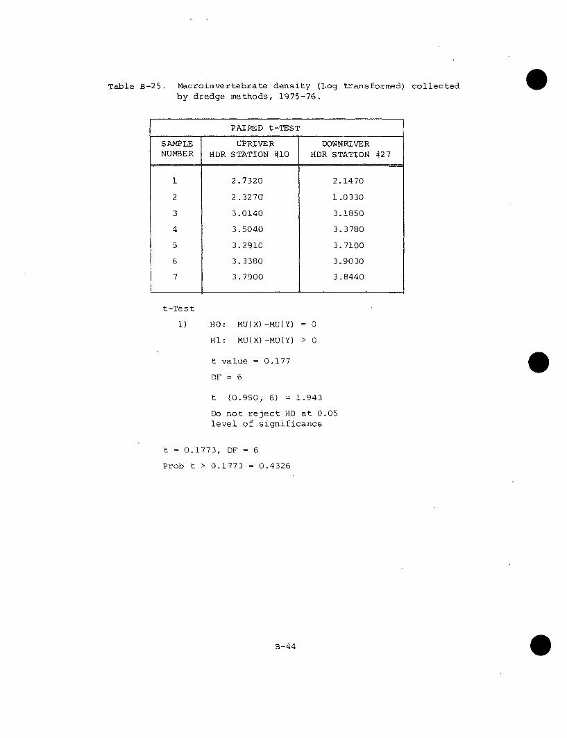
Table B-25. Macroinvertebrate density (Log transformed) collectedby dredge methods, 1975-76.

PAIRED t-TEST

SAMPLE UPRIVER DOWNRIVERNUMBER HDR STATION #10 HDR STATION #27

1 2.7320 2.1470

2 2.327G 1.0330

3 3.0140 3.1850

4 3.5040 3.3780

5 3.2910 3.7100

6 3.3380 3.9030

73.7900 3.8440

t-Test

I) HO: MU(X)-MU(Y) = 0

Hl: MU(X)-MU(Y) > 0

t value = 0.177

DF = 6

t (0.950, 6) = 1.943

Do not reject HO at 0.05level of significance

t = 0.1773, DF = 6

Prob t > 0.1773 = 0.4326

B-44 0

Table B-26a. Total macroinvertebrate density collected by artificial substrate method (1975).

HDR STATION NUMBER 6 10 12 21 25

STATION CODE 1 1 2 3 5 6

MONTH CODE 1 MONTH DENSITY (Number/m 2 )

2 February 0 - 0 5.4 0

3 March 0 - 5.4 745.2 48.6

4 April - - - 10,492.2 0

5 May - - - 847.8 -

L-I July 7,214.4 - 3,607.2 3,342.b -

8 August 7,797.6 7,214.4 4,439.7 40,282.4 6,480.0

9 September 5,540.5 5,947.9 3,223.6 16,415.8 9,169.4

11 November - 22,164.3 37,432.8 60,177.6 194,839.9

12 December - - 24,422.2 526.5

lAs used on the computer printout.

Table B-26b. Total macroinvertebrate density collected by artifi-cial substrate sampler (1976).

HDR STATION NUMBER

STATION CODE1

MONTH CODE1

DENSITY (Number/m2)

14

15

16

18

19

20

22

23

S - -- 4,250 65

14,966 14

-- - 2,967 -

18,565 - 37,940 28,988 22,583

23,227 9,559 28,197 52,925 31,994

14,524 - 32,191 69,284 29,314

13,270 36,084 20,880 38,065 26,986

27 417 514 13,536 7,500

lAs used on the computer printout.

B-46

Tvable B-26c. Total macroinvertebrate density(1977).

collected by Hester Dendy multiplate sampler

HDR STATION NUMBER 6 10 12 21 25

STATION CODE 1 1 2 3 5 6

MONTH CODE] DATE DENSITY (Number/mr2 )

25 January 5 - - 10.75 723.12 852.15

26 February 15 5.38 - 83.33 908.60 247.31

27 March 29 1,196.24 - 1,666.66 - 717.74

29 May 10 4,698.92 13,948.89 4,575.26 18,787.61 20,508.04

1As used on the computer printout.

I

Table B-27. Macroinvertebrate density (Log transformed)collected by artificial substrate methods,May-Oct, 1975-76.

PAIRED t-TEST

SAMPLE NUMBER INTAKE DISCHARGE

1 3.5570 3.5240

2 3.6470 4.6050

3 3.5080 4.2150

4 4.5730 4.7790

5 4.5790 4.4620

6 4.5070 4.8400

7 4.3190 4.5800

8 2,7100 4.1310

t-Test

1) HO: MU(X)-MU(Y) = 0

Hi: MU(X)-MU(Y) < 0

t value = -0.890

DF = 7

t (0.950, 7) = 1.895

Do not reject HO at 0.05level of significance

t = -0.8898, DF = 7

Prob t > -0.8898 = 0.2016

B-48

Table B-28. Macroinvertebrate diversity (dredge).

HDR STATION NUMBER 6 10 12 18 21 25 27

STATION CODE 1 1 2 3 4 5 6 7

MONTH CODE 1 MONTH SHANNON-WEAVER INDEX

1976

1 January 1.68 - 1.43 0.00 0.54 1.47 -

2 February 2.01 1.54 1.37 0.00 0.94 1.96 1.34

4 April 2.53 1.68 2.19 0.58 1.80 2.51 -

5 May 1.53 1.72 1.89 1.53 1.89 2.20 1.62

6 June 1.86 2.10 1.86 1.32 0.21 1.12 2.17

8 August 1.61 2.25 1.02 1.49 1.13 1.70 1.05

9 September 1.74 1.11 0.74 0.54 0.28 1.12 0.55

11 November 0.95 1.01 0.60 0.17 0.35 0.29 0.35

12 December 0.86 - 0.88 0.35 0.52 0.20 -

1975

15 March 1.68 - 1.40 0.00 1.07 1.52 -

19 July 2.07 1.95 1.42 0.95 0.12 0.45 -

21 September 1.46 2.58 2.23 0.59 0.28 2.21 -

22 October 2.26 2.41 2.97 - 0.09 2.77 -

24 December - 2.24 2.22 - 1.15 2.04 -

1As used on the computer printout.

B-49

Table B-29. Macroinvertebrate diversity (artificial substrates).

HDR STATION NUMBER 6 10 12 18 21 25

STATION CODE 1 1 2 3 4 5 6

MONTH CODE 1 DATE SHANNON-WEAVER INDEX

1976

6 June 1.10 - 0.98 0.75 1.30 1.39

7 July 1.38 2.29 1.26 0.53 1.09 1.14

8 August 0.89 - 1.23 1.01 1.10 1.19

10 October 0.73 0.97 1.04 0.32 1.26 0.52

11 November 0.75 1.32 0.81 0.41 0.49 0.06

1975

19 July 2.07 - 1.96 1.72 2.65 -

20 August - 2.19 1.47 0.29 1.40 1.78

21 September 1.46 2.65 1.68 0.06 1.54 2.55

22 October 2.26 - - - - -

23 November - 0.76 0.22 0.03 0.57 0.11

24 December - - - 0.54 0.97 1.86

iAs used on the computer printout.

B-50

'Fable B-30. Data used in stepwise regression I biological variables HDR Station #6 for 1975.

DENSITY (Number/ml)

1 2 3 4 5 6MONTH PHYTOPLANKTON ZOOPLANKTON ROTIFERA CRUSTACEA MACROINVERTEBRATE 2 MACROINVERTEBRATE 3

(PHYTOPLA) 1 (ZOOP) 1 (ROTIF)l (CRUSTAC)l (MACROD) 1 (MACROAS) 1

January - 16.2 7.5 7.5 -

February - 5.7 2.0 3.7 - 0.0

March - 28.0 0.7 26.6 11,589.5 0.0

April - 12.8 2.3 9.4 --

May 10,590 35.8 30.6 4.9

June 9,960 31.8 21.7 3.4 - -

July 4,839 358.9 278.6 75.8 392.4 7,214.4

August 11,265 - - - 7,797.6

September 7,995 91.1 53.1 20.5 457.2 5,540.5

October 25,440 213.9 191.7 19.0 226.8 -

November 6,420 75.8 52.4 20.9 -

December - - -

w0u-

1Abbreviation

2 Collected by3Collected by

as used in the computer printout.

dredge methods.

artificial substrate.

Table B-31. II Water quality variables.

PHOSPHORUSTHOPHOS FILTERABLE RESIDUE AMMONIA NITROGEN NITRITE NITROGENORTHOPHOSPHATE

MONTH B T B T B T B T

(ORTHOB) 1 (ORTHOT)1 (FRESB)1 (FREST) (AMMONIAB) (AMMONIAT)1 (NITRITEB)' (NITRITET)1

9 10 11 12 13 14 15 16

January 0.14 0.17 241 233 0.59 0.63 0.008 0.006

February 0.14 0.17 256 243 1.06 1.06 0.008 0.008

March 0.14 0.16 249 254 0.85 0.82 0.009 0.009

April 0.08 0.08 219 251 0.45 0.42 0.027 0.028

May 0.02 0.01 270 289 <0.01 <0.01 0.021 0.022

June 0.10 0.10 144 127 0.19 0.15 0.036 0.037

July 0.19 0.07 232 224 0.17 0.22 0.029 0.031

August 0.07 0.10 194 195 0.19 0.34 0.028 0.030

September 0.07 0.07 203 203 0.19 0.19 0.028 0.030

October 0.04 0.06 224 224 0.09 0.25 0.020 0.020

November 0.07 0.10 203 203 0.32 0.37 0.010 0.010

wo

IAbbreviation as used in the computer printout. B = bottom; T = top

0

Table B-31. (Continued).

WATERNITRATE NITROGEN CONDUCTIVITY DISSOLVED OXYGEN TEMPERATURE

MONTH B T B T B T B T

(NITRATEB)l (NITRATET)1

(CONDUCTB)1

(CONDUCTT)l A(DISOXB)l (DISOXT)1 (TEMPB)l (TEMPT)'

17 18 19 20 21 22 23 24

January 0.69 0.50 200 235 - - 0.3 0.4

February 0.60 0.54 250 240 0.30 9.85 0.0 0.0

March 0.81 0.75 205 210 3.50 12.40 0.0 1.0

April 3.45 3.61 255 260 1.75 11.95 4.7 4.5

May 1.39 1.18 380 380 7.74 7.79 19.7 19.0

June 4.30 4.20 37.0 380 3.79 8.37 24.4 24.0

July 0.60 0.67 270 270 6.16 6.07 25.4 25.5

August 0.60 0.45 320 320 8.89 7.24 22.4 21.4

September 0.26 0.25 290 305 9.68 8.69 17.4 16.6

October 0.45 0.39 305 310 12.31 10.15 16.4 14.6

November 1.60 0.28 230 230 12.65 12.33 0.8 1.0

tL

uJ

1Abbreviation as used in the computer printout. B = bottom; T = top

Table B-32. Data used in stepwise regression (biological variables) , Sturgeon Lake, HDR

Station No. 6 (1976).

DENSITY (Number/ml)

1 2 3 4 5 6

MONTH PHYTOPLANKTON ZOOPLANKTON ROTIFERA CRUSTACEA MACROINVERTEBRATE 2 MACROINVERTEBRATE 3

(PHYTOPLA) 1 (ZOOP)] (ROTIF)l (CRUSTAC) 1 (MACROD)l (MACROAS) 1

January 19.10 9.53 3.40 644.4

February - 16.20 3.90 2.16 604.8

March 953 28.00 7.97 3.67 -

April 5,145 91.20 42.80 9.13 1,018.8

May. 23,820 938.20 895.07 8.87 1,245.1 -

June 25,560 810.00 378.07 98.60 1,194.8 18,565

July 19,650 576.40 323.92 252.24 - 23,227

August 25,800 851.00 640.84 210.17 566.9 14,524

September 39,525 463.70 312.76 150.99 886.3

October - 500.50 324.34 176.11 - 13,270

December 135.31 130.11 5.21 2,601.4

1Abbreviation as used in the computer printout.

2Collected by dredge methods.3Collected by artificial substrate.

wn

0

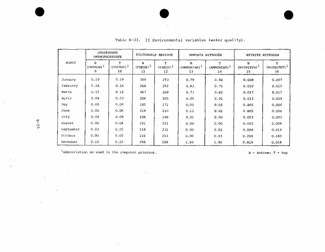
Table B-33. II Environmental variables (water quality).

PHOSPHORUSPHOSPHO TE FILTERABLE RESIDUE AMMONIA NITROGEN NITRITE NITROGENORTHOPHOSPHATE

MONTH B T B T B T B T

(ORTHOB)l (ORTHOT)1 (FRESB)1 (FREST)

1 (AMMONIAB)' (AMMONIAT)l (NITRITEB)I (NITRITET)1

9 10 11 12 13 14 15 16

January 0.19 0.19 309 253 0.79 0.84 0.008 0.007

February 0.18 0.16 268 252 0.83 0.75 0.010 0.012

March 0.15 0.11 267 268 0.77 0.82 0.017 0.017

April 0.04 0.03 206 205 0.05 0.01 0.013 0.014

May 0.00 0.00 185 171 0.02 0.02 0.005 0.004

June 0.06 0.06 219 210 0.12 0.02 0.005 0.001

July 0.09 0.09 196 198 0.01 0.00 0.003 0.003

August 0.06 0.04 221 221 0.00 0.00 0.003 0.004

September 0.03 0.05 219 231 0.00 0.02 0.004 0.014

October 0.00 0.00 216 213 0.00 0.03 0.200 0.160

December 0.22 0.22 298 289 1.60 1.80 0.019 0.018

!o

01

]Abbreviation as used in the computer printout. B = bottom; T = top

Table B-33. (Continued).

WATERNITRATE NITROGEN CONDUCTIVITY DISSOLVED OXYGEN WATER

TEMPERATURE

MONTH B T B T B T B T

(NITRATEB)l (NITRATET)l (CONDUCTB) 1 (CONDUCTT)l (DISOXB) 1 (DISOXT) 1 (TEMPB)l (TEMPT) 1

17 18 19 20 21 22 23 24

January 1.00 0.69 220 225 8.6 9.0 0.3 0.0

Febuary 0.54 0.48 250 230 9.5 8.6 0.5 0.1

March 0.82 0.82 260 260 12.6 12.0 1.5 0.8

April 0.72 0.68 240 245 11.6 11.9 9.9 9.6

May 0.37 0.26 315 315 9.4 12.2 15.5 17.0

June 0.01 0.06 360 360 8.9 8.7 23.7 24.0

July 0.28 0.26 360 370 8.8 9.7 24.5 27.5

August 0.59 0.42 350 355 7.1 8.8 22.4 23.2

September 0.07 0.00 325 325 9.1 9.1 20.5 21.0

October 0.15 0.08 325 320 14.2 14.2 14.1 13.4

December 0.42 0.72 260 265 9.4 9.3 0.8 0.1

w0

1Abbreviation as used in the computer printout. B = bottom; T = top

Table B-34. Data used in stepwise regression (biological variables), HDR Station Nos. 9

and 10 (1976).

DENSITY (Number/ml)

1 2 3 4 5 6MONTH PHYTOPLANKTON ZOOPLANKTON ROTIFERA CRUSTACEA MACROINVERTEBRATE 2 MACROINVERTEBRATE3

(PHYTOPLA)I (ZOOP)I (ROTIF) 1 (CRUSTAC)l (MACROD) 1 (MACROAS)1

wul

March

April

May

June

July

August

September

October

November

lAbbreviation

2 Collected by3Collected by

135

2,280

11,310

36,810

50,400

34.3

45.8

802.4

948.9

793.9

870.0

609.5

312.0

57.7

7.17

21.97

733.97

535.83

592.07

616.86

444.92

216.14

46.33

4.50

4.27

14.57

68.33

201.84

253.81

164.52

95.73

11.28

1,328.3

1,033.4

3,189.8

1,955.5

2,178.0

6,171.5

9,559

36,084

417

____________ _______________ I _____________ I _____________

as used in the computer printout.

dredge methods.

artificial substrate.

Table B-35. II Environmental variables (water quality) HDR Stations 9 and 10, 1976.

PHOSPHIORUSOT PHOS FILTERABLE RESIDUE AMMONIA NITROGEN NITRITE NITROGENORTHOPHOSPHATE

MONTH B T B T B T B T

(ORTHOB)l (ORTHOT)1 (FRESB)l (FREST)1 (AMMONIAB)l (AMMONIAT)I (NITRITEB)l (NITRITET)1

9 10 11 12 13 14 15 16

March 0.12 0.12 276 274 0.71 0.75 0.019 0.019

April 0.04 0.04 149 171 0.06 0.04 0.010 0.010

May 0.00 0.00 161 163 0.05 0.04 0.009 0.009

June 0.05 0.07 225 222 0.05 0.03 0.034 0.037

July 0.05 0.02 196 189 0.00 0.00 0.004 0.003

August 0.01 0.02 217 202 0.00 0.00 0.025 0.006

September 0.01 0.05 270 255 0.10 0.15 0.143 0.145

October 0.00 0.00 222 228 0.00 0.00 0.230 0.220

November 0.23 0.20 250 246 0.97 0.97 0.018 0.018

0

'Abbreviation as used in the computer printout. B = bottom; T = top

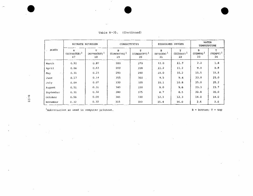
Table B-35. (Continued)

NITRATE NITROGEN CONDUCTIVITY DISSOLVED OXYGENWATER

TEMPERATURE

MONTH

March

April

May

June

July

August

September

October

November

B(NITRATEB) 1

17

T

(NITRATET) 1

18

B(CONDUCTB) 1

19

T

(CONDUCTT)]

20

B(DISOXB) 1

21

T

(DISOXT) 1

22

B

(TEMPB) 1

23

T(TEMPT) 1

24

* -I -t +

0.91

0.66

0.31

0.17

0.09

0.51

0.31

0.56

0.32

0.87

0.63

0.23

0.14

0.07

0.31

0.32

0.00

0.32

280

200

290

355

330

340

380

345

315

270

200

280

360

320

330

375

330

310

12.0

11.2

10.0

9.5

10.1

9.0

8.7

12.1

15.4

11.7

11.2

10.2

9.4

10.8

9.6

8.5

12.3

16.0

2.2

9.0

15.5

23.0

25.0

23.3

20.8

14.0

2.6

1.8

8.8

15.5

23.0

25.2

23.7

20.0

14.0

2.6u-I

'Abbreviation as used in computer printout. B = bottom; T = top

Table B-36. Data used in stepwise regression (biological variables) , HDR Station Nos. 12,13, and 14 (1975).

DENSITY (Number/ml)

1 2 3 4 5 6MONTH PHYTOPLANKTON ZOOPLANKTON ROTIFERA CRUSTACEA MACROINVERTEBRATE 2 MACROINVERTEBRATE3

(PHYTOPLA)1 (ZOOP)] (ROTIF)l (CRUSTAC)1 (MACROD)1 (MACROAS)1

March - 11.4 3.6 7.4 11,230.7 5.4

May 14,490 28.7 19.1 8.7 -

June 17,910 75.3 48.2 20.6 -

July 4,299 263.6 177.1 81.4 205.2 3,607.2

August 18,480 143.0 95.2 45.0 - 4,439.7

September 8,310 127.9 106.8 19.7 136.8 3,223.6

October 22,260 124.8 100.9 22.8 273.6

November - 81.1 55.4 23.8 - 37,432.8

0

lAbbreviation

2Collected by3Collected by

as used in the computer printout.

dredge methods.

artificial substrate.

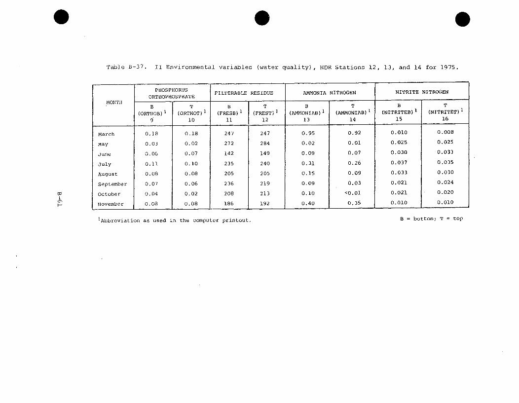
Table B-37. iI Environmental variables (water quality), HDR Stations 12, 13, and 14 for 1975.

PHOSPHORUS FILTERABLE RESIDUE AMMONIA NITROGEN NITRITE NITROGEN

ORTHOPHOSPH-iATEMONTH

B T B T B T B T

(ORTHOB) 1 (ORTHOT)1 (FRESB) 1 (FREST) 1 (AMMONIAB) 1 (AMMONIAB) 1 (NITRITEB) ' (NITRITET) 1

9 10 11 12 13 14 15 16

March 0.18 0.18 247 247 0.95 0.92 0.010 0.008

May 0.03 0.02 272 284 0.02 0.01 0.025 0.025

June 0.06 0.07 142 149 0.09 0.07 0.030 0.033

July 0.11 0.10 235 240 0.31 0.26 0.037 0.035

August 0.08 0.08 205 205 0.15 0.09 0.033 0.030

September 0.07 0.06 236 219 0.09 0.03 0.021 0.024

October 0.04 0.02 208 213 0.10 <0.01 0.021 0.020

November 0.08 0.08 186 192 0.40 0.35 0.010 0.010

w

IAbbreviation as used in the computer printout, B = bottom; T = top

Table B-37 (Continued).

WATERNITRATE NITROGEN CONDUCTIVITY DISSOLVED OXYGEN TEMPERATURE

MONTH B T B T B T B T(NITRATEB) 1 (NITRATET)! (CONDUCTB)l (CONDUCTT)1 (DISOXB)l (DISOXT)l (TEMPB)l (TEMPT)'

17 18 19 20 21 22 23 24

March 0.75 0.78 215 205 10.93 - 0.3 0.0

May 1.26 1.10 380 380 7.80 8.08 19.8 19.9

June 4.20 4.50 430 420 10.50 9.92 24.4 24.4

July 0.81 0.64 340 340 5.87 5.80 24.7 25.3

August 0.56 0.54 320 325 8.02 8.04 22.1 28.8

September 0.17 0.22 295 320 9.50 9.04 17.4 26.0

October 0.45 0.39 320 300 10.25 11.31 15.6 16.2

November 6.20 0.03 230 230 13.01 12.93 0.9 0.8

0,

IAbbrevi.ation as used in the computer printout. B = bottom; T = top

0

Table B-38. Data used in stepwise regression (biological variables) , HDR Station Nos. 12,

13, and 14 (1976)

DENSITY (Number/ml)

1 2 3 4 5 6

PHYTOPLANKTON ZOOPLANKTON ROTIFERA CRUSTACEA MACROINVERTEBRATE 2 MACROINVERTEBRATE 3

(PHYTOPLA) 1 (ZOOP)' (ROTIF)l (CRUSTAC)l (MACROD) 1 (MACROAS)l

January - 30.7 16.17 13.73 378.0

February 20 13.5 2.50 2.63 1,724.4

March 869 240.2 40.90 16.16 -

April 2,835 82.9 37.63 10.46 1,260.0

May 17,940 790.0 706.60 23.64 746.3

June 35,340 547.8 219.03 68.00 1,930.4 37,940

July 56,925 818.2 660.33 157.84 - 28,197

August 38,925 560.3 376.54 183.75 5,938.3 32,191

September - 444.9 295.31 149.54 3,484.0

October 50,700. 363.5 289.12 74.07 - 20,880

November - 115.9 100.82 15.04 5,873.3 514

December 169.9 165.78 4.09 6,971.6

w

01

]Abbreviation

2Collected by

3Collected by

as used in the computer printout.

dredge methods

artificial substrate.

Table B-39. II Environmental variables (water quality), HDR Stations 12, 13, and 14 (intake) for

1976.

PHOSPHORUSORTHOPHOSPHATE FILTERABLE RESIDUE AMMONIA NITROGEN NITRITE NITROGEN

MONTH B T B 'T B T B T

(ORTHOB) 1 (ORTHOT) 1 (FRESB)l (FREST)l (AMMONIAB)l (AMMONIAT) 1 (NITRITEB) 1 (NITRITET)W

9 10 11 12 13 14 15 16

January - 0.16 - 262 - 0.73 - 0.021

February 0.18 0.18 275 272 0.86 0.87 0.011 0.010

March 0.11 0.14 254 233 0.70 0.72 0.018 0.017

April 0.02 0.03 218 211 0.01 0.01 0.016 0.016

May 0.00 0.00 172 169 0.01 0.01 0.003 0.003

June 0.09 0.05 240 225 0.08 0.19 0.028 0.002

July 0.08 0.10 203 217 0.04 0.07 0.003 0.007

August 0.05 0.04 220 230 0.00 0.02 0.004 0.012

September 0.05 0.08 226 241 0.04 0.19 0.010 0.054

October 0.00 0.00 212 212 0.02- 0.03 0.155 0.130

November 0.07 0.08 229 226 0.08 0.10 0.022 0.022

December 0.22 0.21 296 284 1.40 1.60 0.054 0.022

W

'Abbreviation as used in the computer printout. B = bottom; T = top

LEGEND FOR TABLES 5-1 THROUGH 5-5

Q?

Qi

Qr

Q3 6

Q26

Tp

Ta

AT

W~s and Wd

= plant blowdown flow, cfs

= plant intake, cfs

= river flow, cfs

= flow through channel 36, cfs, Figure 4-1

= flow through channel 42, cfs, Figure 4-1

= flow through channel 26, cfs, Figure 4-1

= plant discharge temDerature, degrees F

= ambient temperature, degrees F

= temnerarure rise at Barney's Point

= wind speed and its corresponding direction

1-41

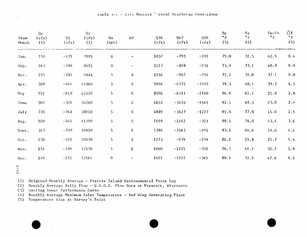
Tab.le D-.i - 4. )/D MoiiulJ.y - "p:1cal. b1schal:ge Condtlions

QvItem (cfs)Month (1)

Jan. 150

Feb. 263

Ma Ir. 255

Apr. 388

May 591.

.June 302

July 735

Aug. 509

S ept1 L. 34 3

Oct. 230

Nov. 154

Dec. 149

QrWs

(mph)Wd Q36

(cfs)Q42(cfs)

Q26(Cfs)

TpOF

(3)

Ta Tp-TaOF,

A T

(5)(cfs)

-1.75

-289

-281.

-414

-618

-326

-761

-541.

-378

-265

-1.90

-1-75

(2) (4)

7995

8691

9944

45860

65220

36200

38010

11.790

10950

1.0070

1.2570

12561.

S

S

S

S

S

S

S

S

S

1037

1.127

1256

5904

8406

4655

4889

1.499

1.389

1.273

1600

1622

-793

-859

-967

-4372

-6211.

-34.55

-3627

-1142

-1.063

-979

-121.5

-1.222

-209

-232

-254

- 1497

-2160

-1.1.65

-1227

-322

-2q1

-259

-350

-365

75.0

73.9

72.1.

79.3

86.9

92.5

91. 8

89.4

83.6

81.5

76.7

80.5

32.5

33.1.

35.0

40..1.

61..1.

69.5

77.8

76.0

64.6

55.8

44.2

32.9

42.5

40.8

37.1

39.2

25.8

23.0

14.0

1.3.4

19.0

25.7

32.5

47.6

8.4

9.0

8.0

4.5

2.8

2.9

2.5

3.6

4.4

5.14

5.8

8.5

H

N.)

(1)

(2)(3)(4)(5)

Weighted Monthly Average - Prairie Island Environmental Event LogMonthly Average Daily Flow - U.S.G.S. Flow Data at Prescott, WisconsinCooling Tower Performance CurveMonthly Average Maximum Inlet Temperature - Red Wing Cenerating PlantTemperature Rise at Barney's Point

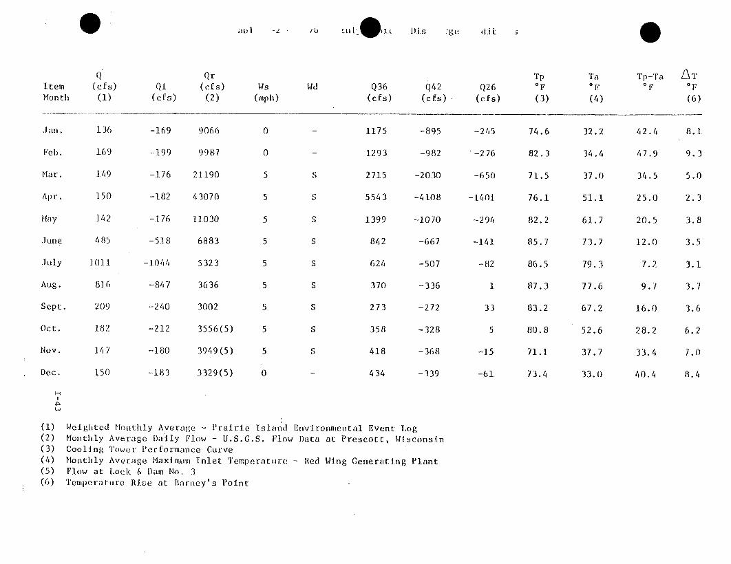
0 ait -)I z l b Lit. @1( 1)ils : ge di t

QItem (cfs)Month (1)

QrQi (cfs)

(cfs) (2)Ws

(mph)Wd Q36

(cfs)Q 42

(cfs)Q26

(cfs)

rp(3F(3)

Ta0 F

(4)

,Jan.

Feb.

Har.

Apr.

May

,June

.Tuly

Aug.

Sept.

Oct.

Nov.

Dec.

136

169

149

150

.142

485

1011

816

209

.182

14 7

150

-169

-199

-1.76

-182

-176

-518

-1044

-847

-240

-212

-180

-183

9066

9987

21190

43070

11.030

6883

5323

3636

3002

3556(5)

3949(5)

3329(5)

0

0

5

5

5

5

5

5

5

5

5

0

S

S

S

S

S

S

S

S

S

1175

1293

2715

5543

1399

842

624

370

273

358

418

434

-895

-982

-2030

-4108

-1070

-667

-507

-336

-272

-328

-368

-339

-2 45

-276

-650

-1401.

-294

-14 1

-82

1

33

5

-1.5

-61

74.6

82.3

71.5

76.1

82.2

85.7

86.5

87.3

83.2

80.8

71.1

73.4

32.2

34.4

37.0

51.1

61.7

73.7

79.3

77.6

67.2

52.6

37.7

33.0

Tp-Ta A T

(6)

42.4 8.1

47.9 9.3

34.5 5.0

25.0 2.3

20.5 3.8

1.2.0 3.5

7.2 3.1

9.7 3.7

1.6.0 3.6

28.2 6.2

33.4 7.0

40.4 8.4

H

(1)(2)(3)(4)(5)(6)

Weighted Monthly Average - Prairie Island Environmental Event LogMonthly Average Daily Flow - U.S.G.S. Flow Data at Prescott, Wisconsin

Cooling Tower Performance CurveMonthly Average Maximum Inlet Temperature - Red Wing Generating Plant

Flow at Lock & Dam No. 3Temperactire Rise at Barney's Point

Table 5-3 - 1975 Monthly treme Discharge Comi~ltions

Q pItem (cfs)Month (1)

Jan. 150

Feb. 420

Ma r. 410

Apr. 490

May 11-90

June 695

July 1.200

Aug. 1000

Sept. 655

Oct. 533

Nov. 296

Dec. 150

Qr(Qi (cfs)

(cfs) (2)

14s(m11ph)

(3)

Wd

(4)Q36

(Cfs)Q42 Q26

Tp01?

(5)

TaOF

(6)

Tp-'ra AT

(8,(efs) (cfs)

-180

-446

-434

-511

-1213

-716

-1225

-1036

-690

-567

-332

-1.82

5900

8680

10100

33600

38400

38300

58500

10000

1.2100

10300

10400

1.4100

0

0

3

5

4

7

10

7(4)

4 (4)

4

6

0

E

S

SE

SE

NW

SE(4)

NE (4)

SE

SW

767

1125

1.267

4319

4940

4927

7449

1.245

1544

1285

1344

1817

-591

-858

-995

-3208

-3664

-3654

-5556

-977

-1185

-1006

-1012

-1363

-1.41

-232

-237

-1076

-1242

-1.238

-1856

-233

-324

-245

-297

-41 8

87.0

76.1

76.3

80.5

87.1

96.5

94 . 3

88.5

87.6

84.8

87.3

87.5

32.0(7)

34.0(7)

39.0

40.0

69.0

69.0

80.0

78.0

72.0

60.0

52.0

55.0

42.1

37.3

40.5

18.1

27.5

1 4. 3

10.5

1.5.6

24.8

35.3

11.:

11. (

9.1

6.1

4.f

4 . f4.'

2.,

14.d

4.'

7.1

7.:

9.135.0(7) 52.5

H

(1) Maximimi Average Daily Blowdown - Prairie Island Environmental Event Log(2) U.S.G.S. Flow Data at Prescott, WisconsIn(3) Prairie Island Meteorology Station(4) Minneapolis Airport Weather Station(5) Cooling lower Performance Curves(6) Maximum Daily Inlet Temperature - Red WIng Generating Plant(7) Assumed Case(8) Temperature Rise at Barney's Point

0 .

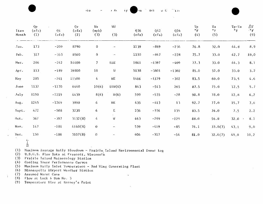
)Ie 11C"i l~y 0 .31-Sc ! U . . L I I

Q[pItem (cfs)Month (I)

Jan. 173

Feb. 317

Mar. 206

Apr. 153

May 205

June 1.137

July 1190

Aug. 1245

Sept. /472

Oct. 367

Nov. 147

Dec. 150

I-H

01

Qi(cfs)

- 209

-353

-242

-189

-241

-1170

-1219

-1269

-508

-397

-1.81.

-180

Qr(cfs)

(2)

8790

8560

14400

39800

11.500

6440

4430

3890

3230

3132(8)

4140(8)

31.07(8)

Ws(mph)

(3)

0

0

7

10

4

10(6)

8(6)

6

6

4

0

0

Wd

(3)

SSE

14

NE

SSW(6)

N (6)

NE

E

W

Q36 Q42(cfs) (cfs)

1139 -869

1110 -847

1841 -1397

5138 -3801

1466 -1129

843 -543

599 -535

435 -413

236 -336

463 -299

539 -419

406 -317

Tip TaQ 26

0 F OF

(c •s) (4) (5)

-236 76.8 32.0

-228 75.7 33.0

-409 77.3 33.0

-1.302 85.0 52.0

-302 83.5 60.0

265 87.5 75.0

-28 90.8 78.0

1.3 92.7 77.0

135 83.5 76.0

-129 88.0 56.0

-85 76. 1 33.0(7)

Tp-Ta /\,'0 F ,0 F

(9)

44.8 8.9

42.7 10.0

44.3 8.1

33.0 3.2

23.5 4.6

12.5 5.7

1.2.8 6.2

15.7 7.6

7.5 2.2

32.0 8.1

43.1 9.0

-54 81.0 32.0(7) 49.0 10.2

(1)(2)(3)(4)(5)(6)(7)(8)(9)

Maximum Average Daily Blowdown - Prairie, Island Environmental Event LogU.S.G.S. Flow Data at Prescott, WisconsinPrairie Island Meteorology StationCooling Tower Performance CurvesMaximum 1)aily Inlet Temperature - Red Wing Generating PlantMinneapolis Airport Weather StationAssumed Worst CaseFlow at Lock & Dam No. 3Temperature Rise at Barney's Point

Table 5- -'Proposed Monthly xtreme DI.scharge Conditions

QpItem (cfs)Month (1)

Jan. 150

Feb. 150

Mar. 150

Apr. 150

May 600

June 8001386

July 1384

Aug. 1381

Sept. 500

Oct. 300

Nov. 150

Dec. 150

QrQt (cfs)

Tp Ta Tp-Ta0 F 01,

1T0F

(cfs) (2)

-175

-175

-175

-185

-629

-829-1410

-1.,410

-141.0

-532

-333

-180

-175

3699

3780

4279

7623

8475

6431.

4299

3390

3680

4010

4/243

3787

Ws(mph)

0

0

10

10

10

10

10

10

10

10

10

0

Ud(cf s) (cfs)

482

Q36

S

S

S

S

S

S

S

S

S

Q42 Q26

493

-31

710

856

483

-25

-334

-231

-121

-43

494

-375

-384

-204

-654

-744

-527

-209

-1

-63

-141

-195

-384

(cfs) (3) (4) (6)

-72 85.0 32.0(5) 53.0 11.1

-74 85.0 32.0(5) 53.0 11.0

270 85.0 32.0(5) 53.0 11.0

-21 85.0 65.0 20.0 4.2

-78 87.3 73.0 14.3 4.6

90.4 11.4 4.480 88.5 79.0 9.5 5.0

268 91.5 83.0 8.5 3.9

357 91.7 85.0 6.7 2.7

328 90.0 78.0 12.0 3.1

296 86.4 70.0 16.4 3.7

27"4 85.0 32.0(5) 53.0 10.9

-75 85.0 32.0(5) 53.0 1].0

cm

(1)(2)(3)(4)(5)(6)

Expected Maximum Blowdown for Future Operation with Existing Systems

Seven-day, 10-year Low Flow - U.S.G.S. Flow Data at Prescott, Wisconsin

Cooling Tower Performance Curves 85.0 0 F"WInter for Ice ControlMaximum Inlet Temperature - Red Wing Generating Plant (unless noted)

Minimum Inlet Temperature

Temperature Rise at Barney's Point

(1928-1.976)

Table 5-6 - Heat Recirculation Rate at intake Structure

1975Typical

1976TvDical

1975Extreme

1976Extreme

ProposedExtremeMonth

Month Extreme

January

February

March

April

May

June

July

August

September

October

November

December

8.6

9.4

3.7

1.8

1.1

2.4

4.0

10.4

9.1

8.3

6.3

6.3

7.8

7.6

3.9

1.4

6.9

14.6

27.9

27.3

15.3

14.0

12.8

12.8

10.2

11.4

10.4

3.5

6.4

3.7

3.2

18.7

11.8

11.8

8.8

5.7

8.3

10.2

6.1

1.6

7.2

27.3

31.1

35.5

19.8

16.8

11.9

13.1

12.4

12.3

15.9

10.2

15.8

23.536.0

44.0

51.0

27.6

20.4

16.0

12.3

"E: Heat recirculation rate at the intake structure isof heat effluent at the discharge structure.

expressed as the percentage

1-47

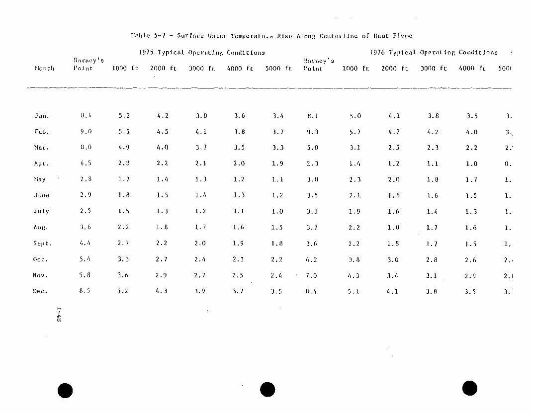
Table 5-7 - Surface Water Temperatu.o Rise

1.975 Typical Operating Conditions

Along Ceniterl.iie of Ifeat Phtime

1976 Typical Operating Conditiona

Barney' sBarney' sPoJ ntMonth 1000 ft 2000 ft 3000 ft: 4000 ft 5000 ft Point 1000 ft 2000 ft 3000 ft 4000 ft 500(

Jail.

Feb.

Mar.

Apr.

May

June

July

Aug.

Sept.

Oct.

Nov.

Dec.

8.4

9.0

8.0

4.5

2 . 8

2.9

2.5

3.6

4.4

5.4

5.8

8.5

5.2

5.5

4.9

2. 8

1.7

1.8

1.5

2.2

2.7

3. 3

3.6

5.2

4.2

4.5

4.0

2.2

1.4

1.5

1.3

1.8

2.2

2.7

2.9

4.3

3.8

4.1

3.7

2.1

1.3

1.4

1.2

1.7

2.0

2. 4

2.7

3.9

3.6

3.8

3.5

2.0

1.2

1.3

1.1

1.6

1.9

2.3

2.5

3.'7

3.4

3.7

3.3

1.9

1. I

1.2

1.0

1.5

1. 8

2.2

2.4

3.5

8.1.

9.3

5.0

2.3

3. 8

3.5

3.1.

3.7

3.6

6.2

7.0

8.4

5.0

5.7

3.1

1.14

2.3

2.1.

1.9

2.2

2.2

3.8

4.3

5 . I

41. 1

4.7

2.5

1.2

2.0

I8

1.6

1.8

1.8

3.0

3.4

4 .1

3.8

4.2

2.3

1.1

1.8

1.6

1.4

1.7

1.7

2.8

3.1

3.8

3.5

4.0

2.2

1.0

1.7

1.5

1.3

1.6

1.5

2.6

2.9

3.5

3.

3.,

2.4

0.

2.

i.

1.

1.

1.

2.1

2.:

3.:

0I

0-Table 5-8 - Surface -itter Tempe.riture Rise Along Centerl.jnf of lieat Pluwe

19Y5 Extreme Operat:jng Condltionslk1l.nIe y '

Po1 11 Ci 10001 fL 2000 ft 3000 ft 4000 ftBarney' s

5000 ft PointMonth

1976 Extreme Operating Conditi-ons

1000 ft 2000 ft 3000 ft 11000 ft 5000

Jan.

Feb.

Mar.

Apr.

May

June

July

Ang.

Sept.

Oct.

Nov.

11.8

9. 4

6.4

4.6

2.7

4.4

4.7

7.0

7.8

6.9

6.8

5.8

4.0

2.8

3.0

1.7

2.7

2.9

4.3

4.8

5.7

5.5

4.7

3.2

2.3

2.4

1.4

2.2

2.4

3.5

3.9

5.1

5.0

4.3

2.9

2.2

2.2

1.3

2.1

2.1

3.2

3.6

4.8

4.7

4.1

2.8

2.0

2.1

1.2

1.9

2.0

3.0

3.4.

4.6 8.9

4.5 10.0

3.9 8.1

2.7 3.2

1.9 4.6

2.0 5.7

1.1 6.2

1.8 7.6

1.9 2.2

2.9 8.1

3.2 9.0

5.5

6.1

5.0

2.0

2. 8

3.5

3.8

4.6

1.3

4.9

5.5

4.4

5.0

4.1

1.6

2.3

2.8

3.1

3.8

1. 1.

3.9

14 4

4.6

3.7

1.5

2.1.

2.6

2.8

3. 4

1.0

3.6

4 .0

3.8

4.3

3.5

1.4

2.0

2.4

2.6

3.2

0.9

3.3

3 - 8

3.

4.

3.

1.

1.'

2.

2.

3.1

0.

3.

3.

Dec. . 9.0 5.6 4.6 4.2 3.9 3.7 10.2 6.2 4.9 4.5 4j .2 4.

Table 5-9 - Surface Water Tempera... ire Rise Along Centerline of Heat Plume

Blarney'st-

P'oint

Proposed Extreme

1000 ft 2000 ft

Operating Conditions

3000 ft 11000 ft 5000 ft

Jan.

Feb.

Ma r.

Apr.

Nay

.Jtune

11.1

11.0

11.0

4.2

4.6

4.4

5.0

3.9

3.1

3. 7

10.9

11.0

6.7

6.7

6.7

2.6

2.8

2.73.1

2 . 4

1.9

2.3

6.6

6.37

5.5

5.4

5.4

2.1

2.3

2.22.5

2.0

1..5

1.8

5.4

5.4

4.9

4.9

4.9

1.9

2.1

2.02.3

1.8

1.4

1.7

4.9

4.9

4".6

4.6

4.6

1.. 8

2.0

1.92.1

1.6

4.14

4.11

4.11

1.7

1.9

1.82.0

1.50 July

Aug. (1)

Sept.

Oct.

Nov.

Dec.

1.3

1.6

4.6

4.6

1.2

1.5

4.4

4.4

( 1 )see Section 5.2.

0

N

U

14 S COMxs I N

HAST I M

. RED

I4 N N ES 0 TA

N FALLS

5 0 5

SCALE IN MILES

FIGURE 3-1LOCATION MAP

THERMAL DISCHARGE ANALYSISPRAIRIE ISLAND NUCLEAR GENERATING PLANT

NORTHERN STATES POWER COMPANY

1-51

WING DAM(rfP)

1~- I

-~ ~ -

MISSISSIPPI RIVER

BARNEY'S POINT-

- -~-- .-

APPROACHCHANNEL

•--_ _ . . --

I,-I NTAKE

L_. N...

/

'-'~2/.

/SHORELINE

BARR I ERWALL -

m <-J

PO, C

SCREENHOUSE HOUSE

500 250 0 500

SCALE IN FEET

FIGURE 3-2GENERAL PLOT PLAN

THERMAL DISCHARGE ANALYSISPRAIRIE ISLAND NUCLEAR GENERATING PLANT

NORTHERN STATES POWER COMPANY

OOLI NGTOWERS (TYP)

1-52

PECYCLE

CAN ALDISCIIARGE BASIN - .ACONITRlOL STRUCTURE "'" RECY

Co NTI I.SCOiTc•-,>--,I .sTRU

CLE CANALROLCTURE 6C I RCIJLAT

WATEId P I1

DI SCIIARGEBAS11 -->-

DI SCIIARGESTRUCTURE

FLOW ->-DI SiR I BUT IONl

BAS I ItDI SCHARGECANIAL

80 11O 2.0 0

SCALE III FEET

H •U I ;~U~

MP4PII'

--FI----rII I'J LJ

COOLING TOWERDISIRIBUTIOll PIPE (TYP)

4

COOLING TOWERRETURN CAtAL

KFIGURE 3-3EXISTING DISCHARGE STRUCTURES

THERMAL DISCHARGE ANALYSISPIlAIRIEI= ISLAND NUCLEAR GI-NI:-ERATING PLANT

NORTIIERN STATES POWER COMPANY

NUCLUAl 1 SIMULATED CLOSED BOUNDARY-- SIMULATED OPEN I•OUNDARY

LANT0 £00 2004.1.

TAKE S; IC•f.IN

I CGHANNEL 42

MISSISSII'PI RIVER

I

4Nil 26

CHIANNEL 36

fIGUIIE 4-1

SITE VICINITY LAYOUTTHERMAL DISCHARGE ANALYSIS

PRAIRIE ISLAND NUCLEAR GENERATING PLANTNORTHERN STATES POWER COMPANY

0

FIGURE 4-2

MISSISSIPPI RIVER LAYOUTTHERMAL DISCHARGE ANALYSIS

PRAIRIE ISLAND NUCLEAR GENERATING PLANTNORTHERN Sr'TAES POWER COMPANY

.. .... .... -PRAIRIE ISLANDNUCLEAR

PREDICTION

--- FIELD MEASUREMENTS(1 MEIER BELOW SURFACE)

-§ -.

H-IJ

-½0 100 .00...s

SCALC

* . .

7-

'ii-

..

-~.

€•~~~~~~~~~~~~~~ ..... ........ .:---•....."-• :" •::•• "m•MIS"SISSIIP |I RIVER -4 • ...,

FIGURE 4-3

COMPARISON BETWEEN PREDICTED AND MIEASURED ISOFI-IERMAL ITHERMAL DISCHARGE ANALYSIS

PRAIRIE ISLAND NUCLEAR GENERATING PLANTNORTHERN STATES POWER COMPANY

LINES, AUGUST 1, 1975

0

DEPTH, METER

DEPTH, METER0

2-

(1)TEMP

°C

35

35

34

33

(2)AREA

9.2

37.3

4.4

3.1

2.1

2.8

5.0

20.3

15.9

(3)TEMP RISE

OF

14.0

13.1

11.3

9.5

(4)WEIGHT

(2)X(3)

1.3

4.9

0.5

0.3

H.

3

4

5

32

31

30

29

28

28

7.7

5.9

4.1

2.3

1.4

0.2

0.2

0.2

0.5

0.2

HOIZ~tONTAL SCALE M ETER

0 25 50

AVERAGE FIELD TEMPERATURE RISE = 8.3 :F

MODEL PREDICTED TEMPERATURE RISE= 8.1 F

FIGURE 4-4

TOTAL HEAT RELEASED INTO MAIN CHANNEL OF MISSISSIPPI RIVER

THERMAL DISCHARGE ANALYSIS

PRAIRIE ISLAND NUCLEAR GENERATING PLANT

NORTHERN STATES POWER COMPANY

SCALE

0 250 500 FEET MISSISSIPPI RIVER0.90 F

* ~~*'q*s

N

)\2.7 0 F

4.90 F 4.50 F

2.7° F/

0.9 0 FBARNEY'SPOINT

0

/

PREDICTED ISOTHERMAL LINE

MEASURED ISOTHE:RMAL LINEm D m

FIGURE 4-5COMPARISON BETWEEN PREDICTED AND MEASURED

ISOTHERMAL LINES, SEPTEMBER 5, 1975THERMAL DISCHARGE ANALYSIS

Pfl4IRIl: I.qLAIlrf NUI•AR (ENFf-lATIN(- PLANMT

NOn [IIIEHN ST/t IPU)WEI-i ;OMi't\NY

FIGURE 4-6COMPARISON BETWEEN PREDICTED AND MEASURED

ISOTHERMAL LINES, AUGUST 1, 1975THERMAL DISCHARGE ANALYSIS

PRAIRIE ISLAND NUCLEAR GENERATING PLANTNORTHERN STATES POWER COMPANY

LL

H

U-iI-

-J0C-)

0oI(D"

WET BULB TEMP. (F)

FIGURE 4-7

COOLING TOWER PERFORMANCE CURVE

0TIIE[R14AL DI SCHIARGE ANlALYS IS

PR . .. 'D V'R P P'"T1IORTIIFRrI '*~WPOWER COMP ANY

0 100 20010 i

SCAILE

F-,

-MISSISSIPPI 1 IVER

FIGURE 5-1

PREDICTED ISOTI-IERMAL CONFIGURATIONS IN SITE VICINITY AUGUST, 1975 TYPICAL CONDITIONTHERMAL DISCHARGE ANALYSIS

PRAIRIE ISLAND NUCLEAR GENERATING PLANTNORTHERN STATES POWER COMPANY

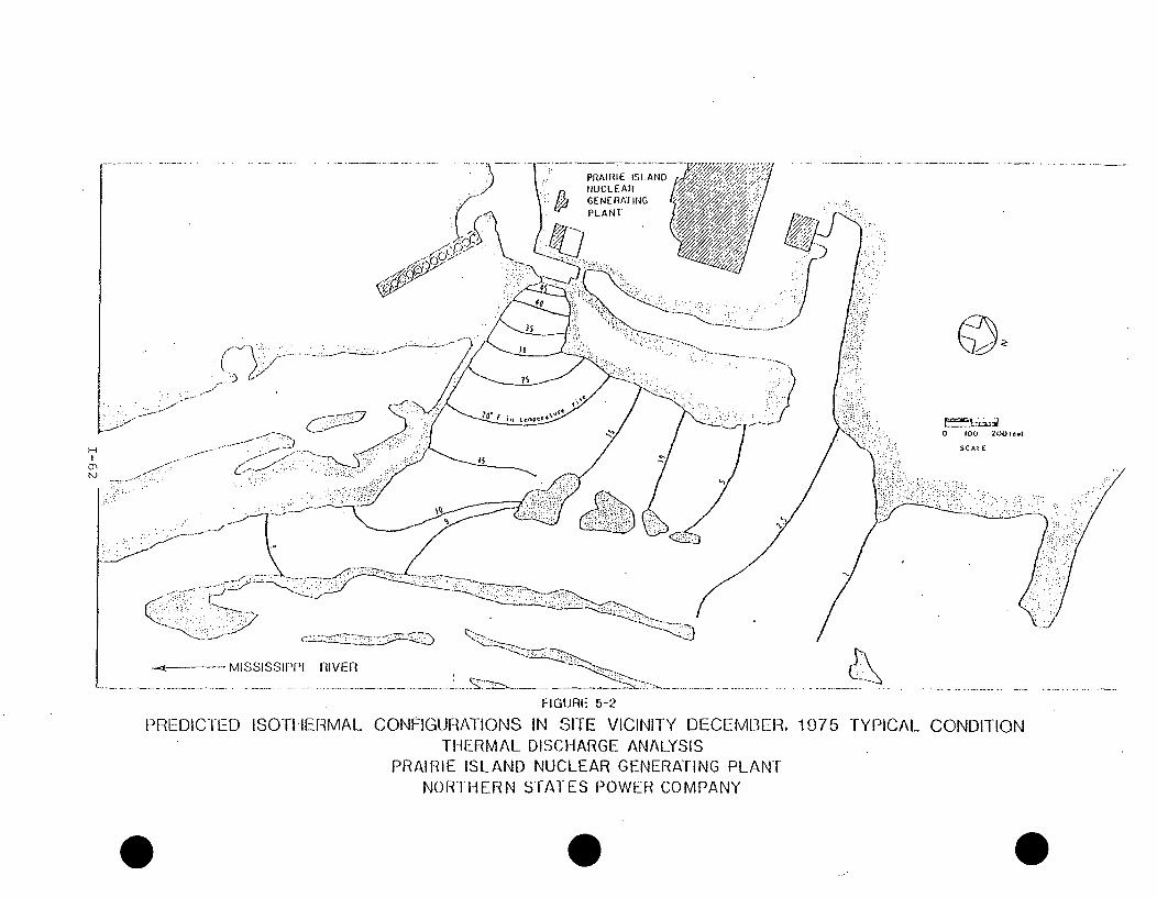
PRAIR~IE ISLAND 1A

I.->--17

H

I' - ..- •

£~ -~'Q**

0 100 2U01-1a

SCAtE

-- - MISSISSIPPI RIVER ..._

FIGURE 5-2

PREDICTED ISOTIIERMAL CONFIGURATIONS IN SITE VICINITY DECEMBER,THERMAL DISCHARGE ANALYSIS

PRAIRIE ISLAND NUCLEAR GENERATING PLANTNORTHERN STATES POWER COMPANY

1975 TYPICAL CONDITION

0

PiiAIRIF ISLANDNUCLEAR

77*.0 100 ?D0I..l

SC AL!

, - MISSISSIPPI RIVER

FIGURE 5-3

PREDICTED ISOTI IERMAL CONFIGURAATIONS IN SITE VICINITY MAY, 1976THERMAL DISCHARGE ANALYSIS

PRAIRIE ISLAND NUCLEAR GENERATING PLANTNORTHERN STATES POWER COMPANY

½TYPICAL CONDITION

PlAiir IS[ ~LAWf

0 100 200I.-1

2 ISCA I.

C)C

i.......W y .. .....

- -MI8SK.);1I-I fIVER

FIGURE 5-'A

PREDICTED ISOTI IERMAL CONFIGURAI-ONS IN SITE VICINITY JUNE, 1975 EXTREME CONDITIONTHE--RErMAL DISCHARGE ANALYSIS

PRAIRIE ISLAND NUCLEAR GENERATING PLANTNORTIIERN STATES POWER COMPANY

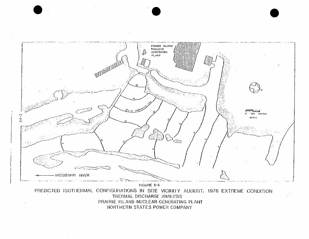
C

•. .............

FIGURE 5-5

PREDICTLED ISOTI IERMAL CONFIGURAFIONS IN SITE VICINITY AUGUST, 1976 EXTREME CONDITIONTHERMAL DISCHARGE ANALYSIS

PRAIRIE ISLAND NUCLEAR.GENERArING PLANT

NORTHERN STATES POWER COMPANY

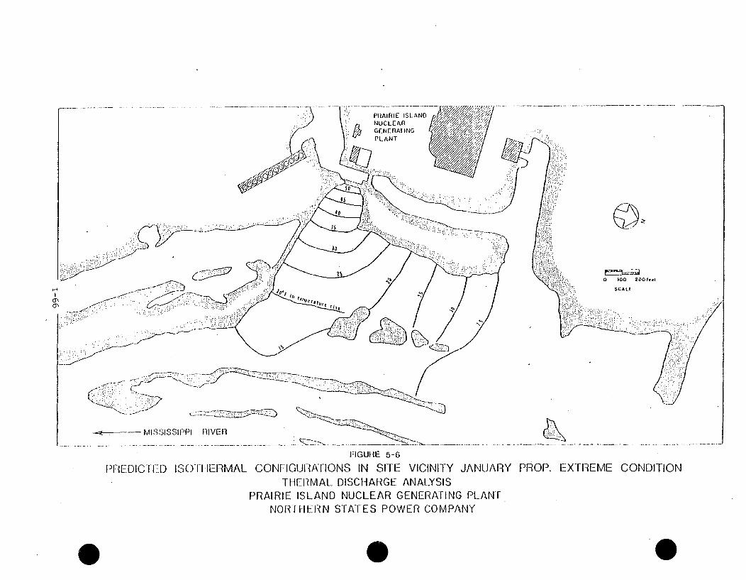
6j2~~ K 0 100 2001..l

SCALL

H4J

- ,----- MISSISSIPPI FIVER

FIGURE 5-6

PIHIEDICTED ISOTHtERMAL CONFIGURATIONS IN SITE VICINIT-THERMAL DISCHARGE ANALYSIS

PRAIRIE ISLAND NUCLEAR GENERATI

NORTHERN STATES POWER COM

*0

e JANUARY PROP. EXTII-EME CONDITION

NG PLANtPANY

PRAIRIE ISLANDNUCLEAR

GENE RAT ING

PLANT

'-'V

(

1-4

6,

0 l0L 200l4..

SCAt.(

-*----- MISSISSIPPI HIVER

FIGURE 5-7

PREDICTED ISOTI IERMAL CONFIGURATIONS IN SITE VICINITY MAY PIRCTHERMAL DISCHARGE ANALYSIS

PRAIRIE ISLAND NUCLEAR GENERATING PLANT

NORTHERN STATES POWER COMPANY

½)P. EXTREME CONDITION

.. . . - --- <CAL

FIGURE 5-8

Pl--EDICTF-D ISOITIEFtMAi_ CONF-IGUR/ATIONS IN SITE VICINITrY AUGUST 1-RO01. EX'TiI:EMI2- CONDIT-IONTHERMAL_ DISCHARGE ANAI-YSIS

13RAIRIE ISLAND NUCLEAR GENERATING PLANTNORTHERN STATES POWER COMPANY

0)•

FIGURE 5-9

PREDICTED ISOTIiERMAL CONFIGURATIONS IN MISSISSIPPI RIV[--_R AUGUST. 1975 TYPICAL CONDITIONTHERMAL DISCHARGE ANALYSIS

PRAIRIE ISLAND NUCLEAR GENERATING PLANTNORTHERN STATES POWER COMPANY

Itevi sedl 4/28/78

:' "• :I,:I0Y •,O ,.,•A4 (

FIGUnE 5-10

PREDICTED ISOTI IERMAL CONFIGURATIONS IN MISSISSIPPI RIVEIR DEC. '75 TYPICAL CONDITION

THERMAL DISCHARGE ANALYSISPRAIRIE ISLAND NUCLEAR GENERýATING PLANT

NORTHERN STATES POWER COMPANY

0 0 ....... ',.,

FIGUMrE 5-11

PFEDIC(TED ISOTHEFRMAL CONFIGURATIONS IN MISSISSIPPI IiVEn MAY '76 TYPICAL CONDITIONTHERMAL DISCHARGE ANALYSIS

PRAIRIE ISLAND NUCLEAR GENERATING PLANTNORTHERN STATES POWER COMPANY

$CAL(

FIGRE 6-12

PREDICTED ISOTI-llz--MAL CONFIGURATIONS IN MISSISSIPPI RIVER--R JUNE. 1975 EXTREME CONDITIONTHERMAL DISCHARGE ANALYSIS

PRAIRIE ISLAND NUCLEAR GENERATING PLANT,NORTHERN STATES POWER COMPANY

0

FiGURE 5-13P-EDICTED ISOTFIERMAL CONFIGURATIONS IN MISSISSIPPI RIVER AUG.

THERMAL DISCHARGE ANALYSISPRAIRIE ISLAND NUCLEAR GENERATING PLANT

NORTHERN STATES POWER COMPANY

'76 EXTREME CONDITION

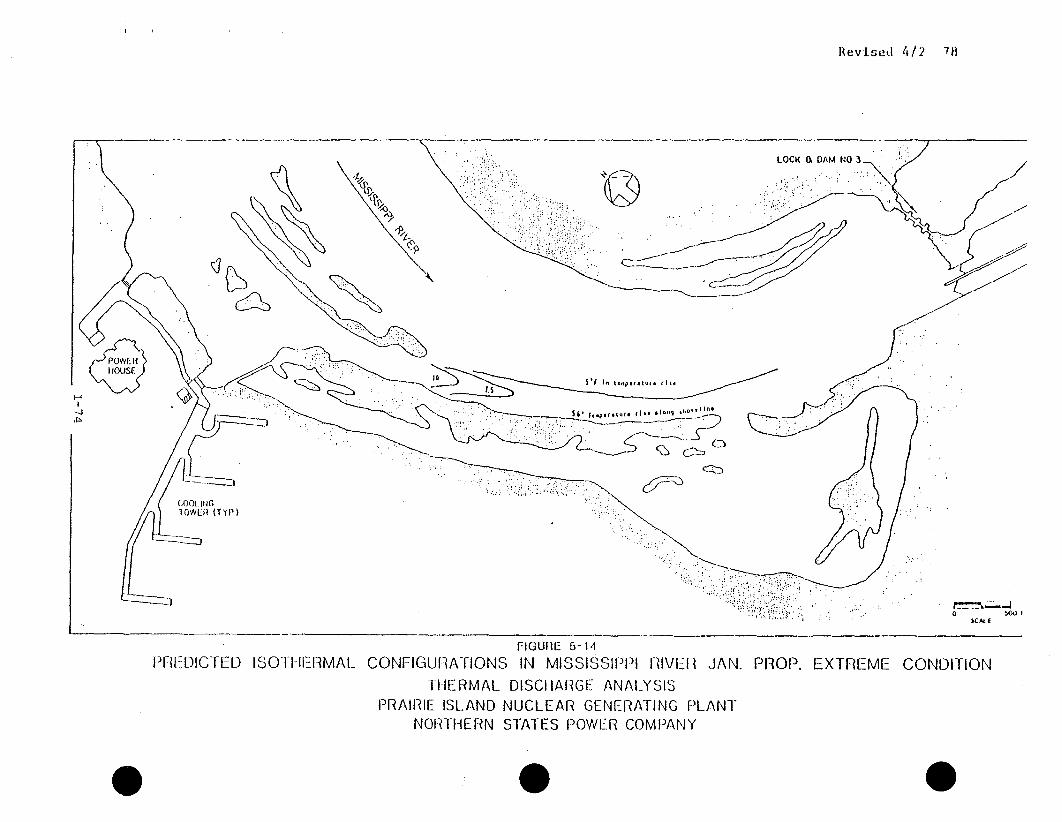
Revised 4/2 78

q .i ;0-nn -

FtGUFIE 5-14

PIIEDICTED ISOTHE1RMAL CONFIGUFiATIONS IN MISSISSIPPI RIVEIR JAN. PROP. EXTREME CONDITION

THERMAL DISCHARGE- ANALYSISPRAIRIE ISLAND NUCLEAR GENERATING PLANT

NORTHERN STATES POWER COMPANY

4/28/710

FIGUME 5-15

PAEHDICTED ISOTHERMAL CONFIGURATIONS IN MISSISSIPPI RIVER MAY PROP. EXTREME CONDITIONTHERMAL DISCHARGE ANALYSIS

PRAIRIE ISLAND NUCLEAR GENERATING PLANTNORTHERN STATES POWER COMPANY

APPENDIX A

Pertinent entries from the Prairie island Environmental Event Log have been

transcribed to a computer file maintained at Northern States Power Company's

general office and are reproduced in the following table. Columns I through 5

in the table represent an entry in the Environmental Event Log sheet which

occurred each time plant blowdown flow was changed. Entries by column

numbers are described as follows:

Column 1: the month, day and year of the records

Column 2: time of the day at which the entry was made

Column 3: blowdown flow

Column 4: condenser inlet temperature

Column 5: river temperature measured at the sensors locatedin the plant intake canal on the river site of

the skimmer wall

Column 6: river temperatures measured at Red Wing Steam Plant

Column 7: river temperatures measured at Lock & Dam No. 3

Column 8: wet bulb temperature measured at Twin Cities Airport

Column 9: number of cooling towers in operation

Column 10: plant discharge temperature

Column 11: evaporation rate

Column 12: monthly average temperature at Red Wing

Column 13: monthly average discnarge temperature

Column 14: monthly average blowdown rate

Column 15: monthly average evaporation

1-77

,ýD - 0 -.oP p I

MODAYR I IfIE SLOW CONO RIVER TEMPS WET TW 0ISCIA EVAP

DOWN4: TE tP PI RtW L03 BULB TEMP

- - - - - -. - . - . - - -. . - - - . - - - -. . - - - . . - -. - - . - .- . .- - - - . .- -

MONTH-LY AVE

RIVR DISCH B ON EVAP

2 1752.1276

::I 212752127521 27S2.1375

. 2157521575215752167521675

217752177521975

21975-1975

22075

220752227522275

22275223752237522375

H ~22S7S22675

S22675

2277522775

22775

3 175

3 1753 1753 3753 4753 875317753177531775"317753177531775317753187531875318753187531875318753197531975

0

1300

1 00

1500

16S1

14341540

2025

200

330

8301050

30

1230

1430

30

4.40

1141300

1915

400

610

1830

1 4 15

541

1813

615830

1345

500

630

230

309

1330

620

1130

14 15

1700

1815

19282028

200

500

625

1002

1030

1935

130

306

185WmWHm 33.0

185 72.3 32.1200 68.1 32.1255ss "*0N "Wx

260ISO

2E0

350150

2443304 10300

374

340374420

140330400

150330•20

3284,20330420330295

330

360295230295

ISO225

295325503405456

397990

410442

9999442Z701952'45

65 . 0 32. 1

S7 .0 32 . I

65. 0 32. 1

61 0 32.1

65 0 32. 16 4. 32. 1

74.2 32 .2

72 0 32. 167 1 32. 1

62. 7 32 1

62. 0 32. 1

66 .0 32 1

58 5 32 0

61 .7 32 0

60 0 3-2 0

67 0 32 0

62 5 32 0

54. 7 32. 1

69 7 32 1

69 0 32. 2

64 0 32 3

66 0 32 0

64 1 32. 5

6S 7 32 4

60 0 32 4

69 0 32 7

33.032.0

32..0

32.032 033 033 033 033 033 033 033 033 033 033 034. 034 034 034 034 0

34.034 034 034 033 033 033 033 0

33 0

33 033 033. 033. 033. 032 034 036 036 036 036 036 036 036 037 037 037 037 037 037 038 038 0

33.8 12 033.8 7 0

33.8 4 0

33.8 4. 0

33.8 2 0

34.7 5.

35 6 25 0

35 6 24, 035 6 24 035 6 23 0

35 6 23 0

35 6 27 0

35 6 28 035 6 7 0

35 6 20 0

35 6 22 0

35 6 15 0

35 6 7. 0

35 6 32 0

35 6 27 0

35 6 25 0

35 6 24. 0

3S 6 0.0 0

35 6 24 0

38 3 29 036 5 19 036 .5 20 0

35 6 13 0

35 .6 15 0

35 6 26 0

35.6 4 03S.6 4. 0

35.6 7. 0

34.7 & .0

35 .6 17 0

35 6 is 041 0 28 0

41 0 35 0

41 0 37 0

4 1 0 35 0

4 1 0 35 0:

41 0 35 0

41 0 35 0

40 1 34 0

40 1 34 0

40 1 34 0

40 1 35 0

40 1 35 0

40 1 29 0

40 1 27 0

40 1 26 0

39999.03 75 .73 74 .239999. 03 74 83 73 83 73 83 70 .9

3 73. 63 73 .13* 79.2

3 78.43 75.53 73 .23 71 03 74 0

3 70 63 73.23 71 .53 75 3

3 72 13 67. 63 75 93 76 14 68 .6

4 69,2

4 68.9

4 71 .24 70 .6

4 70 .6

1 0 031.1

27 327 321 811 .623 321 621.65

23 .528. 926 823 820 823 024 S18 .519.419.324.0

17. 327 , 025 .729.331 .329.1

20.7

33,8

19 .816 .827 116 .630 S23.830 333 .

31.928.531 .630 .536. 033.932 .432 .334.734.726.720 .520.8

32.1 73.9 263.1 26.4

63 .

60 9

67 060 866 16- 1

65 0

72 0

71 065 .4

69.868 278 172.570.470.374. 0

68.960.060.060.2

32 2

32 2

32 132.833 0

33.0

33 0

36 3

35 0

35 6

45 0

44 9

42 239 937 .537 .0

33.933.8

4

4

4

4

4

4

4

4

4

4

4

4

4

4

4

4

4

499

4

3

3

74 .2

74 .2

73.2

74.2

69.9

70.6

69.0

74 .0

73.9

70 6

72 0

72. 0

76 .774. 0

72 .9

72 .9

75. 0

99 . 0

66 .4

70.7

70.7

L GDE -''E F '0P

MOOAYR TIMIE BLOW CONDDOWN TEPIP

RIVER TEMPS WET TW OISCH

PI RW LD3 EULa TEMiP

EVAP MONTHLY AVERIVR 0ISCH B ON EVAP

3197S3197532175321753227532275323753237S32375

32575326753297532975

4 67S

415754157541775'.2475':575

4207551175

H 51175

I 51375Q0 51575

5157551775519755:J75

5217552375524755257552575525 755:775527755:975S29755297552975

6 175

6 1756 3756 4756 4756 5756 5756167561675

900160019502335810

050

82011201340

8451100

12301306

100050

3253.30

1900141510001600

2000180016051000170513001148

4 05135O11051 03S13251725

9301•1451200130014151800

1000Z0002030

8361015

94516:016301910

325 M.A4H410 70.0

285 64.0150 63.0168 64.6100 67.9225 60. 3165 62 3150 68 5245 75 0335 72. 0410 60 0335 60 0

410 69 1.90 64 0410 60 5490 74 0

9999 70 09999 65.7

9999 60.0

270 86.0

3409999

490

655

735

900

750

720

900

1025

1105

I150

1190

980

947

897058775

695

300150347

325

250

190150327490

80.079 0

07 .6

88. 088 086. 078 0

80 081.0

73 0

75 0

76 070 270 0

78 375 575 075 4

0l 0

76 079 1

85 079. 380 .505 506 586 0

85 7

34 .034 .2

35 1

34 8

35 1

35 2

34 .7

34 3

34 2

32. 7

32 8

34 3

41 4

41 .543 .9

42. 3

4 2.642 8

44. 1

44.1

44. 061 .8

61 965 .566 068 068 .771 069 670 271 .372. 6

68 .4

69.0

65 765 665 7

65 .

69 2

69 3

70 868 368 168 069.5

67.2

68.9

38.038.039.039.039.039.0

38. 038 038 036 0

35 0

34 034 0

37 040 04.0 040 043 044.045 0

57 0

57. 0

60. 0

62. 064. 066 069. 069 070 0

70 070 070 070 069. 0619 068 068 0

63.068 0

67. 0

67 .0

68 068 068 068 064 064 .0

40 140 1

41 041 040 1

40 140.140.1

40.137.436.536.536.5

41 045 545 544 645 547 347. 360 B

60 .863 562 662. 665 368 .971. 671 .672 573 474 374 374 373, 473 470 770 770 .7

70 .7

70.770 .770 .770.770 .770.770.768 .968 .9

31 037 .035 035 0

30 0

30 0

30 030 0

31 011 0

17 0

20.0?0 o

27 036 035 0

42 047 0

51 043 0

57 0

49. 0

53 0

50.050 0

61 0

71 0

69. 0

70.066 0

62 071 071 061 0

52. 055 .056. 056 .

59 0

5 4. 050 057 062. 062. 056. 057. 061 064 .0

39999 0

3 70 7

3 74 6

3 73.9

3 74.2

3 76 3

3 76.6

3 72.7

3 76.8

3 77.9

3 76.9

3 69.7

3 69.7

3 70.3

3 74.8

3 72.3

3 82.1

3 80.5

39999.0

39999. 0

39999. 0

3 83.1

3 07.1

39999. 0

3 91.3

3 93.7

3 95.2

3 90.2

3 91.7

3 91.1

3 85.6

3 89.2

3 89.8

39999. 0

3 81.6

3 87.1

3 85.7

3 85.5

3 85.9

3 89.9

20.823.420.720.1

22. 123.8

24. 120 .923.931 .928.9

220

22.0

34 .3

20.418.924.22.0 .820.820 . 020.820.8

36. 024.3

24.3

31 .227.722.618.319. 121 317.7

15 .416 .016. 0

19.323. 321 .220 .9

24 .3

33.925.327.021 .6."2. 427.728.126 .42S. 1

33.5 72.1 255.1 26.0

41.1 79.3 388.2 25.6

57.8 86.9 591.1 27.2

333333333

77.586 .591 .209.289.991 .392. 092.793.3

0PACE 3 ODE L0 0_ 30p -,

M1OOAYR 1 tIE BLOW COND F I

0DWN TEMP P1- - - - - -. - . - - . - -. . - - - . .- - -

VER TEMPS WET TW DISCH EVAP MONTHLY AVE

RW L03 BULB

Co

61675

61675

6 1675

61 87S

61875

61975

6 1975

6197S

61975

62075

62175

62175

62275

6227S

62275

62275

62275

62275

62275

6237S

62375

6:375

62475

62475

6257S

62575

62575

62575

62S7S

625 75

62575

62575

62575

62675

62675

62675

7 675

7 775

7 775

7 775

7 775

7 775

7 775

7 775

7 875

7 075

7 975

71075

71075

71075

71175

200021202210

1749

2013

800

12310

21151630

1 050

135

30032 0

5122

800

1200

17-0

730846

1015

9101207

630

730

750121513001440

153517 52030

41IS

515

630

10531350140014i151430

20236

21002250

130

21300 S25

210

1630530

650

737

69S

615450

520

695

760

654

735

700

780

470

350

330

255•10

371

4 10

325

370

353

370

490

565

820

410

330

363

410

455

530

435

205

150

150

325

420

575

795

820

900

1140

1228

1167

1105

1022

940

910

060

06.788.4

87.480.277 8

84 0

85 386 286 2

89 7

85 387 2

87 0

85 083 0

83 587 304 7

87.0

84 5

86 805. 8

85 087 585 0804 0

83 779 3a 3 9

87 387 387 786 685 0

84 0

83 0

61 3

88 7

89 .4

89 386 28686.586 784.484.0

83.784.0

84 .384,.0

69 9 64 .0

69 7 64 0

70 5 64 0

67 2 66 0

67 6 66 0

67 4 69 0

66 9 69 0

68 3 69. 0

71 9 69 0

72 7 71 0

71 7 73 .0

73 8 73 0

74 . 73 0

73 9 73 0

73 7 73 0

73 0 73 0

72 2 73 0

72 7 73 0

7S 0 73 0

73 1 74. 0

7 Z6 74 0

73 5 74 0

74 0 74. 0

74 8 74 0

75 6 75 0

75 3 75 0

75 3 75 0

76 0 75 0

75S4 75 0

76 1 75 0

76. 6 75 0

77 6 75 .0

70 2 75 . 0

76 3 75 0

75 9 75. 0

75 7 75 .0

a1 0 80.0

80 2 80 0

80 2 80 0

00 4 80 0

80 5 80 0

031 7 80 0

81 7 80 0

81 6 80 0

81 3 80 .0

79. 5 80. 0

7 .5 7 . 0

76 .5 76. 0

76 .0 76. 0

75 .0 76 . 0

73 .6 75. 0

68. 968 968 969 869 871 671 671 671 674 375 .275275.275 2

75.275 2

75 275 275 .2

76 176 176 177 0

77 077 077 077 077 077 077. 077 077 .077. 077.977.977 .9

82.,4

83.383.383.383.303.383 .383 .382.4

82.4600.670.0a78. 878 .877.9

63.0

63.0

63.062.060.0

62. 067. 075. 073. 070. 074 .067. 065 065 065 0

67. 066.068. 068. 064 068 068 0

70. 071 067 067 0

73 073 0

74 074 074 071 069 0

6. 068. 0

73, 072..072 .,0

72 '0,72. 072. 072. 072. 066.059. 057 055 0510

59 053.0

TEMP

93.5

94 . 493.9

019 .7

87.9

91.8

93.8

96.5

95 9

99 1

95 .7

94. 894. 293 .1

92. 0

92. 8

94 .6

93.7

94 .9

9-2.694 .0

94. 3

94 .4

96.093.6

93.1

93.7

92 .2

94 .7

96.8

96.8

97.0

95.6

94 . 1

93.3

92.7

83 0

96.9

96 .9

97.3

97.2

95 6

95.

95 .0

94 3

91 3

91 1

90 1

89.4

91.3

89.8

26 127 326. 622 .221 424 723.721. 121 .92*.420 .925 125.624.323,022.62.5 523 . 024 .624. 324 .423.722 .323. 723 522 .9

21 .s17.3

0 .422'1.312. 3

22 623. 0"2 .822.52.1.9

33.72 4 . 124. 124 624.522.322 .6

.22 .625. 126 .026 .926.828.225.927 .6

RIVR DISCH B"ON EVAII

71.3 92.5 301.9 24.2

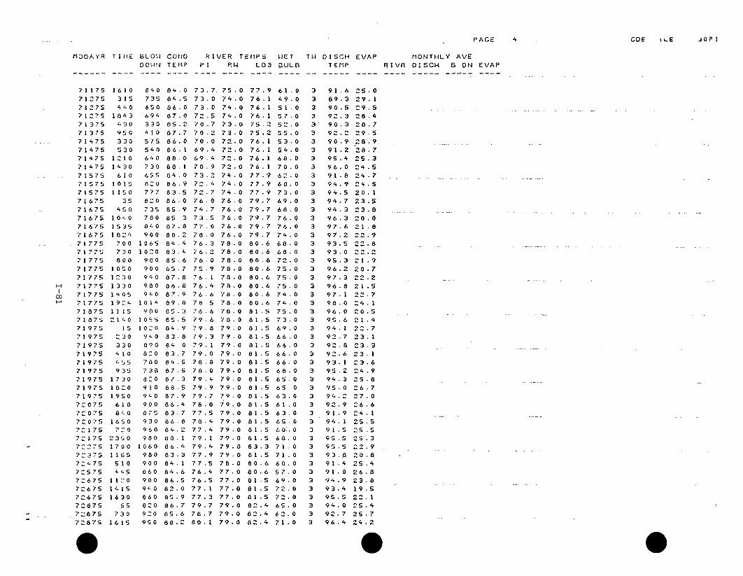
PAGE 4 COE t LE 1Op I

MODAYR TItlE SLOW CONO

DOWN TEM-1PRIVER TEM-PS WET TW DISCH EVAP

Pi P.W L03 BULB TEMPMONTHLY AVE

RIVR OISCH B ON EVAP

71175

71275'? 12 7S71275

71375

7 3757 '475714757147571475

715757 157571575716757167S7167571675716757177571775717757177571 77571 77S7 1775717757 18757 8757 97757197571 975

71 9757197S71975719757197571975

7Z07572075

?:2 1 75

721757227572375724757C575726757267S72675728757287572875

1610

31s440

1843

430

950

330

530

1210

1430

610

10151150

35

458

1 04 0

1535,1824

700

730800

1050

1230

1330

14051924

121021 is0

15

230

330

410

455

935

1730

1820

1950

618

84 0

1650

728

2350

1700

1155

s10

445

1120

14151630

ss

730

1615

840

735650694330

575540

64073065S82077.7820735780840900

106510209009009'4 0980940

1014

980

1055102094.0

890820780

738820910940

900875930

960980

10609809008609809L0

860

8z0920950

04 0

86 087 0a5 .287 786. 086 188 088 1

04 086 983 .5

86 085 985 387 888.2

84 483 1.85 685 787 886 887, 9

89 8as 3

04 983 884 083. 784.-587 S87 388 5

87 986 483 786.8

84.288 106 4.83. 384. 1

84.686.582.08S.986.785.680.2

73.7. 75.073 0 74.073 0 74 0

72.5 74. 070 7 73.070 .2 73.0

70 0 72.069 4 72 0

69 .4 72 070 9 72 073 .2 74 072 4 74 072. 7 74 076 0 76 074 .7 76 .073 5 76 077 0 76 078 0 76 076 3 78 0

76 2 78 076 0 78 075 9 78 0

76 1 78 0

76 4 78 076 6 78 078 5 78 076 6 70 079 6 78 0

79 8 79 079 3 79 079 1 79 079. 0 79 0

78 8 79. 078. 0 79 079 4- 79. 079 9 79. 079 7 79. 078 0 79 077.5 79 0

70 -4 79 077 4 79 079 1 79 079 4 79. 077 9 79 077 .S 78 0

76. 4 77 076.S 77 077. 1 77 077 .3 77. 079.7 79.0

78. 7 79 .080 .1 79. 0

77 .976 176 176 175 .27S8.276 1

76 176 1

77 .977.977 .979.779.779. 779.779.780 .680.680 .680.680.680 .680.680 .68a .581 .501 .581 .5

1 .581 .581 .581 .581 S81 .581 .581.a81.5

1 .581 .561 S83.381 .580. 680 681 .581 .581 .582 .482. 482- .4

61 049 0

51 057 0

52 05S 053 0S54 0

68 070 062 068) 0

73 069 068 076 076 074 068 068 072 075 075 07S 074 074 0

75 073 0

69 066 066 066 066 068 065 065 0

63 061 063 065 06&. 068.071.071.060.0

57 069 072 072. 065 062. 071. 0

91 .6 25 089.3 29 1

90.5 29 5

92.3 28 4

90.3 28. 7

92.2 29.5

90 .9 28 .9

91 .Z 28 7

95 .4 25 3

96. 0 24 5

91 .8 24 .7

94.9 24. 5

94. S 20. 1

94.7 23 .5

94 .3 23 0

96 .3 20 0

97 6 21 8

97 2 22 9

93 5 22 8

93. 0 22 2

95 .3 21 9

96 .2 20 7

97 3 22 .2

96.8 21 5

97. 1 22 7

98. 0 24 1

96. 0 20 .S

95.6 21 .4

94. 1 22 .7

92.7 23.1

92 8 23 3

92.6 23 193.1 -23. 6

95 .2 24 .9

94. 3 25 .8

95. 0 26 .7

94. 2 27 0

92. 9 26 .691 9 24.- 1

94. 1 25 5

91 S 2S .5

95 5 25 .395 .5 22 .9

93.8 20 .8

91 .4 25 .4

91.0 26. 8

94.9 Z3 .8

93.4 19.S

95 .8 22. 1

94. 0 25 .4

92. 7 2 . 7

96. 4 24.2

0

GDE 30P0';P A ,E

MO0AYR T10E ELOW CONO R[

DOCN TEMP P1

VER TEMPS WEET TI01 O-ECI4 EVAP MONTHLY AVE

Rw L03 EULS T E t.P RIVR OISCN B ON EVAP

H

I')

7297572-97S

73075

7307S

73175

73175

8 175

0 175

8 175

8 175

8 175

8 275

8 275

8 275

8 275

8 275

8 275.

8 37S

8 375

8 375

8 3775

8 475

8 575

8 575o 575

8 575

8 5758 575

8 675

8 675

8 775

8 775

0 775

8 775

8 775

8 975

8 975

8 975

8 975

81075

81075

81075

81075

81 175

61175

81175

81175

81175

81375

81575

81575

13301700

21202230IIS

1940

ý40

515

600

2010

2200

345

43S5L5

1945

2120

330

530

94S

1300

1300255

330'25

57)5

1230

1830

1500

16is310

315440

134S5

2045

315505

6001345

1 0001 010

19S02100

SI10

315450

1710

310

600

1430

980

10659809008609'0

1022106311051380

98091-0900860980.900

860620780

7808205 80820

7'0700

8201820B 12 0

13201050

980

82098094081.0655'490

535

575410510

3301602501881502.45

150

87,.388.8

84 .884 .684.987.2

87 086 786 388.084 183 683 883 588.0

86 085 385.5

85 7

89 08/3 6

90 666 3

D5 384 484. 888.5

89 590. 187. 083. 383. 383 .889 .486 885 .9

85.2

85. 0037 .7

84. 485 682.Isas 9

83 183.2833.1

85. 190. 186.1

81 .0

8-1 0282.0

81 .7a /1 3

82 3

81 901 9

81 7.

00.980 9

80 881 081 0

.•81 080 179 879 279 981 880 980 980 880.383.5a1 578 .378 582 1

03 981 .978. 178.9

0 .579.879. 376. 978.201 0

81 081 079 .879.4

79. 078.879.977.376.477.8

80.080.081 .061 ./81 .0

81 .0

82 082 0

82 082 082. 082 0

82 0

82 08,2.0

81 081 0

a 1 03

80 0

80.0

80.0

80.080.078.0

77.0

77. 0

77 .0

77.077.0

77.0

77.0

77.077.0

78.08 0

a8 078 077 0

77 077 077.077.0

83.383.3

83.363.383.383.3

83.383.383 383 383 383 383. 383 363 383. 383 384 284. 284 284.285 184 284.284 .284.284 284 .202 402 480 680 680 680 680 680 680 .680 680 680 680 680 680 680 680 680 680 680 679.779.779.7

74.0

76.0

72.0

72.071 .0

74 .0

70.0

70 0

70 0

69 0

69 0

66. 0

65 065 0

65 0

64 0.•" 0

62 0

60.0

65 0

70 0

69 0

61 0

61 0

61 0b 2 03

66. 0

63 062.0

62 053 03

53 0

54. 056S 065 ? 059.0

63 0

63 0

63 0

71,.0

64.0

64 061 0

61 0

60 0

59 059.0

60 0

71 057 0

62 0

66 0

96 8 22 .398 1 22 .594 9 21 .494 8 21 294 7 21 996 7 22 .2

76.7 36.089.9 31 .489',8 31 .090. 0 33. 188. 6 29.687. 3 30.787 .1 31 .307. 0 31 1

88. 7 35 187. 6 33 787 .4 33 186 8 34 .286.2 35 389 .0 36 0

90 .6 33.290 9 35 686 7 35486 .4 34 .586 .0 33. 786.5 33.6

89 ,2 35 .88 .6 36. 088. 5 36 .0

87 .3 35 .683.2 36 0

83.2 36.0

83.7 36.089 .2 36. /086 3 36. 093 1 25. 6

92 7 2S . 192. 6 25. 096.1 23.892.5 24.293.2 25 0

90 .8 24 192.6 26 390 8 24 890 7 25 290 .6 25 .91 .4 25 496.6 24 591 3 27. 195 1 28 .894.0 24 .7

78.0 91.8 735.3 26.2

PAGE P6OE E suPI

MODAYR TIM1E BLOW COND RIVER TEMIPS tWET

DOWNt TEMP PI RW L03 GULB

- - - -. - . - - .- - . - - - - . .- - - - .- - -

T14 DISCIH EVAPT E tIP

MONTHLY AVE

RIVR DISCH B ON EVAP

817? 581 77S01775

818758187581975

81975

019758197581975

8207582075

82175

82175821758237582375

6 2 37 582475

82'.75

824 758247S0257582575

82575025758257582575

8267502675

82675

82675

82675

82775

82775

82875

82875

82875

82875

82975

82975

82975

82975

82975

82975

83075

83075

83175

83175

83175

83175

8 ,

133014051430

1 1451325

0230920

105014301200

13302105530

12101745

301230131013151 4 4 01540

2230215435550725

20202125115

1235

14101600235011202220

600730

92512302200

235910

103015001523

4.001205

As145310

18832'8

'-88531

450325'39

488652735820

330410

4904 103284 10490576660740660572

4.904 15

3252:.617 015O325

21-5160ISO

230150230310395L 9

32015O1o0

32',, ý? 0

660'90570490410330

8 8.90. 188.5

09 .789 083 5al 0

88 .590 790 087 987.8

90 087 388 185 0

84 487 587 3

87.987 4

07 9

8s 103.

84 684 581 6

85 786 .485 788 8

84 6

83 684.886.084 .889 z87 887 106 6

84 306 984 889 588 582 087 483 783 804 .5

74 6

74. 7

74. 6

73.9

73. 7

76. 1

75 6

73 4

73 S

74 .2

75 6

74 1

73. 3

73. 3

76.0

75 1

73. 3

73. 5

73 .5

76 .2

77 9

80 0

78 3

77 2

76 .6

76. 3

75 9

75 0

74 9

74 1

72. 6

72 6

72. 4

71 7

70 6

72 7

72 1

72 0

72 0

73. 1

74 2

73 8

72 4

72.2

74 .5

74 7

73 3

71 3

73.1

72.7

72.0

76 .0 77.9

76 0 77.9

76 0 77.9

75 0 77. 0

75 0 77 0

75.OANKH

75. Okk M

75. O 0

75. 00 k

75.ONwNH

74.0 76. 1

74. 0 76. 1

74 0 76 1

75 0 77 0

75.0 77 0

75 0 77 0

73 .0 76 1

73. 0 76 1

73. 0 76 1

74 0 77 0

74 0 77 0

74 0 77 0

74 0 77 0

74 0 77 0

74 0 77.0

74 0 77. 0

74 0 77 0

74. 0 77 0

74 .0 77 0

73. 0 76 1

73. 0 76 1

73 0 76 1

73 0 76 1

73 0 76 1

72. 0 74 3

72.0 74 3

72.0 74 3

72. 0 74. 3

72.0 74 3

72.0 74 3

72. 0 75 2

72 0 75 2

72 0 75 .2

72 0 75 .2

7- 0 75 .2

72 0 75.2

72 0 74 3

7Z 0 74 3

72 0 74. 3

72 .0 74 3

72. 0 74 .3

57. 059. 059. 059.0

59. 058. 056 059.0

67. 067. 072 072.0

74 073 071 072. 064 077 077 077 079 079 068 058 053 053 053 056 056 056 059. 061 061 057 064. 064 066 066 069 072 065 064 065 065 068 068 062 063 059 057 057 0

4

4

4

4

4

4

4

4

4

4

4

4

4

4

4

4

4

4

4

4

4

4

4

4

4

4

4

4

4

4

4

4

4

4

4

4

4

4

4

4

4

4

4

4

4

4

4

4

44

4

86 .4 36 0

87. 5 36. 0

86 9 36 0

87. 3 36 0

87. 1 36 0

84 .7 34.4

83 1 33. 0

06 9 36. 0

90 3 36 .0

90 0 36 0

91 1 31 .4

91 1 31. 3

92.6 32.3

91 3 30 3

90 8 32 1

90 1 28.7

7. 0 32. 3

92 .9 28. 3

92. 8 28. 1

92.8 28.2

93.8 27.4

93.8 27.4

08.6 31 .0

84. 0 34 7

83 .7 36 0

83 .7 36.0

82 S 34 .7

85 0 36. 0

85 3 36 0

85 0 36 0

87 0 36 0

86 1 33.9

85 .7 33.0

84.9 35 .9

87.6 33.7

87.2 32.6

89.4 35.8

88 9 34.5

89 7 32.3

90 7 30 .2

87. 3 31 7

87 0 32.'

88 3 34. 1

87 5 32 .2

90 2 35 1

89 8 34 ">

85 4 31 .2

87 8 35 .5

85 1 34. 1

84 5 35 . 0

84 .8 35 .6

945 410 89 .4 71 .2 72 .0 74 3 62. 0 4 88 2 36 . 0

0

PGO:. FILEPACE 7 3 0P !

MlODAYR TIME SLOW4 COrJD RI

DOWJN TEMP PI

- - - - - -. - . - - . - -. . - - - . .- - -

VER TEMPS IJET TW DISCH

RW L03 C-ULB TEMP

EVAP MONTHLY AVER'IVR DISC1 B ON EVAP

83175 1030

83175 1300490 90.2 71.3 72.0 74.3 e2.0

570 89.4 72.3 72.0 74.3 66.0

9 1759 .759 275

9 3759 3759 3759 4759 4759 4759 4759 5759 5759 5759 5759 6759 6759 6759 6759 6759 7759 7759 8759 8759 8759 8759 075

9 9759 9759 9759 9759 9759 9759 97591075

910759 10759 07591 17591 17591 17591 17591 1759 12759 275912.7591275912759137591375

1741730

1130

500

1230

1350

330

'30

515

750

'30

845

1251

1020

130

1000

1120

1330

245

950

10

635

900

1545

164510

300

345830

910930

I155

106

9004130

1200

200'00

1320

1'-05

2230015

1300

1335

1425

1630

400

800

655570655570'90570490

370285'90'30

'90530'00370310'80

.00

440410455240

330l10

'80

9999330245150195240320'10205

375•I0

'00

3702a5'902852051603304101602^45150295

91 0

83 S

84 4

04 6

86 6

84 1

84 0

83 3

86.284.6

87 .4

87.0

86. 1

84+.6

84 0

07 9

83 7

87 3

84. 588 0

83.2

85.0

87.1

87.0

73.6

73 .5

83.4

83.5

87 .2

88.2

88,4

88 0

8a. 9

86 4

87 8

87 184 4

83 8

86.0

85 .9

84.0

03.4

85 5

86 6

87 1

8. 4

83 0

89 4

73 575 372 972 871 .271 .2

72 .572 .472 .473 . 1

71 171 17 1 1

7 1 1

70 770 770 770 .770. 771 .671 671 669 669 669 669.669.674.274 274.*274 2

74 274.270.670.670 670.660.368.2

66.566.565.9

63 8

63 563 S63.463.462. 661 7

72Z . 0 75 .72. 0 75. 272. 0 75 2

72. 0 75. 272. 0 75. 272 0 75.271 0 73.471 0 73.471 0 73.471 0 73 470 0 74 370 0 74. 370 0 74 370 .0 74 370. 0 72 5

70.0 72.!70. 0 72 570. 0 72. 570. 0 72 .569.0 72.569. 0 72 S69 .0 73 469. 0 73 469. 0 73. 469. 0 73. 469 .0 73. 46. 0HU4N

68 0Q

68 04

68.0444 MO

68.0.4 o4 m

68. 0-4HW68. 0444 44

68. 0444444468.Om44468.044444

68.04 ww4 4

60.044444444

68.0mo, m4

65. O4m44"m465,0mmoxm

65.04444444465.ON444

6S. 044N4

65.044444444

65 055 0

63 0

56 062 062 051 051.0

50.0

59 058.0

57 .61 055.0

SI 048 0

56 058 .0

55 050.0

46 0S2 054 0

52 046 044 044 0S 2 0S2 052 0

59 057. 0

65 .069. 069,.057.057. 0

51 050 041.0

44 046 046. 047 047 036. 046. 0

4 88.5 36 . 04 09.S 35.9

4 77.3 36.0

4 83.9 35.6

4 87 .6 34.9

4 84 .5 35 .9

4 86.4 .33.4

4 87.2 35.2

4 83 0 36 0

4 82.9 36 0

4 82 4 36 0

4 8 .1 36. 0

3 91 . 26 S

3 92 S. 28. 7

3 93.2 27. 0

3 91 .4 28 .4

3 89 7 28. 6

3 88 8 29.. 1

3 92 5 29 3

3 90 .7 25 9

3 92. 6 2 34 85. 35 .2

4 85 .6 36 0

4 82 .4 36 0

4 82 0 36 0

4 84 4 36 0

4 84 9 36 0

4 78.9 28. 3

49999.0 28.3

4 80 .9 36. 0

4 80 .9 36. 0

4 04 4 36 .0

4 84 8 36 0

4 .84. 9 36. 0

4 86.7 36.0

4 84 :2 34 .2

4 88. 1 33.6

4 89 9 33 .0

4 89 7 32. 3

4 04 8 35 .5

4 84. 5 35. 0

4 03 .7 36. 0

4 83 .4 36 .0

4 80 .4 36. 0

4 80 .9 36. 0

4 82.2 36. 0

4 82.6 '36. 0

4 83.0 36. 0

4 83.5 36. 0

4 78.8 36. 0

4 83 . 6 36. 0

76.6 89.4 509.0 32.0

Northern States Power Company

414 Nicollet MallMinneapolis. Minnesota 55401Telephone (612) 330-5500

July 24, 1981

Don L. KriensEnforcement SectionDivision of Water QualityMinnesota Pollution Control Agency1935 West County Road B-2Roseville, MN 55113

Prairie Island Nuclear Generating PlantChlorination of Circulating Water to Remove Parasitic Amoeba

Analyses of the circulating water system at the Prairie IslandNuclear Generating Plant have confirmed the continued presenceof the parasitic amoeba, Naeglaria Fowleri. Population densitiesare such that it has been determined necessary to again treatthe system to control the amoeba. The purpose of this letteris to secure MPCA approval for an alteration in the mode ofplant operation and the addition of chemicals to the PrairieIsland circulating water system.

The proposed treatment plan will utilize chlorination and subsequentdechlorination prior to discharge of water from the system. It isplanned to conduct the.treatment in the same manner as that per-formed at Prairie Island on August 28, 1980. The specifics of thatprocedure are contained in our letter ,to the MPCA dated August 19,1980 in which we requested authorization to conduct the treatment.

We 'are requesting your written authorization to conduct the test fora one-day period, tentatively set for September 2, 1981. We willagain coordinate our efforts with the Minnesota Department of NaturalResources to attempt to remove fish from the recirculation canalprior to treatment.

Please contact me at (612) 330-6894 if additional information isrequired. -

R D Clough, Administrator ERAD RECORD CENTEROperating Permits

RDC:jz bcc: G M KuhlL J Micienzi

cc: Russ Frazier - MN Dept of Health J M PappenfusHoward Krosch - MN Dept of Natural Resources R W Steurnagel

E C WardE L Watzl

~,kIVI~ qib

October 14, 1981

Northern States Power Company

414 Nicollet MaliMinneapolis. Minnesota 55401Telephone (612) 330-5500

IN

Don KriensDivision of Water QualityMinnesota Pollution Control Agency1935 West County Road B2Roseville, Minnesota 55113

PRAIRIE ISLAND NUCLEAR GENERATING PLANTCirculating Water Chlorination-Dechlorination

-Pathogenic Ameba• Naegleria fowleria)Control Program

As requested in your letter of August 3, 1981 we are submittingthe results of the Prairie Island circulating water chlorination-dechlorination conducted last month to reduce the population ofpathogenic Naegleria.

Also enclosed is an NSP Testing Lab Report on the procedure anda summary addressing the "Chlorine Effects on Resident FisheriesPopulation." A final report on the amoeba. will be included in-jthe annual Environmental Report for Prairie Island.

If you have any questions concerning this information, pleasecontact Bob Clough at 330-6894.

Senior Consultant

Regulatory Service

ah

enclosure

cc: R D Clough

bcc: L W EberleyJ M PappenfusR W SteuernagelE C WardE L Watzl

VIA*,

Analysis of data prior to and after chlorination in 1981reveals 'a pattern similar to that seen in previous years. Thuspathogenic Naeglaria could be detected in 1 and 10 ml samplesof cooling tower and intake water prior to chlorination. Afterchlorination pathogenic Naegleria could not be detected in 1,10 or 100 ml samples of water from either the intake or coolingtower canal.

4t

-4

Boforn Chlorinations 1981

Site -i. (C,)- Dr't• ?'re/Vo]. 5a-.e

Cooling

Cooling

Cooling

Cooling

Cooling

CoolinG

Cooling

Cooling

Cooling

Cooling

Cooling

Cooling

CoolingC

Cooling

)oling

Cooling

Cooling

Tower

Tower

Tower

Tower

Tower

Tower

Tower

Tower

Tower

Tower

Tower

Tower

Tower

Tower

Tower

Tower

Tower

Tower

30'0

30

30

30

303030

3030

2)0

303030

3030

r/1o

P110

P./It

Ft/ I "8/to

g/108/to

F/10

P/10

/1.0

8/1.0

,0/10

q10o

2•0

•..-0

J20

120.:0

".2o

:20

420

i2O

1120

H ., 20

- lO ori!- I0C~rnl

- 100-.1

- 100-.- 10•I- lOrdl- lOr-l

- 1nl

- 1ml,

Inl

- r-rI

- ml.- I1l- inil

- 1Inl- L'l

Aino'•b i coutfro-that lh•uC

Fos.

Pos.Fos.

Pos.

Fos.P03.

Fos.

Pos.

Fos.Neg.P'os.

Neg.

N;eg.

Neg.

F"ij:cl, Ap!o rance

NT

NT

Fos.

Fos.

Pos.

Pos,

Pos.N:A

T U

NT

NT

NA

NA

KA

NA

P

I:A

INA

la

RA

NA

NA

Pos.

Neg.17NT

Pos8.

NA

NA.

NA.

NA,'

NA

8/10 F-20

NA -

NN-

NP-

1.ot t e.;tTe

Not applicableNot "aithogeoea

!'athogcnic :;aeogleria

In-;at~hog-enic Naegleria

-----------~ -~-'.--',

Frrvalence of Pathogrminc *.aoglnria at the

Prairio IsLornd Plaut

Before Chlorination: 1981

S~t a Teý-I. (c:0) >t2 Ty~/Vol. 5L~~plo31

Cooling

Cooling

Cooling

Cooling

Cooling

Cooling

Cooling

CoolirC

Cooling

Cooling

Cooling,

,oling

Cooling

Cooling

Cooling.

Cooliii

Cooling

Cooling

Cooling

CoolinG

Cooling

Cooling

Tower

Towel.

Tower

Tower

Tower

Tower

Tower

Tower

Tower

Tower

Tower

Tower

Tower

Tower

Tower

Tower

Tower

Tower

Tower

Tower

Tower

Tower

Tower

353535353535

353535

35353535353535353535

35353535

zNT

P/'31

0/31

8/31

V/31,V131

S131

P/31.Po/3:

P/31

'/ i.,./31

P/31

8/318/31

.20 - 100ni

20 - lOOn1 .

20 - 100.1

i20 - lOnI- 0 - lOni- 2

H120 - iO011

H2 0 - On.l

F20 - Io0I

H20 - iO).lH-20 - lo'l,

H20 - 1for

H20 - iml

!,0- I•Il

H20 - I'm12O- iml

20- i•I.)

.20 - )ml

H2 0 1Iml

H20- L-11

.20- irl

Anoebicoutgrowth

at 450 C

Fos.

Neg,

Fos.

Isog,

Fos.Pos.

Fos.Fos.

?os.

Fos,d~eg,

Pos.

e; g.

Fos.

Fos.

Ne.g

Pos.

Fos.

z-1;rel. Appearance

NTNT P/N?

NT FIN?

NA N

k. A. 11

Pos. P/H?

NT M;N

NA 1WL'IT

I'NA

Fos, PN1A

"NA."NA KA

Neg, P

NA NANee

1';og,.N/

Neg. NH/P

::A

A.

FOS.

:'A

'NT

T.

5'OS,

NT* V..A.A

- ::ot appzic25le- ;:or :'ae,~lc.ria

- Fatho~cnic N:a gleria

- "Non-pathogenic Haegloria

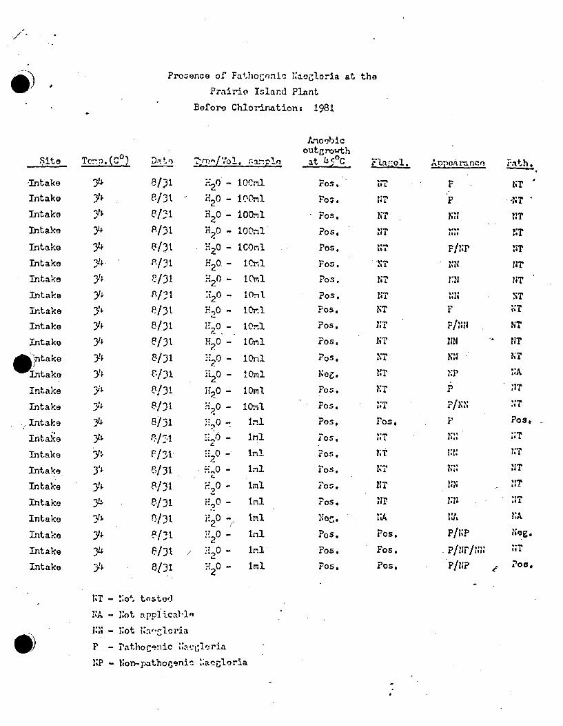
Proeence of Fathor-cnic Naegloria at the

Prairie Island Plant

Before Chlorinations 1981

Site

-Intake

Intake

Intake

Intake

Intake

Intake

Intake

Intake

Intake

Intake

Intake

Intake

Intake

Intake

Intake

Intake

Intake

Intake

Intake.

Intake

Intake

IntakeIntake

Intake

Intake

Te.(C 0)

34

Y3

34

.Y •

3

34

V4

54.

D/31

,/3st

8/31

f,/31

e/31

8/31.

P./31

CP/3 1

8/3t8/318/318/318/31

8131

8/31813181318/31

8/31

8/31.

8/31

*- 0- lOCMl

H20- lO0C1

-20 100-I1H2- 1O~lO.b,

20 ICOnlUH20. -Ic•,l120- 0 1Omi

**20 - lOni

120 - 11.n

HO- tOnl4.

H20 - 1C,•I

"[0- lOnlz.20 - lOmi

W.10- 1 Ora1

.1 0 1mlH20- 10•

."[.0 - Inl

?0O- mu.

• r. -~ Inl.4-

F"0- Iml

0 Iml

20- Innl

.420 - ml

H20 - Iml

Anovbicoutgrowthat 4.'C

Fos.•

Fo;.

Fos.

ros.

Pos.

Fos.

Los.

Fos,

Fos.Pose

Fos.

Fos.Na: g.

L'oS.

Fos.

Fos,

Pos,-A-OS.

ros.Los,

Fos.

Fos.

Fos.Fos.

F~ a~oI. Aopeaancm

NT

INTINTNT

NT

NTNT

NT

Fos.NT

NT

NT

NA

Fos.

NT

NT

Los,

Fos.

Pos,

P

P/NP

NN,

F

MNl

NN

P/1;?P/N;P

?at h,

NT

4NT

NT

NT

NT

NT

NT

NT

NTI;A

NIT

Nos1NT

NA

Neg.

NT

Poo.I'

NA

P,

NP

-:;o testedl

- Not applical'b.

- Not INam-rloia

- Pathocqnic -§i';'Pria

- Non-.athogenic .;aegloria

I.

?revalence of ?athogmnic Naagleria at the

Prairie I3land Plant

After Chlorination: 19,91

oiteg,

Cooling Tower

• Cooling Tower

Cooling Tower

Cooling Tower

Cooling Tower

Cooling Tower

Cooling. Tower

Cooling Tower

Cooling Tower

Cooling Tower

Cooling Tower

Cooling Tower

Cooling Towe r

Cooling Tower

CoolinG Tower

Cooling Tower

Cooling Tower

Cooling Tower

Cooling Tower

Cooling Tower

Cooling Tower

Cooling Tower

Cooling Tower

Cooling TowerCooling Tower

28

28

28

28

28

28

282R

2?

28

29

2A

2$2.'32?

26

28

-4._ Tv,/Vo.. r-.nle

9/89/6

9/8

9/8

9/89/q

9/83

9/8,

9/R

9/8

9/8

9/18

9/8

9/8

9/8

9/fl

*9/8

9/8

9/fl

* 9/fl9/,8

r0

II20H20

42., 0,.2

i:2o

H20F.2 0

-2

i{20.2

H-O

II0S0.

H 2o

HO

. 0.e

2

20F,2 0

- 1O0ml

- 100.I- 1O(~ml

- ockil- looml

- lonl

- lOml

- lOrl

- \.IctI

- total

- l~nl

- lOnl

- linl

•- Il.d- nml

- Inul- iril- Iml

- Ili

- lnl- iml

- nl

Amoebicoutgrowth

Fos.

Fos.

Fos.

Fos.

Fos.

Pos.

ros.

Pos.

Fos,

Fo s.

Pos.

Fos.

Post

Fos.Fos.

pose

FOS,

Pos.

Pos.

Fos.

oeg.

Fla..-el.

NT

Fos.

4% T

NT

NT

Nag.

NT

N;eg.

NA

ros.

NT, IT

NT

!IT

Fos.

NT

NT

Neg'.

Fos.

Appr'araru-"

NA

Im'

Np

K.s

I,''

NAl

IN;

N?

Sn.]

A.,/'

S..

NP

Path.

NT

NT

Neg.

NT

NT

NT

NT

NT

>NT

NT

NA

Neg.

NT

NT

ZIT

NT

NT

N~eg.

14T

NT

1IT

Neg.

NA

41

NT

LrAI

P

* NP

Not t5etedNot a:.:'licabl.e

?athgoLndc ::aegloria

Non-pathogenic iUaegleria

Prevalence of ?athogenlc Naegloria at thePrairie Island Plant

After Chlorinatin ns 1981

Armoebicoutgrowth

)itoe Te.rp.(C°) ;t__- Ty p!Vol. s-vinle at 5°C Fla,:ol, Apamarinco

Intake 27 9/8 0 - Wen! Nag.. :A INA NA

Intake 27 9/8 .20 - 1O0rl Foso NTIntake 27 1/C 0- l00nI Neg. NA NA

Intake 27 •9/8 t" 0 - lOOnl. Pos. NT NNTIn~take 27 9/8 r20 - lOOnl. Pos. Nag. NN/N? N;TIntake 27 9/8 H20 - tO2l Nag. NA NA NA

Intake 27 9/8 it20 - I•0n) Pos. NT gT

Intake 27 9/F Y20 - ICoI Neg. 10A NA NA'2-1

Intake 27 9/8 :0 - tOni. N;o. NA N A NA

27 0'/8 - 1Intake 2.

Intake 27 9 /R 24 o - 1C,'J Ng. NA 'NA NIntake 27 9/8 z2 0 - •I Cg. NA 1.A I(#'

Intake 27 9/8 120- lOnr 1:0[. "ZA NA NAIntake 27 9/8 0 - i0).. .eg. 'A ?A i.A

-Intake 27 -A

Intake 27 9/P H0O - 1. Neg. 1A NA ,.

Intae 27 9 0 - in). AN 9 NA NA

Intake 27 9/8 120 - i.l NOeg. NA ,A -A

Intake 27 9/8 P) ? - lnl Nog. RA NA .A

Intake 27 C/3. 0 - ml Neg. 1- NA 'A

Intake 27 9/8 ?2 0 in) gANAIntake 27 9/8 O2 - inl Neg. NA -AIntake 27 2. H20 - Ir. ,ag,,N,

Intke 7 90 .0 &4I(31,e. NA INA :

Intake 27 ./. 2.,0 - Inl Ne;. NA NA NA

NT- Not tostnl

IN- Not apl 3.c.'b~e

N- Not N:ae;lnria

P - Patho'nnic *:anl,)ria

I 1•P- lson-pathogenlc ;aegliaria

CHLORINE EFFECTS ON RESIDENT FISHERIES POPULATION

An estimated total of 28,095 fishes were lost during the September1981 zhlorination at Prairie Island. Table lists the total numbersand representative length frequency distributions for all fishes lost.Where possible, unmeasured fish were designated and recorded as young-of-the-year (yy) and juvenile or adult. When this was not possiblefish not measured were recorded as "unmeasured".

Gizzard shad ans shiners comprised 77 percent of the total loss.Channel catfish comprised 16 percent; other game species encountered,*in decreasing order of abundance were white bass, bluegill, greensunfish, crappie, walleye, and sauger. Collectively, game fish wereless than four percent of all fishes lost.

To estimate the number of yy and juvenile lost the number of fishfrom three buckets were counted and th eaverage used to extrapolatethe total numbers for all buckets (table). Adults were separated fromthe yy and juveniles and enumerated individually.

In an attempt to drive fish out of the plant circulating water system,one and one-quarter pounds of copper sulfate instant powder were addedto the circulating water system each minute for two hours commencingat 0630 hours. Based upon the estimated volume of the circulatingwater system, the copper sulfate concentration was expected to approachone-half parts-per-million which should repel fish.

The total fish loss during the September 1981 chlorination was considerablyless than the 162,448 fishes lost during the August 1980 chlorination.A number of explanations may be possible. The copper sulfate may havebeen successful, the fact that the two parts-per-million free chlorinewas achieved for only about two hours may have prevented a total killin the circulating water system. Although there is no way to adequatelyassess the effectiveness of the copper sulfate'it is recommended that itbe employed in any subsequent chlorination efforts at Prairie Island.The copper sulfate is relatively cheap and any fish chased from the systemwill not be lost.

Although the number of fish lost during the 1981 chlorination was sub-stantially~less than that of 1980, the relative composition of fish lostwas quite similar. Gizzard shad, shiners, and carp collectively dominatedthe total with channel catfish comprising the next most abundant species.Other game fish comprised less than 13 and 4 percent of the total in 1980and 1981 respectively.

41,

M: I m !F - IMNOWIP, -398M

lain --

TOTAL LENGTH

(MM)

0-19

20-39

-- - -- ------ At ,calk 13a.rdA-A Ch• I ,5O. I 5,4 --

IF-

40-59

60-79

80.99

100-119

120.139

140-159

160-179

180.199

200-219

220-239

240-259

260-279

260.299

300-319

320-339

360.379 _____

- - - -. 4

††††††††††††††1

/

~~~.1'Ii'~ -i7--i* ______ _______ ______

,.- I I

3M0-399

400-419

"40-459

460.479

480499

t

__..___I -/~_____

I -3 Ij___t '71J __ _,1 1 _

__. q __.,__ _

_l ]I -' __ -- _ _ _ _ _ _ _ _ _-I _ _ _

. L .... _ _ _ _

500-519

520-539

540-559

560-579

580-599

600.619

620-639

640-659

-I----~~1~~

660-679 I" 68 .699 A DU LT - ---- [ _ _ "

__________ __ _ .."__ __ _ __ __,,_ __ __

7 _• a 1.I .__ _ _ ..... --- " _ _ _ __ _ _ _ _ _ _ _ _

___~sre -, ZLI _ •

CM'MTAL,COMMENTS:

4 1 40JI2 I I IS 6( q 23

TOTAL LEN4 Wo? RiI' rU Ff7 let uIoVi 7 ?acN(MM) jCcup5,Jd/ " o ,o/ j V ' I s I.s w.

_ o.__ • -- !- . +/

40`S9 ,20"3 __ __ __ .__ _____ __a.__ __J ___. ____.

100-119

120-139

140-159

160-179

180-199

200-219

- ~ I j 1 5-

___~~1~. ___ __I ..A' -____

____ - +220-239

240-259

260-279

280-299

300-319

320-339

340-359

360-379

I4 4r-A- 4- •

Ia1..1-

_ I i 4 -4 4-~ 4

/

-I- L I/

-- .4 4 , -. 4 4 -.-----.---------- .4 .-. II

& ~1____ ___ 5'7

I 4 4*..-4o0-419~~J380-399 J

400-41910 420-439 -9

460-479

480-4995,,,0- 519

520 539

540-559

560-579

2~~ -~

13.

3--3-3--IIL

T

Z~7ii-4--

---I--.--

-1*1-- - I

__________________ I~71

5'I

_ -1.~__ -I--i___ ___

I-_~1~~~__

- -I I._______ ______

-3--I- /

3.

580-599

6004619

620-639

640-"59 /660-679

680-699

~.•. 85

UNMEASURED

UNM. yY+I-!,t.UNM ADULT

I4 + - ---- 4 1- -+ I i - I 4

I4-.4 -- 4 ________ . + 4 4-'-~----4 4

4 4----- + I 4 p z/

P - - -5~Luii ,I Li

I

I- A

3(,3~30

1L

S .4.-

ToT4E.. I 3c~ 137 -oSY

COMMENTS:

......... • %.

TOTAL LENGTHIMM)

0-19

20-39

40-59

60-79

80-99

100-119

120-139140-159

160-179

180-199200-219

.E~III - . - - -----.- -. -

~-T-~

h~~M~dsT~ 1L

--.--

I

____ I CAk.Uc~e

-Li

-- 3,

.1.

-4~i j:_j~j.i'_.-1__ ___ ___

_---1--1 _220-239

240-259

260-279

280-299

300-319320-339

340-359

360-379

380-399

" 4 0 - 1 9

-I--

1 -

-7

4 I + 4

-- ~ -

'3I

4 + 4

I I

:. I--- ___ ____ ____

-'7 ____ ____ _____

01. '2~

Im . /i 4 -t 4

I4- + ~-*---------4-----'--4--~--4- - 4 4 4 4

I-4 -~I

460-479

480499

500-S19

520-539

540-559

560-.579580-599

~1~I F-- -- a -- 4

4 4-.- 4--- 4 4- -4. -a

_______ d/ 4-----. - 4 4 -4-------------- i

I I4 .I-~--4 *-----~ 4-----4 4 1

I600-019'r --- -620-639 _ " :

". 640-659

660-679

680-699

UNjýMEASUIREO -U NM. YY+ In%) 0±

U_!NM ADULT .1

---- 1 4--- 4.- 4 .4 4

I.

k1I I

4 4 4

-rlsmk Z--1 IS- 373 7 ,•' "i ? .COMMENTS:

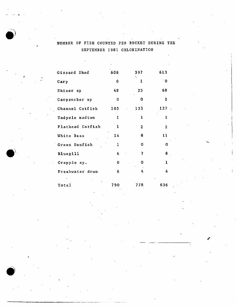
NUMBER OF FISH COUNTED PER BUCKET DURING THE

SEPTEMBER 1981 CHLORINATION

Gizzard Shad 608 597 613

Carp 0 1 0

Shiner sp 48 25 68

Carpsucker sp 0 0 1

Channel Catfish 105 133 127

Tadpole madtom 1 1 1

Flathead Catfish 1 2 2

White Bass 14 8 11

Green Sunfish 1 0 0

Bluegill 6 7 8

Crappie sp. 0 0 1

Freshwater drum 6 4 4

Total 790 778 836

e,

Cfi ~4e bpAk4E.bl ~latJkoi)

F."

Northern States Power Company Ni')

414 Nicollet MallMinneapolis, Minnesota 55401Telephone (612) 330-5500

October 14, 1983

Howard Krosch Don L KriensDivision of Fish & Wildlife Division of Waste QualityMN Dept of Natural Resources MN Pollution Control Agency mCentennial Office Building 1935 West County Road B2St Paul, Minnesota 55155 Roseville, Minnesota 55113

PRAIRIE ISLAND NUCLEAR GENERATING PLANTChlorination of Circulating Water SystemFish Loss Report

Enclosed, for your information, is a report on the fish lossdue to chlorination of the circulating water system at thePrairie Island Nuclear Generating Plant in August, 1983.

Feel free to contact Glen Kuhl at the Prairie Island Environ-mental Lab at (612) 388-1121, extension 349, if you have anyquestions concerning this report.

W EJnenSenior ConsultantRegulatory Services

ah

enclosure

cc: G M Kuhl

Internal CorrespondE nce

Date August 30, 1983

From G. M. Kuhl Location Prairie IslandPhycologist

To S. F. Schmidt Location GO (2)Admin Reg Compliance

Smbject FISH LOSS DUE TO CHLORINATION OF THE PINGP CIRCULATING WATERSYSTEM

An estimated total of 37,124 fish were killed during the chlori-nation of the circulating water system at PINGP on August 20,1983. 'tables 1 and 2 list representative length frequencies andtotals for all species lost. When possible, unmeasured fish weredesignated as young-of-the-year (yy), juvenile, and adult. Dur-ing instances where this was not possible fish not measured wererecorded as "unmeasured".

Gizzard shad comprised 61.7% of the total loss with channel cat-fish representing 26.5% of the total. Other game fish indecreasing order of abundance, included white bass, crappie spp.,bluegill, sauger and walleye. These species comprised 3.9% ofthe total fish loss.

Adult fish were separated from yy and juvenile fish, enumeratedand measured individually (Table 1). Estimated numbers of yy andjuvenile fish were based on the number of fish counted per bucketwith this number extrapolated over all buckets (Table 2).

As in the 1981 chlorination, copper sulfate was used in anattempt to drive fish from the circulating water system prior tochlorination. In cooperation with a Minnesota Department ofNatural Resources licensed applicator, copper sulfate was addedon two occasions. On Friday, August 19, copper sulfate was addedat a rate of two pounds per minute for 15 minutes to the new dis-charge canal while the plant was operating in open helper cycle.This provided adequate mixing and flow to hopefully drive fishfrom the canal. On Saturday, August 20, copper sulfate was addedat a rate of three pounds per minute for 60 minutes to theremainder of the circulating water system. Based on calculationsof the quantity of water in the system the application rates wereexpected to allow copper sulfate concentrations to reach 0.5 ppm,which should repel fish.

6)

Fish loss during the 1983 chlorination was slightly greater thanthe 28,095 lost during 1981 but considerably less than the162,4.48 lost 'during the 1980 chlorination. Species compositionwas similar to previous years with gizzard shad and channel cat-fish being major contributors of fish loss.

J/

G. M. Kuhl

sw

OF~ MN/1 0Minnesota Department of Natural Resources

5•00 Lafayette RoadMM St. Paul, Minnesota 55155-40.

August 10, 2007

James Holthaus, Project ManagerNuclear Management Company1717 Wakonade Drive EastWelch, MN 55089

RE: Prairie Island Nuclear Generating Plant Re-licensing and Environmental Review.

Dear Mr. Holthaus:

The Minnesota Department of Natural Resources (DNR) has reviewed the materials presented in the NEPA IssuesIndex for the Prairie Island Nuclear Generating Plant (PINGP) Environmental Report. The DNR requestsadditional emphasis or clarification on the following issues

Surface Water Quality, Hydrology and UseThe DNR recommends PINGP continue the periodic assessment of best management practices for control of bio-fouling which includes plant system infestations of zebra mussels. The DNR also recommends periodic assessment ofplant chemicals for determining alternative products which do not contain aquatic nutrients or endocrine disruptingsubstances.

The DNR and Xcel have discussed a drawdown of Mississippi River Pool #3 sometime in the near future to improvehabitat conditions. The DNR recommends the environmental report include an evaluation of the issues and impacts toPINGP intake and operations associated with summer drawdowns. This evaluation may already included in the NEAPIssues Index # 13.

Terrestrial ResourcesThe DNR recommends routine review of herbicide product use for reducing aquatic or terrestrial toxicity or endocrinedisruption.

The DNR recommends periodic assessment of best available technology for lighting effects on bird collision withstructures including the communications tower at the PINGP site. This tower is approximately 340 feet in height andis placed within the floodplain of the nations most significant bird migration corridor.

The DNR requests a review of plant emissions of fugitive light and noise not essential for facility security oroperations to minimize disturbance to surrounding residents, recreational users, and terrestrial wildlife.

Thank you for the opportunity to review the PINGP NEPA Issues Index. Please contact me with any questionsregarding this letter.

Si c rely,

attLanga 4, riental PlannerEnvironmental Review UnitDivision of Ecological Resources(651) 259-5115

c: Steve Colvin, Joe Kurcinka, Wayne Barstad, Tim Slagenhaft, Scot Johnson, Jack EnblomD:\AA_OMBS\1 'hq'fto.-gti-9s010:xCom•-gg-_%.497o0 TTY: 651-296-5484 * 1-800-657-3929

Printed on Recycled Paper Containing aAn Equal Opportunity Employer Minimum of 10% Post-Consumer Waste

MINNESOTA

Protecting, maintaining and improving the health of all Minnesotans

April 10, 2008

James J. Holthaus, PMPEnvironmental Project ManagerPrairie Island Nuclear Generating Plant1717 Wakonade Drive East13-Plex (License Renewal)Welch, MN 55089

Dear Mr. Holthaus:

I am writing in response to the letter of January 25, 2008 from Mike Wadley, Prairie Island SiteVice President, regarding the Nuclear Regulatory Commission license renewal for the PrairieIsland Nuclear Generating Plant (PINGP). Mr. Wadley asked the Minnesota Department ofHealth (MDH) for help in determining whether there is any public health-related concerns fromoccurrence of thermophilic organisms in Mississippi River waters affected by the operations ofthe PINGP.

MDH does not monitor Mississippi River waters for occurrence of the organisms mentioned inthe letter. Further, we have no information concerning possible exposures and health risksshould these organisms be found in areas of the Mississippi affected by the PINGP discharge.

If MDH receives any information relevant to your query we will forward it to you. Pleasecontact me if you have additional questions.

Sincerely,

J Line Stine, DirectorEnvironmental Health DivisionP.O. Box 64975St. Paul, Minnesota 55164-0975

General Information: 651-201-5000 ° Toll-free: 888-345-0823 • TTY: 651-201-5797 • www.health.state.mn.us

An equal opportunity employer

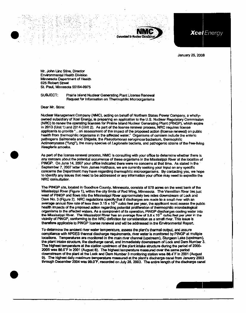
ConMnfad to ulaXC

January 25, 2008

Mr. John Unc Stine. DirectorEnvironmental Health DivisionMinnesota Department of Health625 Robert StreetSt. Paul, Minnesota 55164-0975

SUBJECT: Prairie Island Nuclear Generating Plant License Renewal

Request for Information on Thermophilic Microorganisms

Dear Mr. Stine:

Nuclear Management Company (NMC), acting on behalf of Northern States Power Company, a wholly-owned subsidiary of Xcel Energy, Is preparing an application to the U.S. Nuclear Regulatory Commission(NRC) to renew the operating licenses for Prairie Island Nuclear Generating Plant (PINGP), which expirein 2013 (Unit 1) and 2014 (Unit 2). As part of the license renewal process, NRC requires licenseapplicants to provide *... an assessment of the impact of the proposed action {license renewal) on publichealth from thermophilic organisms in the affected water." Organisms of concern include the entericpathogens Salmonella and Shigella, the Pseudomonas aeruginosa bacterium, thermophilicActinomycetes ("fungi"), the many species of Legionella bacteria, and pathogenic strains of the free-livingNaeglenfa amoeba.

As part of the license renewal process, NMC is consulting with your office to determine whether there Isany concern about the potential occurrence of these organisms in the Mississippi River at the location ofPINGP. On June 14, 2007 your office indicated there were no concerns at that time. As stated in theSeptember 7, 2007 letter from James Holthaus, we are currently seeking your input on any specificconcerns the Department may have regarding thermophilic microorganisms. By contacting you, we hopeto identify any issues that need to be addressed or any information your office may need to expedite theNRC consultation.

The PINGP site, located in Goodhue County, Minnesota, consists of 578 acres on the west bank of theMississippi River (Figure 1), within the city limits of Red Wing, Minnesota. The Vermillion River lies justwest of PINGP and flows into the Mississippi River approximately two miles downstream of Lock andDam No. 3 (Figure 2). NRC regulations specify that if discharges are made to a small river with anaverage annual flow rate of less than 3.15 x 1012 cubic feet per year, the applicant must assess the publichealth impacts of the proposed action regarding potential proliferation of thermophilic microbiologicalorganisms In the affected waters. As a component of its operation, PINGP discharges cooling water Intothe Mississippi River. The Mississippi River has an average flow of 5.8 x 1011 cubic feet per year in thevicinity of PINGP, conforming to the NRC definition for consideration as a smal river. This issue istherefore applicable to PINGP license renewal and will be addressed in the Environmental Report.

To determine the ambient river water temperature, assess the plant's thermal output, and assurecompliance with NPDES thermal discharge requirements, river water is monitored by PINGP at multiplelocations. Temperatures are monitored in the main river channel (upstream), Sturgeon Lake (upstream),the plant intake structure, the discharge canal, and immediately downstream of Lock and Dam Number 3.The highest temperature at the station upstream of the plant intake structure during the period of 2000-2005 was 86.0"F In 2001 (August 8). The highest temperature measured over the same perioddownstream of the plant at the Lock and Dam Number 3 monitoring station was 86.4"F in 2001 (August9). The highest daily maximum temperature measured at the plant's discharge canal from January 2003through December 2004 was 99.0F, recorded on July 28, 2003. The entire length of the discharge canal

and adjoining pordons of the Mississippi River are within the plant's exclusion zone, however, and there isno public access to these areas. Water at these temperatures could, in theory, allow limited survival ofthermophilic microorganisms, but are well below the optimal temperature range for growth andreproduction of thermophilic microorganisms. Thermophilic bacteria generally occur at temperatures from77F to 1760F, with maximum growth at 122OF to 1400F. The probability of the presence of thermophilicmicroorganisms due to plant operations is low.

During the early 1980s, PINGP identified the presence of the parasitic amoeba Naegerda at highpopulation densities within the plant's circulating water system. In cooperation with the MinnesotaPollution Control Agency and Minnesota Department of Natural Resources, PINGP conductedchlorination and subsequent dechlorination of the circulating water system in August 1980, September1981, and August 1983. The chlorination processes were successful in controlling and reducing thepopulations of the organisms; however, the dechlorination process does impact the fish populations in theMississippi River. Although the Minnesota Department of Health did not consider the presence of theorganism to be a public health threat, it was recognized as an occupational health hazard and plantpersonnel were instructed to wear protective equipment when in contact with the circulating water systemcomponents. PINGP continues to periodically chlorinate the circulating water system to controlmicrobiological organisms and zebra mussels in accordance with the NPDES permit requirements.

Given the thermal characteristics at the PINGP discharge and the fact that NMC periodically chlorinatesthe circulating water system, NMC does not expect PINGP operations to stimulate growth or reproductionof thermophilic microorganisms. Under certain circumstances, these organisms might be present inlimited numbers in the station's discharge, but would not be expected in concentrations high enough topose a threat to recreational users of the Mississippi River.

We appreciate your earlier response to general License Renewal Issues. We would appreciate a letterdetailing any concerns you may have about thermophilic microorganisms in the area of PINGP orconfirming NMC's conclusion that operation of PINGP over the license renewal term would not stimulategrowth of thermophilic pathogens. NMC will Include a copy of this letter and your response in the licenserenewal application that we submit to the NRC.

Please direct any requests for additional information, questions and your response to:

James J. Holthaus, PMPEnvironmental Project Manager

Prairie Island Nuclear Generating Plant1717 Wakonade Drive East13- Plex (License Renewal)

Welch, MN 55089651-388-1121 ext 7268

James.holthaus@nmcco.com

Sincerely.

Mike WadleyPrairie Island Site Vice PresidentNuclear Management Company

Enclosures: Figure 1Figure 2

Figure 1PINGP Site Boundary

0 mm •,

OXCIEnww pmwv

Emawu.m~mauPIf 10 WEin am BdM OWA

LMNsqmt~oo, or Rwui Roaw-Rasa

a So 1.00 .00 ZOD 3.,000 00

Nuclar Management CompanyPratrl Island Nuclear Generating Plant

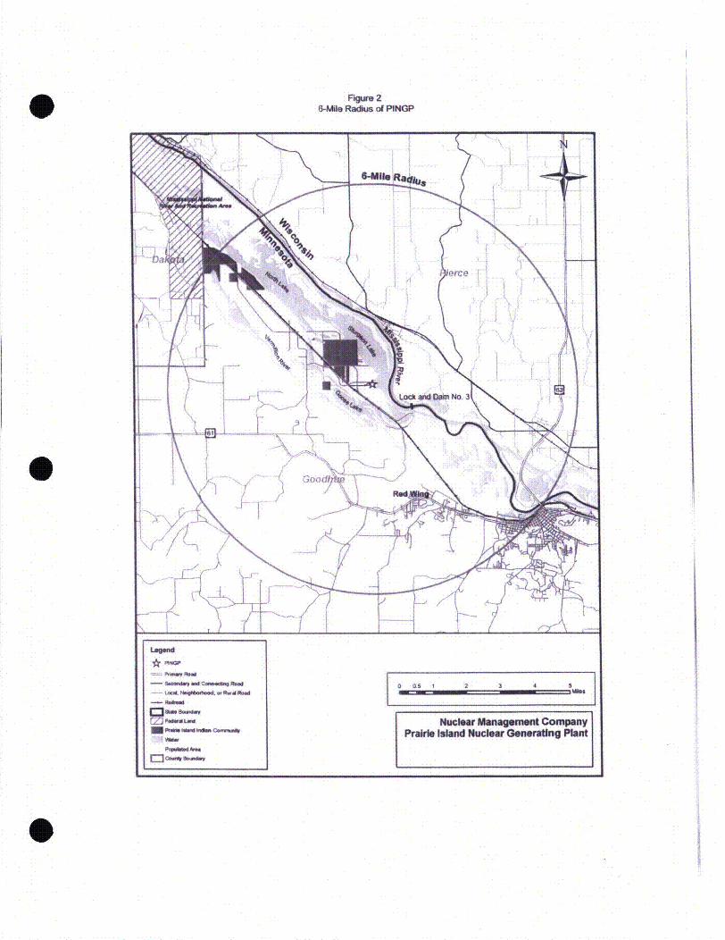
Figm~e 26-M11 Rackus of PINGP

6-20-07

Issues for Prairie Island Nuclear Generating Plant License Renewal Project t..

I. Thermal effluent changes. I understand there will be a small increase in the output ofthe plant. The resulting change in the thermal discharge, especially during wintermonths, should be modeled to identify any changes to the existing thermal requirementsand plume. This and any resulting environmental impacts should be contained inenvironmental review documents.-

2. Environmental Drawdown of Pool 3. The Service and other agencies on the Upper q (3@Mississippi River are pursuing environmental drawdowns in the navigation pools toreestablish aquatic vegetation. Drawdowns (approximately 18 inches at the dam) wereconducted in Pool 8 in 2001 and 2002, and in Pool 5 in 2005 and 2006. Dewatered areas(approximately 3,000 acres) successfully revegetated with submergent and emergentvegetation. We (Water Level Management Task Force comprised of the St. Paul DistrictCorps of Engineers, Minnesota, Iowa and Wisconsin Departments of Natural Resources,Minnesota Pollution Control Agency, towing industry, public) are currently working on adrawdown proposal for Pool 6 in 2008 and are beginning discussions for other pools.Aquatic vegetation in Pool 3 has declined since inundation and we believe a similardrawdown would provide significant benefits to aquatic vegetation and habitat. Weunderstand that the Upper Mississippi River is used for cooling of the Prairie IslandPlant, and a critical issue determining the depth of the drawdown will be the depth andoperational mode of the intake/discharge features. We are hopeful that future discussionsbetween Northern States Power and the interagency Water Level Management TaskForce will lead to a successful Pool 3 drawdown project. Because drawdowns willbecome a common management practice on the Upper Mississippi River to sustainaquatic vegetation, any changes to the infrastructure or operation of the Prairie IslandPlant resulting from the proposed renewal project should take into account futuredrawdowns of Pool 3.

Thanks for the opportunity to comment!

Gary WegeFish & Wildlife BiologistU.S. Fish & Wildlife Service4101 East 80"' StreetBloomington, MN, 55425-1665612-725-3548 ext. 207

Gary WegeR(,fws.gov

Prairie Island Nuclear Generating PlantEnvironmental Review Process

Agency Response Sheet

L)'•r Vci~5,~ 'r~ Sev~'ceAgency Name

)dxes, we have information regarding environmental concerns or historic andarcheological resources.

Please identify the information below, or state if there is an attachment:

LiYes, we would like to meet with NMC individually at this time to discuss ourconcerns.

Contact Information: a

[-No, we do not have any comments or concerns at this time, however we may decideto comment later during the process.

Thank you for your feedback!

Mr. James HolthausEnvironmental Project ManagerPINGP License Renewal (13-Plex)1717 Wakonade Drive EastWelch, MN 55089651-388-1121 ext 7268james.holthaus@nmcco.com

*~ ~ ~-. -'

'A. ~ -C

~XcelEnergy

April 30, 2007

Robyn ThorsonRegional DirectorU.S. Fish and Wildlife ServiceBHW Federal BuildingI Federal DriveFort Snelling, MN 55111-4056

SUBJECT: Environmental Review for Prairie Island Nuclear Generating Plant LicenseRenewal Project

Dear Robyn:

Nuclear Management Company (NMC) acting on behalf of Northern States Power Company, aMinnesota Corporation and wholly owned subsidiary of Xcel Energy, requests your input on theenvironmental review of the license renewal for the Prairie Island Nuclear Generating Plant(PINGP). Xcel Energy owns the Prairie Island nuclear generating facility, while NMC isresponsible for plant operations. NMC is preparing an application for submittal to the U.S.Nuclear Regulatory Commission (NRC) to renew the operating licenses for the PINGP locatedin Goodhue County, Minnesota. The PINGP Is currently licensed to generate electricity through2013 for Unit I and 2014 for Unit 2. Successful renewal of these licenses would extend thePINGP operating licenses for an additional 20 years; i.e., until 2033 and 2034 for Units I and 2respectively.

The NMC environmental review process assesses the NRC requirements for PINGP licenserenewal and evaluates environmental impacts or stakeholder issues associated with potentialcontinued operations. Early participation by your agency ensures timely identification of issuesand information for consideration in this process.

In addition to detailed safety reviews, the license renewal process involves a thorough review,both by NMC and the NRC. of potential environmental impacts In accordance with provisions ofthe National Environmental Policy Act (NEPA). The attached supplement provides an overviewof the process and associated environmental review activities for PINGP. In brief, the NRC hasprepared a generic environmental impact statement (GElS) that addresses environmentalimpacts of license renewal based on its review of plants nationwide. A detailed environmentalreview for individual plants such as PINGP includes preparation of an Environmental Report bythe applicant and a site-specific supplement to the GElS prepared by the NRC. Thesedocuments must include impact assessments for site-specific environmental issues that werenot resolved generically by the NRC in the GElS. They also must Identify any known 'new andsignificant information,* i.e., potentially significant environmental issues or impacts notrecognized as such by the NRC in the GELS, and the NRC's codified findings from the GElS

W (10 CFR 51.53). In accordance with NEPA, the NRC's process for developing the site-specificsupplements to the GElS includes substantial opportunity for participation by agencies and thepublic, Including the opportunity to formally comment on the scope of the NRC's site-specificsupplement and the adequacy of that document.

The PINGP License Renewal Environmental Review Team would appreciate your Agency'searly and active participation in the license renewal environmental review process for PINGP.In the course of evaluating the requirements and developing the Environmental Report,applicants for a renewed operating license routinely consult with resource agencies. Theseconsultations are undertaken to familiarize the agencies with the project, identify agencyconcerns, and obtain pertinent resource information, including any new and potentiallysignificant information, as needed to ensure a complete and accurate application. We welcomeany questions or concerns your agency has in regards to the environmental implications ofrenewing the PINGP's license and any information that your agency may consider to bepotentially *new and significant.* These efforts will help ensure that the Environmental Reportwe prepare is complete. In this regard, we would be pleased to meet with your agencyrepresentative(s) to discuss the PINGP license renewal environmental review in more detail. Ifyou desire a meeting, please contact us as soon as possible to schedule. Time is of theessence as a prompt response will allow for a more thorough review.

NMC respectfully requests you respond to this request by returning the attached response formwithin 30 days of your receipt of this letter, regardless of whether your agency has identified anyconcerns or issues to be raised in the environmental report. Your response simplyacknowledges you received this letter and indicates you either have no concerns at this time orhave attached your concerns to the response form. This does not prohibit your agency fromraising concerns or questions in the future, but it is extremely valuable to the public andstakeholder input process. If you have any questions or concerns about the environmentalreview, or would like to schedule a meeting to discuss your concerns please contact.

Mr. James HolthausEnvironmental Project Manager651-388-1121 ext 7268james.holthaus@nmcco.com

For your convenience, please find a response form as well as a self addressed, stampedenvelope attached. Thank you on behalf of NMC and the PINGP License RenewalEnvironmental Review Team.

Sincerely,

Som Palis Charlie BombergerSite Vice President General Manager, Nuclear Asset ManagementNuclear Management Company Xcel Energy

Attachments

DEPARTMENT OF THE ARMYST. PAUL DISTRICT, CORPS OF ENGINEERS MA 13 IU

SIBLEY SQUARE AT MEARS PARK190 FIFTH STREET EAST, SUITE 401

ST. PAUL MN 55101-1638

March 11, 2008

Environmental and Economic Analysis BranchPlanning, Programs and Project Management Division

Mr. Mike WadleyPrairie Island Site Vice PresidentNuclear Management CompanyPrairie Island Nuclear Generating Plant1717 Wakonade Drive EastWelch, MN 55089

Dear Mr. Wadley:

In response to your March 3, 2008 letter to the U.S. Army Corps of Engineers, St. PaulDistrict requesting information regarding the Federally endangered Higgins eye pearlymusselreintroduction program, we are sending documentation used in the decision making process touse Sturgeon Lake as a relocation site.

Seven documents are on the enclosed CD;

1) 2002clamchronicle.pdf. Minnesota Department of Natural Resources.Specifically, page 4 - June 5th, reports results of a mussel survey at the SturgeonLake site (in part leading to the specific selection of this site - healthy existingmussel community, favorable habitat, zebra mussels nearly absent, etc...)

2) DOI 2001 Higgins eye Federal Register Notice.pdf and DOI Higgins eye2000 Federal Register Notice.pdf. U.S. Fish and Wildlife public notice of theHiggins eye Relocation Plan.

3) DPR notice of Availability.pdf. Corps of Engineers public notice ofavailability of the Relocation Plan for Higgins eye.

4) Higgins eye Final Relocation DPR July 2002.pdf. Corps of Engineers, FinalDefinite Project Report and Environmental Assessment for Relocation Plan forthe Endangered Higgins eye Pearlymussel. Note Section 7.2 CandidateRelocation Sites (page 22). Also note Appendix 6 - Distribution List for theDPR/EA and Public Notice.

5) Higgins eye 2004 Recovery Plan.pdf. Extensive information on Higgins eyehistoric and present distribution, ecology, life history, etc...

6). Sec6FinalReport.pdf. Minnesota Department of Natural Resources. Report(page 1 and 2) on the results of relocating Higgins eye to Pool 2 and 3 prior to theCorps' Relocation Plan implementation.

We have furnished a copy of the enclosed CD to the U.S Fish and Wildlife Service,Twin Cities Field Office as well. We recommend that you coordinate with USFWS concerningpotential impacts to Higgins eye relating to Prairie Island Nuclear Generating Plant. If you havequestions about the project, please call Mr. Dennis Anderson (Project Manager) at (651)-290-5272 or Mr. Dan Kelner (Biologist) at (651) 290-5277.

Sincerely,

Terry J. BirkenstockChief, Environmental and EconomicAnalysis Branch

Copy w/ Enclosures sent to:

Mr. Tony SullinsU.S. Fish and Wildlife ServiceTwin Cities Field Office4101 East 80th StreetBloomington, Minnesota 55425

CLAM CHRONICLES

An account of activities associated with efforts to propagate and repatriateLampsilis higginsii in the Mississippi River, Minnesota - Minnesota

Department of Natural Resources (Mike Davis - Biologist)

2002 FIELD SEASON

I

May 9, 2002: On this day the Lampsilis higginsii listed in the table below were collectedfrom the Pool 2 repatriation site at Hidden Falls and transported to the Genoa NationalFish Hatchery to be used as a source of glochidia for infecting fish hosts.

ID # Length Gravid? Used in fall '01?657 71.4 xC128 58.6 xC1 32 70.0 xDH87 63.9 xDH8 90.1 xDH32 79.1 xC58 78.4 x xDH2 89.2 x08 85.0 xC81 83.6C152 76.5 x xC84 57.0 xC165 80.2 xC154 74.9 xC56 67.7 x xC41 70.0 xC97 64.5 xC183 76.0 xC13 59.3 x x

-3

May 23. 2002: Lampsilis higginsii adults from whom glochidia were harvested werereturned to the Hidden Falls site. Later in the day, a cage at the Hudson propagation sitewas emptied and 37 juvenile Lampsilishigginsii ranging in length from 16.5mm to 28mm were removed and placed into an adjacent cage.

2

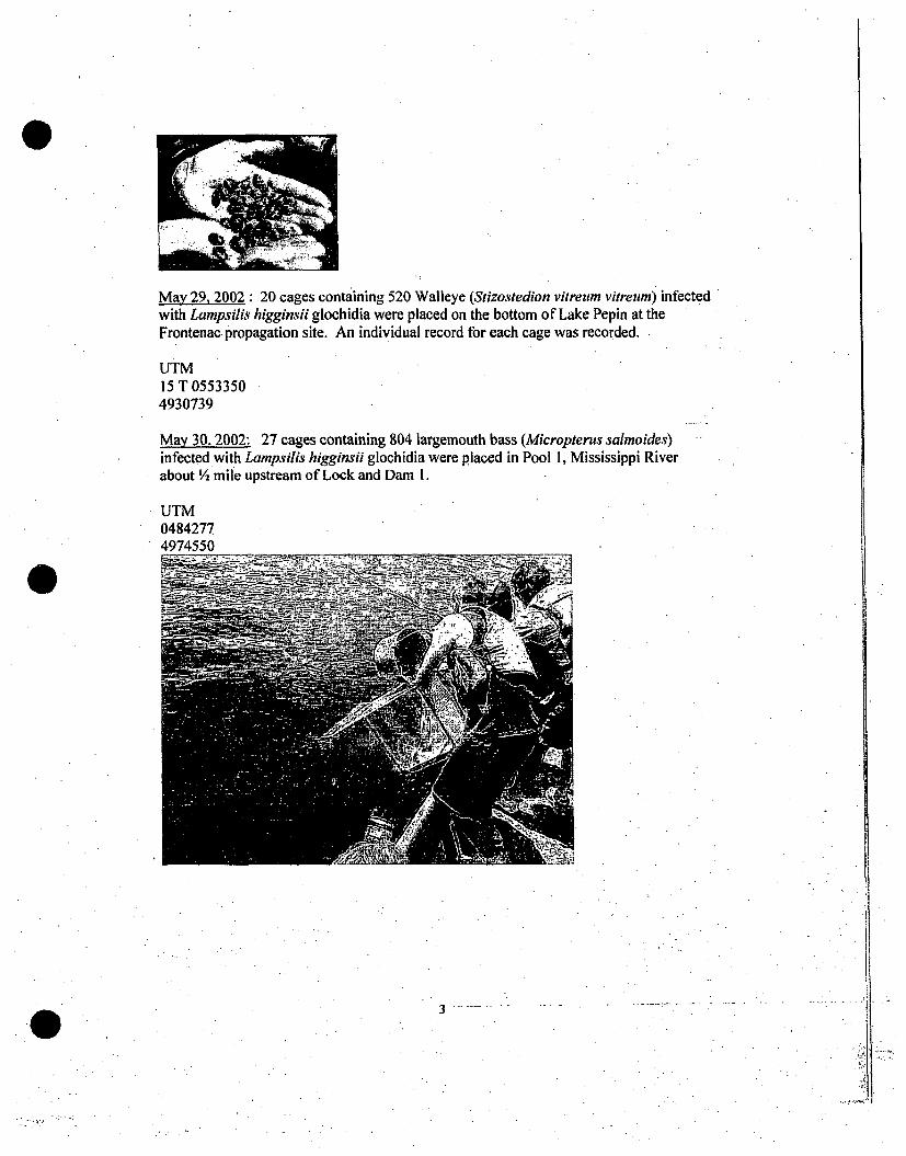
May 29, 2002: 20 cages containing 520 Walleye (Stizostedion vitreum vitreum) infectedwith Lampsilis higginsii glochidia were placed on the bottom of Lake Pepin at theFrontenac propagation site. An individual record for each cage was recorded.

UTM15 T 05533504930739

May 30. 2002: 27 cages containing 804 largemouth bass (Micropterus salmoides)infected with Lampsilis higginsii glochidia were placed in Pool 1, Mississippi Riverabout '/2 mile upstream of Lock and Dam 1.

UTM0484277

3

June 5, 2002: A survey for suitable sites to place propagation cages in Pool 3 led tochoosing a site in Sturgeon Lake immediately downstream of the public access and about50-60 meters offshore.UTM15 T 05291274941821

At this site one diver performed a 25-minute qualitative search to collect all live and deadmussels encountered. Results are in the table below. Species, reported as dead were freshand can be assumed to be living in the area.

Species # found Live/dead #zebesObliquaria reflexa 54. L 0Amblema plicata 31 L 0Qadrula quadrula 18 L 0Pyganodon grandis 5 L 0Fusconaiaflava 4 L 0Quadrula pustulosa 4 L 0Truncilla truncata 2 L 0Potamilus alatus I D IPotamilus ohiensis I D 0Total live mussels 118 1CPUE (catch/minute) 4.72

CPUE at this site indicates that mussels are fairly abundant. Physical conditions arefavorable to cage placement in that this area. We did not observe recent accumulations ofriver bed load at this site. This is because it is near the outlet of Sturgeon Lake and bedload entering the Lake settles near the inlets upstream and on the opposite side, nearlyone mile away. Also there is apparently current of adequate velocity to carry away finesediments in that the bottom substrate at this site is gravel, sand and a thin layer of silt,similar to the propagation site in Lake Pepin. Depth range is 6-12 feet.

June 18, 2002. All cages at the Lake Pepin propagation site were opened to allow fishto escape. Four fish were preserved in ETOH for analysis of their gills at the GenoaNational Fish Hatchery. Condition of the fish appeared to be good and gills of severalexamined with a hand lens appeared to be free of encysted glochidia. A single dead fishwas observed and all cages had live fish present in them. All cages were closed after onehour.

June 19, 2002. Four of five cages placed at this site in 2001 were retrieved from theMississippi River below Prescott, WI. These cages were nearly buried in sediments and.the remaining cage, presumably buried, was not found. The table below summarizeswhat was collected from within each cage.

4

Cage # #higginsii Lengths (mm) Other species found in cage1 2 empty shells Utterbackia imbecillis (1)

Corbicula sp (3)2 3 21,21,15 Leptodeafragilis(8)3 1 17 Arcidens confragosus (1 - 28mm)

Utterbackia imbecillis (42)Potamilus alatus (2)Potamilus ohiensis (1)Corbicula sp., (1)

4 5 33,32,23,28,27 Utterbackia imbecillis (13)Potamilus alatus (1)Potamilus ohiensis (2)Pyganodon grandis (1)Leptodeafragilis (15)Cbrbicula sp. (3)

Total 9 live, 2 dead 74

Lampsilis higginsii from these cages were taken to the propagation site in the St CroixRiver just upstream of the U. S. Highway 10 Bridge and placed into a cage there forgrow-out. Two cages at this site were also retrieved for inspection. One is a small cageinto which transformed juveniles from tanks at the Genoa National Fish Hatchery wereplaced in June of 2001. Three juvenile Lampsilis higginsii were removed from this cage(lengths 10, 11, 12 mm) and placed into a cage bearing tag number 48 along with a singlePleurobema sintoxia (1 7mm) also found within the cage.

One closed bottom cage was retrieved and all mussels removed. This cage contained the3 Lampsilis higginsii'and I Ligumia recta from the year 2000 effort in Lake Pepin.These mussels were measured and the Lampsilis higginsii found to be 32, 37, and 35 mmin length while the black sandshell was 53 mm long. 167 other Lampsilis higginsi wereremoved from this cage and transferred to cage #48 for grow-out. A random sample oflengths produced a range from 7 - 15 mm. Nine empty Lampsilis higginsii juvenileshells were found and have been accessioned into the collections of the James Ford BellMuseum of Natural History. About 20 small zebra mussels were found attached to theclosed bottom cage. On the bottom of the small cage were attached about 3-dozenmudpuppy eggs.

June 20, 2002, At the Hudson propagation site 6 cages were brought to shore andsearched. One cage had been placed for the purpose of rearing transformed animals fromthe Genoa National Fish Hatchery; it was empty. Two open bottom cages were removedfrom and the river and the bottom beneath them searched by hand for juvenile mussels.15 juvenile Lampsilis higginsii were collected from beneath the cage whose bottom was,about 2-3 cm above the riverbed. None were found beneath the other open bottom cagewhose bottom was about, 5 cm above the riverbed. This suggests that the lower cage mayhave offered greater protection from predators. The lengths of the 15 juveniles rangedfrom 19-27mm and averaged 22.5 mm. All of thesejuveniles were moved to the cagepropagation site in Lake, Pepin for grow-out.

5

Three other cages at this site contained 63, 96 and 37 juvenile Lampsilis higginsii, or a,total of 215 from the 2001 propagation effort. Lengths of these juveniles ranged from17 - 31 mm. These were placed into a single cage and returned to the river bottom at thissite for grow-out.

Eleven other Mussels of three Minnesota listed species were collected gravid from thissite on this date and used to infect fish. Ligumia recta, Pleurobema sintoxia, andEllipsaria lineolata propagation efforts are part of a "Bring Back the Natives" grantproposal to the National Fish and Wildlife Foundation.

.June 24, 2002.Two timed searches in Minnesota Slough, Pool 9 Mississippi River produced thefollowing:

UTM (Near the upper end of Minnesota Slough)06406604819083

An 8-minute spot search produced 132 mussels of 9 species resulting in a catch per uniteffort of 16.5 mussels/minute. This is a very high CPUE and suggests high musselabundance and the potential for additional species, including Lampsilis higginsii, to befound here if additional effort were expended. For example, if 60 minutes of searchtime were expended at this site it could be expected that nearly 1000 mussels would becollected.

Species # individuals L/D Min length Max length zebesAmblema plicata 81 L: 28 107 0Obliquaria reflexa 15 L 37 61 0Quadrula quadrula 19 L 56 94 0Pyganodon grandis 6 L 133 156 0Fusconaiaflava 4 L 34 ý 64.5 0Quadrulapustulosa 4 L 47.5 66 0Quadrula nodulata 1 L 56 _ _ 0* Truncilla truncata I L 31 - • 0Toxolasmaparvus I L 22 0TOTAL 132 _ _ 0

UTM (outlet of Goose Lake)06408614819187

A ten-minute spot dive produced 37 individuals of 7 species for a catch per unit effort of3.7 mussels/minute. Over 4 hoursof search time would be neededto collect 1000mussels at this site.

6

Species # individuals L/D Min length Max length ZebesAmblema plicata 24 L 23 107 0Fusconaiaflava 6 L 25 65 0Obliquaria reflexa 3 L 34.5 43 0Quadrula quadrula I L 56 0Quadrula pustulosa 1 -I L 26 0Utterbackia imbecillis 1 _ L 57 0Pyganodon grandis 1 L 120 0Total 37 0

Minnesota Slough - across from New Albin public boat ramp: The bottom of thechannel in this area is covered in old relic shells that included Fusconaia ebena,Lampsilis teres, and Lampsilis higginsfi, but was predominately Amblemaplicata. Fewlive mussels were found although it is difficult to search by feel for live mussels amongall the old shells. Most were covered with zebra mussel byssal threads indicating recent,intense colonization. Additional searching in Minnesota Slough seems promising in thatit has apparently provided excellent mussel habitat in the past and is vast in physicalscale.

July 1, 2002Cages # 49 was placed in Lake Pepin at the propagation site with 11 walleye and 3yellow perch (Percafalvascens) infected with glochidia from Ligumia recta. Cage #50also placed here with 12 walleye similarly infected.

July 9. 2002152 Elliptio dilatata were collected for transplanting into upper Pool 2 from the-musselbed at the foot of Lake Pepin.

UTM05713724918229

These individuals were stored in mesh bags until August 1, 2002 due to unexpected highwater conditions at the transplant site.- Several apparently gravid females were broughtinto the lab for further examination and found to have ovum present but no larvae.' Zebramussels have heavily colonized this site in the recent past. However, it appears thatmany of the zebra mussels died in late 2001 during the hot weather, although there werestill live individuals attached to many of the native spikes.

August 1. 2002An additional 76 Elliptio dilatata were collected from Lake Pepin. The stockpiled spikeswere retrieved from the lake and all were taken to Pool 2 for transplanting. A site waspicked along the left descending bank of the Mississippi just across from the old FtSnelling State Park Interpretive Center and beneath the overhead power'lines. Depth at

7

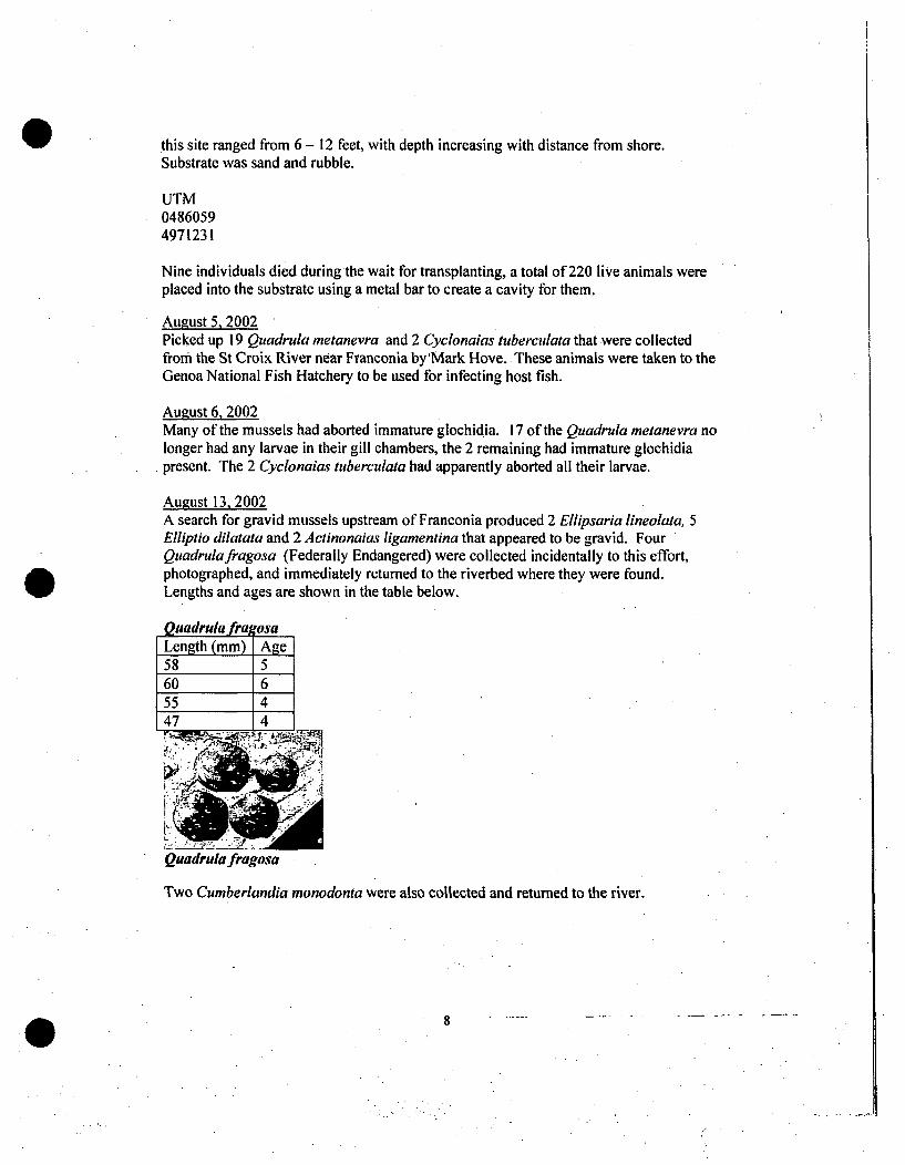
this site ranged from 6 - 12 feet, with depth increasing with distance from shore.Substrate was sand and rubble.

UTM04860594971231

Nine individuals died during the wait for transplanting, a total of 220 live animals wereplaced into the substrate using a metal bar to create a cavity for them.

August 5, 2002Picked up 19 Quadrula metanevra and 2 Cyclonaias tuberculata that were collectedfrom the St Croix River near Franconia by'Mark Hove. These animals were taken to theGenoa National Fish Hatchery to be used for infecting host fish.

August 6, 2002Many of the mussels had aborted immature glochidia. 17 of the Quadrula metanevra nolonger had any larvae in their gill chambers, the 2 remaining had immature glochidiapresent. The 2 Cyclonaias tuberculala had apparently aborted all their larvae.

August 13, 2002A search for gravid mussels upstream of Franconia produced 2 Ellipsaria lineolata, 5Elliptio dilatata and 2 Actinonaias ligamentina that appeared to be gravid. FourQuadrulafragosa (Federally Endangered) were collected incidentally to this effort,photographed, and immediately returned to the riverbed where they were found.Lengths and ages are shown in the table below.

Quadrula fraosaLength (mm) Age58 560 655 447 4

:7

Quadrulafragosa

Two Cumberlandia monodonta were also collected and returned to the river.

8

August 14,2002A collection of 146 Elliptio dilatata was made from the mussel bed at the foot of LakePepin.

UTM05713704918230

Five were taken to Genoa National Fish Hatchery microscopic examination of theirmarsupial chamber contents.

August 15, 2002Mussels collected on 8/13-14/02 were examined at the Genoa National Fish Hatchery anddetermined to have ovum in their gill chambers, not larvae. Actinonaias ligamentina andEllipsaria lineolata were left at the hatchery to see if the ova were fertile and wouldmature into glochidia. The 5 Elliptio dilatata were retained for transfer to the Pool 2transplant site.

Cage # 51 and 52 were placed at the Lake Pepin propagation site each containing 6flathead catfish (Pylodictis olivaris) infected with glochidia from Cyclonaias tuberculatacollected previously from the St Croix River near Franconia. Cage 53 was placed herealso containing 28 tadpole madtoms (Noturus gyrinus) also infected with Cyclonaiastuberculata.

August 16, 2002151 EIliptio dilatata were hand placed into the substrate at the Pool 2 transplant sitebringing the total number of this species repatriated here to 371.

August 28, 2002Cage # 54 containing 6 sauger (Stizostedion canadense) infected with Ligumia recta,

-cage 55 containing 6 walleye infected with Ligumia recta and cage 56 containing3sauger and 3 walleye infected with Ligumia recta were placed at the Lake Pepinpropagation site. These fish were collected from Lake Pepin by the MN DNR Fisheriescrew at Lake City during annual trawling.

September 13, 2002Cages 51-54 at the Lake Pepin propagation site were opened and fish released. Cages 49and 50 were not located in the time allotted for this effort and will be retrieved in 2003.Cage 55 was left alone.

September 16, 2002Cage #21 from the Pool I propagation site was raised and its contents checked. This wasthe only cage found that was not at least partially buried beneath bed load from thesummer flooding.

9

Six juvenile Lampsilis higginsii were found that ranged in length from 15 -26 mm. Inaddition, 12 Uterbackia imbecillis, II Corbicula sp., 7 Leptodeafragilis, and 3Potamilus alatus juveniles were removed from the cage and placed into a second cage onsite.

* September 24, 2002Lake Pepin propagation cage site: eleven cages were lifted from the lake and emptied intoa trough covered with a wire mesh. Lampsilis higginsii collected from these cages wereconsolidated and placed into two cages for continuing grow-out.

10

The table below summarizes what was found in each cage.

Cage # of L. Fish Other species found Min and Max# higginsil remaining Length (mm)7- 25 3 live walleye I Corbicula sp 10-226 93 0 1 Corbicula sp8 1i 0 1 Corbicula sp.,

ST. Parvus18 6 1 dead LMB? 1L.fragilis 10-185 41 1 dead I Tparvus 9- 20

Walleye4 70 2 live walleye 2 Corbicula sp.,

3 T parvus,I Utterbackia imbecillis

10 153 4,live walleye None 9-2212 70 (+ 15 0 5 Corbicula sp., I L. cardium, 1 9 -22

from 2001) L.fragilis, 4 U. imbecilis, 10. (25 -35)reflexa

9 38 I dead none 9-22walleye

1 29 1 live walleye none20 11 1 live, 2 dead 2 T parvus

walleyeTotal 547(+15) 11 live 25 9-22

562

Cage numbers I and 20 were placed back into the lake with all juveniles divided betweenthem.

September 26, 2002Fourcages were retrieved and all juvenile mussels removed from the St. Croix River,Prescott, WI cage propagation site. All juvenile Lampsilis higginsii were placed back'intotwo cages (#s 99 and 100) for grow-out. The table below summarizes the contents ofeach cage. _Cage # of live L. higginsii Other species Min-Max # zebra mussels

found Length attached to juvenile(mm) L. higginsii

PI 7 3 A. plicata, 20-32 31 P. ohiensis,I E. dilatata,I T. parvus

P2 4 none 26-38 9P3 84 5 A. plicata, 18 -36 22

2 T. parvus

I1

t P. sintoxia,I L. fragilis

P4 37 2 A. plicata, .20-35 112 P. ohiensis

P100 185 + (8 dead) 5 A. plicata 20-42 30(previouslyconsolidated cage)

Total 2001 317 23 75juvenilesThree Lampsilis higginsiijuveniles from the 2000 Lake Pepin propagation effort wererecovered and measured. Average length had increased from 34.6 to 44.6 mm since June.A single Ligumia recta from the Lake Pepin effort in 2000 was also recovered and hadgrown from 53 to 66 mm. One juvenile Arcidens confragosus, was moved here from thebelnw Prescott cane site in June- it- lenorth increased from ?R - 45 mm

12

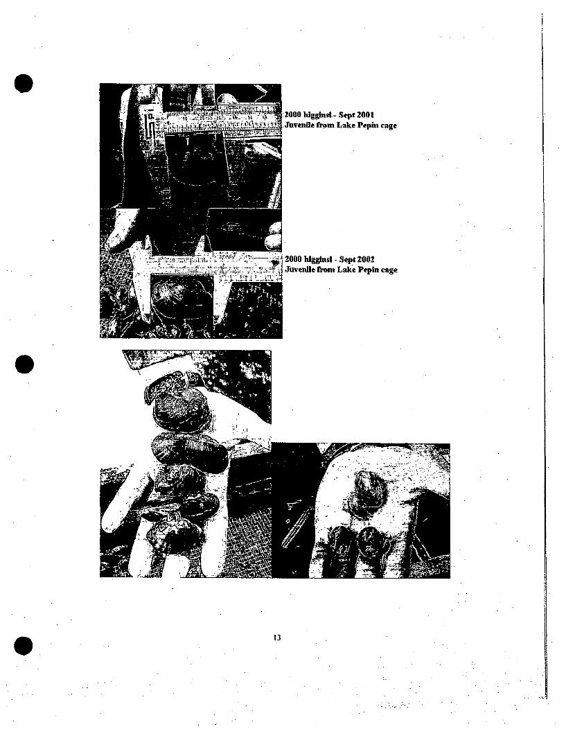
S2000 htigglnsd- Sept 2001I.Juvenile from Lake Pepin cage

2000 u diglrsl - Sept 2002

9uenl from Lak~e Pepin cage

13

Adult Lampsilis higginsii relocation site, Pool 322 Lampsilis higginsii adults that were transferred here from Cassville, WI in Septemberof 2000 were retrieved, measured and examined for reproductive status. The table belowsummarizes these findings. Note that the growth measurements indicate shrinkinglength, this may have been an error in reading the caliper used when the leading edge ofthe instrument was used to read the measurement instead of the zero mark. If this isindeed what happened, then the lengths reported in the table would be 5 mm larger andmost negative growth would become positive.

LUamPsws higginsi moved from Cassville, WI to Upper pool 3, MN In September 2000 !

mussel # gender length 2000 length 2002_ growth In mm

526 m 10 dead 9517 m 89 87 -2523 m __ 98 93 _ _526 m 102 987 -4

_ 527 _ m 97 94 -3528_____ m 81 86 6 ..... -

529 m 89 84 ----533 m 97 94 -3 _ !538 - m 91 741__ 51 _ _ 84 82 -2~

556 m 91_ _ 82 -9.559 m 87_ 85 -2 . .574 f 69 72 33____592 m 74 75 1,596 m 86 84 -21.602 m __ _83

_ _608 f 60__ 619 f _ 87 _

630 f "- -83. ..635 77 . . . ...640 m 971654 f -i--i

"There's nothin' tothis clam measuring,see!"

. 14

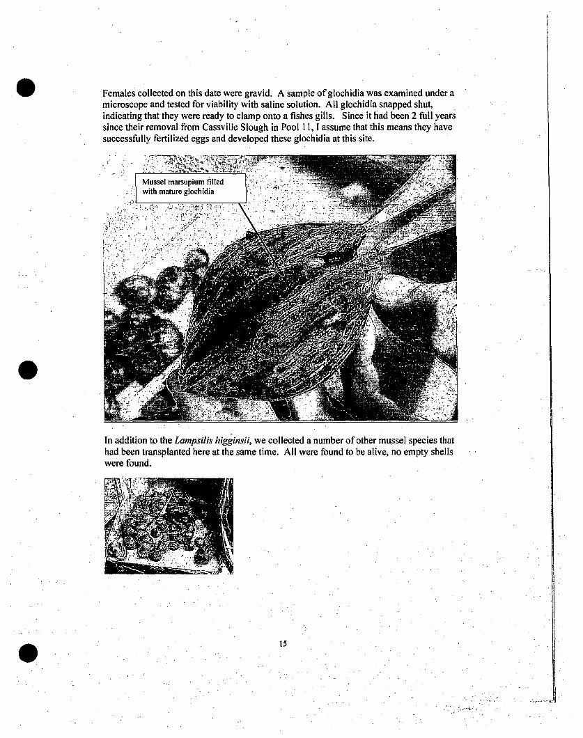
Females collected on this date were gravid. A sample of glochidia was examined under amicroscope and tested for viability with saline solution. All glochidia snapped shut,indicating that they were ready to clamp onto a fishes gills. Since it had been 2 full yearssince their removal from Cassville Slough in Pool 11, I assume that this means they havesuccessfully fertilized eggs and developed these glochidia at this site.

:''.1Mussel marsupium filled

S! with mature glochidia

In addition to the Lampsilis higginsii, we collected a number of other mussel species thathad been transplanted here at the same time. All were found to be alive, no empty shellswere found.

15

Species # of individualsMegalonaias nervosa 5Ligumia recta 6Pleurobema sintoxia IObovaria olivaria 12Ellipsaria lineolata 2Quadrula metanevra 4

September 30, 2002Pool I cage propagation site. Eight cages were retrieved and the contents sieved insearch ofjuvenile Lampsilis higginsii. A single cage produced 2 juvenile Lampsilishigginsii; juvenile mussels representing nine other species populated the cages. One ofthese, Utterbackia imbecillis, was very abundant with as many as 56 individuals found inone cage. In total, 267 juvenile mussels (exclusive of Lampsilis higginsil) were found inthese cages. The Lampsilis higginsii juveniles were taken to the Lake Pepin propagationsite.

Cages at this site were nearly full of sand, silt and wood debris and were very difficult toretrieve. It was concluded that this was a poor site for propagation cages and will beabandoned in favor of more stable environments elsewhere. A winch and boom was usedto lift the cages so that they could be taken into the boat for processing. After these 8cages were processed it was determined that a suction dredge would be used to retrievethe remaining cages because they were buried almost entirely in the sand.

October 1. 2002

Pool I cage site: A 4" diameter hydraulic dredge was used to remove sand and detritusfrom in and around the buried cages so that a diver could carry them to the boat.Substrate that was delivered to the boat was forced through a ¼" mesh wire screen andany mussels removed. No Lampsilis higginsii were collected from the screen. Anadditional 6 cages were retrieved. Twelve cages remain buried in sand at the site.

16

Adult mussel transplant site at Hidden Falls, Pool 2: A collection of 21 Lampsilishigginsii were brought to the boat for examination and measuring. The table belowpresents the results of this effort.

'Casis higginsi moved from Cordova,_IL to Pool 2, Hidden Falls MN in July -200- 77- i---r 177mu ge.!nder

0102 FLC 112 F_

013 F

._•ngj 7/0•1

79.8

length 9102 total growthj May-02

4.21

growth in '02 glochidia harvest? ]gravid faUI02?

58.459.7 60

C15F 765

4.61 -

0. 76.5 0.5-4.11C154 F 74.9 _79

_ _ . I - -fall'01 and sprLing '02 yeJ s 1

spring 02[ ye79

Ii 4.--

1C177 FFF

6875.675.6

F 83.4IC56 F 68.2IC77[6971DH`12-

IDH21

!DH30

FFTM

M

72.76ý3.2

7688.783.688.4

71 378 ____2.4

79 3.4 7685 1.669 0.81 67.77523J___71 7.81192 1689 0.387 34

801 0.8 987 V -2.6]- 90.17W ~8.4 163.9

-13spring-'02 __i yes

MIM0 and springd 02

I .. .. t" 4IDH38 I FIDH8 11F0PH8_7_ Uf

79.289.661.6

3. spring 02I -6-.1 spig.'02

yes-

It Was also noted that several of the Lampsilis higginsii appear to be growing in a peculiarway with exaggerated growth arrest lines and in-turning along the ventral margin of theshell. Otherwise they appeared to be in good health and about 1/3 of the females wereexamined for reproductive status and found to be gravid. -

17

October 14, 2002Eight Megalonaias nervosa were collected from among those transplanted into the Pool 3site and, 3 of these appeared to be gravid. It was hoped that these could be used to infecthost fish that would then be placed into cages in Lake Pepin for the winter to see ifjuveniles could be successfully propagated and also to find out if fish can besuccessfullyover wintered in a cage. We anticipate needing to do this. in order to propagatedQuadrulafragosa some day.

October 15, 2002Three Megalonaias nervosa were taken to the Genoa National Fish Hatchery and thecontents of their marsupia examined. All were found to contain undeveloped larvae, onefemale had completely aborted her marsupia. These females were all left at the hatcheryin a tank in the hope that they might develop mature glochidia later in the fall.

Transplant site maps on following pages-

18

MISSISSIPPI RIVER MUSSEL RELOCATION SITE:Across from Hidden Falls Park. River Mile 846 1

Latitude 44.8973 Longtude 93.1807L/. IJgai and State Listed Specam

*1U MOus •~b. RelocatQion, MflD'pp~~. ~ PMNP.1?r

R0 r il I.4I..

v•

19

MISSISSIPPI RIVER MUSSEL RELOCATION SITE:

Below Ford Dam, River Mile 847 4

Laftde 44.9123 Lao~tuft 931 M9.At Uitad Species

20 1, 41.s A, Phra owelf-JG&U

I)tj I ~I ~

20

MISSISSIPPI RIVER MUSSEL RELOCATION SITE:Below Pike Island, River Mile 844, 0

Latiude 44.8970 Longude 93.1507State Listed Species

M;.4U2I"A P t-14O -. 4-f.Jc-S .R4sx

Ut

21

MISSISSIPPI RIVER MUSSEL RELOCATION SITE:

Near Hastings, River Mile 813.0

,Latitude 44.7492 Longitude 92.8334L. hlgqinsi and State Listed Species

"J300 PC Ct.t 'l q~s tAA ."ot , AIIM ef hI

01

22

W [Federal Register: May 4, 2001 (Volume 66, Number 87)][Notices][Page 22593]From the Federal Register Online via GPO Access [wais.access.gpo.gov][DOCID:fr04my0 I -1171

[[Page 22593]]

----------------- -----------------.-. ----.-. ----- ----.. -.... . ... ........

DEPARTMENT OF THE INTERIOR

Fish and Wildlife Service

Endangered and Threatened Species Permit Application

AGENCY: Fish and Wildlife Service, Interior.

ACTION: Notice of intent to amend endangered species recovery.

. The following applicant has applied for an amended permit toconduct certain activities with endangered species. This notice isprovided pursuant to section 10(c) of the Endangered Species Act of1973, as amended (16 U.S.C. 1531, et seq.).

Permit Number TE023308-2

Applicant: U.S. Fish and Wildlife Service, Twin Cities FieldOffice, Bloomington, Minnesota (Russ Peterson, Field Supervisor).

The applicant holds a permit to take (collect, hold in captivity,propagate, and release) endangered Higgins' eye pearlymussels(Lampsilis higginsi) from locations within their historic range in theStates of Iowa, Minnesota, and Wisconsin. The applicant requestsauthorization to expand the geographical area permitted forreintroducing artificially propagated specimens into the wild toinclude all historical locations of the species, including mainstem andtributaries of the Upper Mississippi River including the Chippewa, St.Croix, Black and Wisconsin Rivers in Wisconsin; the Iowa, Cedar andWapsipinicon Rivers in Iowa; the Illinois, Sangamon, and Rock Rivers inIllinois; and, the Minnesota River in Minnesota. This permit is for theenhancement of survival of the species in the wild to protect fromzebra mussel (Dreissena polymorpha) infestation, in the interest of

recovery.Written data or comments should be submitted to the Regional

Director, U.S. Fish and Wildlife Service, Ecological ServicesOperations, I Federal Drive, Fort Snelling, Minnesota 55111-4056, andmust be received within 30.days of the date of this publication.

Documents and other information submitted with this application areavailable for review by any party who submits a written request for acopy of such documents to the following office within 30 days of thedate of publication of this notice: U.S. Fish and Wildlife Service,Ecological Services Operations, I Federal Drive, Fort Snelling,Minnesota 55111-4056. Telephone: (612/713-5343); FAX: (612/713-5292).

Dated: April 20, 2001.Charlie Wooley,Assistant Regional Director, Ecological Services, Region 3, FortSnelling, Minnesota.[FR Doc. 01-11192 Filed 5-3-01; 8:45 am]

----------------------------------------------------------------------

DEPARTMENT OF THE INTERIOR

Fish and Wildlife Service

Endangered and Threatened Species Permit Application

* AGENCY: Fish and Wildlife Service, Interior.

ACTION: Notice of receipt of application.

The following applicant has applied fora permit to conduct certainactivities with endangered species. This notice is provided pursuant tosection 10(c) of the Endangered Species Act of 1973, as amended (16U.S.C. 1531, et seq.).

Permit Number TE023308-0

Applicant: U.S. Fish and Wildlife Service, Twin Cities FieldOffice, Bloomington, Minnesota (Russ Peterson, Field Supervisor)

The applicant requests a permit to take (collect, hold incaptivity, propagate, and release) endangered Higgins' eyepearlymussels (Lampsilis higginsi) from locations within their historicrange in the States of Iowa, Minnesota, and Wisconsin (St. Croix River,Upper Mississippi River, Chippewa River, and Wisconsin River). Theapplicant proposes to propagate captive mussels at: (1) The U.S. Fishand Wildlife Service's Genoa National Fish Hatchery; (2) a temporaryfacility at the Upper Mississippi River, Pools 1-4 (River Mile 853-787); (3) a temporary facility at the lower Chippewa River (RM 0-15);and (4) a temporary facility at the lower Wisconsin River (RM 0-15).The applicant proposes to subsequently relocate host fish infected withglochidia (resulting from propagation) to a temporary facility in thelower Bad Axe River adjacent to the Genoa NFH. Artificially propagatedand temporarily held specimens will be reintroduced into the wild atthe Upper Mississippi River, Lower Chippewa River, and lower WisconsinRiver. The Field Supervisor, Twin Cities Field Office, proposes toserve as project manager including, but not limited to, designation ofindividuals who meet issuance criteria to work under this permit. Thispermit is proposed for the enhancement of survival of the species inthe wild (protection from zebra mussel (Dreissena polymorpha)infestation, in the interest of recovery.)

Written data or comments should be submitted to the RegionalDirector, U.S. Fish and Wildlife Service, Ecological ServicesOperations, I Federal Drive, Fort Snelling, Minnesota 55111-4056, andmust be received within 30 days of the date of this publication.

Documents and other information submitted with this application areavailable for review by any party who submits a written request for acopy of such documents to the following office within 30 days of thedate of publication of this notice: U.S. Fish and Wildlife Service,Ecological Services Operations, 1 Federal Drive, Fort Snelling,Minnesota 55111-4056. Telephone: (612/713-5350); FAX: (612/713-5292).

Dated: February 24, 2000.Stanley L. Smith,.Acting Assistant Regional Director, Ecological Services, Region 3, FortSnelling, Minnesota.

iNotice of AvaiGabiGityUS Army Corpsof Eiilineers Relodcation Plan for the Endangered Higgins"Eye

St. Paul. District Pearlymussel, Upper Mississippi River andTributaries, Minnesota, Wisconsin, Iowa, andlilinois

Date:, March 29,.2002 In Reply Refer to:t:Environmental and Economic:Analysis Branch,-

Project Proponent. St. Paul District, Corps of Engineers, 190 Fifth Street East, St. Paul;Minnesota 55101-1638

Project Background. This Notice of Availability describes a proposal to establish five newpopulations, through relocation, of the-Federally-listed Endangered Higg-ins' eye pearlymussel.(Lampsilis higinnsii). The Draft Definite Projectd Report anid Environmiental Assessment stemsfrom the'Al6ri 2000 USFWS .fina'l biologic al opin ion re eprt~that: said c6'fitiinuedoeaino h

-FomtNawgat2000 USFWShfinne l boo gicalon ohUppMiionsrepoi thatsaide cyined operationuof they9-Foot Navigation Channelsprojen on the Upper Mississippi River System (UMRS) would ikelyjeopardize the continued existence of the Higgins' eye pearlymdsnel. Due to the upstreamtransport by commercial and recreational craft, zebra mussels are 'now found in the UMRS. Thezebra mussels came from Europe and were introduced into North America by ships dischargingtheir ballast water into, the Great Lakes. The zebra mussels eventually got into the Illinois Riverthrough the 'Chicago Sniiitary and Shipping Canal, and then the Mississippi River, by attaching,themselves to other ships and boats coming out of the Illinois River. Zebra mussels'have asignificant adverse impact on Higgins' eye pearlymussel and other native freshwater mussels.The USFWS biological opinion listed a-reasonable and prudent alternative (RPA) believed'-,necessary, to a•koid jeopardy. "A Reasonable and Prudent Alternative (RPA) is for the Corpsito(1) develop a Higgins' eye pearlymussel Relocation Action Plan and (2) to conduct areconnaissance study to'control zebra mussels in the UMR .".

Project Authority. The River and Harbor Act of July'3, 1930; which authori.es the 9-footchannel navigation project on the Upper Mississippi River, provides'federal authority fortheprojiect. Section 7(a)(2) Of the 1973 Endangered Specie.s Act(ESA) reui'res Federal agencie's toinsure thatactions authorized; funded; or carried'out by them are not likely to jeopardize thecontinufedexkistence of endangered or threatefied species. In addition, ESA establishes as Federalp'licy that "all Federal departments and agencies shall seek to conserve endangered species andthreatened species." In keeping with this ESA requirement and policy, it is within the FederalInterest to implement the Biological Opinion's Reasonable and Prudent Altemative ofconducting a Relocation Plan: forHiggins'-eye pearlymussel.

Project Purpose. The Relocation Plan objective is to establish a minimum of five newand viable populations (minimum of 500 individuals each) of Higgins' eye pearlymussel in areasof the UMRS and/or tributaries that have no orilow levels of zebra mussel infestaitions. "

Project Location. Attempts to establish new populations will occur at a minimum of 10

sites, to ensure that at least five new populations are established. The specific locations have notbeen determined], howvere thde' ollowing potential areas have been identified: Rock and KankakeeRivers in Illinois; Iowa, Cedar,'Des Moines, Upper Iowa, Wapsipinicon, and Turkey Rivers inIowa; Wisconsin, Chippewa, and Black Rivers in Wisconsin; from the head of navigation toMonticello, Minnesota, and pools I through upper 4 and pool 24 on the UMRS; and the first 30miles of the St. Croix River above Taylors Falls, Minnesota.

Proposed Action., The Relocation Plan involves collecting adult Higgins' eye pearlymusselsfromii areas heavily ifested with zebra ̀ mussel§, where survival of the Higgins' eye pearlymusselis in question, and cleaning and moving them to an area with no or low levels of zebra musselinfestation. Relocation efforts will also involve raising juvenile mussels on hostfish species-andat hatcheries, with subsequent stocking at selected relocation sites. A monitoring.program toevaluate the long-term effectiveness of the relocation efforts is also part of the plan.

The Higgins'_ eye pearlymussel Reilcatioii Plan is bnly one.part of the overall effort. TheCorps of Engin'eers is also undertaking, in a separate interrelated effort, areconnaissance/feasibility study of long-term measures for controlling zebra mussels in theUMRS'. Additional mussel work that is under way or will be planned and conducted over thenext several years includes monitoring the health and status of Higgins' eye pearlyrnussel andother mussels; protecting existingHggins eye pearlymussel within Essential Habitat Areas;monitoring the abundance and distribution of zebra mussels; evaluating the opportunity forfish passage at locks and dams;for fish species that are hosts of the Higgins' eyýepearlymussel glochidia; a relocation plani for winged mapleleaf mussels; and public outreachon the threat to native mussels.

Alternatives. No Action: Under the No Action alternative, no Federal actions would beundertaken toQ relocate endangered mussels for the purpose of establishing new populations-inareas with no or low levels of zebra mussel infestation. With the most probable future withoutaction, zebra mussel densities on the main stem of the UMRS are expected to remain high, withsome continued expansion into the tributaries. Higgins' eye pearlymussel may continue to existin the more marginal secondary and essential habitat areas, which contain low to moderatenumbers of zebra mussels, and in areas not infested with zebra mussels. However, until •aneffectivezebra mussel management -program is implemented on the UMRS, zebra mussels willcontinue to be the greatest threat to native musselsof the UMRS. The. USFWS BiologicalOpinion conclutded that continued operation and maintenance of the 9-Foot Channel Project foranother*fifty years would jeopardize the continued.existence of Higgins' eye pearlymussel due to.the indirect effect of zebra mussels.

Schedule. Some limited pilot efforts begin in 2000/1. Full project implementation will beginin May 2002. The Relocation Plan will take 10 years to fully implement. Monitoring of thenewly established populations will continue after the 10-year establishment period.

Summary of Environmental. Impacts. Implementation of the proposed relocation planwould have overall substantial benefits to Higgins' eye pearlymussel populations in general,.

although some mortality to individual Higgins' eye pearlymussel would be associated with theseactivities. Impacts on other natural resources would generally be minor. Relocation of Higgins'eye pearlymussel to tributaries is likely to be controversial because of restrictions on usesassociated with endangered species. One of the factors that will be used in selecting the finalrelocation sites will be degree of local opposition, which should minimize socioeconomic impacts.

The proposed actions would cumulatively aid in the long'term preservation of Higgins' eyepearlymussel populations. Relocation of Higgins' eye pearlymussel would mitigate or reducethe impacts of zebra mussels on this endangered species.

Coordination. The Mussel Coordination Team (MCT), made up of 9 federal and stategovernment agencies and I private non-profit entity, has been extensively involved in thedevelopment of the relocation plan and other on-going mussel related activities. The MCTmembers include the U.S. Army Corps of Engineers; the U.S. Fish and Wildlife Service; the U.S.Geological, Survey; the National Park Service; the U.S. Coast: Guard; the department of naturalresources from the states of Minnesota, Wisconsin, Iowa and Illinois; and the Science Museumof Minnesota.

Who Should Reply? Any interested parties that may be affected by the proposed action areinvited to submit to this office facts, arguments, or objections to the proposal within 30 days ofthis notice. These statements should bear upon the adequacy of plans and suitability of locationsand should, if appropriate, suggest any changes considered desirable. Statements should indicatethat they are in response to this notice of availability. All replies should be addressed to theDistrict Engineer, St. Paul District, Corps of Engineers, ATTN: PM-E, 190 Fifth Street East, St.Paul, Minnesota 55101-1638. The Draft Definite Project Report/Environmental Assessmentmay be obtained electronically at http://www.mvp.usace.army.mil. Mr. Dennis Anderson,telephone number (651) 290-5272 and email dennis .d.anderson@mpOI2 .usace .army.mil, canbe contacted for additional information or to obtain a hard copy of the Draft Definite ProjectReport and Environmental Assessment.

ROBERT T. BALLColonel, Corps of EngineersDistrict Engineer

DEPARTMENT OF THE ARMYST. PAUL DISTRICT, CORPS OF ENGINEERS

190 FIFTH STREET EASTST. PAUL, MINNESOTA 55101-1638

OFFICIAL BUSINESSCEMVP-PM-E

Anderson PM-EMose PM-E,

Bankston OCDesHarnais DPM

O'Hara DD__Ball DE

File name: DPR notice of availability

Dubuque Public Meeting

e,7CA

N-v

L

/! A-'~ \ ')A'~ ~ "~

Ct flFc, /r,/~ n (A

(11s' r,#L4kr&•

lUal

~ 4 p~

K. V.

)

5-2

Prairie du Chien Public Meeting

-~ -- JJ42JLW~~ ~

5-3

Wabasha Public Meeting

-. . , . j.• • , •i•:: .\ .. _ •/ • . • • • . • . .. •s

5-4

Moline Public Meeting

0

5-5

APPENDIX 6

DISTRIBUTION LIST

List of elected officials, Federal, State, and local agencies, interest groups, media, individuals,and libraries that will receive a copy of the draft Definite Project Report/EnvironmentalAssessment and/or Notice of Availability

0

INAME IPOSITION IGENCY . CITY STATE PODEDON WARDMARIA PEARSONG. GENE JONESMR LES HOLLANDCRAIG W. ORILEYMR BOB KRAUSE

JOEL BRINKMAYERMR. BRAD BARRETTMR. ROBERT L HUMPHREY

DON BRAZLTONDALE FAULKNERMR. BILL BALLENTYNEHONORABLE T. R. THOMPSON, JR.MR. ALLEN HILLEMANROYCE J. FICHTNERMR ROBERT SUEPPEL

MR. RICHARD JOHNSONMR. TODD R. HAGAN

HONORABLE TOM HARKINMARK ACKELSONBRENT HALLINGMR BOB RENANDMR DICK VEGORSHONORABLE GREG GANSKEMS DIANNE LIEPAHONORABLE CHARLES E, GRASSLEYMR. LEROY BROWNHONORABLE NEAL SMITHMR. JOHN BELLIZZIHONORABLE WILLIAM 0, PALMER

LYLE ASELLDARRELL MCALLISTERALLEN STOKESANDREWVARLEYARNOLD SOHNDAN LINDQUISTMR. PAUL JOHNSONAL FARRISHONORABLE DALE M. COCHRANHAROLD HOMMESMARY JANE OLREYPATTY JUDGEJ. EDWARD BROWNJACK RIESSENJIM BROWNRALPH CHRISTIANMARION CONOVERHONORABLE SHELDON RITTMERPATRICIA OHLERKINGMR. JEFFREY R. VONKKEE VIN SZCOORONSKIMR. GLENN BUSHMR. JERRY BOOTHHONORABLE JIM NUSSLEMR. JOSEPH MCLAUGHLINMR. ROBERT BORTLEMR. ARNOLD JOHNSONMR. JIM WAHL

MR. RANDALL J. WILLHONORABLE TOM LATHAMMR. ROGER L KEITHJAMES DUNHAM

MR. BRIAN HOLTMR. DENNIS EBERLEMR. LARRY SCHWABMR. STEVE LINDAMANMR. JOHN BAHNSEN

DIRECTOR DEPT OF TRANSPORTATIONGOVE' LlAISON FOR INDIAN AFFAIRS

DEPT OF TRANSPORTATIONLA DEPT OF TRANSPORTATIONDEPT OF TRANSPORTATIONIOWA DOT

DIVISION ADMINISTRATOR FEDERAL HIGHWAY ADMINISTRATIONSBRANCH MANAGER STATE OFIOWA,•

OFFICEOF BRIDGESAND STRUCTURES

CTRE LIBRARYDEPART OF COMMERCEIA ASSN OF COUNTY CONSERVATION BOARDS

BRANCH MANAGER STATE OF IOWACHAIRMAN OF THE BOARD COUNTY OF DECATURMAYOR & CITY COUNCIL CITY HALLDIRECTOR US DEPT OF AGRICULTUREENGINEER COUNTY OF MARSHALLIOWA FIELD OFFICE CONGRESSMAN BOSWELL

PELLA CHAMBER OF COMMERCEBRANCH MANAGER STATE OF IOWAPRINCIPAL MADISON COUNTY ROADS DEPTDIRECTOR STATE OF IOWAUNITED STATES SENATOR

IOWA NATURAL HERITAGE FOUNDATIONIOWA DEPTD OAGRI

IOWA FIELD OFFICE SENATOR GRASSLEYMARKETING MANAGER IOWA DEPT OF ECONOMIC DEVELOPMENTREPRESENTATIVE IN CONGRESSIOWA FIELD OFFICE SENATOR HARKINUNITED STATES SENATORBRANCH MANAGER NATURAL RESOURCES CONSERVATION SERVICEREPRESENTATIVE IN CONGRESSBRANCH MANAGER CITY OF DES MOINESUNITED STATES SENATORDIRECTOR IA DEPT OF SOIL CONSERVATION

IOWA DNRBUREAU CHIEF SURFACE & GROUNDWATER PROT BUREAU-ONRDIVN ADMIN ENVIRONMENTAL PROTECTION

IOWA COMMERCE COMMISSIONCHIEF PLANNING BUREAU - DNRNAT RES ENGR DEPT OF AGRICULTURE & LAND STEWARDSHIPDIRECTOR DNRADMINISTRATOR DNRSECRETARY OF AGRICULTURE

AMESAMESAMESAMESAMESAMESAMESAMESAMESAMESAMESANKENYANKENYINDIANOLALEONMARSHALLTOWNMARSHALLTOWNMARSHALLTOWNOSCEOLAPELLAWILLIAMSWINTERSETDES MOINESDES MOINESDES MOINESDES MOINESDES MOINESDES MOINESDES MOINESDES MOINESDES MOINESDES MOINESDES MOINESDES MOINESDES MOINESDES MOINESDES MOINESDES MOINESDES MOINESDES MOINESDES MOINESDES MOINESDES MOINESDES MOINESDES MOINESDES MOINESDES MOINESDES MOINESDES MOINESDES MOINESDES MOINESDES MOINESDES MOINESDES MOINESDES MOINESDES MOINESDES MOINESDES MOINESDES MOINESMASON CITYMASON CITYMASON CITYBRITTCLEAR LAKEGARNERHAMPTONFORT DODGEPOCAHONTASWEBSTER CITYWEBSTER CITYWEBSTER CITYALLISONALLISONCHARLES CITYCHARLES CITY

IA 50010

[A ,SM10LA 510IA 50010

IA 50010IA 50010IA 50010-0451IA" * 55O0!(.045

IA 50015-0915

IA 15E-2802

IA $0144-1647IA 50158IA 501834548IA $0158-4906IA 550213IA 50219IA &0271LA 50213IA 5030"204IA 50m11IA S0239

IA So302IA 50309IA $0309LA 50309IA 50309IA 50309'LA 5o3594 oIA 50309180

IA 50309IA 503179-70IA 50319IA 50319IA 50319LA 50319IA 50319IA 50319IA 50319IA 50319IA 50319IA 50319IA 50319IA 50319IA 60319IA 50319IA $0319IA 50319IA 90319IA 60319LA 50319LA swi10

IA 5031907IA r0319 0IA 603219.80

LA 5035.03

IA 001-5615IA §03M2-0741LA 60423-0187

IA 50428-1233IA 60438-0040LA 50441-OisIA bal5IA 65574-0189IA 50595LA 50595-0454IA 60559799IA 56002-008LA 90002-082IA 5W616-2229IA 0W18-3TM

..

ENV PROG SUPVLEGISLATIVE LIAISON

UNITED STATES SENATORDEPUTY STATE HISTORIC PRESERV. OFCRDIRECTORMISSISSIPPI RIVER COORDINATORBRANCH MANAGERBRANCH MANAGERREPRESENTATIVE IN CONGRESSBRANCH MANAGERBRANCH MANAGERBRANCH MANAGERBRANCH MANAGER

BRANCH MANAGERREPRESENTATIVE IN CONGRESSCOUNTY EXECUTIVE DIRECTOR

EXECUTIVE DIRECTORDIRECTORBRANCH MANAGERPURCHASINGBRANCH MANAGER

IA DEPT OF AGRI & LAND STEWARDSHIPIOWA DEPT OF AGRIIOWA DEPT OF AGRISTATE WATER COORDINATORDNRDNRBUREAU OF HISTORIC PRESERVATIONDNR

BUREAU OF HISTORIC PRESERVATIONIOWA DNRIA DNRUS DEPT OF TRANSPORTATIONUS DEPT OF AGRICULTURE

US DEPT OF AGRICULTURESTATE OF IOWASTATE OF IOWASTATE OF IOWAUS DEPT OF AGRICULTURECOUNTY OF FRANKLIN

US DEPT OF AGRICULTUREPARK RECREATION & CEMETERY DEPTCENTRAL IOWA TOURISM REGIONHAMILTON COUNTY CONSERVATION BOARDUS DEPT OF AGRICULTURESTATE OF IOWACITY OF CHARLES CITYUS DEPT OF AGRICULTURE

Prairie Island Nuclear Generating Plant (PINGP) Re-Licensing and Environmental Review Page I of I

Holthaus, James J.

rom: Lovejoy, Tom A - DNR [Tom.Lovejoy@Wisconsin.gov]e~nt: Friday, August 31, 2007 10:46 AM

To: Holthaus, James J.

Cc: Siebert, David R - DNR; Koslowsky, Shari - DNR; Benjamin, Ron - DNR; Sullivan, John F - DNR

Subject: Prairie Island Nuclear Generating Plant (PINGP) Re-Licensing and Environmental Review

Attachments: 316b Guidance DNR 10 18_04.doc

By your June 19, 2007 letter to Dave Siebert you requested Wisconsin Department of Natural Resources (WDNR) input inpreparation of environmental review documents associated with an application to Nuclear Regulatory Commission (NRC) forlicense renewal of the Prairie Island Nuclear Generating Plant.

Through various phone calls and emails WDNR subseq'uently alerted you that our contact for threatened and endangeredresources information was Ms. Shari Koslowsky, (608) 261-4382 and that I would get back to you with any other scopingcomments. This provides those additional comments.

1. Fish Impingement and EntrainmentWe are concerned about the extent of fish and other aquatic organism mortality resulting from entrainment and impingement atcooling water intake structures. Will the plant comply with Clean Water Act 316(b) standards for minimizing adverse impacts?How? To assist in this regard attached is draft guidance to WDNR managers to determine if best available technology is beingused.

\.

<<316b Guidance DNR 10 18 04.doc>>2. Pool drawdowns for habitat enhancementWe have.in the past expressed interest in working with the Corps of Engineers and others in conducting water level drawdowns of1-2'in Mississippi River Pool 3 for biological habitat enhancement purposes. We have heard there are PINGP concerns, such as"fhre control or design limits of water intake structure(s), that may conflict with the idea of pool drawdowns. Please describe anyWh concerns and measures that could be employed to allow such pool drawdowns.

3. Thermal discharge effectsA. Biological resourcesWe are aware of past fish kills, particularly associated with effluent thermal mixing during winter cold water conditions, resultingfrom past plant operations. There is also a mussel bed adjacent to the plant. We are interested in minimizing adverse plantoperational impacts to such resources. We understand that the entire river is used as the thermal mixing zone for determiningcompliance with MPCA discharge permits and believe a smaller portion of river flow along the Minnesota shoreline should beused to more accurately protect fish and aquatic life. Has the mussel bed been monitored above and below the plant to determinethermal discharge impacts? Are there other biological monitoring efforts underway or planned in effort to demonstrate little or noadverse thermal effects tobiological communities? We know there have been some operational adjustments made in effort toeliminate/reduce the frequency or extent of fish kills. What are these measures and how successful have they been? What futuremeasures are proposed? What opportunities will exist during the next license term to respond to new threats and issues as theyappear?

B. Recreation opportunitiesWe have routinely received seasonal complaints from the ice fishing public that access to the upper 1/3 of Lake Pepin is adverselyimpacted by PINGP warm water discharges, resulting in delayed ice formation at winter's onset and more rapid ice deteriorationbefore spring thaw. Efforts should be undertaken to document historic PINGP discharge effects on winter ice cover and usability oftraditional ice fisherman access points. Measures to offset adverse effects should be identified and considered for futureoperations over the next NRC license term.

.4. Zebra mussel controlBest management~practices for control of biofouling from zebra mussels and other exotics continues to evolve. PINGP shouldhavela plan in place calling for periodic reassessment of zebra mussel control methods in effort to assure that proven state-of-the-art control methods are in place while also minimizing toxicity to native biological resources.

Baks you for the opportunity to comment. If you have questions or would like to discuss these issues in more detail pleasentact me at (715) 839-3747.

9/4/2007

Guidance for EvaluatingCooling Water Intake Structures

[Implementing Chapter 283.31(6), Wis. Stats., and Section 316(b) of the Clean Water Act]

DRAFT - October 18, 2004

0

This guidance is intended to describe the information needed in order for the Department to evaluate the potentialimpacts of cooling water intake structures (CWIS) on their aquatic environment and to allow for the Department'sdetermination of whether the best technology available (BTA) is being used (or proposed) to minimize adverseenvironmental impacts. Although this guidance provides general guidelines to follow, permits and regional staffresponsible for decision making and water quality and fisheries biologists who best understand the area in questionshould be relied upon for more specific analyses of individual sites.

This document is intended solely as guidance, and does not contain any mandatory requirements except whererequirements found in statute or administrative rule are referenced. This guidance does not establish or affect legalrights or obligations, and is not finally determinative of any of the issues addressed. This guidance does not create anyrights enforceable by any party in litigation with the State of Wisconsin or the Department of Natural, Resources. Any

* regulatory decisions made by the Department of Natural Resources in any matter addressed by this guidance will bemade by applying the governing statutes and administrative rules to the relevant facts.

Guidance For Evaluating Cooling Water Intake Structures [s. 3 16(b)]

Best Technology Available For Minimizing Environmental Impact

Section 316(b) of the Clean Water Act and Chapter 283.31(6), Wis. Stats., require that the location, design,construction, and capacity of cooling water intake structures (CWIS) reflect the best technology available (BTA)for minimizing adverse environmental impact. In order to make decisions regarding whether a facility will meetthese requirements, the Department will need sufficient information to determine whether technologies are thebest available to minimize adverse environmental impact. In the case of existing facilities, this may beaccomplished by providing reliable, quantitative estimates of damage that is occurring and projecting the long-range effect of such damage to the extent reasonably possible. In some cases, reliable estimates of future damagemay be estimated through the use of historical data, pre-operational models, biological studies, and/or theoperating experience of other facilities. However, historical data should be used carefully, and only in situationswhere source water and operating conditions are not believed to have changed significantly over time.

General guidance is provided in this document, outlining the development, conduct, and review of studiesdesigned to determine and evaluate the potential for adverse environmental impact from a CWIS. This documentis intended for use by Department staff who will need to decide whether the proposed (or existing) design,location, construction, and capacity of a CWIS reflects the best technology available (BTA) for minimizingadverse environmental impact, as well as the permittees who will have to provide the information needed to makethese decisions. Staff should remember that environment-intake interactions are highly site-specific, and thereforeBTA decisions should be made on a case-by-case basis. When deciding what is needed to evaluate an existingintake, data requirements should be based on the determination of the potential for adverse impact and theavailability of relevant historical data. In limited instances, existing plants may have enough relevant historicaldata to make further studies unnecessary. Conversely, the process for evaluating new intakes and most existingintakes will probably be more extensive because of a lack of relevant historical data (because there is no historicaldata or because there have been significant changes in the environment since data was collected).

Background

In s. 316b, a cooling water intake structure (CWIS) is defined as the total physical structure and any associatedconstructed waterways used to direct water into the cooling system, where a major portion of the water is used forcooling. The CWIS extends from the point at which water is withdrawn, up to and including the intake pumps. ACWIS can cause adverse environmental impact by pulling large numbers of fish, shellfish, and otherlorganisms ortheir eggs and larvae into a facility's cooling system. There, the organisms may be killed or injured by heat,physical stress, or by chemicals used within the system. Larger organisms may be killed or injured when they aretrapped against screens at the front of the intake structure. Indirect impacts are also possible,1i such as thedisruption of thermal regimes, the disruption of normal water flow, wetland or other upland disturbance (usuallyduring construction), aesthetics, and/or noise.

The goal of s. 316(b) is to minimize impingement mortality and entrainment (IM&E) of organisms in the areaaround a CWIS. Entrainment is the taking in of organisms with the cooling water. The organisms" involved aregenerally of smaller size and include phyto- and zooplankton, fish eggs and larvae, shellfish larvae,'ýetc. As theseentrained organisms pass through the system, they can be subjected to stressors such as mechanical damage due tocontact with internal surfaces of pumps, pipes, and condensers; pressure damage due to passage through pumps;shear damage due to complex water flows; thermal damage due to elevated water temperatures; and toxicity dueto the addition of chemicals to prevent condenser fouling and corrosion. Those organisms that do survive passagethrough the system may then experience delayed mortality after being returned to the receiving water.

Impingement (or entrapment) is the blocking of larger organisms by some type of physical barrier. iFor example,most CWIS include screening equipment (usually 3/8" mesh) installed in the cooling water flow to protectdownstream equipment such as pumps and condensers from damage or clogging. Larger organisms, such as fishwhich enter the system and cannot pass through the screens, are trapped ahead of them. Eventually, if a fishcannot escape or is not removed, it will tire and become impinged on the screens. If impingementýicontinues for

Page 2

Guidance Effective: DRAFT - October 2004

Guidance For Evaluating Cooling Water Intake Structures [s. 316(b)]

long, the fish may suffocate when water currents prevent it's gill covers from opening. If the fish is impinged for a* short period and removed, it may survive. However, it may lose its protective slime and/or scales through contact

with screen surfaces or from the high pressure water jets designed to remove debris from the screens. Delayedmortality following impingement may approach 100 percent. For some species of fish, the intake may represent adouble jeopardy situation where the same population will be subject to increased mortality through entrainment ofeggs and larvae and additional mortality to juveniles and adults through impingement.

CWIS regulations do not specifically identify methods to reduce IM&E in each situation. Instead, these rules setbasic performance standards and allow Department staff to decide what is BTA for each site-specific situation.Examples of existing technologies in use to reduce IM&E include fish diversion or avoidance systems designed to.divert fish away from intakes; passive intake systems such as non-mechanical screens; mechanical screen systemsthat prevent organisms from entering the intake system; and fish return systems that transport live organismsaway from the intake system.

316(b) Rulemaking History

EPA originally issued regulations to implement Section 316(b) of the Clean Water Act in 1976. Soon after, theU.S. Court of Appeals vacated the EPA rules, saying that the Agency had failed to comply with the publicationprovisions of the Administrative Procedure Act. Because of this, determinations of BTA for CWIS technologieshave generally been governed by draft federal guidance ever since, and each state has had substantial discretion todetermine what control requirements would satisfy the BTA criterion. For the most part, regulators have decidedon a case-by-case basis whether CWIS technologies constitute BTA. Following an initial burst of activity in themid 70's and early 80s, EPA has paid little attention to CWIS. In 1993, various environmental groups brought suitagainst EPA to compel the Agency to implement the requirements of s. 316(b). In order to settle the litigation,EPA entered into a consent decree in 1995 that required them to create regulations to implement s. 316(b)according to the following schedule:

. Expected Timeline For New 316(b) Rules* Phase I (completed): New facilities - final rules published December 2001* Phase [I (completed): Existing power generators withdrawing >50 MGD - final rules July 2004* Phase III (under development): Other facilities, including power generators withdrawing <50 MGD; chemical mfg.;

refineries; pulp & paper; steel, aluminum, copper and iron mfg. (proposed November'04; final by June '06)

Power plants are the largest users of cooling water in most cases and, to date, federal regulations have beendirected primarily at this category. In December 2001, EPA published a final rule implementing section 316(b)that applies to new power generating and manufacturing facilities; final rules for existing power generatingfacilities were completed on July 9, 2004. However, EPA has proposed regulations covering other dischargersthat have CWIS. These facilities will also need to show that their CWIS meet BTA standards in the near future.

Phase I: New Facilities. On December 18, 2001, EPA published a final rule implementing s. 316(b) that appliesto new power plants and manufacturing facilities that withdraw water for cooling purposes. This rule for newfacilities is referred to as "Phase I". According to this rule, a new facility is any "greenfield" or "stand-alone"facility that started construction after January 2002, has a design intake flow > 2 MGD, and uses at least 25% ofthe water that is withdrawn for cooling purposes. A greenfield facility is one that is constructed at a site where noother source is located, or that totally replaces the process or production equipment at an existing facility. Astand-alone facility is a new, separate facility that is constructed on property where an existing facility is locatedand whose processes are substantially independent of the existing facility at the same site (see 40 CFR Part 125.83for the full, legal definitions of "new", "greenfield", and "stand alone" facilities).

The new facility rule establishes BTA, based on a two-track approach, for minimizing adverse environmentalimpact associated with the use of a CWIS. Based on size, Track I requires the permittee to select and implementdesign and construction technologies that will minimize IM&E. Based on the assumption that closed-cycle

Page 3

Guidance Effective: DRAFT - October 2004

Guidance For Evaluating Cooling Water Intake Structures [s. 316(b)]

cooling systems cut cooling water usage by about 75-95% compared to once-through cooling systems, therebyreducing IM&E and other aquatic impacts by a similar percentage, Track I basically requires the use of wet,closed-cycle cooling systems with a maximum through-screen velocity of less than 0.5 feet per second (fps).Track II allows applicants to conduct site-specific studies to demonstrate that alternative measures will reduceIM&E to a level of reduction comparable to the level the facility would achieve if it used a closed-cycle coolingsystem and a through-screen velocity of 0.5 fps or less.

The new facility rule also includes alternative requirements that allow facilities to demonstrate that compliancecosts associated with Tracks I and U would be unreasonable; or that air quality impacts, energy generationimpacts ("energy penalties"), or other impacts not related to IM&E, could outweigh the additional IM&E effectsand therefore justify an open loop system.

Phase ii: Existing Power Plants. On July 9, 2004, EPA published a final rule implementing s. 316(b) thatapplies to existing power plants that withdraw >50 MGD cooling water. This rule, known as Phase II, establishesrequirements applicable to the location, design, and capacity of CWIS at existing facilities. This rule defines an"existing facility" as one that commenced construction on or before January 17, 2002, and any modification of, orany addition of a unit at such a facility that does not meet the definition of a new facility at s.125.83. 'According tothe Phase II rule, an existing facility can do one of the following to meet BTA requirements:

I) Demonstrate that technology in use reduces intake capacity to a level commensurate with the use of a closed-cycle,recirculating cooling system. (applies to all waterbody types)

2) Select and implement design and construction technologies, operational measures, and/or restoration'I measures thatmeet specified performance standards:

a) For facilities with CWIS on a freshwater river or stream:i) If the intake flow is <5% of the annual mean flow, must reduce impingement mortality by 80-95%;ii) If the intake flow is > 5% of the annual mean flow, must reduce impingement mortality by 80-95% and

entrainment by 60-90%.

b) For facilities with CWIS on a lake or reservoir other than the Great Lakes:i) Must reduce impingement mortality by 80-95%, and, if they expand their intake capacity, the increase in

intake flow must not disrupt the natural thermal stratification or turnover pattern of the source water.

c) For facilities with CWIS on a Great Lake:i) Must reduce impingement mortality by 80-95% and entrainment by 60-90%.

3) Demonstrate that the facility qualifies for a site-specific determination of BTA because its costs of compliancewould be significantly greater than the environmental benefits of compliance with the performance standards.

4) Demonstrate that it has installed and properly operates and maintains a pre-approved technology. Only onetechnology is pre-approved at this time: submerged cylindrical wedgewire screen technology whichl treats the totalCWIS flow. According to the rule, there are 5 conditions that must be met in order to use this techlology to meetBTA standards: a) The CWIS is located in a freshwater river or stream; b) The CWIS is situated such that sufficientambient counter currents exist to promote cleaning of the screen face; c) The through screen design iintake velocityis 0.5 ft/s or less; d) The slot size is appropriate for the size of eggs, larvae, and juveniles of any fish and shellfish tobe protected at the site; and e) The entire main condenser cooling water flow is directed through 'the technology(small flows totaling <2 MGD for auxiliary plant cooling uses are excluded). Sec. 125.99 of the rule also allows theDepartment to pre-approve other CWIS technologies, after providing public notice and an opportunity to commenton the request for approval of the technology.

The rule states that the baseline against which compliance with the performance standards mentioned aboveshould be assessed is a shoreline intake with the capacity to support once-through cooling and no IM&E controls.

Page 4

Guidance Effective: DRAFT - October 2004

Guidance For Evaluating Cooling Water Intake Structures [s. 316(b)]

Phase I11: Other CWIS Users. Many have assumed incorrectly that the requirements of s. 316(b) apply only tothe power industry. While it is certainly the case that the primary focus in the past has been mostly on thatindustry sector, 316(b) applies broadly to any facility with a CWIS. Phase III of these regulations will, at aminimum, address power plants not covered by Phase II (e.g., those with design intake flows < 50 MGD) andother facilities that employ CWIS. Thus, the rulemaking that EPA has initiated could have major implications forother industrial sectors, including chemicals and allied products, primary metals, petroleum and coal products,and paper and allied products industries, and others. Under the court-ordered consent decree, EPA must proposePhase [II regulations by November 1, 2004 and take fimal action on these regulations by June 1, 2006.

Wisconsin's Authority to Regulate CWIS

The Department's authority to regulate CWIS is directly tied to the issuance of a Wisconsin Pollutant DischargeElimination System (WPDES) permit and can be found in Wis. Stats. Chapter 283.31(6):

"Any permit issued by the department under this chapter which by its terms limits the discharge of one or morepollutants into the waters of the state may require that the location, design, construction and capacity of waterintake structures reflect the best technology available for minimizing adverse environmental impact."

Since the mid 70's, the Department has used EPA guidance and best professional judgment to determine, on acase-by-case basis, whether CWIS technologies used by individual facilities constitute BTA. In order to makeinitial BTA determinations in the 1970's, power plants with a WPDES permit were required to provide site-specific information to estimate the number and weight of fish impinged or entrained by their CWIS.

Recent and future rule revisions at the federal level will mean that the Department must re-evaluate each CWIS atpermit reissuance. In most cases, permittees with a CWIS should expect to demonstrate whether they meet BTArequirements described in s. 316(b).as a part of the permit application and reissuance process. To do this may. require not only the assistance of CWIS technology experts, but also fishery biologists, impact assessmentmodelers, economists, and others (more details are provided throughout the rest of this guidance).

Where Does CWIS Review Fit Into the Permitting Process?

Phase I and II of the 316(b) regulations require that the regulations be implemented through WPDES permitapplications and reissuances. (See page 7 for a discussion of proposed schedules.) When a new. power plant hasbeen proposed, the CWIS coordinator and permits staff will be expected to work closely with the Department'sProject Manager and Regional Coordinator to ensure that permitting and review activities are smoothly integrated'into the process mandated by the Power Plant Siting Law (s. 196.491(3), Wis. Stats.). (See "Statutory Timelinesand Agency Responsibilities for Approval of New Power Plants" in Appendix 1). When a CWIS review is neededfor an existing power plant or other facility, permits 'staff, basin engineers, fisheries staff, and the CWIScoordinator will- work together to ensure that CWIS review activities are smoothly integrated into the permitapplication and reissuance process, where appropriate.

The WPDES Permit coordinator & Basin Engineer share the responsibility for." overall project (permit) coordination* review of plans & study results" drafting Environmental Assessment (EA) & Environmental Impact Statement (EIS) language (as needed)" review of permit monitoring data* determination of compliance with performance standards* main point of contact for Environmental Analysis and Liaison Section, Public Service Commission, region/central office

staff, and other programs" attend meetings with permittee, as needed, to discuss performance standards and CWIS technologies

The CWIS coordinator is responsible for:

* * maintaining CWIS guidance (this document) & standard permit language

Page 5

Guidance Effective: DRAFT - October 2004

Guidance For Evaluating Cooling Water Intake Structures [s. 316(b)]

" providing "expertise" in difficult or complex situations* providing statewide perspective and checks for consistency" assist permit coordinator with EA and EIS language (as needed)0* assist in the review of plans & study results* attend meetings with permittee, as needed, to provide advice and expertise regarding performance standards and CWIS

technologies

Fishery & water quality biologists and other staff will also need to be involved in certain aspects of each project.For example, knowledge of the local fisheries around the CWIS site will be very important when reviewinginformation related to physical waterbody data, expected (or existing) IM&E data and the potential for direct andindirect impacts to aquatic habitats.

In order for the CWIS review process to take place, whether for a new or existing facility, it will be necessary forthe permittee to supply the information needed to determine whether the CWIS will meet BTA standards. Oncethis information is made available, the Department will have to determine which s. 316b performance standardsapply and then review and approve plans, biological studies, source water information, and proposed! technologiesto decide if the proposed (or existing) CWIS will meet BTA criteria. Once the Department has determinedwhether the proposed (or existing) CWIS will meet applicable performance standards, the WPDES permit shouldbe reissued with requirements describing how the permittee will demonstrate compliance with the standards. Thisusually includes monitoring of IM&E levels, maximum intake velocity, and visual or remote inspections of theCWIS to insure technologies are operating as designed.

Information Submittals for Existing (Phase 1I) Facilities

In order to make a BTA demonstration, certain information will be needed (required at 40 CFR Parts 9, 122, 123,124, and 125, National Pollutant Discharge Elimination System--Final Regulations to Establish Requirements forCooling Water Intake Structures at Phase II Existing Facilities). This information is summarized 1ýbelow. Moredetailed information is contained in the federal regulations.

Cooperation and open communication between the permittee and the Department during plan development andstudy implementation is essential and will ensure that everyone is in agreement as to the scope and details of workto be planned and completed. No formal approval of study plans should be necessary, however, staff will need tobe aware of and in general agreement with study objectives, specific goals, and schedules for completion, to makesure that studies address all of the important environmental and operational concerns of all parties.

The Comprehensive Demonstration Study (CDS)

The purpose of the Comprehensive Demonstration Study (CDS) is to characterize impingement mortality andentrainment (IM&E), to describe the operation of each CWIS, and to confirm that the technologie!s, operational

.measures, and/or restoration measures selected and installed, or to be installed, at the facility re flect the besttechnology available (BTA) for minimizing adverse environmental impact.

The final CDS report should specify which compliance alternative(s) are planned to achieve BTA for minimizingadverse environmental impact. Facilities that intend to meet BTA requirements by reducing flow commensuratewith a closed-cycle, recirculating system are not required to submit a CDS. Facilities that intend to meet BTArequirements by reducing their design intake through-screen velocity to <0.5 fps are required to submit a CDSonly for the entrainment requirements, if applicable. Facilities with a capacity utilization rate <15%, withdraw<5% of the mean annual flow of a river, or withdraw cooling water from a lake or reservoir (other than the GreatLakes), are required to submit a CDS only for the impingement mortality requirements.

Facilities that intend to meet BTA requirements by installing a pre-approved technology need to submit only theTechnology Installation and Operation Plan and the Verification Monitoring Plan described belo w. In the final

Page 6

Guidance Effective: DRAFF - October 2004

Guidance For Evaluating Cooling Water Intake Structures [s. 316(b)]

316(b) Phase 11 rule, only submerged cylindrical wedgewire screen technology was pre-approved, and only for* facilities that withdraw cooling water from a river or stream. In order to demonstrate BTA through the use of

submerged cylindrical wedgewire screen technology, the permittee must demonstrate that this technology hasbeen/will be properly installed and properly-operated and maintained. The facility must also meet the followingconditions: (1) the MWIS is situated in the river such that sufficient ambient counter-currents exist to promotecleaning of the screen face; (2) the maximum through-screen design intake velocity < 0.5 fps; (3) the slot size isappropriate for the size of eggs, larvae, andjuveniles of all fish and shellfish to be protected at the site; and (4) theentire main condenser cooling water flow is directed through the technology.

Suggested Information Submittal Timelines. Phase I and It of the 316(b) regulations require that theregulations be implemented through WPDES permit applications and reissuances. Existing facilities whosepermits expire on or after July 7, 2008, and new facilities must comply with 316(b) information submittalrequirements with their application for an initial/reissued WPDES permit. Existing facilities whose permit expiresbefore July 7, 2008, may request a schedule for submission of application materials that is as expeditious aspracticable but does not exceed January 7, 2008, to provide sufficient time to perform the required informationcollection requirements. (This is the latest date that the Department may allow; staff are to use BPJ to determinehow much time is needed.) Below is an example timeline that may be allowed for these facilities:

Task Approximate Time Allowed Suggested Due DatePrepare RFP and select contractor --- 10/30/04Prepare and submit PIC 8 weeks 12/31/04State Review of PIC and Address Comments 60 days, 2 weeks 3/15/05Complete baseline IM&E sampling 1 year 3/31/06Analyze IM&E data and make adaptive management 3 months 6/30/06decisions on compliance (assumes May-Sep sampling)Engage in site-specific studies appropriate to support

* compliance approach 1_year_6/30/07

Prepare and submit final CDS report 7 months 1/7/08"*this is the final date allowed by the Phase It regulations and it cannot be extended.Dates suggested at 10/12/04 DNR/Utilities meeting

The following is a summary of the information that should be included in a final CDS report, depending upon thecompliance alternative selected:

1) Proposal for Information Collection (PIC)

As a first step in the process, the permittee should submit a proposal to the Department describing how theyintend to demonstrate that their proposed (or existing) MWIS will meet BTA standards. This proposal shouldinclude a plan and schedule for the studies that will be conducted to provide the needed information to theDepartment. At a minimum, the PIC should include the following:

a) A description of the technologies, operational measures, and/or restoration measures to be evaluated;b) A description of historical studies characterizing (M&E and the physical/biological conditions in the vicinity of the

CWIS. If the permittee proposes to use existing data, a demonstration should be made of the extent to which the dataare representative of current conditions and that the data were collected using appropriate QA/QC procedures;

c) A summary of any past or ongoing consultations with Federal, State, and Tribal fish and wildlife agencies relevantto this study and a copy of comments received as a result of such consultation;

d) A sampling plan for field studies proposed to ensure that sufficient data is available to develop a scientifically validestimate of IM&E at the site. The plan should document all methods and QA/QC procedures for sampling and dataanalysis. Sampling and data analysis methods should be appropriate for a quantitative survey and take into accountmethods used in other studies performed in the source waterbody. A description of the study area (including theCWIS' area of influence) should be provided, along with taxonomic identifications of the biological assemblages(including all life stages of fish & shellfish) to the extent this is known in advance and relevant to plan development.

Page 7

Guidance Effective: DRAFT - October 2004

Guidance For Evaluating Cooling Water Intake Structures [s. 316(b)]

e) Any other information, where available, that would aid in the review of the plan.

The collection and analysis of information will be an iterative process and plans for information collection 0may change as new data needs are identified. While the PIC is only submitted once, the permittee shouldconsult with the Department as appropriate after the PIC has been submitted, in order to ensure that theDepartment will have all of the information necessary to make decisions regarding whether the location,design, construction, and capacity of each CWIS reflects BTA for minimizing adverse environmental impact.

2) Source Waterbody Flow Information

The natural hydrology of the waterbody and its relationship to the cooling system are key factors inevaluating the potential of a CWIS to impinge and entrain organisms. Organisms most likely to be entrainedare those present in the "hydraulic zone of influence" of the intake. Whether an organism will enter the zoneof influence is determined by the behavior and motion of the organism and the flow of water around and intothe CWIS. To determine how the behavior and motion of local organisms are influenced by the' flows in andaround the CWIS, it is necessary to identify the types of circulation dominant in the waterbody and to collectdata related to currents and other relevant hydrological and physical parameters of the system (e.g., watercurrent, speed and direction; wind speed and direction; tides/local water levels; temperature; water density).

The proximity of a primary spawning or nursery area to a CWIS can be an important influence on theentrainment potential for an individual species. Other factors also interact with proximity Ito determinesusceptibility to entrainment. Predictive 'tools, such as computer models, may be useful in many cases foridentification of the area of potential damage. The selection of the appropriate models and data collectionschemes should be guided by the circulation regime and geomorphology of the waterbody. Field datacollection and modeling should be done to determine the probability that a non-motile organism "released froma given point in the flow field will be entrained into the CW[S.

At a minimum, the following information should be provided:a) A narrative description and scaled drawings showing. the physical configuration of all source waterbodies used by

the facility, including areal dimensions, depths, temperature regimes, and other documentation that supports thedetermination of the waterbody type where each CW[S is located

b) identification and characterization of the source waterbody's hydrological and geomorphological features, as well asthe methods used and the results of any physical studies to determine the CWIS' area of influence

c) locational maps

Facilities that withdraw cooling water from freshwater river or stream:d) documentation showing the mean annual flow of the waterbody and any supporting documentation and engineering

calculations that shows whether they are withdrawing less than or greater than 5 % of the mean annual flow.Representative historical data (from a period of time up to 10 years,'if available) should be used to determine meanannual flow values.

Facilities that withdraw cooling water from a lake (other than the Great Lakes) or reservoir and propose toincrease the facility's design intake flow;e) a narrative description of the thermal stratification of the waterbody and any supporting documentation and

engineering calculations showing that the increased total design intake flow will not disrupt the "natural thermalstratification or turnover pattern (where present) of the source water in a way that adversely impacts fisheries.

3) Facility, Cooling System, and Cooling Water Intake Structure (CWIS) Information

Information will be needed to fully investigate the potential for organisms to become entrapped within theCWIS, impinged on parts of the CWIS, and/or entrained in the water circulated through the lcooling watersystem. It will be necessary to describe the full range of potential physical, chemical, and biological impactswhich could be encountered throughout the cooling system during a typical yearly operation cycle. Thefollowing information should be provided to adequately describe the CWIS and cooling water system:

Page 8

Guidance Effective: DRAFT - October 2004

Guidance For Evaluating Cooling Water Intake Structures [s. 316(b)]

' a) Site Location and Layouti) Map showing locations of all existing and proposed CWIS, associated cooling water systems, and other

pertinent information related to surrounding shore and water features in a 50-mile radius, including:(1) Latitude and longitude in degrees, minutes, and seconds for each CWIS;(2) Proximity of intake to effluent discharge(s), other permittees' discharges and water withdrawals(3) Proximity to areas of biological concern

ii) Larger scale map w/topographic and hydrographic data depicting the specific location of the CWIS, including:(I) Topographic details, including existing site w/topographic features as changed by proposed CWIS(2) Hydrological features, including depth contours(3) Waterbody surface elevations (low and normal)(4) Waterbody boundaries & affected waterbody segment(5) Location and description of other CWIS in waterbody segment(6) Additional stresses on waterbody segment (e.g., existing/planned point sources; etc.)

b) CWIS and Cooling System Descriptionsi) A flow distribution and water balance diagram that includes all sources of water to the facility, recirculating

flows, and dischargesii) A narrative description of the operation of each cooling water system, the relationship to each CWIS, proportion

of the design intake flow used in the system, number of days of the year the system is in operation, and seasonalchanges in operation

iii) A description of CWIS operation; identification of withdrawal type (once-through vs. recycled); type of intakestructure (size, shape, configuration, orientation); location of CWIS with respect to cooling water system;location in water body (horizontal and vertical); depth of intake; distance from shoreline; configurationincluding canals and channels; capacity (volume withdrawn in gpm & MGD; design & actual intake flows);timing, duration, frequency of withdrawal; presence/absence of organism protection technologies (behavioraland physical), fish bypass and handling facilities; average and maximum through-screen and approachvelocities; proportion of water withdrawn to the overall source water flow

iv) CWIS Pump information, including: design details (location in structure, configuration of blades, housing);revolutions per minute; number, capacities, and planned operating schedule; pressure regimes in watersubjected to pumping; velocity shear stresses in pumping; sites of potential turbulence and physical impacts

v) Design and engineering calculations and supporting data to support the descriptions mentioned above, includingengineering drawings of proposed CWIS and cooling system

c) Use of Cooling Water System Biocides and Ice Removal Technologiesi) Location of introduction in systemii) Description and aquatic toxicity information for biocide(s) to be usediii) Concentrations of biocide in various parts of cooling water system and receiving watersiv) Location, amount, timing, and duration of recirculation water for deicing or temperingv) Maintenance procedures, use of heat treatment or deicing procedures

d) Thermal experiencei) i Water temperature in cooling system; temperature change during entrainment, duration of entrainment; resultant

time-temperature experience of organisms subjected to entrainmentii) Annual ambient temperatures, thermal addition to cooling water of various operating capacities

e) Facility Datai) Age and expected lifetimeii) Capacity factor and percent of time at fractional loadsiii) History of intake model

4) Impingement Mortality and/or Entrainment (IM&E) Characterization Study

The permittee should submit an [M&E Characterization Study whose purpose is to provide information tosupport the development of a- calculation baseline and to characterize current and/or to estimate futurepotential for IM&E. In order to properly assess the potential for environmental impact from a CWIS, a one- tothree-year biological survey may be necessary to establish the aquatic life present in the area. A one-yearsurvey is usually of limited value, except in cases where substantial, relevant historical data can be presentedto demonstrate that the intake has little potential for impact. In situations where an existing intake is beingevaluated and relevant historical data is available which is still representative of current conditions, less data

Page 9

Guidance Effective: DRAFT - October 2004

Guidance For Evaluating Cooling Water Intake Structures [s. 316(b)]

collection may be necessary. The type and extent of biological and other data needed in each case will bedetermined by the potential severity of adverse environmental impact.

Adverse aquatic environmental impacts will occur whenever there will be entrainment or impingement as aresult of the operation of a CWIS. The critical question is the magnitude of those effects and the potentialoverall impact on aquatic populations and/or their habitat. Indirect impacts should also be considered,including: disruption of thermal regimes or normal water flow/circulation; wetland or other uplanddisturbance (especially during construction of a new CWIS); aesthetics; and noise. Studies designed to collectbiological information should be designed on a case-by-case basis, recognizing the uniqueness:of biota-site-structure interrelationships. Surveys should be designed to determine the spatial and temporal variability ofeach of the important components of the biota that may be damaged by the intake. Local DNR fish biologistsand water quality specialists should be consulted when selecting appropriate sampling methods andmonitoring program design.

When a new CWIS is being proposed, biological studies may be needed to determine the abundance anddistribution of aquatic organisms in the vicinity of the proposed CWIS. Data from these studies should beused to predict the potential for impingement, entrainment, and other impacts due to the location, design,construction, and capacity of the proposed CWIS. The losses of aquatic life at an existing CWIS can bedetermined in most cases through the direct measurement of numbers, sizes and weights 'of organismsimpinged and entrained (taking into account daily and seasonal variation). Impingement monitonng usuallyinvolves sampling impingement screens or catchment areas, counting the impinged fish, and extrapolating thecount to an annual basis. Entrainment monitoring typically involves intercepting a small portion of the intakeflow at a selected location in the facility, collecting organisms by sieving the water sample through nets orother collection devices, counting the collected organisms, and extrapolating the counts to an annual basis.

Since expected impacts will vary, each case is not expected to require the same level of study. A decision asto the appropriate number of years and type of data necessary should be worked out during drafting andreview of the PIC. At a minimum, the study should include the following:

a) Taxonomic identification of all life stages of fish, shellfish, and any species protected under Federal, IState, or TribalLaw (including threatened or endangered species) that are in the vicinity of each existing and/or proposed CWISi) A list of species (or relevant taxa) for all life stages and their relative abundance in the vicinity of the CWIS;ii) Identification of the species and life stages that would be most susceptible to impingement and entrainment.

Species evaluated should include the forage base as well as those most important in terms of significance tocommercial and recreational fisheries;

iii) Identification of all threatened, endangered, and other protected species that. might be susceptible toimpingement and entrainment at the CWIS

b) A characterization of the species noted above, including a description of the abundance and temporal and spatialcharacteristics in the vicinity of each CWIS, based on sufficient data to characterize annual, seasonal, and dailyvariations in IM&E (related to climate and weather differences, spawning, feeding and water column migration)i) Identification and evaluation of the primary period of reproduction, larval recruitment, and period of peak

abundance for relevant taxa;ii) Data representative of the seasonal and daily activities (e.g., feeding and water column migration) of biological

organisms in the vicinity of the cooling water intake structure;iii) Habitat preferences (e.g., depth, substrate)iv) Principal spawning (breeding) ground; Migratory pathways; Nursery or feeding areasv) Ability to detect and avoid currents; swimming speedsvi) Body size; Age/developmental stagevii) Physiological tolerances (e.g., temperature, dissolved oxygen)viii) Feeding habitsix) Reproductive strategy; Mode of egg and larval dispersalx) Generation timexi) Other functions critical during the life history

Page 10

Guidance Effective: DRAFT - October 2004'.!

Guidance For Evaluating Cooling Water Intake Structures (s. 316(b)]

If the information requested above includes data collected using field studies, supporting documentationshould include a description of all methods and quality assurance procedures for sampling, and data analysisincluding a description of the study area; taxonomic identification of sampled and evaluated biologicalassemblages (including all life stages of fish and shellfish); and sampling and data analysis methods. Thesampling and/or data analysis methods used should be appropriate for a quantitative survey and based onconsideration of methods used in other biological studies performed within the same source water body. Thestudy area should include, at a minimum, the area of influence of the cooling water intake structure.

Once the occurrence and relative abundance of aquatic organisms at various life stages has been estimated, itwill be necessary to determine the potential for their involvement with the CWIS. For example, someorganisms may spend a portion of their life in the pelagic phase and be susceptible to entrainment; othermigratory species may be in the vicinity of the CWIS for only short periods during the year. Often, differentspecies are susceptible to CWIS effects during different life history stages. Knowledge of the organism's lifecycle and determination of local water circulation patterns related to the structure are essential to estimatingan individual species' potential for impacts due to the CWIS.

Once potential involvement is determined, actual effects on organisms can be estimated. One hundred percentloss of individuals impinged, entrapped, or entrained should be assumed unless valid field or laboratory dataare available to support a lower loss estimate. The most commonly entrained life stages include eggs, larvae,and juveniles. Because of their small size, limited or no swimming ability, and highly vulnerable physiology,these life stages will most certainly experience high mortality rates as a result of entrainment. Thepresumption is that entrainment and passage through the cooling system will kill most if not all of theseorganisms. Therefore, any assertions that entrainment survival rates are greater than zero should be viewedwith skepticism, unless evidence to the contrary is quite strong and convincing.

The final step in the IM&E study is* to relate the estimated loss of individuals to effects on the wholepopulation. The magnitude of the expected environmental impact should be estimated both in terms of short

tern and long term impact with reference to the following factors:

c) Documentation of the current IM&E of the species noted above and an estimate of IM&E to be used as thecalculation baseline, including:i) Absolute'damagg (# of organisms impinged or entrained on a monthly or yearly basis);ii) Percent damage (% organisms. impinged or entrained);iii) Absolute and percent damage to any endangered species or otherwise critical aquatic organism;iv) Absolute and percent damage to commercially valuable or sport fisheries;v) Whether the impact might endanger the protection and propagation of a balanced population of fish and

shellfish in and on the body of water from which the cooling water is withdrawn (long term impacts).

5) Technology and Compliance Assessment Information

a) Design and Construction Technology Plan, includes the following: -

If the permittee has chosen to use design and construction technologies and/or operational measures, inwhole or in part to meet BTA requirements, the permittee should submit a Design and ConstructionTechnology Plan to the Department for review and approval. The plan should explain the technologiesand/or operational measures which are in place and/or which have been selected to meet the requirementsand should contain the following information:i) capacity 'utilization rate for the facility (or individual CWIS, where appropriate) and supporting data, including

average annual net generation in megawatt hours as measured over a 5-yr period (if available) of representativeoperating conditions and the total net capacity of the facility in megawatts (MW) and calculations;

ii) A narrative description of the design and operation of all design and construction technologies and/oroperational measures (existing or proposed) to reduce impingement mortality and/or entrainment;

iii) calculations of the reduction in impingement mortality andfor entrainment of all life stages of fish and shellfishthat would be achieved by the technologies and/or operational measures selected based on the ImpingementMortality and/or Entrainment Characterization Study;, and

Page 11

Guidance Effective: DRAFT - October 2004

Guidance For Evaluating Cooling Water Intake Structures [s. 316(b)]

iv) Design and engineering calculations, drawings, and estimates prepared by a qualified professional to support thedescription mentioned in the paragraphs above.

b) Technology Installation and Operation Plan, includes the following:This plan is one of the most important pieces of documentation for implementing the requirements of therule. It serves to (1) guide facilities in the installation, operation, maintenance, monitoring, !and adaptivemanagement of selected design and construction technologies and/or operational measures; '(2) provide aschedule and methodology for assessing success in meeting applicable performance standards; and (3)provide a basis for determining compliance with the rule requirements. If the permittee has chosen to usedesign and construction technologies and/or operational measures in whole or in part to comply with theapplicable requirements, the permittee should submit the following information for review and approvalby the Department:i) A schedule for the installation and maintenance of any new design and construction technologies;ii) A list of operational parameters to be monitored, including the location and the frequency of monitoring;iii) A list of activities that will be undertaken to ensure the efficacy of the installed design and construction

technologies and operational measures, and the schedule for, implementing them; andiv) A schedule and methodology for assessing the efficacy of any installed design and construction technologies

and operational measures in achieving applicable performance standards, including an adaptive managementplan for revising design and construction technologies and/ or operational technologies if the assessmentindicates that applicable performance standards are not being met.

6) Restoration Plan

Facilities may use restoration measures that produce and/or result in levels of fish and shellfish in the facility'swaterbody or watershed that are substantially similar to those that would result through compliance with theapplicable performance standards or alternative site-specific requirements. If the permittee proposes to userestoration measures, in whole or in part, to meet the applicable requirements, the permittee should submit thefollowing information: ia) A demonstration to the Department that the permittee has evaluated the use of design and construction technologies

and/or operational measures and an explanation of how the permittee determined that restoration would be morefeasible, cost-effective, or environmentally desirable;

b) A narrative description of the design and operation of all restoration measures (existing and proposed) that thepermittee has in place or will use to produce fish and shellfish;

c) Quantification of the ecological benefits of the proposed ecological measures;d) Design calculations, drawings, and estimates to document that the proposed restoration measures in combination

with design and construction technologies and/or operational measures, or alone, will meet BTA requirements;e) A plan utilizing an adaptive management method for implementing, maintaining, and demonstrating the efficacy of

the restoration measures the permittee has selected and for determining the extent to which the restoration (incombination with design and construction technologies and operational measures, if appropriate), have met theapplicable requirements;

f) A summary of any past or ongoing consultation with appropriate Federal, State, and Tribal fish and wildlifemanagement agencies on permittee's use of restoration measures;

g) A description of the information to be included in a biannual status report to the Department.

7) Information to Support a Site-specific Determination of BTA

According to EPA's Phase I1 rule, if the permittee requests a site-specific determination of BTA because ofcosts significantly greater than those considered for a similar facility in establishing the applicableperformance standards, the permittee should provide to the Department the information specified inparagraphs a) and c) below. If the permittee requests a site-specific determination of BTA because of costssignificantly greater than the benefits of meeting the applicable performance standards at the site, thepermittee should provide the information specified in paragraphs a), b), and c) below.

a) Comprehensive Cost Evaluation Study. The permittee should perform and submit the results of a study

that includes:

Page 12

Guidance Effective:,DRAFT - October 2004

Guidance For Evaluating Cooling Water Intake Structures [s. 316(b)]

i) Engineering cost estimates in sufficient detail to document the costs of implementing design and constructiontechnologies, operational measures,and/or restoration measures at the facility that would be needed to meet theapplicable performance standards;

ii) A demonstration that the costs documented above significantly exceed either those considered by EPA inestablishing the applicable performance standards or the benefits of meeting the applicable performancestandards; and

iii) Engineering cost estimates in sufficient detail to document the costs of implementing the design andconstruction technologies, operational measures, and/or restoration measures in permittee's Site-SpecificTechnology Plan developed in accordance with paragraph c) below.

b) Benefits Valuation Study. If the permittee is seeking a site-specific determination of BTA because ofcosts significantly greater than the benefits of meeting the applicable performance standards at thefacility, the permittee should use a comprehensive methodology to fully value the impacts of IM&E at thesite and the benefits achievable by meeting the applicable performance standards. In addition to thevaluation estimates, the benefits study should include the following:i) A description of the methodologies used to value commercial, recreational, and ecological benefits;ii) Documentation of the basis for any assumptions and quantitative estimates;iii) An analysis of the effects of significant sources of uncertainty on the results of the study;,iv) A narrative description of any non-monetized benefits that would be realized at the site if the permittee were to

meet the applicable performance standards and a qualitative assessment of their magnitude and significance.

c) Site-Specific Technology Plan. Based on the results of the Comprehensive Cost Evaluation Study andthe Benefits Valuation Study, if applicable, the permittee should submit a Site-Specific Technology Planto the Department for review and approval. The plan should contain the following information:i) A narrative description of the design and operation of all existing and proposed design and construction

technologies, operational measures, and/or restoration measures selected;ii) An engineering estimate of the efficacy of the proposed and/or implemented design and construction

technologies or operational measures, and/or restoration measures;iii) A demonstration that the proposed and/or implemented design and construction technologies, operational

measures, and/or restoration measures achieve an efficacy that is as close as practicable to the applicableperformance standards;

iv) Design and engineering calculations, drawings, and estimates prepared by a qualified professional to support theelements of the Plan.

8) Verification Monitoring Plan

This plan is intended to measure the efficacy of the implemented design and construction technologies and/oroperational measures. The plan should include at least two years of monitoring to verify the full-scaleperformance of the proposed or already implemented design and construction technologies and/or operationalmeasures. Verification monitoring should begin once the technologies and/or operational measures areimplemented and continue for a sufficient period of time (but at least two years) to assess success in reducingIM&E. Components of the Verification Monitoring Plan should include:a) Description of the frequency and duration of monitoring, the parameters to be monitored, and the basis for

determining the parameters and the frequency and duration of monitoring.b) A proposal on how naturally moribund fish and shellfish that enter the CWIS would be identified and taken into

account in assessing success in meeting the performance standards; and,c) A description of the information to be included in a bi-annual status report, used to assess the facility's success in

meeting the performance standards for IM&E reduction and to guide adaptive management in accordance with therequirements in the facility's Technology Installation and Operation Plan.

How Do Staff Determine What Is "Best Technology Available"?

As discussed above, s. 316(b) of the Clean Water Act and ch. 283.31(6), Wis. Stats., require that the location,design, construction, and capacity of a CWIS reflects the best technology available (BTA) for minimizing adverseenvironmental impact. In order to make decisions regarding whether a facility will meet these requirements, the

Page 13

Guidance Effective: DRAFT - October 2004

Guidance For Evaluating Cooling Water Intake Structures (s. 316(b)]

Department will need to evaluate information submitted by the permittee to determine whether proposed (orexisting) technologies are BTA. While some things may be true to most situations, the optimal combination ofmeasures that will most effectively minimize adverse environmental impact will likely be site,ý and facilityspecific. It will be necessary for the Department to determine BTA on a case-by-case basis making full use of allof the relevant information available at the time.

For example, it would seem obvious that a once-through system with a large volume intake, located in an area ofhigh biological value, would not represent BTA to minimize adverse environmental impact. However, anexception might be made if data shows that impacts to the biota are low and subsequent reduction of criticalpopulations is minimal. The opposite case could also be true. A low volume intake in an area of low biologicalvalue would frequently result in a determination of BTA in that location, but exceptions to this could includecases where rare or endangered species may be significantly affected. In each circumstance, biological studiesshould provide useful data when it comes time to make a judgment about appropriate BTA. Site-specific studies,good local knowledge, and informed judgments are essential in all cases. Some example questions that should beconsidered include:

I. Can impingement mortality and/or entrainment be minimized by modification of proposed (or existing)screening systems?

2. Can impacts be minimized by increasing the size of the intake to decrease through-screen velocities?3. Should the existing intake be abandoned and replaced with a new intake with a more appropriate design

and/or at a different location?

When making BTA decisions, staff will need to identify organisms that need protection, identify potential adverseenvironmental impacts (including impingement mortality and entrainment), and consider the potential for indirectimpacts (e.g., disruption of thermal regimes and/or normal water circulation, aesthetics, noise, wetlanddisturbances, etc.). The following discussions should also be considered when evaluating whether a permittee hasmet the requirements of "best technology available."

LocationIntake location is an important factor influencing the potential for impingement, entrainment, and destruction ofhabitat. Careful site selection for a CWIS is the first line of defense in minimizing loss or damage ~to an aquaticpopulation. Once the site is selected, one or a combination of technologies can be employed to further reducelosses due to IM&E. Since the distribution of aquatic organisms is seldom random, historical and recentbiological data in the area of the CWIS should be reviewed carefully. The following are some criteria forconsideration during the selection of an appropriate CWIS location:

1. Generally, a CWIS shouldn't be located in spawning areas, nursery grounds, migratory routes, or river[ mouths, sincethese are areas large concentrations of fish are expected. Impacts to sensitive, threatened, and endangeredlspecies shouldbe avoided. Historical data and current field studies should be designed to clearly illustrate the biological communitypresent at the proposed/existing site. Survey results should be helpful when determining where new intakes and/or intakepipelines should be built to minimize impacts to spawning, feeding, nursery, or migration areas, as well as evaluatingimpacts to sensitive, threatened, and endangered species.

2. The CWIS should be designed to minimize shelter and surface area for attachment or attraction of organisms whichwould counteract attempts to place the intake in an environmentally acceptable location. The CWIS should not serve asan attractant to immature or adult fish, either by physical alteration of the environment, by providing shelter, or by the,influence of heated water (except where heated water is essential for maintenance reasons).

3. Withdrawal from various vertical depths in the water column should be investigated and attempts made to avoid thelargest concentration of fish, eggs, and larvae (keeping in mind daily and seasonal variations).

4. Total design intake flows should not alter the natural stratification of the source water.

Page 14

Guidance Effective: DRAFT - October 2004

I

Guidance For Evaluating Cooling Water Intake Structures Is. 316(b)]

5. If a new CWIS is proposed, a Chapter 30, Stats., permit for placing a structure on the bed and/or removal of materialfrom the waterway may be required. As part of that permitting process, a s. NR 347, Wis. Adm. Code, sampling plan forreviewing the presence / absence of contaminants that may be dredged, moved or disturbed as the intake structure andpipeline are constructed may also be required.

6. Navigation impacts should be evaluated. A minimum water depth should be maintained above the structure to avoidboats and other watercraft, where possible. (These issues will likely be evaluated at the time of Chapter 30 permitreview, where appropriate.)

CapacityOne of the best ways to minimize the impacts of a CWIS is to reduce the rate and amount of the water that iswithdrawn. This may only be an option for facilities with once through cooling and could come at the expense ofan increase in heat through the discharge. Both of these consequences should be considered prior to making finaldecisions on the intake rate and amount.

Cooling water withdrawals that result in water loss or consumptive use (likely for all power plants) that will be >2MGD must comply with ch. NR 142, Wis. Adm. Code, Water Resources Management and Conservation.Department staff that process Chapter 30 permits will likely use s. 142.06(3) as the approval/denial process.

Design/TechnologyIt is impossible to design any one type of uniform structure that will minimize environmental impact in everysituation. However, in general, most designs should incorporate some type of outside screening device that willguard against impingement losses. If field studies reveal a location where entrainment of fish eggs or larvae arealso a concern, and the intake can't be located differently, screens with even smaller slots may be necessary.Regardless of screen mesh size, CWIS should be designed to minimize through-screen velocities. A maximumthrough screen velocity of 0.5 fps is thought to be protective of most fish species. Additional intake designs thatmaximize survival of impinged fish exist and may also be implemented. These include fish-handling systems suchas fishbuckets, fish troughs, fish baskets, fish pumps, fish elevators and spray wash systems. These designs eitherdivert organisms away from the intake structure or collect impinged organisms, protect them from further damageand return them back to the source water. In order to decide which technologies are best suited to obtain BTA fora given site, staff will need to understand the range of technologies available that address entrainment andimpingement. As discussed previously, the location and design of each CWIS will be unique to the site-specificsituation.

Since the 1970s, industry and other groups have been working on CWIS technologies that would be bothbiologically- and cost-effective. This has led to the development of a variety of technologies that address differentbiological, environmental, and engineering concerns associated with different target species, waterbodytypes, andphysical locations (onshore, offshore, in-river). Research continues on new technologies, as- well as modificationsto existing technologies.

Example CWIS Technologies.Descriptions and other information regarding the most commonly used CWIS technologies are contained inUSEPA's "Technical Development Document for the Final Regulations Addressing Cooling Water IntakeStructures for New Facilities" (Chapter 5) and "Technical Development Document for the Proposed Section316(b) Phase II Existing Facilities Rule" (Chapter 3) which also contains additional references on intake impacts.

USEPA 2001. Technical Development Document for the Final Regulations Addressing Cooling Water Intake Structures for NewFacilities. Office of Water. EPA-82 I-R-0 1-036. htto://www.ea.gov/waterscicnco'3l6b/tcchnical/technicaldd.html.

USEPA 2002. Technical Development Document for the Proposed Section 316(b) Phase 1 Existing Facilities Rule. Office of Water.EPA-82 1-R-02-003. httn://www.ema.covlwaterscience•3 16b/devdocl.

Page 15

Guidance Effective: DRAFT - October 2004

Guidance For Evaluating Cooling Water Intake Structures [s. 316(b)]

Monitoring Requirements in WPDES Permits

Once proposed technologies and/or restoration measures have been implemented to meet BTA standards, follow-up monitoring should be required in the WPDES permit in order to determine whether these measures are in factmeeting the performance standards. IM&E monitoring can usually be accomplished through direct measurementof the numbers, sizes and weights of organisms impinged and entrained (accounting for daily and seasonalvariation). Impingement monitoring usually involves sampling screens and/or catchment areas, counting impingedorganisms, and extrapolating the count to an annual basis. Entrainment monitoring typically involves sampling aportion of the intake flow at a select location, collecting organisms by sieving water through nets or othercollection devices, counting the organisms, and extrapolating the counts to an annual basis.

In cases where a CWIS has been present for some time (without significant modification), and some monitoringhas been done which demonstrates ongoing compliance, it may be acceptable to reduce the level of monitoringrequired in the WPDES permit from previous levels. However, where a new CWIS has been approved, or wheresignificant changes in intake location, design, construction, capacity, or operation have taken place, a morevigorous monitoring program should be required to demonstrate that the CWIS is meeting BTA standards.

WPDES permit language should include monitoring requirements for permittees with approved CWIS' to1;demonstrate compliance with the appropriate standards. Monitoring programs should include measurements ofimpingement, entrainment, maximum through-screen velocity, and visual or remote inspections to insure thatchosen technologies are operating as designed.

Additional Guidance On Cooling Water Intake Structures And Related Topics

* WDNR site - htp://dnr.wi.gov/org/es/science/energy/oe.htm0 Public Service Commission of Wisconsin -http://psc.wi.gov/* Electric Power Research Institute - http://www.epri.com/* EPA website - http://www.epa.gov/ost/316b/

Page 16

Guidance Effective: DRAFT - October 2004

Guidance For Evaluating Cooling Water Intake Structures [s. 316(b)]

APPENDIX 1:Statutory Timelines and Agency Responsibilities for Approval of New Power Plants

The Public Service Commission (PSC) and the Department are both involved in making regulatory decisions regarding severalcategories of energy-related projects, including new electric-generating facilities. The PSC and DNR are also responsible forcomplying with the Wisconsin Environmental Policy Act (WEPA).and the Power Plant Siting Law (s. 196.491(3), Wis. Stats.).The Power Plant Siting Law establishes a tight schedule for review of proposed power plant projects.

The formal process begins with the DNR's review of an "Engineering Plan" to identify the regulatory requirements for thefacility, which must be submitted at least 60 days before the filing of an application with the PSC. The Department's review ofthe Engineering Plan must be completed within 30 days of it's receipt. The applicant then has 20 days to submit applications forthe permits identified during the review of the Engineering Plan and the Department has another 30 days to determine if thoseapplications are complete. In making the application completeness determination, the Department also considers whether it hasenough information to do an adequate WEPA review (including an environmental impact statement or environmentalassessment) and shares those conclusions with the PSC. Once the Department finds the applications to be complete, it has 120days to make regulatory decisions for the permits or approvals necessary for construction of the facility to begin.

The applicant must also file an application for a Certificate of Public Convenience and Necessity (CPCN) with the PSC. ThePSC then has only 180 days from finding that an application is complete to make a final determination on whether to approvethe project. If the PSC does not make its determination within the statutory time frame, the CPCN is automatically granted.Within this time frame, the PSC (generally with the Department as a cooperating agency) must complete the WEPA process,hold a public hearing on the CPCN application, make a decision at an open meeting, and draft an order for final approval at afuture open meeting.

FIGURE 1. SCHEDULE OF STATUTORY EVENTS FOR REVIEWING POWER PLANTS(S. 196.491, WIS. STATS.)

Day 0 - Engineering Plan received by DNRDay 30 - DNR response to Engineering Plan regarding permits and approvals requiredDay 50 - Project proponent submits applications for DNR permitsDay 60 - Project proponent submits CPCN application to PSCDay 80- DNR makes determination of application(s) completenessDay 90 - PSC makes determination of CPCN application completeness

(DNR and PSC review permit applications, prepare WEPA document, hold public hearings)Day 200 - DNR makes decisions on permits needed for construction of the facilityDay 270 - PSC makes decision on CPCNDay 271 - Construction of power plant facilities may commence

The rapid, statutorily required schedule described above puts considerable pressure on the Department to accelerate the reviewof proposed power generation facilities and complete activities necessary to issue the appropriate permits, when appropriate. Inorder to insure that strict timelines are met and all needed information is gathered and assessed appropriately, the Departmentusually assigns a team of staff to review each power plant project, including someone responsible for the review of CWISsubmittals and requirements.

The Department's new Office of Energy is assigned responsibility for overseeing the overall implementation of new powerplant project review procedures and for coordinating the review of Engineering Plans for proposed power plants. For eachproject, a "Project Manager" may be appointed from either the central office or region, a case-by-case basis. The affectedRegion will designate a Regional Coordinator for the project (may be the same as the "Project Manager" if that person is in theRegion). The Project Manager and Regional Coordinator are charged with establishing and maintaining effectivecommunication between (and within) the Department, the PSC, and all affected outside parties. (Additional informationregarding the Department's Office of Energy is available at http://dar.wi.gov/or,/es/science/energv/oe.htmh

Appendix One

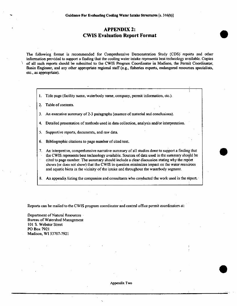
Guidance For Evaluating Cooling Water Intake Structures (s. 316(b)]

APPENDIX 2:CWIS Evaluation Report Format

The following format is recommended for Comprehensive Demonstration Study (CDS) reports and otherinformation provided to support a finding that the cooling water intake represents best technology available. Copiesof all such reports should be submitted to the CWlS Program Coordinator in Madison, the Permit Coordinator,Basin Engineer, and any other appropriate regional staff (e.g., fisheries experts, endangered resources specialists,etc., as appropriate).

1. Title page (facility name, waterbody name, company, permit information, etc.).

2. Table of contents.

3. An executive summary of 2-3 paragraphs (essence of material and conclusions).

4. Detailed presentation of methods used in data collection, analysis and/or interpretation.

5. Supportive reports, documents, and raw data.

6. Bibliographic citations to page number of cited text.

7. An interpretive, comprehensive narrative summary of all studies done to support a finding thatthe CWIS represents best technology available. Sources of data used in the summary should be

cited to page number. The summary should include a clear discussion stating why the reportshows (or does not show) that the CWIS in question minimizes impact on the water resourcesand aquatic biota in the vicinity of the intake and throughout the waterbody segment.

8. An appendix listing the companies and consultants who conducted the work used in the report.

Reports can be mailed to the CWIS program coordinator and central office permit coordinators at:

Department of Natural ResourcesBureau of Watershed Management101 S. Webster StreetP0 Box 7921Madison, WI 53707-7921

Appendix Two

Northern States Power Company

....... 414 Nicollet MallMinneapolis, Minnesota 55401-1927Telephone (612) 330-5500

September 21, 2000

Metro/Major FacilitiesAttn: Discharge Monitoring ReportsMinnesota Pollution Control Agency520 Lafayette Road' NorthSt. Paul, MN 55155

Attention: Mary Hayes

PRAIRIE ISLAND NUCLEAR GENERATING PLANTNPDES Permit No. MN0004006Monthly Discharge Monitoring Reports

In accordance with Chapter 6 Part 3 of the subject NPDES permit, we are submittingour Discharge Monitoring Reports for discharges SD-001, SD-002, SD-003, SD-004,SD-005, SD-006, SD-007, SD-012, WS-001 and WS-002 at the Prairie Island NuclearGenerating Plant. These reports cover the period August 1, 2000 throughAugust 31, 2000. We are also submitting the Bromine/Chlorine Monthly SupplementalReport. With the summary information to be found on the discharge SD-001monitoring report form, we propose to discontinue this supplemental report after theMPCA and NSP determine any further need for it.

Please note that the flows reported for discharges WS-001 and WS-002 include a totalof both outfalls.

In accordance with Chapter 2 Part 4 of the subject NPDES permit, we are submittingthe records of the daily maximum, minimum, and average temperatures for themonitoring locations of the temperature monitoring system. As approved by theMPCA, the discharge monitoring report forms for stations SW-001, SW-002, SW-003,and SW-004 have been discontinued since the summary data requested by each formis found in the attached records. Discharge canal monitoring was out of service oroperating incorrectly August 17 to 25.

A plant status report of the continuous chlorination/bromination treatment program isincluded with the Bromine/Chlorine Monthly Supplemental Report, and provides asummary of August operations including the monthly demand result., With the crossconnect valve open the unit 2 chemical injection system fed both cooling watersystems in the continuous bromination mode from August 18 to 22. The cross connectvalve was closed while the chemical injection systems were operating during the rest ofthe month. With the cross connect valve shut, both systems were operated in the

Page Two

continuous bromination mode except for several shutdown periods and except Whilethe unit 2 system was in continuous chlorination mode from August 27 to 31. Thedates of the unit 1 chemical injection system shutdown periods were August 14 untilsupply from unit 2 through the opened cross connect valve on August 18, and August27 to 31. The dates of the unit 2 chemical injection system shutdown peri6ds wereAugust 15 and August 16 to 18.

The enclosed memorandum titled "August River Temperatures' describes two periodsin August after average ambient river temperature had been at 78°F or above for twoconsecutive days. This ambient temperature condition triggers the permit requirementto run all cooling towers to the maximum practical extent, which was considered theoperation scenario at the time. For your information, attached with the memorandum isthe Star Tribune summary of the Twin Cities air temperatures for the month.

The report on the zebra mussel control treatment conducted on the unit 1 circulatingwater system on August 15 and on the unit 2 circulating water system on August 17 isenclosed. The treatment was conducted with approved levels of Nalco-Calgon'sEVAC, and the report provides details of the treatment levels, durations andeffectiveness as well as information on the resultant loss of fish within the plant'scirculating water system. Attached with the report is the assessment of fish loss asdiscussed at the follow up meeting with state agencies on August 28.

If you have any questions, please call me at 612-330-6625.

erely,

Jim odensteinerS ior Environmental Analyst

Enclosures

c: Terry CossMarilyn Danks (DNR)Gary Gramm (Dept of Ag)Kevin HolstromGerald JoachimGary KolleKatherine. Logan (MPCA Rochester)Ken MuellerSteve SchaeferJohn Sullivan (WI DNR)ERAD Record Center

w:jjb/rpts/mpraire.doc

XCEL ENERGYPrairie Island Nuclear Generating Plant. 1717 Wakonade Drive EastWelch, Minnesota 55089(651)-388-1121

DATE SEPTEMBER 01,2000

NAME JIM BODENSTEINERADDRESS ENVIROMENTAL SERVICES

SUBJECT:,CONTINUOUS CHLORINATION/BROMINATION

The plant operated in the continuous bromination mode in a splitfeed mode(cross-connect shut) until the middle of August when there werenumerous system manipulations during the addition of the zebra musselchemical(Calgon EVAC) to the intake canal.

At 1800 August 14th Unit 1 chem injection system was shutdown and thecross-connect valve remained shut. At 1000 August 15th Unit 2 chem injectionsytem was shutdown for minor maintenance. At 2200 August 15th Unit 2 cheminjection sytem was restarted in continuous bromination mode with crossconnect valve shut. At 1600 August 16th Unit 2 chem injection system wasshutdown. At 1630 August 18th Unit 2 chem injection system was restartedin the continuous bromination mode with the cross connect valve OPEN so itwas feeding both cooling water systems. At 0600 August 22nd the crossconnect valve was shut for repair on Unit 1 system. At 1400 August 23rdUnit 1 chem injection system was restarted in continuous bromination modewith the cross connect valve SHUT. At 0810 August 27th Unit 1 cheminjection system was shutdown for repair and the cross connect valveremained shut. At 0600 August 28th Unit 2 chem injection system sodiumbromide pump was off for unknown reason. Tank level. changes seems toindicate that it may have tripped off late on, August 27th. This put theplant in a continuous chlorination mode. Operation continued in thiscontinuous chlorination mode until 1130 August 31 st when Unit 1 cheminjection system was restarted in continuous bromination mode and Unit 2sodium bromide pump was restarted placing Unit 2 chem injection system ina continuous bromination mode(cross connect SHUT). At 1530 Unit 1 cheminjection system was shutdown for maintenance(cross connect SHUT)

On August 19th and 20th the normal sample point for Unit 1 coolingwater(WS001) was plugged and the daily sample was taken at an alternatesample point slightly upstream of the normal sample point which would haveresulted in slightly higher sample results(conservatively higher). Thesample point was unplugged and was returned to service on August 21st.

Please contact me at Ext. 4440 if additional information is needed.Thank you.

Sinc rely yours,

SGe ald Jonac PmSenior Radiation Protection Specialist

XCEL ENERGYPrairie Island Nuclear Generating Plant1717 Wakonade Drive EastWelch, Minnesota 55089(651)-388-1121

DATE SEPTEMBER 01,2000

NAME JIM BODENSTEINERADDRESS ENVIROMENTAL SERVICES

SUBJECT: AUGUST RIVER TEMPERATURES

A late July weather warmup that lasted into early August causedthe daily average upstream river, temperature to rise above 78 degrees withthe second consecutive day occurring on August 1st. In addit!ion an earlyAugust warmup caused daily average upstream river temperature to rise above78 degrees for seven days. Daily average upstream temperatures listed below.

UPSTREAM RIVER TEMPERATUREDAILY AVERAGE

Augustl 79.2S2 79.03 78.2

10 80.311 79.512 79.513 80.014 80.415- 80.316 78.3

The plant NPDES permit requires "running all: cooling towers to themaximum practical extent" after the second:,consecutive day above 78....degrees. The plant met this permit requirement by running. all four towersand 46 of the possible 48 fans. 2 fans remained out of. service becauserepair would require turning off 24 fans for around 1lday.-

The daily average upstream.river temperature remained below 78 forthe rest of August. The highest-daily average downstream temperature was,81.5 degrees on August 14th.

The discharge canal temperature system was out'of service from lateAugust 17th to late afternoon August 25th..

#121 intake screen remained out of service until 1100 August 31stdue to bearing problems.

Please contact me at Ext. 4440 if additional information is needed.Thank you.

Sinc rely yours,

rald Joa imSenior Radiation Protection Specialist

9 0

High/low temperatures for August 2uuu

100 0Iluur i ~~,Ag v M -il)•iiii~~~~~~i~~' i s ":~:i. :. 1: < . ..ii! : •••1.

VII JjjJ~ *. ~C 4 1 .1. (2. 0--- . -

80

'60

I.

.. .. .. -J ...... I

.... •.::.. ....... ::•..:...-.... :.-...... k( ...... :.U .. ,.•:.?.p ; ,-¾ ..<...~$ : ,:~z .... .cc,':::•:-".g.:.:.4S...c...$>Th%' ":; ....• :-.,J:;.x

1 2 3 4 56 7. 8 9.101112 13141516 171819202122232425262728293031.

Prm/ . -rt7 ? ),iGs.

pN

fz- ýK- 0 , \' - '.. .. . . 9_

NSP - Prairie Island Nuclear Generating

Plant

Report on the Zebra Mussel control treatment of the Circ water system.

This is a report on the treatment of the Unit 1 and Unit 2 Circulating

water systems at the

Prairie Island Nuclear Generating Plant. This report discusses

the chronology of events,

the killing of fish and the effectiveness of the treatment.

Finally, some changes for the

2001 treatments will be discussed.

Summary:NSP treated the Unit I circ water system on 15 August 2000. The Unit.2 side of the circ

water system was treated two days later on 17 August. The treatment

was very

successful in eradicating

Zebra Mussels. An unfortunate

effect was the killing of

approximately 100,000 primarily

small fish in the circ Water system. For the treatment

in

2001, a longer treatment time using a lower dosage of thebiocide

will be considered,

Also the treatments will likely be separated

by approximately a week.

Report:NSP contracted

with the NALCO chemical

company to provide services and the

chemical biocide to treat the circ. water systems..

The biocide used was EVACTM.

The treatment of Unit 1 cire water system was performed

on 15 August 2000. During the

summer months the circ water system at Prairie Island iso6perated in a once through

configuration. Intake water is pumped

through the plant, and then over four cooling

towers. After the towers, the water flows through the'cooling tower return canal, down a

/ mile discharge canal, and finally out to the Mississippi

rivei.The Unit I treatment

duration was 7 hrs. 4i5 min•utes:(! (145 to.1930)."

The chemical

addition rate was raised to the maximum

permitted rate of 4 ppm active ingredient.

The

flow treated was 270,000 gpm;. This ,isslightly.over

.half ofath.e total circ water flow of

525,000 gpm. In the targeted

area, whiCh was§primarily the platscreen

house,

concentrations of 1.3 to 2.3 ppmractive

ingredient were-obtained.:.

The. next day, 16 August,.dead fish were reported

inhe discharge canal. A rough

estimate of the number of dead fish wasg 75,000.,: Theappropriaite

state'agencies were

notified. The estimated;

nurm berof fish kiled was.presented in a press release the same

day. The dead fish were almot'setxcluelsively 2to, 3: inchesý in length. A few adult fish

were killed. It is importa t to note that EVACiM attacksf he gi`llofaquatipc

organisms,

suffocating them. As a resultý,EVACTM

isnot a threat to scavengers' feeding on the dead

fish.

It had not been expected that fish would be killeld:,in

the discharge canal.,A

few hundred

fish in the intake canal were expected to be affected,

:Based on experience with earlier

chemical treatments,

plant personnel expected

three mechanisms would removeýnearly

all

of the biocide by the time the water reached the discharge canal. First, there is a high

biological demand in the water and in the cooling towers.

Second, the river water has a

high concentration of suspended

solids, Suspended solids tie up the EVACTM,

making is

unavailable to organisms.

Finally, because only one Unit was treated at a time, the

C:\TEMP\PI CW Aug 00 ZM treat revl.doc,

09/21/00

I

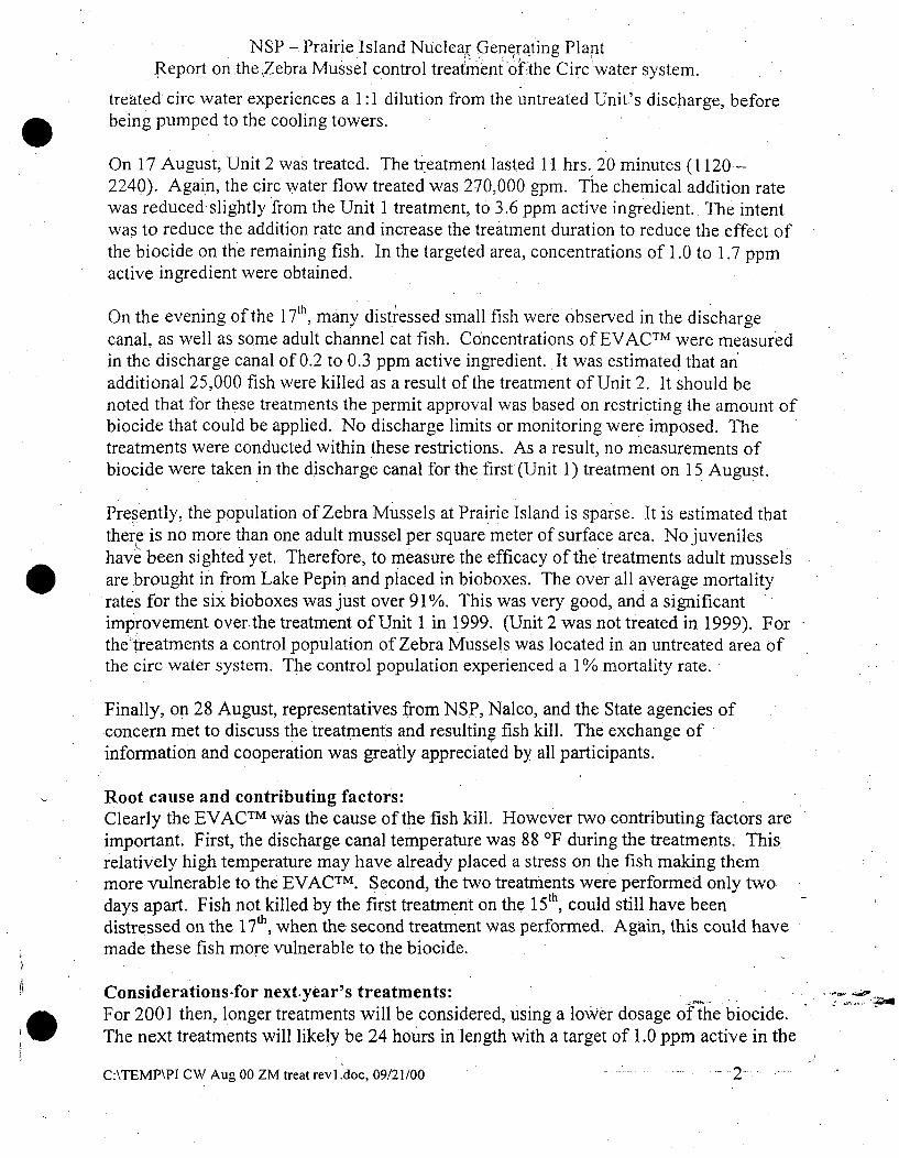
NSP - Prairie Island Nuclear Generating PlantReport on the.Zebra Mussel control treatment0oftIhe Circ water system.

treated circ water experiences a 1: 1 dilution from the untreated Unit's discharge, beforebeing pumped to the cooling towers.

On 17 August, Unit 2 was treated. The treatment lasted 11 hrs. 20 minutes (1120 -2240). Again, the circ water flow treated was 270,000 gpm. The chemical addition ratewas reduced slightly from the Unit 1 treatment, to 3.6 ppm active ingredient. The intentwas to reduce the addition rate and increase the treatment duration to reduce the effect ofthe biocide on the remaining fish. In the targeted area, concentrations of 1.0 to 1.7 ppmactive ingredient were obtained.

On the evening of the 1 7th, many distr'essed small fish were observed in the dischargecanal, as well as some adult channel cat fish. Concentrations of EVACTM were measuredin the discharge canal of 0.2 to 0.3 ppm active ingredient. It was estimated that anadditional 25,000 fish were killed as a result of the treatment of Unit 2. It should benoted that for these treatments the permit approval was based on restricting the amount ofbiocide that could be applied. No discharge limits or monitoring were imposed. Thetreatments were conducted within these restrictions. As a result, no measurements ofbiocide were taken in the discharge canal for the first (Unit 1) treatment on 15 August.

Presently, the population of Zebra Mussels at Prairie Island is sparse. It is estimated thatthere is no more than one adult mussel per square meter of surface area. No juvenileshave been sighted yet. Therefore, to measure the efficacy of the treatments adult musselsare brought in from Lake Pepin and placed in bioboxes. The over all average mortalityrates for the six bioboxes was just over 91%. This was very good, and a significantimprovement over the treatment of Unit 1 in 1999. (Unit 2 was not treated in 1999). Forthe :treatments a control population of Zebra Mussels was located in an untreated area ofthe circ water system. The control population experienced a 1 %.mortality rate.

Finally, on 28 August, representatives from NSP, Nalco, and the State agencies of-concern met to discuss the treatments and resulting fish kill. The exchange ofinformation and cooperation was greatly appreciated by all participants.

Root cause and contributing factors:Clearly the EVACTM was the cause of the fish kill. However two contributing factors areimportant. First, the discharge canal temperature was 88 'F during the treatments. Thisrelatively high temperature may have already placed a stress on the fish making themmore vulnerable to the EVACTM. Second, the two treatments were performed only twodays apart. Fish not killed by the first treatment on the 15th, could still have beendistressed on the 17t, when the second treatment was performed. Again, this could havemade these fish more vulnerable to the biocide.

Considerations-for next year's treatments:For 2001 then, longer treatments will be considered, using a loWer dosage of the biocide.The next treatments will likely be 24 hours in length with a target of 1.0 ppm active in the

C:\TEMP\Pl CW Aug 00 ZM treat rev Ldoc, 09/2 1 /00 .2

NSP - Prairie Island Nuclear Generating PlantReport on the Zebra Mussel control treatment of the Circ water system..

portions of the circ. water systems being treated (i.e. the plant screen house). Also,consideration will be given to spacing the treatments out, increasing the time betweentreatments to around 5 to 7 days. Thought will be given to performing the treatmentwhen the discharge canal temperature is cooler, however cooler discharge temperaturesmean cooler intake temperatures. The biocide is less effective in cooler water, so thiscould be counter productive.

C:\TEMP\PI CW Aug 00 ZM treat rev 1.doc, 09/21/00 3

Joachim, Gerald J

From: Mueller, Kenneth N. Sent: Thursday, August 31, 2000 3:02 PMTo: Gruber, Mark E; Kolle, Gary; Bodensteiner, James JCc: *dl PI Environmental; Schuelke, Don; Giese, Bradley; Orr, Daniel J; Coss, Terry E -Subject: PI Aug.- 2000 Fish-kill Assessment

Importance: High

Report prepared 8/31/00 by KN Mueller- Environmental Analyst

The following explanation is provided with intent to clarify rationale, assumptions, and calculations used for determiningestimated numbers and composition of small fish killed in the discharge canalas a result of zebra mussel controltreatments performed Tuesday 8/15 and Thursday 8/17 at the Prairie Island Plant.

On Wed. 8/16/00 at approximately noon, KNM was paged by Mark Gruber alerting him to dead fish in thedischarge canal. At approximately 3 pm KNM, DJO and BDG inspected the discharge canal betweenelectrofishing runs. Thecomposition was estimated as 50% yoy channel catfish (1½"- 4") and 50%shiner/minnow species (juv. & adult). No attemptwas made at that time to determine total numbers or collectfish, because we had to continue electrofishing.

That afternoon M.Gruber & G.Kolle spot-checked areas around the discharge canal, and counted fish within a 10'section of shoreline that appeared representative of the entire discharge canal shoreline. They arrived atapproximately 150 fish within that 10' section. They estimated - 15 fish/foot, which they multiplied by the numberof feet of discharge canal shoreline: 15 fish/foot X 5000 feet = ~ 75,000 fish (original reported estimate).' Usingthe composition estimate, that equates to - 37,500 yoy channel catfish (1½1/" - 4") and - 37,500 shiner/minnowspecies (juv. & adult).

On Fri. 8/18/00 KNM estimated approximately 20 fish/foot along the shoreline of the discharge canal, but therewas a higher percentage of shiner/minnow species and green sunfish, and fewer additional small catfish than wereobserved on 8/16. The dead fish observed in the canal on Wednesday were not removed, so it was assumed thatan additional 5 fish/foot had accumulated. The additional 5 fish/foot adds 25,000 fish to the original estimate of75,000.

The following percent composition is for the additional 25,000 small fish estimated on Friday. Percent compositionwas based on shoreline observations and further supported by examination of 11/2 5-gal. pails of small fishcollected from the discharge canal:

- 80% shiner/minnow species (~ 20,000)- 10% channel catfish (- 2,500)- 10% green sunfish (~ 2,500)

The following is the final estimated total number of small fish lost in the discharge canal:

8/16 8/18- 37,500 + - 20,000 = ~ 57,500,shiner/minnow species- 37,500 + - 2,500 = - 40,000 channel catfish

~ 2,500 green sunfish~ 100,000 small fish

Assessment summaries of fish killed in the intake canal and large fish collected from the discharge canal are attached asTable 1 and Table 2, respectively.

I

Table 1.xls Table 2.xis

0

02

TABLE 1. .,_Screen house dead fish (count and lengths) I TtCh. cal. F-w drum Gr. Sun Bl. Gill F-h cal S-m buff Giz. Shad Carp Walleye Sauger S-h redh W. bass S-m bass R. carpsu Mooneye Goldeye Shiner Bowfin _ Total

2 2 1 12 7 ... 703 5 6 8 28 82 24 4 37 15 12 1 15 5 10 11 15 116 16 1 33 17 36 4 45 1 1

8 120 12 11 29 82 11 1

10 41 I" 15 2

11 12 10 3Leng•th '12 110 S3. . . .. ... . . ..... ..

(Inches) 13 6 1 114 17 715 9 116 10 3 1 1 2

17 8 1 2 118 7, 1 21: 3 4

1.9 3 1 220 1 1 1 6 1.21 1 1 422 2 2 3123 "1124 2 1125 1126 1 127i 128i29

!Total 4 1 11 3 11 __ 2 1 I 701 4 952

-- ] -. I IN4--20mm

TABLE 2. Discharge canal dead adult fish (count and lengths) I

Ch. cat Gr. Sun S-r buff Carp Total

1 _ _ _1__ __ _ _

2 _ _ 3_3 34 105 36 3 27 2 18 69 3

10 13 111 5

Length 12 . 19(Inches) 13 13

14 3115 2816 2617 2318 4619- 1820 3621 1322 1723 1324 1825 726 927 528 429 330 10 4

Total 371 23 1 5 400

1+56 unmeasured •_

0 S 0

BROMINATION/CHLORINATION REPORT

From: 01-AUG-00 To: 31-AUG-00

Day

12345678

,9101112131415

161718

20212223

24252627282930.31

BromineKgms/day

72.772.767.167.167.167.172.744.728.055.978.055.967.161 .5 ....28.0

33.60

5 .6 '....

28.0

28.044.739.267.1

78.3111.9

89.567.1

0 '00.

11.2

ChlorineKgms/day

79.976.678.878.877.6

78.982.682.693.395.795.791.091.384.134.8

34.80

10.8

52.5

:44. 749.950.5.

.65.2

70.6•70.6

93.284.0

S21.481.851.164.0

Timemins/day

14401440144014401440144014401440144014401440144014401440

960

108o0

90

1440

:1440144014401440

14401440

14401.440

144014401440

U-IResidual

0.090.110.080.110.110.110.080.150.140.160.150.150.150.15

<0.01<0. 01<0.01<NIS><NIS><0.01<0.01<0 * 01

0.070.080.070.050.020.13.0.190.-1950.190.17

<0.01<0. 01<0.01<0. 01

0.15

U-2Residual,

0.100.100.070.090.080.100.090.1401150.160.150.160.170.120.090.110.12

<NIS>,<NIS>

0.210.220..22

0.090.100-11~o0.080.160.190.240.220.230.2210.170.210.260.220.20

OutfallResidual

<.001<.001<.001<.001<.001<.001<.001<.001<.001<.001<.001<.001<.001<.001<.001

<.pOl<NIS><NIS><.001

<.001<.001<.001<.001<..001<.001

< .001<001

<.001<.001<.001<.001<.001<.001<.001

Maximum Daily Chlorination Rate = 182.7 Kgms/day on the 26th.

FACILITY NAMEIADDRESS:NSP - Prairie Island Nuclear Power Plant1717 Wakonade Dr EWelch, MN 55089

STATION INFORMATION:SD-001 (Combined Effluent)

Surface Discharge, Effluent To Surface Water

WASTEWATER TREATMENTDISCHARGE MONITORING REPORT

V ~ER~ _L 1IMI TUNS1 FORMER #MN0004006 FINAL 0Ol0M I

NIO I F- -0

PERMITTEE NAME/ADDRESS:

NSP

414 Nicollet Mall

Minneapolis, MN 554011993

I-I No Discharge I

~AM~JýDAYFRO 2TOCO10/0 _0008/~j31

50050

pH

00400

Phosphorus

Total (as P)

00665

Chlorine Rate

50059

Send original with supplemental DMR (if I certify that Iam familiar with the 0 // &-<---applicable) by the 21st day of month following information contained in thisreporting period to: report and that to the best of my SIGNAT OF PR) CIPAL EXECUTIVE OFFICER OR AUTHORIZED AGENT DATE

MINNESOTA POLLUTION CONTROL AGENCY knowledge and belief the infor-520 LAFAYETTE RD mation is true, complete, andST. PAUL, MN 55155-4194, accurate.ATTN: Discharge Monitoring Report SIGNATUOF CHIEF OPERATOR PHONE DATE _ IFICATION

COMMENTS: W 'We D3 of D24

FACILITY NAME"IRE-:NSP - Prairie Isla~clear Power Plant1717 Wakonade DrEWelch, MN 55089

STATION INFORMATION:SD-001 (Combined Effluent)Surface Discharge, Effluent To Surface Water

.WASTEWATER TREI-NTDISCHARGE MONITORII PORT

PERMITTEE NAME/ADDRESS:NSP414 Nicollet Mail

Minneapolis. MN 554011993[__ER__T_ _ - O LIlT ý-FSTAJS T_0RMER# ftMN0004006- FINAL 0D

A _ MONITORItNG -PffERIOD

FROM O I UUDAY I

FROM 206f-8/_017A" DL AYA

To 200008/3

-~ PfcsefTa~t-~ ce~a5c4Q,~ /4 1 eczA2r~~-~ ~r'S>1Le~

Send original with supplemental DMR (if I certify that I am familiar with the V" -0applicable) by the 21st day of month following information contained in thisEXECUTIVUROFFICEREU AUTHORIZED AGENT 7-DATEreporting period to: report and that to.'the best of my.. IGAU R AiVE OFFICER OR AUH

MINNESOTA POLLUTION CONTROL AGENCY knowledge and belief the infor-520 LAFAYETTE RD mation is true, complete, andST. PAUL, MN,55155-4194 accurate.ATTN: DlschargeMonitoring Report SIGNATURE OF CHIEF OPERATOR PHONE DATE CERTIFICATIONJ

COMMENTS:Page D4 of D24

FACIUTY NAMEJADDRESS:NSP -: Prairie Island: Nuclear Power Plant1717 Waýonade Or EWelch, MN. 55089'.

STATION INFORMATION:SD-002 (Steam Generator Blowdown Discharge)Surface Discharge, Effluent To Surface Water

. WASTEWATER TREATMENT .DISCHARGE MONITORING REPORT

PERMITTEE Nt•MEADORESS:Northern States Power Co414 Nicollet MallMinneapolis, MN 554011993

t:YMNT00406 IMIT SlTATLUS FORMiERLMN0004006 ý_FINAL 011M I

&~?MONITORING PERIO' - - - --- q

FROM 206o/08/01[EARI MO DAYI

TOI 2000/08/31 I I Min flicrhorno I

I

Send original with supplemental DMR (ifapplicable) by the 21st day of month followingreporting period to:

MINNESOTA POLLUTION CONTROL AGENCY520 LAFAY'EUE.flST. PAUL, MN 194

I certify that I am familiar with theMinformation contained in thisreport and. that to the best of my,.knowledge and belief the infor-mation is true, complete, andaccurate.

Mk , bp 70•# If•J I'll I• T

DATE

J

SIGNAT L1E5FPp'NCIPAL EXECUTIVE OFFICER OR AUTHORIZED AGENT

/.

SIGNATa)F CHIEF OPERATOR PHONE DATE M FICATIONAI1 I

Report P~D27 of 0184

DischargIMnitoring Reportjv I.J.w P3.ge Q.27 of D184

FACILITY NAMEaESS:NSP - Prairie Isian••lear Power Plant1717 Wakonade Dr. EWelch, MN 55089

STATION INFORMATION:SD-003 (Radwaste Treatment Effluent)Surface Discharge, Effluent To Surface Water

WASTEWATER TRE TDISCHARGE MONITORIN G PORT

PERMITTEE NAME/ADDRESS:Northern States Power Co414 Nicollet MallMinneapolis, MN 55401199307C T: " fMI 1TrS'T4TOS§ FORMER # ~

MN0004006 FINAL 012M 1

SMQNII•ORIN GERIlOD tX&{;91FO "Iuu.MO DAY,.'

FROMI 2000/08/01fi TO 2000/08/31 I I Nn rlicrh~rna I

. . .. . ...........

Send original with supplemental DMR (if I certify that ! am familiar with the. . t -applicable) by the 21st day of month following information contained in this SIGNATURE OFPINCIP-/EXECUTIVE OFFICER OR AUTHORIZED AGENT DATEreporting period to: report and that to the-best of my

MINNESOTA POLLUTION CONTROL AGENCY knowledge and belief the infor-520 LAFAYETTERD. mation is true, complete, andST. PAUL.,MN55155-4194 I accurate. . . SIGNATUREOF CHIEF OPERATOR PHONE DATE CERTIFICATIONý

ATTN- Discharge Monitoring Report Page D39 of D184

FACILITY:NAMEIADDRESS:NSP.- Prairie Island Nuclear Power Plant1717.Wakonade DrIEWelch, MN 55089

STATION INFORMATION:SD-004 (Neutralizer + Resin Rinse Discharge)Surface Discharge, Effluent To Surface Water

WASTEWATER TREATMENTDISCHARGE MONITORING REPORT

PERMITTEE NAMEIADDRESS:Northern States PowerCo414 Nicollet MallMinneapolis; MN 554011993FV ýý -,PIT,#Y--LIM It STATU:Sj ORME*

E-MNooo400e FINAL 01 3M 1

L~tS~CsMP$!3ORING-,PERlOD ~ ZFOIŽuuJu2AY

FROMJ 2000/08/01o] TO 2000/08/3 1 I Mn I ncrhnrnc I

Ki

Send original with supplemental DMR (if I certify that I am familiar with the ' .;applicable) by the 21st day of month following nformation contained in this SIGNATURE O-,-PINCIP,-/EXECUTIVE OFFICE R AUTHORIZED AGENT

reporting period to: report and that to the best of my -_

MINNESOTA POLLUTION CONTROL AGENCY knowledge and belief the infor-520 LAFAYETTE RD marion is true, complete, and - l FST. PAUL MN 5 j194 accurate. SIGNAT FCHIEF OPERATOR PHONE DATE A FICATION#

_ATTVýDischa rg1W ito ring Report W Page D51 of D184

FACILITY NAMEhI ESS:NSP - Prairie Islandclear Power Plant1717 Wakonade DrEWelch, MN. 55089

STATION INFORMATION:SD-005. (Unit 1 Turbine Bldg Sump Dschg)Surface Discharge, Effluent To Surface Water

WASTEWATER TREASTDISCHARGE MoNITORIN PORT

PERMITTEE NAMEJADDRESS:Northern States Power Co414 Nicollet MallMinneapolis, MN 554011993I PERMITW # LIMIT STATUS IFORMER #.

MN0004006 FINAL 014M 1

MONlTORINQJiPERIMODext~Ž:jyý--MO I. ,DAY

FROM 12000/08/011 TO n 2000/08/3I I I Mn flicrh~rnn I

Send original with supplemental DMR (if I certify that I am familiar with the I " ( -

applicable) by the 21st day of month following information contained in this SIGNATURE OF PlI [iPAL CE/CUTIVE OFFICER OR AUTHORIZED AGENT DATEreporting period to: report and that to the best of my

MINNESOTA POLLUTION CONTROL AGENCY knowledge and belief the infor-.520 LAFAYETTERD: . . mation is true, complete, andST. PAUL,>MNW55155-4194 accurate. "SIGNATURE OF CHIEF OPERATOR PHONE DATE CERTIFICATION

ý8 Ris,5ýharge:Monitodng Report Page D63 of D184

FACILITY NAME/ADDRESS:NSP - Prairie Island Nuclear Power Plant1717 Wakonade Dr EWelch, MN 55089

STATION INFORMATION:SD-006 (Unit 2 Turbine Bldg Sump Dschg)Surface Discharge, Effluent To Surface Water

WASTEWATERTRMEATMENT.DISCHARGE MONITORING REPORT

PERMITTEE'NAMEJADDRESS:Northern States Power Co

414 Nicollet MallMinneapolisMN 554011993Fr P;E$MITS#7 LIMIT STAR ORE

LMN0004006 FINAL 015M 1

4-MONITORZING•PERIOD

FROML 2000/08/01T EAJMOu.JpAY;l

TO 200n,'0813 1 I No Discharoe I

Send original with supplemental DMR (if I certify that l am familiar with the -- "

applicable) by the 21st day of month following information contained in this SIGNATURE OF-PR lIeIPAL EtECUTIVE OFFICER OR AUTHORIZED AGENT DATEreporting period to: report and that to the best of my

MINNESOTA POLLUTION CONTROL AGENCY knowledge and belief the infor-520 LAFAYETTE RD mation is true, complete, andST. PAUL, MN AM-194 accurate. -SIGNATU -F CHIEF OPERATOR PHONE DICATIONST AU N 5 194rtoin Reor . DATEf 018ATTNý DischargdWitoring Report Aw PagTe T;75 of D 184

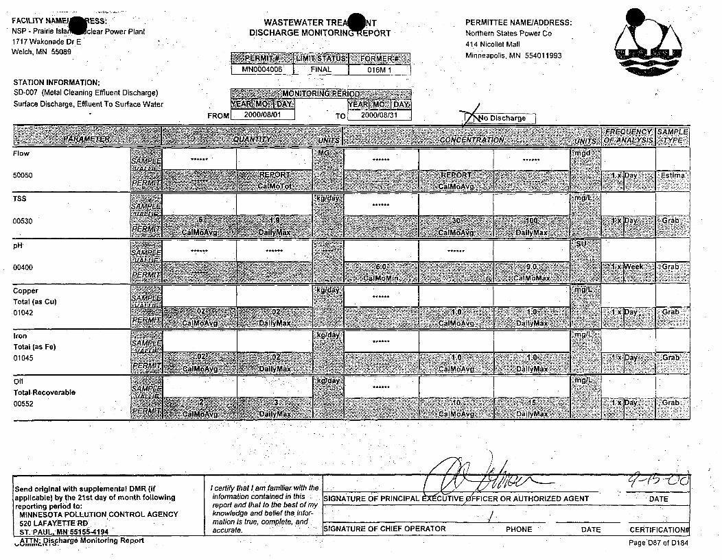
FACILITY t4AMEIMESS:NSP - Prairie Isla~clear Power Plant1717 WakonadeDr EWelch, MN 55089

STATION INFORMATION:SD-007 (Metal Cleaning Effluent Discharge)

Surface Discharge, Effluent To Surface Water

WASTEWATER TRE NTDISCHARGE MONITORINGNEEPORT

PERMITTEE NAME/ADDRESS:Northern States Power Co414 Nicollet MallMinneapolis, MN 554011993[PiEMIT~#, 4L1-m'OtSTATUSI FORMERI R 4

MN00406 FINAL 016M 1

I 'MONITORING PERI OD 4ýýI - ilr l " ' " ill .*1 ...... ......... . .

FROM L 'u uu u1'MEA O. DA

TO 200/08/31l 0/TVo Discharge

Send original with supplemental DMR (if /certifythatlam familiar with the /"-applicable) by the 21st day of month following information contained in this SIGNATURE OF PRINCIPAL -XfCUT IVE FFICER OR AUTHORIZED AGENT DATEreporting period to: report and that to the best of my

MINNESOTA POLLUTION CONTROL AGENCY knowledge and belief the. infor-520 LAFAYETTE RD - mation is true, complete, andST. PAUL, MN 55155-4194 accurate. "SIGNATURE OF CHIEF OPERATOR PHONE DATE CERTIFICATION#

Discharge Monitoring Repprt Page D87 of D184

FACILITY NAME/ADDRESS:NSP - Prairie Island Nuclear Power Plant1717 Wakonade Dr EWelch, MN 55089

STATION INFORMATION:SD-012 (Intake Screen Backwash + Fish Reitn)Surface Discharge, Effluent To Surface Water

WASTEWATER TREATMENT.DISCHARGE MONITORING REPORT

PERM•TTEE NAME/ADDRESS:Northern States Power Co.414 Nicollet MallMinneapolis, MN 554011993~tPEkMtr# JI;iItVIISTT~US&VuF~a 0 I9

MN0004006 j FINAL f 030M 1I

` tMO NITORING PERIOD:AsA

FROM 2 900u/08/01

OEA I DAY]

TO[ 200T0/08/3 1 I Mn n;er~rna

14ý 1i'?At

Send original with supplemental DMR (if certify that / am familiar with the N <• ,applicable) by the21st day of month following information contained in this SIGNATURE OF PRINCIPAL EX UTIVE OFFICER OR AUTHORIZED AGENT DATEreporting period to: report and that to the best of my

MINNESOTA POLLUTION CONTROL AGENCY knowledge and belief the infor-520,LAFAYETTE RD mation is true, complete, andST. PAUL MN accurate. SIGNA CHIEF OPERATOR PHONE DATE BIFICATION

•ATN DIscharM nitoring Report 1q Pal•jr•)103 of D 184

FACILITY NAMEJ*ESS:

NSP - Prairie Islainlclear Power Plant

1717 Wakonade Dr E

Welch, MN 55089

STATION INFORMATION:WS-001 (Unit 1 Plant Cooling Water Dschg)

Waste Stream, Internal Waste Stream

WASTEWATER TREA&TDISCHARGE MONITORINGtEPORT PERMITTEE NAMEIADDRESS:Northern States Power Co414 Nicollet MallMinneapolis, MN. 554011993

MN004006 FINAL~

MQNITQRING1R1ERIOD

FROM I 2000/08/01 TOI 2000/08/31j I INnFtnw I

VOTE4°, PFLoLJ I S A- ThrPrG 0oF- WSCs r LcocŽs &~ C-C.-oczt.

/011 If

Send original with supplemental DMR (if certify that, lam amiliar.with the ; - tapplicable) by the 21st day of month following information contained in this. SIGNATURE OF PRNC EX TIVE OFFICER OR UTHORZED AGENT DATEreporting perio.d to: report and that to the best of my

MINNESOTA POLLUTION CONTROL AGENCY knowledge and belief the infor-520LAFAYETTE-RD mation is true, complete, and.ST. ýPAUL, MN,:551554194 accurate. SIGNATURE OFCHIEF OPERATOR PHONE' DATE CERTIFICATIONMAT8N Discharge Monitoring Report Page D1 63 of D1 84

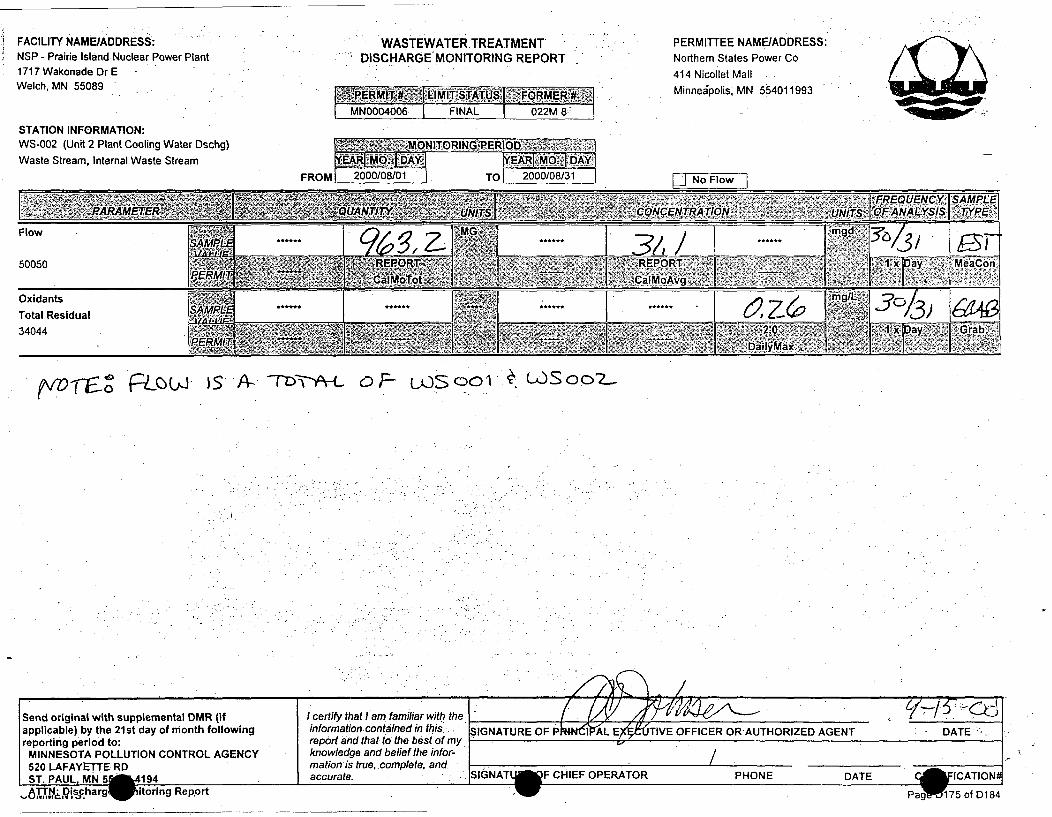
FACILITY NAME/ADDRESS:NSP - Prairie Island Nuclear Power Plant1717 Wakonade Or EWelch, MN 55089

STATION INFORMATION:WS-002 (Unit 2 Plant Cooling Water Dschg)Waste Stream, Internal Waste Stream

WASTEWATER TREATMENTDISCHARGE MONITORING REPORT

PERMITUEE NAME/ADDRESS:Northern States Power Co414 Nicollet MallMinne~polis, MN 554011993

MN0004006 FINAL 022M 8

$Jj•:c~MNITORING;,PER1`OD-- 7»FMDAY

FROM 1 2000/08/0 1 TO r 2000/08/31 I 1 No Flow I

gv-(Ctcý Fto W is XA- Wi-A'-1P-L o F- w.soo1 t WSoaL.

/Send original with supplemental DMR (if I certify that!I am familiar with. the I/$-'---applicable) by the 21st day of month following information contained in this.... SIGNATURE OF PRINCIPAL E!? TIVE OFFICER ORAUTHORIZED AGENT DATEreporting period to: report and that to the best of my

DATE,

MINNESOTA POLLUTION CONTROL AGENCY knowledge and belief the infor-520 LAFAYETTE RD mation is true,.complete, andST. PAUL, MN 5" 194 1 accurate. .SIGNAT"A F CHIEF OPERATOR PHONE DATE

A DischarglW itoring Report .W Pag'W75 of D184

Cý q le Z- Lj't6f

4WM-p M.Northern Staes Power Company:"e""-,'

414 Nicollet MallMinneapolis, Minnesota 55401Telephone (612) 330-5500

I A1 ,October 14, 1983

Howard Krosch Don L KriDivision of Fish & Wildlife DivisionMN Dept of Natural Resources MN PollutCentennial Office Building 1935 WestSt Paul, Minnesota 55155 RosevillE

PRAIRIE ISLAND NUCLEAR GENERATING PLANTChlorination of Circulating Water SystemFish Loss Report

ensof Waste Quality.ion Control Agency '/County Road B2

e, Minnesota 55113

MA) 900

Enclosed, for your information, is a report on the fish lossdue to chlorination of the circulating water system at thePrairie Island Nuclear Generating Plant in August, 1983.

Feel free to contact Glen Kuhl at the Prairie Island Environ-mental Lab at (612) 388-1121, extension 349, if you have anyquestions concerning this report.

W E J6nsrenSenior ConsultantRegulatory Services

ah

enclosure

cc: G M Kuhl

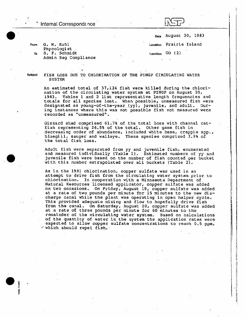
Internal Correspondc nce

Date August 30, 1983

From G. M. Kuhl Location Prairie IslandPhycologist

To S. F. Schmidt Location GO (2)Admin Reg Compliance

Subject FISH LOSS DUE TO CHLORINATION OF THE PINGP CIRCULATING WATERSYSTEM

An estimated total of 37,124 fish were killed during the chlori-nation of the circulating water system at PINGP on August 20,1983. tables 1 and 2 list representative length frequencies andtotals for all species lost. When possible, unmeasured fish weredesignated as young-of-the-year (yy), juvenile, and adult. Dur-ing instances where this was not possible fish not measured wer.erecorded as "unmeasured".

Gizzard shad comprised 61.7% of the total loss with channel cat-fish representing 26.5% of the total. Other game fish indecreasing order of abundance, included white bass, crappie spp.,bluegill, sauger and walleye. These species comprised 3.9% ofthe total fish loss.

Adult fish were separated from yy and juvenile fish, enumeratedand measured individually (Table 1). Estimated numbers of yy andjuvenile fish were based on the number of fish counted per bucketwith this number extrapolated over all buckets (Table 2).

As in the 19.81 chlorination, copper sulfate was used in anattempt to drive fish from the circulating water system prior tochlorination. In cooperation with a Minnesota Department ofNatural Resources licensed applicator, copper sulfate was addedon two occasions. On Friday, August 19, copper sulfate was addedat a rate of two pounds per minute for 15 minutes to the new dis-charge canal while the plant was operating in open helper cycle.This provided adequate mixing and flow to hopefully drive fishfrom the canal. On Saturday, August 20, copper sulfate was addedat a rate of three pounds per minute for 60 minutes to theremainder of the circulating water system. Based on calculationsof the quantity of water in the system the application rates wereexpected to allow copper sulfate concentrations to reach 0.5 ppm,

-which should repel fish.

11

Fish loss during the 1983 chlorination was slightly greater thanthe 28,095 lost during 1981 but considerably less than the162,4.48 lost .during the 1980 chlorination. Species compositionwas similar to previous years with gizzard shad and channel cat-

fish being major contributors of fish loss.

G. M. Kuh

SW

It

Section 316 (b) Demonstration for theP~rairie Island Generating Plant on the

Mississippi River near-Red Wing, Minnesota

December, 1976:

Nus Corporation

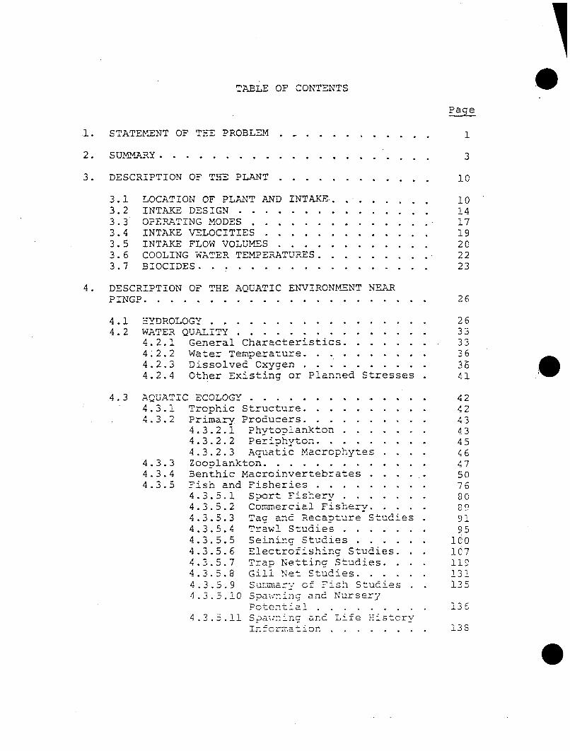
TABLE OF CONTENTS

Page

.1. STATEMENT OF THE PROBLEM . .............. 1

2. SUMMARY ............ ...................... 3

3. DESCRIPTION OF THE PLANT ........... ............ 10

3.1 LOCATION OF PLANT AND INTAKE . ..... .I........103.2 INTAKE DESIGN ........ ............... 143.3 OPERATING MODES ...... .................. 173.4 INTAKE VELOCITIES ...... ............. 193.5 INTAKE FLOW VOLUMES .......... ............ 203.6 COOLING WATER TEMPERATURES ................ 223.7 BIOCIDES ........... .................. 23

4. DESCRIPTION OF THE AQUATIC ENVIRONMENT NEARPINGP ............... ...................... 26

4.1 HYDROLOGY .......... ................. 264.2 WATER QUALITY ........ ............... 33

4.2.1 General Characteristics ........... .. 334*2.2 Water Temperature ....... .......... 364.2.3 Dissolved Oxygen .................. 3.4.2.4 Other Existing or Planned Stresses 41

4.3 AQUATIC ECOLOGY ...... ............... 424.3.1 Trophic Structure ............. .. 424.3.2 Primary Producers ....... .......... 43

4.3.2.1 Phytop1ankton ...... ....... 434.3.2.2 Periphyton ............ .. 454.3.2.3 Aquatic Macrophytes . .. 46

4.3.3 Zooolankton ..... ............. .. 474.3.4 Benthic Macroinvertebrates ....... 504.3.5 Fish and Fisheries ... ......... .. 76

4.3.5.1 Sport Fishery. ......... ..4.3.5.2 Commercial Fishery. ......4.3.5.3 Tag and Recapture Studies 914.3.5.4 Trawl Studies ......... 954.3.5.5 Seining Studies ...... . i1004.3.5.6 Electrofishing Studies. 1074.3.5.7 Trap Nettina Studies. . 1194.3.5.8 Gill Net Studies ....... 1314.3.5.9 Suimmarx of Fish Studies 1254.3.3.10 Spaýning and Nursery

Potential ....... ......... 13C4.3.5.11 Spaw;ninc and --i e -4'stcor

Information. ...... ........ 13S

TABLE OF CONTENTS (CONTINUED)

Page

5 INTAKE-RELATED STUDIES. 139

5.1 INTRODUCTION . ...........5. 2 METHODS USED FOR INTAKE-RELATED STUDIES.

5.2.1 Entrainment-related Studies5.2.1.1 Phytoplankton .........5.2.1.2 Zooplankton ...........5.2.1.3 Fish. ..............

5.2.2 Impingement-related Studies . . .5.2.2.1 Data Collection......5.2.2.2 Statistical Analysis

13!914 0

140• 140. 144

148

155155137

5.3 RESULIS OF INTAKE-RELATED STUDIES ........5.3.1 Entrairnent Studies ..... ........

5.3.1.1 Phytoplankton ...........5.3.1.2 Zooplankton ............5.3.1.3 Fish ...... . . .......

5.3.1.3.1 Taxonomic Com-position.

5.3.1.3.2 Comparison ofSampling Locations

5.3.1.3.3 Die! Variations inFish Entrainment.

5.3.2 Impingement ....... ............

6 I:HPACT ASSESSMENT ......................

6.1 PRIDLkRY PRODUCERS ........ .............6.2 ZOOPLANKTON .......... ................6.3 BENTHIC MACROIhVERTEBRATES ..... ........6.4 FISH EGGS AND LARVA/• ENTRAINMENT ........6.5 FISH IMPINGEMENT ......... .............

7 LITERATURE CITED. . . ......... ............

APPENDIX I INTAKE "VELOCITIES AT PINGP, JUNE 23AND 28, 1976

APPENDIX 2 NOTES ON SPAWNING AND REPRODUCTIONOF 26 SPECIES OF FISH OCCURRING NEARPINGP

APPENDIX 3 MEAN AqND STANDA-RD DEVIATION OF DATAON EGGS AND YOUNG FISH COLLECTED INPINGP ENTRAITNENT STUDIES, 1975.

160160160164168

168

171

105

186

230

2382

240241243258

264

TABLE OF CONTENTS (CONTINUED)

APPENDIX 4 RESULTS OF CORRELATION ANALYSIS OFFISH IMPINGEMENT, PLANT OPERATINGAND WATER TEMPERATURE DATA AT PINGP,1975.

TABLE OF CONTENTS (CONTINUED)

Pace

5 INTAKE-REL.ATED STUDIES . .3.

5.1 INTRODUCTION ..... . . . . . . . . . .. . 1395.2 METHODS USED FOR INTAKE-RELATED STUDIES. . 140

5.2.1 Entrairnment-related Studies . . . . i45.2.1.1 Phytoplankton ...... ....... 1405.2.1.2 Zooplankton ............. 1445.2.1.3 Fish . ............... 148

5.2.2 Impingement-related Studies . . . 1555.2.2.1 Data Collection ...... 1555.2.2.2 Statistical Analysis . . . 157

5.3 RESULIS OF INTAKE-RELATED STUDIES ..... 1605.3.1 Entrainment Studies .......... 160

5.3.1.1 Phytoplankton ......... 1605.3.1.2 Zooplankton ........... 1645.3.1.3 Fish ............... 162

5.3.1.3.1 Taxonomic Com-position. . 163

5.3.1.3.2 Comparison ofSampliha'Locations 171

5.3.1.3.3 Diel Variations inFish Entrainment. 105

5.3.2 Impingement ........... ............ 136

6 I>PACT ASSESSMENT . ... ........................ 230

6.1 PRIMARY PRODUCERS ...... ............. 23S6.2 ZOOPLANKTON .......... ................ 2406.3 BENTHIC MACROI-N'VRTEBRATES .......... 2416.4 FISH EGCS AND LARVAZi ENTRPAINMENT ..... 2436.5 FISH IMPINGEMENT ............ ............. 253

7 LITERATURE CITED .......... ................ . 264

APPENDIX 1 INTAKE VELOCITIES AT PINGP, JUJNE 23AND 28, 1976

APPENDIX 2 NOTES ON SPAWNING AUND REPRODUCTIONOF 26 SPECIES OF FISH OCCU•R•ING NEARPINGP

APPENDIX 3 MEAN AND STANDARD DEVIATION OF DATAON EGGS AND YOUNG FISH COLLECTED INPINGP ENTRAINMENT STUDIES, 1975.

LIST OF FIGURES

Fiaure Page

3.1-1 GENERAL LOCATION OF PINGP .... .......... . 1

3.1-2 IMMEDIATE LOCATION OF PINGP. ... ........ 12

3.2-1 FLOW PATHS IN THE PINGP CONDENSER SYSTEM . 15

3.2-2 CROSS-SECTION OF PINGP SCREENHOUSE ..... 15

3.3-1 FLOW RATES IN THE CLOSED-CYCLE MODE FORCONDENSER COOLING AND THE SERVICE WATERSYSTEM ..................... ............... 18

3.6-1 MINI-MUM AND MAXIMUM TEMPERATURE IN THE PINGPINTAKE CANAL, JANUARY 1, 1974 TO DECEMBER 31,1975 ................ .................... 24

4.1-1 MEAN FLOW DURATION CURVE FOR MISSISSIPPI RIVERAT PRESCOTT, WISCONSIN, OCTOBER 1928-SEPTEMBER 197/4 .............. .......... 27

4.1-2 CONSECUTIVE DAY AVERAGE LOW FLOW FREQUENCIES,MISSISSIPPI RIVER AT PRESCOTT, WISCONSIN1928-1974 ................ .................. 30

4.1-3 STURGEON LAKE FLOW VS. MISSISSIPPI RIVERFLOW, AS MEASURED AT LOCK AND DAM NO. 3. 32

4.2-3 MAXIMUM A2D MINIMUM MONTHLY DISSOLVED OX-YGENCONCENTRATION IN THE MISSISSIPPI RIVER NEARTHE PINGP INTAKE CANAL, JULY 1970-DECEMBER1975 ....................................... 39

4.3-1 AREAS OF SUBMERGED AQUATIC VEGETATION IN THE

VICINITY OF PINGP, 1975.... ............ 48

4.3-2 BENTHOS SAMPLING STATIONS NEAR PINGP, 1971

AND 1972 ............ ......... ......... 52

4.3-3 ADDITTONAL BENTHOS ST._PLING STATIONS NEAIRPINGP, 1973 ........ ................. 56

4.3-4 LIGHT TRAP STATIONS USED IN EMERGENCE STUDIESAT PINGP, 1974 ........... ............... 58

0

LIST OF FIGURES (CONTINUED)

Figure Page

4.3-5 CREEL SURVEY AREAS NEAR PINGP, 1973-1975 81

4.3-6 FISH STUDY AREAS NEAR PINGP, 1970-1975 . . . . 96

5.2-1 SAMPLING STATIONS FOR PRODUCTIVITY, 1975 . . . 141

5.2-2 SAMPLING STATIONS FOR PHYTOPLANKTON STUDIES,1974-1975. .......................... 143

5.2-3 SAMPLING STATIONS FOR ZOOPLANKTON STUDIES,1974 ................ ..................... 146

5.2-4 SAMPLING STATIONS FOR ZOOPLANKTON STUDIES,1975 ................ ..................... 147

5.2-5 LOCATION OF FISH EGG AND LARVA SAMPLINGSTATIONS AT PINGP IN 1975 .... ........... 154

5.3-1 PHYTOPLANKTON DEGRADATION (PERCENT DEPLETIONOF PHOTOSYNTHESIS, RESPIRATION, AND CHLOROPHYLLa) DUE TO PASSAGE THROUGH PINGP, MAY-OCTOBER1975 ................ ..................... 162

5.3-2 .MEAN DENSITY (NO/100 m 3) OF YOUNG FISH COLLECTEDIN THE STURGEON LAKE AREA BY MDNR AND AT THEBAR RACK STATION IN THE P!NGP INTAKE CANALBETWEEN MAY 15 AND SEPTEM•BER 4, 1975 ....... 173

5.3-3 DTEL VARIATION IN MEAN DENSITY (NO/l00 m3)

OF EGGS AND LARVAE AT THE RECIRCULATIONCANAL AND BAR RACK STATIONS AT PiNGP, MY 15-JULY 2, 1975 .................... . 181

5.3-4 DIEL VARIATION IN MEAN DENSITY (NO/i00 m 3) OFEGGS AND LA-RVAE AT THE SKIMMER WALL AND BARRACK STATIONS AT PINGP, July 10-SEPTEMBER 4,1975 ................ ..................... 182

5.3-5 NUMBERS OF GIZZARD SHLAD COLLECTED FROM THETRASHBASKETS AT PINGP, 1974 .... .......... .. 201

5.3-6 NUMBERS OF GIZZARD SlAD COLLECTED FROM THET'RASHBASKETS AT PINGP, 1975 ........ .......... 202

LIST OF FIGURES (CONTINUED)

Figure

5.3-7

5.3-8

5.3-9

5.3-10

5.3-11

5.3-12

5.3-13

5.3-14

5.3-1'5

5.3-16

5. 3-17

5.3-18

5.3-19

Page

TOTAL NUMBERS OF FISH LESS GIZZARD SHADCOLLECTED FROM THE TRASHBASKETS AT PINGP,1974 .................. .....................

NUMBERS OF FISH LESS GIZZARD SHAD COLLECTEDFROM THE TRASHBASKETS AT PINGP, 1975 ........

NUMBERS OF CHANNEL CATFISH COLLECTED FROMTHE TRPASHBASKETS AT PINGP, 1974-1975 ........

NUMBERS OF WHITE BASS COLLECTED FROM THETRA.SEBASKETS AT PINGP, 1974-1975 ...........

NUMBERS OF FRESHWATER DRUM COLLECTED FROMTHE TRASHBASKETS AT PINGP, 1974-1975 ........

NUMBERS OF CRAPPIES COLLECTED FROM THETRASHBASKETS AT PINGP, 1974-1975 ...........

NUMBERS OF BLACK BULLH-EAD COLLECTED FROM THETRASHBASKETS AT PINGP, 1974-1975 ...........

LENGTH FREQUENCY OF CHAýN-NEL CATFISH IM.PINGEDAT PINGP, 1975 .......... ................

LENGTH FREQUENCY OF WHITE BASS IMPINGED AT?INGP, 1975. ............ ................

LENGTH FREQUENCY OF FRESHWATER DRUM IMPINGEDAT PINGP, 1975 .......... ................

LENGTH FREQUENCY OF CRAPPIE SPP. IMPINGED ATPINGP, 1975 ............. .................

LENGTH FREQUENCY OF BLACK BULLHEAD. IMPINGEDAT PINGP, 1975 .......... ................

LENGTH FREQUENCY OF NORTHERN PIKE IMPINGEDAT PINGP, 1975 .......... ................

203

204

205

206

207

208

209

213

214

215

216

217

218

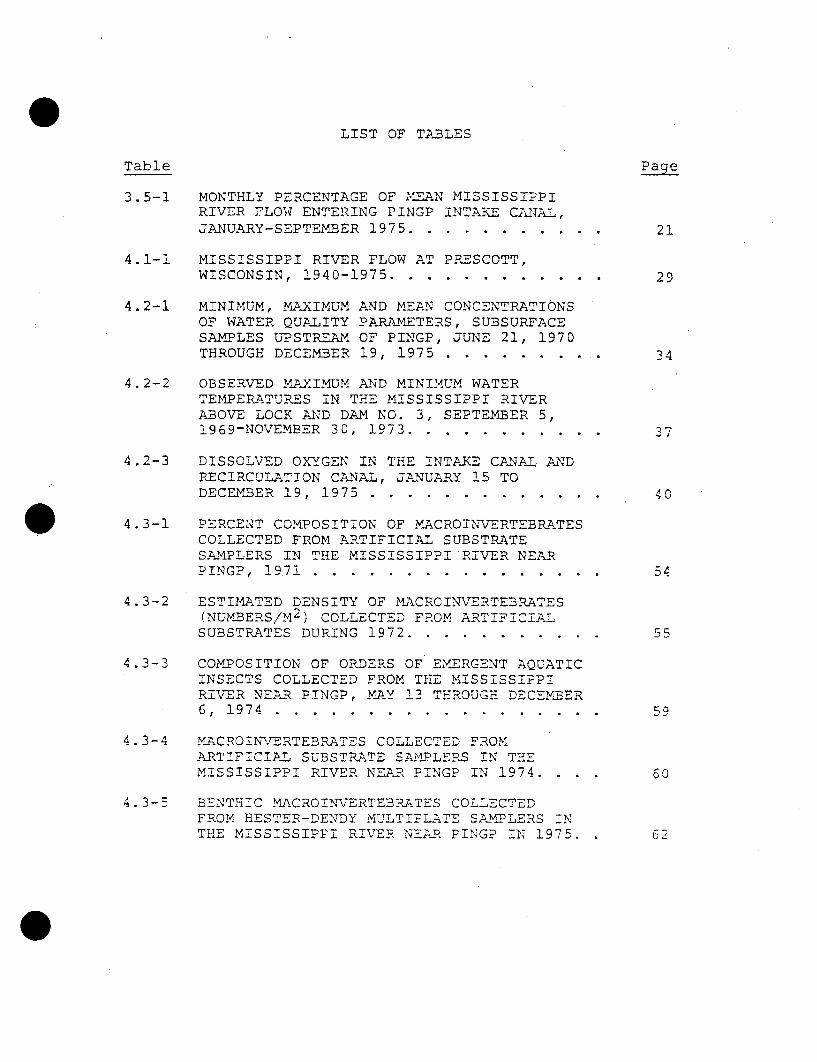
LIST OF TABLES

Table Page

3.5-1 MONTHLY PERCENTAGE OF M-LEAN MISSISSIPPIRIVER FLOW ENTERING P INGP INTAKE CANAL,JANUARY-SEPTEMBER 1975 ........... ........... 21

4.1-1 MISSISSIPPI RIVER FLOW AT PRESCOTT,WISCONSIN, 1940-1975 ............. ............ 29

4.2-1 MINIMUM, MAXIMUM AND MEAIN CONCENTRATIONSOF WATER QUALITY PARAMETERS, SUBSURFACESAMPLES UPSTREAM OF PINGP, JUNE 21, 1970THROUGH DECEMBER 19, 1975 ................ 34

4.2-2 OBSERVED MAXIMUM AND MINIMUM WATERTEMPERATURES IN THE MISSISSIPPI RIVERABOVE LOCK AND DAM NO. 3, SEPTEMBER 5,1969-NOVEMBER 30, 1973 ...... ........... 37

4.2-3 DISSOLVED OXYGEN IN THE INTAKE CANAL ANDRECIRCULATION CANAL, JANUARY 15 TODECEMBER 19, 1975 .......... ............. 40

4.3-1 PERCENT COMPOSITION OF MACROINVERTEBRATESCOLLECTED FROM ARTIFICIAL SUBSTRATESAMPLERS IN THE MISSISSIPPI RIVER NEARPINGP, 1971 ............. ................ 54

4.3-2 ESTIMATED DENSITY OF MACROINVERTEBRATES(NUMBERS/M 2 ) COLLECTED FROM ARTIFICIALT

SUBSTRATES DURING 1972 ...... ........... 55

4.3-3 COMPOSITION OF ORDERS OF EM-ERGENT AQUATICINSECTS COLLECTED FROM THE MISSISSIPPIRIVER NEAR PINGP, MAY 1-3 T .ROUGH DECEMBER6, 1974 ................. .................. 59

4.3-4 MACROINViERTEBRATES COLLECTED FROMARTIFICIAL SUBSTRATE SAMPLERS IN THE

MISSISSIPPI RIVER NEAR PINGP IN 1974. . . . 60

4.3-5 BENTHIC MACROINVERTEBRATES COLLECTEDFROM HESTER-DENDY MULTIPLIATE SAMPLERS INTHE MISSISSIPPI RIVER NEA-R PINGP IN 1975. . 62

LIST OF TABLES (CONTINUED)

Table Pace

4.3-6 BENTHIC MACROINVERTEBRATES COLLECTED INTHE VICINITY OF PINGP IN 1975 ......... 72

4.3-7 COMMON AND SCIENTIFIC FISH NAMES ANDMETHODS OF FISH CAPTURE IN THE PINGP AREA,1975 ................ .................... 77

4.3-8 ESTIMATED HARVESTS OF THREE MAJOR GAMESPECIES CAUGHT IN THE VICINITY OF PINGP1973 AND 1974 ......... .............. .. 83

4.3-9 ESTIMATED NUMBERS OF FISH HARVESTED IN THEVICINITY OF PINGP, 1975, BASED ON OVERALLCATCH RATES AND ESTIMATED MAN-HOURS....... 84

4.3-10 OVERALL CATCH RATE OF ALL ANGLERS FISHINGTHE PINGP AREA MAY 10-NOVEMBER 5, 1973 ANDPERCENT SUCCESSFUL ANGLERS ............... 85

4.3-11 OVERALL CATCH RATE FOR INTERVIEWED ANGLERSIN PINGP VICINITY, APRIL 30-DECEMBER 3,1974 ................ .................... 87

4.3-12 OVERALL CATCH R.ATES FOR INTERVIEWED INPINGP VICINITY, 1975 ............ ............ 88

4.3-13 COMlMERCIA.L CATCH OF FISH (POUNDS) IN POOLS3, 4 AND 4A (IAKE PEPIN) DURING 1970-1974.WISCONSIN AND MINNESOTA LANDINGS COMBINED 90

4.3-14 POPULATION ESTIMATES OF SPORT FISHES IN THE12-MILE PINGP STUDY AREA BASED ON PETERSONAND SCHNABEL TAG AND RECAPTURE MTHODS. 92

4.3-15 TRAI' CATCH OF FISHES IN NORTH LAKE ANDPINGP PLANT AREA (INTAKE AND DISCHARGE) IN1973, 1974 AND 1975 ....... ............ 98

4.3-16 SEINE CATCH IN THE PINGP REGION, 1974 . . . 101

4.3-17 SEINE CATCH IN THE PINGP REGION, 1975 . . . 103

4.3-18 SEINE CATCH (NUMBER PER HECT? RE) IN THEPINGP REGION, 1973-1975 ..... .......... i06

LIST OF TABLES (CONTINUED)

Table Page

4.3-19 ELECTROFISHING CATCH IN THE MISSISSIPPIRIVER NEAR PINGP, 1970 AND 1971 ......... .. 108

4.3-20 ELECTROFISHING CATCH IN THE MISSISSIPPIRIVER NEAR PINGP, 1973 ........... ........... 110

4.3-21 ELECTROFISHING CATCH IN THE PINGP REGION,SPRING, 1974 .......... .................. l1

4.3-22 ELECTROFISHING CATCH IN THE PINGP REGION,SUMMER, 1974 .... ................... . ... 112

4.3-23 ELECTROFISHING CATCH IN THE PINGP REGION,FALL, 1974 ................ ................. 113

4.3-24 ELECTROFISHING CATCH IN PINGP REGION,SPRING, 1975 .................. ........ 1.... 114_

4.3-25 ELECTROFISHING CATCH IN PINGP REGION,SUMMER, 1975 .......... ................ 115

4.3-26 ELECTROFISHING CATCH IN PINGP REGION, FALL,1975 ................ .................... 116

4.3-27 ELECTROFISHING CATCH (NUMBER/HOUR) OF MAJORFISH SPECIES IN THE MISSISSIPPI RIVER NEARPINGP, 1974 AND 1975 ....................... 117

4.3-28 TRAP NETTING CATCH IN THE MISSISSIPPI RIVERNEAR PINGP IN 1970, 1972 AND 1973 ..... 121

4.3-29 TRAP NET CATCH IN PINGP REGION, SPRING, 1974. 123

4.3-30 TRAP NET CATCH IN PINGP REGION, SUMMER, 1974. 124

4.3-31 TRAP NET CATCH IN PINGP REGION, FALL, 1974. 125

4.3-32 TRAP NET CATCH IN PINGP -REGION, SPRING, 1975. 126

4.3-33 TRAP NET CATCH IN PINGP REGION, SUMMER, 1975. 127

4.3-34 TPR- NET CATCH IN PINGP REGION, FALL, 1975. 128

4.3-35 TrPAP NETTING CATCH OF MAJOR SPECIES IN PINGPREGION, 1974 ............ ................. 129

LIST OF TABLES (CONTINUED)

Table Pace

4.3-36 TRAP NETTING CATCH OF MAJOR SPECIES INPINGP REGION, 1975 ........ ............. 130

4.3-37 FISH CATCH IN GILL NETS IN PINGP REGION,1972 AND 1973 ..................... .... 132

4.3-38 GILL NET CATCH IN PINGP REGION, SPRING ANDFALL, 1974 .............. .............. 133

4.3-39 GILL NET CATCH IN PINGP REGION, SPRING ANDFALL, 1975 ............ .......... ....... 134

5.2-1 SAMP;LING DATES AND CORRESPONDING SAMPLINGPERIOD .............. ................... 153

5.3-1 THE EFFECT OF PASSAGE OF PHYTOPLANKTONTHROUGH PINGP ON CHLOROPHYLL a, PHOTO-S"YNHESIS AND RESPIRATION, 1974. . ......... 161

5.3-2 ESTIMATED PERCENT MORTALITY OF ZOOPLANKTONDUE TO PLANT PASSAGE AT PINGP IN.1974 . . . 165

5.3-3 ESTIMATED PERCENT MORTALITY OF ZOOPLANKTONDUE TO PLANT PASSAGE AT PINGP IN 1975 AND1976 . . . .. .. . ......... .. . .... ..... 16.6

5.3;4 FISH EGGS AND YOUNG COLLECTED IN ENTRAINMENTSAMPLING AT PINGP, 1975 .................... 169

5.3-5 MEEAN DENSITY AND PERCENT OF CATCH OF YOUNGFISH COLLECTED IN ENTRAINMENT SAMPLING ATPINGP, 1975 ........... ................ 172

5.3-6 MEAN DENSITY OF FISH LARVAE AT THE BAR RACKSTATION AT PINGP, 1975 ....... ........... 174

5.3-7 ESTIMATED NUMBER OF LluRVAE AND JU'VENILESPASSING THROUGH THREE LOCATIONS AT PINGP,1975 ........ ...................... ..... 183

5.3-8 NUMBER OF FISH PER WEEK COLLECTED FROM THETRASHBASKETS AT P±NGP, 1974 ......... ........ 287

5.3-9 NUMBER OF FISH PER WEEK COLLECTED FROM THETRASHBASKETS AT PINGP, 1975 ........ 191

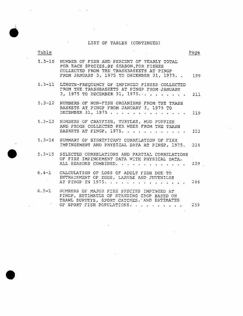
LIST OF TABLES (CONTINUED)

Table Paae

5.3-10 NUMBER OF FISH AND PERCENT OF YEARLY TOTALFOR EACH SPECIES,BY SEASON,FOR FISHESCOLLECTED FROM THE TRASHBASKETS AT PINGPFROM JANUARY 3, 1975 TO DECEMBER 31, 1975. 199

5.3-11 LENGTH-FREQUENCY OF IMPINGED FISHES COLLECTEDFROM THE TRASHBASKETS AT PINGP FROM JANUARY3, 1975 TO DECEMBER 31, 1975 ............ 211

5.3-12 NUMBERS OF NON-FISH ORGANISMS FROM THE TRASHBASKETS AT PINGP FROM JANUARY 3, 1975 TODECEMBER 31, 1975 ............... .............. 219

5.3-13 NUMBERS OF CRAYFISH, TURTLES, MUD PUPPIESAND FROGS COLLECTED PER WEEK FROM THE TRASHBASKETS AT PINGP, 1975. ... .... .......... 222

5.3-14 SUM!MARY OF SIGNIFICANT CORRELATION OF FISHIMPINGEMENT AND PHYSICAL DATA AT PINGP, 1975. 226

5.3-15 SELECTED CORRELATIONS AND PARTIAL CORRELATIONSOF FISH IMPINGEMENT DATA WITH PHYSICAL DATA,ALL SEASONS COMBINED ...... .................. 229

6.4-1 CALCULATION OF LOSS OF ADULT FISH DUE TOENTRAINMENT OF EGGS, LARVAE AND JUVENILESAT PINGP IN 1975 ............. ............. 246

6.5-1 NUMBERS OF MAJOR FISH SPECIES IMPINGED AT

PINGP, ESTIMATES OF STANDING CROP BASED ONTRAWL SURVEYS, SPORT CATCHESKAND ESTIMATESOF SPORT FISH POPULATIONS.. ................ 259

1. STATEMF-NT OF THE PROBLEM

The Federal Water Pollution Control Act Amendments of 1972

(P.L. 92-500), Section 316(b), require that cooling water

intake structures reflect the best technology available

for minimizing adverse environmental impact. Adverse

impact can result from entrainment and impingement of aquatic

organisms. Entrainment is the withdrawal of organisms into

the cooling water system. It involves organisms which are

small enough to pass through the intake screen mesh, including

primarily planktonic forms such as phytoplankton, zooplankton,

ichthyoplankton, and benthic drift organisms. Mortality can

vary, depending on the system and the trophic level involved,

and is usually less than 100 percent in open systems but may

approach 100 percent in closed systems.

Larger organisms can become entrapped or impinged against

screening equipment. These larger organisms are predominantly

fish which may tire or become injured and are unable to

escape. High impingement mortality often results from

natural die-offs or weakening of fish prior to impingement

(Edsali and Yocun 1972, Quirk, Lawler and Matuskv 1974) or

cold-induced lethargy (EPA 1976a, USAC 1972). The use of

traveling screens may reduce mortality but frequently induces

additional injury.

According to the current EPA draft guidance manual (1976a)

for Section 316(b), "Regulatory agencies should clearly

recognize that some level of intake damage can be acceptable

and thus represents a minimization of environmental impact."

This demonstration provides "best possible estimate of what

damage is or may be occurring" and relates this to population

levels and natural variability of the indigenous Mississippi

River populations near the Prairie island Nuclear Generating

Plant (PINGP).

2

2. SUMMARY

Section 316(b) of the Federal Water Pollution Control Act

Amendments of 1972 requires cooling water users to determine

biological effects of their intake systems and to demonstrate

that the design, construction, location and operation re-

flect the best technology available for minimizing impact.

Under the National Pollutant Discharge Elimination System''

(NPDES) Section 402 of P.L. 92-500, Minnesota has been given

the authority to administer the law using the Section 316(b)

amendments and Minnesota Regulation WPC(u) (3).

The Minnesota guide for the administration of Section 316(b)

requires the demonstrator to show the environmental effects

of cooling water intakes through documentation of the magnitude

of impingement and entrainment impacts (MWCA 1975). Supple-

mental information on the aquatic ecosystem in the intake

region is also requested. Federal and state requirements

have been addressed in this demonstration by providing

extensive baseline data and a detailed presentation and

analysis of entrainment and impingement data at the Prairie

Island Nuclear Generating Plant (PINGP).

Northern States Power Company (NSPY has conducted six years

of studies of the Mississippi River ecosystem near PINGP

and, since plant operaticn began in 1974, NSP has conducted

3

extensive intake studies. The river at PINGP can be classified

as somewhat eutrophic and supporting a healthy and very

diverse flora and fauna. The main channel and the associated

side channels of slack water provide a mixture of lentic and

lotic habitats.

The entrainment of primary producers (phytoplankton) reduced

standing crops of chlorophyll a but did not produce detect-

able effects on total numbers of algae. Chlorophyll a

reduction usually amounted to 50 percent or less., Primary

productivity of entrained algae was depressed up to 90 per-

cent from passage through PINGP. Respiration was similarly

depressed on most collection dates. In summary, while

the numbers of intact algae are not greatly affected by

plant passage, the biological activity of the algal community

is frequently reduced by 50 percent or more.

Studies of the effects of plant passage on phytoplankton

failed to produce any detectable differences in the community

of the main channel of the Mississippi River, either in

species composition or primary productivity, corroborating

the conclusion of EPA (1976b) that entrainment effects on

phytoplankton are usually of short duration and confined

to a relatively small portion of the water body.

4

Zooplankton entrained by PINGP was noticeably affected on W

two-thirds of the dates sampled. Usually only one or two

groups exhibited detectable mortality after plant passage.

Excepting cladocerans, some mortality was observed for all

groups on some collection dates.

Zooplankton collected at the intake and discharge was also

compared to zooplankton collected in the water body near the

plant. No significant differences in total zooplankton densities

could be detected, even within the recirculation canal. Some

preliminary data indicated reduction of copepods in areas

directly within the discharge. The low degree of entrainment

impact at PINGP is further supported by EPA's (1976b) comment

that in most cases the effects of zooplankton entrainment

are of relatively short duration and confined to a relatively

small area of the water body.

The entrainment of benthos was not studied; however, the

extensive program of artificial substrate studies permitted

a prediction of taxa most likely to be entrained. Benthic

entrainment is not predicted to seriously affect aquatic

communities near PINGP.

There are two potential sources of impact to the fish

communities near PINGP: entrainment of eggs and young

and impingement of larger fish. A total of 8,371,000 eggs

and 61,645,000 larvae and juvenile fish were estimated to

have been entrained between May 12 and September 10, 1975.

However, larval and juvenile entrainment represented only an

estimated 6 percent of the 1,038,000,000 young fish estimated

to have passed through the outlet of Sturgeon Lake during

the same period. This represents a conservative estimate of

loss to the total system because fish eggs and larvae

are also present in the main channel.

Entrainment losses of eggs and young fish were estimated to

represent 2,830,000 potential adult fish, 99 percent of

which were forage species. This loss of forage fish could

decrease predator production by an estimated 3,400 kg (7,500

lbs) or 5,900 fish. However, the larval and juvenile forace

fish entrained represent only about 3 percent of the esti-

mated number nassina through the outlet of Sturgeon Lake.

Entrained sport and commercial species represented less than

one percent cf the total Dotential adult loss. Sauger had

the greatest potential loss among the sport fish (5,600

fish). This potential loss is 0.9 to 2.4 percent of the

estimated population for the Sturgeon Lake to Lake Pepin

region. The impact of the potential adult loss will probably not

be detectable due to the highly mobile nature of sauger in

6

the PINGP area. Approximately 730 potential adult white

bass are estimated to be lost due to entrainment. This

represents 0.4 to 0.5 percent of the population estimated

between Sturgeon Lake and Lake Pepin. Walleye, sunfish,

crappies, northern pike and yellow perch were the other

sport fish that were entrained. Estimated adult loss for these

species represented less than 10 percent of their combined

annual angler harvest, and probably a much smaller percent-

age of their actual populations in the PINGP area.

Commercially important fishes that were entrained included

reshwater drum, carp, buffalo, catfish, sucker and carp-

sucker. The potential loss of carp and catfish appears

insignificant compared to commercial catch data; the impact

on the other taxa is unclear due to low commercial catches.

However, a comparison of numbers entrained to estimated

numbers of young passing through the mouth of Sturgeon Lake

indicates low potential impact to resident populations.

Impingement analyses were conservative estimates based on

the number of fish impinged per year in relation to the best

population estLmates that could be determined from available

data.

7

Small fish, mostly 40-200 mm, accounted for most of the

146,063 fish impinged in 1974 and 93,466 fish impinged in

1975.

Although gizzard shad composed more than three-fourths of the

fish impinged,losses represent only 1 to 2 percent of the

estimated 1973 Sturgeon Lake population.

Potential impact on the channel catfish population was

inconclusive due to apparently low population estimates

based on trawl samples. However, the numbers of young

impinged represent a small fraction of the number which

could be produced in one year by the estimated adult popula-

tion or number of catfish commercially harvested in one

year.

The numbers of impinged freshwater drum represented 10 to 12

percent of the young estimated for the plant area or North

Lake, based on trawl collections, and 5.2 percent cf the

commercial harvest of adults in 1974.

Annual impingement losses of young white bass, sauger and

walleye were 0.1 to 1 percent of the estimated sport fish

populations between Sturgeon Lake and Lake Pepin. Potential

8

adult losses would be substantially less die to mortality

between the young and sport harvest sizes.

The combined impact of the impingement and entrainment

losses for fish, plankton and benthos is considered to

represent an acceptable level of impact for a generating

facility of the size of PINGP. Losses to lower trophic

levels are, at most, barely detectable in the immmediate

plant vicinity. Fish entrainment losses represent such low

percentages of ambient populations that no short or long

term effects are expected to be detectable.

The numbers of young fish impinged per year appear to re-

present only a small percentage increase in the mortality

resulting from natural causes and fishing. The numbers of

young white bass, walleye and sauger Lmpinged are approxi-

mately 0.2 percent of their adult populations in the region

and represent an even smaller percentage loss of recruitment

into the sport fishery. Due to the apparent excess of

forage fish (most gizzard shad) and minimal cropping of

sport fish, there is not expected to be a noticeable change

in the dynamic predator/prey relationship or in recruitment

into the harvested populations.

0

3 DESCRIPTION OF TH.E P'LANT

The Prairie Island Nuclear Generating Plant (PINGP) is a two-

unit plant utilizing pressurized water nuclear steam supply

systems. Each unit produces a gross electrical output of

560 MWe for Northern States Power Company's network system.

Unit 1 operation began in December 1973 and Unit 2, one year

later.

3.1 LOCATION OF PLANT AND INTAKE

PINGP is located on the Minnesota shore of the Mississippi

River 65 km (40 mi) southeast of Minneapolis and St. Paul,

Minnesota and 10 km (6 mi) upstream of Red Wing, Minnesota

(Figure 3.1-1). The plant is situated on Prairie Island,

a low island terrace peninsula formed by the Mississippi

River on the east and the Vermillion River on the west.

Most of the land surrounding the plant is under cultivation.

Relatively small areas of forest and swamp vegetation occur

in some lowlands. The Mississippi River in the vicinity of

PINGP is a complex system of river lakes, sloughs, channels

and islands (Figure 3.1-2). Major features include North

and Sturgeon lakes, just upstream of the plant, and the main

river channel, which is closer to the Wisconsin shore. Lock

and Dam No. 3, which controls the levels of the Mississippi

River and Sturgeon Lake, is 2 km (1 mi) downstream of the

10

I 'I

-ST. PAUL

MINNEAPOLIS-+I

H--

U. S. HIGHWAY W• 61

RED

SCALE0 50 100

KILOMETERS

.1

z ,t

WINONA

CROSSEI".'

1;O

.-

V•

..SI'" .

FIGURE 3.1-1

GENERAL LOCATION OF PINGP

LOCK a DAMNO.3

STURGEON 7

MISSISSIPPI-RIV ER

SREFAG

t*. - N -A tGit. - A U

AKIN . p A. .. ' " ' ~

A' A''~ 1..4 O'A '.AA4 *A'.A

A', - 10 0 0 0.0O

tO0 §00 100o 200 MI00 400 500

FIGURlE 3.1-2

IMMEDIATE T"'"ATION OF PINGP

site. The average monthly river discharge at Prescott,

Wisconsin, which is 24 km (15 mi) upstream from PINGP, is

457 m /sec (16,130 cfs) (USGS 1928-1975).

13

3.2 INTAKE DESIGN

Cooling water is drawn from the river into an intake canal,

which is 34 m (112 ft) wide and 231 m (758 ft) long. A

skimmer wall at the mouth of the intake canal excludes

floating debris from the intake (Figure 3.2-1). At the

screenhouse (Figure 3.2-2), the water passes through a bar

rack, which consists of 1 cm wide vertical steel bars spaced

7.6 cm apart. The water then passes through eight vertical

traveling screens. The screens are constructed of wire mesh

with 1 cm square openings. After passing throuah the traveling

screens, the water enters one of four circulating water

pumps [capacity of one pump = 10.08 m3 /sec (356 cfs)] and is

pumped through the condensers. Water velocities in the

intake system vary from 2 to 6 cm/sec (0.1-0.2 fps) at the

skimmer wall and from 6 to 30.5 cm/sec (0.2-2.5 fps) in front

of the bar rack.

Any debris collecting on the traveling screens as the water

passes through is washed from the rotating screens by high-

pressure water jets. The debris is carried into a sluice

canal and then to the trash baskets. These baskets are

constructed of metal grating with 1.7 X 3.3 cm openings and

are 1.5 X 1.5 X 1.5 m overall.

14

N

S§CALE0 500 1000

FE ET

WINGDAMS

Ln

0-I-JUL

I

FIGURE 3.2-1

FLOW PATHIS IN THE PINGP CONDENSER SYSTEM

0

"TRAVr&LI Nc

5CREENGRA•DE

RACK

PL ANT

C I RCULATI NG

WATER, PUMP

FIGURE 3.2-2

CROSS-SECTION OF PINGP SCflEENHOU(],E

3.3 OPERATING MODES

There are three possible modes of operation at PTNGP

because of the condenser cooling-water design. These are

the open cycle mode, the helper cycle mode, and the closed

cycle mode. Cooling towers do not operate in the open cycle

mode and water taken through the condensers from the intake

is discharged directly to the river. The helper cycle

mode also signifies once-through flow but with the cooling

towers in operation to decrease the temperature of the system

water before it is discharged back to the river.

Under closed cycle operation (Figure 3.3-1), the normal

operating mode of the plant, water is piped from the con-

densers to the cooling tower pump basin and then to the

cooling towers. Water from the cooling towers drains into

the discharge basin and is routed through the recycle canal

and intake canal back to the screenhouse. Under these

conditions, up to 90 percent of the intake water is recycled.

Under normal closed-cycle operation with cooling towers in

operation, the intake or makeup water appropriation is 5.2 m3 /sec

3(183 cfs) to make up for the loss of 1 m /sec (33 cfs)

cooling tower evaporation and 4.2 m 3/sec (150 cfs) discharge.

17

TOWER LOSS33 cfs (MAX.)60 cfs

60FROMRIVER183 cfs

SCREEN CON-HOUSE 1424 cfs DENSERS 1424 cfs 1484 cfs

cfs1RECYCLES C RE IPEEN

10WASH

FIGURE 3.3-1

FLOW RATES IN THE CLOSED-CYCLE MODE FOR CONDENSERCOOING AND TUE SERVICE WATER SYSTEM

3.4 INTAKE VELOCITIES W

Intake velocities were measured on June 23 and June 28,

1976. Velocity profiles (Appendix 1) were taken in front of

the bar rack and immediately in front of the skimmer wall.

During the June 23 survey, the blowdown rate was 7.8 m3 /sec

(275 cfs). In front ofthe skimmer wall, velocities ranged

from 0.0 to 0.2 m/sec (0.0-0.7 fps). Velocities in front

of the bar rack were higher, with most readings varying

between 0.2 and 0.4 m/sec (0.7-1.3 fps).

During the June 28 survey, velocities at the skimmer wall

were measured at blowdown rates of 18.5 m 3/sec (655 cfs)

and 36.8 m3 /sec (1300 cfs). At the lower blowdown rate,

velocities at the skimmer wall were between 0.00 and 0.25

m/sec (0.00-0.82 fps). At the blowdown rate of 36.8 m 3/sec

(1300 cfs), roughly equivalent to helper cycle operations,

the velocities at the skimmer wall ranged from 0.05 to 0.30

M/sec (0.16-0.09 fps).

3.5 INTAKE FLOW VOLUMES

Recent studies indicated that intake flow volumes are an

important factor in impingement and entrainment (EPA 1976a).

Under closed cycle mode, the makeup water appropriation

or intake volume at PINGP is approximately 5.2 m3 /sec (183

cfs). During 1975, the average makeup water appropriation

was approximately 11.2 m 3/sec (400 cfs). A frequency analysis

for appropriations based on 1975 plant records is:

Appropriation Appropriation* (m /sec) (cfs) Percent of Year (1975)

<2.8 <100 <0.12.8-5.7 100-200 40.85.7-11.3 200-400 19.7

11.3-17.0 400-600 17.017.0-22.7 600-800 6.122.7-28.3 800-1000 8.6

>28.3 >1000 3.1no data no data 4.7

3All appropriation flows greater than 17.0 m /sec occurred

between May and September. Highest intake volumes were

reported in July when appropriation was greater than 22.43

m /sec more than 70 percent of the time. Peak intake volumes

corresponded with the peak flow periods for the Mississippi

River near PINGP and the appropriation was less than 5

percent of the total Mississppi River flow measured at

Prescott, Wisconsin (Table 3.5-1). The maximum percent

withdrawal for 1975 was recorded on September 8, when approxi-

mately 14 percent of Mississippi River flow was used for the

appropriation flow.

20

TABLE 3.5-1

PERCENTAGE OF MEAN MONTHLY MISSISSIPPI RIVER FLOW",T ENTERINGPINGP INTAKE CANAL, JANUARY-SEPTEMBER 1975

Month

January

February

March

ADril

May

June

July

August

September

River Flowa

7,995

8,691

9,944

45,C60

65,220

36,200

38,010

11,790

10,950

Percent ofAverage Mean Monthly River

Intake Flow Flow Entering(cfs) 'Intake Canal

188 2.4

299 3.4

341 3.4

454 0.1

791 1.2

304 0.8

782 2.1

576 4.9

415 3.8

a1975 USGS data (cfs) at Prescott, Wisconsin

21

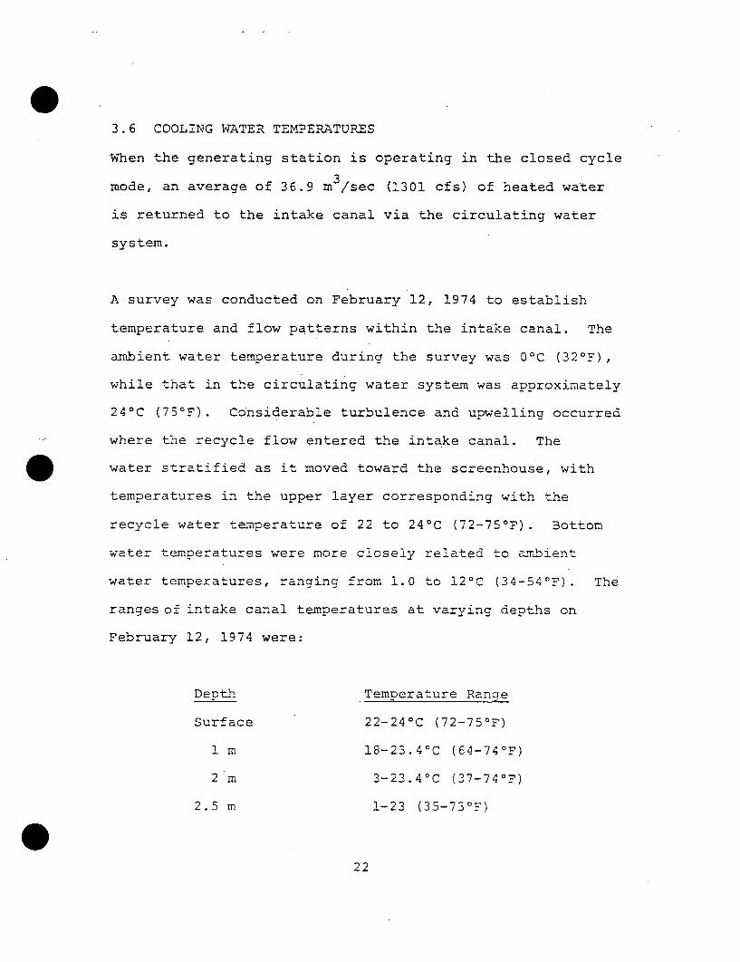
3.6 COOLING WATER TEMPERATURES

When the generating station is operating in the closed cycle

mode, an average of 36.9 m 3/sec (1301 cfs) of heated water

is returned to the intake canal via the circulating water

system.

A survey was conducted on February 12, 1974 to establish

temperature and flow patterns within the intake canal. The

ambient water temperature during the survey was 00 C (320F),

while that in the circulating water system was approximately

241C (750F). Considerable turbulence and upwelling occurred

where the recycle flow entered the intake canal. The

water stratified as it moved toward the screenhouse, with

temperatures in the upper layer corresponding with the

recycle water temperature of 22 to 241C (72-75'F). Bottom

water temperatures were more closely related to ambient

water temperatures, ranging from 1.0 to 12'C (34-54'F). The

ranges of intake canal temperatures at varying depths on

February 12, 1974 were:

Depth TemDerature Range

Surface 22-24 0 C (72-750F)

1 m 18-23.4-C (64-74-F)

2 m 3-23.4 0 C (37-74°F)

2.5 m 1-23 (35-730F)

22

Water temperatures near the bottom increased as flow pro-

ceeded along the intake canal. Water temperatures near the

screenhouse were nearly homogeneous from top to bottom

(22.8-240 C) (73-75 0 F).

Temperatures in the intake, discharge and circulation canal

are recorded automatically. Figure 3.6-1 shows the monthlyminimum and maximum water temperatures in the intake canal

for the first two years of full time operation (1.974 and

1975).

3.7 BIOCIDES

Chlorine is used in many generating plant condensers and

cooling towers to control biological growth, especially

algae. PINGP employs a mechanical tube cleaning system;

thus, no chemical additions are required for this aspect of

plant operation. However, the inlet water for the service

water system is chlorinated. Chlorine is injected for 20-

minute periods three times a day. The injection rate is

controlled so that total residual chlorine is less than 0.3

mg/l at the point where the service water system flow enters

the circulating water system. The service water system flow

at that point represents about 4 percent of the circulating

water volume (see Figure 3.3-1); thus the maximum total

23

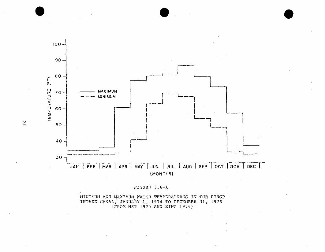
000IOO

90-

80-

TO 70- MAXIMUM~~~~MINIMUM r - - ._

Lo 60- I

50I

40 ------

30-

JAN 1 FEB IMAR i APR MAY I JUN t JUL t AUG SEP IFOCT(MONTHS)

FIGURE 3.6-1

MINIMUM AND MAXIMUM WATER TEMPERATURES IN THE PINGPINTAKE CANAL, JANUARY 1, 1974 TO DECEMBER 31, 1975

(FROM NSP 1975 AND KING 1976)

1

residual chlorine concentration which is present after W

mixing with the recirculation water is 0.02 mg/l.

The chlorine residual is further reduced by the chlorine-

demand constituents of the recirculation water and by dilution

which occurs when the recirculation water enters the intake

canal. The permissible limit for total chlorine in the State

of Minnesota for intermittent discharges is 0.2 mg/1, for

periods not to exceed 2 hours (Olsen, personal communcation).

Chlorine levels in the intake canal are, therefore, well below

the permissible limits.

250

4. DESCRIPTION OF THE AQUATIC ENVIRONMENT NEAR PINGP

4.1 HYDROLOGY

The river basin above PINGP has a drainage area of approxi-

mately 72,500 km2 (45,000 mi2 ). The basin covers central

and southern Minnesota, and includes portions of Wisconsin,

South Dakota and Iowa.

The numerous lakes in the region are the result of Pleistocene

glaciation. The flow characteristics of the Mississippi

River and its tributaries are largely determined by the

natural storage provided by these lakes and numerous swamps

(USAEC 1973). The nearest permanent USGS hydrological

gauging station is located at Prescott, Wisconsin, approxi-

mately 24 km (15 mi) upstream from PINGP. Flow records at

Prescott are available from 1928 through 1975.

Records for the 48 years show an average monthly discharge

of 457 m /sec (16,130 cfs). The annual mean flow duration curve

for the Mississippi River at Prescott is show-n in Figure

4.1-1. Maximum discharge for the period of record was

36,460 m /sec (228,000 cfs), reported on April 18, 1965;. the

3minimum flow was 39.1 m /sec (1,380 cfs), registered on July

13, 1940. The minimum consecutive-day, low-flow rates from

1928 to 1975 show that the five lowest years of record all

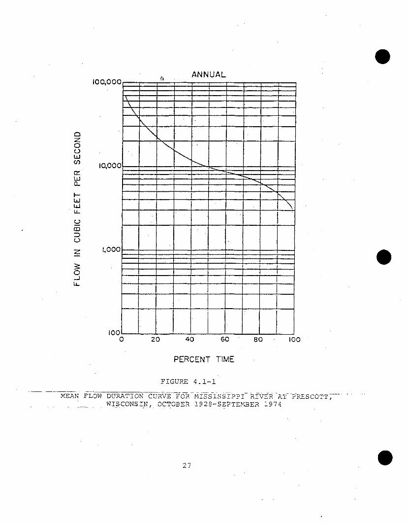
ANNUAL

0z -

o0

z I-,000

Z ~1,000.. ,

L... - - - -

Li....

I00 - --- - . - . -

0 20 40 60 80 t00

PERCENT TIME

FIGURE 4.1-1

MEAN FLOW DURATION CURVE FOR MISSISSIPPI RIVER AT ]PRESCOTT,.. - WISCONSIN, OCTOBER 1922-SEPTEMBER 1974

27

occurred before 1941; thus it appears that structures, such

as Lock and Dam No. 3, on the river have served to augment

low flow (USAEC 1973). Median monthly flows and projected

7-day, 10-year. low flows are listed in Table 4.1-1. Con-

secutive day, average-low flow frequencies for the Mississippi

River at Prescott are shown in Figure 4.1-2.

Flood flow conditions are most common during the spring and

early summer months; highest frequencies occur in April.

The most serious flooding is associated with heavy rainfall

and melting of heavy snows. Major floods in the main streams

occur on the average of 2-3 years out of 10 (USAEC 1973).

The maximum flood of record for the upper Mississippi River

occurred in April, 1965. The frequency probability of this

flood was estimated as that occurring once in 150 years.

The numerous side channels of slack-water areas are of

special importance to PINGP. The North Lake-Sturgeon Lake

chain has several cross connections resulting in a diversion

of part of the Mississippi River flow through the lakes. In

analysis of the flow through the lake, it was estimated

that between 19 and 32 percent of the total river flow at

Lock and Dam No. 3 passed through the outlet of Sturgeon

Lake at river flows between 226.4 and 1867.8 m 3/sec,

respectively. (Grotbeck personal communication). This was

28

TO

60

X o0-i5

2

I010

00 5 10 20 25

STURGEON LAKE FLOW ( X &3 cfs)

VIGURE 4.1-3.

STURGEON LAKE FLOW VS. MISSISSIPPI RIVER FLOW, ASMEASURED AT LOCK AND DAM NO. 3

22

4.2 WATER QUALITY

4. 2. 1 General Character~istics

PINGP is located in a section of the Mississippi River

that is affected by discharges from the Minneapolis-St. Paul

metropolitan complex. Other environmental factors which

influence water quality near the site include the 2.7 m

(9 ft) minimum depth navigation channel, nutrient and

sediment runoff from surrounding croplands and the lock and

dam system.

Water quality at or near PINGP has been monitored from

June 21, 1967 to the present. Table 4.2-1 lists the

minimum, maximum and mean concentrations for the chemical

parameters examined.

Waters near PINGP show relatively high nutrient levels, a

characteristic of waters located downstream from municipal

waste treatment facilities. As a result of these enriched

conditions, somewhat eutrophic conditions prevail. Phosphorus

and nitrogen levels are generally highest during the winter-

spring transition period and decrease markedly during the

summer. Largely because of assimilation of CO2 by algae,

there is also a trend toward higher pH as summer progresses.

33

TABLE 4.2-1 (Sheet 1 of 2)

MINIMUM, MAXIMUM AND MEAN CONCENTRATIONS OF WATER QUALITYPARAMETERS, SUBSURFACE SAMPLES UPSTREAM OF PINGP,

JUNE 21, 1970 THROUGH DECEMBER 19, 1 9 7 5 a

Concentration(mg/i unless otherwise noted)

Solids, Total

Solids, Dissolved

Solids, Suspended

Hardness, Total (as CaCO3 )

Hardness, Calcium (as CaCO 3 )

Hardness, Magnesium (as CaCO3 )

Alkalinity, Total (as CaCO 3 )

Alkalinity, Phenolphthalein (as CaCO3

.Ammonia Nitrogen (N)

Carbonateb (C0 3 )b

Bicarbonate (HCO 3 )

Chloride (Cl)

Nitrate Nitrogenc (N)

Sulfate (SO 4 )CPhosvhorus , Soluble (P)

Silica (S 1 0 2 )b

Cal ci um (Ca)b

Magnesium (Mg)

Sodium, (Na)

Iron, Totalc (Fe)

Colorc (APHA units)

Turbidity (JTU)

Ryznar Index (at 77 0 C)

Conductivity (}h o s/cm)

pH

BODb

Minimum

192

134

1.4

116

76

40

102

0

0

0

103

2

0.03

10

0.005

0.4

30.4

9.7

3.9

0.04

20

1

5.9

245

7.4

! .I

Maximum

443

367

85

268

180

100

232

24

1.14

27.6

235

32.9

4.2

110

0.550

16.2

72

24

28-5

2.36

100

52

8.5

572

9.2

9.45

Me an

272

244

29

185

120

66

156

2.9

0.39

2.2

178

12.8

1.03

39

0.15

8.6

48

16

11.5

0.68

53

13

7.2

390

8.0

3.2

34

TABLE 4.2-1 (Sheet 2 of 2)

aPrior to plant operation (1970-1973) samples collected at site loca.or

bMinimum, maximum and mean calculated for the period of June 1970

to December 1975.

CMinimum, maximum and mean calculated for the period of January

1970 to December 1975.

35

4.2.2 Water Temperature

Monthly minimum and maximum temperatures at Lock and Dam No.

3 from September 5, 1969 to November 30, 1973 (before plant

operation) are listed in Table 4.2-2. The temperature patterns

are typical of large temperate river systems. Water tempera-

tures typically remain between 0.0 and 1.70C (32-35cF) from

late November through early March and rise rapidly during

the spring. Maximum water temperatures were reported in

July and August. The ambient temperature regimes in the

area are not likely to produce any stress on the fauna that

would contribute to entrainment or impingement suscepti-

bility (USAEC 1973).

4.2.3 Dissolved Oxygen

Organisms undergoing stress as a result of reduced dissolved

oxygen (DO) levels may be more susceptible to impingement

and entrainment. Reduced DO levels have been shown to

reduce maximum sustained swimming speed of fish (Davis et

al. 1963), as well as to affect reproduction, vigor and

development.

Dissolved oxygen levels have been monitored in the Mississippi

River near the PINGP intake canal since July 1970. The

pattern of DO in the Mississippi River at PINGP is character-

istic of an enriched or eutrophic lotic environment.

36

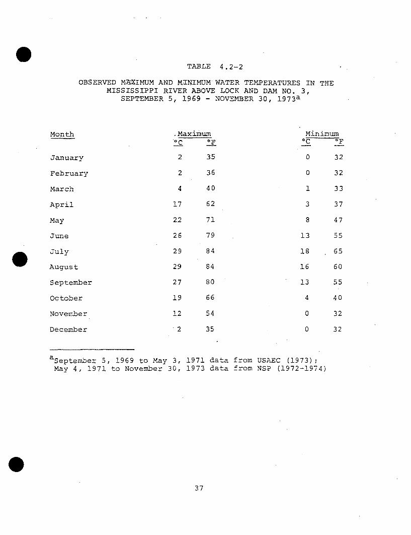
TABLE 4.2-2

OBSERVED MAXIMUM AND KINIMUM WATER TEMPERATURES IN THEMISSISSIPPI RIVER ABOVE LOCK AND DAM NO. 3,

SEPTEMBER 5, 1969 - NOVEMBER 30, 1 9 7 3a

Month

January

February

March

April

May

, Maximum,cC OF

2 35

2 36

4 40

17 62

22 71

26 79

29 84

29 84

27 80

19 66

12 54

2 35

Minimumcc OF

0 32

0 32

1 33

3 37

8 47

13 55

18 65

16 60

13 55

4 40

0 32

0 32

June

July

August

September

October

November

December

aSeptember 5, 1969 to May 3,May 4, 1971 to November 30,

1971 data from USAEC (1973);1973 data from NSP (1972-1974)

37

Significant fluctuations in DO occur over the course of the

year and during the diel cycle. Maximum monthly DO levels

show supersaturation levels, especially during the spring

and summer, whereas minimum levels are, in many cases,

significantly undersaturated. Surface waters may contain 2

to 3 times more DO than bottom waters. Measurements taken

from 1970 to 1975 in the Mississippi River near the intake

canal show that DO levels fell below 5 mg/1 only once (to

3.65 mg/l on August 3, 1972), during that period (Figure

4.2-3).

During the past 4 years, DO levels in the river near the

intake canal and in the main channel have generally in-

creased, probably as a result of improved waste treatment in

the Minneapolis-St. Paul area. No critically low dissolved

oxygen levels (below 5 mg/i) have been reported since August

1972. Thus, it appears that ambient levels of DO will not

contribute to the susceptibility of organisms to entrainment

or impingement.

Dissolved oxygen within the intake and recirculation canals

was monitored in 1975 (Table 4.2-3). DO readings in the

intake and recirculation canal were also taken in 1974 during

one unit operation. DO was measured at two stations within

38

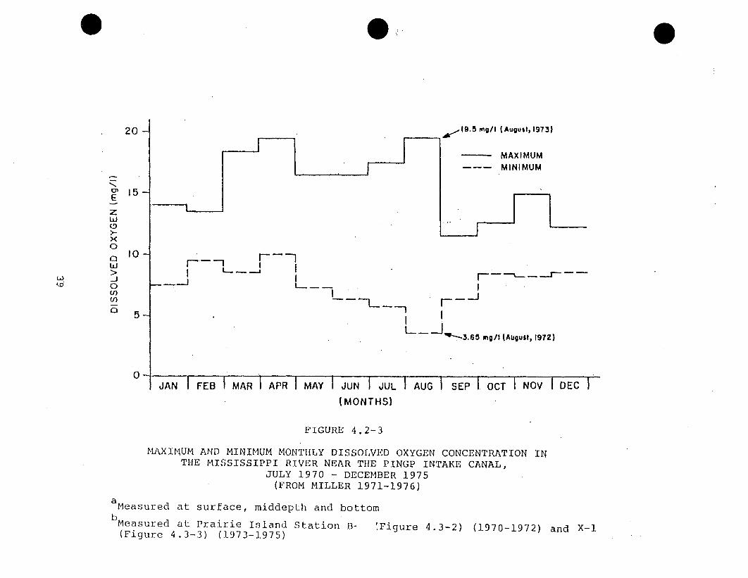
20 19.5 mg/I jAugusi, 1973

MAXIMUMMINIMUM

15-

z

0

>- L.i

X

0 t.

U)

Q 5-

L I-"* 3.65 mg/I (AfigustI 1971

JAN I FEB I MAR 1 APR-I MAY i JUN 1 JUL 1 AUG 1-SEP I OCT I NOV

(MONTHS)

FIGURE 4.2-3

MAXIMUM AND MINIMUM MONTHLY DISSOLVED OXYGEN CONCENTRATION INTHE MISSISSIPPI RIVER NEAR THE PINGP INTAKE CANAL,

JULY 1970 - DECEMBER 1975(FROM MILLER 1971-1976)

aMeasured at surface, middepth and bottombMeasured at Prairie Island Station B- 'Figure 4.3-2) (1970-1972)

(Figure 4.3-3) (1973-1975)

5)

2)

and X-1

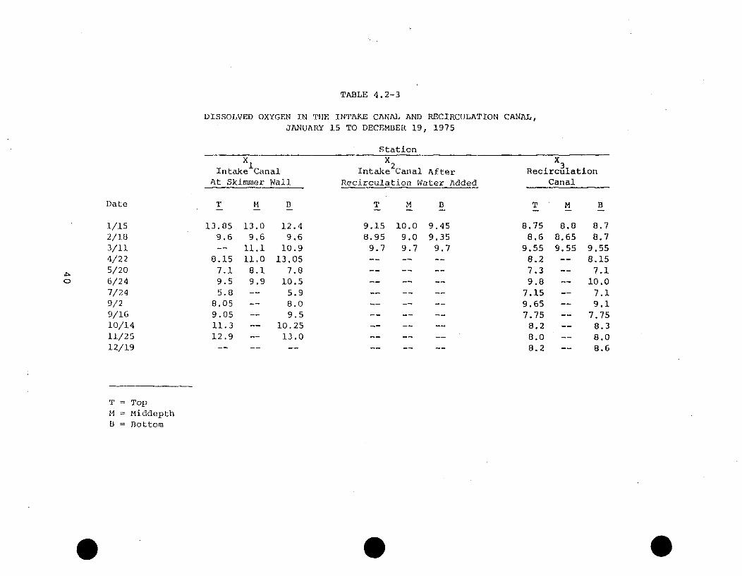
TABLE 4.2-3

DISSOLVED OXYGEN IN THE INTAKE CANAL AND RECIRCULATION CANAL,JANUARY 1.5 TO DECEMBER 19, 1975

StationXI

Intake CanalAt Skimmer Wall

X2Intake Canal After

Recirculation Water Added

X3Recirculation

Canal

D)ate

1/152/1.83/il4/225/20

Co 6/247/249/29/1610/1411/2512/19

T M B T M B T M

13.859.6

8.157.19.55.8

8.059.0511.312.9

13.09,6

11.111i.0

8.19.9

12.49.6

10.913.05

7.010.5

5.98.09.5

10.2513.0

9.158.95

9.7

10.09.09.7

9.459.35

9.7

8.758.6

9.558.27.39.8

7.159.657.75

8.28.08.2

8.88.659.55

B

8.78.7

9.558.15

7.110.0

7.19.1

7.758.38.08.6

T = Top

M = Middepth

B = Bottom

the intake canal (Xl and X2) and one station in the re-

circulation canal (see Figure 4.3-4).

DO levels'in the intake canal at the skimmer wall ranged

from 5.8 to 13.85 mg/l, with lowest levels being reported

in July. DO measurements at Station X2 were taken during

the first 3 months of 1975, and indicated that levels followed

those at the skimmer wall and, to a greater degree, the

recirculation canal. Recirculation water showed relatively

high DO levels throughout the year, ranging between 7.1 mg/l

and 9.8 mg/l (Table 4.2-3).

4.2.4 Other Existing or Planned Stresses

The major factor contributing to the eutrophic character of

the Mississippi River near PINGP is the cumulative effect of

effluents from the Twin Cities, approximately 28 miles (45 kmn)

upstream of the site.

In the PINGP area, maintenance dredging of the navigation

channel has been required once since 1930: in 1950 the

Army Corps of Engineers removed 150,000 cubic yards of

material. Barge traffic on the river causes resuspension of

particulate matter.

There are no other known planned stresses to the Mississippi

River near PINGP.

41

4.3 AQUATIC ECOLOGY

The biotic community of the Mississippi River near PINGP has

been studied since 1969. Dr. Alan J. Brook of the University

of Minnesota began phytoplankton surveys in 1969 and NSP began

monitoring other biotic groups in 1970. These environmental

monitoring programs are continuing as outlined in the Environ-

mental Technical Specifications for PINGP.

4.3.1 Trophic Structure

The aauatic communities of the PINGP area of the Mississippi

River may be characterized as typical of large midwest

rivers and as having a trophic status of "eutrophic". Major

factors affecting the river ecology are the proximity of the

Twin Cities, the lock and dam system, the wing-dam system,

barge traffic, and the numerous side channels and associated

lakes of the Mississippi River. Particularly in the PINGP

area, the river has a dual character: lotic in the main

channel and lentic in the associated side channels and lakes,

such as Sturgeon Lake. The planktonic communities in the

PINGP area are well developed due to the impoundments and the

numerous slackwater areas associated with the river channel.

The flushing effect of the river is somewhat compensated by

recruitment from associated lentic waters.

42

The food web of the Mississippi River near PINGP is very

complex due to the interaction of the lotic and lentic

environments. Benthic macroinvertebrates, excluding most

molluscs, are an important link in adult fish food chains.

Benthos of the PINGP area depends largely upon detritus and

plankton within the water column, as evidenced by the large

numbers of filter feeders in the benthic community. Thus,

the planktonic input from the associated lentic habitats may

be one of the major "fuels" for the ecosystem near PINGP.

4.3.2 Primary Producers

Primary production in the PINGP area results from phyto-

plankton, periphyton and macrophytes. Periphyton and macro-

phytes are restricted to areas of favorable habitat and are

thus excluded from much of the deep river channel. Phyto-

plankton is likely the most important source of primary

production (see 4.3.1) and, due to its potential for being

entrained, is the primary producer that will be emphasized in

this report. Primary production in the Mississippi River near

PINGP may be somewhat depressed because of turbidity caused

by barge traffic on the river.

4.3.2.1 Phytoplankton

The phytoplankton studies which began in 1969 (Brook 1971)

have continued to the present (Brook 1972; Brook 1973; Baker

and Baker 1974, 1975, 1976; Baker 1975, 1976). The following

generalizations are derived from all the cited studies.

43

The phytoplankton associations of the PINGP area are typical

of large rivers (Hynes 1972) and are dominated by diatoms

most of the year. The dominant diatoms were species of

Stephanodiscus and Cyclotella. Benthic diatoms (species of

Navicula, Nitzschia and Synedra) were also common. While

the centric diatoms tended to dominate much of the year,

during the six years of phytoplankton studies at PINGP there

were varying degrees of abundance of greens and blue-greens

in summer and early autumn. Cryptophytes were usually abun-

dant in late summer due to the influence of the St. Croix

River. Brook (1972) reported large concentrations of

Ankistrodesmus falcatus and Scenedesmus species in the

summer and Aphanizomenon flos-aquae and Anabaena species in

late summer and considered the area eutrophic, based on the

Nygaard Quotient of 18.5.

Densities often reached 10,000 to 20,000 organisms/ml during

spring and fall peaks. Lower densities occurred in 1972

and were attributed to high river flows. The studies con-

cluded that flow is the most important determinant in algal

density, phytoplankton densities being inversely proportional

to flow. Baker (1975) states that "phytoplankton concentration

near Prairie Island approaches the upper limit that is

found in any aquatic system".

44

Production and productivity of the phytoplankton at PINGP have

been studied using chlorophyll, biovolume, suspended particle

mass and dissolved oxygen methods. Baker (1975) considered

summer productivity relatively similar from 1970 through

1974. Productivity was generally higher in Sturgeon Lake

than in the main channel of the Mississippi River. Within

Sturgeon Lake there was often an increase in productivity

along its downstream axis. Baker (1976) considers the

phytoplankton of the PINGP area "nutrient-unlimited" and

feels that the only productivity-limiting factors are light

and the flushing rate of the Mississippi River.

4.3.2.2 Periphyton

Since periphyton is composed of largely sessile algae, it

has little potential for entrainment at PINGP. The only

organisms that will be entrained will be those that are

scoured free from substrates and enter the phytoplankton

community.

Periphyton studies at PINGP started in 1972 (NSP 1973) using

glass slide artificial substrate samplers and chlorophyll a

analyses. Baker (1974) started analyses of community com-

position in 1972 and continued in 1973, 1974 (Baker 1974) and

1975 (Baker 1975). Periphyton densities were generally

maximum in summer months and resulted from several diatom

45

species. Production was not considered limited by nutrients,

but by light and temperature, depending on the season.

The communities of the main channel were composed of numerous

centric diatoms (many of which were planktonic in origin) as

well as typical pennate attached taxa. In early winter the

diatoms Stephanodiscus niagarae and Cyclotella kutzingiana

were abundant and were likely of planktonic origin. Early

spring communities were dominated by Gomphonema species,

Nitzschia dissipata and Cocconeis placentula. Later in

spring Melosira varians became abundant and, along with

species of Fragilaria, Nitzschia, Navicula and Gomphonema,

dominated the collection until late fall. Navicula cincta

and Nitzschia dissipata were the dominant species.

4.3.2.3 Aquatic Macrophytes

Aquatic macrophytes are generally not considered very

significant as a source of food in lotic food webs. However,

as a habitat former they are very significant; in particular,

macrophytes provide important cover for fish and often serve

as spawning and nursery areas. Macrophytes have been. studied

in the .PING2 area from 1970 to the -present. (MillerJ1971, 1972;

Vose 1974; Mueller 1975,-1976).

46

Mueller (1975, 1976) examined submerged macrophytes and

found the major plants to be Potamogeton crispus, P. nodosus,

P. pectinatus and Vallisneria americana. The plant beds were

similar in location (Figure 4.3-1) in both years although the

densities of plants were somewhat less in 1975, probably due

to high waters. The main channel of the river is essentially

lacking in macrophytes; protected areas such as upper

Sturgeon Lake support an abundant flora. The area immediately

surrounding the intake supports little vegetation.

4.3.3 Zooplankton

Zooplankton, while of limited trophic significance to most

lotic systems, is entrainable and thus is potentially subject

to impact from plant operation. Zooplankton studies' at

PINGP began in 1970 (Miller 1971) and continued to the

present (Miller 1972, 1973; Szluha 1974, 1975; Daggett 1976;

Middlebrook 1975, 1976).

Trends in seasonal species succession and density peaks

were similar for the five years of study. However, total

zooplankton densities varied considerably from year to

year. In 1974, mean annual densities ranged from 200 to

323/liter and monthly values often exceeded 500/liter,

whereas in 1975 mean annual densities ranged between 68 and

129/liter and monthly values did not exceed 400/liter.

47

)

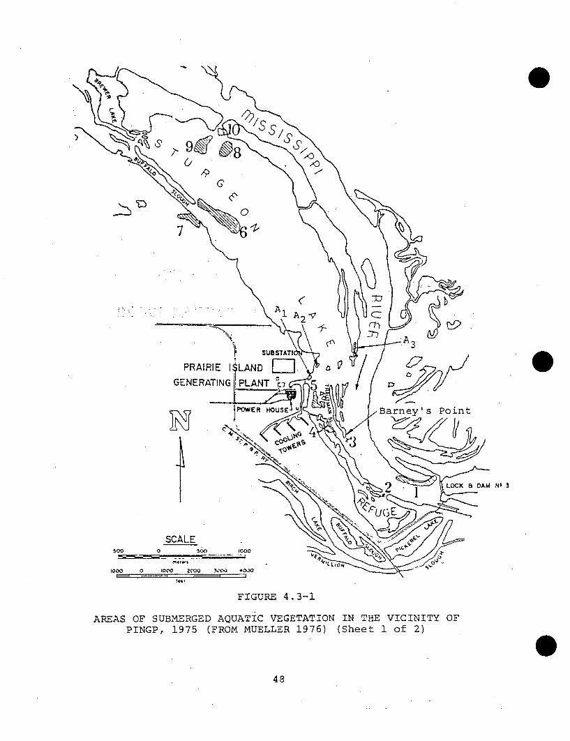
7

SUBSTATIC

PRAIRIE I$LAND [

GENERATING !PLANT 0cj C:

SCALESoo 0 500 1000

1000 0 1000 200o0 3C0 4000

FIGURE 4.3-1

AREAS OF SUBMERGED AQUATIC VEGETATION IN THE VICINITY OFPINGP, 1975 (FROM MUELLER 1976) (Sheet 1 of 2)

48

Code:

a. Curled pondweed = Potamogeton crispus (L.)b. River pondweed = Potamogeton nodosus (Poir.)c. Sago pondweed = Potamogeton pectinatus (L.)d. Wild celery = Vallisneria americana (Michx.)

Area 1. a, b, c

2. -

3. -

4. C

5. a, b,

6.- a, b,

7. a, b,

8. a, c

C

C

C

9.

10.

A.1

A.2

A.3

a

a, b, c, d

a

c

a, c

FIGURE 4.3-1 (Sheet 2 of 2)

49

Seasonal trends in densities indicated maxima in summer or

fall and minima. in winter and spring.

Rotifers generally dominated the zooplankton of the PINGP

area, as they usually do in river systems (Hynes 1972).

Dominant rotifer taxa included Brachionus angularis,

B. calyciflorus, B. budapestinensis, B. caudatus,

Kellicottia longispina, Keratella cochlearis, K. guadrata,

Polyarthra spp. and Synchaeta spp. Daggett (1976) considers

the abundance of Brachionus species to indicate eutrophy.

Crustaceans were seldom dominant at the PINGP site, although

in June 1974 Cyclops vernalis, Daphnia sp. and copepod nauplii

dominated samples. Protozoans or copepods occasionally

dominated winter or spring samples.

4.3.4 Benthic Macroinvertebrates

Macroinvertebrates of the Mississippi River near PINGP have

been studied since July 1970. Preoperational information

comprises about 3-1/2 years of study and operational informa-

tion presently includes 2 years of study.

Several different collecting techniques were used to sample

the different types of aquatic habitats near PINGP. Sub-

strates in the main river channel and near the plant are

50

composed of sand, silt and organic muck which are continually

shifting. The Army Corps of Engineers artificial wing dams

and shore stabilization areas are constructed of willow and

rock. Quantitative samples of soft substrates (Miller 1973,

McConville 1974, Haynes 1976) were taken with Ponar or

Peterson grabs. Quantitative samples of the wing dams and

shore stabilization construction were taken with artificial

substrates. The artificial substrates used included a

design by Miller (1971) which is composed of two concrete

and two balsa wood blocks; this design was used for about 2-

1/2 years in the preoperational .study. Other types used

included a concrete block sampler similar to that of Britt

(1955), a barbeque basket sampler (Mason et al. 1967), and

the Hester-Dendy multiplate sampler (Hester and Dendy 1962).

Qualitative samples, collected by dip nets and hand picking,

were used to describe the benthos of shallow littoral zones

that are not sampled by quantitative methods.

The organisms which colonized artificial substrates upstream

of PINGP will be emphasized because they represent the

species which could potentially be entrained through the

phenomenon of drift.

The stations used by Miller (1972) in his preoperational

studies of 1971 and 1972 are shown in Figure 4.3-2.

.51

N

iNSTURGEON

LAKE

-P iN G-i•-•-= J•..

KE-YSBENTHO SAMPLIN STAION

FIGURE 4.3-2

BENTHOS SAMPLING STATIONS NEAR PINGP,1971 - 1972 (FROM MILLER 1972)

52

Miller (1972) experimented with various exposure times and

finally decided on a 30 day exposure period for coloniziation.

The 1971 studies show that Trichoptera, Ephemeroptera, and

Diptera are the major macroinvertebrates to colonize the

Miller substrate apparatus (Table 4.3-1). In 1972, these

same three orders dominated the artificial substrates

(Table 4.3-2).

In October, 1973 an additional series of sampling stations

was established in the area of the intake, recycle and

discharge canals (Figure 4.3-3). Station X-l, a control

station, was located immediately outside the skimmer wall of

the intake canal. Station X-2 was located immediately

outside the screenhouse within the intake canal. Station X-3

was in the recycle canal above the juncture of recycled

water and incoming make-up water from the river.

Unit 1 of PINGP began operation in 1974, although the plant

was in operation for only four periods during this year

(Simonet 1975). McConville (1974) states that the intermittent

operation had a minimal effect on the river environment

and, although subtle changes may have begun to occur, long

term studies would be required to substantiate them.

53

TABLE 4.3-1

PERCENT COMPOSITION OF MACROINVERTEBRATES COLLECTEDFROM ARTIFICIAL SUBSTRATE SAMPLERS IN THE MISSISSIPPI

RIVER NEAR PINGP, 1971(FROM MILLER 1972)

Transect Trichoptera Ephemeroptera Diptera Other

Minn W 42.3 17.9 38.7 1.2Min C 71.7 14.7 10.6 2.6Wisc W 59.7 8.3 26.4 5.5

C 32.3 14.1 30.3 23.2

W 32.1 5.6 47.1 15.1M- n C 68.7 8.9 14.9 7.4A cW 29.3 8.6 60.8 1.0Wisc C 46.0 20.1 22.2 11.1

W 37.5 14.6 20.8 27.1B-1 C 13.2 17.3 4.0 65.3Bi W 42.0 4.0 52.0 2.0

C 25.0 65.0 8.8 1.2

Minn W 50.8 22.1 27.1 0.0B-2 C 70.6 10.2 8.0 0.0W 56.9 8.8 32.1, 2.2

Center C 68.1 13.0 14.0 4.6

aSee Figure 4.3-2; Minn = Minnesota side, Wisc = Wisconsin side,

Center = island that divides channel from main channel; W =balsa wood blocks, C = concrete blocks

054

TABLE 4 .3-2

2ESTIMATED DENSITY OF MACROINVERTEBRATES (NUMBERS/M

COLLECTED FROM ARTIFICIAL SUBSTRATES DURING 1972

(FROM MILLER 1973)

(a)Station Substrate (b) June

AIW

AIM

A2W

A2M

TWTCBWBCTWTCBWBCTWTCBWBCTWTCBWBCTWTCBWBCTWTCBWBCTWTCBWBC

418215.514215

1084122

1027151533590230237209108114

50399

79647

50609187704158

1065165

1103179

July

1655280

1349266

2682294

2149287

1369266

1617244742208932280

742151780

65647115894108

September

1217129932108

67141586741812274356431

3443545

84071062808311271484

3092073

287

91336

60993

October

4413395

3214395

3424545

3538560

3119416

3899251

5744388

4717667

9015158

782647

29742187

140793

91343

BIW

BIM

B2M

aSee Figure 4.3-2; W = Wisconsin side, M = Minnesota side

= top wood; TC = top concrete; BW = bottom wood; BC = bottcm concrete

55

0 400

1 inch - 400 Ft

Intake Canal

S TLU R G E 0 N

L A KE

xl

L

Dii

-- Skimmer wall

X2

slant Site r

X3

Recycling Canal-

Y21

FIGURE 4.3-3.

ADDITIONAL BENTHOS SAMPLING STATIONS NEAR PINGP, 1973(FROM McCONVILLE 1974)

56

In addition to the regular baseline studies, an emergence

study was conducted between May 13 and-December 6, 1974

(McConville 1975). Emergent organisms were collected with

black light insect traps at four stations (Figure 4.3-4).

Some of the insects, in particular the caddisflies, emerge

by migrating from the bottom of the water column and those

emerging near the intake could be susceptible to entrainment

at PINGP. Table 4.3-3 describes the numbers and percentage

composition of the adults collected in the study.

The colonization period for the two types of artificial

substrate studies was 30 days in 1974. Table 4.3-4 quali-

tatively lists the taxa taken from concrete block samplers

and barbeque basket samplers from all the control stations

as well as Station X-2 in the intake and Station X-3 in the

recycling channel.

Hester-Dendy multiplate samplers were utilized for the

colonization studies in 1975. A 6 week exposure period was

allowed for colonizing the substrate with exception of the

first two collection dates. Table 4.3-5 describes the mean

number of organisms/m2 and mean relative abundance of taxa

per colonization period in stations above or in the

intake structure plus Station X-3 in the recycle channel.

57

STURGEON LAKE

&WA250 METE

IWATER FLOW

-RS,

/2

tTRAP ORIENTATION

MISSISSIPPIXi-- INTAKE RIVER

GENERATINGPLANT

FIGURE 4.3-4

LIGHT TRAP STATIONS USED IN EMERGENCE STUDIES AT PINGP, 1974(FROM McCONVILLE 1975)

58

TABLE 4.3-3

COMPOSITION OF ORDERS OF EMERGENT AQUATIC INSECTS COLLECTED FROM THEMISSISSIPPI RIVER NEAR PINGP, MAY 13 THROUGH DECEMBER 6, 1974

(FROM McCONVILLE 1975)

aOrder/Family Sturgeon Lake X-I Recycle Canal

Number Percent Number Percent Number Percent

TrichopteraHydropsychidae 151277 81.89 9155 52.26 8113 61.78Psychomiidae 13406 7.26 4228 24.14 2078 15.82Leptoceridae 7240 3.90 1171 6.68 1507 11.47Hydroptilidae 12801 6.93 2960 16.89 1428 10.87Other 4 *,? 3 * 7 *

Total 184728 100.00 17517 100.00 13133 100.00

EphemeropteraCaenidae 740 51.75 2980 86.85 1766 98.77Ephemeridae 670 46.85 439 12.80 8 0.45Other 20 1.40 12 0.35 14 0.78

Total 1430 100.00 3431 100.00 1788 100.00

DipteraChironomidae 440602 99.13 71581 98.69 80679 99.20Other 3888 0.87 947 1.31 647 0.80

Total 444490 100.00 72528 100.00 81326 100.00

aSee Figure 4.3-4

b less than 0.10 percent

TABLE 4.3-4 (Sheet 1 of 2)

MACROINVERTEBRATES COLLECTED FROM ARTIFICIAL SUBSTRATE SAMPLERS IN THEMISSISSIPPI RIVER NEAR PINGPa IN 1974

(FROM McCONVILLE 1975)

Macroinvertebrates

GastropodaR sp.

AcariHydrachnae

InsectaColeoptera

ElmidaeDineutus sv.Berosus sp.Hydrochus sp.Hydraena sp.

DipteraCeratopogonidaeChironomidaeChaoborus sp.Simuliidae

EphemeropteraBaetis sp.Psuedocloeon sp.Baetisca sp.Caenis sp.Hexagenia sp.Cinygma sp.Rhithrogena sp.Stenonema sp.Isonychia sp.

LepidopteraElophila sp.

OdonataAnisopteraZygopteraP lecoptera

Alloperla sp.Taeniovteryx sp.

PerlidaeTrichoptera

Cheumatopsyche sp.Hydropsyche sp.Athripsodes sp.Oecetis sp.

Block SamplersB-1 X-1 X-2 X-3

Basket SamplersSL B-1 X-1 X-2 X-3

* * * *

*

* * * * * * * *

*

*

*

*

*

* *

* *

* *

* *

* *

* * * * * * *

* * * ~* *

* * * *

* * * *

*

* * * ,.*

*

*

**

*

*

*

*

*

*

*

*

* *

* * * .*

*

*

*

*

*

* * *

*

*

* * * * * * *

*

*

*

*

*

*

*

*

*

* * * *

* * * *

*

* * *

* *. *

* * *

*

*

*

*

*

60

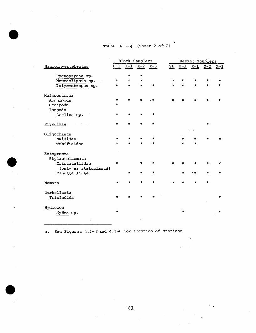
TABLE 4.3-4 (Sheet 2 ofý 2)

Block SamplersB-I X-1 X-2 X-3

Basket SamplersSL B-1 X-1 X-2 X-3Macroinvertebrates

Pycnopsyche sp.Neureclipsis sp.Polycentropus sp.

*

* *

* *

*

*

*

*

* *

* * * *

* * * *

MalacostracaAmphipodaDecapodaIsopoda

Asellus sp.

*

*

* * ~* * * * * *

Hirudinae

* * * *

* * * *

* * * *

* * * *

*

OligochaetaNaididaeTubificidae

* * * *

EctoproctaPhylactolaemata

Cristatellidae(only as statoblasts)

Plumatellidae,

* * * * * * * *

* ~* * ** * *

Nemata

TurbellariaTricladida

HydrozoaHydra sp.

* * * *

* * * *

*

* * * *

*

**

a. See Figures 4.3- 2 and 4.3-4 for location of stations

61

TABLE 4.3-5 (Sheet I of 9)

BENTHIC MACROINVERTEBRATES COLLECTED FROM HESTER-DENDY MULTIPLATE SAMPLERSIN THE MISSISSIPPI RIVER NEAR PINGP IN 1975

(ADAPTED FROM:HAYNES 1976)

Station a

,S.L. B-I X-1 X-2 X-3Numberb Percentc Number Percent Number Percent Number Percent Number Percent

FEBRUARY 3, 1975

Taxa

Turbellaria

Nexnertina

OligochactaNaididab

10.8 <1.0 43.2

- - 54.0

1.4

1.7

- 3294.0 99.0 3024.0 96.2

0• GastropodaPhysa app.

Crustaceaflyalella azteca

Ephemeroptera

Tricorythodes ap.

Total Individuals

Total Taxa

- - 10.8 -1.0

10.8 <1.0 10.8 <1.0

3142.90

10.8

3326.4

<1.0

0 045 4 5

0

TABLE 4.3-5 (Sheet

TaxaS.L. - B-I

NumberPerWeUnt Number Percent

2 of 9 )

Station8X-1

Number Percent

MARCH 3, 1975

X-2Number Percent

16.2 <1.0

21.6 <1.0

- X-3Number Percent

Turbellaria

Nemertina

Nematoda

OligochaetaNaididae

GastropodaPhysa Opp.

DipteraCr cotoeuapp.Total Diptere

Total Individuals

Total Taxa

5.4 100.0

10.8

5.4

11.1

5.6

- - 4617.0 99.0 37.8 38.9

- 43.2 44.4

a%S - 10.8

- - 10.8

5.4 4665.6

<1.0<1.0

97.20

0 4

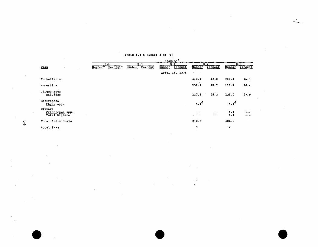
TABIB 4.3-5 (Sheet

TaxaS.L. B-i

Nuberb Percent: Number Percent

3 of 9)

Stationa

X-1Number Percent

APRIL 15, 1975

X-2Number Percent

X-3Number Percent

Turbellaria

Hemertina

OligochaetaNaididae

GastropodaPhysa app.

DipteraCrcot! us spp.

Tot era

M• Total Individuale

Total Taxa

340.2 42.0 226.8 46.7

232.2 28.7 118.8 24.4

237.6 29.3 135.0 27.8

5.4 d 5. 4 d

5.4- 5.4"

810.0 486.0

3 4

1.11.1

TABLE 4.3-5 (Sheet 4 of 9 )

TaxaS.L. B-I

Number- Percent- Number Percent

StationaX-i1

Number PercentX-2 X-3

Number Percent Number Percent

MAY 27, 1975

Turbellaria

Naemertina

183.6 3.1 -

64.8 1.1 -

0)Ln

EctoproctaPlumatella repens

OligachaetaNaldidae

GastropodaPhysa app.

EphemeropteraCaenis op.Total Ephemeroptera

PlecopteraIpoperla op.Total Plecoptera

TrichopteraA g 'lea ap.

thr-Uipsodes tarel-punctatusllydrop~syche ANNi

Total Trichoptera

DipteraConchapelopia ep.Cricotopus app.Dtcrotendies sp.Cl ypotdpea op.Labrundinia sp.Parach ronomus ap.Polypedilum (Pentapedllum) up.

Bec-t-r~cadius ap.SImulium jenningsii

.nilentified ChironomidaeTotal Diptera

Total Individuals

Total Taxa

205.2 3.5

+ e +e

5.4 5.95.4 5.9

5.4 <1.05.4 <1.0

21.65.4

59.491.B

178.2

237.6610.2394.243.2

.21.6685.3

10. 82393.6799.2

<1.0<1.0

1.01.63.1

4.110.5

6.8<1.0<1.011.8<1.041.013.7

5.4

75.6

5.9

82.4

5.994.1

- - 5.45196.3 09.1 86.4

5833.4 91.9

17 4

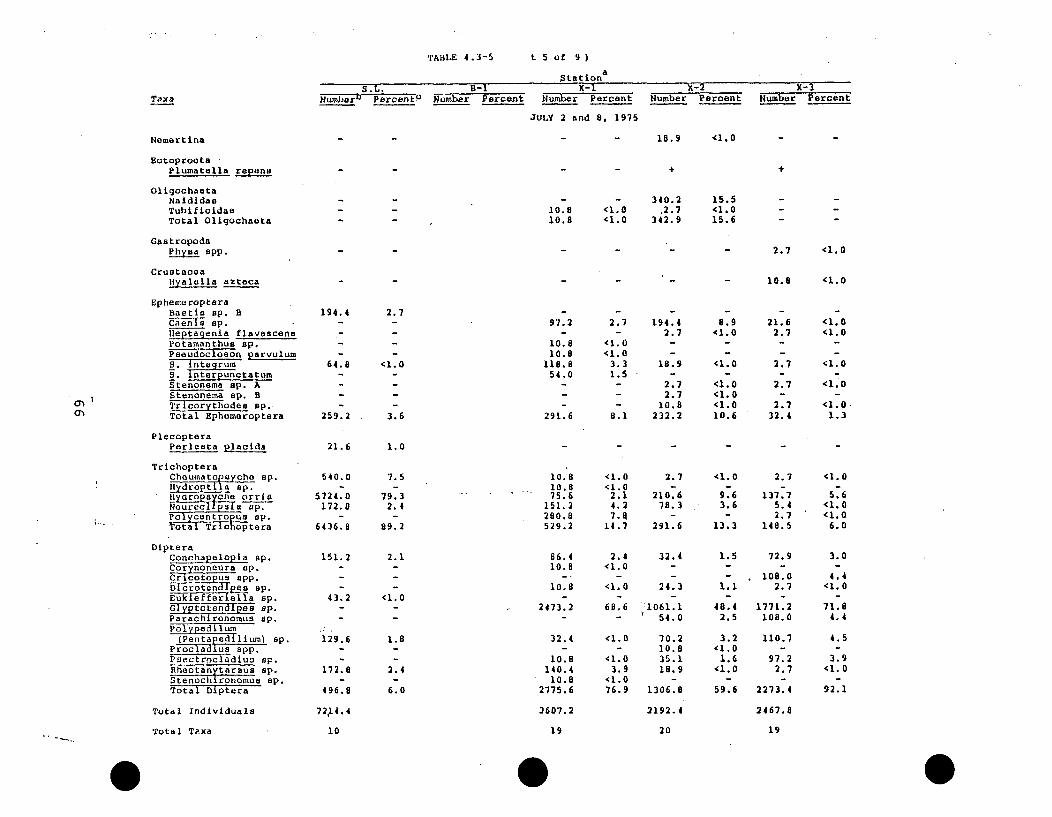
TABLE 4.3-5 t 5 of 9 )

S.L.Number" Percento

B-iNumber Percent

StationaX-1

Number PercentX-2

Number PercentX-3

Number Percent

Neamertina

JULY 2 and 8, 1975

- 18.9 <1.0

- -

oW

EctoprootaPlumatella repens

OligoohaetaNaididaeTubifioidaeTotal Oligochaeta

GastropodaPhysa opp.

Crustaoea1_yaleLla azteca

EphemeropteraBaetis up. BC op.lleptagenia flavescenaPotamanthus op.Pseudocloeon parvulumS inegrumS. interpunctatumStenonema up. AStenonema sp. BTricorythode. Sp.Total Ephemeroptera

PlecopteraPerlesta placida

TrichopteraChmtoppych• op.Hydroptila up.HM21rosacne orrisNeure .7 a up.P1y~cent us op.

-oralTrchoptera

DipterAConchapelopia up.Corynoneura up.£S.osapp.Dicrotendi e up.

F lea up.

GTly , 9 op.ParachironomEUs up.Polypedilum

Pentapedilithu) up.Pr0cladiusjiPp.Fs'ectrocladius up.Rheotan tarsus up.S tenochirnomus up.Total Diptera

Total Individuals

Total Taxa

10.810. B

- 340.2 15.5 - -<1.0 2.7 <1.0<1.0 342.9 15.6 -

- - 2.7 <1.0

- 10.8 <1.0

194.4

64.8

259.2

2.7

<1.0

3.6

97.2

10.810.8

118.854.0

291.6

2.7

<1.0<1.0

3.31.5

8.1

194.42.7

18.9

2.72.7

10.8232.2

8.9

<1.0

<1.0

<1.0<1.0<1.010.6

21.62.7

2.7

2.7

2.732.4

<1.0<1.0

<1.0

<1.0

<1.01.3

+

21.6 1.0

540.0

5724.0172.8

6436. 8

151.2

43.2

129.6

172,8

496.8

72ý1 4. 4

7.5

79.32.4

89.2

2.1

<1.0

10.810.875.6

151.2280.8529.2

86.410.8

10.8

2473.2

<1.0<1.0

2.14.27.0

14.7

2.4

<1.0

<1.0

68.6

<1.0

<1.03.9

<1.076.9

2.7

210.678.3

291.6

32.4

24.3

:1061.154.0

70.210.835.118.9

1306.8

2192.4

<1.0

9.63.6

13.3

1.5

1,1

48.42.5

3.2<1.0

1.6<1.0

59.6

2.7

137.75.42.7

148.5

72.9

108.02.7

1771.2108.0

110.7

97.22.7

2273.4

2467.8

<1.0

5.6<1.0<1.0

6.0

3.0

4.4<1.0

71.84.4

4.5

3.9<1.0

92.1

1.8

2.4

6.0

32.4

10.8140.4

10.82775.6

3607.2

10 19 20 19

TABLE 4.3-5 (Sheet 6 of 9)

Taxa 8 'L.Nmer's Percent'

B-iNumber Percent

StationaX-1

Number PercentX-2

Number PercentX-3

Number Percent

AUGUST 19, 1975

Hlydrozoa

Turbellaria

Nematoda

OligochaetaNaididae

EphemeropteraBeetle ep. B

e p. cCani p.

e e flavescensIaonychia op.Stenonema exiquum

S. guilnguepinatumStenonema up. BStenonema up.Tricorythodes up.Total Ephomeroptera

861.3 1.0

,10.8 A 10

648.0 5.3 507.6 <1.0

5313.6 43.8 74884.5 96.6

194.443.2

43.2

129.621.621.6

453.6

2.5<1.0

<1.0

1.7<1.0

5.8

16.9

55.412.2

84.5

129.675.621.6

194.421.697.2

43.2

583.2

712.810.8

4546.8345.6

291.6280.8

6188.4

1.81.0

<1.0

2.7<1.0

1.3

<1.0

.8.1

9.9<1.063.0

4.8

4.0

3.985.8

5.410.813.5

5.462.1

2.799.9

<1.0<1.0<1.0

<1.0,1.4

1.02.3

<1.0

2.89.53.6

<1.0

16.5

2.7

2.7<1.0

TrichopteraCheumatopsyche up. 1317

,yrpyche frisoniI1. orr 4320

eurl sina op. 950Polycentropus op.

fla~71va

Unidentified -lydropaychidaeTotal Trichoptera 6588

ColeopteraStenelmie Bpp.

18.9

124.2421.2162.0

5.4

731.7

86.432.4

5270.410.8

140.4172.8

5713.2

<1.0<1.043.5<1.0

1.21.4

47.1

156.6

64.8

21.6

243.0

<1.0

<1.0

<1.0

<1.0

43.2 <1.0 - 2.7 <1.0

DipteraA~Dix3~esmia op.Conchape1opia op.DIicrotedi~ea p.G~ypooen I peu op.IHererod~romlaopT.Perachironomus op.

(Pentapedillum. op.Psectrocladius op.Rheotanytaruu op.Tr ibeloouop.Total Diptera

Total individuals

86.4 1.1

410.4 5.3

237.6

21.6

756.0

7797.6

162.0

32.4

194.4

10.8

399.6

7214.4

2.,2

<1.0

2.7

<1.0

5.5

194.45.4

3346.92.75.4

16.229.7

5.43608.1

4439.7

4.4<1.075.4<1.0<1.0

<1.0<1.0

<1.001.3

3.0

<1.0

9.7

97.210.8

270.010.821.6

43.2

453.6

12128.4

<1.0<1.0

2.2<1.0<1.0

56.721.6

912.6

2.7

<1.0<1. 0

1.2

<1.0

<1.0

1.3

<1.0 2.7

3.7 996.3

77508.9

Total Tax& 13 18 19 14 14

TABLE 4.3-5 (Sheet 7 of 9)

Taxa

StationaS.L. B-I X-1 X-2 X-3

Number" Percent' Number Percent Number Percent Number Percent Number Percent

SEPTEMBER 29, 1975

- - 27.0 <1.0

- - 27.0 <1.0

0CO0

Hydrozoa

Turbellarla

EctoproctaPectinatella magnificaPlumatella repens

Endoprocta

OligochaetaNaldidae

EphemeropteraBaet'e up. CIsonychia op.Stenonema integrum

i. interpunctatumStenonema op. ATotal Ephemeroptera

OdonataEnallagma up.

TrichopteraCheugatoIe,,h8 up.y-Yopche fr inoni

H. orrisNeu-re-c--•l~pss op.

poycentropul up.Potamy a flavaUnidenti fied

IlydropsychidaeTotal Trichoptera

ColeopteraStenelmis app.

DipteraAblabesmyla sp.Conchapelopia op.

sjcto u app.Dicrotend pea sp.~jp~~d eap.

Parachironomus op.Pypedoum

(Penta edilum) op.Psectrocladius sp.Rheoytnarau op.UnidentifiedChironomidae (pupae)

Total Diptera

Total Individuala

. Total Taxa

+

+ +

- 267.3 8.3 48599.9 85.4 159494.4 99.4

10.8

10.821.6

<1.0

<1.0<1.0

21.637.867.5

126.9

<1.0<1.0

1.1

2.1

8.1

2.7

10.8

<1.0<1.0

<1.0

+ - - +- - - - +

- 10.6 <1.0

326.7

1304.2275.4

10.8367.2

5.9

23.55.0

<1.06.6

756.0

2646.0129.6

86.4406.0

12.7

44.52.21.58.2

4.473. 4

27.0245.7194.410.8

<1.07.66.0

<1.0

124.210.8

7732.832.4

218.721.6

8140.51036.8 18.7 259.23321.1 59.9 4363.2 477.9 14.8

<1.0<1.013.6<1.0<1.0<1.0

14.3

<1.0<1.0

<I. 0

108.027.0

<1.0<1.0

27.0 <1.0162.0 <1.0

- 5.4 <1.0

48.6

121.51428.3

<1.0

2.225.8

97.2

140.3

874.7

1.62.4

14.7

2 .1

118.82251.8

<1.0

3.769.9

10.82.7

145.8 617.127.0

<1.0<1.0

<1.0

75.6 1.4523.8 9.5

- 18.9302.4 5.1 54.043.2 <1.0

<1.01.7 5.4 <1.0 54.0

2197.8

5540.5

13

39.7 1457.8 24.5 2451.6

5947.9 3223.6

14 0@14

- - - 54.0 <1.076.1 164.7 <1.0 752.1 <1.0

56905.1

11

160462.5

10

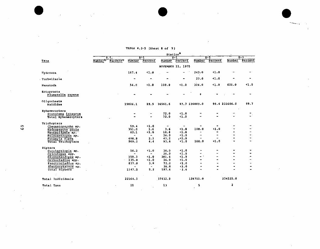
TABLE 4.3-5 (Sheet 8 of 9)

Taxa-s. t. B-1

Number" Porce-n-tu Number Perce-nt

StationaX-1 X-2 X-3

Number Percent Number Percent Number Percent

NOVEMBER 11, 1975

- - 243.0 <1.0Hlydrozoa

Turbellaria

Nematoda

167.4 <1.0

.... 27.0 <1.0

54.0 <1.0 108.0 <1.0 324.0 <1.0 621.0 <1.0

0.,

EctoproctaPlumatella repens

OligochaetaNaididae

EphemeropteraStenonema IntegruTotal Ephemeroptera

TrichopteraCheumatopsyche op.11yd~ropaIchorr__s

Nerclipsls sp.-Po ycantropuIs up.Potma flavaTotal richoptera

DipteraConchapelopla up.Crc2oto us opp.Glyptotenipes up.Orthocladlus app.Psectrocladlus up.ihiotan tarsus up.Total Diptera

Total Individuals

19826.1 09.5 36561.6 97.7 126009.0 99.4 233604.0

- 72.0 <1.0- 72.0 <1.0

99.7

59.4351.0

62.1

496.8969.3

16.2

159.3135.0837.0

1147.5

22164.3

<1.01.6

<1.0

2.24.4

<1.0

<1.0<1.0

3.0

5.2

3.610.836.043.293.6

36.036.0

381.636.072.036.0

597.6

<1.0<1.0

<1.0

<1.0<1.0<1.0<1.0<1.0<1.0

"1.6

108.0

108.0

<1.0

<1.0

234225.037432.8 126711.0

Total Taxa 11 13 5 2

TABLE 4.3-5 (Sheet 9 of 9)

S.L. B-I

Numberý Percentc Number PercentTaxa

Turbellaria

X-i X-2

Humber Percent Number Percent

13.5.0 <1.0

783.0 1.8

umbe.r P2ercent

13905.0 12.1Nematoda

EctoproctaPlumatella repens

01igochaetaNaididae

GastropodsPhysa app.

Trichopterailydropoyche orrisTotal TricrioFt-te-{a

DipteraCricotou ap.L-ps app.

GEyptotendines op.Poypedium Pentapedilum} op.Total Di---ptera

42228.0 97.4 100927.0 87.8

54.0 <1.0

54.0 <1.054.0 <1.0

54.0 1.0

-jCO54.027.027.0

108.0

<1.0<1.0<1.0'1.0

Total Individuals 43362.0

a

114886.0

3Total Taxa

aSee Figure 4.3-2 1bMean number of organisms per wa2

cMean corcant relative abundance

dDead at time of collection, not included in totals

a+ - present as colonies; not included in totals

The faunal composition shown in the colonization studies of

1974 and 1975 is important because the community formed

is a result of drift phenomenon. Thus, the taxa of this

community could potentially be entrained.

During the 1975 survey a total of 147 macroinvertebrate taxa

was collected by all sampling methods (Table 4.3-6).

Fifty-one taxa were exclusive to qualitative sampling, 13

to Petersen grab-sampling, and 23 to the multiplate samplers.

Throughout all years of study, the quantitative grab samples

contained mainly 0ligochaeta and Chironomidae. Numerous

Mollusca were also collected in the grab samples.

71

TABLE 4.3-6

BENTHIC MACROINVERTEBRATES COLLECTEDIN THE VICINITY OF PINGP IN 1975

(FROM HAYNES 1976) (Sheet 1 of 4)

Petersen Multlplate Qualitative

Taxa Dredge Sampler Samples

Porifera +

Hydrozoa +

Turbellaria + + +

Nemertina +

Nematoda + +

EctoproctaPectinatella manifica Leidy + + +

Plurnatella repens (Linnaeus) + +

EntoproctaUrnatella gracilis Leidy +- +

AnnelidaOligochaeta

Branchiura sowerbyi Beddard + +

Other Tubificidae + + +

Naididae* + + +

Dina lateralis (Verrill) +

Erpobdella punctata (Leidy) +

Helobdella stagunlis (Linnaeus) +

Placobdella montifera Moore +

P. parasitica (Say) +

Unidentified Hirudinea +

MolluscaGastropoda

Amnicola sp. + +

Bulimnaea EeEasoma (Say) +

Ferrissia sp. + +

Goniobasis sp. + +

Gyraulus sop. + +

Heliosoma spp. + +

Lymnaea sp. + +

Physa spp. + + +

Pleurocera sp. + +

Stagnicola sp. + +

Valvata tricarinata (Say) +

Unidentified Gastropoda +

72

TABLE 4.3-6 (Sheet 2 of 4)

Petersen Multiplate QualitativeTaxa Dredge Sampler Samples

PelecypodaLampsilis sp. +Leptodea fragilis Rafinesque +Pisidium sp. +Sphaerium sp. + +Unidentified Unionaceae +

ArthropodaHydracarina +

CrustaceaAsellus sp. + + +Crangonyx gracilis group Smith +Gammarus lacustris Sars +G. pseudolimnaeus Bousfield +Gammarus sp. +Hyalella azteca (Saussure) + +Orconectes sp. +

CollembolaIsotomurus palustris (Muller) +

EphemeropteraBactis sp. A +Baetis sp. B +Baetis sp. C +Baetisca bajkovi Neave +Baetisca sp. +Caenis sp. + + +Ephemerella temporalis McDunnough +Ephoron album (Say) +-eptagenia flavescens (Walsh) +

Hexagenia limbata (Serville) +Isonychia sp. +Leptophlebia sp. +Metretopus borealis Eaton +Potamanthus sp. + +Pseudocloeon parvulum HcDunnough + +Pseudocloeon sp. +Siphlonurus alternatus (Say) +Stenonema exiguum Traver +S. integrum (HcDunnough) + +S. interpunctatum (Say) + +S. quinguespinatum Lewis + +S. tripunctacum (Banks) +Stcnoncma sp. A +Stenonema sp. B +Tricorythodes sp. + +

73

TABLE 4.3-6 (Sheet 3 of 4)

Peterscn Multiplate Qualitative

Taxa Dredge Sampler Samples

OdonataArgia sp. +Enallagma sp. + +Unknown Zygoptera +

PlecopteraIsoperla bilineata (Say) + +Isoperla sp. +Perlesta placida (Hagen) +Taeneopteryx maura Pictet +

HemipteraBelastoma sp. +Corixidae +Cerris sp. +Plea striola +Ranatra sp. +Saldidae: +Trepobates sp. +

NeuropteraCiimacoa arcclaris (+

TrichopteraAgraylea sp. +Athripsodes tarsi - punctatus (Vorhies) + +Cheumatopsyche sp. + + +Hydropsyche frisoni Ross +H. orris Ross + + +Hydroptila sp. + +Leptocella sp. +Neureclepsis sp. + + +Orthotrichia sp. +Polycentropus sp. + +Potamyia flava (Hagen) + + +Pycnopsyche sp. +Unidentified Hydroosychidae + +Unidentified Hvdroptilidae +

ColeopteraBerosus sp. +Coptotomus nr. interrogatus (Fabricius) +Dubiraphia vitctaa (adults) (Melsheimer) +Dubiraphia sp. (larvae) + +Dineutus nr. discnlor Aube +Gyrinus sp. A +Gvrinussp. B +Haliplhs sp.

74

TABLE 4.3-6 (Sheet 4 of 4)

Petersen Mu~tiplate Qualitative

Taxa Dredge Sampler Samples

ColeopteraHelophorus sp. +Hygrotus sp. +Laccobius sp. +Liodessus sp. +Peltodytes spp. +Stenelmis spp. + + +Tropisternus lateralis (adults) (Fabricius) +Tropisternus sp. (larvae) +Unidentified Hydrophilidae +

DipteraAblabesmyia sp. + + +Chaoborus punctipennis (Say) + +Chironomis spp. + +Coelotanypus sp. +Conchapelopia sp. + + +Corynoneura sp. + +Cricotopus spp. + + +Cryptochironomus spp. + + +Dicrotendipcs sp. + +Endochironomus sp. + +Eukiefferiella sp. +Glyptotendioes sp. + + +Hemerodromia sp. + + +Labrundinia sp. +Micropsecta sp. +Nanocladius sp. +Orthocladius spp. +Palpomyia spp. group + +Parachironomus demijerea +Parachironomus sp. + +Polypedilum (Fallax) sp. +P. (Pentaoedilum) sp. + + +Procladius spp. + +Psectrocladius sp. +Rheotanytarsus sp. +Simulium jenningsii Malloch + +Stenochironomus sp. + +Tanypus sp. +Tribelos sp. + +Trissocladius sp. +Xenochironomus sp. +Unidentified Chironomidae + + +

Totals 147 54 69 105

Mixed populations of Nais spp. and Pristina sp., the former predominating.

75

4.3.5 Fish and Fisheries

Fishes in the vicinity of PINGP have been the subject of

intensive studies since 1970. Additional data on commercial

fishing are available from the Wisconsin and Minnesota

Departments of Natural Resources.

Species collected at PINGP by type of gear in 1975 and

species colIected by all types of gear in 1973 and 1974 are

presented in Table 4.3-7. Sampling was conducted with

multiple gears to reduce the inherent bias resulting-from

gear selectivity. Electrofishing and seining yielded more

species than the other sampling methods. However, seining

data are biased against fishes which are large and occur

offshore whereas electrofishing data are biased against

smaller and demersal fishes. Standing crops of small fishes

can be estimated from seining data for shallow waters and

trawl data for deeper waters. Gill net and trap net data

permit spatial comparisions of the relative numbers of the

larger and most important species.

Fishes of the PINGP region have been classified according to

their value and size by Gustafson et al. (1976) as follows.

76

TABLE 4.3-7

COMMON AND SCIENTIFIC FISH NAMES AND METHODS OF FISH CAPTURE IN THE PINGP AREA, 1975(FROM GUSTAFSON ET AL. 1976) (Sheet 1of 3)

Method of CaptureScientific Name Trapnet Gillnet Trawl Electro-Fishing Seine 1973 1974Common Name

Chestnut lampreySilver lampreyLongnose garShortnose garBowfinAmerican eelGizzard shadGoldeyeMooneyeNorthern pike

SCarpBrassy minnowSilvery minnowSilverchubGolden shinerEmerald shinerRiver shinerCommon shinerPugnose minnowBlacknose shinerSpottail shinerRed shinerRosyface shinerSpotfin shinerRedfin shinerMimic shinerBluntnose minnowFathead minnow

Ichthyomyzon caataneusIchthyomyzon unicuspiaLepisosteuB osseusLepisosteua piatostomusAmia calvaAnquilta roatra-a.Dorosoma cepedianumHiodon alosiodesHiodon tergisusEaox luciusCyprinue carpioHybognathus hankonsoniHybognathus nuchalisHybopsis atorerianaNotemigonus orysoleucaaNotropus atherinoidesNotropus bienniusNotropia oornutuBNotropis emiliaeNotropis heterolepisNotropis hudsoniuaNotropis lutrensisNotropia rubellueNotropis spilopterusNotropis umbratilisNotropia Volucel usPimephales notatusPimephalea promelas

xxx

x

xxx

xxx

xxxxx

x

x

x

x

xx

x

xx

x

xxx

x

"X.xx

x

xx

xx

x

x xx xx x

xx x

xx

x xx xx

xxxxxxxxxxxxxxx

xxxx

xx

x

x

x

x

x

x

xxxxx

x

TABLE 4.3-7 (Sheet 2 of 3)

Method of CaptureTrapnet Gillnet Trawl Electro-Fishing Seine 1973.Common Name Scientific Name 1974

Bullhead minnow'Carpsucker species

'White suckerSmallmouth buffaloBigmouth buffaloSpotted suckerSilver redhorseRiver redhorseShorthead redhorseBlack bullheadYellow bullheadBrown bullheadChannel catfish

- Tadpole madtomc Flathead catfish

Trout perchBurbotWhite bassRock bassGreen sunfishPumpkinseedBluegillHybrid sunfishSmallmouth bassLargemouth bassWhite crappieBlack crappieJohnny darter

Pimephales eigilax.Carpiodes speciesCatostomus commersoniIctiobus buballisIotiobus cypinellusMinytrema melanopsMoxostoma anisurumMoeostoma carinatumMoxostoma macrolepidotumIctalurus melisIctalurue natalieIctalurus nebulosusIctalurus punctatusNoturus gyrinusPylodictis olivarisPercopsis omiscomaycusLota IotaMorone chrysopsAmbloplites rupestrisLepomis cyanellusLepomis gibbosusLepomis macrochirusLepomis maoroohirus X?Micropterus dolomieuiMicropterus salmoidesPomoxis annularisPomoais nigromaculatusEtheostoma nigrum

xxxx

x

xx

xx

x

xx

x

x

xx

xx

x

xx

xx

xxx

x

x

x

x

x

'C

x

'C

'C

'C

x'C

x'C

'C

'C

'C

xx'C'C

xxxx

x

'C'C

x 'C

'C 'C '

'C '

x x xx x 'C

x'C X

xx x 'C

xx 'C

x x'C X 'Cx

'C

'C

'Cx

'C

x

'C

'C

x x'C

x'C '

'C ''C '

'C X'C X

'Cx x'C '

'C ''C X

x

TABLE t,5-7 (Sheet 3 of 3)

Method of CaptureCommon Name Scientific Name Trapnet GMilinet Tfrawl Eiectro-fishing Seine 1973 1974

Yellow perch Perca fiavescena x x x x xLog perch Peraina caprodes x x xSauger Stizoatedion canadenee x x x x x x xWalleye Stizoatedion vitreun vitreum x x x x x x xFreshwater drum Aplodinotus grz•nniens x x x x x x x

Large rough fish (carp, carpsuckers, shorthead redhorse)

Game fish (channel catfish, smallmouth bass, walleye,

sauger, white bass, northern pike)

Panfish (rock bass, bluegill)

Minnows and darters

Other fish (gizzard shad, mooneye, black bullhead,

freshwater drum)

These categories will be used in subsequent discussions to

summarize the voluminous data collected in the PINGP area.

4.3.5.1 Sport Fishery

In the PINGP area the angling season is continuous for all

species except sturgeon. Although tip-up apparatuses can be

used for ice fishing, there is little ice fishing because of

ice-choked channels and treacherous conditions.

A creel survey was undertaken to establish a series of

guidelines or indices to be used in assessing sport fishery

success, pressure, and harvest in relation to PINGP operation

(Hawkinson 1974). During 1973-1975, six river sections

(Figure 4.3-5) were surveyed in rotation. PINGP is located

at the lower end of sections 1 and 2 and at the upper end

of section 3. Section 4 includes the tail-waters of Lock

and Dam No. 3.

80

0

f/

.,'..• o I 2 , 3 4 5 6

SCALE IN MILES

o i 2 3 . 4 5 6 7 8 9 1o

SCALE IN KILOMETERS

co a, S.

NAlli

:....!:..o.:

FIGURE 4.3-5

CREEL SURVEY AREAS NEAR PINGP, 1973-1975(FROM NAPLIN AND GUSTAFSON, 1975)

Estimated sport harvest and catch rates of fish in the PINGP

region are shown in Tables 4.3-8 through 4.3-12.

Fishing pressure was very similar in 1973 and 1974 but de-

clined by about 33 percent in 1975. In March and April, in

the fishery in the tailwaters of the dam, there was a steady

increase in fishing pressure from 18,378 man-hours in 1971

to 93,594 man-hours in 1974 and a decline to 88,855 man-

hours in 1975.

There is little fishing pressure in Sturgeon Lake, the main

channel above the Lock and Dam No. 3 and the immediate plant

area. The highest fishing pressure occurs in section 4,

especially in March and April (Gustafson et al. 1976) be-

cause (1) fishing is good in this section and highly

publicized, (2) the section is easily accessible and easy

to fish, and (3) sauger, walleyes and white bass concentrate

in the tailwaters.

Interviews with fishermen indicated that the most sought

after species were saugers, walleyes and "anything that

bites." The most commonly caught fish were walleyes,

saugers, white bass and drum. The composition of the May-

November sport catch was similar from 1973 through 1975,

82

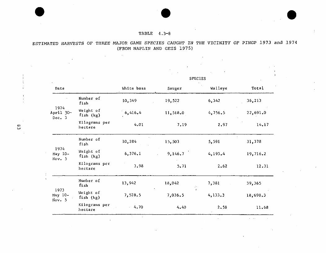
00TABLE 4.3-8

ESTIMATED HARVESTS OF THREE MAJOR GAME SPECIES CAUGHT IN THE VICINITY OF PINGP 1973 and 1974

(FROM NAPLIN AND GEIS 1975)

SPECIES

Date

1974April 30-

Dec. 3

Number offish

Weight offish (kg)

Kilograms perhectare

White bass

10,349

6,416.4

4.01

Sauger

19,522

11,518.0

7.19

Walleye

6,342

4,756.5

2.97

Total

36,213

22,691.0

14.17

Number of 10,284 15,503 5,591 31,378fish

1 9 7 4W e g t o197 Weight of 6,376.1 9,146.7 4,193.4 19,716.2May 10- fish (kg)

Nov. 5Kilograms per 3.98 5.71 2.62 12.31hectare

Number of 13,942 18,042 7,381 39,365fish

19731973i0 Weight ofMay 10- fish (kg) 7,528.5 7,036.5 4,133.3 18,-698.3tNov. 5

Kilograms perhectare 4.70 4.40 2.58 11.68

TABLE 4.3-10

aOVERALL CATCH RATE OF ALL ANGLERS FISHING THE PINGP AREA MgY 10 - NOVEMBER 5, 1973

AND PERCENT SUCCESSFUL ANGLERS(FROM HAWKINSON 1974) (Sheet 1 of 2)

*Fishing Success (fWsh/m-h)

Sectiona

.1 2

4.o

3

3.0 2,643.0

51,820.0

6

6oo.0

Total

5,081.0H-h sarveyed

% successrulanglars

11.0

75 100 59 56 51 57

Spocies Caught

Northern pikeWalley*SaugerWhite bassCrappiesBluegill sunfishPumpkinseed srh.Green sunfishHlybrid sunfishL. H. bassS. H. bassPerchFlathead catfishBuckers & Rdho.carpDrum

0.50(2)

0.25(l)

,(6)0.o0 (96)0.30(787)

0.33(1) 0.29 (72)0.01 (23

* (5)

* (1) 0.02(10o.16(291 0.10(62o.14(254 0o.13 700.03 (6o 0.05(300.01 (25 o..oi (60.01 (10 * (10.02 (100.02 (35, a t11

a (IT0.09 (11510.22(11200.17 (8640.01 154

* 160.01 (00.01 35

0.02 (85* (I

0.01 (250.02 (115)

0.36

a (5)

o.02 (44)

0.01 (Ii)0.03 (70)

0.02 (3.)

0.01 (1

0.02(14)

a In fish/man-hours; numbers of fish caught in parenthesis next to the rate and the man-

bhours fished under the section numberAt least one fish caught

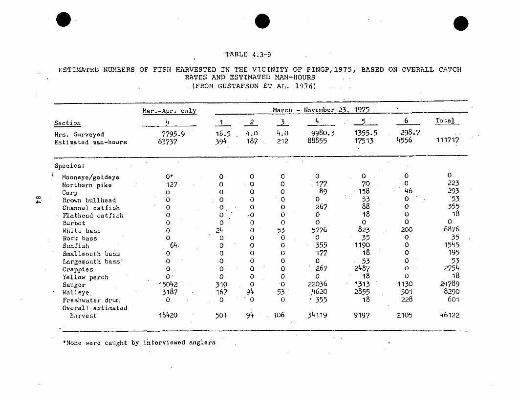
TABLE 4.3-9

co

ESTIMATED NUMBERS OF FISH HARVESTED IN THE VICINITY OF PINGP, 1975,' BASED ON OVERALL CATCHRATES AND ESTIMATED MAN-HOURS

.... (FROM GUSTAFSON ET AL., 1976)

Mar.-Apr. only March - November 23, 1975

Section __________ 2 4' 5 6 Total

Hrs. Surveyed 7795.9 16.5 4.0 4. 9980.3 1355.5 298.7Estimated man-hours 63737 394 187 212 88855 17513 4556 111717

Species:

Mooneye/goldeye 0' 0 0 0 0 0 .. 0 0Northern pike 127 0 0 0 177 70 0 223Carp 0 0 0 0 89 158 46 293Brown bullhead 0 0 0 0 0 53 0 53Channel catfish 0 0 0 0 267 88 0 355Flathead catfish 0 0 0 0 0 18 0 18Burbot 0 0 0 0 0 0 0 0White bass 0 24 0 53 5776 823 200 6876Rock bass 0 0 0 0 0 35 0 35Sunfish 64. 0 0 0 355 1190 0 1545Smallmouth bass 0 0 0 0 177 18 0 195Largemouth bass 0 0 0 0 0 53 0 53Crappies 0 0 0 0 267 2487 0 2754Yellow perch 0 0 0 0 0 18 0 18Sauger 15042 310 0 0 22036 1313 1130 24789Walleye 3187 167 94 53 ,4620 2855 501 8290Freshwater drum 0 0 -0 0 355 18 228 6o0Overall estimated

harvest 18420 501 94 106 34119 9197 2105 46122

*None were caught by interviewed anglers

(Sheet 2of 2)

'Ohl, rih/h

I

carRock I3as

Catch/rzbr

0.75(3)

34.

0.69(.131.)

0. -36(4)

5

* (i)

O.44(2~91)

Total6

0o

0.36(e16) O.56(28)6)

TABLE 4.3-11

OVERALL CATCH RATE FOR INTERVIEWED ANGLERS IN PINGP VICINITY,APRIL 30-DECEMBER 3, 1974(FROM NAPLIN AND GEIS 1975).

SECTION1974

1 2 3 4. 5 6 Total

Han-hours surveyed 16.3 14.5 2872.8 961,1 226.3 4091.0

Percent Successful 64 84 63 55 45 61anglers*

SPECIES CAUGHT

Carp 0.01 (20) 0.01 (6) 0.01 (2) 0,01 (28)

Channel catfish 0.31 (5) 0.14 (2) tr** (11) tr (3) 0.02-(4) 0.01 (25)

Brown bullhead tr (8) tr (8)

Flathead catfish tr (1) tr (1), tr (2)

Northern pike 0.07 (1) tr (12) 0.01 (9) O.0i (2) tr (24)

White bass 0.49(8) 1.38 (20) 0.18 (510) 0.02 (21) 0.06 (14) 0.14 (573)

Sauger 0.07 (1) .0.37 (1061) .0.10 (94) 0.12 (26) 0.29 (1182)

Walleye 0.18 (3) 0.07 (1) . 0.03 (81) 0.22 (214) 0.19 (44) 0.08 (343)

Smallmouth bass 1 tr (10) tr (10)

Largemouth bass tr(1) tr (2) tr (3)

Sunfish*** tr (2) 0.05 (46) 0.01 (48)

Rock bass 0 0.01 (19) 0.01 (19)

Crappies tr (4) 0.01 (7) tr (11)

Freshwater drum 1.23 (20) 0.41 (6) 0.02 (60) 0.01 (11) 0.06 (13) 0.03 (110)

197.4 Total 2.21 (36) 2,14 (31) 0.63 (1800) 0.43 (414) 0.46 (105) 0.58 (2386)

0)

ixi le oft LLSII CaUgt.

**O < trace (tr) < 0.005

***Bluegillt pumpkinseed, green sunfish, and hybrid sunfish

TABLE 4.3-12

OVERALL CATCH RATES FOR INTERVIEWED ANGLERS IN PINGP VICINITY, 1975

(FROM GUSTAFSON AND DIEDRICH 1976)

co0O

Par.-Apr. Only March-November 23, 1975

Section 4 1 2 _ 4 . 6 Total

Hrs. Surveyed 7,795.9 16.5 4.0 4.0 9,980.3 1,355.5 298.7 11,659.0Estimated Man-hours 63,737 394 187 212 88,855 17,513 4,556 111,717

Species:

Mooneye/goldeye - - -tr (2) - - tr (2)

Northern pike 0.002 (14) - - - 0.002 (20) 0.004 (6) - 0.002 (26)Carp - 0.001 (7) 0.009 (12) 0.010 (3) 0.002 (22)Brown bullhead .... tr (1) 0.003 (4) - tr (5)Channel catfish ... 0.003 (26) 0.005 (7) - 0.003 (33)Flathead catfish .... tr (4) 0.001 (i) - tr (5)Burbot .... tr (2) - - tr (2)White bass tr (1) 0.O61 (1) 0.250 0.065 (650) 0.047 (64) 0.044 (13) 0.063 (729)Rock bass .- tr (2) 0.002 (3) - tr (5)Sunfish O.O01 (6) - - 0.004 (39) 0.068 (92) - 0.012 (131)Smallmouth bass .... 0.002 (24) 0.001 (2) - 0.002 (26)Largemouth bass .- 0.003 (4) - tr (4)Crappies tr (3) - - 0.003 (35) o.142(192) - 0.019 (227)Yellow perch .... - 0.001 (2) - tr (•)Sauger 0.236(1,842) 0.788(13) - - 0.248(2,472) 0.075(102) 0.248 (74) 0.228(2,661)Walleye 0.050 (393) 0.424 (7) 0.500(2) 0.250(1) 0.052 (516) 0.163(221) 0.110 (33) 0.067 (780)Freshwater drum ... 0.004 (41) 0.001 (2) 0.050 (15) 0.005 (58)Overall estimatedI

harvest 0.290(2,259). 1.273(21) 0.500(2) 0.500(2) 0.385(3,841) 0.527(714) 0.462(138) 0.405(4,718)

*None were caught 'y interviewed anglers*ý0 <trace (tr) <.Cr1

aCatch/man-hour with number caught by interviewed anglers in parentheses

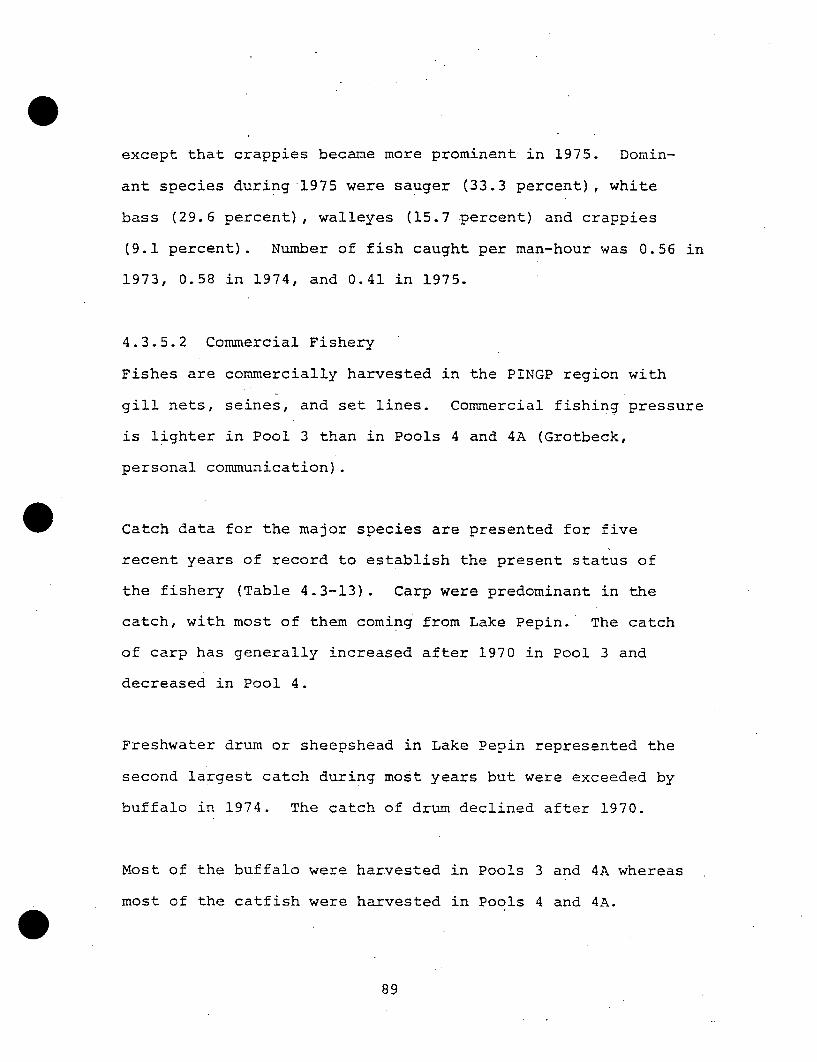
except that crappies became more prominent in 1975. Domin-

ant species during 1975 were sauger (33.3 percent), white

bass (29.6 percent), walleyes (15.7 percent) and crappies

(9.1 percent). Number of fish caught per man-hour was 0.56 in

1973, 0.58 in 1974, and 0.41 in 1975.

4.3.5.2 Commercial Fishery

Fishes are commercially harvested in the PINGP region with

gill nets, seines, and set lines. Commercial fishing pressure

is lighter in Pool 3 than in Pools 4 and 4A (Grotbeck,

personal communication).

Catch data for the major species are presented for five

recent years of record to establish the present status of

the fishery (Table 4.3-13). Carp were predominant in the

catch, with most of them coming from Lake Pepin. The catch

of carp has generally increased after 1970 in Pool 3 and

decreased in Pool 4.

Freshwater drum or sheepshead in Lake Pepin represented the

second largest catch during most years but were exceeded by

buffalo in 1974. The catch of drum declined after 1970.

Most of the buffalo were harvested in Pools 3 and 4A whereas

most of the catfish were harvested in Pools 4 and 4A.

89

TABLE 4.3-13

COMMERCIAL CATCH OF FISH (POUNDS) IN POOLS 3, 4 AND 4A (LA2E PEPIN)DURING 1970-1974. WISCONSIN AND MINNESOTA LANDINGS COMBIllED

(FERNHOLZ, PERSONAL COMMUNICATION)

Catfish Buffalo3 4 4A 3 4 4A

1970 759 19,223 27,181 83,234 7,405 56,364

1971 202 14,556" 23,193 23,749 7,033 51,518

1972 652 17,912 12,935 39,141 5,350 65,936

1973 630 9,246 19,792 47,967 5,418 31,970

1974 64 19,854 17,902 13,285 4,387 80,279

1970

1971

1972

1973

1974

26,231

13,418

195,820

307,908

231,093

Ca-rpI14

109,104

197,484

51,333

35,512

56,371

4A

1,500,784

2,026,879

969,236

1,355,626

987,362

Freshwater Drum3 4 4A

5,492 3,919 186,029

594 2,617 187,865

1,449 2,092 101,128

1,076 3,187 60,836

913 4,771 55,587

90

Other species of fish are unimportant in the harvest. These

include suckers, quillback, mooneye, goldeye, bowfin and

gars. Turtles are also harvested.

A majority of the total fish harvested were from Lake Pepin.

The catch of catfish and drum was relatively low in Pool 3 and

the catch of buffalo and drum was. relatively low in Pool 4.

4.3.5.3 Tag and Recapture Studies

Sport fishes were tagged and released near PINGP during

1973, 1974 and 1975. Some of the species moved considerable

distances upstream and downstream. The average distance

moved in 1975 was 52.6 miles for white bass, 17.6 miles for

sauger, and 22.2 miles for walleye. These studies indicate

that discrete populations of these species do not occur in

the PINGP region.

Although not designed for population estimates, the tag and

recapture data can be used to obtain a rough estimate of the

population numbers within the angling size range (Table 4.3-14).

The simplest method of population estimation assumes that

the rate of capture of tagged fish is identical to the rate

of capture in the whole population. Thus, the percentage

of tagged fish caught is equivalent to the percentage of the

total population caught within the same size range of those

91

TABLE 4.3-14

POPULATION ESTIMATES OF SPORT FISHES INTHE 12-MILE PINGP STUDY AREA BASED ON

PETERSON AND SCHNABEL TAG AND RECAPTURE METHODS a

Species

Northern pike

Channel catfish

White bass

Smallmouth bass

Largemouth bass

Sauger

Walleye

Number in 1:2-Mile Study Area

Peterson Schnabel

2,442 - b

22,720

173,910 155,335

7,215

795

609,809 228,784

162,721 123,512,

aEstimates for number of fish within the size

range caught by fishermen. Calculated fromdata in Gustafson et al. (1976) and Naplinand Geis (1975).

bDash indicates no estimate made because total

catch not determined in 1974.

92

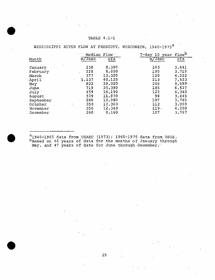
TABLE 4.1-1

MISSISSIPPI RIVER FLOW AT PRESCOTT, WISCONSIN, 1 9 4 0 - 1 9 7 5 a

Median Flowm/3sec cfs

7-day 10 yearm/i3secMonth

JanuaryFebruaryMarchAprilMayJuneJulyAugustSeptemberOctoberNovemberDecember

238228377

1,137822719459339286350350260

8,3908,050

13,32040,12529,02025,39016,19011,97010,08012,36012,3409,160

103105120213246185123

98107112119ý107

flowbcfs

3,6413,7194,2227,5238,6996,5274,3403,4453,7853,9694,2003,767

a 1 9 4 0 -1 9 6 5 data from USAECbBased on 46 years of data

May, and 47 years of data

(1973); 1965-1975 data from USGS.for the months of January throughfor June through December."

29

-" 4000--

3000-o 3- DAY

---JiLDAYLý

2000-

2000-

1000-

0 2 5 10 20 40 100RETURN INTERVALS (YEARS) BASED ON INDEPENDENT ANNUAL LOWS

FIGURE 4.1-2

CONSECUTIVE DAY AVERAGE LOW FLOW FREQUENCIES,MISSISSIPPI AT PRESCOTT, WISCONSIN 1928-1974

the range of flows from May 21 through September 4, 1975

when fish entrainment studies were conducted. The average

flow for this period was 650 m3 /sec. The relationship

between the flow through Sturgeon Lake and the flow in the

main channel of the Mississippi River is shown in Figure

4.1-3.

The approximate retention times for the North Lake-Sturgeon

Lake chain are 74 and 7.6 hours for total river flows of

226.4 and 1867.8 m3 /sec, respectively, based on lake volumes

given in Stefan (1973). Sturgeon Lake alone had estimated

retention times of 42.6 and 3.8 hours for the above flows.

31

tagged. Assuming that tags were observed and conscientiously

reported, there is no reason to expect that the ratio of

recaptured fish (R) to tagged fish (M) does not represent the

rate of exploitation due to fishing in the region. Rate of

exploitation (u) is given by Ricker (1975) as:

R

Having established u for the PINGP region, the distribution

of the population to be estimated is determined by the

distribution of the catch or sample taken for census.(C).

The sport fish catch in the 12-mile (1,601 hectares) PINGP

study area (Section 4.3.5.1) is taken as C to estimate sport

fish populations (N) in the same region. The formula for

the Petersen method (Ricker*1975) is:MC _C

N- R u

These parameters are more specifically defined as follows:

N = total number of fish in the 12-mile study areafrom Sturgeon Lake to the headwaters of Lake Pepin

M = total number of fish tagged in 1974 and 1975 (totalof 3,737 for all species) minus the number (92) ofrecaptures in 1974. In this case, data were treatedas a single census by estimating the numbers oftagged fish at large in 1975. This approachprovides a somewhat high estimate of tagged fishavailable in 1975 because natural mortality of fishtagged in 1974 is not accounted for.

C =-sport catch of each species in the 12-mile studyarea. The fact that many of the tagged fish movedout of the study area does not affect the rate ofrecapture if it is assumed that all tagged fishwere reported or that distance from the site didnot affect degree of reporting.

93

In an electrofishing study of river carpsuckers, Behmer

(1969) concluded that the Schnabel method gave a low

estimate and the Peterson method (Ricker 1975) gave a

maximum estimate of the population. Application of both

methods gives a possible range which is expected to include

the actual population size.

Ricker's (1958) formula for the Schnabel method for a multiple

census is:

N = EI CtMt)

R+1

where

Ct = total catch on day t,ý

mt.= total tagged fish at large oiý day t,

R = total number of recaptures

For this analysis the formula is applied as:

N CM197.4 +CM19.75

R 1974 & 1975 + 1

This formula gives a high estimate because many of the fish

were not tagged until the summer of each year and therefore

were less available for recapture.

94

Of the six assumptions needed to justify tag and recapture

estimates (Ricker 1975), five were probably reasonably met:

(1) marked and unmarked fish suffer the same mortality, (2)

marked and unmarked fish are equally vulnerable to capture,

(3) marked fish do not lose their marks, (4) marked fish

become randomly mixed or at least disperse both upstream or

downstream, (5) there is a negligible amount of recruitment

to the population between tagging and recapturing, or at least

recruitment is balanced by movement out of the area.'- Because

the sixth assumption (that all tags are reported) may not be

met, the population estimates may be somewhat high for the

size ranges considered.

4.3.5.4 Trawl Studies

Fishes were trawled in the immediate PINGP plant area in

1973, and in North Lake and the intake and discharge area

during the spring, summer and fall of 1974 and spring and

fall of 1975. (Figure 4.3-6). In 1974 and 1975, a semi-

balloon trawl having a 29 ft (8.8 m) footrope and 24 ft (7.3

m) headrope was trawled approximately 600 m (2000 ft) in 7

minutes at each station. Area sampled per tow (0.2788 ha or

0.689 acre) was calculated from an estimated effective

sampling width of 15 ft times distance of tow. Efficiency

of the trawl is assumed to be approximately 50 percent due

95

/1.1

0

1

SEC. 2,-"''or.,. 2 0

PRAIRIE _ ----ISLAND • A,/I,,.SCA

SEC. 4/

• SEC. 3--

/RED WIN

FIGURE 4.3-6

FISH STUDY AREAS NEAR PINGP, 1970-1975(FROM GUSTAFSON ET AL. 1976)

SCALE IN MILES

4 5 6 7

LE IN KILOMETERS

8 9 0.

2 3 4 5 6

F! |

I.'!.

f :1

to partial closing of the net and avoidance reaction to the

net. A definitive efficiency factor is not available.

Fish trawling studies were conducted in the PINGP region

during 1973-1975 (Table 4.3-15). Consistent sampling protocol

during the last two years permitted calculation (described

in Table 4.3-15) of standing crop in terms of number per

hectare. Data for the three years can be directly compared

in terms of catch per hour since number per hectare is

approximately half of catch per hour in the 1974 and 1975 data.

In the pre-operational (1973) sampling of the plant area,

catches were dominated by YOY (young-of-year) freshwater

drum (88 percent), followed by YOY channel catfish, YOY

gizzard shad, and carp. These species and several important

sport fish species showed no decline in subsequent years and

often showed much higher population densities than in 1973

when YOY were recruited into the populations near the plant.

Relatively large numbers of gizzard shad, white bass, white

crappie, and black crappie in the North Lake samples were

dominated by YOY. Thus, the habitats occurring in North

Lake are more important as a nursery ground than those in

the plant area.

97

0

TABLE 4.3-15

TRAWL CATCH OF FISLES IN NORTH VKE AND PINGP PLANT AREA (INTAKE AND DISCHARGE) IN 1973 a1974 , AND 1975 . DENSITIES ROUNDED TO NEAREST WHOLE NUMBER.

Sp~ecies

Shortnose garHooneyeGold eyeGizzard shadBigmouth buffaloSmallmouth buffaloCarpsucker app.Shorthead redhorseCarpRiver shinerSilver chub

00 Pugnose minnowEmerald shinerSpottail shinerBullhead minnowChannel catfishTadpole madtomNorthern pikeTrout-perchWhite bassBluegillWhite crappieBlack crappie

WalleyeSaugerFreshwater drumTotal

Plant area 1973Catch/hour

Plant area 1974Spring Summer Fall

North Lake 1974Spring Summer Fall

3

Plant area 1975Spring Fall

North Lake 1975Spring Fall

8 c3

19 2724

248

2 2

326 c

32

1

1

2

521

36

3

7

3

25831212

618

1115 24 20 2 4 3

7

1

316

13 24 4 3

84 c 1 321

21

1

4

4

2 60 63 1

6 2117 3

211

4 22 214 119 10

52 144 c 334 c

2 22 18

4 54

9 81 c 13470o -669 889

3

1

877 c1,000

1

1

52559

25 1

1

5 i794 c 79S5-5 160

105

4

3410T8

2

2

1 316 42

5 6137 5

110 493 35

3

2 94-2 T82

abCatch/hour; data from Hawkinaon (1974).

'Number/hectare; 1974 data from Naplin and Geis (1975),1975 data from Gustafson at al. (1976). CaTrawl hadSingle tow area calculated as 15 ft. width (to allow for partial closing of net and avoidance of trawl)

0.2788 hectares. Density timea,-2 - catch/hour.0 Predominantly or entirely YOY.

29 ft. footrope and 24 ft. headrope.times 2000 ft. per tow - 30.000 sq. ft. -

Assuming that trawl samples were representative of the

water bodies sampled, total population estimates can be

calculated. Maximum densities observed during 1974 and

1975 were multiplied by surface areas given by Hawkinson

(1974): 438 ha (1,082 acres) for North Lake and 83.4 ha

(206 acres) for the plant area. Population estimates for'

certain dominant or important species are:

Plant Area North Lake

Gizzard Shad 2,252 270,684Carp 2,002 4,818Channel Catfish 2,669 4,818White Bass 2,190 60,006Crappies 417 154,176Walleye 250 2,190Sauger 417 1,752Drum 66,220 58,692

The calculations represent low population estimates because

these species are likely to concentrate in habitats that

were not trawled (e.g., shallows, heavy beds of macroflora,

other types of cover). Due to the pelagic nature of gizzard

shad, many of them would be missed by bottom trawling. The

estimate of six million gizzard shad in the 323.8 ha (800

acre) Sturgeon Lake during the late summer of 1973 (Andersen

1975) may be a more realistic standing crop.

99

4.3.5.5 Seining Studies

Seining studies have been conducted in the PINGP region

from 1971 through 1975. A 100 ft (30.5 m) seine used in

the early studies was replaced with a 50 ft (15.3 m) seine

in 1974 and 1975. Area seined (300 sq m (3,228 sq ft)]

was estimated from the length of the seine and the distance

seined per tow in 1974 and 1975.

The 1971 and 1972 studies established the species composition

and general distribution of the small species and YOY of

the area.

Fish were seined near and above PINGP during the summer of

1973. Subsequently sampling was expanded to below Lo'ck and

Dam No. 3 during spring, summer and fall.

Seining data for 1974 (Table 4.3-16) and 1975 (Table 4.3-17)

permit a comparison of the relative abundance of fishes along

the shoreline in the three major study areas. Areas seined

(Gustafson et al. 1976) were used to determine total number

of fish per hectare.

Seine catches were highest in the tailwaters of Lock and Dam

No. 3 in 1974, followed by the region above the plant and

the immediate plant area. In these samples, species of

100

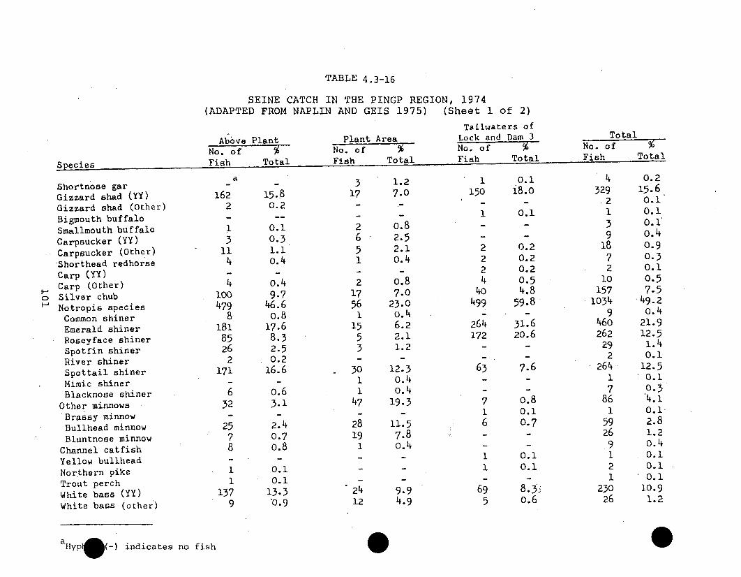
TABLE 4.3-16

SEINE CATCH IN THE PINGP REGION, 1974(ADAPTED FROM NAPLIN AND GEIS 1975) (Sheet 1 of 2)

Tailwaters ofAbove Plant Plant Area Lock and Dam 3 Total

No. of % No. of % No. of % No. of

Species Fish Total Fish Total Fish Total Fish Totala 1 0.1

Shortnose gar - - 3 1.2 1 . 0.2

Gizzard shad (YY) 162 15.8 17 7.0 150 18.0 329 15.6

Gizzard shad (Other) 2 0.2 - - - .2 0.1

Bigmouth buffalo - -- - 1 0.1 1 0.1

Smallmouth buffalo 1 0.1 2 o.8 - - 3 0.1

Carpsucker (YY) 3 0.3 6 2.5 - - 9 o.4

Carpsucker (Other) 11 1.1 5 2.1 2 0.2 18 0.9Shorthead redhorse 4 0.4 1 0.4 2 0.2 7 0.3Carp (YY) - - - 2 0.2 2 0.1

Carp (Other) 4 0.4 2 o.8 4 0.5 10 0.517 7.0 40 4.8 157 7.5

c: Silver chub 100 9-7 13 4 .

Notropis species 479 46.6 56 23.0 499 59.8 1034 49.2

Common shiner 8 O.8 1 0.4 - - 9 o.4

Emerald shiner 181 17.6 15 6.2 264 31.6 460 21.9Roseyface shiner 85 8.3 5 2.1 172 20.6 262 12.5Spotfin shiner 26 2.5 3 1.2 - - 29 1.4

River shiner 2 0.2 - - - 2 0.1

Spottail shiner 171 16.6 30 12.3 63 7.6 264 12.5Mimic shiner - - 1 0.4 - - 1 0.1Blacknose shiner 6 0.6 1 0.4 - - 7 0.3

Other minnows 32 3.1 47 19.3 7 0.8 86 4.1Brassy minnow - - - - 1 0.1 1 0.1.Bullhead minnow 25 2.4 28 11.5 6 0.7 59 2.8Bluntnose minnow 7 0.7 19 7.8 , - - 26 1.2

Channel catfish 8 0.8 1 0.4 - - 9 0.4Yellow bullhead - - - 1 0.1 1 0.1

Northern pike 1 0.1 - 1 0.1 2 0.1

Trout perch 1 0.1 - - - - 1 0.1

White bass (YY) 137 13.3 24 9.9 69 8.3; 230 10.9

White bass (other) 9 -0.9 12 4.9 5 0.6 26 1.2

aHyp*(-) indicates no fish 0

TABLE 4.3-16. (Sheet 2 of 2)

Above PlantNo. of %

Species Fish Total

Plant AreaNo. of %Fish Total

Tailwaters ofLock and. Dam 3No. of TtFish Total

TotalNo. of %Fish Total

Yellow perchSauger'(YY)Sauger (Other)Log perchJohnny darterSmallmouth bassGreen sunfishBluegill (YY)Bluegill (Other)Rock bassWhite crappie (YY)White crappie (Other)Black crappie (YY)Black crappie (Other)Drum (YY)Drum (Other)

372323

10

1

51

141

192

0.30.70.20.30.20.3

1.0

0.10.50.11.40.11.90.2

2245

4

912124311

0.80.8

1.72.1

1.73.70.40.80.40.81.71.24.5

4

71

HC-O~

6

33

12392

0.1

0.50.8

0.1

0.7

0.40.41.40.41.10.3

498

14834

19739630

7394

0.20o40.40.70.40.10.20.90.30.10.40.31.40.31.90.2

Total

Hectares seinedFish per hectare

1027

0.811268

835 2105

1.411493

0.27900

0.332530

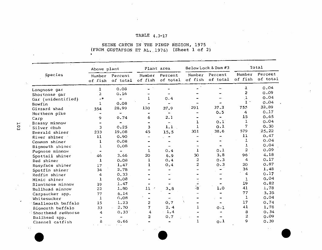
TABLE 4.3-17

SEINE CATCH IN THE PINGP REGION, 1975(FROM GUSTAFSON ET AL. 1976) (Sheet 1 of 2)

Species

Above plant Plant area Below Lock.& Dam #3

Number Percent Number Percent Number Percentof fish of total of fish of total of fish of total

Total

Number Percentof fish of total

H•0

Longnose garShortnose garGar (unidentified)BowfinGizzard shadNorthern pikeCarpBrassy minnowSilver chubEmerald shinerRiver shinerCommon shinerBigmouth shinerPugnose minnowSpottail shinerRed shinerRosyface shinerSpotfin shinerRedfin shinerMimic shinerBluntnose minnowBullhead minnowCarpsucker spp.WhitesuckerSmallmouth buffaloBigmouth buffaloShorthead redhorseBullhead spp.Channel catfish

12

I

354

9

3233

4611

461

173441

192277

11533

4

0.080.16

0.0828.99

0.74

0.2519.080.900.080.08

3.660.081.472.780.330.081.471.806.140.081.232.700. 33

0.66

110

6

345

120

1

Ii

2742

0.4

37.9

2.1

1.1

15.5

0.46.90.40.4

3,8

0.72.41.4

0.7

I291

11

301

130

22

•8

1

1

37.30.5

0.10.1

38.6

0.13.80.30.3

1.0

0-1

0.1

75

1

571

9

23

I47

14

.1 0.042 0.091 0.041 - 0.045 32.894 0.17.5 0.651 0.047 0.30'9 25.221 0.471 0.041 0.042 0.096 4.184 0.17.0 0.874 1.484 o.171 0.04.9 0.821 1.78'7 3.351 0.04

L7 0.741I 1.788 0.342 0.099 0.39

0

TABLE 4.3-17 (Sheet 2 of 2)

H

Above plant Plant area Below Lock.&Dam-#3 TotalSpecies

Number Percent Number Percent Number Percent Number Percentof fish of total of fish of total of fish of total of fish of total

Tadpole madtom 3 0.25 - - 3 0.13Troutperch. - - - - 7 0.9 7 0.33White bass 223 18.26 29 10.0 107 13.8 359 15.65Rock bass - - 2 0.7 - - 2 0.09Green sunfish 2 0.16 2 0.7 - 4 0.17Bluegill 17 1.39 8 2.8 - 25 1.09Smallmouth bass 5 0.41 - - - 5 0.21White crappie 25 2.05 9 3..l 1 06] 35 1.52Black crappie 12 0.98 - - 4 0.5 16 0.74Crappie spp. - - 21 7.2 - - 21 n.c. 0.91Johnny darter 5 0.41 2 0.7 2 0.3 9 0.39Yellow perch 4 0.33 2 0.7 - - 6 0.26Logperch .15 1.23 - - 6 0.8 21 0.91Sauger II 0.90 3 0.4 14 0.61Walleye 1 0.08 - - 1 0.4 2 0.09

Freshwater drum 2 0.16 1 0. 3 7 0. 9 10 0.43

Total 1223 100.00 290 100.00 781 100.00 2294 100.00

* Hyphen (-) indicates no fish were caught.

Notropis (minnows) accounted for approximately half of the

total numbers. The most abundant non-cyprinid YOY were

gizzard shad (15.6 percent) and white bass (10.9 percent).

The 1975 catch was similar to that of 1974 in terms of

species composition and relative numbers in the three regions.

However, total standing crop estimates were higher in 1975.

Species of Notropis and YOY gizzard shad each comprised

approximately one-third of the 1975 catch (Table 4.3-17).

The dominant species of Notropis was the emerald shiner,

as in 1974. YOY white bass were again a major component

of the catch (15.6 percent).

Table 4.3-18 compares numbers of fishes seined at all

stations during 1974 and 1975 and those sampled above Lock

and Dam No. 3 in 1973. The tally excludes the older fish

included in Tables 4.3-16 and 4.3-17 with the exception of

minnows and darters.

The 1973 seine catches are not directly comparable to sub-

sequent surveys because sampling was done at different

times of the year and a larger seine was used in 1973 (Gustafson

et al. 1976) The large catch of gizzard shad, carpsucker,

white bass and freshwater drum YOY in 1973 may be attributable

105

0TABLE 4.3-18

SEINE CATCH (NUMBER PER HECTARE -) IN THE PINGP REGION, 1973-1975

(ADAPTED FROM GUSTAFSON ET AL, 1976)

Species1 9 7 3 a

0.33 ha seined

Number No./ha

1974 b

1.41 ha seined

Number No./ha

1.38 ha seined*

Number No./ha

Longnose garShortnose garBowfinGizzard shadNorthern pikeCarpMinnows & dartersSmallmouth buffaloBigmouth buffaloCarpsuckerWhite suckerShorthead redhorseBullheadsChannel catfishTadpole madtomWhite bassSunfishCrappiesSmallmouth bassYellow perchSaugerWalleyeFreshwater drum

1729

4504

98

15231322

26

100

- 2

5239.39 329- 1

12.12 21527.27 1300

- 3

296.97 9

- 7- 1

- 9

4615.15 23039 ; 39 2366.67 39

- 1- 8

78.79 9

303.03 39

1.42

233.330.711.42

921.992.13

6.38

4.960.716.38

163.1216.3127.660.715.676.38

27.66

1

755

676

174177

182

3201"

2672

16

14210

0.72

0.72547.10

489.86

12.3229.7155.800.725.801.45

2.17145.6518.8452.170.724.35

10.141.457.25

4019 12,178.79 2012Total 1426.95 1914 1386.96

* 1975 area isan estimate.

**Hyphen (-) indicates no fish were caught.

a 100 ft seine; summer

50 ft seine; spring, summer and fall

106

to the greater effectiveness of the larger seine and the fact

that sampling was limited to the summer. However, a strong

year class of gizzard shad in 1973 is also apparent from

electrofishing studies (Section 4.3.5.6).

A comparison of the 1974 and 1975 data reveals a marked

similarity in total catch and dominance by the same taxa.

However, the data suggest stronger age classes of gizzard

shad and suckers and a decline in the minnow/ darter com-

ponent in 1975.

4.3.5.6 Electrofishing Studies

Electrofishing studies have been conducted in the PINGP

region from 1970 to 1975. The earlier studies were limited

in scope, but provide information on species composition

which can be compared to more recent data. During the

summer and fall of 1970, fish were sampled in Sturgeon Lake

and tailwaters of Lock and Dam No. 3. Carp and white bass

were the dominant species, followed by mooneye, walleye,

black crappie, freshwater drum, and 11 other species (Table

4.3-19).

The 1971 survey from above Lock and Dam No. 3 yielded larger

numbers of carp and fewer white bass than the 1970 survey.

YOY gizzard shad were abundant in the late summer of 1971.

107

TABLE 4.3-19

ELECTROFISHING CATCH IN THE MISSISSIPPI RIVERNEAR PINGP, 1970 AND 1971(FROM MILLER 1971, 1972)

Species

1 9 7 0 a 1 9 7 1 b

Summer Fall EarlyýSu. mner

Longnose garShortnose garBowfinGizzard shadMooneyeNorthern pike-CarpSilver chubAmerican eelWeed shinerWhite suckerCarpsucker spp.Smallmouth buffaloBigmouth buffaloSilver redhorseShorthead redhorseYellow bullheadChannel catfishWhite bassRock bassGreen sunfishBluegillSmallmouth bassLargemouth bassWhite crappieBlack crappieSaugerWalleyeFreshwater drum

242

20

68

3

268

33

6149

31

814 1

141 170

1

LateFall

571

110c1

41147

423

12

413

53

94

176

8

2

2911

28

1296

16

318

6

511

27

331417

aData for above and below Lock and Dam No.total catch given; from Miller (1971)

bsturgeon Lake and Mississippi River above

No. 3, total catch; from Miller (1972)

3 combined,

Lock and Dam

CPredominantly or entirely YOY

108

Electrofishing surveys were conducted from 1973 to 1975 in

the Mississippi River above PINGP, in the plant area, and

below the plant at stations described by Hawkinson (1974).

Stations above the plant include locations in North Lake,

Sturgeon Lake, Brewer Lake, and the main river channel.

Stations sampled in the plant area were located in the main

channel above Lock and Dam No. 3, in the intake and discharge

areas, and in several sloughs in the area. Below the plant,

sampling was conducted in the tailwaters of Lock and Dam No.

3 and in the main and back channels to the Highway 63 bridges.

Table 4.3-20 presents summer electrofishing catches for 1973

in terms of total numbers and catch per hour. YOY gizzard

shad dominated the catches in all three regions and were

most abundant in the tailwaters. YOY of carpsucker, black

crappie, and freshwater drum were also commonly caught.

Larger sport fishes were most commonly caught in the tail-

waters of the lock and dam.

Electrofishing catches for 1974 and 1975 are presented by

season to permit an analysis of the temporal variability as

related to recruitment of young fishes (Tables 4.3-21 through

4.3-26). Data are summarized for major species in Table

4.3-27. For 1974 and 1975, the number of fish per kilometer

is roughly equivalent to catch per hour times 0.75. 0109

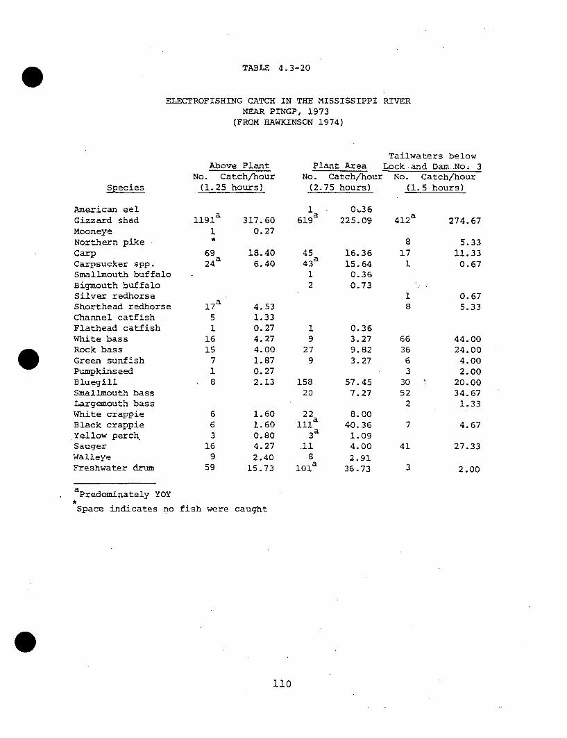
TABLE 4.3-20

ELECTROFISHING CATCH IN THE MISSISSIPPI RIVERNEAR PINGP, 1973

(FROM HAWKINSON 1974)

Above PlantNo. Catch/hour

(1.25 hours)

Tailwaters belowPlant Area Lock and Dam No. 3

No. Catch/hour No. Catch/hour(2.75 hours) (1.5 hours)Species

American eelGizzard shadMooneyeNorthern pikeCarpCarpsucker spp.Smallmouth buffaloBigmouth buffaloSilver redhorseShorthead redhorseChannel catfishFlathead catfishWhite bassRock bassGreen sunfishPumpkins eedBluegillSmallmouth bassLargemouth bassWhite crappieBlack crappie

.Yellow perchSaugerWalleyeFreshwater drum

aPredomi nately YOY

1191 a

1*

692 4 a

17 a

51

1615

718

663

169

59

1 0-.36619a 225.09317.60

0.27

18.406.40

4.531.330.274.274.001.870.272.13

1.601.600.804.272.40

15.73

4 1 2 a

4543 a

12

19

279

15820

22

3 a

.118

101a

16.3615.640.360.73

0.363.279.823.27

57.457.27

8.0040.361.094.002.91

36.73

817

1

18

274.67

5.3311.330.67

0.675.33

44.0024.004.002.00

20.0034.67

1.33

4.67

27.33

663663

3052

2

7

41

3 2.00

Space indicates no fish were caught

110

TABLE 4..3-21

aELECTROFISHING CATCH IN THE PINGP REGION, SPRING, 1974

(FROM N;CPYJIN AND GEIS .1975)

Above Plant Plant Area Below Lock Dam 3Catch/Hour Catch/Hour Catch/Hour

Species No. (7.5 Hours) No. (2.5 Hours) No. (2.5 Hours)

Silver lamprey - -...Shortnose gar 2 0.27 ....Longnose gar ..... .Bowfin 1 0.13 ....-Mooneye 3 0.40 ....Goldeye - -...

Gizzard shad - - 1 0.40 - -

Bigmouth buffalo 3 0.40 2% 0.80 4 1.60Smallmouth buffalo - - - - 1 0.40Carpsucker spp. 62 8.27 3 1.20 <>1 O.4OWhite sucker - - - - 2 0.8oSilver redhorse 2 0.27 - -. 1 0.40Shortheadredhorse 53 7.07 17 6.80 24 9.60

Carp 214 28.53 152 60.80 73 29.20Silver chub 24 3.20 2 0.80 - -Pugnose minnow - - - -Golden minnow - - 1 0.40 - -Common shiner - - - - -

Bulerald shiner 28 3.73 - - 2 0.80Rooyface shiner 10 1.33 - - 2 0.80Spotfin shiner 0. ..Spottail shiner - I 1 .40 o

Silvery minnow .....

Fathead minnow - - -.Bullhead minnow 1 0.13 1.8.Bluntnose minnow 3 0.40 -...

Channel catfish 6 0.80 4 1.62 0 1 .40Flathead catfish ..... .-

Northern pike 5 0.67 1 0.40 5 2.00White bass 76 10213 12 4 1.80 97 38.80Yellow perch 3 0.40 - - -

Sauger 36 4.8p 8 3.20 30 12.00Walleye 7 0.93 1 2.40 17 6.80Logperch - - - -

Smallmouth bass 20 2.67 3 1.20 9 3.60Largemouth bass - - 1 0.40 - -Green sunfish 2 0.27 0..Pumpkinseed - - 3 1.20 - -Bluegill 15 2.00 5 2.00 17 6.80

Hybrid sunfish n .. .Rock bass 1? 2.27 8 3.20 45 18.OOWhite crappie ... i 0 .4oBlack crappie 2 0.27 1 0.40 6 2.4oFreshwater drum 68 9.07 11 4.4o 25 1O.00

Burbo t ..... 7-.. . ...

aCatch/hour 'X 0.75 = ish/km

Hyphen indicates no fish Tvere caught

-. TAkBLE .4 .3-2.2

ELECTROFISHING CATCH IN THE PINGP REGION, SU~MMER, 1974___ (FROM NAPLIN AND GEIS 1975)

Above PlantCatch/Hour

No. (7.5 Hours)

Plant AreaCatch/Hour

No. (2.5 Hours)

Below Lock & Dam 3Catch/Hour

No. (2.5 Hours)

Silver lampreyShortnose garLongnose garBowfinMooneyeGoldeyeGizzard shad aBigmouth buffaloSmallmouth buffaloCarpsucker spp.White suckerSilver redhorseShorthead redhorseCarpSilver chubPugnose minnowGolden minnowCommon shinerEmerald shinerRosyface shinerSpotfin shinerSpottail shinerSilvery minnowFathead minnowBullhead minnowBluntnose minnowChannel catfishFlathead catfishNorthern pikeWhite bass aYellow perchSaugerWalleyeLog perchSmallmouth bassLargemouth bassGreen sunfishPumpkinseedBluegillHybrid sunfishRock bassWhite crappieBlack crappieFreshwater drumaBurbot

2 0.27

140 18.671 0.132 0.27

27 3.60

23 3.07139 18.53

19 2.53

25 3.338 1.07

4 0.53

2 0.27

4 0.531 0.132 0.27

69 9.208 1.07

32 4.276 0.805 0.67

27 3.60

1 0.13

25 3.33

2 0.27

4 0.5376 10.13

31

152167

18121

5

28

12

24

2

966

18

5211

41

2523

5411176

1

1.200.40

6o.8O0.402.4o2.80

7.2048.402.00

0.803.20

0.400.80

9.6oo.80

38.402.407.20

2.008.400.40

16.40

100.801.20

21.6oO.404.4o

30.400.40

1

54514

20672

164

414

112

2593

2753

2023

34

6122

0.40

21.602.000.401.6o

8.0026.800.80

6.401.60

1.600.401.60

44.80

10.003.601.20

lO.8O2.001.20

8o.8o1.20

13.60

2.404.800.80

a Predominantly YOY112

TABLE 4.3-23

ELECTROFISHING CATCH IN(FROM -IAPLIN

PINGP REGION, FALL, 1974AND GEIS 1975)

Above PlantCatch/Hour

Species No. (7.5 Hours)

Plant AreaCatch/Hour

No. (2.5 Hours)

Below Lock & Dam 3Catch/Hour

No. (2.5'Hours)

Silver lampreyShortnose garLongnose garBowfinMooneyeGoldeyeGizzard shadaBigmouth buffaloSmallmouth buffaloCarpsucker spp.White suckerSilver redhorseShorthead redhorseCarpSilver chubPugnose minnowGolden minnowCommon shinerEmerald shinerRosyface shinerSpotfin shinerSpottail shinerSilvery minnowFathead minnowBullhead minnowBluntnose minnowChannel catfishFlathead catfishNorthern pikeWhite bassYellow perchSaugerWalleyeLog perchSmallmouth bassLargemouth bassGreen sunfishPumpkinseedBluegillHybrid sunfishRock bassWhite crappieBlack crappieFreshwater drumBurbot

3.1

2

540

92

1196253

1"631

161

322

44777

154

36

5219

121647

0.40

0.13

0.27

72.00

1.200.27

1.4712.803.330.40

0.130.80

0.400.132.130.13

0.400.270.27

0.536.270.930.932.000.534.80

1.47

6.930.131.201.602.136.27

2 0.80

388 152.20 100 4o.o0

6

356

1

3

4

10

11

16

3221

116

50

3428

5212

94

2.4014.oo2.40

0.401.20

1.6o

4.00

o.40O.40

6.401.200.800.800.404.402.4o

20.00

136.803.20

20.804.803.601.60

1

7181

2

2

45

4

54118

151

1425

9

2751

14

142

o.4o

2. bo72.400.80

0.80

o.4o

1.60

2.0016.400.403.206.00o.4o5.60

10.003.60

110.000.405.60

5.6o0.80

a Predominantly YOY

113

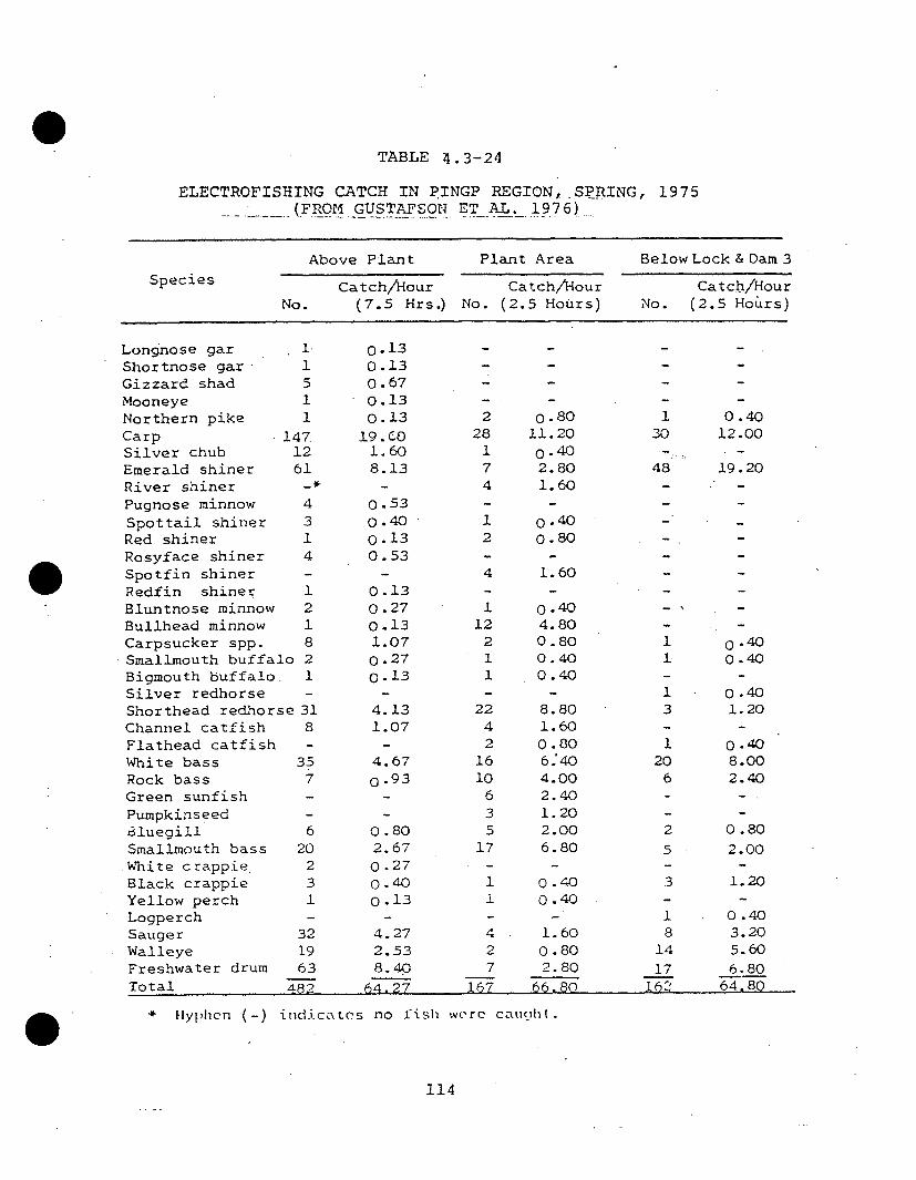
TABLE 4.3-24

ELECTROFISHING CATCH IN PINGP REGION, SPRING, 1975(FROM GUSTAFSON ET AL. 1976)

Above Plant Plant Area Below Lock & Dam 3Species Catch/Hour Catch/Hour Catch/Hour

No. (7.5 Hrs.) No. (2.5 Hours) No. (2.5 Hours)

Longnose gar 1-Shortnose gar 1Gizzard shad 5Mooneye 1Northern pike 1Carp -147Silver chub 12Emerald shiner 61River shinerPugnose minnow 4Spottail shiner 3Red shiner 1Rosyface shiner 4Spotfin shiner -

Redfin shiner 1Bluntnose minnow 2Bullhead minnow 1Carpsucker spp. 8Smallmouth buffalo 2Bigmouth buffalo. 1Silver redhorse -

Shorthead redhorse 31Channel catfish 8Flathead catfish -White bass 35Rock bass 7Green sunfish -

Pumpkinseed8luegill 6Smallmouth bass 20White crappie. 2Black crappie 3Yellow perch 1LogperchSauger 32Walleye 19Freshwater drum 63Total A82

0.130.13o.670.130.13

19. 01.608.13

0.530.400.130.53

0.130.270.131.070.270.13

4.131.07

4.67O0.93

0.802.670.270.400.13

4.272.538.40

64. 27

2 0.8028 11.20

1 0.407 2.804 1.60

1 0.402 0.80

4 1.60

1 0.4012 4.80

2 0.801 0.401 0.40

22 8.804 1.602 0•80

16 6.4010 4.006 2.403 1.205 2.00

17 6.80

1 0.401 0.40

4 1.602 0.807 2.80

167 66.80

werC cauLhit .

1

30

48

I1

1

3

120

6

0.4012.00

19.20

0.400.40

o.40

1.20

0.408.002.40

0.802.00

1.20

0.403.205.606.80

64 8R

25

3

18

1417

* Hyphen (-) indicates no fish

114

TABLE 4.3-25

ELECTROFISHING CATCH IN PINGP REGION, SUMMER, 1975(FflOM GUSTA.-SON ET AL. 1976)

Species Above Plant Plant Area Below Lock & Dam3Catch/Hour Catch/Hour Catch/Hour

No. (7.5 Hours) No. (2.5 Hours) No. (2.5 Hours)

Silver lamprey -* - .1 0.40Longnose gar 1 0.13 .- -

Bowfin 1 0.13 - - -

Gizzard shad 226 30.13 57 22.80 29 11.60Mooneye - - - - 1 0.40Northern pike 4 0.53 - - 1 0.40Carp 97 12.93 44 17.60 386 15.20Silver chub 20 2.67 4 1.60 2 0.80Emerald shiner 52 6.93 2 0.80 75 30.00Spottail shiner 6 0.80 1 0.40 - -Rosyface shiner 33 0.40 1 0.40 14 5.60Spotfin shiner 2 0.27 - - - -

Redfin shiner 3 0.40 - - 1 0.40Bluntnose minnow 4 0.53 4 1.60 2 0.80Fathead minnow - - 1 0. 4 0 - -Bullhead minnow 9 1.20 10 4.00 - -

Carpsucker ssp. 27 3.60 3 1.20 4 1.60Smallmouth buffalo 6 0.80- 12 4.80 - -Bigmouth buffalo - - 1 0.40 - -

Silver redhorse 1 0.13 - - 1 0.40Shorthead redhorse 25 3.33 - - 18 7.20Black bullhead 1 0.13 2 0.80 17 6.80Channel catfish 5 0.67 3 1.20 4 1.60Flathead catfish 3 0.40 1 0.40 3 1.20Burbot - - - - 1 0.40White bass 37 4.93 17 6.80 114 45.60Rock bass 11 1.47 11 4.40 21 8.40Green sunfish 3 0.40 16 6.40 6 2.40Pumpkinseed 2 0.27 - - 1 0.40Lluegill 22 2.93 37 14.80 71 28.40Smallmouth bass 28 3.73 14 5.60 55 22.00Laraemouth bass - - - 4 1.60White crappie - - 2 0.80 - -

Black crappie 4 0.53 2 0.80 4 1.60Johnny darter 1 0.13 - -.

Yellow perch 32 4.27 3 1.20 1 0.40Log perch 17 2.27 1 0.40 4 1.60Sauger 38 5.07 3 1.20 6 2.40Walleye 22 2.93 4 1.60 20 8.00Drum 66 8.80 8 3.20 5 2.00

Thtal 809 107.87 274 109.60 524 209.60

Hyphen (-) indicates no fish were caught.

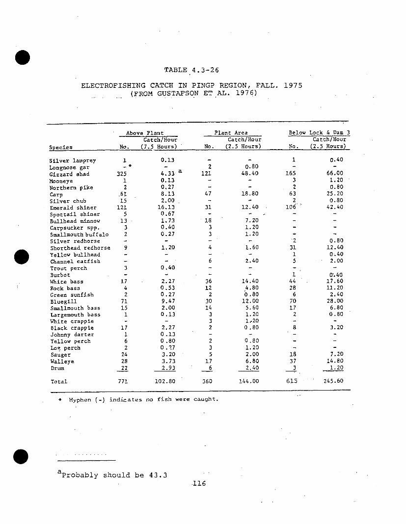
TABLE 4.3-26

ELECTROFISHING CATCH IN PINGP REGION, FALL, 1975(FROM GUSTAFSON ET' AL. 1976)

Above Plant Plant Area Below Lock & Dam 3Catch/Hour Catch/Hour Catch/Hour

Species No. (7.5 Hours) No. (2.5 Hours) No. (2.5 Hours)

Silver lamprey 1 0.13 - - 1 0.40Longnose gar - - 2 0.80 - -Gizzard shad 325 4.33 a 121 48.40 165 66.00Mooneye 1 0.13 - - 3 1.20Northern pike 2 0.27 - - 2 0.80Carp .61 8.13 47 18.80 63 25.20Silver chub 15 2.00 - - 2 0.80Emerald shiner 121 16.13 31 12.40 106 42.40Spottail shiner 5 0.67 - -.Bullhead minnow 13 1.73 18 7.20 - -Carpsucker spp. 3 0.40 3 1.20 - -Smallmouth buffalo 2 0.27 3 1.20 - -Silver redhorse .... 2 0.80Shorthead redhorse 9 1.20 4 1.60 31 12.40Yellow bullhead - -1 0.40Channel catfish - - 6 2.40 5 2.00Trout perch 3 0.40 - 1 - ,-Burbot -.... 1 0:.40White bass 17 2.27 36 14.40 44 17.60Rock bass 4 0.53 12 4.80 28 11.20Green sunfish 2 0.27 2 0.80 6 2.40Bluegill 71 9.47 30 12.00 70 28.00Smallmouth bass 15 2.00 14 5.60 17 6.80Largemouth bass 1 0.13 3 1.20 2 0.80White crappie - - 3 1,20 - -Black crappie 17 2.27 2 0.80 8 3.20Johnny darter 1 0.13 - -.Yellow perch 6 0.80 2. 0.80 - -LoR perch 2 0 .27 3 1.20 - -Sauger 24 3.20 5 2.00 18 7.20Walleye 28 3.73 17 6.80 37 14.80Drum 22 2.93 6 2.40 3 1.20

Total 771 102.80 360 144.00 615 245.60

Hyphen (-) indicates no fish were caught.

aprobably should be 43.3

116

TABLE 4.3-27

ELECTROFISHING CATCH (NUMBER/HOUR) OF MAJOR FISH SPECIES IN THE MISSISSIPPI RIVERNEAR PINGP, 1974 AND 1975a

Spring Summer FallAbove Plant Below Above Plant Below Above Plant Below

Species Plant Area Lock Plant Area Lock Plant Area Lock

1974

Gizzard shad 0.4; 1 8 .7b 6 0 .8b 2 1.6b i.7 2 .0b 1 5 2 . 2 b 4 0 . 0 b

Carpsucker 8.3 1.2.. 0.4 3.6 2.8 1.6 1.2Shorthead redhorse 7.1 6.8 9.6 3.1 7.2 8.0 1.5 2.4 2.8

Carp 28.5 60.8 29.2 18.5 48.4 26.8 12.8 14.0 72.4

Channel catfish 0.8 1.6 0.4 0.5 9.6 1.6 0.3 0.4 1.6Northern pike 0.7 0.4 2.0 0 .3b 1.6 0.5 2.0White bass 10.1 4.8 38.8 9.2 3 8 . 4b 4 4 . 8 b 6.3 .6.4 16.4Sauger 4.8 3.2 12.0 4.3 7.2 10.0 0.9 0.8 3.2Walleye 0.9 0.4 6.8 0.8 3.6 2.0 0.8 6.0Smallmouth bass 2.7 1.2 3.6 3.6 8.4 10.8 4.8 4.4 5.6Bluegill 2.0 2.0 6.8 3.3 100.8 80.8 6.9 136.8 110.0Black crappie 0.3 0.4 2.4 0 5 4.4 2.4 2.1 3.6 5.6Freshwater drum 9.1 4.4 10.0 10:1k 30.4b 4 8b 6.3 1.6 0.8

1975

Gizzard shad 0.7 30.1 22.8 11.6 43.3; 48.4 66.0Carpsucker 1.1 0.8 0.4 3.6 1.2 1.6 0.4 1.2Shorthead redhorse 4.1 8.8 1.2 3.3 7.2 1.2 1.6 12.4Carp 19.6 11.2 12.0 12.9 17.6 15.2 8.1 18.8 25.2Channel catfish 1.1 1.6 0.7 1.2 1.6 2.4 2.0

Northern pike 0.1 0.8 0.4 0.5 0.4 0.3 0.8White bass 4.7 6.4 8.0 4.9 6.8 '45.6 0.5. 4.8 11.2Sauger 4.3 1.6 3.2 5.1 1.2 2.4 3.2 2.0 7.2Walleye 2.5 0.8 5.6 2.9 1.6 8.0 3.7 6.8 14.8Smallmouth bass 2.7 6.8 2.0 3.7 5.6 22.0 2.0 5.6 6.8Bluegill 0.8 2.0 0.8 2.9 14.8 28.4 9.5 12.0 28.0Black crappie 0.4 0.4 1.2 0.5 0.8 1.6 2.3 0.8 3.2Freshwater drum 8.4 2.8 6.8 8.8 3.2 2.0 2.9 2.4 1.2

a,From Naplin ahd Geis (1975) and Gustaf: al. (1976)

0

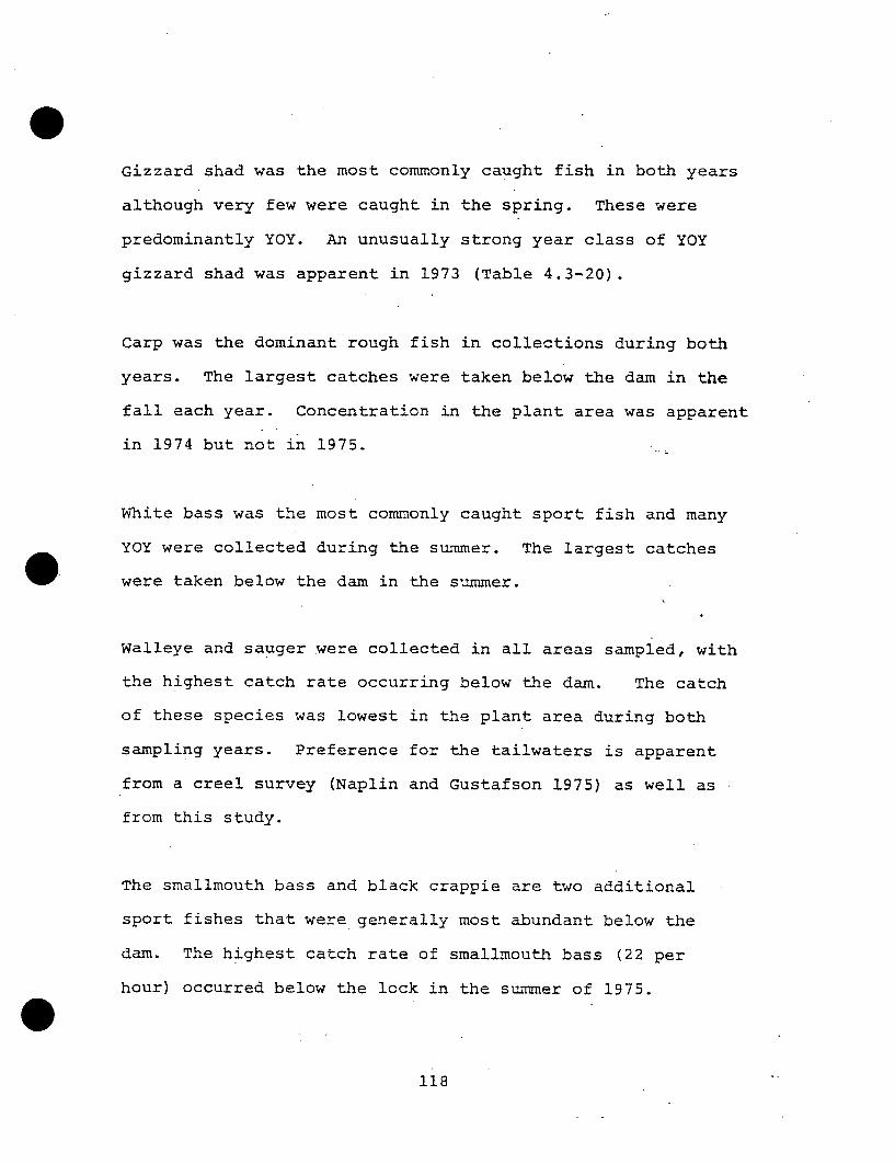
Gizzard shad was the most commonly caught fish in both years

although very few were caught in the spring. These were

predominantly YOY. An unusually strong year class of YOY

gizzard shad was apparent in 1973 (Table 4.3-20).

Carp was the dominant rough fish in collections during both

years. The largest catches were taken below the dam in the

fall each year. Concentration in the plant area was apparent

in 1974 but not in 1975.

White bass was the most commonly caught sport fish and many

YOY were collected during the summer. The largest catches

were taken below the dam in the summer.

Walleye and sauger were collected in all areas sampled, with

the highest catch rate occurring below the dam. The catch

of these species was lowest in the plant area during both

sampling years. Preference for the tailwaters is apparent

from a creel survey (Naplin and Gustafson 1975) as well as

from this study.

The smallmouth bass and black crappie are two additional

sport fishes that were generally most abundant below the

dam. The highest catch rate of smallmouth bass (22 per

hour) occurred below the lock in the summer of 1975.

118

Electrofishing studies were also conducted during the night

in October of 1974 and summer and fall of 1975. Lower night-

time catch rates of gizzard shad, bluegill, and smallmouth

bass, in comparison to daytime catches, were partially

attributable to reduced visibility. However, catches of

walleye, sauger, and white bass were highest at night.

4.3.5.7 Trap Netting Studies

Trap nets were fished experimentally in Pool 4 in 1957 and

1963 (Anonymous 1964). Both studies were performed at

approximately the same time of year and at the same locations.

In 1957 the most abundant fish were walleye, black crappie,

bluegill, white bass, carp, freshwater drum, and shorthead

redhorse. The 1963 catch was similar except that walleye

and carp catches had declined and northern pike and white

crappie catches were higher.

Fish were trap netted in the PINGP area from 1970 to 1975.

Fyke nets were used during 1970 and 1972. A trap net des-

cribed by Krosch (1968) was used subsequently. Nets were

fished in 24-hour sets. Sampling was limited to August

in 1973 (Hawkinson 1974) and expanded to spring, summer, and

fall in subsequent years.

119

Table 4.3-28 indicates a dominance of carp, shorthead red-

horse, white bass, crappies, sauger, and freshwater drum

in 1970, 1972 and 1973. The higher 1973 catches may be

attributable to using a more effective net.

Trap net data for 1974 and 1975 are presented in Tables

4.3-29 through 4.3-34 and summary Tables 4.3-35 and 4.3-36.

For the 1973-1975 sampling period, the summer catch per

lift of fishes above the plant was highest during 1974 when

large numbers of carp and white bass were collected. In

the plant area, the summer catch per lift was also highest

in 1974, with freshwater drum and carp dominating the catch.

Additional studies will be needed to assess possible popula-

tion trends.

Total catch per net of major species was highest above the

plant except during the spring when large numbers of carp

and freshwater drum were collected below Lock and Dam No. 3.

Catches of major sport fishes (white bass, walleye, sauger)

were generally highest above the plant although these fish

are known to concentrate in the tailwaters in the spring

(Section 4.3.5.1). None of the major species demonstrated a

clear preference for the plant area.

120

TABLE 4.3-28

TRAP NETTING CATCH IN THE MIgSISSIPPI RIVER NEAR PINGP19720 AND 1973c (Sheet 1 of 2)

Above and Below Lock Down No.31970a 1972 b Plant Area 1973c

No. No. Catch/lift No. Catch/lift(52 lifts) (70 lifts)

aIN 1970

Above Plant 1973 cNo. Catch/lift

(40 lifts)

Fj

Longnose garShortnose garBowfinGizzard shadMooneyeNorthern pikeCarpCarpsuckerWhite suckerSmallmouth buffaloBigmouth buffaloSilver redhorseShorthead redhorseGreater redhorseYellow bullheadBrown bullheadChannel catfishFlatheadWhite bassRock bassBluegillPumpkinseedLargemouth bassWhite crappieBlack crappieYellow perchSaugerWalleyeDrum

968

1

2522

2

41

2211

413

138

128 2.46

12

364

711

161

28215

413

22

110

125

2311019

1

661

1123

24202

0.040.960.100.160.010.873.740.210.060.190.030.031.57

0.010.030.07

3.300.140.270, 01

0.090.870.011.760.342.89

362

771

48134

14

1221

87

0.081.550.180.180.021.203.350.35

0.300.050.022.18

1 0.02

3 0.08

90 1.73

28 0.54

5425

1.030.48

198691

343

1801978

4.950.150.220.02

0.081.080.022.000.481.95

20 0.38

26 0.50

TABLE 4.3-28 (Sheet 2 of 2)

aFrom Miller 1971. Total catch in fall with fyke nets.

bFrom Miller 1973. Catch of dominant species with fyke nets in August.

cFrom H-awkinson 1974. Summer catch with trap nets. Above plant data for

North, Sturgeon, and Brewer lakes.

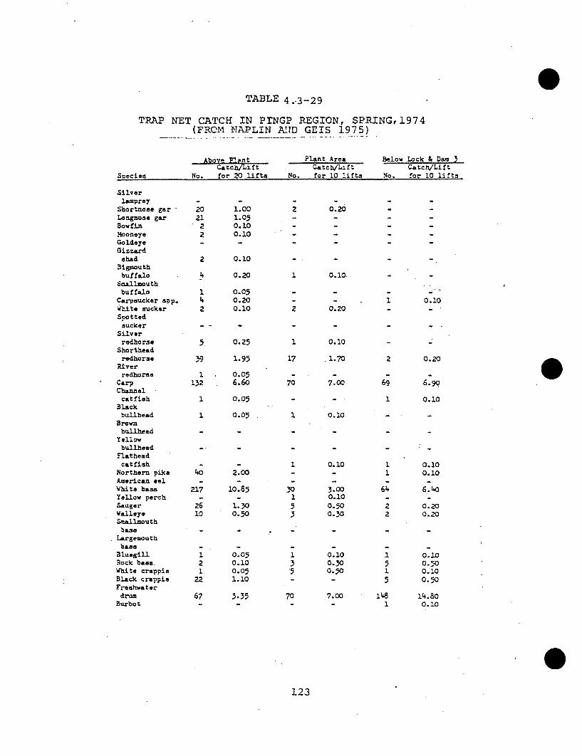
TABLE 4.3-29

TRAP NET CATCH IN PINGP REGION, SPRING,1974(FROM NAPLIN AIND GEIS 1975)

Abo. o PlantCatch/LitNo. for 20 lifts

Plant AreaCatch/Lift

No.. fo,- 10 •Iftq

Below Lock & Dam 3Catc./Li f t

No_ fin- In 1 ftsSnar.srSnecies No for 10 lifts

Silverlamprey

Shortnose garLoannose garBowfinMooneyeGoldeyeGizzardshad

Bigmouthbuffalo

Smallmouthbuffalo

Carpeucker spp.White suckerSootted

suckerSilver

redhorseShorthead

redhorseRiverreodorse

CarpChannelcatfish

Blackbullbead

Brownbullhead

Yellowbullhead

Flatheadcatfish

Northern pikeAmerican eelWhite bassYellow perchSaugerWalleyeSmallmouthbase

Largemouthbass

BluegillRock base.White crappieBlack crappieFreshwaterdrum

Burbot

20212

1.001.050.100.10

2 0.20

2 0.10

2

2

0.20

0.050.200.10 2

1 0.10.

0.201 0.10

5. 0.25

39 1.95

1 0.05132 6.60

1 0.05

1 0.05

40 2.00

1 0.10

17 .1.70

70 7.00

1 0.10

2 0.20

69 6.99

1 0.10

1 0.10 1 0.101 0.10

217

2610

21

22

10.85

1.300.50

0.050.100.051.10

30153

3.000.100.500.30

0.100.300.50

64

22

6.40

0.20

0.20

0.100.500.100.50

135

1

515

67 3.35 70 7.00 148 14.8o1 0.10

123

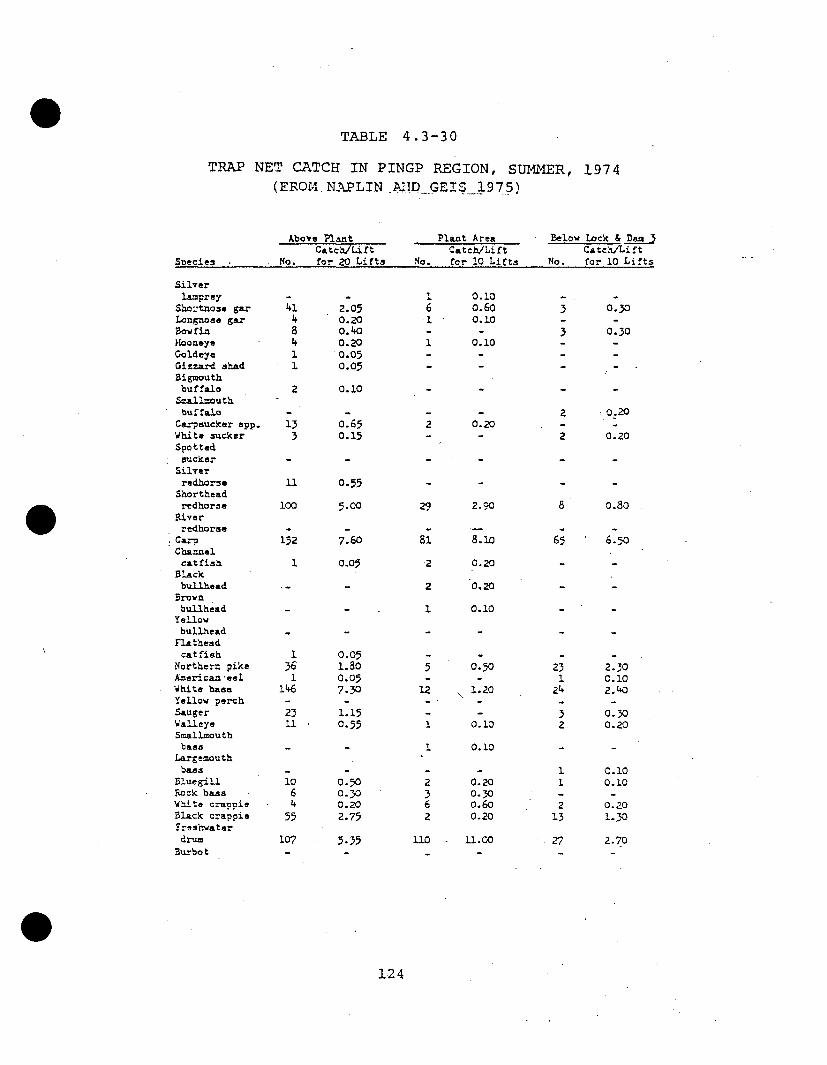
TABLE 4.3-30

TRAP NET CATCH IN PINGP REGION, SUMMER, 1974

(EROM NA-PLIN AI:D_ GEI_1975)

Above PlantCatch/Lift

No. for 20 Lifts

Plant AreaCatch/Lift

No. for 10 Lift-

Below Lock & DamCatch/Lift

No. for 10 LiftsSnecies

Silverlamprey

Shoatnose &arLongnase gsrBow finHooneyeGoldeyeGizzard shadBigmouthbuffalo

Sma.llmouthbuffalo

Carpsucker spp.White suckerSpatted

suackerSilverredhorse

Shortheadredhorse

Riverredhorse

CarpChannel

catfishBlackbullheadBrawnbullhead

Yellowbullhead

Flatheadcatfish

Northern pikeAmerican "eelWhite bansYellow perchSaugerWalleyeSmallmouthbass

Largemouthbass

BluegillPxck bassWhite cranpieBlack crappieFreshwaterdrum

Burbot

41 2.054 0.208 o.4o4 0.201 0.051 0.05

2 0.10

16I

1

0.10o.6o0.10

0.10

0.20

3

3

2

2

8

0.30

0.30

0.20

0.20

o.8o

133

0.650.15

2

U 0.55

100 5.00 29 2.90

152

1

1

361

146

2311

10

64

55

107

7.60

0.05

0.051.800.057.30

1.150.55

0.500.300.202.75

5.35

81

2

2

1

.5

12

1

2

362

110

8.10

0.20

0.20

0.10

0.50

1.20

0.10

0.10

0.200.300.600.20

.1.00

65 6.50

231

24

32

21

213

27

2.3oC. 102. 40

0.300.20

C.100.10

0.201.30

2.70

124

TABLE 4.3-31

TRAP NET CATCH IN PINGP REGION, FALL, 1974(FROM NAPLIN AN4D GEIS 1975)

Above Plant -

Catch/Li ftSpecies No. -for 20 Lifts

Plant AreaCatch/Lift

No. for 10 Lifts

Below Lock & Dam 3Catch/Lift

No. for 10 Lifts

Silverlamprey

Shortnose garLongnose garBowfinMooneyeGoldeyeGizzard shadBigmouthbuffalo

Smallmouthbuffalo

Carpsucker spp.White suckerSpotted suckerSilverredhorse

Shortheadredhorse

Riverredhorse

CarpChannelcatfish

Blackbullhead

Brownbullhead

Yellowbullhead

Flatheadcatfish

Northern pikeAmerican eelWhite bassYellow perchSaugerWalleyeSmallmouthbass

Largemouthbass

BluegillRock bassWhite crappieBlack crappieFreshwater drumBurbot

51

1

1

8

241

2.90

0.050.0.5

0.05

0.4o

0.100.200.05

0.20

3.30

3.20

1 0.10 11

11

0.100.10

21

0.100.10

0.200.10

0.10

0.10

5.00

4 1

66 13

64

1.30

50

1 0.05 7

1

1

215

315

228

1

0.100.75

15.75

1.100.40

0.05

1.450.150.251.251.40

1

47

7

0.70

0.10

0.10

0.10

4.70

0.70

11

23

94

0.100.10

2.30

0.900.40

2935

2528

1942

1921

1.900.400.201.902.10

12

.2

6231

1

1.20

0.206.203.100.10

TABLE 4.3-32

TRAP NET CATCH IN PINGP REGION, SPRING, 1975(FROM GUSTAFSON tET AL. 1976)

Above Plant Plant Area Below Lock&Dam3

Species Catch/lift Catch/lift Catch/lift

No. 361ifts No. 20 lifts No. 16 lifts

Longnose gar 2 0.06 - -Shortnose gar 22 0.61 7 0.35 - .Bowfin 8 0.22 - - 3 0.19

Gizzard shad 1 0.03 -

Mooneye - .. - -

Northern pike 36 1.00 3 0.15 - 4 0.25Carp 123 3.42 68 3.40 117 7.31Carpsucker 6 0.17 3 0.15 - _White sucker 3 0.08 1 0.05 2 0.13Smallmouth buffalo 1 0.03 - - -

Bigmouth buffalo - - 2 0.10Silver redhorse - -- -

Shorthead redhorse 33 0.95 10 0.50 6 0.38Black bullhead 2 0.06 1 0.05 6 0.38Brown bullhead .- - -

Channel catfish 2 0.06 3 0.15 -

Flathead catfish - - -.White bass 106 2.94 15 0.75 37 2.31Rock bass 4 0.11 2 0.10 3 0.19Bluegill 9 0.25 7 0.35 1 0.06Smallmouth bass - - - -

White crappie 5 0.14 7 0.35 2 0.13Black crappie 31 0.86 5 0.25 9 0.56Yellow perch - - - - 1 0.06Sauger 11 0.31 6 0.30 4 0.25Walleye 8 0.22 2 0.10 7 0.44Drum 35 0.97 57 2.85 146 9.13

* Hyphen (-) indicates no fish were caught.

126

TABLE 4..3-33

TRAP NET CATCH IN PINGP REGION, SUMMER,1975-- (FROM GUSTAFSON ET AL. 1976)

Above Plant Plant Area Below Lock& Dam3

Species Catch/lift Catch/lift Catch/lift

No. 36 lifts No. 20 lifts No. 16 lifts

Longnose gar 13 0.36 4 0.20 - -

Shortnose gar 64 1.78 9 0.45 3 0.19Bowfin 22 0.61 - - 3 0.19

Gizzard shad ---.....

Mooneye 7 0.19 - - .2 0.13

Northern pike 78 2.17 1 0.05 22 1.38Carp 168 4.67 52 2.60 75 4.69Carpsucker 15 0.42 3 0.15 - -White sucker 1 0.03 - - 4 0.25Smallmouth buffalo 18 0.50 3 0.15 - -Bigmouth buffalo 32 0.89 1 0.05 - -Silver redhorse 5 0.14 - - 2 0.13Shorthead redhorse 44 1.22 4 0.20 2 0.13Black bullhead - - 4 0.20 ,1 0.06Brown bullhead - - - 1 0.06Channel catfish 1 0.03 - - - -

Flathead catfish 2 0.06 6 0.30 1 0.06White bass 138 3.83 28 1.40 13 0.81Rock bass - 1 0.05 1 0.06Bluegill 13 0.36 1 0.05 4 0.25Smallmouth bass 1 0.03 . .. .White crappie 9 0.25 10 0.50 10 0.63Black Crappie 174 4.83 19 0.95 19 1.19Yellow perch 1 0.03 1 0.05 - -

Sauger 15 0.42 3 0.15 2 0.13Walleye 5 0.14 - - 6 0.38Drum 47 1.31 53 2.65 36 2.25

Hyphen (-) indicates no fish were caught.

127

- TABLE 4.3-34

TRAP NET CATCH IN PINGP REGION, FALL, 1975

. (FROMGUSTAFSON ET AL. 1976)

Above Plant PrTffEl Area Below Lock & Dajfi-3

SpeciesCatch/lift

No. 36 liftsCatc]

No., 20h/lift Catch/liftlifts No. 16 lifts

Longnose garShortnose garBowfinGizzard shadMooneyeNorthern pikeCarpCarpsuckerWhite suckerSmallmouth buffaloBigmouth buffaloSilver redhorseShorthead redhorseBlack bullheadBrown bullheadChannel catfishFlathead catfishWhite bassRock bassBluegillSmallmouth bassWhite crappieBlack crappieYellow perchSaugerWalleyeDrum

347

27

1783

8

1211131

3411

15

752

6271573

0.940.190.75

0.472.310.220.030.060.030.310.81

9.470.030.42

0.191.440.170.750.422.03

1

4

313

2

110

121

15

2214

262

21

0.05

0.20

0.150.65

0.10

0.050.50

0.051.05

0.75

1.100.700.100.300.101.05

2

3 0.192 0.131` • 0.067 0.4422 1.38

1 0.06

5 0.942 0.130 0.63

8 0.508 4.88'

7 0.44

1

1

7

* Hyphen (-) indicates no fish were caught.

1"28

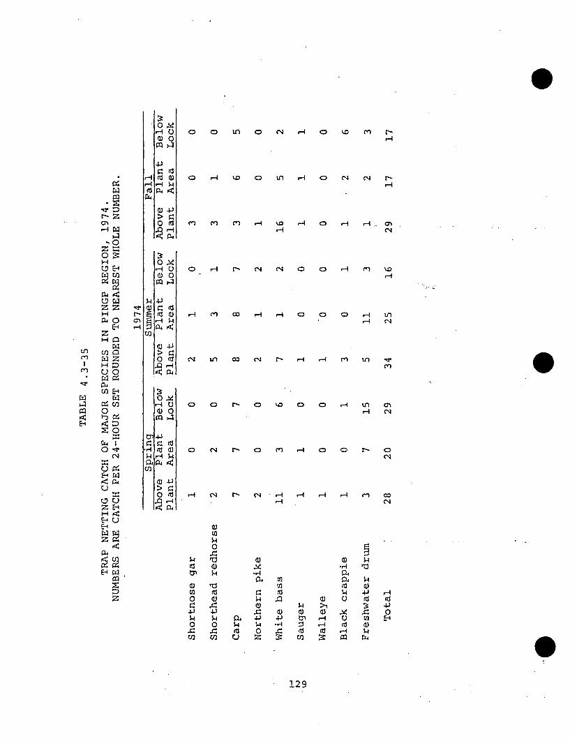
HC

-4 5-4

zzH

0E-1

z

u 0

E-4

m00E-4 :0:

E-4 W

ZE-4

E-4~

r4I

a

0

0CD

o U C C,4 r-4 0 %.0 C C,-4

,l t.0 C) ul ,--4 C) N4 ¢q r-

r'1 m -4 ~H

H- 0 4 4 -CN

r-4

s-i4.)

rrsQ)

Q 4-)

a45-

a4j 4.

Hn co N- N- 0ý 0) C-4 r) L

r.1 Co -4~-i 0 0 0 -4 Ul

N

0

0 e

U, co CN r, r-i H m U, ~ 0o) r- 0 1.0 0 0) H1 U, CN

,-'4 C14

"4 r- C0 m) r-i 0 0 r- DN4

04

M-

CN r-~ CN -4 r4 M co

0s::

0X.,

0

5-4-

0to

ra~ ~ a44 -

54 >1 3: 4) )a~d ) 0) -% . 0

4.4) 4- l t r-4 U U) E-s- *,- m5 H )54

cr50 0

129

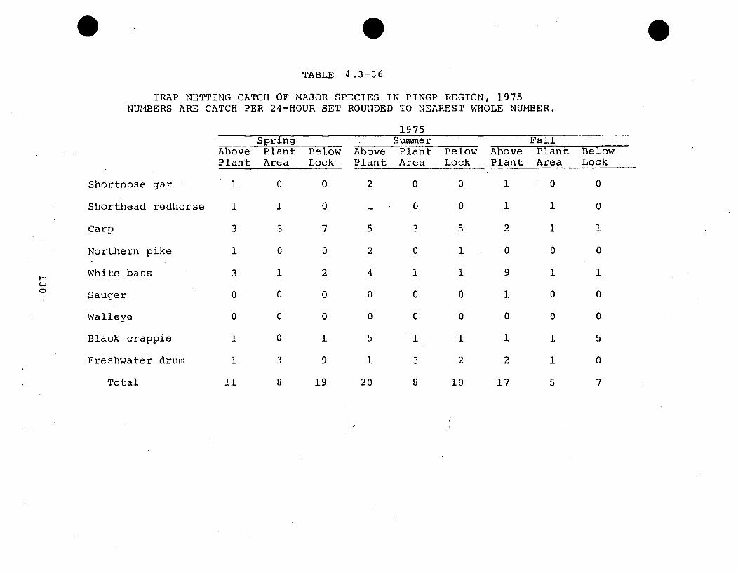
0TABLE 4.3-36

TRAP NETTING CATCH OF MAJOR SPECIES IN PINGP REGION, 1975NUMBERS ARE CATCH PER 24-HOUR SET ROUNDED TO NEAREST WHOLE NUMBER.

1975SummerSpring

Above Plant BelowPlant Area Lock

Above Plant BelowPlant Area Lock

FallAbove Plant BelowPlant Area Lock

Shortnose gar

Shorthead redhorse

Carp

Northern pike

White bass

Sauger

Walleye

Black crappie

Freshwater drum

1

1

3

1

3

0

0

1

1

0

1

3

0

1

0

0

0

3

0

0

7

0

2

0

0

1

9

2

1

5

2

4

0

0

5

1

0

0

3

0

1

0

0

1

3

0

0

5

1

1

0

0

1

2

1

1

2

0

9

1

0

1

2

0

1

1

0

1

0

0

1

0

0

1

0

1

0

0

5

0

FJUjC

1

Total 11 8 19 20 8 10 17 5 7

4.3.5.8 Gill Net Studies

Fish populations were studied in the PINGP region by

sampling with gill nets from 1972 to 1975 (Tables 4.5-37

through 4.3-39). An experimental gill net having dimen-

sions of 250 ft x 6 ft (76 x 1.8 m) and mesh (stretch) of

1-1/2, 2, 2-1/2, 3 and 4 inches (3.8, 5, 6.4, 7.6, 10.2 cm)

was used (Hawkinson 1974). Lifts were made at 24-hour

intervals.

Gill netting data permit some assessment of temporal

and spatial distribution of fishes. Sauger dominated the

1972 catch. The 1973 program yielded more species in the

lakes above the plant (18) than in the plant area (11) and

showed highest population densities in the lakes above the

plant area for several species (e.g., gizzard shad, white

bass, and possibly walleye).

The spring catches of 1974 and 1975 were dominated by carp,

sauger, white bass, shorthead redhorse, and shortnose gar.

Major species were fairly evenly distributed with the excep-

tion of longnose gar, walleye, and crappies which were most

abundant above the plant. No preference for the plant area

was apparent for any species in 1974 and 1975.

131

TABLE 4.3-37

FISH CATCH IN GILL NETS IN PINGP REGION, 1 9 7 2 a AND 1 9 7 3b

1972

No. Catch/lift

1973

No. Catch/lift. Plantl.area

No. Catch/lift

Shortnose garLongnose garGoldeyeMooneyeGizzard shadNorthern pikeCarpCarpsuckerSmallmouth buffaloShorthe.ad redhorseChannel catfishWhite bassRock bassBlack crappieYellow perchSaugerWalleyeFreshwater drum

141414

15

1631110

0.500.500.50

0.54

5.820.390.36

2182

757c14144

3 c

1023

103241

1204224 c

0.130.060.500.13

47 .31

0.880.880.250.190.631.446.440.130.250.067.502.631.75

3 5c

143 c

12

11

193

11.670.331.331.00

0.330.670.330.33

6.331.005.00

toJ

a Miller 1973; 28 gill nets;fall, region not given; only dominant species listed

b Hawkinson 1974; summer; North, Sturgeon and Brewer Lakes

cpredominantly or entirely YOY

TABLE 4.3-38

GILL NET CATCH IN PINGP REGION, SPRING AND FALL, 1974(FROM NAPLIN AND GEIS 1975)

SPRINCAbove Plant

Catch/LiftNo. (for 20 Lifts)

Plant Area

Catch/LiftNo. (for Lifts)

FALLAbove Plant Plant Area

Catch/LiftNo. (for 5 Lifts)

Catch/Li ftNo. (for 20 Lifts)

S-e-ies

to(A

Shortnose garLongnose garBowfinMooneyeGoldeyeGizzard. shadBigmouth buffaloSmallmouth buffaloCarpsucker app.White sucker -Shorthead redhorseCarpChannel catfishBlack bullheadBrown bullheadYellow bullheadNorthern pikeWhite bassYellow perchSaugerWalleyeS:nallmouth bassBluegillRock bassWhite crappieBlack crappieFreshwater drum

21 1.0519 0.95

1 0.052 0.10

1 0.052 0.10

1 0.051 0.05

34 1.70

112 5.607 0.351 0.05

17 0.8538 1.90

96 4.8018 0.901 0.05

2 0.101 0.055 0.25

13 0.65

6

1

637

1

616

911

4

142

1.20

0.20

1.20

0.20

1.203.20

1.8o0.200.20

0.800.200.800. 10

22

74

6021

14

127

11018.

2.900.100.100.350.20

•30.100.050.70

0.051.355.500.90

2117

21

9126

14

459

312

881

0.%023.40

o.4o0.20

1.802.401.20

0.20o.8o9.001.806.200.%0

1.601.6o0.20

1 0.05

19249

614o37

2'

182621

0.9512.450.307. 001.85

0.050.100.901.301.05

TABLE 4.3-39

GILL NET CATCH IN PINGP REGION, SPRING AND FALL ,1975

(FROM GUSTAFSON ET AL. 1976)

SPRINGO FALL

Above Plant Plant Area Above Plant Plant Area

Catch/lift Catch/lift Catch/liftNo. 16 lifts No. 8 lifts No. 16 lifts No. 8 lifts

Shortnose gar 48 3.00 29 3.63 - - 1 0.13Longnose gar 26 1.63 .- - -

Bowfin 6 0.38 - - 14 0.88 - -

Gizzard shad 45 2.81 24 3.00 -874 54.63 --562 70.25Goldeye 1 0.06 2 0.25 12 0.75 - -Mooneye 5 0.31 - - 5 0.31 2 0.,25Northern pike 26 1.63 5 0.63 30 0.31 2 0.25Carp 108 6.75 66 8.25 36 2.25 18 2.25Silver chub 1 0.06 - - - - - -Carpsucker 5 0.31 1 0.13 2 0.13 8 1.00Smallmouth buffalo 2 0.13 2 0.25 4 0.25 5 0.63Bigmouth buffalo - - - 1 0.06 1 0.13Silver redhorse 1 0.06 - - - - -Shorthead redhorse a3 1.43 29 3.63 14 0.88 10 1.25Black bullhead 2 0.13 22 2.75 1 0.06 4 0.50Brown bullhead - - - - - - 1 0.13Channel catfish 14 0.88 13 1.63 20 1.25 6 0.75Burbot - - - - 1 0.06 - -White bass 48 3.00 16 2.00 48 3.00 27 3.38Rock bass 3 0.19 1 0.13 1 0.06 - -Bluegill 1 0.06 - - 2 0.13 1 0.13Smallmouth bass 1 0.06 - - - - - .White crappie 2 0.13 9 1.13 9 0.56 5 0.63Black crappie 3 0.19 4 0.50 19 1.19 2 0.25Yellow perch 3 0.19 1 0.13 1 0.06 4 0.50Sauger 49 3.06 43 5.38 136 8.50 105 13.13Walleye 22 1.38 2 0.25 25 1.56 15 1.88Drum 17 1.06 8 0.50 5 0.31 6 0.75

* Hyphen (-) indicates no fish were caught.

134

During the fall of 1974 and 1975 the same .species were

dominant except that the shortnose gar had declined and

gizzard shad was highly dominant. There was no apparent

preference of dominant species for either of the regions

when both years of data are considered.

- An-analysis of population level trends is hampered by

variability of sampling stations and the inherent sampling

error which resuits from variability of weather and sampling

conditions. However, catch-per-lift data for sport fishes

(northern pike, white bass, crappies, sauger, walleye) have

remained stable or have generally increased during the study

period.

4.3.5.9 Summary of Fish Studies

Tagging studies show that sport fishes move on the average

of 18 to 53 miles (29-85 km) or more upstream and downstream

in a single year. Therefore, the populations affected by

PINGP are highly mixed and very large in comparison to the

"populations" estimated for the PINGP region.

Assessment of population trends during 1973-1975 is complicated

by variation in sampling procedures and conflicting results with

different types of sampling gear. Relatively large seine

catches of YOY of gizzard shad, white bass, and freshwater

135

drum in 1973 may be attributable to sampling exclusively in

the summer or to size of seine used. A strong 1973 year

class of gizzard shad was also apparent from electrofishing

catches, but not from trawl catches.

Trawl, electrofishing, and gill net catches indicate that

the major sport fish (walleye, sauger, white bass) maintained

their levels in the plant region during 1973-1975 and generally

throughout the study area. A relatively high abundance of

sauger below the lock and dam in 1973 was apparent from

electrofishing and seine data, but not from trawl or gill net

data.

Seasonal changes in populations result primarily from recruit-

ment and mortality of YOY. Year-to-year variability is

determined primarily by differences in year-class strengths.

Both types of population fluctuation were parallel in all

three study areas.

4.3.5.10- Spawning and Nursery Potential

Adult fish which have been reported to occur in the vicinity

of PINGP can be assumed to spawn in the area also. A variety

of habitats are utilized for spawning and early development.

136

A large number of species (e.g., shortnose gar, gizzard

shad, northern pike, carp, catfish)* that occur near the

generating plant prefer backwater areas, sloughs, or flooded

vegetated lowlands with minimal current for spawning.

Areas of this nature provide protection from predation,

prevent downstream displacement of eggs and/or larvae by

river currents, and may contain a rich zooplankton food

supply which may be critical in the early development period.

Pool 3 appears to contain an abundance of such habitats.

Species such as white sucker, spotted sucker, silver red-

horse, shorthead redhorse, sauger, and walleye prefer to

spawn in swift-flowing water where the substrate varies from

rock to gravel. The water currents in such areas provide a

means of downstream dispersal for larvae and juveniles.

This movement balances the upstream migration of these

species. Areas of this habitat type are limited in the

main or secondary channels in the vicinity of PINGP.

However, walleye and sauger will spawn in rivers and lakes

on substrates ranging from small stones to rock riprap

along shore where wave action can prevent the eggs from being

silted over.

Other fish, including mooneye, goldeye, and freshwater drum,

produce eggs which are non-adhesive and buoyant. Eggs of 0137

this type aid in downstream dispersal. This group of fish

may utilize the main channel or backwater areas of Pool 3

for spawning purposes.

In general, it appears that most species of fish that inhabit

Pool 3 in the vicinity of PLNGP prefer shallow backwater

areas, where currents are minimal, for spawning activities.

These species generally produce eggs which are demersal and

adhesive in nature and are not commonly found in the water

column and are therefore less susceptible to entrainment.

The young of these species are also probably most abundant

in backwater and shallow shore zone areas of the river.

The young of other species, including carp, sauger, walleye,

white sucker, black crappie, and white crappie, can be

expected to occur throughout the water column and in deeper

waters.

4.3.5.11 Spawning and Life History Information

Spawning and life history information for major species

occurring in the PINGP region are given in Appendix 2.

This information is useful in assessing the impact of PINGP

on the production of fish stocks.

138

5 INTAKE-RELATED STUDIES

5.1 INTRODUCTION

Entrainment and impingement are the two major sources of

intake impact for large water users such as PINGP. In order

to assess the impact of plant intakes, EPA (1976b) has out-

lined a suggested program of monitoring for entrainment and

impingement. Northern States Power Company has conducted

several years of intake related studies at PINGP; the most

recent studies include extensive impingement and entrainment

programs that are similar to those recommended in the current

draft guidelines (EPA 1976b). The following sections summarize

the methods and results of these studies.

The following section, as well as Section 6, often uses

Sturgeon Lake as a basis for comparison to plant intake

effects. This will be especially true for entrainment

effects. Baker (1975) demonstrated that, in spite of the

dredged channel leading to the main channel of the Mississippi

River, the source of plant water was largely, if not entirely,

from Sturgeon Lake. While Sturgeon Lake is not totally

isolated from the Mississippi River, it is sufficiently protected

from main channel flow (see Section 4.1) that it tends to

have a somewhat lentic character (see Section 4.3).

139

5.2 METHODS USED FOR INTAKE RELATED STUDIES

5.2.1 Entrainment-related Studies

5.2.1.1 Phytoplankton

The effects of entrainment on phytoplankton productivity

were studied by Baker (1974, 1975). Productivity was measured

using "light" and "dark" bottles suspended for 2 to 4 hours

during midday at a depth of 25 cm (10 in.). Different

studies were conducted to determine (among other things) the

source of plant water, the effects of entrainment on phyto-

plankton and the overall effects of the plant on river

productivity. To accomplish these goals, nine sampling

stations were used: three in Sturgeon Lake, four in the

main channel, one in the intake canal between the bubble

curtain and the skimmer wall, and one in the discharge canal

at the discharge gates (Figure 5.2-1). The entrainment

studies were conducted from July to December 1974 and from

May to October 1975.

The effects of entrainment on phytoplankton standing crop

were investigated using chlorophyll a and mass of suspended

particulates. Chlorophyll a was measured by spectrophoto-

metric analyses .of samples filtered through 0.45 micron pore

membrane filters and extracted with 90 percent acetone

saturated with magnesium carbonate. Pigment concentration

140

° o.

STA. 4

STA. 5

• " " .• STA. --3,.

.- • STA. 6 .

PLANT SITE-S -STA. 9

,-"00,- STA. 80 STA. 7

LOCK a DAM1L

FIGURE 5.2-1

SAMPLING STATIONS FOR PHYTOPLANKTON PRODUCTIVITY, 1975(FROM.BAKER 1976)

...":'....

Ns

141

was calculated using Lorenzen's (1967) formulae. Suspended

particle mass was determined by filtration into pre-weighed

membrane filters (0.45 micron pore size), desiccation and

weighing.

To measure the degradation of entrained phytoplankton in

1975 studies, Baker (1976) used:

((I-D)/I) X 100

where I = value in intake sample and D = value in discharge

sample, resulting in a percentage of degradation.

Baker and Baker (1975, 1976) studied phytoplankton from 18

stations, including stations in the intake and discharge

canals of PINGP (Figure 5.2-2). Samples were preserved in

Lugol's, sedimented, and counted and identified using an

inverted microscope with a 50X oil immersion objective.

Organisms (filaments, colonies) were counted as units. Cell

volumes were calculated and used to compute the biovolume

contribution of each species. Results of these studies

were used to evaluate the cumulative effect of plant passage

and heated effluent on phytoplankton and can be considered

a good measure of the significance of entrainment effects

on the main channel phytoplankton.

142

W ISCONJ SIN

}

~TA.

Cc

( VI- , H-, ;-ICf-

M I N N ES O"TA

FIGURE 5.2-2

SAMPLING STATIONS FOR PHYTOPLANKTON STUDIES, -1974-1975(FROM BAKER AND BAKER 1975-1976)

143

5.2.1.2 Zooplankton

Middlebrook's (1975, 1976) studies on zooplankton entrain-

ment used a pump to obtain samples, which were then concen-

trated through a 64 micron net submersed in a tank. Samples

were collected monthly from July 1974 through December 1974

(except August) and from June 1975 through May 1976 (except

July). Collections were taken in the intake canal immediately

outside the skimmer wall and in the discharge canal immediately

outside the discharge gates.

Samples were taken to the laboratory where they were portioned

into two subsamples, one to be counted in live condition and

one preserved in formalin. The "live" samples were immediately

studied'and all organisms exhibiting no external or internal

movement were considered dead and were enumerated. The number

of "dead" organisms was subtracted from total organism

counts made from preserved samples to determine the proportion

that had been living at the time of collection. Counts were

made in Sedgwick-Rafter cells and adjusted for volume sampled

and prepared to provide organisms per liter. Organisms

were grouped into Copepoda and copepodites, nauplii, Cladocera

and Rotifera.

Counts of organisms from the intake and discharge canals

were compared using the Students two-tailed t-test. When

mortality was significant, confidence limits were determined.

144

To determine the effects of total plant operation (including

intake effects) Szluha (1975) evaluated zooplankton of the

recycle canal, discharge area and other areas in proximity

to the plant (Figure 5.2-3). Samples were collected in Van

Dorn bottles, filtered through a Wisconsin net and counted

in a Sedgwick-Rafter cell. ANOVA analyses were used to

determine differences in zooplankton among the collection

stations and what effect PINGP had on zooplankton near the

plant. Daggett (1976) conducted similar studies using nine

sampling stations (Figure 5.2-4).

145

MN

B-1X-1

X-3Y-1Y-27

x- . .

c-3

Lock & Dam Nc

FIGURE 5.2-3

SAMPLING STATIONS FOR ZOOPLANKTON STUDIES, 1974(FROM SZLUHA 1975)

146

,. 3

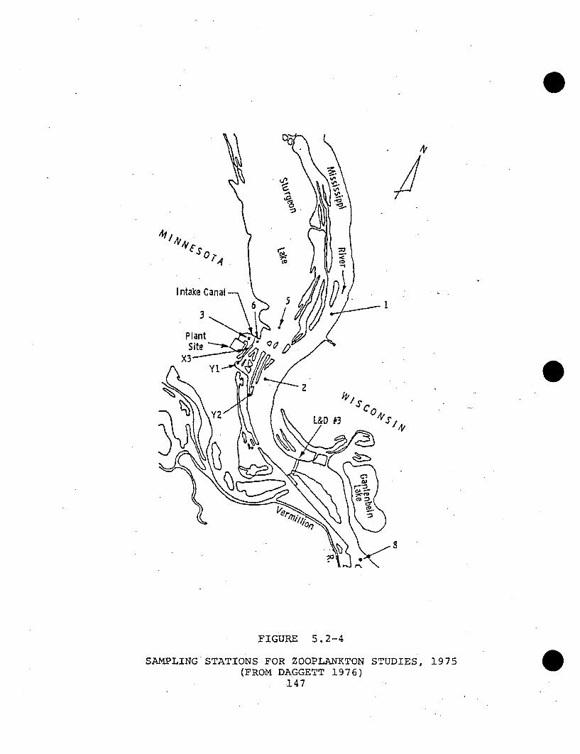
/ V

.~oi

FIGURE 5.2-4

SAMPLING STATIONS FOR ZOOPLANKTON STUDIES, 1975(FROM DAGGETT 1976)

147

5.2.1.3 Fish

Entrainment monitoring studies were conducted at PINGP

between April 25 and September 5, 1975. Field collection

and taxonomic enumeration were performed and supervised by

Kenneth Mueller, NSP Field Biologist. Samples were collected

during one 24-hour period each week, except for the week of

August 24-30 when no samples were collected. Three stations

were sampled. Samples were collected in front of the bar

rack, on the plant side of the skimmer wall, and in the

middle of the recirculation canal.

The Bar Rack Station was sampled throughout the study. The

Bar Rack Station is the point of greatest flow of make-up

water (water that had not previously passed through PINGP)

through the intake canal. This point was located by a

temperature survey completed in April, 1975.

The Recirculating Canal Station was sampled from April 25

through July 3, 1975. This station was used to sample the

eggs and larvae reintroduced into the intake canal when

cooling water was routed through the recirculating canal

during closed cycle operation.

The Skimmer Wall Station was sampled from July 10 through

the termination of the study. Because it was felt that the

148

closed cycle mode of operation (5.3 m 3/sec water appropriation)

would not provide sufficient flow to effectively fish the

nets, this station was not sampled during the first half of

the study. However, during the course of the study, make-up

water appropriations were as low as 5 m 3/sec only a few

times so the Skimmer Wall Station was added to the program.

All samples were collected with plankton nets constructed of

560 micron mesh nylon gauze. Each net was 2.5 m long and2

was attached to a frame 42.5 cm square (0.181 m mouth

area). A General Oceanics Model 2030 flowmeter with an R-2

low speed rotor was fitted in the mouth of each net.

All nets were fished as stationary drift nets. Betwieen 3

and 7 nets were stacked vertically, depending on location

and water depth. Early in the program all 7 nets were

fished at the Bar Rack Station because of excessively high

water. After May 9, only 3 or 4 nets were needed at each

station to cover the entire water column.

During the first 3 weeks of the program a considerable

amount of experimentation with sampling time and frequency

was conducted. After May 9, collections were standardized

to once every 4 hours for 24 hours with the nets in the

water 2 hours of each 4 .hour period. Sampling generally

began at 0800 hr throughout the study.

.149

Within 10 minutes of collection, all samples were returned to

the Prairie Island laboratory where they were condensed into

0.5 gallon jars for storage. Samples were concentrated

by pouring them into a #60 brass sieve (0.250 mm mesh) and

washing the strained material into an 0.5 gallon jar. The

samples were stained with rose bengal dye and preserved in

3 percent buffered formalin.

Prior to sorting, samples were again poured into a #60 brass

sieve and washed in running water to remove the formalin.

The contents of the sieve were rinsed into glass or enamel

sorting pans. Both reflected light and transmitted light

were used to sort samples. Fish eggs and larvae were removed

from the sorting pans with fine forceps and/or pipettes and

were stored in 3 percent buffered formalin until identified

at a later date.

Larvae were identified to the species level when possible,

but in many cases identification was possible only to the

generic or family level. Eggs or larvae which could not be

identified because of physical damage were termed unidenti-

fiable. Those which could not be identified due to a lack

of taxonomic information were labeled unidentified. References

used in the identification of larvae included Fish (1932),

Gerlach (1973), Lippson and Moran (1974), May and Gasaway

150

(1967), Meyer (1970), Nelson (1968), Norden (1961), Snyder

(1971), Snyder and Snyder (1976), and Taber (1969).

The criteria used to differentiate the early developmental

periods into phases are those proposed by Snyder and Snyder

(1976):

Egg - the period that starts with oogenesis and terminates

upon hatching

Protolarva - the larval phase which begins at hatching

continues until the appearance of at least 3 distinct

fin rays in the finfold

Mesolarva - the larval phase which begins at the end of

the protolarval phase and continues until just before

the appearance of pelvic fins or fin buds, and the

appearance of the full complement of soft fin rays in

the median fins

Metalarva - the larval phase which extends from the

termination of the mesolarval phase to just before the

disappearance of the undifferentiated finfold and

attainment of the full complement of spines and fin rays

with segmentation apparent in the soft rays,

151

Juvenile - the period extending from the end of the

metalarval phase to sexual maturation.

The total number of eggs, larval fish and juvenile fish for

each taxon entrained was calculated as follows:

16N.=E X...V.

Sj=l 13

where Ni = the total number of eggs, larvae or juvenile of

taxon i

Xij = the mean density of taxon i during week j

V. the total circulating water volume for period j

j = the sampling period corresponding to the designated

sampling date, i.e., May 15, May 22...September 4.

A sampling period was defined as the 7 day period

centered on the actual sampling dates (Table 5.2-1).

Studies related to intake monitoring were conducted by the

Minnesota Department of Natural Resources (MDNR) who collected

fish eggs and larvae in the vicinity of the PINGP weekly

between May 19 and August 15, 1975. Sampling procedures and

stations (Figure 5.2-5) are detailed in Gustafson et al.

(1976).

152

TABLE 5.2-1

SAMPLING DATES AND CORRESPONDING SAMPLING PERIOD

aSampling Date

May 15

May 21

May 29

June 5

June 12

June 19

June 26

July 2

July 10

July 17

July 24

July 31

Aug. 7

Aug. 14

Aug. 21

Sept. 4

Days in Period

7

6

7

7

7

7

7

7

7

7

7

7

7

7

11

13

* Exten - of'Sampling Period

May 12 - May 18

May 19 - May 24

May 25 - June 1

June 2 - June 8

June 9 - June 15

June 16 -June 22

June 23 - June 29

June 30 - July 6

July 7 - July 13

July 14 - July 20

July 21 - July 27

July 28 - Aug. 3

Aug. 4- Aug. 10

Aug. 11 - Aug. 17

Aug. 18 - Aug. 28

Aug. 29 - Sept. 10

aSampling also took place on April 25, May 2 and May 8; however,these dates have been omitted because of the considerableexperimentation and lack of consistency on these dates.

153

N

LAKE

MILES

a ./4 k/s 3/4

KILOMETERS

S M 11 31 I 1/4 1/2 3/4

PLAMT

FIGURE 5.2-5

LOCATION OF SOURCE WATER FISH EGG AN'D LARVA SAMPLIGSTATIONS AT PINGP IN 1975

154

5.2.2 Impingement-Related Studies

5.2.2.1 Data Collection

Impingement sampling procedures were similar in 1974 and

1975 as described by Mayhew and Hess (1976). The 1974

sampling period ran from January 2, 1974 to January 2, 1975;

the 1975 sampling period ran from January 1 to December 31.

Trash baskets remained in place from January 2, 1974 to

December 31, 1975. Trash baskets were lifted and emptied,

with few exceptions, one to three times per week. All

impinged organisms were separated from debris and counted.

Organisms overlooked because of heavy debris loads were

estimated at less than 2 percent of the total. All fish

except gizzard shad were individually counted. Whený more

than 1,000 gizzard shad were present in a sample, the total

number of gizzard shad was estimated by counting the number

of fish in a full pail and multiplying this number by the

number of pails of gizzard shad in the sample.

Generally, total lengths of all fish were recorded. However,

when the number of fish of a species exceeded 150 to 200 fish,

a subsample of 50 to 100 fish was randomly chosen and

measured.

155

Whenever feasible, live fish were released in Sturgeon Lake

or the discharge canal. This occurred particularly in

spring when a great number of bullheads survived the rigors

of impingement. In addition, special efforts were made to

rescue and release live fish during late October and early

November.

Some species were grouped in reporting impingement losses.

With the exception of carp and silver chub, all members of

the family Cyprinidae were grouped as "minnow spp." This

group included at least 10 species of minnows, shiners, and

dace. River carpsucker and quillback were grouped as "carp-

sucker spp." "Crappie spp." included both white and black

crappie. Many black, yellow, and brown bullheads were

listed as "bullhead spp.", primarily in spring. Sauger and

walleye were frequently reported as "sauger-walleye spp."

These groupings were necessary because of the deteriorated

condition of many fish and, often, the sheer numbers of fish

in a sample.

Ambient water temperature and recycle canal water temperature

data were taken from hourly plant computer logs; average

circulating water flow, and blowdown flow and make-up water

appropriation data were taken from plant thermal effluent

logs. Weekly mean values were calculated from these data.

156

0Ambient water temperature sensors were located approximately

150 m (492 ft) out from the skimmer wall on the river side

of the plant.

Recycle canal water temperatures generally corresponded with

upper layer intake canal water temperatures. Ambient water

temperatures were similar to bottom intake canal water

temperatures.

5.2.2.2 Statistical Analysis

Pearson product-moment correlation coefficients (Sokal and

Rohlf 1969) were calculated for the 1975 data to determine

the association between average circulating water (cfs), 0makeup-water appropriation (cfs), recycle canal water

temperature ('F) and river water inlet (ambient) temperature

( 0 F) with the number of impinged channel catfish, white

bass, freshwater drum, black bullhead, and crappie spp.

These species were selected because of impingement impor-

tance. The sample statistic calculated was:

r = Z (Xi-X) (Yi-Y)

[ Xi-X 1/2

where: Xi = Sample observation of variable X

S= Mean of all observations of variable X

Yi = Sample observation of variable Y

Y = Mean of all observations of variable Y *

157

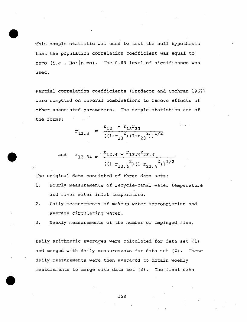
This sample statistic was used to test the null hypothesis

that the population correlation coefficient was equal to

zero (i.e., Ho:Ip1=o). The 0.05 level of significance was

used.

Partial correlation coefficients (Snedecor and Cochran 1967)

were computed on several combinations to remove effects of

other associated parameters. The sample statistics are of

the forms:

r 12 -r 1 3 r 2 3r1.2.-3= [(El-r 1 3 2 (1-r2 3 2)]1/2

and r 12 .3 4 r12'.4 - ro13.4 r23 .4

[( -13.4 2 .(i-r 23.42)']1/

The original data consisted of three data sets:

1. Hourly measurements of recycle-canal water temperature

and river water inlet temperature.

2. Daily measurements of makeup-water appropriation and

average circulating water.

3. Weekly measurements of the number of impinged fish.

Daily arithmetic averages were calculated for data set (1)

and merged with daily measurements for data set (2). These

daily measurements were then averaged to obtain weekly

measurements to merge with data set (3). The final data

158

set was used to calculate correlation coefficients. Computer

programs used in performing the statistical analyses in-

cluded selected programs from the Statistical Analysis

System developed by North Carolina State University (Barr

and Goodnight 1972).

159

5.3 RESULTS OF INTAKE-RELATED STUDIES

5.3.1 Entrainment Studies

5.3.1.1 Phytoplankton

Studies conducted by Baker (1975) demonstrated that the

major source of water and phytoplankton withdrawn by PINGP

is lower Sturgeon Lake, which generally supports greater

densities of algae than the main channel of the river.

Standing crops of phytoplankton were lower in the dis-

charge canal than in the intake canal in 1974 and 1975

(Table 5.3-1 and Figure 5.3-1), based on chlorophyll a data.

There were no evident trends in suspended particulate mass

after passage through the plant, indicating that the algae

may remain physically intact although they have lost some

photosynthetic capacity. Loss of chlorophyll a was at

times as high as 58 percent but usually was 50 percent or

less.

Primary productivity of phytoplankton in the discharge canal

was reduced up to 90 percent over that of the intake canal

(Table 5.3-1, Figure 5.3-1). Seasonal trends in produc-

tivity degradation were not evident in 1975, but in 1974 the

highest degradation occurred during high ambient temp-

eratures. In 1975 two units were in operation,

160

TABLE 5.3-1

THE EFFECT OF PASSAGE OF PHYTOPLANKTON THROUGH PINGPON CHLOROPHYLL a, PHOTOSYNTHESIS AND RESPIRATION, 1974

(FROM BAKER 1975)

Destruction of b Reduction of Reduction ofDate Chlorophyll aa' Photosynthesisga Respiration a

July 16 58% 75% 80%

22 54 90 18

23 49 84 45

31 24 73 54

Aug. 6 51 76 30

10 24 74 59

14 29 72 60

22 34 61 --

29 34 63 82

Nov. 2 0 35 Stimulated

9 17 44 Stimulated

25 0 31 Stimulated

Dec. 3 40 60 Stimulated

apercent Destruction or Reduction = 100 x (1 - discharge level/

intake level) .

bChlorophyll a destruction estimates are conservative.

I

0161

ml~

H-H->1

'40H0

C

-00Ln

01~o0

0C-'-I0

*0

- I0Cl

z0

a 0D

0

C LZ~ 0

1'

1**.

00

0

00- I

00coo

0o

0

o0

I00

- IOr,3

0'

zHE-

rH

E4H-

00

Hz

0Ocn

HHV

W 04L

z r0z

00~4Ht/

04-,0

0ý40

z0HH4

A.

0,-H

In 0

NOUV'A~aS90 JO T'DNanoaud

162

probably explaining the higher percentage of time that

productivity was severely depressed due to passage through

PINGP.

Respiration was usually depressed by passage through PINGP

(Table 5.3-1, Figure 5.3-1), although in 1974 respiration

was stimulated by plant passage in late fall. There were no

late fall studies in 1975.

The apparent lack of pattern to phytoplankton degradation

is likely due to the variable plant operation modes (Baker

1976). Baker (1976) also calculated photosynthetic capacity

(the productivity efficiency of phytoplankton based on

oxygen production per unit of chlorophyll a) for phyto-

plankton before and after entrainment. These calculations

were performed on 1974 data which the author considered more

reliable, although they only reflected one unit operation.

Photosynthetic capacity of the non-entrained algae was

twice that of the entrained algae.

In 1974, Baker (1975) studied productivity differences in

the main channel of the Mississippi River and concluded

that "any effects of Sturgeon Lake or the power plant on

the productivity of the main stream were immeasurable,

0163

and were probably insignificant because of the predominant

flow of the main channel."

The studies by Baker and Baker (1974, 1975) indicated little

detectable damage to phytoplankton that had passed through

the plant. Subtle differences were evident in the discharge

canal. In 1974 concentrations of blue-green algae were usually

lower than in the intake and Aphanizomenon flos-aguae was

visibly damaged by plant passage. In 1975 there were

increases of algae in the plant effluent on some dates and

decreases on other dates. There were no detectable

differences in phytoplankton composition or densities in the

main river channel that could be attributed to the plant

operation in either 1974 or 1975. These conclusions corroborate

those of EPA (1976b) who stated that if there are effects from

phytoplankton entrainment they are of short duration and

confined to a relatively small portion of the water body.

5.3.1.2 Zooplankton

Middlebrook (1975, 1976) found that zooplankton at PINGP

was significantly affected by entrainment on a number of

dates. Of the fifteen dates sampled from 1974 to 1976, 66

percent of the samples were significantly affected by

entrainment, based on t-tests of copepod, nauplius, cladoceran

and rotifer densities (Tables 5.3-2 and 5.3-3).

164

TABLE 5.3-2

ESTIMATED PERCENT MORTALITY OF ZOOPLANKTON DUE TO PLANT PASSAGEAT PINGP IN' 1974 (FROM MIDDLEBROOK 1975)

Organism July 30 August 14 September 4 November 21 Decem

Copepoda 51.0+15.9* 36.2+30.0 N.S. N.S. N

Nauplii 41.0+14.7* 33.2+28.3 N.S. N.S. 65.

Cladocera N.S. N.S. N.S. N.S. N

Rotifera N.S. 33.6+26.1 15.3+14.4 N.S. 48.

AT (OF) 23.9 19.3 20.9 30.0 3

aEvaluated using two-tailed Student t-test, paired observations (P<0.05)

*Significant at P<0.01NS = No significant difference

ber 18

,.S.

9+29.0

.S.

4+6.4

0.7

FILn

0

TABLE 5.3-3

ESTIMATED PERCENT MORTALITY OF'ZOOPLANKTON DUE TO PLANT PASSAGEAT PINGP IN 1975 AND 1976 (FROM MIDDLEBROOK 1976)

Date AT (OF) -Copepoda Nauplii Cladocera

June 13, 1975 22.5 NS NS NS

Aug 7, 1975 15.7 30.6+25.5 NS NS

Sep 8, 1975 23.0 NS NS NS

Oct 9, 1975 25.6 26.6+22.7 NS NS

Nov 5, 1975 30.0 NS NS NS

Dec 9, 1975 38.5 NP 18.7+60.3 NP

Jan 12, 1976 28.1 NP NS NP

Feb 9, 1976 36.2 NS 13.3+12.8 NP

Mar 4, 1976 33.9 NS NS NP

Apr 5, 1976 13.5 NS NS NS

May 4, 1976 22.1 19.9+10.7* 26.6+16.7* NS

Rotifera

NS

19.8+13.5*

15.0+6.5*

NS

NS

NS

NS

NS

NS

NS

25.4+13.5*

aEvaluated using two-tailed Student t-test, paired observations (P<0.05)

NS = No significant difference in mortality between intake and dischargeNP = Calculation not possible -

* = Significant at P<0.01

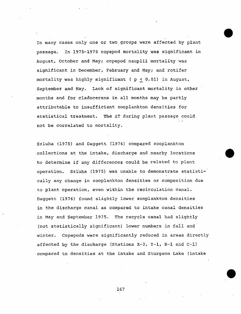
0In many cases only one or two groups were affected by plant

passage. In 1975-1976 copepod mortality was significant in

August, October and May; copepod nauplii mortality was

significant in December, February and May; and rotifer

mortality was highly significant ( p < 0.01) in August,

September and May. Lack of significant mortality in other

months and for cladocerans in all months may be partly

attributable to insufficient zooplankton densities for

statistical treatment. The AT during plant passage could

not be correlated to mortality.

Szluha (1975) and Daggett (1976) compared zooplankton

collections at the intake, discharge and nearby locations

to determine if any differences could be related to plant

operation. Sziuha (1975) was unable to demonstrate statisti-

cally any change in zooplankton densities or composition due

to plant operation, even within the recirculation canal.

Daggett (1976) found slightly lower zooplankton densities

in the discharge canal as compared to intake canal densities

in May and September 1975. The recycle canal had slightly

(not statistically significant) lower numbers in fall and

winter. Copepods were significantly reduced in areas directly

affected by the discharge (Stations X-3, Y-l, B-1 and C-l)

compared to densities at-the intake and Sturgeon Lake (intake

167

source), but Daggett (1976) stresses that these data are

preliminary.

5.3.1.3 Fish

Entrainment of fish eggs and young (larval and juvenile

fish) was monitored on 19 dates between April 25 and

September 4, 1975 (Table 5.2-1). The three earliest sampling

dates (April 25, May 2 and May 8) were considered experimental

because of marked-differences in sampling procedures and

times and were not used in the development of entrainment

losses.

Collections on the three early dates yielded only 22

carp larvae, 1 unidentified percid larva and 2 burbot larvae.

Collections from the remaining 16 dates between May 15 and

September 4 resulted in mean densities of 2.39 eggs/100 m 3 ,

19.5 larvae/100 m3 and 0.05 juveniles/100 m3

5.3.1.3.1 Taxonomic Composition

A total of 39 taxa, including at least 26 species from 12

families, were represented in the collections (Table 5.3-4).

Freshwater drum eggs accounted for 89 percent of the eggs

and mooneye eggs less than 0.1 percent; the remainder of

the eggs were unidentified. Emerald shiners were the most

abundant young fish collected, followed by gizzard shad,

168

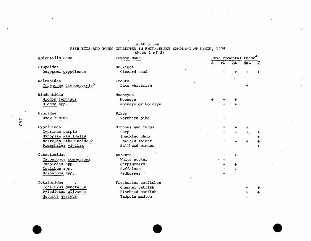
FISH EGGS AND YOUNG

Scientific Name

ClupeidaeDorosoma cepedianum

SalmonidaeCoregonus clupeaformis?

HiodontidaeHiodon tergisusHiodon spp.

TABLE 5.3-4COLLECTED IN ENTRAINMENT SAMPLING AT PINGP, 1975

(Sheet 1 of 2)Common Name

HerringsGizzard shad

TroutsLake whitefish

Developmental Phasea

E PL ML MeL J

.+ + + +

+

014,0

EsocidaeEsox lucius

CyprinidaeCyprinus carpioH ybopsis aestivalisNotropis atherinoides?Pimephales vigilax

CatostomidaeCatostomus commersoniCarpiodes spp.Ictiobus spp.Moxostoma spp.

IctaluridaeIctalurus punctatusPylodictus olivarusNoturus gyrinus

MooneyesMooneyeMooneye or Goldeye

PikesNorthern pike

Minnows and Carps,CarpSpeckled chubEmerald shinerBullhead minnow

SuckersWhite suckerCarpsuckersBuffaloesRedhorses

Freshwater catfishesChannel catfishFlathead catfishTadpole madtom

+ ++

+

++

+ + +

+ + + ++

+ ++ ++

+++++

+

+

+

+++

++

TABLE 5.3-4 (Sheet 2 of 2)

Scientific Name

PercopsidaePercopsis omiscomaycus

Common Name

Trout-perchesTrout-perch

Developmental Phasea

E PL ML MeL J

GadidaeLota Iota

PercicthyidaeMorone chrysops

CodfishesBurbot +

Temperate bassesWhite bass + + +I

-I0

CentrarchidaeAmbloplites rupestrisLepomis gibbosusL. macrochirusLepomis spp.Pomoxis annularisPomoxis nigromaculatusPomoxis spp.

PercidaeEtheostoma nigrumEtheostoma spp.Perca flavescensPercina caprodes ?Percina shumardi ?Percina spp.Stizostedion canadenseS. vitreumStizostedion spp.

SciaenidaeAplodinotus grunniens

SunfishesRock bassPumpkinseedBluegillunidentified sunfishWhite crappieBlack crappieunidentified crappie

PerchesJohnny darterunidentified dartersYellow perchLog perch 'River darterunidentified dartersSaugerWalleyeSauger or Walleye

+1* +

++ + + +

+ +-++

+ +

+ +

+

+ +

++

++

+ ++ + +

++- ++ + ++ + +

DrumsFreshwater drum + + + + +

a. E = Egg; PL = Protolarva; ML = Mesolarvae; MeL = Metalarva; J = Juvenile

unidentified suckers, white bass, carp, freshwater drum,

buffalo, sauger, unidentified minnows and carpsuckers (Table

5.3-5). These 10 taxa comprised 90 percent of the catch of

young fish.

Eggs were taken between May 15 and July 31 and again on

September 4, whereas young fish were collected throughout

the study.

Peak egg density (27.5/100 m 3) occurred on May 29; a secondary

peak (3.34/100 m 3) occurred on June 19 (Appendix 3). On

both occasions the collections were dominated by freshwater

drum eggs.

Peak density of young (101/100 m ) occurred on May 29.

Secondary peaks occurred on May 21, June 26, July 10 and

July 24 (Figure 5.3-2, bar rack data). On May 29, the

collections were dominated by emerald shiner, white bass

and gizzard shad (Table 5.3-6). Young gizzard shad and

carp were most abundant on June 26, with emerald shiner,

carp and sunfish predominant on July 10, and emerald shiner

and freshwater drum on July 24.

5.3.1.3.2 Comparison of Sampling Locations

In the present study samples were collected at 3 locations

within the cooling systems of PINGP: the skimmer wall,

171

TABLE 5.3-5MEAN DENSITY AND PERCENT OF CATCH OF YOUNG FISH

COLLECTED IN ENTRAINMENT SAMPLINGAT PINGP, 1975

No/1100m3

Notropis atherinoides?Dorosoma cepedianumCatostomidaeMorone chrysopsCyprinus carpioAplodinotus grunniensIctiobus sppStizostedion canadenseCyprinidaeCarpiodes sppPercina sppHiodon tergisusLepomis sppPercidaePercina shumardi?Pomoxis sppIctalurus punctatusStizostedion vitreumHiodon spPerca flavescensSt--•izostedion sppLepomis macrochirusPercopsis omiscomaycusEtheostoma nigrumEtheostoma sppPercina ca2prodes?Pomoxis nigromaculatusCoregonus clupeaformis?Esox luciusHy-•-p'sisaestivalisPimephales vigilaxCatostomus commersoniMoxostoma sppNoturus gyrinusPylodictus oiivarisAmbloplites rupestrisLepomis macrochirusPomoxis annularisCentrarchidaeUnidentifiableUnidentified

4.364.002.452.261.361.030.620.550.510.440.330.320.260.260.170.120.090.090.060.030.030.020.010.010.010.010.01

0.01

Percent

22.320.512.511.6

7.05.33.22.82.62.21.71.61.31.30.90.60.50.50.30.10.10.1

0.6

172

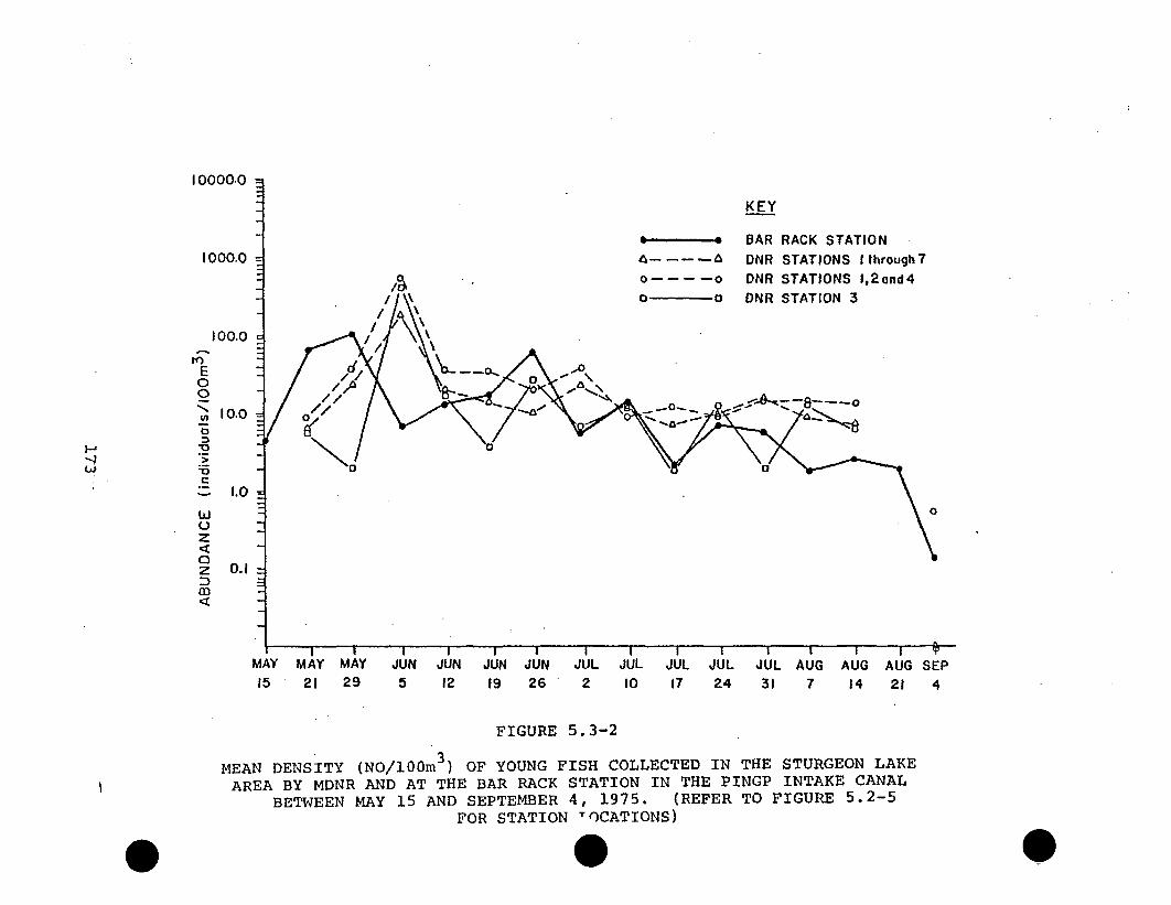
10000.0

.-. BAR RACK STATION1000.0 =--- - DNR STATIONS Ithrough

/---o-o DNR STATIONS 1,2and4- , DNR STATION 3

100.0 ~\

E/00

10.0

0 4

- 1.0

whi

z0z 0.1m

I I I I I i I I I I I I I

MAY MAY MAY JUN JUN JUN JUN JUL JUL JUL JUL JUL AUG AUG AUG15 21 29 5 12 19 26 2 10 17 24 31 7 14 21

FIGURE 5.3-2

MEAN DENSITY (NO/100m 3) OF YOUNG FISH COLLECTED IN THE STURGEON LAKEAREA BY MDNR AND AT THE BAR RACK STATION IN THE PINGP INTAKE CANAL

BETWEEN MAY 15 AND SEPTEMBER 4, 1975. (REFER TO FIGURE 5.2-5FOR STATION TOCATIONS)

7

SEP4

TABLE 5.3-6

MEAN DENSITY OF FISH LARVAE AT THEBAR RACK STATION AT PINGP, 1975

174

MEAN DENSITY INO./100 CUBIC METERS) OF FISH LARVAE COLLECTED AT THE

BAR RACK STATION IN THE INTAKE CANAL OF THE PRAIRIE ISLAND GENERATING PLANT

ON EACH COLLECTION DATE IN 1975.

MAY MAY MAY JUNE JUNE JUNE JUNE JULY JULY JULY JULY JULY AUG AUG

15 21 29 5 12 19 26 2 t0 17 24 31 7 14

PAGE I

AUG SEPT21 4 AVG.

UNIDENTIFIABLE a

PROTOLARVA 0.03 0.38 0.72 0.03 0.0 0.12 0.24 0.0 0.04 0.17 0.0 0.0 0.0 0.0 0.0 0.0 0.11

NESOLARVA 0.0 0.0 0.02 0.0 0.0 0.0 0.0 0.0 0.0 0.0 0.0 0.0 0.0 0.0 0.09 0.0 0.01

TOTAL 0.03 0.38 0.73 0.03 0.0 0.12 0.24 0.0 0.04 0.17 0.0 0.0 0.0 0.0 0.09 0.0 0.11

UNIDENTIFIEDbEGG 0.01 1.09 2.00 0.17 0.0 0.0 0.56 0.0 0.0 0.18 0.0 0.0 0.0 0.0 0.0 0.13 0.26

PROTOLARVA 0.0 0.13 0.0 0.0 0.0 0.0 0.0 0.0 0.0 0.0 0.0 0.06 0.0 0.0 0.0 0.0 0.01

TOTAL 0.0 0.13 0.0 0.0 0.0 0.0 0.0 0.0 0.0 0.0 0.0 0.06 0.0 0.0 0.0 0.0 0.01

APLODINOTUS GRUNNIENS

EGG 0.0 0.32 25.52 2.90 0.61 3.34 0.76 0.10 0.05 0.41 0.01 0.0 0.0 0.0 0.0 0.0 2.13

PROTOLA14VA 0.0 0.01 0.93 2.02 0.44 3.30 0.99 0.20 0.04 0.13 1.02 0.81 0.09 0.33 0.58 0.0 0.68

MESULARVA 0.0 0.0 0.0 0.06 0.22 4.36 0.18 0.0 0.0 0.01 0.01 0.0 0.05 0.0 0.09 0.0 0.31.

METALARVA 0.0 0.0 0.0 0.0 0.0 0.08 0.05 0.0 0.02 0.01 0.01 0.02 0.0 0.10 0.02 0.0 0.02L JUVENILE 0.0 0.0 0.0 0.0 0.0 0.0 0.21 0.0 0.0 0.0 0.0 0.0 0.0 0.0 0.0 0.0 0.03

TOTAL 0.0 0.01 0.93 2.08 0.66 7.75 1.43 0.20 0.06 0.25 1.05 0.83 0.14 0.44 0.69 0.0 1.03

COREGONUS CLUPEAFORMIS ?METALARVA 0.0 0.0 0.02 0.0 0.0 .0.0 0.0 0.0 0.0 0.0 0.0 0.0 0.0 0.0 0.0 0.0 0.00

TOTAL 0.0 0.0 0.02 0.0 0.0 0.0 0.0 0.0 0.0 0.0 0.0 0.0 0.0 0.0 0.0 0.0 0.00

MORONE CHRYSOPS

PROTOLARVA 1.05 2.38 3.45 0.22 0.07 0.16 0.25 0.0 0.0 0.0 0.01 0.0 0.0 0.0 0.0 0.0 0.47

MESOLARVA 0.0 0.0 18.23 0.65 0.18 0.19 0.09 0.0 0.0 0.0 0.0 0.0 0.0 0.0 0.0 0.0 1.21

METALARVA 0.0 0.0 0.0 0.97 7.24 0.69 0.14 0.0 0.0 0.0 0.0 0.0 0.0 0.0 0.0 0.0 0.56

JUVENILE 0.0 0.0 0.0 0.0 0.0 0.0 0.15 0.0 0.0 0.02 0.0 0.0 0.0 0.0 0.0 0.0 0.01

TOTAL 1.05 2.38 21.68 1.84 7.49 1.03 0.63 0.0 0.0 0.02 0.01 0.0 0.0 0.0 0.0 0.0 2.26

PERC IDAEPROTOLARVA 0.16 0.56 3.12 0.0 0.0 0.08 0.0 0.0 0.0 0.0 0.02 0.0 0.0 0.0 0.0 0.0 0.25

MESOLARVA 0.0 0o.0 0.21 0.0 0.0 0.0 0.0 0.0 0.0 0.0 0.0 0.0 0.0 0.0 0.0 0.0 0.01

TOTAL 0.16 0.56 3.34 0.0 0.0 0.08 0.0 0.0 0.0 0.0 0.02 0.0 0.0 0.0 0.0 0.0 0.26

STIZOSTEDION SPP.

PROTOLARVA 0.37 0.05 0.0 0.0 0.0 0.0 0.0 000 0.0 0.0 0.0 0.0 0.0 0.0 0.0 0.0 0.03

TOTAL 0.37 0.05 0.0 0.0 0.0 0.0 0.0 "0.0 0.0 0.0 0.0 0.0 0.0 0.0 0.0 0.0 0.03

STIZOSTEDION VITREUM

PROTOLARVA 0.72 0.6.0 0.0 0.0 0.0 0.0 0.0 0.0 0.0. 0.0 0.0 0.0 0.0 0.0 0.0 0.0 0.08

MESOLARVA 0.0 0.07 0.0 0.0 0.0 0.0 0.0 0.0 0.0 0.0 0.0 0.0 0.0 0.0 0.0 0.0 0.00

TOTAL 0.72 0.67 0.0 0.0 0.0 0.0 0.0 0.0 0.0 0.0 0.0 0.0 0.0 0.0 0.0 0.0 0.09

MEAN DENSITY (NO./100 CUBIC METERS) OF FISH LARVAE COLLECTED AT THEBAR RACK STATION IN THE INTAKE CANAL OF THE PRAIRIE ISLAND GENERATING PLANT

ON EACH COLLECTION DATE IN 1975

PAGE 2

MAY MAY MAY JUNE JUNE15 21 29 5 12

JUNE JUNE JULY19 26 2

JULY JULY JULY JULY

10 17 24 31AUG

7AUG AUG SEPT

14 21 4 AVG.

STIZOSTEDION CANADENSE

PROTOLARVA 0.57 7.02 0.03 0.0 0.0 0.0 0.0 0.0 0.0 0.0 0.0 0.0 0.0 0.0 0.0 0.0 0.48

MESOLARVA 0.0 1.08 0.10 0.0 0.0 0.0 0.0 0.0 0.0 0.0 0.0 0.0 0.0 0.0 0.0 0.0 0.07

METALARVA 0.0 0.0 0.02 0.0 0.0 0.0 0.0 0.0 0.0 0.0 0.0 .0.0 0.0 0.0. 0.0 0.0 0.00

TOTAL. 0.57 8.1o 0.15 0.0 0.0 0.0 0 0 0 0.0 0.0 0.0 0.0 0.0 0.0 0.0 0.0 0.55

PERCINA SPP.PROTOLARVA 0.09 1.09 3.49 0.41 0.0 0.07 0.0 0.0 0.0 0.0 0.0 0.0 0.0 0.0 0.0 0.0 0.32

MESOLARVA 0.0 0.0 0.04 0.06 O.d 0.01 0.0 0.0 0.0 0.0 0.0 0.0 0.0 0.0 0.0 0.0 0.01

TOTAL 0.09 1.09 3.53 0.47 0.0 0.08 0.0 0.0 0.0 0.0 0.0 0.0 0.0 0.0 0.0 0.0 0.33

PERCINA SHUMARDI?MESULARVA 0.0 0.0 0.34 0.14 .0.0 2.27 0.0 0.0 0.0 0.0 0.0 0.0 0.0 0.0 0.0 0.0 0.17

TOTAL 0.0. 0.0 0.34 0.14 0.0 2.27 0.0 0.0 0.0 0.0 0.0 0.0 0.0 0.0 0.0 0.0 0.17

- PERCINA CAPRODES?

PROTOLARVAH . MESOLARVA

METALARVATOTAL

0.0 0.05 \0.0 0.0 0.00.0 0.0 05 oo0.06 0.0

0.0 0.0 0.0 0.03 0.00.0 0.05 0.05 0.09 0.0

0.0 0.0 0.0

0.0 0.0 0.0

0.0 0.0 0.0

0.0 0.0 0.0

0.0 0.0 0.0 0.0 0.0 0.0 0.0 0.0 0.00

0.0 0.0 0.0 0.0 0.0 0.0 0.0 0.0 0.01

0.0 0.0 0.0 0.0 0.0 0.0 0.0 0.0 0.00

0.0 0.0 0.0 0.0 0.0 0.0 0.0 0.0 0.01

PERCA FLAVESCENS

PROTOLARVA 0.04 0.20 0.02 0.0 0.0 0.08 0.07 0.0 0.0 0.0 0.0 0.0 0.0 0.0 0.0 0.0 0.03

MESOLARVA 0.0 0.03 0.02 0.0 0.0 0.0 0.0 0.0 0.0 0.0 0.0 0.0 0.0 0.0 0.0 0.0 0.00

METALARVA 0.0 0.0 0.05 0.0 0.0 0.0 0.0 0.0 0.0 0.0 0.0 0.0 0.0 0.0 0.0 0.0 0.00

TOTAL 0.04 0.23 0.08 0.0 0.0 0.08 0.07 0.0 0.0 0.0 0.0 0.0 0.0 0.0 0.0 0.0 0.03

ETHEOSTOMA SPP.PROTOLARVA 0.0 0.01 0.0 0.0 0.09 0.0 0.0 0.0 0.0 0.0 0.0 0.0 0.0 0.0 0.0 0.0 0.01

TOTAL 0.0 0.01 0.0 0.0 0.09 0.0 0.0 0.0 0.0 0.0 0.0 0.0 0.0 0.0 0.0 0.0 0.01

ETHEOSTOMA NIGRUM

PROTOLARVA 0.0 0.08 0.07 0.0 0.0 0.0 0.0 0.0 0.0 0.0 0.0 0.0 0.0 0.0 0.0 0.0 0.01JUVENILE 0.0 0.0 0.0 0.0 0.0 0.08 0.0 0.0 0.0 0.0 0.0 0.0 0.0 0.0 0.0 0.0 0.01

TOTAL 0.0 0.08 0.07 0.0 0.0 0.08 0.0 0.0 0.0 0.0 0.0 . 0.0 0.0 0.0 0.0 0.0 0.01

PERCOPSIS OMISCOMAYCUS

PROTOLARVA 0.0 0.08 0.04 0.0 0.0 0.0 0.0 0.0 0.0 0.0 0.0 0.0 0.0 0.0 0.0 0.0 0.01

TOTAL 0.0 0.08 0.04 0.0 0.0 0.0 0.0 0.0 0.0 0.0 0.0 0.0 0.0 0.0 0.0 0.0 0.01

PYLODICTIS OLIVARIS

METALARVA 0.0 0.0 0.0 0.0 0.0 0.0 0.0 0.0 0.0 0.02 0.0 0.0 0.0 0.0 0.0 0.0 0.00

JUVENILE 0.0 0.0 0.0 0.0 0.0 0.0 0.0 0.0 0.0 0.0 0.0 0.0 0.06 0.0 0o0 0.0 0.00

TOTAL 0.0 0.0 0.0 0.0 0.0 0.0 0.0 O0O 0.0 0.02 0.0 0.0 0.06 0.0 0.0 0.0 0.00

MEAN DENSITY (NO./300 CUBIC METERS) OF FISH LARVAE COLLECTED AT THE

BAR RACK STATION IN THE INTAKE CANAL OF THE PRAIRIE ISLAND GENERATING PLANT

ON EACH COLLECTION DATE IN 1975

PAGE 3

MAY MAY MAY JUNE JUNE JUNE JUNE15 21 29 5 12 19 26

JULY JULY JULY JULYa 10 17 24

JULY AUG AUG

31 7 14

AUG SEPT

21 4 AVG.

NOTURUS GYRINUS

METALARVA 0.0 0.0 0.0 0.0 0.0 0.0 0.0 0.0 0.0 0.0 0.0 0.01 0.0 0.0 0.0 0.0 0.00

TOTAL 0.0 0.0 0.0 0.0 0.0 0.0 0.0 0.0 0.0 0.0 0.0 0.01 0.0 0.0 0.0 0.0 0.00

ICTALURUS PUNCTATUSMETALARVA 0.0 0.0 0.0 0.0 0.10 0.04 0.0 0.0 0.70 0.11 0.0 0.24 0.15 0.0 0.0 0.0 0.08

JUVENILE 0.0 0.0 0.0 0.0 0.0 0-0 0.0 0.0 0.0 0.02 0.0 0.02 0.01 0.0 0.0 0.0 0.00

TOTAL o.o 0.0 0.0 0.0 0.10 0.04 0.0 0.0 0.70 0.13 0.0 0.25 0.16 0.0 0.0 0.0 0.09

HIODON SPP.

PROTOLARVA 0.0 0.74 0.0 0.0 0.0 0.0 0.0 0.0 0.0 0.0 0.0 0.0 0.0 0.0 0.0 0.0 0.05

MESCLARVA 0.0 0.16 0.0 0.0 0.0 0.0 0.0 0.0 0.0 0.0 0.0 0.0 0.0 0.0 0.0 0.0 0.01

TOTAL 0.0 0.91 0.0 0.0 0.0 0.0 0.0 0.0 0.0 0.0 0.0 0.0 0.0 0.0 0.0 0.0 0.06

HIODON TERGISUSEGG

PROTOLARVA

MES.LARVA

TOTAL

0.0 0.01 0.0 0.0 0.0 0.0 0.0

0.09 4.23 0.02 0.10 0.0 0.0 0.00.0 0.73 0.0 0.0 0.0 0.0 0.00.09 4.97 0.02 0.10 0.0 0.0 0.0

0.0 0.0 0.0 0.0

0.0 0.0 0.0 0.00.0 0.0 0.0 0.00.0 0.0 0.0 0.0

0.0 0.0 0.0

0.0 0.0 0.00.0 0.0 0.00.0 0.0 0.0

0.0 0.0 0.00

0.0 0.0 0.28

0.0 0.0 0.05

0.0 0.0 0.32

ESOX LUCIUS

PROTOLARVA 0.02 0.0 0.0 0.0 0.0 0.0 0.0 0.0 0.0 0.0 0.0 0.0 0.0 0.0 0.0 0.0 0.00

TOTAL 0.02 0.0 0.0 0.0 0.0 0.0 0.0 0.0 0.0 0.0 0.0 0.0 0.0 0.0 0.0 0.0 0.00

CYPRINIDAEPROTOLARVA 0.0 0.07 0.84 0.40 0.32 0.07 3.89 0.41 3.01 0.41 0.50 0.53 0.27 0.68 0.15 0.0 0.47MESOLARVA 0.0 0.0 0.04 0.03 0.0 0.0 0.0 0.0 0.09 0.02 0.0 0.0 0.0 0.20 0.15 0.0 0.03METALARVA 0.0 0.0 0.0 0.0 0.0 0.04 0.0 0.0 0.03 0.01 0.01 0.0 0.0 0.0 0.0 0.0 0.01

TOTAL 0.0 0.07 0.88 0.42 0.32 0.11 3.89 0.41 1.13 0.43 0.51 0.53 0.27 0.87 0.30 0.0 0.51

PIMEPHALES VIGILAXJUVENILE 0.0 0.0 0.0 0.0 0.0 0.0 0.0 0.0 0.0 0.0 0.0 0.0 0.0 0.0 0.02 0.0 0.00

TOTAL 0.0 0.0 0.0 0.0 0.0 0.0 0.0 0.0 0.0 0.0 0.0 0.0 0.0 0.0 0.02 0.0 0.00

NOTROPIS ATHERINOIDES?PROIOLARVA 0.0 0.18 48.00 0.0 0.0 0.0 3.02 1.88 3.85 0.02 4.07 3.63 0.39 0.25 0.02 0.0 4.08MESULARVA 0.0 0.0 0.0 0.07 0.0 0.0 0.0 0.20 0.71 0.09 0.52 0.50 0.07 0.43 0.48 0.0 0.19METALARVA 0.0 0.0 0.0 0.0 0.20 0.03 0.0 0.0 0.21 0.03 0.04 0.08 0.03 0.15 0.42 0.0 0.07JUVENILE 0.0 0.0 0.0 0.0 0.0 0.0 0.0 0.0 0.0 0.05 0.01 0.0 0.02 0.0 0.0 0.15 0.01

TOTAL 0.0 0.18 48.00 0.07 0.20 0.03 3.02 2.08 4.77 0.20 4.65 4.21 0.52 0.83 0.92 0.15 4.36

HYSOPSIS AESTIVALISJUVENILE 0.0 0.0 0.0 0.0 0.0 0.0 0.0 0.0 0.0 0.0 0.0 '0.02 0.02 0.0 0.0 0.0 0.00

TOTAL 0.0 0.0 0.0 0.0 0.0 0.0 0.0 0.0 0.0 0.0 0.0. 0.02 0.02 0.0 0.0 0.0 0.00

MEAN DENSITY (NO./I00 CUBIC METERS) OF FISH LARVAE COLLECTED AT THE

BAR RACK STATION IN THE INTAKE CANAL OF THE PRAIRIE ISLAND GENERATING PLANTON EACH COLLECTION DATE IN 1975

MAY MAY MAY JUNE JUNE JUNE JUNE JULY JULY JULY JULY JULY AUG

15 21 29 5 12 19 26 2 10 17 24 31 7

PAGE 4

AUG AUG SEPT

14 21 4 AVG.

CYPRINUS CARPIDPROTOLARVA 0.82 2.11 0.53 0.0 0.20 0.0 14.86 0.62 0.44 0.0 0.07 0.0 0.0 0.0 0.0 0.0 1.23

MESOLARVA 0.0 0.0 0.07 0.0 0.0 0.0 0.0 0.20 1.65 0.01 0.03 0.0 0.04 0.0 0.0 0.0 0.12

HE7ALARVA 0.0 0.0 0.0 0.0 0.0 0.0 0.0 0.0 0.03 0.02 0.0 0.0 0.0 0.0 0.0 0.0 0.00

JUVENILE 0.0 0.0 0.0 0.0 0.0 0.0 0.0 0.0 0.03 0.0 0.0 0.0 0.0 0.0 0.0 0.0 0.00

TOTAL 0.62 2.11 0.60 0.0 0.20 0.0 14.86 0.82 2.15 0.03 0.10 0.0 0.04 0.0 0.0 0.0 1.36

DOROSOMA CEPEDIANUMPROTOLARVA 0.0 0.87 14.79 Io04 0.44 1.28 29.98 1.37 0.32 0.03 0.02 0.64 0.49 0.0 0.16 0.0 3.21

MESOLARVA 0.0 0.0 1.00 0.55 2.64 1.13 4.14 0.60 0.53 0.25 0.0 0.05 0.10 0.43 0.12 0.0 0.72

METALARVA 0.0 0.0 0.0 0.0 0.0 0.0 0.08 0.0 0.34 0.23 0.01 0.0 0.0 0.22 0.0 0.0 0.06

JUVENILE 0.0 0.0 0.0 0.0 0.0 0.0 0.0 0.0 0.02 0.15 0o04 0.0 0.0 0.0 0.0 0.0 0.01

TOTAL 0.0 0.87 15.79 3.59 3.09 2.41 34.20 1.96 1.21 0.67 0.07 0.69 0.59 0.66 0.28 0.0 4.00

CENTRARCCHIDAE

PROTOLARVA 0.0 0.0 0.01 0.0 0.0 0.0 0.03 0.0 0.0 0.0 0.0 0.03 0.0 0.0 0.0 0.0 0.00

TOTAL 0.0 0.0 0.01 0.0 0.0 0.0 0.03 0.0 0.0 0.0 0.0 0.03 0.0 0.0 0.0 0.0 0.00-J

*: . OMOXIS SPP.

PROTOLARVAMESOLARVA

TOTAL

0.0 0.16 1.68 0.0 0.0 0.0 0.0 0.0 0.02 0.0 0.0 0.00.0 0.0 0.07 0.0 0.0 0.0 0.0 0.0 0.0 0.0 0.0 0.00.0 0.16 1.75 0.0 0.0 0.0 0.0 0.0 0.02 0.0 0.0 0.0

0.0 0.0 0.0 0.0 0.120.0 0.0 0.0 0.0 0.000.0 0.0 0.0 0.0 0.12

PONOXIS NIGROMACULATUS

MESOLARVA 0.0 "0.0 0.0 0.0 0.0 0.05 0.0 0.0 0.0 0.0 0.0 0.0 0.0 0.0 0.0 0.0 0.00

METALARVA 0.0 0.0 0.0 0.0 0.0 0.02 0.0 0.0 0.0 0.0 0.0 0.0 0.0 0.0 0.0 0.0 0.00

JUVENILE 0.0 0.0 0.0 0.0 0.0 0.0 0.0 0.0 0.0 0.03 0.0 0.0 0.0 0.0 0.0 0.0 0.00

TOTAL 0.0 0.0 0.0 0.0 0.0 0.08 0.0 0.0 0.0 0.03 0.0 0.0 0.0 0.0 0.0 0.0 0.03

POMOXIS ANNULARIS

MESOLARVA 0.0 0.0 0.0 0.02 0.0 0.0 0.0 0.0 0.0 0.0 0.0 0.0 0.0 0.0 0.0 0.0 0.00

IOTAL 0.0 0.0 0.0 0.02 0.0 0.0 0.0 0.0 0.0 0.0 0.0 0.0 0.0 0.0 0.0 0.0 0.00

LEPOMIS SPP.PROTOLARVA 0.0 0.0 0.0 0.0 0.14 0.0 1.75 0.20 1.81 0.04 0.13 0.0 0.0 0.0 0.0 0.0 0.25

MESOLARVA 0.0 0.0 0.0 0.0 0.0 0.0 0.0 0.0 0.01 0.04 0.0 0.0 0.0 0.0 0.0 0.0 0.00

JUVENILE 0.0 0.0 0.0 0.0 0.0 0.0 0.0 0.0 0.01 0.0 0.0 0.0 0.0 0.0 0.0 0.0 0.00

TOTAL 0.0 0.0 0.0 0.0 0.14 0.0 1.75 0.20 1.84 0.08 0.13 0.0 0.0 0.0 0.0 0.0 0.26

LEPONIS MACROCHIRUSPROTOLARVA 0.0 0.0 0.0 0.0 0.0 0.0 0.10 0.0 0.18 0.0 0.01 0.0 0.0 0.0 0.0 0.0 0.02

MESOLARVA 0.0 0.0 0.0 0.0 0.0 0.0 0.0 0.0 0.02 0.02 0.0 0.0 0.0 0.0 0.0 0.0 0.00

METALARVA 0.0 0.0 0.0 . 0.0 0.0 0.0 0.0 0.0 0.0 0.01 0.0 0.0 0.0 0.0 0.0 0.0 0.00

JUVENILE 0.0 0.0 0.0 0.0 0.0 0.0 0.0 0.0 0.0 0.0 0.01 0.0 0.0 0.0 0.0 0.0 0.00

TOTAL 0.0 0.0 0.0 0.0 0.0 0.0 0.10 0.0 0.19 0.05 0.03 0.0 0.0 0.0 0.0 0.0 0.02

MEAN DENSITY (NO./I00 CUBIC METERS) OF FISH LARVAE COLLECTED AT THE

BAR RACK STATION IN THE INTAKE CANAL OF THE PRAIRIE ISLAND GENERATING PLANTON EACH COLLECTION DATE IN 1975

PAGE 5

MAY MAY MAY JUNE JUNE JUNE JUNE JULY

15 21 29 5 12 19 26 2JULY JULY JULY JULYt0 17 24 31

AUG7

AUG AUG SEPT14 21 4 AVG.

LEPOMIS GIBBOSUSPROlDLARVA 0.0 0.0 0.0 0.0 0.0 0.0 0.0 0.0 0.05 0.0 0.0 0.0 0.0 O0O 0.0 0.0 0.00

TOTAL 0.0 0.0 0.0 0.0 0.0 0.0 0.0 0.0 0.05 0.0 0.0 0.0 0.0 0.0 0.0. 0.0 0.00

AMBLOPLITES RUPESTRIS

MESOLARVA 0.0 0.0 0.0 0.0 0.0 0.0 0.0 0.0 0.0 0.01 0.0 0.0 0.0 0.0 0.0 0.0 0.00

JUVENILE 0.0 0.0 0.0 0.0 0.0 0.0 0.0 0.0 0.0 0.01 0.0 0.0 0.0 0.0 0.0 0.0 0.00

TOTAL 0.0 0.0 0.0 0.0 0.0 0.0 0.0 0.0 0.0 0.02 0.0 0.0 0.0 0.0 0.0 0.0 0.00

CATOSTOM IDAEPROTOLARVA 0.20 34.61 0.81 0.3B 0.23 0.09 1.37 0.0 0.38 0.38 0.50 0.11 0.0 0.0 0.0 0.0 2.44

MESOLARVA 0.0 0.0 0.06 0.0 0.0 0.0 0.0 0.0 0.0 0.0 0.0 0.05 0.0 0.0 0.0 0.0 0.01

TOTAL 0.20 34.61 0.87 0.38 0.23 0.09 1.37 0.0 0.38 0.38 0.50 0.16 0.0 0.0 0.0 0.0 2.45

/ MOXOSTOMA SPP.PROTOLARVA

kTOTAL

0.0 0.05 0.0 0.0 0.0 0.0 0.0 0.00.0 0.05 0.0 0.0 0.0 0.0 0.0 0.0

0.0 0.0 0.0 0.0 0.0 0.0 0.0 0.0 0.000.0 0.0 0.0 0.0 0.0 0.0 0.0 0.0 0.00

ICTIODUS SPP*PHOTOLARVA. 0.0 8.74 0.0 0.0 0.0 0.0 0.22 0.0 0.02 0.0 0.0 0.0 0.0 0.0 0.0 0.0 0.56

MESOLARVA 0.0 0.0 0.85 0.06 0.0 0.0 0.0 0.0 0.0 0.0 0.0 0.0 0.0 0.0 0.0 0.0 0.06

TOTAL 0.0 8.74 0.88 0.06 0.0 0.0 0.22 0.0 0.02 0.0 0.0 0.0 0.0 0.0 0.0 0.0 0.62

CARPIODES SPP.

PROTOLARVA 0.0 5.20 0.36 0.09 0.0 0.0 0.68 0.0 0.03 0.0 0.0 0.0 0.0 0.0 0.0 0.0 0.40

MESOLAkVA 0.0 0.0 0.68 0.0 0.0 0.0 0.0 0.0 0.0 0.0 0.0 0.0 0.0 0.0 0.0 0.0 0.04

TOTAL 0.0 5.20 1.04 0.09 0.0 0.0 0.68 0.0 0.03 0.0 0.0 0.0 0.0 0.0 0.0 0.0 0.44

CATOSTOHUS COMMERSONI

PROTOLARVA 0.0 0.02 0.0 0.0 0.0 0.0 0.0 0.0 0.0 0.0 0.0 0.0 0.0 0.0 0.0 0.0 0.00

TOTAL 0.0 O.OZ 0.0 0.0 0.0 0.0 0.0 0.0 0.0 0.0 0.0 0.0 0.0 0.0 0.0 0.0 0.00

aLoo damaged or deteriorated for identification

tataxonomic data or characteristics insufficient for identification

0

the bar rack and the recirculation canal (see Section

5.2.1.3). No consistent differences between the densities

of eggs and young at the Bar Rack Station and those at the

Recirculating Canal Station or at the Skimmer Wall Station

were apparent (Figures 5.3-3 and 5.3-4). Densities occasion-

ally appeared to be higher at both the Recirculating Canal

Station and the Skimmer Wall Station than at the Bar Rack

Station, probably as a result of the inherent variability

in ichthyoplankton densities. The Bar Rack Station apparently

yields as good a representation of the number of larvae

entrained as the Skimmer Wall Station, and is not markedly

influenced by eggs or young fish recirculated through the

recirculation canal.

The Minnesota Department of Natural Resources (MDNR) collected

fish egg and larva samples in the vicinity of the PINGP

intake and in Sturgeon Lake on a weekly basis between May 19

and September 5, 1975 (Gustafson et al. 1976).

These data were used to estimate total numbers of young

fish passing through the Sturgeon Lake Outlet, which, in

turn, were compared to the total numbers entrained by

PINGP on a weekly basis (Table 5.3-7). The MDNR data are

considered low estimates of young fish densities due to

their sampling methods: 1) sampling was only conducted in

daytime, when densities are usually lower, and 2) sampling

180

300.

RECIRC. CANAL

0.0

300.

BAR RACK

0.0

DIEL VARIATION INAND LARVAE AT THE

STATIONS AT

FIGURE 5.3-3

MEAN DENSITY (No./100 m 3) OF EGGSRECIRCULATION CANAL AND BAR RACKPINGP, MAY 15-JULY 2, 1975

181

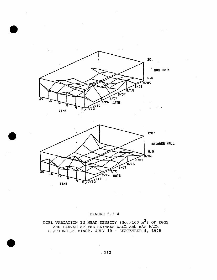
20.

TIME

BAR RACK

0.0

/04

20.;'

SKIMMER WALL

0.01/04

FIGURE 5.3-4

DIEL VARIATION IN MEAN DENSITY (No./100 m 3 ) OF EGGSAND LARVAE AT THE SKIMMER WALL AND BAR RACK

STATIONS AT PINGP, JULY 10 - SEPTEMBER 4, 1975

182

TABLE 5.3-7ESTIMATED NUMBER OF LARVAE AND JUVENILES PASSING TIHRUGH THREE LOCATIONS AT PINGP, 1975a

Bar Rack (BR)

MDHR Station 3b

(Skimmer-Wall)

Sturgeon Lakeb

Outlet (SLI

Percent entrainedBR/sL x 100

Mayis 21 29

0.975 17.0 23.7

-- 0.655 0.308

-- 20.0 61.0

-- 85.0 38.8

5

0.908

19.2

12

1.55

0.580

19

3.28

0.365

26

7.45

1.50

2

0.438

0.193

10

3.17

1.86

June July17

0.591

0.302

24

1.72

2.37

31

1.66

0.326

August7 14 21

0.366 0.435 0.887

2.01 0.231 --

September4

0.068

0

0.43610 36 54 38 140 26 24 6.2 8.6 5.4 3.1 3 .0 d

0.1 4.3 6.1 19.6 0.3 12.2 2.5 27.7 19.3 .6.8 14.0 32.2 15.8

-- No sample taken or value could not be computedH Total Number of larvae and juveniles x 10 per week

c omputed from data of Gustafson et al. (1976)Estimated from previous and succeeding dates,

was done with 787 micron mesh nets (compared to 560 micron

nets in present study) for the first half of the study, when

small larvae were most abundant, possibly resulting in loss

of specimens. Thus the estimates of entrainment as percent-

ages of Sturgeon Lake discharge (Table 5.3-7) are probably

high.

The mean density of young for all MDNR stations (Stations

1-7) and for the MDNR stations in the vicinity of the PINGP

intake (Stations 1, 2, and 4) were generally higher than or

equal to those at the Bar Rack Station in the PINGP canal.

However, there were no evident trends in the fluctuations in

abundance (Figure 5.3-2). Densities peaked at the Bar Rack

Station a week earlier than in Sturgeon Lake. Over the

remainder of the sampling program, the density at the Bar

Rack Station fluctuated widely from week to week while at

the same time the mean densities for all MDNR stations and

Stations 1, 2 and 4 exhibited a fairly constant rate of

decline. However, densities at MDNR Station 3 fluctuated

with those at the Bar Rack Station during late June, July

and early August. These fluctuations are probably attribut-

able to a number of factors including: 1) differing sampling

procedures used for the present study and in MDNR studies,

2) changes in plant operation mode, and 3) changes in intake

area of influence due to river flow changes. At present no

single factor can explain the variations.-

184

5.3.1.3.3 Diel Variations in Fish Entrainment

During the first half of the sampling program (May 15 to

July 2), there was no consistent pattern in the abundance of

eggs and larvae over the 24-hour sampling period at either

the Recirculating Canal Station or the Bar Rack Station.

During the second half of the program, however, densities of

young fish at both the Bar Rack Station and the Skimmer Wall

Station were generally higher between sunset and sunrise

(i.e., 2000-0000 hrs, 0000-0400 hrs and 0400-0800 hrs sampling

periods).

An examination of the vertical distribution of eggs and

young of the ten most abundant taxa collected at the Bar

Rack Station appears to indicate that, for most taxa, densities

were consistently higher near the bottom. This did nto

appear to be influenced by the time of day or the date the

collections were made. White bass, the only exception,

showed no consistent pattern in depth distribution.

185

5.3.2 Impingement

A total of 44 species representing 14 families were impinged

in 1974; 48 species and one hybrid fish representing 16

families were impinged during 1975. In the 1974 study,

146,063 fish, representing an average of 400 fish per day,

were impinged (Table 5.3-8). In 1975, the total number of

impinged fishes was 93,466, representing a daily average of

256 fish (Tables 5.3-9 and 5.3-10). Gizzard shad comprised

94 percent of the total in 1974 and 75 percent of the total

in 1975. Other than gizzard shad, freshwater drum, white

bass, crappies, channel catfish, black bullhead, and minnows

were the most abundant fishes in the impingement catch.

Impingement rates showed wide seasonal variability. 'Gizzard

shad were most frequently impinged in fall and winter

(Figures 5.3-5 and 5.3-6). Impingement of other species

occurred primarily during April-May and July-November (Figures

5.3-7 and 5.3-8). Peaks shown reflect impingement of channel

catfish, white bass, freshwater drum, crappies, and black

bullhead (Figures 5.3-9 through 5.3-13, respectively).

Gizzard shad were impinged primarily during the winter.

Bullheads were caught primarily during the spring of 1975.

Carp, white bass, and crappie spp. occurred in greatest

numbers in the summer. Gizzard shad, channel -catfish,

freshwater drum, and minnow spp. were impinged in greatest

numbers in the fall.

186

NUMBERS OF FISHTABLE 5.3-8 (SHEET 1 OF 4)

PER WEEK COLLECTED FROM THE TRASHBASKETS AT PINGP, 1974

1-21-2to

SPECIES 1-9

Weekly Periods1-9 1-16 1-23 1-3 2-6 2-13 2-20to to to to to to

1-16 1-23 1-30 2-6 2-13 2-20 2-27

2-27 3-6 3-13 3-20 3-27 4-3to. to to to to to

3-6 3-13 3-20 3-27 4-3 o4-10

Hca

Chestnut lampreySilver lampreyUndetermined lampreyLongnose garShortnose garGizzard shadGoldeyeHooneyeNorthern pikeCarpSilver chubMinnowsCarpsucker app.Stealimouth buffaloBigmouth buffaloShorthead redhorsaBlack bullheadBrown bullheadChannel catfishTadpole madtomFlathead catfishUndetermined ictaluridTrout-perchBurbotWhite bassRock bassGreen sunfishBluegillLargemouth bassSmallmouth bassCrappie app.Undetermined centrarchidYellqw perchLogpprchSaugerWalleyeSauger-walleyeFreshwater drumUndetermined fish

TOTAL FISH

TOTAL FISH LESS GIZZ.RDS IMD

I

8750 .3500 859 242 42.63 650 134 18". 81 21

1

2

12

I3

1

2

114

13

233

50

1I

1 4 3 5

I

1

I I2

4

14

17I1

1. 3 1

1

13

1

2

25

3I

I

7 12 6 48 143

38

16

89 0 10 .3

I

4

1

3 . 1 12 11 3 15 12 1 124

211

30 8 7 8 98 424

491 61 107 47

I

8819 3515 889 262 4431 745 242 102 219 94

311 . 39

2

2 427

2 31369 15 30 20 L68 95 108 84 138 73

0

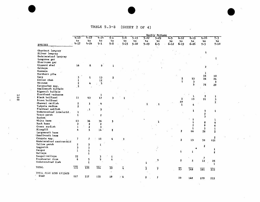
0TABLE 5.3-8 (SHEET 2 OF 4)

t-1O 4-17 4-2tto to to

4-17 4-24 5-1

5-1to

5-8

5-V 5-15to to

5-15 5-22

Weekly Periods5-22 5-29to to

5-29 6-5

6-5 6-12 6-.9 6-26 7-3to to to to to

6-12 6-19 6-26 7-3 7-10

aOO3

SPECIES

Chestnut lampreySilver lampreyUndetermined lampreyLongnose garShortnose garGizzard shadColdeyeMooneyeNorthern pikeCarpSilver chubMinnowsCarpsucker app.Smallmouth buffaloBigmouth buffaloShorthead redhorseBlack bullheadBrown bullheadChannel catfishTadpole madtomFlathead catfishUndetermined Lctalurid,Trout-perchBlurbotWhite bassRock bassGreen sunfish.BluegillLargemouth bass

'Smallmouth bassCrappie app.Undetermined centrarchidYellow perchLogperchSaugerWalleyeSauger-walleyeFreshwater drumUndetermined fish

I

16 a 9 1

31

23

1

4

13123

2 531 3

5

116 1026 26

276 29

2 121 3

2

I11 43 17

I

3 1 210I2

2

I

432I4

1 4

.1 5

1 1

I13

4

2

36225

3623

14

t0

I

3 II

2I

2 44

523

893

26

I

66

22

7 7 4 32

2 13 59 111

23I

226

52

I

5I

24

I II2

3 19 4 5

TOTAL 1i3*3 125 4-4 TO

72 5 12 25

S T4_8 101 i 3-3

23 148 279 233

TflTAL FiISH LESS GCLZzAMSHLAD 117 117 135 19 4 2 7

TABLE 5.3-8 (SHEET 3 OF 4)

7-10 7-17 7-24 7-3]to to to to

7-17 7-24 7-31 8-7

Weekly Perlod.9- 8-7 8-14 8-21 , 8-28 9-4 9-11 9-18 9-25 10-2 10-9

to to to to to to to to to to8-14 8-21 8-28 9-4 9-li 9-18 9-25 10-2 1o-9 1o-16

SPECIES

Chestnut lampreySilver lampreyUndetermined lampreyLongnose garShortnose garGizzard shad61deyeMooneyeNorthern pikeCarpSilver chubMinnowsCarpsucker app.

H• Smallmouth buffalo00 Bigmouth buffalo

Shorthead redhorseBlack bullheadBrown bullheadChannel catfishTadpole madtomFlathead catfishUndetermined ictalurtdTrout-perchBurbotwhitt. bassRock bassGreen sunfishBluegillLargemouth bassSmallmouth bassCrappie app.Undetermined centrarchidYellow perchLogperchSaugerWalleyeSauger-walleyeFreshwater drumUndetermtned fish

t

7

2

961047

2

1

19 1451

12 96 77 54 289 104 590 2 9

1133

222

1

95

262I

42 101 3

261

3

2

318

I

t

I

12

I1 1

1I

II

24

128 , 1 43 1 1

46 19 20 61 23 I

7 ' I I 2

I

67313

53 1645

1 62 43

553

1

1757

15

43 20

4 2

231

2

8 7

2' 9

2

162 25 41

I13 3 23

2 --

223 77 75

139189 284 178 70

L

20 992

87 lit 174 39

744 529 743 2 52TOTAL 329 150 492 122 517 355 388

TOTAL FISH LESS GIZZARD322 . 131 347 110 421 310 334 455 425 153 0 43

TABLE 5.3-8 (SHEET 4 OF 4)

SWeekly. Periods

ko0D

10-16to

*10-23SPECIES

Chestnut lampreySilver lampreyUndetermined lampreyLongnose garShortnosa garGizzard shadColdeyeHooneyeNorthern pikeCarpSliver chubMinnowsCarpsucker app.Smallmouth buffaloBigmouth buffaloShorthead redhorseBlack bullheadBrown bullheadChannel catfishTadpole madtomFlathead catfishUndetermined ictaluridTrout-perchBurbotWhite bassRock bassGreen sunfishBluegillLargemouth bassSmallmouth bassCrappie spp.Undetermined centrarchidYellow perchLogperchSaugerWalleyeSauger-walleyeFreshwater drumUndetermined fish

1u-;3to

10-30

10-3o 11-bto to

u.-6 11-13

11-13to

11-20

11-20to

11-27

11-27to

12-4,

12-4to

12-11

12-11to

12-18

12-i0to

12-26

I

2

137971

67

3361

1

I

23445 57189

I

521 273 71831

2559 2700 2458 6470

11021

1

9

211

4

1

I1 1 4

318 98 14

I1

2 2I5

33

24

12-26to

1-2

24

I2

2

I2 2

31 3

32474

1432

25157

l4

112

131

2312

24 2 3 14 15

AnnualTotal

24262

136,66721

35296

9877679

93

1814612

6373135

32619

1.3675756

6745

131,704

1131313

569

3,143___2 I

146,063

9,396

14 301 21 1

91 1772 2

120 27

1 13

9 8 125 362 1

4 16 19 1o

120

2

559

I12

328

II

216 7

123

I.9 9

I

II 2 11

490 115611 3894

15553 24011

22

1 1 1

166 21 13 21 173

TOTAL 57955 675 351 7651 2669 2752 2575 6581 •

TOTAL FISH LESS GIZZARDSIAD

1756 566 . 766 154 78 468 11o 52 117 III

TABLE 5.3-9NUMBER OF FISH PER WEEK COLLECTED

(SHEET 1 OF 8)FROM THE TRASHBASKETS AT PINGP, 1975

1-2 1-9 1-16to to to

1-9 V-1 1-21

tý

spoo led

Chestnut lamprey

iblver lamprey

Lamprey app.

Ingmnoae gar

Shortnose gar

Car app.

powrln

alisard shad

Goldays

Hoooeys

Ooldeye/tooneye Opp.

Central mo"lnnow

lorthern pike

Carp

silver chub

minnow app.

Carpsucker app.

Carpsucker-buffalo app.

ma l1outh buffalo

Sigasouth buffalo

Ihorthead redhore.

%hite sucker

black bullhead

grown bullhead

Tellow bullhead

iullhead app.

Total bullheads

1-23 1-30to to

1-30 2-6

WIIKLT PURIOD82-6 2-11 2-20to to to

2-13 2-IQ 2-17

2-27 3-6to to

3-6 3-13

1

2

4,364 2,263 750 1.80) 3,257 2,136 3,519 459 1,250 703 1.344 455 364 264

I

3-13 3-20 3-27 4-3to to to to

3-20 3-27 4-3 4-10

4 3 2 2 2 1 2

2 3 4 3 5 1 4

t

1 3

1 4

4 7

I

2 11

1

I

1

3

3I

3

I

2

2

2 2I 2

I

.2 I

it 3 2 12 22 3

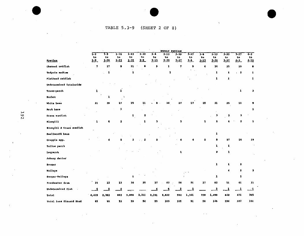
TABLE 5.3-9 (SHEET 2 OF 8)

Ht'J

speci es

channel catflih

Tadpole madtom

rlethead catfish

Undeteriined lctaluridv

Trout-petch

burbot

chite bass

Baock bass

Green eunfish

slueqill

Bluegill X Green sunfish

Smallmout) base

Crappi. app.

Tallow porch

LOgnprch

Johnny darter

Sauget

Walleye

Sauger-Walleyo

freshwater druin

UndeteItined fish

Total

Total long olizzrd Shad

I I I 1 1 2

1 1 1

31

31 39

I

17

1

15 11 24 27 11 15 21 25 11 9

WhZKLT PERPOW1-2 1-9 1-16 1-23 1-30 2-4 2-13 2-20 2-27 3-6 3-13 3-20 1-27 4-3to to to to -to to to to to to to to to to

1-9 1-16 1-23 1-30 2-_ - 3-13 2-20 2-27 3-6 3-13 3-20 3-27 4-3 4-10

7 17 S 11 6 1 7 9 4 24 25 10 s

1 2

I

3 2 3

1 2 41. 6 2 3 3 1

4 3 -. 2 . 4 4 2 5 57 15 29

1 1

I 1 2

15 12 13 20 25 27 63 5s 51 27 62

4 4 4 4 6 2 21 2

4,429 2,363 s03 1,996 3,311 20191 2,622 594 1,341 759 1,490

65 99 31 59 54 55 103 105 91 56 146

4 2 3

1

51 41 31

649 471 365

194 107 101

TABLE 5.3-9 (SHEET 3 OF 8)

I"

species

Chestnut lamprey

silver lamprey

Lamprey app.

Longnoae Vat

Shortnove gar

Oar Epp.

Rovwln

Gizzard shad

Goldeys

Mooneys

GoldeyeoAooneye app.

Central audminnow

Northern pike

Carp

silver chub

minnow app.

Carpsuokor app.

Carpsucker-buf falo app.

Smllmouth buffalo

Iquouth buffalo

Shorthead redhorse

White sucker

Black bullhead

Drovn bullhead

urolye bullhead

Bullhead app.

Total Sullheads

1 2 3 2

120 274 375 495 113

1 1

3 4

5 1

2 1

6 £ 5 25

1 5 26 26 7

6 50 48 101 13

1 2 2 7 .1

2 2

23 1 3

2 2 1 2 1.,

1

,31

S

3 , 3 2

I1I I

VI I=Ly PBaIOaS4-10 4-07 4-24 S-i S-S "-IS 5-32 5-29 9-5 6-12 6,19 6-16 7-1 7-10to to to to to to to to to to to to to to

4-17 4-24 5-1 S-. 5-15 5-22 5-29 6-5 6-12 6-19 6-26 7-3 7-10 7-17

4 1 1

a p i 1

3 19 25 15 13

5 23 10 a i5

7 53 SO 43 91

1 S 17"

I

1 a 3 *1 1

4 31 1.75) 831 42 22 34 19 14

12 21 .2I 2 31

324 230 50

4 32 "1,767 1,377 273 24 64 19 14

1

1

OTABLE 5.3-9 (SHEET 4 OF 8)

WK'KLY PfRIOOS

4-10 4-11 4-34 5-1 $-1 S'15 3 -22 5-29 6-5 6-12 6-19 6-26 7-3 7-10to to to to to to to to to to to to to to

4-17 4-24 s-I 5- 5-15 5-22 5-29 6-5 6 6-1 19 6-26 1- L O 1-17

9 1 1 1 21 2 a a 1 1 1

FA

Channel catfish

Tadpole imdtol

Flathe&4 catfish

Undetermined Ictalurlde

Trout-perch

burbot

WhIte bass

Rock basg

Green sunfish

luegill

aluegill I Green sunfish

Snelleouth bass

crappie mpp.

TYllow p•erch

Zogporch

Johnny darter

:augar

Valleye

8auger-Walleye

freshwater drum

Undetermined fish

Total

Total lees Gizsard shad

2

I 1

4 21

I

1 3 3

S

2

.1

S

13 42 5? 74 14

5 4 4 5 7

2 1 1 12 2

2 4 .6

1*

51 20

5 .6

P 2

19 5

I .1

3 3

2 4

1 2

I

I

21

4

1

22

4

34 06 33 20

38 18 6 2

as 28 1i 21

2 1 1

I 4

1

I

3 12 21 11.I 2 3

1 1

1 19 1

17 26 9 45 49 20 8) 25 10"110 1

- 1 4 1 _

215 488 2,316 2,263 690 124 507 232 141 171 12 34

95 214 2,041 1,760 371 121 S00 229 134 169 12 29

Spoala.

Chestnut lauvrey

Silver lamprer

Laieprey app.

LongnaVe gar

Shortnose gar

Gar opp.

Dowf in

Olueard $had

TABLE 5.3-9 (SHEET 5 OF 8)

WTMLY PRIoO5.-17' 7-24 7-31 6-7 0-14 8-31 0-28 9-4 i-II 9-18 9-25 10-2 19-9 10-16to to to to to to to to to to to to to to

7-34 7-31 6-7 e-14 8-21 8-20 9-4 9-11 -18 -5 10-2 10-9 10-1 10-33

1

I 2 .3

3

I I 1 1 3

I I

1

90

1 1 1.

213 1680 1,216 1,566 358 516 283 431 332 529 878 3,660 592

LnH~

Goldays

hooneys

Goldeya-Noosye app.

Central muwifnnov

Northern pike

Carp

Silver chub

Minnov *pp.

Carpauckar app.

Carpsucker-buffalo app.

6mallmouth buffalo

Digmouth buffalo

fuffalo app.

hoorthead tedhorse

White sucker

Slack bullhead

Drovn bullhead

Yellow bullhead

Rullhead *pp.

I I.

I

33

1521

36

32

1s

76

11

53

14

4

14 13 4 3 1

21 7 2

32 23 3 5 4

16 43 50 8ia 75

20 1

Is 33 23 a I

1 1

4 1

7 6 5

44 91 45

.1

3 2 1

2 9 a 6

63 116 179 149

4 3 1 2

I

1 1 1 6 I

1

1

1 1

1 4I 3 1 1i 4

1

1

1 41

0I

4

'@4 4 0

0TABLE 5.3-9 (SHEET 6 OF 8)

species

Channel catfish

Tadpole mad3to

rlaLhead catfish

Undeterminod Ictalurlds

Trout-perch

Burbot

Nhlta baat

Rock bass

Green sunfish

Bluegill

Bluegill X Oroen sunfish

Bmal lmouth bass

Crappie app.

Unldentified Centrarchtd

Yellow perch

Logperch

WEEKLY PMI0037- 17L 7-24 7-31 8-7 8-14 8-21 8-26 9-4 9-11 9-18 9-25 10-1 10-9 10-16

to to to to to to to to to to to to to to7-24 7-31 B-7 0-14 8-21 8-28 9-4 8-11 9-10 9-25 10-2 10-9 10-16 10-23

7 a 24 171 6G 381 173 53 99 109 060 1,650 290 228

1 6 2 3 1 3

1 9 31 11 6 3 1 3 1 1 4

8

I I

1

390 218 100 138

6 3 2

3 1

1

61 207 00

1

1 21 14

73 78 38 29 51 66 22

1

1 2 2 1 £ 1 3

4 2 2 3 15 23" 7H-0JO

301 158 56 42 81 105 102 168 153 60 35 77 43 8

1 3

1 1

1 2

1

I

Johnny darter I

ssuger 1 2

Walleye 2

Uauger-Wallaye 16 7 6 1 2 1

• raeshwater drum 33 64 49 00 60 96 48 49 56 86 147 366 729 100

Undetermined fish 1 14 7 13 24 19 10 14 2 2

Total 1,115 960 602 1.801 1,944 1,439 1,059 713 939 684 1,105 3,202 5,013 1,133

Total loss olzzard shad 1,025 647 434 599 718 1,081 543 428 488 351 1,176 2,324 1,353 541

1IMany fish not Identif1edor countead due to decomposition

-J

Chestnut lamprey

Silver lamprey

Lampry app.

Longnome gar

Shortnes gar

Gar app.

bow fin .

OIzzard shad

Goldeaye

Mooney.

Goldeye/mooneys app.

Central wuA inngw

lNorthern pike

Carp

Bilver chub

Minnov Opp.

Carpsuoker app.

Carpaucker-butftao app.

."llpouth buffalo

519i6outh buffalo

Buffalo app.

fhorthead redhoree

White sucker

Black bullhead

Drown bullhead

bu"Ioy bullhead

Bullhead app.

Total Bullheads

I 1

1 *1

I'

12

a

12.519 2,932 5.581 1,684 2,306 1,578

17

916 3.098 1,623 1,622 .70,506

$2

TABLE 5.3-9 (SHEET 7 OF 8)

WEEMiY PERIODS10-23 10-30 11-4 11-13 11-20 11-3T 11-4 12-11 12-19 12-Y6to to to to , to to to to to to Annual

10-30 11-6 11-13 11-20 11-21 12-4 12-IL 12-18 12-36 1-2 Total

1 2 1 S

1 1 36

3

2

185

1 2

1 1

79 71

1* 2

.1

1 1

.34 63

2 1

3

1

110

3 * 427

539

38 1 2 2,231

2 150

83

1 11

S

t is

I

22

1

34

is

I I

2 1 2

I

2,797

36

4

611

3,651

01 2 1

0

0TABLE 5.3-9 (SHEET 8 OF 8)

spec ies

Channel catfish

Tadpole wadton

Flathead catfish

Undetermined lotaturida

Trout-parch

Durbot

Whits basl

R~ock bass

Oreen sunfish

blusqill

aluegill X arson sunfish

Bsmallmouth bas.

Crapple app.

Undetermi ned Centrerchid

Yellow perch

V"-XLV PKRIODS10-13 1o-30 11-4 11-11 11-20 H1-27 12-4 12-11 12-18 12-26to to to to to to to to to to Annual

10-30 11-6 11-13 11-20 2127 12-4 12-i1 12-18 12-26 1-2 Total

71 45 321 656 181 51 87 71 153 212 6,223

1 1 33

1 3 4 9o

12

1 45

1

53 52

1 2

10

2*11 1

25 18

2

1 1

24 164 140. 28 39

1 7

3 2 6 4 5

12 a 7 3 3

6

27 51 31 2,712

2 1 76

2 • 2 111

1 1 •242

1Htoco

2

29 17 30 I 2,030

6

81

15.3

Johnny darttr I

gauger 2 S 13 21 2 97

Walleys 9 3 1 1 27

gauger-Wulleye spp. 4 4 5 2 1 73

Freshwater drum 395 133 90 92 243 16 t9 15 S 4 !3,789

Undetermined fish 3 1 1 1 160

Total 13,274 3,310 6,145 2,418. 3,02) 1,714 1,127 5.274 1,842 2.078 93.466

Total loc. Oluvard Shad 754 370 564 994. 717 136 211 176 219 256 23,960

TABLE 5.3-10 (Sheet 1 of 2)

NUMBER OF FISH AND PERCENT OF YEARLY TOTAL FOR EACH SPECIES, BY SEASON,FOR FISHES COLLECTED FROM THE TRASH BASKETS AT PINGP

FROM JANUARY 3, 1975 Ta DECEMBER 31, 1975

H

Chestnut lamorey

Sliver lamprey

Lamprey app.

Longnose gar

Bhortn6ae gar

Oar app.

Sowftn

Gizzard shad

Goldeye

Hooneye

Ooldeye/Mooneye app.

Central mudminnow

Northern pike

Carp

Silver chub

Hinnow app.

Carpsucker app.

Carpaucker/buffalo dpp.

Smallmouth buffalo

Bigmouth buffalo

Buffalo app.

Shorthead redhorse

white sucker

Black bullhead

S.WinterJan. 3 to Her. 20Number I of Total

1 2.3

Paer. .0 .Jn 1

Number Sof Total

3 37.5

28 77.7

2 66.7

6 50.0

20.912. 29.7

1 4.0

June 19 toE0ept. 19Number I of Total

7

2,3783

3

23

*6

17

119

125

473

26

1

26

6

3

I

0.,

6.1

2.3

1.7

0.7

27.3

4.5

41.2

3.4

60.0

83.1

75.0

15.5

27.9

48.3

21.2

17.3

27.3

45.3

47.1

93.3

93.5

a 50.0

3 25.0

1 50.0

3 47.0.

4,965 7.0

1 4.0

1 100.0

2 25.0

91 32.7

265 26.2

92 35.5

647 29.0

79 52.7

83 100.0

3 21.3

10 45.5

1 100.0

12 35.3

1 6.7

20 o.7

ranlDept. 1a to Dec. 31

Number I of Total

4 50.0

8 22.3

1 33.3

8 50.0

3 25.0

1 50.0

.2 11.8

42,251 59.9

2 40.0

1 3.9

1

17

36

1,072

44

2

1

0.9

3.9

13.9

48.1

29.3

19.1

4.5

3

10

2 6.3

6 (0.1

16

14

2,755

4 11.3

16 <0.1

TABLE 5.3-10 (Sheet 2 of 2)

N)C:C:

ope ule

Brown bullhead

Yellow bullhead

Bullhead app.

Channel catfish

Tadpole madtom

rlathead oatfish

Undetermined latalurids

Trout-perch 7'

Burbot

White bass

Rock bass

Green sunfish

Bluegill

Bluegill X green sunfish

Smalimouth bass

Crappie app.

Undetermined Centrarchid

Yellow perch

Logperoh

Johnny darter

Bauger

Walleye

Gauger/Walleye app.

Freshwater drum

Undetermined fish

WinterJan. 3 to Mar. 20

Number S of Total

1 2.6

SprlpqMar. 20 to June 19

Number I of Total

35 92.2

4 100.0

804 99.1

154 2.5

11 33.3

4 4.4

4 33.3

39 86.7

SummerJune 19 to Sept. 10

Number I of Total

1 2.6

99

4

2

1

225

1

6

19

31

1

3

1.6

12.1

1.1

4.4

16.7

8.3

1.3

5.4

7.9

50.0

1.5

1.2

20.0

323

45

52

56

1'

11.9

59.2

46.6

24.0

100.0

7

975

13

71

3

2

1.343

15

7

56

1,171

I

2

1

3

2

33

557

78

0.9

15.7

39.4

78.9

6.7

33.3

49.5

19.7

6.3

23.1

FallSept. S6 to Dec. 31

Number I of Total

1 2.6

4,995

5

14

a

1

3

821

15

46

109

80.2

15.6

15.6

66.7

2.2

50.0

30.3

19.7

41.5

45.0

486 23.9

1 1.0

77

4

1

59

22

408

16

95.1

26.7

50.0

60.8

40.7

30.1

10.6

10.0

57.7

1.2

13.3

50.0

3.1

7.4

45.2

14.7

40.1

S1 50.0

342 16.9

6 100.0

2 2.5

6 40.0

373

28

2.7

9.8

17.5

34

14

16

2,451

38

35.1

51.9

22.0

64.7

23.7

5000O

C0I-

L -ýr4000-

ILl

300C

LI)

0 -

z

JAN. FEB.IMAR APR. MAY JNE .IJULYK I SEPT. I OCT. I V.I I.EQ

FIGURE 5.3-5NUMBERS OF GIZZARD SHAD COLLECTED FROM THE TRASHBASKETS AT PINGP, 1974

80000

IL300

5L2000

0

K30

JA. I FEB.' MAL API. I MAY I'•ME IJULY I AU.I SEPT. OCT. I ,OV. I DEC.

FIGURE 5.3-6

NUMBERS OF GIZZARD SHAD COLLECTED FROM THE TRASHBASKETS AT PINGP, 1975

80-

wi 7oo -

CiC.

4C,

Ui.0

wC132 0C

z

IiJAR IFEB. ItAAR AP" MAY IJUNE IJULY IAUG. iSEPT. OCT.:'"V. 'DEC.

FIGURE 5.3-7TOTAL NUMBERS OF FISH LESS GIZZARD SHAD

COLLECTED FROM THE TRASHBASKETS AT PINGP, 1974

floss 11041,

tal

a.

U)

40

0

a:

I JAH. IFEB.I MAR. IApil. IMAY IJUNE JULY IAMJ. ISEPT. 'OCT. I NOV. I DEC.

FIGURE 5.3-8NUMBERS OF FISH LESS GIZZARD SHAD

COLLECTED FROM THE TRASHBASKETS AT PINGP, 1.975

700

197.5ci:_ 600

ILdIL

tw. 400C)

00

300 I

ILOS200-

JAN. I FEB. I MAR. I APl. I MAY I ,JUNE I JULY AUG. SEPT. I OCT. I NOV. DEC.

FIGURE 5.3-9NUMBERS OF CHANNEL CATFISH COLLECTED FROM THE TRASHBASKETS AT PINGP, 1974-1975

S 0 0

600

GI 'oo-

nl

0Oea.

500

u 4-

Ii.0

k) 300

wm 200 --

IJAN. JFEB.IMAR. APIM. Y M"JUNE JULY AUG.ISEPT. OCT. NO.ov.DEC.

FIGURE 5.3-10

NUMBERS OF WHITE BASS COLLECTED FROM THE TRASHBASKETS AT PINGP, 1974-1975

80C

n:600w0..

400

0300

:3

zOCc

-19.7 ~

I,,~~j¶*111IIII.I.'

~,, *

I jlII I I

. I

v0

I JAn. I FE& I MAR. I APR. I MAY I JUNE I JULY I AUO. I SEPT. I OCT. I NOV. I DEC.

FIGURE 5.3-11NUMBERS OF FRESHWATER DRUM COLLECTED FROM THE TRASHBASKETS AT PINGP, 1974-1975

eoct-

ILl

600-w -U.

5ot

C)

Wi.20

03 20CY-

z-

10-

! JAN. I FEB. I MAR. I APR. 1 AY I JUNE I JULY i AUG. I SEPT. i oct. I NOV. I DEC.

FIGURE 5.3-12NUMBERS OF CRAPPIES COLLECTED FROM THE TRASHBASKETS AT PINGP, 1974-1975

1.31

til 1955800 -.

w LL11600 -

Iil

500

LL40C;--

0300

W

(r 200-

1001--

I JAN. EEL I MAR. I APR. I MAY I JUNE I JUL I U: SEPT. I OCT. I tOV. I DEC.

FIGURE 5.3-13NUMBERS OF BLACK BULLHEAD COLLECTED FROM THE TRASHBASKETS AT PINGP, 1974-1975

a B 0

Size ranges of all impinged fishes (Table 5.3-11) and the

ranges for six selected species (Figures 5.3-14 through 5.3-

5.3-19) indicate that impingement primarily affected juveniles

in 1975. Generally, impingement did not affect many fishes

under 60 mm or over 150-200 mm during 1974 or 1975.

Data on impingement of organisms other than fish in 1975 are

presented in Tables 5.3-12 and 5.3-13. A wide variety of

organisms were encountered; dominant animals were crayfish',

turtles, and clams. Many of the organisms recorded,

particularly birds and mammals, probably died elsewhere and

floated passively into the intake. Crayfish were impinged

more frequently during winter and spring. Turtles occurred

primarily during late summer and early fall.

/

Correlation tests were made on the 1975 data to compare

impingement of five fish species with water temperature and

intake flow data (Tables 5.3-14 and 5.3-15; Appendix 4).

The data are based on weekly impingement totals for each

species and weekly mean values of temperature and flow data.

Correlations between various physical data, e.g. river water

inlet temperature with makeup-water appropriation, were

included to assist in finding the strongest correlations of

impingement with physical data when several were apparent.

210

TABLE 5.3-11 (Sheet 1 of 2)

LENGTH-FREQUENCY OF IMPINGED FISHES COLLECTED FROM THE TRASH BASKETS ATPINGP FROM JANUARY 3, 1975 TO DECEMBER 31, 1975.

Total Lape th In Hillalotara - otal

1 3 4 1

341 1 9 1 1 5 23 1 221 1 1

Chestnut lamprey

silver lamprKey

lwignoge gat

fihortnose 96C

powftin

Oiasar4 shad

Gaidaye

btoonoys

1 1

1.135 1,080 217 41 13 3 4 31

1 1

2 2

21

1 1

1 4 4 16

9

6,451

4

51 294 744 2,177

1 1

s0 17 0 3 2 3

HH

central udmirnnou

Uotthern pike

Carp

8ilver chub

Hinnow @pp.

Carpiucker upp.

Carpsucker/Buffalo app.

smalimouthButfalo

2

12 44

37 214 332

16 20

.4

13

17

395

9

21

46

40

3

'3

11

3

3

3

1

2 1

11 13 12

3 2

5

, 3 5 3 1

5

1

5 12 5 12 16 1s is

1 3 1a 1 2 0 I 3 1

4

1 4 5 3 26

10

09

1 291

250

1,521

7342 1 3 2 1 3 I I 1

402 10 25 3

3 1 1 1 1 I

bigmouthBuffalo

buffalo $pp.

Shorthoa4 radhorse

%hits Sucker

Black bullhead

Brown bullhead

1 7 4

4 5

11 64 3i

1

1

.12 1 5 3 2,~ *1 I 1 37

1

41 102

1

59 113 44 25

1 1

1 3 1

12 5 1

1

2 4 21

I

1

I I

I

29

14

517

7

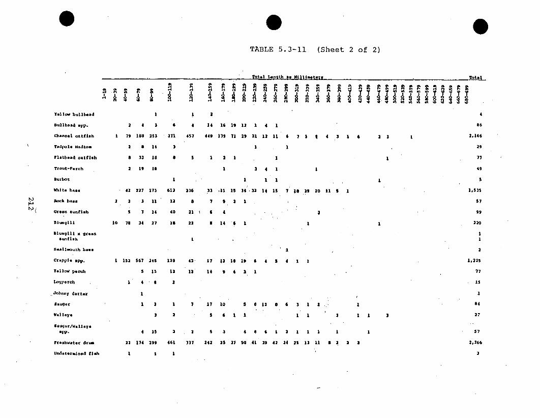
TABLE 5.3-11 (Sheet 2 of 2)

Total Lenqt~h *s )4L111imterg Total1

ld

I

Yellow bullhead

Bullhea4 app.

channel catfish

Tadpole Hadtom

flathead cattish

Trout-Perch

burbot

White bass

Rock bass

Green auntish

blueLIlL

Bluegill x greensunfish

remal lmouth base

Crapple app.

Yellow parch

Lope rch

.Johnny darter

gauger

al leye

•a4agr/Val eyeapp.

Freshwater drLm

Undateranead fish

2

1 79

2

8

2

S42t

S

10 "78

4

188

32

227

3

7

34

1

3

14

18

is

173

14

27

4

457

a

14 16 19 12 1 4 .1

449 179 71 29 21 12 11 6 7 3 4 4 3 1 6

85

2.166371

3

23 I

S 5 1 3

1

1

3 4

1 1

1

1 1

1

15 7 l6 23 20 11 9J 1

I 77

49

I

612

12

40

1S

236

22

33

7

6

I

.11 15 34

14 "6 1

.32 14 1,535

57

99

220

11

2

1,225

77

15

4

2

4|4 1 11 152 567

5

1 4

248

15

a I

128

12

2

42"

1i

17

14

12 16 11

1

1 2

3

11 17

2 S

2 .3 5

461 731 242

10

3

25

5 8 12 9 6 3 1 2 ,:

11 11

1

1 1

1

84

272 3

4 15

174 299

4 6 1 2 1 1 1 1

31 S0 .41 39 43 34 2S 13 11.t 8 2 3 3

I

22

1

57

2,266

3

* 0

800

X 600U)

0400•

tn

- N

Z 200-

N F0C wrma.

TOTAL LENGTH AS MILLIMETERS

FIGURE 5.3-14

V

I-

Ill

VE

LENGTH FREQUENCY OF CHANNEL CATFISH IMPINGED AT PINGP, 1975

300-

X 600 0

tL .0

400-

"31

'>-:

:3Z 2 00 -

w

-4 -4 t4 N N N 4 N M

TOTAL LENGTH AS MILLIMETERS

FIGURE 5.3-15

LENGTH FREQUENCY OF WHITE BASS IMPINGED AT PINGP, 1975

N

800-

:C 600-U)

U.q

400

Z 2 0 0 -

00

TOTAL LENGTH AS MILLIMETERS

FIGURE 5.3-16

LENGTH FREQUENCY OF FRESHWATER DRUM IMPINGED AT PINGP, 1975

V.,0a,

800

X:600 -'

0400-

Z 200

cn c +mNN m mc n " C-- -"-- -"tq A,1'- m ",M"V-

TOTAL LENGTH AS MILLIMETERS

FIGURE 5.3-17

LENGTH FREQUENCY OF CRAPPIE SPP, IMPINGED AT PINGP, 1975

- N

0 0

200

3:150-

1000

Z50

in

0*M a(n)am) M a)m MM(

00 0 000

TOTAL LENGTH AS

FIGURE 5.3-18

MILLIMETERS

LENGTH FREQUENCY OF BLACK BULLHEAD IMPINGED AT PINGP, 1975

200

riso

X ISO-U)

IL.0

100

co~ m

Z 50

N C'J4

~)@r C4bU r4)1 10 0 C ,4 C 4 M ) mC 010 0)In0

,4Mmaa l-(~itr (1.a ) %C-4 mIl m m 't 4Mf -4 Ln u(

TiVIIFI , *

TOTAL LENGTH AS MILLIMETERS

FIGURE 5.3-19

LENGTH FREQUENCY OF NORTHERN PIKE IMPINGED AT PINGP, 1975

db

TABLE 5.3-12 (Sheet 1 of 3)

NUMBERS OF NON-FrSH ORGANISMS COLLECTED FROM THE TRASH BASKETSAT PINGP FROM JANUARY 3, 1975 TO DECEMBER 31, 1975

Organism

Crustaceans

Orconectes virilis-..

Orconectes imnmunis

cambaruS diogenes

Female crayfish

unidentified crayfish

Reptiles

Snapping turtle

Spiny softshelll turtle

Western painted turtle

Map turtle

False map turtle

Turtle carapace

Amphibians

Leopard frog

Unidentified frog

American toad

Mudpuppy

Molluscs

Lemtodea fraqilis

Proptera laevissima

219

No. Collected

31

45

2

62

8

1

59

9

4

2

1

11

2

7

30

5

1

TABLE 5.3-12 (Sheet 2-of 3)

Organism

Molluscs (Continued)

Unidentified clam

Land snail

Insects

HexacLen.ia

Hydrophilidae

Belostomidae

Dytiscidae

Birds

Sparrow

Pigeon

Starling

Unidentified bird skeleton

Unidentified bird skull.

Unidentified bird

Duck bones

Bird skull (pigeon)

Miscel.laneous

Unidentified leech

F ilamentous algae

P ectinatella magnifica

No. Collected

134

2

1

2

4

.3

6

2

4

.,9

*1

2

2

3

220

TABLE 5.3-12

(Sheet 3 of 3)

Organism

Miscellaneous

(Continued)

Pocket gopher

Meadow vole

Muskrat skull

Mouse

Unidentified

small mammal

Unidentified

mammal skull

No. Collected

1

2

1

1

2

1

q

221

TABLE 5.3-13 (Sheet 1 of 4)

NUMBERS OF CRAYFISH, TURTLES, MUD PUPPIES AND FROGS COLLECTED PER WEEK FROMTHE TRASH BASKETS AT PINGP, 1975

species

Camiarus diogenes

Orconectem virlils

Oronectes Jmmunie

Crayfish (fuale)

Undeteralned oreytish

Total crayfish

Snapping turtle

Spiny sottuhell turtle

Western painted turtle

Map turtle

False map turtle

Total turtle

rudpuppy

Leopard fxog

1-1to

izL

I

I

1

MyEKL PZRIOD81-' 1-14 1-21 1-14 1-- 2-11 2-20to to to to to to to

1-16 1-21 1-30 2-6 2-13 2-20 2-27

2-27 1-6 1-13 3- -0 3-21 4-3to to to to to to

3-6 2-13 3-20 3-27 4-_ 4-10

4-10 4-11to to

4-17 4-24

2

I I

2

I

1

1

4

1

4

S3

1 2 2 2

1 1 2 4

4 i 5 4 4

2

I 6

2 3 2 S 10' 6 a 4 8 6 10 4 1

1

1

£

I

3 2 4

1

I

3I a. 3 1 I

TABLE 5.3-13 (Sheet 2 of 4)

4-24 5-1 5-6 5-19 S-23 .- 29 6-5 6-12 6-19 6-26 7-3 7-10 7-17 7-34 7-31 8-7to to to to to to to to to to to to to to to to

5-1 5-6 5-15 5-22 5-29 6-3 6-12 6-19 6-26 7-3 7 1,0 1-17 7 -24 7-31 . 8-7 _-14

'Cambarue daogenew

Orconectes vlrtlle

Orconectes Irmunis

Crayfish (females)

Undetermined crayfish

Total crayfish

Snapping turtle

Spiny softahell turtle

Wastern painted turtle

map turtle

ralse map turtle

Total turtle

mudpuppy

Leopard frog

I I

1 2 1 2 I

I" I

I

1

3 a I I I I 1 1 2 1 2

N)

3 3

2

3 -

*1

TABLE 5.3-13 (Sheet 3 of 4)

WZML P3IMX0IJI-14 5-31 0-28 9-4 9-11 9-1' 91-iS 10-3 10-9 16-14 10-23 10-30 11-6 11-13 11-20 11-27

to to tA to to to to to to to to to to to to0-21 8-28 9-4 9-11 9-1i 9-23 10-2 .0-9 10-15 10-23 10-30 11-6 11-13 11-20 11-27 12-4

Cambarum dlogenes

Orconectes virillm

Orconectes twounim

Crayfish (females)

Undetsrmined crayfish

Total crayfish

anapping turtle

Spiny boftmwhel turtle

Western painted turtle

I V'

I I

1 1 1 11 .1

1

1 S

4 ,2

S S

1

I

1 1 2 1 1 1

t\3

.t~.

1

11I 4

1

2 2 3 5 3 1

Map turtle

raise sap turtle

Total turtle

Mudpuppy

Leopard1 Iraq

I

a 7 is 1 I 3 3 2 5 2 I 2

2

TABLE 5.3-13 (Sheet 4 of 4)

VUBXL PETUODU13-4 12-11 12-1 12-26to to to to

12-It 12-18 12ý26 12-31specie.

Cambarus, diogenes

Orconecte. virtle

Orconectu. lmmunim

Crayfish (females)

Undetermined crayfish

Total crayfish

snappindg turtle

Spiny softetiell turtle

Western pRInte4 turtle

map turtle

ratues mup turtle

Total turtle

Hudpupvy

XLeopard frog

3

1

4

9

3

4

31

45

£2

75

30

SI .1 4NJI'j

1

4

I

2

4

4

0

TABLE 5.3-14 (Sheet 1 of 3)

SUMMARY OF SIGNIFICANT CORRELATIONS OF FISH IMPINGEMENTAND PHYSICAL DATA AT PINGP, 1975

winter - 1/1-3/9 (N

chancat vs. rwit -

frhwdrm vs. mwa -

rcwtrt vs. acw -

rwit vs. date

mwa vs. date

Spring- 3/20-6/19 (N

blJkbu.l vs. acw -

crappie vs. mwa -

frhwdrm vs.. mwa -.

rwit vs. date

Summer- 6/20-9/18 (N

acw vs. rcwtrt -

mwa vs. rcwtrt -

rwit vs. date

Fall - 9/19-12/31 (N

chancat vs. rwit -

chancat vs. mwa -

crappie vs. rwit -

crappie vs. rcwtrt-

crappie vs. mwa -

frhwdrm vs. rwit.-

12)

r = 0.79;

r 0.93;

r " 0.70;

r 0.65;

r 0.*73;

= 13)

r= 0.61;

r = 0.67;

r = 0.63;

r = 0.91;

= 13)

r = 0.63;

r= 0.80;

r -0.78;

= 14)

r =0.57;

r = 0.79;

r = 0.79;

r -0.60;

r = 0.89;

r = 0.64;

<0. 01

<0.01

0.01

0.02

•-0.01l

p

p

p

= 0.02

0.02

0.04

= <0.01

0.02

<0.01

<0.01

p

p

p

p

p

p

= 0.03

= <0.01

= <0.01

= 0.02

= <0.01

= 0.02

226

TABLE 5.3-14 (Sheet 2 of 3)

Fall - 9/19-12/31 (Continued)

frhwdrm vs. rcwtrt-.

frhwdm vs7. mwa -

rcwtrt vs..*wit -

acw vs. rwit

mwa vs. rwit

mwa vs. rcwtzt -

date vs. rwit

date vs. rcwtrt -

date vs. acw

date vs. mwa

All Seasons Combined

blkbull vs. acw -

blkbull vs. mwa -

whtbass vs. rwit -

whtbass vs. mwa -

crappie vs. rwit -

crappie vs. rcwtrt-

crappie vs. mwa -

frhwdrm vs. rcwtrt-

frhwdrm vs. acw -

:cwtrt vs. rwit -

mwa vs. rwit -

r =-0.67; p = <0.01

r -

:r

r

r

r

0.68;

-0.88;

0.55;

0.67;

-0.59;

-0.94;

0.86;

0. 64;

-0.56;

52)

-0.41;

0.32;

0.37;

0.41;

0.53;

-0.44;

0.57;

-0.30;

0.29;

-0.70;

0.63;

p = <0.01

p = <0.01

p = 0.04

p = <0.01

p = 0.03

p = <o. 01

p = <0.01

p*= 0.02

p = 0.04

p = <0.01

p = 0.02

p <0.01

p = <0.01

p = <0.01

p = <0.01

p = <0.01

p = 0.03

p = 0.04

p = <0.01

p = <0.01

227

TABLE 5.3-14 (Sheet 3.of 3)

All Seasons Combined (N = 52)

mwa vs. rcwtrt

date vs. rwit

- r = .- 0.35; p = 0.02

- r = 0.28; p = 0.04

blkbull black bullheadchancat = channel catfishwhtbass = white basscrappie = crappie sp.frhwdrm = freshwater drum

twit = river water inlet temperaturercwtrt = recycle-canal water temperatureacw = average circulating watermwa = makeup-water appropriationr = correlation coefficientp - level of significance

I

22Q

TABLE 5.3-15 CSheet 1 of 2)

SELECTED CQRRELATIONS AND PARTIAL CORRELATIONSOF FISIT IMPINGEMENT DATA WITE PHYSICAL DATA,

ALL SEASONS COMBINED CN = 52)

blkbu.ll vs.

blkbull vs.

blkbull vs.

blkbull vs.

whtbass vs.

whthbass vs.

whtbass vs.

whtbass vs.

crappie vs.

crappie vs.

crappie vs.

crappie vs.

crappie vs.

crappie vs.

frhwdm vs.

frhwdr vs.

frhwdzm vs.

frhwdr vs.

acw

mwa

acw

mwra

rwit

*mwa

rwit

mwa.

rwit

rcwtrt

mwa

rwit

rcwtrt

mwa

rcwtzt

ac-w

rcwtrt

acw

-- r

- r 1 2 .3

- r1 3 .2

-- r

- r

12.34

- r 1 4 . 2 3

-r

- r

r12. 34

- r 1 3 . 2 4

- r 1 4 . 2 3

r12.34

- r13.24

- -0.41;

= 0.32;

= -0.51;

= 0.45;

= 0.37;

= 0.41;

= 0.01;

= 0.34;

= 0.53;

= -0.44;

= 0.57;

= 0.06;

= 0.20;

= 0.40;

= -0.30;

= 0.29;

= -0.30;

= 0.30;

p = <0.001

p = 0.02

p <0.01

p =<0.01

p = 7:<0.01

p = <0.01

p = >0.05

p= 0.03

p = <0.01

p = <0.01

p =. <0.01

p = >0.05

p = >0.05

p = <0.01

p= 0.03

p= 0.04

p= 0.03

p= 0.03

(N.S.)

(N.S.)

(N . S.)

re: blkbull: r12.3= partial correlation coefficient of

blkbull vs. acw minus mwa effect

229

TABLE 5.3-15 (Sheet 2-of 2)

re: whtbass:

re: crappie:

re: frhwdrm:

r 3 -2 partial correlation coefficient of" blkbull vs. mwa minus acw effect

r 1 2. 3 4 = partial correlation coefficient ofwhtbass vs. rwit minus date and mwaeffect

= partial correlation coetficient ofwhtbass vs. mwa minus date and rwiteffect

r 1 2 .3 4 partial correlation coefficient ofcrappie vs. rwit minus rcwtrt and mwaeffect

r 1 3 . 2 4 = partial correlation coefficient ofcrappie vs. rc-wrt minus. rwit and mwaeffect

= partial correlation coefficient ofcrappie vs. mwa minus rwit and rcwtrteffect

r partial correlation coefficient of.12.34 frhwdrm vs. rcwtrt minus date and acw

effectr 1 3 . 2 4 partial correlation coefficient of

frhwdrm vs. acw minus rcwtrt and dateeffect

230

On a seasonal basis, few significant correlations were

determined between impingement rates and physical parameters

for winter and spring and none for summer. However, a

number of correlations were realized for the fall period,

when river water inlet temperature fell and recycle canal

water temperature remained relatively higher. Little con-

sistency was found in the correlations from season to

season. There was a significant positive correlation between

freshwater drum impingement and make-up water appropriation in

winter, spring and fall; however, no correlation was found

on an annual basis (all seasons combined; Table 5.3-14).

Also, channel catfish impingement was correlated with river

water inlet temperature in winter and fall, but not for all

seasons combined. White bass impingement was correlated

with river water inlet temperature and makeup-water appro-

priation on a yearly basis, but not in any one season.

Because of these inconsistencies, the low number of ob-

servations within a season (11-13) compared to the

yearly basis (52), and the need to reduce the effect of

time (seasons) on the correlations, further analyses were

concentrated on the annual correlations.

Black bullhead, white bass, crappie spp., and freshwater

drum all showed significant correlations with at least two

physical parameters on an annual basis (Table 5.3-14).

231

It is difficult to estimate cause and effect relationships

on the basis of the multiple correlations. For example,

although white bass impingement was highly correlated with

river water inlet temperature and makeup-water appropriation,

these physical parameters did not necessarily affect white

bass impingement because both were also highly correlated

with each other (Table 5.3-14).

To examine the relationship of a given impingement rate with

a single physical parameter, free of the influence bf other

physical or time (date) parameters, partial correlation

coefficients were computed for the pertinent combinations

(Table 5.3-15). In the case of the black bullhead, high

correlations with average circulating water volume and

makeup-water appropriation were retained after partial

correlations were computed. The high correlation of white

bass with river water inlet temperature was rendered insig-

nificant after the partial correlation was computed, remov-

ing the date and makeup-water appropriation effects. The

partial correlation of white bass and makeup-water appropria-

tion retained its statistical significance. Of the para-

meters (two temperatures and one flow) originally correlated

with crappie impingement, only crappies vs. makeup-water

appropriation remained significantly correlated after

partial correlations were computed. Freshwater drum

232

impingement remained significantly correlated with recycle-

canal water temperature and average circulating water volume.

After subjecting the annual correlations to partial corre-

lation analysis, flow parameters, either makeup-water appro-

priation or average circulating water volume, remained

significantly correlated with impingement rates in almost

all cases while temperature parameters were no longer

correlated. One exception was the partial correlation of

freshwater drum with recyle canal water temperature.

Average circulating water volume was also highly correlated

with freshwater drum impingement.

These correlations do not imply a direct cause and effect

relationship. They strongly suggest that some aspect of

flow volume may be influencing impingement rates. Fish

impingement may be influenced by changes in velocity in the

intake or recycle canal due to changes in flow volume.

The occurrence and abundance of impinged fishes at PINGP

during 1974 and 1975 was generally similar to that in 1973

(See Anonymous 1974) with a few exceptions. Two minnows

(stone-roller and redbelly dace) were collected from the

screens during 1975 but were not collected during the 1973 or

233

1974 impingement studies, nor during the 1974 waterbody

sampling reported by Naplin and Geis (1975). Bluntnose

minnow and johnny darter were reported from screen washes

for the first time in 1975; previously they had been reported

only from waterbody sampling.

Of the abundant fishes in the 1975 impingement catch, white

bass, gizzard shad, freshwater drum, and crappie were also

reported as abundant from the surrounding waterbody areas

(including Sturgeon and North Lakes) in 1974 by Napiin and

Geis (1975). Channel catfish and black bullhead were abundant

in the 1975 impingement catch but insignificant in the

waterbody catch in 1975; they were insignificant in the

waterbody and impingement Catches in 1974.

The total number of impinged fishes in 1975 was 36 percent

less than the total impinged in 1974. The lower 1975 total

was due to reduced gizzard shad impingement; this species

comprised 75 percent of the total in 1975 compared to 94

percent in 1974. Freshwater drum, white bass, and crappie

were abundant in 1975, as in 1974. Channel catfish, black

bullhead, and minnows were relatively insignificant in 1974

compared to 1975.

234

Some annual variation in impingement was apparent. Nearly

137,000 gizzard shad were impinged in 1974; 70,506 were

impinged in 1975. Gizzard shad impingement rates for 1973

(see Anonymous 1974) were apparently high, as 65,000 fish

were impinged in less than three months, a number nearly as

high as the total recorded for a full year of sampling in

1975. Extreme yearly variation occurred in black bullhead

impingement. The numbers of black bullheads impinged during

the mid-March'through April period of 1973, 1974, and 1975

were 833, 76, and 1,792, respectively. Annual variations

may involve one or more factors, such as fish year-class

strength, environmental conditions (e.g., temperature and

pool level), or plant operating modes.

The correlation analyses of the 1975 data present a somewhat

different picture than that suggested by the 1974 data. The

correlations in the 1974 data were inferred from simple

plots of two parameters (e.g., white bass impingement rate

and makeup-water appropriation) against time (see Figures

17-21 in Andersen 1975). These plots suggest correlations

between white bass and recycle canal water temperature,

crappies and river water inlet temperature, and crappies and

recycle canal water temperature. No correlation was indicated

for freshwater drum with average circulating water and

recycle canal water temperature, crappies with makeup water

235

appropriation, or white bass with makeup water appropriation.

In each case, the corresponding correlation analysis for

1975 data gave opposite results. Inferences made from the

1974 data are considered to depict gross correlations. The

more sophisticated correlation analyses performed on the

1975 data allow for greater accuracy in pinpointing relation-

ships between impingement and physical parameters. The

result of the correlations on the 1975 data, i.e., that flow

parameters appear to be the key plant operational characteristic

affecting impingement, was also acknowledged in the 1973 and

1974 reports (Anonymous 1974 and Andersen 1975).

Increased flow volumes and greater velocities in the intake

and recirculating canals at PINGP could be a significant

factor affecting impingement (Anonymous 1974). Intake flow

velocities have been demonstrated to be an important factor

in fish impingement (Kerr 1953, Sazaki et al. 1973, USAEC

1972, Bibko et al. 1974). However, flow volume or velocity

is not always a primary factor in impingement rates (EPA

1976a). Grotbeck and Bechthold (1975) found little or no

association of pumping rate with impingement, except for

black crappie, at NSP's Monticello plant on the Mississippi

River. Edwards et al.. (undated) found no apparent corre-

lation between impingement and intake flow at four Duke

236

Power Company plants. Grimes (1975) found cold water

temperature during darkness to be a major factor in impingement.

From the above, it is clear that each case is unique and

must be examined independently in order to pinpoint factors

affecting impingement.

237

6 IMPACT ASSESSMENT

6.1 PRIMARY PRODUCERS

Phytoplankton is likely the most important primary producer

in the PINGP area of the Mississippi River. Assuming a

relatively random distribution of phytoplankters, it may be

assumed that entrainment will be directly proportional to

water appropriation. Thus, the entrainment of phytoplankton

is estimated at 0.1 to 4.9 percent over the year based on

1975 operation data (Table 3.5.1). However, in a nQrmal

year the seasonal distribution of entrainment would follow a

different pattern (see Section 5.2.1).

The damage to phytoplankton resulting from entrainment has

been studied for two years, mainly in the summer and fall

(see 5.2.1). Standing crops of chlorophyll a and the rates

of photosynthesis have been shown to be reduced after passage

through PINGP. Under two unit operation the reduction of

productivity of,entrained phytoplankton may exceed 50 percent.

In spite of the obvious degradation of photosynthetic ability

of the entrained algae, Baker (1975) was unable to detect

any effect on the productivity of main channel phytoplankton

below the plant, based on 1974 one unit data. No conclusion

was drawn from 1975 data; however, the lack of detectable

difference due to Sturgeon Lake input to main channel

238

productivity (Baker 1975) would indicate that a reduction

of the normally higher Sturgeon Lake productivity through

entrainment would only further serve to mask effects of the

lake or plant. The conclusions of Baker and Baker (1975,

1976) indicate that there are no detectable differences in

composition or density of phytoplankton in the main river

that may be attributable to PINGP operation.

Considering the s6mewhat enriched status of the Mississippi

River and the potential enhancement of already high algal

populations due to Sturgeon Lake inputs, reductions in algal

production due to entrainment at PINGP cannot be considered

an adverse effect. The conclusions of the phytoplankton

studies at PINGP agree with EPA (1976b) which states that

entrainment effects on phytoplankton are of short duration

and usually confined to a relatively small portion of the

water body.

0239

6.2 ZOOPLANKTON

Zooplankton is susceptible to entrainment in proportion to

the water appropriation at PINGP, assuming a relatively uni-

form distribution of organisms in the source water body (which

is chiefly Sturgeon Lake). Entrainment studies (see Section

5.3.1.2) have shown some detectable mortality among three of

the four major groups of zooplankters. However, in 1974,

during one-unit operation, Szluha (1975) was unable to

detect significant differences among stations associated

with the plant and those outside of plant influence. Daggett

(1976) concluded preliminarily, that while total zooplankton,

total rotifers and total cladocerans were not significantly

different among plant-affected and control stations, there

were reductions in copepod densities that could be associated

with plant passage.

Entrainment effects appear to produce minimally detectable

effects on the cladocerans in the discharge area of PINGP,

but even the total effects of plant operation do not detect-

ably affect total numbers of zooplankton. As noted by EPA

(1976b), zooplankton entrainment does not present a potential

for significant adverse impact due to the rapid reproduction

rates and short life spans.

240

6.3 BENTHIC MACROINVERTEBRATES

Benthic macroinvertebrates comprise a major link in the food

webs of the PINGP area (see Section 4.3.1). A number of

benthic organisms are sessile, some burrow, some attach to

substrates and others move around freely on the river bottom.

Many benthic organisms drift freely or are scoured loose

from substrates and many aquatic insects also enter the

water column when emerging as adult flying insects. Either

of the latter cases make the organisms vulnerable to entrainment.

Species composition of these benthic organisms which may be

entrained can partially de determined from artificial substrate

data. The organisms that colonize these substrates are

generally non-burrowing surface-residing invertebrates that

are likely to be the major components of the normal drift

fauna of the river. Caddisflies (Trichoptera), mayflies

(Ephemeroptera) and flies (Diptera) were the major groups

colonizing artificial substrates (see Section 4.3.4). Caddisflies

were Hydropsyche, Cheumatopsyche, Potamyia, Polycentropus,

Neureclipsis, Ceraclea, Agralea, Hydroptila and unidentified

species. Mayflies included Caenis, Baetis, Isonychia,

Heptagenia, Stenonema, Tricorythodes and Potamanthus.

Flies were mainly represented by Chironomidae and lesser

numbers of Chaoborus, Polpomyia and Simulium. In.some

periods of 1975 the worms Naididae dominated collections.

241

Another estimate of the benthic invertebrates that may be

entrained may be made from the emergence studies (NSP 1975)

in which Hydropsychidae, Psychomyiidae and Hydroptilidae

were the dominant families collected. Representatives of

these families would be entrainable during emergence.

242

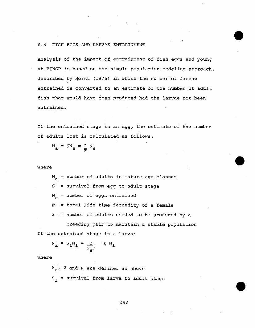
6.4 FISH EGGS AND LARVAE ENTRAINMENT

Analysis of the impact of entrainment of fish eggs and young

at PINGP is based on the simple population modeling approach,

described by Horst (1975) in which the number of larvae

entrained is converted to an estimate of the number of adult

fish that would have been produced had the larvae not been

entrained.

If the entrained stage is an egg, the estimate of the number

of adults lost is calculated as follows:

N = SN 2 Na e - eF

where

Na = number of adults in mature age classes

S = survival from egg to adult stageN = number of eggs entrained

e

F = total life time fecundity of a female

2 = number of adults needed to be produced by a

breeding pair to maintain a stable population

If the entrained stage is a larva:

N = N = 2 X Na 11 SFe

where

N 2 and F are defined as above

S = survival from larva to adult stage

243

N1 = number of larvae entrained

Se = survival from egg to larva

The following assumptions are made in this analysis:

o There is 100 percent mortality of entrained eggs and

larvae on passage through the plant

o The populations are at equilibrium and the total

lifetime'fecundity produces 2 adults

o That 0.5 percent of the eggs produced by a species

with high fecundity and/or randomly broadcast eggs

and little parental protection survive to the larval

stage

o that 75 percent of the eggs produced by a species which

exhibits nesting behavior and a high degree of parental

care survive to the larval stage.

Before estimating the number of adults lost it was necessary

to consolidate some taxonomic groups because of a lack of

reproductive information for certain taxa. In some cases,

such as the suckers, the individuals which could only be

identified to family level were divided among the genera

of that family based on the proportion of the larval catch

comprising each genus. If only a few larvae were captured

in each of several taxonomic categories, they were combined

at the family level with the exception of emerald shiner and

carp. Larvae were never grouped above the family level.

244

A total of 8,371,000 (+ 4,694,000 at 95 percent confidence

.interval) fish eggs and 61,645,000 (± 34,529,000) larval and

juvenile fish were estimated to be entrained by PINGP

between May 12 and September 10, 1975. The number of larval

and juvenile fish entrained represents about 6 percent

of the total number of larvae and juveniles passing through

the Sturgeon Lake outlet during the same period (based on a

conservative estimate from data collected by the MNDR of

about one billion larvae and juveniles, Section 5.3.1.3.2).

Weekly estimates of entrained larvae and juveniles ranged

from less than 1 to 85 percent of the estimated Sturgeon

Lake production. These estimates are conservative because

they do not take into account the larvae and juveniles in

the main channel. No estimates of larvae and juveniles in

the main channel are available.

The entrained eggs and young represent a potential loss of

about 2,830,000 adult fish from at least 28 taxa. The

number of eggs and young entrained, the number of adults

lost and the values for fecundity and survival used to

calculate the losses are summarized in Table 6.4-1.

Over 99 percent of the potential adult fish loss consisted

of 8 taxa of forage fish. Taxa of either sport or commercial

importance (e.g., sauger, walleye, white bass', sunfish,

245

TABLE 6.4-1

OF LOSS OF ADULT FISH DUE TO ENTRAINMENT OF EGGS, LARVAE AND JUVENILES AT

PINGP IN 1975. (Sheet 1 of 2)

a.69.*

Dorosoma capedianumCoregonus c1IuikfaormiqflT-55-7-E-rTi ausEsox -uciusCyp1nu carploNotropis atherinoidesCyorinidaeuarp~oces appCatostomus comnersoniIctiobus sppMoxostoma upoIctalurus punctatusNoturus gyrnuPladictlys-o-livaris

Percops~ I miscomaycusMorone chr sopsm to, rupestris

isgibbosusL. macroch1IrusP-omoxis appEtheostom~a nigrumPerca TIavesconsPercina caprodesP. shum-ardi.Stizostedion canadenseS. vitreum

PercidaseAplodinotus grunniens

EggsLarvae L Juveniles

Unidentifiable Larvae

.CALCULATION

NumberM trained

10,370,0004,000

1,221,0004,000

3,257,00015,961,0001,575,0004,598,000

13,0006,617,000

36,000325,000

3,00016,00025,000

7,297,0005,000

122,000742,000480,00067,000

102,00088,000

1,711,0001,881,000

319,000956,.000

7,484,0003,408,000

403,000

Fecunditya

1,560,000178,00060,000

981,0007,360,000b

2,9002,900b

619,200954,000

1,610,000135,000214,800

200108,300

1,4003,390,000

63,00016,42597,000

462,2001,600

436,8006,00021,200

159,5002,257,000

477,000

1,300,000

SurvivalEgg to Larva

0.0050.0050.0050.0050.0050.0050.0050.0050.0050.0050.0050.750.75.40.750.0050.0050.750.750.750.750.750.030.0050.0050.0050.0050.005

0.005

Larvae Produced Survivalby One Female Larvae to Adult

7,800 0.0003900 0.002300 0.007

4,900 0.000436,800 0.00006

15 0.1315 0.13

3,100 0.00064,800 0.00048,000 0.0002

680 0.003160,000 0.00001

150 0.01500 0.004

7 0.317,000 0.0001

300 0.00712,000 0.000273,000 0.0000335,000 0.000061,200 0.002

13,100 0.000130 0.07

6 0.3800 0.003

11,300 0.00022,400 0.0008

Number ofAdults Lost

3,1118

8,5472

1952,075,000

204,7002,759

51,323

1083

3064

7,500730

35242229

13410

6,160513,300

5,64364

765

EconomicClassificationc

FCC,SSCFFCCCCCFCFSSSSSFSFFSS,

6,500 0.0003 111,022

TABLE 6.4-1 (Sheet 2. pf 2)

Unidentifiable eggsUnidentified Larvae

Total EggsTotal Larvae & Juveniles

NumberEntrained

887,00039,000

8,371,00061,645,000

FecundityaSurvival Larvae Produced Survival Number of Economic

Egg to Larva by One Female L4rvae to Adult Adult Lost Classificationc

TotalForageSport/Commercial

2,831,3042,809,935

21,339

aFecundity information obtained from Scott andCrossman (1973); Wrenn (19 8U) Swee and McCrimmon (1966);(1953); Winn (1958)1 Wolfert (1969)1 Ulrey, Risk and Scott (1968)

bb~Average of fecundities of several similar species.

F - Foragel C - Commerciall S - Sport.

Bodola (1955), Daiber

0

crappies, freshwater drum, carp, buffaloes and-carpsuckers)

represented less than 1 percent of the adults lost.

Minnows (mainly emerald shiner) accounted for 80 percent of

the potential adult loss. Darters (logperch, river darter

and johnny darter) and unidentified percids comprised the

next greatest proportion (18 percent) of the potential adult

loss. Gizzard shad (0.1 percent) and trout-perch (0.3

percent) were the remaining forage taxa.

Since there are no catch statistics for forage species,

another means of relating the extent of impact was used. If

it is assumed that each fish weighed about 8 grams (0.3 oz,

the average weight of young emerald shiner in the fall as

reported by Scott and Crossman 1973) when consumed by predators,

approximately 22,500 kg (49,600 lbs) or 144 kg/ha (131

lbs/acre) of forage would be lost to the PINGP area (1600 ha

MNDR study area). If all 22,500 kg were consumed and were

converted to predator biomass at an efficiency of 15 percent,

about 3,400 kg (7,500 lbs) of predator production could be

eliminated from the PINGP area. The average individual

weight of the three major predators (sauger, walleye and

white bass) found in the area as determined from creel

censuses between 1968 and 1975 was 0.57 kg (1.26 lbs)

248

(Gustafson and Diedrich 1976). Based on this weight, the

estimated loss in predator production would be 5,900 fish.

However, the surplus production of forage fish may be

sufficient to accomodate both predation and exploitation due

to entrainment with no loss of sport fish production.

If ;these estimated losses are looked at by themselves, it

appears that there has been a significant loss to the forage

base in the PINGP area. Another approach is to compare the

number of young forage fish entrained to the total number

available. This can be accomplished by using the larval

fish data collected in 1975 by the MNDR (Gustafson et al.

1976) at stations near the mouth of Sturgeon Lake to develop

an estimate of the total number of young forage fish passing

through the Sturgeon Lake outlet (see Section 5.3.1.3.2

for discussion of MNDR data). It is assumed that the taxonomic

composition of the young in the outlet is similar to that at

the bar rack in the intake canal. The number of young

forage fish entrained represents only 3 percent of the

available production (51 million young, based on Sturgeon

Lake outlet densities) of the North Lake-Sturgeon Lake

complex.

Although sport and commercial species represented less than

1 percent of the total adult loss, the actual numbers of

249

adults lost of several of the individual taxa appear to be

high. Approximately 5,600 saugers (based on all mature

age classes), one of the most sought after sport fish in

the PINGP vicinity, were estimated to be lost due to the

entrainment of larvae (Table 6.4-1). This represents about

0.9 to 2.4 percent of the estimated population between

Sturgeon Lake and Lake Pepin or one-third the average

spring angler harvest from section 4 of the PINGP survey

area, which annually contributes about 70 percent of the

entire sauger harvest for the survey area (Naplin and

Gustafson 1975, Gustafson and Diedrich 1976). It is nearly

18 times the annual harvest for the area above Lock and Dam

No. 3.

The impact of the loss of 5,600 sauger to the PINGP area

fishery depends on the size of the population, the geograph-

ical distribution of the population and spawning activity

and the proportion of available young entrained. The

greatest impact would occur if Pool 3 had a small, discrete

population of sauger and a majority of the spawning activity

for the population occurred in the lakes upstream of the PINGP

intake with .a large proportion of the young produced being

entrained. If, on the other hand, the population was rather

250

mobile, capable of free movement into and out of Pool 3

and/or spawning activity were spread over a large portion of

the Upper Mississippi River, the impact on the population

would not be as great.

Hawkinson (1974) stated that data from tagging studies con-

ducted by Krosch (1969) and Finke (1964) indicated that

the larger fish which inhabit the PINGP area are extremely

mobile and move throughout the area between Taylors Falls

on the St. Croix River and Lansing, Iowa on the Mississippi

River. Preliminary analysis of tag returns from the PINGP

tagging study seem to indicate that the sauger found in the

plant area are highly mobile (Gustafson et al. 1976). On

the basis of preliminary tagging data, it would seem'that

Pool 3 does not have a discrete population of sauger. It

also seems unlikely that North and Sturgeon Lakes are unique

and, as a consequence, are not primary spawning areas for the

population. There appears to be a considerable amount of

similar spawning habitat in Pool 3 which would be available

to the sauger population utilizing the PINGP area. Further-

more, the number of larvae entrained represents less than 3

percent of the sauger larvae carried out of Sturgeon Lake

during May, (assuming that larval drift from Sturgeon Lake

has a taxonomic composition similar to that at the Bar Rack

Station in the intake canal).

251

Because of the high mobility of adult sauger, the wide

availability of suitable spawning habitat, and the low

proportion of sauger larvae available that are actually

entrained, it is not anticipated that entrainment of larvae

by ;the PINGP will have a significant impact on the local

sauger population.

Approximately 730 adult white bass were estimated to be lost

due to the entrainment of larvae at PINGP (Table 6.4-1).

This represents only 0.4 to 0.5 percent of the population

estimated between Sturgeon Lake and Lake Pepin -

and only 7 percent of the average annual sport harvest of

10,400 fish, and appears to be only a small portion of the

total production for the North Lake-Sturgeon Lake cotnplex.

If it is again assumed that the taxonomic composition of the

larvae in the Sturgeon Lake Outlet is similar to that at the

Bar Rack Station, about 250 million white bass larvae would

be present in the North Lake-Sturgeon Lake complex. Using

the same method of calculation as was used for deriving

entrainment losses, this would result in the production of

about 25,000 adults, nearly 35 times the entrainment loss.

Nearly 11 million freshwater drum eggs and larvae were

entrained at PINGP during the 1975 sampling period, resulting

252

in a potential loss of about 1,000 adults (Table 6.4-1).

This was approximately 1.5 percent of the population of

young drum in the plant area, one-third of the total annual

sport harvest (Section 4.3.5.1) and about equal to the

average commercial harvest (Pool 3) reported by the MDNR

(Section 4.3.5.2). At present, however, this species does

not appear to be heavily exploited by either the recrea-

tional or sport fishery above Lock and Dam No. 3. Sport

fishing pressures in Pool 4 during the 1960's were 300 to

700 times higher than current levels in the area above Lock

and Dam No. 3 and harvests were 38 to 50 times greater

(Skrypek 1964, Sternberg 1969, Hawkinson 1974, Naplin and

Gustafson 1975, Gustafson and Diedrich 1976). During the

same period, the abundance of drum in Pool 4, indicdted by

experimental gill net and trap net catches, was equal to or

less than current levels in the area upstream of Lock and

Dam No. 3 (Skrypeck 1966, Anonymous 1964, Hawkinson 1974,

Naplin and Geis 1975, Gustafson et al. 1976). This indicates

that the drum population in the PINGP area can stand consider-

ably more exploitation pressure without serious damage.

Other sport fishes sustaining entrainment losses include

walleye, and species of sunfish, crappies, northern pike and

yellow perch (Table 6.4-1). The total adult loss was

estimated to be 184 fish, which is less than 10 percent

253

in a potential loss of about 1,000 adults (Table 6.4-1).

This was approximately 1.5 percent of the population of

young drum in the plant area (Table 6.5-1), one-third of the

total annual sport harvest (Section 4.3.5.1) and about equal

to the average commercial harvest (Pool 3) reported by the MNDR

(Section 4.3.5.2). At present, however, this species does

not appear to be heavily exploited by either the recreational

or sport fishery above Lock and Dam No. 3. Sport fishing

pressures in Pool 4 during the 1960's were 300 to 700 times

higher than current levels in the area above Lock and Dam

No. 3 and harvests were 38 to 50 times greater (Skrypek

1964, Sternberg 1969, Hawkinson 1974, Naplin and Gustafson

1975, Gustafson and Diedrich 1976). During the same period,

the abundance of drum in Pool 4, indicated by experimental

gill net and trap net catches, was equal to or less than

current levels in the area upstream of Lock and Dam No. 3

(Skrypeck 1966, Anonymous 1964, Hawkinson 1974, Naplin and

Geis 1975, Gustafson et al. 1976). This indicates that the

drum population in the PINGP area can stand considerably

more exploitation pressure without serious damage.

Other sport fishes sustaining entrainment losses include

walleye, and species of sunfish, crappies, northern pike and

yellow perch (Table 6.4-1). The total adult loss was

estimated to be 184 fish, which is less than 10 percent

254

of the combined annual angler harvest for these species.

The operation of PINGP should not cause a significant de-

crease in the number of these sport fish available in the

area of the plant.

Commercial fish whose larvae were entrained at PINGP in-

cluded carp, buffalo, catfish, suckers and carpsuckers

(quillbacks). Since the MDNR publishes only total weights

of harvested species it was necessary to convert the

number of adults lost to weights for comparison to

commercial landings. This was accomplished by multiplying

the number lost by an average weight per individual, which

was usually obtained from information given in Scott and

Crossman (1973).. All commercial fishery data were obtained

from MDNR unpublished reports.

Nearly 3.3 million carp larvae were entrained in 1975,

resulting in a potential loss of 195 adults. At an average

weight of 9 kg, this loss represents 1,755 kg (3,869 lbs)

or about 8 percent of the average annual commercial catch

from Pools 3 and 4.

Over 6.6 million buffalo larvae were entrained, resulting

in a potential adult fish loss of 1,323 fish. At an average

individual weight of 2.3 kg (5.1 lbs), the loss represents

255

3,043 kg (6,708 lbs.), an amount about equal to the average

commercial harvest for Pools 3 and 4 during the period 1970

to 1974 (Section 4.3.5.2).

Approximately 4.6 million carpsucker larvae were entrained

in 1975. This represents a potential adult loss of 2,759

fish or about 25,000 kg (55,000 ibs). The average annual

catch for Pools 3 and 4 between 1970 and 1975 was 103 kg

(227 ibs).

Over 300,000 channel and flathead catfish young were entrained,

resulting in an estimated loss of 122 kg (269 lbs or 67

fish) or 5 percent of the average annual commercial catch.

The mooneye is listed as an incidental catch in both the

commercial and sport fisheries statistics. It has not been

abundant in the catch of any type of experimental gear

fished in the PINGP area between 1973 and 1975, but in 1975

it accounted for 2 percent of the larvae entrained at the

PINGP. The estimated number of adults lost due to entrain-

ment of larvae was 8,547. This is considerably higher than

the combined annual sport and commercial harvest.

Losses of carp and catfish do not appear to be significant

when compared to commercial catches. The impact on the

256

fishery of losses of the magnitude exhibited by buffaloes,

carpsuckers and mooneye is unclear. It is unknown whether

the low numbers of these taxa in commercial landings are

due to low abundance in Pools 3 and 4 or a lack of interest

by commercial fishermen.

Experimental gear catch data suggests that these fish have

been low in abundance in the PINGP area between 1973 and

1975. However, if the number of larvae of each taxon at

the outlet of Sturgeon Lake is considered, (assuming a

taxonomic compositionsimilar to that at the Bar Rack Station),

it appears that the experimental catch may not be an adequate

indicator of abundance of these species. (This is especially

true since the MNDR data on'larvae Of Sturgeon Lake Outlet

are probably relatively low estimates as discussed in

Section 5.3.1.3.2). Approximately 111 million buffalo

larvae, 21 million mooneye larvae and 78 million carpsucker

larvae were estimated to have passed the PINGP intake in

1975. These larvae would have been the progeny of 96,00C,

280,000 and 202,000 spawning pairs of buffalo, mooneye and

carpsuckers, respectively. Potential losses of adults due

to entrainment represent only a small proportion of those

adults which produced young that were estimated to have

passed the PINGP intake; therefore, it is not likely that

significant impact has or will result from larval entrainment.

257

6.5 FISH IMPINGEMENT

Fish losses due to impingement at PINGP were 146,063 in 1974

and 93,466 in 1975. The significance of losses of fish

because of impingement at PINGP can be subjected to a general

evaluation based on comparisons with population estimates

(Table 6.5-1).

The most obvious result of studies at PINGP (Section 5.3.2)

is the large numbers of gizzard shad impinged. Most of the

gizzard shad were impinged during the late fall and winter.

As pointed out by Andersen (1975), the high impingement

rates appear to be temperature-related. A number of investi-

gators have reported apparent temperature-related fall die-

offs of gizzard shad (Wickliff 1953, Agersborg 1930; Miller

1960, Bodola 1966). The large number of gizzard shad in

Sturgeon Lake and nearby areas and their sensitivity to

temperature changes in the fall are apparently major factors

causing high impingement rates at PINGP. Andersen (1975)

pointed out that gizzard shad die-offs in the PINGP area

appear to begin when the water temperature falls to near

12 0 C (53.6 0 F).

Total numbers of gizzard shad impinged at PINGP were 136,667

in 1974 and 70,506 in 1975 (Table 6.5-1). Bottom trawling

data probably provide a low estimate of gizzard shad

258

TABLE 6.5.-i

NUMBERS OF MAJOR FISH SPECIES IMPINGED AT PINGP, ESTIMATES OF STANDINGCROP BASED ON TRAWL SURVEY, SPORT CATCHES, AND ESTIMATES

OF SPORT FISH POPULATIONS

Total impingedb

1974 1975

CTrawl survey

Plant area North Lake33.4 ha 438 ha

dTag and recapture

Peterson Schnabel

Gizzard shada

Channel catfishWhite bassCrappiesDrumWalleyeSaugerSauger/walleye

136,667637

1,3671,7043,143

51387

70,5066,2232,7122,0303,789

2,2522,6692,190

41766,220

250417667

270,6844,818

60,006154,176

58,6922,1901,7523,942

22,720173,910

162,721609,809772,530

155,335

123,512228,784352,296197

t'J

asix million estimated for Sturgeon Lake (Andersen 1975)

bSection 5.2

CSection 4.5, 1974 - 1975.

dSection 4.5, Sturgeon Lake to Lake Pepin, 1974 and 1975.

populations because this species is a filter-feeder and

occurs throughout the water column (Scott and Crossman

1973). Population estimates for the plant area are not

directly comparable to impingement data because trawling was

not conducted during the late fall and winter when most

gizzard shad were impinged. The MNDR estimated that roughly

six million gizzard shad were present in the 324 ha (800 ac)

Sturgeon Lake in late summer of 1973 (Andersen 1975).

Assuming this to-be a representative figure, the 1974 and

1975 losses represent approximately 1 to 2 percent of the

Sturgeon Lake population. Losses of this magnitude would

not reduce the forage value of this species.

Trawl survey data are relatively appropriate for interpre-

tation of losses of sport and commercial species because

similar size fish occur in both trawl and impingement catches.

However, trawling yields low population estimates due to

concentration by certain species in untrawlable habitats

such as nearshore shallows, macroflora beds, or other cover.

The average number of catfish impinged (3,430) is roughly

equivalent to the apparently low population estimates for

the 83.4 ha plant area and 438 ha North Lake (Table 6.5-1).

However, the Peterson population estimate (22,720) and 1974

commercial landings (37,820 lbs) of adult fish suggest that

260

the number of impinged catfish represent a small fraction of

the young occurring in the region.

Young white bass losses were comparable to the trawl popula-

tion estimates occurring in the plant area and represent 6.8

percent of the numbers estimated for North Lake. The young

white bass represent about 1 percent of the sport fish

populations estimated in tag and recapture studies. Due to

natural mortality, the number of white bass impinged would

have yielded an even smaller number of adults.

The number of impinged crappies is greater than the popula-

tion estimated for the plant area from trawl survey data, but

represents only 2.4 percent of the North.Lake population.

Low population estimates in the plant area are probably due

to concentration of crappies in relatively unsampled habitats.

Freshwater drum in the PINGP area would be highly vulnerable

to impingement, judging by the large population occurring in

the plant area. However, impingement losses represent only

10 percent and 12 percent of the estimated young occurring

in the plant area and North Lake, respectively.

Walleyes and saugers were impinged at a low rate relative to

other species and represent 43 percent of the estimated

261

plant area populations, 3.6 percent of the estimated North

Lake populations and less than 0.1 percent of the estimated

sport fish populations.

Assessment of life-of-the-plant effects on fishes near

PINGP is complicated by a number of interacting factors.

A balanced indigenous species of fish is multi-aged and

fluctuates in relation to variability of year-class strengths,

exploitation, natural mortality, and density-dependent

mechanisms. Year-class strength is determined primarily by

abiotic factors, especially water temperature regimes, during

spawning and early development stages. Exploitation is

often the major source of mortality in adult fish.

Surplus production is the substainmJble yield or production

of new weight by a fishable stock, plus recruits added to

it, less what is lost to natural mortality (Ricker 1975).

In a discrete population, surplus production will increase

as exploitation increases until the total rate of exploitation

from fishing and power plants reduces surplus production below

the level needed to sustain the population (McFadden 1975).

McFadden's hypothetical model shows that a population will

not decline when exploitation from power plants and fishing

is less than 40 percent per year.

262

When the Oneida Lake walleye population was subjected to

exploitation of approximately 40-50 percent in one year, it

exhibited high growth rates and population levels in sub-

sequent years (Forney 1967). Adult walleyes in Lake Erie

showed no decline when subjected to 70-78 percent exploitation

per year during 1962-1966 (Regier et al. 1969). High rates of

exploitation resulted from heavy fishing pressure in Lake

Erie and low abundance of forage fish in other lakes

(Forney 1976, Moyle 1949). These studies suggest that

fairly high rates of exploitation will not cause a sustained

decline if year class formation and recruitment are normal.

Additional exploitation associated with operation of a

power plant would represent a relatively minor source of

mortality in the long-term fluctuations of upper Mississippi

River fish populations. Even in the immediate plant area,

entrainment and impingement losses may be masked due to the

great mobility of fish in the PINGP area.

263

7 REFERENCES CITED

Agersborg, H. P. K. 1930. The influence of temperature onfish. Ecology 2(l):136-144.

Andersen, R. A. 1975. Impingement of fishes and otherorganisms on the Prairie Island Plant intake travelingscreens. In: Environmental monitoring and ecologicalstudies program, Northern States Power 1974 annual report,Vol. II, for the Prairie Island Nuclear Generating Plantnear Red Wing, Minnesota.

Anonymous. 1964. Exploratory fishing in Pools 3, 4, 5 and5A of the Mississippi River, 1957 and 1963. MinnesotaDepartment of Conservation.

Anonymous. 1974. Impingement of fishes and other-oxrganismson the Prairie Island Plant traveling screen. In:Environmental monitoring and ecological studies program,Northern States Power 1973 annual report, Vol. II, for thePrairie Island Nuclear Generating Plant near Red Wing, Minnesota.

Baker, A. L. 1974. Studies of the periphyton of theMississippi River, near the Prairie Island Nuclear Generat-ing Plant -- 1973. In: Environmental monitoring andecological studies program, Northern States Power'1973annual report, Vol. II, for the Prairie Island NuclearGenerating Plant near Red Wing, Minnesota.

Baker, A. L. 1975. Primary productivity of the phytoplanktonin the Mississippi River at Prairie Island; the effects ofheated water discharge on the levels of production; and aturbidometric analysis of mass flow. In: Environmentalmonitoring and ecological studies program, Northern StatesPower 1974 annual report, Vol. I, for the Prairie IslandNuclear Generating Plant near Red Wing, Minnesota.

Baker, A. L. 1976. Studies of the productivity of thephytoplankton of the Mississippi River at Prairie Island -

1975. In: Environmental monitoring and ecological studiesprogram, Northern States Power 1975 annual report, Vol. I,for the Prairie Island Nuclear Generating Plant near RedWing, Minnesota.

264

0Baker, K. K. and A. L. Baker. 1974. Studies of the phyto-

plankton of the Mississippi River, near the Prairie IslandNuclear Generating Plant -- 1973. In: Environmentalmonitoring and ecological studies program, Northern StatesPower 1973 annual report, Vol. II, for the Prairie IslandNuclear Generating Plant near Red Wing, Minnesota.

Baker, K. K. and A. L. Baker. 1975. Studies of the phyto-plankton of the Mississippi River, near the Prairie IslandNuclear Generating Plant -- 1974. In: Environmentalmonitoring and ecological studies program, Northern StatesPower 1974 annual report, Vol. I, for the Prairie IslandNuclear Generating Plant near Red Wing, Minnesota.

Baker, K. K. and A. L. Baker. 1976. Studies of the phyto-plankton of the Mississippi River, near the Prairie IslandNuclear Generating Plant 1975. In: Environmentalmonitoring and ecological studies program, Northe-rn StatesPower 1975 annual report, Vol. I, for the Prairie IslandNuclear Generating Plant near Red Wing, Minnesota.

Barr, A. J. and J. H. Goodnight. 1972. A user's guide tothe statistical analysis system. North Carolina StateUniversity, Sparks Press, Raleigh, North Carolina.

Behmer, D. J. 1969. Schooling of river carpsuckers and apopulation estimate. Trans. Amer. Fish. Soc. 98(3):520-523.

Bibko, P. N., L. Wirtenan and P. E. Kueser. 1974. Prelim-inary studies on the effects of air bubbles and intenseillumination on the swimming behavior of the striped bass(Morone saxatilis) and the gizzard shad (Dorosomacepdanum). pp. 293-304 In: Jensen, L. D., (ed.).Proceedings of the second entrainment and intake screeningworkshop. Electric Power Research Institute Report No. 15.Palo Alto, California.

Bodola, A. 1966. Life history of the gizzard shad Dorosomacepedianum (Le Sueur) in western Lake Erie. Fishery Bull.65(2):391-425.

Britt, N. W. 1955. New methods of collecting bottom faunafrom shoals or rubble bottoms of lakes and streams.Ecology 36:524-525.

0265

Brook, A. J. 1971. Phytoplankton study. In: Environmentalmonitoring and ecological studies program, Northern StatesPower 1970 annual report for the Prairie Island NuclearGenerating Plant near Red Wing, Minnesota.

Brook, A. J. 1972. Phytoplankton. In: Environmentalmonitoringand ecological studies program, Northern StatesPower 1971 annual report for the Prairie Island NuclearGenerating Plant near RedWing, Minnesota.

Brook, A. J. 1973. Phytoplankton. In: Environmentalmonitoring and ecological studies program, Northern StatesPower 1972 annual report for the Prairie Island NuclearGenerating Plant near Red Wing, Minnesota.

Daggett, R. F. 1976. Zooplankton study. In: Environ-mental monitoring and ecological studies program, NorthernStates Power 1975 annual report, Vol. I, for the PrairieIsland Generating Plant near Red Wing, Minnesota.

Daley, S. A. and J. S. Skrypek. 1964. Angler creel censusof Pools 4 and 5 of the Mississippi River, Goodhue andWabasha Counties, Minnesota in 1962-63. MinnesotaDepartment of Conservation.

Davis, S. E. et al. 1963. The influence of oxygen con-centrations on the swimming performance of juvenilePacific salmon at various temperatures. Trans. Amer. Fish.Soc. 92(2):111-124.

Edsall, T. A. and T. G. Yocum. 1972. Review of recenttechnical information concerning the adverse effects ofonce-through cooling on Lake Michigan. U.S. Fish andWildlife Service, Great Lakes Fisheries Laboratory, AnnArbor, Mich.

Edwards, T. J., W. H. Hunt, L. E. Miller and J. J. Sevic.Undated. Fish impingement at four Duke Power Companysteam generating facilities. Duke Power Company, Environ-mental Sciences Unit, Charlotte, North Carolina. Manuscript.

EPA. 1976a. Development document for best technology avail-able for the location, design, construction and capacityof cooling water structures for minimizing adverse environ-mental impact. U.S. Environmental Protection Agency,Washington, D.C. (Draft).

266

EPA. 1976b. Guidance for determining best technologyavailable for the location, design, construction, andcapacity of cooling water intake structures for minimizingadverse environmental impact, section 316(b) P.L. 92-500.U.S. Environmental Protection Agency, Draft 2.

Fernholzr W., Work Unit Supervisor, State of Wisconsin Dept.Natural Resources. Personal communication to V. Kranz,NUS Corporation, Pittsburgh, Pa. Letter of September 23,1975.

Finke, A. H. 1964. White bass tagging study upper MississippiRiver. Wisconsin Department of Conservation, Division ofFish Management, Management Report No. 6.

Fish, M. P. 1932. Contributions to the early life historiesof sixty-two species of fishes from Lake Erie and itstributary waters. Bull. U.S. Bur. Fish. 47: 293-3.9.8.

Forney, J. L. 1967. Estimates of biomass and mortality ratesin a walleye population. N. Y. Fish Game J. 14: 176-192.

Gerlach, J. M. 1973. Early development of the quillbackcarpsucker, Carpiodes cyprinus. M.A. Thesis, MillersvilleState College, Millersville, Pa.

Grimes, C. B. 1975. Entrapment of fishes on intake ,waterscreens at a steam electric generating stations. Ches.Sci. 16(3):172-177.

Grotbeck, L. M. and J. L. Bechtold. 1975. Fish impingementat Monticello Nuclear Plant. J. Power Div., ASCE, Vol. 101,No. PO1, Proc. Paper 11409, pp. 69-83.

Gustafson, S. P. and P. J. Diedrich. 1976. Progress reporton the Prairie Island creel survey March 1 - November 2,3,1975. In: Environmental monitoring and ecological studiesprogram, Northern States Power 1975 annual report, Vol. II,for the Prairie Island Nuclear Generating Plant near RedWing, Minnesota.

Gustafson, S. P., J. L. Geis and P. J. Diedrich. 1976.1975 progress report on the Prairie Island fish populationstudy. In: Environmental monitoring and ecological studiesprogram, Northern States Power 1975 annual report, Vol. II,for the Prairie Island Nuclear Generating Plant near RedWing, Minnesota.

267

Hawkinson, B. S. 1974. Progress report on the Prairie Islandcreel survey May 10 - November 5, 1973. In: Environ-mental monitoring and ecological studies program, NorthernStates Power 1973 Annual Report, Vol. I, for the PrairieIsland Nuclear Generating Plant near Red Wing, Minnesota.

Hawkinson, B. S. 1974. 1973 fish population study progressreport of Mississippi River near Prairie Island July 1973 -

February 1974. In: Environmental monitoring and ecologicalstudies program, Northern States Power 1973 annual report,Vol. 1, for the Prairie Island Nuclear Generating Plantnear Red Wing, Minnesota.

Haynets, C. 4. 1976. Macroinvertebrate study. In:Environmental monitoring and ecological studies program,Northern States Power 1975 annual report, Vol. I, for thePrairie Island Nuclear Generating Plant near Red Wing,Minnesota.

Hester, F. E. and Dendy, J. S. 1962. A multiplate samplerfor aquatic ipacroinvertebrates. Trans. Amer. Fish. Soc.91(4).

Horst, T. J. 1975. The assessment of impact due to entrain-ment of ichthyoplankton. In: Saila S.B. 1975. Fisheriesand energy production, a symposium. D. C. Heath and Co.,Lexington, Mass.

Hynes, H. B. N. 1972. The ecology of running water. Universityof Toronto Press.

Kerr, J. E. 1953. Studies on fish preservation at the ContraCosta Steam Plant of the Pacific Gas and Electric Company.Calif. Dept. Fish and Game Fish. Bull. 92.

Krosch, H. F. 1969. 1968 progress report on Lake St. Croixfish population study. In: Environmental monitoring andecological studies program, Northern States Power 1968annual report for the Prairie Island Nuclear GeneratingPlant near Red Wing, Minnesota.

Lorenzen, C. J. 1967. Determination of chlorophyll andpheopigments: spectrophotometric equations. Limnol.Oceanogr. 12:343-346.

Lippson, A. J. and R. L. Moran. 1974. Manual for identifi-cation of early development stages of fishes of the PotomacRiver Estuary. Envir. Tech. Center, Martin Marietta Corp.,Baltimore, Md. PPSP-MP-13.

268

May, E. B. and C. R. Gasaway. 1967. A preliminary key tothe identification of larval fishes of Oklahoma withparticular reference to Canton Reservoir, including aselected bibliography. Oklahoma Department of WildlifeConservation, Oklahoma Fisheries Resource Laboratory,Bull. No. 5.

Mayhew, D. A, and H. K. Hess. 1976. Impingement of fishesand other organisms on the Prairie Island Plant intaketraveling screens. In: Environmental monitoring andecological studies program, Northern States Power 1975annual report, Vol. I, for the Prairie Island NuclearGenerating Plant near Red Wing, Minnesota.

McConville, D. R. 1974. Macroinvertebrate studies. In:Environmental monitoring and ecological studies program,Northern States Power 1973 annual report, Vol. I, forthe Prairie Island Nuclear Generating Plant near Red Wing,Minnesota.

McConville, D. R. 1975. Macroinvertebrate studies. In:Environmental monitoring and ecological studies program,Northern States Power 1974 annual report, Vol. I, for thePrairie Island Nuclear Generating Plant near Red Wing,Minnesota.

McFadden, J. T. 1975. Environmental impact assessment for.fish populations. pp. 89-138 In: R. K. Sharma et al.(eds.) Proceedings of the conference on the biologicalsignificance of environmental impacts. USNRC, Washington,D.C.

Meyer, F. A. 1970. Development of some larval centrarchids.Prog. Fish-Cult. 32(3):130-136.

Middlebrook, K. 1975. Zooplankton entrainment. In:Environmental monitoring and ecological studies program,Northern States Power 1974 annual report, Vol. I, for thePrairie Island Nuclear Generating Plant near Red Wing,Minnesota.

Middlebrook, K. 1976. Zooplankton entrainment. In:Environmental monitoring and ecological studies program,Northern States Power 1975 annual report, Vol. I, for thePrairie Island Nuclear Generating Plant near Red Wing,Minnesota.

Miller, E. F. 1971. Ecological studies. In: Environmentalmonitoring and ecological studies program, Northern StatesPower 1970 annual report for the Prairie Island NuclearGenerating Plant near Red Wing, Minnesota.

269

Miller, E. F. 1972. Ecological studies. In: Environmentalmonitoring and ecological studies program, Northern StatesPower 1971 annual report for the Prairie Island NuclearGenerating Plant near Red Wing, Minnesota.

Miller, E. F. 1973. Fisheries study. In: Environmentalmonitoring and ecological studies program, Northern StatesPower 1972 annual report for the Prairie Island Nuclear*Generating Plant near Red Wing, Minnesota.

Miller, R. R. 1960. Systematics and biology of the gizzardshad (Dorosoma cepedianum) and related fish. Fish. Bull.60:371-392.

Moore, G. A. 1957. Fishes: Part 2, pp. 21-165 In: W. F. Blair,et al., Vertebrates of the United States. 2nd edition. 1968.McGraw-Hill Book Co., New York.

Moyle, J. B. 1949. Fish population concepts and managementof Minnesota lakes for sport fishing. Trans. N. Am. WildlifeConf. 14:283-294.

Mueller, K. N. 1975. Aquatic vegetation of the Prairie Islandarea 1974. In: Environmental monitoring and ecologicalstudies program, Northern States Power 1974 annual report,Vol. II, for the Prairie Island Nuclear Generating Plantnear Red Wing, Minnesota.

Mueller, K. N. 1976. Prairie Island aquatic vegetationstudy - 1975. In: Environmental monitoring and ecologicalstudies program, Northern States Power 1975 annual report,Vol. II, for the Prairie Island Nuclear Generating Plantnear Red Wing, Minnesota.

MPCA. 1975. Minnesota's guide for biological demonstrationsfor administration of 316(a) and (b) for the Federal WaterPollution Control Act Amendments of 1972 and MinnesotaRegulation WPC 36 (u)(3). Minnesota Pollution ControlAgency, Division of Water Quality.

Naplin, R. L. and J. L. Geis. 1975. 1974 progress report onthe Prairie Island fish population study. In: Environmentalmonitoring and ecological studies program, Northern StatesPower 1974 annual report, Vol. II, for the Prairie IslandNuclear Generating Plant near Red Wing, Minnesota.

270

Naplin, R. L. and S. P. Gustafson. 1975. Progress report onthe Prairie Island creel survey April 30 - December 3, 1974.In: Environmental monitoring and ecological studiesprogram, Northern States Power 1974 annual report, Vol. II,for the Prairie Island Nuclear Generating Plant near RedWing, Minnesota.

Nelson, W. R. 1968. Embryo and larval characteristics ofsauger, walleye, and their reciprocal hybrids. Trans.Am. Fish. Soc. 97(2) :167-174.

Norden, C. R. 1961. The identification of larval yellowperch, Perca flavescens, and walleye, Stizostedionvitreum. Copeia 1961 (3):282-288.

NSP. 1972. Environmental monitoring and ecological studiesprogram, Northern States Power 1971 annual report for thePrairie Island Nuclear Generating Plant near Red Wing,Minnesota.

NSP. 1973. Environmental monitoring and ecological studiesprogram, Northern States Power 1972 annual report for thePrairie Island Nuclear Generating Plant near Red Wing,Minnesota.

NSP. 1974. Environmental monitoring and ecological studiesprogram, Northern States Power 1973 annual report f6r thePrairie Island Nuclear Generating Plant near Red Wing,Minnesota.

Olsen, L., MPCA. Personal communication to J. Ericson, NUSCorporation, Pittsburgh, Pa. Letter of October 18, 1976.

Quirk, Lawler and Matusky. 1974. Nine Mile Point aquaticecology studies, Vol. II, fish impingement. NiagaraMohawk Power Corporation.

Reiger, H. A., V. C. Applegate, and R. A. Ryder. 1969. Theecology and management of the walleye in western Lake Erie.Great Lakes Fish. Comm. Tech. Rep. 15.

Ricker, W. E. 1975. Handbook of computation and inter-pretation of statistics of fish populations. Fish. Res.Bd. Canada Bull. No. 191.

Sazaki, M., W. Heubach and J. E. Skinner. 1973. Somepreliminary results on the swimming ability and impingementtolerance of young-of-the-year steelhead trout, king salmonand striped bass. Final report for Anadromous FisheriesAct Project AFS-13. Manuscript.

271

Scott, W. B. and E. J. Crossman, 1973. Freshwater fishes ofCanada. Fish. Res. Bd. Canada Bull. No. 184.

Simonet, R. J. 1975. Macroinvertebrate study. In:Environmental monitoring and ecological studies program,Northern States Power 1974 annual report, Vol. II, forthe Prairie Island Nuclear Generating Plant near Red Wing,Minnesota.

Skrypek, J. 1966. Analysis of physical and biologicalchanges at selected sampling stations in the MississippiRiver. Minnesota Department of Conservation.

Snedecor, B. W. and W. G. Cochran. 1967. Statistical methods.6th ed. Iowa State University Press, Ames, Ia.

Snyder, D. E. 1971. Studies of larval fishes in Muddy RunPumped Storage Reservoir near Holtwood, Pennsylvania.A.S.' Thesis, Cornell University, Ithaca, N. Y.

Snyder, D. E. and M. B. M. Snyder. 1976. Identificationof larvae of Notemigonus crysoleucas, Notropis spilopterus,and Pimephales promelas. J. Fish. Res. Bd. Canada 32:

* 000-000. (Recently submitted for publication).

Sokal, R. R. and F. J. Rohlf. 1969. Biometry. W. H.,Freeman and Co., San Francisco.

Stefan, H. 1973. A preliminary evaluation of the flowthrough Sturgeon Lake upstream of Lock and Dam No. 3 onthe Mississippi River. Prepared for John W. Gorman, Inc.and Northern States Power Company.

Sternberg, R. B. 1969. Angler creel census of Pools 4 and5 of the Mississippi River, Goodhue and Wabasha Counties,Minnesota in 1967-68. Minnesota Department of Conservation,Division of Game and Fish. Report No. 306.

Szluha, A. 1974. Zooplankton study. In: Environmentalmonitoring and ecological studies program, Northern StatesPower 1973 annual report, Vol. I, for the Prairie IslandNuclear Generating Plant near Red Wing, Minnesota.

Szluha, A. 1975. Zooplankton study. In: Environmentalmonitoring and ecological studies program, Northern StatesPower 1974 annual report, Vol. I, for the Prairie IslandNuclear Generating Plant near Red Wing, Minnesota.

272

Taber, C. A. 1969. Distribution and identification oflarval fishes in the Buncombe Creek Arm of LakeTexoma with observations on spawning habits and relativeabundance. Ph.D.Thesis, University of Oklahoma, Norman,Oklahoma.

USAEC. 1972. Draft environmental impact statement forIndian Point Nuclear Generating Plant Unit No. 3, Con-solidated Edison Company of New York, Inc. U. S. AtomicEnergy Commission. Docket No. 50-286.

USAEC. 1973. Draft Environmental Statement by the UnitedStates Atomic Energy Commission Directorate of Licensingrelated to the proposed issuance of an operating licensefor the Prairie Island Nuclear Generating Plant by NorthernStates Power. Docket Nos. 50-282 and 50-306.

USGS. 1928-1975. Water resources data for MinnesotaiPart 2. Surface water records. U. S. Geological Survey.

Vose, R. 1974. Aquatic macrophyte study. In: Environmentalmonitoring and ecological studies program, Northern StatesPower 1973 annual report, Vol. I, for the Prairie IslandNuclear Generating Plant near Red Wing, Minnesota.

Wickliff, E. L. 1953. Gizzard shad rides again. OhioConserv. Bull. 17:23-25.

0273

APPENDIX 1

INTAKE VELOCITY PROFILES AT PINGPJUNE 23 AND 28, 1976

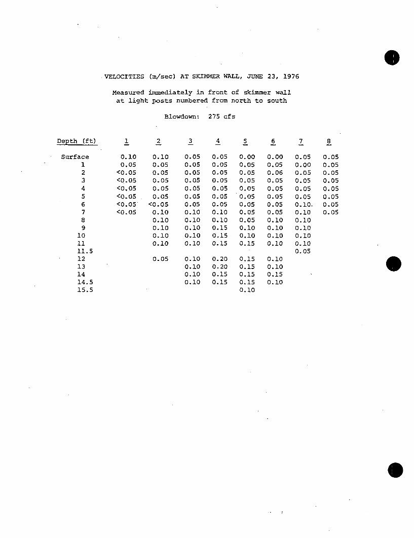
VELOCITIES (m/sec) AT SKIMMER WALL, JUNE 23, 1976

Measured immediately in front of skimmer wallat light posts numbered from north to south

Blowdown: 275 cfs

Depth (ft)

Surface123456789

101i11.512131414.515.5

2

0.100.05

<0.05<0.05<0.05<0.05<0.05<0.05

0.100.050.050.050.050.05

<0.050.100.100.100.100.10

3 4 5 6 7 8

0.05 0.05 0.00 0.00 0.05 0.0.05 0.05 0.05 0.05 0.00 0.0.05 0.05 0.05 0.06 0.05 0.(0.05 0.05 0.05 0.05 0.05 0.0.05 0.05 0.05 0.05 0.05 0.0.05 0.05 0.05 0.05 0.05 0.0.05 0.05 0.05 0.05 0.10. 0.(0.10 0.10 0.05 0.05 0.10 0.0.10 0.10 0.05 0.10 0.100.10 0.15 0.10 0.10 0.100.10 0.15 0.10 0.10 0.100.10 0.15 0.15 0.10 0.10

0505050505050505

0.05 0.100.100.100.10

0.200.200.150.15

0.150.150.150.150.10

0.100.100.150.10

0.05

0

VELOCITIES (m/sec) AT BAR RACK, JUNE 23, 1976

Measured 4.5 ft in front of bar rack at 24equidistant points numberea from east to west-

Blowdown: 275 cfs

1, 2 3 4 5 6 7 8Depth (ft)

Surface123456789

101111.51212.51313.51414.5

0.300.400.400.450.500. 450.400.350.300.250.250.200.20

0.400.350.400.400.400.350.350.400.300.300.300.25

0.300.400.400.400.350.400.300.350.250.250.250.25

0.300.300.300.300.300.300.300.100 100.200.200.20

0.20

0.300.300.350.300.300.300.200.200.200.200.250.20

0.300.250.300.300.300.200.200.200.250.250.200.25

. 0.25

0.300.300.300.300.300.200.200.100.200.200.15

0.350.400.300.300.300.300.150.150.100.250.300.20

0.20 0.25 0.20 0.20 0.20 0.20

0.20

0.200.10

0.30 0.100.10

0.20 0.200.10

0.200.10

VELOCITIES (m/sec) AT BAP, RACK, JUNE 23, 1976

(Continued)

Depth (ft)

Surface123.456789

1011121313.51414.5

9

0.300.300.300.300.300.300.250.200.200.25-0.250.250.200.20

0.10

10 11 12 13 14 *15 16

0.250.250.300.250.200.300.200.200.150.250.200.200.250.200.20

0.250.300.300.300.350.200.150.250.300.250.250.200.200.15

0.300.300.300.250.300.300.300.200.200.200.300.250.200.20

0.200.250.250.300.250.300.250.100.100.250.200.200.200.20

0.200.300.250.300.250.250.200.200.200.200.200.250.150.20

0.250.300.300.300.200.200.200.300.250.200*300.300.300.20

0.200.250.300.250.200.200.300.200.300.150.300.200.200.20

0.10 0.10 0.20 0.20 0.100.10

0

0

VELOCITIES (m/sec) AT BAR RACK, JUNE 23,1976

(Continued)

Depth (ft) 17: 18 19 20 21 22: 23

Surface123456789

10111212.51313.51414.5

0.300.300.300.300.300.300.200.250.200.200.200.200.25

0.200.10

0.300.300.300.300.350.250.200.250.200.300.250.200.30

0.250.300.300.300.300.200.100.200.200.150.200.200.10

0.300.300.300.350.300.350.300.250.200.300.250.300.20

0.300.350.300.400.400.400.300.300.300.200.300.300.25

0.300.400.250.300.350.300.200.250.300.200. 200.200.25

0.400.350.300.300.300.300.300.250.300.300.250.200.150.10

0.20 0.200.20 0.20

0.25 0.25 0.15

0.25 0.20 0.200.20

VELOCITIES (m/sec) AT SKIMMER WALL, JUNE 28, 1976

Measured immediately in front of.skimmer wallnumbered from north to south

at light posts

Blowdown: 655 cfs

Depth (f t)

Surface123456789

1011121313.51415

1 2 3 4 5 6 7 8

0.000.000.050.050.050.050.050.05

0.100.150.150.150.150.100.050.050.100.100.200.200.200.150.15

0.050.100.100.050.050.100.100.150.200.250.250.250.250.20

0.050.050.050.050.050.100.100.100.100.150.200.200.200.20

0.050.050.050.050.050.100.100.100.100.100.150.200.200.20

0.100..050.050.100.100.100.150.150.150.150.150.150.150.15

0.10

0.050.100.100.050.200.150.150.150.100.100.150.15

0.100.10

0.000.050.050.000.050.050.050.05

0.20 0.20 0.200.20 0.15 0.10 0

0

VELOCITIES (m/sec) AT SKIMMER WALL, JUNE 28, 1976

Measured immediately in front of skimmer wall atnumbered from north to south

Blowdown: 1300 cfs

light posts

Depth (ft)

Surface123456789

101i121313.51415

1 2 3 4 5 6 7 8

0.150.150.100.050.050.05.0.050.05

0.150.200.200.100.100.100.100.150.200.250.250.300.300.300.20

0.050.050.100.100.100.150.150.150.150.200.250.250.300.30

0.100.050.050.100.100.150.150.200.250.300.300.300.300.25

0.050.050.050.100.100.100.150.200.250.250.300.300.250.20

0.100.100.100.100.100.150.150.200.200.250.250.250.250.25

0.20

0.200.200.200.200.250.250.200.200.200.200.200.200.150.10

0.100.050.100.10

0.200.150.100.10

0.30 0.25 0.200.25 0.20 0.20

APPENDIX 2

NOTES ON SPAWNING AND REPRODUCTION OF 26 SPECIESOF FISH OCCURRING NEAR PINGP

0

APPENDIX 2

NOTES ON SPAWNING AND REPRODUCTION OF 26 SPECIESOCCURRING AT THE PINGP SITE

Species Amia calva (Bowfin)

Maturation byYear - Class or Length(mm total length) Male: III-V6 , 457; 3805;

Female: 6106 .

Fecundity 23,600-64,0005

Spawning Season

"Temperature (oC)

Area

Egg Deposition

Mid-May through June, possibly asearly as late April (Canada) 6 ;late March through May 5 .

16-195

Shallow vegetated waters inlakes and rivers-'; shallow,sluggish, stagnant water up to122cm or deeper 5 .

38-76 cm diameter nets amongthick vegetation hollowed outcircular or elliptical depressionwith bottom of fibrous roots,water-soaked leaves or gravel,also under stumps, logs, and bushes.2,000-5,000 eggs per nest; eggsattach to decaying vegetationand reeds by thread-like exten-sions of egg surface 5 .

Adhesive, darker from originalcreamy yellow6 ; attachment struc-ture5 .

2.2-3.0,capsule progressively 5distends to twice original size

8_106; 4-145.

86; 3-75

Larvae attach to vegetation withadhesive on the tip of the snoutfor 7-9 days by which time theyare 10-13 mm total length, youngguarded by male parent for sev-eral weeks until young are about

Type

Water-hardened Size (mm)

Incubation Period (days)

LarvaeHatching Size (mmtotal length)Habits, BehaviorSurvival

Amia calva (cont'd.)

102 mm total length 6 ; larvaealso attach to roots and lie onbottom of nest, then form tightguarded swarms, larvae 9-13 mmat yolk absorbtion, youngamong weeks in shallows 5 .

0

Species

Maturation byYear - Class or Length(mm total length)

Fecundity

Spawning Season

Temperature (oC)

Area

Egg Deposition

Esox lucius (Northern pike)

Male: I-I, 3032; II-III6;Female: II-IV, 3252

595,000,32,0006; 2,000-545,0002;32,0001.

March through May (Canada) 6 ;March to May (Michigan)l; Feb-ruary to mid-June 2 .

4.4-11.16; 5-142.

Heavily vegetated flood plainsof rivers, marshes, and bays;larger lakes, often in waterno deeper than 18cm6 ; shallowareas with vegetation 2 ; swamps,ponds, and lakesI; grassy orrush beds 4 .

Eggs scattered at random andattach to vegetationO; no nest 2 ;no parental care 4 ; eggs clearand amber 6 .

Demersal, adhesive 6

2.5-3.06; 2.2-3.4 1 .

12-14, 4.5 @!7.8-20OC6

Fertility rate over 50%6, 52-99%fertile, 64-90% egg hatch 2 .

6-76; 6.5-8 with average of 72;9-104

99.8% mortality prior to youngleaving spawning grounds; youngattach to vegetation with ad-hesive glands on head for 6-10days while consuming yolk; younggrow rapidly, 43 mm by first

Type

Water-hardened Size (mm)

incubation Period (days)

Survival

LarvaeHatching Size

Habits, Behavior,Survival

Esox lucius (cont'd.)

month and 152 mm by the end offirst summer, young after yolkabsorption feed on larger zoo-plankton and immature insects for7-10 days -then begin consumingsmall fish; by 50 mm, fish are apredominant food6; begin feedingat 13.3-15.1 mm, 99.6-99.9%mortality from egg to fingerling2 .

0

Species Cyprinus carpio (Carp)

Spawning Season

Temperature (°C)

'Area

Late A2ril to mid-August (GreatLakes) b; mid-May through August(Wisconsin) 2 ; May through mid-

August (Pennsylvania) 7 ; mid-Mayto early July (Maryland) 5 ; Marchthrough August (U.S.) 5 . Late Marchthrough mid-June (Okla.)8.

17-286; 14.5-23.4 but mostly at18.5-202 &.5, 10-30 but optimalat 225.

Weedy or grassy shallows of lakes,ponds, tributaries, swamps,flood plains, and marshes; 8-180cm in depthl, 2, 4, 5,.6, 8, 9.

Broadcast randomly, eggs attachfrequently in clusters to weeds,grasses or rootsl, 2, 4, 5, 6, 8, 9.

Egg Deposition

Type Adhesivel, 2, 5, 6

Water-hardened Size (mm)

Incubation Period (days)

Survival

16 F 1.0-2 .05 .3-66; 3-16, 3-5 @ 200C, 4-8 @

17.6-18.4-C, 12-161; 2-3 at 22-C 5 .

High mortality8

LarvaeHatching Size(mm total length)Habits, Behavior,Survival

3-6.4S

Larvae attach to or lie amongvegetation after hatching 5

1 'most larvae remain in shallowwater, few are found in deeperopen water 8 ; after 12 mm,total length, young appear tomove from near-shore surfacewater to deeper water 7 .

Species Notropis hudsonius (Spottailshiner)

Spawning Season May through July (Lake Erie) 46June to early July (Lake Erie)

Temperature (*C) 20.02

Area Over sandy shoals in water 90-150cm deep 6 .

Egg Deposition Found in algae masses along LakeErie shore.

Fecundity (mm Total 2Length) 100-2600

0

0

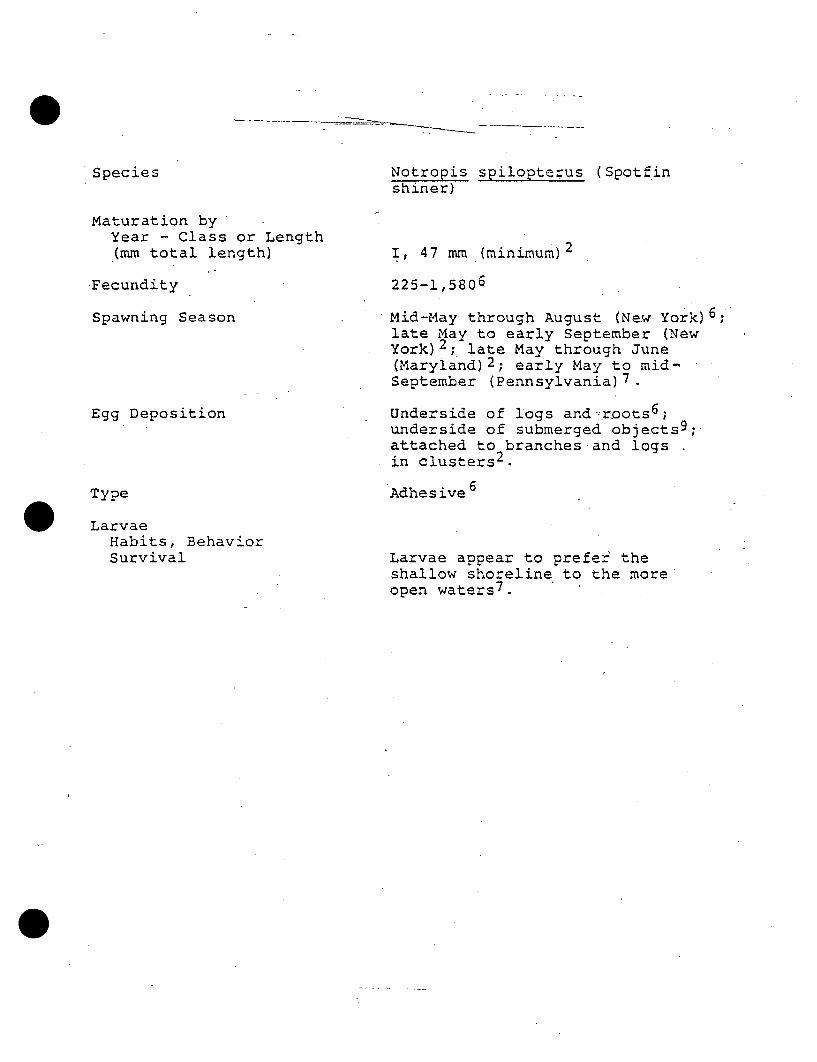
Species Notropis spilopterus (Spotfinshiner)

Maturation byYear - Class or Length(mm total length) I, 47 mm (minimum) 2

225-1,5806Fecundity

Spawning Season

Egg Deposition

Type

LarvaeHabits, BehaviorSurvival

Mid-May through August (New York) 6 ;late May to early September (NewYork) 2 ; late May through June(Maryland) 2 ; early May to mid-September (Pennsylvania)7.

Underside of logs and roots 6 ;underside of submerged objects 9 ;•attached to branches and logsin clusters 2 .

Adhesive6

Larvae appear to prefer' theshallow shoreline to the moreopen waters 7 .

Species Notropis dorsalis (Bigmouthshiner)

Spawning Season Late May to early September 2 ;late June to late August(Colorado) i.

Area Probably spawns in mid-stream2 .

Egg Deposition Eggs probably carried by.current 2 .

Type Pelagic 2

0

0

Species

Maturation byYear - Class or LengLI,(mm.total., length)

Fecundity

Spawning Season

Temperature (oC)

Area

Egg Deposition

Pimephales notatus (Bluntnoseminnow)

Male:-: 116; 1112; Female:ý .16;

1,743-2.223 averaging 2,0052.

May to mid-August (Canada) 6 ;May through August (Michigan) 2 ;mid-April through August (Illi-nois, Pennsylvania) 2 , 7; lateMay to early August (Wisconsin) l.

21-262; 27.84

Shallow water up to 62 cm deep,sand and gravel bottom shoals 1

Male hollows out nest beneathstone or other object upon whichthe eggs are laid on the under-side6 ; intermittent sp'awners,200-500 eggs per spawning 2 ;several broods per nestl1

Adhesive6Type

Water-hardened Size (mm)

Incubation Period (days)

LarvaeHatching Size(mm total length)Habits, Behavior,Survival

1-1.56

7-146; 8-9 @ 21-24OC1.

_96

Larvae are 12 mm 2 weeks afterhatching6 .

Species

Fecundity

Rhinichthys cataractae(Longnose dace)

200-1,2006; 160-6802.

Spawning Season

Temperature (°C)

Area

Egg Deposition

Late April through July (Canada) 6 ;late April to mid-June (Maryland) 2 ;late Maý to early September (Min-nesota)

11.7 minimum6

In riffles 6

Over gravelly bottom, in ornear Nocomis micropogon nests,one parent believed to guardarea though no nest is built 6-.

Type Adhesive 6

Incubation Period (days)

LarvaeHabits, Behavior,Survival

7-10 @ 15.6°C

0Yolk absorbed 7 days afterhatching, young are pelagic 6and remain so for about 4 months

0

I

Species

Maturation byYear - Class or Length(mm total length)

Fecundity

Spawning Season

Temperature (°C)

Area

Semotilus atromaculatus (Creekchub)

Male: 1116; IV 2 ; Female: 116;II12

2,820-4,671; 4,250 average for76-703 mm total length1 .

Late April to mid-July (Canada) 6 ;April to mid-May (Illinois) 2 ;*early March to mid-June (Iowa) 2 ;mid-April to July (Michigan) 2 .

12.8 minimum6 ; 12.8-16.71

Small, gravelly streams insmooth water just above or belowa riffle 6 ; in quiet riffles orgravel bar in a lake1 .

Male creates a nest or depres-sion (trench); eggs depositedin pit, then covered withstones and gravel, male guardsnest 6 ; conspicuous nests withlarge stone ridge and oval pitl-

Egg Deposition

Type Demersal 6

Species

Maturation byYear - Class or Length(rm total length)

Fecundity.

Spawning Season

Temperature (OC)

Area

Catostomus commersoni (Whitesucker)

III-VII1 6 ; 76 mm minimum;Male: IV-VI1 2 ; Female: III-IX 2

20*,000-139,0006; 775-139,000 forfish 120-510 mm total length 2 ;,average of 20,000-50,000 for.fish 410-540 total length1 .

April through mid-June (Canada) 6 ;late March to mid-May (Wisconsin)l;earls May to early July (Wiscon-sin) ; late March to mid-June(Lake Erie)1; April-May (Michi-gan) 2 ; mid-March through earlyApril (Illinois) 2 ; early Maythrough early June (New York) 1 ;early March through July. (U. S.) 5, 8

6-235; usually 10-208.

Gravelly stream, lake marginsor quiet areas in blocked streams,usually shallow with gravel,sometimes in rapids 6 ; in rifflesover gravel 2 ; shallow swift waterover gravel, may spawn in lakesbut not typical'.

Eggs scattered; adhere to gravelor drift downstream6 .

Pelagic, adhesive 4 ; slightlyadhesive until water-hardened;demersal 5 .

8-11 @ 10-150 C; 5 @ 18 0 C;7 @ 15.5-16.1 0 C, 11 @ 13.6oC2 ;4 @ 21.1 0 C, 7 @ 15.6 0 C, 17-21@ average of 10.3oC5.

Larvae remain in gravel 1-2weeks then migrate to lake or

Egg Deposition

Type

Incubation Period (days)

LarvaeHabits, BehaviorSurvival

Catostomus commersoni (cont'd.)

river at which time they are 12-17mm, may be as little as 3% sur-vival from egg to migrant larvae 6 ;prolarvae lie on bottom, larvaein schools in quiet shallows 5 ;12-14 mm at first downstreammovement 2 ; occasionally pelagic 7 •

0.Species Moxostoma anisurum (Silver

redhorse)

Maturation byYear - Class or Length(mm total length) V2

Fecundity

Spawning Season

Temperature (oC.)

Egg Deposition

Type

-LarvaeHabits, Behavior,Survival

14,190736,3406

April and May 2 ; late May throughmid-June, possibly as early aslate March (Chippewa River,Canada)6.

13.52; 13.36.

Swiftly flowing streams, mainchannel of turbid rivers in30-91 cm of water, do not as-cend tributary streams 6 ;spawn upstream4 .

On gravel to rubble bottoms 6 . 0Young inhabit slow-moving watersover hard or soft bottoms withoverhanging banks 6 .

0

Species Moxostoma macrolepidotum(Shorthead redhorse)

Maturation byYear - Class or Length(mm total length)

Fecundity 13,580-29,7326;13,500-27,150Q5

Spawning Season

Temperature (OC)

Area

Egg Deposition

Early April to early May (Iowa) 2 ;late May through July (Canada) 6 ;early April through May 2 ; mid-March through June (Maryland)5 "

11.16

Small rivers or streams gra-velly riffles 6 ; quieter upperparts of streams at least 10 mwide, also over sand bottoms 5 -

Eggs scattered 6 ; scattered insmall lots, buried in bottom5-

Species Ictalurus melas(Black bullhead)

Maturation byYear - Class or Length,(mm total length) 111, 2542.

3O000-68006; 3000-40001;1638-62002.

Fecundity

Spawning Season

Temperature (OC)

Area

Egg Deposition

Late April through June, possiblythrough August6; June throughJuly (Wisconsin)l; late May toJuly (Ohioj.; early May to July(Illinois) •

216; begins @ 21-25.:ý

Shallow water among moderate toheavy vegetation6 .

Female excavates nest; intermitent.spawning, both parents guardand care for eggs, about 200 eggsper brood 6 .

Somewhat adhesive; *gelatinous coat;pale cream color 6 .

36

5 @ high temperature.

Newly hatched young school inloose sphere about parent until25 mm in length6 ; young school byday 2 .

Type

Water-hardened Size (nun)

Incubation Period (Days)

LarvaeHabits, Behavior,

Survival

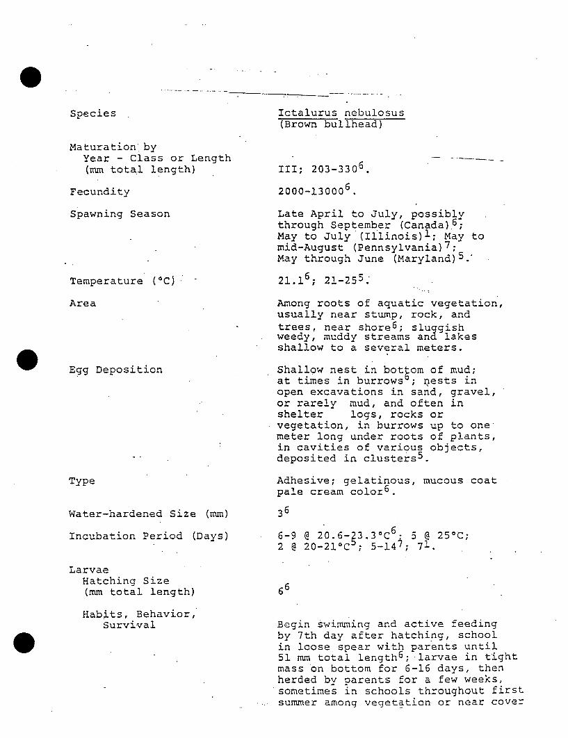
Species Ictalurus nebulosus(Brown bullhead)

Maturation byYear - Class or Length(mm total length) III; 203-3306

2000-130006.Fecundity

Spawning Season

Temperature ( 0 C)

Area

Egg Deposition

Late April to July, possiblythrough September (Canada) 6 ;May to July (Illinois)l; May tomid-August (Pennsylvania)7;May through June (Maryland) 5 .

21.16; 21-255.

Among roots of aquatic vegetation,usually near stump, rock, andtrees, near shore 6 ; sluggishweedy, muddy streams and lakesshallow to a several meters.

Shallow nest in botoam of mud;at times in burrowst; nests inopen excavations in sand, gravel,or rarely mud, and often inshelter logs, rocks orvegetation, in burrows up to onemeter long under roots of plants,in cavities of various objects,deposited in clusters 5 .

Adhesive; gelatinous, mucous coatpale cream color 6 .

36

6-9 @ 20.6-ý3.30C6 5 @ 25°C;2 @ 20-21*C ; 5-14i; 71.

66

Begin swimming and active feedingby 7th day after hatching, schoolin loose spear with parents until51 mm total length6 ; larvae in tightmass on bottom for 6-16 days, thenherded by parents for a few weeks,sometimes in schools throughout firstsummer among vegetation or near cover

Type

Water-hardened Size (mm)

Incubation Period (Days)

LarvaeHatching Size(mm total length)

Habits, Behavior,Survival

0Species Percopis omiscomaycus

(Trout-perch)

16; male 12; female I-I12

Maturation byYear - Class or Length(mm total.length)

Fecundity

Spawning Season

Temperature (*C)

Area

Type

240-728; averaging 3496

Late April to June6; late Aprilthrough May, possibly to September(Lake Erie) ; Lake May throughAugust (Minnesota) 6 ; late Aprilthrough June 2 ; late May to mid-June (Lake Erie) 2 .

16-202; 19-21.41.

Shallow rocky streamns, also sandand gravel bottom in 0-1.3 mshoreline water of lakes 6 ; shallowswift water over rocky.or gravelbottom1 .

Single 0.7 mm diameter; o'lglobule in fertalized eggadhesive demersal 2 .

1.36-1.85; 1.25-1.456.

8 days-at 201C1250 degree-daysabove 60c2.

6.04

Young feed mainly on ostracods,Gammarus, Leotodora, chironomids,or zooplanktonz.

Water-hardened Size (mm)

Incubation Period (Days)

Hatching Size (mm)

LarvaeHabits, Behavior,

Survival

Species Lota lota(Burbot)

Maturation byYear - Class or Lenath(mm total length)

Fecunaity

Spawning Season

Temperature (*C)

Area

i III-IV,. 280-480. ;'111, 1343-4192

• 45,600-13620076; 68498-ll531442;160,000-6700001.

Late December through March (Canada) 6 ;mid-January to March 2 ; lateSeptember through March, possiblythrough April 1 ,

0.6-1.76.

30-120 cm of water over sand orgravel in shallow bays or gravelshoals 1.5-3 m deep, usuallyin lakes but has been known tomove into rivers 6 ; deep holes instreams or "Bear" deep water 1 .

Spawn as a writing bal!,,61 cm indiameter of 10-12 interwined andconstantly moving individuals; nonest or parental care 6 ; eggs scatteredloose on bottom ; 250 eggs at a time 2 .

Semi-pelagic 6 ; non-adhesive1 .

Egg Deposition

Type

Water-hardened Size (mm)

Incubation Period (Days)

1.25-1.776; 1.71

30 @ 6.1*C; 3-4 weeksI.

Species Ambloplites rupestris(Rock bass)

Maturation byYear - Class or Length(mm total length) 11-V but typically 11-IlI3;

109-2676.

Fecundity

Spawning Season

Temperature (°C)

Area

3,000-11,0006; averaging over 5,0003.

Late March through July3 ; lateApril to July (Lake Erie) 4 ; 1late March to July (New York) ;May-June (Indiana) ; May toAugust (Pennsylvania) 7.

6 315.6-21.16; 20.5-26

Swamps to gravel shoals,very diverse 6 ; near vegetation inshallow water up to 62 cm deepl.

Male digs shallow nest up to 61 cmdiameter; female spawns intermittently•male guards eggs; nest producesaverage of 800 larvae6¾ nests ongravel, soil, marl, in swampy places,near rocks, sticks, etc. 1

.6Adhesive

Egg Deposition

Type

Incubation Period (Days)

LarvaeHabits, Behavior,

Survival

3-4 @ 20.5-21.0 0 C.

Male broods young for short time;young usually inhabit protectedareas onlyl.

Species Micropterus salmoides(Largemouth bass)

Maturation byYear - Class or Length(mm total length)

Fecundity

Spawning Season

Temperature ('C)

Area

II-V, occasionally less than 13

male: IV-V 6 ; female: III-IV6 .

2,000-109,314, average 7,000-94,1573.

Late March to August (Lake Erie)4.late March to July (New York)';mid-April to July (Illinois,Missouri, New Hampshire) 3 ; May (NewYork, Indiana) 1 , 3 ; mid-April toearly July (Wisconsin, Pennsyl-vania)jl,3i 7 . Earlý April throughmid-August (Okla.).. .

11.5- 29, 1,4.4-23.93; 17.81;

16.7-18.36.

In quiet bays among emergentvegetation, gravelly sand, marl, orsolt mud in reeds, bullrushes orwater lilies 6 ; in shallow water,usually less than 61 cm deep, overclean sand, gravel, roots or aquaticvegetation, sometimes on fallenleavesl, 3 ; usually near boulders, 3pilings or under sandstone ledges

Nest 61-92 cm diameter; 2-20 cmdeep, and 9 m apart; eggs laid overwhole bottom of nest, nest guardedby male, nests produced 751-11,457(averaging 5000-7000) larvae 6 ;will.not nest on silt bottoms 3 ; eggsattach to stones 4 ; eggs attach toroots and other objects in nests1 .

Adhesive 4 ; demersal, amber to paleyellow6 .

Egg Deposition

Type

Water-hardened Size (mm)

Incubation Period (Days)

1.5-1.7

3-56; 1.5-13.2, 1.5 @ 30'C, 2.9 @20-22.5'C; 4-43 @ 17.5%, 6.8 @ 15'C;13.2 @ 10-C 3 .

0-94%, averaging 80%, usually 92-100%3Survival

Micropterus salmoides (cont'd.)

LarvaeHatching Size(mm total length)

Habits, Behavior,Survival

36

Young remain on bottom of nest for6-7 days and rise and begin tofeed at 5.9-6.3 mm total length;brood may remain together for 31days and 15 guarded by male all orpart of the time 6 ; free-swimmingat 6.2 mm total length; remain innest two weeks then leave as acompact schooll, 4 ; survival from90 days to fall is 58-91% from47 days to fall is 19-100%3.

Species Micropterus dolomieui(Smallmouth bass)

Maturation byYear - Class or LentLh(mm total length) II-IV but usually III-IV3 ; male

II-IV6 ; female IV-VI.

5,000-14,0006; 2,000-20,825,averaging 5,040-13,8633.

Fecundity

Spawning Season

Temperature (0 C)

Area

Egg Deposition

Early May through July6 ; mid-Aprilto early June '(Ohio, Missouri) ;May to early July (Maryland, NewYork, Michigan) 3 ; late May throughJuly (Cayuga Lake) 3 ; late Aprilthrough July (Pennslyvaania, LakeErie) 47. -

16.1-18.36; 15.5-17.8; 11.7-21,usually 15-213.

Lakes and rivers; sandy, gravely orrocky bottom usually near rocks, logs,or more rarely dense vegetation 6 ;usually in shallow water near over-head cover, stumps, stones, steepbanks or at edges of pools, intributatries 1 , ,4,8; along lakeshores1 .

Nests, depressions, formed in cleangravel or sand with bedrock, wooddebris, or clam shells on bottom1 ,3,4, 8 "nest circular, 30-120 cm in diameter-eggs usually attach to stones at 6center of nest; nest guarded by male

Demersal, adhesive, light amber topale yellow6 .

1.2-2.56.

2.2-161,3,4; 2.2 @ 75'C, 9'8 @12.8 0 C, 7 @ 15.°C 3.2 @ 21.1-C3 ;4-106.

55.2 - 100%,average 94.1%3.

Type

Water-hardened Size (mu)

Incubation Period (Day!;)

Survival

LarvaeHatching Size 5.6-5.96.

Habits, Behavior,Survival

Micropterus dolomieui (cont'd.)

Young guarded for 2-10 days orup to 28 days after leaving nests 3 ;yolk absorbed 12 days after hatchingat which time they are 8.7-9.9mmtotal length and leave the nest,still guarded 6.

Species Lepomis macrochirus(Bluegill)

Maturation byYear - Class or Length(mm total length)

Fecundity

Spawning Season

Temperature (*C)

Area

I-II, rarelK 03; Ii; female III-IV 6 ;male I-111

7,208-38,184, 4,670-224,9006j 2,36G-81,104, means of 3,820-58,000 forfish 122-151 mm total length 3 .

Late April to mid-September:(Wisconsin) 3 ; June to mid-October(Michigan) 3 ; June to July (Indiana)l;mid-May through August (Pennsylvania) 7 ;late April through September(Illinois) 3 . EarlyM-ay through late

September (Okla.) 8 .

24.56; 22-26, 17-323.

Water less than 120 cm deep overvariety of substrates but finegravel or clean sand preferred,area usually exposed to sun 3 .

Nests in colonies over hardbottom of sand or mud-with littlevegetationl; nest is a shallowdepression 45-60 cm in diameter;guarded by male 6 .Adhesive, demersal, amber 6 ; very

heavy1 .

3.56; 13.3, 3 @ 22.6WC; 1.4 @ 26.9'C;1.3 @ 22.3WC; 2.1 @ 240C; 1.7 @23.5WC in light but 1.8 in dark 3 .

56% @ 22.6*C; 83% @ 26.9'C; 90% @27.3oC 3 ; survival higher wheredense vegetation is present 3 .

Egg Deposition

Type

Incubation Period (Days)

Survival

LarvaeHatching Size(mm total length) 2-36.

Habits, Behavior,Survival

Lepomis macrochirus

Mortality rate of larvae is veryhigh6 ; young free-swimming fourdays after hatching leave nests andremain in littoral zone until10-12 mm when they move to limeticzone; when 21-25 mm they returnto littoral zone 3 ; larvae found inboth limetic and littoral zones 7 .

0

Species Poxomis annularis(White crappie)

Maturation byYear - Class or Length(mm total length)

Spawning Season

Temperature (*C)

Area

Egg Deposition

Type

Water-hardened Size (mm)

Incubation Period (Days)

LarvaeHabits, Behavior,

Survival

1 .6II-IIll; II-IV; 152-203

Late April to mid-July (Ohio)l;"mid-May through July (Pennsylvania) 7 .mid-March to mid-Jtine (Okla.) 8

14-23, mostly 16-206.

Shallow water up to 1.7 metersdeep8 ; near or under overhangingledges1 .

Eggs adhere to plants .and rootletsl, 8 ;clean ill-defined nests, 300 mmdiameter with no depression overa variety of bottoms, nests isolatedor in colonies of 35-50, 61-122 cmapart, eggs adhere to substate,especially algae and each other 6 .

6Adhesive; demersal, colorless

0.896

2-2.2 @ 21.1-23.3OC3 ; 2-4.5,4 @ 14.4°C6 .

Larvae present in limnetic and nearshore waters of Conewingo Reservoir,PA (Darrel E. Snyder); tiny youngremain in nest for a very short time,sometimes only four daysb.

Species Pomoxis nigromaculatus(Black crappie)

Maturation byYear - Class or Length(mm total length) II-IV

6

Fecundity

Spawning Season

Temperature (M.)

Area

Egg Deposition

20.,000-140,0001; 26,700-65,570,averaging 37,7966/

Late April to early August (Indiana,South Dakota)l; late April throughJune 6 .

17.81; 19-206.

Shallow water, usually with bottomof fine sand or gravel 6 .

Male clears shallow depression orjust section of bottom of sand,gravel, or mud where there issome vegetation; nests, 20-40 cmdiameter, colonial, 1.6-1.9 mapart, male guards nesf 6 .

Type Adhesive, demersal, whitish,6transparent

Water-hardened Size (mm)

Incubat'ion Period (Days) 3-56

LarvaeHabits, Behavior,

Survival Male guards young in nest until afew days after hatching 6 .

Species Etheostoma nigrum(Johnny darter)

Spawning Season

Area

Egg Deposition

May to early July

Shallow water, usually small streams 1 .

Eggs deposited one by one onunderside of rocks, 30-200 eggs ateach of 5 or 6 spawning sessions,male guards-territory including nestand eggs (even if eggs or rock witheggs are removed) 6 ; eggs laid onunder surface of submerged objectsin single layer1 .

Adhesive 6 ; sphericall.>__

5-8 @ 22-240C

Type

Incubation Period (Days)

Species Perca flavescens(Yellow perch)

Maturation byYear - Class or Length(mm total length)

Fecundity

Spawning Season

Temperature (1C)

Area

Egg Deposition

Male: III6; Female: IV6 .

3,035-109,0006.

Mid-March to July. (Lake Erie)4;mid-April through May, possiblythrough July;6 mid-April throughMay (Lake Erie).ll

6.7-12.21; 8.9-12.26; 6.6-12.611

Usually over or neai aquaticvegetation or brush ; shallowsof lakes, tributary streams, 6sometimes over gravel or sand

Eggs extruded in uniqu- transparent,gelatinous, accordian-folded strandsas long as 2.1 m and as wide as 51to 102 mm weighing as much as akilogram and containing' 2,000 to90,000 eggs (average: 23,000), strandsundulate by water movement andadhere to bottom or submergedvegetation, eggs are easily cast 6ashore and lost, no parental care

Adhesive in gelatinous, porousstrands; transparent, semiiXýbuoyantl.

3.56

66

27 @ 8. 30C; 8-106

Larvae limnetic, late May to earlyJune (D.E. Snyder personal obser-vations based on Conowingo Reser-voir collections 1966-1971). InOneida Lake, N.Y., larvae pelagicsoon after hatching to 25.4 mm(May and June) and usually occupy

,upper 6 m of water column. 1 2

Type

Water-hardened Size (mm)

Incubation Period (Days)

LarvaeHatching Size(mm total length)

Habits, Behavior,Survival

0

Species

Spawning Season

Area

Egg Deposition

Water-hardened Size (mm)

Survival

Percina caprodes(Logperch)

Mid-March through May (Oklahoma) 8

Probably a short distance fromcreek mouth 4 ; sandy inshoreshallows 6 .

Female joined by male on bottomsubstrate to spawn their vibrationtends to bury the eggs; 10-20 eggsreleased with each spawning session;act repeated with other males 6 .

1.36

Embryos survive 22 days @ 260C 6 .

Larvae limnetic (D. E. Snyder)

LarvaeHabits, Behavior,

Survival

Species Stizostedion vitreum(Walleye)

Maturation byYear - Class or Length(mm total larvae)

Fecundity

Spawning Season

Temperature (OC)

Area

Female: III-VI, 356,432;Male: II-IV, , 2796;Male: II 1Female: III

50,000-3,000,000 1; 612,000 for an801 nmn specimen 6 ; 72,000-110,000per 3,178-3,405 g femalel 3 .

Mid-March to early July ; mid-Marchthrough April (Lake Erie) 4 ; mid-April to early July 6 ; April andMayll and 13; April (Lake Erie) 1 4

4.4-101; 5.6-11.16; 3.9-10.011.

Upstream spawning runs soon afterice breaks, prefers sandy bars inshallow water spawns in water 1-3 mdeep, usually on gravel or sand Wwith good water flOwl; rocky areasin white water below impassible fallsand dams in rivers, or boulder tocoarse gravel shoals of lakes. 6

Eggs spread over bottoml; eggsreleased in shallow water 6 . Broad-cast and fall into crevices in sub-strate. 14,17

Adhesive 16; non-adhesive afterwater hardening 6 .

1.5-26

12-186 (at temperatures prevalenton spawning grounds)

6-8.6 mm total length

Egg Deposition

Type

Water-hardened Size (mm)

Incubation Period (Days)

LarvaeHatching Size(mm total length)

Habits, Behavior,Survival Larvae begin feeding before yolk

is completely absorbed; yolkabsorbed rapidly; larvae disperseto upper levels of open water10-15 days after hatching6 . Pela-qic but become demersal near endof summer. 6

1. Breder and Rosen. 1966.

2. Carlander. 1969.

3. Carlander. Undated.

4. Pish. 1932.

5. Mansueti and Hardy. 1967.

6. Scott and Crossman. 1973.

7. Snyder. 1971.

8. Taber. 1969. -

9. Trautman. '1957.

10. Snyder. 1975. Personal communication.

11. Ohio Department of Natural Resources. Undated.

12. Noble. 1968.

13. Parsons. 1972.

14. Ohio Department of Natural Resources. 1971.

APPENDIX 3

MEAN AND STANDARD DEVIATION OF DATA ON EGGS AND YOUNG

FISH COLLECTED IN PINGP ENTRAINMENT STUDIES, 1975

APPENDIX 3 (Page 1 of 2)

MEAN AND STANDARD DEVIATION (S.D.) OF EGGS AND YOUNG FISHCOLLECTED IN PINGP ENTRAINMENT STUDIES, 1975

Bar RackRecirculation

CanalMean S.D.

Skimmer WallMean S.D.Date Mean S.D.

5/15-16/75

5/21-22/75

5/29-30/75

6/5-6/75

6/12-13/75

6/18-19/75

6/26-27/75

7/2-3/75

7/10-11/75

EggsYoungTotal

EggsYoungTotal

EggsYoungTotal

EggsYoungTotal

EggsYoungTotal

EggsYoungTotal

EggsYoungTotal

EggsYoungTotal

EggsYoungTotal

EggsYoungTotal

0.014.174.18

1.4371.6973.12

27.51100.89128.40

3.067.36

10.43

0.6112.5013.11

3.3414.2217.56

1.3260.4361.74

0.105.675.77

0.0512.5712.62

0.075.29

5.30

2.4770.1570.69

34.93134.54145.20

3.049.209.14

1.0534.3334.56

4.6419.2922.89

1.29117.51117.41

0.3914.0414.01

0.205.785.98

0.79141.73142.52

2.6130.3532.96

0.497.778.26

0.231.862.09

1.808.179.96

0.6715.5216.20

0.006.636.63

0.474.374.31

1.3070.5271.36

1.5114.8914.78

0.8510.0110.40

0.502.282.43

1.894.314.83

0.6116.1016.11

0.005.975.97

0.158.738.70

1.221.852.77

0.0412.4512.49

0.099.569.55

7/17-18/750.592.382.97

0.28 0.372.042.32

1.121.14

APPENDIX 3 (Page 2 of 2)

Bar Rack

Date Mean S.D.

RecirculationCanal

Mean S.D.Skimmer WallMean S.D.

7/24-25/75

7/31-8/1/75

8/7-8/75

8/14-15/75

8/21-22/75

EggsYoungTotal

EggsYoungTotal

EggsYoungTotal

.EggsYoungTotal

EggsYoungTotal

EggsYoungTotal

0.017.067.07

0.006.786.78

0.001.801.80

0.002.792.79

0.002.442.44

0.130.150.28

0.054.914.90

0.005.275.27

0.001.491.49

0.004.564.56

0.003.283.28

0.420.440.57

0.066.656.71

0.000.960.96

0.002.042.04

0.003.363.36

0.004.424.42

0.000.020.02

0.2111.0110.99

0.000.820.82

0.001.821.82

0.005.315.31

0.009.349.34

0.000.110.11

9/4-5/75

I

APPENDIX- 4

RESULTS OF CORRELATION ANALYSIS

OF FISH IMPINGEMENT, PLANT OPERATING

AND WATER TEMPERATURE DATA AT PINGP, 1975;

Results of correlation analysls of fish .Lp$ngawmnt. plant operatini a"d water tampe.artuae data at Prairie Ialand Plant during 1975.

blkbtll chanoat whtbae. crappie frhwdra rwit: rutrat sow date.

Wlnter

r.it a--0.09 r - 0.79 r - 0.22 r - 0.52 r- 0.44p- 0.77 p- 0.003 p - 0.51 p - 0.08 p 0.15

N.B. #& N.S. N.S. M.S.

rcwtrt r - 0.37 r - 0.02 r - 0.29 r - -0.03 • - 0.06p - 0.24 p - 0.95 p - 0.64 p - 0.43 p - 0.65

H.S. H.S. U.S. U.S. M.S,

ACV K- 0.44 r - 0.10 r - 0.33 a- 0.22 r - 0.05p - 0.15 p- 0.76 p - 0.30 p- 0.50 p - 0.91

H.S. U.S. M.G. H.a. N.M.

ma w - -0.11 • - 0.16 • - 0.15 • - 0.25 r - 0.93p - 0.73 p - 0.62 p - 0.64 p - 0.56 p - <0.01

M.A .S U.S M.S of

. -o-.22p - 0.51

N.B.

r - -0.28 r- 0.42 r - 0.65p- 0.63 p- 0.17 p - 0.02

N.M. aM.. A

r - 0.70 1 - 0.00 r - -0.20- p - 0.01 p - 0.99 p - 0.53

N.M.S. W.B.

.... a - 0 .00 - -0 .3 9..... p - 0.99 p - 0.20.... 1.M. N .M.

r- 0.73...... p- 0.01

3/20-6119

rwit: r - -0.28 r - -0.24 - -0.04 r - -0.01 •- -0.10p - 0.65 p - 0.57 p- 0.90 p - 0.96 p- 0.74

M.M. N.M. S.M. M.a. M.B.

r - -0.21 r - -0.28 a - 0.22p - 0.51 p - 0.65 p - 0.52U.S. U.S. M.S.

- 0.91p - <0.01

rcwtrt a - -0.25 r - 0.26 v - 0.18 a - 0.25 a - 0.47p - 0.50 p - 0.61 p - 0.56 p - 0.58 p- 0.11

N.S. H.M. N.M. H.S. M.G.

acy • - -0.61 r - -0.17 r - -0.16 • - -0.10 • - 0.36p - 0.02 p - 0.58 p - 0.60 p - 0.74 p - 0.23

H N.S. N.M. U.S. N.M.

a- 0.49 - 0.33 r - -0.37p- 0.08 p- 0.33 p - 0.21

U.S. U.S. N.M.

a - 0.54 r - -0.41p - 0.09 p - 0.10

N.8. U.M.

Kwa a - 0.47 r - -0.3Sp - 0.14 p - 0.30

N.S. H.S.

a - 0.43 x - 0.67 a - 0.63p - 0.18 p - 0.02 p - 0.04

H.S. & 6

a - 0.04p- 0.90

N.M.

blkbull. chancat vhtbccc crappie r~ttcvdtrcwtrt acw date

Sumer6/20-9/IB

3v1 t r - 0.07 r -- 0.22 r - 0.28 r - -0.05 r - -0.30p - 0.81 p - 0.53 p - 0.65 p- 0.87' p- 0.33

U.S. W.S. N.B. U.S. U.S.

--- - 0.19 • 0. 3 •- 0.55 •--0.78p" 0.53 p 0.19 p. 0.06 p - <

0.

0 1

U.S. U.S. U.S. t.

-- --- - 0.63 r- 0.80 r - 0.07-. - p. 0.02 p - (0.01 p - 0.82

*a U.S.

rcwtrt v - -0.16 r , -0.22 r - 0.39 r - 0.41 r - 0.10p - 0.60 p - 0.53 p - 0.18 p - 0.16 p - 0.75

U.S. U.S. U.S. U.S. M.S.

acv r - 0.17 r - 0.16 r - 0.31 r - 0.51 r- 0.36p - 0.59 p. 0.62 p.- 0.30 p - 0.07 p - 0.22

U.S. M.S. U.S. U.S. U.S.

r - 0.09 r - -0.35 v - 0.51 r - 0.37 r - -0.11p - 0.76 p .- 0.24 p - 0.07 p - 0.21 p - 0.73

M.S. U.S. M.S. M.S. U.G.

r - 0.46 r - 0.51p - 0.11 p - 0.07

U.S. U.S.

-- 0.38p - 0.20

U.S.

rall9/19--12/31

xvi I .- 0.27p.- 0.65

U.S.

r 0 0.57 r - -0.09 r.- 0.79p .- 0.03 p - 0.75 p - <0.01

4 U.S. S.

r - 0.64p - 0.02

" - -0.88p - <0.01

66

- 0.55 r - 0.67 r - -0.94p - 0.04 p - <0.01 p - <0.01

o 66

rowtrt r - -0.41 - -0.17 r - 0.22 r - -0. 60 r - -0.67p - 0.14 p - 0.19 p - 0.55 p - 0.02 p - <0.

0 1

M.S. M.S. U.8. S a&

-r - -0.40-- • p - 0.16

U.S.

r - -0.59 r - 0.86p - 0.03 p - <0.01

acc r - 0.40p - O.1S

U.Sa.

wwsa r - 0.26p - 0.62

H.a.

v - 0.20p - 0.50

r - 0.79p < <0..01

06

v - 0.16p '- 0.60

M.S.

•- -0.04p.- 0.89

M.S.

K 0.45p.- 0.10

• - 0.89p - <0.01

a*

v - 0.39p.- 0.11

r 0.60p - '0.01

r - 0.23p - 0.56

U.B.

r - -0.64p - 0.02

- -0.56p - 0.04

1.

AllSeasoamCogabined

rwit

blkbull chanoat whtbaes crappie frh•n"m

g--0.07 e 0.10 e 0.37 T - 0.53 r - 0.08p.- 0.61 p- 0.50 p- 0.Ol p - <0.01 p - 0.56

U.S. US. a t U.S.

EAt rcwtrt. acV date

r--0.70 x - -0.07 r - 0.63 V - 0.28p-<0.01 p - 0.60 p- <0.01 p - 0.04

U.S.

- -0.04 r- -0.35 •- -0.07p - 0.77 p - 0.02 p - 0.61

M.S. * U.S.

rcwtrt r - 0.01 r - -0.16 r - -0.23 r - -0.44p - 0.95 p - 0.26 p - 0.10 p. <

0.

0 1

U.S. H.S. U.S. so

•e -0.30p - 0.03

acw r - -0.41 r - 0.18 r - 0.19 • - 0.22 r - 0.29p - <0.01 p - 0.20 p- 0.18 p - 0.11 p - 0.04

66 U.S. 11.8. M.8. *

WWII w 0.32 r -- 0.31 •- 0.41 r- 0.57 r . -0.08p - 0.02 p - 0.62 p - <0.

0 1 p- <0.01 p - 0.59

& H.S. t a*U M.S.

r - 0.20 rg 0.03p - 0.16 p., 0.83

U.S. U.S.

--- 0.08-- p.- 0.57

--- " 1 .8.

blkbull - black bullheadchancat - channel catfishwhtbasa - white base

orappLe - crappie opp.frhwdru - frebhwater drumrwit - river water Inlet temperature

rcwgrt - xeCyol.-oanal vater temperaturemcc - average circulatling watermwe -- makeup-water appropriation

U.S. - not significent0 - eigntfloant at 0.05 level*a - significant at 0.01 levelr . oorrelatlion coefficientp - level of significance

4.

j~~1

IL C-'- r & WEBE, R ENGINEERING CORPORATIONP. 0. BOX 5456, DENVER. COLORADO 80217

DATE 4/1/83

ILTR. NO. S-N-REF. T2.2VIA.

fMrf. L.A.. Winter

Project Manager

TO Northern States Power CompanyPrairie Island Nuclear Generating PlantRoute 2Welch, Minnesota 55089.

DEAR SIRS:

THE FOLLOWING ARE ATTACHED: 0 SENT SEPARATELY:

MICROFILMCOPIES - PRINTS - REPRODUCIBLES.-- APERTURE CARDS

EACH OF

n DRAWINGS 0 SPeCIFICATIONS

E DOCUMENTS 0 NOTES OP CONFERENCEL- -J

STATUS PLEASE NOTE SENT FOR YOURFINAL A APPROVED 0 REVISIONS 0 OMISSIONS 0 APPROVAL 0 COMMENT

0 PRELIMINARY 0 APPROVED AS REVISED AISD 0DEFINED ADDITIONS C IONS 1 USE 1 INFORMATIONIN SPECIFICATION CORECTON US C

.0 SUGGESTIONS AS NOTED 1 .

YOUR ATTENTION IS DIRECTED TO THE FOLLOWING:

RELEASED FOR: 0 FABRICATION [ PURCHASE OF NECESSARY MATERIALS

0 PLEASE REVISE AND SUBMIT - PRINTS REPRODUCIBLS - MICROFILM APERTURE CARDS.

03 PLEASE SUBMIT- PRINTS -- APRODUCIBLES " MICROFILM APERTURE CARDS OP 0 DOCUMENTS Q DRAWINGS E- SHOP DETAIL

O PLEASE RETURN ONE COPY EACH OF THIS MATERIAL BEARING YOUR APPROVAL OR COMMENTS.

0 PLEASE ACKNOWLEDGE RECEIPT OF THIS MATERIAL BY SIGNING AND RETURNING THE ENCLOSED COPY OF THIS FORM.

OWE TRUST THAT THESE NOTES ARE IN ACCORDANCE WITH YOUR UNDERSTANDING: IF NOT. PLEASE ADVISE US.

SHOULD ANY REVISION TO DOCUMENTS OR DRAWiNGS'•RET6RNE0 HEREWITH INVOLVE A PRICE INCREASE. THE SUPPLIER MUST NOTIFY STONE tiIMPORTANT WEBSTER PURCHASING DEPARTMENT WITHIN TEN 101 DAYS EVEN THOUGH A DEFINITE ESTIMATE CANNOT BE GIVEN AT THE TIME. OTHERWISE. THI.

PURCHASER WILL CONSIDER THE REVISIONS MADE WITHOUTCOST.

F/SAL SYSTEM DESCRIPTIONMODIFY CIRCnLATING WATER

- INTAKE AND DISCHARGEPRAIRIE ISLAND NUCLEAR GENERATING PLANT

Transmitted herewith for your use and files are six (6) copies ofversion of the project system description.

the final

If you have any questions please call me.

Project Engineer

Copy to:D.R. Brown1/4

CLM: CMS

VXX<FilIe copy

PI Lab

i.i .. / "'I

I)-i-ffi-

SWEC J.O. No. 12911.09 March 1983NSP J.O. No. E-78Y073

MODIFY CIRCULATING WATERINTAKE AND DISCHARGE

SYSTEM DESCRIPTIONAND

DESIGN CRITERIA

PRAIRIE ISLAND NUCLEAR GENERATING PLANT

a0648B

CONTEN"TS

1.0 Summary

1.1 Design Criteria

1.1.1 General

1.1.2 Hydraulic

1.1.3 Environmental

1.1.4 Geotechnical

1.1.5 Structural

1.1.6 Electrical

1.1.7 Mechanical

2.0 System Description

2.1 Hydraulic

2.2 Environmental

2.3 Geotechnical

2.4 Structural

2.5 Electrical

2.6 Mechanical

2.7 Quality Assurance

2.8 Codes & Standards

3.0 System Operation

3.1 System Arrangement

3.2 Description of Intake and Discharge Flows

3.3 Two Unit Winter Startup

4.0 System Limitations & Setpoints

00648B

5.0 Safety Features

6.0 System Maintenance

6.1 Maintenance Approach

6.2 Preventive Maintenance

6.3 Testing and Surveillance

6.4 Inservice Inspection

Appendix A - Electrical Design Criteria

Al Electrical conduit notes STD-ME-1-3-5

A2 Electrical conduit, tray and lighting notes STD-ME-l-l-4

A3 Electrical grounding notes STD-ME-2-1-6

A4 Electrical grounding notes STD-ME-2-2-7

A5 Induction motor data sheet-sample,

Appendix B - Logic Description

B1.0 Logic System Design

B1.1 System Arrangement

B1.2 Control and Instrumentation

B1.3 Annunciators

B1.4 Indicators

B1.5 Instrumentation I/O for screenhouse programmable controller

0648B

Page I of 29. 1.0 SUMMlARY

The intake and discharge modifications are required to reduce theimpact of the Prairie Island Nuclear Generating Plant on aquaticorganisms in the Mississippi River.

The .i nt.ake moId ifica t Iions . prevent fis.h, larvae. .and eggs, from enteringthe plant cooling water intake canal by removing, and. trsporting ,themdownstream, where. they are returned, to the river at a location which isoutside'. of the inifluence of intake f low.

The discharge modifications provide a submerged jet discharge topromote rapid mixing, exclude fish from the system, minimize fish coldshock potential and prevent recirculation of warm water back to theintake (outside the system). By removing this heat source, thepotential for attracting fish to the area of the intake screenhouse isminimized.

The reduced intake temperatures also result in greater plantefficiency. Increased water appropriation and changes in operatingmodes prevent excessive circulating water temperature variations to theoperating plant.

1.1 DESIGN CRITERIA

1..1 General

The modifications to the intake and discharge systems are designed toexclude aquatic organisms from the circulating water system andeliminate cold shock to fish. This has been accomplished withconstruction of an intake screenhouse with traveling water screens,ý.afish. return system, a deicing pumphouse, an environmental monitoringlaboratory, a screen storage building, and a discharge structure withsubmerged jet discharge for rapid thermal mixing.

The intake screenhouse is located on the north side of the intakechannel. The structure contains equipment to remove aquatic organismsand debris from the intake flow. Traveling water screens are equippedwith fish lift buckets. Bypass gates have been provided to maintain acontinuous flow in the event that flow through the screens is reducedbecause of extraordinary clogging. A deicing system is available todistribute warm water across the inside face of the structure toprevent formation of ice on the exposed surfaces. Aquatic organisms,washed off the traveling water.. screens, are collected in a trough whichfeeds into the fish return line for return to the river.

0648B

Page 2 of 29

The discharge structure is located approximately 500 ft. downstream ofBarney's. Point, 2150 ft. downstream of the former discharge, andprovides a submerged jet discharge at an angle of 45 degrees to themain channel flow of the Mississippi River. Dikes convey dischargeflow from the distribution basin to the discharge structure through anextension of the discharge canal. 'The former dike, downstream of theformer discharge has been removed.

A flood and drain gate has been installed in the west dike to provideflooding and draining capability for an area, west of the dike, to beused by the Minnesota Department of Natural Resources as a water fowlsanctuary.

The design. bases, system ..idesigný and .operating considerations -.of the'circulating water system are given in Section 10.2.9 of the 'PrairieI sland Final Safety Analysis Report (subsequently referred to as the..SAR)

1.1.2 Hydraulic

1.1.2.1 Water Levels - Mississippi River *

Maximum Operating Water Level. (Pool 3) EL. 678.0 ft.

Normal Operating Water Level (Pool 3) EL. 673.5 ft.

Extreme Low Water Level (Pool 3) EL. 672.5 ft.

Flat Pool (Pool 3) EL. 674.5 ft.

10 yr. flood EL. 682.5 ft.

100 yr. flood EL. 687.4 ft.

150 yr. flood EL. 688.1 ft.

*M.S.L. 1929 adjustment

The 150 year flood level was used as a basis for determining deckelevations such that motors and electrical equipment will not beinundated.

1.1.2.2 Velocities and Flow Rates

In accordance with permit requirements, the average face velocitythrough the gross area of the 0.5 millimeter mesh screen materialshould not exceed 0.5 fps based on low water level and corresponding toa discharge flow rate of 800 cfs.

0648B

*

Page 3 of 29

The average face velocity through the gross area of the 3/8 inch screenmaterial should not exceed 0.88 fps corresponding to a maximum intakeflow rate of 1410 cfs.

For exclusion of fish from the discharge system and for rapid thermalmixing, velocity in the discharge pipes is a minimum of 8 fps and amaximum'of 10 fps. Minimum pipe length is 80 ft.

The combination of the 8 ,fps velocity and the 80 ft. pipe length formsa barrier through which the local fish cannot swim. A maximum velocityof 10 fps was established in order to limit head loss across t'fiestructure to a maximum of 3 ft.

The velocity limit at the edge of the navigation channel is 4 ft/sec.for barge traffic. This is the maximum limit of the average velocitycomponent normal to river flow.

1.1.2.3 Deicing

Warm deicing water is provided during cold weather to prevent theformation of ice on trash racks, traveling water screens and bypassgates. Warm water is pumped from the discharge channel, immediatelydownstream of the distribution basin. Minimum water temperature at theintake after deicing is 32.5'F. For design purposes, the given plantdischarge water temperatures are 571F for one unit operation and 820Ffor two unit operation. Two unit operation normally entails partialrecirculation. One unit operation will be open cycle with norecirculation.

1.1.3 Environmental

1. 1. 3. 1 Traveling Water Screens

Traveling water screens are of the through flow type of sufficient areato screen the desired intake flow. The screens are equipped withbuckets to transport aquatic organisms to the return system.

1.1.3.2 Mesh Size

During the period April 16 to August 31, the screen mesh size is 0.5 mmor as fine as practicable. During the remainder of the year, a screenmesh size of up to 3/8' inch may be used. Screen panels are replaceableand interchangeable.

1.1.3.3 Screen Speeds

ýThe traveling speeds of the screens have been designed to resistclogging. and to minimize the impact on aquatic organisms. The drivesprovide flexibility to vary speeds,. as required, during various periodsof the year.

0648B

Page 4 of 29

:i1..3.4 Fish Return System

Aquatic organisms impinged on the traveling water screens and in theattached buckets are lifted to the level of the fish sprays and washedoff within 4 minutes into a fish collection trough. Removal of thefish and organisms is accomplished on the ýiupward: travel side withý a.lowpressure .(0. psi insi i:spray when fine mesh is used' and with a low

pressure (20 psi) outside spray when coarse mesh screen is used.Debris is removed by a backside interior high pressure (50 psi for finemesh and 100 psi for coarse mesh) spray system. The pump supplying the50 psi fine mesh spray can be run at a higher speed to provide a 125psi spray to supplement the 100 psi coarse mesh spray during periods ofhigh trash loads. Separate f ishand debris troughs combine to form a.pipeline which transports the effluent to a point .;near the downstream.end. of:.th~e existing discharge, channel.ý

Diverting tr~oughs or ýtaps have. been provided for sampling capability .atthe. intake. screenhouse and near the discharge. Debris can" be collectedin a. trash: basket: during sampling periods and during:. high river flowperiods.

The fish return, line has ýbeen designed. for velocities between 3 and 5fps with higher velocities (less than 10 fps) being encountered for ashort duration to dissipate energy prior to discharge to the river.Ail"l ý.internal surfaces are . .smooth, to preclude abrasion. damage.Organisms. are discharged., from:. the pipeline below the mean low waterelevation at a depth (below Elev. 670) which ensures submergence below.the ice cover.

1.1.3.5 Thermal Limitations

Effective on the date the discharge structure becomes operational andlasting until June 30, 1985, the following thermal limitations, as setforth in the final NPDES Permit #MN0004006, shallbe in effect:

* From April 1 through November 30, the temperature of the receivingwater, as measured immediately below Lock and Dam No. 3, shall notbe raised by more than 5VF above natural, based on the monthlyaverages of the maximum daily temperatures, except in no case shallit exceed a daily average temperature of 86 0 F.

* From December 1 through March 31, the mixed river temperatureimmediately below Lock and Dam No. 3 shall not be raised above 430Ffor an extended period of time. Should the mixed river temperatureequals or exceeds 430F for two consecutive days the Director andthe Minnesota Department of Natural Resources shall be notified.

00680648B

Page 5 of 29

1.1.4 Geotechnical

1.1.4.1 Design

The design criteria are based upon information contained in the PrairieIsland FSAR Volume 5 supplemented by "Report on Test Borings", datedJune 13, 1980 by Stone and Webster Engineering Corporation(Subsequently referred to as SWEC) and by Geotechnical calculations

1.A.4.2 Allowable Bearing Capacity

Allowable bearing pressure for structures founded on the sandy soils atPrairie Island vary with the size and shape of footing and the depth ofembedment. Net maximum bearing capacity for the de-icing pumphouse is-4000 psf. Net maximum bearing capacity for the discharge structure was25C0 psf allowing for a settlement of less than 1.5 in., 3000 psf forless than 1.8 in. The screenhouse was designed for a net bearingcapacity of 8000 psf.

1.1.4.3 Soil Properties

Intake Screenhouse and Pumphouse Areas

In situ soil above El. 640 TSAT = 126 pcf, TMoist = 116 pcf, 0=330In situ soil below El. 640 ISAT = 133 pcf, 0 = 350

Discharge Structure

Sand fill above El. 671 ISAT = 127 pcf, TMoist = 119 pcf, =3

Clay El. 671 -665 ISAT = 113 pcf, for C = 0 psf. 0 = 27 *before Ist stage dike Construction for 0 = 00, C = 400 psfafter 1st stage dike Construction for 0 = 0', C =.750 psf

Sand below El. 671 TSAT= 124 pcf

Other soil properties were determined by the Lead GeotechnicalEngineer, as required, from the above soils information and boring logs.

1.1.4.4 Permeability

Permeabilities determined from a well pump test as referenced in Volume5, Section 3.14 of the Prairie Island FSAR range from 0.093 - 0.37 feetper minute.

1.1.4.5 Earth Pressure Coefficients

Active and passive earth pressures are a function of wall deformation.The relationships between the active and passive earth pressurecoefficients, Ka and Kp, versus wall deformation are presented inFigure 1, page 28. It is important to note that these relationshipswere developed for the conditions of insitu soils, vertical wall,nonsloping backfill, and no wall friction. The Lead GeotechnicalEngineer established values for Ka and Kp for conditions differing fromthose assumed above on an individual basis.,

0648B

Page 6 of 29

1.1.4.6 Emergency Cooling Water Intake Piping

No sheetpile was driven within a 20 foot radius of the emergencycooling water pipe.

1

1.1.4.7 Cut Slopes

Side slopes of the intake and discharge canals and dikes are onevertical to three horizontal except as noted on the drawings. Theslope of the approach canal to the intake screenhouse are one verticalto five horizontal. On the exit side of the screenhouse the channelslope is one vertical to four horizontal.

1.1.4.8 Intake Canal Cutoff

The intake canal cutoff was designed for overtopping as well as adifferential head of 5 ft.

1.1.4.9 Erosion Protection

The discharge dike overflow section and the intake cutoff dike has beenprotected with rockfill to prevent erosion when overtopped.

The discharge structure, approach and discharge basin has been protectedby riprap with an average diameter of 1Z inches.

Riprap has also been provided immediately upstream and downstream ofthe intake scrjenhouse on the north bank of the intake canal.

Discharge dike slopes were covered with topsoil and'seeded as shown ondrawings.

1.1.5 Structural

The purpose of these criteria is to provide the structural informationused to design the intake screenhouse, discharge structure, andde-icing pumphouse. In general, the structural design criteria and thecomponent design criteria from Appendix B, Section B.6 and B.7,respectively, of the FSAR for the Prairie Island Nuclear GeneratingPlant were used.

The intake screenhouse, discharge structure and de-icing pump house andcomponents were designed as QA Type III structures.

1.1.5.1 Codes

As a minimum, structures were designed in accordance with theapplicable codes as listed.

A. American Concrete Institute Codes; ACI 318-77, ACI 301-(R75), andother sections of the ACI Codes as applicable.

6648B

Page 7 of 29

B. American Institute of Steel Construction "Specification for theDesign, Fabrication and Erection of Structural Steel Buildings,"1980 Edition.

C. International Conference of Building Officials "Uniform BuildingCode," 1979 Edition.

D. Current versions of applicable codes except for piping and valves

are listed in paragraph B.3 Appendix B of the FSAR.

E. Project Analysis report.

1.1.5.2 Loads

All structures and components were designed to withstand various kinds-and combinations of loads.

The different kinds of loads treated in the design are described in thesubsequent paragraphs.

A. Environmental Loads

These consist of snow and wind loads:

Snow load (SL) of 50 lbs. per sq. ft. of horizontal projectedarea was used in the design of structures and componentsexposed to snow.

Normal wind loads (WL) applied to the structure were asdescribed herein. Wind loads are based on ANSI StandardA58.1-1972 which formalizes the recommendations of theAmerican Society of Civil Engineer's paper ASCE 3269 "WindForces on Structures." A 100 mph design wind speed was usedper the FSAR.

B. Live Loads (LL) consist of loadings not permanently on thestructure. The following live loads were used.

The screenhouse deck was designed for a live load of not lessthan 250 psf or an HIO truck loading plus 10 percent impact,whichever governs.

The decks of the discharge structure and de-icing pumphouse weredesigned for a live load of at least 100 psf. The storagebuilding floor slab and the floor of the environmental lab weredesigned for a live load of not less than 200 psf. The floor ofthe office in the environmental lab was designed for a live loadof not less than 80 psf.

0648B

Page 8 of 29

C. Dead Loads

Dead loads consist of the weight of structural steel, concrete,and equipment. The weight of the equipment was as specified onthe manufacturer's drawings. Soil loads were considered to be a.Dead Load.

D. Load Allowances

Load allowances are provided to account for concentrations ofminor unknown loads from pipe hangers, cable supports, lightingfixtures, etc. Steel beams and girders were 'designed to supportthe following concentrated loads applied to the midspan of themembers:

Roof Beams or Joists 3.0 KipsRoof Girders 6.0 KipsAll Other Beams 5.,0 KipsAll Other Girders. 8.0 Kips

Reactions of beam load allowances were not accumulated intogirders and only girder load allowances. were carried to thecolumns.

E. Seismic Loads

The seismic loads used were in accordance with the requirementsof the Uniform Building Code. This code specifies the locationof the plant site to be in "Zero" earthquake area. However, forconservatism earthquake loads applicable to Zone 1 areas wereused in the design.

1.1.5.3 Load Combinations

The following combinations of loads were used to design the structures:

A. Normal Operating: Dead and Live loads together with

Environmental loads (wind and snow, separately).

DL + LLDL + LL 4- WLDL + LL + SL

B. Other: Dead and Live loads together with Uniform Building CodeEarthquake.

DL + LL + UBC Zone 1 Earthquake.

1.1.5.4 Stress Design Criteria

Concrete allowable stresses were from ACI 318-77 with no increase instresses for earthquake, wind, or snow conditions. Structural steelallowable stresses were from AISC-1980 with no increase in stressesfor earthquake, wind or snow conditions.

0648B

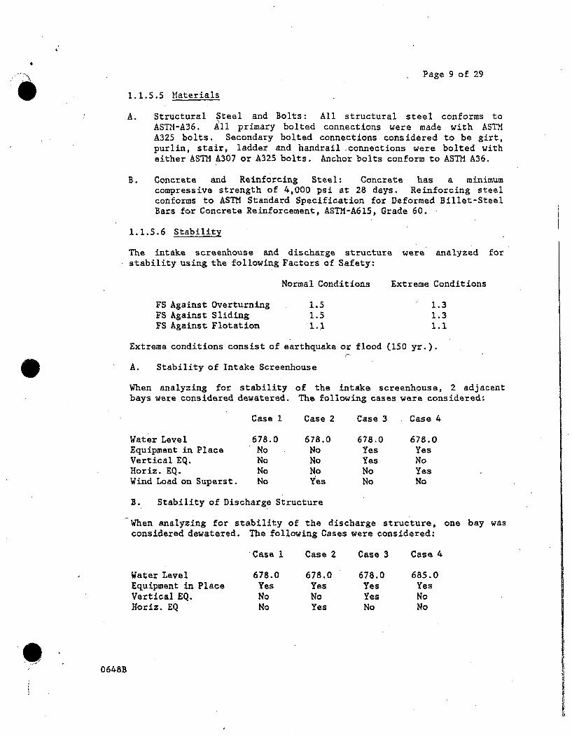
Page 9 of 29

1.1.5.5 Materials

A. Structural Steel and Bolts: All structural steel conforms toASTMI-A36. ll primary bolted connections were made with ASTMA325 bolts. Secondary bolted connections considered to be girt,purlin, stair, ladder and handrail -connections were bolted witheither ASTM A307 or A325 bolts. Anchor bolts conform to ASTM A36.

B. Concrete and Reinforcing Steel: Concrete has a minimumcompressive strength of 4,000 psi at 28 days. Reinforcing steelconforms to ASTM Standard Specification for Deformed Billet-SteelBars for Concrete Reinforcement, ASTM-A615, Grade 60.

1.1.5.6 Stability

The intake screenhouse and discharge structure were analyzed forstability using the following Factors of Safety:

Normal Conditions Extreme Conditions

FS Against Overturning 1.5 1.3FS Against Sliding 1.5 1.3FS Against Flotation 1.1 1.1

Extreme conditions consist of earthquake or flood (150 yr.).

A. Stability of Intake Screenhouse

When analyzing for stability of the intake screenhouse, 2 adjacentbays were considered dewatered. The following cases were considered:

Case 1 Case 2 Case 3 Case 4

Water Level 678.0 678.0 678.0 678.0Equipment in Place No No Yes YesVertical EQ. No No Yes NoHoriz. EQ. No No No YesWind Load on Superst. No Yes No No

B. Stability of Discharge Structure

When analyzing for stability of the discharge structure, one bay wasconsidered dewatered. The following Cases were considered:

Case 1 Case Z Case 3 Case 4

Water Level 678.0 678.0 678.0 685.0Equipment in Place Yes Yes Yes YesVertical EQ. No No Yes NoHoriz. EQ No Yes No No

0648B

Page 10 of 29

1.1.6 Electrical

The purpose of these criteria is to provide the electrical basesrequired to support the intake and discharge modifications to thePrairie Island Nuclear Generating Plant. The electrical design w~sbased on a combination of design criteria from the Prairie IslandFSAR, Prairie Island Project Design Manual and on SWEC designstandards.

1.1.6.1 NSP Furnished Criteria

A. General Electrical Design Bases

Design bases for the plant electrical systems are given inSection 8.1 of the FSAR.

B. 480-volt Auxiliary System

480-volt system design is given in Section 8.3.6 of the FSAR.

C. 120 VAC Instrument Bus System

120 VAC Instrument Bus System design is given in Section 8.3.8 ofthe FSAR.

D. Circulating water system

The design bases, system design and operation considerations forthe circulating water system are given in Section 10.2.9 of theFSAR.

E. General Instrumentation and control

The design bases for instrumentation and control are given inSection 7 of the FSAR.

F. Main Control Board

The design and layout of the Main Control Board is given inSection 7.7.3 of the FSAR.

G. Raceway

Raceway conforms to Section 4, Index 324.52 and 324.53 of thePrairie Island Project Design Manual. This section includes, butis not limited to, the design criteria, material requirements,separation criteria, cable spacing and tie down requirements intrays, normal voltage restrictions for cables entering thecontrol room and grounding requirements used for the originalraceway design. Raceway coding and identification conform toSection 4 Index 3.24.54 of the Prairie Island project DesignManual. NSP has assigned identification numbers to raceway. NSPprovided routing for cable in the turbine building cable traysystem as required.

0648B

Page 11 of 29

H. Wire and Cable

Cable derating, routing, fire protection, separation, tray andother considerations are given in Section 8.3.11 of the FSAR.Electrical wire and cable was used from the Northern States PowerCompany's existing plant surplus when possible. Wire and cablecoding and identification conforms to Section 4, Index 324.54 ofthe Prairie Island Project Design Manual. NSP has assignedidentification numbers to wire and cable.

I. Classifications

Design classifications and QA classifications are consistent withthose used for the original plant. These definitions areprovided in Appendix C of the FSAR.

J. Fire Stops

NSP provided up to date cable seal and fire stop requirements forinsertion into the installation specification.

1.1.6.2 SWEC Modified Criteria

A. Raceway

Conduit is rigid steel or electrical metallic tubing. Conduit sizeand fill are based on National Electric Code recommendations (1981revision). Conduit is in accordance with SWEC standard designdrawings STD-ME-l-1-4 and *1-3-5 (copies provided in Appendix A),unless otherwise specified in the drawings. The existing cable traysystem was used when possible.

B. Wire and Cable

Wire and cable were specified and purchased as QA Type III and met theintent of IEEE 383-1974. All power cable was provided with an overallinterlocked aluminum or galvanized steel armor. All new cable hadcopper conductors. Power cable was selected and sized in accordancewith IEEE S-135, IPCEA P-46-426 power cable ampacity tables.

C. Grounding

Grounding is in accordance with SWEC standard design drawingsSTD-ME-2-1-6 and 2-2-7 (copies provided in Appendix A) unlessotherwise specified.

0648B

Page 12 of 29

D. Motors

All motors were provided with the driven equipment. Induction motordata sheets SWEC form SM-34-9, 74 (copy provided in Appendix A), wereprepared for all motors.

E. Instrumentation and Control

Instrumentation and control requirements and operation for thespecific system are given in logic descriptions in Appendix B.Instrument data sheets were completed for all instruments.

F. Power Sources

All electrical power sources required to support the modification wereselected on the basis of the following:

1. QA Classification2. Maintaining equipment required to support other equipment on

the same bus as the supported equipment3. Maintaining redundant or backup equipment on different buses

where possible.4. Not exceeding the capacity of any power source5. Load balancing between buses when possible.

G. Modification to Turbine Building Equipment

All modifications to the turbine building cable tray system or maincontrol board were accomplished without impairing the originalintegrity or violating the original design classification of themodified equipment. All modifications to said equipment were approvedby NSP prior to modification. Cable tray systems and main controlboard were visually inspected prior to preparation of the modificationdrawings to verify the accuracy of the existing drawings.

H. Additional Electrical, Instrumentation, and Control Equipment

All modifications to the main control board used equipment that wasconsistent with that presently in use at Prairie Island and wasapproved by NSP.

1.1.7 Mechanical

Heating, ventilating and fire protection equipment was provided asagreed upon by SWEC and by NSP. Ambient design air temperatures atthe plant will be -14* F in the winter and 89* F in the summer.

0648B

\ Page 13 of 29

W 2.0 SYSTEM DESCRIPTION

2.1 HYDRAULIC

2.1.1 Intake Screenhouse Equipment

Plant intake flow from the Mississippi River enters the intakescreenhouse through eight 18.5 ft. by 11.2 ft. bay openings. Thebottom of the inlet skimmer wall is at Elev. 667.0. Each bay isequipped with a raked trash rack and a traveling water screen with lowpressure fish wash sprays and high pressure trash wash sprays.

The intake screenhouse also contains the following:

a. High and low pressure screenwash pumps and piping.

b. Traveling rake to clean trash racks.

S gates which.will. enable dewatering of 2 screen bays.

d. Bypass gates which will automatically open when the headloss across the traveling water screens exceeds 18 in.This could occur when trash loading is so high thatclogging of the screens results.

e. Screenwash system pipeline strainers.

f. Overhead traveling crane to service all equipment withinthe structure and to handle screen storage racks.

g. Air compressors for service air and instrument air.

h. Fish and trash troughs to collect screenwash water.

2.1.1.1 Traveling Water Screens

Eight through flow traveling water screens equipped with fish buckets,high and low pressure sprays have been provided to remove debris andorganisms from the intake water from the Mississippi River. Eachscreen is 10 ft. wide and extends from the operating deck (El. 685')to the floor (El. 648.5'). Screen panels are easily replaceable. A0.5 mm mesh will be used during the period extending from April 16through August 31, and a 3/8 inch (9.5 mm) mesh will be used theremainder of the year. The screens are capable of operation atseveral different speeds, as necessitated by trash loading. Thescreens are designed to withstand an 8 ft. head differential and tooperate continuously at a 3.5 ft. differential. Screen panels will bestored in a building close to the screenhouse.

0648B

[

Page 14 of 29

There are larval and fish screenwash systems on the front or ascendingside with a fish trough, and a high pressure two header spray systemon the back with a debris trough. The drive for each screen isprovided by a 5 hp variable speed motor.

The traveling screen specification H-109A. discusses the screens indetail.

2.1.1.2 Trash Racks and Rake

One inclined trash rack, consisting of mounted 3/8" by 3" steel barswith 1-1/2" clear spacing, has been installed in each bay. Oneconventional trash rake with hopper traverses all eight bays on railsembedded in the deck. Space. has been1 provided. for the future

einstallaion"of eight stationary bar screens if the need arises.

An alarm system will sound in the screen 'house and in the plantcontrol room if a water level differential of 6 inches across thetrash rack occurs. The racks have been structurally designed towithstand 5 feet of differential head.

The trash rake can traverse the intake screenhouse at a speed of 30-feet per minute.

The trash rake specification H-IIOM discusses the rake in detail.

2.1.1.3. Screenwash Pumps

A total of eight screenwash pumps have been provided as follows!

No. ofPumpsDuty Capacity4A Pressure

2 Fish Spray 150 GPM 20 psi2 Larvae Spray 190 GPM 10 psi2 Trash-Fine Mesh 120 GPM 50 psi2 Trash-Coarse.Mesh 250 GPM 100 psi

*Flows as listed are per screen

One pump for each spray duty has been provided for each of two banksof four .,screens.

The feine screen trash removal spray pumps are two speed machines.1buring periods of extremely high trash loading,:. these pumps '.can beo 6perated. at the higher speed and the discharge will be used to..supplement the coarse screen spray through the fine mesh trash sprayheader.

0648B

Page 15 of 29

The pumps are of the vertical wet-pit type and draw water from behindthe stop gates at the downstream side of the intake screenhouse. Pumpdischarges are equipped with 1/8 in. mesh manual blowdown y-typestrainers.

Distribution piping for the two screenwash systems was designed formaximum flexibility. The fish spray pumps and the coarse meshscreenwash pumps start automatically on a preset differential acrossthe screens. The larvae spray pumps and the fine mesh screenwashpumps will be started manually and will operate continuously fromApril 16 to August 31.

The screenwash pump Specification P-226L discusses the pumps in detail.

2.1.1.4 Bypass Gates

The bypass gates are of the vertical lift gate type with rollers.The gates open automatically when the head differential across thetraveling water screens reaches 18" or when the head differentialacross the intake screenhouse reaches 2 4 ". Either of these couldoccur if the screens experience severe clogging that cannot be cleanedby the screenwash sprays. After cleaning the clogged screens, thebypass gates close by manually activated controls located in theintake screenhouse. The gate operators are designed to lift the gatesat a speed of 5 feet per minute. The gates, when fully open, have atotal of 500 sq. ft. of clear area to pass the full flow of 1400c.f.s. with a head loss not exceeding 4 inches. Unscreened water willflow on downstream to the screenhouse where debris will be removed.

The top of the gates are below low water elevation to ensure completesubmergence for ice protection. The bottom of the gates rest on a2.75 foot high sill to allow for silt accumulation.

Differential water level sensors are installed in each of the screenbays to measure head loss across the traveling water screens.

The bypass gates Specification H-107S discusses the gate in detail.

2.1.1.5 Stop Gates

The stop gates are steel-bulkhead type. There are four gates, toenable dewatering of two bays concurrently. Each gate consists offour sections provided with dogging devices to enable removal of thesegates in sections. Gate sections will be placed and removed by thetraveling crane. To remove a gate, head difference across the gatemust be less than 6 inches. Gates are designed to withstand adifferential head of 30 feet.

The stop log gates Specification H-106A discusses the gates in detail.

0648B

Page 16 of 29

2.1.1.6 Traveling Crane

A traveling crane has been provided in the screenhouse to service allequipment contained therein. The crane is a 15 ton capacity overheadbridge traveling crane. Crane capacity is based upon the maximumanticipated equipment load. The crane is operated from the deck ofthe intake screenhouse by means of a suspended pendant.

2.1.1.7 Siltation

A program of sediment monitoring and dredging will be prepared toassure that sediment accumulation does not affect the traveling screenoperation. The sediment monitoring program will be designed tomeasure the sediment build-up as frequently as required.

2.1.2 Discharge Structure

Flow enters the discharge structure through four 10 ft. by 11 ft.openings and proceeds through separate bays to four motor operatedsluice gates (5 ft., 6 ft., 7 ft., and 8 ft. square), then to theriver through four submerged pipes. Flow through the four submergedpipes ranges from 150. cfs to 1390 cfs. Discharge velocities in eachpipe is in the approximate range of 8 fps to 10 fps. Differentialhead losses across the structure are approximately 2.0 ft. and 3.0 ft.respectively.

The discharge pipe arrangement consists of four concrete pipes, oneeach of 5 ft., 6 ft., 7 ft., and 8 ft. diameters. They are installedparallel to each other in order of ascending diameters with the 5 ft.pipe at the. southerly or downstream end of the structure and the 8 ft.pipe at the northerly or upstream end.

The following table shows the discharge capacity of all the variouspipe combinations in the discharge structure.

PIPES USED(Diam. in Feet)

567

5&68

5&76&75&86&8

5,6&77&8

5,6&85,7&86,7&8

5,6,7&8

DISCHARGE (C.F.S) AT VELOCITY SHOWNV=8 f.p.s. V=10 f.p.s.

157 196226 150 283308 3 385383 479402 40o 503465 581534 668559 699628 785691 864710 888785 982867 1084936 1170

1093 1390*

At a discharge of 1390 c.f.s. the velocity is 10.17 fps.

0648B

Page 17 of 29

Outfall pipes are placed on flat grade with inverts at Elev, 659.8.Downstream of the pipe, a discharge basin slopes down at one verticalto four horizontal to Elev. 652.

Slope erosion protection consisting of 12 in. (D50) rip-rap has beenprovided on the westerly and southerly sides of the outfall basinbetween Elev. 652 and Elev. 658.

The sluice gates are designed to withstand 20 ft. of unseating head.The gates can be operated locally or remotely either fully opened orfully closed.

The details of the sluice gates are specified in Specification H-107S.

Stop gates are provided for gate maintenance. They are the same stopgates that are used and stored in the intake structure. Removal ofthe gates will require equal water levels on both upstream anddownstream surfaces. Use of the stop gates will not allow dewateringof the bays but will cut off flow through a bay.

The details of the gates are specified in Specification H-106A.

A parking area has been provided at the south end of the dike, withtwo boat ramps, one for access to the area inside the dike, the otherfor access outside the dike.

Space has been provided in the parking area near the dischargestructure to allow for future installation of dechlorination equipment.

A channel was cut through the island approximately 400 ft. downstreamof the discharge structure to allow circulation of river water intothe slough and to provide boat access to the main channel. An 8 inchdischarge pipe through the south end of the dike was provided todeliver warm water from the discharge canal to the slough in the eventthat the dissolved oxygen level in the slough becomes undesirablylow. The pipe is placed on flat grade with invert at Elev. 675.0. Itis capped at both ends with no control valve provided.

In accordance with the Minnesota Department of Natural Resources(MDNR) criteria, a control gate located at the west dike was providedto flood and drain the backwater area, which will be used as asanctuary for water fowl. Operation will be as directed by MFDNR.

The same control gate will also be used to drain the backwater areaback into the discharge canal. It will be necessary to lower thewater level in the discharge canal to accomplish this. Operationguidelines will be developed later.

0648B

Page 18 of 29

2.2 ENVIRONMENTAL

2.2.12I Fish Return System

The organisms and debris washed off the traveling water screens iscollected in a common trough and returned to the river through aburied pipe approximately 2200 feet long. The pipe discharges intothe Mississippi River at a point approximately 1500 feet south of theintake screenhouse.

Because of potential icing problems, a partial flow of warm water,taken from the deicing line, is maintained in the system when thescreenwash pumps are not in operation.'

2.2.2 Environmental Monitoring Laboratory

A sampling laboratory is located northwest of the intake screenhouse.The laboratory contains a sampling tank .to collect organisms anddebris from the screens. It houses a larval table and adult fishsampling tanks and also contains a water quality lab and new officespace to replace the present facilities. Two full size pumps, eachrated at 300 gpm, are located in the sampling laboratory. These pumpsprovide ambient river water to the lab for use in the collection andstoring of samples. The design of the environmental monitoringlaboratory is covered in specification 12911.09-SOOLB.

2.2.3 Deicing System

The de-icing pumphouse is located north of the discharge canal,immediately downstream of the distribution basin. A buried 3 ft.diameter concrete intake pipe supplies warm water to the pumphouse.

Two 50 percent capacity pumps supply the de-icing water to the intakescreenhouse. The pumps are vertical, wet pit propeller type unitsrated to deliver about 6550 gpm each, against a total dynamic head of16 feet. Pump motors are each rated at 40 horsepower. Each pump hasa motor operated discharge butterfly valve. The discharge from thetwo pumps manifold into a 30 inch diameter line which carries thede-icing water to the intake screenhouse. Removable roof panelsprovide access to the pumps in case they need to be removed forservicing.

The 30 inch pipeline delivering de-icing water to the intakescreenhouse is buried below the frostline. The pipeline is installedat a slope which provides for drainage of the line when not in use.Where low points in the pipeline could not be avoided, drains wereprovided at the low points. At the intake screenhouse, the deicingwater pipeline expands from 30 in. to 42 in. and is routed to thebottom of the intake channel directly in front of the screenhouse basemat. Vertical risers, connected to the 42 in. diameter header pipe,are attached to the upstream face of the screenbay piers. The risersterminate at Elev. 667.5, which is 0.5 ft. above the bottom elevationof the upstream curtain wall.

0648B

Page 19 of 29

The risers located between adjacent screenbays are 18 in. in diameterwith 3 in. diameter horizontal pipes acting as discharge ports. Thedischarge ports are 3 ft. on centers, extending from Elev. 650.5 toElev. 665.5. Each riser has 12 discharge ports, 6 directed towardeach of the two adjacent bays.

The risers which are located on the outermost screen bay piers are 12in. in diameter with six 3 in. horizontal discharge ports located atthe same elevations as discussed above.

The total deicing flow to each screenbay is approximately 3.2 cfs.

Deicing water for the by-pass gates is routed to the downstream sideof the gates by two 4 in. diameter pipes. The pipes deliverapproximately 0.5 cfs per gate. All guides and rollers for the gatesare on the downstream side and are subject.ed to the deicing waterflow.

2.3 GEOTECHNICAL

2.3.1 Discharge Dike

On the island, the dikes are founded on silty clay at Elev. 671. Allmaterials above Elev. 671 (typically muck) were excavated andspoiled. The dike which crosses the slough west of the dischargestructure and the dike across the former discharge canal is founded onsand. All soils containing less than 50% sand beneath the dikes wereexcavated and spoiled. Soil beneath the west dike was excavated to aminimum depth of one foot and stockpiled for use as topsoil. In thevicinity of the backwater drain, soil beneath the dike was excavatedto stable subgrade.

Excavation of soil to founding depth and placement of fill took placesimultaneously to minimize swell and/or disturbance with consequentloss of strength of the island foundation soils.

Dike fill consists of material excavated from the intake and fromspoil banks which were stockpiled southwest of the cooling towers.Dike fill consist of sands and gravel containing less than 12% fineswhen placed underwater and less than 20% fines when placed above water.

0648B

Page 20 of 29

2.4 STRUCTURAL

The intake screenhouse is a box type structure founded mostly belowgrade and water surface. The foundation is a concrete mat founded oncut. The substructure is reinforced concrete.

The superstructure consists of structural steel framing with metalclad siding. Front and rear walls of the intake screenhousesubstructure extend down into the water, acting as a seal 'againstfloating debris and outside air. Elevations of the bottoms of thefront and rear skimmer walls are 667.0 and 670.50 respectively. Deckelevation of the intake screenhouse is 685.0 with motors andelectrical equipment placed above the floor so as to minimize damagedue to flooding.

The discharge structure consists of a remotely controlled gatestructure and four buried discharge pipes. 'The gate structure is areinforced concrete box structure founded on cut. The discharge pipesconsist of interlocking reinforced concrete pipe founded on cut andburied with earthfill. Sheet piling is used to retain slopes upstreamof the gate structure.

The de-icing pumphouse consists of an ungated concrete pumpwell with ametal superstructure. The pumphouse is founded on cut and backfillplaced against the four sides of the pumpwell to existing grade. Theintake pipe for the pumphouse consists of interlocking reinforcedconcrete pipe. The discharge pipe is welded steel. Both pipes arefounded on cut and buried. See Deicing System, section 2.2.3.

2.5 ELECTRICAL

2.5.1 13.8 KV Power

Two 13.8 KV Power feeders provide power to the intake structure. Onefeed originates at the #10 Bank Transformer and the other at the CTITransformer in the switchyard. The loads are divided equally betweenthese two sources.. Disconnect devices are provided by NSP on eachfeeder at the switchyard end.

2.5.2 480 VAC Power

Each 13.8 KV Power feed energizes a 1000/1333 KVA (AA/FA), 13.8KV-480V transformer which in turn powers a double ended 480 Vswitchgear section. A bus tie breaker has been provided so thateither source can supply the entire screenhouse. - Main breakers oneach switchgear source are interlocked with the tie breaker to allowonly two out of three breakers closed at any one time. Eachswitchgear section then feeds a motor control center. One 480 V feedfrom the intake screenhouse powers motor control centers at thede-icing pumphouse and at the discharge structure.

0648B

4.

Page 21 of 29

The motor control center horizontal bus is rated 600A and vertical busrated 300A. The bus work is braced for 22,000 Amps symmetrical. A 2"x 1/4". copper ground bus is supplied in each MCC. The MCCrequirements are detailed in Specification E-015Q. The switchgear andtransformer requirements are given in Specification E-015N.

2.5.3 120 VAC Power

480/277-240/120V transformers and corresponding distribution panelsare provided for lighting, control panel power, and othermiscellaneous 120 VAC loads at the intake, discharge, and de-icingpumphouse. Lighting circuits are 277V single phase. Transformers anddistribution panels are divided between buses.

2.5.4 Grounding

All mechanical equipment, cable tray, conduit, motors, and buildingsteel is tied to the existing plant grounding system. Ground rodswere added as required at the remote structures to maintain aresistance to ground of less than 1 ohm per IEEE Standard 142.

2.5.5 Instrumentation and Control

Instrumentation, control requirements, and operation for the specificsystem is given in the logic descriptions (Appendix B) and logicdiagrams.

2.5.6 Lighting, 120 VAC Receptacles, and Welding Receptacles

The area lighting level in the intake structure and de-icing pumphouseis designed to be between 10 and 30 foot candles. Additional lightingis provided as required. Emergency egress lighting is provided inbuildings.

The lighting level at the discharge structure' is designed to bebetween 2-5 foot candles.

Convenience and welding receptacles are provided and located asrequired.

A bill of material for the lighting system, 120 VAC receptacles, andwelding receptacles was prepared by SWEC for purchase by theElectrical Contractor.

0648B

Page 22 of 29

2.5.7 Security

Security system requirements were determined by NSP.

2.5.8 Raceway

Power, control, and instrument cable installed from the turbinebuilding to the intake structure and from the intake structure to thede-icing pumphouse and discharge structure is direct burial ratedcable.

Cable tray installed in the intake screenhouse is aluminum. The cabletray in the plant itself is used for routing new cables when possible.

Cables installed in the turbine building use the existing cable traysystem.Raceway was specified by SWEC in the installation specification for

purchase by the Electrical Contractor.

2.5.9 Wire and Cable

Specification E-024A details'600V control cable requirements.Specification E-023A details 600V and 13.8KV power cable requirements.Specification E-024Pdetails 300V instrument cable requirements.

2.5.10 Miscellaneous

All electrical equipment at the intake screenhouse, deicing pumphouseand discharge structure is located above the 150 year floodelevation. All indoor electrical equipment enclosures are NEMA 1A orbetter. Outdoor enclosures are NEMA 4 or better. Indoor motors areopen drip-proof. Outdoor motors are totally enclosed.

2.5.11 Cathodic Protection

Cathodic Protection is provided at the intake screenhouse and fordirect buried conduit as required.

2.6 MECHANICAL

2.6.1 Ventilation

A ventilation system was provided for the intake screnhouse in orderto provide an indoor air temperature of 104*F when the outdoor airtemperature is 89gF. The required air movement is 15,200 cfm. Airexhaust is provided by two power operated roof top ventilators. Airintake is provided by louvered openings in the west wall. Allventilation openings are provided with bird screens and are designedto prevent weather penetration.

0648B

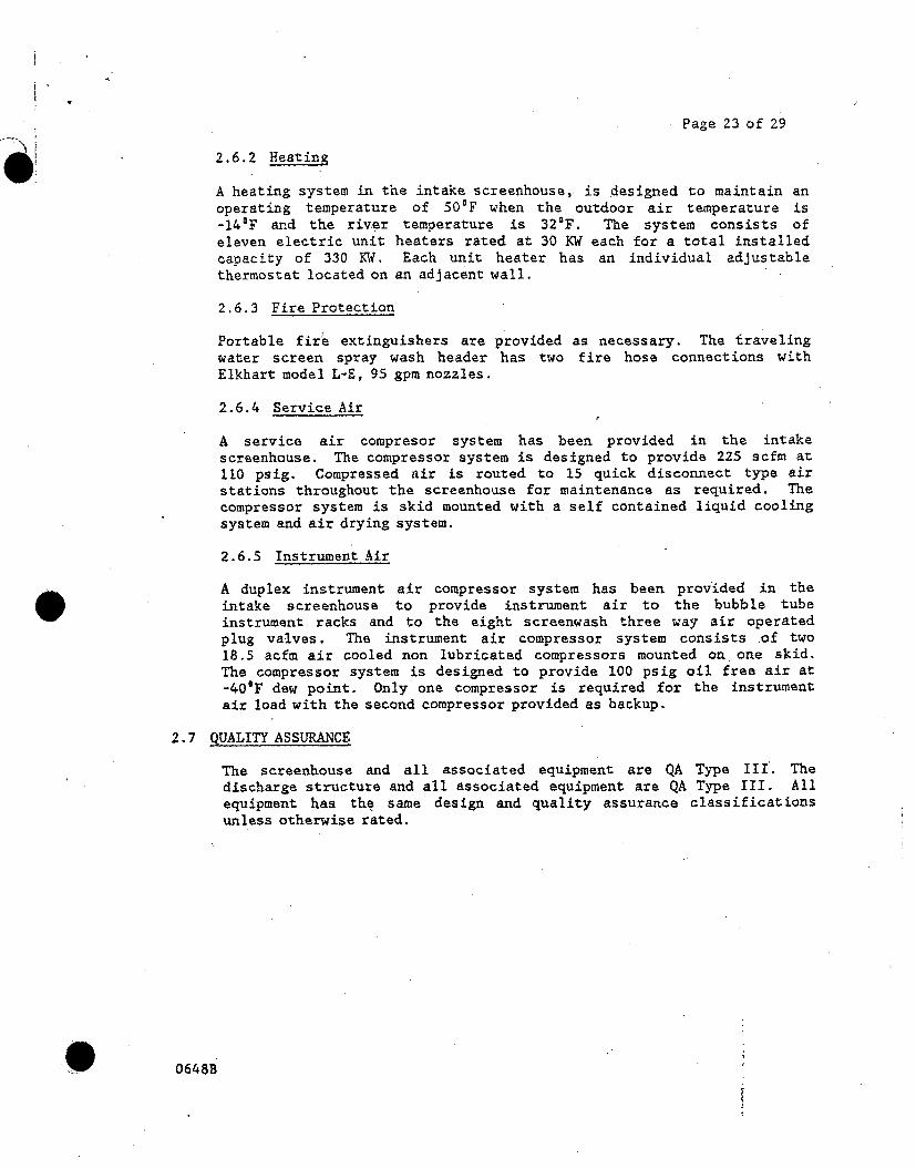
Page 23 of 29

2.6.2 Heating

A heating system in the intake screenhouse, is designed to maintain anoperating temperature of 50'F when the outdoor air temperature is-14OF and the river temperature is 324F. The system consists ofeleven electric unit heaters rated at 30 KW each for a total installedcapacity of 330 Mi. Each unit heater has an individual adjustablethermostat located on an adjacent wall.

2.6.3 Fire Protection

Portable fire extinguishers are provided as necessary. The travelingwater screen spray wash header has two fire hose connections withElkhart model L-E, 95 gpm nozzles.

2.6.4 Service Air

A service air compresor system has been provided in the intakescreenhouse. The compressor system is designed to provide 225 scfm at110 psig. Compressed air is routed to 15 quick disconnect type airstations throughout the screenhouse for maintenance as required. Thecompressor system is skid mounted with a self contained liquid coolingsystem and air drying system.

2.6.5 Instrument Air

A duplex instrument air compressor system has been provided in theintake screenhouse to provide instrument air to the bubble tubeinstrument racks and to the eight screenwash three way air operatedplug valves. The instrument air compressor system consists of two18.5 acfm air cooled non lubricated compressors mounted on one skid.The compressor system is designed to provide 100 psig oil free air at-40'F dew point. Only one compressor is required for the instrumentair load with the second compressor provided as backup.

2.7 QUALITY ASSURANCE

The screenhouse and all associated equipment are QA Type III. Thedischarge structure and all associated equipment are QA Type III. Allequipment has the same design and quality assurance classificationsunless otherwise rated.

0648B

Page 24 of 29

2.8 CODES AND STANDARDS

The screenhouse and associated equipment was designed in accordancewith the following codes and standards as indicated by the ProjectAnalysis Report:

Screen Pumps Manufacturers Standard

Traveling Water Screens Manufacturers Standard

Trash Rack & Rake Manufacturers Standard

Strainers Manufacturers Standard

Bypass Gates Manufacturers Standard,

Stop Gates Manufacturers Standard

Valves USAS-B31.1-1967

USAS-B16.5-1968

MSS SP-61

Piping (Steel) USAS B31.1-1967

Piping (Fiberglass) ANSI B31-1980

Motors NEMA MG-1-1972

Steel Structure AISC - 1980

Concrete Structures ACI 318-77

Electric Cable IEEE 383-1974

Sluice Gates Manufacturers Standard

3.0 SYSTEM OPERATION

3.1 System Arrangement

The system arrangement is as indicated on drawing number NF-92703 forthe intake and NF-92704 for the discharge.

90648B

Page 25 of 29

3.2 Description of Intake and Discharge Flows

3.2. 1 Normal Operation

Discharge flow rates are limited during specified periods byprovisions in the NPDES permit as listed below:

April 150 cfsMay 300 cfsJune 1-15 400 cfsJune 16-30 800 cfs

During these periods the intake flow rates cannot exceed the allowabledischarge rates plus an allowance for evaporative and drift lossesfrom the cooling towers.

During other periods of the year the intake flow rate may vary toprovide maximum plant efficiency provided the thermal criteria listedin Section 1.1.3.5 is not exceeded.

3.2.2 Infrequent Operation

Higher intake flow rates than those permitted by the dischargeprovisions listed in Section 3.2.1 will be allowed in order to preventcondenser inlet temperatures from exceeding 85 0 F. The NPDES permitallows for these higher flow rates provided they are minimized to theextent practical. During these periods the discharge thermal criteriamust still be met.

3.3 Two Unit Winter Startup

In the event that both plants must be shut down during winter months,the warm water source for de-icing will be lost. Both bypass gates inthe intake screenhouse should be manually opened if not already openand it should be verified that at least one sluice gate is open. Thebypass gates and sluice gate should be verified open at the onset ofthe outage and remain open for the duration of the outage to allowplant startup.

4.0 SYSTEM LIMITATIONS AND SETPOINTS

Maximum Operating Water Level 678 ft.

Normal Operating Water Level 673.5 ft

Minimum Operating Water Level 672.5 ft.

Average Net Screen Face Velocity0.5 fps at 800 cfs.0.88 fps at 1410 cfs.

0648B

Page 26 of 29

4.1 EQUIPMENT

4.1.1 Screen Size

Larval Season April 16 to Aug. 31 0.5 mm meshRemainder of Year Sept. 1 to April 15 9.5 mm mesh

SpeedDifferential PressureIn W.G. Across Screens

0"

4"

8"

10"

"18"

9.5 mm

0 fpm

3 fpm

20 fpm

Alarm

Bypass Gate Open

Design Maximum Differential Pressure 8 ft. WG

Design Operating Differential Pressure 3.5 ft. WG

4.1.2 Trash Rack and Rake

Design Maximum Differential 5 ft. WGTraversing Speed 30 fpm

4.1.3 Screen Wash Pumps

4.1.3.1 Coarse Screen Trash Removal PumpsNumber of pumpsHPRPMCapacity (gpm per pump)

4.1.3.2 Two Speed Fine Screen Trash Removal PumpsNumber of pumpsHPRPMCapacity (gpm per pump)

4.1.3.3 Coarse Screen Fish Removal PumpsNumber of pumpsHPRPMCapacity (gpm per pump)

0.5 mm

3 fpm

3 fpm

20 fpm

Alarm

BypassGate Open

2100

18001000

233/751200/1800480/760

215

1800600

00648B

{

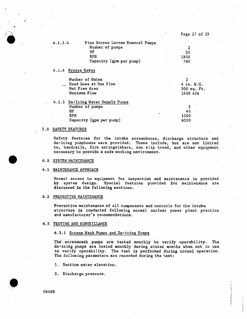
Page 27 of 29

4.1.3.4 Fine Screen Larvae Removal PumpsNumber of pumps 2HP 20RPM 1800Capacity (gpm per pump) 760

4.1.4 Bypass Gates

Number of Gates 2Head Loss at Max Flow 4 in. W.G.Net Free Area 500 sq. Ft.Maximum Flow 1410 cfs

4.1.5 De-Icing Water Supply PumpsNumber of pumps 2HP 40RPM 1200Capacity (gpm per pump) 6550

5.0 SAFETY FEATURES

Safety features for the intake screenhouse, discharge structure andde-icing pumphouse were provided. These include, but are not limitedto, handrails, fire extinguishers, non slip tread, and other equipmentnecessary to provide a safe working environment.

6.0 SYSTEM MAINTENANCE

6.1 MAINTENANCE APPROACH

Normal access to equipment for inspection and maintenance is providedby system design. Special features provided for maintenance arediscussed in the following sections.

6.2 PREVENTIVE MAINTENANCE

Preventive maintenance of all components and controls for the intakestructure is conducted following normal> nuclear power plant practiceand manufacturer' s recommendations.

6.3 TESTING AND SURVEILLANCE

6.3.1 Screen Wash Pumps and De-icing Pumps

The screenwash pumps are. tested monthly to verify operability. Thede-icing pumps are tested monthly during winter months when not in useto verify operability. The test is performed during normal operation.The following parameters are recorded during the test:

1. Suction water elevation.

2. Discharge pressure.

0648B

Page 28 of 29

3. Vibration amplitude.

6.3.2 Valves

A. All valves except vent, drain, instrument, test valves andmaintenance isolation valves are partially stroked onceevery three months, and fully stroked annually.

B. All check valves are tested annually.

6.4 INSERVICE INSPECTION

All components are visually examined while in operation every threemonths.

0648B

Page 2Z of 2?. & . I A

I

I) -- . ILI13 A d

u) .-w '-i - I V.

AI . I;- . . I T -1UA . I

1 1.F ".1 1

aI I .

J7 I

I .

f 7-14

I.

Th77-I-

i T_ i -,i -

-- EL> EL)

11;I . I :

. . a-6

"j- t ~ V~

' t, w c r ii C NO " N IN I N RA-Pace

f UOTES:

ri 1. ALL CONDUIT IS SHOWN DIAGRAMMATIC ALLY EXCEPT WHERE SPACE ALLOCATIC;ilHAS BEEN DESIGNIATED. WHERE SPACE ALLOCATION HAS BEEII SHOWN THE CO;NDUITSHALL BE RUN WITHIN THE DIMENSIONED LIMITS. CONDUIT, WHEN DIMENSIONED,SHALL BE i11STALLED AS INDICATED.

2i B

n a 2. WHERE EXPOSED CONDUIT CROSSES A VIBRATION JOINT OR WHERE CONDUIT EXPANSIONC2 dc . PROVISION IS RECUIRED, A SHORT LENGTH OF FLEXIBLE CONDUIT SHALL BE INSTALLED.

X61 CL 3. CONCEALED OR BURIED CONDUIT SUBJECT TO FLOODING SHALL BE SLOPED TOWARD

w 0o BOXES, HANDHOLES OR MANHOLES FOR DRAINAGE.

4. ALL CONDUIT LOCATED IN SCREENWELLS, UNDERGROUND TUNNELS, PITS ANDOUTDOORS ON EXTERIOR WALLS SHALL BE MOUNTED SO THERE IS AT LEAST

-< La ONE-QUARTER INCH AIR SPACE BETWEEN THE CONDUIT AND THE SUPPORTI LGSURFACE.

- 0 5. WHERE UNGROUNDED CONDUCTORS ENTER A CONDUIT IN A CABINET, PULL BOX,,. JUNCTION BOX, OR AUXILIARY GUTTER, THE CONDUCTORS SHALL BE PROTECTED

in 'BY A SUBSTANTIAL BUSHING O-Z ELECTRICAL MFG CO TYPE "B" OR APPROVED93• EQUIVALENT, PROVIDING A SMOOTHLY ROUNDED INSULATING SURFACE, UNLESS

w THE CONDUCTORS ARE SEPARATED FROM THE CONDUIT FITTING BY SUESTAN'TIALINSULAING MATERIAL SECURELY FASTENED IN PLACE. WHERE CONDUIT

: = BUSHINGS ARE CONSTRUCTED WHOLLY OF INSULATING MATERIA.L, A LOCKNUTSHALL BE INSTALLED BOTH INSIDE AND OUTSIDE THE ENCLOSURE TO WHICHTHE CONDUIT IS ATTACHED.

"6. ALL CONDUIT CONNECTIONS TO ALL MOTORS VIBRATING EZUIPMENT, BELT

< = DRIVEN EQUIPMENT, PRESSURE AND LEVEL SWITCHES, THERMOCOUPLES,c 62 ETC, TO BE MADE WITH FLEXIBLE CONDUIT.

0I-ou 7. RIGID STEEL CONDUIT RUN IN EARTH AND NOT ENCASED IN CON;CRETE

SHALL HAVE .A PVC JACKEr., OR BE COATED WITH ASPHALTUM.06

8. ALUMINUM CONDUIT SHALL NOT BE EMBEDDED W CONCRETE.

c 9L. WHERE CONDUIT CROSSES V'BRATION JOINTS IN SLAB, USE 18e LENGTH OF FLEXIBLESTEEL CON"UIT WRAPPED WITH " OF OAY;iM AND THREE ThICKNESSES OF BURLAP,

o = THOROUGHLY PAIffT-ED WITH ASPHALTUM.

3. 0 ;- )0. CONDUIT ENTERING SHEET STEEL OR ALUMINUM BOXES, WITHOUT HUBS, EXPOSED TOWATER OR RAIN, SHALL BE TERMINATED WITH A CONDUIT FITTING APPLETON ELECTRIC CO

= • = TYPE "HUB"ITHOMAS a BETTS CO BULLET HUB SERIES 370 OR APPROVED EQUAL.,.

-R C -T- Isu

-5~

P :,-

,.- ,7D

..- POwERLOSR RU ELECTRICAL :REVISED NOTE "

=• ,.•CECE .K76G CONDUIT NOTES

t 0- o : =,vr.• I-• 7-7-601 STANOD-=. DSIGN O.RA\ING. I _-- ..-- ,-- - - -______ F-Aj .- 1

roti ST £ EtpS Eý,!1 El4 Ez -I- I Z,,,, .- pac 2 f 57

N

Ja.

@00

- 4C

ozu

go

in.060C

in

01

to

ILZ

w1~oy

NOTES:

1. ALL CONDUIT, WIRE AND ELECTRICAL EQUIPMENT TO BE INSTALLED It?ACCORDANCE WITH THE LATEST STANDARDS OF THE 4NATIONAL ELECTRICALVCODE" AS ADOPTED BY THE NATIONAL FIRE PROTECTION ASSOCIATION,UNLESS OThERWISE NOTED IN THESE STANDARDS.

*Z. MARK NUMBERS REFER TO ITEMS IN BILL OF ELECTRICAL MATERIAL OR

COMPUTER PRINTOUTS.

3. FOR CABLE NUMBERS REFER TO CABLE SCHEDULES OR COMPUTER PRINTOUTS.

*4. FOR ABBREVIATIONS REFER TO STONE & WEBSTER ENGRG 'CORPSTD-MG-1000 SERIES.

*5. FOR LOCATION AND DATA FOR INSTRUMENT TRANSMITTERS, THERMOCOUPLES,

PRESSURE SWITCHES, ETC , REFER TO EQUIPMENT LIST.

6. CENTER LINE OF ALL POWER RECEPTACLES AND PUSH BUTTON STATIONS TO BE4!0" ABOVE FLOOR ELEVATION UNLESS OTHERWISE NOTED.

7. THE TOP OF ALL CONTACTOR AND STARTER GROUPS SHALL BE 6' 0" ABOVEFLOOR ELEVATION UNLESS OTHERWISE NOTED. THE EXACT DETAILS OFARRANGEMENT SHALL BE DETERMINED BY THE CONTRACTOR; HOWEVER, THEGENERAL ARRANGEMENT SHALL FOLLOW IN SO FAR AS PRACTICABLE THE-ARRANGEMENT AS SHOWN ON WIRING DIAGRAMS.

8. CLEARANCE, IF REQUIRED FOR ALL STRUCTURAL MEMBERS, CONDUIT, TRAYS ANDEQUIPMENT FOR THE ISOLATED PHASE BUS SHALL BE INDICATED ON THEDRAWING. CONDUIT FOR SECONDARIES OF GENERATOR CURRENT TRANSFORMERLEADS, BOTH PHASE AND NEUTRAL SIDES, SHALL BE INSULATED IN ACCORDANCEWITH MANUFACTURER'S DRAWINGS.

*Notes 2, 4, 5 are lot applicable to Job 12911.09 (NS? E-781073)I I

pcPOWER INDUSTRY GROUPI

CMECXED I E S.K 7/G/601

ELECTRICALCONDUIT, TRAY A LIGHTING NOTES

GENERAL® REDRAWN ADCE0

PROPRIETARY, DELETE D, REVISE0 NOTES

CORRECT H.AT7.7/7/650A.P"RoED I cWA 7/7/6o1

[Iiic CESCRIPTION

STANDARD DESIGN DRAWINGI__ i :U _

17 STO- ME-I 1- -4I -.-q L: F. " •10

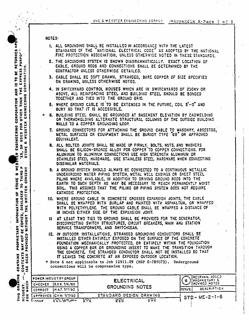
3Nr- r, WERS7R EtJGINCERMS ~O )NAzendc"x A- Pace -1 of 3

"C

a hi

0

IL

00

00g.

21

1-0h

at

NOTES:

I. ALL GROUNDING SHALL BE INSTALLED IN ACCORDANCE WITH THE LATESTSTANDARDS OF THE "NATIONAL ELECTRICAL CODE" AS ADOPTED BY THE NATIONALFIRE PROTECTION ASSOCIATION, UNLESS OTHERWISEE NOTED IN THESE STANDARDS.

2. THE GRCUNDING SYSTEM IS SHOWN DIAGRAMMATIC=LLY. EXACT LOCATION OFCABLE, GROUND RODS AND CONNECTIONS SHALL BE DETERMINED BY THECONTRACTOR UNLESS OTHERWISE DETAILED.

3. CABLE SHALL BE SOFT DRAWN, STRANDED, BARE COPPER OF SIZE SPECIFIEDON DRAWING, UNLESS OTHERWISE NOTED.

4. IN SWITCHYARD CONTROL HOUSES WHICH ARE IN SWITCHYARDS OF 230KV ORABOVE, ALL REINFORCING STEEL AND BUILDING STEEL SHOULD BE BONDEDTOGETHER AND TIED INTO THE GROUND GRID.

5. WHERE GROUND CABLE IS TO BE EXTENDED IN THE FUTURE, COIL 5'-0 ANDBURY SO THAT IT IS ACCESSIBLE.

* 6. BUILDING STEEL SHALL BE GROUNDED AT BASEMENT ELEVATION BY CADWELDINGOR THERMOWELDING ALTERNATE STRUCTURAL COLUMNS OF THE OUTSIDE BUILDINGWALLS TO A COPPER GROUNDING LOOP.

7. GROUND CONNECTORS FOR ATTACHING THE GROUND CABLE TO MASONRY, ABSESTOS,METAL SURFACES OR EOUIPMENT SHALL BE BURNDY TYPE "GB OR APPROVEDEQUIVALENT.

8. ALL BOLTED JOINTS SHALL BE MADE UP FIRMLY. BOLTS, NUTS, AND WASHERSSHALL BE SILICON-BRONZE ALLOY FOR COPPER-TO COPPER CONNECTIONS. FORALUMINUM TO ALUMINUM CONNECTIONS USE HIGH STRENGTH ALUMINUM ORSTAINLESS STEEL HARDWARE. USE STAINLESS STEEL HARDWARE WHEN COIN;ECTINGDISSIMILAR MATERIALS.

9. A GROUND SYSTEM SHOULD ALWAYS BE CONN;ECTED TO A CONTINUOUS METALLICUNDERGROUND WATER PIPING SYSTEM, METAL WELL CASINGS OR SHEET STEELPILING WHERE AVALABLE, IN ADDITION TO DRIVING GRCUNO RODS INTO THEEARTH TO SUCH DEPTH AS MAY BE NECESSARY TO REACH PERMANENTLY MOISTSOIL. THIS ASSUMES THAT THE PILING OR PIPING SYSTEM DOES NOT REQUIRECATHODIC PROTECTION.

10. WHERE GROUND CABLE IN CONCRETE CROSSES EXPANSION JOINTS, THE CASLESHALL BE WRAPPED WITH BURLAP AND PAINTED WITH ASPHALTUM, OR WRAPP-EDWITH POLYETHYLENE. THE GROUND CABLE SHALL EE WRAPPED A DISTANCE OF18 INCHES EITHER SIDE OF THE EXPANSION JOIANT.

It AT LEAST TWO TIES TO GROUND SHALL BE PROVIDED FOR THE GENERATOR,DISCONNECTING SWITCH STRUCTURES, CIRCUIT BSEAKERS, MAIN ANU STATIONSERVICE TRANSFORMERS, AND SWITCHGEAR.

12. IN OUTDOOR INSTALLATIONS, STRANDED GROUNDING CONDUCTORS SHALL BEINSTALLED EITHER ENTIRELY EXPOSED ON THE SURFACE OF THE CONCRETEFOUNDATION MECHANICALLY PROTECTED, OR ENTIRELY WITHIN THE FOUn;DATIONUSING A COPPER BAR OR GROUNDING INSERT TO MAKE THE TRANSITION THROUGHTHE CONCRETE. THE STRANDED CONDUCTOR SHALL NOT BE INSTALLED SO THATIT LEAVES THE CONCRETE -AT AN EXPOSED OUTDOOR LOCATION.

* Note 6 not applicable to Job 12911.09 (NSP E-78Y073).connections will be compression type.

Underground

POWER INCUSTRYGROUP ELECTRICAL NP.1:,--:)

CHECCED LSK.7/6/60 G UREVISDG NOOTES

CORRECT IHA.T.7/7'60 GROUNDING NOTES OESCRPTCU

PROV~ ~CWM 7/7/40 I STANJDARD DESIGN DRA,'INGI A PPROV!:0 1'r-',YM 7/7/60 1

(A a Ov"ý' In7I -- ); ýV'%1 STD- ME-2-1-6I

etl fo WESSTE ENI N Coppoq Ioj0,Appen*4iX A-Pace 4 oO 5I

CL U

hC a.a -4

ha0

Zit

z 2~

V1.- >

00

hw 1 '

- h

3K2

2oOi =2I

NOTES (CONT ):

* 13. CONNECTIONS BETWEEN THE GROUND CABLE AND CONNECTOR MAY BE MADE BYCOMPRESSION, BOLTS OR , CONNECTIONS BETWEEIN, THECONNECTOR AND THE EQUIPMENT SHALL BE BY MEANS OF BOLTS. CONNECTIONS BETWEENTHE GROUND CABLE AND SUPPORTING STRUCTURE MAY BE A'41TH BOLTS IF A C•':;•ECTCRIS USED OR EXOTHERM!C PROCESS IF THERE IS NO CONNECTOR. A TYPICAL BOLTEDCONNECTOR WOULD BE BURNOY TYPE "MA" OR APPROVED EQUIVALENT.

14. ELECTRICAL EQUIPMENT, TRAYS, AND CONDUIT SHALL BE BONDED TOGETHER TOINSURE ELECTRICAL CONTINUITY. CABLE TRAYS SHALL BE GROUNDED VIA COPPERTO BUILDING STEEL ON EACH END AND NOT MORE THAN EVERY 100 FT. ALL CONLDUITFROM CABLE TRAYS TO ELECTRICAL EQUIPMENT SHALL BE BON'DED TO THE TRAY.AT ELECTRICAL EQUIPMENT WHERE CONDUIT DROPS ARE NOT USED AND CABLE IS RUNFROM THE CABLE TRAYS INTO THE EQUIPMENT, THE CABLE TRAY SHALL BE BONDEDTO THE EQUIPMENT. AT METAL-CLAD SWITCHGEAR, LOAD CENTERS AND MOTORCONTROL CENTERS, THE BONDING JUNIPER SHALL BE Z/O CABLE.

15. ALL METALLIC STRUCTURES, MOTORS AT 2300V AND ABOVE, SWITCHGEAR, MOTORCONTROL CENTERS, CONTROL AND RELAY BOARDS, LIGHTING CABINETS, CONTACTOR.,CABLE TRAYS, AND CON;UIT SHALL BE PERMANENTLY AND EFFECTIVELY GROUNDEDBY A GROUND CABLE CONNECTED TO THE GROUID GRID. OTHER EQUIPMENT MAY BEBOLTED TO SUPPORTING STRUCTURE OR CONNECTED TO THE STRUCTURE WITH A GROUNDCABLE. ALL MOTORS LESS THAN 25 HP AT 575V OR LESS MAY BE GROUNDEDTHROUGH THE CONDUIT SYSTEM. EXPANSION JOINTS IN CONDUIT SHALL BE MADEELECTRICALLY CONTI'NUOUS BY A BONDING JUMPER.

16. BURIED OR SUBMERGED EQUIPMENT SUCH AS TRAVELING SCREENS AND THEIRFOUNDATION BOLTS OR PIPING TO WHICH CATHOOIC PROTECTION MAY BE APPLIEDMUST NOT BE IN METALLIC CONTACT WITH REINFORCING RODS, METALLIC CONDUIT,GROUNDING CABLE OR OTHER PIPING. THEY SHOULD BE SEPARATED AS FAR APARTAS CONDITIONS WILL PERMIT. INSULATING FLANGES, UNIONS OR COUPLINGS MAY BEREQUIRED IN THE PIPE RISERS JUST ABOVE GROUND ELEVATION.

17. ALL GROUNDING CABLE IN CATHODIC PROTECTION AREA SHALL HAVE INSULATIONSUITABLE FOR DIRECT BURIAL IN EARTH.

18. FOR ELECTRICAL CONTINUITY OF METAL RACEWAY CONTAINING WIRES OPERATINGABOVE 25OV, PROVIDE TWO LOCKNUTS, ONE INSIDE AND ONE OUTSIDE OF BOXESAND CABINETS.

19. ALL SHIELDED CABLE SHALL BE TERMINATED AND GROUNDED ACCORDING TO THERECOMMENDATION AND INSTRUCTIONS GIVEN BY THE ENGINEER, UNLESS OTHERWVISESHOWN ON DRAWINGS.

20. ARMORED CABLES SHALL HA,'E THE CABLE ARMOR GROUNDED IN ACCORDANCE WITHINSTRUCTIONS GIVEN BY 1HE ENGINEER.

* No F•xotbermic procesg connections shall be made on Job 12911.09(NSP E-78Y073)

POWERINDUSTRYGROUP ELECTRICAL REDRAWN &

Ec.K I..7/6'/sO - GROUNDING NOTES ISSUE DEScRiPTIC S

APPROVED ICWM.1-.7/7/60 1

issuJe I%.j'A;.- •J

STANDARD DES0;C3N DRAWINGST D -M E-2-2-7

t0i 'I@1

. . . . . . . . . . . ,

Appendix A-Page 5 of 5Ii

Sk

STONE 5 WEBSTER ENGItEERING CORPORATION

INDUCTION MOTOR DATA

PROJECT

PAGE NO

J.O. NO.

I CLIENT

t

i

2 FURN;SHED BY ODATE B3 MARK OR ITEM NO.

PURCHASER'S RE-"GUIREMENTS DATA FURNISHE-D By SELLER5 SERVICE I MA•E* TYPE ( FRAIAE NO.7 NO OF UNITS I MORSEPOWERI MOUNTING I SERvICE FACTORI ELEC. C),ARACTERISTICS. V PH HZ I FULL LOAD RPM

so SYNCH. SPE... RPM FULL LOAD AM;PIs HORSEPOWER LOCKED ROTOR AMPa2 SERVICE FACTOR j STARTING TORCUE. % F.L.13 ENCLOSURE j PULL-OUT TOROUE. % FL.14 INSULATION CLASS I EFF. FULL LOAD. %15 INSULATIO,4 TREATMENT I EFF. 3/4 LOA0D. %36 AMBIENT TEMP-C I EFF.- I/Z LOA0. %I7 STATOR TEMP RISE -C I PF-FULL LOAD,.%Q0 BEARING TYPE I PF- 3/4 LOAD. %

is BEARING TEMP RELAY i P.F.-/Z LOAD. *"20 BEARING THERMOCOUPLE I PF. AT STARTING. %21 HALF COUPLOR SHEAVE MTD SBY -SHORT R.IR-JIT A-C TIME CON4STANT. SEC.22 ROTATION * i X/R RATIO23 WKZ OF ORIVEN EOUIR. (L-"TZ) I SPACE HTRS.. TOTAL WATTS24 BRKWY. TORG. OPVN. EOUIP. 1 RAcI-L BEARIi.NG-TYPE25 OVERSIZE COND. BOX 1 THRUST SEARING-TYFP:26 COND. BOX LCCA-lON * j BE-ARING SERVICE-HR2? SPACE HEATERS. VOLTAGZ. P-4AS- I NORMAL BRG. OPER. TEMR-C23 SPLIT END SELLS INET WEIGHT-LB

29 TERMINAL LUGS. TYPE I OIL COOL. SYS. REQ'D30 STATOR t4IGm TEMP DEVICer I aRG, OIL PRESS. RANGE. PSI

3t" ADJUSTABLE SL!CE RAILS i BRG OIL RE')'D EA.. BRG. GPM32 SOLEPLATES I NA;ME PLATE CODE LETTER33 PROJECT ELEV..FT PERMISSIBLE STARTS PER H.-RWITH:34 SHAFT (HOLLOW. SOLIDI T MOTOR AT AMB:ENT TEMP.35 COUPLING (SELF-RELEASE. I MOTOR AT RATED TOTAL TEV.36 SOLID. NONREVERSING. I TYPE 57ALED INSUL. SYS.37 AOJUSTA3LE.FLEXIeLE) IOESCRI,-lION OF INSUL. SYS.

3, DOWuTHRUST-CCNTINUO'.'S I MAX. STALL TIME WITH L.R. AMPS, SEC.

39 UPTHRUST-C-CNT;NUOIJS I ACCEL. TIME. FULLY LOADED40 UPTHRLJST- MOMENTARY __WITH 100% V. SEC.

41 DOWNTI.RLST-kMGME4TARY I WITH 80% V. SEC.42 I * WITH % V. SEC.

43 SiDE THRUST _44 MIA* REVERSE SPEED i45 DRAIN PLUG --43 VENT46 AIR INTAKE AN.O OISC-ARGE SCREENS _

47 CT. RATIO 1WKZ OF ROTOR,LS-FTZ

46 SURGE CAPA,.TCRSTdn ANTI-FRICT. BRG. SERVICE-HR I

SoMINI MUM STARTIN11G VOLT AGE %

52 REMARKS: REMARKS:53 ALL PERFO-R.MANCE DATA a_-SED ON NOPMAL RATED I ALL PERFORMANCE DATA BASEDGON NC'.A•-L RTr,%54 VOLTAGE AND FREQUENCT I VOLTAGE AND FREOUENCY55 ITEMS 34-44 APPLr TO vE•..:.. MCTCRS ONLY _

st9f£aii'VIE'Aco rFzvG ENO CPPOcZITC CC'..I!NG ENO

APPENDIX BLOGIC DESCRIPTION

B 1.0 LOGIC SYSTEM DESIGN

B 1.1 System Arrangement

B 1.1.1 Intake Screenhouse

The intake screenhouse is served by eight traveling water screens,one traveling trash rake, two 50 percent-capacity coarse screentrash removal pumps, two (two-speed) 50 percent-capacity fine orcoarse screen trash removal pumps, two 50 percent-capacity coarsescreen fish removal pumps, two 50 percent-capacity larvae removalpumps, twelve differential level sensing points, one fish returnline temperature sensor, two bypass gates, one overhead bridgecrane, and one jib crane.

All pumps will have motor-driven butterfly valves on the discharge.

The screenhouse load will be supplied by two 13.8 KV feeders fromthe switchyard. (Transformers CTM and 10 Bank.)

B 1.1.2 Deicing Pumphouse

The deicing system is comprised of two 50 percent-capacity deicingpumps, each with a motor-driven butterfly valve. These valves areinterlocked to the pumps to prevent the pump from starting against aclosed valve. One 480 volt feeder from the intake screenhouse willsupply power to a local motor control center for the deice system.

B 1.1.3 Discharge Structure

The discharge structure is served by four motor-operated dischargegates, one discharge canal level sensor, and four temperaturesensors. The control signal for the gates will originate from theplant "Main Control Board". One, 480 volt feeder from the deicingpumphouse will supply power to a local motor control center for thegate drive motors.'

B 1.2 Control and Instrumentation

... B 1.2.1 Description of Operation

B 1.2.1.1 New Screenhouse

A. Traveling Screens

Each traveling water screen is driven by a variable speed A.C. motorgiving a speed range from 3 to 20 fpm. Each traveling screen hastwo types of screen panels. The fine mesh screen panels are usedfrom April 16 to August 31, and the coarse mesh screen panels areused during the rest of the year.

379BF

Page 2 of 24

WLocally mounted at each screen is a JOG-REMOTE selector switch and

a JOG pushbutton. The REMOTE position will enable theOFF-INVERTER selector switch mounted on the screenhouse controlboard to function. The JOG position will enable a pushbutton tojog a screen for maintenance purposes. The jog speed is the 60cycle speed of approximately 20 fpm. The OFF position willdisable the respective screen. The INVERTER position will run thescreen at the speed determined by the inverter frequency.

.. The mode of operation for each bank of four screens is controlledby a MANUAL-AUTO selector switch on the screenhouse controlboard. When the switch is in the MANUAL position, the fourcorresponding screens will run off the inverter at a speedmanually selected on a potentiometer mounted on the controlboard. A START and STOP pushbutton for each bank of four screenswill initiate the manual run sequence. Ip the AUTO position thebank of four screens will run at a speed required by the controlsystem.

A signal from any one of four screen differential level sensorsassociated with a group of four traveling screens will start theoperation of that group. If one or more of the traveling screensis not in the INVERTER position, the control input from the levelsensor for that traveling screen will be disabled and the rest ofthe traveling screens will continue to operate as normal.

A two position switch (fine-coarse) for each set 'of four travelingscreens is used to select the type of screen panels currently inservice, either fine mesh screen panels or coarse mesh screenpanels. In the FINE position, the screens will continually run at3 fpm when the differential is 4 inches or less. In the COARSEposition, the traveling screens and the fish and trash spray washsystems will not run as long as the differential is less than 4inches. When any 1 screen within a group of 4 exceeds 4 inchesdifferential for a period of two minutes, a signal will beinitiated to start all four screens in that group at 3 fpm.

Operation at differentials 4 inches and above is the same for bothfine and coarse mesh screens. If the differential increases above4 inches for either type of screen the speed will automaticallyincrease proportionally until reaching the maximum speed of 20 fpmat 8 inches of head differential.

The coarse screens will remain in this load follow mode until thedifferential drops below 3 inches for 20 minutes, then they willshut off. The fine screens will continue to run at 3 fpm below 4inches of differential'.

The •. screens will. automatically rotate ,(with wash sprays) 1-1/3revolutions if they have not operated in the last 8 hours. Thespeed will be the same &s used during jogging.

*G379 8F

Page 3 of 24

At 10 inches differential of water, an alarm will be sounded onthe annunciators at the plant "Main Control Board" and in theintake screenhouse.

In the event of an inverter failure the screens will betransferred to a 60 hertz backup power source that will run thescreens at about 20 fpm.

B. Screen Wash Pumps

There are two identical screen wash pump systems, one system eachfor a group of four screens.

During the time period of April 16 to August 31 when the-fine meshscreen% panels are.% being us ed, j ne: low pressure larv.ae removalspray pump. and one, low pressure: trash remoVal spray, puI wil runcontinuous ly for eac bank of . four screens. '.The. ': trash .removalpumps are two speed. pumps .:.that should be in the slow speedposition during this' time.

A RUN-STOP/RESET and SLOW-FAST control switch is provided for eachof these pumps at the screenhouse control board. In the RUNposition the pumps will start and run. In the STOP/RESET position.he pumps will stop.

During the balance of the year, when the coarse screen panels areused, separate high pressure fish and trash removal spray pumpswill be used. Each of the coarse screen pumps are controlled by aMANUAL-OFF/RESET-AUTO control switch mounted in the controlboard. The MANUAL position will start and run the correspondingpump and the OFF/RESET position will stop the pump. In the AUTOposition both the trash and fish removal spray wash systems willstart once any of the screens in that bank of four are signaled tostart. Prior to. starting :the screens, the coarse screen pumpsýwill start and :run for. 2 minutes to fill the.,return lines, %andwill- ontinue to. run for 10 minutes after the screens stop toflush the return lines.

A motor-operated valve on the discharge of each pump will open assoon as the pumps are started. If the valve does not fully openwithin 15 seconds, an alarm will sound and the pump will stop.The RESET function of the STOP or OFF position allows the pumps tobe restarted after a valve open failure. Each motor-operateddischarge valve can also be opened or closed manually using aCLOSE-AUTO-OPEN control switch on the control board.

3798F

Page 4 of 24

The fine screen larvae pump and coarse screen fish pump use acommon pipe header to the screens for each system. The coarsescreen fish pump is interlocked to the fine screen larvaedischarge valve to prevent the pump from starting if the oppositedischarge valve is open.

During heavy trash. loading in the coarse screen mode of ope ration,a :seconda. trash spray header on each screen ma•y be placedin operation... .This may be done by opening, the manual valve,:ýon: thesecondary trash removal header and %manually starting the finescree~n .trash removal pumps in the fast speed..

C. Bypass Gates

Each of the two hydraulic bypass gates will be controlled by aAUTO-LOCAL control switch on each units control box. The LOCALposition enables the UP and DOWN pushbuttons to function on thehydraulic units.

In the AUTO position both gates will open in unison whenever thedifferential level across any one screen in the INVERTER modewithin both groups of four screens exceeds 18 inches, thedifferential level across the entire screenhouse exceeds 24inches, total deicing system failure, or all power to the newintake structure is lost.

Once open, the gates will latch in place. The gates must firstrelease the automatic "dogging device" before they can be closed.In the event of a power failure, each gate accumulator will havesufficient capacity to automatically open the gate after a timedelay of two minutes to eliminate spurious trips. If one of thetwo hydraulic pump units should fail, manual cross-tie valving can'be opened to allow any one pump to be used singly on either gate.

D. Trash Rake

The intake screenhouse will be provided with one traveling trashrake which will run along a rail in the deck of the structure.The trash rake is, manually controlled. A differential levelsensor across the trash rack in each bay will alarm at 6 inchesindicating that trash needs to be removed.

E. Overhead Crane

A 15 ton capacity traveling overhead bridge crane is available forservicing equipment in the intake screenhouse. It is manuallycontrolled from a suspended pendant control box above thescreenhouse deck.

3

379 8F

Page 5 of 24

F. Jib Crane

A jib crane is located and manually controlled on the north sideof the intake screenhouse building to aid in the removal andemptying of the trash baskets.

B 1.2.1.2 Deicing System

Two manually started deicing pumps are available to keep thetraveling screens from icing up during the winter months. Waterwill be supplied from the discharge of the plant and pumped to thescreenhouse to submerged diffusers in front of each bay. Motordriven butterfly valves on the discharge of each pump will openbefore its associated pump can start. The pumps and valves can bestarted or opened at the screenhouse control board or locally atthe pump.

B 1.2.1.3 Discharge Structure

The required flowrate and discharge velocity will be maintained bythe control room operator opening an appropriate combination ofthe four sluice gates. Each gate will have a REMOTE-LOCAL andOPEN-CLOSE switch locally and an OPEN-CLOSE control switch in the"Main Control Room" that will enable the operator to either fullyopen or fully close the respective gate.

A calculated discharge flowrate and open/close gate position willbe displayed along with the average temperature of the opendischarge pipes on the "Main Control Board Mimic Bus".

B 1.2.2 Component Control Description

B 1.2.2.1 Intake Screenhouse

A. TRAVELING SCREENS - Typical of eight (Two groups of four)(CT-067-I1I through CT-067-118)(Ref drawings NF-92780-1, NF-92780-2)

1. Each individual traveling screen will manually start from thecontrol board in the intake screenhouse whenever all of thefollowing conditions are satisfied:

a. The screen bank selector switch (CS-91800-48, 49) is inthe MANUAL position.(Speed range of 3 fpm to 20 fpm may be selected manuallyon a potentiometer mounted on the control board.)

b. The individual screen selector switch (CS-91800-03through CS-91800-10) is in the INVERTER position.

I 3798F

Page 6 of 24

c. The screen bank START pushbutton (PB-91800-59, 60) isdepressed.

d. The individual local screen selector switch (CS-91900-02through 91907-02) is in the REMOTE position.

e. Motor circuit breaker closed.

f. Motor thermal overload reset.

2. Each individual traveling screen can be manually jogged fromthe screen location whenever all of the following conditionsare satisfied:

a. The individual local screen selector switch (CS-91900-02through CS-91907-02) is in the JOG position. (Speedduring jog will be approximately 20' fpm.)

b. Jog button (PB-91900-01 through PB-91907-01) is depressedat the screen location.

c. The individual screen selector switch (CS-91800-03 through

0S-91800-10) is in the INVERTER position.

d. Motor circuit breaker closed.

e. Motor thermal overload reset.

3. Each bank of four traveling screens will automatically startwith coarse screens whenever all of the following conditionsare satisfied:

a. The individual selector switch' for each of the fourscreens in the bank (CS-91800-03 through CS-91800-l0) isin the INVERTER position.

b. The screen bank selector switch (CS-91800-48, 49) is inthe AUTOMATIC position.

c. Differential level across any one screen in the bankexceeds 4 inches for more than 2 minutes.

d. The screen selector switch (CS-91800-23, 24) is in the

COARSE position. (September 1 to April 15.)

e. 2 minutes has elapsed after the spraywash pump start.

f. Header pressure of the screen fish removal system(PS-91602, PS-91603) must exceed 15 psig.

3798F

Page 7 of 24

g. Header pressure on the screen trash -removal system(PS-91600 or PS-91604, PS-91601 or PS-91605) must exceed45 psig.

h. The individual local screen selector switch (CS-91900-02through CS-91907-02) is in the REMOTE position.

i. Motor circuit breaker closed.

j'. Motor thermal overload reset.

4. Each bank of four traveling screens will continuously run atminimum speed with fine screens whenever all of the followingconditions are satisfied:

a. The individual selector switch for each of the fourscreens in the bank (CS-91800-03"through CS-91800-l0) isin the INVERTER position.

b. The screen bank selector switch (CS-91800-48, 49) is inthe AUTOMATIC position.

c. The screen selector switch (CS-91800-23, 24) is in theFINE position. (April 16 to August 31.)

d. Screen differential less than 4 inches.

e. Header pressure of the screen larvae removal system(PS-91602, PS-91603) must exceed 15 psig.

f. Header pressure on the screen trash removal system(PS-91604, PS-91605) must exceed 45 psig.

g. The individual local screen selector switch (CS-91900-02through CS-91907-02) is in the REMOTE position.

h. Motor circuit breaker closed.

i. Motor thermal overload reset.

5. Each. traveling screen will automatically start and. run for1-1/3 revolutions at approximately 20 fpm whenever all of thefollowing conditions are satisfied.

a. The screen bank selector switch (CS-91800-48, 49) is inthe AUTOMATIC position.

b. 8 hours has passed since the screen has been run.

3798F

Page .8 of 24

c. The individual selector switch for each of the fourscreens in the bank (CS-91800-03 through CS-91800-I0) isin the INVERTER position.

d. The individual local screen selector switch (CS-91900-02through CS-91907-02) is in the REMOTE position.

e. The screen mesh selector switch (CS-91800-23, 24) is in

the COARSE position.

f. 2 minutes has elapsed after the spraywash pump start.

g. Header pressure of the screen fish (PS-91602, PS-91603)removal system must exceed 15 psig.

h. Header pressure on the screen trash removal system(PS-91600, PS-91601) must exceed 45 psig.

i. Motor circuit breaker closed.

j. Motor thermal overload reset.

6. Each individual traveling screen will stop whenever any of thefollowing conditions are satisfied:

a. The individual selector switch (CS-91800-03 throughCS-91800-I0) is in the OFF position.

b. The screen bank STOP pushbutton (PB-91800-61, 62) isdepressed.

c. The screen selector switch (CS-91800-23, 24) is in theCOARSE position, the individual screen selector switch(CS-91800-03 through CS-91800-I0) is in the INVERTERposition, the screen bank selector switch (CS-91800-48,49) is in the AUTOMATIC position, and the differentiallevel (DPT-91700 through DPT-91707) across all the screenswithin a bank of 4 that are in the INVERTER position, dropbelow 3 inches for more than 20 minutes.

d. Header pressure on the screen fish removal system(PS-91602, PS-91603) drops below 10 psig.

e. Header pressure on the screen trash removal system(PS-91600 and PS-91604, PS-91601 and PS-91605) drops below40 psig.

f. Motor circuit breaker open.

g. Motor thermal overload.

3798F

Page 9 of 24

B. Coarse Screen Fish Removal Pump - Typical for two(Ref. drawing NF-92780-4)

1. The coarse screen fish removal pump (CS-045-1033, 1034) willmanually start from the control board in the intakescreenhouse whenever all of the following conditions aresatisfied:

a. The pump selector switch (CS-91800-12, 14) is in theMANUAL position.

b. Motor circuit breaker closed.

c. Motor thermal overload reset.

2. The coarse screen fish removal pump will automatically startwhenever all the following conditions are satisfied:

a. The pump selector switch (CS-91800-12, 14) is in theAUTOMATIC position.

b. The fine screen larvae removal pump discharge valve(MV-91208, 9) is closed.

c. Differential level (DP-91704 'through DP-91707, DP-91713through DP-91716) across any of 4 traveling screens in thecorresponding bank exceeds 4 inches for 2 minutes, or thescreens have not been run for 8 hours. (Note: Theindividual screen selector switch (CS-91800-03 throughCS-91800-l0) must be in the INVERTER position beforedifferential level can be considered for that screen.)

d. Screen mode selector switch (CS-91800-23, 24) is in theCOARSE position.

e. Motor circuit breaker closed.

f. Motor thermal overload reset.

3. The coarse screen fish removal pump will sto whenever any ofthe following conditions are satisfied:

a. The pump selector switch (CS-91800-12, 14) is in theOFF/RESET position.

b. Ten (10) minutes has elapsed since the corresponding bankof screens automatically stopped.

c. The screen operation mode selector switch (CS-91800-23,24) is in the FINE position.

3798F

Page 10 of 24

d. 15 seconds has elapsed since the pump has started and thedischarge valve has not opened. (Note: The pump can nowonly be restarted in the AUTOMATIC position by firstmanually placing the appropriate selector switch in theOFF/RESET position and then returning it to the AUTOMATICposition.)

e. Motor circuit breaker open.

f. Motor thermal overload.

C. Coarse Screen Trash Removal Pump - Typical for two(Ref. drawing NF-92780-3)

1. The coarse screen trash removal pump (CT-045-1023, 1024) willmanually, start from the control board in the intakescreenhouse whenever all of the following conditions aresatisfied:

a. The pump selector switch (CS-91800-II, 13) is in the

MANUAL position.

b. Motor circuit breaker closed.

c. Motor thermal overload reset.

2. The coarse screen trash removal pump will automatically startwhenever all the follcwing conditions are satisfied:

a. The pump selector switch is in the AUTOMATIC position.

b. Differential level (DP-91704 through DP-91707, DP-91713through DP-91716) across any of 4 traveling screens in thecorresponding bank exceeds 4 inches for 2 minutes, or thescreens have not been run for 8 hours. (Note: Theindividual screen selector switch (CS-91800-03 throughCS-91800-l0) must be in the INVERTER position beforedifferential level can be considered for that screen.)

c. Screen mode selector switch (CS-91800-23, 24) is in the

COARSE position.

d. Motor circuit breaker closed.

e. Motor thermal overload reset.

3798F

Page 11 of 24

3. The coarse screen trash removal pump will stop whenever any ofthe following conditions are.satisfied:

a. The pump selector switch (CS-91800-ll, 13) is in theOFF/RESET position.

b. Ten (10) minutes has elapsed since the corresponding bankof screens automatically stopped.

c. Screen operation mode selector switch (CS-91800-23, 24) isin the FINE position.

d. 15 seconds has elapsed since the pump started and thedischarge valve has not opened. (Note: The pump can nowonly be restarted in the AUTOMATIC position by firstmanually placing the appropriate selector switch in theOFF/RESET position and then returhing it to the AUTOMATICposition.)

e. Motor circuit breaker open.

f. Motor thermal overload.

D. Fine Screen Larvae Removal Pump - Typical for Two(Ref. drawing NF-92780-4)

1. The fine screen larvae removal pump (CT-045-1031, 1032) willmanually start from the control board in the intakescreenhouse whenever all of the following conditions aresatisfied:

a. The pump selector switch (CS-91800-27, 32) is in the RUNposition.

b. Motor circuit breaker closed.

c. Motor thermal overload reset.

2. The fine screen larvae removal pump will manually stopwhenever any of the following conditions are satisfied:

a. The pump selector switch is in the STOP/RESET position.

b. 15 seconds has elapsed since the pump started and thedischarge valve has not opened. (Note: The pump can onlybe restarted by first manually placing the appropriateselector switch in the STOP/RESET position and thenreturning it to the RUN position.)

c. Motor circuit breaker open.

d. Motor thermal overload.

3798F

Page 12 of 24

E. Fine Screen Trash Removal Pump - Typical for Two(Re. drawing NF-92780-3)

1. The fine screen trash removal pump (CT-045-1021, 1022) willmanually start from the control board in the intakescreenhouse whenever all of the following conditions aresatisfied.

a. The pump selector switch (CS-91800-25, 30) is in the RUNposition.

b. The speed selector switch (CS-91800-26, 31) is either inthe FAS' or SLOW position.

c. Motor circuit breaker closed.

d. Motor thermal overload reset.

2. The fine screen trash removal pump will stop whenever any ofthe following conditions are satisfied:

a. The pump selector switch (CS-91800-25, 30) is in theSTOP/RESET position.

b. 15 seconds has elapsed since the pump has started and thedischarge valve has not opened. (Note: The pump can onlybe restarted by first manually placing the appropriateselector switch in the STOP/RESET position and thenreturning it to the RUN position.)

c. Motor circuit breaker open.

d. Motor thermal overload.

F. Coarse Screen Fish and Trash Removal Pump DischargeValves - Typical of four (MV-91202 through bIV-91205).(Ref. drawings NF-92780-3 and NF-92780-4)

1. The discharge valves for the coarse screen trash and fishremoval pumps will manually open from the control board in theintake screenhouse whenever all of the following conditionsare satisfied.

a. The valve selector switch (CS-91800-16, 17, 21, 22) is inthe OPEN position.

b. Motor circuit breaker closed.

c. Motor thermal overload reset.

3798F

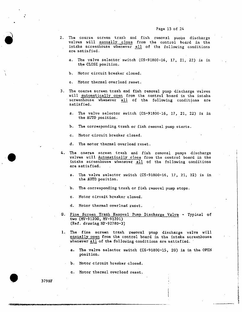
Page 13 of 24

2. The coarse screen trash and fish removal pumps dischargevalves will manually close from the control board in theintake screenhouse whenever all of the following conditionsare satisfied.

a. The valve selector switch (CS-91800-16, 17, 21, 22) is inthe CLOSE position.

b. Motor circuit breaker closed.

c. Motor thermal overload reset.

3. The coarse screen trash and fish removal pump discharge valveswill automatically open from the control board in the intakescreenhouse whenever all of the following conditions aresatisfied.

a. The valve selector switch (CS-91800-16, 17, 21, 22) is inthe AUTO position.

b. The corresponding trash or fish removal pump starts.

c. Motor circuit breaker closed.

d. The motor thermal overload reset.

4. The coarse screen trash and fish removal pumps dischargevalves will Automatically close from the control board in theintake screenhouse whenever all of the following conditionsare satisfied.

a. The valve selector switch (CS-91800-16, 17, 21, 22) is in

the AUTO position.

b. The corresponding trash or fish removal pump stops.

c. Motor circuit breaker closed.

d. Motor thermal overload reset.

G. Fine Screen Trash Removal Pump Discharge Valve - Typical oftwo (MV-91200, MV-91201)(Ref. drawing NF-92780-3)

1. The fine screen trash removal pump discharge valve willmanually open from the control board in the intake screenhousewhenever all of the following conditions are satisfied.

a. The valve selector switch (CS-91800-15, 20) is in the OPENposition.

b. Motor circuit breaker closed.

c. Motor thermal overload reset.

3798F

Page 14 of 24

2. The fine screen trash removal pump discharge valve willmanually close from the control board in the intakescreenhouse whenever all of the following conditions aresatisfied.

a. The valve selector switch (CS-91800-15, 20) is in theCLOSE position.

b. Motor circuit breaker closed.

c. Motor thermal overload reset.

3. The fine screen trash removal pump discharge valve willautomatically open from the control board in the intakescreenhouse whenever all of the following conditions aresatisfied.

a. The valve selector switch (CS-918Y0-15, 20) is in the AUTOposition.

b. The fine screen trash removal pump has started.

c. Motor circuit breaker closed.

d. Motor thermal overload reset.

4. The fine screen trash removal pump discharge valve willautomatically close from the control board in the intakescreenhouse whenever all of the following conditions aresatisfied.

a. The valve selector switch (CS-91800-15, 20) is in the AUTO

postion.

b. The fine screen trash removal pump stops.

c. Motor circuit breaker closed.

d. Motor thermal overload reset.

H. Fine Screen Larvae Removal Pump Discharge Valve - Typical oftwo (MV-91208, MV-91209)(Ref. drawing NF-92780-4)

1. The fine screen larvae removal pump discharge valve willmanually open from the control board in the intake screenhousewhenever all of the following conditions are satisfied.

a. The valve selector switch (CS-91800-57, 58) is in the OPENposition.

b. Motor circuit breaker closed.

c. Motor thermal overload reset.

3798F

Page 15 of 24

2. The fine screen larvae removal pump discharge valve willmanually close from the control board in the intakescreenhouse whenever all of the following conditions are

.satisfied.

a. The valve selector switch (CS-91800-57, 58) is in theCLOSE position.

b. Motor circuit breaker closed.

c. Motor thermal overload reset.

3. The fine screen larvae removal pump discharge valve willautomatically open from the control board in the intakescreenhouse whenever all of the following conditions aresatisfied.

a. The valve selector switch (CS-91800-57, 58) is in the AUTOposition.

b. The fine screen larvae removal pump has started.

c. Motor circuit breaker closed.

d. Motor thermal overload reset.

4. The fine screen larvae removal pump discharge valve willautomatically close from the control board in the intakescreenhouse whenever all of the following conditions aresatisfied.

a. The valve selector switch (CS-91800-57, 58) is in the AUTOposition.

b. The fine screen larvae removal pump has stopped.

c. Motor circuit breaker closed.

d. Motor thermal overload reset.

I. Bypass Gates - Typical for two (CT-062-301, 302)(Ref. drawing NF-92780-5)

1. Either bypass gate will manually open from the local controlbox in the intake screenhouse whenever all of the followingconditions are satisfied:

a. Local control box selector switch is in the LOCAL position.

b. UP pushbutton is depressed on the local control box.

c. Hydraulic accumulator is charged.

3798F

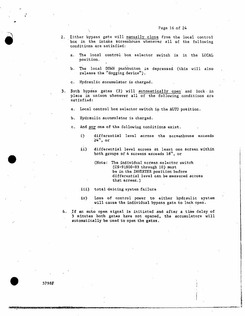
Page 16 of 24

2. Either bypass gate will manually close from the local controlbox in the intake screenhouse whenever all of the followingconditions are satisfied:

a. The local control box selector switch is in the LOCALposition.

b. The local DOWN pushbutton is depressed (this will alsorelease the "dogging device").

c. Hydraulic accumulator is charged.

3. Both bypass gates (2) will automatically open and lock inplace in unison whenever all of the following conditions aresatisfied:

a. Local control box selector switch in the AUTO position.

b. Hydraulic accumulator is charged.

c. And any one of the following conditions exist.

i) differential level across the screenhouse exceeds.24", or

ii) differential level across at least one screen withinboth groups of 4 screens exceeds 18", or

(Note: The individual screenselector switch(CS-91800-03 through 10) mustbe in the INVERTER position beforedifferential level can be measured acrossthat screen.)

iii) total deicing system failure

iv) Loss of control power to either hydraulic systemwill cause the individual bypass gate to lock open.

4. If an auto open signal is initiated and after a time delay of3 minutes both gates have not opened, the accumulators willautomatically be used to open the gates.

3798F

Page 17 of 24

B 1.2.2.2 Deicing System

A. Deicing Pu&ip - Typical for two (CT-045-1041, 1042)(Ref. drawing NF-92781)

1. The deicing pump will manually start from the control board inthe intake screenhouse whenever all of the following* conditions are satisfied:

/

a. Control board pump selector switch (CS-91800-28, 29) ismomentarily in the RUN position.

b. Deice pump discharge valve MV-91206 or MV-92107 havepreviously been manually opened.

c. Motor circuit breaker is closed.

d. Motor thermal overload reset.

2. The deicing pump will manually start from the deicingpumphouse whenever all of the following conditions aresatisfied:

a. The local pump selector switch (CS-91908, CS-91909) ismomentarily in the RUN position.

b. Deice pump discharge valve MV-91206 or MV-92107 havepreviously been manually opened.

c. Motor circuit breaker is closed.

d. Motor thermal overload reset.

3. The deicing pump will stop whenever any of the followingconditions are satisfied:

a. Control board pump selector switch (CS-91800-28, 29) ismomentarily in the STOP position.

b. Local pump selector switch (CS-91908, CS-91909) ismomentarily in the STOP position.

c. Deice pump discharge valves (MV-91206, MV-91207) is closed.

d. Motor circuit breaker is open.

e. Motor thermal overload.

3798F

Page 18 of 24

B. Deicing Pump Discharge Valves - Typical for two (MV-91206,MV-91207)(Ref. drawing NF-92781)

1. The deicing pump discharge valve will manually open from thecontrol board in the intake screenhouse whenever all of thefollowing conditions are satisfied.

a. Control board valve selector switch (CS-91800-18, 19) inthe OPEN position.

b. Motor circuit breaker is closed.

c. Motor thermal overload is reset.

2. The deicing pump discharge valve will manually close from thecontrol board in the intake screenhouse whenever all of thefollowing conditions are satisfied.

a. Control board valve selector switch (CS-91800-18, 19) isin the CLOSE position.

b. Motor circuit breaker is closed.

c. Motor thermal overload is reset.

3. The deicing pump discharge valve will manually open from thedeice building whenever all of the following conditions aresatisfied.

a. The local valve selector switch (CS-91910, 11) is in theOPEN position.

b. Motor circuit breaker is closed.

c. Motor thermal overload is reset.

4. The deicing pump discharge valve will manually close from thedeice building whenever all of the, following conditions aresatisfied.

a. The local valve selector switch (CD-91910, 11) is in theCLOSE position.

c. Motor circuit breaker is closed'.

d. Motor thermal overload is reset.

3798F

h.

Page i9 of 24

B 1.2.2.3 Discharge Structure

A. Sluice Gate - Typical for four (CT-062-391 thru 394)(Ref. drawing NF-92782)

1. The sluice gate will manually open from the plant "MainControl Board" whenever all of the following conditions aresatisfied:

a. Control room selector switch (49060 thru 49063) is in theOPEN position.

b. Local selector switch (91924, 91926, 91928, 19130) is inthe REMOTE position.

c. Motor electrical fault reset.

d. Motor thermal overload reset.

2. The sluice gate will manually close from the plant "MainControl Board" whenever all of the following conditions aresatisfied:

a. Control room selector switch (49060 thru 49063) is in theCLOSE position.

b. Local selector switch (91924, 91926, 91928, 91930) is inthe REMOTE position.

c. Motor electrical fault reset.

d. Motor thermal overload reset.

3. The sluice gate will manually open at the discharge structurewhenever all of the following conditions are satisified:

a. Local selector switch (91924, 91926, 91928, 91930) is inthe LOCAL position.

b. Local selector switch (91925, 91927, 91929, 91931) is in

the OPEN position.

c. Motor electrical fault reset.

d. Motor thermal overload reset.

4. The sluice gate will manually close at the discharge structurewhenever all of the following conditions are satisfied:

a. Local selector switch (91924, 91926, 91928, 91930) is inthe LOCAL position.

3798F

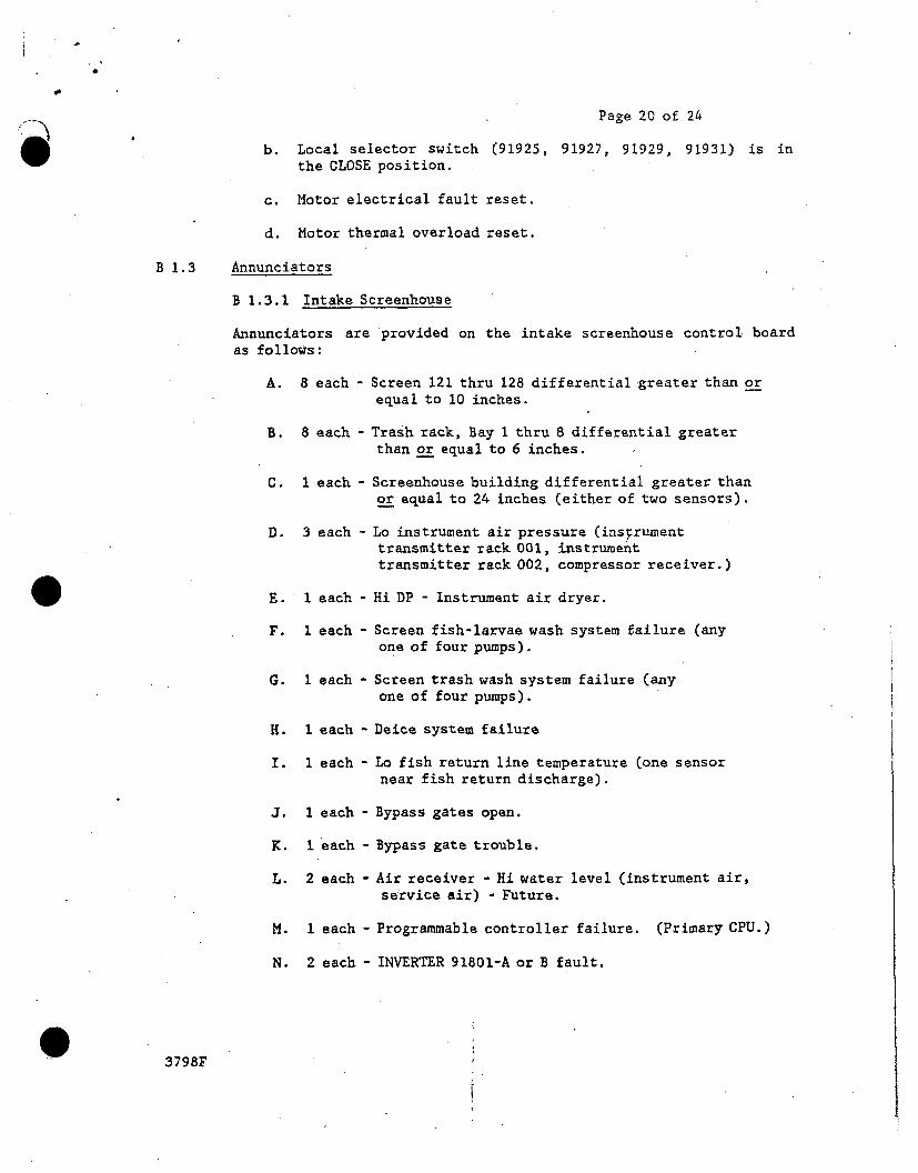
Page 20 of 24

b. Local selector switch (91925, 91927, 91929, 91931) is inthe CLOSE position.

c. Motor electrical fault reset.

d. Motor thermal overload reset.

B 1.3 Annunciators

B 1.3.1 Intake Screenhouse

Annunciators are provided on the intake screenhouse control boardas follows:

A. 8 each - Screen 121 thru 128 differential greater than orequal to 10 inches.

B. 8 each - Trash rack, Bay 1 thru 8 differential greaterthan or equal to 6 inches.

C. 1 each - Screenhouse building differential greater thanor equal to 24 inches (either of two sensors).

D. 3 each - Lo instrument air pressure (instrumenttransmitter rack 001, instrumenttransmitter rack 002, compressor receiver.)

E. 1 each - Hi DP - Instrument air dryer.

F. 1 each - Screen fish-larvae wash system failure (anyone of four pumps).

G. 1 each - Screen trash wash system failure (anyone of four pumps).

H. 1 each - Deice system failure

I. 1 each - Lo fish return line temperature (one sensornear fish return discharge).

J. 1 each - Bypass gates open.

K. I each - Bypass gate trouble.

L. 2 each - Air receiver - Hi water level (instrument air,service air) - Future.

M. 1 each - Programmable controller failure. (Primary CPU.)

N. 2 each - INVERTER 91801-A or B fault.

3798F

Page 21 of 24

0. 1 each - Screenhouse load center trouble.

P. I each - Envir Lab Basement

Q. 1 each - Lock and Dam #3 Equipment Problem

B 1.3.2 Main Control Room

Annunciators using existing spare windows are provided on theplant "Main Control Board" as follows:

A. Screen differential greater than or equal to 10 inches.

B. Screenhouse differential greater than or equal to 24inches.

C. Bypass gates. open.

D. General alarm - screenhouse.

E. Bypass gate trouble.

B 1.4 Indicators

B 1.4.1 Screenhouse Control Board IndicationThe following variables will be displayed on the intakescreenhouse control board.

A. 2 - Building differential level (one from each of twosensors).

B. 8 - Screen differential level (one from each of eightsensors).

C. 8 - Trash rack differential level (one from each of eightsensors). /

D. 1 - Fish return line discharge temperature.

E. 2 - Screen speed (one for each bank of 4 screens).

B 1.4.2 "Mimic Bus Insert" IndicationThe following variables will be added to the display in theplant control room.

A. Intake river temperature.

B. Traveling water screen RUN/STOP.

C. Bypass gate OPEN/CLOSE.

D. Deice pumps RUN/STOP.

03798F

r-

.4

4 f

Page 22 of 24

E. Deice pump discharge valve OPEN/CLOSE.

F. Average - discharge temperature.

G. Discharge flow rate.

H. Discharge canal level.

Note: These signals are in addition to signals already includedin the control room.

Instrumentation I/O for screenhouse programmable controller(PC)

B 1.5

B 1.5.1 Analog Input

A. Trash Rack Differential Pressure

Instrument: 8 each - Foxboro Model 823, 2-wire,pressure transmitter, span set at 0-25 inches watermade output to PC.

differentialequals 4-20

B. Travelinx Screen Differential Pressure

Instrument: 8 each - Foxboro Model 823, 2-wire,pressure transmitter, span set at 0-25 inches watermadc output to PC.

differentialequals 4-20

C. Screenhouse Differentail Pressure

Instrument: 2 each - Foxboro Model 823, 2-wire, differentialpressure transmitter, span set at 0-25 inches water equals 4-20made output to PC.

D. Screenhouse Intake Level

Instrument: 1 each - Drexelbrook admittance level probe andtransmitter, 2 wire, span set at 0-13 feet equals 4-20 madc outputto PC.

E. Discharge Canal Level

Instrument: 1 each - Drexelbrook admittance level probe andtransmitter, 2 wire, span set at 0-13 feet equals 4-20 madc outputto PC.

F. Discharge Temperature

Instrument: 4 each - Action Pak model TP621N 052 - Type TThermocouple transmitter, span set at 0-180 degree F equals 4-20made output to PC.

3798F

Page 23 of.24

G. Fish Return Line Temperature

Instrument: 1 each - Action Pak model TP621N 052 - Type TThermocouple transmitter, span set at 0-180 degree F equals 4-20made output to PC.

B 1.5.2 Digital Input (120 Volt)

A. Discharge Gate (Open or Close)

4 each - 1 open limit switch (normally open) per discharge gate, 4discharge gates total, contact closure indicates gate not closed.

B. Screen Drive Inverter Fault

2 each - I normally closed contact per each inverter drive, 2inverter drives total, contact closure indicator inverter fault.

B 1.5.3 Analog Output (4-20 madc)

A. Screen Drive Inverter Signal

2 each - 4 to 8 inches water differential pressure across any oneof four screens in the INVERTER mode will cause a correspondingoutput of 4-20 madc to the appropriate screen drive inverter.

B. Screenhouse Intake Level - Mimic

1 each - PC input change of 4-20 madc (0-13 ft. span) will cause acorresponding output of 4-20 madc to the main plant Mimic BusInsert.

C. Discharge Canal Level - Mimic

1 each - PC input change of 4-20 madc (0-13 ft. span) will cause acorresponding output of 4-20 madc to the main plant Mimic BusInsert.

D. Plant Discharge Flow - Mimic

1 each - PC output of 4 to 20 made to correspond to 0-1500 cfs byusing the following calculation:

-(Ks Is + Ks Is + K7 I, + Ka I,) [1Isi-hI]

379BF

PRAIRIE ISLAND NUCLEAR GENERATING PLANT

ENVIRONMENTAL MONITORING

AND

ECOLOGICAL STUDIES PROGRAM

2006 ANNUAL REPORT

Prepared for

Northern States Power Company d/b/a Xcel Energy

Minneapolis, Minnesota

By

Environmental Services

Water Quality Department

.

¾

TABLE OF CONTENTS

Water Temperature and Flow ............................. Section I

Summary of the Fish Population Study ................... Section II

SECTION I

PRAIRIE ISLAND NUCLEAR GENERATING PLANT

ENVIRONMENTAL MONITORING PROGRAM'2006 ANNUAL REPORT

WATER TEMPERATURE AND FLOW

Report

by'B. D. Giese

Environmental Services

Water Quality Department

WATER TEMPERATURE AND FLOW

INTRODUCTION AND METHODS

The Mississippi River is the source-water body for circulating and cooling water systems at thePrairie Island Nuclear Generating Plant (PINGP). This report presents daily plant operating

hours, river inlet temperatures, site discharge temperatures and flows (blowdown). Sitedischarge temperatures are determined by thermocouples located downstream at U.S. ArmyCorps of Engineers Lock and Dam 3. Plant inlet (ambient river) temperatures are determined by

remote sensors located in Sturgeon Lake, and the main channel at Diamond Bluff. Inlettemperatures are also recorded from thermocouples located in front of the intake screenhouse,which are maintained for back-up. Data presented in this report are for environmental studies

comparison, and are not intended as NPDES temperature compliance reporting.

Also presented in this report are daily and monthly average Mississippi River flows, as providedby U.S. Army Corps of Engineers at Lock and Dam 3. Other monthly averages reported include

PINGP intake flows, and the percentage of Mississippi River water entering the plant.

RESULTS AND DISCUSSION

Daily average river inlet and site discharge temperature data are presented by month in Table 1.

Daily Mississippi River flows recorded at Lock and Dam 3 ranged from 2,400 to 65,100 cfs in2006 (Table 2). Daily mean site discharge flow (blowdown) from the PINGP external circulating

water log ranged from 141 to 1,208 cfs (Table 1).

PINGP withdrew an annual average of 4.5 percent of the Mississippi River flow during 2006(Table 3). Table 4 shows the monthly average Mississippi River flows for the years 1985through 2006. The average river flow in 2006 was 17,800 cfs, which was lower than the averageriver flow of 22,100 cfs for years 1985-2005. The range of annual average river flows is 8,709

cfs in 1988 to 37,772 cfs in 1986.

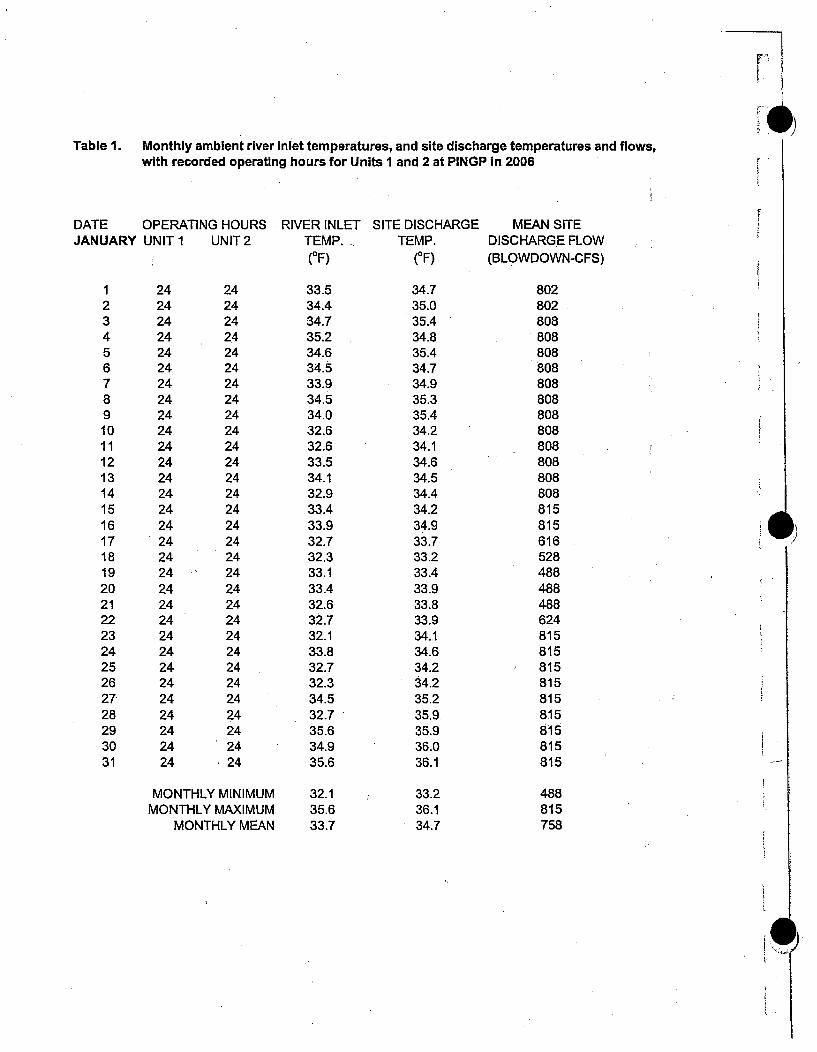
4Table 1. Monthly ambient river inlet temperatures, and site discharge temperatures and flows,

with recorded operating hours for Units 1 and 2 at PINGP in 2006

DATE OPERATING HOURSJANUARY UNIT I UNIT 2

12345678910111213141516171819202122232425262728293031

24242424242424242424242424242424242424242424242424242424242424

24242424242424242424242424242424242424242424242424242424242424

RIVER INLETTEMP.(OF)

33.534.434.735.234.634.533.934.534.032.632.633.534.132.933.433.932.732.333.133.432.632.732.133.832.732.334.532.735.634.935.6

SITE DISCHARGETEMP.

(OF)

34.735.035.434.835.434.734.935.335.434.234.134.634.534.434.234.933.733.233.433.933.833.934.134.634.234.235.235.935.936.036.1

MEAN SITEDISCHARGE FLOW(BLOWDOWN-CFS)

802802808808808808808808808808808808808808815815616528488488488624815815815815815815815815815

MONTHLY MINIMUMMONTHLY MAXIMUM

MONTHLY MEAN

32.135.633.7

33.236.134.7

488815758

Table 1. Monthly ambient river inlet temperatures, and site discharge temperatures and flows,with recorded operating hours for Units I and 2 at PINGP in 2006

DATE OPERATING HOURSFEBRUARY UNIT 1 UNIT 2

12345678910111213141516171819202122232425262728

24242424242424242424242424242424242424242424242424242424

24242424

23.5000000000000000

2124242424242424

RIVER INLETTEMP.(CF)

35.935.035.133.032.232.132.632.232.131.932.532.531.932.732.532.432.331.531.331.731.832.332.532.231.931.833.132.5

SITE DISCHARGETEMP.

(CF)

36.235.635.833.933.632.733.033.133.033.133.133.033.133.033.032.932.833.332.832.833.033.733.934.034.434.835.035.0

MEAN SITEDISCHARGE FLOW(BLOWDOWN-CFS)

815828815815828413413413413413392392360413413423402402540475500855869869869869869869

MONTHLY MINIMUMMONTHLY MAXIMUM

MONTHLY MEAN

31.335.932.6

32.736.233.7

360869605

F•

Table 1. Monthly ambient river inlet temperatures, and site discharge temperatures and flows,with recorded operating hours for Units I and 2 at PINGP In 2006

DATE OPERATING HOURSMARCH UNIT 1 UNIT2

12345678910111213141516171819202122232425262728293031

24242424242424242424242424242424242424242424242424242424242424

24242424242424242424242424242424242424242424242424242424242424

RIVER INLETTEMP.(CF)

31.334.634.333.735.534.835.636.436.636.238.738.4

35.334.034.034.733.634.835.136.735.936.038.338.338.738.439.638.840.742.641.8

SITE DISCHARGETEMP.

(OF)

35.436.035.936.636.635.936.437.2"37.838.340.239.236.435.235.035.034.835.836.437.337.136.738.338.639.239.540.440.241.943.943.8

MEAN SITEDISCHARGE FLOW(BLOWDOWN-CFS)

869869889855855855855855869815815882882838815822822822855842849849849849849846869869875875875

MONTHLY MINIMUMMONTHLY MAXIMUM

MONTHLY MEAN

31.342.636.6

34.843.937.8

815889853

Table 1. Monthly ambient river inlet temperatures, and site discharge temperatures and flowslwith recorded operating hours for Units I and 2 at PINGP in 2006

DATE OPERATING HOURS RIVER INLET SITE DISCHARGE MEAN SITEAPRIL UNIT 1 UNIT 2 TEMP. TEMP. DISCHARGE FLOW

(OF) (OF) (BLOWDOWN-CFS)

1 24 24 41.4 42.5 8752 *23 *23 41.6 42.6 8693 24 24 39.9 41.7 8624 24 24 39.6 42.0 8825 24 24 39.7 42.7 8626 24 24 41.7 43.4 8627 24 24 42.5 44.6 8628 24 24 42.3 44.5 8629 24 24 43.6 46.1 86910 24 24 45.5 47.8 86911 24 24 47.5 50.0 86912 24 24 49.2 52.2 86913 24 24 49.9 52.6 82214 24 24 51.6 54.8 68415 24 24 52.4 54.7 29116 24 24 53.5 55.5 29117 24 24 53.8 55.6 291 918 24 24 54.5 56.5 26719 24 24 56.0 57.4 14420 24 24 55.3 56.8 14121 24 24 54.9 56.8 29122 24 24 54.5 56.2 28323 24 24 55.7 56.7 26724 24 24 57.2 62.1 29925 24 24 55.0 56.6 28326 24 24 56.4 57.4 29127 24 24 56.7 58.1 29128 24 24 58.2 58.8 27529 3.6 24 56.8 57.3 28330 0 24 56.1 56.6 275

* Daylight savings

MONTHLY MINIMUM 39.6 42.0 141MONTHLY MAXIMUM 58.2 58.8 882

MONTHLY MEAN 50.1 52.0 539

F-

ri

Table 1. Monthly ambient river inlet temperatures, and site discharge temperatures and flows,with recorded operating hours for Units 1 and 2 at PINGP in 2006

DATE OPERATING HOURS RIVER INLET SITE DISCHARGEMAY

12345678910111213141516171819202122232425262728293031

UNIT I UNIT 2

0

00000000000000000000000000000

24242424242424242424242424242424242424242424242424242424242424

TEMP.(OF)

55.756.257.856.855.655.756.657.958.959.559.156.155.554.756.356.658.258.159.059.559.660.160.662.864.766.568.268.972.572.473.5

TEMP.(OF)

56.356.457.857.555.856.457.958.259.659.459.256.755.655.755.957.959.160.160.361.860.760.962.964.666.267.470.071.272.474.074.4

MEAN SITEDISCHARGE FLOW(BLOWDOWN-CFS)

291291

,291283283283283283283283283283283283283283283299299299299299291291299275283291291291275

MONTHLY MINIMUMMONTHLY MAXIMUM

MONTHLY MEAN

54.773.560.4

55.774.461.4

275299288

.Table 1. Monthly ambient river Inlet temperatures, and site discharge temperatures and flows,

with recorded operating hours for Units I and 2 at PINGP In 2006

DATE OPERATING HOURS RIVER INLET SITE DISCHARGEJUNE UNIT 1 UNIT 2

123456789101112131415161718192021222324252627282930

00000

15.9242424242424242424242424242424242424242424242424

242424242424242424242424242424242424242424242424242424242424

TEMP.(OF)

74.974.775.275.273.774.175.175.874.670.567.168.969.871.671.2,71.673.374.273.373.373.774.074.074.373.373.374.073.074.575.0

TEMP.(OF)

75.675.875.974.974.674.476.176.674.471.169.468.571.172.372.072.874.475.474.974.074.174.373.974.473.773.574.374.374.775.9

MEAN SITEDISCHARGE FLOW(BLOWDOWN-CFS)

384396396384396396396434423392392392392392392760760760768760760760760760760768776768760760

0)

MONTHLY MINIMUMMONTHLY MAXIMUM

MONTHLY MEAN

67.175.873.2

69.476.673.9

384776580

9)

Table 1. Monthly ambient river inlet temperatures, and site discharge temperatures and flows,with recorded operating hours for Units I and 2 at PINGP in 2006

DATE OPERATING HOURSJULY UNIT 1 UNIT2

12345678910111213141516171819202122232425262728293031

24242424242424242424242424242424242424242424242424242424242424

24242424242424242424242424242424242424242424242424242424242424

RIVER INLETTEMP.C0F)

76.077.077.377.676.275.977.177.477.277.078.277.678.778.680.281.680.779.879.677.378.077.777.478.978.980.180.881.383.283.582.7

SITE DISCHARGETEMP.

(OF)

77.477.979.378.477.978.278.678.778.978.679.679.281.082.181.783.082.781.681.479.880.078.979.881.381.481.982.883.885.885.283.6

MEAN SITEDISCHARGE FLOW(BLOWDOWN-CFS)

869118011801180118011941194119411941194119411941194119411941194119411941194119411941194119411941194119411941194119411941194

MONTHLY MINIMUMMONTHLY MAXIMUM

MONTHLY MEAN

75.983.578.8

78.285.280.7

86911941182

L,

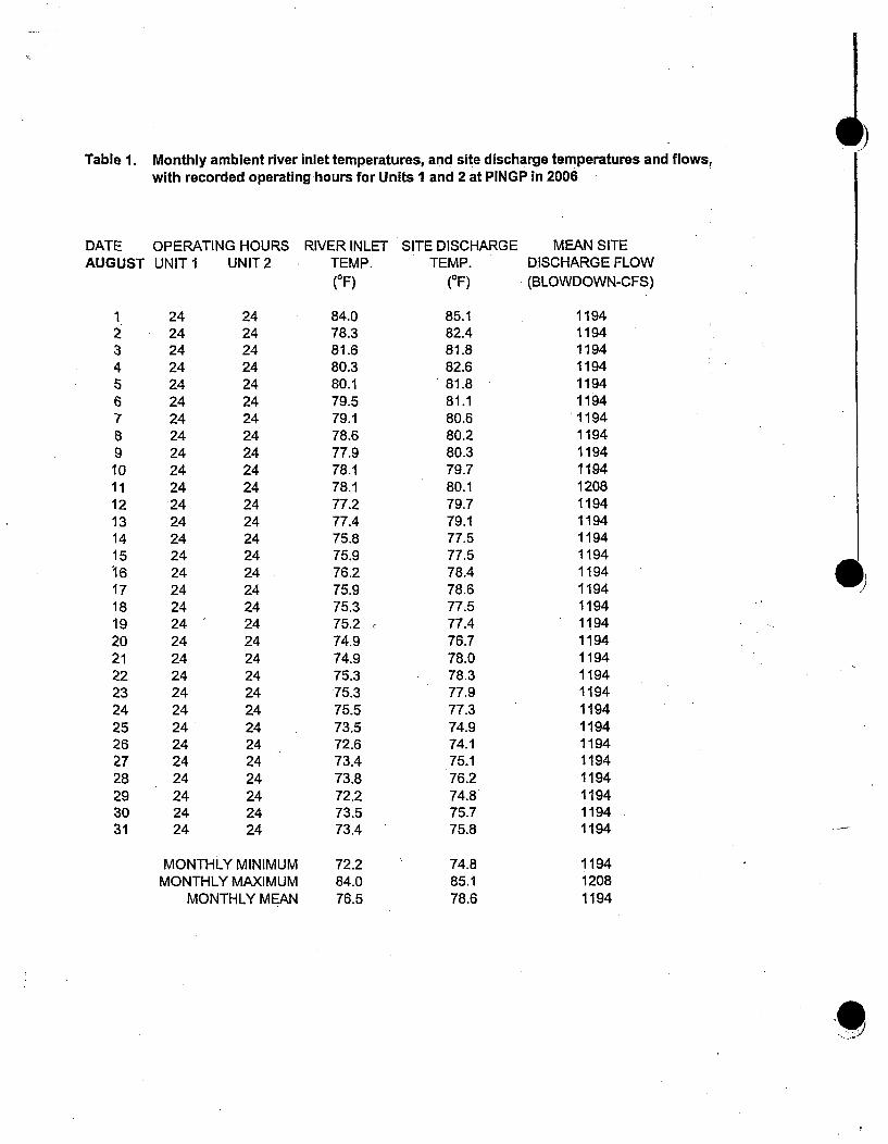
Table 1. Monthly ambient river inlet temperatures, and site discharge temperatures and flows,with recorded operating hours for Units 1 and 2 at PINGP in 2006

DATE OPERATING HOURS RIVER INLET SITE DISCHARGEAUGUST UNIT 1 UNIT 2 TEMP.

(OF)TEMP.

(OF)

1

12

345678910111213141516171819202122232425262728293031

24242424242424242424242424242424242424242424242424242424242424

24242424242424242424242424242424242424242424242424242424242424

84.078.381.680.380.179.579.178.677.978.178.177.277.475.875.976.275.975.375.274.974.975.375.375.573.572.673.473.872.273.573.4

72.284.076.5

85.182.481.882.681.881.180.680.280.379.780.179.779.177.577.578.478.677.577.476.778.078.377.977.374.974.175.176.274.875.775.8

74.885.178.6

MEAN SITEDISCHARGE FLOW(BLOWDOWN-CFS)

1194119411941194119411941194119411941194120811941194119411941194119411941194119411941194119411941194119411941194119411941194

119412081194

0)r

MONTHLY MINIMUMMONTHLY MAXIMUM

MONTHLY MEAN

F

Table 1. Monthly ambient river inlet temperatures, and site discharge temperatures and flows,with recorded operating hours for Units I and 2 at PINGP In 2006

DATE OPERATING HOURSSEPTEMBER UNIT 1 UNIT 2

RIVER INLETTEMP.(OF)

SITE DISCHARGETEMP.

(OF)

MEAN SITEDISCHARGE FLOW(BLOWDOWN-CFS)

123456789101112131415161718192021222324252627282930

242424242424242424242424242424242424242424242424242424242424

242424242424242424242424242424242424242424242424242424242424

72.972.473.271.472.072.872.773.470.868.766.765.164.865.265.766.367.666.464.161.561.560.159.560.160.360.661.360.359.658.9

76.175.375.373.774.575.175.475.472.471.469.367.366.868.369.269.670.467.964.464.265.162.960.960.663.263.463.061.361.760.6

60.675.468.2

11941180118011941194119411941194119411941194118011801180118011801180 (1152113811381138115211521152115211521152115211521012

101211941166

MONTHLY MINIMUMMONTHLY MAXIMUM

MONTHLY MEAN

58.973.465.9

Table 1. Monthly ambient river inlet temperatures, and site discharge temperatures and flows,with recorded operating hours for Units 1 and 2 at PINGP in 2006

DATE OPERATING HOURS RIVER INLET SITE DISCHARGE MEAN SITEOCTOBER UNIT I UNIT 2 TEMP. TEMP. DISCHARGE FLOW

(OF) (OF) (BLOWDOWN-CFS)

1 24 24 59.1 60.9 10122 24 24 61.1 63.3 11663 24 24 62.2 64.5 11804 24 24 62.2 65.1 11805 24 24 61.2 64.0 11806 24 24 60.6 63.4 11807 24 24 60.0 61.9 11808 24 24 60.4 62.2 11809 24 24 59.3 60.8 1194

10 24 24 57.8 59.4 119411 24 24 56.9 57.9 119412 24 24 52.2 53.7 119413 24 24 49.8 50.9 119414 24 24 47.4 48.5 108215 24 24 46.7 49.1 108216 24 24 49.2 51.7 111017. 24 24 48.8 52.2 1110 *

18 24 24 49.8 50.6 111019 24 24 49.0 50.7 111020 24 24 49.4 51.6 12421 24 24 49.0 51.8 108222 24 24 46.7 49.3 108223 24 24 46.9 49.2 106824 24 24 45.2 48.8 112425 24 24 45.3 49.5 112426 24 24 46.1 49.1 112427 24 24 45.6 49.1 112428 24 24 45.8 49.6 112429 *25 *25 46.2 49.4 112430 24 24 46.5 50.1 112431 24 24 45.0 48.7 1124

* Daylight savingsMONTHLY MINIMUM 45.0 48.7 1012

MONTHLY MAXIMUM 62.2 65.1 1194MONTHLY MEAN 52.0 54.4 1135

I

Table 1. Monthly ambient river inlet temperatures, and site discharge temperatures and flows,with recorded operating hours for Units I and 2 at PINGP in 2006

DATE OPERATING HOURSNOVEMBER UNIT 1 UNIT2

123456789101112131415161718192021222324252627282930

242424242424242424242424242424242424242424242424242424242424

24242424242424242424242424

20.30000000000000000

RIVER INLETTEMP.(OF)

43.542.139.841.741.842.244.045.646.345.143.842.642.339.840.941.739.041.339.539.240.440.540.341.540.740.441.942.241.437.3

SITE DISCHARGETEMP.

(CF)

47.445.443.844.545.446.647.549.450.847.747.247.545.344.742.442.142.341.741.340.541.541.941.842.642.741.842.443.742.338.1

MEAN SITEDISCHARGE FLOW(BLOWDOWN-CFS)

111011101082967967973967973973973973973973973955880880392392392392392392381381381392392392381

MONTHLY MINIMUMMONTHLY MAXIMUM

MONTHLY MEAN

37.346.341.6

38.150.844.1

3811110725

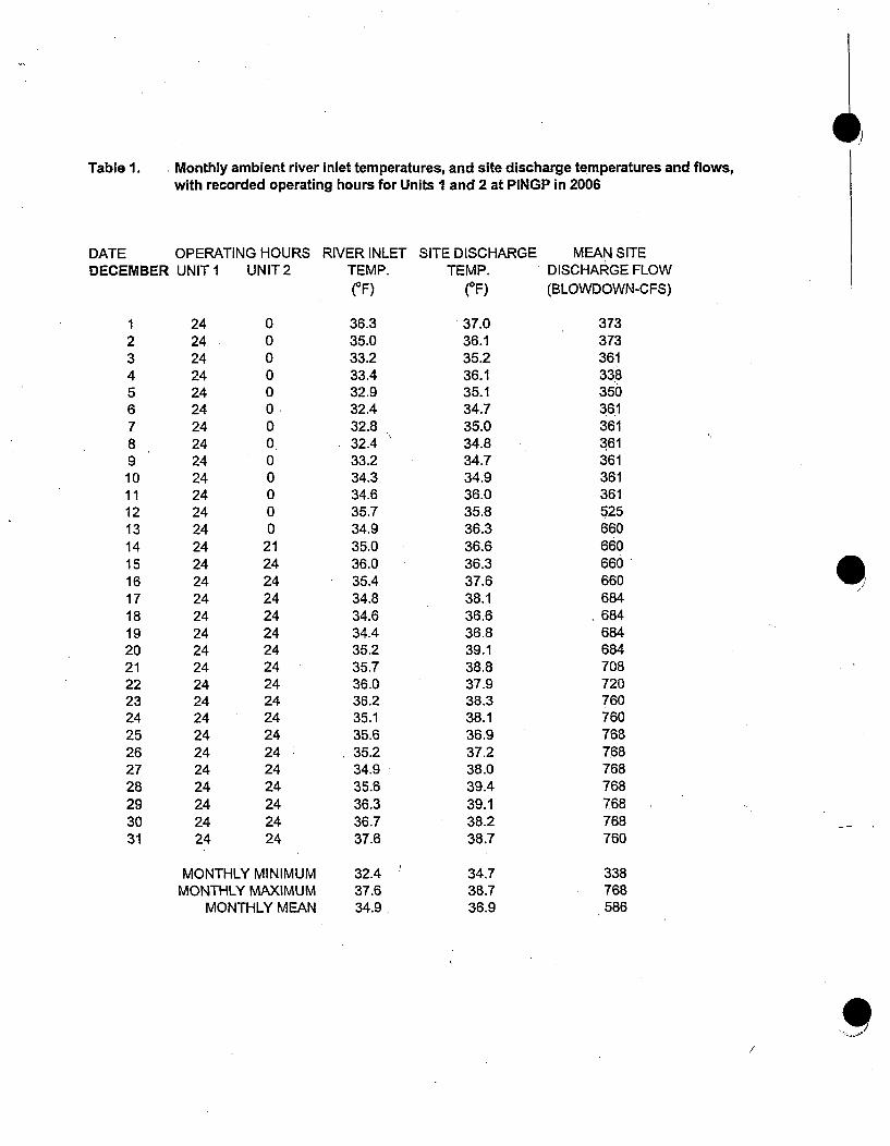
Table 1. Monthly ambient river inlet temperatures, and site discharge temperatures and flows,with recorded operating hours for Units I and 2 at PINGP in 2006

DATE OPERATING HOURS RIVER INLET SITE DISCHARGE MEAN SITEDECEMBER UNIT 1 UNIT 2 TEMP. TEMP. DISCHARGE FLOW

(OF) (OF) (BLOWDOWN-CFS)

1 24 0 36.3 37.0 3732 24 0 35.0 36.1 3733 24 0 33.2 35.2 3614 24 0 33.4 36.1 3385 24 0 32.9 35.1 3506 24 0 32.4 34.7 3617 24 0 32.8 35.0 3618 24 0 32.4 34.8 3619 24 0 33.2 34.7 36110 24 0 34.3 34.9 36111 24 0 34.6 36.0 36112 24 0 35.7 35.8 52513 24 0 34.9 36.3 66014 24 21 35.0 36.6 66015 24 24 36.0 36.3 66016 24 24 35.4 37.6 66017 24 24 34.8 38.1 68418 24 24 34.6 36.6 68419 24 24 34.4 36.8 68420 24 24 35.2 39.1 68421 24 24 35.7 38.8 70822 24 24 36.0 37.9 72023 24 24 36.2 38.3 76024 24 24 35.1 38.1 76025 24 24 35.6 36.9 76826 24 24 35.2 37.2 76827 24 24 34.9 38.0 76828 24 24 35.6 39.4 76829 24 24 36.3 39.1 76830 24 24 36.7 38.2 76831 24 24 37.6 38.7 760

MONTHLY MINIMUM 32.4 34.7 338MONTHLY MAXIMUM 37.6 38.7 768

MONTHLY MEAN 34.9 36.9 586

0,Table 2 Daily 2006 Mississippi River Discharge Flow rate (cfs) at Lock Dam 3

1

2

3

4

5

6

78

9

10

11

12

13

14

15

16

17

18

19

20

21

22

23

24

25

-26

27

28

29

30

31

MIN

JAN FEB

18100 19300

18500 22800

18500 22600

18400 24300

19300 23400

19800 22300

19000 21400

18800 21400

18900 21100

18600 20200

18500 20100

17600 20300

18100 19600

19000 18000

17800 18300

18100 18300

19200 17600

18400 11600

17500 12300

17400 13600

17300 13800

16600 14300

16600 15800

15800 15700

15900 16500

15400 15900

15200 14800

15600 13900

17100

18000

18500

15200 11600

MAR

13800

13700

14000

13800

13200

13600

14100

14200

16000

15800

15600

17100

21001

24100

22800

22500

22800

23500

23500

23300

23200

23400

24000

24100

24100

23500

23700

24700

27700

31700

35500

APR

38500

36200

36900

42200

48200

54600

59700

63100

64300

64700

65100

65100

64500

63600

62500

61800

60600

58900

56900

54400

51500

49200

46900

44500

42600

40700

38600

36900

35200

34500

34500

65100

51400

MAY JUN JUL

33900 28300 14800

34300 26400 13700

35000 25500 12500

36400 24200 11500

38000 23100 11500

39900 21800 9600

41800 23000 9000

43500 21300 9100

45300 18800 10500

47200 18800 8900

48400 18500 7600

49000 20300 7700

48800 20000 8300

48700 20100 3200

48400 20700 7000

48300 19100 7000

48200 18600 7000

48000 22200 6200

47300 21900 5400

46400 23700 7000

45000 25000 6900

43500 24900 6200

41900 23800 6200

38000 23300 5500

36100 22300 6900

33400 20700 6900

32600 19300 6900

32100 17700 6200

31200 16500 3900

31000 15500 2400

29300 6300

29300 15500 2400

49000 28300 14800

41000 21500 7800

AUG

6300

15000

17400

11900

6700

5300

9700

10300

6900

7000

6900

3900

9000

6900

6900

5400

4700

5500

5500

6100

6100

5400

5400

6900

10200

11500

7400

7500

6200

7000

6200

SEP

4700

5500

6300

10000

8300

5400

5500

7100

7500

4600

4700

5500

5500

5400

4700

4600

6100

7600

7000

3100

3200

6100

11300

8300

6900

7800

9300

8400

6900

6300

OCT

84008300

8200

6900

6800

6800

5400

7000

9200

6900

5500

7100

6900

6400

6300

5500

7000

9400

9800

6100

8400

'9000

6800

6900

6200

7000

7800

7800

6900

6900

7200

NOV DEC

6300 8400

7900 8400

7700 4700

6900 3200

6900 3700

6900 4600

6900 4500

6200 4500

7100 6900

8500 7800

8400 7100

4600 7300

6200 8100

6900 7900

7000 7200

7700 7000

7700 7200

7000 7300

7000 7700

7800 7500

6900 6800

6800 8100

-6900 8900

6900 7400

7000 7200

7000 7100

7000 6500

7500 6400

7800 6600

8600 6800

7100

4600 3200

MAX 19800 24300

MEAN 17800 18200

13200

35500

20800

3900 3100 5400

17400 .11300 9800 8600 8900

7600 6500 7300 7100 6800

YEAR MAX

YEAR MIN

65100

2400.1

11Table 3 2006 Percentage of mean monthly Mississippi River flow entering theXcel Energy Prairie Island Generating Plant intake

Mean Plant Flow Mean River Flow Percentage of Mean River FlowMonth (cfs) (cfs) Entering the Plant IntakeJanuary 758 1:7800 4.3%February 605 18200 3.3%March 853 20800 4.1%April 539 51400 1.0%May 288 41000 0.7%June 580 21500 2.7%

1182 7800 15.2%August 1194 7600 15.7%September 1166 6500 17.9%October 1135 7300 15.5%November 725 7100 10.2%December 586 6800 8.6%Averages 801 17800 4.5%

0

9

Table 3sectionl 2006.docI

Table 4. Mean Monthly Mississippi River Flow for 1985 - 2006, in cubic feet per second (cfs).

Month 2006 2005 2004 2003 2002 2001 2000 1999 1998 1997 1996January 1780 9,900 6,700 929 10,932 11271 8,7 1079 9,806 14831,2February 1820 1160 6,700 7,87 1010 1047 9,548 12,589 14,911 13,95 15,041March 20,800 1470 15,000 13,210 11,497 10,948 22,219 17,897 2657 24,177 2,7April 51,400 4470 24,700 25,613 40,657 1273 15,570 4201 51,477 106,073 57,517

Ma 4100 3,0 19,400 4219 33,974 8261 18,839 4742 2268 39,316 46,535June 21,500 39,200 46,000 27,413 26,323 53,177 22,070 34,423 25,690 1948 33790July 7,800 21,900 19,500 32,739 34,597 23,981 21,052 2754 2647 36,119 2,3August 7,0 9,800 10,600 1008 2906 12,16 10,026 24,432 10,742 2807 3,0Septemi-ber 6,500 15,200 19,200 7,07 24,51 9,9 6,687 18,013 7,060 1666 930October 7,300 3590 19,500 6,771 28,600 9,577 6,9 14,200 12,597 14,155 1140November 7,0 1920 21,900 8,167 18,467 11,040 17,463 13,24 19,773 23,353December 6,800 19,10 12,300 8,31 12,135 13,813 9,558 9,671 15,645 12,694 1,1Averages 17,800 1 22,700 18,500 16,557 23,405 30,083 14,066 22,687 20,286 28;308 1 24,333

Mouth 1995 1994 1993 1992 1991 1990 1989 1988 1987 1986 1985January 11,365 13,090 9,326 15,658 5,542 4,965 6,294 7,303 13,758 13,1710 12,526

February 9,371 12,61-1 8,936 13,978 5,879 4,889 6,529 7,634 12,586 12,804 10,239

March 29,061 28,542 12,513 43,661 15,081 17,484 11,300 14,810 17,287 24,790 32,265

April 48,507 40,830 55,473 32,668 34,268 12,842 33,264 21,463 20,267 84,870 45,317

May 45,135 47,548 48,571 25,474 44,753 22,310 24,287 13,119 13,655 817242 43,518

June 30,667 26,913 65,377 17,920 44,960 31,610 13,237 4,667 14,573 37,043 30,105

July 27,323 29,403 84,123 28,985 33,856 20,323 7,'690 2,903 11,674 34,684 25,676

August 29;129 19,971 41,135 14,532 21,535 16,322 4,658 5,103 10,477 301,813 18,226

September- 19,860'- 21,203 30,717 15,686 25,182 9,923 8,307 6,080 7,183 41,957 29,665October 31,061 25,581 19,516 15,374 15,458 11,135 6,358 7,019 7,771 49P319 39,590

INovember 30,703 1 20,173 18,773 19,076 1 22,467 1 9,903 1 6,793 1 7,919 8,693 1 24,260 121,337

Decemnber 17,494 14,432 16,490 12,126 20,503 6,184 4,961 6,487 9,016 17 ,774 16,094

Avrgs 27,473 f 25,025 34,246 21,262 24,124 13,991 11,140 8,709 12,245 37-,772 27,047

Note: Mean monthly river flow data for the years 1985, 1990,Table 2 of the corresponding annual report for each year.

1991 and 1992 have been adjusted to reflect the averages found in

SECTION II

PRAIRIE ISLAND NUCLEAR GENERATING PLANT

ENVIRONMENTAL MONITORING PROGRAM

2006 ANNUAL REPORT

SUMMARY OF THE 2006 FISH POPULATION STUDY

Report

by

B. D. Giese

Environmental Services

Water Quality Department

0"T

SUMMARY OF THE 2006 FISH POPULATION STUDY

INTRODUCTION

To fulfill part of the continuing environmental monitoring requirements of the Prairie Island

Nuclear Generating Plant, (PINGP), the Mississippi River fisheries population was sampled nearRed Wing, Minnesota, May through October, 2006. The study area extends from 3.6 milesupstream of the plant (River mile 802) to 10.8 miles downstream of the plant (River mile 787.5),

(Figure 1). The original objective of the study was to "determine existing ecological

characteristics before plant operation and to assess any significant changes to the aquaticenvironment after operation" (NSP 1972). The objective was changed slightly after the plant

became operational in 1973; to "determine environmental effects of the PINGP on the fishcommunity in the Mississippi River and it's backwaters" (Hawkinson 1973). Presently, the

objective is to monitor and assess the status of the fishery in the vicinity of the PINGP (Mueller1994). Parameters analyzed and compared to previous years include species composition,

length-weight regressions, percent contribution (fish/hr), length-frequency distributions, and

catch per unit effort (CPUE) for selected species.

METHODS AND MATERIALS

Fish were collected using a Smith-Root SR-18 Electrofishing boat equipped with a 5.0 GPP

electrofishing unit (Figure 6). The power source was a 5.0 GPP generator. The 5000 watt

generator has a maximum output of 16 amps, and a range of 0-1000 volts. The generator has thecapability to be either pulsed AC or DC with a pulse frequency of 7.5, 15, 30, 60, and 120 Hz.

The annode consists of two umbrella arrays, each with six dropper cables. The 18 foot boat and

dropper cables hung from the front of the boat serve as the cathode. Collection occurred duringdaylight hours with a pulsed direct current. Due to the constantly changing river conditions,

Electrofisher output was varied to enhance the effectiveness.

Sampling was done monthly, May through October, within four established sectors of the studyarea (Figures 1-5). The runs within each sector are similar to previous years sampling to ensure a

similar set of relative data indices for yearly comparison. At the end of each "run", the elapsedshocking time was recorded from a digital timer, which only tallied the seconds that the electrical

field was energized. A run was terminated after approximately 450 seconds shocking time or

when the end of the prescribed run was reached.

Stunned fish were captured with one-inch stretch mesh landing nets equipped with eight-foot

insulated handles. Fish were placed in live-wells, supplied with river water constantly, until the

end of each run. At the end of each run fish were identified, measured to the nearest millimeter(total length), weighed to the nearest 10 grams, and released. Parameters used to describe the

fisheries include species composition, length-weight regressions, percent contribution, length-

frequency distributions, and catch per unit effort (CPUE). It is assumed that population

dynamics and spatial distribution is represented by CPUE.

Electro fishing CPUE was computed as numbers of fish per hour for each sector. Length

frequencies in 20 millimeter intervals were calculated for all fish species. Length-weight

relationships were calculated using the length-weight formula:

logW= log a+b logL,

where W is the weight in grams, a is the y axis intercept, b is the slope of the regression line, and

L is the total length in millimeters.

RESULTS

Initial PINGP preoperational annual environmental reports simply listed all data collected

without discussion or analysis (NSP 1972). Individual species were not discussed, due to the

amount of data collected during initial sampling efforts. Representative species were selected in

1975 for abundance comparisons based on electrofishing data (Gustafson et. al. 1975), modified

in 1986 after seining was eliminated (Donkers 1986), and in 1989 smallmouth and largemouth

bass were added as they "have been seen more frequently in the electrofishing catch during recent

years in the PINGP study area" (Mueller 1989).

Electrofishing collection methods changed before the 1982 sampling season. The mesh size of the dip

nets was increased to one inch stretch mesh. The larger mesh size enabled small adult fish and some

young of the'year fish of certain species to avoid collection. Currently, individual gizzard shad,

freshwater drum, and white bass less than 160 mm are not collected. Also, logperch and cyprinids (other

than carp) are no longer collected, due to their small size (Donkers 1987). Therefore, a direct

comparison of electrofishing CPUE prior to 1982 is inappropriate to later years.

Species collected in 2006 are compared to previous years in Table 1. A total of 7,124 fish,

comprising 38 species, was collected in the, 2006 survey (Table 2).

All species collected in 2006 are ranked according to electrofishing CPUE and listed in Table 2.

Summaries for selected species (Tables 3-9) are based on electrofishing and trapnetting data for

years 1977 through 1987, and on electrofishing data only for years 1988 through 2006, since

trapnetting was discontinued after 1987 (Orr 1988). Annual CPUE for selected species is

compared to previous years (Figures 15-22), by sector (Figures 23-30), and by date (Figures 31-

38).

The top three abundant species, based on CPUE, was determined for each sector.

Sector One; shorthead redhorse, carp, freshwater drum

Sector Two; carp, bluegill, freshwater drum

Sector Three; white bass, smallmouth bass, carp

Sector Four; white bass, freshwater drum, gizzard shad

Overall CPUE Average; carp, white bass, freshwater drum

Table 10 summarizes the percent contribution of historically predominant species in the annual

catch. Length frequency distributions for selected species are illustrated by sector in Figures 7

through 14.

DISCUSSION

When dealing with a large river environment, a high degree of natural variability exists in habitat

conditions and therefore, in fish distribution. Palmquist (1982) proposed the wide range in

species abundance between study sectors was largely due to habitat preferences of a species

rather than PINGP induced. A high degree of variability in species abundance exists within

sectors from year to year. Differences in collection efficiency and year class strengths may

explain this variability.

A qualitative and quantitative discussion for selected species, with respect to other years,

includes: 1) CPUE, 2) rank, 3) percent composition of catch, 4) population condition as depicted

by length-weight regression analysis, and 5) mean length.

Average mean length was calculated by splitting the length data for each species into 20 mm

intervals and multiplying the number of fish in each interval by the median length of that interval

(Example: The number of fish in the 260-279 mm interval was multiplied by 270 mm). Interval

totals were summed, divided by the total number of fish, and rounded to the nearest 10 mam.

GIZZARD SHAD

Electrofishing CPUE for gizzard shad decreased from 17.60 fish/hr in 2004 to 14.06 fish/hr in

2005 to 7.91 in 2006 (Figure 15). CPUE decreased in all sectors from 2005 to 2006 (Figure 23).

CPUE was also examined for each sampling month for 2006, with the highest occurring in Sector

4 in May (Figure 31).

Shad ranked eighth in 2006 (Table 2), and presently comprise five percent of the catch (Table

10). The general condition of gizzard shad, 2.854, falls into the range of previous years, 2.388 to

3.934' from 1982-2005 (Table 3). Carlander (1969) sites a population in Canton Lake, Oklahoma

with a range in total fish length of 173 to 335 mm and a regression slope of 3.066 which

compares well to the fish in this study. The mean length for gizzard shad (340 mm) decreased

from 2005 (Table 3). The length frequency data indicates a range of approximately 170-470 mm,

with peaks occurring at approximately 240 and 350 mm (Figure 7).

FRESHWATER DRUM

Freshwater Drum CPUE for 2006, (16.61 fish/hour) decreased from 32.02 fish/hr in 2005, and

was the lowest CPUE since 1996 (Figure 16). CPUE was lower in all sectors when comparing

2006 to 2005 (Figure 24). The highest CPUE in a sector for any month occurred in Sector 4 in

May (Figure 32).

Freshwater drum CPUE ranked third in 2006 (Table 2). Presently, adult freshwater drum

comprise 11 percent of the catch (Table 4).

The general condition of freshwater drum has remained relatively stable, as depicted by a

regression slope of 3.258 in 2006, in comparison to a range of slopes of 2.598 to 3.276 from

previous years of the study (Table 4). The mean length for freshwater drum was approximately

320 mm in 2006 (Table 4). The length frequency data for freshwater drum suggest that a peak

occurs at approximately 310 mm (Figure 8).

SHORTHEAD REDHORSE

Electrofishing CPUE for shorthead redhorse has ranged from 7.07 to 25.94 fish/hour (Figure 17).

CPUE for 2006 (14.38 fish/hr) is slightly higher than 2005, but is still low compared to valuesfrom the last 10 years (Table 5). Historically, the CPUE within each sector is highly variable

(Figure 25). The 2006 CPUE is also variable between sectors, ranging from 23.00 fish/hour in

Sector 3, to 7.71 fish/hour in Sector 4 (Table 2). CPUE for each sector is highly variable during

the collection year, with the highest CPUE occurring in Sector 3 in September (Figure 33).

Shorthead redhorse ranked fourth in 2006 (Table 2), comprising ten percent of the catch (Table

5).

The general condition of shorthead redhorse has remained relatively stable, as depicted by a

regression slope of 2.772 in 2006, in comparison to a range of slopes of 2.571 to 3.041 from

previous years of the study (Table 5). The length-weight regression slope of shorthead redhorse

in the vicinity of Prairie Island is about the same as that of another population of Upper

Mississippi River shorthead redhorse as reported by Carlander (1969) as having a slope of 2.83.The mean length for shorthead redhorse at Prairie Island was approximately 370 mm in 2006

(Table 5). The length frequency data show that the main peaks occur at approximately :230, 320

and 400 mm (Figure 9).

WHITE BASS

Electrofishing CPUE for white bass in 2006 (16.71 fish/hr) is the lowest recorded since 1994

(Table 6 and Figure 18). CPUE decreased in all four sectors when comparing 2006 to 2005

(Figure 26). A large difference is evident when comparing CPUE upstream of Lock and Dam 3

to downstream of Lock and Dam 3 (Table 2). Overall CPUE appears cyclic (Figure 18) with year

to year variability within each sector (Figure 26). Highest CPUE for any month sampled,

occurred in Sector 3 in May with 80+ fish/hr (Figure 34).

White bass ranked second in 2006 (Table 2). Presently, white bass comprise 12 percent of the

catch (Table 10).

The general condition of white bass has remained relatively stable, as depicted by a regression

slope of 2.886 in 2006, in comparison to a range of slopes of 2.441 to 3.085 from previous years

of the study (Table 6). The mean length for white bass is similar to the last ten years (Table 6).

The length frequency data shows that peaks occur for white bass at approximately 330 and 380

mm, with a smaller peak at approximately 250 mm (Figure 10).

WALLEYE

Electrofishing CPUE for walleye in 2006 (2.77 fish/hour), although slightly higher than 2005, is

still low compared to the last 10 years (Figure 19). CPUE increased in all sectors, except Sector

2, when comparing 2006 to 2005 (Figure 27). The highest CPUE for any sector in any month

was Sector 3 in October (Figure 35).

Walleye ranked 13th in 2006 in overall catch abundance (Table 2). Presently, adult walleye

comprise two percent of the catch (Table 7).

The general condition of walleye has remained relatively stable, as depicted by a regression slope

of 3.352 in 2006, in comparison to a range of slopes of 2.852 to 3.318 from previous years of the

study (Table 7). The mean length for v~alleye is the same as 2005, which was the highest

recorded since the study began (Table 7). The length-frequency relationship indicates a main

peak occurring at approximately 500 mm (Figure 11).

SAUGER

Electrofishing CPUE for sauger was the lowest recorded since 1990 (Table 8 and Figure 20).

Sauger CPUE decreased in all sectors in 2006, compared to 2005 (Figure 28). Sector 3 had the

highest CPUE in September of any sector in any month (Figure 36).

Sauger ranked twelfth in 2006 (Table 2), comprising two percent of the catch (Table 8).

The general condition of sauger has remained relatively stable, as depicted by a regression slopeof 3.042 in 2006, in comparison to a range of slopes of 2.648 to 3.356, in previous years of thestudy (Table 8). The mean length for sauger was approximately 280 mm in 2006 (Table 8). Thelength frequency data exhibit a range from 150-510 mm, with peaks occurring at approximately

200, 300, 360 and 400 mm (Figure 12).

SMALLMOUTH BASS

Electrofishing CPUE for smallmouth bass appears cyclic with the .peak CPUE (17.02 fish/hour)occurring in 2000, while 2006 CPUE was 13.39 fish/hr (Figure 21). CPUE in Sectors 1-4, appearcyclic (Figure 29) with curves appearing similar in shape to the curve for all sectors combinedshown in Figure 21. The highest CPUE occurred in Sector 3, in September (Figure 37).

Smallmouth bass ranked fifth in 2006 (Table 9), comprising nine percent of the catch.Smallmouth bass have a length frequency range of approximately 80-450 mm, with peaksoccurring at approximately 200 and 300 mm (Figure 13).

LARGEMOUTH BASS

Largemouth.bass CPUE for 2006, (8.57 fish/hour), is the highest recorded Since the study began

(Figure 22). This was probably due to the extreme low flows and low water levels in pool 4

during August, September and October, which may have forced largemouth out of the backwaterareas. The CPUE for Sector 1 was virtually zero for all sampling dates, while Sectors 2-4 have a

little more variability (Figure 30). The highest CPUE occurred in Sector 3 in September (Figure

38).

Largemouth bass ranked seventh in 2006,. which is the highest ranking since the study began(Table 9), comprising six percent of the catch. Historically, largemouth bass rank has varied

greatly, ranging from 9th to 20th (Table 9).

The length frequency data indicates a range of 1340-460 mm, with peaks occurring at 220, and

320 mm (Figure 14).

GENERAL

The ten most abundant species collected during 2006 in descending order, based on average

CPUE for all sectors combined were: 1) carp, 2) white bass, 3) freshwater drum, 4) shortheadredhorse, 5) smallmouth bass, 6) bluegill, 7) largemouth bass, 8) gizzard shad, 9) black crappie,and 10) silver redhorse (Table 2).

Total average CPUE for all species and sectors combined decreased from 193.89 fish/hr in 2003,to 174.73 fish/hr in 2004 to 148.66 in 2005 to 145.06 in 2006 (Table 2).

LITERATURE CITED

Carlander, K. D. 1969. Handbook of Freshwater Fisheries Biology. Volume One. The IowaState University Press, Ames, Iowa.

Carlander, K. D. 1977. Handbook of Freshwater Fisheries Biology. Volume Two. The IowaState University Press, Ames, Iowa.

Donkers, C. A. 1986. Summary of the 1986 fish population study. IN: Prairie Island NuclearGenerating Plant Environmental Monitoring Program 1985 Annual Report. NorthernStates Power Company, Minneapolis, MN.

Donkers, C. A. 1987. Summary of the 1987 fish population study. IN: Prairie Island NuclearGenerating Plant Environmental Monitoring Program 1987 Annual Report. NorthernStates Power Company, Minneapolis, MN.

Giese, B. D. and Mueller, K. N. 2005. Summary of the 2005 fish population study. IN:r PrairieIsland Island Nuclear Generating Plant Environmental Monitoring Program 20051 AnnualReport. Northern States Power Company, Minneapolis, MN.

Gustafson, S. P., J. L. Geise, and P. J. Diedrich. 1975. 1975 Progress Report on the PrairieIsland Fish Population Study. IN: Environmental Monitoring and Ecological StudiesProgram, Prairie Island Nuclear Generating Plant, 1975 Annual Report. Northern StatesPower Company, Minneapolis, MN.

Hawkinson, B. W. 1973. 1973 Fish Population Study Progress Report of the Mississippi RiverNear Prairie Island July 1973-February- 1974. IN: Environmental Monitoring andEcological Studies Program, Prairie Island Nuclear Generating Plant, 1973 AnnualReport. Northern States Power Company, Minneapolis, MN.

Mueller, K. N. 1989. Summary of the 1989 fish population study. IN: Prairie Island NuclearGenerating Plant Environmental Monitoring Program 1989 Annual Report. NorthernStates Power Company, Minneapolis, MN.

Mueller, K. N. 1994. Summary of the 1994 fish population study. IN: Prairie Island NuclearGenerating Plant Environmental Monitoring Program 1994 Annual Report. NorthernStates Power Company, Minneapolis, MN.

NSP. 1972. Environmental Monitoring and Ecological Studies Program for the Prairie IslandNuclear Generating Plant Near Red Wing, Minnesota. Prepared by: engineering VicePresidential Staff Department, Northern States Power Company. February 1, 1970,revised May 1, 1972. Northern States Power Company, Minneapolis, MN.

Orr, D. J. 1988. Summary of the 1988 fish population study. IN: Prairie Island NuclearGenerating Plant Environmental Monitoring Program 1981 Annual Report. NorthernStates Power Company, Minneapolis, MN.

Palmquist, P. R. 1982. Summary of the 1982 fish population study. IN: Prairie Island Nuclear OFG6nerating Plant Environmental Monitoring Program 1982 Annual Report. NorthernStates Power Company, Minneapolis, MN.

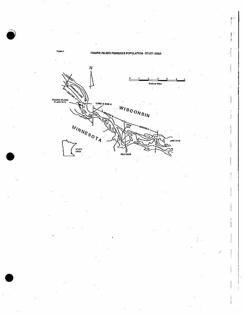
Fluum I...... I - PRAIRIE ISLAND FISHERIES POPULATION - STUDY AREA

0 1 2 3 4 5

Scale In Male$

PRAIRIE ISLANDPLANT SITE LOOK A *Am a "

INI

PRAIRIE ISLAND FISHERIES POPULATION STUDYSampling Locations

Upstream

Sea I Runs 1-20

Electrofishing Runs

Pt4

PRAIRIE ISLAND9NUCLEAR• "

GENERATIN

r

Figure 3. PRAIRIE ISLAND FISHERIES POPULATION STUDYSampling LocationsPlant Area(Sec 2 Runs 1-10)

PRAIRIE ISLAND- NUCLEAR

LOCK & DAM 3

Electrof-shing Runs =

Figure 4. PRAIRIE ISLAND FISHERIES POPULATION STUDYSampling LocationsDownstream(Sec 3 Runs 1-10)

Lock & Dam 3

)

4,

34

Electrofishing Runs kpvw4

HWY 63

CA

340

Figure 5. PRAIRIE ISLAND FISHERIES POPULATION STUDYSampling LocationsDownstream(Sec 4 Runs 1-20)

Electrofishing Runs -=-- 0.4*

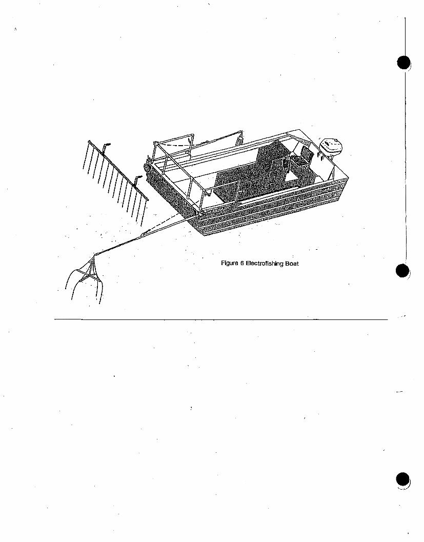
Figure 6 Eectrofishlng Boat

q-1)

PRAIRIE ISLAND 2006

90

80-

- LENGTH FREQUENCY GIZZARD SHAD

70-

60-

50.

40-

30-

20-

10-

U fl~i~ Pi dI.J]fl Jh1i1

Legendm SECTOR 1

CM SECTOR 2MI SECTOR 3

1- SECTOR 4-f AnJ]TiIfl.-* -. ___________________ ________________________________________

150 200 250 .300 350

LENGTH mm400 450 500

Figure 7

7-7 7777

PRAIRIE ISLAND 2006 - LENGTH FREQUENCY FRESHWATER DRUM

U

I:z1

Legend- SECTOR 1M~ SECTOR 2

WASECTOR 3ED SECTOR 4

LENGTH mm

Figure 8

S

PRAIRIE ISLAND 2.006 - LENGTH FREQUENCY SHORTHEAD REDHORSE

60

50'

40"

~30

LegendM SECTOR 1IMI SECTOR 2

SECTOR 3

ED SECTOR 4

100 150 200 250 300 ' 350 400 450 500 550

LENGTH mm

Figure 9

.4 1

PRAIRIE ISLAND 2006 - LENGTH FREQUENCY WHITE BASS

70-1

60-

50-

so.-

U40.-

. 30-

20-

10-

I

ffl Ii

LegendM SECTOR 1=I] SECTOR 2M SECTOR 3

F1 SECTOR 4J0

100 150 200 250 300

.- . ..LENGTH mm

350 400 450

Figure 10

PRAIRIE ISLAND 2006 - LENGTH FREQUENCY WALLEYE

12"

10-

8-

4-

2- Legend- SECTOR .1=li SECTOR 2

In M SECTOR3F-M SECTOR 4

.100 200 300 400 500, 600 700 800

LENGTH mm

Figure 11

.. ...... , . . ..I

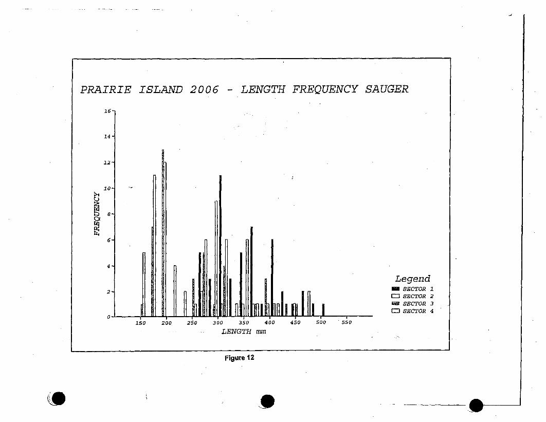
PRAIRIE ISLAND 2006

16]

14

- LENGTH FREQUENCY SAUGER

U

10-

8-

6-

4-

B11I IHTI I[II Im I I*I iLegend

M SECTOR 1=- SECTOR 2

M SECTOR 3E• SECTOR 4I

0 -I . . I - l - -l L.JL , ,.u .5| l.............. m . ... . -

150 2002250 300

1I I I I350 400 450 500 550

LENGTH mm

Figure 12

4o

PRAIRIE XSLA.ATD 2006 - LENGTH FREQUENCY SMALLMOUTH BASS

45-

40-

35-

30"

25-

C920-

15-

51 Allat

IFI 1111I11i

JIlii 111KA

Legendm SECTOR 1

I=- SECTOR 2FM SECTOR 3

M- SECTOR 4F'm 1:I I m LI In~j - .-- - -

50 1I00 150 200 250 300. 350 400 450

LENGTH min

Figure 13

- -U,

PRAIRIE ISLAND 2006 - LENGTH FREQUENCY LARGEMOUTH BASS

30-

25-

20-

15'

10-

5-

fl I BLegend

- SECTOR 1F-SECTOR 2

MSECTOR 3F- SECTOR 4I H1r I r

n -A- - I.- Ka • -I • .a ~id. ~ - a S m .. . . iA - S i

1;00 150 200

FEgTHe 14

350 400 450

Figure 14

Figure 15. Electrofishing CPUE (fish/hour) for Gizzard shad for years 1982ý2006in the vicinity of PINGP.

i'

Gizzard shad

45-

40-

35 -

30-

25-

.20-

a

O

015-f

1045-

0-~,r4J M~ LOl M t'- WD M 0 'Ts C), tfl W0 r-. W W 0 N M' V~ LO a* CWD MD MD MD WD W M M M M 0) 0)C) 0) 0) 0) M 0M 0 0 0 0 0D C

0) ) ) ) 0 0 a a)0)0)C) ) ) ) 0 0 0 M 0 0 0 0 0 0 C

Year

D

Figure 16. Electrofishing CPUE (fish/hour) for Freshwater drum for years 1982-2006in the vicinity of PINGP.

Freshwater drum

50

45 -

40

35

S300

25-

E 20 • •

15 • S •

10 5 •1

5 S

0N (0) V LO to r- CO 0) 0 M to~ 0C sC 0 ~ DC(o Co CD CD CD CD CD Co a) a) a) 0% a)a0% ) ) 0%00%% 0% 0 0 0 0 00M C) 0 W 0) 0) 0W 0M 0M 0M 0) CD 0) 0) a) 0) 0) 0) 0) 0 0 0 0 0 0 0

Year

Figure 17. Electrofishing CPUE (fish/hour) for Shorthead redhorse for years 1982-2006in the vicinity of PINGP.

Shorthead redhorse

30

25 -

20 S •

0

15cL

10 • S • 0

5 *

N -41 LO 10 D P,~ CO 0O 0 s ~ 0 C D M.TLnt - CO a) 0CD N M~ V LO toCO Co. CO CO CO CO CO CO 0n m1 a) 01 m1 CD 0 D 01 m1 C 0 0 0 0) 001 Om 01 01 01 01 01 01 0) 0) m m m 0 0 0T m T1 C0 m 0 3 0 0 0 0

Year

Figure 18. Electrofishing CPUE (fish/hour) for White bass for years 1982-2006in the vicinity of PINGP.

White bass

45-

40 0

35 •

301

025 •

m20 S S

15 *

10 5 5

5-

00o 01 0o 01 01 01 01 01 01 0 0 1 0% 1 01 01 013 01 0 01 0 0o 0 0 0 0 001 01 01"01 01 0 01 01 O•0 01 01) 01 01 01 013 01 01 0 0 0 0 0 0% 0D

Year

)

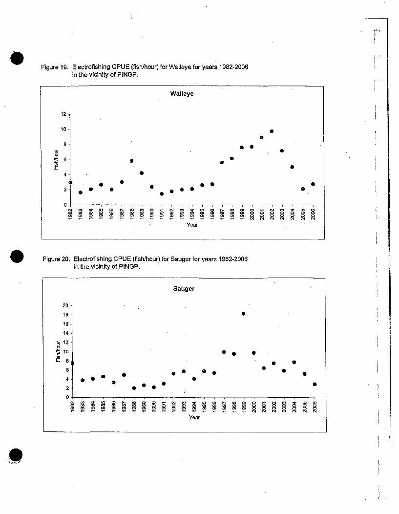
Figure 19. Electrofishing CPUE (fish/hour) for Walleye for years 1982-2006in the vicinity of PINGP.

Walleye

12

10 0a

8-• •

0Co

MA

6-

4-

0 SSa

0

20S

S S0O

0 ,a 0 0S

0 1 1 1 1 . I I .

N m~ It O (D I.- M) m) 030) 0 0" 0) 0) 0) 0) 0) O0) 0 0) ) 0) 0) 0 0) ) 0 0)~ m) 0m0 ) 0 ) 0 0 0 0 0 0

0)~~~~ 0m0 ) 0 0 ) 0 0 m 0ý 0

Year

LO

N

toCD00a

Figure 20. Electrofishing CPUE (fish/hour) for Sauger for years 1982-2006in the vicinity of PINGP.

Sauger,

20

18 S

16

14

120

S10 0* S

E 86

4- •

0 0 0

N M' V C') (D t- CO 0) 0 - N ") V 0L CD r. M 0) 0 S N M~ toL) CooCO w) w) w) w) w) 0) 0) m) 0D 0) 0 ) 0) 0 0) 0 0 0 0 0 0

0 0) 0 0) 0 0) 0 0)0) 0) 0) 0D 0) CD0 ) 0) 0 0T 9!-T-9!----T------- - - - - - NT N N

Year

Figure 21. Electrofishing CPUE (fish/hour) for Smallmouth bass for years 1982-2006in the vicinity of PINGP.

Smallmouth bass

18

16 S 0.0

14 *

12

10 -

6 • *

4 •

2 'S• *

N o C' • LO It 0 1- Co C 0• o • to 'J It) CD •- Co 0 0 '- N o C • to CD

a ear) m m m m C 0 0 0 0 0-~~~ -- -- - -r ,- r .- r N4 N1 N N N N (N

Year

Figure 22. Electrofishing CPUE (fish/hour) for Largemouth bass for years 1982-2006in the vicinity of PINGP.

Largemouth bass

9.

80 !

71

6 S

S *aS

.e4

U..5

3

2

0CVCO

S S0

0S

aa S

SS

S 00 0

00 CO tO C.D CO CO C3C) C) C) C) C) c) c)C)3 C) C)3 C) C) C C) C• m C) C) mC m m C) C) 0 0a 0 0

-a N N N N N

Year

LO0C,C0

CD0

Figure 23. Electrofishing CPUE (fish/hour) by sector for Gizzard shad for years 1982-2006 in the vicinity of PINGP.

Sector I Sector 2

35

30-

25

20

15 S

10-

5 0 +

0-

U~~~a) 0)~~ U U U U O Q O a ) 0 00 0a) ]) C) a) a ) Yea) a) a) aa 0-) T a) a) a) 00 0 0 0 00

rrr rr r. rr -r NN N N1 0N C4

Year

25

20-

o 15

.9 10U.

5.

n,

9S

S * *

S - .1S

- @5,m .....

0)0)0)0 o mC mm)))00 mm OMMa)M0)00 0C 000)~~~ a) a) 0) a) a) 0) 0)0 )0 )0 ))))a 0 0 0~-rrrrr rN C4.CM C-r4 N N NN

Year

Sector 3 Sector 4

90

80 S

70

60* 50-• 40R: 30. S

20

10 SAS 0 0 G

MOO)a) 0)a)0) 0Yar a)M00000-- -- -- -- -- -- rrrrrrrrrrrrrrrrrrrrN NN N N N N

Year

60

50 .

40-0

30 5U)

E: 20 S .0

10 •

S, .* Sar

r~N N N N N NN

Year

Figure 24. Electrofishing CPUE (fish/hour) by sector for Freshwater drum for years 1982-2006 in the vicinity of PINGP.

Sector 1 Sector 2 ________

U)

454.0-3530 0 •

25 €

20 * @. .0.0120 - 0

15 0 0O0 0 0 0) 0 010 00O 005, •

oo C O O CO Y) 0 ) 0 a)0) 0)M)0 0 0) 0) 0r. 2r r, rr .- rrT- No (J ,4 c, Nl c No

Year

0

70

60-

50

40-

30

20

10

0

0

lee

@000. 0.0

I. .

No It LW r- W0) ) r C 1(0)0 0 W )0)0 0 ) )) )0)0 00 0)- 0)' 0 0 00 00

0)00))0))00)00))0))00)T0))M 0 0 0S8aC,100

Year

Sector 3 Sector 4

60

50

40- 040

30 0

U.20 00O 0-

10 S0

0C4 M 0 LO toI- 0) 0CD N (~ 0 O0 D 0) t0)0 N~ (0) 8 0 to0

11090 00000

Year

0

U.

40

35

30

25-

20

151

10-5-0

0

0*0 .0 0

0

~0 000 0

osooS 0 0

I

-rr - - -- - ,- - .- - - - '- -- r N N N IN N N N

Year

Figure 25. Electrofishing CPUE (fish/hour) by sector for Shorthead redhorse for the years 1982-2006 in the vicinity of PINGP.

Sector 1

40

35 g •

30 @•

25-0

20 - a

if 15 *10 0. .

5

0N M) V t)C Co W ) 0- W -C N M~ '-T L) CoP- cO 0D 0 (N4 M) 'q U (D

0)M 0) 0) 0) 0) 0) 0) a) 0)n )0 )0 0 0 0 0YeN " (N 4 NYear

Sector 2

0

E-

-25

20- 0

15 0

10

004 m) 't to (O . Co 0) 0 N04 't) U) Co I-- Co 0) 0 N4 -q 0 0)CCo CO CO CO CO Co 'Co 0) 0) 0) 0m m m 0 0 0 0 0 0 0

m)0)0 0) m) m) 03 0) 0) C) a) a) a))0)0 0 0 0Ya r2 o! o• -0 !! N N CN N N N ooYear

Sector 3 Sector 4

0

rz

U.

40

35

30

25

20

15

10

5.

0

0 0

00 0

I0

LL

25

20 •

15 S 0

10 5 *.• o

101

0 - 1 1 • l 1 1 1 . . .I I l J

G~o C Go COD CO w0)00Year

Year

04UmV ) 0 r- w m0 ,0! mV 00 w0) o -C,4 0 §0 (CO OD00CO WOCD) 9MM MM 000O

- -r - - ,- -- - - .- .- r- i- N NCN 040N404 NN

Year

...... ...... ...... . . - - -- . ..

Figure 26. Electrofishing CPUE (fishihour) by sector for White bass for years 1982-2006 in the vicinity of PINGP.

Sector 1 Sector 2 ___________ _____ ___

25-

20 6

w10-5 .

00

NCli mJ It CD 1- m m C) N m' It to WD r- m) U 0 C1 ')t W ) w000 w) w) 00 0 W) CO CO 0) (n (n U) 0) 0) a) U) 0)0 ) 0 0 0 000

U) ) m) m) U)U ) U) U U) 0) 0) U) C) U) g! 0) 0 ,000 0 )00

Year

0

Ui

30

25

20

15,

10

5-

0-

00

p

N M ') LO U) CO- W) U 0 N 0' r U) WN t" MU) 0.- N M' 8 m) CU))) UU'0000 00

.a4 N N 4 N N

Year

Sector 3 Sector 4

0

I.C

10090-80-70-60-50140-30-20-10-

0S 0

0 0 0 00

0

,T

60

50

40

30

20

10

0

00 000

o00Goo 000

i ..... ,--F

n

N C) ~ U C N U)U)0- C) U)CDN- ) )N N N' U) Cm

Year Year

4

Figure 27. Electrofishing CPUE (fish/hour) by sector for Walleye for years 1982-2006 in the vicinity of PINGP.

10 01,

Sector 1 Sector 2 ___ ___

1413S1211

4-3 0oo T2 a

0 1 so. . . .

I14 0V0) 4)0 C 000 )0) 4 ' ) 00)0)00000000) 0) 0) C O OG 0) 0) 0) 0 ) 0) 0) m) a)0 )0 ) m) 0 0) 00 a00000C

rrrrrrrrrrrrrN (N N 04 N 4

Year

1.!20.

1098765.43'21-0

SS

S

00o

0

.00S. 0 0O0m00.6

N M~ '- LO W0 r- W 0) 0 N (1) V tO WD C- W 0) a E N M~ 't to W0

0) u' c.2 0) T) 0 m) T) 0) 0) c2 0) 0 T C3co 0) 0) 0 00 0 0r.- rrr-r rrn .- r. N CN CVC14C14N

Year

Sector 3

IUi

1816141210.8.6-412-0

S SS S

6

S.**e. *sggg S 0

Sector 4

1o9-o8-s7-•10

f . 10L3-00 a 0 00 0

1 -

0Mar 0 ) ) 0 0

Year

I

r.- ~-.-.-r - N NI N N N N CN

Year

Figure 28. Electrofishing CPUE (fish/hour) by sector for Sauger for years 1982-2006 in the vicinity of PINGP

Sector 1I______ __________ Sector 2

0

U.

14

12

10

8

65

4.

2-

0

S

S0O

0

0* 0* 0@0 0 0

Sesso

0

LL

8-

7-

6 -

51 04- •

3 * 00 020 01 0

10 ., . . .

0

v

0)00)00)0G)00)O)0)0)0000000) 0m 0a 00)00)00 0)00)00)00))0) 0 0 000 C

Year

N M-lr 0)w0) 0) ) 0 N MIL 0) D N0) )0) ww ww mm 0)0 ) )0 ) )0 ) )0 ) M0)0) ) o0

Year

04 M CV* LO~ CD00C>000)0

0)C 00 000CN CN 0N NI N CM

Sector 3 Sector 4

0

4035

30-

25

2015-

5

100

000 *0000 000.0 * • ,00

. . . .S ,,, . . . . .

21 •

18

15-=012- 0o

91U-6 goSg 0.0

0. 00 0006- *

0-0' J J • ,' ~ l , , .

N) 0) in 0 D 0) 0) J 0) 0) 0) l 0) ý 0)0 ) 0) 1- O) 0) Q0)00 M0000COOD w w wo 0

rear- - ----- N N N N N N N

Year

vNCl) 'OW N0)0)0NC0) C N )Vt N0 ,CC) 0 0N 0) 1

n40)0 I00)0 00)0)0 )C0)00))m0)C)0a) 0) 0)0)0 00 Q 00C0) 0)D 0) ! CD 0) Q)0 )0 )0 )0 0 )0 0 0 0

rr.-.-q-r ~ ~ ~ ~ 0 . -r-r, -NNNN N N N1

Year

O 0O

Figure 29. Electrofishing CPUE (fish/hour) by sector for Smallmouth bass for years 1982-2006 in the vicinity of PINGP.

Sector 1 Sector 2

24

20-

16 -04 12-

4 00 0,60

0wwww www MMM)0NC") C) aCD

marmmT 0) 0 0rrrrrrrrrrrrrrrrrrrrrrrrr04 (ONN N N N N N

- Year

20

16 .* 0

0 12-

U.T

4 0

0

0) a) 0 ) mm a) m 0) m 0m 0m m m 8Yar 0 Co 0- -- - -- - -- r--r r-N N N N N N~ N4

Year

Sector 3 Sector 4

I)

Li

4540-35-30 -

25-20-15-10

500

0

0 00

S 0S S

S *geS. S

I

5- •4-

0

.I)U. 2 *

1 *S 0 • s o

0Yea 00 00

Year0- T) T) T) a T) Co M 0) 0) 0) Ya a a a) 0 000

Year

A

----.-.-.-.-----..- ~......-..--.----------- .----- ~--.-----.-------.---

Figure 30. Electrofishing CPUE (fish/hour) by sector for Largemouth bass for years 1982-2006 in the vicinity of PINGP.

Sector 1 Sector 2

0

U..

12

9.

6

.3

0

LL

98 -

7 - •

6-5- 04-3 -. •

2-

(N to Iq CtO wo r- w 0 a N m) V to w r.- W 0 a (N M 0 0oC1 w w www 0 a• 000

arN N N N 4 N NYear

- a0 == U* = 1* M -. = =, U = = =U - =-,===v

NCV) m VUt (0 N tO 0) 0 ~-N CO to CO r- 00 a) 0 r N V) ,T LO tDtO to CO CO 00 CO CO 00 6) 6) a) a) a) m) 0) (D 6) 6) 0Z;000 0080

6)6 )6 6 )6 ) )6 )6 01 )n T) M) 6) 6 ) 000 0 00.- r r r r r r r rr N (N N N. (N N1 (N

Year

Sector 3 Sector 4

0

U.

25.

20

15 -

10 0 0

0 9 •IC14 0 0 0w0aNC0 00 • V) to

Year

14

12

10-

0 o a0-

L- .. Yea0-T-rr.-.N -.- r N .- LO r 1- W- N (N( CO N N

- .Year

IMF

PRAIRIE ISLAND 2006 CATCH PER UNIT EFFORT (FISH/HR) GIZZARD SHAD

40

N,<30"

20"

A Legend"0 N- SECTOR 1

o SECTOR 2

[" SECTOR 3

o SECTOR '4

MAY 22-25 JUNE 12-15 JULY 10-13 AUG 14-17 SEPT 11-14 OCT 16-19

DATE

Figure 31

.- , -. ?T~i

PRAIRIE ISLAND 2006 CATCH PER UNIT EFFORT (FISH/BR) FRESHWATER DRUM

.i00

40

20

0MAY

LegendX SECTOR I

[j SECTOR 2

0 SECTOR 3

0 SECTOR 4

DATE

.Figure 32

0

PRAIRIE ISLAND 2006 CATCH PER UNIT EFFORT (FISH/HR) SHORTHEAD REDHORSE

D4)

Legend* SECTOR 1

0 SECTOR 2

0 SECTOR 3

0 SECTOR 4

MAY 22-25 JUNE 12-15 JULY 10-13 AUG 14-17 SEPT 11-14 OCT 16-19

DATE

Figure 33

____-ffi

PRAIRIE ISLAND 2006 CATCH PER UNIT EFFORT (FISH/HR) WHITE BASS

P4)IN

30

LegendM SECTOR I

o SECTOR 2

) SECTOR 3

0 SECTOR 4

10

MAY 22-25 JUNE 12-15 JULY 10-13 AUG 14-17 SEPT 11-14 OCT 16-19DATE

Figure 34

.

PRAIRIE ISLAND 2006 CATCH PER UNIT EFFORT (FISH/HR) WALLEYE

10'

N

H

Legend* SECTOR 1

o SECTOR 2

O SECTOR 3

0 SECTOR 40 1 " I

MAY 22-25 JUNE 12-15 JULY 10-13 AUG 14-17 SEPT 11-14 OCT 16-19

DATE

Figure 35

- -- ~ ~ 771

ý i

PRAIRIE ISLAND 2006 CATCH PER UNIT EFFORT (FISH/HR) SAUGER

16-

14-

12"

10.

6-

P41

Legend* SECTOR 1

o SECTOR 2

0 SECTOR 3

m 0 SECTOR 4

SEPT 11-14MAY 22-25 JUNE 22-15 JULY 10-13 AUG 14-F7

DATE

Figure 36

0

PRAIRIE ISLAND 2006 CATCH PER UNIT EFFORT (FISH/HR) SMALLMOUTH BASS

CA)HI~Z.4

LegendA SECTOR 1

o SECTOR 2

0 SECTOR 3

0 SECTOR 4

MAY 22-25 JUNE 12-15 JULY 10-13 AUG 24-27 SEPT 22-24

DATEOCT 16-19

Figure 37

PRAIRIE ISLAND 2006 CATCH PER UNIT EFFORT (FISH/HR) LARGEMOUTH BASS

45-

40

35- /N30-

~25-

10, LegendM SECTOR 2

5 SECTOR 3

___, _____ ~,0 SECTOR 4

DATE

Figure 38

Table 1.

Species

Species of fish captured In the Mississippi River in the vicinity of the Prairie Island Nuclear Generating Plant 1983-2006.

83 84 85 86 87 88 89 90 91 92 93 94 95 96 97 98 99 00 01 02 03 04 05 06

Chestnut lampreyIchthyomvzon castaneusSilver lampreylcthvomyzon unicuspusPaddlefishPolyodon spathulaLongnose gar.Leoisosteus osseusShortnose garLepisosteus platostomusBowfinAmia calvaAmerican eelAnguilla rostrataGizzard shadDorosoma cepedianumGoldeyeHiodon alosoidesMooneyeHiodon teraisusBrown troutSalmo truttaNorthern pikeEsox luciusMuskyEsox masauinonqyCarpCyorinus carpoCarpsucker SpeciesCarpiodes speciesRiver carpsuckerCarpiodes carpioQuillbackCarpiodes cyorinusHighfin carpsuckerCarpiodes veliferWhite suckerCatostomus commersoni

x x x x

x x x x x x

x

x x

X X x x x x

x x xx x x x x x x x

x

x

x

x

X

X

x

x

x

x

x

x

x

x

x

x

X,

x

x

x

x

x

x

x

x

x

x

x

x

x

x xx x xx

x xx xx x

x x x x x .x

x xx x xx

x xx xx x

x

x x x x x x

x

x

x

x

x

x

x

x

x

x

x

x

x

x x

x

x x x x

x

x xx x

x x x

x x

x x

x x

x

x x

x x

x x

x x

x

x x

x x

x x

x

x x

x

x

x

x

x

x x

x x

x x

x

x x

x

x

x

x

x x x x x x x x x

x

x

x

x

x

xx x

x

x x

x x

x x

x

x

x

x

x

x

x

x x

x x

x x

x

x x

x

x x

x x

x x

x x

x

x x xx x

x

x x

x x

x x

x xx x x

x

x xx x x

x x x x xx x x x x

x

x

x

x

x

x

x

x

x

x

x

x

x

x

x

x

x

x

x

x

x

x

x

x

x

x

x

x

x

x

x

x x xx x

x xx x x

x

x xx x x

x

x

x

x

x

x

x

x

x

x

x

x

x

x

J

Table 1 (cont.)

Species

Blue suckerCycleptus elonqatusNorthern hogsuckerHyeentelium niaricansSmallmouth buffaloIctiobus bubalus.Bigmouth buffaloIctiobus cyorinellusSpotted suckerMinytrema melanopsSilver redhorseMoxostoma anisurumRiver redhorseMoxostoma carinatumGolden redhorseMoxostoma erythrurumGreater redhorseMoxostoma valenciennesiShorthead redhorseMoxostoma macrolepidotumBlack bullheadIctalurus melasYellow bullheadIctalurus natalisBrown bullheadIctalurus nebulosusChannel catfishIctalurus bunctatusFlathead catfishPylodictus olivarisBurbotLota :Iota---White bassMarone chrysopsRock bassAmbloolites rupestrisGreen sunfishLepommis cyanellus

Species of fish captured In the Mississippi River in the vicinity of the Prairie Island Nuclear Generating Plant 1983-2006.

83 84 85 86 87 88 89 90 91 92 93 94 95 96 97 98 99 00 !1 02 03 04 05 06

x x x x x xxx xxx xxx x xx x x x x

x x x

xx x x x x x x x x x x x x x x x x x x x x x x

x x X X X X X X X x xx x x x x x x x x x x x

x x x x x x x x x

x x x x x x x x x x x x x x x x x x x x x x x x

x x x xxx x xx xxx x x x x x x

x xx x xx x xx x xx x xx x xx x xx xx x

x

x x

x x

x

xX

x

x

x

x

x

x

x

x

x

x

x x

x x

x x x x x x

x

x

x

x xx x

x

x

x

x

x

x

x

x x

x x x

x

x x

x x

x x

x x

x x

x x

x

x

x

x

x

x

x

x

x

x

x

x

x

x

x

x

x

x

x

x

x

x

x

-X

x

x

x

x

x

x

x

x

x

X

x

x

x

x

x

x

x

x

x

x

x

x

x

x

x

x

x

x

x

x

x

x

x

x

x

x

x

x

x

x

x x

x x

x x

x x

x x

x x

x

x

x

x

x

x

x

x

x

x

x

x

x

x

x

x

x

x

x

x

x

x

x

x

x xx x

x xx x

x xx x

x xx x

x xx x

x x x x

AkI-m-mv

0)Table I (cont.)

Species

PumpkinseedLepomis .ibbosusOrangespotted sunfishLepomis humilisBluegillLePomis macrochirusSmallmouth bassMicrooterus dolomieulLargemouth bassMicropterus salmoidesWhite crappiePomoxis annularisBlack crappiePomoxis nicqromaculatusYellow perchPerca flavensSaugerSander canadenseWalleyeSander vitreumSaugeyeS. vitreum x S. canadenseFreshwater drumAplodinotus grunniensLake sturgeonAcipenser fulvescens

Species of fish captured In the Mississippi River in the vicinity of the Praide Island Nuclear Generating Plant 1983-2006.

83 84 85 86 87 88 89 90 91 92 93 94 95 96 97 98 99 00 01 02 03 04 05 06

x x x x x x x x x x x x x x x x x x

x

x

x

x

x

X

x

x

x

x

x

x

x

x

x

x

x

x

x

x

x

x

x

x

x

x

x

x

x

x

x

x

x x x x xx x xx x x x

x x x x xx x x x x x x

x x x x x x x x x x x x

x xx x x x x x x x X x

x xx x xx x xx xx x

x x x x x x x x x X x

x xx x xx x xx xx x

x x x x x x x x x x X. x

x x

x xx x x x x x x x x x

x

x

x

x

x

x

x

x

x

x

x x

x x

x x

,,( x

x x

x x

x

x•x

x x

x

x x

x

x

x

x

x

x

x

x

x

x

x

x

x

x

x

x

x

x

x

x

x

x

x

x

x

x

x

x

x

x

x

x

x

x

x

x

x

x

x

x

x

x

x

x

x

x

x

x

x

x

x

xx x x x

Table 2. Electrofishing CPUE (fish/hour) for each sector in the vicinity of PINGPand total number of each species collected during 2006.Species are listed in descending order according to average CPUE.

NumberSector I Sector 2 Sector 3 Sector 4 Average collectedRank Species

1 Carp2 White bass3 Freshwater drum4 Shorthead redhorse5 Smallmouth bass6 Bluegill7 Largemouth bass8 Gizzard shad9 Black crappie

10 Silver redhorse11 Quillback carpsucker12 Sauger13 Walleye14 Flathead catfish15 Channel catfish16 Smallmouth buffalo17 Green sunfish18 White crappie19 Bowfin20 Mooneye21 Bigmouth buffalo22 Blue sucker23 Longnose gar24 Shortnose gar25 Northern pike26 Silver lamprey27 River carpsucker28 Rock bass29 Golden redhorse30 Burbot31 Yellow perch32 White sucker33 River redhorse34 Pumpkinseed35 Orange spotted sunfish36 Brown trout37 Chestnut lamprey38 Spotted sucker

17.509.09

13.9218.138.580.910.112.220.744.321.992.733.241.361.311.710.170.060.061.420.280.510.570.000.110.460.110.060.170.000.060.060.280.000.000.000.000.06

31.715.08

14.128.67

10.0315.85

1.986.322.483.595.200.871.242.736.812.73.4.582.350.000.250.250.370.620.250.000.250.250.120.000.000.120.000.000.120.120.000.000.00

29.0832.5118.3623.0032.1820.0219.356.522.992.882.434.424.205.311.111.991.000.000.440.110.770.550.330.890.220.440.330.220.330.550.110.110.110.110.110.110.110.00

15.2020.1520.03

7.712.76

13.1312.8416.5811.864.033.863.922.421.440.521.380.171.792.360.230.580.170.000.170.920.000.230.400.290.000.120.230.000.120.000.000.000.00

23.3716.7116.6114.3813.3912.488.577.914.523.703.372.982.772.712.441.951.481.050.710.500.470.400.380.330.310.290.230.200.200.140.100.100.100.090.060.030.030.01

1091845873731571553416437266201166163147119

9794525146322420181320141111115566421I1

7124Totals 92.27 129.06 213.32 145.59 145.06

Table 3. Fisheries summary for Gizzard shad 1977-2006.

ELECTRO TRAPNET CATCHCPUE CPUE COMP MEAN

YEAR Fish/hr Fish/hr (%) N LENGTH LENGTH WEIGHT REGRESSION1977 7.92 0.61 4 135 NA LOG W=3.101 LOG L-5.1631978 10.20 0.20 5 73 NA LOG W=3.068 LOG L-5.0781979 1.81 0.06 1 NA NA NA1980 10.83 0.14 7 NA NA NA1981 23.03 0.38 9 917 216 LOG W=2.748 LOG L-4.3481982 7.39 0.09 3 276 329 LOG W-2.917 LOG L-4.7411983 3.57 0.26 2 155 355 LOG W=3.029 LOG L-5.0491984 0.84 0.08 1 48 281 LOG W=2.684 LOG L-4.1711985 0.81 0.01 1 31 325 LOG W=2.388 LOG L-3.4311986 0.14 0.06 <1 13 274 LOG W=3.248 LOG L-5.6341987 1.08 0.05 1 55 256 LOG W=3.030 LOG L-5.0461988 3.25 NA 3 139 288 LOG W=2.629 LOG L-4.0151989 1.07 NA <1 47 323 LOG W=3.025 LOG L-5.0211990 3.99 NA 3 170 326 LOG W=2.956,LOG L-4.8571991 2.39 NA 4 198 338 LOG W=2.601 LOG L-3.9401992 1.82 NA 1.8 9i 357 LOG W=3.459 LOG L-6.1271993 1.99 NA 1.9 62 375 LOG W=2.920 LOG L-4.7281994 0.28 NA( <1 14 394 LOG W=3.371 LOG L-5.9551995 5.10 NA 4 204 272 LOG W=2.625 LOG L-4.0731996 0.76 NA <1 27 330 LOG W=3.275 LOG L-5.6661997 0.66 NA <1 23 400 LOG W=3.934 LOG L-7,3731998 4.07 NA 2 176 260 LOG W=3.104 LOG L-5.2181999 27.12 NA 12 1222 290 LOG W=2.981 LOG L-4.9882000 40.85 NA 17 1634 290 LOG W=3.274 LOG L-5.6972001 10.43 NA 6 455 340 LOG W=3.767 LOG L-6.9672002 14.02 NA 7 612 350 LOG W=3.200 LOG L-5.5182003 9.51 NA 5 373 380 LOG W=3.469 LOG L-6.1982004 17.60 NA 10 859 290 LOG W=2.863 LOG L-4.6072005 14.06 NA 9 682 350 LOG W=3.072 LOG L-5.1472006 7.91 NA 5 437 340 LOG W=2.854 LOG L-4.585

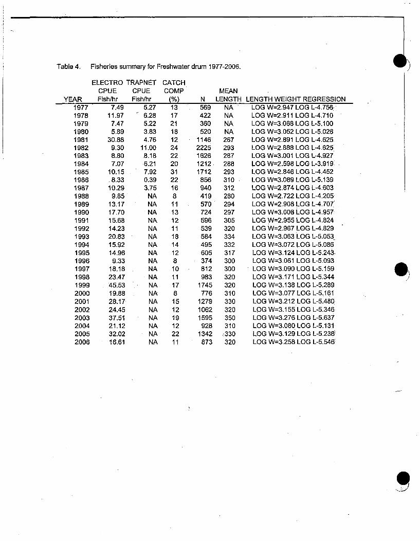
Table 4. Fisheries summary for Freshwater drum 1977-2006.

ELECTRO TRAPNET CATCHCPUE CPUE COMP MEAN

YEAR Fish/hr Fish/hr (%) N LENGTH LENGTH WEIGHT REGRESSION1977 7.49 5.27 13 569 NA LOG W=2.947 LOG L-4.7561978 11.97 6.28 17 422 NA LOG W=2.911 LOG L-4.7101979 7.47 5.22 21 360 NA LOG W=3.068 LOG L-5.1001980 5.89 3.83 18 520 NA LOG W=3.052 LOG L-5.0261981 30.88 4.76 12 1146 267 LOG W=2.891 LOG L-4.6251982 9.30 11.00 24 2225 293 LOG W=2.888 LOG L-4.6251983 8.80 8.18 22 1626 287 LOG W=3.001 LOG L-4.9271984 7.07 6.21 20 1212 288 LOG W=2.598 LOG L-3.919"!1985 10.15 7.92 31 1712 293 LOG W=2.846 LOG L-4.452'1986 8.33 0.39 22 856 310 LOG W=3.089 LOG L-5.139"1987 10.29 3.75 16 940 312 LOG W=2.874 LOG L-4.6031988 9.85 NA 8 419 280 LOG W=2.722 LOG L-4.2051989 13.17 NA 11 570 294 LOG W=2.908 LOG L-4.707'1990 17.70 NA 13 724 297 LOG W=3.008 LOG L-4.9571991 15.68 NA 12 596 305 LOG W=2.955 LOG L-4.8241992 14.23 NA 11 539 320 LOG W=2.967 LOG L-4.8291993 20.83 NA 18 584 334 LOG W=3.063 LOG L-5.0531994 15.92 NA 14 495 332 LOG W=3.072 LOG L-5.0861995 14.96 NA 12 605 317 LOG W=3.124 LOG L-5.243.1996 9.33 NA 8 374 300 LOG W=3.061 LOG L-5.0931997 18.18 NA 10 812 300 LOG W=3.090 LOG L-5.1591998 23.47 NA 11 983 320 LOG W=3.171 LOG L-5.3441999 45.53 NA 17 1745 320 LOG W=3.138 LOG L-5.2892000 19.88 NA 8 776 310 LOG W=3.077 LOG L-5.1612001 28.17 NA 15 1279 330 LOG W=3.212 LOG L-5.4802002 24.45 NA 12 1062 320 LOG W=3.155 LOG L-5.3462003 37.51 NA 19 1595 350 LOG W=3.276 LOG L-5.6372004 21.12 NA 12 928 310 LOG W=3.080 LOG L-5.1312005 32.02 NA 22 1342 c330 LOG W=3.129 LOG L-5.238i2006 16.61 NA 11 873 320 LOG W=3.258 LOG L-5.546

Table 5. Fisheries summary for Shorthead redhorse 1977-2006.

ELECTRO TRAPNET CATCHCPUE CPUE COMP MEAN

YEAR Fish/hr Fish/hr (%) N LENGTH LENGTH WEIGHT REGRESSION1977 5.39 1.58 5 259 NA LOG W=2.902 LOG L-4.6911978 2.96 1.09 4 125 NA LOG W=2.978 LOG L-4.9171979 2.08 0.45 3 67 NA LOG W=3.041 LOG L-5.0901980 6.08 0.70 7 137 NA LOG W=2.894 LOG L-4.6781981 11.67 1.34 7 686 376 LOG W=2.791 LOG L-4.4281982 13.56 0.92 7 675 392 LOG W=2.814 LOG L-4.4961983 8.96 0.79 6 454 387 LOG W=2.849 LOG L-4.5901984 9.74 0.51 7 435 386 LOG W=2.571 LOG L-3.8401985 7.36 0.51 7 374 389 LOG W=2.787 LOG L-4.4151986 7.07 0.19 8 319 398 LOG W=2.911 LOG L-4.7301987 13.80 1.24 12 722 403 LOG W=2.860 LOG L-4.6081988 17.48 NA 13 667 381 LOG W=2.696 LOG L-4.1761989 24.52 NA 17 902 370 LOG W=2.792 LOG L-4.4481990 22.60 NA 14 838 361 LOG W=2.825 LOG L-4.5441991 13.58 NA 11 538 355 LOG W=2.784 LOG L-4.4431992 19.35 NA 14 721 403 LOG W=2.841 LOG L-4.5871993 10.86 NA 10 332 382 LOG W=3.011 LOG L-4.9911994 13.51 NA 14 505 389 LOG W=2.872 LOG L-4.6551995 9.67 NA 8 450 364 LOG W=2.925 LOG L-4.8081996 13.42 NA 11 551 380 LOG W=2.897 LOG L-4.7191997 19.21 NA 10 833 350 LOG W=2.982 LOG L-4.9601998 23.94 NA 12 1047 360 LOG W=2.982 LOG L-4.9601999 21.17 NA 9 931 350 LOG W=3.016 LOG L-5.0502000 25.94 NA 11 1099 360 LOG W=2.905 LOG L-4.7602001 17.43 NA 9 777 370 LOG W=3.039 LOG L-5.1012002 17.23 NA 9 781 370 LOG W=2.954 LOG L-4.8922003 20.92 NA 11 878 390 LOG W=3.033 LOG L-5.0712004 25.63 NA 15 1141 360 LOG W=2.948 LOG L-4.8552005 12.85 NA 9 562 350 LOG W=2.833 LOG L-4.5442006 14.38 NA 10 731 370 LOG W=2.772 LOG L-4.375

0t

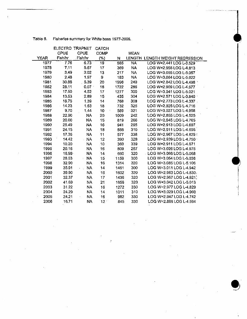
Table 6. Fisheries summary for White bass 1977-2006.

ELECTRO TRAPNET CATCHCPUE CPUE COMP MEAN

YEAR Fish/hr Fish/hr (%) N LENGTH LENGTH WEIGHT REGRESSION1977 7.76 6.73 19 565 NA LOG W=2.441 LOG L-3.5291978 7.11 5.67 17 369 NA LOG W=2.956 LOG L-4.8131979 3.49 3.02 13 217 NA LOG W=3.055 LOG L-5.0571980 2.48 1.97 9 183 NA LOG W=3.064 LOG L-5.0221981 30.88 5.39 20 1996 240 LOG W=2.842 LOG L-4.4981982 28.11 0.07 18 1722 286 LOG W=2.909 LOG L-4.6771983 17.50 4.52 17 1277 300 LOG W=3.041 LOG L-5.0211984 13.53 2.89 15 435 304 LOG W=2.571 LOG L-3.8401985 16.75 1.39 14 768 308 LOG W=2.773 LOG L-4.3371986 14.23 1.63 18 732 325 LOG W=2.926 LOG L-4.7161987 9.70 1.44 10 589 321 LOG W=3.027 LOG L-4.9581988 22.90 NA 20 1009 242 LOG W=2.855 LOG L-4.5251989 20.00 NA 15 819 266 LOG W=2.945 LOG L-4.7651990 25.49 NA 16 941 295 LOG W=2.913 LOG L-4.6971991 24.15 NA 18 886 310 LOG W=2.911 LOG L-4.6961992 17.36 NA 11 577 338 LOG W=2.967 LOG L-4.829.1993 14.42 NA 12 390 328 LOG W=2.939 LOG L-4.7501994 10.20 NA 10 360 339 LOG W=2.911 LOG L-4.6711995 20.16 NA 16 809 267 LOG W=3.026 LOG L-4.9751996 16.99 NA 14 660 320 LOG W=3.066 LOG L-5.0681997 28.53 NA 15 1159 300 LOG W=3.054 LOG L-5.0381998 32.90 NA 16 1314 320 LOG W=3.085 LOG L-5.1061999 35.91 NA 14 1461 300 LOG W=3.011 LOG L-4.9422000 39.90 NA 16 1602 320 LOG W=2.963 LOG L-4.8302001 32.37 NA 17 1436 320 LOG W=2.967 LOG L-4.8212002 41.69 NA 21 1656 320 LOG W=3.042 LOG L-5.0132003 31.22 NA 16 1272 330 LOG W=2.977 LOG L-4.8292004 24.29 NA 14 1011 310 LOG W=3.029 LOG L-4.9602005 24.21 NA 16 982 330 LOG W=2.947 LOG L-4.7422006 16.71 NA 12 845 330 LOG W=2.886 LOG L-4.594

Table 7. Fisheries summary for Walleye 1977-2006.

YEAR197719781979198019811982198319841985198619871988198919901991199219931994199519961997199819992000200120022003200420052006

ELECTRO TRAPNETCPUE CPUEFish/hr Fish/hr

1.36 0.371.54 0.961.57 0.311.20 0.133.53 0.392.96 0.161.63 0.212.04 0.112.64 0.131.99 0.153.00 0.095.80 NA4.19 NA2.36 NA1.44 NA2.30 NA2.00 NA2.11 NA2.63 NA2.75 NA5.63 NA6.16 NA7.63 NA7.72 NA8.93 NA9.75 NA7.18 NA5.02 NA2.11 NA2.77 NA

CATCHCOMP

(%)122121

22225321122223333554312

N20

283422

189135

9093

1191011322341739552826074

107118248272308

325399415304232

86147

MEANLENGTH

NANANANA335415432378413404386450408420477403465439333360400420440460400390450440510510

LENGTH WEIGHT REGRESSIONLOG W=3.137 LOG L-5.377LOG W=3.056 LOG L-5.197LOG W=3.225 LOG L-5.640LOG W=3.250 LOG L-5.693LOG W=3.082 LOG L-5.240LOG W=3.097 LOG L-5.293LOG W=3.095 LOG L-5.295LOG W=2.852 LOG L-4.615LOG W=3.159 LOG L-5.461LOG W=3.085 LOG L-5.269LOG W=3.151 LOG L-5.446LOG W=3.103 LOG L-5.272LOG W=3.140 LOG L-5.379LOG W=3.214 LOG L-5.594LOG W=3.318 LOG L-5.870LOG W=3.257 LOG L-5.727LOG W=3.001 LOG L-5.020LOG W=3.261 LOG L-5.720LOG W=3.208 LOG L-5.586LOG W=3.159 LOG L-5.467LOG W=3.215 LOG L-5.617LOG W=3.148 LOG L-5.440LOG W=3.238 LOG L-5.690LOG W=3.250 LOG L-5.717LOG W=3.296 LOG L-5.837LOG W=3.257 LOG L-5.744LOG W=3.253 LOG L-5.726LOG W=3.175 LOG L-5.494LOG W=3.225 LOG L-5.633LOG W=3.352 LOG L-5.964

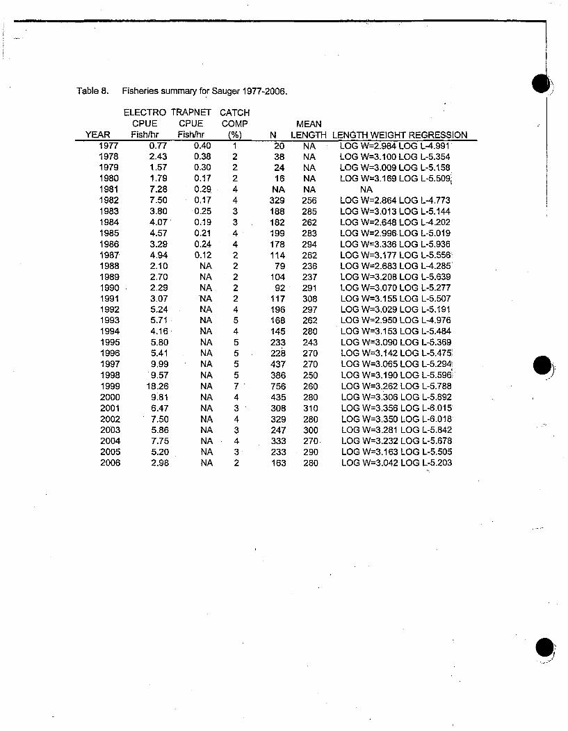
Table 8. Fisheries summary for Sauger 1977-2006.

ELECTRO TRAPNET CATCHCPUE CPUE COMP MEAN

YEAR Fish/hr Fish/hr (%) N LENGTH LENGTH WEIGHT REGRESSION1977 0.77 0.40 1 20 NA LOG W=2.984 LOG L-4.99111978 2.43 0.38 2 38 NA LOG W=3.100 LOG L-5.3541979 1.57 0.30 2 24 NA LOG W=3.009 LOG L-5.158!1980 1.79 0.17 2 16 NA LOG W=3.169 LOG L-5.509,1981 7.28 0.29 4 NA NA NA1982 7.50 0.17 4 329 256 LOG W=2.864 LOG L-4.7731983 3.80 0.25 3 188 285 LOG W=3.013 LOG L-5.1441984 4.07 0.19 3 182 262 LOG W=2.648 LOG L-4.2021985 4.57 0.21 4 199 283 LOG W=2.996 LOG L-5.0191986 3.29 0.24 4 178 294 LOG W=3.336 LOG L-5.9361987 4.94 0.12 2 114 262 LOG W=3.177 LOG L-5.556'1988 2.10 NA 2 79 236 LOG W=2.683 LOG L-4.285'1989 2.70 NA 2 104 237 LOG W=3.208 LOG L-5.639;1990 2.29 NA 2 92 291 LOG W=3.070 LOG L-5.2771991 3.07 *NA 2 117 308 LOG W=3.155 LOG L-5.5071992 5.24 NA 4 196 297 LOG W=3.029 LOG L-5.1911993 5.71 NA 5 168 262 LOG W=2.950 LOG L-4.9761994 4.16 NA 4 145 280 LOG W=3.153 LOG L-5.4841995 5.80 NA 5 233 243 LOG W=3.090 LOG L-5.3691996 5.41 NA 5 228 270 LOG W=3.142 LOG L-5.475'1997 9.99 NA 5 437 270 LOG W=3.065 LOG L-5.294,11998 9.57 NA 5 386 250 LOG W=3.190 LOG L-5.596:1999 18.26 NA 7 756 260 LOG W=3.262 LOG L-5.7882000 9.81 NA 4 435 280 LOG W=3.306 LOG L-5.8922001 6.47 NA 3 308 310 LOG W=3.356 LOG L-6.0152002 7.50 NA 4 329 280 LOG W=3.350 LOG L-6.0182003 5.86 NA 3 247 300 LOG W=3.281 LOG L-5.8422004 7.75 NA 4 333 270, LOG W=3.232 LOG L-5.6782005 5.20 NA 3 233 290 LOG W=3.163 LOG L-5.5052006 2.98 NA 2 163 280 LOG W=3.042 LOG L-5.203

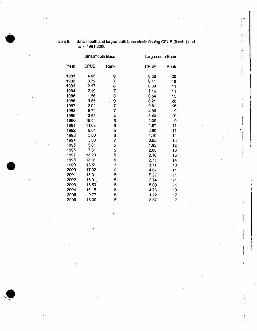
FTable 9. Smallmouth and largemouth bass electrofishing CPUE (fishfhr) and

rank, 1981-2006.r

Smallmouth Bass

Year CPUE Rank

Largemouth Bass

CPUE Rank

19811982198319841985198619871988198919901991199219931994199519961997199819992000200120022003200420052006

4.653.722.172.191.560.852.945.72

13.5216.4411.03

9.615.803.835.817.31

13.2315.0113.5117.0213.0115.9115.5916.15

9.7713.39

97878977

455567555576555665

0.580.410.801.160.540.210.614.063.402.391.872.501.100.651.932.082.102.753.714.675.216.145.094.731.228.57

201811111520

169

109

1111141512101514131111111110177

Table 10. Species composition expressed as % of total annual catches for PINGPfisheries studies, electrofishing and trapnetting combined for 1981-1987,and electrofishing only for 1988 through 2006.

Year19811982198319841985198619871988*1989*1990*1991 *1992*1993*1994*1995*1996*1997*1998*1999*2000*2001 *2002*2003*2004*2005*2006*

Carp1723182620212723202024262834303429231716151413141416

Whitebass2018171514181020151618121210161415161416172116141612

FreshwaterDrum

1224222031221681113121118141281011178151219122211

Sauger4433442221

2454555574343432

BlackCrappie

159161299

-11

31

<111

<1<11

212

.322211

<13

ShortheadRedhorse

77677812131714111410148111012911991115910

Walleye211222253

2I

22222

333355431"2"

GizzardShad

93211

<113<13422<1

4.<1<1

12

176751095

Total %8689858687848177706973727678787673748277727472737461

*Electrofishing only

4