ML022030448.pdf - Nuclear Regulatory Commission
238
SOLVIA Verification Manual Nonlinear Examples EXAMPLE B68 UNCONFINED SEEPAGE FLOW THROUGH A GRAVITY DAM Objective To perform an unconfined seepage flow analysis using PLANE conduction elements. Physical Problem The steady-state free surface seepage through the dam shown in the figure below is considered. The dam material is isotropic with permeability constants ky = k, = 2.5 ft/hr. Finite Element Model The figures on page B68.2 show the finite element mesh employed. The permeability matrix is evaluated using (4 x 4) Gauss integration. The bottom figure shows a contour plot of the distortion of the elements expressed in degrees. Solution Results The input data on page B68.4 has been used for the solution. A contour plot of the pressure is shown in the top figure on page B68.3. A good comparison with the free surface solution in [1], page 223 (full line in figure above) can be observed. A vector plot of the flux is shown in the bottom figure on page B68.3. Reference [1] Harr, M.E., Groundwater and seepage, McGraw Hill, New York, 1962. Version 99.0 B68.1
-
Upload
khangminh22 -
Category
Documents
-
view
4 -
download
0
Transcript of ML022030448.pdf - Nuclear Regulatory Commission

SOLVIA Verification Manual Nonlinear Examples
EXAMPLE B68
UNCONFINED SEEPAGE FLOW THROUGH A GRAVITY DAM
Objective
To perform an unconfined seepage flow analysis using PLANE conduction elements.
Physical Problem
The steady-state free surface seepage through the dam shown in the figure below is considered. The dam material is isotropic with permeability constants ky = k, = 2.5 ft/hr.
Finite Element Model
The figures on page B68.2 show the finite element mesh employed. The permeability matrix is evaluated using (4 x 4) Gauss integration. The bottom figure shows a contour plot of the distortion of the elements expressed in degrees.
Solution Results
The input data on page B68.4 has been used for the solution. A contour plot of the pressure is shown in the top figure on page B68.3. A good comparison with the free surface solution in [1], page 223 (full line in figure above) can be observed. A vector plot of the flux is shown in the bottom figure on page B68.3.
Reference
[1] Harr, M.E., Groundwater and seepage, McGraw Hill, New York, 1962.
Version 99.0 B68.1
SOLVIA Verification Manual
B68 UNCONFINED SEEPAGE FLOW THROUGH A GRAVITY DAM
ORIGINAL • • Z
SOLVIA-PRE 99.0 SOLVIA ENGINEERING AB
B68 UNCONFINED SEEPAGE FLOW THROUGH A GRAVITY DAM
ORIGJNAL 1i . L
r, V '8 6' I k
Ii / I
SCLVIA-PRE 99.0
S~DISTOR7TON 'lAX 4S*O
42 273 S36. 8 ' 8 S3'.363
25 908 '-2453
S9.55,129 .0880
IN 1 .360S
CLVA ENGINEERING A3
Version 99.0
Nonlinear Examples
B68.2

SOLVIA Verification Manual
B68 NNC3NFINED SEEPAGI
OR<ETNAL T-"E I
SOLVIA-POST 99.0
-LOW THROUGH A GRAVITY DAY
z
PRESSURE
MAX 0.C0003 J .37,174
S0.32416
0.27359 0o.2230: S.17243 S0.12:86 0 .071279
., C. 20702
MIN-4.5864E-3
SOLVIA ENGINEERING AB
B68 UNCONFINED SEEPAGE FLOW THROUGH A GRAVITY DAM
ORIGINAL I I TIME 1
SEEPACE F UX
L.A486,
SOLVI/A ENGINEERING AB:,ECL.','A-POST 99
Version 99.0
z I-
I
Nonlinear Examples
B68.3

SOLVIA Verification Manual
SOLVIA-PRE input
HEADING 'B68 UNCONFINED SEEPAGE FLOW THROUGH A GRAVITY DAM'
DATABASE CREATE COORDINATES / ENTRIES NODE Y Z
1 / 2 12.64 / 3 16. / 4 12. 4. / 5 4. 4. LINE STRAIGHT 1 2 EL*f6 MIDNODES=I LINE STRAIGHT 2 3 EL=4 MIDNODES=1
LINE COMBINED 1 3 2 LINE STRAIGHT 1 5 EL-5 MIDNODES=1 RATIO-i.
T-MATERIAL 1 SEEPAGE PERMEABILITY=2.5 GAMMA-.1
EGROUP 1 PLANE STRAIN INT=4 GSURFACE 1 3 4 5 EL1=20 EL2=5 NODES=8
T-LOADS SEEPAGEHEADS INPUT=LINES 1 5 4. 2 3 0.
T-LOADS SEEPAGEHEADS INPUT=NODES DELETE 2
MESH NSYMBOLS=MYNODES NNUMBERS=MYNODES MESH NSYMBOLS=MYNODES CONTOUR-DISTORTION
SOLVIA-TEMP END
SOLVIA-POST input
* B68 UNCONFINED SEEPAGE FLOW THROUGH A GRAVITY DAM
T-DATABASE CREATE
WRITE FILENAME='b68.1is' SET OUTLINE=YES NSYMBOLS=MYNODES
MESH CONTOUR=TPRESSURE MESH VECTOR=TFLUX
EMAX NUMBER=3 END
Version 99.0
Nonlinear Examples
1368.4

SOLVIA Verification Manual
EXAMPLE B69
SEMI-INFINITE REGION UNDERGOING TWO PHASE CHANGES
Objective
To verify the TRUSS conduction element for analysis of phase changes.
Physical Problem
The figure below shows the semi-infinite region considered. The initial temperature within the domain is To = 100' and the surface temperature is prescribed to be T, = 0'. The first and second phase change temperature interval is 0'. The thermal conductivity and specific heat are constant between the temperature 0' and 100'.
A00
T0 =1000 - 0
k = 1.0 thermal conductivity C = 1.0 specific heat per
unit volume
y00
Finite Element Model
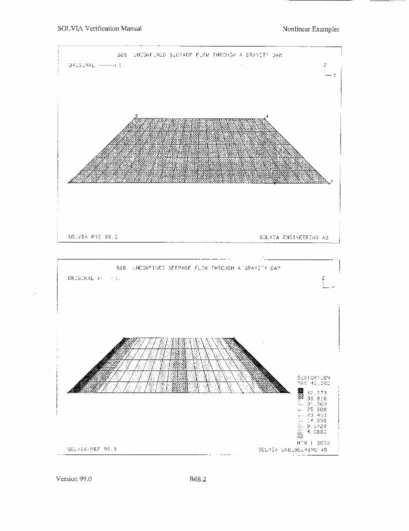
The figure on page B69.2 shows the used finite element model which consists of forty TRUSS conduction elements. The temperature degree of freedom at node 1 is deleted to impose the zero surface temperature. The element conduction matrix is evaluated using one point integration and a lumped specific heat matrix is employed. The time integration is performed using the Euler backward method in 67 time steps.
Version 99.0
Ts = 0°
Nonlinear Examples
B69.1
SOLVIA Verification Manual
Solution Results
The numerical solution results are obtained by using the input data on pages B69.4 and B69.5. The temperature distributions within the domain are given in the top figure on page B69.3 for the solution times 0.2, 0.4 and 1.0 and are compared with the corresponding analytical solutions ([1] page 290). The heat flux in the element at time 1.0 is shown in the bottom figure on page B69.3.
User Hints
* The material conductivity and specific heat are assumed to remain constant in the entire range of temperatures from 0' to 1000. As a result, the semi-infinite domain is discretized using linear TRUSS conduction elements with constant material properties.
Reference
[1] Carslaw, H.S., and Jaeger, J.C., Conduction of Heat in Solids, 2nd Ed., Oxford University Press, Inc., N.Y., 1959.
B69 SE,'I-iNFTNITE REG-LON UNDERGOING T.40 PHASE
ORIG:NAL .-- 0.S
ORIG NAL -- 0
-HANGES
z i
z
-X
SCL"/A-PRE 99.0 SGLV:A \N' ThORNAB
Version 99.0
i I ---- 1-11 --- I ---- I I - I - - - - - - I - - - - -
Nonlinear Examples
B69.2

SOLVIA Verification Manual Nonlinear Examples
B69 SE>- INF!N 9EGION UNDERGO 3 G 0>0 O PHASE CHANGz
ST ... .......... .. . .: .. : ( ..... .. ...... . .. ... . .... .........
'D 1
(% x
K / 2• 7 •
(01,,>
0
TAN'
SOLV A-POST 99.0
6 7 3
SOLVEA ENG:NEERING AB
369 SEMd-INFINITE UEGION UNDERGOING TW; P-AS
f.
2
SOLVIA-POST 99 CL/IA ENGC7 EEI\NG AB
Version 99.0
2W
CHANGES
I
B69.3

SOLVIA Verification Manual
SOLVIA-PRE input
HEADING 'B69 SEMI-INFINITE REGION UNDERGOING TWO PHASE CHANGES'
DATABASE CREATE T-MASTER NSTEP=30 DT=0.004 20 0.01 17 0.04 T-ANALYSIS TRANSIENT HEATMATRIX=LUMPED METHOD=BACKWARD-EULER T-ITERATION TTOL=i.E-6 ITEMAX=i00
COORDINATES 1 0. TO 2 8.
T-MATERIAL 1 CONDUCTION K=i. SPECIFICHEAT=i. LH1=80. LH2=30.
LINE STRAIGHT 1 2 EL=-00 RATIO=20 EGROUP 1 TRUSS GLINE 1 2 EL-f00 EDATA / 1 1.
T-INITIAL TEMPERATURE INPUT=LINE 1 2 100.
T-PHASETRANSITIONS 50. 0. 0 90. 0. 0
FIXBOUNDARIES TEMPERATURE / 1 .
SET NSYMBOL=YES VIEW=-Y MESH NNUMBERS=MYNODES SUBFRAME=12 MESH BCODE=TEMPERATURE .
SOLVIA-TEMP END
SOLVIA-POST input
* B69 SEMI-INFINITE REGION UNDERGOING TWO PHASE CHANGES
T-DATABASE CREATE
WRITE FILENAME='b69.1is'
AXIS ID=i VMIN-0. VMAX=8. LABEL='DISTANCE' AXIS ID-2 VMIN=0. VMAX=i00. LABEL='TEMPERATURE' USERCURVE 1 / READ 'B69TI02.DAT' USERCURVE 2 / READ 'B69TI04.DAT' USERCURVE 3 / READ 'B69TI10.DAT' NPLINE NAME=NODES / 1 101 TO 199 2
SET DIAGRAM=GRID NLINE LINENAME=NODES TIME=0.2 XAXIS=1 YAXIS=2 SYMBOL=i SET SUBFRAME=OLD NLINE LINENAME=NODES TIME=0.4 XAXIS=-i YAXIS=-2 SYMBOL=2 NLINE LINENAME=NODES TIME=i.0 XAXIS=-i YAXIS=-2 SYMBOL=4 PLOT USERCURVE 1 XAXIS=-i YAXIS=-2 PLOT USERCURVE 2 XAXIS=-i YAXIS=-2 PLOT USERCURVE 3 XAXIS=-I YAXIS=-2
EPLINE NAME=TRUSS / 1 1 TO 100 1 ELINE LINENAME=TRUSS KIND:TFLUX OUTPUT=ALL SUBFRAME=NEXT END
Nonlinear Examples
Version 99.0 1369.4

SOLVIA Verification Manual
EXAMPLE B70
USER-SUPPLIED MATERIAL MODEL (RAMBERG-OSGOOD)
Objective
To demonstrate the implementation of the Ramberg-Osgood constitutive law as a user-supplied material model for SOLID elements.
Physical Problem
A cantilever structure subjected to uniaxial compression is considered as shown in figure below.
I .- y
Po Mi)
The chosen Ramberg-Osgood constitutive law constants:
E=3x 10⁷
v=0.30
a0 =6x10⁴
S=0.05
n =10.0
Tolerance for effective stress iterations = 101° Iteration limit for effective stress iterations = 25
In the uniaxial load case the stress-strain relation can be described by
- =-+p i - go G O (0 L ) "
so = yield strain
O = yield stress
S= material constant
n = power hardening exponent
Material Model
The FORTRAN source subroutine used to implement the constitutive law is given on pages B170.5 to B170.9.
Finite Element Model
The cantilever structure is discretized using 4 twenty-node SOLID elements, see figure on page B70.2. The solution is obtained using the full Newton iteration with line searches.
Solution Results
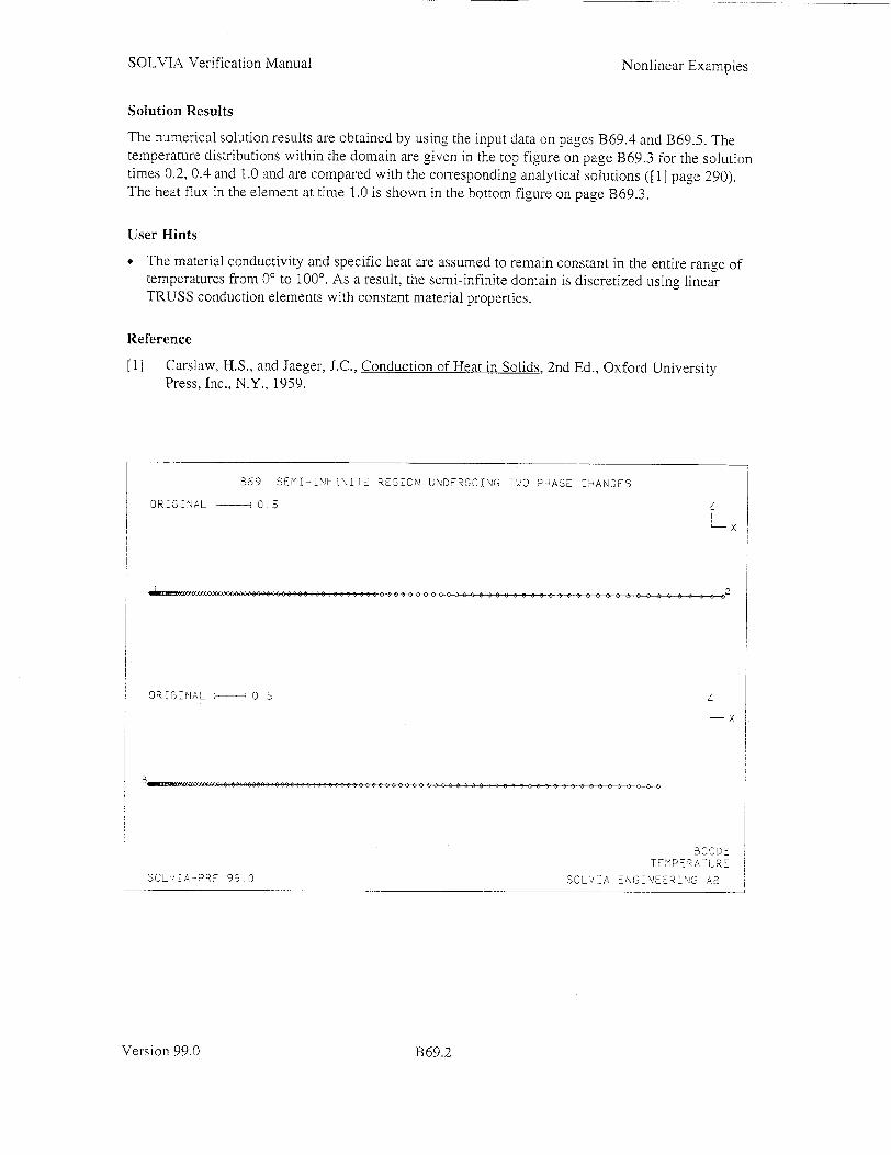
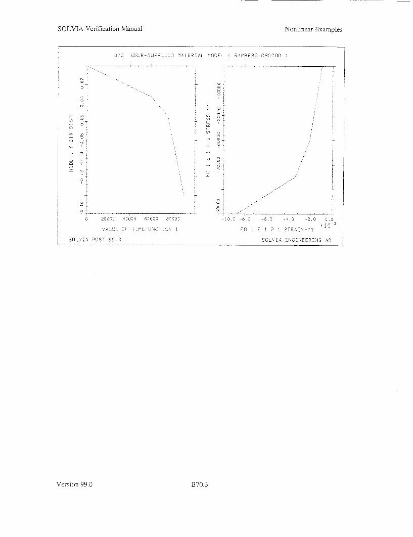
Using the input data given on page B170.4 the obtained numerical solution is shown in the figures on page B70.3. The obtained solution agrees well with the corresponding analytical solution.
Version 99.0
'ID
where
Nonlinear Examples
B70.1

SOLVIA Verification Manual Nonlinear Examples
B70 USER-SUPP.IED MATER AL M0DEL RAMBEoG-OSSOOC
CRI3NA TIME I
SOLV:A-PRE 99.0
370 USER-SUPPLIED MATERIAL MODEL RAMBERG-CSGOOD
ORIGINAL - - I. MAX D:$PL. 0- 0. 4037 TIME A
)
0 . IA-IOST 9 CLIA ENGINEERING AS
Version 99.0
PRESSURE
30000
MASTER 000 11
H 111111 SOLViA ENGINEERING AB
z
K Y
Y-D-R DISPL. MlAX 0
-8. 766SE-3
-0.02630C
" 0 043833 -0.06'.366 -. 0 378899
-0.3964329
-. 1 1396
MrNAKC2
B70.2
SOLVIA Verification Manual Nonlinear Examples
B7C LSE-S-J PI - 77 ATR A~IL 'ICFE
-Ij
ýANBEPG-OSGOOD
;701
0 20030 400330 60000 8C003
VA~j C- 77NFF Nýý -C I
SOLVIA-POST 99.0
3. -8.0 - . -4, -2.0 0 -1
E STPATN-YY
SLVIA ENCINEE.N R7
Version 99.0B0.
0
B70.3

SOLVIA Verification Manual
SOLVIA-PRE input
HEADING 'B70 USER-SUPPLIED MATERIAL MODEL ( RAMBERG-OSGOOD
DATABASE CREATE MASTER IDOF=000111 NSTEP=4 TOLERANCES TYPE=F RNORM=0.6 ITERATION METHOD=FULL-NEWTON LINE-SEARCH=YES
TIMEFUNCTION 1 0 0 / I 3E4 / 2 6E4 / 4 9E4
COORDINATES 1 0. 16. / 2 / 3 1. / 4 1, 16.
NGENERATION NSTEP=4 ZSTEP=-- / 1 TO 4
MATERIAL 1 USER-SUPPLIED CTIT=3.E7 CTI2-0.3 CTI3=6.E4, CTI4=0.05 CTIS=10 SCPT=1.E-10 SCP2=25 INTER=10 -200 0 0 0 0 0 0 200 0 0 0 0 0 0
EGROUP 1 SOLID GVOLUME 1 2 3 4 5 6 7 8 EL1=4 EL2=1 EL3=1 NODES=20 LOADS ELEMENT INPUT=SURFACE
1 4 5 8 1.
FIXBOUNDARIES 1 INPUT=LINES / 5 6 / 1 2 / 2 6 FIXBOUNDARIES 2 INPUT=SURFACE / 2 3 6 7 FIXBOUNDARIES 3 INPUT=LINES / 3 4 / 1 2 / 2 3 LOADS TEMPERATURE TREF=0.
VECTOR LENGTH=0.5 MESH NSYMBOLS=MYNODES NNUMBERS=MYNODES BCODE=ALL VECTOR=LOAD
SOLVIA END
SOLVIA-POST input
* B70 USER-SUPPLIED MATERIAL MODEL ( RAMBERG-OSGOOD
DATABASE CREATE
WRITE FILENAME='b70.lis'
MESH ORIGINAL=DASH DMAX=1 CONTOUR=DY
NHISTORY NODE=1 DIRECTION=2 OUTPUT=ALL XVARIABLE=1 SUBFRAME=21 EXYPLOT ELEMENT=i POINT=1 XKIND=EYY YKIND=SYY OUTPUT=ALL END
Version 99.0
Nonlinear Examples
B70.4

SOLVIA Verification Manual
SUBROUTINE CUSER3 ( KTR, STRESS, STRAIN, SIG, EPS, DEPS, DEPST, 1 THSTRi, THSTR2, SCP, ICP, ARRAY, IARRAY, D, 2 ALFA, CTD, ALFAA, CTDD, CTI, CTJ, PROP, 3 TMPI, TMP2, TIME, DT, INTER, KEY )
C* --- ---------------------------------------------------- SOLVIA CUSER3 C*I C*I USER-SUPPLIED MATERIAL MODEL FOR SOLID ELEMENT C*I C*I This subroutine is to be supplied by the USER to calculate C*I the STRESSES and CONSTITUTIVE MATRIX of a special material. C*I C*I This subroutine is called in USER3 for each INTEGRATION POINT C*I for each SOLID element to perform the following operations C*I C*I KEY = 1 Initialize the working arrays during INPUT phase C*I KEY = 2 Calculate element stresses C*I KEY = 3 Calculate the stress-strain matrix C*I KEY = 4 Print element stresses and other desired variables C*I C*I VARIABLES C*I C*I NUMBEL Element number C*I IPT Integration point number C*I STRESS(6) Stress components, received at time TAU and C*I updated by USER-SUPPLIED coding to correspond C*I to time TAU + DTAU C*I STRAIN(6) Total strain components at time T + DT C*I EPS(6) Total strain components at time T C*I DEPS(6) Subdivided incremental strain components C*I DEPS(I) = ( STRAIN(I) - EPS(I) )/INTER - DEPST(I) C*I ( Passed to subroutine CUSER3 by SOLVIA program ) C*I DEPST(6) Components of subincremental thermal strain C*I ( Passed to subroutine CUSER3 by SOLVIA program ) C*I THSTRI(6) Total thermal strain at time TAU C*I THSTR2(6) Total thermal strain at time TAU + DTAU C*I INTER Number of subdivisions for the strain increments C*I KTR Current subdivision number C*I EQ. 1, First subdivision C*I EQ. INTER, Last subdivision C*I SCP(5) User-defined solution control parameters C*I ICP(5) User-defined solution control parameters C*I ARRAY(23) Working array ( REAL ), received at time TAU and C*I updated by USER-SUPPLIED coding to correspond to C*I time TAU - DTAU C*I IARRAY(2) Working array ( INTEGER ), received at time TAU C*I and updated by USER-SUPPLIED coding to correspond C*I to time TAU + DTAU C*I D(6,6) Stress-strain matrix, to be calculated by USERC*I SUPPLIED coding C*I ALFA Coefficient of thermal expansion at time TAU C*I CTD(5) Temperature-dependent material constants at C*I time TAU C*I ALFAA Coefficient of thermal expansion at time C*I TAU + DTAU C*I CTDD(5) Temperature-dependent material constants at C*I time TAU + DTAU C*I CTI(8) User-defined constant material properties C*I CTJ(8) User-defined constant material properties C*I PROP(16,*) User-defined material property table C*I TMPI Temperature at integration point at time TAU C*I TMP2 Temperature at integration point at time C*I TAU + DTAU C*I TIME Time at current step, T + DT C*I DT Time step increment, DT C*I
Version 99.0
Nonlinear Examples
B70.5

SOLVIA Verification Manual
C*I Note that the variables passed to the subroutine CUSER3 C*I when KEY = 3, 4 are these calculated last; i.e., calculated C*I in the last subdivision when KEY = 2. Hence, these variables C*I are not calculated when KEY = 3, 4. C*I C*I Note also that when a mixed formulation is used, C*I PRESSURE-INTERPOLATION = YES in EGROUP command, the stressC*I strain matrix D is used in the stress calculation, KEY = 2, C*I in the SOLVIA program. The user should keep the D-matrix C*I updated during the integration of stresses for a correct C*I pressure interpolation. C*I C*I There are no controls or error checking of user input data C*I for the User-Supplied material model in SOLVIA-PRE. C*I
IMPLICIT DOUBLE PRECISION ( A-H, O-Z COMMON /COMTEM/ RTEMP(100), JTEMP(200) COMMON /EL/ IND,ICOUNT,NPAR(30),NUMEG,NEGL,NEGNL,IMASS,IDAMP,
1 ISTATNDOF,KLINIEIG,IMASSNIDAMPN COMMON /VAR/ NG,MODEX,IUPDTKSTEP,ITEMAX, IEQREF,ITE,KPRI,
1 IREF,IEQUIT, IPRI,KPLOTN,KPLOTE COMMON /ELDATA/ NUMBEL,NEL,IPT,IELD,ND,IPS,ISVE,IPRNT COMMON /DISDR/ DISD(9) COMMON /THREED/ DE,NPT,IDW,NND9,ISOCOR COMMON /TAPES/ IIN,IOUT COMMON /INCOMP/ CUDIS(6,6),CUPRE(6),PRESEL(4),PPROJ,PKAPPA,PREDI,
1 IDINCONPRESS,NPRACC,NPROLD,N3C C
DIMENSION STRESS(*), STRAIN(*), SIG(*), EPS(*), DEPS(*), 1 DEPST(*), THSTRI(*), THSTR2(*), SCP(5), ICP(5), 2 ARRAY(23), IARRAY(2), D(6,*), CTD(5), CTDD(5), 3 CTI(8), CTJ(8), PROP(16,*)
GOTO ( 100, 200, 300, 400 ), KEY C*I C*I C*I K EY 1 C*I C*I Initialize components of real and integer working arrays, C*I ARRAY(23) and IARRAY(2) C*I 100 CONTINUE
C*I C*I I N S E R T U S E R - S U P P L I E D C O D I N G C*I
GOTO 900 C*I C*I C*I K E Y = 2 C*I C*I Integration of element stresses, STRESS C*I
200 CONTINUE C*I C*I **I N S E R T U S E R -S U P P L I E D C O D I N G C*I C*I Ramberg-Osgood material C*I C*I CTI( 1 ) Youngs modulus C*I CTI( 2 ) Poissons ratio C*I CTI( 3 ) Yield stress C*I CTI( 4 ) Beta, material parameter C*I CTI( 5 ) N, power hardening constant C*I SCP( 1 ) Tolerance for effective stress iterations C*I SCP( 2 ) Iteration limit for effective stress iterations
Version 99.0
Nonlinear Examples
1370.6

SOLVIA Verification Manual
ARRAY( 1 ARRAY( 2 ARRAY( 3 ARRAY( 4 ARRAY( 5
Ratio of effective stress Total effective strain Constant in stress-strain Constant in stress-strain Constant in stress-strain
to yield stress
matrix matrix matrix
TOLER = I.D-6
C*I C*I C*I C*I C*I C*I
C*I
C*I
C*I C*I C*I
C*I
CTI( 1 ) CTI( 2 CTI( 3 CTI( 4 ) CTI( 5 = SCP( 1 = INT( SCP( 2
Xl = 2.D0 / 9.D0 X2 = 2.D0 * ( 1.D0 XNl = XN - 1.D0 YE = YS / YM
) )
- PR ) / 3 .00
Effective strain
E12 = STRAIN( 1 ) - STRAIN( E23 = STRAIN( 2 ) - STRAIN( E31 = STRAIN( 3 ) STRAIN( E4 = STRAIN( 4 E5 = STRAIN( 5 E6 = STRAIN( 6
2 3 1
EQE ( E12 * E12 + E23 * E23 E31 * E31 ) * X1 1 (E4 *E4 + E5 *E5 + E6 *E6 * *15.D0
IF ( EQE .LT. 1.D-20 ) GOTO 230 EQE = SQRT( EQE ) RE = EQE / YE RS ARRAY( 1 IF ( RS .LT. TOLER ) RS = TOLER
*I *I Newton-Raphson iteration to obtain equivalent stress 2*I
ITR = 0 210 F BB * RS ** XN + X2 * RS - RE
IF ( ABS( F ) .LT. TOLS ) GOTO 220 ITR ITR + i IF ( ITR GT. IMAX ) GOTO 800 FP - XN * BB * RS ** INI - X2 IF ( ABS( FP ) LT. TOLS ) GOTO 810 RS RS - F / FP IF ( RS .LT. TOLER ) RS = TOLER GOTO 210
;*1
2*1 Element stresses *I
220 ET - RS * YS / EQE ARRAY( 1 ) - RS GOTO 240
ET = DVOL DDEV DD = DV = DF =
YM / X2 = YM/( 3.D* (l.D0 - 2.D0 * PR = ET * X1 DVOL + 2.D0 * DDEV 1.5D0 * DDEV DVOL - DDEV
Version 99.0
YM = PR = YS = BB = XN = TOLS IMAX
C C C
C C C
C*I 230 240
C*I
Nonlinear Examples
) ) ) ) )
) ) )
B70.7

SOLVIA Verification Manual
ARRAY( 2 ARRAY( 3 ARRAY( 4 ARRAY( 5
= EQE = DD = DF = DV
C*I DO 250 I = 1, 6 DO 250 J = 1, 6 D( I, J ) 0.D0
250 CONTINUE C*I
DO 260 I 1 1, 3 D( I, I ) = DD II = I + 3 D( II, II ) - DV
260 CONTINUE D( 1, 2 ) = DF D( 1, 3 ) = DF D( 2, 3 ) DF D( 2, 1 ) - DF D( 3, 1 ) = DF D( 3, 2 ) = DF
C*I
C*I
C*I C*I C*I 800
C*I 810
C*I C*I C*I C*I C*I C*I
300 C*I C*I C*I
C*I
310 C*I
STRESS STRESS STRESS STRESS( STRESS STRESS
1 2 3 4 5 6
= DD = DD = DD = DV = DV = DV
*
*
*
*
*
*
STRAIN( STRAIN( STRAIN( STRAIN( STRAIN( STRAIN(
GOTO 900
Convergence failed
WRITE IOUT, 8000 NPAR( WRITE IOUT, 8100 ITR STOP
WRITE IOUT, 8000 NPAR( WRITE IOUT, 8200 STOP
1 2 3 4 5 6
DF * (STRAIN(2) + STRAIN(3) DF * (STRAIN(l) + STRAIN(3) ) DF * (STRAIN(l) + STRAIN(2)
30 ), NUMBEL, IPT
30 ), NUMBEL, IPT
K E Y = 3
Form constitutive law, stress-strain matrix D
CONTINUE
* * INSERT
00 = ARRAY( 3 ) DF = ARRAY( 4 ) DV = ARRAY( 5 )
DO 310 I = DO 310 J = D( I, J CONTINUE
U S E R - S U P P L I E D COD ING
1, 6 1, 6 0.D0
DO 320 I 1, 3 D( I, I ) DD II = I + 3 D( II, II ) DV
Version 99.0
Nonlinear Examples
) ) ) )
B70.8

SOLVIA Verification Manual
320 CONTINUE D( 1, 2 ) DF D( 1, 3 ) DF D( 2, 3 ) DF D( 2, 1 = DF D( 3, 1 = DF D( 3, 2 ) DF
C*I GOTO 900
C*I C*I C*I K E Y = 4 C*I C*I Print of element results, STRESS and STRAIN, etc. C*I
400 CONTINUE C*I C*I * I N S E R T U S E R - S U P P L I E D C O D I N G C*I C*I C*I Current effective stress C*I
EQS ARRAY( )*CTI( 3) C*I C*I Print heading and element number C*I
IF ( IPT .EQ. 1 ) WRITE ( IOUT, 2000 ) NUMBEL WRITE ( IOUT, 2100 ) IPT, ( STRESS( I ), I = 1, 6 ), EQS
C*I GOTO 900
C*I 2000 FORMAT ( /, ' ELEMENT POINT STRESS-XX STRESS-YY', 5X,
1 'STRESS-ZZ STRESS-XY STRESS-XZ STRESS-YZ', 3X, 2 'EFF. STRESS', //, lX, 15 )
2100 FORMAT C 12X, 13, 1X, 7( IX, IPEl3.5 8000 FORMAT ( /, ' ***ERROR: SOLVIA program STOPS', / 14X,
1 'EGROUP 1', 4, ' ( SOLID User-Supplied model )', / 14X, 2 'Element 5', I, ' Integration point = ', 13
8100 FORMAT ( 14X, 'Number of iterations = ', I5, / 14X, 1 'Max number of iterations reached in the effective stress 2 'iterations', / 14X, 'Subroutine CUSER3', / )
8200 FORMAT ( 14X, 'Newton-Raphson iterations failed due to zero', /, 1 14X, 'derivative in effective stress calculations', / 14X, 2 'Subroutine CUSER3', /
900 RETURN C
END
Version 99.0
Nonlinear Examples
B70.9
SOLVIA Verification Manual
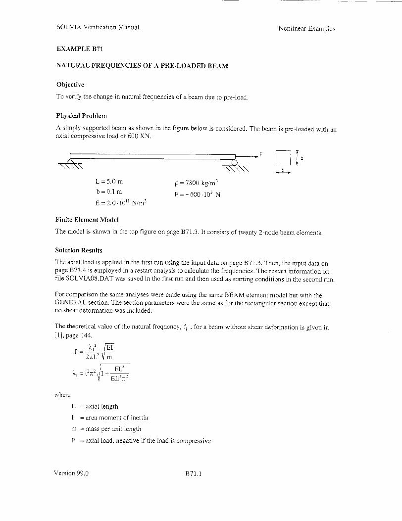
EXAMPLE B71
NATURAL FREQUENCIES OF A PRE-LOADED BEAM
Objective
To verify the change in natural frequencies of a beam due to pre-load.
Physical Problem
A simply supported beam as shown in the figure below is considered. The beam is pre-loaded with an axial compressive load of 600 KN.
FF Fb
L-= 5.Om p =7800kg,'m3
b=0.1m F=-600.103 N
E =2.0.10"' N/m 2
Finite Element Model
The model is shown in the top figure on page B71.3. It consists of twenty 2-node beam elements.
Solution Results
The axial load is applied in the first run using the input data on page 1371.3. Then, the input data on page B71.4 is employed in a restart analysis to calculate the frequencies. The restart information on file SOLVIA08.DAT was saved in the first run and then used as starting conditions in the second run.
For comparison the same analyses were made using the same BEAM element model but with the GENERAL section. The section parameters were the same as for the rectangular section except that no shear deformation was included.
The theoretical value of the natural frequency, fl, for a beam without shear deformation is given in [I], page 144.
Ei2 -7I
.i 22-FC"
where
L = axial length
I = area moment of inertia
m = mass per unit length
F = axial load, negative if the load is compressive
Version 99.0
Nonlinear Examples
B71.1

SOLVIA Verification Manual
Calculated frequencies (Hz):
Nonlinear Examples
Theory SQOLVIA SOLVIA
with shear def. without shear def.
Frequency 1 2.726 2.709 2.722
Frequency 2 32.28 32.21 32.27
Frequency 3 78.36 78.03 78.35
The mode shapes are shown in the figure below and in the figure on page B71.3.
An analysis with no pre-load gave the following frequencies (Hz):
Theory SOLVIA SOLVIA with shear def. without shear def.
Frequency 1 9.185 9.181 9.185
Frequency 2 36.74 36.68 36.74
Frequency 3 82.66 82.36 82.66
Reference
[1] Blevins, Robert D., Formulas for Natural Frequency and Mode Shape, Van Nostrand Reinhold Company, 1979.
37' NATURAL
'lAX DISPL. ! SE-3 TIIE I
AREQUENCIES OF A PRELCADED BEAN
z
LOAD
£ES
3 'D'O11
C 0O11
ZRE.FERELNrc i O. CAX DS25L. - 3.37394
MO0DE ' FREO 2.7994
SOL!IA-CSOS 9. -LVIA _NG NEER !F G A,(
Version 99.0 B71.2

SOLVIA Verification Manual
B/' NA-URAL -RE'zUENCIES CF A DRE< Aý
R EERENCE I 1< .
"MAX D CSPL C,07161s MCDE 2 FREC 32.207
IAX DCSP. P -0 010716!1 M1DE 3 FRED 78.033
SCLVIA-PGST 99.0 SOLVIA ENGINE-RING AB
SOLVIA-PRE input, first run
HEADING 'B71 NATURAL FREQUENCIES OF A PRELOADED BEAM'
* First run
DATABASE CREATE MASTER IDOF=i00011 KINEMATICS DISPLACEMENT=LARGE ITERATION METHOD=BFGS
COORDINATES 1 / 2 0. 5.
MATERIAL 1 ELASTIC E=2.Ell DENSITY=7800
EGROUP 1 SECTION 1 BEAMVECTOR GLINE 1 2
BEAM RECTANGULAR WTOP / 1 0. 0. 1.
AUX=-1 EL=20
FIXBOUNDARIES 23 FIXBOUNDARIES 3 LOADS CONCENTRATED
SOLVIA END
/ /
0.1 D=0.1
! 2
2 2 -600.E3
Version 99.0
BE AM'
z
z
Nonlinear Examples
B71.3

SOLVIA Verification Manual
SOLVIA-POST input, first run
* B71 NATURAL FREQUENCIES OF A PRELOAD BEAM
* First run
DATABASE CREATE END
SOLVIA-PRE input, second run
* B71 NATURAL FREQUENCIES OF A PRELOADED BEAM
* Second run
DATABASE OPEN MASTER MODEX=RESTART TSTART=l.0 ANALYSIS TYPE-DYNAMIC MASSMATRIX=LUMPED FREQUENCIES SUBSPACE-ITERATION NEIG-3 SSTOL=i.E-10
SOLVIA END
SOLVIA-POST input, second run
* B71 NATURAL FREQUENCIES OF A PRELOADED BEAM
* Second run
DATABASE RESTART
WRITE FILENAME='b7la.lis'
FREQUENCIES EMAX
SET NSYMBOLS-YES VIEW=X MESH NNUMBER-MYNODES BCODE=ALL VECTOR=LOAD SUBFRAME=12
SET RESPONSETYPE=VIBRATIONMODE ORIGINAL=YES MESH TIME=i MESH TIME=2 SUBFRAME=12 MESH TIME=3 END
Version 99.0
Nonlinear Examples
1371.4

SOLVIA Verification Manual
EXAMPLE B72
PLASTIC COLLAPSE OF A BEAM STRUCTURE, PIPE-SECTION
Objective
To verify the PIPE element in a collapse analysis using the automatic iteration method.
Physical Problem
A plane frame with hinged support is subjected to a horizontal load, see figure below. The frame has a pipe section and the material is elastic-perfectly plastic.
F
h 74l 7,
17% I D
h = 1200 mm
D = 120 mm
t=2.5 mm
E =2.0.105 N/mm 2
v=0.3
Gy = 250 N/mm 2
Finite Element Model
Seven 2-node PIPE elements are used in the model. At the junctions of the horizontal and vertical members short elements are used to describe the plastic mechanism. A small displacement analysis is used. The model is shown in the left figure on page B72.2.
Solution Results
The input data on page B72.3 is used to calculate the collapse load with eight integration points along the circumferential direction (TINT=8). In addition, results for TINT=12 and TINT=24 have been obtained for comparison.
Case Collapse load, KN
Theory 15.00
SOLVIA TINT=8 14.23
SOLVIA TINT= 12 14.67
SOLVIA TINT=24 14.92
Deflection of node 6 as function of the load multiplier and a contour plot of the t-moment are shown in the right figure on page B72.2.
Version 99.0
Nonlinear Examples
B72.1

SOLVIA Verification Manual Nonlinear Examples
User Hints
* Note that the model used is intended for calculation of the limit load. For a more detailed analysis of the stress distribution a finer mesh needs to be used also in areas away from the locations of plastic mechanism.
872 P5_ASTC CCLLAPSE OF A 0EAM STRUCTURE0 P'PE-SE5T'ON
3R8GINAL - 20. Z
MAST-R i IC01
Y.l lR3GINAL - 200
TiME
41 6
FORCE
SOLV'A ANOONERN 08
872 PLAST/0 C COL5APS OF A BEAM STRUCTURE. PIPE-SECTEON
' 'S
200 1000 6000 800 2000 12000 11000
-CAD MULTO I ER 0MBD1A
2MAX D:SPL - 35.532 TIME i0
-1
SOLVIA-POST 99.0
SMONMENT-T7 NO AVERAGTNG
MAX 8.5374E6
7 .4703E6 S 3359E6 , 312O:SE6 3. 0672E -t 0672E5
-3 20. SE 5.3359E5 7 4703E6
71N-5.8374E5
SOLVIA ENGONEE'RNG A8
Version 99.0
SOLV0A-0RE 99 0
1J @" Y7
a
B72.2

SOLVIA Verification Manual
SOLVIA-PRE input
HEADING 'B72 PLASTIC COLLAPSE OF A BEAM STRUCTURE, PIPE-SECTION' ,
DATABASE CREATE MASTER IDOF=100011 NSTEP=10 AUTOMATIC-ITERATION NODE=3 DIRECTION=2 DISPLACEMENT=-0,
CONTINUATION=YES DISPMAX=100
COORDINATES / ENTRIES NODE Y Z 1 / 2 0. 1100. / 3 0. 1200. / 4 100. 1200. 5 1100. 1200. / 6 1200. 1200. / 7 1200. 1100. 8 1200. / 9 600. 600.
MATERIAL 1 PLASTIC E=2.E5 NU=0.3 YIELD=250. ET=0.
EGROUP 1 PIPE TINT=8 RESULTS=FORCES SECTION 1 DIAMETER=120 THICKNESS=2.5 ENODES / 1 9 1 2 TO 7 9 7 8
FIXBOUNDARIES 23 / 1 8 FIXBOUNDARIES 234 / 9 LOADS CONCENTRATED / 3 2 1.
SET VIEW=X NSYMBOLS=YES PLOTORIENTATION-PORTRAIT MESH NNUMBERS=YES BCODE=ALL SUBFRAME-12 MESH ENUMBERS=YES VECTOR=LOAD .
SOLVIA END
SOLVIA-POST input
* B72 PLASTIC COLLAPSE OF A BEAM STRUCTURE, PIPE-SECTION
DATABASE CREATE
WRITE FILENAME='b72.1is'
SET PLOTORIENTATION=PORTRAIT VIEW=X SUBFRAME 12 NHISTORY NODE=6 DIRECTION=2 SYMBOL:1 OUTPUT=ALL
CONTOUR AVERAGE=NO MESH CONTOUR:MT DMAX=TRUE END
Version 99.0
Nonlinear Examples
B 72. 3

SOLVIA Verification Manual
EXAMPLE B73
PLASTIC COLLAPSE OF A BEAM STRUCTURE, BOX-SECTION
Objective
To verify the ISOBEAM element and RIGIDLINK in a collapse analysis using the AUTOMATICITERATION method.
Physical Problem
A plane frame with hinged support is subjected to a horizontal load, see figure below. The frame has a uniform box cross-section and the material is elastic-perfectly plastic.
F
h I74 74
- Rigid link Beam section 1
Center node
h " Beam section 2
Geometry h = 2000 mm
b = 100 mm
t=2 mm
Material E = 2.0-105 N/mm 2
v =0.3
-y = 250 N/mm2
Finite Element Model
The 2-node ISOBEAM element and RIGIDLINK are used in the model. Each side of the box section is modeled using an ISOBEAM and connected to the center of the section with a RIGIDLINK. At the junctions of the horizontal and vertical members short elements are used to describe the plastic mechanism. A small displacement analysis is used. The model is shown in the figures on page B73.2.
Solution Results
The input data on pages B73.3 and B73.4 is used. The obtained SOLVIA collapse load is compared with the analytical solution.
Collapse load, N
SOLVIA 7366
Theory 7204
The deflection at node 17 as a function of the load multiplier and the deformed mesh with the applied load are shown in the figure on page B73.3.
Version 99.0
Nonlinear Examples
1373.1
SOLVIA Verification Manual Nonlinear Examples
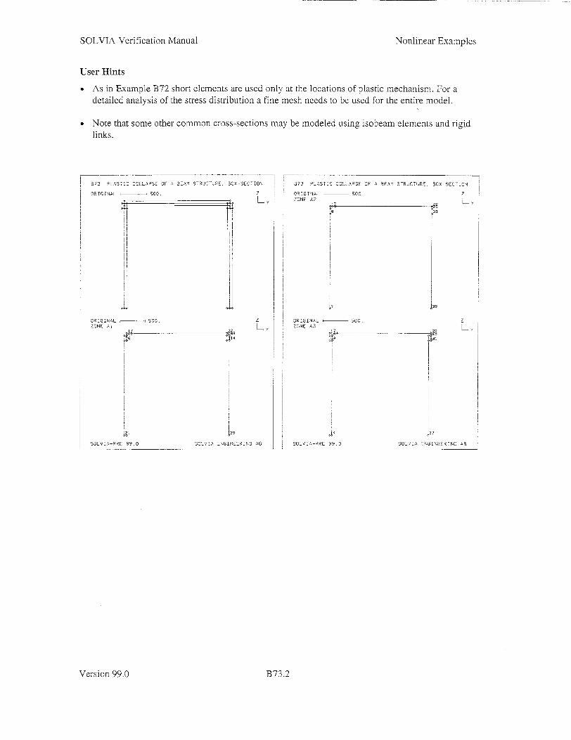
User Hints
"* As in Example B72 short elements are used only at the locations of plastic mechanism. For a detailed analysis of the stress distribution a fine mesh needs to be used for the entire model.
"* Note that some other common cross-sections may be modeled using isobeam elements and rigid links.
B73 PLASTIC COLLAPSE OF A BEAM TRJUCTURE. 30X-SE:77ON
0RIGINAL - - •00. Z
C. L
373 PLASTIC COLLAPSE OF A BEAM STRUCTURE, BOX
0R7GINAL - 00 ZONE A2
V
0ROGINAL - C00 ZONE A.
,ý7
90 V SOLVWA,-RE 990 SOL.A UNOINEI
Z
LK
E.RNG AB
Version 99.0
SEC-ION
Z E '
U!
ORIGINAL - oo. ZONE A3
V -9
0 LV.A-RE 99.0
327
SOL'¢ZA SNGfN.A NG AS
1373.2

SOLVIA Verification Manual Nonlinear Examples
B73 ASTIC C3L I APSE OF A BEAM' SRUCTURE, BOX-SET -3N
,AX SPL. 6-- p-6.71 Z 0T _ 'I TIE 0 IL y
T -il
- L
L CAD
OAD N 1,TV PIP. _A'BDA 76 .
1 OLVIA-PCST 99.0 SLV/IA ENG-INEERING AB
I• I
SOLVIA-PRE input
HEADING B73 PLASTIC COLLAPSE OF A BEAM STRUCTURE, BOX-SECTION'
DATABASE CREATE MASTER IDOF=100011 NSTEP-10 AUTOMATIC-ITERATION NODE-li DIRECTION=2 DISPLACEMENT=10,
CONTINUATION-YES DISPMAX-500
COORD INAT ES 1 / 2 0. -49. /3 -4. 4 0. 49. 5 49.
16 0. 0. 2000. /17 0. 0. 2049. /18 -49. 0. 2000. 19 0. 0. 1951. 20 49. 0. 2000.
NGENERATION NSTEP=5 ZSTEP--1900 / 1 To 5 NGENERATION NSTEP-10 ZSTEP-2000 / 1 TO 5 NOENERATION NSTEP=5 YSTEP-2000 /16 TO 20 NGENERATION NSTEP=25 YSTEP=2000 ZSTEP=-2000 /1 TO 5 N CENERATION NSTEP230 YSTEP=2000 ZSTEP01900 1 TO 5
NGENERATION NSTEP--35 YSTEP=2000 / 1 To 5
MATERIAL 1 PLASTIC E9S2.EA NUG0.3 YIELDE250. ET0.
EGROUP 1 ISOBEAM SECTION 1 SDIMD2. DDIMN100. SECTION 2 SDIM CO2. TDIMN96.
Version 99.0 B73.3

SOLVIA Verification Manual
SOLVIA-PRE input (cont.)
ENODES 1 1 2 7 TO 4 5 6 7 12 TO 8 9 16 17 22 TO 12
13 26 27 32 TO 16 17 31 32 37 TO 20 EDATA / ENTRIES EL
1 1 STEP 2 TO 19 1
Nonlinear Examples
1 5 10 6 10 15
16 20 25 26 30 35 31 35 40
SECTION / 2 2 STEP 2 TO 20 2
RIGIDLINK 2 1 TO
22 21 TO5 1/
30 21 /7 6 TO
32 31 TO10 6 / 35 31 /
12 11 TO 20 11 37 36 TO 40 36
FIXBOUNDARIES 23 / 1 36 LOADS CONCENTRATED / 11 2 1.
SET ZONE ZONE ZONE MESH MESH MESH MESH
VIEW=X NSYMBOL=YES PLOTORIENTATION=PORTRAIT NAME=A1 INPUT=ELEMENTS / 1 5 9 15 19 NAME=A2 INPUT=ELEMENTS / 2 6 9 14 18 NAME=A3 INPUT=ELEMENTS / 3 7 9 13 17 SUBFRAME=12 ZONENAME=A1 NNUMBER=YES ZONENAME=A2 NNUMBERS=YES SUBFRAME=12 ZONENAME=A3 NNUMBERS=YES
SOLVIA END
SOLVIA-POST input
* B73 PLASTIC COLLAPSE OF A BEAM STRUCTURE, BOX-SECTION
DATABASE CREATE
WRITE FILENAME='b73.1is'
SUBFRAME 21 NHISTORY NODE=17 DIRECTION=2 SYMBOL=1 OUTPUT=ALL MESH VIEW=X VECTOR-LOAD
ELIST END
ZONENAME=EL14 SELECT=S-EFFECTIVE
Version 99.0 B73.4

SOLVIA Verification Manual
EXAMPLE B74
ANALYSIS OF A RUBBER BUSHING
Objective
To verify the PLANE STRAIN element and the use of rigid links in large strain rubber analysis.
Physical Problem
The figure below shows the rubber bushing considered. The shaft and the frame are assumed to be perfectly bonded to the rubber. The problem considered is to evaluate the radial stiffness of the long bushing [1].
Fram e
Shaft
[ L .L
D = 60 mm
d=30 mm
Rubber material
CI = 0.177 N/mm2
C2 = 0.045 N/mm2
S= 666 N/mm2
Finite Element Model
Due to symmetry only one half of the model is considered. The shaft is modeled using rigid links and the rubber is modeled using 32 9-node PLANE STRAIN elements. The frame is assumed to be rigid so the nodes on the outer surface of the rubber are fixed in Y- and Z-directions. Prescribed displacements in the negative Z-direction of the shaft is used as applied loading. The figures on page B174.3 show the finite element model used in the analysis.
Solution Results
Theoretical results under small displacement assumptions can be found in [ 1 ], page 21. This problem is also analyzed in [2],
An approximate value for the radial (z-direction in model) stiffness for long bushings in [1] is
k = 3LLG = 59.9.L N/mm (using G = 2(Ci +C 2 )= 0.444N/mm2 )
Using the input data as shown on pages B74.6 and B74.7 we get a radial bushing stiffness of
k = 58.9 -L N/mm
for a displacement of 1 mm.
As shown in the SOLVIA-POST figures on page B74.4 the bushing has an almost linear radial stiffness characteristic up to 5 mm shaft displacement.
Version 99.0
Nonlinear Examples
1374.1

SOLVIA Verification Manual
Contour plots of the shear strain and the hydrostatic pressure and a vector plot of principal stretches for a shaft displacement of 3 mm are also shown on page B74.4.
An approximate value for the radial stiffness for short bushings in [1] is
k = f3LG = 93.2 N/mm for L=10mm
Using a PLANE STRESS finite element model we get a radial bushing stiffness of
k = 94.1 N/mm
The corresponding contour and vector plots from the PLANE STRESS analysis can be seen on page B74.5.
User Hints
"* Note that in rubber analysis the elements may become highly distorted giving bad performance. It is important to have a fine mesh in regions with high strain concentrations. A finer mesh is necessary in this example if the response should be traced further up to 10 mm shaft displacement.
"* Note that the 8- and 9-node PLANE Strain/Axisymmetric elements have a linear pressure assumption in the mixed (displacement-pressure) formulation. The 4-node element has a constant pressure assumption.
References
[1] Lindley, P.B., "The Stiffness of Rubber Springs" in Allen, P.W., Lindley, P.B., and Payne, A.R. (eds), "Use of Rubber in Engineering", Proceedings, Conference, Imperial College, London, 1966.
[2] Zdunek, A.B., and Bercovier, M., "Numerical Evaluation of Finite Element Methods for Rubber Parts", Proceedings of the Sixth International Conference on Vehicle Structural Mechanics, Society of Automotive Engineers, Detroit, 1986.
Version 99.0
Nonlinear Examples
B74.2

SOLVIA Verification Manual Nonlinear Examples
374 ýV'NALYSS OF A
SOLVTA-PRE 9 9 .0 SO\/T14 ENGINEER-1NG AB
374 ANALYSTS OF A RUBBER BLSH NG
ORTG:NAL i - . z LY
EAXEq-
v-.4 ~ .(' EN IEE I G 4
SOLVIA-PRE
Version 99.0B7.
!R IG: \A iI
UBE BLSH:N
1374.3

SOLVIA Verification Manual Nonlinear Examples
B74 ANALYT OF A P SBB 3USH-N I G
r-AX D:PTIME 3
___- 4.9501 L 'IAX : 7- ll 3
Ly
ST-RA N-RS NO AIERAAOINC
'lAX 13011
0.63110 0 :8445 O0.2622C.
,'-7N-2.2721
j SOLVIA-PCST 99.0
ýL - 2>.SC
I; lEA N 7
MIAX 2.2987
0.6290S
-I.3745 2. 0123 -2 71,02
MIN-3. 044 1
SOLVIA ENGINEERING AS
371 ANAL. -ýS OF A R~UBBER BUSHING
M'AX D15PI -H 495C(2 TI,-IE 3
.7-
P, 7
6357
)L--DCS 92 D Sol ' TA .. NC-INE--&i\ ASý
Version 99.0B7. B74.4

SOLVIA Verification Manual
B74A ,ANALYSIS OF A RUBBER BUSH NG, PLANE
Z MAX DISP. 3 L, TIMIF 3
STRA, N-RS NO AVERAG:NG MAX 0.020277
M, •-7 C ý1273 1 ý,3 0.078747
" "'-C 4476 -0.2L378 -0. 27680
- 34281 S-o3 A72 5 ' -0.40883 -0 . 4748S
M:N-O. 50785
SOLVIA-POST 99.0
B74A ANALYSIS OF A
MAX DISPL. - 3 T-ME 3
R U BBER
Ly
LY
N.
LL
U0
N.
N
BUSHING,
MEAN STRESS j NO AVERAGrTNGMAX 0 .7834
3. "0668
.0.57238 8.7978E- 3
-0. 039642 - 088082 -0. 13652 -0 18496
MIN-. 039'8
SCL\/IA ENGINEERING AB
PLANE STRESS
._• _ • - _ •._ • .,_ _,_. __• _• _, _ _ • _, • .• .• _ • _ _,. _, -., -.J
p
S RET CH
I .279
C.71586
C01 ,IA -RCST 99. 0
1'.IA ,UE O L - A
S~' I-L'/A
Version 99.0
MAX DISP' TiM- 3
TRESS
:3
--NCTi
ENGINN
Nonlinear Examples
-R
1374.5

SOLVLk Verification Manual Nonlinear Examples
SOLVIA-PRE input
HEADING 'B74 ANALYSIS OF A RUBBER BUSHING'
DATABASE CREATE
MASTER IDOF-I00111 NSTEP=-0 DT=0.5 KINEMATICS DISPLACEMENTS=LARGE STRAINS=LARGE TOLERANCES TYPE=F RNORM=1. ITERATION FULL-NEWTON LINE-SEARCH=YES *
TIMEFUNCTION 1 o o / 10 10
SET NODES-9 SYSTEM 1 CYLINDRICAL COORDINATES / ENTRIES NODE R THETA
1 30 -90 / 2 15 -90 / 3 15 90 4 30 90 / 5
MATERIAL 1 RUBBER CG=0.177 C2=0.045 KAPPA-666
EGROUP 1 PLANE STRAIN PRESSURE-INTERPOLATION=YES GSURFACE 1 4 3 2 ELI=8 EL2=4 SYSTEM=1
FIXBOUNDARIES 23 INPUT=LINES 1 4 FIXBOUNDARIES 2 INPUT=LINES / 1 2 3 4
FIXBOUNDARIES 2 INPUT=NODES / 5
RIGIDLINKS INPUT=LINES 2 3 5
LOADS DISPLACEMENTS 5 3 -1.
MESH NSYMBOLS=MYNODES NNUMBERS=MYNODES MESH EAXES=STRESS-RST BCODE=ALL
SOLVIA END
Version 99.0 B74.6

SOLVIA Verification Manual
SOLVIA-POST input
* B74 ANALYSIS OF A RUBBER BUSHING
DATABASE CREATE STRESSREFERENCE=ELEMENT
WRITE FILENAME='b74.1is'
TOLERANCES *
SET NSYMBOLS-MYNODES CONTOUR AVERAGE=NO MESH CONTOUR-ERS TIME=3 SUBFRAME=21 MESH CONTOUR=SMEAN TIME=3 *
MESH VECTOR-STRETCH TIME=3 SUBFRAME=21 NHISTORY NODE=5 DIRECTION=3 KIND=REACTION XVARIABLE=1 OUTPUT=ALL
EMAX SELECT=STRETCH NUMBER=3 TYPE=MAXIMUM EMAX SELECT=STRETCH NUMBER=3 TYPE-MINIMUM
END
Version 99.0
Nonlinear Examples
1374.7

SOLVIA Verification Manual
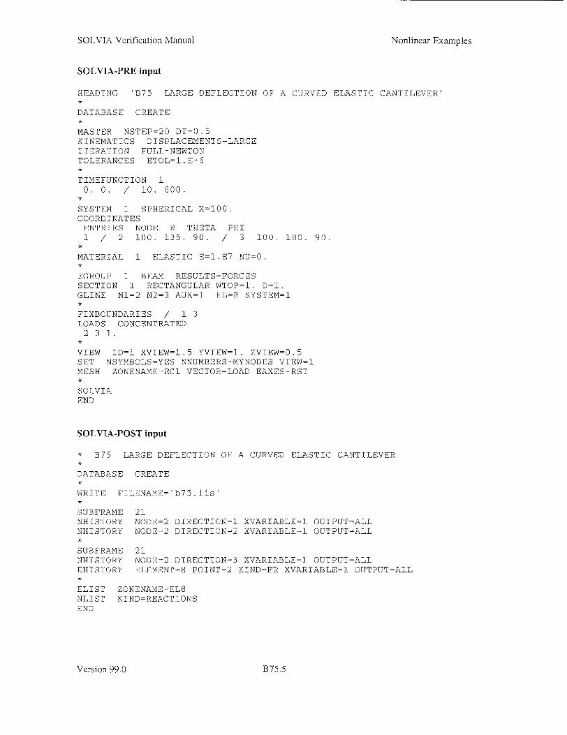
EXAMPLE B75
LARGE DEFLECTION OF A CURVED ELASTIC CANTILEVER
Objective
To verify the large displacement behaviour of the BEAM element in a curved structure.
Physical Problem
A curved elastic cantilever, 45-degree bend, is subjected to a concentrated vertical tip load as shown in the figure below. The bend has a radius of 100 in. The large displacement 3D-response of the cantilever shall be calculated for a tip load of 600 lb.
z
Y
Beam cross-section
aLa= 1 in.
Elastic material
Ez= 107 psi
v=0.
F
-- R=100 in.
Finite Element Model
The cantilever bend is modeled using eight BEAM elements. A concentrated load is applied at the tip end in the Z-direction and the other end of the bend is fixed, see bottom figure on page B75.2. The load is incremented with twenty equal increments up to 600 lb. and the Full-Newton method is used in the equilibrium iterations. The element meshing of the model is made as described in [jI].
Solution Results
The input data shown on page B75.5 is used in the SOLVIA analysis.
The history of the tip node displacements can be seen in the figures on page B75.3. The history of the axial force at the fixed end is also shown on page B75.3.
The following results can be compared with results presented in [1].
Tip displacements Load level SOLVIA Crisfield [1,2]
X Y Z X Y Z
150 -2.6304 -4.5051 25.399
300 -7.0864 -12.220 40.464 -7.14 -12.18 40.53
450 -10.784 -18.801 48.698 -10.86 -18.78 48.79
600 -13.559 -23.895 53.609 -13.68 -23.87 53.71
Version 99.0
x
Nonlinear Examples
45*
B75.1

SOLVIA Verification Manual
A solution has also been made using thirty-two 27-node SOLID elements.
The following results were obtained:
Load level Tip displacements, SOLID case X Y z
150 -2.5951 -4.3464 25.109
300 -7.0470 -11.935 40.195
450 -10.784 -18.477 48.506
600 -13.607 -23.567 53.477
The graphical output from SOLVIA-POST can be seen on page B75.4. The axial stress arr is shown
along the line of integration points closest to the inner lower comer of the beam.
References
[1] NAFEMS, Ref. R0024, "A Review of Benchmark Problems for Geometric Non-Linear Behaviour of 3-D Beams and Shells" (SUMMARY), Prinja, N.K., and Clegg, R.A.
[2] Crisfield, M.A., "A Consistent Co-Rotational Formulation for Non-Linear, Three-Dimensional Beam Elements", J. Computer Methods in Applied Mechanics and Engineering, Vol. 81 (1990), pp. 13 1-15 0 .
B75 LARGE DEFLECTION OF A CLRVED ELASTIU CANTILEVER
Z
X -_ v
, AXES\ RST I SCL',iZA ENGINEERING AB I
Version 99.0
ORIS7NAL TI'1E C ZONE EG3
SCL I/A-DRE 90
Nonlinear Examples
B75.2

SOLVIA Verification Manual
B75 -RE
Nonlinear Examples
CN 37A CURVED *LASTIC CAN -, EV E
'4
-J
z
9-00
VALUF
SOLVIA 22 - 99.0
TT'1EFNC7-2N
200 i0o 0
7'L Cý: T'1-MEJN -CNI
SC -VA ENCTNLERING AB
B7 ARGE DEF-E TON OF A CURVWC
-'O
"2, 0
V4ýLUE F ft ''F- J C 1 -N I
/ZI-TA-CST 99.0
ELAST7C CAN-- 1 0
0
1
Gd
SOL/IA \ >7EERING AB
Version 99.0B5.
i L
(r.
201
B75.3

SOLVIA Verification Manual Nonlinear Examples
j37SA L4F<- EFLE O 30 F A 'J RVE
Crý
AST Iý A,\ 1ER ,SL I
T DI E
~0
00, 3
ý'EFJNCT1N
4C 60 86
C UR
SOL V7A -POST 99.0 SCLVI'\ ENTNý
B7SA LARO_ DEFLETION CF A CURVE~
-RING AB
ELASTIr CAN\TI EER, S
M'AX DI:SPL. 60.212 TIME 'C
Z
'- AD
26 .6
SOLK/A \C \NEERI\K. ABC-. V -N(- 11
Version 99.0B74
N
(3
L.
zN
B75.4
SOLVIA Verification Manual
SOLVIA-PRE input
HEADING 'B75 LARGE DEFLECTION OF A CURVED ELASTIC CANTILEVER' .
DATABASE CREATE
MASTER NSTEP=20 DT=0.5 KINEMATICS DISPLACEMENTS=LARGE ITERATION FULL-NEWTON TOLERANCES ETOL=I.E-6
TIMEFUNCTION 1 0. 0. / 10. 600.
SYSTEM 1 SPHERICAL X=i00. COORDINATES
ENTRIES NODE R THETA PHI 1 / 2 100. 135. 90. / 3 100. 180. 90.
MATERIAL 1 ELASTIC E=-.E7 NU 0.
EGROUP 1 BEAM RESULTS-FORCES SECTION 1 RECTANGULAR WTOP:1. D-i. GLINE Ni=2 N2=3 AUX=1 EL-8 SYSTEM=I
FIXBOUNDARIES / 1 3 LOADS CONCENTRATED 2 3 1.
VIEW ID=i XVIEW=i.5 YVIEW=I. ZVIEW=0.5 SET NSYMBOLS=YES NNUMBERS=MYNODES VIEW-i MESH ZONENAME=EGi VECTOR=LOAD EAXES=RST *
SOLVIA END
SOLVIA-POST input
* B75 LARGE DEFLECTION OF A CURVED ELASTIC CANTILEVER
DATABASE CREATE
WRITE FILENAME='b75.1is'
SUBFRAME 21 NHISTORY NODE=2 DIRECTION=1 XVARIABLE=i OUTPUT-ALL NHISTORY NODE=2 DIRECTION=2 XVARIABLE=i OUTPUT=ALL
SUBFRAME 21 NHISTORY NODE=2 DIRECTION=3 XVARIABLE=i OUTPUT=ALL EHISTORY ELEMENT=8 POINT=2 KIND=FR XVARIABLE=! OUTPUT=ALL
ELIST ZONENAME=EL8 NLIST KIND-REACTIONS END
Version 99.0
Nonlinear Examples
B75.5

SOLVIA Verification Manual
EXAMPLE B76
INITIAL STRAIN IN A CURVED BEAM
Objective
To verify the BEAM, ISOBEAM and PIPE elements when using the initial strain option. Note that when the initial strain is nonzero for any of these elements then the corresponding element group is considered nonlinear by the program.
Physical Problem
A curved beam as shown in the figure below has an initial axial strain of 0.001. The radial displacement due to the initial strain is to be calculated.
R=2 m
E=2.l10[ N/im 2
einit = 0.001
u = radial displacement
uZ
Finite Element Model
Three separate models of the same structure as shown on page B76.2 are considered.
Model 1: 2-node BEAM element
Model 2: 4-node ISOBEAM element
Model 3: 4-node PIPE element
Solution Results
The theoretical radial displacement is u = -R -eirtit
A minus sign is needed because a positive initial strain means that the beam shrinks when it is released from the initial configuration. The initial strain is the strain occurring in the configuration with zero displacements and with zero thermal strain.
The input data shown on pages B76.3 and B76.4 gives the following results for the radial displacement in [mm]:
Version 99.0
Nonlinear Examples
B76.1

SOLVIA Verification Manual Nonlinear Examples
B76 IN'TAL STRA-N -N! A UR"/WED BEAM
ORIGfNAL . S
C32
3!3
)- 33
SOLVIA 295 99,C
308
30
'0
'?305
\30 \,3
C22 2:1t
2ý
209
208
207 4)3
2062C
"220 3
\ 2
,20 t
4 B12 1
03
302
'30!
3''
z
1 0 S
0.
ý100
02
MAS T ER
B '0:1~
C E 0 AS
SOLV7A ENIGINEER\ING AB
376 INITIAL STRAIN IN A CURVED 3EAM
S/>?
I<\ A- ' -t
A
-A
-4
-- 4
D-7SPLACEMEN7
2E-3 ý0LV,/A ENGiNEEý,R7,'G 4B_/:A-POST 99.0
Version 99.0
ORIGINAL MAX DISP! TIME I
-2E-3 z
X
B76.2

SOLVIA Verification Manual Nonlinear Examples
SOLVIA-PRE input
HEAD 'B76 INITIAL STRAIN IN A CURVED BEAM' ,
DATABASE CREATE MASTER IDOF=-00011
SYSTEM 1 CYLINDRICAL COORDINATES SYSTEM=i
ENTRIES NODE R THETA XL 1 2. 0. 0. 2 2. 90. 0. 3 0.
21 2. 0. 2. 22 2. 90. 2. 23 0. 0. 2. 31 2. 0. 4. 32 2. 90. 4. 33 0. 0. 4.
MATERIAL 1 ELASTIC E=2.Eii NU=0.3
EGROUP 1 BEAM MATERIAL=1 RESULT=FORCES SECTION 1 RECTANGULAR WTOP=0.02 D=0.02 SET SYSTEM=1 GLINE 1 2 3 EL=12 EDATA / ENTRIES EL INIT-STRAIN 1 0.001 TO 12 0.001
EGROUP 2 ISOBEAM MATERIAL=i RESULT=FORCES SECTION 1 SDIM=0.02 TDIM=0.02 GLINE 21 22 23 EL=4 NODES=4 NFIRST=201 EDATA / ENTRIES EL INIT-STRAIN 1 0.001 TO 4 0.001
EGROUP 3 PIPE MATERIAL=1 RESULT=FORCES SECTION 1 DIAMETER=0.02 THICKNESS=0.002 GLINE 31 32 33 EL=4 NODES=4 NFIRST=301 EDATA / ENTRIES EL INIT-STRAIN
1 0.001 TO 4 0.001
FIXBOUNDARIES / 3 23 33 FIXBOUNDARIES 24 / 2 22 32 FIXBOUNDARIES 34 / 1 21 31
SET HEIGHT=0.25 MESH NNUMBER=YES NSYMBOL=YES BCODE=ALL
SOLVIA END
Version 99.0 B76.3

SOLVIA Verification Manual
SOLVIA-POST input
* B76 INITIAL STRAIN IN A CURVED BEAM
DATABASE CREATE
WRITE 'b76.1is'
MESH ORIGINAL=DASHED VECTOR=DISPLACEMENT NSYMBOL=YES
NPLINE NPLINE NPLINE
LINE-EGI LINE-EG2 LINE-EG3
/ 2 111 STEP -1 TO 101 1 / 22 211 STEP -1 TO 201 21 / 32 311 STEP -1 TO 301 31
NVARIABLE DISPY DIRECTION=2NVARIABLE NVARIABLE NVARIABLE RESULTANT
RLINE RLINE RLINE
END
DISPZ DIRECTION=3 Y DIRECTION=2 KIND=COORDINATE Z DIRECTION=3 KIND:COORDINATE DISP-RAD STRING=' (Y*DISPY+Z*DISPZ)/(SQRT(Y*Y+Z*Z))'
LINE-EGi DISP-RAD OUTPUT=LIST LINE-EG2 DISP-RAD OUTPUT=LIST LINE-EG3 DISP-RAD OUTPUT=LIST
Version 99.0
Nonlinear Examples
B76.4
SOLVIA Verification Manual
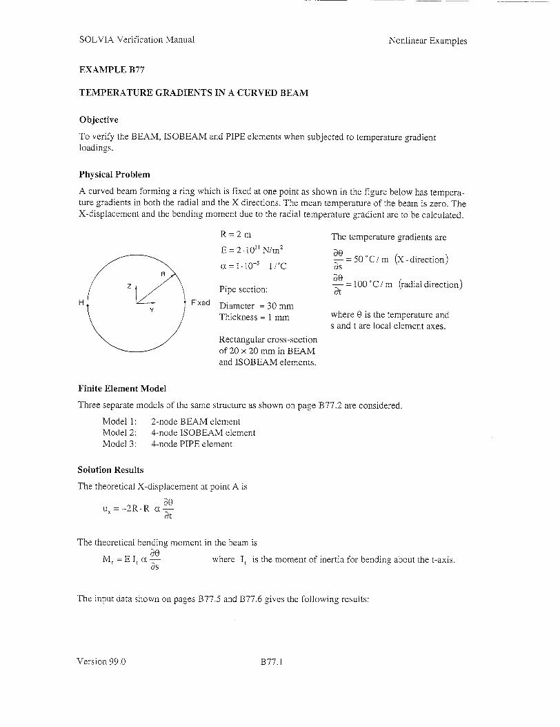
EXAMPLE B77
TEMPERATURE GRADIENTS IN A CURVED BEAM
Objective
To verify the BEAM, ISOBEAM and PIPE elements when subjected to temperature gradient loadings.
Physical Problem
A curved beam forming a ring which is fixed at one point as shown in the figure below has temperature gradients in both the radial and the X directions. The mean temperature of the beam is zero. The X-displacement and the bending moment due to the radial temperature gradient are to be calculated.
R-2 m
E=2.101 N/m 2
a=l-10-1 1/°C
Pipe section:
Diameter = 30 mm Thickness = 1 mm
The temperature gradients are
- = 50oC/m (X-direction) as
-= 100 °C / m (radial direction) at
where 0 is the temperature and s and t are local element axes.
Rectangular cross-section of 20 x 20 mm in BEAM and ISOBEAM elements.
Finite Element Model
Three separate models of the same structure as shown on page B77.2 are considered.
Model 1: 2-node BEAM element Model 2: 4-node ISOBEAM element Model 3: 4-node PIPE element
Solution Results
The theoretical X-displacement at point A is
u.X=-2R.R a DO at
The theoretical bending moment in the beam is
Mt = E It a. where It is the moment of inertia for bending about the t-axis. as
The input data shown on pages B77.5 and B77.6 gives the following results:
Version 99.0
H Fixed
Nonlinear Examples
B77.1

Nonlinear ExamplesSOLVIA Verification Manual
X-displacement in [mm] at point A:
The t-axis bending moment in Nm for a rectangular cross-section:
The t-axis bending moment in Nm for a pipe section:
The t-axis bending moment along the elements are shown on pages B77.3 and B77.4.
B77 'P -,ATURE GRADIENTS ',N A CURVE'D BEAN
3RIINAL ý- 3.5 z
X .. __.
34
V
33ý6
EAXES=RST
B A A 10
LVOA EANEARDIO ASS L'IA- 99.
Version 99.0 B77.2

SOLVIA Verification Manual Nonlinear Examples
377 -"7vPERATURE GRADIENTS '\1 A CURVED BEAM
8E-3OR: CNAMAX - SPI
TIME
SOLVIA-POST 99.0 SOLVIA ENGINEERING AB
B77 '7\PERATURE SRAD EN7S IN A CURVED BEAM
ORGTNAL i-I z
X
po
BEAM
SCL/IA 7\GCNEERIN(
Version 99.0
X
DISPLACEMENT
8E-3
TiME I
L A 9S ' AB
m t
r... -
B77.3

SOLVIA Verification Manual Nonlinear Examples
377ýPýRAT RE SRA
ITil 71E
DiE\,q IN A
- <½ 2W.�( A -
I CB LRA'
3CLVIA POST 99.C
P IPE
SO' \IA -INC-NEER>j'C- AB
Version 99.0B'7.
:JR~V. SEA M
T I."'
01
Ti-o
B77.4

SOLVIA Verification Manual
SOLVIA-PRE input
HEAD 'B77 TEMPERATURE GRADIENTS IN A CURVED BEAM' DATABASE CREATE
SYSTEM 1 CYLINDRIC COORDINATES SYSTEM=i
ENTRIES NODE X R 1 0 2 2 0 0 3 3 2 4 3 0 5 6 2 6 6 0
MATERIAL 1 THERMO-ELASTIC TREF=0 -i00 2.Eii 0.3 i.E-5 100 2.Eli 0.3 i.E-5
EGROUP 1 BEAM MATERIAL-i RESULT=FORCES SECTION 1 RECTANGULAR WTOP=0.02 D=0.02 GLINE 1 1 AUX=2 EL-72 SYSTEM=i LOADS ELEMENTS TGRADIENTS
1 S 50. 50. TO 72 s 50. 50. 1 t 100. 100. TO 72 t 100. 100.
EGROUP 2 ISOBEAM MATERIAL=i RESULT=FORCES SECTION 1 SDIM=0.02 TDIM=0.02 GLINE 3 3 AUX=4 EL=24 NODES=4 SYSTEM-I LOADS ELEMENTS TGRADIENTS
1 s 50. 50. TO 24 s 50. 50. 1 t 100. 100. TO 24 t 100. 100.
EGROUP 3 PIPE MATERIAL=i RESULThFORCES SECTION 1 DIAMETER=3E-2 THICKNESS=i.E-3 GLINE 5 5 AUX=6 EL 24 NODES=4 SYSTEM=i LOADS ELEMENTS TGRADIENTS
1 s 50. 50. TO 24 s 50. 50. 1 t 100. 100. TO 24 t 100. 100.
LOAD TEMPERATURE TREFE0. *
FIXBOUNDARIES INPUT=ZONE ZONE=MYNODES
SET HEIGHT=0.25 MESH NNUMBER=MYNODES NSYMBOL-MYNODES BCODE=ALL EAXES=RST
SOLVIA END
Version 99.0
Nonlinear Examples
1377.5

SOLVIA Verification Manual
SOLVIA-POST input
* B77 TEMPERATURE GRADIENTS IN A CURVED BEAM *
DATABASE CREATE
WRITE 'b77.iis' NMAX EGI DIRECTION=i NMAX EG2 DIRECTION=i NMAX EG3 DIRECTION=i EMAX
SET SMOOTHNESS=YES MESH ORIGINAL=DASHED VECTOR=DISP
EGROUP 1 EPLINE BEAM 1 1 2 TO 72 1 2
EGROUP 2 EPLINE ISOBEAM 1 1 2 TO 24 1 2
EGROUP 3 EPLINE PIPE 1 1 2 TO 24 1 2
MESH PLINES=ALL SUBFRAME=21 ELINE BEAM KIND=MT ELINE ISOBEAM KIND=MT SYMBOL=i SUBFRAME=21 ELINE PIPE KIND=MT SYMBOL=i END
Version 99.0
Nonlinear Examples
B77.6

SOLVIA Verification Manual
EXAMPLE B78
TEMPERATURE GRADIENTS IN A PLATE
Objective
To verify the SHELL elements when using the temperature gradient option and the SOLID element when subjected to a linear temperature field.
Physical Problem
A circular plate with a concentric circular hole is exposed to a uniform temperature gradient through its thickness.
R,=2m
R2 = 0.5 m
h=0.2 m (thickness) E=2.10" N/m 2
A y Fixed v = 0.3
oa= 1.10-5 1/°C a =100 °C/m at
where 0 is the temperature and t is the element t-direction (positive thickness direction and positive X-direction).
Finite Element Model
Four separate models of the same structure as shown on page B78.2 are considered.
Model 1: 4-node SHELL element Model 2: 9-node SHELL element Model 3: 16-node SHELL element Model 4: 27-node SOLID element
The temperature load is applied as element temperature gradients in the SHELL elements and as nodal temperatures for the SOLID elements.
Solution Results
The theoretical X-displacement at point A is
at
The input data shown on pages B78.4 to B78.6 gives the following results for the displacement in mm at point A:
Version 99.0
Nonlinear Examples
B78.1

SOLVIA Verification Manual
Theory 4-node SHELL 9-node SHELL 16-node SHELL 27-node SOLID
-8.000 -8.000 -8.000 -8.000 -8.000
Contour plots of the von Mises effective stress are shown on pages B78.3 and B78.4. The plate should be stress free in this example. The stress free condition corresponds to a spherical shape of the plate which cannot exactly be modelled by the isoparametric elements. The von Mises stresses are, however, very small which can be seen by a comparison with the temperature stress at zero displacements:
Ea= =-28.57.106 N / m 2 (0=o10C) 1-V
B78 TEMPERATURE GRAD7ENTS IN A PLATE
ORIGINAL I TIME I
z
x Y
MASTER7 P 88 2000
3 0 0!00
CC 0 0O
TGRADIENT
SOLVIA ENGINEERING ABSOLV A-PRE 99.0
Version 99.0
Nonlinear Examples
B78.2

SOLVIA Verification Manual Nonlinear Examples
B78 TEMPERATURE GRADIENTS iN A PLATE
ORIGINAL ý-- --4 I. ý.AX DISPL.; 8.00 E-3, TIME
z
X •'
DISPLACEMENT
8.00SE-3
SOLVIA-POST 99.0 SOLVIA ENGTNEERING AB
B78 TEMPERATURE GRADIENTS IN A PLATE
MAX DISPL. -8E-3 TIME , ZONE ED:
4-node SHELL eiements
SOL/AA-POST 99 0
Z z
MISES GASE ON2 ZXNE SHEL. 'TOP MAX 3,3307E
3.1243E-4 2. 7jSE-4 2 29871E 1[.8860E1 4732E-4
,• .0604E-41 .4763E-5
2.348SE-I
MIN 2.8462E-6
SOLVIA ENGINEERING AG
B78 TEMPERATURE GRADIENTS :N A PLATE
MAX DISPL. -SXE-3 TIME I ZONE -r2
9-node SHELL elemens
SOLVIA-GOST 99 0
2 Y
MISES BASED ON ZONE SHELL TOP
MAY 962 27
991 .06
808.63 :: 706 .20
6503.7
S296.58 tS ,94,06 TIN 142.84
SOLVTA ENGINEERING 3
B78.3Version 99.0

SOLVIA Verification Manual Nonlinear Examples
878 TEMPERATURE GRADIENTS 7N A PLATE
MAX DSPL R8E-3
ZONE EG3
16-node SHELL elements
SOLVIA-POST 990
Z
MISES BASED ON ZONE SHELL TOP MAX 5419.3
!5143.6 S4Sg1.1 4038.6 3486.2 2933.7 238t.2 1928.8
S1278.3 MIN 1000. 1
SOLVIA ENGINEERING AB
B78 TEMPERATURE GRADIENTS 7N A PLATE
MAX D1APL. - S • OSE-3 TIME 1 ZONE EG4
27-node SOLED elements
SOLVIA-POST 99.0
BASED ON ZONE M AX 81446
773.01 S690 09
524,27
?• 441.3S !i 358.44 27S 23
807MG8RI A[
SOLVIA ENGINEERING AB
SOLVIA-PRE input
HEAD 'B78 TEMPERATURE GRADIENTS IN A PLATE'
DATABASE CREATE
SYSTEM 1 CYLINDRIC COORDINATES SYSTEM=i
ENTRIES NODE X R 1 0 2 2 0 0.5
*
11 12
21 22
31 32 33 34 35 36
-3.0 2 -3.0 0.5
-6.0 2 -6.0 0.5
-9. 0 -9 .0 -9 .2 -9. 2 -9.1 -9.1
2 0.5 2 0.5 2 0.5
Version 99.0 B78.4

SOLVIA Verification Manual
SOLVIA-PRE input (cont.)
Nonlinear Examples
MATERIAL 1 THERMO-ELASTIC TREF=0. -1000 2.E11 0.3 i.E-5
1000 2.E11 0.3 i.E-5
EGROUP 1 SHELL MATERIAL=i SET SYSTEM=1 GSURFACE 2 1 1 2 EL1=4 EL2=36 NODES=4 THICKNESS 1 2.E-1 LOAD ELEMENTS TYPE=TGRADIENT 1 100. TO 144 100. FIXBOUNDARIES / 1 FIXBOUNDARIES 3 / 2
EGROUP 2 SHELL MATERIAL=1 GSURFACE 12 11 ii 12 EL1=4 EL2=36 NODES=9 THICKNESS 1 2.E-1 LOAD ELEMENTS TYPE-TGRADIENT
1 100. TO 144 100. FIXBOUNDARIES / 11 FIXBOUNDARIES 3 / 12
EGROUP 3 SHELL MATERIAL=i
GSURFACE 22 21 21 22 EL1=4 EL2=36 NODES=-6 THICKNESS 1 2.E-1 LOAD ELEMENTS TYPE=TGRADIENT
1 100. TO 144 100. FIXBOUNDARIES / 21 FIXBOUNDARIES 3 / 22
LINE CYLINDRIC 31 31 EL=36 MIDNODES=*
LINE CYLINDRIC 32 32 EL=36 MIDNODES=i LINE CYLINDRIC 33 33 EL=36 MIDNODES=1 LINE CYLINDRIC 34 34 EL=36 MIDNODES=1
EGROUP 4 SOLID MATERIAL=1 GVOLUME 32 31 31 32 34 33 33 34 EL1=4 EL2=36 NODES=27 SYSTEM=i LOAD TEMPERATURE TREFE0. INPUT=N6DES INTERPOLATION=X COORDi=-9.6
V1=-50. COORD2=-8.6 V2=50. SYSTEM=0 31 TO 36
2327 TO 4264
FIXBOUNDARIES 35 FIXBOUNDARIES 23/ 31 FIXBOUNDARIES 3 / 36
MESH NNUMBER=MYNODES NSYMBOL=MYNODES BCODE=ALL CONTOUR=T-GRADIENT
SOLVIA END
Version 99.0 B78.5
SOLVIA Verification Manual
SOLVIA-POST input
* B78 TEMPERATURE GRADIENTS IN A PLATE
DATABASE CREATE
write 'b78.lis'
N*AX EGI DIRECTION=I23
NMAX EG2 DIRECTION=123 NMAX EG3 DIRECTION=123
NMAX EG4 DIRECTION=123
MESH ORIGINAL=DASHED VECTOR=DISPLACEMENT
SET PLOTORIENTATION=PORTRAIT CONTOUR AVERAGING=ZONE MESH EGi CONTOUR=MISES TEXT '4-node SHELL elements' YPT=2
MESH EG2 CONTOUR=MISES TEXT '9-node SHELL elements' YPT=2
MESH EG3 CONTOUR=MISES TEXT '16-node SHELL elements' YPT=2
MESH EG4 CONTOUR=MISES TEXT '27-node SOLID elements' YPT=2
END
Nonlinear Examples
Version 99.0 B78.6

SOLVIA Verification Manual
EXAMPLE B79
REINFORCED CONCRETE BEAM, ISOBEAM
Objective
To verify the rebar section option in a reinforced concrete beam analysis using ISOBEAM elements.
Physical Problem
A simply supported reinforced concrete beam subjected to two symmetrically applied concentrated loads as shown in the figure below is considered. The steel reinforcement area Ast = 0.62 in2 is to be
used in this analysis and the steel reinforcement is located 2.06 in. from the bottom surface of the beam. This problem is also analyzed in Example B 19 using PLANE STRESS elements.
P/2 P/2
PLANE OF CONTRAFLEXURE
PLANE OF CONTRAFLEXURE
12, 62 in"2 P/2 I Ast= a2"OO in2
BEAM DIMENSIONS
Material parameters CONCRETE: Density Initial tangent modulus Poisson's ratio Uniaxial cut-off tensile strength Uniaxial maximum compressive stress (SIGMAC) Compressive strain at SIGMAC Uniaxial ultimate compressive stress Uniaxial ultimate compressive strain
STEEL: Density Young's modulus Initial yield stress Strain hardening modulus
0.2172. 10-3
3060 0.2
0.458 -3.74
-0.002 -3.225 -0.003
0.7339 .10-3
30000 44
300
lbf s2/in 4
ksi
ksi ksi in/in ksi in/in
lbf. s2/in4
ksi ksi ksi
Finite Element Model
Using symmetry only one-half of the structure need to be considered. Ten parabolic ISOBEAM elements are used in the finite element model as shown in the left figure on page B79.2. REBAR sections with an elastic-plastic material model are used to model the reinforcement. The solution is obtained using the AUTOMATIC-ITERATION method.
Version 99.0
Nonlinear Examples
1379.1

SOLVIA Verification Manual Nonlinear Examples
Solution Results
The input data on pages B79.4 and B79.5 is used in the finite element analysis.
The right figure below shows the mid-span deflection of the beam as a function of the load. The response curve for the ISOBEAM element model with symbols included is compared with the
corresponding result curve from Example B 19 which is shown as a solid line without symbols.
The top figure on page B79.3 shows the axial stress-strain history at the four integration point levels closest to the midspan. The bottom figure shows the variation of the axial stress along the four integration point levels for the last solution time.
User Hints
"* The ISOBEAM element is constrained so that plane sections remain plane during deformation.
Therefore, the ISOBEAM model shows a somewhat larger load capacity than the PLANE STRESS model in Example B 19.
" The plastic strain concentration observed in the PLANE STRESS model is not present in the
ISOBEAM model because of the constraint. No variation of the stresses can be observed in the axial direction for the constant moment portion of the beam.
" Listing and scanning of REBAR and CONCRETE results can be obtained in SOLVIA-POST by using the SELECT parameter in the ELIST, EEXCEED and EMAX commands.
879 REINFORCED CONCRETE BEAM, 10BEAM
OR:GINAL - tO. TINE I
ORIGINAL - "
t 2 3 4 5 6 7 9 9 10
SOLVIA-PRE 99.0
. L0
"F0RCE 0.5
MASTE 1O001:
Z Y
9 :0y
t
6AXES=RST
SOLV0A ENGINEERING AB
B79 REINFORCED CONCRETE BEAM. :SOBEAM
P 01
0
2 4 6 4 '
LAMBDA
SOL/IA-POST 99.0 SOLVfA ENGINEER:NG AB
Version 99.0
z
E_ m
B79.2

F'6LS
Q,t
.n .N....' ... .... . ......
..... ...
09 oi
A' -
½ �2
jF
0-66 UO1SJ10A
0 66!06V/CO
-1 / -2 -
r7 (2,
I2
7 (2 -F
N) 22
F!)
22 .At 22
0'.
"0 ]�-JK.
02 02z 0
~c7,
7 1
02 9 3, 07
WV39OSI 'L4V]9 31--)ZDNC3 a3dOJ0NI2d 6L5
ý]V SNIdDýNION] VIAOOOS
0- 0 1-~'
S ý-N Fzi ZOF S 00
- N,
0'66 iSOc VIAOýOS
9-01 0 O
~N~NI~ -c 'Z d 0; J 03 e
0 , 0 05os 0 00;ý- C 3SF,
C
0
9JDF N\'�I" 00 2 ('U-'
5 0 SF F 01
2'�CF&. F
IaF'
F-. -
At')
0
k7v]('CsI -Fv2g 1-:ýZ2NG3 CDKAONT3ýý 6C6
s~idtxwx~ fl~UiIUuNItfUNAT uOIILC0)UJQA VIA"IOS
'F-
-A
Cf2
I -ýLliýlr
1
soldLuuxj jrouquoN

SOLVIA Verification Manual
SOLVIA-PRE input
HEADING 'B79 REINFORCED CONCRETE BEAM, ISOBEAM'
DATABASE CREATE MASTER IDOF100011 NSTEP=30 AUTOMATIC-ITERATION NODE=3 DIRECTION=3 DISPLACEMENT=-0.01,
DISPMAX=0.6 CONTINUATION=YES TOLERANCES TYPE=F RNORM=10 RMNORM=50 RTOL=0.01
COORDINATES / ENTRIES NODE Y Z 1 / 2 50. / 3 68. / 4 0. 10.
MATERIAL 1 CONCRETE EO=3.06E3 NU=0.2 SIGMAT=0.458, SIGMAC=-3.74 EPSC=-0.002 SIGMAU=-3.225 EPSU=-0.003, BETA=0.75 KAPPA=15 STIFAC=0.0001 SHEFAC=0.5
MATERIAL 2 PLASTIC E=3.E4 YIELD=44 ET=300.
EGROUP 1 ISOBEAM RESULT=TABLES MATERIAL=i REBARMATERIAL=2 GLINE 1 2 4 EL=6 NODES=3 GLINE 2 3 4 EL=4 NODES=3 SECTION 1 SDIM=12. TDIM=6. REBARSECTION 1
1 -3.94 0. 0.62 STRESSTABLE 1 112 122 132 142 212 222 232 242
FIXBOUNDARIES 3 1 FIXBOUNDARIES 24 / 3 FIXBOUNDARIES 234 / 4
LOADS CONCENTRATED / 2 3 -0.5
SET VIEW=X NSYMBOLS=YES PLOTORIENTATION=PORTRAIT MESH NNUMBERS=MYNODES VECTOR=LOAD BCODE=ALL SUBFRAME=d2 MESH EAXES=RST ENUMBERS=YES GSCALE=OLD ,
SOLVIA END
Version 99.0
Nonlinear Examples
1379.4

SOLVIA Verification Manual
SOLVIA-POST input
* B79 REINFORCED CONCRETE BEAM, ISOBEAM
DATABASE CREATE
WRITE FILENAME='b79.1is'
AXIS 1 VMIN=-0.6 VMAX=0. LABEL='DISPLACEMENT' AXIS 2 VMIN=0. VMAX=i2. LABEL-'LAMBDA'
USERCURVE 1 SORT=NO READ FILENAME='b79disp.dat'
SET VIEW=X DIAGRAM=GRID SET PLOTORIENTATION=PORTRAIT NHISTORY NODE=3 DIRECTION=3 OUTPUT=ALL XAXIS-2 YAXIS=PLOT USERCURVE 1 XAXIS=-2 YAXIS=-- SUBFRAME=OLD
SET PLOTORIENTATION-LANDSCAPE SUBFRAME 22 EXYPLOT ELEMENT=10 POINT=212 EXYPLOT ELEMENT=-0 POINT=222 EXYPLOT ELEMENT=-0 POINT=232 EXYPLOT ELEMENT=-0 POINT=242
EPLINE LEVEL1 / 1 112 212 TO EPLINE LEVEL2 / 1 122 222 TO EPLINE LEVEL3 / 1 132 232 TO EPLINE LEVEL4 / 1 142 242 TO SUBFRAME 22 ELINE LEVEL1 KIND=SRR SYMBOL=i ELINE LEVEL2 KIND=SRR SYMBOL=1 ELINE LEVEL3 KIND=SRR SYMBOL-i ELINE LEVEL4 KIND=SRR SYMBOL=1
ELIST SELECT=CONCRETE ELIST SELECT=REBAR END
(KIND=ERR YKIND=SRR SYMBOL=i (KIND=ERR YKIND=SRR SYMBOL=i (KIND=ERR YKIND=SRR SYMBOL-i (KIND-ERR YKIND=SRR SYMBOL=i
L0 112 212 L0 122 "222 L0 132 232 L0 142 242
Version 99.0
SYMBOL=I
Nonlinear Examples
]
B79.5

SOLVIA Verification Manual
EXAMPLE B80
REINFORCED CONCRETE BEAM, NONLINEAR-ELASTIC ISOBEAM
Objective
To verify the NONLINEAR-ELASTIC material model in a concrete beam structure analysis using ISOBEAM elements.
Physical Problem
The same simply supported reinforced concrete beam as analyzed in Example B79 is to be analyzed, but using the NONLINEAR-ELASTIC material to model the uniaxial behaviour of the concrete material model.
P/2 P/2
5 01 36) - 50 - - -
PLANE OF d CONTRAFLEXURE
PLANE OF
CONTRAFLEXURE
BEAM DIMENSIONS
Finite Element Model
Using symmetry only one-half of the structure need to be considered. Ten parabolic ISOBEAM elements are used in the finite element model as shown in the left bottom figure on page B180.2. The concrete material is modeled using the NONLINEAR-ELASTIC material model and the steel reinforcement is modeled using the REBAR section option. The solution is obtained using the AUTOMATIC-ITERATION method.
Solution Results
The input data on pages B80.4 and B80.5 is used in the finite element analysis.
The right figure on page B180.2 shows the mid-span deflection of the beam as a function of the load. The response curve for the nonlinear-elastic model with symbols included is compared with the corresponding results from the concrete model in Example B79 which are shown as a solid line without symbols. The two curves are almost coinciding.
The top figure on page B80.3 shows the axial stress-strain history at the four integration point levels closest to the midspan. The bottom figure shows the variation of the axial stress along the four integration point levels for the last solution time.
Version 99.0
Nonlinear Examples
1380.1

SOLVIA Verification Manual Nonlinear Examples
User Hints
" The NONLINEAR-ELASTIC material model can be used to simulate concrete materials in simple beam structures as in this example. Two reasons for the good agreement between the two material models are the one-dimensional action of the concrete in the beam structure and that the principal stresses do not change directions significantly during the response.
" The uni-axial stress-strain curve for the concrete model can be obtained by performing a one element analysis as shown in the input data on page 180.6. A 4-node PLANE STRESS2 element with dimensions 1 x 1 is subjected to uni-axial compression using prescribed displacements. The Poisson's ratio is set to zero and the load is applied in small increments up to the uni-axial ultimate strain, EPSU. The corresponding stress-strain curve can be found in SOLVIA-POST by using the EXYPLOT command and the stress-strain data can be included in a NONLINEAR-ELASTIC material model. The uni-axial stress-strain curve can be seen in the figure on page B80.4.
B80 RE'NFORCED CONCRETE BEAM. NONLINEAR-ELASTIC TSOBEAM
ORIGINAL F-------- 10. Z TIME I L
FORCE
0.$
MA3TER iOCoit
C h01
ORIGINAL 1 0. Z L•
i 2 3 4 5 7
89 iG
SOLVIA-PRE 99
L
.AXES=RST SOLVIA ENGINEERING AS
990 REINFORCED CONCRETE BEAM, NONL:NEAR-ELASTIC ISOBEAM
-N 0
0 2 4 6
ILAM9DA
SOLVIA-POST 99.0
Version 99.0
8 12
SOLVIA ENGINEERING AS
°
i
1380.2

SOLVIA Verification Manual Nonlinear Examples
B80 REINFCRCED CONCRETE BEAM, NONL:NEAR-ELASTTC 1SOBEAM
.3
ES E 10 P 232 STRA N-RR
SOLVIA-POST 99.0
"22
o0
00 0. 1.0 1 5 2.0 2.5
S E !0 P 212 STRAL•N[-RR
0 .... ... ... ............ .. .. .... .... .... .... ..... ........ .... .... ... 0
-S0.0 -[00.0 S-0.0 0.n S0.0o
.... ....
(NJ
�2••l
-1.0 -0.8 -o.6 -0.4 -0.2 -Ai0 - 3
EG 10 P 242 STRA7N-RR
SOLVIA ENGINEERING AB
B80 REINFORCED CONCRETE BEAM, NONLINEAR-ELASTIC ISOBEAM
TIME 25
0 20 40 60 80
,LEVE i
0 20 40 F025
TME 2S•
0• 0•
.0)
.00y•
91
L0•
'2"
TIME 25
• i ...... ........ ......... .. ;:, ...... . • -, • .................... ... ...... ....... .. ....... ..................
0 20 40 60 80
LEVEL2
TIME 2S
? ... . ........ ...... . ............ . ...... ..
10 60 80 0 '0 40 60
OLEEL
SOLV A-POST 99.0 SOLVIA ENGINEERTNG ,
Version 99.0
G00 2 A El P . 2 .2 2 S T.R A .N RR
0• 0•
(.1 9) -J '2•
2)
-Y 2.
0•
0 20
L EVE-L3
SC
ýE
1380.3

SOLVIA Verification Manual
OjUNu r Ni-aXlt STREBS-SrRAIN CUVE SC ý9 N•0•, E
5OLS1A-POST 99 0
.0
SOtt JSSEER!NG
SOLVIA-PRE input
HEADING 'B80 REINFORCED CONCRETE BEAM, NONLINEAR-ELASTIC ISOBEAM'
DATABASE CREATE MASTER IDOF=100011 NSTEP=30
AUTOMATIC-ITERATION NODE=3 DIRECTION=3 DISPLACEMENT=-0.01, ALFA=1 DISPMAX=0.5 CONTINUATION=YES
TOLERANCES TYPE=F RNORM=5 RMNORM=20 RTOL=0.01
COORDINATES / ENTRIES NODE Y Z
1 / 2 50. / 3 68. / 4 0. 10.
MATERIAL 1 NONLINEAR-ELASTIC -0.003 -3.225 -0.00285 -3.34155 -0.0027 -3.45087 -0.00255 -3.54928 -0.0024 -3.63242 -0.00225 -3.69530 -0.0021 -3.73244 -0 .002 -3.74 -0.00195 -3.73802 -0.0018 -3.70629 -0.00165 -3.63190 -0.0015 -3.51049 -0.00135 -3.33912 -0.0012 -3.11675 -0.00105 -2.84450 -0.0009 -2.52571 -0.00075 -2.16570 -0.0006 -1.77127 -0.00045 -1.35007 -0.0003 -0.90985 -0.00015 -0.45781 -0.00003 -0.0918 0. 0. 1.496732E-4 0.458 2 .2451E-3 0. 1. 0.
MATERIAL 2 PLASTIC E=3.E4 YIIELD=44 ET=300.
Version 99.0
Nonlinear Examples
B 80.4

SOLVIA Verification Manual Nonlinear Examples
SOLVIA-PRE input (cont.)
EGROUP 1 ISOBEAM RESULTS=TABLES MATERIAL=i REBARMATERIAL=2 GLINE 1 2 4 EL=6 NODES=3 GLINE 2 3 4 EL=4 NODES=3 SECTION 1 SDIM=12. TDIM=6. REBARSECTION 1
1 -3.94 0. 0.62 STRESSTABLE 1 112 122 132 142 212 222 232 242
FIXBOUNDARIES 3 / 1 FIXBOUNDARIES 24 / 3 FIXBOUNDARIES 234 / 4 LOADS CONCENTRATED / 2 3 -0.5
SET MESH MESH
VIEW=X NSYMBOLS=YES PLOTORIENTATION=PORTRAIT NNUMBERS=MYNODES VECTOR=LOAD BCODE=ALL SUBFRAME=12 EAXES=RST ENUMBERS=YES GSCALE=OLD
SOLVIA END
SOLVIA-POST input
* B80 REINFORCED CONCRETE BEAM, NON-LINEAR-ELASTIC ISOBEAM
DATABASE CREATE
WRITE FILENAME='b80.1is'
AXIS 1 VMIN=-0.6 VMAX=0. LABEL='DISPLACEMENT' AXIS 2 VMIN=0. VMAX=12. LABEL='LAMBDA' .
USERCURVE 1 SORT=NO READ FILENAME='b80disp.dat'
SET VIEW=X DIAGRAM=GRID SET PLOTORIENTATION=PORTRAIT NHISTORY NODE=3 DIRECTION=3 OUTPUT=ALL XAXIS=2 YAXIS=1 PLOT USERCURVE 1 XAXIS=-2 YAXIS=-1 SUBFRAME=OLD
SYMBOL=1
SET PLOTORIENTATION=LANDSCAPE SUBFRAME 22 EXYPLOT ELEMENT=10 POINT=212 EXYPLOT ELEMENT=10 POINT=222 EXYPLOT ELEMENT=10 POINT=232 EXYPLOT ELEMENT=10 POINT=242
EPLINE LEVEL1 / 1 112 212 TO 10 EPLINE LEVEL2 / 1 122 222 TO 10 EPLINE LEVEL3 / 1 132 232 TO 10 EPLINE LEVEL4 / 1 142 242 TO 10 SUBFRAME 22 ELINE LEVELI KIND=SRR SYMBOL=1 ELINE LEVEL2 KIND=SRR SYMBOL=1 ELINE LEVEL3 KIND=SRR SYMBOL=i ELINE LEVEL4 KIND=SRR SYMBOL=i
XKIND=ERR XKIND=ERR XKIND=ERR XKIND=ERR
112 122 132 142
YKIND=SRR SYMBOL=1 YKIND=SRR SYMBOL=1 YKIND=SRR SYMBOL=1 YKIND=SRR SYMBOL=1
212 222 232 242
ELIST ELIST SELECT=REBAR
SUMMATION KIND=LOAD SUMMATION KIND=REACTION DETAILS=YES END
Version 99.0 1380.5

SOLVIA Verification Manual
SOLVIA-PRE input
HEADING 'B80UNI UNI-AXIAL STRESS-STRAIN CURVE FOR CONCRETE,
DATABASE CREATE MASTER IDOF=100111 NSTEP=100 TIMEFUNCTION 1 0. 0. / 100. 1.
COORDINATES / ENTRIES 1 1. 1. / 2 0. 1.
NODE Y Z 3 / 4 1.
MATERIAL 1 CONCRETE E0=3.06E3 NU=0. SIGMAT=0.458, SIGMAC=-3.74 EPSC=-0.002 SIGMAU=-3.225 EPSU=-0.003, BETA=0.75 KAPPA=15 STIFAC=0.0001 SHEFAC=0.5
EGROUP 1 PLANE STRESS2 ENODES / 1 1 2 3 4 EDATA / 1 0.1
FIXBOUNDARIES 2 / 1 2 3 4 FIXBOUNDARIES 3 / 3 4 LOADS DISPLACEMENTS 1 3 -0.003 / 2 3 -0.003
,
SOLVIA END
SOLVIA-POST input
* B80UNI UNI-AXIAL STRESS-STRAIN CURVE FOR CONCRETE ,
DATABASE CREATE
WRITE FILENAME='bBOuni.lis'
SET PLOTORIENTATION=PORTRAIT DIAGRAM=GRID EXYPLOT ELEMENT=1 POINT=1 XKIND=EZZ YKIND=SZZ OUTPUT=ALL END
Version 99.0
Nonlinear Examples
B80.6

SOLVIA Verification Manual
EXAMPLE B81
BRESLER-SCORDELIS CONCRETE BEAM
Objective
To verify the PLANE concrete material model and demonstrate the use of the AUTOSTEP method in
a concrete analysis.
Physical Problem
Bresler and Scordelis investigated experimentally the shear strength in reinforced concrete beams [1].
A total of 12 simply supported beams were tested. One of the beams, called OA-2 in [1], is to be
analyzed in this example. The figure below shows the concrete beam and the reinforcement.
. P
L/2 L/2
L = 4.57 m
h = 0.56 m
b = 0.305 m
d = 0.465 m
Ast = 3290.10-' 62
Concrete
E0 = 28700MPa
v =0.2
a, = -23.7 MPa
-9 = -0.0022
a, = 4.33MPa
Steel
E = 218000 MPa
CY = 555 MfPa
ET- = 10000 MPa
Finite Element Model
The finite element model consists of fifty 8-node PLANE STRESS2 elements using the concrete material model. The steel reinforcement is modeled with ten parabolic TRUSS elements using an elastic
plastic material model- The AUTOSTEP method is used to control the load incrementation up to the
collapse load of the beam. Force tolerances are used with a force norm of 80 kN and a force tolerance
of one percent. The BFGS iteration method is employed. Due to symmetry only half of the beam needs to be considered as shown in the finite element model on page B81.3.
Solution Results
The input data used in the SOLVIA analysis is shown on pages B81.8 and B81.9.
Bresler and Scordelis reported an ultimate load of 80 kips (appr. 356 kIN) with a maximum mid-span
deflection of 0.46 in (appr. 11.7 mm) for the OA-2 beam.
Version 99.0
hd
i 4 pi 4
Nonlinear Examples
B81.1

SOLVIA Verification Manual
In the experimental study the OA-2 beam showed typical initial flexural cracks in the lower part of the beam section followed by diagonal tension cracks. The failure mode of the OA-2 beam was denoted a "diagonal tension failure" and it occurred as a result of longitudinal splitting in the compression zone near the point load and also by horizontal splitting along the tensile reinforcement near the end of the beam [1].
In the first analysis the value for SIGMAT, the tensile strength, is set equal to the modulus of rupture for the concrete material. The results from this analysis can be seen on pages B81.3 and B81.4. The mid-span deflection of the beam as a function of the load can be seen in the bottom figure on page B81.3. A vector plot of crack normals and a contour plot of the state of the concrete in the last load step can be seen on page B81.4. Note that the concrete has crushed in the compressed region under the point load and that a large number of flexural cracks have opened in the concrete but we see no longitudinal splitting in the compressed zone or horizontal splitting along the reinforcement. SOLVIA calculates the ultimate load as 360.8 kN with a maximum mid-span deflection of 11.7 mm.
In the second analysis, B81A, SIGMAT is set to half the value of the modulus of rupture. The KAPPA-value is increased to keep the tension stiffening effect constant. The SHEFAC value is increased to 0.75 to keep the shear strength in the crack planes. The results from the analysis can be seen on pages B81.5 and B81.6. The mid-span deflection as a function of the load can be seen in the top figure on page B81.5. A vector plot of crack normals in the bottom figure on page B81.5 shows that a horizontal crack has started in the compressed zone and that diagonal cracks have developed along the reinforcement near the end of the beam. A zone under the point load is crushed as seen in the top figure on page B81.6.
SOLVIA calculated the ultimate load as 351.2 kN with a maximum mid-span deflection of 12.9 mm.
In the third analysis, B81B, a nonlinear-elastic material model is used to simulate the concrete behaviour. In the nonlinear-elastic model the directions of the principal stresses and principal strains coincide so it is a simple "rotating crack plane" approach. The results from the analysis can be seen on pages B81.6 and B81.7. The ultimate load is found to be 339.6 kN with a mid-span deflection of 10.4 mm.
User Hints
"° Note that the shear stress in an active crack plane cannot be larger than SIGMAT*SHEFAC in the SOLVIA concrete model. This restriction is included in the model to prevent non-physical large shear stresses in crack planes.
° Note that the value of SIGMAT, the maximum tensile strength in the concrete, is critical in this example. Decreasing the value of SIGMAT by fifty percent, the "diagonal tension" failure mode found in the experiments is indicated in analysis B81A.
Reference
[1] Bresler, B., and Scordelis, A., "Shear Strength of Reinforced Concrete Beams", ACI Journal, Proceedings V. 60, No. 1, January, 1963.
Version 99.0
Nonlinear Examples
B81.2

SOLVIA Verification Manual Nonlinear Examples
B81 BRESLER-SCORDEL7S CONCRETE BEAM
ORIGINAL - 0.2 TIME 1
FORCE
i00100
M1ASTER
B 101 C i10111
ORIGINAL -- 0.2 z
-- y
EAXES=RST
SOLVIA ENGINEERING ABSOLVIA-PRE 99.0
B81 BRESLER-SCORDELIS CONCRETE BEAM
1-
C
C ',KCz
,NI
tS-0 200 25 0 300
VALUE OF TINEFJNC -LCN i
SOLVTA-POST 99 0 SOLVIA ENG1 NEERING AB
Version 99.0 B81.3

SOLVIA Verification Manual Nonlinear Examples
B81 BRESLER-SCORDEL>S CONCRETE BEAM
H-- 0. 01186
-Y
SOLVIA-POST 99.0 SOLVIA ENGINEERING AB
B81 BRESLER-SCORDELIS CONCRETE BEAM
MAX DISPL. i-- 0.0:186 TIME 18.04
SOLViA-POST 99.0 SOLVIA ENG:NEERING AB
Version 99.0
ý'AX DSPL. TIME 18.04
CRACK NORMA
z Ly
LOAD
I .804E5
CONCRETE
U CRUSHED
MNORMAL .:CLOSED
I CRACK 2 CRACKS 3 CRACKS
B81.4

SOLVIA Verification Manual Nonlinear Examples
B8IA BRESLER-SCORDELiS CONCRETE BEAM, SIGMAT=2.15 MP1
,<1
J.
2:
2:
C so [0s 200 250 300 350 qo06
VALUE 0F TZMEFJNCCTON 1
SOLVIA-POST 99.0 SOLVIA ENGINEERING AB
B81A BRESLER-SCORDELDS CONCRETE BEAM, SIGMAT=2.,1S MPa
MAX DISPL. -- 0.012959 TIME t7.575
CRACK NORMAL
SOLVIA-POST 99.0 SOLVIA ENGINEERING AB
Version 99.0
z
Ly
O
\.
B 81.5

SOLVIA Verification Manual Nonlinear Examples
B81A BRESLER-SCORDELIS CONCRETE BEAM, SI*MAT=2.!5 MP
MAX DISPL. i 0.012959 TIME 17575
SOLVIA-POST 99.0 SOLVIA ENGINEERING AB
B81B BRESLER-SCORDELIS CONCRETE BEAM, NONLINEAR-ELASTiC PLANE
C D.
0J
--O I---200 250 300
VALUE OF Ti"ft FNC
SOLVIA-POST 99.0 SOLV7A ENGINEERING AB
Version 99.0
Z
Y
LOAD
1.7S7SES
CONCRETE
SCRUSHED
NCRMAL CLOSED I CRACK 2 CRACKS 3 CRACKS
0
"IN I
I
O
C)
-- T-SO
B81.6

SOLVIA Verification Manual Nonlinear Examples
B81B 3RESLER-SCORDEL.S CONCRETE BEAM, NONLINEAR-ELASTIC PLANE
MAX DISPL.' 0.01056 TIME !6.981 Y
SPRINCIPAL
2.3594E7
-2.3594E7
SOLVIA ENGINEERING ABSOLVIA-POST 99.0
381B BRESLER-SCORDELTS CONCRETE BEAM, NONLINEAR-ELASTIC PLANE
MAX D7SPL. .0.01056 Z TIME 16.981 1
REACTION
8. $748E5
TRESCA MAX 2. 4105E7!
S2.2599E7
046 2E 7 ' 1.... 3559E7
7. 5329E6 4. 5197E6 :.5066E6
MIN 0
SOLVIA ENGINEERTNG ABSOL!IA-POST 99.0
Version 99.0 1381.7

SOLVIA Verification Manual
SOLVIA-PRE input
HEADING 'B81 BRESLER-SCORDELIS CONCRETE BEAM' ,
DATABASE CREATE MASTER IDOF=I00111 NSTEP=50 ITERATION METHOD=BFGS AUTO-STEP DTMAX=1 ITELOW=7 ITEHIGH=15 FDECREASE=0.2 TMAX=20.
TOLERANCES TYPE=F RNORM=80.E3 RTOL=0.01 ITEMAX=30 STOL=0.3
TIMEFUNCTION 1 0. 0. / 20. 400.
COORDINATES 1 0. 0.56 3 0. 0.095 5 0. 0.
/ / / /
ENTRIES NODE Y Z 2 2.285 0.56 4 2.285 0.095 6 2.285
MATERIAL 1 CONCRETE EO=28700.E6 NU=0.2 SIGMAT=4.33E6, SIGMAC=-23.7E6 EPSC=-0.0022 SIGMAU=-20.2E6, EPSU=-0.0031 BETA=0.75 KAPPA=iS. STIFAC=0.0001, SHEFAC=0.5
MATERIAL 2 PLASTIC E=218000.E6 YIELD=555.E6 ET-10000.E6
EGROUP 1 PLANE STRESS2 MATERIAL=1 GSURFACE 2 1 3 4 EL1=10 EL2=4 NODES=8 GSURFACE 4 3 5 6 EL1=10 EL2=1 NODES=8 EDATA / 1 0.305
EGROUP 2 TRUSS MATERIAL=2 GLINE 3 4 EL=-0 NODES=3 EDATA / 1 0.00329
FIXBOUNDARIES 3 INPUT=NODE FIXBOUNDARIES 2 INPUT-LINE LOADS CONCENTRATED / 2 3
/ 5 / 2 4
-500./ 4 6
SET MESH MESH
VIEW=X NSYMBOLS=MYNODES NNUMBERS=MYNODES VECTOR=LOAD EAXES=RST GSCALE=OLD
BCODE=ALL SUBFRAME=12
SOLVIA END
Version 99.0
Nonlinear Examples
B81.8

SOLVIA Verification Manual
SOLVIA-POST input
* B81 BRESLER-SCORDELIS CONCRETE BEAM *
DATABASE CREATE *
WRITE FILENAME='b8l.1is' *
SET VIEW=X DIAGRAM=GRID NHISTORY NODE=4 DIRECTION=3 XVARIABLE=1 OUTPUT=ALL *
MESH VECTOR=CRACK-NORMAL MESH VECTOR=LOAD CONTOUR=CONCRETE
SUMMATION KIND=LOAD SUMMATION KIND=REACTION DETAILS=YES
EGROUP 1 ZONE NAME=MID INPUT=ELEMENT / 1 STEP 10 TO 41 ELIST ZONENAME=MID SELECT=CONCRETE ELIST ZONENAME=TRUSS END
Version 99.0
Nonlinear Examples
B 81.9

SOLVIA Verification Manual
EXAMPLE B82
COMPRESSION OF A RUBBER O-RING, PLANE STRAIN
Objective
To verify the rubber material model in a PLANE STRAIN and PLANE AXISYMMETRIC contact
analysis.
Physical Problem
The compression characteristics of O-rings have been investigated by Lindley [1]. One of these 0
rings, denoted A2, will be analyzed using a plane strain approach. The geometry of the O-ring section
can be seen in the figure below. Lindley has used a constant Young's modulus, E, in his investigation
as defined in the figure below. For comparison, a PLANE AXISYMMETRIC model with and without
friction is also analyzed.
P D = 9.73 cm
d= 1.2cm A C, = 2.75 kgf./cm2
d C2 = 0.50 kgf./cm 2
K = 29250 kgf./cm2
"E = 19.5 kgf./cm2
L~D
Finite Element Model
In the first model, the toroidal rubber ring is idealized as a rubber cylinder pressed between two
plates. Due to symmetry only a quarter of the cylinder needs to be considered. The model consists of
150 4-node PLAIN STRAIN elements with 10 elements in the radial direction and 15 elements in the
circumferential direction. The applied loading is described using prescribed displacements. The con
tact conditions are modeled with the contactor surface defined on the rubber cylinder and a rigid
frictionless target surface defined as the lower plate. The Mooney-Rivlin constants C, and C, and the
bulk modulus K are defined in the figure above. Ten equal load steps are applied for the prescribed
displacement using Full-Newton equilibrium iterations. The finite element model can be seen in the
top figure on page B82.3.
Solution Results
The input data used in the SOLVIA analysis can be seen on pages B82.9 and B82.10.
In his experimental study, Lindley found an empirical force-displacement relationship
P A)3/2
S-=Ed( 1.25(-d +50 d
where Young's modulus is held constant.
Version 99.0
Nonlinear Examples
1382.1

SOLVIA Verification Manual
The bottom figure on page B82.3 shows the force-displacement curve with symbols as calculated in
the SOLVIA analysis. The solid line without symbols is the empirical formula described by Lindley.
The top figure on page B82.4 shows the effective stress distribution in the rubber in the last load step
and the bottom figure on the same page shows the hydrostatic pressure distribution in the last load
step. The figures on page B82.5 show the distribution of maximum and minimum principal stretches.
For comparison a PLANE AXISYMMETRIC model has also been used to analyze the rubber O-ring
as shown in the top figure on page B82.6. In example B82A the friction coefficient between the
rubber and the steel plate is 0.7 which corresponds to a dry O-ring [I]. The SOLVIA-PRE input is given on page B82.11.
The bottom figure on page B82.6 shows the force-displacements curve with symbols as calculated by
SOLVIA together with the empirical formula described by Lindley drawn as a solid line. The figures
on page B82.7 show the von Mises stress distribution and the hydrostatic pressure distribution in the last load step.
In example B82B the friction coefficient between the rubber and the steel plate is 0. The top figure on
page B82.8 shows the force-displacement curve with symbols as calculated by SOLVIA together with
the curve from Lindley. The bottom figure on page B82.8 shows the distribution of the von Mises
stress distribution in the last load steps. Note that with no frictional resistance between the rubber and
the steel plate the radial displacement of the O-ring is large and the force needed to compress the
rubber is significantly reduced.
User Hints
"* Note that the friction between the rubber and the steel is important in the PLANE
AXISYMMETRIC analysis as the friction stiffens the O-ring.
" The 4-node PLANE STRAIN/AXISYMMETRIC element with the u/p-formulation has a constant pressure assumption.
" Note that the axisymmetric element extends one radian in the circumferential direction.
Reference
[1] Lindley, P.B., "Compression Characteristics of Laterally-unrestrained Rubber O-rings", J. Instn Rubb. Ind. 4, pp. 209-213, 1967.
Version 99.0
Nonlinear Examples
B82.2

SOLVIA Verification Manual Nonlinear Examples
B82 COMPRESS7ON OF A RUBBER O-RING, PLANE STRAIN
ORIGINAL • H 0.i
SOLVIA ENGINEER!NG ABSOLVIA-PRE 99.0
B82 COMPRESSION OF A RUBBER O-RING, PLANE STRAIN
,Li L-1
C,
0.00 O.OS3.. .. . . i. ..
0.20
DISPLACEL-IENI1
SOLVA -POST 99.0
0.5 0.30
SOLViA ENGINEER NG AB
Version 99.0
z
y
t3
B 82.3

SOLVIA Verification Manual Nonlinear Examples
B82 COMPRESSION OF A RUBBER O-RING PLANE STRAIN
CRIGINAL - 0.1 MAX DISPL. 0.49575 7I7E 10
z I-
REACTION
14.6So
MISES MAX 30. 532
28. 657 24.907 21 . 158 17.408 13. 658 9.9077 6. 1-578 2. 4079
MIN 0.53294
SOLVIA ENGINEERING ABSOLVWA-POST 99.0
B82 COMPRESSION OF A RUBBER O-RING PLANE STRAIN
ORIGINAL i-- 0.1 MAX DISPL. 0 .4957-5 TIME 10
SOLVIA-POST 99
z
L y
CONTACT
9.38ai
MEAN STRESS MAX 0.46248
0.7S980 ý-3.2041
-S. 6489 -8. 0935
S-'0. 538 :-1.2.983 -15. 427
-:7.87?
MIN-9. 094
SOLVTA ENGINEERING AB
Version 99.0
7.. .. . . I
/ /
/
/ /
/ /
I
1382.4

SOLVIA Verification Manual Nonlinear Examples
B82 COMPRESSION OF A RUBBER r-RING PLANE STRAIN
ORI 0 \NAL -- 0.1 MAX DISPL. 0. 49575 TIME 13
z I
/
PRINCIPAL STRETCH MAX
MAX 2.3262
S2. 2450
2.082 9 99
1-iii .75741 1 .5949 .4324
1 .2699 1.1074
MIN 1.0261
SOLVIA ENGINEERING ABSOLVIA-POST 99.0
B82 COMPRESSION OF A RUBBER O-RING PLANE STRAIN
z LyORIGINAL , - 0.1
MAX DISPL. 0.49575 TIME 10
/ /
/
PRINCIPAL STRETCH MTN
MAX 0.97973
0o.94536 ::0. 87661
0.80786 0. 7391.
0. 67036 0. 6016. "0 53286
MIN 0 42973
COLVIA ENGINEERING ABSOLV A-POST 99.0
Version 99.0
Y
B82.5

SOLVIA Verification Manual
B82A COMPRESS-7N OF A RUBBER C-RING AXIS(MMETRIC
ORIGINAL H - ; 0.2
2221 20,19 18 17 18 15 t4 1311 10 9 8 7 6 5 4 3 2 1
,25
SOLVIA-PRE 99.0 SOLVIA ENGINEERING AB
B82A COMPRESSTON OF A RUBBER O-RING, AXISYMMETRIC
- -�10.�
- -
-:1
2'o
O.OC
3.,O3 0 t0 0 .5
. .. . ... .. .. .. .. .... ... .. . ..... . . . . . . . .. .. . . . . ..... ....... . .. ........ ..... .. ..... . .. .. .. .. . . . . . . .. .
.. ..-.. ... ......... ..
0. 20 0.25 J.30
SOLVIA-P1ST 99.0 SOLVIA ENGINEERING AB
Version 99.0
Nonlinear Examples
z
R
:2
Di£SPLACEIE N 1-
B82.6

SOLVIA Verification Manual Nonlinear Examples
B82A COMPR! 3N OF A RUBBER O-RING, AXISY1MMETRIC
,-- 39.2 1 0. 52894 Y
R
,/
SOLVIA-POST 99.0
REACTION
188. 13
MISES MAX 44.721
S42. 029 36. 44 311 . 259 25.874 20. 188 ' S. 103 9.7183 4.3332
MIN 1.6406
SOLVIA ENGINEERING AB
B82A COMPRESSION OF A RUBBER 0-RING, AXISYMMETRTC
ORIGINAL 0.2 MAX DISPL. iC0.2894 TIME 10
/'-7-/
z
Ly R
CONTACT
97.585
MEAN STRESS MAX 3.0303
r7 .0 7 1 i 6 9 3
iii-3. 9098 ;(-8.8-366 •<-13.1 -63 ii~i- - 7. 790 i• -22.4i7 !iiii-27.0o41 iii-3 ' .6 7
MIN-33.984
SOLV'A- POST 99.0 SOLVIA ENGINEER NG A8
Version 99.0
ORIGINAL MAX DISPI TIME 10
B82.7

SOLVIA Verification Manual
B82B COMPRESSION OF A RUBBER O-RING
.05 0. t O. 15
AXISYMMETRIC
0.20
DISPLACEMENT
SOLVIA-POST 99.0 SOLVIA ENGINEERING AB
B82B COMPRESSION OF A RUBBER C-RING, AXISYMMETRIC
ORIGINAL , 0 . MAX DISPL. 1.6838 TIME 10
z
LY R
REACTION
85. 332
MISES MAX 18.241
S7. 41S 1 5.762
1;: -2.4S7
i _ 805 :::9. 5.S24
7. 4998 . 8473
MIN 5 0211
SOLVIA ENGINEERING ABSOLVIA-POST 99.I
Version 99.0
0*
0 -
0.00
i10.2S C .30
/
Nonlinear Examples
"'r•)
1382.8
SOLVIA Verification Manual
SOLVIA-PRE input
HEADING 'B82 COMPRESSION OF A RUBBER O-RING, PLANE STRAIN'
DATABASE CREATE
MASTER IDOF=100111 NSTEP=10 DT=-. ITERATION METHOD=FULL-NEWTON TOLERANCES TYPE F RNORM-10. RTOL=0.01
TIMEFUNCTION 1 0. 0. / 10. 0.3
SYSTEM 1 CYLINDRICAL COORDINATES / ENTRIES NODE R THETA
1 0.6 0. TO 11 / 12 0.6 -90. / 13 0.6 -12. COORDINATES SYSTEM=- / ENTRIES NODE Y Z
14 0. -0.6 / 15 0.9 -0.6
MATERIAL 1 RUBBER C1=2.75 C2=0.5 KAPPA=29250.
EGROUP 1 PLANE STRAIN PRESSURE-INTERPOLATION:YES GSURFACE 11 12 13 11 ELi=i0 EL2=13 NODES=4 SYSTEM=i GSURFACE 11 13 1 11 EL1=10 EL2=2 NODES-4 SYSTEM=i
CGROUP 1 CONTACT2 SUBTYPE-STRAIN CONTACTSURFACE 1 INPUT=LINE
12 13 CONTACTSURFACE 2 INPUT=NODE
15 14 CONTACTPAIR 1 CONTACTOR=1 TARGET=2
FIXBOUNDARIES / 14 15 FIXBOUNDARIES 2 LINE / 11 12 CONSTRAINTS
1 3 11 3 1. TO 10 3 11 3 1. LOADS DISPLACEMENTS / 11 3 -1.
MESH NNUMBERS=MYNODES NSYMBOLS=MYNODES
SOLVIA END
Version 99.0
Nonlinear Examples
B82.9

SOLVIA Verification Manual
SOLVIA-POST input
* B82 COMPRESSION OF A RUBBER O-RING, PLANE STRAIN
DATABASE CREATE *
WRITE FILENAME='b82.1is' *
AXIS 1 VMIN-0. VMAX=0.3 LABELSTRING='DISPLACEMENT' AXIS 2 VMIN=--5. VMAX=O. LABELSTRING='FORCE' *
USERCURVE 1 READ B82DISP.DAT
SET VIEW=X DIAGRAM=GRID OUTLINE=YES ORIGINAL=YES NHISTORY NODE=1 DIRECTIONW3 KIND-REACTION XAXIS=- YAXIS=2,
SYMBOL=l XVARIABLE=l OUTPUT=ALL PLOT USERCURVE 1 XAXIS=-l YAXIS=-2 SUBFRAME=OLD
MESH CONTOUR=MISES VECTOR=REACTION MESH CONTOUR=SMEAN VECTOR=CONTACT
MESH CONTOUR=LPMAX MESH CONTOUR=LPMIN
CLIST GLIST ZONENAME=Cl
EMAX SELECT=S-EFFECTIVE NUMBER=5 EMAX SELECT=STRETCHES TYPE-MAXIMUM NUMBER=5 EMAX SELECT=STRETCHES TYPE=MINIMUM NUMBER=5 END
Version 99.0
Nonlinear Examples
B82.10

SOLVIA Verification Manual
SOLVIA-PRE input B82A
HEADING 'B82A COMPRESSION OF A RUBBER O-RING, AXISYMMETRIC'
DATABASE CREATE
MASTER IDOF=100111 NSTEP=10 DT=-. ITERATION METHOD-FULL-NEWTON TOLERANCES TYPE=F RNORM=10. RTOL=0.01
TIMEFUNCTION 1 0. 0. / 10. 0.3
SYSTEM 1 CYLINDRICAL Y=4.865 Z=0.6 COORDINATES / ENTRIES NODE R THETA
1 0.6 0. TO 11 / 12 0. 180. TO 22 0.6 180 23 0.6 -168. / 24 0.6 -12.
DELETE 12 COORDINATES SYSTEM=0 / ENTRIES NODE Y Z
25 3.865 / 26 5.865
MATERIAL 1 RUBBER C1=2.75 C2=0.5 KAPPA=29250.
EGROUP 1 PLANE AXISYMMETRIC PRESSURE-INTERPOLATION=YES GSURFACE 11 22 23 11 EL1=10 EL2=2 NODES=4 SYSTEM=I GSURFACE 11 23 24 11 EL1=10 EL2=26 NODES=4 SYSTEM=1 GSURFACE 11 24 1 11 EL1=10 EL2=2 NODES-4 SYSTEM=i
CGROUP 1 CONTACT2 SUBTYPE=AXISYMMETRIC CONTACTSURFACE 1 INPUT=LINE
23 24 CONTACTSURFACE 2 INPUT=NODE
26 25 CONTACTPAIR 1 CONTACTOR=1 TARGET=2 FRICTIONCOEFFICIENT=0.7
FIXBOUNDARIES / 25 26 CONSTRAINTS
1 3 ii 3 1. TO 10 3 11 3 1. 13 3 11 3 1. TO 22 3 11 3 1.
LOADS DISPLACEMENTS / 11 3 -1.
MESH NNUMBERS=MYNODES NSYMBOLS=MYNODES
SOLVIA END
Version 99.0
Nonlinear Examples
B82.11

SOLVIA Verification Manual
EXAMPLE B83
COMPLEX-HARMONIC ANALYSIS OF A PRE-LOADED BEAM
Objective
To verify the the COMPLEX-HARMONIC method on a pre-loaded structure.
Physical Problem
A simply supported beam as shown in the figure below is considered. A large axial compressive preload and a small mid-span sinusoidal force are applied.
yPin F l b
P=10N E=2.0.10" N/m 2
L=5m p = 7800 kg/m 3
b = 0.1 m F = -600.10 3 N
1=8.3333.l0- m A=b.b=0.01 m 2
Finite Element Model
The model is shown on page B83.4 and consists of twenty 2-node BEAM elements. Mass proportional Rayleigh damping which corresponds to a modal damping ratio of 0.02 at the first natural frequency is considered. Since co, = 27c. 2.7212 radians per second the mass proportional damping
coefficient a to be used in Rayleigh damping is u. = 2. - (o = 0.6839. Transverse shear deformation effects are excluded.
Solution Results
The analytical steady state solution is based on the Euler-Bemoulli beam theory. If the displacement in the Y-direction is denoted v(x,t) then the equilibrium equation is
aD v D'v a2 v
pA +apA-+ EI x - Psin t a t
xx=- +na-x 2
Separation of variables by v = p(x). Y(t) gives the undamped mode shapes and circular frequencies as
% n(x)= sin~n1JL n= 1,2,3,....
_n 2 T2 EI1+ L2F
L2 ýpA n 27g2EI
We may note that setting w,, = 0 gives the Euler buckling loads
Fcr n 7cEl F 1- 2E
Version 99.0
Nonlinear Examples
B83.1
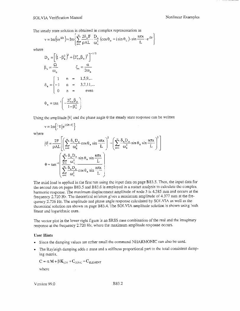
SOLVIA Verification Manual
The steady state solution is obtained in complex representation as
V=Imtveiot J= l•-" F D P. (cos0n +isinO,).sin n-rx .eint
where p2 = ( -[•) + (2(p )21 -1/2
COn 20)n,
I n 1,5,9,...
I n 3,7,11,....
{ n even
0 =tan -' 2 _. P n
Using the amplitude I-V and the phase angle 0 the steady state response can be written
v = Im{ I v [e
where =c o s O s i n I + 8 .s i n . sn s -- 2 1 pA C02 L n~ CO 2
[ D • sin 0 sin n -tx W 2 = o n- L
0 =tan - ' si n
| 8. . cos 8, nrcx 2 L)
The axial load is applied in the first run using the input data on page B83.5. Then, the input data for
the second run on pages B83.5 and B83.6 is employed in a restart analysis to calculate the complex
harmonic response. The maximum displacement amplitude of node 3 is 4.385 mm and occurs at the frequency 2.720 Hz. The theoretical solution gives a maximum amplitude of 4.377 mm at the frequency 2.726 Hz. The amplitude and phase angle response calculated by SOLVIA as well as the
theoretical solution are shown on page B83.4. The SOLVIA amplitude solution is shown using both linear and logarithmic axes.
The vector plot in the lower right figure is an SRSS case combination of the real and the imaginary response at the frequency 2.720 Hz, where the maximum amplitude response occurs.
User Hints
• Since the damping values are rather small the command NHARMONIC can also be used.
"* The Rayleigh damping adds a mass and a stiffness proportional part to the total consistent damping matrix.
C = O• + ±KLIN + CCONC + CELEMENT
where
Version 99.0
Nonlinear Examples
B83.2

SOLVIA Verification Manual
M Total system mass matrix.
KLIN Stiffness matrix based on the elements in all linear element groups.
a, [3 Rayleigh damping factors specified by user.
CcoNc Damping matrix contributed by the concentrated nodal dampers.
CELEMENT Damping matrix contributed by the GENERAL and SPRING elements with viscous
damping and PLANE, SOLID and SHELL with material damping.
The relation between the modal damping ratio and the Rayleigh damping factors
2wo 2
The relation is shown graphically for a = 0.6839 and [3= 5. 10 3 in the figure below.
* Stiffness proportional damp
tfMass proportional damping:
• r ' ' 20 ' 350 4 0 0o
CIRCULAR FRECUENCY
* We can only use mass proportional Rayleigh damping in this example, since the BEAM elements
are considered nonlinear due to the calculation of the geometric stiffness.
• For PLANE, SOLID and SHELL elements viscous and hysteretic material damping can be used in COMPLEX-HARMONIC analysis.
* The same model is used in example B71 where the natural frequency with a lumped mass matrix assumption was calculated to 2.722 0z.
"* The BEAM element with a consistent mass matrix includes rotary inertia which lowers the natural frequencies somewhat. The theoretical frequencies for the Euler-Beoulli beam do not consider
rotary inertia. "* The complex harmonic method in SOLVIA includes the effect of damping also on the distribution
"of the amplitude response. Hence, the amplitude distribution at a resonant frequency may not correspond exactly to the corresponding mode shape calculated for the undamped model.
References "[1] Clough. R.W., and Penzien, J., Dynamics of Structures, Second Edition, McGraw-Hill, 1993.
[2] Blevins, Robert D., Formulas for Natural Frequency and Mode Shape, Van Nostrand Reinhold
Company, 1979.
Version 99.0
Nonlinear Examples
B83.3

SOLVIA Verification Manual Nonlinear Examples
883A COMP1CX-KARMONIC ANALYSIS OF A PRE-LOADEO BEAM. SECOND RUN
2 6
ar
SOLVIA-POST 99. 5 OLVIA ENGINEER:NG AB
B83A COMPLEX-HARMONIC ANALYSIS OF A PRE-.OADED BEAM. SECOND RUN T'eoretical so!ion
'NI' I on
~~~~~~~~~ .. . . . . .. . .. . . . . . . . . . .. . . ... . .
SOL,/A-00ST 99A SOLVIA ENGINE01 RBNG AB
Version 99.0
383A COMPLEX-HARMONIC ANALYSIS OF A PRE-LOADED BEAM, SECOND RUN
IN. : i ..... ... . .. .... .... ..... ...... ........
2 3 4 S
FRECBELOCY
• ! I . . . ... . .. . . . ... . ..! ..... ... . . . . . . ........ . .. . .. .... ....... ... .. . ... . . .. . .. .
C ! I
SOLVIA -OST 99.0 SOLVIA ENGINEERING AB
CL3 -CPE-AMC NA C'C O RELAEDBA, SIOO U
CO N .CO .. N..... .. C ..............
2 3 0 S
SOL1ý-POT 993 SLVIFENGIEERIG A
C83A CO PCECARC0NI AALOS:S . A PRE-LOADED BEAC. SECCND RUN
ORIGINAL -
CGINAL - -CL IA. VALUE • , ZSýE-l _,
OX SLACE-I.T
A P C ANC L C L C E., T_ 93.4 EN;INE_ýING Ab
83.4

SOLVIA Verification Manual
SOLVIA-PRE input, first run
HEADING 'B83 COMPLEX-HARMONIC ANALYSIS OF A PRE-LOADED BEAM, FIRST RUN'
.
DATABASE CREATE MASTER IDOF=001110 KINEMATICS DISPLACEMENT=LARGE ITERATION METHOD=BFGS .
COORDINATES 1 / 2 5. / 3 2.5
MATERIAL 1 ELASTIC E=2.EI1 DENSITY=7800 *
EGROUP 1 BEAM SECTION 1 GENERAL RINERTIA=1.40577000E-05
SINERTIA=8.33333333E-06 TINERTIA=8.33333333E-06 AREA=1.E-02
BEAMVECTOR / 1 0. 0. 1. GLINE 1 2 AUX=-- EL-20
FIXBOUNDARIES 12 FIXBOUNDARIES 2 LOADS CONCENTRATED
/ 1 /2
/ 2 1 -600.E3
SOLVIA END
SOLVIA-PRE input, second run
DATABASE OPEN
HEADING 'B83A COMPLEX-HARMONIC ANALYSIS OF A PRE-LOADED BEAM, SECOND RUN' MASTER IDOF=001110 MODEX=RESTART TSTART=-. RAYLEIGH-DAMPING ALPHA=0.6839 BETA-0. COMPLEX-HARMONIC
1.0 8 / 2.6 200 / 2.8 20 / 4.0 6 6.0
DELETE LOADS
SOLVIA END
LOADS CONCENTRATED CONCENTRATED / 3 2 i0.
Version 99.0
Nonlinear Examples
1383.5

SOLVIA Verification Manual
SOLVIA-POST input, second run
* B83A COMPLEX-HARMONIC ANALYSIS OF A PRE-LOADED BEAM, SECOND RUN *
DATABASE CREATE
WRITE 'b83a.lis'
SET PLOTORIENTATION PORTRAIT DIAGRAM=GRID NCOMPLEX-HARMONIC NODE=3 DIRECTION=2 KIND=DISPLACEMENT OUTPUT=ALL
AXES-SCALE=3
NCOMPLEX-HARMONIC NODE=3 DIRECTION=2 KIND=DISPLACEMENT AXES-SCALE=l
,
USERCURVE 1 XLABEL='FREQUENCY' / READ B83DISP.DAT USERCURVE 2 XLABEL='FREQUENCY' YLABEL='PHASE ANGLE'
READ B83PHASE.DAT AXIS 1 VMIN=- VMAX=5.OE-3 LABEL='DISPLACEMENT'
PLOT USERCURVE 1 YAXIS=l TEXT STRING='Theoretical solution' X=2 Y=23.5 SET PLOTORIENTATION=LANDSCAPE PLOT USERCURVE 2 TEXT STRING='Theoretical solution' X=3 Y=15.75
MESH VIEW-Z BCODE=ALL NNUMBER=MYNODES NSYMBOL=YES ORIGINAL=YES DEFORMED=NO SUBFRAME=I2
CASECOMBINATION 1 STANDARD FUNCTION=SRSS 2.720 1. REAL 2.720 1. IMAGINARY SET RESPONSETYPE=CASECOMBINATION MESH ORIGINAL=YES NSYMBOL=YES VECTOR=DISPLACEMENT NLIST N3 END
Version 99.0
Nonlinear Examples
B83.6

SOLVIA Verification Manual
EXAMPLE B84
IMMERSION OF A SHELL STRUCTURE INTO WATER, BUOYANCY EFFECTS
Objective
To verify the SHELL element load option with interpolation of intensity along a global coordinate axis considering large displacements.
Physical Problem
The figure below shows a shell structure to be immersed into water. The buoyancy force as a function
of the immersion depth is to be calculated.
z R=l m
vLength L =4 m
Thickness h = 0.020 m
E =2.1.10" N/m 2
v=0.3
Pwater = 10 0 0 kg / in 3
-- =9.81 n/s 2
Finite Element Model
The finite element model is shown on page B84.2 and consists of 4-node SHELL elements. Prescribed displacements at node 2 and constraint equations are used to move the structure in the negative Z-direction. The prescribed displacements are applied in ten time steps. Full-Newton iteration and force tolerances are used.
The water pressure load is applied by the element load option of a linear pressure variation fixed in space. When the model is immersed into the water the pressure is automatically calculated based on the current large displacement configuration. The element load option of an element fixed pressure is also available. Both options of pressure load are deformation dependent.
Solution Results
If the shell structure is assumed to be rigid the total vertical reaction F can be expressed as a function
of the immersion depth 8 as
F=-gp rLR2(0 -sin )/2 where 0=2arccos- RR---) for 3Ž0
The input data on pages B84.4 and B84.5 gives the following results:
Version 99.0
Vertical displacement Total vertical reaction force (N) 8 Theory SOLVIA
m B84 B84A 0.1 -2304 -2273 -2304 0.2 -6416 -6352 -6407 0.5 -24101 -24027 -24081 1.0 -61638 -61378 -61571
Nonlinear Examples
B84.1

SOLVIA Verification Manual
Case B84A has the same input as B84 except that 40 elements instead of 20 are used along the
circumference.
The top figure on page B84.3 shows the force-displacement diagram calculated by SOLVIA for case
B84 together with the theoretical solution. The two curves almost coincide. The configuration in the
last solution step together with the reaction force are shown in the bottom figure.
The nodal loads on the structure at time 10 are shown in the top figure on page B84.4.
User Hints
"* With 4-node SHELL elements the geometry of the half cylinder is approximated by an assembly
of flat elements with all nodes lying on the midsurface of the cylinder. Hence, the volume of the
model is smaller than the volume of the perfect half cylinder.
The pressure variation along the edge of the flat 4-node element is linear, which agrees with the
water pressure variation. Hence, the calculated buoyancy force is smaller than the theoretical value
for a perfect half cylinder, since the only error is due to the smaller volume.
" A better description of the circular geometry is achieved by the 9-node and 16-node SHELL
elements. However, the pressure variation along the edges of these elements is still linear. Since
the actual pressure along the circular boundary varies in a sinusoidal manner there will be an
approximation in the pressure load application, which counteracts the better geometry of these
SHELL elements.
"* The change in volume due to elastic deformation of the SHELL structure could be significant if
the SHELL thickness is small.
B84 IMMERSION OF A SHELL STRUCTURE INTO WATER, BUOYANCY EFFECTS
ORIGINAL ; 0 . ZONE SHELL
Z
x -y
E.
MASTER
0: 0 !3u _ 0 B 01O00O
C iO 00G
S HELL TOP SSHEL BOTTON
NON-SHELL
SOLVTA-PRE 9SOLV A ENGINEERING AB
Version 99.0
Nonlinear Examples
9.0
B84.2

SOLVIA Verification Manual Nonlinear Examples
B84 :MMERSTCN OF A SHELL STRUCTURE INTO WATER, 3UOYANCY EFFECTS
N
w
0
0 -I
0.0 0 .0)
SOLVIA-POST 99.0
0.2 0.3 0.4 0.s
DISPLACEIENT
0.6 0 7 0.8 0.9
SOLVIA ENGINEERING AB
B84 IMMERSICN OF A SHELL STRUCTURE INTO WATER, BUOYANCY EFFECTS
ORIGINAL -- -ý 0 .S MAX DISPL. i t TIME 10 ZONE SHELL
REACTION
61378
SOLVIA ENGINEERING ABSOLVTA-POST 99.0
Version 99.0
z
X- I-Y N
.................... .... .....................
.. ..... ... ..........
B84.3

SOLVIA Verification Manual
B84 IMMERSICN OF A SHELL STRUCTURE INTO WATER, BUOYANCY EFFECTS
ORIGINAL 0- .2 7TME 10
LOAD
1018.9
SOLVIA ENGINEERING ABSOLVIA-POST 99.0
SOLVIA-PRE input
DATABASE CREATE HEADING 'B84 IMMERSION OF A SHELL STRUCTURE INTO WATER,
BUOYANCY EFFECTS'
PARAMETER $CIRC=20 $LONG=6 $SHORT=4 SET NODES=4
MASTER NSTEP=10 DT=1 MEMORY SOLVIA=20 KINEMATICS DISPLACEMENT=LARGE ITERATION METHOD=FULL-NEWTON TOLERANCES TYPE=F RTOL=1.E-3 RNORM=I.E5 RMNORM=1.E5 PORTHOLE SAVEDEFAULT=NO TIMEFUNCTION 1 / 0. 1. / 10 1.0 TIMEFUNCTION 2 / 0. 0. / 10 1.0
COORDINATES ENTRIES NODE X Y Z 1 4. 1. TO 3 4. -1. / 4 0. 1. TO 6 0. -1.
MATERIAL 1 ELASTIC E=2.0E11 NU=0.3 DENSITY=-.
Version 99.0
z iZ
Nonlinear Examples
B84.4
SOLVIA Verification Manual
SOLVIA-PRE input (cont.)
EGROUP 1 SHELL MATERIAL=i SYSTEM 1 CYLINDRIC LINE CYLINDRIC 1 3 EL=$CIRC ROTATION=NEGATIVE SYSTEM=i LINE CYLINDRIC 4 6 EL=$CIRC ROTATION=NEGATIVE SYSTEM=i GSURFACE 1 3 6 4 EL2=$LONG GSURFACE 2 3 1 2 ELI=$SHORT GSURFACE 5 4 6 5 EL1=$SHORT THICKNESS 1 0.020 LOADS ELEMENT INPUT=SURFACE INTERPOLATION=Z
SYSTEM=GLOBAL-SPACEFIXED COORD1=-I. Vi=0. COORD2=-2. V2=9810. VMIN=0.
1 3 6 4 t . . . . . 1 2 3 1 2 t . . . . . 1 5 4 6 5 t . . . . . 1
FIXBOUNDARIES 1 INPUT=LINE / 1 2 / 2 3 / 4 5 / 5 6 FIXBOUNDARIES 2 INPUT-LINE / 1 4 / 3 6 LOAD DISPLACEMENT 2 3 -1. 2
CONSTRAINTS 1323/3323/4323/5323/6323
COLOR EFILL=SHELL VIEW ABC X=2 Y-i Z=0.5 SET BCODE=ALL NNUMBER=MYNODES NSYMBOL=MYNODES MESH ZONE=SHELL VIEW=ABC SOLVIA END
SOLVIA-POST input
* B84 IMMERSION OF A SHELL STRUCTURE INTO WATER, * BUOYANCY EFFECTS *
DATABASE CREATE
WRITE 'b84.1is'
AXIS 1 VMIN=.0 VMAX=1.0 LABELSTRING='DISPLACEMENT' AXIS 2 VMIN=-7.5E4 VMAX=0.0 LABELSTRING='FORCE' USERCURVE 1 / READ B84.DAT
SET DIAGRAM=GRID NHIST NODE=2 DIRECTION=3 KIND=REACTION XAXIS=i YAXIS=2,
SYMBOL=i XVAR=2 OUTPUT=ALL PLOT USERCURVE 1 XAXIS=-i YAXIS=-2 SUBFRAME=OLD *
VIEW ABC X=2 Y=1 Z=0.7 MESH ZONE-SHELL ORIGINAL=DASHED VECTOR=REACTION VIEW=ABC MESH VECTOR=LOAD VIEW=X ORIGINAL=YES DEFORMED=NO
END
Version 99.0
Nonlinear Examples
B84.5

SOLVIA Verification Manual
EXAMPLE B85
PURE SHEAR OF A RUBBER SHEET
Objective
To verify the rubber material model in plane pure shear deformation using PLANE STRESS2 and
PLANE STRAIN elements.
Physical Problem
A quadratic rubber sheet of unit side length deforms with displacement u in pure shear.
Initial configuration at time 0 Deformed configuration at time t
Mooney-Rivlin constants:
C 1 =0.125MPa
SC 2 = 0.025 MPa
I0, = 103 MPa (bulk modulus) 0 0
0 1 0 1 1+u
Finite Element Model
In the first analysis one PLANE STRESS2 element has been used and in the second analysis one
PLANE STRAIN element. The deformation is prescribed using LOADS DISPLACEMENT in ten
increments with a total displacement of u = 2. Full Newton equilibrium iterations are used.
Solution Results
The plane deformation in pure shear is described by
tt X= 0
x 1 +U 0
X2
tX2 = 0X,
where X and 'x 2 are the deformed coordinates of the point with the original coordinates 0x, and 0x2.
The displacement u is defined in the figure. The following deformation measures can be formed:
0 = [0x'] [1 ?] (Deformation gradient tensor)
St x 00=[I 1 j ] (Cauchy - Green deformation tensor)
( c-I)= 0 u/2] (Green- Larangestrain tensor) 0 ý FkCI uI 2 2/2] Larng,
The left indices t and 0 indicate that the tensor quantity is occurring in the deformed configuration at
solution time t and referenced to the original undeformed configuration at time 0. In the following description of this example the left indices are not written out but are understood to be there. Hence,
for example, the following understanding regarding the notation is used:
X= X , 'C=C and gE=e
Version 99.0
Nonlinear Examples
B85.1

SOLVIA Verification Manual
The principal stretches X are obtained from
det(C- _2I)= 0
which gives
u2 +4]
The principal directions On referenced to the initial configuration are obtained from
(C- k22)0n = 0
which gives
°n =[=2 1]
n2 =L 1]
The principal stretch directions 'n in the deformed configuration are obtained from
tn = X On
which gives
1n, = [2 +u, 1] n2=-I +u, 1]
Extending this plane problem to three dimensions we can write
x Io u u u 0]L0 u/2 0] X= 1 C = l IU 2 01 Cu=/U
+u 0 00
The term x33 is unity for pure shear in the plane stress case because the material is incompressible. Since the volume of a differential element is constant during deformation we have that
det X= I
which gives x33 = 1.
The term x33 is also unity in the plane strain case because, by definition, there is no deformation in
the x3 - direction.
In the calculation of the analytical expressions for the stresses we need to distinguish between the plane stress and the plane strain case.
Plane Stress
In the plane stress case the incompressibility of the rubber material is enforced by
C 33 = (Cl C 21 -C 12 C 2 1- I
since incompressibility means that also det C = 1.
Version 99.0
Nonlinear Examples
B85.2

SOLVIA Verification Manual
The invariants of the Cauchy-Green deformation tensor are
It = C 1 1 +C22 +C 3 3 = C11 +C 2 2 +(Cl 1 C 2 2 -_C 2 C21)
12 = Cl C22 +C 2 2 C 3 3 +C3 3 CH -C12 C21 = C11 C 2 2 +-(cH +C22 XCII C 22 -C1 2 Cz 1 )-Y -C 2 C21
13 =detC=l
The Mooney-Rivlin material model is determined by the potential
W= C, (i, -3)+C 2 (02 -3)
where C1 and C2 are the Mooney-Rivlin material constants. The second Piola-Kirchhoff stresses are
calculated from the potential as
Sij = -W = 2 -W =23W a Il +2 DW a3I
ac i C½j all aCij DI2 aCij
which gives
S1 =-2Clu2-2 C 2 u2(2+ U2)
S2 2 =•-2C 2u2
St2 =2C0u+2C 2(l+u2)u
S 33 = 0
The transformation to Cauchy stresses is performed by 1 I*XSXT
det X
which gives
"t711 = SIl +2uS 12 +u 2S 22 = 2C1 u 2
T22 =S 22 =-2 C2 u 2
'r2 =St2 +uS2 2 =2(C 1 +C 2 )u 1133 = 0
Plane Strain
In the plane strain case the rubber material is compressible and a bulk modulus is specified. A separately interpolated pressure field is employed to subtract in an integration over each element the
hydrostatic pressure calculated by the interpolated displacements. This procedure allows the material to be almost incompressible.
The invariants of the Cauchy-Green deformation tensor are
I1 =C 11 +C 2 2 ±C 33
12 -C 1 l C 2 2 +C 22 C 33 +C3 3 CH -C 12 C 2 1
13 = C 3 3 (C 1 1 C 22 -C12 C 2 1 )
The Mooney-Rivlin material model is determined by the potential
w = c, (J, - 3)+ c2 0 ( 2 - 3)+ - K(J 3 - 1)2
Version 99.0
Nonlinear Examples
B85.3

SOLVIA Verification Manual
where J- U 1"3!3 J 5"3-2/3 J?=[1/2 Ji = 11 * 13 J2 1* 3 3 3
and where K is the bulk modulus. The isochoric (volume preserving) deformation (in J1 and J2 ) and
the dilatational (volume changing) deformation (in J ) are then separated in the potential, see [I ]. The
second Piola-Kirchhoff stress components based on the displacement interpolation are calculated as
aw aw
where
_aw D1 1 a W aw DJ 2 .W DJ 3 aC i i l aJ c O ii DJ2 aC ij WJ3 aCij
and
D _ I r a il I a 3 _] -1 /3 aCij aCij 3i3 aCij 3
-J2 = ( _3 212 . I 3 )I -213
i ac 313 aC-)
DJ 3 - I__L a C ij 2 3 a C ii
Using the prescribed displacement field for pure shear we obtain 2 U2
S 1 u
2u5 S 22 =-(C1 + 2C 2)-2
3
S33= (C 2+ u2) 2 Cu
33
Transformation to Cauchy stresses gives
'r I = (2 C , + C 2 ) -
3 2u5 =2 =-(C I + 2 C2)--2-
2u5 1133 = (C2 -Cl)-2
3 T12 = (Cl -C 2 )2u
We note that the hydrostatic pressure based on the interpolated displacements is zero since Irl + T22 + T33 = 0. Hence, the separately interpolated pressure, in addition to the interpolation of displacements, is not needed in this case. The interpolated pressure amplitudes are consequently zero.
Version 99.0
Nonlinear Examples
B85.4
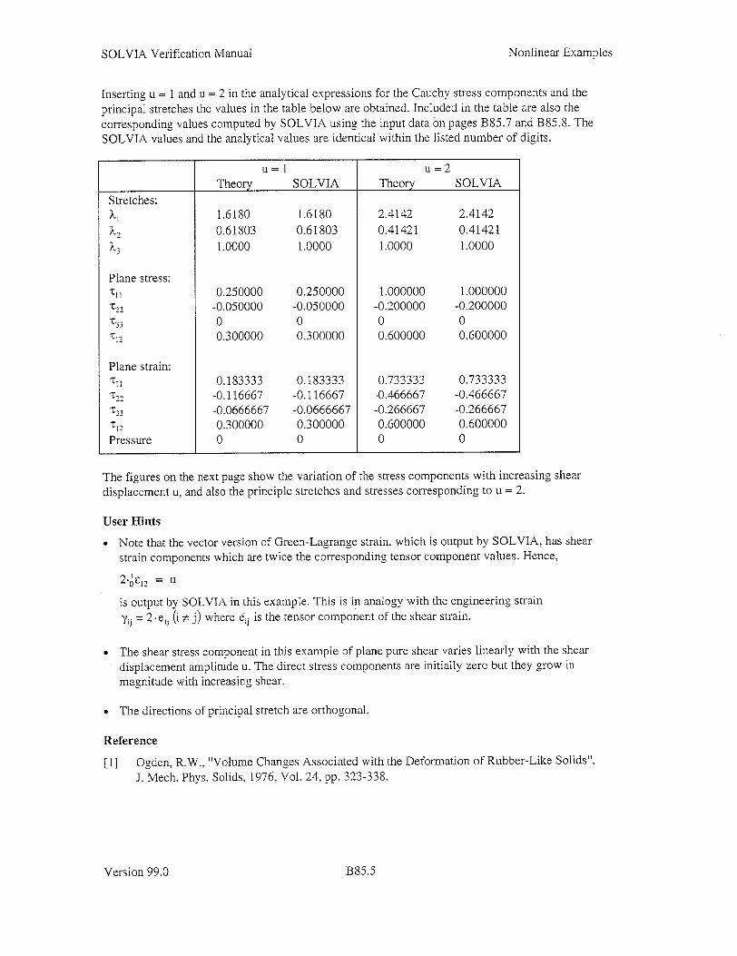
SOLVIA Verification Manual
Inserting u = 1 and u = 2 in the analytical expressions for the Cauchy stress components and the principal stretches the values in the table below are obtained. Included in the table are also the corresponding values computed by SOLVIA using the input data on pages B85.7 and B85.8. The SOLVIA values and the analytical values are identical within the listed number of digits.
u=l u=2 Theory SOLVIA Theory SOLVIA
Stretches: Xt 1.6180 1.6180 2.4142 2.4142
X2 0.61803 0.61803 0.41421 0.41421
k.3 1.0000 1.0000 1.0000 1.0000
Plane stress: ""i1 0.250000 0.250000 1.000000 1.000000 T22 -0.050000 -0.050000 -0.200000 -0.200000 "733 0 0 0 0
""12 0.300000 0.300000 0.600000 0.600000
Plane strain: "0.183333 0.183333 0.733333 0.733333
t 2 2 -0.116667 -0.116667 -0.466667 -0.466667 -0.0666667 -0.0666667 -0.266667 -0.266667
'r2 0.300000 0.300000 0.600000 0.600000
Pressure 0 0 0 0
The figures on the next page show the variation of the stress components with increasing shear displacement u, and also the principle stretches and stresses corresponding to u = 2.
User Hints
° Note that the vector version of Green-Lagrange strain, which is output by SOLVIA, has shear strain components which are twice the corresponding tensor component values. Hence,
2-0F12 = u
is output by SOLVIA in this example. This is in analogy with the engineering strain
-ij = 2. e (i j) where ej is the tensor component of the shear strain.
" The shear stress component in this example of plane pure shear varies linearly with the shear displacement amplitude u. The direct stress components are initially zero but they grow in magnitude with increasing shear.
" The directions of principal stretch are orthogonal.
Reference
[1] Ogden. R.W.. "Volume Changes Associated with the Deformation of Rubber-Like Solids", J. Mech. Phys. Solids, 1976, Vol. 24, pp. 323-338.
Version 99.0
Nonlinear Examples
B85.5
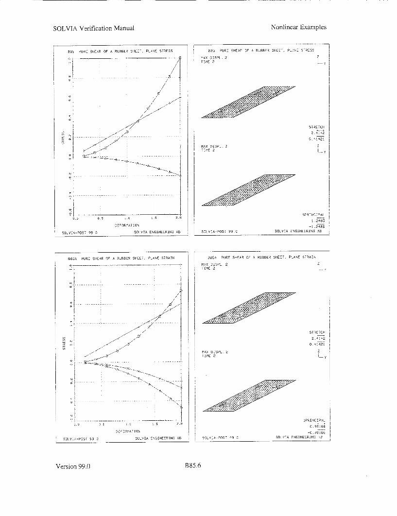
SOLVIA Verification Manual Nonlinear Examples
BBS PURE SHEAR OF A RUBBER SHEET, PLANE STRESS
A
SOLVA
- 7 H 7
91
91<
A�A.
o I o L.5 2 .
DEFORMATION
-POST 99 0 SOLVEA ENGINEERING AB
85 PURE SHEAR OF A RUBBER SHEET, PLANE STRESS
MAX OISPL. 2 TIME 2
MAX DISPL. 2 TIME 2
SOLVIA-POST 99.0
Z
STRETCH
2.4ý 2
- y
SPRINCIPAL
i.2485
-1.248S
SOLVIA ENGINEERING AB
BASA PURE SHEAR OF A RUBBER SHEET. PLANE STRAIN
i I .... .. .. .. .. .. .. ......... .... ..... .. ...... .. .. .. .... .
OLVIA-POST 990
Version 99.0
�-�- I Al.1 .s 2.0
DE LAORMAAi AON
SOLVIA ENGINEERING AB
BSSA PURE SHEAR OF A RUBBER SHEET, PLANE STRAIN
MAX DISPL. 2
TIME 2
z LKy
STRETCH
. 41421 0.z2
LMAX DISPL. 2 T!ME 2
SOLVIA-POST 99 0
SPRINCIPAL
0 98 86
-09 8186
SOLVIA ENGINEERING AB
B85.6
. 1
LJ
--- ý_--A_
,2ý
:iZT----x-

SOLVIA Verification Manual
SOLVIA-PRE input
HEADING 'B85 PURE SHEAR OF A RUBBER SHEET, PLANE STRESS'
DATABASE CREATE MASTER IDOF=i00111 NSTEP=10 DT=0.2 ITERATION FULL-NEWTON .
TIMEFUNCTION 1 0. 0./ 2. 2.
COORDINATES / ENTRIES NODES Y Z 1 1. 1. / 2 0. 1. / 3 / 4 1.
MATERIAL 1 RUBBER C1=0.125 C2=0.0250 KAPPA=1000.
EGROUP 1 PLANE STRESS2 ENODES
1 1234 EDATA / 1 0.1 FIXBOUNDARIES 3 1 TO 4 FIXBOUNDARIES 2 / 1 4
LOADS DISPLACEMENTS 1 2 1. / 2 21.
SOLVIA END
SOLVIA-POST input
* B85 PURE SHEAR OF A RUBBER SHEET, PLANE STRESS *
DATABASE CREATE
WRITE FILENAME='b85.1iS'
AXIS 1 VMIN=0. VMAX=2. LABELSTRING='DEFORMATION' AXIS 2 VMIN--0.5 VMAX=i. LABELSTRING='STRESS' *
SET DIAGRAM=GRID PLOTORIENTATION=PORTRAIT EHISTORY ELEMENT=4 POINT=i KIND=SYY XAXIS:1 YAXIS=2 SYMBOL=-,
OUTPUT=ALL EHISTORY ELEMENT=1 POINT=i KIND=SZZ XAXIS=-I YAXIS=-2 SYMBOL=2,
OUTPUT=ALL SUBFRAME=OLD EHISTORY ELEMENT=i POINT=1 KIND=SYZ XAXIS=-I YAXIS=-2 SYMBOL:3,
OUTPUT=ALL SUBFRAME=OLD *
ELIST TSTART=I ELIST SELECT=STRETCH TSTART=ELIST TSTART=2 ELIST SELECT=STRETCH TSTART=2
MESH VECTOR=STRETCH SUBFRAME=i2 MESH VECTOR=SPRINCIPAL END
Version 99.0
Nonlinear Examples
B 85.7

SOLVIA Verification Manual
SOLVIA-PRE input
HEADING 'B85A PURE SHEAR OF A RUBBER SHEET, PLANE STRAIN' ,
DATABASE CREATE MASTER IDOF=-00111 NSTEP=10 DT=0.2 ITERATION FULL-NEWTON
TIMEFUNCTION 1 0. 0. / 2. 2.
COORDINATES / ENTRIES NODES Y Z 1 1. 1. / 2 0. 1. / 3 / 4 1.
MATERIAL 1 RUBBER Ci=0.125 C2=0.0250 KAPPA-O000.
EGROUP 1 PLANE STRAIN PRESSURE-INTERPOLATION=YES ENODES
1 1 2 3 4
FIXBOUNDARIES 3 1 TO 4 FIXBOUNDARIES 2 / 1 4
LOADS DISPLACEMENTS 1 2 1. / 2 21.
SOLVIA END
SOLVIA-POST input
* B85A PURE SHEAR OF A RUBBER SHEET, PLANE STRAIN
DATABASE CREATE
WRITE FILENAME='b85a.lis'
AXIS 1 VMIN=C. VMAX=2. LABELSTRING='DEFORMATION' AXIS 2 VMIN=-0.5 VMAX=1. LABELSTRING='STRESS'
SET DIAGRAM=GRID PLOTORIENTATION=PORTRAIT EHISTORY ELEMENT=i POINT=i KIND=SYY XAXIS=i YAXIS=2 SYMBOL=-,
OUTPUT=ALL EHISTORY ELEMENT=i POINT=i KIND=SZZ XAXISý-i YAXIS=-2 SYMBOL=2,
OUTPUT=ALL SUBFRAME=OLD EHISTORY ELEMENT=i POINT=I1 KIND=SYZ XAXIS=-I YAXIS--2 SYMBOL=3,
OUTPUT=ALL SUBFRAIE=OLD EHISTORY ELEMENT=i POINT=i KIND=SXX XAXIS=-i YAXIS=-2 SYMBOL=4,
OUTPUT=ALL SUBFRAME=OLD
ELIST STRAIN=YES TSTART=i ELIST SELECT=STRETCH TSTART=1 ELIST STRAIN=YES TSTART=2 ELIST SELECT=STRETCH TSTART=2
MESH VECTOR=STRETCH SUBFRAME=i2 MESH VECTOR=SPRINCIPAL END
Version 99.0
Nonlinear Examples
B85.8

SOLVIA Verification Manual
EXAMPLE B86
IN-PLANE BUCKLING OF AN UNSYMMETRIC DEEP ARCH
Objective
To verify the AUTOMATIC-ITERATION method for post collapse analysis with PLANE STRESS2 elements.
Physical Problem
A deep elastic arch as shown in the figure below is to be analyzed. Only deformation in the arch plane
is considered. The boundary conditions are unsymmetric.
Geometry data
r = 100.0 m
a=1.0 m
ct =215'
Material properties
E=210.109 N/m 2
v=0.0
Reference load
El Pref = - = 1750-103 N
Finite Element Model
The arch is modeled using 64 8-node PLANE STRESS2 elements. The model is shown in the figure
on page B86.2. The reduced integration order of 2 x 2 and the force convergence criterion are used.
Skew system is employed at the right boundary to achieve plane stress conditions. The vertical load is
distributed in a consistent way along the nodes of the load application section. Details of the model at
the boundaries and at the load application are shown on page B86.3.
Solution Results
The input data is shown on pages B86.5 and B86.6. The deformed mesh at four solution steps are
shown in the bottom figure on page B86.3. The horizontal and vertical displacements at one of the
load application nodes (node 2) are drawn using symbols in the top figures on page B86.4. The curves
without symbols in the same figures are the corresponding solution from [1]. The two curves are almost coinciding.
Version 99.0
Nonlinear Examples
B86.1

SOLVIA Verification Manual
The bottom figure on page B86.4 shows the vertical reaction at the hinged support.
The peak load and the corresponding horizontal and vertical displacements are compared with the results reported in [1]:
Peak load factor Y-displacement (in) Z-displacement (in)
SOLVIA 8.967 -61.2 -114.0
Reference [11 9.027 -60.4 -112.7
Reference
[1] Lyons, P. and Holsgrove, S., "Finite Element Benchmarks for 2D Beams and Axisymmetric Shells Involving Geometric Nonlinearity (Summary), NAFEMS, Ref. ROO 10
B86 IN-PLANE BUCKLrNG OF AN UNSYMMETRIC DEEP ARCH
CRIGINAL 20. TIME I ZONE EGI
Z Ly
A E RCA 1 6667T-6
SOLVIA ENGINEERING AB
Version 99.0
Nonlinear Examples
SOLV_,A-PRE 99-C
B86.2

SOLVIA Verification Manual Nonlinear Examples
OR:GINALTME I
ZONE E33
386 !N-PLANE BUCKLING OF
Z
-y
FORCE
1. 1667E6
NAXES=SKE:
MASTER 1001I,
AN UNSYMMETRIC DEEP ARCH
ORIGINAL 1. Z TIME 1 L ZONE E32
FORCE
1. 16667E6
C
NAXES=SKEW
MASTER 100111
ORTGINA; - 2. TIME 1 ZONE N3+I
SOLVIA-PRE 99.0
ORIGINAL • 2. TIME . ZONE Ni+1
LOAD 0.0
C
NAXES=SKE
MASTER 100B 1'I
S Ii~i11
/
H-
Z
Ly_OAD 0.0
a b
NAXES=SKEW
MASTER
B 1011! C l:1i!l
SOLVIA ENGINEERING AB
B86 IN-PLANE BUCKLING OF AN UNSYMMETRIC DEEP ARCH
ORIGINAL - 20. MAX DISPL. i.63.22 TIME 21
Z
Ly
LOAD
I.4648E5
3CV[A ENGINEERING A3;OLI A-POST 99.0
Version 99.0 B86.3
i2 11
Z IL,

SOLVIA Verification Manual Nonlinear Examples
B86 IN-PLANE 8UC<LNG OF AN UNSYMMETRIC DEEP ARCH
'N
'-4
7 1'
26 a2 4 10
COAD MULTIPLIER LAMBDA
SOLVHA-POST 99.0 SOLV:A ENGINEERING AB
B86 IN-PLANE BUCKLING OF AN UNSYMMETREC DEEP ARCH
COAD
SCLVIA-POST 99.0
4 A 4 Io
MTULTIPLIER LAMBDA
SOLVIA ENGINEERING AB
Version 99.0
386 IN-PLANE BUCKLING OF AN UNSYMIIETRIC DEEP ARCH
4
SID
S• 'N
2o
LDALD NUCfIRL ER LArBDA
SOLVIA-TOST 99.0 SOLVIA ENGDNEERING AB
B86.4

SOLVIA Verification Manual
SOLVIA-PRE input
HEADING 'B86 IN-PLANE BUCKLING OF AN UNSYMMETRIC DEEP ARCH' DATABASE CREATE
MASTER IDOF=100111 NSTEP=100 KINEMATICS DISPLACEMENTS=LARGE AUTOMATIC-ITERATION NODE=2 DIRECTION=3 DISPLACEMENT=-1. ,
DISPMAX=120.5 CONTINUATION=YES TOLERANCES TYPE=F RNORM=1.E5
SYSTEM 1 CYLINDRIC COORDINATES
ENTRIES NODE R THETA 1 100.5 -17.5 2 100.5 90.0 3 100.5 197.5 4 100.0 -17.5 5 99.5 -17.5 6 99.5 90.0 7 99.5 197. 5 8 100.0 197.5 9 100.0 90.0
SKEWSYSTEM EULERANGLES 1 -17.5
NSKEWS 11 / 51
MATERIAL 1 ELASTIC E=210.E9 NU=0.
EGROUP 1 PLANE STRESS2 INT=2 EDATA / 1 1. GSURFACE 1 2 6 5 EL1=32 EL2=1 NODES=8 SYSTEM=1 GSURFACE 2 3 7 6 EL1=32 EL2=1 NODES=8 SYSTEM=I
FIXBOUNDARIES 23 / 4 8 FIXBOUNDARIES 3 / 1 5
LOADS CONCENTRATED 2 3 -291.666E3 6 3 -291.666E3 9 3 -1166.666E3
SET VIEW=X NSYMBOLS=MY VECTOR=LOAD MESH EGi SUBFRAME 22 SET NNUMBERS=MY BCODE=ALL NAXES=SKEW MESH E33 MESH E32 MESH N3+1 MESH N1+1
SOLVIA END
Version 99.0
Nonlinear Examples
B86.5
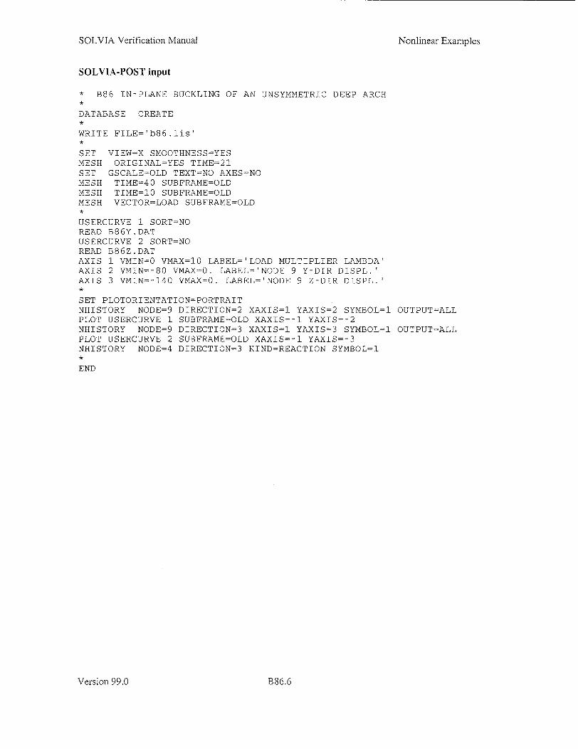
SOLVIA Verification Manual
SOLVIA-POST input
* B86 IN-PLANE BUCKLING OF AN UNSYMMETRIC DEEP ARCH *
DATABASE CREATE
WRITE FILE='b86.1is'
SET VIEW=X SMOOTHNESS=YES MESH ORIGINAL=YES TIME=21 SET GSCALE=OLD TEXT=NO AXES=NO MESH TIME=40 SUBFRAME=OLD MESH TIME=-0 SUBFRAME=OLD MESH VECTOR=LOAD SUBFRAME=OLD *
USERCURVE 1 SORT=NO READ B86Y.DAT USERCURVE 2 SORT=NO READ B86Z.DAT AXIS 1 VMIN=O VMAX=-0 LABEL='LOAD MULTIPLIER LAMBDA' AXIS 2 VMIN=-80 VMAX=O. LABEL='NODE 9 Y-DIR DISPL.' AXIS 3 VMIN=-140 VMAX=-. LABEL='NODE 9 Z-DIR DISPL.'
SET PLOTORIENTATION=PORTRAIT NHISTORY NODE=9 DIRECTION=2 XAXIS=i YAXIS=2 SYMBOL=i OUTPUT=ALL PLOT USERCURVE 1 SUBFRAME=OLD XAXIS=-I YAXIS=-2 NHISTORY NODE=9 DIRECTION=3 XAXIS=1 YAXIS=3 SYMBOL=i OUTPUT=ALL PLOT USERCURVE 2 SUBFRAME=OLD XAXIS=-1 YAXIS=-3 NHISTORY NODE=4 DIRECTION=3 KIND=REACTION SYMBOL=1
END
Version 99.0
Nonlinear Examples
1386.6

SOLVIA Verification Manual
EXAMPLE B87
LATERAL BUCKLING OF A RIGHT-ANGLE FRAME
Objective
To verify the AUTOMATIC-ITERATION method and the BEAM element in buckling and postbuckling analysis of a three dimensional beam structure.
Physical Problem
A very slender right-angle frame shown in the figure below is analyzed. No shear effects in the beams are considered.
L Section data:
b=30mm b - -- t = 0.6 mm (thickness)
A = 18.0 mm 2
1, = 2.1329 ram4
I = 1350.0 mrnm 4
It =0.54mMn
Perturbation load in Z-direction at tip: 1P0i-4
Pz = Pref
Reference load at tip:
pr L4 L 0.820035 N
b
Length L 240 mm Material, E = 71240 N/mrm 2
"v = 0.31
Finite Element Model
The frame is modeled using eight 2-node BEAM elements. The model is shown in the left figure on page B87.2. The AUTOMATIC-ITERATION method with force/moment convergence criterion is used.
Solution Results
The input data on pages B87.4 and B87.5 is used. The deformed mesh and the displacements of nodes 3 and 2 as function of the load factor are shown in figures on pages B87.2 and B87.3. The load-lateral displacement curve shows a good agreement with the results reported in reference [1].
The analysis case B87A is a linearized buckling analysis using the input data on page B87.6. The applied load is 10% of Pref and the critical load factor obtained is 10.0212 giving a critical buckling load of 0.822, Pref" This value is in good agreement with the buckling load of 0.838. Pref reported in [1].
Version 99.0
Nonlinear Examples
B87.1

SOLVIA Verification Manual Nonlinear Examples
User Hints
"* This structure is quite extreme since the ratio b/t=50. The buckling is rather sudden and the buckling displacement is predominantly in the lateral (Z) direction. The buckling also includes torsion.
" The post-buckling behaviour is first associated with a very small tangent stiffness but the load carrying capacity in the negative Z-direction is then gradually increasing.
" The convergence rate for this example is quite slow and many load steps are needed in the automatic-iteration analysis.
" The linearized buckling analysis in this example is straight-forward and presents no difficulties. The moment caused by the load gives a rotation that is practically zero due to the section dimensions of the force and the direction of the load. The moment does then not jeopardize the application of linearized buckling. For a further discussion of the limits for application of linearized buckling, see Example B88.
Reference
[1] Kouhia, R. "On Kinematical Relations of Spatial Framed Structures", J. Computers & Structures, Vol. 40, No. 5, pp. 1185-1191, 1991.
Y
L,
FORCE
0.82003S
IASTER 000R0
I 11N1N SOL'I!A ENGTNEERING AB
B87 LATERAL BUCKLING OF A RIGHT-ANGLE FRAME
_OAO AULTP TEN IADA
i 2,3
SOLVIA-POST 99.0
OAD '1ULTTPL:EQ LAMEDA
SOLVIA ENGINEERING AB
Version 99.0
B87 LATERAL BUCKLING OF A RIGHT-ANGLE FRAME
ORIGINAL -- 50. TIME I
SOLVIA-PRE 99.0
¢o
g
B87.2

SOLVIA Verification Manual Nonlinear Examples
887 LATERAL BUCKLING OF A RIGHT-ANGLE FRAME
S///
, S 1.0 20
LOAD MULTIPLOER .A90
O's 1.0 t.5 2.0
SOLVIA-POST 99.0
LOAD MULTIP9IER LAMBOA
0 SOLVIA ENGRIEERING AB
887 LATERAL BUCKLING OF A RTGHT-ANGLE FRAME
LOAD MULT:PLIER LAMBDA
t2
0.
00 l. 13 'S 2
SOLVIA-POST 99.0
LOAD MULTIP.IER LAMBDA
SOLVIA ENGINEERING AS
987 LATERAL BUCKLING OF A RIGHT-ANGLE FRAME
ORIGINAL - ' so. MAX DISPL. 364.88 TlME 1500
I
LKx
LOAD
1 .3901
LXORIG:NAL - - 00 MAX DISPL 364.88 TIME !SO0
SOLVIA/0OST 99 0
CAD
E.3901 SOLVIA ENGINEERING AB
B87 LATERAL BUCKLING OF A RIGHT-ANGLE FRAME
ORIGINAL I o O. MAX DISPL. 364.88 TIME ISS0
SOL/IA-POST 99.0
Y
LK
LOD
t.3901
SOLVIA ENGINEERING AS
Version 99.0
o
? x oa g
B 87.3

SOLVIA Verification Manual Nonlinear Examples
387A LIIIEAR:ZZD LATERAL BUCKL:NG OF A RIGHT-ANGLE -RAME
REFERENCE - So. Y
MAX DISPL - 17 461 MODE 1 LAMBDA 10 .32
REFERENCE - - 20. MAX DISPL •- 17 .61
MODE I LAMBDA 10.021
I SOLV:A-DOST 99.0
Z
L-x
SOLVIA ENGINEERING AB
B87A LINEARIZED LATERAL BUCKLING
REFERENCE - -50. MAX DISPL.- 17. 461 MODE I LAMBDA 10.021
SOLVIA-POST 99.0
II
OF A RIGHT-ANGLE FRAME
LLA
SOLVIA ENGINEERING AB
SOLVIA-PRE input
DATABASE CREATE HEADING 'B87 LATERAL BUCKLING OF A RIGHT-ANGLE FRAME'
MASTER NSTEP=1500 KINEMATICS DISPLACEMENTS=LARGE AUTOMATIC-ITERATION NODE=3 DIRECTION=i DISPLACEMENTS=-0.05,
DISPMAX=400 CONTINUATION=YES TOLERANCES TYPE=F RNORM=10. RMNORM=1000 RTOL=0.001
COORDINATES 1 0 240 2 240 240 3 240 0
MATERIAL 1 ELASTIC E=71.24E3 NU=0.31
EGROUP 1 BEAM RESULT=FORCE BEAMVECTOR
1 0 0 1 GLINE 1 2 AUX=-I EL=4 GLINE 2 3 AUX=-I EL=4
Version 99.0 B87.4

Nonlinear ExamplesSOLVIA Verification Manual
SOLVIA-PRE input (cont.)
SECTION 1 GENERAL RINERTIA=2.1329 SINERTIA=i350.0 /
TINERTIA=0.54 AREA=18.0
FIXBOUNDARIES / 1 LOADS CONCENTRATED
3 1 -. 820035 3 3 .820035E-4
SET PLOTORIENTATION=PORTRAIT VIEW=Z MESH NSYMBOL=YES NNUMBERS=MYNODES BCODE=ALL VECTOR-LOAD SOLVIA END
SOLVIA-POST input
* B87 LATERAL BUCKLING OF A RIGHT-ANGLE FRAME
DATABASE CREATE
WRITE FILENAME= 'b87. lis'
SET DIAGRAM=GRID PLOTORIENTATION=PORTRAIT SUBFRAME 12 NHISTORY NODE=3 DIRECTION=3 NHISTORY NODE=3 DIRECTION=1 SUBFRAME 12 NHISTORY NODE=3 DIRECTION=2 NHISTORY NODE=2 DIRECTION=3 SUBFRAME 12 NHISTORY NODE=2 DIRECTION=i NHISTORY NODE=2 DIRECTION=2 SUBFRAME 12 SET ORIGINAL=DASHED NSYMBOL=YES VECTOR=LOAD MESH VIEW=Z MESH VIEW=-Y SUBFRAME 12 VIEW 1 -1 0 0 ROTATE=-90 MESH VIEW-i END
Version 99.0 B87.5

SOLVIA Verification Manual
SOLVIA-PRE input, linearized buckling
DATABASE CREATE HEADING 'B87A LINEARIZED LATERAL BUCKLING OF A RIGHT-ANGLE FRAME'
MASTER NSTEP=1500 KINEMATICS DISPLACEMENTS=LARGE BUCKLINGLOADS NEIG=1 TOLERANCES TYPE=F RNORM=10. RMNORM=1000 RTOL=0.001
COORDINATES 1 0 240 2 240 240 3 240 0
MATERIAL 1 ELASTIC E=71.24E3 NU=0.31
EGROUP 1 BEAM RESULT=FORCE BEAMVECTOR 1 0 0 3.
GLINE 1 2 AUX=-- EL=4 GLINE 2 3 AUX=-- EL=4 SECTION 1 GENERAL RINERTIA=2.1329 SINERTIA=1350.0
TINERTIA=0.54 AREA=18.0
FIXBOUNDARIES / 1 LOADS CONCENTRATED
3 1 -. 820035E-1
SET PLOTORIENTATION=PORTRAIT VIEW=Z MESH NSYMBOL-YES NNUMBERS=MYNODES BCODE-ALL VECTOR=LOAD SOLVIA END
SOLVIA-POST input, linearized buckling
* B87A LINEARIZED LATERAL BUCKLING OF A RIGHT-ANGLE FRAME
DATABASE CREATE
WRITE FILENAME-'b87a.lis'
BUCKLINGLOADS ,
SET DIAGRAM=GRID PLOTORIENTATION=PORTRAIT SET RESPONESTYPE=BUCKLING SET ORIGINAL=DASHED NSYMBOL=YES SUBFRAME 12 MESH VIEW-Z MESH VIEW=-Y SUBFRAME 12 VIEW 1 -1 0 0 ROTATE=-90 MESH VIEW=1 END
Version 99.0
Nonlinear Examples
B 87.6

SOLVIA Verification Manual
EXAMPLE B88
LEE'S FRAME BUCKLING PROBLEM
Objective
To verify the AUTOMATIC-ITERATION method and the PLANE STRESS2 element in a large displacement analysis with snap-through and snap-back behaviour.
Physical Problem
A plane frame as shown in the figure below is to be analyzed. Only deformation in the plane of the frame is considered.
Geometry data
4lF/,
L= 1.2 m
d = 0.02 m (in-plane thickness)
t= 0.03 m (out-of-plane thickness)
Material properties
E = 71.74.109 N/m 2
v=0.0
Reference load
El P -ef - = 996.389 N
Finite Element Model
The frame is modeled using 8-node PLANE STRESS2 elements. The model is shown in the figure on page B88.3. The force convergence criterion is used. Details of the model at the boundaries and at the load application are shown in the top figure on page B88.4.
Solution Results
The input data is shown on pages B88.6 and B88.7. The deformed meshes at 8 solution steps are shown in the bottom figure on page B88.4. The vertical displacement at the load application node (node 2) is shown as a function of the applied load factor X using symbols in the top figure on page B88.5. The curve without symbols is the corresponding solution from [1]. The two curves are very close.
The bottom figure on page B88.5 shows the vertical reaction force at the bottom of the column (node 11) as a function of the load factor k.
The peak load at the instability point is compared with the results reported in [1]:
Version 99.0
I0.2 L 0.8 L
P4
F.L
SOLVIA Reference [1]
Peak load factor 18.51 18.55
Nonlinear Examples
B88.1

SOLVIA Verification Manual
User Hints
" As can be seen from the load-displacement diagram on page B88.5 this example is a large displacement problem which exhibits a snap-through and snap-back behaviour. The last portion of the loading shows a significant stiffening since most of the load is taken by axial stress in the nearly vertical beam, which was initially horizontal. The changes in the tangent stiffness can be seen to be gradual without any sudden instability.
"* Also the first portion of the load-displacement curve up to the first instability point is nonlinear with large displacements since the vertical load introduces a moment in the column. This moment causes the column to deform laterally and the axial load in the column amplifies this lateral deformation.
" This example is not suitable to be analyzed by the linearized buckling method in the program. In linearized buckling it is assumed that the geometric stiffness matrix changes in a linear manner with the load. It is further assumed that the prebuckling displacements are small so that the shape of the stress distribution is the same during the loading and only the levels of stress are changed. Linearization based on the configurations at times t and t+At gives then the equilibrium equation at an arbitrary prebuckling load level after time t as
(tK-XAK)u= AR (1)
where tK, `+AtK are the tangent stiffness matrices at times t and t+At, respectively,
tR, t+AtR are the load vectors at times t and t+At, respectively,
AR = t+AtR - tR is the load increment vector from the configuration at time t,
AK = tK -t+AtK is the geometric stiffness matrix for the load increment AR, u is the displacement increment vector from the configuration at time t, k. is the load factor.
In practice, the stress-free configuration, usually at t=0, is often selected to be the reference configuration. When the assumptions for linearized buckling are satisfied tK is then the linear tangent stiffness matrix and AK is the geometric stiffness matrix corresponding to the load level AR as in classical linearized buckling.
At the buckling load level an infinite number of displacement increment vectors satisfy equilibrium. Taking two such displacement increment vectors and subtracting the corresponding equilibrium equations we obtain the eigenvalue problem
(tK - •cAK) (p = 0 (2)
where (p is the buckling mode shape (the difference between the two displacement increment vectors) and kc, is the load factor at buckling. Since the right hand side of (2) is a zero force
vector, the mode shape (p scaled by a factor c to any selected magnitude can be added to the solution of (1) at the critical buckling load level.
XAR In schematic terms the load-displacement relation
X.oAR (tK- ocrAK)(U+IcP) from the reference configuration is shown in the figure for the lowest buckling load and for positive X. Upon loading the load-displacement curve is governed by (1). At the buckling load level an infinite
XAR = (tK -AK)u number of displacement solutions is possible since the eigenmode equation (2) is satisfied. The lowest
Subuckling load is 'R + Xcr AR.
Version 99.0
Nonlinear Examples
B88.2

SOLVIA Verification Manual
" In this frame buckling example the basic assumptions for application of linearized buckling are not satisfied. Even if a very small load is used for linearization, comparatively large moments are introduced in the frame causing rotations. A consequence is that the matrix AK is not the geometric stiffness matrix which in classical linearized buckling could be formed for the column and beam under axial membrane load.
Examples of linearized buckling analysis are given in B43, B45, B46, B50 and B87.
"* If the vertical load is moved to the corner of the frame the problem can meaningfully be analyzed by the linearized buckling method.
" If linearized buckling analysis is applied to a structure it is recommended to always check the buckling behaviour by successively increasing the load using small steps in a large displacement analysis in which the model is disturbed from its perfect geometrical form. The buckling mode shapes can often be used to create such a disturbance when scaled to a magnitude that safely corresponds to the actual physical conditions.
Reference
[1] Lyons, P. and Holsgrove, S., "Finite Element Benchmarks for 2D Beams and Shells Involving Geometric Nonlinearity (Summary), NAFEMS, Ref. ROO10
Axisymmetric
Version 99.0
B88 LEES FRAME BUCKLING PROBLEM
z L~yORIGINAL --- 0.2 TIME i
I
FORCE
996.389
SOLVIA ENGINEERING ABSOLVIA-PRE 99 0
Nonlinear Examples
B88.3

SOLVIA Verification Manual Nonlinear Examples
B88 LEES FRAME BUCKLING PROBLEM
ORIGINAL 0 CO.S ZONE CCRNER
Z ORIGINAL 0.02
L ZONE NS+23
MASTER 100111
ORIGINAL i-- 0.02 7nNF N 1+2
Z OR7GINAL -- 0.02
L TiME I ZONE N2+2
,tMASI ER 10011
B t1 t1 11
SOLV!A-PRE 99.0
~FORCE 996.389
,"'ASTER 1~0 01[I1
SOLVIA ENGINEERING AB
B88 LEES FRAME BUCKLING PROBLEM
ORIGINAL v-- - 0. 2 MAX DTSPL. i 0.28244 TIME S
SOLVIA-POST 99.0 SOLVIA ENGINEERING AB
Version 99.0
Z
Ly
MAST .R 1001 11111
Z
B
Z
LOAD
36090
B88.4

SOLVIA Verification Manual Nonlinear Examples
B88 LEES FRAME BUCKLING PROBLEM
a
-'
4
t=:e --' • =• --- :_I .Th
-10 -S 1l0 Is 20 25 30 35
LOAD MULTIPLIER LAMBDA
SOLVIA-POST 99.0 SOLVIA ENGINEERING AB
B88 LEES FRAME BUCKLING PROBLEM
I
-'44-
/ (4/
/,
/
4,-, '
a- -- -'-'0 1 -4 0 5 10 1s 0 25 30
-CAD, -Li'PLIEP L,-\MBDA
SCLV A-POST 99.0 OLVIA ENDGNEERING AB
Version 99.0
I
-I
r
I L',O
1 01
C-,,> t•
B88.5

SOLVIA Verification Manual Nonlinear Examples
SOLVIA-PRE input
HEADING 'B88 LEES FRAME BUCKLING PROBLEM'
DATABASE CREATE .
MASTER IDOF=-00111 NSTEP=50 KINEMATICS DISPLACEMENTS=LARGE TOLERANCES TYPE=F RNORM=1000. RTOL=d.E-4 AUTOMATIC-ITERATION NODE=2 DIRECTION=3 DISPLACEMENT=-0.04
DISPMAX=0.94 CONTINUATION=YES *
COORDINATES ENTRIES NODE Y Z
1 1.2 1.21 2 0.24 1.21 3 0.01 1.21 4 -0.01 1.21 5 1.2 1.2 6 1.2 1.19 7 0.24 1.19 8 0.01 1.19 9 -0.01 1.19
10 0.01 11 12 -0.01
MATERIAL 1 ELASTIC E=71.74E9 NU=0.3
EGROUP 1 PLANE STRESS2 EDATA / 1 0.03 SET NODES=9 GSURFACE 1 2 7 6 EL1=24 EL2=2 GSURFACE 2 3 8 7 EL1=8 EL2=2 GSURFACE 3 4 9 8 EL1=2 EL2=2 ADDZONE=CORNER GSURFACE 9 12 10 8 EL1=32 EL2=2
FIXBOUNDARIES 23 / 5 11
LOADS CONCENTRATED 2 3 -996.389
MESH VECTOR=LOAD NSYMBOLS-MYNODS SET NSYMBOL=YES NNUMBER-MYNODES BCODE=ALL MESH CORNER SUBFRAME=22 MESH N5+2 MESH N11+2 MESH N2+2 VECTOR=LOAD
SOLVIA END
Version 99.0 B88.6

SOLVIA Verification Manual
SOLVIA-POST input
* B88 LEES FRAME BUCKLING PROBLEM
DATABASE CREATE
WRITE b88.1is
COLOR LINE MESH ORIGINAL=DASHED TIME=5 SET SUBFRAME=OLD TEXT=NO AXES=NO SET GSCALE=OLD MESH TIME=9 MESH TIME=-I MESH TIME=20 MESH TIME-25 MESH TIME=32 MESH TIME=38 MESH VECTOR=LOAD SET SUBFRAME=NEXT
USERCURVE 1 SORT=NO / READ B88.DAT AXIS 1 VMIN=--0 VMAX=40 LABEL='LOAD MULTIPLIER LAMBDA' AXIS 2 VMIN=-i VMAX=0 LABEL='NODE 2 Z-DIR DISPL.' AXIS 3 VMIN=O VMAX=16.E3 LABEL='NODE ii FORCE-ZZ'
NHISTORY NODE=2 DIRECTION=3 XAXIS=I YAXIS=2 SYMBOL=i OUTPUT=ALL PLOT USERCURVE 1 SUBFRAME-OLD XAXIS=-i YAXIS=-2 NHISTORY NODE=-i DIRECTION=3 YAXIS=3 KIND=REACTION SYMBOL=I END
Version 99.0
Nonlinear Examples
B88.7

SOLVIA Verification Manual
EXAMPLE B89
BRESLER-SCORDELIS CONCRETE BEAM, A-2 WITH STIRRUPS
Objective
To demonstrate the SOLID concrete material model in a reinforced concrete beam analysis.
Physical Problem
The experimental study by Bresler and Scordelis [1] included twelve reinforced concrete beams. One such beam, denoted OA-2, is analyzed in Example B81 using PLANE STRESS2 elements. In this example the beam denoted A-2 will be analyzed. The figure below shows the concrete beam and the steel reinforcement.
a P
\\\ \
LU2
b
L = 4.57 m
h =0.56 m
b =0.305 m
d =0.465 m
c =0.05 m
[12s-I
Stirrup spacing, a = 0.21 m
A,, (bottom) = 3290- 10-6 m2
ASc (top) = 252- 10-6 m2
A,, (stirrup) = 645.10-6 m 2
Concrete
E0 = 28700 MPa
v =0.2
a, = -24.3 MPa
ZC = -0.0021
Steel (bottom)
E= 218000 MPa
Gy = 555MPa
ET = 10000 MPa
Steel (top)
E = 201400 MIPa
-y = 345 MPa
ET =10000 MPa
Steel (stirrup)
E = 189700 MPa
Gy = 325MPa
ET = 10000 MPa
at = 3.72 MPa
u = 0.0031
6, = -21.6 MPa
The main difference between the OA-2 and the A-2 beam is the stirrup reinforcement including two longitudinal bars at the top of the beam section. The spacing of the stirrup reinforcement along the beam is 0.21 m in the experiment. The values of the uniaxial cut-off tensile stress a, and the
minimum compressive stress a, have been given the values of f and f, respectively, listed in [].
Version 99.0
Nonlinear Examples
[I
1389.1

SOLVIA Verification Manual
Finite Element Model
The finite element model is shown in the figures on page B89.4 and the top figure on page B89.5. Due to symmetry only one quarter of the beam need to be considered. The concrete is modelled using 27-node SOLID elements and the steel reinforcement is modelled using 3-node TRUSS elements. The area of the TRUSS elements is distributed in a consistent way. The procedure is similar to calculation of consistent nodal forces due to pressure loading and line loading.
The beam load is applied as a triangular pressure load over the mid-section cover layer element. Reinforcement is used in the lateral direction of the cover layer element. This can be compared with the steel plate used in the experimental study.
One elastic solid element is used at the support to avoid excessive nonlinear effects due to stress concentrations.
Advantage of the repetitive nature of the structure is taken in the model generation so that the basic building block of elements shown at the top of page B89.4 is copied 9 times.
The coefficient KAPPA in the concrete material model is set to 30 which gives a slow decrease of the tensile stress following a tensile failure.
The AUTOSTEP method is used to trace the incremental response and the equilibrium iterations are performed using the BFGS method.
Solution Results
The input data to the SOLVIA analysis can be found on pages B89.12 to B89.14.
In the experimental study the A-2 beam showed similar diagonal tension cracking as the OA-2 beam but there was no sudden failure. Instead the A-2 beam with web reinforcement could withstand larger deflections prior to failure and local plastic yielding may have developed in the stirrup reinforcement [I ]. The collapse load was measured to 110 kips (489 kN) and the failure mechanism was denoted as shear-compression failure.
The results from the SOLVIA analysis can be seen in the figures on pages B89.5 to B89.8.
The bottom figure on page B89.5 shows the calculated mid-span deflection as a function of the load together with the experimental results from ref. [1]. The experimental curve is drawn without symbols. The top figure on page B89.6 shows a vector plot of the crack normal pattern and the bottom figure shows the state of concrete in the last load step. The top figure on page B89.7 shows a contour plot of the force distribution in the stirrup reinforcement in the last load step. The stress along the top and bottom reinforcement and in the concrete along 4 lines SECT1 to SECT4 in the vertical direction are shown on page B89.8. The location of the lines are plotted in the bottom figure of page B89.7. History plots of the highest stressed truss element in the stirrup and top reinforcement are shown in the bottom figures on page B89.8.
Version 99.0
Nonlinear Examples
B89.2

SOLVIA Verification Manual
The analysis stops when the top reinforcement starts to yield and the concrete begins to crush at the top surface. No local yielding in the stirrup or the bottom horizontal reinforcement has occurred in the analysis.
The results for a case B89A with a reduced cut-off tensile stress (Q = 2.0.106 N/mm2 ) and an
increased shear stiffness factor (SHEFAC = 0.75) are shown on pages B89.9 to B89.1 1. The calculated mid-span deflection curve is closer to the experimental curve than in the previous analysis. At the load level of 380 kN an increased transfer of stress to a stirrup element occurs which gives local stirrup yielding, see the left bottom figure on page B89. 11. The corresponding crack pattern in the middle of the beam with inclined cracks due to the beam section shear is shown in the bottom figure on page B89.9.
User Hints
" The complexities in a reinforced concrete analysis are already evident in the earlier concrete examples, see B 19, B79, B80 and B81. With an increased amount of reinforcement as in this example it is particularly important to realize that the stress transfer between the concrete and the reinforcement is difficult to analyze in all details. A coarser model may remove some of these difficulties but the price is a higher degree of averaging.
The mid-span deflection curve shows a stiffer behaviour in case B89 than in B89A. The larger value for the tensile cut-off stress in case B89 in combination with the value of 30 for KAPPA results in larger tensile stresses in the cracked portion of the beam than in case B89A and hence a stiffer behaviour.
" The value of SHEFAC governs the capacity to transfer shear stresses across crack planes. A larger value of SHEFAC decreases in general the numerical difficulties that may be encountered during the analysis. In case B89A a larger value of SHEFAC was used to balance the effect of the lower cut-off tensile stress on the shear transfer capacity across crack planes.
" Local difficulties due to concentrated load applications and point type of supports may often occur in reinforced concrete analysis. It is important to spread out the loadings and support reactions over a realistic area. In this example the central load is modeled as a pressure load and the element closest to the hinged support has an elastic material. Local difficulties are also relieved by distributing the areas of the TRUSS element reinforcement in a consistent way.
"* Details of the SOLVIA concrete material model are given in [2].
Reference
[1] Bresler, B., and Scordelis, A., "Shear Strength of Reinforced Concrete Beams", ACI Journal, Proceedings V. 60, No. 1, January, 1963.
[2] "The Concrete Material Model in SOLVIA", SOLVIA Engineering AB report, rev. August, 1995.
Version 99.0
Nonlinear Examples
B89.3
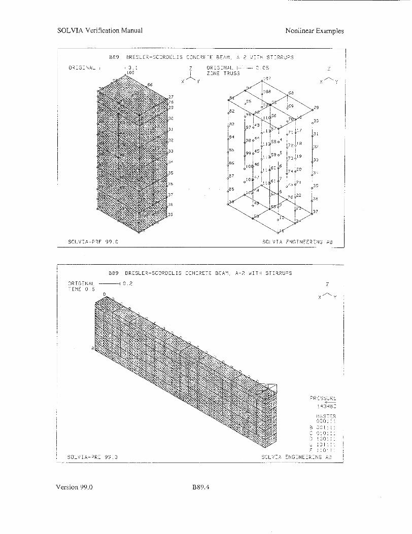
SOLVIA Verification Manual
889 BRESLER-SCORDELIS CONCRETE BEAM, A-2 WITH STIRRUPS
ORIGINAL P r -. 1 Z ORIGINAL C C0.S 1 05 X '.. y ZONE TRUSS y.7
SOLVTA-PRE 99.0 SOLVIA ENGINEERING AB
B89 BRESLER-SCORDELIS CONCRETE BEAM, A-2 WITH STIRRUPS
ORIGINAL --- 0.2 TIME 0.S
Z
x y
PRESSURE 43L80
MASTER
0111 [) 100 1 : E 101 :1 F 1 101 !
SOLVIA ENGINEERING ABSOLVIA-PRE 99.0
Z
I
Version 99.0
Nonlinear Examples
B89.4

SOLVIA Verification Manual Nonlinear Examples
B89 BRESLER-SC RDELIS CONCRETE BEAM, A-2 WIT. STIRRUPS
ORIGINAL • 0.2 ZONE TRUSS
X Y -Y
SOLVIA-PRE 99.0
300
SOLVIA ENGINEE-RING AS
B89 BRESLERISCORDELIS CONCRETE BEAM, A-2 WITH STIRRUPS
I L
•2
(I)
C
7
9K
S,~
•2.2
SII
>2
0 tO0 O 200 350 100 GO
SOLVIA-COST 99.0 \OLV/A ENGINEERING AB
Version 99.0 B89.5

SOLVIA Verification Manual Nonlinear Examples
B89 BRESLER-SCORDELS CONCRETE BEAM, A-2 UITH STIRRUPS
MAX DISPL. - 0.013218 TIME 21.2S ZONE SOLID
Z
X/ y
I CRACK NORMAL
SOLVIA ENGINEERTNG ABSOLVIA-POST 99.0
B89 BRESLER-SCORDELIS CONCRETE BEAM, A-2 1-TH STIRRUPS
MAX D7SPL.i 0.0132[8 TIME 21.25
Z
X 1,Y
REACTION
3. 3685E5
CONCRETE
7 CRUSHED
NORMAL CLCSED
i CRACK 2 CRACKS 3 CRACKS
SOLVIA-POST 99.0 SOLV A ENGINEER7NG AB
Version 99.0 B89.6
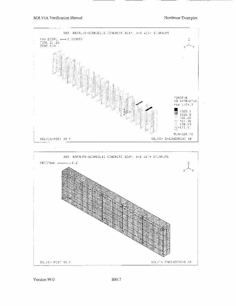
SOLVIA Verification Manual Nonlinear Examples
B89 BRESLER-SCORDELIS CONCRETE BEAK
MAX DISPL. - C 013209 TIME 2t.25 ZONE EG4
A-2 WITH STIRRUPS
Z
X y
FORCE-R NO AVERAGING MAX 1 474.7
!132S. 1
.... t 02S. 8 S726. 6C S427.36
1t28. 13
P->
144-00
MIN-320.72
SOLVIA ENGINEERING ABSOLVIA-POST 99.0
B89 BRESLER-SCORDELIS CONCRETE BEAM, A-2 W4ITH STIRRUPS
ORIGINAL 0.2
SOLVIA-POST 99.0 SOLV]A EN(
G
X Y
GINC>RINC AB
Version 99.0 B89.7
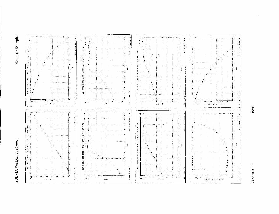
00
00
cyll f-0 V)
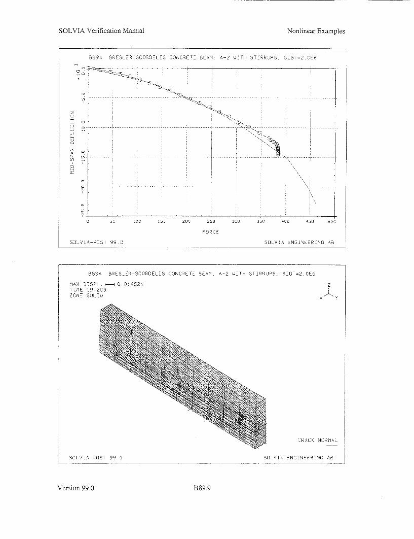
SOLVIA Verification Manual
B89A
Nonlinear Examples
BRESLER-SCORDELIS CONCRETE BEAM, A-2 WITH STIRRUPS, S-GT=2.0E6
22.. ... . . . . . . . .
SOLVIA-POST 99.C
I0o i,"0 200 250 300 350 400 450 500
FORCE
SOLVITA ENGINEERING AB
B89A BRESLER-SCORDELIS CONCRETE BEAM, A-2 WITH STIRRUPS, SIGT=2.OE6
MAX DTSPL.i 0.014S21 TIME 19.209 ZONE SOLID
SOLVIA-DOST 99.0
Version 99.0
L CRACK NORMA
CL',!TA ENGTNEE.RNG AE
B89.9
Z
X y
<¢-

SOLVIA Verification Manual Nonlinear Examples
B89A BRESLER-SCORDELIS CONCRETE 3EAM, A-2 A!TH STIRRUPS, SIGT=2.0E6
MAX DISPL. 0.014521 I7ME 19.209
RE
Z
xA O
ACTION
3.4345SE5
CONCRETE
CRUSHED
NORMAL CLOSED I CRACK 2 CRACKS 3 CRACKS
SOLVIA POST 99.0 SOLVIA ENGINEERING AB
B89A BRESLER-SCORDELIS CONCRETE BEAM, A-2 WITH STIRRUPS, SIGT:2.CE6
MAX DISPL. 0.014521 TIME 19.209 ZONE EG4
!29 j-
SOLVIA-POS 99. 0
FORCE-R NO AVERAG NG MAX 3816.9
[] 374.8
2790 6 "2106.3 14.. £ 22 .1
737.85 i"53.6!4
MIN-288.51
OLV-A ENGINEERING AB
Version 99.0
Z
X
B89.10

* 20'
It 333
/ -1R C' ":
'1
a -i CA C a
6
C'
A
11 :N :11 N,
Co
39
'N
wc CIO
1
'23
'3
3)
0
-<
-< a '�1
C) a 0 a
a a a a
3 3,
-3C -2$
I '� �''
3 0
-3 9
A
£33.3 33
LI
z 0 a a a a -i
at a S
�0 C CA

SOLVIA Verification Manual
SOLVIA-PRE input HEADING 'B89 BRESLER-SCORDELIS CONCRETE BEAM, A-2 WITH STIRRUPS'
DATABASE CREATE MASTER IDOF=000111 NSTEP=50 DT=0.5 AUTO-STEP DTMAX=1 DTMIN=IE-5 FDECREASE=0.2 ITELOW=5 ITEHIGH=15
TMAX=25 TOLERANCES TYPE=F RNORM=80.E3 RTOL=0.05 ITEMAX=30 STOL=0.3 SET MYNODES=200 PRINTOUT MIN
TIMEFUNCTION 1 0. 0. / 25. 500.
COORDINATES ENTRIES NODE Z 1 0.56 TO 3 0.51 TO 11 0.095 TO 13
NGENERATION TIME=2 NSTEP=13 XSTEP=-0.07625 1 TO 13
NGENERATION TIME=2 NSTEP=39 YSTEP=-0.11425 1 TO 39
MATERIAL 1 CONCRETE EQ 28700.E6 NU=0.2 SIGMAT=3.72E6, SIGMAC=-24.6E6 EPSC=-0.0021 SIGMAU=-21.6E6, EPSU=-0.0031 BETA=0.75 KAPPA=30. STIFAC=0.0001, SHEFAC=0.5
MATERIAL 2 PLASTIC E=218000.E6 YIELD=555.E6 ET=*0000.E6 MATERIAL 3 PLASTIC E=201400.E6 YIELD=345.E6 ET=10000.E6
MATERIAL 4 PLASTIC E=189700.E6 YIELD=325.E6 ET=10000.E6 MATERIAL 5 ELASTIC E=28700.E6 NU=0.2
SET NODES-27 EGROUP 1 SOLID MATERIAL=1 GVOLUME 79 1 27 105 81 3 29 107 EL1=1 EL2=1 EL3=1 GVOLUME 81 3 29 107 89 11 37 115 EL1=1 EL2=1 EL3=4 GVOLUME 89 11 37 115 91 13 39 117 EL1=1 EL2=1 EL3=1
SET NODES=3 EGROUP 2 TRUSS MATERIAL=2 GLINE 11 89 / GLINE 24 102 / GLINE 37 115 EDATA 1 274.2E-6 / 2 1096.4E-6 / 3 274.2E-6
EGROUP 3 TRUSS MATERIAL=3 ENODES GLINE 3 81 / GLINE 16 94 / GLINE 29 107 EDATA
1 21.E-6 / 2 84.E-6 / 3 21.E-6
EGROUP 4 TRUSS MATERIAL-4 GLINE 3 29 / GLINE 42 68 / GLINE 81 107 GLINE 37 11 / GLINE 76 50 / GLINE 115 89 GLINE 29 37 EL=4 / GLINE 68 76 EL=4 / GLINE 107 115 EL=4 GLINE 16 24 EL=4 / GLINE 55 63 EL=4 / GLINE 94 102 EL=4 GLINE 3 11 EL=4 / GLINE 42 50 EL=4 / GLINE 81 89 EL=4
Version 99.0
Nonlinear Examples
B 89.1I2

SOLVIA Verification Manual
SOLVIA-PRE input (cont.) EDATA 1 5.85E-6 / 2 23.39E-6 4 5.85E-6 / 5 23.39E-6 7 0,97E-6 TO 10 0.97E-6
15 0.97E-6 TO 18 0.97E-6 23 15.60E-6 TO 26 15.60E-6 31 0.97E-6 TO 34 0.97E-6 39 0.97E-6 TO 42 0.97E-6
/ / / / / /
3 5.85E-6 6 5.85E-6 11 3.90E-6 19 3.90E-6 27 3.90E-6 35 3.90E-6
MESH NNUMBERES=YES NSYMBOL=YES SUBFRAME=21 MESH TRUSS NNUMBERES=YES NSYMBOL=YES TRANSLATE ZONENAME=ELEMENTS Y=-0.2285 COPIES-9
EGROUP 5 GLINE 80 1i GLINE 79 1 GLINE 876 8" EDATA
1 23.39E-6 4 5.85E-6 7 5.85E-6
TRUSS MATERIAL=4 06 EL=i / GLINE 05 EL-I / GLINE 74 EL=i / GLINE 8
/ / /
2 5 8
93. 6E-6 23. 39E- 6 23. 39E- 6
/ / /
41 67 EL=1 / GLINE 40 66 EL=i / GLINE 89 887 EL=i / GLINE
2 28 EL-i 1 27 EL=I 902 900 EL=I
3 23 . 39E-6 6 5. 85E-6 9 5.85E-6
SET NODES=27 EGROUP 6 SOLID MATERIAL=5 GVOLUME 874 796 822 900 876 798 824 902 EL1=1 EL2=1 EL3=1
ZONE XSYM GLOBAL-LIMITS XMIN=-0.153 XMAX=-0.152 ZONE YSYM GLOBAL-LIMITS YMIN=-1.E-3 YMAX=1.E-3 FIXBOUNDARIES 1 INPUT=ZONE XSYM FIXBOUNDARIES 2 INPUT-ZONE YSYM FIXBOUNDARIES 3 INPUT=LINE / 876 902
EGROUP 1 LOADS ELEMENT
1 t 0. 14348. ENODES DELETE 60
14348. 0.
MESH VECTOR=LOAD BCODE=ALL MESH TRUSS NSYMBOL=MYNODES SOLVIA END
Version 99.0
TO TO TO TO
14 22 30 38
3.90E-6 3.90E-6 3.90E-6 3.90E-6
Nonlinear Examples
B 89.13

SOLVIA Verification Manual
SOLVIA-POST input * B89 BRESLER-SCORDELIS CONCRETE BEAM, A-2 WITH STIRRUPS
DATABASE CREATE
WRITE FILENAME='b89.1is'
USERCURVE 1 / READ B89.DAT AXIS 1 VMIN=0 VMAX=500 LABEL='FORCE' AXIS 2 VMIN=-23E-3 VMAX=0 LABEL='MID-SPAN DEFLECTION'
SET DIAGRAM=GRID NHISTORY NODE=29 DIRECTION=3 XVAR=1 XAXIS=1 YAXIS=2 SYMBOL=-,
OUTPUT=ALL PLOT USERCURVE 1 XAXIS=-1 YAXIS=-2 SUBFRAME=OLD *
MESH SOLID VECTOR=CRACKNORMAL MESH VECTOR=REACTION CONTOUR=CONCRETE *
ZONE REINF INPUT=EGROUP / 2 3 CONTOUR LEVEL=6 AVERAGING=NO MESH ZONENAME=EG4 CONTOUR=FR EGROUP 4 MESH EL114 ENUMB=YES NSYMBOL=YES GSCALE=OLD TEXT=NO SUBFRAME=OLD
EGROUP 2 EPLINE BOTTOM 28 2 1 STEP 3 TO 1 2 1 EGROUP 3 EPLINE TOP 28 2 1 STEP 3 TO 1 2 1 EGROUP 1 EPLINE SECT1
1 9 8 7 TO 6 9 8 7 EPLINE SECT2 13 9 8 7 TO 18 9 8 7 EPLINE SECT3 25 9 8 7 TO 30 9 8 7 EPLINE SECT4 37 9 8 7 TO 42 9 8 7
MESH PLINE=ALL ELINE BOTTOM KIND=SRR SYMBOL=i ELINE TOP KIND=SRR SYMBOL=i
AXIS 3 VMIN=-30E6 VMAX=5E6 LABEL='STRESS-YY'
ELINE SECT1 KIND=SYY SYMB=* YAXIS=3 ELINE SECT2 KIND=SYY SYMB=1 YAXIS=3
ELINE SECT3 KIND=SYY SYMB=1 YAXIS=3 ELINE SECT4 KIND=SYY SYMB=1 YAXIS=3
*
EGROUP 4 EHISTORY EL=114 POINT=2 KIND=SRR XVAR=1 XAXIS=1 SYMBOL=d EGROUP 3 EHISTORY EL=3 POINT=i KIND=SRR XVAR=- XAXIS=1 SYMBOL=I
EMAX EMAX EG4 NUMBER=5 END
Version 99.0
Nonlinear Examples
B89.14

SOLVIA Verification Manual
EXAMPLE B90
COMPOUND CYLINDER
Objective
To verify the PLANE AXISYMMETRIC element with a thermo-orthotropic and a thermo-elastic material under pressure and temperature loading.
Physical Problem
A long compound cylinder with free and open ends are subjected to an internal pressure and a uniform temperature. Away from the ends the plane cross-section of the cylinder remain plane under the deformation, i.e., uniform axial strain. The inner material is isotropic and the outer material is orthotropic.
Material orientation
C a
r3 t C
Load case 1: Internal pressure p, = 200 N/mm 2
Load case 2: Internal pressure p, = 200 N/mm 2 and temperature rise of 130 0 C
Geometry
r, = 23 mm
r, = 25 mm
r = 27 mm
Inner material, isotropic
E =2.1.10' N/mm 2
v=0.3 a•=2.10-' 1/°C
Outer material, orthotropic
Ea =Eb =5. 103 N/mm 2
E, = 1.3_105 N/mm 2
Vac = 'Vbc = Vab - 0.25
f2a =ab =2.10-5 1/°C
ac, =3.10-6 1 /C
Gab = 0.5.104 N/mm2
Gac = Gbc = 1. 104 N/mm2
Finite Element Model
The top figure on page B90.4 shows the finite element model. It consists of ten PLANE AXISYMMETRIC elements. Constraint equations are used to obtain a uniform axial strain in the elements.
Solution Results
The hoop, radial and axial directions are denoted as 1, 2 and 3, respectively, in the index notation below for Young's modulus, Poisson's ratio and the thermal expansion coefficient. The material relation is then
Version 99.0
Nonlinear Examples
B90.1
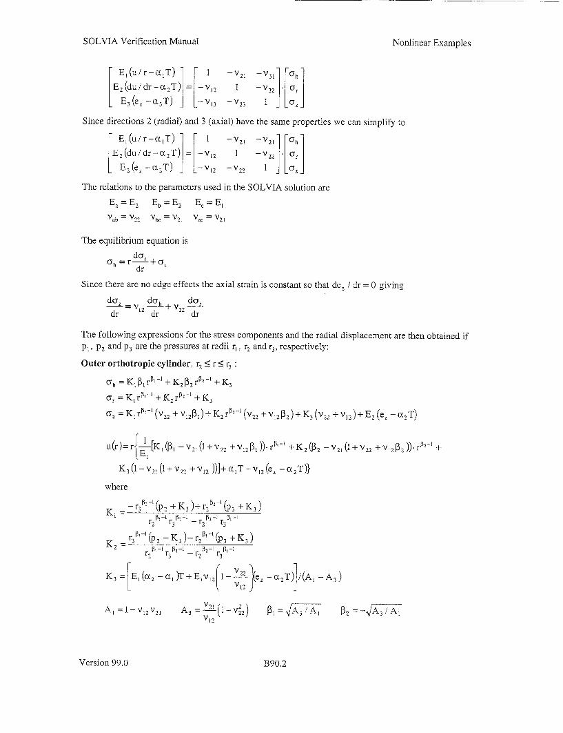
SOLVIA Verification Manual
E-I -vu W -(X, 31 lFhl E2 (du /dr-c 2 T) = 12 1 -V 32 " r E3 (eý - 3T) - 13 - V23 I G'j
Since directions 2 (radial) and 3 (axial) have the same properties we can simplify to [ , E(u/ r - aT) = 1 -V2 [ -V21 .l(Yhl E2 (du / dr- ct 2T) H -V12 1 -V22
LE2 (ý- ,T) L-V 1 2 -V 2 2 I
The relations to the parameters used in the SOLVIA solution are
Ea = E 2 Eb= = E 2 Ec = El
Vab =22 "Vbc = V'2 1 Vac = V 2 1
The equilibrium equation is
Chy = r + Ur dr
Since there are no edge effects the axial strain is constant so that de, / dr = 0 giving
d&F = dub dor
dr dr + dr
The following expressions for the stress components and the radial displacement are then obtained if
PI, P2 and p3 are the pressures at radii r1, r2 and r3, respectively:
Outer orthotropic cylinder, r2 _ r <r 3
uh = K, 3PrP-1l + K 2 32 r P2 +K 3
S= K, r 3'- + K 2 r -1 +K3
a = K, rI'-I (v 22 + vI2 1 ) + K2 r0- 1 (V22 + v1 2 P32 ) + K3 (v22 + v12 )+ E2 (e - (X2T)
u(r)= r{ I[Ki(P -v 21 (1 +v 22 +v 12 P3))-r"-' +K 2(0 2 -V2 2,(1 +v 22 +Vs2 3)).rPz' +
K3 (l-V2, (1+,,22 +V12 ))]+ <T--V,2 (e7 - a2T)I
where
K r -3 ' (P2 + K3 )+ r,-2 (-3 +K 3 ) r2.,0-1 r3 r2 r3P
r31 -' (P2 + K3 )- r. 1 '1 (p3 +K 3 ) K3 1 1,- 3-I 1 - r2 13 - r3 3 -I _r 2 3-1 r3 13
K3 = El(a 2 -a )T + EIv12 I _ - }e, - aT /(A, - A 3 )
A, = -V1 2 V21 A 3 = V[2(1- V 2 ) 031=A 3 /A, /[ 2 -VA; Al
Version 99.0
Nonlinear Examples
B90.2

SOLVIA Verification Manual
Inner isotropic cylinder, r, < r _ r, :
h = rl~, p , -r"P 2 r (2 -p_ )/rI)/(r22 r.)
Gr2(r pl-r~p2 +r~r2(p 2 2p)/(r r- 2)
ur) = 2~r~ 1 { P r '-p2 (r - 2) +E(e p2 - c PT )
[r', -.' ,2r2 -r1 )(l+V' Il+ctT-v(ecxTd u(r) =r irPr 2P( v~)rr2 _2 Pi
The total axial load must be zero: 2j radr+ frazdr =0 Sr, r )
A further equation is obtained since the radial displacement at the interface radius r = r, must be the same for the outer and inner cylinders. Hence, we have two equations which can be solved for the unknowns P2 , the pressure at the interface, and e, the axial strain.
The analytical solution for the stresses at the three radii is given in the table below together with the solution obtained by SOLVIA using the input data on pages B90.7 and B90.8:
Stresses in (N/mm 2) Inner cylinder Outer cylinder r` 1r2 r2 r3
Load case 1 ah Theory 1565 1430 875 759
SOLVIA 1565 1430 875 759
c7 Theory -200 -64 -64 0 SOLVIA -200 -64 -64 0
•7 Theory 10 10 -17 -2 SOLVIA 10 10 -17 -2
Load case 2 Gh Theory 1381 1260 1056 935
SOLVIA 1381 1260 1056 935
Gr Theory -200 -78.5 -78.5 0 SOLVIA -200 -78.5 -78.5 0
oy Theory 9 9 -18 1 SOLVIA 9 9 -18 1
As can be seen in the table the SOLVIA results are in excellent agreement with the analytical results. The SOLVIA results have been obtained from the contour stress figures on pages B90.4 and B90.5.
The variation of the stress components in the radial direction is shown on page B90.6.
Version 99.0
Nonlinear Examples
B90.3
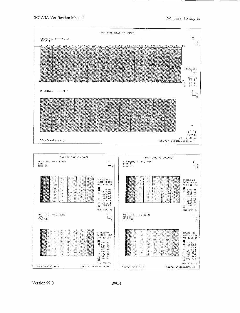
SOLVIA Verification Manual Nonlinear Examples
390 COMPOUND CYLINDER
OR7GINAL - 0.2 TIME 2
ORIGINAL H-- 02
EAXESORTHOTROPIC
SOLVIA ENGINEERING ABSOLVIA-DRE 99.0
890 COMPOUND CYLONDER
MAX 0ISPL. - 0 .17769 TIME I ZONE -G!
MAX DISPL TIME 1 ZONE EG2
S0.17216
I ____
SOLVIA-POST 99.0
7 L Y
R
STRESS-XX BASED ON ZONE MAX 1565,34
1555.86 L 539. 92
1522 97 55 6. 02
1489 07 1472.1 1t45. 18 1438.23
M1N 1429.76
Z LY
R
STRESS-XX 3ASED ON ZONE "MAX 874.64
S867.40 &52.92 838. 45
S823.97 8509.49 795.02 780,58
766.06
MIN 758.3-
SOLVIA ENGINEERING AB
MAX D:SPL, 0 T75E 2 ZONE E51
890 COMPOUND CYLINDER
2!749
MAX DISPL. s- 0.21749 TOME 2 ZONE E32
SOLVIA-POST 990 SOLVWA ENGINEERING A8
Version 99.0
2 Ly
78E
PRESSURE
200
MASTER
2S
8 01"[
L
L Y R
Z
LY R
STRESS-XX BASED ON ZONE MAX :381. 40
.!373.81 1 1358,62 . 343.44 S328. 2 1313,08 .1297 90 1282 72
5267 53
MIN 1259.94
Z LY
R
STRESS-XX 3ASED ON ZONE MAX -'. 06ý02
!1018 24 1:003. t2 S988.009
:;972.856 957 783
MT N 935.11'3
B90.4
I

SOLVIA Verification Manual Nonlinear Examples
590 COMPOUND CYL:NDER
MAX DISPL. - 0.17769 TIME t ZONE E'5l
MAX DISPL -- 0 .172i6 TIME , ZONE ES2
SOLVIA-POST 99.0
S, STRESS-YY BASED ON ZONE
MAX- 64 .222
-72. 793 .- 89 736 -106.68
-1744 5 -191 .39
Z
R
S3TRESS-YY BASED 3N ZONE MAX 0.032095
•-3. 9924
- 20
-160 120111
-20 090 -28 139 -36 188 -44 237 -52 286
-60 335
MIN-64.359
8OLVIA ENGINEERING A9
MAX DISPL. - 0.21749 T-ME 2 ZONE EG2
SOLVIA-POST 99.0
STRESS-YY BASED ON ZONE MAX-78. 459
1-56.0 48
101 23 -116.40 -131 .58
6 -1476 161 .93
-177. ,1. ,-192.29
MIN-199.88
Z Ly
R
37RESS-YY BASED IN ZONE
MAX 04036023
: -4.68S
-34.3*3
-44 127 -53.941 -63. 755
,,-73.569
M11N-78. 76
SOLVIA ENGINEERING A0
B90 COMPOUND CYLINDER
MAX OISPL. 0---.21749 TIME 2 ZONE EG1
MAX DOSPL. 0 21749 ZIME 2 ZONE EG2
SOLV/!A-OST 99.0
Z L Y R
STRESS-ZZ BASED ON ZONE MAX 8 75740
8 75299 0 '4117 8 73535 8 72653 8 7177 8 70808 8.70006 8.6912'
0N0 8. 68683
Z
R
SRESS-ZZ BASED ON 2ONE 'lAX 0.76957
S90,38453 -2.627 -5000 9
"-9.6173 - 925
-16.542
MIN-t7.696
SOLVIA ENGINEERING AS
Version 99.0 B90.5

7i 0 ý7_
cz
7m

SOLVIA Verification Manual
SOLVIA-PRE input
DATABASE CREATE HEAD 'B90 COMPOUND CYLINDER'
MASTER IDOF=-00111 COORDINATES
ENTRIES NODE Y Z 1 23. 0. TO 13 25. 0. TO 25 27. 0.
51 23. 1. TO 63 25. 1. TO 75 27. 1.
MATERIAL 1 THERMO-ELASTIC -1000 2.1E5 0.3 2E-5
1000 2.1E5 0.3 2E-5
MATERIAL 2 THERMO-ORTHOTROPIC, EA=5E3 EB=5E3 EC=1.3E5, NUAC=0.25 NUBC=0.25 NUABE0.25 , GAB=0.5E4 GAC=d.0E4 GBC=1.0E4, ALPHAA=2E-5 ALPHAB=2E-5 ALPHAC=3E-6
EGROUP 1 PLANE AXISYMMETRIC MATERIAL=d GSURFACE 1 13 63 51 ELI=6 NODES-9
EGROUP 2 PLANE AXISYMMETRIC MATERIAL=2 GSURFACE 13 25 75 63 EL1=6 NODES=9
FIXBOUNDARIES 3 INPUT=LINE / 1 25 CONSTRAINT
52 3 51 3 TO 75 3 51 3
EGROUP 1 LCASE 1 LOADS ELEMENT INPUT=LINE
1 51 200. LOADS TEMPERATURE 1 0. TO 125 0.
*
LCASE 2 LOADS ELEMENT INPUT=LINE
1 51 200. LOADS TEMPERATURE
1 130. TO 125 130.
SET HEIGHT=0.25 MESH NSYMBOL=MYNODES NNUMBER=MYNODES BCODE=ALL
ENUMBERS=GROUP VECTOR=LOAD SUBF=12 MESH EAXES=ORTHOTROPIC SOLVIA END
Version 99.0
Nonlinear Examples
B90.7

SOLVIA Verification Manual Nonlinear Examples
SOLVIA-POST input
* B90 COMPOUND CYLINDER
DATABASE CREATE
WRITE 'b90.1is'
CONTOUR AVERAGING=ZONE SET PLOTORIENTATION=PORTRAIT MESH EGi TIME=1 SUBFRAME=12 MESH EG2 TIME=I MESH EGi TIME=2 SUBFRAME=12 MESH EG2 TIME=2 SET CONTOUR=SYY MESH EG1 TIME=i SUBFRAME=I2 MESH EG2 TIME=i MESH EGi TIME=2 SUBFRAME=i2 MESH EG2 TIME=2 SET CONTOUR=SZZ MESH EGL TIME=i SUBFRAME=12 MESH EG2 TIME=i MESH EGi TIME=2 SUBFRAME=i2 MESH EG2 TIME=2
CONTOUR=SXX
SET PLOTORIENTATION=LANDSCAPE EGROUP 1 EPLINE THICK 1 9 6 3 TO 6 9 6 3 EGROUP 2 EPLINE THICK 1 9 6 3 TO 6 9 6 3 *e
ELINE ELINE ELINE *E
ELINE ELINE ELINE
END
THICK THICK THICK
THICK THICK THICK
KIND=SXX KIND=SYY KIND=SZZ
KIND=SXX KIND=SYY KIND=SZZ
TIME-i TIME=I TIME=1
TIME=2 TIME-2 TIME=2
SYMBOL=i SYMBOL=i SYMBOL=i
SYMBOL=i SYMBOL=i SYMBOL=I
OUTPUT=ALL
OUTPUT=ALL
Version 99.0 B90.8

SOLVIA Verification Manual
EXAMPLE B91
CONCRETE SLAB UNDER UNIAXIAL MOMENT, JAIN AND KENNEDY
Objective
To verify the SHELL element under uniaxial moment loading when used with the CONCRETE material model and with rebar layers.
Physical Problem
A concrete slab simply supported along two lines, see figure. The slab is singly reinforced with two layers of steel. Four cases are to be analyzed having the first layer of steel located with the [3-angles 0, 15, 30 and 45 degrees, respectively. The second layer of steel is orthogonal to the first layer and placed directly on top of the first layer. The uniaxial moment is generated by two line loads, each located at a distance of 0.150 m to the nearest support line. Experimental results for this problem have been reported by Jain and Kennedy [I].
0.860,m
rebar layer 2 rebar
'ayerI
P12 P/2
0.150l 0.460 0.150r
"'r' 0.760, .,
0.460 , Pt- -- -- -
0050,,
Concrete data: E0 = 29.10 9 N/m 2
= -34 MPa = -0.002
v=0 T =0.038 m
(7= 1-5 MPa (Y, =-32 MPa F- -0.003 K= 10
Steel data: E = 200.10 9 N/i 2
Gy = 220 MPa Layer 1: Diameter = 0.0048 m
cc1 = 0.065m t= 0.0119 in (0.625 of half thickness)
Layer 2: Diameter = 0.0048 m cc 2 = 0.055 m t2 = 0.0071 m (0.376 of half thickness)
Finite Element Model
The finite element model is shown on page B91.3. The entire slab has been modeled since the cases with inclined reinforcement have no symmetry planes. A separate element group is used for the constant moment part of the slab. The force is applied as element line load along two of the boundaries of this element group. The concrete material model has been assumed to have a tensile strength of 1.5 MPa and a tension stiffening coefficient of K = 10.
Version 99.0
/2T
,0 050 ,
1391.1
Nonlinear Examples
I
o ash m[" 't

SOLVIA Verification Manual
Solution Results
The input data for the first run B91A, where the orientation of the reinforcement is aligned with the
sides of the slab (13 = 0), is shown on pages B91.9 - B91.10. The input data for the following three
runs B91B, B91C and B9lD are the same except that the value for 13 is set to 15, 30 and 45 degrees,
respectively, in the EDATA command of the two element groups.
The calculated curve for the moment load as a function of the center deflection of the slab is shown
for each of the four cases on pages B91.4 - B91.8 and can be compared with the corresponding
experimental curve from [1 ] drawn as a solid line without symbols. The ultimate moment loads
obtained in the experiment are practically the same for the four cases and the calculated values agree
well with the experimental values. It can be noted that the calculated cases 3 = 15 and 13 = 30 show an
almost constant moment load level already when the first steel layer yields. The ultimate moment
load level, when also the second steel layer yields, occur for a significant additional deflection of the
slab. Such two moment load levels are not so apparent in the corresponding experimental curves.
Calculated principal moments, crack normal directions at the lower slab face, deformations and
reactions, rebar stress histories for element 2, rebar plastic strains, concrete stress-strain history at the
lower slab face of element 2 and the concrete bending stress distribution in the thickness direction at
element 2 are shown for each of the four cases on pages B91.4 - B91.8. The integration point in
element 2 closest to the center of the slab has been selected.
Only rebar layer 1 is stressed in the case 13 = 0 which gives a symmetric response of the slab. Both
rebar layers are stressed about the same amount in the case 13 = 45. A slight asymmetry in the
response must occur since the rebar layers cannot act isotropically at all load levels due to the varying
distance to the uncracked portion of the concrete. In the cases 13 = 15 and 3 = 30 the rebar layer 1 is
stressed much before rebar layer 2 so the response is clearly asymmetric with reaction forces that
cause some torsion moment loading of the slab. The asymmetry of the response is however gradually
decreasing with the plastic elongation of rebar layer 1.
With the selected material data for the concrete the calculated moment-deflection curve agrees well
with the experimental results also during the loading portion up to the ultimate moment for the cases
with 0 and 15 degrees orientation of the reinforcement. The cases with 30 and 45 degrees rebar
directions show, however, larger deflections for the calculated response compared to the experimentally obtained deflections.
Kinks in the calculated response curves occur when the concrete starts to crack at an integration point.
In the cases with 30 and 45 degrees rebar directions cracking at the third integration point in the
thickness direction results in a rather sudden increase in deflection. A larger number of integration
points in the thickness direction should give a more continuous advancement of the cracking. In the
analysis 6 integration points were used in the thickness direction of the slab. When the ultimate
moment load is approached only the upper integration point layer of the slab shows significant
compressive stresses in the bending direction while the lower integration point layers have practically
no stresses in the bending direction.
User Hints
• The value of the concrete tensile strength and the amount of tension stiffening affect the calculated
moment-deflection curves significantly. The values assumed in the analyses have been selected
based on the response for the case 3 = 0, which is reasonably close to the experimental curve.
"* It is important to have more integration points in the thickness direction of the slab than the default
number. Six Gauss integration points were used in this example.
Nonlinear Examples
B91.2Version 99.0

SOLVIA Verification Manual Nonlinear Examples
Note that a specified line load is applied to all element edges of the current element group which
belong to the line. If the line is internal of the element group the line load would then be applied at
least twice, since each portion of an internal line is part of at least two element edges by definition.
In this example two element groups are used so that the line load can be applied along the
boundary of one of the element groups.
Reference
[1] Jain, S., and Kennedy, J., Yield Criterion for Reinforced Concrete Slabs, Journal of the
Structural Division, Proceedings of the American Society of Civil Engineers, Vol. 100,
No ST3, March, 1974.
B91A CONCRETE SLAB JNDER JNIAXIAL MOMENT.
ORIGINAL - 0. TIME So
JAIN AND KENNEDY, BETA=O
391A CONCRETE SLAB JNDER UNIAXIAL MOMENT. JAIN AND KENNEDY. BETA=O
ORi:SNAL -- 0. TIME 50
EFOSRC 333,333
MASTSR oO O0I
A 00100, C tOOO0t D ICIOOA
SCtLVA -NG:NEERING ABSOLVTA-PRE 99.0
Version 99.0
yz
1391.3

EuI.)
o
0
a•
SI
K A
Eu,
a: 2 2
I I'
I
0 ON,
ON
Vi
- ' -- -- -
~~~~~~~~ .. . . . . . .. . . . . .I

cv
6
V ¼ ¼ ¼ ¼ ¼ ¼ ¼ ¼ ¼ ¼ ¼
¼ ¼�3¼��¼¼3¼ ¼ ¼ ¼¼¼¼¼¼ - ¼ ¼'
¼*4L �I�U�!
¼ ¼ -� ¼ ¼
¼ ¼ ¼ ¼ ¼ ¼ ¼
0
cv �1
0
0
LU
0
cv -t
eli
S
CI�
¼ZO*.�.
N
N
C, I r : ý I ý. - I.; " , ý 11 -

Li
/
A A A A
0)
0
6::
V
�A'� �AU�A�
to
A 2 T
C/)
0
0t

I
/ .4/
.04
(4
4 4
I,.
U
(4
(S
.4
t.14
..4�
N
0 ON ON 0 0
3-"
- - ----- - N -----

:3-:3% -51e:3
49r-14
0
z
CZ
0
0
V)
5S 4 6 ~ Z i' 91 31
3 '5 N :3� * :3
:3
4¼
:3
'5 I-1 �l
:3
AT
s
00
-0 U0
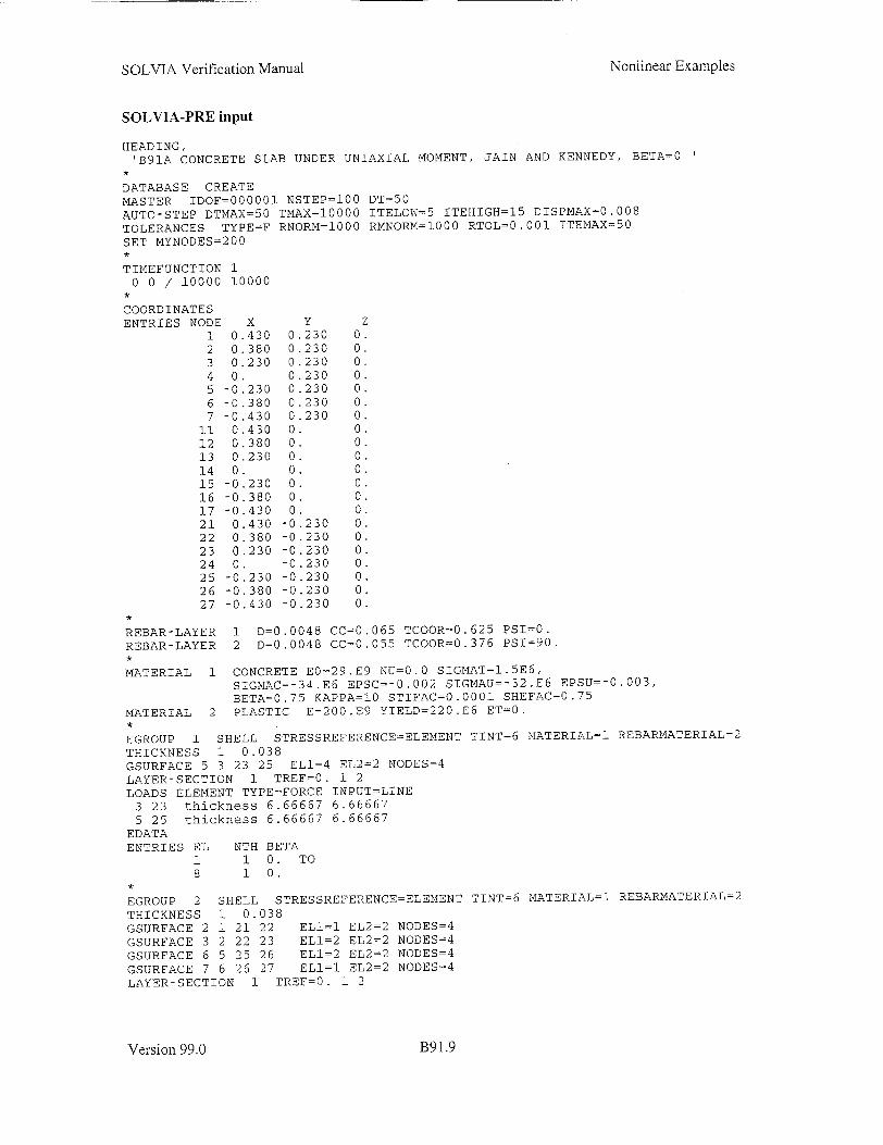
SOLVIA Verification Manual Nonlinear Examples
SOLVIA-PRE input
HEADING, 'B91A CONCRETE SLAB UNDER UNIAXIAL MOMENT, JAIN AND KENNEDY, BETA=0
*
DATABASE CREATE MASTER IDOF=000001 NSTEP=100 DT=50 AUTO-STEP DTMAX=50 TMAX=10000 ITELOW=5 ITEHIGH=15 DISPMAX=0.008 TOLERANCES TYPE=F RNORM=1000 RMNORM=1000 RTOL=0.001 ITEMAX=50 SET MYNODES=200
TIMEFUNCTION 1 0 0 / 10000 10000
COORDINATES ENTRIES NODE X Y Z
1 0.430 0.230 0. 2 0.380 0.230 0. 3 0.230 0.230 0. 4 0. 0.230 0. 5 -0.230 0.230 0. 6 -0.380 0.230 0. 7 -0.430 0.230 0.
11 0.430 0. 0. 12 0.380 0. 0. 13 0.230 0. 0. 14 0. 0. 0. 15 -0.230 0. 0. 16 -0.380 0. 0. 17 -0.430 0. 0. 21 0.430 -0.230 0. 22 0.380 -0.230 0. 23 0.230 -0.230 0. 24 0. -0 .230 0. 25 -0.230 -0.230 0. 26 -0.380 -0.230 0. 27 -0.430 -0.230 0.
REBAR-LAYER 1 D=0.0048 CC=0.065 TCO0R=0.625 PSI=0. REBAR-LAYER 2 D=0.0048 CC=0.055 TCOOR=0.376 PSI=90.
MATERIAL 1 CONCRETE EO=29.E9 NU=0.0 SIGMAT=1.5E6, SIGMAC=-34.E6 EPSC=-0.002 SIGMAU=-32.E6 EPSU=-0.003, BETA=0.75 KAPPA=10 STIFAC=0.0001 SHEFAC=0.75
MATERIAL 2 PLASTIC E=200.E9 YIELD=220.E6 ET=0.
EGROUP 1 SHELL STRESSREFERENCE=ELENENT TINT=6 MATERIAL=1 REBARMATERIAL=2 THICKNESS 1 0.038 GSURFACE 5 3 23 25 ELi=4 EL2=2 NODES=4 LAYER-SECTION 1 TREF=0. 1 2 LOADS ELEMENT TYPE=FORCE INPUT=LINE
3 23 thickness 6.66667 6.66667 5 25 thickness 6.66667 6.66667
EDATA ENTRIES EL NTH BETA
1 1 0. TO 8 1 0.
EGROUP 2 SHELL STRESSREFERENCE=ELEMENT TINT=6 MATERIAL=i REBARMATERIAL=2 THICKNESS 1 0.038 GSURFACE 2 1 21 22 EL1=1 EL2=2 NODES=4 GSURFACE 3 2 22 23 EL1=2 EL2=2 NODES=4 GSURFACE 6 5 25 26 EL1=2 EL2=2 NODES=4 GSURFACE 7 6 26 27 ELi=1 EL2=2 NODES=4 LAYER-SECTION 1 TREF=0. 1 2
Version 99.0 B91.9

SOLVIA Verification Manual Nonlinear Examples
SOLVIA-PRE input (cont.)
EDATA ENTRIES EL NTH BETA
1 1 0. TO 12 1 0.
FIXBOUNDARIES 3 INPUT=LINES / 2 22 / 6 26 FIXBOUNDARIES 12 / 14 FIXBOUNDARIES 1 / 4
SET NNUMBERS=MYNODES NSYMBOL=MYNODES BCODE=ALL VECTOR=LOAD MESH EAXES=RST MESH ENUMBERS=GROUP VIEW=-I *
SOLVIA END
SOLVIA-POST input
* B91A Concrete slab under uniaxial moment, Jain and Kennedy , beta=0 deg
DATABASE CREATE
TOLERANCES WRITE 'b9la.lis'
SYSTEM 1 CARTESIAN PHI=180
AXIS I VMIN=0. VMAX=0.009 LABEL='Center deflection (m)'
AXIS 2 VMIN=0. VMAX=2200 LABEL='Moment load (Nm/m)'
SET DIAG=GRID
NXYPLOT XNODE=14 XDIR=3 YKIND=TIME YDIR=l OUTPUT=ALL XAXIS=1 YAXIS=2,
SYSTEM=1 SYMBOL=* read test result
USERCURVE 1 / READ 'B91A.DAT'
PLOT USERCURVE 1 XAXIS=1 YAXIS=2 SUBFRAME=OLD
CONTOUR AVERAGING=NO
MESH CONTOUR=MPMAX VECTOR=MPRINCIPAL
SHELLSURFACE TOP
MESH CONTOUR=CONCRETE VECTOR=CRACKNORMALS
MESH WHOLE CONTOUR=D3 SYSTEM=l VECTOR=REACTIONS VIEW=-I
EGROUP 1
EHIST E=2 P=i KIND=SAA REBAR=1
EHIST E=2 P=1 KIND=SAA REBAR=2
SHELLSURFACE REBAR=1
MESH CONTOUR=EPACC EAXES=REBAR VIEW=I
SHELLSURFACE REBAR=2 MESH CONTOUR=EPACC EAXES=REBAR
EXYPLOT E=2 P=6 XKIND=ERR YKIND=SRR
EPLINE THICK / 2 6 5 4 3 2 1
ELINE THICK KIND=SRR SYMBOL=l
ELIST E2
END
Version 99.0 B91.10

SOLVIA Verification Manual
EXAMPLE B92
TILTING-PAD JOURNAL BEARING, RIGID PADS
Objective
To demonstrate the use of FILM elements in a tilting-pad journal bearing with the assumption that the
pad and shaft surfaces are rigid and do not conduct any heat.
Physical Problem
The geometry of the pivoted-pad journal bearing is shown in the figures below. Three pivoted pads
are used. Each pad is free to rotate about the pivot point. This bearing is analyzed with elastic pads
including thermal deformations in Example B93. Elasticity and heat conduction in both the shaft and
the pads are treated in Example B96.
AZ t
Geometry:
Radii rshat = 140- 10-3 m
"rpad = 140.210-10-3 m
Angles 0A =35' OB = 7.5'
Distance pad surfacepivot point d =100.10- 3 m
Bearing axial width w=210-10- 3 m
Bearing characteristics:
Machined-in clearance c = rpad - rsbaft = 210.10-- m
Pivot circle clearance c'= 126.10.4 m
Preload factor c - c'
m:= -=:0.4 c
Rotational speed (o = 314.16 rad / s
Vertical load F= 100-103 N
Oil properties:
Density p = 880 kg/m 3
Conductivity k=0.145W/m°C atl 0 °C k =0.133 W/m°C at 150 'C
Specific heat
c, =1.71.106 j/m 3 °C
The absolute viscosity of the oil as function of temperature is shown in top figures on page B92.2
Reservoir oil temperature T, = 45 °C
Version 99.0 B92.l
Version 99.0
I I
Nonlinear Examples
B92.1
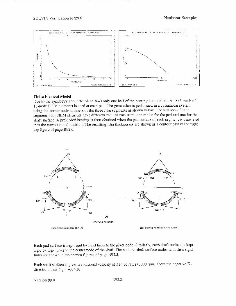
SOLVIA Verification Manual
io
o o * 6 60 6o 6 1 6iz •0/ .6
262[A SNGACEeR6G 2
I B2 I Dl O 17 AS CJ6001- or S -C , .: IC S
SO6 IA N[NGICEEDI61 AB
Finite Element Model Due to the symmetry about the plane X=0 only one half of the bearing is modelled. An 8x3 mesh of
18-node FILM elements is used at each pad. The generation is performed in a cylindrical system using the comer node numbers of the three film segments as shown below. The surfaces of each segment with FILM elements have different radii of curvature, one radius for the pad and one for the
shaft surface. A preloaded bearing is then obtained when the pad surface of each segment is translated into the correct radial position. The resulting film thicknesses are shown as a contour plot in the right top figure of page B92.6.
film 3 3film 1
99
reservoir oil node
user defined nodes at X =0 user defined nodes atX=-0.105 m
Each pad surface is kept rigid by rigid links to the pivot node. Similarly, each shaft surface is kept
rigid by rigid links to the center node of the shaft. The pad and shaft surface nodes with their rigid links are shown in the bottom figures of page B92.5.
Each shaft surface is given a rotational velocity of 314.16 rad/s (3000 rpm) about the negative Xdirection, thus co, =-314.16.
Version 99.0
SOL'IIA-PDST 99 0
Nonlinear Examples
•01VIA-pOST 99.0 SO'IIIA-POST 91 0
B92.2
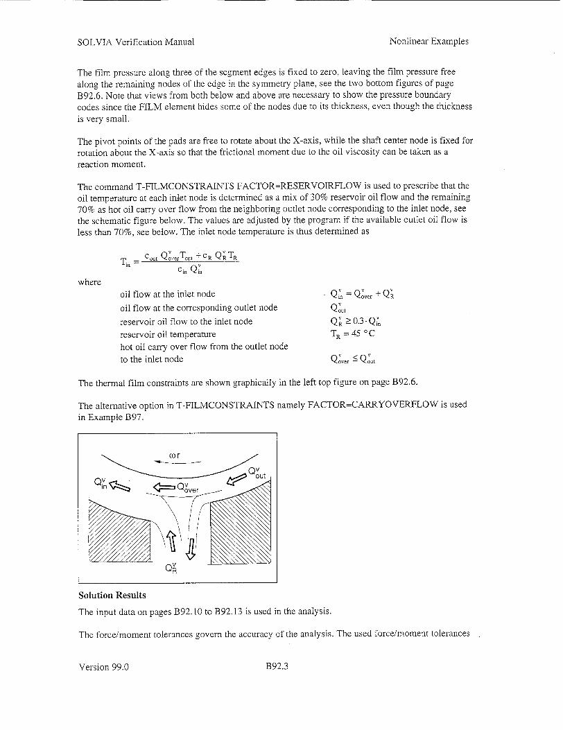
SOLVIA Verification Manual
The film pressure along three of the segment edges is fixed to zero, leaving the film pressure free
along the remaining nodes of the edge in the symmetry plane, see the two bottom figures of page
B92.6. Note that views from both below and above are necessary to show the pressure boundary codes since the FILM element hides some of the nodes due to its thickness, even though the thickness is very small.
The pivot points of the pads are free to rotate about the X-axis, while the shaft center node is fixed for rotation about the X-axis so that the frictional moment due to the oil viscosity can be taken as a reaction moment.
The command T-FILMCONSTRAINTS FACTOR=RESERVOIRFLOW is used to prescribe that the oil temperature at each inlet node is determined as a mix of 30% reservoir oil flow and the remaining 70% as hot oil carry over flow from the neighboring outlet node corresponding to the inlet node, see the schematic figure below. The values are adjusted by the program if the available outlet oil flow is
less than 70%, see below. The inlet node temperature is thus determined as
cout QoverToul +cR QvTR Cin Qin
whereoil flow at the inlet node
oil flow at the corresponding outlet node
reservoir oil flow to the inlet node
reservoir oil temperature
hot oil carry over flow from the outlet node to the inlet node
= QOVr +Q V
Q) >0.3-Qi
TR = 45 °C
Qover -< QOut
The thermal film constraints are shown graphically in the left top figure on page B92.6.
The alternative option in T-FILMCONSTRAINTS namely FACTOR=CARRYOVERFLOW is used in Example B97.
Solution Results
The input data on pages B92.10 to B92.13 is used in the analysis.
The force/moment tolerances govem the accuracy of the analysis. The used force/moment tolerances
Version 99.0
Nonlinear Examples
B92.3

SOLVIA Verification Manual
govern also the accuracy of the pressure and temperature solutions since a small change in pressure or
in temperature causes a large change in the film surface loads compared to the force/moment
tolerance values. The prescribed pressure and temperature tolerances are therefore rather loose which
also has a positive effect on the initial convergence rate.
The artificial springs of the two lower film segments have the default value of 1.0- 10N1/ m3 for the
spring stiffness. This means that a pressure of 10 MPa causes a spring deformation of 100 gtm during
the iterations, which stabilizes the iteration path to convergence. However, the oil pressure for the top
film segment will be small in the converged configuration due to the increase in film thickness when
the shaft is moving downwards under the action of the vertical load. The top film segment needs,
therefore, a lower value for the artificial spring stiffness when the film pressure becomes small. This
is achieved by specifying the spring stiffness variation with pressure, parameter DKDP in command
FILMVELOCITY, to be 1.0 104 N / (m3Pa). The artificial spring stiffness varies then with the
pressure and is for example 1.0.1011 N / m 3 when the pressure is 10 MPa and 1.0 1010N / m3 when the
pressure is 1 MPa. A too large artificial spring stiffness will cause slow convergence, since the out-of
balance forces can only achieve very small displacement corrections during the iterations.
The used values of tolerances and artificial spring stiffnesses give good convergence characteristics and the solution can be obtained in one step.
The displacement vector plot on page B92.7 shows the essentially vertical displacement of the shaft
and the rotations of the pads. The distributions of film temperature, film flow, film power loss, film
thickness and Reynolds number are shown as contour plots on pages B92.7 and B92.8. Diagram
results of film temperature, film pressure and film thickness are shown on pages B92.8 and B92.9. In
these diagrams the element result lines are defined using result points nearest the symmetry plane and
nearest the side edge. The edge results have symbols in the diagrams.
The numerical results are summarized in the tables below. Note that the results apply to half the bearing.
Film element results, Pad I Pad 2 Pad 3 Total half bearing model:
Summation of pressure load in -25.9- 10' 1.9-10, -25.9- 10' -50.1- 103
vertical Z-direction, N
Inlet oil flow m 3 /s 2.1.-10- 4.6 10-4 2.3"10-4 9.0.10-4
Power loss W 4.6.10' 2.4- 103 5.1"103 12.1- 103
Film thickness, max m 132- 10-6 209. 10 140 10'
Film thickness, min m 60-10-6 180.10- 67-10
Film pressure, max NI/m 2 4.8. 106 0.2. 106 4.8.106
Inlet film temperature') 0 C 64.0 57.3 55.9
Outlet film temperature') 0°C 79.7 60.3 71.7
1) At the element result point nearest the symmetry plane.
Version 99.0
Nonlinear Examples
B92.4

SOLVIA Verification Manual Nonlinear Examples
User Hints
0 Note that the summation of the film pressure in a film element is performed over the top surface (t=+ 1) of the element with the positive pressure forces acting in the positive t-axis direction.
The thickness of the film element at an integration point is calculated as the projection onto the taxis of the line between the interpolated top and bottom surface points corresponding to the location of the integration point. The t-axis is always normal to the midsurface of the FILM element.
B92 TILTING-PAD JOURNAL SEARANG. R7GID PADS
ORIGINAL - 0 05 ZONE R1G!LL:NKS
B92 TILTING-PAD JOURNAL BEARING, R7IGD PADS
ORIGINAL - -- .OS ZONE SHAFTZ
Y X
SOLVIA ENGINEERING AS SOLVIA-PRE 99 3 SOLlIA ENGWNEERING AS
Version 99.0
Finite element results at the center of the shaft (node 7), half bearing model:
Vertical displacement e'z , m -65.1.10
Horizontal displacement e'y , m -6.1. 10.6
Attitude angle 0 = tanlf(e'Y/e'z) , degrees 5.4
Eccentricity ratio iF= e'/c' 0.52
Frictional torque, reaction moment Tx , Nm -38.5
Frictional power cox Tx, W 12.1-10'
Z
X
SOLV0A-PRE 99.0
0112
k! 3
B92.5

LUL , JL'JL'•L0LU' L T - CL'"
CL LU LU
zo 'o >
I '2",,
a °
LU, o
2'
00.. CL C
r'
>';L

SOLVIA Verification Manual Nonlinear Examples
592 T-LTING-PAD JOURNAL BEARING, RIGID PAD5
MAX D:SRL. -. 5355E-S TIME L
SOLVIA-POST 99.0
Z
L
DISPLACEMENT
6.5S3SSE-S
SOLVIA ENGINEERING AB
392 TILT NG-PAD JOURNAL BEARING, R-GID PADS
MAX DISPL 6.535SE-S -'ME I ZONE F_.L
SOLVIA-POST 99.0
-Y
X
ILLM TEMPERATURE
MAX 79.9t8
! 78.32275.[29 7* 936 58. 743 65 SSO 52.357 59.164 55 97'
MIN 54.374
SOLVIA ENGINEERING AB
B92 TILTING-PAD JOURNAL BEARING, RI1ID PADS
MAX DISPL 65355E-5 OTME I
ZONE FILM Z I ý
y
B92 TILTING-PAD JOURNAL BEARING, RIG7D PADS
MAX DISPL. 6.5355E-5 7ME 1 ZONE F:LM
SOLVIA-POST 99.0
1 2. 8'.16!E5
S •!i•d !'FLPRESSUREZM'42-FO
M AX 1.864tE6
S4.5587E6 ... 3.948IE5 ; 3.33 745E6 i 2.72685E6
10 2I.16126 INEER1.5055E6 ii 8.9-82E5
i 2.841655
MINI21163
SOLVIA ENGINEERING AB
A1
SCLV.A-POST 99.0
•' - FILM POWERLOSS
'lAX 3.3373E.
2.94767-5 2.6879ES
2 .583ES Si.9085E I .6488E5
M I 38 .290E5 M[IN G A2BgE
SOLVCA ENGZNE5PIN AB
B92.7
2 X F-
Version 99.0
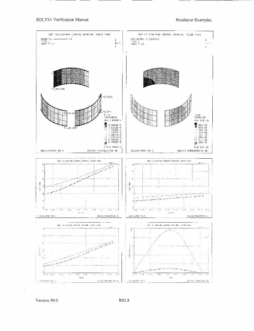
SOLVIA Verification Manual Nonlinear Examples
892 0 LTING-PAD DDURNAL BEARING. RIGID PADS
OR0G:NA - 0
ZONE F 0.'K7
F',LI12 oYM
SOLVIA POST 99.0
7 M3SYF FILM THICKESS
MAX 2.0958E
S2.0023E-4 I St52E-I .6282E-1 .4412E-4, 12S41E-4~ 1087!0 4
8.8005E-51 8 6.302E S'
MIN S 99506-0
SOLVIA ENGIGNEERING AB
892 71-TING-PAD 'OURNWL BEARA'NG RIGID -ACD
ZONE FILM
89Z T.IC INT PA JOUORNR N080
TN. RIGID PADS
I � 01-0 -�
OUT;I E..GI1EER01G0 0
392 TI 00 GPIT TORNA SE00 NG 00 GI PADS 0
,VIRA E90GI0E1090 A
Version 99.0B9S
Z
y
X
'IýE i ........ ..
;ýLIIA-S7 SS D CLIIA EýIGIII-Eý111G 1,3 L'ý-IýST 1ý G
392 -ILITIIG-PAO J0JR11L --1RI11G, RIGID -1G1
--. 1-1 ..... ........ --.- Lýk -!- I
I : I.- !
B92.8
MI-E
FIL.'11-S'TM

0
z
CI 'ol'
ON ci ON
0 ON ON
0 0 C'S
:73-
C 1
- --------
2 1

SOLVIA Verification Manual Nonlinear Examples
SOLVIA-PRE input
HEADING 'B92 TILTING-PAD JOURNAL BEARING, RIGID PADS'
DATABASE CREATE MASTER IDOF=100011 TEMPERATURE=COUPLED TOLERANCES RNORM=1E3 RMNORM=1E3 RTOL=0.01 TYPE=F ITEMAX=100 T-ITERATION TTOL=0.1
PARAMETER $RI=140E-3 SR2=140.21E-3 $R3=240E-3 PARAMETER $MAT=1 SET EPS=1.E-8 MYNODES=200 SET PLOTORIENTATION=PORTRAIT NSYMBOL=MYNODES NNUMBERS=MYNODES VIEW 1 1 0 1
SYSTEM 1 CYLINDRICAL COORDINATES SYSTEM=1 ENTRIES NODE R THETA
1 $R1 -82.5 2 $R1 -12.5 3 $R1 55.0 4 SRi 125.0 5 $R1 -167.5 6 SRi -97.5 7 0. 0.
11 $R2 -82.5 12 $R2 -12.5 13 $R3 -47.5 99 400E-3 -45
NGENERATION TIMES=2 SYSTEM=1 YSTEP=137.5 NSTEP=10 11 TO 13
NGENERATION ZSTEP=-0.105 NSTEP=i00 SYSTEM=i 1 TO 6 / 11 12 / 21 22 / 31 32
READ B92.DAT ,
SET NODES=i8 EGROUP 1 FILM MATERIAL=1 GVOLUME 32 31 131 132 6 5 105 106 EL1=8 EL2=3 SYSTEM=i ADDZONE=FILMi FILMVELOCITY INPUT=SURFACE OMEGA=314.16
AX=0. AY=C. AZ=C. BX=-1. BY=0. BZ=0.0 5 6 106 105
EGROUP 2 FILM MATERIAL=1 GVOLUME 22 21 121 122 4 3 103 104 ELi=8 EL2=3 SYSTEM=1 ADDZONE=FILM2 FILMVELOCITY INPUT=SURFACE OMEGA=314.16
AX=C. AY=0. AZ=C. BX=-1. BY=-. BZ=0.0, DKDP=1E4 KMIN=1E9
3 4 104 103 ,
EGROUP 3 FILM MATERIAL=i GVOLUME 12 11 111 112 2 1 101 102 EL1=8 EL2=3 SYSTEM=1 ADDZONE=FILM3 FILMVELOCITY INPUT=SURFACE OMEGA=314.16
AX=C. AY=C. AZ=C. BX=-1. BY=-. BZ=0.0 1 2 102 101
RIGIDLINK INPUT=SURFACE ADDZONE=PAD1 31 32 132 131 33
RIGIDLINK INPUT=SURFACE ADDZONE=PAD2 22 21 121 122 23
RIGIDLINK INPUT=SURFACE ADDZONE=PAD3 12 11 I11 112 13
MESH RIGIDLINKS NSYMBOLS=YES
Version 99.0 1392.10
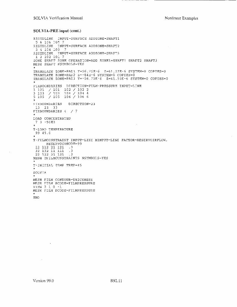
SOLVIA Verification Manual Nonlinear Examples
SOLVIA-PRE input (cont.)
RIGIDLINK INPUT=SURFACE ADDZONE=SHAFT1 5 6 106 105 7
RIGIDLINK INPUT=SURFACE ADDZONE=SHAFT2 3 4 104 103 7
RIGIDLINK INPUT=SURFACE ADDZONE=SHAFT3 1 2 102 101 7
ZONE SHAFT ZONE OPERATION=ADD ZONEl=SHAFTI SHAFT2 SHAFT3 MESH SHAFT NSYMBOLS=YES
TRANSLATE ZONE=PAD1 Y=56.75E-6 Z=61.93E-6 SYSTEM=0 COPIES=TRANSLATE ZONE=PAD2 Z=-84E-6 SYSTEM=0 COPIES=0 TRANSLATE ZONE=PAD3 Y=-56.75E-6 Z=61.93E-6 SYSTEM=0 COPIES=0
FIXBOUNDARIES DIRECTION=FILM-PRESSURE INPUT=LINE 1 101 / 101 102 / 102 2 3 103 / 103 104 / 104 4 5 105 / 105 106 / 106 6
FIXBOUNDARIES DIRECTION=23 13 23 33
FIXBOUNDARIES 4 / 7
LOAD CONCENTRATED 7 3 -50E3
T-LOAD TEMPERATURE 99 45.0
T-FILMCONSTRAINT INPUT=LINE MINPUT=LINE FACTOR=RESERVOIRFLOW, RESERVOIRNODE=99
12 112 21 121 .3 32 132 11 111 .3 22 122 31 131 .3
MESH TFILMCONSTRAINTS NSYMBOLS=YES ,
T-INITIAL TEMP TREF=45 *
SOLVIA ,
MESH FILM CONTOUR=THICKNESS MESH FILM BCODE=FILMPRESSURE VIEW 2 1 0 -1 MESH FILM BCODE=FILMPRESSURE
END
Version 99.0 B92.11

SOLVIA Verification Manual Nonlinear Examples
SOLVIA-PRE read file B92.DAT
* File B92.DAT ,
MATERIAL $MAT OIL DENSITY=880 PRESSURE-FACTOR=2.7E-8 * temperature viscosity pressure
10. 0.1210 15. 0.0890 20. 0.0660 25. 0.0510 30. 0.0400 35. 0.0330 40. 0.0260 45. 0.0210 50. 0.0175 55. 0.0145 60. 0.0123 65. 0.0105 70. 0.0090 75. 0.0080 80. 0.0070 85. 0.0062 90. 0.0054 95. 0.0049
100. 0.0044 105. 0.0041 110. 0.0038 115. 0.0035 120. 0.0032 125. 0.00295 130. 0 .0027 135. 0 .0025 140. 0.0023 145. 0 .00215 150. 0.0020
END DATA .
T-MATERIAL $MAT TEMP-CONDUCTION * temperature conductivity specific heat
10. 0.145 1.71E6 150. 0.133 1.71E6
END DATA
SOLVIA-POST input
* B92 TILTING-PAD JOURNAL BEARING, RIGID PADS
SET PLOTORIENTATION=PORTRAIT DIAGRAM=GRID
DATABASE CREATE WRITE 'b92.iis'
EGROUP 1 EPLINE FILM1-SYM 1 9 6 3 TO 8 9 6 3 EPLINE FILMI-EDGE 17 7 4 1 TO 24 7 4 1 EGROUP 2 EPLINE FILM2-SYM 1 9 6 3 TO 8 9 6 3 EPLINE FILM2-EDGE 17 7 4 1 TO 24 7 4 1
Version 99.0 B92.12
0-66 UOTS-TOA
CNE
MOqEWqIl=GNIN MqIa NOIIVWWnS MOqJWqI2=GNlN ZW=2 NOIIVKWnS
MOqdWqIZ=QNIN TWqIa NOIIVNKnS MOqaNqIJ=GNIN WqIa NOIIVWWnS
SEnSS2ýIdWqIJ=GXIN WqIa NOIIVWNnS
SSOqHSMOdWqI3=GNIN WqIa NOIIVKWnS
ffZ69
ISIrINNOIlDVEýl=GNIN ý-N
LN ISIqN
E=SIXV2ý ýT=SIXVX E=SI=i ZT=SIXVX
TT=SIXVX
SSaNN3IHIWqIZ=QNIN SSRNN3IHIWrlId=CINIA SS2NNDIHIWqIJ=GNI]q
N2ýS- ZKUI,ý W71S - Z=E
N,7ýS-T=Z
RNIrI:4 HNIrIE SNIrI2
GqO=HNVUJ2nS T=709H7,S ýT-SIXVX SýIOSS9HdWrIIa=QNIY SDC3 - ENrII2 HNI72 ET=SIXVX 2ýInSS9'ddN7Ia=CININ N7ýS - HNI72
070=9NVýIZSJOS T='109N2ýS E-SIXV-Tý ZT-=SIXVX SdfISSaUdNrIIZ=GNIN S9GH- ýWrI I Z SNI72
EýT=SIXVX SýIfISSHddNrlIa=GNIX NTS-EWrIIJ SNI72
CqO=ENVUa9nS T=rIOEN7,S TT-=SIXVX HýMSSSUdNHa=GNIN H9G2-TN'III SNI72 Z=SIXV2ý TT=SIXVX HýMSSaUdNrHa=(INIM N,ýS-TWr= aNIrIS
R9GR-EWqIZ ENT= W2ýS-EW=a aNIrIE
GrIo=aNvýIjarls SE)G2-ZwrIIj UNIrIE
W2ýS-ZWIIZ HNIrIH
2DGS-TWrIIJ SNYIE W2ýS-TWUIZ RNIrIS
T=rIORW7.S T-SIXV2ý ET-=SIXVX T=SIXVK CT=SIXVX E=VUHdWHIWqIJ=GNIN
T=qOgK,ýS T-=SIX)fA ZT-=SIXVX S=VE2dWSlWqIJ=GNIM T=SIXV7, ZT=SIXVX
T=qOGN7,S T-SIXV2ý TT-=SIXVX
T=SIXV.7, TT=SIXVX HHnIVýlHdKSIWqIJ=GNIN2dvDsGNvq=NOIIVIN2IUoloqd 12S
ST'O=XVWA ZNUII, =rl2gVrI BT * O=XVWA ýTWqIlý=qEgVq 8T'O=XVWA
9-20ZF=XVWA 93S=XVWA 08=XVWA
O=NINA O=NIKA O=NINA O=NIKA O=NIKA
OS=NIKA
ET ET TT E
T
SIX'V sixv sixv sixv sixv sixv
HSEW HSHK HSHN HSEW Hs9N MEIA HS2K
SGqON.7,aEWqIS=ýInOINOD WaIZ
qqV=SHNIqd SSHNNDIHIWqIZ=UDOINOD NUId
SSOqESMOdWqIZ=EnOINOD NUIJ
-MOq3-NqIZ='dOIDEA 2EnSSSýIdWqIS=UnOINOD NUId HUnIVUSdWalWqIZ=EnOINOD WaIZ
T 0 T DEV SINSWSDVqdSIG=WIDaA X=MHIA
T V L tZ 01 T V ý LT ESCI2-ýWrIIff HNIrIdE
E 9 6 9 0,1 E 9 6 T W7,S-EN-IIZ SNIIdE
dDOEDS
(-Iuoz)) Indut JSOI-VIA'IOS
junuel/V uOIIL'Z)UIJ3A VIA-10Ssoldwuxa mouquoN

SOLVIA Verification Manual
EXAMPLE B93
TILTING-PAD JOURNAL BEARING, ELASTIC PADS
Objective
To demonstrate the use of FILM elements in a tilting-pad journal bearing with thermo-elastic pads
that are cooled on the external surfaces.
Physical Problem
The geometry of the bearing and the elastic pads are shown in the figures below. The pads have a
thermo-elastic material and have convection surfaces on the outside faces. A rigid shaft with
axisymmetric thermal conditions is assumed. Each pad is free to rotate about the X-direction at the
pivot point. This bearing is analyzed in Example B92 with rigid pads and no heat conduction.
Elasticity and heat conduction in both the shaft and the pads are treated in Example B96.
3
The values of rahaft, rpadI c', F, wo and the
properties of the oil are the same as in Example B92.
Pad material and geometry:
Young's modulus E = 2.10" N / m2 Conductivity k = 51.9 W / m°C
Poisson's ratio v = 0.3 Convection coefficient h = 200 W I m C
Thermal expansion coefficient Ambient temperature Ta = 45 0C
a=1.1.10-5 m/m°C
Angles = 35° c = 42.5' Pad thickness h -5010- 3 m
Distance pad surface - pivot point Reference temperature giving zero thermal
d = 100- 10-3 m stresses TREF = 25°C
Nonlinear Examples
B93.1Version 99.0

SOLVIA Verification Manual
Finite Element Model
Due to the symmetry about the plane X=0 only one half of the bearing is considered. The key nodes of the model are shown on page B93.4. Pad 3 is first generated using a sequence of GVOLUME commands. A single pivot point is used but the pivot force on the pad is distributed to a line load in the symmetry plane. The line is kept rigid by rigid links to the pivot point. The external faces of the pad is cooled using thermal convection surfaces. Pad 3 is then copied by rotation to create pads 1 and 2, and all three pads are moved to the correct radial position.
The film segment at each pad consists of 8x 3 16-node FILM elements.
Each circumferential line of shaft nodes is constrained to be thermally axisymmetric in order to model the averaging effect due to the shaft rotation. The shaft surface is made rigid by rigid links to the center node.
The film pressure boundary conditions, the applied vertical shaft load and the thermal constraints for the oil film inlet and outlet flows are defined as in Example B92.
Solution Results
The input data on pages B93.8 - B93.12 is used in the analysis.
The vertical shaft force of 100 kN and the rotational speed of 314.16 rad/s (3000 rpm) are applied in a single load step.
The force/moment tolerance governs the accuracy of the analysis as described in Example B92. The reference force and moment are, however, set to larger values since the norms of the unbalance force and moment vectors have now many more components due to the much increased number of displacement degrees of freedom. The achieved accuracy can be checked in SOLVIA-POST using the command TOLERANCES.
The artificial spring stiffnesses used by the FILM elements are the same as in Example B92.
The displacement boundary conditions for the pads are shown on page B93.4. The convection surfaces of the pads are indicated by yellow color in the left top plot of page B93.5. The film thickness is displayed in a contour plot on the same page as well as the film temperature constraints and the axisymmetric temperature constraints for the shaft surface.
The displacement vector plot on page B93.5 shows the essentially vertical displacement of the shaft and the rotations of the pads. The distributions of pad temperature, film temperature, film flow, film pressure, film power loss, film thickness and Reynolds number are shown as contour plots on pages B93.5 and B93.6.
Diagram results of film temperature, film pressure and film thickness are shown on pages B93.6 and B93.7. In these diagrams the element result lines are defined using result points nearest the symmetry plane and nearest the side edge. The edge results have symbols in the diagrams.
The thermal expansion of the pads in the radial direction gives somewhat smaller film thicknesses and larger film pressures, in particular for the upper pad, than calculated in Example B92. The film thickness is also affected by the elasticity and the thermal gradients in the pads.
The numerical results are summarized in the tables below. Note that the results apply to half the bearing.
Version 99.0
Nonlinear Examples
B93 .2

SOLVIA Verification Manual
Film element results, Pad 1 Pad 2 Pad 3 Total
half bearing model:
Summation of pressure load in -28.9- 103 7.8-103 -28.9.- 10' -50.0 .103
vertical Z-direction, N
Inlet oil flow m 3 / s 2.3.10-4 4.1-10-4 25-10-4 8.9.10-4
Power loss W 4.7- 103 2.8. 10' 5.1 -10' 12.6- 103
Film thickness, max m 170-10- 220. 10' 172-10-.6
Film thickness, min m 49.10' 133-10-6 58-10'
Film pressure, max N / Mi 6.4- 106 1.0-10 6 6.1.10'
Inlet film temperature' °C 67.1 58.9 58.3
Outlet film temperature') °C 83.7 63.6 76.1
1) At the element result point nearest the symmetry plane.
User Hints
The solution is based on the assumption of laminar oil flow which prevails when Reynolds number
is smaller than about 500 - 1500, depending on a number of detail flow conditions for the oil. The
maximum Reynolds number is calculated to be 683, see the contour plot on page B93.6.
The oil flow portion at a film inlet node that comes from the reservoir is defined to be minimum
30%, see command T-FILMCONSTRAINT FACTOR=RESERVOIRFLOW in the input data on
page B93.10. However, a larger portion is taken from the reservoir when the outlet oil flow from
the neighboring oil film node is not sufficient to make up the remaining 70%. In this case the inlet
oil temperature will be proportionally lower. The alternative option T-FILMCONSTRAINTS FACTOR=CARRYOVERFLOW is used in Example B97.
Finite element results at the center of the shaft (node 7), half bearing model:
Vertical displacement e' , m -55.2- 10-6
Horizontal displacement e'y , m -25.-10-6
Attitude angle = tan-(e',/e'z) , degrees 2.6
Eccentricity ratio F'= e/c' 0.44
Frictional torque, reaction moment Tx , Nm -40.1
Frictional power cox -.T, W 12.6. 103
Nonlinear Examples
Version 99.0 B93.3

SOLVIA Verification Manual Nonlinear Examples
CZ
11
filmfilm
99
reservoir oil node
user defined nodes at X=O user defined nodes at X =-0.105 m
B93 TILTING-PAO JOURNAL BEARING. ELASTIC PADS
ORIGINAL •0.05 ZONE SOLID
Z
'1ASTiR
5B OOO0A S i!OCLO
A 222222
SOLVSA ENGINEERING AB
393 TTLTING-PAO JOURNAL BEARINS, ELASTIC PADS
ORIGINAL - 0.05 Z ZONE SOLID
Y 'SX
SOLV'A-PRE 99
'A OS7F
N I 1AS
A 22?22A SOL/:A ENGINEER!NG AB
Version 99.0
SOLVIA-PRE 99.0
B93.4
Z
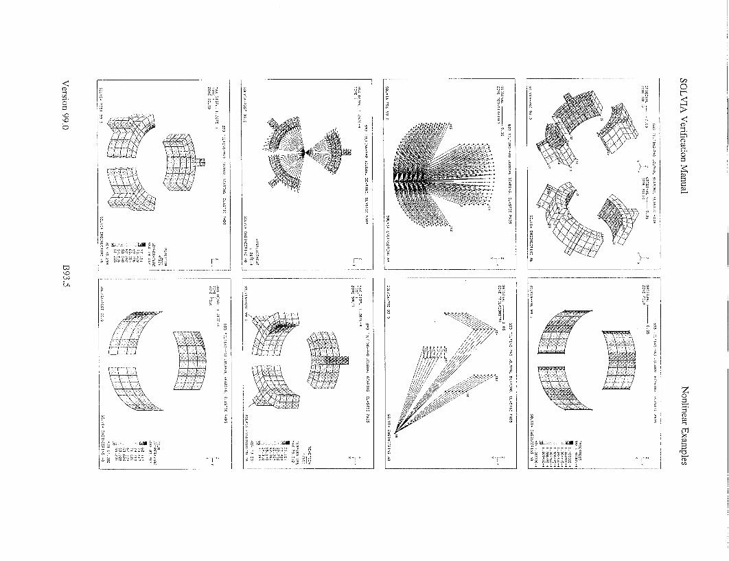
law tS,
p
-ci a CA
0
6
47 ̀
V :5
0
0p
a•
ŽA'77.7y
/
U-)
a'
8 2
N
cn
• .
•°I -ci

Cl)
V
a z
0
0
0
Himff
ph
man•
aLa] a, '.1
0
q 03
aim 1A-
Jý
Vill
h xu=mg 1 is pass, NtW7
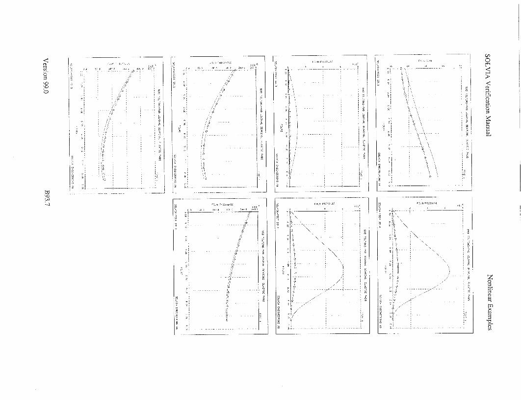
SOLVIA Verification Manual Nonlinear Examples
SOLVIA-PRE input
HEADING 'B93 TILTING-PAD JOURNAL BEARING, ELASTIC PADS' *
DATABASE CREATE MASTER TEMPERATURE=COUPLED TOLERANCES TYPE=F RNORM=1E5 RMNORM=lE5 RTOL=0.01 ITEMAX=100
T-ITERATION TTOL=0.1
PARAMETER $RI=140E-3 $R2=140.21E-3 $R3=190E-3 $R4=240E-3 SET EPS=1.E-6 MYNODES=l000
SYSTEM 1 CYLINDRICAL COORDINATES SYSTEM=l ENTRIES NODE R THETA
1 $Rl -82.5 2 $Rl -12.5 3 SRI 55.0 4 $Rl 125.0 5 $RT -167.5 6 $R1 -97.5
11 $R3 -12.5 12 $R2 -12.5 13 $R2 -38.75 14 $R2 -56 .25 15 $R2 -82 .5 16 $R3 -82.5 17 $R3 -51.875 18 $R3 -43.125 19 $R4 -51.0 TO 21 $R4 -44.0
99 400E-3 -45 7 0 0
NGENERATION TIMES=2 SYSTEM=l YSTEP=137.5 NSTEP=10 12 15
NGENERATION ZSTEP=-0.105 NSTEP=100 SYSTEM=1 1 TO 6 / 11 TO 35
*
SET MIDNODES=l LINE CYLINDRIC 12 13 EL=3 / LINE CYLINDRIC 112 113 EL=3 LINE CYLINDRIC 13 14 EL=2 / LINE CYLINDRIC 113 114 EL=2 LINE CYLINDRIC 14 15 EL=3 / LINE CYLINDRIC 114 115 EL=3
LINE COMBINED 12 15 13 14 / LINE COMBINED 112 115 113 114
* Oil material PARAMETER $MAT=1 READ B92.DAT
* Pad material
MATERIAL 2 THERMO-ELASTIC TREF=25 -10000 2.Eli 0.3 1.IE-5 10000 2.ElT 0.3 1.IE-5
T-MATERIAL 2 TEMP-CONDUCTION -10000 51.9 0.
10000 51.9 0.
* Pad convection material
T-MATERIAL 4 CONVECTION H=200.
* Film elements, each pad film is an element group
SET NODES=16 EGROUP 1 FILM MATERIAL=l
GVOLUME 32 35 135 132 6 5 105 106 ELl=8 EL2=3 SYSTEM=l ADDZONE=FILM1
Version 99.0 B93.8
Nonlinear ExamplesSOLVIA Verification Manual
SOLVIA-PRE input (cont.)
FILPVELOCITY
5 6 106 105
INPUT=SURFACE OMEGA=314.16 , AX=C. AY=0. AZ=C. BX=--. BY=C. BZ=0.0
EGROUP 2 FILM MATERIAL=1 GVOLUME 22 25 125 122 4 3 103 104 ELi=8 EL2=3 SYSTEM=i ADDZONE=FILM2
FILMVELOCITY INPUT=SURFACE OMEGA=314.16 ,
AX=C. AY=C. AZ=-. BX=-1. BY=C. BZ=0.0 DKDP=-E4 KMIN=-E9
3 4 104 103 ,
EGROUP 3 FILM MATERIAL=i GVOLUME 12 15 115 112 2 1 101 102 ELi=8 EL2=3 SYSTEM=i ADDZONE=FILM3 FILMVELOCITY INPUT=SURFACE OMEGA=314.16 ,
AX=-. AY=C. AZ=C. BX=-1. BY=C. BZ=0.0 1 2 102 101
* Generate pad 3
SET NODES=20 EGROUP 4 SOLID MATERIAL=2 GVOLUME ii 12 13 18 111 112 113 118 ELi=2 SYSTEM=1 ADDZONE=PAD3
GVOLUME 18 13 14 17 118 113 114 117 SYSTEM=1 ADDZONE=PAD3
GVOLUME 17 14 15 16 117 114 115 116 SYSTEM=1 ADDZONE=PAD3
GVOLUME 21 18 17 19 121 118 117 119 ELI=2 EL3=3 SYSTEM=1 ADDZONE=PAD3
* Boundaries for pad 3
FIXBOUNDARIES 12356 / 20
* Rigid links at pivot point
RIGIDLINK INPUT=LINE ALPHA=l.1E-5 TREF=25 ADDZONE=PAD3 * nl n2 masternode
19 21 20 ,
* Convection surfaces for pad 3
T-BOUNDARIES SEGMENTS CON-MATERIAL=4 INPUT=SURFACE 11 18 118 111 / 18 21 121 118 / 21 19 119 121
19 17 117 119 / 17 16 116 117 / 111 112 113 118
113 114 117 118 / 114 115 116 117 / 118 117 119 121
12 11 111 112 / 16 15 115 116 T-LOADS ENVIRONMENT CONVECTION=YES INPUT=MATERIAL
4 45.
* Generate pad 2 ROTATE PAD3 Ni=7 ROTATE PAD3 Ni=7
and pad 1 N2=15 N3=25 ADDZONE=PAD2 N2=15 N3=35 ADDZONE=PAD1
* Move all pads to correct radial position
TRANSLATE ZONE=PADI Y=56.75E-6 Z=61.93E-6 SYSTEM=C COPIES=C TRANSLATE ZONE=PAD2 Z=-84E-6 SYSTEM=C COPIES=C
TRANSLATE ZONE=PAD3 Y=-56.75E-6 Z=61.93E-6 SYSTEM=C COPIES=C
* Axisymmetric temperature condition for shaft surfaces
LINE COMBINED 1 6 2 3 4 5 T-CONSTRAINT INPUT=LINE ADDZONE=T-SHAFT
1 6 1 1. TRANSLATE ZONE=T-SHAFT X=-0.0175 SYSTEM=0 COPIES=6 ADDZONE=ABCD
* Make shaft surfaces rigid
RIGIDLINK INPUT=SURFACE ADDZONE=SHAFT 1 2 102 101 7 3 4 104 103 7 5 6 106 105 7
Version 99.0 B93.9

SOLVIA Verification Manual Nonlinear Examples
SOLVIA-PRE input (cont.)
* Film pressure boundary conditions FIXBOUNDARIES DIRECTION=FILM-PRESSURE INPUT=LINE
1 101 / 101 102 / 102 2 3 103 / 103 104 / 104 4 5 105 / 105 106 / 106 6
* Load and boundary conditions, shaft center node LOADS CONCENTRATED
7 3 -50E3 FIXBOUNDARIES 1456 / 7
* Symmetric boundary conditions for pad plane X=0 ZONE XSYM INPUT=CYLINDRICAL XLMIN=0 SYSTEM=l FIXBOUNDARIES 1 INPUT=ZONE ZONEl=XSYM
* Temperature and boundary condition for reservoir oil node FIXBOUNDARIES / 99 T-LOAD TEMPERATURE
99 45.0 *
* Define the oil inlet flow portion from reservoir
T-FILMCONSTRAINT INPUT=LINE MINPUT=LINE FACTOR=RESERVOIRFLOW, RESERVOIRNODE=99
2 102 3 103 0.3 4 104 5 105 0.3 6 106 1 101 0.3
,
T-INITIAL TEMP TREF=25 *
SOLVIA
SET PLOTORIENTATION=PORTRAIT NSYMBOL=MYNODES COLOR EFILL=ORANGE MESH ZONE=SOLID VIEW=I BCODE=ALL MESH ZONE=SOLID VIEW=-I BCODE=ALL SET PLOTORIENTATION=LANDSCAPE COLOR EFILL=CON-MATERIAL MESH ZONE=SOLID VIEW=I NNUMBERS=MY SUBF=21 MESH ZONE=SOLID VIEW=-I NNUMBERS=MY VIEW 1 1 0 1 MESH ZONE=FILM CONTOUR=THICKNESS SET NNUMBERS=MY MESH TCONSTRAINTS NSYMBOLS=YES MESH TFILMCONSTRAINTS NSYMBOLS=YES END
Version 99.0 B93.10

SOLVIA Verification Manual
SOLVIA-POST input
* B93 TILTING-PAD JOURNAL BEARING, ELASTIC PADS
SET MODE=BATCH PLOTORIENTATION=LANDSCAPE DIAGRAM=GRID
DATABASE CREATE WRITE 'b93.1is' VIEW ABOVE 1 0 1 VIEW BELOW 1 0 -1
EGROUP 1 EPLINE FILMi-SYM 1 9 6 3 TO 8 9 6 3 EPLINE FILMi-EDGE 17 7 4 1 TO 24 7 4
Nonlinear Examples
1
EGROUP 2 EPLINE FILM2-SYM 1 9 6 3 TO 8 9 6 3 EPLINE FILM2-EDGE 17 7 4 1 TO 24 7 4 1
EGROUP 3 EPLINE FILM3-SYM 1 9 6 3 TO 8 9 6 3 EPLINE FILM3-EDGE 17 7 4 1 TO 24 7 4 1
MESH MESH MESH MESH MESH MESH *
MESH MESH MESH MESH
AXIS AXIS AXIS AXIS AXIS AXIS
*
ELINE ELINE
VIEW=X VECTOR=DISP SOLID CONTOUR=TEMP VECTOR=REACTION SOLID CONTOUR=TEMP VECTOR=REACTION FILM CONTOUR=FILMTEMP VIEW=ABOVE FILM CONTOUR=TEMP VIEW=ABOVE FILM CONTOUR=TEMP VIEW=BELOW
FILM FILM FILM FILM
1 2 3
11 12 13
VIEW=ABOVE VIEW=BELOW
CONTOUR=FILMPRESSURE VECTOR=FILMFLOW VIEW=ABOVE CONTOUR:FILMPOWERLOSS CONTOUR=FILMTHICKNESS PLINE=ALL CONTOUR=FILMREYNOLDS
VMIN=50 VMIN=0 VMIN=0 VMIN=0 VMIN=0 VMIN=0
VMAX=90 LABEL='FILM-TEMP' VMAX=8E6 LABEL='FILM-PRESSURE' VMAX=216E-6 LABEL='FILM-THICKNESS' VMAX=0.18 LABEL='FILMI' VMAX=0.18 LABEL='FILM2' VMAX=0.18 LABEL='FILM3'
FILMi-SYM KIND=FILMTEMPERATURE XAXIS=11 YAXIS= FILMi-EDGE KIND=FILMTEMPERATURE XAXIS=-11 YAXIS= SUBFRAME=OLD SYMBOL=1
ELINE FILM2-SYM KIND=FILMTEMPERATURE ELINE FILM2-EDGE KIND=FILMTEMPERATURE
SUBFRAME=OLD SYMBOL:1
ELINE FILM3-SY* KIND=FILMTEMPERATURE ELINE FILM3-EDGE KIND=FILMTEMPERATURE
SUBFRAME=OLD SYMBOL=I
ELINE FILMI-SYM KIND=FILMPRESSURE XAXIS=11 YAXIS=2 ELINE FILMI-EDGE KIND:FILMPRESSURE XAXIS=-Il YAXIS=2
SUBFRAME=OLD SYMBOL=I
Version 99.0
1 OUTPUT=ALL
XAXIS=12 YAXIS=1 OUTPUT=ALL XAXIS=-12 YAXIS=-l ,
XAXIS=13 YAXIS=1 OUTPUT=ALL XAXIS:-13 YAXIS=l ,
B93.11

Nonlinear ExamplesSOLVIA Verification Manual
SOLVIA-POST input
XAXIS=12 YAXIS=2
XAXIS=-12 YAXIS=2ELINE FILM2-SYM KIND=FILMPRESSURE
ELINE FILM2-EDGE KIND=FILMPRESSURE
SUBFRAME=OLD SYMBOL=1
ELINE FILM3-SYM KIND=FILMPRESSURE XAXIS=13 YAXIS=2
ELINE FILM3-EDGE KIND=FILMPRESSURE XAXIS=-13 YAXIS=2
SUBFRAME=OLD SYMBOL=1
ELINE FILM1-SYM KIND=FILMTHICKNESS XAXIS=11 YAXIS=3
ELINE FILMI-EDGE KIND=FILMTHICKNESS XAXIS=-ll YAXIS=3
SUBFRAME=OLD SYMBOL=1
ELINE FILM2-SYM KIND=FILMTHICKNESS XAXIS=12 YAXIS=3
ELINE FILM2-EDGE KIND=FILMTHICKNESS XAXIS=-12 YAXIS=3
SUBFRAME=OLD SYMBOL=1
ELINE ELINE
FILM3-SYM KIND=FILMTHICKNESS XAXIS=13 YAXIS=3
FILM3-EDGE KIND=FILMTHICKNESS XAXIS=-13 YAXIS=3
SUBFRAME=OLD SYMBOL=1
NLIST N7
NLIST N7 KIND=REACTIONS
SUMMATION FILM KIND=FILMPOWERLOSS
SUMMATION FILM KIND=FILMPRESSURE
SUMMATION FILM KIND=FILMFLOW
SUMMATION FILM1 KIND=FILMFLOW
SUMMATION FILM2 KIND=FILMFLOW
SUMMATION FILM3 KIND=FILMFLOW
SUMMATION PAD1 KIND=REACTION
SUMMATION PAD2 KIND=REACTION
SUMMATION PAD3 KIND=REACTION
SUMMATION KIND=REACTION
TOLERANCES
END
B93.12Version 99.0

SOLVIA Verification Manual
EXAMPLE B94
JOURNAL BEARING, FULL SOMMERFELD SOLUTION
Objective
To verify the pressure solution produced by the FILM element when the film temperature is constant
and the oil material model is specified as independent of the oil pressure.
Physical Problem
The journal bearing shown in figure below is to be analyzed when the rotational speed is 3000 rpm.
No side leakage of oil shall occur. Shaft and bearing axes are assumed to be parallel. The full
Sommerfeld solution is sought. z
A
Bearing radius Shaft radius
Eccentricity Y Bearing width
Absolute viscosity
Rotational speed Pressure at maximum film thickness (0=0)
r, = 0.1001 m rb = 0.1000 m
e = 20-10-6 m B = 0.05 m - = 0.02 Pa s
Ob = 314.16 rad/s
Po"= Pa
Finite Element Model
The finite element model consists of 60X2 16-node FILM elements. The top left figure on page B94.3 shows a contour plot of the film thickness. Two cylindrical systems are used to generate the film
elements. All nodes of the FILM elements have zero displacements. The command
FIXBOUNDARIES is not used for all nodes because a displacement solution requires at least one
active displacement degree of freedom. Therefore, the shaft nodes were selected to have zero Z
displacements using the LOADS DISPLACEMENTS command.
Solution Results
The theoretical solution for this problem can be found for example in reference [I], page 221.
Pressure:P(-rP0 n 69Lco (2+)+ cosO)
where c =ra rb F= e/ c
e is defined in the figure above.
Version 99.0
e
Nonlinear Examples
B94.1

SOLVIA Verification Manual
Maximum pressure:
Load capacity:
Film oil flux:
Pma, - PO = O)b Pm
3F(4-E 2 )J(4-5 2 +e4 ) where p m =
2(2+ 2)(1- 2)
F,=0
q -f rbmo hm
where h.- 2 c (1 -2 (the film thickness at maximum pressure)
The input data used in the SOLVIA analysis can be seen on pages B94.4 and B94.5.
A comparison with the analytical solution is given in the table:
Analytical SOLVIA
Maximum film pressure (MPa) 7.74 7.75
Load capacity in Y-direction (kN) -119 -119
Load capacity in Z-direction (N) 0 5.3.10-*
Oil film flux in 0 direction (in 2 / s) 0.00148 0.00148
A contour plot of the film pressure is shown in top right figure on page B94.3. The film pressure around the shaft is shown in a diagram on page B94.3 together with the analytical solution. A very good agreement with the analytical solution is observed. The distributions of film power loss, film thickness and oil film flux are also shown.
User Hints
" The oil film flux is defined as the volume oil flow per unit film width and is, therefore, constant around the shaft. It is analytically evaluated at the points having maximum (or minimum) pressure, where it is equal to the Couette flow per unit length, since the oil flow due to the pressure gradient
is zero at these points.
" An oil pressure much below the vapor pressure of the oil cannot occur in practice since it would
result in cavitation. The FILM element is currently formulated for incompressible oil flow without any cavitation. The solution of this example corresponds to the case that a hydrostatic pressure is
applied to the oil film so that both positive and negative pressures with respect to the reference hydrostatic pressure is possible.
Version 99.0
Nonlinear Examples
B94.2

SOLVIA Verification Manual Nonlinear Examples
The midsurface of the FILM element is used as the reference surface by SOLVIA when
calculating the oil film pressure (and temperature). The midsurface is obtained by taking the
average deformed coordinates of corresponding top and bottom surface nodes. The analytical reference surface is positioned at the shaft surface. The applied surface velocity and the film
thickness are thus the same in SOLVIA as in the analytical solution but the circumferential length
of the two reference surfaces are slightly different.
Reference
[1] Hamrock, Bernard, J., Fundamentals of fluid film lubrication, McGraw-Hill, 1994
ORGNI 00 702 1 0 00 000L 000
9, OUlRA F02 00 o o.7 z.
SOLIA SNEýEýI -A
*• 090 OSE-,
O 000S0V0-I
0C00 90 000 00oo-
0 L11lA 0099 0
094 OURNAL BEARI0NG. 0ULL 00MMERFEL0 SOLUTION
SOL 'A . -100N< ERING 0 0
B94 JOURNAL SEARING. FULL SoGMERFELO SCLUTION
MIX D0S0L U0SS6C-24 z r ezcNEFI FL
so o os o j C 00. 11100 . 0
MIN 90750E6
S ; - 1,0SL: •Eý31 TI 18OZ
i 394 JýURNA- BEAR!NG •ULSMM•ENFELD SOLUTIOýN
~~~~~~~~~~G %! EN IN ER I .. . ..AB.. . . . . . . . . . . . . . . .
790 0CU'NA7E0N. 0 0 L_ 0nE0FEL _ OU I0 394 JOUR NAL 0EAR0 NG, 0 ULL SO 0MER0 ELD SOLUTIO N
IT
10 0 0. 1.•NE•N 1. SOL',0-0SI 7 99
Version 99.0
-J00\,,. 010
: jML__
L,'iA-POS7 99
;0URN•L
53L-IA-VS 3
B94.3

SOLVIA Verification Manual
SOLVIA-PRE:
HEADING 'B94 JOURNAL BEARING, FULL SOMMERFELD SOLUTION'
DATABASE CREATE MASTER IDOF=100111 NSTEP=1 TEMPERATURE=LOAD SET EPS=1.E-6
PARAMETER sX=0.05 $RB=0.i $RA=0.1001 $ANG=90 $EL-60
SYSTEM 1 CYLINDRICAL Z=0. SYSTEM 2 CYLINDRICAL Z=-20.E-6 COORDINATES SYSTEM=i
ENTRIES NODE XL R THETA 1 0. $RA SANG 2 $X $RA $ANG
COORDINATES SYSTEM=2 ENTRIES NODE XL R THETA
3 0. $RB SANG 4 $X $RB $ANG
SET MIDNODES=i LINE CYLINDRICAL Ni=i N2=1 EL=$EL SYSTEM=i ROTATION=LONG
LINE CYLINDRICAL Ni-2 N2=2 EL=$EL SYSTEM-i ROTATION-LONG
LINE CYLINDRICAL Ni=3 N2=3 EL=$EL SYSTEM=2 ROTATION=LONG
LINE CYLINDRICAL Ni=4 N2=4 EL=SEL SYSTEM=2 ROTATION=LONG
MATERIAL 1 OIL -1000. 0.02
1000. 0.02 END DATA
SET NODES=d6 EGROUP 1 FILM MATERIAL=i RSINT=2
GVOLUME 1 1 2 2 3 3 4 4 EL2=2 FILMVELOCITY INPUT=SURFACE OMEGA=314.16 MOTION=ROTATION,
AX=0. AY-0. AZ=-20.E-6 BX=i. BY=0. BZ=-20.E-6 3344
FIXBOUNDARIES DIRECTION=23 INPUT=SURFACE 3344
FIXBOUNDARIES DIRECTION=2 INPUT=SURFACE 1122
FIXBOUNDARIES DIRECTION FILMPRESSURE INPUT=LINE 12
LOADS DISPLACEMENTS INPUT=SURFACE 1 1 2 2 3 0.
INITIAL TEMPERATURE TREF=30. LOADS TEMPERATURE TREF=30.
MESH FILM CONTOUR-THICKNESS ZONE OUTER CYLINDRICAL SYSTEM*I RMIN=0.10005
ZONE INNER CYLINDRICAL SYSTEM=2 RMAX=0.i0005
SOLVIA END
Version 99.0
Nonlinear Examples
B94.4
SOLVIA Verification Manual
SOLVIA-POST input
* B94 JOURNAL BEARING, FULL SOMMERFELD SOLUTION
DATABASE CREATE *
SET ZONE=FILM DIAGRAM-GRID WRITE 'b94.1is' MESH CONTOUR=FILMPRESSURE
AXIS 1 VMIN:0 VMAX=0.7 AXIS 2 VMIN=-1OE6 VMAX=1OE6 EPLINE JOURNAL
1 3 1 TO 60 3 1
ELINE JOURNAL KIND=FILMPRESSURE XAXIS=1 YAXIS=2USERCURVE 1 READ B94.DAT PLOT USERCURVE
ELINE ELINE ELINE
JOURNAL JOURNAL JOURNAL
1 XAXIS=-I YAXIS=-2 SUBFRAME=OLD
KIND=FILMPOWER KIND=FILMTHICKNESS KIND=FILMFLUX
EMAX SUMMATION SUMMATION SUMMATION SUMMATION SUMMATION END
KIND=FILMPRESSURE KIND=FILMPOWERLOSS KIND=FILMFLOW
OUTER KIND=REACTION INNER KIND=REACTION
Version 99.0
Nonlinear Examples
B94.5

SOLVIA Verification Manual
EXAMPLE B95
HEAT GENERATION IN A PARALLEL-SURFACE SLIDER BEARING
Objective
To verify the temperature and pressure solution for the FILM element when an isoviscous oil material
is used.
Physical Problem
A parallel-surface slider bearing with constant film thickness is to be analyzed. No heat transfer to the
mating surfaces is assumed, i.e. adiabatic conditions. The oil film is assumed to be infinitely wide so
that no side flow can occur. The inlet pressure is 10 MPa which causes a linear variation of the
pressure to the outlet pressure of 0 Pa.
z
T- inlet - outlet
Geometry: Oil properties: Speed ti = 10 m/s
Bearing length 1= 0.1 m Absolute viscosity pt = 0.02 Pa s
Bearing width w = 0.1 m Density p = 800 kg/iM3
Film thickness h = 100.10-6 m Thermal conductivity k = 0.15 W/m 0 C
Specific heat per unit volume c= 1.106 J/m 3°C
Inlet conditions (X = 0.0): Outlet conditions ( X = 0.1):
P =10-106 Pa P = 0.0 Pa T=0 0C
Finite Element Model
The model is shown in the top left plot on page B95.3. Twenty 8-node FILM elements are used to
model the oil film. The fixed boundary conditions for displacements are specified by the command
LOADS DISPLACEMENT so that loads and reactions will be available for the top and bottom film
surfaces. The temperature boundary conditions are given by the command T-FILMCONSTRAINTS
and all inlet nodes are dependent of node 9, which is designated to be the oil reservoir.
Solution Results
The input data on pages B95.4 and B95.5 is used in the analysis.
Version 99.0
Nonlinear Examples
1395.1

SOLVIA Verification Manual
The energy equation in one dimension with adiabatic conditions along the length is
d d dhk aT pV-2(cT)--I bk- = dx dx( dx)
where c = specific heat per unit mass (= c, / p)
V =ih h3 dp = volume oil flow per unit width (film flux)
2 12,g dx
pV = mass flow of oil per unit width
p c V = heat flow of oil per unit width and unit temperature
=h 3 dp) + 'u62 q dpL = generated heat per unit surface area (film power loss)
q 1 ý Ydx) h 1
In this example hk << pVc so the solution to the energy equation is
T= q qX pcV
where X is the distance from the inlet boundary with zero temperature.
The shear stress is
h dp+ th (at the top surface) ('~x'P=2 d- h
h p= -2dx-+ ýth (at the bottom surface) (lz')bt - 2 dx h
The shear forces in the positive X-direction acting on the surfaces with area A are
(F,) top =--(Zuzx) top .A
(FX)bot = (zx) bot *A
The following analytical values are then obtained and the values agree excellently with the
corresponding SOLVIA results:
Result type Unit Analytical SOLVIA
Film flux m2 / s 0.91667.10.3 0.91667-10.3
Film power loss W/ m2 61667 61667
Outlet oil temperature C 6.7273 6.7273
Shear force on top surface N 30.000 30.000
Shear force on bottom surface N 70.000 70.000
Pressure force on top surface N 50000 50000
Pressure force on bottom surface N -50000 -50000
The SOLVIA reactions are the same as the corresponding forces but with reversed signs. Contour
plots of film temperature, film heat flux, film pressure, film flux, film power loss and the Reynolds
number are shown on pages B95.3 and B95.4. The heat flux in the film thickness direction at the top
surface (film t-top flux) is also shown to verify that the boundary is indeed adiabatic.
Version 99.0 B95.2
Nonlinear Examples

SOLVIA Verification Manual Nonlinear Examples
User hints
i The command SUMMIATION KIND=FILMPRESSURE gives the total force due to pressure alone (no shear force from the viscosity) acting at the top surface bounding the film. However, both the pressure and the shear forces are included when summation of applied forces and calculated reactions are requested.
i Note that SUMMATION KIND=TFLOW does not consider heat flow in FILM elements. The heat flow in the thickness direction of FILM elements through the top and bottom surfaces can be obtained by SUMMATION KIND=FILMTFLUX.
In the summation of applied forces over both surfaces the force components in the Z-direction (due to pressure) cancel each other. However, the X-direction force components (due to viscosity) are added since the shear stresses due to the pressure flow act in the same direction at both surfaces.
SDLIA SR 99 1 NE9IS A S9 ' EC sE EZ EIIA R i
9S HEAT ZENERATION IN A PAZRAALE-SURACE SLIDER CEARENG
ZONC F: 9
CR[SIN-L 0011E
E1& .
9A 9S EATM EE~zNI A A'E-SR'C LAE R 6ERNOIEFI
50 -1 -N AEN RATIOS NARRRALCEL SURFRCE SLIDER 3EARING
IO'RIGINALrM - o 31z
ioNEý 'ILI ×Y
A9 6N7273
16,1
2.9432 2 993Z
42915
IIL'IIA EICIINEIRlii AS
945 MEAT , NE9ATION 1 1 A
9A AT E C ERAITCN :N A TRARLLEL-SURAC IOE BEARIG
IIX ISIL I 125E-21 I
<f•. ~ ~ ~ ý , SL• L,
1 6R10
* 3 A2SOEC
SOLVIA ECO E.RING AB
BT E 'EATE SRATION TN A RALHE -SURFRCE SF :D 49E 9
MAX ýC[SýL 2,325E-21 TI1. 201E FILN
0 :14 FL UX
:121C
Version 99.0
ARALL -AURFACE SLIER NEAR:NG
> L
NIrc TIX
ZONE F1-
SO0VIA-o0Sl 99 1
B95.3

Nonlinear ExamplesSOLVIA Verification Manual
49$ -$ 7 ,ENA:0NN :7 N A PARL9EL-4U$ E S9q 4E24N0
4 2SPL 2 D25-22
ZONE F:Lý
IIX 16-6 667
8 666. 6
j1667.$86 , ; 396670207
49664.$67
61664 287
5 1 7 916$ 667 SOVAPS 9aSOLVIA NGNE ERIN1G A I
$95 A 97N1A N 162$ L-LURFACN 2L:DEý 9E 9G
6, 9'5 2 92$-2
9r.E I 701E IlLtl
RLIA EYNOLDS jii $9 6969501
7(6 9 4 9978
$ S-31_ 6$-D7 99.0
SOLVIA-PRE input
HEADING 'B95 HEAT GENERATION IN A PARALLEL-SURFACE SLIDER BEARING'
DATABASE CREATE MASTER IDOF=000111 NSTEP=1 TEMPERATURE=COUPLED SET EPS=1.E-6
TIMEFUNCTION 1 0. 0. / 1. 1.
COORDINATES 1 0.1 0.1 50.E-6 3 0.0 0.0 50.E-6 5 0.1 0.1 -50.E-6 7 0.0 0.0 -50.E-6 9 -0.05 0.05
/ / / /
2 4 6 8
0.0 0 .1 0.1 0.0 0.0 0.1 0.1 0.0
50 .E-6 50 .E-6
-50 .E-6 -50 .E-6
MATERIAL 1 OIL DENSITY=800 * temp viscosity
-1000. 0.02 1000. 0.02
END DATA T-MATERIAL 1 TEMP-CONDUCTION * temp conductivity specific heat
-1000. 0.15 1.E6 1000. 0.15 1.E6
END DATA .
T-INITIAL TEMPERATURE TREF=0.
SET NODES=8 EGROUP 1 FILM MATERIAL=1 RSINT=2
GVOLUME 1 2 3 4 5 6 7 8 EL1=10 EL2=2 EL3=1
FILMVELOCITY INPUT=SURFACE OMEGA=10 MOTION=TRANSLATION TIMEFUNCTION=1,
AX-0. AY=0. AZ=0. BX=-. BY=0. BZ:0. 1234
LOADS FILMPRESSURE INPUT=LINE * nl n2 p1 p 2 timefunction
2 3 1.E7 1.E7 1 1 4 0. 0. 1
LOADS DISPLACEMENTS INPUT=SURFACE * nl n2 n3 n4 dir value
1 2 3 4 1 0. 1 2 3 4 2 0.
1 2 3 4 3 0.
5 6 7 8 1 0. 5 6 7 8 2 0.
5 6 7 8 3 0.
Version 99.0 B95.4

SOLVIA Verification Manual Nonlinear Examples
SOLVIA-PRE input (cont.)
T-LOADS TEMPERATURE
* node value timefunction
9 0. 1 T-FILMCONSTRAINTS INPUT=LINE M-INPUT=NODE * snl sn2 master factor
2 3 9 1.
MESH CONTOUR=THICKNESS NNUMBER=MYNODES NSYMBOL=MYNODES
SOLVIA END
SOLVIA-POST input
* B95 HEAT GENERATION IN A PARALLEL-SURFACE SLIDER BEARING
* Results from temperature analysis
T-DATABASE CREATE
SET ZONE=FILM
WRITE 'b95.lis'
SET LINESPERPAGE=9999 NEWPAGE=NO
MESH CONTOUR=FILMTEMPERATURE
MESH CONTOUR=FILMTFLUX
MESH CONTOUR=FILMTTOPFLUX ELIST ZONENAME=ELI
SUMMATION KIND=TFLOW
SUMMATION KIND=FILMTFLUX
* Results from stress analysis
DATABASE CREATE
MESH CONTOUR=FILMPRESSURE VECTOR=FILMFLOW
MESH CONTOUR=FILMFLUX VECTOR=FILMFLUX
MESH CONTOUR=FILMPOWERLOSS MESH CONTOUR=FILMREYNOLDS
ZONE UPPER GLOBAL ZMIN=0.
ZONE LOWER GLOBAL ZMAX=0.
SUMMATION UPPER KIND=LOADS
SUMMATION LOWER KIND=LOADS
SUMMATION KIND=LOADS
SUMMATION UPPER KIND=REACTIONS
SUMMATION LOWER KIND=REACTIONS
SUMMATION KIND=REACTIONS
SUMMATION KIND=FILMPRESSURE
SUMMATION KIND=FILMPOWERLOSS
SUMMATION KIND=FILMFLOW
END
Version 99.0 B95.5

SOLVIA Verification Manual
EXAMPLE B96
TILTING-PAD JOURNAL BEARING, ELASTIC PADS AND SHAFT
Objective
To demonstrate the use of FILM elements in a tilting-pad journal bearing with thermo-elastic pads and shaft. The pads are cooled on the external surfaces and the shaft on the end surface.
Physical Problem
The same bearing as in Examples B92 and B93 is selected to be analyzed. Example B92 treats the case with rigid shaft and pads and with adiabatic film conditions. Elastic pads including thermal deformation and heat conduction are analyzed in Example B93. In this example both the shaft and the pads are elastic and can deform due to the temperature. The pads have convection surfaces on the outside faces and the shaft has a convection surface at the end face. Axisymmetric thermal conditions for the shaft are considered. The pivoted pads are supported with radial elastic springs.
An overall picture of the geometry is shown below. The geometry and material properties of the pads are shown in the figures on page B 93.1. The values of rshaft, c', F, co and the properties of the oil are the same as in Examples B93 and B92. The radial pad spring stiffness is krad = 1200 N / .m.
ZSection A-A
k rdi2
Shaft data:
Version 99.0
X=O
shaft
film
pad
Young's modulus E = 2-10" N/ m2 Convection coefficient h = 200 W / m 2 °C
Poisson's ratio v = 0.3 Ambient temperature of the shaft Ta = 45 'C
Thermal expansion coefficient ca = 1.1 .10-5 1/'C Zero thermal stresses for TREF = 25 ° C
Bearing width w = 210. 10-3 m Conductivity k = 51.9 W / m°C
B96.1
Nonlinear Examples
1° °Z

SOLVIA Verification Manual
Finite Element Model
Due to the symmetry about the plane X=0 only one half of the bearing is considered. The pads and the film elements are generated as in example B93. The shaft consists of 20-node SOLID elements. Each
circumferential line of shaft nodes at the the oil film surface is constrained to be thermally
axisymmetric in order to model the averaging effect due to the shaft rotation. A convection surface is applied at the end of the shaft.
Each pad is supported by a radial spring to allow radial expansion of the pad pivot due to an assumed elasticity in the support structure.
The key nodes of the model and the displacement boundary conditions are shown on page B96.4. The
pad convection surfaces are colored yellow in the plot of convection surfaces on page B96.5. A contour plot of the initial film thickness is also shown on page B96.5 together with two plots of thermal constraint couplings.
Solution Results
The input data on pages B96.9 - B96.14 is used in the analysis.
Default values of the FILM element artificial spring stiffness are used for the bottom pads. The top
pad uses the artificial stiffness KNORM=3. 10".
The displacement vector plot on page B96.6 shows the essential displacements. The shaft has a vertical displacement due to the external load and a radial displacement due to thermal expansion. The pads rotate around the pivot node and translate in the radial direction.
The distribution of temperature and film temperature are shown as contour plots on page B96.6. The
distribution of film pressure, film power loss, film thickness and Reynolds number are shown on page B96.7. Diagram results of film temperature, film pressure and film thickness are shown on page B96.7 - B96.8. In these diagrams element result lines are defined using result points nearest the sym
metry plane and nearest the edge. The edge results have symbols in the diagrams.
The numerical results are summarized in the tables below. Note that the results apply to half the bearing.
FILM element results Pad 1 Pad 2 Pad 3 Total
Summation of pressure load in -31.4.103 12.7- 103 -31.4-103 -50.1 _ 103
vertical Z-direction, N
Inlet oil flow m 3 / s 2.0-10-4 3.2 10-- 2.2- 10-4 7.4.l0-4
Power loss W 4.6.10' 3.2. 10' 4.9.03 12.7.03
Film thickness, max m 157- 10 181 -10-6 155.10
Film thickness, min m 43 -10- 96-10-6 49. 10-6
Film pressure, max Pa 7.2.106 1.7.106 6.8.106
Version 99.0
Nonlinear Examples
B96.2

SOLVIA Verification Manual
') At the element result points nearest the symmetric line.
User Hint
It is important in this example that the pivot nodes have a radial stiffness that models the elasticity
in the supporting structure. The temperature of the supporting structure is assumed to be the same
as the reference temperature, thus no thermal expansion. If no elasticity in the supporting structure
is used in the analysis then the thermal expansion of the shaft and the pads would cause the oil
film thickness to approach zero. If this models an actual physical situation it could indicate shaft
seizure.
In this example the thermal constraint for the inlet oil flow in command T-FILMCONSTRAINTS
is set to the option FACTOR=RESERVOIRFLOW. The alternative option
FACTOR=CARRYOVERFLOW is used in Example B97. Note that the two options may not
always be each others inverse. For example, when FACTOR=RESERVOIRELOW the available
carry over flow may be less than the portion (inlet flow) - (specified minimum reservoir flow), in
which case the reservoir flow portion is increased by the program.
Version 99.0
FILM element results, cont. Pad 1 Pad 2 Pad 3 Total
Inlet film temperature" 0°C 72.2 63.5 63.4
Outlet film temperature' ) °C 89.9 70.8 83.3
Radial displacement at pad 71. 10. 21-10' 71.10.
pivot node, m
Heat flow from the oil film to 0.22- 10' 0.13- 103 0.18-10 3 0.53.103
the pads, W
Heat flow from the oil film to 0.50. 103 -0.29- 103 0.0- 10i 0.2 t- 103
the shaft W
Finite elements results at the center of the shaft (node 7 ), half bearing model:
Vertical displacement e'z , m -72-5.10-6
Horizontal displacement e'y , m -1.1-10-6
Attitude angle q = tan-'(e'y/e'z) degrees 0.9
Eccentricity ratio s' = e'/c' 0.58
Frictional torque, reaction moment Tx , Nm -40.5
Frictional power, ox .Tx, W 12.7-10'
Nonlinear Examples
B96.3

SOLVIA Verification Manual
filmfilm
99
Nonlinear Examples
11
reservoir oil node
user defined nodes at X=0user defined nodes at X=-0.105 m
B96 TILTING-PAD JOURNAL BEARING. ELASTIC PADS AND SHAFT
ORIGINAL - S-.5 Z ZONE ELE MENT7SI
x y
MASTER
C 1000" O 01011
F2 0 U1, G 222222
SLVTA-PRA F 99 0 SOLVIA ENGINEERING AB
396 TI-T/NG-PAD JOURNAL BEARING. ELASTIC PADS AND SHAFT
ORIGINAL "--0.05 Z ZONE ELEMENTS
A90
SOL/IA-PRE 99.0
MASTER
C 1000!I D 1010

P
2"0 ON ON
4�E2n' T
CD (A
0 0
"0
0
(1� �1
0
0
0
0 0
0
0
0 0
0
(A

r�W1 �
04 e
�L.
ro
Cl
C?
F -t
-Fl-V
vF 7
F -F
-F -F -F
... -.. ...
;,q - p-
ON
ON ON
0 0
1� II)
C5

00
p A
-- --- -
�. 7'I
JI,
0
-i
0
0 0
0 0
z 0 0 0 (V �1
01 0

Nonlinear ExamplesSOLVIA Verification Manual
SOLVIA-PRE input
HEADING 'B96 TILTING-PAD JOURNAL BEARING, ELASTIC PADS AND SHAFT'
DATABASE CREATE MASTER TEMPERATURE=COUPLED TOLERANCES TYPE=F RNORM=5E4 RMNORM=5E4 RTOL=-E-2 ITEMAX=100
ITERATION FULL-NEWTON T-ITERATION TTOL=0.1 PRINTOUT MIN
PARAMETER $RI=140E-3 $R2=140.21E-3 SET EPS=1.E-6 MYNODES=1000
SYSTEM 1 CYLINDRICAL COORDINATES SYSTEM=1 ENTRIES NODE R THETA
$Ri $Ri $RI $Ri $Ri $Ri
$R3 $R2 $R2 $R2 $R2 $R3 $R3 $R3 $R4 $R4 $R5 $Ri
1 2 3 4 5 6
12 13 14 15 16 17 18 19 21 90 91
99 7
NGENERATION 12 15
NGENERATION I TO 7 /
NGENERATION 1 TO 7 /
SET MIDNODES=1 LINE CYLINDRICAL LINE CYLINDRICAL LINE CYLINDRICAL LINE COMBINED 12 LINE CYLINDRICAL LINE CYLINDRICAL
* Oil material PARAMETER $MAT=1 READ B92.DAT
-82.5 -12.5
55.0 125.0
-167.5 -97.5
-12.5 -12.5 -38.75 -56.25 -82.5 -82.5 -51.875 -43.125 -51.0 TO -44.0 -47.5
90.0
$R3=190E-3 $R4=240E-3 SR5=270E-3
400E-3 -45 0 0
TIMES=2 SYSTEM=1 YSTEP=137.5 NSTEP=10
ZSTEP=-0.105 NSTEP=100 SYSTEM=i 11 TO 35 ZSTEP=-0.210 NSTEP=200 SYSTEM=1 11 TO 35
12 13 EL=3 13 14 EL=2 14 15 EL=3 15 13 14 / 2 3 EL=3 6 1 EL=i
/ LINE CYLINDRICAL 112 113 EL=3 / LINE CYLINDRICAL 113 114 EL=2
/ LINE CYLINDRICAL 114 115 EL=3 LINE COMBINED 112 115 113 114
/ LINE CYLINDRICAL 4 5 EL-3 ROTATION=SHORT
* Pad and shaft material
MATERIAL 2 THERMO-ELASTIC TREF=25
-10000 2.Eli 0.3 1.1E-5
10000 2.El 0.3 1.1E-5
T-MATERIAL 2 TEMP-CONDUCTION -10000 51.9 0. 10000 51.9 0.
Version 99.0 1396.9

SOLVIA Verification Manual Nonlinear Examples
SOLVIA-PRE input (cont.)
* Pad convection material
T-MATERIAL 4 CONVECTION H=200.
* Film elements, each pad film is an element group
SET NODES=16 EGROUP 1 FILM MATERIAL=l GVOLUME 32 35 135 132 6 5 105 106 ELi=8 EL2=3 SYSTEM=I ADDZONE=FILMI
FILMVELOCITY INPUT=SURFACE OMEGA=314.16 NA=7 NB=107 5 6 106 105
EGROUP 2 FILM MATERIAL=1 GVOLUME 22 25 125 122 4 3 103 104 ELI=8
FILMVELOCITY INPUT=SURFACE OMEGA=314.16 3 4 104 103
,
EGROUP 3 FILM MATERIAL=l
GVOLUME 12 15 115 112 2 1 101 102 EL1=8
FILMVELOCITY INPUT=SURFACE OMEGA=314.16 1 2 102 101
EL2=3 SYSTEM=l ADDZONE=FILM2 NA=7 NB=107 KNORM=3E10
EL2=3 SYSTEM=i ADDZONE=FILM3 NA=7 NB=107
* Generate pad 3 SET NODES=20 EGROUP 4 SOLID MATERIAL=2 GVOLUME 11 12 13 18 111 112 113 118 ELi=2 SYSTEM=1 ADDZONE=PAD3
GVOLUME 18 13 14 17 118 113 114 117 SYSTEM=l ADDZONE=PAD3
GVOLUME 17 14 15 16 117 114 115 116 SYSTEM=l ADDZONE=PAD3
GVOLUME 21 18 17 19 121 118 117 119 EL1=2 EL3=3 SYSTEM=1 ADDZONE=PAD3
* Symmetric boundary condition for the pads at X=0
ZONE XSYM-PADS INPUT=CYLINDRICAL XLMIN=0 SYSTEM=1
FIXBOUNDARIES 1 INPUT=ZONE ZONE1=XSYM-PADS
* Boundaries for pad 3
FIXBOUNDARIES / 90 BOUNDARIES 101011 / 20
SKEWSYSTEM EULERANGLES 1 -47.5 0 0 NSKEW 20 1
* Spring element to pivoted pad node
EGROUP 5 SPRING DIRECTION=AXIALTRANSLATION PROPERTYSET 1 K=600.E6 ENODES ADDZONE=PAD3 1 20 90 ,
* Rigid links at pivot point to distribute pivot force
RIGIDLINK INPUT=LINE ALPHA=.-IE-5 TREF=25 ADDZONE=PAD3 * ni n2 masternode
19 21 20
* Convection surface T-BOUNDARIES SEGMENT
11 18 118 ll / 19 17 117 119 /
113 114 117 118 / 12 11 i1 112 /
T-LOADS ENVIRONMENT 4 45.
s for pad 3 S CON-MATERIAL=4 INPUT=SURFACE
18 21 121 118 / 21 19 11
17 16 116 117 / 111 112 11
114 115 116 117 / 118 117 11
16 15 115 116 CONVECTION=YES INPUT=MATERIAL
9 121 3 118 9 121
* Generate pad 2 and pad 1
ROTATE PAD3 N1=7 N2=15 N3=25 ADDZONE=PAD2
ROTATE PAD3 Ni=7 N2=15 N3=35 ADDZONE=PADl
Version 99.0 B96.10

SOLVIA Verification Manual
SOLVIA-PRE input (cont.)
* Move all pads to correct radial position
TRANSLATE ZONE=PAD1 Y=56.75E-6 Z=61.93E-6 SYSTEM=- COPIES=TRANSLATE ZONE=PAD2 Z=-84E-6 SYSTEM=- COPIES=TRANSLATE ZONE=PAD3 Y=-56.75E-6 Z=61.93E-6 SYSTEM=C COPIES=C
* Axisymmetric temperature condition for the shaft surface LINE COMBINED 1 1 2 3 4 5 6 T-CONSTRAINT INPUT=LINE ADDZONE=T-SHAFT* snl sn2 master factor
1 1 1 1. COPYSETTINGS FIXBOUNDARY=NO TRANSLATE ZONE=T-SHAFT X=-0.0175
* The elastic shaft EGROUP & SOLID MATERIAL=2
2 3 4 5 6 1
102 103 104 105 106 i01
1 2 3 4 5 6
i01 102 103 104 105 106
i01 102 103 104 105 106 201 202 203 204 205 206
102 103 104 105 106 i01
202 203 204 205 206 201
7 7 7 7 7 7
107 107 107 107 107 107
7 7 7 7 7 7
107 107 107 107 107 107
* Shaft convection material T-MATERIAL 5 CONVECTION H=200.
* Convection at shaft end surface
T-BOUNDARIES SEGMENTS CON-MATERIAL 201 202 207 207 / 202 203 207 207 204 205 207 207 / 205 206 207 207
T-LOADS ENVIRONMENT CONVECTION=YES 5 45.
SYSTEM=- COPIES=6 ADDZONE=ABCD
107 107 107 107 107 107 207 207 207 207 207 207
107 107 107 107 107 107 207 207 207 207 207 207
ELI=3
EL1=3
EL2=2 EL1=3
ELl=3
SYSTEM=1 SYSTEM=I SYSTEM=l SYSTEM=1 SYSTEM=l SYSTEM=l SYSTEM=i SYSTEM=l SYSTEM=l SYSTEM=1 SYSTEM=i SYSTEM=l
ADDZONE=SHAFT ADDZONE=SHAFT ADDZONE=SHAFT ADDZONE=SHAFT ADDZONE=SHAFT ADDZONE=SHAFT ADDZONE=SHAFT ADDZONE=SHAFT ADDZONE=SHAFT ADDZONE=SHAFT ADDZONE=SHAFT ADDZONE=SHAFT
= INPUT=SURFACE / 203 204 207 207 / 206 201 207 207 INPUT=MATERIAL
* Constrain the rotation of the shaft as a rigid body CONSTRAINT * slave dir master dir factor
91 2 7 2 1. 7 4 -140E-3
* Film pressure boundary conditions
FIXBOUNDARIES DIRECTION=FILM-PRESSURE INPUT=LINE1 i01 / i01 3 103 / 103 5 105 / 105
102 / 102 2 104 / 104 4 106 / 106 6
* Load and boundary conditions for shaft center node LOADS CONCENTRATED
7 3 -5CE3 FIXBOUNDARIES 156 / 7 * Use prescribed X-rotation to get reaction torque LOADS DISPLACEMENT 7 4 0.
* Symmetric boundary condition for the shaft at X=C
FIXBOUNDARIES 1 INPUT=SURFACE 12 77 / 2 3 77 /3 4 7 7 4 5 77 / 5 6 77 /6 1 7 7
Version 99.0
GVOLUME GVOLUME GVOLUME GVOLUME GVOLUME GVOLUME GVOLUME GVOLUME GVOLUME GVOLUME GVOLUME GVOLUME
Nonlinear Examples
B96.11

SOLVIA Verification Manual Nonlinear Examples
SOLVIA-PRE input (cont.)
* Temperature and boundary conditions for the reservoir oil node
FIXBOUNDARIES / 99 T-LOAD TEMPERATURE
99 45.0
* Define the oil inlet flow portion from reservoir
T-FILMCONSTRAINT INPUT=LINE MINPUT=LINE FACTOR=RESERVOIRFLOW, RESERVOIRNODE=99
* snl sn2 mnl mn2 factor 2 102 3 103 0.3 4 104 5 105 0.3 6 106 1 101 0.3
*
T-INITIAL TEMP TREF=25
ZONE PADS INPUT=EGROUP / 4 SOLVIA *
SET PLOTORIENTATION=PORTRAIT NSYMBOL=MYNODES NNUMBER-MYNODES COLOR EFILL=ORANGE MESH ZONE=ELEMENTS VIEW=I BCODE=ALL MESH ZONE=ELEMENTS VIEW=-I BCODE=ALL SET PLOTORIENTATION=LANDSCAPE MESH ZONE=PADS VIEW=I MESH ZONE=SHAFT NNUMBER=MYNODES MESH ZONE=SPRING NNUMBER=YES NSYMBOL=YES COLOR EFILL=CON-MATERIAL MESH ZONE=ELEMENT VIEW=I SUBF=21 MESH ZONE=ELEMENT VIEW=-I MESH ZONE=SOLID HIDDEN=NO OUTLINE=YES NNUMBER=NO VIEW=I MESH ZONE=FILM CONTOUR=THICKNESS MESH ZONE=TCONSTRAINTS MESH ZONE=TFILMCONSTRAINTS END
Version 99.0 B96.12

SOLVIA Verification Manual
SOLVIA-POST input
* B96 TILTING-PAD JOURNAL BEARING, ELASTIC PADS AND SHAFT
SET MODE=BATCH PLOTORIENTATION=LANDSCAPE DIAGRAM=GRID *
DATABASE CREATE WRITE 'b96.1is' VIEW ABC 1 0 1 VIEW DEF 1 0 -1 *
EGROUP 1 EPLINE FILMI-SYM 1 9 6 3 TO 8 9 6 3 EPLINE FILMI-EDGE 17 7 4 1 TO 24 7 4 1
EGROUP 2 EPLINE FILM2-SYM 1 9 6 3 TO 8 9 6 3 EPLINE FILM2-EDGE 17 7 4 1 TO 24 7 4 1
EGROUP 3 EPLINE FILM3-SYM 1 9 6 3 TO 8 9 6 3 EPLINE FILM3-EDGE 17 7 4 1 TO 24 7 4 1
ZONE PADS INPUT=EGROUP 4
MESH VIEW=X VECTOR=DISP ORIGINAL=YES DEFORMED=NO CONTOUR VMIN=50. MESH ELEMENT CONTOUR=TEMP VIEW=I VECTOR=REACTION MESH ELEMENT CONTOUR=TEMP VIEW=-I VECTOR=REACTION CONTOUR VMIN=AUTO MESH PADS CONTOUR=TEMP VIEW=I MESH SHAFT CONTOUR=TEMP
MESH FILM CONTOUR=FILMTEMP VIEW=ABC MESH FILM CONTOUR=TEMP VIEW=ABC MESH FILM CONTOUR=TEMP VIEW=DEF
MESH FILM CONTOUR=FILMPRESSURE VECTOR=FILMFLOW VIEW=ABC MESH FILM CONTOUR=FILMPOWERLOSS MESH FILM CONTOUR=FILMTHICKNESS PLINE=ALL MESH FILM CONTOUR=FILMREYNOLDS
AXIS I VMIN=50 VMAX=90 LABEL='FILM-TEMP' AXIS 2 VMIN=0 VMAX=8E6 LABEL='FILM-PRESSURE' AXIS 3 VMIN=0 VMAX=216E-6 LABEL='FILM-THICKNESS' AXIS 11 VMIN=0 VMAX=0.18 LABEL='FILM1' AXIS 12 VMIN=0 VMAX=0.18 LABEL='FILM2' AXIS 13 VMIN=0 VMAX=0.18 LABEL='FILM3'
ELINE FILMI-SYM KIND=FILMTEMPERATURE XAXIS=11 YAXIS=1 OUTPUT=ALL ELINE FILMT-EDGE KIND=FILMTEMPERATURE XAXIS=-11 YAXIS=-1
SUBFRAME=OLD SYMBOL=i
ELINE FILM2-SYM KIND=FILMTEMPERATURE XAXIS=12 YAXIS=1 OUTPUT=ALL ELINE FILM2-EDGE KIND=FILMTEMPERATURE XAXIS=-12 YAXIS=-
SUBFRAME=OLD SYMBOL=1
Version 99.0
Nonlinear Examples
B96.13

tl'969 0-66 UOISJOA
ONE NOIIVKNns NOIIVKWnS
NOIIVNWnS NOIIVWNnS
NOIIVKWnS NOIJVKNnS NOIIVKNnS
NOIIVKWnS
asvavlval
moqai=GNIN 99a MOqdl=QNI'A VSH
Moaal=GNIN Eava moqjl=GNIN ýGvd
MOqal=GNIY TGVd xnqalwaIz=QNIm ý:Ds Xn'IZIW'IIZ=GNIN ZSR
TOS HIVS'dD
NOII3VH'd=GNIN DNIddS JSIqN
DNI'ddS IS= DNI'ddS ISIUN
waij xvwa wqis XVKH wqia
NOIIVwxfls NOIIVNNDS
NOIIVWwns
NOIIVKWfIS Noijvwwns
NOIIVWNnS NOIIVKwns Noilvillwns NOIIVKNnS
NOIIVKWnS
LN ISIIN
LN ISFIN ýf.
NIN=Hd7,1 K7IJ=I3ZqHS XVW=3d7,1 W719=IDEUSS
NOIIZ)VsU=GNI)l NOIIDVS'd=GNIY EGVd
NOII3V2'd=GNIH ZGVd
NOIIDVSE=GNIý4 TC[Vd MOqJW'IIZ=GNIN ý:WUIZ
MOqlWaIZ=GNIN ZNUIJ MOq3WrII3=GNIN TNqIg
MOqJWrIIZ=(JNIN WaIZ H'dnSSSýIdWrIIZ=CINIX WrIId
SSOrDIEMOdNrIIZ=GNIN N'IIq
SNOII3VHE=GNIM
T='109NTS GqO=HNVElEnS E=SIXV.7 ET-=SIXVX SSSNADIHIN'IIZ=GNIN aDCH-ENqIa aNIqS
ý:=SIXVA ET=SIXVX SSHNHDIHINqId=GNI)3 W2ýS-MqIl RNIIE
T=rlOgK-TS ClJO=ENVýIZEnS
E=SIXV.7 ZT-=SIXVX SSSNNDIHIWqIa=GNIN HOGE-ZNqIJ HNII2
E=SIXV;ý ZT=SIXVX SSRNN3IHIW'IIE=GND3 W2ýS-ýWqId SNI712
T='lOgK7,S GUO=RKV8ZEnS E=SIXV,'ý TT-=SIXVX SSSNNZ)IHIWrIIZ=(ININ RDG2-TWqIa HNII2 E=SIXVT, TT=SIXVX SS2NYZ)IHIWqIZ=CNIN W-TS-TNqIJ aNIqZ
T='IOgN.KS CIUO=2KVEZEJ2S ET-=SIXVX RUnSS2EdW'IIZ=CININ 9D(J2-EWqIJ UNYI2
Z=SIXVT ýT=SIXVX HdnSSHHdNIIa=CININ W2ýS-MaIZ HNIIS
T=rlOgK7,S C1qO=HNV8ZEDS Z=SIXV,ý ZT-=SIXVX HdfISSEýldW7IIE=CININ RDCIR-ZNqIJ aNII2
Z:=SIXV-T ZT=SIXVX HýH'ISSSEdW'Ha=(ININ W7ýS-ZW=l 2NIq2
T=rIOgK-TS TIO=HNVýIZEnS Z=SIXV7ý TT-=SIXVX SdfISSSddWrIIZ=CININ R9C[2-TWqI3 HNIIS Z=SIXVJý TT=SIXVX SUnSS2ý1dWrII2=CNIN W2ýS-TWrIIJ 2NIrIE
T=rIOgKIS GaO=HNVEZ9j2S T=SIXV)ý ýT-SIXVX 2ýInJVUSdW2lNrIIZ=CNIN aDGE-EN7Ia RNIq2
q'IV=JndJnO T=SIXV2ý ýýT=SIXVX SdnIVE2dNHlWrIIa=CININ K7,S-MaIa HNIrIS
(-Iuozo) Indut JLSO(I-VIA-IOS
sojdwuxg.mouijuoN InnurIN UOTILIDUPOA VIA-IOS

SOLVIA Verification Manual
EXAMPLE B97
TILTING-PAD THRUST BEARING, SPRING SUPPORTED
Objective
To verify the use of the FILM element in an axial thrust bearing with spring supported thermo-elastic pads and temperature dependent oil viscosity.
Physical Problem
The thrust bearing selected to be analyzed in the steady-state condition is represented in the figure below by one of its 12 identical pads. The pads are supported by springs and circumferential motion is fixed at two support points for each pad. The external surfaces of the pads are cooled by the surrounding oil. The response is cyclicly symmetric so it is sufficient to consider one of the pads.
ojr I r(igid ru nn er
ZA
Tsupport point -
•h0
t/2
't/2 I X
t,1
Geometry
r, = 0.3125 m
r2 = 0.475 m
t = 0.060 m
t = 0.050m
Initial film thickness
ho = 120.10-6 m
Reservoir oil temperature TR = 450 C
Pad oil temperature T, = 35°C
Pad convection coefficient h = 500 W / m 2 ° C
Hot oil carry over factor = 0.95
Rotational speed (o, = -62.832 rad / s (600 rpm)
Vertical load on each pad F = 100 .10 N
Oil density
Oil conductivity
Oil specific heat
Pad material
E=2.06.10" N/M2
v = 0.3 (x=12.10-6 1/°C TR, = 20 'C (giving G = 0) k = 45 W/ m°C
Elastic bed
Ez =70_10 6 N/iM2
E. =Ey =I_10-3 N/M 2
G=1.103 N/ M3
p = 880 kg/ M3
k=0.145W/m°C atl 0 °C
k=0.133W/rm°C at 150 'C
cv=1.71.10 6 j/m 3 OC
The absolute viscosity of the oil as function of temperature is shown on page B97.2.
Version 99.0
film
pad Ta
elastic bedI
Nonlinear Examples
1397.1i
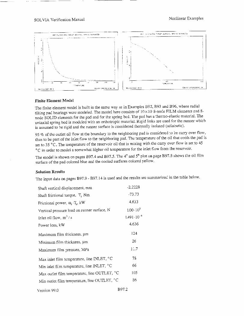
SOLVIA Verification Manual Nonlinear Examples
a91 T T THUDSI 3LG:,PTT, -- StNI S"P -ED P [ S91 T N-1- - T.3-9 !IS -1N 0F'3G 9R'
I ,~
-C E3%I EýIT CC!
Finite Element Model
The finite element model is built in the same way as in Examples B92, B93 and B96, where radial
tilting pad bearings were modeled. The model here consists of 10 x 10 8-node FILM elements and 8
node SOLID elements for the pad and for the spring bed. The pad has a thermo-elastic material. The
uniaxial spring bed is modeled with an orthotropic material. Rigid links are used for the runner which
is assumed to be rigid and the runner surface is considered thermally isolated (adiabatic).
95 % of the outlet oil flow at the boundary to the neighboring pad is considered to be carry over flow,
thus to be part of the inlet flow to the neighboring pad. The temperature of the oil that cools the pad is
set to 35 'C. The temperature of the reservoir oil that is mixing, with the carry over flow is set to 45
'C in order to model a somewhat higher oil temperature for the inlet flow from the reservoir.
The model is shown on pages B97.4 and B97.5. The 4" and 5"' plot on page B97.5 shows the oil film
surface of the pad colored blue and the cooled surfaces colored yellow.
Solution Results
The input data on pages B97.9 - B97.14 is used and the results are summarized in the table below.
Shaft vertical displacement, mm -2.2228
Shaft frictional torque, T, Nm -73.73
Frictional power, co,, -Ti, kW 4.633
Vertical pressure load on runner surface, N 1.00.105
Inlet oil flow, M 3 /.S 1.491.10.
Power loss, kW 4.636
Maximum film thickness, ýtm 124
Minimum film thickness, atm 26
Maximum film pressure, MPa 11.7
Max inlet film temperature. line INLET, 'C 78
Min inlet film temperature, line INLET, 'C 66
Max outlet film temperature, line OUTLET, aC 105
Min outlet film temperature. line OUTLET, 'C 86
Verstion 99.0ults.
B97.2Version 99.0
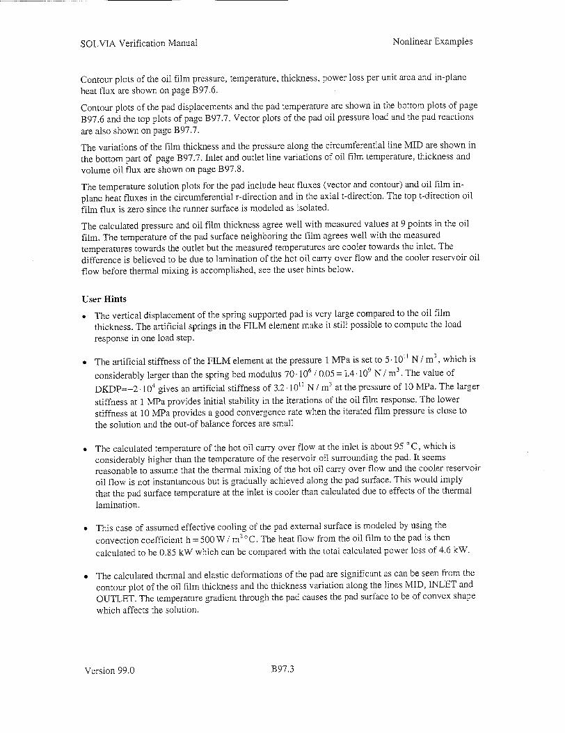
SOLVIA Verification Manual
Contour plots of the oil film pressure, temperature, thickness, power loss per unit area and in-plane
heat flux are shown on page B97.6.
Contour plots of the pad displacements and the pad temperature are shown in the bottom plots of page
B97.6 and the top plots of page B97.7. Vector plots of the pad oil pressure load and the pad reactions
are also shown on page B97.7.
The variations of the film thickness and the pressure along the circumferential line MID are shown in
the bottom part of page B97.7. Inlet and outlet line variations of oil film temperature, thickness and
volume oil flux are shown on page B97.8.
The temperature solution plots for the pad include heat fluxes (vector and contour) and oil film in
plane heat fluxes in the circumferential r-direction and in the axial t-direction. The top t-direction oil
film flux is zero since the runner surface is modeled as isolated.
The calculated pressure and oil film thickness agree well with measured values at 9 points in the oil
film. The temperature of the pad surface neighboring the film agrees well with the measured
temperatures towards the outlet but the measured temperatures are cooler towards the inlet. The
difference is believed to be due to lamination of the hot oil carry over flow and the cooler reservoir oil
flow before thermal mixing is accomplished, see the user hints below.
User Hints
"* The vertical displacement of the spring supported pad is very large compared to the oil film
thickness. The artificial springs in the FILM element make it still possible to compute the load
response in one load step.
" The artificial stiffness of the FILM element at the pressure 1 MPa is set to 5-1011 N / M 3 , which is
considerably larger than the spring bed modulus 70.106 /0.05 = 1.4. 10 N / M 3 . The value of
DKDP=-2 -104 gives an artificial stiffness of 3.2 .101 N / m3 at the pressure of 10 MPa. The larger
stiffness at 1 MPa provides initial stability in the iterations of the oil film response. The lower
stiffness at 10 MPa provides a good convergence rate when the iterated film pressure is close to
the solution and the out-of balance forces are small
" The calculated temperature of the hot oil carry over flow at the inlet is about 95 'C, which is
considerably higher than the temperature of the reservoir oil surrounding the pad. It seems
reasonable to assume that the thermal mixing of the hot oil carry over flow and the cooler reservoir
oil flow is not instantaneous but is gradually achieved along the pad surface. This would imply
that the pad surface temperature at the inlet is cooler than calculated due to effects of the thermal
lamination.
"* This case of assumed effective cooling of the pad external surface is modeled by using the
convection coefficient h = 500 W / m2 °C. The heat flow from the oil film to the pad is then
calculated to be 0.85 kW which can be compared with the total calculated power loss of 4.6 kW.
" The calculated thermal and elastic deformations of the pad are significant as can be seen from the
contour plot of the oil film thickness and the thickness variation along the lines MID, INLET and
OUTLET. The temperature gradient through the pad causes the pad surface to be of convex shape
which affects the solution.
Version 99.0
Nonlinear Examples
B97.3

SOLVIA Verification Manual
bed
x
B97 TILTING-PAD THRUST BEAP:NG SPRING SUPPORTED
OLVIA-PRE 99.0 SOLVIA ENG-NI RiNG AB
Version 99.0
ORIGINAL z
x -, y
22
32
!.42
Nonlinear Examples
B97.4

1/� /M' j ��,1/
'II
/
04 0
F
'4
V
4 4
44 � 4 4
r 4 4 4 4
I 4�4� 4 4
F � �
4 � 4* 4 4 4
4 4* 4 2 j
4 4 4
1�
/ 7
C/) 0
CD
CD
0
CD

q)
0
'a301 00
-5 :0 0 cO
:0 0 C-' C)
S 0 Co
;3�31 �r
K"
r
�'0
NY
K'/
/-3
N, K
CD
0
U)

r.E
a0
0
CI/)
ON
ON
0 0
�I)
/
II
I ,--T .

04
ci
0 -s
0 z1
u
I-i
I�j
jip1�Ž
i
I -
IC)
sZ SI S
5111111'S '111151 CI TIll PC
�-½� 'CrZ
�ŽC'-CC'C' --- C CCC
a; -
0 ON ON 0 0 Cd)
C)
00
C-: ON

SOLVIA Verification Manual
SOLVIA-PRE input
HEADING 'B97 TILTING-PAD THRUST BEARING, SPRING SUPPORTED' *
DATABASE CREATE MASTER TEMPERATURE=COUPLED TOLERANCES TYPE=F RTOL=lE-3 RNORM=1.E5 ITEMAX=100 T-ITERATION TTOL=10. SET EPS=1.E-6 PARAMETERS $TRES=45 $TPAD=35 $FLOW=0.95
PARAMETERS $KNORM=5E11 $PNORM=IE6 $DKDP=-2E4
PARAMETER $MAT=2 $TINIT=70 $H=500 PRINTOUT MIN *
SYSTEM 1 CYLINDRICAL THETA=-90.0 COORDINATES ENTRIES NODE R THETA XL
1 0.475 -10.4 0.06012 2 0.475 13.5 0.06012 3 0.3125 13.5 0.06012
4 0.3125 -10.4 0.06012 5 0. 0. 0.06012
11 0.475 -10.4 0.060 12 0.475 13.5 0.060 13 0.3125 13.5 0.060 14 0.3125 -10.4 0.060
21 0.475 -10.4 0.030 22 0.475 14.6 0.030 23 0.3125 14.6 0.030 24 0.3125 -10.4 0.030 25 0.475 -14.6 0.030 26 0.3125 -14.6 0.030 27 0.475 0.0 0.030 28 0.3125 0.0 0.030
31 0.475 -10.4 0.0 32 0.475 14.6 0.0 33 0.3125 14.6 0.0 34 0.3125 -10.4 0.0 35 0.475 -14.6 0.0 36 0.3125 -14.6 0.0
41 0.475 -10.4 -0.050 42 0.475 14.6 -0.050 43 0.3125 14.6 -0.050 44 0.3125 -10.4 -0.050 45 0.475 -14.6 -0.050
46 0.3125 -14.6 -0.050
51 0.4 20.0 0.062
* Pad material
MATERIAL 1 THERMO-ELASTIC TREF=20 -1000 2.06EII 0.3 12.E-6 5000 2.06E11 0.3 12.E-6
T-MATERIAL 1 TEMP-CONDUCTION -1000 45 3.588E6 5000 45 3.588E6
* Spring bed material
MATERIAL 3 ORTHOTROPIC EA=IE3 EB=1E3 EC=70E6 GAB=IE3 GAC=1E3 GBC=1E3
Version 99.0
Nonlinear Examples
1397.9

SOLVIA Verification Manual
SOLVIA-PRE input (cont.)
T-MATERIAL 3 TEMP-CONDUCTION -1000 1. I.E6 5000 1. l.E6
T-MATERIAL 4 CONVECTION H=$H
* Oil material READ B97ISOVG68.DAT
* Oil film
EGROUP 1 FILM MATERIAL=$MAT SET SYSTEM=l NODES=8
GVOLUME 1 2 3 4 11 12 13 14 EL1=10 EL2-10 EL3=1
FILMVELOCITY INPUT=SURFACE OMEGA=62.831853, AX=- AY=C AZ=- BX=- BY=C BZ=-1. KNORM=$KNORM PNORM=$PNORM DKDP=$DKDP
1 2 3 4
LINE CYLINDRICAL 22 27 EL=6 LINE CYLINDRICAL 27 21 EL=4 LINE COMBINE 22 21 27 LINE CYLINDRICAL 23 28 EL=6 LINE CYLINDRICAL 28 24 EL=4 LINE COMBINE 23 24 28
* Pad EGROUP 2 SOLID MATERIAL=l GVOLUME 11 12 13 14 21 22 23 24 EL2=10 EL3=2 GVOLUME 21 22 23 24 31 32 33 34 EL3=2 GVOLUME 21 24 26 25 31 34 36 35 EL2=2
* Spring bed EGROUP 3 SOLID MATERIAL=3 GVOLUME 31 32 33 34 41 42 43 44 GVOLUME 35 31 34 36 45 41 44 46 AXES-ORTHOTROPIC 1 NODI=31 NODJ=32 NODK=33 .
T-INITIAL TEMPERATURE TREF=$TINIT
* Reservoir oil temperature at node 51
T-LOADS TEMPERATURE 51 $TRES
* Constrained inlet film temperature T-FILMCONSTRAINT INPUT=LINE M-INPUT=LINE RESERVOIRNODE=51
.FACTOR=CARRYOVERFLOW * snl sn2 mnl mn2 factor
2 3 1 4 SFLOW
* Spring bed boundaries FIXBOUNDARIES DIR=123 INPUT=SURFACE
41 42 43 44 45 41 44 46
* Boundaries for pad pivot nodes
FIXBOUNDARIES DIR=i / 28 27 FIXBOUNDARIES DIR=2 / 28
* Film element pressure boundaries FIXBOUNDARIES DIR=FILMPRESSURE INPUT=LINE 12 / 23 / 34 / 41
Nonlinear Examples
Version 99.0 B97.10

SOLVIA Verification Manual
SOLVIA-PRE input (cont.)
* Cooling of external pad surfaces T-BOUNDARIES SEGMENTS CON-MATERIAL=4 INPUT=SURFACE
31 32 33 34 35 31 34 36 25 35 36 26 21 25 26 24 11 21 24 14 22 12 13 23 32 22 23 33 14 13 23 24 24 23 33 34 26 24 34 36 12 11 21 22 22 21 31 32 21 25 35 31
T-LOADS ENVIRONMENT CONVECTION=YES INPUT=SURFACE 31 32 33 34 $TPAD 35 31 34 36 $TPAD 25 35 36 26 $TPAD 21 25 26 24 $TPAD 11 21 24 14 $TPAD 22 12 13 23 $TPAD 32 22 23 33 STPAD 14 13 23 24 $TPAD 24 23 33 34 $TPAD 26 24 34 36 $TPAD 12 11 21 22 $TPAD 22 21 31 32 STPAD 21 25 35 31 $TPAD
* Rotor load LOADS CONCENTRATED * node dir fac
5 3 -100.E3 RIGIDLINK INPUT=SURFACE * nl n2 n3 n4 master
1 2 3 4 5 FIXBOUNDARIES 12456 INPUT=NODE / 5 ,
SOLVIA
SET NNUMBER=MYNODES NSYMBOL=MYNODES COLOR EFILL=GROUP MESH MESH EGi CONTOUR=THICKNESS MESH EG3 BCODE=ALL COLOR EFILL=CON-MATERIAL MESH EG2 VIEW=I BCODE=ALL MESH EG2 VIEW=-I BCODE=ALL MESH RIGIDLINK BCODE=ALL VIEW=I COLOR LINE MESH FILM VIEW=Z EAXES=RST MESH FILM ENUMBER=YES MESH FILM NNUMBER=Y NSYMBOL=YES END
Version 99.0
Nonlinear Examples
B97.11

SOLVIA Verification Manual
SOLVIA-PRE read file B971SOVG68.DAT
"* ISOVG68 OIL "* Discretization from cSt-curve assuming constant density=880 Kg/m3 "* Extrapolation above 110 degrees C
MATERIAL $MAT OIL DENSITY=880 PRESSURE-FACTOR=2.7E-8 * temperature viscosity pressure
10. 0.4000 15. 0.2700 20. 0.1900 25. 0.1400 30. 0.1000 35. 0.0790 40. 0.0610 45. 0.0460 50. 0.0380 55. 0.0310 60. 0.0260 65. 0.0210 70. 0.0180 75. 0.0150 80. 0.0130 85. 0.0115 90. 0.0100 95. 0.0088
100. 0.0077 105. 0 .0070 110. 0 .0063 120. 0.0051 130. 0.0044 140. 0.0037 150. 0.0032
END DATA *
T-MATERIAL $MAT TEMP-CONDUCTION * temperature conductivity specific heat
10. 0.145 1.71E6 150. 0.133 1.71E6
END DATA
Version 99.0
Nonlinear Examples
B97.12

SOLVIA Verification Manual Nonlinear Examples
SOLVIA-POST input
* B97 TILTING-PAD THRUST BEARING, SPRING SUPPORTED
*
DATABASE CREATE
WRITE 'b97.1is'
COLOR EFILL GROUP
SET ZONE=FILM OUTLINE=YES
MESH CONTOUR=FILMPRESSURE VECTOR=FILMFLOW
MESH CONTOUR=FILMTEMPERATURE
MESH CONTOUR=FILMTHICKNESS
MESH CONTOUR=FILMPOWERLOSS
MESH CONTOUR=FILMFLUX VECTOR=FILMFLUX *
SET.ZONE=SOLID MESH CONTOUR=DISP VIEW=I
SET ZONE=EG2
MESH CONTOUR=DX
MESH CONTOUR=DY
MESH CONTOUR=DZ
MESH CONTOUR=TEMPERATURE *
SET ZONE=SOLID
MESH VECTOR=LOAD
MESH VECTOR=REACTION VIEW=-I *
SET ZONE=EGi
EPLINE MID
50 2 4 TO 41 2 4
MESH PLINES=MID VIEW=Z
ELINE MID KIND=FILMTHICKNESS SYMBOL=1
ELINE MID KIND=FILMPRESSURE SYMBOL=1
EPLINE INLET
100 1 2 STEP 10 TO 10 1 2
EPLINE OUTLET
91 3 4 STEP 10 TO 1 3 4
DELETE EPLINE MID
MESH PLINES=ALL *
AXIS 1 VMIN=48 VMAX=110 LABEL='FILMTEMPERATURE'
AXIS 2 VMIN=0 VMAX=0.18 LABEL='INLET (symbols) and OUTLET'
AXIS 3 VMIN=0 VMAX=2E-3 LABEL='FILM FLUX IN CIRCUMFERENTIAL DIRECTION'
AXIS 4 VMIN=0 VMAX=130E-6 LABEL='FILM THICKNESS'
ELINE INLET KIND=FILMTEMPERATURE YAXIS=* XAXIS=2 SYMBOL=1
ELINE OUTLET KIND=FILMTEMPERATURE YAXIS=1 XAXIS=2 SUBFRAME=OLD
ELINE INLET KIND=FILMTHICK YAXIST 4 XAXIS=2 SYMBOL=X
ELINE OUTLET KIND=FILMTHICK YAXIS=4 XAXIS*2 SUBFRAME=OLD
ELINE INLET KIND=FILMFLUXR YAXIS=3 XAXIS=2 SYMBOL=U
ELINE OUTLET KIND=FILMFLUXR YAXIS=3 XAXIS=2 SUBFRAME=OLD
Version 99.0 B97.13
Nonlinear ExamplesSOLVIA Verification Manual
SOLVIA-POST input (cont.)
SUMMATION ZONENAME=FILM KIND=)
SUMMATION ZONENAME=FILM KIND=
ZONE INLET INPUT=NODES
2 110 TO 118 3
ZONE OUTLET INPUT=NODES
1 128 TO 136 4
SUMMATION ZONENAME=FILM KIN]
SUMMATION ZONENAME=INLET KIN]
SUMMATION ZONENAME=OUTLET KIN]
SUMMATION ZONENAME=SOLID KIN]
SUMMATION ZONENAME=SOLID KINI
NLIST N5
NLIST N5 KIND=REACTION
EMAX FILM
EMAX FILM SELECT=FILM
EMAX FILM SELECT=FILM TYPE=MIN
TOLERANCES INTERMEDIATE=YES
FILMPOWERLOSS FILMPRESSURE
D=FILMFLOW D=FILMFLOW
D=FILMFLOW
D=LOAD
D=REACTION
DETAILS=YES DETAILS=YES
T-DATABASE CREATE
MESH EG2 CONTOUR=TFLUX VECTOR=TFLUX VIEW=I
MESH EG2 CONTOUR=TFLUX VECTOR=TFLUX VIEW=-I
SET ZONE=FILM VIEW=Z
MESH CONTOUR=FILMTRFLUX
MESH CONTOUR=FILMTSFLUX
MESH CONTOUR=FILMTTOPFLUX
MESH CONTOUR=FILMTBOTFLUX *
SUMMATION FILM KIND=FILMTFLUX
ELIST E1+1 SELECT=BASICS
END
Version 99.0 B97.14
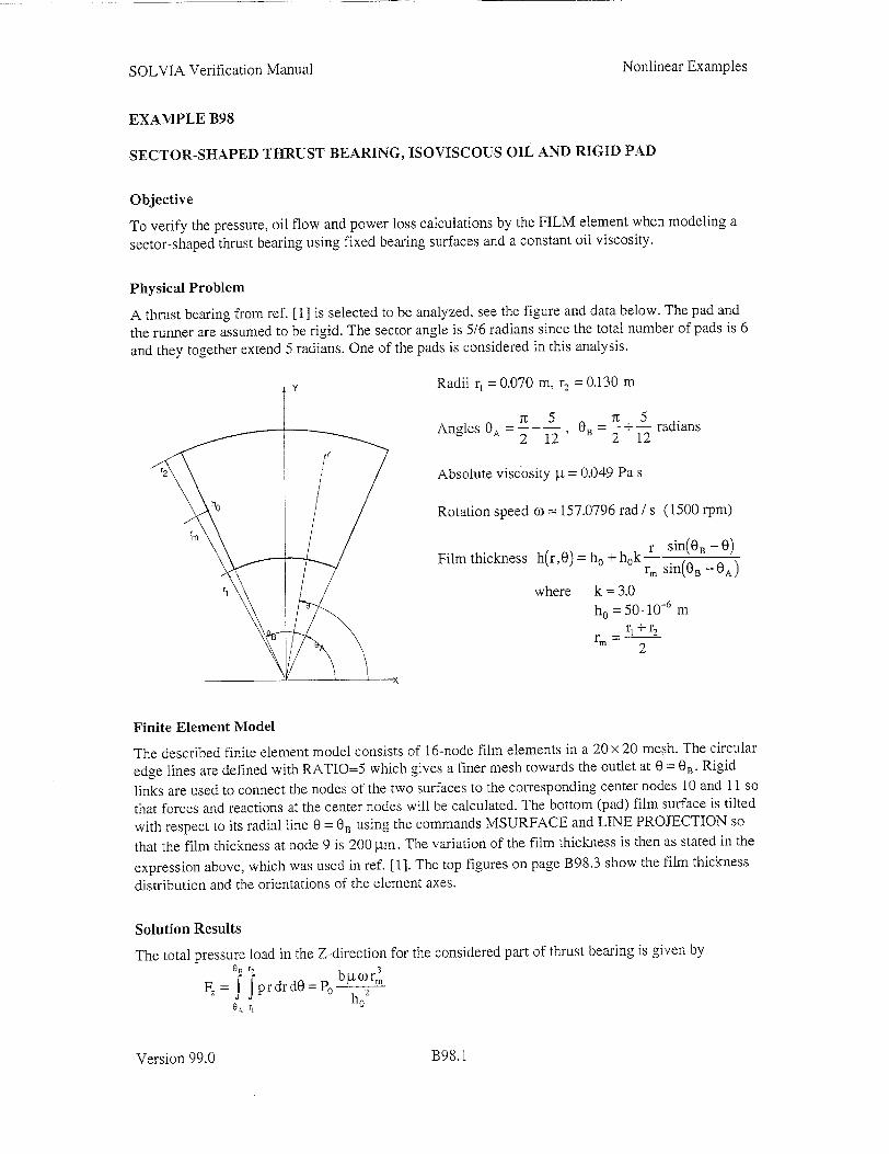
SOLVIA Verification Manual
EXAMPLE B98
SECTOR-SHAPED THRUST BEARING, ISOVISCOUS OIL AND RIGID PAD
Objective
To verify the pressure, oil flow and power loss calculations by the FILM element when modeling a
sector-shaped thrust bearing using fixed bearing surfaces and a constant oil viscosity.
Physical Problem
A thrust bearing from ref. [1I is selected to be analyzed, see the figure and data below. The pad and
the runner are assumed to be rigid. The sector angle is 5/6 radians since the total number of pads is 6
and they together extend 5 radians. One of the pads is considered in this analysis.
Radii rj = 0.070 m, r2 = 0.130 m
Tu 5 T1
Anles B =- + - radians 0 2 12 2 12
2 Absolute viscosity p. = 0.049 Pa s
Rotation speed co = 157.0796 rad / s (1500 rpm)
Film thickness h(r,0)= h0 +h0k r sin(B - 0)
r/rm sin(oB - 0A) where k = 3.0
h0 = 50-10-6 m
1 r r1 +r 2 2
Finite Element Model
The described finite element model consists of 16-node film elements in a 20 x 20 mesh. The circular
edge lines are defined with RATIO=5 which gives a finer mesh towards the outlet at 0 = OB. Rigid
links are used to connect the nodes of the two surfaces to the corresponding center nodes 10 and 11 so
that forces and reactions at the center nodes will be calculated. The bottom (pad) film surface is tilted
with respect to its radial line 0 = 0 B using the commands MSURFACE and LINE PROJECTION so
that the film thickness at node 9 is 200 4tm. The variation of the film thickness is then as stated in the
expression above, which was used in ref. [1]. The top figures on page B98.3 show the film thickness
distribution and the orientations of the element axes.
Solution Results
The total pressure load in the Z-direction for the considered part of thrust bearing is given by 0a, rý3
F, J f prdrdO =Po
OAr, h °
2
Version 99.0
Nonlinear Examples
B98.1
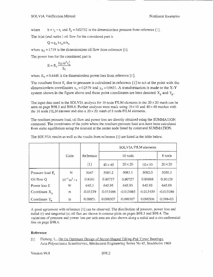
SOLVIA Verification Manual
where b = r2 - r1 and P0 = 0.02732 is the dimensionless pressure from reference [I].
The inlet (and outlet ) oil flow for the considered part is
Q = q0 brO)h0
where q 0 = 1.719 is the dimensionless oil flow from reference [1].
The power loss for the considered part is
E = Eo b ho r3
where E0 = 0.4448 is the dimensionless power loss from reference [11].
The resultant force F, due to pressure is calculated in reference [1] to act at the point with the
dimensionless coordinates x0 = 0.2579 and y0 = 0.9631. A transformation is made to the X-Y
system shown in the figure above and these point coordinates are here denoted Xp and Yp.
The input data used in the SOLVIA analysis for 16 node FILM elements in the 20 x 20 mesh can be seen on page B98.5 and B98.6. Further analyses were made using 10 x 10 and 40 x 40 meshes with the 16 node FILM element and also a 20 x 20 mesh of 8 node FILM elements.
The resultant pressure load, oil flow and power loss are directly obtained using the SUMMATION command. The coordinates of the point where the resultant pressure load acts have been calculated from static equilibrium using the moment at the center node listed by command SUMMATION.
The SOLVIA results as well as the results from reference [I] are listed in the table below.
SOLVIA FILM elements
Units Reference 16 node 8 node
[1] 40x40 20x20 1OxlO 20x20
Pressure load F. N 5047 5083.2 5083.1 5082.0 5050.3
Oil flow Q 10-4m 3 / S 0.8101 0.80757 0.80727 0.80608 0.80158
Power loss E W 645.3 645.95 645.95 645.93 645.09
Coordinate Xp m -0.01539 -0.015466 -0.015465 -0.015459 -0.015386
Coordinate YP m 0.09851 0.098507 0.098507 0.098506 0.098483
A good agreement with reference [1] can be observed. The distribution of pressure, power loss and radial (r) and tangential (s) oil flux are shown in contour plots on pages B98.3 and B98.4. The variations of pressure and power loss per unit area are also shown along a radial and a circumferential line on page B98.4.
Reference
[1] Floberg, L., On the Optimum Design of Sector-Shaped Tilting-Pad Thrust Bearings, Acta Polytechnica Scandinavica, Mechanical Engineering Series No 45, Stockholm 1969
Version 99.0
Nonlinear Examples
B98.2

0
CD
'C-�44�� / 0
0 0 0 0 0 0 000000 0 0
(000 o0 [0
4(2 - 0)0�( .NN C) z . NA Co N0�-G)(n)00W
� O)CC)0GIO)Ot. ,)C0 >NNO(0U(0 (0 :0nmmnOPiP( :0
A0
0 0 0 0 00 0 -) 0 0 0 0 0
1� C', :000
r 0
I!C/)
C'D
0I
CD 0n

0
C)
td ýo
FILI

SOLVIA Verification Manual Nonlinear Examples
SOLVIA-PRE input
HEADING 'B98 SECTOR-SHAPED THRUST BEARING, ISOVISCOUS OIL AND RIGID PAD'
DATABASE CREATE
PARAMETER $Ri=0.070 $R2=
PARAMETER $FIB=I13.8732
SET EPS=i.E-6 SYSTEM 1 CYLINDRICAL
COORDINATES / ENTRIES
1 $R1 SFIB $HO /
3 $R2 $FIA SHO /
5 $RI $FIB 0. / 7 $R2 $FIA 0. / 9 $RM $FIA $Hi /
11 0. 0. SHO
SET MIDNODES=I
LINE CYLINDRICAL
LINE CYLINDRICAL LINE CYLINDRICAL
LINE CYLINDRICAL
MSURFACE 1 PLANE
LINE PROJECTION
LINE PROJECTION
MATERIAL 1 OIL
-1000. 0.049 1000. 0.049
SET NODES=16
N1=i N1=5
N1=4 Ni=8
0.130 $RM=0.100 $FIA=66.1268 $HO=-50E-6 $Hi=-200E-6
AZ=I. BX=1.
NODE R THETA XL
2 $R1 $FIA $HO
4 $R2 $FIB $HO
6 $R1 $FIA 0.
8 $R2 $FIB 0.
10 0. 0. 0.
N2=2 N2=6 N2=3 N2 =7
EL=20
EL=20
EL=20 EL=20
RATIO=5 RATIO=5 RATIO=5
RATIO=5
NI=i N2=4 N3-9
NI=1 N2=2 TARGETSURFACE=i ZDIR=I.
NI=3 N2=4 TARGETSURFACE=i ZDIR=I.
DENSITY=900.
EGROUP 1 FILM MATERIAL=1 RSINT=2
GVOLUME 8 5 6 7 4 1 2 3 ELI=20 EL2=20 EL3=1
FILMVELOCITY INPUT=SURFACE OMEGA=-57.0796 BZ=I.0
8567
INITIAL TEMPERATURE TREF=60.
LOADS TEMPERATURE TREF=60.
RIGIDLINKS INPUT=SURFACE M-INPUT=NODE
4 1 2 3 1i
8 5 6 7 10
LOADS DISPLACEMENTS
i0 i 0. /10 2 0. /10 3 0. /i0 4 0. /i0 5 0. /10 6 0.
ii 0. /11 2 0. /11 3 0. /i1 4 0. /i1 5 0. / ii6 0.
FIXBOUNDARIES DIRECTION=FILM-PRESSURE INPUT=LINE
12 / 23 / 34 / 41
SOLVIA
SET PLOTORIENTATION=PORTRAIT NNUMBERS=MY NSYMBOLS=MY VIEW=Z
MESH CONTOUR=THICKNESS
MESH FILM EAXES=RST
END
Version 99,0 B98.5

SOLVIA Verification Manual
SOLVIA-POST input
* B98 SECTORSHAPED THRUST BEARING, ISOVISCOUS OIL AND RIGID PAD
DATABASE CREATE
WRITE 'b98.lis'
SET DIAGRAM=GRID OUTLINE=YES VIEW=Z ZONE=FILM
MESH
MESH MESH
MESH
CONTOUR=FILMPRESSURE
CONTOUR=FILMRFLUX VECTOR=FILMFLOW
CONTOUR=FILMSFLUX VECTOR=FILMFLOW
CONTOUR=FILMPOWERLOSS
EPLINE CIRCLE
9 2 1 STEP 20 TO 389 2 1
EPLINE RADIUS
260 1 3 TO 241 1 3
MESH PLINE=ALL
ELINE RADIUS KIND=FILMPRESSURE
ELINE RADIUS KIND=FILMPOWERLOSS
ELINE CIRCLE KIND=FILMPRESSURE
ELINE CIRCLE KIND=FILMPOWERLOSS
SUMMATION SUMMATION
SUMMATION ZONE UPPER
ZONE LOWER
SUMMATION SUMMATION
SUMMATION SUMMATION END
KIND=FILMPRESSURE KIND=FILMFLOW
KIND=FILMPOWERLOSS GLOBAL ZMIN=-20E-6
GLOBAL ZMAX=-20E-6
UPPER KIND=LOAD
UPPER KIND=REACTION
LOWER KIND=LOAD
LOWER KIND=REACTION
Version 99.0
Nonlinear Examples
1398.6
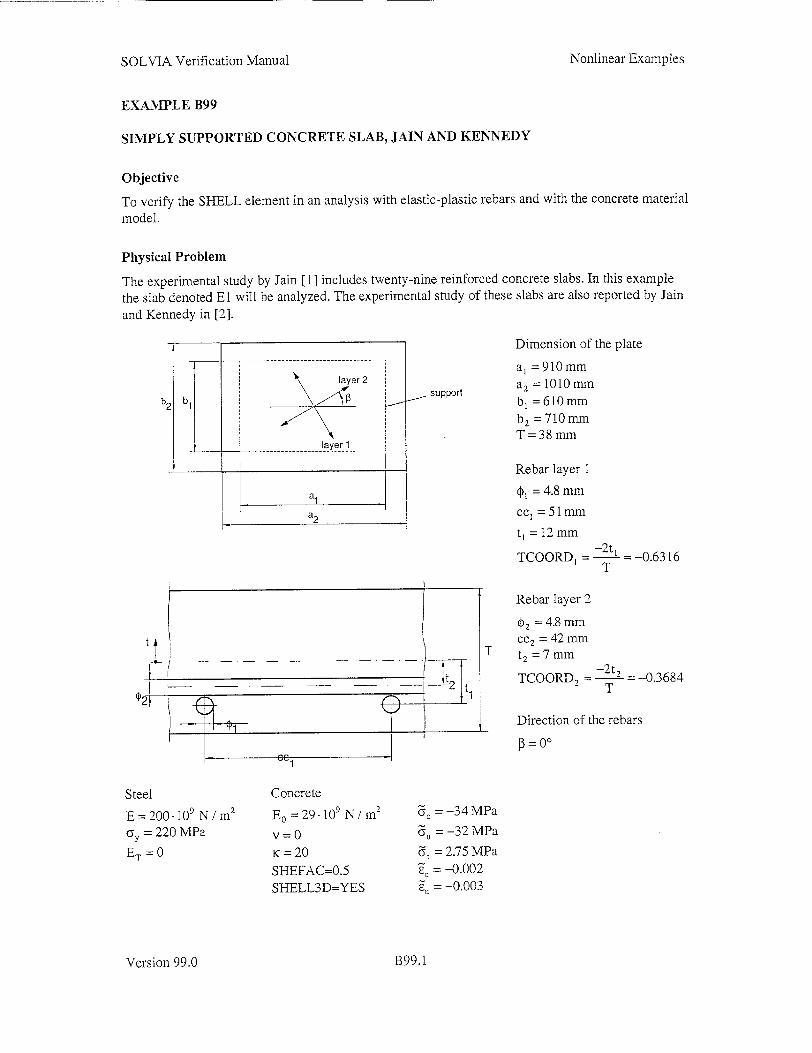
SOLVIA Verification Manual
EXAMPLE B99
SIMPLY SLPPORTED CONCRETE SLAB, JAIN AND KENNEDY
Objective
To verify the SHELL element in an analysis with elastic-plastic rebars and with the concrete material
model.
Physical Problem
The experimental study by Jain [1 I includes twenty-nine reinforced concrete slabs. In this example
the slab denoted El will be analyzed. The experimental study of these slabs are also reported by Jain
and Kennedy in [2].
Dimension of the plate
a, = 910 mm a1 = 1010 mm
2 b1 "- pb, =610 mm
b2 = 710mm T=38mm
----- laye-r 1 -- --
_ _ Rebar layer 1
a1 , = 4.8 mm
a2 cc 1 = 51 mm
t, = 12 mm
TCOORD , = -2t =-0.6316 T
Rebar layer 2
02 = 4.8 mm t A cc 2 = 42 mm
T t, =7mm
---TCOORD --2t 2 -0.3684
Direction of the rebars
P=0c
Steel Concrete
E=200-109 N/rM E0 =29-109 N/I 2 M F =-34MPa
c7 = 220 MPa v=0 . = -32 MPa
ET = 0 K = 20 d, = 2.75 MPa
SHEFAC=0.5 'E = -0.002 SHELL3D=YES su = -0.003
Version 99.0
Nonlinear Examples
B99.1

SOLVIA Verification Manual
Finite Element Model
The finite element model is shown on page B99.3. The 4-node SHELL element is used. Due to symmetry when P3 = 0' only one quarter of the plate needs to be considered. The simply supported boundary conditions are modeled by nonlinear spring elements to allow comer uplifting of the plate. The spring elements have only stiffness in compression. The AUTO-STEP method and BFGS iteration method are used.
Solution Results
The input data to the SOLVIA analysis can be found on pages B99.6 - B99.8. The calculated load deflection curve is shown on page B99.3 together with the experimental results. The experimental curves are drawn without symbols. A good agreement can be observed.
Contour plots of the results at the last load step are shown on pages B99.3 - B99.5. The principal moments, maximum and minimum, are shown on page B99.3. Contour plots of the maximum principal stress at the bottom and top surfaces are shown on pages B99.3 - B99.4. The concrete crack state at the bottom, mid and top surfaces are shown on page B99.4. The contour plots of stress, strain and accumulated plastic strain in the rebars are shown on pages B99.4 and B99.5. The rebar results are displayed without nodal averaging.
History plots of the stress in the rebars of the center element 144, point 1, show that rebar layer 2 reaches the plastic state before rebar layer 1.
In case B99A the only input data change compared to B99 is that the material parameter SHELL3D=NO. The calculated load - deflection curve for case B99A can be seen on page B99.5 to be very close to the curve for case B99.
In case B99B the only input data change compared to B99 is that the material parameter cut-off tensile stress is reduced from 2.75 MPa to 1.5 MPa and the calculated load - deflection curve is shown on page B99.5. The ultimate load when dt = 1.5 MPa is close to the ultimate load when
a, = 2.75 MPa but larger deflections occur during the loading phase.
Reference
[1] Jain, S. C., "Ultimate Strength and Behavior in Reinforced Concrete Slabs," thesis presented to the University of Windsor, at Windsor, Canada, in 1971, in partial fulfillment of the requirements for the degree of Doctor of Philosophy.
[2] Jain, S. C. and Kennedy, J.B., "Yield Criterion for Reinforced Concrete Slabs", Journal of the Structural Division, ASCE, Vol. 100, No. ST3, March 1974.
User hint
When SHELL3D=YES is specified for the concrete material of SHELL elements with midsurface nodes then no strain occurs in the thickness direction except for possible thermal strain. This is equivalent to rigid stirrups so direct stresses 7, in the thickness direction of the concrete can
develop. The capability to accommodate inclined principal compressive stresses in the concrete due to out-of-plane shear improves. In this particular example with v = 0 and mainly plate bending the influence of the value of the SHELL3D parameter on the load - deflection curve can be seen to be small.
Version 99.0
Nonlinear Examples
B99.2

A:
j3 i
UN C) ON
f-I-I
0 C) 0
0 0 z
C) 0 C) C)
C) 0
C) 0
C)
0 CO
-K
2 j
,-,UI� �Cr�
'K
V
K,Ii
Io CO ON ON
C•
C)
.2-

'9
A
V)
0
z
cC7
CIO
2<
12
A6K 2
�ri -;-�
A
22 2 2
2 2 2 2
NC� '2� N
N �N�'N N
N.
N N NA N, N
N C N N N
NN N
N' NN N\ N N'
N �\ N N
¾ ,'� 'N N'� NC,/
N N
N4 N 2
N
'<'C V 0 cn
-K r
A
-t
W7
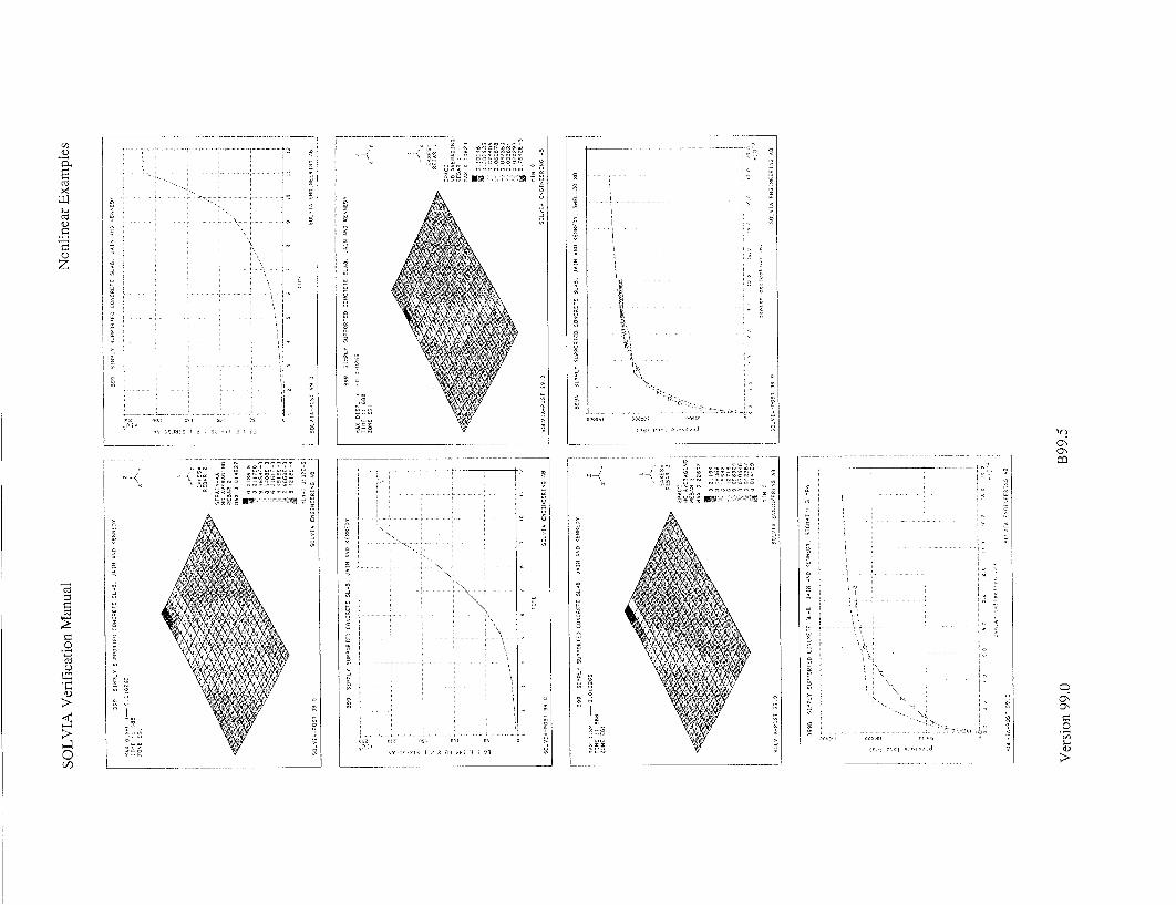
F "K2
II
ON
0
0
0 z
I 0 0 0 U
1�
II�)
0 rJ)
N
ON ON 0 0
A 0;

SOLVIA Verification Manual Nonlinear Examples
SOLVIA-PRE input
HEADING 'B99 SIMPLY SUPPORTED CONCRETE SLAB, JAIN AND KENNEDY
DATABASE CREATE
MASTER NSTEP=100
AUTO-STEP DTMAX=1 TMAX=20 ITELOW=5 ITEHIGH=i5 DISPMAX=0.010
TOLERANCES TYPE=F RNORM=1000 RMNORM=1000 RTOL=0.1 ITEMAX=50
SET MYNODES=200 *
TIMEFUNCTION 1
0 0 / 20 200000
COORDINATES
ENTRIES NODE X Y Z
1 0.455 0.305 0. TO
13 0. 0.305 0. TO
25 0. 0. 0. TO
37 0.455 0. 0. TO
49 0.455 0.305 0.
51 0. 0.355 0.
52 0.455 0.355 0.
53 0.505 0.355 0.
54 0.505 0.305 0.
55 0.505 0. 0.
101 0.455 0.305 -0.020 TO
113 0. 0.305 -0.020
137 0.455 0. -0.020 TO
149 0.455 0.305 -0.020
DELETE 49 149 1
REBAR-LAYER 1 D=0.0048 CC=0.051 TCOOR=-0.6316 PSI=0. REBAR-LAYER 2 D-0.0048 CC-0.042 TCOOR=-0-3684 PSI=90.
MATERIAL 1 CONCRETE EQ=29.E9 NU=0.0 SIGMAT=2.75E6,
SIGMAC=-34.E6 EPSC=-0.002 SIGMAU=-32.E6 EPSU=-0.003,
BETA=0.75 KAPPA=20 STIFAC=0.0001 SHEFAC=0.5 SHELL3D=YES
MATERIAL 2 PLASTIC E=200.E9 YIELD=220.E6 ET=0.
EGROUP 1 SHELL STRESSREFERENCE=ELEMENT TINT=6 MATERIAL=1 REBARMATERIAL=2
THICKNESS 1 0.038
GSURFACE 1 13 25 37 EL1=12 EL2=12 NODES=4
GSURFACE 52 51 13 1 EL1=12 EL2=2 NODES=4
GSURFACE 53 52 1 54 EL1=2 EL2=2 NODES=4
GSURFACE 54 1 37 55 ELi=2 EL2=12 NODES=4
LAYER-SECTION 1 TREF=0. 1 2
LOADS ELEMENT INPUT=SURFACE
1 13 25 37 t 1.0
EDATA
ENTRIES EL NTH BETA
1 1 0. TO
196 1 0.
Version 99.0 B99.6
SOLVIA Verification Manual
SOLVIA-PRE input (cont.)
FIXBOUNDARIES 156 INPUT=LINE / 25 13 / 13 51
FIXBOUNDARIES 246 INPUT=LINE / 25 37 / 37 55
FIXBOUNDARIES / 101 TO 148
EGROUP 2 SPRING DIRECTION=AXIALTRANSLATION ENODES
1 1 101 TO
13 13 113
14 37 137 TO
25 48 148 *
PROPERTYSET 1 K=TABLE
DISP-FORCE / 1 1 / IE-20 1 / -1 -IE9
PROPERTYSET 2 K=TABLE
DISP-FORCE / 1 3 / 1E-20 3 / -1 -2E9
EDATA
ENTRIES EL PROPERTYSET 13 1 / 14 1
1 2 TO 12 2
15 2 TO 25 2
MESH SHELL NNUMBERS=MYNODES NSYMBOL=MYNODES BCODE=ALL
MESH SHELL CONTOUR=PRESSURE VECTOR=LOAD
MESH SHELL
COLOR EFILL=GROUP EGROUP 1
MESH E144 ENUMBER=YES GSCALE=OLD SUBFRAME=OLD
MESH SPRING NNUMBERS=MYNODES NSYMBOL=MYNODES BCODE=ALL *
SOLVIA END
Version 99.0
Nonlinear Examples
B99.7
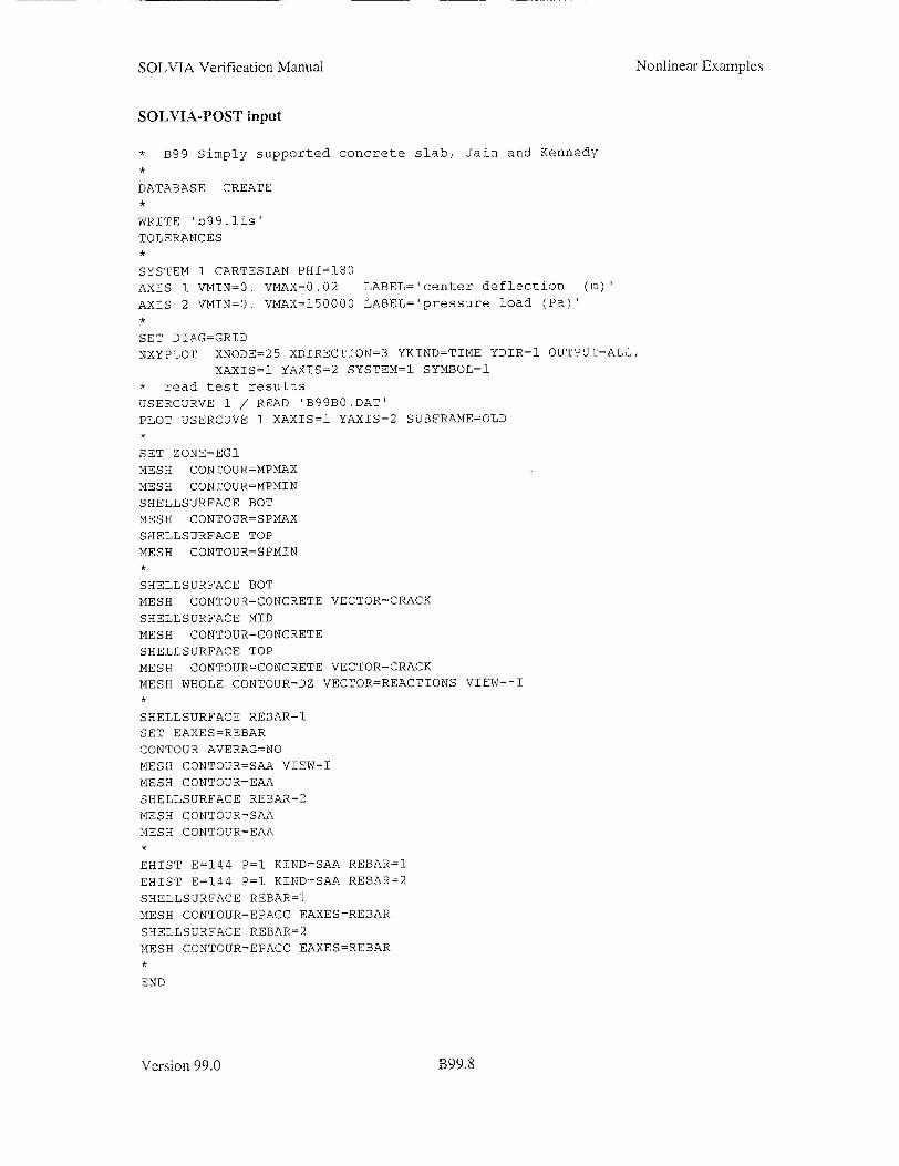
SOLVIA Verification Manual
SOLVIA-POST input
* B99 Simply supported concrete slab, Jain and Kennedy
DATABASE CREATE
WRITE 'b99.lis' TOLERANCES
SYSTEM 1 CARTESIAN PHI=180 AXIS 1 VMIN=0. VMAX=0.02 LABEL=-center deflection (m)'
AXIS 2 VMIN=0. VMAX=l50000 LABEL='pressure load (Pa)'
SET DIAG:GRID NXYPLOT XNODE=25 XDIRECTION=3 YKIND=TIME YDIR=l OUTPUT=ALL,
XAXIS=1 YAXIS=2 SYSTEM=1 SYMBOL=1 * read test results
USERCURVE 1 / READ 'B99B0.DAT' PLOT USERCUVE 1 XAXIS=- YAXIS=2 SUBFRAME=OLD
SET ZONE=EGI MESH CONTOUR=MPMAX MESH CONTOUR=MPMIN SHELLSURFACE BOT MESH CONTOUR=SPMAX SHELLSURFACE TOP MESH CONTOUR=SPMIN
SHELLSURFACE BOT MESH CONTOUR=CONCRETE VECTOR=CRACK SHELLSURFACE MID MESH CONTOUR=CONCRETE SHELLSURFACE TOP MESH CONTOUR=CONCRETE VECTOR=CRACK MESH WHOLE CONTOUR=DZ VECTOR=REACTIONS VIEW=-I ,
SHELLSURFACE REBAR=1 SET EAXES=REBAR CONTOUR AVERAG=NO MESH CONTOUR=SAA VIEW=I MESH CONTOUR=EAA SHELLSURFACE REBAR=2 MESH CONTOUR=SAA MESH CONTOUR=EAA
EHIST E=144 P=* KIND=SAA REBAR=1 EHIST E=144 P=1 KIND=SAA REBAR=2
SHELLSURFACE REBAR=1 MESH CONTOUR=EPACC EAXES=REBAR SHELLSURFACE REBAR=2 MESH CONTOUR=EPACC EAXES=REBAR
END
Version 99.0
Nonlinear Examples
B99.8

SOLVIA Verification Manual
INDEX
Arch circular B45 deep B86 shallow B21 TRUSS B40
Beam, see also Cantilever building frame B22 compressive load effect on frequencies
B71 curved B75, B76, B77 reinforced concrete B19, B79, B80, B81 simply supported B47, B83 temperature gradient B77
Bearings, see FILM element Birth/death option B32, B37 Buckling
imperfections B4, B44 large displacement B3, B87, B88 linearized B43, B45, B46, B50, B87, B88 snap-back B41, B86 snap-through B40, B41, B42, B86 thermal B50
Buoyancy B84 Building, impact load B22 Cable B1O,B51,B58
failure modeling B33 Cantilever
creep B5, B39 curved B75 deformation-dependent load B48 end moment B52 plastic B26, B27, B34 PLATE bending B25, B27 SHELL bending B24, B26 thermal stress B38 torsion B53
Column B46 Complex-harmonic analysis B83 Concrete
beam B19, B79, B80, B81, B91 cylinder B35 material curves B20 slab B91, B99
Contact dynamic B6, B7, B59, B60, B61, B62 friction B58, B59, B82 Hertz axisymmetric B56
Hertz plane strain B57 rubber B82 3-D B59, B62
Coupled displacement-temperature analysis, see FILM element
Creep beam B5, B39 Creep law no. 1 (Bailey-Norton) B63 Creep law no. 2 (primary and secondary)
B64 cylinder B 15 PLANE STRESS2 element B5, B39 thick-walled cylinder B 15
Cyclic loading creep B15 isotropic hardening B8 kinematic hardening B9
Cylinder compound B90 concrete B35 panel B3 thick-walled B13, B14, B15, B35, B49
Damping Rayleigh B83
Dam seepage B67, B68 Deformation dependent loading B48, B84 Excavation B32 FILM element
journal bearing B92, B93, B94, B96 thrust bearing B97, B98 tilting pad B92, B93, B96, B97 slider bearing B95 Sommerfeld B94 rigid pads B92 elastic pads B93, B96, B97 elastic rotor B97
Frame buckling B87, B88 building B22, B33 plastic collapse B72, B73
Frequency analysis B7, B71 Freezing, melting B30, B31, B69 Friction B58, B59, B82 Gap, TRUSS element B6, B7 Geologic material
curve-description B18 Drucker-Prager B23
Version 99.0
Nonlinear Examples
1.1

SOLVIA Verification Manual
Hardening isotropic B8, B54 kinematic B9, B55
Impact load B22, B61 Imperfections B4, B44 Initial strain B10, B51, B76 Latent heat, see Freezing, melting Linearized buckling, see Buckling Mode superposition analysis B7, B47 Mooney-Rivlin material, see Rubber Nonlinear-elastic material B33, B80 Oil film bearing, see FILM element O-ring B82 Orthotropic cylinder B90 Pendulum B2 Phase transition, thermal B30, B31, B69 Pipe whip
direct time integration B6 mode superposition B7
Plastic analysis cantilever bending B26, B27, B34 collapse, limit load B72, B73 multi-linear model B54, B55 spherical cap B36 thick-walled cylinder B 13, B 14, B49 torsion B53
Plate buckling B4, B43, B44, B50 large displacements B 16 stiffened B43, B44 temperature gradient B78
Pre-load axial compressive in beam B71, B83
Prestressing, see Initial strain Ramberg-Osgood material B70 Reinforced concrete, see Concrete Removal, addition of elements B32, B37 Residual stresses B14, B34 Restart
dynamic B47, B71, B83 static B21, B39
Rubber bushing B74 o-ring B82 pure shear B85 sheet BIl
Seepage flow free surface B67, B68 one-dimensional B66
Shell bending PLATE element B25, B27 SHELL element B24, B26
Soil specimen B23 Solidification B30, B31 Space shuttle temperatures B29 Spherical shell B12, B36, B42, B65 Spurious modes B4 Stiffened plate, see Plate Substructures B22 Temperature analysis
stationary B38 transient B28, B29, B30, B31, B69 variable time-step B28
Temperature boundary conditions convection B28 heat flow B29 radiation B28, B29
Temperature gradient load beam B77 plate B78
Thermal stress B14, B17, B38, B50, B90 Tilting pad bearing, see FILM element Torsion B53 TRUSS structures B1, B40, B41 Tunnel B18, B32 ULJ (Updated-Lagrangian-Jaumann)
analysis B48 Unloading/reloading B 13 User-supplied material B70 Water pressure B84 Wave propagation B61
Version 99.0
Nonlinear Examples
1.2

10 State Street, Wohwrn, M'1assachusetts 01801 Stevenson & Associates Tel 617 932 9580 Fax 617 933 4428
A structural-mechanical consulting engineering firm BOSTON-CLL 7E-AND
July 2, 2002
American Electric Power Nuclear Generation Group .. 500 Circle Drive Buchanan, MI 49107
Subject: License for SOLVIA Computer Code
Let this letter serve as a license for American Electric Power Company to use SOLVIA copyrighted verification documentation1 for the purposes of regulatory compliance in answering of questions as posed by the USNRC. This grants American Electric Power the right have a copy of this documentation and to send a copy of the same to the USNRC for their use in the review of the SOLVIA code.
The SOLVIA verification documents transmitted herewith each bear a SOLVIA copyright notice. The NRC is permitted to make the number of copies of the information contained in these reports which are necessary for its internal use in connection with generic and plantspecific reviews and approvals as well as the issuance, denial, amendment, transfer, renewal, modification, suspension, revocation or violation of a license, permit, order, or regulation, copyright protection notwithstanding. The NRC is permitted to make the number of copies beyond those necessary for its internal use which are necessary in order to have one copy available for public viewing in the appropriate docket files in the public document room in Washington, DC and in local public document rooms as may be required by NRC regulations if the number of copies submitted is insufficient for this purpose. Copies made by the NRC must include the copyright notice in all instances.
Stevenson & Associates hereby grants this license as US distributor of the SOLVIA code.
Very truly yoLrs,
W lterDj rdjevic P re '- en
a) SOLVIA Finite Element Program, Version 99.0, SOLVIA Verification Manual Linear
Examples, Report SE 99-4, SOLVIA Engineering AB, 2000. b) SOLVIA Finite Element Program, Version 99.0, SOLVIA Verification Manual Nonlinear Examples, Report SE 99-5, SOLVIA Engineering AB, 2000.

ATTACHMENT 7 TO AEP:NRC:2520
COMMITMENTS
The following table identifies those actions committed to by Indiana Michigan Power Company (I&M) in this document. Any other actions discussed in this submittal represent intended or planned actions by I&M. They are described to the Nuclear Regulatory Commission (NRC) for the NRC's information and are not regulatory commitments.
Commitment Date I&M will revise the ice condenser endwall structural calculation and August 23, 2002 provide the NRC the results of the revised calculation with respect to required rebar yield strength.