Bio

Inin

Di

da

MaDaa Dipb Labc CN

C. R. Biologies 338 (2015) 511–520

A R

Artic

Rece

Acce

Avai

Keyw

Ecos

Ben

Hea

Rive

Self-

Mot

Sant

Ben

Met

Rivi

Cart

*

http

163

diversity/Biodiversite

vertebrate diversity in relation to chemical pollution an Umbrian stream system (Italy)

versite des invertebres en relation avec la pollution chimique

ns un reseau hydrographique d’Ombrie (Italie)

tteo Pallottini a,b,c, Enzo Goretti a,*, Elda Gaino a, Roberta Selvaggi a,vid Cappelletti a, Regis Cereghino b,c

artimento di Chimica, Biologia e Biotecnologie, Universita degli Studi di Perugia, Via Elce Di Sotto, 06123 Perugia, Italy

oratoire « Ecologie fonctionnelle et Environnement », universite de Toulouse, INP, UPS EcoLab, 31062 Toulouse, France

RS, EcoLab (UMR CNRS 5245), 118, route de Narbonne, 31062 Toulouse, France

T I C L E I N F O

le history:

ived 22 December 2014

pted after revision 26 April 2015

lable online 1 June 2015

ords:

ystem health

thos

vy metals

rs

organizing maps

s cles :

e des ecosystemes

thos

aux lourds

eres

es auto-organisatrices

A B S T R A C T

We used self-organizing maps (SOM, neural network) to bring out patterns of benthic

macroinvertebrate diversity in relation to river pollution. Fourteen stations were sampled

over various seasons in the Nestore drainage basin (Central Italy) and characterized for

macroinvertebrate communities, nutrient and heavy metal concentrations. Physicochem-

ical variables were introduced into a SOM previously trained with macroinvertebrate data.

Patterns of communities matched spatial and seasonal changes in environmental

conditions, including water chemistry related to economic activities in the catchment.

Although our analyses did not allow us to establish the specific effect of any given

environmental parameter upon macroinvertebrate community composition based on the

field study, they enabled us to map the ecological health of river ecosystems in a readily

interpretable manner.

� 2015 Academie des sciences. Published by Elsevier Masson SAS. All rights reserved.

R E S U M E

Nous avons utilise les cartes auto-organisatrices (SOM, reseau de neurones) pour degager

des patrons de diversite des macro-invertebres benthiques en relation avec la pollution des

rivieres. Quatorze stations ont ete echantillonnees sur plusieurs saisons dans le bassin du

Nestore (Italie centrale) et caracterisees a partir de leurs communautes d’invertebres, des

concentrations en nutriments et metaux lourds. Les variables physicochimiques ont ete

introduites dans une SOM prealablement etablie sur la base des communautes

d’invertebres. Les patrons de diversite des communautes suivent les changements

spatio-temporels des conditions environnementales, dont ceux de la chimie de l’eau, en

relation avec les activites economiques dans le basin versant. Bien que nos analyses ne

nous aient pas mis en mesure d’etablir l’effet d’un parametre environnemental en

Corresponding author. Dipartimento di Chimica, Biologia e Biotecnologie, Universita degli Studi di Perugia, Via Elce Di Sotto, 06123 Perugia, Italy.

E-mail address: enzo.goretti@unipg.it (E. Goretti).

Contents lists available at ScienceDirect

Comptes Rendus Biologies

ww w.s c ien c edi r ec t . c om

://dx.doi.org/10.1016/j.crvi.2015.04.006

1-0691/� 2015 Academie des sciences. Published by Elsevier Masson SAS. All rights reserved.

M. Pallottini et al. / C. R. Biologies 338 (2015) 511–520512

1. Introduction

Worldwide freshwater ecosystems face a range ofanthropogenic pressures, including pollution, flow regimealterations, overfishing, habitat destruction, and biologicalinvasions. In particular, many lowland regions concentrateagricultural and/or industrial activities, which adverselyaffect biological diversity in rivers [1]. Important sources ofagriculture-derived pollution are the inflow of nutrients,pesticides, and heavy metals [2–4]. Industrial activities canbe a source of a variety of other xenobiotic substances that,through run-off and/or precipitation, affect the waterbodies [5]. Because river sediments have a strongadsorption capacity for pollutants [6–8], contaminationis often greater within sediments than within the watercolumn [9]. Also, sediments can behave as reservoirs ofheavy metals that are then released into the water columnand/or accumulate in plant and animal tissues beforeentering food chains [10–13]. The consequences ofelevated nutrient concentrations on freshwater diversityare well known [14], but the effects of heavy metals on thecomposition of biological communities and species abun-dance patterns are widely understudied [15–17]. More-over, whilst heavy metals have obvious impacts onindividuals and populations (e.g., mouthpart deformitiesin aquatic insects [18]), such effects do not necessarilyecho at the community level [19], thus complicating theassessment of ecosystem health through routine biologicalsurveys. Therefore, in light of both economic developmentand current water policies schemes (e.g., the US CleanWater Act or Europe’s Water Framework Directive 2000/60/EC), characterizing the impacts of nutrient and heavymetal pollution on ecosystem health through BiologicalQuality Elements (BQEs, either fish, macroinvertebrates,aquatic plants or microalgae) is of major relevance toidentify threats to freshwater ecosystems, and to designlocal-to regional-scale management plans.

Macroinvertebrates constitute an important compo-nent of secondary production within freshwater ecosys-tems, and are tightly integrated into the structure andfunction of their habitats (organic matter processing,nutrient retention, food resource for amphibians, fish, orbirds) [20]. Hence, they are widely used as biologicalindicators of ecosystem health [21,22], because thestructure of macroinvertebrate communities is expectedto vary consistently in relation to the intensity of any givendisturbance type in any given area. In running waters, mosttaxa are benthic and therefore related to the sediment,making them potential bioindicators of sediment qualitywhere heavy-metal pollutions are identified or suspected[23–26]. Identifying the (combined) effects of varioustypes of contaminants on macroinvertebrate communitystructure is however challenging, because of the spatial

independently account for community diversity patterns.In addition, ecological data such as macroinvertebrate andenvironmental variables often vary and co-vary in anonlinear fashion. Thus, nonlinear modelling methodsshould theoretically be preferred to illustrate relationshipsbetween physicochemical gradients and community pat-terns [27].

To be effective, environmental management effortsmust rely on explicit distribution schemes that ‘‘map’’ thepatterns of biological and physicochemical quality indi-cators in a readily interpretable manner. In this study, weassessed the influence of a set of water chemistryparameters (including heavy metal concentrations) onthe community composition and abundance patterns ofmacroinvertebrates at the river catchment scale, usingArtificial Neural Networks (ANNs). Neural networks havebeen successfully implemented in various aspects ofecological modeling such as classifying groups, patterningcomplex relationships, predicting population and commu-nity development, modeling habitat suitability, andassessment of water quality [28]. Combining clusteringand ordering abilities, the Self-Organizing Map algorithm(SOM, unsupervised ANN [29]) has shown particularrelevance to pattern detection in biological communitiesin relation to environmental data, because the gradientdistribution of some environmental variables (here heavymetals and water chemistry) can be visualized in a SOMpreviously trained with biological variables [30,31]. TheNestore River basin (Central Italy) provides a suitablecontext to examine how macroinvertebrate communitiesrespond to chemical (nutrient) and heavy metal contami-nation in space and time, because it is affected bynumerous sources of pollution resulting from urbaniza-tion, industry, agriculture, and extensive livestock produc-tion. In addition, sewage systems in the area are eitherinefficient or absent. We sampled macroinvertebratecommunities in a range of undisturbed to contaminatedsites (according to the site classification by the RegionalEnvironmental Agency [32]) at various seasons, and usedSOM, in order to:

� relate community diversity to gradients of pollution;� bring out either congruent or differing patterns between

particular chemical and/or heavy metal contaminants.

2. Methods

2.1. Study area

This study was conducted in the Nestore River basin,Umbria, Central Italy (Fig. 1). The drainage basin area is1116 km2, and the length of the main stream is 48 km

particulier sur la base d’une etude de terrain, elles nous ont permis de cartographier la

sante ecologique des ecosystemes de riviere sous une forme immediatement

interpretable.

� 2015 Academie des sciences. Publie par Elsevier Masson SAS. Tous droits reserves.

[33]. The Nestore River is a right tributary of the Tiber

covariance in different physicochemical factors that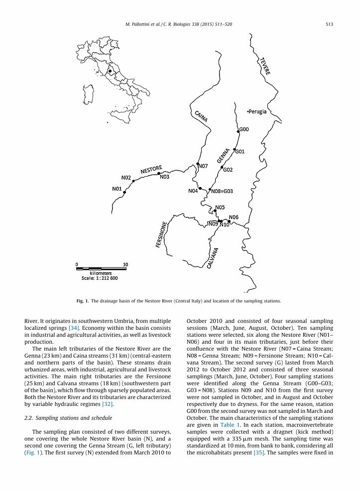

Rivlocain ipro

Genandurbact(25of tBotby

2.2.

onesec(Fig

M. Pallottini et al. / C. R. Biologies 338 (2015) 511–520 513

er. It originates in southwestern Umbria, from multiplelized springs [34]. Economy within the basin consists

ndustrial and agricultural activities, as well as livestockduction.The main left tributaries of the Nestore River are thena (23 km) and Caina streams (31 km) (central-eastern

northern parts of the basin). These streams drainanized areas, with industrial, agricultural and livestockivities. The main right tributaries are the Fersinone

km) and Calvana streams (18 km) (southwestern parthe basin), which flow through sparsely populated areas.h the Nestore River and its tributaries are characterizedvariable hydraulic regimes [32].

Sampling stations and schedule

The sampling plan consisted of two different surveys, covering the whole Nestore River basin (N), and aond one covering the Genna Stream (G, left tributary). 1). The first survey (N) extended from March 2010 to

October 2010 and consisted of four seasonal samplingsessions (March, June, August, October). Ten samplingstations were selected, six along the Nestore River (N01–N06) and four in its main tributaries, just before theirconfluence with the Nestore River (N07 = Caina Stream;N08 = Genna Stream; N09 = Fersinone Stream; N10 = Cal-vana Stream). The second survey (G) lasted from March2012 to October 2012 and consisted of three seasonalsamplings (March, June, October). Four sampling stationswere identified along the Genna Stream (G00–G03;G03 = N08). Stations N09 and N10 from the first surveywere not sampled in October, and in August and Octoberrespectively due to dryness. For the same reason, stationG00 from the second survey was not sampled in March andOctober. The main characteristics of the sampling stationsare given in Table 1. In each station, macroinvertebratesamples were collected with a dragnet (kick method)equipped with a 335 mm mesh. The sampling time wasstandardized at 10 min, from bank to bank, considering allthe microhabitats present [35]. The samples were fixed in

Fig. 1. The drainage basin of the Nestore River (Central Italy) and location of the sampling stations.

M. Pallottini et al. / C. R. Biologies 338 (2015) 511–520514

70% alcohol. In the laboratory, macroinvertebrates wereidentified to species, genus or family level using varioustaxonomic keys [36] and enumerated.

2.3. Chemical and physicochemical characterization of

surface water

The following four physicochemical water parameterswere measured seasonally in situ, always at the samedaytime: temperature and dissolved oxygen (DO; Oxime-ter F-Simplair Syland Scientific, accuracy 1% of the scalevalue, measuring range: 0.0–20.0 O2 mg�L�1), pH (pH-meter Hanna Instruments HI-98150, range: –4.00–19.99,resolution 0.01 pH, precision � 0.02 pH); conductivity(HI8733-Hanna Instruments, range: 0–1999 mS�cm�1, accu-racy 1%, resolution 1 mS�cm�1).

Seasonal water samples were also collected in 500-mLpolyethylene bottles, and then stored at 5 8C in therefrigerator for subsequent anionic and cationic character-ization and COD determination.

Chemical oxygen demand (COD) determination wasperformed by colorimetric method (Smart 2 Colorimeter LaMotte Company, COD Low Range Reagent Kit, 0–150 mg�L�1 COD, detection limit 0.5 mg�L�1). The concen-trations of anion and cation species (anions = F–, Cl–, NO2

–,Br–, NO3

–, PO43–and SO4

2–; cations = Li+, Na+, NH4+, K+, Mg2+

and Ca2+) were determined by suppressed ion chromatog-raphy with a conductivity detector using a Dionex Series4500i chromatograph. Commercially produced standardsolutions (Fluka-TraceCERT1 Standard Solutions,1000 mg�L�1� 4 mg�L�1) in ultrapure water (18.2 MV at25 8C) were used to prepare appropriate calibration stan-dards. The analyses were operated after filtration of sampleswith cellulose filters (0.2 mm) [37]. Li+ was excluded insubsequent analyses because it was below detection limits inevery sample.

2.4. Heavy metals in sediments

Samples of bottom sediments were taken at eachsampling date for heavy metal analyses. Sediment sampleswere obtained by dredging the superficial layer (about5 cm) of the bottom sediments with a hand dredge. The

samples (500 g) were preserved in Pyrex glass bottles andkept refrigerated at –18 8C [38].

Concentrations of heavy metals in sediments (Cr, Cd,Cu, Ni, Zn and Pb), for the first survey (N), were determinedby flame Atomic Absorption Spectrometry (AAS, Perki-nElmer 3300, instrumental detection limit 0.01–0.20mg�L�1) after sample acid digestion. Commercially pro-duced standard solutions (Fluka-TraceCERT1 StandardSolutions, 1000 mg�L�1� 4 mg�L�1) in 2% nitric acid, wereused to prepare appropriate elemental calibration standards[38,39]. Concentrations of heavy metals (Cr, Cd, Cu, Ni, Zn andPb) in sediments samples, for the second survey (G), weredetermined by Inductively Coupled Plasma Optical EmissionSpectrometry (ICP-OES, Ultima 2, HORIBA Scientific)equipped with ultrasonic nebulizer (CETAC Technologies,U-5000AT) after sample acid digestion. Instrumental detec-tion limits were in the range 0.14–1.58 mg�L�1. Commerciallyproduced (ICP multi-element standard solution IV Certi-PUR1, VWR Merck Chemicals and Reagents) standardsolutions (1000 mg�L�1) in nitric acid were used to prepareappropriate elemental calibration standards [18,38].

The sediment samples from both surveys were air-dried, disaggregated using a mortar and pestle to passthrough a 2-mm mesh sieve, dried at 105 8C for 24 h anddigested as follows: 15 mL of concentrated ultrapure nitricacid (Fluka, TraceSELECT1, for trace analysis � 69%) wereadded to the sample (2.0 g) and heated to 160 8C for 1 h;then, the vessel was cooled to room temperature and10 mL ultrapure concentrated hydrochloric acid (Fluka,TraceSELECT1, for trace analysis � 37%) were added andthe flask was heated to 160 8C for 1 h. The mixture wascooled, filtered (Whatman Grade No. 42, particle retention2.5 mm) and diluted with ultrapure water to 50 mL.

2.5. Modeling procedure

To sort the 47 samples (2010 survey (N): 37 seasonalsamples at ten stations; 2012 survey (G): 10 seasonalsamples at four stations), we used the Self-Organizing Mapalgorithm (SOM Toolbox version 2 for Matlab1, see [40] forpractical instructions). The strengths of the SOM incomparison with conventional multivariate analyses werediscussed in [41]. Combining ordination and gradientanalysis functions, the SOM is convenient to visualize high-dimensional data in a readily interpretable mannerwithout prior transformation. The SOM algorithm is anunsupervised learning procedure that transforms multi-dimensional input data into a two-dimensional mapsubject to a topological (neighbourhood preserving)constraint (detailed in [42]). The SOM thus plots thesimilarities of the data by grouping similar data itemstogether onto a 2D-space (visualized as a grid) using aniterative learning process that was detailed in [30]. TheSOM algorithm is specifically relevant for analyzing sets ofvariables that vary and co-vary in non-linear fashions, and/or that have skewed distributions. Additionally, the SOMalgorithm averages the input dataset using weight vectorsthrough the learning process and thus removes noise. A fulldescription of the modeling procedure employed here(training, map size selection, number of iterations, mapquality measurements) was detailed in [30,31].

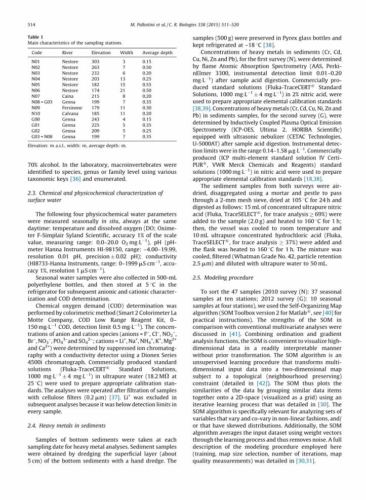
Table 1

Main characteristics of the sampling stations.

Code River Elevation Width Average depth

N01 Nestore 303 3 0.15

N02 Nestore 263 7 0.50

N03 Nestore 232 6 0.20

N04 Nestore 203 13 0.25

N05 Nestore 182 15 0.55

N06 Nestore 174 21 0.50

N07 Caina 215 8 0.20

N08 = G03 Genna 199 7 0.35

N09 Fersinone 179 11 0.30

N10 Calvana 185 11 0.20

G00 Genna 243 4 0.15

G01 Genna 225 5 0.35

G02 Genna 209 5 0.25

G03 = N08 Genna 199 7 0.35

Elevation: m a.s.l., width: m, average depth: m.

twointe(onandvisusevneutoppasfor

repclosthema(acthefor

rithunito tof cBoucluto

taxvarvisuin gthe[42

abiphywhthemaphybioordtaxcomorg

mudistcomentphyparstat(ve

3. R

3.1.

pat

erro

M. Pallottini et al. / C. R. Biologies 338 (2015) 511–520 515

The structure of the SOM for this analysis consisted of layers of neurons connected by weights (or connectionnsities): the input layer was composed of 78 neurons

e per invertebrate taxon) connected to the 47 samples, the output layer was composed of 35 neuronsalized as hexagonal cells organized on an array with

en rows and five columns. The number of 35 outputrons was retained after testing quantization andographic errors (QE and TE, see [31]). We note insing that the map size, based on local minimum valuesQE and TE, matched well the heuristic rule by [43]orting that the optimal number of output neurons ise to 5Hn, with n the number of samples. At the end of

training, each sample is set in a hexagon of the SOMp. Samples appearing distant in the modeling spacecording to the invertebrate abundance data used during

training) represent the expected chemical differencesreal environmental characteristics. A k-means algo-m was applied to cluster the trained map [44]. The SOMts (hexagons) were divided into 2–8 clusters accordinghe weight vectors of the neurons, and the final numberlusters (3) was justified according to the lowest Davisldin Index, i.e. for a solution with low variance within

sters and high variance between clusters [45]. In orderanalyze the contribution of each macroinvertebrateon to cluster structures of the trained SOM, each inputiable calculated during the training process wasalized in each neuron (hexagon) of the trained SOMrey scale. This visualization method directly describes

discriminatory powers of input variables in mapping].Finally, in order to bring out relationships betweenotic and biotic variables, we introduced the 23 chemical,sicochemical and heavy metal variables into the SOM,

ich was previously trained with the abundance data for 78 macroinvertebrate taxa. During training, we used ask function to give a null weight to the 23 chemical,sicochemical and heavy metal variables, whereas the

logical ones were given a weight of 1 so that theination process was based on the 78 macroinvertebratea only [1]. Setting mask value to 0 for a given

ponent removes the effect of that component onanization [46].In order to further highlight macroinvertebrate com-nity and environmental patterns among clusters, theributions of taxonomic richness, number of individuals,munity evenness (Simpson index) [47], community

ropy (Shannon index) [48], Chao index [49,50],sicochemical and heavy metals variables were com-ed among clusters using Mann-Whitney tests. Theseistical tests were performed using the Past software

rsion 3.02) [51].

esults

Classification of samples and invertebrate distribution

terns

Based on minimum quantization and topographicrs, the map size was selected as 7 � 5 neurons. The

35-unit map trained with macroinvertebrate abundancedata had a quantization error of 0.117 and a topographicerror of 0.0001. This map thus preserved well the typologyof the input data [42], and was relevant for subsequentinterpretations. After training the SOM algorithm with themacroinvertebrate abundance data, the k-means algo-rithm helped to delineate three clusters of samples(clusters A–C) according to the quantitative structure ofmacroinvertebrate assemblages (Fig. 2a). The SOM clus-tering revealed both spatial and seasonal variation in themacroinvertebrate community structure. Cluster Agrouped four samples from the most upstream, headwaterstations N01-N02. Cluster B grouped all samples fromstations N09-N10 (right tributaries of Nestore River), andmostly spring (March) samples from N01-N08. Cluster Cgrouped all seasonal samples from Genna stream (exceptN08 in March) and almost all summer to autumn samplesof stations N03–N07 also grouped in cluster C.

When the distribution of each macroinvertebrate taxonwas visualized on the trained SOM using a shading scale(see Fig. 2b for selected taxa), cluster A had eight taxa thatwere not found in other clusters (Deronectes moestus

(Fairmaire), Elmis, Gyrinus, Halesus, Haliplus, Helophorus,Mystacides azurea (Linnaeus), Sericostoma); cluster B had10 specific taxa (Atherix, Choroterpes picteti (Eaton),Gyraulus, Muscidae, Nemoura, Paraleptophlebia, Pisidium,Potamon fluviatile (Herbst), Potamopyrgus antipodarum

(Gray), Siphonoperla torrentium (Pictet)); and cluster Chad four taxa that were not found in other clusters(Culicinae, Haemopis sanguisuga (Linnaeus), Procambarus

clarkii (Girard), Trocheta). Hence, these taxa contributedmost to the delineation of the three clusters, and can beconsidered as indicators of environmental conditionsassociated with the corresponding samples.

3.2. Environmental gradients

Chemical, physicochemical and heavy metal variableswere introduced into the SOM previously trained withmacroinvertebrate data, thus forming explanatory vari-ables (Fig. 3); in particular, the ordinate on the SOMshowed a gradient of pH, DO and Ni, from low (bottom) tohigh (top of the map), and a reverse gradient of Pb andNO2

–. Values for Cl–, PO43–, Na+, NH4

+, K+, Cd, Cu, COD andconductivity increased from right-top to left-bottom areasof the map. We also noted gradients of F– and NO3

– fromleft-top to right-bottom areas of the SOM.

3.3. Between-cluster variability

Box-plots of diversity metrics (Fig. 4) showed a trendfor decreasing community diversity from cluster A tocluster C. Specifically, taxonomic richness and the Chaoindex differed significantly among clusters (Mann-Whit-ney tests, P < 0.05), Simpson’s evenness differed betweenclusters A and C, and Shannon’s entropy was significantlydifferent between cluster C and other clusters. Last, therewas no significant difference in terms of number ofindividuals among clusters. Clusters A and B werecharacterized by higher values for pH, DO and Ni, andcluster C was characterized by higher values for F–, Cl–,

M. Pallottini et al. / C. R. Biologies 338 (2015) 511–520516

PO43–, Na+, NH4

+, K+, Cd, Cu, Pb, NO2–, NO3

–, COD andconductivity. Only conductivity and K+ differed signifi-cantly among all three clusters (Mann-Whitney tests,P < 0.05). Values for pH, DO, COD, Cl–, PO4

3–, Na+, NH4+, Cr

and Ni differed significantly between cluster C and otherclusters. NO3

– and SO42– were significantly different

between clusters A and other clusters. Mg+2 was signifi-cantly different between clusters B and other ones. Watertemperature and Cd differed between clusters B and C, andCa+2 differed between clusters C and A. Finally, F–, NO2

–,Br–, Cu, Zn and Pb showed no significant differences amongclusters.

4. Discussion

Environmental management planning requires explicitschemes such as distribution patterns of biological diversityin relation to geomorphological, physical, and/or chemicalattributes of ecosystems, to subsequently evaluate thedeviation from a reference state, define quality objectives,and eventually anticipate ecological risk. Among thequestions that are asked of the scientific experts, the mostcommon ones are probably the following:

� which areas within a regional system are most impactedby industrial or agricultural activities?

� which physical and/or chemical stressors are detrimen-tal to the biological quality of recipient ecosystems?

Additionally, if threats associated with current activi-ties and future development plans align with zones ofconservation interest (e.g., presence of flagship species),this could add new impetus to freshwater managementpolicies. Given these settings, the SOM visualization hasproven an efficient analytical tool to illustrate relation-ships between sample locations, biological and environ-mental variables [31]. Through its iterative learningprocess, the SOM also minimizes the problem of outliers(e.g., presence of singletons) where each outlier is assignedto one unit of the map, and only the weights of that unitand its nearest neighbours are affected. Finally, by over-lapping species and or explanatory variable maps, anyspatial overlap or segregation on the output map becomesclear and can be interpreted in a straightforward manner.

SOM clusters revealed spatial, and to a lesser extentseasonal patterns of macroinvertebrate communities inrelation to environmental quality and land use in the Nestoredrainage basin. Among different taxa, Trichoptera andColeoptera particularly declined from cluster A to clusterC both in terms of number of taxa and abundance ofindividuals, while Annelida (Tubificidae and Hirudinea)showed increasing numbers of taxa and individuals.However, based on macroinvertebratecommunity structure,

Fig. 2. a: distribution and clustering of samples on the self-organizing map (SOM) according to the abundance of 78 macroinvertebrate taxa. Codes within

each hexagon (e.g., N01M, G03J) correspond to individual samples (see also Table 1): N (Nestore survey, 2010), G (Genna survey, 2012), 00-10 sampling

stations, M = March, J = June, A = August, O = October. Clusters A–C (separated by the bold line) were derived from the k-means algorithm applied to the

weights of the 78 taxa in the 35 output neurons of the SOM; b: gradient analysis of the abundance (number of individuals) for selected taxa (exclusive of

each cluster: Sericostoma, cluster A; Atherix, cluster B; Haemopis sanguisuga, cluster C; and shared between clusters: Tabanidae, cluster A and B, Dina, cluster

B and C; Gordiidae, cluster A and C; Baetis, cluster A, B and C) on the trained SOM represented by a shaded scale (dark = high abundance, light = low

abundance).

somaccN08cluthepopthetebticeshifseawasum

che[53nitiactof

Fig.

calc

M. Pallottini et al. / C. R. Biologies 338 (2015) 511–520 517

e stations could shift from one cluster to anotherording to the season. Interestingly, Nestore stations N03–

tend to shift from cluster B (intermediate pollution) toster C (heavier pollution) in summer–autumn, althoughse seasons theoretically correspond to the renewal ofulations through reproduction and egg hatching, and are

refore supposedly species-rich periods for stream inver-rates [52]. Further data on agricultural–industrial prac-s would be needed to properly assess whether temporalts in local biodiversity are mostly related to invertebratesonality (life cycle patterns) or to seasonal patterns inter pollution (e.g. intensified agricultural practices in

mer).With regard to spatial patterns, land use influences themical and biological characteristics of river ecosystems] and the structure of lotic macroinvertebrate commu-es may be subsequently influenced by economicivities within catchments [54]. Here, the introductionexplanatory variables into the SOM trained with

macroinvertebrate data provided additional insights intoour understanding of community patterns in relation tohuman activities. Several chemicals and heavy metalsshowed congruent patterns, although the latter variableswere given a null weight during the ordination andclassification process (i.e. they did not influence thegrouping of samples); in particular, higher Cr and Niconcentrations were associated with higher pH and DO inclusters A and B. Headwater reaches of the Nestore(stations N01 and N02, cluster A) are only surroundedby sparse habitation. Economic activity in the area islimited to a glass factory, located upstream of station N02.Stations in cluster B are either surrounded by intensivelyfarmed landscapes and urban/industrial lands. Ni and Crcould thus be waste products of different types ofindustries. Stations in cluster C showed higher concentra-tions of Pb, Cd and Cu matched to the increasing gradientsof conductivity, COD, nitrate, nitrite, ammonium, phos-phates, chloride, sodium, and potassium. Accordingly, all

3. Visualization of physicochemical parameters of water and heavy metals of sediments (shades of gray). The mean value for each variable was

ulated in each output neuron of the SOM previously trained with macroinvertebrate data. Darker/lighter tones represent higher/lower values.

Fig. 4. Boxplots of diversity metrics (taxonomic richness, number of individuals, Simpson, Shannon and Chao indices) and environmental variables

(physicochemical parameters of water, heavy metals in sediments) for the three clusters. Significant differences between clusters were tested with Mann-

Whitney tests; lowercase letters above boxes indicate significant differences at P < 0.05.

M. Pallottini et al. / C. R. Biologies 338 (2015) 511–520518

statturarethissugconfooin

prepro

struremvarcomfielbiotherevwaundexatheandcomremtors

ma(seadistsysbiotooorgwhof sto tdesknoStilrivemation

Dis

inte

Ack

promoear

Ref

[1]

M. Pallottini et al. / C. R. Biologies 338 (2015) 511–520 519

ions in cluster C are surrounded by intensive agricul-al activities and livestock (80 farms recorded in thea). Lower values for DO (oxygenation of the water) for

cluster (Genna Stream and the lower Nestore River)gest a high level of organic pollution. Higher Cucentrations can be related to livestock as it is used ind for animals, and contaminated sludges are then usedagriculture as soil fertilizers [55]. In addition, Cu issent in pesticides and fertilizers, but can also be wasteduct in industry.Whilst the SOM illustrated co-variation in communitycture and a series of nutrients and heavy metals, itains difficult to establish the specific effect of the

ious stressors upon macroinvertebrate communityposition. This is however inherent to observational

d studies where anthropogenic disturbance subjectslogical communities to mixtures of pollutants. Never-less, the SOM analysis of the biological data did well atealing the extent of pollution among stations, to assesster quality at the drainage basin level. Further studieser experimental conditions would be needed tomine how heavy metals act and interact in nature to

detriment of certain taxa, either in terms of occurrence abundance patterns. On an empirical basis, however, amon and efficient way to assess environmental qualityains to interpret the distribution of biological indica-

across gradients of environmental conditions.In conclusion, qualitative and quantitative changes incroinvertebrate communities in space (sites) and timesons) can be expected in relation to anthropogenicurbance that affect water chemistry at local to stream-

tem levels, together with potential changes in terms oflogical traits. Whilst biological indices are a universall to rate river health, spatial schemes of communityanization still provide the explicit models againstich deviation from reference conditions, in the formcores or water quality classes, are assessed [56]. Owinghe limited size of our dataset, we did not attempt toign a biotic index that would fit, for instance, the well-wn guidelines of the EU Water Framework Directive.l, through the SOM clustering, the ecological health ofr ecosystems can be mapped in a readily interpretable

nner, taking into account gradients of chemical pollu- sensu lato.

closure of interest

The authors declare that they have no conflicts ofrest concerning this article.

nowledgements

The Foundation ‘‘Cassa di Risparmio di Perugia’’ (Italy)vided financial support for this research. Two anony-us reviewers provided insightful comments on anlier version of this paper.

erences

A. Compin, R. Cereghino, Spatial patterns of macroinvertebrate func-tional feeding groups in streams in relation to physical variables and

[2] J. Kreuger, Pesticides in stream water within an agricultural catchment insouthern Sweden, 1990–1996, Sci. Total Environ. 216 (1998) 227–251.

[3] V. Novotny, Diffuse pollution from agriculture – a worldwide outlook,Water Sci. Technol. 39 (1999) 1–13.

[4] P.N.M. Schipper, L.T.C. Bonten, A.C.C. Plette, S.W. Moolenaar, Measuresto diminish leaching of heavy metals to surface waters from agricul-tural soils, Desalination 226 (2008) 89–96.

[5] M.S. Holt, Sources of chemical contaminants and routes into thefreshwater environment, Food Chem. Toxicol. 38 (Suppl.) (2000) 21–27.

[6] M.A. Cairns, A.V. Nebeker, J.H. Gakstater, W.L. Griffis, Toxicity of copper-spiked sediments to freshwater invertebrates, Environ. Toxicol. Chem.3 (1984) 435–445.

[7] P.M. Chapman, The sediment quality triad approach to determiningpollution-induced degradation, Sci. Total Environ. 97/98 (1990) 815–825.

[8] A. Estebe, H. Boudries, J. Mouchel, D.R. Thevenot, Urban runoff impactson particulate metal and hydrocarbon concentrations in River Seine:suspended solid and sediment transport, Water Sci. Technol. 36 (1997)185–193.

[9] P.M. Chapman, Current approaches to developing sediment qualitycriteria, Environ. Toxicol. Chem. 8 (1989) 589–599.

[10] R.J. Gibbs, Transport phases of transition metals in the Amazon andYukon rivers, Geol. Soc. Am. Bull. 88 (1977) 829–843.

[11] C.K. Jain, M.K. Sharma, Distribution of trace metals in the Hindon Riversystem, India. J. Hydrol. 253 (2001) 81–90.

[12] A.V. Filgueiras, I. Lavilla, C. Bendicho, Chemical sequential extractionfor metal partitioning in environmental solid samples, J. Environ.Monitor. 4 (2002) 823–857.

[13] O.I. Davutluoglu, G. Seckin, C.B. Ersu, T. Yilmaz, B. Sari, Heavy metalcontent and distribution in surface sediments of the Seyhan River,Turkey, J. Environ. Manage. 92 (2011) 2250–2259.

[14] S.I. Dodson, S.E. Arnott, K.L. Cottingham, The relationship in lakecommunities between primary productivity and species richness, Ecol-ogy 81 (2000) 2662–2679.

[15] C.W. Hickey, W.H. Clements, Effects of heavy metals on benthic macro-invertebrate communities in New Zealand streams, Environ. Toxicol.Chem. 17 (1998) 2338–2346.

[16] M. De Jonge, B. Van de Vijver, R. Blust, L. Bervoets, Responses of aquaticorganisms to metal pollution in a lowland river in Flanders: a compar-ison of diatoms and macroinvertebrates, Sci. Total Environ. 407 (2008)615–629.

[17] Q. Zhou, J. Zhang, J. Fu, J. Shi, G. Jiang, Biomonitoring: an appealing toolfor assessment of metal pollution in the aquatic ecosystem, Anal. Chim.Acta 606 (2008) 135–150.

[18] A. Di Veroli, F. Santoro, M. Pallottini, R. Selvaggi, F. Scardazza, D.Cappelletti, E. Goretti, Deformities of chironomid larvae and heavymetal pollution: from laboratory to field studies, Chemosphere 112(2014) 9–17.

[19] M. Liess, M. Beketov, Traits and stress: keys to identify communityeffects of low levels of toxicants in test systems, Ecotoxicology 20(2011) 1328–1340.

[20] B. Oertli, Leaf litter processing and energy flow through macroinverte-brates in a woodland pond (Switzerland), Oecologia 96 (1993) 466–477.

[21] D.M. Rosenberg, V.H. Resh, Introduction to freshwater biomonitoringand benthic macroinvertebrates. Freshwater biomonitoring benthicmacroinvertebrates, Chapman and Hall, New York, USA, 1993.

[22] N. Bonada, N. Prat, V.H. Resh, B. Statzner, Developments in aquaticinsect biomonitoring: a comparative analysis of recent approaches,Annu. Rev. Entomol. 51 (2006) 495–523.

[23] T.J. Naimo, A review of the effects of heavy metals on freshwatermussels, Ecotoxicology 4 (1995) 341–362.

[24] K.C. Yu, L.J. Tsai, S.H. Chen, S.T. Ho, Correlation analysis on bindingbehaviour of heavy metals with sediment matrices, Water Res. 4 (2001)2417–2428.

[25] A. Santoro, G. Blo, S. Mastrolitti, F. Fagioli, Bioaccumulation of heavymetals by aquatic macroinvertebrates along the Basento River in thesouth of Italy, Water Air Soil Pollut. 201 (2009) 19–31.

[26] V. Archaimbault, P. Usseglio-Polatera, J. Garric, J.G. Wasson, M. Babut,Assessing pollution of toxic sediment in streams using bio-ecological traitsof benthic macroinvertebrates, Freshwater Biol. 55 (2010) 1430–1446.

[27] S. Lek, J. Guegan, Artificial neuronal networks: application to ecologyand evolution, Springer, Berlin, Germany, 2000.

[28] A.M. Kalteh, P. Hjorth, R. Berndtsson, Review of the self-organizing map(SOM) approach in water resources: analysis, modelling and applica-tion, Environ. Model. Softw. 23 (2008) 835–845.

[29] T. Kohonen, Self-organizing maps: optimization approaches, Proceed-ings of ICANN’91. International Conference on Artificial Neural Net-works, volume II, Amsterdam, North-Holland, 1991, pp. 981–990.

[30] Y.S. Park, R. Cereghino, A. Compin, S. Lek, Applications of artificialneural networks for patterning and predicting aquatic insect species

richness in running waters, Ecol. Model. 160 (2003) 165–280. land-cover in Southwestern France, Landsc. Ecol. 22 (2007) 1215–1225.

M. Pallottini et al. / C. R. Biologies 338 (2015) 511–520520

[31] R. Cereghino, Y.S. Park, Review of the self-organizing map (SOM)approach in water resources: commentary, Environ. Model. Softw.24 (2009) 945–947.

[32] Agenzia Regionale per la Protezione Ambientale (ARPA), Umbria,Bacino idrografico del Fiume Nestore–Monitoraggio chimico e micro-biologico di acque e scarichi–Relazione tecnica, 2010.

[33] M. Mearelli, M. Lorenzoni, A. Carosi, M.L. Petesse, G. Giovinazzo, L.Cingolani, L. Ghetti, G. Montilli, M. Mossone, P. Nelli, C. Uzzoli, CartaIttica della Regione Umbria: bacino del F. Nestore, Regione Umbria,Perugia, Italy, 1996.

[34] M. Lorenzoni, M. Corboli, E. Grillo, G. Pedicillo, A. Carosi, P. Viali, L. Ghetti,G. Baldini, A. Zeetti, M. Natali, R. Dolciami, A. Biscaro Parrini, A. Mezzetti,M. Mussone, M. Andreani, A. Bruchia, S. Cassieri, M. De Luca, S.L. Quon-dam, C. Uzzoli, M. Di Brizio, La carta ittica della Regione Umbria: bacinodel Fiume Nestore, Regione Umbria, Perugia, Italy, 2004.

[35] P.F. Ghetti, G. Bonazzi, I macroinvertebrati nella sorveglianza ecologicadei corsi d’acqua, in: Collana del progetto finalizzato promozione dellaqualita dell’ambiente, C.N.R. AQ/1/127, 1981.

[36] H. Tachet, P. Richoux, M. Bournaud, P. Usseglio-Polatera, Invertebresd’eau douce. Systematique, biologie, ecologie, CNRS Editions, Paris,2010.

[37] R. Selvaggi, N. Colonna, F. Lupia, M.S. Murgia, A. Poletti, Water qualityand soil natural salinity in the southern Imera Basin (Sicily, Italy), Ital. J.Agron. 3 (2010) 81–89.

[38] Ministero dell’Ambiente e della Tutela del Territorio, (MATT), Agenziaper la Protezione dell’Ambiente e per i servizi Tecnici (APAT), Progettonazionale di monitoraggio acque superficiali (IRSA, CNR), Gli ecosis-temi e i sedimenti: Caratterizzazione dei sedimenti, 2005.

[39] A. Di Veroli, R. Selvaggi, R.M. Pellegrino, E. Goretti, Sediment toxicityand deformities of chironomid larvae in Lake Piediluco (Central Italy),Chemosphere 79 (2010) 33–39.

[40] J. Vesanto, J. Himberg, E. Alhoniemi, J. Parhankangas, Self-organizingmap in Matlab: the SOM toolbox, in: Proceedings of the Matlab DSPConference 35-40, 1999.

[41] J.-L. Giraudel, S. Lek, A comparison of self-organizing map algorithmand some conventional statistical methods for ecological communityordination, Ecol. Model. 146 (2001) 329–339.

[42] T. Kohonen, Self-organizing maps, Third edition, Springer, Berlin, 2001.

[43] J. Vesanto, J. Himberg, E. Alhoniemi, J. Parhankangas, SOM Toolbox forMatlab 5, Technical Report A57, Neural Networks Research Centre,Helsinki University of Technology, Helsinki, Finland, 2000.

[44] A. Ultsch, G. Guimaraes, D. Korus, H. Li, Knowledge extraction fromartificial neural networks and applications. World Transputer CongressTAT/WTC 93, Springer, Aachen, Germany, 1993.

[45] R. Cereghino, Y.S. Park, A. Compin, S. Lek, Predicting the species richnessof aquatic insects in streams using a limited number of environmentalvariables, J. North Am. Benthol. Soc. 22 (2003) 442–456.

[46] M. Sirola, G. Lampi, J. Parviainen, Using self-organizing map in a com-puterized decision support system, in: International Conference onNeural Information Processing (ICONIP), LNCS 3316, 2004, pp. 136–141.

[47] E.H. Simpson, Measurement of diversity, Nature (London) 163 (1949) 688.[48] C.E. Shannon, A mathematical theory of communication, Bell. Syst.

Tech. J. 27 (1948) 379–423.[49] A. Chao, Non-parametric estimation of the number of classes in a

population, Scand. J. Stat. 11 (1984) 265–270.[50] R.K. Colwell, J.A. Coddington, Estimating terrestrial biodiversity

through extrapolation, Phil. Trans. R. Soc. B. 345 (1994) 101–118.[51] Ø. Hammer, D.A.T. Harper, P.D. Ryan, PAST: Paleontological Statistics

Software Package for education and data analysis, PalaeontologiaElectronica 4 (1) (2001) (art. 4, 9 p., 178 kb) http://palaeo-electronica.org/2001_1/past/issue1_01.htm.

[52] R. Cereghino, P. Lavandier, Influence of hydropeaking on the distribu-tion and larval development of the Plecoptera from a mountain stream,Regul. Rivers Res. Manage. 14 (1998) 297–309.

[53] A.A. Moore, M.A. Palmer, Invertebrate biodiversity in agricultural andurban headwater streams: implications for conservation and manage-ment, Ecol. Appl. 15 (2005) 1169–1177.

[54] R.A. Sponseller, E.F. Benfield, H.M. Valett, Relationships between landuse, spatial scale and stream macroinvertebrate communities, Fresh-water Biol. 46 (2001) 1409–1424.

[55] P. Mantovi, G. Bonazzi, Riduzione del tenore di rame e zinco neimangimi, L’Informatore Agrario 4 (2004) 61–64.

[56] C.P. Mondy, B. Villeneuve, V. Archaimbault, P. Usseglio-Polatera, A newmacroinvertebrate-based multimetric index (I2M2) to evaluate eco-logical quality of French wadeable streams fulfilling the WFD demands:a taxonomical and trait approach, Ecol. Indic. 18 (2012) 452–467.