www.elsevier.com/locate/optcom

Optics Communications 273 (2007) 324–333

Incoherently coupled screening photovoltaic spatial solitonsin biased photovoltaic photorefractive crystals

S. Konar a,*, Soumendu Jana a, S. Shwetanshumala b

a Department of Applied Physics, Birla Institute of Technology, Mesra 835 215, Ranchi, Jharkhand, Indiab Department of Physics, A. N. College, Patna 800 013, India

Received 31 August 2006; received in revised form 11 January 2007; accepted 24 January 2007

Abstract

Propagation characteristics and stability properties of two-component composite screening photovoltaic spatial solitons have beenanalyzed in this paper. Employing paraxial ray approximation, we have identified a very large family of new two-component compositescreening photovoltaic solitons in photovoltaic–photorefractive crystals. These composite solitons can exist only when the carrier beamshave the same polarization, wavelength and are mutually incoherent. We have identified a wide parameter space involving spatial widthand power where these composite solitons can exist as a stationary entity. The identified regions of existence of solitons give a deeperunderstanding of these solitons and reveal some interesting properties. We have shown that composite solitons with different widths can-not propagate as a stationary entity. A relevant example has been provided where the crystal is LiNbO3 or BaTiO3. In addition, we haveshown that in the new family of solitons, a degenerate pair with equal peak power possesses bistable property. Both paraxial theory andnumerical simulation show that the identified family of composite solitons is stable.� 2007 Elsevier B.V. All rights reserved.

1. Introduction

Photorefractive spatial solitons observed experimentallyby Duree et al. [1] just a year after its theoretical predictionby Segev et al. [2] in 1992 and have been the subject ofactive research both theoretically and experimentally sincethen [3–10]. Although solitons are ubiquitous in variousbranches of physics, the self trapped photorefractive spatialsolitons (PRSS) possess some very attractive features whichmake them potentially useful for various applications likeall optical switching and routing, interconnects, parallelcomputing, optical storage etc [9–13]. In addition, sincephotorefractive crystal (PR) has the ability to create opticalsolitons at very low optical power, of order of microwatts[9], it is the most promising and prospective media forexperimental verification of theoretical models. PRSS canbe operated at telecommunication wavelength [14]

0030-4018/$ - see front matter � 2007 Elsevier B.V. All rights reserved.

doi:10.1016/j.optcom.2007.01.051

* Corresponding author. Tel.: +91 6512276274; fax: +91 6512275401.E-mail address: swakonar@yahoo.com (S. Konar).

(�1.5 lm) at very low power (�lm) with fast response[15,16], response time being of the order of microsecond.A large number of review articles are now available high-lighting applications of photorefractive spatial solitons[17–20].

Formation of photorefractive spatial solitons is similarto that formed in optical fiber where spatial soliton isformed by the balance of diffraction with the nonlinearityof the medium of propagation. When light falls, spacecharge field is set up due to charge separation by the exci-tation and the movement of the charge carriers present inthe donor and acceptor levels, resulting in the modulationof the refractive index of the photorefractive material med-ium [4,21]. High light intensity is required for soliton for-mation in optical fiber as the nonlinearity inducedrefractive index change is small where as PRSS is formedat optical powers in microwatt since the induced refractiveindex is large even at that small power. One additional fea-ture of PR medium is that their nonlinear behavior is wave-length sensitive [22,23]. This property is utilized for guidingand steering light beams of different wavelength. A spatial

S. Konar et al. / Optics Communications 273 (2007) 324–333 325

solitons generated using one wavelength at low opticalpower is capable of guiding another diffracting light of dif-ferent wavelength. Several beams can be combined to pro-duce self trapped states called vector solitons which arestationary localized solutions of coupled nonlinear Schro-dinger equations. One of the components of such acomposite state induces an effective waveguide which sup-ports other components.

Till date, three different types of steady state photore-fractive solitons have been predicted. The one which wasidentified first is the screening solitons. Both bright anddark screening solitons (SS) in the steady state are possiblewhen an external bias voltage is applied to a non-photovol-taic photorefractive crystal [2–7]. The second kind is thephotovoltaic solitons [8–24], the formation of which, how-ever, requires an unbiased PR crystal that exhibits photo-voltaic effect, i.e., generation of dc current in a mediumilluminated by a light beam. Recently, a third kind ofphotorefractive solitons has been introduced [25–29], whicharises when an electric field is applied to a photovoltaicphotorefractive crystal. These solitons owe their existenceto both photovoltaic effect and spatially nonuniformscreening of the applied field and are also known as screen-ing photovoltaic solitons (SP). Bright, dark and grey [30]SP solitons have been investigated. It has been shown thatif the bias field is much stronger than the photovoltaic field,then the screening photovoltaic solitons are just like screen-ing solitons. On the other hand, if the applied field isabsent, then they degenerate into photovoltaic solitons inthe closed circuit condition. Our goal in this paper is todemonstrate the existence of a new very large family oftwo-component composite screening photovoltaic spatialsolitons in biased photovoltaic–photorefractive crystals.In addition, we reveal several important properties of thesetwo-component composite solitons. The paper is organizedas follows: The mathematical model for (1 + 1)D two-com-ponent screening photovoltaic spatial solitons has beendeveloped in Section 2. In this section, we have employedthe paraxial ray approximation method to derive dynami-cal equations of spatial widths of these composite solitons.In Section 2.1 we have investigated stationary points ofthese dynamical equations which lead to identification ofbroad parameter region where stationary composite soli-tons exist. In Section 2.2 we have performed numerical sim-ulation experiment to validate the predictions of paraxialtheory. We have added a brief conclusion in Section 3.

2. Mathematical model

To start with, we assume that two optical beams are col-linear and are propagating in a biased photovoltaic–photo-refractive crystal along the z-direction. They are of samefrequency but mutually incoherent. The polarization ofboth optical fields is assumed to be parallel to the x-axiswhich is also the direction of applied external bias electricfield. The crystal here is taken to be LiNbO3 or BaTiO3

with its optical c-axis oriented along the x-coordinate.

The two optical beams are allowed to diffract only alongthe x-direction and for the sake of simplicity the photore-fractive material is assumed to be lossless. The two opticalbeams can be obtained by splitting a laser beam by a polar-izing beam splitter. These two beams can be made mutuallyincoherent at the input face of the crystal by making theiroptical path difference greatly exceed the coherence lengthof the laser. Thus, no stationary interference grating can beformed within a time scale comparable with the responsetime of the crystal. These two beams act as soliton-formingbeams and note that a similar arrangement has been previ-ously employed [31,32] to experimentally and theoreticallyinvestigate incoherently coupled soliton pairs in photore-fractive crystals. The optical fields are expressed in theform ~E1 ¼ xE1ðx; zÞ expðikzÞ and ~E2 ¼ xE2ðx; zÞ expðikzÞ;where k is the propagation constant and E1 and E2 areslowly varying envelopes. It can be readily shown thatslowly varying envelopes of two interacting spatial solitonsthrough the photovoltaic PR crystal is governed by thecoupled modified nonlinear Schrodinger equations(MNLSE) [25,26]

ioE1

onþ 1

2

o2E1

os2� d

E1

1þ jE1j2þ jE2j2þ a

jE1j2þ jE2j2

1þ jE1j2þ jE2j2E1 ¼ 0;

ð1Þ

ioE2

onþ 1

2

o2E2

os2� d

E2

1þ jE1j2þ jE2j2þ a

jE1j2þ jE2j2

1þ jE1j2þ jE2j2E2 ¼ 0;

ð2Þ

where, d ¼ ðk0x0Þ2 n4e r33

2E0, a ¼ ðk0x0Þ2 n4

e r33

2Ep, Ep ¼ kpcRNA

el ,k0 ¼ 2p

k0, n ¼ z

k0nex20

, s ¼ xx0

, ne is the unperturbed extraordi-

nary index of refraction, k0 is the free space wavelengthof the light wave employed, r33 is the electro-optic coeffi-cient, E0 is the external bias electric field, Ep is photovoltaicfield constant, x0 is an arbitrary spatial width and thepower density has been scaled with respect to dark irradi-ance; cR; l; e; kp and NA are, respectively, the carrier recom-bination rate, electron mobility, electronic charge,photovoltaic constant and the acceptor density. Thesetwo solitons of the two-component composite solitons aresupported by both nonlinear self and cross-phase modula-tion terms, and the saturating nature of the interaction isevident from the above equations. With the growing appli-cations of self focusing and spatial solitons in modern tech-nology, several mathematical methods have evolved toaddress these phenomena. For (1 + 1) dimensional spatialsolitons in Kerr nonlinear media, where diffraction in onlyone transverse direction is balanced by spatial self focusing,elegant exact single soliton solutions are obtained by meansof inverse scattering technique (IST) [33,34]. However, thiselegant formalism is applicable only in certain specific idealcases of single and coupled NLSE. Several methods, whichare not exact, are also available to deal single as well ascoupled modified NLSE. Among them, paraxial theory ofAkhmanov et al. [35,36], moment method due to Vlasov[37] and the variational method of Anderson [38] are very

326 S. Konar et al. / Optics Communications 273 (2007) 324–333

familiar. All these three formulations assume self similarsolutions of the MNLSE, where the optical beam preservesits structural form while propagating through the media.Out of these three methods, however, the paraxial theoryof Akhmanov is the simplest and though approximatemethod, is able to capture a clear physical picture of theproperties of the solution. Therefore, since to the best ofour understanding, Eqs. (1) and (2) can be exactly solvedonly by adopting numerical procedure, hence, in this pres-ent investigation we plan to employ paraxial theory ofAkhmanov et al. [35,36] to look for spatial soliton solu-tions of above coupled MNLSE. However, since the theoryis not exact, its prediction needs to be verified by detailnumerical experiment. In order to analyze the behaviorof these coupled solitons, we substitute in (1) and (2) solu-tions of the form

E1ðs; nÞ ¼ A1ðs; nÞe�iX1ðs;nÞ; ð3ÞE2ðs; nÞ ¼ A2ðs; nÞe�iX2ðs;nÞ: ð4Þ

Upon substituting these solutions in (1) and (2), we get twosets of two equations as follows:

oX1

onA1 �

1

2

oX1

os

� �2

A1 þ1

2

o2A1

os2� dU1A1 þ aU2A1 ¼ 0; ð5Þ

oX2

onA2 �

1

2

oX2

os

� �2

A2 þ1

2

o2A2

os2� dU1A2 þ aU2A2 ¼ 0; ð6Þ

oA1

on� oX1

osoA1

os� 1

2

o2X1

os2A1 ¼ 0; ð7Þ

oA2

on� oX2

osoA2

os� 1

2

o2X2

os2A2 ¼ 0; ð8Þ

where U1 ¼1

1þ jA1j2 þ jA2j2and U2 ¼

jA1j2 þ jA2j2

1þ jA1j2 þ jA2j2:

ð9Þ

The last three terms of (5) and (6), respectively, determinethe behavior of the eikonal X1 and X2, i.e., the convergenceor divergence of two optical beams. The fourth and fifthterms in these two equations represent nonlinear refractionwhile the third term determines diffraction. Eqs. (7) and (8),respectively, determine the evolution of the beam envelopesA1 and A2. Screening photovoltaic solitons arise as a resultof photovoltaic effect and spatially nonuniform screeningof the applied field in a biased photovoltaic–photorefrac-tive crystal. Therefore, properties of these solitons dependboth on external bias field and photovoltaic property ofthe crystal. In (5) and (6), U1 and U2, respectively, representthe contribution from nonuniform screening of the appliedelectric field and photovoltaic properties of the crystal. It isnow well recognized that SP solitons are combined form ofscreening solitons and photovoltaic solitons in closed cir-cuits realization. We can obtain bright screening solitonswhen U1 is nonzero and U2 is absent, whereas, we obtainphotovoltaic solitons when U1 is zero and U2 nonzero.

We look for lowest order localized bright solitons forwhich light is confined in the central region of the solitons,

i.e., A1ðs ¼ 0Þ ¼ A1max ;A2ðs ¼ 0Þ ¼ A2max and ðA1;A2Þ ¼ 0 ass!1. We further assume that these solitons maintaintheir self similar character while they propagate. It is nowwell known that the nonlinear Schrodinger equation(NLSE) in Kerr media with constant coefficients is one ofthe basic equations of physics. The simplest and most fun-damental solution of this equation is the one bright solitonrepresented by sech function. Eqs. (1) and (2) are modifiedcoupled nonlinear Schrodinger equations which are nonin-tegrable in nature. Generally speaking, the two-wave soli-ton solutions of these two coupled equations can be onlyfound numerically. However, approximate analytical meth-ods can be adopted to extract useful guidelines for numer-ical simulations. In both numerical and approximateanalytical methods, occasionally sech profile is used as itis the closest profile to the exact solitonic shape in manycases. However, most widely used approximate solutionsfor nonintegrable systems are of Gaussian type [38–48]instead of sech. The justification of using Gaussian ansatzis manifold. Firstly, use of Gaussian profile makes the cal-culations remarkably easier. Second, numerically com-puted exact profiles are not widely different fromGaussian one in most cases. Furthermore, Gaussian profileis qualitatively very close to sech profile having nearly thesame half width and the integral contents under the twoprofiles are comparable (differs only by a factor of 0.054)[38]. Also, in most cases the same analytical simplificationis not expected by using sech ansatz [48]. Therefore, use ofGaussian profile provides much simplicity in calculationwithout major loss of information. In a trend setting paper[38], Anderson argued in favour of using Gaussian profilein variational methods that has been adopted subsequentlyby many researchers in nonlinear optics. In addition toVariational approach, Gaussian shaped ansatz has beensuccessfully used in collective variable approach [45] as wellas moment method [46]. Although Gaussian solution is anapproximate solution, it can give useful guidelines for fullnumerical simulations. Thus, in this paper we introduceGaussian ansatz which has been extensively adopted bysoliton community [38–48] in a similar situation. However,we wish to point out that this is only an approximate solu-tion whose prediction should be validated by full numericalsimulation which will be undertaken in the later part of thepaper. Hence, the solutions of above equations are taken tobe Gaussian with amplitude and phase of the followingform:

Aiðs; nÞ ¼Ai0ffiffiffiffiffiffiffiffiffiffifiðnÞ

p e� s2

2r2i

f 2iðnÞ; ð10Þ

Xiðs; nÞ ¼s2

2biðnÞ þWiðnÞ; ð11Þ

biðnÞ ¼ �1

fi

dfi

dn; i ¼ 1; 2; ð12Þ

where, A10 and A20, respectively, represent the peak powerof these solitons, r1 and r2 are two positive constants, f1ðnÞand f2ðnÞ are variable beam width parameters; r1f1 and r2f2

S. Konar et al. / Optics Communications 273 (2007) 324–333 327

are, respectively, the spatial widths of these solitons. For apair of non diverging solitons at n ¼ 0, we should havef1 ¼ f2 ¼ 1 and df1

dn ¼df2

dn ¼ 0. The nonlinear terms U1 andU2 are expanded in Taylor’s series and under first orderapproximation, they read as,

U1ðA1;A2Þ ffi1

1þ A210

f1þ A2

20

f2

þ x2 A210

r21f 3

1

þ A220

r22f 3

2

� �1

1þ A210

f1þ A2

20

f2

� �2;

ð13Þ

U2ðA1;A2Þ ffiA2

10

f1þ A2

20

f2

1þ A210

f1þ A2

20

f2

� x2 A210

r21f 3

1

þ A220

r22f 3

2

� �1

1þ A210

f1þ A2

20

f2

� �2:

ð14Þ

It is observed that the first order contribution of U1 and U1

are equal in magnitude but opposite in sign. Substitutingfor A1, A2, X1 and X2 in (5) and (6), using paraxial rayapproximation [35,36,49] and equating coefficients of s2

on both sides of (5) and (6), we obtain

o2f1

oz2¼ 1

r41f 3

1

� CP 1

r21f 2

1

þ P 2f1

r22f 3

2

� �1

1þ P 1

f1þ P 2

f2

� �2; ð15Þ

o2f2

oz2¼ 1

r42f 3

2

� CP 1f2

r21f 3

1

þ P 2

r22f 2

2

� �1

1þ P 1

f1þ P 2

f2

� �2; ð16Þ

where A210 ¼ P 1; A2

20 ¼ P 2 and C ¼ 2ðdþ aÞ. Eqs. (15) and(16) form a complete set of equations whose solutionsshould give stationary and nonstationary composite soli-tons of (1) and (2) for given set of power and spatial width.

2.1. Stationary composite solitons

Since we are interested in the nondiverging two-compo-nent composite bright solitons, we first look for the equilib-rium points of above ordinary differential equations(ODE), which can be obtained by setting left-hand sidesof (15) and (16) equal to zero, thus

1

r41

� CP 1

r21

þ P 2

r22

� �1

ð1þ P 1 þ P 2Þ2¼ 0; ð17Þ

and

1

r42

� CP 1

r21

þ P 2

r22

� �1

ð1þ P 1 þ P 2Þ2¼ 0: ð18Þ

To find stationary composite solitons we should look forcommon solutions of (17) and (18). These can be identifiedby equating left-hand side (l.h.s) of (17) with l.h.s of (18),yielding the condition r1 ¼ r2, i.e., each component of thestationary composite solitons has equal spatial width.Therefore, composite solitons with different spatial widthscannot propagate as a stationary entity. This is an interest-ing finding. To find out required power for such stationarycomposite solitons, we set r1 ¼ r2 ¼ r in either of (17) or(18) and get the required relationship which relates the

peak power of these stationary composite spatial solitonswith their widths as follows:

Cr2 ¼ ð1þ P 1 þ P 2Þ2

P 1 þ P 2

: ð19Þ

The above relationship is the existence equation of com-posite solitons. Kindly note that for bright–bright com-posite pair C should be positive. Also it is worthpointing out that though spatial width of each of thetwo components is equal, their respective peak powercan have different values. Eq. (19) is equivalent to a qua-dratic equation in P1,

P 21 þ P 1ð2P 2 þ 2� Cr2Þ þ P 2

2 þ 2P 2 � Cr2P 2 þ 1 ¼ 0: ð20ÞSince in (20), P1 and P2 are in the same footing, by settingP 1 ! P 2 in (20), another quadratic equation of P2 can beeasily obtained as

P 22 þ P 2ð2P 1 þ 2� Cr2Þ þ P 2

1 þ 2P 1 � Cr2P 1 þ 1 ¼ 0: ð21ÞThe root of (20) is obtained as

P 1 ¼ ðCr2 � 2P 2 � 2Þ�

�ffiffiffiffiffiffiffiffiffiffiffiffiffiffiffiffiffiffiffiffiffiffiffiffiffiffiffiffiffiffiffiffiffiffiffiffiffiffiffiffiffiffiffiffiffiffiffiffiffiffiffiffiffiffiffiffiffiffiffiffiffiffiffiffiffiffiffiffiffiffiffiffiffiffiffiffiffiffiffiffiffiffiffiffiffiffiffiffiffiffiCr2 � 2P 2 � 2� 2 � 4 P 2

2 þ 2P 2 þ 1� Cr2P 2

� q �2:

ð22Þ

Both P1 and P2 should be real and positive, hence, alwaysCr2 P 4. For a given value of C ¼ 2ðdþ bÞ, this relation-ship dictates a minimum width for propagating solitons.In addition, the requirement that P1 and P2 are real andpositive leads to identification of two different regimes ofsoliton power as follows:

(i) Region-I: 2ðP 2 þ 1Þ � Cr2 � ðP 2þ1Þ2P 2

, and (ii) region-II:ðP 2þ1Þ2

P 2� Cr2 � 2ðP 2 þ 1Þ. In region I, we should have

P 2 �� 1, hence, it is a low power region, whereas, inregion-II, we should have P 2 �� 1, hence this is the regionwhere solitons possess large power.

The variation of P1 with P2 for various values of r

has been depicted in Fig. 1a and b. Each point on anycurve of these figures represents a stationary compositesoliton with a definite spatial width and peak power. Italso predicts the existence of such composite solitons inwhich the peak power of one component could be onlya fraction of the other component. This has importantconsequence, for example, a very weak optical beam ofappropriate width could be self trapped and made topropagate as a stationary spatial soliton with the aidof another co-propagating strong beam due to self andcross phase modulation phenomena. This particular pre-diction will be verified soon by full numerical simulationof the coupled nonlinear Schrodinger equations. Overall,since each point on any curve of Fig. 1 corresponds to astationary composite soliton, this figure is unique in asense that it captures the existence criteria of an infinitelylarge family of single hump bright stationary compositesolitons of different width and peak power.

0 0.05 0.1 0.150

0.05

0.1

0.15 aP 2

0 10 200

10

20 b

P1

P 2

Cr2=6.5

8

10

15 20

30

50

Cr2=35

30 25

20

15

10 6.5

4

Fig. 1. Existence curve of screening photovoltaic solitons: (a) low power;(b) high power.

328 S. Konar et al. / Optics Communications 273 (2007) 324–333

An important issue is for a given peak power of one ofthe component of the composite, whether other componentexists with only one or multiple values of peak power. Inorder to address this issue we have plotted in Fig. 2 the var-iation of width with peak power of one component keepingpeak power of other component constant. It is evidentfrom the figure that P1 has a range of values for a fixedP2, thus with fixed P2 other component can exist with dif-ferent values of P1.

To this end we take up a degenerate case in which peakpower of two components is same and having same spatialwidth. Setting P 1 ¼ P 2 ¼ P in 20), we obtain a quadratic

0 0.5 1 1.54

6

8

10

12

14

P1

Cr2

0 5 10 150

20

40

60

80

100

P1

Cr2

P2 =0.1

P2 =0.2

P2 =0.3

P 2=3

0

P 2=2

0

P 2=10

Fig. 2. Variation of peak power P1 of one of the component of thecomposite soliton with spatial width r while the peak power of othercomponent P2 is constant.

equation of P, the solution of which is obtained as

P ¼ Cr2 � 2�ffiffiffiffiffiffiffiffiffiffiffiffiffiffiffiffiffiffiffiffiffiffiffiffiffiffiffiffiffiðCr2 � 4Þ2 � 4

q� =4, which implies that

spatial width r of each component of the composite solitonshould be greater than 2ffiffiffi

Cp , i.e., a two-component composite

soliton whose individual spatial width is less than abovevalue cannot propagate as a self trapped mode. This is alsoanother important finding. In Fig. 3 we have displayed var-iation of r with peak power P. From figure, existence of abistable regime [51] is evident, i.e., two sets of soliton pairexist with same spatial width but having different peakpower and consequently different peak amplitudes. Kindlynote that only this degenerate case possesses bistableproperty.

To display dynamic behavior of these propagating com-posite solitons, we first choose a value of r (and hence Cr2)and select a point arbitrarily on the curve lebeled with thisvalue in Fig. 1. For this point we first calculate values of P1

and P2. The values of P1, P2 and r, thus obtained, are thenemployed in (15) and (16) to solve for f1 and f2 with initialconditions fj ¼ 1 and

dfj

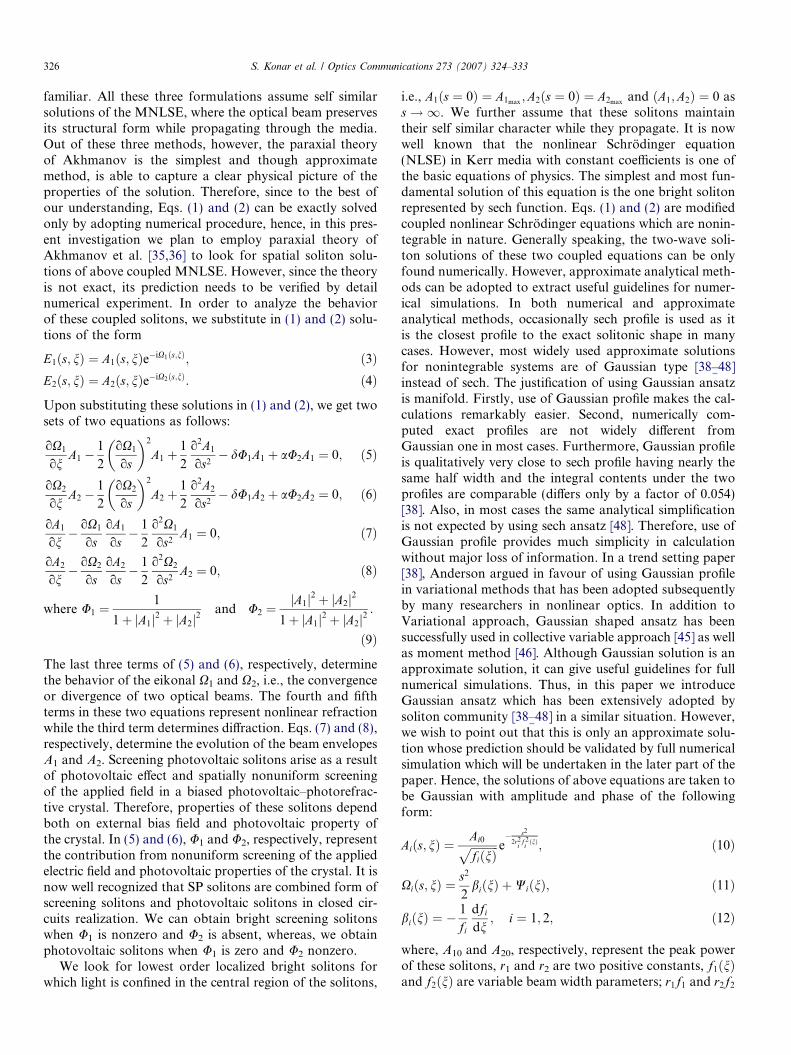
dn ¼ 0 at n ¼ 0, where j ¼ 1; 2. Thevalues of f1 and f2, as predicted earlier, remain constant,signifying stationary propagation of the soliton pair. Asan illustration, we first choose C ¼ 100 and r ¼ 1=2. Wechoose a point on the curve leveled Cr2 ¼ 25 in Fig. 1awhich depicts solitons peak power variation in the lowpower region and obtain P 1 ¼ 0:02178; P 2 ¼ 0:02178.The behavior of f1 and f2 for these values has been obtainedfrom (15) and (16) and depicted in Fig. 4a which show f1

and f2 remain invariant, thus spatial soliton pair is station-ary. We now choose a point on curve leveled Cr2 ¼ 4 in thehigh power region, i.e., the point is selected form Fig. 1band obtain P 1 ¼ 0:8333; P 2 ¼ 0:1666: The behavior of f1

and f2 for these values has been obtained numerically anddepicted in Fig. 4b which show f1 and f2 invariant, thusspatial soliton pair is stationary. This stationary propertyhas been verified for several other randomly chosen pointstaken from different curves of Fig. 1. Therefore, the presenttheory, based on paraxial ray approximation, identifies a

0 1 2 3 43

4

6

8

10

P

Cr2

A B

Fig. 3. Variation of peak power P of the degenerate composite solitonwith spatial width r. Nature of the curve signifies existence of bistableproperty.

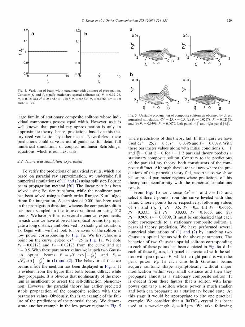
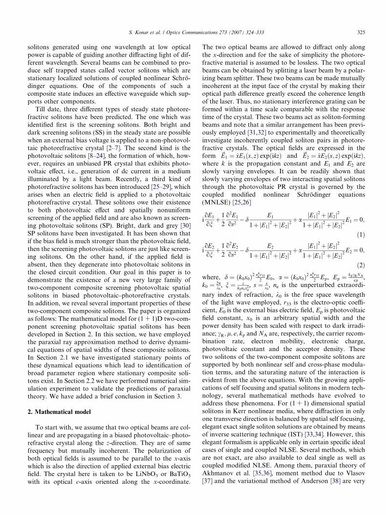
Fig. 5. Unstable propagation of composite solitons as obtained by directnumerical simulation. Cr2 ¼ 25, r ¼ 0:5. (a) P 1 ¼ 0:02178, P 2 ¼ 0:02178;and (b) P 1 ¼ 0:0396, P 2 ¼ 0:0079. Left panel jA1j2 and right panel jA2j2.

0 5 100.8

0.9

1

1.1

1.2

ξ

f 1,f 2

a

0 5 100.8

0.9

1

1.1

1.2

ξ

b

Fig. 4. Variation of beam width parameter with distance of propagation.Constant f1 and f2 signify stationary spatial solitons: (a) P 1 ¼ 0:02178,P 2 ¼ 0:02178,Cr2 ¼ 25andr ¼ 1=2;(b)P 1 ¼ 0:8333,P 2 ¼ 0:1666,Cr2 ¼ 4:0and r ¼ 1=5.

S. Konar et al. / Optics Communications 273 (2007) 324–333 329

large family of stationary composite solitons whose indi-vidual components possess equal width. However, as it iswell known that paraxial ray approximation is only anapproximate theory, hence, predictions based on this the-ory need verification by other means. Nevertheless, thesepredictions could serve as useful guidelines for detail fullnumerical simulations of coupled nonlinear Schrodingerequations, which is our next task.

2.2. Numerical simulation experiment

To verify the predictions of analytical results, which arebased on paraxial ray approximation, we undertake fullnumerical simulations of (1) and (2) using split step Fourierbeam propagation method [50]. The linear part has beensolved using Fourier transform, while the nonlinear parthas been solved using a fourth order Rungee–Kutta algo-rithm for integration. A step size of 0.001 has been usedin the propagation direction, whereas the composite solitonhas been sampled in the transverse direction using 512points. We have performed several numerical experiments,in each case we have allowed the optical beams to propa-gate a long distance and observed no shading of radiation.To begin with, we first look for behavior of the soliton atlow power corresponding to Fig. 1a. We first choose apoint on the curve leveled Cr2 ¼ 25 in Fig. 1a. We noteP 1 ¼ 0:02178 and P 2 ¼ 0:02178 from the curve and setr ¼ 0:5. With these parameter values we launch two Gauss-ian optical beams E1 ¼

ffiffiffiffiffiP 1

pexp � s2

2r2

� �and E2 ¼ffiffiffiffiffi

P 2

pexp � s2

2r2

� �in (1) and (2). The behavior of the two

beams inside the medium has been displayed in Fig. 5. Itis evident from the figure that both beams diffract whilethey propagate. It is obvious that nonlinearity of the med-ium is insufficient to arrest the self-diffraction phenome-non. However, the paraxial theory has earlier predictedstable propagation of the composite soliton with theseparameter values. Obviously, this is an example of the fail-ure of the predictions of the paraxial theory. We demon-strate another example in the low power regime in Fig. 5

where predictions of this theory fail. In this figure we haveused Cr2 ¼ 25, r ¼ 0:5, P 1 ¼ 0:0396 and P 2 ¼ 0:0079. Withthese parameter values along with initial conditions fi ¼ 1and dfi

dn ¼ 0 at n ¼ 0 for i ¼ 1; 2 paraxial theory predicts astationary composite soliton. Contrary to the predictionsof the paraxial ray theory, both constituents of the com-posite diffract. Although these are instances where the pre-dictions of the paraxial theory fail, nevertheless we showbelow broad parameter regions where predictions of thistheory are inconformity with the numerical simulationsresults.

From Fig. 1b we choose Cr2 ¼ 4 and r ¼ 1=5 andselect different points from the curve leveled with thisvalue. Chosen points have, respectively, following valuesof P1 and P2, (i) P 1 ¼ 0:5, P 2 ¼ 0:5, (ii) P 1 ¼ 0:6666,P 2 ¼ 0:3333, (iii) P 1 ¼ 0:8333, P 2 ¼ 0:1666, and (iv)P 1 ¼ 0:909, P 2 ¼ 0:0909. It must be emphasized that eachpoint corresponds to a stationary composite soliton, aparaxial theory prediction. We have performed severalnumerical simulations of (1) and (2) by launching twoGaussian optical beams with the above parameters. Thebehavior of two Gaussian spatial solitons correspondingto each of these points has been depicted in Fig. 6a–d. Ineach of these figures, left panel is associated with the sol-iton with peak power P1 while the right panel is with thepeak power P2. In each case both Gaussian beamsacquire solitonic shape asymptotically without majormodification within very small distance and then theypropagate almost as a stationary composite soliton. Itis evident from these figures that a soliton with largepower can trap a soliton whose power is much smallerand both can propagate as a stationary bound state. Atthis stage it would be appropriate to cite one practicalexample. We consider that a BaTiO3 crystal has beenused at a wavelength k0 ¼ 0:5 lm. We take following

Fig. 7. Stable propagation of composite solitons as obtained by directnumerical simulation. Cr2 ¼ 6:25, r ¼ 1=4. (a) P 1 ¼ 2:0, P 2 ¼ 2:0; (b)P 1 ¼ 3:333, P 2 ¼ 0:666; and (c) P 1 ¼ 3:6363, P 2 ¼ 0:3636. Left panel jA1j2and right panel jA2j2.

Fig. 8. Stable propagation of composite solitons as obtained by directnumerical simulation. Cr2 ¼ 25, r ¼ 1=2. (a) P 1 ¼ 11:478, P 2 ¼ 11:478; (b)P 1 ¼ 19:13, P 2 ¼ 3:826; and (c) P 1 ¼ 20:869, P 2 ¼ 2:086. Left panel jA1j2and right panel jA2j2.

Fig. 6. Stable propagation of composite solitons as obtained by directnumerical simulation. Cr2 ¼ 4, r ¼ 1=5. (a) P 1 ¼ 0:5, P 2 ¼ 0:5; (b)P 1 ¼ 0:6666, P 2 ¼ 0:3333; (c) P 1 ¼ 0:8333, P 2 ¼ 0:1666; and (d)P 1 ¼ 0:909, P 2 ¼ 0:0909. Left panel jA1j2 and right panel jA2j2.

330 S. Konar et al. / Optics Communications 273 (2007) 324–333

crystal parameters [26] ne ¼ 2:365, r33 ¼ 80� 10�12 m=V,Ep ¼ 105 V=m. We take arbitrary spatial scale x0 ¼40 lm and look for coupled soliton pair at an externalbias voltage E0 ¼ 5:8� 104 V=m. With these parametervalues we find d ¼ 18:4; a ¼ 31:58; C ¼ 2ðaþ dÞ ¼99:96: For Cr2 ¼ 4; r 0:20, thus, in natural units theintensity FWHM (i.e., 1.665r) of two components isfound to be 13.32 lm. An important point to note is thatthe present investigation is also valid for LiNbO3. TheLiNbO3 parameters could be taken as ne ¼ 2:2, r33 ¼30� 10�12 m=v, jEpj ¼ 4� 106 V=m. However, it shouldbe pointed out that, while Ep could be either positiveor negative for BaTiO3, depending on the polarizationof light, the experimental results [27] show that Ep isalways negative for LiNbO3. Therefore, with properchoice of the value of E0, C ¼ 2ðaþ dÞ could be madepositive, and hence bright–bright coupled soliton paircould also be observed in LiNbO3.

We have extended our numerical investigations furtherto solitons possessing spatial width and peak power differ-ent from what is being considered so far. From Fig. 1b wechoose Cr2 ¼ 6:25, set r ¼ 1=4 and select different pointson the curve leveled Cr2 ¼ 6:25 to obtain a set of allowedvalues of P1 and P2 as follows: (i) P 1 ¼ 2:0, P 2 ¼ 2:0,(ii) P 1 ¼ 3:333, P 2 ¼ 0:0666, and (iii) P 1 ¼ 3:6363, P 2 ¼0:3636. The results of corresponding numerical simulationsare shown in Fig. 7a–c. These figures show stationary prop-agation of composite solitons, thereby confirming the pre-dictions of paraxial ray theory.

In yet another numerical experiment we turn our atten-tion to solitons possessing large peak power. Therefore, wechoose Cr2 ¼ 25, r ¼ 1=2. The values of P1 and P2 forselected points on Cr2 ¼ 25 curve in Fig. 1a are as follows:(i) P 1 ¼ 11:478, P 2 ¼ 11:478, (ii) P 1 ¼ 19:13, P 2 ¼ 3:826,and (iii) P 1 ¼ 20:869, P 2 ¼ 2:086. The behavior of corre-sponding Gaussian optical beams is demonstrated in

Fig. 8a–c, which validates the prediction of paraxial raytheory.

We now proceed to obtain bistable composite solitonsnumerically. From Fig. 3 we choose two points A and B,each corresponds to one pair of composite soliton. Thesetwo points have equal values of Cr2 (=4.2) but two differ-ent values of soliton peak power P. We have taken C ¼ 50,hence r ¼ 0:290 for both A and B. Peak power P for pointsA and B are, respectively, 0.321 and 0.779. Numericallyobtained dynamic evolution of a pair of composite bistablesoliton corresponding to above values has been demon-strated in Fig. 9. In the figure, the upper panel representsone composite soliton while the lower panel representsanother one. From figure it is evident that both compo-nents of the composite in the upper panel remain abso-

Fig. 9. Propagation of bistable composite solitons. Peak powers andwidth of these solitons have been chosen from points A and B of Fig. 3which correspond to Cr2 ¼ 4:0. Upper panel corresponds to point A andlower panel corresponds to point B. Solitons of both upper and lowerpanels have same width, i.e., each component has spatial width r ¼ 0:290.Peak power of each component in the upper panel P ¼ 0:321. Peak powerof each component in the lower panel P ¼ 0:779.

0 2 40.8

1

1.2

f 1,f 2

a

0 2 40.8

1

1.2

f 1,f 2

c

0 2 40.8

1

1.2

f 1,f 2

ξ

b

0 2 40.8

1

1.2

f 1,f 2

ξ

d

Fig. 10. Stable propagation of composite solitons in the presence ofperturbation, as obtained by paraxial theory. Cr2 ¼ 6:25. (a) Initial peakamplitudes of both components have been perturbed by 15% from theirstationary value. While initial widths of both components are equal tostationary state value. (b) Initial peak amplitude is equal to stationarystate value. Spatial widths of both components have been perturbed by15% from their stationary value. (c) Initial peak amplitude of only onecomponent has been perturbed by 15% from its stationary value, whileinitial spatial widths of each component have been chosen as theirstationary value. (d) Initial peak amplitudes of both solitons are kept atstationary value. Spatial width of one is kept at stationary value while theother is perturbed by 15%. Thick line f1 and thin line f2.

Fig. 11. Stable propagation of composite solitons in the presence ofperturbation, as obtained by full numerical simulation. Cr2 ¼ 6:25. Initialpeak amplitudes of both components are equal to their respectivestationary value. Spatial width of one component is kept at its stationaryvalue while the other is perturbed by 15%. Corresponding contour plotshave been shown in the lower panel.

S. Konar et al. / Optics Communications 273 (2007) 324–333 331

lutely stationary as they propagate, an example where par-axial theory prediction complies with high accuracy. How-ever, in the lower panel, both components of the compositepropagate as stable self-trapped modes though they keepon breathing. Hence, in this case, though prediction of par-axial approximation is not very accurate, yet it is able tocapture the overall features broadly.

2.3. Stability properties

Finally, we discuss stability properties of these compos-ite solitons. We investigate stability using both paraxial raytheory and full numerical simulation as well. In general, wehave found that bright–bright pairs are stable against smallperturbation in peak amplitude and spatial width. Fordemonstration, using the paraxial theory, we have pre-sented four different cases of stable propagation after per-turbing soliton parameters. In the first example we haveperturbed soliton peak amplitude of both components by15% from their stationary values, in the second the widthof both components have been perturbed by 15%, and inthe third example the peak amplitude of only one compo-nent has been perturbed by 15% from its stationary value.In the last example initial peak amplitudes of both solitonsare kept at stationary value. Spatial width of one is kept atstationary value while the other is perturbed by 15%.Results of paraxial theory have been depicted in Fig. 10.Beam width parameters f1 and f2 oscillate around the sta-tionary value with small amplitude as they propagate.Fig. 11 depicts an example of the evolution of the two com-ponents of the perturbed coupled pair as obtained by directnumerical simulation. Evidently, the pair exhibits robust-ness and does not diffract too much or breakup, and

instead oscillates around the stationary soliton solution.Thus, both paraxial theory and numerical simulation con-firm stable coupled soliton pairs.

Before closing, it would be appropriate at this stage tocompare our results with those available in literature.

332 S. Konar et al. / Optics Communications 273 (2007) 324–333

Recently, several workers have investigated coupled screen-ing photovoltaic spatial solitons. Notable among those areworks of Hou et al. [52] and Keqing et al. [53]. Under thesteady state conditions, Hou et al. [52] have investigatedthe properties of multiple mutually incoherent spatial soli-tons in biased photovoltaic–photorefractive crystals. Threekey features distinguish our work with that of Hou et al.The first difference is that while we have treated a bright–bright pair, they have studied coupled bright–dark solitonswhere number of dark and bright solitons could be morethan one. Second and perhaps the most important pointis that, in the present paper we have identified an analyticformula for soliton existence that allows nearly infinitechoice of solitons power, all of which correspond to unam-biguous formation of stable bright–bright pairs. We haveshown that for a particular peak power of one componentthe other component can have infinite number of differentpeak powers, whereas in the result of Hou et al., such flex-ibility is not admissible. The works of Keqing et al. [53]also suffer from this deficiency. Thirdly, for the existenceof multiple mutually incoherent spatial solitons thatreported by Hou et al., the total intensity of the brightbeams should be approximately equal to that of darkbeams. Whereas in our case there is no such restriction,rather we have shown that either of the two componentsof the composite soliton can have power which is only afraction of the other.

3. Conclusion

Propagation characteristics and stability properties oftwo-component composite screening photovoltaic spatialsolitons have been analyzed in this paper. Employing theprinciple of paraxial ray approximation, we have identifieda new very large family of two-component compositescreening photovoltaic solitons in photovoltaic–photore-fractive crystals. We have obtained the necessary condi-tions for mutual trapping of two beams forming suchcomposite solitons in the photovoltaic–photorefractivecrystals. These composite solitons can exist only when thecarrier beams have the same polarization, wavelength andare mutually incoherent. We have identified a wide param-eter space involving spatial width and power where thesecomposite solitons can exist as a stationary entity. Theidentified regions of existence of solitons give a deeperunderstanding of these solitons and reveal some interestingproperties. We have shown that composite solitons withdifferent widths cannot propagate as a stationary entity.In addition, we have shown that in the new family of soli-tons, a degenerate pair with equal peak power possessesbistable property. We have demonstrated that these bista-ble solitons can exist only if their widths are above certainminimum value. Both paraxial theory and numerical simu-lation show that identified composite solitons are stable. Arelevant example has been provided where the crystal isBaTiO3. These self trapped solitons have potential forexciting applications.

Acknowledgements

This investigation is supported by Defence Research andDevelopment Organization (DRDO), Ministry of Defence,Government of India, through a Grant No. RIP/ER/0403457/M/01 and the support is thankfully appreciated.One of the authors thank Mr. M. Mishra for computa-tional aid.

References

[1] G. Duree, J.L. Slultz, G. Salamo, M. Segev, A. Yariv, B. Crosignani,P. DiPorto, E. Sharp, R.R. Neurgaonkar, Phys. Rev. Lett. 71 (1993)533.

[2] M. Segev, B. Crosignani, A. Yariv, B. Fischer, Phys. Rev. Lett. 68(1992) 923.

[3] M.F. Shih, M. Segev, G.C. Valley, G.J. Salamo, B. Crosignani, P.DiPorto, Electron. Lett. 31 (1995) 826.

[4] in P. Gunter, J.P. Huignard (Eds.), Topic in Applied Physics inPhotorefractive Materials and Their Applications I, II, vol. 61/62,Springer, Berlin, 1998.

[5] G.C. Duree, J.L. Shultz, G.J. Salamo, M. Segev, A. Yariv, B.Crosingnani, P. DiPorto, E.J. Sharp, R.R. Neurgaonkar, Phys. Rev.Lett. 71 (1993) 533.

[6] D.N. Christodoulides, M.I. Carvalho, J. Opt. Soc. Am. B 12 (1995)1628.

[7] Z. Chen, M. Mitchel, M.F. Shih, M. Segev, M.H. Garrett, G.C.Valley, Opt. Lett. 21 (1996) 629.

[8] G. Couton, Herve Maillotte, M. Chauvet, J. Opt. B: QuantumSemiclass. Opt. 6 (2004) S223.

[9] K. Kos, H. Ming, G. Salamo, M. Shih, M. Segev, G.C. Valley, Phys.Rev. E 53 (1996) R4330.

[10] S. Lan, E. DelRe, Z. Chen, M. Shih, M. Segev, Opt. Lett. 24 (1999)475.

[11] S. Lan, M. Shih, G. Mizell, J. Giordmaine, Z. Chen, C. Anastossiou,J. Martin, M. Segev, Opt. Lett. 24 (1999) 1145.

[12] S. Lan, J.A. Giordmaine, M. Segev, D. Rytz, Opt. Lett. 27 (2002) 737.[13] C. Bosshard, P.V. Mamyshev, G.I. Stageman, Opt. Lett. 19 (1994) 90.[14] M. Chauvet, S.A. Hawkins, G. Salamo, M. Segev, D.F. Bliss, G.

Bryant, Appl. Phys. Lett. 70 (1997) 2499.[15] M. Shih, M. Segev, G.C. Valley, G. Salamo, B. Crosignani, P.

DiPorto, Electron. Lett. 31 (1995) 826.[16] A.A. Zozulya, D.R. Anderson, A.V. Mamaev, M. Staffman, Euro-

phys. Lett. 36 (1996) 419;A.A. Zozulya, D.R. Anderson, A.V. Mamaev, M. Staffman, Phys.Rev. A 57 (1998) 522.

[17] M. Segev, Opt. Photon. News 13 (2002) 2.[18] M. Segev, D.N. Christodoulides, in: S. Trillo, W. Torruellas (Eds.),

Spatial Solitons, Springer, Berlin, 2001, p. 87.[19] Zhigang Chen, M. Segev, D.N. Christodoulides, J. Opt. A: Pure

Appl. Opt. 5 (2003) S389.[20] W. Korlokowski, B. Luther-Davies, C. Denz, IEEE. J. Quantum

Electron. 39 (2003) 3.[21] P.M. Johansen, J. Opt. A.: Pure Appl. Opt. 5 (2003) S398.[22] Z. Chen, M. Mitchell, M. Segev, Opt. Lett. 21 (1996) 716.[23] J. Petter, C. Denz, A. Stepken, F. Kaiser, J. Opt. Soc. Am. B 19

(2002) 1145.[24] J. Liu, Phys. Rev. E 68 (2003) 026607.[25] L. Jinsong, Lu Kequing, J. Opt. Am. B 16 (1999) 550.[26] J. Liu, Z. Hao, J. Opt. Soc. Am. B 19 (2002) 513.[27] M. Taya, M.C. Bashaw, M.M. Fejer, M. Segev, G.C. Valley, Phys.

Rev. A 52 (1995) 3095.[28] Jinsong Liu, Kequing Lu, Jun Xu, Zhonghua Hao, Proc. SPIE 3554

(1998) 81.[29] Lu Kequing, Tang Tiantong, Zhang Yanpeng, Phys. Rev. A 61 (2000)

053822.

S. Konar et al. / Optics Communications 273 (2007) 324–333 333

[30] C. Hou, Yan Li, Xiaofu Zhang, B. Yuan, X. Sun, Opt. Commun. 181(2000) 141.

[31] D.N. Christodoulides, S.R. Singh, M.I. Carvalho, Appl. Phys. Lett.68 (1996) 1763.

[32] Z. Chen, M. Segev, T.H. Coskun, D.N. Christodoulides, Y.S.Kivshar, J. Opt. Soc. Am. B 14 (1997) 3066.

[33] C.S. Gardner, J.M. Green, M.D. Kruskal, R.M. Miura, Phys. Rev.Lett. 19 (1967) 1095.

[34] M.J. Ablowitz, H. Segur, Solitons and the Inverse ScatteringTechnique, SIAM, Philadelphia, 1981.

[35] S.A. Akhmanov, A.P. Sukhorukov, R.V. Khokhlov, Sov. Phys. USP10 (1968) 609.

[36] S.A. Akhmanov, A.P. Sukhorukov, R.V. Khokhlov, in: A.T. Arechi,E.D. Shulz Dubois (Eds.), Laser Handbook, vol. II, North Holland,Amsterdam, 1972, p. 1151.

[37] S.N. Vlasov, V.A. Petrischev, V.I. Talanov, Sov. Radiophys. 14(1971) 1062.

[38] D. Anderson, Phys. Rev. A 27 (1983) 3135.[39] B. Malomed, D. Anderson, M. Lisak, M.L. Quiroga-Teixeiro, L.

Stenflo, Phys. Rev. E 55 (1997) 962.

[40] V. Skaraka, V.I. Berezhiani, R.M. Klaszewski, Phys. Rev. E 56 (1997)1080.

[41] Z. Liu, W. Zang, J. Tian, W. Zhou, C. Zhang, G. Zhang, Opt.Commun. 219 (2003) 411.

[42] V. Skaraka, N.B. Aleksic, Phys. Rev. Lett. 96 (2006) 013903.[43] Yi Huang, Q. Guo, J. Cuo, Opt. Commun. 261 (2006) 175.[44] Soumendu Jana, S. Konar, Phys. Lett. A 362 (2007) 435.[45] P. Tchofo Dinda, A.B. Moubissi, K. Nakkeeran, J. Phys. A: Math.

Gen. 34 (2001) L103.[46] J. Santhanam, C.J. McKinstrie, T.I. Lakoba, G.P. Agrawal, Opt.

Lett. 26 (2001) 1131.[47] J.H.B. Nijhof, W. Forysiak, N.J. Doran, IEEE J. Sel. Topics

Quantum Electron. 6 (2000) 330.[48] J. Nathan Kutz, Steffen D. Koehler, L. Leng, Keren Bergman, J. Opt.

Soc. Am. B 14 (1997) 636.[49] S. Konar, A. Sengupta, J. Opt. Soc. Am. B 11 (1994) 1644.[50] G.P. Agrawal, Nonlinear Fiber Optics, Academic, Boston, MA, 1995.[51] C. De Angelis, IEEE J. Quantum Electron. 30 (1994) 818.[52] C. Hou, Z. Zhou, B. Yuan, X. Sun, Appl. Phys. B 72 (2001) 191.[53] Lu. Keqing, Zhang Yanpeng, Tang Tiantong, Li Bo, Phys. Rev. E 64

(2001) 056603.